Working Group III – Mitigation of Climate Change TS Technical Summary
101
Working Group III – Mitigation of Climate Change TS Technical Summary
Transcript of Working Group III – Mitigation of Climate Change TS Technical Summary

Working Group III – Mitigation of Climate Change
TS
Technical Summary

*Note: this document of the Technical Summary differs in minimal formatting only from the version made available on April 15, 2014.*
Note:
This document is the copy‐edited version of the final draft Report, dated 17 December 2013, of the Working Group III contribution to the IPCC 5th Assessment Report "Climate Change 2014: Mitigation of Climate Change" that was accepted but not approved in detail by the 12th Session of Working Group III and the 39th Session of the IPCC on 12 April 2014 in Berlin, Germany. It consists of the full scientific, technical and socio‐economic assessment undertaken by Working Group III.
The Report should be read in conjunction with the document entitled “Climate Change 2014: Mitigation of Climate Change. Working Group III Contribution to the IPCC 5th Assessment Report ‐ Changes to the underlying Scientific/Technical Assessment” to ensure consistency with the approved Summary for Policymakers (WGIII: 12th/Doc. 2a, Rev.2) and presented to the Panel at its 39th Session. This document lists the changes necessary to ensure consistency between the full Report and the Summary for Policymakers, which was approved line‐by‐line by Working Group III and accepted by the Panel at the aforementioned Sessions.
Before publication, the Report (including text, figures and tables) will undergo final quality check as well as any error correction as necessary, consistent with the IPCC Protocol for Addressing Possible Errors. Publication of the Report is foreseen in September/October 2014.
Disclaimer:
The designations employed and the presentation of material on maps do not imply the expression of any opinion whatsoever on the part of the Intergovernmental Panel on Climate Change concerning the legal status of any country, territory, city or area or of its authorities, or concerning the delimitation of its frontiers or boundaries.
A report accepted by Working Group III of the IPCC but not approved in detail.

Final Draft Technical Summary IPCC WGIII AR5
1 of 99
Title: Technical Summary
Authors: CLAs: Ottmar Edenhofer, Ramon Pichs‐Madruga, Youba Sokona, Susanne Kadner, Jan Minx, Steffen Brunner
LAs: Shardul Agrawala, Giovanni Baiocchi, Igor Bashmakov, Gabriel Blanco, John Broome, Thomas Bruckner, Mercedes Bustamante, Leon Clarke, Mariana Conte Grand, Felix Creutzig, Xochitl Cruz‐Núñez, Shobhakar Dhakal, Navroz K. Dubash, Patrick Eickemeier, Ellie Farahani, Manfred Fischedick, Marc Fleurbaey, Reyer Gerlagh, Luis Gomez‐Echeverri, Shreekant Gupta, Sujata Gupta, Jochen Harnisch, Kejun Jiang, Frank Jotzo, Sivan Kartha, Stephan Klasen, Charles Kolstad, Volker Krey, Howard Kunreuther, Oswaldo Lucon, Omar Masera, Yacob Mulugetta, Richard Norgaard, Anthony Patt, Nijavalli H. Ravindranath, Keywan Riahi, Joyashree Roy, Ambuj Sagar, Roberto Schaeffer, Steffen Schlömer, Karen Seto, Kristin Seyboth, Ralph Sims, Pete Smith, Eswaran Somanathan, Robert Stavins, Christoph von Stechow, Thomas Sterner, Taishi Sugiyama, Sangwon Suh, Kevin Urama, Diana Ürge‐Vorsatz, Anthony Venables, David Victor, Elke Weber, Dadi Zhou, Ji Zou, Timm Zwickel
CAs: Adolf Acquaye, Kornelis Blok, Gabriel Chan, Jan Fuglestvedt, Edgar Hertwich, Elmar Kriegler, Oliver Lah, Sevastianos Mirasgedis, Carmenza Robledo Abad, Claudia Sheinbaum, Steven Smith, Detlef van Vuuren
REs: Tomas Hernandez‐Tejeda, Roberta Quadrelli

Final Draft Technical Summary IPCC WGIII AR5
2 of 99
TS: Technical Summary
Contents
TS.1 Introduction and framing ............................................................................................................ 3
TS.2 Trends in stocks and flows of greenhouse gases and their drivers .......................................... 10
TS.2.1 Greenhouse gas emission trends ...................................................................................... 10
TS.2.2 Greenhouse gas emission drivers ...................................................................................... 18
TS.3 Mitigation pathways and measures in the context of sustainable development .................... 21
TS.3.1 Mitigation pathways .......................................................................................................... 22
TS.3.1.1 Understanding mitigation pathways in the context of multiple objectives .............. 22
TS.3.1.2 Short‐ and long‐term requirements of mitigation pathways ..................................... 23
TS.3.1.3 Costs, investments and burden sharing ..................................................................... 31
TS.3.1.4 Implications of transformation pathways for other objectives ................................. 35
TS.3.2 Sectoral and cross‐sectoral mitigation measures .............................................................. 39
TS.3.2.1 Cross‐sectoral mitigation pathways and measures ................................................... 39
TS.3.2.2 Energy supply ............................................................................................................. 46
TS.3.2.3 Transport .................................................................................................................... 51
TS.3.2.4 Buildings ..................................................................................................................... 58
TS.3.2.5 Industry ...................................................................................................................... 62
TS.3.2.6 Agriculture, forestry and other land‐uses (AFOLU) .................................................... 70
TS.3.2.7 Human Settlements, Infrastructure, and Spatial Planning ........................................ 75
TS.4 Mitigation policies and institutions .......................................................................................... 81
TS.4.1 Policy design, behaviour and political economy ............................................................... 81
TS.4.2 Sectoral and national policies ............................................................................................ 83
TS.4.3 Development and regional cooperation ........................................................................... 90
TS.4.4 International cooperation ................................................................................................. 92
TS.4.5 Investment and finance ..................................................................................................... 96

Final Draft Technical Summary IPCC WGIII AR5
3 of 99
TS.1 Introduction and framing
‘Mitigation’, in the context of climate change, is a human intervention to reduce the sources or enhance the sinks of greenhouse gases (GHGs). One of the central messages from Working Groups I and II of the Intergovernmental Panel on Climate Change (IPCC) is that the consequences of unchecked climate change for humans and natural ecosystems are already apparent and increasing. The most vulnerable systems are already experiencing adverse effects. Past emissions have already put the planet on a track for substantial further changes in climate, and while there are many uncertainties in factors such as the sensitivity of the climate system many scenarios lead to substantial climate impacts, including direct harms to human and ecological well‐being that exceed the ability of those systems to adapt fully.
Because mitigation is intended to reduce the harmful effects of climate change, it is part of a broader policy framework that also includes adaptation to climate impacts. Mitigation, together with adaptation to climate change, contributes to the objective expressed in Article 2 of the United Nations Framework Convention on Climate Change (UNFCCC) to stabilize “greenhouse gas concentrations in the atmosphere at a level to prevent dangerous anthropogenic interference with the climate system… within a time frame sufficient to allow ecosystems to adapt… to ensure that food production is not threatened and to enable economic development to proceed in a sustainable manner”. However, Article 2 is hard to interpret, as concepts such as ‘dangerous’ and ‘sustainable’ have different meanings in different decision contexts (see Box TS.1). 1 Moreover, natural science is unable to predict precisely the response of the climate system to rising GHG concentrations nor fully understand the harm it will impose on individuals, societies, and ecosystems. Article 2 requires that societies balance a variety of considerations some rooted in the impacts of climate change itself and others in the potential costs of mitigation and adaptation. The difficulty of that task is compounded by the need to develop a consensus on fundamental issues such as the level of risk that societies are willing to accept and impose on others, strategies for sharing costs, and how to balance the numerous tradeoffs that arise because mitigation intersects with many other goals of societies, including socio‐economic development. Such issues are inherently value‐laden and involve different actors who have varied interests and disparate decision‐making power.
This report examines the results of scientific research about mitigation, with a special attention on how knowledge has evolved since the Fourth Assessment Report (AR4) published in 2007. Throughout, the focus is on the implications of its findings for policy, without being prescriptive about the particular policies that governments and other important participants in the policy process should adopt. In light of the IPCC’s mandate, authors in WGIII were guided by several principles when assembling this assessment: (1) to be explicit about mitigation options, (2) to be explicit about their costs and about their risks and opportunities vis‐à‐vis other development priorities, (3) and to be explicit about the underlying criteria, concepts, and methods for evaluating alternative policies.
1 Boxes throughout this summary provide background information on main research concepts and methods that were used to generate insight.

Final Draft Technical Summary IPCC WGIII AR5
4 of 99
Box TS.1. Many disciplines aid decision making on climate change
Something is dangerous if it leads to a significant risk of considerable harm. Judging whether human interference in the climate system is dangerous therefore divides into two tasks. One is to estimate the risk in material terms: what the material consequences of human interference might be and how likely they are. The other is to set a value on the risk: to judge how harmful it will be.
The first is a task for natural science, but the second is not [Section 3.1]. As the Synthesis Report of AR4 states, “Determining what constitutes ‘dangerous anthropogenic interference with the climate system’ in relation to Article 2 of the UNFCCC involves value judgements”. Judgements of value (valuations) are called for, not just here, but at almost every turn in decision making about climate change [3.2]. For example, setting a target for mitigation involves judging the value of losses to people’s wellbeing in the future, and comparing it with the value of benefits enjoyed now. Choosing whether to site wind turbines on land or at sea requires a judgement of the value of landscape in comparison with the extra cost of marine turbines. To estimate the social cost of carbon is to value the harm that emissions do [3.9.4].
Different values often conflict, and they are often hard to weigh against each other. Moreover, they often involve the conflicting interests of different people, and are subject to much debate and disagreement. Decision makers must therefore find ways to mediate among different interests and values, and also among differing viewpoints about values. [3.4, 3.5]
Social sciences and humanities can contribute to this process by improving our understanding of values in ways that are illustrated in the boxes contained in this report. The sciences of human and social behaviour—among them psychology, political science, sociology, and non‐normative branches of economics—investigate the values people have, how they change through time, how they can be influenced by political processes, and how the process of making decisions affects their acceptability. Other disciplines, including ethics (moral philosophy), decision theory, risk analysis, and the normative branch of economics, investigate, analyze, and clarify values themselves [2.5, 3.4, 3.5, 3.6]. These disciplines offer practical ways of measuring some values and trading off conflicting interests. For example, the discipline of public health often measures health by means of ‘disability‐adjusted life years’ [3.4.5]. Economics uses measures of social value that are generally based on monetary valuation but can take account of principles of distributive justice [3.6, 4.2, 4.7, 4.8]. These normative disciplines also offer practical decision‐making tools, such as expected utility theory, decision analysis, cost‐benefit and cost‐effectiveness analysis, and the structured use of expert judgment [2.5, 3.6, 3.7, 3.9].
There is a further element to decision making. People and countries have rights and owe duties towards each other. These are matters of justice, equity, or fairness. They fall within the subject matter of moral and political philosophy, jurisprudence, and economics. For example, some have argued that countries owe restitution for the harms that result from their past emissions, and it has been debated, on jurisprudential and other grounds, whether restitution is owed only for harms that result from negligent or blameworthy emissions. [3.3, 4.6]

Final Draft Technical Summary IPCC WGIII AR5
5 of 99
The remainder of this summary offers the main findings of this report.2 This section continues with providing a framing of important concepts and methods that help to contextualize the findings presented in subsequent sections. Section TS.2 presents evidence on past trends in stocks and flows of GHGs and the factors that drive emissions at the global, regional, and sectoral scales including economic growth, technology, or population changes. Section TS.3.1 provides findings from studies that analyze the technological, economic, and institutional requirements of long‐term mitigation scenarios. Section TS.3.2 provides details on mitigation measures and policies that are used in different economic sectors and human settlements. Section TS.4 summarizes insights on the interactions of mitigation policies between governance levels, economic sectors, and instrument types. References in [square brackets] indicate chapters, sections, figures, tables, and boxes in the underlying report where supporting evidence can be found.
Climate change is a global commons problem that implies the need for international cooperation in tandem with local, national, and regional policies on many distinct matters. Because the emissions of any agent (individual, company, country) affect every other agent, an effective outcome will not be achieved if individual agents advance their interests independently of others. International cooperation can contribute by defining and allocating rights and responsibilities with respect to the atmosphere [Sections 1.2.4, 3.1, 4.2, 13.2.1]. Moreover, research and development (R&D) in support of mitigation is a public good, which means that international cooperation can play a constructive role in the coordinated development and diffusion of technologies [1.4.4, 3.11, 13.9, 14.4.3]. This gives rise to separate needs for cooperation on R&D, opening up of markets, and the creation of incentives to encourage private firms to develop and deploy new technologies and households to adopt them.
International cooperation on climate change involves ethical considerations, including equitable effort‐sharing. Countries have contributed differently to the build‐up of GHG in the atmosphere, have varying capacities to contribute to mitigation and adaptation, and have different levels of vulnerability to climate impacts. Many less developed countries are exposed to the greatest impacts but have contributed least to the problem. Engaging countries in effective international cooperation may require strategies for sharing the costs and benefits of mitigation in ways that are perceived to be equitable [4.2]. Evidence suggests that perceived fairness can influence the level of cooperation among individuals, and that finding may suggest that processes and outcomes seen as fair will lead to more international cooperation as well [3.10, 13.2.2.4]. Analysis contained in the literature of moral and political philosophy can contribute to resolving ethical questions raised by climate change [3.2, 3.3, 3.4]. These questions include how much overall mitigation is needed to avoid ‘dangerous interference’ [Box TS.1, 3.1], how the effort or cost of mitigating climate change should be shared among countries and between the present and future [3.3, 3.6, 4.6], how to account for such factors as historical responsibility for emissions [3.3, 4.6], and how to choose among alternative policies for mitigation and adaptation [3.4, 3.5, 3.6, 3.7]. Ethical issues of wellbeing, justice, fairness, and rights are all involved. Ethical analysis can identify the different ethical principles that underlie different viewpoints, and distinguish correct from incorrect ethical reasoning [3.3, 3.4].
Evaluation of mitigation options requires taking into account many different interests, perspectives, and challenges between and within societies. Mitigation engages many different
2 Throughout this summary, the validity of findings is expressed as a qualitative level of confidence and, when possible, probabilistically with a quantified likelihood. Confidence in the validity of findings is based on the type, amount, quality, and consistency of evidence (e.g., theory, data, models, expert judgment) and the degree of agreement. Levels of evidence and agreement can be disclosed instead of aggregate confidence levels. Where appropriate, findings are also formulated as statements of fact without using uncertainty qualifiers. For more details, please refer to the Guidance Note for Lead Authors of the IPCC Fifth Assessment Report on Consistent Treatment of Uncertainties.

Final Draft Technical Summary IPCC WGIII AR5
6 of 99
agents, such as governments at different levels—regionally [14.1], nationally and locally [15.1], and through international agreements [13.1]—as well as households, firms, and other non‐governmental actors. The interconnections between different levels of decision making and among different actors affect the many goals that become linked with climate policy. Indeed, in many countries the policies that have (or could have) the largest impact on emissions are motivated not solely by concerns surrounding climate change. Of particular importance are the interactions and perceived tensions between mitigation and development [4.1, 14.1]. Development involves many activities, such as enhancing access to modern energy services [7.9.1, 16.8], the building of infrastructures [12.1], ensuring food security [11.1], and eradicating poverty [4.1]. Many of these activities can lead to higher emissions, if achieved by conventional means. Thus, the relationships between development and mitigation can lead to political and ethical conundrums, especially for developing countries, when mitigation is seen as exacerbating urgent development challenges and adversely affecting the current well‐being of their populations [4.1]. These conundrums are examined throughout this report, including in special boxes in each chapter highlighting the concerns of developing countries.
Economic evaluation can be useful for policy design and be given a foundation in ethics, provided appropriate distributional weights are applied. While the limitations of economics are widely documented [2.4, 3.5], economics nevertheless provides useful tools for assessing the pros and cons of mitigation and adaptation options. Practical tools that can contribute to decision making include cost‐benefit analysis, cost‐effectiveness analysis, multi‐criteria analysis, expected utility theory, and methods of decision analysis [2.5, 3.7.2]. Economic valuation can be given a foundation in ethics, provided distributional weights are applied that take proper account of the difference in the value of money to rich and poor people [Box TS.2, 3.6]. Few empirical applications of economic valuation to climate change have been well‐founded in this respect [3.6.1]. The literature provides significant guidance on the social discount rate for consumption, which is in effect inter‐temporal distributional weighting. It suggests that the social discount rate depends in a well‐defined way primarily on the anticipated growth in per capita income and inequality aversion [Box TS.10, 3.6.2].

Final Draft Technical Summary IPCC WGIII AR5
7 of 99
Box TS.2. Mitigation brings both market and non-market benefits to humanity
The impacts of mitigation consist in the reduction or elimination of some of the effects of climate change. Mitigation may improve people’s livelihood, their health, their access to food or clean water, the amenities of their lives, or the natural environment around them.
Mitigation can improve human wellbeing through both market and non‐market effects. Market effects result from changes in market prices, in people’s revenues or net income, or in the quality or availability of market commodities. Non‐market effects result from changes in the quality or availability of non‐marketed goods such as health, quality of life, culture, environmental quality, natural ecosystems, wildlife, and aesthetic values. Each impact of climate change can generate both market and non‐market damages. For example, a heat wave in a rural area may cause heat stress for exposed farm labourers, dry up a wetland that serves as a refuge for migratory birds, or kill some
crops and damage others. Avoiding these damages is a benefit of mitigation. 3.9
Economists often use monetary units to value the damage done by climate change and the benefits of mitigation. The monetized value of a benefit to a person is the amount of income the person would be willing to sacrifice in order to get it, or alternatively the amount she would be willing to accept as adequate compensation for not getting it. The monetized value of a harm is the amount of income she would be willing to sacrifice in order to avoid it, or alternatively the amount she would be willing to accept as adequate compensation for suffering it. Economic measures seek to capture how strongly individuals care about one good or service relative to another, depending on their
individual interests, outlook, and economic circumstances. 3.9
Monetary units can be used in this way to measure costs and benefits that come at different times and to different people. But it cannot be presumed that a dollar to one person at one time can be treated as equivalent to a dollar to a different person or at a different time. Distributional weights
may need to be applied between people 3.6.1, and discounting may be appropriate between times.
Box TS.10, 3.6.2
Most climate policies intersect with other societal goals, either positively or negatively, creating the possibility of ‘co‐benefits’ or ‘adverse side‐effects’. Since the publication of AR4 a substantial literature has emerged looking at how countries that engage in mitigation also address other goals, such as local environmental protection or energy security, as a ‘co‐benefit’ and conversely [1.2.1, 6.6.1, 4.8]. This multi‐objective perspective is important because it helps to identify areas where political, administrative, stakeholder, and other support for policies that advance multiple goals will be robust. Moreover, in many societies the presence of multiple objectives may make it easier for governments to sustain the political support needed for mitigation [15.2.3]. Measuring the net effect on social welfare requires examining the interaction between climate policies and pre‐existing other policies [Box TS.11, 3.6.3, 6.3.6.5].
Mitigation efforts generate tradeoffs and synergies with other societal goals that can be evaluated in a sustainable development framework. The many diverse goals that societies value are often called ‘sustainable development’. A comprehensive assessment of climate policy therefore involves going beyond a narrow focus on distinct mitigation and adaptation options and their specific co‐benefits. Instead it entails incorporating climate issues into the design of comprehensive strategies for equitable and sustainable development at regional, national, and local levels [4.2, 4.5]. Maintaining and advancing human wellbeing, in particular overcoming poverty and reducing inequalities in living standards, while avoiding unsustainable patterns of consumption and production, are fundamental aspects of equitable and sustainable development [4.4, 4.6, 4.8.]. Because these aspects are deeply rooted in how societies formulate and implement economic and social policies generally, they are critical to the adoption of effective climate policy.

Final Draft Technical Summary IPCC WGIII AR5
8 of 99
Variations in goals reflect, in part, the fact that humans perceive risks and opportunities differently. Individuals make their decisions based on different goals and objectives and use a variety of different methods in making choices between alternative options. These choices and their outcomes affect the ability of different societies to cooperate and coordinate. Some groups put greater emphasis on near‐term economic development and mitigation costs, while others focus more on the longer‐term ramifications of climate change for prosperity. Some are highly risk averse while others are more tolerant of dangers. Some have more resources to adapt to climate change and others have fewer. Some focus on possible catastrophic events while others ignore extreme events as implausible. Some will be relative winners, and some relative losers from particular climate changes. Some have more political power to articulate their preferences and secure their interests and others have less. Since AR4, awareness has grown that such considerations—long the domain of psychology, behavioural economics, political economy, and other disciplines—need to be taken into account in assessing climate policy [Box TS.3]. In addition to the different perceptions of climate change and its risks, a variety of norms can also affect what humans view as acceptable behaviour. Awareness has grown about how such norms spread through social networks and ultimately affect activities, behaviours and lifestyles, and thus development pathways, which can have profound impacts on emissions and mitigation policy. [1.4.2, 2.4, 3.8, 3.10, 4.3]
Box TS.3. Deliberative and intuitive thinking are inputs to effective risk management
When people—from individual voters to key decision makers in firms to senior government policy makers—make choices that involve risk and uncertainty, they rely on deliberative as well intuitive thought processes. Deliberative thinking is characterized by the use of a wide range of formal methods to evaluate alternative choices when probabilities are difficult to specify and/or outcomes are uncertain. They can enable decision makers to compare choices in a systematic manner by taking into account both short and long‐term consequences. A strength of these methods is that they help avoid some of the well‐known pitfalls of intuitive thinking, such as the tendency of decision makers to favour the status quo. A weakness of these deliberative decision aids is that they are often highly complex and require considerable time and attention.
Most analytically‐based literature, including reports such as this one, is based on the assumption that individuals undertake deliberative and systematic analyses in comparing options. However, when making mitigation and adaptation choices, people are also likely to engage in intuitive thinking. This kind of thinking has the advantage of requiring less extensive analysis than deliberative thinking. However, relying on one’s intuition may not lead one to characterize problems accurately when there is limited past experience. Climate change is a policy challenge in this regard since it involves large numbers of complex actions by many diverse actors, each with their own values, goals, and objectives. Individuals are likely to exhibit well‐known patterns of intuitive thinking such as making choices related to risk and uncertainty on the basis of emotional reactions and the use of simplified rules that have been acquired by personal experience. Other tendencies include misjudging probabilities, focusing on short time horizons, and utilizing rules of thumb that selectively attend to subsets of goals and objectives. [2.4]
By recognizing that both deliberative and intuitive modes of decision making are prevalent in the real world, risk management programmes can be developed that achieve their desired impacts. For example, alternative frameworks that do not depend on precise specification of probabilities and outcomes can be considered in designing mitigation and adaptation strategies for climate change. [2.4, 2.5, 2.6]
Final Draft Technical Summary IPCC WGIII AR5
9 of 99
Effective climate policy involves building institutions and capacity for governance. While there is strong evidence that a transition to a sustainable and equitable path is technically feasible, charting an effective and viable course for climate change mitigation is not merely a technical exercise. It will involve myriad and sequential decisions among states and civil society actors. Such a process benefits from the education and empowerment of diverse actors to participate in systems of decision making that are designed and implemented with procedural equity as a deliberate objective. This applies at the national as well as international levels, where effective governance relating to global common resources, in particular, is not yet mature. Any given approach has potential winners and losers. The political feasibility of that approach will depend strongly on the distribution of power, resources, and decision‐making authority among the potential winners and losers. In a world characterized by profound disparities, procedurally equitable systems of engagement, decision making and governance may help enable a polity to come to equitable solutions to the sustainable development challenge. [4.3]
Effective risk management of climate change involves considering uncertainties in possible physical impacts as well as human and social responses. Climate change mitigation and adaption is a risk management challenge that involves many different decision‐making levels and policy choices that interact in complex and often unpredictable ways. Risks and uncertainties arise in natural, social, and technological systems. Effective risk management strategies not only consider people’s values, and their intuitive decision processes but utilize formal models and decision aids for systematically addressing issues of risk and uncertainty [Box TS.3, 2.4, 2.5]. Research on other such complex and uncertainty‐laden policy domains suggest the importance of adopting policies and measures that are robust across a variety of criteria and possible outcomes [2.5]. A special challenge arises with the growing evidence that climate change may result in extreme impacts whose trigger points and outcomes are shrouded in high levels of uncertainty [Box TS.4, 2.5, Box 3.9]. A risk management strategy for climate change will require integrating responses in mitigation with different time horizons, adaptation to an array of climate impacts, and even possible emergency responses such as ‘geoengineering’ in the face of extreme climate impacts [1.4.2, 3.3.7, 6.9, 13.4.4]. In the face of potential extreme impacts, the ability to quickly offset warming could help limit some of the most extreme climate impacts although deploying these geoengineering systems could create many other risks. One of the central challenges in developing a risk management strategy is to have it adaptive to new information and different governing institutions [2.5].

Final Draft Technical Summary IPCC WGIII AR5
10 of 99
Box TS.4. ‘Fat tails’: unlikely vs. likely outcomes in understanding the value of mitigation
What has become known as the ‘fat‐tails’ problem relates to uncertainty in the climate system and its implications for mitigation and adaptation policies. By assessing the chain of structural uncertainties that affect the climate system, the resulting compound probability distribution of possible economic damage may have a fat right tail. That means that the probability of damage does not decline with increasing temperature as quickly as the consequences rise.
The significance of fat tails can be illustrated for the distribution of temperature that will result from a doubling of atmospheric CO2 (climate sensitivity). IPCC Working Group I (WGI) estimates may be used to calibrate two possible distributions, one fat‐tailed and one thin‐tailed, that each have a median temperature change of 3°C and a 15% probability of a temperature change in excess of 4.5°C. Although the probability of exceeding 4.5°C is the same for both distributions, likelihood drops off much more slowly with increasing temperature for the fat‐tailed compared to the thin‐tailed distribution. For example, the probability of temperatures in excess of 8°C is nearly ten times greater with the chosen fat‐tailed distribution than with the thin‐tailed distribution. If temperature changes are characterized by a fat tailed distribution, and events with large impact may occur at higher temperatures, then tail events can dominate the computation of expected damages from climate change.
In developing mitigation and adaptation policies, there is value in recognizing the higher likelihood of tail events and their consequences. In fact, the nature of the probability distribution of temperature change can profoundly change how climate policy is framed and structured. Specifically, fatter tails increase the importance of tail events (such as 8°C warming). While research attention and much policy discussion have focused on the most likely outcomes, it may be that those in the tail of the probability distribution are more important to consider. [2.5, 3.9.2]
TS.2 Trends in stocks and flows of greenhouse gases and their drivers
This section summarizes historical GHG emission trends and their underlying drivers. As in most of the underlying literature, all aggregate GHG emission estimates are converted to CO2eq based on Global Warming Potentials with a 100‐year time horizon (GWP100) [Box TS.5]. The majority of changes in GHG emission trends that are observed in this section are related to changes in drivers such as economic growth, technological change, human behaviour, or population growth. But there are also some smaller changes in GHG emissions estimates that are due to refinements in measurement concepts and methods that have happened since AR4. Since AR4 there is a growing literature on uncertainties in global GHG emission data sets. This section tries to make these uncertainties explicit and reports variation in estimates across global data sets wherever possible.
TS.2.1 Greenhouse gas emission trends
Total anthropogenic GHG emissions have risen more rapidly from 2000 to 2010 than in the previous three decades (high confidence). Total anthropogenic GHG emissions were the highest in human history from 2000 to 2010 and reached 49 (±4.5) GtCO2eq/yr in 2010. Current trends are at the high end of levels that had been projected for the last decade. Emission growth has occurred despite the presence of a wide array of multilateral institutions as well as national policies aimed at mitigating emissions. From 2000 to 2010, GHG emissions grew on average 2.2% per year compared to 1.3% per year over the entire period from 1970 to 2000 [Figure TS.1]. The global economic crisis 2007/2008 has temporarily reduced global emissions but not changed the longer‐term trend. Whereas more recent data are not available for all gases, initial evidence suggests that growth in global CO2 emissions from fossil fuel combustion has continued with emissions increasing by about

Final Draft Technical Summary IPCC WGIII AR5
11 of 99
3% between 2010 and 2011 and by about 1–2% between 2011 and 2012. [1.3, 5.2, 13.3, 15.2.2, Figure 15.1]
CO2 remains the major anthropogenic GHG with 76% of total GHG emissions in 2010 weighed by GWP100 (high confidence). Since AR4 the shares of the major groups of GHG emissions have remained stable. The share of CO2 emission was 76% in 2010, CH4 contributed 16%, N2O about 6% and the combined fluorinated‐gases3 (F‐gases) about 2% [Figure TS.1]. Using the most recent GWP100 values from the Fifth Assessment Report [WG1 8.6] global GHG emission totals would be slightly higher (52 GtCO2eq/yr) and non‐CO2 emission shares would be 20% for CH4, 5% for N2O and 2% for F‐gases. Emission shares are sensitive to the choice of emission metric and time horizon, but this has a small influence on global, long‐term trends. If a shorter, 20‐year time horizon were used, then the share of CO2 would decline to just over 50% of total anthropogenic GHG emissions and short‐lived gases would rise in relative importance. The choice of emission metric and time horizon involves explicit or implicit value judgements and depends on the purpose of the analysis [Box TS.5]. [1.2, 3.9, 5.2]
Figure TS.1. Total annual anthropogenic GHG emissions (GtCO2eq/yr) by groups of gases 1970-2010: CO2 from fossil fuel combustion and industrial processes; CO2 from Forestry and Other Land Use (FOLU); methane (CH4); nitrous oxide (N2O); fluorinated gases3 covered under the Kyoto Protocol (F-gases). At the right side of the figure GHG emissions in 2010 are shown again broken down into these components with the associated uncertainties (90% confidence interval) indicated by the error bars. Total anthropogenic GHG emissions uncertainties are derived from the individual gas estimates as described in chapter 5 [5.2.3.6]. Emissions are converted into CO2-equivalents based on Global Warming Potentials with a 100 year time horizon (GWP100) from the IPCC Second Assessment Report. The emissions data from FOLU represents land-based CO2 emissions from forest and peat fires and decay that approximate to net CO2 flux from the FOLU as described in chapter 11 of this report. Average annual growth rate for the four decades are highlighted with the brackets. The average annual growth rates from 1970 to 2000 is 1.3% per year. [Figure 1.3]
3 In this report data on fluorinated gases is taken from the EDGAR database (Annex A.II.9), which covers substances included in the Kyoto Protocol.
Final Draft Technical Summary IPCC WGIII AR5
12 of 99
Over the last four decades total cumulative CO2 emissions have increased by a factor of 2 from about 900 GtCO2 for the period 1750–1970 to about 2000 GtCO2 for 1750–2010 (high confidence). In 1970 the cumulative CO2 emissions from fossil fuel combustion, cement production and flaring since 1750 was 420±35 GtCO2; in 2010 that cumulative total had tripled to 1300 ±110 GtCO2 (Figure TS.2). Cumulative CO2 emissions associated with Forestry and Other Land Use (FOLU)4 since 1750 increased from about 490±180 GtCO2 in 1970 to approximately 680±300 GtCO2 in 2010. [5.2]
Regional patterns of GHG emissions are shifting along with changes in the world economy (high confidence). More than 75% of the 10 Gt increase in annual GHG emissions between 2000 and 2010 was emitted in the energy supply (47%) and industry (30%) sectors [see Annex II.9.I for sector definitions]. 5.9 GtCO2eq of this sectoral increase occurred in upper‐middle income countries,5 where the most rapid economic development and infrastructure expansion has taken place. GHG emission growth in the other sectors has been more modest in absolute (0.3–1.1 Gt CO2eq) as well as in relative terms (3%–11%). [1.3, 5.3, Figure 5.18]
Current GHG emission levels are dominated by contributions from the energy supply, AFOLU, and industry sectors; industry and building gain considerably in importance if indirect emissions are accounted for (robust evidence, high agreement). Of the 49(±4.5) GtCO2eq emissions in 2010, 35% of GHG emissions were released in the energy supply sector, 24% in Agriculture, Forestry and Other Land‐Use (AFOLU), 21% in industry, 14% in transport, and 6.4% in buildings. When indirect emissions from electricity and heat production are assigned to sectors of final energy use, the shares of the industry and buildings sectors in global GHG emissions grow to 31% and 19%, respectively (Figure TS3). [1.3, 7.3, 8.2, 9.2, 10.3, 11.2]
4 FOLU (Forestry and Other Land Use) – also referred to as LULUCF (Land use, land‐use change, and forestry) – is the subset of AFOLU emissions and removals of greenhouse gases related to direct human‐induced land use, land‐use change and forestry activities excluding agricultural emissions (see Annex I).
5 When countries are assigned to income groups in this Technical Summary, the World Bank income classification for 2013 is used. For details see Annex A.II.3.

Final Draft Technical Summary IPCC WGIII AR5
13 of 99
Figure TS.2. Historical anthropogenic CO2 emissions from fossil fuel combustion, flaring, cement, and Forestry and Other Land Use (FOLU) in five major world regions: OECD-1990 (blue); Economies in Transition (yellow); Asia (green); Latin America (red); Middle East and Africa (brown). Emissions are reported in gigatonnnes of CO2 per year (Gt/yr). Left panels show regional CO2 emission trends 1750–2010 from: (a) the sum of all CO2 sources (c+e); (c) fossil fuel combustion, flaring, and cement; and (e) FOLU. The right panels report regional contributions to cumulative CO2 emissions over selected time periods from: (b) the sum of all CO2 sources (d+f); (d) fossil fuel combustion, flaring and cement; and (f) FOLU. Error bars on (d) and (f) give an indication of the uncertainty range (90% confidence interval). See Annex II.2 for regional definitions. [Figure 5.3]

Final Draft Technical Summary IPCC WGIII AR5
14 of 99
Figure TS.3. Allocation of GHG emissions across sectors and country income groups. Panel a: Share (in %) of direct GHG emissions in 2010 across the sectors. Indirect CO2 emission shares from electricity and heat production are attributed to sectors of final energy use. Panel b: Shares (in %) of direct and indirect emissions in 2010 by major economic sectors with CO2 emissions from electricity and heat production attributed to the sectors of final energy use. Lower panel: Total anthropogenic GHG emissions in 1970, 1990 and 2010 by economic sectors and country income groups. GHG emissions from international transportation are reported separately. The emissions data from Agriculture, Forestry and Other Land Use (AFOLU) includes land-based CO2 emissions from forest and peat fires and decay that approximate to net CO2 flux from the Forestry and Other Land Use (FOLU) sub-sector as described in chapter 11 of this report. Emissions are converted into CO2-
Final Draft Technical Summary IPCC WGIII AR5
15 of 99
equivalents based on Global Warming Potentials with a 100 year time horizon (GWP100) from the IPCC Second Assessment Report. Assignment of countries to income groups is based on the World Bank income classification in 2013. For details see Annex II.2.3. Sector definitions are provided in Annex II.9. [Figure 1.3, Figure 1.6]
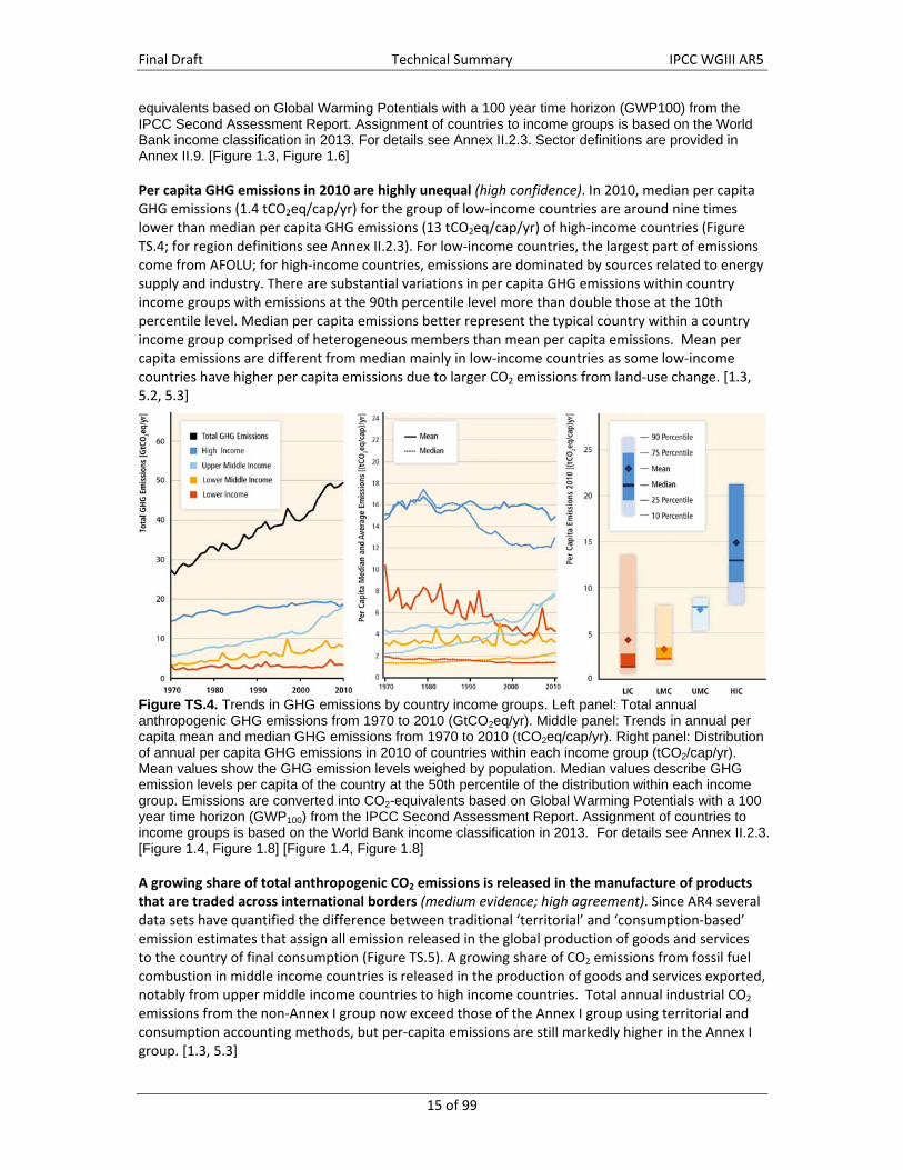
Per capita GHG emissions in 2010 are highly unequal (high confidence). In 2010, median per capita GHG emissions (1.4 tCO2eq/cap/yr) for the group of low‐income countries are around nine times lower than median per capita GHG emissions (13 tCO2eq/cap/yr) of high‐income countries (Figure TS.4; for region definitions see Annex II.2.3). For low‐income countries, the largest part of emissions come from AFOLU; for high‐income countries, emissions are dominated by sources related to energy supply and industry. There are substantial variations in per capita GHG emissions within country income groups with emissions at the 90th percentile level more than double those at the 10th percentile level. Median per capita emissions better represent the typical country within a country income group comprised of heterogeneous members than mean per capita emissions. Mean per capita emissions are different from median mainly in low‐income countries as some low‐income countries have higher per capita emissions due to larger CO2 emissions from land‐use change. [1.3, 5.2, 5.3]
Figure TS.4. Trends in GHG emissions by country income groups. Left panel: Total annual anthropogenic GHG emissions from 1970 to 2010 (GtCO2eq/yr). Middle panel: Trends in annual per capita mean and median GHG emissions from 1970 to 2010 (tCO2eq/cap/yr). Right panel: Distribution of annual per capita GHG emissions in 2010 of countries within each income group (tCO2/cap/yr). Mean values show the GHG emission levels weighed by population. Median values describe GHG emission levels per capita of the country at the 50th percentile of the distribution within each income group. Emissions are converted into CO2-equivalents based on Global Warming Potentials with a 100 year time horizon (GWP100) from the IPCC Second Assessment Report. Assignment of countries to income groups is based on the World Bank income classification in 2013. For details see Annex II.2.3. [Figure 1.4, Figure 1.8] [Figure 1.4, Figure 1.8]
A growing share of total anthropogenic CO2 emissions is released in the manufacture of products that are traded across international borders (medium evidence; high agreement). Since AR4 several data sets have quantified the difference between traditional ‘territorial’ and ‘consumption‐based’ emission estimates that assign all emission released in the global production of goods and services to the country of final consumption (Figure TS.5). A growing share of CO2 emissions from fossil fuel combustion in middle income countries is released in the production of goods and services exported, notably from upper middle income countries to high income countries. Total annual industrial CO2 emissions from the non‐Annex I group now exceed those of the Annex I group using territorial and consumption accounting methods, but per‐capita emissions are still markedly higher in the Annex I group. [1.3, 5.3]

Final Draft Technical Summary IPCC WGIII AR5
16 of 99
Regardless of the perspective taken, the largest share of anthropogenic CO2 emissions is emitted by a small number of countries (high confidence). In 2010, 10 countries accounted for about 70% of CO2 emissions from fossil fuel combustion and industrial processes. A similarly small number of countries emit the largest share of consumption‐based CO2 emissions as well as cumulative CO2 emissions going back to 1750. [1.3] The upward trend in global fossil fuel related CO2 emissions is robust across databases and despite uncertainties (high confidence). Global CO2 emissions from fossil fuel combustion are known within 8% uncertainty. CO2 emissions related to FOLU have very large uncertainties attached in the order of 50%. Uncertainty for global emissions of CH4, N2O, and the F‐gases has been estimated as 20%, 60%, and 20%. Combining these values yields an illustrative total global GHG uncertainty estimate of order 10% (Figure TS.1). Uncertainties can increase at finer spatial scales and for specific sectors. Attributing emissions to the country of final consumption increases uncertainties, but literature on this topic is just emerging. GHG emission estimates in the AR4 were 5–10% higher than the estimates reported here, but lie within the estimated uncertainty range. All uncertainties reported here are reported for a 90% confidence interval. [5.2]
Figure TS.5. Total annual CO2 emissions (GtCO2/yr) from fossil fuel combustion for country income groups attributed on the basis of territory (solid line) and final consumption (dotted line). The shaded areas are the net CO2 trade balance (difference) between each of the four country income groups and the rest of the world. Blue shading indicates that the country group is a net importer of embodied CO2 emissions, leading to consumption-based emission estimates that are higher than traditional territorial emission estimates. Orange indicates the reverse situation – the country group is a net exporter of embodied CO2 emissions. Assignment of countries to income groups is based on the World Bank income classification in 2013. For details see Annex II.2.3. [Figure 1.5]

Final Draft Technical Summary IPCC WGIII AR5
17 of 99
Box TS.5. Emissions metrics depend on value judgements and contain wide uncertainties
Emission metrics provide ‘exchange rates’ for measuring the contributions of different GHGs to climate change. Such exchange rates serve a variety of important purposes, including apportioning mitigation efforts among several gases and aggregating emissions of a variety of GHGs. However, it turns out that there is no perfect metric that is both conceptually correct and practical to implement. Because of this, the choice of the appropriate metric depends on the application or policy at issue. [3.9.6]
GHGs differ in their physical characteristics. For example, per unit mass in the atmosphere, methane causes a stronger instantaneous radiative forcing compared to CO2, but it remains in the atmosphere for a much shorter time. Thus, the time profiles of climate change brought about by different GHGs are different and consequential. Determining how emissions of different GHGs are compared for mitigation purposes involves comparing the resulting temporal profiles of climate change from each gas and making value judgments about the relative significance to humans of these profiles, which is a process fraught with uncertainty. [3.9.6; WGI 8.7]
A commonly used metric is the Global Warming Potential (GWP). It is defined as the accumulated radiative forcing within a specific time horizon (e.g., 100 years—GWP100), caused by emitting one kilogram of the gas, relative to that of the reference gas CO2. This metric is used to transform the effects of different emissions to a common scale (CO2‐equivalents).
6 One strength of the GWP is that it can be calculated in a relatively transparent and straightforward manner. However, there are also some important limitations, including the requirement to use a specific time horizon, the focus on cumulative forcing, and the insensitivity of the metric to the temporal profile of climate effects and its significance to humans. The choice of time horizon is particularly important for short‐lived gases, notably methane: when computed with a shorter time horizon for GWP, their share in calculated total warming effect is larger and the mitigation strategy might change as a consequence. [1.2.5]
Many alternative metrics have been proposed in the scientific literature. All of them have advantages and disadvantages, and the choice of metric can make a large difference for the weights given to emissions from particular gases. For instance, methane’s GWP100 is 28 while its Global Temperature Potential (GTP), one alternative metric, is 4 for the same time horizon (AR5 values, see WGI Section 8.7). In terms of aggregate mitigation costs alone, GWP100 may perform similarly to other metrics (such as the time‐dependent Global Temperature Change Potential or the Global Cost Potential) of reaching a prescribed climate target; however, there may be significant differences in terms of the implied distribution of costs across sectors, regions, and over time. [3.9.6, 6.2]
An alternative to a single metric for all gases is to adopt a ‘multi‐basket’ approach in which gases are grouped according to their contributions to short and long term climate change. This may solve some problems associated with using a single metric, but the question remains of what relative importance to attach to reducing emissions in the different groups. [3.9.6; WGI 8.7]
6 In this summary, all quantities of GHG emissions are expressed in CO2‐equivalent (CO2eq) emissions that are calculated based on GWP100. Unless otherwise stated, GWP values for different gases are taken from the Second Assessment Report (SAR). Although GWP values have been updated several times since, the SAR values are widely used in policy settings, including the Kyoto Protocol, as well as in many national and international emission accounting systems. Modelling studies show that the changes in GWP100 values from SAR to AR4 have little impact on the optimal mitigation strategy at the global level. [6.3.2.5, A.II.9.1]
Final Draft Technical Summary IPCC WGIII AR5
18 of 99
TS.2.2 Greenhouse gas emission drivers
This section examines the factors that have, historically, been associated with changes in emission levels. Typically, such analysis is based on a decomposition of total emissions into various components such as growth in the economy (GDP/capita), growth in the population (capita), the energy intensity needed per unit of economic output (energy/GDP) and the emission intensity of that energy (GHGs/energy). As a practical matter, due to data limitations and the fact that most GHG emissions take the form of CO2 from industry and energy, almost all this research focuses on CO2 from those sectors.
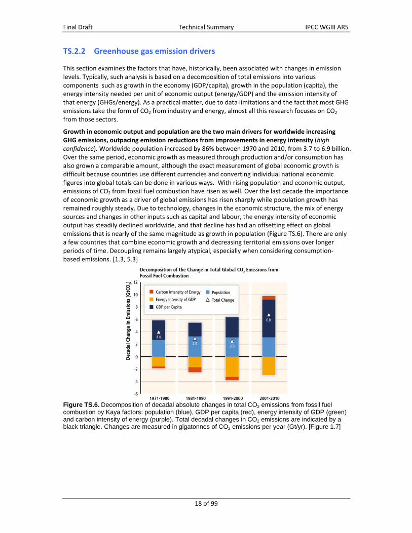
Growth in economic output and population are the two main drivers for worldwide increasing GHG emissions, outpacing emission reductions from improvements in energy intensity (high confidence). Worldwide population increased by 86% between 1970 and 2010, from 3.7 to 6.9 billion. Over the same period, economic growth as measured through production and/or consumption has also grown a comparable amount, although the exact measurement of global economic growth is difficult because countries use different currencies and converting individual national economic figures into global totals can be done in various ways. With rising population and economic output, emissions of CO2 from fossil fuel combustion have risen as well. Over the last decade the importance of economic growth as a driver of global emissions has risen sharply while population growth has remained roughly steady. Due to technology, changes in the economic structure, the mix of energy sources and changes in other inputs such as capital and labour, the energy intensity of economic output has steadily declined worldwide, and that decline has had an offsetting effect on global emissions that is nearly of the same magnitude as growth in population (Figure TS.6). There are only a few countries that combine economic growth and decreasing territorial emissions over longer periods of time. Decoupling remains largely atypical, especially when considering consumption‐based emissions. [1.3, 5.3]
Figure TS.6. Decomposition of decadal absolute changes in total CO2 emissions from fossil fuel combustion by Kaya factors: population (blue), GDP per capita (red), energy intensity of GDP (green) and carbon intensity of energy (purple). Total decadal changes in CO2 emissions are indicated by a black triangle. Changes are measured in gigatonnes of CO2 emissions per year (Gt/yr). [Figure 1.7]

Final Draft Technical Summary IPCC WGIII AR5
19 of 99
Between 2000 and 2010 increased use of coal relative to many other energy sources has reversed a long‐standing pattern of gradual decarbonization of the world’s energy supply (high confidence). Increased use of coal, especially in developing Asia, is exacerbating the burden of energy‐related GHG emissions (Figure TS.6). Estimates indicate that coal, and unconventional gas and oil resources are large; therefore reducing the carbon intensity of energy may not be primarily driven by fossil resource scarcity, but rather by other driving forces such as changes in technology, values, and socio‐political choices. [5.3, 7.2, 7.3, 7.4; SRREN Figure 1.7]
Technological innovations, infrastructural choices, and behaviour affect emissions through productivity growth, energy‐ and carbon‐intensity and consumption patterns (medium confidence). Technological innovation improves labour and resource productivity; it can support economic growth both with increasing and with decreasing emissions. The direction and speed of technological change also depends on policies. Technology is also central to the choices of infrastructure and spatial organization, such as in cities, which can have long‐lasting effects on emissions. In addition, a wide array of attitudes, values, and norms can inform different lifestyles, consumption preferences, and technological choices all of which, in turn, affect patterns of emissions. [5.3, 5.5, 5.6, 12.3]
Without explicit efforts to reduce GHG emissions, the fundamental drivers of emissions growth are expected to persist despite major improvements in energy supply and end‐use technologies (high confidence). Atmospheric concentrations in baseline scenarios collected for this assessment (scenarios without explicit additional efforts to constrain emissions) exceed 450 ppm CO2eq by 2030. They reach CO2eq concentration levels from 750 to more than 1300 ppm CO2eq by 2100. The range of 2100 concentrations corresponds roughly to the range of CO2eq concentrations in the Representative Concentration Pathways RCP 6.0 and RCP 8.5 pathways7, with the majority of scenarios falling below the latter. Based on calculations consistent with the scenario evidence presented in this report, atmospheric CO2eq concentrations were about 400ppm CO2eq in 2010. This represents full radiative forcing including greenhouse gases, halogenated gases, tropospheric ozone, aerosols, and albedo change. The scenario literature does not systematically explore the full range of uncertainty surrounding development pathways and possible evolution of key drivers such as population, technology, and resources. Nonetheless, the scenarios strongly suggest that absent any explicit mitigation efforts, cumulative CO2 emissions since 2010 suggest that will exceed 700 GtCO2 by 2030, 1,500 GtCO2 by 2050, and potentially well over 4,000 GtCO2 by 2100. [6.3.1]
7 For the Fifth Assessment Report of IPCC, the scientific community has defined a set of four new scenarios, denoted Representative Concentration Pathways (RCPs, see Glossary). They are identified by their approximate total radiative forcing in year 2100 relative to 1750: 2.6 W m‐2 for RCP2.6, 4.5 W m‐2 for RCP4.5, 6.0 W m‐2 for RCP6.0, and 8.5 W m‐2 for RCP8.5.

Final Draft Technical Summary IPCC WGIII AR5
20 of 99
Figure TS.7. Global baseline projection ranges for Kaya factors. Scenarios harmonized with respect to a particular factor are depicted with individual lines. Other scenarios depicted as a range with median emboldened; shading reflects interquartile range (darkest), 5th – 95th percentile range (lighter), and full extremes (lightest), excluding one indicated outlier in population panel. Scenarios are filtered by model and study for each indicator to include only unique projections. Model projections and historic data are normalized to 1 in 2010. GDP is aggregated using base-year market exchange rates. Energy and carbon intensity are measured with respect to total primary energy. [Figure 6.1]
Final Draft Technical Summary IPCC WGIII AR5
21 of 99
Box TS.6. The use of scenarios in this report
Scenarios of how the future might evolve capture key factors of human development that influence GHG emissions and our ability to respond to climate change. Scenarios cover a range of plausible futures, because human development is determined by a myriad of factors including human decision making. Scenarios can be used to integrate knowledge about the drivers of GHG emissions, mitigation options, climate change, and climate impacts.
One important element of scenarios is the projection of the level of human interference with the climate system. To this end, a set of four ‘representative concentration pathways’ (RCPs) has been developed. These RCPs reach radiative forcing levels of 2.6, 4.5, 6.0, and 8.5 W/m2 (corresponding to concentrations of 450, 650, 850, and 1370 ppm CO2eq), respectively, in 2100, covering the range of anthropogenic climate forcing in the 21st century as reported in the literature. The four RCPs are the basis of a new set of climate change projections that have been assessed by Working Group I. [WGI 6.4, 12.4]
Scenarios of how the future develops without additional and explicit efforts to mitigate climate change (‘baseline scenarios’) and with the introduction of efforts to limit emissions (‘mitigation scenarios’), respectively, generally include socio‐economic projections in addition to emission, concentration, and climate change information. Working Group III has assessed the full breadth of baseline and mitigation scenarios in the literature. To this end, it has collected a database of more than 1200 published mitigation and baseline scenarios. In most cases, the underlying socio‐economic projections reflect the modelling teams’ individual choices about how to conceptualize the future in the absence of climate policy. The baseline scenarios show a wide range of assumptions about economic growth (ranging from threefold to more than eightfold growth in per capita income by 2100), demand for energy (ranging from a 40% to more than 80% decline in energy intensity by 2100) and other factors, in particular the carbon intensity of energy. Assumptions about population are an exception: the vast majority of scenarios focus on the low to medium population range of nine to 10 billion people by 2100. Although the range of emissions pathways across baseline scenarios in the literature is broad, it may not represent the full potential range of possibilities (Figure TS.7). [6.3.1]
The concentration outcomes of the baseline and mitigation scenarios assessed by Working Group III cover the full range of RCPs. However, they provide much more detail at the lower end, with many scenarios aiming at concentration levels in the range of 450, 500, and 550 ppm CO2eq in 2100. The climate change projections of Working Group I based on RCPs, and the mitigation scenarios assessed by Working Group III can be related to each other through the climate outcomes they imply. [6.2.1]
TS.3 Mitigation pathways and measures in the context of sustainable development
This section assesses the literature on mitigation pathways and measures in the context of sustainable development. Section TS 3.1 first examines the emissions characteristics and potential temperature implications of mitigation pathways leading to a range of future atmospheric CO2eq concentrations. It then explores the technological, economic, and institutional requirements of these pathways along with their potential co‐benefits and adverse side‐effects. Section TS 3.2 then examines options for managing emissions by sector and how mitigation strategies may interact across sectors.

Final Draft Technical Summary IPCC WGIII AR5
22 of 99
TS.3.1 Mitigation pathways
TS.3.1.1 Understanding mitigation pathways in the context of multiple objectives Society will need to both mitigate and adapt to climate change if it is to effectively avoid harmful climate impacts (robust evidence, high agreement). There are demonstrated examples of synergies between mitigation and adaptation [11.5.4, 12.8.1] in which the two strategies are complementary. More generally, the two strategies are related because increasing levels of mitigation imply less future need for adaptation. Although major efforts are now underway to incorporate impacts and adaptation into mitigation scenarios, inherent difficulties associated with quantifying their interdependencies have limited their representation in models used to generate mitigation scenarios assessed in WGIII AR5 [Box TS.7]. [2.4.4.4, 6.3.3]
There is no single pathway to stabilize greenhouse gas concentrations at any level; instead, the literature points to a wide range of mitigation pathways that might meet any concentration level (high confidence). Choices, whether deliberated or not, will determine which of these pathways is followed. These choices include, among other things, the emissions pathway to bring atmospheric CO2eq concentrations to a particular level, the degree to which concentrations temporarily exceed (overshoot) the long‐term level, the technologies that are deployed to reduce emissions, the degree to which mitigation is coordinated across countries, the policy approaches used to achieve mitigation within and across countries, the treatment of land use, and the manner in which mitigation is meshed with other policy objectives such as sustainable development. A society’s development pathway—with its particular socioeconomic, political, cultural and technological features—enables and constrains the prospects for mitigation. [4.2, 6.3]
Mitigation pathways can be distinguished from one another by a range of outcomes or requirements (high confidence). Decisions about mitigation pathways can be made by weighing the requirements of different pathways against each other. Although measures of aggregate economic costs and benefits have often been put forward as key decision‐making factors, they are far from the only outcomes that matter. Mitigation pathways inherently involve a range of synergies and tradeoffs connected with other policy objectives such as energy and food security, the distribution of economic impacts, local air quality, other environmental factors associated with different technological solutions, and economic competitiveness. Many of these fall under the umbrella of sustainable development. In addition, requirements such as the rates of upscaling of energy technologies or the rates of reductions in emissions may provide important insights into the degree of challenge presented by meeting a particular long‐term goal. [4.5, 4.8, 6.3, 6.4, 6.6]
Final Draft Technical Summary IPCC WGIII AR5
23 of 99
Box TS.7. Scenarios from integrated models to help understand how actions affect outcomes in complex systems
The long‐term scenarios assessed in this report were generated primarily by large‐scale computer models, referred to here as ‘integrated models’, because they attempt to represent many of the most important interactions among technologies, relevant human systems (e.g., energy, agriculture, the economic system), and associated GHG emissions in a single integrated framework. A subset of these models is referred to as ‘integrated assessment models’, or IAMs. IAMs include not only an integrated representation of human systems, but also of important physical processes associated with climate change, such as the carbon cycle, and sometimes representations of impacts from climate change. Some IAMs have the capability of endogenously balancing impacts with mitigation costs, though these models tend to be highly aggregated. Although aggregate models with representations of mitigation and damage costs can be very useful, in this assessment only integrated models with sufficient sectoral and geographic resolution to understand the evolution of key processes such as energy systems or land systems have been included.
Scenarios from integrated models are invaluable to help understand how possible actions or choices might lead to different future outcomes in these complex systems. They provide quantitative, long‐term projections (conditional on our current state of knowledge) of many of the most important characteristics of mitigation pathways while accounting for many of the most important interactions between the various relevant human and natural systems. For example, they provide both regional and global information about emissions pathways, energy and land use transitions, and aggregate economic costs of mitigation.
At the same time, these integrated models have particular characteristics and limitations that should be considered when interpreting their results. Many integrated models are based on the rational choice paradigm for decision making, excluding the consideration of some behavioural factors. Scenarios from these models capture only some of the dimensions of development pathways that are relevant to mitigation options, often only minimally treating issues such as distributional impacts of mitigation actions and consistency with broader development goals. In addition, the models in this assessment do not effectively account for the interactions between mitigation, adaptation, and climate impacts. For these reasons, mitigation has been assessed independently from climate impacts. Finally, and most fundamentally, integrated models are simplified, stylized, numerical approaches for representing enormously complex physical and social systems, and scenarios from these models are based on uncertain projections about key events and drivers over often century‐long timescales. Simplifications and differences in assumptions are the reason why output generated from different models, or versions of the same model, can differ, and projections from all models can differ considerably from the reality that unfolds. [3.7, 6.2]
TS.3.1.2 Short‐ and long‐term requirements of mitigation pathways Mitigation scenarios point to a range of technological and behavioral measures that would allow the world’s societies to follow emissions pathways compatible with atmospheric concentration levels between about 450 ppm CO2eq to more than 750 ppm CO2eq by 2100; this is comparable to CO2eq concentrations between RCP 2.6 and RCP 6.0 (high confidence). As part of this assessment, about 900 mitigation scenarios (out of more than 1200 total scenarios) have been collected from integrated modelling research groups from around the world [Box TS.7]. These scenarios have been constructed to reach a range of atmospheric CO2eq concentrations and cumulative GHG emissions levels under very different assumptions about energy demands, international cooperation, technology, the contributions of CO2 and other forcing agents, as well as the degree by which concentrations peak and decline during the century (concentration overshoot) [Box TS.8]. No multi‐model comparison study and only a limited number of individual studies have explored pathways to atmospheric concentrations of below 430 ppm CO2eq by 2100 [Figure TS.8, left panel]. [6.3]

Final Draft Technical Summary IPCC WGIII AR5
24 of 99
Figure TS.8. Development of total GHG emission for different long-term concentration levels (left panel) and for scenarios reaching 430–530 ppm CO2eq in 2100 with and without net negative CO2 emissions larger than 20 GtCO2/yr (right panel). Ranges are given for the 10–90th percentile of scenarios. The grey bars to the right of the top panels indicate the full 2100 range (not only the 10th–90th percentile) for baseline scenarios. [Figure 6.7]
Box TS.8. Assessment of temperature change in the context of mitigation scenarios
Long‐term climate goals have been expressed both in terms of concentrations and temperature with Article 2 of the UNFCCC calling for the need to ‘stabilize’ concentrations of greenhouse gases. Stabilization of concentrations is generally understood to mean that the CO2eq concentration reaches a specific level and then remains at that level indefinitely until the global carbon and other cycles come into a new equilibrium. The notion of stabilization does not necessarily preclude the possibility that concentrations might exceed, or ‘overshoot’ the long‐term goal before eventually stabilizing at that goal. The possibility of ‘overshoot’ has important implications for the required emissions reductions to reach a long‐term concentration level and implies more flexibility for the system to reach specific long‐term concentration levels with comparatively less mitigation in the near term.
The temperature response of the concentration pathways assessed in this report focuses on transient temperature change over the course of the century. This is an important difference with WGIII AR4, which focused on the long‐term equilibrium temperature response, a state that is reached millennia after the stabilization of concentrations. The temperature outcomes in this report are thus not directly comparable to those presented in the WGIII AR4 assessment. Transient temperature response is less uncertain than the equilibrium response and correlates more strongly with GHG emissions in the near and medium term. An additional reason this assessment focuses on transient temperature is that the mitigation pathways assessed in AR5 do not extend beyond 2100 and are primarily designed to reach specific concentration goals for the year 2100. The majority of these pathways do not stabilize concentrations in 2100, which makes the assessment of the equilibrium temperature response ambiguous and dependent on assumptions about post 2100 emissions and concentrations.
Transient temperature goals might be defined in terms of the temperature in a specific year (e.g., 2100), or based on never exceeding a particular level. This report explores the implications of both types of goals. The assessment of temperature goals are complicated by the uncertainty that surrounds our understanding of key physical relationships in the earth system, most notably the relationship between concentrations and temperature. It is not possible to state definitively whether any long‐term concentration pathway will limit either transient or equilibrium temperature change below a specified level. It is only possible to express the temperature implications of particular concentration pathways in probabilistic terms, and such estimates will be dependent on the source of the probability distribution of different climate parameters. This report employs a distribution of
Final Draft Technical Summary IPCC WGIII AR5
25 of 99
climate parameters that result in temperature outcomes with dynamics similar to those from the Earth System Models assessed in WGI. For each emissions scenario, a median transient temperature response is calculated to illustrate the variation of temperature due to different emissions pathways. In addition, a temperature range for each scenario is provided, reflecting the climate system uncertainties. Information regarding the full distribution of climate parameters was utilized for estimating the likelihood that the scenarios would maintain transient temperature below specific levels. Providing the combination of information about the plausible range of temperature outcomes as well as the likelihood of meeting different targets is of critical importance for policy making, since it facilitates the assessment of different climate objectives from a risk management perspective. [6.2]
Limiting peak atmospheric concentrations over the course of the century—not only reaching long‐term concentration levels—is critical for limiting temperature change (high confidence). The temperature response results presented in this assessment are based on climate simulations with dynamics similar to those from the Earth System Models assessed in WGI. Scenarios that reach 2100 concentrations between 530 ppm and 580 ppm CO2eq while exceeding this range during the course of the century are unlikely to limit transient temperature change to below 2°C over the course of the century compared to pre‐industrial levels.8 The majority of scenarios reaching long‐term concentrations between 430 to 480 ppm CO2eq in 2100 are likely to keep temperature change below 2°C over the course of the century relative to pre‐industrial levels and are associated with peak concentrations below 530 ppm CO2eq [Table TS.1, Box TS.8]. Only a limited number of studies have explored emissions pathways consistent with limiting long‐term temperature change to below 1.5°C in 2100 relative to pre‐industrial times. In these scenarios, temperature peaks over the course of the century and is brought back to 1.5°C with a likely chance at the end of the century. These scenarios assume immediate introduction of climate policies as well as the rapid upscaling of the full portfolio of mitigation technologies combined with low energy demand in order to bring concentration levels below 430 ppm CO2eq in 2100. [6.3]
Many scenarios that reach atmospheric concentrations of 430 to 580 ppm CO2eq by 2100 are based on concentration overshoot; concentrations peak during the century before descending toward their 2100 levels (high confidence). Overshoot involves relatively less mitigation in the near term, but it also involves more rapid and deeper emissions reductions in the long run. The vast majority of scenarios reaching between 430 to 480 ppm CO2eq in 2100 involve concentration overshoot, since most models cannot reach the immediate, near‐term emissions reductions that would be necessary to avoid overshoot of these concentration levels. Many scenarios have been constructed to reach 530 to 580 ppm CO2eq by 2100 without overshoot. Many overshoot scenarios rely on the deployment of carbon dioxide removal (CDR) technologies to remove CO2 from the atmosphere (negative emissions) in the second half of the century; however, CDR technologies are also valuable in non‐overshoot scenarios. The majority of scenarios with overshoot of greater than 0.4 W/m2 (>35–50 ppm CO2eq concentration) deploy CDR technologies to an extent that net global CO2 emissions become negative. These scenarios are associated with lower flexibility with respect to choices about the technology portfolio, since they rely on negative emissions from the deployment of CDR technologies whose availability and scale is uncertain. A variety of CDR technologies have been identified with diverse risk profiles. Long‐term mitigation scenarios in the literature have focused on large‐scale afforestation and bioenergy coupled with CCS (BECCS) (Figure TS.8, right panel). [6.3, 6.9]
8 Based on the longest global surface temperature dataset available, the observed change between the average of the period 1850‐1900 and of the AR5 reference period (1986–2005) is 0.61°C (5–95% confidence interval: 0.55 to 0.67°C) [WGI AR5 SPM.E], which is used here as an approximation of the change in global mean surface temperature since pre‐industrial times, referred to as the period before 1750.

Final Draft Technical Summary IPCC WGIII AR5
26 of 99
Table TS.1: Key characteristics of the scenarios collected and assessed for WGIII AR5. For all parameters, the 10th to 90th percentile of the scenarios is shown1,2. [Table 6.3]
CO2eqConcentrationsin2100(CO2eq)
Categorylabel(concentration
range)9
SubcategoriesRelativepositionoftheRCPs5
CumulativeCO2emission3(GtCO2)
ChangeinCO2eqemissionscomparedto
2010in(%)4Temperaturechange(relativeto1850–1900)5,6
2011–2050 2011–2100 2050 2100 2100Temperaturechange(°C)7
Likelihoodofstayingbelowtemperatureleveloverthe21stcentury8
1.5°C 2.0°C 3.0°C 4.0°C
<430 Onlyalimitednumberofindividualmodelstudieshaveexploredlevelsbelow430ppmCO2eq450
(430–480)Totalrange1,10 RCP2.6 550–1300 630–1180 ‐72 to ‐41 ‐118 to ‐78 1.5–1.7(1.0–2.8) Moreunlikely
thanlikely Likely
Likely
Likely
500(480–530)
Noovershootof530ppmCO2eq 860–1180 960–1430 ‐57 to ‐42 ‐107 to ‐73 1.7–1.9(1.2–2.9)
Unlikely
Morelikelythannot
Overshootof530ppmCO2eq 1130–1530 990–1550 ‐55 to‐25 ‐114 to ‐90 1.8–2.0(1.2–3.3) Aboutaslikelyasnot
550(530–580)
Noovershootof580ppmCO2eq 1070–1460 1240–2240 ‐47 to ‐19 ‐81 to ‐59 2.0–2.2(1.4–3.6)Moreunlikelythanlikely12
Overshootof580ppmCO2eq 1420–1750 1170–2100 ‐16 to 7 ‐183 to ‐86 2.1–2.3(1.4–3.6)
(580–650) TotalrangeRCP4.5
1260–1640 1870–2440 ‐38 to 24 ‐134 to ‐50 2.3–2.6(1.5–4.2)
(650–720) Totalrange 1310–1750 2570–3340 ‐11 to 17 ‐54 to ‐21 2.6–2.9(1.8–4.5) Unlikely
Morelikelythannot
(720–1000) Totalrange RCP6.0 1570–1940 3620–4990 18 to54 ‐7 to72 3.1–3.7(2.1–5.8)Unlikely11
Moreunlikelythanlikely
>1000 Totalrange RCP8.5 1840–2310 5350–7010 52 to 95 74 to 178 4.1–4.8(2.8–7.8) Unlikely11 Unlikely Moreunlikelythanlikely
1 The 'total range' for the 430–480 ppm CO2eq scenarios corresponds to the range of the 10–90th percentile of the subcategory of these scenarios shown in table 6.3. 2 Baseline scenarios (see SPM.3) are categorized in the >1000 and 720–1000 ppm CO2eq categories. The latter category includes also mitigation scenarios. The baseline scenarios in the latter category reach a temperature change of 2.5–5.8°C above preindustrial in 2100. Together with the baseline scenarios in the >1000 ppm CO2eq category, this leads to an overall 2100 temperature range of 2.5–7.8°C (median: 3.7–4.8°C) for baseline scenarios across both concentration categories. 3 For comparison of the cumulative CO2 emissions estimates assessed here with those presented in WGI, an amount of 515 [445 to 585] GtC (1890 [1630 to 2150] GtCO2), was already emitted by 2011 since 1870 [Section WGI 12.5]. Note that cumulative emissions are presented here for different periods of time (2011–2050 and 2011–2100) while cumulative emissions in WGI are presented as total compatible emissions for the RCPs (2012–2100) or for total compatible emissions for remaining below a given temperature target with a given likelihood. [WGI Table SPM.3, WGI SPM.E.8] 4 The global 2010 emissions are 31% above the 1990 emissions (consistent with the historic GHG emission estimates presented in this report). CO2eq emissions include the basket of Kyoto gases (CO2, CH4, N2O as well as F‐gases). 5 The assessment in WGIII involves a large number of scenarios published in the scientific literature and is thus not limited to the RCPs. To evaluate the greenhouse gas concentration and climate implications of these scenarios, the MAGICC model was used in a probabilistic mode (see Annex II). For a comparison between MAGICC model results and the outcomes of the models used in WGI, see Section WGI 12.4.1.2 and WGI 12.4.8 and 6.3.2.6. Reasons for differences with WGI SPM Table.2 include the difference in reference year (1986–2005 vs. 1850–1900 here), difference in reporting year (2081–2100 vs 2100 here), set‐up of simulation (CMIP5 concentration driven versus MAGICC emission‐driven here), and the wider set of scenarios (RCPs versus the full set of scenarios in the WGIII AR5 scenario database here). 6 Temperature change is reported for the year 2100, which is not directly comparable to the equilibrium warming reported in AR4 (Table 3.5, Chapter 3 WGIII). For the 2100 temperature estimates, the transient climate response (TCR) is the most relevant system property. The assumed 90th percentile uncertainty range of the TCR for MAGICC is 1.2–2.6°C (median 1.8°C). This compares to the 90th percentile range of TCR between 1.2–2.4°C for CMIP5 (WGI 9.7) and an assessed likely range of 1–2.5°C from multiple lines of evidence reported in the IPCC AR5 WGI report (Box 12.2 in chapter 12.5). 7 Temperature change in 2100 is provided for a median estimate of the MAGICC calculations, which illustrates differences between the emissions pathways of the scenarios in each category. The range of temperature change in the parentheses includes in addition also the carbon cycle and climate system uncertainties as represented by the MAGICC model (see 6.3.2.6 for further details). The temperature data compared to the 1850–1900 reference year was calculated by taking all projected warming relative to 1986–2005, and adding 0.61°C for 1986–2005 compared to 1850–1900, based on HadCRUT4 (see WGI Table SPM.2). 8 The assessment in this table is based on the probabilities calculated for the full ensemble of scenarios in WGIII using MAGICC and the assessment in WGI of the uncertainty of the temperature projections not covered by climate models. The statements are therefore consistent with the statements in WGI, which are based on the CMIP5 runs of the RCPs and the assessed uncertainties. Hence, the likelihood statements reflect different lines of evidence from both WGs. This WGI method was also applied for scenarios with intermediate concentration levels where no CMIP5 runs are available. The likelihood statements are indicative only (6.3), and follow broadly the terms used by the WGI SPM for temperature projections: likely 66–100%, more likely than not >50–100%, about as likely as not 33–66%, and unlikely 0–33%. In addition the term more unlikely than likely 0 ‐ <50% is used.

Final Draft Technical Summary IPCC WGIII AR5
27 of 99
9 The CO2 equivalent concentration includes the forcing of all GHGs including halogenated gases and tropospheric ozone, aerosols and albedo change (calculated on the basis of the total forcing from a simple carbon cycle/climate model MAGICC). 10 The vast majority of scenarios in this category overshoot the category boundary of 480 ppm CO2eq concentrations. 11 For scenarios in this category no CMIP5 run (WGI AR5: Chapter 12, Table 12.3) as well as no MAGICC realization (6.3) stays below the respective temperature level. Still, an ‘unlikely’ assignment is given to reflect uncertainties that might not be reflected by the current climate models. 12 Scenarios in the 580–650 ppm CO2eq category include both overshoot scenarios and scenarios that do not exceed the concentration level at the high end of the category (like RCP4.5). The latter type of scenarios, in general, have an assessed probability of more unlikely than likely to exceed the 2°C temperature level, while the former are mostly assessed to have an unlikely probability of exceeding this level.

Final Draft Technical Summary IPCC WGIII AR5
28 of 99
Reaching atmospheric concentrations levels of 430 to 530 ppm CO2eq by 2100 will require cuts in GHG emissions and limits on cumulative CO2 emissions in both the medium‐ and long‐term (high confidence). The majority of scenarios reaching 430 to 480 ppm CO2eq by 2100 are associated with GHG emissions reductions of over 40% to 70% by 2050 compared to 2010. The majority of scenarios that reach 480 to 530 ppm CO2eq in 2100 without exceeding this concentration at any point during the century are associated with CO2eq emissions reductions of 40% to 55% by 2050 compared to 2010 [Figure TS.8, left panel]. In contrast, in some scenarios in which concentrations exceed 530 ppm CO2eq during the century before descending to concentrations below this level by 2100, emissions rise to as high as 20% above 2010 levels in 2050, but these scenarios are characterized by negative emissions of over 20 GtCO2 in the second half of the century [Figure TS.8, right panel]. Cumulative CO2 emissions between 2011 and 2100 are 630–1180 GtCO2 in scenarios reaching 430 to 480 ppm CO2eq in 2100; they are 960–1550 GtCO2 in scenarios reaching 480 ppm to 530 ppm CO2eq in 2100. The variation in cumulative CO2 emissions across scenarios is due to differences in the contribution of non‐CO2 greenhouse gases and other radiatively active substances as well as the timing of mitigation [Table TS.1]. [6.3] In order to reach atmospheric concentration levels of 430 to 530 ppm CO2eq by 2100, the majority of mitigation relative to baseline emissions over the course of century will occur in the non‐OECD countries (high confidence). In scenarios that attempt to cost‐effectively allocate emissions reductions across countries and over time, the total CO2eq reductions from baseline emissions in non‐OECD countries are greater than in OECD countries. This is, in large part, because baseline emissions from the non‐OECD countries are projected to outstrip those from the OECD countries, but it also derives from higher carbon intensities in non‐OECD countries and different terms of trade structures. In these scenarios, emissions peak earlier in the OECD countries than in the non‐OECD countries. [6.3]
Reaching atmospheric concentrations levels of 430 to 650 ppm CO2eq by 2100 will require large‐scale changes to global and national energy systems over the coming decades (high confidence). Scenarios reaching atmospheric concentrations levels between 430 ppm and 530 ppm CO2eq by 2100 are characterized by a tripling to nearly a quadrupling of the share of low‐carbon energy supply from renewables, nuclear energy, and fossil energy with carbon dioxide capture and storage (CCS) by the year 2050 relative to 2010 (about 17%) [Figure TS.10, left panel]. The increase in total low‐carbon energy supply is from three‐fold to seven‐fold over this same period. Many models cannot reach 2100 concentration levels between 430 ppm and 480 ppm CO2eq if the full suite of low‐carbon technologies is not available. Studies indicate a large potential for energy demand reductions, but also indicate that demand reductions on their own would not be sufficient to bring about the reductions needed to reach levels of 650 ppm CO2eq or below by 2100. [6.3, 7.11]
Mitigation scenarios indicate a potentially critical role for land‐related mitigation measures and that a wide range of alternative land transformations may be consistent with similar concentration levels (medium confidence). Land use dynamics in mitigation are heavily influenced by the production of bioenergy and the degree to which afforestation is deployed as a negative emissions, or carbon dioxide removal (CDR) option. They are, in addition, influenced by forces independent of mitigation such as agricultural productivity improvements and increased demand for food. The range of land use transformations depicted in mitigation scenarios reflects a wide range of differing assumptions about the evolution of all of these forces. Many scenarios reflect strong increases in the degree of competition for land between food, feed, and energy uses. [6.3, 6.8, 11.4.2]
Delaying mitigation through 2030 will increase the challenges of, and reduce the options for, bringing atmospheric concentration levels to 530 ppm CO2eq or lower by the end of the century (high confidence). The majority of scenarios leading to atmospheric concentration levels between 430 ppm CO2eq and 530 ppm CO2eq at the end of the 21st century are characterized by 2030

Final Draft Technical Summary IPCC WGIII AR5
29 of 99
emissions roughly between 30 GtCO2eq and 50 GtCO2eq. Scenarios with emissions above 55 GtCO2eq in 2030 are predominantly driven by delays in mitigation [Figure TS.9, left panel; Figure TS.11]. These scenarios are characterized by substantially higher rates of emissions reductions from 2030 to 2050 (mean emission reductions of 6%/yr as compared to just over 3%/yr) [Figure TS.9, right panel]; much more rapid scale‐up of low‐carbon energy over this period (a quadrupling compared to a doubling of the low‐carbon energy share) [Figure TS 10, right panel]; a larger reliance on CDR technologies in the long term [Figure TS.8, right panel]; and higher transitional and long term economic impacts [Figure TS 13, left panel]. Due to these increased challenges, many models with 2030 emissions in this range could not produce scenarios reaching atmospheric concentrations levels in the range between 430 and 530 ppm CO2eq in 2100. [6.4, 7.11]
The Cancún Pledges for 2020 are higher than GHG emission levels from scenarios that reach atmospheric concentrations levels between 430 and 530 ppm CO2eq by 2100 at lowest global costs. The Cancun Pledges correspond to scenarios that explicitly delay mitigation through 2020 or beyond relative to what would achieve lowest global cost (robust evidence, high agreement). The Cancún Pledges are broadly consistent with scenarios reaching 550 ppm CO2eq to 650 ppm CO2eq by 2100 without delays in mitigation. Studies confirm that delaying mitigation through 2030 has substantially larger influence on the subsequent challenges of mitigation than do delays through 2020 [Figure TS.11]. [6.4]
Figure TS.9 The implications of different 2030 GHG emissions levels for the pace of CO2 emissions reductions to 2050 in mitigation scenarios reaching 430–530 ppm CO2eq concentrations by 2100. Left panel shows the development of GHG emissions to 2030. Right panel denotes the corresponding annual CO2 emissions reduction rates for the period 2030–2050. The scenarios are grouped according to different emissions levels by 2030 (coloured in different shades of green). The range of global GHG emissions in 2020 implied by the Cancún Pledges is based on an analysis of alternative interpretations of national pledges (see Section 13.13.1.3 for details). The right panel compares the median and interquartile range across scenarios from recent intermodelling comparisons with explicit 2030 interim goals with the range of scenarios in the WG III AR5 Scenario Database. Annual rates of historical emissions change (sustained over a period of 20 years) are shown in grey. Note: Only scenarios with default technology assumptions are shown. Scenarios with non-optimal timing of mitigation due to exogenous carbon price trajectories are excluded. [Figure 6.32]

Final Draft Technical Summary IPCC WGIII AR5
30 of 99
Figure TS.10 The upscaling of low-carbon energy in scenarios meeting different 2100 CO2eq concentration levels (left panel). The right panel shows the rate of upscaling subject to different 2030 GHG emissions levels in mitigation scenarios reaching 430–530 ppm CO2eq by 2100 (from model intercomparisons with explicit 2030 interim goals). Bars show the interquartile range and error bands the full range across the scenarios. Low-carbon technologies include renewables, nuclear energy and fossil fuels and bioenergy with CCS. Note: Only scenarios with default technology assumptions are shown. In addition, scenarios with non-optimal timing of mitigation due to exogenous carbon price trajectories are excluded in the right panel. [Figure 7.16]
Figure TS.11 Near-term GHG emissions from mitigation scenarios reaching 430–530 ppm CO2eq concentrations by 2100. Includes only scenarios for which temperature exceedance probabilities were calculated. Individual model results are indicated with a data point when 2°C exceedance probability is below 50%. Colours refer to scenario classification in terms of whether net CO2 emissions become negative before 2100 and the timing of international participation (immediate vs. delay). Number of reported individual results is shown in legend. The range of global GHG emissions in 2020 implied by the Cancún Pledges is based on analysis of alternative interpretations of national pledges (see Section 13.13.1.3 for details). Note: In the AR5 scenarios database, only four reported scenarios were produced based on delayed mitigation without net negative emissions while still lying below 530 ppm CO2eq by 2100. They do not appear in the figure, because the model had insufficient coverage of non-gas species to enable a temperature calculation. Delay in these scenarios extended only to 2020, and their emissions fell in the same range as the “No Negative/Immediate” category. Delay scenarios include both delayed global mitigation and fragmented action scenarios. [Figure 6.31]
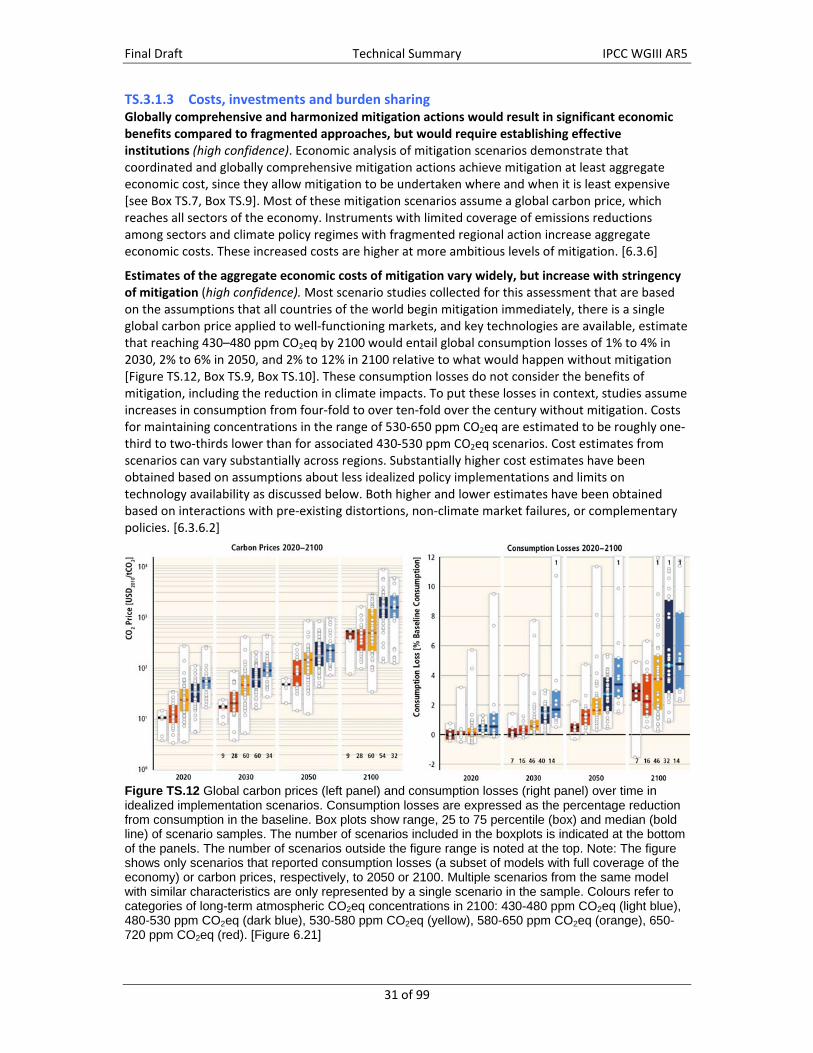
Final Draft Technical Summary IPCC WGIII AR5
31 of 99
TS.3.1.3 Costs, investments and burden sharing Globally comprehensive and harmonized mitigation actions would result in significant economic benefits compared to fragmented approaches, but would require establishing effective institutions (high confidence). Economic analysis of mitigation scenarios demonstrate that coordinated and globally comprehensive mitigation actions achieve mitigation at least aggregate economic cost, since they allow mitigation to be undertaken where and when it is least expensive [see Box TS.7, Box TS.9]. Most of these mitigation scenarios assume a global carbon price, which reaches all sectors of the economy. Instruments with limited coverage of emissions reductions among sectors and climate policy regimes with fragmented regional action increase aggregate economic costs. These increased costs are higher at more ambitious levels of mitigation. [6.3.6]
Estimates of the aggregate economic costs of mitigation vary widely, but increase with stringency of mitigation (high confidence). Most scenario studies collected for this assessment that are based on the assumptions that all countries of the world begin mitigation immediately, there is a single global carbon price applied to well‐functioning markets, and key technologies are available, estimate that reaching 430–480 ppm CO2eq by 2100 would entail global consumption losses of 1% to 4% in 2030, 2% to 6% in 2050, and 2% to 12% in 2100 relative to what would happen without mitigation [Figure TS.12, Box TS.9, Box TS.10]. These consumption losses do not consider the benefits of mitigation, including the reduction in climate impacts. To put these losses in context, studies assume increases in consumption from four‐fold to over ten‐fold over the century without mitigation. Costs for maintaining concentrations in the range of 530‐650 ppm CO2eq are estimated to be roughly one‐third to two‐thirds lower than for associated 430‐530 ppm CO2eq scenarios. Cost estimates from scenarios can vary substantially across regions. Substantially higher cost estimates have been obtained based on assumptions about less idealized policy implementations and limits on technology availability as discussed below. Both higher and lower estimates have been obtained based on interactions with pre‐existing distortions, non‐climate market failures, or complementary policies. [6.3.6.2]
Figure TS.12 Global carbon prices (left panel) and consumption losses (right panel) over time in idealized implementation scenarios. Consumption losses are expressed as the percentage reduction from consumption in the baseline. Box plots show range, 25 to 75 percentile (box) and median (bold line) of scenario samples. The number of scenarios included in the boxplots is indicated at the bottom of the panels. The number of scenarios outside the figure range is noted at the top. Note: The figure shows only scenarios that reported consumption losses (a subset of models with full coverage of the economy) or carbon prices, respectively, to 2050 or 2100. Multiple scenarios from the same model with similar characteristics are only represented by a single scenario in the sample. Colours refer to categories of long-term atmospheric CO2eq concentrations in 2100: 430-480 ppm CO2eq (light blue), 480-530 ppm CO2eq (dark blue), 530-580 ppm CO2eq (yellow), 580-650 ppm CO2eq (orange), 650-720 ppm CO2eq (red). [Figure 6.21]

Final Draft Technical Summary IPCC WGIII AR5
32 of 99
Box TS.9. The meaning of ‘mitigation cost’ in the context of mitigation scenarios.
Mitigation costs represent one component of the change in human welfare from climate change mitigation. Mitigation costs are expressed in monetary terms and generally are estimated against baseline scenarios, which typically involve continued, and sometimes substantial, economic growth and no additional and explicit mitigation efforts [3.9.3, 6.3.6]. Because mitigation cost estimates focus only on direct market effects, they do not take into account the welfare value (if any) of co‐benefits or adverse side‐effects of mitigation actions [Box TS.11, 3.6.3]. Further, these costs do not capture the benefits of reducing climate impacts through mitigation [Box TS.2].
There are a wide variety of metrics of aggregate mitigation costs used by economists, measured in different ways or at different places in the economy, including changes in GDP, consumption losses, equivalent variation and compensating variation, and loss in consumer and producer surplus. Consumption losses are often used as a metric because they emerge from many integrated models and they directly impact welfare.
Mitigation costs need to be distinguished from emissions prices. Emissions prices measure the cost of an additional unit of emissions reduction; that is, the marginal cost. In contrast, mitigation costs usually represent the total costs of all mitigation. In addition, emissions prices can interact with other policies and measures, such as regulatory policies directed at GHG reduction. If mitigation is achieved partly by these other measures, emissions prices may not reflect the actual costs of an additional unit of emissions reductions (depending on how additional emission reductions are induced).
In general, model‐based assessments of global aggregate mitigation costs over the coming century from integrated models are based on largely stylized assumptions about both policy approaches and existing markets and policies, and these assumptions have an important influence on cost estimates. For example, idealized implementation scenarios assume a uniform price on CO2 and other GHGs in every country and sector across the globe, and constitute the least cost approach in the idealized case of largely efficient markets without market failures other than the climate change externality. Most long‐term, global scenarios do not account for the interactions between mitigation and pre‐existing or new policies, market failures, and distortions. Climate policies can interact with existing policies to increase or reduce the actual cost of climate policies. [3.6.3.3, 6.3.6.5]
Delays in mitigation through 2030 or beyond could substantially increase mitigation costs in the decades that follow and the second‐half of the century (high confidence). Although delays by any major emitter will reduce near‐term mitigation costs, they will also result in more investment in carbon‐intensive infrastructure and then rely on future decision makers to undertake a more rapid, deeper, and costlier future transformation from this infrastructure. Studies have found that costs, and associated carbon prices, rise more rapidly to higher levels in scenarios with delayed mitigation compared to scenarios where mitigation is undertaken immediately. Recent modelling studies have found that delayed mitigation through 2030 can substantially increase the mitigation costs of meeting 2100 concentrations between 430 ppmv CO2eq and 530 ppmv CO2eq, particularly in scenarios with emissions greater than 55 GtCO2eq in 2030. Many models could not reach 2100 concentrations levels of 430 to 530 ppm CO2eq from such emission levels in 2030 [Figure TS.13, left panel]. [6.3]
The technological options available for mitigation greatly influence mitigation costs and the challenges of reaching atmospheric concentration levels between 430 and 580 ppm CO2eq by 2100 (high confidence). Many models in recent model intercomparisons could not produce scenarios reaching atmospheric concentrations between 430 and 480 ppm CO2eq by 2100 with broadly pessimistic assumptions about key mitigation technologies. In these studies, the character and availability of CCS and bioenergy were found to have a particularly important influence on the

Final Draft Technical Summary IPCC WGIII AR5
33 of 99
mitigation costs and the challenges of reaching concentration levels in this range. For those models that could produce such scenarios, pessimistic assumptions about these increased discounted global mitigation costs of reaching concentration goals in the range of 430–480 ppm and 530–580 ppm CO2eq by the end of the century significantly, with the effect being larger for more stringent mitigation scenarios. The studies also showed that reducing energy demand could potentially decrease mitigation costs significantly [Figure TS.13, right panel]. [6.3]
Figure TS.13. Left panel shows the relative increase in net present value mitigation costs (2015–2100, discounted at 5% per year) from technology portfolio variations relative to a scenario with default technology assumptions. Scenario names on the horizontal axis indicate the technology variation relative to the default assumptions: No CCS = unavailability of CCS, Nuclear phase out = No addition of nuclear power plants beyond those under construction; existing plants operated until the end of their lifetime; Limited Solar/Wind = 20% limit on solar and wind electricity generation; Limited Bioenergy = maximum of 100 EJ/yr bioenergy supply [Figure 6.24] Right panel shows increase in long-term mitigation costs for the period 2050-2100 (sum over undiscounted costs) as a function of reduced near term mitigation effort, expressed as the relative change between scenarios implementing mitigation immediately and those that correspond to delayed mitigation (referred to here as ‘mitigation gap’). The mitigation gap is defined as the difference in cumulative CO2 emissions reductions until 2030 between the immediate and delayed mitigation scenarios. The bars in the lower right panel indicate the mitigation gap range where 75% of scenarios with 2030 emissions above (dark blue) and below (red) 55 GtCO2, respectively, are found. [Figure 6.25]
Effort‐sharing frameworks can help to clarify discrepancies between the distribution of costs based on mitigation potential and the distribution of responsibilities based on ethical principles, and they can help reconcile those discrepancies through international financial transfers (medium confidence). Studies find that in order to reach concentrations of 430 ppm to 580 ppm CO2eq in 2100 at lowest global cost, the majority of mitigation investments over the course of century will occur in the non‐OECD countries. Studies estimate that the financial transfers to ameliorate this asymmetry could be in the order of hundred billions of USD per year before mid‐century to bring concentrations within the range of 430‐530 ppm CO2eq in 2100. Most studies assume efficient mechanisms for international transfers, in which case economic theory and empirical research

Final Draft Technical Summary IPCC WGIII AR5
34 of 99
suggest that the choice of effort sharing allocations will not meaningfully affect the globally efficient levels of regional abatement or aggregate global costs. The actual implementation of international transfers can deviate from this assumption. [6.3, 13.4.2.4]
Geoengineering denotes two clusters of technologies that are quite distinct: carbon dioxide removal (CDR) and solar radiation management (SRM). Mitigation scenarios assessed in AR5 do not assume any geoengineering options beyond large scale CDR due to afforestation and bioenergy coupled with CCS (BECCS). Carbon dioxide removal techniques include afforestation, using biomass energy along with carbon capture and storage (BECCS), and enhancing uptake of CO2 by the oceans through iron fertilization or increasing alkalinity. Most terrestrial CDR techniques would require large‐scale land‐use changes and could involve local and regional risks, while maritime CDR may involve significant transboundary risks for ocean ecosystems, so that its deployment could pose additional challenges for cooperation between countries. With currently known technologies, CDR could not be deployed quickly on a large scale. Solar radiation management includes various technologies to offset crudely some of the climatic effects of the build‐up of GHGs in the atmosphere. It works by adjusting the planet’s heat balance through a small increase in the reflection of incoming sunlight such as by injecting particles or aerosol precursors in the upper atmosphere. Solar radiation management has attracted considerable attention, mainly because of the potential for rapid deployment in case of climate emergency. The suggestion that deployment costs for individual technologies could potentially be low could result in new challenges for international cooperation because nations may be tempted to prematurely deploy unilaterally systems that are perceived to be inexpensive. Consequently, SRM technologies raise questions about costs, risks, governance, and ethical implications of developing and deploying SRM, with special challenges emerging for international institutions, norms and other mechanisms that could coordinate research and restrain testing and deployment. [1.4, 3.3.7, 6.9, 13.4.4]
Knowledge about the possible beneficial or harmful effects of SRM is highly preliminary. Solar radiation management would have varying impacts on regional climate variables such as temperature and precipitation, and might result in substantial changes in the global hydrological cycle with uncertain regional effects, for example on monsoon precipitation. Non‐climate effects could include possible depletion of stratospheric ozone by stratospheric aerosol injections. A few studies have begun to examine climate and non‐climate impacts of SRM, but there is very little agreement in the scientific community on the results or on whether the lack of knowledge requires additional research or eventually field testing of SRM‐related technologies. [1.4, 3.3.7, 6.9, 13.4.4].

Final Draft Technical Summary IPCC WGIII AR5
35 of 99
Box TS.10. Future goods should be discounted at an appropriate rate
Investments aimed at mitigating climate change will bear fruit far in the future, much of it more than 100 years from now. To decide whether a particular investment is worthwhile, its future benefits need to be weighed against its present costs. In doing this, economists do not normally take a quantity of commodities at one time as equal in value to the same quantity of the same commodities at a different time. They normally give less value to later commodities than to earlier ones. They ‘discount’ later commodities, that is to say. The rate at which the weight given to future goods diminishes through time is known as the ‘discount rate’ on commodities.
There are two types of discount rates used for different purposes. The market discount rate reflects the preferences of presently living people between present and future commodities. The social discount rate is used by society to compare benefits of present members of society with those not yet born. Because living people may be impatient, and because future people do not trade in the market, the market may not accurately reflect the value of commodities that will come to future people relative to those that come to present people. So the social discount rate may differ from the market rate.
The chief reason for social discounting (favouring present people over future people) is that commodities have ‘diminishing marginal benefit’ and per capita income is expected to increase over time. Diminishing marginal benefit means that the value of extra commodities to society declines as people become better off. If economies continue to grow, people who live later in time will on average be better off—possess more commodities—than people who live earlier. The faster the growth and the greater the degree of diminishing marginal benefit, the greater should be the discount rate on commodities. If per capita growth is expected to be negative (as it is in some countries), the social discount rate may be negative.
Some authors have argued, in addition, that the present generation of people should give less weight to later people’s wellbeing just because they are more remote in time. This factor would add to the social discount rate on commodities.
The social discount rate is appropriate for evaluating mitigation projects that are financed by reducing current consumption. If a project is financed partly by ‘crowding out’ other investments, the benefits of those other investments are lost, and their loss must be counted as an opportunity cost of the mitigation project. If a mitigation project crowds out an exactly equal amount of other investment, then the only issue is whether or not the mitigation investment produces a greater return than the crowded‐out investment. This can be tested by evaluating the mitigation investment using a discount rate equal to the return that would have been expected from the crowded out investment. If the market functions well, this will be the market discount rate. [3.6.2]
TS.3.1.4 Implications of transformation pathways for other objectives Recent multi‐objective studies show that mitigation reduces the costs of reaching energy security and/or air quality objectives (medium confidence). The mitigation costs of most of the scenarios in this assessment do not consider the economic implications of the cost reductions for these other objectives [Box TS.9]. There is a wide range of co‐benefits and adverse side‐effects other than air quality and energy security [Tables TS.3.3–3.7]. The impact of mitigation on the overall costs for achieving many of these other objectives as well as the associated welfare implications are less well understood and have not been assessed thoroughly in the literature [Figure TS.14, Box TS.11]. [3.6.3, 4.8, 6.6]
The majority of mitigation scenarios show co‐benefits for energy security objectives, enhancing the sufficiency of resources to meet national energy demand as well as the resilience of the energy supply (medium confidence). The majority of mitigation scenarios show improvements in terms of

Final Draft Technical Summary IPCC WGIII AR5
36 of 99
the diversity of energy sources and reduction of energy imports, resulting in energy systems that are less vulnerable to price volatility and supply disruptions [Figure TS.14]. [6.3.6, 6.6, 7.9, 8.7, 9.7, 10.8, 11.13.6, 12.8]
Mitigation policy may devalue endowments of fossil fuel exporting countries, but differences between regions and fuels exist (medium confidence). There is uncertainty over how climate policies would impact energy export revenues and volumes. The effect on coal exporters is expected to be negative in the short‐ and long‐term as policies could reduce the benefits of using coal as an energy source provided that no cost‐competitive CCS technologies are available. Gas exporters could benefit in the medium term as coal is replaced by gas. The overall impact on oil is more uncertain. Several studies suggest that mitigation policies reduce export revenues from oil. However, some studies find that mitigation policies could increase the relative competitiveness of conventional oil vis‐à‐vis more carbon‐intensive unconventional oil and coal‐to‐liquids. [6.3.6, 6.6, 14.4.2]
Fragmented mitigation policy can provide incentives for emission‐intensive economic activity to migrate away from a region that undertakes mitigation (medium confidence). Scenario studies have shown that such ‘carbon leakage’ rates of energy related emissions to be relatively contained, often below 20% of the emissions reductions. Leakage in land use emissions could be substantial, though fewer studies have quantified it. While border tax adjustments are seen as enhancing the competitiveness of GHG and trade intensive industries within a climate policy regime, they can also entail welfare losses for non‐participating, and particularly developing, countries. [5.4, 6.3, 13.8, 14.4]
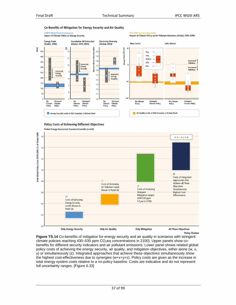
Final Draft Technical Summary IPCC WGIII AR5
37 of 99
Figure TS.14 Co-benefits of mitigation for energy security and air quality in scenarios with stringent climate policies reaching 430–530 ppm CO2eq concentrations in 2100). Upper panels show co-benefits for different security indicators and air pollutant emissions. Lower panel shows related global policy costs of achieving the energy security, air quality, and mitigation objectives, either alone (w, x, y) or simultaneously (z). Integrated approaches that achieve these objectives simultaneously show the highest cost-effectiveness due to synergies (w+x+y>z). Policy costs are given as the increase in total energy system costs relative to a no-policy baseline. Costs are indicative and do not represent full uncertainty ranges. [Figure 6.33]
Final Draft Technical Summary IPCC WGIII AR5
38 of 99
Mitigation scenarios leading to atmospheric concentration levels between 430 and 530 ppm CO2eq in 2100 are associated with significant co‐benefits for air quality, human health and ecosystem outcomes. Associated welfare gains are expected to be particularly high where currently legislated and planned air pollution controls are weak (high confidence). Stringent mitigation policies result in co‐controls with major cuts in air pollutant emissions significantly below baseline scenarios (Figure TS.14). Co‐benefits for health are particularly high in today’s developing world. The extent to which air pollution policies, targeting for example black carbon, can mitigate climate change is uncertain and subject to scientific debate. [WGIII 5.7, 6.3, 6.6, 7.9, 8.7, 9.7, 10.8, 11.7, 11.13.6, 12.8; WGII 11.9]
Potential adverse side‐effects of mitigation due to higher energy prices, for example, on improving access of the poor to clean, reliable, and affordable energy services, can be avoided (medium confidence). Whether mitigation scenarios will have adverse distributional effects and thus impede achieving energy access objectives will depend on the climate policy design and the extent to which complementary policies are in place to support the poor. About 1.3 billion people worldwide do not have access to electricity and about 3 billion are dependent on traditional solid fuels for cooking and heating with adverse effects on development, ecosystems and severe health implications. Scenario studies show that the costs for achieving nearly universal access are between USD 72–95 billion per year until 2030. The contribution of renewable energy‐to‐energy access can be substantial. Achieving universal energy access reduces air pollutants emissions, such as sulfur dioxide (SO2),
nitrogen oxides (NOx), carbon monoxide (CO), and black carbon (BC), and yields large health benefits but only negligibly higher GHG emissions from power generation. [4.3, 6.6, 7.9, 9.7, 11.13.6, 16.8]
The effect of mitigation on water use depends on technological choices and the portfolio of mitigation measures (high confidence). While the switch from fossil energy to renewable energy like solar photovoltaic (PV) or wind can help reducing water use of the energy system, deployment of other renewables, such as some forms of hydropower, concentrated concentrated solar power, and bioenergy may have adverse effects on water use. [6.6, 7.9, 9.7, 10.8, 11.7, 11.13.6]
Transformation pathways and sectoral studies show that the number of co‐benefits for energy end use mitigation measures outweighs the number of the adverse side‐effects, whereas the evidence suggests this is not the case for all supply‐side measures (high confidence). [Tables TS.3.2.2‐3.2.6; Sections 4.8, 5.7, 6.6, 7.9, 8.7, 9.7, 10.8, 11.7, 11.13.6, 12.8]

Final Draft Technical Summary IPCC WGIII AR5
39 of 99
Box TS.11. Accounting for the co-benefits and adverse side-effects of mitigation
A government policy or a measure intended to achieve one objective (such as mitigation) will also affect other objectives (such as local air quality). To the extent these side‐effects are positive, they can be deemed ‘co‐benefits’; otherwise they are termed ‘adverse side‐effects’. In this report, co‐benefits and adverse side‐effects are measured in non‐monetary units. Determining the value of these effects to society is a separate issue. The effects of co‐benefits on social welfare are not evaluated in most studies, and one reason is that the value of a co‐benefit depends on local circumstances and can be positive, zero, or even negative. For example, the value of the extra tonne of SO2 reduction that occurs with mitigation depends greatly on the stringency of existing SO2 control policies: in the case of weak existing SO2 policy, the value of SO2 reductions may be large, but in the case of stringent existing SO2 policy it may be near zero. If SO2 policy is too stringent, the value of the co‐benefit may be negative (assuming SO2 policy is not adjusted). While climate policy affects non‐climate objectives [Tables TS.3.2.2–3.2.6] other policies also affect climate change outcomes. [3.6.3, 4.8, 6.6, Annex I]
Mitigation can have many potential co‐benefits and adverse side‐effects, which makes comprehensive analysis difficult. The direct benefits of climate policy include, for example, intended effects on global mean surface temperature, sea level rise, agricultural productivity, biodiversity, and health effects of global warming [WGII TS]. The co‐benefits and adverse side‐effects of climate policy could include effects on a partly overlapping set of objectives such as local air pollutant emissions and related health and ecosystem impacts, energy security, income distribution, efficiency of the taxation system, labour supply and employment, urban sprawl, and the sustainability of the growth of developing countries [3.6, 4.8, 6.6, 15.2].
All these side‐effects are important, because a comprehensive evaluation of climate policy needs to account for benefits and costs related to other objectives. If overall social welfare is to be determined and quantified, this would require valuation methods and a consideration of pre‐existing efforts to attain the many objectives. Valuation is made difficult by factors such as interaction between climate policies and pre‐existing non‐climate policies, externalities, and non‐competitive behaviour. [3.6.3]
TS.3.2 Sectoral and cross‐sectoral mitigation measures
Anthropogenic greenhouse gas emissions result from a broad set of human activities, most notably those associated with energy supply and consumption and with the use of land for food production and other purposes. A large proportion of emissions arise in urban areas. Mitigation options can be grouped into three broad sectors: 1) energy supply, 2) energy end‐use sectors including transport, buildings, industry, and 3) agriculture, forestry, and other land use (AFOLU). Emissions from human settlements and infrastructures cut across these different sectors. Many mitigation options are linked. The precise set of mitigation actions taken in any sector will depend on a wide range of factors, including their relative economics, policy structures, normative values, and linkages to other policy objectives. The first section examines issues that cut across the sectors and the following subsections examine the sectors themselves.
TS.3.2.1 Cross‐sectoral mitigation pathways and measures Without new mitigation policies GHG emissions are projected to grow in all sectors, except for CO2 emissions in the land‐use sector (robust evidence, medium agreement). Energy supply sector emissions are expected to continue to be the major source of GHG emissions in baseline scenarios. As a result, significant increases in indirect emissions from electricity use in buildings and the industry sector are expected. Deforestation decreases in most of the baseline scenarios, which leads

Final Draft Technical Summary IPCC WGIII AR5
40 of 99
to a decline in CO2 emissions from the land‐use sector. In some scenarios the land‐use sector changes from an emission source to a net emission sink around 2050. (Figure TS.15)
Figure TS.15. Direct (left panel) and direct and indirect emissions (right panel) of CO2 and non-CO2 GHGs across sectors in baseline scenarios. Non CO2 GHGs are converted to CO2 equivalents using 100-year global warming potentials from the IPCC SAR (see Box TS.5). Note that in the case of indirect emissions, only electricity emissions are allocated from energy supply to end-use sectors. The numbers at the bottom refer to the number of scenarios included in the ranges that differ across sectors and time due to different sectoral resolution and time horizon of models. [Figure 6.34]
Infrastructure developments and long‐lived products that lock societies into GHG intensive emissions pathways may be difficult or very costly to change (robust evidence, high agreement). This lock‐in risk is compounded by the lifetime of the infrastructure, by the difference in emissions associated with alternatives, and the magnitude of the investment cost. As a result, land‐use planning related lock‐in is the most difficult to eliminate, and thus avoiding options that lock high emission patterns in permanently is an important part of mitigation strategies in regions with rapidly developing infrastructure. In mature or established cities, options are constrained by existing urban forms and infrastructure, and limits on the potential for refurbishing or altering them. However, longer lifetimes of low‐emission products and infrastructure can ensure positive lock‐in as well as avoid emissions through dematerialization (i.e. through reducing the total material inputs required to deliver a final service). [5.6.3, 9.4, 12.3, 12.4]
Systemic and cross‐sectoral approaches to mitigation are expected to be more cost‐effective and more effective in cutting emissions than sector‐by‐sector policies (medium confidence). Cost‐effective mitigation policies need to employ a system perspective in order to account for inter‐dependencies among different economic sectors and to maximize synergistic effects. Stabilizing atmospheric CO2eq concentrations at any level will ultimately require deep reductions in emissions and fundamental changes to both the end‐use and supply‐side of the energy system as well as changes in land‐use practices and industrial processes. In addition, many low‐carbon energy supply technologies (including CCS) and their infrastructural requirements face public acceptance issues limiting their deployment. This applies also to the adoption of new technologies, and structural and behavioural change, in the energy end‐use sectors (robust evidence, high agreement) [7.9.4, 8.7,

Final Draft Technical Summary IPCC WGIII AR5
41 of 99
9.3.10, 9.8, 10.8, 11.3, 11.13]. Lack of acceptance may have implications not only for mitigation in that particular sector, but also for wider mitigation efforts.
Integrated models identify three categories of energy system related mitigation measures: the decarbonization of the energy supply sector, final energy demand reductions, and the switch to low‐carbon fuels, including electricity, in the energy end use sectors (robust evidence, high agreement) [6.3.4, 6.8, 7.11]. The broad range of sectoral mitigation options available mainly relate to achieving reductions in GHG emissions intensity, energy intensity and changes in activity (Table TS.2) [7.5, 8.3, 8.4, 9.3, 10.4, 12.4]. Direct options in AFOLU involve storing carbon in terrestrial systems (for example, through afforestation) and providing bioenergy feedstocks [11.3, 11.13]. Options to reduce non‐CO2 emissions exist across all sectors, but most notably in agriculture, energy supply, and industry.
Demand reductions in the energy end‐use sectors are a key mitigation strategy and affect the scale of the mitigation challenge for the energy supply side (high confidence). Limiting energy demand: 1) increases policy choices by maintaining flexibility in the technology portfolio; 2) reduces the required pace for up‐scaling low‐carbon energy supply technologies and hedges against related supply side risks (Figure TS.16); 3) avoids lock‐in to new, or potentially premature retirement of, carbon‐intensive infrastructures; 4) maximizes co‐benefits for other policy objectives, since the number of co‐benefits for energy end‐use measures outweighs the adverse side‐effects which is not the case for all supply‐side measures (see Tables TS.3–7); and 5) increases the cost effectiveness of the transformation (as compared to mitigation strategies with higher levels of energy demand) (medium confidence). However, energy service demand reductions are unlikely in developing countries or for poorer population segments whose energy service levels are low or partially unmet. [6.3.4, 6.6, 7.11, 10.4]

Final Draft Technical Summary IPCC WGIII AR5
42 of 99
Figure TS.16. Influence of energy demand on the deployment of energy supply technologies in 2050 in mitigation scenarios reaching 430–530 ppm CO2eq concentrations by 2100. Blue bars for ‘low energy demand’ show the deployment range of scenarios with limited growth of final energy of <20% in 2050 compared to 2010. Red bars show the deployment range of technologies in case of ‘high energy demand’ (>20% growth in 2050 compared to 2010). For each technology, the median, interquartile, and full deployment range is displayed. Notes: Scenarios assuming technology restrictions are excluded. Ranges include results from many different integrated models. Multiple scenario results from the same model were averaged to avoid sampling biases; see Chapter 6 for further details. [Figure 7.11]
Behaviour, lifestyle, and culture have a considerable influence on energy use and associated emissions, and can have a high mitigation potential through complementing technological and structural change (limited evidence, medium agreement). Emissions can be substantially lowered through: changes in consumption patterns (e.g., mobility demand, energy use in households, choice of longer‐lasting products); dietary change and reduction in food wastes; and change of lifestyle (e.g., stabilizing/lowering consumption in some of the most developed countries, sharing economy and other behavioural changes affecting activity) (Table TS.2). [8.1, 8.9, 9.2, 9.3, Box 10.2, 10.4, 11.4, 12.4, 12.6, 12.7]
Evidence from mitigation scenarios indicates that the decarbonization of energy supply is a key requirement for stabilizing atmospheric CO2eq concentrations below 580ppm (robust evidence, high agreement). In most long‐term mitigation scenarios not exceeding 580ppm CO2eq by 2100, global energy supply is fully decarbonized at the end of the twenty‐first century with many scenarios relying on a net removal of CO2 from the atmosphere. However, because existing supply systems are largely reliant on carbon intensive fossil fuels, energy intensity reductions can equal or outweigh decarbonization of energy supply in the near‐term. In the buildings and industry sector, for example, efficiency improvements are an important strategy for reducing indirect emissions from electricity generation (Figure TS.15). In the long term, the reduction in electricity emissions is accompanied by an increase in the share of electricity in end uses (e.g., for space and process heating, potentially for some modes of transport). Deep emissions reductions in transport are generally the last to emerge in integrated modelling studies because of the limited options to switch to low‐carbon energy

Final Draft Technical Summary IPCC WGIII AR5
43 of 99
carriers compared to buildings and industry (Figure TS.17). [6.3.4, 6.8, 8.9, 9.8, 10.10, 7.11, Figure 6.17]
The availability of carbon dioxide removal technologies affects the size of the mitigation challenge for the energy end‐use sectors (robust evidence, high agreement) [6.8, 7.11]. There are strong interdependencies between the required pace of decarbonization of energy supply and end‐use sectors. The more rapid decarbonization of supply generally provides more flexibility for the end‐use sectors. However, barriers to decarbonizing the supply side, resulting for example from a limited availability of CCS to achieve negative emissions when combined with bioenergy, require a more rapid and pervasive decarbonisation of the energy end‐use sectors in scenarios achieving low CO2eq concentration levels (Figure TS.17). The availability of mature large‐scale energy generation or carbon sequestration technologies in the AFOLU sector also provides flexibility for the development of mitigation technologies in the energy supply and energy end‐use sectors [11.3] (limited evidence, medium agreement), though there may be adverse impacts on sustainable development.
Figure TS.17. Direct emissions of CO2 and non-CO2 GHGs across sectors in mitigation scenarios that reach around 450 (430-480) ppm CO2eq concentrations in 2100 with using CCS (left panel) and without using CCS (right panel). The numbers at the bottom of the graphs refer to the number of scenarios included in the ranges that differ across sectors and time due to different sectoral resolution and time horizon of models. [Figures 6.35]
Spatial planning can contribute to managing the development of new infrastructure and increasing system‐wide efficiencies across sectors (robust evidence, high agreement). Land use, transport choice, housing, and behaviour are strongly interlinked and shaped by infrastructure and urban form. Spatial and land use planning, such as mixed use zoning, transport‐oriented development, increasing density, and co‐locating jobs and homes can contribute to mitigation across sectors by a) reducing emissions from travel demand for both work and leisure, and enabling non‐motorized transport, b) reducing floor space for housing, and hence c) reducing overall direct and indirect energy use through efficient infrastructure supply. Compact and in‐fill development of urban spaces and intelligent densification can save land for agriculture and bioenergy and preserve land carbon stocks. [8.4, 9.10, 10.5, 11.10, 12.2, 12.3]
Interdependencies exist between adaptation and mitigation at the sectoral level and there are benefits from considering adaptation and mitigation in concert (medium evidence, high agreement). Particular mitigation actions can affect sectoral climate vulnerability, both by

Final Draft Technical Summary IPCC WGIII AR5
44 of 99
influencing exposure to impacts and by altering the capacity to adapt to them [8.5, 11.5]. Other interdependencies include climate impacts on mitigation options, such as forest conservation or hydropower production [11.5.5, 7.7], as well as the effects of particular adaptation options, such as heating or cooling of buildings or establishing more diversified cropping systems in agriculture, on GHG emissions and radiative forcing [11.5.4, 9.5]. There is a growing evidence base for such interdependencies in each sector, but there are substantial knowledge gaps that prevent the generation of integrated results at the cross‐sectoral level.

Final Draft Technical Summary IPCC WGIII AR5
45 of 99
Table TS.2: Main sectoral mitigation measures categorized by key mitigation strategies (in bold) and associated sectoral indicators (highlighted in grey) 1
2
GHG emission intensity reduction Energy intensity reduction by improving technical efficiency
Production and resource efficiency improvement
Structural and systems efficiency improvement
Activity indicator change
Energy
Emissions / secondary energy output Energy input / energy output Embodied energy / energy output Final energy use
Greater deployment of RES, nuclear energy, and (BE)CCS; fuel switching within the group of fossil fuels; reduction of fugitive (methane) emissions in the fossil fuel chain
Extraction, transport, conversion of fossil fuels; electricity, heat, fuel transmission, distribution, and storage; CHP (cogeneration, see Buildings)
Energy embodied in manufacturing of energy extraction, conversion, transmission and distribution technologies
Addressing integration needs Demand from end‐use sectors for different energy carriers (see Transport, Buildings and Industry)
Transport
Emissions / final energy Final energy/transport service Shares for each mode Total distance per year
Fuel carbon intensity (CO2eq/MJ): Fuel switching to low‐carbon fuels (e.g., electricity/hydrogen from low‐carbon sources (see Energy); specific biofuels in various modes (see AFOLU)
Energy intensity (MJ/p‐km, t‐km): Fuel‐efficient engines and vehicle designs; more advanced propulsion systems and designs; use of lighter materials in vehicles
Embodied emissions during vehicle manufacture, material efficiency; and recycling of materials (see Industry); infrastructure lifecycle emissions (see Human Settlements)
Modal shifts from LDVs to public transit, cycling/walking, and from aviation and HDVs to rail; eco‐driving; improved freight logistics; transport (infrastructure) planning
Journey avoidance; higher occupancy/loading rates; reduced transport demand; urban planning (see Human Settlements)
Build
ings
Emissions / final energy Final energy / useful energy Embodied energy / operating energy Useful energy / energy service Energy service demand
Fuel carbon intensity (CO2eq/MJ): Building integrated RES; fuel switching to low‐carbon fuels, e.g., electricity (see Energy)
Device efficiency: heating/ cooling (high‐performance boilers, ventilation, air‐conditioning, heat pumps), water heating, cooking (advanced biomass stoves), lighting, appliances
Building lifetime; component, equipment,and appliance durability; low(er) energy & emission material choice for construction (see Industry)
Systemic efficiency: integrated design process; low/zero energy buildings; building automation and controls; urban planning; district heating/cooling and CHP; smart meters/grids; commissioning
Behavioural change (e.g., thermostat setting, appliance use); lifestyle change (e.g., per capita dwelling size, adaptive comfort)
Industry
Emissions / Final energy Final energy / material production Material input / product output Product demand / service demand Service demand
Emissions intensity: Process emissions reductions; use of waste (e.g., MSP/ sewage sludge in cement kilns) and CCS in industry; HFC replacement and leak repair; fuel switching among fossil fuels, to low‐carbon electricity (see Energy) or biomass (see AFOLU)
Energy efficiency/BAT: Efficient steam systems; furnace and boiler systems; electric motor (pumps, fans, air compressor, refrigerators, and materialhandling) and electronic control systems; (waste) heat exchanges; recycling
Material efficiency: Reducing yield losses; manufacturing/construction: process innovations, new design approaches, re‐using old material (e.g., structural steel); product design (e.g., light weight car design); fly ash substituting clinker
Product‐service efficiency: More intensive use of products (e.g., car sharing, using products such as clothing for longer, new and more durable products)
Reduced demand for, e.g., products such as clothing; alternative forms of travel leading to reduced demand for car manufacturing
Human
Settlements Emissions / Final energy Final energy / useful energy Material input in infrastructure Useful energy / energy service Service demand per capita
Integration of urban renewables; urban scale fuel switching programmes
Cogeneration, heat cascading, waste to energy
Managed infrastructure supply; reduce primary materials input for infrastructure
Compact urban form; increased accessibility; mixed land use
Increasing accessibility: shorter travel time, more transport mode options
Agriculture, Forestry
and other Land use
Supply‐side improvements Demand‐side measures
Emissions / area or unit product (conserved, restored) Animal/crop product consumption per capita
Emission reduction: of methane (e.g., livestock management) and nitrous oxide (fertilizer and manure management) and prevention of emissions to the atmosphere by conserving existing carbon pools in soils or vegetation (reducing deforestation and forest degradation, fire prevention/control, agroforestry), reduced emissions intensity (GHG/unit product).
Sequestration: Increasing the size of existing carbon pools, and thereby extracting carbon dioxide from the atmosphere (e.g., afforestation, reforestation, integrated systems, carbon sequestration in soils)
Substitution: of biological products for fossil fuels or energy‐intensive products, thereby reducing CO2 emissions, e.g., biomass co‐firing/CHP (see Energy), biofuels (see Transport), biomass‐based stoves, insulation products (see Buildings)
Demand‐side measures: Reducing losses and wastes of food, changes in human diets towards less emission‐intensive products, use of long‐lived wood products)
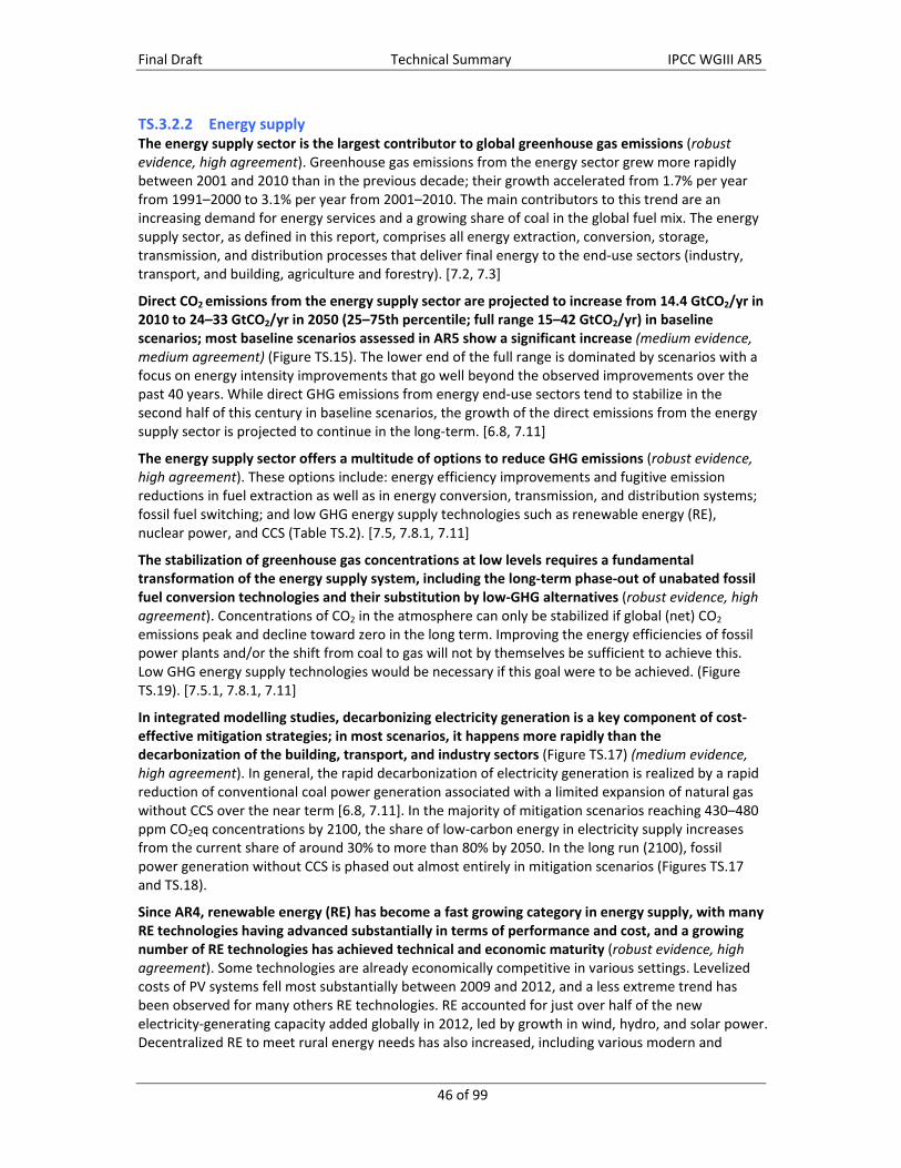
Final Draft Technical Summary IPCC WGIII AR5
46 of 99
TS.3.2.2 Energy supply The energy supply sector is the largest contributor to global greenhouse gas emissions (robust evidence, high agreement). Greenhouse gas emissions from the energy sector grew more rapidly between 2001 and 2010 than in the previous decade; their growth accelerated from 1.7% per year from 1991–2000 to 3.1% per year from 2001–2010. The main contributors to this trend are an increasing demand for energy services and a growing share of coal in the global fuel mix. The energy supply sector, as defined in this report, comprises all energy extraction, conversion, storage, transmission, and distribution processes that deliver final energy to the end‐use sectors (industry, transport, and building, agriculture and forestry). [7.2, 7.3]
Direct CO2 emissions from the energy supply sector are projected to increase from 14.4 GtCO2/yr in 2010 to 24–33 GtCO2/yr in 2050 (25–75th percentile; full range 15–42 GtCO2/yr) in baseline scenarios; most baseline scenarios assessed in AR5 show a significant increase (medium evidence, medium agreement) (Figure TS.15). The lower end of the full range is dominated by scenarios with a focus on energy intensity improvements that go well beyond the observed improvements over the past 40 years. While direct GHG emissions from energy end‐use sectors tend to stabilize in the second half of this century in baseline scenarios, the growth of the direct emissions from the energy supply sector is projected to continue in the long‐term. [6.8, 7.11]
The energy supply sector offers a multitude of options to reduce GHG emissions (robust evidence, high agreement). These options include: energy efficiency improvements and fugitive emission reductions in fuel extraction as well as in energy conversion, transmission, and distribution systems; fossil fuel switching; and low GHG energy supply technologies such as renewable energy (RE), nuclear power, and CCS (Table TS.2). [7.5, 7.8.1, 7.11]
The stabilization of greenhouse gas concentrations at low levels requires a fundamental transformation of the energy supply system, including the long‐term phase‐out of unabated fossil fuel conversion technologies and their substitution by low‐GHG alternatives (robust evidence, high agreement). Concentrations of CO2 in the atmosphere can only be stabilized if global (net) CO2 emissions peak and decline toward zero in the long term. Improving the energy efficiencies of fossil power plants and/or the shift from coal to gas will not by themselves be sufficient to achieve this. Low GHG energy supply technologies would be necessary if this goal were to be achieved. (Figure TS.19). [7.5.1, 7.8.1, 7.11]
In integrated modelling studies, decarbonizing electricity generation is a key component of cost‐effective mitigation strategies; in most scenarios, it happens more rapidly than the decarbonization of the building, transport, and industry sectors (Figure TS.17) (medium evidence, high agreement). In general, the rapid decarbonization of electricity generation is realized by a rapid reduction of conventional coal power generation associated with a limited expansion of natural gas without CCS over the near term [6.8, 7.11]. In the majority of mitigation scenarios reaching 430–480 ppm CO2eq concentrations by 2100, the share of low‐carbon energy in electricity supply increases from the current share of around 30% to more than 80% by 2050. In the long run (2100), fossil power generation without CCS is phased out almost entirely in mitigation scenarios (Figures TS.17 and TS.18).
Since AR4, renewable energy (RE) has become a fast growing category in energy supply, with many RE technologies having advanced substantially in terms of performance and cost, and a growing number of RE technologies has achieved technical and economic maturity (robust evidence, high agreement). Some technologies are already economically competitive in various settings. Levelized costs of PV systems fell most substantially between 2009 and 2012, and a less extreme trend has been observed for many others RE technologies. RE accounted for just over half of the new electricity‐generating capacity added globally in 2012, led by growth in wind, hydro, and solar power. Decentralized RE to meet rural energy needs has also increased, including various modern and

Final Draft Technical Summary IPCC WGIII AR5
47 of 99
advanced traditional biomass options as well as small hydropower, PV, and wind. Nevertheless, many RE technologies still need direct support (e.g., feed‐in tariffs (FITs), RE quota obligations, and tendering/bidding) and/or indirect support (e.g., sufficiently high carbon prices and the internalization of other externalities), if their market shares are to be increased. Additional enabling policies are needed to address their integration into future energy systems. (medium evidence, medium agreement) (Figure TS.18) [7.5.3, 7.6.1, 7.8.2, 7.12, 11.13]
Figure TS.18. Share of low-carbon energy in total primary energy, electricity and liquid supply sectors for the year 2050. Dashed horizontal lines show the low-carbon share for the year 2010. Low-carbon energy includes nuclear, renewables, and fossil fuels with CCS. [Figure 7.14]
The use of RE is often associated with co‐benefits, including the reduction of air pollution, local employment opportunities, few severe accidents compared to some other energy supply technologies, as well as improved energy access and security (medium evidence, medium agreement) (Table TS.3). At the same time, however, some RE technologies can have technology and location‐specific adverse side‐effects, which can be reduced to a degree through appropriate technology selection, operational adjustments, and siting of facilities. [7.9]
Infrastructure and integration challenges vary by RE technology and the characteristics of the existing energy system (medium evidence, medium agreement). Operating experience and studies of medium to high penetrations of RE indicate that integration issues can be managed with various technical and institutional tools. As RE penetrations increase, such issues are more challenging, must be carefully considered in energy supply planning and operations to ensure reliable energy supply, and may result in higher costs. [7.6, 7.8.2]
Nuclear energy is a mature low GHG emission technology but its share in world power generation has continued to decline (robust evidence, high agreement) (Figure TS.19). Nuclear electricity accounted for 11% of the world’s electricity generation in 2012, down from a high of 17% in 1993. Pricing the externalities of GHG emissions (carbon pricing) could improve the competitiveness of nuclear power plants. [7.2, 7.5.4, 7.8.1]
Barriers to an increasing use of nuclear energy include concerns about operational safety and (nuclear weapon) proliferation risks, unresolved waste management issues, as well as financial and regulatory risks (robust evidence, high agreement) (Table TS.3). New fuel cycles and reactor technologies addressing some of these issues are under development. Investigation of mitigation scenarios not exceeding 580 ppm CO2eqhas shown that excluding nuclear power from the available portfolio of technologies would result in only a slight increase in mitigation costs compared to the full technology portfolio (Figure TS.13). If other technologies, such as CCS, are also constrained the role of nuclear power expands. [6.3.6, 7.5.4, 7.8.2, 7.9, 7.11]
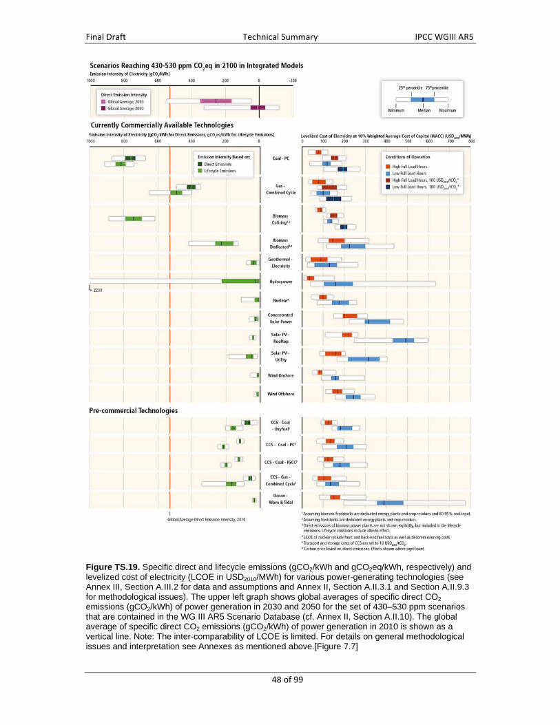
Final Draft Technical Summary IPCC WGIII AR5
48 of 99
Figure TS.19. Specific direct and lifecycle emissions (gCO2/kWh and gCO2eq/kWh, respectively) and levelized cost of electricity (LCOE in USD2010/MWh) for various power-generating technologies (see Annex III, Section A.III.2 for data and assumptions and Annex II, Section A.II.3.1 and Section A.II.9.3 for methodological issues). The upper left graph shows global averages of specific direct CO2 emissions (gCO2/kWh) of power generation in 2030 and 2050 for the set of 430–530 ppm scenarios that are contained in the WG III AR5 Scenario Database (cf. Annex II, Section A.II.10). The global average of specific direct CO2 emissions (gCO2/kWh) of power generation in 2010 is shown as a vertical line. Note: The inter-comparability of LCOE is limited. For details on general methodological issues and interpretation see Annexes as mentioned above.[Figure 7.7]

Final Draft Technical Summary IPCC WGIII AR5
49 of 99
Where natural gas is available and the fugitive emissions associated with its extraction and supply are low, near‐term GHG emissions from energy supply can be reduced by replacing coal‐fired with highly efficient natural gas combined cycle (NGCC) power plants or combined heat and power (CHP) plants (robust evidence, high agreement). In mitigation scenarios reaching 430‐480 ppm CO2eq concentrations by 2100, the contribution of natural gas power generation without CCS is below current levels in 2050 and further declines in the second half of the century (medium evidence, medium agreement). [7.5.1, 7.8, 7.9, 7.11, 7.12]
Carbon dioxide capture and storage (CCS) technologies could reduce the specific CO2eq lifecycle emissions of fossil fuel power plants (medium evidence, medium agreement). Although CCS has not yet been applied at scale to a large, commercial fossil‐fired power generation facility, all of the components of integrated CCS systems exist and are in use in various parts of the fossil energy chain. Carbon dioxide capture and storage power plants will only become competitive with their unabated counterparts if the additional investment and operational costs faced by CCS plants are compensated (e.g., by direct support or sufficiently high carbon prices). Beyond economic incentives, well‐defined regulations concerning short‐ and long‐term responsibilities for storage are essential for a large‐scale future deployment of CCS. [7.5.5]
Barriers to large‐scale deployment of CCS technologies include concerns about the operational safety and long‐term integrity of CO2 storage, as well as risks related to transport and the required upscaling of infrastructure (limited evidence, medium agreement) (Table TS.3). There is, however, a growing body of literature on how to ensure the integrity of CO2 wells, on the potential consequences of a CO2 pressure build‐up within a geologic formation (such as induced seismicity), and on the potential human health and environmental impacts from CO2 that migrates out of the primary injection zone. [7.5.5, 7.9, 7.11]
Combining bioenergy and carbon dioxide capture and storage (BECCS) could result in net removal of CO2 from the atmosphere (limited evidence, medium agreement). Until 2050, bottom‐up studies estimate the economic potential to be between 2–10 GtCO2 per year [11.13]. Some mitigation scenarios show higher deployment of BECCS towards the end of the century. Technological challenges and risks include those associated with the provision of the biomass feedstock, as well as with the capture, transport, and long‐term storage of CO2. Currently, no large‐scale projects have been financed. [6.9, 7.5.5, 7.9, 11.13]

Final Draft Technical Summary IPCC WGIII AR5
50 of 99
Table TS.3: Overview of potential co-benefits (green arrows) and adverse side-effects (orange arrows) of the main mitigation measures in the energy supply sector; arrows pointing up/down denote a positive/negative effect on the respective objective or concern; a question mark (?) denotes an uncertain net effect. Co-benefits and adverse side-effects depend on local circumstances as well as on the implementation practice, pace, and scale (see Table 7.3). For an assessment of macroeconomic, cross-sectoral, effects associated with mitigation policies (e.g., on energy prices, consumption, growth, and trade), see e.g., Sections 3.9, 6.3.6, 13.2.2.3 and 14.4.2. The uncertainty qualifiers in brackets denote the level of evidence and agreement on the respective effects (see TS.1). Abbreviations for evidence: l=limited, m=medium, r=robust; for agreement: l=low, m=medium, h=high.
Energy Supply Effect on additional objectives/concerns
Economic Social Environmental Other
For possible upstream effects of biomass supply for bioenergy, see Table TS.7.
Nuclear replacing coal
↑
↑
↑
Energy security (reduced exposure to fuel price volatility) (m/m)
Local employment impact (but uncertain net effect) (l/m)
Legacy cost of waste and abandoned reactors (m/h)
↓↑
↑
Health impact via
Air pollution and coal mining accidents (m/h) Nuclear accidents and waste treatment, uranium mining and milling (m/l)
Safety and waste concerns (r/h)
↓↑
Ecosystem impact via
Air pollution (m/h) and coal mining (l/h) Nuclear accidents (m/m)
Proliferation risk (m/m)
RE (Wind, PV, CSP, hydro, geothermal, bioenergy) replacing coal
↑
↑
↑
↑
Energy security (resource sufficiency, diversity in the near/medium term) (r/m)
Local employment impact (but uncertain net effect) (m/m)
Irrigation, flood control, navigation, water availability (for reservoirs and regulated rivers)(m/h)
Extra measures to match demand (for PV, windand some CSP) (r/h)
↓↓
↑
?
↑
Health impact via
Air pollution (except bioenergy) (r/h) Coal mining accidents (m/h)
Contribution to (off‐grid) energy access (m/l)
Project‐specific public acceptance concerns (e.g., visibility of wind) (l/m)
Threat of displacement (for large hydro) (m/h)
↓↓↑↑
↓
↑
Ecosystem impact via
Air pollution (except bioenergy) (m/h) Coal mining (l/h) Habitat impact (for some hydro) (m/m) Landscape and wildlife impact (for wind) m/m)
Water use (for wind and PV) (m/m)
Water use (for bioenergy, CSP, geothermal, and reservoir hydro) (m/h)
Higher use of critical metals for PV and direct drive wind turbines (r/m)
Fossil CCS replacing coal
↑↑ Preservation vs lock‐in of human and physical capital in the fossil industry (m/m)
↑↑
↑
Health impact via
Risk of CO2 leakage (m/m) Upstream supply‐chain activities (m/h)
Safety concerns (CO2 storage and transport) (m/h)
↑
↑
Ecosystem impact via upstream supply‐chain activities (m/m)
Water use (m/h)
Long‐term monitoring of CO2 storage (m/h)
BECCS replacing coal See fossil CCS where applicable. For possible upstream effect of biomass supply, see Table TS.7.
Methane leakage prevention, capture or treatment
↑ Energy security (potential to use gas in some cases) (l/h)
↓
↑
Health impact via reduced air pollution (m/m)
Occupational safety at coal mines (m/m)
↓ Ecosystem impact via reduced air pollution (l/m)

Final Draft Technical Summary IPCC WGIII AR5
51 of 99
TS.3.2.3 Transport Since AR4, emissions in the transport sector have grown in spite of more efficient vehicles (road, rail, watercraft, and aircraft) and policies being adopted (robust evidence, high agreement). Road transport dominates overall emissions but aviation could play an increasingly important role in total CO2 emissions in the future. [8.1, 8.3, 8.4]
Direct CO2 emissions from transport are projected to increase from 6.7 GtCO2/yr in 2010 to 9.3–12 GtCO2/yr in 2050 (25–75
th percentile; full range 6.2–16 GtCO2/yr) in baseline scenarios; most of the baseline scenarios assessed in AR5 foresee a significant increase (medium evidence/medium agreement) (Figure TS.15). Without aggressive and sustained mitigation policies being implemented, transport sector emissions could increase faster than in the other energy end‐use sectors and could lead to more than a doubling of CO2 emissions by 2050. [6.8, 8.9, 8.10]
While the continuing growth in passenger and freight activity constitutes a challenge for future emission reductions, analyses of both sectoral and integrated studies suggest a higher mitigation potential in the transport sector than in the AR4 (medium evidence, medium agreement). Transport energy demand per capita in developing and emerging economies is far lower than in Organisation for Economic Co‐operation and Development (OECD) countries but is expected to increase at a much faster rate in the next decades due to rising incomes and the development of infrastructure. Baseline scenarios thus show increases in transport energy demand from 2010 out to 2050 and beyond. However, sectoral and integrated mitigation scenarios indicate that energy demand reductions of 10–45% are possible by 2050 relative to baseline (Figure TS.20, left panel) (medium evidence, medium agreement). [6.8.4, 8.9.1, 8.9.4, 8.10, Figure 8.9.4]
Figure TS.20. Final energy demand reduction relative to baseline (left panel) and development of final low carbon energy carrier share in final energy (including electricity, hydrogen, and liquid biofuels; right panel) in transport by 2030 and 2050 in mitigation scenarios from three different CO2eq concentrations ranges shown in box plots (see Section 6.3.2) compared to sectoral studies shown in shapes assessed in Chapter 8. Filled circles correspond to sectoral studies with full sectoral coverage. [Figures 6.37 and 6.38]

Final Draft Technical Summary IPCC WGIII AR5
52 of 99
A combination of low‐carbon fuels, the uptake of improved vehicle and engine performance technologies, behavioural change leading to avoided journeys and modal shifts, investments in related infrastructure and changes in the built environment, together offer a high mitigation potential (high confidence) [8.3, 8.8]. Direct (tank‐to‐wheel) GHG emissions from passenger and freight transport can be reduced by:
using fuels with lower carbon intensities (CO2eq/MJ);
lowering vehicle energy intensities (MJ/passenger km or MJ/tonne km);
encouraging modal shift to lower‐carbon passenger and freight transport systems coupled with investment in infrastructure and compact urban form; and
avoiding journeys where possible (Table TS.2).
Other short‐term mitigation strategies include reducing black carbon, aviation contrails, and NOx emissions. [8.4]
The required energy density of fuels makes the transport sector difficult to decarbonize, and integrated and sectoral studies broadly agree that opportunities for fuel switching are low in the short term but grow over time (medium evidence, medium agreement) (Figure TS.20, right panel). Electric, hydrogen, and some biofuel technologies could help reduce the carbon intensity of fuels, but their total mitigation potentials are very uncertain (medium evidence, medium agreement). In particular, the mitigation potential of biofuels (particularly advanced ‘drop‐in’ fuels for aircraft and other vehicles) will depend on technology advances and sustainable feedstocks (medium evidence, medium agreement). Up to 2030, the majority of integrated studies expect a continued reliance on liquid and gaseous fuels, supported by an increase in the use of biofuels. During the second‐half of the century, many integrated studies also include substantial shares of electricity and/or hydrogen to fuel electric and fuel‐cell light‐duty vehicles (LDVs).
Energy efficiency measures through improved vehicle and engine designs have the largest potential for emission reductions in the short term (high confidence). Potential energy efficiency and vehicle performance improvements range from 30–50% relative to 2010 depending on mode and vehicle type (Figure TS.21, TS.22). Realizing this efficiency potential will depend on large investments by vehicle manufacturers, which may require strong incentives and regulatory policies in order to achieve GHG emissions reduction goals (medium evidence, medium agreement). [8.3, 8.6, 8.9, 8.10]

Final Draft Technical Summary IPCC WGIII AR5
53 of 99
Figure TS.21. Indicative emission intensity (tCO2/p-km) and levelized costs of conserved carbon (LCCC in USD2010/tCO2 saved) of selected passenger transport technologies. Variations in emission intensities stem from variation in vehicle efficiencies and occupancy rates. Estimated LCCC for passenger road transport options are point estimates ±100 USD2010/tCO2 based on central estimates of input parameters that are very sensitive to assumptions (e.g., specific improvement in vehicle fuel economy to 2030, specific biofuel CO2 intensity, vehicle costs, fuel prices). They are derived relative to different baselines (see legend for colour coding) and need to be interpreted accordingly. Estimates for 2030 are based on projections from recent studies, but remain inherently uncertain. LCCC for aviation are taken directly from the literature. Table 8.3 provides additional context (see Annex III, Section A.III.3 for data and assumptions on emission intensities and cost calculations and Annex II, Section A.II.3.1 for methodological issues on levelized cost metrics).
Shifts in transport mode and behaviour, impacted by new infrastructure and urban (re)development, can contribute to the reduction of transport emissions (medium evidence, low agreement). Over the medium‐term (up to 2030) to long‐term (to 2050 and beyond), urban redevelopment and new infrastructure, linked with land use policies, could evolve to reduce GHG intensity through more compact urban form, integrated transit, and urban planning oriented to support cycling and walking. This could reduce GHG emissions by 20–50% compared to baseline. Pricing strategies, when supported by public acceptance initiatives and public and non‐motorized transport infrastructures, can reduce travel demand, increase the demand for more efficient vehicles
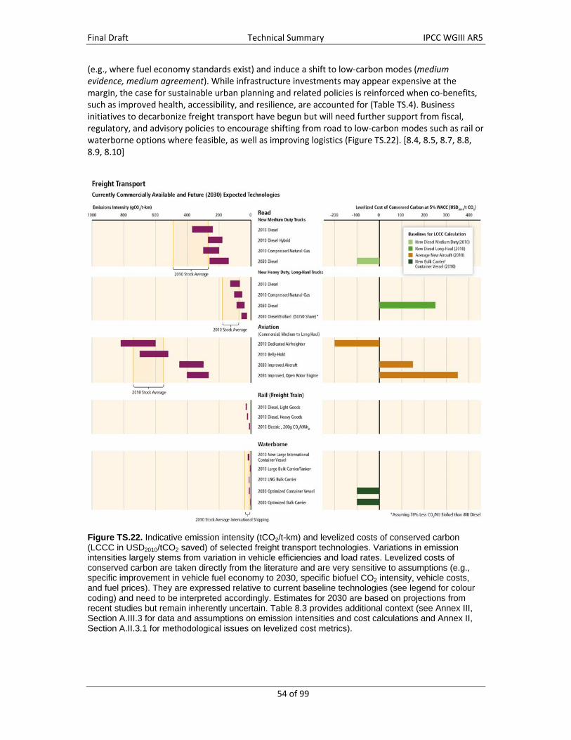
Final Draft Technical Summary IPCC WGIII AR5
54 of 99
(e.g., where fuel economy standards exist) and induce a shift to low‐carbon modes (medium evidence, medium agreement). While infrastructure investments may appear expensive at the margin, the case for sustainable urban planning and related policies is reinforced when co‐benefits, such as improved health, accessibility, and resilience, are accounted for (Table TS.4). Business initiatives to decarbonize freight transport have begun but will need further support from fiscal, regulatory, and advisory policies to encourage shifting from road to low‐carbon modes such as rail or waterborne options where feasible, as well as improving logistics (Figure TS.22). [8.4, 8.5, 8.7, 8.8, 8.9, 8.10]
Figure TS.22. Indicative emission intensity (tCO2/t-km) and levelized costs of conserved carbon (LCCC in USD2010/tCO2 saved) of selected freight transport technologies. Variations in emission intensities largely stems from variation in vehicle efficiencies and load rates. Levelized costs of conserved carbon are taken directly from the literature and are very sensitive to assumptions (e.g., specific improvement in vehicle fuel economy to 2030, specific biofuel CO2 intensity, vehicle costs, and fuel prices). They are expressed relative to current baseline technologies (see legend for colour coding) and need to be interpreted accordingly. Estimates for 2030 are based on projections from recent studies but remain inherently uncertain. Table 8.3 provides additional context (see Annex III, Section A.III.3 for data and assumptions on emission intensities and cost calculations and Annex II, Section A.II.3.1 for methodological issues on levelized cost metrics).

Final Draft Technical Summary IPCC WGIII AR5
55 of 99
Sectoral and integrated studies agree that substantial, sustained, and directed policy interventions could limit transport emissions to be consistent with low concentration goals, but the societal mitigation costs (USD/tCO2 avoided) remain uncertain (Figures TS.21, TS.22, TS.23). There is good potential to reduce emissions from LDVs and long‐haul heavy‐duty vehicles (HDVs) from both lower energy intensity vehicles and fuel switching, and the levelized costs of conserved carbon (LCCC) for efficiency improvements can be very low and negative (limited evidence, low agreement). Rail, buses, two‐ wheel motorbikes, and waterborne craft for freight already have relatively low emissions so their potential is limited. The mitigation cost of electric vehicles is currently high, especially if using grid electricity with a high emissions factor, but their LCCC are expected to decline by 2030. The emissions intensity of aviation could decline by around 50% in 2030 but the LCCC, although uncertain, are probably over USD 100/tCO2eq. While it is expected that mitigation costs will decrease in the future, the magnitude of such reductions is uncertain. (limited evidence, low agreement). [8.6, 8.9]
Figure TS.23. Direct global CO2 emissions from all passenger and freight transport are indexed relative to 2010 values for each scenario with integrated model studies grouped by CO2eq concentration levels by 2100, and sectoral studies grouped by baseline and policy categories. Where the data is sourced from the AR5 scenario database, a line denotes the median scenario and the boxes in bold colours highlight the inter-quartile range. The specific observations from sectoral studies are shown as dots (policy) and squares (baseline) with boxes to illustrate the data ranges. [Figure 8.9]
Barriers to decarbonizing transport for all modes differ across regions but can be overcome, in part, through economic incentives (medium evidence, medium agreement). Financial, institutional, cultural, and legal barriers constrain transport technology uptake and behavioural change. They include the high investment costs needed to build low‐emissions transport systems, the slow turnover of stock and infrastructure, and the limited impact of a carbon price on petroleum fuels that are already heavily taxed. Regional differences are likely due to cost and policy constraints. Oil price trends, price instruments on emissions, and other measures such as road pricing and airport charges can provide strong economic incentives for consumers to adopt mitigation measures. [8.8]
There are regional differences in transport mitigation pathways with major opportunities to shape transport systems and infrastructure around low‐carbon options, particularly in developing and emerging countries where most future urban growth will occur (robust evidence, high agreement). Possible transformation pathways vary with region and country due to differences in the dynamics of motorization, age and type of vehicle fleets, existing infrastructure, and urban development processes. In least developed countries, prioritizing access to pedestrians, integrating non‐motorized and public transport services, and managing excessive road speed for both urban and rural travellers can result in economic and social prosperity. In fast‐growing emerging economies, investments in mass transit and other low‐carbon transport infrastructure can help avoid future lock‐in to carbon

Final Draft Technical Summary IPCC WGIII AR5
56 of 99
intensive modes. In OECD countries, advanced vehicle technologies could play a bigger role than structural and behavioural changes since economic growth will be slower than for non‐OECD countries. (limited evidence, medium agreement) [8.4, 8.9]
A range of strong and mutually supportive policies will be needed for the transport sector to decarbonize and for the co‐benefits to be exploited (robust evidence, high agreement). Transport strategies associated with broader non‐climate policies at all government levels can usually target several objectives simultaneously to give lower travel costs, improved mobility, better health, greater energy security, improved safety, and increased time savings. Activity reduction measures have the largest potential to realize co‐benefits. Realizing the co‐benefits depends on the regional context in terms of economic, social, and political feasibility as well as having access to appropriate and cost‐effective advanced technologies (Table TS.4). (medium evidence, high agreement) Since rebound effects can reduce the CO2 benefits of efficiency improvements and undermine a particular policy, a balanced package of policies, including pricing initiatives, could help to achieve stable price signals, avoid unintended outcomes, and improve access, mobility, productivity, safety, and health (medium evidence, medium agreement). [8.4, 8.7, 8.10]

Final Draft Technical Summary IPCC WGIII AR5
57 of 99
Table TS.4: Overview of potential co-benefits (green arrows) and adverse side-effects (orange arrows) of the main mitigation measures in the transport sector; arrows pointing up/down denote a positive/negative effect on the respective objective or concern; a question mark (?) denotes an uncertain net effect. Co-benefits and adverse side-effects depend on local circumstances as well as on implementation practice, pace and scale (see Table 8.4). For an assessment of macroeconomic, cross-sectoral, effects associated with mitigation policies (e.g., on energy prices, consumption, growth, and trade), see e.g., Sections 3.9, 6.3.6, 13.2.2.3 and 14.4.2. The uncertainty qualifiers in brackets denote the level of evidence and agreement on the respective effects (see TS.1). Abbreviations for evidence: l=limited, m=medium, r=robust; for agreement: l=low, m=medium, h=high.
Transport Effect on additional objectives/concerns
Economic Social Environmental Other
For possible upstream effects of low‐carbon electricity, see Table TS.3. For possible upstream effects of biomass supply, see Table TS.7.
Reduction of fuel carbon intensity: e.g., electricity, H2, CNG, biofuels, and other measures
↑
↑
Energy security (diversification, reduced oil dependence, and exposure to oil price volatility) (m/m)
Technological spillovers (e.g., battery technologies for consumer electronics) (l/l)
? ↓↑↓
↓
Health impact via urban air pollution by
CNG, biofuels: net effect unclear (m/l) Electricity, H2: reducing most pollutants (r/h) Diesel: potentially increasing pollution (l/m) Noise (electrification and fuel cell LDVs) (l/m)
Road safety (silent electric LDVs at low speed) (l/l)
↓↑
Ecosystem impact of electricity and hydrogen via
Urban air pollution (m/m) Material use (unsustainable resource mining) (l/l)
Ecosystem impact of biofuels: see AFOLU
Reduction of energy intensity
↑
Energy security (reduced oil dependence and exposure to oil price volatility) (m/m)
↓
↑
Health impact via reduced urban air pollution (r/h)
Road safety (via increased crash‐worthiness) (m/m)
↓ Ecosystem and biodiversity impact via reduced urban air pollution (m/h)
Compact urban form + improved transport infrastructure Modal shift
↑
↑
?
Energy security (reduced oil dependence and exposure to oil price volatility) (m/m)
Productivity (reduced urban congestion and travel times, affordable and accessible transport) (m/h)
Employment opportunities in the public transport sector vs. car manufacturing (l/m)
↓↑↓
↑
↑
Health impact for non‐motorized modes via
Increased activity (r/h) Potentially higher exposure to air pollution (r/h) Noise (modal shift and travel reduction) (r/h)
Equitable mobility access to employment opportunities, particularly in developing countries (r/h)
Road safety (via modal shift and/or infrastructure for pedestrians and cyclists) (r/h)
↓↓
Ecosystem impact via
Urban air pollution (r/h) Land‐use competition (m/m)
Journey reduction and avoidance
↑
↑
Energy security (reduced oil dependence and exposure to oil price volatility) (r/h)
Productivity (reduced urban congestion, travel times, walking) (r/h)
↓ Health impact (non‐motorized transport modes) (r/h)
↓↑
↓
Ecosystem impact via
Urban air pollution (r/h) New/shorter shipping routes (r/h)
Land‐use competition (transport infrastructure) (r/h)

Final Draft Technical Summary IPCC WGIII AR5
58 of 99
TS.3.2.4 Buildings Greenhouse gas emissions from the building sector have more than doubled since 1970, accounting for 19% of global GHG emissions in 2010, including indirect emissions from electricity generation. The share rises to 25% if AFOLU emissions are excluded from the total. The building sector also accounted for 32% of total global final energy use, approximately one‐third of black carbon emissions, and an eighth to a third of F‐gases, with significant uncertainty (medium evidence, medium agreement) [9.2].
Direct and indirect CO2 emissions from buildings are projected to increase from 8.8 GtCO2/yr in 2010 to 13–17 GtCO2/yr in 2050 (25–75th percentile; full range 7.9–22 GtCO2/yr) in baseline scenarios; most of the baseline scenarios assessed in AR5 show a significant increase (medium evidence, medium agreement) (Figure TS.15) [6.8]. The lower end of the full range is dominated by scenarios with a focus on energy intensity improvements that go well beyond the observed improvements over the past 40 years. Without further policies, building sector final energy use may grow from approximately 120 EJ/yr in 2010, to 270 EJ/yr in 2050 [9.9].
Significant lock‐in risks arise from the long lifespans of buildings infrastructure (robust evidence, high agreement). If only currently planned policies are implemented, the final energy use in buildings that could be locked‐in by 2050, compared to a scenario where today's best practice buildings become the standard in newly built structures and retrofits, is equivalent to approximately 80% of 2005 building sector final energy use . [9.4]
Improvements in wealth, lifestyle, urbanization, and the provision of access to modern energy services and adequate housing will drive the increases in building energy demand (robust evidence, high agreement). The manner in which those without access to adequate housing (0.8 billion people), modern energy carriers, and sufficient levels of energy services including clean cooking (3 billion people) and heating meet these needs will influence the development of building related emissions. In addition, migration to cities, decreasing household size, increasing levels of wealth, and lifestyle changes, including increasing dwelling size and number and use of appliances, all contribute to considerable increases in building energy services demand. The substantial amount of new construction taking place in developing countries represents both a risk and opportunity from a mitigation perspective. [9.2, 9.4, 9.9]
The recent proliferation of advanced technologies, know‐how, and policies in the building sector, however, make it feasible that global total sector final energy use stabilizes or even declines by mid‐century (robust evidence, medium agreement). Recent advances in technology, design practices and know‐how, coupled with behavioural changes, can achieve a two to ten‐fold reduction in energy requirements of individual new buildings and a two to four‐fold reduction for individual existing buildings largely cost‐effectively or sometimes even at net negative costs (see Box TS.12) (robust evidence, high agreement). [9.6]
Advances since AR4 include the widespread demonstration worldwide of very low, or net zero energy buildings both in new construction and retrofits (robust evidence, high agreement). In some jurisdictions, these have already gained important market shares with, for instance, over 25 million m2 of building floorspace in Europe complying with the ‘Passivehouse’ standard in 2012. However, zero energy/carbon buildings may not always be the most cost‐optimal solution, nor even be feasible in certain building types and locations. [9.3]
High‐performance retrofits are key mitigation strategies in countries with existing building stocks, as buildings are very long‐lived and a large fraction of 2050 developed country buildings already exists (robust evidence, high agreement). Reductions of heating/cooling energy use by 50–90% have been achieved using best practices. Strong evidence shows that very low‐energy construction and retrofits can be economically attractive. [9.3]

Final Draft Technical Summary IPCC WGIII AR5
59 of 99
With ambitious policies it is possible to keep global building energy use constant or significantly reduce it by mid‐century compared to baseline scenarios which anticipate an increase of more than two‐fold (medium evidence, medium agreement) (Figure TS.24). Detailed building sector studies indicate a larger energy savings potential by 2050 than do integrated studies. The former indicate a potential of up to 70% of the baseline for heating and cooling only, and around 35–45% for the whole sector. In general, deeper reductions are possible in thermal energy uses than in other energy services mainly relying on electricity. With respect to additional fuel switching as compared to baseline, both sectoral and integrated studies find modest opportunities. In general, both sectoral and integrated studies indicate that electricity will supply a growing share of building energy demand over the long term, especially if heating demand decreases due to a combination of efficiency gains, better architecture, and climate change. [6.8.4, 9.8.2, Figure 9.19]
Figure TS.24. Final energy demand reduction relative to baseline (left panel) and development of final low carbon energy carrier share in final energy (from electricity; right panel) in buildings 2030 and 2050 in mitigation scenarios from three different CO2eq concentrations ranges shown in boxplots (see Section 6.3.2) compared to sectoral studies shown in shapes assessed in Chapter 9. Filled circles correspond to sectoral studies with full sectoral coverage while empty circles correspond to studies with only partial sectoral coverage (e.g., heating and cooling). [Figures 6.37 and 6.38]
The history of energy efficiency programmes in buildings shows that 25–30% efficiency improvements have been available at costs substantially lower than marginal energy supply (robust evidence, high agreement). Technological progress enables the potential for cost‐effective energy efficiency improvements to be maintained, despite continuously improving standards. There has been substantial progress in the adoption of voluntary and mandatory standards since AR4, including ambitious building codes and targets, voluntary construction standards, and appliance standards. At the same time, in both new and retrofitted buildings, as well as in appliances and information, communication and media technology equipment, there have been notable performance and cost improvements. Large reductions in thermal energy use in buildings are possible at costs lower than energy supply, with the most cost‐effective options including very high‐performance new commercial buildings; the same holds for efficiency improvements in some appliances and cooking equipment. [9.5, 9.6, 9.9]

Final Draft Technical Summary IPCC WGIII AR5
60 of 99
Lifestyle, culture, and other behavioural changes may lead to further large reductions in building and appliance energy requirements beyond those achievable through technologies and architecture. Energy use has been shown to vary by 3–5 fold for similar levels of energy service (low evidence, high agreement). In developed countries, evidence indicates that behaviours informed by awareness of energy and climate issues can reduce demand by up to 20% in the short term and up to 50% by 2050 (medium evidence, medium agreement). There is a high risk that emerging countries follow the same path as developed economies in terms of building‐related architecture, lifestyle, and behaviour. But the literature suggests that alternative development pathways exist that provide high levels of building services at much lower energy inputs, incorporating strategies such as learning from traditional lifestyles, architecture ,and construction techniques. [9.3]
Most mitigation options in buildings have considerable and diverse co‐benefits (robust evidence, high agreement). These include, but are not limited to: energy security; less need for energy subsidies; health and environmental benefits (due to reduced indoor and outdoor air pollution);; productivity and net employment gains; the alleviation of fuel poverty; reduced energy expenditures; increased value for building infrastructure; and improved comfort and services. (Table TS.5) [9.8]
Especially strong barriers in this sector hinder the market uptake of cost‐effective technologies and practices; as a consequence, programmes and regulation are more effective than pricing instruments alone (robust evidence, high agreement). Barriers include imperfect information and lack of awareness, principal/agent problems and other split incentives, transaction costs, lack of access to financing, insufficient training in all construction related trades, and cognitive/behavioural barriers. In developing countries, the large informal sector, energy subsidies, corruption, high implicit discount rates, and insufficient service levels are further barriers. Therefore, market forces alone are not expected to achieve the necessary transformation without external stimuli. Policy intervention addressing all levels of the building and appliance lifecycle and use, plus new business and financial models are essential. [9.7]
A large portfolio of building‐specific energy efficiency policies was already highlighted in AR4, but further considerable advances in available instruments and their implementation have occurred since (robust evidence, high agreement). Evidence shows that many building energy efficiency policies worldwide have already been saving emissions at large negative costs. Among the most environmentally and cost‐effective policies are regulatory instruments such as building and appliance standards and labels, as well as public leadership programmes and procurement policies. Progress in building codes and appliance standards in some developed countries over the last decade have demonstrated the feasibility of stabilising or even reducing total building energy use, despite growth in population, wealth, and corresponding energy service level demands. Developing countries have also been adopting different effective policies, most notably appliance standards. However, in order to reach ambitious climate goals, these need to be substantially strengthened and extended to further jurisdictions, and to other building and appliance types. Due to larger capital requirements, financing instruments are essential both in developed and developing countries to achieve deep reductions in energy use. [9.9]

Final Draft Technical Summary IPCC WGIII AR5
61 of 99
Table TS.5: Overview of potential co-benefits (green arrows) and adverse side-effects (orange arrows) of the main mitigation measures in the building sector; arrows pointing up/down denote a positive/negative effect on the respective objective or concern. Co-benefits and adverse side-effects depend on local circumstances as well as on implementation practice, pace and scale (see Table 9.7). For an assessment of macroeconomic, cross-sectoral, effects associated with mitigation policies (e.g., on energy prices, consumption, growth, and trade), see e.g., Sections 3.9, 6.3.6, 13.2.2.3 and 14.4.2. The uncertainty qualifiers in brackets denote the level of evidence and agreement on the respective effects (see TS.1). Abbreviations for evidence: l=limited, m=medium, r=robust; for agreement: l=low, m=medium, h=high.
Buildings Effect on additional objectives/concerns
Economic Social Environmental Other
For possible upstream effects of fuel switching and RES, see Table TS.3.
Fuel switching, RES incorporation, green roofs, and other measures reducing emissions intensity
↑
↑
↑
↑
Energy security (m/h)
Employment impact (m/m)
Lower need for energy subsidies (l/l)
Asset values of buildings (l/m)
↓↑
↓
↑
Fuel poverty (residential) via
Energy demand (m/h) Energy cost (l/m)
Energy access (for higher energy cost) (l/m)
Productive time for women/children (for replaced traditional cookstoves) (m/h)
↓↓↓
↓
↑
Health impact in residential buildings via
Outdoor air pollution (r/h) Indoor air pollution (in DCs) (r/h) Fuel poverty (r/h)
Ecosystem impact (less outdoor air pollution) (r/h)
Urban biodiversity (for green roofs) (m/m)
Reduced Urban Heat Island Effect (UHI) (l/m)
Retrofits of existing buildings (e.g., cool roof, passive solar, etc.) Exemplary new buildings Efficient equipment
↑
↑
↑
↑
↑
↑
Energy security (m/h)
Employment impact (m/m)
Productivity (for commercial buildings) (m/h)
Lower need for energy subsidies (l/l)
Asset values of buildings (l/m)
Disaster resilience (l/m)
↓
↓
↑
↑
Fuel poverty (for retrofits, efficient equipment) (m/h)
Energy access (higher cost for housing due to the investments needed) (l/m)
Thermal comfort (for retrofits and exemplary new buildings) (m/h)
Productive time for women and children (for replaced traditional cookstoves) (m/h)
↓↓↓↓↓
↓
↓
Health impact via
Outdoor air pollution (r/h) Indoor air pollution (for efficient cookstoves) (r/h) Indoor environmental conditions (m/h) Fuel poverty (r/h) Insufficient ventilation (m/m)
Ecosystem impact (less outdoor air pollution) (r/h)
Water consumption and sewage production (l/l)
Reduced UHI (retrofits and new exemplary buildings) (l/m)
Behavioural changes reducing energy demand
↑
↑
Energy security (m/h)
Lower need for energy subsidies (l/l)
↓
↓
Health impact via less outdoor air pollution (r/h) & improved indoor environmental conditions (m/h)
Ecosystem impact (less outdoor air pollution) (r/h)

Final Draft Technical Summary IPCC WGIII AR5
62 of 99
Box TS.12. Negative private mitigation costs
A persistent issue in the analysis of mitigation options and costs is whether there are mitigation opportunities that are privately beneficial—generating private benefits that more than offset the costs of implementation—but which consumers and firms do not voluntarily undertake. There is some evidence of unrealized mitigation opportunities that would have negative cost. Possible examples include investments in vehicles [8.1], lighting and heating technology in homes and commercial buildings [9.3], as well as industrial processes [10.1].
Examples of negative private costs imply that firms and individuals do not take opportunities to save money. This might be explained in a number of ways. One is that status‐quo bias can inhibit the switch to new technologies or products [2.4, 3.10.1]. Another is that firms and individuals may focus on short‐term goals and discount future costs and benefits sharply; consumers have been shown to do this when choosing energy conservation measures or investing in energy efficient technologies [2.4.3, 2.6.5.3, 3.10.1]. Risk aversion and ambiguity aversion may also account for this behaviour when outcomes are uncertain [2.4.3, 3.10.1]. Other possible explanations include: insufficient information on opportunities to conserve energy; asymmetric information – for example, landlords may be unable to convey the value of energy efficiency improvements to renters; split incentives, where one party pays for an investment but another party reaps the benefits; and imperfect credit markets, which make it difficult or expensive to obtain finance for energy saving [3.10.1, 16.4].
Some engineering studies show a large potential for negative‐cost mitigation. The extent to which such negative‐cost opportunities can actually be realized remains a matter of contention in the literature. Empirical evidence is mixed [Box 3.10].
TS.3.2.5 Industry Currently, in the industry sector direct and indirect emissions (the latter being associated with electricity consumption) are larger than the emissions from either the buildings or transport end‐use sectors and represent just over 30% of global GHG emissions in 2010 (the share rises to 40% if AFOLU emissions are excluded from the total) (high confidence). Despite the declining share of industry in global GDP, global industry and waste/wastewater GHG emissions grew from 10 GtCO2eq in 1990, to 13 GtCO2eq in 2005 and to 16 GtCO2eq in 2010. [10.3]
Direct and indirect CO2 emissions from industry are projected to increase from 13 GtCO2/yr in 2010 to 20–24 GtCO2/yr in 2050 (25–75th percentile; full range 9.5–34 GtCO2/yr) in baseline scenarios; most of the baseline scenarios assessed in AR5 show a significant increase (medium evidence/medium agreement) (Figure TS.15) [6.8]. The lower end of the full range is dominated by scenarios with a focus on energy intensity improvements that go well beyond the observed improvements over the past 40 years.
The wide‐scale deployment of best available technologies, particularly in countries where these are not in practice, and in non‐energy intensive industries, could reduce the energy intensity of the sector by up to 25% (robust evidence, high agreement). Despite long‐standing attention to energy efficiency in industry, many options for improved energy efficiency still remain. Through innovation, additional reductions of approximately up to 20% in energy intensity may potentially be realized (low evidence, medium agreement). Barriers to implementing energy efficiency relate largely to the initial investment costs and lack of information. Information programmes are the most prevalent approach for promoting energy efficiency, followed by economic instruments, regulatory approaches, and voluntary actions. [10.4]
An absolute reduction in emissions from the industry sector will require deployment of a broad set of mitigation options that go beyond energy efficiency measures (medium evidence, high agreement) [10.4, 10.7]. In the context of continued overall growth in industrial demand, substantial reductions from the sector will require parallel efforts to increase emissions efficiency (e.g., through fuel and feedstock switching or CCS); material use efficiency (e.g., less scrap, new product design);

Final Draft Technical Summary IPCC WGIII AR5
63 of 99
recycling and re‐use of materials and products; product service efficiency (e.g., more intensive use of products through car sharing, longer life for products); radical product innovations (e.g., alternatives to cement); as well as service demand reductions [10.4, 10.7]. (limited evidence, high agreement) (Table TS.2, Figure TS.25)
Figure TS.25. A schematic illustration of industrial activity over the supply chain. Options for mitigation in the industry sector are indicated by the circled numbers: (1) energy efficiency; (2) emissions efficiency; (3a) material efficiency in manufacturing; (3b) material efficiency in product design; (4) product-service efficiency; (5) service demand reduction [Figure 10.1]
While detailed industry sector studies tend to be more conservative than integrated studies, both identify possible industrial final energy demand savings of around 30% by 2050 in mitigation scenarios not exceeding 650ppm CO2eq by 2100 relative to baseline scenarios (medium evidence, medium agreement) (Figure TS.26). Integrated models in general treat the industry sector in a more aggregated fashion and mostly do not explicitly provide detailed sub‐sectoral material flows, options for reducing material demand, and price‐induced inter‐input substitution possibilities. Due to the heterogeneous character of the industry sector, a coherent comparison between sectoral and integrated studies remains difficult. [6.8.4, 10.4, 10.7, 10.10.1, Figure 10.14]
Mitigation in the industry sector can also be achieved by reducing material and fossil fuel demand by enhanced waste use, which concomitantly reduces direct emissions from waste disposal (robust evidence, high agreement). The hierarchy of waste management places waste reduction at the top, followed by re‐use, recycling, and energy recovery. As the share of recycled or reused material is still low, applying waste treatment technologies and recovering energy to reduce demand for fossil fuels can result in direct emission reductions from waste disposal. Only about 20% of municipal solid waste (MSW) is recycled and about 14 % is treated with energy recovery while the rest is deposited in open dumpsites or landfills. About 47% of wastewater produced in the domestic and manufacturing sectors is still untreated. The largest cost range is for reducing emissions from landfilling through the treatment of waste by anaerobic digestion. The costs range from negative (see Box TS.12) to very high. Advanced wastewater treatment technologies may enhance GHG emissions reduction in the wastewater treatment but they are clustered among the higher cost options (medium evidence, medium agreement). (Figure TS.29) [10.4, 10.14]

Final Draft Technical Summary IPCC WGIII AR5
64 of 99
Figure TS.26. Final energy demand reduction relative to baseline (left panel) and development of final low carbon energy carrier share in final energy (including electricity, heat, hydrogen, and bioenergy; right panel) in industry by 2030 and 2050 in mitigation scenarios from three different CO2eq concentration ranges shown in boxplots (see Section 6.3.2) compared to sectoral studies shown in shapes assessed in Chapter 10. Filled circles correspond to sectoral studies with full sectoral coverage. [Figures 6.37 and 6.38]
Waste policy and regulation have largely influenced material consumption, but few policies have specifically pursued material efficiency or product service intensity (robust evidence, high agreement) [10.11]. Barriers to improving material efficiency include lack of human and institutional capacities to encourage management decisions and public participation. Also, there is a lack of experience and often there are no clear incentives either for suppliers or consumers to address improvements in material or product service efficiency, or to reduce product demand. [10.9]
CO2 emissions dominate GHG emissions from industry, but there are also substantial mitigation opportunities for non‐CO2 gases (robust evidence, high agreement). Key opportunities comprise, e.g., reduction of hydrofluorocarbon (HFC) emissions by leak repair, refrigerant recovery and recycling, and proper disposal and replacement by alternative refrigerants (ammonia, HC, CO2). Nitrous oxide (N2O) emissions from adipic and nitric acid production can be reduced through the implementation of thermal destruction and secondary catalysts. The reduction of non‐CO2 GHGs also faces numerous barriers. Lack of awareness, lack of economic incentives and lack of commercially available technologies (e.g., for HFC recycling and incineration) are typical examples. [10.7]
Besides sector specific technologies, cross‐cutting technologies and measures applicable in both large energy intensive industries and Small and Medium Enterprises (SMEs) can help to reduce GHG emissions (robust evidence, high agreement). Cross‐cutting technologies such as efficient motors, and cross‐cutting measures such as reducing air or steam leaks, help to optimize performance of industrial processes and improve plant efficiency very often cost‐effectively with both energy savings and emissions benefits. Industrial clusters also help to realize mitigation, particularly from SMEs. [10.4] Cooperation and cross‐sectoral collaboration at different levels—for

Final Draft Technical Summary IPCC WGIII AR5
65 of 99
example, sharing of infrastructure, information, waste heat, cooling, etc.—may provide further mitigation potential in certain regions/industry types [10.5].
Several emission‐reducing options in the industrial sector are cost‐effective and profitable (medium evidence, medium agreement). While options in cost ranges of 0–20 and 20–50 USD/tCO2eq and even below 0 USD/tCO2eq exist, achieving near‐zero emission intensity levels in the industry sector would require the additional realization of long‐term step‐change options (e.g., CCS), which are associated with higher levelized costs of conserved carbon (LCCC) in the range of 50–150 USD/tCO2eq. Similar cost estimates for implementing material efficiency, product‐service efficiency, and service demand reduction strategies are not available. With regard to long‐term options, some sector specific measures allow for significant reductions in specific GHG emissions but may not be applicable at scale, e.g., scrap‐based iron and steel production. Decarbonized electricity can play an important role in some subsectors (e.g., chemicals, pulp and paper, and aluminium), but will have limited impact in others (e.g., cement, iron and steel, waste). In general, mitigation costs vary regionally and depend on site‐specific conditions. (Figures TS.27, TS.28, TS.29) [10.7]
Mitigation measures are often associated with co‐benefits (robust evidence, high agreement). Co‐benefits include enhanced competitiveness through cost‐reductions, new business opportunities, better environmental compliance, health benefits through better local air and water quality and better work conditions, and reduced waste, all of which provide multiple indirect private and social benefits (Table TS.6). [10.8]
There is no single policy that can address the full range of mitigation measures available for industry and overcome associated barriers. Unless barriers to mitigation in industry are resolved, the pace and extent of mitigation in industry will be limited and even profitable measures will remain untapped (robust evidence, high agreement). [10.9, 10.11]

Final Draft Technical Summary IPCC WGIII AR5
66 of 99
Figure TS.27. Indicative CO2 emission intensities for cement (top panel) and steel (bottom panel), as well as indicative levelized cost of conserved carbon shown for various production practices/technologies and for 450ppm CO2eq scenarios of a limited selection of integrated models (for data and methodology, see Annex III). [Figures 10.7, 10.8]

Final Draft Technical Summary IPCC WGIII AR5
67 of 99
Figure TS.28. Global CO2eq emissions for chemicals production (top panel) and indicative CO2 emission intensities for paper production (bottom panel) as well as indicative levelized cost of conserved carbon shown for various production practices/technologies and for 450ppm CO2eq scenarios of a limited selection of integrated models (for data and methodology, see Annex III). [Figures 10.9, 10.10]

Final Draft Technical Summary IPCC WGIII AR5
68 of 99
Figure TS.29. Indicative CO2 emission intensities for waste (top panel) and wastewater (bottom panel) of various practices as well as indicative levelized cost of conserved carbon (for data and methodology, see Annex III). [Figures 10.19 and 10.20]

Final Draft Technical Summary IPCC WGIII AR5
69 of 99
Table TS.6: Overview of potential co-benefits (green arrows) and adverse side-effects (orange arrows) of the main mitigation measures in the industry sector; arrows pointing up/down denote a positive/negative effect on the respective objective or concern. Co-benefits and adverse side-effects depend on local circumstances as well as on the implementation practice, pace and scale (see Table 10.5). For an assessment of macroeconomic, cross-sectoral, effects associated with mitigation policies (e.g., on energy prices, consumption, growth, and trade), see e.g., Sections 3.9, 6.3.6, 13.2.2.3 and 14.4.2. The uncertainty qualifiers in brackets denote the level of evidence and agreement on the respective effects (see TS.1). Abbreviations for evidence: l=limited, m=medium, r=robust; for agreement: l=low, m=medium, h=high.
Industry Effect on additional objectives/concerns
Economic Social Environmental Other
For possible upstream effects of low‐carbon energy supply (incl CCS), see Table TS.3. For possible upstream effects of biomass supply, see Table TS.7.
CO2/non‐CO2 emission intensity reduction
↑
Competitiveness and productivity (m/h) ↓ Health impact via reduced local air pollution and better work conditions (PFC from aluminium) (m/m)
↓
↑
Ecosystem impact via reduced local air pollution and reduced water pollution (m/m)
Water conservation (l/m)
Energy efficiency improvements via new processes/technologies
↑
↑
↑
↑
Energy security (lower energy intensity)(m/m)
Employment impact (l/l)
Competitiveness and productivity (m/h)
Technological spillovers in DCs (due to supply chain linkages) (l/l)
↓
↑
↑
↑
Health impact via reduced local pollution (l/m)
New business opportunities (m/m)
Water availability and quality (l/l)
Safety, working conditions and job satisfaction (m/m)
↓↓
Ecosystem impact via:
Fossil fuel extraction (l/l) Local pollution and waste (m/m)
Material efficiency of goods, recycling
↓
↑
↑
↑
National sales tax revenue (medium term) (l/l)
Employment impact (waste recycling) (l/l)
Competitiveness in manufacturing (l/l)
New infrastructure for industrial clusters (l/l)
↓
↑
↓
Health impacts and safety concerns (l/m)
New business opportunities (m/m)
Local conflicts (reduced resource extraction) (l/m)
↓
↓
Ecosystem impact via reduced local air and water pollution and waste material disposal (m/m)
Use of raw/virgin materials and natural resources implying reduced unsustainable resource mining (l/l)
Product demand reductions
↓ National sales tax revenue (medium term) (l/l) ↓
↑
Local conflicts (reduced inequity in consumption)(l/l)
New diverse lifestyle concept (l/l)
↓ Post‐consumption waste (l/l)
1
Final Draft Technical Summary IPCC WGIII AR5
70 of 99
TS.3.2.6 Agriculture, forestry and other land‐uses (AFOLU) Since AR4, emissions from the AFOLU sector have stabilized but the share of total anthropogenic emissions has decreased (robust evidence, high agreement). The average annual total GHG flux from the AFOLU sector was 10–12 GtCO2eq in 2000–2010, with global emissions of 5.0–5.8 GtCO2eq/yr from agriculture on average and around 4.3–5.5 GtCO2eq/yr from forestry and other land uses. Non‐CO2 emissions derive largely from agriculture, dominated by N2O emissions from agricultural soils and methane emissions from livestock enteric fermentation, manure management, and emissions from rice paddies, totalling 5.0–5.8 GtCO2eq/yr in 2010 (robust evidence, high agreement). Over recent years, most estimates of forestry and other land use (FOLU) CO2 fluxes indicate a decline in emissions, largely due to decreasing deforestation rates (limited evidence, medium agreement). The absolute levels of emissions from deforestation and degradation have fallen from 1990 to 2010 (robust evidence, high agreement). Over the same time period, total emissions for high income countries decreased while those of low income countries increased. In general, AFOLU emissions from high income countries are dominated by agriculture activities while those from low income countries are dominated by deforestation and degradation. [Figure 1.3, 11.2]
Net annual baseline CO2 emissions from AFOLU are projected to decline over time with emissions potentially less than half of what they are today by 2050, and the possibility of the terrestrial system becoming a net sink before the end of century. However, there is significant uncertainty in historical and well as projected baseline AFOLU emissions. (medium evidence, high agreement) (Figure TS.15) [6.3.1.4, 6.8, Figure 6.5] As in AR4, most projections suggest declining annual net CO2 emissions in the long run. In part, this is driven by technological change, as well as projected declining rates of agriculture area expansion related to the expected slowing in population growth. However, unlike AR4, none of the more recent scenarios projects growth in the near‐term. There is also a somewhat larger range of variation later in the century, with some models projecting a stronger net sink starting in 2050 (limited evidence, medium agreement). There are few reported projections of baseline global land‐related N2O and CH4 emissions and they indicate an increase over time. Cumulatively, land CH4 emissions are projected to be 44–53% of total CH4 emissions through 2030, and 41–59% through 2100, and land N2O emissions 85–89% and 85–90%, respectively (limited evidence, medium agreement). [11.9]
Opportunities for mitigation in the AFOLU sector include supply‐ and demand‐side mitigation options (robust evidence, high agreement). Supply‐side measures involve reducing emissions arising from land use change, in particular reducing deforestation, land and livestock management, increasing carbon stocks by sequestration in soils and biomass, or the substitution of fossil fuels by biomass for energy production (Table TS.2). Further new supply‐side technologies not assessed in AR4, such as biochar or wood products for energy intensive building materials, could contribute to the mitigation potential of the AFOLU sector, but there is limited evidence upon which to make robust estimates. Demand‐side measures include dietary change and waste reduction in the food supply chain. Increasing forestry and agricultural production without a commensurate increase in emissions (i.e., one component of sustainable intensification; Figure TS.30) also reduces emission intensity, (i.e., the GHG emissions per unit of product), a mitigation mechanism largely unreported for AFOLU in AR4, which could reduce absolute emissions as long as production volumes do not increase. [11.3, 11.4]

Final Draft Technical Summary IPCC WGIII AR5
71 of 99
Figure TS.30. GHG emissions intensities of selected major AFOLU commodities for decades 1960s–2000s. i) Cattle meat, defined as GHG (enteric fermentation+ manure management of cattle, dairy and non-dairy)/meat produced; ii) pig meat, defined as GHG (enteric fermentation+ manure management of swine, market and breeding) /meat produced; iii) chicken meat, defined as GHG (manure management of chickens)/meat produced; iv) milk, defined as GHG (enteric fermentation+ manure management of cattle, dairy)/milk produced; v) eggs, defined as GHG (manure management of chickens, layers)/egg produced; vi) rice, defined as GHG (rice cultivation)/rice produced; vii) cereals, defined as GHG (synthetic fertilizers)/cereals produced; viii) wood, defined as GHG (carbon loss from harvest)/roundwood produced. [Figure 11.15]
Among supply‐side measures, the most cost‐effective forestry options are reducing deforestation and forest management; in agriculture, low carbon prices (20 USD/tCO2eq) favour cropland and grazing land management and high carbon prices (100 USD/tCO2eq) favour restoration of organic soils (medium evidence, medium agreement). When considering only studies that cover both forestry and agriculture and include agricultural soil carbon sequestration, the economic mitigation potential in the AFOLU sector is estimated to be 7.18 to 10.6 (full range of all studies : 0.49–10.6) GtCO2eq/yr at carbon prices up to 100 USD/ tCO2eq, about a third of which can be achieved at <20 USD/ tCO2eq (medium evidence, medium agreement). The range of global estimates at a given carbon price partly reflects uncertainty surrounding AFOLU mitigation potentials in the literature and the land use assumptions of the scenarios considered. The ranges of estimates also reflect differences in the GHGs and options considered in the studies. A comparison of estimates of economic mitigation potential in the AFOLU sector published since AR4 is shown in Figure TS.31. [11.6]
While demand‐side measures are under‐researched, changes in diet, reductions of losses in the food supply chain, and other measures could have a significant impact on GHG emissions from food production (0.76–8.55 GtCO2eq/yr by 2050) (Figure TS.31) (limited evidence, medium agreement). Barriers to implementation are substantial, and include concerns about jeopardizing health and well‐being, and cultural and societal resistance to behaviour change. However, in countries with a high consumption of animal protein, co‐benefits are reflected in positive health impacts resulting from changes in diet (robust evidence, high agreement). [11.4.3, 11.6, 11.7, 11.9]

Final Draft Technical Summary IPCC WGIII AR5
72 of 99
Figure TS.31. Estimates of economic mitigation potentials in the AFOLU sector published since AR4, (AR4 estimates shown for comparison, denoted by black arrows), including bottom-up, sectoral studies, and top-down, multi-sector studies. Supply side mitigation potentials are estimated for around 2030, ranging from 2025 to 2035, and are for agriculture, forestry or both sectors combined. Studies are aggregated for potentials up to ~20 USD/tCO2eq (actual range 1.64–21.45), up to ~50 USD/tCO2eq (actual range 31.39–50.00), and up to ~100 USD/tCO2eq (actual range 70.0–120.91). Demand-side measures (shown on the right hand side of the figure) are for ~2050 and are not assessed at a specific carbon price, and should be regarded as technical potentials. Smith et al. (2013) are the mean of the range. Not all studies consider the same measures or the same GHGs. [11.6.2, Figure 11.14]
The mitigation potential of AFOLU is highly dependent on broader factors related to land‐use policy and patterns (medium evidence, high agreement). The many possible uses of land can compete or work in synergy. The main barriers to mitigation are institutional (lack of tenure and poor governance), accessibility to financing mechanisms, availability of land and water, and poverty. On the other hand, AFOLU mitigation options can promote innovation, and many technological supply‐side mitigation options also increase agricultural and silvicultural efficiency, and can reduce climate vulnerability by improving resilience. Multifunctional systems that allow the delivery of multiple services from land have the capacity to deliver to many policy goals in addition to mitigation, such as improving land tenure, the governance of natural resources, and equity [11.8] (limited evidence, high agreement). Recent frameworks, such as those for assessing environmental or ecosystem services, could provide tools for valuing the multiple synergies and trade‐offs that may arise from mitigation actions (Table TS.7) (medium evidence, medium agreement). [11.7, 11.8]

Final Draft Technical Summary IPCC WGIII AR5
73 of 99
Table TS.7: Overview of potential co-benefits (green arrows) and adverse side-effects (orange arrows) of the main mitigation measures in the AFOLU sector; arrows pointing up/down denote a positive/negative effect on the respective objective or concern. These effects depend on the specific context (including bio-physic, institutional and socio-economic aspects) as well as on the scale of implementation (see Table 11.9 and 11.12). For an assessment of macroeconomic, cross-sectoral, effects associated with mitigation policies (e.g., on energy prices, consumption, growth, and trade), see e.g., Sections 3.9, 6.3.6, 13.2.2.3 and 14.4.2. The uncertainty qualifiers in brackets denote the level of evidence and agreement on the respective effects (see TS.1). Abbreviations for evidence: l=limited, m=medium, r=robust; for agreement: l=low, m=medium, h=high.
AFOLU Effect on additional objectives/concerns
Economic Social Environmental Institutional
Note: co‐benefits and adverse side‐effects depend on the development context and the scale of the intervention (size). Supply side: forestry, land‐based agriculture, livestock, integrated systems, and bioenergy (marked by *) Demand side: reduced losses in the food supply chain, changes in human diets, changes in demand for wood and forestry products
↑
↓
↑
↑
↑
↑
↑
↑
* Employment impact via
entrepreneurship development (m/h) use of less labour‐intensive (m/m) technologies in agriculture
* Diversification of income sources and access to markets (r/h)
* Additional income to (sustainable) landscape management (m/h)
* Income concentration (m/m)
* Energy security (resource sufficiency) (m/h)
Innovative financing mechanisms for sustainable resource management (m/h)
Technology innovation and transfer (m/m)
↑
↓
↑
↑
↓
↑↑
* Food‐crops production through integrated (r/m) systems and sustainable agriculture intensification
* Food production (locally) due to large‐scale monocultures of non‐food crops (r/l)
Cultural habitats and recreational areas via (m/m) (sustainable) forest management and conservation
*Human health and animal welfare e.g., through less pesticides, reduced burning practices, and practices like agroforestry & silvo‐pastoral systems (m/h)
*Human health when using burning practices (in agriculture or bioenergy) (m/m)
* Gender, intra‐ and inter‐generational equity via
participation and fair benefit sharing (r/h) concentration of benefits (m/m)
↑ ↓
↑
↑
↓
↑
↑
Provision of ecosystem services via
ecosystem conservation and sustainable management as well as sustainable agriculture (r/h) * large scale monocultures (r/h)
* Land use competition (r/m)
Soil quality (r/h)
Erosion (r/h)
Ecosystem resilience (m/h)
Albedo and evaporation (r/h)
↑↓
↑↓
↑
* Tenure and use rights at the local level (for indigenous people and local communities) especially when implementing activities in natural forests (r/h)
Access to participative mechanisms for land management decisions (r/h)
Enforcement of existing policies for sustainable resource management (r/h)

Final Draft Technical Summary IPCC WG III AR5
74 of 99
Policies governing practices in agriculture as well as forest conservation and management need to account for the needs of both mitigation and adaptation (medium evidence, high agreement). Economic incentives (e.g., special credit lines for low carbon agriculture, sustainable agriculture and forestry practices, tradable credits, payment for ecosystem services) and regulatory approaches (e.g., enforcement of environmental law to protect forest carbon stocks by reducing deforestation, set‐aside policies, air and water pollution control reducing nitrate load and N2O emissions) have been effective in different cases. Investments in research, development, and diffusion (e.g., increase of resource use‐efficiency (fertilizers), livestock improvement, better forestry management practices) could result in synergies between adaptation and mitigation. Successful cases of deforestation reduction in different regions are found to combine different policies such as land planning, regulatory approaches and economic incentives (limited evidence, high agreement). [11.10, 15.11]
Reducing Emissions from Deforestation and Forest Degradation (REDD+)9 can be a very cost effective policy option for mitigating climate change, if implemented in a sustainable manner (limited evidence, medium agreement). REDD+ includes: reducing emissions from deforestation and forest degradation; conservation of forest carbon stocks; sustainable management of forests; and enhancement of forest carbon stocks. It could supply a large share of global abatement of emissions from the AFOLU sector, especially through reducing deforestation in tropical regions, with potential economic, social and other environmental co‐benefits. To assure these co‐benefits, the implementation of national REDD+ strategies would need to consider financing mechanisms to local stakeholders, safeguards (such as land rights, conservation of biodiversity and other natural resources), and the appropriate scale and institutional capacity for monitoring and verification. [11.10]
Bioenergy deployment offers significant potential for climate change mitigation, but also carries considerable risks (medium evidence, medium agreement). The IPCC’s Special Report on Renewable Energy Sources and Climate Change Mitigation (SRREN) suggested potential bioenergy deployment levels to be between 100–300 EJ. This assessment agrees on a technical bioenergy potential of around 100 EJ (medium evidence, high agreement), and possibly 300 EJ and higher (limited evidence, low agreement). Integrated models project between 15–245 EJ/yr deployment in 2050, excluding traditional bioenergy. Achieving high deployment levels would require, amongst others, extensive use of agricultural residues and second‐generation biofuels to mitigate adverse impacts on land use and food production, and the co‐processing of biomass with coal or natural gas with CCS to produce low net GHG‐emitting transportation fuels and/or electricity (medium evidence, high agreement). The integration of crucial sectoral research (albedo effects, evaporation, counterfactual land carbon sink assumptions) into transformation pathways research, and the exploration of risks of imperfect policy settings (for example, in absence of a global CO2 price on land carbon) is subject of further research. [11.9, 11.13.2, 11.13.4]
Small‐scale bioenergy systems aimed at meeting rural energy needs synergistically provide mitigation and energy access benefits (robust evidence, high agreement). Decentralized deployment of biomass for energy, in combination with improved cookstoves, biogas, and small‐scale biopower, could improve livelihoods and health of around 2.6 billion people. Both mitigation potential and sustainability hinge crucially on the protection of land carbon (high density carbon ecosystems), careful fertilizer application, interaction with food markets, and good land and water management. Sustainability and livelihood concerns might constrain beneficial deployment of dedicated biomass plantations to lower values. [11.13.3, 11.13.5, 11.13.7]
9 UN Programme on Reducing Emissions from Deforestation and Forest Degradation in developing countries, including conservation, sustainable management of forests and enhancement of forest carbon stocks.

Final Draft Technical Summary IPCC WG III AR5
75 of 99
Lifecycle assessments for bioenergy options demonstrate a plethora of pathways, site‐specific conditions, and technologies that produce a wide range of climate‐relevant effects (high confidence). Specifically, land‐use change emissions, nitrous oxide emissions from soil and fertilizers, co‐products, process design and process fuel use, end‐use technology, and reference system can all influence the total attributional lifecycle emissions of bioenergy use. The large variance for specific pathways points to the importance of management decisions in reducing the lifecycle emissions of bioenergy use. The total marginal global warming impact of bioenergy can only be evaluated in a comprehensive setting that also addresses equilibrium effects, e.g., indirect land‐use change emissions, actual fossil fuel substitution, and other effects. Structural uncertainty in modelling decision‐making renders such evaluation exercises uncertain. Available data suggest a differentiation between options that offer low lifecycle emissions under good land‐use management (e.g., sugarcane, Miscanthus, and fast‐growing tree species) and those that are unlikely to contribute to climate change mitigation (e.g., corn and soybean), pending new insights from more comprehensive consequential analyses. [8.7, 11.13.4]
Land‐demand and livelihoods are often affected by bioenergy deployment (high confidence). Land demand for bioenergy depends on (1) the share of bioenergy derived from wastes and residues; (2) the extent to which bioenergy production can be integrated with food and fibre production, and conservation to minimize land‐use competition; (3) the extent to which bioenergy can be grown on areas with little current production; and (4) the quantity of dedicated energy crops and their yields. Considerations of tradeoffs with water, land, and biodiversity are crucial to avoid adverse effects. The total impact on livelihood and distributional consequences depends on global market factors, impacting income and income‐related food‐security, and site‐specific factors such as land tenure and social dimensions. The effects of bioenergy deployment on livelihoods are often site‐specific and have not yet been comprehensively evaluated [11.9, 11.13].
TS.3.2.7 Human Settlements, Infrastructure, and Spatial Planning Urbanization is a global trend transforming human settlements, societies, and energy use (robust evidence, high agreement). In 1900, when the global population was 1.6 billion, only 13% of the population, or some 200 million, lived in urban areas. Today, more than half of the world’s population—roughly 3.6 billion—lives in urban areas. By 2050, the urban population is expected to increase to 5.6–7.1 billion, or 64–69% of the world population. [12.2]
Urban areas account for more than half of global primary energy use and energy‐related CO2 emissions (medium evidence, high agreement). The exact share of urban energy and GHG emissions varies with emission accounting frameworks and definitions. Taking account of direct and indirect emissions, urban areas account for 67–76% of global energy use (central estimate) and 71–76% of global energy‐related CO2 emissions. Taking account of direct emissions only, the urban share of emissions is 44% (Figure TS.32). [12.2, 12.3]
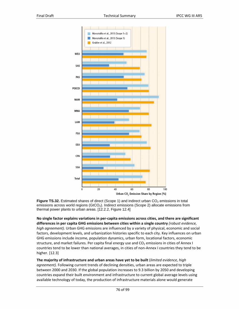
Final Draft Technical Summary IPCC WG III AR5
76 of 99
Figure TS.32. Estimated shares of direct (Scope 1) and indirect urban CO2 emissions in total emissions across world regions (GtCO2). Indirect emissions (Scope 2) allocate emissions from thermal power plants to urban areas. [12.2.2, Figure 12.4]
No single factor explains variations in per‐capita emissions across cities, and there are significant differences in per capita GHG emissions between cities within a single country (robust evidence, high agreement). Urban GHG emissions are influenced by a variety of physical, economic and social factors, development levels, and urbanization histories specific to each city. Key influences on urban GHG emissions include income, population dynamics, urban form, locational factors, economic structure, and market failures. Per capita final energy use and CO2 emissions in cities of Annex I countries tend to be lower than national averages, in cities of non‐Annex I countries they tend to be higher. [12.3]
The majority of infrastructure and urban areas have yet to be built (limited evidence, high agreement). Following current trends of declining densities, urban areas are expected to triple between 2000 and 2030. If the global population increases to 9.3 billion by 2050 and developing countries expand their built environment and infrastructure to current global average levels using available technology of today, the production of infrastructure materials alone would generate

Final Draft Technical Summary IPCC WG III AR5
77 of 99
about 470 GtCO2 emissions. Currently, average per capita CO2 emissions embodied in the infrastructure of industrialized countries is five times larger than those in developing countries. [12.2, 12.3]
Infrastructure and urban form are strongly interlinked, and lock in patterns of land use, transport choice, housing, and behaviour (medium evidence, high agreement). Urban form and infrastructure shape long‐term land use management, influence individual transport choice, housing, and behaviour, and affect the system‐wide efficiency of a city. Once in place, urban form and infrastructure are difficult to change (Figure TS.33). [12.2, 12.3, 12.4]
Urban mitigation options vary across urbanization trajectories and are expected to be most effective when policy instruments are bundled (robust evidence, high agreement,). For rapidly developing cities, options include shaping their urbanization and infrastructure development towards more sustainable and low carbon pathways. In mature or established cities, options are constrained by existing urban forms and infrastructure and the potential for refurbishing existing systems and infrastructures. Key mitigation strategies include co‐locating high residential with high employment densities, achieving high land use mixes, increasing accessibility and investing in public transit and other supportive demand management measures (Figure TS.33). Bundling these strategies can reduce emissions in the short term and generate even higher emissions savings in the long term. [12.4, 12.5]
The largest opportunities for future urban GHG emissions reduction might be in rapidly urbanizing countries where infrastructure inertia has not set in; however, the required governance, technical, financial, and institutional capacities can be limited (high confidence). The bulk of future infrastructure and urban growth is expected in small‐ to medium‐size cities in developing countries, where these capacities can be limited or weak. [12.4, 12.5, 12.6, 12.7]
Thousands of cities are undertaking climate action plans, but the extent of urban mitigation is highly uncertain (robust evidence, high agreement). Local governments and institutions possess unique opportunities to engage in urban mitigation activities and local mitigation efforts have expanded rapidly. However, little systematic reporting or evidence exists regarding the overall extent to which cities are implementing mitigation policies, and even less regarding their GHG impacts. Climate action plans include a range of measures across sectors, largely focused on energy efficiency rather than broader land‐use planning strategies and cross‐sectoral measures to reduce sprawl and promote transit‐oriented development (Figure TS.34). [12.6, 12.7]
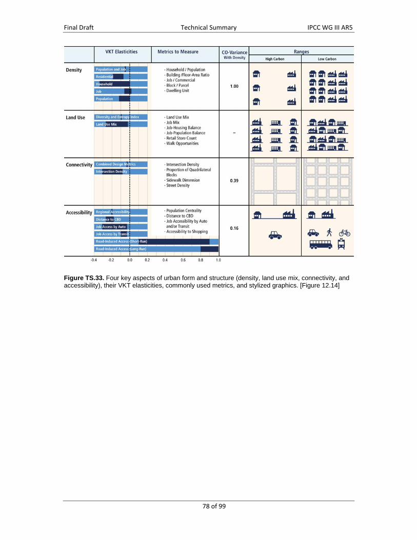
Final Draft Technical Summary IPCC WG III AR5
78 of 99
Figure TS.33. Four key aspects of urban form and structure (density, land use mix, connectivity, and accessibility), their VKT elasticities, commonly used metrics, and stylized graphics. [Figure 12.14]

Final Draft Technical Summary IPCC WG III AR5
79 of 99
Figure TS.34. Common mitigation measures in Climate Action Plans. [Figure 12.22]
The feasibility of spatial planning instruments for climate change mitigation is highly dependent on a city’s financial and governance capability (robust evidence, high agreement). Drivers of urban GHG emissions are interrelated and can be addressed by a number of regulatory, management, and market‐based instruments. Many of these instruments are applicable to cities in both developed and developing countries, but the degree to which they can be implemented varies. In addition, each instrument varies in its potential to generate public revenues or require government expenditures, and the administrative scale at which it can be applied (Figure TS.35). A bundling of instruments and a high level of coordination across institutions can increase the likelihood of achieving emissions reductions and avoiding unintended outcomes. [12.6, 12.7]

Final Draft Technical Summary IPCC WG III AR5
80 of 99
Figure TS.35. Key spatial planning tools and effects on government revenues and expenditures across administrative scales. Figure shows four key spatial planning tools (coded in colours) and the scale of governance at which they are administered (x-axis) as well as how much public revenue or expenditure the government generates by implementing each instrument (y-axis). [Figure 12.20]
For designing and implementing climate policies effectively, institutional arrangements, governance mechanisms, and financial resources should be aligned with the goals of reducing urban GHG emissions (high confidence). These goals will reflect the specific challenges facing individual cities and local governments. The following have been identified as key factors: 1) institutional arrangements that facilitate the integration of mitigation with other high‐priority urban agendas; 2) a multilevel governance context that empowers cities to promote urban transformations; 3) spatial planning competencies and political will to support integrated land‐use and transportation planning; and 4) sufficient financial flows and incentives to adequately support mitigation strategies. [12.6, 12.7]
Successful implementation of urban climate change mitigation strategies can provide co‐benefits (medium evidence, high agreement). Co‐benefits of local climate change mitigation can include public savings, air pollution and associated health benefits, and productivity increases in urban centres, providing additional motivation for undertaking mitigation activities. [12.5, 12.6, 12.7, 12.8]

Final Draft Technical Summary IPCC WG III AR5
81 of 99
TS.4 Mitigation policies and institutions
The previous section shows that since AR4 the scholarship on transformation pathways has begun to consider in much more detail how a variety of real world considerations—such as institutional and political constraints, uncertainty associated with climate change risks, the availability of technologies and other factors—affect the kinds of policies and measures that are adopted. Those factors have important implications for the design, cost, and effectiveness of mitigation action. This section focuses on how governments and other actors in the private and public sectors design, implement, and evaluate mitigation policies. It considers the ‘normative’ scientific research on how policies should be designed to meet particular criteria. It also considers research on how policies are actually designed and implemented a field known as ‘positive’ analysis. The discussion first characterizes fundamental conceptual issues, and then presents a summary of the main findings from AR5 on local, national, and sectoral policies. Much of the practical policy effort since AR4 has occurred in these contexts. From there the summary looks at ever‐higher levels of aggregating, ultimately ending at the global level and cross‐cutting investment and finance issues.
TS.4.1 Policy design, behaviour and political economy
There are multiple criteria for evaluating policies. Policies are frequently assessed according to four criteria [3.7.1, 13.2.2, 15.4.1]:
Environmental effectiveness – whether policies achieve intended goals in reducing emissions or other pressures on the environment or in improving measured environmental quality.
Economic effectiveness – the impact of policies on the overall economy. This criterion includes the concept of economic efficiency, the principle of maximizing net economic benefits. Economic welfare also includes the concept of cost‐effectiveness, the principle of attaining a given level of environmental performance at lowest aggregate cost.
Distributional and social impacts – also known as ‘distributional equity,’ this criterion concerns the allocation of costs and benefits of policies to different groups and sectors within and across economies over time. It includes, often, a special focus on impacts on the least well off members of societies within countries and around the world.
Institutional and political feasibility – whether policies can be implemented in light of available institutional capacity, the political constraints that governments face, and other factors that are essential to making a policy viable.
All criteria can be applied with regard to the immediate ‘static’ impacts of policies and from a long run ‘dynamic’ perspective that accounts for the many adjustments in the economic, social, political systems. Criteria may be mutually reinforcing, but there may also be conflicts or tradeoffs among them. Policies designed for maximum environmental effectiveness or economic performance may fare less well on other criteria, for example. Such tradeoffs arise at multiple levels of governing systems. For example, it may be necessary to design international agreements with flexibility so that it is feasible for a large number of diverse countries to accept them, but excessive flexibility may undermine incentives to invest in cost‐effective long‐term solutions.
Policymakers make use of many different policy instruments at the same time. Theory can provide some guidance on the normative advantages and disadvantages of alternative policy instruments in light of the criteria discussed above. The range of different policy instruments includes [3.8, 15.3]:
Economic incentives, such as taxes, tradable allowances, fines, and subsidies
Direct regulatory approaches, such as technology or performance standards
Information programmes, such as labelling and energy audits

Final Draft Technical Summary IPCC WG III AR5
82 of 99
Government provision, for example of new technologies or in state enterprises
Voluntary actions, initiated by governments, firms, and NGOs
Since AR4, the inventory of research on these different instruments has grown, mostly with reference to experiences with policies adopted within particular sectors and countries as well as the many interactions between policies. One implication of that research has been that international agreements that aim to coordinate across countries reflect the practicalities on the particular policy choices of national governments and other jurisdictions.
The diversity in policy goals and instruments highlights differences in how sectors and countries are organized economically and politically as well as the multi‐level nature of mitigation. Since AR4, one theme of research in this area has been that the success of mitigation measures depends in part on the presence of institutions capable of designing and implementing regulatory policies and the willingness of respective publics to accept these policies. Many policies have effects, sometimes unanticipated, across multiple jurisdictions—across cities, regions and countries—because the economic effects of policies and the technological options are not contained within a single jurisdiction. [13.2.2.3, 14.1.3, 15.2, 15.9]
Interactions between policy instruments can be welfare‐enhancing or welfare‐degrading. The chances of welfare‐enhancing interactions are particularly high when policy instruments address multiple different market failures – for example, a subsidy or other policy instrument aimed at boosting investment in R&D on less emission intensive technologies can complement policies aimed at controlling emissions, as can regulatory intervention to support efficient improvement of end‐use energy efficiency. By contrast, welfare‐degrading interactions are particularly likely when policies are designed to achieve identical goals. Narrowly targeted policies such as support for deployment (rather than R&D) of particular energy technologies that exist in tandem with broader economy‐wide policies aimed at reducing emissions (for example, a cap‐and‐trade emissions scheme) can have the effect of shifting the mitigation effort to particular sectors of the economy in ways that typically result in higher overall costs. [3.8.6, 15.7, 15.8]
There are a growing number of countries devising policies for adaptation, as well as mitigation, and there may be benefits to considering the two within a common policy framework (medium evidence, low agreement). However, there are divergent views on whether adding adaptation to mitigation measures in the policy portfolio encourages or discourages participation in international cooperation [1.4.5, 13.3.3]. It is recognized that an integrated approach can be valuable, as there exist both synergies and tradeoffs [16.6].
Traditionally, policy design, implementation, and evaluation has focused on governments as central designers and implementers of policies, but new studies have emerged on government acting in a coordinating role (medium confidence). In these cases, governments themselves seek to advance voluntary approaches, especially when traditional forms of regulation are thought to be inadequate or the best choices of policy instruments and goals is not yet apparent. Examples include voluntary schemes that allow individuals and firms to purchase emission credits that offset the emissions associated with their own activities such as flying and driving. Since AR4, a substantial new literature has emerged to examine these schemes from positive and normative perspectives. [13.12, 15.5.7]
The successful implementation of policy depends on many factors associated with human and institutional behaviour (very high confidence). One of the challenges in designing effective instruments is that the activities that a policy is intended to affect—such as the choice of energy technologies and carriers and a wide array of agricultural and forestry practices—are also influenced by social norms, decision‐making rules, behavioural biases, and institutional processes [2.4, 3.10]. There are examples of policy instruments made more effective by taking these factors into account, such as in the case of financing mechanisms for household investments in energy efficiency and

Final Draft Technical Summary IPCC WG III AR5
83 of 99
renewable energy that eliminate the need for up‐front investment [2.4, 2.6.5.3]. Additionally, the norms that guide acceptable practices could have profound impacts on the baselines against which policy interventions are evaluated, either magnifying or reducing the required level of policy intervention [1.2.4, 4.3, 6.5.2].
Climate policy can encourage investment that may otherwise be suboptimal because of market imperfections (very high confidence). Many of the options for energy efficiency as well as low‐carbon energy provision require high up‐front investment that is often magnified by high‐risk premiums associated with investments in new technologies. The relevant risks include those associated with future market conditions, regulatory actions, public acceptance, and technology cost and performance. Dedicated financial instruments exist to lower these risks for private actors – for example, credit insurance, feed‐in tariffs, concessional finance, or rebates [16.4]. The design of other mitigation policies can also incorporate elements to help reduce risks, such as a cap and trade regime that includes price floors and ceilings [2.6.5, 15.5, 15.6].
TS.4.2 Sectoral and national policies
There has been a considerable increase in national policies and institutions to address climate change since AR4 (Figure TS.35). Policies and strategies are in their early stages in many countries, and there is inadequate evidence to assess whether and how they will result in appropriate institutional and policy change, and therefore, their impact on future emissions. However, to date these policies, taken together, have not yet achieved a substantial deviation in emissions from the past trend. Theories of institutional change suggest they might play a role in shaping incentives, political contexts, and policy paradigms in a way that encourages emissions reductions in the future [15.1, 15.2]. However, many baseline scenarios (i.e., those without additional mitigation policies) show concentrations that exceed 1000 ppm CO2eq by 2100, which is far from a concentration with a likely probability of maintaining temperature increases below 2°C this century. Mitigation scenarios suggest that a wide range of environmentally effective policies could be enacted that would be consistent with such goals [6.3]. In practice, climate strategies and the policies that result are influenced by political economy factors, sectoral considerations, and the potential for realizing co‐benefits. In many countries, mitigation policies have also been actively pursued at state and local levels. [15.2, 15.5, 15.8]

Final Draft Technical Summary IPCC WG III AR5
84 of 99
Figure TS.36. National Climate legislation and strategies in 2007 and 2012. In this figure, climate legislation is defined as mitigation-focused legislation that goes beyond sectoral action alone. Climate strategy is defined as a non-legislative plan or framework aimed at mitigation that encompasses more than a small number of sectors, and that includes a coordinating body charged with implementation. International pledges are not included, nor are sub-national plans and strategies. The panel shows proportion of GHG emissions covered. [Figure 15.1]
Since AR4, there is growing political and analytical attention to co‐benefits and adverse side‐effects of climate policy on other objectives and vice versa that has resulted in an increased focus on policies designed to integrate multiple objectives (high confidence). Co‐benefits are often explicitly referenced in climate and sectoral plans and strategies and often enable enhanced political support [15.2]. However, the analytical and empirical underpinnings for many of these interactive effects, and particularly for the associated welfare impacts, are under‐developed [1.2, 3.6.3, 4.2, 4.8, 6.6]. The scope for co‐benefits is greater in low‐income countries, where complementary policies for other objectives, such as air quality, are often weak. [5.7, 6.6, 15.2].
The design of institutions affects the choice and feasibility of policy options as well as the sustainable financing of mitigation measures. Institutions designed to encourage participation by representatives of new industries and technologies can facilitate transitions to low emission pathways [15.2, 15.6]. Policies vary in the extent to which they require new institutional capabilities to be implemented. Carbon taxation, in most settings, can rely mainly on existing tax infrastructure and is administratively easier to implement than many other alternatives such as cap and trade [15.5]. The extent of institutional innovation required for policies can be a factor in instrument choice, especially in developing countries.
Sector‐specific policies have been more widely used than economy‐wide, market‐based policies (medium evidence, high agreement). Although economic theory suggests that market‐based, economy‐wide policies are generally more cost‐effective than sectoral approaches, political economy considerations often make those policies harder to achieve than sectoral policies [15.2.3, 15.2.6, 15.5.1]. In some countries, emission trading and taxes have been enacted to address the market externalities associated with GHG emissions, and have contributed to the fulfilment of sector‐specific GHG reduction goals (medium evidence, medium agreement) [7.12]. In the longer term, GHG pricing can support the adoption of low GHG energy technologies. Even if economy‐wide policies were implemented, sector‐specific policies may be needed to overcome sectoral market failures. For example, building codes can require energy efficient investments where private

Final Draft Technical Summary IPCC WG III AR5
85 of 99
investments would otherwise not exist [9.10]. In transport, pricing policies that raise the cost of carbon‐intensive forms of private transport are more effective when backed by public investment in viable alternatives [8.10]. Table TS.8 presents a range of sector specific policies that have been implemented in practice. [15.1, 15.2, 15.5, 15.8, 15.9]

Final Draft Technical Summary IPCC WGIII AR5
86 of 99
Table TS.8: Sector policy instruments. The Table brings together evidence on policy instruments discussed in Chapters 7 to 12. [Table 15.1] Policy Instruments
Energy [Section 7.12] Transport [8.10] Buildings [9.10] Industry [10.11] AFOLU [11.10] Human Settlements and Infrastructure [12.5]
Economic Instruments – Taxes (Carbon taxes may be economy‐wide)
‐ Carbon tax (e.g.,
applied to
electricity or fuels)
‐ Fuel taxes
‐ Congestion charges,
vehicle registration
fees, road tolls
‐ Vehicle taxes
‐ Carbon and/or energy
taxes (either sectoral
or economy wide)
‐ Carbon tax or energy tax
‐ Waste disposal taxes or
charges
‐ Fertilizer or Nitrogen
taxes to reduce
nitrous oxide
‐ Sprawl taxes, Impact fees,
exactions, split‐rate property
taxes, tax increment finance,
betterment taxes,
congestion charges
Economic Instruments – Tradable Allowances (May be economy‐wide)
‐ Emission trading
‐ Emission credits
under CDM
‐ Tradable Green
Certificates
‐Fuel and vehicle standards
‐ Tradable certificates
for energy efficiency
improvements (white
certificates)
‐ Emission trading
‐ Emission credit under CDM
‐ Tradable Green
Certificates
‐ Emission credits
under CDM (Adam)
‐ Compliance schemes
outside Kyoto
protocol (national
schemes)
‐ Voluntary carbon
markets
‐ Urban‐scale Cap‐and‐Trade
Economic Instruments – Subsidies
‐ Fossil fuel subsidy
removal
‐ Feed in tariffs for
renewable energy
‐ Biofuel subsidies
‐ Vehicle purchase
subsidies
‐ Feebates
‐ Subsidies or Tax
exemptions for
investment in efficient
buildings, retrofits
and products
‐ Subsidized loans
‐ Subsidies (e.g., for energy
audits)
‐ Fiscal incentives (e.g., for
fuel switching)
‐ Credit lines for low
carbon agriculture,
sustainable forestry.
‐ Special Improvement or
Redevelopment Districts
Regulatory Approaches
‐ Efficiency or
environmental
performance
standards
‐ Renewable
Portfolio standards
(RPS) for renewable
energy (RE)
‐ Fuel economy
performance
standards
‐ Fuel quality
standards
‐ GHG emission
performance
standards
‐ Regulatory
restrictions to
encourage modal
shifts (road to rail)
‐ Restriction on use of
‐ Building codes and
standards
‐ Equipment and
appliance standards
‐ Mandates for energy
retailers to assist
customers invest in
energy efficiency
‐ Energy efficiency
standards for equipment
‐ Energy management
systems (also voluntary)
‐ Voluntary agreements
(where bound by
regulation)
‐ Labelling and public
procurement regulations
‐ National policies to
support REDD+
including monitoring,
reporting and
verification
‐ Forest law to reduce
deforestation
‐ Air and water
pollution control GHG
precursors
‐ Land‐use planning and
governance
‐ Mixed use zoning
‐ Development restrictions
‐ Affordable housing
mandates
‐ Site access controls
‐ Transfer development rights
‐ Design codes
‐ Building codes
‐ Street codes
‐ Design standards
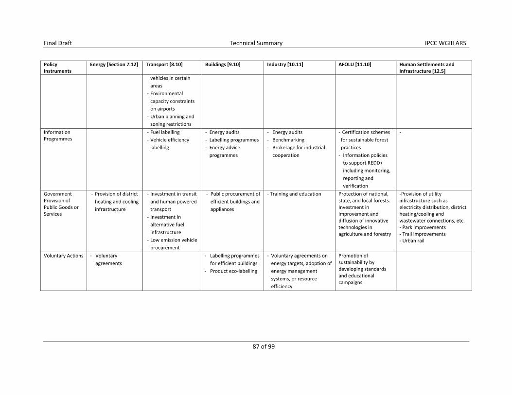
Final Draft Technical Summary IPCC WGIII AR5
87 of 99
Policy Instruments
Energy [Section 7.12] Transport [8.10] Buildings [9.10] Industry [10.11] AFOLU [11.10] Human Settlements and Infrastructure [12.5]
vehicles in certain
areas
‐ Environmental
capacity constraints
on airports
‐ Urban planning and
zoning restrictions
Information Programmes
‐ Fuel labelling
‐ Vehicle efficiency
labelling
‐ Energy audits
‐ Labelling programmes
‐ Energy advice
programmes
‐ Energy audits
‐ Benchmarking
‐ Brokerage for industrial
cooperation
‐ Certification schemes
for sustainable forest
practices
‐ Information policies
to support REDD+
including monitoring,
reporting and
verification
‐
Government Provision of Public Goods or Services
‐ Provision of district
heating and cooling
infrastructure
‐ Investment in transit
and human powered
transport
‐ Investment in
alternative fuel
infrastructure
‐ Low emission vehicle
procurement
‐ Public procurement of
efficient buildings and
appliances
‐ Training and education Protection of national, state, and local forests. Investment in improvement and diffusion of innovative technologies in agriculture and forestry
‐Provision of utility infrastructure such as electricity distribution, district heating/cooling and wastewater connections, etc. ‐ Park improvements ‐ Trail improvements ‐ Urban rail
Voluntary Actions ‐ Voluntary
agreements
‐ Labelling programmes
for efficient buildings
‐ Product eco‐labelling
‐ Voluntary agreements on
energy targets, adoption of
energy management
systems, or resource
efficiency
Promotion of sustainability by developing standards and educational campaigns

Final Draft Technical Summary IPCC WGIII AR5
88 of 99
Carbon taxes have been implemented in some countries and—alongside technology and other policies—have contributed to decoupling of emissions from GDP (high confidence). Differentiation by sector, which is quite common, reduces cost‐effectiveness that arises from the changes in production methods, consumption patterns, lifestyle shifts, and technology development, but it may increase political feasibility, or be preferred for reasons of competitiveness or distributional equity. In some countries, high carbon and fuel taxes have been made politically feasible by refunding revenues or by lowering other taxes in an environmental fiscal reform. Mitigation policies that raise government revenue (e.g., auctioned emission allowances under a cap‐and‐trade system or emission taxes) generally have lower social costs than approaches which do not, but this depends on how the revenue is used [3.6.3]. [15.2, 15.5.2, 15.5.3]
Fuel taxes are an example of a sector‐specific policy and are often originally put in place for objectives such as revenue – they are not necessarily designed for the purpose of mitigation (high confidence). In Europe, where fuel taxes are highest, they have contributed to reductions in carbon emissions from the transport sector of roughly 50% for this group of countries. The short‐run response to higher fuel prices is often small, but long‐run price elasticities are quite high, or roughly‐0.6 to ‐0.8. This means that in the long run, 10% higher fuel prices correlate with 7% reduction in fuel use and emissions. In the transport sector, taxes have the advantage of being progressive or neutral in most countries and strongly progressive in low‐income countries. [15.5.2]
Cap‐and‐trade systems for GHGs are being established in a growing number of countries and regions. Their environmental effect has so far been limited because caps have either been loose or have not yet been binding (limited evidence, medium agreement). There appears to have been a tradeoff between the political feasibility and environmental effectiveness of these programmes, as well as between political feasibility and distributional equity in the allocation of permits. Greater environmental effectiveness through a tighter cap may be combined with a price ceiling that improves political feasibility. [14.4.2, 15.5.3]
Different factors reduced the price of EU Emissions Trading System (ETS) allowances below anticipated levels, thereby slowing investment in mitigation (high confidence). While the European Union demonstrated that a cross‐border cap‐and‐trade system can work, the low price of EU ETS allowances in recent years provided insufficient incentives for significant additional investment in mitigation. The low price is related to unexpected depth and duration of the economic recession, uncertainty about the long‐term emission reduction targets, import of credits from the Clean Development Mechanism (CDM), and the interaction with other policy instruments, particularly related to the expansion of renewable energy as well as regulation on energy efficiency. It has proven to be politically difficult to address this problem by removing emission permits temporarily, tightening the cap, or providing a long‐term mitigation goal. [14.4.2]
Adding a mitigation policy to another may not necessarily enhance mitigation. For instance, if a cap‐and‐trade system has a sufficiently stringent cap then other policies such as renewable subsidies have no further impact on total emissions (although they may affect costs and possibly the viability of more stringent future targets). If the cap is loose relative to other policies, it becomes ineffective. This is an example of a negative interaction between policy instruments. Since other policies cannot be ‘added on’ to a cap‐and‐trade system, if it is to meet any particular target, a sufficiently low cap is necessary. A carbon tax, on the other hand, can have an additive environmental effect to policies such as subsidies to renewables. [15.7]
Reduction of subsidies to fossil energy can achieve significant emission reductions at negative social cost (very high confidence). Although political economy barriers are substantial, many countries have reformed their tax and budget systems to reduce fuel subsidies that actually accrue to the relatively wealthy, and utilized lump‐sum cash transfers or other mechanisms that are more targeted to the poor. [15.5.3]

Final Draft Technical Summary IPCC WGIII AR5
89 of 99
Direct regulatory approaches and information measures are widely used, and are often environmentally effective, though debate remains on the extent of their environmental impacts and cost‐effectiveness (medium confidence). Examples include energy efficiency standards and labelling programmes that can help consumers make better‐informed decisions. While such approaches often work at a net social benefit, the scientific literature is divided on whether such policies are implemented with negative private costs to firms and individuals [Box TS.12, 3.9.3, 15.5.5, 15.5.6]. Since AR4 there has been continued investigation into the ‘rebound’ effects that arise when higher efficiency leads to lower energy costs and greater consumption. There is general agreement that such rebound effects exist, but there is low agreement in the literature on the magnitude [Box TS.13, 3.9.5, 5.7.2, 15.5.4].
Box TS.13. The rebound effect can reduce energy savings from technological improvement
Technological improvements in energy efficiency (EE) have direct effects on energy consumption and thus GHG emissions, but can cause other changes in consumption, production, and prices that will, in turn, affect GHG emissions. These changes are generally called ‘rebound’ or ‘takeback’ because in most cases they reduce the net energy or emissions reduction associated with the efficiency improvement. The size of EE rebound is controversial, with some research papers suggesting little or no rebound and others concluding that it offsets most or all reductions from EE policies [3.9.5, 5.7.2].
Total EE rebound can be broken down into three distinct parts: substitution‐effect, income‐effect, and economy‐wide effect [3.9.5]. In end‐use consumption, substitution‐effect rebound, or ‘direct rebound’ assumes that a consumer will make more use of a device if it becomes more energy efficient because it will be cheaper to use. Income‐effect rebound or ‘indirect rebound’, arises if the improvement in EE makes the consumer wealthier and leads her to consume additional products that require energy. Economy‐wide rebound refers to impacts beyond the behaviour of the entity benefiting directly from the EE improvement, such as the impact of EE on the price of energy.
Analogous rebound effects for EE improvements in production are substitution towards an input with improved energy efficiency, and substitution among products by consumers when an EE improvement changes the relative prices of goods, as well as an income effect when an EE improvement lowers production costs and creates greater wealth.
Rebound is sometimes confused with the concept of carbon leakage, which often describes the incentive for emissions‐intensive economic activity to migrate away from a region that restricts GHGs (or other pollutants) towards areas with fewer or no restrictions on such emissions [5.4.1, 14.4]. Energy efficiency rebound can occur regardless of the geographic scope of the adopted policy. As with leakage, however, the potential for significant rebound illustrates the importance of considering the full equilibrium effects of a mitigation policy [3.9.5, 15.5.4].
There is a distinct role for technology policy as a complement to other mitigation policies (high confidence). Properly implemented technology policies reduce the cost of achieving a given environmental target. Technology policy will be most effective when technology‐push policies (e.g., publicly funded R&D) and demand‐pull policies (e.g., governmental procurement programmes or performance regulations) are used in a complementary fashion. While technology‐push and demand‐pull policies are necessary, they are unlikely to be sufficient without complementary framework conditions. Managing social challenges of technology policy change may require innovations in policy and institutional design, including building integrated policies that make complementary use of market incentives, authority, and norms (medium confidence). Since AR4, a large number of countries and sub‐national jurisdictions have introduced support policies for renewable energy such as FIT and RPS. These have promoted substantial diffusion and innovation of new energy technologies such as wind turbines and photovoltaic panels, but have raised questions

Final Draft Technical Summary IPCC WGIII AR5
90 of 99
about their economic efficiency, and introduced challenges for grid and market integration. [2.6.5, 7.12, 15.6.5]
Worldwide investment in research in support of mitigation is small relative to overall public research spending (medium confidence). The effectiveness of research support will be greatest if it is increased slowly and steadily rather than dramatically or erratically. It is important that data collection for program evaluation to be built into technology policy programmes, because there is limited empirical evidence on the relative effectiveness of different mechanisms for supporting the invention, innovation and diffusion of new technologies. [15.6.2, 15.6.5]
Government planning and provision can facilitate shifts to less energy and GHG‐intensive infrastructure and lifestyles (high confidence). This applies particularly when there are indivisibilities in the provision of infrastructure as in the energy sector [7.6] (e.g., for electricity transmission and distribution or district heating networks); in the transport sector [8.4] (e.g., for non‐motorized or public transport); and in urban planning [12.5]. The provision of adequate infrastructure is important for behavioural change [15.5.6].
Successful voluntary agreements on mitigation between governments and industries are characterized by a strong institutional framework with capable industrial associations (medium confidence). The strengths of voluntary agreements are speed and flexibility in phasing measures, and facilitation of barrier removal activities for energy efficiency and low emission technologies. Regulatory threats, even though the threats are not always explicit, are also an important factor for firms to be motivated. There are few environmental impacts without a proper institutional framework. [15.5.7]
TS.4.3 Development and regional cooperation
Regional cooperation offers substantial opportunities for mitigation due to geographic proximity, shared infrastructure and policy frameworks, trade, and cross‐border investment that would be difficult for countries to implement in isolation (high confidence). Examples of possible regional cooperation policies include regionally‐linked development of renewable energy power pools, networks of natural gas supply infrastructure, and coordinated policies on forestry. [14.1]
At the same time, there is a mismatch between opportunities and capacities to undertake mitigation (medium confidence). The regions with the greatest potential to leapfrog to low‐carbon development trajectories are the poorest developing regions where there are few lock‐in effects in terms of modern energy systems and urbanization patterns. However, these regions also have the lowest financial, technological, and institutional capacities to embark on such low‐carbon development paths [Figure TS.36] and their cost of waiting is high due to unmet energy and development needs. Emerging economies already have more lock‐in effects but their rapid build‐up of modern energy systems and urban settlements still offers substantial opportunities for low‐carbon development. Their capacity to reorient themselves to low‐carbon development strategies is higher, but also faces constraints in terms of finance, technology, and the high cost of delaying the installation of new energy capacity. Lastly, industrialized economies have the largest lock‐in effects, but the highest capacities to reorient their energy, transport, and urbanizations systems towards low‐carbon development. [14.1.3, 14.3.2]
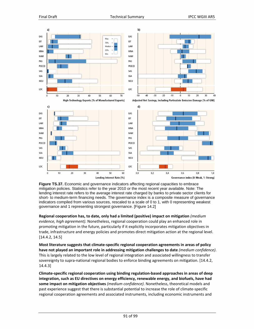
Final Draft Technical Summary IPCC WGIII AR5
91 of 99
Figure TS.37. Economic and governance indicators affecting regional capacities to embrace mitigation policies. Statistics refer to the year 2010 or the most recent year available. Note: The lending interest rate refers to the average interest rate charged by banks to private sector clients for short- to medium-term financing needs. The governance index is a composite measure of governance indicators compiled from various sources, rescaled to a scale of 0 to 1, with 0 representing weakest governance and 1 representing strongest governance. [Figure 14.2]
Regional cooperation has, to date, only had a limited (positive) impact on mitigation (medium evidence, high agreement). Nonetheless, regional cooperation could play an enhanced role in promoting mitigation in the future, particularly if it explicitly incorporates mitigation objectives in trade, infrastructure and energy policies and promotes direct mitigation action at the regional level. [14.4.2, 14.5]
Most literature suggests that climate‐specific regional cooperation agreements in areas of policy have not played an important role in addressing mitigation challenges to date (medium confidence). This is largely related to the low level of regional integration and associated willingness to transfer sovereignty to supra‐national regional bodies to enforce binding agreements on mitigation. [14.4.2, 14.4.3]
Climate‐specific regional cooperation using binding regulation‐based approaches in areas of deep integration, such as EU directives on energy efficiency, renewable energy, and biofuels, have had some impact on mitigation objectives (medium confidence). Nonetheless, theoretical models and past experience suggest that there is substantial potential to increase the role of climate‐specific regional cooperation agreements and associated instruments, including economic instruments and

Final Draft Technical Summary IPCC WGIII AR5
92 of 99
regulatory instruments. In this context it is important to consider carbon leakage of such regional initiatives and ways to address it. [14.4.2, 14.4.1]
In addition, non‐climate‐related modes of regional cooperation could have significant implications for mitigation, even if mitigation objectives are not a component (medium confidence). Regional cooperation with non‐climate‐related objectives but possible mitigation implications, such as trade agreements, cooperation on technology, and cooperation on infrastructure and energy, has to date also had negligible impacts on mitigation. Modest impacts have been found on the level of emissions of members of regional preferential trade areas if these agreements are accompanied with environmental agreements. Creating synergies between adaptation and mitigation can increase the cost‐effectiveness of climate change actions. Linking electricity and gas grids at the regional level has also had a modest impact on mitigation as it facilitated greater use of low carbon and renewable technologies; there is substantial further mitigation potential in such arrangements. [14.4.2]
TS.4.4 International cooperation
Climate change mitigation is a global commons problem that requires international cooperation, but since AR4, scholarship has emerged that emphasizes a more complex and multi‐faceted view of climate policy (very high confidence). Two characteristics of climate change necessitate international cooperation: climate change is a global commons problem, and it is characterized by a high degree of heterogeneity in the origins of emissions, mitigation opportunities, climate impacts, and capacity for mitigation and adaptation [13.2.1.1]. Traditional policy‐making efforts focused on international cooperation as a task centrally focused on the coordination of national policies that would be adopted with the goal of mitigation. More recent policy developments suggest that there is a more complicated set of relationships between national, regional, and global policy‐making, based on a multiplicity of goals, a recognition of policy co‐benefits, and barriers to technological innovation and diffusion [1.2, 6.6, 15.2]. A major challenge is assessing whether highly decentralized policy action is consistent with and can lead to global mitigation efforts that are effective, equitable, and efficient [6.1.2.1, 13.13.1.3].
International cooperation on climate change has become more institutionally diverse over the past decade (very high confidence). Perceptions of fairness can facilitate cooperation by increasing the legitimacy of an agreement [3.10, 13.2.2.4]. The United Nations Framework Convention on Climate Change (UNFCCC) remains a primary international forum for climate negotiations, but other institutions have emerged at multiple scales, namely: global, regional, national, and local [13.3.1, 13.12]. This institutional diversity arises in part from the growing inclusion of climate change issues in other policy arenas (e.g., sustainable development, international trade, and human rights). These and other linkages create opportunities, potential co‐benefits, or harms that have not yet been thoroughly examined. Issue linkage also creates the possibility for countries to experiment with different forums of cooperation (‘forum shopping’), which may increase negotiation costs and potentially distract from or dilute the performance of international cooperation toward climate goals. [13.3, 13.4, 13.5] Finally, there has been an emergence of new transnational climate related institutions not centred on sovereign states (e.g., public‐private partnerships, private sector governance initiatives, transnational NGO programmes, and city level initiatives) [13.3.1, 13.12].
Existing and proposed international climate agreements vary in the degree to which their authority is centralized. The range of centralized formalization spans strong multilateral agreements (such as the Kyoto Protocol targets), harmonized national policies (such as the Copenhagen/Cancún pledges), and decentralized but coordinated national policies (such as planned linkages of national and sub‐national emissions trading schemes) [Figure TS.37, 13.4.1, 13.4.3]. Four other design elements of international agreements have particular relevance: legal bindingness, goals and targets, flexible mechanisms, and equitable methods for effort‐sharing [13.4.2]. Existing and proposed modes of international cooperation are assessed in Table TS.9. [13.13]
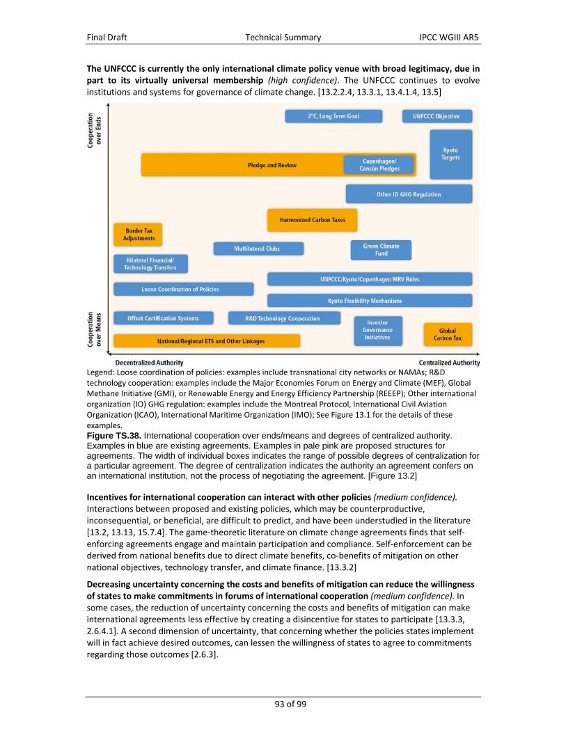
Final Draft Technical Summary IPCC WGIII AR5
93 of 99
The UNFCCC is currently the only international climate policy venue with broad legitimacy, due in part to its virtually universal membership (high confidence). The UNFCCC continues to evolve institutions and systems for governance of climate change. [13.2.2.4, 13.3.1, 13.4.1.4, 13.5]
Legend: Loose coordination of policies: examples include transnational city networks or NAMAs; R&D technology cooperation: examples include the Major Economies Forum on Energy and Climate (MEF), Global Methane Initiative (GMI), or Renewable Energy and Energy Efficiency Partnership (REEEP); Other international organization (IO) GHG regulation: examples include the Montreal Protocol, International Civil Aviation Organization (ICAO), International Maritime Organization (IMO); See Figure 13.1 for the details of these examples. Figure TS.38. International cooperation over ends/means and degrees of centralized authority. Examples in blue are existing agreements. Examples in pale pink are proposed structures for agreements. The width of individual boxes indicates the range of possible degrees of centralization for a particular agreement. The degree of centralization indicates the authority an agreement confers on an international institution, not the process of negotiating the agreement. [Figure 13.2]
Incentives for international cooperation can interact with other policies (medium confidence). Interactions between proposed and existing policies, which may be counterproductive, inconsequential, or beneficial, are difficult to predict, and have been understudied in the literature [13.2, 13.13, 15.7.4]. The game‐theoretic literature on climate change agreements finds that self‐enforcing agreements engage and maintain participation and compliance. Self‐enforcement can be derived from national benefits due to direct climate benefits, co‐benefits of mitigation on other national objectives, technology transfer, and climate finance. [13.3.2]
Decreasing uncertainty concerning the costs and benefits of mitigation can reduce the willingness of states to make commitments in forums of international cooperation (medium confidence). In some cases, the reduction of uncertainty concerning the costs and benefits of mitigation can make international agreements less effective by creating a disincentive for states to participate [13.3.3, 2.6.4.1]. A second dimension of uncertainty, that concerning whether the policies states implement will in fact achieve desired outcomes, can lessen the willingness of states to agree to commitments regarding those outcomes [2.6.3].
Final Draft Technical Summary IPCC WGIII AR5
94 of 99
International cooperation can stimulate public and private investment and the adoption of economic incentives and direct regulations that promote technological innovation (medium confidence). Technology policy can help lower mitigation costs, thereby increasing incentives for participation and compliance with international cooperative efforts, particularly in the long‐run. Equity issues can be affected by domestic intellectual property rights regimes, which can alter the rate of both technology transfer and the development of new technologies. [13.3, 13.9]
In the absence of—or as a complement to—a binding, international agreement on climate change, policy linkages between and among existing and nascent international, regional, national, and sub‐national climate policies offer potential climate benefits (medium confidence). Direct and indirect linkages between and among sub‐national, national, and regional carbon markets are being pursued to improve market efficiency. Linkage between carbon markets can be stimulated by competition between and among public and private governance regimes, accountability measures, and the desire to learn from policy experiments. Yet integrating climate policies raises a number of concerns about the performance of a system of linked legal rules and economic activities. [13.5.3] Prominent examples of linkages are among national and regional climate initiatives (e.g., planned linkage between the EU ETS and the Australian Emission Trading Scheme, international offsets planned for recognition by a number of jurisdictions), and national and regional climate initiatives with the Kyoto Protocol (e.g., the EU ETS is linked to international carbon markets through the project‐based Kyoto Mechanisms) [13.6, 13.7, 14.4.2].
International trade can promote or discourage international cooperation on climate change (high confidence). Developing constructive relationships between international trade and climate agreements involves considering how existing trade policies and rules can be modified to be more climate friendly; whether border adjustment measures or other trade measures can be effective in meeting the goals of international climate policy, including participation in and compliance with climate agreements; or whether the UNFCCC, WTO, a hybrid of the two, or a new institution is the best forum for a trade‐and‐climate architecture. [13.8]
The Montreal Protocol, aimed at protecting the stratospheric ozone layer, achieved reductions in global GHG emissions (very high confidence). The Montreal Protocol set limits on emissions of ozone‐depleting gases that are also potent GHGs, such as chlorofluorocarbons (CFCs) and hydro chlorofluorocarbons (HCFCs). Substitutes for those ozone‐depleting gases (such as HFCs, which are not ozone‐depleting) may also be potent GHGs. Lessons learned from the Montreal Protocol, for example, the effect of financial and technological transfers on broadening participation in an international environmental agreement, could be of value to the design of future international climate change agreements. [Table TS.9, 13.3.3, 13.3.4, 13.13.1.4,]
The Kyoto Protocol was the first binding step toward implementing the principles and goals provided by the UNFCCC, but it has not been as successful as intended (medium evidence, low agreement). While the parties of the Kyoto Protocol surpassed their collective emission reduction target, the Protocol’s environmental effectiveness has been less than it could have been because of incomplete participation and compliance of Annex I countries and crediting for emissions reductions that would have occurred without the Protocol in economies in transition. Additionally, the design of the Kyoto Protocol does not directly regulate the emissions of non‐Annex I countries, which have grown rapidly over the past decade. [Table TS.9, 13.13.1.1]
The flexible mechanisms under the Protocol have cost‐saving potential, but their environmental effectiveness is less clear (medium confidence). The CDM, one of the Protocol’s flexible mechanisms, created a market for emissions offsets from developing countries, generating credits equivalent to over 1.3 billion tCO2eq as of July 2013. The CDM’s environmental effectiveness has been mixed due to concerns about the limited additionality of projects, the invalid determination of some project baselines, the possibility of emissions leakage, and recent price decreases. Its distributional impact has been unequal due to the concentration of projects in a limited number of countries. The

Final Draft Technical Summary IPCC WGIII AR5
95 of 99
Protocol’s other flexible mechanisms, Joint Implementation and International Emissions Trading, have been undertaken both by governments and private market participants, but have raised concerns related to government sales of emission units. [Table TS.9, 13.7.2, 13.13.1,]
Recent UNFCCC negotiations have sought to include more ambitious commitments from countries listed in Annex B of the Kyoto Protocol, mitigation commitments from a broader set of countries than those covered under Annex B, and substantial new funding mechanisms. Voluntary pledges of quantified, economy‐wide emission reductions targets by developed countries and voluntary pledges to mitigation actions by many developing countries were formalized in the 2010 Cancún Agreement. The distributional impact of the agreement will depend in part on sources of financing, including the successful fulfilment by developed countries of their expressed joint commitment to mobilize USD 100 billion per year by 2020 for climate action in developing countries. [Table TS.9, 13.5.1.1, 13.13.1.3, 16.2.1.1]
TableTS.9: Summary of performance assessments of existing and proposed forms of cooperation. Forms of cooperation are evaluated along the four evaluation criteria described in Sections 3.7.1 and 13.2.2. [Table 13.3]
Mode of International Cooperation
Assessment Criteria
Environmental Effectiveness
Aggregate Economic Performance
Distributional Impacts
Institutional Feasibility
Existing forms of cooperation [13.13.1]
UNFCCC Aggregate GHG emissions in Annex I countries declined by 6 to 9.2% below 1990 levels by 2000; a larger reduction than the apparent ‘aim’ of returning to 1990 levels by 2000.
Authorized joint fulfilment of commitments, multi-gas approach, sources and sinks, and domestic policy choice. Cost and benefit estimates depend on baseline, discount rate, participation, leakage, co-benefits, adverse side-effects, and other factors.
Commitments distinguish between Annex I (industrialized) and non-Annex I countries. Principle of “common but differentiated responsibility.” Commitment to “equitable and appropriate contributions by each [party].”
Ratified (or equivalent) by 195 countries and regional organizations. Compliance depends on national communications.
The Kyoto Protocol Aggregate emissions in Annex I countries were reduced by 8.5 to 13.6 percent below 1990 levels by 2011, more than the Protocol’s first commitment period collective reduction target of 5.2 percent. Reductions occurred mainly in EITs; emissions increased in some others. Incomplete participation in in the first commitment period (even lower in the second)
Cost-effectiveness improved by flexible mechanisms (Joint Implementation, Clean Development Mechanism, International Emissions Trading) and domestic policy choice. Cost and benefit estimates depend on baseline, discount rate, participation, leakage, co-benefits, adverse side-effects, and other factors.
Commitments distinguish between developed and developing countries, but dichotomous distinction correlates only partly (and decreasingly) with historical emissions and with changing economic circumstances. Intertemporal equity affected by short term actions.
Ratified (or equivalent) by 192 countries and regional organizations, but took 7 years to enter into force. Compliance depends on national communications, plus Kyoto Protocol compliance system. Later added approaches to enhance measurement, reporting, and verification.
The Kyoto Mechanisms About 1.4 billion tCO2eq credits under the Clean Development Mechanism (CDM), 0.8 billion under Joint Implementation (JI), and 0.2 billion under International Emissions Trading (IET). Additionality of CDM projects remains an issue but regulatory reform underway.
CDM mobilized low cost options, particularly industrial gases, reducing costs, except for some project types. Medium evidence that technology is transferred to non-Annex I countries.
Limited direct investment from Annex I countries. Domestic investment dominates, leading to concentration of CDM projects in few countries. Limited contributions to local sustainable development.
Helped enable political feasibility of Kyoto Protocol. Has multi-layered governance. Largest international carbon markets to date. Has built institutional capacity in developing countries.

Final Draft Technical Summary IPCC WGIII AR5
96 of 99
Further Agreements under the UNFCCC
Pledges to limit emissions made by all major emitters under Cancún Agreements. Unlikely sufficient to limit temperature change to 2°C. Depends on treatment of measures beyond current pledges for mitigation and finance. Durban Platform calls for new agreement by 2015, to take effect in 2020, engaging all parties.
Efficiency not assessed. Cost-effectiveness might be improved by market-based policy instruments, inclusion of forestry sector, commitments by more nations than Annex I countries (as envisioned in Durban Platform).
Depends on sources of financing, particularly for actions of developing countries.
Cancún Conference of the Parties decision; 97 countries made pledges of emission reduction targets or actions for 2020.
Agreements outside the UNFCCC
G8, G20, Major Economies Forum (MEF)
G8 and MEF have recommended emission reduction by all major emitters. G20 may spur GHG reductions by phasing out of fossil fuel subsidies.
Action by all major emitters may reduce leakage and improve cost-effectiveness, if implemented using flexible mechanisms. Potential efficiency gains through subsidy removal. Too early to assess economic performance empirically.
Has not mobilized climate finance. Removing fuel subsidies would be progressive but have negative effects on oil-exporting countries and on those with very low incomes unless other help for the poorest is provided.
Lower participation of countries than UNFCCC, yet covers 70 percent of global emissions. Opens possibility for forum-shopping, based on issue preferences.
Montreal Protocol on Ozone-Depleting Substances (ODS)
Spurred emission reductions through ozone-depleting substances phase outs approximately 5 times the magnitude of the Kyoto Protocol’s first commitment period targets. Contribution may be negated by high-GWP substitutes, though efforts to phase out hydrofluorocarbons (HFCs) are growing.
Cost-effectiveness supported by multi-gas approach. Some countries used market-based mechanisms to implement domestically.
Later compliance period for phase-outs by developing countries. Montreal Protocol Fund provided finance to developing countries.
Universal participation. but the timing of required actions vary for developed and developing countries
Voluntary Carbon Market
Covers 0.13 billion tCO2eq, but inconsistencies in certification remain.
Credit prices are heterogeneous, indicating market inefficiencies.
[No literature cited.]
Fragmented and non-transparent market.
Proposed forms of cooperation [13.13.2]
Proposed architectures
Strong multilateralism
Tradeoff between ambition (deep) and participation (broad).
More cost effective with greater reliance on market mechanisms.
Multilateralism facilitates integrating distributional impacts into negotiations and may apply equity-based criteria as outlined in Chapter 4
Depends on number of parties; degree of ambition
Harmonized national policies
Depends on net aggregate change in ambition across countries resulting from harmonization.
More cost effective with greater reliance on market mechanisms.
Depends on specific national policies
Depends on similarity of national policies; more similarity may support harmonization but domestic circumstances may vary. National enforcement.
Decentralized architectures, coordinated national polices
Effectiveness depends on quality of standards and credits across countries
Often (though not necessarily) refers to linkage of national cap-and-trade systems, in which case cost effective.
Depends on specific national policies
Depends on similarity of national policies. National enforcement.
Effort (burden) sharing arrangements
Refer to Sections 4.6.2 for discussion of the principles on which effort (burden) sharing arrangements may be based, and Section 6.3.6.6 for quantitative evaluation.
TS.4.5 Investment and finance
A transformation to a low‐carbon economy implies new patterns of investment. A limited number of studies have examined the investment needs for different mitigation scenarios. Information is largely limited to energy use. Mitigation scenarios that stabilize atmospheric CO2eq concentrations in the range from 430 to 530 ppm CO2eq by 2100 (without overshoot) show substantial shifts in

Final Draft Technical Summary IPCC WGIII AR5
97 of 99
annual investment flows during the period 2010–2029 if compared to baseline scenarios [Figure TS.38]: annual investment in the existing technologies associated with the energy supply sector (e.g., conventional fossil fuelled power plants and fossil fuel extraction) would decline by USD 30 (2 to 166) billion per year (roughly 20%) (limited evidence, medium agreement). Investment in low‐emissions generation technologies (renewable, nuclear, and fossil fuels with CCS) would increase by USD 147 (31 to 360) billion per year (roughly 100%) during the same period (limited evidence, medium agreement) in combination with an increase by USD 336 (1 to 641) in energy efficiency investments in the building, transport and industry sectors (limited evidence, medium agreement). Higher energy efficiency and the shift to low‐emission generation technologies contribute to a reduction in the demand for fossil fuels, thus causing a decline in investment in fossil fuel extraction, transformation and transportation. Scenarios suggest that average annual reduction of investment in fossil fuel extraction in 2010–2029 would be USD 116 (‐8 to 369) billion (limited evidence, medium agreement). Such spillover effects could yield adverse effects on the revenues of countries that export fossil fuels. Mitigation scenarios also reduce deforestation against current deforestation trends by 50% reduction with an investment of USD 21 to 35 billion per year (low confidence). [16.2.2]
Figure TS.39. Change of average annual investment in mitigation scenarios (2010–2029). Investment changes are calculated by a limited number of model studies and model comparisons for mitigation scenarios that stabilize concentrations within the range of 430–530 ppm CO2eq by 2100 compared to respective average baseline investments. The vertical bars indicate the range between minimum and maximum estimate of investment changes; the horizontal bar indicates the median of model results. Proximity to this median value does not imply higher likelihood because of the different degree of aggregation of model results, low number of studies available and different assumptions in the different studies considered. The numbers in the bottom row show the total number of studies assessed. [Figure 16.3]
Estimates of total climate finance range from USD 343 to 385 billion per year between 2010 and 2012 (limited evidence, medium agreement). The range is based on 2010, 2011, and 2012 data. Climate finance was almost evenly invested in developed and developing countries. Around 95% of the total was invested in mitigation (limited evidence, high agreement). The figures reflect the total financial flow for the underlying investments, not the incremental investment, i.e., the portion attributed to the mitigation/adaptation cost increment [Box TS.14]. In general, quantitative data on climate finance are limited, relate to different concepts, and are incomplete. [16.2.1.1]

Final Draft Technical Summary IPCC WGIII AR5
98 of 99
Depending on definitions and approaches, climate finance flows to developing countries are estimated to range from USD 39 to 120 billion per year during the period 2009 to 2012 (medium agreement, limited evidence). The range covers public and the more uncertain flows of private funding for mitigation and adaptation. Public climate finance was USD 35 to 49 billion (2011/2012 USD) (medium confidence). Most public climate finance provided to developing countries flows through bilateral and multilateral institutions usually as concessional loans and grants. Under the UNFCCC, climate finance is funding provided to developing countries by Annex II Parties and averaged nearly USD 10 billion per year from 2005 to 2010 (medium confidence). Between 2010 and 2012, the ´fast start finance´ provided by some developed countries amounted to over USD 10 billion per year (medium confidence). Figure TS.39 provides an overview of climate finance, outlining sources and managers of capital, financial instruments, project owners, and projects. [16.2.1.1]
Figure TS.40. Types of climate finance flows. ‘Capital’ includes all relevant financial flows. The size of the boxes is not related to the magnitude of the financial flow. [Figure 16.1]
Private climate finance is important and dependent on an enabling environment. The private sector contribution to total climate finance is estimated at an average of USD 267 billion (74%) per year in the period 2010 to 2011 and at USD 224 billion (62%) per year in the period 2011 to 2012 (limited evidence, medium agreement) [16.2.1]. In a range of countries, a large share of private sector climate investment relies on low‐interest and long‐term loans as well as risk guarantees provided by public sector institutions to cover the incremental costs and risks of many mitigation investments. A country’s broader context—including the efficiency of its institutions, security of property rights, credibility of policies, and other factors—has a substantial impact on whether private firms invest in new technologies and infrastructure [16.3]. By the end of 2012, the 20 largest emitting developed and developing countries with lower risk country grades for private sector investments produced 70% of global energy related CO2 emissions (low confidence). This makes them attractive for international private sector investment in low‐carbon technologies. In many other countries, including most least developed countries, low carbon investment will often have to rely mainly on domestic sources or international public finance. [16.4.2]
A main barrier to the deployment of low‐carbon technologies is a low risk‐adjusted rate of return on investment vis‐à‐vis high carbon alternatives (high confidence). Public policies and support instruments can address this either by altering the average rates of return for different investment

Final Draft Technical Summary IPCC WGIII AR5
99 of 99
options, or by creating mechanisms to lessen the risks that private investors face [15.12, 16.3]. Carbon pricing mechanisms (carbon taxes, cap‐and‐trade systems), as well as renewable energy premiums, feed‐in tariffs, portfolio standards, investment grants, soft loans and credit insurance can move risk‐return profiles into the required direction. [16.4]. For some instruments, the presence of substantial uncertainty about their future levels (e.g., the future size of a carbon tax relative to differences in investment and operating costs) can lead to a lessening of the effectiveness and/or efficiency of the instrument. Instruments that create a fixed or immediate incentive to invest in low‐emission technologies, such as investment grants, soft loans, or feed‐in tariffs, do not appear to suffer from this problem [2.4.4].
Box TS.14. There is no agreed definition of ‘climate finance’
Total climate finance includes all financial flows whose expected effect is to reduce net greenhouse emissions and/or to enhance resilience to the impacts of climate variability and the projected climate change. This covers private and public funds, domestic and international flows, expenditures for mitigation and adaptation, and adaptation to current climate variability as well as future climate change. It covers the full value of the financial flow rather than the share associated with the climate change benefit. The share associated with the climate change benefit is the incremental cost. The total climate finance flowing to developing countries is the amount of the total climate finance invested in developing countries that comes from developed countries. This covers private and public funds for mitigation and adaptation. Public climate finance provided to developing countries is the finance provided by bilateral and multilateral institutions for mitigation and adaptation activities in developing countries. Under the UNFCCC, climate finance is not well‐defined. Annex II Parties provide and mobilize funding for climate related activities in developing countries..
The incremental climate investment is the extra capital required for the initial investment for a mitigation or adaptation project in comparison to a reference project. Incremental investment for mitigation and adaptation measures is not regularly estimated and reported, but estimates are available from models. The incremental cost reflects the cost of capital of the incremental investment and the change of operating and maintenance costs for a mitigation or adaptation project in comparison to a reference project. It can be calculated as the difference of the net present values of the two projects. Many mitigation measures have higher investment costs and lower operating and maintenance costs than the measures displaced so incremental cost tends to be lower than the incremental investment. Values depend on the incremental investment as well as projected operating costs, including fossil fuel prices, and the discount rate. The macroeconomic cost of mitigation policy is the reduction of aggregate consumption or gross domestic product induced by the reallocation of investments and expenditures induced by climate policy. These costs do not account for the benefit of reducing anthropogenic climate change and should thus be assessed against the economic benefit of avoided climate change impacts. [16.1]