
Work Session on Demographic Projections, Lisbon, 28-30 ...
580
20 10 edition Methodologies and Working papers ISSN 1977-0 375 Work session on demographic projections Lisbon, 28-30 April 2010
-
Upload
khangminh22 -
Category
Documents
-
view
1 -
download
0
Transcript of Work Session on Demographic Projections, Lisbon, 28-30 ...

2010 edition
KS-RA-09-001-EN
-C
M e t h o d o l o g i e s a n d W o r k i n g p a p e r s
ISSN 1977-0375
Work session on demographic projections Lisbon, 28-30 April 2010


2010 edition
M e t h o d o l o g i e s a n d W o r k i n g p a p e r s
Work session on demographic projections Lisbon, 28-30 April 2010

More information on the European Union is available on the Internet (http://europa.eu). Cataloguing data can be found at the end of this publication Luxembourg: Publications Office of the European Union, 2010 ISBN 978-92-79-15862-9ISSN 1977-0375 doi:10.2785/50697 Cat. No. KS-RA-10-009-EN-N Theme: Population and social conditions Collection: Methodologies and working papers © European Union, 2010
Europe Direct is a service to help you find answers to your questions about the European Union
Freephone number (*):
00 800 6 7 8 9 10 11(*) Certain mobile telephone operators do not allow access
to 00 800 numbers or these calls may be billed.

Foreword
1Work Session on Demographic Projections, Lisbon, 28-30 April 2010
FOREWORD
Eurostat is the Statistical Office of the European Union (EU). Its mission is to provide the EU with high quality statistical information. It gathers and analyses data from the National Statistical Institutes (NSIs) across Europe and provides comparable and harmonised data for the EU to use in the definition, implementation and analysis of EU policies. Its statistical products and services are also of great value to Europe’s business community, professional organisations, academics, librarians, NGOs, the media and citizens.
Eurostat and the United Nations Economic Commission for Europe (UNECE) have a long tradition in jointly organising Work Sessions on Demographic projections which are part of the Work Programme of the Conference of European Statisticians. These Work Sessions provide a high level forum for discussion among producers and users of population projections.
Population projections are valuable tools that provide information about the likely future size and structure of the population based on certain assumptions. Current demographic trends, characterised by low fertility and increasing longevity, lead to an ageing population that has economic and budgetary implications. Moreover, ethno-cultural diversity, changing patterns in partnership behaviours and household formation confront our society with complex challenges.
The Work Session in Lisbon was attended by a large number of participants coming from national statistical offices, demographic research institutes, universities and other institutions, and representing 30 countries from all over the world. It was hosted by Statistics Portugal (Instituto Nacional de Estatística) who provided excellent facilities for this meeting which were greatly appreciated.
The papers from this Work Session, the oral presentations and the discussions addressed a very large spectrum of methodological and policy issues. These covered not only fertility, mortality, household and migration projections and small population and sub-national population projections, but also new approaches to population projections considering ethno-cultural diversity and religiosity and their challenge for policy-makers over the medium-term.

Acknowledgments
2Work Session on Demographic Projections, Lisbon, 28-30 April 2010
ACKNOWLEDGMENTS
The Eurostat-UNECE Work Session on Demographic Projections was organised jointly by the Statistical Office of the European Union – Eurostat and the United Nations Economic Commission for Europe (UNECE) Statistical Division with the support of Statistics Portugal (Instituto Nacional de Estatística).
The joint work session was held in Lisbon, Portugal, on 28-30 April 2010 at the invitation of Statistics Portugal.
The meeting was organised under the Work Programme of the Conference of European Statisticians.
We would like to thank the members of the Organising Committee for their much-appreciated contribution to the success of the Work Session, as well as the participants for their scientific contributions in the demographic projection domain. We would also like to thank the chairpersons for their valuable efforts that made the completion of this meeting possible:
Mr. BRAVO Jorge Miguel – Universidade de Évora, Portugal
Ms. CASELLI Graziella – University of Rome “La Sapienza”, Italy
Ms. CUNHA Vanda – Ministry of Finance and Public Administration, Portugal
Ms. GAMPE Jutta – Max Planck Institute for Demographic Research Rostock, Germany
Ms. MENDES Maria Filomena – Portuguese Demographic Association
Mr. PEIXOTO João – Universidade Técnica de Lisboa, Portugal
Mr. POULAIN Michel – Université Catholique de Louvain, Belgium
The views expressed in the current publication are purely those of the authors and may not in any circumstances be regarded as stating an official position of the European Commission.
Members of the Organising Committee
Mr. GIANNAKOURIS Konstantinos – Eurostat
Mr. LANZIERI Giampaolo – Eurostat
Ms. LUNDKVIST Lena – Statistics Sweden
Ms. MAGALHÃES Graça – Statistics Portugal
Ms. MENDES Maria Filomena – University of Évora, Portugal
Ms. PEREIRA Leonor – Statistics Portugal
Ms. PINA Claudia – Statistics Portugal
Mr. VALENTE Paolo – UNECE
Ms. WANDERS Anne-Christine – UNECE

Agenda
3Work Session on Demographic Projections, Lisbon, 28-30 April 2010
ECONOMIC COMMISSION FOR EUROPE
EUROSTAT (THE STATISTICAL OFFICE OF THE EUROPEAN UNION)
CONFERENCE OF EUROPEAN STATISTICIANS
Joint Eurostat-UNECE Work Session on Demographic Projections
Lisbon (Portugal) 28-30 April 2010
AGENDA AND TIMETABLE
The meeting will be held at Statistics Portugal/Instituto Nacional de Estatística (INE),
Lisbon, starting on 28 April 2010, at 10:00 a.m
SUMMARY OF AGENDA ITEMS
1. Opening of the work session 2. Key note lectures 3. Challenges and use of demographic projections 4. Constructing assumptions for Mortality: data, methods and analysis 5. Constructing assumptions for Fertility: data, methods and analysis 6. Forecasting demographic components: Fertility 7. Forecasting demographic components: Mortality 8. Constructing assumptions for Migration: data, methods and analysis 9. Forecasting demographic components: Migration 10. Small population and sub-national population projections 11. Beyond population projections by age and sex 12. Stochastic techniques for demographic projections 13. Stochastic national demographic projections 14. Round table discussion 15. Proposals for future work 16. Adoption of the report

Timetable
4Work Session on Demographic Projections, Lisbon, 28-30 April 2010
TIMETABLE
Time Item Session/Activity
DAY 1 – WEDNESDAY 28 April 2010
– CONFERENCE ROOM 1 –
10:00-10:30 Registration of participants
10:30-11:00 1 OPENING OF THE WORK SESSION
Welcome, adoption of the agenda and election of chair Alda de Caetano Carvalho – Statistics Portugal
Inna Šteinbuka – European Commission, Eurostat Paolo Valente – United Nations Economic Commission for Europe (UNECE)
11:00-12:30 2 KEY NOTE LECTURES
11:00-11:45 2.1 ♦ Regional population change and cohesion policy Ronald Hall – European Commission, Directorate General for Regional Policy (DG REGIO)
11:45-12:30 2.2 ♦ Demographic changes, demographic projections Maria Filomena Mendes – Portuguese Demographic Association
14:00-15:30 3 CHALLENGES AND USE OF POPULATION PROJECTIONS Chair: Vanda Cunha – Ministry of Finance and Public Administration, Portugal
14:00-14:20 3.1 ♦ INE-Spain strategy on population estimates and projections: facing the challenge of the statistical measure of population
Miguel Ángel Martínez Vidal, Sixto Muriel de la Riva – National Statistics Institute of Spain
14:20-14:40 3.2 ♦ Making use of long-term demographic projections in multilateral policy coordination in the European Union
Giuseppe Carone, Per Eckefeldt – Directorate General for Economic and Financial Affairs of the European Commission (DG ECFIN)
14:40-15:00 3.3 ♦ Essay on ageing and health projections in Portugal Filipa Castro Henriques, Teresa Ferreira Rodrigues – Universidade Nova de Lisboa, Portugal
Paper not presented
3.4 ♦ Current status and future challenges of the national population projection in South Korea concerning super-low fertility patterns: a case study through international comparison
Kwang-Hee Jun – Chungnam National University, Republic of Korea Seulki Choi – Seoul National University, Republic of Korea
15:00-15:30 Questions & Discussion
16:00-17:30 4 CONSTRUCTING ASSUMPTIONS FOR MORTALITY: DATA, METHODS AND ANALYSIS
Chair: Graziella Caselli – University of Rome “La Sapienza”, Italy
16:00-16:20 4.1 ♦ Cohort and period mortality in Sweden in a very long perspective and projection strategies
Hans Lundström – Statistics Sweden

Timetable
5Work Session on Demographic Projections, Lisbon, 28-30 April 2010
Time Item Session/Activity
16:20-16:40 4.2 ♦ Increasing longevity and decreasing gender mortality differentials: new perspectives from a study on Italian cohorts
Graziella Caselli – University of Rome “La Sapienza”, Italy Marco Marsili – ISTAT - Istituto Nazionale di Statistica, Italy
16:40-17:00 4.3 ♦ Towards advanced methods for computing life tables Sixto Muriel de la Riva, Margarita Cantalapiedra Malaguilla, Federico López Carrión – National Statistics Institute of Spain
17:10-17:30 Questions & Discussion
– CONFERENCE ROOM 2 –
14:00-15:30 5 CONSTRUCTING ASSUMPTIONS FOR FERTILITY: DATA, METHODS AND ANALYSIS
Chair: Maria Filomena Mendes – Portuguese Demographic Association
14:00-14:20 5.1 ♦ Trend reversal in childlessness in Sweden Lotta Persson – Statistics Sweden
14:20-14:40 5.2 ♦ Is fertility converging across the Member States of the European Union? Giampaolo Lanzieri – European Commission, Statistical Office of the European Union (Eurostat)
14:40-15:00 5.3 ♦ Explanations for regional fertility reversal after 2005 in Japan: demographic, socio-economic and cultural factors
Miho Iwasawa, Ryuichi Kaneko – National Institute of Population and Social Security Research, Tokyo, Japan
15:00-15:30 Questions & Discussion
16:00-17:30 6 FORECASTING DEMOGRAPHIC COMPONENTS: FERTILITY Chair: Maria Filomena Mendes – Portuguese Demographic Association
16:00-16:20 6.1 ♦A probabilistic version of the United Nations World Population Prospects: methodological improvements by using Bayesian fertility and mortality projections
Gerhard K. Heilig, Thomas Buettner, Nan Li, Patrick Gerland, Francois Pelletier – United Nations Population Division Leontine Alkema – National University of Singapore Jennifer Chunn, Hana Ševčíková, Adrian Raftery - University of Washington, USA
16:20-16:40 6.2 ♦ Applying a fertility projection system to period effect analysis: an examination of the recent fertility upturn in Japan
Ryuichi Kaneko – National Institute of Population and Social Security Research, Tokyo, Japan
16:40-17:00 6.3 ♦ Forecasting the number of births in Portugal António Caleiro – Universidade de Évora, Portugal
17:00-17:30 Questions & Discussion
END OF DAY 1

Timetable
6Work Session on Demographic Projections, Lisbon, 28-30 April 2010
Time Item Session/Activity
DAY 2 – THURSDAY 29 April 2010
– CONFERENCE ROOM 1 –
9:30-10:00 4 CONSTRUCTING ASSUMPTIONS FOR MORTALITY: DATA, METHODS AND ANALYSIS (continued)
Chair: Graziella Caselli – University of Rome “La Sapienza”, Italy
9:30-9:50 ♦ Estimating life expectancy in small population areas Jorge Miguel Bravo – Universidade de Évora, Portugal Joana Malta – Statistics Portugal
9:5-10:00
4.4
Questions & Discussion
10:00-12:00 7 FORECASTING DEMOGRAPHIC COMPONENTS: MORTALITY Chair: Graziella Caselli - University of Rome “La Sapienza”, Italy
10:00-10:20 7.1 ♦ Application of age-transformation approaches to mortality projection for Japan Futoshi Ishii – National Institute of Population and Social Security Research, Tokyo, Japan
10:20-10:40 7.2 ♦ Lee-Carter mortality projection with "Limit Life Table" Jorge Miguel Bravo – University of Évora, Portugal
10:40-11:00 Questions & Discussion
11:30-11:50 7.3 ♦ Mortality projections in Portugal Edviges Coelho, Maria da Graça Magalhães - Statistics Portugal Jorge Miguel Bravo - University of Évora, Portugal
11:50-12:00 Questions & Discussion
12:00-14:30 8 CONSTRUCTING ASSUMPTIONS FOR MIGRATION: DATA, METHODS AND ANALYSIS
Chair: Michel Poulain – Université Catholique de Louvain, Belgium
12:00-12:20 8.1 ♦ International migration data as input for population projections Anne Herm, Michel Poulain – Estonian Interuniversity Population Research Centre and Université Catholique de Louvain, Belgium
12:20-12:30 Questions & Discussion
14:00-14:20 8.2 ♦ Prospective immigration to Israel through 2030: methodological issues and challenges
Sofia Phren, Nitzan Peri – Central Bureau of Statistics, Israel 14:20-14:30 Questions & Discussion
14:30-17:00 9 FORECASTING DEMOGRAPHIC COMPONENTS: MIGRATION Chair: Michel Poulain – Université Catholique de Louvain, Belgium
14:30-14:50 9.1 ♦ Dealing with uncertainty in international migration predictions: from probabilistic forecasting to decision analysis
Jakub Bijak – University of Southampton, United Kingdom
14:50-15:10 9.2 ♦ Model to forecast the re-immigration of Swedish-born persons Christian Skarman, Stina Andersson, Anders Ljungberg – Statistics Sweden
15:10-15:30 Questions & Discussion
16:00-16:20
9.3 ♦ The role of social networks in the projection of international migration flows: an Agent-Based approach
Carla Anjos – University of Aveiro, Portugal Pedro Campos – Statistics Portugal and University of Porto, Portugal

Timetable
7Work Session on Demographic Projections, Lisbon, 28-30 April 2010
Time Item Session/Activity
16:20-16:40 ♦ Forecasting migration flows to and from Norway using an econometric model Helge Brunborg, Ådne Cappelen – Statistics Norway
16:40-17:00
9.4
Questions & Discussion
– CONFERENCE ROOM 2 –
9:30-12:00 10 SMALL POPULATION AND SUB-NATIONAL POPULATION PROJECTIONS Chair: João Peixoto - Universidade Técnica de Lisboa, Portugal
9:30-9:50 10.1 ♦ How to deal with sub-national forecasts in spatially very heterogeneous countries? Towards using some spatial theories and models
Branislav Bleha – Comenius University, Bratislava, Slovakia Boris Vaňo – Demographic Research Centre, Institute of Informatics and Statistics, Slovakia
9:50-10:10 10.2 ♦ The problematic of population projections in small island states: the case of Cape Verde
Pedro Moreno de Brito – Universidade Nova de Lisboa, Portugal Teresa Rodrigues – Institute of Statistics and Information Management Systems, Portugal
Paper not presented
10.3 ♦ Using national data to obtain small area estimators for population projections on sub-national level
Michael Franzén, Therese Karlsson – Statistics Sweden 10:10-10:30 Questions & Discussion 11:00-11:20 10.4 ♦ Austrian Regional Population Projections below NUTS-3
Alexander Hanika – Statistics Austria 11:20-11:40 10.5 ♦ Sub-national and foreign-born population projections: the case of Andalusia
Juan Antonio Hernández, Silvia Bermúdez, Joaquín Planelles Instituto de Estadística de Andalucía, Spain
11:40-12:00 Questions & Discussion
14:00-16:30 11 BEYOND POPULATION PROJECTIONS BY AGE AND SEX Chair: Jorge Miguel Bravo - Universidade de Évora, Portugal
14:00-14:20 11.1 ♦ Projections of religiosity for Spain Marcin Stonawski, Vegard Skirbekk, Samir KC, Anne Goujon International Institute for Applied Systems Analysis, Austria
14:20-14:40 11.2 ♦ New projections of the ethnocultural composition of the Canadian population using Demosim microsimulation model
Éric Caron Malenfant, Laurent Martel, André Lebel – Statistics Canada 14:40-15:00 Questions & Discussion 15:30-15:50 11.3 ♦ Tertiary education enrolment trends and projections in Latvia
Zane Cunska – University of Latvia 15:50-16:10 11.4 ♦ Projecting race and Hispanic origin in the U.S. population projections and an
examination of the impact of net international migration David G. Waddington, Victoria A. Velkoff – U.S. Census Bureau
16:10-16:30 Questions & Discussion
END OF DAY 2

Timetable
8Work Session on Demographic Projections, Lisbon, 28-30 April 2010
Time Item Session/Activity
DAY 3 – FRIDAY 30 April 2010
– CONFERENCE ROOM 1 –
9:30-12:00 12 STOCHASTIC TECHNIQUES FOR DEMOGRAPHIC PROJECTIONS Chair: Jutta Gampe – Max Planck Institute for Demographic Research Rostock, Germany
9:30-9:50 12.1 ♦ Combining deterministic and stochastic population projections Salvatore Bertino, Eugenio Sonnino – University of Rome "La Sapienza", Italy Giampaolo Lanzieri – European Commission, Eurostat
9:50-10:10 12.2 ♦ A mate-matching algorithm for continuous-time microsimulation models Sabine Zinn – Max Planck Institute for Demographic Research Rostock, Germany
10:10-10:30 12.3 ♦Bayesian population forecasts for England and Wales Guy Abel, Jakub Bijak, Jonathan Forster, James Raymer, Peter Smith - University of Southampton, United Kingdom
10:30-11:00 Questions & Discussion
11:30-11:50 12.4 ♦Practical population forecasting by microsimulation: application of the MicMac software
Ekaterina Ogurtsova, Jutta Gampe, Sabine Zinn – Max Planck Institute for Demographic Research Rostock, Germany
11:50-12:00 Questions & Discussion
12:00-13:00 13 STOCHASTIC NATIONAL DEMOGRAPHIC PROJECTIONS Chair: Jutta Gampe – Max Planck Institute for Demographic Research Rostock, Germany
12:00-12:20 13.1 ♦ Immigration, ethnocultural diversity and the future composition of the Canadian labour force
Alain Bélanger – Institut National de la Recherche Scientifique, Canada Nicolas Bastien – Centre Urbanisation Culture Société, Canada
12:20-12:40 13.2 ♦ Developing stochastic population forecasts for the United Kingdom: Progress Report and plans for future work
Emma Wright, Steve Rowan – Office for National Statistics, United Kingdom 12:40-13:00 Questions & Discussion
14:30-15:30 14 ROUND TABLE DISCUSSION Chair: Maria Filomena Mendes – Portuguese Demographic Association
♦ Is it necessary, and to what extent, to incorporate "feedback mechanisms" in demographic projections, in particular in population projections?
Michel Poulain – Université Catholique de Louvain, Belgium Graziella Caselli – University of Rome "La Sapienza", Italy Jutta Gampe - Max Planck Institute for Demographic Research Rostock, Germany Jorge Miguel Bravo – Universidade de Évora, Portugal Vanda Cunha – Ministry of Finance and Public Administration, Portugal
16:00-16:15 15 PROPOSALS FOR FUTURE WORK Eurostat and UNECE
16:15-16:30 16 Adoption of the report
16:30 CLOSING OF THE WORK SESSION

Table of contents
9Work Session on Demographic Projections, Lisbon, 28-30 April 2010
TABLE OF CONTENTS
SESSION 3: CHALLENGES AND USE OF POPULATION PROJECTIONS
INE-Spain strategy on population estimates and projections: facing the challenge of the statistical measure of population…………………………………………………….…....15
Miguel Ángel Martínez Vidal, Sixto Muriel de la Riva – National Statistics Institute of Spain
Making use of long-term demographic projections in multilateral policy coordination in the European Union.…………………………………………..……….……...………….…....33
Giuseppe Carone, Per Eckefeldt – European Commission, Directorate General for Economic and Financial Affairs of the European Commission (DG ECFIN)
Essay on ageing and health projections in Portugal………………………………….…......…51 Filipa Castro Henriques, Teresa Ferreira Rodrigues – Universidade Nova de Lisboa, Portugal
Current status and future challenges of the national population projection in South Korea concerning super-low fertility patterns: a case study through international comparison…...69
Kwang-Hee Jun – Chungnam National University, Republic of Korea Seulki Choi – Seoul National University, Republic of Korea
SESSION 4: CONSTRUCTING ASSUMPTIONS FOR MORTALITY: DATA, METHODS AND ANALYSIS
Cohort and period mortality in Sweden in a very long perspective andprojection strategies………………………………………………………………..………..….…87
Hans Lundström – Statistics Sweden
Towards advanced methods for computing life tables…………………………..…….….......95 Sixto Muriel de la Riva, Margarita Cantalapiedra Malaguilla, Federico López Carrión National Statistics Institute of Spain
Estimating life expectancy in small population areas ……………………..……………….…113 Jorge Miguel Bravo – Universidade de Évora, Portugal Joana Malta – Statistics Portugal
SESSION 5: CONSTRUCTING ASSUMPTIONS FOR FERTILITY: DATA, METHODS AND ANALYSIS
Trend reversal in childlessness in Sweden.…………………………………………………...129 Lotta Persson – Statistics Sweden
Is fertility converging across the Member States of the European Union?….……….……..137 Giampaolo Lanzieri – European Commission, Eurostat

Table of contents
10Work Session on Demographic Projections, Lisbon, 28-30 April 2010
Explanations for regional fertility reversal after 2005 in Japan: demographic, socio-economic and cultural factors…………………………………………………….….......155
Miho Iwasawa, Ryuichi Kaneko National Institute of Population and Social Security Research, Tokyo, Japan
SESSION 6: FORECASTING DEMOGRAPHIC COMPONENTS: FERTILITY
A probabilistic version of the United Nations World Population Prospects: methodological improvements by using Bayesian fertility and mortality projections………………..….……171
Gerhard K. Heilig, Thomas Buettner, Nan Li, Patrick Gerland, Francois Pelletier United Nations Population Division Leontine Alkema - National University of Singapore Jennifer Chunn, Hana Ševčíková, Adrian Raftery - University of Washington, USA
Applying a fertility projection system to period effect analysis: an examination of the recent fertility upturn in Japan…………………………………………………………...….185
Ryuichi Kaneko – National Institute of Population and Social Security Research, Tokyo, Japan
Forecasting the number of births in Portugal ………………………………………………….203 António Caleiro – Universidade de Évora, Portugal
SESSION 7: FORECASTING DEMOGRAPHIC COMPONENTS: MORTALITY Application of age-transformation approaches to mortality projection for Japan ………….217
Futoshi Ishii – National Institute of Population and Social Security Research, Tokyo, Japan
Lee-Carter mortality projection with "Limit Life Table"……………………………..…….……231 Jorge Miguel Bravo – University of Évora, Portugal
Mortality projections in Portugal ………………………………………………….……….……241 Edviges Coelho, Maria da Graça Magalhães – Statistics Portugal Jorge Miguel Bravo – University of Évora, Portugal
SESSION 8: CONSTRUCTING ASSUMPTIONS FOR MIGRATIONS: DATA, METHODS AND ANALYSIS
International migration data as input for population projections.………………………..…...255 Anne Herm, Michel Poulain – Estonian Interuniversity Population Research Centre and Université Catholique de Louvain, Belgium
Prospective immigration to Israel through 2030: methodological issues and challenges…………………………………………………..……..269
Sofia Phren, Nitzan Peri – Central Bureau of Statistics, Israel
SESSION 9: FORECASTING DEMOGRAPHIC COMPONENTS: MIGRATION
Dealing with uncertainty in international migration predictions: from probabilistic forecasting to decision analysis……………………………………….……281
Jakub Bijak – University of Southampton, United Kingdom

Table of contents
11Work Session on Demographic Projections, Lisbon, 28-30 April 2010
Model to forecast the re-immigration of Swedish-born persons.…………………..……..….289 Christian Skarman, Stina Andersson, Anders Ljungberg – Statistics Sweden
The role of social networks in the projection of international migration flows: an Agent-Based approach……………………………………………………………...……..…305
Carla Anjos – University of Aveiro, Portugal Pedro Campos - Statistics Portugal and University of Porto, Portugal
Forecasting migration flows to and from Norway using an econometric model……..…..…321 Helge Brunborg, Ådne Cappelen - Statistics Norway
SESSIONS 10: SMALL POPULATION AND SUB-NATIONAL POPULATION PROJECTIONS
How to deal with sub-national forecasts in spatially very heterogeneous countries? Towards using some spatial theories and models.………………………………………...…347
Branislav Bleha – Comenius University, Bratislava, Slovakia Boris Vaňo – Demographic Research Centre, Institute of Informatics and Statistics, Slovakia
The problematic of population projections in small island states: the case of Cape Verde………………………………………………………………………..…359
Pedro Moreno de Brito – Universidade Nova de Lisboa, Portugal Teresa Rodrigues – Institute of Statistics and Information Management Systems, Portugal
Using national data to obtain small area estimators for population projections on sub-national level ………………………………………………………………………..…….…377
Michael Franzén, Therese Karlsson - Statistics Sweden
Austrian Regional Population Projections below NUTS-3………………..………...…….…..389 Alexander Hanika – Statistics Austria
Sub-national and foreign-born population projections: the case of Andalusia.……..…...…407 Juan Antonio Hernández, Silvia Bermúdez, Joaquín Planelles – Instituto de Estadística de Andalucía, Spain
SESSION 11: BEYOND POPULATION PROJECTIONS BY AGE AND SEX
Projections of religiosity for Spain………………..………………………………….……….....421
Marcin Stonawski, Vegard Skirbekk, Samir KC, Anne Goujon – International Institute for Applied Systems Analysis, Austria
New projections of the ethnocultural composition of the Canadian population using the Demosim microsimulation model ………………………………………………...…439
Éric Caron Malenfant, Laurent Martel, André Lebel – Statistics Canada
Tertiary education enrolment trends and projections in Latvia…………………….….….….453 Zane Cunska - University of Latvia
Projecting race and Hispanic origin in the U.S. population projections and an examination of the impact of net international migration………………………..….….…469
David G. Waddington, Victoria A. Velkoff – U.S. Census Bureau

Table of contents
12Work Session on Demographic Projections, Lisbon, 28-30 April 2010
SESSION 12: STOCHASTIC TECHNIQUES FOR DEMOGRAPHIC PROJECTIONS
Combining deterministic and stochastic population projections.……………………..……...485 Salvatore Bertino, Eugenio Sonnino - University of Rome "La Sapienza", Italy Giampaolo Lanzieri – European Commission, Eurostat
A mate-matching algorithm for continuous-time microsimulation models.………………….491 Sabine Zinn – Max Planck Institute for Demographic Research Rostock, Germany
Bayesian population forecasts for England and Wales.…………………………….…..…....511 Guy Abel, Jakub Bijak, Jonathan Forster, James Raymer, Peter W. F. Smith University of Southampton, United Kingdom
Practical population forecasting by microsimulation: application of the MicMac software…………………………………………………….….……525
Ekaterina Ogurtsova, Jutta Gampe, Sabine Zinn – Max Planck Institute for Demographic Research Rostock, Germany
SESSION 13: STOCHASTIC NATIONAL DEMOGRAPHIC PROJECTIONS
Immigration, ethnocultural diversity and the future composition of the Canadian labour force …………………………..…………………………………..………543
Alain Bélanger – Institut National de la Recherche Scientifique, Canada Nicolas Bastien – Centre Urbanisation Culture Société, Canada
Developing stochastic population forecasts for the United Kingdom: Progress Report and plans for future work……………………………………………….……557
Emma Wright, Steve Rowan – Office for National Statistics, United Kingdom

Challenges and uses of population projections Chair: Vanda Cunha
Session 3


3 Challenges and uses of population projections
15Work Session on Demographic Projections, Lisbon, 28-30 April 2010
INE-SPAIN STRATEGY ON POPULATION ESTIMATES AND PROJECTIONS: FACING THE CHALLENGE OF
THE STATISTICAL MEASURE OF POPULATION
Miguel Ángel MARTÍNEZ VIDAL1, Sixto Muriel de la RIVA1
Abstract
The first years of the 21st century are representing a period of exceptional relevance for Spain demographic evolution and thus for the demographic statistics. They are being a burning issue of the academic, social and political debate, focused on the pressing interest in knowing the volume and structure of the resident population and its most foreseeable evolution, at least, in the near future.
Such exceptionality is deeply determined by the extraordinary intensity of the foreign immigration flux since the end of the nineties, which has greatly altered its demographic structure and behaviours. It has also become Spain in one of the more significant cases of socio-demographic transformation over the Old World, getting a place between the countries with higher percentage of foreign resident population, lightly exceeded by USA, and behind Canada and Australia.
Therefore, this new context has raised a crucial challenge over the INE work plans: the traditional approach to the statistical measures of population trough classics censuses and occasional long term population projections should be replaced by a more modern strategy of continue monitoring of demographic changes which results could be integrated in updated current population estimates and demographic projections. Consequently, new INE action plan is based on:
• Giving the best statistical approach to the current resident population in every moment (monthly series): Population Now Cast.
• Making continuous forecast of the future demographic and population evolution: Short Term Population Projections (annually updated) and Long Term Population Projections (updated every three years).
We can label Spain Population Now Cast as a synthesis statistic that integrates results from different primary sources of information in order to get consistent estimates of the resident population in Spain and its regions, at every present moment. Population Now Cast uses the most updated information about the recent demographic evolution (Monthly Demographic Now Cast) and its results are broken down by basic demographic characteristics (sex, generation, age and citizenship). For all these reasons, we could assert that Population Now Cast represents over the demography field of official statistics a similar role as National Accounts over economics statistics: a systematic and detailed representation in an integrated and consistent system of stocks and flux of the resident population as a whole.
1 National Statistics Institute of Spain

3 Challenges and uses of population projections
16Work Session on Demographic Projections, Lisbon, 28-30 April 2010
In addition, taking Population Now Cast for January 1st of the current year as starting point, INE produces:
• Short Term Population Projections, for the following ten years, according to the foreseeable hypothesis of demographic events evolution. It lets users follow the current demographic progress in Spain, its regions and provinces, trough permanent updated results to the last available information. INE provides it since 2008 and its results are disseminated in an annual basis.
• Long Term Population Projections of Spain resident population, for forty years, as simulation exercise about future population, under the hypothesis of continuity in recent demographic trends. It will be carried out every three years.
From a methodological side, Spain population projections are based on the implementation of component method using a complex multiregional model2 which makes possible the total consistency between all considered territorial levels and a complete coherence among demographics flux and population stocks for every demographic breakdowns (sex, generation and age). It becomes the projective exercise in a complete demographic projection, including population stocks and demographics events between its results.
In addition, Spain Population Now Cast represents a genuine and advance application of component method (multiregional model2), adapted to the ambitious objective of offering monthly population and current demographic trends estimates. It consists of a multiregional calculus of a one year projection (auxiliary projection) and a linear interpolation mechanism that guarantees a perfect consistence between population stocks of every date of the current year and monthly demographic flows estimated.
Population Now Cast is considered as the best statistical approach to the current resident population in Spain. For this reason it constitutes the reference population figures for all the other INE products (household surveys, socioeconomic indicators, national accounts, etc.) and the official population figures that Spain transmits to international organisms such as Eurostat, International Monetary Fund and UN.
1. Introduction
Since the middle of the last century the main concern about the challenges of national offices of statistics had been strongly biased toward economy field. The development of harmonized and standard account systems and indicators, which give a detailed and systematic measure of the economy as a whole (production, investment and consume flows, capital and labour force stocks, prices evolution, etc.), was professed as the leading goal for national office and international statistical authorities. A huge catalogue of statistical action and products found their meeting point in the development of national accounts systems during the last quarter of the 20th century.
On the other hand, the worries about demographic field of statistics has been arisen with a limited relevance, focused on the measurement of vital events (births and deaths) and the historic and long term evolution of fertility and mortality. Only once in a while, attention was paid on the question “How many are we?” with occasion of every population census.
However, during the last years a general interest about the current and future evolution of the population has emerged. In particular, Spanish media have gathered in many occasions a generalized worrying about it, as a symbol of an intense political, academic and social debate.
Firstly, the consolidation of Spain as a significant migratory destiny during the first decade of the new century should be pointed out as the main reason for such growing interest. Nonetheless, this was only the light that drove to a winding rode: How can we deal with the inexorable population ageing? Is migration 2 Based on Willekens, F.J. and Drewe, P. (1984) “A multiregional model for regional demographic projection”, in Heide, H. y
Willekens, F.J. (ed) Demographic Research and Spatial Policy, Academic Press, London.

3 Challenges and uses of population projections
17Work Session on Demographic Projections, Lisbon, 28-30 April 2010
the key solution for our depressed population pyramid? What about fertility? Are our current fertility levels enough to have a feasible demographic future?
Secondly, the changeable current demographic evolution, mainly due to the unpredictable behaviour of the international migration phenomena, broke the classic strategy of giving national population figures through sporadic population census and population projections for the post-census period.
And thirdly, all of these issues are decisive questions for the purpose of the macroeconomic analysis and research. In fact, we should not forget that, over an above its own relevance, the strong sensitivity of the current and long term evolution of several economic indicators determinates, nowadays, the fundamental motivation for improving the capacities of the official statistics to monitor and explain the demographic change.
These are the reasons why National Statistics Institute of Spain and, in general, the national offices of statistics, have opened the 21st century with a new pressing and unavoidable targets over the field of demography:
• The improvement of the statistical sources of demographic information, broadening the detail and quality of their results and reducing the traditional delay in producing data.
• A definitive rise in the confidence of the statistical system in giving accurate population figures and punctual, detailed and consistent information over the current demographic evolution and every component of the demographic change (fertility, mortality and migrations).
These two aims lead official statistic to see unavoidable the promotion of systematic systems of demographic information that, with a similar role than national accounts systems in economic statistics, integrates consistent information about population stocks and demographic flows provided by such improved sources, giving to the society updated and timely information about the current demographic change and its future implications, and closing the coherent circle of information.
Such feeling marks the course of action of the new plans of the National Statistical Institute of Spain over the present and the future of the demographic statistics. A first approach to this modern conception of the demographic information system is defined in the new national strategy over the field of population estimates and projections, together with a first package of improvements of the demographic information infrastructure and sources.
2. Demographic sources: catalogue for a new infrastructure of demographic information
2.1 Vital Statistics Vital Statistics is a statistical action with a long tradition in the Spanish system, which quantify the births, deaths and marriages happened in Spain and its regions along a calendar year, disaggregated by basic characteristics. Definitive figures for the reference year t are available in December of the year 1+t .
For every national office, Vital Statistics are a fundamental tool for the retrospective analysis of basic demographics phenomena (mainly fertility and mortality), which population projections exercises are traditionally based on. Nevertheless, the delay in availability of definitive figures could be stressed as one important limitation of theses statistical product nowadays, in a context of quickly changing demographic evolution.

3 Challenges and uses of population projections
18Work Session on Demographic Projections, Lisbon, 28-30 April 2010
2.2 Population register (Padrón) Municipal population registers are the administrative file where every inhabitant of the municipality should be registered. They are built, kept and revised by the local authority and they are obliged to transmit to INE all variations in the register on a monthly basis that allows INE to centralize the management and coordination of local registers, following the Spanish law.
Nowadays, beyond its administrative purpose and restrictions, Padrón represents, from a statistical point of view, an essential element of the national statistical system, principally regarding the continuing monitoring of the migration flows, which set INE in a exceptional situation for its capacities to measure migration flows over the European and international context, spite the extraordinary dimension of the migration event in Spain.
2.3 Basic demographic indicators Collection of indicators which describes the retrospective evolution of basic demographic phenomena (fertility, mortality and nuptiality), broken down by basic demographic characteristics and by regions and provinces. Special mention should be done for the annual calculation of life tables, through a new and advanced methodology since the last year.
All of them are carried out using final figures of the Vital Statistics, so definitive data are available one year after the end of reference calendar year too.
2.4 Monthly Demographic Now Cast The National Statistics Institute of Spain started the development of this project in 2007, with the eagerness to enhance the demographic information provided to society, under this new perspective of great general interest on demography and its socioeconomic impact. In particular, Monthly Demographic Now Cast brings into demographic statistics field a monthly base, very innovative, but traditional in economy statistics.
One of the more significant conditions in carrying out accurate population estimates and updated projections, specially in a context of strong instability of demographic evolution, is the availability of statistical information about the most recent evolution of demographic phenomena. Although it is quite clear that basic demographic sources have reached important achievements in their quality, the delay in the availability of definitive results continues being insufficient to face such changeable reality. Beyond the monthly analysis, we find the main reason to exist of Monthly Demographic Now Cast here: the reduction in the delay of availability of basic demographic information since the reference dates.
2.4.1 General methodology Regarding to methodology, we can assert that the own nature of these monthly demographic estimates has nothing to do with classic a traditional techniques of demographic analysis and prospecting. They are not based on observed regularities or trends in demographic behaviours, but on measuring certain regularities in information circuit, that is to say, in their administrative path from original sources (Civil Registers in case of vital events and Local Padrón in case of migrations) to INE databases.
Basically, the estimation in a given moment of the total events happened in a given month, is carried out taking the partial number of such events arrived until the estimation time in INE databases and an expanding coefficient based on the past regularity in the delay in the arrival of this information from its original administrative source. In other words, such expanding coefficient replies the monthly rhythm in the arrival of information of the previous year:
Defining the variable delay as the number of months that an event happened in a given month takes in arriving to INE databases and giving 1a,mE − the total events (births, deaths, marriages, migrations, etc.)
happened during the month m of the year 1a − and given r1a,mE − the partial number of such events

3 Challenges and uses of population projections
19Work Session on Demographic Projections, Lisbon, 28-30 April 2010
received in INE database until the delay r , we define the expanding coefficient corresponding to the month m of the year a in the delay r :
r1a,m
1a,mra,m E
ECE
−
−=
Then, given rk,a,mE the total number of events happened during the month m of the year a , in a
subpopulation determined by demographic characteristics k received in INE databases until the delay r , the estimate of the total events happened in the month m of the year a in subpopulation k , k,a,mE , is:
rk,a,m
ra,mk,a,m ECEE ⋅=
Besides, opposite the appearing randomness of administrative process, the designed methodology betrays itself extremely robust, keeping in mind that few months after the reference date most of events have been registered in INE databases. In fact, the number of estimated events is minimum. Furthermore, we should emphasize other decisive feature of these advanced estimates: the estimation error is decreasing with the gap between the reference month and the month of estimation. So Monthly Demographic Now Cast are convergent to definitive results of basic demographic statistics.
Finally, it should be clarified that, in case of migrations, such simple methodology is not enough. Basically, it is due to the fact that Monthly Demographic Now Cast has the variations observed in local population registers like original source, as it has been mentioned before. However, under-record of external emigrations movements is a general lack of national population registers. As a consequence, some additional statistical procedure are needed to complete the estimation process, for example: statistical imputation of the exact date of departure for emigrations counted through administrative corrections in population register and, therefore, not declared by the emigrant; estimation procedures of final resolution of expiry registration processes; and use of auxiliary sampling actions in estimating the part of the flow not covered by the Padrón.
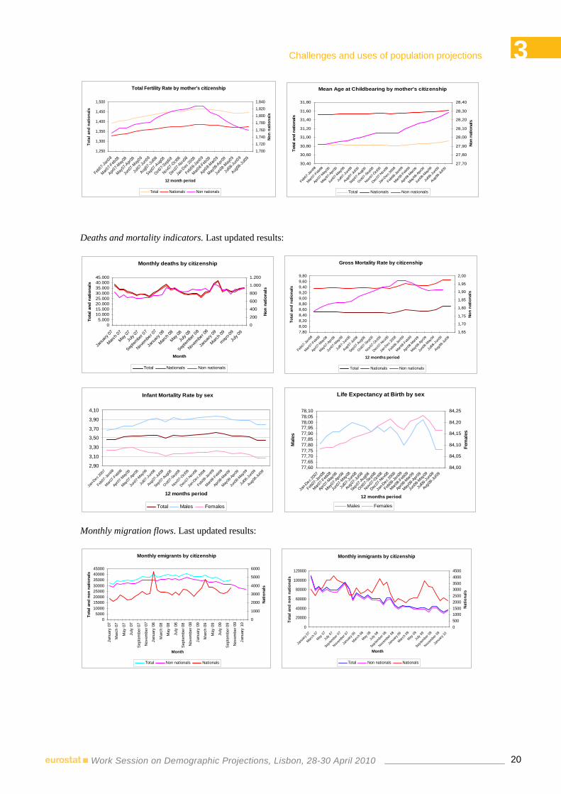
2.4.2 Monthly Demographic Now Cast Results Births and fertility indicators. Last updated results:
Monthly births by mother's nationality
05.000
10.00015.00020.00025.00030.00035.00040.00045.00050.000
Janu
ary 0
7
March 0
7
May 07
July
07
Septem
ber 0
7
Novem
ber 0
7
Janu
ary 0
8
March 0
8
May 08
July
08
Septem
ber 0
8
Novem
ber 0
8
Janu
ary 0
9
March 0
9
mayo-0
9
July
09
Month
Tota
l and
nat
iona
ls
0
2.000
4.000
6.000
8.000
10.000
12.000
Non
nat
iona
ls
Total Nationals Non nationals
Gross Fertility Rate by mother's citizenship
9,00
9,50
10,00
10,50
11,00
11,50
12,00
Feb0
7-Ja
n08
Mar07
-Feb
08
Apr0
7-May
08
May07
-Apr
08
Jun0
7-May
08
Jul07
-Jun
08
Aug0
7-Ju
l08
Sep0
7-Au
g08
Oct07-
Sep0
8
Nov07
-Oct0
8
Dec07
-Nov
08
Jan-D
ec 20
08
Feb0
8-Ja
n09
Mar08
-Feb
09
Apr0
8-Mar
09
May08
-Apr
09
Jun0
8-May
09
Jul08
-Jun
09
Aug0
8-Ju
l09
12 month period
Tota
l and
nat
iona
ls
18,2018,4018,6018,8019,0019,2019,4019,6019,80
Non
natio
nals
Total Nationals Non nationals
3 Challenges and uses of population projections
20Work Session on Demographic Projections, Lisbon, 28-30 April 2010
Total Fertility Rate by mother's citizenship
1,250
1,300
1,350
1,400
1,450
1,500
Feb07-J
an08
Mar07-F
eb08
Apr07-M
ay08
May07
-Apr0
8
Jun0
7-May
08
Jul07
-Jun0
8
Aug07
-Jul08
Sep07
-Aug
08
Oct07-S
ep08
Nov07-O
ct08
Dec07-N
ov08
Jan-D
ec 20
08
Feb08-J
an09
Mar08-F
eb09
Apr08-M
ar09
May08
-Apr0
9
Jun0
8-May
09
Jul08
-Jun0
9
Aug08
-Jul09
12 month period
Tota
l and
nat
iona
ls
1,700
1,720
1,740
1,760
1,780
1,800
1,820
1,840
Non
nat
iona
ls
Total Nationals Non nationals
Mean Age at Childbearing by mother's citizenship
30,40
30,60
30,80
31,00
31,20
31,40
31,60
31,80
Feb07
-Jan0
8
Mar07
-Feb
08
Apr07
-May
08
May07
-Apr
08
Jun0
7-May
08
Jul07
-Jun
08
Aug07
-Jul08
Sep07
-Aug
08
Oct07-
Sep08
Nov07
-Oct0
8
Dec07
-Nov0
8
Jan-D
ec 200
8
Feb08
-Jan0
9
Mar08
-Feb
09
Apr08
-Mar
09
May08
-Apr
09
Jun0
8-May
09
Jul08
-Jun
09
Aug08
-Jul09
Tota
l and
nat
iona
ls
27,70
27,80
27,90
28,00
28,10
28,20
28,30
28,40
Non
nat
iona
ls
Total Nationals Non nationals
Deaths and mortality indicators. Last updated results:
Monthly deaths by citizenship
05.000
10.00015.00020.00025.00030.00035.00040.00045.000
Janu
ary 07
March 0
7
May 07
July
07
Septem
ber 0
7
Novembe
r 07
Janu
ary 08
March 0
8
May 08
July
08
Septem
ber 0
8
Novembe
r 08
Janu
ary 09
March 0
9
mayo-0
9
July
09
Month
Tota
l and
nat
iona
ls
0
200
400
600
800
1.000
1.200
Non
nat
iona
ls
Total Nationals Non nationals
Gross Mortality Rate by citizenship
7,808,008,208,408,608,809,009,209,409,609,80
Feb07
-Jan0
8
Mar07-F
eb08
Apr07-M
ay08
May07
-Apr0
8
Jun0
7-May
08
Jul07
-Jun0
8
Aug07
-Jul08
Sep07
-Aug
08
Oct07-S
ep08
Nov07
-Oct0
8
Dec07
-Nov0
8
Jan-D
ec 200
8
Feb08
-Jan0
9
Mar08-F
eb09
Apr08-M
ar09
May08
-Apr0
9
Jun0
8-May
09
Jul08
-Jun0
9
Aug08
-Jul09
12 months period
Tota
l and
nat
iona
ls
1,65
1,70
1,75
1,80
1,85
1,90
1,95
2,00
Non
natio
nals
Total Nationals Non nationals
Infant Mortality Rate by sex
2,90
3,10
3,30
3,50
3,70
3,90
4,10
Jan-D
ec 200
7
Feb07
-Jan0
8
Mar07-F
eb08
Apr07-M
ay08
May07
-Apr0
8
Jun0
7-May
08
Jul07
-Jun0
8
Aug07
-Jul08
Sep07
-Aug
08
Oct07-S
ep08
Nov07
-Oct0
8
Dec07
-Nov0
8
Jan-D
ec 200
8
Feb08
-Jan0
9
Mar08-F
eb09
Apr08-M
ar09
May08
-Apr0
9
Jun0
8-May
09
Jul08
-Jun0
9
Aug08
-Jul09
12 months period
Total Males Females
Life Expectancy at Birth by sex
77,6077,6577,7077,7577,8077,8577,9077,9578,0078,0578,10
Jan-D
ec 200
7
Feb07
-Jan0
8
Mar07-F
eb08
Apr07-M
ay08
May07
-Apr0
8
Jun0
7-May
08
Jul07
-Jun0
8
Aug07
-Jul08
Sep07
-Aug
08
Oct07-S
ep08
Nov07
-Oct0
8
Dec07
-Nov0
8
Jan-D
ec 200
8
Feb08
-Jan0
9
Mar08-F
eb09
Apr08-M
ar09
May08
-Apr0
9
Jun0
8-May
09
Jul08
-Jun0
9
Aug08
-Jul09
12 months period
Mal
es
84,00
84,05
84,10
84,15
84,20
84,25
Fem
ales
Males Females
Monthly migration flows. Last updated results:
Monthly emigrants by citizenship
05000
1000015000200002500030000350004000045000
Janu
ary
07
Mar
ch 0
7
May
07
July
07
Sep
tem
ber 0
7
Nov
embe
r 07
Janu
ary
08
Mar
ch 0
8
May
08
July
08
Sep
tem
ber 0
8
Nov
embe
r 08
Janu
ary
09
Mar
ch 0
9
May
09
July
09
Sep
tem
ber 0
9
Nov
embe
r 09
Janu
ary
10
Month
Tota
l and
non
nat
iona
ls
0
1000
2000
3000
4000
5000
6000
Natio
nals
Total Non nationals Nationals
Monthly inmigrants by citizenship
0
20000
40000
60000
80000
100000
120000
Janu
ary 07
March 0
7
May 07
July
07
Septem
ber 0
7
Novem
ber 0
7
Janu
ary 08
March 0
8
May 08
July
08
Septem
ber 0
8
Novem
ber 0
8
Janu
ary 09
March 0
9
May 09
July
09
Septem
ber 0
9
Novem
ber 0
9
Janu
ary 10
Tota
l and
non
nat
iona
ls
050010001500200025003000350040004500
Month
Natio
nals
Total Non nationals Nationals

3 Challenges and uses of population projections
21Work Session on Demographic Projections, Lisbon, 28-30 April 2010
Monthly net migration flow by citizenship
0100002000030000400005000060000700008000090000
Janu
ary 07
March 0
7
May 07
July
07
Septem
ber 0
7
Novem
ber 0
7
Janu
ary 08
March 0
8
May 08
July
08
Septem
ber 0
8
Novem
ber 0
8
Janu
ary 09
March 0
9
May 09
July
09
Septem
ber 0
9
Novem
ber 0
9
Janu
ary 10
Month
Tota
l and
non
nat
iona
ls
-3000-2500-2000-1500-1000-5000500100015002000
Natio
nals
Total Non nationals Nationals
Monthly inter-provinces migrants
010.00020.00030.00040.00050.00060.00070.00080.00090.000
Janu
ary 0
7
March
07
May 07
July
07
Septem
ber 0
7
Novem
ber 0
7
Janu
ary 0
8
March
08
May 08
July
08
Septem
ber 0
8
Novem
ber 0
8
Janu
ary 0
9
March
09
May 09
July
09
Sept
embe
r 09
Novem
ber 0
9
Janu
ary 1
0
Month
Total Non nationals Nationals
3. The integration of demographic information: population estimates and projections
There is no doubt that the exposed improvements in demographic data have increased the quantity and quality of available information about the past and most recent demographic progress of Spain population. However, a decisive challenge for modern demographic statistics will be to integrate all statistical inputs in a systematic and coherent system of information which let national statistics offices explain every component of the demographic change and, even so, work out the value of such determinant information. Definitely, the internal coherence and consistency of information contribute to get it reliable enough for users and general public. In fact, the experience of national offices in raising a harmonized National Accounts Systems as integrating and summarizing instrument of economic information, generally and well accepted by public and private users and analysts as official economic data, is the better witness of such assertion.
A first attempt to lead Spanish demographic statistics towards such modern concept crystallizes in the new INE strategy on populations estimates and projections, formally stated in National Plan of Statistics 209-2012 and the respective Annual Programs3, which is based on:
1. The development of current population estimates continuously updated with the last available information about demographic developments: Spain Population Now Cast.
2. A new way of focusing the production of future population projections in a periodic basis: Short Term and Long Term Population Projections.
Both represent a first approach to the objective of getting a more integrated system of demographic information.
3.1 Current population estimates Population Now Cast is the statistical action that INE has developed during the last years to face the challenge of measuring the current resident population in our country and in every region and province, once the unexpected intensity of immigration phenomena shook the past quiet demographic evolution. Both, the National Statistics System and external users of official statistics, required population figures permanently updated with the present demographic reality. Population Now Cast was the answer from INE.
This statistical product has some general features, which determinate its significance as well as set its own limits:
1. Population Now Cast constitutes a synthesis statistic, which uses several primary sources of information, whose results are integrated in the estimation mechanism giving place to consistent
3 http://www.ine.es/en/normativa/leyes/plan/legplan_en.htm

3 Challenges and uses of population projections
22Work Session on Demographic Projections, Lisbon, 28-30 April 2010
estimates of the resident population stock at the present moment and of the estimated demographic flows which determinate the population evolution, all of them broken down by basic characteristics like sex, year of birth and age.
2. Population Now Cast makes use of the most updated available information on the recent demographic evolution: Vital Statistics, registered variations in Padrón and, specially, the last results of the Monthly Demographic Now Cast.
3. Population Now Cast are calculated every quarter, few days after the end of the quarter, providing the estimation of the resident population referred to the first day of every month of the quarter and to the first day of the following quarter. This immediacy respect to the reference date gives the character of advanced population figures to these estimates.
4. Population Now Cast methodology guarantees the complete consistency between population stock at every date of the current year and the estimated demographic flows happened during the time being of the year.
5. Population Now Cast results are not subject to revision, unless there is enough evidence about significant deviations from real population evolution.
6. Population Now Cast is considered as the most accurate estimate of the current population residing in Spain and its regions and provinces. That is the reason why it works as the reference population figures for all INE production and it is transmitted to international institutions (Eurostat, United Nations, International Monetary Fund, etc.) as Spain population figures for any purpose.
In conclusion, the own character of synthesis statistics, the use of all available information about recent demographic evolution and the total coherence between estimated population figures and demographic flows confer to the Population Now Cast over the field of demographic statistics a similar role than national accounts systems over the field of business statistics: beyond evident conceptual differences they both are a detailed and systematic representation of the demographic and economic reality, respectively, as a whole, trough a consistence balance of stocks and flows.
3.1.1 Production and dissemination calendar Both the internal demand of homogeneous population figures which works as reference for all INE statistical products and the strong requirement on the updating of such figures to the current demographic evolution, impose a really demanding timetable for carrying out the development of Population Now Cast. Those are the reasons why INE produces Population Now Cast results during the first days after the end of every quarter, with reference to the last day and to several intermediate dates of the quarter. In other words:
Population Now Cast referred to the first day of the months 1m + and 2m + of the quarter q and to the first day of the month m of the quarter 1q + is calculated and disseminated at the first days of the quarter 1q + .
3.1.2 General methodology: adapted components method The design of Population Now Cast general methodology was deeply determined by three main requirements:
a) The availability of results in a quarterly basis, with reference at different intermediate date of the reference quarter.
b) The absolute immediacy of the time of calculation and dissemination respect to the dates of reference.

3 Challenges and uses of population projections
23Work Session on Demographic Projections, Lisbon, 28-30 April 2010
c) Population Now Cast results are definitive, so they are immovable points of the estimates series along the current year.
Keeping in mind these three general premises, Population Now Cast are carried out through a genuine adaptation of the component method, which consists of providing population figures with reference to the first day of a month m of the current year in two steps:
1. For every month of the quarter, performing an auxiliary population with horizon in the January 1st of the following year. This projection is performed though the component method, according to a multiregional model4, which keeps a necessary consistence between demographic flows and population stocks and among all territorial levels.
Besides, the migration input of this auxiliary projection consists of a linear extrapolation to the whole year of estimated monthly migration flows along the current year until the time of estimation.
2. Calculating a linear interpolation between the Population Now Cast on January 1st of the current year and the result of the auxiliary projection for January 1st of the following year.
Such procedure guarantees that the demographic change happened (estimated) during the current year is completely consistent with flows of births, deaths and migrations.
For example, we can go over the calculation process of Population Now Cast corresponding to the first quarter of 2009, developed at the beginning of April of 2009. At this moment we had already got the Population Now Cast figures referred to 1st January of 2009 since the last estimation period (fourth quarter of 2008), which works as our starting point . We follow the estimation process trough annual auxiliary projections and linear interpolations in the following graphics and table:
Population Now Cast on 1 February 2009
Population Now Cast1st quarter of 2009
45800000
45850000
45900000
45950000
46000000
46050000
46100000
January
FebruaryMarc h Apr i l M ay
J une JulyAug ust
Sep tembeO ctobe r
N ovembe
DecembeJ anuary
Auxiliary projection, January 2009Population Now Cast
4 Willekens, F.J. y Drewe, P. (1984) “A multiregional model for regional demographic projection”, en Heide, H. y Willekens,
F.J. (ed) Demographic Research and Spatial Policy, Academic Press, London.

3 Challenges and uses of population projections
24Work Session on Demographic Projections, Lisbon, 28-30 April 2010
Population Now Cast at 1st February of 2009
Estimated February migration flows
Inmigrants Emigrants45.223 33.689
Auxiliary projection of January 2009
1st January 2009 population Births-Deaths Inmigrants Emigrants
1st January 2010 population(*)
45.828.172 104.962 542.676 404.265 46.071.545
(*) Auxiliary projected figures
Population Now Cast at 1st February 2009 45.848.453
Demographic change during January 2009 20.281
Births-Deaths 8.747
Inmigrants 45.223
Emigrants 33.689
Population Now Cast on 1 March 2009
Population Now Cast1st quarter of 2009
45800000
45850000
45900000
45950000
46000000
46050000
46100000
Janu
ary
Februa
ryMarch Apri
lMay
June Ju
ly
August
Sep tembe
r
Octobe
r
Novembe
r
Decem
ber
Janua
ry
Auxiliary projection, January 2009Auxiliary projection, February 2009Population Now Cast
Population Now Cast on 1 April 2009
Population Now Cast1st quarter of 2009
45800000
45850000
45900000
45950000
46000000
46050000
46100000
January
FebruaryMarch
Apr i l MayJune July
Aug ust
Sep tember
O ctobe r
November
December
January
Auxiliary projection, January 2009Auxiliary projection, February 2009Auxiliary projection, Marcha 2009Population Now Cast

3 Challenges and uses of population projections
25Work Session on Demographic Projections, Lisbon, 28-30 April 2010
3.1.3 Special mention of estimation procedure of monthly migrants flows Regarding Population Now Cast, one of the essential elements is the estimation of monthly migration flow along the current year, taking into account that:
1. Nowadays, this is the most significant component of the demographic change.
2. In general, international migration is one of the principal lack in official statistics.
3. The monthly migration flow estimates gives a very important relevance to Population Now Cast in national system, which provides the only advanced flash estimate of the current demographic evolution.
As it has been explained before, Population Now Cast is produced for every quarter, few days after the end of the quarter. This timetable imposes a high challenge in estimation of immigration flow during the months of reference. Basically, Monthly Demographic Now Casts are timely enough in providing accurate estimates of Spanish and foreign migration fluxes during the two first month of the quarter. The migration flow of the third month is estimated trough a detailed analysis of the trend and seasonal behaviour of the monthly migration series.
This simple procedures are really robust, thus the comparison between 2008 monthly immigrants flows provided by Population Now Cast and updated information of finally registered ones shows:
Estimated and registered monthly inmigrants in 2008
01000020000300004000050000600007000080000
Janu
ary 0
8
Februa
ry 08
March
08
April
08
May
08
June
08
July
08
Augu
st 08
Septem
ber 0
8
Octobe
r 08
Novem
ber 0
8
Decem
ber 0
8
Months
Estimated Registered
3.2 Population Projections
3.2.1 How should a population projection be focused like? Availability of future population evolution perspectives implies an element of structural relevance in any socioeconomic analysis or planning activity, either from the public or private sector. In fact, it is one of the statistical actions with a longer tradition for national statistics office and international statistics institutions. Until now, INE has satisfied this aim providing projections with occasion of each new census, after population census figures were available.
However, the use and public understanding of this kind of exercises is one of the most controversial aspects of official demographic statistics. Often, users wonder: Should we take it as a real forecasting? What is the statistical error associated with the results? Could we give a measure of reliability? Which possible scenarios should we use? How can we guess the future?
On the other hand, nowadays we stay in front of one of the more serious demands raised in official statistics. The extreme worries about the unstoppable growth of the world population, even above of natural resources, and the demographic future of European and occidental countries, deeply branded by a

3 Challenges and uses of population projections
26Work Session on Demographic Projections, Lisbon, 28-30 April 2010
increasing population ageing, result of the continuous extensions in life expectancy and accentuated by generalized low levels of fertility, makes the production of statistical simulation of future population an unavoidable goal for official statistical organisms.
Therefore, official statistics are obliged to give a convincing answer to this strong social and political requirement. But, it should be done with a useful and pragmatic approach, avoiding the utopia of forecasting future population and, at the same time, providing clear messages to society about future demographic risks. Precisely, these are the guidelines that have leaded the design of a new national strategy on providing population projections, based on three main principles:
1. A population projection is not a forecast. Then, non statistical errors should be associated to results.
2. A population projection should be a statistical simulation of future population according some hypothesis on demographic evolution.
3. The most important use of a population projection is to warn the public opinion about the future consequences of today’s demographic structure and trends.
3.2.2 INE new strategy on population projections Following these premises, INE has developed a new plan over the subject of population projections which is focused on carrying out Short Term and Long Term Population Projections in a periodic basis, which allows INE to provide continuous simulation of future resident population according to recent demographic trends. In fact, Short Term Population Projections are carried out every year, since 2008, providing a simulation of future population residing in Spain, its regions and provinces, on January 1st of the following ten years, broken down by sex and year of birth; Long Term Population Projections will be carried out every three years, since 2009, providing a simulation of future population residing in Spain on January 1st of the following forty years, broken down by sex, age and year of birth.
The periodic calendar of performance lets INE give, in a continuous way, an updated simulation of the demographic future of the country with the last available information about current evolution of demographic phenomena, in a context of significant changes. Therefore, this strategy avoids a quick obsolescence of the results that would become them useless. In addition, periodic Population Projections have as starting point the Population Now Cast for January 1st of the current year, so they are consistent with current reference population figures and complete the circle of coherence of the whole past, present and future demographic system and population series.
Both, Short Term and Long Term Population Projections are calculated trough the component method, using a multiregional model5, which guarantees the consistency between demographic flows and population stock in all territorial level (in case of Short Term Projections) and demographic characteristics (sex and year of birth). That lets population projections results include detailed demographic events which explain future population figures evolution. In other words, we are talking about complete demographic projections, not only population projections.
3.3 Some methods for the projection of demographic evolution As mentioned before, the calculation of Population Now Cast and Short Term and Long Term Population Projections are based on a multiregional model4, which inputs define the present or future evolution of each demographic phenomenon: fertility, mortality and migrations. We should stress two comments on that:
5 Willekens, F.J. y Drewe, P. (1984) “A multiregional model for regional demographic projection”, en Heide, H. y Willekens,
F.J. (ed) Demographic Research and Spatial Policy, Academic Press, Londres.

3 Challenges and uses of population projections
27Work Session on Demographic Projections, Lisbon, 28-30 April 2010
1. Projection methods are determined by the new approach chosen in population projections: statistical simulation of present demographics behaviours and trends.
2. The chosen methods are applicable in the estimation of current demographic evolution in Population Now Cast and in the projection of future demographic evolution, based on an extrapolation of present trends, in Short Term and Long Term Population Projections too.
The designed methodology for projecting Spain fertility, mortality or internal migrations is a good example of such implications.
3.3.1 Fertility The general method for projecting fertility of women residing in Spain consists of modelling retrospective series of specific fertility rates by age, using the following log-linear model:
)1995tln(baf xxtx −+= , where 49,...,15x = y ,...1999,1998t =
Being txf the specific fertility rate at age x during the year t , provided by Basic Demographic Indicators
and by Monthly Demographic Now Cast for the last 12 months period available. The model parameters, xa and xb , are estimated trough linear least squares. Next graph shows specific mortality rate observed
(1998-2007), estimated by Monthly Demographic Now Cast (2008) and projected in Short Term Population Projection 2009-2049 (2009-2018).
Specific fertility rates by age
0,000
0,040
0,080
0,120
15 16 17 18 19 20 21 22 23 24 25 26 27 28 29 30 31 32 33 34 35 36 37 38 39 40 41 42 43 44 45 46 47 48 49
1996 2001 2006 2007 2008 2009
2013 2018
The projection of fertility in lower territorial level (provinces) is carried out using a log-linear modelization of the differential in fertility intensity (Total Fertility Rate, TFR ) and fertility calendar (Mean Age at Childbearing, MAC , and Intercuartilic Range, IR) of provinces respect to the whole country:
)1993tln(DF ovinceProvincePrt
ovincePr −β+α= , ,...1999,1998t = , being tSpain
tovincePrt
ovincePrTFR
TFRDF =
)1993tln(MAC ovinceProvincePrt
ovincePr −β+α= , where ,...1999,1998t =
)1993tln(IR ovinceProvincePrt
ovincePr −β+α= , where ,...1999,1998t =

3 Challenges and uses of population projections
28Work Session on Demographic Projections, Lisbon, 28-30 April 2010
From these parameters, specific fertility rates per every province are developed using the Gompertz Relational model, following the methodological proposal of Zeng Yi and others6:
))1t(ISF)1t,x(F~(Y)
)t(ISF)t,x(F(Y tt −
−⋅β+α=
Where: ∑=
=x
15i
t,ovincePrif)t,x(F , being t,ovincePr
if specific fertility rate at age i in the province during the
year t ; ∑=
−=−x
15i
1t,ovincePrif
~)1t,x(F~ , being t,ovincePrif
~ the smoothed specific fertility rate at age i in the
province during the year t ; ))xln(ln()x(Y −−= ; )TFR
)1t,MAC(F(Y)5,0(Y 1tovincePr
1tovincePr
tt −
− −⋅β−=α ;
t
ovincePr
1tovincePr
tRI
IR −=β .
3.3.2 Mortality The method for projecting mortality is based on an extrapolation of recent trends in mortality risks by sex and age, according to an exponential model of the retrospective smoothed path of them:
ttx,s
x,sx,seq~ β+α= , += 100,99,...2,1,0x . For 1x ≥ , ,...1992,1991t = ; for 0x = , ,...1999,1998t =
Where tx,sq~ is the mortality risk of people with sex s and age x during the year t provided by Spain
Mortality Tables and by Monthly Demographic Now Cast for the most recent 12 months period available. Model parameters, x,sα and x,sb , are estimated through least squares method.
An intermediate smoothing process of series x,sβ and re-estimation of the first parameter x,sα is required in order to guarantee a soft transition between last observed years and projected ones.
Mortlity risks by ageMales
0,0000
0,0001
0,0010
0,0100
0,1000
1,00000 6 12 18 24 30 36 42 48 54 60 66 72 78 84 90 96
Age
Sem
iloga
ritm
ic s
cale 2002
20052008
2009
2013
2018
Mortlity risks by ageFemales
0,0000
0,0001
0,0010
0,0100
0,1000
1,00000 6 12 18 24 30 36 42 48 54 60 66 72 78 84 90 96
Age
Sem
iloga
ritm
ic s
cale 2002
20052008
20092013
2018
The projection of mortality incidence in every province is based on the relational method proposed by W. Brass, called Brass’ logits7, which bind the territorial level to the national results:
6 Zeng Yi, Wang Zhenglian, Ma Zhongdong y Chen Chunjun. 2000. "A simple method for projecting or estimating and: An
extension of the Brass Relational Gompertz Fertility Model", Population Research and Policy Review 19:525–549. 7 William Brass, (1975), Methods for estimating fertility and mortality from limited and defective data.

3 Challenges and uses of population projections
29Work Session on Demographic Projections, Lisbon, 28-30 April 2010
Being ovincePrx,sl and Spain
x,sl the survivor series by sex s and age x ( )95,...,40x = of mortality tables of the corresponding province and Spain, respectively, and its logistic transformation, the following linear model is estimated trough least squares method:
⎟⎟
⎠
⎞
⎜⎜
⎝
⎛ −= ovincePr
x,s
ovincePrx,s
ovincePr0,sovincePr
x,s lll
ln21lLogit ,
⎟⎟
⎠
⎞
⎜⎜
⎝
⎛ −= Spain
x,s
Spainx,s
Spain0Spain
x,s lll
ln21lLogit
Spainx,s
ovincePrs
ovincePrs
ovincePrx,s lLogitlLogit ×β+α=
3.3.3 Internal Migration
The specific inter-provinces, i and j , migration rate by sex s an age x could be factorized in:
tj,i,x,s
tx,s,i
ts,i
tj,i,x,s acintTMRm ⋅⋅= where
ts,iintTMR is the Total Internal Migration Rate from the province i of people with sex s during the year
t ; tx,s,ic is the calendar of internal migration by age x of people of sex s residing in the province i
during the year t ; and tj,i,x,sa is matrix of percentage provincial interchanges in every sex s and age x
during de year t .
Then projection method is based in a genuine regression model with delays in dependant variable, which modelizes the evolution of internal mobility intensity with relation to the foreign immigrants flow ( INM ) of the same year and the year before and the own trend of the dependent variable.
1ts,i3
ts,i2
1ts,i10
ts,i INMINMintTMRintTMR −− β+β+β+β=
The least squared estimated parameters of the model are consistent, since autocorrelation in errors are refused with statistical evidence.
The projection process is completed with the calculation of projected calendars of internal migration tx,s,ic
and the matrix of percentage provincial interchanges tj,i,x,sa through average data of the last four
observed years.

3 Challenges and uses of population projections
30Work Session on Demographic Projections, Lisbon, 28-30 April 2010
Annex
Recent evolution of Spain population pyramid
Population Now CastJanuary 1st 2002 and 2010
100 80 60 40 20 0 20 40 60 80 100 0 años 4 años
8 años 12 años 16 años
20 años 24 años 28 años
32 años 36 años 40 años
44 años 48 años 52 años 56 años
60 años 64 años 68 años
72 años 76 años 80 años
84 años 88 años 92 años
96 años 100 y
2010
2002
Males Females
Males+females=10000
Simulated future evolution of Spain pyramid population
Short Term Population Projections (2009-2019) and Long Term Population Projections (2009-2049)
100 80 60 40 20 0 20 40 60 80 100
0
5
10
15
20
25
30
35
40
45
50
55
60
65
70
75
80
85
90
95
100+
Males Females
Males+females=10000
2049
2039
2029
2019
2009

3 Challenges and uses of population projections
31Work Session on Demographic Projections, Lisbon, 28-30 April 2010
References
INE. What is the Population Now Cast?
http://www.ine.es/en/daco/daco43/epoba/estima_pob_en.pdf
INE, January 2010. Population Now Cast. Methodology
http://www.ine.es/metodologia/t20/t2030259.pdf
INE. What are the Short Term Population Projections
http://www.ine.es/metodologia/t20/t20269_proyec.pdf
INE, 2008. Short Term Population Projection. Project
http://www.ine.es/metodologia/t20/t20269_proyet.pdf
INE, September 2009. Short Term Population Projection. Methodology
http://www.ine.es/en/metodologia/t20/t20269_m2009_en.pdf
INE, December 2010. Long Term Population Projection. Methodology
http://www.ine.es/metodologia/t20/t2030251.pdf
INE. Vital Statistics. General methodology
http://www.ine.es/en/metodologia/t20/t203030166_en.pdf
INE. Basic Demographic Indicators. Description
http://www.ine.es/en/daco/daco43/idb/meto_idb_en.htm
INE, October 2009. Life Tables. Methodology
http://www.ine.es/en/daco/daco42/mortalidad/metodo_9107_en.pdf
Willekens, F.J. y Drewe, P. (1984) “A multiregional model for regional demographic projection”, en Heide, H. y Willekens, F.J. (ed) Demographic Research and Spatial Policy, Academic Press, Londres.
Zeng Yi, Wang Zhenglian, Ma Zhongdong y Chen Chunjun. 2000. "A simple method for projecting or estimating and: An extension of the Brass Relational Gompertz Fertility Model", Population Research and Policy Review 19:525–549.
Lambrecht and Paul, November 2004. Quotients de mortalité prospectifs, Bureau Fédéral du Plan.
William Brass, 1975. Methods for estimating fertility and mortality from limited and defective data.


3 Challenges and uses of population projections
33Work Session on Demographic Projections, Lisbon, 28-30 April 2010
MAKING USE OF LONG-TERM DEMOGRAPHIC PROJECTIONS IN MULTILATERAL POLICY
COORDINATION IN THE EU1
Giuseppe CARONE∗ and Per ECKEFELDT∗∗
*European Commission, **DG ECFIN
Abstract
The key challenge for policy-makers in the EU over the medium-term will be to transform the European social models such that the implications arising from an ageing population will become manageable for the European societies.
In order to enable policy-makers to make informed decisions on the design of policies that can have long-lasting effects, the Commission, in close cooperation with the EU Member States (through ECOFIN Council committees), analyses the impact of ageing populations on economic activity and budgetary developments. The starting point for the projection exercise is the population projection by Eurostat (EUROPOP2008). A key feature of the population projection is that the methodology is common across Member States and this allows meaningful cross-country comparisons.
Based on the population projections, developments of the labour force over the long-term are calculated, which combined with assumptions on productivity is used to project potential GDP growth. Finally, this set of macroeconomic projections are used to make projections for public expenditure on pensions, health care, long-term care, education and unemployment transfers for all EU Member States (the latest projections cover the period up to 2060). The comparability of the projections across countries is a very important aspect. This provides for ownership of the results by the Member States such that they can be used in different multilateral surveillance exercises' at EU level.
The analysis based on these projections are a key input to the assessment of the sustainability of public finances carried out as part of the EU budgetary surveillance under the Stability and Growth Pact; in the context of the open method of co-ordination on pensions, health care and long-term care (social OMC); in the follow-up to the renewed Lisbon strategy for jobs and growth (Europe 2020), and in the analysis on the impact of ageing populations on the labour market and potential growth.
This paper presents, based on the main results of the 2009 Ageing Report, the economic and budgetary implications of demographic change over the long-term in the EU, as a whole, and at Member State level. In particular, it addresses the extent to which there is a need for policy change in the Member States and point to policy options that might mitigate the challenges that population ageing is likely to pose.
1 The authors are economists working in the European Commission’s Directorate General for Economic and Financial Affairs.
This paper draws heavily upon the work carried out jointly with the EPC-AWG within the framework of the 2009 Ageing report. Finally, as customary, the views expressed in this paper are the responsibility of the authors alone and should not be attributed to the European Commission.
∗ Head of Unit, ECFIN C2 – Sustainability of public finances, European Commission. Email: [email protected] ∗∗ Deputy Head of Unit - C2 – Sustainability of public finances, European Commission. Email: [email protected]
(contact author).

3 Challenges and uses of population projections
34Work Session on Demographic Projections, Lisbon, 28-30 April 2010
1. Overview of the 2009 projection of age-related expenditure
Long-term projections provide important information for the economic policy-making process, as they facilitate the formulation of time-consistent policies beyond the medium term. They provide an indication of the timing and scale of economic challenges that would result from an ageing population, assuming no change in labour market and welfare policies. The projections show where, when, and to what extent, ageing pressures will accelerate as the baby-boom generation retires and the average life span continues to increase.
The European Commission (DG ECFIN), in cooperation with the Economic Policy Committee (Ageing Working Group) has recently carried out long-term economic and budgetary projections on the basis of the latest population projection by EUROSTAT (EUROPOP2008), in line with the mandate given by the ECOFIN Council in 2006. The projections of government expenditure items (pension, healthcare, long term care, education and unemployment benefits) are made on the basis of common macroeconomic assumptions endorsed by the EPC and of a 'no policy change'' assumption, i.e. reflecting only already enacted legislation (see the 2009 Ageing Report for details).2
1.1 The mandate and broad principles In 2006, the ECOFIN Council gave the Economic Policy Committee (EPC) a mandate to update and further deepen its common exercise of age-related expenditure projections by the autumn of 2009 on the basis of a new population projection to be provided by Eurostat (the EUROPOP2008 demographic projection was released in April 2008).
The new projection exercise follows those carried out in 2001 and 2006. The age-related expenditure projections feed into a variety of policy debates at EU level. In particular, they are used in the annual assessment of the sustainability of public finances carried out as part of the Stability and Growth Pact; in the context of the open method of co-ordination on pensions; and, in the analysis on the impact of ageing populations on the labour market and potential growth which is of great relevance for the Europe 2020 (former Lisbon strategy) and the Integrated Guidelines.
The work has been carried out by the EPC Working Group on Ageing Populations (AWG) and the Commission (Directorate-General for Economic and Financial Affairs - DG ECFIN) with a view to update and further improve the previous projection exercises so as to enhance comparability across countries, consistency across expenditure items and the economic basis for the underlying assumptions. The work has been guided by the agreed principles of simplicity, comparability, consistency, prudence and transparency. The EPC endorsed the progress report by the AWG, outlining the progress and agreements reached.3
1.2 Participation in the budgetary projection exercise and working method The work has been prepared by experts from 27 Member States, Norway, and the Commission (represented by DG ECFIN, the Directorate-General for Economic and Financial Affairs). DG ECFIN has provided analysis and calculations. Eurostat has played a central role by preparing the population projection (Europop2008). In the preparation of the population projection, Eurostat actively consulted national statistical institutes in the Member States.4
2 European Commission- Economic Policy Committee (2008), "2009 Ageing Report: Underlying assumptions and projection
methodologies (207-2060)", European Economy, No.7 and "2009 Ageing Report: Economic and budgetary projections for the EU-27 Member States (2008-2060)", European Economy No. 2.
http://ec.europa.eu/economy_finance/publications/publication_summary13784_en.htm 3 See 'The 2009 budgetary projection exercise of the Ageing Working Group: Second progress report to the EPC',
ECFIN/CEFCPE(2008)REP/ 52951 rev, Brussels, 23/06/2008. 4 Through meetings of Eurostat’s Working Group on Population Projection and by using the “Population Projection” Interest
Group on CIRCA.

3 Challenges and uses of population projections
35Work Session on Demographic Projections, Lisbon, 28-30 April 2010
Graph 1. Overview of the 2009 projection of age-related expenditure
Source: Commission services, EPC.
1.3 Coverage and general overview Graph 1 above presents an overview of the entire age-related projection exercise. The starting point is the EUROPOP2008 population projection for the period 2008 to 2060. Next, the EPC agreed a common set of assumptions and methodologies in order to make projections on a set of exogenous macroeconomic assumptions covering the labour force (participation, employment and unemployment rates), labour productivity and the real interest rate. These combined assumptions enable the calculation of GDP for all Member States up to 2060.
On the basis of these assumptions, separate budgetary projections are being run for five age-related expenditure items. The projections for pensions are run by the Member States using their own national model(s). The projections for health care, long-term care, education and unemployment are run by the European Commission, on the basis of a common projection model for each expenditure item. The results of this set of projections will be aggregated to provide an overall projection of age-related public expenditures.
2. Demographic projections
2.1 Population projections: talking through the demographics Population projections are not forecasts, but what-if scenarios built on assumptions. They show the likely size and age-structure of the population in the future, given a number of demographic assumptions. The work on the impact of ageing of the Commission (DG ECFIN) and the Economic Policy Committee (Ageing Working Group) is based on Eurostat's population projections: the future population by age and gender is the first input to project the labour force and potential GDP growth, which is then used to make projections for public expenditure on pensions, health care, long-term care, education and unemployment transfers for all EU Member States and Norway. Last projections are based on the EUROPOP20085 population projection released by Eurostat. Eurostat applies a common methodology to all Member States, which is essential to ensure that projections for public expenditure are comparable across Member
5 See EUROPOP2008 convergence scenario. See also Statistics in Focus, Ageing characterises the demographic perspectives of
the European societies, No. 72, 2008.

3 Challenges and uses of population projections
36Work Session on Demographic Projections, Lisbon, 28-30 April 2010
States and can be used for the analysis of the sustainability of public finances, where countries are classified according to different categories of risk. If national population projections would have been used, rather than a common projection, different assumptions on rates of fertility, mortality or net migration would drive the results of the macroeconomic and budgetary projections and these would not be comparable across Member States. Clearly, the assumptions on fertility rates and net migratory flows are key to future trends in the working-age population and the labour force, while mortality rates at older ages are crucial for projecting future expenditure on pensions, health care or long-term care to elderly people.
Life expectancy continues to increase, the fertility rates projected to rise slightly
The convergence scenario approach employed in the EUROPOP2008 projection entails a process of convergence of fertility rates across Member States to that of the forerunners over the very long-term projection period. For the EU, the total fertility rate (TFR) is projected to rise from 1.52 in 2008 to 1.57 by 2030 and 1.64 by 2060. In the euro area, a similar increase is projected, from 1.55 in 2008 to 1.66 in 2060.
The fertility rate is projected to increase over the projection period in all Member States except Ireland and France (where it will nevertheless remain above 1.85), while in Denmark, Finland, Sweden and the UK it is projected to remain stable. In all countries the fertility rate will remain below the natural replacement rate of 2.1. The largest increases in fertility rates are projected to take place in Slovakia, Poland and Lithuania which have the lowest rates in the EU in 2008. The increase is projected to occur gradually, approaching the current EU average rates only in 2060.
In the EU, life expectancy at birth for males is projected to increase by 8.5 years over the projection period, from 76 in 2008 to 84.5 in 2060. For females, life expectancy at birth is projected to increase by 6.9 years for females, from 82.1 in 2008 to 89 in 2060, implying a narrowing gap between males and females life expectancy.
The largest increases in life expectancy at birth, for both males and females, are projected to take place in the new Member States. Life expectancy for males in 2008 is lowest in Estonia, Latvia, Lithuania, Hungary, Slovakia, Poland, Bulgaria and Romania, at between 66 and 71 years. Some catching-up will take place over the projection period, as life expectancy in these countries increases by more than 10 years – a bigger increase than in the rest of the EU. Overall however, life expectancy at birth is projected to remain below the EU average in all new Member States except Cyprus throughout the projection period, especially for males. This reflects a convergence of life expectancy. Still, by 2060 the life expectancy for many of these countries remains below the average in the EU.
The projection compresses the spread across the Member States of life expectancy at birth for males, from 13.1 years in 2008 (from a high of 79 in Sweden to a low of 65.9 in Lithuania) to 5 years in 2060 (85.5 in Italy compared with 80.4 in Lithuania). For females, there is less of a reduction in the differential in life expectancy at birth, from 7.7 years in 2008 (84.3 in France to 76.6 in Romania) to 4.1 years in 2060 (90.1 in France to 86.5 in Bulgaria).
In the EU, life expectancy at age 65 is projected to increase by 5.4 years for males and by 5.2 years for females over the projection period. In 2060, life expectancy at age 65 will reach 21.8 years for males and 25.1 for females. The projected difference between males and females in 2060 is 3.3 years, less than the 4.5 year difference in life expectancy at birth.
Inward net migration to the EU expected to continue but at decelerated pace
For the EU as a whole, annual net inflows are projected to fall from about 1,680,000 people in 2008 (equivalent to 0.33% of the EU population) to 980,000 by 2020 and thereafter to some 800,000 people by 2060 (0.16% of the EU population).
Over the entire projection period, the cumulated net migration to the EU is 59 million, of which the bulk is concentrated in the euro area (46.2 million). Net migration flows are projected to be concentrated in a few destination countries: Italy (12 million cumulated up to 2060), Spain (11.6 million), Germany (8.2

3 Challenges and uses of population projections
37Work Session on Demographic Projections, Lisbon, 28-30 April 2010
million), and the UK (7.8 million). According to the assumptions, the change of Spain and Italy from origin to destination countries will be confirmed in coming decades. Countries that are currently experiencing a net outflow (EE, LT, LV, PL, BG and RO) are projected to see it taper off or reverse in the coming decades.
2.2 The size and age structure of the population The age structure of the EU population is projected to dramatically change in coming decades due to the dynamics of fertility, life expectancy and migration rates. The population is projected to be slightly larger, and much older, in 50 years' time than it is now. It will increase (from 495.4 million in 2008) by almost 5% by 2035, when it will peak (at 520.1 million). It will then decline steadily, shrinking by nearly 3%, to 505.7 million by 2060, slightly higher than in 2008. The most numerous cohorts in 2008 are those around the age of 40 for men and women. The median age is projected to rise from 40.4 years in 2008 to 47.9 years in 2060. Elderly people are projected to account for an increasing share of the population due to continued gains in life expectancy over the projection period. At the same time, the base of the age pyramid will become smaller during the projection period due to below-replacement fertility rates. As a consequence, the shape of the age-pyramids gradually changes from pyramids to pillars.
While the EU population is projected to be slightly larger in 2060 than in 2008, there are wide differences in population trends until 2060 across Member States. The total population is projected to decrease in about half of the EU Member States (BG, CZ, DE, EE, EL, IT, LV, LT, HU, MT, PL, RO, SI and SK). For the other Member States an increase is projected.
The young population (aged 0-14) is projected to decline gradually from 2020 onwards. According to the projections, the working-age population (aged 15-64) will start to decline as of 2010 and, over the whole projection period, it will drop by 15 per cent in the EU. However, it is projected to increase in 7 Member States (Belgium, Ireland, France, Cyprus, Luxembourg, Sweden and the UK). The elderly population (aged 65 and above) will increase very markedly throughout the projection period. The number of the elderly will almost double, rising from 85 million in 2008 to 151 million in 2060 in the EU. The number of very old people (aged 80 years and above) is projected to increase by even more, almost tripling from 22 million in 2008 to 61 million in 2060. As a result of these different trends among age-groups, the old-age dependency ratio (people aged 65 or above relative to the working-age population aged 15-64) is projected to increase from 25.4% to 53.5% in the EU over the projection period. The largest increase will occur during the period 2015-35, when year-on-year increases of over 2 p.p. are projected. Hence, the dependency ratio is projected to more than double by 2060. This means that the EU would move from having 4 working-age people for every person aged over 65 to a ratio of 2 to 1. The increase in the total dependency ratio (people aged 14 and below and aged 65 and above relative to the population aged 15-64) is also large, rising by a two thirds.
3. Labour force projections
Projected increases in overall participation rates…
Labour force projections are carried out by cohort simulation model developed by the Commission (DG ECFIN) and validated by the AWG (EPC).6 The overall participation rate (for the age group 15 to 64) in the EU27 is projected to increase by 3.5 percentage points over the period 2007-2060 (from 70.6% in 2007 to 74.1% in 2060). For the euro area, a similar increase is projected, (from 70.8% in 2007 to 74.5% in 2060). For the age-group 15-71, the current and projected participation rates as well as the increase are smaller. Almost all of the increase is projected to materialise in the period to 2020.
The biggest increase in participation rates is projected for older workers7 (around 20 percentage points for females and 10 p.p. for males) in the EU27, and a slightly higher increase in the euro area (22 p.p. for
6 See Carone G. (2005), "Long-term labour force projections for the 25 EU Member States: A set of data for assessing the
economic impact of ageing", European Commission, European Economy, Economic Papers, No. 235/2005. 7 Age group 55-64.

3 Challenges and uses of population projections
38Work Session on Demographic Projections, Lisbon, 28-30 April 2010
females and 13 p.p. for males). As a result of these dynamics, the gap between male and female participation rates is projected to gradually narrow, especially in countries with a large gap in 2007.
… but labour supply will decline because of the projected population trends
The overall labour force (aged 15 to 71) in the EU27 is projected to increase by 3.7% from 2007 to 2020. In terms of numbers, this means an increase in the labour force of roughly 8.6 million. In the euro area, an increase of almost 5% is projected.
The increase in labour supply over the period 2007 to 2020 is mainly due to the increase in female labour supply, while the male labour force is projected to remain substantially unchanged. However, the positive trend in female labour supply is projected to reverse during the period 2020-2060 and, as male labour supply drops too, the overall labour force is expected to decrease by as much as 13.6%, equivalent to around 33 million people (24.4 million if compared with the level in 2007) in the EU. In the euro area, the projected fall in labour supply between 2020 and 2060 is 12.6%, which translates into 20.4 million people (13 million if compared with the level in 2007).
In the first part of the projection (from 2007 to 2020), a majority of EU countries (excluding DK, NL, FI, CZ, EE, LT, LV, PL, SI, BG, RO), are projected to record an increase in labour supply. This trend is projected to reverse in the second part of the projection period (from 2020 to 2060), when most countries are projected to record a decrease, except for CY (+19.8%), LU (+19.5%), IE (+11%), FR (+3.1%) SE (+2.2%) and the UK (+9.2%). As already mentioned, the projected negative labour force growth over the period 2020-2060 in the EU can be ascribed almost exclusively to negative demographic developments, given that the participation rates over the period 2020-2060 are projected to continue to increase, albeit at a slower pace than during 2007-2020.
Assumptions on unemployment
The general assumption on unemployment was the projection that the NAIRU (structural unemployment rate) should remain unchanged over the projection period. To avoid extrapolating forward high levels of NAIRU for countries which are still above the estimated medium-term EU15 average of the NAIRU (6.2%)8 (Belgium, Germany, Greece, Spain, France, Portugal, Hungary, Malta and Slovakia), the EPC agreed that these countries should converge to this average in the period up to 2020. Overall, a reduction in the EU unemployment rate of around 1 ½ percentage points is projected (from 7.2% in 2007 to 5.7% in 2020). A fall of a similar magnitude is projected for the euro area (from 7.5% in 2007 5.9% in 2020).
Employment projections
Given the population projection, the unemployment rate assumptions and the labour force projection, the overall employment rates (of people aged 15 to 64) in the EU are projected to increase from 65.5% in 2007 to 66.6% in 2010, 69% in 2020, and almost 70% in 2060. In the euro area, a similar development is projected and employment will surpass 70% at the end of the projection period.
The employment rate of females is projected to rise from 58.4% in 2007 to 63.4% in 2020 and to 65.1% in 2060. The employment rate for older workers (55-64) will increase even more, from 44.9% in 2007 to 54.5% in 2020 and further to 59.8% in 2060. For the euro area, the increase in the employment rate of older workers (55-64) is higher than in the EU, rising by 17.7 p.p. compared with 14.9 p.p. in the EU. The older workers employment rate in 2060 is projected to be 60.3% in the euro area.
The number of people employed (according to the European Labour Force Survey definition) is projected to record an annual growth rate of only 0.4% over the period 2007 to 2020, which will reverse to a negative annual growth rate of a similar magnitude in the subsequent period 2020 to 2060. As a result of these opposite trends, the overall employment in the EU is projected to shrink by about 19.4 million people over the period 2007 to 2060. Rises in immigration levels in some countries and increases in
8 Based on the Spring 2008 economic forecast by DG ECFIN.

3 Challenges and uses of population projections
39Work Session on Demographic Projections, Lisbon, 28-30 April 2010
labour force participation rates moderate the fall in employment owed to the ageing of the population and the negative population growth projected for the period 2020 to 2060.
Projection of labour input (total hours worked)
Compared with the projections in the 2006 Ageing Report, the definition of labour input has been changed from number of employees to number of hours worked so as to ensure consistency with the commonly agreed production function used to calculate potential GDP growth and output gaps for the purpose, inter alia, of estimating cyclically adjusted budget balances (CABs) in the context of the European Commission’s multilateral budgetary surveillance.
The population projection, unemployment rate assumptions, labour force projection, projected employment rates (of people age 15 to 71) and assumptions on changes in hours worked per person, result in a projection of total hours worked in the EU Member States.
4. Macroeconomic assumptions: labour productivity and potential growth rates
Macroeconomic assumptions: labour productivity and potential growth rates
Total factor productivity is assumed to converge to 1.1%
Total factor productivity (TFP) drives labour productivity growth in the long-run. A prudent assumption was set: Member States' TFP growth rates are assumed to converge to a long-term historical average in the EU of 1.1%, as was seen over the period 1970 to 2004, which is close to productivity growth in the US over the same period. The speed of convergence is determined by the relative income position of the Member States. Specifically, the lower the current GDP per capita, the higher the real catching-up potential, which materialises by a period of higher TFP growth.
A sharp decline in potential growth rate is projected
Even without incorporating the potential negative impact of the current economic crisis, the annual average potential GDP growth rate in the EU is projected to fall from 2.4% in the period 2007-2020, to 1.7% in the period 2021-2030 and to a meagre 1.3% in the period 2041-2060. Output growth rates in the euro area are very close to those in the EU27 over the projection period, as the area represents more than two thirds of total EU27 output. While all EU Member States would experience a future slowdown in their potential growth rates, owing to the adverse impact of demographic trends, growth rates would differ substantially from country to country.
The sources of economic growth are also projected to change: labour productivity will become the key driver of growth in the EU
For the EU, labour productivity growth is projected to remain fairly stable at close to 1.7%. The small increase in the growth rate expected until the 2030s is due to the higher productivity growth assumed in Member States that are catching up. Total hours of work - the labour input - are projected to increase up to the 2020s. Thereafter, demographic ageing, with a reduction in the working-age population, is expected to act as a drag on growth. Over time, labour productivity will become the only driver of growth in the EU.
In the first half of the projection period, the main source of the divergence across countries is productivity growth, due to different rates at the outset of the projection and different trends according to the catching-up potential. In the latter part of the projection period, developments in the labour input have a dominant role in explaining divergent patterns, working through different demographic developments.

3 Challenges and uses of population projections
40Work Session on Demographic Projections, Lisbon, 28-30 April 2010
5. Budgetary projections
5.1 Overall results of the long-term age-related public expenditure projections
The budgetary projections point to sizeable fiscal challenges coming from a higher share of the total population in older age cohorts and a decline in the economically active share of the population. The fiscal impact of ageing is projected to be substantial in almost all Member States, with effects becoming apparent already during the next decade. On the basis of current policies, age-related public expenditure is projected to increase on average by about 4 ¾ percentage points of GDP by 2060 in the EU - and by more than 5 percentage points in the euro area (see Table 1). Most of the projected increase in public spending over the period 2007-2060 will be on pensions (+2.4 p.p. of GDP), health care (+1.5 p.p. of GDP) and long-term care (+1.1 p.p. of GDP). Potential offsetting savings in public spending on education and unemployment benefits are likely to be very limited (-0.2 p.p. of GDP for each item).
In terms of the different Member States situation, the following points can be made:
The age-related increase in public spending will be very significant in nine Member States (Luxembourg, Greece, Slovenia, Cyprus9, Malta, Romania, the Netherlands, Spain and Ireland) with a projected increase of 7 p.p. of GDP or more, although for some countries the large increase will be from a fairly low level. These Member States have so far made only limited progress in reforming their pension systems or have maturing pension systems.
For a second group of countries – Belgium, Finland, the Czech Republic, Lithuania, Slovakia, the UK, Germany and Hungary10 - the age-related increase in public spending is more limited, ranging from 4 p.p. to 7 p.p. of GDP. Several of these countries have taken significant steps in reforming public expenditure systems that contribute to limit the increase in future expenditure.11
Finally, the increase is more moderate, 4 p.p. of GDP or less, in Bulgaria, Sweden, Portugal, Austria, France, Denmark, Italy, Latvia, Estonia and Poland; this is also thanks to the implementation of substantial pension reforms. For many of them, the projected increase in expenditure on health-care and generally on long-term care is higher than increases in pensions.
Coping with the challenge posed by an ageing population will require determined policy action along the three-pronged strategy decided by the Stockholm European Council in 2001, i.e.: (i) reducing debt at a fast pace; (ii) raising employment rates and productivity; and (iii) reforming pension, healthcare and long-term care systems.
These results reveal that in some countries, there is a need to take due account of future increases in government expenditure, including through modernisation of social expenditure systems. In others, policy action has been taken, significantly limiting the future increase in government expenditure. A comprehensive assessment of risks to the long-term sustainability of public finances, including the identification of relevant policy responses, will be made in the 2009 update of the Commission's Sustainability Report.
9 The projections do not take into account legislation enacted on March 6 2009 involving reform of the Social Insurance Fund,
including stricter criteria for eligibility for pension benefits. Details of this reforms and their significant impact on the public finances are outlined in the stability programme of Cyprus for 2008-2012 of March 13 2009.
10 A part of the increase in gross pension expenditures from 2007 to 2060 in Hungary is explained by the introduction of pension taxation as of 2013 and so does not reflect an increase in expenditures effectively burdening the budget. Taxes on public pensions in 2060 are calculated to be 0.7% of GDP.
11 The projection results for public spending on long term care use the methodology agreed by the AWG/EPC. In the case of Germany, it does not reflect current legislation where benefit levels are indexed to prices only. A scenario which reflects current rules projects that public spending would remain constant as a share of GDP over the projection period. The increase of the total age related costs would then be lower than 4 p.p. of GDP.

3 Challenges and uses of population projections
41Work Session on Demographic Projections, Lisbon, 28-30 April 2010
Pension reforms implemented in recent years in some Member States are having visible positive impacts. Nonetheless, in some countries, the scale of reforms has been insufficient and they need to be pursued further to cope with the inexorable increasing share of older persons in Europe. At the same time, implementing other measures, for instance promoting higher employment rates of older workers that contribute to more adequate retirement incomes in the future might be required in order to ensure the lasting success of already implemented pension reforms.
At the current juncture, uncertainty over the medium-term economic prospects is exceptionally high. For this reason, additional scenarios were run to capture the potential impact of the economic crisis, by simulating both temporary and permanent shocks to economic activity. These simulations show that there might be a sizeable adverse economic and budgetary impact over the long-term compared with the baseline scenario, and that the impact would be higher the longer it takes to get back on track. Hence, these additional simulations provide useful information on the sensitivity of the projection results with respect to shocks, which is crucial for its interpretation notably at times characterized by unusually large uncertainties.
5.2 The projection results for public spending on pensions For the EU, the projections show an increase in public pension expenditures of 2.4 p.p. of GDP over the period 2007-2060. For the euro area, a slightly larger increase of 2.8 p.p. of GDP is projected. The diversity across Member States is very large. Public pension expenditure (social security pensions) is projected to increase by more than 10 p.p. of GDP in 3 Member States (Greece, Cyprus, and Luxembourg). Spending is expected to grow by between 5 and 10 p.p. of GDP in another five Member States (Ireland, Malta, Spain, Romania, Slovenia). In most Member States (Belgium, Bulgaria, the Czech Republic, Germany, France, Lithuania, Hungary, the Netherlands, Austria, Portugal, Slovakia, Finland, the UK), the change of the ratio is below 5 p.p. By contrast, in Denmark, Sweden, Latvia, Italy, and Estonia the ratio either stays at the 2007 level or drops below it. Some countries are projecting a decrease over the entire period of projections (Poland, Estonia, Denmark, Italy and Latvia), although this masks an increase over part of the projection period (such as in the case of Italy).
The lion's share of the projected increase in public pension expenditure is due to old-age and early pensions, while, given their limited size, a smaller increase is projected for other pension expenditure, mainly disability and survivor pensions, which increase only slightly (0.1. p.p. of GDP) in the euro area. As regards disability and survivor pensions, they are projected to increase only in 8 countries (Portugal, Romania, Slovenia, Slovakia, Finland, Sweden, the UK and Norway), although these increases would be slight.
The demographic transition to an older population is the main driver behind the projected increase in public pension expenditure. This effect alone would push up expenditures very significantly in all Member States (especially in Slovenia, Romania, Poland, Greece, although more limited in the UK, Estonia, Sweden, Latvia). However, some factors, also related to past reforms of pension systems, are expected to mitigate the increase:
• a tightening of the eligibility for a public pension (through higher retirement age and/or reduced access to early retirement and better control of alternatives to early retirement like disability pensions) would constrain public pension expenditure in nearly every Member State.
• higher employment rates are projected as reforms that provide stronger work incentives reduce structural unemployment rates in a number of countries;
• reduced generosity of pensions relative to wages. It is captured at an aggregate level by the pension benefit ratio, i.e. the average pension as a share of the average wage. This effect shows very considerable differences across EU Member States. In some (Denmark, Ireland, Greece, Cyprus, Romania, the UK), average pensions relative to wages remain unchanged or even increase over the projection period, while in most others, and especially in Bulgaria, Estonia, France, Italy, Latvia, Austria, Poland, Portugal, Slovakia, and Sweden they are projected to have fallen significantly by 2060. While resulting in budgetary savings, the adequacy of pensions

3 Challenges and uses of population projections
42Work Session on Demographic Projections, Lisbon, 28-30 April 2010
should be kept under review. Inadequate pension levels may lead to future demands for ad-hoc government interventions to address declines in public pensions relative to wage developments and the risk of poverty of pensioners.
A number of countries have implemented systemic pension reforms, shifting part of the previously public pillar to a mandatory funded private pillar (Bulgaria, Estonia, Latvia, Lithuania, Hungary, Poland, Romania, Slovakia and Sweden). At present, these private pillars are making very small disbursements since they mainly only started to be implemented during the previous decade, but their importance will increase in the future. Some countries (e.g. Sweden, Denmark and the Netherlands) also rely on second pillar occupational pension to a certain extent. Third pillar non-mandatory pension schemes are increasingly being introduced, but their importance is generally small. There are potential policy issues with ‘privatizing pensions’. While it reduces explicit public finance liabilities and improves the sustainability of public finances, moving towards an increasing role for private sector pension provision creates new challenges and risks for both pensioners and policy makers. In particular, the importance of appropriate regulation of private pension funds and of careful surveillance of their performance for securing adequate retirement income becomes a more and more demanding political task, as the current financial and economic crisis has made adamantly clear. Furthermore, since many occupational and private pensions are to a very large part funded, their contribution to future retirement income will be affected by the crisis. Large losses in equity prices can have strong lasting effects on the future pension benefit.
6. The potential impact of the economic crisis on the long-term budgetary projection results
The financial and economic crisis that started to take hold in 2008 has led to an unusually sharp and rapid deterioration in economic activity. The current slowdown has gradually transformed into a world recession, particularly affecting the US and also the economies of most EU countries. This has prompted the question of the extent to which the worsened short-term outlook would also have implications over the medium- and longer-term.
The AWG/EPC macroeconomic scenario was finalized in 2008 and does not incorporate the sharp deterioration of economic activity in Europe. Factoring in this large deterioration in macroeconomic prospects would imply a downward revision of EU GDP over a number of years at the beginning of the projections, although it would only have limited effects over the remainder of the period up to 2060, at least to the extent that long-run growth potential is only temporarily affected. In order to simulate the order of magnitude of the risks related to the ongoing economic crisis, alternative simulation scenarios were devised that complement the baseline scenario of the AWG.
Two types of shocks were considered. First, temporary shocks are simulated in two alternative scenarios: a rather optimistic 'rebound', recovery included for illustrative purposes, and in addition a 'lost decade' scenario. These scenarios entail two different assumptions on the duration of the shock. The 'rebound recovery' assumes that the European economy will rebound soon and will already have returned to the pre-crisis level of GDP in 2020. The "lost decade" scenario, assumes that it could take until 2020 to get back to the growth rates (but not the GDP level) set in the AWG baseline. Second, a permanent shock to the growth potential of the EU economies is simulated in a "worst case" scenario. This assumes that the current crisis will lead to a permanently higher unemployment rate (1 p.p.) and a permanently lower labour productivity growth rate (about 1.5%) compared with the baseline (1.7%).
The temporary shock scenarios have an impact on the long-term growth potential. Potential GDP growth for the EU27 coincides with the AWG baseline from 2020. Over the projection period 2007-2060, the average revision of potential GDP growth in the 'lost decade' scenarios is 0.2 p.p. per year for the EU27. In the 'permanent shock' worst case scenario, a larger downward revision of the average annual GDP growth by 0.4 p.p. over the whole projection period would materialize (see Graph 2).
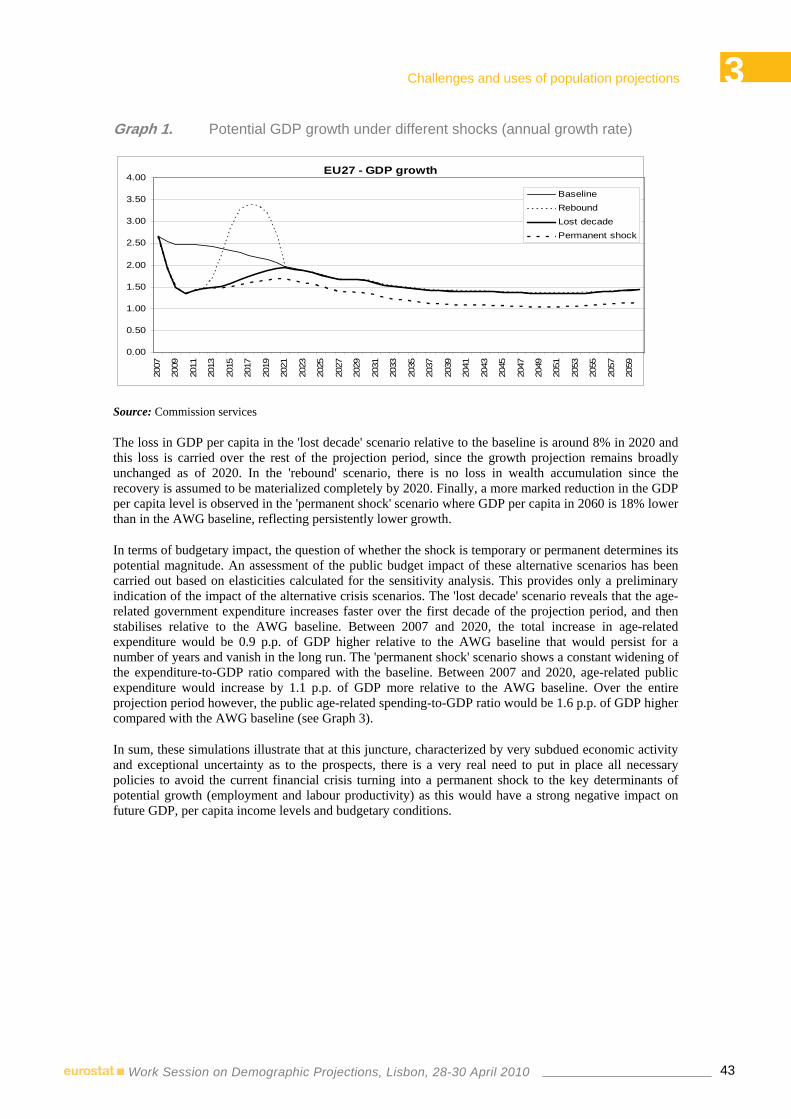
3 Challenges and uses of population projections
43Work Session on Demographic Projections, Lisbon, 28-30 April 2010
Graph 1. Potential GDP growth under different shocks (annual growth rate)
EU27 - GDP growth
0.00
0.50
1.00
1.50
2.00
2.50
3.00
3.50
4.00
2007
2009
2011
2013
2015
2017
2019
2021
2023
2025
2027
2029
2031
2033
2035
2037
2039
2041
2043
2045
2047
2049
2051
2053
2055
2057
2059
BaselineReboundLost decadePermanent shock
Source: Commission services
The loss in GDP per capita in the 'lost decade' scenario relative to the baseline is around 8% in 2020 and this loss is carried over the rest of the projection period, since the growth projection remains broadly unchanged as of 2020. In the 'rebound' scenario, there is no loss in wealth accumulation since the recovery is assumed to be materialized completely by 2020. Finally, a more marked reduction in the GDP per capita level is observed in the 'permanent shock' scenario where GDP per capita in 2060 is 18% lower than in the AWG baseline, reflecting persistently lower growth.
In terms of budgetary impact, the question of whether the shock is temporary or permanent determines its potential magnitude. An assessment of the public budget impact of these alternative scenarios has been carried out based on elasticities calculated for the sensitivity analysis. This provides only a preliminary indication of the impact of the alternative crisis scenarios. The 'lost decade' scenario reveals that the age-related government expenditure increases faster over the first decade of the projection period, and then stabilises relative to the AWG baseline. Between 2007 and 2020, the total increase in age-related expenditure would be 0.9 p.p. of GDP higher relative to the AWG baseline that would persist for a number of years and vanish in the long run. The 'permanent shock' scenario shows a constant widening of the expenditure-to-GDP ratio compared with the baseline. Between 2007 and 2020, age-related public expenditure would increase by 1.1 p.p. of GDP more relative to the AWG baseline. Over the entire projection period however, the public age-related spending-to-GDP ratio would be 1.6 p.p. of GDP higher compared with the AWG baseline (see Graph 3).
In sum, these simulations illustrate that at this juncture, characterized by very subdued economic activity and exceptional uncertainty as to the prospects, there is a very real need to put in place all necessary policies to avoid the current financial crisis turning into a permanent shock to the key determinants of potential growth (employment and labour productivity) as this would have a strong negative impact on future GDP, per capita income levels and budgetary conditions.

3 Challenges and uses of population projections
44Work Session on Demographic Projections, Lisbon, 28-30 April 2010
Graph 2. Potential budgetary impact of the economic crisis
EU27, Cost of Ageing, change in p.p of GDP, 2007-60
0.0
1.0
2.0
3.0
4.0
5.0
6.0
7.0
Baseline Rebound Lost decade Permanent shock
+ 0.0
+ 0.9 + 1.6
Source: Commission services.
7. Conclusions and policy implications
Ageing populations will have large repercussions for EU labour markets, economic growth, and public finances. Ageing, however, is not a "tsunami" that will overwhelm public finances when the baby boom generation start to retire some years from now. It is a slow-moving, largely predictable, process which is therefore manageable provided policy makers act in an efficient and timely manner. We would like to draw four main conclusions on the implications of the economic and budgetary projections for the policies of EU Member States, and also on how future common projections at EU level could be improved.
Firstly, the projections underpin the thrust of the EU's economic policy strategy as defined in the Growth and Job Strategy ( Lisbon strategy, now Europe 2020) i.e. focussing on policies to raise labour utilisation with an emphasis on older workers and extending working lives, as well as on measures to increase labour productivity with an emphasis on the reform of education and human capital policies over the entire life course. However, the projections also underline the dangers of the gap between commitments to undertake reform and concrete actions. There is fast closing "window of opportunity" during which employment and demographic trends are set to remain broadly favourable to reform.
Secondly, pension reforms appear to be working. This conclusion is based on the recent upsurge in the employment rates of older workers in many European countries, plus a comparison of the recent pension projections with those made in 2006 which point to a much lower projected increases in spending on pensions in countries that have made reforms, e.g. Germany, France and Austria. While some reforms may not be fully sufficient to cope with the economic and budgetary consequences of ageing populations, real progress has been made in recent years. Caution is required as there is an ever-present danger of back-sliding as governments face constant pressure to enact special, more favourable, pension or early retirement schemes regimes for special interest groups.
Thirdly, welfare systems need to design to be adaptable and sustainable in the face of uncertain economic and demographic developments. Recent measures to link pension entitlement to future changes in life expectancy are an interesting step in this direction, and can help avoid the need for frequent reforms to pension systems.
Finally, ageing may pose complex challenges in the area of health care and long-term care compared with pensions. The control of public spending through aggregate cost-containment measures (controls on volume, prices and wages, as well as budgetary caps) are likely to remain key elements in comprehensive health care strategies of Member States: however, their effectiveness may diminish over time as suppliers alter their behaviour and they risk introducing distortions that could lead to costly inefficiencies.

3 Challenges and uses of population projections
45Work Session on Demographic Projections, Lisbon, 28-30 April 2010
Measures to improve cost efficiency, to create incentive structure that encourage rational resource use, and to achieve an effective management of technological will be of critical importance.
The current situation of coming out of the worst financial and economic crisis in the post-war period must be used as an opportunity to combine determined efforts to overcome the recession with reforms that will restore confidence in the longer-term outlook for public finances, by strengthening investment in a more sustainable economy and society and by putting ageing-related spending on a sustainable path. This is particularly important if Europe wants to exploit the narrow window of opportunity – a period of about ten years during which employment growth remains possible – before dependency ratios begin to rise rapidly. Hence, getting the policy response right in a co-ordinated manner would limit the loss of wealth creation in Europe and would also lead to less expenditure than would otherwise be the case. Indeed, delays in implementing the needed policies would require stronger measures to achieve the same fiscal outcome by mid-century. It will be particularly important, therefore, to intensify the reform agenda in view of the longer-term challenges outlined above, so as to emerge stronger from the current economic crisis, and to get our economies back on a path of long-term growth. For this to happen, a comprehensive exit strategy built on structural reforms across the board will be necessary to restore credibility and confidence in the public finances. Once out of the crisis, in planning a new fiscal course, due account needs to be taken of the diagnosis of the problems related to ageing. To start to bend back the curve of long-term costs, and to get our economies back on a path of long-term growth, modernization of pensions and health care as well as expanding the degree to which existing factors of production have been used so far is the key.

46
Table 1. 2009 and 2006 projections compared, demographic assumptions
2008 2050 change 2008 2050 change 2008 2050 change 2008 2050cumulated 2008-2050 as % of totalpop. in 2008
2008 2050 change 2008 2050 change 2008 2050 change 2008 2050cumulated 2008-2050 as % of totalpop. in 2008
BE 1.75 1.78 0.03 76.7 83.1 6.5 82.3 87.8 5.5 51 25 13.5% 0.10 0.08 -0.02 0.3 0.8 0.6 -0.2 -0.5 -0.3 30 7 5.8%BG 1.38 1.52 0.14 69.7 79.6 9.9 76.7 84.9 8.2 -1 2 0.5% 0.15 0.02 -0.13 -0.5 1.4 1.9 -0.1 2.3 2.4 10 -1 3.1%CZ 1.33 1.49 0.16 73.9 81.6 7.7 80.2 86.5 6.4 24 22 10.2% 0.13 -0.01 -0.14 0.7 1.9 1.2 0.7 2.4 1.8 20 2 4.0%DK 1.85 1.85 0.00 76.4 82.9 6.5 81.0 87.2 6.2 10 6 6.0% 0.08 0.05 -0.03 0.5 2.0 1.5 0.9 3.5 2.6 2 -1 0.7%DE 1.34 1.49 0.15 77.3 83.6 6.3 82.6 88.0 5.4 160 136 8.4% -0.06 0.04 0.10 0.5 1.6 1.1 0.2 1.1 0.9 -47 -43 -1.5%EE 1.55 1.64 0.09 68.0 78.8 10.8 78.7 86.1 7.4 -1 0 -0.1% 0.12 0.04 -0.08 1.8 3.9 2.1 1.2 3.0 1.8 1 -1 -1.7%IE 1.90 1.88 -0.02 77.5 83.9 6.4 81.9 88.0 6.1 63 7 17.9% -0.01 0.08 0.09 1.1 1.5 0.4 0.5 1.0 0.5 47 -5 4.1%GR 1.41 1.54 0.13 77.4 83.6 6.1 82.6 87.6 5.1 40 31 14.2% 0.04 0.04 0.00 0.5 3.3 2.7 0.7 2.5 1.9 0 -4 0.1%ES 1.39 1.52 0.13 77.4 83.7 6.3 83.9 88.6 4.8 623 135 22.8% 0.05 0.12 0.07 0.1 2.3 2.2 -0.2 0.7 1.0 472 34 12.3%FR 1.98 1.94 -0.04 77.5 83.9 6.4 84.3 89.1 4.8 99 70 6.0% 0.10 0.09 -0.01 0.4 1.2 0.8 0.2 0.0 -0.2 37 11 1.8%IT 1.38 1.52 0.14 78.5 84.3 5.8 84.2 89.0 4.8 260 193 17.1% 0.02 0.12 0.10 0.4 0.7 0.3 0.4 0.2 -0.2 141 80 8.6%CY 1.45 1.57 0.12 78.2 84.0 5.8 81.7 87.5 5.8 9 7 42.8% 0.02 0.07 0.05 1.1 2.1 1.0 0.3 2.4 2.1 3 2 14.9%LV 1.36 1.50 0.14 66.0 78.1 12.2 76.7 85.2 8.5 -1 1 -0.3% -0.02 -0.10 -0.08 0.6 3.8 3.3 0.0 2.7 2.7 1 -2 -2.0%LT 1.35 1.51 0.16 65.9 78.1 12.2 77.4 85.3 7.9 -2 1 -0.3% 0.06 -0.09 -0.15 -1.2 2.6 3.8 -0.8 1.6 2.4 4 -3 -1.9%LU 1.65 1.71 0.06 76.3 83.2 6.8 81.2 87.3 6.1 4 3 33.1% -0.06 -0.09 -0.03 0.4 1.6 1.1 -0.9 0.6 1.5 2 0 7.5%HU 1.35 1.50 0.15 69.7 79.9 10.2 78.1 85.8 7.7 20 18 8.4% 0.04 -0.10 -0.14 0.1 1.8 1.7 0.5 2.4 1.9 5 -2 1.1%MT 1.38 1.52 0.14 76.0 83.0 7.0 81.1 87.4 6.3 1 1 10.2% -0.15 -0.08 0.07 -1.1 1.2 2.3 -0.3 2.4 2.7 -2 -2 -14.7%NL 1.72 1.76 0.04 77.9 83.7 5.8 82.2 87.8 5.6 8 7 2.6% -0.03 0.01 0.04 1.1 3.5 2.4 1.0 4.2 3.2 -25 -24 -5.7%AT 1.41 1.54 0.13 77.4 83.6 6.2 82.9 88.1 5.2 33 25 15.2% 0.00 0.09 0.09 0.4 0.0 -0.4 0.1 0.4 0.3 9 4 4.4%PL 1.27 1.44 0.17 71.4 80.7 9.3 79.9 86.7 6.8 -16 26 1.0% 0.09 -0.16 -0.25 -0.1 1.6 1.7 0.6 2.3 1.7 14 -7 -0.1%PT 1.36 1.51 0.15 75.8 82.7 6.9 82.4 87.7 5.3 52 39 18.7% -0.14 -0.09 0.05 0.8 2.3 1.5 0.6 1.1 0.5 31 24 12.4%RO 1.32 1.48 0.16 69.8 79.9 10.2 76.6 85.0 8.4 -6 13 1.2% 0.00 -0.02 -0.02 0.5 2.3 1.9 0.5 3.0 2.5 8 4 3.2%SI 1.32 1.48 0.16 74.7 82.2 7.5 81.9 87.6 5.7 6 3 8.3% 0.10 -0.02 -0.12 1.3 2.4 1.1 1.0 2.4 1.4 0 -4 -4.8%SK 1.25 1.43 0.18 70.9 80.2 9.3 78.7 85.9 7.2 4 6 3.9% 0.08 -0.17 -0.25 0.4 2.5 2.1 0.3 2.5 2.2 6 1 1.6%FI 1.84 1.84 0.00 76.1 83.0 6.8 83.0 88.2 5.2 10 5 5.4% 0.06 0.04 -0.02 -0.1 1.1 1.1 0.5 1.7 1.2 3 -1 0.4%SE 1.85 1.85 0.00 79.0 84.3 5.4 83.1 88.3 5.1 47 17 11.3% 0.03 0.00 -0.03 0.2 1.0 0.9 0.2 1.8 1.5 22 -5 0.8%UK 1.84 1.84 0.00 77.4 83.8 6.4 81.5 87.7 6.1 188 126 10.8% 0.11 0.09 -0.02 0.2 0.9 0.7 -0.2 1.1 1.2 66 28 3.5%NO 1.90 1.89 -0.01 78.4 84.1 5.7 82.9 88.1 5.3 22 10 12.6% : : : : : : : : : : : :EU27 1.54 1.65 0.11 76.1 83.2 7.0 82.1 87.9 5.8 1684 924 10.2% 0.04 0.05 0.01 0.3 1.6 1.2 0.3 1.3 1.0 863 91 3.2%EA 1.53 1.64 0.10 77.5 83.7 6.2 83.4 88.5 5.1 1418 687 12.4% 0.01 0.07 0.06 0.4 1.6 1.1 0.3 0.9 0.6 702 79 3.8%EA12 1.54 1.64 0.10 77.5 83.8 6.2 83.4 88.5 5.1 1402 676 12.3% 0.01 0.07 0.06 0.4 1.6 1.1 0.3 0.8 0.6 701 82 3.8%EU15 1.59 1.68 0.09 77.5 83.8 6.2 83.1 88.3 5.3 1647 825 12.0% 0.03 0.07 0.04 0.4 1.4 1.1 0.2 0.9 0.7 792 104 3.7%EU10 1.30 1.47 0.16 71.2 80.6 9.4 79.4 86.4 7.0 44 85 4.1% 0.08 -0.11 -0.20 0.1 1.9 1.8 0.5 2.3 1.8 53 -16 0.5%EU25 1.55 1.65 0.10 76.5 83.3 6.8 82.5 88.1 5.6 1691 910 10.7% 0.04 0.05 0.01 0.4 1.5 1.2 0.2 1.2 0.9 845 88 3.2%
Males Females Males Females
Projection exercise 2009 (EUROPOP2008) Projection exercise 2009 - Projection exercise 2006Fertility rate Life expectancy at birth Net migration (1000's) Fertility rate Life expectancy at birth Net migration (1000's)
Source: EUROSTAT (EUROPOP2008), Commission services (DG ECFIN), EPC (AWG).

47
Table 2. 2009 and 2006 projections compared, population projections
2008 2050 % change 2008 2050 p.p change 2008 2050 p.p change 2008 2050 % change 2008 2050 p.p changeBE 10.7 12.2 14.4% 25.8 43.9 18.1 51.4 70.7 19.3 0.2 1.3 10.6% -0.2 -3.3 -3.1BG 7.6 5.9 -22.5% 25.0 55.4 30.4 44.3 77.3 33.0 0.1 0.8 10.1% : : :CZ 10.3 9.9 -4.4% 20.6 54.8 34.2 40.7 77.1 36.5 0.2 1.0 8.0% -0.1 0.0 0.0DK 5.5 5.9 7.7% 23.6 41.3 17.7 51.6 68.8 17.2 0.0 0.5 8.0% 0.1 -0.6 -0.7DE 82.2 74.5 -9.4% 30.3 56.4 26.1 51.0 78.0 26.9 -0.6 -0.2 0.4% 0.3 4.7 4.3EE 1.3 1.2 -11.7% 25.2 47.2 22.0 47.0 72.1 25.1 0.0 0.1 3.5% 0.3 4.1 3.7IE 4.4 6.5 47.9% 16.3 40.4 24.1 46.1 70.2 24.1 0.2 1.1 18.3% -0.6 -4.8 -4.2GR 11.2 11.4 2.0% 27.8 57.0 29.2 49.1 80.7 31.6 0.0 0.8 7.1% 0.2 -3.4 -3.6ES 45.3 53.2 17.5% 24.1 58.7 34.5 45.4 82.8 37.4 1.1 10.4 20.6% -0.5 -6.9 -6.4FR 61.9 71.0 14.8% 25.3 44.7 19.4 53.4 74.4 20.9 0.9 5.3 7.1% 0.0 -1.7 -1.6IT 59.5 61.2 2.9% 30.5 59.2 28.8 51.7 81.6 29.8 1.0 8.5 12.8% -0.3 -3.0 -2.6CY 0.8 1.3 57.5% 17.7 37.7 20.0 42.7 62.1 19.4 0.0 0.3 30.2% -0.8 -5.5 -4.7LV 2.3 1.8 -20.5% 25.0 51.2 26.2 44.9 73.0 28.2 0.0 -0.1 -3.2% -0.1 7.1 7.2LT 3.4 2.7 -18.7% 23.0 51.1 28.1 45.3 72.2 26.9 0.0 -0.1 -3.9% -0.3 6.3 6.5LU 0.5 0.7 44.6% 20.9 37.8 16.9 47.8 64.5 16.7 0.0 0.1 7.6% -0.5 1.7 2.2HU 10.0 9.1 -9.8% 23.5 50.8 27.3 45.3 73.2 27.9 0.0 0.1 1.3% -0.1 2.5 2.6MT 0.4 0.4 1.0% 19.8 49.8 30.0 43.1 71.3 28.2 0.0 -0.1 -21.3% 0.8 9.1 8.3NL 16.4 16.9 3.1% 21.8 45.6 23.8 48.4 71.2 22.8 -0.1 -0.5 -2.1% 0.5 5.0 4.5AT 8.3 9.1 9.5% 25.4 48.3 22.9 48.1 71.5 23.4 0.1 0.9 9.5% -0.1 -4.1 -4.0PL 38.1 33.3 -12.7% 18.9 55.7 36.7 40.7 76.1 35.3 0.2 -0.4 -1.4% 0.2 4.7 4.6PT 10.6 11.4 7.8% 25.9 53.0 27.0 48.7 75.8 27.1 0.0 1.4 13.7% 0.1 -5.6 -5.7RO 21.4 18.1 -15.3% 21.3 54.0 32.7 43.1 74.6 31.5 -0.1 1.0 5.0% : : :SI 2.0 1.9 -7.2% 23.0 59.4 36.4 42.8 82.7 39.9 0.0 0.0 -1.8% 0.0 3.8 3.8SK 5.4 4.9 -10.0% 16.6 55.5 38.9 38.4 75.3 37.0 0.0 0.1 1.6% 0.0 4.8 4.8FI 5.3 5.4 2.8% 24.8 46.6 21.8 50.1 73.9 23.8 0.0 0.2 3.8% 0.2 -0.1 -0.3SE 9.2 10.7 16.2% 26.7 41.9 15.2 52.2 69.5 17.3 0.1 0.5 4.3% 0.0 1.0 1.1UK 61.3 74.5 21.6% 24.3 38.0 13.7 50.7 65.4 14.7 0.8 10.2 15.3% -0.2 -7.1 -6.9NO 4.7 5.9 24.5% 22.1 41.4 19.3 51.0 69.8 18.8 : : : : : :EU27 495.4 515.3 4.0% 25.4 50.4 25.0 48.7 75.0 26.4 4.1 43.3 7.9% : : :EA 319.5 337.3 5.6% 27.1 52.8 25.7 50.3 77.5 27.2 2.8 29.6 8.4% : : :EA12 316.3 333.8 5.5% 27.2 52.8 25.6 50.3 77.5 27.2 2.8 29.4 8.5% -0.1 -0.8 -0.7EU15 392.2 424.9 8.3% 26.7 49.6 22.9 50.5 74.9 24.5 3.6 40.5 9.4% -0.1 -2.0 -1.9EU10 74.1 66.4 -10.5% 20.2 54.1 33.9 41.7 75.3 33.6 0.4 0.9 0.7% 0.1 3.7 3.6EU25 466.3 491.2 5.3% 25.6 50.2 24.6 49.0 75.0 26.0 4.1 41.4 8.0% -0.1 -1.2 -1.2
Projection exercise 2009 (EUROPOP2008) Projection exercise 2009 - Projection exercise 2006Total population Old-age dependency ratio Total dependency ratio Total population Old-age dependency ratio
Source: EUROSTAT (EUROPOP2008), Commission services (DG ECFIN), EPC (AWG).

48
Table 3. 2009 and 2006 projections compared, labour force projections
2007 2050 p.p.
change
2007 2050 p.p.
change
2007 2050 p.p.
change
2007 2050 p.p.
change
2007 2050 p.p.
change
2007 2050 p.p.
change
2007 2050 p.p.
change
2007 2050 p.p.
change
2007 2050 p.p.
change
2007 2050 p.p.
changeBE 62.3 65.4 3.1 34.6 47.6 13.0 67.3 69.7 2.3 36.2 49.4 13.2 7.5 6.2 -1.3 1.4 -0.1 -1.5 4.3 3.3 -1.0 1.6 -0.3 -1.9 5.1 4.5 -0.6 0.1 -0.3 -0.4BG 62.1 64.7 2.5 43.4 45.4 2.0 66.8 67.9 1.0 46.6 47.6 1.0 7.0 4.7 -2.3 : : : : : : : : : : : : : : :CZ 66.2 70.2 4.0 46.6 64.5 17.8 70.0 73.5 3.5 48.9 66.8 17.9 5.4 4.5 -0.9 0.7 0.5 -0.2 0.9 5.6 4.6 -1.1 -1.1 0.0 1.5 6.7 5.2 -2.5 -2.0 0.5DK 77.2 78.3 1.2 59.1 68.4 9.3 80.3 81.0 0.7 61.3 70.3 9.0 3.9 3.2 -0.6 0.9 0.5 -0.4 -2.6 1.6 4.2 0.6 -0.4 -1.0 -2.6 1.3 3.9 -0.4 -1.0 -0.6DE 69.6 74.8 5.2 51.4 68.7 17.3 76.2 79.7 3.5 57.3 73.9 16.5 8.7 6.2 -2.5 1.6 1.3 -0.3 6.4 3.0 -3.4 1.5 0.7 -0.7 6.6 4.7 -1.9 -0.4 -0.8 -0.4EE 69.4 71.2 1.8 60.2 60.1 -0.1 72.9 73.7 0.8 62.4 61.9 -0.5 4.8 3.5 -1.3 3.1 0.4 -2.7 6.1 -1.6 -7.7 0.7 -2.4 -3.1 5.0 -1.8 -6.7 -3.4 -3.5 -0.2IE 69.1 72.5 3.4 53.8 66.5 12.7 72.5 76.3 3.9 55.1 68.3 13.1 4.7 5.1 0.4 -0.3 -2.1 -1.8 1.0 -2.4 -3.4 0.6 -0.9 -1.5 1.5 -1.3 -2.7 1.3 1.6 0.4GR 61.4 64.8 3.4 42.8 50.0 7.2 67.1 69.1 1.9 44.3 51.3 7.0 8.5 6.2 -2.3 0.0 -0.3 -0.3 -1.1 -3.0 -1.9 -0.5 -0.9 -0.3 -0.8 -2.4 -1.6 -0.8 -0.8 0.0ES 65.6 72.8 7.2 44.7 69.7 24.9 71.6 77.6 6.0 47.5 73.1 25.6 8.3 6.2 -2.1 1.4 1.4 0.0 1.0 7.2 6.2 0.7 0.8 0.1 1.3 9.2 7.9 -1.1 -0.8 0.3FR 64.7 67.1 2.4 38.9 46.5 7.7 70.3 71.5 1.2 41.0 48.4 7.5 8.0 6.2 -1.8 0.9 -0.9 -1.8 -3.0 -6.3 -3.3 0.3 -1.6 -1.9 -2.6 -5.7 -3.1 -0.9 -0.8 0.1IT 58.7 64.0 5.3 33.8 61.3 27.5 62.6 67.9 5.3 34.7 62.8 28.2 6.2 5.8 -0.4 -0.2 -1.6 -1.5 1.1 6.7 5.6 -1.3 -2.3 -1.0 0.9 7.5 6.5 -1.6 -0.7 0.8CY 69.7 75.3 5.6 55.9 63.7 7.9 72.9 78.0 5.1 57.6 65.4 7.8 4.4 3.4 -0.9 -2.7 -2.0 0.6 -1.6 -5.3 -3.7 -2.2 -2.7 -0.5 -1.7 -5.2 -3.5 0.7 -0.8 -1.5LV 68.5 68.5 0.1 57.7 52.4 -5.3 72.9 72.0 -0.9 60.4 54.4 -6.0 6.1 4.8 -1.2 1.4 -2.8 -4.2 8.3 -6.3 -14.6 0.1 -4.7 -4.8 8.0 -6.1 -14.1 -1.7 -2.2 -0.5LT 65.1 65.2 0.1 53.4 53.2 -0.2 68.1 67.6 -0.5 55.5 54.8 -0.7 4.4 3.5 -0.9 -0.1 -6.5 -6.4 3.0 -13.0 -16.0 -4.1 -9.5 -5.5 0.3 -13.6 -13.9 -5.2 -3.5 1.7LU 63.6 64.0 0.4 32.3 41.4 9.1 66.4 67.1 0.6 33.0 42.3 9.3 4.2 4.6 0.4 -0.2 -1.5 -1.3 -1.5 -0.4 1.1 -0.2 -1.3 -1.1 -1.2 0.1 1.3 0.0 0.4 0.4HU 57.2 60.9 3.7 32.7 47.8 15.1 61.7 64.9 3.2 34.1 49.4 15.2 7.4 6.2 -1.2 -2.5 -2.4 0.1 -2.7 -1.7 1.0 -0.9 -1.5 -0.6 -1.9 -0.7 1.2 2.7 1.4 -1.2MT 55.8 60.4 4.6 30.5 48.8 18.3 59.5 64.4 4.9 31.6 51.1 19.5 6.2 6.2 0.0 0.4 -1.0 -1.4 -0.5 15.7 16.2 -1.2 -1.6 -0.4 -0.3 17.3 17.6 -2.6 -0.8 1.8NL 76.1 78.0 1.8 51.4 55.9 4.5 78.7 80.4 1.7 53.3 57.8 4.5 3.2 3.0 -0.2 1.2 0.1 -1.1 4.3 0.8 -3.5 1.2 -0.1 -1.3 5.3 1.8 -3.5 0.0 -0.2 -0.2AT 71.5 74.2 2.7 38.8 54.6 15.7 74.8 77.5 2.7 40.0 56.0 16.0 4.5 4.3 -0.2 -0.5 -2.2 -1.6 4.2 -3.5 -7.7 0.3 -1.5 -1.8 3.9 -3.2 -7.1 1.1 0.9 -0.2PL 57.1 61.7 4.6 29.9 44.3 14.3 63.3 65.5 2.2 32.1 46.2 14.1 9.8 5.9 -3.9 2.5 -4.4 -6.8 -1.5 -4.4 -2.9 -2.9 -5.5 -2.6 -1.7 -3.1 -1.4 -7.7 -1.1 6.6PT 67.8 71.8 4.0 51.0 64.3 13.3 74.1 76.6 2.5 54.5 67.5 13.0 8.5 6.2 -2.3 -3.1 -1.5 1.6 -3.8 -0.4 3.4 -1.0 -1.1 -0.1 -2.2 1.3 3.4 2.9 0.6 -2.3RO 58.7 56.9 -1.9 41.4 43.4 2.0 63.0 60.5 -2.5 42.4 44.2 1.8 6.8 6.0 -0.8 : : : : : : : : : : : : : : :SI 67.8 68.3 0.4 33.4 47.0 13.6 71.4 71.6 0.3 34.5 48.3 13.8 4.9 4.7 -0.3 1.6 -1.1 -2.7 -0.9 -5.6 -4.7 1.3 -1.8 -3.1 -0.3 -4.8 -4.4 -0.6 -0.9 -0.3SK 61.2 66.0 4.9 36.2 50.2 14.0 68.8 70.4 1.6 39.4 52.6 13.1 11.1 6.2 -4.9 0.7 -2.7 -3.4 2.2 -1.0 -3.2 -3.4 -3.5 -0.1 2.1 0.6 -1.6 -5.2 -0.8 4.4FI 70.5 74.5 4.0 55.6 65.1 9.4 75.8 79.1 3.3 59.4 68.5 9.1 7.0 5.8 -1.2 0.4 0.1 -0.2 0.9 0.2 -0.7 0.4 -0.5 -0.9 2.0 1.0 -1.0 0.0 -0.7 -0.7SE 74.3 77.5 3.2 70.3 74.1 3.8 79.2 82.4 3.2 73.2 77.1 3.9 6.2 5.9 -0.3 -0.2 -0.1 0.0 -0.4 -2.5 -2.1 1.4 1.3 -0.1 0.1 -2.0 -2.1 1.9 1.6 -0.3UK 71.5 74.3 2.8 57.8 69.0 11.2 75.6 78.6 3.0 59.7 71.3 11.6 5.4 5.4 0.0 -0.7 -0.4 0.3 2.2 5.1 2.9 -0.1 0.2 0.3 2.6 6.0 3.4 0.8 0.8 0.0NO 76.8 74.8 -2.1 69.2 65.5 -3.7 78.8 78.0 -0.8 69.9 66.5 -3.4 2.5 4.1 1.6 : : : : : : : : : : : : : : :EU27 65.5 69.7 4.2 44.9 59.4 14.5 70.6 73.9 3.3 47.5 62.0 14.5 7.2 5.7 -1.5 : : : : : : : : : : : : : : :EA 65.5 70.4 4.8 42.6 60.8 18.2 70.8 74.7 3.9 45.4 63.7 18.3 7.5 5.8 -1.6 : : : : : : : : : : : : : : :EA12 65.5 70.4 4.8 42.6 60.9 18.2 70.9 74.7 3.9 45.5 63.8 18.3 7.5 5.9 -1.7 0.4 -0.1 -0.5 0.9 2.1 1.2 0.0 -0.6 -0.6 1.1 3.3 2.1 -0.6 -0.6 0.0EU15 66.7 71.4 4.7 45.9 62.8 16.9 71.8 75.7 3.9 48.6 65.6 17.0 7.1 5.7 -1.4 0.1 -0.1 -0.3 0.8 2.5 1.7 -0.1 -0.4 -0.3 1.1 3.6 2.5 -0.3 -0.3 0.0EU10 59.9 65.0 5.2 34.8 50.9 16.1 65.2 68.8 3.6 36.9 52.9 16.0 8.3 5.5 -2.8 1.1 -2.0 -3.1 -1.7 -1.0 0.7 -2.4 -3.0 -0.6 -1.8 0.1 2.0 -4.8 -1.1 3.7EU25 65.6 70.5 5.0 44.1 60.9 16.8 70.7 74.8 4.1 46.7 63.6 16.9 7.3 5.7 -1.6 0.3 -0.3 -0.6 0.4 2.1 1.6 -0.4 -0.7 -0.2 0.6 3.2 2.5 -1.0 -0.4 0.6
Projection exercise 2009 - Projection exercise 2006Employment rate (55-64) Participation rate (15-64) Participation rate (55-64) Unemployment rate (15-64)Employment rate (15-64)Unemployment rate (15-64)
Projection exercise 2009Employment rate (15-64) Employment rate (55-64) Participation rate (15-64) Participation rate (55-64)
Source: Commission services (DG ECFIN), EPC (AWG).

49
Table 4. 2009 and 2006 projections compared, economic growth projections
Productivity TFP Capital
deepeningTotal pop.
Empl. rate Share of
change in average Productivity
TFP Capital deepening
Total pop.
Empl. rate Share of
change in average
(GDP per hour
worked)
Working age pop.
hours worked
(GDP per
worker)
Working age pop.
hours worked
1=2+5 2=3+4 3 4 5=6+7+8+9 6 7 8 9 10=1-6 1=2+5 2=3+4 3 4 5=6+7+8+9 6 7 8 9 10=1-6BE 1.9 1.6 1.1 0.6 0.3 0.3 0.1 -0.2 0.0 1.5 BE 0.2 -0.1 -0.1 0.0 0.2 0.2 -0.1 0.1 -0.1BG 2.4 3.0 1.5 1.4 -0.6 -0.6 0.3 -0.3 0.0 3.0 BG 2.4 3.0 1.5 1.4 -0.6 -0.6 0.3 -0.3 3.0CZ 2.1 2.5 1.6 0.9 -0.3 -0.1 0.0 -0.3 0.0 2.2 CZ 0.2 -0.2 0.2 -0.3 0.4 0.2 0.0 0.2 -0.1DK 1.8 1.7 1.1 0.6 0.0 0.2 0.1 -0.2 0.0 1.6 DK 0.1 -0.1 -0.1 0.0 0.1 0.2 0.0 0.0 0.0DE 1.3 1.7 1.1 0.6 -0.4 -0.2 0.2 -0.3 -0.1 1.5 DE -0.1 0.1 0.0 0.1 -0.2 -0.1 -0.1 0.0 0.0EE 2.7 3.1 1.7 1.4 -0.4 -0.3 0.1 -0.2 0.0 3.0 EE 0.0 -0.1 -0.1 0.0 0.1 0.1 -0.1 0.1 -0.1IE 2.8 1.8 1.2 0.7 0.9 1.1 0.1 -0.1 -0.1 1.7 IE -0.1 -0.5 -0.4 -0.1 0.3 0.4 -0.2 0.2 -0.5EL 2.0 2.1 1.2 0.9 -0.1 0.1 0.1 -0.3 0.0 1.9 EL 0.5 0.3 0.3 0.0 0.0 0.1 -0.2 0.1 0.4ES 2.1 1.8 1.1 0.7 0.4 0.5 0.3 -0.3 -0.1 1.6 ES 0.6 0.0 0.1 0.0 0.4 0.5 -0.2 0.2 0.1FR 1.8 1.7 1.1 0.6 0.2 0.4 0.1 -0.2 -0.1 1.5 FR 0.1 0.0 0.0 0.1 0.1 0.2 -0.1 0.1 -0.1IT 1.4 1.4 0.9 0.5 0.0 0.1 0.2 -0.3 0.0 1.3 IT 0.1 -0.1 -0.1 0.0 0.2 0.3 -0.1 0.1 -0.2CY 3.1 1.9 1.2 0.7 1.2 1.2 0.1 -0.1 0.0 1.9 CY 0.1 -0.5 -0.2 -0.2 0.4 0.5 -0.2 0.2 -0.4LV 2.5 3.2 1.7 1.4 -0.7 -0.5 0.1 -0.2 0.0 3.0 LV -0.6 -0.4 -0.2 -0.2 -0.2 -0.1 -0.2 0.1 -0.5LT 2.5 3.0 1.7 1.3 -0.5 -0.5 0.1 -0.2 0.1 3.0 LT -0.4 -0.3 -0.1 -0.1 -0.2 -0.1 -0.3 0.1 -0.3LU 2.9 1.7 1.1 0.7 1.2 0.9 0.4 -0.2 0.0 2.0 LU -0.2 -0.1 0.0 -0.1 -0.1 0.2 -0.3 0.0 -0.4HU 2.0 2.5 1.4 1.0 -0.5 -0.2 0.0 -0.2 0.0 2.3 HU -0.1 0.0 0.1 -0.1 -0.1 0.0 -0.2 0.1 -0.1MT 1.9 2.0 1.2 0.7 -0.1 0.1 0.1 -0.2 -0.1 1.8 MT -0.5 0.0 0.1 -0.1 -0.6 -0.4 -0.2 0.1 -0.1NL 1.6 1.7 1.1 0.6 -0.1 0.1 0.1 -0.2 -0.1 1.5 NL -0.1 0.1 0.0 0.0 -0.1 -0.1 0.0 0.0 0.0AT 1.7 1.7 1.1 0.6 0.1 0.3 0.0 -0.2 0.0 1.5 AT 0.2 0.0 0.0 0.0 0.2 0.2 -0.2 0.1 0.0PL 2.2 2.6 1.5 1.1 -0.4 -0.3 0.1 -0.2 0.0 2.5 PL -0.2 -0.2 -0.2 0.1 -0.2 0.0 -0.4 0.2 -0.2PT 1.9 1.9 1.2 0.7 0.0 0.2 0.1 -0.3 0.0 1.7 PT 0.4 -0.1 0.0 0.0 0.5 0.3 0.1 0.2 0.1RO 2.5 3.2 1.8 1.4 -0.7 -0.4 -0.2 -0.2 0.1 2.9 RO 2.5 3.2 1.8 1.4 -0.7 -0.4 -0.2 -0.2 2.9SI 1.9 2.4 1.3 1.1 -0.5 -0.1 0.0 -0.4 0.0 2.0 SI -0.2 -0.1 -0.1 -0.1 -0.1 0.0 -0.2 0.1 -0.2SK 2.6 2.9 1.8 1.1 -0.3 -0.2 0.1 -0.2 0.0 2.8 SK 0.2 0.1 0.1 0.0 0.0 0.1 -0.3 0.2 0.1FI 1.9 1.9 1.3 0.6 0.0 0.1 0.2 -0.2 0.0 1.8 FI 0.1 0.0 -0.1 0.1 0.1 0.1 0.0 0.1 0.0SE 2.1 1.8 1.2 0.6 0.3 0.4 0.0 -0.1 0.0 1.7 SE -0.1 -0.2 -0.2 0.0 0.1 0.1 -0.1 0.0 -0.2UK 2.2 1.8 1.1 0.7 0.4 0.5 0.1 -0.1 -0.1 1.7 UK 0.3 -0.1 -0.1 0.0 0.4 0.3 0.0 0.1 -0.1NO 2.1 1.7 1.2 0.5 0.5 0.6 0.0 -0.1 0.0 1.6 NO
EU27 1.8 1.8 1.1 0.7 0.0 0.1 0.1 -0.2 0.0 1.7 EU27EA 1.7 1.7 1.1 0.6 0.0 0.2 0.2 -0.3 0.0 1.5 EA
EA12 1.7 1.7 1.1 0.6 0.0 0.2 0.2 -0.3 0.0 1.5 EA12 0.2 0.0 0.0 0.0 0.1 0.2 -0.1 0.1 0.0EU15 1.8 1.7 1.1 0.6 0.1 0.2 0.1 -0.2 0.0 1.5 EU15 0.2 0.0 0.0 0.0 0.2 0.2 -0.1 0.1 0.0EU10 2.2 2.6 1.5 1.1 -0.4 -0.2 0.1 -0.2 0.0 2.4 EU10 -0.1 -0.1 -0.1 0.0 -0.1 0.0 -0.3 0.2 -0.2EU25 1.8 1.8 1.1 0.7 0.0 0.2 0.1 -0.2 -0.1 1.6 EU25 0.1 0.0 0.0 0.0 0.1 0.2 -0.1 0.1 0.0
Due to growth in:
Labour input
Projection exercise 2009 - Projection exercise 2006
GDP growth in 2004-2050
Due to growth in:
GDP per capita
growth in 2004-2050
Labour input
2009 projection
GDP per capita
growth in 2004-2050
GDP growth in 2004-2050
Source: Commission services (DG ECFIN), EPC (AWG).

50
Table 5. Age-related government expenditure, 2007-2060, percentage points of GDP
Level Change Change Level Change Change Level Change Change Level Change Change Level Change Change Level Change Change 2007 2007 2007 2007 2007 2007 2007 2007 2007 2007 2007 2007
2007 2035 2060 2007 2035 2060 2007 2035 2060 2007 2035 2060 2007 2035 2060 2007 2035 2060BE 10.0 4.4 4.8 7.6 1.0 1.2 1.5 0.7 1.4 1.9 -0.4 -0.4 5.5 -0.1 0.0 26.5 5.6 6.9 BEBG 8.3 0.7 3.0 4.7 0.6 0.7 0.2 0.1 0.2 0.1 0.0 0.0 3.3 -0.5 -0.2 16.6 0.8 3.7 BGCZ 7.8 -0.2 3.3 6.2 1.4 2.2 0.2 0.2 0.4 0.1 0.0 0.0 3.5 -0.5 -0.3 17.9 0.9 5.5 CZDK 9.1 1.4 0.1 5.9 0.8 1.0 1.7 1.1 1.5 1.0 -0.2 -0.2 7.1 0.4 0.2 24.8 3.6 2.6 DKDE 10.4 1.4 2.3 7.4 1.4 1.8 0.9 0.7 1.4 0.9 -0.3 -0.3 3.9 -0.5 -0.4 23.6 2.6 4.8 DEEE 5.6 -0.2 -0.7 4.9 0.7 1.2 0.1 0.0 0.1 0.1 0.0 0.0 3.7 -0.4 -0.2 14.3 0.1 0.4 EEIE 5.2 2.8 6.1 5.8 0.9 1.8 0.8 0.4 1.3 0.8 0.1 0.1 4.5 -0.4 -0.3 17.2 3.7 8.9 IEEL 11.7 7.7 12.4 5.0 0.9 1.4 1.4 0.8 2.2 0.3 -0.1 -0.1 3.7 -0.3 0.0 22.1 9.1 15.9 ELES 8.4 3.4 6.7 5.5 1.0 1.6 0.5 0.5 0.9 1.3 -0.4 -0.4 3.5 -0.3 0.1 19.3 4.3 9.0 ESFR 13.0 1.4 1.0 8.1 1.0 1.2 1.4 0.5 0.8 1.2 -0.3 -0.3 4.7 0.0 0.0 28.4 2.7 2.7 FRIT 14.0 1.2 -0.4 5.9 0.9 1.1 1.7 0.5 1.3 0.4 0.0 0.0 4.1 -0.6 -0.3 26.0 2.0 1.6 ITCY 6.3 5.4 11.4 2.7 0.4 0.6 0.0 0.0 0.0 0.3 -0.1 -0.1 6.1 -1.2 -1.2 15.4 4.5 10.8 CYLV 5.4 0.7 -0.4 3.5 0.4 0.6 0.4 0.2 0.5 0.2 0.0 0.0 3.7 -0.6 -0.3 13.2 0.6 0.4 LVLT 6.8 1.9 4.6 4.5 0.7 1.1 0.5 0.2 0.6 0.1 0.0 0.0 4.0 -1.0 -0.9 15.8 1.8 5.4 LTLU 8.7 8.0 15.2 5.8 0.9 1.2 1.4 0.7 2.0 0.4 0.0 0.0 3.8 -0.5 -0.5 20.0 9.1 18.0 LUHU 10.9 0.6 3.0 5.8 0.7 1.3 0.3 0.1 0.4 0.3 -0.1 -0.1 4.4 -0.7 -0.4 21.6 0.7 4.1 HUMT 7.2 2.5 6.2 4.7 2.2 3.3 1.0 0.9 1.6 0.4 0.0 0.0 5.0 -1.2 -1.0 18.2 4.4 10.2 MTNL 6.6 3.4 4.0 4.8 0.9 1.0 3.4 2.8 4.7 1.1 -0.1 -0.1 4.6 -0.2 -0.2 20.5 6.9 9.4 NLAT 12.8 1.2 0.9 6.5 1.2 1.5 1.3 0.6 1.2 0.7 0.0 0.0 4.8 -0.6 -0.5 26.0 2.3 3.1 ATPL 11.6 -2.3 -2.8 4.0 0.7 1.0 0.4 0.2 0.7 0.1 -0.1 -0.1 4.4 -1.3 -1.2 20.5 -2.7 -2.4 PLPT 11.4 0.9 2.1 7.2 1.0 1.9 0.1 0.0 0.1 1.2 -0.4 -0.4 4.6 -0.6 -0.3 24.5 1.1 3.4 PTRO 6.6 5.0 9.2 3.5 0.7 1.4 0.0 0.0 0.0 0.2 0.0 0.0 2.8 -0.6 -0.5 13.1 5.0 10.1 ROSI 9.9 4.9 8.8 6.6 1.4 1.9 1.1 0.9 1.8 0.2 0.0 0.0 5.1 -0.2 0.4 22.9 6.9 12.8 SISK 6.8 1.0 3.4 5.0 1.5 2.3 0.2 0.1 0.4 0.1 -0.1 -0.1 3.1 -1.0 -0.8 15.2 1.6 5.2 SKFI 10.0 3.9 3.3 5.5 0.9 1.0 1.8 1.7 2.6 1.2 -0.2 -0.2 5.7 -0.2 -0.3 24.2 6.1 6.3 FISE 9.5 -0.1 -0.1 7.2 0.6 0.8 3.5 1.3 2.3 0.9 -0.1 -0.1 6.0 -0.3 -0.3 27.2 1.5 2.6 SEUK 6.6 1.3 2.7 7.5 1.2 1.9 0.8 0.3 0.5 0.2 0.0 0.0 3.8 0.0 -0.1 18.9 2.7 5.1 UKNO 8.9 4.3 4.7 5.6 1.0 1.3 2.2 1.2 2.7 0.2 0.2 0.2 7.9 0.1 0.1 24.9 6.8 9.0 NO
EU27 10.2 1.7 2.4 6.7 1.0 1.5 1.2 0.6 1.1 0.8 -0.2 -0.2 4.3 -0.3 -0.2 23.1 2.7 4.7 EU27EA 11.1 2.1 2.8 6.7 1.0 1.4 1.3 0.7 1.4 1.0 -0.2 -0.2 4.2 -0.3 -0.2 24.3 3.2 5.2 EA
EU15 10.2 1.8 2.4 6.9 1.0 1.5 1.3 0.6 1.2 0.8 -0.2 -0.2 4.3 -0.3 -0.1 23.5 3.0 4.8 EU15EU12 9.2 0.4 2.3 4.7 0.8 1.3 0.3 0.2 0.5 0.2 0.0 0.0 3.9 -0.9 -0.7 18.3 0.4 3.4 EU12EU25 10.2 1.6 2.3 6.8 1.0 1.5 1.2 0.6 1.2 0.8 -0.2 -0.2 4.3 -0.3 -0.2 23.3 2.7 4.7 EU25EA12 11.1 2.1 2.8 6.7 1.0 1.4 1.3 0.7 1.4 1.0 -0.2 -0.2 4.2 -0.3 -0.2 24.4 3.3 5.2 EA12EU10 9.7 -0.5 1.0 4.9 0.9 1.4 0.4 0.2 0.6 0.2 0.0 0.0 4.2 -1.0 -0.8 19.2 -0.4 2.1 EU10
Education Total Pensions Health care Long-term care Unemployment benefits
Source: Commission services, EPC.

3 Challenges and use of population projections
51Work Session on Demographic Projections, Lisbon, 28-30 April 2010
ESSAY ON AGEING AND HEALTH PROJECTIONS IN PORTUGAL
Filipa CASTRO HENRIQUES*, Teresa FERREIRA RODRIGUES**
Abstract
This article has two main objectives: 1) to present the main Portuguese demographic dynamics; 2) to analyze the extent of future changes in demographic structures by age and sex, as well as educational level, and their effects on average health status of the Portuguese population. We will a) consider ageing phenomenon as a global trend and its impact on the future health status; b) point out expected trends in health care support and needs; c) forecast the impact on the population’s health status due to recent demographic changes in age structure; d) evaluate to what extent educational levels can be considered as predictors of health status and care needs; e) analyze the consequences of the expected compression of morbidity of most aged groups for the coming decades.
1. An overview
Our aim in this research is to explore different projections methods on ageing and health status, with an overview on national and international literature. We intend to measure the extent and implications of these links for Portugal until 2021, crossing theoretical presupposition and demographic and econometrical techniques, which we believe will allow a multidisciplinary overview on the possible impacts of ageing in Portuguese society for the next decades.
Studies1 have proved a strong relationship between health status and educational levels2, in a context of ageing process. Today population ageing phenomenon is recognised a global issue and its impacts are known, as well as its consequences on health care and other areas of social policies. Although the economic impacts of those changes are not consensual, changes are inevitable. Individuals are living longer and disability is declining in many countries. This is a very positive achievement, but the problem relies on the decrease of the ratio between young and old persons.
In 2005, Henriques3 studied the impacts of socioeconomic inequalities in Portugal and its consequences in future health of elderly individuals. The authors’ purpose was to analyze to what extent future changes in demographic structures by age, sex and educational level would affect average health status of Portuguese population.
Results suggest that in Portugal, as in other European countries, there is a significant relationship between health status and educational level4. This is particularly relevant in a country where the educational level attained by older population is still low.
* Filipa Castro Henriques is Invited Professor, Department of Political Studies, FCSH – Universidade Nova de Lisboa. Email:
[email protected] . ** Teresa Ferreira Rodrigues is Associated Professor, Department of Political Studies, FCSH – Universidade Nova de Lisboa.
Email: [email protected] . 1 Lutz et al., 2007. 2 Joung et al., 2000. 3 Henriques, 2005. 4 Gaymu et al., 2008.

3 Challenges and use of population projections
52Work Session on Demographic Projections, Lisbon, 28-30 April 2010
Main conclusions confirm that this situation will probably undergo major changes in the near future, due to a successful improvement in educational levels for adult and elderly people. So, the possible negative impact of death concentration on advanced ages, associated to the rise of incapacitating and chronic diseases, can be counterbalanced by the rise of average educational levels.
In methodological terms, the authors tried to incorporate econometric and demographic techniques. In both cases the possible conclusions where limited by major difficulties with data, mostly due to impossibility of crosschecking the information. This paper must be considered as an initial essay in applying possible methodologies, according to availability on Portuguese information systems on health status and demographic dynamics.
We propose an essay on these new methodologies for the Portuguese reality, as well as a comparison between results, using national data on Census, demographic annual data reports on births and deaths, deaths certificates, Heath National Surveys.
We will present alternative demographic scenarios until 2021, based on projections of Portuguese population dynamics (fertility, mortality and international migrations) using the Cohort Component Method. For projections on education levels we applied a ratio method to project age structure of education levels5. We know that microsimulation methodology has been used on projections by age structure, health and education for several countries6, including Portugal. But death rates were not estimated from Portuguese reality but from a proxy from Wales, which can introduce major errors on final rates.
2. Data and Methodology
2.1 Data The present study uses two data sets: 1) Census and Demographic data from Portuguese Institute of Statistics; 2) National Health Survey7 (NHS) conducted by Portuguese Institute of Statistics and the National Institute of Health.
We used Census data from 1900 until 2001 to make a forecast for Portuguese population from 2001to2021. Data was provided by, sex, age and educational level. We used information from birth and death certificate, by sex, as well as data from the National Health Survey, which is representative of Portuguese population.
Our sample of the NHS provides information of 21,640 individuals aged 25 or more, on selected variables8. In our sample women are relatively overrepresented, standing for 63% of the observations. The distribution of the whole sample by age structure is the following: 21.1 % are aged 25-39; 17.7 % are in the class 40-49; 18.1% are included in the 50-59 aged class; 20.8% in the 60-69 group; and finally 22.1% of the individuals are older than 70. Regarding the educational attainment, in our sample, 21.6 % of the individuals have no education and this percentage is significantly higher for women (24.6%) than for men (16.5%). A significant percentage of the individuals (about 47%) have no more than lowest educational level9 and only a small proportion have attained the highest educational levels (12%).
These statistics are in accordance with national figures, which place Portugal in the lowest position within the 15 EU countries regarding educational attainment.10 As for the health status, 27.8 % of the individuals declared themselves to be in bad health and this prevalence is higher for women (31.5%) than for men (21.6%). 5 A first synthesis was recently published on this issue: Henriques et al., 2009. 6 FELICIE, PROJECT www.felicie.org 7 National Health Survey, 1999. For this present study we haven’t been able to have the recent 2005/2006 Survey. 8 Selected variables: Age, Sex, Marital Status, Level Education, Self Reported Health, Chronic Diseases and Smoking. 9 This is a total of the first four academic years (4th year, 1st cycle, Primary School). 10 OECD, 2007.

3 Challenges and use of population projections
53Work Session on Demographic Projections, Lisbon, 28-30 April 2010
Both methods were used in an independent way. The combination of both data sets was used to infer the future pattern of the Portuguese population health status.
3. Methodology
To attain our main objectives, we assumed a three-step approach. First, we estimated the relationship between health status and socio-economic conditions, using data from the NHS. Secondly, using the Portuguese Census data for 2001 and developing cohort survivors by sex and age for 2021 and thirdly estimating proportions of educational levels based on Census of 2001 and crossing them with the ageing scenarios already foreseen in the previous step.
Before proceeding to demographic projections we studied population dynamics based on Demographic bookkeeping (or balancing) equation:
attattattatttat EIDNPP +++++ −+−+= ,,,,
Where,
tP represents the population in moment t
atP +
represents the population in moment t+a
attN +,
births occurred between t and t+a
attD +,
deaths occurred between t and t+a
attI +,
immigrants arriving between t and t+a
attE +,
emigrants leaving between t and t+a
To obtain future population from 2001 to 2021 we used the Cohort Component Method. In this framework components of change were estimated and applied to a base population (present) to form a new population (future). The demographic components (mortality, fecundity and migration) are projected separately and by this order. By projecting each component separately it is possible to assume different future trends for each of them and provide a complete model which we assume to be closer to reality11. Once the population age groups by each 5 years have been forecast, we added future projections on education, and calculated future proportions by age and sex for the years 2006, 2011, 2016 and 2021(5x5).
Based on NHS data we determined the current differences in health by age and educational level using logistic regression models12. This model considered health status (Y=1 if the individual declares that he is in bad and very bad health and Y=0 if he is in good or very good health) as our dependent variable (the variable to be explained). The explanatory variables are age, educational level and the existence of a certain disease. We considered two separate models13 for men and women.
The estimated probabilities are used, together with the projections of the composition of the future Portuguese population to predict possible scenarios for health status. Contrary to Joung et al. (2000), we only used the scenario where it is assumed that the estimated coefficients in the logistic regression remain unchanged over time. This assumption was based on two facts.
11 Caselli et al., 2004 12 as in Joung et. al, 2000. 13 More details on the estimation method can be found in Henriques which is available upon request (2005).

3 Challenges and use of population projections
54Work Session on Demographic Projections, Lisbon, 28-30 April 2010
Firstly, the preliminary estimation results obtained from the 2005/06 National Health Survey suggest that, for Portuguese population, the coefficients (odds ratio) seemed to be stable over time14.
On the other hand, evidence for ten European countries15 also concludes that socioeconomic inequalities in self-assessed health showed a higher degree of stability over time.
In methodological terms, we have tried to incorporate econometric and demographic techniques, but as already mentioned, our conclusions were limited by data quality, mostly due to impossibility of crosschecking the information. So, this paper should be considered as an initial essay in applying possible methodologies, according to the available Portuguese information systems on health status and demographic dynamics. The inclusion of education levels on individual death certificates could be of major importance to allow future investigations on this subject, inducing differential trends on morbidity and mortality according to education, as happens elsewhere.
3.1 From Regional Differences to a Global Ageing Society Ageing has become a global phenomenon during the 20th century, as the percentage of people aged 65 and older has grown faster than the total population. In 2009, about 8 percent of the world’s population was aged 65 years and over16. Meanwhile, the percentage of people aged 0 to 14 years old has declined.
People are living longer everywhere, but ageing phenomenon is both a question of increasing rates on life expectancy and the consequence of birth rate decrease. The average World Life Expectancy at Birth rose from 47 to 65 years from 1950-1955 to 2000-2005 and is expected to continue rising. By 2045-2050 it will be 30 years higher than it was in the middle of the 20th century. Between 1950 and 2008 average World Total Fertility Rate felt from 5.0 to 2.6 and it is expected to reach 1.9 by 2045-205017. A major consequence of this transition from high to low fertility and mortality rates has been the enormous growth of the world’s population during the last few decades and in the next ones.
3.2 Portugal in an ageing process: past reality and future trends In the long term, changes in Portuguese mortality rates are a consequence of political and economic conjunctures, as well as a late and slow demographic transition process18. Portuguese demographic model19 shows some idiosyncrasies which are related to the country’s recent political and social history. In a long term analysis, national demographic increase rates were small, due to high levels of mortality and fertility and regularly overcoming mortality crises20..The main characteristics of morbidity and mortality rates didn’t change until the second half of the 20th century, in spite of a slight reduction after 1890, which led to a slight increase of average life expectancy at birth. Nevertheless, several factors interfered and locally altered these indicators: a) differences between life conditions in rural and in urban areas; b) increase of feminine participation rates in the labor market; c) regionally differing ratios of young or elderly people; d) political and/or economic instability21. Nevertheless mortality rates presented a unique model, according to different survival probabilities by age 22.
Major changes have occurred during the last hundred years, which can be explained by the industrialization process, urban growth and internal migrations.
14 Martins et al., 2008. 15 Kunst et al., 2004. 16 PRB, 2009. 17 United Nations, 2008. 18 Henriques e Rodrigues, in Rodrigues et al., 2009 19 Veiga, 2003 20 The last one occurred in 1918; it was caused by a pneumonic flu epidemic. (Rodrigues et al., 2009) 21 Veiga, 2004 22 Veiga, 2005

3 Challenges and use of population projections
55Work Session on Demographic Projections, Lisbon, 28-30 April 2010
These last three factors were the basis of social changes and influenced collective behaviours and spatial concentration in coastal urban areas.23 In the last decade of the 19th century, the first steps to transition process took place. Mortality levels started to decline mainly amongst youngsters. From that moment and up to 1920 global mortality rates reduced 17% and population growth rates would have been significant if migratory movements were less negative.
The comparison between the total annual growth and the net migratory rates from 1900 onwards (Figure 1) shows that Portugal’s total growth rates during the 20th century depended on the intensity of migration fluxes (especially emigration).24
After 1970 internal migration levels increased, reinforcing a new pattern vis-à-vis fertility and mortality ratios.25 This new pattern partly explains the population’s demographic dynamic to urban coastal areas.26
Figure 1. Global Demographic Trends Portugal 1900 to 2001
0,86
1,20
-0,34
0,14
0,79
-0,65
1,24 1,26
-0,02
1,241,15
0,09
0,891,05
-0,16
0,48
1,22
-0,74
-0,21
1,15
-1,36
1,29
0,85
0,44
0,03
0,34
-0,31
0,450,08
0,37
-1,50
-1,30
-1,10
-0,90
-0,70
-0,50
-0,30
-0,10
0,10
0,30
0,50
0,70
0,90
1,10
1,30
1,50
1900-1911 1911-1920 1920-1930 1930-1940 1940-1950 1950-1960 1960-1970 1970-1981 1981-1991 1991-2001
Total RateNatural RateNet Migrations
NR: Natural annual growth; TR: Total annual growth; NM: Net Migration growth.
Source: Henriques, 2009. Estatísticas Demográficas, 1968, p. LXX, 1970-2001 e XIº a XIVº Recenseamento Geral da População Portuguesa, 1970,1981,1991 e 2001.
23 Rodrigues et al., 2009 24 Baganha, 1998 25 Nazareth, 1988 26 Not considering migrations, the demographic increase would be almost uniform up to the 60’s, decaying thereafter and
increasing in the 90’s due to immigration from Africa, South America (Brazil) and Eastern Europe. After 2007 total growth is only due to migration rates. (EUROSTAT, a) 2008)
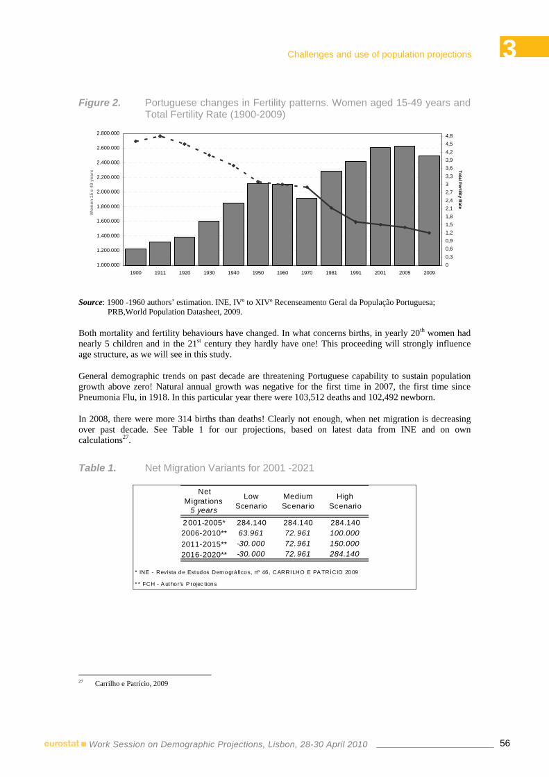
3 Challenges and use of population projections
56Work Session on Demographic Projections, Lisbon, 28-30 April 2010
Figure 2. Portuguese changes in Fertility patterns. Women aged 15-49 years and Total Fertility Rate (1900-2009)
1.000.000
1.200.000
1.400.000
1.600.000
1.800.000
2.000.000
2.200.000
2.400.000
2.600.000
2.800.000
1900 1911 1920 1930 1940 1950 1960 1970 1981 1991 2001 2005 2009
Wom
en 1
5 e
49 y
ears
00,30,60,91,21,51,82,12,42,733,33,63,94,24,54,8
Total Fertility Rate
Source: 1900 -1960 authors’ estimation. INE, IVº to XIVº Recenseamento Geral da População Portuguesa; PRB,World Population Datasheet, 2009.
Both mortality and fertility behaviours have changed. In what concerns births, in yearly 20th women had nearly 5 children and in the 21st century they hardly have one! This proceeding will strongly influence age structure, as we will see in this study.
General demographic trends on past decade are threatening Portuguese capability to sustain population growth above zero! Natural annual growth was negative for the first time in 2007, the first time since Pneumonia Flu, in 1918. In this particular year there were 103,512 deaths and 102,492 newborn.
In 2008, there were more 314 births than deaths! Clearly not enough, when net migration is decreasing over past decade. See Table 1 for our projections, based on latest data from INE and on own calculations27.
Table 1. Net Migration Variants for 2001 -2021
Net Migrat ions
5 years
Low Scenario
Medium Scenario
High Scenario
2 001-2005* 284.140 284.140 284.1402006-2010** 63.961 72.961 100.0002011-2015** -30.000 72.961 150.0002016-2020** -30.000 72.961 284.140
* INE - Revista de Estudos Demográ ficos, nº 46 , CARRI LHO E PA TRÍ CIO 2009
* * FCH - A uthor's P rojec tions
27 Carrilho e Patrício, 2009

3 Challenges and use of population projections
57Work Session on Demographic Projections, Lisbon, 28-30 April 2010
2001 2002 2003 2004 2005 2006 2007 2008 2009 201065000 70000 63500 47240 38400 26.100 19.500 9.361 9000** 9000**
284140 72.96126.100 19.500 9.361 4500** 4500**
63.96126.100 19.500 9.361 22520** 22519**
100.000INE - Revista de Estudos Demográficos, nº 46, CARRILHO E PATRÍCIO 2009
** FCH - Author's Projections
Net Migrations 5 years
Migration Projections presented in this study are much lower than the ones showed by INE in their latest Projections28. The reason for our low performance in migrations is mainly due to international financial and economic crises, that outbreak in the summer of 2007. This major fact changed economic growth all over the World and particularly in our small domestic economy. Portugal is no longer such an attractive country for migrations, as it used to be. Immigration is mainly from Portuguese spoken language countries and people have generally low education levels and skills. They come to work in construction activities and domestic and restaurant services. Otherwise, national emigration to developed countries decreased, especially to Spain. So, in 2008 net migration was the lowest since 1993 (only 8.000).
We believe that due to socio-economic situation and with a decrease in private and public investment foreseen by recent PEC29 immigration will most probably slow down and emigration can increase up until the 2021. Combining decreasing fertility with slowing net migrations, we believe that in 2021 Portuguese population can range between 10,248,567 (less than 2001) and will not exceed 10,773,840 (Figure 3).
Figure 3. Portuguese population and future trends. 1900-2021
5446760
88893928663252
10773840
6080135
6802429
9862670
10.438.03910.248.567
10355824
60801355999146
7755423
8510240
9833014
10.627.29510.572.537
5300000
6300000
7300000
8300000
9300000
10300000
1900 1911 1920 1930 1940 1950 1960 1970 1981 1991 2001 2006 2011 2016 2021
Low
High
M edium
Source: INE, IVº to XIVº Recenseamento Geral da População Portuguesa. Henriques, 2009.
28 INE, 2009
2008 2009 2010 2011 2012 2013 2014 2015 2016 2017 2018 2019 2020 2006-2010 2011-2015 2016-2021High Scenari 22.778 26.054 29.332 32.885 35.885 39.162 42.439 45.716 48.993 52.269 55.547 55.547 55.547 123.764 196.087 267.903derate Scen 21.053 22.606 24.160 25.712 27.265 28.818 30.371 31.925 33.477 35.030 36.584 36.584 36.584 113.419 144.091 178.259Low Scenari 19.330 19.159 18.989 18.818 18.647 18.476 18.306 18.135 17.964 17.794 17.623 17.623 17.623 103.078 92.382 88.627
INE - Projecções da população residente em Portugal 2008-2060
Net Migrations projected by INE 2008-2020
29 PEC – Programa de Estabilidade e Crescimento, Ministério das Finanças, 2010.

3 Challenges and use of population projections
58Work Session on Demographic Projections, Lisbon, 28-30 April 2010
In a long term analysis, Portugal will take 100 years to double its population, and we believe that this beginning of 21st century we are stabilizing and the decrease is announced. When? No one knows. We strongly give an explanation in what concerns the expected decrease in the coming decade, based on present reality. But recent projections made by INE are delaying a decade for population’s break (Figure 4).
Figure 4. Authors’ and INE’s Scenarios for Portugal (2001– 2021)
10248567
10438039
10773840
10489159
10837798
10100000
10200000
10300000
10400000
10500000
10600000
10700000
10800000
10900000
2001 2006 2011 2016 2021
FCH LOW
FCH M EDIUM
FCH HIGH
INE BASE (2004)
INE BASE (2008)
Source: Henriques, 2009.
Life expectancy grew without ceasing since 1920 (Figure 5) and stands at 76 years for men and 82.3 for women in 200830. This is a result of the positive effects of the generalization of efficient means of treatment and the expansion of public and personal hygiene and health care. Life expectancy at birth doubled during last century.
Men and women are now living a second extra life…The main beneficiaries were the most vulnerable groups: firstly, young people, children under a year old and then the most aged ones. Infant Mortality rate decreased from values around 136 per thousand births in yearly 20th century, for 3.4in 200931, one of the World’s best results.
Besides today, Portugal ranks 8th in the World, as it refer to ageing process. The turning point came during the 70’s.32 Changes were relevant in collective behaviours and new migration trends in the last decades of the 20th century33.
30 Carrilho and Patrício, 2009 31 PRB, 2009 32 Veiga, 2003 33 Carrilho et al., 2007

3 Challenges and use of population projections
59Work Session on Demographic Projections, Lisbon, 28-30 April 2010
Figure 5. Life Expectancy in Portugal by sex (1900- 2008)
73,4 76,1
70,469,1
64,2
60,7
55,5
48,6
44,8
35,836,2
82,3
80,477,476,7
70,8
66,8
60,5
52,8
49,2
40,039,8
30
40
50
60
70
80
90
1900 1920 1930 1940 1950 1960 1970 1981 1991 2001 2008
Men
Women
Source: Estatísticas Demográficas, INE.
Figure 6. Age distribution of young and elderly people in Portugal. 1900-2021
34 34
3332 32
28
26
20 21
1514
1515
16
29 29
191818
16
6 6 6 6 6
78
1011
14
0,00
5,00
10,00
15,00
20,00
25,00
30,00
35,00
40,00
1900 1911 1920 1930 1940 1950 1960 1970 1981 1991 2001 2006 2011 2016 2021
Young Elderly
Source: INE Recenseamentos Gerais da População Portuguesa. Henriques, 2009
From 1900 to 2001 the youngest age groups were reduced by 46 per cent, while people aged 65+ increased 300 per cent. Today this last group exceeds the first by more than 190.000 people and in 2021 this difference will be more than 700.000 people.
Nevertheless, regional and gender differences exist: old people are more represented in rural areas and are mostly women, although affected by degenerative and chronic diseases. Men live for a shorter time, but with better health status34.
34 INE; INSRJ, 2000

3 Challenges and use of population projections
60Work Session on Demographic Projections, Lisbon, 28-30 April 2010
Figure 7. Portuguese Demographic Age Structure (1900 – 2001)
MEN AGE WOMEN85 +
80-8475-79 70-7465-6960-6455-59 50-5445-4940-4435-3930-3425-2920-2415-1910-145-90-4
0%1%2%3%4%5%6% 0% 1% 2% 3% 4% 5% 6%
Source: INE, IVº and XIVº Recenseamento Geral da População Portuguesa
Figure 8. Portuguese Demographic Age Structure. 2001- 2021
MEN AGE WOMEN85 +
80-84
75-79 70-7465-6960-6455-59 50-5445-4940-4435-3930-3425-29
20-2415-1910-145-90-4
0%1%2%3%4%5%6% 0% 1% 2% 3% 4% 5% 6%
Source: Henriques, 2005
Apart from different migration scenario, forecasts confirm a double ageing process, with average life expectancies greater than 76 years for men and 83 for women by 2021.
By then, the younger generations will represent no more than 14 per cent, whilst old people will exceed 21 per cent. For every 10 youngsters there will be 15 people aged 65 years or more.

3 Challenges and use of population projections
61Work Session on Demographic Projections, Lisbon, 28-30 April 2010
4. Ageing, socio-economic conditions and health
The Portuguese mortality model shows a clear concentration of death amongst older age groups35. In such a context, growing old in a healthy way has become one of the important goals of policies which aim for a healthy survival. The cumulative effects of adverse inputs, resulting from harmful life styles and food diets, have impacts throughout life and will negatively influence older ages. Several chronic pathologies are precociously aggravated inducing morbid irreversible conditions, due to a life style with multiple stress factors, lack of physical exercise, an unbalanced diet and nicotine and alcohol addictions. Socio-economic differences36 and their consequent impact in health unevenness have been studied, discussed and registered for many years under several disciplines. However, we still do not know precisely and clearly the mutual relationship between socio-economic conditions, health status and the supporting needs for the Portuguese population37. Different exposures to specific risks partially explain the differences found in health profiles38. We can confidently state that socio-demographic factors, such as gender, age, marital status, education level and socio-economic status, among many others, constitute powerful determinants for morbidity and mortality39.
Many studies have attempted to determine how individuals’ social and economic characteristics are related to health status40.
Some major findings emerged from these studies: firstly, there is a significant association between factors like educational level, age, income and self assessed health status; secondly, the impact of each of these variables on health status depends to some extent on the considered region; finally, there is some evidence showing that the magnitude of these associations probably did not change over time.
Populations’ age and its educational attainments appear to be, within this context, two particularly important determinants of self reported health status. On one hand, older people, when compared with younger, report a worse health status. On the other hand, more educated individuals, when compared with less educated ones, reveal an enhanced health status. Since we expect a forthcoming population older but also better educated, the effect of ageing on heath status is ambiguous. Some studies41 go more in detail and make an attempt to evaluate the impact of ageing on health care expenditures. The findings obtained by this line of research are not conclusive. The study by Zweifel et al. (1999) proposed that proximity to death has a more important influence on health care costs than age, suggesting that demographic changes, per si, will not have a large impact on future aggregate health expenditures. These findings have been criticized namely by the studies developed by Seshamani (2004). Using a hospital data set for the UK and a population projection by age and sex, the authors concluded that both population ageing and time of death are important determinants of health care costs.
The study by Joung et al. underlines another point and argues that future changes in the composition of the population by educational level will also affect their average health status. This might counterbalance some of the effects of ageing. In an initial stage, the authors used logistic regression methods to estimate the odds ratio for age and educational level. Separate models were fitted for men and women. In a second step, the estimation results are used to calculate the expected proportion of ill-health for each specific category of sex, age and educational level. The projected proportion of ill-health within the total population was estimated applying these expected proportions to the number of people in the appropriate specific stratum.
35 Veiga, 2005. 36 Huisman, et al., 2004. 37 Henriques et al., 2009. 38 Casey et al., 2003. 39 Fernandes et al., 2008; Godinho et al., 1987. 40 Smith et al., 2007; Fernandez-Olano et al., 2006; Joung et al., 2000. 41 Seshamani, 2004; Zweifel et al., 1999.

3 Challenges and use of population projections
62Work Session on Demographic Projections, Lisbon, 28-30 April 2010
Their study concluded that the rise in educational level counteracts to a substantial degree the expected increases in ill-health due to population ageing. They prove that changes in educational level must be taken into account when morbidity and health forecasting is concerned.
Our work is based on this perspective of interaction between health, education and ageing. In Portugal, a few studies42 had been developed regarding these three perspectives.
It is more usual to find demographic projections separated from other variables. Henriques and Rodrigues43 have developed a work with Gaymus et al. (2008) involving Portugal and other European countries. Although 9 countries were involved, main conclusions for Portugal were based on static projections by socioeconomic variables, a) using volume estimations, b) assuming England and Wales fertility and mortality models and c) excluding a direct cross projection with data from educational level. It has been impossible to cross demographic and educational level projections, due to general nature of death certificates in Portugal.
Up until these studies were developed, death certificate didn’t cross level of education of the deceased but included his parents’ education! It’s impossible to determine survivors by sex, age and level of education in Portugal, using this data. In Gaymus et al. we used a proxy of other countries with similar reality; in Henriques (2005) we used separated estimations: demographic (cohort), education and health, as did the first studies in this field developed for Dutch people by Joung et al.. Main conclusions comparing both methods revealed that studies using separated projections present a higher prevalence for lower range of health status than those combining method. These last studies had more optimistic results in what concerns elderly survivors by health status.
We think that these studies are particularly important to develop in Portuguese case: 1) there are few published studies on this subject for Portugal, both as a hole when taking into account regional diversity and European context; 2) ageing phenomena is particularly pronounced in Portugal, although with major internal differences; 3) education attainment is strongly different between nowadays old generations and future old generations; and 4) there is a need to reduce the actual health care burden, namely the public expenses with health care use.
5. Portuguese educational level: the role of educational policies
The educational policies implemented by European countries all over the 20th century had a general positive effect, leading to a progressive fall in the percentage of illiteracy and low-educated people. Comparing cohorts all over Europe44 show differences over time due to variations in their educational policies. Portugal can be considered a late transition country, as it shows a slow decline in the proportion of low-educated people. Rates of illiteracy among the current older population are still very high. Today more than 50 per cent of oldest old (85+ years) don’t know how to write or read! It is one of the highest proportions among European countries.
42 Henriques, 2005; Nogueira et al., 2006; Koivusalo et al., 2007; Gaymu et al., 2008. 43 And Fernandes, in Gaymus et al., 2007. 44 Gaymus et al., 2007.

3 Challenges and use of population projections
63Work Session on Demographic Projections, Lisbon, 28-30 April 2010
Figure 9. Portuguese Educational level by Age Structure. 2001
0%
20%
40%
60%
80%
100%
25-35 35-45 45-55 55-65 65-75 75-85 85+No education Low Level (4 years or less)Medium Level (from 5 to 9 years) Medium- high Level (from 9 to 12 years)High Level (University attendance incomp or complete)
Source: Authors calculation based on data from INE, XIVº Recenseamento Geral da População Portuguesa
Figure 9 represents cohort evolution by educational level. Analyzing deeply this reality one can see that shifts took place between the 1930s and 1960s, during the so-called Estado Novo45. Four main educational policies influenced national changes in birth cohorts, three46 of those before 1974. The first one includes cohorts that went to school in the 1930s, when educational policies were not favorable and most people, especially women, are illiterate; the second group concerns those who went to school in the 1940s and experiences a slight raise in school attendance. Many schools were built throughout the country. The main goal was to ensure that all children received a moral and ideological education; the third group went to school in the mid-twentieth century. By then, attendance was obligatory for four years. After 1974, further reforms were introduced and education was extended to all, on the basis of equal rights in all areas and for each and every pupil. Changes were significant in national educational policies and will have major impacts in future elderly population.
6. Ageing, education and health in Portugal
As expected, the estimation results based on a logistic regression47 suggest that the educational level is negatively associated with health status. People with higher educational level declare themselves with better health than people with lower educational levels48. Moreover, the estimated impact of education on health status is significantly higher for men than it is for women. As anticipated, our results also propose that age49 is associated with health status. Older people have a higher probability of declaring themselves in bad health than younger ones. As for this variable, the results between women and men are not as different as those regarding educational level. These conclusions are analogous to those obtained in other related studies50.
45 Estado Novo - fascist regime that came to power in the late 1920s. 46 More information Fernandes, Rodrigues e Henriques, in Gaymus et al., 2007. 47 Logistic regression was applied to search for the impacts of each explanatory variable (education, sex, age, etc.) on the
probability of an individual declaring to be in bad or very bad health as a whole. 48 A man with no education has a 10.59 greater probability of declaring himself to be in bad or very bad health than a man with a
high educational level (the reference group). 49 Results: A women aged 70+ reveals a probability of 4.4 of declaring himself to be in bad or very bad health as compared to a
woman in the 25-39 age groups. 50 Joung et al., 2000, Cavelaars et al., 1998, Groot et al, 2008.

3 Challenges and use of population projections
64Work Session on Demographic Projections, Lisbon, 28-30 April 2010
Joung et al. and Groot and Van den Brink51, also found a significant correlation between increase of numbers of years of education and health status. This evidence is more obvious for men than for women.
Bringing to a closer conclusion, our findings corroborate the idea that future changes in the composition of the population by educational level will also affect population’s global average health rate. More than in other European countries, huge changes in average educational levels of the Portuguese population are expected in the coming decades, as showed in previous chapter. The extent to which the rise in educational levels will counterbalance some of the effects of ageing is as yet unknown.
By analyzing 1) the projections of the Portuguese population by sex and age and 2) the ratio proportions of educational level, we expect 3) to be able to answer this essential question. Figures 10 and 11 present two scenarios on the composition of Portuguese population by educational level, considering people aged 60-69 in 2001 and those who will be over 70 in 2021.
Figure 10. Level of Education by Sex (60- 69 years) in 2001 and 2021
0%
10%
20%
30%
40%
50%
60%
70%
2001 2021 2001 2021 2001 2021 2001 2021
No education Low level ofeducation
Md level ofeducation
High leveleducation
Men
Women
Source: Henriques et al., 2009
Figure 11. Educational levels by Sex (70 or more years) in 2001 and 2021
0%
10%
20%
30%
40%
50%
60%
70%
2001 2021 2001 2021 2001 2021 2001 2021
No education Low level ofeducation
Md level ofeducation
High leveleducation
Men
Women
Source: Henriques et al., 2009
51 2008.

3 Challenges and use of population projections
65Work Session on Demographic Projections, Lisbon, 28-30 April 2010
Among older men and women there are substantial changes in the highest attained education level between 2001 and 202152.
These results are in accordance with those found for the Dutch population, and suggest that the negative effect of ageing on health status will be counterbalanced at least partially by higher educational levels. In future research, based on the results from the National Health Survey 2005/06, we intend to measure the impact of the increase in educational levels on the future health care burden associated with ageing phenomena in Portugal.
7. Conclusions
The purpose of this study was to analyze to what extent future changes in demographic structures by age, sex and educational level will affect the average health status of the Portuguese population. In a demographic global ageing scenario, Portugal stands as a case study with specific interest, due to some major differences related to its historical past. Our estimation results suggest that, as in other European countries, there is a significant relationship between health status and educational level. This is particularly relevant in a country where the educational level attained by older population is still low. Nevertheless, we have shown that this situation will probably undergo major changes in the near future, due to a successful improvement in educational levels for adult and elderly people. So, the possible negative impact of death concentration on advanced ages, associated to the rise of incapacitating and chronic diseases, can be counterbalanced by the rise in educational levels.
As ageing process is unstoppable this is of major concern. Knowing how many years one will live is not as important as knowing in which quality one can expect to achieve them! If you have a higher education level, you have a stronger probability to have a healthier old age.
References
Baganha, Maria Ioannis, “A emigração atlântica e as migrações internas em Portugal”, Los 98 Ibericos y el mar, IV, Lisboa, (1998) 215-228
Carrilho, Mª. José, Patrício, Lurdes, “A situação demográfica recente em Portugal”, Revista de Estudos Demográficos 40 (2007) 39-75
Carrilho, Mª. José, Patrício, Lurdes, “A situação demográfica recente em Portugal”, Revista de Estudos Demográficos 46 (2009) 59-96
Caselli, Graziella et al., Démographie: analyse et sinthèse. Histoire du peuplement et prévisions, INED, Paris (2004)
Casey, Bernard. Oxley, Howard. White House, Edward. Antolin, Pablo. Duval, Romain, Leibfritz, Willi, “Policies for an ageing society: recent measures and areas for further reform”. Economics Department working papers, 369 (2003) http://www.oecd.org/eco
Cavelaars, A.E.J.M., Kunst, A.E., Geurts, J.J.M., Crialesi, R., Grotvedt, L., Helmert, U., Lahelma, E., Matheson, J., Mielck, A., Mizrahi, A., Mizrahi, A., rasmussen, N.K., Regidor, E., Spuhler, T., Mackenbach, J.P., “Differences in self-reported morbidity by educational level: A comparison of 11 Eastern European countries”, J Epidemiological Community Health 52 (1998) 219-227
EUROSTAT, a) EUROPOP2008 (EUROstat POpulation Projections 2008-based), Convergence scenario, national and regional, 2008
52 As an example, for people aged 60-69, the proportion of women having no education decreases from 41% in 2001 to less than
5% in 2021 and the proportion of women with higher education increases from 4% to 16%.

3 Challenges and use of population projections
66Work Session on Demographic Projections, Lisbon, 28-30 April 2010
EUROSTAT, b) Statistics in Focus, 81 (2008)
Fernandes, Ana. Veiga, Teresa R., Henriques, Filipa de Castro, “Future Trends in Education among older people”, 5, in Joelle Gaymu, Patrick Festy, Michel Poulain, Gijs Beets eds, Future Elderly Living Conditions in Europe. Quelles conditions de vie pour les Européens âgés de demain? Paris, 2008
Fernandez-Olano, C., Lopez-Torres, H.J.D., Cerda-Diaz, R., Requena-Gallego, M. Urbistondo-Cascales, L., A. Otero-Puime (2006), Factors associated with health care utilization by elderly in a public health care system, Health Policy, 75, 131-139;
Gaymu, Joelle, Festy, Patrick, Beets, Gijs, Poulain, Michel (2008) “From elderly population projections to policy implications”, Future Elderly Living Conditions in Europe, L’avenir des conditions de vie des Européens âgés, INED, Cahier 162, 257-291
Godinho, Joana M. e Lucas João S., “Doença e Morte: Diferenças entre sexos”, V Jornadas de Economia de Saúde. Lisboa, 1987
Groot, W., Van den Brink, H.M., “Health- adjusted life expectancy of the British population”, Applied Economics, 40 (2008) 1373-1386
Henriques, Filipa de Castro, Envelhecimento, Educação e Saúde: uma análise prospectiva 2001-2021. UNL- ISEGI, Lisboa, 2005
Henriques, Filipa Castro; Rodrigues Teresa Ferreira and Martins, Maria Fraga O. Ageing, Education and Health in Portugal: Prospective from the 19th to the 21st Century Hygiea Internationalis 2009 8:1, 81–96 http://www.ep.liu.se/ej/hygiea/
Huisman, M., Kunst, A.E., Andersen, O., Bop., M., Borgan, J-K., Borrell, C., Costa, G., Deboosere, P., Desplanques, G., Donkin, A., Gadeyne, S., Minder, C., Regidor, E., Spadea, T., Valkonen, T. & Mackenbach, J.P., “Socioeconomic inequalities in mortality among elderly people in 11 European populations”, J Epidemiological Community Health, 58 (2004) 468-475
INE/INSRJ, Esperança de vida sem incapacidade física de longa duração. 10, Instituto Nacional de Saúde/ Instituto Nacional de Saúde Dr. Ricardo Jorge. Lisboa. 2000
INE, Projecções da populaçõa residente em Portugal 2008-2060. 2009
Joung, I.M.A, Kunst, A.E., Imhoff, E.Van & Mackenbach, J.P. Education, “Ageing and health, to what extent can the rise in educational level relieve the future health (care) burden associated with population aging in the Netherlands?”, Journal of Clinical Epidemiology 53 (2000) www.sciencedirect.com
Koivusalo M., Wyss. K, Santana, P. (2007) Effects of decentralization and recentralization on equity dimensions of health systems, in Decentralization in Health Care, European Observatory on Health Systems and Policies Series, 2007, 189-205
Lutz, Wolfgang; Goujon, Anne; Samir K.C.; Sanderson, Warren. (2007). “Reconstruction of Populations by Age, Sex and Level of Educational Attainment for 120 Countries for 1970-2000”. International Report. International Institute for Applied Systems Analysis Schlossplatz, Austria.
Kunst, A.E., Bos, V., Lahelma, E., Barthey, M., Lissau, I., Regidor, E., Mielck, A., Cardano, M., Dalstra, J., Geurts, J., Helmert, U., Lennartsson, C., Ramm, J., Spadea, T., Strnegger, W., Mackenbach, J.P., “Trends in Socioeconomic inequalities in self-assessed health in 10 European countries”, International Journal of Epidemiology, 34 (2004) 295-305

3 Challenges and use of population projections
67Work Session on Demographic Projections, Lisbon, 28-30 April 2010
Martins, F.O.R., Oliveira, D., Rodrigues, T., “Differences in self reported morbidity by educational level: a comparison between the 1998/99 and 2005/06 Portuguese Health Survey Results”, European Journal of Public Health, Volume 18, Supplement 1, November 2008.
Nazareth, Manuel, Portugal. Os próximos 20 anos, Vol.III – Unidade e diversidade da demografia portuguesa no final do século XX, Fundação Calouste Gulbenkian, Lisboa, 1988
Nogueira, H., Santana P., Santos, R. (2006) "Impacts of social and material environment on health perception". Regional Responses to Global Changes a view from the Antipodes, IGU, Brisbane, Proceedings
OECD, Education at a Glance, 2007
Population Reference Bureau, Datasheet 2009 http://www.prb.org/pdf09/09wpds_eng.pdf
Rodrigues, Teresa, Moreira, Maria João, Henriques, Filipa, A população portuguesa. Das longas permanências à conquista da modernidade, Afrontamento, Porto, 2008
Rodrigues, Teresa, Moreira, Maria João, As Regionalidades Demográficas no Portugal Contemporâneo, CEPESE (Working Paper), 2008.http://cepese.up.pt/principal.php?IDNivel=77
Santos, Paula Santana, C., Costa, Fernandes, M., Nogueira, H. (2006) “ Indicadores e Metas do Plano Nacional de Saúde”, Alto Comissariado da Saúde, Ministério da Saúde, Lisboa
Seshamani, M. Gray, A. (2004), Time to death and health expenditure: an improved model for the impact of demographic change on health care costs, Age and Ageing, 33, 556-561.
Smith, Kimberly V. and Noreen Goldman Socioeconomic Differences in Health among older adults in Mexico, Social Science & Medicine, 65, 1372-1385; ELSEVIER. July 2007
Veiga, Teresa, Moreira, Maria João, Fernandes, Ana, “Health and Social Change – The case of Portugal”, Hygiea Internationalis, volume 4, nº1, Linköping (2004), 255-276 (www.ep.liu.se/ej/hygiea)
Veiga, Teresa Rodrigues. “A população portuguesa no último século: permanências e mudanças”, Ler História 45, Lisboa (2003) 91-101
Veiga, Teresa, “A Dinâmica das Populações Humanas e os Modelos de Mortalidade”, Fórum Sociológico, 11/12, Lisboa (2004) 11-29
Veiga, Teresa, "Modelos de Mortalidade em Portugal", Ler História, 49, Lisboa (2005) 145-169
2008 World Population Data Sheet, PRB, Set.2008 (www.prb.org)
United Nations, World Population Prospects, the 2008 revision, New York, 2005
Zweifel, Peter; Felder, Stefan and Meiers, Markus Ageing of Population and health care expenditures: a red herring? Health Economics, 8, 485-496. 1999


3 Challenges and use of population projections
69Work Session on Demographic Projections, Lisbon, 28-30 April 2010
CURRENT STATUS AND FUTURE CHALLENGES OF THE NATIONAL POPULATION PROJECTION IN SOUTH
KOREA CONCERNING SUPER-LOW FERTILITY PATTERNS: A CASE STUDY THROUGH
INTERNATIONAL COMPARISON
Kwang-Hee JUN1, Seulki CHOI2
Abstract
South Korea has experienced a rapid fertility decline and notable mortality improvement. As the drop in TFR was quicker and greater in terms of tempo and magnitude, it cast a new challenge of population projection - how to improve the forecasting accuracy in the country with a super-low fertility pattern. This study begin with the current status of the national population projection as implemented by Statistics Korea by comparing the 2009 interim projection with the 2006 official national population projection. Secondly, this study compare the population projection system including projection agencies, projection horizons, projection intervals, the number of projection scenarios, and the number of assumptions on fertility, mortality and international migration among super-low fertility countries. Thirdly we illustrate a stochastic population projection for Korea by transforming the population rates into one parameter series. Finally we describe the future challenges of the national population projection, and propose the projection scenarios for the 2011 official population projection. To enhance the accuracy, we suggest that Statistics Korea should update population projections more frequently or distinguish them into short-term and long-term projections. Adding more than four projection scenarios including additional types of "low-variant" fertility could show a variety of future changes. We also expect Statistics Korea to pay more attention to the determination of a base population that should include both national and non-national populations. Finally we hope that Statistics Korea will find a wise way to incorporate the ideas underlying the system of stochastic population projection as part of the official national population projection.
Key Words: Projection Scenarios, Stochastic Population Projection
1. Introduction
Most developed countries in Europe, North America, and Japan of East Asia have experienced a series of huge demographic changes since the second quarter of the 20th century. These changes include drop in fertility and mortality rates, rapid evolution of population aging, and increases in international migration as accompanied by secular trends in regional integration and economic globalization. Meanwhile, the beginning of the 'second" demographic transition in the 1960s in most European countries and the emergence of the so-called "lowest-low" fertility patterns in Southern and Eastern Europe in the 1990s have contributed significantly to the heightening of either scholarly or policy-oriented interests in the
1 Kwang-Hee JUN Chungnam National University 2 Seulki CHOI Ewha Womans University
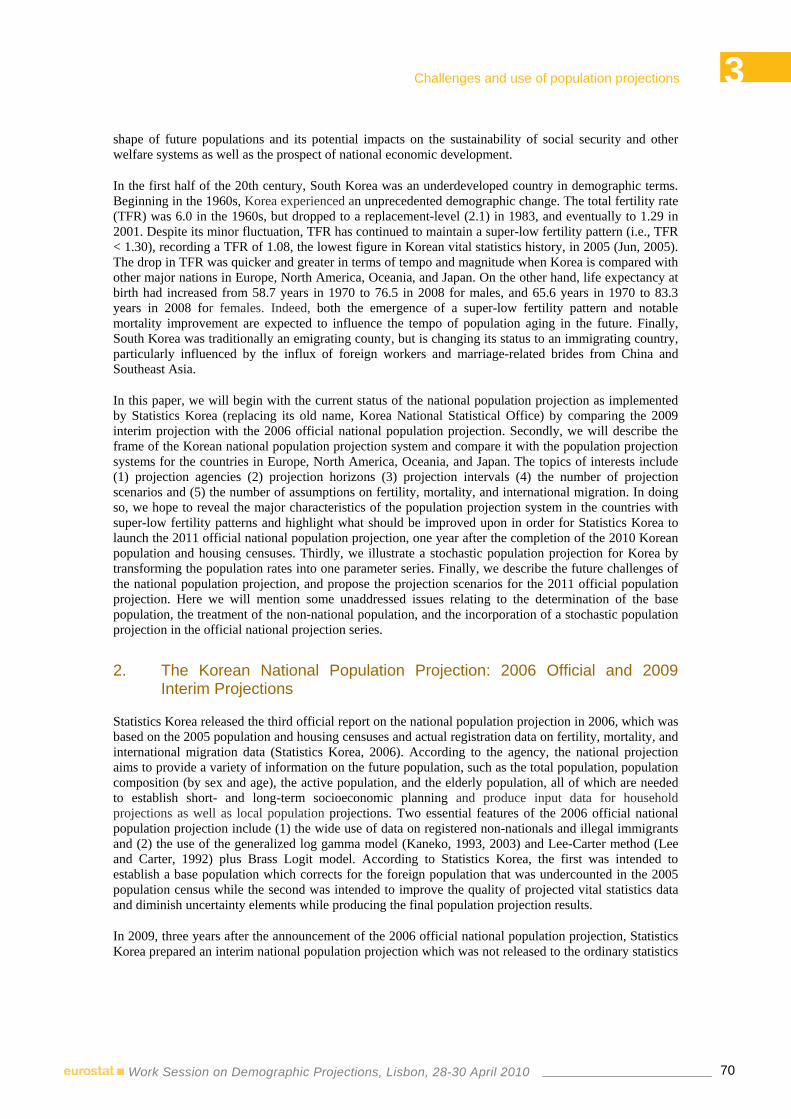
3 Challenges and use of population projections
70Work Session on Demographic Projections, Lisbon, 28-30 April 2010
shape of future populations and its potential impacts on the sustainability of social security and other welfare systems as well as the prospect of national economic development.
In the first half of the 20th century, South Korea was an underdeveloped country in demographic terms. Beginning in the 1960s, Korea experienced an unprecedented demographic change. The total fertility rate (TFR) was 6.0 in the 1960s, but dropped to a replacement-level (2.1) in 1983, and eventually to 1.29 in 2001. Despite its minor fluctuation, TFR has continued to maintain a super-low fertility pattern (i.e., TFR < 1.30), recording a TFR of 1.08, the lowest figure in Korean vital statistics history, in 2005 (Jun, 2005). The drop in TFR was quicker and greater in terms of tempo and magnitude when Korea is compared with other major nations in Europe, North America, Oceania, and Japan. On the other hand, life expectancy at birth had increased from 58.7 years in 1970 to 76.5 in 2008 for males, and 65.6 years in 1970 to 83.3 years in 2008 for females. Indeed, both the emergence of a super-low fertility pattern and notable mortality improvement are expected to influence the tempo of population aging in the future. Finally, South Korea was traditionally an emigrating county, but is changing its status to an immigrating country, particularly influenced by the influx of foreign workers and marriage-related brides from China and Southeast Asia.
In this paper, we will begin with the current status of the national population projection as implemented by Statistics Korea (replacing its old name, Korea National Statistical Office) by comparing the 2009 interim projection with the 2006 official national population projection. Secondly, we will describe the frame of the Korean national population projection system and compare it with the population projection systems for the countries in Europe, North America, Oceania, and Japan. The topics of interests include (1) projection agencies (2) projection horizons (3) projection intervals (4) the number of projection scenarios and (5) the number of assumptions on fertility, mortality, and international migration. In doing so, we hope to reveal the major characteristics of the population projection system in the countries with super-low fertility patterns and highlight what should be improved upon in order for Statistics Korea to launch the 2011 official national population projection, one year after the completion of the 2010 Korean population and housing censuses. Thirdly, we illustrate a stochastic population projection for Korea by transforming the population rates into one parameter series. Finally, we describe the future challenges of the national population projection, and propose the projection scenarios for the 2011 official population projection. Here we will mention some unaddressed issues relating to the determination of the base population, the treatment of the non-national population, and the incorporation of a stochastic population projection in the official national projection series.
2. The Korean National Population Projection: 2006 Official and 2009 Interim Projections
Statistics Korea released the third official report on the national population projection in 2006, which was based on the 2005 population and housing censuses and actual registration data on fertility, mortality, and international migration data (Statistics Korea, 2006). According to the agency, the national projection aims to provide a variety of information on the future population, such as the total population, population composition (by sex and age), the active population, and the elderly population, all of which are needed to establish short- and long-term socioeconomic planning and produce input data for household projections as well as local population projections. Two essential features of the 2006 official national population projection include (1) the wide use of data on registered non-nationals and illegal immigrants and (2) the use of the generalized log gamma model (Kaneko, 1993, 2003) and Lee-Carter method (Lee and Carter, 1992) plus Brass Logit model. According to Statistics Korea, the first was intended to establish a base population which corrects for the foreign population that was undercounted in the 2005 population census while the second was intended to improve the quality of projected vital statistics data and diminish uncertainty elements while producing the final population projection results.
In 2009, three years after the announcement of the 2006 official national population projection, Statistics Korea prepared an interim national population projection which was not released to the ordinary statistics

3 Challenges and use of population projections
71Work Session on Demographic Projections, Lisbon, 28-30 April 2010
users (Statistics Korea, 2009)3. The agency cited three reasons for doing so. First, TFR was suddenly on the rise and fall after registering the worst level of 1.08 births per woman in 2005. The TFR rose to 1.13 births in 2006 and 1.29 births in 2007, but fell to 1.19 births in 2008. In 2005, the number of marriages increased due to the so-called "twin-spring year" effect and also the "golden boar" effect4 contributed significantly to the TFR's modest recuperation in 2006 and 2007. At that time, the Korean government spared little efforts to promote the visible effects of "pronatalist population policy programs" on the rise in TFR, after the initiation of their so-called "SAEROMAJI" project whose basic purpose was to cope with super-low fertility and the aging of population. Second, the crude death rate was relatively stable at 5.0 per thousand, and the annual number of deaths was between 240 and 268 thousand in the years between 2000 and 2008. Third, there was a significant shift of international migration from net emigration (42 thousand) to net immigration (13 thousand) in the years between 2005 and 2008. Korea is now changing from an emigrating country to an immigrating one as a result of the increased inflow of foreign workers and nubile women, compared with the nearly constant or slightly decreasing outflow of people with Korean citizenships to other countries.
It might be tempting to shorten the 5-year projection interval in the countries that have experienced rapid and unexpected sudden changes in each of the demographic components that have uncertain effects on the shape of future populations. Indeed, Statistics Korea had to prepare and release the 2005 interim population projection, four years after the announcement of the 2001 official national population projection, which in turn was constructed one year after the completion of the 2000 population and housing censuses. There have been greater concerns by policy planners and parliamentarians about the official projection determined by the projection exercise designated by the Korean statistics ordinance when fertility dropped sharply from 1.47 births in 2000 to 1.08 births in 2005. Statistics Korea had been under great pressure to produce more accurate predictions and surpass straightforward projections or "forecasting" while the other government agencies have done little policy efforts to stop rapid drop in fertility to a super-low level, as we have seen in some parts of Europe.
In the 2006 interim national projection, Statistics Korea aimed to update the forecasted values on fertility rate and death rates, using the actual vital statistics data whose quality is being rapidly improved in recent years. The national statistical agency has done a careful examination of the 1970-2008 vital statistics data by distinguishing the vital events that occurred in the country proper from those that occurred abroad. Also it decided to continue exploiting the merits of new basic methodology adopted for the 2006 official national population projection, such as the generalized log gamma distribution model for fertility projection, the Lee-Carter method and the Brass Logit model for mortality projection, and the ARIMA model for migration projection (Statistics Korea, 2009).
Table 1 shows the difference between the 2009 interim national projection and the 2006 official national projection in the values forecasted for the assumptions on fertility, mortality, and international migration. For the 2006 official projection, the target fertility (TFR) at the end of projection horizon is 1.28 births per woman, but it increases moderately to 1.30 births per woman in the 2009 interim projection. Between the two national projections, the difference in life expectancy at birth (for both male and female) tend to increase to a maximum of 0.6 years (in 2015), but gradually decreases or in fact the life expectancy at birth is a little lower in the 2009 interim projection than in the 2006 official projection. Finally, international migration is also forecasted differently between the two national projections: during the entire projection horizon the 2006 national projection is characterized by a net outflow of 16 thousands but the 2009 interim national projection is characterized by a net inflow of 13 thousands. This reflects both the recent trend of decrease in the outflow of Korea's domestic population and increase in the inflow
3 An anonymous reviewer recommends using the name of a person in charge instead of the institution's name in the case of
unreleased report. But, as the projection was performed under the auspices of the national statistical agency, it would be better to establish the institution's legitimate responsibility rather than attributing it simply to a staff's intellectual curiosity.
4 This recent fertility increase was concurrent with the Year of the Golden Boar in the Asian lunar calendar. As in some other East Asian countries (e.g. China), children, especially boys, born during this year are thought to be prosperous and lucky. Moreover, because the lunar calendar is based on a cycle of 60 years (12 animals and five characteristics), meaning that the next Year of the Golden Boar will not come till 2067, it is likely that many Mongolian parents wanted to bear their child during this favorable year, producing hence a tempo distortion in Korean fertility.

3 Challenges and use of population projections
72Work Session on Demographic Projections, Lisbon, 28-30 April 2010
of foreign workers and nubile women, both of whom came from mainland China as well as Vietnam and the Philippines in Southeast Asia.
According to the 2009 interim projection result, the total population size reaches its peak at 50.6 thousands in 2025 (Table 2). On the other hand, the projected total population size at its peak for the 2006 official national population projection is 49.0 thousand in 2018, and 50.0 thousands for the 2005 interim population projection.
In both of the projection exercises (plus the 2006 projection with the assumption of zero international migration), the persistence of a super-low fertility pattern has the strongest effect on reducing the size of the peak population and accelerating the timing to reach it. However, the shift of international migration from net outflow to net inflow tends to increase the size of the peak population and delay its timing.
Table 1. Differences in Assumed Values between the 2009 and 2006 Korean Population Projections
2005 2006 2007 2008 2010 2015 2020 2025 2030 2040 2050
TFR (per woman)
2009 1.08 1.12 1.25 1.19 1.15 1.18 1.23 1.26 1.29 1.30 1.30
2006 1.08 1.13 1.14 1.15 1.15 1.17 1.20 1.25 1.28 1.28 1.28
Difference (2009-2006) -0.01 -0.01 0.11 0.04 0.00 0.02 0.03 0.01 0.01 0.02 0.02
Male life expectancy at birth (in years)
2009 75.1 75.7 76.1 76.2 76.5 77.7 79.1 79.7 80.4 81.6 82.7
2006 75.1 75.3 75.5 75.7 76.1 77.1 78.0 78.9 79.8 81.4 82.9
Difference (2009-2006) 0.0 0.4 0.6 0.5 0.4 0.6 1.0 0.8 0.6 0.2 -0.2
Female life expectancy birth (in years)
2009 81.9 82.4 82.7 83.0 83.5 84.4 85.5 86.1 86.6 87.6 88.6
2006 81.9 82.1 82.3 82.5 82.9 83.8 84.7 85.5 86.3 87.7 88.9
Difference (2009-2006) 0.0 0.3 0.4 0.5 0.6 0.6 0.8 0.6 0.3 0.0 -0.3
International migration (thousand)
2009 50 7 118 2 5 12 16 15 14 13 13
2006 -40 -39 -39 -38 -36 -32 -27 -25 -24 -21 -16
Difference (2009-2006) 90 46 157 40 41 44 43 40 38 34 29

3 Challenges and use of population projections
73Work Session on Demographic Projections, Lisbon, 28-30 April 2010
Table 2. Peak Population and Peak Year in Recent Korean Population Projections
2005 Projection (interim)
2006 Projection (official)
2009 Projection (interim)
Population in 2008 (thousand) 48,877 48,607 48,972
Peak Population (thousand) 49,956 49,340 50,672
Peak Year 2020 2018 2025
Table 3. Population Composition by Major Age Groups in Recent Korean Population Projections
2009 2010 2080 2020 2030 2040 2050
0-14 17.4 16.2 12.7 12.4 11.4 10.3 8.9
15-64 72.3 72.9 72.9 72.0 64.4 57.2 53.0 2006 projection (A)
65+ 10.3 11.0 14.3 15.6 24.3 32.5 38.2
0-14 17.4 16.1 12.8 12.5 11.3 10.3 8.9
15-64 72.4 72.9 72.8 71.9 64.4 57.3 52.9 2009 projection (B)
65+ 10.3 10.9 14.3 15.6 24.3 32.5 38.2
0-14 17.4 16.2 13.0 12.7 11.6 10.7 9.4
15-64 72.4 72.9 72.8 71.8 64.5 57.7 53.7 2009 projection (C) (no migration)
65+ 10.3 10.9 14.2 15.5 23.9 31.6 36.9
0-14 0.0 0.0 0.1 0.1 0.0 0.0 0.0
15-64 0.1 0.1 -0.1 -0.1 0.0 0.0 -0.1 B-A
65+ -0.1 0.0 0.0 0.0 0.0 0.0 0.1
0-14 0.0 0.0 0.2 0.3 0.3 0.4 0.5
15-64 0.1 0.0 -0.1 -0.1 0.2 0.4 0.7
Difference
C-A
65+ -0.1 -0.1 -0.1 -0.1 -0.4 -0.8 -1.2
Population composition by major age groups (14 years and younger, 15-64 years, and 65 years and older) reveals little significant differences between the 2006 official projection and the 2009 interim projection (Table 3). In both projections, the percentage shares of those aged 14 and younger and those aged 15-64 years decline from 17.4 percent and 72.3 percent in 2009 to 8.9 percent and 53 percent in 2050, respectively. On the other hand, the percentage share of those aged 65 years and over increases from 10.3 percent in 2009 to 38.2 percent in 2005. Comparing the 2006 official projection with the 2009 interim projection, the percentage shares of those aged 14 and younger and those aged 15-64 decrease a little more slowly from 17.4 percent and 72.4 percent in 2009 to 8.9 percent and 52.9 in 2050, respectively. On the other hand, the percentage share of those aged 65 years and over increases from 10.3 percent in 2009 to 38.2 percent in 2050. With the assumption of no migration at 2009 projection, the percentage shares of those aged 14 and younger and those aged 15-64 increase a little bit. In 2050, the percentage share of

3 Challenges and use of population projections
74Work Session on Demographic Projections, Lisbon, 28-30 April 2010
those aged 14 and younger will be 9.4 percent, those aged 15-64 53.7 percent and those aged 65 years and over 36.9 percent.
The percentage share of the elderly population does not reveal any major differences between the 2006 official projection and the 2009 interim projection (Table 4). In both 2006 and 2007 projections, the percentage share of those aged 75 years and over increases from 6.6 percent in 2009 to 30.2 percent in 2050, and the percentage share of those aged 85 years and over increases from 1.7 percent in 2009 to 14.5 percent in 2050. Comparing the 2009 interim projection which assumes no migration with the 2006 official projection, the percentage share of those aged 75 years and over increases a little more slowly from 6.5 percent in 2009 to 29.2 percent in 2050 and the same is true for those aged 85 and over showing an increase from 1.7 percent in 2009 to 13.9 percent in 2050. In Korea, where the total fertility rate is very low, the shift of international migration from net outflow to net inflow does not have any noticeable effect on the tempo of population aging. South Korea will be one of the countries that have the highest share of elderly population in the world by the middle of the 21st century.
Table 4. The Structure of Elderly Population in Recent Korean Population Projections
2009 2010 2080 2020 2030 2040 2050
65+ 10.3 11.0 14.3 15.6 24.3 32.5 38.2 75+ 6.6 7.3 9.7 10.4 16.5 24.1 30.2 2006 projection -A75+ 85+ 1.7 1.9 3.3 3.6 5.3 9.5 14.5 65+ 10.3 10.9 14.3 15.6 24.3 32.5 38.2 75+ 6.5 7.2 9.7 10.4 16.5 24.2 30.2 2009 projection -B75+ 85+ 1.7 1.9 3.3 3.6 5.3 9.5 14.5 65+ 10.3 10.9 14.2 15.5 23.9 31.6 36.9 75+ 6.5 7.2 9.6 10.3 16.2 23.5 29.2 2009 projection -C75+
(no migration) 85+ 1.7 1.9 3.2 3.6 5.2 9.3 13.9 65+ -0.1 0.0 0.0 0.0 0.0 0.0 0.1 75+ 0.0 0.0 0.0 0.0 0.0 0.0 0.0 B-A 85+ 0.0 0.0 0.0 0.0 0.0 0.0 0.0 65+ -0.1 -0.1 -0.1 -0.1 -0.4 -0.8 -1.2 75+ 0.0 0.0 -0.1 -0.1 -0.3 -0.6 -1.0
Difference
C-A 85+ 0.0 0.0 0.0 0.0 -0.1 -0.2 -0.5
Statistics Korea made a decision that it would not officially release the 2009 interim population projection to the ordinary statistical users for three main reasons. First, the sudden rise of TFRs to 1.17 and 1.25 births in 2006 and 2007 might not be sustained in the aftermaths of the global economic crisis which began with the subprime mortgage crisis in the United States. Indeed, TFR dropped again to 1.19 births in 2008 and 1.15 births in 2009. Since 2001, when TFR fell to 1.30 births after the millennium's baby boom (TFR = 1.47) in 2000, the average TFR between 2002 and 2008 was 1.28 births, and it was most probable that TFR would continue to fall below the current level. In this case, there has been great uncertainty about the prospect that the total fertility would rise to 1.30 births. In addition, many demographers believe that TFR will continue to fall below 1.0 in the near future, considering that the government does not pay attention to strong family support programs, such as cash support, which help those who wish to have more children.
With regard to mortality, crude death rates likely before 2020 were relatively stable at 5.0 deaths per thousand, which is somewhat earlier than the year of its peak population. However, the compilation of death statistics has revealed that life expectancy at birth has increased more rapidly than what was assumed in the 2006 national population projection. On the basis of the 2006 official and 2009 interim population projections, Statistics Korea expects that the decreasing number of deaths will delay the exact

3 Challenges and use of population projections
75Work Session on Demographic Projections, Lisbon, 28-30 April 2010
timing of depopulation. Yet this will reinforce the negative effect on the workings of Korean society by accelerating the tempo of population aging, defined as the percentage share of the population aged 65 and over, and the elderly dependency ratios, defined as those aged 65 years and over divided by those aged 15-64 years.
With regard to international migration, Statistics Korea believes that the national population projection results cannot be used to predict a long-term direction of immigration and emigration policies although the Korean government shifts its policy focus to the importation of foreign workers and marriage-related immigrants to overcome the shortage of the domestic workforce in the manufacturing and tertiary sectors and the shortage of Korean brides who wish to marry with Korean grooms in rural and medium-sized cities. According to recent migration statistics, the net outflow of Korean nationals will continue since they leave Korea in order to obtain overseas job and study abroad. On the other hand, the net inflow of Korean non-nationals will continue because they wish to get jobs and live with their marriage partners in Korea, and particularly when the Korean government sticks to the current direction of immigration policy for people from China (including ethnic Korean) and various countries in Southeast Asia.
From both of the 2006 and 2009 population projections, Statistics Korea concludes that the overall effect of the total fertility rate and the number of deaths on the reduction of the total population size will be fairly stable and limited in its magnitude. With the persistence of a super-low fertility pattern and gradual rise in life expectancy at birth, the projection results indicate that international migration should be an option for directing the future total population size to a sustainable one. However, this does not clarify the genuine effect of the super-low fertility pattern on the eventual size of the national population and the tempo of population aging.
3. The Korean National Population Projection: In Comparison with Other Countries
In this part, we discuss a broad strategy for population projection implementation in order to understand the current status of Korea's national population projection while comparing it with the national population projections determined by developed countries and international organizations, such as the United Nations and the European Union (United Nations, 2008, Eurostat, 2009). The national population projections are usually implemented by the national statistical agencies or departments, which release their major projection results either through paper publications or on official websites.
Table 5 summarizes the name of the national projection agencies, projection horizon, and projection interval for a selected number of countries and two international organizations. According to our review, the projection methods are essentially the same, namely, the cohort component method. This method projects future populations by calculating the annual changes due to the aging of individuals from each age bracket for each component (birth, death, and international migration). As for the preexisting individuals, the future population is calculated by subtracting the number of deaths due to aging and international migration. The new born population is determined by calculating the number of live births from the female population in the reproductive ages (15-49 years) and the number of babies remaining after death while international migration is also added to the population of the following year.
In the projection process, the cohort component method requires the following input data: (1) the base or launch population (2) the future fertility rate (and the sex ratio at birth), (3) the future survival rate, and (4) the future international migration rates (numbers). This projection method requires a set of assumptions by implementing projection techniques based on actual statistics for each component. Given that future changes in fertility and mortality are inherently indeterminate or uncertain, the national statistical agency or international organization believes that this routine practice provides a range of population projections based on alternative assumptions.

3 Challenges and use of population projections
76Work Session on Demographic Projections, Lisbon, 28-30 April 2010
Table 5. Projection Outline for Selected Countries and International Organizations
Country Population Projection Agency or Department Projection Horizon1) Projection Interval
Korea, Republic of Statistics Korea 2006-2050 5 years
Japan National Institute of Population and Social Security Research 2006-2055 5 years
Austrailia Austrailian Bureau of Statistics 2005-2101 2-3 years
Austria Statistics Austria 2007-2050 1 year
Canada Statistics Canada 2006-2031 5 years
Denmark Statistics Denmark 2007-2050 2 years
France National Institute of Statistics and Economic Studies 2006-2050 5 years
Germany Federal Statistical Office 2006-2050 irregular interval (or 3-5 years)
Italy Italian National Institute of Statistics 2008-2051 4-5 years
New Zealand Statistics New Zealand 2009-2061 2-3 years
Norway Statistics Norway 2010-2060 1 year (since 2009)
3years (prior to 2009)2)
Portugal Statistics Portugal 2008-2060 2 years
Spain Statistics Spain
2002-2060 (long-term)
2008-2012 (short term)
5 years (long term) 1 year (short term)
Sweden Statistics Sweden 2007-2050 5 years
Switzerland Statistics Switzerland 2005-2050 5 years
United Kingdom UK Office for National Statistics 2006-2081 2 years
United States US Bureau of Census 2001-2050 10 years3)
European Union Eurostat (Statistical Office of the European Commission) 2005-2051 3-5 years
United Nations United Nations Population Division 2009-2050 2 years
Note: 1) The length of projection horizon is relevant to the national population projection only. Not 2) Statistics Norway began to release the national projection once every year since 20009, but the interval was 3
years before 2009. Not 3) The US Census Bureau releases the national projection results every 10 years, each time one year after
decennial census is completed. In the meantime, interim projections are carried out irregularly.

3 Challenges and use of population projections
77Work Session on Demographic Projections, Lisbon, 28-30 April 2010
To establish the base population or the starting point for the national population projection, Statistics Korea uses population flow data on births, deaths, and international migration as well as census data on the total population by age and sex. Statistics Korea uses the post-enumeration survey and civil population register data as well as data from registered non-citizen population and illegal immigrants in correcting for the census population figures and preparing the mid-year base population. In the countries reviewed in this paper, there are different practices in preparing the base population. For example, the United Kingdom conducts the census coverage survey to adjust for enumeration errors in the main census survey, and the Nordic countries widely use their population registers along with results from register-based censuses in establishing the base population. In Japan, the national population projection accepts the population census figures as they are in establishing the base population. In general, however, the accuracy of the base population becomes more and more problematic in the era of globalization and borderless migration.
In the deterministic projection model, the core of the cohort component method is how to establish the main assumption on future changes in fertility, mortality, and international migration, but in most cases alternative assumptions are established along with the main assumption to cope with the uncertain issue governing the future demographic trends. In the projection exercises, Statistics Korea combines the main and alternative assumptions on each of the three demographic components to provide broader insight into the shape of future populations.
In most countries, probably except Japan, the national statistical agency or department produces the official national projection results on behalf of the national government. In Japan, the National Institute of Population and Social Security Research, as a government research institution affiliated with the Ministry of Health, Labor, and Welfare, is responsible for producing projection statistics on the behalf of the Japanese government. The horizon length or range of the official projection usually lasts between 45 and 55 years in the majority of selected countries, but often extends to 100 years in the United States, Japan, and Australia. In recent years, Statistics Korea has released 50-year length official projection results, but the other government agencies, such as the National Pension Fund, extend them for only for the additional 50-year population projection when they are needed. In some very low-fertility countries, like Spain, the national statistics agencies tend to classify the official national population projections into two classes, short-term (10 years) and long-term (40 years) projections, and update the long-term projection once every three years on the basis of annual short-term projections.
The intervals of national population projections are varied. Projections are produced once every year in Austria, Denmark, Norway (since 2009), and Sweden; once every 2-3 years in Australia, New Zealand, the United Kingdom, and the United Nations, and the European Union, and once every 5 years in the rest of the selected countries. The United States produces the official national population projections once every ten years, but the interim projections once every 2 years to process it as an input data for the projection of the social security funding requirement. By statistical ordinance, Statistics Korea produces the official projection results once every five years, usually one year after the completion of population and housing censuses which are conducted every five years in the calendar years ending with zeros and fives. In Germany, the Federal Statistical Office had once produced the official population projection at irregular intervals, but in recent years produces projection results more regularly at 3-5 year intervals. In general, more and more countries try to shorten the length of projection intervals to reduce projection error due to uncertainty elements in the trend of fertility, and mortality, and fertility. In addition, statistics Korea hopes to produce the official population projection results once every year by compiling improved vital statistics data probably after the completion of a register-based population census planned in 2015.
Among the international organizations which produce national population projections are United Nations Population Division and Eurostat, the official statistical department of the European Union. The United Nations population projections are revised once every two years, and the horizon of the most recent projection lasts 43 years (2008-2050). In 2004, the Eurostat began to produce the first official, single-framework population projection for each of its member states plus acceding countries (Bulgaria and Romania). The Eurostat releases its revised projection once every two or three years and the horizon in the most recent projection lasts 63 years (2008-2060). The international organizations produce a single-frame, unified approach to the national population projection for each of their member countries, while
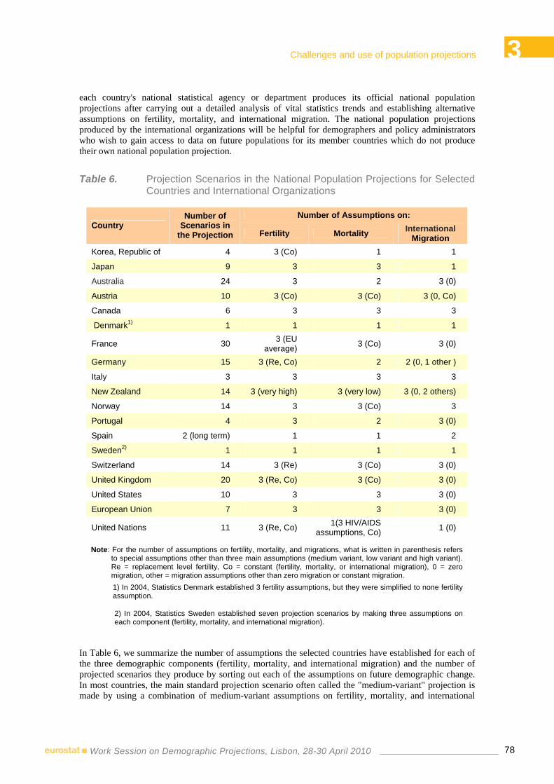
3 Challenges and use of population projections
78Work Session on Demographic Projections, Lisbon, 28-30 April 2010
each country's national statistical agency or department produces its official national population projections after carrying out a detailed analysis of vital statistics trends and establishing alternative assumptions on fertility, mortality, and international migration. The national population projections produced by the international organizations will be helpful for demographers and policy administrators who wish to gain access to data on future populations for its member countries which do not produce their own national population projection.
Table 6. Projection Scenarios in the National Population Projections for Selected Countries and International Organizations
Number of Assumptions on: Country
Number of Scenarios in
the Projection Fertility Mortality International Migration
Korea, Republic of 4 3 (Co) 1 1
Japan 9 3 3 1
Australia 24 3 2 3 (0)
Austria 10 3 (Co) 3 (Co) 3 (0, Co)
Canada 6 3 3 3
Denmark1) 1 1 1 1
France 30 3 (EU average) 3 (Co) 3 (0)
Germany 15 3 (Re, Co) 2 2 (0, 1 other )
Italy 3 3 3 3
New Zealand 14 3 (very high) 3 (very low) 3 (0, 2 others)
Norway 14 3 3 (Co) 3
Portugal 4 3 2 3 (0)
Spain 2 (long term) 1 1 2
Sweden2) 1 1 1 1
Switzerland 14 3 (Re) 3 (Co) 3 (0)
United Kingdom 20 3 (Re, Co) 3 (Co) 3 (0)
United States 10 3 3 3 (0)
European Union 7 3 3 3 (0)
United Nations 11 3 (Re, Co) 1(3 HIV/AIDS assumptions, Co) 1 (0)
Note: For the number of assumptions on fertility, mortality, and migrations, what is written in parenthesis refers to special assumptions other than three main assumptions (medium variant, low variant and high variant). Re = replacement level fertility, Co = constant (fertility, mortality, or international migration), 0 = zero migration, other = migration assumptions other than zero migration or constant migration.
1) In 2004, Statistics Denmark established 3 fertility assumptions, but they were simplified to none fertility assumption.
2) In 2004, Statistics Sweden established seven projection scenarios by making three assumptions on each component (fertility, mortality, and international migration).
In Table 6, we summarize the number of assumptions the selected countries have established for each of the three demographic components (fertility, mortality, and international migration) and the number of projected scenarios they produce by sorting out each of the assumptions on future demographic change. In most countries, the main standard projection scenario often called the "medium-variant" projection is made by using a combination of medium-variant assumptions on fertility, mortality, and international

3 Challenges and use of population projections
79Work Session on Demographic Projections, Lisbon, 28-30 April 2010
migration. In addition, the basic alternative projection scenarios are high-variant and low-variant scenarios which combine high-variant and low-variant assumptions on fertility, mortality, and international migration.
In most selected countries, the national statistical agency develops additional scenarios that combine main and alternative assumptions on future demographic changes in addition to the three major projection scenarios.
Sweden and Denmark develop one single, main projection scenario without either low-variant or high-variant scenarios because they produce the national population projection once every year. In a sense, this single scenario approach to population projection may provide easier access to ordinary statistical users. Among the countries and international organizations with more than 20 projection scenarios are France (32 scenarios), Australia (24 scenarios), and the United Kingdom (20 scenarios). Among those with the projection scenarios ranging between 10 and 15 are Germany (15 scenarios), Switzerland (14 scenarios), New Zealand (14 scenarios), Norway (14 scenarios), the United Nations (11), Austria (10 scenarios), and the United States (10). Finally, among those with the projection scenarios smaller than 10 are Japan (9 scenarios), Sweden (7 scenarios), the European Union (6 scenarios), Canada (6 scenarios), Korea (4 scenarios), Poland (4 scenarios), Italy (3 scenarios), and Spain (3 scenarios). In general, the countries with a super-low fertility pattern, such as Italy and Spain in Southern Europe and South Korea in East Asia tend to develop a smaller number of projection scenarios compared to the countries of Western Europe, North America, and Oceania, probably due to the lack of concern with regards to the potential impact of mortality and international migration on the shape of future populations.
In most countries, the national statistical agency develops three major fertility assumption, say, medium, high, and low-variant assumptions as well as comparing cohort fertility with period fertility and establishing target fertility at the end of the projection horizon. In the 2006 official national projections, Statistics Korea adopted another additional, so-called "constant" fertility assumption, which highlights the continuity of currently super-low TFR lower than 1.3 births per woman to the end of the entire projection horizon. In some countries of Western Europe and Oceania, the national statistical agency develops another supplementary fertility assumption that the current fertility will recuperate to the replacement level at a given time within the entire projection horizon.
The number of assumptions on mortality and international migration is mainly three (medium, high, and low variant), which reveal smaller variations than the number of assumptions on fertility. For mortality assumptions, the national statistical agency and the international organization often establishes the so-called "no mortality change" assumption that highlights the continuity of the current mortality pattern to the end of the entire projection horizon. In addition, the United Nations develop various HIV/AIDS-related mortality assumptions to measure the HIV/AIDS effects on the evolution of future populations. For international migration, many countries in Western Europe develop the "zero migration" assumption to measure the pure effects of natural growth (births minus deaths) on the shape of future population.
4. A Stochastic National Population Projection: Illustration for Korea
The 2006 official and 2009 interim population projections rest on deterministic models. In these models, today's population and assumptions on the development of demographic rates determine future population. To account for forecast uncertainty, the 2006 official projections used four major scenarios, based mainly on "high", "medium", "low", or "constant" assumptions of fertility rate. This technique -though common practice - suffers mainly from two shortcomings: First, it does not provide information on the probability of a certain projection scenario. Second, modeling uncertainty by means of different projection scenarios is necessarily inconsistent.
To overcome these problems, probabilistic approaches to population forecasting have been developed in recent years (Lee, 1998; Choi, 2004). The main goal of probabilistic population projections is to obtain prediction intervals of demographic variables and thus to measure projection uncertainty. Probabilistic projections make use of historical forecast errors (Keyfitz, 1981), rest on expert opinion (Lutz,

3 Challenges and use of population projections
80Work Session on Demographic Projections, Lisbon, 28-30 April 2010
Sanderson, and Scherbov, 1998) or rely on time series analysis to project future population parameters (Lee, 1998).
We illustrate a stochastic projection for Korea in which we use a time series analysis to project future demographic parameters using actual statistics on fertility from 1984 to 2008, which was below a replacement level of 2.1 births and actual data on mortality from 1970 to 2008. The length of the projection horizon is 50 years which ranges between 2009 and 2058. In the projection, the first stepis to transform raw input data. We first establish the fertility boundary, using TFR. The upper boundary is 8 births, approaching the so-called natural TFR found in pre-industrial populations, while low boundaries are set to 0.6, 0.7, 0.8, and 0.9 births. Mortality is projected using the Lee-Carter method, by gender and two age groups (0-64 years, and 64 years and over). The second step is to find the ARIMA model of input data (simple exponential smoothing with growth is selected). The third step is to predict the future input considering the error term distribution. The fourth step is to apply the cohort component method. The fifth step is to iterate step 3 and step 4, 1000 times. The sixth and final step is to find a median and 70% and 95% confidence interval. In this projection exercise, international migration is not considered (no migration is assumed), and the base population is the 2009 mid-year registered population, which comes from the Korean Statistical Information System (Statistics Korea, 2010).
Figure 1. Confidence Interval (95%, 70%) of the forecasted TFR of Korea from 2009 to 2058

3 Challenges and use of population projections
81Work Session on Demographic Projections, Lisbon, 28-30 April 2010
It is a very hard question to establish the lower fertility boundary in Korea with a super-low fertility pattern, particularly since there is prevalent pessimistic mood with respect to the future direction of fertility (Golini, 1998; Bongaarts and Feeney, 2000). Thus, it would be desirable for the stochastic projection to prepare not a single model, but four models that assume 4 different limits and then compare the predicted results. The future TFRs are different by the fertility boundary assumptions. If the boundary is assumed to range between 0.6 and 8 then the medium TFR will be 0.646, if between 0.7 and 8 then it will be 0.728, if between 0.8 and 8 then it will be 0.815, and if between 0.9 and 8 then it will be 0.90 (Figure 1). All of them are lower than the assumptions by Statistics Korea in both the 2006 official projection and the 2009 interim projection. Statistics Korea assumes the TFR at the end of the projection horizon (here 2050) will be a little higher than the TFR in 2005 or 2008, where this time series projection assumes the current decreasing trend will persist until the end of the projection horizon. The 95% probabilities of future TFRs show the effect of the boundary assumption. The highest plausible TFRs are almost identical. The TFR will increase in the near future, and then by 2058 it will decrease a little. As the upper boundary (8) is far from the projected fertility rates and the effect of boundary limitation increases as the rate approach to the boundary, the upper boundary effect here is small. However the lower boundaries of the confidence interval are changed by the ultimate boundary assumption. Figure 3 shows that the lower boundaries compress the confidence interval and that they make the median projection approach the lower boundary.
Figure 2. The Confidence Interval (95%, 70%) of the forecasted population of Korea from 2009 to 2058

3 Challenges and use of population projections
82Work Session on Demographic Projections, Lisbon, 28-30 April 2010
Based on these assumptions, future populations are like those found in Figure 2. The total population size will start to decrease soon. The overall patterns are similar but according to the fertility assumption, the lower limits of the confidence intervals are somewhat different. When the lower TFR boundary is 0.6, the population will be more likely to shrink quickly. The future population is expected to decrease by more than 25 percent. The median population in 2058 will be 77 percent of the population in 2009 if the boundary is 0.7 to 8. Also, if the boundary is 0.8 to 8, then it will be 78 percent, and if 0.9 to 8 then it will be 80%.
This illustrative stochastic projection provides useful insights into the significance of fertility assumptions for the determination of the future population size. When the lower TFR boundary is 0.6, the size of the median total population in 2050 will be 3.8 percent smaller in this illustrative projection than in the 2009 interim national population projection assuming zero migration; the size of the median total population in 2050 will be 2.7 percent smaller than in the 2009 interim projection if the boundary is 0.7 to 8. If the boundary is 0.8 to 8, then it will be 1.5 percent smaller, and if 0.9 to 8, then it will be nearly identical as the figure in the interim projection. This indicates that the shape of the future population is more likely to be determined by the direction of a super-low fertility pattern in Korea, and it might be unreasonable to put more emphasis on the total population impact of international migration, which assumes growing importance as repeated by some scholars and policy administrators in the slogan of multiculturalism or multi-ethnic society in Korea.
5. Future Challenges of the Korean National Population Projection
In the country, like Korea with a super-low fertility pattern, we believe, the national population projections can improve their forecasting accuracies by updating them more frequently or distinguishing them into short-term and long-term projections. In the case of minor fluctuations in fertility or international migration, it might be more desirable to update a short-term national projection on an annual basis (as seen in the Spanish system of national population projection) than to restructure an entire long-term national projection. Also, the national population projections should develop means on how to improve the quality of data on vital statistics for the non-national population, particularly, those who immigrate to the country for marital reasons, and how the assumed values of births and deaths for the non-national foreign population should be taken into consideration in relation to those among population whose nationalities are Korean. This is because many policy administrators believe that the influx of foreign workers and marriage-related immigrants, rather than the persistence of a super-low fertility pattern, might contribute more significantly to the delay of both the timing of depopulation and the speed of population aging in Korea.
In preparing for the 2011 official population projection, Statistics Korea will hopefully develop more than four projection scenarios and take into account more than four assumptions on fertility, more than one mortality assumption, and more than one international migration assumption. Similar to the system of population projection in France, Australia, and the United Kingdom, Statistics Korea will need to prepare and release a total of 27 population projection scenarios, which consider (1) three fertility assumptions (medium, low, high) (2) three mortality assumptions (medium, low, high) and (3) three migration assumptions (medium, low, high). In addition, we may add "constant" assumptions on fertility, mortality, and international migration. However, both of the 2006 official and 2009 interim national population projections indicate that the "constant" and "medium-level" fertility assumptions will not make any large differences in the final projection results, since in the "medium-variant" assumption the level of target fertility at the end of the projection horizon is a little larger than the level of fertility observed at the beginning of the projection horizon. In such a case, it would be more desirable for the national fertility projection to pay more attention to additional types of "low-variant" fertility assumptions by taking into consideration the notion that the current super-low fertility pattern may deteriorate to its much worse level, say, a TFR lower than the target fertility forecasted for the "low-variant" assumption in the 2006 official national population projection.

3 Challenges and use of population projections
83Work Session on Demographic Projections, Lisbon, 28-30 April 2010
In preparing the 2011 official national population projection, we expect Statistics Korea to pay more attention to the determination of a base population that should include both national and non-national populations. We believe that various demographic techniques must be used to determine the base population, since Korea is changing rapidly to an immigrating country, and since the census undercounts the non-national population. Statistics Korea wishes to implement a register-based population census beginning in 2015 and the determination of the base population will be facilitated by the adoption of a one-number-census approach in the United Kingdom or the dual-system estimation approach used in the 2008 Israel's integrated population census.
The long-term fertility which is often the target fertility forecasted for the end of the projection horizon in the national population projection is an important element in determining details for the population projection results (Jun, Kim, and Cho, 2005). In both the 2006 official projection and the 2009 interim projection, the quantum and tempo of cohort fertility is taken into consideration to establish the target fertility in period terms (Bongaarts and Feeney, 2000). In the study commissioned by Statistics Korea, the medium-variant assumption establishes the target fertility of the cohort born in 1991 as 1.28, which is a little smaller than in the 2005 interim population projection. This clearly signifies that marital fertility continues to decline together with a steady rise in marriage age and increasing proportions of single or divorced women during the reproductive span. We expect that the target fertility of the 2011 official national population projection can be more reasonably determined by using the result from the 2010 population and housing censuses, which include the topics on marital status, age at first marriage, actual number of children born, and the number of children whom the female respondents plan to have. These census topics, as well as actual vital statistics data, will have to be fully exploited to avoid the error of input parameters in the national population projection, while refining the generalized log gamma distribution which is used in the Japanese system of population projection
Finally, we hope that Statistics Korea will find wise ways to incorporate the ideas underlying the system of stochastic population projection as part of the official national population projection. One merit of the stochastic population projection model is to use it as a framework for assessing the value of demographic sensitivity tests with various "pronatalist" population policy models. More specifically, they will be used to describe particular problems, such as (1) how the omission of random shocks in each component of demographic change, particularly, fertility (e.g., increase in births due to millennium baby boom, twin-spring years and golden swine years), or international migration (e.g., increase in immigration of foreign-born brides resulting from imbalances of gender composition in the rapid drop of fertility over past 30 years) will lead to population sizes growing beyond all projected population sizes as soon as the projections are released; (2) to what extent the practice of restricting demographic changes at the beginning of the projection horizon leads to confusing results for trends in age structure; and (3) with a discussion of the value of stochastic population projections, which are a promising alternative to the current deterministic approach.
References
Bongaarts, J. and G. Feeney (2000) "On the Quantum and Tempo of Fertility" Population and Development Review 24: 271-291.
Choi, Seulki (2004) "A Stochastic Population Projection for Japan: 2000-2050" Master of Arts thesis, University of North Carolina.
Eurostat, Statistical Office of the European Commission (2009) Population Projection: 2008-2060: Convergence Scenario, National and Regional Level.
Golini, A. (1998) "How Low Can Fertility Be? Empirical Evidence" Population and Development Review 24: 59-73.
Jun, Kwang-Hee (2005) "The Transition to Sub-replacement Fertility in Korea: Implications and Prospects for Population Policy" The Japanese Journal of Population 3(1): 26-57.

3 Challenges and use of population projections
84Work Session on Demographic Projections, Lisbon, 28-30 April 2010
Jun, Kwang-Hee, Tai-Hun Kim, and Youngtae Cho (2005) "Fertility and Mortality Models for the National Population Projection" A Research Report by the Korean Population Association to Statistics Korea
Kaneko, Ryuichi (1993) "Projection System of Age-Specific Fertility Rate" (in Japanese) Japanese Journal of Population Problems 49(1): 12-38
Kaneko, Ryuichi (2003) "Elaboration of the Coale-McNeil Model as the Generalized Log Gamma Distribution: A New Identity and Empirical Enhancements" Demographic Research 9:223-262.
Keyfitz, N. (1981) "The Limits of Populations Forecasting" Population and Development Review 7: 579-593.
Lee, R. D. (1998) "Probabilistic Approaches to Population Forecasting" Population and Development Review. Supplement 24: 156-190.
Lee, R. D. and L. Carter (1992) "Modeling and Forecasting the Time Series of US Mortality" Journal of the American Statistical Association 87: 659-671.
Lutz, W., W. C. Sanderson, and S. Scherbov (1998) "Expert-based Probabilistic Population Projections" Population and Development Review. Supplement 24: 139-155.
Statistics Korea (2006) The Population Projection of Korea: 2006-2050 Statistics Korea
Statistics Korea (unpublished) The 2009 Interim Population Projection of Korea: 2009-2050 Statistics Korea
Statistics Korea (2010) The Korean Statistical Information System. http://www.kosis.kr
United Nations (2008) World Population\Prospects: The 2008 Revision

Constructing assumptions for mortality: data, methods and analysis Chair: Graziella Caselli
Session 4


4 Constructing assumptions for mortality: data, methods and analysis
87Work Session on Demographic Projections, Lisbon, 28-30 April 2010
COHORT AND PERIOD MORTALITY IN SWEDEN IN A VERY LONG PERSPECTIVE AND PROJECTION
STRATEGIES
Hans LUNDSTRÖM1
Abstract
The present method for mortality projections in Sweden is a combination of the Lee-Carter method and argument-based adjustments. It is a two-factor model taking age and period into account. With long time series of mortality now available from year 1861 from both a period and a cohort perspective it is tempting to use more of the potential in the data to improve projections. One obvious strategy is to use the age and cohort information available and test the three-factor model expressing rates as a function of age, period and cohort. A project is under way to add cohort cause of death data for more recent years.
1. Data
In preparation of a newly published report Cohort mortality in Sweden mortality data for the period 1861 to 2008 has been updated. Using the extinct cohort method, population size has been recalculated for ages 60 and up. The recalculation has been based on the most reliable statistics, the number of deaths by age. Age is available in one-year age classes and based on register information of date of birth and date of death. Age is calculated and we have no indications of any systematic errors. If in doubt about stated time of birth and death the parish registers were consulted.
The database starts with the calendar year 1861, the first year when very detailed population statistics became available. Keeping track of migrants is more problematic than keeping track of deaths. To get as reliable calculations as possible using the extinct cohort method the recalculations have been restricted to the ages 60 and up. In those ages migrants are very few, if any. For ages below 60 the official population size has been kept unchanged. Cohorts born after 1910 cannot be followed until the last person has died. For those cohorts the recalculation of the population size had to start with latest information available, the official population size at the end of year 2008.
2. Period mortality
From 1860 up to present time the composition of the Swedish population has changed a lot. In all, 1.5 million persons emigrated from Sweden during the 1861-1930 periods and some 0.4 million immigrated. This means a net loss of more than one million persons out of a total population of round four million. The largest excess of emigration can be observed for cohorts born in 1861-75. These cohorts were decimated by some 20 per cent for men and by some 16 per cent for women. The corresponding percentage for cohorts born in the 1890s is only nine for men and five for women. From 1930 onwards we have had a large net immigration. Between year 1860 and 2008 life expectancy nearly doubled from 47 to 81 years. The cause of death pattern has changed a lot during this period too. A decline in infectious diseases began after the middle of the eighteenth century.
1 Hans LUNDSTRÖM Statistics Sweden, Stockholm

4 Constructing assumptions for mortality: data, methods and analysis
88Work Session on Demographic Projections, Lisbon, 28-30 April 2010
The victory over infectious diseases was the main reason for the increasing life expectancy. Living longer, the chronic degenerative diseases became the main cause of death during the twentieth century.
In spite of all these changes and many more, mortality rates show a smooth and gradual change over time and age. It was only the Spanish Flu in 1918 that temporarily broke that pattern.
We see random variations, of course, but the long-term trend has been relatively stable. This seems to be an ideal situation for projection and the use of for instance the Lee-Carter model.
Some trend shifts make an extrapolation of mortality rates problematic however. In the 1940s female mortality started to decline at a faster rate than before. In the mid 1960s the decline slowed down for women and even turned into an increase for middle age men. At that time some persons believed we were close to the biological limit having reached a life expectancy of 75 for women and 71 for men. That turned out to be wrong. Mortality started to decline rapidly once more and it was mainly due to a decline in mortality from cardiovascular diseases.
The mortality decline since 1980 has been faster for men than for women. The trend shifts makes the choice of period over which the trends are to be determined crucial. The Lee-Carter method project constant rates of improvements for a given age. This may lead to an implausible profile of mortality rates at successive ages if the projection extend a long time into the future. This problem can often be eliminated by choosing an optimal fitting period which in turn introduces other effects. The Lee-Carter method has an advantage in its simplicity and the possibility to produce measures of uncertainty. In figure 1 mortality rates for women and men can be followed for the period 1861 to 2008. To make it more readable selected ages are shown. Mortality rates show a smooth and gradual change over time for each age. The mortality pattern over time is very similar between ages too. The pattern of mortality change for let say age 70 is very similar to mortality change for those slightly younger and older than 70.
Figure 1. Mortality rates for Sweden 1861-2008 by sex and age. Logarithmic scale.
10
0,0001
0,0010
0,0100
0,1000
1,0000
1860 1880 1900 1920 1940 1960 1980 2000
50
40
70
80
90
30
20
0
Dödstal
100
60
År 1860 1880 1900 1920 1940 1960 1980 2000
50
40
70
80
90
30
20
0
100
60
År
MenWomen

4 Constructing assumptions for mortality: data, methods and analysis
89Work Session on Demographic Projections, Lisbon, 28-30 April 2010
3. Cohort mortality Cohort mortality gives another perspective of mortality decline compared to period data (Figure 2 and 3). Nearly 50 cohorts, born 1861 or later, can be followed from birth to the last person died. For the remaining cohorts information is lacking for the first or last part of the life cycle. Like period mortality rates the cohort approach show a relatively smooth pattern over cohorts. In the ages above 40 we see a more or less parallel downward shift of the curves from one cohort to the next. At first this shift in the mortality curve was not so pronounced. As from cohorts born around 1880 a more rapid decline of female mortality started. For men the mortality decline started some 20 years later with the cohorts born around 1900.
Figure 2. Mortality by year of birth for selected cohorts. Women, logarithmic scale
0,00001
0,0001
0,001
0,01
0,1
1
0 20 40 60 80 100
1780
1800
1820
1840
1860
1880
1900
1920
1940
1960
1980
Dödstal
1960
1940
1920
1900
1980
1820
Ålder
1800
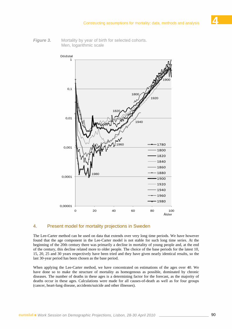
4 Constructing assumptions for mortality: data, methods and analysis
90Work Session on Demographic Projections, Lisbon, 28-30 April 2010
Figure 3. Mortality by year of birth for selected cohorts. Men, logarithmic scale
0,00001
0,0001
0,001
0,01
0,1
1
0 20 40 60 80 100
1780
1800
1820
1840
1860
1880
1900
1920
1940
1960
1980
Dödstal
1960
1940
1920
1900
1980
1820
Ålder
1800
4. Present model for mortality projections in Sweden
The Lee-Carter method can be used on data that extends over very long time periods. We have however found that the age component in the Lee-Carter model is not stable for such long time series. At the beginning of the 20th century there was primarily a decline in mortality of young people and, at the end of the century, this decline related more to older people. The choice of the base periods for the latest 10, 15, 20, 25 and 30 years respectively have been tried and they have given nearly identical results, so the last 30-year period has been chosen as the base period.
When applying the Lee-Carter method, we have concentrated on estimations of the ages over 40. We have done so to make the structure of mortality as homogenous as possible, dominated by chronic diseases. The number of deaths in these ages is a determining factor for the forecast, as the majority of deaths occur in these ages. Calculations were made for all causes-of-death as well as for four groups (cancer, heart-lung disease, accidents/suicide and other illnesses).

4 Constructing assumptions for mortality: data, methods and analysis
91Work Session on Demographic Projections, Lisbon, 28-30 April 2010
In a final step information from the different Lee-Carter projections were put together to an assumption on future mortality development. In the long term, the drop in the mortality rate is expected to continue but to slow down as a result of changes in the cause of death panorama.
5. Discussion
One way to improve mortality forecasts is to gain insight into the causes and predictors of mortality. To be able to do that we must know the “risk profile”of previous and current cohorts. Furthermore we must know the relationship between risk factors and mortality and be able to forecast changes in the risk factors. This seems to be an approach for the future. For present time other approaches are needed.
Short-term projections are often based on the general principle that the near future resembles the recent past. Long-term projections are a more difficult enterprise. Adding cause-of –death information may give some clues of what is to come. A much cited example of a successful cause of death projection appeared in a study by Pollard in 1949 indicating a rise in mortality in the 1960s. The projection turned out to be remarkably accurate (National Statistics Quality Review Series. Report No 8 2001).
Adding cohort cause-of –death data will give some more insights into the factors behind the mortality decline. The approach is problematic however for at least two reasons. The reconstruction of consistent time series by cause of death is a challenging task. Different revisions of ICD classification, changes in coding practises, improved diagnostics over time and declining rates of autopsies are a few challenges. On top of that old-age mortality is one key component of any population projection model.
Figure 4. Cohort life table deaths out of 100 000 born. Three selected cohorts. Women
0
1000
2000
3000
0 20 40 60 80 100
Deaths
Age
1900
1950
1861
Declining mortality has resulted in an ageing population. Out of women born in 1920 over 50 percent is still alive at the age of 80 and for younger cohorts this age will most probably raise. Apart from high infant mortality the typical age at death nowadays is around the age of 80 to 90.

4 Constructing assumptions for mortality: data, methods and analysis
92Work Session on Demographic Projections, Lisbon, 28-30 April 2010
Among the oldest-old the underlying cause of death cannot be easily identified. Booth and Tickles draw the conclusion that the perceived advantages of decomposition of mortality by cause of death are outweighed by the limitations involved (Booth 2008).
Figure 5. Proportion surviving by sex, age and year of birth
0
20
40
60
80
100
0 20 40 60 80 100
186118701880189019001910192019301940195019601970198019902000
1861
1920
Percent
Women
Age
0
20
40
60
80
100
0 20 40 60 80 100
186118701880189019001910192019301940195019601970198019902000
1861
1920
Percent
Men
Age Primarily the two-factor model Age and Cohort and the three-factor model Age Period Cohort will be tested using the long time series available.
The Lee-Carter model has lately been extended to incorporate cohort effects and is worth a closer look (Renshaw 2006). In a later stage cause of death statistics by cohort may be added with cause of death specified in just a few broader groups.

4 Constructing assumptions for mortality: data, methods and analysis
93Work Session on Demographic Projections, Lisbon, 28-30 April 2010
References
Booth, H., Maindonald, J., and Smith, L. (2002) Applying Lee-Carter under conditions of variable mortality decline. Population Studies, 56, 325-336.
Booth, H. & Tickle, L. (2008). Mortality modelling and forecasting: A review of methods. ADSRI Working Paper No. 3. The Australian National University.
Caselli, G., Vallin, J. and Marsili, M. (2008). How Useful Are the Causes of Death When Extrapolating Mortality Trends. An Update. Social Insurance Studies No 4 2008. Swedish Social Insurance Agency.
Kohortdödligheten i Sverige: Dödlighetsutvecklingen sedan 1861. (Cohort Mortality in Sweden. Mortality statistics since 1861). Demografiska rapporter 2010:1. Statistiska centralbyrån.
National Population Projections: Review of Methodology for projecting Mortality. Government Actuary’s Department. National Statistics Quality Review Series. Report No. 8.
Renshaw, A. E. & Haberman, S. (2006). A cohort-based extension of the Lee-Carter model for mortality reduction factors. Insurance:Mathematics and Economics, 38,556-570.
Tabeau, E., Ekamper, P., Huisman, C, and Bosch, A. (1999). Improving Overall Mortality Forecasts by Analysing Cause of death, Period and Cohort Effects in Trends. European Journal of Population, 15, 153-183.
The future population of Sweden (2009). Demographics Reports. Statistics Sweden.
Vaupel, J.W. (2009). Lively Questions for Demographers about Death at Older Ages. Population and Development Review, 35,347-356.


4 Constructing assumptions for mortality: data, methods and analysis
95Work Session on Demographic Projections, Lisbon, 28-30 April 2010
TOWARDS ADVANCED METHODS FOR COMPUTING LIFE TABLES
Sixto Muriel DE LA RIVA1,
Margarita CANTALAPIEDRA MALAGUILLA1
Federico LÓPEZ CARRIÓN1
Abstract
Life tables are, of course, a longstanding task of government statistics. Now, a major effort of research and methodological innovation should open the way to optimal utilisation of the available data on deaths, better international comparability of mortality indicators, and a finer approach to the measurement of mortality over small territorial areas.
INE Spain puts compiled data and literature in a series of tests and comparative analyses in order to select the best-suited methodologies for the mentioned objectives. The outcome of this testing stage was a two-part report on our methodological research on life tables.
The first part tries shows three different approaches to constructing a complete annual life table for the Spain resident population, in a growing sophistication scale: the first one assumes that deaths over the reference year at each age are distributed absolutely uniformly; the second, assumes uniform distribution of deaths over the year at each age within a given generation (uniformity in Lexis triangles), following the protocols of the Human Mortality Database2; the third and genuine method uses observational data from the vital statistics on the date of occurrence of each recorded death to get the best approach to population at risks in specific mortality rates.
Besides, this part shows the considerable distance between uniformity and the temporal distribution (within the observed year) of deaths in low and advance ages. It is followed that the third method provides the most accurate measurement of the biometric functions of a life table.
The second part of the report focus on life tables for sub-national territories (devolved regions and provinces, NUTS-2 and NUTS-3). It analyses three possible ways to construct life tables at disaggregated territorial levels (abbreviated five-yearly age ranges life tables, full life tables with five yearly age ranges output and smoothing survivor function of regional life table according to national data). It aims to provide an understanding of the short-term (annual) incidence of mortality in each territory while minimising the effect of reporting randomness and of possible inconsistencies between observed deaths and the estimates used as reference population figures. Advantages and disadvantages of every proposed method are deeply analysed and commented.
1 National Statistics Institute of Spain 2 Collaborative project sponsored by the University of California at Berkeley, United States and the Max Planck Institute for
Demographic Research, Rostock, Germany. / www.mortality.org

4 Constructing assumptions for mortality: data, methods and analysis
96Work Session on Demographic Projections, Lisbon, 28-30 April 2010
1. Introduction
Life tables computing constitutes a traditional work in the field of demographic analysis and projections, for the majority of the official statistical offices. In the present paper, several methodological options for the calculus of life tables are shown and discussed, both for the national and for the regional level.
This work has the following objectives:
The maximum use of the demographic information generated by the Spain resident population Statistical System, so as to optimise the accuracy of mortality measurements for all the populations considered.
To assure the necessary methodological consistency in the definitions and the assumptions underlying the calculus of all the biometric functions of the complete life table, and also in the definition of its derived indicators.
As far as possible, to reflect annual behaviour of mortality incidence in the Spain resident population, avoiding the influence of randomness in observed data.
To improve the accuracy when measuring mortality incidence at the most advanced ages, given the prevailing aging process of the Spain Population and the important recent advances in life expectancy at those ages.
To provide measures of mortality incidence for sub national populations, i.e., regions and provinces, in a regular basis.
To support international comparability of the mortality indicators and facilitate their interpretation by users.
Three different options are tested for the construction of complete life tables for the total, male and female Spain resident populations. Another three options are tested for the regional life table. All of them make use of the registered data on deaths occurred among residents in Spain during a one-year interval and the corresponding population stocks exposed to risk of dying. Year 2006 was used for the national life tables and years 2005 and 2006 for the regional and provincials life tables.
2. Methods for computing national life tables
In this first part of the paper three methodological approaches are presented for the computation of life tables at the national level. Differences among the three options are due to the three different hypothesis made about the time lived by the observed population between ages x and 1x + .
In the first option, uniform distribution of deaths inside the age interval )1x,x( + is supposed. For the second option, based on the protocols of the Human Mortality Database3 project, uniform distribution within the two corresponding generations of annual deaths in the age interval )1x,x( + is assumed. In the third option, observed data on the date of occurrence of each registered death of annual Vital Statistics are used. For all the options birth dates are supposed uniformly distributed along each year.
3 Department of Demography at University of California, Berkeley (USA) and Max Planck Institute for Demographic Research.

4 Constructing assumptions for mortality: data, methods and analysis
97Work Session on Demographic Projections, Lisbon, 28-30 April 2010
In general, the functions of the period life table are defined as follows:
The mortality rate )s,x,t(m , for year t, age x and sex s , is a quotient where the numerator is the number of deaths occurring in the year t among individuals at age x and sex s , and the denominator is the total time, in years, lived by the individuals of age x and sex s , during the year, i.e., the person-years of individuals of age x and sex s during year t .
Now, let a fictitious generation with an incidence of mortality according to the mortality rates that has been defined. So:
The death probability )s,x(q is the probability of an individual of sex s of the fictitious generation that reaches the age x lives until next birthday.
The survivors )s,x(l is the number of individuals from the fictitious generation that reach the x age for each sex s .
The deaths )s,x(d is the number of deceases from the fictitious generation at each age x and for each sex s .
Survivors )s,x(l and deaths )s,x(d are obtained recursively:
000.100)s,0(l = , )s,x(q)s,x(l)s,x(d = y )s,x(d)s,x(l)s,1x(l −=+ for += 100,99,...,1,0x
The average number of years lived in the last year of life for those individuals dying in the age interval )1x,x( + is denoted by )s,x(a .
The stationary population )s,x(L is the total time lived for all the individuals of the fictitious generation that are x years old and sex s .
The total years lived )s,x(T is the total amount of years lived for all the individuals of the fictitious generation aged x or more.
)s,x,t(L)s,1x,t(T)s,x,t(T ++= for += 100,99,...,1,0x
Finally, the life expectancy is the mean number of years left to live for an individual of age x and sex s.
)s,x,t(l/)s,x,t(T)s,x,t(e = , for += 100,99,...,1,0x
2.1 Option 1 - Assumption of uniform distribution of deaths in the age interval (x,x+1) The main objective of option 1 is to perform a sensitivity analysis, i.e., to show the effect of the alternative options in comparison to uniform distribution.
Under this assumption, the denominator of )s,x,t(m is estimated by the expression )s,x,1t(P21)s,x,t(P21 ++ , assuming uniform distribution of the birthdays of all individuals in the
population not dying over the year at a given age.

4 Constructing assumptions for mortality: data, methods and analysis
98Work Session on Demographic Projections, Lisbon, 28-30 April 2010
Hence:
)s,x,1t(P21)s,x,t(P21
)s,x,t(D)s,x,t(m++
=
Where:
t is the reference year, period or calendar time.
x is the age or completed years , += 100,99,...,1,0x .
s is sex, which may be male, female or both sexes.
)s,x,t(D is the number of deaths between residents in Spain during the year t, at age x and sex s .
)s,x,t(P is the stock of resident population in Spain at 1st January of the year t , with age x and sex s .
In addition, for this option the following key expressions for some of the biometric functions are adopted:
The estimated probability or risk of dying )s,x(q , will be:
)s,x(m)21(1)s,x(m)s,x(q
⋅+= 99,...,1,0x = and .1)s,100(q =+
The stationary population at age x and sex s , for 99,...,1,0x = , on the assumption of uniform distribution of deaths over the year, is estimated as:
)s,x(d2/1)s,1x(l)s,x(L ++= for 99,...,1,0x = .
Finally, the aggregate of years lived by individuals of the fictitious generation reaching the age of 100, from that age to their deaths, is approximated by:
)s,100(m)s,100(l)s,100(L
++=+
2.2 Option 2 - Assumption of uniform distribution of deaths by age and generation
This alternative follows the protocols of Human Mortality Database4 for the construction of life tables. In this case, the denominator of )s,x,t(m is estimated assuming uniform distribution of deaths among individuals of the same age and generation (Lexis triangle) by the expression:
))s,1g,x,t(D)s,g,x,t(D(6/1)s,x,1t(P2/1)s,x,t(P2/1 −−+++
where:
g is the generation of individuals completing x years in year gxt,e.i,t =−
)s,g,x,t(D is the number of individuals dying in year t , at age x , from generation g and sex s .
Hence:
))s,1g,x,t(D)s,g,x,t(D(61)s,x,1t(P21)s,x,t(P21)s,1g,x,t(D)s,g,x,t(D)s,x,t(m
−−⋅++⋅+⋅−+= , for += 100,99,...,1,0x .
4 Department of Demography at University of California, Berkeley (USA) and Max Planck Institute for Demographic Research.

4 Constructing assumptions for mortality: data, methods and analysis
99Work Session on Demographic Projections, Lisbon, 28-30 April 2010
For this option the following key expressions for some of the functions are adopted: The estimated probability or risk of dying will be obtained by:
)s,x,t(m))·s,x(a1(1)s,x,t(m)s,x(q
−+= for 99,...,1,0x = and .1)s,100(q =+
being a(x,s) approximated by:
)s,1g,x,t(D)s,g,x,t(D)s,1g,x,t(D·3/2)s,g,x,t(D·3/1)s,x(a
−+−+=
For the open-ended group the average time lived in the reference year t is estimated for ages of 100 and above and sex )s,100(a,s + , as:
)s,100(m1)s,100(a
+=+
2.3 Option 3 - Real distribution of date of death events is taken into account In this case, the denominator of )s,x,t(m comes from the expression:
∑+++i
i)s,x,b(t,s)x,1,1/2·P(ts)x,(t,P·2/1
Where: )i,s,x,t(b is defined as the difference (in years) between the date of death and the date of birthday (in
year t ) of each individual i , of sex s , dying in year t at completed age x . Hence:
∑+++=
i
i)s,x,b(t,s)x,1,1/2·P(ts)x,1/2·P(t,s)x,D(t,s)x,(t,m , for += 100,99,...,1,0x .
For this option the following key expressions for some of the biometric functions are adopted: The probability or risk of dying, )s,x(q will be:
)s,x,t(m))·s,x(a1(1)s,x,t(m)s,x(q
−+=
Being the average number of years lived in the last year of life for those individuals dying in the age interval )1x,x( + , )s,x(a , approximated by the average of the time (years) lived in t for the individual i dying in the age interval )1x,x( + during the observed year t , )i,s,x,t(a :
)s,x,t(D
)i,s,x,t(a)s,x,t(a
)s,x,t(D
1i∑
== , 99,...,1,0x = .
Besides, for the open-ended group the average time lived in the reference year t is estimated for ages of 100 and above and sex s , )s,100(a + , as:
)s,100(m1)s,100(a
+=+
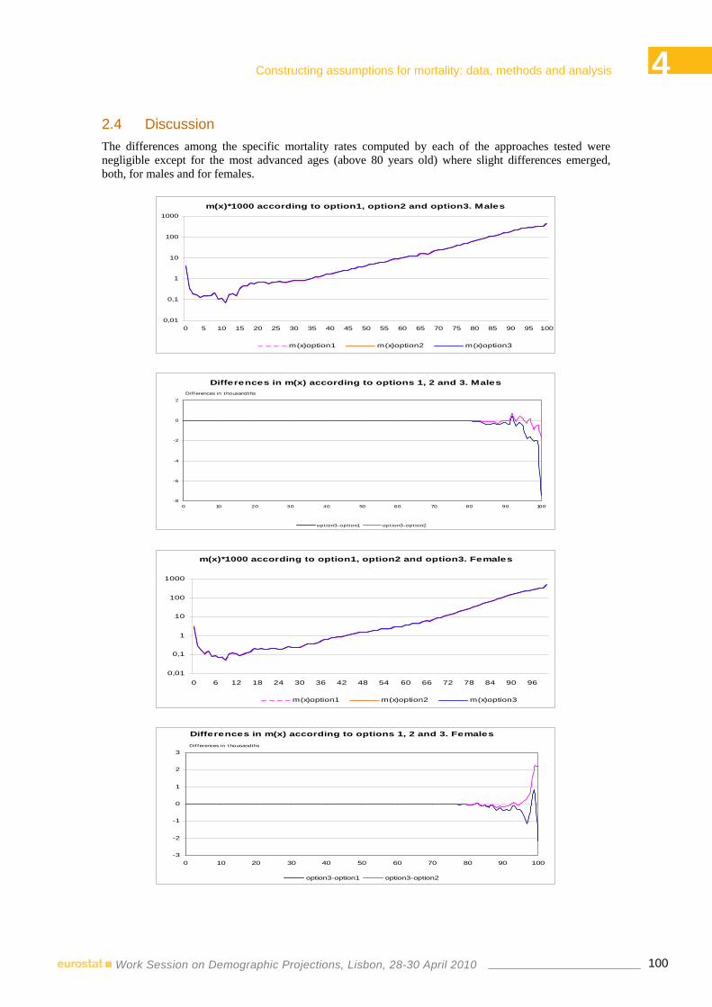
4 Constructing assumptions for mortality: data, methods and analysis
100Work Session on Demographic Projections, Lisbon, 28-30 April 2010
2.4 Discussion The differences among the specific mortality rates computed by each of the approaches tested were negligible except for the most advanced ages (above 80 years old) where slight differences emerged, both, for males and for females.
m(x)*1000 according to option1, option2 and option3. Males
0,01
0,1
1
10
100
1000
0 5 10 15 20 25 30 35 40 45 50 55 60 65 70 75 80 85 90 95 100
m(x)option1 m(x)option2 m(x)option3
Differences in m(x) according to options 1, 2 and 3. Males
-8
-6
-4
-2
0
2
0 10 20 30 40 50 60 70 80 90 100
option3-opt ion1 option3-opt ion2
Differences in thousandths
m(x)*1000 according to option1, option2 and option3. Females
0,01
0,1
1
10
100
1000
0 6 12 18 24 30 36 42 48 54 60 66 72 78 84 90 96
m(x)option1 m(x)option2 m(x)option3
Differences in m(x) according to options 1, 2 and 3. Females
-3
-2
-1
0
1
2
3
0 10 20 30 40 50 60 70 80 90 100
option3-option1 option3-option2
Differences in thousandths

4 Constructing assumptions for mortality: data, methods and analysis
101Work Session on Demographic Projections, Lisbon, 28-30 April 2010
Mentioned differences at advanced ages reflect that deaths deviate from uniform distribution between the ages x and 1x + : in fact, at advanced ages, deaths are concentrated among the individuals of the youngest generation of the two which complete deaths al the age interval )1x,x( + during the year t .
The differences shown among the specific mortality rates are likewise visible for the probabilities of death.
q(x)*1000 according to option1, option2 and option3. Males
0,01
0,1
1
10
100
1000
0 4 8 12 16 20 24 28 32 36 40 44 48 52 56 60 64 68 72 76 80 84 88 92 96
q(x)option1 q(x)option2 q(x)option3
Differences in q(x) according to options 1, 2 and 3. Males
-4,5
-4
-3,5
-3
-2,5
-2
-1,5
-1
-0,5
0
0,5
0 5 10 15 20 25 30 35 40 45 50 55 60 65 70 75 80 85 90 95 100
Differences in thousandths
option3-option1 option3-option2
q(x)*1000 according to option1, option2 and option3. Females
0,01
0,1
1
10
100
1000
0 4 8 12 16 20 24 28 32 36 40 44 48 52 56 60 64 68 72 76 80 84 88 92 96
q(x)option1 q(x)option2 q(x)option3
Differences in q(x) according to options 1, 2 and 3. Females
-3,5
-2,5
-1,5
-0,5
0,5
0 5 10 15 20 25 30 35 40 45 50 55 60 65 70 75 80 85 90 95 100
option3-opt ion1 option3-opt ion2

4 Constructing assumptions for mortality: data, methods and analysis
102Work Session on Demographic Projections, Lisbon, 28-30 April 2010
Nevertheless, the calculation of these probabilities of death is also influenced by differences in estimated average number of years lived in the last year of life for those individuals dying in the age interval
)1x,x( + , )s,x(a . In particular, the differences are noteworthy in the approximation by each method of )s,0(a . Not even option 2 produces a good approximation of observed reality. The most accurate
approximation is provided by option 3.
a(x) according to option1, option2 and option3. Males
0
0,5
1
1,5
2
2,5
0 5 10 15 20 25 30 35 40 45 50 55 60 65 70 75 80 85 90 95 100
a(x)
a(x)opt ion1 a(x)opt ion2 a(x)option3
Differences in a(x) according to options 1, 2 and 3. Males
-0,4
-0,3
-0,2
-0,1
0
0,1
0,2
0 5 10 15 20 25 30 35 40 45 50 55 60 65 70 75 80 85 90 95 100
Differences in units
option3-option1 option3-option2
a(x) according to option1, option2 and option3. Females
0
0,4
0,8
1,2
1,6
2
0 5 10 15 20 25 30 35 40 45 50 55 60 65 70 75 80 85 90 95 100
a(x)
a(x)opt ion1 a(x)opt ion2 a(x)opt ion3
Differences in a(x) according to options 1, 2 and 3. Females
-0,3
-0,25
-0,2
-0,15
-0,1
-0,05
0
0,05
0,1
0,15
0,2
0 5 10 15 20 25 30 35 40 45 50 55 60 65 70 75 80 85 90 95 100
Differences in units
option3-option1 option3-option2

4 Constructing assumptions for mortality: data, methods and analysis
103Work Session on Demographic Projections, Lisbon, 28-30 April 2010
Finally, the differences emerging in each of the mortality table functions resulting from each method have only a negligible effect on the resulting values of life expectancy at birth, as shown in the following charts.
Life expectancy according to options 1, 2, 3. MalesAge
option1 option2 option3 option3-option1 option3-option20 77,589 77,591 77,595 0,005 0,0045 72,971 72,973 72,978 0,006 0,00515 63,072 63,074 63,079 0,006 0,00525 53,407 53,408 53,413 0,006 0,00535 43,778 43,779 43,784 0,006 0,00545 34,427 34,428 34,433 0,006 0,00555 25,668 25,670 25,674 0,007 0,00565 17,709 17,711 17,715 0,007 0,00575 10,825 10,828 10,831 0,006 0,00385 5,830 5,835 5,836 0,006 0,00195 3,131 3,145 3,146 0,015 0,001
e(x) Differences
Differences in e(x) according to options 1, 2 and 3. Males
-0,010
0,000
0,010
0,020
0,030
0,040
0,050
0 5 10 15 20 25 30 35 40 45 50 55 60 65 70 75 80 85 90 95 100
Differences in years
option3-option1 option3-option2
Life expectancy according to options 1, 2, 3. FemalesAge
option1 option2 option3 option3-option1 option3-option20 84,089 84,091 84,094 0,005 0,0035 79,418 79,420 79,424 0,006 0,00415 69,487 69,489 69,492 0,005 0,00425 59,614 59,615 59,619 0,006 0,00435 49,773 49,774 49,778 0,006 0,00445 40,125 40,127 40,131 0,006 0,00455 30,743 30,745 30,748 0,006 0,00465 21,656 21,658 21,662 0,006 0,00475 13,280 13,283 13,286 0,006 0,00385 6,757 6,761 6,762 0,005 0,00195 3,192 3,201 3,192 0,000 -0,008
e(x) Differences
Differences in e(x) according to options 1, 2 and 3. Females
-0,015
-0,010
-0,005
0,000
0,005
0,010
0 5 10 15 20 25 30 35 40 45 50 55 60 65 70 75 80 85 90 95 100
Differences in years
option3-option1 option3-option2

4 Constructing assumptions for mortality: data, methods and analysis
104Work Session on Demographic Projections, Lisbon, 28-30 April 2010
Option 3, shows a slight improvement in life expectancy at each age, as a result of the slight decrease in mortality rates in the upper ages. The life expectancy gains are more significant at those ages, where present improvements of such indicator are concentrated.
3. Methods for computation of life tables at lower territorial levels
The second part of this paper addresses the questions for an accurate measurement of mortality at lower territorial levels, trying to minimize the limitations originated by the small size of the observed population.
Three different options are tested to construct annual mortality tables for the regions and the provinces of Spain. For the first approach, abbreviated life tables by five-year age intervals are computed. For the second option in a first step, complete life tables for all sub national populations considered are calculated; in a second step, aggregated results by five-year age intervals are obtained. The third method consists of adjusting the survivors series of the complete mortality tables using the Brass logits model 5 to derive the rest of the life table series.
3.1 Option 1 - Abbreviated life table Under this option, the denominator of the specific mortality rate, )s.n,x,t(m , is computed just assuming uniform distribution of birthdays of all individuals of the population not dying over the year at the age x by means of the following expression:
∑+++i
i)s,n,x,b(t,s)n,x,1,1/2·P(ts)n,x,(t,P·2/1
where:
)s,n,x,t(P is the stock of resident population in the considered region, at January the 1st of year t , in the age interval [ )nx,x + and sex s .
)i,s,n,x,t(b is defined as the difference (in years) between the dates of death and birth in the year t , of each individual i , of sex s , dying in year the t with age in the interval [ )nx,x + .
Hence:
∑+++=
i
i)s,n,x,b(t,s)n,x,1,1/2·P(ts)n,x,1/2·P(t,s)n,x,D(t,s)n,x,(t,m for += w...5,1,0x .
Where:
)s,n,x,t(D D(t,x,n,s) is the number of deaths of individuals with age in the interval [ )nx,x + , of sex s , among the resident population in the considered region during the year t .
Then, the following key expressions for some of the biometric functions are adopted:
The probability or risk of dying, )s,n,x(q is derivated by:
s)n,x,s))·m(t,n,a(x,-n·(11s)n,x,n·m(t,s)n,(x,q
+= for 99,.,2,1,0x = .
1s),(100q =+
5 Brass, William. Methods for estimating fertility and mortality from limited and defective data.(1975)

4 Constructing assumptions for mortality: data, methods and analysis
105Work Session on Demographic Projections, Lisbon, 28-30 April 2010
Being he average number of years lived in the last year of life for those individuals dying in the age interval )nx,x( + , )s,n,x(a , approximated by the average of the time (years) lived in t for the individual i dying in the age interval )nx,x( + during the observed year t , )i,s,n,x(a :
s)n,x,D(t,
i)s,n,x,a(t,s)n,x,(t,a
s)x,N(t,
1i∑
== , 5w,...,5,1,0x −= .
Besides, for the open-ended group the average time lived in the reference year t is estimated for ages of w and above and sex s , )s,w(a + , as:
)s,w(m1)s,w(a+
=+
3.2 Option 2 - Aggregated results from complete life tables The starting-point for this alternative is a complete life table, constructed, for each sub-national population, according to the third option concerning total population, as described in the first part of the present paper. From the survivors function of this complete life table, a life table with aggregated results by groups of ages is defined, as described in the following points.
The survivors function, )s,x(l , for the life table with aggregated results takes the values of the same function of the complete life table for ages w,5w,...,15,10,5,1,0x −= .
Then, the deaths series, )s,n,x(d , can be calculated as:
)s,nx(l)s,x(l)s,n,x(d +−= for +−= w,5w,...,15,10,5,1,0x and 4,1n = or 5 (as applicable).
From the deaths and the survivors functions, the probability of dying within the age interval )nx,x[ + , )s,n,x(q , is estimated by the expression:
s)l(x,s)n,d(x,s)n,(x,q = for 5w,...,15,10,5,1,0x −= .
1)s,w(q =+
And, the stationary population at ages )nx,x[ + and sex s , )s,n,x(L is developed from the same function of the starting complete table, )s,x(L , as follows:
∑+≤≤
=nxyx
)s,y(L)s,n,x(L , for +−= w,5w,...,15,10,5,1,0x .
Besides, average number of years lived in the last year of life by individuals of sex s dying within the age interval )nx,x[ + during year t , )s,n,x(a , is obtained from:
s)n·d(x,s)L(x,-s)n·l(x,-1s)n,(x,a = for 5w,...,15,10,5,1,0x −= .
)s,w(m1s,w(a+
=+

4 Constructing assumptions for mortality: data, methods and analysis
106Work Session on Demographic Projections, Lisbon, 28-30 April 2010
Eventually, the mortality rates series, )s,n,x(m , is deduced from the following formula:
s)n,L(x,s)n,d(x,s)n,(x,m = for +−= wwx ,5,...,15,10,5,1,0 .
3.3 Option 3 - Complete life tables adjusted by the Brass logits method The Brass method establishes a functional relation between the survivors function, )h,s,x(l , of the complete life table of each territorial unit h and the survivor function of the complete life table for Spain,
)Spain,s,x(I :
)h,s,x()Spain,s,x(it)·logh,s()h,s()h,s,x(itlog ε+β+α=
Where:
)h,s(α and )h,s(β are the parameters of the regression model and )h,s,x(ε is the random error term in the model, and:
)h,s,x(l)h,s,x(l000.100·ln(
21)h,s,x(itlog −= )
)Spain,s,x(l)Spain,s,x(l000.100·ln(
21)Spain,s,x(itlog −= )
The parameters of the linear model between logistic transformation of the survivor functions for the reference territorial unit h are estimated by Least Squared Method. Then estimated survivors function,
)h,s,x(l , results from the estimated model.
After that, the following expressions for some of the key biometrics functions of the complete life table are adopted:
),,1(ˆ),,(ˆ),,(ˆ hsxlhsxlhsxd +−=
)h,s,x(l)h,s,x(d)h,s,x(q = , for 99,...,1,0x = .
000.100)h,s,0(l =
)h,s,100(l)h,s,100(d +=+
1)h,s,100(q =+
In addition to that, the robustness of infant mortality in all territorial levels considered allows to impute the probability of dying at age 0 with the observed value.
Besides, the average number of years lived in the last year of life for those individuals dying in the age interval )1x,x[ + , )h,s,x(a , is taken 1/2, except for the age 0 where the observed value over studied population during the year t is taken.

4 Constructing assumptions for mortality: data, methods and analysis
107Work Session on Demographic Projections, Lisbon, 28-30 April 2010
Finally, the stationary population, )h,s,x(L , is calculated as follows:
)h,s,x(d)h,s,x(a)h,s,1x(l)h,s,x(L ⋅++= , 99,...,1,0x = .
And for the open-ended age group is approximated by:
∑∑
≤≤
≤≤=+
99x95
99x95
)Spain,s,x(l
)i,s,x(l)i,s,100(L
3.4 Discussion The option 1 suffers from the limitation of not isolating the effect of the age structure within each age interval. On the contrary, option 2 eliminates the effect of the age structure of the population, even within every age interval.
In addition, the deviations in the risks of death between the two methods must therefore arise from this limitation of option 1 with respect to option 2, which leads to a less accurate measurement of the incidence of mortality in the reference population independently of the age structure of the population. The deviations increase with distance from uniformity of the distribution of deaths in each age interval. The effect is imperceptible in young and adult age groups, but becomes visible in the upper age intervals.
There follow some examples exhibiting the differences between the results discussed:
Comunidad de Madrid. Females. 2005.Differences in q(x). Method 2 minus Method 1
-50
-40
-30
-20
-10
0
10
0 1-4 5-9 10-14 15-19 20-24 25-29 30-34 35-39 40-44 45-49 50-54 55-59 60-64 65-69 70-74 75-79 80-84 85-89 90-94 95-99
dif q(x)M2-M1
Thousandths
Age group
Canarias. Males. 2006.Differences in q(x). Method 2 minus Method 1
-6
-4
-2
0
2
4
6
0 1-4 5-9 10-14 15-19 20-24 25-29 30-34 35-39 40-44 45-49 50-54 55-59 60-64 65-69 70-74 75-79 80-84 85-89 90-94 95-99
dif q(x)M2-M1
Thousandths
Age group
These deviations in the risks of death obtained by each option in the upper age intervals entail that option 1 quantifies life expectancies at all ages that are slightly above the values produced by option 2:

4 Constructing assumptions for mortality: data, methods and analysis
108Work Session on Demographic Projections, Lisbon, 28-30 April 2010
Comunidad de Madrid. Females. 2005.Differences in e(x). Method 2 minus Method 1
-0,08
-0,07
-0,06
-0,05
-0,04
-0,03
-0,02
-0,01
0
0,01
0 1-4 5-9 10-14 15-19 20-24 25-29 30-34 35-39 40-44 45-49 50-54 55-59 60-64 65-69 70-74 75-79 80-84 85-89 90-94 95-99
dif e(x)M2-M1
Years
Age group
Canarias. Males. 2006.Differences in e(x). Method 2 minus Method 1
-0,07
-0,06
-0,05
-0,04
-0,03
-0,02
-0,01
00 1-4 5-9 10-14 15-19 20-24 25-29 30-34 35-39 40-44 45-49 50-54 55-59 60-64 65-69 70-74 75-79 80-84 85-89 90-94 95-99
dif e(x)M2-M1
Years
Age group
However, the randomness of data on deaths by age recorded in a given year in the smaller regions and provinces, and the greater relative error that the population estimates used for such territorial units may have, at advanced ages especially, do of course distort the visibility of this effect.
This is the case of territories such as Teruel where the deviations between risks of death and life expectancies resulting from the two methods are harder to interpret:
Teruel. Males. 2006.Differences in q(x). Method 2 minus Method 1
-10
-5
0
5
10
15
20
25
0 1-4 5-9 10-14 15-19 20-24 25-29 30-34 35-39 40-44 45-49 50-54 55-59 60-64 65-69 70-74 75-79 80-84 85-89 90-94 95-99
dif q(x)M2-M1
Thousandths
Age group
Teruel. Males. 2006.Differences in e(x). Method 2 minus Method 1
-0,14
-0,12
-0,10
-0,08
-0,06
-0,04
-0,02
0,00
0,02
0,04
0 1-4 5-9 10-14 15-19 20-24 25-29 30-34 35-39 40-44 45-49 50-54 55-59 60-64 65-69 70-74 75-79 80-84 85-89 90-94 95-99
dif e(x)M2-M1
Units
Age group

4 Constructing assumptions for mortality: data, methods and analysis
109Work Session on Demographic Projections, Lisbon, 28-30 April 2010
But both options have the drawback of providing less detailed results than a complete table by simple ages. However, they mitigate the randomness of results that any complete life table for a small population displays and, in general, they avoid the problems of a very low or null number of deaths observed at some simple ages in such populations.
On the other hand, option 3 allows for constructing a complete life table. The method emerges from an adjustment of observed data designed to eliminate intrinsic randomness and to avoid inconsistencies imported by the population estimates used, while achieving the aim of measuring the incidence of mortality for the reference period. If we compare the results of this methodological option to the results of a complete life table constructed directly, at ages under 90, no significant differences are perceptible in the risks of death, as a general rule. Besides, deviations increase with age and decrease with population size. Above age 90, the differences are larger, especially in the smaller populations. By way of example, we present the differences between the risks of death resulting from option 3 and those provided by a complete life table calculated directly for small populations, such as the female population of Soria in 2006:
Soria. Females. 2006.Differences in q(x). Method 3 minus Observed
-100
-50
0
50
100
0 5 10 15 20 25 30 35 40 45 50 55 60 65 70 75 80 85 90 95 100
dif q(x) M3-ObservedAge
Thousandths
Respect to life expectancies at birth resulting from option 3 and from a complete life table constructed directly, the differences are negligible in most cases. In fact, they exceed six months only in most extreme cases. Furthermore, the differences are also seen to decrease with reference population size.
Soria. Females. 2006.Differences in e(x). Method 3 minus Observed
-0,40
-0,20
0,00
0,20
0,40
0 5 10 15 20 25 30 35 40 45 50 55 60 65 70 75 80 85 90 95 100
dif e(x) M3-Observed
Years
Age
In addition to all that, the main problem of option 3 is the distortion imported into life expectancies at the most advanced ages with respect to observed life expectancies upon direct construction. This is observed, for example, in the male population of Cataluña in 2006:

4 Constructing assumptions for mortality: data, methods and analysis
110Work Session on Demographic Projections, Lisbon, 28-30 April 2010
Catalunia. Males. 2006.Differences in e(x). Method 3 minus Observed
-0,40
-0,20
0,00
0,20
0,40
0,60
0,80
0 5 10 15 20 25 30 35 40 45 50 55 60 65 70 75 80 85 90 95 100
dif e(x) M3-Observed
The distortion created by the Brass method in the upper age intervals is absent from options 1 and 2, given the results obtained even in the smaller populations:
Lugo. Females. 2005.Differences of the methods versus the observed.
-0,60
-0,40
-0,20
0,00
0,20
0 5 10 15 20 25 30 35 40 45 50 55 60 65 70 75 80 85 90 95 100
dif e(x) M3-Observed dif e(x)M2-Obs dif e(x)M1-ObsAge
Years
Almeria. Males. 2005.Differences of the methods versus the observed.
-8,00
-6,00
-4,00
-2,00
0,00
2,00
0 5 10 15 20 25 30 35 40 45 50 55 60 65 70 75 80 85 90 95 100
dif e(x) M3-Observed dif e(x)M2-Obs dif e(x)M1-ObsAge
Years
This methodological approach, on the other hand, is the only one that provides mortality curves and other functions by simple ages, while avoiding the undesirable effects of the intrinsic randomness of observed annual deaths in small populations and potential inconsistencies between population estimates used as a reference and the results obtained.
4. Conclusions
According to the discussions related to national life tables, the three options are designed to capture the annual behaviour. They also keep consistency in the definitions and calculation assumptions stated. Nevertheless, option 3 is the one that maximizes the use of the available data form Spanish statistical system, getting maximum accuracy in measuring the incidence of mortality and the living time over the whole range of ages, especially in advanced ages.

4 Constructing assumptions for mortality: data, methods and analysis
111Work Session on Demographic Projections, Lisbon, 28-30 April 2010
However, this third option for the national life tables is not suitable for regional life tables due to the random factors that punish small size populations. Besides, first and third option proposed for regional life tables are rejected since they are not consistent with national life tables and they present some other mentioned handicaps. On the other hand, the second option keeps all the good properties followed by the chosen option for national tables.
References
J.R.Wilmoth, K.Andreev, D.Jdanov, and D.A.Glei. Methods Protocol for the Human Mortality Database. http://www.mortality.org/Public/Docs/MethodsProtocol.pdf
Julio Vinuesa and Dolores Puga. Técnicas y ejercicios de Demografía. (2007)
Brass, William. Methods for estimating fertility and mortality from limited and defective data.(1975)
INE. Tablas de mortalidad. Metodología. (2009) http://www.ine.es/daco/daco42/mortalidad/metodo_9107.pdf


4 Constructing assumptions for mortality: data, methods and analysis
113Work Session on Demographic Projections, Lisbon, 28-30 April 2010
ESTIMATING LIFE EXPECTANCY IN SMALL POPULATION AREAS1
Jorge Miguel Bravo2, Joana Malta3
Abstract
In recent years we have seen an increasing demand for indicators of mortality for smaller (sub-national, sub-regional) areas, either to examine geographic inequalities in mortality, to monitor the effects of Public Health policies, to inform local strategies or to prepare long-term sub-national population projections. The usual way to obtain life expectancy indicators involves the construction of complete or abridged life tables. Attempts to calculate mortality rates directly from small numbers of counts and deaths often results in highly erratic schedules that are very difficult to interpret.
In this paper we give an in-depth overview of the method adopted by Statistics Portugal for estimating life expectancy in small population (sub-national) areas (NUTS II and NUTS III). The method uses parametric graduation techniques to smooth crude age-specific mortality rates in order to construct a survival model presented in the form of a life table. We give an overview of parametric and non-parametric graduation methods and revisit the graduation methodology developed by the Continuous Mortality Investigation Bureau (CMIB) and its extension to generalized linear models, recently adopted by Statistics Portugal. The method uses a family of parametric (generalised Gompertz-Makeham) functions estimated by means of generalized linear models in order to graduate crude mortality estimates. We discuss the statistical tests and procedures used to evaluate the goodness-of-fit of the models. The methodology is empirically tested using data for the Portuguese sub-national region of Lisbon and for the period 2006-2008.
We conclude that the Gompertz-Makeham functions estimated by means of generalized linear models offer a good alternative for estimating life expectancy in small population areas. The method is flexible and applicable to mortality data for a wide range of ages from any geographical conditions.
1. Introduction
Life expectancy at birth and at adult ages has long been used as an indicator of the health status and of the level of mortality experienced by a population. It is well known that its main advantage over other methods of measuring mortality is that it does not reflect the effects of the age distribution of an actual population and does not require the adoption of a standard population for comparing levels of mortality among different populations. Life expectancy is a summary measure of mortality at every age that allows us to compare mortality/longevity between geographical areas (and time periods) that may exhibit very diverse population structures. Although there are alternative methods to derive life expectancy, the usual way to obtain it involves the construction of a life table, a process which entails rigorous and exhaustive data requirements and often requires a great deal of both personal and computational time.
1 The analyses, opinions and findings contained in this paper represent the views of the authors and are not necessarily those of
Statistics Portugal. 2 Center for Advanced Studies in Management and Economics of the University of Évora, Largo dos Colegiais, 2, 7000-803
Évora, Portugal, [email protected]. 3 Statistics Portugal, Department of Demographic and Social Statistics, Av. António José de Almeida, 1000-043 Lisbon,
Portugal, [email protected].

4 Constructing assumptions for mortality: data, methods and analysis
114Work Session on Demographic Projections, Lisbon, 28-30 April 2010
In recent years we have seen an increasing demand for indicators of mortality for smaller (sub-national, sub-regional) areas, either to examine geographic inequalities in mortality, to monitor the effects of Public Health policies, to inform local strategies or to prepare long-term sub-national population projections.
Given the above data and time requirements, and the particularities of small population data (ages or age bands with zero deaths, reduced population counts, increasing volatility of death rates, oldest-old mortality rates,...) calculating life expectancies for small geographical areas is not often possible or entails more complex methodological challenges.
In theory, there are several methodologies that could be used to estimate life expectancy for small population areas. They include methods based on stable population concepts (see, e.g., Coale and Demeny, 1966), methods based on biological theories of aging (see, e.g., Siler, 1979), methods based on the estimation of population by age (see, e.g., Irwin, 1980), regression equation methods that exploit the relationship between life expectancy and other demographic indices (see, e.g., Mazur, 1969), methods based on the construction of abridged life tables (see, e.g., Chiang, 1984), Brass-type relational methods (Brass, 1971) or solutions that combine traditional complete life table construction techniques with smoothing or graduation methods. The method currently used by Statistics Portugal lies in this later category.
The methodology based on stable population concepts in clearly inappropriate for small areas because it relies on the assumption of the stability of both mortality and fertility rates and on the absence of migration, since we know that migration is probably the most influential source of variation in population change in small areas. Methods based on biological theories of aging have extensive data requirements that cannot be met with the data usually available for small geographical areas. Methods based on the estimation of population by age rely on census data available once every 10 years or on postcensal estimates that suffer from high levels of inaccuracy for certain ages groups and that are available some time after the estimate. The Brass two-parameter logit model system is based on a linear relation between the logit of the survival function in the current population and the logit of the survival function in a standard or reference population. The model provides a trajectory well suited to extrapolation in a space of only two parameters but strongly relies on the stationarity of model parameters. An alternative approach is to use a model life table chosen on the basis of observed mortality, an approach that is free of the stochastic variability due to small numbers but may seriously mis-estimate life expectancies either because the stability assumption is violated or because the shape of the model table significantly departs from the mortality underlying the observed mortality rates.
Attempts to calculate mortality rates directly from small numbers of counts and deaths often results in highly erratic schedules that are very difficult to interpret. Statistical significance may be improved by aggregating data over time or age groups if there is adequate vital registration, but this is not an option when records are poor or lacking altogether.
The study of mortality and methods to estimate life expectancy in small population areas is a key element for producing high quality demographic projections. In this paper, we intend to give an in-depth overview of the method adopted by Statistics Portugal for estimating life expectancy in small population (sub-national) areas (NUTS II and NUTS III). The method uses parametric graduation techniques to smooth crude age-specific mortality rates in order to construct a survival model presented in the form of a life table. This approach can be framed under the most recent developments undertaken in mortality studies conducted in actuarial studies, where the knowledge of the dynamics of age-specific mortality indicators and of life expectancy changes is of the utmost importance.
The paper is organized as follows: in Section 2 we briefly review the main parametric and non-parametric graduation methods suggested in the literature; in Section 3 we give an in-depth review of the graduation methodology developed by the Continuous Mortality Investigation Bureau (CMIB) and its extension to generalized linear models recently adopted by Statistics Portugal. The method uses a family of parametric (generalised Gompertz-Makeham) functions estimated by means of generalized linear models in order to graduate crude mortality estimates. The criteria used to select the model order and to evaluate the goodness-of-fit are succinctly described. We present the model used to extrapolate the probability of death at very old ages and to generate complete life tables for small population areas; in Section 4 we
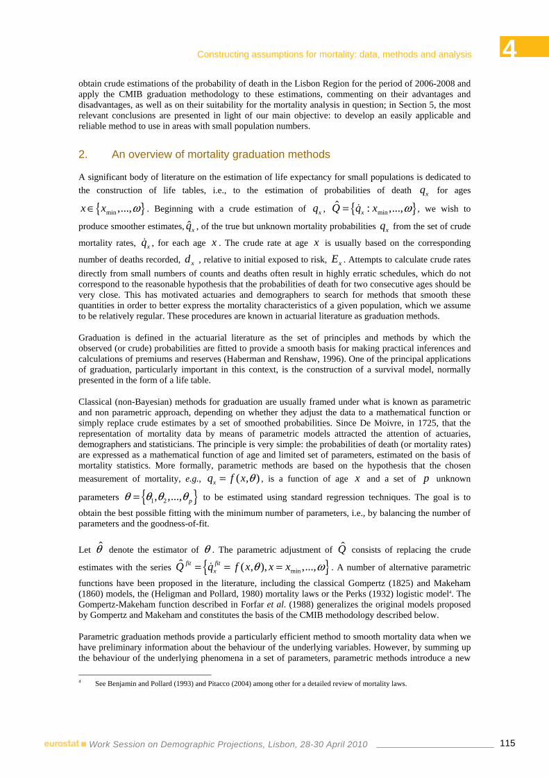
4 Constructing assumptions for mortality: data, methods and analysis
115Work Session on Demographic Projections, Lisbon, 28-30 April 2010
obtain crude estimations of the probability of death in the Lisbon Region for the period of 2006-2008 and apply the CMIB graduation methodology to these estimations, commenting on their advantages and disadvantages, as well as on their suitability for the mortality analysis in question; in Section 5, the most relevant conclusions are presented in light of our main objective: to develop an easily applicable and reliable method to use in areas with small population numbers.
2. An overview of mortality graduation methods
A significant body of literature on the estimation of life expectancy for small populations is dedicated to the construction of life tables, i.e., to the estimation of probabilities of death xq for ages
min ,...,x x ω∈ . Beginning with a crude estimation of xq , minˆ : ,...,xQ q x ω= & , we wish to
produce smoother estimates, ˆxq , of the true but unknown mortality probabilities xq from the set of crude
mortality rates, xq& , for each age x . The crude rate at age x is usually based on the corresponding
number of deaths recorded, xd , relative to initial exposed to risk, xE . Attempts to calculate crude rates directly from small numbers of counts and deaths often result in highly erratic schedules, which do not correspond to the reasonable hypothesis that the probabilities of death for two consecutive ages should be very close. This has motivated actuaries and demographers to search for methods that smooth these quantities in order to better express the mortality characteristics of a given population, which we assume to be relatively regular. These procedures are known in actuarial literature as graduation methods.
Graduation is defined in the actuarial literature as the set of principles and methods by which the observed (or crude) probabilities are fitted to provide a smooth basis for making practical inferences and calculations of premiums and reserves (Haberman and Renshaw, 1996). One of the principal applications of graduation, particularly important in this context, is the construction of a survival model, normally presented in the form of a life table.
Classical (non-Bayesian) methods for graduation are usually framed under what is known as parametric and non parametric approach, depending on whether they adjust the data to a mathematical function or simply replace crude estimates by a set of smoothed probabilities. Since De Moivre, in 1725, that the representation of mortality data by means of parametric models attracted the attention of actuaries, demographers and statisticians. The principle is very simple: the probabilities of death (or mortality rates) are expressed as a mathematical function of age and limited set of parameters, estimated on the basis of mortality statistics. More formally, parametric methods are based on the hypothesis that the chosen measurement of mortality, e.g., ( , )xq f x θ= , is a function of age x and a set of p unknown
parameters 1 2, ,..., pθ θ θ θ= to be estimated using standard regression techniques. The goal is to
obtain the best possible fitting with the minimum number of parameters, i.e., by balancing the number of parameters and the goodness-of-fit.
Let θ denote the estimator of θ . The parametric adjustment of Q consists of replacing the crude
estimates with the series minˆ ( , ), ,...,fit fit
xQ q f x x xθ ω= = =& . A number of alternative parametric
functions have been proposed in the literature, including the classical Gompertz (1825) and Makeham (1860) models, the (Heligman and Pollard, 1980) mortality laws or the Perks (1932) logistic model4. The Gompertz-Makeham function described in Forfar et al. (1988) generalizes the original models proposed by Gompertz and Makeham and constitutes the basis of the CMIB methodology described below.
Parametric graduation methods provide a particularly efficient method to smooth mortality data when we have preliminary information about the behaviour of the underlying variables. However, by summing up the behaviour of the underlying phenomena in a set of parameters, parametric methods introduce a new
4 See Benjamin and Pollard (1993) and Pitacco (2004) among other for a detailed review of mortality laws.

4 Constructing assumptions for mortality: data, methods and analysis
116Work Session on Demographic Projections, Lisbon, 28-30 April 2010
source of risk, namely the risk that the analytical model is inappropriately specified. For this reason, a number of alternative non-parametric methods have been proposed to smooth mortality data. These methods consist of replacing the crude estimate Q with a smoothed series, noted
minˆ , ,...,smo smo
xQ q x x ω= =& . Instead of resuming mortality rates by a mathematical formula of a
limited set of parameters, non-parametric graduation describe mortality by considering the original
min 1xω − + probabilities, smoothed using a specific procedure. The information provided by the original data is preserved and any influence that does not come from the predictor variable is eliminated.
The representation of mortality data by means of nonparametric models attracted significant attention of actuaries, demographers and statisticians. The basic method was "bin smoothers" and moving weighted averages. More recently, the power of modern computers made more complex and powerful smoothing procedures considerably more accessible and easier to apply in graduation. These include the use of splines (cubic, B-Splines, P-Splines), Whittaker-Henderson method locally-weighted regression (LOESS), kernel smoothing and Generalised Additive Models (GAM)5.
3. Graduation of sub-national mortality data in Portugal
The method developed by the Continuous Mortality Investigation Bureau (CMIB) was adopted by Statistics Portugal in 2007, and is now the main procedure to calculate graduated mortality rates for sub-national levels (regions NUTS II and NUTS III). This method can be framed under the parametric graduation procedures, and is an extension of the Gompertz and Makeham models. In following, we present the methodology developed by the CMIB and its extension to generalized linear models.
3.1 The CMI Bureau methodology The Continuous Mortality Investigation (CMI) Bureau of the Institute and Faculty of Actuaries of London was created in 1924, when the continuous collection of mortality data began. It is responsible for constructing standard life tables for use in Great Britain’s insurance industry. The methodology that is normally used by the CMIB to produce such tables is described in detail in Forfar et al. (1988). This methodology is, in essence, a generalization of the Gompertz (1825) and Makeham (1860) models. It was applied to Portuguese insurance data by Bravo (2007) and adopted by Statistics Portugal in 2007.
Consider a group of consecutive ages x and the series of independent deaths xd and corresponding
exposure to risk xE . The graduation procedures uses a family of parametric functions know as
Gompertz-Makeham of the type ( , )r s . They are functions with r s+ parameters of the form
1 1
,
0 0
( ) expr s
r s i ji j
i j
GM x x xθ α β− −
= =
⎞⎛= + ⎟⎜
⎝ ⎠∑ ∑ (1)
where parameters r and s give the order of the model, and can only assume positive integer values, excluding the possibility of both being zero; θ is a vector containing the estimated mortality curve parameters ( )1 1 1 1,..., ; ,...,r sθ α α β β− −= . The model presented in (1) contains both a polynomial and
an exponential component. We assume that when 0r = , (1) includes only its exponential term, whereas if 0s = , equation (1) is reduced to its polynomial component. In some applications it is useful to establish the following Logit Gompertz-Makeham functions of the type ( , )r s , defined as
5 For a review of smoothing life tables see, e.g., Wang (2005).

4 Constructing assumptions for mortality: data, methods and analysis
117Work Session on Demographic Projections, Lisbon, 28-30 April 2010
,
,,
( )( )1 ( )
r sr s
r s
GM xLGM xGM x
θθ
θ
=+
(2)
Given a vector of parameters θ , the methodology developed by CMIB states that the expression
, ( )r sxq LGM xθ= (3)
results in an adequate adjustment. Note that, since ]1,0[∈xq , the adequate function to consider for
graduation of gross death probabilities is the Logit-Gompertz-Makeham ( LGM ), as it guarantees values within that interval.
This method recommends the use of an orthogonal base for the polynomial component of the , ( )r sGM xθ equation. Special emphasis is given to the Chebycheff and Legendre polynomials (Bravo, 2007). The use of orthogonal polynomials requires some form of age scaling so that range of ages lies, e.g., in the [ ]1,1− interval. Therefore, the transformations suggested are as follows:
' x ux xv−→ = , with
max min
2x xu += and
max min
2x xv −= ,
from which we have [ ]max min ', 1,1x x x x⎡ ⎤∈ → ∈ −⎣ ⎦ .
Gathering all referred aspects, the equation used for estimation is given by
1 1
,,
0 0( ) exp
r sp r s
u v i i j ji j
x u x uGM x p pv vθ α β
− −
= =
⎛ ⎞− −⎛ ⎞ ⎛ ⎞= + ⎜ ⎟⎜ ⎟ ⎜ ⎟⎝ ⎠ ⎝ ⎠⎝ ⎠
∑ ∑ (4)
where ( ) , : , 0,1, 2,...i jp x i j = defines the adopted polynomial base, and all other parameters have
the same meaning as before.
To estimate the model parameters, two optimization criteria are considered: maximum likelihood and the minimum Chi-Squared. Empirical studies show that, in practice, the two criteria produce similar graduations (see, e.g., Forfar et al., 1988, and Bravo, 2007). The maximum likelihood method is based on the maximization of the appropriate (Binomial, Poisson, etc.) likelihood function. The minimum Chi-Squared criteria correspond to the usual 2χ statistic, namely the sum of squared standardized residuals.
The methodology described above can be reformulated and extended in the framework of generalized linear and non-linear models. Generalized linear models (GLM) are an extension of linear models for non normal distributions and non linear transformations of the interest variable. Their use in the graduation of either the probability of death at age x , xq , or the force of mortality at age x , xμ , is justified because both response variables are not normal. As an alternative to the classical regression linear models, the GLM allows, using a link function, estimation of a mean function of the response variable, written as a linear combination of all independent variables. The use of GLM in the context of graduation is explored in Renshaw (1991), Renshaw and Hatzopoulos (1996), Haberman and Renshaw (1996), Renshaw et al. (1997), Verrall (1996), Delwarde et al. (2004) and Bravo (2007). We now give some details about modelling and probability distribution assumptions for the death probability within the GLM approach.

4 Constructing assumptions for mortality: data, methods and analysis
118Work Session on Demographic Projections, Lisbon, 28-30 April 2010
Assume that xE individuals initially exposed to the risk of death come under observation at age x and
continue under observation until they survive to 1x + or, otherwise, die before that. In addition, suppose that the probability of death during the year for each one of them is xq , and that the death or survival of
one is independent of the death or survival of the others. Let xD denote the random variable which
represents the number of deaths observed in the year. In this case, we can write ( , )x x xD Bin E q . The general expression of the maximum likelihood function is given by
( )
[ ]
max
min
max
min
max
min
( ) 1
exp log( ) ( )log(1 )
exp log log(1 ) .1
x xx
xE dd
x xx x
x
x x x x xx x
xx
x x xx x x
L q q q
d q E d q
qd E qq
−
=
=
=
= −
⎧ ⎫⎪ ⎪= + − −⎨ ⎬⎪ ⎪⎩ ⎭⎧ ⎫⎡ ⎤⎞⎛⎪ ⎪= + −⎨ ⎬⎢ ⎥⎟⎜ −⎝ ⎠⎪ ⎪⎣ ⎦⎩ ⎭
∏
∑
∑
(5)
The graduation of xq is performed using the function
( , )( , )
1 ( , )xGM r sq LGM r s
GM r sθ
θθ
= =+
(6)
using the logit transformation as the canonical link of the binomial family, i.e.,
log1
xx
x
η⎛ ⎞
= ⎜ ⎟−⎝ ⎠ (7)
with inverted function
exp( )
1 exp( )x
xx
q ηη
=+
(8)
To evaluate the goodness-of-fit of the model, an appropriate measure is the so-called scaled deviance, defined as
( )max
min
ˆ( ; ) 2 log logˆ ˆ
xx x x
x x xx x x x x
d E dD y m d E dm E m=
⎡ ⎤⎛ ⎞ ⎛ ⎞−= + −⎢ ⎥⎜ ⎟ ⎜ ⎟−⎢ ⎥⎝ ⎠ ⎝ ⎠⎣ ⎦∑ (9)
where 1 ˆˆ ( )x xm g η−= represents the adjusted values generated by the estimated model.
Leaving aside the constant values and taking the logarithm from the maximum likelihood function, the ( , )s rθ α β= parameters of the Gompertz-Makeham function are estimated via maximum likelihood or,
in other words, by resolving the following minimization problem

4 Constructing assumptions for mortality: data, methods and analysis
119Work Session on Demographic Projections, Lisbon, 28-30 April 2010
( ) ( )max
min
, ,ˆ arg min log 1 ( ) log ( )x
r s r sx x
x xE GM x d GM xθ θ
θθ
=
⎧ ⎫⎪ ⎪= + −⎨ ⎬⎪ ⎪⎩ ⎭∑ (10)
3.2 Assessing model fit The goodness-of-fit is evaluated by means of the classical non-parametric tests. For completeness, we briefly review the use of these tests in a graduation context6. The first indicator of model performance involves comparing the absolute and relative deviations generated by the model. Let xDev denote the absolute deviance for each age x , i.e.,
expx x xDev d d= − (11)
where expxd represents the expected number of deaths, estimated by multiplying the mortality rates by the
number of individuals initially exposed to risk. The corresponding relative deviances (or Pearson residuals), xz , is given by
( )
xx
x
DevzVar d
= (12)
where ( )xVar d stands for the variance of deaths, obtained under the distributional hypothesis established for the probability of the random variable. Therefore, the goodness-of-fit is assessed by whether or not deviances are randomly distributed when taken sequentially, and if its distribution is in accordance to the established hypothesis adopted for the model under analyses.
Other useful tests to evaluate the model adjustment in a graduation environment are the Signs Test and the Runs tests. The Signs Test considers only the deviation sign (positive or negative). Considering the binomial distribution, it is possible to assess the probability for the number of positive signs not to exceed its observed value. If this probability is too low, the number of positive deviations is unexpectedly low; if it is too high, we have an excessively high number of positive deviations. In both cases, it should be concluded that the graduated probabilities of death are too far from the observed values, resulting in a poor fit. The Runs Test takes into account the number of same sign consecutive deviations. The test assumes that deaths follow a normal distribution by specific ages, and that the deviations are independent and their signs randomly distributed. It is possible to obtain the exact probability for the number of consecutive same sign deviations to be the same or less than the observed equivalent. A small probability is associated with an excessive linearity of the estimated graduation model, resulting in a poor adjustment.
The Kolmogorov-Smirnov test can be useful to detect abnormal graduation models, e.g. in cases where the deviations are great or very small (Forfal et al., 1988). The KS test is usually used to test or compare the distribution of the interest variable with a known distribution. In this case, the KS test is used to compare the expected and observed deaths accumulated distributions between the maximum and the minimum ages. It should be noted that, since the two series are not independent, the test has to be approached with caution. The Chi-Square test is a widely used non parametric test to assess model fit. This test can be used to test independency between observations or assess goodness-of-fit. A model can be considered to have a better adjustment if the value of the Chi-Square statistic is higher.
Finally, other tests used to asses model fit are the auto-correlation tests, based on the analyses of the correlations between the relative deviations in each age. Every relative deviation should be normally
6 For a detailed analysis see, e.g., Benjamin and Pollard (1993) and Forfar et al. (1988).

4 Constructing assumptions for mortality: data, methods and analysis
120Work Session on Demographic Projections, Lisbon, 28-30 April 2010
distributed, with zero mean and unitary variance. There are two auto-correlation tests usually used: the Portmanteau Test and the Ljung-Box Test. Both tests, using different statistics, test the hypothesis that all auto-correlation coefficients for different levels of deviations equal zero. Lastly, another way to evaluate the adjustment of the graduation model is simply to observe the graphical representation of both the crude and the graduated mortality curves. In practical terms, this is a very good way to immediately assess the overall model fit to the original series of data considered.
3.3 Projecting probabilities of death at older ages The calculation of crude age specific mortality rates at advanced ages suffers from several problems. The main issue concerns the quality and the availability of data on population estimates for the oldest-old. Effectively, although data on deaths are in general of good quality, mortality rates may be contaminated by random fluctuations due to either the small number of those surviving up to very old ages, to age misreporting problems or to the lack of coherence between deaths and the number of those exposed to risk.
In order to construct complete life tables for sub-national levels, it was decided to remove fluctuations by smoothing crude estimates via a projection method. Various methodologies have been proposed for estimating mortality rates at oldest ages7. From these, we adopted the method proposed by Denuit and Goderniaux (2005), a method that is applied directly to crude death probabilities and establishes a limiting age for the life table. Formally, the following log-quadratic model is fitted by weighted-least squares:
( )2 2ˆln , 0,x x xq a bx cx Nε ε σ= + + + (13)
to age-specific death probabilities observed at advanced ages. Two restrictions are imposed to equation (13), as to assure a concave configuration to the mortality curve at older ages and restrict a horizontal tangent at the maximum age point considered. The imposed restrictions are:
max
1xq = (14)
max
' 0xq = (15)
The inclusion of (14) and (15) into (13) will lead to a new expression of the model equation, given by
( )( ) ( )2 2 2max maxˆln 2 , 0,x x xq x x x x c Nε ε σ= − + + (16)
One of the critical aspects related to this model is determining the adequate age from which to replace the gross mortality probabilities by its correspondent adjusted estimates. The ad hoc method suggested in Denuit and Goderniaux (2005) and Bravo (2007), among others, recommends choosing the age so that the regression coefficient R2 is maximized, by ranging the initial age of the calibration procedure in the [ ]50,85 interval. Attention is also drawn to the possible need for smoothing the mortality series around the cut age point, so as to avoid abrupt discontinuities between the two series. The suggestion is to apply a geometrical mean to the death probabilities around ages 0 05,..., 5x x x= − + .
7 For a review see, e.g., Buettner (2002) and Pitacco (2004).

4 Constructing assumptions for mortality: data, methods and analysis
121Work Session on Demographic Projections, Lisbon, 28-30 April 2010
4. Application to mortality data of the Lisbon Region
In this section we describe the results, published by Statistics Portugal, of implementing the approaches described above in constructing life tables and estimating life expectancy for the Portuguese sub-national NUTS II region of Lisbon, with combined sexes. We use aggregate population and death figures corresponding to the three-year period of 2006-2008. These two data sets were published by Statistics Portugal (INE) and are classified by age (ranging from 0 to 100 or older) and sex. They are coherent in that both refer to the Lisbon Region as the place of residence. As the population census takes place every 10 years and during the first year of the ten-year period, the population data for the three-year period of 2006-2008 is based on inter-census estimations calculated by INE. Dating back to December 31, 2006, the estimated population resident in the Lisbon region was of 2794226 individuals.
The first step is to calculate the crude estimates of xq from the data. The revised methodology developed
by Statistics Portugal (INE, 2007) considers life tables based on age specific probabilities of death xq calculated directly using three-year periods, by pooling deaths and exposures first and then dividing the former by the latter. In the period under study, there were nearly 5.63 million men and women exposed to risk. In the same period, nearly 50.2 thousand men and women died, with the great majority, approximately 91.3%, doing so after the age of 50.
The modelling of xq has been done through the functions ( , )LGM r sθ , [ ]0,4r ∈ and [ ]2,7s ∈ , using generalized linear models of the binomial family. The first step in applying this graduation procedure is to determine the order ( , )r s of the Gompertz-Makeham model that best fits the data. To do so, a total of 30 different combinations are tested by ranging the order ( , )r s of the model in the above
intervals. The order of ( , )LGM r sθ is finally determined by selecting the model with highest rank in all (or the majority) of the goodness-of-fit indicators.
Table 1 summarises the results obtained for the log-likelihood function and for the deviance. As expected, as we go along a line or column in the log-likelihood or the deviance table, the values decrease. Our goal is to reach a balance between the number of parameters and the goodness-of-fit of the model. Graduation studies sometimes emphasize the goodness-of-fit without considering the statistical stability of the parameters involved in the regression. The result is an over-parameterization of the model. Recall that the null hypothesis that the difference between the deviance of two adjacent rows/columns can be tested against a chi-squared distribution with one degree of freedom.
Table 1. Log-likelihood and (unscaled) deviance, Lisbon 2006-2008, sexes combined
r s = 2 s = 3 s = 4 s = 5 s = 6 s = 70 21 7 94 7 .2 21 6 71 6 .8 21 6 5 23 .6 2 16 5 21 .1 2 16 5 12 .1 2 16 4 89 .11 21 7 28 3 .4 21 6 68 9 .8 21 6 5 23 .1 2 16 5 05 .9 2 16 5 04 .6 2 16 4 88 .42 21 6 76 7 .0 21 6 50 0 .2 21 6 5 22 .0 2 16 5 05 .1 2 16 4 81 .2 2 16 4 49 .73 21 6 50 5 .6 21 6 50 0 .1 21 6 4 98 .9 2 16 4 89 .4 2 16 4 51 .4 2 16 4 41 .54 21 6 50 2 .2 21 6 49 8 .8 21 6 4 73 .3 2 16 4 61 .0 2 16 4 50 .6 2 16 4 42 .4
r s = 2 s = 3 s = 4 s = 5 s = 6 s = 70 34 6 4.6 5 10 0 3.8 9 6 1 7 .4 1 61 2 .4 7 59 4 .35 54 8 .331 21 3 6.9 9 9 4 9.7 8 6 1 6 .4 6 58 2 .0 5 57 9 .41 54 7 .082 11 0 4.2 3 5 7 0.6 3 6 1 4 .1 6 50 8 .3 8 43 2 .61 46 9 .583 5 8 1.4 6 5 7 0.4 4 5 6 8 .0 2 54 8 .9 2 47 3 .01 45 3 .204 5 7 4.6 2 5 6 7.7 5 5 1 6 .7 8 49 2 .1 3 47 1 .48 45 5 .06
L og -Li klih o od
D evi ance
Li sb oa 2 00 6 -20 0 8, H M

4 Constructing assumptions for mortality: data, methods and analysis
122Work Session on Demographic Projections, Lisbon, 28-30 April 2010
Simultaneously, in selecting the optimal model, all the other goodness-of-fit measures should be taken into account. Table 2 presents all relevant overall goodness-of-fit indicators previously discussed. The first column refers to the order of the model. The next two columns show the value of the unscaled χ2 statistic and the correspondent p-value. Columns four to eight present all p-values for the tests used as a complement to assess model fit and referred to in the previous section (Signs Test, Runs Test, KS Test, Portmanteau Test and Ljung-Box Test). The column denominated as ‘Par. Sign.’ stand for the significance (Y) or not (N) of the entire model estimated parameters. Obtaining non significant estimates should be interpreted as a first sign of over-parameterization of the proposed model.
In the column ‘Conf.’, the letter ‘Y’ (‘N’) stands for a good (bad) graphical configuration of the adjusted mortality curve, assessed as the ability of the model to generate a plausible mortality curve, particularly the ability of the model to generate increasing probabilities of death at older ages. Finally, ‘Int. Conf.’ gives information on the goodness-of-fit in the ages where exposure to risk is higher, assessed as the ability of the model to produce small confidence intervals that contain most of the gross probabilities of death.
Table 2. LGM(r,s) - Goodness-of-fit measures, Lisbon, 2006-2008, sexes combined
(r,s) χ2 p(χ2) Signs p(+)
Runs p(runs)
KS p(.)
Portm. p(.)
LJ-Box p(.)
Par. Sign
Conf. Int. Conf.
(0,2) 4075.259 0.112 0.999 0.000 1 0.000 0.000 Y N N(0,3) 980.508 0.546 0.136 0.000 1 0.000 0.000 Y N N(0,4) 606.224 0.531 0.309 0.002 1 0.096 0.040 Y N Y(0,5) 609.297 0.495 0.184 0.001 1 0.182 0.094 Y N Y(0,6) 582.128 0.537 0.242 0.146 1 0.166 0.082 N N Y(0,7) 534.917 0.547 0.460 0.132 1 0.157 0.069 Y Y Y(1,2) 2142.277 0.474 0.382 0.001 1 0.000 0.000 Y N N(1,3) 943.541 0.499 0.618 0.001 1 0.000 0.000 Y Y N(1,4) 602.602 0.543 0.309 0.001 1 0.078 0.031 N N Y(1,5) 568.938 0.543 0.382 0.058 1 0.161 0.077 Y Y Y(1,6) 564.738 0.550 0.242 0.295 1 0.137 0.061 N Y Y(1,7) 534.125 0.545 0.382 0.058 1 0.151 0.065 N Y Y(2,2) 1140.533 0.392 0.097 0.001 1 0.000 0.000 Y N N(2,3) 555.101 0.556 0.242 0.295 1 0.158 0.072 Y Y Y(2,4) 598.726 0.550 0.309 0.001 1 0.051 0.018 N N Y(2,5) 566.304 0.547 0.382 0.058 1 0.134 0.059 N Y Y(2,6) 520.866 0.540 0.618 0.007 1 0.797 0.701 Y N Y(2,7) 454.656 0.566 0.460 0.088 1 0.629 0.507 Y N Y(3,2) 571.059 0.530 0.618 0.484 1 0.192 0.097 Y Y Y(3,3) 554.898 0.555 0.309 0.140 1 0.160 0.074 N Y Y(3,4) 553.648 0.550 0.136 0.329 1 0.200 0.100 N Y Y(3,5) 533.329 0.558 0.460 0.021 1 .0273 0.147 N Y Y(3,6) 456.045 0.577 0.816 0.659 1 0.586 0.468 Y Y Y(3,7) 440.299 0.557 0.540 0.366 1 0.620 0.493 Y N Y(4,2) 563.553 0.533 0.460 0.270 1 0.216 0.113 Y N Y(4,3) 553.782 0.548 0.309 0.283 1 0.205 0.104 N Y Y(4,4) 503.466 0.550 0.618 0.057 1 0.661 0.538 Y N Y(4,5) 477.450 0.561 0.691 0.090 1 0.620 0.495 Y N Y(4,6) 456.482 0.566 0.460 0.917 1 0.650 0.529 N Y Y(4,7) 440.099 0.568 0.758 0.790 1 0.609 0.485 N Y Y
Considering the last three indicators, the only models where all estimates are significant and the curve configuration is acceptable both at younger and older ages are models (0,7)LGM , (1,5)LGM ,
(3, 2)LGM and (3,6)LGM . From these candidate solutions, if we take into account all other goodness-of-fit measures, the best model is (3,6)LGM . The coefficients of the optimal model are shown in Table 3 and are all statistically significant.

4 Constructing assumptions for mortality: data, methods and analysis
123Work Session on Demographic Projections, Lisbon, 28-30 April 2010
As a complement for the information discussed previously, it can be helpful to observe some selected graphical representations not only of the overlap between the gross and estimated mortality curve, but also of the residuals, so as to better understand their distribution. Figures 1 to 3 help visualising the fit obtained in the selected model.
Table 3. Coefficients of model LGM(3,6), Lisbon, 2006-2008, sexes combined
Coef. se t -ratio p -valueα0 0,003332 0,00009 35,743 < 0.0001α1 0,009357 0,00031 30,308 < 0.0001α2 0,006380 0,00027 23,997 < 0.0001β0 -7,895357 0,15654 -50,436 < 0.0001β1 5,667404 0,27884 20,325 < 0.0001β2 10,428748 0,71621 14,561 < 0.0001β3 -8,786856 0,94184 -9,329 < 0.0001β4 -9,507530 0,87421 -10,876 < 0.0001β5 10,509087 0,98526 10,666 < 0.0001
In figure 1, the gross and graduated probabilities of deaths are represented, as well as the 95% confidence intervals. In figure 2, the Pearson residuals by age for the optimum model are represented, as well as a comparison between the quantiles of a standardized normal distribution and the obtained residual distribution.
Some observations can be seen to fall into the tails of the standardized normal distribution, mainly at older ages. Apart from this fact, the overall model seems to result in an acceptable fit, having most of observations within the estimated confidence interval.
Figure 1. Adjusted mortality curve, and confidence intervals, Lisbon, 2006-2008, sexes combined
It is important to remember that population estimates at older ages are less reliable, meaning also that graduated probabilities of death suffer a considerable bias.
0 20 40 60 80 100
-8-6
-4-2
0
Prob. Brutas vs Prob Graduadas
Idade
log(
qx)
0 20 40 60 80 100
-8-6
-4-2
0
Gross vs. Graduated probabilities of death
Age

4 Constructing assumptions for mortality: data, methods and analysis
124Work Session on Demographic Projections, Lisbon, 28-30 April 2010
As explained earlier, applying the Denuit-Goderniaux method for estimating mortality probabilities at older ages will result in a more adequate curve shape, and consequently reflect the known mortality laws in a more adequate way. Note that Statistics Portugal established as the life table limit the age of 115, meaning that at this age, the death probability is restricted to 1.
Figure 2. Residuals from LGM(3,6) model, Lisbon, 2006-2008, MF
Quantiles of Standard Normal
rel.d
ev
-2 -1 0 1 2
-50
510
Scaled Deviations
age
scal
ed.re
ldev
0 20 40 60 80 100
-20
24
The DG models tested led us to apply an estimation from age 75, and to consider age 81 as the point of junction of the two estimated series, with no need for smoothing procedures. Figure 3 represents the profile of the three mortality curves.
Figure 3. Comparison between crude and fitted death probabilities
-12,0
-10,0
-8,0
-6,0
-4,0
-2,0
0,0
2,0
1 11 21 31 41 51 61 71 81 91 101 111
Gross Grad Grad+DG
5. Conclusions
In this paper we discussed the use of graduation methods in smoothing mortality data as a feasible solution for estimating life expectancy indicators for small population areas. In particular, we give a comprehensive presentation of the parametric method developed by the Continuous Mortality Investigation Bureau (CMIB) and its extension to generalized linear models, recently adopted by Statistics Portugal. The methodology is empirically tested using data for the Portuguese sub-national region of Lisbon and for the period of 2006-2008. Our results show that the methodology is robust and can be used to construct life tables and estimate life expectancy. The flexibility of the method makes it applicable to mortality data for a wide range of ages from any geographical conditions.

4 Constructing assumptions for mortality: data, methods and analysis
125Work Session on Demographic Projections, Lisbon, 28-30 April 2010
References
Benjamin, B. and Pollard, J. (1992). The Analysis of Mortality and Other Actuarial Statistics, 6th edition. London: Butterworth-Heinemann.
Benjamin, B. and Pollard, J. (1993). The Analysis of Mortality and other Actuarial Statistics. Third Edition. The Institute of Actuaries and the Faculty of Actuaries, U.K.
Brass, W (1971). On the Scale of Mortality. Brass. W. Biological Aspects of Demography. London: Taylor & Francis.
Bravo, J. M. (2007). Tábuas de Mortalidade Contemporâneas e Prospectivas: Modelos Estocásticos, Aplicações Actuariais e Cobertura do Risco de Longevidade. Tese de Doutoramento, Universidade de Évora.
Buettner, T. (2002). Approaches and experiences in projecting mortality patterns for the oldest-old. North American Actuarial Journal, 6(3), 14-25.
Chiang C, (1984). The life table and its application. Malabar, Fl., Robert E. Krieger Publishing Co.
Chiang, C. (1979). Life table and mortality analysis. World Health Organization, Geneva.
Coale, A. and Demeny, P. (1966). Regional Model Life Tables and Stable Populations (Princeton, N. J., Princeton University Press.
Delwarde, A., Kachakhidze, D., Olié, L., & Denuit, M. (2004). Modèles linéaires et additifs généralisés, maximum de vraisemblance local et méthodes relationnelles en assurance sur la vie. Bulletin Français d’Actuariat 6, 77-102.
Denuit, M. and Goderniaux, A. (2005). Closing and projecting life tables using log-linear models. Bulletin of the Swiss Association of Actuaries, 29-49.
Forfar, D., McCutcheon, J. and Wilkie, D. (1988). On Graduation by Mathematical Formula. Journal of the Institute of Actuaries 115, 1-135.
Gompertz, B. (1825). On the nature of the function of the law of human mortality and on a new mode of determining the value of life contingencies. Philosophical Transactions of The Royal Society, 115, 513-585.
Haberman, S. and Renshaw, A. (1996). Generalized linear models and actuarial science. The Statistician, 45, 407-436.
Heligman, L. and Pollard, J. (1980). The age pattern of mortality. Journal of the Institute of Actuaries, 107, 49-80.
Irwin, R. (1980). Methodology for Estimates of the Population of Counties by Age and Sex: July 1, J975. Current Population Reports N. 103, U.S Bureau of Census, Washington.
Makeham, W. (1860). On the law of mortality. Journal of the Institute of Actuaries, 13, 325-358.
Mazur, D. (1969). Expectancy of Life at Birth in 36 Nationalities of the Soviet. Union: 1958-60. Population Studies, 23, 225-46.
Perks W. (1932). On some experiments in the graduation of mortality statistics. Journal of the Institute of Actuaries, 63, 12-57.

4 Constructing assumptions for mortality: data, methods and analysis
126Work Session on Demographic Projections, Lisbon, 28-30 April 2010
Pitacco, E. (2004). Survival models in a dynamic context: A survey. Insurance: Mathematics & Economics 35, 279-298.
Renshaw, A. (1991). Actuarial graduation practice and generalised linear models. Journal of the Institute of Actuaries, 118, 295-312.
Renshaw, A. and Hatzopoulos, P. (1996). On the graduation of amounts. British Actuarial Journal, 2, 185-205.
Renshaw, A., Haberman, S., and Hatzopoulos, P. (1997). On the duality of assumptions underpinning the construction of life tables. Astin Bulletin, 27, 5-22.
Siler, W. (1979). A competing risk model for animal mortality, Ecology, 60, 750-757.
Verrall, R. (1996). A unified framework for graduation. Actuarial Research Paper, 91, 2-25.
Wang, J. (2005). Encyclopedia of Biostatistics, Chap. Smoothing Hazard Rates. Willey, 2nd edition

Constructing assumptions for fertility: data, methods and analysis Chair: Maria Filomena Mendes
Session 5


5 Constructing assumptions for fertility: data, methods and analysis
129Work Session on Demographic Projections, Lisbon, 28-30 April 2010
TREND REVERSAL IN CHILDLESSNESS IN SWEDEN
Lotta PERSSON1
Abstract
In the calculations of the future fertility rates for Sweden a cohort approach is used. For every year estimates of cohort fertility rates for the first, second, third and fourth(+) child are calculated. Fertility rates of the first child are based on assumptions on ultimate levels of childlessness for each cohort.
The proportion of childlessness among women who just completed their fertile period is about 14 percent. This proportion is lowest for cohorts born in the mid 1940s, around 12 percent. So far, we have believed in a continued increase in childlessness due to the postponement of childbearing. Since fecundity declines with age one may expect such a development.
Data from the very last years, though, suggest a quite remarkable fertility recuperation. Cohorts born in the 1970s have not only managed to catch up with the first birth fertility levels of the 1960s cohorts, but also passed them, and we are now seeing a trend reversal in childlessness.
This study examines whether the trend reversal is visible in different socioeconomic groups with special focus on educational levels. In the study some possible explanations of the trend reversal are also explored such as changes in attitudes and norms, and the increasing numbers of infecundity treatments since the 1990s.
The patterns of decreasing levels of childlessness are especially interesting because Sweden is a country that often has been regarded as a forerunner in demographic behaviour.
1. Childlessness is a component in the fertility model
Statistics Sweden has studied the development of childlessness among women since the early 1980s. One reason was that the level of childlessness was included in the calculation model for prediction of future fertility. In the early 1980s it was believed that childlessness would increase from 12 percent, the level for women who just had completed their childbearing ages at that time, to 17 percent for women in the future (Statistics Sweden 1981). The future women at that time are women who today just have completed their fertile years and between 13 and 14 percent ended up childless. Fewer than the forecasters thought in the 1980s. The assumption on the future level of childlessness has since then fluctuated between 15 and 17 percent.
In the assumption on future births we distinguish between persons born in Sweden and persons born outside of Sweden. Persons born outside Sweden are divided into several groups depending on their country of birth. Separate assumptions for Swedish-born and the different groups of foreign-born have been made since 2008 as fertility differ.
For Swedish-born the calculations on the future fertility is based on information on cohorts. Estimations are made for every year on the probability that women will give birth in that year to their first, second, third or fourth (or more) child. The estimations for each cohort and parity occur with what is known as incidence rates (the number of occurrences divided by the average population of women in each cohort).
1 Lotta PERSSON Statistics Sweden, Stockholm E-mail: [email protected]

5 Constructing assumptions for fertility: data, methods and analysis
130Work Session on Demographic Projections, Lisbon, 28-30 April 2010
The total of the cohort’s incidence rates (for the first, second, third and fourth or more child) is the same as the cohort’s age-specific fertility rate.
The assumption of incidence rates for the first child is based on an assumption of the percent of childless per cohort. Then the age specific incidence rates for the first child are estimated up to age 50, so that the cohort reaches the assumed childlessness.
The method for producing the assumptions for foreign-born is more simple than the one used for Swedish-born. No parity-specific assumptions are made for foreign-born, but the age specific fertility rate is projected forward.
A more thorough description of the model for the fertility projection can be found in The future population of Sweden 2009-2060 (Statistics Sweden 2009).
2. The development of childlessness in Sweden
At least since the late 1960s there has been a continuous postponement in childbearing (se figure 1). In 1970, the average age for women to have the first child was 24. Today the average age is 29. This upward shift accelerated during the 1990s because of the economic recession at that time. The recession led to greater difficulties for women and men to get establish on the labour market. That was particularly true for younger men and women. In Sweden several studies have shown that those outside the labour force are less likely to have children (Statistics Sweden, 2008:1). This is largely due to the Swedish parental insurance system, where the compensation paid out to parents is based on income from gainful employment. So in the 1990s an increasing number of young women instead went on to higher education and postponed having children. This pattern has remained in the 2000s.
Figure 1. Mean age at birth of first child in Sweden 1970–2009
22
23
24
25
26
27
28
29
30
1970 1975 1980 1985 1990 1995 2000 20050
The postponement in childbearing since the late 1960s has resulted in an increase in childlessness in Sweden. The ability to have children declines with increasing age. The main reason is that the quality of the eggs that women are born with deteriorates with age. The proportion childless is least among women born in the mid-1940s, who were also the youngest first-time mothers (se figure 2). Just over 11 percent of them have ended up as childless. Childlessness has increased slightly among later born cohorts and the proportion of childless among women who just completed their fertile period is about 13-14 percent.

5 Constructing assumptions for fertility: data, methods and analysis
131Work Session on Demographic Projections, Lisbon, 28-30 April 2010
Figure 2. Childless women, cohort 1930–1964. Percent.
0
5
10
15
20
1930 1935 1940 1945 1950 1955 1960Cohort
Childlessness at age 45
To get an idea of the development of childlessness among cohorts who have not yet passed their fertile years, childlessness in ages 30-45 is compared for five cohorts.
Figure 3 shows the development of childlessness from age 30 for cohorts born in 1960, 1965, 1970, 1975 and 1977. Data is derived from Statistics Sweden’s Multi-Generation Register as well as the Historical Database. Data on the foreign-born residents are excluded. Data include information on the childbearing histories of all women up until the end of year 2008.
Results show that the percentage of women who have not had any children in their 30s is higher for women born in 1970, compared to women born in 1960 and 1965. However, data from the very last years, suggest a quite remarkable fertility recuperation. Cohorts born in the 1970s have not only managed to catch up with the first birth fertility levels of the 1960s cohorts, but also passed them, and we are now seeing a trend reversal in childlessness, at least for the Swedish-born.
Figure 3. Childless women at certain ages by year of birth. Percent.
0
5
10
15
20
25
30
35
40
45
50
30 31 32 33 34 35 36 37 38 39 40 41 42 43 44 45
Age
1960
19651970
1975
1977
Women born in 1960, 1965, 1970, 1975 and 1977

5 Constructing assumptions for fertility: data, methods and analysis
132Work Session on Demographic Projections, Lisbon, 28-30 April 2010
3. The relationship between educational level and childlessness
To see if the trend reversal applies to different socioeconomic groups the data on childbearing histories have been linked to individual data on educational levels for the five different cohorts: 1960, 1965, 1970, 1975 and 1977. In the analyses educational level attained at age 30 is used.
As can be seen in figure 4 there has been a rapid educational expansion in Sweden during the recent decades, and the proportion of women with higher education has increased substantially across cohorts (figure 4). In the 1960 cohort, 11 percent of Swedish women had attained more than 3 years of tertiary education by age 30, while the corresponding proportion for cohort 1977 was 41 percent. At the same time, the group with primary or secondary education has declined.
Figure 4. Women’s educational level at age 30 for cohorts 1960-1977
0
20
40
60
80
100
1960 1965 1970 1975Cohort
Primary school
Secondary school
Tertiary education < 3 years
Tertiary education > 3 years
Figure 5 shows the development of childlessness from age 30 for five cohorts of women with different educational levels. It is only for women with the highest level of education that has a clear trend reversal. Women born in 1965, is to a smaller extent childless after the age of 35 compared to women born in 1960. Childlessness seems to fall even further for women born 1970 and later. Among women born in 1965, the share of childless is now smaller for women with the highest level of education in ages over 40 than it is for those with the lowest educational level.
There is a strong relationship between educational level and age at first motherhood. Women with higher education start their childbearing later than women with lower education. One would expect that this would lead to a higher level of childlessness as fecundity is related to age. This has turned out to be true. Women with a higher education have to a larger extent ended up childless. Data from the very last years, however, show that this does not have to be true in the future. Among women born in 1965, childlessness is now lower among women with the highest educational level than among the less educated.

5 Constructing assumptions for fertility: data, methods and analysis
133Work Session on Demographic Projections, Lisbon, 28-30 April 2010
Figure 5. Share of childless women by age and educational level. Women born in 1960, 1965, 1970, 1975 and 1977
0
10
20
30
40
50
60
30 35 40 45
1960 1965 19701975 1977
Primary school
Age
0
10
20
30
40
50
60
30 35 40 45
1960 1965 19701975 1977
Secondary education
Age
0
10
20
30
40
50
60
30 35 40 45
1960 1965 19701975 1977
Tertiary education <3 years
Age
0
10
20
30
40
50
60
30 35 40 45
1960 1965 19701975 1977
Tertiary education > 3 years
Age
Educational attainment at age 30

5 Constructing assumptions for fertility: data, methods and analysis
134Work Session on Demographic Projections, Lisbon, 28-30 April 2010
4. Infecundity treatments
What is the reason for the trend reversal in childlessness among women with a high educational level? One possible explanation is an increased possibility to get infecundity treatments. For example, the number of IVF treatments increased from around 3 000 in 1991, to over 12 000 in 2007. Today, around one fourth of the treatments lead to a live born child (Swedish National Board of Health and Welfare, 2009).
A survey carried out by Statistics Sweden in spring 2009 about women’s and men’s attitudes towards having children showed that it was common to have used aid to have children (Statistics Sweden (2009:2).
Nearly 40 percent of those who had their first child after the age of 34 had used one or multiple forms of aid to have children. The most common was the use of an ovulation test to get help to become pregnant. The second most common was aid by In Vitro Fertilization and the third most common was hormone treatments.
In figure 6 the share of women who used aid to have children has been broken down by educational level. It is obvious that women with a tertiary education are more likely to have used aid to become pregnant than women with a lower educational level. That is true for all age groups. Maybe those with higher education have better knowledge of and access to infecundity treatments. That could possibly be an explanation to why the trend reversal is mainly visible among the highly educated.
Figure 6. Share of women who used aid to have children by educational level and age at birth of first child.
0
10
20
30
40
50
Primary school Secondary school Tertiary education
-27 years
28-33 years
34-40 years
Educational level at time of survey
5. Attitudes to having children
Through administrative registers it is impossible to find the reasons for childlessness. It is therefore difficult to distinguish who is childless because of free choice or who is involuntary childless. Through attitude surveys it is possible to get an idea of the causes of childlessness. In such surveys questions about women’s and men’s plans and desires when it comes to having children or not can be asked. In the survey conducted by Statistics Sweden in 2009 childless women have been asked if they think they will have children at some time in the future. Among cohabiting or married women the proportion responding “yes” is highest for women with a higher educational level (figure 7). This could mark a slightly more positive attitude toward having children for the more educated. Unfortunately we are not able to find out if the attitudes among the highly educated have changed over time. If so, that could be another explanation to the trend reversal.

5 Constructing assumptions for fertility: data, methods and analysis
135Work Session on Demographic Projections, Lisbon, 28-30 April 2010
Figure 7. Share of cohabiting or married women who answer “yes” to the question: Do you think you will have children in the future?” by age and educational level
0
20
40
60
80
100
Primary school Secondary school Tertiary education
-27 years 28-33 years 34-40 years
Educational level at time of survey
6. Discussion and conclusions
The level of childlessness is used in the model for calculating the future fertility rates for Sweden. In the last population forecast (Statistics Sweden 2009) an increased level of childlessness was assumed, from today’s level 13-14 percent to 15 percent in the future. Now we see evidence of a trend reversal in childlessness. Data from the very last years suggest a quite remarkable fertility recuperation. Cohorts born in the 1970s have not only managed to catch up with the first birth fertility levels of the 1960s cohorts, but also passed them. When studying the development for women with different educational levels, it is obvious that the trend reversal is visible mainly for women with high levels of education, a group that has increased substantially in number. Some possible explanations to the trend reversal could be changes in attitudes and norms, and an increased use of aid to get pregnant.
The pattern of decreasing levels of childlessness is especially interesting because Sweden is a country that often has been regarded as a forerunner in demographic behaviour. In explanations of the timing and level of fertility, the role of education has often been emphasized. Higher educational levels have been seen as a gradient of depressing fertility. Results from this study shows that the role of education on childbearing is not yet quite clear.
In Sweden, at Statistics Sweden, the new pattern will perhaps lead to a reconsideration of the assumption on the future level of childlessness in future population projections.
References
Statistics Sweden (1981) Have children – the development of childbearing 1960-1978. Information in forecast issues 1981:2. (Available only in Swedish)
Statistics Sweden (2008) Work and childbirth – Comparisons of native and foreign born women and men. Demographic reports 2008:1. (Available only in Swedish, but with a summary in English)
Statistics Sweden (2009) Having children or not? – Results from a questionnaire survey about women’s and men’s attitudes towards having children. (Available only in Swedish, but with a summary in English)
Statistics Sweden (2009) The future population of Sweden 2009-2060. Demographic reports.
Swedish National Board of Health and Welfare (2009) Pregnancies, Deliveries and Newborn Infants. Health and Medical Care. (Available only in Swedish, but with a summary in English).


5 Constructing assumptions for fertility: data, methods and analysis
137Work Session on Demographic Projections, Lisbon, 28-30 April 2010
IS FERTILITY CONVERGING ACROSS THE MEMBER STATES OF THE EUROPEAN UNION?*
Giampaolo LANZIERI**
1. Introduction
Population projections are one of the major outcomes in demography and are mostly produced on a regular basis by national statistical offices, research institutes and international organisations. When the projections exercise is carried out over a set of geographical entities (regions, countries, areas of the world, etc.1), an additional requirement is the consistency of the results across those entities. In fact, producing multi-country projections adds a cross-sectional dimension to the usual time series framework. For instance, if countries are (demographically) moving in the same way, then this supplementary information should be taken into account in the assumptions-setting process.
Typical examples of potential constraints are the First and Second Demographic Transition theories. The former theory explains the fall first of mortality and then of fertility to lower levels; the latter focuses on fertility and family changes in a wider social and cultural context. Thus, whilst the engine of the First Demographic Transition is mortality, the engine of the Second Demographic Transition is fertility (van de Kaa, 2004). The former theory is commonly accepted in the scientific literature, while the contribution of the latter to the understanding of demographic changes is still questioned (e.g. Coleman, 2004). Embedded in the theory of demographic transition is the idea of convergence.
Whilst largely debated in the economics literature, where it stems from Solow’s neoclassical model of growth and it has a number of relevant policy implications, convergence as such has received relatively little attention in demography in terms of empirical evidence. Yet, if demographic convergence holds across countries, then assumptions can profitably be developed that fit with such a theoretical framework. By doing so, the ‘international’ consistency of the results is ensured with regard to that specific hypothesis. In this paper, I therefore address the issue of fertility convergence in a specific set of 27 European countries currently belonging to the European Union (EU).
In wide social terms, there are several indications of convergence in Europe. According to some scholars, during the past century Western European societies have shown a clear process of social integration (Kleibke, 1990). Although still unobserved in the countries which only recently joined the EU, convergence towards the European social model may well take place in the future (Draxler and Van Vliet, 2010). Focusing on the demographic point of view, Watkins (1990) showed that, during the 19th and 20th centuries, there was a tendency among the regions towards greater demographic homogeneity within nations.
Focusing on the European Union Member States (MSs), it is plausible to assume that common policies and sharing of best practices may strengthen convergence in several areas. In fact, convergence is a concept which is central to many EU policies. For instance, the primary aim of the Structural Funds, which are among the largest channels of EU funding, is to narrow the gap between the development levels of the various EU regions (referred to as the ‘convergence’ objective), improving their social
* The views expressed in this paper are exclusively those of the author and do not necessarily represent the views of the
European Commission. ** European Commission — Eurostat, Population Unit, Luxembourg. E-mail: [email protected]. 1 For the sake of simplicity, I refer from here onwards to the case of countries.

5 Constructing assumptions for fertility: data, methods and analysis
138Work Session on Demographic Projections, Lisbon, 28-30 April 2010
cohesion and economic well-being. Convergence is therefore a natural conceptual framework for assumptions setting in the context of the European Union.
The first hypothesis to be assessed is then if demographic convergence has taken place in Europe, regardless of whether a country is a member of the EU. The attention is here limited to fertility, as childbearing is basically the result of individual decisions and fertility is essential to the theory of the Second Demographic Transition, which is supposed to be occurring nowadays in Europe. Going one step further, another hypothesis to be tested is whether the policy efforts, mainstreamed at EU level and targeting socio-economic convergence across Member States, may have imparted additional impetus to — or even caused — convergence in fertility.
The article is structured as follows: in Section 2, I present the various concepts of convergence proposed in the literature together with the related indicators; in Section 3, I define my method of analysis and propose a new simple indicator of convergence; in Section 4, using ordinary methods, I assess the presence of convergence in the whole set of 27 countries currently belonging to the European Union; in Section 5, applying the indicator presented in Section 3, I analyse the possible impact of accession to the European Union on convergence in fertility for some of the enlargements that have occurred in the past; in Section 6, I conclude by discussing the implications for making assumptions in the projections exercises.
2. Definitions and measures of convergence
In the economics literature it is possible to find several definitions of convergence (see, for instance, Sala-i-Martin, 1995). The first, most widely used concept describes the convergence of a group of geographical units (countries, regions, counties, etc.) as the reduction over time of the dispersion of a given indicator (e.g. GDP per capita), usually measured by means of the standard deviation or related measures2. This is called σ-convergence, and it thus relates to the shrinking of the cross-countries distribution over time. Therefore, there is said to be σ-convergence if:
Ttt +> σσ (1)
where tσ is the standard deviation (or assimilated measure) of the indicator at time t. Another common concept is referred to as β-convergence. This definition originated from the work of Barro and Sala-i-Martin, who used regressions of the mean growth rate of GDP per capita over a given period on the log of the initial level:
( ) titiTtti ya ,,,, ln εβγ +⋅+=+ (2)
where ( ) Tyy tiTtiTtti ,,,, ln ++ =γ is the mean annualised growth rate of variable y in country i in the
period (t, t+T) under examination, tiy , is its value at the initial time t and ti,ε are the corresponding residuals. Model (2) is often referred to as a Barro regression, in which a negative slope coefficient would imply that entities at lower levels of y have grown more, in the period under examination, than those at higher initial levels. Thus β-convergence is based on the catching-up of the countries at a lower initial level towards those at a higher level, due to different mean growth rates. Young et al. (2008) demonstrate that β-convergence is a necessary but not sufficient condition for σ-convergence; in contrast, σ-convergence is a sufficient but not necessary condition for β-convergence (Sala-i-Martin, 1995).
2 Commonly found in the literature are the standard deviation of the log of the indicator, as well as the coefficient of variation of
the variable itself, both invariant with the mean. The pure standard deviation of the indicator is also sometimes used.

5 Constructing assumptions for fertility: data, methods and analysis
139Work Session on Demographic Projections, Lisbon, 28-30 April 2010
Despite this approach being much criticised, starting from Friedman (1992) and Quah (1993), a large number of applications are recorded in the economic literature, as well as further developments. In order to remove the dependency of the slope coefficient in model (2) from the length of the period of analysis, Sala-i-Martin (1995) proposes also a non-linear model3 to test for the presence of β-convergence:
( ) titi
T
Ttti yTea ,,,, ln1 εγ
λ+⋅⎟
⎟⎠
⎞⎜⎜⎝
⎛ −−=⋅−
+ (3)
where λ can be interpreted as the speed of convergence. Sala-i-Martin (1994) claims that, for the economies he analysed, these speeds are surprisingly all about 2 % per year, thus supporting the idea of a kind of ‘natural rate of convergence’. This statement was assessed by Abreu et al. (2005) using a meta-analysis of a large body of literature, and they found the convergence rate to be rather sensitive to the model specification bias. Where the unobserved heterogeneity (e.g. in technological levels) is taken into account, the convergence rate is usually higher.
When the analysis is carried out at national level, it may be difficult to accept the assumption that all countries share the same technology and preferences; however, each country can still converge towards a different steady state, but at a rate common to all. This concept is referred to as conditional β-convergence, and it may be detected with the inclusion in the specification of the Barro regression of an additional set of explanatory variables, meant to account for varying technologies and preferences. Where convergence is instead taking place between sub-groups of countries, these are referred to as convergence clubs. They are usually identified by means of dummy variables included in the conditional convergence model. In addition, Azzoni et al. (2003) stress the importance of testing for convergence using micro-data instead of macro-data, as these latter may be affected by compositional bias. Cole and Neumayer (2003) highlight the need for weighting by population size in income distribution studies.
Following the criticisms of the capacity of model (2) to test for β-convergence, Boyle and McCarthy (1997) propose a simple measure aiming to capture the extent of intra-distributional mobility over time. To do so, it uses an indicator based on the Kendall index of ranks concordance, RC:
( )[ ]0
0
1 i
T
tit
t RTVar
RVarRC
⋅+=
∑=
(4)
where Rit is the rank of country i at time t. These authors propose also a biannual version of the multi-annual index RC reported in (4):
( )( )0
0
2 i
itit RVar
RRVarRCa⋅+
= (5)
These indexes range between zero and one: the lower the value, the greater the extent of mobility within the distribution.
3 The equation should be solved using non-linear methods. It is also possible to solve it using ordinary least squares and
deriving the beta parameter afterwards through the conversion formula ( )[ ]TT ⋅+−= βλ 1ln1 ; however, when the time window is large and/or the negative value of the estimated slope is high in absolute terms, this approach would give a negative value for the logarithm of the conversion formula and it cannot therefore be used.

5 Constructing assumptions for fertility: data, methods and analysis
140Work Session on Demographic Projections, Lisbon, 28-30 April 2010
Several other concepts of convergence and related methods of detection have been proposed in the literature. For instance, Maeso-Fernandez (2003) applies time series analysis to study the gap between a number of countries and the US. Laurini et al. (2005) use non-parametric methodologies to identify income convergence clubs in Brazilian municipalities. Tomljanovich and Vogelsang (2002) apply a different econometric approach to assess GDP convergence across US regions. Phillips and Sul (2007) develop a new method which makes it possible to test for convergence and club convergence using a log regression model.
The Barro regression, relating the mean annualised growth rate to an initial level, in fact masks any variation within the period under examination. Therefore, in some studies, the period is broken down into sub-periods to assess breaks for the examined variable. This applies also to analysis based on the econometric approach, where the presence of structural breaks may affect the performance of unit roots tests.
2.1 Some studies on fertility convergence
In comparison with applications in the economic domain, there are relatively few studies on convergence in fertility. Wilson (2001), using indicators based on the distribution of the world population by total fertility at given moments in time, highlights the presence of convergence at world scale in the second half of the past century. He noted how the common economic distinction between poor and rich countries is becoming of less importance for demography, and that demographic convergence can be seen as one element of the socio-demographic change that seems to have taken place more rapidly than economic development. However, Dorius (2008) argued that the evidence is for divergence rather than convergence. He focused on relative, rather than absolute, inter-country differences in fertility intensities to measure the variation in inequality; in particular, Dorius used three indexes of inequality (Gini coefficient, Mean Log Deviation and Theil index) to locate the source of change in fertility inequality in the distribution of countries by fertility. The findings of his analysis based on population-weighted σ- and β-convergence and inequality measures show that convergence began only in the last part of the period 1955-2005, and therefore he concluded that the second half of the twentieth century cannot be considered a period of fertility convergence on a global scale. In order to disentangle economic and demographic effects, Herbertsson et al. (2000) focus on the conditional model and found evidence for convergence, both absolute and conditional, of fertility rates between 1978 and 1998 for about 190 countries.
Tomka (2002) takes a different perspective, analysing the demographic convergence between a specific country (Hungary) and a group of countries (Western Europe). To do so, he proposes indexes based on standardised differences from the Western European averages, on the basis of which he concludes that Hungary converged from the beginning to the middle of the past century and then diverged starting from the mid-1960s.
Other studies refer instead to the regional dimension within a country. For instance, Franklin (2002, 2003), using σ-convergence, found that regional fertility actually diverged in Italy from unification until the early post-WWII years, followed by a period of convergence until the 1970s and then again a marginal divergence. However, analysing the β-convergence, the same author concluded that after WWII there was indeed convergence in fertility across Italian regions at a rate greater than 2 %, and that the inclusion of spatial dependence did not significantly improve the model at regional level (while it did so for further disaggregation at provincial level). For another Mediterranean country, Kotzamanis and Duquenne (2006) found evidence of convergence of the demographic structures of the Greek regions; in particular for fertility, both period and cohort fertility indicators showed overall a clear tendency to homogeneity.
Another area of research in demography concerns the convergence between groups of population within a defined geographical unit, for instance trend analysis of the differences in demographic behaviour between ethnic groups or between native- and foreign-born (e.g. Haines, 2002). There is no attempt in this paper to cover also this domain.

5 Constructing assumptions for fertility: data, methods and analysis
141Work Session on Demographic Projections, Lisbon, 28-30 April 2010
3. Data and method of analysis
The data used for the analysis are mainly national data as provided to Eurostat (freely available in Eurostat’s database), supplemented with personal estimates. The countries4 are the 27 Member States (MSs) of the European Union: Belgium (BE), Bulgaria (BG), the Czech Republic (CZ), Denmark (DK), Germany (DE), Estonia (EE), Ireland (IE), Greece (EL), Spain (ES), France (FR), Italy (IT), Cyprus (CY), Latvia (LV), Lithuania (LT), Luxembourg (LU), Hungary (HU), Malta (MT), the Netherlands (NL), Austria (AT), Poland (PL), Portugal (PT), Romania (RO), Slovenia (SI), Slovakia (SK), Finland (FI), Sweden (SE) and the United Kingdom (UK). In particular, data for France refer to Metropolitan France, thus excluding the French Overseas Departments (DOM) and Overseas Territories (TOM), data for Cyprus refer to the government-controlled area from 1974 and data for Germany always include East Germany.
As shown above, convergence is a multi-dimensional concept. For the first hypothesis under examination, as presented in Section 1, the aim of this study is to assess the presence of convergence in fertility regardless of the form in which this occurs, for instance in terms of shrinking of the cross-countries distribution or as intra-distributional mobility. I will therefore analyse the presence of σ-convergence, unconditional β-convergence and γ-convergence5 using the simplest measures, i.e. by means of the indicators reported in (1), (2), (4) and (5). Since fertility, unlike mortality, is not fatal and it is renewable, I consider two indicators of fertility: the total fertility rate (TFR) and the mean age at childbearing (MAC). The former is the sum of the age-specific fertility rates in a given year, while the second is the average age weighted with the same distribution. Therefore, the TFR gives the intensity of fertility, while the MAC gives its tempo (Vallin and Caselli, 2006). By doing so, the scope of the convergence analysis is broadened to cover not only the level, but also the timing of fertility.
Detecting unconditional β-convergence implies that all the countries would reach the same long-term equilibrium (steady state, in economics terminology) at the same time. Adopting the TFR for the β-convergence analysis has an interesting interpretation from the demographic point of view. It is known (see Preston et al., 2001) that, in stable populations, the intrinsic growth rate r can be expressed as:
( )G
ApSTFRr M++= lnln (6)
where S is the proportion of female births constant across ages of mothers, ( )MAp is the probability of surviving from birth to the mean age of childbearing and G is the mean length of generation. Keeping constant the values of these components from time t1 to time t2, the change in the intrinsic growth rate in the period (t1, t2) can be expressed as:
G
TFRTFR
r⎟⎟⎠
⎞⎜⎜⎝
⎛
=Δ 1
2ln
(7)
Under the simplifying conditions listed just above, the dependent variable in the Barro regression used for the TFR β-convergence is therefore in fact proportional6 to the change in the intrinsic growth rate of the stable equivalent population.
For the assessment of the second hypothesis, concerning the influence of accession to the EU on the demographic behaviour of the newcomer Member States, the indexes used here for the overall analysis of 4 The countries are listed following the official EU protocol order (based on the alphabetical order of the country name in the
country’s language) and with the official abbreviations. It is in this order that data on these countries are published in EU publications.
5 In order to distinguish the coefficient of the Barro regression from the rank concordance indexes, I follow the proposal of Boyle and McCarthy (1999) to refer to these latter as γ-convergence.
6 By a factor equal to G/T, which may also be equal to unity if the period of analysis is chosen as equal to the mean length of generation.

5 Constructing assumptions for fertility: data, methods and analysis
142Work Session on Demographic Projections, Lisbon, 28-30 April 2010
convergence do not seem to be ‘fit for purpose’. In this case, the interest is not in the convergence across countries but in the convergence of a set of countries (the newcomers) towards the Member States already in the EU. In this theoretical framework, it is implicitly assumed that the ‘old’ Member States share common values, towards which the ‘new’ Member States are assumed to converge. Apart from some econometric methods not considered in this work, an index appropriate for this context could be the one proposed by Tomka (2002):
σ
μ−= xz (8)
where x is the value for the country under examination, and μ and σ are respectively the mean and the standard deviation of the set of countries towards which convergence is assessed. A natural extension for this index to cover the situation where more than one country is analysed could be the simple average of the country-specific indexes:
∑∑==
−==
k
i
ik
ii
xzZ11 σ
μ (9)
However, such an indicator is sensitive to changes in the dispersion within the set of reference. The focus of my analysis is instead on the convergence process of the ‘new’ Member States, regardless of whether the ‘old’ Member States are diverging or converging among themselves. I refer to this form of convergence towards a value — either observed or theoretical — ‘external’ to the set of countries under examination as relative convergence.
A first easy solution to this problem could be the usual coefficient of variation, but calculated over the values for the newcomer countries and an EU aggregated value, composed of the ‘old’ (meaning before the accession under examination) Member States. I indicate this measure by CV*, to mark the difference from the coefficient of variation CV calculated over the full set of countries. From this point of view, the variability within the EU before the new memberships could be seen as the variability of regions within a country, which is usually neglected when convergence is assessed across countries. However, although removing the variability within the group of ‘old’ Member States, this measure does not give an idea of the convergence towards.
To build a simple measure of relative convergence, I then start considering the squared deviation of each newcomer country from the EU value, calculated by aggregating the input data7 of the ‘old’ Member States, and I average on the number of cases. This is nothing other than the variance around a given value and therefore this index could be treated in the same way as the measures used in the σ-convergence analysis. For each time t of the period of analysis, I thus define the index of relative convergence (IRC) as:
( )∑
=
−==
n
i
ttitt n
xIRCIRC
1
2,2 μ
(10)
and the coefficient of relative convergence (CRC) as:
t
tt
IRCCRCμ
= (11)
where μt is the EU average value referring only to the ‘old’ Member States. Looking at the time series of these measures, shrinking values indicate convergence towards the given value, and vice versa. If the
7 If the input data are not available, the EU value could be obtained by averaging the national values, weighted by the
population sizes.

5 Constructing assumptions for fertility: data, methods and analysis
143Work Session on Demographic Projections, Lisbon, 28-30 April 2010
convergence of only one country towards the EU is examined, the IRC reduces to the simple difference between the country and the EU values, and the CRC to the relative difference.
The IRC has a useful property. It can be easily shown that the square of the IRC can be decomposed as follows:
( ) ( ) ( ) 222
1
2,
1
2,2 Δ+=−+
−=
−= ∑∑
==Ntt
n
i
ttin
i
ttit x
nxx
nx
IRC σμμ
(12)
where x is the average over the newcomer countries N, 2Nσ is their variance and Δ is the difference
between the average of the new Member States and the EU value of the ‘old’ Member States.
This decomposition helps us to understand whether the convergence/divergence is due to the convergence within the newcomer countries under analysis and/or to the convergence between their average and the EU value.
The IRC and CRC can obviously be used also in analyses of convergence towards predefined values (for instance, theoretically defined), or in studies of convergence between subgroups of population, for instance the convergence of the demographic behaviour of foreign-born groups to the demographic behaviour of the native-born population.
4. Convergence in 27 European countries
Due to data restrictions, the analysis of the whole set of EU-27 Member States is limited to the period 1977-2007. During these 30 years, the dispersion of the TFR reduced by a quarter until the beginning of the 1990s, when it started to remain more stable around a value of 0.155. Over the same period, the MAC first diverged and then, starting from 1993, converged to the initial level of dispersion (Figure).
Figure 1. Fertility σ-convergence in the EU
TFR σ-convergence in the EU-27, 1977-2007
0.00
0.05
0.10
0.15
0.20
0.25
1977 1980 1983 1986 1989 1992 1995 1998 2001 2004 2007
Coe
ffic
ient
of v
aria
tion
MAC σ-convergence in the EU-27, 1977-2007
0.00
0.01
0.02
0.03
0.04
0.05
0.06
0.07
1977 1980 1983 1986 1989 1992 1995 1998 2001 2004 2007
Coe
ffic
ient
of v
aria
tion
From the point of view of the σ-convergence, it thus seems that convergence in fertility took place until the beginning of the 1990s as regards the intensities and thereafter as regards the timing of childbearing.
Looking at the Barro regressions (Figure 2), the slope of the unconditional β-convergence model is negative for both the TFR and the MAC, respectively equal to -0.042 and to -0.012, meaning that the countries with a higher initial level of fertility saw a bigger rate of decrease than those at a lower level (thus ‘catching down’), while this process took place to a lesser extent as regards the tempo of fertility, and in the opposite direction (thus ‘catching up’).

5 Constructing assumptions for fertility: data, methods and analysis
144Work Session on Demographic Projections, Lisbon, 28-30 April 2010
Figure 2. Fertility β-convergence in the EU
TFR β-convergence across the EU-27 Member States, 1977-2007
y = -0.0421x + 0.02R2 = 0.762
-0.030
-0.025
-0.020
-0.015
-0.010
-0.005
0.000
0.005
0.010
0.2 0.4 0.6 0.8 1.0 1.2 1.4
ln(TFR 1977)
mea
n an
nual
ized
TFR
gro
wth
rat
e
MAC β-convergence across the EU-27 Member States, 1977-2007
y = -0.0123x + 0.0435R2 = 0.2146
0.000
0.001
0.002
0.003
0.004
0.005
0.006
3.2 3.2 3.3 3.3 3.4 3.4 3.5
ln(MAC 1977)
mea
n an
nual
ized
MA
C g
row
th r
ate
However, it should be noted that in the period 1977-2007 both indicators changed direction: on average, the TFR was mostly decreasing and recently started to grow again, while the MAC has shown the opposite behaviour, with a slight decline at the beginning of the period followed by a constant increase. The use of a linear model over the whole period may thus be inappropriate. The estimated speed of convergence of the MAC is about 1.5 %, meaning that the time necessary to halve the distances would be 45 years. No similar calculation was possible for the TFR with the conversion formula. For the sake of brevity, no attempt is made in this paper to consider sub-periods, or to deepen the analysis of the rate of convergence. It can be noted that β-convergence occurred regardless of the presence of σ-convergence, as indeed the former is a necessary but not sufficient condition for the latter; in the same way, it can be said that whenever there was σ-convergence, there was β-convergence as well, as the former is a sufficient but not necessary condition for the latter. Overall, the application of the β-convergence concept and model to this fertility convergence analysis is still perplexing, and it is not further exploited here.
The analysis of γ-convergence confirms that intra-distributional mobility for both the TFR and the MAC occurred between 1977 and 2007. In order to highlight the relation with σ-convergence, the values of the two RC indexes (biannual and multiannual) are shown together with the corresponding coefficient of variation, normalised to the initial value; further, to facilitate the comparison between fertility indicators, the left and right panels of Figure 3 have the same scale. The MAC shows less mobility in its distribution than the TFR, thus national mean ages at childbearing seem to be more ‘moving together’ than crossing each other in comparison with the TFR.
Figure 3. Fertility γ-convergence in the EU
TFR σ- and γ-convergence in the EU-27 Member States, 1977-2007
0.0
0.2
0.4
0.6
0.8
1.0
1.2
1.4
1.6
1977 1982 1987 1992 1997 2002 2007
Ken
dall'
s ran
k co
ncor
danc
e (R
C) i
ndex
es a
ndno
rmal
ized
coe
ffic
ient
of v
aria
tion
of th
e T
FR
Bi-annual RC Multi-annual RC Norm CV(EU-27)
MAC σ- and γ-convergence in the EU-27 Member States, 1977-2007
0.0
0.2
0.4
0.6
0.8
1.0
1.2
1.4
1.6
1977 1982 1987 1992 1997 2002 2007
Ken
dall'
s ran
k co
ncor
danc
e (R
C) i
ndex
es a
ndno
rmal
ized
coe
ffic
ient
of v
aria
tion
of th
e M
AC
Bi-annual RC Multi-annual RC Norm CV(EU-27)

5 Constructing assumptions for fertility: data, methods and analysis
145Work Session on Demographic Projections, Lisbon, 28-30 April 2010
5. Relative convergence and EU enlargements
As described above, the assumption here under test is that membership of the EU contributes to the spread of the demographic drivers characterising the ‘old’ Member States into the new acceding country(ies), implying a convergence of fertility towards EU values. To verify whether this hypothesis occurred in the past, attention has been focused on the various enlargements of the EU, looking for empirical evidence supporting the assumption of convergence between Member States especially after accession to the EU. In the following, EU-6 refers to the European Union composed of six Member States, EU-9 to the EU with 9 Member States, and so on. In total, three out of six enlargements are taken into account, as the latest two took place too recently to see any impact on the demographic trends of the newcomers, and two enlargements have in fact been aggregated for the sake of simplicity (Greece in 1981 together with Spain and Portugal in 1986).
It is useful to begin with the analysis of fertility convergence in the six founding countries of the EU-6 (Belgium, Germany, France, Italy, Luxembourg and the Netherlands). Figure 4 and Figure show respectively the trends in the fertility indicators and their coefficients of variation. The trends in both the TFR and the MAC seem to be ‘moving together’, rather than ‘moving apart’, or converging towards the same level.
Figure 4. Fertility indicators in the EU-6
Total fertility rates of the EU-6 Member States, 1960-2007
0.0
0.5
1.0
1.5
2.0
2.5
3.0
3.5
1960 1965 1970 1975 1980 1985 1990 1995 2000 2005
Liv
e bi
rths
per
wom
an
BE DE FX IT LU NL
Mean ages at childbearing in the EU-6 Member States, 1960-2007
23
24
25
26
27
28
29
30
31
32
1960 1965 1970 1975 1980 1985 1990 1995 2000 2005
Mea
n ag
e at
chi
ldbe
arin
g
BE DE FX IT LU NL
Figure 5. Fertility σ-convergence in the EU-6
TFR σ-convergence in the EU-6, 1968-2007
0.00
0.02
0.04
0.06
0.08
0.10
0.12
0.14
0.16
0.18
1968 1971 1974 1977 1980 1983 1986 1989 1992 1995 1998 2001 2004 2007
Coe
ffic
ient
of v
aria
tion
CV(EU-6)
MAC σ-convergence in the EU-6, 1968-2007
0.000
0.005
0.010
0.015
0.020
0.025
1968 1971 1974 1977 1980 1983 1986 1989 1992 1995 1998 2001 2004 2007
Coe
ffic
ient
of v
aria
tion
CV(EU-6)
Accordingly, Figure 5 reveals a pattern of cycles rather than a constant convergence/divergence over time. The CV for the TFR goes down to 0.08 in 1983 from a peak of 0.16 reached ten years earlier (see the left panel of Figure 5); afterwards, there is a slow recovery to values around 0.14. If convergence/divergence is indicated by the decrease/increase in the coefficient of variation, then strictly speaking there seems not to be conclusive evidence over a time span of four decades for these six countries. Data could be interpreted either as a period of convergence followed by a slight divergence, or as long-term fluctuations around an average CV of 0.11. The same applies for the MAC: there is convergence until 1975, then stationarity for ten years, followed by divergence until 1997 and then again

5 Constructing assumptions for fertility: data, methods and analysis
146Work Session on Demographic Projections, Lisbon, 28-30 April 2010
convergence for the remaining ten years. Again, this could be interpreted as cycles around an average CV value of 0.02.
In 1973, Denmark, Ireland and the United Kingdom joined the EU. This is the first case of relative convergence that can be tested; unfortunately, data availability does not allow us to go back before 1973, thus making impossible a comparison pre- and post-membership. To facilitate the interpretation of the measures of σ-convergence and relative convergence, the trends in the TFR and the MAC are also displayed (Figure ). It can there be noted how Ireland has clearly converged towards the other EU countries both in levels and timing of fertility: this path will have evident consequences in the assessment of the convergence.
Figure 6. Fertility indicators in the EU-9
Total fertility rates of DK, IE, UK and EU-6, 1960-2007
0.0
0.5
1.0
1.5
2.0
2.5
3.0
3.5
4.0
4.5
1960 1965 1970 1975 1980 1985 1990 1995 2000 2005
Liv
e bi
rths
per
wom
an
DK IE UK EU-6 avg NewMS
Accession to the EU-6of DK, IE and UK
Mean ages at childbearing in DK, IE, UK and EU-6, 1960-2007
23
24
25
26
27
28
29
30
31
32
1960 1965 1970 1975 1980 1985 1990 1995 2000 2005
Mea
n ag
e at
chi
ldbe
arin
g
DK IE UK EU-6 avg NewMS
Accession to the EU-6of DK, IE and UK
Two measures of σ-convergence have been calculated (Figure 7): the first is the usual coefficient of variation, CV, among the nine Member States (the six founding members plus the three newcomers of the first enlargement); the second measure, CV*, considers the EU-6 Member States as a single entity (EU-6) and thus the convergence is calculated over four units: the three new members and the ‘common’ EU-6 fertility values. These latter measures should help to assess the convergence towards EU values following membership, disentangling it from the effects of the variability among the ‘older’ (in terms of membership of the EU) Member States. For the TFR, looking at the coefficient of variation between the EU-9 Member States, there is a clear σ-convergence until 1990, and then stability; however, if the variability within the EU-6 Member States is excluded using the measure CV*, then the TFR continues to converge after 1990 even if at a more moderate speed. Also the MAC converges until 1994, and then remains stationary with both coefficients of variation just above 0.02, in fact several times lower than the corresponding values for the TFR.
Figure 7. Fertility σ-convergence in the EU-9
TFR σ-convergence in the EU-9, 1973-2007
0.00
0.05
0.10
0.15
0.20
0.25
0.30
0.35
1973 1976 1979 1982 1985 1988 1991 1994 1997 2000 2003 2006
Coe
ffic
ient
s of v
aria
tion
CV(EU-9) CV(EU-9)*
Accession to the EU-6of DK, IE and UK
MAC σ-convergence in the EU-9, 1973-2007
0.00
0.01
0.02
0.03
0.04
0.05
0.06
1973 1976 1979 1982 1985 1988 1991 1994 1997 2000 2003 2006
Coe
ffic
ient
s of v
aria
tion
CV(EU-9) CV(EU-9)*
Accession to the EU-6of DK, IE and UK

5 Constructing assumptions for fertility: data, methods and analysis
147Work Session on Demographic Projections, Lisbon, 28-30 April 2010
So far, convergence in the EU-9 has been analysed without reference to the path of the ‘newcomers’ towards ‘old’ Member States. Figure 8 shows the coefficients of relative convergence, which display a strong decrease for the TFR from 0.40 in 1979 to 0.15 in 2005, and the halving of the coefficient for the MAC in about ten years, during the 1980s. It can therefore be concluded that the three newcomer countries have converged in fertility towards the other Member States.
Figure 8. Fertility relative convergence in the EU-9
TFR relative convergence of DK, IE and UK to the EU-6, 1973-2007
0.00
0.05
0.10
0.15
0.20
0.25
0.30
0.35
0.40
0.45
1973 1976 1979 1982 1985 1988 1991 1994 1997 2000 2003 2006
Coe
ffic
ient
of r
elat
ive
conv
erge
nce
Accession to the EU-6of DK, IE and UK
MAC relative convergence of DK, IE and UK to the EU-6, 1973-2007
0.00
0.01
0.02
0.03
0.04
0.05
0.06
0.07
1973 1976 1979 1982 1985 1988 1991 1994 1997 2000 2003 2006C
oeff
icie
nt o
f rel
ativ
e co
nver
genc
e
Accession to the EU-6of DK, IE and UK
Figure 9. helps to understand the reason behind the shrinking of the coefficient of relative convergence, CRC: in the TFR, the reduction until the beginning of the 1990s is mostly due to the vanishing of the variability between the newcomers, and afterwards to a more moderate contraction of the difference between the averages of the two sets of Member States (old and new); for the MAC, there is a reduction in both the variability of the newcomers and the distance between averages until the mid-1990s, after which the stability of the CRC is due to the persistence of the former component.
Figure 9. Decomposition of the relative convergence in the EU-9
Decomposition of the TFR relative convergenceof DK, IE and UK to the EU-6, 1973-2007
0.0
0.2
0.4
0.6
0.8
1.0
1.2
1973 1976 1979 1982 1985 1988 1991 1994 1997 2000 2003 2006
var NewMS delta2
Accession to the EU-6of DK, IE and UK
Decomposition of the MAC relative convergenceof DK, IE and UK to the EU-6, 1973-2007
0.0
0.5
1.0
1.5
2.0
2.5
3.0
3.5
1973 1976 1979 1982 1985 1988 1991 1994 1997 2000 2003 2006
var NewMS delta2
Accession to the EU-6of DK, IE and UK
For the sake of brevity, the analysis is not reported in detail for the other EU enlargements: in the 1980s to Greece, Spain and Portugal (from Figure 10 to Figure 13), in 1995 to Austria, Finland and Sweden (from Figure 14 to Figure 17 and in the mid-2000s to the remaining Member States (from Figure 18 to 21). I simply report here the main elements, focusing on the demographic behaviour after EU membership: for the enlargement from EU-9 to EU-12, there is relative divergence in the TFR and a recent relative convergence for the MAC; for the enlargement to EU-15, there is a recent relative divergence for the TFR and a moderate relative convergence for the MAC; for the latest enlargement, no conclusion can be drawn considering the very few years that have passed since the accession to the EU of these countries, but referring to the past 30 years, an alternation of relative convergence/divergence can be observed for both indicators.
Therefore, conclusive full evidence does not exist to support the assumption that membership of the EU imparts (additional) impetus to the convergence of fertility towards common EU values. The intensity of fertility, as measured by the TFR, looks overall to be less converging (in fact, mostly diverging), in relative terms, than the tempo of fertility. Even when convergence seems to take place, past experience

5 Constructing assumptions for fertility: data, methods and analysis
148Work Session on Demographic Projections, Lisbon, 28-30 April 2010
shows that this may well be just the continuation of trends appearing already before the accession. However, although the results on past values do not convincingly support the assumption of convergence towards EU standards, there are some arguments in favour of the adoption of this hypothesis.
First of all, there is now greater awareness of the implications of demographic trends and therefore more attention is paid to them by policy-makers. In particular, the EU Heads of State and Government decided in 2007 to set up a European Alliance for Families to serve as a platform for the exchange of views and experience on family-friendly policies and good practices between Member States. The spreading of best practices in policies trying to influence the demography of the Member States could thus become more effective than in the past.
Moreover, longer time windows may be necessary to identify relevant long-term relative convergence trends following EU accession. For the first enlargements, 34 years of observations are available, but the period becomes not more than 26 years for the second and only 12 years for the last enlargement taken into consideration. Longer time series may be necessary especially in the cases of crossing to make a clear distinction between short-term fluctuations around the average and long-term diverging/converging tendencies.
Last but not least, the variability may be already so low that further reductions may be difficult to achieve. Once below certain thresholds, the countries could be considered to have — at least partially — achieved convergence. This point, which applies to absolute as well as relative convergence, requires deeper analysis and could be further investigated by means of an analysis of conditional convergence.
Figure 10. Fertility indicators in the EU-12
Total fertility rates of EL, ES, PT and EU-9, 1960-2007
0.0
0.5
1.0
1.5
2.0
2.5
3.0
3.5
1960 1965 1970 1975 1980 1985 1990 1995 2000 2005
Liv
e bi
rths
per
wom
an
EL ES PT EU-9 avg NewMS
Accession of EL to the EU-9
Accession of ES and PT to the EU-10
Mean ages at childbearing in EL, ES, PT and EU-9, 1960-2007
23
24
25
26
27
28
29
30
31
32
1960 1965 1970 1975 1980 1985 1990 1995 2000 2005
Mea
n ag
e at
chi
ldbe
arin
g
EL ES PT EU-9 avg NewMS
Accession of EL to the EU-9
Accession of ES and PT to the EU-10
Figure 11. Fertility σ-convergence in the EU-12
TFR σ-convergence in the EU-12, 1973-2007
0.00
0.05
0.10
0.15
0.20
0.25
0.30
1973 1976 1979 1982 1985 1988 1991 1994 1997 2000 2003 2006
Coe
ffic
ient
s of v
aria
tion
CV(EU-12) CV(EU-12)*
Accession of EL to the EU-9
Accession of ES and PT to the EU-10
MAC σ-convergence in the EU-12, 1973-2007
0.00
0.01
0.02
0.03
0.04
0.05
0.06
1973 1976 1979 1982 1985 1988 1991 1994 1997 2000 2003 2006
Coe
ffic
ient
s of v
aria
tion
CV(EU-12) CV(EU-12)*
Accession of EL to the EU-9
Accession of ES and PT to the EU-10

5 Constructing assumptions for fertility: data, methods and analysis
149Work Session on Demographic Projections, Lisbon, 28-30 April 2010
Figure 12. Fertility relative convergence in the EU-12
TFR relative convergence of EL, ES and PT to the EU-9, 1973-2007
0.00
0.05
0.10
0.15
0.20
0.25
0.30
0.35
0.40
1973 1976 1979 1982 1985 1988 1991 1994 1997 2000 2003 2006
Coe
ffic
ient
of r
elat
ive
conv
erge
nce
Accession of EL to the EU-9
Accession of ES and PT to the EU-10
MAC relative convergence of EL, ES and PT to the EU-9, 1973-2007
0.00
0.01
0.02
0.03
0.04
0.05
0.06
0.07
1973 1976 1979 1982 1985 1988 1991 1994 1997 2000 2003 2006
Coe
ffic
ient
of r
elat
ive
conv
erge
nce
Accession of EL to the EU-9
Accession of ES and PT to the EU-10
Figure 13. Decomposition of relative convergence in the EU-12
Decomposition of the TFR relative convergenceof EL, ES and PT to the EU-9, 1973-2007
0.0
0.1
0.2
0.3
0.4
0.5
0.6
0.7
0.8
0.9
1973 1976 1979 1982 1985 1988 1991 1994 1997 2000 2003 2006
var NewMS delta2
Accession of EL to the EU-9
Accession of ES and PT to the EU-10
Decomposition of the MAC relative convergenceof EL, ES and PT to the EU-9, 1973-2007
0.0
0.5
1.0
1.5
2.0
2.5
3.0
3.5
1973 1976 1979 1982 1985 1988 1991 1994 1997 2000 2003 2006
var NewMS delta2
Accession of EL to the EU-9
Accession of ES and PT to the EU-10
Figure 14. Fertility indicators in the EU-15
Total fertility rates of AT, FI, SE and EU-12, 1960-2007
0.0
0.5
1.0
1.5
2.0
2.5
3.0
1960 1965 1970 1975 1980 1985 1990 1995 2000 2005
Liv
e bi
rths
per
wom
an
AT FI SE EU-12 avg NewMS
Accession to the EU-12of AT, FI and SE
Mean age at childbearing of AT, FI, SE and EU-12, 1960-2007
24
25
26
27
28
29
30
31
1960 1965 1970 1975 1980 1985 1990 1995 2000 2005
Mea
n ag
e at
chi
ldbe
arin
g
AT FI SE EU-12 avg NewMS
Accession to the EU-12of AT, FI and SE

5 Constructing assumptions for fertility: data, methods and analysis
150Work Session on Demographic Projections, Lisbon, 28-30 April 2010
Figure 15. Fertility σ-convergence in the EU-15
TFR σ-convergence in the EU-15, 1973-2007
0.00
0.05
0.10
0.15
0.20
0.25
0.30
1973 1976 1979 1982 1985 1988 1991 1994 1997 2000 2003 2006
Coe
ffic
ient
s of v
aria
tion
CV(EU-15) CV(EU-15)*
Accession to the EU-12of AT, FI and SE
MAC σ-convergence in the EU-15, 1973-2007
0.00
0.01
0.02
0.03
0.04
0.05
0.06
1973 1976 1979 1982 1985 1988 1991 1994 1997 2000 2003 2006
Coe
ffic
ient
s of v
aria
tion
CV(EU-15) CV(EU-15)*
Accession to the EU-12of AT, FI and SE
Figure 16. Fertility relative convergence in the EU-15
TFR σ-convergence of AT, FI and SE to the EU-12, 1973-2007
0.00
0.05
0.10
0.15
0.20
0.25
1973 1976 1979 1982 1985 1988 1991 1994 1997 2000 2003 2006
Coe
ffic
ient
of r
elat
ive
conv
erge
nce
Accession to the EU-12of AT, FI and SE
MAC σ-convergence of AT, FI and SE to the EU-12, 1973-2007
0.00
0.01
0.02
0.03
0.04
0.05
0.06
0.07
1973 1976 1979 1982 1985 1988 1991 1994 1997 2000 2003 2006
Coe
ffic
ient
of r
elat
ive
conv
erge
nce
Accession to the EU-12of AT, FI and SE
Figure 17. Decomposition of relative convergence in the EU-15
Decomposition of the TFR relative σ-convergenceof AT, FI and SE to the EU-12, 1973-2007
0.00
0.02
0.04
0.06
0.08
0.10
0.12
0.14
0.16
0.18
0.20
1973 1976 1979 1982 1985 1988 1991 1994 1997 2000 2003 2006
var NewMS delta2
Accession to the EU-12of AT, FI and SE
Decomposition of the MAC relative σ-convergenceof AT, FI and SE to the EU-12, 1973-2007
0.00
0.10
0.20
0.30
0.40
0.50
0.60
0.70
0.80
0.90
1.00
1973 1976 1979 1982 1985 1988 1991 1994 1997 2000 2003 2006
var NewMS delta2
Accession to the EU-12of AT, FI and SE

5 Constructing assumptions for fertility: data, methods and analysis
151Work Session on Demographic Projections, Lisbon, 28-30 April 2010
Figure 18. Fertility indicators in the EU-27
Total fertility rates of BG, CZ, EE, CY, LV, LT, HU, MT, PL, RO, SI, SK and EU-15, 1977-2007
0.0
0.5
1.0
1.5
2.0
2.5
3.0
1977 1980 1983 1986 1989 1992 1995 1998 2001 2004 2007
Liv
e bi
rths
per
wom
an
BG CZ EE CY LV LT HUMT PL RO SI SK EU-15 avg NewMS
Mean ages at childbearing in BG, CZ, EE, CY, LV, LT, HU, MT, PL, RO, SI, SK and EU-15, 1977-2007
20
22
24
26
28
30
32
1977 1980 1983 1986 1989 1992 1995 1998 2001 2004 2007
Mea
n ag
e at
chi
ldbe
arin
g
BG CZ EE CY LV LT HUMT PL RO SI SK EU-15 avg NewMS
Figure 19. Fertility σ-convergence in the EU-27
TFR σ-convergence in the EU-27, 1977-2007
0.00
0.05
0.10
0.15
0.20
0.25
1977 1982 1987 1992 1997 2002 2007
Coe
ffic
ient
s of v
aria
tion
CV(EU-27) CV(EU-27)*
Accession of CZ, EE, CY, LV, LT HU, MT, PL, SI and SK to the EU-15
Accession of BG and RO to the EU-25
MAC σ-convergence in the EU-27, 1977-2007
0.00
0.01
0.02
0.03
0.04
0.05
0.06
0.07
1977 1982 1987 1992 1997 2002 2007
Coe
ffic
ient
s of v
aria
tion
CV(EU-27) CV(EU-27)*
Accession of CZ, EE, CY, LV, LT HU, MT, PL, SI and SK to the EU-15
Accession of BG and RO to the EU-25
Figure 20. Fertility relative convergence in the EU-27
TFR relative convergence of BG, CZ, EE, CY, LV, LT, HU, MT, PL, RO, SI and SK to the EU-15, 1977-2007
0.00
0.05
0.10
0.15
0.20
0.25
0.30
1977 1980 1983 1986 1989 1992 1995 1998 2001 2004 2007
Coe
ffici
ent o
f rel
ativ
e co
nver
genc
e
MAC relative convergence of BG, CZ, EE, CY, LV, LT, HU, MT, PL, RO, SI and SK to the EU-15, 1977-2007
0.00
0.02
0.04
0.06
0.08
0.10
0.12
0.14
1977 1980 1983 1986 1989 1992 1995 1998 2001 2004 2007
Coe
ffici
ent o
f rel
ativ
e co
nver
genc
e

5 Constructing assumptions for fertility: data, methods and analysis
152Work Session on Demographic Projections, Lisbon, 28-30 April 2010
Figure 21. Decomposition of relative convergence in the EU-27
Decomposition of the TFR relative convergence of BG, CZ, EE, CY, LV, LT, HU, MT, PL, RO, SI and SK to the EU-15, 1977-2007
0.00
0.05
0.10
0.15
0.20
0.25
0.30
0.35
1977 1980 1983 1986 1989 1992 1995 1998 2001 2004 2007
var NewMS delta2
Decomposition of the MAC relative convergence of BG, CZ, EE, CY, LV, LT, HU, MT, PL, RO, SI and SK to the EU-15, 1977-2007
0
1
2
3
4
5
6
7
8
9
10
1977 1980 1983 1986 1989 1992 1995 1998 2001 2004 2007
var NewMS delta2
6. Conclusions
In this article, I assert the importance of taking into account additional constraints of consistency when preparing the projections assumptions for a set of countries. In the case of fertility, this may be expressed in the form of convergence between countries, with which the future national demographic behaviour could be required — in the assumptions setting — to comply. This ‘international’ constraint may have both theoretical and empirical grounds.
From the theoretical point of view, this may be linked to the demographic transition theories; for the empirical evidence, it is necessary to define in operative terms the concept of convergence. Taking advantage of the large body of literature on the topic of economic convergence, I first speculate on the occurrence of absolute convergence in fertility, according to three commonly used concepts: σ-, β- and γ-convergence. With the aim of covering not only the intensity, but also the tempo of fertility, I use two indicators appropriate for international comparisons: the total fertility rate and the mean age at childbearing. The analysis over three decades for 27 European countries shows that fertility convergence, in whatever form, occurred, although periods of divergence also took place. However, there is no clear empirical evidence pointing to future developments, as the dispersion of the TFR is mostly stationary in the most recent period, and the MAC does indeed converge, but after a period of divergence similar in intensity and time length to the one observed for convergence. This confirms that absolute convergence is a constraint that may be used in the assumptions setting, but needs to be supported on theoretical grounds. I therefore investigate an additional hypothesis: does membership of the European Union play any role in the national demographic behaviour? In fact, this may make it necessary to assume that there are common, shared EU values, towards which the newcomer countries may converge. I consider the tools available in literature (at least, the most simple measures) not to be sufficient for the purpose of exploring this assumption, and I therefore develop and apply an indicator of relative convergence, a concept by which I wish to stress the idea of convergence towards a defined value (either theoretical or the expression of a set of countries of reference), different from the convergence across countries. If such relative convergence did occur in the past, then the assumption of fertility convergence across Member States could have a further supporting argument. To test that hypothesis, I analyse the enlargements of the European Union that took place in 1973, in 1981-86 and in 1995, using what I call the coefficient of relative convergence. The overall outcome is somewhat fuzzy, as I do not obtain conclusive evidence of fertility convergence of the new Member States towards the common EU value expressed by the countries that are already members of the European Union. Nevertheless, considerations such as the limited time series used for the analysis, as well as specific policy efforts and the exchange of best practices and experience in the area of fertility in the EU, would support the conclusion that fertility convergence across Member States is a plausible assumption for projections at EU level.

5 Constructing assumptions for fertility: data, methods and analysis
153Work Session on Demographic Projections, Lisbon, 28-30 April 2010
No attempt has been made in this paper to test for conditional convergence, or for the presence of convergence clubs within the European Union. Neither is anything said about the timing of convergence, or on the value towards which convergence would take place. On the former issue, the tool proposed in this paper may, however, provide help. Supposing that a convergence value has been identified on theoretical grounds, the observed time series of the coefficient of relative convergence can be used to assess the speed of convergence. For instance, such time series could be properly extrapolated to calculate when the forecasted value becomes zero.
Further, the decomposition property of the coefficient of relative convergence could make it possible to assess whether this convergence would occur in both the variability of the distribution and the difference between average and convergence value, or only in one of these components. Indeed, countries may well retain a certain difference among them, while their average value converges towards the theoretical one. If this assumptions-setting exercise is carried out with regard to both the TFR and the MAC, then with a few additional assumptions a whole fertility pattern of reference could be developed for the year of convergence (e.g. Schmertmann, 2003, 2005) and the entire fertility evolution from the base year to the end of the projections period derived accordingly (see, for instance, Lanzieri, 2009).
References
Abreu M., H.L.F. de Groot and R.J.G.M. Florax (2005): ‘A Meta-Analysis of Beta-Convergence: The Legendary Two-Percent’. Discussion Paper TI 2005-001/3, Tinbergen Institute, Amsterdam-Rotterdam.
Azzoni C., N. Menezes-Filho and T. Menezes (2003): ‘Opening the Convergence Black Box’. Discussion Paper No 2003/56. WIDER — World Institute for Development Economics Research, United Nations University.
Boyle G.E. and T.G. McCarthy (1997): ‘A simple measure of β-convergence’. Oxford Bulletin of Economics and Statistics, 59(2):257-264.
Boyle G.E. and T.G. McCarthy (1999): ‘Simple measures of convergence in per capita GDP: a note on some further international evidence’. Applied Economics Letters, 6:343-347.
Cole M.A. and E. Neumayer (2003): ‘The pitfalls of convergence analysis: is the income gap really widening?’. Applied Economics Letters, 10:355-357.
Coleman D. (2004): ‘Why we don’t have to believe without doubting in the “Second Demographic Transition” — some agnostic comments’. Vienna Yearbook for Population Research, 11-4.
Draxler J. and O. Van Vliet (2010): ‘European Social Model: No Convergence from the East’. European Integration, 32(1):115-135.
Dorius S.F. (2008): ‘Global Demographic Convergence? A Reconsideration of Changing Intercountry Inequality in Fertility’. Population and Development Review, 34(3), 519-537.
Franklin R.S. (2002): ‘Fertility Convergence Across Italy’s Regions, 1952-1995’. Paper presented at the 41st Annual Meeting, Western Regional Science Association, Monterey, CA, February 2002.
Franklin R.S. (2003): ‘Italian Fertility, 1864 to 1961: An Analysis of Regional Trends’. Prepared for the 43rd European Congress of the Regional Science Association, Jyväskylä, Finland, 27-30 August 2003.
Friedman M. (1992): ‘Do Old Fallacies Ever Die?’. Journal of Economic Literature, XXX:2129-2132.
Haines M.R. (2002): ‘Ethnic differences in demographic behaviour in the United States: has there been convergence?’. Working Paper 9042, National Bureau of Economic Research, Cambridge (MA).
Herbertsson T.T., J.M. Oszag and P.R. Orszag (2000): ‘Population Dynamics and Convergence in Fertility Rates’.

5 Constructing assumptions for fertility: data, methods and analysis
154Work Session on Demographic Projections, Lisbon, 28-30 April 2010
Kaelble, H. (1990): ‘A Social History of Western Europe, 1880-1980’. Barnes and Noble.
Kotzamanis B. and M.-N. Duquenne (2006): ‘Les disparités démographiques en Grèce, convergence ou divergence?’. Balkan Demographic Paper vol. 7. Demobalk Network.
Lanzieri G. (2009): ‘EUROPOP2008: a set of population projections for the European Union’. Paper for the XXVI IUSSP International Population Conference, Marrakech, October 2009.
Laurini M., E. Andrade and P.L. Valls Pereira (2005): ‘Income convergence clubs for Brazilian municipalities: a non-parametric analysis’. Applied Economics, 37:2099-2118.
Maeso-Fernandez F. (2003): ‘A time series approach to β-convergence’. Applied Economics, 35:1133-1146.
Phillips P.C.B. and D. Sul (2007): ‘Transition modelling and econometric convergence tests’. Econometrica, 75(6):1771-1855.
Preston S.H., P. Heuveline and M. Guillot (2001): ‘Demography — Measuring and Modelling Population Processes’. Blackwell Publishers.
Quah D. (1993): ‘Galton’s Fallacy and Tests of Convergence Hypothesis’. Scandinavian Journal of Economics, 95(4):427-443.
Sala-i-Martin X. (1994): ‘Regional Cohesion: Evidence and Theories of Regional Growth and Convergence’. Economics Working Paper 104. Department of Economics and Business, Universitat Pompeu Fabra.
Sala-i-Martin X. (1995): ‘The Classical Approach to Convergence Analysis’. Economics Working Paper 117. Department of Economics and Business, Universitat Pompeu Fabra.
Schmertmann C. (2003): ‘A system of model fertility schedules with graphically intuitive parameters’. Demographic Research, 9:81-110.
Schmertmann C. (2005): ‘Quadratic spline fits by nonlinear least squares’. Demographic Research, 12:105-106.
Tomljanovich M. and T.J. Vogelsang (2002): ‘Are U.S. regions converging? Using new econometric methods to examine old issues’. Empirical Economics, 27:49-62.
Tomka B. (2002): ‘Demographic Diversity and Convergence in Europe, 1918-1990: The Hungarian Case’. Demographic Research, 6:19-48.
Vallin J. and G. Caselli (2006): ‘The Hypothetical Cohort as a Tool for Demographic Analysis’. In Caselli G., J. Vallin, and G. Wunsch (2006): ‘Demography: Analysis and Synthesis’, vol. I, chap. 14, 163-195, Academic Press.
Van de Kaa D.J. (2004): ‘Is the Second Demographic Transition a useful research concept? Questions and answers’. Vienna Yearbook for Population Research, 4-10.
Watkins S.C. (1990): ‘From Provinces into Nations: Demographic Integration in Western Europe, 1870-1960’. Princeton University Press.
Wilson C. (2001): ‘On the Scale of Global Demographic Convergence 1950-2000’. Population and Development Review, 27, 155-171.
Young A.T., M.J. Higgins and D. Levy (2008): ‘Sigma Convergence versus Beta Convergence: Evidence from U.S. County-Level Data’. Journal of Money, Credit and Banking, 40, 1083-1093.

5 Constructing assumptions for fertility: data, methods and analysis
155Work Session on Demographic Projections, Lisbon, 28-30 April 2010
EXPLANATIONS FOR REGIONAL FERTILITY REVERSAL AFTER 2005 IN JAPAN: DEMOGRAPHIC,
SOCIO-ECONOMIC AND CULTURAL FACTORS
Miho IWASAWA1, Ryuichi KANEKO1
Abstract
The major goal of this paper is to explore the explanations for the total fertility rate (TFR) upturn in Japan after 20052. Following the view on the retreat from lowest-low fertility in European countries (Castiglioni and Dalla Zuanna 2008, Goldstein, Sobotka and Jasilioniene, 2009), we focus on possible factors such as elimination of tempo effects, increase of foreign mothers, improvement of the economic condition, and policy improvement on work-family reconciliation. Using weighted least squares models or weighted spatial error models, we estimate the influence of these factors on prefecture (state)-level TFR change from 2005 to 2008 by birth order. Our results suggest that the TFR upturn is mostly explained by increase in late fertility. While increase in foreign mothers and decline in unemployment rates also pushed TFR upward, change in maternal labor force participation was negatively associated with the TFR change. Cultural factor also explains the TFR variations. The higher proportion of extended family households contributes to fertility increase in third and higher birth order, but this relationship was not observed for lower-order fertility.
1. Introduction
Rapid population change due to extremely low birth rate has a significant impact on future societies, thus great attention has been paid to understand current fertility trend for plausible population projections. In the past, most population projections hold the assumption that the post-transitional fertility would eventually stay close to the replacement level (Bongaarts 2002). Today, many of the official population projections including the United Nation’s projection3, however, consider such assumption unrealistic. These projections assume that very low fertility will continue for a while, especially for countries with extremely low fertility rates (total fertility rate (TFR) less than 1.3) (UN 2008, Moriizumi 2008). Kohler and his colleagues (2002) suggest the possibility of these nations, what they call the nations with “the lowest low fertility,” remaining the same for several decades. Despite such pessimistic view, since the latter half of the 1990s, the fertility rates showed some recovery in Italy and Spain, two of the title holders of the lowest low fertility. Other lowest-low fertility nations in Central Europe, Eastern Europe, and East Asia also showed such recovery in fertility since 2000. In Japan, the TFR appears to recover after it reached the record low of 1.26 in 2005. In 2008, the TFR was 1.37 and expected to remain the same level in 2009 (MHLW 2009) (see Figure 1).
Currently, various scholars introduced new perspectives to understand nations with the lowest-low fertility (Castiglioni and Dalla Zuanna 2008, Billari 2008, Goldstein, Sobotka and Jasilioniene 2009, Caltabiano, Castiglioni and Rosina 2009). These scholars focused on the fertility upturn in Europe, thus 1 National Institute of Population and Social Security Research, Tokyo, Japan 2 This project is contributed by Kenji Kamata, National Institute of Population and Social Security Research (Tokyo, Japan),
and James M. Raymo and Kimiko Tanaka, University of Wisconsin at Madison (United States). 3 The medium-variant fertility assumption used for the United Nation biannual population projection in 1996 states that nations
experiencing below the replacement fertility rates will recover to the replacement level of 2.1 in 2050. In the projections in 1998, however, the assumption was changed stating that fertility would only recover to 1.8 by 2050. In 2008, it is assumed that nations with cur-rent TFR below 1.85 will not possibly return to the same level even in 2050 (UN 1996, 1998, 2008).
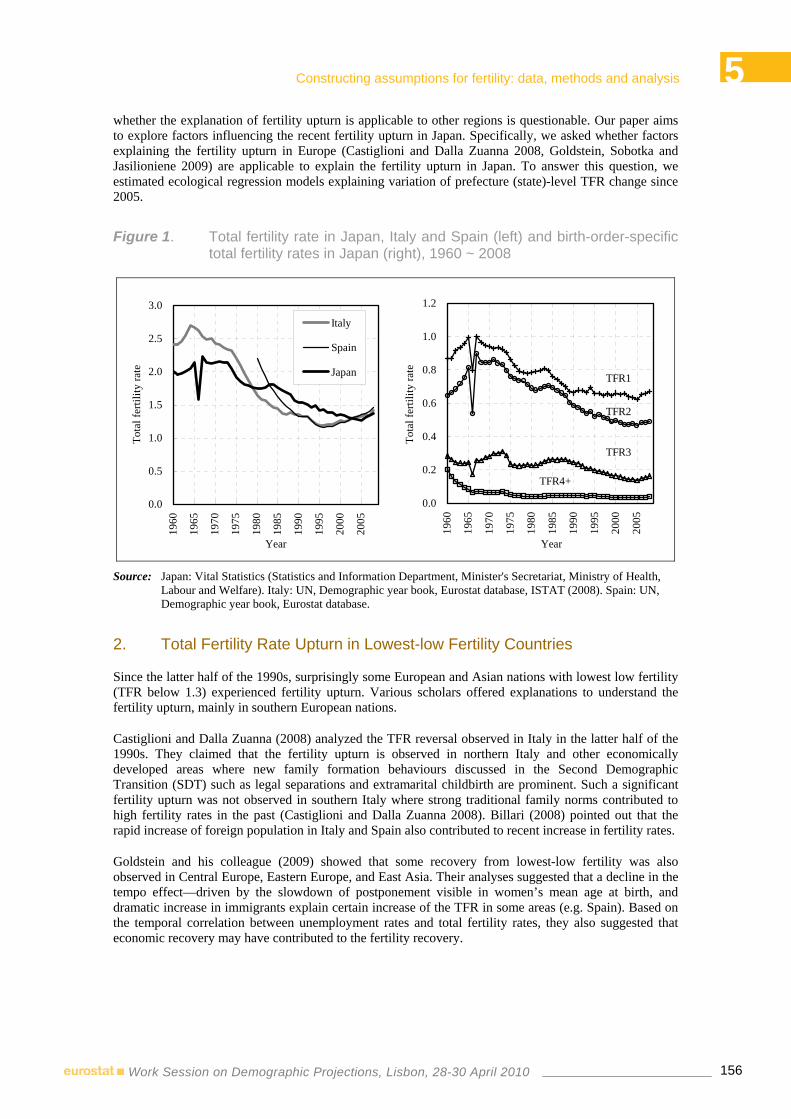
5 Constructing assumptions for fertility: data, methods and analysis
156Work Session on Demographic Projections, Lisbon, 28-30 April 2010
whether the explanation of fertility upturn is applicable to other regions is questionable. Our paper aims to explore factors influencing the recent fertility upturn in Japan. Specifically, we asked whether factors explaining the fertility upturn in Europe (Castiglioni and Dalla Zuanna 2008, Goldstein, Sobotka and Jasilioniene 2009) are applicable to explain the fertility upturn in Japan. To answer this question, we estimated ecological regression models explaining variation of prefecture (state)-level TFR change since 2005.
Figure 1. Total fertility rate in Japan, Italy and Spain (left) and birth-order-specific total fertility rates in Japan (right), 1960 ~ 2008
0.0
0.5
1.0
1.5
2.0
2.5
3.0
1960
1965
1970
1975
1980
1985
1990
1995
2000
2005
Year
Tota
l fer
tility
rate
Italy
Spain
Japan
0.0
0.2
0.4
0.6
0.8
1.0
1.2
1960
1965
1970
1975
1980
1985
1990
1995
2000
2005
Year
Tota
l fer
tility
rate
TFR3
TFR1
TFR2
TFR4+
Source: Japan: Vital Statistics (Statistics and Information Department, Minister's Secretariat, Ministry of Health,
Labour and Welfare). Italy: UN, Demographic year book, Eurostat database, ISTAT (2008). Spain: UN, Demographic year book, Eurostat database.
2. Total Fertility Rate Upturn in Lowest-low Fertility Countries
Since the latter half of the 1990s, surprisingly some European and Asian nations with lowest low fertility (TFR below 1.3) experienced fertility upturn. Various scholars offered explanations to understand the fertility upturn, mainly in southern European nations.
Castiglioni and Dalla Zuanna (2008) analyzed the TFR reversal observed in Italy in the latter half of the 1990s. They claimed that the fertility upturn is observed in northern Italy and other economically developed areas where new family formation behaviours discussed in the Second Demographic Transition (SDT) such as legal separations and extramarital childbirth are prominent. Such a significant fertility upturn was not observed in southern Italy where strong traditional family norms contributed to high fertility rates in the past (Castiglioni and Dalla Zuanna 2008). Billari (2008) pointed out that the rapid increase of foreign population in Italy and Spain also contributed to recent increase in fertility rates.
Goldstein and his colleague (2009) showed that some recovery from lowest-low fertility was also observed in Central Europe, Eastern Europe, and East Asia. Their analyses suggested that a decline in the tempo effect—driven by the slowdown of postponement visible in women’s mean age at birth, and dramatic increase in immigrants explain certain increase of the TFR in some areas (e.g. Spain). Based on the temporal correlation between unemployment rates and total fertility rates, they also suggested that economic recovery may have contributed to the fertility recovery.

5 Constructing assumptions for fertility: data, methods and analysis
157Work Session on Demographic Projections, Lisbon, 28-30 April 2010
Although further studies are necessary, they concluded that expansion of work and family reconciliation policies is likely to lead to recovery of fertility rates (Goldstein, Sobotka and Jasilioniene 2009).
In our study, we focus on the factors Goldstein and his colleagues used to explain fertility upturn in their cross-national study. They are: (1) diminishing tempo effects, (2) increase in foreigners, (3) economic improvement, and (4) policy improvement on work and family reconciliation. In addition, we also looked at the influence of family culture. The study by Castiglionin and Dalla Zuanna (2008) suggested the association between fertility decline and family culture where traditional gender norms are emphasized. Since Japan shares the similar family culture with Italy where families play a central role in caring for their family members rather than relying on public services, we find it important to include it as an additional factor to explain variation in fertility change in Japan.
Besides the fact that most studies have focused on studying fertility upturn in Western European nations, there are several advantages in studying fertility upturn in Japan in terms of the data quality. First, official register-based statistics maintained in time-series are available from prefectural-level data sources. Second, since immigration controls in Japan are relatively reliable, highly accurate data set is available on international migration. Moreover, racial diversification is relatively small compared with other industrialized nations. In fact, foreign national including immigrants count for 1.4 percent of the total population in 2008, which allows for simple models that does not take into account racial heterogeneity.
3. Method
We estimate weighted least squares models (WLS) and weighted spatial error models (WSE), and select the more appropriate model for explaining prefecture-level variation in TFR change.
The unit of our analysis is geographically associated aggregated data. Geographically referenced data often show spatial autocorrelation. Spatial autocorrelation refers to a situation in which values on a variable of interest are systematically related to geographic location. Thus, if an ordinary least-square regression model that assumes the error terms to be independently, identically, and normally distributed is used without taking the existence of spatial autocorrelation among residuals, the standard errors of the regression coefficient estimates can be underestimated or overestimated (Chi and Zhu 2008).
For this reason, our study not only estimates an ordinary least squared model but also estimates a spatial error model which explicitly models spatial autocorrelation of such error terms, and select the more appropriate model in terms of model fitness and significance of the spatial autoregressive coefficients of the models. A spatial error model is specified as follows (Anselin 1988, Ward and Gleditsch 2008):
( )INWuu
uXy
2,0~,
,
σεελ
β+=
+=
where y is a (n x 1) vector representing the dependent variables, X is a (n x k) matrix representing the k-1 independent variables, β is a (k x 1) vector of regression parameters to be estimated, u is a (n x 1) vector of error terms presumed to have a covariance structure as given in the second equation, λ is a spatial autoregressive coefficient to be estimated, W is a (n x n) weight matrix defining the “neighbourhood” structure that reflects the potential interaction between neighbouring locations and zeros out pairs of locations for which spatial correlation is ruled out a priori, and ε is a (n x 1) vector of independently distributed (spatially uncorrelated) errors (i.i.d.). We used a first-order queen convention to define neighbours for the weight matrix used in estimating spatial regression model.
In Japan, population size varies significantly among prefectures. For example, the population of Tokyo is 12 million, by contrast Tottori prefecture has only 600, 000 citizens, approximately a twentieth of the population in Tokyo. Since the variables we use, which will be mentioned in the next section, are mostly related to behaviours among women of reproductive ages, we used female population in reproductive ages (15 – 49 years of age) in each prefecture for weights.

5 Constructing assumptions for fertility: data, methods and analysis
158Work Session on Demographic Projections, Lisbon, 28-30 April 2010
We used “spdep” package in the open source programming language R for model estimations. The selected model is used to examine the association between explanatory variables and fertility upturn by predicting the national values in fertility change after 2005 and showing the contribution of each factor to fertility increase.
4. Data and Variables
For the dependent variables, the change of all-birth TFR and the change in birth-order-specific TFR by prefecture from 2005 to 2008 are used.
For the explanatory variables, we used four factors Goldstein and his colleagues (2009) focused on to explain fertility upturn in their cross-national study (diminishing tempo effects, increase in foreigners, economic improvement, and policy improvement on work and family reconciliation) and also used a contextual factor reflecting family culture.
4.1 Diminishing Tempo Effect: Change in Late Fertility Tempo effects are caused by postponement of childbearing. If the postponement trend visible in women’s mean age at birth stops, the tempo effects observed in the past are expected to diminish. Under this circumstance, women who postponed childbearing in their 20s start to catch up in their 30s or later. Thus we expect that diminishing tempo effects would be accompanied by fertility increase in the 30s.
In our study, diminishing tempo effect was measured as increase in “late fertility.” For simplicity, we assume that late fertility accounts for approximately 20% of the total. Late fertility is thus defined as fertility at 35 years old or over for all births (which accounts for 18.1% of the total fertility rate as of 2008), 33 years old or over for the first births (20.6%), 35 years of age or over for the second births (20.2%), 36 years old or over for the third births (22.6%), and 38 years old or over for the fourth and higher-order births (22.4%) (see Figure 2). For the variable, we used the change in fertility rate limited to these ages from 2005 to 2008.
Figure 2. All birth and birth order-specific age-specific birth rates - 2002, 2005, 2008
0.00
0.02
0.04
0.06
0.08
0.10
0.12
15 20 25 30 35 40 45 50Age
Ferti
lity
rate
TFR 2002TFR 2005
TFR 2008
All birth
Late fertility
0
0.01
0.02
0.03
0.04
0.05
0.06
0.07
15 20 25 30 35 40 45 50Age
Ferti
lity
rate
1st birth
2nd birth
3rd birth
4th+ birth
Late fertility
Source: Vital Statistics (Statistics and Information Department, Minister's Secretariat, Ministry of Health, Labour
and Welfare).

5 Constructing assumptions for fertility: data, methods and analysis
159Work Session on Demographic Projections, Lisbon, 28-30 April 2010
4.2 Increase in Foreigners: Change in Fertility Rate by Foreign Mothers The period TFR provided officially by the Ministry of Health, Labour and Welfare are calculated for new born children with Japanese nationality. The calculation does not include children born to foreign couples living in Japan but includes children whose mothers are foreign who married to Japanese men4, because these children have Japanese nationality. Nonetheless, the female population used as the denominator is limited to Japanese women, and their foreign mothers are not included5. This invites an increase of the total fertility rate through a structural factor of an increasing number of foreign women giving birth to Japanese children, even if the actual fertility of Japanese women remains unchanged.
In Japan, the percentage of international marriages has been increasing from the late 1990s. The percentage of marriages where wives are foreign accounts for 2.8% of total number of marriages in 1990, which increased to 4.6% in 2005. Since the female population used as the denominator is limited to Japanese women, an increasing number of foreign women giving birth to Japanese children may be causing recent fertility upturn. In other words, we expect prefectures where increase in foreign mothers is observed to be positively associated with fertility change.
In our study, the influence of increase in foreign mothers is measured as change in TFR “inflated” by foreign mothers. Specifically, we use change from 2005 to 2008 in TFR contributed by foreign mothers (TFR x percentage of births born to foreign mothers)6.
4.3 Economic Improvement: Change in Employment Rate In Japan, the unemployment rate has been falling since around 2004. Since it was followed by upturn in TFR, improvement in economic condition is likely to play a role in the recovery of the fertility rate. In other words, the association between prefectures with economic improvement and fertility change is expected to be positive.
In our study, using the Labour Force Survey, economic improvement was measured by change in employment rate (complementary number of the unemployment rate) by prefecture. Since there expected to be a time lag for the recovery from unfavourable economic conditions to influence fertility, we looked at change in employment rate from 2002 to 2007.
4.4 Policies on Work and Family Reconciliation: Change in Labour Force Participation Rate among Mothers having Preschool Children Living in Nuclear Family
Family policies variation across space can help us study the effect of such policies on fertility (Neyer and Anderson 2008). Japanese government has been promoting the work and family reconciliation programs as part of policy initiatives aiming to stimulate higher fertility since 2000 as represented by “New Angel Plan” (Ogawa 2003, Moriizumi 2008)7. From 2005 to 2009, the “Children and Childcare Plan” was established, instead of the “New Angel Plan.”
4 In Japan, nationality is difficult to receive even foreign mothers married to Japanese men. 5 Definition of total fertility rate in the Vital Statistics is as follows: Total fertility rate = Sum for ages (15-49) [(Number of births born to Japanese mothers) + (Number of children with Japanese
nationality born to foreign mothers*)]/ (Population of Japanese females). *This refers to a child whose father has Japanese nationality.
6 Since the number of births by mother’s nationality is not available by birth order, we used the percentage of births born to foreign mothers out of the total number for the birth-order specific TFR as well.
7 In addition to the “New Angel Plan” in 2000 to 2004 (reinforcement of child-rearing services, improvement of employment environment for reconciliation of work and family life, correction of corporate climate whereby gender division of labour and priority on workplace are taken for granted), the Zero Children on Waiting List Strategy was started in 2001 for the purpose of building up sufficient child-care centers. In 2003, the Law for Measures to Support the Development of the Next Generation (promotion of concentrated and systematic measures of 10 years by municipalities and corporations) was formulated.

5 Constructing assumptions for fertility: data, methods and analysis
160Work Session on Demographic Projections, Lisbon, 28-30 April 2010
There are improvements in the benefits of child-care leave and implementation of the After-school Childcare plan (securing places of activity for children after school in all elementary school zones).
In 2007, the “Action Agenda for Promoting Work-life Balance” was resolved as a priority task of the “Strategies for Japan to Support Children and Families.” More importantly, after 2005, each municipality is obliged to take its own measures according to its action plans based on the Law for Measures to Support the Development of the Next Generation. This might have caused differences in the progress of policies of reconciliation of work and family life depending on the region. In other words, we expect to see a positive effect on prefectures with better family policies on fertility upturn since more women will give a birth in areas where they have more supportive policies for women to balance between work and family.
There are no established measurement for the effectiveness of policies on family and work. In our study, we measured the effectiveness of policies on family and work by the change in the employment rate of mothers. Improvement in public services and corporations regarding reconciliation of work and family life are considered to bring about larger effects among mothers of nuclear families who cannot easily receive support from relatives such as grandmothers/fathers. Thus we focus on mothers of nuclear families with children under 6 years of age. We use the change in their employment rate between 2002 and 2007, obtained from the Employment Status Surveys for each prefecture conducted in 2002 and 2007.
4.5 Family culture: Proportion of extended families among households including pre-school children
As in Italy, there are regional differences in family systems in Japan. Ohbayashi (1996) classified the regionality of social organizations, and claimed that paternalistic family organizations played important decision-making roles in northern part of Japan (Tohoku Region) (Ohbayashi 1996). On the other hand, in western Kyushu, coastal Shikoku, Hokuriku, and coastal Tokai, the village organizations had more important decision-making roles than family organizations (Ohbayashi 1996). Therefore, there are variations in family culture across regions as in Italy. According to Kato (2008), pattern of living arrangement reflects the strength of family culture. In eastern regions with strong family culture, historically an older couple (parents) and a younger couple (son and daughter-in-law) co-reside in a single household. In contract, in western Japan, a parent couple lives in an independent household from children’s family, usually on the same lot.
In our study, we measured strength of family culture by the prevalence of extended family households. Based on the 2005 census, we calculated the proportion of the extended family among households including children of less than six years of age in each prefecture. As such a characteristic does not change in the short term, we include it in our model as a fixed effect. We expect to see negative relationship between prefectures with strong family culture and fertility change as in the case of Italy.
4.6 Model The model used to examine each effect of elimination of tempo effects, inflation by foreign mothers, economic improvement, policies on work and family reconciliation, and family culture can be expressed as follows. Δ represents difference.
ΔTFR (2005-2008) = Constant
+ Δ Late fertility (2005-2008) + ΔTFR inflated by foreign mothers (2005-2008) + Δ Employment rate (2002-2007) + Δ Labour force participation rate among mothers having preschool children
living in a nuclear family (2002-2007) + Proportion of extended families among households including preschool
children (fixed effect) (2005)

5 Constructing assumptions for fertility: data, methods and analysis
161Work Session on Demographic Projections, Lisbon, 28-30 April 2010
We fit this model to the data for all-birth TFR and birth-order specific TFR using weighted least squares regression (WLS) and weighted spatial error regression (WSE).
5. Results
5.1 Descriptive statistics Table 1 shows descriptive statistics of variables we used in the analysis. The values of Moran's I8 suggest that all of the dependent variables are spatially auto-correlated. For explanatory variables, the following factors showed significant spatial autocorrelation: change of late fertility for all-birth fertility, first birth fertility and fourth and higher-order fertility, change of fertility inflated by foreign mothers for all-birth and all birth-order-specific births, change of employment rate, and proportion of extended family.
Table 1. Descriptive statistics for variables used in the analyses
Change in TFR All birth 2005-08 Vital Statistics 3) 0.1069 0.1051 0.0089 0.1628 0.343 ***
1st birth 2005-08 Vital Statistics 3) 0.0472 0.0470 -0.0275 0.0818 0.304 **
2nd birth 2005-08 Vital Statistics 3) 0.0291 0.0281 -0.0186 0.0470 0.252 **
3rd birth 2005-08 Vital Statistics 3) 0.0242 0.0237 -0.0116 0.0429 0.136 #
4th + birth 2005-08 Vital Statistics 3) 0.0064 0.0063 0.0003 0.0182 0.494 ***
Change in late fertility age 35+ All birth 2005-08 Vital Statistics 3) 0.0459 0.0435 0.0108 0.0575 0.189 *
age 33+ 1st birth 2005-08 Vital Statistics 3) 0.0248 0.0234 0.0087 0.0350 0.427 ***
age 35+ 2nd birth 2005-08 Vital Statistics 3) 0.0190 0.0180 0.0054 0.0269 0.006
age 36+ 3rd birth 2005-08 Vital Statistics 3) 0.0056 0.0069 -0.0006 0.0126 0.003
age 38+ 4th + birth 2005-08 Vital Statistics 3) 0.0011 0.0011 -0.0036 0.0037 0.222 *
All birth 2005-08 Vital Statistics 3) 0.0020 0.0019 -0.0047 0.0085 0.406 ***
1st birth 2005-08 Vital Statistics 3) 0.0009 0.0009 -0.0024 0.0042 0.422 ***
2nd birth 2005-08 Vital Statistics 3) 0.0006 0.0006 -0.0020 0.0029 0.383 ***
3rd birth 2005-08 Vital Statistics 3) 0.0004 0.0003 -0.0005 0.0011 0.329 ***
4th + birth 2005-08 Vital Statistics 3) 0.0001 0.0001 -0.0001 0.0003 0.368 ***
2002-07Labour Force
Surveys4) 0.0150 0.0155 -0.0010 0.0270 0.284 **
1) 2002-07Employment
Status Surveys4) 0.0554 0.0556 -0.0066 0.1636 -0.051
2) 2005 Census 4) 0.1878 0.1839 0.0789 0.5011 0.379 ***
*** p<.001 ** p<.01 * p<.05 # p<.11) For mothers of in nuclear families 2) For households including preschool children3) Statistics and Information Department, Minister's Secretariat, Ministry of Health, Labour and Welfare4) Statistics Bureau, Ministry of Internal Affairs and Communications5) Reproductive age female population (15-49) in 2005 is used as a weight.
Proportion of extended families
Change in TFR inflated by non-Japanesemothers
Max
Expl
anat
ory
vari
able
sD
epen
dent
var
iabl
es
Change in employment rate
Change in labor force participation rate among mothershaving preschool children
Spatial autocorrelation
Moran's I 5 )
VariablePeriod ofchange
Prefecture-level data (N=47)Source
National-levelvalue
WeightedMean5) Min
8 Moran's I statistic measures the degree of linear association between an attribute (y) at a given location and the weighted
average of the attitude at its neighbouring locations (Wy), and can be interpreted as the slope of the regression of (Wy) on (y) (Cliff and Ord 1973, Moran 1950). As for the spatial weight matrix to specify a neighbourhood structure, we use queen's case contiguity weight matrix of order one, as well as for the spatial regression analyses.

5 Constructing assumptions for fertility: data, methods and analysis
162Work Session on Demographic Projections, Lisbon, 28-30 April 2010
5.2 Model estimations Weighted least squares (WLS) models and weighted spatial error (WSE) models are estimated for all-birth and birth-order specific TFR (first, second, third, and fourth and higher-order births). Model coefficients and diagnosis for spatial autocorrelation among model residuals are shown in Table 2 (first, second, and third birth model only).
For change in the first-order TFR, the following four variables were significant in both WLS and WSE models: changes in late fertility (+), fertility inflated by foreign mothers (+), employment rate (+), and mothers' employment rate (+).The directions of the effect of late fertility rate, fertility rate inflated by foreign mothers, and employment rate were expected. However, the change of mothers' employment rate had unexpected negative effect. The constant is negative, but insignificant suggesting that there was no common effect.
For change in the second-order TFR, the late fertility rate (+), change of fertility rate inflated by foreign mothers (+), and proportion of extended families (-) are statistically significant in both WLS and WSE models. The direction of each coefficient is as we expected. The constant is positive, but insignificant.
For change in the third-order TFR, the effects of change in late fertility rate (+) and proportion of extended families (+) are statistically significant in both WLS and WSE models. Unlike second-order TFR, the effect of the proportion of extended families is positive, which implies that prefectures with higher proportion of extended families have higher increase in third birth fertility. The constant is positive and significant, suggesting overall common positive effect regardless of explanatory variables.
As for the fourth and higher-order birth model, the effects of changes of late fertility (+), fertility inflated by foreign mothers (+), and mothers' employment rate (-) are statistically significant factors. As in the case of third birth, the proportion of extended families are positive and statistically significant. The constant is also positive and significant.
For change in the TFR for all births, the effects of changes in late fertility (+), fertility inflated by foreign mothers (+), and mothers' employment rate (-), and the proportion of extended families (-) are statistically significant. Although the constant is positive, it is not significant.
According to the Lagrange Multiplier test for spatial autocorrelation, as for the first and third birth models, the WLS models fit better than the WSE models; for all-birth, second birth, and fourth and higher-order birth models, the WSE models specifying autocorrelation among residual of neighbouring prefectures fit better than the WLS models (see Table 2).

5
163
Table 2. Coefficients of regression models of change in total fertility rates: first, second and third birth
Variable
β β ' Std.error β β ' Std.
error β β ' Std.error β β ' Std.
error β β ' Std.error β β ' Std.
errorConstant -0.01 0.01 -0.01 0.01 0.01 0.01 0.01 0.01 0.01 0.01 * 0.01 0.00 **
Change in late fertility 1) 1.95 0.52 0.35 *** 2.03 0.54 0.34 *** 0.90 0.31 0.36 * 1.02 0.35 0.28 *** 1.75 0.52 0.47 *** 1.42 0.42 0.43 **
Change in TFR inflated by non-Japanesemothers 5.61 0.29 1.76 ** 5.70 0.29 1.69 *** 5.74 0.39 1.41 *** 6.86 0.46 1.27 *** 3.00 0.10 3.59 5.67 0.19 3.57
Change in employment rate 0.78 0.18 0.35 * 0.81 0.18 0.34 * 0.18 0.07 0.22 0.13 0.05 0.20 -0.03 -0.02 0.20 -0.01 -0.01 0.20
Change in labor force participation rateamong mothers having preschool children -0.16 -0.22 0.07 * -0.16 -0.22 0.06 ** -0.01 -0.02 0.04 -0.02 -0.06 0.03 -0.04 -0.15 0.04 -0.02 -0.06 0.03
Proportion of extended families 2) -0.02 -0.07 0.02 -0.02 -0.07 0.02 -0.03 -0.25 0.01 * -0.03 -0.25 0.01 ** 0.02 0.26 0.01 # 0.02 0.23 0.01 #
Lambda (spatial autoregressive coefficient) 0.15 0.43 0.25Likelihood Ratio Test (H0: Lambda =0) 0.62 11.30 *** 1.02R-squared 0.80 0.68 0.34Adjusted R-squared 0.78 0.64 0.26AIC -259.2 -257.8 -304.6 -313.9 -311.0 -310.0N 47 47 47 47 47 47Diagnostics for spatial autocorrelation
Moran's I (residuals) 0.10 # 0.05 0.36 *** -0.03 0.10 # -0.05
LM (error) 1.08 8.02 ** 0.31LM (lag) 0.00 0.28 1.08Robust LM (error) 1.24 7.81 ** 0.08Robust LM (lag) 0.16 0.08 0.86LM (SARMA) 1.25 8.10 * 1.17
*** p<.001 ** p<.01 * p<.05 # p<.1β represents a coefficient and β' represents a standardized coefficient.
2) Centered values are used.
1) For 1st birth model, late fertility rate represents fertility rates over age 33, for 2nd birth model, fertility rates over age 35, and for 3rd birth model, fertility rates over age 36.
Weighted spatial errormodel
Lagrange multiplier diagnostics for spatialautocorrelation
Change in 1st birth TFR Change in 3rd birth TFRChange in 2nd birth TFR
Weighted least squares Weighted spatial errormodel Weighted least squaresWeighted least squares Weighted spatial error
model

5 Constructing assumptions for mortality: data, methods and analysis
164Work Session on Demographic Projections, Lisbon, 28-30 April 2010
5.3 Contribution of each factor to national TFR increase Based on the regression coefficients estimated by the well-fit model, the contribution of each explanatory variable is summarized in Table 3. The increase of the national TFR from 2005 to 2008 can be decomposed into each contribution of factors using the model estimated. Estimating the in-crease using the national figure of each variable, the change of late fertility accounted for 98% of the increase in first-order TFR, and the increase of fertility inflated by foreign mothers accounted for 11%. The increase of employment rate explained 24%. Contrary to our expectation, the increase of employment rate of mothers with preschool children accounted for decrease in the TFR by 18%. It also shows 15% decrease as a common effect regardless of the change of each factor (see Table 3).
As for second-order TFR, in addition to the 20% common effect, the increase of late fertility accounted for 64% and increase in fertility inflated by foreign mothers accounted for 14%. Contribution of employment rate and mothers' employment rate were 7% and -4%, respectively.
As for third-order TFR, the contribution of the common effect that cannot be explained by factors examined here is as high as 62%. The increase of late fertility explains 45% and fertility inflated by foreign mothers explains 5% of the increase in third-order TFR. Employment rate and mothers' employment rate were -2% and -10%, respectively.
As for fourth and higher-order birth TFR, the common effect is as high as 98%, indicating that there are important factors not examined here. The increase of late fertility accounts for 16% and fertility inflation contributed by foreign mothers accounts for 23% of the increase in fourth and higher-order TFR. Employment rate and mothers' employment rate accounts for -22% and -15%, respectively.
Based on these, we found19% of increase in all birth TFR is accounted by the common effect, 72% by the change in later fertility, 11% by the change in fertility contributed by foreign mothers, 11% by the change in employment rate, and -12% by the change of mothers' employment rate.
Table 3. Decomposition of change in total fertility rate in Japan from 2005 to 2008
1st birth TFR 2nd birth TFR 3rd birth TFR 4th+ birth TFR All birth TFR All birth TFR(1) (2) (3) (4) (1)+(2)+(3)+(4)
TFR in 2005 0.62404 0.46433 0.13935 0.03238 1.26010 1.26010TFR in 2008 0.67124 0.49340 0.16354 0.03879 1.36697 1.36697
Change from 2005 to 2008 0.04720 0.02907 0.02420 0.00641 0.10687 0.10687Decomposition
Common effect -0.00710 0.00566 0.01489 0.00629 0.02068 0.01975
Change in late fertility(Declining tempo effect)
0.04644 0.01866 0.01092 0.00101 0.07274 0.07703
Change in TFR inflated by non-Japanese mothers(Contribution of immigration)
0.00494 0.00403 0.00127 0.00147 0.01128 0.01170
Change in employment rate(Ecomonic improvement)
0.01125 0.00193 -0.00056 -0.00140 0.01174 0.01121
Change in maternal LFP(Policy improvement on work/family reconciliation)
-0.00832 -0.00120 -0.00233 -0.00096 -0.00957 -0.01282
Contribution (%)Common effect -15.0 19.5 61.5 98.2 19.4 18.5 Change in late fertility 98.4 64.2 45.1 15.8 68.1 72.1 Change in TFR inflated by non-Japanese mothers 10.5 13.9 5.2 22.9 10.6 11.0 Change in employment rate 23.8 6.6 -2.3 -21.9 11.0 10.5 Change in maternal LFP -17.6 -4.1 -9.6 -15.0 -9.0 -12.0
Model used for predictions Weighted LSWeighted
spatial errormodel
Weighted LSWeighted
spatial errormodel
Weightedspatial error
model-
5 Constructing assumptions for mortality: data, methods and analysis
165Work Session on Demographic Projections, Lisbon, 28-30 April 2010
Based on the regression coefficients and the correlation coefficients between explanatory variables and the dependent variable, we obtain the variance explained by the explanatory variables. For the all-birth TFR, late fertility rate explains approximately 33% of total variance on fertility change, 28 % by fertility inflated by foreign mothers, 5% by employment rate, 3% by mothers' employment rate, and 10 % by proportion of extended families (all explanatory variables explain 79% of total variance). The result suggest that demographic factors such as late fertility rate and fertility inflated by foreign mothers account for approximately 60% of the variation in change, the fixed effect of the proportion of extended families explains 10%, and economic improvement and policies on work and family reconciliation explain 5% and 3% of the variation, respectively. The remaining 20% of the variation is explained by other factors not included in our study.
6. Discussions
The goal of this study was to explore the explanations for the TFR upturn after 2005 in Japan, one of the “lowest low fertility” countries. We focused on the following factors based on previous studies in Europe: (1) diminishing tempo effect, (2) increase in foreigners, (3) economic improvement, and (4) policies initiative on work and family reconciliation, and (5) family culture. We estimated models to explain the prefecture-level variation of change in TFR from the variation of the relevant variables (change in late fertility, change in fertility contributed by foreign mothers, change in employment rate, change in maternal employment rate, and the proportion of extended family house-holds).
The factors such as change in late fertility, change in fertility contributed by foreign mothers, and change in employment rate are positively associated with TFR change as we expected. The improving in employment rate of mothers with preschool children living in nuclear families, however, shows a negative relationship to the change in TFR. This suggests that the level of TFR has in-creased much in the area where the change in mothers' employment rate is smaller than other areas. The result suggests continuing difficulty for a working mother with children to have another child. Conversely, we may need to take into consideration the recent state of day-care centres in urban areas. The areas where TFR has increased since 2005 include prefectures including large metropolitan areas such as Tokyo, Kanagawa, and Miyagi. In these prefectures, the proportion of children on the waiting lists of day-care centres among all preschool children has significantly increased dramatically since 2006. It is speculated that there was an increase in the number of mothers who decided to have children hoping to raise children while working, but dropped out of the labour market because there were no vacancies at day-care centres. Therefore, if the shortage of day-care services in these areas can be resolved, it will not only reduce the number of children on waiting lists but also in-crease the employment rate of mothers from the present level so that potential jobseekers can be employed.
Whatever the case, as Neyer and Andersson (2008) suggested that, macro-analytical investigations based on aggregate indicators are considered to be insufficient to examine the impact of family policies on fertility, since macro indicators do not take fertility-relevant structuring effects of family policies into account and cannot reveal group-specific effects. Thus we need to have research de-signs and methods that enable us to grasp the impact of family policies on individual behaviour for a clearer assessment.
Other than short-term variable factors such as tempo effect, immigrant mother effect, economic effect, and policy effect above, 19% increase in TFR between 2005 and 2008 is estimated by the constant term of the model. However, these factors are not statistically significant in the all-birth model, although significantly in third birth and fourth and higher-order birth models. This is thought to be a common nationwide positive effect regardless of prefecture specific factors. It is possible that the idea that childbearing should be supported by society has been widely accepted and it encouraged the younger generations to have many children. If nationwide economic recovery is included in the common effect, the impact of a economic recession after 2008 could be larger than 0.01 reflecting only economic variation between prefectures.
Lastly, the proportion of extended families used as an indicator of family culture showed a negative impact in the all-birth and second birth models as in the case of Italy. Namely, the recent recovery of the fertility rate is weaker in areas such as the Tohoku region where strong family attitude remain strong.

5 Constructing assumptions for mortality: data, methods and analysis
166Work Session on Demographic Projections, Lisbon, 28-30 April 2010
Conversely, our results suggest that parenting has become easier even in urban areas where family culture is relatively weak. In these areas, conditions favourable to family formation other than family support may be established. Since proportion of extended families shows positive impact in third and higher-order birth models, economic or physical support from co-residing grandparents may play important roles even today.
In Japan, part of the TFR upturn since 2005 can be explained by short-term conditional change such as an increase in international marriages and economic recovery. Therefore, it is possible that the TFR will decline again in the near future. On the other hand, an increase in late fertility accounts for as much as 70% of the change in our analysis, suggesting there may be a moderate increase in TFR due to the elimination of the tempo effect for some time. However, whether such a catch-up behaviour is followed by subsequent generations depends on whether women in their 30s who finally had children can continue to work as they expected. Problems such as a recent increase of children on the waiting lists of day-care centres in metropolitan areas and “ikugyu-giri (firing due to taking parental leave)”, which came to the surface in the economic recession since 2008, may negatively influence the TFR through increasing pessimistic views on working conditions for mothers. While urgent countermeasures are called for, it is necessary to carefully monitor the uptake of policies on work and family reconciliation when we foresee future trends of fertility.
References
Anselin, L. (1988). Spatial econometrics: Methods and models. Dordrecht, the Netherlands: Kluwer Academic Pub.
Billari, F.C. (2008). Lowest-low fertility in Europe: Exploring the causes and finding some surprises. The Japanese Journal of Population 6(1):2-18.
Billari, F.C.and Kohler, H.P.(2004). Patterns of low and lowest-low fertility in Europe. Population Studies 58(2):161-176.
Bongaarts, J. and Feeney, G. (1998). On the quantum and tempo of fertility. Population and Development Review 24(2):271-291.
Bongaarts, J. (2001). Fertility and reproductive preferences in post-transitional societies. Population and Develop-ment Review 27 Supplement: Global Fertility Transition: 260-281.
Bongaarts, J. (2002). The end of the fertility transition in the developed world. Population and Development Review 28(3):419-443.
Blossfeld, H.-P., Klijzing, E., Mills, M., and Kurz, K. (2005). Globalisation, uncertainty, and youth in society. Lon-don: Routledge.
Chi, G.and J. Zhu. 2008. “Spatial regression models for demographic analysis.” Population Research and Policy Re-view 27(1):17-42.
Castiglioni, M. and Dalla Zuanna, G. (2008). Marital and reproductive behavior in Italy after 1995: Bridging the gap with Western Europe? European Journal of Population 25:1-26.
Caltabiano, M., Castiglioni, M., and Rosina, A. (2009). Lowest-low fertility: Signs of a recovery in Italy? Demo-graphic Research 21(23):681-718.
Cliff, A.D. and Ord,J.K. (1981). Spatial processes: Models and applications. London, England: Pion Ltd.
Goldstein,J.R., Sobotka,T., and Jasilioniene, A. (2009). The end of ‘Lowest-Low’ fertility? Paper presented at the an-nual meeting of Population Association of America, Detroit, USA, April 30 – May 2 2009.

5 Constructing assumptions for mortality: data, methods and analysis
167Work Session on Demographic Projections, Lisbon, 28-30 April 2010
ISTAT (2008). Indicatori demografici anno 2008 [electronic resource]. Rome: ISTAT. http://www.demo.istat.it/altridati/indicatori/index_e.html
Katō, A. (2008). Kazoku kozo to jinko gensyo no chiikisei. Paper presented at the annual meeting of Population Asso-ciation of Japan. Tokyo, Japan, June 7-8 2008. (in Japanese)
Kohler, H.-P., Billari, F.C., and Ortega, J.A. (2002). The Emergence of lowest-low fertility in Europe during the 1990s. Population and Development Review 28(4): 641-680.
Ministry of Health, Labour and Welfare. (2006). Hesei 18 nenban Rodo keizai no bunseki. (in Japanese)
Ministry of Health, Labour and Welfare. (2009). Hesei 21 nen Jinkodotai tokei no nenkan suikei (Estimates for Vital Statistics of Japan, 2009). (in Japanese)
Moran, P.A.P.(1950). Notes on continuous stochastic phenomena. Biometrika 37:17-23.
Moriizumi, R. (2008). Shorai jinko suikei no kokusai hikaku: Nihon to Syuyosenshinkoku no jinko no yukue. Jinko Mondai Kenkyu 64(3):45-69. (in Japanese)
Moriizumi, R. (2008). Jisedai ikusei shien taisaku. In: Kanekiyo, H. and Anzo, S. (eds.) Jinkogensyojidai no syakai-hosyo. Tokyo: Harasyobo: 119-151. (in Japanese)
National Institute of Population and Social Security Research (2007a). Nihon no Syorai Suikei Jinko (Population Projection for Japan: 2006-2055), Tokyo: Kosei Tokei Kyokai.
National Institute of Population and Social Security Research (2007b). The 13th National Fertility Survey (Kekkon to Syussan ni Kansuru Zenkoku Chosa) Dai I Hokokusyo, Waga-kuni Fufu no Kekkon-Katei to Syussyoryoku, Chosa Kenkyu Hokoku Shiryo, No.23, Tokyo: Kosei Tokei Kyokai.
National Institute of Population and Social Security Research (2007c). The 13th National Fertility Survey (Kekkon to Syussan ni Kansuru Zenkoku Chosa) Dai II Hokokusyo, Waga-kuni Dokushin-so no Kekkon-Kan to Ka-zoku-Kan, Chosa Kenkyu Hokoku Shiryo, No.24, Tokyo: Kosei Tokei Kyokai.
Neyer, G. and Andersson, G. (2008). Consequences of family policies on childbearing behavior: effects or artifacts. Population and Development Review 34(4):699-724.
Ogawa, N. (2003). Japan’s changing fertility mechanisms and its policy responses. Journal of Population Research 20(1):89-106.
Ohbayashi, T. (1996). Syakaisoshiki no chiikiruikei. In: Kreiner, Y. (ed.) Chiikisei kara mita Nihon: Tagenteki rikai no tameni. Tokyo: Shinyosya: 13-37. (in Japanese)
United Nation. (1996). World Population Prospects: The 2008 Revision.
United Nation. (1998). World Population Prospects: The 2008 Revision.
United Nation. (2008). World Population Prospects: The 2008 Revision.
Ward, M.D. and Gleditsch, K.S. (2008). Spatial regression models. Los Angeles: Sage Publications.


Forecasting demographic components: Fertility Chair: Maria Filomena Mendes
Session 6

6 Forecasting demographic components: Fertility
171Work Session on Demographic Projections, Lisbon, 28-30 April 2010
A PROBABILISTIC VERSION OF THE UNITED NATIONS WORLD POPULATION PROSPECTS:
METHODOLOGICAL IMPROVEMENTS BY USING BAYESIAN FERTILITY AND MORTALITY
PROJECTIONS1,2
Gerhard K. HEILIG3, Thomas BUETTNER4, Nan LI5, Patrick GERLAND6, Francois PELLETIER7, Leontine ALKEMA8, Jennifer
CHUNN9, Hana ŠEVČÍKOVÁ10, Adrian E. RAFTERY11
1. Introduction
The Population Division of the Department of Economic and Social Affairs of the United Nations Secretariat produces the official United Nations population estimates and projections for all countries in the world. The set of estimates and projections revised every two years by the Population Division has become the standard input for monitoring population goals, preparing sectoral projections, modeling complex economic or environmental processes that depend on population trends and preparing development plans. The most recent set of population estimates and projections is the 2008 Revision of World Population Prospects.1
Every Revision of World Population Prospects prepared since 1980 has included several projection variants. The three most commonly considered are those that vary among themselves in the path that fertility levels will take in the future. The central path is embodied by the medium variant, which is used as the most indicative of what the future may hold. Starting with the 2002 Revision, future fertility change in the medium variant has been based on the past relationship observed between the change in total fertility over two consecutive five-year periods and the level of total fertility prevailing over the first of the two. That relationship was derived from the combined experience of all countries between 1950 and 2000. It therefore produced an overall declining trend in fertility. During the projection, reductions of total fertility were stopped when its level reached 1.85 children per woman. For countries that had a total fertility below 1.85 children per woman at the start of the projection period, an increasing fertility trend was projected using a different model.2
1 The views expressed in this paper are those of the authors and do not necessarily reflect the views of the United Nations. The
designations employed and the presentation of material in this paper do not imply the expression of any opinion whatsoever on the part of the United Nations concerning the legal status of any country, territory, city or area or of its authorities, or concerning the delimitation of its frontiers or boundaries. The research of Alkema, Chunn and Raftery was supported by NICHD grant R01 HD054511.
2 This paper has been edited by Hania Zlotnik. 3 Chief, Population Estimates and Projections Section, United Nations Population Division. e-mail: [email protected] 4 Chief of Population Branch, Deputy Director, United Nations Population Division. 5 Population Affairs Officer, Population Estimates and Projections Section, United Nations Population Division. 6 Population Affairs Officer, Population Estimates and Projections Section, United Nations Population Division. 7 Chief, Mortality Section, United Nations Population Division. 8 Assistant professor, Department of Statistics and Applied Probability, National University of Singapore. 9 Graduate Student, University of Washington. 10 Senior Research Scientist, Department of Computer Science & Engineering, University of Washington. 11 Blumstein-Jordan Professor of Statistics and Sociology at the University of Washington.

6 Forecasting demographic components: Fertility
172Work Session on Demographic Projections, Lisbon, 28-30 April 2010
Once the path of total fertility in the medium variant was established for each country, two other variants were used in projecting the population. Named the “low” and “high” variants, they differ from the medium variant by having a total fertility that is, in the low variant, half a child below and, in the high variant, half a child above the total fertility of the medium variant over most of the projection period. The range of variation of total fertility between the low and high variants is therefore insensitive to either the level of fertility a country has or its past trends. That relatively small variation of fertility was used to illustrate the importance of fertility trends for the future size and age structure of the population. The range of fertility variation between the low and the high variants, amounting to one child, is low by the standards of the past four decades, when many populations have experienced reductions of fertility amounting to 3 or 4 children. But, when fertility has already reached relatively low levels, the evidence suggests that sharp variations of more than one child have not been common. Nevertheless, the official population projections of the United Nations have not heretofore been prepared taking explicit account of past variability in outcomes because they have not incorporated a probabilistic approach to the analysis of past trends.
This paper summarizes the results of a recent effort by the Population Division to explore the use of a probabilistic approach for the production of population projections. The results presented here illustrate both the use of new methods to determine the future paths of total fertility and life expectancy and a comparison of the results obtained with the official population projections presented in World Population Prospects: The 2008 Revision. The probabilistic projections described here were prepared for illustrative purposes and are not yet a part of the official set produced by the Population Division.
2 Previous examples of work related to probabilistic population projections
The explicit incorporation of probabilistic models for the projection of the components of population growth has been developed by a number of researchers. In the 1980s, Keyfitz3 and Stoto4 focused on historical forecast errors. In the 1990s, Lutz and colleagues5, 6 used expert opinion to estimate future variability, while Lee and colleagues7, 8, 9 used time series analysis to project future population parameters determining fertility and mortality.
Existing probabilistic projections have been made for a single country,10, 11, 12, 13, 14 for a few countries,15 for a specific region (Europe)16 or for the major regions of the world to produce global projections.17, 18 No one has yet produced probabilistic projections for all countries in the world. By applying a Bayesian Hierarchical Model (BHM) to the estimates of fertility and life expectancy from the official United Nations population projections, the Population Division has prepared probabilistic population projections for all countries of the world.
3 A Bayesian approach to probabilistic population projections
The approach to the projection of total fertility and life expectancy used by the Population Division in preparing the official population projections of the United Nations is the starting point for the application of a Bayesian statistical approach developed by Alkema et al.19 and Chunn et al.20 at the University of Washington, in collaboration with staff of the Population Division.
3.1 The probabilistic projection of total fertility
The Bayesian model used to project total fertility has two components. The first is used to project fertility from levels well above replacement to a low level close to replacement level. Once this “turnaround level” is reached, a second model is used to project low fertility.
The first model starts from the bi-logistic function that had been fitted to total fertility data for most countries of the world over the period 1950-2000 to relate the change in total fertility between two consecutive five-year periods to the level that total fertility had over the first of those periods2 and that had been used to project fertility in the medium variant starting with the 2002 Revision. Whereas in the 2008 Revision that model of total fertility change had been applied to all countries with a single set of parameters, in the Bayesian approach estimates of the parameters of the bi-logistic function were made

6 Forecasting demographic components: Fertility
173Work Session on Demographic Projections, Lisbon, 28-30 April 2010
for each country using a hierarchical model. Each of the parameters of the model was drawn from a probability distribution representing the range of values that the parameter had taken across countries. Hence, for each country, the posterior distribution of the relevant parameters is determined by the experience of all countries combined as well as by the country’s own fertility decline up to the start of the projection period.
The second model takes the form of a first order autoregressive time series AR(1) model with a mean set at replacement level so that it produces random fluctuations of total fertility around that level.
To convert the projections of total fertility into the age-specific fertility rates required for the application of the component method of population projections, the country- and period-specific percentage distributions of total fertility by age used to produce the official United Nations population projections (2008 Revision) were also used in the preparation of the probabilistic projections.
3.2 The probabilistic projection of life expectancy
For the projection of future life expectancy, expected gains over a period are modeled as a function of current level with random variation added in. The Bayesian model is used to generate paths of future male life expectancy and female life expectancies are derived by assuming the same country-specific sex differentials in life expectancy as those embodied in the official United Nations population projections (2008 Revision).
To convert the projected levels of life expectancy to the age-specific mortality rates needed to project the population, the standard Lee-Carter method was used for periods before 2010 and for the future, a modified Lee-Carter method was used in which the time parameter was derived by fitting the trajectories of life expectancy at birth as projected by the Bayesian method.
In projecting life expectancy using the Bayesian approach, no explicit allowance was made for the specific impact of HIV/AIDS. However, to the extent that the shape of the age-specific mortality rates used for the 2008 Revision already include the effects of HIV/AIDS for the countries that are considered to be highly affected by the epidemic, they are also reflected in the age distribution of survivorship used in the probabilistic projections of the population.
3.3 The projection of international migration
No attempt was made to make a probabilistic projection of international migration. Consequently, the probabilistic projections discussed below incorporate for each country the same assumptions about future net international migration and its distribution by age and sex as those used for the preparation of the 2008 Revision of World Population Prospects.
3.4 The calculation of probabilistic population projections
In total, 35,000 trajectories of future total fertility and future life expectancy were generated for each of the 196 countries with at least 100,000 inhabitants in 2009. Among them, a sample of 1,000 was selected to produce full population projections for each of the 196 countries over the period 2010-2050. Then, for each set of projections, the median population size for each quinquennial period over the projection horizon was calculated together with the paths corresponding to the 95 per cent confidence intervals for each country (See examples in Appendix 1 and 2).
4. Comparison of the probabilistic projections with the official United Nations population projections
Because the probabilistic projections were prepared so that they would be directly comparable with the official United Nations population projections (2008 Revision), it is of interest to compare them so as to gain insights about what each set tells us about possible future population trends. The key findings deriving from such comparisons are:

6 Forecasting demographic components: Fertility
174Work Session on Demographic Projections, Lisbon, 28-30 April 2010
In over 4 out of every 5 countries, the median population in 2050 produced by the probabilistic projections is within 10 per cent of the population produced by the medium variant. Figure 1 shows the high correlation between the two values.
In one out of every 5 countries, the median population in 2050 produced by the probabilistic projections is substantially higher or lower than the one produced by the medium variant. These countries include many of those still having high fertility in 2000-2005 and those where the change in fertility over recent periods has been exceptionally fast.
In 3 out of every 5 countries, the populations produced by the low and high variants of the official United Nations projections fall within the 95 per cent confidence intervals of the probabilistic projections. As Figure 2 shows, the countries where the 95 per cent confidence intervals for the population in 2050 produced by the probabilistic projections are wider than those produced by the low and high variants are mainly those where total fertility in 2000-2005 was above 3 children per woman. As shown in Map 1, those countries are mostly located in Africa and many belong to the group of least developed countries. That is, for countries that are still at the early stages of the fertility transition there is considerable uncertainty about what future fertility may be and hence about the size of their future population.
Figure 2 also indicates that the probabilistic projections tend to produce narrower confidence intervals for countries that have already reached low fertility than those implied by the low and high variants. That is the case for the vast majority of developed countries (see Map 1).
5. Discussion
In preparing population projections, there are various sources of uncertainty. The accuracy of the population estimates for the base year is a major source of error for projections of future population. Methods that project the future on the basis of past trends can be subject to biases stemming from errors in past estimates.
In preparing the official United Nations population estimates for 1950-2010, the Population Division makes use of all the data available on population size, age distribution, fertility, mortality and international migration. However, especially in developing countries, the data available are deficient in many respects. For some countries, they are sparse and subject to reporting errors. In others, data are more abundant but they paint an inconsistent or fuzzy picture of past population trends. Often, the estimates of a given indicator derived from different data sources produce “data clouds” that reveal considerable variability around the estimates ultimately adopted. If such variability had been reflected in the derivation of the Bayesian model used to derive probabilistic projections, the results obtained would likely show even wider confidence intervals for developing countries than those actually obtained.
So far, the Population Division has produced only a single version of past population estimates. However, for many countries, those “estimates” are in fact projections starting from the most recent data available and are therefore subject to the added uncertainty regarding changes in the components of population change. To make explicit the uncertainty surrounding the estimates produced, a probabilistic approach could be applied over the estimation period itself.
In the Bayesian probabilistic approach used to derive the projections presented in this paper, future variability results from considering the variability in the official United Nations estimates of fertility and mortality. Over the past 60 years those trends have shown considerable structure, being associated with a nearly universal transition from high levels of mortality and fertility to low levels of both. As that process of demographic transition runs its course, the sources of variability are likely to change. Furthermore, the demographic transition has stalled in some countries and it may be that their populations will not follow it as others have done. Demographers have called attention to what seems to be stalling fertility in countries that still have high or moderately high fertility levels.21 There is also considerable uncertainty about the feasibility of increasing life expectancy for all, especially as health care costs rise, health systems in developing countries remain weak and the epidemic of obesity expands. The possibility of deadly pandemics also cannot be totally discounted. The probabilistic projections have made some allowance for

6 Forecasting demographic components: Fertility
175Work Session on Demographic Projections, Lisbon, 28-30 April 2010
such occurrences by adding a random distortion term to future trajectories of life expectancy, a term whose variability has been estimated on the basis of past distortions in all countries.
A full analysis of the preliminary results of the probabilistic projections remains to be carried out. The results shown here are a useful adjunct to the results of the official United Nations population projections because they provide further insights on the nature of uncertainty regarding future population growth. It is important to stress, however, that the probabilistic projections are by nature quite different from the variants or scenarios that are part of the official United Nations projections. Specifically, the United Nations variants provide a set of populations and population indicators that are internally consistent, that is, it is possible to relate given levels of fertility and mortality to a particular path for the rate of population change and the evolving age structure. In the probabilistic approach, the set of median populations are not necessarily linked to the set of median fertility levels or median life expectancies. Although one can calculate the confidence interval of each indicator, the boundaries of one confidence interval do not produce the boundaries of the confidence interval of another indicator. Mainly for that reason, many applications of population projections will still rely on population variants or scenarios where the relation between the components of population change and the resulting trends is straightforward. The probabilistic approach therefore complements but does not yet supplant the preparation of projection variants.
Figure 1. Total Population in 2050: Probabilistic Median versus Medium Variant of the World Population Prospects (2008 Revision)
10
100
1,000
10,000
100,000
1,000,000
10,000,000
10 100 1,000 10,000 100,000 1,000,000 10,000,000
World Population Prospects, 2008 Revision: Total Population - Medium Variant (logarithmic scale)
Stoc
hast
ic P
roje
ctio
ns b
ased
on
BH
M: M
edia
n of
Tot
al P
opul
atio
n (lo
garit
hmic
sca
le)

6 Forecasting demographic components: Fertility
176Work Session on Demographic Projections, Lisbon, 28-30 April 2010
Figure 2. Ratio of the probabilistic projection interval and the high-low range in the World Population Prospects for 2050 versus total fertility in 2000-2005

177
Map 1. Ratio of the probabilistic projection confidence interval and the high-low range of WPP in 2050
Note: The map displays the ratio of the 95% confidence interval (CI) in the probabilistic population projection divided by the high-low range (HL) in the variants of the
2008 Revision of the World Population Prospects for the year 2050.

6 Forecasting demographic components: Fertility
178Work Session on Demographic Projections, Lisbon, 28-30 April 2010
Appendix 1
Total population of selected Least Developed Countries, 2000-2050: Probabilistic projections and World Population Prospects (2008 Revision)
Note: All population numbers are in thousands

6 Forecasting demographic components: Fertility
179Work Session on Demographic Projections, Lisbon, 28-30 April 2010
Note: All population numbers are in thousands
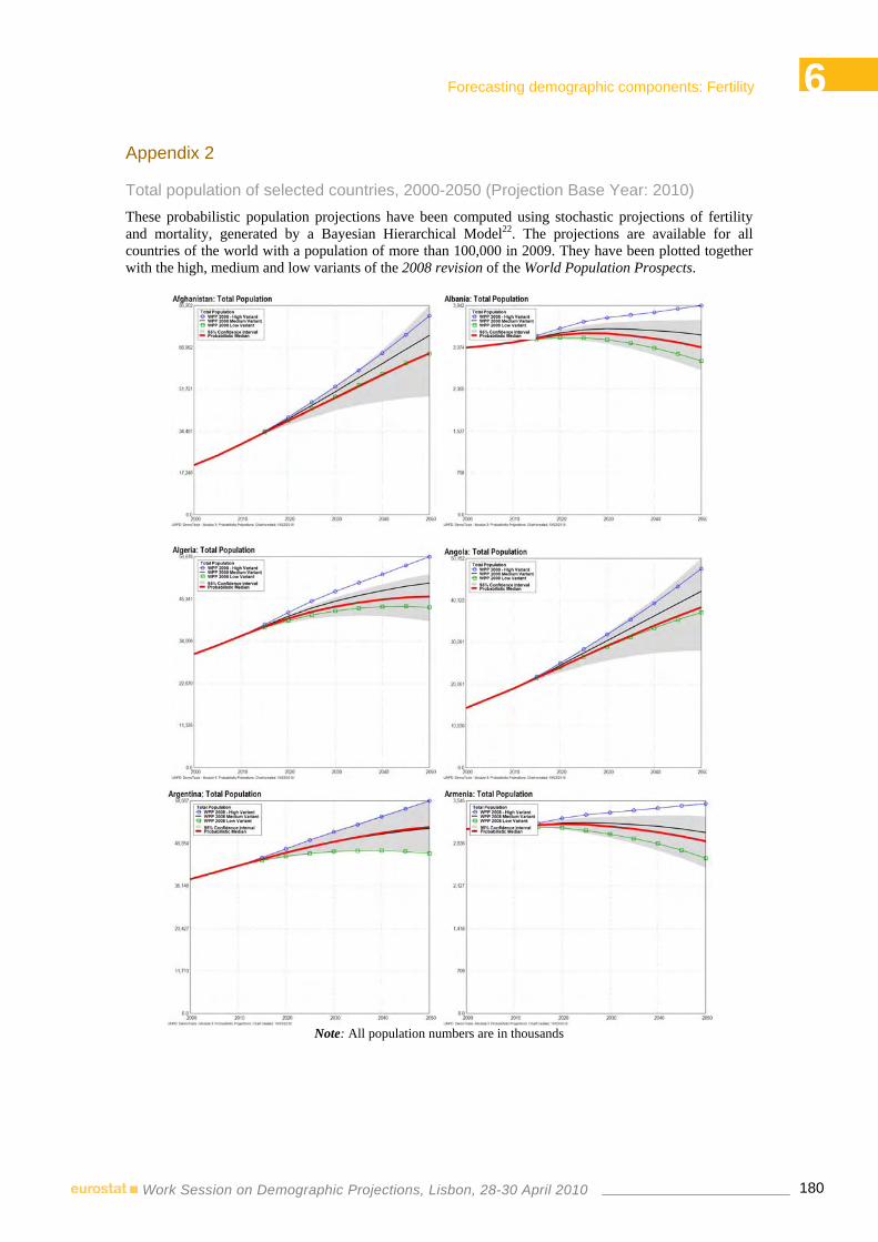
6 Forecasting demographic components: Fertility
180Work Session on Demographic Projections, Lisbon, 28-30 April 2010
Appendix 2
Total population of selected countries, 2000-2050 (Projection Base Year: 2010) These probabilistic population projections have been computed using stochastic projections of fertility and mortality, generated by a Bayesian Hierarchical Model22. The projections are available for all countries of the world with a population of more than 100,000 in 2009. They have been plotted together with the high, medium and low variants of the 2008 revision of the World Population Prospects.
Note: All population numbers are in thousands
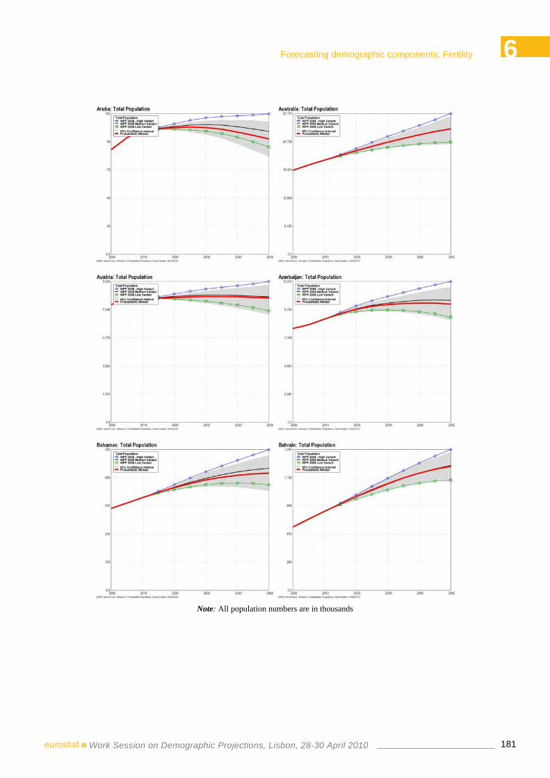
6 Forecasting demographic components: Fertility
181Work Session on Demographic Projections, Lisbon, 28-30 April 2010
Note: All population numbers are in thousands

6 Forecasting demographic components: Fertility
182Work Session on Demographic Projections, Lisbon, 28-30 April 2010
Note: All population numbers are in thousands

6 Forecasting demographic components: Fertility
183Work Session on Demographic Projections, Lisbon, 28-30 April 2010
References 1 United Nations (2009). World Population Prospects: The 2008 Revision, Volume I, Comprehensive Tables, United Nations publication Sales No. 10.XIII.2.
2 United Nations (2006). World Population Prospects: The 2004 Revision, Volume III: Analytical Report. United Nations publication Sales No. E.05.XIII.7.
3 Keyfitz, Nathan (1981). The limits of population forecasting. Population and Development Review, No. 7, pp. 579-593.
4 Stoto, M. A. (1983). The accuracy of population projections. Journal of the American Statistical Association, vol. 78, pp. 13-20.
5 Lutz, Wolfgang, ed. (1996). The Future Population of the World: What Can We Assume Today? Earthscan Publications: London, United Kingdom.
6 Lutz, Wolfgang, Warren Sanderson and Serguey Scherbov (1998). Frontiers of population forecasting. Supplement. Population and Development Review, vol. 24, pp. 139-155.
7 Lee, Ronald D. and L. R. Carter (1992). Modeling and forecasting U.S. mortality. Journal of the American Statistical Association, vol. 87, pp. 659-671.
8 Lee, Ronald D. (1993). Modeling and forecasting the time series of U.S. fertility: Age distribution, range and ultimate level. International Journal of Forecasting, vol. 9, pp. 187-202.
9 Lee, Ronald D. and Timothy Miller (2001). Evaluating the performance of the Lee-Carter method for forecasting mortality. Demography, vol. 38, pp. 537-549.
10 Lee, Ronald D. and S. Tuljapulkar (1994). Stochastic population forecasts for the United States: Beyond high, medium and low. Journal of the American Statistical Association, vol. 89, pp. 1175-1189.
11 Alho, Juha M. (1998) A Stochastic Forecast of the Population of Finland. Statistics Finland: Helsinki, Finland.
12 Lutz, Wolfgang and Serguey Scherbov (1998). An expert-based framework for probabilistic national population projections: The example of Austria. European Journal of Population, vol. 14, pp. 1-17.
13 Lutz, Wolfgang and Serguey Scherbov (2004). Probabilistic projections for India with explicit consideration of the education-fertility link. International Statistical Review, vol. 72, pp. 81-92.
14 Keilman, N., Pham, D. Q. & Hetland, A. Why population forecasts should be probabilistic - illustrated by the case of Norway. Demographic Research 6, 409-454, doi:10.4054/DemRes.2002.6.15 (2002)
15 Alders, M., N. Keilman and H. Cruijsen (2007). Assumptions for long-term stochastic population forecasts in the 18 European countries, vol. 23, pp. 33-69.
16 Ahlo, Juha M. (2006). New forecast: Population decline postponed in Europe. Statistical Journal of the United Nations Commission of Europe, vol. 23, pp. 1-10.
17 Lutz, Wolfgang, Warren Sanderson and Serguey Scherbov (2001). The end of world population growth. Nature, vol. 412, pp. 543-545.
18 Lutz, Wolfgang, Warren Sanderson and Serguey Scherbov (2008). The coming acceleration of global population ageing. Nature, vol. 451, pp. 716-719.

6 Forecasting demographic components: Fertility
184Work Session on Demographic Projections, Lisbon, 28-30 April 2010
19 Alkema, L. et al. (2010). Probabilistic projections of the total fertility rate for all countries, Working Paper No. 97, University of Washington, Seattle.
20 Chunn, J., A. E. Raftery and P. Gerland (2010). Bayesian probabilistic projections of mortality. Paper presented at the Annual Meeting of the Population Association of America held in Dallas, Texas, in April 2010.
21 Bongaarts, John (2006). The causes of stalling fertility transitions. Studies of Family Planning, vol. 37, pp. 1-16.
22 Raftery, A.E. et al (2009). Probabilistic projections of the total fertility rate for all countries for the 2010 World Population Prospects. Paper UN/POP/EGM-FERT/2009/16, presented at the Expert Group Meeting on Recent and Future Trends in Fertility, New York, 2-4 December 2009. Available at http://www.un.org/esa/population/meetings/EGM-Fertility2009/egm-fertility2009.html.

6 Forecasting demographic components: Fertility
185Work Session on Demographic Projections, Lisbon, 28-30 April 2010
APPLYING A FERTILITY PROJECTION SYSTEM TO PERIOD EFFECT ANALYSIS:
AN EXAMINATION OF THE RECENT FERTILITY UPTURN IN JAPAN1
Ryuichi KANEKO2
Abstract
Models of population projection play a significant role in analyzing current demographic processes as well as in forecasting their future course. In this study, I utilize a fertility projection based on the official population projection for period effect analysis of current fertility trends in Japan. The objective of the paper is threefold; first, I demonstrate the usefulness of population projection models in analyzing demographic processes in the past and present as well as in the future, secondly I classify and clarify the period effects in terms of the cohort fertility schedule so that causes and mechanisms of fertility changes can be identified, and thirdly I apply the framework to the recent peculiar fertility development in Japan, especially the upturn since 2006. Unlike previous upturns seen among countries in Europe and North America, the pure period effects that are separated from the tempo effect played a major role in the recent decline and subsequent rise in Japanese fertility, although the recuperation mechanism is also induced in an irregular manner by the effects.
1. Introduction
The role of population projections is to provide information on various future changes in demographic structure (e.g., population size and age composition by sex) based on assumptions on the future course of vital events such as fertility, mortality and migration. However, since they offer a comprehensive demographic model, they can be broadly applied to analyzing population processes. In this paper, I describe the use of a fertility projection employed in the official population projection for analysis of the period effects in past and current fertility trends in Japan.
It is crucial to understand the relationships between the period and cohort observations of fertility in order to identify the essential trends and prospects. As adjustments and adaptation behavior in an individual’s reproductive process take place along his/her life course, most of the large-scale regularities in fertility rates tend to emerge in cohort experiences. Demographic measures, however, usually trace fertility development annually, and try to provide a description of it with the “lifecycle” measures by means of the hypothetical cohort of the period. Hence two lifecycle measures with different values, i.e. those for true and hypothetical cohorts, describe the very same phenomena. There has been much effort to connect these measures, most notably by Bongaarts and Feeney (1998).
In addition to these formal issues, problems often arise in attempts to understand fertility changes in terms of period and cohort effects, which affect fertility trends via different mechanisms. In most cases, these efforts are unsuccessful due to the mixture of those effects in practice.
1 This is a draft paper presented to the Joint Eurostat-UNECE Work Session on Demographic Projections (Lisbon, Portugal, 28-
30 April, 2010), and to be revised. Do not cite any material in the preset paper. 2 National Institute of Population and Social Security Research, Japan. e-mail: [email protected]

6 Forecasting demographic components: Fertility
186Work Session on Demographic Projections, Lisbon, 28-30 April 2010
In the present paper, therefore, the period effects are first sorted out according to their means of effect on the cohort fertility schedule. Then applying the cohort-based fertility projection model, we separate the period effect from fertility fluctuations observed in recent Japan in order to identify the driving forces of changes.
Accordingly, this paper has three objectives; (1) to demonstrate the utility of population projection models in analyzing demographic processes in the past and present as well as in the future, (2) to measure and understand the period effects in terms of modifiers of the cohort fertility schedule, and applying those new procedures (3) to identify factors and mechanisms of the recent peculiar fertility development in Japan, paying particular attention to the question of whether the small upturn in Japan is induced by the similar mechanisms as those behind the fertility upturns recently observed among most of the countries in Europe and North America.
2. Background
2.1 Historic population trends and the lowest low fertility in Japan The year 2005 is a dividing line for population trends in Japan in several senses; first, the population of Japan was announced to have decreased from the previous year for the first time after about hundred and fifty years of steady rise since the closing period of the Tokugawa era except the turmoil during the Second World War, and second, the proportion of the population aged 65 and above exceeded one fifth (20.2 percent), attaining the highest in the world.
Though the combination of a low fertility rate and high longevity is the cause these striking changes in the population of Japan, the principal driver is the prolonged continuation of low fertility rates far below replacement level fertility, which Japan has been experiencing since the mid-1970s
In spite of a series of government measures and escalating public awareness, fertility continued to decline until it fell into the so called “lowest low” level for the first time in 2003, and finally reached the lowest ever TFR of 1.26 in 2005. The number of live births, which exceeded 2.09 million in 1973, had decreased by nearly half, to 1.06 million, in 2005 – again the lowest number recorded since the Second World War.
Because of the population momentum, the broad course of these historic population changes is already inevitable at this point. However, the upcoming levels and pace of changes depend on the future fertility rates. As such, the impact on society of rise or further fall of the fertility rates could be of great significance.
As a matter of fact, fertility made an upturn immediately after achieving the lowest ever TFR. In 2006, the TFR rose by 0.06 to 1.32, which is the largest increase since the 1970s. Fertility kept rising to 1.34 in 2007, and 1.37 in 2008. The last three year period of rising TFR was during the period 1982-1984. Although the extent of the increase is relatively minor and the overall level still far below replacement, this recent upturn of fertility is a significant turnaround: such a rise is a unique development both in terms of magnitude and deviation from the downward trend. We now proceed to engage in a detailed examination of this phenomenon.
2.2 The upturn of the period fertility rate in 2006 and onward As already explained, the total fertility rate (TFR) in Japan reached its lowest value ever in 2005. In the following year, however, it showed a surprisingly strong recovery and has been increasing thereafter, at least until 2008. Figure 1 shows the TFR trend together with the development of the population replacement level and different assumptions used for the Population Projections for Japan. In this graph, the values recorded in the three years from 2006 to 2008 are shown as dots. This reversal gives the impression that the constant decline throughout the years leading up to 2005 has suddenly turned around. In fact, the TFR values in 2007 and 2008 are higher than any of the fertility assumptions of the latest official population projections based on the values until 2005, even the high variant assumption.

6 Forecasting demographic components: Fertility
187Work Session on Demographic Projections, Lisbon, 28-30 April 2010
In the past, such sudden upturns were also observed in the three-year period from 1982 to 1984 as well as in 1994. In the case of the upturn in 1982 to 1984, the TFR of 1.74 in 1981 had increased by 0.07 by 1984. In 1994, an increase of 0.04 was recorded in a single year.
The increase observed from 2006 to 2008 amounts to 0.11, which is clearly a significant increase compared to these past upturns. Moreover, the increase of 0.06 in 2006 is the greatest increase observed in a single year since the 1970s.
Figure 1. Trends of Total Fertility Rate: Observed and Assumed.
0.0
0.5
1.0
1.5
2.0
2.5
1950 1960 1970 1980 1990 2000 2010 2020 2030 2040 2050
Tota
l fer
tility
rate
Year
Assumedtrends
Observedtrend
High variant 1.55
Medium variant 1.26
Low variant 1.06
Upturn trend in 2006-2008
Population replacement level
Source: The Vital Statistics, NIPSSR(2007).
Looking at the TFR in the years immediately following the periods of past increase, both 1985 and 1995 witnessed relatively sharp reductions of -0.05 and -0.08, respectively. It is not known if this most recent increase will follow the same profile as in the past, or if it might last for a relatively long period of time. However, looking at the monthly development shown below, some deceleration and signs of stagnation can already be observed in 2009.
Whether this recent upturn is temporary or caused by actual, substantive changes in the basic course is of significant importance when investigating the future fertility trend. The assumptions on fertility rate in the latest population projection, in particular, are based on the actual values measured until 2005, and in the medium-variant scenario the long-term TFR value is projected to end up at the very low level of 1.26. Since this assumption was established by projecting cohort fertility rates, a deviation of actual values in recent years does not directly imply that these assumptions are inappropriate. Nonetheless, if the deviation occurs as a result of more basic changes in reproductive behaviors, the assumption must be reviewed for the future projections. Thus, this upturn is examined in more detail in the following discussion.
From the mid-1990s to the beginning of the second millennium, one by one the so-called lowest low fertility countries in Europe experienced reversals of their fertility rate trends. Indeed, as of the time of this writing, the majority of these countries have broken away from the lowest low fertility status (Goldstein et al. 2009). In fact, while the occurrence of reversal of fertility rate trend is not limited to low fertility countries, and the period and degree vary, it can be said that the US and most of the countries in Europe are currently experiencing a steady upturn in fertility rates.

6 Forecasting demographic components: Fertility
188Work Session on Demographic Projections, Lisbon, 28-30 April 2010
To begin with, with few exceptions, the decline of fertility rates in these countries was generally caused by a general delay of childbearing known as “postponement transition” (Kohler et al. 2002, Sobotka 2004, Billari 2008); Goldstein et al. explain that the fertility rate upturns in recent years were caused by the weakened tempo effects on the period fertility rate due to this transitional trend diminishing or dying out. They call this process “tempo transition” (Goldstein et al. 2009).
One very important point in this perspective is the interpretation that the actual cohort fertility rates have not reached the level of 1.3, called the lowest low, in any of the countries but rather that this level in the period TFR is a transient phenomenon due to the aforementioned tempo effect.
If this interpretation is correct and the fertility rate upturn in Japan observed since 2006 is caused by a mechanism similar to that of the trend observed in the US and countries in Europe, there is a possibility that the recovery may continue for a relatively long period of time. In this case it is unlikely that the future cohort fertility rate will drop below the lowest low level, as projected by the medium (and low) variant assumptions in the Population Projections in Japan.
3. Demographic analysis of the upturn
3.1 A close look at the upturn – Examination of monthly data In order to analyze changes in the various fertility rates in Japan in recent years more closely, the observed data is first plotted on a monthly basis. Figure 2 shows monthly fertility rates and their trends after making seasonal adjustments by birth order in the period from January 2002 to June 2009 (the latest values obtained as of November 2009). In the figure, fertility rates are indicated as annual values (corresponding to 365 days), obtained by adjusting the age-specific number of births in individual months to have the same number of days and dividing the values by the projected population by age in the middle of the given month. Moreover, seasonal adjustment is performed according to the U.S. Census Bureau’s X-11 method. Please note that the annually published values of fertility rates in Japan use the population as of October 1, rather than the middle of the period, as the denominator. Thus the fertility rate values become slightly higher than is the case here, where the population in the middle of a month is used.
Figure 2. Monthly Progress of Fertility Rates by Birth Order: 2002-2009.
1.20
1.25
1.30
1.35
1.40
1.45
1.50
2002/1 2003/1 2004/1 2005/1 2006/1 2007/1 2008/1 2009/1 2010/1
Total
fertility
rate
Birth order = Total
Time (month)
0.57
0.59
0.61
0.63
0.65
0.67
0.69
0.71
2002/1 2003/1 2004/1 2005/1 2006/1 2007/1 2008/1 2009/1 2010/1
Total
fertility
rate
Birth order = First birth
Time (month)
0.42
0.44
0.46
0.48
0.50
0.52
2002/1 2003/1 2004/1 2005/1 2006/1 2007/1 2008/1 2009/1 2010/1
Total
fertility
rate
Birth order = Second birth
Time (month)
0.15
0.16
0.17
0.18
0.19
0.20
0.21
0.22
2002/1 2003/1 2004/1 2005/1 2006/1 2007/1 2008/1 2009/1 2010/1
Total
fertility
rate
Birth order = Third and higher
Time (month) Note: Dots with thin lines denote monthly time series of annualized TFR by birth order, and lines represent
seasonally adjusted trends with the U.S. Census Bureau’s X-11 method.

6 Forecasting demographic components: Fertility
189Work Session on Demographic Projections, Lisbon, 28-30 April 2010
First, looking at the monthly changes of the overall TFR by birth order, we see that the TFR began to drop suddenly in December 2004, and remained low for six months until May 2005. Then, after bottoming out at this point, the TFR shows a subsequent sharp rise. This rising trend accelerates from around December 2005, exhibiting the largest increase in March 2005. Although the rate of increase significantly drops starting around June 2005, the rise itself continues steadily until October 2008 and exhibits a local maximum in November. The TFR then declines slightly or levels off for seven months afterward.
The period where these changes occurred is divided into the following detailed phases:
(1) December 2004 to May 2005 (6 months): Sudden drop
(2-1) June 2005 to November 2005 (6 months): Sharp rise
(2-2) December 2005 to May 2006 (6 months): Sharpest rise
(3-1) June 2006 to February 2007 (9 months): Level off for 1st and 2nd children
(3-2) March 2007 to November 2008 (21 months): Slow increase
(4) From December 2008 and onward: Level off or decline
Each of the four phases––(1) sudden drop, (2) sharp rise, (3) slow increase, and (4) level off or decline––shows significant change. The phases where the TFR rises, (2) and (3), can further be divided into two sub-periods each, according to the difference in pace. The most remarkable change in this period is the change from phase (1) to phase (2), where the TFR bottoms out in May 2005 and shifts from dropping sharply to rising sharply. The time period and pattern of this change are common to the TFR for all birth orders (except that the fertility rate of the first child does not bottom out until June 2005), and it looks as if a sudden restraint and release of childbearing occurred simultaneously among women of all parities.
The second remarkable change is the change from phase (2) to phase (3), where the TFR of the first and second children sharply increases until December 2006 and then shifts to a slow rise, which continues until December 2008. Note that this pattern is not observed in the TFR of the third and further children; in this particular case, the trend continues to rise at a consistent pace until phase (4).
Since these children were conceived approximately nine months before each phase, it is necessary to retrace the timing of pregnancy for each phase in order to investigate the triggers of phase shifts. However, no obvious factors have been found so far (one significant event that occurred in August 2004, i.e., nine months before May 2005, where the greatest change was observed, is the 28th Summer Olympic Games held in Athens, Greece, from August 13 to 29; however, the influence of this event on pregnancy is unknown).
The leveling-off trend observed among all birth orders at the same time in December 2008 and onward in phase (4) may quite possibly signal the end of the rising trend and should be observed closely. Some care must be taken when computing seasonal adjustment according to X-11, as the method tends to generate instability at the terminal parts of time-series data (values may change due to addition of new data), but there can be no doubt that a new trend is beginning in this phase. This phase corresponds to the time period where the influence of the global financial crisis started to spread. However, the period of conception of those births is nine months earlier, where there are no obvious events that might have influenced childbearing to be found.

6 Forecasting demographic components: Fertility
190Work Session on Demographic Projections, Lisbon, 28-30 April 2010
3.2 Examination of the Tempo Effect – Is it Due to a Catch-up Effect? The fact that the monthly changes in the fertility rates show the same patterns among all birth orders suggests that the driving force behind these changes is a period effect. That is, if each cohort goes through different changes, there must be some time lag in terms of the changes occurring among higher birth orders. The term period effect here refers to a change in fertility rates caused by certain temporary factors (usually meaning social economic events, such as times of war and economic crisis). In order to examine such changes in the following, it is necessary to define them more precisely.
One of the important aspects of a period effect is that it leaves little influence on the completed fertility of any cohorts involved, although it may bring about significant changes in annual fertility rates. Here, we will use this characteristic as the definition of a period effect for the time being. That is, a period effect is a fertility rate change observed in a certain period, which does not influence the cohort completed fertility (cohort TFR).
According to this definition, a period effect can be said to be a change in timing occurring in the childbearing schedule in terms of cohort fertility rates. A cohort is considered to have a unique childbearing schedule with a certain potential regularity, and a period effect is a change that causes the actual fertility rates to deviate temporarily from the original schedule without affecting the long-term balance. Not affecting the long-term balance of cohorts means that the change is redeemed by other periods.
It is possible to consider several different types of such changes in cohort childbearing schedules. The first group of changes is the case where the childbearing timing of a cohort as a whole shifts. In this case, a well-known tempo effect acts on the fertility rate for a period. That is, if the mean age at birth (MAB) of a cohort is rising, for example, a tempo effect causes the period TFR to go down. On the other hand, if the rise of the MAB stops or the MAB drops, a tempo effect that pushes up the period TFR comes into play. In this paper, these effects are called type-T period effects (see figure 3 for illustration).
As shown in the figure, there are three different types of effect identified as type-T period effects, i.e. shift in location of fertility schedule on age axis (type-Tl), shift in dispersion (type-Td), and shift in shape (type-Ts).
Another type of change encompasses disturbances occurring only for parts of a cohort childbearing schedule (the last graph in Figure 3). That is, this type encompasses fertility rate changes caused by a cohort reacting to certain events occurring in the environment and hastening or postponing its childbearing time period.

6 Forecasting demographic components: Fertility
191Work Session on Demographic Projections, Lisbon, 28-30 April 2010
Figure 3. Types of Period Effect in Terms of Cohort Fertility Schedule.
0.00
0.02
0.04
0.06
0.08
0.10
0.12
0.14
0.16
0.18
0.20
15 20 25 30 35 40 45 50
Ferti
lity
rate
Age
Type-Tl
0.00
0.02
0.04
0.06
0.08
0.10
0.12
0.14
0.16
0.18
0.20
15 20 25 30 35 40 45 50
Ferti
lity
rate
Age
Type-Td
0.00
0.02
0.04
0.06
0.08
0.10
0.12
0.14
0.16
0.18
0.20
15 20 25 30 35 40 45 50
Ferti
lity
rate
Age
Type-Ts
0.00
0.02
0.04
0.06
0.08
0.10
0.12
0.14
0.16
0.18
0.20
15 20 25 30 35 40 45 50
Ferti
lity
rate
Age
Type-H
Note: The period fertility exhibits similar changes due to different type of changes in the cohort fertility level and
schedule. The period effect of type-T is caused by the shift of the cohort fertility schedule. The period effect of type-H is caused by the temporary fluctuation that is redeemed in another period, while the type-H' effect is a temporary fluctuation that continues to change the completed level of cohort fertility. Thus the type-H' effect is not a genuine period effect by our definition.
In fact, a case example that clearly shows the second type of change exists in recent Japanese history: the so-called Hinoe-uma (Fiery Horse) phenomenon, which occurred in 1966. The Hinoe-uma is a calendar event based on Chinese astrology occurring once every 60 years. Due to the superstition that girls born in that year would cause bad luck for their husbands, many couples avoided having children in that year, and the fertility temporarily dropped by one fourth from the average level (the TFR in 1966 was 1.58 or 75 percent of the average level over 1963 through 1969 except 1966, see changes of TFR in Figure 1). However, all the main cohorts involved in childbearing in this year (the cohorts born from 1923 to 44, who were 22 to 49 years of age at that time) compensated for this loss in the following years and no cohorts exhibited TFR values lower than 2.0. In other words, the Hinoe-uma phenomenon had little effect on the cohort TFR, making it an example of a pure period effect (Figure 4). This type of fertility rate change is called type-H period effects here.

6 Forecasting demographic components: Fertility
192Work Session on Demographic Projections, Lisbon, 28-30 April 2010
Figure 4. Age-specific Fertility Rate of Japanese Female Cohort Born in 1935.
0.00
0.05
0.10
0.15
0.20
15 20 25 30 35 40 45 50
Note: Female cohort born in1935 experienced the Hinoe-uma in1966 at age 31.
It should be noted, however, that some fertility rate changes that occur in reaction to changes in social economy do have lasting influence on the cohort completed fertility. Because they are changes in individual cohorts, it is appropriate to call them period-cohort effects, considering them as a type of cohort effect induced by a certain period. However, whether this kind of period changes is limited to pure period effects (i.e., type-H period effects) or is a period-cohort effect affecting the cohort’s long-term balance, cannot be known until the affected cohorts complete their childbearing process. Moreover, in terms of the occurrence mechanism, it is irrelevant whether or not it affects a cohort’s long-term balance. For this reason, there should be no problems in handling such period changes as type-H period effects from the viewpoint of investigating causes of the occurrence. Period-cohort effects may simply be considered to be the results of prolonged type-H period effects (hereinafter written as type-H'), as illustrated in Figure 5.
Now, in recent fertility changes in Japan, it is speculated that type-H period effects are important because the same changes are seen among all the fertility rates by birth order, as explained above. Moreover, if the changes that occurred in this period are the results of type-T period effects, it would mean that low fertility rates before reaching the point of reversal were caused by tempo effects due to postponement transitions for each cohort and that upturns of fertility rates would signify regression to cohort fertility level due to the shift in childbearing timing ending. However, this hypothesis can be ruled out by observing the monthly MAB development simultaneously. The MAB has been increasing without leveling off throughout the entire period of drop and upturn in the fertility rate since 2002 for the first and second children, who are the main force of fertility. Thus, it is unlikely that the reversal trend is a sign of reverting to the cohort level due to tempo effects dying out, i.e., “tempo transition.”

6 Forecasting demographic components: Fertility
193Work Session on Demographic Projections, Lisbon, 28-30 April 2010
Figure 5. Types of Period Effect in Terms of Cohort Fertility Schedule.
0.00
0.02
0.04
0.06
0.08
0.10
0.12
0.14
0.16
0.18
0.20
15 20 25 30 35 40 45 50
Fe
rtility ra
te
Age
Type-H
0.00
0.02
0.04
0.06
0.08
0.10
0.12
0.14
0.16
0.18
0.20
15 20 25 30 35 40 45 50
Fe
rtility ra
teAge
Type-H'
Bongaarts and Feeney (1998) proposed an index that eliminates tempo effects from period TFR. Here, we will use this index to check the development of the effects acting on the period TFR in Japan and whether or not they are tempo effects3. The index proposed by Bongaarts and Feeney is referred to as ATFRp in the following. Figure 6 illustrates the development of ATFRp along with the normal TFR. Tempo effects are represented as the differences between ATFRp and TFR. It is seen that relatively large tempo effects have been in action even after the start of the upturn in 2006, reflecting the continuous rise of the MAB mentioned above. It can furthermore be seen that the tempo effects in 2006 and 2007 amount to 0.17 and 0.14, respectively, which are substantially larger than the value of 0.12 in 2005 when the TFR bottomed out. The value for 2008, 0.09, is only tentative, but at least it does not appear as if the rise of TFR since 2006 is caused by tempo effects dying out (here fertility rates are calculated only with births to Japanese women).
Now, the ATFRp approach estimates tempo effects under certain assumptions. That is, the age-specific period fertility rate is composed of age-specific fertility rates of a large number of cohorts, but the ATFRp index proposed by Bongaarts and Feeney assumes that the age-specific period fertility rate is composed of age-specific fertility rates of all cohorts who are experiencing the timing shift at the same speed, and then eliminates the tempo effects (or tempo distortion) caused by this shift (Bongaarts and Feeney 1988). The uniform timing shift speed r(t) in year t is given as the change in the average age of childbearing in a given period compared to the previous year (in this paper, the average value of change from the previous year and the change to the next year is used).
This view implicitly allows the timing change speed of fertility rate f(tc+a, a) experienced at a certain age (a) in a certain year (t= tc+a) to fluctuate by age a (that is, for each year t) when focus is placed on a 3 Since the fertility rate (i.e., including children with Japanese nationality born to non-Japanese women) and the total fertility
rate (see the formula below) defined in the same way as in the Vital Statistics corresponding to the aforementioned fertility rate composition all depend on the demographic compositions of Japanese and non- Japanese women, they can be calculated as a result of population projection. Handling such individually defined fertility rates in the overall fertility rate assumptions of the future population projection makes the projection methodology considerably more complicated, though it is an indispensable mechanism for accurate reproduction of the future population status where international population exchanges have advanced.
Definition of the total fertility rate of the Vital Statistics;
*A child with Japanese nationality born from a non-Japanese female is a child whose father is Japanese.

6 Forecasting demographic components: Fertility
194Work Session on Demographic Projections, Lisbon, 28-30 April 2010
single cohort (birth year tc) and, instead, assumes that all cohorts involved have a common timing change speed within a given year (period-shift framework). That is: ATFRp(t) = Σ f(t,a) / (1 - r(t)), where Σ is the sum for age a (note that this calculation is performed for each birth order and the value is obtained by summing up the results).
This view prioritizes harmonization among age-specific period fertility rates. However, in some cases it might be more appropriate to give precedence to harmonization of age-specific cohort fertility rates; that is, a framework in which r, the timing change speed of fertility rate, would be seen as a characteristic of a cohort and its tempo effect on the period total fertility is also a characteristic unique to the cohort (We refer to this as a cohort-shift framework). This can be achieved by expressing the timing change speed of a cohort as a function of the cohort born in year tc, and the timing effect on the periods from this cohort as τ(tc) = 1/(1 + r(tc)) (van Imhoff 2001), and the period TFR with adjusted timing effects as ATFRc(t) = Σ f(t,a) / τ(t-a), where Σ is the sum for age a (note that this calculation is also performed for each birth order and the value is obtained by summing up the results).
Note that in this calculation, in addition to the measured age-specific fertility rates, the timing change for related cohorts is required, and has to be obtained from cohort fertility rate assumptions in the Population Projections. However, we emphasize that it is only the timing changes in future fertility rates that are required - the fertility rates themselves are not used.
Figure 6 shows the result of calculating the ATFRc index from the fertility trend data recorded in Japan. In the period leading up to 2000, both ATFRp and ATFRc follow very similar paths. From 2000, however, they show slightly different behaviors. In particular, in 2000 and onward, ATFRc continues dropping alongside the TFR trend and also indicates a rapid increase at the upturn in the same way as for TFR. Assuming that the cohort-based timing change is essentially continuous, the period effects are leveled out and show smooth development, but persistent tempo effects still appear clearly, suggesting that the true cohort TFR is actually higher than the values observed in each period.
The two adjusted TFR indices show an upturn in the same way as for the measured TFR, suggesting the increase in this period is not the recovery brought about by the elimination of type-T tempo effects, but rather a substantive rise of type-H effects.
Figure 6. Trends of the Total Fertility Rates with/without Tempo-adjustment
1.0
1.2
1.4
1.6
1.8
2.0
2.2
2.4
1960 1965 1970 1975 1980 1985 1990 1995 2000 2005 2010
Total
fertil
ity ra
te
Year
TFR of tempo-adjustedcohort fertility rate
ATFRp
TFR
ATFRC
~~~~
Bongaarts-Feeney'stempo-adjusted TFR
Note: The fertility rates are calculated based on births by Japanese women only.

6 Forecasting demographic components: Fertility
195Work Session on Demographic Projections, Lisbon, 28-30 April 2010
Now, the discussion above suggested that the main cause of the recent upturn in the fertility rate is a type-H period effect. However, it has also been confirmed that the MAB for the first and second children continuously rises over this period, which means that tempo effects that push down the period TFR exist. These tempo effects can also be seen from the development of the ATFRp and ATFRc indices for this period. The question now becomes, how can the scale of type-H period effects be measured while such tempo effects exist.
We propose to apply a model based on the population projections. In the “Population Projections for Japan,” a cohort model is used for formulating fertility rate assumptions4. In particular, the childbearing schedule in the entire reproductive life course is projected for individual single year cohorts of women, and this schedule is then reorganized in order to project age-specific fertility rates on a yearly basis from the past into the future (Kaneko et al. 2008).
The projection model is particularly good at describing the age-specific cohort fertility rate, and we believe it is fully capable of describing and expressing regularities latent at the base of the cohort childbearing schedule (see figure 7). Of course, there are cases where the achieved values deviate from the regularities for some ages. In fact, these deviations are precisely period effects of type-H. For this reason, the period effect can be obtained as the difference between the fertility rate achieved in a given year/age and the corresponding model value. On the other hand, type-T period effects caused by the shift of cohort childbearing schedule are included in the projected fertility rate and are thus excluded from the period effect obtained as the difference between the projected value and achieved value; only type-H period effects are captured in this way.
Under normal circumstances, the model fertility rates used in the Population Projections for Japan are future predictions that have not yet been achieved. In contrast, the method proposed here uses model values of years and ages in the past. The accuracy of the measurement result achieved by this method depends on the accuracy of the cohort model. For cohorts who have completed their childbearing process up to reasonably high ages, the applicability and accuracy of the cohort model has been established, as shown in the graphs above. For young cohorts with little experience in the childbearing process, however, there are various speculative factors involved in their remaining childbearing schedule and the accuracy of the model is less well understood. Therefore, the measurement values should be treated as provisional for the most recent years, where such cohorts contribute more.
Figure 8 illustrates the result of measuring type-H period effects using the method proposed above. Figure 8-a and Figure 8-b shows projected values of type-H period effects by age group and by birth order as bar graphs, respectively (left scale). Both figures show the total period effect, i.e., period effects on TFR, as line plots (right scale) as well. Note that the right scale is twice as large as the left scale.
4) The model is based on the probability density function of the generalized log-gamma distribution, which is one of standard
distributions in statistics. The fertility rate at age x for n-th birth is ( )nf x : ( ) ( ); , ,n n n n nf x C x u bγ λ= ⋅
where, ( ) 22 1 22; , , ( ) exp exp
( )nn n n
n n n n n n nn nn n
x u x ux u bb bb
λλγ λ λ λ λ λ
λ−− − −
−
⎡ ⎤⎧ ⎫⎛ ⎞ ⎛ ⎞− −⎪ ⎪= −⎢ ⎥⎨ ⎬⎜ ⎟ ⎜ ⎟Γ ⎪ ⎪⎢ ⎥⎝ ⎠ ⎝ ⎠⎩ ⎭⎣ ⎦
.
Here, γ and exp are the gamma and exponential functions, respectively. Cn, un, bn, and λn are parameters of the fertility rate function of birth order n; this is an extension of the Coale-McNeil Model. The further adjustment is made so that the distribution will reproduce the characteristics of Japanese age-specific fertility rate precisely. A standard pattern of errors (εn) was identified by comparison with the actual fertility rates and the modeled rates and used to adjust the model schedule. As a result, the function of cohort fertility rate by age x, f(x) is given as follows. See Kaneko (2003) for the details.
( ) ( )∑+
= ⎭⎬⎫
⎩⎨⎧
⎟⎟⎠
⎞⎜⎜⎝
⎛ −+⋅=4
1,,;
n n
nnnnnn b
uxbuxCxf ελγ .

6 Forecasting demographic components: Fertility
196Work Session on Demographic Projections, Lisbon, 28-30 April 2010
Figure 7. Actual and Modelled Fertility Rates of Japanese Female Cohorts by Birth Order
0.00
0.02
0.04
0.06
0.08
0.10
15 20 25 30 35 40 45 50
Ferti
lity ra
te
Age
Cohort 1960
0.00
0.02
0.04
0.06
0.08
0.10
15 20 25 30 35 40 45 50
Ferti
lity ra
te
Age
Cohort 1970
0.00
0.02
0.04
0.06
0.08
0.10
15 20 25 30 35 40 45 50
Ferti
lity ra
te
Age
Cohort 1980
0.00
0.02
0.04
0.06
0.08
0.10
15 20 25 30 35 40 45 50Fe
rtility
rate
Age
Cohort 1965
0.00
0.02
0.04
0.06
0.08
0.10
15 20 25 30 35 40 45 50
Ferti
lity ra
te
Age
Cohort 1975
0.00
0.02
0.04
0.06
0.08
0.10
15 20 25 30 35 40 45 50
Ferti
lity ra
te
Age
Cohort 1985
Note: Actual age specific fertility rates by birth order for female cohorts are plotted by dots, while modeled rates are plotted by lines. The actual rates are calculated only for female with Japanese nationality. The model rates are those employed in the official population projection conducted in 2006 as the medium assumption.

197
Figure 8. Estimates of Period Effects as Differences between Actual and Projected Fertility Rates by Five Year Age Groups: 1985-2008.
a. Age groups
-0.06
-0.04
-0.02
0.00
0.02
0.04
0.06
0.08
0.10
0.12
0.14
-0.03
-0.02
-0.01
0.00
0.01
0.02
0.03
0.04
0.05
0.06
0.07
1985 1986 1987 1988 1989 1990 1991 1992 1993 1994 1995 1996 1997 1998 1999 2000 2001 2002 2003 2004 2005 2006 2007 2008Diff
eren
ce b
etw
een
actu
al a
nd p
roje
cted
fx
( ~ P
erio
d ef
fect
s te
ntat
ive
Year
15-1920-2425-2930-3435-3940+
Total period effect ~differences between actual and projected TFR (see right scale)
b. Birth orders
-0.06
-0.04
-0.02
0.00
0.02
0.04
0.06
0.08
0.10
0.12
0.14
-0.03
-0.02
-0.01
0.00
0.01
0.02
0.03
0.04
0.05
0.06
0.07
1985 1986 1987 1988 1989 1990 1991 1992 1993 1994 1995 1996 1997 1998 1999 2000 2001 2002 2003 2004 2005 2006 2007 2008Diffe
rence
betw
een a
ctual
and p
rojec
ted fx
( ~ P
eriod
effec
ts ten
tative
Year
1st birth2nd birth3rd birth4th & higher
Total period effect ~differences between actual and projected TFR (see right scale)
Note: The total period effects (solid line – right scale) is drawn in half the scale of the effects by age group (bar graph – left scale). Fertility rates are calculated based on births
by Japanese women only here as well.

6 Forecasting demographic components: Fertility
198Work Session on Demographic Projections, Lisbon, 28-30 April 2010
In the period up to 2005, the absolute value of period effects on the TFR (the scale on the right axis) exceeds 0.03 only in 1989 and 1994. In other years, the period effects, in general, amount to very little. In 1989 and 1994, some changes can be recognized in the figures showing the annual TFR development (figures 1). 1989 is the year the TFR dropped below the value in the year of Hinoe-uma and achieved the lowest value in recorded history and is also the year of “Merkmal” that triggered widespread societal awareness in Japan of the low fertility rates. Note that the period effect value is -0.034; the absolute value is not very large. On the other hand, in 1994, the period effect value is 0.058, which is quite prominent in the period up to 2005. Although the cause of this effect is not certain, one possible cause that has been suggested is the marriage between Crown Prince Naruhito to Princess Masako Owada in June of the previous year, which attracted the attention of many citizens.
In other years, positive period effects are observed in the three-year period from 2000 to 2002, among 20 to 24-year old women and for the first children only. Millennium effects were anticipated in this period, but the TFR itself did not show any significant rise. At closer inspection, it is noted that the fertility rates of the age group of 22 to 25 years show actual values higher than expected from the cohort model for first children.
In the sections above, the relatively prominent changes that occurred up to 2005 were discussed. Compared to those changes, the recent three-year period from 2006 to 2008 shows a very strong rise in terms of period effects. The projected period effects are high, 0.065, 0.095, and 0.134, respectively, and indicate a yearly upward trend. Looking at the values by age group (figure 8-a), the upward effects in the 30s age group are notable in each year. In 2007 and 2008, the value shows a dramatic rise for the age group in the latter half of the 20s as well. Looking at the values by birth order (figure 8-b), the period effect seems to contribute to all orders roughly equally.
Table 1 shows the contributions of age-specific and birth-order-specific subgroups to the entire period effects for both 1989 and 1994, for the purpose of comparison. In 1994, which shows relatively large positive period effects, the relative contribution of the age group of 25 to 29 years of age is large, while in 2006 to 2008, the contributions of the age groups of 30 to 34 years of age and especially 35 to 39 years of age are dramatically high. Moreover, in terms of birth order, while the contribution of the first children is large in 1994, the contribution of the third and further children is large in 2006 to 2008. Taking these characteristics into account, the period effect patterns in these recent three years are clearly different from the past.
Table 1. Contribution of Subgroups to Period Effects of Type H in Selected Years
a. Age groups (%)
Years whose "period effect" exceeds 0.03
1989 1994 2006 2007 2008
15-19 4.2 - 2.0 - 6.8 - 5.2 - 2.9
20-24 26.1 10.3 7.8 1.7 2.5
25-29 58.0 42.6 7.9 11.5 16.1
30-34 17.9 32.0 46.5 43.1 39.0
35-39 - 4.0 18.8 42.5 45.5 41.8
40+ - 2.2 - 1.7 2.2 3.4 3.5
Total 100.0 100.0 100.0 100.0 100.0 (values) (-0.034) ( 0.058) ( 0.065) ( 0.095) ( 0.134)
b. Birth orders (%)
Years whose "period effect" exceeds 0.03
1989 1994 2006 2007 2008
1st birth 57.9 58.9 42.5 40.4 40.8
2nd birth 34.3 27.3 33.6 29.8 30.0
3rd birth 5.6 9.7 19.4 24.0 22.8
4th & higher 2.1 4.1 4.5 5.7 6.4
Total 100.0 100.0 100.0 100.0 100.0(values) (-0.034) ( 0.058) ( 0.065) ( 0.095) ( 0.134)
Age group
Birth order
Note: Comparatively outstanding values for the age groups and birth order are underlined.

6 Forecasting demographic components: Fertility
199Work Session on Demographic Projections, Lisbon, 28-30 April 2010
In general, the rise of fertility in this period is known as “last-minute birth” and similar terms. These descriptions generally imply that women who delayed having children are now having more children while they are still able to. The age patterns of period effects show an upward movement in age groups from the middle of the 30s to the early 40s, which also supports this view. This generation includes the second baby boomers that were born in the period from 1971 to 1974. They tend to be promoters of lower fertility rates, who significantly postponed family formation and/or childbearing. For this reason, if they wish to have a fixed number of children in their lives, this period is their last chance. If only period effect patterns are examined, however, women in this age range not only tended to give birth to the first and second children they felt compelled to have in order to avoid childlessness and having an only-child, but also exhibited an increasing number of births to third and further children in a rather prominent manner. This suggests that the people who shifted towards more reproductive behaviors were not limited to those who had delayed family formation specifically, but encompassed a wider range of people as well. The significance of this interpretation will be examined in the subsequent discussion.
6. Discussion
In this paper, I utilized fertility projection prepared for the official population projection to analyze the period effects that are latent within the past and current fertility trends. Before applying the framework, I operationally defined a period effect as a fertility rate change observed in a certain period of time, which does not influence the cohort completed fertility (cohort TFR). Then I sorted out several types of period effect according to its effect on cohort fertility schedule, i.e. three different types of type-T period effect (Tl, Td, and Ts), and type-H. Type-T period effect is equivalent to a so called tempo effect.
Using this decomposition, period fertility rates synthesized from projected cohort fertility schedules are compared with observed rates. The former includes cohort changes and type-T period effects, but is free from the type-H period effects. Therefore difference between the projected and observed period fertility rate identifies the type-H (or type-H') period effects which should be induced by some period specific events.
Three temporal aspects of driving factors, i.e. period, cohort and age effects, are recognized in trends of demographic measures in general. In our framework, the age effects are expressed with a function of age as the regularity approximated by a mathematical function, while the cohort effects (variation by cohort) is represented by the different parameter values of the function. The period effects are disturbances to the age schedules shaped by the function with the certain parameter values affecting simultaneously many cohorts at different ages.
The fertility rates dropped continuously until 2005 in Japan, and the so-called lowest low fertility was attained for a three-year period from 2003 to 2005. However, from 2006 to 2008, an upward trend has been observed in the fertility rates, and the breadth of this upsurge is quite extraordinary as compared to past fluctuations seen since the fertility decline below replacement level started in 1974. Considering how important the fertility trends are for a society already in a phase of depopulation and rapid aging, it is extremely interesting to consider whether or not the recent rise in fertility rates is likely to affect the long term outlook. For this reason, this paper investigated the nature of the upturn, by closely examining the monthly development of fertility rates in this period, attempting to estimate tempo effects caused by adjusted TFRs such as the index proposed by Bongaarts and Feeney, and by estimating period effects (type-H period effects) that exclude tempo effects.
As a result, it was estimated that the recent upturn of fertility rates could generally be explained by type-H period effects. That is, we found that the upturn is an emergent change that cannot be reproduced by continuous changes in each cohort and which occurred in a manner deviating from the regularity of childbearing schedules of each cohort. For some cohorts in higher ages concluding their reproductive processes, however, it is likely the completed fertilities become slightly larger than previously estimated, from a windfall type effect of type-H'.
In the US and Europe, upturns of fertility rates have been observed since the 1990s in one country after another, and the majority of the countries experiencing lowest low fertility rates have already broken

6 Forecasting demographic components: Fertility
200Work Session on Demographic Projections, Lisbon, 28-30 April 2010
away from that status at the time of this writing. Thus, it is crucial to identify whether the upturn in Japan is qualitatively similar to those observed in the US and Europe.
However, whereas the upturns in the US and Europe are generally considered to have occurred because the period TFR returned to the long-term cohort TFR as tempo effects die out due to completion of postponement transition (Goldstein et al. 2009), it is suggested that the upturn being observed in Japan is of a different nature and is caused by other, peculiar causes.
From a long-term perspective, if the rise in fertility currently being observed is purely caused by type-H period effects, the period fertility rate should decline again within the next several years and will ultimately not significantly change the long-term outlook for the fertility rate. In fact, according to observation of the monthly development, fertility rates have already been turning around to a downward trend again for at least eleven months since December 2008.
On the other hand, this downturn itself might have been caused by transient disturbances related to the financial crisis starting roughly in September 2008 (Goldstein et al. 2009) and may actually be indicative of a complicated situation where different period effects overlap in some way.
Meanwhile, if the circumstances that brought about the recent upturn also serve to keep the fertility rates at higher levels than in the past for an extended period of time, overcoming this transient period of decline, the end result will be a positive influence on the cohort fertility, where the long-term outlook will involve a higher fertility than in the past. In this case, current period effects are modified from type-H to type-H'.
Therefore, it is important to attempt to understand the causes of the upturn. According to the analysis of observed age-specific fertility rates, the main players in the recent reversal are the so-called second baby boomers, i.e., the generation born in the period from 1971 to 1974. The second baby boomers were expected to give birth to the third baby boomers in the latter half of the 1990s and onward. However, this event was never realized due to significant postponement of family formation and/or childbearing.
On the contrary, their fertility rates kept on falling in 2000 and onward as well and reached the lowest low level in 2003. However, eventually it likely became clear to members of this group that if they wished to have a certain number of children in their lives, they were approaching the age limit to realize this desire. This childbearing urge should have reached super-saturation in 2003 and onward. Assuming these conditions hold, it appears that pregnancy and childbirth were further suppressed from 2004 to the first half of 2005 for some reason. One can thus imagine that excessive energy recoil had been accumulated.
Continuing this line of thought, it is possible that the changes in the social economic mood, which among other things involved a generally improved employment environment, triggered the sudden release of this pent-up desire among the second baby boomer generations.. In other words, although the trigger itself was a very ordinary change, there is a distinct possibility that it led to abrupt, significant changes in the trend due to the interaction with the circumstances of the players.
If that is the case, the decline of fertility from around 2003, particularly the drop in 2005, was caused by type-H period effects in the negative direction and the rise afterward occurred as a rebound to the decline, caused by type-H period effects in the positive direction. Note that the recent rise is actually accelerating and is exceeding the level of the rebound in 2004 to 2005, suggesting the possibility that additional factors are involved.
For example, the large-scale second baby boomer generation’s growing desire to get married and/or have children itself forms a market demographic and is likely to gather momentum through mass media and similar channels. Magazines targeting women aged 30 years and up began to feature many positive articles featuring marriage, pregnancy, childbirth, and childrearing, and fashionable new words related to

6 Forecasting demographic components: Fertility
201Work Session on Demographic Projections, Lisbon, 28-30 April 2010
such subjects are becoming commonplace1. Furthermore, the national government and local governments are advertising their measures to promote childbearing as well. Spearheaded by the mass media, such measures seem to form a positive feedback relationship with the increasing fertility. Namely the initial rise from the rebound caused an increase in media coverage about marriage and family, which in turn promoted further marriages and caused additional births to occur.
What will happen to this reversal trend of fertility in the future? First, if the rise in most cohorts ends up as a simple type-H period effect from rebound and temporary boom, the fertility rates will regress on the line of the previous prospect. In this scenario the recent boom comes to an end soon and it becomes difficult to maintain the current level when the fertility starts to stagnate and the feedback cycle with popular culture is cut. Signs hereof may be already beginning to show in the monthly development.
On the contrary, if the boom continues for long enough to make the increases type-H' and so raise the levels of completed fertility, and if those age patterns are continually succeeded by the following cohorts, then it means that the shrinking trend of cohort fertility reverses and the long term prospects of fertility should be revised to be as high as improved level of cohort completed fertility. In this case, the feedback relationship would be maintained. It is possible the group of single people and families of under-parity has ballooned to a huge size by now, because it contains the second baby boomers.
There are several other factors affecting the future course of fertility, among which the new child allowance is particularly notable. The new government has promised the adoption of this policy, and it amounts to 26,000 yen (about 290 US dollar) a month per every child through junior high. The current plan is to enact half the amount of allowance in April 2010, and the full amount in April 2011. Though it may have a certain impact on fertility, it seems necessary that it be perpetual and publicly viewed as reliable to alter the long term trends beyond just period fertility in the short term.
7. Conclusion
In this paper, we pursued three objectives: (1) to show the usefulness of population projection models in analyzing demographic processes in the past and present as well as in the future, (2) to measure and understand the period effects in terms of modifiers of the cohort fertility schedule, and (3) to identify factors and mechanisms of the recent peculiar fertility development in Japan, using the proposed framework.
Fertility projection is utilized to analyze the period effects that are latent within the past and current fertility trends. It seems that the framework is useful to separate out the type-H and H' period effects from the type-T period effects (the tempo effects) and cohort effects so that causes of changes in fertility trend may be identified.
The fertility rates in Japan have dropped continuously below the replacement level from the mid 1970s until 2005, and Japan experienced the so-called lowest low fertility for a three-year period from 2003 to 2005. However, in the recent three years from 2006 to 2008, an upturn trend has been observed in the fertility rates, and the TFR rose to 1.37 in 2008.
Using the period effect analysis composed with the fertility projection system, it is estimated that the recent upturn can mainly be explained by the period effect, which does not change cohort completed fertility, and particularly the effects that cause temporal shifts and are redeemed in other periods (termed the period effect of type-H). For some cohorts in higher ages, however, it is likely the completed fertilities become slightly larger than previously estimated as a result of the type-H' effect. These are different in causes from the upturns seen in the US and Europe, where the period fertility rates have been reversed mostly by "the tempo transition" (Goldstein et al 2009) which is the completing phase of the
1 “Kon-katsu" (activities to look for marriage partners) - there is affirmative nuance for the activities. "Ara-for"(Around Forty) -
a somewhat positive title for single women around age 40, who are typically active in work and romance. "Sosyoku-danshi" (herbivorous boy) – a label for young men who are passive to romance and marriage, suggesting that women should be active to make those come into existence.

6 Forecasting demographic components: Fertility
202Work Session on Demographic Projections, Lisbon, 28-30 April 2010
"postponement transition"(Kohler et al 2002). This corresponds to the period effect of type-T in our terminology.
The upturn in Japan seems to be caused by a rebound of the short term too-low fertility in the lowest low period, or in 2003-2005, followed by a boom induced mainly by the media targeting the single's and family of under parity's market whose size is unprecedented in these years, partly because it includes the second baby boomers.
It is possible that the long term prospects of fertility formed in the latest population projection, which are based on the data corrected by the year 2005, might be underestimated in light of the present situation. It depends on whether the rise in fertility schedules of cohorts in their mid-thirties and beyond in this period is continually succeeded by the following cohorts ending up with rises in their cohort completed fertilities.
References
Billari, Francesco C. (2008). Lowest-low fertility in Europe: Exploring the causes and finding some surprises. Japanese Journal of Population (Tokyo) vol.6, No.1, pp. 2-18.
Bongaarts, John and Griffith Feeney (1998). On the quantum and tempo of fertility. Population and Development Review (New York) vol.24, No.2, pp.271-291.
Goldstein Joshua R. Tomáš Sobotka, and Aiva Jasilioniene (2009). The end of ‘lowest-low’ fertility? Paper presented at the XXVI IUSSP International Population Conference, Marrakech.
Kaneko, Ryuichi (2003). Elaboration of the Coale-McNeil nuptiality model as the generalized log gamma distribution: A new identity and empirical enhancements Demographic Research (Rostock) Vol. 9, No. 10, pp.223-262. http://www.demographicresearch.org/Volumes/Vol9/10/9-10.pdf
Kaneko, Ryuichi, Akira Ishikawa, Futoshi Ishii,Tsukasa Sasai, Miho Iwasawa, Fusami Mita, and Rie Moriizumi (2008). Population projections for Japan: 2006-2055: outline of results, methods, and assumptions. The Japanese Journal of Population (Tokyo), Vol.6, No.1, pp.76-114. http://www.ipss.go.jp/webj-ad/WebJournal.files/population/2008_4/05population.pdf
Kohler, Hans-Peter, Francesco C. Billari, and José A. Ortega (2002). The emergence of lowest-low fertility in Europe during the 1990s. Population and Development Review (New York) vol.28, No.4, pp.641-680.
National Institute of Population and Social Security Research (NIPSSR), 2007. Nihon no Syorai Suikei Jinko (Population Projection for Japan: 2006-2055), Tokyo: Kosei Tokei Kyokai.
Sobotka, Tomáš (2004). Is lowest-low fertility explained by the postponement of childbearing? Population and Development Review (New York) vol.30, No.2, pp.195-220.
van Imhoff, Evert (2001). On the Impossibility of Inferring Cohort Fertility Measures from Period Fertility Measures, Demographic Researc (Rostock) Vol. 5, No. 2, pp. 24-64. http://www.demographic-research.org/Volumes/Vol5/2/5-2.pdf

6 Forecasting demographic components: Fertility
203Work Session on Demographic Projections, Lisbon, 28-30 April 2010
FORECASTING THE NUMBER OF BIRTHS IN PORTUGAL
António CALEIRO1
Abstract
Portugal is characterised by a noteworthy decline in fertility. Notwithstanding the downward trend in fertility, a careful observation of the data on the number of births in Portugal indicates that there are months where the number of births is clearly higher, as well as others where it seems to be lower. Generally speaking, in analysing the seasonal patterns of births, the literature has considered two major kinds of explanations: (a) societal/cultural explanations, and (b) environmental/climatic explanations. The paper extends the first kind of explanation for birth seasonality by the consideration of socio-economic factors, namely marriage patterns and end-of-year (economic) expectations, in order to understand how these factors help improving the forecasts of births. This is done using ARIMA models with regression variables allowing for seasonal effects. In particular, ex-post prediction analyses are performed in order to assess the apparent importance of those socio-economic factors when forecasting the number of births in Portugal.
Keywords: Births, Confidence, Forecasts, Marriages, Portugal, Seasonality.
JEL Codes: C22, C53, J11, J12, J13.
1. Introduction and motivation
The decline in fertility that characterizes many countries around the world is particularly evident in Portugal. This phenomenon requires some intervention given the costs, namely economic and social, associated with it. Despite the significant downward trend in fertility, a careful observation of the data on the number of births in Portugal indicates the existence of birth seasonality, i.e. that there are months where the number of births is apparently much higher, as well as others where the number of births seems to be much lower (Caleiro, 2010).2
The existence of peaks and valleys in the number of births (in Portugal) leads to the need of identification of the factors that apparently explain that kind of seasonality. This is important as these factors could then be used as a basis for demographic policies intended to increase fertility or, at least, to reduce the decrease in it.
Generally speaking, in analysing the seasonal patterns of births, the literature has considered two major kinds of explanations: (a) societal/cultural explanations, based upon social phenomena such as religious
1 António CALEIRO Departemento de Economia & CEFAGE-UE Universidade de Evora Portugal [email protected] I would
like to thank Maria da Graça Magalhães for having called my attention to the Work Session event. Further motivation for my participation at this event is due to my involvement on the FCT project: O Futuro da População Portuguesa (PTDC/SDE/68126/2006). The comments and questions from the audience at the Work Session are also gratefully acknowledged.
2 As a matter of fact, the seasonality in the number of births is an issue that has long deserved some attention. In a seminal work, Huntington (1938) called attention to the fact that seasonal variations in the number of births could essentially be explained by reasons related to climate/weather.

6 Forecasting demographic components: Fertility
204Work Session on Demographic Projections, Lisbon, 28-30 April 2010
practice, marriage patterns and the timing of holidays, and (b) environmental/climatic explanations, based upon variations in temperature and photoperiod.
In fact, for some time, authors have been proposing climate/weather or, more specifically, temperature, as an explanatory factor although other factors are generally considered to be necessary to an explanation of the observed seasonal patterns on births (see, among others, Seiver, 1989).
The most consistent result seems to be that extreme temperatures, especially summer heat, according to Lam & Miron (1991,1996), suppress fecundity. This may partly explain the September peak in births for some northern hemisphere countries, but, even after controlling for temperature, some peaks in births, such as the persistent spring peak in births in northern Europe, do not seem to be completely explainable by temperature.
Closely related is the importance of photoperiod on reproduction. Barber (2002) supports the hypothesis that human reproduction is indeed suppressed by short photoperiods and low temperatures. Mathers & Harris (1983) also seem to confirm that environmental factors are more important than socio-cultural ones given the significant geographical trend in the seasonality of births that characterise a single, but vast enough, country, such as Australia, where the more northern states present a February-March peak whereas the more southern states present a September-October peak.3
From the previous studies one may conclude that environmental factors may be (more) important but also that they do not explain all the seasonal variations in the number of births. In general, several authors call attention to the additional (primordial or secondary) importance of socio-cultural factors, namely marriage patterns and holiday practices (related to religiosity).4
For instance, Matsuda & Kahyo (1994), considering the case of Japan from 1974 to 1983, conclude that seasonal variations in marriage are relevant to the seasonality of first births, while the seasonality of subsequent births is essentially due to other features such as environmental ones. Chatterjee & Acharya (2000) conclude that the distribution of conceptions over calendar months in rural west Bengal is indeed negatively associated with the average monthly temperature but that the marriage pattern of the community also has a significant effect on the monthly distribution of births. Grech et al. (2003), considering the case of Malta, conclude that the seasonality of births is closely related to the seasonality of marriages, as is also concluded by Demoliates & Katsouyiannopoulos (1995) for Greece, 1956-80.
As a matter of fact, most of the authors acknowledging the importance of marriage seasonality also admit that this is not the most important factor affecting the seasonality of births (Trovato & Odynak, 1993).
Other authors do not even find any relationship between the two – see Polašek et al. (2005) for the case of Croatia. Rather, they point to the increased number of conceptions during (religious) holidays, such as Easter and, most notably, Christmas, as the most important explanation for birth seasonality. This would explain the spring and September peaks in births (James, 1990; Polašek et al., 2005).
Concerning the September peak in births, it is particularly worth mentioning that this seasonality may be associated with a “Christmas effect”, although, in fact, this may not necessarily be of a strictly Christian religious nature given that the peak in births in that month is also a characteristic of non-Christian countries (Cesario, 2002). Some authors call attention to the importance of leisure time, which increases during holidays or vacations. Following this argument, the September peak in births could substantiate such a ‘holiday theory’. This is the explanation provided by Haandrikman & van Wissen (2008) considering the case of The Netherlands. This view could also be used to explain the (late) spring peak in
3 Nevertheless, for the Czech Republic, for instance, Bobak & Gjonca (2001) show that socio-demographic factors are more
important than temperature or photoperiod. 4 As Polašek et al. (2005) point out, the seasonality of marriages could be related to climatic and/or cultural factors given that
the appropriate period for weddings may depend on meteorologically suitable conditions and/or the existence of (religious) holidays.

6 Forecasting demographic components: Fertility
205Work Session on Demographic Projections, Lisbon, 28-30 April 2010
births following increased leisure time during summer vacations, as generally happens in Europe (Cesario, 2002).
Despite some evidence supporting the diminishment of birth seasonality around the world (Seiver, 1985; Roenneberg, 2004; Cancho-Candela et al., 2007), in what concerns Portugal seasonality in births seems to exist, being more evident in the most recent years. This impression is confirmed by Caleiro (2010), based upon a time series analysis of the data, which show that, in general, May and September are, indeed, months where more births take place and that December and February are months where fewer births take place. In particular, the September peak in births is the most impressive result.
With regards to the main results of the literature, as surveyed above, the results in Caleiro (2010) are more in accordance with a predominance of socio-cultural factors as the main determinants of the seasonality of births in Portugal. In particular, the local peak in May seems to reflect both an increase in leisure time associated with summer vacations, as well as the surge in marriages that, traditionally, take place in August in Portugal.
Regarding the birth peak on September, which may also reflect the local peak in weddings that take place on December, this seems to be closely associated with an aspect that the literature has largely ignored, i.e. the expectations that couples form at the end of the year, which depend upon confidence in the economic evolution of the country.
This paper builds upon the kind of explanation for birth seasonality in Portugal offered by Caleiro (2010), namely marriage patterns and end-of-year (economic) expectations, in order to understand how these factors help improving the forecasts of births. This is done using ARIMA models with regression variables allowing for seasonal effects (and eventual differencing of the data). In particular, ex-post prediction analyses are performed in order to assess the importance of those socio-economic factors when forecasting the number of births in Portugal.
The remaining part of this paper is structured as follows. Section 2 describes the data. Section 3 introduces and applies the specific time series methodology in order to forecast the number of births. Section 4 concludes.
2. Data
The data for the number of births by month, which covers the period January 1977 to December 2008, is readily available at the Eurostat site.5 These observations, in terms of daily averages given the different durations of the months, are plotted in Figure 1.
5 In fact, the available data starts on January 1969. Given the demographic transformations that occurred in Portugal soon after
the implantation of democracy on April 1974, which led to the return of people living in Portugal’s former colonies, I decided to consider only the data after the apparent settlement of those transformations, in the case January of 1977.

6 Forecasting demographic components: Fertility
206Work Session on Demographic Projections, Lisbon, 28-30 April 2010
Figure 1. The daily average of births in Portugal
250
300
350
400
450
500
550
1980 1985 1990 1995 2000 2005
Roughly speaking, Figure 1 shows that from 1977 onwards there was a general decline in the number of births, which lasted up to around 1996, after which a tentative increase could be observed until 2001. This increase in the number of births is said to be due to a specific demographic policy aimed at family support, which coincided with a favourable economic situation in the country. Besides these characteristics, there is also marked seasonality in the data, in particular at the end of the period.
In what concerns marriages, the data for the number of marriages by month, which covers the period January 1977 to December 2008, is also readily available at the Eurostat site.6 These 384 observations, in terms of daily averages given the different durations of the months, are plotted in Figure 2.
Figure 2. The daily average of marriages in Portugal
50
100
150
200
250
300
350
400
450
500
550
1980 1985 1990 1995 2000 2005
Figure 2 shows a tendency for a diminishment in the number of marriages and a clear seasonality. In fact, August is an evident peak and December is a peak of second order in marriages.
In what concerns confidence, the data covers the period June 1986 to December 2008, and is also readily available at the Eurostat site. Figure 3 plots the data. It shows the usual behaviour of confidence, i.e. some 6 In fact, the available data (for Portugal) starts in January 1950 and finishes in December 2006. Given the beginning of data
for births, only data after January of 1977 is considered. The data for 2007 and 2008 was obtained through the Estatísticas Demográficas from the Instituto Nacional de Estatística.

6 Forecasting demographic components: Fertility
207Work Session on Demographic Projections, Lisbon, 28-30 April 2010
evident volatility, being also clear an abrupt decline around the end of 1991 and a significant increase at the end of 1993 until mid-1997, followed by another significant decline until the end of period, despite a slight recover during the period 2003-2006.
Figure 3. The monthly confidence indicator in Portugal
-50
-45
-40
-35
-30
-25
-20
-15
-10
-5
0
1990 1995 2000 2005
3. The forecast of the number of births
Observing the pattern exhibited by the number of births brings about a crucial question: if there are months that are characterised by a significantly different number of births, what explains it?
In particular, it seems important to understand what may lead couples to have more babies in certain months of the year, whether from planned or unplanned pregnancies. An explanation to this fact is provided in Caleiro (2010). Given that there are regularly peaks in the number of births in May and, even more notably, in September we would like to test that explanation by the use of the well-known autoregressive moving average (ARMA) (with seasonal factors) methodology.
The ARMA(p,q) is a model that considers p autoregressive terms and q moving average terms and is given by the following expression:
t
q
iiti
p
iitit YY εεβα ∑∑
=−
=− ++=
11,
possibly adjusted to take into account seasonal factors.
However, regarding the series for the number of births, the application of that model appears to be a problem, given the need of considering stationary series. From the observation of Figure 1, is evident that the time series of births is likely to have a downward trend and seasonal spikes, which implies level non-stationarity. Therefore I decided to use the methodology behind the SEATS/TRAMO approach as it handles, in an accurate way, all the problems that the original series seems to present (Gómez & Maravall, 1996).

6 Forecasting demographic components: Fertility
208Work Session on Demographic Projections, Lisbon, 28-30 April 2010
By the use of that methodology a one-year ex-post forecast of the number of births, i.e. until December 2008, is particularly appropriate as it enables to verify how the time series of births itself is able to forecast well the number of births.7 Figure 4 shows the results.
Figure 4. The ex-post prediction of the number of births for 2008
260
270
280
290
300
310
320
330
2008
Birthsforecast
Plainly, the ex-post prediction values are reasonably close to the actual ones, despite being evident also some underestimation in the forecasted number of births. This leads to a possible improvement of the forecasts by the consideration of explanatory factors (other than the series of births itself). Furthermore, of particular relevance is the notable peak of births in September.
Although the local peak of births in May does not show up in 2008, Caleiro (2010) shows that, in general, that peak is also relevant.
From the explanatory factors suggested in the literature, the peaks in births can be associated with socio-cultural practices, such as the marriage pattern, which in Portugal, shows a global peak in August and a local peak in December (Caleiro, 2008).8 As shown in Caleiro (2008), the degree of synchronisation between marriage seasonality and birth seasonality, where a nine month lag is particularly relevant, and the fact that marriages do explain births in Portugal, support the fact that the May peak in births may reflect the marriage practice in Portugal. In addition, most Portuguese choose to take their summer vacation in August.9
Considering the number of marriages occurred nine months before as an explanatory factor of births, requires the use of autoregressive moving average models with exogenous variables (ARMAX). In this case ARMAX(p,q,b) is a model that considers p autoregressive terms, q moving average terms and the last b terms of an exogenous time series Xt. As such, is given by the following expression: 7 This methodology was applied through the module TramoSeat in gretl (Gnu Regression, Econometrics and Time-series
Library), freely available at http://gretl.sourceforge.net. 8 Unfortunately, due to the kind of data that is available, Caleiro (2008) does not distinguish first births from the rest of the
parities. Still, if the seasonality of marriages does explain the seasonality of all births, it is to be expected that more/better would explain first births.
9 As a curiosity, when the author asked an obstetrician if summer vacations could help explain the birth peak in May, the answer was clearly in favour of an increased number of conceptions being due to the increase of leisure time, enjoyed together by couples, on summer holidays.

6 Forecasting demographic components: Fertility
209Work Session on Demographic Projections, Lisbon, 28-30 April 2010
t
b
iiti
q
iiti
p
iitit XYY εγεβα ∑∑∑
=−
=−
=− +++=
111.
By the use of the methodology behind SEATS/TRAMO, the ex-post prediction results for 2008 (as well as for 2009), with regression effects of marriage assigned to the seasonal component, are plotted in Figure 5.10
Figure 5. The ex-post prediction of the number of births (with marriages)
B ir th s : F O R EC A S T S O R IG IN A L S ER IES
3 9 63 8 43 7 23 6 03 4 8
3 5 4 ,4 1 5
3 3 3 ,5 6 7
3 1 2 ,7 1 9
2 9 1 ,8 7 1
2 7 1 ,0 2 3
2 5 0 ,1 7 5
2 2 9 ,3 2 7
In order to verify how the inclusion of marriages in the model changed the forecasts of births let us consider Figure 6, which shows the results of both ex-post forecasts exercises, as well as the real numbers for births in 2008.
Figure 6. The ex-post prediction of the number of births (with and without marriages)
260
270
280
290
300
310
320
330
2008
BirthsForecast_wo_marForecast_w_mar
10 The results were obtained through the use of TSW (Tramo Seats for Windows), freely available at
http://www.bde.es/servicio/software/tswe.htm.

6 Forecasting demographic components: Fertility
210Work Session on Demographic Projections, Lisbon, 28-30 April 2010
Clearly, the consideration of marriages helps to improve the forecasts, even if by some a small amount, as it does not underestimate so much the real numbers.
Figure 6 shows also that the September peak, despite being detected, assumed a value considerably higher than the forecasted one. As pointed out before, the most remarkable peak of September could be explained as some sort of holiday-related peak, or due to the increased number of conceptions allegedly taking place immediately after (or even before) marriages in December, (which register an increase in Portugal in this month). However, this does not appear to be the complete story.
Indeed, if it were only the result of those two factors, i.e. some sort of Christmas effect or mid-winter festivities, in conjunction with the increased number of marriages that take place in December, then one should obtain peaks in births in (almost) every September. In fact, as shown in Caleiro (2010), there are some years where that does not occur. Moreover, even in the years associated with the existence of a September peak in births these register somewhat distinct magnitudes/sizes. It is our hypothesis that this has to do with a factor that, to the best of our knowledge, has not yet been explicitly considered as an explanation for the September peak in births, i.e. the expectations that couples form at the end of the year about the situation they will face during the year ahead.
In order to proxy the level of expectations the most appropriate measure is the (consumer) confidence indicator, given its prospective nature and applicability to the generality of the population – see Caleiro (2006) to verify how this prospective indicator relates to some relevant macroeconomic variables. Given that the level of confidence is quite sensitive to the evolution of the economy, I decided to consider this other explanatory variable but in differenced terms. Again using the methodology behind SEATS/TRAMO, the ex-post prediction results for 2008 (as well as for 2009), with regression effects of marriage and confidence assigned to the seasonal component, are to be obtained.
Due to the fact that data for confidence only starts in June 1986, these results are not directly comparable to those presented so far, as these consider the period 1977-2008. As a matter of fact, the data for births starts on March 1987 (data for marriages and variation of confidence start 9 months before) and finishes on December 2007, leaving the months of 2008 as the ex-post prediction interval. The results are plotted in figures 7 and 8.
Figure 7. Forecast without regressors Figure 8. Forecast with regressors
Births: FORECASTS ORIGINAL SERIES
264252240228
333,917
314,275
294,633
274,99
255,348
235,706
216,064
Births: FORECASTS ORIGINAL SERIES
264252240228
346.472
329.148
311.825
294.501
277.178
259.854
242.53
Clearly, the results are similar despite being also visible some change in the pattern of forecasts and the end of the year. Figure 9 clarifies these facts by plotting both kind of forecasts as well as the actual numbers of births that occurred in 2008.

6 Forecasting demographic components: Fertility
211Work Session on Demographic Projections, Lisbon, 28-30 April 2010
Figure 9. A comparison of the results
260
270
280
290
300
310
320
330
Jan-08 Abr-08 Jul-08 Out-08 Jan-09 Abr-09 Jul-09 Out-09
Births Forecasts without regressors Forecasts with regressors
The results clearly show that the inclusion of the regressors marginally increased the quality of results. As a matter of fact, this is already of significance given that when the ARIMA (without regressors) methodology is correctly applied (i.e. by experienced researchers, experts and/or recurring to well-founded automatic procedures, such as the one considered in SEATS/TRAMO), the inclusion of lagged values of regressors may not improve the forecasts of an ARIMA model, which has already exploited the history of the original time series.
4. Conclusions and directions for further research
This paper builds upon the existence of a month effect, understood as a seasonality effect, in the number of births in Portugal. This issue is assumed to be relevant because, as we know, Portugal has been characterised by a remarkable decline in fertility: roughly speaking, at the beginning of the 1970s about 500 babies were born every day, while this number is now around 300. This is, obviously, a serious problem that needs to be addressed, given the costs of this phenomenon. 11
The paper extends the usual explanations for birth seasonality by the consideration of socio-economic factors, namely marriage patterns and end-of-year (economic) expectations, in order to understand how these factors help improving the forecasts of births. This is done using ARIMA models with regression variables allowing for seasonal effects. In particular, ex-post prediction analyses are performed in order to assess the importance of those socio-economic factors when forecasting the number of births in Portugal.
The results show that those two factors help in forecasting the number of births despite being apparent a subsidiary importance. As a matter of fact, an improvement in forecasting by the use of the ARIMA methodology, when this is already being used in a most efficient way, should always be non-ignorable.
As for further work, one may consider to proceed with a better modelization of the regressors’ effects. Given that births are occurring (much more) outside marriage and that the possible link between births and marriages, which clearly is to exist (if so) essentially for first births, the consideration of this variable,
11 These include some (well-known) consequences, such as the pressure on the social security system, as well as some other (not
so well-known) consequences (not necessarily costs), such as the fact that the ageing population makes pensioners more important from an electoral point of view.

6 Forecasting demographic components: Fertility
212Work Session on Demographic Projections, Lisbon, 28-30 April 2010
i.e. first births, to be the interesting one may clarify the real importance of that regressor, i.e. marriages. To robustify the results, the analysis of births that occur outside marriages is also a possibility.
In what concerns confidence, it seems possible to consider other approaches rather than assuming that the variation over two months is a factor that may help to explain some variation in the number of births (Caleiro, 2006). In this sense, by considering, for instance, that confidence is (much more) important only at the end of the year (than in the rest of the year), this may increase the congruence of the forecasting model. Another possibility is to add regressors, which being of dummy/intervention nature, may reveal its importance in a clearer way than continuous variables. For instance, one may consider intervention variables associated with demographic policies (such as those supporting families) and/or changes in the time pattern of the school year.
References
Barber, N. (2002). On the Relationship between Fertility and Geographic Latitude: A Cross-National Study, Cross-Cultural Research, 36(1), 3-15.
Bobak, M. & A. Gjonca (2001). The seasonality of live birth is strongly affected by socio-demographic factors, Human Reproduction, 16(7), 1512-7.
Caleiro, A. (2006). How is confidence related to unemployment in Portugal, Applied Economics Letters, 13, 887-90.
Caleiro, A. (2008). Uma Análise de Causalidade entre o número de Casamentos e de Nascimentos em Portugal”, Documento de Trabalho n.º 2008/03, Julho, Departamento de Economia, Universidade de Évora. (Available at http://www.decon.uevora.pt/content/download/5929/26978/file/2008_03.pdf)
Caleiro, A. (2010). Exploring the peaks and valleys in the number of births in Portugal, Human Ecology, 38(1), 137-145.
Cancho-Candela, R., J.M. Andrés-de Llano & J. Ardura-Fernández (2007). Decline and loss of birth seasonality in Spain: analysis of 33 421 731 births over 60 years, Journal of Epidemiology and Community Health, 61, 713-8.
Cesario, S.K. (2002). The “Christmas Effect” and Other Biometeorologic Influences on Childbearing and the Health of Women, Journal of Obstetric, Gynecologic, & Neonatal Nursing, 31(5), 526-35.
Chatterjee, U. & R. Acharya (2000). Seasonal Variation of Births in Rural West Bengal: Magnitude, Direction and Correlates, Journal of Biosocial Science, 32, 443–58.
Demoliates, Y. D. & V.C. Katsouyiannopoulos (1995). Seasonality of births: changing pattern correlated with the seasonality of marriage, Journal of Epidemiology and. Community Health, 49(1), 110-1.
Gómez, V. & A. Maravall (1996). Programs TRAMO and SEATS. Instructions for the User (with some updates), Working Paper n.º 9628, Research Department, Banco de España.
Grech, V., C. Savona-Ventura, H. Agius-Muscat & L. Janulova (2003). Seasonality of Births is Associated with Seasonality of Marriages in Malta, Journal of Biosocial Science, 35, 95-105.
Haandrikman, K. & L.J.G. van Wissen (2008). Effects of the Fertility Transition on Birth Seasonality in The Netherlands, Journal of Biosocial Science, 40, 655-72.
Huntington, E. (1938). Season of Birth: Its Relation to Human Abilities, New York: John Wiley & Sons, Inc.
James, W.H. (1990). Seasonal variation in human births, Journal of Biosocial Science, 22(1), 113-9.

6 Forecasting demographic components: Fertility
213Work Session on Demographic Projections, Lisbon, 28-30 April 2010
Lam, D.A. & J.A. Miron (1991). Temperature and the seasonality of births, Advances in Experimental Medicine and Biology, 286, 73-88.
Lam, D.A. & J.A. Miron (1996). The effects of temperature on human fertility, Demography, 33(3), 291-305.
Mathers C.D. & R.S. Harris (1983). Seasonal distribution of births in Australia, InternationalJournal of Epidemiology, 12(3), 326-31.
Matsuda, S. & H. Kahyo (1994). Geographical Differences and Time Trends in the Seasonality of Birth in Japan, International Journal of Epidemiology, 23(1), 107-118.
Polašek, O., I. Kolčić, A. Vorko-Jović, J. Kern & I. Rudan (2005). Seasonality of Births in Croatia, Collegium Antropologicum, 29(1), 249-55.
Roenneberg, T. (2004). The decline in human seasonality, Journal of Biological Rhythms, 19, 193-5.
Seiver, D.A. (1985). Trend and variation in the seasonality of U.S. fertility, Demography, 22, 89-100.
Seiver, D.A. (1989). Seasonality of fertility: New evidence, Population & Environment, 10(4), 245-57.
Trovato, F. & D. Odynak (1993). The seasonality of births in Canada and the provinces, 1881-1989: theory and analysis, Canadian Studies in Population, 20(1), 1-41.


Forecasting demographic components: Mortality Chair: Graziella Caselli
Session 7


7 Forecasting demographic components: Mortality
217Work Session on Demographic Projections, Lisbon, 28-30 April 2010
APPLICATION OF AGE-TRANSFORMATION APPROACHES TO MORTALITY PROJECTION
FOR JAPAN
Futoshi ISHII1
Introduction
For projecting future mortality in ”Population Projection for Japan: 2006-2055” (NIPSSR 2007), a new ”age-shifting model”, which incorporates age-shifting as well as age-scaling of mortality, has been developed and used (Ishii 2008). These kinds of operations could be incorporated into a more general framework, i.e. an age-transformation approach.
This paper serves to examine and propose a novel method for the mortality projection of Japan that is an application of the age-transformation approach.
1. Two Representations of the Log Mortality Surface
In this section, we discuss two representations of the log mortality surface and define certain functions to describe the log mortality and its inverse functions.
Let [ )∞+= ,0X be the space of age and ( )+∞∞−= ,T be the space of time. In the following
discussion for modeling mortality, we will use tx,μ the hazard function for exact age Xx ∈ at time
Tt ∈ . In this paper, we express the log hazard function of mortality as txtxy ,, log μλ == , where
( )+∞∞−=∈ ,Yy is the value of the function. Then, the set ),,( ,txyytxS λ== determines a
surface in 3ℜ , called the log mortality surface. This is a conventional representation of the log mortality surface. In this representation, txy ,λ= would be considered as the height from the TX − plane in
3ℜ .
Here, we consider another representation of the log mortality surface under a set of assumptions.
We assume that tx,λ is a smooth continuous function with respect to x and t defined on
TXttTX ×⊂×=× ][],0[ 1,000 ω , where +∞<ω is the finite maximum age for mortality models.
For the purpose of modeling adult mortality, we can further assume that tx,λ exhibits a strictly
monotonic increase with respect to x for each t and )(0 txx > . Here, )(0 tx represents the lower
1 National Institute of Population and Social Security Research

7 Forecasting demographic components: Mortality
218Work Session on Demographic Projections, Lisbon, 28-30 April 2010
bound of x above which tx,λ exhibits a strictly monotonic increase for each t . Then, for each t , the
function )(xtλ defined by
txttt xYX ,def
~)(,: λλλ =→
is the injective (one to one) function of x , where [ ]ω),(0
~txX t = . Let )(
~~ttt XY λ= , then
ttt YXx~~
:)( →λ has an inverse function ttt XYyv~~
:)( → defined on tY~
for each t.
Let us define 0Y as follows:
][ 1,0def0 yyY = where tTt
Yy~
0 minsup0∈
= , tTt
Yy~
1 maxinf0∈
=
Then, we can define 000, : XTYv ty →× by )(def, yvv tty =
tyv , gives the age x at which the value of the log hazard function is equivalent to a value y at time t.
Moreover, we define the following two differential functions by time t: (1) ty ,ρ : the mortality
improvement rate and (2) ty ,τ : the force of age increase.
tttxtx
tx ∂∂
−=∂
∂−= ,,
def,
log μλρ
tv ty
ty ∂∂
= ,
def,τ
2. Age-transformation
Next, we introduce an age-transformation in mortality analysis. In this paper, we define the age-transformation as follows.
Def 1. Let [ )∞∈ ,0, zx be coordinates for age. If we have a transformation xzft →: , which is
continuous and monotonically increasing, we call tf as an age-transformation from x to z at time t.
Let us consider graphical representations of the age-transformation. We use the following two representations, the graph of )(zfx t= and an ”iso transformed-age map”.
Here, we look at these graphs with an example of shifting age-transformation, which is defined by the following equation.
)0,5max()(def
ztzfx t +== 2) 1, 0, 1,- 2,- ( =t
The relationship among x, z and t is expressed in three-dimensional space as shown in Figure 1.

7 Forecasting demographic components: Mortality
219Work Session on Demographic Projections, Lisbon, 28-30 April 2010
One way to project this relationship onto two-dimensional space is by plotting the graph of )(zfx t= for each t on the X-Z plane. Figure 2 illustrates this graph. From this, we are able to read which age in the original coordinate (x) corresponds to the transformed one (z).
Another way to project onto two-dimensional space is to consider which ages in the original coordinate are identified by this transformation. We can express this by showing a plot )(yft for y = 0, 1,···,110. We call it ”iso transformed-age map”. Figure 3 is the iso transformed-age map for this shifting age-transformation. The red lines shows the age 0, 10, ..., 110.
Figure 1: Relationship between x, z and t (shifting)
Figure 2. Age-transformation Function (shifting)
Figure 3. Iso Transformed-age Map (shifting)
3. Lee-Carter model and Age-transformation Approach
In Section 2, we introduced an age-transformation approach for mortality analysis. In this section, we review our preceding work for Japanese mortality projection that combined the Lee-Carter model with age-transformation (Ishii 2008).
The Lee-Carter model (abbreviated as LC) is expressed by the following formula (Lee and Carter 1992).
xtxtxtx bka +== ,, log μλ
where xa is a standard age pattern of mortality.
Taking a partial derivative by time t, we obtain the following relationship.
xtxt
tx bkbdtdk '
def, −=−=ρ
This equation shows that the age distribution of tx,ρ is constant in the LC model. If we further assume
that tk is linear over time, tx,ρ is constant over time. Therefore, the LC model works well when the age-specific rate of mortality improvement is considered to be constant over time, that is, the mortality improvement is considered as decline.
Then, when does the LC model fail to express mortality improvement? To observe this point, we examine the following stylized examples.
Here, we consider two piecewise linear log mortality functions. At t = 0, both functions are identical: 2, −=txλ for age 0, −8 for age 25, −6 for age 50, −3 for age 75 and −1 for age 100. In Example 1, age-

7 Forecasting demographic components: Mortality
220Work Session on Demographic Projections, Lisbon, 28-30 April 2010
specific rates of improvement are constant over time. The annual rate of decline is 0.12 for age 0, 0.06 for age 25, 0.06 for age 50, 0.07 for age 75 and 0.04 for age 100.
In Example 2, age-specific rates of improvement for ages under 25 are constant and the same as in Example 1. However, for ages above 50, the mortality curve shifts to the right 3/5 years annually.
Figure 4 shows tx,λ (top figure) and tx,ρ (bottom figure) for Example 1. From the bottom figure, we can observe that the rates of mortality improvement are constant over time.
Figure 5 shows the same figures for Example 2. From the bottom figure, we can observe that the peak of the rates of mortality improvement is shifting to the right over time. Such mortality improvement could not be expressed by the LC model. The black line shows the rate of mortality improvement, which is equal to the xb function under the LC model. We can observe that this line exhibits an average rates of
mortality improvement for the entire period, even though no actual tx,ρ shows such rates of mortality improvement.
Figure 4. λx,t and ρx,t Example 1 Figure 5. λx,t and ρx,t Example 2
Following these observations, we could say that use of the LC model may not be considered appropriate if the mortality improvement is considered as shifting. We proposed age-transformation approaches for projecting Japanese mortality rates since we observed the recent mortality improvement in Japan could be considered as shifting, though this point is reconsidered later.
The age-transformation approach works as follows. Let us denote the LC modeling and projecting
procedure as L; then the modeled and projected mortality tx,
∧μ by the LC procedure would be obtained as
L(μx,t). We proposed performing the Lee-Carter procedure after some age-transformation, and modelling and projecting the rates by inverse age-transformation, i.e., )( ,
1txALA μ− .
[Lee-Carter model] [Lee-Carter model with Age-transformation]
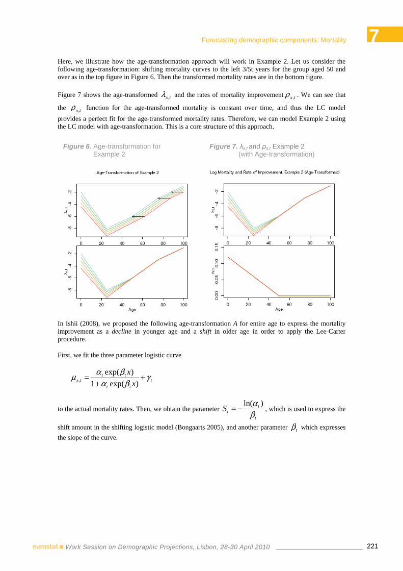
7 Forecasting demographic components: Mortality
221Work Session on Demographic Projections, Lisbon, 28-30 April 2010
Here, we illustrate how the age-transformation approach will work in Example 2. Let us consider the following age-transformation: shifting mortality curves to the left 3/5t years for the group aged 50 and over as in the top figure in Figure 6. Then the transformed mortality rates are in the bottom figure.
Figure 7 shows the age-transformed tx,λ and the rates of mortality improvement tx,ρ . We can see that
the tx,ρ function for the age-transformed mortality is constant over time, and thus the LC model provides a perfect fit for the age-transformed mortality rates. Therefore, we can model Example 2 using the LC model with age-transformation. This is a core structure of this approach.
Figure 6. Age-transformation for Example 2
Figure 7. λx,t and ρx,t Example 2 (with Age-transformation)
In Ishii (2008), we proposed the following age-transformation A for entire age to express the mortality improvement as a decline in younger age and a shift in older age in order to apply the Lee-Carter procedure.
First, we fit the three parameter logistic curve
ttt
tttx x
x γβα
βαμ ++
=)exp(1
)exp(,
to the actual mortality rates. Then, we obtain the parameter t
ttS
βα )ln(−= , which is used to express the
shift amount in the shifting logistic model (Bongaarts 2005), and another parameter tβ which expresses the slope of the curve.

7 Forecasting demographic components: Mortality
222Work Session on Demographic Projections, Lisbon, 28-30 April 2010
Next, let x be the original age and z be the transformed one, and define the relation )(zfx t= as follows.
( )( )
( )⎪⎪⎪
⎩
⎪⎪⎪
⎨
⎧
≤+−
≤≤+−
−
⎭⎬⎫
⎩⎨⎧
−+−
≤
=
zBSSz
BzBBBB
BzBSSB
Bzz
zf
ttt
t
ttt
tt
2
21112
112
1
def
)(
)()(
0
0
0
0
ββ
ββ
Then set , ( ),def tz t f z tμ μ∧
=
Figure 8. Age-transformation Function Age-Transformation
Figure 9. Iso Transformed-age Map Iso transformed-age Map
Figure 8 shows an example of age-transformation function, and Figure 9 shows the iso transformed-age map. Using the age-transformation A , modeling and projecting mortality rates are performed as )( ,
1txALA μ− .
4. Mortality Improvement: Decline or Shift?
In Section 3, we reviewed the age-transformation approach developed in Ishii (2008). For the modelling of adult mortality, the projection is based on the assumption that the mortality improvement is considered as shifting. It is suggested from the trends in tx,μ and ,x tl that the recent improvement in adult mortality in Japan could be better understood when considering it as shifting. In this section, we reconsider whether it is more plausible to understand mortality improvement in Japan as declining or shifting. First, we describe the definitions of the proportional hazard model and the Lee-Carter model, which are decline-type models. Then, we introduce the horizontal shifting model and the horizontal Lee-Carter model, which are shift-type models corresponding to the two decline-type ones. Through this consideration, we propose a new type of adult mortality model and discuss another way to define age-transformation.

7 Forecasting demographic components: Mortality
223Work Session on Demographic Projections, Lisbon, 28-30 April 2010
4.1 Decline-Type Mortality Models
4.1.1 The Proportional Hazard Model (PH) The proportional hazard model (abbreviated as PH) is a simple model that expresses mortality improvement as decline. In the PH model, tx,λ : the log hazard rate function at time t is expressed by
txtxtx ka +== ,, log μλ
where ax: the baseline logged hazard rates.
In the PH model, tx,ρ : the rate of mortality improvement
', t
ttx k
dtdk −=−=ρ
is constant with respect to age. This is the differential form for this model. In this paper, we fit and numerically evaluate the models against the Japanese female mortality. We use
ctxm , , )25(== sxx ,…, )110(=ex and )1970(== sc tt ,…, )2007(=et
from the HMD (Human Mortality Database), where ct is a calendar year. Here, we set xa as the average
log hazard rate in the entire period. Figure 10 shows the actual log hazard rates (ctx,λ ) and the estimated
rates with the PH model. We can observe that the estimated rates do not exhibit good fit particularly in the older age groups. Figure 11 shows the difference between the actual and estimated rates. From this graph, we can see that the actual values are higher than those of the model for age around from 60 to 80 in 1970, whereas these values are decreasing over time. However, opposite movement is observed for ages over 90. This is caused by the limitation of the PH model whereby the rate of mortality improvement is constant with respect to age.
Figure 10. Mortality rates (Actual and model, PH)
Figure 11. Difference of mortality rates (actual-Model, PH)

7 Forecasting demographic components: Mortality
224Work Session on Demographic Projections, Lisbon, 28-30 April 2010
4.1.2 The Lee-Carter Model (LC) The LC model is already defined in Section 3. It expresses mortality improvement as decline in a more general manner as compared with the PH model. Here, we set xa as the average log hazard rate for the
entire period. Figure 12 shows the actual log hazard rates (ctx,λ ) and the estimated rates by the LC
model. This figure illustrates that the fit with the actual values is fairly improved by using the LC model, due to its flexibility which admits different mortality improvement rates by age.
However, we can observe from Figure 13 that the difference between the actual and estimated rates exhibits a trend whereby the actual values are higher in younger age groups and lower in older age groups near the beginning and the end of the entire period, whereas the opposite is true around the middle of the period. The reason why this trend for the error components is observed is ascribed to the change in the age-specific mortality improvement rates over time. Therefore, we will next examine the tx,ρ functions for these two models.
Figure 12. Mortality rates (actual and model, LC)
Figure 13. Difference of mortality rates (actual-model, lC)
Figures 14 and 15 show the ctx,ρ functions for the actual values and the estimated values for each of the
two models. The blue lines show the ctx,ρ by the actual mortality rates. We can observe that most of the
mortality improvement rates have mountain-shaped curves with peaks. In contrast, the mortality improvement rates under the PH model, expressed by the pink line, are horizontal. This difference in shape would be viewed as a cause that the estimates by the PH model are not well-fitted, as we observed before. The mortality improvement rate by the LC model, indicated with the green curves, has a peak like that of the actual value, and this improves the fit as we have seen before. However, the age distribution of the rates is fixed in the LC model, whereas it changes dynamically in the actual values. Thus, the actual age distribution of mortality improvement rates change over time and are not constant as in the LC model, and caused the propensity for the error in the LC model observed in Figure 13. We could see this result as a limitation when the mortality improvement is considered as decline.

7 Forecasting demographic components: Mortality
225Work Session on Demographic Projections, Lisbon, 28-30 April 2010
Figure 14. Comparison of mortality improvement rates (1974-1989)
Figure 15. Comparison of mortality improvement rates (1990-2005)
4.2 Shift-Type Mortality Models
4.2.1 The Horizontal Shifting Model (HS) Next, we discuss models that express mortality improvement through a shift. The simplest model for shifting would be one whereby the entire log hazard curve moves to the right-hand side. We can restate this model using the inverse function of log hazard mortality tyv , , that is, the proportional hazard model
for tyv , .
This model that we call the horizontal shifting model (abbreviated as HS) here is formally expressed as follows:
tyty kav +=,
In the differential form,
', t
tty k
dtdk ==τ
Parameter estimation for the HS model is completely identical to the PH models, except for adapting these procedures to
ctyv , instead of cty ,λ . Figures 16 and 17 are the actual inverse mortality rates (
ctyv , ) and the estimated rates by the HS model, and the difference between the actual and the estimated. We can see that the performance of fitting by the HS model is much better than by the PH model, even though both have the same structure. For 1970, indicated with the light blue line, the actual values are higher in younger ages and lower in older ages, though the errors are not as high for other years.

7 Forecasting demographic components: Mortality
226Work Session on Demographic Projections, Lisbon, 28-30 April 2010
Figure 16. Inverse mortality rates (actual and model, HS)
Figure 17. Difference of inverse mortality rates (actual and model, HS)
4.2.2 The Horizontal Lee-Carter Model (HL) As we considered the LC model which admits a different amount of decline by age and provides a more general framework compared with the PH model, we can also consider the Lee-Carter model for tyv , which in turn supports a more general shifting feature. We call it the horizontal Lee-Carter model (abbreviated as HL).
ytyty bkav +=,
In the differential form,
ytyt
ty bkbdtdk '
, −==τ
Figures 16 and 17 are the actual inverse mortality rates (ctyv , ) and the estimated rates under the HS
model, and the difference between the actual and the estimated. We can see that the HL model seems to be improved compared to the HS model. However, it is also observed that the improvement between the shift pair is not as large as the decline pair. This means that relaxing the limitation, which the force of age increase in the HS model is restricted to the constant function, does not cause significant improvement of fit in the HL model. It could be explained by the difference in the shape of
cty ,τ , the force of age
increase. Figures 20 and 21 show the cty ,τ functions for the actual values and the estimated values by the
two shifting models. We observe that the green curves, which correspond to cty ,τ by the HL model, are
close to a horizontal line, which coincides with the force of age increase by the HS model shown in the pink lines. This fact endorses that the improvement between the shift pair is not as large as the decline pair.

7 Forecasting demographic components: Mortality
227Work Session on Demographic Projections, Lisbon, 28-30 April 2010
Figure 18. Inverse Mortality Rates (actual and model, HL)
Figure 19. Difference of Inverse Mortality Rates (actual and model, HL)
However, from the observation of these figures, we have noticed that the blue lines for the actual cty ,τ for
each year could be more well-modelled by a linear function of y, which has led us to the development of a new model: the linear difference model. We will define and examine this new model in the next section.
Figure 20. Comparison of the force of age increase by log mortality rate (1974-1989)
Figure 21. Comparison of the force of age increase by log mortality rate (1990-2005)

7 Forecasting demographic components: Mortality
228Work Session on Demographic Projections, Lisbon, 28-30 April 2010
4.3 The Linear Difference Model (LD)
First, we describe the linear difference model (abbreviated as LD) in the continuous form as we did in other models. In the LD model, we assume that ty ,τ is a linear function of y for each t.
yck ttty''
, +=τ
This is the differential form. By integrating both sides with t, we obtain
yttty ayckv ++=,
where ya denotes a standard pattern of inverse log hazard rates.
Figures 22 and 23 are the actual inverse mortality rates and the estimated rates by the LD model, and the difference between the actual and the estimated. From these figures, we can observe that the LD model fits quite well with the actual values.
This is also confirmed from the observation of ty ,τ functions in Figures 20 and 21. We can observe that
the linear assumption for cty ,τ in the LD model works better than in the other two models.
Figure 22. Inverse mortality rates (actual and model, LD)
Figure 23. Difference of inverse mortality rate (actual and model, LD)
4.4 Comparison of the Models from a Statistical Viewpoint In this section, we compare the LC and LD models from a statistical viewpoint to examine whether it is more plausible to understand the recent Japanese mortality as declining or shifting. Our approach is as follows.
1. The true mortality rates are assumed to be those that are estimated by models.
2. The number of deaths follows a binomial distribution ),( ,, cc txtx pNB , where ctxN , : the number
of the population and ctxp , : the death rate for age x and calendar year tc.

7 Forecasting demographic components: Mortality
229Work Session on Demographic Projections, Lisbon, 28-30 April 2010
3. ctxN , is approximated by the closest integer to
ctxE , : exposure to risk.
Here, we took 0.01% as a critical value to construct the confidence intervals (CI), since txN , would present too large value for the Japanese female population. Figure 24 shows the proportion where the log actual mortality rates are outside of the CIs for each age in the LC and LD models. This indicates that even though the proportions of LD are higher for certain ages, LD’s performance would be considered as fairly better than LC’s as a whole. This result suggests that shift is more strongly supported as recognition of the recent mortality improvement in Japan than decline.
Figure 24. proportion that log actual values are outside of CI (critical value=0.01%)
Figure 25. log mortality surface and two differential functions.
4.5 Differential Forms and Age-transformations Next, we consider the relationship between differential forms and age-transformations, and discuss how the LD model is related to the age-transformation approach.
In section 1, we defined tx,ρ and ty ,τ on the log mortality surface S. Then, the vectors
),1,0(),,(00 ,000 txytx ρρ −=
)0,1,(),,(00 ,000 tyytx ττ =
are tangent vectors on S as shown in Figure 25. Each tangent vector defines a tangent vector field on S. In general, an iso-transformed age map is defined by the projection of the integral curve induced by the tangent vector field onto a X-T plane. For example, the iso-transformed age map induced by ρ is an identity age-transformation, and one by τ is an age-transformation that identifies the ages that yield the same log hazard rates. If we define another tangent vector field on S, then another iso-transformed age map is induced. Therefore, a tangent vector field on S is considered as another representation of an age-transformation.
Let us recall that the LD model is defined by a differential form that is a modeling of ty ,τ . Therefore, the LD model defines an age-transformation through the vector field interpretation with a tangent vector τ . This relationship relates the LD model to the age-transformation approach.

7 Forecasting demographic components: Mortality
230Work Session on Demographic Projections, Lisbon, 28-30 April 2010
5. Concluding Remarks
In this paper, we examined and proposed a new method for mortality projection for Japan as an application of the age-transformation approach.
We considered which is more plausible to understand mortality improvement in Japan as decline or shift. First, we described the definitions of the proportional hazard model and the Lee-Carter model, which are decline-type models. Then, we introduced the horizontal shifting model and the horizontal Lee-Carter model, which are shift-type models corresponding to the two decline type ones. Next, we noticed that the actual
cty ,τ for each year could be well-modelled by a linear function of y, and proposed the linear difference (LD) model. We observed that the LD model coincided quite well with the actual values.
Then, we compared the LC and LD models from a statistical viewpoint to examine whether it is more plausible to understand the recent Japanese mortality as a decline or shift. We observed that LD’s performance would be considered advantageous over LC’s as a whole. This result suggests that shift is more strongly supported as recognition of the recent mortality improvement in Japan than decline.
Finally, we considered the relationship between differential forms and age-transformations, and discussed how the LD model is related to the age-transformation approach. In general, an iso-transformed age map is defined by the projection of the integral curve induced by the tangent vector field onto X − T plane. Therefore, a tangent vector field on S is considered as another representation of an age-transformation. The LD model is defined by a differential form that is a modelling of ty ,τ . Therefore, the LD model defines an age-transformation through vector fields interpretation with tangent vector τ. This relationship relates the LD model to the age-transformation approach.
In this paper, we confirmed that the LD model is efficient, although we noted further points that should be examined. First, we discussed only the adult mortality model here, whereas the entire age model should be developed. Second, we focused on the modelling of the actual values in this paper, whereas we should consider how to project the parameters. These points should be studied in future.
References
Bongaarts, J. (2005) “Long-range Trends in Adult Mortality: Models and Projection Methods”, Demography, Vol. 42, No. 1, pp. 23–49.
Human Mortality Database. University of California, Berkeley (USA) and Max Planck Institute for Demographic Research (Germany). Available at www.mortality.org or www.humanmortality.de.
Ishii, F. (2008) “Mortality Projection Model for Japan with Age-Shifting Structure”, Paper presented at 2008 Annual Meeting of Population Association of America (New Orleans).
Lee, R. and L. Carter (1992) “Modeling and Forecasting U.S. Mortality”, Journal of the American Statistical Association, Vol. 87, No. 419, pp. 659–675.
NIPSSR (2007) Population Projections for Japan: 2006-2055 (With long-range Population Projections: 2056-2105).

7 Forecasting demographic components: Mortality
231Work Session on Demographic Projections, Lisbon, 28-30 April 2010
LEE-CARTER MORTALITY PROJECTION WITH "LIMIT LIFE TABLE"
JORGE MIGUEL BRAVO1
Abstract
The Lee-Carter Model and extensions have been used for decades by official Statistic Bureaus has the standard framework for projecting future mortality rates in population projections. Intrinsically, the model assumes that the dynamics of death rates over time are driven by a single time-varying parameter and that mortality forecasts rely on the extrapolation of this index using appropriate statistical time-series methods. Despite its simplicity and appealing features, the asymptotic behaviour of mortality rates projected by LC model cannot be considered satisfactory. Empirical studies conducted using LC model show a decreasing pattern for the time index parameter tk , combined with positive finite parameters xα
and xβ . In this scenario, it can easily be shown that the extrapolation of past time index trends into the future will invariably lead to zero mortality rates at all ages. In this paper we develop a new variant of the so called Poisson Lee-Carter model in which mortality projections are bounded by a limit life table to which future mortality improvements converge over time. This model explicitly assumes that over a fixed time range there are lower bounds to mortality rates. We assume that these limit rates are exogenously determined, either by expert subjective judgements on the limits to human longevity, or by considering that the limit table resembles that of a more advanced population in terms of socio-economic conditions (target life table), or by admitting that the limit table can be expressed by a parametric mortality law that conveys information on the main trends in population mortality.
Keywords: mortality projections; projected life tables, Lee-Carter, Limit Table.
1. Introduction
The Lee-Carter Model and extensions have been used for decades by official Statistic Bureaus has the standard framework for projecting future mortality rates in population projections. Intrinsically, the model assumes that the dynamics of death rates over time are driven by a single time-varying parameter and that mortality forecasts rely on the extrapolation of this index using appropriate statistical time-series methods.
The Lee-Carter method and its extensions belong to a class of extrapolative methods which assume that future mortality patterns can be estimated by projecting into the future trends observed in the recent to medium-term past. Despite its simplicity and appealing features, the asymptotic behaviour of mortality rates projected by LC model cannot be considered satisfactory.
In fact, empirical studies conducted using LC model show a decreasing pattern for the time index parameter tk , combined with positive finite parameters xα and xβ . In this scenario, it can easily be shown that the extrapolation of past time index trends into the future will invariably lead to zero mortality rates at all ages, an unlikely scenario according to the experts’ judgment on the mortality phenomenon.
1 University of Évora - Department of Economics and CEFAGE-UE Center for Advanced Studies in Management and
Economics of the University of Évora, Largo dos Colegiais, 2,7000-803 Évora, Portugal, [email protected].

7 Forecasting demographic components: Mortality
232Work Session on Demographic Projections, Lisbon, 28-30 April 2010
As an alternative to extrapolative methods, expert-opinion methods involve the use of informed expectations about the future, often accompanied by some alternative low and high scenarios, or a targeting approach. These methods have the advantage of incorporating, in a qualitative way, demographic, epidemiological, medical and other relevant knowledge, but its relative subjectivity and potential for bias should be taken into attention.
In this paper we develop a new variant of the LC model, formulated within a Generalized Linear Model framework with a generalised error distribution, in which mortality projections are bounded by a limit life table to which future mortality improvements converge over time. This model explicitly assumes that over a fixed time range there are lower bounds to mortality rates. We assume that these limit rates are exogenously determined, either by expert subjective judgements on the limits to human longevity, or by considering that the limit life table resembles that of a more advanced population in terms of socio-economic conditions (target life table), or by admitting that the limit life table can be mathematically represented by a parametric mortality law that conveys information on the main trends in population mortality. The methodology is based on a combination of extrapolative and expert-opinion based methods and has been used in the projection of the component mortality within the 2008 Portuguese Population Projections exercise. This methodology allows us to explicitly consider expert judgment together within a statistical extrapolative model, which is important to ensure that forecasted values based on past trends in mortality are within biologically reasonable boundaries. The paper is organized as follows. In Section 2, we briefly describe the classical age-period Lee-Carter mortality forecasting method, focusing on the asymptotic properties of projected mortality rates. In Section 3, we develop an extension of the LC considering the existence of a limit life table. We discuss the critical aspects in the application of this LC variant, namely the alternatives approaches that can be followed to select an appropriate limit life table. Section 4 concludes.
2. Classical Lee-Carter mortality modelling
The classical LC modelling approach has dominated the recent literature in the field of mortality forecasting (see Brouhns et al. 2002, Booth 2006, Booth and Tickle 2008 and further references therein). According to Booth and Tickle (2008), the LC-based approach is broadly considered in the current literature to be among the most efficient and transparent methods used to generate plausible life expectancy forecasts for use within population projection exercises, prospective life table construction or life insurance actuarial calculations.
The classical age-period AP LC model was first introduced by Lee and Carter (1992), combining a demographic model for the mortality rate, dependent only on factors related to age and period, describing the historical change in mortality, a method for fitting the model and a time series model for the time component which is used for forecasting. The classical AP LC model is expressed as
( ), ,ln x t x x t x tm kα β ε= + + (1)
where txm , denotes the central mortality rate at age x in year t , tk represents a time-index level of
mortality, xα and xβ are vectors of age-specific constants denoting, respectively, the general (average over time) pattern of mortality by age and the relative rate of response at age x to changes in the overall level of mortality over time, and tx,ε are Gaussian distributed ),0( 2
εσN random effects by age and time.
The equation underpinning the Lee-Carter model is known to be over parameterized due to the log-bilinear multiplicative term x tkβ . Because of this, the identifiability problem is traditionally resolved by
ensuring that parameters xβ and tk satisfy the following constraints

7 Forecasting demographic components: Mortality
233Work Session on Demographic Projections, Lisbon, 28-30 April 2010
max max
min min
1, 0x t
x tx x t t
kβ= =
= =∑ ∑ (2)
As a result of these constraints, the parameter xα is calculated simply by averaging the )ln( ,txm over time. The main statistical tool of Lee and Carter (1992) is least-squares estimation via SVD decomposition of the matrix of )ln( ,txm . The authors incorporated an adjustment to the estimated tk so that fitted deaths match observed total deaths in each year. In the classical AP LC type modelling approach, the age effects ( xα and xβ ) are assumed to be constant in time and the time-variant period
effects are projected forward using autoregressive time series models. Specifically, the period factors tk are extrapolated in time by standard univariate stochastic ARIMA processes in order to make forecasts of the future force of mortality and, implicitly, future (period- and cohort-based) life expectancy.
In terms of forecasting, the LC family of models are part of the extrapolative stochastic methods that assume that future mortality patterns can be estimated by projecting into the future the historical trends of human mortality observed in the recent to medium-term past. Although the validity of these assumptions is frequently debated (see, e.g., Gutterman and Vanderhoof 2000), the inherent complexity of the factors affecting human mortality and the current lack of understanding of the intricate mechanisms governing the aging process, together with the relative stability of the past trends, is used by many authors as a justification for the use of past trends as a reliable basis for future projections.
The way the demographic model is defined in the LC family of models ensures that death rates exhibit a pattern of exponential decrease, without imposing any arbitrary asymptotic limit to future gains in life expectancy. Although this behaviour is consistent with the pattern of mortality decline observed in developed countries, the asymptotic behaviour of deaths rates (or life expectancy) projected by the LC family of models should somehow be considered unsatisfactory.
In fact, most empirical studies conducted using the LC models (see, e.g., Lee and Carter 1992, Brouhns et al. 2002), including some on the Portuguese population (Bravo 2007, INE 2008), show a clear downward trend for the estimated time index tk and positive estimates of xβ , a result anticipated in a context characterised by a mortality decline over time. Assuming that the age effects are constant in time, the use of time-series methods to extrapolate tk over long-term horizons leads us invariably to asymptotic
deaths rates approaching zero. Formally, given positive xβ 's and finite xα 's it is clear that
( ),ˆ ˆˆ ˆˆlim lim exp 0x t x x tk k
kμ α β→−∞ →−∞
= + = (3)
This is an unlikely scenario based on our current understanding of the mortality phenomena. The linear projections of log of mortality rates implicit in the LC method may produce implausible age patterns in the long run if any assumed rate trends differ, since these differences will be augmented in the projections. For instance, linear extrapolation of past LE trends for Portugal and Japan will lead to huge future differences between these two countries because of their different past trends. The same argument is valid for extrapolation of male and female LE. In effect, since in most countries male and female LE at birth are converging, simple extrapolation of these trends will inevitably lead to male LE exceeding female LE.
Moreover, forecasts based on the LC model are likely to imply increasing divergence in life expectancy in the long run, contradicting the observation made by Wilson (2001) who documented a global convergence in mortality. This motivated modifications in the LC method to ensure non-divergence (see, e.g., Lee 2000).

7 Forecasting demographic components: Mortality
234Work Session on Demographic Projections, Lisbon, 28-30 April 2010
3. Lee-Carter Model with "Limit Life Table"
Concerns over the asymptotic behaviour of projection models motivated the development of solutions that require, in principle, an arbitrary positive number for deaths rates in the long run. The approach used in these studies lies in the field of so-called projection models with limit table (or objective table). Initially developed by Bourgeois-Pichat (1952), these models admit the existence of an “optimal” life table to which longevity improvements over time converge. In other words, these models explicitly admit that there are (at least in a limited time horizon) natural limits to human longevity, i.e., mortality levels below which it is considered impossible to descend in the projection interval. There are many arguments used as a justification for a limited duration of life, the most critical is the one that states that there is a decline in the physiological parameters associated with ageing in humans, but other arguments include stylized facts such as the slowdown in life expectancy at birth increases observed in many developed countries.2
In this paper we present and upgrade an extension of the Lee-Carter model developed by Bravo (2007) in which future mortality developments are guided by a particular limit life table to which future longevity
improvements tend to converge. Let limxμ and lim
xq denote, respectively, the instantaneous death rate and the probability of death corresponding to this target life table. Assume that, given any integer age x and calendar year t , the age-specific forces of mortality are constant within each rectangle of the Lexis diagram but allowed to vary from one to the next, i.e.,
txtx ,, μμ τξ =++ for 0 , 1ξ τ≤ < . (4)
We follow Brouhns et al. (2002) and assume that the LC model can be formulated within a Generalized Linear Model (GLM) framework with a generalised error distribution. Specifically, we assume that the age- and period-specific numbers of deaths ,x tD are independent realizations from a Poisson distribution with parameters
, , ,x t x t x tE D E μ=⎡ ⎤⎣ ⎦ and , ,x t x tVar D E Dφ=⎡ ⎤ ⎡ ⎤⎣ ⎦ ⎣ ⎦ (5)
where ,x tE denotes the number of individuals exposed-to-risk at age x during calendar year t , and φ is a measure of over-dispersion to allow for heterogeneity. To incorporate an upper limit to life span in the LC family of models, we replace parameterization (1) by
lim, ,
adx t x x tμ μ μ= + (6)
with
( ), expadx t x x tkμ α β= +
(7)
As can be observed, the model stipulates that the number of deaths expected at age x in year t is determined by the corresponding exposure ,x tE and by a force of mortality that results from the sum of
the limit value limxμ with an additional (contemporary) value ,
adx tμ , defined by the classical Lee-Carter
parameterization. In spite of this, parameters xα , xβ and tk maintain, in essence, their original
2 We note that this slowdown in LE increases is paralleled by an accelerated decline in mortality at older ages. Moreover, the
fastest decline of mortality has been observed in countries with the lowest levels of old-age mortality, i.e., the opposite of what is expected if mortality were pushing against an upper limit.

7 Forecasting demographic components: Mortality
235Work Session on Demographic Projections, Lisbon, 28-30 April 2010
interpretation. Equation (6) provides a simple (additive) solution to incorporate the existence of a limit life table within the LC framework. Alternative formulations could be considered, e.g., by assuming different rates of converge to the target value over time.
Equations (5), (6) and (7) correspond to a GLM model of the response variable ,x tD with logarithmic
link and non-linear parameterized predictor ,x tη :
( ) ( )( ) ( )
, , , ,
lim,
ˆlog log
log log
x t x t x t x t
x t x x x t
d E
E k
η μ
μ α β
= =
= + + + (8)
In order to obtain unique parameter values, the above model is formulated in line with the together with usual identification restrictions (2), while ( ) ( )lim
,log logx t xE μ+ is treated as an offset value during
fitting.
Model (8) is conceptually different from the original LC framework (1), because the modelling errors have a generalised class of distribution (member of the exponential family) that are determined by the direct fitting of the number of deaths instead of the logarithmic transform of the mortality rates. That is, the GLM regression is based on ML methods with theory-based distributional assumptions in contrast to the SVD fitting, which relies on empirical measures (i.e. least squares). Moreover, the parameter estimates under the original framework (1) can be considered a particular case of the GLM regression since they can derived within the GLM approach by adjusting the target variable to ( ), ,logx t x tD m= and applying the identity link function with a Normal error structure.
Given equations (5), (6) and (7) and model assumptions, it can be shown that the parameter estimates are obtained by maximizing the following log-likelihood function
( )( )
( )
,max max
min min
max max
min min
, ,
,
lim, ,
exp( , , ) ln
!
ln( exp ) exp( )
x tdx tx t x t
x x tx x t t x t
x t
x t x x x t x t x x tx x t t
L kd
d k E k c
λ λα β
μ α β α β
= =
= =
⎧ ⎫⎞⎛ −⎪ ⎪⎟⎜= ⎨ ⎬⎜ ⎟⎪ ⎪⎝ ⎠⎩ ⎭
= + + − + +
∏ ∏
∑ ∑ (9)
where ( )( )lim, , , expx t x t x t x x x tE D E kλ μ α β= = + +⎡ ⎤⎣ ⎦ and c denotes a constant term. The presence
of the log-bilinear term x tkβ in (9) prevents the estimation of model parameters using standard statistical packages that include GLM Poisson regression. Because of this, we resort to an iterative algorithm for estimating log-bilinear models developed by Goodman (1979) based on a Newton-Raphson algorithm. The algorithm proceeds as follows: in iteration step 1v + , a single set of parameters is updated fixing the other parameters at their current estimates using the following updating scheme
( )
( 1) ( 1)2 ( )
2
( , , )
ˆ ˆ( , , )
vx x t
jv vj j v
x x t
j
L k
L k
α βθ
θ θα β
θ
+ +
∂∂
= −∂
∂
(10)

7 Forecasting demographic components: Mortality
236Work Session on Demographic Projections, Lisbon, 28-30 April 2010
Similar to the original LC model, we have in our application three sets of parameters, namely the xα ,
xβ and tk terms. For example, the updating scheme for parameter xα can be represented, for a given
starting value (0)ˆxα , as follows
( )
max
min
max
min
( , , ),( 1,1) ( , , )
, , ,lim ( , , ),
lim ( , , ),( 1,2) ( , , )
, , ,2lim ( , , ),
(( 1) ( )
ˆˆ ˆ
ˆ
ˆˆ ˆ
ˆ
ˆˆ ˆ
ad v v vtx tv ad v v v
x x t x t x tad v v vt t x x t
ad v v vtx x tv ad v v v
x x t x t x tad v v vt t x x t
vv v x
x x
d E
d E
μα μ
μ μ
μ μα μ
μ μ
αα α
+
=
+
=
+
⎞⎛= − ⎟⎜ ⎟+⎝ ⎠
⎞⎛⎟⎜= −⎟⎜ +⎝ ⎠
= −
∑
∑1,1)
( 1,2)ˆ vxα
+
+
(11)
where
( )( )( ) ( )( , , ),ˆ exp kvv vad v v v
x t x x tkβαμ α β= + .
Similar schemes are derived for parameters xβ and tk .
Finally, the initial parameter estimates generated by the algorithm are adjusted in order to fulfil the identification constraints, i.e.,
( )
( )
m ax
m in
m ax
m in
m ax m in
1 ˆˆˆ ˆ , 1
ˆ ˆ ˆ ˆ ˆ ,
ˆˆˆ
t
x x x tt t
x
t t xx x
xx
k k kt t
k k k ξ ξ
ξ
α α β
β β β
βββ
=
=
← + =− +
← − =
←
∑
∑
(12)
One of the critical aspects in the application of the LC mortality projection model with limit life table refers to the selection of the limit table, i.e., to the definition of what are considered the plausible limits to human longevity or to what are the extreme levels of mortality which will be reasonably reached over a given limited time horizon. Although there are biological arguments in favour of an upper age limit, there is an ongoing debate about the value of this limit with many proposals for the maximum of xe& or life span found in the literature (see, e.g., Harman, 2001).
To determine this limit, a number of subjective or informed assumptions about the future development of a set of important biological, economic and social variables have to be made. Using a biodemographic approach, Olshansky (1990) refers to the schedule of age-specific death rates as an “intrinsic mortality signature”, which might change only when the forces of selection acting to maintain the genetic composition of a population are disrupted (either through environmental challenges, interventions, or diseases).
In practical applications, this prospective exercise may however reveal very difficult or even impossible. In this case, a different way of interpreting the model is to consider the limit table as a life table that reflects the pattern of mortality in a more advanced population in terms of economic and social development (target population) to which current experience will converge in a given time horizon. For instance, Oeppen and Vaupel (2002) recommended using the observed gaps between countries and

7 Forecasting demographic components: Mortality
237Work Session on Demographic Projections, Lisbon, 28-30 April 2010
regions. In this case, the life expectancy in the countries with the highest life expectancy can set as the achievable limit for all.
Alternative approaches include a combination of the lowest mortality rates observed by sex-age groups, or gaps between countries (i.e., considering the time needed by a specific country to catch up the most advanced countries), or estimates of the lowest achievable cause-specific death rates. Eradication of one or more causes of deaths and the resulting change in mortality rates have been used to predict achievable gains in life expectancy (see, e.g., Nusselder et al. 1996). One of the problems here is the lack of independency between causes of deaths. Alternatively, attainable (target) life expectancy can be estimated by combining the lowest mortality rates observed worldwide. Recently, Vallin and Meslé (2008) used a similar approach by combining the lowest age- and cause-specific mortality rates worldwide from 1950 to 2000. In 2000, the authors conclude that the resulting 0e& would reach 84.4 years
in men and 88.9 years in women. By comparing the highest observed 0e& and the potential 0e& resulting
from the model the authors argue that observed 0e& reached potential 0e& about 25-30 calendar years later.
An alternative solution is to take some parametric function - mortality law (Gompertz-Makeham, Weibull, Heligman-Pollard,...) - on which to examine different scenarios on the main trends in human longevity (e.g., rectangularization of the survival function, evolution of life expectancy, mode of the survival function, entropy,...) by incorporating recent statistical information and expert-opinion judgements. In this line of research, Duchêne and Wunsch (1988) proposed a hypothetical limit life table based on the Weibull mortality law
1
limx
xα
αμβ β
−⎞⎛= ⎟⎜
⎝ ⎠ (13)
with 95β = and 14.40198275α = . The authors assume also that the highest attainable age is 115
years old, that the modal age is 95 years old, that 0 0.002q = and that of a total of one million of newborns only one will survive until age 114. From (13), the corresponding survival function is given by
expx xxl l
α
β⎡ ⎤⎞⎛= −⎢ ⎥⎟⎜⎝ ⎠⎢ ⎥⎣ ⎦
(14)
and is represented in Figure 1 .

7 Forecasting demographic components: Mortality
238Work Session on Demographic Projections, Lisbon, 28-30 April 2010
Figure 1. Duchêne-Wunsch limit life table, survival function 0llx x→
Idade
l(x)/l
(0)
0 20 40 60 80 100
0.0
0.2
0.4
0.6
0.8
1.0
We note that this limit life table establishes a significant rectangularization of the survival curve. As one of the many possible alternatives, the 2008 Portuguese population projection exercise used the so-called second Heligman and Pollard (1980) mortality law, defined by
( )( ) 2exp (ln ln )1
Cx
x Bx x
GHq A D E x FKGH
+= + − − ++
(15)
where xq denotes the death probability at age x and A , B , C , D , E , F , G , H and K are parameters to be estimated by non-linear weighted least squares methods. Equation (13) includes three distinct terms, each reflecting a separate component of mortality. The first term, an exponential function rapidly decreasing, represents the decrease in mortality during the first years of life. The second term, a sort of lognormal function, represents the mortality at intermediate adult ages and is referenced in demographic and actuarial literature as describing the incidental mortality for both sexes, and maternal mortality for the female population. The third term reflects the traditional Gompertz mortality law, which reflects the exponential growth of mortality at older ages. Figure 1 gives an example of a mortality scenario generated by the Heligman-Pollard (HP) mortality law based on the following parameters
Table 1. Parameter values of a specific mortality scenario generated by the HP mortality law
Parameter A B C D E F G H K
Coefficient 0,00023 0,05 0,10 0,00150 2,200 85,0 0,00001 1,10350 0,060
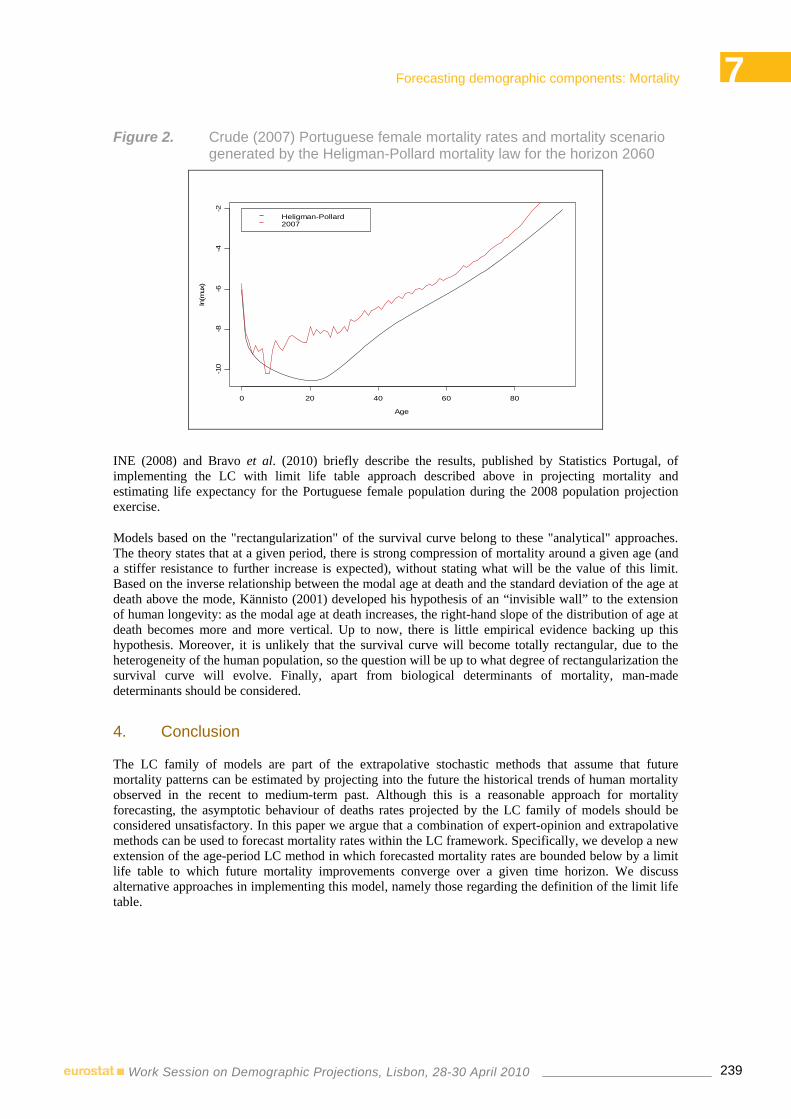
7 Forecasting demographic components: Mortality
239Work Session on Demographic Projections, Lisbon, 28-30 April 2010
Figure 2. Crude (2007) Portuguese female mortality rates and mortality scenario generated by the Heligman-Pollard mortality law for the horizon 2060
Age
ln(m
ux)
0 20 40 60 80
-10
-8-6
-4-2
Heligman-Pollard2007
INE (2008) and Bravo et al. (2010) briefly describe the results, published by Statistics Portugal, of implementing the LC with limit life table approach described above in projecting mortality and estimating life expectancy for the Portuguese female population during the 2008 population projection exercise.
Models based on the "rectangularization" of the survival curve belong to these "analytical" approaches. The theory states that at a given period, there is strong compression of mortality around a given age (and a stiffer resistance to further increase is expected), without stating what will be the value of this limit. Based on the inverse relationship between the modal age at death and the standard deviation of the age at death above the mode, Kännisto (2001) developed his hypothesis of an “invisible wall” to the extension of human longevity: as the modal age at death increases, the right-hand slope of the distribution of age at death becomes more and more vertical. Up to now, there is little empirical evidence backing up this hypothesis. Moreover, it is unlikely that the survival curve will become totally rectangular, due to the heterogeneity of the human population, so the question will be up to what degree of rectangularization the survival curve will evolve. Finally, apart from biological determinants of mortality, man-made determinants should be considered.
4. Conclusion
The LC family of models are part of the extrapolative stochastic methods that assume that future mortality patterns can be estimated by projecting into the future the historical trends of human mortality observed in the recent to medium-term past. Although this is a reasonable approach for mortality forecasting, the asymptotic behaviour of deaths rates projected by the LC family of models should be considered unsatisfactory. In this paper we argue that a combination of expert-opinion and extrapolative methods can be used to forecast mortality rates within the LC framework. Specifically, we develop a new extension of the age-period LC method in which forecasted mortality rates are bounded below by a limit life table to which future mortality improvements converge over a given time horizon. We discuss alternative approaches in implementing this model, namely those regarding the definition of the limit life table.

7 Forecasting demographic components: Mortality
240Work Session on Demographic Projections, Lisbon, 28-30 April 2010
References
Booth, H. (2006). Demographic forecasting: 1980 to 2005 in review. International Journal of Forecasting 22(3), 547–581.
Booth, H. and Tickle, L. (2008). Mortality modelling and forecasting: A review of methods. ADSRI Working Paper No. 3.
Bourgeois-Pichat, J. (1952). Essai sur la mortalité biologique de l’homme. Population, 7(3), 1-31.
Bravo, J. M. (2007). Tábuas de Mortalidade Contemporâneas e Prospectivas: Modelos Estocásticos, Aplicações Actuariais e Cobertura do Risco de Longevidade. Dissertação de Doutoramento em Economia, Universidade de Évora.
Bravo, J. M., Coelho, E. and Magalhães, M. G. (2010). Mortality projections in Portugal. Proceeding of the EUROSTAT/UNECE Joint Session on Demographic Projections, Lisbon, Portugal, 28-30 April 2010, forthcoming.
Brouhns, N., Denuit, M. e Vermunt, J. (2002). A Poisson log-bilinear regression approach to the construction of projected life tables. Insurance: Mathematics and Economics, 31, 373-393.
Duchêne, J. e Wunsch, G. (1988). From the demographer's cauldron: single decrement life tables and the span of life. Genus, Vol. XLIV, 3-4, 1-17.
Goodman, L. (1979). Simple models for the analysis of association in cross classifications having ordered categories. Journal of the American Statistical Association, 74, 537-552.
Gutterman, S. and Vanderhoof, I. (2000). Forecasting changes in mortality: a search for a law of causes and effects. North American Actuarial Journal 2, 135–138.
Harman D. (2001). Aging: Overview. Annals of the NY Academy of Sciences, 928(1), 1-21.
Heligman, L. and Pollard, J. (1980). The age pattern of mortality. Journal of the Institute of Actuaries, 107, 49-80.
INE (2008). Projecções de População Residente em Portugal 2008-2060. Instituto Nacional de Estatística, Série Estudos, Setembro 2008.
Kannisto V. (2001). Mode and dispersion of the length of life. Population, 13(1), 159-171.
Lee, L. (2000). The Lee-Carter method for forecasting mortality, with various extensions and applications. North American Actuarial Journal 4, 80–93.
Lee, R. e Carter, L. (1992). Modelling and forecasting the time series of US mortality. Journal of the American Statistical Association, 87, 659-671.
Nusselder W.J, van d, V, van Sonsbeek J.L, Lenior ME, van den Bos G.A. (1996). The elimination of selected chronic diseases in a population: the compression and expansion of morbidity. American Journal of Public Health, 86(2), 187-194.
Oeppen J, Vaupel J. W. (2002). Broken limits to life expectancy. Science 296, 1029-1031.
Olshansky S.J, Carnes B.A and Cassel C. (1990). In search of Methuselah: estimating the upper limits to human longevity. Science 250, 634-640.
Vallin J, Mesle F. (2008). Les plus faibles mortalités. Unpublished Work.
Wilson C. (2001). On the Scale of Global Demographic Convergence 1950-2000. Population and Development Review, 27(1), 155-172.

7 Forecasting demographic components: Mortality
241Work Session on Demographic Projections, Lisbon, 28-30 April 2010
MORTALITY PROJECTIONS IN PORTUGAL1
Edviges COELHO2, Maria Graça MAGALHÃES3
Jorge Miguel BRAVO4
Abstract
Population forecasts are used for important policy decisions both in the public and private sector. Forecasts produced using the cohort-component method requires, for each cohort, a projection of the fertility, migration and mortality components. In this paper we describe the methodology used in the projection of the component mortality within the 2008 Portuguese Population Projections exercise. The methodology is based on a combination of extrapolative and expert-opinion based methods. Specifically, we use the Lee and Carter (1992) log-bilinear model and its extension by Brouhns et al. (2002) based on heteroskedastic Poisson error structures, together with a new variant of the model proposed by Bravo (2007) in which the Poisson-Lee-Carter framework includes a limit life table to which future mortality improvements converge. This allows us to explicitly consider expert judgment together within a statistical extrapolative model, which is important to ensure that forecasted values based on past trends in mortality are within biologically reasonable boundaries. Additionally, we describe the methodology used to close life tables at older ages. Finally, we give an example on how to use this model considering mortality scenarios concerning the future development of mortality generated by the Heligman-Pollard mortality law for the Portuguese female population.
1. Introduction
Population forecasts are used for important policy decisions both in the public and private sector. The 2008 Portuguese Population Projections exercise provides projections of resident population through 2060, discriminated by age and sex. The projections originate with a base population from 1st January 2008 estimates of resident population and are produced using the cohort-component method. The three components of population change (fertility, mortality, and net migration) are projected separately for each birth cohort (persons born in a given year). The base population is advanced each year by using projected survival rates and net international migration by single year of age and sex. Each year, a new birth cohort is added to the population by applying the projected age specific fertility rates to the female population aged 15 to 45 years, and updating the new cohort for the effects of mortality and net international migration. The assumptions underlying the three components of population change are based on a blend of past trend analysis, expert judgment and stochastic models.
In this paper we describe the methodology used in the projection of the component mortality within the 2008 Portuguese Population Projections exercise. The methodology is based on a combination of extrapolative and expert-opinion based methods. Specifically, we use the Lee and Carter (1992) log-bilinear model and its extension by Brouhns et al. (2002) based on heteroskedastic Poisson error structures, together with a new variant of the model proposed by Bravo (2007) in which the Poisson-Lee-Carter framework includes a limit life table to which future mortality improvements converge. This
1 The analyses, opinions and findings contained in this paper represent the views of the authors and are not necessarily those of
Statistics Portugal. 2 Department of Demographic and Social Statistics ([email protected]). 3 Department of Demographic and Social Statistics ([email protected]). 4 Department of Economics and CEFAGE-UE ([email protected]).

7 Forecasting demographic components: Mortality
242Work Session on Demographic Projections, Lisbon, 28-30 April 2010
allows us to explicitly consider expert judgment together within a statistical extrapolative model, which is important to ensure that forecasted values based on past trends in mortality are within biologically reasonable boundaries. The estimated parameters obtained from these models and forecasts for the time trend were used in the models’ framework to create mortality schedules required for the cohort-component method. Expert’s judgments on the future of human longevity in Portugal were accounted for as boundaries to the decline of death rates over the projection period.
The Lee-Carter model assumes that a single dynamic temporal process drives the changes in death rates at all ages over time. This method implicitly assumes that the errors are homoskedastic, which has proven to be unrealistic since the logarithm of the observed death rates is much more volatile at older ages. Brouhns et al. (2002) developed a maximum likelihood estimation solution of the Lee-Carter model based on the assumption that the number of deaths follows a Poisson distribution. The Poisson Lee-Carter method is used to model and projected the mortality in the 2008 Population Projections for Portugal.
The Lee-Carter method and its extensions are based on the assumption that the future mortality will continue to improve at the same rate as in the past. Being an extrapolative method, in contexts characterised by the decline of death rates, the model leads us invariably to asymptotic death rates approaching zero, an unlikely scenario according to the experts’ judgment on the mortality phenomenon. In order to consider the experts’ opinions we resort to an extension of the Lee-Carter model with a limit life table developed by Bravo (2007). This allows us to explicitly consider the expert judgment, which is an important factor in ensuring that the model is not forecasting mortality levels that are beyond biologically feasible levels. Two assumptions where established concerning the future development of mortality: one optimistic and another moderate. In the optimist assumption, the Poisson Lee-Carter was applied. In what concerns the moderate assumption, limits to the decline of age specific deaths rates were imposed through the use of the Heligman and Pollard (1980) mortality law, based on opinions of national experts.
The projection of mortality at advanced ages is particularly important due to the increasingly concentration of deaths at ages more and more advanced, with reductions of mortality beyond these ages having a growing contribution to future gains in life expectancy. Observed death rates at oldest ages, however, show a rather erratic pattern justified by the fact that these figures may be heavily contaminated by random fluctuations, due to the small number of those surviving up to very old ages as well as to the probable misreporting of ages occurred at the censuses to at very old ages. Following the study of mortality in old age in the calculation of complete life tables for Portugal (Coelho, Magalhães and Bravo, 2007), the probability of dying at ages above 85 years for men and women are estimated using the method of Denuit and Goderniaux (2005). The paper is organized as follows. In Section 2 we describe the major trends observed in the Portuguese mortality and the major expected improvements for the next 50 years. In Section 3, we briefly describe the classical Lee-Carter method, the extension proposed by Brounhs et al. (2002) and the limit table extension proposed by Bravo (2007). In Section 4, we describe the methodology used to close life tables at older ages. In Section 5 we briefly describe the results of implementing the approaches described above in projecting mortality for the Portuguese female population during the 2008 population projection exercise. Section 6 concludes.
2. Past and current trends in mortality and longevity in Portugal
Life expectancy at birth in Portugal has nearly doubled in less than a century, attaining 75.18 years for men and 81.57 years for women in the period 2005- 2007. Similar to other developed countries, two major trends dominated the mortality decline in Portugal during the last century: a huge decrease in infant mortality, more evident during the first half of the century, and a decrease in mortality at older ages, more pronounced during the second half. This pattern is somehow expected since the ongoing increase in life expectancy is driven by the mortality decline among older persons. This has important consequences in many areas, ranging from population projections to the provision of health care or the management of social security systems.
In the opinion of experts, further improvements in mortality among the elderly might still be expected in the future. A common prediction among researchers on the limits of human longevity is that the decline in premature deaths will continue to occur in the future. The modal age at death, which can be interpreted

7 Forecasting demographic components: Mortality
243Work Session on Demographic Projections, Lisbon, 28-30 April 2010
as an indicator of the mean longevity at a given time, increased steadily in the last decades. Among adults, the variability of age at death decreased during the last decades, signalling a compression of mortality (rectangularization of the survival curve). As a consequence, the proportion of those surviving up to older ages increased and the age of maximum mortality gradually shifted towards older ages.
In what concerns infant mortality, there is not great scope for further gains as the current levels are already very low. In 2007, infant mortality rate was 3.4 deaths per thousand live births. This figure is not far from the estimated endogenous mortality (mortality occurring in the first year of life resulting from congenital, hereditary defects or injuries caused during delivery) that, by definition, is not preventable. Experience from other developed countries regarding the effects of improvements in legislation on occupational safety and traffic accidents supports expectations of further declines in mortality at young and medium adult ages.
Concerning differences in longevity between men and women, the pace of growth of average life expectancy of women has been historically higher, contributing to the increase of the longevity gap between men and women. However, in recent years we observe a reduction in the gender life expectancy at birth gap. This convergence phenomenon has been already observed for some time in countries like the Netherlands, Sweden and Denmark but is relatively recent in Portugal. Between 1997 and 2007, the difference in life expectancy at birth declined from 7.3 years to 6.4 years. In the opinion of experts, the evolution of gender differences in mortality is consistent with lifestyle (e.g., smoking) patterns. Recent changes will probably reduce sex differences in longevity in the coming decades.
To sum up, recent trends in mortality indicate that further declines in mortality can be expected, particularly at advanced ages. Longevity improvements are also expected from the decline in "avoidable" mortality at adults ages, particularly associated with the reduction of risk of death from external causes, particularly among males (flattening of the accident hump). Increases in average life expectancy of the population will continue to occur in the future, however at a slower pace than in the past.
The model of mortality in Portugal has changed profoundly in the last century. The probability of occurrence of similar reductions in mortality levels, namely the dramatic reductions in infant mortality, is virtually zero. Future improvements in mortality will tend to be similar to the most recent trends in mortality. So, more recent data on mortality is the most relevant to the establishment of assumptions about future behaviour of mortality. Therefore, for modelling and projection of mortality we have considered estimates of the resident population on 1st January 2008, by sex and single age, the number of deaths by sex, age and year of birth and the number of live births by sex, for the period 1980 - 2007.
3. Log-bilinear model for mortality forecasting: Lee-Carter model and extensions
Mortality forecasting methods currently in use can be classified in many different ways. Roughly speaking, they can be clustered into extrapolative methods, explanatory methods and expert-opinion based methods (Booth and Tickle, 2008). Extrapolative methods assume that future mortality patterns can be estimated by projecting into the future trends observed in the recent to medium-term past. This approach includes the classical and relatively simple extrapolation of aggregate measures such as life expectancy, as well as stochastic and more complex methods such as the Lee-Carter method. Explanatory methods of mortality forecasting are based on structural or causal epidemiological models and analyse the relationship between age-specific risk factors (e.g., smoking, obesity, socio-economic status, marital status) and their effects on mortality. Expert-opinion methods involve the use of informed expectations about the future, often accompanied by some alternative low and high scenarios, or a targeting approach. These methods have the advantage of incorporating, in a qualitative way, demographic, epidemiological, medical and other relevant knowledge, but its relative subjectivity and potential for bias should be taken into attention. The mortality component of the 2008 Portuguese Population Projections exercise is based on a combination of extrapolative and expert-opinion based methods. Specifically, we use the log-bilinear Lee and Carter (1992) model and its extension by Brouhns et al. (2002) and a new variant proposed by Bravo (2007) in which the Poisson-Lee-Carter framework includes a limit life table to which future mortality improvements converge.

7 Forecasting demographic components: Mortality
244Work Session on Demographic Projections, Lisbon, 28-30 April 2010
3.1. The Lee-Carter Model The Lee-Carter method (Lee and Carter, 1992) combines a demographic model, describing the historical change in mortality, a method for fitting the model and a time series model for the time component which is used for forecasting. The classical two-factor Lee-Carter model is
( ), ,ln x t x x t x tm kα β ε= + + (1)
where txm , denotes the central mortality rate at age x in year t , tk represents a time-index level of
mortality, xα and xβ are vectors of age-specific constants denoting, respectively, the general (average over time) pattern of mortality by age and the relative rate of response at age x to changes in the overall level of mortality over time, and ,x tε is the residual. The residual term, tx,ε , with mean 0 and variance
2εσ , reflect particular age-specific historical influences not captured by the model. The equation
underpinning the Lee-Carter model is known to be over parameterized. To ensure model identification, Lee and Carter (1992) add the following constraints to the parameters
max max
min min
1, 0x t
x tx x t t
kβ= =
= =∑ ∑ (2)
to obtain unique parameter estimates. As a result of these constraints, the parameter xα is calculated
simply by averaging the )ln( ,txm over time.
The main statistical tool of Lee and Carter (1992) is least-squares estimation via singular value decomposition of the matrix of )ln( ,txm . The authors incorporated an adjustment to the estimated tk so
that fitted deaths match observed total deaths in each year. To forecast, Lee and Carter assume that xα
and xβ remain constant over time and forecast future values of tk using a standard ARIMA univariate time series model.
One of the main criticisms to the Lee-Carter method (see, e.g., Lee and Miller, 2001, Booth and Tickle, 2008) refers to the hypothesis that residuals tx,ε are normally distributed with constant variance. This homoskedasticity hypothesis is quite unrealistic since the logarithm of the observed mortality rates is much more variable at older ages than at younger ages because of the much smaller absolute number of deaths at older ages. Between the many improvements to the Lee-Carter estimation basis Brouhns et al. (2002) developed an alternative approach to mortality forecasting based on heteroskedastic Poisson error structures. In this extension of the LC method, ordinary least-squares are replaced with Poisson regression for the death counts and model parameters are estimated by maximizing a Poisson log-likelihood.
3.2. The Poisson Lee-Carter Model Assume that the age-specific forces of mortality are constant within bands of age and time, i.e., within each rectangle of the Lexis diagram, but allowed to vary from one band to the next. More formally, given any integer age x and calendar year t , we assume that
txtx ,, μμ τξ =++ for 0 , 1ξ τ≤ < . (3)

7 Forecasting demographic components: Mortality
245Work Session on Demographic Projections, Lisbon, 28-30 April 2010
Under this constant force of mortality assumption, tx,μ may be estimated as the quotient between the
number of deaths and the number of exposed to the risk of dying or txm , .
Brouhns et al. (2002) developed a maximum likelihood estimation solution of the Lee-Carter model based on the assumption that ,x tD , the number of deaths recorded at age x during calendar year t , follows a Poisson distribution, i.e.,
( )txtxtx EPoissonD ,,, ~ μ
(4)
with
( )txxtx kβαμ += exp, (5)
These deaths originate from an exposure-to-risk ,x tE . The model preserves the log-bilinear structure for
tx,μ but replaces the classical assumptions on the error term tx,ε by a Poisson law for txd , . In spite
of this, parameters xα , xβ and tk maintain, in essence, their original interpretation. Instead of resorting to SVD procedures, parameter estimates maximize the following log-likelihood function
max max
min min
, ,( , , ) ( ) exp( )x t
x x t x t x x t x t x x tx x t t
L k d k E k cα β α β α β= =
= + − + +∑ ∑ (6)
where c is a constant. The presence of the log-bilinear term x tkβ in (5) prevents the estimation of model parameters using standard statistical packages that include Poisson regression. Because of this, we resort to an iterative algorithm for estimating log-bilinear models developed by Goodman (1979) based on a Newton-Raphson algorithm.5 Finally, a reparametrization of the model is necessary in order guarantee that the parameter estimates xα , xβ and tk generated by the ML procedure verify the model identification constraints. To forecast, as in the Lee–Carter method we use the above time series methods to make long-run forecasts of age–sex-specific mortality rates.
The Poisson-Lee-Carter model has some advantages over the classical version of the model that make it especially attractive. First, the model explicitly recognizes the integer nature of txD , unlike the Lee-Carter method. Second, the model drops the assumption of homoscedasticity of the error term and recognizes the greater variability of tx,μ at older ages. Third, the possibility of using maximum likelihood methods to estimate the parameters instead of using the least squares method implemented by singular value decomposition makes the estimation more efficient. Finally, contrary to the classical LC approach there is thus no need of a second-stage estimation of tk since the error applies directly on the number of deaths in the Poisson regression approach.
One of the virtues of both the classical and the Poisson versions of the Lee-Carter method concerns the way the demographic model is defined, which ensures that death rates exhibit a pattern of exponential decrease, without imposing any arbitrary asymptotic limit or restriction that limit the gains in life expectancy.
5 Details of the fitting procedure can be found in Brouhns et al. (2002).

7 Forecasting demographic components: Mortality
246Work Session on Demographic Projections, Lisbon, 28-30 April 2010
Although this behaviour is consistent with a pattern of mortality decline observed in developed countries, when the model parameters are estimated from empirical mortality data we usually find positive xβ ’s
and a decreasing trend for tk . Positive xβ 's imply that the death rates are decreasing in the tk ’s or, put
in another way, if the tk ’s are projected to decline in the future life lengths will continue to increase indefinitely. Given the current knowledge on human longevity, this result is unacceptable and should somehow be incorporated in the projection exercise.
3.3. Poisson Lee-Carter Model with Limit Life Table The asymptotic behaviour of deaths rates projected by the Lee-Carter model and the Poisson Lee-Carter might, however, in some cases, prove to be unsatisfactory. Empirical studies conducted on this models (including some on the Portuguese population) show a clear downward trend for the estimated time index
tk , and positive estimates of xβ , a result anticipated in a context characterised by a mortality decline
over time. In this sense, the use of time-series methods to extrapolate tk over long-term horizons leads
us invariably to asymptotic deaths rates approaching zero. Formally, given positive xβ 's and finite xα 's it is clear that
( ) 0ˆˆˆexplim
ˆ=+
−∞→txx
kkβα
(7)
This is an unlikely scenario based on our current understanding of the mortality phenomena. Empirical studies showed that extrapolation without constraints usually produces implausible results in the long run. Thus, choosing an upper limit to life span is a reasonable approach in projecting mortality. Concerns over the asymptotic behaviour of projection models motivated the development of solutions that require, in principle, an arbitrary positive number for deaths rates in the long run. Among the arguments for a limited duration of life, the most critical is the one that states that there is a decline in the physiological parameters associated with ageing in humans, but other arguments include stylized facts such as the slowdown in life expectancy at birth increases observed in Portugal and in other several developed countries.
The approach used in these studies lies in the field of so-called projection models with limit table (or objective table). Initially developed by Bourgeois-Pichat (1952), these models admit the existence of an “optimal” life table to which longevity improvements over time converge. In other words, these models explicitly admit that there are natural limits to human longevity, i.e., mortality levels below which it is considered impossible to descend in the future (or at least in a given time horizon).
In this line of research, Bravo (2007) developed an extension of the Poisson Lee-Carter model in which future mortality developments are guided by a particular limit life table to which future longevity
improvements tend to converge. Let limxμ and lim
xq denote the instantaneous death rates and probabilities of death corresponding to this target life table. The incorporation of a limit life table on the Poisson model requires the replacement of the hypothesis (4) by
( )lim, , , ,~ ( ad
x t x t x t x tD Poisson E μ μ+
(8)
With
( ), expadx t x x tkμ α β= +
(9)
and the usual identification restrictions.

7 Forecasting demographic components: Mortality
247Work Session on Demographic Projections, Lisbon, 28-30 April 2010
As can be observed, the model stipulates that the number of deaths expected at age x in year t is determined by the exposure ,x tE and by a force of mortality that results from the sum of the limit value
limxμ with the additional value (contemporary) ad
xμ , defined by the classical Lee-Carter equation. Given the above assumptions, parameter estimates are again obtained by maximizing the log-likelihood function, resorting to an iterative algorithm adapted from Goodman (1979). Finally, the initial parameter estimates generated by the algorithm are adjusted so as to comply with the identification constraints.6
One of the critical aspects in the application of projection models with limit table refers to the selection of the limit table, i.e. the definition of what are considered the plausible limits to human longevity. To determine this limit, a number of subjective or informed assumptions about the future development of a set of important biological, economic and social variables have to be made. In practical applications, this prospective exercise may however reveal very difficult or even impossible. In this case, a different way of interpreting the model is to consider the limit table as a life table that reflects the pattern of mortality in a more advanced population in terms of economic and social development (target population) to which current experience will converge in a give time horizon. An alternative solution is to take some parametric function (mortality law) on which to examine different scenarios on the main trends in human longevity (e.g., rectangularization of the survival function, evolution of life expectancy, mode of the survival function, entropy,...) by incorporating recent statistical information and expert-opinion judgements.
Among the many mortality laws considered, the 2008 Portuguese population projection exercise finally used the so-called second Heligman and Pollard (1980) mortality law, defined by
( ) 2exp (ln ln )1
Cx
x Bx x
GHq A D E x FKGH
+ ⎡ ⎤= + − − +⎣ ⎦ + (10)
where xq denotes the death probability at age x and A , B , C , D , E , F , G , H and K are parameters to be estimated by non-linear weighted least squares methods.
Equation (10) includes three distinct terms, each reflecting a separate component of mortality. The first term, an exponential function rapidly decreasing, represents the decrease in mortality during the first years of life. The second term, a sort of lognormal function, represents the mortality at intermediate adult ages and is referenced in demographic and actuarial literature as describing the incidental mortality for both sexes, and maternal mortality for the female population. The third term reflects the traditional Gompertz mortality law, which reflects the exponential growth of mortality at older ages.
4. Closing the Life Table at older ages
The estimate of the gross death rates is in general possible only up to an age limit relatively far away from the maximum survival age. The calculation of crude age specific mortality rates at advanced ages suffers from several problems. The main issue concerns the quality and the availability of data on population estimates for the oldest-old. Effectively, although data on deaths are in general of good quality, mortality rates may be contaminated by random fluctuations due to either the small number of those surviving up to very old ages, to age misreporting problems or to the lack of coherence between deaths and the number of those exposed to risk.
In order to construct complete life tables, it was decided to remove fluctuations by smoothing crude estimates via a projection (closing) method. Various methodologies have been proposed for estimating mortality rates at oldest ages7.
6 Details of the fitting procedure can be found in Bravo (2007). 7 For a review see, e.g., Buettner (2002) and Pitacco (2004).

7 Forecasting demographic components: Mortality
248Work Session on Demographic Projections, Lisbon, 28-30 April 2010
From these, we adopted the method proposed by Denuit and Goderniaux (2005), a method that is applied directly to crude death probabilities and establishes a limiting age for the life table. Formally, the following log-quadratic model is fitted by weighted-least squares:
( )22 ,0~ , ˆ ln σεε Ncxbxaq xxx +++= (11)
to age-specific death probabilities observed at advanced ages. Two restrictions are imposed to equation (11), as to assure a concave configuration to the mortality curve at older ages and restrict a horizontal tangent at the maximum age point considered. The imposed restrictions are:
max
1xq = (12)
max
' 0xq = (13)
The inclusion of (12) and (13) into (11) will lead to a new expression of the model equation, given by
( )( ) ( )22max
2max ,0~ , 2ˆ ln σεε Ncxxxxq xxx ++−= (14)
To understand the influence of the limit age on the performance of the model, we tested three different versions of (11) considering max 110,115,120x ∈ . The final value for maxx is chosen to be the one that better describes the data.
One of the critical aspects related to this model is determining the adequate age from which to replace the gross mortality probabilities by its correspondent adjusted estimates. The ad hoc method suggested in Denuit and Goderniaux (2005) and Bravo (2007), among others, recommends choosing the age so that the regression coefficient R2 is maximized, by ranging the initial age of the calibration procedure in the [ ]50,85 interval. Attention is also drawn to the possible need for smoothing the mortality series around the cut age point, so as to avoid abrupt discontinuities between the two series. The suggestion is to replace initial estimates ˆxq by a five-year geometric average of the death probabilities around ages
0 05,..., 5x x x= − + .
5. Some illustrative results of the 2008 mortality projection exercise
In this section we briefly describe the results, published by Statistics Portugal, of implementing the approaches described above in projecting mortality and estimating life expectancy for the Portuguese female population during the 2008 population projection exercise.8 The database used in this exercise comprises two elements: the observed number of deaths and the population size at December 31 of each year. These two data sets were published by Statistics Portugal and are classified by age (ranging from 0 to 100 or older) and sex and were considered in the estimation window 1980-2007. Figure 1 gives a first indication of the evolution of the female mortality in the estimation period. Three trends dominate the mortality decline: a reduction in mortality at younger ages; a decline in the importance of the mortality hump in the age interval 15-30; a decline in the mortality at older ages.
8 For a detailed analysis of the results see INE (2008).

7 Forecasting demographic components: Mortality
249Work Session on Demographic Projections, Lisbon, 28-30 April 2010
Figure 1. Crude mortality curves for the period 1980-2007, female
0,000010
0,000100
0,001000
0,010000
0,100000
1,0000001 21 41 61 81 101
mxt
We apply the Poisson-Lee-Carter with and without limit table models to the Portuguese female mortality data. First, we calibrate the second Heligman and Pollard (1980) mortality law to data by estimating the model parameters using non-linear weighted least squares methods. Next, we define a set of high and low mortality scenarios by changing the model parameters in order to reflect alternative expert-opinion judgements about the evolution of the rectangularization of the survival function, about the evolution of life expectancy and so on. Each scenario for the model parameters defines a scenario for the limit life table in the horizon 2060. Figure 2 gives an example of a mortality scenario generated by the Heligman-Pollard (HP) mortality law based on the following parameters
Table 1. Parameter values of a specific mortality scenario generated by the HP mortality law
Parameter A B C D E F G H K
Coefficient 0,00023 0,05 0,10 0,00150 2,200 85,0 0,00001 1,10350 0,060 This is a relatively conservative scenario that stipulates little margin for mortality improvements at younger ages but leaves significant room for longevity increases at middle-aged and older ages.

7 Forecasting demographic components: Mortality
250Work Session on Demographic Projections, Lisbon, 28-30 April 2010
Figure 2. Crude (2007) mortality rates and mortality scenario generated by the Heligman-Pollard mortality law for the horizon 2060
Age
ln(m
ux)
0 20 40 60 80
-10
-8-6
-4-2
Heligman-Pollard2007
Next, for each scenario we estimate the parameters of the Poisson-Lee-Carter model with (restricted) and without (unrestricted) limit table using the maximum-likelihood estimation procedure presented above. In the Poisson-Lee-Carter with limit table case, the target life table is given by the corresponding HP mortality law scenario. The iterative algorithm is started considering the following initial values:
(0)ˆ 0xα = , (0)ˆ 1xβ = and (0)ˆ 0.1tk = . The criterion used to stop the iterative algorithm is a very small
increase in the log-likelihood function (in our case 610− ). The routine was implemented within the SAS statistical package.
Figures 3 and 4 plot the estimated xα , xβ and tk (for the female population) generated by the standard Poisson-Lee-Carter (PLC) model and by the PLC with limit table for the above HP scenario. As can be seen, the parameter estimates of PLC model with limit table exhibit, roughly speaking, the same patterns generated by the classical model.
The fitted values of xα , i.e., the general shape of the mortality schedule is, has expected, slightly lower in the limit table case, particularly for those ages for which the limit table scenario considered stipulates some room for mortality improvements.
The fitted values of xβ , that represent the age-specific patterns of mortality change, are very similar in
both models. However, we can observe that the shape of the xβ profile tells us that, roughly speaking, mortality rates for ages below (above) 50 are relatively more (less) sensitive to changes in the time trend under the traditional PLC model when compared with its limit table version. Finally, estimates of tk show that the (negative) slope of the shape of the time trend is slightly more pronounced in PLC with limit table case.
To have a more comprehensible perception on the influence of the inclusion of a limit life table within the PLC model we represent in Figure 5 the crude estimates of 80,ˆ tμ for the period 1980-2007, together with its projected values generated by the two version of the PLC mortality model for the period 2008-2060.

7 Forecasting demographic components: Mortality
251Work Session on Demographic Projections, Lisbon, 28-30 April 2010
As can be seen, the convergence of projected mortality rates towards a zero mortality level implicit in the traditional PLC model is replaced by a steady convergence of projected mortality rates towards a positive lower limit lim
80, 0,01864tμ = defined by the target limit life table.
Figure 3. Estimates of xα and xβ generated by the Poisson-Lee-Carter with/without limit table
Age
Alph
a
0 20 40 60 80
-8-7
-6-5
-4-3
-2
Poisson-Lee-CarterPLC Limit Table
Age
Beta
0 20 40 60 80
0.0
0.01
0.02
0.03
0.04
0.05
Poisson-Lee-CarterPLC Limit Table
Figure 4. Estimates of ki generated by the Poisson-Lee-Carter (PLC) with/without limit table
Year
kapp
a
1980 1985 1990 1995 2000 2005
-40
-20
020
40
Poisson-Lee-CarterPLC Limit Table
Figure 5. Crude and projected mortality rates for the period 1980-2060, age 80
Year
mux
1980 2000 2020 2040 2060
0.0
0.02
0.04
0.06
0.08
Crude ratesPLC Limit TablePoisson-Lee-Carter

7 Forecasting demographic components: Mortality
252Work Session on Demographic Projections, Lisbon, 28-30 April 2010
6. Conclusion
Mortality projections are one the most important tasks in determining the level of the population’s natural growth, population’s growth rate, in evaluating the population health and social levels, in calculating mortality prospects and creating life tables. In this paper we describe the methodology used in the projection of the component mortality within the 2008 Portuguese Population Projections exercise. The methodology is based on a combination of extrapolative and expert-opinion based methods.
The paper briefly summarizes and compares three different models that have been developed in the literature for modelling and forecasting human mortality rates over the age range. The first two models are the classical Lee-Carter log-bilinear model and its extension considering heteroskedastic Poisson error structures. The third model is a new variant of the LC model in which the Poisson-Lee-Carter framework includes a limit life table. The model is implemented by setting up scenarios for future mortality rates using the second Heligman and Pollard mortality law.
We give an overview of the methods, discuss their applications and evaluate their performance.
References
Booth, H. and Tickle, L. (2008). Mortality modelling and forecasting: A review of methods. ADSRI Working Paper No. 3.
Bourgeois-Pichat, J. (1952). Essai sur la mortalité biologique de l’homme. Population, 7(3), 1-31.
Bravo, J. M. (2007). Tábuas de Mortalidade Contemporâneas e Prospectivas: Modelos Estocásticos, Aplicações Actuariais e Cobertura do Risco de Longevidade. Dissertação de Doutoramento em Economia, Universidade de Évora.
Brouhns, N., Denuit, M. e Vermunt, J. (2002). A Poisson log-bilinear regression approach to the construction of projected life tables. Insurance: Mathematics and Economics, 31, 373-393.
Buettner, T. (2002). Approaches and experiences in projecting mortality patterns for the oldest-old. North American Actuarial Journal, 6(3), 14-25.
Coelho, E., Magalhães, M. and Bravo, J. M. (2007). Mortality and longevity projections for the oldest–old in Portugal. . in Working Session on Demographic Projections, Bucharest, Romania, 10-12 October, 2007, EUROSTAT (Series: Population and social conditions, Collection: Methodologies and working papers), ISBN: 978-92-79-04759-6.
Denuit, M. and Goderniaux, A. (2005). Closing and projecting life tables using log-linear models. Bulletin de l’Association Suisse des Actuaries, 1, 29-49.
Goodman, L. (1979). Simple models for the analysis of association in cross classifications having ordered categories. Journal of the American Statistical Association, 74, 537-552.
Heligman, L. and Pollard, J. (1980). The age pattern of mortality. Journal of the Institute of Actuaries, 107, 49-80.
INE (2008). Projecções de População Residente em Portugal 2008-2060. Instituto Nacional de Estatística, Série Estudos, Setembro 2008.
Lee, R. and Miller, D. (2001). Evaluating the Performance of the Lee-Carter Method for Forecasting Mortality. Demography, 38(4), 537-549
Lee, R. e Carter, L. (1992). Modelling and forecasting the time series of US mortality. Journal of the American Statistical Association, 87, 659-671.
Pitacco, E. (2004). Survival models in a dynamic context: a survey. Insurance: Mathematics and Economics, 35, 279-298.

Constructing assumptions for migration: data, methods and analysis Chair: Michel Poulain
Session 8


8 Constructing assumptions for migrations: data, methods and analysis
255Work Session on Demographic Projections, Lisbon, 28-30 April 2010
INTERNATIONAL MIGRATION DATA AS INPUT FOR POPULATION PROJECTIONS
Anne HERM1, Michel POULAIN1
1. Introduction
It is widely known that the migration component is the most problematic basic data for population projections. Most countries are facing difficulties to produce international migration data needed for reliable national population projections.
The first part of this contribution will discuss the situation of availability and reliability of data on international migration while the in the second part of the contribution we intend to discuss the possible way to face that situation and some concrete proposals will be given in order to estimate the missing figures on immigration and emigration flows for country which data are not sufficiently reliable or are missing. For conclusion, we intend to evaluate the impact of using bad data on international migration in population projections.
2. Implementing the migration component in population projection
There are several reasons why the migration component is often handled on a simplified way in population projections, a choice that does not help to increase the reliability of the results:
• In several countries migration flow data, both immigrations and emigrations are not available while in some other countries only immigration data are produced.
• Where data are available they are often not fully reliable as can be seen when confronting immigration and emigration data related to the same migration flow between a pair of countries in a double-entry migration matrix.
• Moreover, for a given country, the level of reliability may vary largely between immigration and emigration and between different groups of migrants, like nationals, EEA citizens and non-EEA citizens.
• Time series on international migrations present brakes that are related to changes in data collection or applied administrative rules. They have often limited length, so that trends may not be easily identified for the projection purpose.
• Finally the situation can be even worse when the detailed age and gender composition of migrants is concerned.
Considering the international migration component by using the concept of “net migration” is not appropriate. The net migration is the arithmetic result of the difference between two flows that cannot be subtracted as they are composed by different persons with specific characteristics.
1 Estonian Interuniversity Population Research Centre, Estonia and Université Catholique de Louvain, Belgium

8 Constructing assumptions for migrations: data, methods and analysis
256Work Session on Demographic Projections, Lisbon, 28-30 April 2010
Moreover different levels of reliability are observed. In fact immigration and emigration flows are never collected with the same level of reliability due to the fact that a country does not have the same interest to measure immigrations and emigrations for nationals, EEA citizens and non-EEA citizens.
While higher level of reliability is often observed for immigrations of non-EEA citizens in the EU Member States through residence permits databases, the weakest level is related to emigration of nationals, and that has also a consequent impact on (return) immigration data on nationals. Moreover the age and gender distribution of “net migrants” does not fit with any classical “model migration schedule”. Therefore it is more appropriate to project separately the age and sex composition of immigration and emigration flows than to project the age and sex composition of 'net migrants'.
Even if the projection is related to the whole population, it is also better to project the migration flows by considering separately different groups of migrants, namely nationals, other EEA citizens, non-EEA citizens. Age and sex composition of each flow can be dependent on the main phases of the migration process, the latter being specific for each group of migrants. In addition, the impact of migration-related policies is clearly different towards immigration and emigration flows as well as to migration of national citizens and most of foreigners. Accordingly different assumptions may be done for immigration and emigrations of these groups of migrants and these will depend if the country is mainly an emigration country or an immigration country.
3. Requested migration flow data
Net migration versus immigration and emigration flows
In many population projections the migration component is reduced to the net migration. In the literature on population forecasts it is quite common to find discussion about “age- and sex-specific mortality”, “age-specific fertility” and “net migration by age and sex” and not about ”age and sex-specific immigration” or ”age and sex-specific immigration”. From the viewpoint of migration researcher the annual immigration and emigration flows are independent and consequently the net migration has no meaning when disaggregated by age and sex. There are no 'net migrants'; there are, rather, people who are arriving at places and leaving them. Why they are doing so is central to understanding the dynamics of (...) growth and decline (Morrison 1977).
To consider better assumptions for the future of international migration, replacing the immigration and emigration data by net migration will cause additional uncertainty because the net migration is more volatile. Moreover, the net migration is very often calculated as a residual between total population change and natural increase or decrease being not always fully consistent to the immigration and emigration flows.
The practice of using net migration in population projections and forecasts is assumedly caused by relatively bad availability of migration flows data compared to those of births and deaths, and introducing net migration as the migration component is considered being more acceptable than keeping “zero migration” assumption. Actually, the advantages and disadvantages exist in both cases - when using net migration and when separately immigration and emigration flows data (Figure 1). On one side, the positive argument for using net migration is that it could be more easily available than migration flow data as it can be easily calculated as the difference between total population change and natural change. Also, in the situation where both immigration and emigration flows are under- or over-registered the under-coverage has less impact on net migration than on migration flows as the same person moving shortly may not be counted neither as immigrant nor as emigrant. From another side, net migration is more volatile that immigration and emigration flows considered separately and therefore more difficult to predict for a longer period, even if it may be more easily linked to economic changes. When net migration is calculated as difference between immigration and emigration, the net migration may have double effect from errors or under-coverage of both flows. Net migration rates cannot be properly calculated for net migration as there is no corresponding “at risk population”, and when calculated, they hide well-established regularities in the age pattern of geographical mobility (Rogers, 1990). In case of migration flows data, missing age distribution of immigrants and emigrants can be solved with using age models for migration schedule such standard tool does not exist for the net migration.

8 Constructing assumptions for migrations: data, methods and analysis
257Work Session on Demographic Projections, Lisbon, 28-30 April 2010
Figure 1. Advantages and disadvantages related to concept used for the migration component.
In order to understand the possible future developments in the international migration, the data on both immigration and emigration flows should be analysed distinctly and not just net migration. Therefore, where any data exist on migration flows, these should be used (and not net migration) even if they cover only partly the migration pattern in the country. All possibilities to assess and improve the available immigration and emigration flows data should be checked and introduced in order to project future migration. Still, there are reasons why some countries may want to use net migration. As the possibilities to improve the reliability of net migration figures and forecast its trend are limited, we do not suggest using net migration in population projection and will no longer consider this possibility in this contribution.
Age- and sex-specific immigration and emigration flows
As for the population data generally, age and sex distribution is necessary in case of migration data. Even if the age distribution of immigrants and emigrants has the same general character, the concrete immigration and emigration flows of a country represent a specific age and sex distribution that depends on several factors, including such as if country is predominantly immigration or emigration country. The following example proves that flows of male and female migrants can be significantly different (Figure 2).

8 Constructing assumptions for migrations: data, methods and analysis
258Work Session on Demographic Projections, Lisbon, 28-30 April 2010
Figure 2. Immigration of male and female foreign EU citizens in Germany, 2006 Eurostat database, April 2010)
Disaggregation by sex is compulsory in all demographic data collection, including migration data, as well in population projections. Where data exist on migration flows, these are generally disaggregated by sex. Indeed, according to the information available in Eurostat database, all countries in UNECE region having data on international migration flows have these data separately on males and females.
Disaggregation by age is also compulsory in all demographic data, including migration. The question is on which level disaggregation by age the data are most appropriate for producing projections. One may argue if by single year of age is necessary or five year groups would be satisfactory. We believe that even if the projection is done by single year of age up to 110+, such detailed level of disaggregation is not needed and even not recommended for international migration flows. If data are available by single year age, it may include age peaks and random variations, and therefore would need to be smoothed, while data by 5 years age could be disaggregated, in order to be introduced in the population projection by single year of age, by using models.
Concerning the highest age group, the distribution up to age 110 years is considered as useless. Ideally, the age distribution up to age 100 years would be the best, but in fact, there are only a limited number of migrants in old ages. Thus, the most appropriate age distribution for migration flows would be 5-years groups up to the age-group “80 years and older“ as these data are usually more reliable and less volatile compared to more detailed age distribution. Moreover, if needed, the single year age distribution up to 110+ can be calculated on this base by using migration schedule models.
Citizenship or origin and destination of migrants
In addition to age and sex, which other characteristics of migrants should be considered as essential? Clearly only total numbers of immigrants and emigrants are not sufficient for predicting future trends of the international migration to be included in population projections. Data by country of citizenship are needed as country of citizenship is the most policy-relevant characteristic of international migration. Despite there is a general pattern of age distribution of international migrants, the total flow consists from several groups of migrants that have different age structures. These groups of migrants are accepted in country under very different conditions and administrative registration rules.
Concretely, the conditions for immigrating or emigrating depend on the citizenship of migrants and the most important difference exists between migrants with free or with restricted movement rights. More

8 Constructing assumptions for migrations: data, methods and analysis
259Work Session on Demographic Projections, Lisbon, 28-30 April 2010
precisely there are fully different conditions for immigration of nationals and foreigners to the most of countries. Even among foreigners, in EEA countries, rules are different when migrant is EEA citizen, and when he or she does not have citizenship of an EEA country.
Finally, the differences were introduced between EU citizens as the result of enlargement – the majority of “old” 15 Member States established restrictions for free movement for citizens of new Member States for a transition period of 3 or 5 years.
Thus, in order to project the total migration flows we recommend to disaggregate the available migration data into citizenship groups. As most of countries have important flows of migrants of some particular citizenship (most often the neighbour countries), data on these citizenships would be useful to analyse separately.
Recommended groups of country of citizenship:
NATIONALS
FOREIGNERS
of which :
EU or EEA
Non-EU or non-EEA
most important partner countries (e.g. neighbouring countries).
Such grouping of countries may be useful also because data may be more easily available on some specific groups (i.e. non-EU or non-EEA foreigners who need residence permit to live in country). Figures hereunder show how the trends by groups of citizenship may be different (Figures 3, 4 and 5).
Figure 3. Immigration by groups of country of citizenship for Lithuania (1999-2008) (Eurostat database, April 2010)

8 Constructing assumptions for migrations: data, methods and analysis
260Work Session on Demographic Projections, Lisbon, 28-30 April 2010
Figure 4. Immigration by groups of country of citizenship for the Netherlands (1999-2008) (Eurostat database, April 2010)
Figure 5. Immigration of citizens of non-EU countries (left) and nationals (right) in Germany, 2006(Eurostatdatabase,April2010)
It may be argued that country of birth is a better characteristic than country of citizenship, particularly because the latter can be changed while the first is fixed. We consider that in the situation where people are more and more moving between countries, country of birth is not any more the indicator that identifies the most important bound between a person and a country. Moreover, in some situations it is difficult to establish the country of birth for time series (as well as for different countries) in a comparable way because the borders between several countries have changed during the last century. Nevertheless, analysing stocks by country of birth collected by census may help to validate the existing migration flows data. In addition when migrants have specific origin or destination country, it would be helpful to consider these flows separately in details.

8 Constructing assumptions for migrations: data, methods and analysis
261Work Session on Demographic Projections, Lisbon, 28-30 April 2010
3.1 Availability of past immigration and emigration flows.
Eurostat website shows that almost all EEA countries and EU candidate countries have some data on international migration flows. Information given hereunder represents the situation with electronically available data at the beginning of April 2010 (Figure 6).
At first, data were extracted from Eurostat database and thereafter checked and completed by adding information that was available on national websites, mainly at national statistical institutions. Availability of data on Eurostat database depends largely on the programme of the data collection by the Eurostat and that has been linked to the stages of the EU enlargement. One may assume that more data have been produced and published by countries during last decades but probably these are available only in publications that are not available by electronic means.
At the beginning of April 2010 the most complete data as far as totals on immigration flows are concerned were available for the year 2007 (Figure 6). From 34 observed European countries only 3 did not have these data on Eurostat or national websites. However with more and more countries become available, there are also more gaps in their data series. Migration flow data are not necessary more available on census year but seems that census results may have some influence on both, for starting publishing international migration data or in some cases, for stopping to publish.
Figure 6. Availability of data on total number of international immigrations and emigrations (Eurostat database and NSI websites, April 2010)
Note: Black cells indicate that total number of migrants is available for this year.

8 Constructing assumptions for migrations: data, methods and analysis
262Work Session on Demographic Projections, Lisbon, 28-30 April 2010
How long should be time series in order to identify a correct trend that can be extrapolated? As seen in Figure 6 migration data of several EU Member States (Belgium, Denmark, Germany, Netherlands, Norway, Spain and Sweden) are available in the Eurostat database from the 1960’s. Assumedly these countries may have even longer data series in their own databases or paper publications and such series exist also in many other countries but not in Eurostat database.
For the projection purposes, however, such long trends are not necessary and even using these for projections is not recommended. Indeed, a very long time series (e.g. 30 years) may appear useless because it includes too many historical changes influencing trends that will not probably occur any more in the future (Figure 7). Longer period means that more changes may have occurred in the administrative rules or statistical methods of the data collection. Moreover, it is usually not easy distinguishing in the migration trends the administrative or methodological changes and the actual changes that occurred long time ago. Series longer than 20 years will not necessary give additional value and help to do more clear assumption for future trend.
Figure 7. Time series of immigration flows in selected countries, 1960 – 2009 (Eurostat and NSIs websites, April 2010)
0
20000
40000
60000
80000
100000
120000
140000
160000
1960
1963
1966
1969
1972
1975
1978
1981
1984
1987
1990
1993
1996
1999
2002
2005
2008
DKBESENL
Figure 8. Total immigration flow, total emigration flow and net migration for Iceland (Iceland Statistics and Eurostat database, April 2010)

8 Constructing assumptions for migrations: data, methods and analysis
263Work Session on Demographic Projections, Lisbon, 28-30 April 2010
Also, a too short time series (e.g. less than 5 years) is not appropriate as this reflects only recent temporary fluctuations in the levels while global trends may be hidden (Figure 8). It seems that a period covering 10 to 15 years would be the most suitable. However, the length of series of data to be used may vary somewhat depending on the country specific situation and migration history of its population. Looking on the availability of data by countries in the figure 6, one can see that majority of EEA countries may satisfy this requirement at least on the level on total flows. Some small gaps in series (lasting one or two years) would not be problem because both level and trend can be indentified based on available data.
3.2 Reliability of levels abd trends of International migration flows.
The availability of data on time series is not all what is needed for doing assumptions concerning international migration flows for population projections. In order to introduce correct assumptions, one has also to ensure that observed trends and levels of immigration and emigration flows are reliable, meaning that they reflect the real situation in the migration considering all relevant population groups.
Levels of migration flows observed and reported in statistics depend from one hand on both statistical methods of data collection and availability of data from administrative sources, and from another hand, on the strength of administrative systems that provide these data. Because of the first two, some groups of migrants can be excluded from statistical data. For example, some countries do not include in the immigration flows data students who enter country for studies and in emigration flows who leave for studies. Some countries are not able to count national migrants. In such cases, estimations on these specific groups would be needed. In another case, where the data on migration flows are based on voluntary registration and deregistration of the place of residence in the country, the total migration flows may be undercounted even if all relevant groups are covered.
Generally countries are publishing migration data as they are observed, without adjusting for eliminating the under-coverage due to incomplete registration etc. Therefore, the observed level of flows can be underestimated compared to the actual migration flows. In opposite situation, where country legislation requires registration of all arrivals, including those for short-term stay, the level of migration flows may be theoretically overestimated. In order to assess the reliability of available data on international migration flows it would be useful to analyse census data (stocks by citizenship and country of birth, place of residence 1 or 5 years before census) in order to ensure that the levels are correct as well as the age and sex composition of migrants.
3.3 Comparability over time, impact of EU regulation on trends.
Data on migration trends may be biased because of (i) administrative or legal measures against migrants like changes in the registration and regularisation of illegal migrants, or (ii) the changes in the statistical methodology, i.e. using new data sources, definitions etc. In order to introduce correct assumptions on future migration in the projection, the real changes in the trends must be identified in the available statistics on immigration flows. The artificial changes or breaks in series can easily be taken by error as the change in migration trend. Examples shown in the Figure 9 and 10 represent changes in trends due to above mentioned reasons: Sweden introduced asylum seekers in the migration flows statistics in 2006 while Italy had increased immigration figures in 2003 and 2004 due to regularisation of illegal migrants. Spain have done several change in their methodology during recent years, including adding new categories of data in both immigration and emigration statistics (Table 1 and 2).

8 Constructing assumptions for migrations: data, methods and analysis
264Work Session on Demographic Projections, Lisbon, 28-30 April 2010
Figure 9. Sweden: total immigration, total emigration and net migration, 1998 – 2009 (Eurostat and Statistics Sweden, April 2010)
Figure 10. Italy: total immigration, total emigration and net migration, 1998 – 2005 (Eurostat database, April 2010)

8 Constructing assumptions for migrations: data, methods and analysis
265Work Session on Demographic Projections, Lisbon, 28-30 April 2010
Table 1. Immigration flow in Spain by different groups of immigrants that are or not in statistics, 2000-2006
Years National Immigrations
Foreign Immigrations with
well known country of origin
Foreign Immigrations with unknown country
of origin
Total number of Immigrations as
available in official Statistics
2000 31 587 330 881 Not Included 362 4682001 20 724 394 048 Not Included 414 7722002 40 175 443 085 Not Included 483 2602003 40 486 429 524 Not Included 470 0102004 38 717 520 152 125 692 684 5612005 36 573 578 736 103 975 719 2842006 37 873 679 840 123 131 840 8442007 37 732 807 908 112 626 958 2662008 33 781 550 260 141 968 726 009
(INE, Spain)
Table 2. Spain: Emigration flow for Spain by different groups of emigrants that are included or not in statistics, 2002-2006
Years National Emigrations
Foreign Emigrations
with well known country of destination
Foreign Emigrations
with unknown country of destination
Foreign Emigrations with unknown country of destination due
to the 'expiry procedure'
Total number of Emigrations as
available in official
Statistics
2002 29 674 6 931 Not Included Not Included 36 6052003 15 990 9 969 Not Included Not Included 25 9592004 13 156 13 589 28 347 Not Included 55 0922005 19 290 17 756 30 965 Not Included 68 0112006 22 042 23 223 40 429 56 602 142 2962007 28 091 29 630 34 659 134 685 227 0652008 34 453 37 627 52 065 142 315 266 460
(INE, Spain)
These changes were implemented because of the need to improve national statistics due to recently introduced Council Regulation on migration statistics. Accordingly, several EU Member States may show rapid changes in the trends because of need to apply definitions as requested by this regulation. Particularly, it concerns those countries which national definition on migrants was not in accordance with that internationally recommended (that is considering 12 months duration of stay for defining a migration event). These changes in data series are expected starting from 2009 data, while in 2010 all countries must produce the data according to harmonised definitions. Of course countries may continue to produce another set of migration data according to their “old” national definitions. Nevertheless, the user of data must make sure to choose comparable data over time.

8 Constructing assumptions for migrations: data, methods and analysis
266Work Session on Demographic Projections, Lisbon, 28-30 April 2010
Figure 11. Change of definition of immigrant (adding temporary migrants) in Poland in 2008 (Eurostat database, April 2010)
Figure 12. Example of on-going improvements linked to the implementation of the EU Regulation: immigration in Estonia (2004-2008) (Eurostat database, April 2010
In many countries on-going improvements linked to the implementation of the EU Regulation have impact to the migration data already during several years and because of this it may be impossible to fix concrete year of the break in series.
Here some examples are Poland where temporary international migrants were introduced in the migration flows statistics (Figure 11), and Estonia where the improvement of the population registration system, including the introduction the obligation to register the place of residence in the Population Register Act has been partly forced by the above mentioned regulation (Figure 12). The best example presenting the impact of the regulation is Denmark where two sets of data can be found for year 2009, one based on national definition of migrant and another based on definitions requested by the regulation (Figure 13).

8 Constructing assumptions for migrations: data, methods and analysis
267Work Session on Demographic Projections, Lisbon, 28-30 April 2010
Figure 13. Impact of the change of definition of immigrant in Denmark in 2008 (Eurostat website for the EU definition and Denmark Statistics for the national definition, April 2010)
3.4 Comparability between countries for multinational projection.
International migration is a phenomenon that can be measured in two countries, in the country of origin (as emigration) and in the country of destination (as immigration). Therefore, as a referee, the data from other countries can be used for checking the reliability of levels and trends produced from national data sources for international migration data. It is particularly useful in case of intra-European (or intra-EEA) migrations where the conditions of free movement do not support the complete registration of migrants.
For assessing the reliability of the levels of migration observed in a country it would be useful to compare the flows data with the same flows observed by another (partner) country. The so-called “double entry migration matrices” have already a long history and have been used in order to assess the comparability of migration data on international level. Recently, adjustment factors were produced for immigration and emigration flows between EU Member States by an EU funded research project MIMOSA (http://mimosa.gedap.be/). These adjustment factors could be the best tool for correcting the difference in the level and overall underestimation of migration flows for EU Member States (Table 3). However these factors cannot be applied for non-EU citizens or non-EU origin and destination.
2 (MIMOSA,http://mimosa.gedap.be/Documents/Mimosa_2009b.pdf)
Table 3. Estimates of adjustment factors for immigration and emigration, selected EU Member States, 2002/20072. Country Immigration Emigration AT 1.06 1.74 IS 0.57 0.74 PL 17.85 10.64 CY 1.06 5.29 IT 1.42 2.92 SE 1.00 1.21 CZ 2.14 3.33 LT 2.33 2.45 SI 5.18 2.71 DE 1.03 0.69 LU 5.65 2.43 SK 18.90 43.69 DK 0.74 0.80 LV 2.92 6.22 UK 1.21 1.18 ES 0.82 4.90 NL 0.97 1.25 FI 1.26 1.22 NO 0.84 1.19

8 Constructing assumptions for migrations: data, methods and analysis
268Work Session on Demographic Projections, Lisbon, 28-30 April 2010
Time series may show trends that reflect either real trends or are the consequence of changes in data collection. In order to check if a specific trend is a real one or not, it is possible to compare this trend with the trend that is presented for the same flow by the partner country. Because the different methodology introduced in the partner country may cause difference in the level of migration, absolute figures can be not compared, but the relative figures on trends would still give a good indication if the trend is real or not. Whenever these two trends are different, it would be needed to check if there is no change in the methodology of the data collection or in administrative rules.
4. Conclusion
International migration is an important component to be taken into consideration in population projections and this is more specifically the case for short-term projections. Imputing international migration figures only through ‘net migration’ is not appropriate for several reasons largely detailed above. The separate use of both immigration and emigration flows is recommended. Sex and age distribution is needed and the distribution by 5 years groups up to age 80+ is the most suitable option. Model migration schedules may be used to estimate single year of age and figures for older ages. Considering separately migrants by group of country of citizenship is also profitable as levels and trends of migration flows for nationals, EEA citizens and non-EEA citizens may be largely different. Time series of 10 – 15 years should be the best compromise between too short and too long series but considering specific situation and migration history of the country is helpful. Assessing real levels and trends for international migration flows is also compulsory considering the weak quality of migration data. Therefore using data from other countries and some adjustment factors as those proposed by MIMOSA could be helpful. Fortunately, the Council Regulation on Community statistics of migration and international protection (2007) is expected to have a positive impact on the reliability and the harmonisation of international migration data and a substantial improvement is expected for data related to the year 2010.
References
Morrison P (1977), The functions and Dynamics of the migration process. In Internal migration: A Comparative perspective, edited by A. A. Brown and E. Neuberger, pp. 66-72. New York: Academic Press.
Rogers Andrei (1990), Requiem for the net migrant. In Geographical Analysis, Vol. 22, No. 4 (October 1990), pp. 283 – 300. Ohio State University Press

8 Constructing assumptions for migrations: data, methods and analysis
269Work Session on Demographic Projections, Lisbon, 28-30 April 2010
PROSPECTIVE IMMIGRATION TO ISRAEL THROUGH 2030: METHODOLOGICAL ISSUES AND CHALLENGES
Sofia PHREN1, Nitzan PERI1
Abstract
In this paper we present an estimate of expected immigration to Israel2 within the next number of decades, including of amounts, countries of origin, and possible demographic implications. Future immigration to Israel is difficult to predict by using existing demographic methods, since it is largely affected by political and economic developments in Israel and the sending countries as well. Despite that, we would like to suggest three possible scenarios – high, medium and low – for future immigration through the year of 2030. The assumptions for future immigration are based on recent immigration trends and information on current Jewish population outside Israel, who constitute the main source of immigration to Israel. In each scenario total immigration will diminish over time, though the extent of reduction is changing.
1. Introduction
The immigration of the Jewish population to Israel (including their non-Jewish family relatives) has been a significant component in the growth and development of the Israeli state. Thus, Israel can be defined as a state of immigrants. Since its founding in 1948, Israel has absorbed around 3 million immigrants, mainly through waves of mass immigration from different geographic areas around the world, creating a diverse population in terms of cultural and socioeconomic status, as well as demographic differences (Sicron, 2004).
The importance of immigration to the size and structure of the population in Israel is reflected in the high share of net migration of total population growth. Thus, nearly 40 percent of the total increase of the Israeli population, from the State’s founding until 2008, is due to migration balance (Central Bureau of Statistics, 2009b:89). Consequently, Israel has a relatively high percent of foreign born citizens: Almost 30 percents of the Jewish population in Israel today were born abroad, while in earlier periods their share was even higher: around 40 percent in the 1980s, over 50 percent in early 1970s and nearly two thirds in 1948 (Central Bureau of Statistics, 2009b:158; Sicron, 2004:57).
Therefore, estimates of future immigration to Israel and its demographic characteristics are invaluable for calculating projections for the total population of Israel.
1 Central Bureau of Statistics, Israel 2 In this paper we refer to immigrants with an intention to settle in Israel, including immigrating citizens and cases of family
reunification or formation – those who receive a permanent resident status in Israel under the Law of Entry. Other components of immigration to Israel such as foreign workers, students, refugees and asylum seekers are not included in this analysis.

8 Constructing assumptions for migrations: data, methods and analysis
270Work Session on Demographic Projections, Lisbon, 28-30 April 2010
2. Theories of Migration
Migration is the most volatile component of population growth, since it is highly susceptible to economic, social and political factors that can change abruptly.
Therefore, it is more difficult to project future trends in migration than in fertility or mortality. In addition, there is no single, compelling theory of migration; hence, projections are generally based on past trends and current policies (O’Neill et al. 2001; Smith et al. 2001).
There are a number of theories that attempt to explain migration from different disciplinary perspectives. For example, economic approaches to international migration focus on differentials in wages and employment conditions between countries. These theories see individuals as rational actors who decide to migrate after considering the estimated benefits against the costs of moving in order to maximize their income (O’Neill et al. 2001; Massey et al. 1993).
However, economic incentives are only partial explanation for international migration, and political factors should also be taken into consideration, such as migration policies. Other factors include the need to escape from life-threatening situations, the existence of kin or other social networks in destination countries, and changes in cultural perceptions of migration in sending countries that are induced by migration itself (O’Neill et al. 2001).
The Jewish immigration to Israel was mainly dominated by “push” factors, such as responsiveness to crisis. Many Jews have immigrated to Israel as a result of national and religious persecutions and Antisemitism, for example, the migration of Jewish communities from predominantly Muslim countries in Asia and Africa and Holocaust survivors, mainly from Eastern Europe. In other cases an economic crisis in the country of origin played an important role, for example, the cases of immigration from the Former Soviet Union (FSU) and from Argentina (DellaPergola et al., 2000; Sicron, 2004).
On the other hand, many Jewish immigrants came to Israel on ideological/ Zionistic and/or religious grounds. This especially characterized the migration from Western Europe and North America (Sicron, 2004). It should be noted that the decision to immigrate to Israel was sometimes affected by both push factors (economic crisis, discrimination on religious grounds) and pull factors (living in a Jewish state) combined (Rosenbaum-Tamari, 2004).
Therefore, the immigration to Israel is rather unique in terms of motivations to immigrate. While international migration is usually explained by economic opportunities and labor market conditions, the immigration to Israel was mainly driven by political and ideological factors. In addition, there are other regulations, specific to Israel, which encourage Jewish immigration. For example, the Jewish Agency promotes and facilitates Jewish immigration to Israel from many different countries. Moreover, the government provides financial assistance and support in housing and employment for immigrants in their first years of arrival.
3. Immigration to Israel, 1948-2008
Jewish immigration to Israel was legally established in 1950, when the Knesset adopted the Law of Return, which determines the right of every Jew to immigrate to Israel and become an Israeli citizen. Moreover, a child or a grandchild of a Jew, a Jew’s spouse and a spouse of the child or grandchild of a Jew who are not Jewish themselves are also entitled to this right, according to the amendment to the Law of return in 1970 (Israel Ministry of Foreign Affairs, 2001).
Two thirds of the total of 3 million immigrants, who arrived in Israel since 1948 came from Europe and America, over half of them from the FSU. Another third originated in Asia and Africa. The immigration to Israel has always been characterized by waves of immigration of a few years, followed by low periods which lasted about the same time (Central Bureau of Statistics, 2009a).

8 Constructing assumptions for migrations: data, methods and analysis
271Work Session on Demographic Projections, Lisbon, 28-30 April 2010
During the three years following the founding of the State (1948-1951), the Jewish population doubled with the arrival of 690,000 immigrants. Nearly half of them came from Muslim countries in the Middle East and North Africa, while the rest were primarily European, including many refugees from World War II (Central Bureau of Statistics, 2009a; Friedlander, 2002).
Between 1952 and 1968 there were more moderate waves of immigration, with a total of 600,000 immigrants who arrived in Israel throughout this period. Three quarters of them came from Arab countries in North Africa, and the rest were from East Europe (Central Bureau of Statistics, 2009a).
After the Six-Day War (1967), the number of immigrants from western countries, including Western Europe, North and South America, and Australia increased, and they constituted a third of the total of 280,000 immigrants which arrived in 1969-1974. The majority of immigrants from this period came from the FSU (ibid).
This wave was followed by the longest decline of immigration in Israel’s history, which lasted for 15 years (from 1975 to 1989), with an average of less than 20,000 immigrants per year (ibid).
The period of low immigration to Israel ended in 1989, with the fall of the Iron Curtain. By the end of this year thousands of Soviet Jews were given a permission to leave the Soviet Union, as a result of a liberalized emigration policy3 (Moore, 1992).
This change of policy led to a massive wave of immigration from the former Soviet Union which lasted throughout the 1990s and the beginning of the 2000s. The highest number of immigrants from the FSU arrived in 1990-1991 (nearly 350,000), and since then (with the exception of 1999) there was a moderate but steady decline in the number of immigrants arriving each year (Central Bureau of Statistics, 2009a).
Overall, during the years 1990 and 2001 more than one million immigrants arrived in Israel, most of them (86%) came from the former Soviet Union. In addition to that, around 40,000 immigrants arrived from Ethiopia in a special governmental operation (Central Bureau of Statistics, 2009a).
The last wave of mass immigration increased the Israeli population by 20 percent and had a significant influence on the population’s structure as well, as the immigrants from FSU were characterized with a significantly lower fertility rate than that of the Israeli Jewish population and an older age structure. The Ethiopian immigrants who arrived at the same time were quite the opposite in demographic terms, with relatively high fertility levels and a younger age structure. However, the weight of the latter within the total immigration in this period was much lower (Sicron, 2004).
In addition to the immigrants who come to Israel under the Law of Return, the immigration to Israel includes also “immigrating citizens”, who were born to an Israeli citizen during his stay abroad and enter Israel with an intention to settle. Most immigrating citizens are children aged 0-4, nearly half of them are from the United States and around 40% are from Europe. There are approximately 3,500 immigrating citizens entering Israel each year (Central Bureau of Statistics, 2009a).
Another source of immigration to Israel is “family reunification”, which refers to people who receive a permanent resident status in Israel under the Law of Entry. These usually include non-Jews who were unable to receive permanent resident status under the Law of Return. In most cases these immigrants are non-Jews spouses or first kin of citizens or permanent residents of Israel (Hleihel, 2009). The scale of family reunification is approximately 4,500 persons a year.
However, the main interest of the current work is to follow the Jewish immigration, which constitutes the largest segment of the total immigration to the state of Israel.
3 Another result of the liberalization process in the Soviet Union was that its citizens could no longer apply for a refugee status
in other Western countries.

8 Constructing assumptions for migrations: data, methods and analysis
272Work Session on Demographic Projections, Lisbon, 28-30 April 2010
Figure 1. Immigrants by year of immigration and last continent of residence*
0
50,000
100,000
150,000
200,000
250,000
300,00019
48
1951
1954
1957
1960
1963
1966
1969
1972
1975
1978
1981
1984
1987
1990
1993
1996
1999
2002
2005
2008
Year of immigration
Abs
olut
e nu
mbe
rs
Not known Europe-America Africa **Asia
*Excluding immigrating citizens and family reunif ication.** As of 1995, "Asia" also includes immigrants born in the Asian republics of the FSU.
4. Projecting Future Immigration
The main source of immigration to Israel is the Jewish population outside of it. Hence, its size and demographic trends are important for estimating the prospective immigration to Israel (Sicron, 2004). It should also be noted that Israel has no defined immigration quota, so there is no upper limit to the number of prospective Jewish immigrants.
At present, the largest Jewish community outside Israel is found in the United States, with a core Jewish population that is estimated at 5.3 million4. Another large community is located in France, with nearly half a million Jews. The Jewish population in Canada is estimated at 375,000 and in the United Kingdom, there are almost 300 thousands Jews (DellaPergola, 2009). The Jewish population in the former Soviet Union diminished from 1.5 million in 1989 (DellaPergola et al., 2000:138) to nearly 340,000 in 2008, the majority of them (60%) reside in the Russian Federation (DellaPergola, 2009).
The migration potential to Israel from the Middle East, North Africa, Ethiopia, Eastern Europe and the Balkans is limited, since most of the Jewish population there has already moved out, either to Israel or to North America and Western Europe. It should also be noted that unlike the Jewish population in Israel, the Jews outside of Israel have a negative population growth rate, mainly as a result of low fertility levels (between 0.9 to 1.7 children) and an older age structure in most Diaspora communities. In addition to that, there is an increasing phenomenon of intermarriage and assimilation among Diaspora Jewry (DellaPergola et al., 2000).
4 The “core” Jewish population includes persons who define themselves as Jewish, or persons of Jewish parentage with no
current religious or ethnic identity.

8 Constructing assumptions for migrations: data, methods and analysis
273Work Session on Demographic Projections, Lisbon, 28-30 April 2010
In recent years, the former Soviet Union is still the largest source of immigration to Israel, although the number of immigrants is in a constant decline. Thus, their share among all immigrants has dropped by more than half (from 65% in 1999-2003 to 29% in 2004-2008).
On the other hand, there was a slight increase in the number of immigrants from the United States and France, which constituted together 16 percent of all immigrants in 2004-2008. Another major source of immigration to Israel in recent years is Ethiopia, which constituted 12 percent of all immigrants in this period, although it is assumed that most of the Jewish population in Ethiopia has already immigrated to Israel. Between the years 2004-2008 an average of 27,000 immigrants arrived in Israel each year, including immigrating citizens and family reunification (Central Bureau of Statistics, 2009b).
In the next section, we will describe the methods that are being used to estimate the number of immigrants that are expected to arrive in Israel in the coming years.
5. Data and Assumptions
The immigration data is based on files received from the Ministry of the Interior, based on data reported on the Immigrant Registration Questionnaire. These questionnaires are completed by all immigrants upon arrival to Israel, and include details on country of birth, last country of residence, citizenship, date of birth, sex, marital status, occupation abroad, number of accompanying the head of family, years of schooling, and first address in Israel (Central Bureau of Statistics, 2009a). The immigration data for Israel are considered to be of high quality (Hleihel, 2009).
In order to construct scenarios of future immigration to Israel, we divided the different sources of immigration into seven major groups and specified three alternatives (high, medium and low) for each one. The total prospective immigration to Israel is the sum of the high, medium and low scenarios of each group.
The projections are sub-divided into five years periods: 2006-2010, 2011-2015, 2016-2020, 2021-2025, and 2026-2030, while the first period is partially based on observed records from 2006-2008. Therefore, the projection for 2006-2010 is identical for all three alternatives. In most sources of immigration the assumption for the medium scenario is the average number of immigrants during the last decade: 1999-2008. However, in cases of a constant decline in the number of immigrants arriving each year, or when the potential for future immigration is weak, we assumed a continued decrease for the medium alternative. The specific assumptions for each source of immigration are described below.
6. Scenarios of Future Immigration
The first grouping of immigrants is sourced in the former Soviet Union, which constitutes the largest source of immigration to Israel. Despite that, there is a constant decrease in the number of immigrants from the FSU since the year 2000. Thus, all three alternatives assume that the number of immigrants from the FSU will continue to drop, but in a different rate: the high alternative assumes a reduction from 33,000 in the first period to 21,000 immigrants in 2026-2030, while the medium and low alternatives assume a sharper decline until the last period of projection (10,000 and 5,000 respectively).
The second group includes two countries: the United States and France.
These countries have been a steady source of immigration to Israel throughout the last 30 years, with an annual average of nearly 2,000 immigrants from each country. The high alternative assumes a gradual increase from 21,000 immigrants in the first period of the projection to 29,000 in 2026-2030. The rational for the increase is the slight increase in the number of immigrants from these countries during the last decade. In addition to that, there is a large Jewish population in these countries and therefore the potential for immigration to Israel is relatively high.

8 Constructing assumptions for migrations: data, methods and analysis
274Work Session on Demographic Projections, Lisbon, 28-30 April 2010
The medium alternative is the fixed average immigration throughout the years 1999-2008, which was 18,000. The low alternative offers a gradual decrease from 21,000 to 13,000, similar to the figures that were recorded in late 1980s.
The third group is Ethiopia, from where Jewish migration to Israel was almost non-existent until the 1980s. During the period 1980-2008 most of the Jewish population in Ethiopia was brought to Israel (over 80,000 immigrants) (Central Bureau of Statistics, 2009a). The remaining of Ethiopians with a (limited) eligibility to immigrate to Israel, are estimated at less than 9,000 people5.
Therefore, the high alternative is that in the upcoming years the immigration from Ethiopia will decline gradually to a level of 1,000 immigrants in 2026-2030, while the medium scenario is that the immigration will be ceased by 2020. The low alternative assumes that the immigration flow from Ethiopia will cease in the next few years and be close to zero throughout the entire projection period.
The fourth group is Argentina, from which around 1,000 immigrants arrived each year between 1980 and 2001. The exception year was 2002, when a particularly high volume of immigrants – nearly 6,000 - came to Israel as a result of the severe economic crisis in Argentina. However, in the following years there was a sharp decrease in the immigration flow from Argentina to Israel, and the number of immigrants was reduced to less than 500 a year. Therefore, the high alternative is based on the average immigration in 1999-2008, which includes the peak year of 2002. The medium projection is the average of the same period of time, excluding the year 2002. The low alternative is based on the last three years (2006-2008) in which the immigration from Argentina was in a low point.
Immigration from other countries: Throughout the 1980s, an average of 6,000 immigrants arrived each year from this group. Since then, their number decreased by half and estimated today at around 3,000 immigrants per year. The high and the medium alternatives are a fixed number of 16,000 throughout the projection period, same as the average number in 1999-2008. According to the low assumption, there will be a moderate decrease from 16,000 to 8,000 immigrants at the end of the projection period, decline that is similar to the one that occurred between 1980s and 2000s.
The last two groups of immigration to Israel include immigrating citizens and family reunification: From 1986 to 1996 the number of immigrating citizens doubled from 2,000 a year to nearly 4,000. However, throughout the last decade their number stabilized at 3,600 people each year. Therefore, we suggest for the high alternative an increase from 18,000 in 2006-2010 to 22,000 at the end of the projection period. For the medium and low alternatives, we assume a fixed number of 18,000 immigrating citizens for all periods of projections.
The component of family reunification is the most difficult to project, since it is highly dependent on governmental policies. During the last five years (2004-2008), this figure was stable around 4,800 immigrants a year. In the high scenario, there will be an increase from 25,000 in 2006-2010 to 29,000 in the last projection period. The medium scenario is based on the fixed average of 2004-2008: 24,000 immigrants. The low scenario suggests a gradual decline to 20,000 immigrants in 2026-2030, similar to the level in 2001-2005.
The sum of immigration projections from each source provide us with three different alternatives for the total immigration to Israel:
1. High scenario – throughout the projection period (2006-2030) a total of 623,000 immigrants will arrive in Israel. Their number is expected to decline from 129,000 in 2006-2010 to 122,000 in 2016-2020 and increase to124,000 in the last projection period. On average nearly 25,000 immigrants would arrive each year.
2. Medium scenario – during the years 2006-2030 a total of 522,000 would immigrate to Israel - on average about 21,000 immigrants each year. Their number is expected to decrease every period from 129,000 to 89,500 at the end of the projection period.
5 According to the North American Conference on Ethiopian Jewry: http://www.nacoej.org/mission.htm

8 Constructing assumptions for migrations: data, methods and analysis
275Work Session on Demographic Projections, Lisbon, 28-30 April 2010
3. Low scenario – a total of 444,000 immigrants would arrive to Israel throughout the projection period, with a decrease from 129,000 in 2006-2010 to 65,000 in 2026-2030. On average, about 18,000 immigrants would arrive every year during the years 2006-2030.
Table 1. Observations and projections of the immigration to Israel*
Observations Projections Source of
Immigration 1996-2000
2001-2005
Alternative First Period
2006-2010
Last Period
2026-2030
Total 2006-2030
Total Immigration 372,000 180,500 High
Medium Low
129,000
124,000 89,500 65,000
623,000 522,000 444,000
Former Soviet Union 277,000 84,000
High Medium
Low
33,000
21,000 10,000
5,000
135,000 104,000 84,000
United States and France 16,000 18,000
High Medium
Low
21,000
29,000 18,000 13,000
125,000 93,000 79,000
Ethiopia 11,000 16,000 High
Medium Low
15,000
1,000 - -
23,000 19,000 15,000
Argentina 5,000 9,500 High
Medium Low
1,000
6,000 3,500 1,000
25,000 15,000
5,000
Other Countries 21,000 15,000 High
Medium Low
16,000
16,000 16,000
8,000
80,000 80,000 60,000
Immigrating Citizens 19,000 18,000
High Medium
Low
18,000
22,000 18,000 18,000
100,000 90,000 90,000
Family Reunification 23,000 20,000
High Medium
Low
25,000
29,000 24,000 20,000
135,000 121,000 111,000
*the full projection appears in Appendix 1.
Overall, it can be seen that the number of immigrants arriving to Israel is expected to decrease under every alternative of the future projections. The main explanation for the vast decline is the ending of the period of mass immigration from the former Soviet Union and the exhaustion of immigration from other regions, such as Ethiopia.
Moreover, considering the constant negative population growth of Diaspora Jewry throughout the last decades, a rise in the number of immigrants arriving in Israel seems unlikely.
7. Discussion
Immigration to Israel has played an important role in the growth and development of the state, and has had a crucial influence on the demographic characteristics of the Israeli Jewish population. However, in recent years immigration to Israel has become less prominent, both in absolute terms and in relation to the total population. This trend is expected to continue in the future, as the sources of potential immigration to Israel are shrinking.

8 Constructing assumptions for migrations: data, methods and analysis
276Work Session on Demographic Projections, Lisbon, 28-30 April 2010
The main reason for the reduction in the number of immigrants is the fact that most of the Jewish populations in countries that constitute the main source of immigration to Israel (the former Soviet Union and Ethiopia) have already moved there.
Today, the vast majority of the Jewish Diaspora is located in western countries in North America and Western Europe (especially the United States, France, Canada, and the United Kingdom). The share of immigrants coming to Israel from these countries has been relatively small. Therefore, the potential immigration to Israel today is lower than in previous periods (DellaPergola et al., 2000; Sicron, 2004).
Another reason for the shrinking sources of immigration is the negative natural increase of the Jewish Diaspora, and a generally negative balance of accessions to and secession from Judaism.
These developments, in addition to immigration data from past years, formed the basis for the assumptions of future immigration to Israel presented in this paper. All three alternatives for prospective immigration in the next decades, assume that the number of immigrants would decrease.
It should also be noted that immigration from some regions might increase during the period of projection. For instance, in recent years there was a rise in the number of immigrants from United States, France and the United Kingdom. Immigration from these countries is usually motivated by ideological factors. Furthermore, in Argentina, an event of economic crisis could repeat itself and cause an increase in immigration to Israel as happened in the past. Another possible scenario that might affect immigration from all countries is a rise in the incidences of Anti-Semitism, which could raise the number of immigrants to Israel as well. However, another event of mass immigration to Israel is less likely to occur.
The main sources of future immigration to Israel for the next two decades will determine the demographic traits of the prospective immigrants. Thus, if most immigrants are expected to arrive from North America and Western Europe (as well as from the former Soviet Union), they will be characterized by much lower birthrates and an older age structure in comparison to the Israeli population (DellaPergola et al., 2000).
Estimating the vital statistics of immigrants, in addition to their size, is important when producing projections for the total population of Israel. However, these estimates demand further research and development which are beyond the scope of the current report.
The effect of immigration on the Israeli population is also dependent on emigration rates of the immigrants, which are considerably higher than those of the veteran population of Israel. Out of every immigration wave a certain percentage (7%-15%) leaves the country, especially during the first years following their arrival (Sicron, 2004).
Thus, exploring the different sources of immigration to Israel, as well as its demographic patterns and trends will help to create a more accurate portrait of the expected immigration in the future and therefore will enable better projections for the entire population of Israel.

8 Constructing assumptions for migrations: data, methods and analysis
277Work Session on Demographic Projections, Lisbon, 28-30 April 2010
References
Central Bureau of Statistics. (2009a). Immigration to Israel. Jerusalem: Central Bureau of Statistics, Israel.
Central Bureau of Statistics. (2009b). Statistical Abstract of Israel, 2009. Jerusalem: Central Bureau of Statistics, Israel.
DellaPergola, S. (2009). World Jewish Population 2009. The A. Harman Institute of Contemporary Jewry, the Hebrew University of Jerusalem.
DellaPergola, S., Rebhun, U., and Tolts, M. (2000). Prospecting the Jewish future: Population projections, 2000-2080. American Jewish Yearbook, 100, pp. 103-146.
Friedlander, D. (2002). Fertility in Israel: Is the transition to replacement level in sight? Paper presented to the Expert Group Meeting on Completing the Fertility Transition, U.N. Population Division, New York.
Hleihel, A. (2009). Steps necessary for the Israeli system to conform to international requirements for migration statistics. In Cantisani, G. (Ed.) Final report: Migration statistics. Medstat II, Euro-Mediterranean Statistical Cooperation. pp. 26-28.
Israel Ministry of Foreign Affairs (2001). http://www.mfa.gov.il/MFA/MFAArchive/2000_2009/2001/8/The%20Law%20of%20Return-%201950
Massey, D. S., Arango, J., Hugo, G., Kouaouci, A., Pellegrino, A., and Taylor, J. E. (1993). Population and Development Review, 19 (3), 431-466.
Moore, J. W. (1992). Immigration and demographic balance: Israel and the occupied Territories. Middle East Policy, 1 (3), 88-105.
O’Neill, B. C., Balk, D., Brickman, M., and Ezra, M. (2001). A guide to global population projections. Demographic Research, 4(8), 200-288.
Rosenbaum-Tamari, Y. (2004). Immigrants from former Soviet Union: Motivation to immigrate and commitment for living in Israel. The Ministry of Immigrant Absorption, Planning and Research Department. [Hebrew]
Sicron, M. (2004). Demography: Israel’s population – Characteristics and trends. Jerusalem: Carmel. [Hebrew]
Smith, S. K., Tayman, J., and Swanson, D. A. (2001). State and local population projections: Methodology and analysis. New York: Kluwer Academic/ Plenum Publishers.

8 Constructing assumptions for migrations: data, methods and analysis
278Work Session on Demographic Projections, Lisbon, 28-30 April 2010
Appendix 1 - Projections of the immigration to Israel by periods
Projections Source of Immigration
Alternatives 2006-2010 First
Period
2011-2015
2016-2020
2021-2025
2026-2030 Last
Period
2006-2030 Total
Total Immigration
High
Medium
Low
129,000
125,000
108,500
93,000
122,000
100,500
83,000
123,000
94,500
74,000
124,000
89,500
65,000
623,000
522,000
444,000
Former Soviet Union
High
Medium
Low
33,000
30,000
26,000
21,000
27,000
20,000
15,000
24,000
15,000
10,000
21,000
10,000
5,000
135,000
104,000
84,000
United States and
France
High
Medium
Low
21,000
23,000
18,000
16,000
25,000
18,000
15,000
27,000
18,000
14,000
29,000
18,000
13,000
125,000
93,000
79,000
Ethiopia
High
Medium
Low
15,000
5,000
3,000
-
1,000
1,000
-
1,000
-
-
1,000
-
-
23,000
19,000
15,000
Argentina
High
Medium
Low
1,000
6,000
3,500
1,000
6,000
3,500
1,000
6,000
3,500
1,000
6,000
3,500
1,000
25,000
15,000
5,000
Other Countries
High
Medium
Low
16,000
16,000
16,000
14,000
16,000
16,000
12,000
16,000
16,000
10,000
16,000
16,000
8,000
80,000
80,000
60,000
Immigrating Citizens
High
Medium
Low
18,000
19,000
18,000
18,000
20,000
18,000
18,000
21,000
18,000
18,000
22,000
18,000
18,000
100,000
90,000
90,000
Family Reunification
High
Medium
Low
25,000
26,000
24,000
23,000
27,000
24,000
22,000
28,000
24,000
21,000
29,000
24,000
20,000
135,000
121,000
111,000

Forecasting demographic components: Migration Chair: Michel Poulain
Session 9


9 Forecasting demographic components: Migration
281Work Session on Demographic Projections, Lisbon, 28-30 April 2010
DEALING WITH UNCERTAINTY IN INTERNATIONAL MIGRATION PREDICTIONS: FROM PROBABILISTIC
FORECASTING TO DECISION ANALYSIS
Jakub BIJAK1
1. Introduction
The paper focuses on the uncertainty of international migration predictions, as well as on their consequences for population projections and information delivered to decision makers. One of the key questions about probabilistic population forecasting is how its outcomes – the predictive distributions – can be useful for policy making and planning purposes. Some insights in that respect can be drawn from the statistical decision analysis, which takes into account the potential costs of both under- and overestimation of the variables under study, for example of current or future migration flows. The on-going paradigm shift in demographic projections, from deterministic to stochastic, can thus be brought even further, to the field of decision support. In that regard, the paper presents the preliminaries of Bayesian decision analysis together with some examples concerning international migration forecasts.
Another important issue concerns the assumptions made about the migration component of demographic projections. In that respect, this paper discusses and evaluates consequences of various assumptions concerning stationarity and variability of migration processes. In this context, the limitations of predictability are sketched for consideration both by forecast providers and users. Such limitations include, among others, the plausible horizon of population predictions, as well as realistic expectations with respect to the outcomes of forecasts. In addition, several decision-making strategies under low predictability, alternative to formal statistical analysis, are discussed on the basis of recent advancements in the area of decision sciences. It is argued that instead of striving for unachievable precision of forecasts, especially with respect to migration, the providers and users of demographic predictions could make a joint attempt to encompass the inevitable uncertainty within the decision-making process. With focus on this objective, a draft outline of interactive population forecasting based on the Bayesian statistical paradigm is proposed, together with a brief discussion of some promising areas of future research.
The current paper makes an attempt to deal with the uncertain forecasts from the policy-oriented perspective of forecast users (decision makers). Hence, Section 2 presents a brief introduction to the decision analysis from the Bayesian perspective. Section 3 contains an overview of literature and a discussion on the generic limits of predictions under uncertainty.
Finally, in Section 4, an interactive approach to demographic forecasting is proposed, with an increased role of the dialogue between forecasters and users of migration and population predictions.
1 Centre for Population Change, Division of Social Statistics and S3RI, School of Social Sciences, University of Southampton,
Southampton SO17 1BJ, United Kingdom. Email: [email protected] This research is funded by ESRC Grant number RES-625-28-0001. The Centre for Population Change is a joint initiative
between the University of Southampton and a consortium of Scottish Universities in partnership with ONS and GROS. The findings, interpretations, and conclusions expressed in this paper are entirely those of the author and should not be attributed in any manner to any institution, with which the author is affiliated.
An extended version of this paper is to appear in Chapter 11 of J. Bijak (2010) Forecasting International Migration in Europe: A Bayesian View. Springer Series on Demographic Methods and Population Analysis; Springer, Dordrecht.

9 Forecasting demographic components: Migration
282Work Session on Demographic Projections, Lisbon, 28-30 April 2010
2. Introduction to Bayesian decision analysis
Decision analysis and support cover many methods, such as mathematical statistics and operational research, as well as many areas of applications. In public policy and planning related to demography and migration, decisions are made on a variety of levels, from local authorities through national governments to multi-national bodies, such as the European Union. A distinction can be made between planning-related decisions, as in the case of spatial organisation, and more general and strategic policy design, such as immigration policies of particular countries or of the whole EU. Planning-related decisions require some numerical input, whereas the strategic ones are guided by more general, largely qualitative, advice; still, all of them are made under the conditions of uncertainty. This section deals with a statistical decision analysis, suitable for the former (quantifiable) types of problems, while Section 3 provides some general guidance to the second type of policy challenges, proposed on the basis of recent advancement in forecasting and decision science.
The approach presented here follows the Bayesian perspective, since the very axiomatic construction of Bayesian statistics is firmly grounded in the decision analysis, as thoroughly discussed e.g. by DeGroot (1970/1981), Bernardo and Smith (2000), or Robert (2001). Within the framework of statistical decision problems, such as estimation or prediction, the decisions often concern the choice of one value from the relevant probability distributions, depicting the possible ‘states of nature’ and how likely are they to occur. In the context of demography, the decision analysis was discussed for example by Alho and Spencer (2005), referring to population estimates, whereas the current paper will focus more on applications to population forecasting.
The decision-analytic foundations of Bayesian statistics rely on the axiomatic definition of the (usually bounded) utility function u, being a measure of preference, defined over the space of possible outcomes Ω of decisions D, so that u: Ω × D → R (e.g. Robert, 2001). As most persons, and even more so the policy makers, appear to be risk-averse, their utility functions are concave and bounded from above, convex functions being reserved for “risk lovers” (idem). For public policy applications the cautious attitude to uncertainty is especially vital due to the possible large-scale consequences of wrong decisions, in particular involving taxpayers’ money.
Within the Bayesian paradigm, the decision analysis offers a useful framework for calculating point estimates or forecasts from the relevant posterior or predictive distributions. In order to do it, a non-negative loss function L: Ω × D → R, has to be defined over the space of possible states of nature2, w ∈ Ω, and decisions d ∈ D. In the simplest form, the loss function can be defined simply as negative utility, L(w, d) = – u(w, d) (DeGroot, 1970/1981: 106; Robert, 2001: 60). This function describes the loss (or cost) of making particular decisions d about w, in particular, the wrong ones.
In order to obtain an optimal decisions in a Bayesian framework, let P denote the probability distribution defined over w ∈ Ω. For every possible decision d ∈ D, the expected loss under this distribution, known as risk and denoted by ρ(P, d) can be calculated as (e.g. DeGroot, 1970/1981: 106):
ρ(P, d) = ∫Ω
dwwpdwL )(),( , for continuous P, or: (1a)
ρ(P, d) =∑Ω∈w
wpdwL )(),( , for discrete P, (1b)
where p(w) respectively denotes the density or probability function of the distribution P. It is additionally assumed that such expected loss exists and is finite. The optimal Bayesian decision d* is then such d for which the risk (1) is minimised (idem):
d* = arg mindρ(P, d). (2) 2 In the general case Ω can relate to any quantity of interest, such as parameter estimates or forecasts, reflected through their
respective posterior or predictive distributions depicting uncertainty. Notation in this paper follows DeGroot (1970/1981).
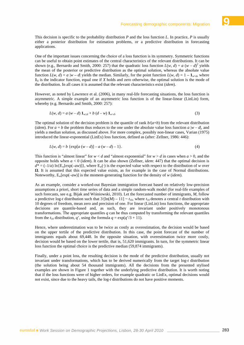
9 Forecasting demographic components: Migration
283Work Session on Demographic Projections, Lisbon, 28-30 April 2010
This decision is specific to the probability distribution P and the loss function L. In practice, P is usually either a posterior distribution for estimation problems, or a predictive distribution in forecasting applications.
One of the important issues concerning the choice of a loss function is its symmetry. Symmetric functions can be useful to obtain point estimates of the central characteristics of the relevant distributions. It can be shown (e.g., Bernardo and Smith, 2000: 257) that the quadratic loss function L(w, d) = a (w – d)2 yields the mean of the posterior or predictive distribution as the optimal solution, whereas the absolute value function L(w, d) = a |w – d| yields the median. Similarly, for the point function L(w, d) = 1 – 1w=d, where 1X is the indicator function, equal one if X holds and zero otherwise, the optimal solution is the mode of the distribution. In all cases it is assumed that the relevant characteristics exist (idem).
However, as noted by Lawrence et al. (2006), in many real-life forecasting situations, the loss function is asymmetric. A simple example of an asymmetric loss function is of the linear-linear (LinLin) form, whereby (e.g. Bernardo and Smith, 2000: 257):
L(w, d) = a (w – d) 1w≤d + b (d – w) 1w>d. (3)
The optimal solution of the decision problem is the quantile of rank b/(a+b) from the relevant distribution (idem). For a = b the problem thus reduces to the one under the absolute value loss function a |w – d|, and yields a median solution, as discussed above. For more complex, possibly non-linear cases, Varian (1975) introduced the linear-exponential (LinEx) loss function, defined as (after: Zellner, 1986: 446):
L(w, d) = b exp[a (w – d)] – a (w – d) – 1. (4)
This function is “almost linear” for w < d and “almost exponential” for w > d in cases when a > 0, and the opposite holds when a < 0 (idem). It can be also shown (Zellner, idem: 447) that the optimal decision is d* = (–1/a) lnEw[exp(–aw)], where Ew(·) is the expected value with respect to the distribution of w over Ω. It is assumed that this expected value exists, as for example in the case of Normal distributions. Noteworthy, Ew[exp(–aw)] is the moment-generating function for the density of w (idem).
As an example, consider a worked-out Bayesian immigration forecast based on relatively low-precision assumptions a priori, short time series of data and a simple random-walk model (for real-life examples of such forecasts, see e.g. Bijak and Wiśniowski, 2010). Let the forecasted number of immigrants, M, follow a predictive log-t distribution such that 3·[ln(M) – 11] ~ t10, where t10 denotes a central t distribution with 10 degrees of freedom, mean zero and precision of one. For linear (LinLin) loss functions, the appropriate decisions are quantile-based and, as such, they are invariant under positively monotonous transformations. The appropriate quantiles q can be thus computed by transforming the relevant quantiles from the t10 distribution, q’, using the formula q = exp(q’/3 + 11).
Hence, where underestimation was to be twice as costly as overestimation, the decision would be based on the upper tertile of the predictive distribution. In this case, the point forecast of the number of immigrants equals about 69,448. In the opposite situation, with overestimation twice more costly, decision would be based on the lower tertile, that is, 51,620 immigrants. In turn, for the symmetric linear loss function the optimal choice is the predictive median (59,874 immigrants).
Finally, under a point loss, the resulting decision is the mode of the predictive distribution, usually not invariant under transformations, which has to be derived numerically from the target log-t distribution (the solution being about 54 thousand immigrants). All the decisions from the presented stylised examples are shown in Figure 1 together with the underlying predictive distribution. It is worth noting that if the loss functions were of higher orders, for example quadratic or LinEx, optimal decisions would not exist, since due to the heavy tails, the log-t distributions do not have positive moments.

9 Forecasting demographic components: Migration
284Work Session on Demographic Projections, Lisbon, 28-30 April 2010
Figure 1. Examples of optimal decisions for a log-t distribution with10 d.f.
Source: own elaboration in R
From the statistical point of view, the quantile-based solutions under simple LinLin functions have convenient properties. Firstly, quantiles are robust against the presence of outliers in the distributions. Secondly, they remain invariant under positively monotonous transformations. Thirdly, alternative statistics may not always exist, as moments in heavy-tailed distributions, or more than one solution may exist, as distributions can have many modes. Besides, from the point of view of interactions between forecasters and forecast users, elaborated further in Section 3, information on such functions as the LinLin can be more straightforward to obtain.
3. Limitations of migration and population predictions
The optimal decisions, such as the ones outlined in the precious section, can be useful in the context of planning, where the decisions should be based on certain numerical parameters, such as the expected numbers of migrants, associated costs, etc. However, there are many other decision settings in which, given the prevalent uncertainty, the room for manoeuvre is much more limited. In that regard, the most notable problems with the traditional approach to forecasting include assumptions that the future will resemble the past and that events under study are independent, which need not hold in complex, network-based systems (Makridakis and Taleb, 2009). Among other flaws of the traditional approach, the use of tractable, thin-tailed error terms (such as Gaussian), the assumption of the existence of a finite variance3, and the human tendency to underestimate uncertainty can be mentioned (idem).
A synthetic typology of decision situations under uncertainty was proposed by Taleb (2009). He distinguished four classes according to the type of uncertainty: thin-tailed versus all other types, including unknown; and the type of payoffs: linear versus non-linear. The ‘payoffs’ here are akin to the utility (or negative loss) functions introduced in Section 2. Taleb’s analysis further focused on the hardly- or completely unpredictable events carrying possibly non-linear payoffs. As discussed in the previous section, for the thin-tailed (e.g. Gaussian) uncertainty, optimal decisions exist even for some non-linear loss functions, such as the LinEx. Under linear loss functions, moment-based optimal decisions exist even 3 Note that in the examples presented in the current study, the log-t predictive distributions for migration rates are heavy-tailed
and their positive moments (including variance) do not exist.

9 Forecasting demographic components: Migration
285Work Session on Demographic Projections, Lisbon, 28-30 April 2010
for heavy-tailed distributions, assuming that the latter can be properly approximated. However, in heavy-tailed non-linear cases, the statistical decision theory fails.
In such instances, it has to be replaced by general, common-sense decision-making strategies, unless the problem can be reduced to other types, for example by changing or bounding the loss function (idem)4. This is important especially in the migration context, where the relevant distributions can rarely be expected to be thin-tailed, due to the dynamic and changing nature of the process.
Makridakis and Taleb (2009) summarised several common-sense strategies for the use of forecasts. Their most important recommendations include: avoiding the “illusion of control” (or illusion of having accurate predictions, which can bring about dangerous or costly consequences; very relevant for demographic and migration applications), adopting protective strategies, and setting up backup plans and additional “reserves” of resources (idem). Such reserves may seem redundant and unnecessary from the point of view of optimal decision making, although the latter approach, labelled by Taleb (2009) as “overoptimisation”, was heavily criticised for making the complex systems in question much more vulnerable to unpredictable or hardly predictable events.
Another strategy suggested by Makridakis and Taleb (2009) is to apply the minimax approach to decision making, minimising the maximum potential losses5. However, from the Bayesian point of view this strategy, if it uniquely exists, has several drawbacks. Minimax decisions exhibit bias towards the worst-case scenarios (the least favourable prior distributions), do not take into account all information available and despite their construction can sometimes lead to worse outcomes than the approaches that are less pessimistic with respect to the states of nature (Robert, 2001: 66–77). According to Bernardo and Smith (2000: 449), although some minimax solutions may be acceptable as optimal Bayesian decisions under certain pessimistic priors, a general minimax rule “seems entirely unreasonable”. Besides, in practical application, derivation of the least favourable distributions may pose a serious problem. Current attempts to do so include the analysis of robustness of Bayesian decisions against changes in prior distributions. Some options here consist in limiting the optimisation of the risk function ρ(p, d) to a certain class Γ of prior distributions P. The resulting solutions are referred to as conditional Γ-minimax estimates or predictions (Męczarski, 1998).
The notion of conditional Γ-minimax decision rules has led to a concept of ‘stable’ estimates or predictions. As defined by Męczarski (1998: 113), a stable decision d# with respect to a parameter θ or prediction xP is the one, for which the oscillations of risk ρ(P, d) are minimal for all prior probability distributions P∈Γ:
supP∈Γρ(P, d#) – infP∈Γρ(P, d#) = infd∈DsupP∈Γρ(P, d) – infP∈Γρ(P, d) (5)
Męczarski (1998) offered a number of analytical solutions for Γ-minimax and stable decisions d# for some classes of prior distributions, whilst noting that a more general treatment of different statistical models seems hardly possible. Nevertheless, from a policy perspective, the presented notions are certainly appealing, since they could potentially inform the policy makers, how robust are their decisions against different types of uncertainty depicted by prior distributions P.
For demographers, exploring these options would additionally enrich the possibilities offered by decision analysis to the practical applications, following the suggestions of Alho and Spencer (2005).
4 As one of the practical ways of putting ‘caps’ on payoffs or loses, Taleb (2009) proposed insurance, although
admitting that this strategy may still not work well under very heavy-tailed distributions, such as in the case of catastrophe insurance (and reinsurance).
5 In fact, the original suggestion of Makridakis and Taleb (2009) was the maximin strategy, maximising the minimal payoffs. The two can be seen as broadly equivalent, exact to the possible asymmetry between the utility of gains and losses, pointed out for example by Gilboa (2009: 155). In this argument, for the sake of simplicity, gains and losses are assumed to be symmetric.

9 Forecasting demographic components: Migration
286Work Session on Demographic Projections, Lisbon, 28-30 April 2010
Regardless of the future methodological advancements, from the point of view of forecast users, a crucial question becomes: what types of decision problems can be answered or aided by forecasts. In this context, Orrell (2007) argued that appropriate risk assessments are crucial, especially if the potential dangers (negative payoffs) are large. At the same time, Orrell warned against being too risk averse, which can lead to negative externalities in such situations, when policy responses can be more damaging than the problem they were trying to resolve. In the context of migration, examples of such externalities of either too restrictive or too lax immigration policies can be, respectively, the loss of human capital of potential migrants, or an increased financial strain on public services and possible challenges to social cohesion.
One reason for extreme responses, as suggested by Lawrence et al. (2006: 504), can be that forecast users tend to focus on extreme probabilities of events, close to zero or one, and thus prefer such 1 – γ predictive intervals, for which γ is very small (for example, 1 – γ = 0.95 or 0.99). This is an additional argument for presenting predictive intervals for lower probabilities (e.g., with 1 – γ = 0.8 or 0.667), as a way to avoid the illusion of control (see also Lutz et al., 2004: 37). Lawrence et al. (2006) cite several studies which suggest that, notwithstanding, forecast users tend to prefer interval forecasts to point forecasts, the former clearly providing more information.
Therefore, a tentative recommendation for the forecasters and the forecast users would be that interval forecasts are useful and can provide valuable information for the decision making, although the intervals should not be based on too high probabilities in order to avoid overconfidence.
Narrower probability ranges suggest additional caution, as the probability that the variables under study fall outside the predictive intervals cannot be in such cases seen as negligible and ignored. On the part of the users, as noted by Lawrence et al. (2006), an additional caveat would be that the performance and expertise of the forecasters should not be assessed on the basis of their ability to minimise the width of interval whilst maximising the probability. Such forecasts are not only very likely to miss, but also to contribute to unjustified “illusion of control” among the policy makers and ultimately generate further problems in addition to the ones they were supposed to contribute to solving.
A migration-related example of very narrow predictive intervals is the forecast of post-EU enlargement immigration to the United Kingdom (Dustmann et al., 2003). The underprediction of actual flows by over one order of magnitude resulted, among others, from assuming stationarity of the underlying process, which assumption in case of migration can be problematic. At this point it is worth reiterating the potential of Bayesian methods, which allow for including expert judgement, for example on the low precision of forecasts, next to the data. Moreover, the Bayesian interpretation of probabilities as subjective measures of belief, if made explicit to the users, can be also helpful in avoiding overconfidence in forecasts and admitting their inherent frailties. Finally, the limited predictability of such volatile processes as migration poses limits on plausible forecast horizons. For example, the expert-based Bayesian forecasts of immigration into seven European countries, prepared by Bijak and Wiśniowski (2010) suggest a plausible horizon of ten years at most, echoing earlier suggestions of Holzer (1959).
4. Conclusion: From predictions to decisions
As argued before, the Bayesian approach can provide an umbrella framework for forecasting and decision making, providing a coherent mechanism of inference and decision support. However, unlike in other approaches to forecasting, the decision support requires a dialogue between forecasters and decision makers aimed at tackling a specific decision problem. This dialogue can further include experts in the field, who can provide prior information, especially vital in the absence of reliable quantitative data, as it is often the case in migration studies. Besides, as argued by Lawrence et al. (2006), combining judgment with data, the very essence of Bayesian inference, leads to better forecasts than relying on either data or judgment alone.

9 Forecasting demographic components: Migration
287Work Session on Demographic Projections, Lisbon, 28-30 April 2010
Such interactive expert-based Bayesian forecasts of migration (or, more generally, population) could be summarised as follows. After the forecast users have formulated the problem, the decision framework is obtained (elicited) from them by the forecasters – researchers or official statisticians. This framework includes the loss functions, required horizon and other parameters of the decision.
In order to make full use of the possibilities offered by the Bayesian approach, prior distributions of the parameters of the forecasting models can be additionally elicited from the domain experts. Subsequently, these elements are then combined with data in the forecasting models, and the final outcomes – forecasts – are reported back to the users.
The final outcome of the procedure is a set of user-specific forecasts enhanced by simple decision advice provided to the decision makers. Such forecasts should ideally comprise other elements and caveats, most importantly including an explicit uncertainty assessment and a clear statement of the limits of predictability. Such interactive forecasts would inevitably lose generality, having to respond to specific problems faced by the decision makers. The researchers would also be no longer fully autonomous in preparing the forecasts and interpreting their outcomes, as these would emerge in a multi-stage process involving dialogue with forecast users and possibly also other experts. In this way, the paradigm shift in demographic forecasting from deterministic point forecasts, through variant to stochastic predictions, would continue towards the decision-analytic outcomes. Such forecasts would then become an explicit tool of well-defined decision support rather than merely a numerical exercise.
Also the distinction between specific planning-related and more general policy-relevant decisions will have an impact on what is possible in terms of decision support from the point of view of the forecasters. In the former case it can be a proper statistical decision analysis, such as the Bayesian one presented before, while in the latter it can be, for example, a set of scenarios, equipped with clear caveats about uncertainty. In the same way as the forecasters should not promise the impossible and clearly state the limits of predictability, the users should not expect the impossible from the providers of predictions. Therefore, confronting the users’ expectations with what is actually possible from the scientific point of view should constitute the most important element of the dialogue between the forecasters and forecast users.
References
Alho J and Spencer B (2005) Statistical Demography and Forecasting. Springer, Berlin-Heidelberg.
Bernardo J M and Smith A F M (2000) Bayesian Theory. John Wiley, Chichester.
Bijak J and Wiśniowski A (2010) Bayesian forecasting of immigration to selected European countries by using expert knowledge. Journal of the Royal Statistical Society A, 173(4): 775–796.
DeGroot M H (1970) Optimal Statistical Decisions. McGraw-Hill, New York [(1981) Optymalne decyzje statystyczne. PWN, Warszawa].
Dustmann C, Casanova M, Fertig M, Preston I and Schmidt C M (2003) The impact of EU enlargement on migration flows. Home Office Report 25/03. Home Office, London.
Gilboa I (2009) Theory of decision under uncertainty. Cambridge University Press, Cambridge, MA.
Holzer J Z (1959) Prognoza demograficzna Polski na lata 1960–1975 wg województw [Demographic forecast of Poland for 1960–1975, by voivodships]. PWG, Warsaw.
Lawrence M, Goodwin P, O’Connor M and Önkal D (2006) Judgemental forecasting: A review of progress over the last 25 years. International Journal of Forecasting, 22(3): 493–518.

9 Forecasting demographic components: Migration
288Work Session on Demographic Projections, Lisbon, 28-30 April 2010
Lutz W, Sanderson W C and Scherbov S (eds.) (2004) The End of World Population Growth in the 21st Century: New Challenges for Human Capital Formation and Sustainable Development. Earthscan, London.
Makridakis S and Taleb N (2009) Living in a world of low levels of predictability. International Journal of Forecasting, 25(4): 840–844.
Męczarski M (1998) Problemy odporności w bayesowskiej analizie statystycznej [Robustness issues in Bayesian statistical analysis]. “Monografie i opracowania” 446, Warsaw School of Economics, Warsaw.
Orrell D (2007) The Future of Everything. The Science of Prediction. Thunder’s Mouth Press, New York.
Taleb N N (2009) Errors, Robustness, and The Fourth Quadrant. International Journal of Forecasting, 25(4): 744–759.
Varian H R (1975) A Bayesian Approach to Real Estate Assessment. In: S E Fienberg and A Zellner (eds.), Studies in Bayesian Econometrics and Statistics. Essays in Honor of Leonard J. Savage. North-Holland, Amsterdam: 195–208.
Zellner A (1986). Bayesian estimation and prediction using asymmetric loss functions. Journal of the American Statistical Association, 81(394), 446–451.

9 Forecasting demographic components: Migration
289Work Session on Demographic Projections, Lisbon, 28-30 April 2010
MODEL TO FORECAST RE-IMMIGRATION OF SWEDISH-BORN PERSONS
Christian SKARMAN*, Stina ANDERSSON*
Anders LJUNGBERG*
Foreword
Every third year Statistics Sweden conducts a population projection for the country that is published in the series “Demographic Reports”. The most recent edition was published in the spring of 2009. Only minor adjustments are made as needed for the years in between, and these adjustments are published in the series “Statistical Reports”.
The population projection is based on analyses of births, deaths, immigration and emigration. This report describes the estimations of expected numbers of Swedish-born persons who will re-immigrate. In the latest published forecast “The Future Population of Sweden 2009-2060”, the model is only described broadly due to limited space, while this report intends to give a more detailed description of the model.
Acknowledgements
The respondents – private individuals, enterprises, authorities and organisations –, who make it possible for Statistics Sweden to produce reliable and timely statistics that meet the demands for information from society.
Summary
In the latest forecast “The Future Population of Sweden 2009-2060”, the model used for estimating re-immigration of Swedish-born persons is only described in broad terms. This report intends to give a more detailed description of the model.
Swedish-born persons comprise one of the largest immigrant groups. Unlike other immigrant groups, it is easier to construct a mathematical model to forecast re-immigration of Swedish-born persons.
In order to estimate the return immigration of Swedish-born persons, a model has been developed in which information on immigration and emigration for 1851-2007 has been used to build up a population of Swedish-born persons abroad. For each year, Swedish-born persons who have emigrated have been added to the Swedish population abroad, re-immigrants have been subtracted and the expatriate Swedish population has been reduced with the same death risks that applied to Swedes living in Sweden. According to these estimates, 780 000 Swedes lived abroad in the early 1900s. Afterwards, the number of Swedish-born persons living abroad decreased until the 1980s, when the number of expatriate Swedes again began to increase. In the forecasting model, re-immigration of Swedish-born persons is based on the estimated information on how many Swedes can be assumed to be abroad, combined with information on emigration of Swedish-born persons three years earlier.
* Statistics Sweden

9 Forecasting demographic components: Migration
290Work Session on Demographic Projections, Lisbon, 28-30 April 2010
1. Introduction
Swedish-born persons comprise one of the largest immigrant groups. Therefore it is an important group to study more closely to be able to make predictions on Sweden's future immigration and emigration. Unlike other immigrant groups, it is easier to construct a mathematical model to forecast re-immigration of Swedish-born persons. The frame for how many people can re-immigrate is set by the number of people who emigrate, which can in turn be estimated based on emigration risks.
The model for re-immigration is built in three stages. The first stage is to estimate how many Swedish-born persons are abroad and thus belong to the risk population. The second stage is to estimate the re-immigration risks based on information on re-immigration and the size of the risk population. Finally, a model is constructed based on risks for re-immigration.
2. Swedes abroad
To determine the risks of re-immigration, information is first needed on Swedish-born persons who are abroad. This information is based on one-year categories and sex. There is no comprehensive register of Swedes abroad. The Swedish Social Insurance Agency has information on persons who live abroad and who have or have had an income in Sweden. However, this information does not include those who have not had an income in Sweden, such as those who emigrate at a young age. The National Tax Board has information on those eligible to vote who are outside of the country. But this information is only saved for ten years. After ten years, persons are removed who have not applied to remain in the register for another ten years. Therefore the number of Swedes living abroad must be estimated. These estimates are based on information on emigration and immigration by country of birth.
2.1 Immigration and emigration of Swedish-born persons As illustrated in figure 1, Sweden was a nation of emigration for nearly one hundred years. From 1850 to 1930, nearly 1.5 million people emigrated from Sweden. 1.2 million of these emigrants went to North America. Emigration was highest 1881-1882 and 1887-1888 when the harvests were poor in Sweden and the economy was booming in the US1. Roughly 20 percent of the men and 15 percent of the women born in Sweden during the latter part of the 1800s emigrated from the country. The pattern changed after World War II and since then immigration has been higher than emigration, with the exception of 1972 and 1973. As a result of the high labour force immigration a few years earlier, emigration was particularly high during these years.
1 Statistics Sweden (2004) Immigration and emigration in the post-war period, Demographic Reports 2004:5

9 Forecasting demographic components: Migration
291Work Session on Demographic Projections, Lisbon, 28-30 April 2010
Figure 1. Immigration/emigration 1850-2007, in total and for Swedish-born persons
Number
0
20 000
40 000
60 000
80 000
100 000
120 000
1850 1875 1900 1925 1950 1975 2000
Immigration (total)
Immigration Swedish-born
Emigration (total)
Emigration Swedish-born
Year
The increased emigration during these years consists largely of children of labour force immigrants who return to their home countries.
During the 1990s, the number of Swedish-born emigrants doubled from some 10 000 people per year during the 1970s and 1980s to more than 20 000 people per year by 1998. Emigration then decreased for a few years but it has picked up momentum in recent years. In 2008 the number of Swedes who took up residence abroad amounted to almost 21 000 people. The tendency to emigrate is greater among Swedish-born persons who have a parent born abroad and greatest for those with both parents who were born abroad. In line with increased emigration of Swedish-born persons, re-immigration has also increased. Thus, it seems there is a clear connection between immigration and emigration. This connection will be studied closer in a coming section.
2.2 Data sources Several different data sources have been used to follow immigration and emigration of Swedish-born persons2. Information for 1968-2007 has been taken from the historical population register. This information includes country of birth, so immigration and emigration of Swedish-born persons can be followed.
Information for 1949-1968 does not include immigration and emigration by country of birth, but does include information on citizenship. Because information on country of birth is not available, citizenship3 has been used. Those with Swedish citizenship are assumed to be Swedish-born persons.
No information on the migrants' country of citizenship is available for 1936-1948, but in Statistics Sweden's annual publication on the population movement ("Befolkningsörelsen"), information is
2 Persons who move abroad and who will be away one year or more are normally no longer registered in Sweden. It should be
noted that there is both overcoverage and undercoverage in the Population Register as a result of unreported moves to and from Sweden. Overcoverage means that the register includes people who no longer reside in the country. This occurs when people emigrate without reporting it. The converse is undercoverage which means that the register includes people residing in the country but not registered here. For example, this is the case with hidden refugees. In the forecast we disregard measurement errors of this type and the population forecast is thus a projection of the registered population.
3 For the period 1961-66, information on migration has been taken from Statistics Sweden's publication on population changes 1961-66, and for 1949-60, information has been taken from Statistics Sweden's publication on the population movement up until 1960.

9 Forecasting demographic components: Migration
292Work Session on Demographic Projections, Lisbon, 28-30 April 2010
available on which countries migrants move to and from4. During World War II and especially during the years immediately following, migration flows increased within Europe.
In case information was lacking on the percentage of migrants who were Swedish, a rather rough assumption is made that migration of Swedish-born persons within Europe is a zero sum game. Equal numbers of Swedish persons are assumed to have re-immigrated as have emigrated. In the long term there are always more emigrants than immigrants, because it is sufficient that one Swedish-born person chooses to stay in the new country to obtain a negative net migration. But during times of war in Europe, it can be assumed that many Swedes try to return home to Sweden. In technical terms, the material is handled so that immigration and emigration within Europe is set at zero. Instead, statistics on migration are assumed between Sweden and the rest of the world to represent Swedish migration during these years. The flows will probably be lower than in actual fact, but hopefully net migration will be somewhat correct. Concerning migration exchange with the rest of the world for 1936 - 1948, the largest flows were to and from the US, where many Swedish-born persons lived.
For 1911 - 1920, information on citizenship of immigrants is available in Statistics Sweden's publication on emigration and immigration 1911 - 1920. For other years before 1936, the percentage of Swedish citizens of immigrants is based on the observed distribution for immigrants during 1911 - 1913, that is, the years just before World War I.
For the year 1935 and earlier years, it is assumed that Swedish-born persons comprise 90 percent of emigrants.
Of the 35 627 foreign-born persons in Sweden in 1900, only 7 514 persons were foreign citizens5. We thus see that very few foreign-born persons lived in Sweden around the early 1900s. The increase between 1890 and 1900 is largely due to the children born in America who followed their parents when they re-immigrated. The increase in the number of foreign-born persons can appear to be quite significant, considering that immigration to Sweden from other countries than North America was not particularly high. Table 1 illustrates a rough estimate to try to get an idea of how high a percentage of immigrants who are assumed to be foreign-born. Immigrants to America are not included since many of them are considered to be Swedish-born re-immigrants or children who are too young to emigrate in the next few years. According to the census in 1930, the number of foreign-born persons was 61 700, that is, one percent of the population6. Due to lack of information, it is assumed that 90 percent of the emigrants were born in Sweden in the years before 1936.
Table 1. Change in the number of foreign-born persons immigration/emigration 1871 – 1900
Year 1871–1880 1881–1890 1891–1900
Immigration, not from America 18 635 28 832 31 637
Emigration, total 150 269 376 401 246 772
Change, foreign-born 6 567 5 966 11 079
Estimated emigration, foreign-born* 12 068 22 866 20 558
Estimated percentage of foreign-born emigrants** 8% 6% 8%
* Estimated emigration of foreign-born = immigration - change in foreign-born ** Estimated percentage of foreign-born emigrants = Estimated emigration of foreign-born / total emigration.
Source: Statistiska centralbyråns underdåniga berättelese för år 1900, A) (Statistics Sweden's Report to the King for the year 1900, A) Population statistics), and SCB (1999) Befolkningsutveckling under 250 år, Demografiska rapporter 1999:2. (Statistics Sweden (1999) Population development in Sweden in a 250-year perspective 1999:2.)
4 Statistics Sweden, Befolkningsrörelsen (Population movement), 1939 - 1948 (where information goes back to 1936) 5 SCB (1907) Statistiska centralbyråns underdåniga berättelese för år 1900, A Befolkningsstatistik, Ny följd. XLII:3 (Statistics
Sweden (1907) Statistics Sweden's Report to the King for the year 1900, Population statistics XLII: 3) 6 Statistics Sweden (2004) Immigration and emigration in the postwar period, Demographic Reports 2004:5

9 Forecasting demographic components: Migration
293Work Session on Demographic Projections, Lisbon, 28-30 April 2010
2.3 Age structure
2.3.1 Emigration For the years 1969 - 2007, the age structure for Swedish-born persons is based on observations from the Historical Population Register.
The age structure of Swedish-born emigrants for the years 1946 - 1968 is assumed to be the same as for 1969 - 1971.
The age structure for the years 1851 - 1945 has been taken from historical information7 concerning the years 1861 - 1940. For the years 1941 - 1945, the distribution for 1940 is used. This historical information does not contain information on country of birth or citizenship, and therefore Swedish-born persons and all emigrants have the same age structure. There is no information at all on age and sex structure for the years 1851-1860, so the structure for 1861 has been used for these years.
For the years 1861 -1915 there is information on emigrants by sex and five-year categories up to the age class 65 years and above. For the years 1916 -1940, information by sex is only available for the age groups 0-14, 1519, 2929, 30-39, 40-64 and 65-w.
2.3.2 From age groups to one-year categories Historical information grouped by age categories has been broken down to one-year categories based on the age structure for 1969 - 1971. The percentage of age groups has been calculated from the total number of emigrants. This percentage has then been divided by the percentage that the same age group had 1969 - 1971. By doing so, we obtain a ratio for the size of the difference.
By using these ratios for five-year categories, we can then raise or lower the percentages of each one-year category for each calendar year that was observed for the years 1969-1971. This is done by multiplying the ratios of the five-year categories with the age distribution by one-year categories as constructed based on the years 1969-1971.
All calculations are broken down by sex.
2.3.3 Immigration For the years 1969-2007, the age structure of Swedish-born immigrants is based on observations from the Historical Population Register. Swedish-born persons who immigrate but have not emigrated are not included in the model. This applies to children of foreign-born mothers where the child has been born in Sweden before the mother received a residence permit. When the parent receives a residence permit, the child is registered as a Swedish-born immigrant, but has never been a part of the population of Swedish-born persons living abroad.
No information is available on age structure of immigrants broken down by country of birth or citizenship for the years before 1968. For the years 1946 -1968, an age structure is used that is based on the observations for 1969 - 1971.
For the years 1875 - 1945, age structure has been taken from historical information8 concerning the years 1916-1940. It is assumed here that the age structure was the same as for all immigrants 1916 - 1940.
For the years 1851 - 1915, no information is available on age and sex structure at all, so the age and sex structure for 1916 was used for these years. For the years 1916 - 1940, there is information on sex in the age groups 0-14, 15-19, 20-29, 30-39, 40-64 and 65- w.
7 Statistics Sweden (1969), Historical Statistics of Sweden Part 1. Population. Second edition 1720 - 1967 8 Statistics Sweden (1969), Historical Statistics of Sweden Part 1. Population. Second edition 1720 - 1967

9 Forecasting demographic components: Migration
294Work Session on Demographic Projections, Lisbon, 28-30 April 2010
In the same way as with the emigrants, the historical information in grouped age categories has been broken down to one-year categories based on age structure for the years 1969-1971.
2.3 Number of Swedish-born persons living abroad Estimations of the number of Swedish-born persons are based on the compiled information on immigration and emigration of Swedish-born persons.
The population of Swedish persons abroad is created in about the same way as in a population forecast, but is based on actual observed immigration and emigration instead of estimations of those components. For each year that a newly emigrated Swedish-born person is added to the population of Swedish persons abroad, re-immigration is subtracted and the number of Swedish persons abroad is reduced by the same death risks that are observed for Swedes living in Sweden. It may be so that those who emigrated had been somewhat healthier than those who stayed behind, but this has not been taken into consideration. To estimate the Swedish-born population abroad the following formula has been used.
All calculations are made for one-year categories and sex.
The number of Swedish-born persons living abroad is calculated:
)1(1 ttttt qBIEB −+−= −
where tE is the number of emigrants in the year t
tI is the number of immigrants in the year t
tq are the death risks in the year t
The estimated number of Swedish-born persons living abroad was highest in 1913 when roughly 780 000 Swedes were living abroad. Afterwards, the number of Swedish-born persons abroad drops when those who emigrated at the end of the 1800s begin to reach ages where death risks are high.
Graph 2. Estimated number of Swedish-born persons abroad 1851-2007
Number
0
100 000
200 000
300 000
400 000
500 000
600 000
700 000
800 000
900 000
1850
1860
1870
1880
1890
1900
1910
1920
1930
1940
1950
1960
1970
1980
1990
2000
Year

9 Forecasting demographic components: Migration
295Work Session on Demographic Projections, Lisbon, 28-30 April 2010
According to a review9 of censuses from different countries, it was assessed that 693 000 Swedish-born persons were living abroad in 1900, which is relatively close to the above estimation of 657 000 persons. The difference is probably because of a low registration number for emigrants10.
Table 2. Swedish-born persons living abroad around 1900
Country Number of Swedish-born persons
North America 574 625
Norway 49 662
Denmark 35 555
Finland 1 597
Germany 12 191
United Kingdom 6 195
Other European countries 4 000
Rest of the world 10 000
Total 693 825
Source: Statistiska centralbyråns underdåniga berättelese för år 1900, A Befolkningsstatistik. (Statistics Sweden's Report to the King for the year 1900, Population statistics.)
According to the Emigration study 11 the official statistics on emigration would need to be increased by at least two-thirds for the 1850s, by 20 percent from 1860-1870 and by 10 percent for 1880-1884. During the period 1885 - 1893, the lists of the number of emigrants seem to be nearly exact. After 1893, the statistics once again worsened because permission to emigrate was no longer given to those liable for military service. As a result, illegal emigration occurred and was not registered in the church records or official statistics. If emigration is written up by 67 percent for the years 1851 - 1859, 20 percent for 1860 - 1879, 10 percent for 1880 - 1884 and by 10 percent from 1894 to 1913 (the year before World War I broke out) - we arrive at a population of 720 000 persons for Swedish-born persons abroad in 1900 and at most 870 000 persons in 1913.
9 SCB (1907) Statistiska centralbyråns underdåniga berättelese för år 1900, A Befolkningsstatistik, Ny följd. XLII: 3 (Statistics
Sweden (1907) Statistics Sweden's Report to the King for the year 1900, Population statistics XLII: 3) 10 Emigrationsforskningsgruppen (1976), Uppsala University, From Sweden to America: a history of the migration 11 Emigration study (1910), appendix IV Pages 251-252

9 Forecasting demographic components: Migration
296Work Session on Demographic Projections, Lisbon, 28-30 April 2010
Graph 3. Sex and age structure for the estimated number of Swedish-born persons living abroad in 2007
Number
0
500
1 000
1 500
2 000
2 500
3 000
3 500
4 000
0 10 20 30 40 50 60 70 80 90 100
Men
Women
Year
3. Forecast model
When the population of Swedish-born persons living abroad is estimated, it is possible to estimate the risks for re-immigration for the persons in this population. The first step is to study the possibility to predict re-immigration based only on risks for re-immigration. Then, we test the possibility to improve the accuracy of the forecast by combining the risk-based re-immigration with information on the size of emigration at different points in time before re-immigration.
3.1 Risks for re-immigration Information on re-immigrating Swedes is divided by the number of Swedes living abroad. By doing so, we create age and sex-specific re-immigration risks. Risks for re-immigration are calculated for the years 2002 - 2005 and 2007. 2006 has not been included because in that year Swedish-born children of persons who received resident permits were affected by the temporary change in the asylum law12 which drove up the risks for those of very young ages.
Re-immigration risks based on 5-year average values are calculated for ages 0 - 74 as:
∑
∑
=−
=−∧
= 4
0)(
4
0)(
iit
iit
t
M
IR
12 On 9 November 2005, the Swedish Parliament decided that temporary legislation for residence permits would apply up until
the new Aliens Act which would be enacted on 31 March 2006. The temporary legislation was mainly directed towards families with children who had lived in Sweden for a long time and to people from countries where deportation is not an option. Roughly 31 000 matters were handled according to the temporary legislation, and about 17 000 residence permits were granted.

9 Forecasting demographic components: Migration
297Work Session on Demographic Projections, Lisbon, 28-30 April 2010
where tI is the number of Swedish-born immigrants in year t
tM is the average size of the Swedish-born population living abroad in year t
The following calculation is used for those aged 75 and above
∑∑
∑∑∞
=−
=
∞
=−
=∧
=
75)(
4
0
75)(
4
0
xxit
i
xxit
it
M
IR
3.2 Business cycle fluctuations As illustrated in graph 4 below, the percentage of those who re-immigrate differs among the different emigration cohorts13. The variations in the percentage of those who re-immigrate occurred during the first and second year after emigration, and then evened out somewhat with time. It is thus the first and second year after emigration that the percentage of those who re-immigrate differ from the different emigration cohorts. As a result, these years are the most sensitive for fluctuations in the business cycle. In graph 4 this can be seen because the lines move in parallel over the years that the differences in levels of the first years' re-immigration have not changed especially.
Graph 4. Proportion of Swedish-born persons that has re-immigrated after 2, 4, 5 and 10 years, by year of emigration 1970-2007
Percent
0
10
20
30
40
50
60
70
1970 1975 1980 1985 1990 1995 2000 2005
Return after 10 yearsReturn after 5 years
Return after 3 years
Return after 2 years
Year of emigration
Comment: Of those who emigrated in 1995, 30 percent had re-immigrated to Sweden after two years, and 55 percent had re-immigrated after 10 years.
13 Emigration cohorts refer here to persons who emigrated during a certain year.

9 Forecasting demographic components: Migration
298Work Session on Demographic Projections, Lisbon, 28-30 April 2010
Graph 5. Proportion of re-immigrated Swedish-born persons who re-immigrate by year of emigration 1970-2007 and time since emigration.
Percent
0
2
4
6
8
10
12
14
16
18
20
1970 1975 1980 1985 1990 1995 2000 2005
Return after 10 years
Return after 0 years
Return after 1 year
Return after 2 yearsReturn after 3 years
Return after 5 years
Year of emigration
Comment: Of those who emigrated in 1995, roughly 5 percent re-immigrate before one year has passed (1 to 12 months), 14 percent re-immigrate after they have been abroad for one year (13-24 months) etc.
Graph 6 illustrates the risk to re-immigrate in relation to the number of employed persons in Sweden. On the right axis we see development of the total re-immigration risks, while the left axis shows the development of the number of employed persons according to Statistics Sweden's Labour Force Survey (LFS). As seen in the graph, the risk to re-immigrate increases when the number of employed persons increases. This could be interpreted that those who emigrate just before a slowdown in the economy do not re-immigrate to the same degree as those who emigrate just before a boom in the economy. A linear regression where total risks of re-immigration14 is the dependent variable and the number of employed persons is the independent variable, results in a significant connection on the one percent level with a coefficient of determination of 25 percent. However, a coefficient of determination of 76 percent is received when only looking at the years 1993-2007. The possibility to change jobs and get a new job in one's home country seems to affect re-immigration to a certain degree. It may be because if a person stays abroad somewhat longer for various reasons, the probability of staying abroad increases.
This type of behaviour would be in line with observations for foreign-born immigrants who come to Sweden, where the tendency to re-immigrate decreases the longer the immigrant stays in the country15.
The connection between the economic cycle and the tendency to re-immigrate would be interesting to study in more detail, but in this paper we only conclude that such a connection exists.
14 Total risks of re-immigration inform how many times an emigrant would on average re-immigrate if that person was abroad
during an entire lifetime (0 - 75 years) according to age-specific re-immigration risks. Just because it gives an average re-immigration for more than one time does not mean that everyone re-immigrates. This is because those persons who actually re-immigrate do so within a short period of time. When 50 percent have re-immigrated after five years, we get risks than imply that after 75 years abroad, a person would have re-immigrated a couple of times on average.
15 Statistics Sweden (2004) Immigration and emigration in the post-war period, Demographic Reports 2004:5

9 Forecasting demographic components: Migration
299Work Session on Demographic Projections, Lisbon, 28-30 April 2010
Graph 6. Total re-immigration risks (age 0-75) and number of employed persons (thousands) in Sweden 1978-2007
Employed persons
0
2
4
6
8
10
12
14
3 400
3 600
3 800
4 000
4 200
4 400
4 600
1978 1983 1988 1993 1998 2003
Re-immigration risks
Employed
Year
Re-immigration risks
3.3 Model for immigration of Swedish-born persons As illustrated in graph 7, an estimation of immigration only based on re-immigration risks does not follow the observed development particularly well. In the graph we also see that re-immigration follows emigration quite well, but with a delay by a few years. However, a linear regression where immigration created by re-immigration rates, combined with information on emigration three years earlier gives a goodness of fit. This regression has a coefficient of determination of 97 percent when it is based on the years 1981 - 2007, and 71 percent when based on the years 1998 - 2007. This is also illustrated in graph 7. Both of the regression equations give a re-immigration that lies quite close to the results according to the Total Population Register. It is natural that the equation that is created from the data between 1981 - 2007 also shows a trend that is closest to the outcome for this period. However, it is interesting that the equation that is created for the years 1998 - 2007 gives a re-immigration that is also close to the outcome for the years before 1998.
The latter equation based on the years 1998 - 2007 will be used in the model. Because the model has shown to work well in estimating trends back in time, it is also assumed to function as a model to forecast the future re-immigration of Swedish-born persons. The model also has the best fit for recent years. In today's globalised world with increased mobility, we can assume that the most recent years will contribute to a better basis for estimation of future migration patterns, than by using a migration pattern from a time when mobility was less.
Migration three years previously is the variable that gave the best coefficient of determination, but the variable also has the advantage that the economy does not have as great an influence after three years, compared to the first two years after emigration. The model is thus not as sensitive for economic swings, as it would be if the first two years had been included in the calculations.
The forecast is calculated as follows:
1
5
−
∧∧⋅= tt
r
t BRI

9 Forecasting demographic components: Migration
300Work Session on Demographic Projections, Lisbon, 28-30 April 2010
337266,090683,05059 −
∧∧⋅+⋅+−= t
r
t
reg
t EII
)1(1 tt
reg
ttt qBIEB −⋅+−= −
∧
For those aged 0, tt EB =
Graph 7. Forecast for 1981-2007 based on re-immigration risks and regression model where the re-immigration risks are combined with data for the emigration three years earlier, and the observed immigration and emigration
Immigrants
0
5000
10000
15000
20000
25000
1981
1982
1983
1984
1985
1986
1987
1988
1989
1990
1991
1992
1993
1994
1995
1996
1997
1998
1999
2000
2001
2002
2003
2004
2005
2006
2007
Observed emigrationObserved immigrationRisk-based re-immigrationRegression, base years 1997-2007
Year
4. Results
As an example of results from the model, we illustrate here the forecast of immigration and emigration of Swedish-born persons in the latest population forecast16 where the model was used for the first time. Because emigration largely determines re-immigration, the model for emigration of Swedish-born persons is also presented here.
4.1 Emigration of Swedish-born persons The results of the model for re-immigration largely depend on the assumed size of emigration. Emigration of Swedish-born persons is determined in the official population forecast based on emigration rates. In the first forecast year, emigration rates created from emigration for 1999 - 2008 are used as a starting point. Because emigration has tended to increase in recent years, the emigration rates (which are ten-year average values) are lifted up to the level for the last three years. To give better stability for estimates, the moving averages for those over age 35 are used. For persons aged 36 - 79, a moving average spanning three ages is used. Persons aged 80 and above are given the same emigration figure.
Swedish-born persons with a foreign-born parent have a higher tendency to emigrate. The tendency to emigrate is especially high for Swedish-born persons with two foreign-born parents, as illustrated in graph 8.
16 Statistics Sweden (2009), The future population of Sweden 2009-2060, Demographic Reports 2009:1

9 Forecasting demographic components: Migration
301Work Session on Demographic Projections, Lisbon, 28-30 April 2010
Graph 8. Emigration rates (per thousand) for Swedish-born persons with two Swedish-born parents and Swedish-born with two foreign-born parents. Average for the years 1999-2008
Per thousand
0
2
4
6
8
10
12
14
16
18
20
0 5 10 15 20 25 30 35 40 45 50 55 60 65 70 75 80
Foreign background - women
Foreign background - men
Swedish-born parents – women
Swedish-born parents – men
Age
Emigration rates are calculated for four sub-groups of Swedish-born persons: Swedish-born persons with two Swedish-born parents, Swedish-born persons with two foreign-born persons, Swedish-born persons with a Swedish-born father and a foreign-born mother, and Swedish-born persons with a Swedish-born mother and a foreign-born father.
Presently, no forecasts are made for Swedish-born persons by background. In the calculations of emigration rates, it has been assumed that the percentage with foreign-born parents abroad increases in a linear manner based on the rate of increase that was observed during the last ten years.
For each forecast year, the percentages of the four groups are calculated as a share of the total Swedish-born population. These percentages are multiplied by the emigration rate for each group by one-year categories and sex. Then they are aggregated as emigration risks for the entire group of Swedish-born persons. Like the total fertility rate for women, the emigration rates are totalled for men and women respectively, arriving at a total emigration rate. Based on these total emigration rates, the rate of change is created in the form of ratios that are multiplied by the emigration rate for each forecast year, as described in the above paragraph.
4.2 Immigration of Swedish-born persons The forecast model gives a re-immigration that increases during the entire forecast period. The long-term increase in the estimated number of persons re-immigrating during the forecast period is because the number of Swedish-born persons abroad increases according to the calculations. However, the annual variations are largely due to the size of emigration three years earlier, which in turn depends on how many Swedish-born persons living abroad are of the age when the tendency to emigrate is considerable.

9 Forecasting demographic components: Migration
302Work Session on Demographic Projections, Lisbon, 28-30 April 2010
Graph 9. Forecast of emigration and re-immigration for 2009 – 2010
0
5 000
10 000
15 000
20 000
25 000
30 000
35 000
2000 2010 2020 2030 2040 2050 2060 2070 2080 2090 2100 2110
Re-immigrationEmigration
Year
In the beginning of the forecast period it is assumed that the number of Swedish-born persons abroad will increase rather sharply, and will then stabilise at a level of just below 400 000 at the end of the forecast period (graph 10). The lower rate of increase of Swedish-born persons abroad is because those who emigrated at the start of the 2000s have reached an age where death risks are high.
Graph 10. Forecast of number of Swedish-born persons living abroad 1850 – 2100
0
100 000
200 000
300 000
400 000
500 000
600 000
700 000
800 000
900 000
1850
1900
1950
2000
2050
2100
Year
The age structure of those who re-immigrate is based on the observed distribution for the years 2003 - 2005 and 2007 - 200817. There are roughly equal numbers of men and women among Swedish-born immigrants (see graph 11). The women are somewhat younger than the men when they leave Sweden, which is also reflected in immigration.
17 When the asylum law was temporarily changed in 2006, many children born in Sweden with foreign-born parents received
residence permits. This has influenced the age structure in 2006, and thus this year is excluded.

9 Forecasting demographic components: Migration
303Work Session on Demographic Projections, Lisbon, 28-30 April 2010
Graph 11. Age and sex distribution for re-immigrants, based on data for 2003 - 2005 and 2007 - 2008
0,00
0,20
0,40
0,60
0,80
1,00
1,20
1,40
1,60
0 10 20 30 40 50 60 70 80 90 100
Men
Women
Age
References
Emigrationsforskningsgruppen (1976), Uppsala University, From Sweden to America: a history of the migration
Emigrationsutredningen (1910), appendix IV pages 251 – 252
Statistiska centralbyråns underdåniga berättelese för år 1900, A Befolkningsstatistik, Ny Följd. XLII:3 (Statistics Sweden (1907) Statistics Sweden's Report to the King for the year 1900, Population statistics XLII: 3)
Statistics Sweden (1911 - 1960) Population for the years 1911 – 1960
Statistics Sweden (1961 - 66) Changes in the population for the years 1961 - 66
Statistics Sweden (1969), Historical Statistics of Sweden Part 1. Population. Second edition 1720– 1967
Statistics Sweden (1999) Population development in Sweden in a 250-year perspective, Demographic Reports 1999:2.
Statistics Sweden (2004) Immigration and emigration in the postwar period, Demographic Reports 2004:5
Statistics Sweden (2009), Future Population of Sweden 2009 - 2060, Demographic Report


9 Forecasting demographic components: Migration
305Work Session on Demographic Projections, Lisbon, 28-30 April 2010
THE ROLE OF SOCIAL NETWORKS IN THE PROJECTION OF INTERNATIONAL MIGRATION
FLOWS: AN AGENT-BASED APPROACH
Carla ANJOS1, Pedro CAMPOS2
Abstract
In recent years, migration has been modelled within the perspective of social networks. Models are based on the idea that migration flows are influenced by the social networks where the agents operate. In this work we use a Multi-Agent System to simulate social networks of migrants and analyse the impact of the structure of these networks in the flow of migrants. The model we propose uses information of a IPUMS database of immigrants in the United States. We focused in four different countries of origin: Germany, Mexico, Portugal and China and in six variables: age, educational level, income, number of people in the household, labour status and number of individuals in the social network of the agent. We have analysed four important measures of network structure: density and three measures of degree centralization: input, output and general. Results indicate that Mexicans have higher input and general degree centralization, meaning that their networks have higher levels of influence of the agents. We concluded that the agents that stay in the U.S. (and do not go away to their country of origin), have network connections that are weaker than those of other agents.
1. Introduction
Social network analysis has had a great development in recent times, although the main concepts were proposed between 1960 and 1970. According to Mitchell (1969), “a social network is a specific set of links among a set of persons”, with the additional property that the characteristics of these links as a whole may be used to interpret the social behaviour of the persons involved. Likewise the network structure reflects the pattern of relationships between individuals (Newman & Girvan, (2004), Wasserman & Faust, (1994)). Migration is often modelled within the perspective of social networks (McKenzie & Rapoport (2007), Woodruff & Zenteno (2007), Hussey (2007)). In general it appears that migration flows towards a specific country B with origin in country A induce further migration of other individuals from A to B (Helmenstein & Yegorov, 2000).
In this work we use a Multi-Agent System to model the flow of migrants in social networks. Agent-Based Computational Demography (ABCD) is a computational approach to Demography, with emphasis placed on simulation based on agents (Billari and Prskawetz, 2005). In particular, in ABCD models, it is relatively easy to integrate micro-based demographic behavioural theories with aggregate-level demographic outcomes. In such models, space and networks can be formalized as additional entities in which the agents will interact (Billari, Ongaro, Prskawetz, 2003). Our model is based on the idea that migration flows are influenced by the structure of the social network where the agents operate. The proposed model of migration uses four countries (Germany, Mexico, Portugal and China) and six variables: age (y), educational level, (e), household income (r), number of people in the household, (p), labour status (working/not working), (w) and number of individuals in the social network of the agent (s).
1 University of Aveiro 2 Statistics Portugal and University of Porto Corresponding author: [email protected]

9 Forecasting demographic components: Migration
306Work Session on Demographic Projections, Lisbon, 28-30 April 2010
The social network of the individual is simulated, based on a correlation with the number of persons in the household. We have used information from the IPUMS (Integrated Public Use Microdata Series, Ruggles et al, (2009)), containing data of migration flows to the United States between 2001 and 2008. We decided to consider four communities in the U.S. with origin in four different countries (Portugal, Mexico, China and Germany), and identified the force that these communities have to attract new migrants from the country of origin, as well as to repel those already leaving in the U.S. We used a gravitational model incorporating the mass of the agent (Ma) that includes the household income (r), the number of people of their household (p), the agent's age (y) and the labour status of the agent, or working situation, (w).
Similarly, the mass of the corresponding social network of the agent (MN) was computed. To determine the gravitational force of migration, a distance d between the agent and their social network was defined. The Euclidean distance was chosen as the distance measure. Migration costs have also been considered. We analysed the structural properties of the generated networks and compared the impact of these structures on the magnitude of the migration flows. Empirical validation was applied in order to evaluate the quality of the model. The simulation was initialized with real data of 2000, based on the clustering of the main properties of the individuals coming from the four different countries of origin. After running the model and iterating it for nine years, we compared the simulated migration flows with the real data observed in the US in the period of analysis.
Measures of network structure were used: density degree centralization (input, output and general). The latter constitute signs of agents’ influence in network since the higher these degree centralization measures, the more central agents are in the social network. We concluded that the agents that stay in the U.S. (and do not go away to their country of origin), have higher values of individual mass, Ma, and are associated with less average distance with the members of their social networks. Networks where these agents belong are more cohesive. According to the results of the simulation, in 2008, Germans, Chinese and Portuguese have similar values of the degree centralization measures, meaning that agents occupy central positions in networks. Simultaneously, the networks keep growing during the period. Centrality is therefore an important property for the growth of networks. We have concluded that Mexicans have higher input and general degree centralization, meaning that their networks have higher levels of influence of the agents.
The paper is structured as follows: in Section 2, an overview of the concepts of Migration and Social Networks is made. In Section 3, we introduce the approach of Agent-Based Computational Demography (ABCD) and the methodology we have used in this study. Results are discussed in Section 4. In this section we also analyse the stability and the validation of the model. Conclusions are in section 5, where we propose topics for further work.
2. Migration and Social Network
2.1 Migration Studies Studies on migratory flows are essential to the achievement of more accurate demographic forecasts. Migration flow is to be viewed as the movement of a person through a limited space, with the intention of changing residence temporarily or permanently. International migration (migration between countries) and internal migration (migration within a country or within a particular region – within a country or an aggregation of countries) constitute different perspectives approaching the problem. Internal flows of migrants associated with the movements of persons within a country are difficult to register. In some situations like in European Union, country borders have lost some of their previous economical sense, and internal flows of persons, goods and services can now circulate with fewer restraints in the whole territory. Therefore it is not easy to correlate these flows with the specific borders of each country and alternative measures are needed to calculate migration flows.
There are several methods for the development of studies of migratory flows: registers of the entries and exits can be produced in most regions where the possibility of having such control in the borders exists. In other situations, national and international sampling surveys produce information on the flow of

9 Forecasting demographic components: Migration
307Work Session on Demographic Projections, Lisbon, 28-30 April 2010
migrants: different countries may combine statistics obtained from these surveys and estimate their own flows in the perspective either of the exits (emigration) or the entry (immigrants). For example, Portuguese emigrants in France are considered immigrants in that country.
There are other different approaches to the prediction of migration flows, such as modelling migration flows using stochastic and deterministic models, as in Maier and Weiss (1991) where a random utility, model (based in the regional utility of migration) is presented. Stillwell and Congdon (1991) make a very complete approach of deterministic and stochastic migration models.
When the results of migratory flows obtained with these models are included in population projections, the corresponding values are therefore considered in the equations for estimating or projecting the population totals, according to the most appropriate methods (Shyrock et al. (1976)): (i) for computing post-censitary estimates associated to current and past flows, after a census, taking into account all the census until (and including) a particular one, not including further census; (ii) Projections, associated to periods after the last census, for which there is not available data.
2.2 The Social Network perspective In recent years, migration has been modelled within the perspective of social networks. The works of McKenzie and Rapoport (2007), Woodruff & Zenteno (2007) and Hussey (2007) are examples of such applications. In general it appears that migration flows towards a specific country B with origin in country A induce further migration of other individuals from A to B (Helmenstein & Yegorov, 2000). Social network analysis has had a great development in last decades. According to Mitchell (1969), “a social network is a specific set of links among a set of persons”, with the additional property that the characteristics of these links as a whole may be used to interpret the social behaviour of the persons involved. Likewise the network structure reflects the pattern of relationships between individuals (Newman & Girvan, (2004), Wasserman & Faust, (1994)). In the literature of social networks, relationships are explored in network construction and shaped by the analyst in the most appropriate format. Wasserman and Faust (1994), for instance, describe a full comprehensive approach of the role of social networks in the Social Sciences.
In the work of Woodruff and Zenteno (2007), migration induces the reduction of inequality between individuals of the same community. The model takes into account the relationship between the wealth of individuals and migration. Hussey (2007) reports a study on migration of medical doctors in order to identify the countries with the highest rate of migration in the United States. Neto and Mullet (1998) study a group of 40 Portuguese adolescents according to 20 different variables. The group is also quantitatively divided into descendants of the working class and middle class. The authors identified several interesting features in this study, as the intention to migrate (which is much higher when family or friends exist in the host country), the effect of the wage gap (which is greater when the job opportunity in question is good, as it has greater influence when there is already a social network in the host country. The effect of employment opportunities has a greater influence when there is a network and the network effect is greater when the job opportunity is relatively good. On the other hand, the way how employment opportunities affect the wage gap varies depending on the presence or absence of a social network.
2.3 Some concepts of Social Networks Social Network analysis examines the relationships between individuals (actors or agents) and is based on graph theory. A graph is a set of nodes (agents, or vertices) and lines: lines represent links, meaning relationship between the vertices (Lemieux and Ouimet (2008)). It is assumed therefore that society is an organized structure of agents and not just an aggregation of agents. Each agent is an individual, (a person), or a set of social, economic or cultural units. The main purpose of social network analysis is not only to analyse the population, but rather to detect and interpret social standards (Nooy et al. (2005)).
In social network analysis the relationship between two nodes or agents may or may not have an orientation. If the relation between two agents A and B is oriented, then the link between them is named “arc”, defining the targeted transmission of a flow (that represents information, goods, etc.) and can be of two types: from A to B (A →B), or, instead, from B to A (A ←B). If, on the other hand, the relation

9 Forecasting demographic components: Migration
308Work Session on Demographic Projections, Lisbon, 28-30 April 2010
between two agents has not a specific orientation, but it only means that two agents A and B are connected (the orientation being represented as A↔B or simply A-B), then the relation is called “edge” or “link “(Lemieux and Ouimet (2008); Nooy et al. (2005)).
The graphical representation of the network structure is an important step for understanding and interpreting the social network. For that purpose, specific programs exist, such as Pajek (Pajek (2010)), where it is possible to display the structure and calculate the parameters that characterize the social network. In this work we are interested in determining the importance of each agent in the network. Therefore, a set of measures of node centrality are used. In each vertex it is possible to measure a level (degree) of centrality, corresponding to the number of lines involving the vertex. If the network is not oriented, the degree of each vertex is equal to the number of its neighbours (the adjacent vertices). However the calculation is different when networks are oriented. In this case it is necessary to distinguish the links leaving the vertex (outdegree) from those that are coming to the vertices (indegree) (Nooy et al. (2005)). Centrality is a measure aiming at comparing the position (more or less central) of an agent, and is given by the ratio between the number of connections of agents and the total number of connections. There are at least three measures of centrality most frequently cited (Freeman (1977; (1979)):
• Centrality degree (degree centrality) - measures the number of direct connections of each agent in a graph.
• Centrality of proximity (closeness centrality) - measures the length of the shortest path connecting two agents.
• Betweenness centrality - measure the importance of a member in the network.
In addition to these measures of centrality, there are several other possible measures for network analysis (Campos (2008)), such as:
• Clustering (transitivity) - measures the connectivity within the network, and it is expressed by the probability that two neighbours of a given vertex are connected;
• Density - defined as the ratio between the number of relationships and the number of possible relationships. If the network is oriented, the number of possible relationships is equal to the number of vertices N multiplied by N-1. If the network is not oriented, then the number of possible relationships is given by N (N-1) / 2 (Lemieux and Ouimet (2008)).
• The average path length - measures the length of the network, and is given by the average number of links in the shortest path between any two pairs of vertices;
• Diameter - measures the length of the network, and is the result of the maximum number of links in the shortest path between any two vertices;
• Degree of centralization (degree centralization) – it is determined based on the centrality of the degree of network agents, and measures the centrality that exists on the network.
In the present study, we analyse the centrality and density of networks. Our aim is to verify to what extent the existence of networks with major centrality contributes to favour the increase the number of migrants. We believe that in cases of higher centrality, the information flows easily through the links and nodes of the network, but the center of the network is critical for the transmission of information. The degree of centralization of a network is the ratio between the variation in degrees of the vertices and the maximum degree of variation, which is possible in a networks having the same size (Nooy et al. (2005)). The centralization degree may be analysed in three different perspectives in oriented networks: input centralization degree (taking into account the arcs of entrance towards an agent), output centralization degree (taking into account the arcs of exit from an agent) and general centralization degree (taking into account both input and output degrees).

9 Forecasting demographic components: Migration
309Work Session on Demographic Projections, Lisbon, 28-30 April 2010
These network measures are analysed later in Section 4. In the next section, we introduce the model within the Agent-Based model perspective.
3. ABCD, MAS, and the modelling of migration networks
3.1 Agent-Based Computational Demography (ABCD) In this section, we introduce the ABCD perspective of modelling demographic issues and present the Agent-Based approach to model the role of Social Networks in the projection of international migration flows.
In the last decades, simulation has been a useful tool in Demography. Recently, the area of Agent-Based Models was applied to Demography. In fact, Agent-Based Models may be seen as containing (or being contained in) the wide scope of simulation techniques. Agent-Based Computational Demography (ABCD), suggested in Billari et al. (2003a) and Prskawetzy and Billari (2005), focuses more on the explanation of the behaviour of agents in Demography than on the usual demographic forecast. Thus, individual agents are modelled and the overall result of their interaction is studied in a "bottom-up" perspective.
According to the social model of Coleman, cited by Billari and Prskawetzy (2005), there are three transitions that explain the phenomenon at the macro level (Figure 1). The first transition occurs from the macro to the micro and concerns the influence of a social macro affecting each individual. In the second transition, the interactions of individuals are explored. Finally the last transition is the influence of interactions, at the individual level, on the macro level.
Figure 1. Diagram of the interaction of social mechanisms in Agent-Based Computational Demography adapted from Billari and Prskawetzy (2005)
One of the goals in applying ABCD is to understand the transition from the micro to the macro level. In fact, simulation using Multi-Agent Systems has turned out to be a very useful technique and is rapidly becoming important in every scientific field because of its simplicity and efficiency when run on existing computers. The fact that it is not required to use fully rational agents is a challenge for the classical mathematical models which defines formal equations to guide agents’ behaviours. Another advantage of ABCD is the capacity to build models that provide answers to problems that do not have analytical solutions (Billari et al. (2003a); Billari and Prskawetzy (2005)). In addition, agent-based models are used in situations that can be solved by other models, but models with agents are more "visual" and easy to understand (Axtell (1999)).
Situacional Mechanism
Mechanism of formation
Transformational Mechanism
Macro Level
Micro Level

9 Forecasting demographic components: Migration
310Work Session on Demographic Projections, Lisbon, 28-30 April 2010
Agent software has been much influenced by the work of Artificial Intelligence, (AI) especially the subfield called Distributed Artificial Intelligence (DAI) (Bond and Grasser, 1988). DAI is very important to social simulation, because it pays attention to building networks of intelligent agents and investigating their properties.
In the literature of Multi-Agent Systems (MAS), an agent is usually defined as an entity that lives in a particular environment and has the ability to interact with other agents. According to Ferber (1999) an agent has the following characteristics:
• Action and interaction - agents interact with other individuals and the environment. Actions modify the environment of the agents, and hence future decisions to be taken;
• Communication with other agents - the main form of communication with other agents;
• Aims and individual autonomy - agents are not controlled by commands from the user or another agent, but by a set of "trends" that may take the form of individual objectives or survival functions that agents try to maximize;
• Perception - the agents have only a limited or partial perception of the environment in which they live. They have a global perception of everything that happens around them. Often it is assumed that agents have a "bounded rationality" in the sense that use a limited computing resources to extract the consequences of what was seized.
Wooldridge (2002) and Gilbert and Troitzsch (1999) present a complementary definition of the aspects described above. According to these authors, in order to characterize an agent it is necessary to include other aspects such as reactivity, pro-activity, social skills and autonomy. These aspects are not characterized in the present study. In Section 3.3., the social skills of agents are defined with more detail, as it is important to have a good adherence between models and reality.
3.2 Motivation and Hypothesis The promising developments presented in the studies of social networks and the desire to frame social factors in the migration of individuals constitutes the motivation of this work. The general hypothesis to be tested is that the structure of social network influences the level of migratory flow. To this end, the analysis of social networks resulting from the simulation is very important. This analysis aims at highlighting two important aspects, which can be seen as research Hypotheses:
1) The density of the network influences the quantity of the migratory flow;
2) The degree of centralization of the network influences the quantity of the migratory flow.
To calculate the density that is used in Hypothesis 1), both the number of arcs (links) of the network, and the total number of agents (persons) are computed. Higher density means more connections between individuals, reflecting a more intense social network structure. The degree of centralization is used to evaluate the performance of social relations in the network.

9 Forecasting demographic components: Migration
311Work Session on Demographic Projections, Lisbon, 28-30 April 2010
3.3 Data and Methods
3.3.1 Data and representative groups of agents As referred above, when simulation is used, then the social skills of agents have to be defined with more detail, according to empirical observations, as it is important to have a good adherence between models and reality.
A real database, selected from the IPUMS project has been used, in order to gather information about the actual situation of the population to be modelled in the Multi-Agent System. IPUMS3 database has been used for this project, containing micro-data (individual registers) gathered from several surveys conducted in the United States of America.
Table 1. Variables collected in the IPUMS database
variable Description Scope y Age of the agent 1, …, 95 e Educational level of the agent 1, 2, 3 r Income of the houseold ($/1000) [2; +∞[ p Number of individuals in the household 1, 2, …, 15 s Number of individuals in the agents’ social network 2, …, 20 w Labour status (working situation: working/not working) 0,1
Six variables were selected to describe the most important aspects that we aim at modelling. The original database of IPUMS contains information about the main variables of migration for several years. It addresses 154 countries of origin with immigrants living in the United States. For this study, we have selected nine years (2000 to 2008) and four countries of origin: Germany, China, Mexico, and Portugal. The reasons for the selection of the countries are the following:
• Countries belong to three different continents, with different territorial dynamics;
• Different development stages: Germany and Portugal, are developed countries, and the other, China and Mexico, are countries in the developing world, China being a country with a strong potential for economical growth.
• The migration of each country and the type of immigrants found in the United States have different characteristics.
The analysis of the individual features was made by grouping the initial dataset in clusters. This way, it is easier to understand the characteristics of the individuals in the database, for each country, and it is possible to institute a set of representative groups. In order to define a set of representative groups of agents for each country, three clusters of individuals have been created, for each country, using k-means, a non-hierarchical multivariate clustering method (Hair, 2009).
For the whole period of analysis (2000 to 2008), three natural clusters were found for every country (forming 3X4=12 clusters in total), each of which having distinct characteristics with respect to the variables that have been selected. This information is important to characterize the agents to simulate starting in the year 2000. In Table 2, the main results of the clustering process are described for each country.
3 IPUMS is the Integrated Public Use Microdata Series of the Minnesota Population Center (Ruggles et al., 2009).

9 Forecasting demographic components: Migration
312Work Session on Demographic Projections, Lisbon, 28-30 April 2010
Table 2. Results of the clustering process for the creation of representative agents
Cluster Age(y) HH dimension (p)
HH Income (r) % workers (w)
GERMANY
1 31 a 50 2 a 4 134 a 174 - 2 12 a 34 3*a 5 35,2 a 71,4 -
1st and 3th quartiles
3 37 a 70 1 a 2 24,3 a 64,5 - 1 N(41;17) - N(168;59) - 2 N(23;13) - N(54,3;27,9) -
3 N(54;19) - N(45,7;29,0) - 1 - 83,7 - 68,9 2 - 83 - 39,4
(%) Representative
3 - 82,4 - 55 CHINA
1 36 a 55 2*a 4 139 a 188 - 2 20 a 44 3*a 6 34,3 a 82,7 -
1st and 3th quartiles
3 37 a 67 1*a 3 16,2 a 74,9 - 1 N(46;12) - N(178;73,1) - 2 N(31;17) - N(59,8;29,6) -
3 N(53;18) - N(48,1;32,5) -
1 - 76,2 - 85,9 2 - 82,4 - 51,4
(%) Representative
3 - 87,4 - 56,4 MEXICO
1 27 a 50 1*a 5 128 a 170 - 2 20 a 37 3*a 7** 19,7 a 50,9 -
1st and 3th quartiles
3 32 a 56 1 a 3 16,0 a 43,0 - 1 N(38;15) - N(160;50) -
2 N(29;13) - N(38,2;25,2) -
3 N(45;17) - N(32,9;22,7) - 1 - 78,8 - 73,4 2 - 86,7 - 53,2
(%) Representative
3 - 84,9 - 61,8 PORTUGAL
1 47 a 57 4 a 5 147 a 289 - 2 22 a 40 4 a 5** 31,2 a 60,0 -
1st and 3th quartiles
3 41 a 63 2 a 4** 17,4 a 54,6 - 1 N(52;8) - N(211;73) - 2 N(32;11) - N(45,6;22,4) -
3 N(52;16) - N(39,2;26,7) - 1 - 76,4 - 64,7 2 - 82,3 - 69,4
(%) Representative
3 - 80,97 - 54,1
);xN( xσ
);xN( xσ
);xN( xσ
);xN( xσ

9 Forecasting demographic components: Migration
313Work Session on Demographic Projections, Lisbon, 28-30 April 2010
According to Table 2, it is possible to conclude that the educational level in all groups is equal or grater than 2. The dimension of the Chinese community in the U.S. in 2000, is lower than the German community. However these two communities have very similar characteristics. The third cluster is the one with the highest percentage of individuals represented.
The second cluster represents the group of younger individuals, probably young couples, households with higher than individuals of other clusters, but with relatively low incomes. The percentage of workers is the lowest compared to the other two clusters.
3.3.2 Gravitational Model In the gravitational model of Newton, every massive particle in the universe attracts every other massive particle with a force which is directly proportional to the product of their masses and inversely proportional to the square of the distance between them. Likewise, the essence of the gravitational model applied to migration flows is that the act of migrating may be influenced by the attraction exerted by the social network. Boyd (1989) stresses the importance of family relationships and friendships within a community and in social networks. In our work, immigrant communities in the U.S. have been created on the basis of the dimension of the social networks. We aim at measuring the force that these communities have to attract new migrants from the country of origin to the U.S., as well as to repel those who are already in the U.S.
In order to adapt the Newton’s model to this context, some forces have been defined. Fm in Equation (1) determines the force of migration, i.e., the level of attraction of the social network in the country of destiny to an agent in the country of origin.
2aN
m dmM
GF = (1)
MN is mass of the social network, ma is the mass of the agent and d is the average Euclidean distance between the agent and the other agents in the social network. Here, G (the constant measuring the gravitational constant in the gravitational model of Newton) is equal as 1. The masses MN and ma involved in the model represented in Equation (1) are now substituted by other values that correspond to more realistic measures in this context: MN is replaced by a quantity that takes into account the values of the social network: the average of the income (r) of the households, the median of the number of persons in the household (pN) the average age of the agent (y) and the situation in workforce (w). The mass ma is replaced by similar measures that are computed at the level of the individual agent (see Equation 2)
( ) ( )( )
( )( )
2a
aa
aaN
N
NN
m d
w10y
prlogw%
10ypmedianrlog
GF⎟⎟⎠
⎞⎜⎜⎝
⎛+
××⎟⎟⎠
⎞⎜⎜⎝
⎛+
×
=
(2)
We have computed a level of the propensity to migrate (PM) that considers the difference between the GDP per capita in the U.S. (fEUA) and the GDP per capita in the country of origin (fo). The value h is the geographical distance between the two countries (see Equation 3).
( )100hffP OEUA
M−=
(3)
The final model that includes all the previous aspects can be formulated in Equation 3 (in which we have included the cost of migration, CM) and may be interpreted as follows: the chance of an agent to migrate, defined as Ma, is a function of the propensity to migrate (PM), associated with each nationality, and the

9 Forecasting demographic components: Migration
314Work Session on Demographic Projections, Lisbon, 28-30 April 2010
gravitational force of migration (FM). These forces, PM and FM are summed up in this equation, since they can be taught as complementary forces. In this sense, the higher the propensity to migrate, the greater the chance that the agent has to migrate (or to leave the U.S.).
( )MmMa PFCM +×= (4)
3.3.3 The simulation Some initial considerations have to be made before writing the final simulation algorithm: for the sake of simplification, we have assumed that social networks connecting elements of a particular country can only attract elements of that country. For example, a social network of Mexican persons in the U.S is not able to attract Portuguese persons from their country of origin.
Another important issue is the number of representative agents that were created according to Table 2. A distribution of agents proportional to the number of immigrants was chosen. Some attention was paid to the hardware capacity, as the software that was used to perform the simulation needs a considerable quantity of resources. Therefore, the number of agents created for the starting of the simulation in 2000 for the Germans, Chinese, Mexican and Portuguese was, respectively 459, 449, 404 and 348. Each agent is associated to a identification label, so that it is possible to trace its evolution. At the moment of the creation of an agent, a set of variables is immediately defined according to Table 1: age, educational level, household income, the number of persons in the household and working situation (working/not working). For the year 2001 (and subsequent), new agents were created following a Normal distribution
( )nnN σ, where n is the expected number of agents and nσ is the corresponding standard deviation. A different Normal distribution has been defined for each country. After the creation of the agents, an evolutionary simulation is performed: in each time step, the age of the agent is updated. In the following lines, the main rules used to update the main variables are dscribed:
a. Age(y) – if the age in year t (yt)
i. yt ≤ 94 then yt+1 = yt +1;
ii. yt = 95 then the agent die.
b. Educational level (e) – depends on variable age:
i. If et = 1 and 1 ≤ yt+1 ≤ 14, then et = et+1 = 1;
ii. If et = 1 e 15 ≤ yt+1 ≤ 18, então et+1 = U(1, min(2, maxe));
iii. If et = 1 e 19 ≤ yt+1 ≤ 94, então et+1 = U(1, min(2, maxe))
iv. If et = 2 e 19 ≤ yt+1 ≤ 94, então et+1 = U(2, min(3, maxe));
c. Income (r) varies in [2;+∞[, and depends on the inflation rate of USA (equal to 3 %). In t+1, the value of r is given by: rt+1=rt+[U(-1,1)x0,03].
d. Labour status (w) depends on variable age:
i. If 1 ≤ yt+1 ≤ 15 then w t+1 = 0;
ii. If 16 ≤ yt+1 ≤ 94 then w t+1 = Bernoulli(k), being k the fraction w of working people in USA.

9 Forecasting demographic components: Migration
315Work Session on Demographic Projections, Lisbon, 28-30 April 2010
e. Number of individuals in the household (p):
i. If pt = 1, then p t+1 = pt + U(0,1);
ii. If pt = 15, then p t+1 = pt + U(-1, 0);
iii. If 2 ≤ pt+1 ≤ 14 then p t+1 = pt + U(-1,1);
f. The Number of individuals in the agents’ social network (s) varies according to the value of MN in the previous year.
The software REPAST - Recursive Porous Agent Simulation Toolkit, (North et al., 2007), with Java implementations has been used. One of the advantages of this software is the ability to create multi-agent systems coping with social behaviours. In order to represent and analyse the structure of social network structure that emerged from the simulation, we have used Pajek (Pakek, 2010).
4. Results and discussion
The main aspects explored in this section are the stability of the results, the possibility of validating the outcomes and the analysis of the social networks. A ML (Migration Level) was defined exogenously in order to define a scenario of migration. For each agent, the value Ma defined in Equation (4) is computed and compared to ML. If ML is greater than the value Ma, then the agent remains in the country of origin. Otherwise, the agent will migrate or stay in U.S. We assumed that three different levels of ML may occur (low, medium and high). These values are defined as 1,5, 4,0 and 5,0 respectively, corresponding to the three different scenarios of migration. In Scenario I, ML=1,5 is low, and agents tend to migrate to the U.S. In Scenarios, II and III, agents are more predisposed to stay in the country of origin, or else to leave the U.S. in the case they are already out of their country of origin.
4.1 Stability The stability of the model was analyzed for the three scenarios and for all countries. Each scenario was repeated 15 times. As an example, Table 3 illustrates the results of the main variables for Scenario I (and for Germans). We can state that there is a great stability of the values, confirmed by the variation coefficient (the standard deviation being always smaller than 5% of the mean). The values for the other countries are even more stable than these.

316
Table 3. Average values and Variability (values in %) of the main variables for German population
Variables 2000 2001 2002 2003 2004 2005 2006 2007 2008
Household Dimension (p)
2,40±0,03 (1,4%)
2,73±0,07 (2,5%)
2,90±0,06 (2,2%)
3,01±0,06 (1,9%)
3,11±0,06 (1,8%)
3,17±0,04 (1,3%)
3,23±0,05 (1,6%)
3,27±0,05 (1,6%)
3,30±0,05 (1,5%)
Age (y) 43,8±0,7 (1,6%)
39,4±1,1 (2,7%)
38,0±0,8 (2,0%)
37,4±0,8 (2,2%)
37,1±0,6 (1,7%)
37,1±0,6 (1,5%)
37,2±0,6 (1,7%)
37,6±0,6 (1,6%)
38,0±0,6 (1,5%)
Social Network 7,85±0,21 (2,7%)
7,31±0,14 (1,9%)
7,39±0,13 (1,8%)
7,57±0,15 (2,0%)
7,79±0,14 (1,8%)
8,02±0,14 (1,7%)
8,22±0,15 (1,8%)
8,39±0,16 (1,9%)
8,53±0,15 (1,8%)
Houseold Income (r) 65,5±1,5 (2,2%)
61,9±1,6 (2,5%)
61,4±1,7 (2,8%)
61,1±1,7 (2,8%)
61,0±1,7 (2,7%)
61,1±1,8 (2,9%)
61,5±1,8 (2,9%)
61,4±1,7 (2,7%)
61,4±1,5 (2,4%)
% Workers (w) 0,476±0,023 (4,9%)
0,552±0,017 (3,1%)
0,504±0,022 (4,4%)
0,473±0,016 (3,3%)
0,465±0,017 (3,7%)
0,460±0,011 (2,3%)
0,455±0,010 (2,3%)
0,457±0,014 (3,1%)
0,460±0,010 (2,2%)
Note: The values in this table may be interpreted as follows: in the year 2001, for example, the mean values of the household dimension for Germans is 2,73 with a variation between -0,07 and +0,07 corresponding to a percentage of standard deviation of 2,5% (variation coefficient).

9 Forecasting demographic components: Migration
317Work Session on Demographic Projections, Lisbon, 28-30 April 2010
4.2 Validation Validation is a very important step in the simulation, since we need to measure the adequacy of the model. Fagiolo et al. (2007) and Windrum et al. (2007) suggests several ways of validating computational models, such as historic friendly validation, calibration, etc. According to Bianchi et al. (2007), the most intuitive form is made by comparing simulated values with real ones. In our case, a Wilcoxon test (Conover, 1999) was applied. In this test, a set of hypotheses (HoI to Hoiv ) is defined as: “the medians of the variables in the paired populations r and s are equal: HoI: ys=yr ; HoII:rs=rr ; HoIII:ps=pr ; HoIV: ws=wr” (where r denotes the real values and s denotes the simulated ones and the indexes y, r, p and w stand for the variables of the problem – see Table1). If we reject the null hypotheses, corresponding to a p-value that is lower than 0,05, then it means that there is statistical evidence that differences between real data and simulated data exist (with 5% of significance). Each set of hypotheses is applied to a country. Table 4 contains the results of the Wilcoxon bilateral tests for the variables and countries in which the null hypotheses are not rejected (there is no statistical evidence that differences between real data and simulated data exist (with 5% of significance).
Table 4. Results for the Wilcoxon Bilateral tests for which real data is similar to simulated data
Country of origin Variable Scenario Z* p-value
Germany Working situation (w) I -1,718 0,0858
China HH Income (r) I -1,362 0,1731
Working situation (w) I -0,889 0,3743
Mexico HH Income (r) I -1,362 0,1731
Hh Income (r) II -1,244 0,2135
Hh Income (r) III -1,125 0,2604
4.3 Analysis of Social Networks At this point we are interested in analysing the social networks that emerged from the interaction among individuals and to verify in what extent the shape of these networks are important to the international migration flows. In particular, we aim at verifying the impact of network density on the quantity of the migratory flow and to verify if the degree of centralization of the network influences the quantity of the migratory flow.
We focused our attention in specific scenarios: scenarios II and III are more realistic than scenario I. The latter is strongly inductive for immigration since the value ML=1,5 contributes to more exits from the country of origin. So, we base our further analysis in Scenarios II and III. Mexico is the country with higher growth rate in terms of immigration in USA during the period of analysis. As the size of the social network of Mexicans increases, the density decreases, in general. Germans have the lowest values of density of all four countries.
The centralization degree may be analysed in three different perspectives in oriented networks: input centralization degree (taking into account the arcs of entrance towards an agent), output centralization degree (taking into account the arcs of exit from an agent) and general centralization degree (taking into account both input and output degrees). These measures are signs of network centrality. The higher these degree centralization measures, the more central agents are in the social network and therefore the higher influence the agents have in the network. We concluded that the agents that stay in the U.S. (and do not go away to their country of origin), have higher values of Ma (see Equation 4), and have less average distance among the members of their social networks. Networks of these agents are more cohesive. According to the results of the simulation, in 2008, Germans, Chinese and Portuguese have similar values of the degree centralization measures, meaning that agents occupy central positions in networks.
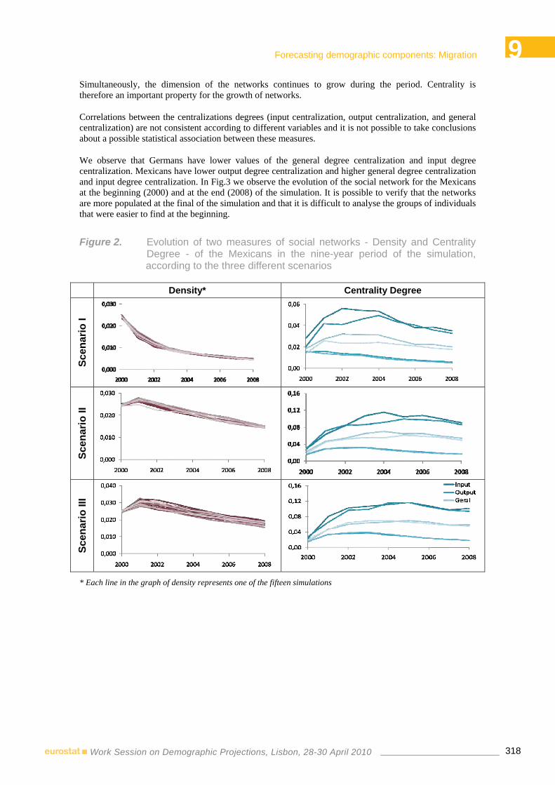
9 Forecasting demographic components: Migration
318Work Session on Demographic Projections, Lisbon, 28-30 April 2010
Simultaneously, the dimension of the networks continues to grow during the period. Centrality is therefore an important property for the growth of networks.
Correlations between the centralizations degrees (input centralization, output centralization, and general centralization) are not consistent according to different variables and it is not possible to take conclusions about a possible statistical association between these measures.
We observe that Germans have lower values of the general degree centralization and input degree centralization. Mexicans have lower output degree centralization and higher general degree centralization and input degree centralization. In Fig.3 we observe the evolution of the social network for the Mexicans at the beginning (2000) and at the end (2008) of the simulation. It is possible to verify that the networks are more populated at the final of the simulation and that it is difficult to analyse the groups of individuals that were easier to find at the beginning.
Figure 2. Evolution of two measures of social networks - Density and Centrality Degree - of the Mexicans in the nine-year period of the simulation, according to the three different scenarios
Density* Centrality Degree
Scen
ario
I
Scen
ario
II
Scen
ario
III
* Each line in the graph of density represents one of the fifteen simulations

9 Forecasting demographic components: Migration
319Work Session on Demographic Projections, Lisbon, 28-30 April 2010
Figure 3. Evolution of the social network (Mexicans): 2000 (A) and 2008 (B)
5. Conclusions and further work
In this work we use a Multi-Agent System to model the flow of migrants in social networks. Our model is based on the idea that migration flows are influenced by the structure of the social network of the agents. The proposed model of migration uses four countries (Germany, Mexico, Portugal and China) and six variables: age (y), educational level, (e), household income (r), number of people in the household, (p), labour status (working/not working), (w) and number of individuals in the social network of the agent (s). The social network is based on the number of persons in the household. We have used information from the IPUMS, containing data of migration flows to the United States between 2001 and 2008.
Our goal was to verify to what extent the existence of networks with major centrality contributes to favour the increase the number of migrants. We believe that in cases of higher centrality, the information flows easily through the links and nodes of the network, but the center of the network is critical for the transmission of information. This analysis aims at highlighting two important aspects, which can be seen as research Hypotheses: 1) The density of the network influences the quantity of the migratory flow; 2) The degree of centralization of the network influences the quantity of the migratory flow.
A gravitational model has been applied to migration flows in the sense that the act of migrating may be influenced by the attraction exerted by the social network. In our work, immigrant communities in the U.S. have been created on the basis of the dimension of the social networks. We aim at measuring the force that these communities have to attract new migrants from the country of origin to the U.S., as well as to repel those who are already in the U.S.
The stability of the model was analyzed for three different scenarios of migration level (ML) and for all countries. It is possible to confirm that there is a great stability of the values, confirmed by the variation coefficient. We focused our attention in specific scenarios: scenarios II and III are more realistic than scenario I. The latter is strongly inductive for immigration. We concluded that the agents that stay in the U.S. (and do not go away to their country of origin), have higher values of Ma, and have less average distance among the members of their social networks. Networks of these agents are more cohesive. Centrality is therefore an important property for the growth of networks. In addition, Germans have lower values of the general degree centralization and input degree centralization. Mexicans have lower output degree centralization and higher general degree centralization and input degree centralization.
A B

9 Forecasting demographic components: Migration
320Work Session on Demographic Projections, Lisbon, 28-30 April 2010
References
Axtell, R. (1999), "Why Agents? On the Varied Motivations for Agent Computing in the Social Sciences", Workshop on Agent Simulation: Applications, Models, and Tools, Argonne National Laboratory, Argonne, Illinois, USA.
Bianchi, C., P. Cirillo, et al. (2007), "Validating and Calibrating Agent-Based Models: A Case Study", Computational Economics, Vol. 30, Nº 3, pp. 245-264.
Billari, F. C., & Prskawetzy, A. (2005). Studying population dynamics from the bottom-up: the crucial role of agent-based computational demography. International Union for the Scientific Study of Population - XXV International Population Conference (p. 13). Tours, France: IUSSP
Billari, F. C., Ongaro, F., & Prskawetz, A. (2003). Introduction: Agent-Based Computational Demography. In F. C. Billari, & A. Prskawetz, Agent-Based Computational Demography: Using Simulation to Improve Our Understanding of Demographic Behaviour (p. 210). New York: Physica-Verlag.
Bond, A. H., and L. Grasser (1988), Readings in Distributed Artificial Intelligence, Los Altos, Morgan Kauffmann
Boyd, M. (1989), "Family and Personal Networks in International Migration: Recent Developments and New Agendas", International Migration Review, Vol. 23, Nº 3, pp. 638-670.
Campos, P. (2008), "Organizational Survival and the Emergence of Collaboration Networks: A Multi-Agent Approach", Faculty of Economics, University of Porto, PhD Thesis.
Conover, W. J. (1999), Practical Nonparametric Statistics, 3rd Edition, USA, John Wiley and Sons
Fagiolo, G., A. Moneta, et al. (2007), "A Critical Guide to Empirical Validation of Agent-Based Models in Economics: Methodologies, Procedures, and Open Problems", Computational Economics, Vol. 30, Nº 3, pp. 195-226.
Ferber, J. (1999), Multi-Agent Systems: An Introduction to Artificial Intelligence: Addison-Wesley.
Freeman, L. C. (1977), "Set of Measures of Centrality Based on Betweenness", Sociometry, Vol. 40, Nº 1, pp. 35-41.
Gilbert, N. e K. G. Troitzsch, (1999), Simulation for the Social Scientist: Open University Press.
Hair, J. F., Black., (2009), Multivariate Data Analysis, Prentice Hall
Helmenstein, C., & Yegorov, Y. (2000). The dynamics of migration in the presence of chains. Journal of Economic Dynamics & Control , 24, pp. 307-323.
Hussey, P. S. (2007). International migration patterns of physicians to the United States: A cross-national panel analysis. Health Policy , 84, pp. 298–307.
Lemieux, V. e M. Ouimet (2008), Análise Estrutural Das Redes Sociais, Instituto Piaget, Lisboa
Mckenzie, D., & Rapoport, H. (2007). Network effects and the dynamics of migration and inequality: Theory and evidence from Mexico. Journal of Development Economics , 84, pp. 1–24.
Mitchell, J. C. (1969), “The Concept and Use of Social Network" in J. C. Mitchell (editor), Social Networks in Urban Situations, Manchester, UK, Manchester University Press, pp. 1-50
Neto, F. e E. Mullet (1998), "Decision-Making as Regards Migration: Wage Differential, Job Opportunity, and the Network Effect", Acta Psychologica, Vol. 98, Nº 1, pp. 57-66.
Newman, M. E., & Girvan, M. (2004). Finding and evaluating community structure in networks. PHYSICAL REVIEW E , 69, p. 026113.
Nooy, W., Mrvar, A., Batagelj, V., (2005) Exploratory Social Network Analysis with Pajek, Cambridge University Press

9 Forecasting demographic components: Migration
321Work Session on Demographic Projections, Lisbon, 28-30 April 2010
FORECASTING MIGRATION FLOWS TO AND FROM NORWAY USING AN ECONOMETRIC MODEL1
Helge BRUNBORG2, Ådne CAPPELEN2
Abstract
Immigration to Norway has increased rapidly in recent years, with net immigration tripling in only three years. Net immigration currently makes up more than half of the population growth and it is, therefore, important to make realistic assumptions about the migration flows to be used in the population forecasts. A large part of the increased immigration to Norwegian is caused by labour migration. At the same time, the expansion of EU to Eastern Europe in recent years has vastly expanded the potential supply of labour to Norway. Through Norway’s membership in the European Economic Cooperation area (EEA), citizens of EU member countries have almost unrestricted access to work and live in Norway. A large part of the recent immigration increase is due to labour immigration, the other main categories being refugees and asylum seekers, establishing and reunification of families, and education.
The high immigration level is to a large extent caused by the favourable economic situation in Norway in recent years, with one of the lowest unemployment rates and highest income levels in the world. This has made it easy for immigrants to obtain employment with relatively high wages
To produce more realistic population forecasts, we have estimated an econometric model where net immigration to Norway from the EEA is a function of the unemployment rate in Norway and the income level in Norway relative to the average of OECD countries, adjusted for purchasing power differences. The estimation yields stable parameters and these are consequently used to forecast net immigration to Norway, based on forecasts of unemployment and level and relative income. It is expected that the growth in the Norwegian economy will decreased in the future, in the short run because of deteriorating international business cycles, and in the long run because of reduced revenue from oil and gas production. The petroleum reserves in the North Sea are expected to be depleted in 2040-2050. The model implies that net immigration will continue in the short run, followed by a rapid fall as a consequence of declining relative income of Norway.
The resulting net immigration flows have been incorporated into recently published population forecasts by age and sex for all of Norway, as well as for each of 430 municipalities. These flows have also been used to project the immigrant population by two groups of country of origin (1) EEA/EFTA, North America, Australia and New Zealand, and (2) The rest of the world.
The financial and economic crisis has so far affected Norway less than most other countries, but there has nevertheless been a decline in economic activity, especially in the construction industry, with reduced the demand for labour. The net immigration Norway has now peaked and is expected to decline further in future years.
This modelling approach has proved very useful and has greatly improved the basis for our migration assumptions. Previously these were made as a rather ad hoc simple extrapolation of past trends, which is the prevalent approach in most countries.
1 We are grateful for comments to an earlier version of this paper from Nico Keilman and Joel E. Cohen. 2 [email protected] and [email protected], Research Department, Statistics Norway

9 Forecasting demographic components: Migration
322Work Session on Demographic Projections, Lisbon, 28-30 April 2010
1. Introduction
Global migration flows have increased significantly in the last decades. This is caused both by income disparities between countries and to crises and conflicts in many regions of the world. There is an upward trend in migration to industrial countries although significant annual variations. This presents a challenge for population forecasters, especially after the onset of the financial and economic crisis in 2008. Will the level of immigration to industrial countries remain high - or perhaps increase further - because income differences between poor countries will remain in spite of the financial crisis, or will the reduced demand for labour in the rich countries result in reduced immigration and increased emigration? The answers to these questions depend on a number of factors, including migration policies and the emergence of crisis situations, but not the least on the economic development in the coming years, in both rich and poor countries.
In this paper we present an econometric analysis of migration between Norway and other countries, both individual countries and groups of countries. The analysis is based on demographic and economic data for the period 1970-2008, and is used to project migration flows to and from Norway. Although the literature abounds with theoretical and empirical studies of the relationship between economic factors and migration, there are very few attempts at utilizing such analyses to project future migration flows. One of the reasons for this is the lack of a general theory of international migration but also that it is usually more difficult to project economic parameters than demographic factors such as fertility and mortality.
Around 1970 Norway changed from being a country of net emigration to becoming a country of net immigration. Since then net immigration has increased steadily, but with significant fluctuations from year to year. Since 2004 net immigration to Norway has been increasing very fast, with net immigration tripling in only three years (Figure 1). Net immigration currently makes up more than half of the population growth and it is, therefore, important to make realistic assumptions about the migration flows to be used in the population forecasts. A large part of the increased immigration to Norwegian is caused by labour migration, which has been facilitated by the expansion of EU to Eastern Europe in 2004 and 2007. Through Norway’s membership in the European Economic Cooperation area (EEA), citizens of EU member countries have almost unrestricted access to work and live in Norway. The growth has been particularly rapid for Polish citizens, whose net immigration to Norway grew from 300 in 2003 to 12 000 in 2008.
Figure 1. Migration to and from Norway, 1970-2008
-10 000
0
10 000
20 000
30 000
40 000
50 000
60 000
70 000
1970 1975 1980 1985 1990 1995 2000 2005 2010
Immigration
EmigrationNet immigration

9 Forecasting demographic components: Migration
323Work Session on Demographic Projections, Lisbon, 28-30 April 2010
The rapidly increasing immigration to Norway has made it even more difficult to make population projections. The past practice of more or less ad hoc extrapolation of past trends of net immigration, with stable levels after some years seems unsatisfactory. In 2005, for example, the projected net immigration for the first projection year, 2005, was fully 23 per cent below the actual number that was registered a few months after the projections had been published.
Making a stochastic time series projection is tempting, but with rapidly changing migration flows the confidence intervals easily become so large that they are of little or no value for users of the projections. Keilman et al. (2001) found that a random walk model gave totally unusable estimates whereas an ARMA (1,1) model resulted in large but useful confidence intervals.
The growth has been particularly rapid for labour migration to Norway, which multiplied 12 times from 2003 to 2008, as shown in Figure 2. This is an indication that the growth in immigration to Norway obviously is related to economic factors, both in Norway and in other countries, i.e., both demand for labour in Norway and supply of labour elsewhere.
Thus, it seems natural to look at economic theory of international migration and try to develop a model that can be used to forecast migration to and from Norway.
Figure 2. Immigration to Norway by registered reason for immigration*
0
5 000
10 000
15 000
20 000
25 000
1990 1995 2000 2005
Work FamiyRefugee Education
*Does not include citizens of the other Nordic countries (Denmark, Finland, Iceland and Sweden)
Source: Statistics Norway
2. How are migration flows projected?
“A projection of population must rest, in part, on a projection of immigration. Yet most official immigration projections, both in the United States and abroad, continue to rely on ad-hoc assumptions based on little theory and virtually no definable methodology.” (Howe and Jackson 2006)
Most official population forecasts made by statistical offices are based on trend-based extrapolation of migration. The most common approach is to assume constant net immigration for all or most of the projection period. In the Eurostat Demographic Outlook for 2007 and 2008 for most European countries only two countries appear to have based their migration assumptions on an analysis taking economic or

9 Forecasting demographic components: Migration
324Work Session on Demographic Projections, Lisbon, 28-30 April 2010
other factors specifically into consideration. Migration to and from Belgium is based on “… an indicator of the standard of living that is supposed to reflect the relative attractiveness of the Belgian economy in the whole of Europe.” (Eurostat 2009a). Statistics Sweden assumes that immigration from several countries, especially labour migration due to the deteriorating economic situation, will decline in the coming years, but there is no formal modelling of the future migration flows (Statistiska centralbyrån 2009).
In the Convergence scenario of EUROPOP 2008, which includes population projections of the 27 EU member countries, Norway and Switzerland until 2061, it is assumed that fertility, mortality and migration will converge in the final convergence year, which was fixed at 2150, implying zero net migration between EU member countries (Eurostat 2009b; Lanzieri 2009). This is based on the hypothesis that these countries will be more or less similar in 2150 with regard to social and economic conditions. This implicitly assumes that there will be no driving factors causing net migration between these countries, including income differentials. EUROPOP 2008 is not, however, based on any modelling or estimation of the relationship between net migration and income differences.
Howe and Jackson (2006) mention several countries that make more sophisticated projections of international migration (USA, France, Germany, The Netherlands, UK, Australia, Canada), although they are not based on specific economic models.
There are very few examples of forecasting of migration flows that are based on economic modelling. Some examples, although not of official statistical agencies forecasting international migration, include Gorbey, James and Poot (1999), who have looked at migration forecasting between Australia and New Zealand “… in a Bayesian or unrestricted vector autoregression (VAR) model, which includes foreign and domestic economic variables.” Schrier and McRae (1999) have used provincial unemployment rate differentials and the differential between the British Columbia and the rest of Canada growth in real GDP to forecast net interprovincial migration for British Columbia.
3. Theoretical framework
Our basic model dates back to Roy (1951) and is elaborated by Borjas (1987). For a recent application see also Mayda (2009). There are two countries: (o)rigin and (d)estination. The log of wages that an individual living in the origin country would receive if not migrating (wo) is
ln wo = μo + εo where εo ~ N (0, σo2) (1)
Here μo is interpreted as determined by individual observables such as education, gender etc., while εo captures unobservable characteristics with zero mean and a constant variance. To simplify, for individuals who migrate there is a similar wage model in the destination country
ln wd = μd + εd where εd ~ N (0, σd2) (2)
The error terms are possibly correlated with a correlation coefficient ρ.
The decision to migrate or not, is determined by the sign of an index I:
I = ln (wd/(wo + c)) ≈ (μd - μo - δ ) + εd - εo (3)
where c is the level of mobility costs while δ is the wage equivalent mobility cost. Migration occurs if the index I is positive. The emigration probability (P) from the origin country is then given by
P = Pr (εd - εo > - (μd - μo - δ )) = 1 – Ф (-(μd - μo - δ )/σε) (4)

9 Forecasting demographic components: Migration
325Work Session on Demographic Projections, Lisbon, 28-30 April 2010
Here, σε2 is the variance for the error term difference εd - εo and Ф is the standard normal distribution.3
Equation (4) captures some important features of empirical models of migration. Higher income in the origin country lowers P, while higher income in the destination country increases P. In addition, the income effects are the same but with opposite signs and this has strong implications for the econometric specification. Notice also that P is the emigration probability defined as emigration divided by the population in the origin country. If we respecify the model using the number of emigrants as the endogenous variable while the size of the population of the origin country enters as a regressor, one could test this restriction. This is done by Karemera et al. (2000) who include the (log) population in the emigration equation but their results do not support using the emigration rate specification.
Higher costs of migration relative to income in the destination country reduce migration. A theoretical model of the effects of mobility costs is the focus of Carrington et al. (1996). The idea here is that mobility costs decrease with the number of migrants already settled in the destination country because they send information about job and housing markets to friends and family in the origin country and generally provide a network for new entrants. The empirical specification of mobility costs is a central part of econometric analyses of migration. Standard proxies used are language differences, geographical distance, and migration policy indicators. It is common to include social indicators like crime and corruption indicators of political systems in order to explain migration flows. All studies referred to earlier use more or less these variables in their econometric specifications.
The model by Borjas (1987) also includes the income distribution as a feature affecting migration. He finds that countries with more income inequality have lower emigration rates and that this negative effect is consistent with his model if there is a negative selection in the immigrant pool. For this to be the case there must be a strong positive correlation between earnings for immigrants in the origin and the destination countries and less income inequality in the destination country. If the mean income in the destination country is higher than in the origin country – which is a major motive for emigration in the first place – and inequality increases in the origin country, then high-income persons in that country will have fewer incentives to emigrate while low-income persons in the origin country are not affected. Total emigration is then reduced. Thus, changes in the distribution of income in the origin country select or motivate on average different people to emigrate.4
One issue not discussed much in the theoretical literature referred to earlier is the effect of income taxes and government spending on education and social transfers. The model in equations (1) and (2) focuses on wages but is not precise on how to measure wages in empirical applications. The standard method is to use GDP per capita (adjusting for purchasing power differences, PPPs) as an indicator. However, tax rates vary a lot between countries and consequently income differences adjusted for taxes may be quite different from GDP figures. On the other hand, government services and transfers will usually moderate these tax differences. One possibility is therefore to include government spending (and even only on certain items) to take into account the wedge between GDP and take home pay. However, one should be careful when interpreting a variable like this. If taxes are high in, say, the destination country, government spending will usually also be high. To the extent that government spending provides services in the destination country free of charge, using a gross income measure is not so problematic since taxes net of government spending on individual services like education and social services may not differ much between countries.
Migration often involves young people who study abroad for some years and then return to their native country. Likewise, people move to a country to work for some years in order to earn enough money to buy a house, etc. The intention may not be to settle down for a long time but it may turn out that the transaction costs related to moving were larger than expected, resulting in a reversal of the decision. In order to capture this possibility we include previous gross migration flows in our model so that, say, emigration from Norway to Sweden in year t is made a function of immigration from Sweden to Norway in a previous year.
3 σε2 is a function of the other variances and the covariance of the ε’s. 4 Mayda (2008) argues for including the square of relative income inequality and finds empirical support for this specification.

9 Forecasting demographic components: Migration
326Work Session on Demographic Projections, Lisbon, 28-30 April 2010
4. Data
The demographic data on the number of migrants to and from Norway are taken from the Central Population Register (CPR) of Norway, which was established in 1964. The register includes information on personal identification number (PIN), date of birth, sex, date of immigration, country of origin, country of birth, and reason for immigration. It also included the PIN of family members migrating to Norway simultaneously or who are already living in Norway. Our analysis is based on macro data, although micro data are also available for migrants, but with limited information on socio-economic variables for most immigrants to Norway.
A person is considered an immigrant to Norway when he or she intends to stay in Norway for at least 6 months. Citizens from the other Nordic countries (Denmark, Finland, Iceland and Sweden) do not need a permit to settle in Norway, an arrangement that was introduced in the 1950s. Norway is not a member of the European Union but Norway’s membership in the European Economic Cooperation area (EEA) gives citizens of EU member countries almost unrestricted access to work and live in Norway. For citizens from the Eastern European EU countries certain conditions need to be met (i.e. having a job) to get residence and work permits, but these conditions are very liberal and were abolished in 2009 (except for Bulgaria and Romania). Citizens of non-EEA countries need to apply for a residence permit.
There is some under registration of emigration as some people do not report their move. Thus, there are some people in the CPR who are registered as living in Norway but who have left the country.
People who come on short-term work contracts or commute from other countries to work in Norway are registered as residents and not included in the CPR.
Asylum seekers and other people who want to live in Norway are given a unique personal identity number (PIN) and registered in the Central Population Register (CPR) only after their applications have been approved. This implies that there are several thousand asylum seekers who live transitionally in Norway in special institutions and who are not included in the population projections.
The number of unauthorized foreigners has been estimated at 18 200, with a 95 per cent confidence interval of between 10 500 and 31 900 (Zhang 2008).
The income data used in the estimation are all taken from OECD databases. We approximate wages by GDP per capita where GDP is measured using purchasing power parities (PPPs). These data are downloaded from the OECD web-site. The same is the case for unemployment series which are defined as "standardized unemployment rates" by the OECD. Measures of income distribution are defined as the Gini-coefficient of income distribution and are downloaded from the web-site of the Luxembourg Income Study (LIS).
The forecast for unemployment and GDP for Norway are taken from Statistics Norway (2009c).
5. Empirical results for immigration and emigration to Norway
Our analysis concerns immigration and emigration to Norway only. This makes our study somewhat different from many other studies in the literature. We study gross flows between Norway and two other Nordic countries, Denmark and Sweden, and for the “OECD-countries” as well as “Asia and Africa”.5 For the Nordic countries there are no changes in the migration policy regime in our estimation period. There have been no restrictions on labour mobility or passport controls since the 1960s and our estimation period covers 1970-2008. Language, culture and religious effects are negligible so the standard “non-economic” variables often included in the empirical literature on migration are not relevant. Even
5 The whole of America is included in “the rest of the OECD” but migration to and from Latin-America is normally very small.
Japan and South-Korea are likewise included in their geographical region and not in the OECD. Again this is due to minute migration flows between Norway and these two countries.

9 Forecasting demographic components: Migration
327Work Session on Demographic Projections, Lisbon, 28-30 April 2010
migration costs are small. In many cases there are just as large or even larger migration costs related to internal migration inside Norway as there are between Norway and Sweden. Our basic model for the gross migration flow, or actually the gross migration probability from country i to country j, is
log(Mij/Popi) = a0 + a1 * log (incomei/incomej) + a2 * Ginii + a3 * Ui + a4 * Uj + a5 * Mji t-1 (5)
Mij is migration from country i to j and is related to the population Popi in country i. The first term is the relative income between the two countries (measured by GDP per capita in PPPs), and Ginii is the coefficient of income distribution based on the Luxembourg income study (LIS). The Us are unemployment rates. The last term in eq. (5) captures the possibility that previous immigration from a country may increase later emigration to the same country. The time subscript is only indicative in the sense that we leave it to the data in order to arrive at a more precise dating of the effect. All data come from OECD data or national sources.
5.1 Results for the Scandinavian countries Traditionally there has been substantial mobility between the Scandinavian countries6. Labour mobility has been unrestricted since the 1960s and there has been no passport control since that time. It is the mobility between Sweden and Norway that is most important and this has been increasing for quite some time, although with large fluctuations related to business-cycles in Norway and Sweden, see Figure 3. Flows between Denmark and Norway show less variation and trend over time, cf. Figure 4. Cultural and language differences between these countries are quite small.
Figure 3. Migration flows between Norway and Sweden
-8 000
-6 000
-4 000
-2 000
0
2 000
4 000
6 000
8 000
10 000
12 000
1970 1975 1980 1985 1990 1995 2000 2005
Immigration
Emigration
Net Immigration
6 The unrestricted movement actually includes the Nordic countries Finland and Iceland as well as the Scandinavian countries
Denmark, Norway and Sweden. But in terms of migration to and from Norway it is Denmark and Sweden that matter.

9 Forecasting demographic components: Migration
328Work Session on Demographic Projections, Lisbon, 28-30 April 2010
Figure 4. Migration flows between Norway and Denmark
Results from estimating the model in (5) for the Scandinavian countries are shown in Table 1. In this table we show only the estimated long run effects implied and not the model actually estimated in order to highlight the main result in the text.
Table 1. Estimation of the rate of migration from Sweden and Denmark to Norway (eq. 5)
Migration from Sweden to
Norway Norway to Sweden
Denmark to Norway
Norway to Denmark
Constant -10.029 (-24.6) -13.80 (-14.50) -7.25 (-37.4) -13.60 (-19.8)
Relative income - 0.504 (-2.97) 0.131 (1.41)
Inequality 9.254 (5.01)
Unempl. Origin 0.035 (2.76) 0.140 (4.26) 0.060 (5.69)
Unempl.destination - 0.223 (-3.31)7 -0.474 (-4.82) -0.089 (-1.77) -0.035 (-4.21)
Prev. immigration 0.814 (7.00) 0.787 (9.20)
Period 1972-2008 1973-2008 1973-2008 1975-2008
σ (of eqcm) 0,071 0.111 0.098 0.046
AR1-2 F(2,26)=1.66 (0.21) F(2,27)=0.83 (0.45) F(2,28)=2.07 (0.14) F(2,23)=0.19 (0.83)
ARCH1-1 F(1,26)=0.58 (0.45) F(1,27)=1.58 (0.22) F(1,28)=2,31 (0.14) F(1,23)=1.58 (0.22)
Normality Χ2 (2) = 1.85 (0.40) χ2 (2)=0.35 (0.84) χ2 (2)=0.63 (0.73) χ2 (2)=1.22 (0.54)
Heterosc. F(15,12)=0.27 (0.99) F(11,17)=0.87(0.58) F(9,20)=1.21 (0.34) F(15,9)=0.25 (0.99)
Estimation was carried out using PcGive 10.3, cf. Doornik and Hendry (2000). The AR test is based on Harvey (1981), the ARCH-test is based on Engle (1982), the normality test is based on Doornik and Hansen (1994), and the heteroskedasticity test is based on White (1980). Estimated t-values are shown in parentheses. The estimated standard error of regression is that of the actual equilibrium correction model (eqcm) estimated.
7 This estimate is for the change in unemployment and not the level.
-1 000
-500
0
500
1 000
1 500
2 000
2 500
3 000
3 500
4 000
1970 1975 1980 1985 1990 1995 2000 2005
Emigration
Net immigration
Immigration

9 Forecasting demographic components: Migration
329Work Session on Demographic Projections, Lisbon, 28-30 April 2010
In the first column of Table 1 we show the result from estimating a model for migration from Sweden to Norway. In line with theory we have significant effects of relative income so that higher incomes in Sweden relative to Norway reduce emigration from Sweden to Norway. We also find that higher unemployment in Sweden increases emigration. A partial increase in unemployment in Norway reduces migration but a significant estimated effect was only found for changes in unemployment, meaning that in the very long run there is no effect on migration of the level of unemployment. There is a positive effect of Swedish inequality on migration so that more unequal incomes within Sweden increase emigration. This does not go against the arguments made earlier because the Swedish distribution of income is more equal than Norway’s so the argument is simply turned on its head. The short run effect of increased inequality is quite strong and so is the effect of higher unemployment in Sweden. In the long run, a one per cent increase in Norwegian earnings relative to the Swedish increases the migration probability by half a percentage point.
In the second column we show the long run model of Norwegian migration to Sweden. Here there are few separate effects. Nearly all effect in the long run comes through the previous migration from Sweden to Norway, i.e. through the a5 coefficient being positive.
The third column shows Danish emigration to Norway being influenced only by labour market conditions in the long run. However, there are short run income effects present that are in line with theory. The fourth column of Table 1 shows that Norwegian emigration to Denmark is affected by relative income effects and labour market factors. In addition, there is an effect of previous Danish immigration to Norway on later emigration from Norway to Denmark as was the case for Sweden. These effects fit well with anecdotal observations of young people from Denmark and Sweden working in Norway for a few years before returning home. Given that unemployment is much lower in Norway than in the other two countries, it has usually been easy for young people to find employment in Norway.
5.2 Results for broad aggregates of countries We have also estimated a version of eq. (5) for two broad aggregates Europe, America and Oceania (“EurAm”) on the one hand and Africa and Asia (“AfrAsia”) being the other. For the first aggregate we have used OECD-averages instead of actual data corresponding to the country group. The error we make is that Latin-America is included in the migration data but not in the explanatory variables. As migration from Norway to Latin-America is very small, this error is minor. Migration for people from African and Asian countries is generally more restricted than for people belonging to the first group of countries. Estimation result for long run effects are shown in Table 2.
For migration to and from “EurAm” there is a strong income effect explaining migration to Norway. There is no significant income effect explaining outmigration from Norway but implicitly there is an income effect through the variable “previous immigration”. We have tried to include also relative government expenditures to capture differences in welfare spending, but without any significant or sensible results. Unemployment effects are significant in both migration models but there are no long term effects. We have included these terms in the table in spite of them being short run effects while the income effects are long run. Notice also that the effects are quite symmetric in explaining migration to and from Norway. This would indicate that a pooled model that explains migration to and from Norway with identical marginal parameters and only a fixed effect could work well as the signs are opposite. However, the income effects are quite different.8 We do not show dummy variables related to changes in migration policies in Table 2. These are shown in the appendix. The expansion of the European Union to include Eastern European countries has affected regulation of labour markets in many European countries since 2004. A significant change in the constant term captures this event. It could be argued that this event may lead to a more substantial change in the model structure than only a change in the constant but we would need more historical data and experience to identify this. There are also two step dummies to take account of the influx of people for Bosnia (1993) and Kosovo (1999).
8 A formal test should be undertaken but has not been done yet.

9 Forecasting demographic components: Migration
330Work Session on Demographic Projections, Lisbon, 28-30 April 2010
The third and fourth columns of Table 2 model migration to and from Africa and Asia. For migration to Norway there is a strong income effect. We should, however, be careful in interpreting the size of this effect as we to simplify have used average income in the OECD for these countries and not income for the relevant country group. For this group of countries there are no reliable time series for unemployment dating back to 1970. It is noticeable that we have not been able to model migration from Norway to these countries very successfully in terms of economic variables except that a level effect of unemployment is significant. This means that if there is high unemployment in Norway more people migrate to these countries. The explanation is perhaps that some ants to Norway from these countries return to their country of origin if they are not able to get a job.
Table 2. Estimation of migration for broad aggregates of countries
Migration from
“EurAm” to Norway
Norway to “EurAm”
“AfrAsia” to Norway
Norway to “AfrAsia”
Constant -8.55 (-7.89) -12.58 (-17.90) -2.29 (-0.79) 7.50 (64.20)
Relative income 0.953 (4.17) 2.34 (3.88)
Unempl. origin9 0.078 (1.49) 0.079 (5.01) 0.089 (3.09)
Unempl.destination - 0.132 (-3.81) -0.111 (-3.52) -0.62 (-1.69)
Prev. immigration 0.713 (10.00)
Period 1972-2008 1973-2008 1973-2008 1972-2008
σ (of eqcm) 0,069 0.062 0.071 0.061
AR1-2 F(2,27)=1.28 (0.29) F(2,27)=0.79 (0.47) F(2,27)=0.89 (0.42) F(2,31)=1.62 (0.21
ARCH1-1 F(1,27)=3.15 (0.09) F(1,27)=0.12 (0.73) F(1,27)=1,07 (0.31) F(1,31)=0.99 (0.33)
Normality Χ2 (2) = 1.87 (0.39) χ2 (2) = 1.22 (0.54) χ2 (2) = 2.79 (0.25) χ2 (2) = 0.30 (0.86)
Heterosc. F(11,17)=0.41(0.93) F(11,17)=1.82(0.13) F(10,18)=0.65(0.75) F(6,26)=0.46 (0.83)
Estimation was carried out using PcGive 10.3 cf. Doornik and Hendry (2000). The AR test is based on Harvey (1981), the ARCH-test is based on Engle (1982), the normality test is based on Doornik and Hansen (1994) and the heteroskedasticity test is based on White (1980). Estimated t-values shown in parenthesis.
The specification tests shown in Table 2 all indicate that the migration models are not misspecified. Recursive estimates of the parameters indicate reasonably stable models since the mid 1990s so that these models are candidates for forecasting gross migration flows to and from Norway, see the Appendix.
6. Forecasting migration
The main purpose of estimating these models is to use them as input to a demographic model that is used regularly for forecasting the population of Norway. This focus for modelling migration is somewhat different from what is common in the demographic literature. When the model is used for forecasting, we need to check that our equations fulfil some design criteria so that we can have confidence in the quality of our forecasts. One way to do this is to run a large set of statistical specification tests on our models. These are shown in the appendix. If our model passes these tests to a reasonable extent, we think there are reasons for assuming that they may perform well in forecasting. However, these tests are of course no guarantee against future structural changes making our model inadequate.
9 The unemployment variables are specified as changes not levels, except for the effect in the fourth column where there is a
level effect.

9 Forecasting demographic components: Migration
331Work Session on Demographic Projections, Lisbon, 28-30 April 2010
When using the models discussed earlier for forecasting we first of all need a forecast of all the explanatory variables that enter the estimated equations. In our case this is relative income and unemployment. For the latter two variables we have used recent macroeconomic forecast based on Consensus Forecasts (2009) for 2009 and 2010. We have assumed that the current recession gradually disappears and that unemployment rates return to more normal levels as shown in Figure 5.
Figure 5. Unemployment rates in OECD and in Norway, 1970-2030
0
2
4
6
8
10
1970 1980 1990 2000 2010 2020 2030
OECD
Norway
The most important variable that we need to forecast is relative income, proxied by GDP per capita using PPPs. Since it is relative income that matters, we focus on how Norwegian income may develop compared to the average OECD level. Norway’s current situation is influenced by its petroleum production combined with high oil prices. It is generally expected that petroleum output will continue to decline so that the oil sector gradually will contribute less to GDP. According to the most recent long term projections from the Norwegian government the contribution of the oil sector to GDP will fall from roughly 37 % in 2008 to 10 % in 2030.10 Most of this decline in output will correspond to a fall in petroleum rents, which is defined as excess profits from exploiting this natural resource. It is not reasonable to assume that Norway will have access to another resource that will provide the country with similar incomes. In the very short run we expect oil prices to pick up somewhat again and more than compensate for the decline in production but this is not reasonable in the long run. For non-oil GDP per capita we assume that there is no change in relative income. This motivates our assumption with regard to the development of relative income between Norway and the OECD average. Historical figures and the forecast are shown in Figure 6 below.
10 Cf. Figure 7.2 on page 129 of Perspektivmeldingen 2009, St.meld.nr.9 (2008-2009) Ministry of Finance, Oslo, 2009.

9 Forecasting demographic components: Migration
332Work Session on Demographic Projections, Lisbon, 28-30 April 2010
Figure 6. GDP per capita in PPPs. Norway relative to OECD. Observations 1970-2008 and forecast 2009-2030
90
100
110
120
130
140
150
160
170
180
1970 1980 1990 2000 2010 2020 2030
Based on these assumptions and no impact of possible changes in migration policies, we can make a forecast for gross migration flows to and from Norway. The forecasting equations used are those presented in the appendix. The results are shown on Figure 7. For gross flow into Norway the decline in the short run is mainly due to the decline in income. As oil prices are expected to grow in the next cyclical upturn, this tells us that migration into Norway should increase again but in the long turn the decline in income due to declining oil and gas production will lead to lower immigration.
The gross emigration from Norway has a hump shape in the near future that is a result of higher unemployment in Norway as well as declining relative income in the short run. In 2010, higher oil prices are assumed to increase relative incomes again and it is only when the volume of petroleum production starts to decline that the long run tendency for declining income becomes strong and net migration also falls.
Figure 7. Gross and net migration flows to Norway. History and forecasts 1970 to 2030.
-10 000
0
10 000
20 000
30 000
40 000
50 000
60 000
70 000
1970 1980 1990 2000 2010 2020 2030
Immigration
Net immigration
Emigration

9 Forecasting demographic components: Migration
333Work Session on Demographic Projections, Lisbon, 28-30 April 2010
One may ask how sensitive this forecast is to the assumption of the development in long term relative income. It is not interesting to study the effect of higher or lower unemployment since these variables mainly have short run effects and it is not reasonable to assume a long lasting trend in unemployment in spite of the fact that such a change can go on at least for a decade, cf. Figure 5. One rather extreme alternative would be to assume that relative incomes would show absolute convergence in the long run, meaning that sometimes in the not very distant future Norway’s income relative to the OECD average would be back at its level of the early 1970s, i.e. before oil made a big impact on Norway’s incomes. Using the long run solution of the estimated models yields the following striking results. Net immigration from Europe, America and Oceania would be 3 000 persons per year and the immigration from Africa and Asia would be quite similar. Thus, a return to the relative income levels that Norway enjoyed before oil made an impact on the economy would bring net immigration nearly back to the levels of the early 1970s as shown on Figure 7. That this should be the conclusion is, of course, not a surprise. The models we have estimated reproduce the historical development quite well. Assuming that exogenous variables take on values of the early 1970s should by model design reproduce the values for the endogenous variables that were observed at that time.
7. Application in official population projections
When Statistics Norway published population projections for the periods 2009-2060 the assumptions for net immigration were based on a modification of the results of the analysis presented here (Statistics Norway 2009a, b). The reason for this is that it is difficult to explain to the public the various troughs, peaks and inflection points shown in Figure 7. After all, the econometric model is not a perfect model of reality, as many variables have not been included, such as migration flows between other countries, more country-specific data on economic conditions in sending countries, etc. Moreover, the econometric analysis shows that the model does not match the data perfectly. To allow for this we did some smoothing of the model-produced migration flows.
There is substantial uncertainty about the effects of relative income and unemployment on migration flows, and about the future levels of these economic factors. To account for this uncertainty we designed high and low series of net immigration, with the same general shape as the medium series. This was done in a rather ad hoc way, taking into account previous trends and levels in the migration flows and likely future variations in these trends, since no alternative high and low variants of the economic forecasts were available, nor were there any probability distributions of these.
The modified series of net immigration were made separately for the two groups of countries that the analysis was made for:
Group 1: Immigrants from EEA/EFTA, North America, Australia and New Zealand,
Group 2: Immigrants from the rest of Eastern Europe, Africa, Asia (with Turkey), Latin America, and the rest of Oceania.
These country groups correspond closely to the analysis presented in this paper, with minor differences. Immigrants from Group1 are mostly labour immigrants whereas immigrants from Group 2 are mostly refuges and family members.
The immigration assumptions are shown in Figures 8, 9 and 10.

9 Forecasting demographic components: Migration
334Work Session on Demographic Projections, Lisbon, 28-30 April 2010
Figure 8. Net immigration to Norway from Group 1 countries. Registered 1990-2008 and projected 2009-2060
0
5 000
10 000
15 000
20 000
25 000
30 000
1990 2000 2010 2020 2030 2040 2050 2060
Figure 9. Net immigration to Norway from Group 2 countries. Registered 1990-2008 and projected 2009-2060
0
5 000
10 000
15 000
20 000
1990 2000 2010 2020 2030 2040 2050 2060
Figure 10. Total Net immigration to Norway. Registered 1990-2009 and projected 2009-2060
-10
0
10
20
30
40
50
2040203020202010200019901980
Number in 1 000s
Registered
Medium
High
Low
Low
Medium
High
High
Medium
Low

9 Forecasting demographic components: Migration
335Work Session on Demographic Projections, Lisbon, 28-30 April 2010
The analyses presented here have been the basis for the forecast of net immigration used in the official projections of the Norwegian population, for the whole country as well as for the 430 municipalities (Statistics Norway 2008a, 2009a).11 They have also been used to make national projections of immigrants and their children born in Norway by country background, i.e. own and parents’ country of birth (Statistics Norway 2008b, 2009b).
After the projections were made in published in June 2009 migration data for all of 2009 have become available. They show that our assumption for 2009 was very close to the observed number, as shown in Figure 10.
8. Summary and concluding remarks
The analysis presented here is novel in several ways:
An econometric model of migration flows to and from Norway has been estimated.
The estimation results are used, together with economic forecasts, to project future migration to and from Norway.
The resulting net migration flow shows a clear picture that cannot be achieved by simple extrapolation: First, a decline from a high level due to the financial and economic crisis, then an increase following the economic recovery, and finally a long-term gradual decline because Norway’s advantaged economic position will decline, due to reduced petroleum production.
It is unusual that a projection model is able to project a complete turn-around of a trend.
The decline in net immigration to Norway due to the current financial crisis and other factors is in line with other studies (Sward 2009; OECD 2009; Statistics Sweden 2009). This is also confirmed by recent migration data, as shown in Figure 10. Gross immigration to Norway peaked in the third quarter of 2008, while outmigration has been increasing.
The predicted decline in future immigration to Norway is consistent with public opinion surveys in several countries that find that the majority of the population wants a more restrictive immigration policy (PEW 2008). However, only a minority of the Norwegian population (38 per cent) support a more restrictive policy towards refugees and asylum seekers, while the majority (53 per cent) is satisfied with the current policy (Blom 2008).
References
Blom, S. (2008): Holdninger til innvandrere og innvandring 2008, Rapport 2008/57, Statistics Norway
Borjas, G.J. (1987): Self-Selection and the Earnings of Immigrants, American Economic Review 77 (4): 531-553.
Borjas, G.J., (1994): The economics of immigration, Journal of Economic Literature, 32 (December), 1667–1717.
11 For each of 19 regions emigration probabilities were estimated on the basis of registered emigration for the previous five
years. The sum of these flows for each projection year, which is the total emigration from Norway, was added to the assumed total net immigration, yielding total immigration fro each year. This number was distributed over 94 projection regions by age and sex, according to a distribution based on registered immigration for the previous five years. Finally, the population growth for each projection region was disaggregated to the municipalities in each region (ranging from 1 to 18 municipalities in each projection region). The projections regions are identical to economic regions, NUTS-4 in EU terminology, except that the largest cities are treated as separated projection regions.

9 Forecasting demographic components: Migration
336Work Session on Demographic Projections, Lisbon, 28-30 April 2010
Brunborg, H., I. Texmon and S.V. Pettersen (2008): Nye befolkningsframskrivinger. Økonomiske analyser 3/2008: 29-41, http://www.ssb.no/emner/08/05/10/oa/200803/brunborg.pdf
Carrington, W.J., E. Detragiache, and T. Vishwanath (1996): Migration with Endogenous Moving Costs, American Economic Review 86 (4): 909- 930.
Consensus Forecasts (2009): Consensus Forecasts, Survey Date February, 10, 2009, Consensus Economics Inc, London, UK.
Doornik, J.A. and H. Hansen (1994): A Practical Test for Univariate and Multivariate Normality, Discussion Paper, Nuffield College, Univ. of Oxford.
Doornik, J.A. and D.F. Hendry (2007): Empirical Econometric Modelling using PcGive, Volume I, Timberlake Consultants LTD, London.
Engle, R.F. (1982): Autoregressive Conditional Heteroscedasticity with Estimates of the Variance of United Kingdom Inflation, Econometrica 50: 987-1007.
Eurostat (2007): Demographic outlook. National reports on the demographic developments in 2006. Methodologies and Working Papers, Eurostat, Luxembourg.
Eurostat (2009a): Demographic outlook. National reports on the demographic developments in 2007. Methodologies and Working Papers, Eurostat, Luxembourg.
Eurostat (2009b): EUROPOP2008 - Convergence scenario, national level. http://epp.eurostat.ec.europa.eu/cache/ITY_SDDS/EN/proj_08c_esms.htm
Gorbey, S., D. James and J. Poot (1999): Population Forecasting with Endogenous Migration: An Application to Trans-Tasman Migration. International Regional Science Review 22(1): 69-101.
Harvey, A.C. (1981): The Econometric Analysis of Time Series, Philip Allan, Oxford.
Howe, N. and R. Jackson (2006): Long-Term Immigration Projection Methods: Current Practice and How to Improve it, WP 2006-3, Center for Retirement Research, Boston College
Karemera, D. V.I. Oguledo, and B. Davis (2000): A gravity model analysis of international migration to North America, Applied Economics 32: 1745-1755.
Keilman, N., D. Q. Pham and A. Hetland (2001): Norway's Uncertain Demographic Future, Social and Economic Studies 105, Statistics Norway.
Lanzieri, G. (2009): EUROPOP2008: A set of population projections for the European Union. Paper presented at the IUSSP International Population Conference, Marrakech, 27 Sep.– 2 Oct. 2009.
Mayda, A. M. (2009): International Migration: A Panel Data Analysis of the Determinants of Bilateral Flows, Journal of Population Economics, DOI 10.1007/s00148-009-0251-x
Péridy, N. (2008): A generalized model of international migration determinants: An application to European immigration from Southern Mediterranean countries. Paper presented at the European Science Foundation Seminar “Estimation and Projection of International Migration”, 17 - 19 September 2008, University of Southampton.
PEW (2007): World Publics Welcome Global Trade -- But Not Immigration. 47-Nation Pew Global Attitudes Survey, http://pewglobal.org/reports/display.php?ReportID=258

9 Forecasting demographic components: Migration
337Work Session on Demographic Projections, Lisbon, 28-30 April 2010
Schrier, D. and D. McRae (2000): An Econometric Model Describing the Movement of the Population Between British Columbia and the Rest of Canada, Population Section, BC Stats, Ministry of Finance and Corporate Relations, Government of British Columbia.
Statistics Norway (2008a): Continued population growth, http://www.ssb.no/english/subjects/02/03/
Statistics Norway (2008b): Strong growth in immigrant population, http://www.ssb.no/innvfram_en/.
Statistics Norway (2009a): High population growth in the future, http://www.ssb.no/english/subjects/02/03/folkfram_en/.
Statistics Norway (2009b): High growth in the number of immigrants, http://www.ssb.no/innvfram_en/.
Statistics Norway (2009c): Economic trends for Norway and abroad: Improvement, but slowdown continues, Economic survey 3/2009, http://www.ssb.no/kt_en/.
Statistiska centralbyrån (2009): Sveriges framtida befolkning 2009-2060. Demografiska rapporter 2009:1, Statistiska centralbyrån, Stockholm.
Sward, J. (2009): Migration and the financial crisis: how will the economic downturn affect migrants? Briefing no. 17 of the Development Research Centre on Migration, Globalisation & Poverty. Sussex Centre for Migration Research. http://www.research4development.info/PDF/ Outputs/MigrationGlobPov/BP17.pdf
White, H. (1980): A Heteroskedasticity Consistent Covariance Matrix Estimator and a Direct Test for Heteroskedasticity, Econometrica 48: 817-838.
Zhang, L.-C. (2008): Developing methods for determining the number of unauthorized foreigners in Norway, Documents 2008/11, Statistics Norway

9 Forecasting demographic components: Migration
338Work Session on Demographic Projections, Lisbon, 28-30 April 2010
Appendix: Equations used for forecasting gross migration flows
The estimation results shown in this appendix are those used for forecasting in the paper. Compared to the estimation results shown in the paper these equations have not been specified as migration relative to the population in the origin country or region. Instead we have used a direct level formulation. The reason is mainly to avoid having to forecast population in the origin region in order to be able to forecast gross migration flows to Norway. It proved to be easy to find specifications in levels that are roughly the same as those specified on a rate form. The statistical tests are quite satisfactory.
In general we have chosen a log-linear specification so that each migration flow is the log of the number of migrants. The explanatory variables are usually lagged values of the migration flow with lag of one year denoted by _1, and a lag of two years _2.
The income variable is denoted “LNor gdp per” and is the (natural) logarithm of GDP per capita in Norway compared to the OECD region. Again, it usually enters with a time lag.
The unemployment rate is included in all equations and is usually specified in changes so that Dunempl means changes in the unemployment rate between to consecutive years while D2unempl means changes between year t and year t-2.
In all cases we need binary variables or dummies in order to arrive at well specified tests (basically only to arrive at normally distributed errors), but these dummies have only minor effects on the estimates of the parameters of interest. The dummies are noted so that the number indicates in what year the variable takes on the value “1” (all others being zero).
Migration to Norway from non-Asian and non-African countries (nonasia&afr)
Immigration from the “OECD-area” to Norway is positively related in the relative income level in the long run. Unemployment in both regions have the expected sign but enter only as changes in levels so for a constant level of unemployment there are no long run effects on migration. There is an important dummy that enters the equation and one that picks up an important change in policies. The dummy “dum05” is not a simple step dummy as all other dummies, but one that picks up a change in the constant level related to the enlargement of the EU in 2004 when several East-European countries entered the common labour market of the EU (which Norway belongs to via the European Economic Area treaty. The other two dummies pick up large immigration flows to Norway related to the conflicts in former Yugoslavia. The model specification is fairly stable, in particular the long run effect of income is quite stable and highly significant.
Modelling Lnonasia&afr by OLS. Sample: 1972 to 2008 Coefficient Std.Error t-value t-prob Part.R^2 Lnonasia&afr_1 0.565297 0.08101 6.98 0.000 0.6267 Constant 1.10090 0.5659 1.95 0.061 0.1155 dum99 0.162102 0.07341 2.21 0.035 0.1439 dum93 0.312560 0.07012 4.46 0.000 0.4066 dum05 0.165625 0.05163 3.21 0.003 0.2619 D2unemplnor -0.0621683 0.01289 -4.82 0.000 0.4450 LNor gdp per_2 0.669025 0.1521 4.40 0.000 0.4003 Dunemploecd 0.0342882 0.02300 1.49 0.147 0.0712 sigma 0.0683316 RSS 0.135406988 R^2 0.963221 F(7,29) = 108.5 [0.000]** log-likelihood 51.2915 DW 1.54 AR 1-2 test: F(2,27) = 1.8858 [0.1712] ARCH 1-1 test: F(1,27) = 1.9740 [0.1714] Normality test: Chi^2(2) = 4.0264 [0.1336] hetero test: F(11,17) = 0.3063 [0.9745]

9 Forecasting demographic components: Migration
339Work Session on Demographic Projections, Lisbon, 28-30 April 2010
1975 1980 1985 1990 1995 2000 2005 2010
10.0
10.5
Lnonasia&afr Fitted
1975 1980 1985 1990 1995 2000 2005 2010
-1
0
1
2 r:Lnonasia&afr (scaled)
1990 2000 2010
0.50
0.75
1.00
1.25 Lnonasia&afr_1 × +/-2SE
1990 2000 2010
-5.0
-2.5
0.0
2.5 Constant × +/-2SE
1990 2000 2010
0.5
1.0LNor gdp per_2 × +/-2SE
1990 2000 2010
0.0
0.1
0.2
0.3dum05 × +/-2SE
1990 2000 2010
0.0
0.1
0.2
0.3 dum99 × +/-2SE
1990 2000 2010
-0.075
-0.050
-0.025
0.000D2unempl × +/-2SE
1990 2000 2010
0.00
0.05
0.10Doecdledige × +/-2SE
1990 2000 2010
0.2
0.3
0.4
0.5dum93 × +/-2SE
1990 2000 2010
0.5
1.0Ndn CHOWs 1%

9 Forecasting demographic components: Migration
340Work Session on Demographic Projections, Lisbon, 28-30 April 2010
Migration from Norway to non-Asian & non-African countries (nonasiaafrout)
Outward migration depends in the long run only on inward migration. Changes in unemployment both in Norway and in the “OECD-area” have effects but this only matters for cyclical features in the data.
The specification tests are satisfactory and the recursive estimation of the parameters indicates high stability over time or from the early 1990s, to be more precise. There is one fairly large outlier (1989) but the normality test indicates no rejection so additional dummies are not necessary.
Modelling Lnonasiaafrout by OLS. Sample: 1972 to 2008 Coefficient Std.Error t-value t-prob Part.R^2 Lnonasiaafrout_1 0.574369 0.1082 5.31 0.000 0.4844 Lnonasiaafrout_2 -0.199912 0.09452 -2.12 0.043 0.1298 Constant 0.474308 0.5252 0.903 0.374 0.0265 Lnonasia&afr_1 0.568525 0.07819 7.27 0.000 0.6380 dum08 -0.409033 0.08377 -4.88 0.000 0.4428 Dunemploecd_1 -0.0761716 0.02350 -3.24 0.003 0.2594 D2unemplnor 0.0523885 0.01311 4.00 0.000 0.3475 sigma 0.0647174 RSS 0.125650377 R^2 0.938042 F(6,30) = 75.7 [0.000]** log-likelihood 52.6749 DW 1.76 no. of observations 37 no. of parameters 7 mean(Lnonasiaafrout) 9.69626 var(Lnonasiaafrout) 0.0548107 AR 1-2 test: F(2,28) = 0.80098 [0.4589] ARCH 1-1 test: F(1,28) = 0.35840 [0.5542] Normality test: Chi^2(2) = 0.95524 [0.6203] hetero test: F(11,18) = 1.3032 [0.2984]
1975 1980 1985 1990 1995 2000 2005 2010
9.50
9.75
10.00
Lnonasiaafrout Fitted
1975 1980 1985 1990 1995 2000 2005 2010
-1
0
1
2r:Lnonasiaafrout (scaled)

9 Forecasting demographic components: Migration
341Work Session on Demographic Projections, Lisbon, 28-30 April 2010
1990 1995 2000 2005 2010
0.5
1.0
1.5Lnonasiaafrout_1 × +/-2SE
1990 1995 2000 2005 2010
-0.5
0.0
0.5 Lnonasiaafrout_2 × +/-2SE
1990 1995 2000 2005 2010
-5
0
5Constant × +/-2SE
1990 1995 2000 2005 2010
0.0
0.5
1.0 Lnonasia&afr_1 × +/-2SE
1990 1995 2000 2005 2010
-0.5-0.4-0.3-0.2
dum08 × +/-2SE
1990 1995 2000 2005 2010
-0.10
-0.05
0.00Doecdledige_1 × +/-2SE
1990 1995 2000 2005 2010
0.00
0.05
0.10 D2unempl × +/-2SE
1990 1995 2000 2005 2010
0.0
0.5
1.0 Ndn CHOWs 1%
Migration from Africa and Asia (incl. Turkey) to Norway
The main explanatory variable her is relative income. Only changes in unemployment in Norway affect inward migration. Specification tests are generally good but the Chow test indicates instability in the model in the early 1990s and there is a large outlier in 1994 that perhaps should have been “cleaned”.
Modelling Lafrasiainn by OLS. Sample: 1973 to 2008 Coefficient Std.Error t-value t-prob Part.R^2 DLafrasiainn_2 0.239056 0.08845 2.70 0.011 0.2012 Constant -0.265245 0.4751 -0.558 0.581 0.0106 Lafrasiainn_1 0.865418 0.05051 -2.66 0.012 0.1967 dum87 0.430134 0.07502 5.73 0.000 0.5313 dum02 0.278962 0.07479 3.73 0.001 0.3242 LNor gdp per 0.306458 0.1693 1.81 0.081 0.1015 Dunemplnor_1 -0.0983559 0.02566 -3.83 0.001 0.3363 sigma 0.0711207 RSS 0.146686424 R^2 0.791874 F(6,29) = 18.39 [0.000]** log-likelihood 47.9718 DW 1.58 AR 1-2 test: F(2,27) = 0.89151 [0.4218] ARCH 1-1 test: F(1,27) = 1.0704 [0.3100] Normality test: Chi^2(2) = 2.7947 [0.2473] hetero test: F(10,18) = 0.65272 [0.7517]

9 Forecasting demographic components: Migration
342Work Session on Demographic Projections, Lisbon, 28-30 April 2010
1975 1980 1985 1990 1995 2000 2005 2010-0.25
0.00
0.25
0.50 DLafrasiainn Fitted
1975 1980 1985 1990 1995 2000 2005 2010
-2
-1
0
1
2r:DLafrasiainn (scaled)
1995 2000 2005 2010
0.2
0.4
0.6DLafrasiainn_2 × +/-2SE
1995 2000 2005 2010
-2.5
0.0
2.5Constant × +/-2SE
1995 2000 2005 2010
-0.2
-0.1
0.0Lafrasiainn_1 × +/-2SE
1995 2000 2005 20100.30.40.50.6 dum87 × +/-2SE
1995 2000 2005 20100.10.20.30.4 dum02 × +/-2SE
1995 2000 2005 20100.00.51.01.5
LNor gdp per × +/-2SE
1995 2000 2005 2010-0.15-0.10-0.050.00 Dunempl_1 × +/-2SE
1995 2000 2005 2010
123 Ndn CHOWs 1%

9 Forecasting demographic components: Migration
343Work Session on Demographic Projections, Lisbon, 28-30 April 2010
Migration from Norway to Africa and Asia (incl. Turkey)
In this equation only short and long term effects of unemployment in Norway is the explanatory variable. This is the only equation where the level of unemployment in Norway has a long term effect on migration. Higher unemployment leads to more outward migration. If we impose that only changes in unemployment matter, the specification tests are not passed by standard critical values.
Modelling Lafrasiaout by OLS. Sample: 1972 to 2008
Coefficient Std.Error t-value t-prob Part.R^2 Lafrasiaout_1 0.723103 0.07965 9.08 0.000 0.7141 Constant 2.07688 0.5837 3.56 0.001 0.2773 unemplnor_1 0.0793444 0.01809 4.39 0.000 0.3683 unemplnor_2 -0.0546121 0.02049 -2.67 0.012 0.1771 sigma 0.0612452 RSS 0.123781959 R^2 0.90388 F(3,33) = 103.4 [0.000]** log-likelihood 52.9521 DW 2.18 AR 1-2 test: F(2,31) = 1.6220 [0.2138] ARCH 1-1 test: F(1,31) = 0.98527 [0.3286] Normality test: Chi^2(2) = 0.29987 [0.8608] hetero test: F(6,26) = 0.46178 [0.8300] hetero-X test: F(9,23) = 0.36638 [0.9396] RESET test: F(1,32) = 2.0993 [0.1571]
1975 1980 1985 1990 1995 2000 2005 2010
7.50
7.75
8.00Lafrasiaout Fitted
1975 1980 1985 1990 1995 2000 2005 2010
-2
-1
0
1
2r:Lafrasiaout (scaled)
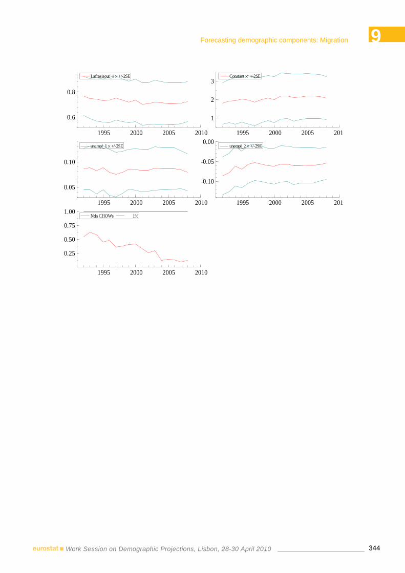
9 Forecasting demographic components: Migration
344Work Session on Demographic Projections, Lisbon, 28-30 April 2010
1995 2000 2005 2010
0.6
0.8
Lafrasiaout_1 × +/-2SE
1995 2000 2005 2010
1
2
3Constant × +/-2SE
1995 2000 2005 2010
0.05
0.10
unempl_1 × +/-2SE
1995 2000 2005 2010
-0.10
-0.05
0.00unempl_2 × +/-2SE
1995 2000 2005 2010
0.25
0.50
0.75
1.00Ndn CHOWs 1%

Small population and sub-national population projections Chair: João Peixoto
Session 10


10Small population and sub-national population projections
347Work Session on Demographic Projections, Lisbon, 28-30 April 2010
HOW TO DEAL WITH SUB-NATIONAL FORECASTS IN SPATIALLY VERY HETEROGENEOUS COUNTRIES? TOWARDS USING SOME SPATIAL THEORIES AND
MODELS
Branislav BLEHA1, Boris VAÑO2
Acknowledgements
The research has been realised within the grant No. 1/0255/08 - New features of spatial organization of social, economic and political phenomena in Slovakia after joining European Union, supported by Scientific Grant Agency (VEGA) of the Ministry of Education of Slovak Republic and Academy of Sciences.
1. Introductory comments
Our intention here is to comment on the position and significance of local and regional population forecasts. At a glimpse at the variety of practical regional forecasts and methodological studies focused on the forecasts it seems that they are in the shade of national forecasts. New methods are logically applied and verified mostly at national levels, too. Demographers and statisticians dealing with the forecasts tend to use the national level. Geographers preferring territorial aspects are rarely immersed in prognostic methods. Demographic (economic) method and methods of spatial research are seldom used jointly, although an efficient methodology for this field of research was well developed in the past. We can mention e. g. Rogers (1975, 1995), Rees (1983), Willekens – Drewe (1984), Rees – Convey (1984), Plane – Rogerson (1985) and others.
We refer to the latest two worksessions on population projections. During the Bucharest worksession in 2007, out of the multiple presentations only two or three were focused explicitly on lower-than-national territorial level. The current Lisbon worksession seems to pay more attention to sub-national forecasts (with a special session reserved for them), however, they will be covered by only a few papers. Thus, structure of papers presumably reflects the interest of demographers in particular topics.
Since the term „sub-national“ is probably too wide, we will strictly differ between regional and local forecasts. The local forecasts correspond to those of cities, municipalities or very small regions, while those projected for European NUTS II, III and IV units can be considered as regional ones, although in each country the size and population of the units might be considerably different.
Not only the authors of the forecasts (from scientific point of view), but also practical users (supreme decision making authorities such as central governments) are far more interested at the national level. Figures presenting EU population decrease by millions or tens of millions or increasing number of seniors by millions are crucial for central measurements and seem to be „frightening“ as presented by media. These are the reasons why the data projected for lower territorial units are in the shade of the national
1 Department of Human Geography and Demogeography, Faculty of Natural Sciences, Comenius University in Bratislava 2 Demographic Research Centre, Institute of Informatics and Statistics, Bratislava

10Small population and sub-national population projections
348Work Session on Demographic Projections, Lisbon, 28-30 April 2010
ones. The EUROSTAT have issued a regional forecast, too, however we dare to estimate that the national forecasts for individual countries are much more in centre of attention.
Thus, the public as well as prognosticators themselves pay less attention to subnational forecasts and it would be inaccurate to believe that they should attract as much attention as the national ones. On the other hand, we suppose that regional and local development will be gaining importance hand in hand with regional population change. Using Slovakia as an example we will briefly show how diverse can be the national societal development at both regional and local levels. This is not only the case of the Slovak Republic, one may find similar trends when comparing data on NUTS III regional units in the EUROSTAT forecast, variations of natural increase and predicted migration attractiveness are sometimes immense.
No doubt that a „healthy“ population development is a primary precondition for regional development. Vice versa, a low natality rate and emigration can indicate economic problems of the region.
Our intention is not to discuss comprehensively all aspects of relationship between demographic trends, human capital and regional development. In the paper we will focus on elementary research methods of demography, geography and related disciplines.
2. Some primary questions to be solved
In this part of the paper we will consider only forecasts by age and sex. Significance of derived forecasts is growing, sooner or later also the „beyond age and sex“ forecasts will become more relevant at the subnational territorial level. Nevertheless, categories of age and sex will stay in the centre of attention of local and regional authorities. In the following part we will discuss on the forecasts by age and sex. Primary questions to be solved before we start calibrating detailed parameters of the model are stated here, too.
2.1 What would be the most suitable territorial units? (delimitation of a reproductive system)
This seems to be a wide and complex issue. It is one of the input steps in the overall multi-step forecast process. Administrative and statistical units are not autonomous populations from the aspect of demographic reproduction, moreover, they are often socially and ethnically heterogeneous. These facts can potentially increase uncertainty of the forecasts. Migration openness and occurrence of stochastic elements are the other reasons for this uncertainty. Issues of other potentially exploitable units were discussed by Bleha (2007) concluding that absence of available data and a low consistency of these „scientific“ units in relationship with the official units would considerably lower the possibilities of their practical use. That is why demographers will have to settle for the official units being more suitable for practical utilisation in decision-making. In spite of that, a further search for „pure“ demographic territorial units should carry on. We can show an example. There are several NUTS IV regions in Slovakia, which might be divided into small homogeneous units based dominantly on their ethnic structure. The region as a whole shows a more or less zero population growth, while the smaller units within may display completely divergent population trends. There are multiple subregions in Slovakia with fertility of minority population exceeding the value of 5, thus the strength of this minority in the whole population will be increasing. Nonetheless, the recent data do not allow to make an accurate estimation on this.
We can also show an example of an intensive suburbanization processes having been well reported in multiple studies after 1989 (such as Spišiak – Kulla 2008, Slavík – Kurta 2009). The adjacent parts of the districts located in neighbourhood of the capital city of Bratislava partly form the city´s suburbanization zone, while remoter parts of the districts have not been hit by the intensive suburbanization inflow yet. In this case, we make a forecast for a territorial unit which is markedly heterogeneous considering the migration aspect. With the absence of sufficient data enabling us to gain data representing the whole

10Small population and sub-national population projections
349Work Session on Demographic Projections, Lisbon, 28-30 April 2010
region by combining the data on NUTS V units (bottom-up approach), one cannot avoid consequential defects.
2.2 Issue of appropriate method In one of the initial parts of the paper we mentioned some authors who had elaborated various methods of multi-regional forecasting, demographic accounting and others. We can also name other methods, such as Bayesian model utilization presented by Bijak (2007) and used it for estimation of international migration. It is inevitable to develop and verify these scientific methods. On the other hand, likewise in question 1, it is quite realistic to believe that the official regional forecasts will be continuously created by a conventional cohort-component method using age-specific net migration or possibly emigration rates. Apart from not always comparable character and extent of the data for member states, we should highlight the issue of overall arduousness of a regular forecast release for all EU regions realized by these methods.
Even if we stay realistic, resign and use the conventional methods, there is still a need to search for the best way how to increase the quality and credibility of both general and detailed assumptions. As shown by Keilman and Kučera (1991), a methodological progress is not always the only way. Czechoslovak forecasts reviewed by them were as precise as Dutch ones, despite of the fact that Dutch methods were more progressive. We really suppose that a quality forecast can be made only by considering as wide and multidisciplinary theoretical knowledge as possible. This is extremely important in case of the regional forecasts where spatial aspect must be respected.
3. General assumptions – the key problem
There is no doubt about the fact that the sources of errors in forecasts made for developed and stable European countries lie predominantly in inaccurate hypotheses. Inaccuracy of starting age structure can be sometimes the reason for errors, too, although because of the insufficient system of migration recording we can hardly find accurate population size estimations either for source territories or for target ones. Inaccuracy rate depends mostly on migration attractiveness of a region and vice versa. In case of Slovakia´s international migration, this was clearly shown by Divinský (2007). For example, any forecast made for the capital city of Bratislava will be biased by the missing population represented by those working and living in Austria. On the other hand, there are ten-thousands of residents of central and eastern Slovakia living and working long-term in Bratislava, yet being registered (so called permanent residence) elsewhere. And lastly, thousands of Bratislava´s residents have moved to the suburban zone of the city but they are still registered in the core city. The starting age structure (at both regional or local levels) is biased by a specific error, then. Let us pay attention to the general assumptions again. In accordance with the conclusions of previous chapter, we will operate with the cohort-component method. We will use some detections and outcomes of recent official regional forecast by Bleha and Vaňo (2008), having been published also as a scientific monograph including detailed comments on the assumptions. Although principally, the best way is to create assumptions individually for each region, yet we decided to use Ward´s cluster method to group the districts into clusters and then make forecasts for these clusters (we have identified different clusters for fertility, mortality and migration). Needless to say that we took the aspect of development (i. e. potential future stability of the clusters) into consideration, too (see Figure 1 of fertility clusters).
3.1 Fertility assumptions In scale of Slovakia as a whole, the fertility development will remain the key factor affecting the general population change trajectory. This is evidently a result of the fact that Slovakia´s population is now in the stage of realization of postponed childbirths related to a specific 1970s generation of women. Identification of the rate of the childbirths postponed to higher age at birth was one of the crucial issues enabling to outline the fertility assumptions. Thus, it was necessary to incorporate some estimations on the postponed childbirths and their relevance (or even their absolute dominance) in recent boost. If so, then corrections of the optimism rate on future population development will be necessary and time-

10Small population and sub-national population projections
350Work Session on Demographic Projections, Lisbon, 28-30 April 2010
modelling of future development will have to be done with expectations of a turbulent (non-linear) population growth for the entire projected time period.
The above stated lines represent only a very general vision of future development of fertility in the Slovak Republic. However, can we anticipate a uniform development line in all regions? We certainly cannot. Now, the main issue is to determine the individual fertility rate development trajectories for each region. Are the regions of Slovakia heading towards convergence? An answer to this question supported by scientific arguments is the clue to solve this problem. This is where various spatially oriented theories may apply.
All in all, a convergence is projected in the EUROSTAT´s convergence scenario, too. Can such general idea be applied to a subnational level, even in the highly heterogeneous territory of Slovakia?
To create assumptions for fertility development, we have delimited 7 clusters being not always spatially coherent, but this was not a precondition for the cluster analysis output. In spite of that, a certain degree of territorial autocorrelation has been confirmed. Identification of spatial autocorrelation (e. g. Getis – Ord 1996, Anselin 2003) and utilization of some other quantitative geographical methods represent one of the ways how to compile assumptions in a preliminary phase for subnational forecasts. They should be combined with demographic theories and regional development theories, mentioned below. For our purposes, we delimited 7 clusters, embracing groups of districts with more or less equal levels and structure of fertility, also respecting its development trends. Afterwards, using statistical indicators a decrease of variability in the 7 clusters was identified. During the recent 10 years, the variation range and standard deviation have been in decline, the clusters seem to converge. However, this cannot be used as a determining and cogent argument declaring that this tendency will persist in future.
Figure 1. Clusters of NUTS IV regions by fertility
Source: Bleha – Vaňo (2008)
Apart from the quantitative methods, we should consider the effect of particular fertility determinants. We suppose that ideological and cultural changes are becoming more and more decisive at the expense of economic determinants. We suppose that they will be spread diffusively. Although the relative role of economic determinants will be generally decreasing, their actual importance will be growing, in case of

10Small population and sub-national population projections
351Work Session on Demographic Projections, Lisbon, 28-30 April 2010
proceeding growth of regional differences. As proved by Korec (2005) and Džupinová et. al. (2008), regional disparities and spatial polarization of the territory of Slovakia were accelerated during the transformation period. This may act to the contrary with the above mentioned relative decrease of role of economic determinants. Unfortunately, Slovak demographers are not offered a satisfactory forecast on regional differentiation by regionalists, who have not concluded whether the regional differences will keep on growing, or if they are to decelerate or even decrease in future. Unluckily, this is one of the fundamental input determinants which should be used at least intuitively.
Let us give a short comment on the ideological and cultural changes again. Diffusion and developmental idealism in post-socialist countries has been considered and presumed in a theory released by Thornton – Philipov (2007). In our attempt to verify, if this kind of diffusion has ever been present in the territory of Slovakia, we can use an indirect evidence, but still a supportive one. Figure 2 shows a diffusion of natural decrease as a virtual continuous phenomenon expressed by isochrons. In this case, the isochron is a line displaying the year with the first record of natural decrease in the relevant region.
Figure 2 displays location of primary cores of reproduction changes resulting in natural decrease and the way these changes were successively spread further from highly urbanized areas (mostly in western part of the country) towards the more conservative and less secularized north and east, or from non-Catholic (Calvinist especially) territories with traditionally lower fertility rate, respectively. Similar territorial pattern would be observed in case of other phenomena, such as total fertility rate, mean age at birth, etc.
This clearly supports our hypothesis that the timing and intensity of fertility in the lagging and pioneer regions (mainly Bratislava) will be more similar in future, though some differences will remain visible. We suppose that in Slovakia as well as other transforming post-socialist countries a gradual weakening of religious and similar cultural determinants affecting fertility will appear. For example, Orava – a traditionally conservative region in northern Slovakia with above-average TFR – did not answer to the transformation-related changes after 1989, there was almost no postponement recorded but it is highly visible today. In other words, Orava and some parts of eastern Slovakia only recently witness the postponement of first births and births, but also higher parity ratios decreasing. It seems that following the patterns of more developed regions is happening but the conservative regions need their role models – something like „driving“ regions.
Figure 2. Spatial spread of natural decrease using isochrons
Note: The isolines depict the first year the surplus of deaths occurred Source: originally published in Mládek - Bleha (2001)

10Small population and sub-national population projections
352Work Session on Demographic Projections, Lisbon, 28-30 April 2010
Results are shown in Figure 3. A thorough cohort analysis finally led to modelling of the timing of transversal fertility in the individual clusters. Also a recent analysis demonstrated that the spatial spread visible in geographical space would be roughly indicated by curves, too. Populations of conservative clusters of districts are represented by curves that appeared 20 or 30 years ago in the urbanized areas. Timing of the pioneer regions can partly serve as a pattern for modelling of timing of conservative regions.
Figure 3. Fertility timing in clusters in 2025
0.00
0.01
0.02
0.03
0.04
0.05
0.06
0.07
0.08
0.09
0.10
0.11
0.12
0.13
0.14
0.15
15 17 19 21 23 25 27 29 31 33 35 37 39 41 43 45 47 49
SVK 2025 Cluster 1 Cluster 2 Cluster 3Cluster 4 Cluster 5 Cluster 6 Cluster 7
;
Source: Bleha – Vaňo (2008)
Concluding the debate on fertility we would like to mention two mutually related sources of uncertainty. The first of them is represented by a scarcely assessable long-term development of supportive measurements in the field of population and family policies which might affect the fertility in future. For example, a one-off paid family allowance for higher-parity-ratios children can preserve a state of higher fertility rate for these ratios, or lower the mean age at birth in some regions, being extremely low anyway.
Population surveys could perhaps be very helpful for the regional overview of fertility and its prediction. These surveys would cover also spatial aspect. A question of ideal or intended number of children is also very important. In Europe, this issue is often a matter of research (for example, see Thomson 1997, Testa – Grilli 2004). It would be very interesting to map the differences between the desired and realized number of children in families in various regions of country, it is not clear whether there would be any differences at all or at least in comparison between highly urbanized and traditional regions (Bratislava vs Northern Slovakia, etc.). We can only assume that the contrasts between wanted and realized numbers of children would be higher in „poor“ traditional territories due to economic situation. Or is the power of tradition the decisive factor? Without a detailed research, it is difficult to conclude. Our contemplation might serve as a demontration of this factor´s importance and encourage to realize this kind of research.
The second source of uncertainty is related to the phenomenon of Romany population and its fertility rate. As suggested by Šprocha (2009), in selected segregated Romany settlements average TFR (1994-2004) reached nearly 5. According to our estimation, in some regions of eastern Slovakia, these births accounts for approximately half of all children to be born in region. Development of fertility of this ethnic group is difficult to predict, moreover, the statistics on the Roma population and its structure are not reliable.

10Small population and sub-national population projections
353Work Session on Demographic Projections, Lisbon, 28-30 April 2010
3.2 Mortality assumptions Due to limited extent of the paper, we can touch upon the issue of mortality only briefly. Generally, mortality development results from parallel operation of two groups of determinants: exogenous and endogenous factors (Casselli – Vallin – Wunsch 2006). In principle, the endogenous factors are fixed, they act spontaneously and do not fluctuate in time. Shifts in mortality course are mostly caused by exogenous factors that can be (unlike the former ones) easily suggestible and thus enable us to control the mortality processes directly. The map of life expectancy in districts of Slovakia indicates a mosaic territorial pattern and it is difficult to give a simple explanation of it, since it is a result of multiple factors. This forced us to use also extrapolation methods and naturally, we discussed the issue of causes of death with medical doctors. Although potential errors in the mortality prediction do not affect excessively the national level of forecasts, they can act so at the sub-national level. Nevertheless, we are quite sure that the mortality rate will be in decline within a long-term time-horizon in all transition societies of central Europe and that no isolated poles of life expectancy decrease will appear in these countries. We can add that the accuracy of specific mortality estimation will probably become more decisive, with respect to the intensive and unavoidable population ageing of the transition territories in transitional countries.
3.3 Migration assumptions As indicated above using example of suburbanization, the trends of intra-regional migration are not immanently included as a determinant, in spite of the fact that these processes contribute to redistribution of population, especially if we consider population flows between rural space and urban cores within a district (region). This kind of migration flow influences indirectly the inter-regional migration, too. We can mention a diffusion of suburbanization processes across the urban hinterland as an example.
Depopulation in some regions of southern and eastern Slovakia can be perceived as a certain “anti-pole” of the suburbanization processes in this scale. This problem afflicts also territories with scattered settlement, which is primarily a result of emigration from these areas. Petrovič (2007) observes that some qualitative and quantitative changes indicate gradual dying-out of these territories. Deducing from available statistical data, the same processes appear in some peripheral regions in transitive societies. In Slovakia, we will probably witness extinction of some rural communities as a result of demographic development for the first time in history. This must be respected in the process of hypotheses creation for regions where these depopulation processes have been detected. First, the general assumption for migration development should be solved.
The analysis of all geographical factors must be very comprehensive. We would highlight the macro-position factor above all. Korec (2005) supposes that this determinant is the key one responsible for west-east polarization of the country. Western Slovakia benefits from its position bordering on the „old“ EU. We have already mentioned a certain diffusion of reproductive behaviour from the west towards the east. Recent migration trends show a reverse east-west gradient. This indicates that net migration flows are heading from the east to the west, albeit the migration effectiveness is not too high. This clearly copies Korec´s division of Slovakia into a „wealthy“ south-west and a „poor“ north-east. This fact supports the macro-economic neo-classical theory which seems to be applicable on the transitive societies. At the same time, the Slovak population mobility (as far as labour migration is concerned) can be considered as below-average, if compared to the Czech Republic, for example.
The above mentioned fact is closely related to regional development perceived in the aspect of spatial polarization – being a very frequent topic of geographical, sociological and economic studies (see for example Woodward 1995, Badcock 1997 and some others). If we agree with recent studies on regional development based on the theory of polarization in Slovakia (Gajdoš – Pašiak 2006, Halás 2008), we might assume the impact of this regional polarization on future migration trends and vice versa. Migration as a manifestation of polarization can even deepen the polarization trends (by migration of young and qualified population towards the growth poles). Research of migration and polarization from hierarchical point of view deserves a particular attention. Two facts are decisive here. According to our analysis of empirical data on migration registration, it seems that at sub-national level smaller districts with smaller nodal centres in central and eastern Slovakia are losing residents while the nearest big district and regional urban centres prove population gains, although there are many exceptions.

10Small population and sub-national population projections
354Work Session on Demographic Projections, Lisbon, 28-30 April 2010
For migration trends, the following two dichotomous polarizations are crucial: a) west-east (north-west – south-east) polarization, and b) peripheral mezo-regions – cores of these regions (centres of regions with over 50,000 residents and their broad hinterland).
The major cities (in Slovakia covered principally by centres of regions and cities over 50,000 inhabitants) should gain population from their broad nodal regions, even from neighbouring districts with smaller nodal centres. The net volumes of these migration flows are probably low, but they can still significantly affect the net migration of the big regional centres (and their districts). On the other hand, the residential suburbanization and deconcentration (outward migration) will probably decrease the effectiveness of the centripetal migration. A serious forecast at sub-national territorial level for the system of nodal or administrative regions will require finding answers to the following questions: will the volume of inner migration be increasing or decreasing? which regions of the country will be affected by migration effectiveness change? These questions have to be answered by regionalists dealing with the increasing social and macro-economic spatial disparities.
Therefore, a serious cross-impact analysis of various system-related geographical factors and theories is inevitable for calibration of any type of forecast model (multiregional, classic models, etc.). In this chapter, we could not present our premises comprehensively, we have only tried to outline the determinants that demographers should take into consideration. We dare to claim that the migration assumptions should not be realized by experts from one or two scientific disciplines only, as this field of research is considerably multidisciplinary.
4. Spatial convergence – assumptions vs results
Decision makers sometimes ask us whether the regional differences in demographic development within a country will be growing or decreasing. Apart from expected uncertainty of any regional prediction, the answer to this question must be presented as following. Our estimations show that a certain confluence (divergence) of reproductive behaviour will be observed sooner or later. Extreme migration gains or decreases will not be frequent. But, the age structure of regional populations varies a lot. Lowering disparities between calibrated parameters will not necessarily result in low disparities between results. This fact has been analysed using the model forecasts. In Table 1, some modelling scenarios are presented. These are based on our not real conditioned presumptions, therefore we cannot introduce them as real forecasts (we prefer distinguishing between „forecast“ and „projection“). Four scenarios are related to fertility, the last one associates with migration. For every scenario, mortality is considered the same as in medium scenario of original forecast. Immediately, we can observe that our expectations have been confirmed. Respecting the age-structural momentum, these model presumptions do not stand for any significant change of results as far as spatial differentiation is concerned. After doing calculations, we made an evaluation of the following four values: number of births, population size, ageing index and mean age of population.

10Small population and sub-national population projections
355Work Session on Demographic Projections, Lisbon, 28-30 April 2010
Table 1. Projection scenarios
Fertility – development until 2025 Mortality until 2025 Migration until 2025
projection I fixed 2007 value likewise in medium
scenario likewise in medium scenario
projection II
the TFR increase higher (by 30%) than in medium scenario
likewise in medium scenario
likewise in medium scenario
projection III
differentiation growth – significant differences in TFR
likewise in medium scenario
likewise in medium scenario
projection IV
homogenization – the fertility rate in all districts equal to the one stated in national forecast
likewise in medium scenario
likewise in medium scenario
projection V likewise in medium scenario likewise in medium
scenario no migration
Source: Own assumptions
If we use the fixed 2007 fertility level, the number of births in 2007 - 2025 would decline by 30 per cent (average decline within group of all NUTS-IV regions calculated by geometric mean), while the original forecast estimated the decline by 10 per cent only. The variation coefficient of the total number of births in the group would reach up to 585.9 (549 in the original forecast and 553 in 2007). Fixating the recent character and level of fertility would mean a sharper decrease of number of births, but also a (moderate) increase of variability of values.
If a rapid growth of TFR is detected (scenario II), the number of births would be higher than in 2007, with its decrease only in case of urban districts of Bratislava and Košice characterised by extremely unbalanced age structured. On the other hand, the number of births would turn higher in districts with high percentage of children who would reach reproduction age in the forthcoming years. Variability of number of births would stay more or less the same as in the original forecast.
Scenario III represents bigger differences among TFR values, that means increasing changes in reproductive behaviour across regions. An extreme growth of variability of births will not occur, though. The variation coefficient would be as high as 595. This fact indicates, that most of the future variability can be explained by the age-structural momentum effect. According to scenario IV, all regional populations would record identical values of fertility. In spite of this, the variation coefficient of number of births would drop down to 541, which is almost equal to the national forecast value (549). Scenario V deals with migration only, its relevance for the number of births should be marginal. Nevertheless, its effects are remarkable, as we can demonstrate on the example of districts that are considerably formed by principal suburbia. Number of births in the districts of Senec (in the hinterland of the city of Bratislava) would decrease (in comparison with the original forecast) only by 4 per cent till 2025. However, if there is no migration surplus (scenario V), the number of births would decrease by 30 per cent in the 2007-2025 period. Neither an extreme fertility growth (according to scenario II) would be sufficient to compensate the modelled loss of reproductive cohort within the suburban migration.
Similarly, we have made an appraisal of demographic ageing. If we fixed the current lowest-low-fertility values, the average ageing index would grow 1.86 times instead of 1.6 times. However, if we took scenario II (high TFR growth) into consideration, the ageing index would increase 1.35 times on average. These differences seem to be quite significant, neither the unrealistic high fertility growth at sub-national level would not stop the ageing process. Respecting the ageing index sensitivity, we decided to use mean age of population for verification purposes. This procedure has confirmed that the mean age oscillates less. Relevant model „interventions“ are necessary in order to change the indicator significantly. While in accordance with scenario II, the mean age would increase by 8.8 per cent on average, it would grow by 13.3 per cent within scenario I.

10Small population and sub-national population projections
356Work Session on Demographic Projections, Lisbon, 28-30 April 2010
5. Conclusion
Although sub-national forecasts are not as frequently discussed in Europe as the national ones, we can expect that their relevance is high and will be growing in future. Regional demographic differences are too high, we can illustrate them by referring to maps of the total population growth of particular regions of Germany, Italy or Slovakia.
In our opinion, elaboration of a quality sub-national population forecast with a high feasibility is an extraordinarily ambitious process from methodological point of view. In the paper we are trying to give arguments that improvement of methods is not the only way, and perfect methods should be combined with determinants of high quality, respectively. To assemble excellent determinants of fertility, mortality and migration trends, one must make use of many more pieces of information and a lot of partial analyses. Demographer cannot do without spatial sciences, mostly geography and regional analysis. A harmonization of „pure“ demography and geographical approach can be a suitable prerequisite for a feasible sub-national forecast. That is why we are trying to imply what should the input analyses be focused on, which spatial theories and methods should be utilized, mainly when considering determinants of fertility and migration. Although we have applied the case of Slovakia, we are absolutely certain that our approach (perhaps with small modifications) can be applied to other transitive societies, with similar processes of polarization, suburbanization, selective growth of regional disparities, etc.
In the final part of the paper, using the model calculations we have tried to point at the fact that most of future differences between individual NUTS IV regions of Slovakia stem from the recent significant disparities in age structure. A total homogenization (identical fertilities applied) would deliver only a mild decrease of variability of the number of births and other demographic events, and the variability would be even lower in case of ageing indicators.
Reference
BIJAK, J. (2007).Bayesian model selection in forecasting international migration: Simple time series models and their extensions. Work session on demographic projections, Eurostat, Methodologies and working papers, pp. 309-318.
BLEHA, B. (2007). Conception of spatial units appropriate for regional popualtion forecasts. Work session on demographic projections, Eurostat, Methodologies and working papers, pp. 319-326.
BLEHA, B., VAŇO, B. (2008). Population development in Slovak districts until 2025. Convergence or divergence?, Infostat, Bratislava. 82 p. (originally in Slovak)
CASELLI, G., VALLIN, J., WUNSCH, G. (2006). Demography: Analysis and Synthesis. Elsevier, London.
DIVINSKÝ, B. (2007). Labor market – migration nexus in Slovakia: time to act in a comprehensive way, IOM, Bratislava, 229 p.
DŽUPINOVÁ, E., et. al. (2008). Peripheriality a spatial polarisation in Slovakia, Geografika, Bratislava. 186 p.
GAJDOŠ, P. – PAŠIAK, J. (2006). Regionálny rozvoj Slovenska z pohľadu priestorovej sociológie. Sociologický ústav SAV, 320 s. (originally in Slovak)
GETIS, A., ORD, J.K. (1996). Local spatial statistics: an overview. In: Longley, P., Batty, M. (eds.) Spatial analysis: Modelling in a GIS enviroment, Cambridge, pp. 261-227.
HALÁS, M. (2008). The spatial polarisation of society with a detailed review of peripheral region of Slovakia. Czech sociological review, Vol. 44, No. 2., pp. 349-369.

10Small population and sub-national population projections
357Work Session on Demographic Projections, Lisbon, 28-30 April 2010
KEILMAN, N., KUČERA, T. (1991). The impact of methodology on accuracy of population forecasts. Evidence from the Netherlands and Czechoslovakia. Journal of Forecasting 10. pp. 371-398.
KOREC, P. (2005). Regional development in Slovakia during 1989-2004. Geografika, Bratislava, 228 p. (originally in Slovak)
MLÁDEK, J., BLEHA, B. (2001). Spatial spread of natural decrease in Slovakia. Slovak demographic conference, Rajecké Teplice. (originally in Slovak)
PETROVIČ, F. (2007). Prognóza krajiny s rozptýlením osídlením. In: Kraft, S., Mičková, K., Rypl, J. - Švec, P. - Vančura, M. (eds.): Česká geografie v europském prostoru. PF Jihočeská univerzita v Českých Budějovicích, s. 474-480.
PLANE, D.A., ROGERSON, P.A. (1985). Economic-demographic models for forecasting interregional migration. Enviroment and Planning, A 17, pp. 185-198.
REES, P.H.(1983). Multiregional mathematical demography. themes and issues. Enviroment and Planning No.15. pp. 1571-1583.
REES P. H., CONVEY, A. (1984) Spatial population accounting. In: Clarke, J. (ed.) Geography and population: approaches and applications. Pergamon Press, Oxford. pp.51-59.
ROGERS, A. (1975). Introduction to Multiregional Mathematical Demography. John Wiley and s. (interscience publications).
ROGERS, A. (1995). Multiregional Demography. Principles, Methods and Extensions. John Wiley and Sons. New York.
SLAVÍK, V., KURTA, T. (2009). Selected manifestations of suburbanization in the hinterland of Bratislava, In: Global changes: Their regional and local aspects, Ed. Wilk, W., University of Warsaw.
SPIŠIAK, P., KULLA, M. (2008). Suburbanization in the Košice hinterland, Masaryk University, Brno, In. Svatoňová, H. et. al. Geography in Czechia and Slovakia, pp. 370-374.
ŠPROCHA, B., PUKAČOVÁ, J. (2009). Specifics of Roma population in Slovakia, pp. 166-186. In: Bleha, B. (ed.) Population development in Slovakia at the milleniums breakthrough: Continuum or the new era?, Bratislava, Geografika. 336 p. (originally in Slovak)
TESTA, M.R., GRILLI, L. (2004). The effects of Childbearing Regional Contexts on Ideal Family Size in Europe: A Multilevel Analysis, European Demographic Research Papers, Vol. 4, 46 p.
THOMSON, E. (1997). Couple Childbearing Desires, Intensions and Births, Demography, Vol. 34, pp. 343-354.
THORTNON, A. – PHILIPOV, D. (2007). Developmental Idealism and Family and Demographic Change in Central and Eastern Europe. European Demographic Research Papers, Vol. 3., 85 p.
WILLEKENS, F.J., DREWE, P. (1984). A multiregional model for regional demographic projection. In: Demographic research and spatial policy, eds.Willekens, F.J. ,Heide, T.H. Academic press.
WOODWARD, R. (1995). Approaches towards the study of social polarization in the UK. Progress in Human Geography, Vol. 19, pp. 75-89.


10Small population and sub-national population projections
359Work Session on Demographic Projections, Lisbon, 28-30 April 2010
THE PROBLEMATIC OF POPULATION PROJECTIONS IN SMALL ISLAND STATES: THE CASE OF
CAPE VERDE
Pedro BRITO1, Teresa RODRIGUES2
Abstract
Population projections are a complex exercise, as they depend on a huge number of socio-demographic variables, whose reliability and trend need to be focused. Data analysis becomes increasingly complex as the size of the population projected decreases. The case of Cape Verde is no exception to this rule, since it is a micro-island state with less than half a million inhabitants, where projection’s exercise requires some finesse, especially given the rapid and consistent changes in collective behaviours. Those changes explain some disagreements between existing and new projection exercises on population volumes and age structure. Besides being a small state, Cape Verde is divided in 10 islands and 22 municipalities, which makes demographic projections even more complex, since it has to take into account the regional diversity and readapt the options made in general terms. We can even doubt on some of the final results reliability and on the validity of some demographic and social indicators, and avoid falling into over or under projections.
We intend to discuss possible alternative methods of performing population projections in micro the political realities with relevant internal diversity, taking Cape Verde as a case study. We will include a critical analysis of the results obtained and make some aggregation tests for the 10 islands, according to their convergence or divergence behaviour patterns (both natural and migratory). We use some of the results obtained by the Principal Author3 in his dissertation, presented and approved in 2003 by ISEGI - UNL, as a partial requirement for obtaining a Master degree. This research projected hypothetical “scenarios” of Cape Verde’s population evolution on the horizon 2025, based on the Census of 2000 and on demographic behaviours and its trend from the 1990s. For this exercise we rely on the method of components (Cohort Survival), which incorporates information on mortality, fertility and migration recent trends, and follows the effectives cohorts by age (5 x 5) and sex. In subsidiary terms we used mathematical methods and ratio. The first one considers the average annual growth rate recorded in the 90’s to project population volume by 2025; the second estimates the same population based on the weight it had in 1990 and in 2000, compared to the population of ECOWAS.
Keys Words: Demographic Projections; Fertility, Birth, Mortality, Migration
1 Student of PhD in Management Information Systems Specific Demographic Information on ISEGI (Instituto Superior de
Estatística e Gestão de Informação) – Universidade Nova de Lisboa 2 PHD in Contemporary History (Demography). Guest Teacher at ISEGI (Instituto Superior de Estatística e Gestãode
Informação) - Universidade Nova de Lisboa, where she is responsible for the scientific area of Demography. 3 Chief of Studies and Planning of the Ministry of Education and Sport in Cape Verde and member of the National Statistics
Council

10Small population and sub-national population projections
360Work Session on Demographic Projections, Lisbon, 28-30 April 2010
1. Introduction
Population projections are a complex exercise, as they depend on a huge number of socio-demographic variables, whose reliability and trend need to be focused. Data analysis becomes increasingly complex as the size of the population projected decreases. The case of Cape Verde is no exception to this rule, since it is a micro-island state with less than half a million inhabitants, where projection’s exercise requires some finesse, especially given the rapid and consistent changes in collective behaviours. Those changes explain some disagreements between results presented by existing and new demographic projections on population volumes and age structure. Besides being a small state, Cape Verde is divided in 10 islands and 22 municipalities, which makes the current exercise even more complex, since it has to take into account the regional diversity and readapt locally the options made in general terms. We can even doubt on some of the final results reliability and on the validity of some demographic and social indicators, and avoid falling into over or under projections.
Cape Verde is an insular Country, located in the Atlantic Ocean in the West African coast, between latitude 17° 12' 15'' and 14º 48' 00'' North latitude and the meridian 22º 39' 20'' and 25 º 20’ 00’’ West longitudes. It stands at approximately 455 km from the cable with the same name, located in Senegal. It is composed by ten islands and several islets and is geographically divided into two groups (Barlavento and Sotavento).
From the demographic point of view, Cape Verde is characterized by an extremely young population: 42% are under 15 years and 54% are under 20 years. According to the latest available information4 crude birth rate stands at 29.5 ‰, mortality rate at 6.4 ‰, infant mortality rate (IMR) at 33.3 ‰, general fertility rate is 123.3 ‰, mean age at procreation is 29 years, synthetic index of fertility is 4.0 children per woman and average life expectancy reaches 71 years. If this trend continues, we will have over the next year’s still very significant demographic growth, especially in major urban centers.
In this article we will present the main results of our projection exercise of Cape Verdean population until 2025. We start with a critical overview on the official results and some tests of aggregation of its islands, according to the convergence / divergence patterns of behavior (natural and migration). We wish to discuss possible alternative methods of performing population projections in micro political universes, yet with great internal diversity, taking Cape Verde as a case study.
1.1 Population projections: the case of Cape Verde Population projections aim to estimate what will be a given population after a certain period of years, by applying a set of methods that reflect some of the assumptions previously made. However, there seems to exist some confusion in the use of the terms projection, perspective, prevision or estimation. According to Pressat’s Dictionary of Demography (Pressat, 1979), the concept Prevision must be seen as "a determination of the future evolution of a population [...]". Prospects are divided into projections or forecasts, according to the objective one wants to achieve. A projection is a "perspective of the population in which, generally, there is the idea of prediction”, while a forecast is a" demographic perspective, due to the formulation of hypotheses, is presented as having predictive value”5.
Other authors, as Veron (1991)6, prefer forecasts and prospects to projections, reserving the term prospects of an previous projection, as a prospective "... define possible situations and emphasizes the means to an end, which is considered the most desirable”. According to the most common uses of the terms set out here they consider that population projections must be either a Forecast or a Prevision. They assume predictions whenever one wishes to determine the various dimensions of a population with the intention of "hitting", and predict when referring to how will be the future reality based on
4 INE-CV, 2000 5 J. Vinuesa et al, op. Cit. p. 237-38 6 Ibidem

10Small population and sub-national population projections
361Work Session on Demographic Projections, Lisbon, 28-30 April 2010
assumptions that are considered most probable. One refers to prospects when the projections were only trying to create scenarios, with the idea of showing how it would be the demographic reality, if certain assumptions will be gathered.
The advantages of predicting the evolution of a given population in dynamic terms for a certain period justifies projections exercise. In general, the starting year coincide with the last year census, in this case with the Recenseamento Geral da População e Habitação 2000. Resident population is 431,989 inhabitants.
This prospective exercise had into account the behavior of micro-demographic variables (mortality and fertility) since 1970. Changes occurred on fertility behaviors were considered to be of major importance in our investigation, as they shown a significant decline over time. In Table 1 we present its past performance based on information available in the Census and fertility surveys conducted in Cape Verde:
Table 1. Evolution of Fertility Rate in Cape Verde (1970 - 2000)
Age Group 1970 1980* 1990 200015 - 19 55,23 68,06 105,08 93,1920 - 24 288,71 238,07 248,44 186,8625 - 29 367,16 300,07 262,05 172,4430 - 34 317,95 274,41 234,92 148,3635 - 39 281,02 234,47 165,44 115,6740 - 44 145,97 13,49 80,66 63,1045 - 49 40,71 24,84 32,00 24,81
General Fertility Rate 201,96 // 185,43 123,30Synthetic Fertility Rate 7,49 6,32 5,64 4,00Gross Reproduction 3,69 3,11 2,78 2,00Average age of procreation 31,10 30,80 29,60 29,30
Source: Instituto Nacional de Estatística de Cabo Verde (INECV), 1970, 1980, 1990 e 2000
Fertility rates decreased significantly from 1960 to 2000: Total Fertility Rate (TFR) dropped from 185 ‰ to 123 ‰. In 1990 the average number of children per woman was about 6 (5.6); in 10 years it felt to 4. Fertility model also changed (Graph 1)
Graph 1. Cape Verde’s Fertility Rate (1970-2005)
Source: Instituto Nacional de Estatística de Cabo Verde (INECV)

10Small population and sub-national population projections
362Work Session on Demographic Projections, Lisbon, 28-30 April 2010
Global mortality rates witnessed similar descending trend, while life expectancy at birth increases. We assumed it will continue to decline during the projection’s horizon, although mortality has already reached low rates and the level of life expectancy is relatively high in African context. According to Statistics General Directorate (1980), Infant Mortality Rate (IMR) also declined from 132.9 ‰ in 1970 to 62.9 ‰ in 1980, wish means a reduction by half in only 10 years. This indicator has fallen from 65 ‰ in 1990 (according to Human Development Report, PNUD-2001), to 31-33 ‰ in 2000 (Census 2000 data corrected with marital status). Gross Mortality Rate (GMR) also suffered a significant reduction, from 9.2 ‰ in 1990 to 6.4 ‰ in 2000 (Census 2000). Life expectancy at Birth experienced gradual increases over time: in 1970 it stood at 54.7 years for men and 56.1 years for women; in 1980 59.1 years for men and 60.6 for women; in 1990 65.7 years for men and 71.3 for women7, and in 2000 for both sexes was 71.2 years (67.1 for men and 74,8 for women).
Migration demographic phenomena are more difficult to observe as they are simultaneously a demographic phenomenon that interferes with the dynamics of population growth and also an inherently social phenomenon. Nevertheless they represent a phenomenon of major importance for Cape Verdean population projection estimates.
Cape Verde is a country historically characterized by high migration levels, linked to its characteristic demographic distribution. As a major characteristic we underline its strong flow of migrants, especially to the United States and Europe and, on a smaller scale, to other African countries. The study of this movement is difficult as most immigration is not still controlled, which means that statistics quality is far from being reliable.
The international migration context makes it also hard to choose the best hypotheses about their possible developments. However, given its tradition as a country of emigration, one can assume that net migration will continue to be negative in the near future (Table 2).
Table 2. Net migration evolution in Cape Verde (1990 - 2000)
Decade 1960 - 70 1970 - 80 1980 - 90 1990 - 2000Balance -14394 -48653 -22651 14360
Source: Instituto Nacional de Estatística de Cabo Verde (INECV)
However, this negative balance tends to improve, due to an expected decrease in migrations net flow, based on the following assumptions: 1) probable reduction of quotas in host countries; 2) improvement in internal economic situation, which can attract both nationals who are in the Diaspora process and foreigners.
1.2 Methods of construction The analysis of micro-demographic variables is the basis for the projection of the segments of birth, mortality and migration and for it we used a Lexis Diagram. To build this diagram we used Princeton’s New Mortality tables for mortality, as well as real Infant Mortality Rate and estimated Life Expectancy at Birth, which will allow us to determine what level you must consider for the different years. For fertility, estimations on birth annual volumes were processed. Finally, we added migration’s possible total and age structure. Using the method of components, we defined two scenarios for the evolution of the Cape Verde’s population by sex and age until 2025:
- Scenario I: Heavy Natural Trend Scenario, which results from the projection of the segments of mortality and fertility / fecundity, in the context of no migration.
7 Mady, Biaye, ,p.36

10Small population and sub-national population projections
363Work Session on Demographic Projections, Lisbon, 28-30 April 2010
- Scenario II: Alternative Scenario, which results from the correction of the natural scenario with net migration plausible volumes.
Finally we present the results for both scenarios and confront them with the results of projections exercise made by Instituto Nacional de Estatística de Cabo Verde, based on the results of the last Census of 2000.
To perform population projections by sex and age presented in this paper we used the so-called method of components, which includes information on trends in mortality, fertility and migration The horizon of the projection comprises an 25 years interval, i.e. from 2000 to 2025. In this method, the demographic variables interact, following the cohorts of people over time, according to their exposition to fertility, mortality and migration laws. Therefore it is necessary to produce estimates and projections of the levels and patterns of each of these components. To project population volumes we rely on the equation of agreement, also known as the equation of equilibrium or balance population, whose analytical expression is:
P (x + n) = P (x) + N (x, x + n) - O (x, x + n) + I (x, x + n) - E (x, x + n), where:
P (x + n) = population in year x + n, P (x) = population in year x, N (x, x + n) = births in the period x, x + n, O (x, x + n) = deaths in the period x, x + n, I (x, x + n) = immigrants in the period x, x + n, E (x, x + n) = emigrants in the period x, x + n, x = time of initial deployment and n = projected range.
In addition to the method of components, we used mathematical methods and the ratio. Mathematical method uses the average annual growth rate recorded in the 90 to project population until 2025, without any concern with possible changes in micro-demographic variables (fertility, mortality and migration). The ratio method uses population estimates as well, based on the relative weight they had in 1990 and 2000, respectively, in relation to the host region, in this case Economic Community West African Stats (ECOWAS).
2. Scenarios
2.1 Natural Trend Scenario (Base) This scenario is a simulation of possible processes of evolution of a given population of a region or a country in a given period, by age and sex. It starts from the actual situation, taking into account assumptions made on the likely pace and nature of this process. It is, therefore, a method to project. However, a few requirements are necessary, such as knowing local history, in order to verify the trend of the behavior of these phenomena (Table 3).
Table 3. Evolution on some major demographic events in Cape Verde (1991-2000)
1991 1992 1993 1994 1995 1996 1997 1998 1999 2000Birth 13075 13303 10658 11112 11051 12472 11313 10557 9623 12746Deaths 2616 2870 2858 2786 3520 2715 3047 2811 2812 2786Deathhs under 1 year 437 738 745 636 651 516 611 442 420 334Child Mortality Rate (Classic) 33 55 70 57 59 41 54 42 44 26
YearsIndicators
Source: INECV, Estatísticas Demográficas de Estado Civil, 1991-1999 e RGPH 2000

10Small population and sub-national population projections
364Work Session on Demographic Projections, Lisbon, 28-30 April 2010
As mentioned, to project mortality segment from 2000 to 2025 we used standardized Princeton’s Mortality Tables. Based on official information we formulated 3 hypotheses for the projection (Table 4):
Table 4. Hypotheses based at Princeton’s Mortality Tables
2000-05 2005-10 2010-15 2015-20 2020-2521W 21W 21W 22W 22W
2000-05 2005-10 2010-15 2015-20 2020-2521W 21W 22W 22W 23W
2000-05 2005-10 2010-15 2015-20 2020-2521W 22W 22W 23W 24WH ip .3
H ip .1
H ip .2
Source: INECV, Author’s own assumptions
Given infant mortality levels (33.3 ‰) and average life expectancy at birth (71.24 years) in Cape Verde for both sexes in 2000 we considered the hypotheses 2 to project country's population, which at present seemed to be the most probable hypothesis for the next 25 years. According to those parameters, a country or a region with an IMR of 31.38 ‰ and a life expectancy at birth of 70 years and an IMR of 41.60 ‰ and 68.01 years of life expectancy at birth for males stands at the Model West, level 21. We begin with an assumption that given the current conditions of mortality and in accordance with the already mentioned descending trend there will be a steady decline in mortality, mainly in infant case, accompanied by a gradual increase in life expectancy. Therefore, if current conditions in Cape Verde are maintained, the country will reach level 23 by 2025. It can easily present an IMR of 15.33‰ and an average life expectancy at birth of 75 and 70.96 years for women and men. This is the most likely hypothesis, although we are aware that Cape Verde is a very vulnerable country in economic terms.
This fact can influence either positive or negatively demographic dynamics. Given the evolution of the general fertility rate we formulated a hypothesis of evolution of fertility and consequently of total birth volumes (Table 5).
Table 5. Fertility hypothetical Model
Modelo Hipotetico 123,3 99,0 75,0 61,0 40,0 40,0
2000 2005 2010 2015 2020 2025
0,111 0,087 0,068 0,051 0,040 Source: Author’s own assumptions
The projection of births using this method follows the assumption that in 2000 Total Fertility Rate in Cape Verde was 123.3 ‰, standing at an average of 111 ‰ in 2000-05 and decreasing gradually to a minimum limit of 40 infants per thousand women at childbearing age (aged 15-49 years) from 2020 to 2025. According to TFR (average value) and the number of women of childbearing age, we projected birth volume (Table 6).
Table 6. Birth projections 2000-2025
1990-2000 2000-05 2005-2010 2010-2015 2015-202 2020-2025Male 34694 32711 30399 26510 21356 18286Female 33070 31177 28974 25267 20355 17429Total 67764 63888 59373 51777 41711 35715
Years
Source: INECV, Author’s own assumptions

10Small population and sub-national population projections
365Work Session on Demographic Projections, Lisbon, 28-30 April 2010
As seen from the previous table, births tend to decrease over the years at an average annual rate of - 2.5%.
2.2 Alternative Scenario Migratory movements are phenomena difficult to analyze, as they are both a demographic variable which interferes with the dynamics of population growth, and also an inherently social phenomenon. Cape Verde is a country characterized by high emigration volumes over the centuries due to its insular character.
The information related to migration appears either in demographic statistics and census. However, the data on this micro-demographic variable is presented with little diversity of information and low quality standards. For this reason we analyzed thoughtfully net migration provided by the Statistic National Institute of Cape Verde in the 1990s and concentrated in the last 5 years.
As it can be seen in the Table 2 the negative Migratory Sold (MS) improved rapidly over the years, which means that each year the emigration decreases in Cape Verde. After the calculation of annual average growth migration rate between 1990-2000, 1990-1995 and 1995-2000, we considered some assumptions about the population development, used as preconditions for the construction of alternative scenarios. We considered three hypothetical migration evolutions from 2000 to 2025:
H 1: a Negative Scenario taking into account the annual average growth migration rate for 1990-2000 (-0.5%). Net migration would result in the following value:
SM= 5 * 431989 * (-0.005) = -10800 MS = 5 * 431989 * (-0,005) = -10800
The negative annual average growth migration rate will continue increasingly negative, by half .
H 2: a Rejection Scenario, given the value of annual average growth migration rate of 1995-2000 (-1%):
SM = 5 * 431989*-0,01 = -21997 MS = 5 * 431989 *- 0.01 = -21997
Migration total would remain constant, i.e., for every five years the region would lose about 22,000 effectives. Given the trend of reduced immigration and increased immigration in Cape Verde, we consider a situation where the country will continue to loose effectives until 2025, but at a much smaller scale, we left for another hypothesis much more plausible and optimistic.
H 3: a new scenario of repulsion, assuming an annual average growth migration rate of -0.2%, which would result in a significant improvement in net migration.
SM = 5 * 431989*-0,002 = -4320MSMS= 5 * 431989 *- 0.002 = -4320
In this case, we have an optimistic scenario. Cape Verde will continue to register negative net migration, but with a tendency to become a country of attraction, when compared to some countries in the sub region. The average negative annual migration impact will be of only 800 effectives per year.
Once the hypothesis for migratory movements evolution is chosen, its structure type is built, an indispensable tool for correcting the setting of heavy natural tendency (Table 7).
From the table-like structure we proceeded to the distribution of net migration of the option chosen, as presented in Table 8. Based on estimated annual average growth migration rate we calculated net migration volumes as well as their distribution and applied it. As the balance was always negative, the alternative scenario chosen is a repulsive one.
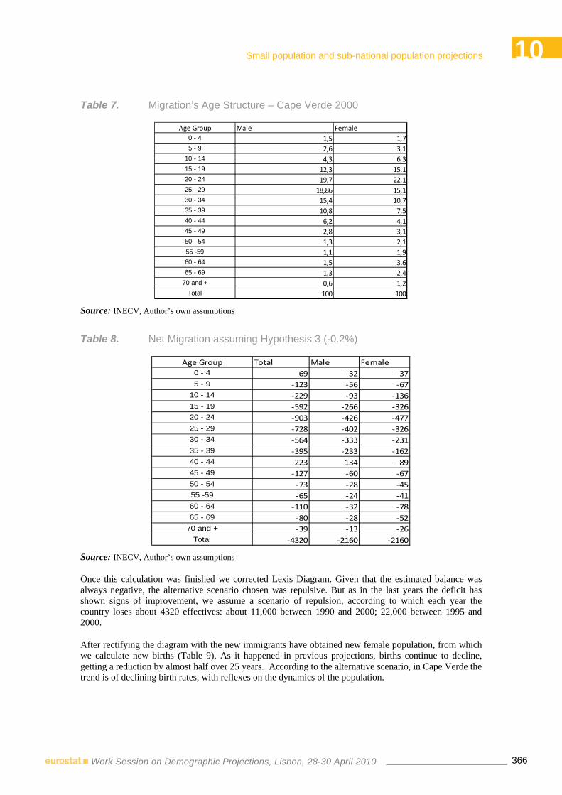
10Small population and sub-national population projections
366Work Session on Demographic Projections, Lisbon, 28-30 April 2010
Table 7. Migration’s Age Structure – Cape Verde 2000
Age Group Male Female0 - 4 1,5 1,75 - 9 2,6 3,1
10 - 14 4,3 6,315 - 19 12,3 15,120 - 24 19,7 22,125 - 29 18,86 15,130 - 34 15,4 10,735 - 39 10,8 7,540 - 44 6,2 4,145 - 49 2,8 3,150 - 54 1,3 2,155 -59 1,1 1,960 - 64 1,5 3,665 - 69 1,3 2,4
70 and + 0,6 1,2Total 100 100
Source: INECV, Author’s own assumptions
Table 8. Net Migration assuming Hypothesis 3 (-0.2%)
Age Group Total Male Female0 - 4 -69 -32 -375 - 9 -123 -56 -67
10 - 14 -229 -93 -13615 - 19 -592 -266 -32620 - 24 -903 -426 -47725 - 29 -728 -402 -32630 - 34 -564 -333 -23135 - 39 -395 -233 -16240 - 44 -223 -134 -8945 - 49 -127 -60 -6750 - 54 -73 -28 -4555 -59 -65 -24 -4160 - 64 -110 -32 -7865 - 69 -80 -28 -52
70 and + -39 -13 -26Total -4320 -2160 -2160
Source: INECV, Author’s own assumptions
Once this calculation was finished we corrected Lexis Diagram. Given that the estimated balance was always negative, the alternative scenario chosen was repulsive. But as in the last years the deficit has shown signs of improvement, we assume a scenario of repulsion, according to which each year the country loses about 4320 effectives: about 11,000 between 1990 and 2000; 22,000 between 1995 and 2000.
After rectifying the diagram with the new immigrants have obtained new female population, from which we calculate new births (Table 9). As it happened in previous projections, births continue to decline, getting a reduction by almost half over 25 years. According to the alternative scenario, in Cape Verde the trend is of declining birth rates, with reflexes on the dynamics of the population.

10Small population and sub-national population projections
367Work Session on Demographic Projections, Lisbon, 28-30 April 2010
Table 9. Birth Projections 2000-2025
1990-2000 2000-05 2005-2010 2010-2015 2015-2022020-2025Male 34694 32472 3026 26218 21139 18286Female 33070 30950 28618 24989 20148 17429Total 67764 63422 31644 51207 41287 35715
Years
Source: INECV, Author’s own assumptions
2.3 Mathematical Method This method is used to estimate the volume of a population by using mathematical equations based on rates such as average annual growth rate (AGR) of a given period, putting hypotheses in future evolution of the population. Its disadvantage relies on the fact that it does not consider the interference of mortality, fertility and migration variables. Table 10 shows some growth assumptions and results for Cape Verde, using this method.
Table 10. Demographic Projection 2000-2025 (Mathematical Methods)
Years 2000 2005 2010 2015 2020 2015
Population 431989 485869 546470 614629 691289 777510
Population 431989 458289 486190 515789 547191 580504
Population 431989 503229 586218 682893 795511 926700
Hypotesis 1: Scenario assuming the 1990s TCMA (2.39%)
Hypotesis 2: Scenario assuming a reduction by half of the TCMA (1.19%)
Hypotesis 1: Scenario assuming the 1960s TCMA (3,1%)
Source: INECV, Author’s own assumptions
According to the three hypotheses used in our exercise, population increases. However, in the first and third ones, the increase is much more significant than the second, as the rates used were higher (2.4% and 3.1%). Given the trend of declining birth rates and mortality observed during this work, the 2nd hypothesis seems more viable. Moreover, when compared to the results from the component method.
2.4 Ratio Method This method is used to estimate the population of a region or country by its relative weight in relation to the region where it is located, in a given time given a few assumptions (Cape Verde / ECOWAS) (Table 11).
Table 11. Population of Cape Verde according to ECOWAS (1990 and 2000)
1990 2000 TCMACape Verde 341491 431989 2,39%ECOWAS 195140310 216220000 1,03%Ratio Cape Verde/ECOWAS 0,2 0,2Source: RGPH 1990 e 2000, INECV; RDH, 2001
Source: Instituto Nacional de Estatística de Cabo Verde (INECV); RGPH 1990, 2000; RDH, 2001

10Small population and sub-national population projections
368Work Session on Demographic Projections, Lisbon, 28-30 April 2010
Taking into consideration the weight of the region into two periods (0.2%), we formulated the two hypotheses represented in Table 12.
Table 12. Demographic Projection 2000-2025 (Ratio Methods)
Year 2000 2005 2010 2015 2020 2015
Population 431989 454723 478654 503384 530360 558271
Population 431989 511154 538054 566370 596176 627551
Hypothesis assuming the same weight of 2000 (0.2%)
Hypothesis assuming a growth rate of the ECOWAS in the period 1990-2000 (1.03%)
Source: Instituto Nacional de Estatística de Cabo Verde (INECV)
3. Results presentation and discussion
All the scenarios, and also mathematical methods and population ratio, assume that Cape Verde will continue to register a positive growth rate over the next 25 years, although at a lower annual average growth rate after 2000 (1.7%) than the one experienced in the 90’s (2.4%), approaching the rate that was recorded in the 1980s (1.5%). That slowdown in growth is, at least partially, explained by the reduction of birth and mortality rates over the 25 years. Between 2010 and 2020 annual average growth rate continues to fall, reaching 1.3% in the last five years and decreases to 0.8%, almost returning to the level registered in the 70s (Tables 13 and 14).
Table 13. Estimation Criteria on Mortality, Fertility and Migration. Trends (2000-2025)
2000 - 2005 2005 - 2010 2010 - 2015 2015 - 2020 2020 - 2025IMR= 28,05 IMR= 25,1 IMR= 22,7 IMR= 20,5 IMR=18,7E0 (M)= 67,2; E0( F)=75,4 E0 (M)= 68,4; E0 (F)=76,2 E0 (M)= 69,4; E0 (F)= 77 E0 (M)= 70,3; E0( F)= 77,7 E0 (M)= 71,1; E0( F)= 78,2Birth (estimates)= 63888 Birth (estimates)= 59373 Birth (estimates)= 51777 Birth (estimates)= 41711 Birth (estimates)= 35715Birth (M)= 31177; Birth (F)= 32711) Birth (M)= 30399; Birth (F)= 28974 Birth (M)= 26510; Birth (F)= 25267 Birth (M)= 21356; Birth (F)= 20355 Birth (M)= 18286; Birth (F)= 17429Migr. Balance= - 4320/5Annual Migratory Rate= -0,2Annual Growth Rate= 2,2% Annual Growth Rate= 1,9 Annual Growth Rate= 1,5 Annual Growth Rate= 1,0 Annual Growth Rate= 0,8
Constant Constant Constant Constant
Source: INECV, Author’s own assumptions
Table 14. National Results, with and without migratory effect 1990 2000
SC 1 SC2 SC 1 SC2 SC 1 SC2 SC 1 SC2 SC 1 SC2Total population 341491 43189 482479 478159 529310 524959 576863 565843 600239 595840 625344 625245Male 161495 207994 235538 233378 262096 258924 283474 281294 300334 298146 314452 312456Female 179996 223995 246941 244781 267214 266035 293389 284549 299905 297694 310892 312789Glogal Fertility Rate 185,43 123,3 99 99 75 75 61 61 40 40 40 40Synthetic Fertility Index 6,32 4 2,9 2,82 2,87 2,78 2,83 2,74 2,8 2,7 2,5 2,3Infant Mortality Rate 65 29,8 26,3 26,3 23,9 23,9 21,4 21,4 19,6 19,6 17,8 17,8Active Renovation Rate 27,2% 22,8% 21,1% 19,9% 20,2% 13,2% 13,4% 12,2% 12,4% 8,7% 9,6%Life Expectancy at Birth (MF) 68,5 70,8 72 72 72,9 72,9 73,8 73,8 74,4 74,4 74,7 74,7Life Expectancy at Birth (M) 65,7 66,5 67,9 67,9 68,9 68,9 69,9 69,9 70,7 70,7 71,1 71,1Life Expectancy at Birth (F) 71,3 74,9 75,8 75,8 76,6 76,6 77,4 77,4 77,9 77,9 78,2 78,2Senario 1 - Natural TrendSenario 2 - Alternative Scenario of the baseline scenario
2005 2010 2015 2020 2025
Source: INECV, Author’s own assumptions

10Small population and sub-national population projections
369Work Session on Demographic Projections, Lisbon, 28-30 April 2010
Graph 2. Cape Verde Population Structure – Natural Trend (2000 and 2025)
Source: INECV, Author’s own assumption
Graph 3. Cape Verde Population Structure – Alternative Trend (2000 and 2025)
Source: INECV, Author’s own assumptions
All demographic projections are a complex exercise, as they involve a lot of demographic and non demographic variables and require good supporting data. However the complexity increases when we work with micro-universes, as it happens in this case.
But projections of small populations are indispensable to provide information and support policies and decisions at various levels. Let us look at Cape Verde’s regional diversity, by applying to municipalities, ie, administrative units corresponding to the islands that compose the country.

10Small population and sub-national population projections
370Work Session on Demographic Projections, Lisbon, 28-30 April 2010
Table 15. Population estimates for Cape Verde’s islands (2000-2025)
2000 2005 2010 2015 2020 2025Santo Antão 46865 52342 57423 62581 65117 67841São Vicente 66764 74567 81805 89154 92767 96647São Nicolau 13583 15171 16643 18138 18873 19663Sal 14727 16449 18045 19666 20463 21319Boavista 4178 4667 5120 5579 5806 6048Maio 6713 7497 8225 8964 9327 9718Santiago 235196 262685 288182 314072 326799 340467Fogo 37201 41549 45582 49677 51690 53852Brava 6762 7553 8286 9030 9396 9789Total 431989 482479 529310 576863 600239 625344
Demographic Projection 2000 -2025 by Municipalies (Trend Scenario)
IslandsYears
Source: INECV, Author’s own assumptions
Table 16. Population estimates for Cape Verde’s islands (2000-2025)
2000 2005 2010 2015 2020 2025Santo Antão 46865 51873 56951 61386 64640 67830São Vicente 66764 73900 81133 87451 92087 96632São Nicolau 13583 15035 16506 17792 18735 19660Sal 14727 16301 17897 19291 20313 21316Boavista 4178 4625 5077 5473 5763 6047Maio 6713 7430 8158 8793 9259 9716Santiago 235196 260333 285813 308072 324404 340414Fogo 37201 41177 45207 48728 51311 53843Brava 6762 7485 8218 8858 9327 9788Total 431989 478159 524959 565843 595840 625245
Demographic Projection 2000 -2025 by Islands (Alternative Scenario)
IslandsYears
Source: INECV, Author’s own assumptions
In demographic terms, we can point out in Cape Verde three groups of islands:
1) Islands with a fast demographic growth, like Santiago, São Vicente and Sal (they represent development concentration poles; as well as moderate fertility levels and positive migratory balance);
2) islands with a moderate demographic growth, as Fogo and Santo Antão (sources of internal and international migrations; they still have high fertility rates, but a negative migratory balance);
3) Islands with a reduced demographic growth, like Boavista, Maio, São Nicolau and Brava (they lose inhabitants due to internal and international migrations; they also present the lowest fertility levels and a very negative migratory balance).

10Small population and sub-national population projections
371Work Session on Demographic Projections, Lisbon, 28-30 April 2010
In fact, three islands have a much reduced population, which corresponds to a very high probability of error for any demographic projection exercise: Brava - 6762 inhabitants, Boavista - 10727 inhabitants, Maio - 4178 inhabitants.
The most relevant risk consists on upper or under estimate the volume of residents. One of the basic factors of these situations is due to the impossibility of controlling the displacement inter islands and municipalities, as internal migrations are not registered, at least directly. These cases can constitute some constraints in the process and influence the results of some indicators. Take educational example: in some municipalities the Enrolment Net Rate is superior to 100%, due to under-estimated projections; in others the Enrolment Net Rate is very low, due to upper-estimated projections.
The municipalities of bigger growth, in both scenarios are Praia, São Vicente and Santa Catarina, as we can observe on the following Tables 16 and 17.
Table 17. Cape Verde’s Municipalities. Demographic Projection 2000-2025 (Base Scenario)
2000 2005 2010 2015 2020 2025Ribeira Grande 21443 23949 26274 28634 29795 31041Paúl 8334 9308 10211 11129 11580 12064Porto Novo 17088 19085 20937 22818 23743 24736São Vicente 66764 74567 81805 89154 92767 96647Tarrafal de SN 5153 5756 6314 6882 7160 7460Ribeira Brava 8430 9415 10329 11257 11713 12203Sal 14727 16449 18045 19666 20463 21319Boa Vista 4178 4667 5120 5579 5806 6048Maio 6713 7497 8225 8964 9327 9718Tarrafal 17685 19752 21669 23616 24573 25601Santa Catarina 40607 45353 49755 54225 56422 58782São Salvador Mundo 9112 10177 11165 12168 12661 13191Santa Cruz 25053 27981 30697 33455 34810 36266São Lourenço Órgãos 7760 8667 9508 10363 10783 11234Praia 96156 107395 117819 128404 133607 139195Ribeira Grande - Santiago 9557 10674 11710 12762 13279 13835São Domingos 13233 14780 16214 17671 18387 19156São Miguel 16033 17906 19645 21409 22277 23209Mosteiros 9413 10513 11533 12569 13079 13626São Filipe 23021 25712 28208 30742 31988 33326Santa Catarina- Fogo 4767 5324 5841 6365 6623 6900Brava 6762 7553 8286 9030 9396 9789Total 431989 482479 529310 576863 600239 625344
Demographic Projection 2000 -2025 by Municipalies (Trend Scenario)
MunicipalitiesYears
Source: INECV, Author’s own assumptions

10Small population and sub-national population projections
372Work Session on Demographic Projections, Lisbon, 28-30 April 2010
Table 18. Cape Verde’s Municipalities. Demographic Projection 2000-2025 (Alternative Scenario)
2000 2005 2010 2015 2020 2025Ribeira Grande 21443 23735 26058 28087 29576 31036Paúl 8334 9224 10127 10916 11495 12062Porto Novo 17088 18914 20765 22383 23569 24732São Vicente 66764 73900 81133 87451 92087 96632Tarrafal de SN 5153 5704 6262 6750 7108 7459Ribeira Brava 8430 9331 10244 11042 11627 12201Sal 14727 16301 17897 19291 20313 21316Boa Vista 4178 4625 5077 5473 5763 6047Maio 6713 7430 8158 8793 9259 9716Tarrafal 17685 19575 21491 23165 24393 25597Santa Catarina 40607 44947 49346 53189 56009 58773São Salvador Mundo 9112 10086 11073 11935 12568 13188Santa Cruz 25053 27730 30444 32815 34555 36260São Lourenço Órgãos 7760 8590 9430 10165 10704 11232Praia 96156 106433 116850 125951 132628 139173Ribeira Grande - Santiago 9557 10579 11614 12518 13182 13833São Domingos 13233 14647 16081 17333 18252 19153São Miguel 16033 17746 19483 21000 22114 23205Mosteiros 9413 10419 11438 12329 12983 13624São Filipe 23021 25482 27976 30155 31753 33320Santa Catarina- Fogo 4767 5276 5793 6244 6575 6899Brava 6762 7485 8218 8858 9327 9788Total 431989 478159 524959 565843 595840 625245
Demographic Projection 2000 -2025 by Municipalies (Alternative Scenario)
MunicipalitiesYears
Source: INECV, Author’s own assumptions
4. Final remarks
Micro-demographic variables, such as birth / fertility, mortality and migration rates are the most important factors for population growth in Cape Verde;
Mortality continues to decline at all age groups and islands, as a result of improvements in sanitation and socio-economic;
Life expectancy at birth increased significantly between 1990 and 2000;
Cape Verdean population will continue to grow in the near future, at least until 2025, no mater the chosen scenario;
The speed of growth will be lower than the one recorded in the 90s;
Birth rates have fallen quite suddenly, standing at almost half the volume they had 25 years ago;

10Small population and sub-national population projections
373Work Session on Demographic Projections, Lisbon, 28-30 April 2010
In all the used scenarios and methods population continues to increase. This growth will have impact at various sectors, particularly in relation to the social and economic ones, such as Health, Education, Employment and Training.
The so-called more developed islands remain as the major poles of attraction for the population (Santiago - Praia and Santa Catarina; São Vicente; Sal and Boavista in some ways).
The more economic and social developed islands remain the major demographic poles of attraction (Santiago; Santa Catarina; São Vicente; Sal and Boavista in some ways).
Islands with higher fecundity rates are not the ones where growth rates are highest.
Migrations (internal and international ones) represent the major importance to explain differentials on population dynamics.
Demographic projections at level of the municipalities are impossible or present major errors, as there are municipalities with very small volumes of residents.
Bibliography
BIAYE, Mady (1995), Análise sumária da situação demográfica em Cabo Verde, Praia, INE-CV.
BRITO, Pedro Moreno (2003), Análise da Situação de Demográfica de Cabo Verde 1990 – 2000 (Prospectiva para 2025), Lisboa, ISEGI/UNL.
CALDAS, José Maria Castro; PERESTRELO, Margarida (1998): Instrumentos de Análise para o Método dos Cenários. I - Análise Estrutural, Working Paper, Lisboa, Dinâmia.
CARRILHO, Maria José (1997), As Projecções Demográficas: aplicações e Métodos in, Cadernos Regionais n.º Abril 1997, Direcção Regional do Centro, Instituto Nacional de Estatística, Lisboa.
CASELLI, Graziella; VALLIN, Jacques; WUNSCH, Guillaume (Eds.) (2001), Démographie: analyse et synthèse, Vol. II, Déterminants de la fécondité, Institut National d’Études Démographiques, Paris.
_._._. (Eds.). (2001), Démographie: analyse et synthèse, Vol. III, Déterminants de la mortalité, Institut National d’Études Démographiques, Paris.
_._._. (2004), Démographie: analyse et synthèse. Vol. V, Histoire du peuplement et prévisions, INED, Paris.
CLELAND, John and WILSON Christopher Demand “Theories of the fertility transition”: In Population Studies, (1987), an iconoclastic view.
COALE, A. e HOOVER, E.M. (1984), World Development Report. The World Bank, Oxford: Oxford University Press.
COALE, A. E DEMENY, P. (1972), Regional model life tables and stable populations, academic Press, Nova Iorque.
COALE, A. e GUO, G. (1990), «Revised Regional Model Life Table at very low levels of mortality», population Index nº 55(4), Princeton University Press.
COURGEAU, Daniel (1988), Méthodes de mesure de la mobilité spatiale: Migrations internes, mobilité temporaire, navettes. Institut National d’Études Démographiques, Paris.

10Small population and sub-national population projections
374Work Session on Demographic Projections, Lisbon, 28-30 April 2010
GODET, M., (1990), Problèmes et Méthodes de Prospective, Paris, Ed. Futuribles.
INE-CV, Inquérito Demográfico e de Saúde Reprodutiva I (IDSR I), 1998.
INE-CV, Inquérito Demográfico e de Saúde Reprodutiva II (IDSR II), 2005.
INE-CV, Recenseamentos Gerais da População e Habitação, www.ine.cv
MAGALHÃES, Maria da Graça, “Projecções da População Residente, Portugal 2000-2050 – Que tendências de Base para a construção de hipóteses?”, in Revista de Estudos Demográficos, nº34, INE, Lisboa, 2004, pp.51-57.
NAÇÕES UNIDAS, Demographic Prospects Revision, 2008. http://esa.un.org/unpp
PRB, (2005), World Population Data Sheet. Demographic Data and Estimates for the Countries and the Regions of the World, Population Reference Bureau, USA.
RODRIGUES, Teresa, “Demografia e Prospectiva. A Região do Minho Lima (1801-2020) ”, in Cadernos Vianenses, tomo 38, 2006, Câmara Municipal Viana do Castelo.
VÉRON, J. (1991), Démographie, Ed. Armand Colin, Paris.
VINUESA, J. ZAMORA, F. GÉNOVA, R. SERRANO, P. e RECANO, J. (1994), Demografia. Analisis y proyecciones, Ed. Sintesis, Madrid.

10Small population and sub-national population projections
375Work Session on Demographic Projections, Lisbon, 28-30 April 2010
Annex 1: Demographic Projection 2000-2025 (Natural Scenario)
2000 2005 2010 2015 2020 20250 - 4 55005 61263 56933 56933 40512 350225 - 9 64246 52739 60786 56649 50040 40397
10 - 14 63307 63744 52328 60641 56514 4996515 - 19 49201 63090 63524 52203 60450 5639720 - 24 36158 48983 62811 63322 52038 6025325 - 29 28654 35913 48652 62503 63012 5186830 - 34 27977 28414 35613 48360 62128 6275935 - 39 25492 27712 28146 35370 48030 6184540 - 44 19218 25197 27393 27907 35069 4775345 - 49 12561 18919 24808 27068 27577 3477350 - 54 6410 12273 18490 24358 26579 2720055 -59 6532 6188 11847 17959 23666 2597860 - 64 10025 6185 5863 11303 17149 2286965 - 69 9095 9211 5683 5444 10492 1610870 - 74 7615 7972 8066 5042 4835 944975 e + 10493 14676 18367 21801 22148 22708Total 431989 482479 529310 576863 600239 625344
Age GroupYears
Source: INECV, Author’s own assumptions
Annex 2: Demographic Projection 2000-2025 (Alternative Scenario)
2000 2005 2010 2015 2020 20250 - 4 55005 61194 56864 50221 40443 350275 - 9 64246 52616 60663 56526 49917 40408
10 - 14 63307 63515 52099 60412 56285 5000815 - 19 49201 62498 62932 51611 59858 5645720 - 24 36158 48080 61908 62419 51135 6030425 - 29 28654 35185 47924 61775 62284 5179230 - 34 27977 27850 35049 47796 61564 6265735 - 39 25492 27317 27751 34975 47635 6177440 - 44 19218 24974 27170 27684 34846 4770845 - 49 12561 18792 24681 26941 27450 3478050 - 54 6410 12200 18417 24285 26506 2721755 -59 6532 6123 11782 17894 23601 2599560 - 64 10025 6075 5753 11193 17039 2291565 - 69 9095 9131 5603 5364 10412 1613270 - 74 7615 7933 8027 5003 4796 946275 e + 10493 14676 18336 21744 22069 22609Total 431989 478159 524959 565843 595840 625245
Age GroupYears
Source: INECV, Author’s own assumptions


10Small population and sub-national population projections
377Work Session on Demographic Projections, Lisbon, 28-30 April 2010
USING NATIONAL DATA TO OBTAIN SMALL AREA ESTIMATORS FOR POPULATION PROJECTIONS ON
SUB-NATIONAL LEVEL
Michael FRANZÉN1, Therese KARLSSON2
Abstract
When forecasting population on small geographical areas it is necessary to have stable and reliable data. In Sweden the population density is small in many areas and the data would not be reliable for forecasting purpose. Furthermore, even if the density is high in some areas the number of inhabitants is too low. Due to few observations, distributions of the demographic components may not be obtained. This is often the case for smaller city districts. Even forecasts on the municipality level may sometimes be unreliable due to few observations, especially when it comes to migration. The data on a national level is however stable and reliable when making population forecasts and the aim of this paper is to suggest how national data may be used on a sub-national level and show how this is used in Sweden.
To obtain these small area estimators we would analyze housing definitions on real-estate level. These estimators should be geographically independent and therefore useable anywhere on sub-national level. The assumption is that people living in for example rentable apartments share the same demographical pattern anywhere in the country.
A cluster analysis on residential types, using the population register and real estate register in Sweden, is used to identify suitable groups. In general, the idea with cluster analysis is to classify observations with homogenous conditions that separate them from other homogenous groups. The analysis results in a division of a number of residential types with homogenous demographic conditions. The cluster analysis shows that age-structure, fertility and probability of moving varies among different residential types and areas. In a demographical sense, people living in an area with larger one-family houses would “behave” differently from people living in an area with mostly small rentable apartments. The division is presented in terms of housing, tenure, year of construction, size of the city where the building is situated and the attraction of the area. These obtained groups contain sufficient demographic data to be used when forecasting future development in small areas consisting of one or more residential types.
Summary
To obtain reliable data for population projections on small areas the idea is to collect data from the whole country that is applicable on these small areas. It has been shown that people in different residential areas behave differently, in a demographic context. For example migration in multi-family dwellings is more frequent than in single-family dwellings. There are also differences between multi-family dwellings that consist of owned or rented apartments and where the dwelling is situated; in large or small cities. The aim in this project is to describe a division of housing that behave similar and for which reliable and stable data can be obtained using data on the national level. The classification presented in this paper resulted in
1 Statistics Sweden 2010 2 Statistics Sweden 2010

10Small population and sub-national population projections
378Work Session on Demographic Projections, Lisbon, 28-30 April 2010
33 different ‘type codes’ all with specific out-migration probabilities, age-distribution of the in-migrants, fertility etc.
1. Introduction
Sweden is divided into 290 municipalities which are responsible for facilities and services such as schools, elderly and child care, housing, public assistance etc. The population in the municipalities varies from 2.500 in the smallest municipality Bjurholm to 830.000 in Stockholm3. All municipalities are divided into subareas set by the municipality council. The number of subareas varies along with the size of the population. For these areas Statistics Sweden provides the municipalities with population statistics that can be used in forecasting the population. Often the statistics on such a low level contains very few observations and the data is not reliable when projecting the population. That is why it is necessary to provide the municipalities with reliable and stable data that can be used on small areas. The idea is to determine how different housing behave, using observations for the whole country, and then apply it to the small areas. The analyze results in a division of housing that behave similar and can be used when projecting the population on small areas. Ten years ago the first division was presented and now Statistics Sweden has started a project that will result in a new and updated division of housing.
2. Background
The first type code classification of real estates in Sweden was made in 1991. Then the classification was made using only a sample of real estates in Sweden. In 1998 it was decided that a classification using all real estates was necessary and that the results from the study should be used in yearly production of statistics for population projections on small areas.
In the classification made in the early 90’s data from 1986-1988 were used. Data on real estates was manually collected from a sample of 30 municipalities and the collection process was time demanding. In 1998 a full coverage register were used for collecting data on real estates. Data for the years 1992-1994 were used when classifying the real estates for the second time.
In both rounds of collecting data for classification of real estates, it was found that the out-migration probabilities do not depend on the year in which the property was built but on the legal form of the house or apartments. In 1998 it was found that the out-migration probabilities in rented homes had increased with 20 percent. In some ages the increase was as much as 50 percent. However, nor an increase or decrease in out-migration probabilities can be observed for owned apartments or small houses (single-family dwellings). It has been discussed what had happened between 1986-1988 and 1992-1994 that made the out-migration probabilities increase. One explanation was that there were large migration flows within the municipalities. This was due to raised rents in the rented homes. During these years people moved in order to find the apartment with the right rent. An increase in movement could not be seen in owned homes, both apartments and small houses, this was probably due to the fact that capital is often tied up when owning an apartment or house. Also, the price on these homes was in larger extent better adjusted to the market prices.
It is these demographical changes one wants to include when producing statistics on properties. The statistics must be easy to update so that one always have the latest demographical data. Since the results from the project in 1998 are completely register based it is now easy to update the tables with new statistics each year. These tables are provided to the municipalities. The tables are sold to approximately 50 municipality councils each year.
3 Stockholm in this context is the municipality, however Stockholm area consists of several municipalities and has a population
of 2 million.

10Small population and sub-national population projections
379Work Session on Demographic Projections, Lisbon, 28-30 April 2010
It has now been ten years since the last classification of properties was done. It is now necessary for Statistics Sweden to renew the classification. The project is not yet finished and therefore the results in this paper are those from the previous classification.
3. Results
3.1 Data sources In this paper ‘property’ and ‘real estate’ are used synonymously. Property and real estate can include more than one actual house. For small houses the property and real estate most often equals only one house. For multi-family houses the property or real estate may include more than one house. In Sweden each person is obliged to report to the tax board when moving – even if the person moves to another apartment within the same property. Therefore in the population register in Sweden there are data on migration even within the properties. In the classification migration within properties is included.
The data is retrieved from both the population register and the real estate register. In the previous project population data for 1992-1994 were used in the clustering process. Population and population flows by age and sex are available from the population register. From the real estate register the following variables are retrieved: Household type (defined as either single-family dwelling or multi-family dwelling), Tenure type (tenant rented, tenant owned or small houses), Year of construction, Size of the urban area (population in the area) and Level factor (describes the attractiveness of the area where the real estate is situated).
In the new project demographic variables for 2006-2008 in housing units older than 3 years were used (1.8 million properties). This is because the data quality for newly built housing units and real-estates tend to be uncertain. For example, a housing unit may not be reported to the register before the whole building project is completed and the real estate may then be populated without any registered housing (people moving in to the apartments before the building is reported as completely built).
3.2 Demographical results In this section we use the latest available data for the type codes to show their differences in demography. Data for 2006-2008 has been used.
The age-structure in multi-family dwellings differs significantly from the age-structure in single-family dwellings as shown in figure 1. In the single-family dwellings the majority of the population is children or adults in the ages 40-65 years. In Sweden in general young adults leave the parental home at the age 21 for women and 22 for men4 and this pattern can be seen in the age-structure of the population in the single-family dwellings. When the young adults leave home they, in most cases, move to a multi-family dwelling, which also can be seen in the age distribution of the multi-family dwellings.
4 Statistics Sweden, Demographic reports2008:5, Leaving home

10Small population and sub-national population projections
380Work Session on Demographic Projections, Lisbon, 28-30 April 2010
Figure 1. Population by age in multi-family dwellings and single-family dwellings 2008
0
10 000
20 000
30 000
40 000
50 000
60 000
70 000
80 000
90 000
100 000
0 10 20 30 40 50 60 70 80 90 100
Multi-family dwellings
Single-family dwellings
The age-distribution among those moving to and from multi-family dwellings and single-family dwellings differs as shown in figure 2 and 3. However we see a similar pattern among the people in their early twenties dominating the out-migration from both multi-family dwellings and single-family dwellings. These movements are often strongly correlated to leaving the parental home. There are, not surprisingly, more people in their twenties and thirties moving in to multi-family dwellings than into single-family dwellings. The single-family dwellings have a negative net-migration in the ages 17-27 years while the multi-family dwellings have a positive net-migration in these ages. The multi-family dwellings have a negative net migration of young children and people in the ages 28-45. This pattern comes from people starting a family in a multi-family dwelling and then moving to a single-family dwelling.
Figure 2. Age-distribution of migrants to and from multi-family dwellings 2006-2008
0
10 000
20 000
30 000
40 000
50 000
60 000
70 000
80 000
90 000
100 000
110 000
120 000
0 10 20 30 40 50 60 70 80 90 100
In Migrants
Out Migrants

10Small population and sub-national population projections
381Work Session on Demographic Projections, Lisbon, 28-30 April 2010
Figure 3. Age-distribution of migrants to and from single-family dwellings 2006-2008
0
10 000
20 000
30 000
40 000
50 000
60 000
70 000
80 000
90 000
100 000
110 000
120 000
0 10 20 30 40 50 60 70 80 90 100
In Migrants
Out Migrants
The probability of moving out of a property differs among different types of properties and different ages. This can be seen in the figure below where the probability of out-migration for both multi and single-family dwellings are described. The probability of moving out is age and sex specific, expressed in percentage terms. The probability is calculated using the number of migrants of a certain age and sex proportional to the population in the same age and sex cohort.
The out-migration probabilities are higher in multi-family dwellings for all ages. For the two types of properties the out-migration probability is at its highest in the ages around 20-30 years. There is also a high risk for young children to move out from multi-family dwellings.
Probably due to the fact that their parents, when having children often move from a small multi-family dwelling to a larger one – or from a multi-family dwelling to a small house. The difference in out-migration probabilities between the two types of housing is at its highest in the age of 1-2 years. For both multi-family dwellings and single-family dwellings there is a increase in out-migration probabilities in the highest ages and this is probably due to elderly people moving to an elderly home and leaving their own apartment or house. The out-migration probability for both multi-family dwellings and single-family dwellings are lowest in the ages 70-80 years.
Figure 4. Probability of moving out. Multi-family dwellings and single-family dwellings, 2006-2008
0
0,1
0,2
0,3
0,4
0,5
0,6
0 10 20 30 40 50 60 70 80 90 100
Multi-family dwellings
Single-family dwellings
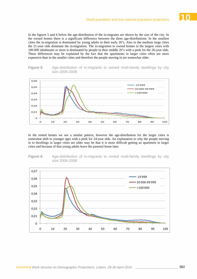
10Small population and sub-national population projections
382Work Session on Demographic Projections, Lisbon, 28-30 April 2010
In the figures 5 and 6 below the age-distribution of the in-migrants are shown by the size of the city. In the owned homes there is a significant difference between the three age-distributions. In the smallest cities the in-migration is dominated by young adults in their early 20’s. Also in the medium large cities the 21-year olds dominate the in-migration. The in-migration to owned homes in the largest cities with 100.000 inhabitants or more is dominated by people in their middle 20’s with a peek for the 26-year olds. These differences may be explained by the fact that the apartments in larger cities often are more expensive than in the smaller cities and therefore the people moving in are somewhat older.
Figure 5. Age-distribution of in-migrants to owned multi-family dwellings by city size 2006-2008
0
0,01
0,02
0,03
0,04
0,05
0,06
0 10 20 30 40 50 60 70 80 90 100
-19 999
20 000-99 999
>100 000
In the rented homes we see a similar pattern, however the age-distribution for the larger cities is somewhat shift to younger ages with a peek for 24-year olds. An explanation to why the people moving in to dwellings in larger cities are older may be that it is more difficult getting an apartment in larger cities and because of that young adults leave the parental home later.
Figure 6. Age-distribution of in-migrants to rented multi-family dwellings by city size 2006-2008
0
0,01
0,02
0,03
0,04
0,05
0,06
0,07
0 10 20 30 40 50 60 70 80 90 100
-19 999
20 000-99 999
>100 000

10Small population and sub-national population projections
383Work Session on Demographic Projections, Lisbon, 28-30 April 2010
In figure 7 below the age-distributions for in migrants who move to multi-family dwellings is shown. The dominating group of in migrants to rented homes is young adults in the ages 20-25 years. The in migrants to owned multi-family dwellings are somewhat older; the dominating group is 25-28 years. The proportion of children moving to rented homes is higher in multi-family dwellings than for the single-family dwellings.
Figure 7. Age-distribution of in-migrants to multi-family dwellings by legal form 2006-2008
0
0,01
0,02
0,03
0,04
0,05
0,06
0 10 20 30 40 50 60 70 80 90 100
Owned
Rented
In figure 8 below the age-distribution of the in-migrants to single-family dwellings by the areas level factor is shown. The level factor describes the attractiveness of the area where the dwelling is situated.
The attractiveness also describes the price of the house which may be an explanation to why the distributions are more and more shift to the right for the young adults when looking at a higher level factor. The age-distribution of level factor 3 and 4 resembles each other and it may therefore in the future be a good idea to merge these two groups of real estates.
Figure 8. Age-distribution of in-migrants to single-family dwellings by level factor 2006-2008
0
0,01
0,02
0,03
0,04
0 10 20 30 40 50 60 70 80 90 100
1
2
3
4

10Small population and sub-national population projections
384Work Session on Demographic Projections, Lisbon, 28-30 April 2010
Given these differences the project resulted in 33 groups of real estates (type codes) for which demographical data can be produced and used when forecasting the population on small areas. A complete list of the 33 different type codes is found in Appendix 1.
3.3 Classification method The aim was to find a division of housing that is similar within each group considering the following demographical variables:
• Age distribution in in-migration
• Age specific out-migration probabilities
• Housing density
The real estate variables used were:
• Household type
• Legal form
• City size (population density)
• Year of construction
• Level factor (attractiveness of the area)
The demographic variables where aggregated by the real estate-variables. These variables are categorical and we need a certain amount of observations to obtain stable distributions of in-migration and the out-migration probabilities. The age-groups that were used was 0-5, 6-16, 17-20 21-30, 45-54 and 60-80 years of age.
The clustering was carried out with chi2-test on the demographic variables for each category of real estates. If the two categories where similar in the distribution of the demographic variable they were grouped into the same cluster.
This process was carried out for the in-migration, out-migration and housing density separately. The three separate analyses gave different clusters but the final categories that were chosen are shown in figure 1.
The break down in multi-family and single-family dwellings is obvious because many studies have shown demographical differences such as age distribution, probability of moving and housing density between the two types of housing. Other break downs were discussed within the project and the result was as follows.

10Small population and sub-national population projections
385Work Session on Demographic Projections, Lisbon, 28-30 April 2010
Figure 9.
Multi-family dwellings Single-family dwelling Legal form Legal form Tenant owned housing Small houses Tenant rented housing Tenant owned houses City size City size -19 999 Not densely populated 20 000-99 999 Densely populated 100 000- Level factor Year of construction 1 1900-1954 2 1955-1964 3 1964- 4 Level factor 1 2
In the new project, a complete clustering is carried out without any chi2-tests. Before the clustering it is necessary to determine some large groups of real estates as in the previous classification. This is made as objectively as possible. For example the construction year is set into 10 year groups before clustering.
4. Conclusions
The results show that people living in real estate with different properties have different demographical behavior. Migration from both multi-family dwellings and single-family dwellings are dominated by people in the ages 20-30. Single-family dwellings have negative net-migration in these ages while multi-family dwellings have a surplus. Multi-family dwellings also have a surplus of people in the ages above 65 years. Multi-family dwellings have negative net-migration of children in the ages 0-10 years whilst single-family dwellings have a surplus.
The age structure in multi-family dwellings and single-family dwellings differs significantly. The population in single-family dwellings is dominated by children and adults in the ages 40-65 years. The population in multi-family dwellings is dominated by young adults in the ages 20-30 years.
Also the out-migration probabilities are different in multi-family dwellings and single-family dwellings. The out-migration probabilities are higher in all ages in multi-family dwellings.
In-migration to multi-family dwellings is dominated by people in the ages 20-30 years and there is relatively few children moving in to multi-family dwellings.
The in-migration to single-family dwellings however is dominated by children and people in the ages 20-35 years. The proportion of in-migration in the ages 65 and above is larger in multi-family dwellings.

10Small population and sub-national population projections
386Work Session on Demographic Projections, Lisbon, 28-30 April 2010
This is probably due to the retirement age which in Sweden is 65 years. Many people living in their single-family dwelling move to a multi-family dwelling when retiring.
There are also differences in the age-structure among the people moving in to multi-family dwellings depending on the properties of the real estate. We have seen that people moving in to owned apartments are somewhat older than the migrants to rented homes. Also the dominating groups of migrants to multi-family dwellings are older in larger cities than in smaller cities which can be explained by the fact that homes are on average more expensive in larger cities.
For single-family dwellings the age-structure for the in migrants are different depending on the attractiveness of the area where the property is situated.
The results show that it is better to use distributions for single-family dwellings than a distribution for all houses when it is known that the small area, for which we would like to project the population, consists only of single-family dwellings.
These differences in demographical behavior between different real estates have resulted in 33 groups; (type codes) that can be used when projecting the population on small areas.
For forecasting purposes it would be optimal to have subareas containing only one type code and then be able to use one set of demographic data. However this is not the case in many municipalities in Sweden. Therefore a common method is to weigh the distribution by population size in each type code to get a distribution for the entire subarea.

10Small population and sub-national population projections
387Work Session on Demographic Projections, Lisbon, 28-30 April 2010
Appendix 1
Type code Type of housing Legal form City size Year of construction Level factor
FBR128 Multi-family dwell ing Tenant owned housing -19 999 -1954 <7,50
FBR138 Multi-family dwell ing Tenant owned housing -19 999 1955-1964 <7,50
FBR148 Multi-family dwell ing Tenant owned housing -19 999 1965- <7,50
FBR228 Multi-family dwell ing Tenant owned housing 20 000 -99 999 -1954 <7,50
FBR238 Multi-family dwell ing Tenant owned housing 20 000 -99 999 1955-1964 <7,50
FBR248 Multi-family dwell ing Tenant owned housing 20 000 -99 999 1965- <7,50
FBR328 Multi-family dwell ing Tenant owned housing 100 000- -1954 <7,50
FBR329 Multi-family dwell ing Tenant owned housing 100 000- -1954 7,50-
FBR338 Multi-family dwell ing Tenant owned housing 100 000- 1955-1964 <7,50
FBR339 Multi-family dwell ing Tenant owned housing 100 000- 1955-1964 7,50-
FBR348 Multi-family dwell ing Tenant owned housing 100 000- 1965- <7,50
FBR349 Multi-family dwell ing Tenant owned housing 100 000- 1965- <7,50
FHR128 Multi-family dwell ing Tenant rented housing -19 999 -1954 <7,50
FHR138 Multi-family dwell ing Tenant rented housing -19 999 1955-1964 <7,50
FHR148 Multi-family dwell ing Tenant rented housing -19 999 1965- <7,50
FHR228 Multi-family dwell ing Tenant rented housing 20 000 -99 999 -1954 <7,50
FHR238 Multi-family dwell ing Tenant rented housing 20 000 -99 999 1955-1964 <7,50
FHR248 Multi-family dwell ing Tenant rented housing 20 000 -99 999 1965- <7,50
FHR328 Multi-family dwell ing Tenant rented housing 100 000- -1954 <7,50
FHR329 Multi-family dwell ing Tenant rented housing 100 000- -1954 7,50-
FHR338 Multi-family dwell ing Tenant rented housing 100 000- 1955-1964 <7,50
FHR339 Multi-family dwell ing Tenant rented housing 100 000- 1955-1964 7,50-
FHR348 Multi-family dwell ing Tenant rented housing 100 000- 1965- <7,50
FHR349 Multi-family dwell ing Tenant rented housing 100 000- 1965- 7,50-
SBR000 Single-family dwell ing Tenant owned houses - - -
SER801 Single-family dwell ing Small houses Not densely populated - <5,50
SER802 Single-family dwell ing Small houses Not densely populated - 5,75-9,50
SER803 Single-family dwell ing Small houses Not densely populated - 10,00-12,00
SER804 Single-family dwell ing Small houses Not densely populated - 13,00-
SER901 Single-family dwell ing Small houses Densely populated - <5,50
SER902 Single-family dwell ing Small houses Densely populated - 5,75-9,50
SER903 Single-family dwell ing Small houses Densely populated - 10,00-12,00
SER904 Single-family dwell ing Small houses Densely populated - 13,00-


10Small population and sub-national population projections
389Work Session on Demographic Projections, Lisbon, 28-30 April 2010
AUSTRIAN REGIONAL POPULATION PROJECTIONS BELOW NUTS-3
Alexander HANIKA1
1. Introduction
The intention of this paper is to describe the work on a small area population projection for Austria by its 35 NUTS 3-regions and 124 districts (including 23 districts of Vienna) by age and sex up to the year 2050. The report illustrates how regions are projected to become demographically diverse over the next decades. In an additional step which will be done after finishing population projections future development of number and structure of the labour force as well as household composition in Austria and its 124 regions should be predicted. Our projections can be used as basic input to many federal, state, and local projection models that produce detailed statistics on education, labour force, health care and other topics. Thus, the results are useful to regional planners in both public and private sectors.
The present small-area population projection is done on behalf of the “Austrian Conference on Spatial Planning” (ÖROK). It should be consistent with the official population projection by Statistics Austria which was published in fall 2009. This is guaranteed due to the same methodical approaches as well as using the same multiregional population model (SIKURS 8.9). Assumptions concerning fertility, mortality, interregional migration and international migration could therefore be synchronized. Moreover, due to final adjustment procedures it will be assured that the results of the population projection by this so called ÖROK-Projection are in concordance with the corresponding main (medium) projection variant by Statistics Austria (top-down approach). Besides the main scenario, nine alternative scenarios were calculated by Statistics Austria on NUTS 2-level comprising different demographic assumptions with high, medium and low variants.
At the time being calculations on the small area projections are not finished yet. Therefore this paper describes primarily the framework of the superior population projection for Austria and its nine Länder (NUTS 2-regions) as well as the assumptions for the small area projection. Preliminary results for the future development of the 124 districts are shown at the end of the paper.
1 Statistics Austria

10Small population and sub-national population projections
390Work Session on Demographic Projections, Lisbon, 28-30 April 2010
Table 1. Assumptions for the Austrian population projection on NUTS 2-level (mean variant)
Para-meter
Austria Burgen-land
Carinthia LowerAustria
UpperAustria
Salz-burg
Styria Tyrol Vorarl-berg
Vienna
Total fertility rate2001 1,33 1,23 1,32 1,35 1,41 1,35 1,23 1,33 1,51 1,312008 1,41 1,31 1,40 1,46 1,51 1,43 1,32 1,39 1,51 1,392010 1,40 1,27 1,36 1,44 1,49 1,42 1,31 1,40 1,52 1,392030 1,50 1,41 1,48 1,53 1,56 1,52 1,44 1,50 1,58 1,49
Mean age of fertility2001 28,4 28,3 28,6 28,2 28,3 28,6 28,2 28,9 28,8 28,32008 29,5 29,4 29,3 29,4 29,3 29,6 29,4 29,8 29,8 29,52010 29,6 29,6 29,5 29,5 29,5 29,8 29,5 30,0 30,0 29,72030 31,0 31,0 31,0 30,9 30,9 31,0 30,9 31,3 31,2 31,0
Male life expectancy2001 75,6 75,1 76,1 75,6 75,8 76,5 75,6 76,7 75,8 74,82008 77,6 76,6 77,6 77,0 78,2 79,2 77,3 79,3 78,3 77,02050 85,9 85,4 86,1 85,6 86,2 86,7 85,9 87,2 86,8 85,3
Female life expectancy2001 81,6 81,9 82,4 81,2 82,0 81,8 81,9 82,5 82,6 80,72008 83,0 83,0 83,7 82,5 83,0 83,9 83,4 83,7 84,1 82,12050 89,5 89,5 90,2 89,1 89,7 90,0 89,9 90,5 90,4 88,6
International immigration2002 108.125 1.980 3.861 13.588 13.103 6.986 10.330 10.652 5.157 42.4682008 110.074 2.762 4.349 13.855 13.539 7.141 10.958 10.665 5.246 41.5592009 100.000 2.000 4.000 12.900 13.100 6.800 9.700 9.300 5.000 37.2002010 102.000 2.040 4.080 13.158 13.362 6.936 9.894 9.486 5.100 37.9442011 106.000 2.120 4.240 13.674 13.886 7.208 10.282 9.858 5.300 39.4322012 110.000 2.200 4.400 14.190 14.410 7.480 10.670 10.230 5.500 40.9202013 110.000 2.200 4.400 14.190 14.410 7.480 10.670 10.230 5.500 40.9202014 111.000 2.220 4.440 14.319 14.541 7.548 10.767 10.323 5.550 41.2922015 112.000 2.240 4.480 14.448 14.672 7.616 10.864 10.416 5.600 41.6642016 111.000 2.220 4.440 14.319 14.541 7.548 10.767 10.323 5.550 41.2922017 108.000 2.160 4.320 13.932 14.148 7.344 10.476 10.044 5.400 40.1762018 106.000 2.120 4.240 13.674 13.886 7.208 10.282 9.858 5.300 39.4322019 105.000 2.100 4.200 13.545 13.755 7.140 10.185 9.765 5.250 39.0602020 104.000 2.080 4.160 13.416 13.624 7.072 10.088 9.672 5.200 38.6882030 105.000 2.100 4.200 13.545 13.755 7.140 10.185 9.765 5.250 39.0602050 110.000 2.200 4.400 14.190 14.410 7.480 10.670 10.230 5.500 40.920
S: Statistics Austria, Population Projection 2009

10Small population and sub-national population projections
391Work Session on Demographic Projections, Lisbon, 28-30 April 2010
2. Population projection for Austria on NUTS 2-level
Austria had a population of 8.34 million in 2008, the reference year for the new population projection. According to the assumptions on future changes in fertility, mortality and migration (see table 1), the total population will increase to 9.05 million people (+8.5 per cent) until 2030 and to 9.47 million (+13.6 per cent) in 2050 (table 2). This increment of growth is mainly based on immigration (see graph 1). The balance of births and deaths will be equalised more or less for the next decades. After the year 2030 the baby boom of the 1960eth will reach higher age. Therefore deaths will overhang births (graph 2).
Graph 1. International migration for Austria 1960 – 2050 (medium variant of projection)
-30-20-10
0102030405060708090
100110120130
1960 1970 1980 1990 2000 2010 2020 2030 2040 2050
in 1.
000
Net migration
Immigration
Emigration
Projection
Austrian fertility is expected to increase slightly from about 1.4 children per woman to 1.5 in the year 2030 and will stay constant afterwards (Total fertility rate; TFR). In the same time span mean age of fertility (based on age specific fertility rates; ASFR) will increase to 31.0 years. Trends to higher education, increasing female labour force participation and all the problems of combining carrier and family should involve those developments, by postponing births to a higher age. On NUTS 2-level further convergence by 1/3 of the current disparities is expected for TFR as well as ASFR.

10Small population and sub-national population projections
392Work Session on Demographic Projections, Lisbon, 28-30 April 2010
Graph 2. Births and deaths in Austria 1950 – 2050 (medium variant of projection)
-40
-20
0
20
40
60
80
100
120
140
160
1950 1960 1970 1980 1990 2000 2010 2020 2030 2040 2050
in 1.
000
Balance of births and deaths
Births
Deaths
Projection
Graph 3. Population growth 2008-2050 by NUTS 2-regions (medium variant of projection; 2008=100)
95
100
105
110
115
120
125
2008 2013 2018 2023 2028 2033 2038 2043 2048
Austria
Burgenland
Carinthia
Lower Austria
Upper Austria
Salzburg
Styria
Tyrol
Vorarlberg
Vienna

10Small population and sub-national population projections
393Work Session on Demographic Projections, Lisbon, 28-30 April 2010
Based on a regression model for age and sex specific mortality rates from the period 1970-2008 life expectancy is extrapolated to increase from 77.6 years (2008) to 85.9 years (2050) for males and from 83.0 to 89.5 years for females.
On NUTS 2-level (9 provinces) regional disparities are kept constant for males but are reduced by 15 per cent for females, which is a conclusion of analysing the historical time series.
Assumptions on international immigration are somewhat based on expectations due to restrictions on the labour market affecting immigrants and long term decrease of the labour force. Therefore some up and downs are assessed, reflecting the end of interim regulations for members of new EU countries (2015) and the long term decline of the labour force (2050). The age and sex specific allocation of immigration is based on data for the years 2002-2008.
Regional allocations of immigration show a very stable pattern. Vienna, the capital city of Austria gathers about 40% of the international immigration. The long term allocation rates are adjusted by a mixed flow/stock approach by foreign born population which leads in the long run to slightly smaller allocation rates for Vienna.
According the modelling of international emigration age and sex specific emigration rates are kept constant based on the figures for the years 2002-2008. Also for internal migration age, sex and direction specific emigration rates are kept constant based on the same time span for which the new Austrian migration statistics are established.
Following the main scenario, the population development will vary substantially among the nine provinces during the next decades (graph 3). Vienna, the capital of Austria (+23 per cent), and Lower Austria (+21 per cent) are expected to have the most marked population growth till 2050, followed by Burgenland and Vorarlberg (+14 per cent), Tyrol (+13 per cent), Upper Austria (+10 per cent), Salzburg (+8 per cent) and Styria (+5 per cent). Carinthia is the only province being expected to lose some population up to the year 2050 (-2 per cent).
3. Changes in the age structure of the population
Table 2. Projected population structure 2008-2075 for Austria (main variant)
Total0 - 19years
20 - 64years
65+years
0 - 19years
20 - 64years
65+years
2008 8,336.549 1,770.673 5,127.992 1,437.884 21,2 61,5 17,2 41,12010 8,396.760 1,744.077 5,177.618 1,475.065 20,8 61,7 17,6 41,52015 8,574.121 1,686.985 5,295.994 1,591.142 19,7 61,8 18,6 42,42020 8,748.917 1,682.845 5,353.623 1,712.449 19,2 61,2 19,6 43,32025 8,903.569 1,702.704 5,295.172 1,905.693 19,1 59,5 21,4 44,12030 9,048.365 1,723.455 5,167.919 2,156.991 19,0 57,1 23,8 44,82035 9,174.298 1,732.243 5,062.481 2,379.574 18,9 55,2 25,9 45,52040 9,287.466 1,727.050 5,054.560 2,505.856 18,6 54,4 27,0 46,12045 9,386.774 1,719.985 5,089.417 2,577.372 18,3 54,2 27,5 46,62050 9,467.172 1,720.522 5,092.697 2,653.953 18,2 53,8 28,0 46,9
absolut in %
S: Statistics Austria, Population Projection 2009
Meanage of
populationYear
Population by broad age groups

10Small population and sub-national population projections
394Work Session on Demographic Projections, Lisbon, 28-30 April 2010
Children and youngsters less than 20 years are projected to account for a slightly smaller proportion of the total population, namely 18 per cent in 2050 as compared to 21 per cent in 2008 (compare graph 4 and 5). The majority of the provinces will follow this trend, except Vienna, where rising proportions are expected. As the “baby-boom generation” (those born between 1955 and 1965) will reach the retirement age after 2015, the size of the elderly population (ages 65 and over) is projected to increase in all of the nine provinces.
Thus for Austria as a whole, the proportion of the elderly population will grow from 17 per cent in 2008 to 28 per cent by 2050. By then, Burgenland and Carinthia (each 32 per cent) and Styria (30 per cent) are expected to remain the “oldest” provinces while the western part of Austria (Tyrol and Vorarlberg) as well as Vienna will still rank as the “youngest” regions. Vienna will hold a share of 23 per cent elderly people by 2050. The average age of Austria’s population will significantly increase over the next decades from 41.1 (2008) to 46.8 years in the year 2050.
Graph 4. Population development 1950-2050 for Austria (medium variant of projection)
0
1
2
3
4
5
6
7
8
9
10
1950 1960 1970 1980 1990 2000 2010 2020 2030 2040 2050
in 1
000 0
00
65+ years
20 bis 64 years
0-19 years
Projection
Graph 5. Age structure 2008, 2015, 2030 and 2050 by NUTS 2-regions (medium variant of projection)
0%
10%
20%
30%
40%
50%
60%
70%
80%
90%
100%
Austr
ia
Vora
rlber
gTy
rol
Salzb
urg
Uppe
r Aus
triaCa
rinthi
aSt
yria
Lowe
r Aus
tria
Vien
naBu
rgen
land
Austr
ia
Vora
rlber
gTy
rol
Salzb
urg
Uppe
r Aus
triaCa
rinthi
aSt
yria
Lowe
r Aus
tria
Vien
naBu
rgen
land
Austr
ia
Vora
rlber
gTy
rol
Salzb
urg
Uppe
r Aus
triaCa
rinthi
aSt
yria
Lowe
r Aus
tria
Vien
naBu
rgen
land
Austr
ia
Vora
rlber
gTy
rol
Salzb
urg
Uppe
r Aus
triaCa
rinthi
aSt
yria
Lowe
r Aus
tria
Vien
naBu
rgen
land
65+ years
20-64 Jahre
0-19 years
2008 20302015 2050

10Small population and sub-national population projections
395Work Session on Demographic Projections, Lisbon, 28-30 April 2010
4. Small area population projection (ÖROK-Projection)
The small area population projection is calculated in one single variant, based on the main scenario by Statistics Austria described above. It covers 124 projection regions which represent 98 administration units outside Vienna as well as 23 districts in the city of Vienna. Some of those very small districts are pooled to a larger projection unit. Six districts had to be divided into two parts in order to be able to aggregate the 35 regions on NUTS 3-level. The smallest projection unit has a population of 16 500 persons, the largest one covers 254 000 inhabitants at the time being (Graz, the capital of Styria).
5. Regional population growth
As shown in graph 6 regional recent population growth varies enormously among the 124 regions. The highest increases of the last two decades between census 1991 and 1 January 2009 occurred around the big cities of Austria, whereas the cities themselves did not grow in the same extend. Some of the cities (capitals of provinces) even stagnated or lost some population. Therefore the highest increases are shown for the regions around the cities of Vienna in the north-east of Austria, Graz (the capital of Styria in the south-east), Linz (Upper Austria), Salzburg and Innsbruck (Tyrol). The growth rates for the 23 districts of Vienna are separately extracted in the graphs.
Graph 6. Population growth 1991/2009 by regions
On the other hand economically underdeveloped regions of old industries as well as regions outskirts suffer population decrease combined with progressive ageing processes. Those regions are found at the borders of Austria, particularly situated near to the former iron curtain. Also the old industrial regions of Styria lose population. Central districts of Vienna lose population, the outskirts grow.

10Small population and sub-national population projections
396Work Session on Demographic Projections, Lisbon, 28-30 April 2010
6. Regional assumptions on fertility
In comparison of the periods 1988/94 and 2002/08 regional disparities in the TFR decreased (Graph 7). The overall level of the TFR went down. In the first period the range went from 1.07 children per women to 1.90, in the second period the extreme values represented 1.05 and 1.62.
Regional fertility rates on the level of 124 districts have to be projected fitting to those given for the higher-level NUTS 2 region. Therefore relative differences of regional TFR’s and the corresponding values on NUTS 2-level for this two periods were calculated. Supported by a cluster analysis 7 groups were identified, namely not converging or slightly diverging on a higher or lower level than the NUTS 2-value, converging to the NUTS 2-average from a higher or lower level and a crossing over in both directions. The 7th group consists of two cities (Linz and Innsbruck), which have shown 1988/94 a very low level of fertility and have converged strongly to the level of its NUTS 2-region in the second period of observation.
Graph 7. Total fertility rates 1984/94 and 2002/08 by regions
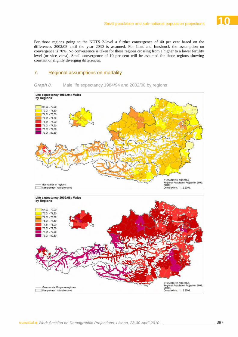
10Small population and sub-national population projections
397Work Session on Demographic Projections, Lisbon, 28-30 April 2010
For those regions going to the NUTS 2-level a further convergence of 40 per cent based on the differences 2002/08 until the year 2030 is assumed. For Linz and Innsbruck the assumption on convergence is 70%. No convergence is taken for those regions crossing from a higher to a lower fertility level (or vice versa). Small convergence of 10 per cent will be assumed for those regions showing constant or slightly diverging differences.
7. Regional assumptions on mortality
Graph 8. Male life expectancy 1984/94 and 2002/08 by regions

10Small population and sub-national population projections
398Work Session on Demographic Projections, Lisbon, 28-30 April 2010
As shown in graph 8 and 9, life expectancy increased explicitly for females and males over all regions. Those districts which show no convergence to the life expectancy of its associated NUTS 2-region are expected to hold differences constant. For regions showing convergence with the related values of its province relative differences in life expectancy will be bisected until the year 2050. This could be different for the both sexes. Therefore in some NUTS 2-regions (Länder) male discrepancies are constant but females converge or vice versa.
Graph 9. Female life expectancy 1984/94 and 2002/08 by regions

10Small population and sub-national population projections
399Work Session on Demographic Projections, Lisbon, 28-30 April 2010
8. Regional assumptions on migration
International immigration by region is determined by the values of the given NUTS 2-projection. Based on migration statistics 2002/08 and a modification considering not only flows of immigration but also the stock of population born abroad the age, sex and region specific allocation rates for the total number of immigrants are compiled. Those rates are kept constant over the whole projection period. The absolute number is given by the higher-ranking population projection for Austria (graph 10). As shown in this map the highest shares of immigrants are gathered by the cities and their environs.
Graph 10. Allocation of immigration 2002/08 by regions (per 1.000)
Graph 11. Emigration rates 2002/08 by regions

10Small population and sub-national population projections
400Work Session on Demographic Projections, Lisbon, 28-30 April 2010
In the long run age and sex specific emigration rates are kept constant as derived from migration statistics 2002/08. In 2002 new migration statistics were developed based on the population register. For the times before no valid migration data are available for Austria.
The pictures of immigration and emigration are more or less congruent. Those areas with high shares of immigration show also higher emigration due to return migration or emigration of the autochthonous population (graph 11).
Graph 12. Internal emigration rates 2002/08 by regions
Graph 13. Internal immigration rates 2002/08 by regions

10Small population and sub-national population projections
401Work Session on Demographic Projections, Lisbon, 28-30 April 2010
As applied in the higher-level NUTS 2-projection also on regional level internal migration is predicted by constant age, sex and direction specific migration rates based on the actual levels as shown by Austrian migration statistics for the years 2002-2008. Graphs 12 to 14 picture the total rates for internal emigration and immigration as well as the balance rate per 1 000 inhabitants.
Highest rates for internal out- and in-migration are counted for the urban areas. Here the centres as well as their surrounding regions show the highest mobility.
The absolute winners of internal migration are primarily the environs of the big cities like Vienna, Graz and Linz. The districts in the centre of Vienna show an negative internal migration balance.
For the 23 districts of Vienna additional attention is drawn to new constructed buildings being settled in the next years. Our projection model SIKURS supports some modifications in the matrix of internal (but also international) migration which allows filling those areas finishing the construction of a significant number of new flats in future with population outside from regular internal migration.
Graph 14. Balance rates of internal migration 2002/08 by regions

10Small population and sub-national population projections
402Work Session on Demographic Projections, Lisbon, 28-30 April 2010
9. The future population development in Austria on regional level (preliminary results)
Graph 15. Total population growth 2002-2030 by regions (preliminary results)
Opposite trends will characterize the regional population development of Austria in the next decades. While the number of inhabitants will increase in some regions significantly, in some other regions of the country a population loss is predicted. The urban agglomerations will be the „winner" of the future population development. Due to economical tendencies of the last years (increase of the service sectors, internationalization of enterprises), cities and suburban areas are attractive both for interregional and international migrants. In all urban agglomerations in Austria the population will increase considerably, especially in the “Vienna Region” and in the region of Graz. However, a counter rotating development is also expected: While the inner cities might lose population, the suburban municipalities will face a strong population growth (graph 15).
Regions outside of commuter belts of Vienna and outside of other regional capital cities will see a population decline. These areas are too far away to commuting and probable less attractive to reactivate new labour markets. In those regions the population will decrease like in Waldviertel in the north of Austria, in the northern part of Styria or in peripheral sited alpine districts in Carinthia and East-Tyrol. Up to the year 2030 the total change of population base on our 124 regions will vary between -11 and +37 per cent.
In the longer run the number of children and youngsters beyond 20 year will decline in most of Austrian’s regions. This is due to the ageing of the baby boom. Numerically smaller generations of parents steaming from the births decline in the last decades are now starting their families (see graph 16).

10Small population and sub-national population projections
403Work Session on Demographic Projections, Lisbon, 28-30 April 2010
Graph 16. Growth of population aged 0-19 years 2002-2030 by regions (preliminary results)
Regions with increasing numbers of younger people are the cities and their environs. This is a consequence on immigration and internal migration as well as rising fertility in urban areas. Immigrants coming from South East European countries have higher fertility which inflects the absolute number of population aged up to 19 years. On the other hand also young families with children move from the cities into the more green surrounding areas. The region with the highest increase of younger persons until 2030 will see a plus of 32 per cent. The strongest decline is forecasted by -29 per cent.
Working age population will also decline in rural areas but will grow in most of the urban regions. The suburbanisation of Vienna escalates more and more. In the meantime not only the surrounding districts of Lower Austria but also the northern parts of the Burgenland are affected by this development.
The picture of Vienna which looks like a muffin is similar concerning all ages. The central districts lose population in total, but also in the age groups of children and working age population. The increase of elderly people is somewhat smaller. On the other hand the districts in the periphery with more free areas for new buildings will gain population.
The range of changing in the regional working age population for the next two decades runs from -18 to +28 per cent.

10Small population and sub-national population projections
404Work Session on Demographic Projections, Lisbon, 28-30 April 2010
Graph 17. Growth of population aged 20-64 years 2002-2030 by regions (preliminary results)
Graph 18. Growth of population aged 65+ years 2002-2030 by regions (preliminary results)
The number of population aged 65 years or more will strongly increase in all 124 projection districts of Austria.

10Small population and sub-national population projections
405Work Session on Demographic Projections, Lisbon, 28-30 April 2010
There is no region having forecasted a smaller figure of elderly persons in the year 2030 than observed today. The smallest increases will see the regions with population decline. Here the increment of elderly people is retarded by out migration. Up to the year 2030 the regional increase of persons older than 65 years will vary between +9 and +85 per cent.
References
D. Ediev: Extrapolative Projections of Mortality: Towards a More Consistent Method. Part I: The Central Scenario. Vienna Institute of Demography, Working Paper 3/2008, Vienna 2008.
A. Hanika, G. Biffl, H. Fassmann, J. Kytir, G. Lebhart, St. Marik, R. Münz: ÖROK-Prognosen 2001-2031, Teil 1: Bevölkerung und Arbeitskräfte nach Regionen und Bezirken Österreichs; Österreichische Raumordnungskonferenz (ÖROK), Schriftenreihe Nr. 166/I; Vienna 2004 (Summary in English).
A. Hanika, E. Bauer, H. Fassmann, G. Lebhart St. Marik, R. Münz: ÖROK-Prognosen 2001-2031, Teil 2: Haushalte und Wohnungsbedarf nach Regionen und Bezirken Österreichs; Österreichische Raumordnungskonferenz (ÖROK), Schriftenreihe Nr. 166/II; Vienna 2005 (Summary in English).
A. Hanika, J. Klotz, St. Marik-Lebeck: Zukünftige Bevölkerungsentwicklung Österreichs 2009 bis 2050 (2075), Neue Bevölkerungsprognose für Österreich und die Bundesländer; in Statistische Nachrichten 11/2009, p963-985, Statistics Austria 2009 (Summary in English).
Kommunales Statistisches Informationssystem KOSIS Verbund: Bevölkerungsprognoseprogramm SIKURS 8.9, http://www.staedtestatistik.de/sikurs.html
A. Rogers, J. Little: Parameterizing age patterns of demographic rates with the multiexponential model schedule. Mathematical Population Studies 3, 1994, p175-195.
Statistics Austria, Bevölkerungsstand 1.1.2009, inkl. Revision seit 1.1.2008. Statistics Austria, Vienna 2009 (Summary in English).
Statistics Austria, Demographisches Jahrbuch 2008. Statistics Austria, Vienna 2009 (Summary in English).
Statistics Austria, Wanderungsstatistik 2008, inkl. Revision 2002-2007. Statistics Austria,


10Small population and sub-national population projections
407Work Session on Demographic Projections, Lisbon, 28-30 April 2010
SUB-NATIONAL AND FOREIGN-BORN POPULATION PROJECTIONS. THE CASE OF ANDALUSIA
Joaquín PLANELLES1, Silvia BERMÚDEZ1,
Juan Antonio HERNÁNDEZ1
Abstract
Over the last fifty years population structure has experienced a dramatic change in Spain, as it has in most European countries. In that period, life expectancy at birth showed an ever-growing trend and fertility rates settled well below replacement ratio. As this process is expected to continue, population ageing has become a key issue and a challenge in our society.
Under those circumstances, natural growth remains slightly above zero-threshold in Spain, so immigration over the last decade is responsible for population growth.
Foreign born population´s sex and age structure differs from the general one, so it modifies the trends in population ageing. But there are two issues which deserve special mention. First, foreign-born population does not settle uniformly across the territory but just in certain locations, so it modifies regional and local dynamics of population change stronger than national ones.
Second, -last but not least- there is strong evidence pointing to a differential demographic behaviour of immigrants, and within immigrants too, depending on their origins. Thus, migration hypothesis might have a significant indirect effect on future fertility, mortality and also on internal-mobility patterns. Unbiased population projections should allow for incorporating different demographic behaviours.
The aim of this paper is to present data sources, methodology and results of the new population projections of Andalusia Region which distinguish several groups of population based on their place of birth. The Andalusian case is especially interesting for our purpose as it presents a wide range of immigrant profiles. On the one hand there is a significant inflow of retired population coming from EU countries; on the other hand labour oriented immigration has increased in recent years.
In the first part of the paper it is discussed whether populations should be distinguished by nationality or place of birth, and the reasons which led us to choose place of birth as criteria. In the second part of this paper we will describe the projection of the components of population change, namely fertility, mortality and migration. Lastly, main results are presented.
1. Nationality versus place of birth
In this work we describe the recent work on population projections made at the IEA (Instituto de Estadística de Andalucía, Statistical Institute of Andalusia). Its main novelty is that population is not only distinguished by sex, age and location, but also using as fourth variable the origin of individuals.
1 Instituto de Estadística de Andalucía

10Small population and sub-national population projections
408Work Session on Demographic Projections, Lisbon, 28-30 April 2010
Different Statistical Institutes have already addressed this issue. However, it is worth mentioning that there is no unanimity on the meaning of the term “origin of individuals”. The most popular choices are to take as origin either the nationality or the place of birth. A different approach has been followed, for instance, in the USA, to project Hispanic-origin population.
The choice of one definition or another is mainly motivated by the data available and also on the plausibility of identifying demographic clusters.
2. Subpopulations
The arrival of immigrants in recent years explains that, although the vegetative growth has been moderate, the increase in population in Andalusia has attained its highest records. This phenomenon is not only seen in Andalusia, since the process has been even more intense in other regions in Spain. Moreover, the immigrant population has different demographic patterns. This motivates the need of a detailed analysis of this population group.
Table 1. Population in Andalusia and Spain. 1900-2009.
As mentioned above, several Statistical Institutes have started to distinguish groups with different patterns for fertility, mortality or mobility. It is customary assumption (not always made explicit) that such patterns will disappear or will be reduced with time. In some cases even the demographic pattern of second generations is considered.
A feature which plays a central role for planning population projections by place of birth or nationality is how many groups should be distinguished. The answer is far from trivial as it requires a balance between groups which are big enough provide a wide sample and groups whose members share similar behavior patterns.
In our population projection system five groups were chosen based on their place of birth. Both population structure and demographic behavior of those five groups were unique to their particular group.
As shown in Figure 1, the EU15 population which settled in Andalusia has a peculiar age structure with two local maximums, one around the age of 35 and a second one at retirement age. The three other pyramids show a strong inclination for people between 20 and 40 years of age and exhibit noticeable gender differences. Male Andalusian population coming from Africa counts for twice their female counterparts. On the contrary, females comprise the majority of those coming from Latin America.
Census Andalusia Spain Andalusia Spain Andalusia Spain Andalusia Spain
1900 3.545 18.6181910 3.800 19.996 256 1.378 7,0‰ 7,2‰1920 4.222 21.390 421 1.394 10,6‰ 6,8‰1930 4.627 23.678 405 2.288 9,2‰ 10,2‰1940 5.254 26.016 627 2.338 12,8‰ 9,5‰1950 5.647 27.977 393 1.961 7,2‰ 7,3‰ 5911960 5.940 30.529 293 2.552 5,1‰ 8,8‰ 871 3.3481970 5.991 34.041 51 3.512 0,9‰ 10,9‰ 922 3.9051981 6.441 37.683 450 3.642 7,1‰ 10,0‰ 745 3.5541991 6.941 38.872 500 1.189 7,5‰ 3,1‰ 462 1.466
Padrón 2001 7.404 41.117 463 2.245 6,6‰ 5,7‰ 233 300Padrón 2009 8.303 46.746 899 5.629 14,4‰ 16,2‰ 212 667
Natural growth (thousands)
Population (thousands)
Total growth (thousands)
Annual growth rates (‰)

10Small population and sub-national population projections
409Work Session on Demographic Projections, Lisbon, 28-30 April 2010
Figure 1. Population pyramids by place of birth. Andalusia 2006.
50‰ 40‰ 30‰ 20‰ 10‰ 0‰ 10‰ 20‰ 30‰ 40‰ 50‰
0-45-9
10-1415-1920-2425-2930-3435-3940-4445-4950-5455-5960-6465-6970-7475-7980-8485-8990-9595-99100+
Male Female
Number of people: 7.995.464Place of birth: ALL
50‰ 40‰ 30‰ 20‰ 10‰ 0‰ 10‰ 20‰ 30‰ 40‰ 50‰
0-45-9
10-1415-1920-2425-2930-3435-3940-4445-4950-5455-5960-6465-6970-7475-7980-8485-8990-9595-99100+
Male Female
Number of people: 7.406.929Place of birth: SPAIN
80‰ 60‰ 40‰ 20‰ 0‰ 20‰ 40‰ 60‰ 80‰
0-45-9
10-1415-1920-2425-2930-3435-3940-4445-4950-5455-5960-6465-6970-7475-7980-8485-8990-9595-99100+
Male Female
Number of people: 188.469Place of birth: UE15
80‰ 60‰ 40‰ 20‰ 0‰ 20‰ 40‰ 60‰ 80‰ 100‰
0-45-9
10-1415-1920-2425-2930-3435-3940-4445-4950-5455-5960-6465-6970-7475-7980-8485-8990-9595-99100+
Male Female
Number of people: 148.202 Place of birth: LATINAMERICA
160‰ 140‰ 120‰ 100‰ 80‰ 60‰ 40‰ 20‰ 0‰ 20‰ 40‰ 60‰
0-45-9
10-1415-1920-2425-2930-3435-3940-4445-4950-5455-5960-6465-6970-7475-7980-8485-8990-9595-99100+
Male Female
Number of people: 135.781Place of birth: ÁFRICA
100‰ 80‰ 60‰ 40‰ 20‰ 0‰ 20‰ 40‰ 60‰ 80‰ 100‰
0-45-9
10-1415-1920-2425-2930-3435-3940-4445-4950-5455-5960-6465-6970-7475-7980-8485-8990-9595-99100+
Number of people: 116.083Place of birth: OTHER

10Small population and sub-national population projections
410Work Session on Demographic Projections, Lisbon, 28-30 April 2010
Why not choosing different criteria such as nationality to identify population groups? The election depends on several factors, mainly the capability to distinguish population groups whose demographic behavior is homogeneous within groups and differs between them. Another important factor is data availability.
In Spanish demographic data sources it is more likely to record nationality than place of birth. Being so, what persuaded us to use place of birth as criteria? Nationality is something that might change over time, and that generates a few drawbacks:
1. First, had we chosen nationality, additional assumptions on future naturalizations would have been required? And naturalizations logicae relies more on legal and administrative rules rather than different demographic behaviors.
2. What nationality should we assign to the offspring of foreign citizens? The answer is not easy and requires additional questioning. Are both parents foreigners? That being the case, where exactly are they from? Moreover, the child would be given the Spanish nationality if he or she remains stateless otherwise. Thus, consistent assignment of nationalities demands additional hypothesis on those fields. Moreover, both parents should be taken into account to study fertility patterns instead of the traditional maternal-based philosophy.
It is interesting to note that other origin-based projections such as US race projections face similar complexities: which race should we assign to future babies? The answer requires information from parents´ races and parents´ likeliness to marry and/or procreate with other races2.
3. Finally, as nationality might change over time, renewable phenomena such as migrations and fertility could experience unexpected changes.
For instance, a mother could have her z+1 child and hold a different nationality than the one she had when her z child has born. In contexts where naturalizations are large, it might mean unexpected changes in fertility patterns.
Finally, it must be acknowledged that both nationality projecting and place of birth projecting are bound to set hypothesis on naturalized population behavior. When choosing nationality, we are assuming that demographic behaviors change together with nationality. Choosing place of birth as criteria implies that demographic behavior is fixed once born.
Nonetheless, not distinguishing groups within population sets a much more convoluted hypothesis; namely that demographic behaviors are the same regardless of a person´s origin.
2 Assignment of race faces additional draw-backs, due to its subjectivity. A clear example comes from Colombia: in 1993
census only 1,5% of population were recorded afro-colombians. Next census, held in 2005, recorded 10,5% instead.

10Small population and sub-national population projections
411Work Session on Demographic Projections, Lisbon, 28-30 April 2010
3. Demographic phenomena
3.1 Fertility Changes in Andalusian and Spanish fertility patterns are similar to the ones recorded in other European countries, though changes were more drastic in Andalusia (and so in Spain) and they began years later.
Figure 2. Fertility indicators in Andalusia, Spain and European Countries 1950-2008
Immigrants’ fertility is greater and it starts sooner than ‘native’ ones. Moreover, the number of immigrants of childbearing age is considerably high and consequently, their contribution to the total number of births surpasses its population weight3.
Figure 3. Fertility patterns and childbearing age population on the base year
0
10.000
20.000
30.000
40.000
50.000
60.000
70.000
80.000
0
20
40
60
80
100
120
12 14 16 18 20 22 24 26 28 30 32 34 36 38 40 42 44 46 48 50
Non-immigrants
Population (right scale)
Fertility rates (‰)
0
1.000
2.000
3.000
4.000
5.000
6.000
0
20
40
60
80
100
120
12 14 16 18 20 22 24 26 28 30 32 34 36 38 40 42 44 46 48 50
Immigrants
Population (right scale)
Fertility rates (‰)
But immigrant population is a heterogeneous crowd. For instance, fertile behavior of EU15 mothers settled in Andalusia is close to Spanish women, while number of births per woman is higher among the other groups. Such diversity of fertility patterns reinforces us to distinguish sub-populations.
3 Nonetheless, immigrant contribution to TFR is not too big. Such a surprising result is due to immigrant´s age profile: the ages
with higher immigrant fertility are ages with a relative scarcity of immigrant women, as it was shown in Figure 3.
1,0
1,5
2,0
2,5
3,0
3,5
4,0
1950 1955 1960 1965 1970 1975 1980 1985 1990 1995 2000 2005
Num
ber o
f life
bir
ths
per w
oman Andalusia Belgium
Spain DenmarkPantomima GermanyFrance ItalyNetherlands AustriaPortugal FinlandSweden United Kingdom
25
26
27
28
29
30
31
1950 1955 1960 1965 1970 1975 1980 1985 1990 1995 2000 2005
Mea
n ag
e at
mot
herh
ood
Andalusia BelgiumSpain DenmarkPantomima GermanyFrance ItalyNetherlands AustriaPortugal FinlandSweden United Kingdom
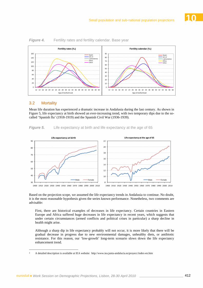
10Small population and sub-national population projections
412Work Session on Demographic Projections, Lisbon, 28-30 April 2010
Figure 4. Fertility rates and fertility calendar. Base year
The methodology used to obtain future fertility rates is based on a parametric model which sets as parameters the TFR (total fertility rate) and MM (mean age at motherhood) 4.
3.2 Mortality Mean life duration has experienced a dramatic increase in Andalusia during the last century. As shown in Figure 5, life expectancy at birth showed an ever-increasing trend, with two temporary dips due to the so-called ‘Spanish flu’ (1918-1919) and the Spanish Civil War (1936-1939).
Figure 5. Life expectancy at birth and life expectancy at the age of 65
30
40
50
60
70
80
90
1900 1910 1920 1930 1940 1950 1960 1970 1980 1990 2000 2010
Life expectancy at birth
Male Female8
10
12
14
16
18
20
22
1900 1910 1920 1930 1940 1950 1960 1970 1980 1990 2000 2010
Life expectancy at the age of 65
Male Female
Based on the projection scope, we assumed the life expectancy trends in Andalusia to continue. No doubt, it is the most reasonable hypothesis given the series known performance. Nonetheless, two comments are advisable:
First, there are historical examples of decreases in life expectancy. Certain countries in Eastern Europe and Africa suffered huge decreases in life expectancy in recent years, which suggests that under certain circumstances (armed conflicts and political crises in particular) a sharp decline in health might arise.
Although a sharp dip in life expectancy probably will not occur, it is more likely that there will be gradual decrease in progress due to new environmental damages, unhealthy diets, or antibiotic resistance. For this reason, our ‘low-growth’ long-term scenario slows down the life expectancy enhancement trend.
4 A detailed description is available at IEA website: http://www.iea.junta-andalucia.es/proyecc/index-en.htm
0
20
40
60
80
100
120
140
160
12 14 16 18 20 22 24 26 28 30 32 34 36 38 40 42 44 46 48 50
Age of motherhood
Fertility rates (‰)
SpainUE 15LatinamericaAfricaOther
0
10
20
30
40
50
60
70
80
90
12 14 16 18 20 22 24 26 28 30 32 34 36 38 40 42 44 46 48 50
Age of motherhood
Fertility calendar (‰)
SpainUE 15LatinamericaAfricaOther

10Small population and sub-national population projections
413Work Session on Demographic Projections, Lisbon, 28-30 April 2010
Besides, as the life expectancy nears the human life biological limit (whatever it might be) a slowdown could be recorded as marginal improvements would become increasingly difficult to overcome.
But where to place such a biological limit? This is the major clue at hand to project long-term mortality rates, and there are heated medical controversies about. Some researchers state the limits are nearby (Olshansky, 1990). Other researchers believe life expectancy will continue to rise, reaching up to 115-120 years which are the longest lives ever recorded (Vaupel, 1996). Finally, there are a few researchers which place human kind at the verge of a medical revolution against genetic ageing itself which might mean an even greater limit (de Grey, 1999).
Moving on to differential place of birth mortality, it is not clear -nor easy- to evaluate whether immigrants hold a different mortality pattern to ‘natives’. On the one hand, a clear positive correlation exists between income and health status. As immigrant income is significantly below the mean Andalusian income, an above-the-mean morbility and mortality pattern for immigrants might be expected. On the other hand, emigration process selects healthy individuals and that points in the opposite direction, to below-the-mean morbility and mortality patterns of immigrants.
Moreover, as shown in Figure 1, Andalusian immigrant population is strongly concentrated between 20 and 45 years of age, ages with a very low likeliness to die. In 2008 foreign-born population accounted for 3% of the total number of deaths in Andalusia –half of them from EU15 countries- while their share on population amounts to 8%. Under those circumstances, it wouldn´t be reliable to specify a specific model for each group.
Research developed in countries with long immigration tradition is not conclusive either. For instance, latino mortality in the US is found to be lower than the medium US citizen (Abraído-Lanza, 1999). Why so? A key factor to explain this is the so-called ‘salmon bias’: latinos are likely to go back to their home countries when they get ill. Thus, immigrants are less likely to be recorded dead but just as returning emigrants. Research developed elsewhere is not conclusive either and sometimes points to below-the-mean immigrant life expectancy (Deboosere, 2005 & Bos, 2004).
Therefore, at the Statistical Office of Andalusia we did not specify a different mortality pattern among immigrants.
3.3 Migrations Migrations represent a key factor in Andalusian recent demographic development. It would be impossible to approach Andalusia recent history without tackling migration phenomenon. Andalusia lost more than a million inhabitants during the period 1950-1975, due to its net migration sign.
After that period net migrations stabilized reaching negligible values. It is only in recent years, from late nineties, that net migrations have recovered its importance due to a tremendous increase in international immigration flows.
Migration is known as the most volatile demographic phenomenon and therefore the most complex to deal with when forecasting. Besides, migration analysis presents other limitations. Firstly, the migration´s information quality is significantly worse compared to other phenomena (births and deaths are perfectly tracked by the Statistical bulletin provided by the Official Civil Register).
Secondly, we should distinguish within phenomena based on the direction of the flow and the geographical scope (i.e: internal & external, in - out migration).
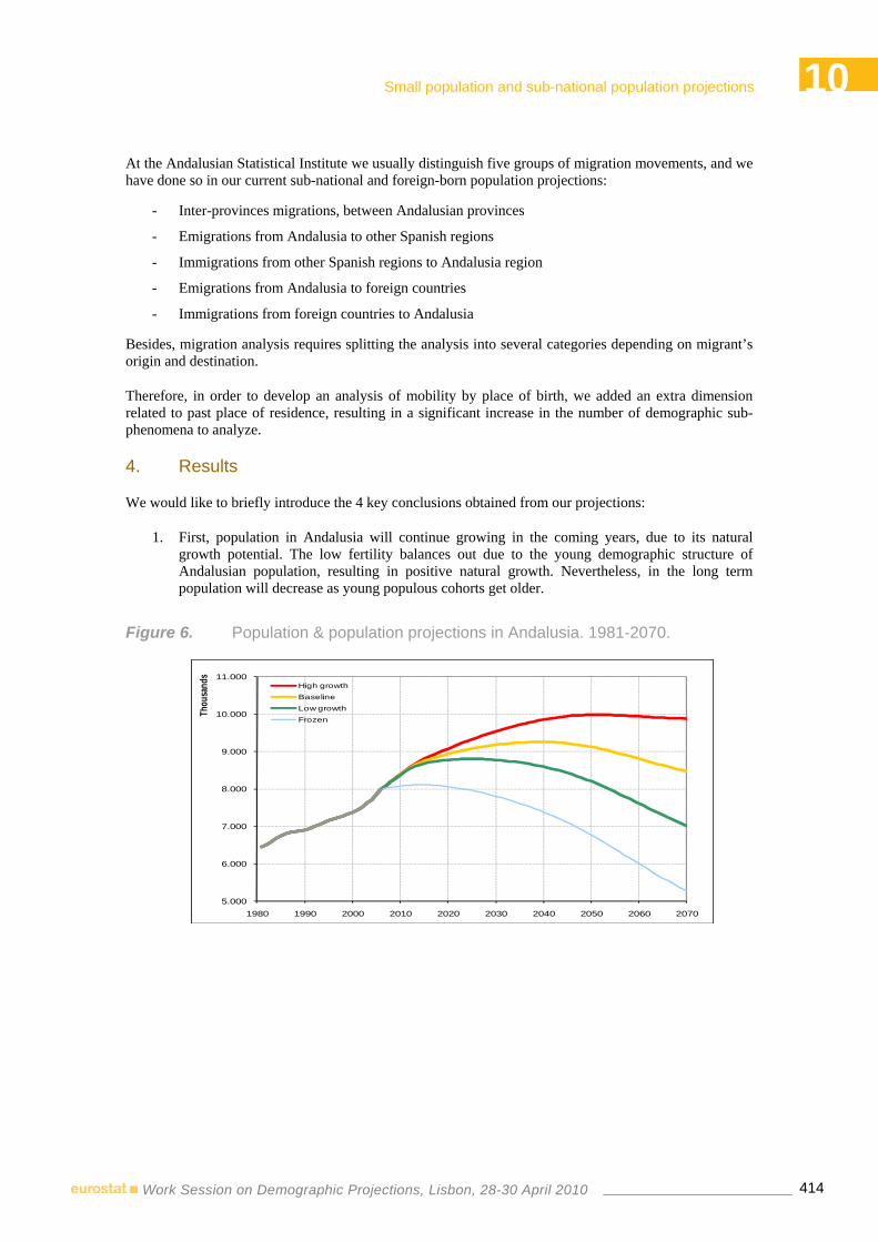
10Small population and sub-national population projections
414Work Session on Demographic Projections, Lisbon, 28-30 April 2010
At the Andalusian Statistical Institute we usually distinguish five groups of migration movements, and we have done so in our current sub-national and foreign-born population projections:
- Inter-provinces migrations, between Andalusian provinces
- Emigrations from Andalusia to other Spanish regions
- Immigrations from other Spanish regions to Andalusia region
- Emigrations from Andalusia to foreign countries
- Immigrations from foreign countries to Andalusia
Besides, migration analysis requires splitting the analysis into several categories depending on migrant’s origin and destination.
Therefore, in order to develop an analysis of mobility by place of birth, we added an extra dimension related to past place of residence, resulting in a significant increase in the number of demographic sub-phenomena to analyze.
4. Results
We would like to briefly introduce the 4 key conclusions obtained from our projections:
1. First, population in Andalusia will continue growing in the coming years, due to its natural growth potential. The low fertility balances out due to the young demographic structure of Andalusian population, resulting in positive natural growth. Nevertheless, in the long term population will decrease as young populous cohorts get older.
Figure 6. Population & population projections in Andalusia. 1981-2070.
5.000
6.000
7.000
8.000
9.000
10.000
11.000
1980 1990 2000 2010 2020 2030 2040 2050 2060 2070
Thou
sand
s
High growthBaselineLow growthFrozen

10Small population and sub-national population projections
415Work Session on Demographic Projections, Lisbon, 28-30 April 2010
Table 2. Projected population in Andalusia.2006-2070
2006 2010 2025 2050 2070 Max. Year Max. Value
High grow th 7.995.464 8.397.688 9.325.403 9.978.712 9.878.831 2051 9.979.904Baseline 7.995.464 8.389.270 9.081.244 9.121.016 8.466.562 2039 9.251.974Low grow th 7.995.464 8.379.598 8.802.420 8.196.691 7.011.851 2025 8.802.420
Frozen 7.995.464 8.074.284 7.954.634 6.768.813 5.267.768 2014 8.106.595
2. Second, the number of births will decrease even in the case of significant increases in fertility rates. The baseline scenario dates the drop in fertility from 2010.
Therefore, we may witness growth in fertility rates in the coming years, but the total number of births will certainly fall as the tiny 80’s and 90’s cohorts reach the childbearing age.
Figure 7. Births & projected births. Andalusia. 1990-2025
60.000
65.000
70.000
75.000
80.000
85.000
90.000
95.000
100.000
105.000
1990 1995 2000 2005 2010 2015 2020 2025
Total
numb
er of
birth
s
High growthBaselineLow growth
3. Currently we observe a high trend towards population ageing.5. In 2050 –according to baseline scenario- the proportion of population over 65 years would reach 29,1% and 9,8% the proportion of population over 80 years (compared to 14,2% and 3,4% nowadays). In other words, the ratio of labour-force population to retired population would change dramatically from 4,6 in 2006 to 1,9 in 2050.
5 We should think about what we mean by ageing. In a situation where life expectancy and free-disabilities life expectancy are
growing, static indicators may become meaningless. E.g.: static indicators such as the proportion of population over 65 hide the fact that this group of population in 2008 is physically and psychologically different from their counterparts in 1950. Despite this remark we have used static indicators in order to measure population ageing in our projections.

10Small population and sub-national population projections
416Work Session on Demographic Projections, Lisbon, 28-30 April 2010
Figure 8. Projected population by age group
500
750
1.000
1.250
1.500
1.750
2.000
1980 1990 2000 2010 2020 2030 2040 2050 2060 2070
Thou
sand
s
<16
High growthBaselineLow growthFrozen
3.000
3.500
4.000
4.500
5.000
5.500
6.000
6.500
1980 1990 2000 2010 2020 2030 2040 2050 2060 2070
Thou
sand
s
16-64
High growthBaselineLow growthFrozen
500
1.000
1.500
2.000
2.500
3.000
1980 1990 2000 2010 2020 2030 2040 2050 2060 2070
Thou
sand
s
65+
High growthBaselineLow growthFrozen
0
200
400
600
800
1.000
1.200
1980 1990 2000 2010 2020 2030 2040 2050 2060 2070
Thou
sand
s
80+
High growthBaselineLow growthFrozen
4. Finally, a brief comment on future foreign-born population. Foreign born population projection is likely to increase moderately in the future. This might help to cope with ageing challenges in the short run. But in the long term, immigrant population will get older too (Figure 9).
Figure 9. Foreign-born population figures and age structure. Baseline scenario.
0%
2%
4%
6%
8%
10%
12%
14%
1999 2001 2003 2005 2007 2009 2011 2013 2015 2017 2019 2021 2023 2025
Foreign-born population share
20‰ 15‰ 10‰ 5‰ 0‰ 5‰ 10‰ 15‰ 20‰
05
1015202530354045505560657075808590
Age
2025
2006
Male Female

10Small population and sub-national population projections
417Work Session on Demographic Projections, Lisbon, 28-30 April 2010
Reference
Abraído-Lanza A.F., et al. (1999) The Latino mortality paradox: a test of the "Salmon bias" and healthy migrant hypothesis. American Journal of Public Health. 1999;89:1543–1548.
Bos, V (2004). Ethnic inequalities in age and cause-specific mortality in the Netherlands. International Journal of Epidemiology. 2004; 33: 112-119.
Deboosere, PD. & Gadein, S. (2005). La sous-mortalité des immigrés adultes en Belgique: une réalité attestée . Population, 60(5-6).
de Grey, Aubrey (1999). The mitochondrial free radical theory of agening. Austin, TX. Landes Bioscience.
Instituto de Estadística de Andalucía (2008). Proyección de la población de Andalucía 2006-2070. Sevilla.
Olshansky S, Carnes B y Cassel, C (1990). In search of Methuselah: estimating the upper limits to human longevity. Science. 250;634-640.
Pérez-Díaz, J. (2003). La feminización de la vejez y estado de bienestar. Revista Española de Investigaciones sociológicas. 104; 91-121.
Vaupel, JW y Lundström, H (1996). The future of mortality al older ages in developed countries. The future population of the world. What can we assume today? IIASA, Laxenbur, Austria


Beyond population projections by age and sex Chair: Jorge Miguel Bravo
Session 11


11Beyond population projections by age and sex
421Work Session on Demographic Projections, Lisbon, 28-30 April 2010
PROJECTIONS OF RELIGIOSITY FOR SPAIN
Marcin STONAWSKI, Vegard SKIRBEKK1,
Samir KC, Anne GOUJON
1. Introduction
In spite of the generally large interest in current and future religious change and its impact on demography only a limited amount of scholarly research has been carried out on the topic of religious projections (Barrett et al. 2001, Goujon et al. 2007, Johnson and Grim 2008, Statistics Canada 2005, Skirbekk et al. 2010). The projections that have been carried out until date focus on denominations - the present study is the first one to focus on demographic projections of religiosity.
The degree of religiosity cuts across religions and more religious subgroups of the population were found to have higher fertility regardless of their affiliation in many settings e.g. in France (Regnier-Loillier and Prioux 2008) and in the USA (Skirbekk et al. 2010). The religion induced variation in fertility cuts across religious groups and has in some studies been shown to have a greater impact on demographic behaviour than type of religious affiliation (Finnas 1991; Jampaklay 2008; Philipov and Berghammer 2007). Religiosity (measured as intensity of belief or practice of adherents of different faiths) has been found to be a powerful determinant of family formation patterns, such as timing and outcome of marriage and fertility, although it interrelates with socio-economic, cultural and political contexts (Lehrer 2004; Philipov and Berghammer 2007; McQuillan 2004). Deeply religious individuals often argue that their current family beliefs and behaviour are primarily the outcomes of their religion’s teachings (Borooah 2004; McQuillan 2004). Moreover, even if changes in religious affiliation may be small, changes in religious intensity could be far greater, one example being the growth in the proportion “belonging without believing” (Marchisio and Pisati 1999).
Spain is an interesting country for the study of religion and religiosity in Europe for several reasons. The Franco regime that saw the installation of Roman Catholicism as the only religion to have legal status and at the time of the Spanish transition to democracy after Francos’s death, the number of non-Catholics was less than 1 percent (Solsten and Meditz 1990). The return of democracy in Spain was accompanied by a rapid increase in secularization rates among the youth, and a rapid decline in fertility that saw the total fertility rate (TFR) decline from 2.8 in 1975 to 2.1 in 1981 and to 1.2 in 1998 (Goujon and K.C. 2009). The third component influencing the religious composition and intensity in Spain is that since the mid-1970s Spain reversed its role as an emigration country and became increasingly a receiving country, first as transit country for migrants heading to the Northern countries (especially to France and Germany) at the end of the 1980s and since the end of the 1990s one of the most important destination countries in Europe for foreign migrants from all over the world mostly from North Africa and South America and recently from the rest of Africa, Asia and Europe.
1 International Institute for Applied Systems Analysis, Schlossplatz 2, 2361 Laxenburg, Austria. Corresponding author: Vegard
Skirbekk, [email protected], tel. 002236807 378

11Beyond population projections by age and sex
422Work Session on Demographic Projections, Lisbon, 28-30 April 2010
2. Method
In this study we carry out multistate population projections by religion and religiosity for Spain in the period 2010-2050. First we estimate the base population, for the year 2005 by age, sex, religion and religious intensity. We identify the size and composition of migration flows by denomination and religiosity. Differentials in childbearing patterns by religion and degree of religiosity are then calculated. We also estimate and model age- and sex-specific religious conversion rates by denomination and religiosity. We further assume that the child’s religion and religiosity assumed is identical to that of mother’s until the age of 15, so that the fertility differentials affect the variation in the religious (both denomination and intensity) composition of the next generation.
We assume that there are no causal relation between mortality and religion (for a discussion see (Goujon 2007)). Several scenarios, based on combining different assumptions for fertility and migration, covering wider uncertainty range of the demographic future are constructed.
The Spanish population disaggregated by age, sex, religion, and degree of religiosity was projected till 2050 according to these scenarios. The results are then analyzed for the sensitivity in the future structure of the population to the different assumptions on fertility and migration of future Spanish population.
2.1 Definition of religiosity Religiosity has been measured in surveys by a range of different questions, including religious attendance, religious practice and self-assessed religiosity (see f. ex. Billiet 2003, Skirbekk et al. 2010). The problem of most of these measures is that they may be suited to compare religiosity within one religion, but may fail to compare religiosity between denominations, as different religions give different weight to the importance of religious attendance and religious practice. In order to increase comparability we choose to focus primarily on self-assessed religiosity.
We use a dichotomous definition of religiosity, where religious groups are either “moderate” or “highly” religious. For the resident Spanish population, we use estimates from the European Social Survey where self assessed religiosity is the basis.
2.2 Baseline estimates The structure of Spanish population by age, sex, religious denomination and intensity in 2005 is estimated using information from various sources. Data on religion affiliation is not available in the census (IRFR 2008). Thus, in our approach we use data from surveys and municipal registers. In order to estimate the share of the main religious groups: Roman Catholics, Unaffiliated and Others by age and sex, we use microdata from the survey Barometro Autonomico 2005 done by The Centro de Investigaciones Sociologicas (CIS) (only these three groups are stated in the survey question). Their data gives 78.20% Catholics, 18.21% Unaffiliated “Nones”, while “Others” are redistributed as explained below into three groups Muslims, Hindu/Buddhists and Protestants and Others.
The substantial increase in the share of Muslims and Hindu/Buddhists is a recent phenomenon driven mainly by migration flows. We use official migrants’ statistics by country of birth (from statistical office INE) in order to estimate shares of religious groups that are mainly the result of relatively recent migration. For instance, the growth of Muslims began in the early 1990s when the size of this group was estimated at just 2350 people (Peach and Glebe 1995).
In 2005, there were 4.8 million immigrants in Spain – 11.1 percent of the total population (World Bank 2006), with Moroccans forming the largest single group. Our approach relies on the assumption that migrants are randomly picked from population of country of origin and that they have the same structure by religious denomination as in the sending country. Information on the percentage of religious denominations by country was collected from the following sources: the CIA World Factbook 2010, ARDA religion database 2010 and World Religion Database 2010. Based on this approach we find that

11Beyond population projections by age and sex
423Work Session on Demographic Projections, Lisbon, 28-30 April 2010
there are 1.60% Muslims and 0.04% Hindus and Buddhists. The share of Protestant and Others were estimated to be about 1.94% (e.g. according to Johnson and Ross (2009) there are 130 thousand Evangelicals and 120 thousand of Protestants in Spain in 2010).
For each religious denomination two intensity levels are created: highly religious and moderately religious. The distinction between the two groups are based on self-assessed religiosity estimated by age, sex and religious denomination using data from European Social Surveys 2002-2008 (IV waves) [11-scale question: Regardless of whether you belong to a particular religion, how religious would you say you are?, recoded: 5-10 “highly religious”, 0-4 “moderately religious”]. Religious intensity for migrants is assumed to be the same as in country of origin. Data on religious intensity comes from the Gallup WorldView survey [2-scale question (Yes/No): Is religion an important part of your life?].
The baseline structure of the Spanish population is given in Figure 1a by religion and religiosity, and by population shares of three religiosity groups in Figure 1b. Figure 1a shows that the older age groups are dominated by the highly religious Catholics, those with no religion have a younger age structure and minority religions tend to be still younger. Figure 1b also shows that the highly religious tend to be older (regardless of denomination), that women are more religious than men and the youngest age groups are somewhat more religious (which follows from the higher fertility of the more religious and a high degree of intergenerational transmissions).
Figure 1a. Structure by age, sex and religious denomination and intensity in Spain in 20052
2 Labels used in graphs: Denomination-H stands for Denomination-highly religious; Denomination-M means Denomination-
moderately religious.

11Beyond population projections by age and sex
424Work Session on Demographic Projections, Lisbon, 28-30 April 2010
Figure 1b. Spanish population by three groups of religiosity
2.3 Conversion rates by age and sex Conversions between religious groups and changes in the degree of religiosity are assumed to take place relatively early in life, at ages 15-29 (gradual change). The assumption that age-change takes place early in life is supported by several studies, including longitudinal, retrospective and age-period-cohort analyses. In particular, conversion and secularisation have been shown to occur mainly in early adulthood based on evidence for a number of European countries (Te Grotenhuis, De Graaf et al. 1997; Crockett and Voas 2006; Skirbekk 2008; Skirbekk et al. 2008; Wolf 2008). In prime age and senior adulthood, switching affiliation and degree of religiosity is much less likely; and therefore religious change tend to take place along cohort lines, where cohort replacement determines religiosity (Crockett and Voas 2006). The human capital model of life cycle change suggests that individuals change their beliefs and religious views in a matching procedure which occur early in life (Becker 1967; Becker 1981). As an individual grows older, one has increasingly invested in one specific religious community and the cost of religious switching increases as the “capital” specific to one religious community grows. Hence, fewer prime-age adults and even fewer seniors will convert (Iannaccone 1992).
For transition rates by religiosity, we have information on attendance at ages 11-12 and religious attendance at the age when interviewed (we do not have information on past-self-assessed religiosity). We use attendance of religious services at least once a month as the cut off point for being highly religious, as this overlaps with the average religiosity scale 5-10 in the ESS I-IV- average. Our estimates are given in Tables 1a and 1b, where transitions between religious intensity groups of Catholic and Protestants as well as secularization rates for these groups are taken into account. Transitions between other groups are not taken into account due to data availability.

11Beyond population projections by age and sex
425Work Session on Demographic Projections, Lisbon, 28-30 April 2010
Tables 1a. Transition rates (in %) - males
Current Religious Group
Catholic-H Catholic-M Prot&Oth-H Prot&Oth-M None
Catholic-H 0.65 0.12 0.00 0.00 0.23
Catholic-M 0.04 0.69 0.00 0.00 0.27
Prot&Oth-H 0.00 0.00 0.64 0.11 0.25 Former
Prot&Oth-M 0.00 0.00 0.04 0.67 0.30
Table1b. Transition rates (in %) - females
Current Religious Group
Catholic-H Catholic-M Prot&Oth-H Prot&Oth-M None
Catholic-H 0.92 0.04 0.00 0.00 0.04
Catholic-M 0.07 0.65 0.00 0.00 0.28
Prot&Oth-H 0.00 0.00 0.92 0.04 0.04 Former
Prot&Oth-M 0.00 0.00 0.07 0.64 0.29
3. Migration
Migration data is given in figure 2a-b, which shows both the resident distribution of migration and the net migrant flow by religion-religiosity. The religion/intensity distribution of the migrant population flow is based on the country of origin database available at the website of Eurostat, which was combined with our estimates of religion structure in the sending countries.
Figure 2a. Structure of Spanish population by religious denomination and religiosity

11Beyond population projections by age and sex
426Work Session on Demographic Projections, Lisbon, 28-30 April 2010
Figure 2b. Structure of Spanish migrant population by religious denomination and religiosity
Immigration is very strong also in comparison with other European countries and as a result Spain has one of the highest percentages of foreign population compared to other European Union countries. The net migration flow in and out of Spain amounted to 698 548 persons in 2006 with 840 844 immigrants (95% foreign born) and 142 296 emigrants (84% foreign born) making Spain one of the countries with highest net migration rate as well as net migration size. Among the immigrants, in 2006, Europeans represented 43% of foreign born population, mostly from Romania (38%), United Kingdom (12%), and Bulgaria (6%) but also from Portugal, Italy, Poland and Germany with 5% each. Immigrants from America represented 39% in 2006 and originated from a large number of countries such as Bolivia (25%), Colombia (11%) and Brazil (10%). Other migrants came from North and Sub-Saharan Africa (15%), of which 67% came from Morocco and 6% from Senegal.
4. Fertility
The estimations of fertility differentials are based on results from the 1999 Spanish Fertility Survey (INE) and municipal registration of births and population by nationality and age of mother (INE, available data from the period 1996-2008). Fertility for Muslims is assumed to be equal to the level calculated for population of Moroccans, Algerians and Pakistanis, which constitute about 84% of estimated Muslim population. For Hindu/Buddhists we use fertility of females from India, Nepal, Thailand and Vietnam.
Relative differences in fertility by intensity are based on results of average children ever born for females 40-49 from survey European Social Survey Round 3 (ESS 2006). It was possible only for Catholics (and for the overall population), because for all other groups the sample size was too small for estimation. In order to get a large enough sample, the relative fertility differences for Muslims is approximated from Muslim respondents for all nations participating in the survey (23 European countries) as they constitute about 3% of total sample of ESS countries. For all other religious groups (Hindu/Buddhists and Protestant and Others) we assume (due to a lack of other data) that the difference between highly and moderately religious is similar as to the total population of Spain. The TFR estimates by religious intensity are given in Figure 3. The fertility of the highest religious groups equals 1.7 children, the moderates 1.2 and for those with no religion about 0.9 children, which supports the notion that the more religious groups have more children.

11Beyond population projections by age and sex
427Work Session on Demographic Projections, Lisbon, 28-30 April 2010
Figure 3. TFR by religious intensity in Spain in 2005-2010
The high fertility of the Muslim population above 4 children is likely to partly reflect that most Muslims in Spain are recent migrants in to Spain (see fig. 4). Many of these migrants come for marriage reasons (which can inflate fertility) and many come from countries with relatively high fertility. Over time, with a longer duration of stay and increased integration, the fertility of this groups is likely to at least partially converge to the levels of the rest of the population, which would be in line with empirical findings from Germany, the UK and Canada (Bélanger and Malenfant 2005; Coleman and Dubuc 2010; Schmid and Kohls 2009).
Figure 4. TFR by religious denomination and intensity in Spain in 2005-2010

11Beyond population projections by age and sex
428Work Session on Demographic Projections, Lisbon, 28-30 April 2010
5. Scenarios
In order to investigate the impact of fertility differentials and migration, we project five different scenarios. The main hypothesis behind the five scenarios is that fertility differentials are assumed to be greater if high migration levels should continue. High migration could imply that many migrants from high fertility regions would increase the fertility of religious minorities and delay integration. Table 1 presents an overview of the scenarios:
FsMs: Fertility differentials are stable and constant from starting year levels; Migration size and composition is stable; Transition rates are stable
FgMg: Fertility differentials are gradually converging to the level of full convergence (100%) in 2050 , Migration gradually phases down (decreases by 50% of present levels by 2050); Transition rates are stable
FrMr: Fertility differentials are rapidly converging (100% convergence in 2030); Migration rapidly phases down (decreases by 90% of present levels by 2050); Transition rates are stable
FsMz: Fertility differentials are stable; Migration is zero; Transition rates are stable
FeMz: No Fertility differentials for the whole projection period; Migration is zero for the whole projection period; Transition rates are stable
We do not have any different scenario on conversion, as the present emphasis is only on migration and fertility.
Table 1. Scenario overview
Migration
Fertility Differentials Stable – Migration
constant structure
Gradually phased down (decreases by 50% by 2050)
Rapidly phased down (decreases by 90% by 2050)
Zero
Stable – Fertility differentials constant FsMs FsMz
Gradually converging (100% by 2050) FgMg
Rapidly converging (100% by 2030) FrMr
No differentials, Fertility equal for all groups FeMz
Regarding the fertility gradually converging (100% by 2050) scenario (FgMg), we include figures which show the gradual convergence of the age-specific fertility rates (ASFRs) from observed 2005-2010 data to the universal ASFRs in 2045-2050. Examples are given for the Muslim-highly religious, the Hindu/Buddhist-highly religious (both which are assumed to experience a fertility decline over the period) while for those with no religion a gradual increase in ASFRs over the period is shown.

11Beyond population projections by age and sex
429Work Session on Demographic Projections, Lisbon, 28-30 April 2010
Figure 5a. Age specific fertility pattern for the highly religious Muslim group 2005-2050
Figure 5b. Age specific fertility pattern for the highly religious Hindu/Buddhist group 2005-2050
Figure 5c. Age specific fertility pattern for the No religion group 2005-2050

11Beyond population projections by age and sex
430Work Session on Demographic Projections, Lisbon, 28-30 April 2010
6. Projection results and discussion
The present research investigates the future of religiosity for the Spanish population. First, we estimate the age-sex distribution of the base population by religious denomination and intensity. Then we take into account fertility differentials between individuals of different groups and assume that religiosity and denomination is transmitted from mothers to children. Migration is also included in our analysis, where religion and religiosity are approximated based on the country of origin.
Our findings are presented in Figures 6 a-i) which show the changes in the proportion of the Spanish population by religious groups from 2005 to 2050. Figures 7 a-c) gives the projections by three religiosity groups. Both fertility and migration tend to lead to an increase in the share of the highly religious. The more religious tend to have higher fertility, regardless of their affiliation, and immigrants tend be more religious than the native populations.
Although fertility differentials and immigration may raise the share of the more religious, there are important mechanisms that are likely to lead to a less religious population. Those without religion have a younger age structure. Population momentum implies that they will gradually grow due to cohort replacement, where the more senior highly religious die out. Furthermore, religious switching gives a substantial net growth in the population share without religion, as secularization is far more common than switching between religious groups or from no religion to a religious group.
If fertility differentials and migration would continue as of today, the share of those who are highly religious will first decline from a level of 58% in 2005 to 54% in 2035, and from then onwards, in spite of losses through conversion, would rise to more than 55% in 2050. On the other extreme, if all groups have the same fertility, there would be a continued decline in the share of highly religious people in Spain to 47% in 2050. The other scenarios resulted in intermediate outcomes.
The moderately religious are likely to decrease in all scenarios, following losses due an older age structure, high levels of secularization and comparatively low fertility. The share of moderately religious is estimated to fall from 24% to 21%-22% towards the end of the projection period.
Roman Catholics will remain the majority over the projection period although their share would diminish from 78% to 60%-67% depending on the scenario. Migration is especially detrimental to Roman Catholics whose share in the migrant population has been declining. Opposite to the Protestant group who is benefitting from the migration and who could see its share rise to almost 8% by 2050 all parameters remaining constant as in the starting year. In 2005, less than 2 percent of the Spanish population was Muslim. According to stable scenario, the Muslim proportion would increase to 8% in 2050. In case of fertility convergence, the share of Muslims would lay between 4.5 and 5.5 % depending on the speed of the fertility decline. The share of other groups such as the Hindu/Buddhist would remain very low, below 1 percent over the projection period. The population share without religion is likely to experience a growth in all scenarios, particularly when there is no migration and fertility differentials diminish or disappear. In the case where there is no migration and fertility is equal across all groups, the share of Nones increases from 18% to 31% during 2005-2050. However, if current trends of migration and fertility differentials should continue, their share is likely to increase to only 23% by 2050.
In sum, in the shorter term (until 2020) one is likely to see a continued rise among the religiously moderate and those without religion. The longer term (until 2050) implies a growth among those without religion, a decline among those who are religiously moderate and a stabilization and an eventual growth of the highly religious.
This growth of the group with no religion, a decline among the religious moderates and an increase among the highly religious implies a polarization of the country. The religiously moderates may have functioned as “bridge-builders” between those without religion and the highly religious - and the shrinking of this group could potentially be a challenge for social cohesion in society. Religious moderation is still not well understood – though moderation of religious society may imply submitting to state control, leaving public spaces like schools to secular societies and values (Buckley 2008). Social

11Beyond population projections by age and sex
431Work Session on Demographic Projections, Lisbon, 28-30 April 2010
cohesion, that is the sense of “supra-identity”, could potentially decrease in more polarized societies and affect willingness to pay for public transfers (Luttmer 2001, Smeeding 2004).
Figure 6a. Projections of religions and religiosity by scenario
Figures 6b. Projections of religions and religiosity by scenario

11Beyond population projections by age and sex
432Work Session on Demographic Projections, Lisbon, 28-30 April 2010
Figure 6c. Projections of religions and religiosity by scenario
Figure 6d. Projections of religions and religiosity by scenario

11Beyond population projections by age and sex
433Work Session on Demographic Projections, Lisbon, 28-30 April 2010
Figure 6e. Projections of religions and religiosity by scenario
Figures 6f. Projections of religions and religiosity by scenario

11Beyond population projections by age and sex
434Work Session on Demographic Projections, Lisbon, 28-30 April 2010
Figures 6g. Projections of religions and religiosity by scenario
Figure 6h. Projections of religions and religiosity by scenario

11Beyond population projections by age and sex
435Work Session on Demographic Projections, Lisbon, 28-30 April 2010
Figure 6i. Projections of religions and religiosity by scenario
Figure 7a. Projections of religious intensity groups by scenario

11Beyond population projections by age and sex
436Work Session on Demographic Projections, Lisbon, 28-30 April 2010
Figures 7b. Projections of religious intensity groups by scenario
Figures 7c. Projections of religious intensity groups by scenario
References
ARDA religion database 2010. (http://www.thearda.com/internationalData/). Web site accessed April 2010.
Barrett, D., G. Kurian, T.M. Johnson (2001). World Christian Encyclopedia. Oxford, Oxford University Press.

11Beyond population projections by age and sex
437Work Session on Demographic Projections, Lisbon, 28-30 April 2010
Becker, G. (1967). The Economic Approach To Human Behaviour. Chicago, University of Chicago Press.
Becker, G. (1981). A Treatise on the Family. Cambridge, M.A., Harvard University Press.
Bélanger, A. and É. C. Malenfant. (2005). Population projections of visible minority groups, Canada, provinces and regions: 2001-2017. Statistics Canada.
Billiet, J. (2003). Cross-cultural equivalence with structural equation modeling. Pp. 247-264 in: Harkness, J., Van de Vijver, F. & Mohler P. (eds.), Cross-cultural survey methods . Hoboken N.J.: John Wiley & Sons.
Borooah, V. (2004). The politics of demography: A study of inter-community fertility differences in India. European Journal of Political Economy 20(3): 551-578.
CIA World Factbook. (2010) (https://www.cia.gov/library/publications/the-world-factbook/), Web site accessed April 2010.
Coleman, D.A. and Dubuc, S. (2010) The fertility of ethnic minorities in the UK, 1960's - 2006' Population Studies: A Journal of Demography, first published on: 19 January 2010
Crockett, A. and D. Voas. (2006). Generations of decline: religious change in Twentieth-century Britain. Journal for the Scientific Study of Religion 45: 567-584.
European Social Survey Round 3 Data. (2006). Data file edition 3.2. Norwegian Social Science Data Services, Norway – Data Archive and distributor of ESS data
Finnas, F. (1991). Fertility in Larsmo: The effect of Laestadianism. Population Studies 45(2): 339-351.
Goujon, A., V. Skirbekk, K. Fliegenschnee, (2007). New times, old beliefs: Investigating the future of religions in Austria and Switzerland. Work session on demographic projections Proceedings– Bucharest, 10-12 October, Eurostat Methodologies and working papers.
Goujon, A. and S. K.C. (2009). Pasado, presente y futuro de las tendencias demográficas en España [Past, Present, and Future Demographic Trends in Spain. In Vallés Ferrer, J. (ed). Economía Española, 2nd edition. Madrid: McGraw-Hill, pp. 75-86. ISBN 8448168062.
Jampaklay, A. (2008). Marital Unions and Unmarried Cohabitation in the Context of Thailand. Paper presented at the IUSSP Conference on Low Fertility and Reproductive Health in East and Southeast Asia, Tokyo, 12-14 November 2008 .
Johnson, T. M. and B. J. Grim (Eds.) (2008). World Religion Database 2008. International Religious Demographic Statistics and Sources. Developed at the Institute on Culture, Religion and World Affairs (CURA) at Boston University. www.brill.nl/default.aspx?partid=227&pid=31080
Johnson T.M. and K.R. Ross . 2009, Atlas of Global Christianity, Edinburgh University Press.
Iannaccone, L. R. (1992). Religious practice: A human capital approach. Journal for the Scientific Study of Religion 29: 297-314.
Lehrer, E. (2004). Religion as a determinant of economic and demographic behavior in the United States. Population and Development Review 30(4): 707-726.
Luttmer, E. (2001). Group loyalty and the taste for redistribution. Journal of Political Economy 109(3): 500-528.

11Beyond population projections by age and sex
438Work Session on Demographic Projections, Lisbon, 28-30 April 2010
Marchisio, R. and M. Pisati. (1999). Belonging without believing: Catholics in contemporary Italy. Journal of Modern Italian Studies 4(2): 236-255.
McQuillan, K. (2004). When does religion influence fertility? Population and Development Review 30(1): 25-56.
Philipov, D. and C. Berghammer. (2007). Religion and fertility ideals, intentions and behaviour: a comparative study of European countries. Vienna Yearbook of Population Research: 271-305. Verlag der Österreichischen Akademie der Wissenschaften.
Regnier-Loilier, A. and F. Prioux. (2008). La pratique religieuse influence-t-elle les comportements familiaux ? Population et sociétés N° 447, july -august 2008: 4.
Skirbekk, V. (2008). Fertility trends by social status. Demographic Research 18: 145-180.
Skirbekk, V., M. Stonawski, et al. (2008). Religiosity projections for Spain. Presented at Vienna Demography Conference - Unpublished paper.
Skirbekk, V., Goujon,A. and E. Kaufmann. 2010. Secularism or Catholicism? The religious composition of the United States to 2043. Journal for the Scientific Study of Religion, Forthcoming June 2010.
Schmid, S. and M. Kohls. (2009). Reproductive behaviour of migrant women in Germany: Data, patterns and determinants Vienna Yearbook of Population Research: 39-61. Verlag der Österreichischen Akademie der Wissenschaften.
Smeeding, T. M. (2004). Income Distribution and Social Expenditure: Health, education, and cash. Presentation. Population Association of America Annual Meeting, Boston.
Solsten, E. and S.W. Meditz (Eds.) (1990). Spain, a country study. Prepared by Library of Congress, Federal Research Division. Washington D.C.: Dept of the Army.
Statistics Canada. (2005). Population projections of visible minority groups, Canada, provinces and regions 2001-2017. Demography Division Catalogue no. 91-541-XIE. Available at www.statcan.ca/english/freepub/91-541-XIE/91-541-XIE2005001.pdf.
Te Grotenhuis, M., N. D. De Graaf, et al. (1997). Komt religiositeit met de jaren? De invloed van leeftijd, welvaart, sociale zekerheid en religieuze opvoeding op kerkbezoek en christelijk geloof in West-Europa. [Does religiosity come with age? Effects of age, welfare, social security, and religious upbringing on church attendance and Christian belief in Western Europe]. Mens en Maatschappij 72: 210-226.
U.S. Department of State. (2009). International Religious Freedom Report 2008: Spain, http://www.state.gov/g/drl/rls/irf/2008/108473.htm
Johnson T.M., Ross K.R. (2009). Atlas of Global Christianity, Edinburgh University Press.
Peach C., Glebe G. (1995). Muslim Minorities in Western Europe, Ethnic and Racial Studies 18(1) (January 1995): 2645.
Wolf, C. (2008). How secularized is Germany? Cohort and comparative perspectives. Social Compass 55: 111-126.
World Religion Database. (2010). (http://www.worldreligiondatabase.org). Web site accessed April 2010.

11Beyond population projections by age and sex
439Work Session on Demographic Projections, Lisbon, 28-30 April 2010
NEW PROJECTIONS OF THE ETHNOCULTURAL COMPOSITION OF THE CANADIAN POPULATION
USING THE DEMOSIM MICROSIMULATION MODEL
Éric CARON MALENFANT, André LEBEL
Laurent MARTEL, Statistics Canada*
Abstract
This paper has two goals. The first one is to provide a brief overview of Demosim, Statistics Canada’s microsimulation model used for population projections. Demosim has recently been revised and enhanced to meet the requirements of a new project requested by the Government of Canada, that is, to project the ethnocultural composition of the Canadian population until 2031. The second goal of the paper is to present the key findings of these projections, which show that the trends leading to an increasingly diverse population, including among the Canadian-born population, could continue over the next two decades. The analysis proposed focuses on the process by which the diversity will be increasing, from one generation to the next.
1. Introduction
Low fertility levels combined with high annual numbers of immigrants coming from non-European countries for two decades has led to rapid changes in the ethnocultural composition of the Canadian population. Thus, the proportion of persons born abroad increased quickly and this population is more ethnoculturally diverse than in the past. Moreover, the ethnocultural portrait of the Canadian-born population has also started to change rapidly through immigrant’s fertility in Canada and fertility of Canadian-born visible minority groups1. Assessed with the rich ethnocultural content of the Canadian censuses2, these trends are also projected using the Statistics Canada’s demographic microsimulation model named Demosim (previously Popsim).
Initially developed to project the foreign-born population, the visible minority groups and religious denomination starting with the 2001 Census3, Demosim has been, over the last two years, reviewed and enhanced: it now uses the 2006 census 20% microdatabase as its base population, all parameters were reestimated, new modules were added and its methods were reviewed.
* The authors would like to thank, for their contribution to this paper, the other members of the Demosim team in Statistics
Canada: Ivàn Carrillo-Garcia, Claude Charette, Patrice Dion, Dominic Grenier, Chantal Grondin, Martin Spielauer and Robert-Charles Titus along with the collaborators outside Statistics Canada: Alain Bélanger (Institut national de la recherche scientifique) and Éric Guimond (Department of Indian and Northern Affairs Canada). They would like also to recognize the contribution of the members of the two committees that were created in the context of these projections: the scientific committee and the project steering committee.
1 The visible minority groups are defined by the Employment Equity Act as composed of 'persons, other than Aboriginal peoples, who are non-Caucasian in race or non-white in colour'. In the census, non-Aboriginal respondents are asked to self-identify as “whites” or as members of the pre-defined visible minority groups (Chinese, South Asian, Black, Filipino, Latin American, Southeast Asian, Arab, West Asian, Korean, Japanese or other).
2 See for instance Chui, Tran and Maheux (2007), Statistics Canada (2008) or Statistics Canada (2003). 3 Statistics Canada (2005) and Bélanger, Caron Malenfant, Martel and Gélinas (2008).

11Beyond population projections by age and sex
440Work Session on Demographic Projections, Lisbon, 28-30 April 2010
The content was also expanded, with the addition of new variables such as generation status4, place of birth (country/region of birth), Aboriginal identity, highest level of schooling and participation in the labour force. Still using the Modgen microsimulation language, Demosim is now projecting the population for a total of 47 places of residence across Canada, including all largest metropolitan areas.
These new developments to Demosim were performed by Statistics Canada following a request of three Canadian Federal Departments, namely Canadian Heritage, Human Resources and Skills Development Canada and Citizenship and Immigration Canada. Responsible for programs related to immigration, labour market integration of new comers, social cohesion, racism and discrimination in Canada, they were interested in detailed projections of the composition of the Canadian population for policy planning purposes. Begun in 2008, the work resulted in the public release of a report entitled Projections of the Diversity of the Canadian Population, 2006 to 2031 in March 2010.
This paper has two main objectives. The first objective is to give a brief overview of the Demosim microsimulation model. The second objective is to present the key projection results published in Projections of the diversity of the Canadian population 2006 to 2031: what would be the ethnocultural composition of the Canadian population by 2031 and what is the contribution of foreign-born and Canadian-born populations to the demographic process leading to an increasingly diverse population5.
2. Brief overview of Demosim
Demosim is a population projection model using microsimulation, developed with the aim of producing projections of key variables reflecting the ethnocultural diversity of the Canadian population. Programmed in Modgen6, the microsimulation language developed and maintained at Statistics Canada, Demosim makes it possible to project, in a coherent manner, in continuous time and on the basis of different scenarios defined by the users, a large number of characteristics of the population, while taking into account those characteristics as predictors of the different events modeled.
Demosim starts with the Canadian censuses microdata file (in this case the 2006 Census 20% sample7), which includes close to 7 million individuals with their characteristics: age, sex, place of residence, place of birth, immigrant status and time elapsed since immigration, generation status, visible minority group, mother tongue, religious denomination, marital status, highest level of schooling and labour force participation, to name only the key ones. Demosim projects individuals one at the time, which means that each of these individuals will be simulated through time while been at risks of living some events (migration, change in highest level of schooling for example). The simulation stops when the horizon of the projection is reached (in this case 2031) or when the individuals die or migrate outside the country. The events hazards as well as the waiting times associated with these events vary according to the individual’s characteristics, to the probability of the events in itself and to the Monte-Carlo draw. The hazards and waiting times are recomputed several times while simulating an individual, in order to take into account changes in the characteristics of that individual. New individuals are also added through fertility and immigration, and are then submitted to the various events while been simulated.
4 The concept of generation status classifies the respondents as being either foreign-born (first generation), Canadian-born with
at least one parent born outside Canada (second generation) or Canadian-born with parents who were also Canadian-born (third or higher generation).
5 This paper follows up on the paper published in the proceedings of the Bucharest conference held in 2007 (Bélanger, Caron Malenfant, Martel and Gélinas (2008)) as it contains, notably, new and more detailed results that take advantage of the newly projected variables, especially generation status. The latter variable makes it possible to shed light on how the Canadian population is expected to progressively change from one generation to the next.
6 To know more about Modgen, please consult the Statistics Canada’s web site at: http://www.statcan.gc.ca/microsimulation/modgen/modgen-eng.htm 7 The sampling weights of the individuals in the database were adjusted in order to take into account the net census
undercoverage by age, sex and place of residence. Please note also that, as the question on religion was not asked in 2006, the data on religion presented in this paper was projected from the 2001 Census and then aligned to the projections that start in 2006.

11Beyond population projections by age and sex
441Work Session on Demographic Projections, Lisbon, 28-30 April 2010
In order to simulate events, hazards need to be computed first, using existing data sources: censuses, surveys, administrative data. The methods used to compute those hazards differ from one module to the next (there is actually one module per simulated event in Demosim). Those methods were selected considering the projections objectives, data availability as well as the aim of keeping a balance between robustness of the estimated parameters and the number of covariates associated with each module. Table 1 summarizes, for the key Demosim modules, the methods, the data sources and the covariates used for each simulated event. The reader interested in more detail can refers to the complete report8.
Demosim allows different assumptions regarding many components of population growth or other components of the model to be defined. These assumptions can be related either to the intensity of a phenomenon, its composition, its geographic distribution or its change through time. For instance, the three assumptions for mortality currently used in Demosim suppose different paces of increase in life expectancy over time for males and females and constant differentials by province, visible minority group, Aboriginal identity, education, immigrant status and time elapsed since immigration. Assumptions are then assembled in scenarios, providing the opportunity to define countless number of different scenarios of future evolution.
8 Statistics Canada (2010).

11Beyond population projections by age and sex
442Work Session on Demographic Projections, Lisbon, 28-30 April 2010
Table 1. Key methods, data sources and variables used for parameters estimates in Demosim
Module Method(s) Data source(s) Variables
Fertility 1 - Base risks : projected fertility rates2 - Relative risks : log-log regressions
2006 Census (to which we applied the own-children method) and Vital statistics
Age, parity, Aboriginal identity, registered Indian status, time elapsed since immigration, generation status, visible minority group, religion, place of residence, place of birth, education and marital status
Characteristics of newborns
1 - Transition matrices of mother tongue, visible minority group, Aboriginal identity and registered Indian status from mother to the child2 - Deterministic and probabilistic imputations of the new-borns' characteristics
Census 2006 (with own-children method for calculation of transition matrices)
For transition matrices: Immigrant status, registered Indian status, visible minority group, Aboriginal identity, mother tongue, marital status, mixed unions and place of residence of the mother
Mortality 1 - Base risks : projected mortality rates using a variant of the Lee-Carter method2 - Relative risks: proportional hazards regressions
Vital statistics and 1991 Census mortality follow-up file
Age, sex, place of residence, time since immigration, education, visible minority group and Aboriginal identity
Immigration 1 - Annual number of immigrants is set according to assumptions2 - Allocation of characteristics using an imputation by donors
Census 2006 and Citizenship and Immigration Canada data
All characteristics assigned to each new immigrants
Emigration 1 - Base risks : emigration ratios 2 - Relative risks: proportional hazards regressions
Statistics Canada population estimates and Longitudinal Administrative Database
Age, sex, place of residence, time elapsed since immigration and place of birth
Internal migration 1 - Out-migration rates: log-log regressions specific to each region2 - Choice of a destination: origin-destination matrices
Censuses 1996, 2001 and 2006 Age, marital status, presence of children at home and age of the youngest child, education, place of birth, time elapsed since immigration, visible minority group, mother tongue, Aboriginal identity, place of residence, generation status and religion
Highest level of schooling 1 - Graduation probabilities calculated using data collected in 2001 : Logistic regressions2 - Probabilities are projected to 2006 3 - Probabilities are adjusted to match the 2006 Census distribution
General Social Survey 2001 and 2006 Census
Birth cohorts, age, sex, place of birth, visible minority group and Aboriginal identity
Change of religion over the life course
1 - Out-religion rates (specific to each religion)2 - Choice of a new religion: origin-destination matrices
Ethnic Diversity Survey 2002 and Censuses 1981, 1991 and 2001
Age, sex and religious denomination
Marital status "Embedded" multiple logistic regressions and time trend parameters
Censuses 2001 and 2006 Age, sex, presence of children at home and age of the youngest child, visible minority group, mother tongue, place of residence, generation status, registered Indian status, Aboriginal identity, education and religion
Departure of children from parental home
Proportional hazards regressions General Social Survey 2006 Age, sex, visible minority status and place of birth of the youngest child, sex and place of birth
Labour market participation
1 - Base rates: projected participation rates2 - Relative rates: ratios
Labour Force Survey and 2006 Census
Age, sex, place of residence, time elapsed since immigration, education and visible minority group
Source: Projections of the Diversity of the Canadian Population, 2006 to 2031, Statistics Canada

11Beyond population projections by age and sex
443Work Session on Demographic Projections, Lisbon, 28-30 April 2010
3. Results
The results presented in this article are coming from a Statistics Canada publication entitled Projections of the Diversity of the Canadian Population, 2006 to 2031 that was released March 9th, 2010. Results of five selected scenarios were published in the document, and three of them – a low-growth, a medium growth and a high-growth9- were analyzed. Scenarios were chosen on the basis of a few criteria: they had to be plausible regarding the possible future evolution of the Canadian population, they had to reflect the uncertainty associated with any population projections exercice and they had to be, when possible, consistent with scenarios selected in other projections produced by Statistics Canada. Assumptions and scenarios were also submitted to an external and independent scientific committee for comments and evaluation.
For brevity, most of the results analyzed here come from the reference scenario (medium-growth) of the projections. The reference scenario combines medium fertility (1.7 children per woman), medium growth in life expectancy, medium immigration levels (rate of 7.5 per thousand) and internal migration patterns based on the 1996, 2001 and 2006 censuses pooled together. Some of the other assumptions of the reference scenario include constant differentials for fertility, mortality and emigration as well as a progressive levelling-off of the trend towards an increase in the education level of the population. This scenario provides an indication of what the population would be if the current situation was to continue over the next two decades. However, the readers have to keep in mind that this reference scenario is not considered by Statistics Canada as the most likely, as the other scenarios available might be just as plausible. To know more on the range of projection outcomes as well as their sensivity to assumptions selected, please consult the full report.
3.1 Ethnocultural diversity among the foreign-born population of Canada
According to the 2006 Census, the foreign-born population, also called the first-generation population, consisted of just over 6.5 million persons and accounted for 19.8% of the Canadian population (32.5 million), or approximately one person in five. Canada has one of the highest proportions of foreign-born of OECD countries, ranking fifth among the countries for which the OECD Factbook report data. In Australia and the United States, countries often compared to Canada, 25% and 14% of the population is foreign-born10.
The relative share of the Canadian population that is foreign-born has increased rapidly since 1991, in conjunction with the upward trends observed for immigration. Between 1991 and 2006, the average annual number of immigrants to Canada was 229,000, making the years 1991 to 2006 one of the longest uninterrupted periods of strong immigration since at least 1871. During this period, and given that emigration remained low, Canada maintained a relatively high net immigration rate (i.e. around 6 per thousand) compared to many other industrialized countries. Between 1951 and 1991, the proportion of foreign-born persons in Canada had changed little, going from 14.7% to 16.1% over a forty-year period.
The results of the projections performed using Demosim show that the proportion of the Canadian population consisting of foreign-born persons would continue to rise, reaching 26.5% in 2031 according to the reference scenario (Figure 1). This would be the highest proportion since 1867, the year Canada as it is known today was created by the Confederation Act. To date, the highest proportions of foreign-born persons were observed between 1911 and 1931 (approximately 22%), a period in which Canada received a large number of immigrants owing to the settlement of Western Canada.
9 These scenarios differ with respect to their assumed fertility, life expectancy and immigration levels. 10 OECD (2010).

11Beyond population projections by age and sex
444Work Session on Demographic Projections, Lisbon, 28-30 April 2010
Figure 1. Proportion of foreign-born population by projection scenario, Canada, 1871 to 2031
0
5
10
15
20
25
30
1871 1881 1891 1901 1911 1921 1931 1941 1951 1961 1971 1981 1991 2001 2011 2021 2031
Low growthReference scenarioHigh growthObserved
percent
Observed Projected
year
Sources: Statistics Canada, population censuses and Demography Division.
In conjunction with this increase, and owing to the changes that Canada has undergone in the sources of its immigration, the place of birth of foreign-born persons living in Canada has considerably changed since the 1980s and could continue to exhibit major changes over the next two decades, if recent trends regarding immigration persist in the near future.
Until 2001, the main continent of birth of foreign-born persons, including those long settled in Canada, was Europe; in fact, more than two persons out of five among the foreign-born population came from Europe up to that time (Figure 2). This situation is attributable to past immigration flows, with Canadian immigration during most of the twentieth century mainly originating from European countries, notably the United Kingdom and Italy.

11Beyond population projections by age and sex
445Work Session on Demographic Projections, Lisbon, 28-30 April 2010
Figure 2. Distribution of the foreign-born population by continent of birth, Canada, 1981 to 2031 (reference scenario)
15.1 15.9 16.1 16.1 15.4 15.3 15.0 14.7 14.4 14.1 13.9
66.7 62.254.3
46.942.0
36.831.9
28.125.0 22.5 20.5
14.118.4
24.631.4
36.540.9
45.248.6
51.3 53.6 55.4
3.8 4.6 5.2 6.0 7.0 7.8 8.5 9.0 9.5
0
10
20
30
40
50
60
70
80
90
100
1981 1986 1991 1996 2001 2006 2011 2016 2021 2026 2031
Oceania and othersAfricaAsiaEuropeAmericas
Observed Projected
year
percent
Sources: Statistics Canada, population censuses and Demography Division.
However, since 1981, the Asian-born population as a proportion of the foreign-born population enumerated in censuses has steadily increased, from 14% in 1981 to 41% in 2006, while the proportion of persons born in Europe has steadily declined from 67% to 37%. In fact, the Asian-born proportion of the foreign-born population exceeded the European-born proportion in 2006 for the first time.
If the trends and patterns assumed with the reference scenario were to continue, 55% of the foreign-born population would be born in Asia in 2031. European-born persons, on the other hand, would then account for only 20% of that population. Markedly older (median age of 57.0 years compared to 46.5 years for all foreign-born), the European-born population would register more deaths, which would barely be offset by the number of newcomers. The Asian-born, who on average would have settled in Canada more recently due to an assumed sustained immigration, would by comparison be younger (with a median age of 40.3 years).
As the foreign-born population from non-European countries stands out from the rest of the Canadian population in several respects (visible minority groups, mother tongue, for instance), these projected changes in the places of birth are expected to translate into other changes for the foreign-born population, especially regarding its ethnocultural composition.
Thus, the proportion of visible minority persons (see definition in footnote 1) within the foreign-born population would reach approximately 71% in 2031 (data not shown), compared to 54% in 2006. Also, still according to the reference scenario, 32 % of Canada’s foreign-born population would have a non-

11Beyond population projections by age and sex
446Work Session on Demographic Projections, Lisbon, 28-30 April 2010
Christian religion11 by 2031. In 2006, the figure was 24 %. Similarly, the proportion of persons with neither English nor French (the official languages of Canada) as their mother tongue would go from 70% in 2006 to about 77% in 2031.
3.2 Ethnocultural diversity among the Canadian-born population
While it was expected that changes in the volume and composition of immigration to Canada would first affect the ethnocultural diversity of the foreign-born population living in Canada, it is inevitable that in the longer run, this diversity will also increase within the Canadian-born population.
Figure 3 shows that in general, within the Canadian-born population, the proportion of persons who belong to a visible minority group, have a non-Christian religion or have neither English nor French as their mother tongue could approximately double between 2006 and 2031. For example, visible minority persons accounted for just over 6% of the Canadian-born population in 2006; they could account for about 15% in 2031. This is an even faster increase than within the foreign-born population.
Figure 3. Proportion of the population born in Canada belonging to a visible minority group, having neither French nor English as their mother tongue or having a non-Christian religious denomination, Canada, 2006 and 2031 (reference scenario)
6.16.7
3.7
13.9
11.7
7.4
14.9
12.3
7.9
15.8
13.1
8.4
0
2
4
6
8
10
12
14
16
18
Visible minorities Mother tongue other than French or English Non-Christians
2006
2031 (Low growth)
2031 (Reference scenario)
2031 (High growth)
percentage
Note: Data on religiousdenomination have been projected from 2001.
Source: Statistics Canada, Demography Division.
11 In this study, persons having a non-Christian religion are those who have a religion (which therefore excludes persons with no
religion) other than Catholic, Protestant, Christian Orthodox or Christian not included elsewhere. The projected non-Christian religions are Islam, Judaism, Buddhism, Hinduism, Sikhism and other non-Christian religions.

11Beyond population projections by age and sex
447Work Session on Demographic Projections, Lisbon, 28-30 April 2010
Using Demosim, the projections results allow the distinction to be made between first generation Canadians (persons born abroad), second generation Canadians (persons born in Canada with at least one parent born abroad) and third or more generation Canadians (persons born in Canada from both parents also born in Canada), making it possible to describe in more detail the changes that could occur in the Canadian-born population over the next two decades.
Figure 4 shows that the increase in the ethnocultural diversity would be rapid, within both the second and third or higher generations. Thus, the proportion of persons belonging to a visible minority group could almost double during the next 25 years within the second-generation population, going from 24% in 2006 to 47% in 2031. In other words, nearly one person in two within the Canadian-born population and belonging to the second generation—the Canadian-born children of immigrants—could belong to a visible minority group within two decades. This situation is related to the fact that the population belonging to the second generation, which is still largely comprised of children of European immigrants who settled in Canada at the beginning of the 20th Century, will progressively be replaced by children of more recent immigrants, mostly non-European.
Figure 4. Proportion of the population belonging to a visible minority group by generation status, Canada, 2006 and 2031 (reference scenario)
54.4
24.3
1.0
71.0
47.5
2.8
0
10
20
30
40
50
60
70
80
First generation Second generation Third generation or over
2006
2031
percent
Source: Statistics Canada, Demography Division.
While diversity is more modest within the third or higher generation, it is for this population that the increase in the proportion of visible minority persons would be fastest, since it could almost triple (from 1% to 3% according to the reference scenario) during the next 25 years. The increase in diversity within this population is expected to continue well beyond 2031. This is indicated by the fact that the proportion of visible minority persons in the 0 to 14 age group of this population would reach approximately 8 % in 2031 (data not shown).

11Beyond population projections by age and sex
448Work Session on Demographic Projections, Lisbon, 28-30 April 2010
3.3 The national picture: ethnocultural diversity quickly on the rise
Higher immigration levels from different countries than before initially resulted in an increase of the ethnocultural diversity of the foreign-born population living in Canada and subsequently, primarily due to fertility, diversity started increasing among the Canadian-born population. Those changes have already modified the face of the Canadian population overall and all the projected ethnocultural diversity indicators show that these trends could continue over time (Figure 5).
Figure 5. Proportion of the population belonging to visible minority groups, having neither French nor English as their mother tongue and having a non-Christian religious denomination, Canada, 1981, 2006 and 2031 (reference scenario)
4.7
9.7
2.6
16.3
19.8
7.7
30.6 30.4
14.3
0
5
10
15
20
25
30
35
Visible minorities Mother tongue other than French or English Non-christian religions
1981
2006
2031
percent
Note: Data on religious denomination have been projected from 2001. Sources: Statistics Canada, population censuses and Demography Division.
In 2006, Canada had more than 5 million persons belonging to visible minority groups accounting for 16% of the overall population, compared with only 5% in 1981. The projections indicate that by 2031, Canada’s visible minority population could more than double to rise to 12.9 million. The proportion that it would represent within the total population would be 31%. Of those, one-third would be Canadian-born, either as the children of immigrants (the second generation) or as the members of families settled in Canada for three generations or more.
The projected increase in the percentage of visible minority persons occurs because this population would grow at a faster rate than the rest of the population due to strong immigration, slightly higher fertility and a younger age structure (median age of 32.5 years compared to 40.4 years for the rest of the population), one that accordingly would be more conducive to births and would generate fewer deaths.
The proportion of people of non-Christian religious denominations, of people who have neither French nor English as a mother tongue, should also increase substantially over the next two decades.

11Beyond population projections by age and sex
449Work Session on Demographic Projections, Lisbon, 28-30 April 2010
The Demosim model allows for more specific projections – specific visible minority groups and religious groups for instance - that goes beyond the latter broad indicators of diversity. Among the specific visible minority groups in 2031, the South Asians and the Chinese should still, as in 2006, be the largest groups (Table 2). Approximately 1.3 million South Asians lived in Canada by 2006; their population could more than double during the next two decades, reaching 3.6 million by 2031. The Chinese population, for its part, could go from 1.3 million in 2006 to 2.7 million in 2031.
Table 2. Population by visible minority groups, Canada, 2006 and 2031 (reference scenario)
thousands percent thousands percentTotal 32 522 100,0 42 078 100,0
Total - Visible minority 5 285 16,3 12 855 30,6Chinese 1 269 3,9 2 714 6,4South Asian 1 320 4,1 3 640 8,7Black 815 2,5 1 809 4,3Filipino 427 1,3 1 020 2,4Latin American 317 1,0 733 1,7Southeast Asian 250 0,8 449 1,1Arab 276 0,8 930 2,2West Asian 164 0,5 523 1,2Korean 148 0,5 407 1,0Japanese 85 0,3 142 0,3Other visible minorities 213 0,7 489 1,2
Rest of the population 27 237 83,7 29 222 69,4
Reference scenarioVisible minority groups 2006 2031
Source: Statistics Canada, Demography Division.
For persons belonging to a visible minority groups, one person in four (25%) was South Asian in 2006; that proportion could rise to approximately 28% in 2031. The proportion of Chinese persons would evolve differently, declining from 24% to approximately 21% between 2006 and 2031, even though the contribution of immigration would be similar to that of South Asians. The main reason for this decline is that unlike South Asian women, Chinese women have one of the lowest fertility rates in Canada. Another contributing factor is that persons born in China have a higher propensity to emigrate than South Asians.
Arabs and West Asians are notable as these visible minority groups could increase the most rapidly between 2006 and 2031. While their numbers were relatively modest in 2006 (276,000 Arabs and 164,000 West Asians), they could more than triple in the next 25 years. This growth is largely attributable to a sustained immigration of these two groups in the selected scenarios, and to higher fertility in the case of the Arabs. The latter have the highest fertility of any visible minority group in Canada, ahead of the South Asians.
3.4 Highly concentrated ethnocultural diversity in some large metropolitan centres
Canadian immigrants’ propensity to settle in large metropolitan areas, especially Toronto, Montréal and Vancouver, has contributed in the past several decades to the concentration of ethnocultural diversity in Canada’s largest cities. Since the early 1990s, Canada’s census metropolitan areas (CMA)12 have
12 A census metropolitan area (CMA) is an area with a population of at least 100,000, including an urban core with a population
of at least 50,000. Canada now has 33 CMAs, the largest of which are Toronto, Montréal and Vancouver.

11Beyond population projections by age and sex
450Work Session on Demographic Projections, Lisbon, 28-30 April 2010
received more than 90% of newcomers. By comparison, these areas were the place of residence of approximately two Canadians in three in 2006.
As a result of this strong metropolitan concentration of immigration compared to the general population, the population living in CMAs is very different than the rest of the country. For example, 46% of persons living in CMAs in 2006 were either born abroad (26%) or born in Canada from at least one parent born abroad (20%), compared to 18% in non-CMA regions (6% and 12%) . Under the reference scenario, this gap would slightly increase by 2031, to 55% and 19% respectively.
Even if there is an important concentration of immigration within the largest metropolitan areas, the picture varies widely across specific CMAs. According to the 2006 Census, the proportion of foreign-born persons (or 1st generation) varies from less than 5% of the CMAs of St. John’s, Québec, Moncton, Trois-Rivières, Saint John and Saguenay to 46% in the Toronto CMA and 40% in the Vancouver CMA (data not shown). Across North America, the proportion of the foreign-born population in Toronto and Vancouver is actually greater than those of Miami, New York and Los Angeles13. According to the projections, sizeable differences from one CMA to another would remain in 2031. In fact, out of their respective projected populations of 8.9 million and 3.5 million residents, the CMAs of Toronto and Vancouver would continue to stand out with 50% and 44% of persons born outside Canada.
The proportion of people either born abroad or born in Canada from at least one parent born abroad also varies greatly in the largest metropolitan areas (Figure 6). By 2031, according to the reference scenario, the proportion of persons belonging to the 1st or 2nd generation could be over 70% in Toronto and Vancouver CMAs but less than 10% in CMAs such as Trois-Rivières, St-John’s and Saguenay. In Canada as a whole, the proportion would be around 46% in 2031.
Figure 6. Proportion of the population belonging to the 1st and 2nd generations by Census Metropolitan Area, Canada, 2031 (reference scenario)
0
5
10
15
20
25
30
35
40
45
50
55
60
65
70
75
80
85
Toro
nto
Vanc
ouve
r
Abb
otsf
ord
Win
dsor
Ott
awa
- Gat
inea
u (O
ntar
io p
art)
Calg
ary
Ham
ilton
Kitc
hene
r
Gue
lph
Mon
tréa
l
Osh
awa
Lond
on
Edm
onto
n
Vict
oria
Win
nipe
g
St.C
atha
rine
s - N
iaga
ra
Barr
ie
Kelo
wna
King
ston
Bran
tfor
d
Pete
rbor
ough
Thun
der
Bay
Ott
awa
- Gat
inea
u (Q
uebe
c pa
rt)
Sask
atoo
n
Hal
ifax
Regi
na
Gre
ater
Sud
bury
Sher
broo
ke
Sain
t Joh
n
Mon
cton
Qué
bec
Troi
s-Ri
vièr
es
St. J
ohn’
s
Sagu
enay
percent
Second generation
First generation
Source: Statistics Canada, Demography Division.
13 Chui, T., K. Tran et H. Maheux. (2007).

11Beyond population projections by age and sex
451Work Session on Demographic Projections, Lisbon, 28-30 April 2010
Accordingly, the ethnocultural composition of the population differs greatly across CMAs. In 2031, the ranking of Canadian CMAs according to the proportion of visible minority, of persons having a non-Christians religion or having a mother tongue other than French or English would be very similar to the one based on the generation status, highlighting the close relationship between immigration and diversity.
4. Conclusion
Results shown in this article highlight the extent to which the ethnocultural diversity of the Canadian population, assessed through characteristics such as visible minority group, foreign-born population, religious denomination and mother tongue, is expected to increase in the next two decades if assumptions, notably about immigration, hold true in the future. This increase is the result of changes initially within the foreign-born population (first generation Canadians) and then in the population born in Canada, first through the progressive replacement of current second generation Canadians by children of recent immigrants and then, on the longer run, among third or more generations Canadians. Some metropolitan areas, such as Toronto and Vancouver, would continue to stand out as regions with a highly diversified population.
The results shown in this article also stress the potential of microsimulation for population projections. Demosim, built using Modgen language, allows detailed and consistent projection results to be computed, but also takes into account a large number of differentials from one group to the other in events simulated and that can have an impact on future size, growth or composition of the population.
The content and flexibility of Demosim in scenario building allow its users to address their needs regarding projections of specific sub-groups of the population, as was done with visible minority groups in this paper.
The projections have a number of limitations that should be kept in mind. These projections are not an attempt to predict the future, but are instead based on a number of assumptions and scenarios regarding future change that were carefully developed and selected for their plausibility, relevance and usefulness. The databases used, while producing high quality parameters subject to little sampling variability, do have some limitations with respect to the coverage of the target populations and the variables that they make available for analysis. Despite these limitations, the projections presented in this document are a useful and relevant tool for estimating future demographic changes in support of program and policy development.
References Bélanger, A., É. Caron Malenfant, L. Martel and R. Gélinas, 2008. Projecting ethno-cultural diversity of the Canadian population using a microsimulation approach, proceedings of the Joint UNECE/Eurostat Work Session on Demographic Projections in Bucharest.
Chui, T., K. Tran et H. Maheux. 2007. "Immigration in Canada: A Portrait of the Foreign-born Population, 2006 Census: Findings", 2006 Analysis series, Statistics Canada Catalogue no. 97-557, Ottawa.
OECD Factbook 2010, www.oecd.org/publications/factbook
Statistics Canada. 2010. Projections of the Diversity of the Canadian Population, 2006 to 2031. Statistics Canada Catalogue no. 91-551, Ottawa.
Statistics Canada. 2008. "Canada's Ethnocultural Mosaic, 2006 Census: Findings", 2006 Analysis series, Statistics Canada Catalogue no. 97-562. Ottawa.
Statistics Canada. 2005. Population Projections of Visible Minority Groups, Canada, Provinces and Regions, 2001 to 2017, Statistics Canada Catalogue no. 91-541, Ottawa.
Statistics Canada. 2003a. "Religions in Canada", Analysis Series, 2001 Census, Statistics Canada Catalogue no. 96F0030. Ottawa.


11Beyond population projections by age and sex
453Work Session on Demographic Projections, Lisbon, 28-30 April 2010
TERTIARY EDUCATION ENROLMENT TRENDS AND PROJECTIONS IN LATVIA
Zane CUNSKA*
Abstract
Demography affects student enrolments in higher education because the size of younger age cohorts is a partial determinant of the number of students. Though, the relationship between HE enrolment levels and the size of the younger age cohorts is not straight forward. This study assesses the demographic potential of higher education student population and projects middle term future development of the tertiary education enrolment in Latvia. The approach used in this study is the enrolment-ratio trend extrapolation method, which uses two components – the readily available population projections and development trends computed from the observed age-specific enrolment ratios in base years – to estimate the future tertiary student population in Latvia and its age structure. Three enrolment trend scenarios are developed in the study: stable enrolment ratio scenario, global education trend scenario, and the crisis scenario. All the three alternative scenarios project falling enrolment in the coming decade, but at a different level, as well as increasing proportion of the non-traditional age students in tertiary education.
Keywords: tertiary enrolment, projections, Latvia
Introduction
The most noticeable trend in higher education in Latvia in recent decades appears to be its expansion, often referred to as the “massification” of higher education. So far the growth in enrolment rates has been related to both positive demographic trends and increase of accessibility of higher education (via access to study loans, wide selection of study forms and programmes). Demographic development though poses growing concerns about the future of higher education in all developed countries. Most European countries are facing an unprecedented aging population situation, with aging and depopulation hitting especially hard the Eastern European countries, incl. Latvia. In the years to come significant expansion of young-age population is not projected in any European country (Eurostat, EUROPOP2008). As a consequence, the impact on education system is inevitable.
The aim of the paper is to assess the demographic potential of the higher education student population and project middle term future development of the HE enrolment in Latvia.
The paper is structured as follows: first, the previous literature on estimating student numbers is analyzed both for Latvia and for rest of the world, concentrating on the methodological approaches used. Secondly, the methodology used is described and trend assumptions set out. Thirdly, three alternative development scenarios are developed and calculated for the time period 2010-2020, conclusions and recommendations drawn.
* Baltic International Centre for Economic Policy Studies and University of Latvia, Strelnieku iela 4a, Riga, LV-1010,
email: [email protected].

11Beyond population projections by age and sex
454Work Session on Demographic Projections, Lisbon, 28-30 April 2010
1. Survey of literature
1.1 Forecasting enrolment The most comprehensive analysis of tertiary education demography has been performed by OECD, which in the report (OECD, 2008)1 concludes “even though the situation varies markedly across OECD countries, growth in the size of higher education systems should remain the norm within the OECD area, allowing for just a few exceptions.” (Ch 2, Vincent-Lancrin), and “highlights the fact that demography has only recently become a concern in debate on higher education policy, and that the past growth of systems in OECD countries has had little to do with demographic changes. The increase in rates of admission to higher education has been of greater importance than the size of age cohorts.” (Ch 5, Teichler and Bürger).
Among other things, the report concludes that: (1) student participation will continue to expand and will in most cases be evident from growth in the size of higher education systems. Contraction will affect only a small number of countries; (2) women will be in the majority in the student population; (3) the mix of the student population will be more varied, with greater numbers of international students, older students and those studying part-time, etc. (4) the social base in higher education will probably continue to broaden. Latvia, not being an OECD country, is not analyzed in the report. With domestic knowledge about the Latvian HE system, we have reason to think though that Latvia may be among the countries affected by contraction, but this will be analyzed later in the paper.
According to the World Bank estimations (Chawia, 20072), by 2025 in Latvia the number of pupils in primary schools will shrink by 25% and in secondary schools by 20%, but the most significant fall is expected in the number of students in higher education – by 40%.Also Mizikaci (2007)3 places attention to the shrinking youth population in Europe and associated effects on higher education systems. She notes that the severest declines will be observed in Estonia, Latvia and Slovenia. Where more than half of the 18-23 age group in 2005 will disappear by 2050. For those countries immigration would not be enough to compensate for the natural decline, especially because they record negative net migration (i.e. emigration for Latvia, Lithuania, Poland, zero net migration for Estonia). In all eastern block countries higher education is under risk due to low fertility rates and emigration, and fail to enrol foreign students. Following the discussions in the Salzburg seminar on the future of higher education, Baumgartl (2007b4) states that due to shifting demographics in Europe some HE institutions will suffer from a lack of students in the very near future, and that “the present and future body of HE population (schooling, students, staff, related institutions, programs) should be examined”.
So far in Latvia, the effects of demography on tertiary education system have not been explicitly studied. The EU Structural Funds funded Ministry of Welfare Labour market projects (2005-2006) studied the graduate life paths and study outcomes, another project studied labour market developments and modelled profession supply and demand in the following years, yet another project studied conformity of HE programmes with labour market requirements.
Latvian Ministry of Education and Science appears to be mostly interested and concentrating on forecasts for labour market demand, and in cooperation with employers have developed a model for forecasting demanded number of specialists by study field. The budget financed study places are allocated according to this model. 1 Higher Education to 2030, Volume 1, Demography, Centre for Educational Research and Innovation, OECD, 2008 2 Chawia, M. Et al (2007). From Red to Grey. Washington, DC: The World Bank, pp 217-261. 3 Mizikaci, F. (2007). Demography: Risks and Opportunities for European Higher Education. From Here to There: Mileposts of
European Higher Education, Baumbgartl, B.Mizikaci, F., Owen D. (eds.). Navreme publications, Vol7a, March 2007, pp 71-85 (available at www.navreme.net).
4 Baumgartl, B.(2007) Relevant Terms of Discussion in Eastern Europe. From Here to There: Mileposts of European Higher Education, Baumgartl, B.Mizikaci, F., Owen D. (eds.). Navreme publications, Vol7b, March 2007, pp 20-21 (available at www.navreme.net).

11Beyond population projections by age and sex
455Work Session on Demographic Projections, Lisbon, 28-30 April 2010
Occasionally the issue of demographic effects on higher education system has been mentioned in media, where (most often) university representatives are cited expressing concerns about diminishing secondary graduation. Overall, these are exactly the higher education establishments where the issue is raised and discussed, usually in form of guessing, since it is crucially important for their development strategies. In the context of the writing of the Latvian sustainable development strategy a few analytical discussions on the issue have taken place in the period 2008-2010. None of the above have been based on or resulted in a research paper.
1.2 Forecasting methods Many methods have been used in enrolment forecasting depending on the aim and purpose of the projections and the availability of data. The first basic distinction is made between the institutional (i.e. micro) level projections and the country or more generally global (macro) level projections. The micro level projections are extensively used by institutions that try to predict the level of enrolment, especially in the US. The macro level projections are usually developed by international institutions or independent researchers/research centres. Given the exercise of this paper that is to explore the HE enrolment at country level, we feature here only the most important macro level studies in the literature.
The OECD (2008) report on future of HE uses trend extrapolation methodology and argues that it is the turning points that in fact play the most important role in demographic trends, and conclude that demographic trends cannot be extrapolated directly, but only explored through forward-looking scenarios incorporating political and economic factors. The projection approach used in OECD report uses the UN population projections as basis and calculates enrolment with the extrapolated trends.
Ahuja and Filmer (1995)5 adopted a very similar approach by taking existing UN population projections and superimposing onto them an educational distribution estimated for two broad age groups (ages 6-24 and 25+) from a given set of enrolment ratios and UNESCO projections.
The research by Wolfgang Lutz with colleagues, resulting in a number of publications (Lutz et al (2007)6, Samir et al (2008)7) adopts a more advanced approach for projections of educational attainment for 120 countries. They apply the demographic methodology of multi-state population projections, based on multi-dimensional expansion of the life table and of the cohort-component projection method. This method allows for longer term projections as they are based in population age and gender structure and take into account also the impact of education on fertility and mortality; the approach, though is very data demanding and requires a complete matrix of the composition of the population by age, sex, and levels of education attainment for different points in time. They estimate the education attainment in four wide education groups (no education, primary, secondary and tertiary), whereas our study attempts to quantify the tertiary enrolment.
Guo (2002)8 compares accuracy of forecasting models and concludes that more complex models are not necessarily more accurate than simpler ones.
5 Ahuja V., Filmer D. (1995). Education Attainment in Developing Countries. New Estimates and Projections Disaggregated by
Gender, World Bank Policy research working paper No.1489 (WPS-1489), The Worls Bank. 6 Lutz W, Goujon A, KC Samir, Sanderson W (2007). Reconstruction of populations by age, sex and level of educational
attainment for 120 countries for 1970–2000. In: Vienna Yearbook of Population Research 2007, pp. 193–235. Verlag der Österreichischen Akademie der Wissenschaften, Vienna, Austria. Available at
www.oeaw.ac.at/vid/publications/VYPR2007/Yearbook2007_Lutz-at-al- Education_pp193-235.pdf 7 KC Samir, Barakat B, Goujon A, Skirbekk V, Lutz W (2008). Projection of Populations by Level of Educational Attainment,
Age and Sex for 120 Countries for 2005–2050. IIASA Interim Report IR-08-038. Available at www.iiasa.ac.at/Admin/ PUB/Documents/IR-08-038.pdf
8 Guo S (2002). Three enrollment forecasting models: issues in enrollment projection for community colleges, Conference paper at Asilomar conference Grounds, California, May 2002

11Beyond population projections by age and sex
456Work Session on Demographic Projections, Lisbon, 28-30 April 2010
2. Data and methods
The higher education in terms of this paper is understood as in the Bologna context – the tertiary education, corresponding to ISCED 1997 level 5 (first stage tertiary education) and level 6 (second stage tertiary education). The level 5 includes here both 5A and 5B. ISCED 5 minimum entry requirements are diplomas of ISCED 3A, 3B or 4A, are of at least 2 years of cumulative theoretical duration and do not lead directly to the award of an advanced research qualification. In the Latvian context therefore these are university college study programmes, all bachelor and professional bachelor programmes, all master and professional master programmes, as well as adult education programmes. The ISCED 6 programmes lead to the award of an advanced research qualification; they are devoted to advanced study and original research and not based on coursework only. In Latvian context these are all doctoral programmes. The analysis here is performed for all fields of education together.
All other things being equal, demography directly affects student enrolments in higher education because the size of younger age cohorts is a partial determinant of the number of students. Around 80% of students in higher education in Latvia are less than 35, and 60% are below 25, the relative impact of younger age cohorts has a major bearing on student enrolment levels. If rates of entry to higher education, together with survival rates, the average length of courses and other student-related factors (age, etc.) remain unchanged, countries in which those cohorts decrease in size will normally experience a fall in their student enrolments (OECD, 2009).
Though, the relationship between HE enrolment levels and the size of the younger age cohorts is not a straight forward. Many factors can offset the effect of change of cohort size, such as changes in the access rates to HE, change of length of study programmes, change in drop-out rates, legislative and policy changes that affect labour market requirements, financing and costs of the programme, the economic and labour market situation in the country.
We can identify four main methods that are used for education enrolment projections, each one having its pros and cons:
(1) Enrolment ratio method, based on projected ratio of students in education and the projected increases in the age groups for the respective education level;
(2) Survival rates method is based on survival of each cohort to the next year or next level of education;
(3) Regression models can be of various forms, such as linear, exponential, autoregression models etc., and projected number of students is estimated as a function of variables that are perceived to have influence. Provided sufficiently long timelines are available, modelling enrolments with regressions have infinite variations by including various variables and testing their significance;
(4) Multistatus (increment-decrement) life tables method is the most advanced, but also the most data demanding and requires life-course data. It explicitly uses the population structure and transition coefficients from one state to another, allows to estimate transition matrices and calculate the expected time spent in each status, typical age for entering studies or graduating and several other indicators that none of the previous methods is capable of supplying.
The approach taken in this paper is the enrolment-ratio method, which is classic for estimating sub-populations and uses two components – the readily available population projections and development trends both (1) extrapolated from the observed ratios in base years9, and (2) estimated based on expert opinions and rationality.
9 Siegel J.S., Swanson D.A (eds) “The methods and materials of demography”, Elsevier Academic Press, 2004, pp 523-537

11Beyond population projections by age and sex
457Work Session on Demographic Projections, Lisbon, 28-30 April 2010
The term enrolment ratio is defined as the proportion of students in a given age group enrolled in higher education programmes. This can be expressed by formula rxt=Ext/Txt where rxt stands for the enrolment ratio of the population at age x on year t, Ext denotes the number of x years old students in tertiary education on year t, and Txt the total age x cohort size on year t. E, which is the variable of our interest, can be determined once rxt and T are known. Analogously, the projected future E can be estimated from credible projected values of rxt and T. The fundamental problem of enrolment projection work is to assign values for them10.
For T, we use Eurostat population projections EUROPOP2008 convergence scenario11, which describes the possible future demographic developments assuming that across countries fertility and mortality converge to the “forerunners” by 215012. Alternative ways would be to use UN population projections, also available for Latvia or National projections.
The Eurostat projections are developed in close cooperation with the Latvian Centre for Demography that work out national forecasts. As a result national and Eurostat forecasts coincide. The United Nations use somewhat different approach suggesting 4 different scenarios (Medium, High, Low, and Constant-Fertility variant). The assumptions on parameters behind these variants are obtained pretty technically from the past statistics and from country groupings in regions. Consequently the UN projections appears to be very standard in contrast to the Eurostat projections that are more individualized and use extensive expert opinion. Two another forthcomings are that UN does not attach any validity estimates to any of the scenarios and estimates are not readily accessible for single-year age groups. Overall according to author judgement the Eurostat projections are more credible and are used therefore.
Also, the Eurostat population databases are used throughout this research, making separate pieces easy to compare. The time period for projections used is 2010 – 2020, limited by the reliability of trends assessed.
The projections already take account of birth, death and migration rates, and we assume the rates being equal for population in and outside tertiary education. The model inherits all the assumptions made for the projections.
3. Trends
The demographic situation in Latvia is characterized by a negative natural rate of increase and by ageing. The depopulation started in early nineties and still continues. Especially the size of younger age cohorts decrease. This is connected to the fact that in the beginning of the nineties the birth rate fell sharply. 18-20 years later the smaller youth population has reached the higher education system and the labour market. As evident from the population projections (Figure 3.1.), the population aged 15-24 will fall by about 40% in the coming 10 years, and would remain equally low in foreseeable future (EUROPOP2008). This fact has to be seen in context of the previous experience of a rising young population associated with high birth rates in nineteen eighties.
10 Jacoby E.G., Methods of school enrolment projection, Educational studies and documents No.32, UNESCO 1959 11 Eurostat, methodological note on EUROPOP2008 convergence scenario, http://epp.eurostat.ec.europa.eu/cache/ITY_SDDS/EN/proj_08c_esms.htm (accessed 26/10/2009) 12 In the Eurostat EUROPOP2008 (European Population Projections, base year 2008) convergence scenario, the population
projections describe the possible future demographic developments assuming that across countries fertility and mortality converge to the “forerunners”, and international migration flows will converge to zero net migration in the same convergence year with the one assumed for fertility and mortality. The methodology consists essentially of setting the values of the demographic indicators for the convergence year (e.g. 2150), i.e. the year in which the theoretical convergence would be achieved, and of appropriately interpolating from the starting value for each country and each demographic component (fertility, mortality). The national values for the year of interest (target year, 2060) are derived (Source: Eurostat).

11Beyond population projections by age and sex
458Work Session on Demographic Projections, Lisbon, 28-30 April 2010
Figure 3.1 Youth population (15-24 years) projections for Latvia
Source: Eurostat population projection statistics (EUROPOP2008)
Latvia has started to experience this decline already. In the 2009/2010 academic year for the first time Latvian HE system experienced a significant fall in number of students. The total enrolment decreased by 10%, and the number of first year bachelor students by 26% in comparison to previous year. According to statistics on the number of students per 10 thousand inhabitants – 492 in 2009/2010 (see Figure 3.2.), it is among highest in the world in line with Finland, UK and Canada. There were as many as 566 students per 10 thousand inhabitants in 2006/2007, it had been increasing since 1993 where the expansion of HE started. Some decrease was seen in 2008/2009 school year, but a significant decline in 2009/2010.
Figure 3.2 Number of students per 10 000 inhabitants in Latvia
Source: Ministry of Education and Science, Latvia.
From the age specific enrolment ratios, i.e. the ratio of students in the respective age population in Latvia, we see that naturally the highest proportion of students is in the 19-24 age cohorts13 (see Figure 3.3.). Starting from age 23 and older the age specific enrolment rates gradually decrease with every older cohort – for 25-28 age cohorts it is in the 8-13% area, for 29-39-year-olds the ratio is 5%, but the older age groups 40-plus – slightly above 1%. The observed expansion of HE has happened in both the younger
13 The changes in the 18-year-old enrolment rate are connected to the structural changes in secondary education system and
transition from 11 to 12 years schooling (primary + secondary) starting on 1991. As a consequence the schooling before tertiary education takes longer, and the number of 18-year-old students decreased.

11Beyond population projections by age and sex
459Work Session on Demographic Projections, Lisbon, 28-30 April 2010
groups, and the older groups. Especially the 29-39-age cohort that stared as low as 1% in 1998 (there were virtually no adults above 30 in HE) has grown to 5% in 2010. Also the number of students that are above 40 has risen from 0.3% in 1998 to slightly above 1% in 2010, but there are still proportionally very few students over 40.
Figure 3.3 Age-specific student ratios in LV (1998-2010)
Source: Ministry of Education and Science and Eurostat, author’s computations
For the 1998-2008 period the enrolment trends have shown unambiguous stable growth both in absolute and relative terms. In the 2009/2010 academic year the situation has changed – proportionally to population in the respective age, enrolment has fallen in all age groups. Naturally, this makes to ask question of what the developments would be in the future.
4. Scenarios
Three development trend scenarios are developed here: stable enrolment ratio scenario (SER), global education trend scenario (GET), and the crisis scenario (CRI). The different scenarios represent the set of plausible alternative outcomes from the changing environment and circumstances.
Stable enrolment ratio (SER) scenario assumes that proportion of students in the respective overall age cohort will continue to change in the same average speed and direction as over the previous period (1998-2010). This implicitly assumes that the transition rates and dropout rates will change at an average annual rate of change experienced in the observation period. It represents the situation of the tertiary education developing smoothly into the future, but the only changes arise from the differences in cohort size. An assumption made here is that the supply of study places is unconstrained.
Mathematically, we extrapolate the trend with the mean square regression according to formula:
ln(Y/Y(t-1)) = alpha/trend
i.e., extrapolate the observed trends over the years 1998-2010, using the OLS and putting a constraint that the growth converges to zero when time converges to infinity.

11Beyond population projections by age and sex
460Work Session on Demographic Projections, Lisbon, 28-30 April 2010
According to availability of data, the trends are calculated separately for single-year age groups for groups aged 17 to 28, one group 29-39, and one group for 40-year-old students and older. The ratio age-year specific enrolment ratio is estimated as population in tertiary education percentage of the overall age cohort in the respective year. An assumption is made for the older age students that none older than 64 is studying, which allows calculating 40+ years old students as percentage of the age group 40-6414.
The enrolment ratios estimated are plotted in Figure A1 (Annex), which also gives the base years ratios as indicators of previous trends. All of calculated trends are positive or virtually constant. According to this scenario, growth is expected in the ratio of younger students (20-23) and of non-traditional age group, i.e., 29-39. The proportions of students in 24-28 and 40-plus age groups would remain stable at 2010 level.
Global education trend scenario (GET) takes into account the schooling pattern across European countries. Given the already high enrolment rates in Latvia exceeding most of other developed countries, this scenario may develop to be either positive or negative.
The rationale behind this scenario is the European higher education area concept and assumes that via the Bologna process eventually academic degree and quality assurance standards are comparable and compatible throughout Europe. Also, it is in line with the general convergence idea of life standards and incomes in Europe. Consequently it is credible to assume that also the lifestyle and study patterns will eventually converge.
The 2011-2020 enrolment ratio structure for Latvia is therefore assumed to converge to that of EU-27 according to the function:
( )YYYY
tt
−=⎟⎟⎠
⎞⎜⎜⎝
⎛−
−1
1
ln β
i.e., we assume that the age-specific enrolment rates Y will converge to the EU-27 average Y (see the EU-27 averages in Annex, Table A1), the speed being dependent on the size of the difference between the rate at t-1 and Y . The obtained results are depicted in Figure A2 (Annex). The cut-off year for the projections are 2020, longer trend lines only depicted for information.
The enrolment ratios in EU-27 have been gradually rising in period 1998-2005, and stabilized since 2005. They are generally lower that Latvian 2010 rates, at certain groups as low as Latvian 1998 levels, consequently, all but 25 and 26 year-old rate trends are negative. The 18-year-old cohort rate (observed odd development in the observation period) is also assumed to converge to EU average.
Crisis scenario (CRI) is designed to capture the possible other effects, that do not follow from statistics but can be concluded from literature on historical development in other countries, author’s observations of the situation, and suggested developments by experts. This scenario is the most subjective of the three and intended to sketch general developments on top of that directly following from data.
During recession some individuals invest in graduate education to position themselves for a better job when the economy revives again. Often people are changing their life plans to apply for master of PhD programme earlier than planned because of the unfavourable economic situation and as alternatives to schooling are less attractive. This behaviour can be observed from two relatively recent historical trends for recessionary periods in the global economy: 1991-1993 and 2000-2002. It is observed that enrolment grows more rapidly during and after recession, and the largest dips happen in boom years.
14 The number of students aged over 64, i.e., pension age, is virtually zero. Even though this may not be entirely
methodologically precise, this is a credible assumption and will let to avoid the effect of rapidly increasing older age cohorts on enrolment projections.

11Beyond population projections by age and sex
461Work Session on Demographic Projections, Lisbon, 28-30 April 2010
Though, a slowdown in enrolment is observed in the very beginning of recession (Moody’s International Public Finance (2009)15, data on Canada, France, Italy, Spain, UK, and US).
In its report Moody’s outlines that universities are expected to experience some stress but be more sheltered than other sectors from the global recession. "This is due to their counter-cyclical business aspects, government support, and growing role in economic development and rebuilding." However, many face conflicting pressures of rising demand for their services while also needing to adjust to a weaker funding outlook.
Hazarika (2002)16 investigated regional recessions effects on enrolments in US and found that wealthier students are more likely to attend college in recession, whereas teens from less wealthy families are affected by credit constraints and less likely to attend college. The access to financing therefore plays a role in enrolment decisions. In Finland in the 1990 crisis period applications to HE grew by about 25%, and participation in entrance examinations by 42% (Kivinen and Rinne, 1996)17. The increased interest though was not supported by sufficient increasing supply of study places so the actual enrolments remained stable.
The impact in a particular country and particular institutions may vary. In the Latvian situation some additional aspects would play role:
• Participation in tertiary education will be a function of people’s beliefs on the speed of recovery of the economy. If people believe in fast recovery (2-3 years?), i.e., believe they will have job, they are willing to invest in education and probably even bear considerable personal cost. In the opposite situation where people believe in slow recovery or stagnation, they may leave the country for study or work. The emigration alternative is relatively easy accessible given the EU open labour market;
• Completion of some degree of tertiary education is already a minimum standard for certain types of employment (government sector, schools), and therefore the enrolment (and graduation) rates have been very high by international standards already before the recession. There is hardly more room for growth in enrolment rates due to saturated local market;
• Very common in Latvia is simultaneous work and study practice, often resulting in prolonged study time (academic breaks, longer programmes). With loss of employment or less working hours, the studying time may actually shorten, as a consequence the total enrolment will be less;
• A reason for not continuing studies are the financial problems and inability to pay study fees; the shortage of money can also prolong study time are people may be forced to take study breaks because of inability to pay tuition fees.
We take into account, that individual behaviour is affected by changes in the labour market in the recession time – the higher unemployment, and people are forced to take decisions if their employment status has changed. Neutral (as much as it can be) HE policy in the country is assumed: HE still relies on local demand and active foreign student attraction does not take place; no further significant cuts in financing to HE takes place, but also no new investments. We assume people believe the economy will return to growth in three years. In this scenario wider age groups are used as assumptions are made for logical groups (Table 4.1).
15 Moody’s International Public Finance (2009). Global Recession and Universities: Funding Strains to Keep Up with Rising
Demand, Special Comment on Higher Education, June 2009. Available at http://www.universityworldnews.com/filemgmt/visit.php?lid=45. 16 Hazarika G. (2002). The Role of Credit Constraints in the Cyclicality of College Enrolments, Education Economics; Aug2002,
Vol. 10 Issue 2, p133-143, 11p 17 Kivinen O., Rinne R. (1996). Higher Education, Mobility and Inequality: The Finnish Case, European Journal of Education,
Vol. 31, No. 3, Access to Higher Education 1985-95: An Extraordinary Decade (Sep., 1996), pp. 289-310 (22 pages)

11Beyond population projections by age and sex
462Work Session on Demographic Projections, Lisbon, 28-30 April 2010
Table 4.1 Summary of assumptions and reasoning for separate age groups
Age Rationale Assumption
17-24
Most mobile of all groups, also the most free in terms of family commitments. Under crisis: the highest proportion leaving the country (for study and/or work) compared to other groups. Employment (traditionally popular among students in Latvia) increasingly difficult to find for younger people without experience and degree. People staying invest time in education in belief of turning of the economy, may be more selective regarding the study area and more demanding.
The two effects (emigration and difficulty to find job) offset each other, enrolment rate is at the pre-crisis level (2008) for 3 years, converges to EU-27 average after 2013.
25-28
More commitments (family, social, work), consequently emigration is more complicated. More prone to stay and use all local opportunities. In case of loss of job ready to invest in education, but selective regarding the programme. Could choose good quality business education, probably looking for shorter 2-3 years executive education. Those who dropped out could go back and finish the degree. Those who postponed decision going to second level higher education may start now.
For the following three years enrolment rate increases by 15% compared to 2008, converges to EU-27 average after 2013.
29 plus
This group is most settled of all. They may see little returns to investments in degree, but probably are more likely to go to some qualification courses to build up on previous education. Some proportion may want to perceive second level tertiary education but with emphasis on professional skills.
Enrolment rate remains constant (for different reasons than for 17-24 population) over following 3 years, converges to EU-27 average after 2013.
The obtained results are depicted in Figure A3 (Annex). According to this scenario, the crisis would have a short-term positive impact on enrolment rates that will slightly increase above the 2010 level and stay there between 2011 and 2013. Especially rise would be expected in the 25-28 age group. After the 2013 the enrolment rates will start to fall approaching the EU-27 level.
5. Results and discussion
This section sets out the results of application of estimated trends to the projections and describes the possible scenarios. No statistical probability is attached to the scenarios.
5.1 Stable enrolment ratio (SER) scenario The projected number of students in higher education according to the SER scenario are depicted in Figure 5.1.
The SER scenario suggests, that the total number of students in tertiary education will decrease from 113 thousands in 2010 to 92 thousands in 2020, the enrolment in 2020 would be 80% of that of 2010. The most severe decline will be observed in the traditional age student groups (18-24) – by 44%, whereas the size of older age student groups (29-39 and 40 plus) will remain stable and would even slightly increase compared to 2010 level as effect of positive enrolment ratio trends and slightly increasing population in the respective age groups.
The projections suggest that in ten years the “traditional” age students (18-24) will be a minority in tertiary education with its proportion decreasing from 64% in 2010 to 44% in 2020, whereas the older age students (over 29) will increase proportionally from 24% to 44%.

11Beyond population projections by age and sex
463Work Session on Demographic Projections, Lisbon, 28-30 April 2010
Figure 5.1 Observed (1998-2010) and projected (2011-2020) number of students in the tertiary education – stable enrolment ratio scenario
5.2 Global education trend scenario (GET) The projected number of students in higher education according to the GET scenario are depicted in Figure 5.2.
Figure 5.2 Observed (1998-2010) and projected (2011-2020) number of students in the tertiary education – global education trend scenario

11Beyond population projections by age and sex
464Work Session on Demographic Projections, Lisbon, 28-30 April 2010
If the Latvian tertiary enrolment structure converges to EU average, we can expect a decline in higher education participation at all ages. The total enrolment in 2020 is expected to approach the level of 1998, i.e., at the level of 70 thousand students. This is a decline of 38% compared to 2010 enrolment.
The combination of two factors working in the same direction – the shrinking cohorts and the lower enrolment rates in EU for younger generation would mean a more than 50% reduction in traditional age student numbers (from 72 to 35 thousands). The older cohorts (29 plus) are not shrinking by 2020, and the fall in enrolments is only affected by lower enrolment rates in EU, which results in a 13% fall (from 17 to 15 thousands) in the older age (29 plus) students. As a result, the student population will be older and the proportion of non-traditional students (older than 25) in the total student population will increase to 50% in contrast to 36% in 2010, and even more dramatically compared to 1998 when the proportion of non-traditional students was as low as 27%.
5.3 Crisis scenario (CRI) In the case of the third scenario where economic recession effect on enrolments is taken into account in similar way to that what has been observed during two earlier recessions in the world, the total number of students in the period 2011-2013 would increase compared to 2009 and 2010 level, but it would not reach the year 2006 peak of 131 thousands students (Figure 5.3). The total number of young students would not be as high as before as neither the enrolment rates, nor the demography is positive for these cohorts. The 25-28 years student group though is expected to remain roughly the same size throughout the entire period 2000-2020. After 2013 the enrolment rates are expected to converge to those of EU average, and the demographic decline is even more to play the role. As a result, the total number of students in 2020 will fall to 81 thousands, less than half (47%) of the students being in the traditional age.
Figure 5.3 Observed (1998-2010) and projected (2011-2020) number of students in the tertiary education – crisis scenario

11Beyond population projections by age and sex
465Work Session on Demographic Projections, Lisbon, 28-30 April 2010
5.4 Summary The three alternative scenarios rely on different assumptions about the enrolment rate future development, though the results indicate very similar future enrolment situation. Under none of the estimated scenarios sustained enrolment increase in Latvia can be expected. Quite the opposite, all variants suggest fall in total enrolment – by 18% in SER, by 38% in GET, and by 28% in case of CRI scenario compared to 2010 (Figure 5.4).
The crisis scenario is the only case where enrolment is expected to increase in short term, and it may turn out to be the ‘best’ case for the higher education system in the following few years.
Figure 5.4 The comparison of estimated trends – total number of students in tertiary education according to three alternative scenarios
The other common characteristic is the changes in student age structure (Table 5.1). Mainly reason being the shrinking of the younger cohorts, the number of traditional age students will decrease proportionally to somewhere between 44% and 50%. Consequently the traditional age students would remain minority in the student population. As a contrast, the proportion of adult students will raise from 24% in 2010 to somewhere between 33% and 44% in 2020 (by a factor of three of four compared to 11% in 1998).
Table 5.1 Comparison of scenarios: total number of students and proportions of wider age groups.
Year 1998 2010 2020
Actual enrolment SER GET CRI Total 70233 112555 92152 69434 80841
Proportions of age groups in total number of students 17-24 73% 64% 44% 50% 47% 25-28 16% 13% 12% 16% 17%
29 plus 11% 24% 44% 33% 36%

11Beyond population projections by age and sex
466Work Session on Demographic Projections, Lisbon, 28-30 April 2010
6. Conclusions
Higher education in Latvia is in facing of big changes. All facts and analysis suggest that under any development scenario the total enrolment is very likely to fall. The enrolment would never in the future be as high as before. By 2020 the number of students in higher education would decrease by 18-38 percent, depending on assumptions believed. Under current developments the big number of higher education institutions cannot be sustained. Most likely the tertiary education would have to rely on the local demand for education. Even if the export of higher education was stimulated via accessible programmes (esp. the language of instruction), legislation changes and marketing, the present enrolment levels are not likely to be possible. To compensate for the shrinking local demand (for example, compared to SER scenario), by 2020 Latvia would have to import some 20 thousand foreign students. This means that the number of foreigners in universities would have to rise by a factor of 12 (in 2009/2010 there are 1715 foreign students in Latvia18).
Nearly all developed countries are experiencing ageing of population and shrinking youth cohorts (at a less dramatic level than in Latvia); therefore the competition for the students internationally is becoming more severe. The real issue therefore is not about competition between universities in Latvia, but about Latvian HE against other countries, that are already working to attract foreign students and successfully drain away them from Latvia. Informed policy decisions will be required.
18 There are 1715 foreign students registered in Latvia in 2009/2010 academic year. Some proportion of those in fact are Latvian
inhabitants holding foreign passports (ex. Russian, Ukrainian etc.) who have lived all their lifes in Latvia and acquired secondary education in Latvia. The real ‘de facto’ foreign student number is less than statistically appears.

11Beyond population projections by age and sex
467Work Session on Demographic Projections, Lisbon, 28-30 April 2010
Annex
Figure A1. Observed (1998-2010) and projected (2011-2020) age-year specific enrolment ratios in Latvia – SER scenario
Figure A2. Observed (1998-2010) and projected (2011-2100) age-year specific enrolment ratios in Latvia – GET scenario

11Beyond population projections by age and sex
468Work Session on Demographic Projections, Lisbon, 28-30 April 2010
Figure A3. Observed (1998-2010) and projected (2011-2020) age-year specific enrolment ratios in Latvia – CRI scenario
Table A1. Students by ISCED level 5-6, by age, Latvia and EU-27, selected years
Latvia EU-27
Age 1998 2010 2007 17 0.576 0.206 1.129 18 21.411 2.588 14.191 19 29.196 32.894 29.978 20 28.919 40.318 34.380 21 25.349 40.033 33.181 22 19.608 35.629 29.671 23 16.494 27.685 25.438 24 17.119 19.322 19.749 25 9.728 13.157 14.708 26 8.821 10.294 11.304 27 6.849 8.857 8.855 28 6.004 7.681 7.259
29-39 1.410 5.010 3.554 40 plus 0.323 1.256 0.515

11Beyond population projections by age and sex
469Work Session on Demographic Projections, Lisbon, 28-30 April 2010
PROJECTING RACE AND HISPANIC ORIGIN FOR THE U.S. POPULATION AND AN EXAMINATION OF THE
IMPACT OF NET INTERNATIONAL MIGRATION
David G. WADDINGTON1, Victoria A. VELKOFF2
Acknowledgment
The authors thank and acknowledge contributions to this paper from Christine Guarneri, Frederick Hollmann, and Jennifer Ortman.
1. Introduction
For more than 50 years, the U.S. Census Bureau has been producing population projections of varying levels of detail. Since the 1970s, the projections have included some level of information about the race and/or Hispanic makeup of the population. Inclusion of race and Hispanic origin has its origins in the uses of the U.S. projections data. Many of the end users of the projections require detailed race and Hispanic origin information. For example, the projections are used by the U.S. Bureau of Labor Statistics as inputs to their labor force projections where labor force participation rates are projected at different levels for different race groups. The most recent projections released by the U.S Census Bureau include four supplemental series that provide projections based on alternative international migration levels. It is these supplemental series, and the original series released in 2008, that comprise what is discussed in this paper. In the following sections of this paper we present a summary of the data and methods used to produce the most recent U.S. projections series, discuss race and Hispanic origin methodology specifically, and present results comparing the different projections series.
2. Data and Methods
The U.S. Census Bureau’s 2008 and 2009 National Projections are based on Census 2000 and provide projections of the resident population of the United States and demographic components of change (births, deaths, and net international migration) by age, sex, race, and Hispanic origin for each year from July 1, 2000 to July 1, 2050. The projections were produced using a cohort-component method in which the components of population change were projected for each birth cohort (persons born in a given year).
For each year in the projection series, we advanced the population one year of age using survival rates and levels of net migration projected for the year. A new birth cohort was added to form the population under one year of age by applying projected age-specific fertility rates to the female population aged 15 to 49, and updating the new cohort for the effects of mortality and net international migration.
1 David G. Waddington Chief, Population Projections Branch U.S. Census Bureau, Population Division Washington, DC
20233-8800 USA ([email protected]) 2 Victoria A. Velkoff Assistant Division Chief for Estimates and Projections U.S. Census Bureau, Population Division
Washington, DC 20233-8800 USA ([email protected]) This paper is released to inform interested parties of research and to encourage discussion. Any views expressed on
statistical,Nmethodological, technical, or operational issues are those of the authors and not necessarily those of the U.S. Census Bureau.

11Beyond population projections by age and sex
470Work Session on Demographic Projections, Lisbon, 28-30 April 2010
The methodology for developing the mortality and fertility components was identical for the 2008 and 2009 series. Mortality was projected based on a time series analysis of vital statistics from 1984 to 2003. These projections include the assumption that overall life expectancy will increase by more than four years to 83.1 years in 2050. Mortality projections were made for three racial and ethnic groups: Hispanic, non-Hispanic Black alone, and non-Hispanic all other race categories. These groups were chosen because of limited availability of race and ethnicity information in the vital records over the historical time series. Table 1 contains the projected life expectancy at birth for the 2008 National Projections by race and Hispanic origin. Fertility was projected within the same racial and ethnic groups for women aged 15 to 49 using data from 1980 to 2003. Fertility projections for the non-Hispanic Black alone population and non-Hispanic all other races group were based on the assumption that fertility rates for these groups would remain at or near the replacement level.3 The fertility rate for the Hispanic population was assumed to be above replacement, though projected to decline over the projection period. In 2001, the total fertility rate (TFR) of the Hispanic population was 2.73, and it is projected to decrease to 2.29 by 2050 (Table 2).
Male Female Male Female Male Female2001 77.2 82.7 68.3 75.2 75.1 80.12010 78.4 83.7 70.1 77.1 76.4 81.12025 79.7 84.7 73.6 80.0 78.1 82.72050 81.9 86.3 79.0 84.3 81.0 85.3
Table 1. Projected Life Expectancy at Birth for the 2008 National Projections, by Race and Hispanic Origin: 2001-2050
Year
Note: The life expectancies presented in this table represent the input assumptions and may not match calculated life expectancies due to rounding and other processing.Source: U.S. Census Bureau, 2008.
Hispanic Non-Hispanic Black alone Non-Hispanic all other races
Year U.S. Total Hispanic Non-Hispanic
Black aloneNon-Hispanic
all other races2001 2.02 2.73 2.10 1.842010 2.06 2.70 1.93 1.902025 2.06 2.53 1.91 1.902050 2.03 2.29 1.88 1.89
Table 2. Projected Total Fertility Rates for the 2008 National Projections, by Race and Hispanic Origin: 2001-2050
Note: The total fertility rates presented in this table represent the input assumptions and may not match calculated total fertility rates due to rounding and other processing.Source: U.S. Census Bureau, 2008.
For the 2008 projections, international migration was projected principally using historical data on foreign-born immigration from 1972 to 2002, and also includes net migration from Puerto Rico, the net movement of the Armed Forces population between the United States and overseas, and the migration of the native born to and from the United States. The 2009 series provide results for four alternative net international migration assumptions: (1) High Net International Migration, (2) Low Net International Migration, (3) Constant Net International Migration, and (4) Zero Net International Migration. In the High and Low Net International Migration series, the projected net international migration from the 2008 series was increased and reduced, respectively, by the ratio of the net international migration data
3 The “replacement level” of fertility is the theoretical level of fertility, which would, if maintained indefinitely in the absence of
migration, ensure a stationary population in the long run. The replacement level is generally associated with a total fertility rate of about 2.1. In addition to the fertility level, the replacement of generations also depends on mortality rates and the age-specific patterns of fertility.

11Beyond population projections by age and sex
471Work Session on Demographic Projections, Lisbon, 28-30 April 2010
produced by the Population Estimates Program to the projected net international migration from the 2008 series for the years 2001 through 2008 (14.1 percent).4 In the Constant Net International Migration series, the level of net international migration is held constant at 975 thousand over the projection period. This series illustrates the effect a level trend in international migration would have if maintained over the projection period. In the Zero Net International Migration series, net international migration is held constant at a value of zero for the entire projection period, thus assuming a closed population and no movement of individuals into or out of the United States. A comparison of the level of net international migration by year for each series is presented in Figure 1.
3. Race and Hispanic Origin
The U.S. Census Bureau has a long history of providing detailed race and ethnic information in its data products. The race and ethnic detail is particularly important to data users who produce other projection series, such as labor force projections. In addition, projections have been used by the U.S. National Institute on Aging for health planning for the older population, the U.S. National Cancer Institute for projecting the incidence of cancer, the U.S. Department of Education for projecting future school enrollment, and the U.S. Centers for Disease Control and Prevention for projecting incidence rates for diabetes. Projections for states or other small geographic areas can provide a useful planning tool for location of businesses or housing development, and even disaster planning. In each of these cases, the distribution of the population by race and Hispanic origin, as well as other characteristics, can have an important impact on both the outcome of other projections and the success of planning efforts.
4 The Population Estimates Program annually produces the official population estimates and components of change for the
United States.

11Beyond population projections by age and sex
472Work Session on Demographic Projections, Lisbon, 28-30 April 2010
3.1 Understanding the Race and Hispanic Origin Concepts The U.S. Office of Management and Budget (OMB) establishes the way in which race and ethnicity are collected and reported by the statistical agencies in the United States. In the U.S. federal statistical system, race and ethnicity (Hispanic origin) are considered two distinct concepts.
In 1997, the OMB revised the federal standards for collecting and presenting data on race and Hispanic origin.5 The 1997 guidelines established the practice of collecting and reporting race where respondents were able to self identify as being one or more races. Prior to 1997, each race category was characteristically defined as a mutually exclusive group, and respondents were only reported as being of a single race. The 1997 guidelines continued the practice of defining race and Hispanic origin as two separate and distinct concepts. There are two minimum categories for data on ethnicity: “Hispanic or Latino” and “Not Hispanic or Latino.” Hispanics may be any race. OMB recognizes five standard race categories: White, Black or African American, American Indian or Alaska Native, Asian, and Native Hawaiian or Other Pacific Islander. The response categories on Census Bureau questionnaires are the five OMB race categories plus Some Other Race. Respondents may identify with any one or more of the categories. The Some Other Race category is included for respondents who are unable to identify with 1 of the 5 OMB race categories. For the population projection products, like all the U.S. population estimates products, the original race data from Census 2000 are modified to eliminate the “Some Other Race” category. This modification is explained in the document entitled “Modified Race Data Summary File” that can be found on the Census Bureau website at
http://www.census.gov/popest/archives/files/MRSF-01-US1.html.6
3.2 Projecting Race and Hispanic Origin In projecting the population by race and Hispanic origin, the basic implementation only requires a base population that includes the race and Hispanic detail of interest, and development of specific assumptions about each group to be projected. We had the former in the form of tabulations from Census 2000. The latter were developed one way for the mortality and fertility assumptions and another for international migration.
Due to limitations in the availability of race and Hispanic origin data in the historical vital statistics, race and Hispanic origin for births and deaths were grouped into three main categories: Hispanic, non-Hispanic Black alone, and non-Hispanic all other. Specific assumptions for each group were developed in the form of age-specific fertility rates (for women aged 15-49) and survival ratios.
The projections were produced in two tiers. We first developed forecasts for the three main groups and then applied the assumptions for those groups to the detailed race groups by assigning them identical assumptions as their parent group.
This means, for example, that we did not attempt to separately project age-specific fertility for non-Hispanic Asians, Native Hawaiians and Other Pacific Islanders, or American Indians and Alaska Natives. As noted earlier, this was due to a lack of sufficient historical data on these groups and also because there have been some discrepancies between reporting of race in the vital statistics and census data.
One challenge to projecting births by race and Hispanic origin is the assignment of race to newborn children. With the revised guidelines for reporting race, we could no longer use the simplifying assumption that the race of child followed that of his/her mother. We addressed this problem by observing the racial and ethnic composition of family households in Census 2000. Using that information, 5 Revisions to the Standards for the Classification of Federal Data on Race and Ethnicity, see:
www.whitehouse.gov/omb/fedreg_1997standards/. 6 In this paper, we refer to each of the races alone and use the Two or More Races category to represent the population
reporting more than one race.

11Beyond population projections by age and sex
473Work Session on Demographic Projections, Lisbon, 28-30 April 2010
race of child was determined (projected) based upon the race of the mother, the racial composition of men in the projected population, and the Census 2000 distribution of race and ethnicity of women and men with children less than 18 years of age in the household.7
International migration was primarily projected in numbers rather than rates since the determination of an affected population for a rate is not easy to establish. As noted earlier, the projections were developed using historical data on immigration of the foreign-born population and other administrative and survey data.
Overall immigration was projected for four large country-of-birth groups deemed to be reasonably homogeneous with respect to race and Hispanic origin, and which offered historically consistent series of immigrant data. The four groups were as follows:
1. Mexico, the Spanish Caribbean islands, Central and South America
2. The non-Spanish Caribbean islands and sub-Saharan Africa
3. South Asia, Southeast Asia, East Asia, and Pacific Islands
4. Canada, Europe, Central Asian countries, and the Middle East
Specific details about which countries were included in each of these groups are available on our web site at: http://www.census.gov/population/www/projections/countryofbirthlisting.xls.
Detailed race and ethnicity were imputed within each of the 4 country-of-birth categories using Census 2000 data on the foreign-born population that arrived between 1995 and the census date in 2000. The four categories were also quite differentiated with respect to their propensity to migrate in or out of the United States, as well as the age and sex of migrants. Age and sex of migrants were assigned based on historical trends in the administrative data.
4. The Impact of Changes in the Level of Net International Migration
As noted earlier, the supplemental projections (released in 2009) included four new series that modified the original series (released in 2008) by changing the level of net international migration. The development of these series was partially motivated by differences between the projected level of net international migration in the 2008 projections and the level of net international migration used in the annual population estimates program. The series were also developed to provide data users alternatives for projections with respect to international migration, which seems to be the component most subject to short-term changes.
In comparing the results of the supplemental series, we found that changes in net international migration have the largest effect on the Asian and Hispanic populations (Table 3). This is a logical finding given the relative size of these populations and that these groups are the primary immigrant groups, with Asians making up 22 percent of the projected net international migration in 2010 (Table 4). Hispanics, who can be of any race, made up 49 percent of the projected net international migration in 2010. Both of these numbers refer to results from the 2008 projection series.
Table 4 provides information on other years and race/ethnic groups from the 2008 projections series. In the following discussion of results, we focus on the four projections series where positive migration was assumed.
7 Further information on this method is reported in “Impact of Racial and Ethnic Exogamy and International Migration on
Forecast Population Distributions for the United States in 2030: Results of a Macro-Simulation,” by Frederick W. Hollmann and W. Ward Kingkade. Presented at the XXVth International Population Conference of the International Union for the Scientific Study of Population, in Tours, France, July 18-23, 2005.
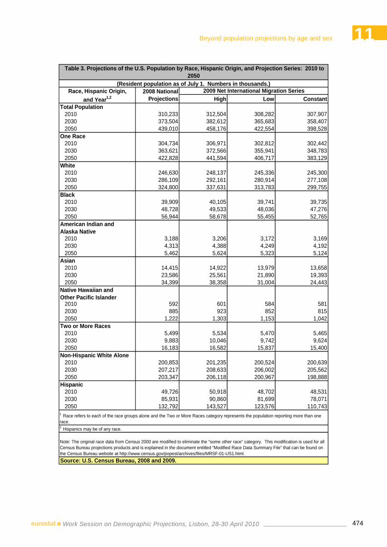
11Beyond population projections by age and sex
474Work Session on Demographic Projections, Lisbon, 28-30 April 2010
High Low ConstantTotal Population
2010 310,233 312,504 308,282 307,9072030 373,504 382,612 365,683 358,4072050 439,010 458,176 422,554 398,528
One Race2010 304,734 306,971 302,812 302,4422030 363,621 372,566 355,941 348,7832050 422,828 441,594 406,717 383,129
White2010 246,630 248,137 245,336 245,3002030 286,109 292,161 280,914 277,1082050 324,800 337,631 313,783 299,755
Black2010 39,909 40,105 39,741 39,7352030 48,728 49,533 48,036 47,2762050 56,944 58,678 55,455 52,765
American Indian and Alaska Native
2010 3,188 3,206 3,172 3,1692030 4,313 4,388 4,249 4,1922050 5,462 5,624 5,323 5,124
Asian2010 14,415 14,922 13,979 13,6582030 23,586 25,561 21,890 19,3932050 34,399 38,358 31,004 24,443
Native Hawaiian and Other Pacific Islander
2010 592 601 584 5812030 885 923 852 8152050 1,222 1,303 1,153 1,042
Two or More Races2010 5,499 5,534 5,470 5,4652030 9,883 10,046 9,742 9,6242050 16,183 16,582 15,837 15,400
Non-Hispanic White Alone2010 200,853 201,235 200,524 200,6392030 207,217 208,633 206,002 205,5622050 203,347 206,118 200,967 198,888
Hispanic2010 49,726 50,918 48,702 48,5312030 85,931 90,860 81,699 78,0712050 132,792 143,527 123,576 110,743
Table 3. Projections of the U.S. Population by Race, Hispanic Origin, and Projection Series: 2010 to 2050
Source: U.S. Census Bureau, 2008 and 2009.
Race, Hispanic Origin, and Year1,2
1 Race refers to each of the race groups alone and the Two or More Races category represents the population reporting more than one race.2 Hispanics may be of any race.
Note: The original race data from Census 2000 are modified to eliminate the “some other race” category. This modification is used for all Census Bureau projections products and is explained in the document entitled “Modified Race Data Summary File” that can be found on the Census Bureau website at http://www.census.gov/popest/archives/files/MRSF-01-US1.html.
2009 Net International Migration Series2008 National Projections
(Resident population as of July 1. Numbers in thousands.)

11Beyond population projections by age and sex
475Work Session on Demographic Projections, Lisbon, 28-30 April 2010
2010 2020 2030 2040 2050
Total 1,338,370 1,472,777 1,664,183 1,855,450 2,046,690Non-Hispanic 679,208 729,375 830,700 931,976 1,033,237
White 254,945 241,162 264,778 288,372 311,969Black 106,642 115,917 135,624 155,304 174,969Asian 299,717 353,449 408,762 464,075 519,398AIAN 1,606 1,308 1,501 1,675 1,863NHPI 3,796 4,213 4,860 5,512 6,154Two or More Races 12,502 13,326 15,175 17,038 18,884
Hispanic 659,162 743,402 833,483 923,474 1,013,453
Total 100.0 100.0 100.0 100.0 100.0Non-Hispanic 50.7 49.5 49.9 50.2 50.5
White 19.0 16.4 15.9 15.5 15.2Black 8.0 7.9 8.1 8.4 8.5Asian 22.4 24.0 24.6 25.0 25.4AIAN 0.1 0.1 0.1 0.1 0.1NHPI 0.3 0.3 0.3 0.3 0.3Two or More Races 0.9 0.9 0.9 0.9 0.9
Hispanic 49.3 50.5 50.1 49.8 49.5
Source: U.S. Census Bureau, 2008.
Number (in thousands)
Percent
Table 4. Projections and Distribution of Net International Migrants by Race and Hispanic Origin for the United States: 2010 to 2050
2008 National ProjectionsRace and
Hispanic Origin1, 2
1 Race refers to each of the race groups alone and the Two or More Races category represents the population reporting more than one race.2 Hispanics may be of any race.
Note: The original race data from Census 2000 are modified to eliminate the “some other race” category. This modification is used for all Census Bureau projections products and is explained in the document entitled “Modified Race Data Summary File” that can be found on the Census Bureau website at http://www.census.gov/popest/archives/files/MRSF-01-US1.html.
The zero net international migration series was illustrative and is not reflective of any realistic “truth” for the future population; however, it does provide insights on the makeup of the projected migrant population.
For low to high levels of net international migration, the Asian and Hispanic populations are projected to more than double in size by 2050. Even if net international migration were maintained at a constant level of nearly one million, the Hispanic population is still projected to more than double by 2050, while the Asian population is expected to increase by 79 percent. Although the populations are growing rapidly, the pace at which the Asian and Hispanic populations will grow is projected to slow considerably (Figures 2 and 3).
Most other race groups are projected to experience a moderate increase in size over the next four decades in all four projection series, and there is little difference in the projected growth rates for these groups across projection series. The one exception to this trend is for the non-Hispanic White alone population, which is projected to begin to decline in size in all series (Figure 4). This decline is projected to begin around 2030 for all series.

11Beyond population projections by age and sex
476Work Session on Demographic Projections, Lisbon, 28-30 April 2010

11Beyond population projections by age and sex
477Work Session on Demographic Projections, Lisbon, 28-30 April 2010
The projected level of migration also has meaningful effects on the proportional distribution of the population by race and Hispanic origin (Table 5). For example, the White alone population decreases as a percentage of the total population in all series. The non-Hispanic White alone population is expected to experience a large decline in proportional representation (Figure 5).
Although the level of net international migration affects the size of the Asian population, its share of the total population remains relatively low in all series (Figure 6). The Black, American Indian and Alaska Native, and Native Hawaiian and Other Pacific Islander populations are expected to maintain or slightly increase their percent share of the population in all series.
The percentage of the U.S. population that is projected to be Hispanic increases substantially in all series (Figure 7). This is even true for the zero migration series (not shown). This is largely due to the current age distribution of the Hispanic population and higher fertility rates that are assumed for them. In contrast, we find that the size and age structure of the Asian population is strongly linked to projected levels of migration.

11Beyond population projections by age and sex
478Work Session on Demographic Projections, Lisbon, 28-30 April 2010
High Low Constant ZeroOne Race
2010 98.2 98.2 98.2 98.2 98.22030 97.4 97.4 97.3 97.3 97.22050 96.3 96.4 96.3 96.1 95.8
White2010 79.5 79.4 79.6 79.7 80.12030 76.6 76.4 76.8 77.3 78.42050 74.0 73.7 74.3 75.2 76.5
Black2010 12.9 12.8 12.9 12.9 13.12030 13.0 12.9 13.1 13.2 13.82050 13.0 12.8 13.1 13.2 14.4
American Indian and Alaska Native
2010 1.0 1.0 1.0 1.0 1.02030 1.2 1.1 1.2 1.2 1.22050 1.2 1.2 1.3 1.3 1.4
Asian2010 4.6 4.8 4.5 4.4 3.82030 6.3 6.7 6.0 5.4 3.72050 7.8 8.4 7.3 6.1 3.3
Native Hawaiian and Other Pacific Islander
2010 0.2 0.2 0.2 0.2 0.22030 0.2 0.2 0.2 0.2 0.22050 0.3 0.3 0.3 0.3 0.2
Two or More Races2010 1.8 1.8 1.8 1.8 1.82030 2.6 2.6 2.7 2.7 2.82050 3.7 3.6 3.7 3.9 4.2
Non-Hispanic White Alone2010 64.7 64.4 65.0 65.2 67.02030 55.5 54.5 56.3 57.4 62.42050 46.3 45.0 47.6 49.9 57.8
Hispanic2010 16.0 16.3 15.8 15.8 14.32030 23.0 23.7 22.3 21.8 17.62050 30.2 31.3 29.2 27.8 21.0
1 Race refers to each of the race groups alone and the Two or More Races category represents the population reporting more than one race.2 Hispanics may be of any race.
Note: The original race data from Census 2000 are modified to eliminate the “some other race” category. This modification is used for all Census Bureau projections products and is explained in the document entitled “Modified Race Data Summary File” that can be found on the Census Bureau website at http://www.census.gov/popest/archives/files/MRSF-01-US1.html.Source: U.S. Census Bureau, 2008 and 2009.
Table 5. Distribution of the U.S. Population by Race, Hispanic Origin, and Projection Series: 2010 to 2050
(Percent of total resident population as of July 1)Race, Hispanic Origin,
and Year1,22008 National
Projections2009 Net International Migration Series

11Beyond population projections by age and sex
479Work Session on Demographic Projections, Lisbon, 28-30 April 2010

11Beyond population projections by age and sex
480Work Session on Demographic Projections, Lisbon, 28-30 April 2010
The aging of the population is a common theme in examinations of population projections. The total population is projected to age to some degree in all projection series (Table 6). In the 2008 projection series, the median age is projected to increase from 36.9 years in 2010 to 39.0 years in 2050. Under the assumption of constant migration, the median age is projected to reach nearly 40 years by 2050. Because international migrants into the United States tend to be younger individuals (typically under the age of 35), changes in migration assumptions influence the extent to which the population is projected to age over the next forty years. Generally, higher levels of migration produce younger populations, while less migration results in an older population.
All projections series show a large increase in the projected median age of the Asian population. For example, the median age increases from 35.9 years in 2010 to 42.3 years in 2050 in the constant series. In the high migration series, the Asian population median age increases to 43.1. The median age for the Black population also shows large increases. The Hispanic population is projected to experience a smaller increase in median age. Under the assumption of a higher level of migration, the median age of the Hispanic population is expected to be 30.9 years in 2050. In contrast, the median age is projected to rise to 33.1 years if net international migration is held constant at nearly one million people per year. Migration levels have minimal effect on the pace of aging for the non-Hispanic White alone population. For this group, the median age is projected to rise to approximately 45 years by 2050 in all scenarios. The median ages for the American Indian and Alaska Native and the Native Hawaiian and Other Pacific Islander populations are projected to increase over time in all scenarios. As shown for the non-Hispanic White alone population, the level of international migration has little effect on how quickly these groups are projected to age.

11Beyond population projections by age and sex
481Work Session on Demographic Projections, Lisbon, 28-30 April 2010
High Low ConstantTotal Population
2010 36.9 36.7 37.0 37.12030 38.7 38.4 39.0 39.22050 39.0 38.6 39.3 39.7
White2010 38.4 38.3 38.5 38.62030 39.6 39.3 39.9 40.42050 39.4 38.9 39.8 40.8
Black2010 31.7 31.7 31.8 31.82030 36.6 36.4 36.7 37.02050 38.9 38.6 39.1 39.9
American Indian and Alaska Native
2010 29.9 29.9 30.0 30.02030 33.8 33.6 34.0 34.32050 34.9 34.6 35.1 35.7
Asian2010 36.0 35.7 36.2 35.92030 41.1 40.7 41.4 40.22050 43.4 43.1 43.8 42.3
Native Hawaiian and Other Pacific Islander
2010 30.5 30.4 30.6 30.52030 35.1 34.8 35.2 35.02050 36.8 36.5 37.0 37.0
Two or More Races2010 19.9 19.9 19.9 19.92030 22.1 22.0 22.1 22.12050 24.7 24.6 24.8 24.9
Non-Hispanic White Alone2010 41.3 41.3 41.4 41.42030 43.7 43.6 43.8 43.92050 44.6 44.5 44.7 45.0
Hispanic2010 27.5 27.3 27.7 28.02030 29.2 28.9 29.5 30.52050 31.2 30.9 31.5 33.1
Source: U.S. Census Bureau, 2008 and 2009.
Table 6. Projected Median Age of the U.S. Population by Projection Series, Race, and Hispanic Origin: 2010 to 2050
1 Race refers to each of the race groups alone and the Two or More Races category represents the population reporting more than one race.2 Hispanics may be of any race.
Note: The original race data from Census 2000 are modified to eliminate the “some other race” category. This modification is used for all Census Bureau projections products and is explained in the document entitled “Modified Race Data Summary File” that can be found on the Census Bureau website at http://www.census.gov/popest/archives/files/MRSF-01-US1.html.
Race, Hispanic Origin, and Year1,2
2008 National Projections
2009 Net International Migration Series

11Beyond population projections by age and sex
482Work Session on Demographic Projections, Lisbon, 28-30 April 2010
Another interesting topic in discussion about the future of the U.S. population is whether (or when) the minority population will become the numeric majority.8 That is, when the non-Hispanic White alone population becomes less than 50 percent of the total population. As expected, we find that the level of net international migration affects the timing of the majority-minority crossover. In each of the four series where migration occurs, the size of the minority population is expected to increase to the point that they represent the numeric majority between 2040 and 2050 (Table 7). Higher levels of net international migration are projected to lead to an earlier crossover of the minority share of the population, while lower levels will delay the timing of this crossover.
Series Year2008 National Projections 20422009 High Net International Migration Series 20402009 Low Net International Migration Series 20452009 Constant Net International Migration Series 2050
Table 7. Projections of the Year of Majority-Minority1
Crossover by Net International Migration Series for the United States
1Minority is defined here as people who are races other than White alone or who are Hispanic.
Source: U.S. Census Bureau, 2008 and 2009.
5. Summary
The most recent U.S. population projections were produced to provide comprehensive detail on the projected population by single year of age, sex, race, and Hispanic origin. The level of detail provided in the U.S. Census Bureau’s products is driven by the needs of end users and federal needs for detailed race and ethnic information. Specifically, the detailed projections provide useful information for planning and making projections of other topics of national interest.
The most recent projections series also provide valuable information about the impact of net international migration on the size and characteristics of the U.S. population. Although international migration affects all aspects of the population, the largest impact is seen for the Asian and Hispanic populations. Higher levels of net international migration also seem to temper the overall aging of the population.
References
Hollmann, Frederick W., and W. Ward Kingkade, Impact of Racial and Ethnic Exogamy and International Migration on Forecast Population Distributions for the United States in 2030: Results of a Macro-Simulation, presented at the XXVth International Population Conference of the International Union for the Scientific Study of Population, in Tours, France, July 18-23, 2005.
Office of Management and Budget, Revisions to the Standards for Classification of Federal Data on Race and Ethnicity, http://www.whitehouse.gov/omb/fedreg_1997standards/, October 1997.
U.S. Census Bureau, Population Estimates, http://www.census.gov/popest/estimates.html.
U.S. Census Bureau, 2008 National Population Projections, http://www.census.gov/population/www/projections/2008projections.html, 2008.
U.S. Census Bureau, 2009 National Population Projections, http://www.census.gov/population/www/projections/2009projections.html, 2009.
8 The minority population is defined here as people who are races other than White alone or who are Hispanic.

Stochastic techniques for demographic projections Chair: Jutta Gampe
Session 12


12Stochastic techniques for demographic projections
485Work Session on Demographic Projections, Lisbon, 28-30 April 2010
COMBINING DETERMINISTIC AND STOCHASTIC POPULATION PROJECTIONS*
Salvatore BERTINO**, Eugenio SONNINO***
Giampaolo LANZIERI****
1. Introduction
Population projections are sometimes requested for assessing the impact of population developments in the very long run. Such a long time horizon clearly undermines whatever significance as a forecast is assigned to the resulting projections. Despite this, users have the tendency to consider long-term projections not as one of the plausible developments of the population under given assumptions, but instead as an ‘almost sure’ outcome. In order to raise users’ awareness of the inherent uncertainty of population projections, the quantification of prediction intervals may play a very important role.
In conventional population projections exercises, this is usually done by producing results corresponding to different paths of evolution of the demographic components. Population projections that are the outcome of these alternative sets of assumptions are called variants. It is common practice of the official institutes producing projections to release several variants, often corresponding to more optimistic/pessimistic developments than those assumed in a baseline projection. However, the user is normally left with no hints as to the higher or lower plausibility of the different variants. Certainly, strategies can be implemented by the users to make a rational and less costly choice among the available options (Duchêne and Wanner, 1999), but nevertheless the message about the uncertainty associated with the various variants is not straightforward. This is better accomplished in a stochastic framework, where probabilities can be associated with projections outcomes.
The quantification of uncertainty can be considered the most important development in population forecasting in the past decade (Wilson and Rees, 2005). Four main approaches have been proposed in the literature to quantify uncertainty in population projections: the first is based on the application of time series techniques directly to demographic components (such as the total fertility rate) or to parameters of a mathematical expression of age-specific rates; the second approach analyses ex-post the errors of previous projections exercises to obtain information about future likely errors; the third builds upon the experts’ judgment; the fourth method uses the output of micro-simulations to quantify the forecast intervals. Attempts to apply a combination of these methods have also been presented in the literature (e.g. Keilman et al., 2002). To the last of the four groups listed above belongs the method proposed by Bertino and Sonnino (2007), based on the simulation of birth, death, immigration and emigration point-event processes, resulting from compounding independent Poisson processes. The same authors have also developed software to implement their method (Bertino and Sonnino, 2010).
Despite the wealth of proposals in the literature, probabilistic projections still have a number of shortcomings that somehow slow down the process of adoption of these methods by the official forecasters. For instance, besides the technical complexity of some of them, which may require
* The views expressed in this paper are exclusively those of the authors and do not necessarily represent the views of the
European Commission. ** University ‘La Sapienza’, Department of Statistical Sciences, Rome. E-mail: [email protected] *** University ‘La Sapienza’, Department of Statistical Sciences, Rome. E-mail: [email protected] **** European Commission — Eurostat, Population Unit, Luxembourg. E-mail: [email protected].

12Stochastic techniques for demographic projections
486Work Session on Demographic Projections, Lisbon, 28-30 April 2010
knowledge not always possessed by demographers (e.g. ARIMA models), subjectivity may still be present to a certain extent (e.g. in the choice of the base period or of the model for extrapolation), or the outcome may sometimes be implausible, or again it may give such a wide range of variation as to be useless for practical purposes. Further, sometimes it is not possible to incorporate demographic knowledge into the stochastic approach, knowledge which is ultimately the real strong point of conventional cohort-component projections, nor can visions of future long-term demographic developments always be easily integrated. These limitations of the probabilistic methods may become more relevant as the time horizon of the projections is set further into the distant future. Therefore, the attempt to combine deterministic and stochastic projections answers the need to preserve the advantages of the conventional approach, whilst quantifying the inherent uncertainty of projections.
This article focuses on how deterministic projections can be integrated within a stochastic framework according to the micro-simulation approach of Bertino and Sonnino (BS hereafter). Section 2 provides a description of the possibilities of linkage between the conventional deterministic projections and the stochastic BS method, including its consequences in terms of estimation of the variability and therefore of the forecast intervals. Section 3 sets out some elements for discussion.
2. The method
In the conventional cohort-component approach, plausible demographic developments take the form of fertility, mortality and migration age-specific (and sex-specific, where appropriate) rates assumed to occur along the time horizon of the population projections. The combination with a stochastic approach would entail that the information represented by the assumed ‘conventional’ deterministic rates is somehow incorporated into that probabilistic method.
The BS method requires the definition of instantaneous rates for the Poisson processes. In its simplest version, it starts from the probabilities of the vital events e (fertility, mortality and migration) for each age a and (where appropriate) sex s at the beginning and at the end of the projections period. Probabilities for intermediate years are obtained by linear interpolation and modified according to a random walk. These probabilities are then transformed into instantaneous rates of Poisson processes by means of the following equation:
( ) ( )[ ]saqsa ee ,1ln, −−=λ (1)
These instantaneous rates, assumed equal within each age-sex category, are modified after each event occurring in the population (for further details on the methodology, see Bertino and Sonnino, 2007). The BS method thus has an entry door for inputting demographic knowledge into its probabilistic framework. It is indeed sufficient to assume that the instantaneous rates for each age and sex group at the beginning of each year of projections are equal to the corresponding deterministic rates used in the conventional projections. Although the instantaneous rates are stochastically modified also between simulations, these deterministic rates may ‘drive’ the stochastic process according to defined long-term scenarios.
In the BS method, given m simulations, any statistic of interest V (e.g. size of age groups, number of live births, old age dependency ratio) can be estimated by:
∑=
=m
iis v
m 1
1μ (2)
where sμ is the estimated average of the determinations iv of the statistic of interest V from the
stochastic simulations. Likewise, the variance 2ˆ sσ of the statistic V can be estimated by:
( )∑=
−−
=m
isis v
m 1
22 ˆ1
1ˆ μσ (3)
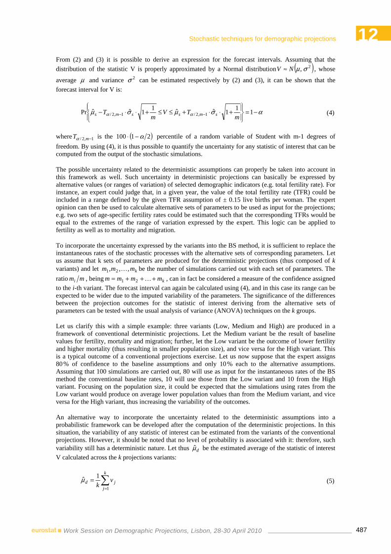
12Stochastic techniques for demographic projections
487Work Session on Demographic Projections, Lisbon, 28-30 April 2010
From (2) and (3) it is possible to derive an expression for the forecast intervals. Assuming that the distribution of the statistic V is properly approximated by a Normal distribution ( )2, σμNV ≈ , whose
average μ and variance 2σ can be estimated respectively by (2) and (3), it can be shown that the forecast interval for V is:
ασμσμ αα −=⎪⎭
⎪⎬⎫
⎪⎩
⎪⎨⎧
+⋅⋅+≤≤+⋅⋅− −− 111ˆˆ11ˆˆPr 1,2/1,2/ mTV
mT smssms (4)
where 1,2/ −mTα is the ( )21100 α−⋅ percentile of a random variable of Student with m-1 degrees of freedom. By using (4), it is thus possible to quantify the uncertainty for any statistic of interest that can be computed from the output of the stochastic simulations.
The possible uncertainty related to the deterministic assumptions can properly be taken into account in this framework as well. Such uncertainty in deterministic projections can basically be expressed by alternative values (or ranges of variation) of selected demographic indicators (e.g. total fertility rate). For instance, an expert could judge that, in a given year, the value of the total fertility rate (TFR) could be included in a range defined by the given TFR assumption of ± 0.15 live births per woman. The expert opinion can then be used to calculate alternative sets of parameters to be used as input for the projections; e.g. two sets of age-specific fertility rates could be estimated such that the corresponding TFRs would be equal to the extremes of the range of variation expressed by the expert. This logic can be applied to fertility as well as to mortality and migration.
To incorporate the uncertainty expressed by the variants into the BS method, it is sufficient to replace the instantaneous rates of the stochastic processes with the alternative sets of corresponding parameters. Let us assume that k sets of parameters are produced for the deterministic projections (thus composed of k variants) and let kmmm ,,, 21 K be the number of simulations carried out with each set of parameters. The ratio mmi , being kmmmm +++= K21 , can in fact be considered a measure of the confidence assigned to the i-th variant. The forecast interval can again be calculated using (4), and in this case its range can be expected to be wider due to the imputed variability of the parameters. The significance of the differences between the projection outcomes for the statistic of interest deriving from the alternative sets of parameters can be tested with the usual analysis of variance (ANOVA) techniques on the k groups.
Let us clarify this with a simple example: three variants (Low, Medium and High) are produced in a framework of conventional deterministic projections. Let the Medium variant be the result of baseline values for fertility, mortality and migration; further, let the Low variant be the outcome of lower fertility and higher mortality (thus resulting in smaller population size), and vice versa for the High variant. This is a typical outcome of a conventional projections exercise. Let us now suppose that the expert assigns 80 % of confidence to the baseline assumptions and only 10 % each to the alternative assumptions. Assuming that 100 simulations are carried out, 80 will use as input for the instantaneous rates of the BS method the conventional baseline rates, 10 will use those from the Low variant and 10 from the High variant. Focusing on the population size, it could be expected that the simulations using rates from the Low variant would produce on average lower population values than from the Medium variant, and vice versa for the High variant, thus increasing the variability of the outcomes.
An alternative way to incorporate the uncertainty related to the deterministic assumptions into a probabilistic framework can be developed after the computation of the deterministic projections. In this situation, the variability of any statistic of interest can be estimated from the variants of the conventional projections. However, it should be noted that no level of probability is associated with it: therefore, such variability still has a deterministic nature. Let thus dμ be the estimated average of the statistic of interest V calculated across the k projections variants:
∑
=
=k
jjd v
k 1
1μ
(5)

12Stochastic techniques for demographic projections
488Work Session on Demographic Projections, Lisbon, 28-30 April 2010
and 2ˆdσ the variance:
( )∑=
−=k
jdjd v
k 1
22 ˆ1ˆ μσ (6)
The variance 2ˆdσ could also be directly expressed by the expert or the result of alternative methods of estimation. Further, (5) could take the form of a weighted average, if preference for one or another variant is expressed:
kjwvw j
k
jjjd ,,110;'ˆ
1
K=∀≤≤⋅=∑=
μ (7)
Given the expression of deterministic uncertainty (6) related to a given statistic of interest, two approaches are possible. In the first, the two variances (deterministic and stochastic) are assumed to be independent and p is the weight assigned to the deterministic component. Then:
( ) ( )( ) ⎥
⎥⎦
⎤
⎢⎢⎣
⎡
⋅−⋅+⋅⋅−=⋅−+⋅=
22
222222222
ˆ1ˆ
1ˆ1ˆ1ˆˆs
dssdV
ppppp
σσσσσσ (8)
and the forecast interval is:
( ) ( ) ασ
σσμσ
σσμ αα −=⎪⎭
⎪⎬⎫
⎪⎩
⎪⎨⎧ ⋅
+−⋅⋅+≤≤⋅
+−⋅⋅− −− 1ˆ
ˆ1ˆˆ
ˆˆ
1ˆˆPr 2
222
1,2/2
222
1,2/s
dsmV
s
dsmV
ppTV
ppT (9)
being:
( ) sdV pp μμμ ˆ1ˆˆ ⋅−+⋅= (10)
If equal confidence is given to the deterministic and to the stochastic component, then (9) becomes:
ασσσμ
σσσμ αα −=
⎪⎭
⎪⎬⎫
⎪⎩
⎪⎨⎧
+⋅⋅+≤≤+⋅⋅− −− 1ˆˆ
12ˆˆ
ˆˆ
12ˆˆPr 2
2
1,2/2
2
1,2/s
dsmV
s
dsmV TVT (11)
An alternative method to incorporate deterministic uncertainty is based on the Bayesian approach (see Piccinato, 2009:177). In this framework, the deterministic forecast and its measure of uncertainty is the initial distribution (before the experiment) of the statistic of interest, while the stochastic forecast is the outcome of an experiment of m independent trials of a simulation procedure. Assuming that the initial distribution is ( )2, ddN σμ and the stochastic simulations are the outcome of a ( )2, VVN σμ , whose variance
is estimated by 2ˆ sσ , the final forecast distribution is:
⎥⎥⎦
⎤
⎢⎢⎣
⎡⎟⎟⎠
⎞⎜⎜⎝
⎛
⋅++⋅
⋅+⋅⋅+⋅
22
22
22
221,
ds
ds
ds
dssd
mmmN
σσσσ
σσσμσμ (12)
12Stochastic techniques for demographic projections
489Work Session on Demographic Projections, Lisbon, 28-30 April 2010
Equation (12) is valid if the parameter 2sσ is known. If this variance is estimated, then:
1,2
22
22
22
22
ˆ1ˆ
ˆˆ
−≈
⎟⎟⎠
⎞⎜⎜⎝
⎛
⋅++⋅
⋅+⋅⋅+⋅
−
m
ds
ds
ds
dssd
T
m
mm
α
σσσσ
σσσμσμμ
(13)
from which:
α
σσσσ
σσσμσμ
σσσσ
σσσμσμ
α
α
−=
⎪⎪⎪
⎭
⎪⎪⎪
⎬
⎫
⎪⎪⎪
⎩
⎪⎪⎪
⎨
⎧
⋅++⋅⋅+
⋅+⋅⋅+⋅
≤
≤⋅+
+⋅⋅−⋅+
⋅⋅+⋅
−
−
1
ˆˆˆ
1ˆˆˆ
ˆˆˆˆ
ˆˆˆ
1ˆˆˆ
ˆˆˆˆ
Pr
22
2
1,222
22
22
2
1,222
22
ds
dsm
ds
dssd
ds
dsm
ds
dssd
mT
mm
Vm
Tmm
(14)
If the two variances (deterministic and stochastic) are equal, then (14) becomes:
ασμμσμμαα −=
⎪⎭
⎪⎬⎫
⎪⎩
⎪⎨⎧
++⋅⋅+
+⋅+
≤≤+
+⋅⋅−+
⋅+−− 1
111ˆ
1ˆˆ
111ˆ
1ˆˆ
Pr 1,21,2 mT
mm
Vm
Tm
msm
sdsm
sd (15)
In this case, the deterministic value is considered as the outcome of a further simulation.
3. Discussion
The importance of quantifying uncertainty in population forecasting has been highlighted by several scholars. In a conventional projections exercise, uncertainty is usually expressed by means of variants; however, in doing so, no probability is associated with the various options, nor is the user guided in the choice of the most appropriate variant. Several methods for stochastic projections have thus been proposed in the literature, by which it is possible to obtain forecast intervals. On the other hand, the ‘demographic knowledge’ incorporated in the assumption-setting for deterministic projections risks being — at least partially — lost when a fully stochastic approach is undertaken. Various attempts are thus being made to link these two aspects of a projections exercise.
This article builds on the method of stochastic projections proposed by Bertino and Sonnino (2007) to develop the integration between deterministic and stochastic projections. The BS method is particularly suitable for this task because it is based on micro-simulations of the behaviour of a population, which gives great flexibility in the outputs that can be derived, and it allows deterministic assumptions to be input straight into the stochastic procedure. The link is straightforward, as it is sufficient to consider as input for the instantaneous rates of the point-event Poisson processes of the BS method the deterministic rates produced for the conventional projections.
In addition, methods are here proposed to include also the uncertainty that may have been formulated in the context of the deterministic exercise. In particular, two methods are proposed: an ex-ante approach directly incorporates in the simulation procedure the deterministic uncertainty, as expressed by alternative sets of deterministic rates; an ex-post method instead includes an estimate of the deterministic variability directly in the formulas for the computation of the forecast intervals. This latter approach is also developed in a Bayesian framework.
The BS method allows the forecast intervals to be calculated for any statistic of interest. This is of considerable importance for certain policy needs, where specific indicators are considered to be of particular relevance. Work is still ongoing to test the proposed approach empirically. In particular, an

12Stochastic techniques for demographic projections
490Work Session on Demographic Projections, Lisbon, 28-30 April 2010
application is currently being developed on EUROPOP2008, a set of population projections for the European Union (for details about these projections, see Lanzieri, 2009).
As conventional deterministic projections are still common practice in the national statistical offices, a possible strategy could then be based on the following steps: first, the deterministic exercise is carried out, including also the release of various variants; second, the deterministic projections are combined with the stochastic method, producing forecast intervals for the statistics of interest. This two-step strategy is easy to implement and allows ‘control’ to be kept over the assumed future demographic scenario, associating at the same time a probability level.
References
Bertino, S. and E. Sonnino (2007): ‘A new technique for stochastic population projections’. Proceedings of the Eurostat-UNECE Workshop on Demographic Projections, Bucharest, 10-12 October 2007, 161-175.
Bertino, S. and E. Sonnino (2010): PRODEST — Proiezioni Demografiche Stocastiche, version 5.051.
Duchêne J. and P. Wanner (1999): ‘Uncertainty in demographic projections and its consequences for the user’. Statistical Journal of the United Nations ECE, 16:267-279.
Keilman, N., D.Q. Pham and A. Hetland (2002): ‘Why population forecasts should be probabilistic — illustrated by the case of Norway’. Demographic Research, 6:409-454.
Lanzieri G. (2009): ‘EUROPOP2008: a set of population projections for the European Union’. Paper for the XXVI IUSSP International Population Conference, Marrakech, October 2009.
Piccinato L. (2009): "Metodi per le decisioni statistiche". Springer-Verlag Italia.
Wilson, T. and P. Rees (2005): ‘Recent Developments in Population Projections Methodology: A Review’. Population, Space and Place, 11:337-360.

12Stochastic techniques for demographic projections
491Work Session on Demographic Projections, Lisbon, 28-30 April 2010
A MATE-MATCHING ALGORITHM FOR CONTINUOUS-TIME MICROSIMULATION MODELS
Sabine ZINN1
Acknowledgements
This work is entirely part of the MicMac project. The Centraal Bureau voor Statistiek in the Netherlands has provided the data of the Fertility and Family Survey for the Netherlands (FFS NL). The Netherland Kinship Panel Study is funded by grant 480-10-009 from Major Investments Fund of the Netherlands Organization for Scientific Research (NWO), and by the Netherlands Interdisciplinary Demographic Institute (NIDI), Utrecht University, the University of Amsterdam and Tilburg University. This paper would never have been written without the help of a couple of persons. Particular thanks go to Jutta Gampe for her fruitful supervision. Ekaterina Ogurtsova assisted in preparating the input data files for the microsimulation example. Jim Oeppen helped with general advices. Basic ideas of mate-matching in continuous-time go back to discussions with Jan Himmelspach and Frans Willekens.
1. Introduction
In the social sciences, including demography, microsimulation is an approach that models dynamics of a system, the population, society or economy by modelling the behavior of its micro-units (typically an individual or a household). Microsimulations go back to the work of Orcutt (Orcutt 1957, Orcutt et al. 1961) and are techniques to produce population projections (Imhoff and Post 1998, Wolf 2001). The central unit of a demographic microsimulation is an individual’s life-course, which is characterized by a sequence of demographic events such as birth, marriage, childbirth, divorce, retirement and finally death. In dynamic microsimulation models, aging of the micro units leads to a time-varying population structure. Both age and calendar time have to enter a realistic demographic microsimulation model, and both can be treated as discrete (usually in units of years or months) or as continuous (Galler 1997). Advantages and disadvantages of discrete- and continuous-time models are discussed at length in Satyabudhi and Onggo (2008), Willekens (2009), and Galler (1997).
Independently of how model time is treated, in a demographic microsimulation model relationships between individuals should be regarded. Neglecting kinship and partnership relations during simulation is a source of biased outcomes. Murphy and Wang (2001), for example, argue that in the U.S., Italy, Norway and Poland “the relationship between fertility of successive generations is becoming stronger with time” (Murphy and Wang 2001, p. 1). Hence, in a related microsimulation model the ignorance of mother - daughter relationships would lead to a distorted fertility pattern. Moreover, a population’s fertility and mortality pattern strongly depends on marriage and partnership processes. A woman, for instance, who lives in a partnership, has a much higher probability of childbirth than a single woman. Another example is that the mortality of married men is lower than of unmarried men. In a microsimulation ignoring the impact that a spouse has on an individual’s life course is, therefore, tenuous.
1 “Max Planck” Institute for Demographic Research 18057 Rostock Germany

12Stochastic techniques for demographic projections
492Work Session on Demographic Projections, Lisbon, 28-30 April 2010
In modelling demographic kinship different problems have to be addressed.
1. How can we model and simulate the onset of relationships?
2. How can we model and simulate correlation between life-courses?
3. How can we model and simulate dissolution events?
We focus in this article on the first problem with particular emphasis on mate-matching in continuous-time microsimulations.
We structure our work as follows. In a first step we review mate-matching algorithms of existing microsimulations.
We continue, in section 3, by describing a mate-matching algorithm that works in continuous time. In section 4, we illustrate the capabilities of the present approach. Running simulations, we forecast a synthetic population based on the population of the Netherlands. We conclude in section 5 by validating the new procedure, and we give an outlook of how we can improve our work.
2. A review of mating models
In the process of developing mating models, several difficulties have to be borne in mind and tackled. The first one concerns the high data demands that are necessary to map mate-matching mechanisms properly. In order to determine synthetic couples, data from actual couples is necessary. Retrospective surveys that record the attributes of spouses before and after the onset of partnerships would be most appropriate. However, in the majority of cases such surveys only gather very limited information on partnership relations (Huinink and Feldhaus 2009). Problems also arise because actual mating processes comprise mechanisms that are not observable, e.g., the formation rules. The modeler is forced to set assumptions and hypothetical rules about mating behavior. Only the effect of these can be simulated and hypothetical outcomes can be contrasted with those actually observed (de Vos and Palloni 1989). A further difficulty emerges due to the fact that in microsimulation models the temporal progression is modelled in reverse: First an event that leads to a partnership onset is simulated and then the question of defining a proper spouse is addressed. Consequently, if a transition implies the onset of cohabitation or a marriage, an individual has to become part of a couple. Otherwise, the outcome of the underlying stochastic model is disregarded.
In the field of demographic microsimulations three different approaches exist to model the onset of partnerships, and marriages in particular: (1) ignoring mating processes, (2) open mating models, and (3) closed mating models. We describe below these approaches in detail, paying special attention to the above listed problems. We do not provide a categorization of existing microsimulations according to the type of mating model used. For an overview of an extensive range of microsimulation models, see O’Donoghue (1999), Zaidi and Rake (2001) and Spielauer (2002).
2.1 No mating model Ignoring mating processes means that individual life-courses are modelled independently of each other. If an individual experiences a partnership event, no synthetic couple is created. As a result, it is impossible to map inter-dependencies between life-course events of spouses.
Ignoring mating is reasonable in the context of one-sex models. An example of this type is the family microsimulation FAMSIM that specifies partnership forms as attributes of women (Spielauer and Neuwirth 2001).
In general, ignoring mating processes has some advantages: Neither data for actual couples is required, nor hypothetical rules that describe mating processes. However, skipping mating processes has two substantial defects. Their effects on the population composition are neglected. For example, a restricted number of available spouses might affect the characteristics of formed partnerships. This, in turn, might

12Stochastic techniques for demographic projections
493Work Session on Demographic Projections, Lisbon, 28-30 April 2010
have an impact on the number of partnership dissolutions. Furthermore, ignoring relationships between individuals prevents the modelling of demographic kinship. As a result, it is, for example, not possible to account for intergenerational inter-dependencies, such as the correlation between the fertility behavior of mothers and daughters.
2.2 Open mating model In an open model, appropriate spouses are created ‘ex nihilo’. Their attributes are generated in such a manner that the characteristics of the newly created couples resemble actual ones. Age and educational attainment are the attributes that are usually regarded as being essential in this context.
As it is not necessary to identify a proper spouse within the model population, the implementation of open models is straightforward. A further advantage of this approach is that simulations for individuals (and their immediate families) can be run independently of other individuals (O’Donoghue 1999). However, open models reveal three major problems. First of all, it is not assured that the newly created individuals are representative of the target population. This might be the case in one-sex models, but the situation differs if whole populations are mapped. Another problem is the interpretation of an open model. The purpose of a microsimulation is to model population dynamics realistically. However, it is not realistic to pull an appropriate spouse out of the hat when needed. A problem that is related to this point is the missing retrospective life-course of a newly created spouse. Smith (1987) describes a method that tackles this problem by creating spouses whose only characteristic is that they are at the right age (relying on age differences that are reported for real couples). A more viable solution is proposed by Holmer et al. (2009). They suggest sampling complete retrospective life courses of spouses from retrospective surveys. Nevertheless, this presupposes the availability of huge sets of event history data.
The discrete-time microsimulation CAMSIM (Smith 1987), and the continuous-time microsimulations PENSIM (Holmer et al. 2009) and LifePaths (Statistics Canada 2004) are examples of the use of open mating models.
2.3 Closed mating model In a closed model, marriage and consensual union partners have to be found among existing individuals. To do so, several problems have to be addressed:
1. How can we determine who is searching?
2. Who matches whom?
3. When are couples formed?
4. What is the data base needed in order to form synthetic couples that resemble actual ones?
To the knowledge of the author, closed mating models have so far only been realized for discrete-time microsimulations.
In a discrete microsimulation model, time changes in discrete steps. After each step all individuals of the model population are inspected whether they experience an event in the next interval and, if yes, which event. This simulation procedure implicitly determines who is searching and also when couples are formed. Searching individuals are collected in a partnership market. A ‘partnership market’ is a construct that is used to pool all those individuals who look for a spouse. The notion ‘market’ might be confusing at this point as it suggests that searching individuals are trading with restricted sets of goods. However, in the literature a ‘partnership market’ is described as a pool of prospective spouses. From the technical point of view, the partnership market can be regarded as a sorted list of individuals. A sorting criterion is, e.g., age.
It has to be ensured that in the matching process those individuals who look for a marriage partner are not paired with persons that search for a common-law spouse, and vice versa. Consequently, the partnership market contains two separated sets of individuals: ‘cohabitation-willing’ and ‘marriage-willing’

12Stochastic techniques for demographic projections
494Work Session on Demographic Projections, Lisbon, 28-30 April 2010
individuals. The latter ones are assumed not to live in cohabitation, when they enter the market. Individuals, who live in cohabitation, already have spouses. If they experience marriage events, their cohabitations are simply converted into marriages. A few microsimulations exist where the partnership market is only accessible for marriage-willing individuals and not for those who look for a common-law spouse. This constraint has been identified as a major inconsistency (Leblanc et al. 2009). Annual or monthly partnership markets are an obvious choice in discrete models. After one year or one month, the partnership market is depleted by pairing individuals.
So far we have addressed the questions of how and when. Two questions remain: Who mates whom, and what data is needed to construct couples that resemble actual/ observed ones? Both questions concern the mating rules that are applied to match individuals. Generally, microsimulation models employ two types of mating rules: stable and stochastic ones (Perese 2002). In order to determine the quality of potential pairings, mating rules make use of a compatibility measure. This measure quantifies the quality of a respective pairing dependent on the attributes of the potential spouses.
2.3.1 Compatibility Measure The compatibility measure is a function that associates female and male attributes with a value between zero and one. This value indicates how compatible a woman and a man are. A large value is a sign for high compatibility. Likewise, a small value points to incompatibility.
We introduce some notation.
• At a fixed point in time the partnership market comprises m women and n men.
• We denote female attributes by wi, j=1,…, m and the male attributes by mj, j=1,…, n.
• The set F comprises all wi and the set M all mj.
The compatibility measure C is defined as follows C: F×M → [0,1]. Often, the domain of C comprises only the age and educational attainment of males and females. However, the domain of C differs between microsimulation models. Bacon and Pennec (2007) provide an extensive review of attributes that have been employed in mating models. Two different specifications of C are used: distance functions, and logit models. Distance functions are employed for minimization of the discrepancy in the attributes of spouses. An example is DYNASIM which employs an exponential distance function (Perese 2002).
In logit models, the idea is to quantify compatibility by the likelihood of a union between potential pairs (Perese 2002, Bouffard et al. 2001). In order to account for different types of partnerships (cohabitations/ marriages) and to differentiate between first and higher order partnerships, typically more than one logit model is applied. Data on observed couples are used to estimate the coefficients of these logit models. Empirical findings show that partners tend to have similar ages and education. Therefore, ideally, the estimated coefficients are in accordance with the theory of assortative mating (Bouffard et al. 2001, Leblanc et al. 2009).2
There exists one problem that most probably emerges in a partnership market: What to do if there are more men than women, or vice versa? Three alternative strategies have been proposed in the literature.
1. In the current period, the model treats remainder individuals as though they did not enter the partnership pool. They are simply left unmarried.
a. In the next period, they are at risk to experience a partnership event (Perese 2002, Leblanc et al. 2009).
b. In the next period, they are automatically members of the pool of potential spouses (Hammel et al. 1990).
2 Naturally, persons that are closely related show strong assortative characteristics. Therefore, in order to avoid incestuous
pairings.

12Stochastic techniques for demographic projections
495Work Session on Demographic Projections, Lisbon, 28-30 April 2010
2. Individuals are added or removed as needed (Leblanc et al. 2009).
3. A totally different approach is simulating partnership events only for females. Appropriate spouses are taken from the pool of unpaired eligible men (Hammel et al. 1976, King et al. 1999).
The first two strategies imply disregarding the outcome of the stochastic model of a dynamic microsimulation. For each individual in the marriage market a partnership event has been simulated. Therefore, removing excess from the marriage pool means to ignore a simulated event. Likewise, adding individuals to the pool means that individuals who are not simulated to experience a marriage event get married. The last strategy implies that female partnership behavior completely determines the dynamics in male partnership behavior. Bacon and Pennec (2007) suggest to use the second strategy and to embed an alignment procedure into the matching process. Their idea is to add and remove individuals until a pre-defined number of couples has been created.
2.3.2 Stable Mating Rules In order to match individuals both stable and stochastic rules can be employed. The problem of finding stable mating rules is equivalent to the stable marriage problem. Gale and Shapley (1962, p. 11) describe the problem as follows: “A certain community consists of n men and n women. Each person ranks those of the opposite-sex in accordance with his or her preferences for a marriage partner.
We seek a satisfactory way of marrying off all members of the community. [...] we call a set of marriages unstable [...] if under it there are a man and a woman who are not married to each other but prefer each other to their actual mates.” They prove that, for any number of men and women, it is always possible to solve the problem and make all marriages stable.
The stable marriage approach requires that, in the partnership market, each woman expresses her preference regarding each man and vice versa. Gale and Shapley (1962) developed an algorithm that produces a set of stable marriages. It is based on a sequence of proposals from men to women. Each man proposes, in descending order, to the women according to his preferences. A man is pausing when a woman agrees to consider his proposal. He is continuing if a proposal is immediately or subsequently rejected. When a woman receives a proposal, she rejects if she already holds a better proposal (relying on her preferences). Otherwise, she agrees to hold the proposal for consideration. In doing so, she rejects any poorer proposal that she may hold. This procedure assures that no man can have a better partner than he gets in this matching and no woman can have a worse one. Consequently, the Gale-Shapley algorithm produces marriages that greatly favor the men’s preferences. Since 1962 several studies have developed the topic and improved the algorithm. Researchers mainly work on two defects of the Gale-Shapley algorithm. The gender that is allowed to give the first bed is favored. Furthermore, the classical Gale-Shapley algorithm does not result in a unique set of stable marriages.
Relying on the theory of assortative mating, the degree of compatibility between a woman and a man is a proper measure of their preferences for each other. From now on, we quantify this degree using the compatibility measure C that has been introduced in paragraph 2.3.1. Its usage for constructing synthetic couples allows a simplified version of the stable marriage algorithm (Bouffard et al. 2001). The preference of a woman for a man might differ from the man’s preference for the woman. The compatibility measure, however, is symmetric in its treatment of men and women.
Using the notation given in the previous paragraph, we define (Perese 2002): A stable set of pairings is reached, if for all couples (wi , mj ) and (wk , ml ), i≠k, j≠l , the following condition holds true: C (wi , mj ) ≥ C (wi, ml ) or C (wk , ml ) ≥ C (wi , ml ). Only if both inequalities fail, would a set of pairings be unstable.

12Stochastic techniques for demographic projections
496Work Session on Demographic Projections, Lisbon, 28-30 April 2010
Applying the following algorithm, a stable set marriages/ consensual unions can be determined:
1. Men and women are separated into two sets.
2. A compatibility measure is computed for all potential pairs.
3. All pairings are ordered according to their compatibility measure (in descending order).
4. The best match is paired. (Those two individuals are matched that have the highest degree of compatibility.)
5. All pairings that include one of the spouses of the newly formed couple are removed from the list of potential couples.
6. The compatibility of the remaining individuals is re-ranked and the next most compatible couple is paired. This procedure is repeated until all matches have been made.
A selection rule has to be applied if there are ties. The algorithm has a time complexity of O(n2).
The stable mating approach has three desirable features (Bouffard et al. 2001):
• It is based on extensive research.
• It is easy to understand and implement.
• Due to the usage of the compatibility measure, both sexes are equally treated. Neither sex is favored.
Nevertheless, the stable mating algorithm suffers from a remarkable defect. In the beginning it produces couples that have high compatibility measures. Finally, only individuals who do not match well remain in the pool. Therefore, matches are created that would have a very low probability in reality. Bouffard et al. (2001) study the effects of this imbalance. In order to analyze the suitability of the outcomes of the stable mating approach, they used the Canadian 1981 census. A logit model was employed to measure compatibility. In their examination, they found that the stable mating algorithm produced too many “extreme” pairings (e.g. age differences of spouses greater than 20 years). Furthermore, they point to a misuse of the information that the compatibility measure comprises: A logit model maps the likelihood of a potential pairing, not one of an optimal match.3 Bouffard et al. (2001) also note on some attempts to overcome the problems of a stable mating algorithm. However, none of the proposed modification leads to a significant improvement in the results.
Recently, Leblanc et al. (2009) described an algorithm (ODD, order of decreasing difficulty) that first finds good matches for those individuals who show undesirable characteristics. It processes to construct pairs along the order of decreasing difficulty.4 However, this algorithm is also not capable of reproducing actual data
Randomly reducing the pool of prospective spouses is another approach to solve the problem of “bad” matches (Cumpston 2009, Leblanc et al. 2009).5 The corresponding procedure is as follows:
1. An individual i is randomly drawn from the pool of prospective spouses.
2. A certain number p of opposite-sex individuals is also randomly selected from the pool.
3. Of these p potential partners, that one is chosen that holds the highest compatibility with i. This procedure is repeated until the marriage market is depleted.
3 Regarding this point Bouffard et al. (2001) refer to conclusions drawn by Easther, R. and J. Vink (2000): “A Stochastic
Marriage Market for CORSIM”, Technical paper. However, despite her greatest efforts the author could not access this article. 4 Concerning the development of the ODD algorithm Leblanc et al. (2009) refer to the work of Redway, H. They cite a
presentation of Redway, H. (July 2005): “Data Fusion by Statistical Matching”, Model Development Unit Presentation. 5 Leblanc et al. (2009) call their technique ‘tournament’ algorithm and Cumpston (2009) denotes his approach ‘best of n’
matching. Notwithstanding, regarding the concept both methods are equivalent.

12Stochastic techniques for demographic projections
497Work Session on Demographic Projections, Lisbon, 28-30 April 2010
Leblanc et al. (2009) reveal that this modified approach still suffers from the problems of the original stable mating algorithm. They find that “the algorithm generates far too many marriages with extreme age differences” (Leblanc et al. 2009, p. 18). Moreover, they figure out that the constructed matchings show a distribution of compatibility measures that diverges significantly from the one estimated from real data.
In conclusion, the main inconsistency of the stable mating algorithm is the incongruity of the concept of the compatibility measure and the matching algorithm itself: For “any arbitrary pairing, the measure’s value should be proportional to the probability that those persons end up marrying. The stable marriage algorithm, however, actively departs from this property because, in its quest for stability, it disproportionately favors for pairings with high compatibility values” (Bouffard et al. 2001, p. 15). Stochastic mating rules are an option to overcome that problem.
The Swedish spatial microsimulation model SVERIGE (Holm et al. 2002) and the U.S. po
licy microsimulation POLISIM (Caldwell et al. 1999, Caldwell 1996, Bouffard et al. 2001, O’Harra and Sabelhaus 2002) are examples of the employment of a stable mating algorithm.
2.3.3 Stochastic Mating Rules In a stochastic mating model, the outcome of a stochastic experiment decides whether a match between two potential spouses occurs. The compatibility measure between a woman and a man indicates the probability of a respective match. A stochastic matching procedure ensures that individuals with a low compatibility also have a chance to get matched. With regard to their compatibility, constructed couples are thus not necessarily optimal ones. As a result, the occurrence of “extreme” matchings is less likely. The latter is a big advantage over the stable mating algorithm.
In microsimulation models, basically, three variants of stochastic mating are applied:
1. Male-dominant mate-matching,
2. Female-dominant mate-matching, and
3. Mixed-dominant mate-matching.
While describing the related algorithms, we make use of the notation that has been introduced in paragraph 2.3.1.
Variant 1: Male-dominant: In an algorithm for male-dominant mate-matching, men choose their spouses from a list of eligible women. The DYNASIM team has developed an efficient algorithm that produces acceptable results in linear time (Perese 2002).
The algorithm is described in Figure 1. Perese (2002) deems the exponential distance function that DYNASIM includes, to be inappropriate for mapping compatibility. Therefore, he replaces it by logit models. He finds that, due to this replacement, many potential couples have very low compatibility measures. As a result, the probability of producing matches declines, and more iterations are needed to find a proper spouse. A significant increase in the algorithm’s run time is the consequence. By applying normalized compatibility measures in DYNASIM’s mate-matching algorithm, Perese tackles this problem. Before matching starts, for each man, the highest compatibility value that he can achieve with a woman is determined. Subsequently, all compatibility measures that a man exhibits with potential spouses are divided by this highest value. The normalization ensures that at least with one woman a man has a compatibility value of 1.

12Stochastic techniques for demographic projections
498Work Session on Demographic Projections, Lisbon, 28-30 April 2010
Figure 1. Male-dominant mate-matching algorithm
Until a match is made, a searching man scans a random number of women. Perese (2002) argues that “this technique creates a more randomized process than the one employed in DYNASIM, which arbitrarily limits the search to 10 women for each man before a match is made with certainty” (Perese 2002, p. 17). However, the modification causes an increase of the run time of the original algorithm. The modified algorithm has time complexity O(n2). The processing of the revised algorithm is given in Figure 2. In order to test the algorithm, Perese estimated logit models using SIPP survey data.6 Simulation runs showed that the algorithm closely replicated actual data.
Variant 2: Female-dominant An algorithm for female-dominant mate-matching is basically equivalent to one for male-dominant mate-matching. Only, the roles of women and men are reversed: a searching woman is allowed to choose among men. Examples of the employment of female-dominant mate-matching procedures are: the first version of SOCSIM (Hammel et al. 1976, Chapter 9), and the DYNAMOD (Kelly 2003, King et al. 1999) microsimulation.
6 SIPP is short for Survey of Income and Program Participation. It is a U.S. survey that records in one of its modules marriages
that started in 1994, 1995, or 1996.

12Stochastic techniques for demographic projections
499Work Session on Demographic Projections, Lisbon, 28-30 April 2010
Figure 2. Male-dominant mate-matching algorithm with normalized compatibility measures
Variant 3: Mixed-dominant In a mixed-dominant mate-matching procedure both genders are equally treated. We differentiate in this article between two variants. We call the first ‘the sequential approach’ and the second one ‘the concurrent approach’. The sequential approach has been realized in the SOCSIM microsimulation (Hammel et al. 1990) and the concurrent approach in the U.S. CORSIM microsimulation and the Canadian DYNASIM microsimulation.
In the sequential approach individuals ‘seek a [...] partner in random order from among the members of the opposite sex in accordance with their criteria of preference” (Wachter 1995, p. 7). (In our terminology, the latter are outcomes of a compatibility measure.) The actual spouse is chosen at random from the opposite-sex candidates with the highest compatibility.
The corresponding processing is presented in Figure 3. Unsuccessful suitors (if in step 5, z=0) remain unpaired. In step 5.3, an arbitrary number between 1 and z can be set for M. If M=1, the sequential algorithm and the revised stable mating algorithm in paragraph 2.3.2 are equivalent. In its worst case, i.e. M=max(n,m), the sequential approach has time complexity of O(n2). It has linear complexity if the minimal criteria (step 4) are rather restrictive and L2 has only few elements. Wachter (1995) and Wachter et al. (1998) find that the algorithm produces feasible results.
The concurrent approach of stochastic mate-matching goes back to the work of Vink and Easther (Bouffard et al. 2001). It had been developed originally for the CORSIM microsimulation model. Its functionality and the suitability of the outcome are extensively discussed by Bouffard et al. (2001).
They deem the approach to be suitable for reproducing actual data. The algorithm comprises the steps described in Figure 4. As compatibility values have always to be computed for all potential pairings, the algorithm has time complexity of O(n2).

12Stochastic techniques for demographic projections
500Work Session on Demographic Projections, Lisbon, 28-30 April 2010
Figure 3. Mixed-dominant sequential mate-matching algorithm
In conclusion, we draw the following lessons from our literature review:
• Closed models are easier to interpret than open models. They enable us to regard the effects of mating processes on the population composition.
• In order to measure the compatibility between two persons, logit models are more appropriate than distance functions.
• Each strategy that has been proposed to obtain the same numbers of women and men in the partnership market shows defects.
• Stochastic mate-matching procedures resemble actual data better than stable mating procedures. The outcome of a stochastic mate-matching algorithm is not significantly affected by the chosen variant (male-, female-, or mix-dominant).
• In the context of stochastic mate-matching, a ‘sequential approach’ is on average more efficient than a ‘concurrent approach’.
The aim of this article is to construct a mate-matching algorithm that works in continuous-time. Relying on the results of our literature review, we opt for a closed model that embodies a ‘sequential’ stochastic mate-matching procedure.

12Stochastic techniques for demographic projections
501Work Session on Demographic Projections, Lisbon, 28-30 April 2010
Figure 4. Mixed-dominant concurrent mate-matching algorithm
3. Mate-matching in continuous-time
In the previous section we have extensively discussed advantages and disadvantages of existing mating models. We deem a closed mating model to be preferable to an open model. As mentioned above, closed models have only been embedded into discrete-time microsimulation models. In a continuous-time microsimulation, individual life-courses are described as sequences of events (Gampe and Zinn 2007, Zinn et al. 2009). The occurrence of events is not determined at fixed points in time, but continuously. Consequently, the probability of concurrent events is a.s. zero. Individuals will never experience partnership events at the same time. Therefore, annual or monthly partnership markets are not suitable.
In a closed model, couples are constructed between existing individuals. For consistency reasons a partnership between individuals has to have a clearly defined formation time. We illustrate the problem using an example. A woman I1 experiences the onset of a partnership at time t1 and a man I2 at time t2. Without loss of generality, we assume t2 < t1. An intuitive way to compute a formation time t~ of a partnership between I1 and I2 is t~ = t2 + c (t1 - t2), c∈[0,1]. Then, instead of t1 and t2, for both I1 and I2 the adjusted t~ is used as starting time of a partnership. Changing simulated event times in this way, affects the outcome of the microsimulation model.
In order to avoid significantly biased outcome, we have to assure that t1 - t2 is small. We define accordingly that I1 and I2 can only be regarded as potential spouses, if t1 ~ t2, where
t1 ~ t2 : t1 ∈Γ2 and t2 ∈Γ1 ,
Γ1 = [ min( tS, t1 – B ), max( t1 + B, tE ) ] and Γ2 = [ min( tS, t2 – B ), max( t2 + B, tE ) ]
tS is the simulation start time, and tE the simulation stop time. B is an arbitrary time period that is shorter than one year. We call iΓ the ‘searching period’ of I1, 2,1=i . With respect to this definition, only individuals can date if their searching periods overlap. In the subsequent, we use B = 0.5 years and c = 0.5. The latter results in t~ = t2 + 0.5(t1 - t2).

12Stochastic techniques for demographic projections
502Work Session on Demographic Projections, Lisbon, 28-30 April 2010
Even if the searching periods of mating willing individuals overlap, their characteristics might not match. A bachelor could be more than twenty years older than a bachelorette. Therefore, besides event times, also individual characteristics have to be checked for conformance. For this purpose, we use a compatibility measure like it has been introduced in section 2.3.1. We employ logit models to evaluate how well the characteristics of potential spouses fit together.
As the microsimulation model that we use is a generic model, the state space is not fixed. Only individual age and gender are mandatory. Depending on the problem to be studied, other relevant demographic states are considered. We can only include covariates in the logit models that the state space comprises. For example, the state space contains the state variables educational attainment, marital status, and fertility. Consequently, we can only include these variables into the logit model. An additional inclusion of, for example, ethnicity would be meaningless.
In order to simulate life-course events, we generate waiting times to next events (Gampe and Zinn 2007, Zinn et al. 2009). For example, at simulation start time tS a woman I1 is a0 years old. She has never been married and is childless at this time. Conditioned on her current state, her age and the current calendar time, we simulate a waiting time of w = 3.6 years to a marriage event. Due to this simulation technique, we already know in advance when individuals will experience partnership events. We employ a partnership market to collect ‘mating-minded’ individuals. As soon as a partnership event has been simulated, an individual becomes member in this market. He or she leaves the partnership market either after he/ she has found a proper spouse or his/ her searching period is expired. In contrast to partnership markets of discrete-time models, individuals can enter and leave the market over the complete simulation time range.
We implement the partnership market using a so called marriage queue M. The marriage queue consists of all unpaired individuals who want to date someone. Each individual in the queue is equipped with a stamp that indicates the time of the upcoming partnership event. The woman I1 of the example enters the market at time tS and her waiting time to marriage is 3.6 years. Her searching period, therefore, is Γ1 = [tS + 3.1 years, tS + 4.1 years]. An appropriate spouse for I1 has to exhibit a searching period that overlaps Γ1. Furthermore, the joint characteristics of I1 and of a potential spouse have to resemble joint characteristics of actual couples.
In our mate-matching procedure we take into account that individuals have cognitive constraints regarding their social network size. Because of the size of their neocortex, humans are restricted to social networks with approximately 150 members (Hill and Dunbar 2003). Considering this fact, for each ‘mating-minded’ individual we restrict the number of potential spouses. We set an upper bound that follows a normal distribution with expectation μ = 120 and standard deviation σ = 30. Furthermore, we assign to each individual a random value that captures his/ her aspiration level regarding a partner. If the compatibility measure between an individual and a potential spouse exceeds the aspiration level, he/ she accepts the pairing. We state that the aspiration level follows a beta distribution. Relying on the theory of initial parental investment, women are choosier than men concerning their partners (Trivers 1972). We parameterize the beta distribution for females and males accordingly.
In order to construct synthetic couples in continuous-time, we use a modified version of the sequential stochastic mate-matching procedure that we have introduced in paragraph 2.3.3. If an individual iI experiences the onset of a partnership, the processing described in Figure 5 is triggered.

12Stochastic techniques for demographic projections
503Work Session on Demographic Projections, Lisbon, 28-30 April 2010
Figure 5. Mate-matching algorithm for continuous-time microsimulation models
In the description of the mate-matching algorithm we apply SOCSIM terminology. Both terms ‘marriage queue’ and ‘working marriage queue’ have been introduced by Hammel et al. (1990). In step 3.5, the minimal criteria are: no incest, no remarriage of previously divorced couples, and no extreme age differences between the spouses.
The presented mate-matching algorithm does not assure that each searching individual will be paired. Mate-matching malfunctions, if a seeker is not able to find within his/ her searching period a spouse with compatible characteristics. In order to be successful, each seeker has to have access to a pool of potential spouses. This can only be assured, if the model population maps a large proportion of an actual population.
Notwithstanding, if the searching period of a ‘mating-minded’ individual is expired, three options exist:
A. Extend the searching period. The individual remains in the marriage queue.
B. Send the individual unpaired back to model population. The individual is removed from the marriage queue. He/ she is again at risk to experience a partnership event.
C. Let a proper spouse immigrate or let the individual emigrate. The individual is removed from the marriage queue.

12Stochastic techniques for demographic projections
504Work Session on Demographic Projections, Lisbon, 28-30 April 2010
The last idea is borrowed from open models. An appropriate spouse is created ‘ex nihilo’. Each of these options entails a major difficulty. Extending the searching period means shifting the time of the partnership event. Sending a seeker back implies ignoring an already scheduled event. Allowing too many immigrated spouses, spoils the representativeness of the model population. Consequently, in order to assure plausible outcome, during simulation expired searching periods have to be an exception.
4. Mate-Matching in Practise
The developed mate-matching algorithm has been implemented in the MicMac microsimulation tool (Zinn et al. 2009, http://www.nidi.knaw.nl/en/micmac/) In order to illustrate its capability we run simulations to forecast a synthetic population based on the population of the Netherlands. The state space that we employ for this purpose consists of the following state variables (corresponding values are given after the colons, separated by semi-colons):
• gender: female; male
• marital status and living arrangement: living at parental home and never married; married for the first time, but never lived in a union before; married for the first time and cohabiting before; remarried; living alone and never lived in a union before; living alone but cohabiting before; living alone and married before; first cohabitation; higher order cohabitation but never married before; cohabitation and married before
• fertility: childless; one child; two children; three or more children
• educational attainment: low (primary education only); medium (lower secondary school); high (upper secondary or tertiary education.
We run simulations over 17 years, starting from January 1, 2004 up to December 31, 2020. During simulation, we only focus on individuals aged between 0 and 63. The initial population consists of 80,459 males and 82,121 females (which corresponds to 1% of the real Dutch population at January 1, 2004). During simulation individuals can experience the following events: giving birth, leaving parental home, launching a cohabitation, marrying, getting divorced and separated, dying, and raising their educational level. In order to assure that each ‘mating-minded’ individual is matched, we apply option A that is described above.
The initial population and transition rates have been estimated using different European data sources. We have applied the EUROPOP 2004 projections for the Netherlands (baseline scenario)7 provided by EuroStat. This data set comprises for the years 2004 to 2050 information on Dutch mortality and fertility. We further have used the Fertility and Family Survey for the Netherlands (FFS_NL) conducted between February and May 2003. This survey contains micro information on fertility behavior and changes in the marital status. Data on educational attainment has been taken from Goujon (2008).
We have constructed the initial population using the method of iterative proportional fitting (ITF). In order to estimate fertility rates and transition rates regarding the marital status we have employed a slightly modified version of MAPLE (Impicciatore and Billari 2007).
The proposed mate-matching procedure requires the computation of compatibility measures between potential spouses. For this purpose we use logit models. We have estimated the effects of the age of spouses, their educational attainment, and their marital status before pairing, as well as the number of children with former partners. For estimating the models, we have used the first wave of the Netherlands Kinship Panel Study that has been conducted in the period from 2002 to 2004 (Dykstra et al. 2005). Only partnerships have been included that started in the years from 1990 to 2002.
7 cp. http://epp.eurostat.ec.europa.eu/portal/page/portal/statistics/, accessed March 2010

12Stochastic techniques for demographic projections
505Work Session on Demographic Projections, Lisbon, 28-30 April 2010
We perform 10 simulation runs. During simulation all demographic events are tracked. Because of unsuccessful search about 10 percent of partnership onsets have to be shifted. In order to evaluate the suitability of the proposed mate-matching algorithm we have analyzed the distribution of joint-spouses characteristics, with special emphasis on differences in educational attainment and age. We compare the differences in the educational level of synthetic couples to those of couples given in the NKPS (in the range from 1990 to 2002).
Figure 6 contrasts simulated and actual data concerning the educational level of the spouses of married males with lower secondary education (graph on left hand side) and cohabitating males with upper secondary and tertiary education (graph on right hand side) often with females who hold a similar educational level.
Figure 6. Differences in the educational level of spouses in observed and simulated couples (low Edu.: primary education, med. Edu.: lower secondary, high Edu.: upper secondary and tertiary education)
The graphs depict the distribution of the educational level of the female spouses. The simulation produces on average 11 (24, 65) percent marriages in which the male has a lower secondary education and the female a primary (lower secondary, upper secondary/ tertiary) education. This is contrasted by 15 (25, 60) percent of comparable marriages in the data. In 8 (22, 70) percent of the synthetic cohabitations high educated males are paired with females who hold a primary (lower secondary, upper secondary/ tertiary) education. By contrast, the NKSP comprises 8 (7, 85) percent of such couples. Consequently, compared to the observed numbers in the simulation high educated males are more often cohabitating with females who hold a middle education and less
This discrepancy is caused by the fact that during simulation the individual aspiration level concerning compatibility decreases with age: The older an individual is at his/her partnership onset the higher is the probability of a non-assortative match. In general, the simulation satisfactorily captures the overall pattern of differences in the educational level of spouses.
Figure 7 depicts the distribution of age differences of cohabitating and married spouses (age of male minus age of female). The shapes of the respective simulated and actual frequency distributions are nearly identical. Stochastic mate-matching algorithms that have so far been developed generally produce age difference distributions that are too flat (Leblanc et al. 2009). They are not capable to reproduce the observed peak at differences of [-1,1]. The proposed mate-matching algorithm is able to overcome this problem. In the case of cohabitations where the female is much older than the male it produces slightly more couples than observed. A reason could be the small number of corresponding cases in both the actual and the simulated data.

12Stochastic techniques for demographic projections
506Work Session on Demographic Projections, Lisbon, 28-30 April 2010
5. Discussion and Outlook
After an extensive literature review, we have proposed a stochastic mate-matching algorithm for continuous-time microsimulations. We have demonstrated its capability using data on fertility and marriage behavior of the contemporary Netherlands. Population forecasts have been conducted over 17 years, from 2004 to 2020. We found that the proposed algorithm produces acceptable result. It reproduces the observed peak of the frequency distribution of age differences of spouses. A problem arises due to the shifts of event times that are performed if mate seekers are not successful in time.
Such shifts provoke distorted simulation outcome. A solution to the problem might be the usage of a combination of the options A, B, and C listed in section 3. Moreover, time-varying preferences concerning the characteristics of a partner should be included in the mate-matching process. So far, we only use compatibility measures that are based on contemporary findings. Generally, pairing individuals raises problems concerning the modelling and simulation of linked lives. For example, if an individual experiences the onset of a dissolution event, what happens to his/ her spouse? A general model to establish and simulate linked lives in continuous-time is currently under examination.
Figure 7. Age differences of spouses in observed and simulated couples

12Stochastic techniques for demographic projections
507Work Session on Demographic Projections, Lisbon, 28-30 April 2010
References
Bacon, B., and S. Pennec. 2007, November. APPSIM - modelling family formation and dissolution. Working Paper 4, University of Canberra, National Centre for Social and Economic Modelling.
Bouffard, N., R. Easther, T. Johnson, R. Morrison, and J. Vink. 2001. Matchmaker, matchmaker, make me a match. Brazilian Electronic Journal of Economics 4 (2).
Caldwell, S. B. 1996. Corsim 3.0: Technical and user documentation. Unpublished manuscript, Cornell University, Department of Sociology.
Caldwell, S. B., M. Favreault, A. Gantman, J. Gokhale, T. Johnson, and L. J. Kotlikoff. 1999. Social security’s treatment of postwar Americans. Tax Policy and the Economy 13:109–148.
Cumpston, R. 2009. Acceleration, alignment and matching in multi-purpose household microsimulations. Paper presented at the 2nd general conference of the International Microsimulation Association, Ottawa, Australian National University, South Melbourne.
de Vos, S., and A. Palloni. 1989. Formal models and methods for the analysis of kinship and household organisation. Population Index 55 (2): 174–198.
Duee, M. 2005. La modélisation des comportements démographiques dans le modèle de microsimulation DESTINIE. Technical report, INSEE, Institute National de la Statistique et des Etudes Economiques, Paris.
Dykstra, P. A., M. Kalmijn, T. C. Knijn, A. C. L. Aafke E. Komter, and C. H. Mulder. 2005. Codebook of the Netherlands kinship panel study, a multi-actor, multi-method panel study on solidarity in family relationships, Wave 1. NKPS Working Paper 4, NIDI, The Hague.
Gale, D., and L. S. Shapley. 1962. College admissions and the stability of marriage. The American Mathematical Monthly 69(1): 9–15.
Galler, H. 1997. Discrete-time and continuous-time approaches to dynamic microsimulation (reconsidered). Technical report, NATSEM - National Centre for Social and Economic Modelling, Faculty of Management, University of Canberra.
Gampe, J., and S. Zinn. 2007. Description of the microsimulation model. Technical report, MicMac project, MPIDR, Rostock.
Goujon, A. 2008. Report on projections by the level of education (Future human capital: Estimates and projections of education transition probabilities). Technical report, MicMac project, Vienna Institute of Demography, Austrian Academy of Sciences.
Hammel, E., D. Hutchinson, K. Wachter, R. Lundy, and R. Deutel. 1976. The SOCSIM demographic-sociological microsimulation program: Operating manual. Institute of International Studies, University of California, Berkeley. Research Series, NO. 27.
Hammel, E., C. Mason, and C. Wachter. 1990. SOCSIM II: A sociodemographic microsimulation program rev. 1.0. operating manual. Regents of the University of California.
Hill, R. A., and R. I. M. Dunbar. 2003. Social network size in humans. Human Nature 14 (1): 53–72.
Holm, E., K. Holme, K. Mkil, M. Mattsson-Kauppi, and G. Mrtvik. 2002. The SVERIGE spatial microsimulation model: content, validation, and example applications. Work report GERUM 2002:4, Kulturgeografiska institutionen/ SMC.

12Stochastic techniques for demographic projections
508Work Session on Demographic Projections, Lisbon, 28-30 April 2010
Holmer, M., A. Janney, and B. Cohen. 2009. PENSIM overview. Policy Simulation Group and the U.S. Department of Labour.
Huinink, J., and M. Feldhaus. 2009. Family research from the life course perspective. International Sociology 24 (299): 299–324.
Imhoff, E., and W. Post. 1998. Microsimulation methods for population projection. Population: An English Selection, New Methodological Approaches in Social Sciences 10 (1): 97–138.
Impicciatore, R., and F. C. Billari. 2007. Age profiles estimation for family and fertility events based on micro data: The MAPLE (method for age profile longitudinal estimation). In Work Sessions on Demographic Projections.
Kelly, S. 2003, December. Australia’s microsimulation model - DYNAMOD. Technical report, National Centre for Social and Economic Modelling, University of Canberra.
King, A., H. Baekgaard, and M. Robinson. 1999. Dynamod-2: An overview. Technical report, NATSEM, National Center for Social and Economic Modelling, University of Canberra.
Leblanc, N., R. Morrison, and H. Redway. 2009. A match made in silicon: Marriage matching algorithms for dynamic microsimulation. Paper presented at the 2nd general conference of the International Microsimulation Association, DYNACAN project, Ottawa.
Murphy, M., and D. Wang. 2001. Family-level continuities in childbearing in low-fertility societies. European Journal of Population 17:75–96.
O’Donoghue, C. 1999. Dynamic microsimulation: A methodological survey. Brazilian Electronic Journal of Economics 4(2).
O’Harra, J., and J. Sabelhaus. 2002, October. Projecting longitudinal marriage patterns for long-run policy analysis. Technical Paper 2002-2, Congressional Budget Office Washington, DC.
Orcutt, G. 1957. A new type of socio-economic system. Review of Economics and Statistics 39 (2): 116–123.
Orcutt, G., M. Greenberger, J. Korbel, and A. Rivlin. 1961. Microanalysis of socioeconomic systems: A simulation study. New York: Harper & Row.
Perese, K. 2002, November. Mate matching for microsimulation models. Technical Paper 3, Long-Term Modeling Group, Congressional Budget Office, Washington, DC.
Satyabudhi, B., and S. Onggo. 2008. Parallel discrete-event simulation of population dynamics. In Proceedings of the 2008 Winter Simulation Conference, ed. S. J. Mason, R. R. Hill, L. Mönch, O. Rose, T. Jefferson, and J. W. Fowler, 1047–1054: Piscataway, New Jersey: Institute of Electrical and Electronics Engineers, Inc.
Smith, J. 1987. Family demography: Methods and their application, Chapter The computer simulation of kin sets and kin counts, 249–266. Clarendon Press, Oxford.
Spielauer, M. 2002. The potential dynamic of microsimulation in family studies: A review and some lessons for FAMSIM+. Working Paper 18, Austrian Institute for Family Studies, Austria.
Spielauer, M., and N. Neuwirth. 2001. Family microsimulation. Brazilian Electronic Journal of Economics 4 (2). Statistics Canada 2004. The lifepath microsimulation model: An overview.
Trivers, R. 1972. Parental investment and sexual selection, Chapter Sexual selection and the descent of man, 1871-1971, 136–179. Aldine, Chicago.

12Stochastic techniques for demographic projections
509Work Session on Demographic Projections, Lisbon, 28-30 April 2010
Wachter, K. 1995, April. 2030’s seniors: Kin and step-kin. Technical report, University of California, Berkeley.
Wachter, K., D. Blackwell, and E. Hammel. 1998, February. Testing the validity of kinship microsimulation: An update. Technical report, University of Carlifornia, Berkeley.
Willekens, F. 2009. New frontiers in microsimulation modelling, Chapter Continuous-time microsimulation in longitudinal analysis, 353–376. Ashgate, Farnham, Surrey, UK. (Book released during 2nd International Microsimulation Conference, Ottawa).
Wolf, D. 2001. The role of microsimulation in longitudinal data analysis. Special Issue on Longitudinal Methodology, Canadian Studies in Population 28 (2): 313–339.
Zaidi, A., and K. Rake. 2001. Dynamic microsimulation models: A review and some lessons for SAGE.
Zinn, S., J. Himmelspach, J. Gampe, and A. M. Uhrmacher. 2009. Mic-core: A tool for microsimulation. In Proceedings of the 2009 Winter Simulation Conference, ed. M. D. Rossetti, R. R. Hill, B. Johansson, A. Dunkin, and R. G. Ingalls. Piscataway, NJ: IEEE.


12Stochastic techniques for demographic projections
511Work Session on Demographic Projections, Lisbon, 28-30 April 2010
BAYESIAN POPULATION FORECASTS FOR ENGLAND AND WALES1
Guy J. ABEL2, Jakub BIJAK, Jonathan J. FORSTER
James RAYMER, Peter W.F. SMITH
Abstract
The Bayesian approach has a number of attractive properties for forecasting uncertainty which have yet to be fully explored in the study of future population change. In this paper, we apply some simple Bayesian time series models to obtain future population estimates with uncertainty for England and Wales. Uncertainty in model choice is incorporated through Bayesian model averaging techniques. The resulting predictive distributions from Bayesian forecasting models have two main advantages over those obtained using more traditional stochastic models. First, uncertainties in the data, the model parameters and model choice are explicitly represented using probability distributions. As a result, more realistic probabilistic population forecasts are obtained. Second, Bayesian models formally allow the incorporation of expert opinion, including uncertainty, into the forecast. We conclude by discussing our results in relation to classical time series methods and existing cohort component estimates.
1. Introduction
This paper explores the use of Bayesian methods for population forecasting. The main rationale for this paper is rooted in two philosophical debates of vital importance for demographers. The first one concerns the need for incorporating uncertainty in population forecasts, advocated by many authors since the 1980s (e.g. Alho and Spencer, 1985; Keyfitz, 1991; Lee 1998), as opposed to deterministic scenario projections with a (near) zero probability of realisation. The second debate relates to the issue of simplicity versus complexity in demographic forecasting (e.g. McNown et al., 1995).
We believe there are three important considerations that could improve our understanding about population forecasts and the various sources of uncertainty about them. First, the Bayesian approach offers an explicit, coherent and transparent mechanism to include uncertainty in the data, parameters of the model and the model itself, by using probability distributions. Second, it allows the inclusion of expert judgements, including uncertainty, into the model framework. Third, the predictive distributions simply follow from the probabilistic model applied. As a result, probabilistic population forecasts, with more reliable and coherent estimates of predictive distributions, can be obtained.
Together, these have the potential to improve the measurement of uncertainty in forecasts, and thus improve our potential for planning and understanding population change.
1 This research is funded by ESRC Grant number RES-625-28-0001. The Centre for Population Change is a joint initiative
between the University of Southampton and a consortium of Scottish Universities in partnership with the Office for National Statistics (ONS) and the General Register Office for Scotland (GROS). The findings, interpretations, and conclusions expressed in this paper are entirely those of the author(s) and should not be attributed in any manner to ONS or GROS.
2 Contact author: ESRC Centre for Population Change, University of Southampton, Southampton SO17 1BJ, United Kingdom; email [email protected].

12Stochastic techniques for demographic projections
512Work Session on Demographic Projections, Lisbon, 28-30 April 2010
To investigate the potential of a Bayesian approach, we apply time series models to prepare forecasts up to 2033 based on a simple data set of population totals. Uncertainty in model choice is incorporated through Bayesian model averaging techniques. The results and their levels of uncertainty are compared with the traditional frequentist methods of time series analysis and model selection. Further contrasts are also made against the Office of National Statistics (ONS) national population projections which rely on deterministic scenarios and cohort component methodologies.
The paper is structured as follows. In the next section, we introduce our data, a time series of data for England and Wales from 1841 to 2007. In Section 3 we introduce the notation, and describe the models used in this study. These include autoregression models for time series, the Bayesian inference used for parameter calculation and model averaging, which is applied to account for model uncertainty and to provide a more robust set of estimates. In Section 4, we apply the models of the previous section to forecast the populations in England and Wales from 2008 to 2033. Section 5 compares these empirical forecasts with the outcome from two other methods, namely traditional frequentist methods of time series analysis and the official, deterministic population projections for England and Wales prepared by the ONS. Finally, we end the paper with a summary and discussion, which include suggestions for extending the proposed approach to more complex population models. These include, for example, models to account for heterogeneity found in the historical data and multivariate models for time series of birth, death and migration rates.
2. Data
To illustrate a Bayesian approach to modelling population data, we focus on the simplest case, i.e., a time series of population estimates obtained from the Human Mortality Database (2009) for England and Wales from 1841 to 2007. The mid-year population totals (including military personnel) are presented in the top panel of Figure 1.
The England and Wales population totals exhibited a steady increase over time, rising from 15.8 million in 1841 to 53.9 million in 2007. A slight decrease is noticeable from the effects of the First World War and the 1918 influenza pandemic. Also noticeable is the slower increase in the population during the late 1970s and early 1980s, a result of net emigration and a slow rate of natural population increase.
The features of population change are more evident when the rates of growth, plotted in the second panel of Figure 1, are considered. In addition, a number of other characteristics become apparent. During the first third of the series the population grew at higher rates than any of the remaining time period. This was predominantly due to the declining mortality occurring substantially before a decline in fertility, which remained at pre-industrial levels for much of this period. Between the two wars the rate of growth remained low in comparison with the later half of the 19th century and early 20th century. This was partly driven by low fertility levels being reached through the economic depression and a change in sociological factors. After the Second World War population growth rates increased as a result of erratic fluctuations in fertility. This occurred initially through a short lived baby boom associated with demobilisation followed by a more substantial increase in fertility during the 1950s and early 1960s. In the late 1970s and early 1980s, the previously mentioned low (and occasionally negative) levels of growth took place followed by a rise in recent decades driven by net immigration and increased fertility levels. For a detailed discussion of England’s population history, see Coleman and Salt (1992) and Hinde (2003).

12Stochastic techniques for demographic projections
513Work Session on Demographic Projections, Lisbon, 28-30 April 2010
Figure 4. England and Wales Population Data, 1841-2007

12Stochastic techniques for demographic projections
514Work Session on Demographic Projections, Lisbon, 28-30 April 2010
3. Models
Let pt be the population size at t and Tt ,...,1= represent an uninterrupted series of time points at which pt is observed. The problem of population forecasting is to obtain estimates of pt for one of more values of t > T. Furthermore, the utility of the forecasts is enhanced when associated measures of uncertainty are provided.
In order to model pt, we first derive the time series of population increments rt where
ttt prp )1(1 +=+ . (1)
However, experience suggests (Chatfield p26, 2004) that if we are to use models which assume stationarity, it is more appropriate to model changes in rt:
1−−= ttt rry . (2)
For our data, time series plots of rt and yt are presented in the second and third panels, respectively, of Figure 1. In the following subsections we introduce autoregression (AR) models for yt.
3.1 Autoregression Models AR models have been used in the demographic context to forecast population (e.g. Saboia (1974), Ahlburg (1987), Pflaumer (1992), Alho and Spencer (2005)). An AR model of order p, denoted AR(p), is defined as
∑=
− +=p
ktktkt zyy
1
φ , (3)
where zt are independent observations from a probability distribution with zero mean and constant variance, σ2. A slightly more flexible model, which we shall use, also allows for a non-zero mean for yt and is defined as
∑=
− +−+=p
ktktkt zyy
1
)( μφμ . (4)
This model for yt implies a mean increase in rt of μ each year. For a fully-specified probability model, we need to assume a distribution for zt. Typically, a normal distribution is assumed.
3.2 Bayesian Inference In Bayesian inference, uncertainty about the (multivariate) parameter θ of a statistical model is described by its posterior probability distribution given observed data ),...,( 1 TT yyy = . The probability density function of yt is obtained by using Bayes Theorem:
)()()|(
)|(
T
TT yf
fyfyf
θθθ = , (5)
where )|( θTyf is the likelihood function and is defined by the model, )(θf is the prior distribution for θ and )( Tyf is a normalising constant. The prior distribution )(θf specifies the uncertainty about θ prior to observing any data.

12Stochastic techniques for demographic projections
515Work Session on Demographic Projections, Lisbon, 28-30 April 2010
Forecasting or prediction is particularly natural in a Bayesian framework. Uncertainty about the next H future values of yt (for HTTt ++= ,...,1 ) is described by the joint predictive probability distribution
∫ ∏=
−++++ = θθθ d ),|()|()|,...,(1
11
H
hhThTTTHTT yyfyfyyyf . (6)
Note that the product term represents the joint predictive distribution in the case that parameter θ is known. The Bayesian predictive distribution simply averages (integrates) this with respect to the posterior probability distribution for θ. Hence, uncertainty about θ in light of the observed data is fully integrated.
In a Bayesian analysis we obtain forecasts and associated measures of uncertainty by calculating marginal probability distributions for quantities of interest by integrating the posterior distribution in (5) or the predictive distribution in (6). Performing these integrations analytically is typically not possible for realistically complex models such as those described above. Historically, this has prevented demographers and others from taking advantages of Bayesian methods for statistical inference. Recent developments in Bayesian computation have focussed on Markov chain Monte Carlo (MCMC) generation of samples from distributions such as (5) or (6); see Gelman et al. (2004) for details. Once a sample has been obtained from a joint distribution, then a sample from a distribution of any component or function of components is readily available. To generate samples from the posterior and predictive distribution in this paper, we used an MCMC sampling approach implemented using the WinBUGS software (Lunn et.al. 2000).
3.3 Model Uncertainty In practical population forecasting, it is unrealistic for the analyst to be sure that any particular statistical model is the right one upon which to base their forecasts. Hence, the statistical methodology adapted should be one which allows for model uncertainty. Furthermore, we consider it essential that the measures of uncertainty associated with any forecast should incorporate both the uncertainty concerning the model and the uncertainty concerning the parameters of each model. In this paper, model uncertainty is directly integrated with parameter uncertainty into a single predictive probability distribution.
Formally, let Mm ,...,1= index the models under consideration and let θm represent the parameter associated with model m. Note that different models may have parameters of different dimensionality. For example, the AR(1) model with non-zero mean has a three-dimensional parameter (μ, ,1φ σ2). The likelihood function for model m is ),|( myf mT θ , the prior distribution for θm is )|( mf mθ and the posterior distribution is
)|(),(),|(
),|(
myf
mfmyfmyf
T
mmTTm
θθθ = , (7)
where )|( myf T is a normalising constant, known as the marginal likelihood for model m and is given by
θθθ d),|()|()|( myfmfmyf mHTmT +∫= . (8)
Prior uncertainty about models is encapsulated by a discrete probability distribution, )(mf , Mm ,...,1= . The prior model probabilities are all usually given the same values, M1 .
The posterior probability distribution for m given observed data yT is obtained by using Bayes Theorem as follows:
)()()|(
)|(
T
TT yf
mfmyfymf = . (9)
Hence, the posterior model probability for any model m is proportional to the product of the prior model probability and the marginal likelihood. Therefore, efficient computation of marginal likelihoods is

12Stochastic techniques for demographic projections
516Work Session on Demographic Projections, Lisbon, 28-30 April 2010
essential for Bayesian inference under model uncertainty. See, for example, those described in O'Hagan and Forster (2004). In our implementation, we use a bridge sampler (Meng and Wong, 1996).
Finally, to obtain a predictive distribution for population forecasts in the presence of model uncertainty, (6) is extended to
,d ),,|(),|()|(
),|,...,()|()|,...,(
1 11
11
1
∑ ∏∫
∑
= =−++
++=
++
=
=
M
mm
H
hmhThTTmT
THTT
M
mTTHTT
myyfmyfymf
myyyfymfyyyf
θθθ
which is the average of predictive distributions for individual models weighted by their posterior probabilities, )|( Tymf .
4. Forecasts
In this section, we present parameter estimates from a range of individual AR models. In addition, the predictive probability distributions from these models are provided in order to gain a better understanding of the effect of expanding the dimensions of θ on future population growth rates. These individual forecasts are compared in the second subsection with a single forecast that accounts for our uncertainty in model choice. Finally, we compare our model averaged forecast against those produced by other means, namely classical time series methods and cohort component methods used by ONS.
4.1 Individual Models A set of nine models were considered for the differenced population growth rate, yt, introduced in (2) and presented in the bottom panel of Figure 1. These consist of an independent normal (IN) model and eight autoregression models (with non-zero means), increasing in order from AR(1) to AR(8). This range of models was selected in order to represent all possible representations of autoregressive processes that might adequately describe the differences in the overall growth rate series. As we have no previous knowledge about the nature of the parameters in each model we assigned non-informative prior distributions: μ ~ N(0, 100), kφ ~ N(0, 1) and σ ~ Uniform(0, 100). An MCMC sample of 10,000 observations was obtained from the posterior distribution for each model.
In a Bayesian analysis, marginal posterior distributions completely describe the uncertainty about each model parameter given the observed data. These are typically summarised using posterior means (as parameter estimates) and posterior standard deviations (as measures of uncertainty). The posterior means and standard deviations for the parameters of each of the nine models are presented in Table 1. Estimates of μ tend to be centred on zero with much lower standard deviations than their prior distributions. This feature was also true for the estimates of σ. In all models, the posterior means of kφ at lower values of k were below zero, indicating negative autocorrelation for their respective lags. Estimates of kφ , where k > 5 tend to be close to zero, signifying that the association between yt and yt-k becomes weak at larger values of k.
Posterior predictive plots of the forecasted rt from all nine models are illustrated in Figure 2. These are obtained from the forecast of yt by rearranging (2) for each set of iterates and assuming r2006 = 0.00609 as in the data. Each shade of the forecasted fan represents a single percentile of the estimated posterior density, where darkest shades correspond to most central values and the lighter shades to the tails of the distribution. Contour lines are also plotted at each decile and the 1st and 99th percentile. Forecasts from the simple independent normal model provide a far greater level of uncertainty of future values. As the order of the AR models is expanded the posterior predictive distribution become comparatively tighter. As noted previously, kφ for k > 5 are close to zero in the higher order AR models. This results in similar posterior predictive distribution for the higher order models, whereby the increase in the number of lagged terms no longer substantially reduces the width of the predictive distribution.

517
Table 1. Posterior Means and Standard Deviations of Model Parameters from MCMC Simulations and Model Comparisons Statistics.
Model μ σ 1φ 2φ 3φ 4φ 5φ 6φ 7φ 8φ AIC BIC )|( Tymf
IN -0.00003
(0.00017)
0.00215
(0.00012) -1558.75 -1556.65 0.03515
AR(1) -0.00003
(0.00017)
0.00213
(0.00012)
-0.1536
(0.07858) -1561.05 -1554.84 0.01803
AR(2) -0.00004
(0.00016)
0.00208
(0.00011)
-0.1913
(0.07848)
-0.23275
(0.07776) -1568.75 -1558.43 0.12161
AR(3) -0.00006
(0.00016)
0.00203
(0.00011)
-0.24421
(0.07692)
-0.27889
(0.07668)
-0.22221
(0.07801) -1575.29 -1560.87 0.54100
AR(4) -0.00007
(0.00016)
0.00202
(0.00011)
-0.27600
(0.08036)
-0.31548
(0.07917)
-0.25796
(0.08042)
-0.1323
(0.07963) -1576.61 -1558.08 0.17431
AR(5) -0.00008
(0.00016)
0.00200
(0.00011)
-0.29726
(0.08085)
-0.35671
(0.08206)
-0.30694
(0.08257)
-0.17762
(0.08225)
-0.15658
(0.08042) -1578.81 -1566.18 0.09724
AR(6) -0.00009
(0.00016)
0.00200
(0.00011)
-0.30782
(0.08120)
-0.36911
(0.08393)
-0.32842
(0.08695)
-0.20312
(0.08828)
-0.17720
(0.08274)
-0.06892
(0.08115) -1577.63 -1550.89 0.01131
AR(7) -0.00009
(0.00016)
0.00200
(0.00011)
-0.30333
(0.08168)
-0.35741
(0.08478)
-0.31624
(0.08925)
-0.18207
(0.09171)
-0.15403
(0.09028)
-0.04924
(0.08455)
0.06089
(0.08002) -1576.20 -1545.35 0.00121
AR(8) -0.00009
(0.00016)
0.00200
(0.00011)
-0.29960
(0.08046)
-0.36279
(0.08516)
-0.32525
(0.08934)
-0.19299
(0.09333)
-0.17334
(0.09382)
-0.07220
(0.09117)
0.04309
(0.08579)
-0.06296
(0.08195) -1574.87 -1543.92 0.00013

518
Figure 2. Posterior Predictive Plots of Population Growth Rates

12Stochastic techniques for demographic projections
519Work Session on Demographic Projections, Lisbon, 28-30 April 2010
4.2 Weighted Model The bridge sampler was used to calculate normalising constants for each model, from which the posterior model probabilities )|( Tymf in Table 1 can be easily derived. These results indicate that over half of the probability rests on the AR(3) model. The next most likely model is the AR(4) model, followed by the AR(2) and AR(5) models. Higher ordered models appear very unlikely, as do the most basic models, with model probabilities below 0.05.
The predicted probability distribution of rt averaged over all models, given the model probabilities, are presented in the left hand panel of Figure 3. Because a sample from the posterior of predicted probability distribution of each individual model is generated in the analysis, calculation of the averaged predicted probability distribution is trivial. Unsurprisingly this plot bares a large resemblance to the forecasts in Figure 2 which had large posterior model probabilities. On the right hand panel of Figure 3 we also present the resulting population forecast from the predicted probability distribution of rt. Our results provide a median predicted population of 61.9 million in 2033. Numerous measures of uncertainty are also available, for example in 2033 the 20th percentile is 56.6 million and the 80th percentile is 67.7 million.
4.3 Comparison with Alternate Methods For comparative purposes, traditional frequentist time series models corresponding to the nine models fitted above were estimated using the arima function in R 2.10.1 (R Development Core Team, 2010). Estimates of kφ in all models were within 0.1 of the mean values presented in Table 1. Estimates from the arima function of μ and σ were also very similar (to a higher degree of accuracy) to those estimated using the Bayesian methodology. The close correspondences between parameter estimates are due to the reliance on data, rather than the (uninformative) priors, in the calculation of posterior distributions.
Model summary statistics from the models fitted in R are also provided in Table 1. The Akaike Information Criteria (AIC) of Akaike (1973) is commonly used for model selection for time series methods (Chatfield p256, 2004). This criteria favoured the AR(5) model, as opposed the model probabilities calculated using the bridge sampler which provided this model with a probability of 0.097. Hence, if we were to use the AIC as an alternative method for model selection in a frequentist setting, only a single model, with an estimated low probability, would be selected. The Bayesian Information Criteria (BIC) of Schwarz (1978), which penalises the inclusion of extra parameters more severely, is also presented in Table 1. This criteria closely resembles the posterior model probabilities and suggests AR(3) as a suitable model.

12Stochastic techniques for demographic projections
520Work Session on Demographic Projections, Lisbon, 28-30 April 2010
Figure 3. Joint Predicted Probability Distribution of the Model Averaged Growth Rates (left) and Resulting Population Forecast in Millions (right).
In Figure 4 we compare the results of the choice of a single model, based on the AIC, against our model averaged forecast. In left hand panel the mean forecast of rt from the AR(5) model is displayed using the dot-dashed line. This was calculated using the predict.arima function in R. In addition, the posterior predictive distributions of model averaged density (as in Figure 3) are also provided. Comparisons of the two measures of central tendency (the mean of the AR(5) model and the median of the posterior predictive distribution) are very similar. However, the AR(5) model provides a smaller amount of uncertainty, from both the parameter estimation and model selection process, when using traditional frequentist time series methods. These similarities and differences are also partly reflected in the forecasts of the total population plotted on the right hand panel of Figure 4. The mean forecasted population for the AR(5) model is 61.4 million in 2033, whilst the upper and lower limits for the 60% prediction intervals are 56.8 and 66.3 million. The closeness in the lower prediction interval with the 20th percentile is due to the lower forecasted values of rt, including a larger fall in the earlier years of the forecast. This early drop results in subsequent values of lower prediction interval of pt to remain below the 20th percentile until 2028.

12Stochastic techniques for demographic projections
521Work Session on Demographic Projections, Lisbon, 28-30 April 2010
Figure 4. Comparison of Alternative Future Growth Rates (left) and Population in Millions (right)
In the United Kingdom, the ONS prepare a set of projected total populations estimated using a cohort component methodology under a range of deterministic scenarios. In this paper we focus on three variants (principal, high and low) published in the latest set of projections for England and Wales (ONS, 2009). All three variants are based on the sets of demographic trend-based assumptions for future fertility, mortality and net migration. The principal variant relies on assumptions considered to best reflect demographic patterns at the time they were adopted. The high (or low) population variant assumes a combination of high (or low) fertility, life expectancy and net migration. They are intended to provide users with a better understanding of future uncertainty in population change. All three variants of population totals are displayed on the right hand panel in Figure 4. On the left hand panel are the derived values of rt. The central, dotted line represents the principal projections, whilst the upper and lower dashed line represent the high and low population variants respectively. The panels in Figure 4 illustrate a number of differences between the ONS principal projection and that of our model averaged forecasts. First, the uncertainty in the ONS rate, represented by their high and low variants, is far smaller than that of our model averaged forecasts at all points of time. Second, the uncertainty in the rate of population growth of the ONS projection does not increase substantially over time. Third, the ONS principal population projection in 2033 of 63.7 million is slightly higher than our model averaged median (61.9 million), despite a reduction in the rate toward the median of the model averaged forecast towards the end of the horizon. This feature is caused by an assumption of higher growth rates throughout the future period. Finally, the high and low variants in the projected population totals by the ONS lie within the 81st and 36th percentiles of the posterior predictive distribution.

12Stochastic techniques for demographic projections
522Work Session on Demographic Projections, Lisbon, 28-30 April 2010
5. Conclusion
In this paper we have demonstrated the use of Bayesian time series methods for the forecasting of the future population of England and Wales using a historical series of population growth rates. The forecasts have explicitly allowed for uncertainties in the data, parameters of the model and the model itself by using probability distributions, which are fully represented in the final probabilistic population forecast.
All of the simple Bayesian time series models assumed stationarity in the yt. However, the bottom panel of Figure 3 indicates that there is some degree of volatility in the differenced population growth rates. More complex time series models exist, such as stochastic volatility models that allow the variance of zt to be time-dependent. Such models replace σ2 in (4) with σt
2, where a time series model, typically a AR(1) process, is then specified for log σt
2. Accounting for this heterogeneity will allow for forecasts to adjust to the level of volatility estimated in the jump off period. Further extensions to the modelling of the growth rate can also be explored by decomposing rt to demographic components of population change. Separate series of births, deaths and migration can be modelled as a multivariate process using Bayesian Vector Autoregressive (VAR) models. We are currently investigating both of these extensions.
Simple time series models were used in this paper to forecast future population growth. The median of our predictive distribution for future populations are slightly lower, but not drastically different to, the principal projection estimated by ONS using a more complex cohort component methodology. Such methodologies require a large amount of data on current age and sex structure and numerous assumptions on rates of demographic components. However, unlike the more complex cohort component method the forecasting methods used in this paper are able to quantify our uncertainty through a posterior predictive distribution.
Our model averaged posterior predictive distribution tended to be wider than those provided by prediction intervals from traditional frequentist time series methods. This is not unexpected as intervals for a single model selected on the basis of a model fit statistics (such as the AIC or BIC) will tend to be too narrow (Chatfield p86, 2004). Causes of these differences are include; uncertainty about the model and a changing environment. Thus, the use of model averaging allows a more realistic picture of the uncertainty of future population to be obtained. In this paper we used the bridge sampler to calculate the normalising constant for each model, and then derive model probabilities. This method can also be applied to deal with a wider range of models including the extensions previously mentioned in this section.
As Booth (2006) notes; the incorporation of informed judgments have formed the basis of many of the assumptions in traditional population projections, either as inputs or in combination with extrapolation or as a sole input. However methods tend to be unsystematic or inadequately documented, even in developed countries. The Bayesian approach allows uncertainty in the data, model parameters and model selection to be fully quantified using probability distributions.
In summary, the use of time series methods for population growth rates offer a simple alternative method to forecast population. In conjunction with Bayesian inference, population forecasts are able to account for multiple sources of uncertainty including data, parameter estimates and model selection. Consequently population forecasts may contain more realistic measurements of uncertainty and thus improve users’ potential for planning and understanding population change.

12Stochastic techniques for demographic projections
523Work Session on Demographic Projections, Lisbon, 28-30 April 2010
References
Ahlburg, Dennis. 1987. Population Forecasts for South Pacific Nations using Autoregressive Models 1985 - 2000. Journal of Population Research, 4(2), 157–167.
Akaike, H. 1973. Information Theory and an Extension of the Maximum Likelihood Principle. Pages 267–281 of: International Symposium on Information Theory, 2nd, Tsahkadsor, Armenian SSR.
Alho, Juha M., & Spencer, Bruce D. 1985. Uncertain Population Forecasting. Journal of the American Statistical Association, 80(390), 306–314.
Alho, Juha M., & Spencer, Bruce D. 2005. Statistical Demography and Forecasting (Springer Series in Statistics). Springer.
Booth, H. 2006. Demographic forecasting: 1980 to 2005 in review. International Journal of Forecasting, 22(3), 547–581.
Chatfield, Chris. 2003. The Analysis of Time Series: An Introduction, Sixth Edition (Chapman & Hall/CRC Texts in Statistical Science). 6 edn. Chapman and Hall/CRC.
Coleman, David, & Salt, John. 1992. The British Population: Patterns, Trends, and Processes. Oxford University Press, USA.
Gelman, Andrew, Carlin, John B., Stern, Hal S., & Rubin, Donald B. 2003. Bayesian Data Analysis, Second Edition (Texts in Statistical Science). 2 edn. Boca Raton, USA: Chapman & Hall/CRC.
Hinde, Andrew. 2003. England’s Population: A History since the Domesday Survey (Arnold Publication). Bloomsbury USA.
Human Mortality Database, 2009. University of California, Berkeley, USA, and Max Planck Institute for Demographic Research in Rostock, German. Retrieved 15th September 2009 URL: http://www.mortality.org/
Keyfitz, Nathan. 1991. Uncertainty in National Population Forecasting: Issues, Backgrounds, Analyses, Recommendations. Population Studies: A Journal of Demography, 45(3), 545–546.
Lee, Ronald D. 1998. Probabilistic Approaches to Population Forecasting. Population and Development Review, 24, 156–190.
Lunn, David J., Thomas, Andrew, Best, Nicky, & Spiegelhalter, David. 2000. WinBUGS – A Bayesian modelling framework: Concepts, structure, and extensibility. Statistics and Computing, 10(4), 325–337.
Lynch, Scott M. 2007. Introduction to Applied Bayesian Statistics and Estimation for Social Scientists (Statistics for Social and Behavioral Sciences). 1 edn. Springer.
McNown, Robert, Rogers, Andrei, & Little, Jani. 1995. Simplicity and complexity in extrapolative population forecasting models. Mathematical Population Studies: An International Journal of Mathematical Demography, 5(3), 235–257.
Meng, Xiao-Li, & Wong, Wing H. 1996. Simulating Ratios of Normalizing Constants via a Simple Identity: A Theoretical Exploration. Statistica Sinica, 6, 831–860.
Office for National Statistics, 2009. Statistical Bulletin: National Population Projections, 2008-base. Retrieved 30th October 2009. URL: http://www.statistics.gov.uk/pdfdir/pproj1009.pdf

12Stochastic techniques for demographic projections
524Work Session on Demographic Projections, Lisbon, 28-30 April 2010
O’Hagan, Antony, & Forster, Jon. 2004. The Advanced Theory of Statistics, Vol. 2B:Bayesian Inference. 2 edn. Wiley.
Pflaumer, P. 1992. Forecasting US population totals with the Box-Jenkins approach. International Journal of Forecasting, 8(3), 329–338.
R Development Core Team. R: A Language and Environment for Statistical Computing. R Foundation for Statistical Computing, Vienna, Austria.
Saboia, Joao L. M. 1974. Modeling and Forecasting Populations by Time Series: The Swedish Case. Demography, 11(3), 483–492.
Schwarz, Gideon. 1978. Estimating the Dimension of a Model. The Annals of Statistics, 6(2), 461–464.

12Stochastic techniques for demographic projections
525Work Session on Demographic Projections, Lisbon, 28-30 April 2010
PRACTICAL POPULATION FORECASTING BY MICROSIMULATION: APPLICATION OF THE MICMAC
SOFTWARE
Ekaterina OGURTSOVA1,2, Jutta GAMPE1, Sabine ZINN1
Abstract
Microsimulation complements traditional macro-projections by additional details on the individual biographies. This wealth of information comes at some price though. Complex input data have to be provided and the simulated individual life courses represent a useful output only if their features are appropriately condensed and summarized. Software for practical applications should therefore provide tools for all these tasks, including the core job of the actual microsimulation. In this paper we describe how these tasks are implemented in the software suite of the MicMac-project.
1. Introduction
While more traditional approaches to population forecasting project aggregate numbers of individuals, classified by age and sex and possibly a few additional characteristics, microsimulation attempts to forecast individual life courses. The size and structure of future populations is then derived by aggregating the simulated individual biographies. To make such an approach useful in practice, the simulated biographies must be driven by realistic behavioural models and have to be based on actual data, combined with plausible assumptions about future developments. This poses several challenges, including proper modelling of individual behaviour, estimating the necessary model parameters from input data, the availability of computationally efficient simulation tools, and finally software that can produce informative summaries from the extensive and detailed output of a microsimulation. Modern technology holds many options to solve these problems, but appropriate software is needed to make microsimulation a convenient alternative in practical population forecasting.
In this paper we will describe the software that was developed in the MicMac-project. First we will discuss the goals, opportunities, but also the obstacles that a microsimulation approach poses. In section 3 we give some background information on the project and describe the underlying multistate model and the basic software structure. The so called pre- and post-processor, which are the software components that the user will have to interact with most intensively, are discussed in detail. Finally, we conclude with a discussion and give an outlook to further developments of the MicMac-software.
2. Microsimulation: Opportunities and Challenges
Microsimulation follows a simple principle, namely to model (and then to simulate) the basic unit of the system under study, which for most demographic applications is an individual. Advantages of this approach are:
1 Max Planck Institute for Demographic Research, Konrad-Zuse-Str. 1, 18057 Rostock, Germany. 2 Corresponding author, e-mail: [email protected].

12Stochastic techniques for demographic projections
526Work Session on Demographic Projections, Lisbon, 28-30 April 2010
• In contrast to macro models, micro models allow the generation of complete distribution of the population being studied. Still basic population summaries can be obtained by aggregation, that is, information is added, not replaced.
• The effect of behavioural changes on the individual level and their outcomes at the population level can be studied in detail. This is a relevant feature if one wants to study the impact of public policies.
• Related to this behavioural component, scenarios for forecasts can be designed in a more versatile way, because different aspects of the lives of individuals can be modified.
The detailed picture that microsimulations can draw comes at a price though. Human behaviour is complex and many models may be too simplistic to cope with this complexity appropriately. Such simplifications may produce unrealistic and unwanted effects on the aggregate level. Therefore, model validation has to play a key role in microsimulation and should be facilitated by the software tool.
Furthermore, complex models are commonly parameterized by input parameters that are not readily available but have to be estimated. The data requirements for this purpose can be substantial, and input information may have to be provided in details that are not at hand immediately. As a consequence, a microsimulation tool should facilitate this step of input preparation.
Focusing on the individual life course also poses some technical challenges. While in macro models the computational effort is determined by the level of disaggregation – i.e., which variables, besides age and sex, should be considered - , in microsimulation both the model complexity and the size of the study population increase the computational effort. The availability of efficient software hence is crucial for microsimulation.
Finally, full information on each individual (simulated) life course gives a lot of details which, however, can be unwieldy and not readily useful, unless there are tools available to condense, extract and display information appropriately. Therefore microsimulation software should also provide tools that allow the user without too much effort to create the output summaries at the level of detail or aggregation that is needed.
In summary, software tools for demographic microsimulation should meet several criteria. On the one hand efficient computation is needed for the core task of creating individual biographies. On the other hand there should be flexible tools, which the potential user can easily interact with, that facilitate the adaptation of the microsimulation to the specific needs of the application under study. These tools should ease the preparation and set-up of the input as well as the generation of the final output of the analysis. The MicMac-project, which will be described in the following, developed software for all these purposes.
3. The MicMac-Project
The MicMac-project was funded by the European Commission under the 6th Framework Programme from 2005-2009. The goal of MicMac was “bridging the micro-macro gap in population forecasting”, by providing methodology that complements conventional demographic projections with projections of “the way people live their lives”. The methodology includes a multistate population model upon which both the macro-projection and the microsimulation rest. This model is described in more detail in the following subsection. To practically use this methodology a software suite has been developed.
The features of the different software components will be described in sections 3.2 to 3.5. More details on the MicMac-project can be found at www.micmac-projections.org.

12Stochastic techniques for demographic projections
527Work Session on Demographic Projections, Lisbon, 28-30 April 2010
4. The MicMac Multistate Model
Both the macro-projection and the microsimulation of MicMac are based of the same multistate model. As the emphasis here is on the microsimulation approach, we will phrase the description of this model for individual life courses. More details on the micro-macro link can be found in [0].
The basic unit of the microsimulation is an individual life course, which is characterized by the sequence of relevant demographic events and the ages as well as the calendar dates at which these events happen. A typical example of such a life course is shown in Figure 1.
Figure 1. Schematic life course of an individual. Bullets refer to the demographic events studied (here changes in living arrangement, marital status and childbirth). Two time-scale are considered, age and calendar time. If date of birth is known then all ages and times of events are known if the length of spells between events are given. For example, the woman whose life-course is depicted above, is born on July 23, 1965, leaves a parental home at age 18.2, and after 0.9 years she enters into cohabitation.
At each point in time each individual is in one of several potential states. A state characterizes all attributes of the individual that are relevant for the practical application. In demographic applications such attributes typically are marital status, living arrangement, children ever born (for women). But they might also include educational attainment, health status, smoking behaviour, labour force participation etc.
A state simultaneously summarises the combination of all relevant attributes of the individual. Events lead to a state change, which we also call a transition. The set of all possible states defines the so-called state-space of the model. Transitions between the states are triggered by transition rates. These transition rates are assumed to depend on age and calendar time, but not on how long an individual already stayed in the current state. (The incorporation of a third time-scale in principle is possible and presents no major change in the microsimulation approach, but it has not been implemented in the MicMac software yet.) In MicMac both age and calendar time are considered to be continuous. The model is Markovian in that the transition rates only depend on the current state of the individual and not on the previously visited states. Technically speaking, the multistate model is continuous time but time-inhomogeneous Markov process with age- and calendar time specific transition rates. In principle, any system that can be described by such a process can be simulated by the MicMac software, also beyond demographic research. There are, however, a few features of the model, which are specifically designed for demographic purposes. The most prominent property is that fertility events (births) not only lead to a state change of the mothers (increase in parity) but also cause the creation of new individuals that are then included in the population and followed over their life courses. Also immigration of new individuals is allowed, as well as emigration, that is, exit from the population both due to death and other reasons is possible.

12Stochastic techniques for demographic projections
528Work Session on Demographic Projections, Lisbon, 28-30 April 2010
The age and calendar time specific transition rates, together with the state-space, are the key ingredients for the model from which individual biographies are simulated. These rates have to be provided by the user. Once these rates are known the sojourn times in each state and the sequence of events can be simulated. How this is technically performed was described in [0].
In the macro model of MicMac employs the same transition rates like the micro model to produce cohort forecasts: for each state of the state space, each age group, and at required points in time (usually on January 1) average numbers of individuals are computed. Additional information, such as the sequence of events that an individual experiences, how long people stay in particular states, at which age they come into a particular state, etc., are not available form the macro-projection though.
5. Software Structure and MicMac-Core
Performing a population forecast by microsimulation involves the following steps:
• Preparing the input data, i.e., the state-space description and the transition rates. Also a starting population has to be defined.
• Scenarios for the future have to be specified. In MicMac these are changes in individual behaviour as expressed in the transition rates.
• Running the microsimulation, i.e., simulation of the sequence of events and transition times/ages, according to the multistate model.
• Summarizing the relevant output from these individual biographies for presenting of results.
Figure 2. The software structure of the MicMac project.
As these steps have to be performed sequentially, the software structure matches this sequential structure, which is depicted in Figure 2. Step 3 in the above list is the key computational activity, and this step is performed by the so called Mic-Core. The Mic-Core is written as a plug-in to JAMES II (JAva-based Multipurpose Environment for Simulation, www.jamesii.org) and is described in [0]. As individuals are generated according to a generic stochastic model, see Section 3.1, no user-interaction within the Mic-Core is needed. Only the input data (state-space, transition rates, initial population, and simulation start and end point) are needed. The Mic-Core expects this input as ASCII files, which contain this input information in a specific format.
The Mic-Core provides the information on the simulated individual biographies in a specific and predefined format. From this information all simulated individual life courses can be reconstructed.
Different applications will differ in the structure of the state-space, the data available to estimate the transition rates and the assumption in the development of these rates in the future. Even though some of these steps will be similar for many applications, it is not possible to foresee all possibilities that may be relevant. Also, the summary of the microsimulation output will be needed in varying detail, depending on the question at hand. Nevertheless some summary information is likely to be produced in any case.

12Stochastic techniques for demographic projections
529Work Session on Demographic Projections, Lisbon, 28-30 April 2010
To provide a set of tools, that to allow for flexibility according the users’ needs but at the same time prepare the input for the Mic-Core in a specific format, the Mic-Core is complemented by a so-called pre- and post-processor. Both are written in R, a free and open source software environment for data analysis and graphics (available at www.r-project.org). The pre- and post-processor contain functions that allow to prepare input data and summarize simulation output for standard situations. Transition rates are transformed into the format the Mic-Core expects. The open-source property allows users to easily change or adapt the functions for their personal needs. Also, if extra features are needed, these can be easily implemented as additional functions in the pre- and post-processor. Generally, the Mic-Core can read input files that are produced by any other software, as long as the required input format is met. In the same way the microsimulation output can be processed by any other software that the user prefers.
In the following we will describe the pre- and post-processor for what could be termed some “standard setting”. Herein, we assume that transition rates are available at least for the starting year of the microsimulation. We purposely omitted the step of estimating transition rates from data for this presentation. As this step strongly depends on the data structure at hand, the sampling scheme involved, etc. this is the most unique step of each application. However, R is a general tool for statistical modelling, therefore, such functionality can be easily incorporated in the pre-processor as well.
6. The MicMac pre-processor
The pre-processor performs a set of broad tasks, which are
• Define basic settings for the simulation (start time, end time, age range, immigration settings, etc.).
• Read original input data. A variety of forms are allowed.
• Make some consistency checks for the input data, such as checking for ambiguously defined states, missing transitions rates etc.
• Define future transition rates in a convenient way to express scenarios for the future.
• Produce the starting population, if necessary.
• Possibly also estimate transition rates from various data sources (skipped here).
• Produce ASCII files as input for the Mic-Core in the required format.
7. An Example
The functionality of the pre-processor is best explained by using a concrete application. In the remainder of this paper we will use the following example.
We use a synthetic population, which is modelled and based on data from Italy. The forecast will be executed over 17 years, starting from the 1st January, 2004 up to the 31st December, 2020. We consider individuals aged between 0 and 99. We include both sexes in the projection.
The data we employ for this purpose have been assembled in the MicMac project. To build an initial population and the required transition rates we used data from the Family and Fertility Survey Italy (FFS-IT) 2003 and EuroPop2004 projections for Italy (baseline scenario) ([0],[0]).
In the example we consider changes in marital status, childbirths (for women) and deaths. Both females and males can marry, they can get divorced or become widowed. Female individuals experience fertility events, which imply transitions to higher order parities. We employ mortality rates that are age- and sex-

12Stochastic techniques for demographic projections
530Work Session on Demographic Projections, Lisbon, 28-30 April 2010
specific and vary over calendar time, as given be the EuroPop projection. The other transition rates are age- and sex-specific, but given only for the first year of simulation.
The transitions that are included in the data:
• Fertility (females only): parity 0, 1, 2, 3, 4 (age- and parity-specific but time-constant rates.)
• Mortality (age- as well as time-specific rates.)
• Marital status: never married, married, divorced, widowed (age-specific but time-constant rates.)
The initial population consists of 584,443 native individuals.
Immigration to the model population is allowed in our example. We make use of an immigration pattern that is typical for contemporary Western European countries. The migration data also rely on the EuroPop2004 projections (baseline scenario) provided by EuroStat [0]. Exit out of the simulated population only happens if an individual experiences death.
The pre-processor runs through several steps to define the model structure, to read, and transform input data. Thereby information given in previous steps in used to check for potential inconsistencies in the input data. If these inconsistencies are not too severe, the user is offered to make appropriate corrections. (Of course, it may also happen that the detection of such inconsistency will force the user to revise the input data.)
The steps of the pre-processor are driven by a sequence of input windows. Because of space limitation we cannot show the complete sequence here, but we will restrict ourselves to a few key features only.
Defining the dimension of the problem.
In the first step some general settings need to be fixed. This information is needed to check in the end whether all necessary information is available (Figure 3). In particular, this refers to the age range (to check whether transition rates for all ages are provided) and the simulation period (to check whether transition rates for all years have been defined) have to be given, and also whether immigration into the population is allowed. The latter information is important because in this case the annual numbers and characteristics of immigrants need to be provided by the user as well. Also the Mic-Core allows that immigrants experience different transition rates than native borns. For this purpose, the additional set of transition rates for immigrants has to be provided as well.
Figure 3. The pre-processor window to define the ‘dimension’ of the simulation. From this entry the pre-processor knows how many age-specific and time-specific transition rates are needed, and whether information on immigrants has to be provided.

12Stochastic techniques for demographic projections
531Work Session on Demographic Projections, Lisbon, 28-30 April 2010
Defining the state-space.
The second important ingredient is the definition of the state-space and the specification of the admissible transitions within the state-space. In a first step, the complete state-space is built from the variables included as attributes in the example. For the example described above the variables include fertility and marital status for females, and marital status only for males. Moreover, the variable “fertility” has five values, namely: “no children”, first child”, “second child”, “third child” and “fourth child”. The variable “marital status” has four values: “never married”, “married”, “divorced”, “widowed”. Hence, we do not distinguish between first marriage and remarriage. “Dead” is a final absorbing state.
The categories for these attributes are: NM – “never married”, M – “married”, D – “divorced” and W – “widowed”. Sexes are defined as “fem” and “male”, the absorbing state is called “dead”.
In a second step, those transitions that are not possible are defined as inadmissible. For example, a transition form ‘married’ to ‘never-married’ will not be permitted. Only for the feasible transitions the corresponding transition rates have to be provided. Selecting admissible transitions is easy, as it is shown by the following window.
Figure 4. The pre-processor window to define admissible transitions between states. States are the combination of all attributes; however, often transitions are limited by only one of the attributes in the state-definition. This window shows the selection of feasible transitions for the marital status attribute.
A few additional steps, which are not shown here, deal with the state newborn should start in (only relevant if fertility is included in the application), the maximum parity to be considered (to check whether the corresponding parity-specific fertility rates are provided) and, in case that immigrants are allowed, whether they will be assigned different transition rates than the native population.
Reading in Transition Rates and Checks
Input data can be provided to the pre-processor in many different ways. But currently consistency checks are only implemented for input in Excel and ASCII format. In case an Excel file is used, all input information has to be stored in one file but in different sheets. Each sheet should contain one kind of information: one sheet for one sex and one type of data. (Kinds of data can be “transition rates”, on the one hand, and “initial population numbers” on the other hand). At the same time, the number of sheets is not limited. The order of columns inside the sheets does not matter either. Figure 5 shows an example of such a data sheet.

12Stochastic techniques for demographic projections
532Work Session on Demographic Projections, Lisbon, 28-30 April 2010
The first row of the rates sheet has to contain the state name of the origin for transitions, the second row has to contain the destination state name. The third row contains the year of the particular transition. In situations when there are time-constant rates, the pre-processor simply copies one column of specific rates for the complete simulation time horizon. In this case the third line in the column has to contain at least the first year of the simulation. From the fourth row of the rates sheet, the values of the transition rates should be given. The first column in the sheet should contain the corresponding age in each row. Some age categories may be missing, if no information is available.
If input data are given via ASCII files, at least four files have to be provided: one for the initial population of females, one for the initial population of males, one file is comprising the transition rates of male individuals, and finally, one file contains transition rates for females. Transition rates of males and females, respectively, can also be distributed over more than one file. Generally, the structure of the files has to be the same as described for the Excel sheets.
The initial population
The first row of an initial population sheet should contain the state name to which the number of people in the initial population refers. From the second row on the initial population data has to be given. As for the rates sheets, the first column in the initial population sheet has to contain the age value for each row. The Excel-file name and names of sheets for each type of information are provided by the user in a dialog window.
Figure 5. An example of the Excel format. On the left hand side, an example of a sheet for the initial population is given and, on the right hand side, an example of the sheet with the transition rates is shown.
After having read the data, the pre-processor analyses the information given and checks for consistency by using the information that has been obtained in the previous steps: for are all possible transitions, for all years of the simulation there should be transition rates available in the user’s file(s). If this is not the case, then the user can provide additional information in later steps of the input dialogue.
Any demographic event creates a state-change, and transition rates depend on the origin state (and age and calendar time). It may, however, be that some transition rates are the same for a subset of states. In our example, we may not want to allow (or simply do not have sufficient information) that death-rates vary by marital status, but only differ by sex. That is, we want to apply the same sex-, age- and calendar time-specific rates, no matter what the marital status of the individual is (Figure 6). Furthermore, it may also be that some rates are not available. For example, in our application, fertility-related transition rates were defined only for three marital-status categories: for never married, for married and for divorced women. Due to a lack of data, we do not have any information about the behaviour of widowed people.

12Stochastic techniques for demographic projections
533Work Session on Demographic Projections, Lisbon, 28-30 April 2010
Concerning fertility we assume therefore that widowed women behave like divorced ones. The transition rates for divorced women can be easily extended to the widowed woman by using the pre-processor features.
Figure 6. The pre-processor window to assign death rates for several transitions. Here the same sex-specific rates are applied to all women or men, respectively, independently of their marital status or the number of children even born.
Very often transition rates are available for the present. On the other hand, high quality projections should include different assumptions about the future changes, to compare different scenarios. The pre-processor has several instruments that allow to define future transition rates rather flexibly: besides to leave them constant for some periods, they may steadily decrease/increase by a constant percentage or can be transformed by a set of functions which can be applied in different calendar periods only and for different age ranges only.
In our example only death rates are time-specific, while other rates are only given for the first year of the simulation. For simplicity we assume only that we want to implement the following few changes in transition rates (Figure 7). These are for illustrative purposes only:
• The transition rates from “never married” to “married” status shall decrease by 25% until the end of the simulation period, i.e. from 2004 to 2020. The change shall happen constantly between 2004 and 2020.
• Similarly, the transition rates between states “married” and “divorced”, in both directions, are increased by 25% for the same time period. Both changes shall apply for all ages.
Figure 7. The pre-processor window that allows to change transition rates for particular ages and/or time periods.
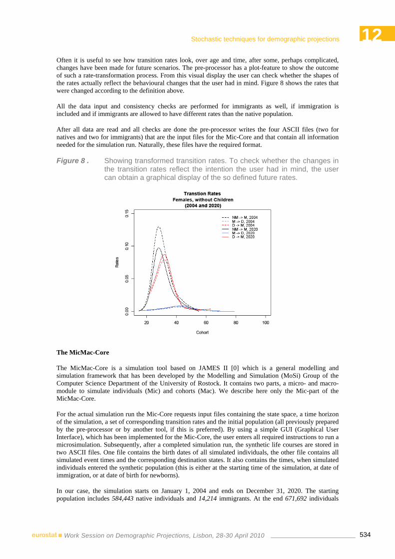
12Stochastic techniques for demographic projections
534Work Session on Demographic Projections, Lisbon, 28-30 April 2010
Often it is useful to see how transition rates look, over age and time, after some, perhaps complicated, changes have been made for future scenarios. The pre-processor has a plot-feature to show the outcome of such a rate-transformation process. From this visual display the user can check whether the shapes of the rates actually reflect the behavioural changes that the user had in mind. Figure 8 shows the rates that were changed according to the definition above.
All the data input and consistency checks are performed for immigrants as well, if immigration is included and if immigrants are allowed to have different rates than the native population.
After all data are read and all checks are done the pre-processor writes the four ASCII files (two for natives and two for immigrants) that are the input files for the Mic-Core and that contain all information needed for the simulation run. Naturally, these files have the required format.
Figure 8 . Showing transformed transition rates. To check whether the changes in the transition rates reflect the intention the user had in mind, the user can obtain a graphical display of the so defined future rates.
The MicMac-Core
The MicMac-Core is a simulation tool based on JAMES II [0] which is a general modelling and simulation framework that has been developed by the Modelling and Simulation (MoSi) Group of the Computer Science Department of the University of Rostock. It contains two parts, a micro- and macro-module to simulate individuals (Mic) and cohorts (Mac). We describe here only the Mic-part of the MicMac-Core.
For the actual simulation run the Mic-Core requests input files containing the state space, a time horizon of the simulation, a set of corresponding transition rates and the initial population (all previously prepared by the pre-processor or by another tool, if this is preferred). By using a simple GUI (Graphical User Interface), which has been implemented for the Mic-Core, the user enters all required instructions to run a microsimulation. Subsequently, after a completed simulation run, the synthetic life courses are stored in two ASCII files. One file contains the birth dates of all simulated individuals, the other file contains all simulated event times and the corresponding destination states. It also contains the times, when simulated individuals entered the synthetic population (this is either at the starting time of the simulation, at date of immigration, or at date of birth for newborns).
In our case, the simulation starts on January 1, 2004 and ends on December 31, 2020. The starting population includes 584,443 native individuals and 14,214 immigrants. At the end 671,692 individuals

12Stochastic techniques for demographic projections
535Work Session on Demographic Projections, Lisbon, 28-30 April 2010
were simulated (newborns included). The sex ratio for newborns was 0.485. Even though the Mic-Core allows transition rates that are different for immigrants, in this example, we do not use this feature. In other words, to simulate life courses the same transition rates are used for natives and immigrants.
The computation took 585.12 seconds (~ 10 minutes) on an average office computer (Intel® Pentium 4CPU, 3.20 GHz, equipped with 3GB memory).
8. The MicMac Post-processor
The MicMac post-processor provides an extensive palette of functions to summarize and illustrate the output of a Mic-Core run. Like the pre-processor the post-processor is also implemented in R, and it is a set of self-contained functions, which are easy to change and to extend.
The post-processor summary functions currently include, among other settings, the following typically used summaries:
• Produce all life courses (i.e., for checking individual biographies).
• Frequency tables of the states occupied at specific dates.
• Population pyramids at specified dates.
• Frequency distribution of the states occupied on January 1, for each year during the simulation period.
• Identification of the most frequent (“typical”) life courses.
Using the post-processor we are able to produce descriptive statistics of the output results in our example. A few results are illustrated in the subsequent.
Figure 9 shows a comparison between the population structure of the initial population and of the simulated population on December 31, 2020. In particular, the graph depicts the number of women and men in each age class and respective numbers of children for women. It is obvious that along the simulation period the number of newborns decreases. Moreover, the alteration of population is evident.

12Stochastic techniques for demographic projections
536Work Session on Demographic Projections, Lisbon, 28-30 April 2010
Figure 9. Comparison of population structure by population pyramids. On the left side, the structure of the initial population is given according to sex, age class, and, for women, according to children even born. On the right side, this is contrasted with the simulated population at simulation ending time.
Figure 10 shows the relative frequency distribution of women experiencing a transition into and out of the “married” status. The distribution has been computed for the corresponding states of origin and states of destination. The proportion of first marriages is high, but only 31% of these marriages are experienced by childless women. The most frequent exit from the state married for women is divorce, and the highest percentage (18%) are women who divorce without having children.
In Figure 10 box-plots are given for the age distribution related to the transition from being childless to the first child (only for females), grouped by marital status. The complete simulation period is summarized here. We can see that the average ages at transition for all three categories are significantly different.

12Stochastic techniques for demographic projections
537Work Session on Demographic Projections, Lisbon, 28-30 April 2010
Figure 10. The relative frequency distribution of origin and destination states to/from being married. Label “other” combines all possible states for which the frequency of transitions to/from is less than 9% (this is mainly done to keep the graph easily legible). (Codes: NM=“never married”, M=“married”, D=“divorced”, W=“widowed”.)
Figure 11. Box-plots of the age distribution at a transition. This graph shows the age at birth of first child for women in different marital status (here married, divorced, widowed). Events are aggregated over the complete simulation period. (Widowed women in this case represent those that have not remarried, but lost their previous partner. This outcome is a consequence of that identical fertility rates for divorced and widowed females were assumed.)

12Stochastic techniques for demographic projections
538Work Session on Demographic Projections, Lisbon, 28-30 April 2010
9. Discussion and Outlook
The MicMac software suite contains a pre-processor for data management and input generation, the Mic-Core for the actual microsimulation, and finally the post-processor for creating useful summaries and appealing graphs. The three parts work hand-in-hand. The choice of this three-part design is due to the fact that both the pre- and post-processor will likely have to be adapted by each user according to the specific needs of the problem to be analyzed. Therefore the free and open-source software R was used for this purpose. The Mic-Core implements high-level performance in the microsimulation, with no need for the user to interfere with this rather technical step. We think that this software design is a pragmatic and efficient compromise between the users’ needs and the technical level demanded by the problem.
The MicMac software currently implements the multistate model which is the basis for the MicMac-project. It is Markovian with age- and calendar time-specific transition rates. A straightforward extension of the model will be the inclusion of a third time-scale in the stochastic model, namely time since entry into current state. This is currently in progress.
Despite the generic and rather flexible multistate model, MicMac has limitations that should be relaxed in the future to allow even more realistic descriptions of individual behaviour and hence population processes. Currently, individual life courses are simulated independently. Hence the concept of linked lives is not yet available in MicMac. The first step into this direction, the implementation of a mate-matching strategy, is already completed [8]. Future developments include the actual simulation of linked lives, after the partners have been linked, and the separation of life courses after a de-linking event, such as divorce or end of cohabitation.
Further complexity in the model formulation and in the simulation, as implemented in the Mic-Core, will, however, also lead to additional requirements for good micro-data to estimate the corresponding empirical transition rates. Also further development of statistical procedures to estimate these transition rates will be needed. Consequently, future progress of microsimulation approaches will be fostered by interdisciplinary collaboration that brings together experts in demographic and social research, computing technology, and statistical methodology.
References
EuroStat (2009). http://epp.eurostat.ec.europa.eu/portal/page/portal/statistics/
Gampe, J. and Zinn, S. (2007). Description of the microsimulation model. Technical report, MPIDR, Rostock. http://www.nidi.knaw.nl/en/micmac/deliverables/new_11/MicMac-D08b+MicMac+microsimulation+model.pdf
JAva-based Multipurpose Environment for Simulation, www.jamesii.org
Impicciatore, R., Billari, C.F., and Beuajouan, E. (2008). Age Profiles Estimation for Family and Fertility Events Base on Micro Data. Technical report, University Bocconi. http://www.nidi.knaw.nl/en/micmac/deliverables/new_28/MicMac-D21+Fertility+and+family+%28age+profiles%29.pdf
R-project, http://www.r-project.org/
Willikens, F. (2006). Multistate model for biographic analysis and projection. Technical report, NIDI.http://www.nidi.knaw.nl/en/output/papers/nidi-wp-2007-01.pdf/nidi-wp-2007-01.pdf
Wissen, L van., Ekamper, P. (2008). Estimating a Starting Population for MicMac. Technical report, NIDI.
Zinn, S. (2010). A Mate-Matching Algorithm For Continuous-Time Microsimulation Models. Submitted.

12Stochastic techniques for demographic projections
539Work Session on Demographic Projections, Lisbon, 28-30 April 2010
Zinn, S., Himmelspach, J., Gampe, J., Uhrmacher, A. (2009). MIC-Core: a tool for microsimulation. Proceedings of the 2009 Winter Simulation Conference. http://www.informs-sim.org/wsc09papers/094.pdf
Acknowledgements
The authors want to thank all partners in the MicMac-project for their input and advice on the software, in particular Nicole van der Gaag and Frans Willekens (NIDI). Discussions and assistance by Jan Himmelspach and Lin Uhrmacher, both at the Modelling and Simulation Research Group at the University of Rostock, were essential for the development of the microsimulation core.


Stochastic national demographic projections Chair: Jutta Gampe
Session 13


13Stochastic national demographic projections
543Work Session on Demographic Projections, Lisbon, 28-30 April 2010
IMMIGRATION, ETHNOCULTURAL DIVERSITY AND THE FUTURE COMPOSITION OF THE CANADIAN LABOUR
FORCE
Alain BÉLANGER1, Nicolas BASTIEN1
Acknowledgements
The authors would like to thank the other members of the DemoSim team: Éric Caron Malenfant, Ivan Carrillo-Garcia, Claude Charette, Rosalinda Costa, Patrice Dion, Marie-France Germain, Dominic Grenier, Steve Gribble, Chantal Grondin, Chantal Hicks, Milorad Kovacevic, Laurent Martel, Geoff Rowe, Martin Spielauer, Robert-Charles Titus, Russell Wilkins and Éric Guimond.
1. Introduction
From 1946 to 1966, Canada has witnessed one of the strongest baby-boom of all industrial countries with its total fertility rates peaking at 3.9 children per woman in 1959 (Romaniuc, 1984). In the following decades, Canada moved rapidly from a high fertility country to a low fertility country. As soon as 1971, its total fertility rate was below replacement level and continued to decline to reach 1.5 children per woman around 2000. Because of this rapid shift in fertility, Canadian population is expected to age rapidly and concerns about possible labour shortages arose as baby-boomers are expected to retire massively from the labour market after 2011. Partly in response to these concerns, Canada raised its immigration intake at the end of the 1980’s and immigration is now the main component of Canadian population growth. The average immigration rate between 1990 and 2009 is 7.5 per thousand. Approximately two-thirds of current Canadian demographic growth is due to net international immigration, a situation that has been observed for a number of years. With each year passing, population growth depends a little more on the contribution of international migration, a trend that is likely to continue in the coming decades as natural increase is expected to remain low and even to become negative (Belanger et al., 2005). With the expected increase in the number and proportion of persons withdrawing from the labour market after 2010 (Martel et al., 2007), pressures to keep immigration rates at fairly high levels will persist.
At the same time, Canadian immigrants are more and more culturally diversified. The majority of immigrants who came to Canada since 1990 have been from Asia, the Middle East and Africa with China, India, Pakistan and the Philippines being the main source countries. As major source regions have shifted from Europe to Asia, immigrants have become more ethnically diverse; a diversity that is expressed through several dimensions. The 2006 Census showed an increase in the numbers and proportions of immigrants, people belonging to visible minority groups and allophones. This transformation should continue in the medium to long term and will impact the ethnocultural composition of the Canadian population and of its labour force.
On the socio-economic side, newcomers show higher levels of educational attainment (Geschender, 1995) and lower labour force participation rates (Model & Lin, 2002; Wannel & Caron, 1994).
1 Institut National de la Recherche Scientifique Centre Urbanisation Culture Société 385, rue Sherbrooke Est Montréal (Québec)
H2X 1E3 CANADA

13Stochastic national demographic projections
544Work Session on Demographic Projections, Lisbon, 28-30 April 2010
Recent researches have shown that recent immigrants encounter greater difficulties than previous waves of immigrants to integrate the labour market (Bloom, Grenier et al. 1994; Picot and Hou 2003; Aydemir and Skuterud 2004; Picot and Sweetman 2005)2. In the years following their arrival in Canada, immigrants usually show lower participation rates, higher unemployment rates and lower total income compared to Canadian natives. While the situation of immigrants landed in the 1970’s and 1980’s rapidly converged to natives’ levels, and even exceeded it after 15 to 20 years of residence in Canada, more recent immigrants seems to struggle much more in their tentative to integrate the labour market.
While newcomers differ in their behaviours from the Canadian-born majority, significant differences are also observed among them. In 2006, the activity rate of non-immigrants aged 25-54 was 87.4 %. This rate was of 86.4 % for established immigrants, 81.6 % for those who immigrated five to ten years earlier, while most recent immigrants had an activity rate of 73.9 %. (Zietsma 2007). During the same period, the unemployment rate of non-immigrants aged 25-54 was 4.9 % which is fairly comparable to the 5.0 % rate for established immigrants. However, the unemployment rate for recent immigrants was 11.5 %. Even though immigrants now come to Canada highly educated, it seems that their high levels of education are not helping them avoid unemployment. In 2006, immigrants who were university graduates had an unemployment rate of 11.4 %, while this number was 2.9 % for non-immigrants (Zietsma 2007).
About 75% of recent immigrants landing in Canada belong to a visible minority groups. Visible minorities are facing greater difficulties in the labour market than people that do not belong to a visible minority. In 2006, visible minorities aged 25-54 had an activity rate of 81.3 % in comparison to 86.6% for those who did not belong to a visible minority group (2006 census). The unemployment rate for the visible minorities aged 25-54 was 7.3 %, while this rate was only of 5.1% for people that did not belong to a visible minority group. Recent immigrants who belong to a visible minority had an unemployment rate 12.2 % while for recent immigrants who did not belong to a visible minority, this rate was 10,3 % (2006 census). It seems that the situation of visible minority immigrants has deteriorated in the last decades. Tran (2004) found that the gap in the unemployment rate of Canadian born that do not belong to a visible minority group and foreign born visible minorities increased between 1981 and 2001. Bélanger and al. (forthcoming) showed that belonging to a visible minority group slowed the access to a first job among new immigrants.
Immigrant women seem to struggle more on the labour market than their male counterpart. They have lower activity rate and higher unemployment rates than males. In 2006, the activity rate for recent immigrant aged 25-54 was 85.4 % and 64.5% respectively for man and women (2006 census). The unemployment rate of recent immigrants aged 25-54 was 10.3 % for men and 13 % for women while for non immigrants these number were 5.2 % and 4.6% respectively for man and women (Zietsma 2007).
Looking at the quality of the employments of immigrants, the situation doesn’t look brighter. In 2008, 42.1 % of immigrants were overqualified for the employment they occupied. In comparison, this number was of 28.1 % for non immigrants. This situation is especially worrying for graduated immigrants. The percentage of overqualified university graduates immigrant was about 1.5 time higher than those of the non-immigrants, 60.1 % compared to 40.5 % (Gilmore 2009). Galarneau and Morisette (2004) studying the proportion of university graduate in a job requiring only a secondary diploma or less (highly dequalified), estimated that in 2001, 25% of recent immigrants were in that situation compared to 12% for non-immigrants. In a more recent article Galarneau and Morisette (2008) showed that between 1991 and 2006 the proportion of immigrants with a university degree who were highly dequalified raised for all the immigrant groups considered.
2 These articles mainly address the declining economic welfare of immigrants by analyzing their revenues. Nevertheless they
give us a good idea of how much immigrants have been struggling on the labour market in the last decades.

13Stochastic national demographic projections
545Work Session on Demographic Projections, Lisbon, 28-30 April 2010
2. Objectives
The main objective of this paper is to chart the future ethnocultural transformations of the Canadian labour force population using the microsimulation projection model DemoSim developed at Statistics Canada (Statistics Canada, 2010). Specifically, we want to project the Canadian labour force until 2031 and look at the change in its ethnocultural and educational composition. We are searching to answer the following question:
1. How demographic components of population growth and changes in participation rates affect the size and the composition of the future labour force?
2. Is Canada really facing a labour shortage?
3. What will be the composition of the future Canadian labour force?
4. Should Canada increase its immigration levels to face potential labour shortage or not?
5. What would be the effect on the labour force population of better economic integration of immigrants?
3. Theoretical background
Microsimulation is necessary to produce demographic and socio-economic projections of the Canadian labour force population in a more diverse ethnocultural context. With the increasing diversity in the origins of Canadian immigrants, the number of dimensions along which this diversity is expressed is also increasing. Thus, to paint a plausible, if not accurate at least unbiased, portrait of the Canadian diversity in the future requires the simultaneous projection of a large number of individual characteristics or attributes: age, sex, place of residence, membership in a visible minority group, religious denomination, mother tongue, age at immigration, period of immigration, education attainment, labour force participation, all of them having several categories (100 age groups, 47 regions of residence, 10 visible minority groups, etc.). The traditional cohort component projection model is not suited to the large number of characteristics needed to be projected in a culturally diversified context. Using a more dynamic approach such as the multistate population projection model would rapidly turn out to be unmanageable, given the size of the transition matrix needed to simultaneously project all possible relevant characteristics. In the multistate model, the state-space consists of all possible combinations of attribute values. In the case of this projection model, the transition matrix would have had to count several hundred billion cells. Clearly, another projection model is needed, namely a microsimulation projection model that enables us to model complex demographic and socio-economic behaviours in a consistent and flexible way (Nelissen, 1991; Alburgh et al., 1998).
For our purpose, microsimulation has several advantages over traditional projection models. Van Imhoff and Post (1998) nicely summarize the circumstances under which microsimulation is more useful than conventional models: 1) if the state space is large (large number of characteristics with large number of values); 2) if the behavioural equation supposes interaction effects between variables (e.g., visible minority group X generation status); 3) if there are interactions between individuals (e.g., if parent characteristics affect children characteristics); and 4) if there are continuous covariates in the model (e.g., age at immigration or duration of residence in Canada).The projection of the ethnocultural diversity of the Canadian labour force encounters all of these conditions and using a microsimulation model is the only proper way to achieve it.

13Stochastic national demographic projections
546Work Session on Demographic Projections, Lisbon, 28-30 April 2010
4. Data and method
DemoSim is a dynamic, continuous time, longitudinal, event-based, open, stochastic (Monte Carlo) spatial microsimulation projection model. It is dynamic as opposed to static in the sense that each individual is aged according to a life-cycle behavioural model, while in a static model, population aging is perform by re-weighting of the initial database using exogenous information (cell-based demographic projections); it is continuous time as opposed to discrete time, which allows for a more accurate representation of behaviours; it is event-based as opposed to time-based in the sense that individual characteristics as well as time are incremented conditionally to the outcome of other modules while time-based models implement modules following a predetermined order (e.g., fertility before mortality or vice-versa); it is open as opposed to closed in the sense that the model allows for new individuals to enter the projected population through immigration or to leave it through emigration; and it is a spatial model as opposed to a single region (national) model in the sense that the model explicitly simulates internal migrations between Canadian metropolitan and non-metropolitan regions. Advantages of such a design are that its dynamic and open features explicitly account for changes in population composition over the projected period. Its continuous time, longitudinal and event-based features does not force the analyst to specify the order in which the events have to be simulated. Finally, its spatial feature allows for spatial analysis of the consequences of immigration, a key element of policy analysis in ethnic diversity and immigration studies.
The base population of this model is composed of the near seven million individuals who answered to the Canadian 2006 Census long form questionnaire. DemoSim simultaneously projects several characteristics (e.g., age, sex, visible minority group, immigrant generation and duration since landing for first generation immigrants, place of birth, education levels, religious denomination and mother tongue) of the Canadian population up to 2031. A fuller description of the model and its demographic assumptions can be found in the projection reports released by Statistics Canada (Bélanger et Caron-Malenfant, 2005; Caron-Malenfant and al. 2010) and can also be found in another chapter of these proceedings Caron-Malenfant et al. (2010). This section will rather describe in details the assumptions and method of estimation of future labour force participation rates.
In this projection, the labour force participation depends on age, sex, immigration status and duration of residence in Canada, education level and visible minority group and region. The estimation of participation rates were realised in two steps. First, we extrapolated the participation rates by age, sex and education levels using the observed annual data of the Labour force survey (LFS) and in a second step, we used the Census 2006 data to measure the differentials in participation rates between immigrant and visible minority groups. Two different scenarios about the future labour force participation trend are created. The first assumes that the age and education-specific activity rates observed in 2008 remain constant over all the projection period, and the second extrapolates the trends in the observed participation rates over the period 1990 to 2008. More specifically, this assumption supposes that the recent trend in increasing labour force participation beyond age 50 would continue for the next decade. The annual rate of change in male age and education-specific participation rates were estimated using linear regressions from the observed annual data of the Canadian Labour Force Survey (LFS). Using the estimated annual rate of change, age and education-specific rates were then extrapolated until 2018, after which they were assumed to remain constant (figure 1).
Not only Canadian females are more and more active in the labour market with their participation rates slowly catching up with those of men, but younger cohorts of women also behave differently in their labour force participation when compared to older cohorts. While older cohorts often withdrew from the labour market after a marriage or at the time of a first birth, more recent cohorts are more likely to continue to participate in the labour market even after marriage or after becoming a mother. In order to account for this cohort effect as well as the recently observed increasing participation rates beyond age 50, female participation rates were obtained by applying female to male participation rate ratios to the extrapolated males participation rates obtained in the previous step. These ratios were calculated taking into accounts age groups and levels of education. As it can be seen in table 1, these ratios are fairly stable over time for the younger age groups, but continue to increase (the cohort catching up process) for the

13Stochastic national demographic projections
547Work Session on Demographic Projections, Lisbon, 28-30 April 2010
older age groups. We thus assume that the 2008 observed ratios would apply over the projection period to women aged less than 50, but as the younger cohorts replace older cohorts, these ratios would increase over time for women aged 50 and over (figure 2).
In addition, the labour force module allows making assumptions concerning the immigrant and visible minority differentials in observed participation rates.
To account for the differentials in participation rates between groups, we calculated ratios of the participation rate of each immigrant groups by duration of residence (4) and visible minority groups (14) to the total participation rate by sex, age groups and education level (4) for Canada using the 2006 Canadian census.
Figure 1. Labour force activity rates by age and education levels for males, Canada 2008 and 2018
0
10
20
30
40
50
60
70
80
90
100
15-19 20-24 25-29 30-34 35-39 40-44 45-49 50-54 55-59 60-64 65+Less than high school diploma High school diploma only
Post-secondary below bachelor level Bachelor level or above
20182008
Table 1. Females to males participation rate ratios by cohort
1993 1998 2003 2008 2013 2018 2023 2028 203315 - 19 0,96 0,99 1,01 1,06 1,06 1,06 1,06 1,06 1,0620 - 24 0,91 0,92 0,95 0,94 0,94 0,94 0,94 0,94 0,9425 - 29 0,85 0,87 0,89 0,90 0,90 0,90 0,90 0,90 0,9030 - 34 0,81 0,84 0,87 0,87 0,87 0,87 0,87 0,87 0,8735 - 39 0,84 0,85 0,88 0,88 0,88 0,88 0,88 0,88 0,8840 - 44 0,85 0,87 0,89 0,90 0,90 0,90 0,90 0,90 0,9045 - 49 0,82 0,87 0,90 0,92 0,92 0,92 0,92 0,92 0,9250 - 54 0,77 0,81 0,87 0,90 0,92 0,92 0,92 0,92 0,9255 - 59 0,65 0,71 0,80 0,86 0,90 0,92 0,92 0,92 0,9260 - 64 0,52 0,57 0,62 0,74 0,86 0,90 0,92 0,92 0,9265+ 0,36 0,34 0,37 0,48 0,74 0,86 0,90 0,92 0,92
Participation rate ratios F/M
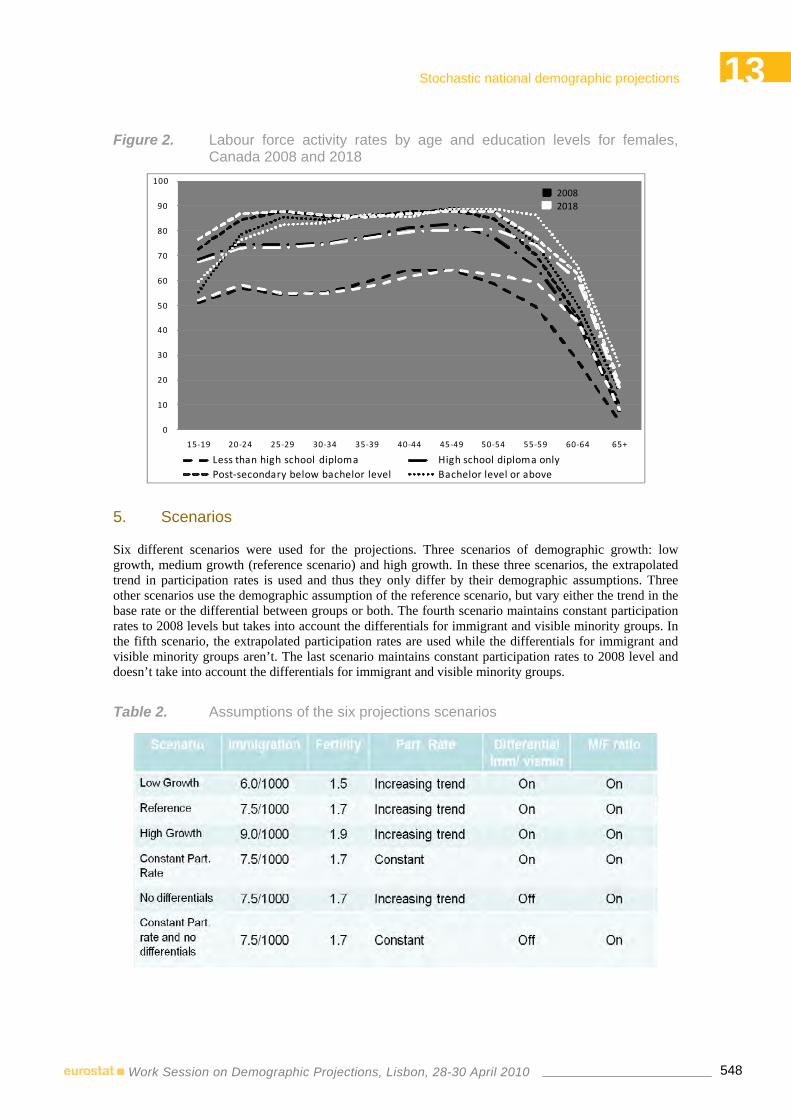
13Stochastic national demographic projections
548Work Session on Demographic Projections, Lisbon, 28-30 April 2010
Figure 2. Labour force activity rates by age and education levels for females, Canada 2008 and 2018
0
10
20
30
40
50
60
70
80
90
100
15-19 20-24 25-29 30-34 35-39 40-44 45-49 50-54 55-59 60-64 65+
Less than high school diploma High school diploma onlyPost-secondary below bachelor level Bachelor level or above
20182008
5. Scenarios
Six different scenarios were used for the projections. Three scenarios of demographic growth: low growth, medium growth (reference scenario) and high growth. In these three scenarios, the extrapolated trend in participation rates is used and thus they only differ by their demographic assumptions. Three other scenarios use the demographic assumption of the reference scenario, but vary either the trend in the base rate or the differential between groups or both. The fourth scenario maintains constant participation rates to 2008 levels but takes into account the differentials for immigrant and visible minority groups. In the fifth scenario, the extrapolated participation rates are used while the differentials for immigrant and visible minority groups aren’t. The last scenario maintains constant participation rates to 2008 level and doesn’t take into account the differentials for immigrant and visible minority groups.
Table 2. Assumptions of the six projections scenarios

13Stochastic national demographic projections
549Work Session on Demographic Projections, Lisbon, 28-30 April 2010
6. Results
Figure 3 presents the evolution of the Canadian labour force population as observed from 1986 and projected to 2031. Interestingly, under all projection scenarios, the projected Canadian labour force population is larger in 2031 than in 2006, meaning that the current levels of immigration are more than sufficient to assure the renewal and even increase of the total labour force. Under the reference scenario, the labour force population would increase from 17.7 million in 2006 to 21.5 million in 2031. This represents an increase of 3.8 million over the 25 years projection. The low growth scenario produces a working force of about 1 million smaller, but still larger than the 2006, while the high growth scenario generates a total of about 1 million larger than the reference scenario. The average annual growth rate of the workforce of 15 per 1000 observed during the 1986-2006 period would remain at that level until 2011 but decline thereafter with the baby-boomer reaching retirement age in mass. Nevertheless, it would remain positive over all the projection period. On average, over the projection period, the annual growth rate (8 per 1000) is about half the level of the preceding 20 years period. Compared to the reference scenario, changes in participation rates and changes in immigrant/visible minority differentials in participation rates produce somewhat smaller variations in the projection horizon labour force population, but not without importance. A constant labour force participation would produce a smaller total labour force population by 280,000, and assuming that the differentials in labour force participation were eradicated, would increase it by 122,000. Note that this is only the effect of changes in the composition of the population. This scenario applies the average (all population) age-sex-education specific participation rates, and thus, it assumes a decrease in the labour force participation rates of the population that does not belong to a visible minority group. In future developments to the projection model, we could use the higher rates observed for the population that does not belong to a visible minority group rather than the average age-sex-education specific rates to measure the total impact on the labour force population of a full integration of the immigrant and visible minority groups to the workforce.
Figure 3. Evolution of the Canadian labour force population (in thousands) under six scenarios, 1986-2031
12000
14000
16000
18000
20000
22000
24000
1986 1991 1996 2001 2006 2011 2016 2021 2026 2031
Low growth Reference
High growth Constant participation rate
No differentials (imm/vis min) Constant participation & no differentials
thousands projectedobserved

13Stochastic national demographic projections
550Work Session on Demographic Projections, Lisbon, 28-30 April 2010
Giving the age structure of the Canadian population, declining overall participation rates are however unavoidable. Currently at around 67%, it could decline to 62% or 63 % according to the different scenarios. This is not a dramatic decline over a 25 year period. This rate is currently historically high and the overall rate had been lower than 62% when the baby-boomers were not all yet in the working age groups. It is interesting to note that the different demographic assumptions have virtually no impact on the evolution of the overall participation rate, even if the low and high growth scenario have fairly different immigration and fertility rates. On the other hand, different evolution of the participation rate produces important differences. The scenario with no differential between immigrants and non-immigrants and between visible and non-visible population is the scenario producing the highest overall participation rate (63%), slightly larger than the high demographic growth scenario (62.7%). Immigration and human resource policy makers should considered seriously that it might be preferable to invest more on employment programs to reduce inter-groups differentials in participation in order to reduce the pressure of population aging, rather than simply increasing immigration levels.
Figure 4. Overall labour force participation rate under six scenarios, Canada 1986-2031
61%
62%
63%
64%
65%
66%
67%
68%
1986 1991 1996 2001 2006 2011 2016 2021 2026 2031
Low growth Reference
High growth Constant participation rate
No differentials (imm/vis min) Constant participation & no differentials
observed projected
Under all scenarios, the Canadian born population in the labour force is larger in 2031 than in 2006. According to the reference scenario, the Canadian born labour force population increases from 13.8 million in 2006, peaks at 14.6 millions in 2016 and slightly declines thereafter to reach 14.5 million in 2031. This is largely due to the assumption about future female participation as even in the constant participation rate scenario (where female rates still increase) we observe an increase of near 600,000 over the 25 years. The future increase of the labour force population is much more due to large number of immigrants entering the labour force. From 3.8 million workers, the Canadian immigrant working force will reach between 5.8 and 7.5 millions, according to the different scenarios. Under the reference scenario and over the 25 year projection period, the labour force annual growth rate is 2 per 1,000 for the native born and 10 times larger (23 per 1,000) for the immigrant population. This of course will have for effect to increase the proportion of immigrants in the total labour force population from about 1 out of 5 (21% in 2006) to 1 out of 3 in 2031 (figure 5).

13Stochastic national demographic projections
551Work Session on Demographic Projections, Lisbon, 28-30 April 2010
Figure 5. Percentage of immigrants in the Canadian labour force, 2006 and 2031 under six scenarios
28,6%30,9%
33,3%30,9% 31,5% 31,5%
0,0%
5,0%
10,0%
15,0%
20,0%
25,0%
30,0%
35,0%
Low growth Reference High growth Constant participation
rate
No differentials
(imm/vis min)
Constant participation
& no differentials
In 2031, the Canadian labour force will not only be much more foreign-born, but it will also be much more diverse in its ethnocultural ethno cultural composition. Under all scenarios, except the high growth scenario, the projected labour force population who does not belong to a visible minority groups (white) would be smaller in 2031 than in 2006. Under the reference scenario, it would decrease by about 300,000 and, according to the high growth scenario it would increase by about 80,000. On the other hand, the labour force population who belong to a visible minority groups would increase rapidly with annual growth rates ranging from 3.3% to 4.1%, according to the different scenarios. From 2.8 million in 2006, the visible minority workforce would reaches 6.2 million and 7.6 million under the low and high growth scenarios, respectively. Consequently, the proportion of visible minority population among the labour force will likely double (figure 6). Under these circumstances, the importance of better addressing the issues relative to a future full economic integration of immigrants and visible minority can only be exacerbated.
Figure 6. Percentage of the Canadian labour force that belong to a visible minority group, 2006 and 2031 under six scenarios.
3 0 ,5 %3 2 ,1 %
3 3 ,6 %3 2 ,2 %
3 3 ,2 % 3 3 ,4 %
0 ,0 %
5 ,0 %
1 0 ,0 %
1 5 ,0 %
2 0 ,0 %
2 5 ,0 %
3 0 ,0 %
3 5 ,0 %
4 0 ,0 %
L o w g r o w th R e fe r e n c e H ig h g r o w th C o n stan t p ar tic ip atio n
r ate
N o d iffe r e n tia ls
( im m /v is m in )
C o n stan t p ar tic ip atio n
& n o d iffe r e n tia ls
2006
2006

13Stochastic national demographic projections
552Work Session on Demographic Projections, Lisbon, 28-30 April 2010
The microsimulation model yields much richer results than the cohort-component approach. Another interesting result from the microsimulation projections is the projected evolution of the educational composition of the labour force. The following figure 7 shows the labour force population growth rate by education level and immigrant status. In total the labour force population growth rates are positive for immigrants and close to 0 for non-immigrants after 2016. For the less educated group, however, these rates are barely positive for immigrants and strongly negative for the larger non-immigrant population. It is even truer for the working force with only a high school diploma where both immigrants and non-immigrants show negative growth rate of about minus 2% per year over the full projection period. For post-secondary non university graduates, the reference scenario projects fairly strong growth rates for the immigrant population, but declining growth rate down to minus 2% per year after 2021 among the non-immigrant population. It is among the university graduates that the model projects the highest annual growth rate in the labour force population. For both, the Canadian and the foreign born, according to the reference scenario, the growth rates are well above the total labour force population growth rates. They also follow the same trends starting from an annual growth rate of near 5% a year in 2006-2011 and going down almost linearly to a growing rate of 3 to 4% a year in 2026-2031.
As a consequence, and according to the reference scenario, the total workforce would increase by about 21% over the 25 years projection period, from 17.7 million to 21.5 million or a total increase of 3.8 millions. However, almost all the increase will be among the university graduates while the less educated labour force population will decline. Actually, the university graduate population will increase by almost 5.5 million people (from 3.9 million to 9.4 million) while the working force with a high school diploma or less will decline by some 1.8 million (from 7.3 million to 5.4 million) and the post-secondary without a university degree will remain almost unchanged at 6.7 million people (table 3).
Figure 7. Labour force population annual growth rate by immigrant status and education levels, reference scenario, Canada 2006-2031
-3%
-2%
-1%
0%
1%
2%
3%
4%
5%
6%
2 006 -201 1 20 11 -2 01 6 201 6-20 21 2 02 1-20 26 20 26 -2 03 1
Less than high school diplom a High school diplom a only
Post-secondary below bachelor level Bachelor level or above
Total
im m igrantsnon im m igrants

13Stochastic national demographic projections
553Work Session on Demographic Projections, Lisbon, 28-30 April 2010
Table 3. Projected labour force population (in thousands) by education level and immigrant status, reference scenario, Canada 2006-2031.
2006 2011 2016 2021 2026 2031Variations 2006-2031
Less than high school diploma 2186 1973 1853 1755 1691 1663 -523High school diploma only 3751 3739 3385 2996 2713 2538 -1213Post-secondary below bachelor level 5194 5431 5331 4965 4509 4101 -1093Bachelor level or above 2632 3297 4052 4812 5523 6213 3581Total 13762 14439 14622 14528 14436 14516 754
Less than high school diploma 468 490 537 578 618 661 193High school diploma only 831 765 691 619 555 501 -330Post-secondary below bachelor level 1283 1575 1832 2075 2283 2459 1176Bachelor level or above 1199 1523 1873 2252 2646 3034 1835Total 3780 4352 4932 5524 6101 6654 2874
Less than high school diploma 2666 2500 2444 2389 2361 2372 -294High school diploma only 4608 4536 4112 3652 3304 3072 -1536Post-secondary below bachelor level 6513 7106 7308 7194 6942 6699 186Bachelor level or above 3890 4912 6039 7182 8284 9356 5466Total 17677 19053 19903 20416 20891 21500 3823
Non-immigrant labour force population
Immigrant labour force population
Total labour force population
7. Conclusion
Under all scenarios, Canada labour force population will continue to increase in the next 25 years, but at a slower rate than in the recent past. Even under the low growth scenario, which assumes lower fertility and lower immigration rates than currently observed, the labour force population would increase by near three million people in the next 25 years. Yet, the fear of labour shortage is too often used to put pressure on the government to increase immigration levels:
The stakes are high. In 2006, Canada welcomed 251,511 immigrants, most of them highly skilled, through its doors. Almost 70 per cent of them landed in Toronto, Montréal and Vancouver, the urban engines of our economy (with Toronto alone accounting for 39 per cent of the total). Yet there is a pressing need for more immigration. The Conference Board estimates that we need 375,000 new immigrants annually in order to stabilize the workforce and ensure economic growth. Finding and attracting them is the first challenge facing this country. Conference Board of Canada (2010)
It is also important to note that if demographic components of population change can have an impact on the size of the future labour force, it cannot modify significantly the future evolution of the overall participation rate which would decline under all scenarios after 2011-2016. This decline in the overall participation rate is unavoidable and results from the current age structure of the population, the large cohorts of baby-boomers now reaching retirement age. If because of population aging, the Canadian overall participation rate can only decline in the near future, this decline is not dramatic and many factors can temper it, but increasing immigration is not one of them. On the other hand, a better economic integration of immigrants can not only increase the total labour force population, but also mitigate the declining overall participation rate. Rather than admitting more immigrants, it could be more effective to encourage people to postpone retirement, help women to conciliate work and family obligations and better integrate the immigrants that Canada currently receives.

13Stochastic national demographic projections
554Work Session on Demographic Projections, Lisbon, 28-30 April 2010
These projections also demonstrate that Canada labour force is likely to witness important changes in its ethnocultural composition. The future increase of the labour force population will be mostly a result of increasing number of immigrants entering the labour force. According to the reference scenario, the total labour force population would increase by 3.8 million people, of which 2.9 million would be immigrants. Second generation non-European immigrants are now entering the labour market and with the projected continued high immigration intakes, the increase in the labour force population that belong to a visible minority group is much larger. According to the reference scenario, the labour force population that belong to a visible minority group would increase from 2.8 million in 2006 to 6.9 million in 2031, a 4.1 million increase and from 15% in 2006, their percentage of the total labour force will reach at least 30% in 2031.
These rapid changes in the ethnocultural composition of the future labour force strengthen the case for a better integration of immigrants and visible minority in the Canadian economy. To assure a full integration of these new workers, Canada is facing several challenges. First, a more diversified immigration means that a smaller fraction of immigrants have a good knowledge of English or French, the two official languages of Canada. Studies have shown that despite their higher education level, the average literacy level of immigrants is lower than the average literacy level of Canadian-born (Statistics Canada, 2005; Gluszynski and Dhawan-Biswal, 2008) and that it can account for about one-half of the earnings gap between native-born and immigrant university graduates (Ferrer and al., 2004).
The second challenge concerns the recognition of foreign experience and education (Schellenberg and Maheux, 2007). All degrees are not equal and part of the learned skills is location specific. Immigrants graduated from non-Western universities seem to struggle more on the labour market than other immigrants (Green and Riddell, 2003; Sweetman, 2004). The projections show that the highly educated labour force will increase rapidly from both the native-born and the foreign-born sides. Unless programs to help immigrants upgrade their education skills and obtain Canadian recognition are put in place, it is likely that disqualification of immigrant degrees will persist. Finally, immigrants and members of visible minority groups in particular might be facing possible discrimination from employers (Pendakur and Pendakur 1998; Oreopoulos 2009).
References
Ahlburg, D. A., Lutz, W. & Vaupel, J. W. (1998). Ways to improve population forecasting: What should be done differently in the future [Supplement: Frontiers of population forecasting]. Population and Development Review, 24, 191-198.
Aydemir, Abdurrahman, and Mikal Skuterud (2004). Explaining the Deteriorating Entry Earnings of Canada’s Immigrant Cohorts: 1966-2000. Statistics Canada. Ottawa. 11F0019MIE: 31 p
Bélanger, Alain, Germain Bingoly-Liworo and Jacques Ledent. (forthcoming). «Analyse longitudinales des facteurs explicatifs de l'intégration sur le marché du travail des immigrants récents dans les provinces de Québec, Ontario et Colombie-Britannique».
Belanger, A. P. & Caron-Malenfant, E. (2005). Population Projections of Visible Minority Groups, Canada, Provinces and Regions 2001-2017. Statistics Canada. Cat. No. 91-541-XIE, 78 p. http://www.statcan.ca/english/freepub/91-541-XIE/91-541-XIE2005001.pdf
Belanger, A. P., Martel, L. & Caron-Malenfant, E. (2005). Population Projections for Canada, Provinces and Regions 2001-2031. Statistics Canada. Cat. No. 91-520-XWE. 214 p. http://www.statcan.ca/english/freepub/91-520-XIE/0010591-520-XIE.htm
Bloom, David E., Gilles Grenier and Morley Gunderson. 1994. «The Changing Labor Market Position of Canadian Immigrants». National Bureau of Economic Research Working Paper Series, vol. 4672.

13Stochastic national demographic projections
555Work Session on Demographic Projections, Lisbon, 28-30 April 2010
Caron-Malenfant, Éric. 2009. «Un aperçu de DemoSim, le modèle de projections démographiques par microsimulation de Statistique Canada». In Conférence 2009 de l’Association internationale de microsimulation.
Caron-Malenfant, Éric, André Lebel and Laurent Martel (2010). Projections de la diversité de la population canadienne. Statistique Canada. Ottawa. 91-551-X
Conference Board of Canada (2010). Immigration. Accessed in May 2010 at:
http://www.conferenceboard.ca/topics/immigration/default.aspx
Ferrer, Ana, David A. Green and W. Craig Riddell (2004). The Effect of Literacy on Immigrant Earnings. Human Resources Development Canada. Ottawa, Statistics Canada. 89-552-MIE: 44 p
Galarneau, Diane, and René Morissette. 2004. «Immigrants: Settling for less?». Perspective, vol. 75-001-XIE, p. 5-16.
--------. 2008. «Scolarité des immigrants et compétences professionnelles requises». Perspective, no 75-001-X, p. 5-19.
Geschwender, J. & Guppy, N. (1995). Ethnicity, educational attainment, and earned income among Canadian-born men and women. Canadian Ethnic Studies, 27(1), 67-84.
Gilmore, Jason (2009). Les immigrants sur le marché du travail canadien en 2008: analyse de la qualité de l'emploi. Ottawa, Statistique Canada. 71-606-X: 39 p
Gluszynski, Tomasz, and Urvashi Dhawan-Biswal (2008). Reading skills of young immigrants in Canada: the effects of duration of residency, home language exposure and schools. Learning research series. Human Resources and Social Development Canada. Ottawa: 37 p
Green, David , and W. Craig Riddell. 2003. «Literacy and Earnings: An Investigation of the Interaction of Cognitive and Unobserved Skills in Earnings Generation». Labour Economics, vol. 10, no 2, p. 165-184.
Martel, L., Caron-Malenfant, E., Vezina, S. & A. P. Belanger (2007). Labour Force Projections for Canada, 2006-2031. Canadian Economic Observer, 20(6), 1-13.
Model, S. & Lin, L. (2002). The cost of not being Christian: Hindus, Sikhs and Muslims in Britain and Canada. International Migration Review,36(4), 1061-1092.
Nelissen, J. H. M. (1991). Household and education projections by means of a microsimulation model. Economic Modelling, 8(4), 410-511.
Oreopoulos. 2009. «Why do Skilled immigrants struggle in the labor market?». Metropolis British Columbia Working Paper Series, vol. 09, no 03, p. 50.
Pendakur, Krishna, and Ravi Pendakur. 1998. «The colour of money: earnings differentials among ethnic groups in Canada». Canadian Journal of Economics, vol. 31, no 3, p. 518-548.
Picot, Garnett, and Feng Hou (2003). The rise in low-income rates among immigrants in Canada. Ottawa, Statistics Canada. 11F0019MIE — No. 198: 54 p
Picot, Garnett, and Arthur Sweetman (2005). The Deteriorating Economic Welfare of Immigrants and Possible Causes: Update 2005. Ottawa, Statistics Canada. 11F0019MIE — No. 262: 26 p
Romaniuc, A. (1984). La fécondité au Canada : Croissance et déclin. Ottawa, Statistique Canada 91-524.158 p.

13Stochastic national demographic projections
556Work Session on Demographic Projections, Lisbon, 28-30 April 2010
Schellenberg, Grant, and Hélène Maheux. 2007. «Perspectives des immigrants sur leurs quatre premières années au Canada». Tendances sociales canadiennes, no 11-008, p. 36.
Statistics Canada (2003). Building on our Competencies: Canadian Results of the International Adult Literacy and Skills Survey. Ottawa, Statistics Canada. Catalogue no. 89-617-XIE: 242 p
Sweetman, Arthur (2004). Immigrant Source Country Educational Quality and Canadian Labour Market Outcomes. Analytical Studies Branch Research Paper Series. Ottawa, Statistics Canada. 11F0019MIE — No. 234: 45 p
Van Imhoff, E. & Post, W. (1998). Microsimulation methods for population projection [Special Issue New Methodological Approaches in the Social Sciences]. Population: An English Selection, 10(1), 97-138.
Wannell, T. & Caron, N. (1994). The Gender Earnings Gap Among Recent Postsecondary Graduates, 1984-92 (Research Paper No. 69). Ottawa: Statistics Canada.
Zietsma, Danielle (2007). Les immigrants sur le marché canadien du travail en 2006: premiers résultats de l’Enquête sur la population active du Canada. Statistique Canada. Ottawa. 71-606-XIF2007001:28p

13Stochastic national demographic projections
557Work Session on Demographic Projections, Lisbon, 28-30 April 2010
DEVELOPING STOCHASTIC POPULATION FORECASTS FOR THE UNITED KINGDOM: PROGRESS REPORT
AND PLANS FOR FUTURE WORK
Steve ROWAN1, Emma WRIGHT1
Abstract
The UK’s Office for National Statistics (ONS) produces national population projections for the United Kingdom every two years. In addition to the principal (main) projections, variant projections are also produced. The variant projections are intended as plausible alternative scenarios and do not represent upper and lower limits for future demographic behaviour. In these variants, the different fertility, mortality and migration assumptions are treated as separate and independent departures from the assumptions in the principal projection.
One of the limitations of the traditional deterministic approach used to produce the national population projections is that no probabilities are attached to the projections; users are therefore given no information about the uncertainty associated with them. ONS is addressing this issue by developing a stochastic forecasting model for the United Kingdom.
This paper outlines the progress to date on developing a stochastic model. It describes how uncertainty about future demographic behaviour has been taken into account by expressing fertility, mortality and migration assumptions in terms of their assumed probability distributions. In each case, the median of the probability distribution is designed to follow the principal assumption from the 2006-based traditional deterministic projections. Three approaches for determining the probability distributions are also discussed. The paper reports the early findings of the research to date, and outlines ONS’s plans for future work in this area.
It should be noted that the research reported is still in progress and, as such, any results presented are provisional only.
Acknowledgements
This paper reports work conducted by Cath Brand, Mita Saha, Chris Shaw and Steve Rowan from the ONS Centre for Demography. Many thanks to Professor Phil Rees from the University of Leeds, Professor Nico Keilman from the University of Oslo, Professor Wolfgang Lutz from the Vienna Institute of Demography and Ruth Fulton and colleagues from ONS Methodology Directorate for their advice and input.
1 Office for National Statistics, UK

13Stochastic national demographic projections
558Work Session on Demographic Projections, Lisbon, 28-30 April 2010
1. Introduction
National population projections (NPP) for the United Kingdom (UK) and its constituent countries are produced by ONS every two years. These demographic-based projections are essential for national planning functions in a range of fields and feed into sub-national, household, labour force and marital status projections. They are dependent on a set of assumptions about future levels of fertility, mortality and migration, which are reviewed and revised for each projection round. Details of the latest (2008-based) projections are described in Population Trends 2 and in the latest national population projections reference volume.3
The complete results of the 2008-based principal (main) and variant projections are obtainable from the ONS website.4 However, the work reported in this paper was conducted prior to the release of the 2008-based projections (in October 2009) and therefore focuses on the previous, 2006-based, national population projections released in October 2007. 5
The principal population projections are based on assumptions considered to be the best that could be made at the time they are adopted. Variant projections are also produced, which are intended as plausible alternative scenarios and do not represent upper or lower limits for future demographic behaviour. In these variant projections, the different fertility, mortality and migration assumptions are treated as separate and independent departures from the assumptions in the principal projections. ‘Single component’ variants, varying just one of the three components, are produced, as well as selected ‘combination’ variants produced by combining two or more of these alternative scenarios.
It is increasingly being recognised, however, that the traditional deterministic approach has a number of limitations. As stated earlier, no probabilities are attached to the principal projections so users are given no information about the uncertainty associated with them or, with respect to the variants, are given no indication of how these compare to the principal projections in terms of certainty. In response to these concerns, increasing attention is now being given to stochastic forecasting methods. Typically, stochastic forecasts use probability distributions for the components of demographic change, namely of fertility, mortality and migration. These are derived using some combination of three recognised approaches: analysis of past projection errors, expert opinion and time series analysis. By using these approaches, ONS is developing a stochastic forecasting model for the United Kingdom.
This paper describes how uncertainty about future demographic behaviour has been taken into account by expressing fertility, mortality and migration in terms of their assumed probability distributions. In each case, the median of the probability distribution was designed to follow the principal assumption from the traditional deterministic projections in order to assess the uncertainty associated with the published deterministic projections.
It is important to recognise that stochastic forecasts have their limitations too. In particular, there is a risk that specifying precise probability ranges may convey a misleading sense of precision to users.6 The true probability distribution for the future total fertility rate (TFR), for example, is not a known quantity. In
2 Wright E (2010). 2008-based national population projections for the UK and constituent countries. Population Trends 139.
Available from 25 March 2010 at: http://www.statistics.gov.uk/StatBase/Product.asp?vlnk=6303 3 ONS (2010) National Population Projections 2008-based (PP2 no. 27). Available from 25 March 2010 at: http://www.statistics.gov.uk/StatBase/Product.asp?vlnk=4611 4 Full results of the 2008-based national population projections available at:
http://www.statistics.gov.uk/statbase/Product.asp?vlnk=8519 5 Full results of the 2006-based national population projections, and previous UK population projections, available on
Government Actuary’s Department (GAD) website at: www.gad.gov.uk/Demography%20Data/Population/index.aspx 6 Lutz W and Goldstein JR (2004) Introduction: How to Deal with Uncertainty in Population Forecasting? International
Statistical Review, Volume 72, Number 1. Available at: http://projecteuclid.org/DPubS?service=UI&version=1.0&verb=Display&handle=euclid.isr/1079360109
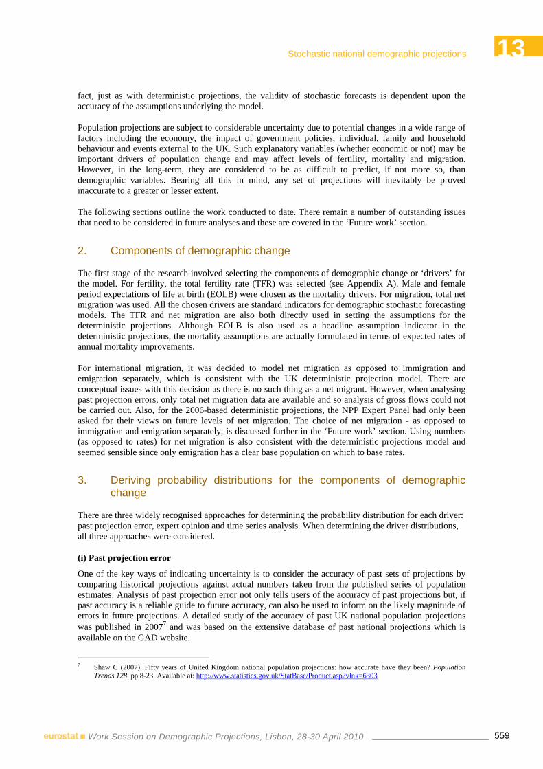
13Stochastic national demographic projections
559Work Session on Demographic Projections, Lisbon, 28-30 April 2010
fact, just as with deterministic projections, the validity of stochastic forecasts is dependent upon the accuracy of the assumptions underlying the model.
Population projections are subject to considerable uncertainty due to potential changes in a wide range of factors including the economy, the impact of government policies, individual, family and household behaviour and events external to the UK. Such explanatory variables (whether economic or not) may be important drivers of population change and may affect levels of fertility, mortality and migration. However, in the long-term, they are considered to be as difficult to predict, if not more so, than demographic variables. Bearing all this in mind, any set of projections will inevitably be proved inaccurate to a greater or lesser extent.
The following sections outline the work conducted to date. There remain a number of outstanding issues that need to be considered in future analyses and these are covered in the ‘Future work’ section.
2. Components of demographic change
The first stage of the research involved selecting the components of demographic change or ‘drivers’ for the model. For fertility, the total fertility rate (TFR) was selected (see Appendix A). Male and female period expectations of life at birth (EOLB) were chosen as the mortality drivers. For migration, total net migration was used. All the chosen drivers are standard indicators for demographic stochastic forecasting models. The TFR and net migration are also both directly used in setting the assumptions for the deterministic projections. Although EOLB is also used as a headline assumption indicator in the deterministic projections, the mortality assumptions are actually formulated in terms of expected rates of annual mortality improvements.
For international migration, it was decided to model net migration as opposed to immigration and emigration separately, which is consistent with the UK deterministic projection model. There are conceptual issues with this decision as there is no such thing as a net migrant. However, when analysing past projection errors, only total net migration data are available and so analysis of gross flows could not be carried out. Also, for the 2006-based deterministic projections, the NPP Expert Panel had only been asked for their views on future levels of net migration. The choice of net migration - as opposed to immigration and emigration separately, is discussed further in the ‘Future work’ section. Using numbers (as opposed to rates) for net migration is also consistent with the deterministic projections model and seemed sensible since only emigration has a clear base population on which to base rates.
3. Deriving probability distributions for the components of demographic change
There are three widely recognised approaches for determining the probability distribution for each driver: past projection error, expert opinion and time series analysis. When determining the driver distributions, all three approaches were considered.
(i) Past projection error
One of the key ways of indicating uncertainty is to consider the accuracy of past sets of projections by comparing historical projections against actual numbers taken from the published series of population estimates. Analysis of past projection error not only tells users of the accuracy of past projections but, if past accuracy is a reliable guide to future accuracy, can also be used to inform on the likely magnitude of errors in future projections. A detailed study of the accuracy of past UK national population projections was published in 20077 and was based on the extensive database of past national projections which is available on the GAD website.
7 Shaw C (2007). Fifty years of United Kingdom national population projections: how accurate have they been? Population
Trends 128. pp 8-23. Available at: http://www.statistics.gov.uk/StatBase/Product.asp?vlnk=6303

13Stochastic national demographic projections
560Work Session on Demographic Projections, Lisbon, 28-30 April 2010
Similarly, the accuracy of the fertility, mortality and migration assumptions from past sets of projections can be compared with actual values. Using the GAD database, 18 sets of projections from the 1971-based projections up to the 2004-based projections were used to identify past projection errors. For each driver, the root mean squared error (RMSE, see Appendix A) was calculated for one year ahead and for all years up to twenty five years ahead. The RMSE provides a single measure of the difference between the original assumptions and actual values at any time into the projection period.
Over the years there have been many population revisions and it is predominantly migration that has been affected. However, no adjustment has been made to allow for such revisions in the calculation of RMSEs. If the first few projection years are ignored, as these will be the most affected, the RMSEs for five years ahead durations (and upwards) are much more reliable indicators of ‘real’ projection error.
(ii) Expert opinion
Expert views on future demographic behaviour have been obtained from the NPP expert advisory panel.8
They provide advice on the appropriate assumptions to use for the NPP. In 2007, ahead of the 2006-based projections, the six experts on the panel were asked to complete a detailed questionnaire in which they were asked for their opinions on the most likely levels (with 67 per cent confidence intervals) for the TFR, male and female EOLB and annual net migration in 2010 and 2030, which was five and twenty five years ahead of the latest data available at the time.
For each of the drivers, a mean of the six responses and a mean of both the upper and lower confidence intervals (CIs) were calculated. Whenever an interval was non-symmetric, the wider interval was chosen to ensure symmetry.
An assumption was made that for each driver, these ‘average’ confidence intervals came from a normal distribution with mean equal to the ‘average’ most likely level. From this, standard deviations were estimated and 95 per cent confidence intervals for five and twenty five years ahead were derived.
(iii) Time series
The time series method of analysis uses the trends and variability of historical time series of fertility, mortality and migration indicators to produce estimates of the standard deviations around future values. The time series models explored included simple exponential smoothing, log linear (Holt) exponential smoothing and linear trends. In general, the resultant probability distributions differed considerably from those distributions derived using past projection error and expert opinion.
Consequently, time series techniques have not been used in this early research to determine the probability distributions described in this paper. However, it is recognised the use of a time series approach needs to be explored more fully in the future (see ‘Future work’ section).
8 Details of the most recent meeting of the NPP Expert Advisory Panel in spring 2009 are available at
http://www.statistics.gov.uk/downloads/theme_population/NPP2008/NatPopProj2008.pdf (see section 11). Details of the meeting of the panel held prior to the production of the 2006-based projections are available at:
http://www.gad.gov.uk/Demography Data/Population/2006/methodology/expert1.html

13Stochastic national demographic projections
561Work Session on Demographic Projections, Lisbon, 28-30 April 2010
4. Comparison of past accuracy and expert opinion approaches
The five and twenty five years ahead standard deviations derived from expert opinion are compared with RMSEs derived from past projection errors in Table A.
Table A. Comparative measures of uncertainty for five and twenty five years ahead
TFR
(number of children)
male EOLB
(years)
female EOLB
(years)
Net migration
(000s) Experts: standard deviation 0.15 1.18 0.79 51.3
Five years ahead Past accuracy: RMSE 0.20 0.78 0.66 58.6
Experts: standard deviation 0.26 2.31 2.05 90.7
Twenty five years ahead Past accuracy: RMSE 0.50 4.79 3.30 162.4
Note: The bold values were used to derive the sample paths for the drivers used in the final model (see ‘Forecast assumptions’ section).
Table A shows the standard deviations derived from expert opinion and the RMSEs derived from past projection error at both five and twenty five years ahead. Although some exploratory work has been carried out, more work is required to test whether differences can be attributed to sampling error by calculating uncertainty around each standard deviation or RMSE. This is particularly important for expert opinion given that the results are based on a small sample of six experts. The accuracy of the estimated standard deviations will also be dependant on the underlying assumption that the experts’ ‘average’ confidence intervals are taken from a Normal distribution. This is discussed further in the ‘Future work’ section.
For past projection error, no distribution has been assumed. The direction of the error over time and any bias towards under or overestimation, are discussed in the ‘Forecast assumptions’ section.
5. The model
The overall model uses a version of the cohort component model used to produce the deterministic projections, as follows:
ttttt MDBPP +−+= −1
where t denotes the year of forecast, 1−tP is the level of the population in the previous year and tB , tD
and tM are total counts of births, deaths and net migration, respectively.
The difference is that instead of specifying fertility, mortality and migration for the whole projection period, this model uses counts of births, deaths and net migration derived from the stochastically determined drivers of fertility, mortality and migration. (The ‘Sample path’ section describes how total counts of births, deaths and net migration were derived.)
The probability distributions for year to year change are generated by carrying out a large number of simulations (or sample paths) of the overall model.

13Stochastic national demographic projections
562Work Session on Demographic Projections, Lisbon, 28-30 April 2010
A random walk with drift (RWD) model was chosen to generate the drivers for each sample path. The level of each driver from one year to the next is:
Drivert = Drivert-1+ Valuet + Driftt
where t denotes the year of forecast, Drivert-1 is the level of the driver in the previous year, Valuet is a random value sampled from a normal distribution of year on year differences with a mean of zero and a pre-selected one-year ahead standard deviation. Details of the one year ahead standard deviations chosen for each driver are given in the ‘Forecast assumptions’ section. Driftt is a drift term which constrains the median of the probability distribution to follow the 2006-based UK principal assumptions. The drift term is calculated as:
Driftt = PDrivert – PDrivert-1 where PDrivert and PDrivert-1 are driver values taken directly from the 2006-based UK principal assumptions.
To get the random value, a random number is generated from a normal distribution using a Box Muller9 approach. Each random number is then multiplied by a pre-selected one year ahead standard deviation (which, for each driver, is fixed throughout the projection period).
The one year ahead standard deviation is calculated as follows:
SD1=SDt / t
where SD1 is the unknown standard deviation at one year ahead; and SDt is the known standard deviation at t years ahead (derived from past projection error or expert opinion).
Making the assumption of perfect correlation between the sexes, the same random numbers were used for male and female EOLB. However, for each of the three different drivers, the random numbers were generated separately. This implicitly assumes the probability distributions for each driver are independent of each other. This does not imply that the number of births and deaths are unaffected by changes in population size due to migration.
6. Forecast assumptions
(i) Fertility
The TFR sample paths were generated using a RWD model where the drift term constrained the median of the probability distribution to follow the TFR principal assumption from the 2006-based UK NPP, namely a long-term TFR of 1.84.
In order for the TFR sample paths to have a probability distribution that closely matched the experts’ ‘average’ 67 per cent CI at twenty five years ahead, the derived experts’ standard deviation of ±0.26 children was chosen (see Table A). A one year ahead standard deviation of 0.05 children was calculated and fed into the random value component (where 0.05=0.26/ 25 ).
Figure 1 shows that the 67 per cent prediction intervals broadly match the high/ low fertility variants of the NPP, but are much narrower than the experts’ ‘average’ 67 per cent CIs at five years ahead. However, the 95 per cent prediction intervals closely match the derived experts’ 95 per cent CI at twenty five years ahead. The RMSEs (based on past projection error) are also included in the chart for information.
9 Golder E and Settle J (1976) The Box-Muller Method for Generating Pseudo-Random Normal Deviates. Applied Statistics,
Vol. 25, No. 1, pp. 12-20

13Stochastic national demographic projections
563Work Session on Demographic Projections, Lisbon, 28-30 April 2010
In describing the traditional variants as “plausible alternatives” rather than limits, experts10 have assumed the TFR range covered by the high and low variant assumptions is approximately 70 per cent and Figure 1 gives some support for this in the short-term (up to 2030). However, since the long-term TFR is held constant in the principal and variant deterministic projections, the gap between the variants and the prediction intervals will widen over time.
Table A shows that the RMSEs for five and twenty five years ahead are higher than the standard deviations estimated from expert opinion. The past projection error encompasses some projections (beginning with 1971-based) made following the 1960s baby boom when fertility levels were falling rapidly and errors were unusually high. In general, for all the projection sets, the past projection errors were positive and increased in magnitude as time from the base year progressed, indicating a systematic past bias towards overestimation of fertility.
Figure 1. 2006-based TFR: Median and prediction intervals compared to the principal projections, variants, experts' CIs and principal NPP±RMSE, 1971-2030 United Kingdom
0.5
1.0
1.5
2.0
2.5
3.0
1971 1976 1981 1986 1991 1996 2001 2006 2011 2016 2021 2026 2031
Year
TFR
Median
Prediction Interval 67%
Prediction Interval 95%
Actual and PrincipalNPP
Variant NPP
Expert Average 67% CI
Derived Expert 95% CI
Principal NPP ± RMSE
projections
(ii) Mortality
For each sex, the EOLB sample paths were generated using a RWD model where the drift term constrained the median of the probability distribution to follow the EOLB principal assumption from the 2006-based UK NPP, namely that the EOLB in 2031 is 82.7 years for males and 86.2 years for females.
In order for the EOLB sample paths to have a probability distribution that closely matched the experts’ ‘average’ 67 per cent CIs at twenty five years ahead, the derived experts’ standard deviation of ±2.31 years for males and ±2.05 years for females was chosen (see Table A). A one year ahead standard deviation of 0.46 years for males and 0.41 years for females was calculated and fed into the random value component (where 0.46=2.31/ 25 and 0.41=2.05/ 25 ).
10 Scherbov S, Mamolo M, Lutz W, Probabilistic Population Projections for the 27 EU Member States Based on Eurostat
Assumptions. Available at: http://www.oeaw.ac.at/vid/download/edrp_2_08.pdf
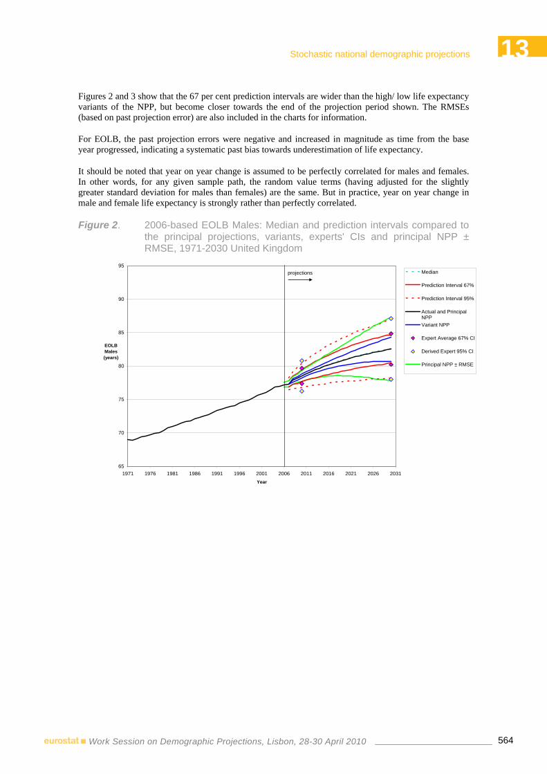
13Stochastic national demographic projections
564Work Session on Demographic Projections, Lisbon, 28-30 April 2010
Figures 2 and 3 show that the 67 per cent prediction intervals are wider than the high/ low life expectancy variants of the NPP, but become closer towards the end of the projection period shown. The RMSEs (based on past projection error) are also included in the charts for information.
For EOLB, the past projection errors were negative and increased in magnitude as time from the base year progressed, indicating a systematic past bias towards underestimation of life expectancy.
It should be noted that year on year change is assumed to be perfectly correlated for males and females. In other words, for any given sample path, the random value terms (having adjusted for the slightly greater standard deviation for males than females) are the same. But in practice, year on year change in male and female life expectancy is strongly rather than perfectly correlated.
Figure 2. 2006-based EOLB Males: Median and prediction intervals compared to the principal projections, variants, experts' CIs and principal NPP ± RMSE, 1971-2030 United Kingdom
65
70
75
80
85
90
95
1971 1976 1981 1986 1991 1996 2001 2006 2011 2016 2021 2026 2031Year
EOLBMales(years)
Median
Prediction Interval 67%
Prediction Interval 95%
Actual and PrincipalNPPVariant NPP
Expert Average 67% CI
Derived Expert 95% CI
Principal NPP ± RMSE
projections

13Stochastic national demographic projections
565Work Session on Demographic Projections, Lisbon, 28-30 April 2010
Figure 3. 2006-based EOLB Females: Median and prediction intervals compared to the principal projections, variants, experts' CIs and principal NPP ± RMSE, 1971-2030 United Kingdom
65
70
75
80
85
90
95
1971 1976 1981 1986 1991 1996 2001 2006 2011 2016 2021 2026 2031
Year
EOLB Females(years)
Median
Prediction Interval 67%
Prediction Interval 95%
Actual and Principal NPP
Variant NPP
Expert Average 67% CI
Derived Expert 95% CI
Principal NPP ± RMSE
projections
(iii) Migration
The net migration sample paths were generated by a RWD model where the drift term constrained the median of the probability distribution to follow the net migration principal assumption from the 2006-based UK NPP, namely a long-term value of +190,000 net migrants per year. Two alternatives for the one year ahead standard deviation were considered.
A) In order for the net migration sample paths to have a probability distribution broadly consistent with the experts’ ‘average’ 67 per cent CI at twenty five years ahead, the derived experts’ standard deviation of ±90,700 net migrants was chosen (see Table A). A one year ahead standard deviation of 18,100 net migrants was calculated and fed into the random value component (where 18,100=90,700/ 25 ).
Figure 4 shows that the 67 per cent prediction intervals are narrower than the high/ low net migration variants of the NPP in the short-term but wider in the longer term; this can in part be explained by the fact that in the deterministic projections, long-term net migration levels are held constant and therefore do not assume a continuous level of uncertainty. The 67 per cent prediction intervals are much narrower than the experts’ ‘average’ 67 per cent CI at five years ahead. However, the 95 per cent prediction intervals closely match the derived experts’ 95 per cent CI at twenty five years ahead. The RMSEs (based on past projection error) are also included in the chart for information. Note: the jagged appearance of the principal NPP ± RMSEs lines are due to a larger error for the year 2004 (in all projection sets) relative to earlier years.

13Stochastic national demographic projections
566Work Session on Demographic Projections, Lisbon, 28-30 April 2010
Figure 4. 2006-based Net Migration: Median and prediction intervals compared to the principal projections, variants, experts' CIs and principal NPP ± RMSE, 1971-2030 (with one year ahead standard deviation set at 18,100) United Kingdom
-200
-100
0
100
200
300
400
500
1971 1976 1981 1986 1991 1996 2001 2006 2011 2016 2021 2026 2031
Year
Net Migration
(thousands)
Median
Prediction Interval 67%
Prediction Interval 95%
Actual and PrincipalNPPVariant NPP
Expert Average 67% CI
Derived Expert 95% CI
Principal NPP ± RMSE
projections
For net migration, the past projection errors were negative and increased in magnitude as time from the base year progressed, indicating a systematic past bias towards underestimation of net migration.
B) In order to ensure a probability distribution broadly consistent with the experts’ ‘average’ 67 per cent CI at five years ahead, the derived experts’ standard deviation of ± 51,300 net migrants was chosen (see Table A). A one year ahead standard deviation of 23,000 net migrants was calculated and fed into the random value component (where 23,000=51,300/ 5 ).
Figure 5 shows that the 67 per cent prediction intervals are wider than the experts’ ‘average’ 67 per cent CI at twenty five years ahead.

13Stochastic national demographic projections
567Work Session on Demographic Projections, Lisbon, 28-30 April 2010
Figure 5. 2006-based Net Migration: Median and prediction intervals compared to the principal projections, variants, experts’ CIs and principal NPP ± RMSE, 1971-2030 (with one year ahead standard deviation set at 23,000) United Kingdom
-200
-100
0
100
200
300
400
500
1971 1976 1981 1986 1991 1996 2001 2006 2011 2016 2021 2026 2031
Year
Net Migration
(thousands)
Median
Prediction Interval 67%
Prediction Interval 95%
Actual and PrincipalNPPVariant NPP
Expert Average 67% CI
Derived Expert 95% CI
Principal NPP ± RMSE
projections
As Figures 4 and 5 illustrate, neither set of probability distributions provides a particularly good fit to the experts’ ‘average’ 67 per cent CIs in both the short-term and longer term. It was decided therefore, to use a one year ahead standard deviation of 23,000 (as shown in Figure 5) to generate sample paths for net migration because it was deemed preferable to overestimate rather than underestimate uncertainty.
7. Sample Path
This section describes the process of how the stochastically determined drivers were converted into counts that fed into the overall model. This process represents one sample path or simulation. A large number of simulations were needed in order to obtain the required probability distributions.
(i) Fertility
For every projection year, the TFR was derived using a RWD model as described in ‘The model’ section. An age distribution by single year of age of mother (ranging from 15 to 46 years old) was derived using the 2007 age-specific fertility rates (ASFR) for the UK. This (fixed) age distribution was applied to the stochastically determined TFRs to give ASFRs for subsequent projection years. See Appendix A for the formulae for ASFRs and age distribution.
Applying the ASFRs to the female population gave a count of births by single year of age of mother. The births were summed to give a count of total births which were then fed into the overall model. To obtain total births by sex required applying the male: female sex ratio of 51.2 : 48.8 to total births.
(ii) Mortality
For every projection year (and separately by sex), EOLBs were derived using a RWD model as described in ‘The model’ section. Each stochastically determined EOLB was fed into a look up procedure that

13Stochastic national demographic projections
568Work Session on Demographic Projections, Lisbon, 28-30 April 2010
picked out the associated 2006 age-specific mortality rate from a model life table based on historic life tables and the 2006-based UK principal mortality assumptions.
A count of deaths by age was generated by applying the relevant age-specific mortality rates to the population (adjusted for net migration). For children not yet born, the given mortality rate (from the model life table) was applied to total births to give counts of infant deaths. The age-specific counts of deaths were summed to give total deaths that were fed into the overall model.
(iii) Migration
For every projection year, total net migration was derived using a RWD model as described in ‘The model’ section. The counts of total net migration were fed into the overall model.
However, as stochastic forecasts by sex and age are required, a number of additional steps were needed to derive age/ sex-specific net migration:
• It was necessary to split net migration into immigration and emigration. Total emigration was fixed to the level of the 2006-based UK principal migration assumptions (475,000 in the long-term) and then total immigration was calculated from the stochastically determined net migration. It is planned to revisit this assumption of a fixed level of emigration.
• Age and sex distributions (different for emigration and immigration), were also taken from the 2006-based UK principal migration assumptions. For each age and sex, net migration was then calculated as the difference between immigration and emigration.
In the deterministic projections, it is assumed that levels of annual net migration beyond 2015 will remain constant. In reality, there will be fluctuations from year to year, but these are very difficult to predict. Short-term assumptions have been applied to the first few years of the deterministic projections and this includes allowance for additional net migration from accession countries.
8. Starting population The mid-2006 UK population estimates published in August 200711 were used as the starting population. These are the same estimates used in the 2006-based UK NPP.
9. The program
The program was written in Microsoft Excel and used an adapted version of the cohort component model used to produce the deterministic projections. For each of the drivers, the value one year ahead was obtained by adding the stochastically determined year on year change and a drift term to the level of the driver in the previous year. The inclusion of the drift term ensured the median of the assumed probability distributions was consistent with the results of the 2006-based UK principal assumptions. However, some very small differences arose due to the way age-specific rates and numbers were obtained.
For each driver, (but simultaneously with the other drivers) a new simulation or sample path was created each time a new set of random numbers was generated. The resultant values were then converted into counts (as described in the ‘Sample path’ section) and added to the total population counts from the previous year. The program was designed to generate 5,000 simulations from 2006 through to the year 2056.
11 Mid-2006 Population Estimates for the UK, August 2007. Available at: http://www.statistics.gov.uk/downloads/theme_population/Mid_2006_UK_England_&_Wales_Scotland_and_Northern_Irelan
d%2022_08_07.zip

13Stochastic national demographic projections
569Work Session on Demographic Projections, Lisbon, 28-30 April 2010
10. Illustrative results
Figures 6 and 7 below show the provisional projected populations and the level of uncertainty at two points in the future (2031 and 2056) by age and sex using the assumptions described in this paper. They are for illustrative purposes only.
Figure 6 shows that, in absolute terms, uncertainty is greatest for the youngest cohorts - particularly those who are yet to be born. Migration will have an impact for those cohorts which pass through the peak ages of migration in the next 25 years. There is also uncertainty at the very oldest ages; however, while this uncertainty may be small in absolute terms, it is significant relative to the median population size for this age group.
The chart also shows that there is least uncertainty for those who are aged about 55-75 years old in 2031 - in other words, those who are currently aged around 30-50 years old. These cohorts are past the peak ages of migration and will not be significantly affected by mortality in the next 25 years.
Figure 6. Provisional UK projected populations: Median and prediction intervals, 2031 United Kingdom
800 600 400 200 0 200 400 600 8000
10
20
30
40
50
60
70
80
90
100
110
120
Age
(ye
ars)
Population (thousands)
95%predictiveinterval
67%predictiveinterval
MedianMales Females
Figure 7 shows how uncertainty clearly increases 50 years into the future - particularly for cohorts yet to be born. Further into the projection period, uncertainty about the number of births is not only dependent on the TFR, but also because of the uncertainty about the size of future child bearing cohorts which will be affected by both fertility and migration uncertainty. The chart shows least uncertainty for those in their late 70s in 2056 (or those who are presently in their late 20s).

13Stochastic national demographic projections
570Work Session on Demographic Projections, Lisbon, 28-30 April 2010
Figure 7. Provisional UK projected populations: Median and prediction intervals, 2056 United Kingdom
800 600 400 200 0 200 400 600 8000
10
20
30
40
50
60
70
80
90
100
110
120
Age
(ye
ars)
Population (thousands)
95%predictiveinterval
67%predictiveinterval
Median
Males Females
11. Future work
(i) Use of a time series approach
The research reported in this paper has been based on past projection error and expert opinion. However, time series models appear to have provided satisfactory results in other stochastic forecasting exercises.12 ONS intends to reconsider the time series approach exploring, in particular, whether the most appropriate models were used. Consideration will also be given to fitting time series models using historical data series of different time spans and comparing the results. This is because results from time series analyses are very sensitive to the historical reference period considered. So, for example, if the period included the 1960s baby boom or the fertility decline in the early 1970s, then this could have an impact. If we believe the TFR will continue around its current level indefinitely, then fitting a time series model from the late 1970s would provide a good representation of observed variability around this level.
(ii) Deriving probability distributions
In this early work, it has been assumed that the ‘average’ 67 per cent confidence intervals for the drivers provided by the expert panel are from Normal distributions with mean equal to the ‘average’ most likely level. Yet many of the confidence intervals provided by individual experts were skewed. Hence this assumption needs further consideration.
The NPP panel were asked to provide both 67 per cent and 95 per cent confidence intervals for the 2008-based NPP and as a result, future distributional assumptions could have a more solid foundation. Future work should also consider the distribution of past projection errors.
12 lders M., Keilman N. and Cruijsen H. (2007) Assumptions for long-term stochastic population forecasts in 18 European
countries. European Journal of Population. Available at: http://www.springerlink.com/content/0453r268h24456q8/fulltext.pdf

13Stochastic national demographic projections
571Work Session on Demographic Projections, Lisbon, 28-30 April 2010
(iii) The RWD model
While the RWD model may be appropriate to produce probability distributions for the drivers, rigorous time series analysis needs to be carried out for each driver to test this assumption, and to determine what the best model is based on the analysis of historical data. Fitting the RWD model to past data will not only provide a good test of the model, but will also provide an estimate of the variance of the random value term. If a RWD model is not appropriate, an ARIMA model could incorporate serial correlations for both assessing the underlying variance and making projections.
State Space or Kalman Filter models could also be considered. These use parameters from past data to predict the future. For every age and parameter there is a random adjustment and these are all correlated.
(iv) Correlations
Correlations between ages and between sexes (in both mortality and migration) need to be considered. The current methodology assumes that all ages are perfectly correlated (within a component) which may not be true. An analysis of the correlation between mortality, fertility and migration over time should also be considered and could be carried out using historical data. Expert opinion could also be sought or existing academic analysis considered.
(v) Net Migration
Further work into the viability of modelling immigration and emigration separately should be considered as it is not only conceptually easier, but would increase the transparency of the assumptions. The NPP panel has provided views on emigration and immigration (in addition to net migration) for the 2008-based NPP. Estimates of the standard deviation for immigration and emigration separately over time could be obtained by examining historic data, and the feasibility of estimating synthetic RMSEs by comparing actual immigration, emigration and net migration from the population estimates with projected net migration could be explored.
In future analysis, consideration could be given to splitting migration flows further, for example, by country of origin and forecasting each flow separately. There are a number of different types of migrants including labour, family, student and asylum migrants suggesting the use of a fuller model with more drivers and possibly the inclusion of external (economic) factors may be more appropriate.
(vi) Age distribution
The age distribution is fixed for fertility and mortality, and also for net migration from 2015. This means the overall model takes no account of possible change in the age distributions over time such as any continued increase in the average age of mother at birth for example, or any change in the long-term disparity between the ages of people leaving the UK compared to those entering. Therefore, the option of disaggregating by age should be explored.
(vii) The program
Future work will consider whether 5,000 simulations are sufficient, whether there is evidence of convergence and test for stability using a trace plot.

13Stochastic national demographic projections
572Work Session on Demographic Projections, Lisbon, 28-30 April 2010
Appendix A
Formulae
• The Root Mean Squared Error (RMSE) for m years ahead is given by
RMSE = )/)((1
2, m
N
ttm NE
m
∑=
where Em,t = m years ahead forecast value from projection set t minus actual value
and Nm = number of sets of projections for m years ahead.
• The age-specific fertility rate (ASFR) in 2007 is given by
1000*)/( 2007,2007,2007,f
nnn PBASFR =
where nB = live births to women at age n,
fnP = female population at age n,
and n = single year of age of mother, (15, …, 46).
• The Total Fertility Rate (TFR) in 2007 is given by
1000/)(46
152007,2007 ∑
=
=
=n
nnASFRTFR
• The age distribution (AD) for fertility in 2007 is given by
∑=
=
=46
152007,2007,2007, /
n
nnnn ASFRASFRAD
1000*/ 20072007, TFRASFRn=
• ASFRs derived for a sample path are given by
1000** 2007,,, ntntn ADTFRASFR =
where t denotes the year of forecast


European Commission Work session on demographic projections Luxembourg: Publications Office of the European Union 2010 — 572 pp. — 21 x 29.7 cm ISBN 978-92-79-15862-9 ISSN 1977-0375 Doi:10.2785/50697 Cat. No KS-RA-10-009-EN-N Theme: Population and social conditions Collection: Methodologies and working papers

terza_copertina.indd 3 24-05-2007 17:58:14
How to obtain EU publicationsFree publications:
• viaEUBookshop(http://bookshop.europa.eu);
• attheEuropeanUnion’srepresentationsordelegations.YoucanobtaintheircontactdetailsontheInternet(http://ec.europa.eu)orbysendingafax to +352 2929-42758.
Priced publications:
• viaEUBookshop(http://bookshop.europa.eu).
Priced subscriptions (e.g. annual series of the Official Journal of the European Union and reports of cases before the Court of Justice of the European Union):
• viaoneofthesalesagentsofthePublicationsOfficeoftheEuropeanUnion (http://publications.europa.eu/others/agents/index_en.htm).

2008 edition
KS-RA-10-009-EN
-N
M e t h o d o l o g i e s a n d W o r k i n g p a p e r s
Domestic tourism manual
ISSN 1977-0375