Why is the overheating problem difficult: The role of entropy

Why is the overheating problem difficult: The role of entropy

Meng-Sing Liou∗

NASA Glenn Research Center, Cleveland, OH 44135, USA

The development of computational fluid dynamics over the last few decades has yielded enormous successesand capabilities being routinely employed today; however there remain some open problems to be properlyresolved–some are fundamental in nature and some resolvable by operational changes. These two categoriesare distinguished and broadly explored previously.1 One fundamental open problem is the so-called overheat-ing problem, especially in rarefying flow. This problem to date still dogs every method known to the author;a solution to it remains elusive. The study in this paper concludes that: (1) the entropy increase is one-to-onelinked to the increase in the temperature increase, (2) the overheating is inevitable in the current computationalfluid dynamics framework in practice, and (3) a simple hybrid method is proposed that removes the overheat-ing problem in the rarefying problems, but also retains the property of accurate shock capturing. This remedy(enhancement of current numerical methods) can be included easily in the present Eulerian codes.

I. Introduction

THE overheating problem remains one of the most prominent open CFD problems; it is typically found in two sce-nariosone related to colliding flows and the other to receding flows. The former, resulting either from reflection of

an approaching flow from a wall or equivalently from two colliding (of equal or different strengths) manifests itself asa spike in temperature near the wall; it has been a well-known problem since it was first recognized by von Neumann.2

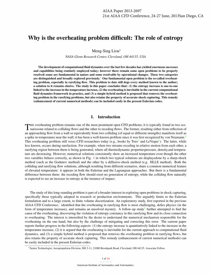
This overheating problem still vexes CFD researchers today (e.g., books by Toro3 and LeVeque4). The latter, whileless known, occurs during rarefaction. For example, when two streams receding in relative motion from each other, ararefying region between them is being generated, where all thermodynamic propertiespressure, density,and tempera-ture are decreasing. However, numerical solutions consistently show an increased temperature even though the othertwo variables behave correctly, as shown in Fig. 1 in which two typical solutions are displayedone by a sharp-shockmethod (such as the Godunov method) and the other by a diffusive-shock method (e.g. HLLE method). Both thecolliding and rarefying flow solutions, although resulting from different scenarios, share a common numerical featureof elevated temperature: it appears in both the Eulerian and the Lagrangian approaches. But there is a fundamentaldifference between them: the receding flow should exert no generation of entropy, while the colliding flow naturallyis expected to see an increase in entropy at the instance of impact.

The study of this long-standing problem is part of a broader interest in exploring open problems in shock capturing,specifically those typically adopted in research or production environments. This arguably limits to the Eulerianformulation and to a large extent, to finite volume discretization. An exploratory study, first reported in the previousAIAA CFD Conference,1 identified that the overheating in rarefying flow is most challenging, defies physics (in theform of temperature increase), and remains an unsolved mystery. A follow-up study5 further attempted to find thecause of the overheating, discovering the violation of entropy constancy in this rarefying flow and its close connectionto overheating. The interest is intensified by the desire to understand the numerical mechanism responsible for theoverheating on the one hand, but also by the challenge of mitigating and correcting this error. The current paperreports further progress in the following aspects: (1) the entropy increase is quantitatively linked to the increase in thetemperature increase, (2) it is argued that the overheating is inevitable for the current approach to computational fluiddynamics, and (3) a simple hybrid method is proposed that removes the overheating problem in rarefying flows, butalso retains the property of accurate shock capturing. This remedy (enhancement of current numerical methods) canbe easily included in the present Eulerian codes.

∗Senior Technologist, Aeropropulsion Division, MS 5-11, 21000 Brookpark Road, Cleveland, OH 44135. Associate Fellow.

1 of 14

American Institute of Aeronautics and Astronautics

AIAA Paper 2013-269721st AIAA CFD Conference, 24-27 June, 2013San Diego, CA

Exact Riemann Solver 100 cells CFL=0.50 N= 50

-1.0 -0.5 0.0 0.5 1.0x

0.0

0.5

1.0

1.5

PressureDensityTemperature

(a) Godunov.

HLLE(Expansion WS)

brbl:Einfeld1

100 cells CFL=0.50 N= 50

-1.0 -0.5 0.0 0.5 1.0x

0.0

0.5

1.0

1.5


(b) HLLE.

Figure 1. Receding flows computed on a grid of 100 cells, with the initial condition, (ρ, p, u)L = (1.0, 0.4,−2.0) and (ρ, p, u)R = (1.0, 0.4, 2.0).

II. Problem statement: Receding flows

In the discussion of the overheating problem and its remedy, we shall exclusively focus on the receding problem.The simplest generic form for the receding problem is a Riemann problem with the initial condition:

uL < 0, ρL, pL and uR > 0, ρR, pR (1)

where the “L” and “R” states may be of same or different magnitudes. The strength of rarefaction is defined bythe relative Mach number |MR − ML|; different combinations of thermodynamic properties will of course result indifferent flow configurations.

As stated above, the computation will be carried out in the finite-volume Eulerian setting. Exact solutions will beused as a reference when judging the calculated solutions. We will use the Godunov resulta to establish the baselinesolution for comparing other methods and also to gauge its own ability to solve the considered problems againstthe exact solution. The explicit Euler and two-step Runge-Kutta methods are used for the first- and second-order timeintegrations respectively. To evaluate numerical methods, we ensure that solutions are physically relevant, numericallystable and mesh-size converged. Hence, it may be necessary for some methods to reduce the time step (CFL) furtherthan others. In other words, we seek to obtain stable and converged solution for the problem studied. Subsequently,results obtained by the AUSM+-up method6 will be presented for comparison purposes.

Exact Riemann Solver CFL=0.50 N= 50

-1.0 -0.5 0.0 0.5 1.0x

0.0

0.5

1.0

1.5


(a) M=0.8, 100 cells.

Exact Riemann Solver CFL=0.50 N=5000

-1.0 -0.5 0.0 0.5 1.0x

0.0

0.5

1.0

1.5


(b) M=0.8, 10,000 cells.


-1.0 -0.5 0.0 0.5 1.0x

0.0

0.5

1.0

1.5


(c) M=2.5, 100 cells.


-1.0 -0.5 0.0 0.5 1.0x

0.0

0.5

1.0

1.5


(d) M=2.5, 10,000 cells.

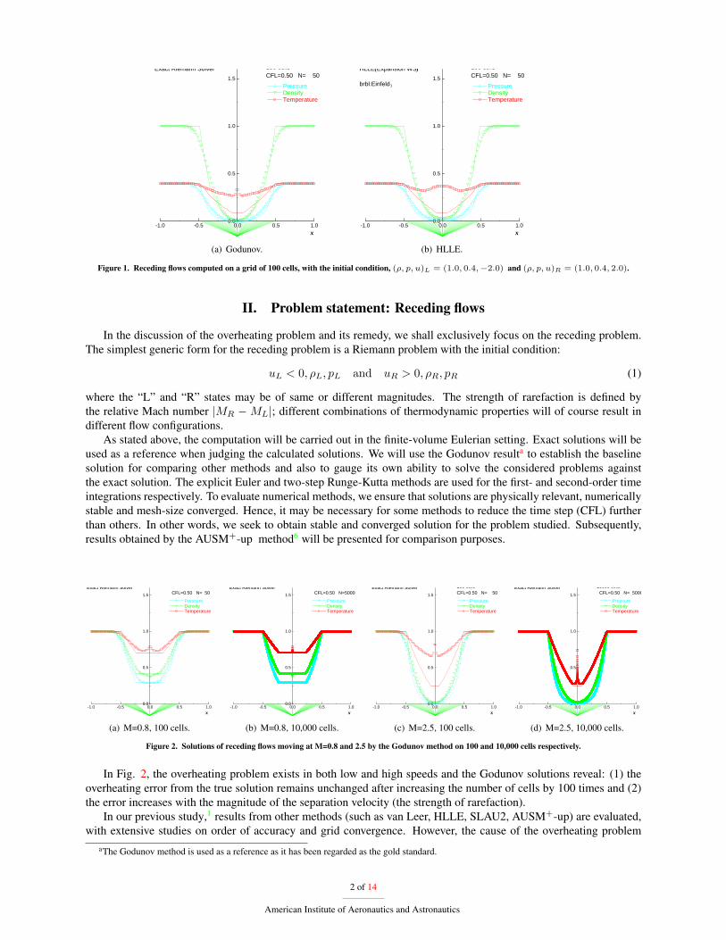
Figure 2. Solutions of receding flows moving at M=0.8 and 2.5 by the Godunov method on 100 and 10,000 cells respectively.

In Fig. 2, the overheating problem exists in both low and high speeds and the Godunov solutions reveal: (1) theoverheating error from the true solution remains unchanged after increasing the number of cells by 100 times and (2)the error increases with the magnitude of the separation velocity (the strength of rarefaction).

In our previous study,1 results from other methods (such as van Leer, HLLE, SLAU2, AUSM+-up) are evaluated,with extensive studies on order of accuracy and grid convergence. However, the cause of the overheating problem

aThe Godunov method is used as a reference as it has been regarded as the gold standard.

2 of 14


remained unknown and no clear clue as to how it occurs emerged. Some representative results are given here toprovide a frame of reference, they are summarized below.

II.A. Effect of spatial discretization accuracy and limiters

Despite the fact that increasing the number of grid points does not lead a way out of the overheating problem, itwould be interesting to see if higher order discretization might be enlightening, since the solution indeed convergesin the major part of the domain in Fig. 2. In Fig. 3 we compare the second-order accurate results with the first-orderone, by using primitive and characteristic variables for interpolation together with the diffusive and sharp–minmod andsuperbee limiters. We observe: (1) the stable time step has to be significantly reduced, (2) the use of primitive variableshas a limited success in reducing the overheating, (3) a significant improvement arises from the use of characteristicvariables, but still with noticeable overprediction in temperature and entropy generation, and (4) the minmod andsuperbee limiters have a dramatic and opposite influence on the entropy distribution and the temperature distributionin the middle low speed region. Notice that the superbee limiter causes a decrease in entropy, thereby producing anovercooling instead! In fact the solution was so overcooled during the calculation that a negative density occurred andthe solution was artificially kept alive by resetting the density to a small positive value.b

Thus, we reiterate: Observation 1: The “overheating” by the first-order method is not reduced by refining the size

of grid or time step. A significant reduction in overheating can be achieved when using the second-order interpolation;but the opposite, overcooling in this case, can be produced by combining the superbee limiter with the characteristicvariables. Hence, the problem remains unresolved.

Exact Riemann Solver CFL=0.50 N= 60

-1.0 -0.5 0.0 0.5 1.0x

0.0

0.5

1.0

1.5 PressureDensityTemperatureMach (rescaled)Entropy/2

-1.0 -0.5 0.0 0.5 1.0x

0.0

0.5

1.0

1.5

(a) O(h1).

Exact Riemann Solveritvd= 1 muscl: primitive variables; (r,u,p)

CFL=0.20 N= 150

-1.0 -0.5 0.0 0.5 1.0x

0.0

0.5

1.0


-1.0 -0.5 0.0 0.5 1.0x

0.0

0.5

1.0

1.5

(b) O(h2), prim. var., minmod.

Exact Riemann Solveritvd= 1 muscl: char.; T - 1 at grid; (r,u,T)

CFL=0.20 N= 150

-1.0 -0.5 0.0 0.5 1.0x

0.0

0.5

1.0


-1.0 -0.5 0.0 0.5 1.0x

0.0

0.5

1.0

1.5

(c) O(h2), char. var., minmod.

Exact Riemann Solveritvd= 4 muscl: char.; T - 1 at grid; (r,u,T)

CFL=0.20 N= 150

-1.0 -0.5 0.0 0.5 1.0x

0.0

0.5

1.0


-1.0 -0.5 0.0 0.5 1.0x

0.0

0.5

1.0

1.5

(d) O(h2), char. v., superbee.

Figure 3. ML=-MR=-2.5; solutions computed by the Godunov method with the first and second order accuracy together with various limiter functions andinterpolated variables with 100 cells.

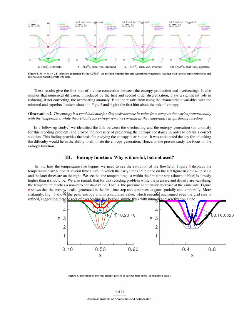
II.B. Effect of numerical flux function

We extensively examined how methods other than the Godunov behaved and presented the findings in previous pa-pers.1, 5 Here we will merely show the representative results by the AUSM+-up method. Figure 4 shows that theaccuracy of these results is comparable to their Godunov counterparts. The peak entropy values by the first order andsecond-order methods are nearly identical to each other respectively, with insignificant differences.

bThis result should have been discounted, it is included to highlight the need for investigating closely the computed result in every aspect eventhough the temperature appears to be in a correct trend.

3 of 14


AUSM -up

a1 / 2=min(aL*, aR

*)kp=0.25 ku=0.75

CFL=0.50 N= 60

-1.0 -0.5 0.0 0.5 1.0x

0.0

0.5

1.0


-1.0 -0.5 0.0 0.5 1.0x

0.0

0.5

1.0

1.5

(a) O(h), 100 cells.

AUSM -upitvd= 1 muscl: primitive variables; (r,u,p)

a1 / 2=min(aL*, aR

*)kp=0.25 ku=0.75

CFL=0.20 N= 150

-1.0 -0.5 0.0 0.5 1.0x

0.0

0.5

1.0


-1.0 -0.5 0.0 0.5 1.0x

0.0

0.5

1.0

1.5

(b) O(h2), prim. var., minmod

AUSM -upitvd= 1 muscl: char.; T - 1 at grid; (r,u,T)

a1 / 2=min(aL*, aR

*)kp=0.25 ku=0.75

CFL=0.20 N= 150

-1.0 -0.5 0.0 0.5 1.0x

0.0

0.5

1.0


-1.0 -0.5 0.0 0.5 1.0x

0.0

0.5

1.0

1.5

(c) O(h2), char. var., minmod

AUSM -upitvd= 4 muscl: char.; T - 1 at grid; (r,u,T)

a1 / 2=min(aL*, aR

*)kp=0.25 ku=0.75

CFL=0.20 N= 150

-1.0 -0.5 0.0 0.5 1.0x

0.0

0.5

1.0


-1.0 -0.5 0.0 0.5 1.0x

0.0

0.5

1.0

1.5

(d) O(h2), char. var., superbee

Figure 4. ML=-MR=-2.5; solutions computed by the AUSM+-up method with the first and second order accuracy together with various limiter functions andinterpolated variables with 100 cells.

These results give the first hint of a close connection between the entropy production and overheating. It alsoimplies that numerical diffusion, introduced by the first and second order discretization, plays a significant role inreducing, if not correcting, the overheating anomaly. Both the results from using the characteristic variables with theminmod and superbee limiters shown in Figs. 3 and 4 give the first hint about the role of entropy.

Observation 2: The entropy is a good indicator for diagnosis because its value from computation varies proportionallywith the temperature, while theoretically the entropy remains constant as the temperature drops during receding.

In a follow-up study,5 we identified the link between the overheating and the entropy generation (an anomalyfor this receding problem) and proved the necessity of preserving the entropy constancy in order to obtain a correctsolution. This finding provides the basis for studying the entropy distribution. It was anticipated the key for unlockingthe difficulty would lie in the ability to eliminate the entropy generation. Hence, in the present study, we focus on theentropy function.

III. Entropy function: Why is it useful, but not used?

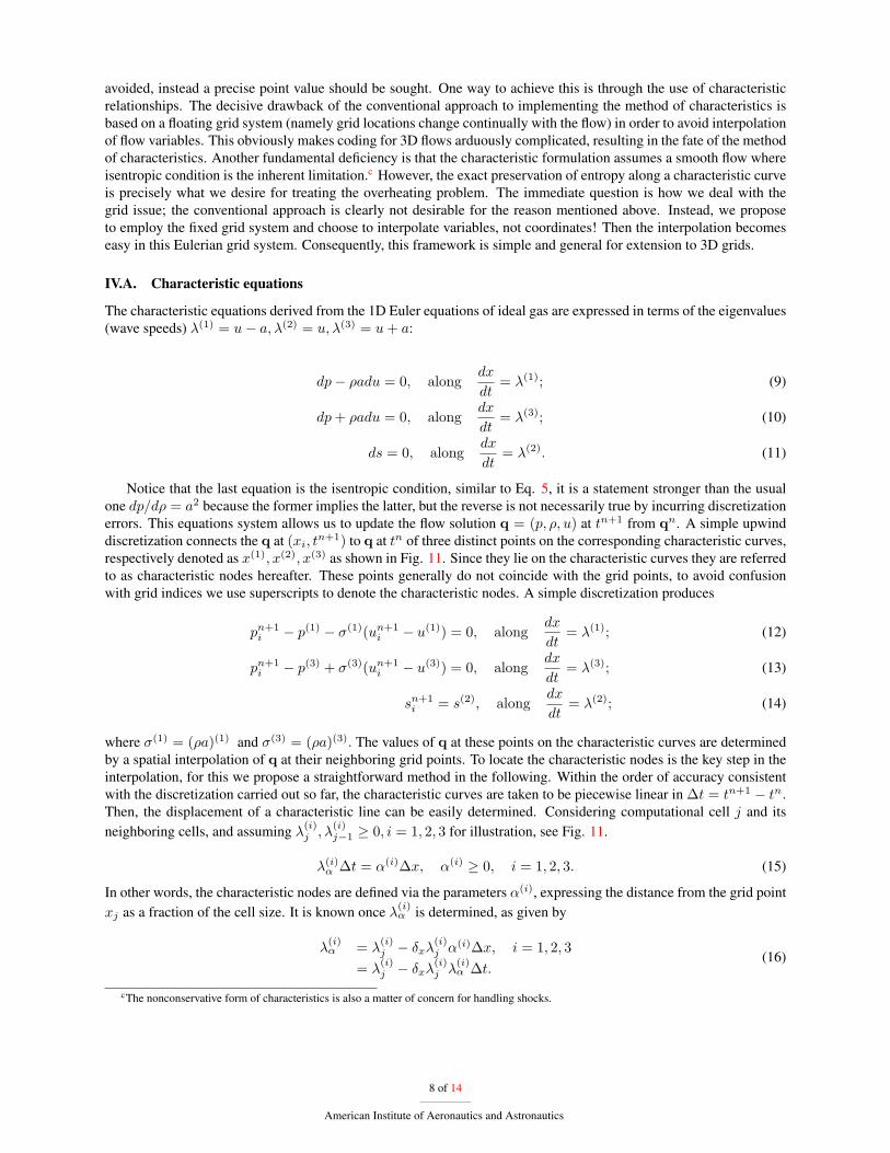
To find how the temperature rise begins, we need to see the evolution of the flowfield. Figure 5 displays thetemperature distribution at several time slices, in which the early times are plotted on the left figure in a blow-up scaleand the later times are on the right. We see that the temperature just within the first time step (shown in blue) is alreadyhigher than it should be. We also remark that for this receding problem while the pressure and density are vanishing,the temperature reaches a non-zero constant value. That is, the pressure and density decrease at the same rate. Figure6 shows that the entropy is also generated in the first time step and continues to grow spatially and temporally. Morestrikingly, Fig. 7 shows the peak entropy attains a saturated value, which remains unchanged even the grid size isrefined, suggesting that the root of overheating lies beyond simple fixes with numerical discretization alone.

Figure 5. Evolution of internal energy, plotted at various time slices (in magnified scale).

4 of 14


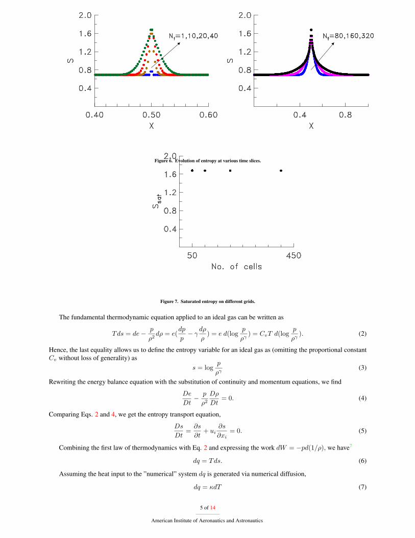
Figure 6. Evolution of entropy at various time slices.

Figure 7. Saturated entropy on different grids.

The fundamental thermodynamic equation applied to an ideal gas can be written as

Tds = de− p

ρ2dρ = e(

dp

p− γ

dρ

ρ) = e d(log

p

ργ) = CvT d(log

p

ργ). (2)

Hence, the last equality allows us to define the entropy variable for an ideal gas as (omitting the proportional constantCv without loss of generality) as

s = logp

ργ(3)

Rewriting the energy balance equation with the substitution of continuity and momentum equations, we find

De

Dt− p

ρ2Dρ

Dt= 0. (4)

Comparing Eqs. 2 and 4, we get the entropy transport equation,

Ds

Dt=

∂s

∂t+ ui

∂s

∂xi= 0. (5)

Combining the first law of thermodynamics with Eq. 2 and expressing the work dW = −pd(1/ρ), we have7

dq = Tds. (6)

Assuming the heat input to the ”numerical” system dq is generated via numerical diffusion,

dq = κdT (7)

5 of 14


here κ is interpreted as the numerical heat conductivity, assumed to be constant (which would be different for differentschemes) in our analysis. Substituting into Eq. 6 and integrating, we get

∆s = s(x(2))− s(x(1)) = κ logT (x(2))

T (x(1))(8)

If the heat input that is to contribute the overheating does so via heat diffusivity, then the numerical entropy shouldfollow the above rule in the numerical solution: (1) the relationship between the entropy and temperature is one toone; the entropy increases as the temperature increases and (2) these two quantities follow the above logarithmicrelationship. In Fig. 9 we plot the variation of these two quantities between two neighboring points for the entirecomputation domain, it reveals that the relationship arrived at in Eq. 8 holds, confirming that the entropy increaseswith temperature and the temperature increase is activated through numerical diffusion. In the region where thenumerical rarefaction wave has not reached, there are no changes in s and T and they are clustered at the center ofthe plot; the points further away from the center correspond to the region of large changes in entropy and temperature,corresponding to the center of the receding flow.

On the other hand, using the entropy equation Eq. 5, in place of the conventional energy equation, completelyeradicates the overheating and yields a correct and grid-converged solution, as shown in Fig. 8. Especially worthnoting is that the slope discontinuity in the middle region is captured accurately. Hence, one is led to confirm directlythat if the entropy conservation is enabled, the overheating problem is solved.

(a) 100 cells, O(h). (b) 400 cells, O(h).

Figure 8. Solution of the receding flow by including the entropy transport equation in place of the energy equation, on 100-cell and 400-cell grids, showingelimination of overheating and grid convergence.

Equation 5 states that the entropy remains constant by following the fluid particle with its velocity u; it describesthe convection of an initial entropy profile by u(x, t). The entropy convection gives no mechanism for describing anentropy-increasing event, such as shock waves. That is, the entropy function remains constant across the shock wavein a shock tube problem as will be evident later, thus rendering the entropy equation unusable for general problemswhere the entropy variation is not simply a convection of its initial profile.

Moreover, the second law of thermodynamics only demands a nondecreasing change in entropy (ds ≥ 0), thestrength of this inequality is clearly problem-dependent and the upper bound is not known a priori. Since a pre-

6 of 14


(a)

Figure 9. Temperature variation ∆x log T vs. entropy variation ∆xs.

cise mathematical expression for describing the convection and generation of entropy is not available, the entropyconvection equation, as presented in Eq. 5, is useless for computation purposes in this regard.

Nevertheless, using the entropy field as a diagnosis tool reveals an interesting insight as to whether a solutionbehaves properly or not. A case of violating the second law of thermodynamics in a numerical solution rarely occurs(since diffusivity is often inherent in a numerical solution), except for the scheme known to branch out to a physicallyinvalid solution, such as expansion shock. For such a scheme, a fix is usually implemented in a code by addingnumerical dissipation. It can be said that satisfying the entropy-nondecreasing condition in a numerical solution isgenerally not a problem; on the other hand, preventing the entropy from increasing where it should not is a challengenumerically. One example is the blunt-body carbuncle solution by the Roe scheme (with and without entropy fix),where the entropy will be generated, but irregularly corresponding to the carbuncle shock profile. Another is thereceding flow. In the case of the Roe-flux solution of the blunt body, knowing that the carbuncle solution does notviolate the entropy condition is comforting, but it does not appear helpful for resolving the carbuncle problem. Theentropy condition for these cases is merely a necessary condition. Hence, we shall primarily use the entropy functionas an additional indicator to evaluate the performance of a numerical flux function.

IV. A new scheme: AUSM+-ups

From the above results and discussion, we can arrive at a conclusion that (1) the entropy, hence overheating, isgenerated in the first instance of time evolution in computation; it stays, grows, and reaches a saturated value. Theproblem should be dealt with at the fundamental level–the current discretization framework is incapable of copingwith it. More precisely, averaging of all waves made up of nonuniform flow structures, see Fig. 10, is performed at theend of each time evolution step, in spite of an exact treatment of flux function as in the case of employing the exactRiemann solver. This averaging ultimately leads to the creation of entropy.

Figure 10. Averaging of wave structures at the new time step tn+1 to yield a single averaged state for the entire cell.

This also suggests that the spatial averaging of all wave structures to provide the cell-averaged value should be

7 of 14


avoided, instead a precise point value should be sought. One way to achieve this is through the use of characteristicrelationships. The decisive drawback of the conventional approach to implementing the method of characteristics isbased on a floating grid system (namely grid locations change continually with the flow) in order to avoid interpolationof flow variables. This obviously makes coding for 3D flows arduously complicated, resulting in the fate of the methodof characteristics. Another fundamental deficiency is that the characteristic formulation assumes a smooth flow whereisentropic condition is the inherent limitation.c However, the exact preservation of entropy along a characteristic curveis precisely what we desire for treating the overheating problem. The immediate question is how we deal with thegrid issue; the conventional approach is clearly not desirable for the reason mentioned above. Instead, we proposeto employ the fixed grid system and choose to interpolate variables, not coordinates! Then the interpolation becomeseasy in this Eulerian grid system. Consequently, this framework is simple and general for extension to 3D grids.

IV.A. Characteristic equations

The characteristic equations derived from the 1D Euler equations of ideal gas are expressed in terms of the eigenvalues(wave speeds) λ(1) = u− a, λ(2) = u, λ(3) = u+ a:

dp− ρadu = 0, alongdx

dt= λ(1); (9)

dp+ ρadu = 0, alongdx

dt= λ(3); (10)

ds = 0, alongdx

dt= λ(2). (11)

Notice that the last equation is the isentropic condition, similar to Eq. 5, it is a statement stronger than the usualone dp/dρ = a2 because the former implies the latter, but the reverse is not necessarily true by incurring discretizationerrors. This equations system allows us to update the flow solution q = (p, ρ, u) at tn+1 from qn. A simple upwinddiscretization connects the q at (xi, t

n+1) to q at tn of three distinct points on the corresponding characteristic curves,respectively denoted as x(1), x(2), x(3) as shown in Fig. 11. Since they lie on the characteristic curves they are referredto as characteristic nodes hereafter. These points generally do not coincide with the grid points, to avoid confusionwith grid indices we use superscripts to denote the characteristic nodes. A simple discretization produces

pn+1i − p(1) − σ(1)(un+1

i − u(1)) = 0, alongdx

dt= λ(1); (12)

pn+1i − p(3) + σ(3)(un+1

i − u(3)) = 0, alongdx

dt= λ(3); (13)

sn+1i = s(2), along

dx

dt= λ(2); (14)

where σ(1) = (ρa)(1) and σ(3) = (ρa)(3). The values of q at these points on the characteristic curves are determinedby a spatial interpolation of q at their neighboring grid points. To locate the characteristic nodes is the key step in theinterpolation, for this we propose a straightforward method in the following. Within the order of accuracy consistentwith the discretization carried out so far, the characteristic curves are taken to be piecewise linear in ∆t = tn+1 − tn.Then, the displacement of a characteristic line can be easily determined. Considering computational cell j and itsneighboring cells, and assuming λ

(i)j , λ

(i)j−1 ≥ 0, i = 1, 2, 3 for illustration, see Fig. 11.

λ(i)α ∆t = α(i)∆x, α(i) ≥ 0, i = 1, 2, 3. (15)

In other words, the characteristic nodes are defined via the parameters α(i), expressing the distance from the grid pointxj as a fraction of the cell size. It is known once λ

(i)α is determined, as given by

λ(i)α = λ

(i)j − δxλ

(i)j α(i)∆x, i = 1, 2, 3

= λ(i)j − δxλ

(i)j λ

(i)α ∆t.

(16)

cThe nonconservative form of characteristics is also a matter of concern for handling shocks.

8 of 14


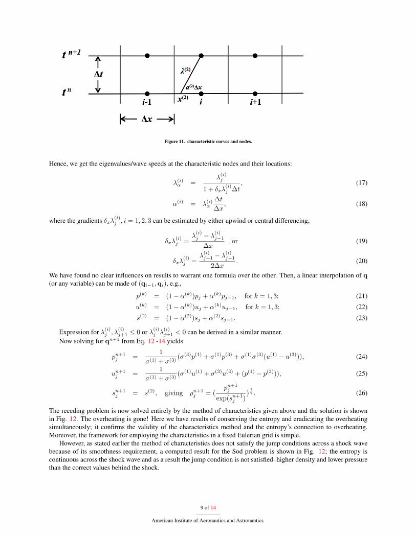
Figure 11. characteristic curves and nodes.

Hence, we get the eigenvalues/wave speeds at the characteristic nodes and their locations:

λ(i)α =

λ(i)j

1 + δxλ(i)j ∆t

, (17)

α(i) = λ(i)α

∆t

∆x, (18)

where the gradients δxλ(i)j , i = 1, 2, 3 can be estimated by either upwind or central differencing,

δxλ(i)j =

λ(i)j − λ

(i)j−1

∆xor (19)

δxλ(i)j =

λ(i)j+1 − λ

(i)j−1

2∆x. (20)

We have found no clear influences on results to warrant one formula over the other. Then, a linear interpolation of q(or any variable) can be made of (qi−1,qi), e.g.,

p(k) = (1− α(k))pj + α(k)pj−1, for k = 1, 3; (21)

u(k) = (1− α(k))uj + α(k)uj−1, for k = 1, 3; (22)

s(2) = (1− α(2))sj + α(2)sj−1. (23)

Expression for λ(i)j , λ

(i)j+1 ≤ 0 or λ(i)

j λ(i)j±1 < 0 can be derived in a similar manner.

Now solving for qn+1 from Eq. 12 -14 yields

pn+1j =

1

σ(1) + σ(3)(σ(3)p(1) + σ(1)p(3) + σ(1)σ(3)(u(1) − u(3))), (24)

un+1j =

1

σ(1) + σ(3)(σ(1)u(1) + σ(3)u(3) + (p(1) − p(3))), (25)

sn+1j = s(2), giving ρn+1

j = (pn+1j

exp(sn+1j )

)1γ . (26)

The receding problem is now solved entirely by the method of characteristics given above and the solution is shownin Fig. 12. The overheating is gone! Here we have results of conserving the entropy and eradicating the overheatingsimultaneously; it confirms the validity of the characteristics method and the entropy’s connection to overheating.Moreover, the framework for employing the characteristics in a fixed Eulerian grid is simple.

However, as stated earlier the method of characteristics does not satisfy the jump conditions across a shock wavebecause of its smoothness requirement, a computed result for the Sod problem is shown in Fig. 12; the entropy iscontinuous across the shock wave and as a result the jump condition is not satisfied–higher density and lower pressurethan the correct values behind the shock.

9 of 14


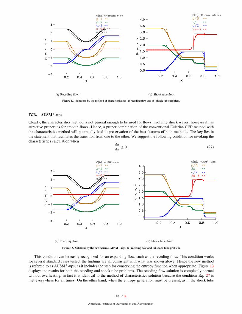
(a) Receding flow. (b) Shock tube flow.

Figure 12. Solutions by the method of characteristics: (a) receding flow and (b) shock tube problem.

IV.B. AUSM+-ups

Clearly, the characteristics method is not general enough to be used for flows involving shock waves; however it hasattractive properties for smooth flows. Hence, a proper combination of the conventional Eulerian CFD method withthe characteristics method will potentially lead to preservation of the best features of both methods. The key lies inthe statement that facilitates the transition from one to the other. We suggest the following condition for invoking thecharacteristics calculation when

du

dx≥ 0. (27)

(a) Receding flow. (b) Shock tube flow.

Figure 13. Solutions by the new scheme–AUSM+-ups: (a) receding flow and (b) shock tube problem.

This condition can be easily recognized for an expanding flow, such as the receding flow. This condition worksfor several standard cases tested, the findings are all consistent with what was shown above. Hence the new methodis referred to as AUSM+-ups, as it includes the step for conserving the entropy function when appropriate. Figure 13displays the results for both the receding and shock tube problems. The receding flow solution is completely normalwithout overheating, in fact it is identical to the method of characteristics solution because the condition Eq. 27 ismet everywhere for all times. On the other hand, when the entropy generation must be present, as in the shock tube

10 of 14


problem, the AUSM+-upkicks in and provides an entropy-consistent solution. As the grid is refined, the computedsolutions converge to the exact solutions as expected, they are included here without undue boredom with similar plots.

IV.C. Further verification

In the following additional tests on problems emphasizing different flow features are included for comparison ofperformance of three methods: AUSM+-up, charateristics, and AUSM+-ups. All calculations presented below arecarried out on a domain of 200 cells using the first-order explicit Euler method for time integration and CFL=0.5.

1. Slowly moving contact discontinuityThe initial condition is set as:

(ρ, u, p)L = (0.1, 0.1aL, 1.0), (ρ, u, p)R = (1.0, 0.1aL, 1.0). (28)

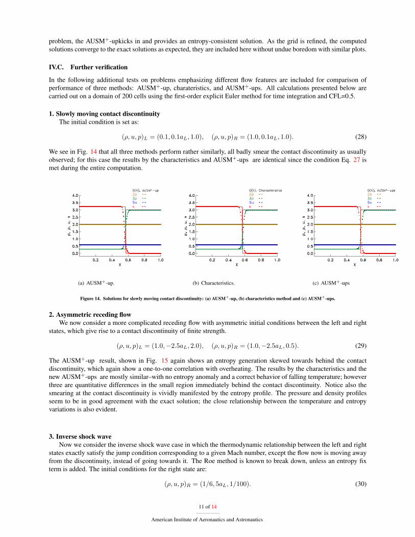
We see in Fig. 14 that all three methods perform rather similarly, all badly smear the contact discontinuity as usuallyobserved; for this case the results by the characteristics and AUSM+-ups are identical since the condition Eq. 27 ismet during the entire computation.

(a) AUSM+-up. (b) Characteristics. (c) AUSM+-ups

Figure 14. Solutions for slowly moving contact discontinuity: (a) AUSM+-up, (b) characteristics method and (c) AUSM+-ups.

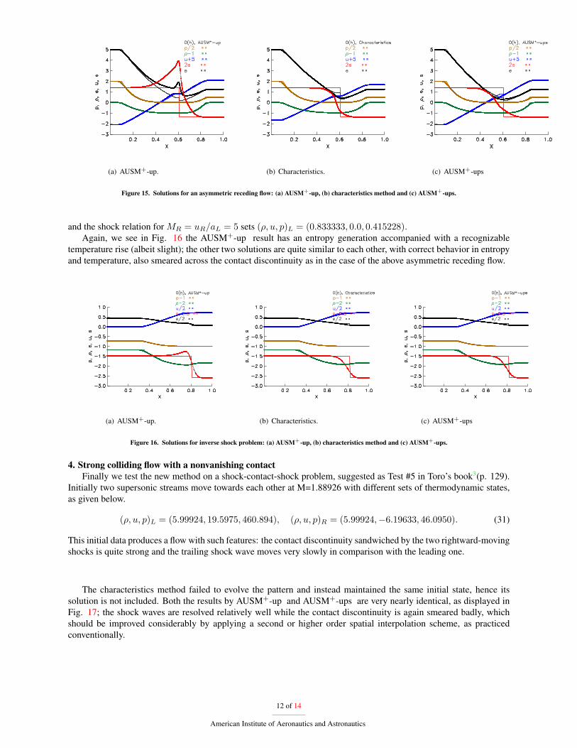
2. Asymmetric receding flowWe now consider a more complicated receding flow with asymmetric initial conditions between the left and right

states, which give rise to a contact discontinuity of finite strength.

(ρ, u, p)L = (1.0,−2.5aL, 2.0), (ρ, u, p)R = (1.0,−2.5aL, 0.5). (29)

The AUSM+-up result, shown in Fig. 15 again shows an entropy generation skewed towards behind the contactdiscontinuity, which again show a one-to-one correlation with overheating. The results by the characteristics and thenew AUSM+-ups are mostly similar–with no entropy anomaly and a correct behavior of falling temperature; howeverthree are quantitative differences in the small region immediately behind the contact discontinuity. Notice also thesmearing at the contact discontinuity is vividly manifested by the entropy profile. The pressure and density profilesseem to be in good agreement with the exact solution; the close relationship between the temperature and entropyvariations is also evident.

3. Inverse shock waveNow we consider the inverse shock wave case in which the thermodynamic relationship between the left and right

states exactly satisfy the jump condition corresponding to a given Mach number, except the flow now is moving awayfrom the discontinuity, instead of going towards it. The Roe method is known to break down, unless an entropy fixterm is added. The initial conditions for the right state are:

(ρ, u, p)R = (1/6, 5aL, 1/100). (30)

11 of 14



Figure 15. Solutions for an asymmetric receding flow: (a) AUSM+-up, (b) characteristics method and (c) AUSM+-ups.

and the shock relation for MR = uR/aL = 5 sets (ρ, u, p)L = (0.833333, 0.0, 0.415228).Again, we see in Fig. 16 the AUSM+-up result has an entropy generation accompanied with a recognizable

temperature rise (albeit slight); the other two solutions are quite similar to each other, with correct behavior in entropyand temperature, also smeared across the contact discontinuity as in the case of the above asymmetric receding flow.


Figure 16. Solutions for inverse shock problem: (a) AUSM+-up, (b) characteristics method and (c) AUSM+-ups.

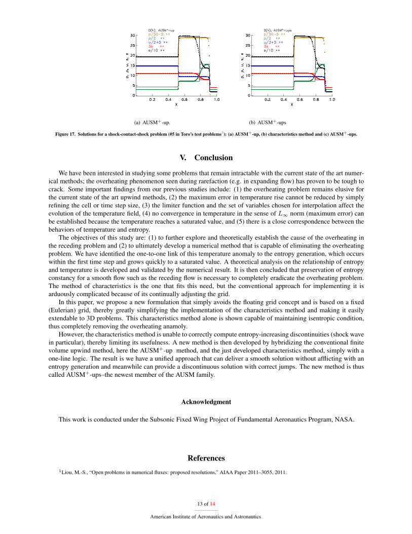
4. Strong colliding flow with a nonvanishing contactFinally we test the new method on a shock-contact-shock problem, suggested as Test #5 in Toro’s book3(p. 129).

Initially two supersonic streams move towards each other at M=1.88926 with different sets of thermodynamic states,as given below.

(ρ, u, p)L = (5.99924, 19.5975, 460.894), (ρ, u, p)R = (5.99924,−6.19633, 46.0950). (31)

This initial data produces a flow with such features: the contact discontinuity sandwiched by the two rightward-movingshocks is quite strong and the trailing shock wave moves very slowly in comparison with the leading one.

The characteristics method failed to evolve the pattern and instead maintained the same initial state, hence itssolution is not included. Both the results by AUSM+-up and AUSM+-ups are very nearly identical, as displayed inFig. 17; the shock waves are resolved relatively well while the contact discontinuity is again smeared badly, whichshould be improved considerably by applying a second or higher order spatial interpolation scheme, as practicedconventionally.

12 of 14


(a) AUSM+-up. (b) AUSM+-ups

Figure 17. Solutions for a shock-contact-shock problem (#5 in Toro’s test problems3): (a) AUSM+-up, (b) characteristics method and (c) AUSM+-ups.

V. Conclusion

We have been interested in studying some problems that remain intractable with the current state of the art numer-ical methods; the overheating phenomenon seen during rarefaction (e.g. in expanding flow) has proven to be tough tocrack. Some important findings from our previous studies include: (1) the overheating problem remains elusive forthe current state of the art upwind methods, (2) the maximum error in temperature rise cannot be reduced by simplyrefining the cell or time step size, (3) the limiter function and the set of variables chosen for interpolation affect theevolution of the temperature field, (4) no convergence in temperature in the sense of L∞ norm (maximum error) canbe established because the temperature reaches a saturated value, and (5) there is a close correspondence between thebehaviors of temperature and entropy.

The objectives of this study are: (1) to further explore and theoretically establish the cause of the overheating inthe receding problem and (2) to ultimately develop a numerical method that is capable of eliminating the overheatingproblem. We have identified the one-to-one link of this temperature anomaly to the entropy generation, which occurswithin the first time step and grows quickly to a saturated value. A theoretical analysis on the relationship of entropyand temperature is developed and validated by the numerical result. It is then concluded that preservation of entropyconstancy for a smooth flow such as the receding flow is necessary to completely eradicate the overheating problem.The method of characteristics is the one that fits this need, but the conventional approach for implementing it isarduously complicated because of its continually adjusting the grid.

In this paper, we propose a new formulation that simply avoids the floating grid concept and is based on a fixed(Eulerian) grid, thereby greatly simplifying the implementation of the characteristics method and making it easilyextendable to 3D problems. This characteristics method alone is shown capable of maintaining isentropic condition,thus completely removing the overheating anamoly.

However, the characteristics method is unable to correctly compute entropy-increasing discontinuities (shock wavein particular), thereby limiting its usefulness. A new method is then developed by hybridizing the conventional finitevolume upwind method, here the AUSM+-up method, and the just developed characteristics method, simply with aone-line logic. The result is we have a unified approach that can deliver a smooth solution without afflicting with anentropy generation and meanwhile can provide a discontinuous solution with correct jumps. The new method is thuscalled AUSM+-ups–the newest member of the AUSM family.

Acknowledgment

This work is conducted under the Subsonic Fixed Wing Project of Fundamental Aeronautics Program, NASA.

References1Liou, M.-S., “Open problems in numerical fluxes: proposed resolutions,” AIAA Paper 2011–3055, 2011.

13 of 14


2Von Neumann, J. and Richtmeyer, R. D., “A Method for the numerical calculation of hydrodynamic shocks,” J. Appl. Phys., Vol. 21, 1950,pp. 232–237.

3Toro, E. F., Riemann solvers and numerical methods for fluid dynamics: a practical introduction, Springer-Verlag, Berlin, Heidelberg, 3rded., 2009.

4LeVeque, R. J., Numerical Methods for Conservation Laws, Birkhauser Verlag, Basel, 1990.5Liou, M.-S., “Unresolved problems by shock capturing: Taming the overheating problem,” 7th International Conf. on Comput. Fluid Dyn.

2012–2203, 2012.6Liou, M.-S., “A sequel to AUSM, Part II: AUSM+-up for all speeds,” J. Comput. Phys., Vol. 214, 2006, pp. 137–170.7Liepmann, H. W. and Roshko, A., Elements of gasdynamics, John Wiley & Sons, 1957.

14 of 14


Why is the overheating problem difficult: The role of entropy

Documents

Transcript of Why is the overheating problem difficult: The role of entropy