GEOPHYSICS, VOL. 68, NO. 4 (JULY-AUGUST 2003); P. 1389–1398, 11 FIGS., 1 TABLE.10.1190/1.1598132

White’s model for wave propagation in partially saturated rocks:Comparison with poroelastic numerical experiments

Jose M. Carcione∗, Hans B. Helle‡, and Nam H. Pham∗∗

ABSTRACT

We use a poroelastic modeling algorithm to computenumerical experiments of wave propagation in White’spartial saturation model. The results are then comparedto the theoretical predictions. The model consists of a ho-mogeneous sandstone saturated with brine and sphericalgas pockets. White’s theory predicts a relaxation mecha-nism, due to pressure equilibration, causing attenuationand velocity dispersion of the wavefield. We vary gas sat-uration either by increasing the radius of the gas pocketor by increasing the density of gas bubbles. Despite thatthe modeling is two dimensional and interaction betweenthe gas pockets is neglected in White’s model, the nu-merical results show the trends predicted by the theory.In particular, we observe a similar increase in velocity athigh frequencies (and low permeabilities). Furthermore,the behavior of the attenuation peaks versus water satu-ration and frequency is similar to that of White’s model.The modeling results show more dissipation and highervelocities than White’s model due to multiple scatteringand local fluid-flow effects. The conversion of fast P-waveenergy into dissipating slow waves at the patches is themain mechanism of attenuation. Differential motion be-tween the rock skeleton and the fluids is highly enhancedby the presence of fluid/fluid interfaces and pressure gra-dients generated through them.

INTRODUCTION

Microstructural properties of reservoir rocks and theirin-situ rock conditions can be obtained, in principle, from seis-mic properties, such as traveltimes, amplitude information, andwave polarization. In particular, although it is known from theearly 1980s that the dominating mechanisms of wave attenu-

Manuscript received by the Editor February 15, 2002; revised manuscript received October 7, 2002.∗Istituto Nazionale di Oceanografia e di Geofisica Sperimentale (OGS), Borgo Grotta Gigante 42c, 34010 Sgonico, Trieste, Italy E-mail:jcarcione@ogs.trieste.it.‡Norsk Hydro a.s., E & P Research Centre, N-5020 Bergen, Norway. E-mail: hans.b.helle@nho.hydro.com.∗∗Norwegian University of Science and Technology, Department of Petroleum Engineering and Applied Geophysics, N-7491 Trondheim, Norway.E-mail: namhp@ipt.ntnu.no.c© 2003 Society of Exploration Geophysicists. All rights reserved.

ation are oscillating flow of the viscous pore fluids and grainboundary friction (e.g., Winkler and Nur, 1982), the use of at-tenuation to characterize the rock properties is still underex-ploited.

Regions of nonuniform patchy saturation occur at gas-oiland gas-water contacts in hydrocarbon reservoirs. Also, duringproduction, gas may come out of solution and create pock-ets of free gas. When laboratory measurements and sonic logsare used to infer the behavior of acoustic properties at seismicfrequencies, the frequency dependence of these properties be-comes a key factor. As demonstrated by White (1975), wavevelocity and attenuation are substantially affected by the pres-ence of partial (patchy) saturation, mainly depending on thesize of the gas pockets (saturation), frequency, permeability,and porosity of rocks.

Patchy saturation effects on acoustic properties were ob-served by Murphy (1984) and Knight and Nolen-Hoecksema(1990). Cadoret et al. (1995) observed the phenomenon in thelaboratory at the frequency range 1–500 kHz. Two differentsaturation methods result in different fluid distributions andproduce two different values of velocity for the same satura-tion. Imbibition by depressurization produces a very homoge-neous saturation, whereas drainage by drying produces hetero-geneous saturations at high water saturation levels. In the lattercase, the experiments show considerably higher velocities, aspredicted by White’s theory. The experimental results of Yinet al. (1992) display consistent peaks in resonance attenuationat high water saturation. A strong dependence on the satura-tion history is evident, with the attenuation peak located at90% water saturation in the drainage experiment and at 98%water saturation for imbibition techniques.

White’s model describes wave velocity and attenuation as afunction of frequency, permeability, and porosity, among otherparameters. Attenuation and velocity dispersion is caused byfluid flow between the water phase and the gas pockets, whichhave different pore pressures. The critical fluid diffusion re-laxation scale is proportional to the square root of the ratio

1389

1390 Carcione et al.

permeability to frequency (e.g., Mavko et al., 1998, 207). Atseismic frequencies, the length scale is very large, and the pres-sure is nearly uniform throughout the medium, but as fre-quency increases, pore pressure differences can cause an im-portant increase in P-wave velocity.

White’s model considers spherical gas pockets located at thecenter of a cubic array saturated with liquid. For simplicity inthe calculations, White considers two concentric spheres, wherethe volume of the outer sphere is the same as the volume of theelementary cube. The theory provides an average of the bulkmodulus for a single gas pocket, without taking into accountthe interactions between gas pockets. Dutta and Ode (1979)rederived White’s model using Biot’s theory. Dutta and Ser-iff (1979) pointed out some corrections in White’s equation,regarding the use of the P-wave modulus instead of the bulkmodulus (see also Mavko et al., 1998, 208). Gist (1994) success-fully used White’s model to fit ultrasonic velocities obtainedfrom saturations established using drainage techniques. Heused saturation-dependent moduli as input to White’s modelinstead of the dry-rock moduli. The predicted velocities, con-sidering local fluid flow, are higher than the velocities predictedby White’s model. Recently, Johnson (2001) developed a gen-eralization of White’s model for patches of arbitrary shape.This model has two geometrical parameters besides the usualparameters of Biot’s theory: the specific surface area and thesize of the patches.

Use of numerical simulations, based on the full-wave solu-tion of the poroelastic equations, can be useful to study thephysics of wave propagation in partially saturated rocks. Al-though White’s model is an ideal representation of patchy sat-uration, its predictions are qualitatively correct, and the modelserves as a reference theoretical framework. In this sense, itis useful to compare the results of White’s model to numer-ical simulations based on Biot’s theory of poroelasticity. Weshould, however, consider that the theory and the modelingcode are based on the same theoretical basis (Biot’s theory,although White’s model does not take into account the inter-action between gas pockets). This investigation can be the basisfor more realistic analyses, where an arbitrary (general) pore-scale fluid distribution is considered. By using computerizedtomography (CT) scans, it is possible to visualize the fluid dis-tribution in real rocks (Cadoret et al., 1995). Fractal models,such as the von Karman autocovariance function, calibrated bythe CT scans, can be used to model realistic fluid distributions.

P-wave and S-wave velocities can be higher in partially satu-rated rocks than in dry rocks, but in some cases they are lower.As predicted by White’s model, this behavior depends on fre-quency, viscosity, and permeability. It is therefore importantto investigate the sensitivity and properties of wave velocityand attenuation versus pore-fluid distribution. This is the basisfor direct hydrocarbon detection and enhanced oil recoveryand monitoring, since techniques such as “bright spot” andamplitude variation with offset (AVO) analyses make use ofthose physical properties. The modeling methodology used inthe present study constitutes a powerful computational tool toinvestigate the physics of wave propagation in porous rocksand, in some cases, can be used as an alternative method tolaboratory experiments.

We solve the poroelastic equations with an algorithm devel-oped by Carcione and Helle (1999), which uses a fourth-orderRunge-Kutta time-stepping scheme and the staggered Fourier

method for computing the spatial derivatives. The stiff part ofthe differential equations is solved with a time-splitting tech-nique, which preserves the physics of the slow quasi-static waveat low frequencies.

PHASE VELOCITY AND ATTENUATION

The concept of complex velocity can be used to obtain thephase velocity and attenuation factor (e.g., Carcione, 2001, 55).Let vc be the P-wave complex velocity obtained with White’smodel (see Appendix). Then, the phase velocity and attenua-tion factor are given by

c =[

Re(

1vc

)]−1

(1)

and

α = −ωIm(

1vc

), (2)

respectively, where ω is the angular frequency. If we approx-imate the porous medium by a viscoelastic solid, the qualityfactor can be expressed as

Q = Re(v2

c

)Im(v2

c

) . (3)

[Otherwise, the Q factor for porous media has a more complexexpression (Carcione, 2001, 289).]. The relation between theattenuation factor and the quality factor Q can be expressedas

α = 2π f

c

(√Q2 + 1− Q

)≈ π f

cQ, (4)

where f =ω/(2π) is the frequency (Carcione, 2001, 139). Thesecond relation in the right side holds for low-loss solid (QÀ 1).

The phase velocity in the numerical experiments is com-puted from the center of gravity of |v|2 versus propagation time,where v is the bulk particle-velocity field (Carcione, 1996). Aset of receivers R1 and R3 located on five radial lines are usedfor the calculations, and receivers R2 are used for verification.The numerical phase velocity is estimated by averaging thevelocities obtained at the five receivers R3. More details aboutthis calculation are given in Carcione et al. (1996) and Carcione(2001, 145). The determination of phase velocity in terms of thelocation of the energy is justified from the fact that for isotropicmedia and homogeneous viscoelastic waves, the phase velocityis equal to the energy velocity (Carcione, 2001, 99).

To estimate attenuation, we use the classical spectral ratioapproach discussed by Toksoz et al. (1979), implying that theamplitude ratio A1/A3 at the dominant frequency f satisfies

ln[

A1( f, r1)A3( f, r3)

]= α(r3 − r1)+ ln

(G1

G3

), (5)

where r i denotes the source-receiver radial distances, and Gi

denotes the respective geometrical spreading factors. Usingrelation (4), equation (5) can be rewritten as

ln[

A1( f, r1)A3( f, r3)

]= π f (r3 − r1)

Qc+ ln

(G1

G3

), (6)

The quality factor is determined from the slope of the line fittedto ln(A1/A3).

White’s Model for Partial Saturation 1391

A source of discrepancy between theory and numerical re-sults can be due to the fact that White’s model is three dimen-sional and the simulations are two dimensional. The travel timeis not affected by the dimensionality of space (see, for instance,Carcione and Quiroga-Goode, 1996). Hence, the wave veloc-ities are not affected. With regard to the amplitudes, equa-tion (6) implicitly has the correction for geometrical spread-ing (1/

√r in 2D space and 1/r in 3D space). Therefore, the

discrepancy could be solely due to the deviation of the 2DGreen’s function from the exponential function. The 2D and3D Green’s function for poroelastic media contain the kernelsH (2)

0 (x) and exp(i x), respectively, where x=ωr/c, and H (2)0 is

the Hankel function of the second kind (e.g., Carcione andQuiroga-Goode, 1996). The Hankel function approaches theexponential function for larges values of |x|. For instance, forc= 3000 m/s, r = 0.05 m, and f = 100 kHz, the argument isx= 10.5 The exact value of the Hankel function is (−0.239,0.061) and the asymptotic value is (−0.238, 0.064). Even forx= 2, the differences are not significant [(0.22, −0.51) versus(0.20, −0.53)]. This fact indicates that the discrepancy due tothe space dimension is not important.

RESULTS

We consider the material properties shown in Table 1, wherethe moduli and density of the grain material correspond to amixture of 90% quartz and 10% clay [the moduli are calculatedas the upper and lower Hashin-Shtrikman bounds (Mavkoet al., 1998, 106)]. The dry-rock moduli are obtained by arelation introduced by Krief et al. (1990) (see Goldberg andGurevich, 1998; and Carcione et al., 2000). Note that White’s(1975) theory does not consider tortuosity [the value of tortuos-ity given in Table 1 is typical of a sandstone (e.g., Johnson et al.,1987)]. If a and b are the outer and inner radii of the gas pock-ets (see Appendix) and we denote the space dimension by n,water saturation can be expressed by Sw = 1− (a/b)n. A sourceof discrepancy between theoretical and numerical results mayarise from the fact that White’s theory does not consider the in-teraction between gas pockets, while this interaction is presentin the numerical simulations.

The transition frequency separating the relaxed and unre-laxed states (that is, the location of the relaxation peak) is

Table 1. Material properties of the rock.

GrainBulk modulus (Ks) 34.3 GPaShear modulus (µs) 35.3 GPaDensity (ρs) 2585 kg/m3

MatrixBulk modulus (Km) 8.67 GPaShear modulus (µm) 6.61 GPaPorosity (φ) 0.3Permeability (κ) 0.55 dTortuosity (T ) 2.5

GasBulk modulus (Kg) 0.01 GPaDensity (ρg) 100 kg/m3

Viscosity (ηg) 0.000 02 Pa sBrine

Bulk modulus (Kw) 2.4 GPaDensity (ρw) 1040 kg/m3

Viscosity (ηw) 0.001 8 Pa s

approximately given by

fc = κKE2

πη2(b− a)2, (7)

where κ is the permeability, KE2 is given in equation (A-6), andη2 is the viscosity of water. Dutta and Seriff (1979) considerb2, instead of (b−a)2, in the denominator. However, the rel-evant relaxation distance should be the thickness of the outershell (i.e., b−a). White considers a harmonic displacement ap-plied to the outer spherical surface, which creates two differentpressures in the outer shell and the inner sphere. Therefore,the relaxation distance should be the difference between thetwo radii (Gist, 1994). Relaxation frequencies of essentially thesame physical nature, but for plane-layered rocks, have beengiven by White et al. (1975), Norris (1993), and Gurevich andLopatnikov (1995).

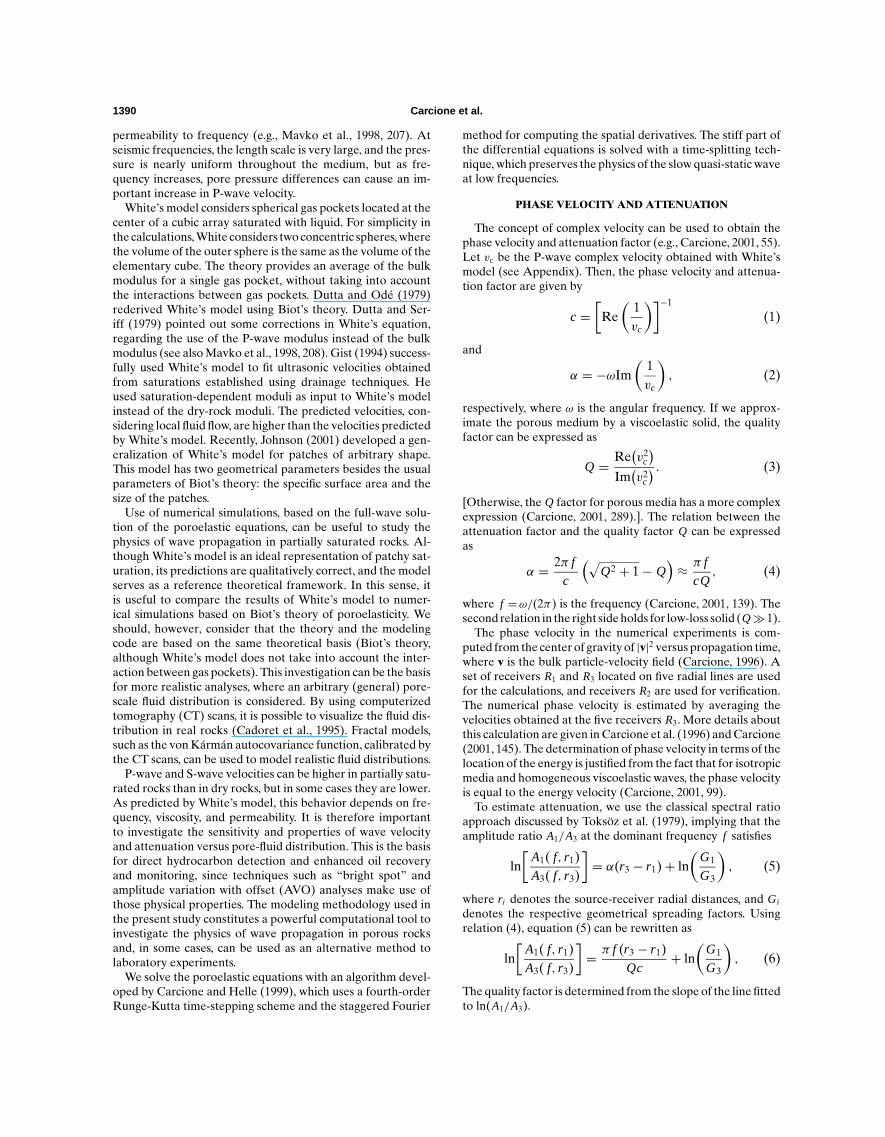
There are two cases giving the same gas saturation. They areillustrated in Figure 1 for a 2D porous medium. Figure 1a showsfour gas pockets, where the gas saturation is Sg= 4πa2 [the sizeof the square is `= 1/2, and b= `/√π (see Appendix)]. We mayincrease the saturation to Sg= 16πa2 in two different ways. InFigures 1b, a is constant, whereas in Figure 1c, b is constant.

When b is constant, we can deduce a critical water satura-tion, Swc, for which the attenuation is maximum. For a given fre-quency, and using Sw = 1−(a/b)3, we obtain from equation (7):

Swc = 1−(

1−√

κKE2

πη2 f b2

)3

. (8)

If a is constant, the critical saturation is given by

Swc = 1−(

1+√

κKE2

πη2 f a2

)−3

. (9)

As stated in the Appendix, the size of the gas pockets, a,should be much smaller than the wavelength. Let us considera reference velocity cr = 3000 m/s, a maximum outer radiusb= 7 mm, and Sg= 0.52 [the upper-limit gas saturation forwhich White’s model holds (see Appendix)]. Since a= bS1/3

g ,the condition a¿ cr / f implies f ¿ 536 kHz. With these limi-tations in mind, we proceed in the following to analyze White’sresults and compare these results with numerical simulations.

The modeling algorithm uses a numerical mesh with rect-angular cells (here we consider square cells). Let us assumethat b is constant. Since the size of the elementary square`=√πb=m1x, where m is a natural number and1x is the gridspacing, 1x=√πb/m. If M is the number of cells of the gaspocket, then M1x2=πa2, and Sg=M/m2. On the other hand,if a is constant, the grid size is computed as 1x=a

√π/M . An

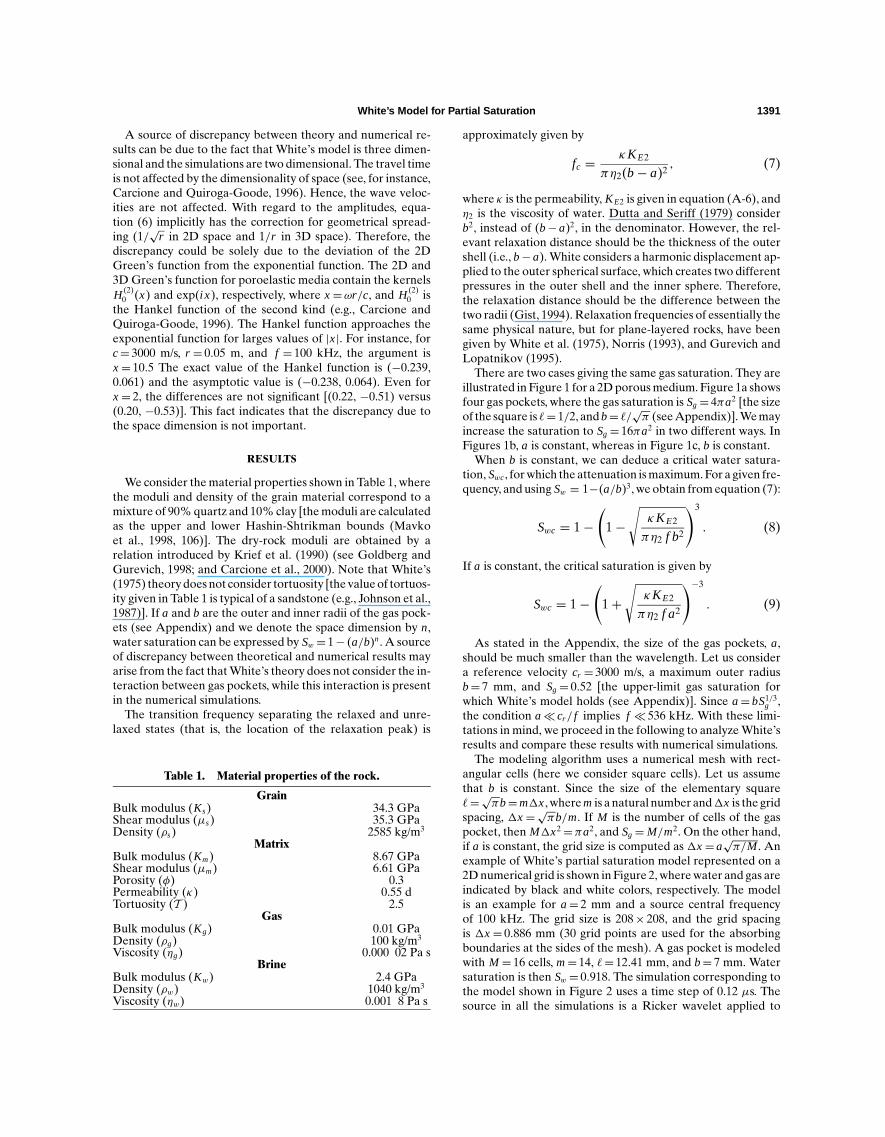
example of White’s partial saturation model represented on a2D numerical grid is shown in Figure 2, where water and gas areindicated by black and white colors, respectively. The modelis an example for a= 2 mm and a source central frequencyof 100 kHz. The grid size is 208× 208, and the grid spacingis 1x= 0.886 mm (30 grid points are used for the absorbingboundaries at the sides of the mesh). A gas pocket is modeledwith M = 16 cells, m= 14, `= 12.41 mm, and b= 7 mm. Watersaturation is then Sw = 0.918. The simulation corresponding tothe model shown in Figure 2 uses a time step of 0.12 µs. Thesource in all the simulations is a Ricker wavelet applied to

1392 Carcione et al.

the solid skeleton and the fluid phase (a bulk source withoutshear components). A region with a radius of 30 grid pointsand 100% water saturation surrounds the source location inorder to obtain a uniform initial wavefront.

FIG. 1. Two different sizes for the gas pockets give the same gassaturation, depending on the values of the outer and inner radiia and b. In (a) the saturation is Sg= 4πa2, whereas in (b) and (c)the saturation is the same and equal to four times the saturationin (a). Gas saturation can then change by varying a and keepingconstant b, or vice versa. (Note that White considers an outersphere of radius b instead of a cube of size `. In 2D space,b= `/√π .)

Let us first consider that the radius of the outer sphere, b, isconstant and equal to 4 mm. Figure 3 shows the P-wave velocity(a) and attenuation factor (b) versus water saturation for dif-ferent frequencies and a permeability of 550 md. The analyticaland numerical (black dots) evaluation of Gassmann’s velocityhas been performed on a homogeneous porous medium byaveraging the fluid bulk modulus with Wood’s equation (e.g.,Mavko et al., 1998, 112). Gassmann’s velocity (e.g. Carcione,2001, 257) is also shown as a dotted curve. The critical water sat-urations, Swc, for 50, 100, 250, and 500 kHz are 99%, 9%, 72%,and 56%, respectively (plus symbols). The differences in veloc-ity can be important for increasing frequency. For instance, thedifference between the seismic velocity (Gassmann’s curve)and the ultrasonic velocity (100 kHz) predicted by White’smodel is 120 m/s at 90% water saturation [the respective wave-lengths are approximately 150 m (seismic frequencies) and 3 cm(100 kHz)]. The simulations predict higher velocities comparedto White’s model, and the relaxation peaks are shifted towardslower water saturations. However, the physics revealed by thenumerical results is similar to that predicted by White’s model.

Figure 4 shows the P-wave velocity (a) and attenuation fac-tor (b) versus water saturation for different permeabilities anda frequency of 100 kHz. The dotted line is Gassmann’s velocity,obtained by mixing the fluid moduli with Wood’s average. Thecritical water saturations, Swc, for 0, 10, 100, 550, and 5000 mdare 2%, 20%, 55%, 91% and 100%, respectively, in fairly goodagreement with the location of the relaxation peaks predictedby White’s model. The numerical phase velocities coincide withWhite’s velocities for low permeabilities. For 550 and 5000 md,the simulations predict higher velocities. This means morevelocity dispersion (see also the higher attenuation levels in

FIG. 2. White’s model on a 2D numerical mesh used for wavesimulation with a 100-kHz source. Water and gas are indicatedby black and white colors, respectively. Source (S) and receivers(Ri ) are indicated. A circular region surrounding the source isfully water saturated to assure a uniform initial wavefront. Gaspocket radius is a= 2 mm, and water saturation is Sw = 0.918(b= 7 mm).

White’s Model for Partial Saturation 1393

Figure 4b) caused by additional dissipation mechanisms whichare not predicted by White’s model.

Figure 5 shows the P-wave velocity (a) and attenuation factor(b) versus frequency for different water saturations. The per-meability is 550 md. The critical frequencies, fc, are indicatedby plus symbols in Figure 5b. As before, higher velocities andattenuation levels, compared to White’s model, are observedin the numerical simulations. The shift of the peaks towardslower frequencies can be an indication of the presence of localfluid flow mechanisms.

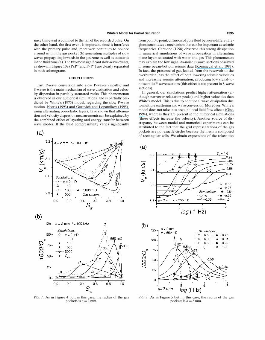
Let us assume now that the radius of the gas pockets, a,is constant and equal to 2 mm. The results, corresponding toFigures 3, 4, and 5, are respectively shown in Figures 6, 7, and8. We observe the same physical behavior as for constant b,indicating that the physics is substantially dependent on thedifference b−a.

FIG. 3. P-wave velocity (a) and attenuation factor (b) versuswater saturation for different frequencies and a permeabilityof 550 md. The continuous line corresponds to White’s theoryand the symbols to the numerical simulations. The dotted line isGassmann’s (low-frequency) velocity, obtained by mixing thefluid moduli with Wood’s average. The size of the outer sphereis b= 4 mm.

Snapshots of the fluid particle velocity relative to the solid(a), fluid pressure (b), and particle velocity of the solid (c) areshown in Figure 9. They correspond to the model shown inFigure 2, with 92% water saturation but a central frequency of500 kHz and a corresponding smaller grid spacing1x= 0.1 mmin a 660× 660 grid to highlight the details (54 grid points areused for the absorbing boundaries at the sides of the mesh).The two main wavefronts are the fast P-wave and the slow P-wave. The conversion of fast P-wave to slow P-wave at eachgas pocket can clearly be appreciated. At 500 kHz, slow waveshave a phase velocity of 841 m/s in the brine saturated regionand 200 m/s in the gas pockets (the fast P-wave velocity is 3210and 3094 m/s, respectively). The primary fast wave P+ generatesslow waves P+P− at the gas pockets. In addition, significant slowwaves are generated by the scattered P+ inside the gas pocket

FIG. 4. P-wave velocity (a) and attenuation factor (b) versuswater saturation for different permeabilities and a frequencyof 100 kHz. The continuous line corresponds to White’s theoryand the symbols to the numerical simulations. The dotted line isGassmann’s (low-frequency) velocity, obtained by mixing thefluid moduli with Wood’s average. The size of the outer sphereis b= 4 mm.

1394 Carcione et al.

(P+P+P−). These are the two main events generated in the fluidphase during passage of the primary P+, and thus representthe most significant loss components, removing energy fromthe front of the pulse and adding to its tail. The fluid particlevelocity of the slow waves (Figure 9a) is high within the gaspocket and less pronounced in the brine, whereas for the fluidpressure (Figure 9b), the situation is the opposite. In the solid(Figure 9c), P+ dominates the wavefield, while the slow wavesare less clearly identified.

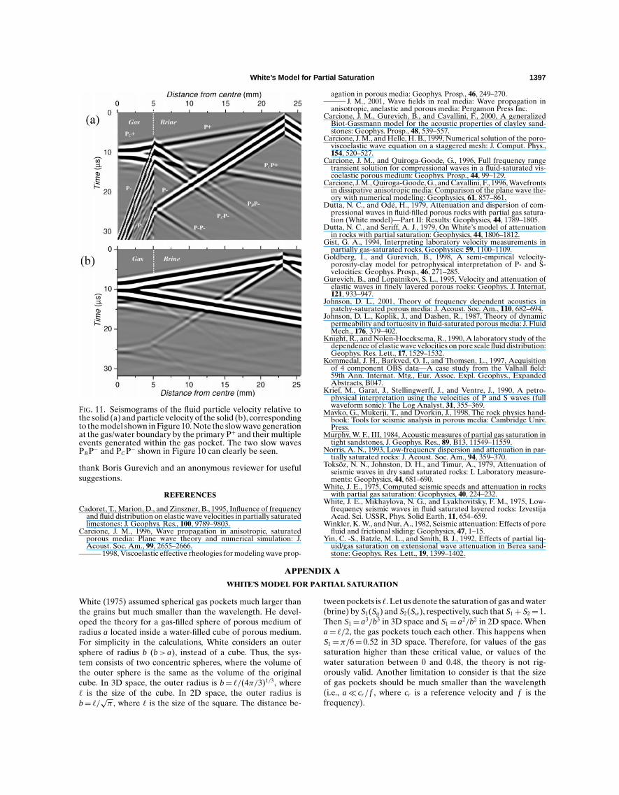
A final numerical experiment to illustrate the phenomenonis shown in Figure 10. Figure 10a shows a gas pocket of radiusa= 5 mm with a circular source located at a distance b= 23 mmfrom its center. The rock and the pore fill are the same asin the previous experiment (Table 1). We use a fine mesh of1x= 0.1 mm and a source frequency of 500 kHz. The seis-mograms of the particle velocity (Figure 10b) are recorded atreceivers located 1 mm away from the fluid/gas boundary in thewater-saturated and gas-saturated rocks. In the solid, it shows

FIG. 5. P-wave velocity (a) and attenuation factor (b) versusfrequency for different water saturations. The continuous linecorresponds to White’s theory and the symbols to the numer-ical simulations. The permeability is 550 md. The size of theouter sphere is b= 4 mm. The location of critical frequenciesis indicated for different saturations.

the P+ arrival and its scattering PCP+ with opposite phase afterfocusing in the center of the gas pocket. In the fluid wavefield,we observe the corresponding slow waves PBP− and PCP−, gen-erated at the the fluid/gas boundary. These are equivalent tothe two consecutive slow waves apparent from the experimentin Figure 9. The tail of arrivals recorded within the gas zone,following the main events, are slow waves due to P+ ringingwithin the gas pocket, whereas the late P− events at the end ofthe record are the direct (in the brine) and transmitted (in thegas) slow wave generated at the source.

More details of these experiments can be appreciated inFigure 11, which shows the seismograms of the fluid (relative)(a) and solid (b) particle velocities along the receiver line. Thefast- and slow-wave events are clearly distinguishable by theirdifferent dips [i.e., low angles (high velocity) for P+ and highangles (low velocity) for P−]. The focusing of the direct P+ iswell expressed in both fluid and solid particle velocities, anda similar focusing of P+ is evident in the lower section of (b),originating from P− to P+ conversion at the water/gas interface.The latter, however, has less relevance for the problem at hand

FIG. 6. As in Figure 3 but, in this case, the radius of the gaspockets is a= 2 mm.

White’s Model for Partial Saturation 1395

since this event is confined to the tail of the recorded pulse. Onthe other hand, the first event is important since it interfereswith the primary pulse and, moreover, continues to bouncearound within the gas pocket (b) generating multiples of slowwaves propagating inwards in the gas zone as well as outwardsin the fluid zone (a). The two most significant slow-wave events,as shown in Figure 10a (PBP− and PCP−) are clearly separatedin both seismograms.

CONCLUSIONS

Fast P-wave conversion into slow P-waves (mostly) andS-waves is the main mechanism of wave dissipation and veloc-ity dispersion in partially saturated rocks. This phenomenonis observed in our numerical simulations, and is partially pre-dicted by White’s (1975) model, regarding the slow P-wavemotion. Norris (1993) and Gurevich and Lopatnikov (1995),using alternating poroelastic layers, have shown that attenua-tion and velocity dispersion measurements can be explained bythe combined effect of layering and energy transfer betweenwave modes. If the fluid compressibility varies significantly

FIG. 7. As in Figure 4 but, in this case, the radius of the gaspockets is a= 2 mm.

from point to point, diffusion of pore fluid between different re-gions constitutes a mechanism that can be important at seismicfrequencies. Carcione (1998) observed this strong dissipationin numerical simulations of wave propagation in alternatingplane layers saturated with water and gas. This phenomenonmay explain the low signal-to-noise P-wave sections observedin some ocean-bottom seismic data (Kommedal et al., 1997).In fact, the presence of gas, leaked from the reservoir to theoverburden, has the effect of both lowering seismic velocitiesand increasing seismic attenuation, producing low signal-to-noise ratio P-wave sections (this effect is not present in S-wavesections).

In general, our simulations predict higher attenuation (al-though narrower relaxation peaks) and higher velocities thanWhite’s model. This is due to additional wave dissipation dueto multiple scattering and wave conversion. Moreover, White’smodel does not take into account local fluid flow effects (Gist,1994), whereas they are present in the numerical simulations(these effects increase the velocity). Another source of dis-crepancy between model and numerical experiments can beattributed to the fact that the grid representations of the gaspockets are not exactly circles because the mesh is composedof rectangular cells. We obtain expressions of the relaxation

FIG. 8. As in Figure 5 but, in this case, the radius of the gaspockets is a= 2 mm.

1396 Carcione et al.

critical frequency and critical saturation for which attenuationhas a maximum value. Our simulations reproduce the trendsregarding the location of the relaxation peaks as a functionof frequency and saturation. That is, the peaks move towards

FIG. 9. Snapshot of the fluid particle velocity relative to thesolid (a), fluid pressure field (b), and particle velocity of thesolid (c), corresponding to the model shown in Figure 2 with92% water saturation but with finer mesh (0.1 mm) and a cen-tral frequency of 500 kHz. Propagation time is 18 µs. The pri-mary fast P+ wave generates slow waves (P+P−) at the gaspockets. Fast waves scattered from the inner boundary, in turn,generate new slow waves (P+P+P−).

higher water saturations for lower frequencies and higher per-meabilities.

The final example shows an analysis of the wavefield for asingle gas pocket, modeling the conditions for which White(1975) has developed the theory. The physical phenomena in-volved in the problem are illustrated by this simulation. Theconversion from fast to slow compressional wave and the mul-tiple events generated at the gas bubble are clearly the mainloss mechanisms of the primary pulse.

ACKNOWLEDGMENTS

This work was financed in part by the European Union un-der the HYGEIA project and by the Norwegian ResearchCouncil under the PetroForsk programme (N. H. Pham). We

FIG. 10. Model of a single gas pocket of radius a= 5 mm and acircular source located at a distance b= 23 mm (a). Fluid (rel-ative) and solid particle velocities (b) are recorded in receiverslocated on either side (1 mm) of the gas/fluid boundary. Thesolid line indicates receivers for the seismograms in Figure 11.P+ denotes the direct fast wave and PCP+ its return from thepocket center (focus). PBP− and PCP− are their associated slowwaves generated at the intersection with the gas/fluid bound-ary. The central frequency is 500 kHz, the grid size is 0.1 mm,and time step is 0.013 22 ms.

White’s Model for Partial Saturation 1397

FIG. 11. Seismograms of the fluid particle velocity relative tothe solid (a) and particle velocity of the solid (b), correspondingto the model shown in Figure 10. Note the slow wave generationat the gas/water boundary by the primary P+ and their multipleevents generated within the gas pocket. The two slow wavesPBP− and PCP− shown in Figure 10 can clearly be seen.

thank Boris Gurevich and an anonymous reviewer for usefulsuggestions.

REFERENCES

Cadoret, T., Marion, D., and Zinszner, B., 1995, Influence of frequencyand fluid distribution on elastic wave velocities in partially saturatedlimestones: J. Geophys. Res., 100, 9789–9803.

Carcione, J. M., 1996, Wave propagation in anisotropic, saturatedporous media: Plane wave theory and numerical simulation: J.Acoust. Soc. Am., 99, 2655–2666.

——— 1998, Viscoelastic effective rheologies for modeling wave prop-

APPENDIX A

WHITE’S MODEL FOR PARTIAL SATURATION

White (1975) assumed spherical gas pockets much larger thanthe grains but much smaller than the wavelength. He devel-oped the theory for a gas-filled sphere of porous medium ofradius a located inside a water-filled cube of porous medium.For simplicity in the calculations, White considers an outersphere of radius b (b>a), instead of a cube. Thus, the sys-tem consists of two concentric spheres, where the volume ofthe outer sphere is the same as the volume of the originalcube. In 3D space, the outer radius is b= `/(4π/3)1/3, where` is the size of the cube. In 2D space, the outer radius isb= `/√π , where ` is the size of the square. The distance be-

tween pockets is `. Let us denote the saturation of gas and water(brine) by S1(Sg) and S2(Sw), respectively, such that S1+ S2= 1.Then S1=a3/b3 in 3D space and S1=a2/b2 in 2D space. Whena= `/2, the gas pockets touch each other. This happens whenS1=π/6= 0.52 in 3D space. Therefore, for values of the gassaturation higher than these critical value, or values of thewater saturation between 0 and 0.48, the theory is not rig-orously valid. Another limitation to consider is that the sizeof gas pockets should be much smaller than the wavelength(i.e., a¿ cr / f , where cr is a reference velocity and f is thefrequency).

agation in porous media: Geophys. Prosp., 46, 249–270.——— J. M., 2001, Wave fields in real media: Wave propagation in

anisotropic, anelastic and porous media: Pergamon Press Inc.Carcione, J. M., Gurevich, B., and Cavallini, F., 2000, A generalized

Biot-Gassmann model for the acoustic properties of clayley sand-stones: Geophys. Prosp., 48, 539–557.

Carcione, J. M., and Helle, H. B., 1999, Numerical solution of the poro-viscoelastic wave equation on a staggered mesh: J. Comput. Phys.,154, 520–527.

Carcione, J. M., and Quiroga-Goode, G., 1996, Full frequency rangetransient solution for compressional waves in a fluid-saturated vis-coelastic porous medium: Geophys. Prosp., 44, 99–129.

Carcione, J. M., Quiroga-Goode, G., and Cavallini, F., 1996, Wavefrontsin dissipative anisotropic media: Comparison of the plane wave the-ory with numerical modeling: Geophysics, 61, 857–861,

Dutta, N. C., and Ode, H., 1979, Attenuation and dispersion of com-pressional waves in fluid-filled porous rocks with partial gas satura-tion (White model)—Part II: Results: Geophysics, 44, 1789–1805.

Dutta, N. C., and Seriff, A. J., 1979, On White’s model of attenuationin rocks with partial saturation: Geophysics, 44, 1806–1812.

Gist, G. A., 1994, Interpreting laboratory velocity measurements inpartially gas-saturated rocks, Geophysics: 59, 1100–1109.

Goldberg, I., and Gurevich, B., 1998, A semi-empirical velocity-porosity-clay model for petrophysical interpretation of P- and S-velocities: Geophys. Prosp., 46, 271–285.

Gurevich, B., and Lopatnikov, S. L., 1995, Velocity and attenuation ofelastic waves in finely layered porous rocks: Geophys. J. Internat,121, 933–947.

Johnson, D. L., 2001, Theory of frequency dependent acoustics inpatchy-saturated porous media: J. Acoust. Soc. Am., 110, 682–694.

Johnson, D. L., Koplik, J., and Dashen, R., 1987, Theory of dynamicpermeability and tortuosity in fluid-saturated porous media: J. FluidMech., 176, 379–402.

Knight, R., and Nolen-Hoecksema, R., 1990, A laboratory study of thedependence of elastic wave velocities on pore scale fluid distribution:Geophys. Res. Lett., 17, 1529–1532.

Kommedal, J. H., Barkved, O. I., and Thomsen, L., 1997, Acquisitionof 4 component OBS data—A case study from the Valhall field:59th Ann. Internat. Mtg., Eur. Assoc. Expl. Geophys., ExpandedAbstracts, B047.

Krief, M., Garat, J., Stellingwerff, J., and Ventre, J., 1990, A petro-physical interpretation using the velocities of P and S waves (fullwaveform sonic): The Log Analyst, 31, 355–369.

Mavko, G., Mukerji, T., and Dvorkin, J., 1998, The rock physics hand-book: Tools for seismic analysis in porous media: Cambridge Univ.Press.

Murphy, W. F., III, 1984, Acoustic measures of partial gas saturation intight sandstones, J. Geophys. Res., 89, B13, 11549–11559.

Norris, A. N., 1993, Low-frequency dispersion and attenuation in par-tially saturated rocks: J. Acoust. Soc. Am., 94, 359–370.

Toksoz, N. N., Johnston, D. H., and Timur, A., 1979, Attenuation ofseismic waves in dry sand saturated rocks: I. Laboratory measure-ments: Geophysics, 44, 681–690.

White, J. E., 1975, Computed seismic speeds and attenuation in rockswith partial gas saturation: Geophysics, 40, 224–232.

White, J. E., Mikhaylova, N. G., and Lyakhovitsky, F. M., 1975, Low-frequency seismic waves in fluid saturated layered rocks: IzvestijaAcad. Sci. USSR, Phys. Solid Earth, 11, 654–659.

Winkler, K. W., and Nur, A., 1982, Seismic attenuation: Effects of porefluid and frictional sliding: Geophysics, 47, 1–15.

Yin, C. -S., Batzle, M. L., and Smith, B. J., 1992, Effects of partial liq-uid/gas saturation on extensional wave attenuation in Berea sand-stone: Geophys. Res. Lett., 19, 1399–1402.

1398 Carcione et al.

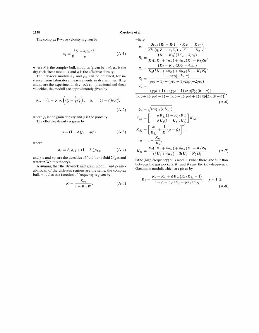
The complex P-wave velocity is given by

vc =√

K + 4µm/3ρ

, (A-1)

where K is the complex bulk modulus (given below), µm is thedry-rock shear modulus, and ρ is the effective density.

The dry-rock moduli Km and µm can be obtained, for in-stance, from laboratory measurements in dry samples. If cP

and cS are the experimental dry-rock compressional and shearvelocities, the moduli are approximately given by

Km = (1− φ)ρs

(c2

P −43

c2S

), µm = (1− φ)ρsc

2S,

(A-2)

where ρs is the grain density and φ is the porosity.The effective density is given by

ρ = (1− φ)ρs + φφ f , (A-3)

where

ρ f = S1ρ f 1 + (1− S1)ρ f 2, (A-4)

and ρ f 1 and ρ f 2 are the densities of fluid 1 and fluid 2 (gas andwater in White’s theory).

Assuming that the dry-rock and grain moduli, and perme-ability, κ , of the different regions are the same, the complexbulk modulus as a function of frequency is given by

K = K∞1− K∞W

, (A-5)

where

W = 3iaκ(R1 − R2)b3ω(η1 Z1 − η2 Z2)

(K A1

K1− K A2

K2

),

R1 = (K1 − Km)(3K2 + 4µm)K2(3K1 + 4µm)+ 4µm(K1 − K2)S1

,

R2 = (K2 − Km)(3K1 + 4µm)K2(3K1 + 4µm)+ 4µm(K1 − K2)S1

,

Z1 = 1− exp(−2γ1a)(γ1a− 1)+ (γ1a+ 1) exp(−2γ1a)

,

Z2 =(γ2b+ 1)+ (γ2b− 1) exp[2γ2(b− a)]

(γ2b+ 1)(γ2a− 1)− (γ2b− 1)(γ2a+ 1) exp[2γ2(b−a)],

(A-6)

γ j =√

iωη j /(κKE j ),

KE j =[

1− αK f j (1− K j /Ks)φK j (1− K f j /Ks)

]K Aj ,

K Aj =[φ

K f j+ 1

Ks(α − φ)

]−1

,

α = 1− Km

Ks.

K∞ = K2(3K1 + 4µm)+ 4µm(K1 − K2)S1

(3K1 + 4µm)− 3(K1 − K2)S1(A-7)

is the (high-frequency) bulk modulus when there is no fluid flowbetween the gas pockets. K1 and K2 are the (low-frequency)Gassmann moduli, which are given by

K j =Ks − Km + φKm

(Ks/K f j − 1

)1− φ − Km/Ks + φKs/K f j

, j = 1, 2.

(A-8)