What's New in NX 6.0.2

What’s New in NX 6.0.2

Proprietary & Restricted Rights Notice

This software and related documentation are proprietary to Siemens ProductLifecycle Management Software Inc.

© 2008 Siemens Product Lifecycle Management Software Inc. All RightsReserved.

All trademarks belong to their respective holders.

2 What’s New in NX 6.0.2

Contents

Introduction to What’s New . . . . . . . . . . . . . . . . . . . . . . . . . . . . . . . . 1-1

Gateway . . . . . . . . . . . . . . . . . . . . . . . . . . . . . . . . . . . . . . . . . . . . . . . . 2-1

Exact lightweight geometry and refile_part utility changes . . . . . . . . . . . 2-1Specify geometry layer in JT files . . . . . . . . . . . . . . . . . . . . . . . . . . . . . . 2-2Move Object enhancements . . . . . . . . . . . . . . . . . . . . . . . . . . . . . . . . . . 2-3

Modeling . . . . . . . . . . . . . . . . . . . . . . . . . . . . . . . . . . . . . . . . . . . . . . . 3-1

Retaining imprinted edges in a Split Body . . . . . . . . . . . . . . . . . . . . . . . 3-1Synchronous Technology face overflow options . . . . . . . . . . . . . . . . . . . . 3-2Synchronize Views in Replace Feature . . . . . . . . . . . . . . . . . . . . . . . . . . 3-4

Assemblies . . . . . . . . . . . . . . . . . . . . . . . . . . . . . . . . . . . . . . . . . . . . . . 4-1

Motion envelopes . . . . . . . . . . . . . . . . . . . . . . . . . . . . . . . . . . . . . . . . . . 4-1Variable positioning and Fix constraints . . . . . . . . . . . . . . . . . . . . . . . . . 4-2

Drafting . . . . . . . . . . . . . . . . . . . . . . . . . . . . . . . . . . . . . . . . . . . . . . . . 5-1

GB Weld Symbols . . . . . . . . . . . . . . . . . . . . . . . . . . . . . . . . . . . . . . . . . . 5-1Detail View color, font, and width . . . . . . . . . . . . . . . . . . . . . . . . . . . . . . 5-1Narrow Arc Length and Angular Dimensions . . . . . . . . . . . . . . . . . . . . . 5-2ESKD Weld Symbols . . . . . . . . . . . . . . . . . . . . . . . . . . . . . . . . . . . . . . . 5-3Section Line Style Enhancements . . . . . . . . . . . . . . . . . . . . . . . . . . . . . . 5-4

PMI . . . . . . . . . . . . . . . . . . . . . . . . . . . . . . . . . . . . . . . . . . . . . . . . . . . . 6-1

PMI objects in JT files . . . . . . . . . . . . . . . . . . . . . . . . . . . . . . . . . . . . . . 6-1

Digital Simulation . . . . . . . . . . . . . . . . . . . . . . . . . . . . . . . . . . . . . . . 7-1

Supported solver versions . . . . . . . . . . . . . . . . . . . . . . . . . . . . . . . . . . . . 7-1NX Nastran 6.1 enhancements . . . . . . . . . . . . . . . . . . . . . . . . . . . . . . . . 7-1General capabilities . . . . . . . . . . . . . . . . . . . . . . . . . . . . . . . . . . . . . . . . 7-3

Command Finder for CAE . . . . . . . . . . . . . . . . . . . . . . . . . . . . . . 7-3Geometry idealization . . . . . . . . . . . . . . . . . . . . . . . . . . . . . . . . . . . . . . 7-5

Midsurface improvements . . . . . . . . . . . . . . . . . . . . . . . . . . . . . . 7-5Materials . . . . . . . . . . . . . . . . . . . . . . . . . . . . . . . . . . . . . . . . . . . . . . . . 7-6

Support for external material libraries . . . . . . . . . . . . . . . . . . . . . 7-6Meshing . . . . . . . . . . . . . . . . . . . . . . . . . . . . . . . . . . . . . . . . . . . . . . . . . 7-8

Persistent display of 2D element thickness . . . . . . . . . . . . . . . . . . 7-8

What’s New in NX 6.0.2 3

Contents

Creating fields from element thickness displays . . . . . . . . . . . . . . 7-9Enhancements for Nastran users . . . . . . . . . . . . . . . . . . . . . . . . . . . . . 7-10

PBUSH structural damping enhancements . . . . . . . . . . . . . . . . 7-10PSHELL structural damping enhancements . . . . . . . . . . . . . . . 7-11End releases for CBEAM elements . . . . . . . . . . . . . . . . . . . . . . 7-12Optional torsional mass moments of inertia for CROD and CBARelements . . . . . . . . . . . . . . . . . . . . . . . . . . . . . . . . . . . . . . . 7-14

New weld-like glue algorithm . . . . . . . . . . . . . . . . . . . . . . . . . . 7-15Shell thickness output for advanced nonlinear analyses . . . . . . . 7-16Bolt pre-loads now supported for Response Simulationanalyses . . . . . . . . . . . . . . . . . . . . . . . . . . . . . . . . . . . . . . . . 7-17

Import and export support . . . . . . . . . . . . . . . . . . . . . . . . . . . . . 7-17Enhancements for Abaqus users . . . . . . . . . . . . . . . . . . . . . . . . . . . . . . 7-24

Abaqus import and export support enhancements . . . . . . . . . . . 7-24Additional hyperelastic material models . . . . . . . . . . . . . . . . . . 7-25Bolt pre-loads now supported for solid elements . . . . . . . . . . . . . 7-27Ability to specify initial clearance values for contact and bolt contactanalyses . . . . . . . . . . . . . . . . . . . . . . . . . . . . . . . . . . . . . . . . 7-28

New thermal conductance boundary condition . . . . . . . . . . . . . . 7-30Initial support for Abaqus output database files . . . . . . . . . . . . . 7-31Ability to animate across load cases . . . . . . . . . . . . . . . . . . . . . . 7-32New option to control the import of ELSETs . . . . . . . . . . . . . . . 7-34

Enhancements for ANSYS users . . . . . . . . . . . . . . . . . . . . . . . . . . . . . . 7-35Additional hyperelastic material models . . . . . . . . . . . . . . . . . . 7-35Cumulative loading options now respected on import . . . . . . . . . 7-36New options to control the deletion of loads at the end of a step . . 7-37Support for importing loads and constraints from binary files . . . 7-37

Enhancements for LS-DYNA users . . . . . . . . . . . . . . . . . . . . . . . . . . . . 7-38Support for additional laminates keywords . . . . . . . . . . . . . . . . 7-38

NX Thermal and Flow, Electronic Systems Cooling, and Space SystemsThermal . . . . . . . . . . . . . . . . . . . . . . . . . . . . . . . . . . . . . . . . . . . . . . . . 7-38

Dialog box text changes . . . . . . . . . . . . . . . . . . . . . . . . . . . . . . . 7-38Enhancement of Report simulation object on 2D Shellelements . . . . . . . . . . . . . . . . . . . . . . . . . . . . . . . . . . . . . . . 7-39

Group import . . . . . . . . . . . . . . . . . . . . . . . . . . . . . . . . . . . . . . 7-40Articulation modeling enhancement . . . . . . . . . . . . . . . . . . . . . 7-41Orthotropic thermal conductivity in cylindrical or sphericalcoordinates . . . . . . . . . . . . . . . . . . . . . . . . . . . . . . . . . . . . . . 7-42

Enhancements to Thermal Coupling — Convection simulationobject . . . . . . . . . . . . . . . . . . . . . . . . . . . . . . . . . . . . . . . . . . 7-44

Duct Opening enhancement . . . . . . . . . . . . . . . . . . . . . . . . . . . . 7-45Density results on duct elements . . . . . . . . . . . . . . . . . . . . . . . . 7-46Radiative Element Subdivision enhancement . . . . . . . . . . . . . . . 7-46Export flow model boundary conditions to CGNS . . . . . . . . . . . . 7-47Mapping enhancements . . . . . . . . . . . . . . . . . . . . . . . . . . . . . . . 7-48

NX FE Model Correlation . . . . . . . . . . . . . . . . . . . . . . . . . . . . . . . . . . . 7-50


Contents

NX Open . . . . . . . . . . . . . . . . . . . . . . . . . . . . . . . . . . . . . . . . . . . . . . . 7-51Enhanced NX Open support in CAE . . . . . . . . . . . . . . . . . . . . . 7-51NX Open support for reading and displaying solver results . . . . 7-52NX Open support for manual creation of all 3D solid elementtypes . . . . . . . . . . . . . . . . . . . . . . . . . . . . . . . . . . . . . . . . . . 7-53

Post Processing . . . . . . . . . . . . . . . . . . . . . . . . . . . . . . . . . . . . . . . . . . 7-53Unaveraged results across feature angle boundaries . . . . . . . . . 7-53Expanded results support in Post-Processing . . . . . . . . . . . . . . . 7-56Context highlighting in Post Processing Navigator . . . . . . . . . . . 7-57

Teamcenter Integration . . . . . . . . . . . . . . . . . . . . . . . . . . . . . . . . . . . . 7-58Teamcenter file browser used when importing simulation resultsfiles . . . . . . . . . . . . . . . . . . . . . . . . . . . . . . . . . . . . . . . . . . . 7-58

Manufacturing . . . . . . . . . . . . . . . . . . . . . . . . . . . . . . . . . . . . . . . . . . 8-1

Turning cutter compensation . . . . . . . . . . . . . . . . . . . . . . . . . . . . . . . . . 8-1Divide by Holder . . . . . . . . . . . . . . . . . . . . . . . . . . . . . . . . . . . . . . . . . . 8-3Post Builder support for Siemens 840 D controller . . . . . . . . . . . . . . . . . 8-5

Weld Assistant . . . . . . . . . . . . . . . . . . . . . . . . . . . . . . . . . . . . . . . . . . . 9-1

Delete in Connected Face Finder . . . . . . . . . . . . . . . . . . . . . . . . . . . . . . 9-1Delete in Weld Advisor . . . . . . . . . . . . . . . . . . . . . . . . . . . . . . . . . . . . . . 9-1New Auto Point options . . . . . . . . . . . . . . . . . . . . . . . . . . . . . . . . . . . . . 9-2Reverse Z Direction in Weld Point . . . . . . . . . . . . . . . . . . . . . . . . . . . . . . 9-3Control Direction in Weld Point . . . . . . . . . . . . . . . . . . . . . . . . . . . . . . . 9-4

Ship Design . . . . . . . . . . . . . . . . . . . . . . . . . . . . . . . . . . . . . . . . . . . . 10-1

Manufacturing features . . . . . . . . . . . . . . . . . . . . . . . . . . . . . . . . . . . . 10-1Reference Line . . . . . . . . . . . . . . . . . . . . . . . . . . . . . . . . . . . . . 10-1Marking Line . . . . . . . . . . . . . . . . . . . . . . . . . . . . . . . . . . . . . . 10-2Plate Preparation . . . . . . . . . . . . . . . . . . . . . . . . . . . . . . . . . . . 10-2XML Output . . . . . . . . . . . . . . . . . . . . . . . . . . . . . . . . . . . . . . . 10-3Material Allowance . . . . . . . . . . . . . . . . . . . . . . . . . . . . . . . . . 10-3Vent Hole Marking Sketch . . . . . . . . . . . . . . . . . . . . . . . . . . . . 10-3Knuckled Profile . . . . . . . . . . . . . . . . . . . . . . . . . . . . . . . . . . . . 10-4Inverse Bending . . . . . . . . . . . . . . . . . . . . . . . . . . . . . . . . . . . . 10-4Profile List . . . . . . . . . . . . . . . . . . . . . . . . . . . . . . . . . . . . . . . . 10-5Weld Preparation . . . . . . . . . . . . . . . . . . . . . . . . . . . . . . . . . . . 10-5

Steel features . . . . . . . . . . . . . . . . . . . . . . . . . . . . . . . . . . . . . . . . . . . . 10-6Profile / Plate . . . . . . . . . . . . . . . . . . . . . . . . . . . . . . . . . . . . . . 10-6Endcut . . . . . . . . . . . . . . . . . . . . . . . . . . . . . . . . . . . . . . . . . . . 10-7Update Steel Library . . . . . . . . . . . . . . . . . . . . . . . . . . . . . . . . 10-7

PCB.xchange . . . . . . . . . . . . . . . . . . . . . . . . . . . . . . . . . . . . . . . . . . . 11-1

PCA import rules . . . . . . . . . . . . . . . . . . . . . . . . . . . . . . . . . . . . . . . . . 11-1PCB.xchange Settings dialog box enhancements . . . . . . . . . . . . . . . . . . 11-2

What’s New in NX 6.0.2 5

Contents

Import ECAD model in a part file . . . . . . . . . . . . . . . . . . . . . . . . . . . . . 11-2ECAD/NX model comparison enhancement . . . . . . . . . . . . . . . . . . . . . . 11-3Filtering enhancements . . . . . . . . . . . . . . . . . . . . . . . . . . . . . . . . . . . . 11-5

PCB.xchange + Zuken . . . . . . . . . . . . . . . . . . . . . . . . . . . . . . . . . . . . 12-1


Chapter

1 Introduction to What’s New

The What’s New Guide briefly summarizes the new features in each release.

This guide highlights what each function does, why it should be used, andwhere it can be found in the user interface. This guide also conveys thebenefit of each new capability.

What’s New in NX 6.0.2 1-1

Chapter

2 Gateway

Exact lightweight geometry and refile_part utility changes

What is it?

The lightweight (faceted) representation format has been enhanced to containexact surface geometry information for faces with analytic surface geometrysuch as faces with planar, cylindrical, spherical, or toroidal surface geometry.

The software uses the exact geometry information while performingcertain operations on faces, edges, and vertices of lightweight bodies. Thisinformation enables the software to perform the operations on lightweightbodies with the same accuracy as on solids. Examples of operations whereexact geometry information is used include Move Component and manytypes of measurement.

If the exact geometry in the part is created or updated in NX 6.0.2 or later,then the exact geometry information will be included in the lightweightrepresentation and used by NX where possible. For parts with geometrylast modified prior to NX 6.0.2, you must regenerate the lightweightrepresentations to benefit from the improvements.

The refile_part and ugmanager_refile utilities have been enhanced tofacilitate the regeneration.

Switch Descriptionregen_lw Regenerates all lightweight representations in

the part, in order to take advantage of NX 6.0.2enhancements to the lightweight format, suchas the embedding of exact surface geometrydefinitions for faces with analytic geometry.

regen_lw_def_tol Regenerates all lightweight bodies using thecurrent default faceting tolerance values.

Note

In Teamcenter Integration,regen_lw_def_tol must be used inconjunction with regen_lw to take effect.


Gateway

Why should I use it?

These enhancements enable you to get precise results in some importantsituations where you would previously have gotten approximate results dueto the faceted nature of the representations.

Where do I find it?

Lightweight representations created or edited in NX 6.0.2 automatically useexact lightweight geometry for analytic faces.

To update other parts to take advantage of the enhanced lightweightrepresentation format, you can run the refile_part utility (in native NX) or theugmanager_refile utility (in Teamcenter Integration), using the new switches,from the command line of your operating system.

See the Utilities and File Management Help and the Teamcenter Integrationfor NX Help for more information.

Specify geometry layer in JT files

What is it?

You can now set customer defaults to specify the layer on which to locatemodel geometry objects when you open a JT file in NX. Geometry objectsinclude solid bodies, sheet bodies, and faceted bodies.

If you want the geometry to be placed on the work layer, select the Use WorkLayer check box.

If you want the geometry objects to be placed on a different layer, clear theUse Work Layer check box, and specify the layer you want in the ModelGeometry Layer box.


The ability to control the geometry placement layer in JT files helps you to:

• Follow your company standards for geometry placement on layers.

• Place geometry objects on the layer that best suits your design intent.

Where do I find it?

Menu File®Utilities®Customer DefaultsLocation in dialogbox

Gateway®Extras®JT Files tab

2-2 What’s New in NX 6.0.2

Gateway

Move Object enhancements

What is it?

The Move Object dialog box has the following new options:

Layer Option list• Work moves or copies the selected objects in the current work layer.

• Original moves or copies the selected objects on their original layer.

• As Specifiedmoves or copies the selected objects to the specified layer.

Layer boxAvailable only when Layer Option is set to As Specified.

Lets you specify the layer to which the selected objects are to be moved orcopied.

AssociativeCreates an associative Move Object feature.

Note

The Associative option is not available in Sketcher and Draftingapplications.


Use the Associative option to create an associative Move Object feature.

The layer options let you specify the layer to which the selected objects areto be moved or copied.

Where do I find it?

Application GatewayToolbar

Standard®Move ObjectMenu Edit®Move ObjectLocation in dialogbox

Result group®Layer Option/Layer

Settings group®Associative


Chapter

3 Modeling

Retaining imprinted edges in a Split Body

What is it?

Keep Imprinted Edges is a new option for the Split Body command that letsyou retain the edges that mark the intersection between the split bodies. TheAdvanced Simulation application uses the edges to automatically create gluecoincident mesh mating conditions between the bodies.

The selected solid body in the figure is the target in a Split Bodyoperation. A highlighted face plane is the tool that will split the body.

The result is two solid bodies adjoining each other.

If Keep Imprinted Edges was selected during the Split Bodyoperation, hiding the cylinder solid body reveals the imprinted edges (topimage).


Modeling

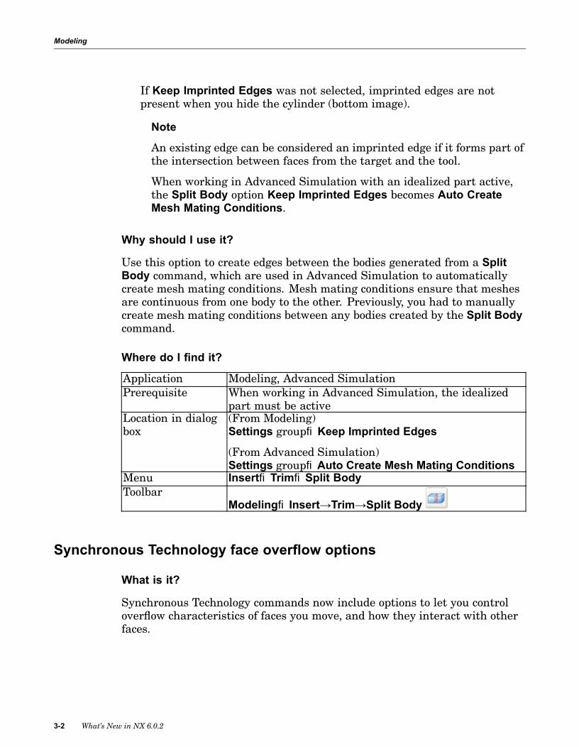
If Keep Imprinted Edges was not selected, imprinted edges are notpresent when you hide the cylinder (bottom image).

Note

An existing edge can be considered an imprinted edge if it forms part ofthe intersection between faces from the target and the tool.

When working in Advanced Simulation with an idealized part active,the Split Body option Keep Imprinted Edges becomes Auto CreateMesh Mating Conditions.


Use this option to create edges between the bodies generated from a SplitBody command, which are used in Advanced Simulation to automaticallycreate mesh mating conditions. Mesh mating conditions ensure that meshesare continuous from one body to the other. Previously, you had to manuallycreate mesh mating conditions between any bodies created by the Split Bodycommand.

Where do I find it?

Application Modeling, Advanced SimulationPrerequisite When working in Advanced Simulation, the idealized

part must be activeLocation in dialogbox

(From Modeling)Settings group®Keep Imprinted Edges

(From Advanced Simulation)Settings group®Auto Create Mesh Mating Conditions

Menu Insert®Trim®Split BodyToolbar

Modeling®Insert→Trim→Split Body

Synchronous Technology face overflow options

What is it?

Synchronous Technology commands now include options to let you controloverflow characteristics of faces you move, and how they interact with otherfaces.


Modeling

Extend ChangeFace

Dragging the selected face extends it into or moves it pastother faces it encounters.

Selected face

Extend IncidentFace

Dragging the selected face extends it until it meets astationary, incident face. The selected face then ceases toextend, and the stationary face extends instead.

Incident faces

Extend Cap Face Dragging the selected face past an overhanging edgecauses it to overflow and cap itself (the bottom of thechange face in the figure below).


Modeling

Automatic Dragging the selected face causes either the selectedface or an incident face to extend, depending on whichoutcome would result in the least amount of change tovolume and area.


Use these options to control how a change face overflows stationary orincident faces in solid bodies.

Where do I find it?

Application ModelingLocation in dialogbox

Settings group®Overflow Behavior

Menu Insert®Synchronous Modeling®Move Face/ OffsetRegion/ Replace Face/ Make Coplanar/ Make Coaxial/Make Tangent/ Make Perpendicular/ Make Parallel/Linear Dimension/ Angular Dimension/ RadialDimension

Toolbar Synchronous Modeling

Synchronize Views in Replace Feature

What is it?

Synchronize Views is a new option in the Replace Feature command. Thisoptions synchronizes the current and replacement views when you replace afeature. When you rotate, pan, zoom, or apply rendering styles in one view,NX automatically synchronizes the other view to match these operations.


Modeling

Before replacement After replacement

The following animation demonstrates the automatic synchronization of thecurrent view and the replacement view as you replace the hole feature fromone block to the other.

A split screen appears only when:

1. The selected feature to replace has downstream dependents that appearin the List subgroup under the Mapping group.

2. You select any of the displayed dependents as reference from the Listsubgroup.


Modeling


Use this option to locate objects that you want to replace in one view, whileNX automatically tracks your movements toward the same location in theother view. This saves mouse clicks and reduces the need to repeat the sameview manipulations in the other view.

Where do I find it?

Application ModelingPrerequisite You must select a dependant reference of the selected

feature to replace from the List subgroup in the Mappinggroup.

ToolbarEdit Feature®Replace Feature

Menu Edit®Feature®ReplaceLocation in dialogbox

Settings group®Synchronize Views


Chapter

4 Assemblies

Motion envelopes

What is it?

The Motion Envelope function, which is used to create a volume of motionfor components, has the following enhancements:

• New underlying swept volume generator technology that createsbetter motion envelopes more quickly. This technology is also used byTeamcenter Visualization.

• A simpler user interface for defining an envelope accuracy in the Customquality option. Beginning in NX 6.0.2, when you set Quality to Custom,the quality is defined using a single Envelope Tolerance option, replacingthe multiple, less intuitive options of the previous releases.

Use the Envelope Tolerance option to specify the maximum distancebetween the theoretical and actual motion envelopes. Smaller tolerancesproduce more accurate envelopes, but require more time and memory.

Motion envelope of a vise handle ball

The new swept volume generator has the following requirements:

• A 3D graphics adapter with 24-bit depth buffer or better (Required)

• A system with at least 2GB of RAM (Recommended)


Assemblies

Note

The generation of high quality envelopes for complex parts may use alarge amount of memory for some motion definitions. If you find thatyou are unable to generate motion envelopes due to virtual memoryor RAM limits on your computer, you could try using a lower qualitysetting for the motion envelope, or restart NX so the largest amount ofmemory is available. Alternatively, try to create the envelope using acomputer with more memory.

The new swept volume generator can make use of multiple CPUs or cores.However, the benefit of having more than two cores decreases rapidly, becausemost of the work is done by the graphics adapter.


Advantages of creating motion envelopes in NX 6.0.2, compared to earlierreleases, include the following:

• Accuracy — the motion envelope is tighter at all quality levels: low,medium, high, and custom.

• Performance — the generation of a motion envelope of any quality ismuch faster.

• Usability — Custom envelope tolerances are much easier to understand.

Where do I find it?

Application AssembliesPrerequisite You must be in the assembly sequencing environment,

and your assembly sequence must include one or moremotion steps.

Toolbar Assembly Sequencing and Motion®Motion Envelope

Menu Tools®Motion Envelope

Variable positioning and Fix constraints

What is it?

When variable positioning is used on a component that includes Fix assemblyconstraints, the inherited version of each Fix constraint is now a Bondconstraint.


Assemblies

When you open an assembly that includes Fix constraints inherited byvariable positioning applied in an earlier release of NX, the higher-levelinherited Fix constraints are converted to Bond constraints.


Inheriting a Fix constraint to a higher-level Fix constraint can causeundesirable behavior such as preventing movement of the fixed component’sparents in higher-level assemblies. Converting the Fix constraint to aBond constraint at higher levels preserves some of the behavior of the Fixconstraint on the component. The higher-level Bond constraint connects thefixed component to its parent, which lets the component and parent move as apair, but restricts independent movement of the component.

Where do I find it?

Application AssembliesPrerequisite You can only use variable positioning on a component

that has at least two assembly levels above it. Thismeans that the component must have at least one parentthat has a parent of its own.

Note

The lowest level can be a subassembly if you donot select any of its components.

Shortcut menu Assembly Navigator®right-click a componentnode®Override Position


Chapter

5 Drafting

GB Weld Symbols

What is it?

GB is a new standard for Weld Symbols that includes additional settings andsymbol types required by the GB (China) Standard. The additional symbolavailable for GB Weld Symbols is:

• Trilateral Weld

Where do I find it?

Application DraftingPrerequisite Drawing views with standard orientationsMenu File®Utilities®Customer

Defaults®Drafting®Extras®Annotation®Weld®UseGB Weld Standard

Detail View color, font, and width

What is it?

You can control the color, font and width settings for:

• Detail view boundary lines.

• Detail view labels on a parent boundary line.

The options to do this are available from Customer Defaults, Preferences,and Style.


Drafting

Detail View with dotted, orange colored boundary and black text


You can use these settings to control how detail views and labels appear onparent boundary lines.

Where do I find it?

Drafting Standard Customer Default

Application DraftingPrerequisite Drawing views with standard orientationsMenu Preferences or Style®View®Detail tab.

Location in dialogbox

File®Utilities®CustomerDefaults®Drafting®General®Standard tab®DraftingStandards®View®Detail View tab

Shortcut menu Graphics window ®right-click®Style (on a viewboundary)

Narrow Arc Length and Angular Dimensions

What is it?

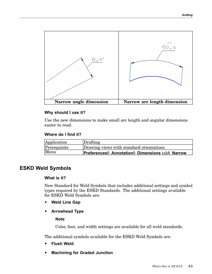
The Narrow formatting option shows the value of a small dimension outsidethe dimension lines. A label shows to which dimension the value applies.Included in the Narrow angle and Narrow arc length dimension options is theability to change the leader attachment location for all Narrow dimensions(Linear, Arc Length, and Angular).


Drafting

Narrow angle dimension Narrow arc length dimension


Use the new dimensions to make small arc length and angular dimensionseasier to read.

Where do I find it?

Application DraftingPrerequisite Drawing views with standard orientationsMenu Preferences®Annotation®Dimensions tab®Narrow

ESKD Weld Symbols

What is it?

New Standard for Weld Symbols that includes additional settings and symboltypes required by the ESKD Standards. The additional settings availablefor ESKD Weld Symbols are:

• Weld Line Gap

• Arrowhead Type

Note

Color, font, and width settings are available for all weld standards.

The additional symbols available for the ESKD Weld Symbols are:

• Flush Weld

• Machining for Graded Junction


Drafting

• Intermittent Weld

• Weld Along Closed Contour

• Weld Along Open Contour

New symbols to meet the ESKD Standards have also been added for:

• Staggered Weld

• Field Weld

Where do I find it?

Application DraftingPrerequisite Drawing views with standard orientationsMenu File®Customer

Defaults®Drafting®General®Standard®CustomizeStandard®Weld

Section Line Style Enhancements

What is it?

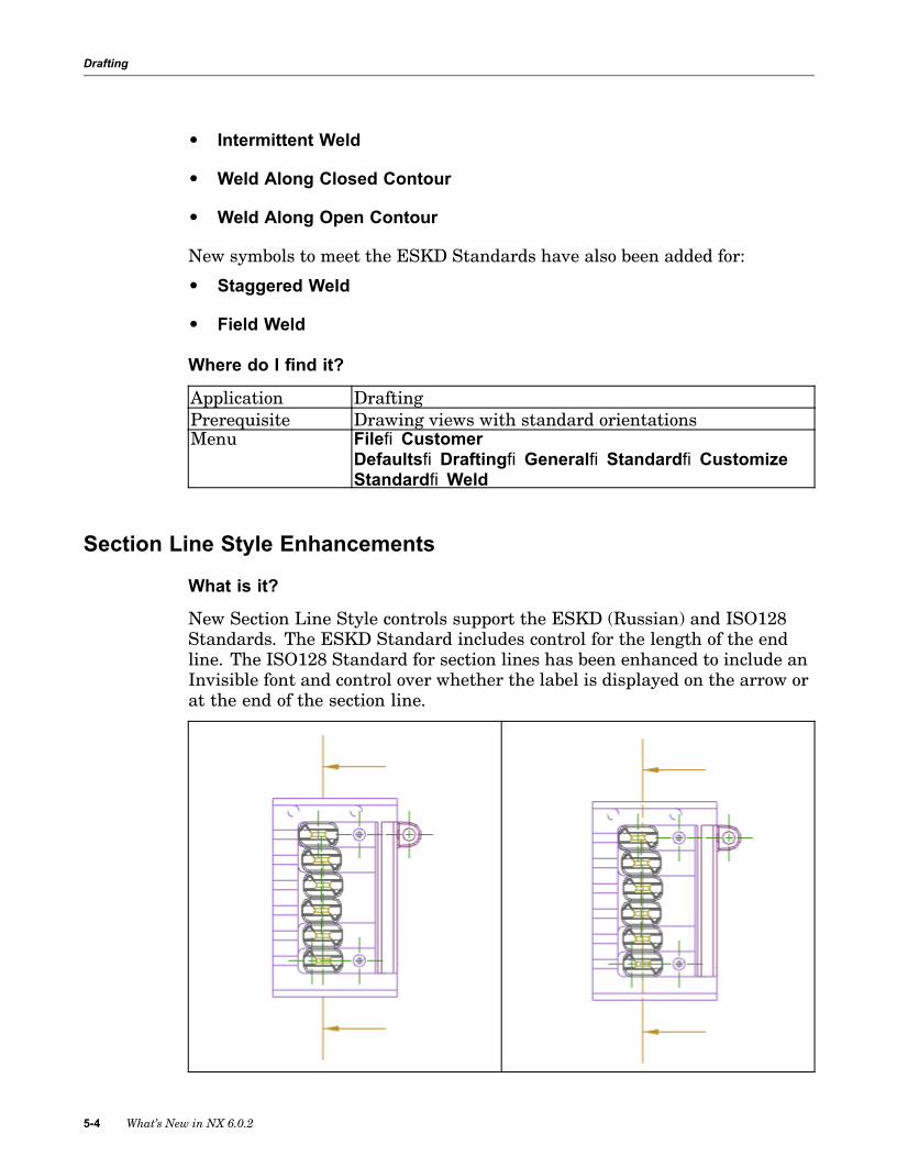
New Section Line Style controls support the ESKD (Russian) and ISO128Standards. The ESKD Standard includes control for the length of the endline. The ISO128 Standard for section lines has been enhanced to include anInvisible font and control over whether the label is displayed on the arrow orat the end of the section line.


Drafting

ESKD Section Line ISO128 Section Line

The Invisible font is only available for section line types that support thickends and breaks. If you set the line font to invisible, the ends and breaksdisplay, but not the lines between them.


Use the new Section Line Style controls when support for ESKD or ISO128is required.

Where do I find it?

Preferences Section Line

Application DraftingPrerequisite Drawing views with standard orientationsMenu Preferences®Section LineShortcut menu Graphics window®right-click®Style (on a section line)

Annotation Style Section Line

Application DraftingPrerequisite Drawing views with standard orientationsMenu Edit®Annotation Style and select Section Line.Shortcut menu Graphics window®right-click®Style (on a section line)


Chapter

6 PMI

PMI objects in JT files

What is it?

When you open a JT file in NX, the following objects now appear if they weresaved in the JT file:

• Assembly-level PMI and model views from Teamcenter JT files. Thisincludes the display of component PMI in assembly model views.

• PMI locator symbols that were created in I-deas or NX.


JT files that are opened in NX now more closely match their source files.

Where do I find it?

ToolbarStandard®Open ®select a JT file

Menu File®Open®select a JT file


Chapter

7 Digital Simulation

Supported solver versions

What is it?

In this release, Advanced Simulation supports the following solver versions:

• NX Nastran 6.1 and earlier versions

• MSC Nastran 2008r1 and earlier versions

• Abaqus 6.8-1 and earlier versions

• ANSYS 11 Service Pack 1 and earlier versions

• LS-DYNA 971 and earlier versions

NX Nastran 6.1 enhancements

What is it?

NX Nastran 6.1, which is included with Advanced Simulation in NX 6.0.2,includes many enhancements. The major enhancements are summarizedin the following list.

For detailed information, see the NX Nastran 6.1 Release Guide in the NX6.0.2 Maintenance Release online Help.

Dynamics

• For RecurDyn and ADAMS multi-body solutions, input commands forexport and results recovery have been consolidated.

• The Rotor Dynamics capability now supports Modal Transient ResponseAnalysis (SOL 112). Also, systems with multiple rotors rotating atdifferent speeds can now be analyzed.

• Grid point force output can now be requested in frequency-based analyses,as well as SORT2.


Digital Simulation

• The RMAXMIN case control command has been enhanced.

• The PBUSH, PBUSHT, and PSHELL bulk entries have been improvedwith the addition of new damping inputs.

• A nonstructural mass (NSM) can now be defined on the PSHELL, PCOMP,PBAR, PBARL, PBEAM, PBEAML, PBCOMP, PROD, CONROD, PBEND,PSHEAR, PTUBE, PCONEAX, and PRAC2D property entries.

• When you request element force output with the FORCE case controlcommand, real element forces will also be stored for the CDAMPi andCVISC element types.

External Superelements

• The superelement workflow introduced in version 6.0 has been enhancedto be more efficient. External superelement results are recovered duringthe system analysis, and results for each superelement can optionally becombined in the .f06 output and into a single datablock for post processingthe assembly.

Contact and Glue enhancements

• Several enhancements have been made to Contact for Solutions 101,103, 111, and 112, including the ability to stop a non-Converged ContactSolution.

• Several enhancements have been made to Surface-to-Surface Glue. TheREFINE parameter is supported by both shell and solid element regions.Also, a weld-like glue algorithm now eliminates the artificial rotationalenergy introduced when you define glue conditions on non-coincidentshell or solid faces.

Element additions

• The pyramid element (CPYRAM) is now supported in solutions 101, 103,105, 107-112, 114, 115, 116, 118, 144, 145, 146, 153, 159, and 187. Also,results for the new solid pyramid element have been added to selectedsolid element test cases in the NX Nastran Verification Manual.

• The torsional mass moment of inertia can now be optionally includedon the CROD and CBAR mass matrices. Also, the default lumped masscalculation for the CROD and CBAR has been updated to use the samemethod as the CBEAM.

• For the axisymmetric elements CTRAX3, CTRAX6, CQUADX4, andCQUADX8, design sensitivity and optimization (solution 200) has beenadded as a supported solution.


Digital Simulation

• The PBUSH bulk entry now supports a value in each degree-of-freedom(GE1, GE2, GE3, GE4, GE5, GE6). Also, the PBUSHT bulk entry nowsupports tabulated frequency-dependent structural damping for eachdegree-of-freedom (TGEID1, TGEID2, TGEID3, TGEID4, TGEID5, andTGEID6).

• The PSHELL bulk entry now supports the structural damping coefficient(GE) included on the associated materials MID1–MID4.

• New nonstructural mass bulk entries have been added that allow moreflexibility when you need to modify the mass of a few or many elements.

DMP enhancements

• A new multilevel RDMODES DMP option has been added to enhanceperformance.

• A new grid compression option has been added to the GPARTN module.

Numerical enhancements

• The matrix multiply-add modules MPYAD and SMPYAD have beenimproved.

Acceleration loads

• Two new bulk entries have been added to expand the gravity/accelerationload options.

General capabilities

Command Finder for CAE

What is it?

Command Finder is a search tool that helps you find a specific NX commandassociated with the words or phrases you enter.

For this release, Command Finder now supports all commands in theAdvanced Simulation and Design Simulation applications.

From the list of commands, you can:

• Display the command location.

• Launch the command, if it is available in the current application.

• Display the Help information for the command.


Digital Simulation

For boundary conditions, you can also search on the solver input name, suchas PLOAD4 for an NX Nastran Pressure load.

Use customer defaults for the Command Finder to:

• Save a cached file of all menu and toolbar commands.

• Identify a location for a custom list of words and phrases associated withspecific commands.

• Search for a command using a secondary language.

Where do I find it?

Command Finder customer defaults

Menu File→Utilities→Customer Defaults→Gateway→UserInterface


Command Finder tab

Command Finder command

Application Advanced Simulation or Design SimulationMenu Help®Command Finder


Digital Simulation

ToolbarStandard toolbar®Command Finder

Geometry idealization

Midsurface improvements

What is it?

This release includes several improvements to the Midsurface command.

Improved usability for Midsurface dialog box

This release includes enhancements to the Midsurface dialog box to improveits usability.

• In previous releases, the Midsurface dialog box closed automatically afteryou generated a single midsurface. Now, the dialog box remains activeuntil you explicitly close it.

• If you select the Automatic Progression check box, you can now createmidsurfaces on multiple bodies without exiting the Midsurface dialog box.If you select Automatic Progression, when you generate a midsurfaceon a body, the software automatically displays only the new sheet bodyin the graphics window. In a model that contains multiple solid bodies,this helps you visually distinguish between the bodies that have definedmidsurfaces and those that do not. You can then more easily select thenext solid body on which to create the midsurface.

Automatic pairing and performance improvements

When you use the Face Pair method with the Auto Create option,improvements have been made to the algorithm the software uses toautomatically pair faces. On certain types of parts, the software now producesmore accurate face pairs as well as more accurately trimmed surfaces.Additionally, on certain types of parts, there are significant performanceimprovements in the time it takes the software to generate the midsurface.These improvements are seen when you create a midsurface with theAdvanced Creation and Trimming check box cleared.

Where do I find it?

Application Advanced SimulationPrerequisite An active idealized partToolbar

Advanced Simulation®Midsurface


Digital Simulation

Materials

Support for external material libraries

What is it?

Several enhancements have been added to the NX Materials capability. Youcan now:

• Maintain two separate custom material libraries. Custom libraries arestored as XML files in the MatML schema version 3.1.5. For schemadetails, see http://www.matml.org.

• Restrict display and editing access to the two custom librariesindependently.

• Create, edit, or delete your custom library materials directly within NX.

• Export local materials (materials created in NX and saved with a model)to a custom material library.

• Import material libraries generated from external sources that adhere tothe MatML 3.1.5 schema.

The new Material Library Manager dialog box lets you export materials to acustom library and edit or delete the custom materials.


http://www.matml.org

Digital Simulation

Use customer defaults for the Materials function to define the default folderlocation of the material libraries, as well as configure access to each library.


• Custom material definitions can be used in multiple NX models, and thesecustom materials are preserved when you upgrade to a newer version ofNX.

• Editing your materials in the NX user interface is much easier thanediting the .dat file used in previous versions.

Where do I find it?

Materials customer defaults

Menu File®Utilities®Customer DefaultsLocation in dialogbox

Gateway®Extras®Materials tab

Material Library Manager command

Application AllMenu Tools®Material Library Manager


Digital Simulation

SimulationNavigator

Advanced Simulation toolbar®Material Library

Manager

Meshing

Persistent display of 2D element thickness

What is it?

The new Display 2D Element Thickness command lets you view a graphicalrepresentation of the thickness of your 2D elements.

The graphical thickness remains displayed for the model until you turn it off.

The thickness display is supported for all methods of defining 2D elementthickness:

• Derived from the thickness of a midsurface.

• Defined in the physical properties for the mesh.

• Defined in Element Associated Data.

• Defined as a field.


This command lets you verify the thickness values the software applies whenyou either export or solve your model.


Digital Simulation

Where do I find it?

Application Advanced Simulation, Design SimulationPrerequisite An active FEM file that contains 2D elements with

thickness.SimulationNavigator

In the FEM, right-click the 2D mesh collector or 2D meshand choose Edit Display. Select Display 2D ElementThickness.

In the Simulation file, right-click the 2D mesh collectoror 2D mesh and choose Create Display Override orEdit Temporary Display. Select Display 2D ElementThickness.

Creating fields from element thickness displays

What is it?

You can now use the Thickness Information command in the SimulationNavigator to create a spatial field of thickness values of the 2D elements inyour model. In the Thickness Information dialog box, when you select thenew Create Field in the Create Thickness Field group, the software generatesa new field and places it in the Fields node in the Simulation Navigator.

Creating a thickness field can be helpful if you are working with a modelin which the thickness of mesh is being derived from a midsurface. On alarge model, the derivation of thickness data from a midsurface can be timeand resource intensive since the software must recalculate the thicknesseach time you use Thickness Information to generate a display. If you areiterating through the meshing process with different element sizes, you canuse the new Create Field option to generate a field from that midsurface datathe first time you use Thickness Information to generate a display. You canthen edit the Mesh Associated Data for that mesh and change the specifiedThickness Source from Midsurface to Field. You can then select the newlycreated thickness field.

The ability to create a thickness field from a display of your 2D elementthicknesses also allows you to edit or copy that thickness data. You can thenreuse that modified data either in the same model or another model. Forexample, you can import a Nastran bulk data file that contains a coarse meshin which the element thickness values are defined directly on the CQUAD4elements. You can then use the new Create Thickness Field capability togenerate a thickness field from that data. If you then remesh the model witha finer mesh, you can use that thickness field to map the original thicknessvalues to the new mesh


Digital Simulation

Where do I find it?

Application Advanced Simulation

Prerequisite An active FEM file that contains a 2D meshSimulationNavigator

Right-click the appropriate 2D mesh collector or 2Dmesh node and select Thickness Information

Enhancements for Nastran users

PBUSH structural damping enhancements

What is it?

For NX Nastran models, new options have been added to the Damping tab inthe PBUSH physical property table dialog box. Use these options to definestructural damping for each degree-of-freedom for CBUSH elements. Theability to define direction-dependent structural damping for the PBUSHbulk data entry was introduced in the NX Nastran 6.1 release. Previously,you could only define a single, structural damping value (GE1) that appliedto all 6 degrees-of-freedom.

The new options in the PBUSH dialog box let you specify separate structuraldamping values for the X, Y, and Z translations and rotations. The values youspecify correspond to the GE1, GE2, GE3, GE4, GE5, and GE6 fields in thePBUSH bulk data entry. If you define a value for any of the Structural optionson the Damping tab, you should define a value for all degrees-of-freedom thatare critical to the result, because a blank field defaults to a value of zero.

This release also includes support for the new BSHDAMP parameter, whichlets you optionally ignore any of the GE2-GE6 fields and only use the GE1field. By default, the software considers the new GE2-GE6 fields. The newBSHDAMP list in the Solution Parameters dialog box (available from theModeling Objects Manager dialog box) lets you control the setting for thisparameter:

• If you select SAME (PARAM, BSHDAMP=SAME), the software ignores theGE2-GE6 fields and only considers the single, structural damping valuedefined in the GE1 field. This corresponds to the behavior available inprevious releases.

• If you select DIFF (PARAM, BSHDAMP=DIFF), the software considers theGE2-GE6 fields.

For more information, see the NX Nastran 6.1 Release Guide and PBUSH inthe NX Nastran Quick Reference Guide.


Digital Simulation

Where do I find it?

Application Advanced SimulationPrerequisite A FEM file active with NX Nastran as the specified solverToolbar

Advanced Simulation®Physical PropertiesMenu Insert®Physical Properties

PSHELL structural damping enhancements

What is it?

Beginning in the NX Nastran 6.1 release, the PSHELL bulk data entry nowsupports including the structural damping coefficient (GE) on the associatedmaterials:

• MID1 = membrane material

• MID2 = bending material

• MID3 = transverse shear

• MID4 = membrane-bending coupling

Previously, NX Nastran used the structural damping coefficient defined onthe MID1 material for all materials associated with the PSHELL entry.

This release includes support for the new NX Nastran SHLDAMP parameter,which lets you turn this capability on and off for a given analysis. The newSHLDAMP list in the Solution Parameters dialog box (available from theModeling Objects Manager dialog box) lets you set this parameter:

• If you select SAME (PARAM, SHLDAMP=SAME), which is the default, thesoftware uses the structural damping coefficient (GE) defined on the MID1material for the PSHELL entry for all MIDi materials for that PSHELL..

• If you select DIFF (PARAM, SHLDAMP=DIFF), the software uses the structuraldamping coefficient (GE) defined on each MIDi for the PSHELL entry,provided that the GE field is defined for any of the MID2, MID3, and/orMID4 materials in at least one PSHELL entry in the input file. Withthis option, if any structural damping coefficient (GE) value is blank, NXNastran treats it as having a value of zero.

For more information, see the PSHELL Structural Damping in the NXNastran 6.1 Release Guide and SHLDAMP in the NX Nastran QuickReference Guide.


Digital Simulation

Where do I find it?

Application Advanced SimulationPrerequisite An active FEM or Simulation file with NX Nastran as

the specified solver.Toolbar

Advanced Simulation®Modeling ObjectsMenu Insert®Modeling Objects

End releases for CBEAM elements

What is it?

You can now define end releases (also known as pin flags) at either endof a Nastran CBEAM element in the Element Associated Data dialog box.Previously, you could define pin flags only at the Mesh Associated Data level.

In a beam, end releases remove connections between a node and selecteddegrees of freedom. The degrees of freedom are defined in the elementcoordinate system. For the following example, a force is defined on thehorizontal span. Because end releases are defined at the ends of the bracingbeams, the solver does not transfer the moment load from the horizontalbeam to the bracing beams. The moments are transferred across the otherelements in the horizontal span.

Bridge model. (1) and (2) represent the end releases; force appliedto horizontal span

Bridge model; deflected shape with end releases


Digital Simulation

Bridge model; deflected shape without end releases

In the Element Associated Data dialog box, under the End Releases group(for End A and or End B of the beam element), you can set DOF1–6 to On todisconnect the following forces:

• DOF1 — axial force in Plane 1

• DOF2 — shearing force in Plane 1

• DOF3 — shearing force in Plane 2

• DOF4 — axial torque in Plane 2

• DOF5 — moment in Plane 2

• DOF6 — moment in Plane 1

Note

Plane 1 is the XY plane formed by the X and Y axes in the elementcoordinate system. Plane 2 is the XZ plane formed by the X and Z axes.

In the previous example, DOF6 is set to On at the ends of the bracing beams(the model is shown in the XY plane).

For more information, see Element associated data overview in the AdvancedSimulation help.


You can define a release at the ends of beam elements to model hinged orpinned connections.

Where do I find it?

Application Advanced SimulationPrerequisite An active FEM file that contains CBEAM elements.Toolbar

Element Operations®Element Associated DataMenu Edit®Element®Modify Associated Data


../../../ugdoc/html_files/advanced/index.html?goto=advanced/element_assoc_data_ov.html&vars=-aux

Digital Simulation

Optional torsional mass moments of inertia for CROD and CBAR elements

What is it?

Advanced Simulation now supports the new TORSIN parameter that wasintroduced in the NX Nastran 6.1 release. The TORSIN parameter lets youoptionally include the torsional mass moment of inertia in the CROD andCBAR element mass matrices. By default, NX Nastran does not calculatetorsional mass for CROD or CBAR elements, though it does for CBEAMelements. This can lead to differences when you compare results betweenequivalent models.

The new TORSIN box in the Solution Parameters dialog box (available fromthe Modeling Objects Manager dialog box) lets you control the setting forthis parameter:

• If you enter 0, the software does not include the torsional mass moment ofinertia for CROD and CBAR elements (the default).

• If you enter 1, the software includes the torsional mass moment of inertiafor CROD and CBAR elements.

• If you enter 2, the software includes the torsional mass moment of inertiafor CBAR elements only.

• If you enter 3, the software includes the torsional mass moment of inertiafor CROD elements only.

For more information, see the NX Nastran 6.1 Release Guide and PBUSH inthe NX Nastran Quick Reference Guide.

CBAR axial torsional mass moment of inertia calculation

NX Nastran calculates the CBAR axial torsional mass moment of inertiasimilarly to the CBEAM element using the equation:

Ixx = rL(I1+I2)

where:

Ixx = torsional mass moment of inertia

r = density

L = the length of the element

I1 and I2 = area moments of inertia

CROD axial torsional mass moment of inertia calculation

NX Nastran calculates the CROD axial torsional mass moment of inertiausing the equation:


Digital Simulation

Ixx = rLIx

where Ix = J = torsional constant.

Where do I find it?


the specified solverToolbar


New weld-like glue algorithm

What is it?

Advanced Simulation now includes support for the new weld-likeglue algorithm that was introduced in the NX Nastran 6.1 release. Asurface-to-surface glue condition on non-coincident shell or solid faces canintroduce artificial rotational energy into the solution. Generally, the problemoccurs because the spring-like glue elements do not transfer moments at theglue interface when glued faces are non-coincident and/or when loads are notnormal to the glued faces. This is particularly noticeable in a normal modesolution when modes are found that contain an artificial rotational energydue to the glue condition. The new NX Nastran algorithm eliminates thisartificial rotational energy. In NX Nastran 6.1, two new fields were addedto the BGPARM bulk data entry to allow you to activate and work with thisnew algorithm.

In Advanced Simulation, the Glue Parameters modeling object has beenupdated to support the new fields on the BGPARM entry. In the GlueParameters dialog box:

• The new Alternate Glue Formulation option corresponds to the newGLUETYPE field on the BGPARM bulk data entry. Use this option tocontrol the glue algorithm that NX Nastran uses.

– SelectWeld-Like Connection to use the new weld-like glue algorithm.

– Select Normal and Tangential Springs to use the original, spring-likeglue algorithm

• The new Unitless Scale Factor for the Stiffness option corresponds to thenew PENGLUE field on the BGPARM bulk data entry. Use this option tospecify the penalty factor for the weld-like glue algorithm.


Digital Simulation

Note

With the Normal and Tangential Springs option, use the PenaltyNormal Direction and Penalty Tangential Direction options tospecify the penalty factor.

In most cases, the new weld-like glue algorithm represents the connectionstiffness more accurately than the spring-like glue algorithm because ittransfers moments at the glue interface.

For more information, see New Weld-Like Glue Method in the NX Nastran 6.1Release Guide and BGPARM in the NX Nastran Quick Reference Guide.

Where do I find it?


the specified solver.Toolbar


Shell thickness output for advanced nonlinear analyses

What is it?

Use the options on the new Shell Thickness page in the Structural OutputRequests dialog box to request the output of shell element thickness valuesfor SOL 601 and 701 (ADVNL 601 and 701) analyses. NX Nastran onlyoutputs shell thickness results for large strain analyses (analyses in whichyou include the parameter PARAM,LGSTRN,1). In Advanced Simulation, toset this parameter, select the new Large Strains check box on the Parameterspage of the Create Solution or Edit Solution dialog box.

When you create a Shell Thickness type of output request, the softwarecreates a SHELLTHK Case Control entry in the Case Control section of yourNastran input file. For more information on shell thickness results, seeSHELLTHK in the NX Nastran Quick Reference Guide.

A new Customer Defaults option lets you control whether the EnableSHELLTHK Request option on the Nonlinear Stress page is selected bydefault. To access this option:

1. From the File menu, choose Utilities®Customer Defaults.

2. In the Customer Defaults dialog box, choose Simulation®Extras.

3. On the Nastran page, either select or clear the Shell Thickness option.


Digital Simulation

Where do I find it?


the specified solver and ADVNL 601,106, ADVNL 601,129, or ADVNL 701 as the solution type

SimulationNavigator

Either right-click a Simulation and select CreateSolution, or right-click the appropriate solution selectEdit Solution

Bolt pre-loads now supported for Response Simulation analyses

What is it?

You can use the Bolt Pre-Load command to to apply a pre-load to a boltmodeled with CBAR or CBEAM type beam elements in a Response Simulation(SEMODES 103 - Response Simulation) analysis. Bolt pre-loads are onlysupported in the first two subcases in a Response Simulation:

• Static Offset

• Stress Stiffening

Where do I find it?

Application Advanced SimulationPrerequisite An active Simulation with NX Nastran as the specified

solver and SEMODES 103 - Response Simulation as thesolution type and with either Subcase - Static Offsetor Subcase - Stress Stiffening active in the SimulationNavigator

ToolbarAdvanced Simulation®Bolt Pre-Load

Import and export support

Nastran import and export support enhancements

What is it?

This release includes enhancements to the import and export support forNastran Bulk Data entries and Case Control commands.


Digital Simulation

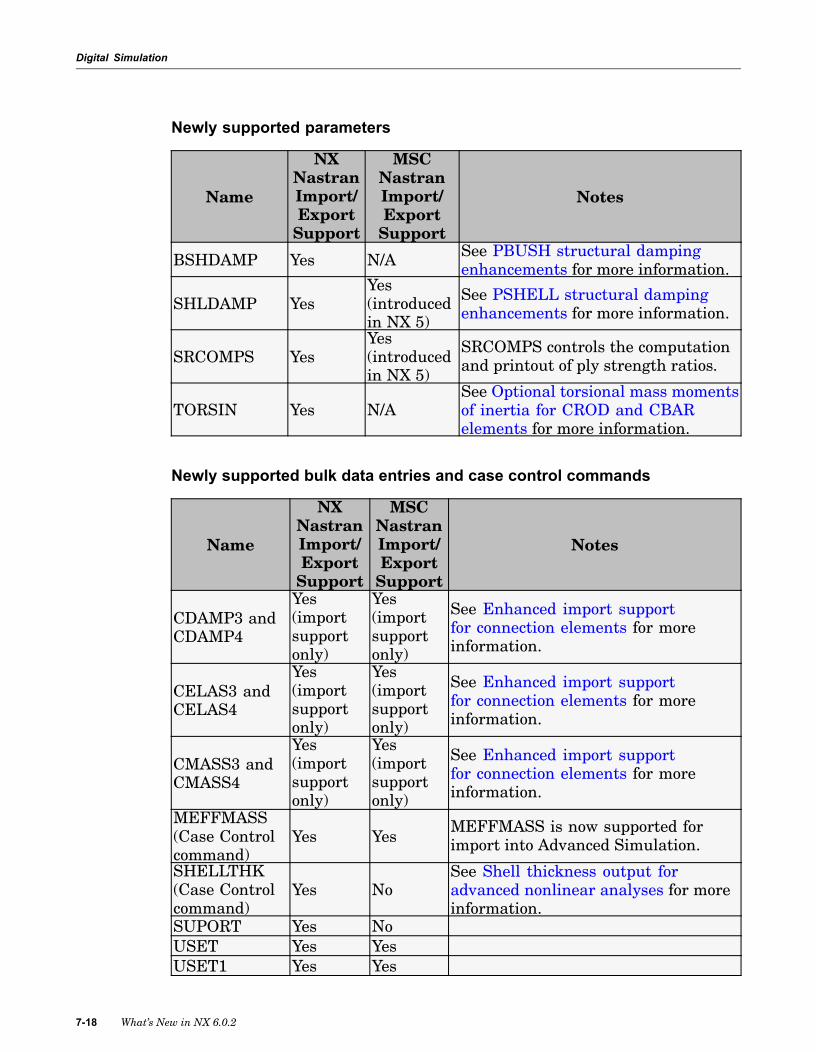
Newly supported parameters

Name

NXNastranImport/ExportSupport

MSCNastranImport/ExportSupport

Notes

BSHDAMP Yes N/A See PBUSH structural dampingenhancements for more information.

SHLDAMP YesYes(introducedin NX 5)

See PSHELL structural dampingenhancements for more information.

SRCOMPS YesYes(introducedin NX 5)

SRCOMPS controls the computationand printout of ply strength ratios.

TORSIN Yes N/ASee Optional torsional mass momentsof inertia for CROD and CBARelements for more information.

Newly supported bulk data entries and case control commands

Name



Notes

CDAMP3 andCDAMP4

Yes(importsupportonly)


See Enhanced import supportfor connection elements for moreinformation.

CELAS3 andCELAS4




CMASS3 andCMASS4




MEFFMASS(Case Controlcommand)

Yes YesMEFFMASS is now supported forimport into Advanced Simulation.

SHELLTHK(Case Controlcommand)

Yes NoSee Shell thickness output foradvanced nonlinear analyses for moreinformation.

SUPORT Yes NoUSET Yes YesUSET1 Yes Yes


Digital Simulation

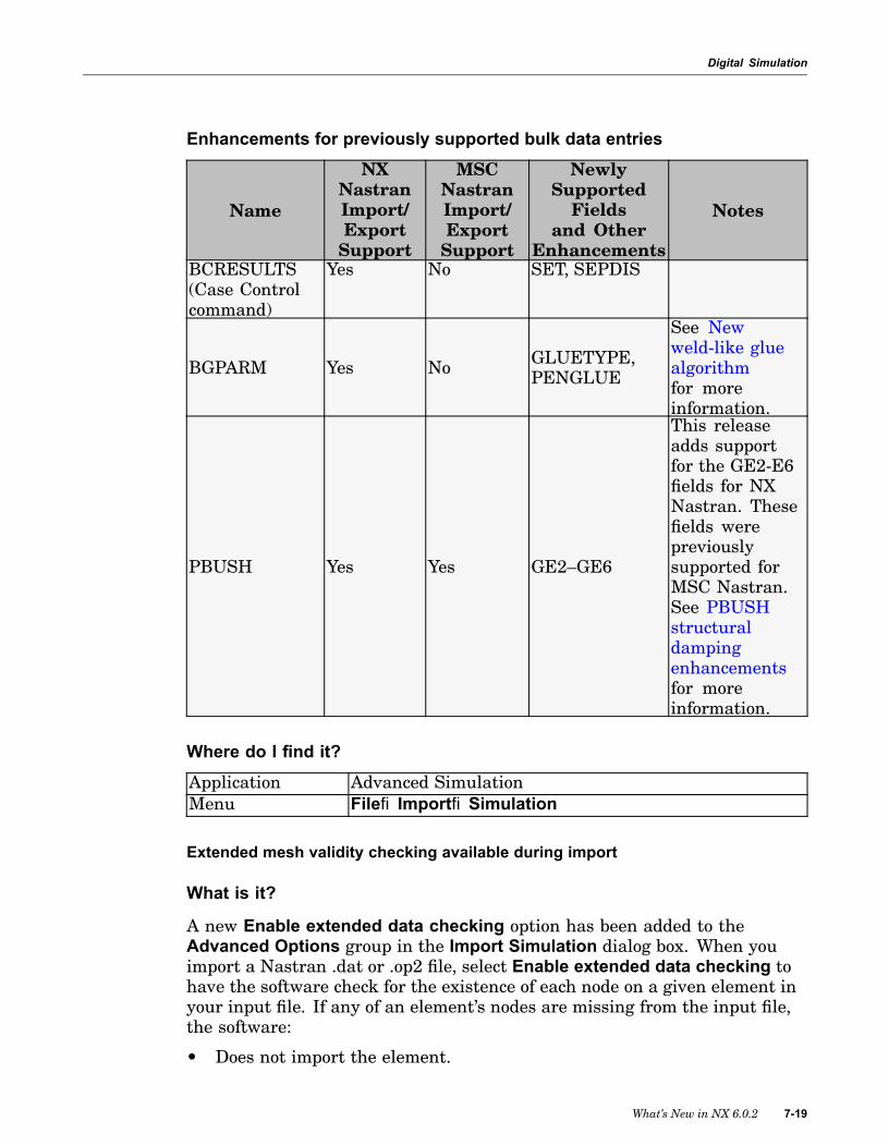
Enhancements for previously supported bulk data entries

Name



NewlySupportedFields

and OtherEnhancements

Notes

BCRESULTS(Case Controlcommand)

Yes No SET, SEPDIS

BGPARM Yes No GLUETYPE,PENGLUE

See Newweld-like gluealgorithmfor moreinformation.

PBUSH Yes Yes GE2–GE6

This releaseadds supportfor the GE2-E6fields for NXNastran. Thesefields werepreviouslysupported forMSC Nastran.See PBUSHstructuraldampingenhancementsfor moreinformation.

Where do I find it?

Application Advanced SimulationMenu File®Import®Simulation

Extended mesh validity checking available during import

What is it?

A new Enable extended data checking option has been added to theAdvanced Options group in the Import Simulation dialog box. When youimport a Nastran .dat or .op2 file, select Enable extended data checking tohave the software check for the existence of each node on a given element inyour input file. If any of an element’s nodes are missing from the input file,the software:

• Does not import the element.


Digital Simulation

• Issues an error message when it first encounters an element with missingnodes.

• Clearly lists that the element failed to import in the Analysis of Importreport as shown below.

In previous releases, if you imported a Nastran input file in which even asingle node was missing, the import operation appeared to proceed normally,though the software did not import the mesh. The software did not issue anyerror messages in the import summary, and it created a mesh node in theSimulation Navigator. The only indication of a problem was the absence of adisplayed model in the graphics window.

Where do I find it?


Import support for Nastran system cells

What is it?

When you import a Nastran input file, Advanced Simulation now imports anysystem cell settings defined in that file. System cells are Executive Systemoperational parameters specified by the NASTRAN statement. In previousreleases, Advanced Simulation did not import any system cells that you haddefined in an input file.

Where do I find it?



Digital Simulation

Enhanced import support for connection elements

What is it?

In this release you can now import the following additional types of NastranCDAMP, CELEAS, and CMASS connection elements from Nastran .dat and.op2 files into Advanced Simulation:

• CDAMP3 and CDAMP4

• CELAS3 and CELAS4

• CMASS3 and CMASS4

Currently, these types of elements are not directly supported in AdvancedSimulation. During the import process, the software converts these elementsto the most closely related, supported element types, as shown in thefollowing table:

Nastran Element Type Type Converted to During ImportCDAMP3 CDAMP1CDAMP4 CDAMP2CELAS3 CELAS1CELAS4 CELAS2CMASS3 CMASS1CMASS4 CMASS2

For more information on these types of elements, see the NX Nastran QuickReference Guide and the NX Nastran Element Library Reference Manual.

Where do I find it?


Import changes for SPOINT entries

What is it?

Nastran uses the SPOINT bulk data entry to define scalar points. Scalarpoints have a single degree-of-freedom. In Nastran:

• You can explicitly define a scalar point by creating an SPOINT entry inthe bulk data section of your input file.

• You can implicitly define a scalar point by referencing the ID of a scalarpoint on a CDAMP1/2/3/4, CMASS1/2/3/4, or CELAS1/2/3/4 element entry.If you specify a scalar point on one of these entries, you do not need toinclude an SPOINT entry in the bulk data section of your input file.


Digital Simulation

In this release, Advanced Simulation now allows you to import implicitlydefined SPOINT (scalar point) bulk data entries. If your .dat file containsCDAMP1/2/3/4, CMASS1/2/3/4, or CELAS1/2/3/4 element that reference anSPOINT, the software imports that SPOINT as a node, places it’s location atthe origin, and fixes DOF 23456. The software gives the new node (GRID)the same ID as the original SPOINT, and it modifies any element definitionsthat originally referenced the SPOINT to reference the new node instead. Ifyou later export this model back to Nastran, the software writes this node outusing a Nastran GRID bulk data entry that is fixed in DOF 23456.

For more information on SPOINTs, see the SPOINT in the NX NastranQuick Reference Guide and Understanding Scalar Points in the NX NastranUser’s Guide.

Where do I find it?


Import support for HAT1 beam cross sections

What is it?

For the PBARL and PBEAML beam cross section property bulk data entries,you can now import the Nastran HAT1 beam cross section type (TYPE field=HAT1). This allows you to import bar and beam elements that have a HAT1type cross section defined in your input file. In previous release, only ROD,TUBE, I1, CHAN, BOX, and BAR type sections were supported.

Note

Because the Section dialog box in Advanced Simulation does notsupport HAT1 as a standard beam cross section shape, AdvancedSimulation imports HAT1 cross sections as user-defined thin walledsections.

When you solve your model, the software computes the following propertiesfor HAT1 cross sections:

• Area

• Iz, Iy, Iyz

• K

• Yelem and Zelem

• The X and Y components of stress recovery points C, D, E, and F


Digital Simulation

Definition of HAT1 Beam Cross-Section Geometry and StressRecovery Points

For more information, see PBARL and PBEAML in the NX Nastran QuickReference Guide.

Where do I find it?


Additional import support for Response Simulation

What is it?

Beginning in this release, you can now import the following loads andboundary conditions used in SOL 103-Response Simulation analyses:

• Fictitious Support (SUPORT)

• Enforced Motion Location (USET,U2 and USET1,U2)

• Nodal Force Location (USET,U3 and USET1,U3)

For more information, see SUPORT, USET, and USET1 in the NX NastranQuick Reference Guide.

Where do I find it?



Digital Simulation

Enhancements for Abaqus users

Abaqus import and export support enhancements

What is it?

This release includes enhancements to the import and export support forAbaqus keywords.

Newly supported keywords

Name Notes

*CLEARANCESee Ability to specify initial clearance valuesfor contact and bolt contact analyses for moreinformation.

*GAP CONDUCTANCE See New thermal conductance boundary conditionfor more information.*OUTPUT/*NODEOUTPUT/*ELEMENTOUTPUT

See Initial support for Abaqus output database filesfor more information.

Enhancements for previously supported keywords

Name Newly SupportedParameters

Notes

*PRE-TENSIONSECTION

SURFACE See Bolt pre-loads nowsupported for solid elementsfor more information.

*HYPERELASTIC

MARLOW, NEO HOOKE,POLYNOMIAL, REDUCEDPOLYNOMIAL, TESTDATA, VAN DER WAALS,YEOH

See Additional hyperelasticmaterial models for moreinformation.

*HYPERFOAM TEST DATASee Additional hyperelasticmaterial models for moreinformation.

Where do I find it?



Digital Simulation

Additional hyperelastic material models

What is it?

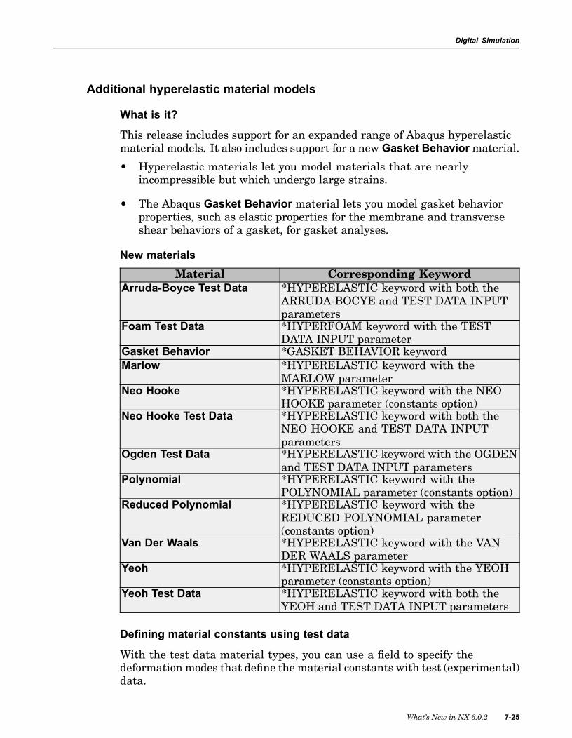
This release includes support for an expanded range of Abaqus hyperelasticmaterial models. It also includes support for a new Gasket Behaviormaterial.• Hyperelastic materials let you model materials that are nearlyincompressible but which undergo large strains.

• The Abaqus Gasket Behavior material lets you model gasket behaviorproperties, such as elastic properties for the membrane and transverseshear behaviors of a gasket, for gasket analyses.

New materials

Material Corresponding KeywordArruda-Boyce Test Data *HYPERELASTIC keyword with both the

ARRUDA-BOCYE and TEST DATA INPUTparameters

Foam Test Data *HYPERFOAM keyword with the TESTDATA INPUT parameter

Gasket Behavior *GASKET BEHAVIOR keywordMarlow *HYPERELASTIC keyword with the

MARLOW parameterNeo Hooke *HYPERELASTIC keyword with the NEO

HOOKE parameter (constants option)Neo Hooke Test Data *HYPERELASTIC keyword with both the

NEO HOOKE and TEST DATA INPUTparameters

Ogden Test Data *HYPERELASTIC keyword with the OGDENand TEST DATA INPUT parameters

Polynomial *HYPERELASTIC keyword with thePOLYNOMIAL parameter (constants option)

Reduced Polynomial *HYPERELASTIC keyword with theREDUCED POLYNOMIAL parameter(constants option)

Van Der Waals *HYPERELASTIC keyword with the VANDER WAALS parameter

Yeoh *HYPERELASTIC keyword with the YEOHparameter (constants option)

Yeoh Test Data *HYPERELASTIC keyword with both theYEOH and TEST DATA INPUT parameters

Defining material constants using test data

With the test data material types, you can use a field to specify thedeformation modes that define the material constants with test (experimental)data.


Digital Simulation

• Use the UNIAXIAL Tension/Compression option to use uniaxial testdata. This option corresponds to the Abaqus *UNIAXIAL TEST DATAkeyword. With UNIAXIAL Tension/Compression, you define a table fieldin which you list the material’s nominal stress (TU) and nominal strainvalues (εU) on each line.

• Use the BIAXIAL Tension option to use biaxial test data. This optioncorresponds to the Abaqus *BIAXIAL TEST DATA keyword. WithBIAXIAL Tension, you define a table field in which you list the material’snominal stress (TB) and nominal strain values (εB) on each line.

• Use the PLANAR - Pure Shear option to use planar (or pure shear) data.This option corresponds to the Abaqus *PLANAR TEST DATA keyword.With PLANAR - Pure Shear, you define a table field in which you listthe material’s nominal stress (TS) and nominal strain in the directionof loading (εS) on each line.

• Use the Pure Volumetric Compression option to use volumetric loadingtest data to include user-defined material compressibility. With PureVolumetric Compression, you define a table field in which you list thematerial’s pressure (p) and the volume ratio, J (current volume/originalvolume) on each line.

Depending upon the material’s type, you can use one or more of these optionsto define the experimental stress-strain data.

• With the Arruda-Boyce Test Data,Marlow, and Foam Test Datamaterials,you can only use one of the test data options to define the experimentaltest data. If you use more than one, when you export or solve your model,the software only writes out the first applicable test data curve. Theorder in which the software searches for the appropriate test data optiondepends on the material type as follows:

– Arruda-Boyce Test Data: BIAXIAL Tension then UNIAXIALTension/Compression

– Marlow: BIAXIAL Tension, then PLANAR - Pure Shear, thenUNIAXIAL Tension/Compression

– Foam Test Data: PLANAR - Pure Shear, then UNIAXIALTension/Compression, then Pure Volumetric Compression

• With the Mooney-Rivlin Test Data, Neo Hooke Test Data, Ogden TestData, Reduced Polynomial, Van Der Waals, and Yeoh Test Data materialtypes, you can use up to four of the options to define the experimentaltest data, If you use more than one, when you export or solve yourmodel, the software writes out the test data option in the following


Digital Simulation

order: BIAXIAL Tension, then PLANAR - Pure Shear, then UNIAXIALTension/Compression, then Pure Volumetric Compression.

For more information, see:

• *HYPERELASTIC, *UNIAXIAL TEST DATA, *BIAXIAL TEST DATA,*PLANAR TEST DATA, and *VOLUMETRIC TEST DATA in the AbaqusAnalysis Keywords Manual.

• “Hyperelastic behavior of rubberlike materials” in the Abaqus AnalysisUser’s Manual.

Where do I find it?

Application Advanced SimulationPrerequisite An active FEM, idealized part, or part with Abaqus as


Advanced Simulation®Material Properties

Bolt pre-loads now supported for solid elements

What is it?

When you are working with Abaqus as your solver, you can now define apre-load on a bolt modeled with solid (continuum) elements. In previousreleases, you could only define a bolt pre-load on a bolt modeled with beam(B31) elements.

In the Bolt Pre-Load dialog box, use the new Force on 3D Elements option onthe Type menu to define a pre-load on solid elements. With this option, youselect either elements or faces that define a pre-tension section. In Abaqus,a pre-tension section is defined as a surface inside the bolt that bisects thebolt into two parts. The software transmits the specified pre-load force acrossthe pre-tension section by means of a pre-tension node that you specify. Thispre-tension node must not be attached to any element in your model. Thesoftware applies the load along a vector that is normal to the pre-tensionsection. The new Section Normal option lets you control how the softwarecomputes this normal.

• If you select Average Surface Normal, the software computes an averagenormal to the section that faces away from the underlying continuumelements.

• If you select User Defined, you can define the vector to specify the normal.This option is useful when the direction in which you want to apply theload is different from the average normal to the pre-tension section.


Digital Simulation

The following graphic shows an example of a bolt created with solid elements.(A) shows the pre-tension section, (B) shows the pre-tension node, and (C)shows the normal to the pre-tension section.

Where do I find it?

Application Advanced SimulationPrerequisite An active Simulation with Abaqus as the specified solverToolbar

Advanced Simulation®Bolt Pre-Load

Ability to specify initial clearance values for contact and bolt contactanalyses

What is it?

You can use the new Contact with Clearance and Bolt Contact with Clearancesimulation objects to define precise initial clearance or overclosure (initialpenetration) values for the nodes on the slave surface in a contact pair. Withboth the Contact with Clearance and Bolt Contact with Clearance commands,the initial clearance or overclosure value you specify overwrites the initialclearance or overclosure value that the software calculates at each slave node.

• Use Contact with Clearance to define initial clearances or overclosureswhen you model contact between two surfaces.

• Use Bolt Contact with Clearance to define initial clearances oroverclosures when you model contact between a single-threaded bolt anda bolt hole.


Digital Simulation

Contact with clearance for threaded bolts

The Bolt Contact with Clearance dialog box includes additional ClearanceDefinition options that let you model the thread characteristics of a bolt evenif detailed thread geometry is not included in the model. These options letyou specify details about the bolt threads, including the half thread angle(a), pitch (p, or the thread-to-thread distance), and major (d) and mean (md)bolt diameters. You also use the Bolt Axis options to define two points (aand b) along the bolt’s axis. The software uses these points to generate thebolt’s contact normal directions.

Clearance or overclosure value can be uniform or spatially varying

In the Contact with Clearance and Bolt Contact with Clearance dialog boxes,you can use the Clearance Definition options to define the clearance oroverclosure value as either uniform or spatially varying for the contact pair.From the Value list:

• If you select Expression, you can specify a uniform clearance oroverclosure value for the contact pair. A positive value indicates aclearance value, and a negative value indicates an overclosure value.

• If you select Field, you can specify spatially varying clearances oroverclosures. With this option, you use a table field to specify theclearance at a single node or set of nodes on the slave surface. In the


Digital Simulation

table field, the node ID is the independent variable, while the clearanceor overclosure value is the dependent variable. You can also specify aScale Factor to apply to the field.

Contact with clearance is supported only in small-sliding contact analyses

You can only use the Contact with Clearance or Bolt Contact with Clearancecommands when you are using the small-sliding contact formulation in youranalysis. In Abaqus, you use the *CONTACT PAIR keyword to specifythe contact formulation. In Advanced Simulation, you use a Contact Pairmodeling object to specify the parameters for the *CONTACT PAIR keyword:

1. In the Contact Pair dialog box, select Small from the Sliding Type list touse the small-sliding formulation instead of the finite-sliding formulation.

2. In the Contact with Clearance or Bolt Contact with Clearance dialogbox, use the Contact Pair option to associate the Contact Pair modelingobject with the simulation object.

Associated Abaqus keywords

When you export or solve your model, the software uses the options youspecify in the Contact with Clearance dialog box to define the *CONTACTPAIR and *CLEARANCE keywords in your Abaqus input file. For moreinformation, see Adjusting Initial Surface Positions and Specifying InitialClearances in Abaqus/Standard Contact Pairs in the Abaqus Analysis User’sManual and *CLEARANCE and *CONTACT PAIR in the Abaqus KeywordsReference Manual.

Where do I find it?


Advanced Simulation®Contact with Clearance or

Bolt Contact with Clearance

New thermal conductance boundary condition

What is it?

When you are working with Abaqus as your solver, you can use the newSurface-to-Surface Thermal Conductance simulation object to modelconductive heat transfer between proximate or contacting surfaces.

In the Surface-to-Surface Thermal Conductance dialog box, you can use theConductance Dependency options to model the conductive heat transferas a function of:


Digital Simulation

• The clearance between the contacting surfaces (Clearance option).

• The contact pressure at the interface between the contacting surfaces(Pressure option).

• Both the clearance and the contact pressure (Clearance and Pressureoption).

In Advanced Simulation, you use fields to define how the heat transfer varieswith the clearance and/or contact pressure.

When you export or solve your model, the software uses the options youspecify in the Surface-to-Surface Thermal Conductance dialog box to definethe *GAP CONDUCTANCE keyword in your Abaqus input file. For moreinformation, see Thermal Contact Properties in the Abaqus Analysis User’sManual and *GAP CONDUCTANCE in the Abaqus Keywords ReferenceManual.

Where do I find it?

Application Advanced SimulationPrerequisite An active Simulation with Abaqus as the specified solver

and Thermal as the selected analysis typeToolbar Advanced Simulation®Surface-to-Surface Thermal

Conductance

Initial support for Abaqus output database files

What is it?

On Windows platforms, this release includes initial support for Abaqusoutput database files (*.odb) files. In this release, you can:

• Import results into Post-Procressing and create displays.

• Output results from selected analysis steps to an ODB file.

In previous releases, Advanced Simulation only supported the Abaqus resultfile (*.fil).

Customer default setting necessary to activate ODB support

ODB file support in Advanced Simulation is controlled through the newABAQUS File Extension option in the Customer Defaults dialog box. Toactivate ODB support:

1. From the File menu, choose Utilities®Customer Defaults.

2. In the Customer Defaults dialog box, choose Simulation®Extras.


Digital Simulation

3. On the ABAQUS page, select ODB as the ABAQUS File Extension default.

The next time you start NX, Advanced Simulation links the Abaquslibraries that are necessary for working with ODB files.

With the ABAQUS File Extension default:

• If you select FIL, you can only import and work with Abaqus results (*.fil)files.

• If you select ODB, you can import and work with both Abaqus results(.*fil) files and ODB files.

Customer default setting also controls default Abaqus result file type

When you select ODB as the ABAQUS File Extension default, the softwarealso sets your default output file type for all Abaqus analyses to ODB. Withthe ODB default selected:

• On the Output page in the Create Solution Step dialog box, theWritten toODB option is selected by default.

• In both the Results node in the Simulation Navigator and in thePost-Processing Navigator, the software looks for files in your currentdirectory that have the .odb extension. If your directory only contains aFIL file and not an ODB file, the software does not display any results.

Note

To display results from a FIL file when ODB is selected as theABAQUS File Extension default, use the File®Import®Simulationcommand.

Supported ODB version

Advanced Simulation currently supports the ODB file format released inAbaqus version 6.8-2. Therefore, you can import files in ODB format version6.8-2 or earlier, and any results that you export from Advanced Simulation toan ODB file will be written in the 6.8-2 format. If you try to import an ODBfile from an earlier version of Abaqus, NX prompts you to convert the fileto the 6.8-2 version.

Ability to animate across load cases

What is it?

For solutions that include multiple load cases, you can now animate theresults across the load cases. The Animation dialog box includes two options:Result and Iterations. The Iterations option lets you specify a Start LoadCase, Start Iteration (if the starting load case contains iterations), and End


Digital Simulation

Load Case, as well as a Step increment to determine the number of framesin the animation.

For example, suppose you have three load cases (1, 2, and 3 in the picturebelow) and you want the animation to start at the first load case and endafter the last load case.

In this example, you would choose Load Case 1 as the Start Load Case andLoad Case 3 as the End Load Case. The following animated picture showsthe result. The first and last load cases each have one static step and thesecond load case has 10 iterations. The Step option is set to 1, which meansthe animation includes a frame for each step and iteration between the startand end load case. Therefore, the animation contains 12 frames. Note theload case and iteration number indicated by the arrow in the picture.


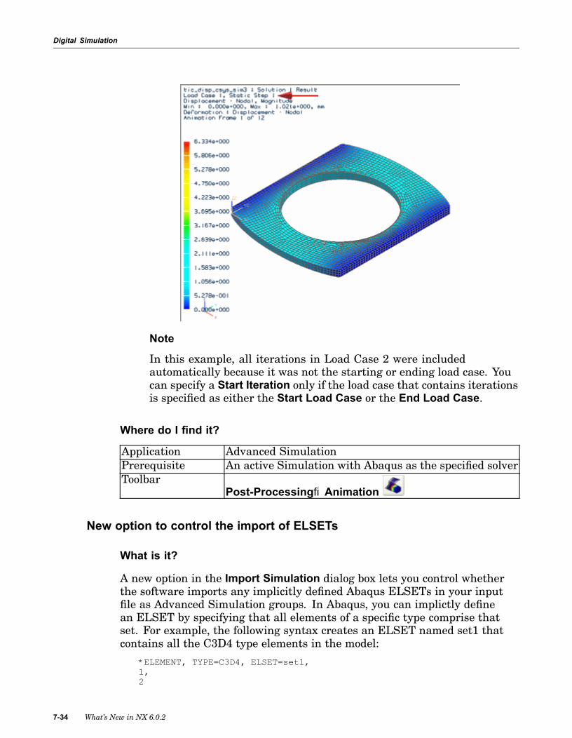
Digital Simulation

Note

In this example, all iterations in Load Case 2 were includedautomatically because it was not the starting or ending load case. Youcan specify a Start Iteration only if the load case that contains iterationsis specified as either the Start Load Case or the End Load Case.

Where do I find it?


Post-Processing®Animation

New option to control the import of ELSETs

What is it?

A new option in the Import Simulation dialog box lets you control whetherthe software imports any implicitly defined Abaqus ELSETs in your inputfile as Advanced Simulation groups. In Abaqus, you can implictly definean ELSET by specifying that all elements of a specific type comprise thatset. For example, the following syntax creates an ELSET named set1 thatcontains all the C3D4 type elements in the model:

*ELEMENT, TYPE=C3D4, ELSET=set1,1,2


Digital Simulation

In contrast, you create an explicitly defined ELSET by directly listing theelements that form that set. For example, the following syntax creates anELSET named set2 that contains elements 6, 7, 8, 17, and 26:

*ELSET, NAME=set26,7,8,17,26

If your input file contains implicitly defined ELSETs, you can use the newImport implict ELSET as group option in the Advanced Options group in theImport Simulation dialog box to control how the software imports those sets.

• If you select Import implicit ELSET as group, the software imports anyimplicitly defined ELSETS in your input file. It uses those ELSETS tocreate groups.

• If you clear the Import implicit ELSET as group check box, the softwaredoes not import any implicitly defined ELSETS as groups.

Clearing the Import implicit ELSET as group check box can improve theimport performance of your input file.

Where do I find it?


Enhancements for ANSYS users

Additional hyperelastic material models

What is it?

This release includes support for an expanded range of ANSYS hyperelasticmaterial models. You can now create the following new types of materials:

Material Corresponding CommandGent TB command with the HYPER,,,,GENT optionNeo Hooke TB command with the HYPER,,,,NEO optionPolynomial TB command with the HYPER,,,,POLY optionYeoh TB command with the HYPER,,,,YEOH option

Where do I find it?

Application Advanced SimulationPrerequisite An active FEM, idealized part, or part with ANSYS as


Advanced Simulation®Material Properties


Digital Simulation

Cumulative loading options now respected on import

What is it?

When you import an ANSYS import file into Advanced Simulation, thesoftware now respects the settings of any cumulative option commands(DCUM, FCUM, SFCUM, and BFCUM). In ANSYS, you use these commandsto specify whether the software should add (ADD), replace (REPL), or ignore(IGNO) a repeated load or constraint on a particular degree-of-freedom.In previous releases, the software always imported any cumulative optioncommand with a setting of “replace” (REPL), regardless of what you actuallyspecified in the input file. Now, the software correctly preserves the specifiedcumulative option setting when you import the file.

Note

Advanced Simulation does not import any cumulative options as aSolution Step attribute. Instead, the software converts the load orboundary condition data into an equivalent load or boundary conditionwith the appropriate cumulative option setting.

For example, suppose you have the following constraints on node ID2:

• Step 1: UX = 1mm, UZ= 1.2mm

• Step 2: UX = 1.5mm, UY=1

In step 2 of the analysis, how the software resolves the constraint on nodeID2 depends on the setting of the DCUM command:

• If the DCUM option is set to REPL, the resolved constraint for node ID2is UX = 1.5, UY = 1 (UZ is removed)

• If the DCUM option is set to ADD, the resolved constraint for node ID2 isUX = 2.5, UY = 1, UZ = 1.2

Where do I find it?

Application Advanced SimulationPrerequisite An active Simulation file with ANSYS as the specified

solverMenu File®Import®Simulation


Digital Simulation

New options to control the deletion of loads at the end of a step

What is it?

A new Delete load options tab has been added to the Create Solution Stepand Edit Solution Step dialog boxes. The options on the Delete load optionspage let you control whether forces and moments, body loads, and elementbody loads will be kept or deleted by ANSYS at the end of the current solutionstep. These options correspond to the ANSYS DDELE, FDELE, BFDELE,and BFEDELE commands.

Note

Currently, you can only use the Delete load options commands todelete the loads or constraints on all nodes or elements to which theyare applied.

Where do I find it?


solverSimulationNavigator

Either right-click a solution and select Create Step, orright-click the appropriate solution step and select EditSolution Step

Support for importing loads and constraints from binary files

What is it?

When you import an ANSYS binary file into Advanced Simulation,the software now imports any loads (forces/moments) and constraints(displacements and temperatures) defined in that file.

Where do I find it?


solverMenu File®Import®Simulation


Digital Simulation

Enhancements for LS-DYNA users

Support for additional laminates keywords

What is it?

Advanced Simulation now supports the import and export of two additionalLS-DYNA keywords for modeling laminates:

• *CONTROL_SHELL

• *MAT_COMPOSITE_DAMAGE

In the NX 6.0.1 release, the software supported both the *MAT_ELASTICand *MAT_ORTHOTROPIC_ELASTIC keywords. However, thesekeywords do not work when a laminate’s ply angles are non-zero.Because *MAT_COMPOSITE_DAMAGE is more versatile, it now replaces*MAT_ELASTIC and *MAT_ORTHOTROPIC_ELASTIC.

Where do I find it?


NX Thermal and Flow, Electronic Systems Cooling, and SpaceSystems Thermal

Dialog box text changes

What is it?

The following minor text changes were made in this release:

Dialog box name Group name Old text New text

Flow BoundaryCondition

Flow Directionand Flow Return

Normal toTangentialVelocity Angle

Normal toResultant VelocityAngle

Particle Injection Parameters Mass per Seconds Mass per UnitTime

Thermo-OpticalProperties —Advanced

InfraredProperties,Solar Properties,and Non GrayProperties

Transparency Transmissivity


Digital Simulation

Supported solvers and analysis types

Solver Analysis Type Solution TypeNX Electronic SystemsCooling

Coupled Thermal-Flow Electronic SystemsCooling

Advanced Thermal/Flowwith ESC

NX Space SystemsThermal

Thermal Space Systems Thermal

Thermal Thermal

Advanced ThermalFlow Flow

Advanced Flow

NX Thermal and Flow

Coupled Thermal-Flow Thermal-Flow

Advanced Thermal-Flow

Where do I find it?

Application Advanced SimulationToolbar

Advanced Simulation toolbar ® SimulationObject Type

Advanced Simulation toolbar® Modeling Objects

Enhancement of Report simulation object on 2D Shell elements

What is it?

You can now specify on which side of 2D shell elements you want to calculatethermal results when using a Report simulation object of following types:

• Per Element

• Per Region

• Between Regions

• Heat Maps

You can ask for results on the following sides of 2D shell elements:

• Top and Bottom

• Top

• Bottom


Digital Simulation

For a Between Regions type of Report, you can separately set the side forelements in the primary and secondary regions.



Coupled Thermal-Flow Electronic SystemsCooling

Advanced Thermal/Flowwith ESC



Thermal Thermal

Advanced ThermalFlow Flow

Advanced Flow

NX Thermal and Flow

Coupled Thermal-Flow Thermal-Flow

Advanced Thermal-Flow

Where do I find it?

Application Advanced SimulationSimulationNavigator

Right-click the simulation object container ® NewSimulation Object ® Report

ToolbarAdvanced Simulation toolbar® Report

Group import

What is it?

When you import NX THERMAL / FLOW, NX SPACE SYSTEMS THERMAL,NX ELECTRONIC SYSTEM COOLING, or IDEAS UNV simulations, thesoftware now also imports any groups containing elements and nodes.

Where do I find it?

Application Advanced SimulationPrerequisite An active FEM or SIM with NX THERMAL / FLOW,

NX SPACE SYSTEMS THERMAL, or NX ELECTRONICSYSTEM COOLING solver

Menu File ® Import ® Simulation


Digital Simulation

Articulation modeling enhancement

What is it?

You now have more flexibility when defining time step options for thearticulation movement. You can select one of the following four options in theTime Step Option list of the Articulation Parameters group on the TransientSetup page of the Create Solution or Edit Solution dialog box:

• At Constant Time Intervals— you control the starting and ending timesfor the articulation as well as the calculation interval.

• Total Number — you control the starting and ending times for thearticulation as well as the number of time steps.

• At Specified Times— you specify the articulation movement times in alist of the Articulation Times dialog box by clicking .

• Interval versus Time Table— you specify a table containing the desiredcalculation intervals at specified times. For example:

Time Interval0.0 1.010.0 2.020.0 3.4

The thermal calculation for the articulation movement is performed atfollowing times:

0.0 1.0 2.0 3.0 4.0 5.0 6.0 7.0 8.0 9.0 10.0 12.0 14.0 16.0 18.0 20.0

The last row of the table indicates the articulation end time; thecalculation interval is a dummy number.

In previous releases, the only available time step control option was AtConstant Time Intervals.



Coupled Thermal-Flow Advanced Thermal/Flowwith ESC



Thermal Advanced ThermalNX Thermal and FlowCoupled Thermal-Flow Advanced Thermal-Flow


Digital Simulation

Where do I find it?

Application Advanced SimulationSimulationNavigator Right-click the solution node and choose SolveToolbar

Advanced Simulation toolbar ® Solve ® EditSolution Attributes

Orthotropic thermal conductivity in cylindrical or spherical coordinates

What is it?

You can now specify orthotropic materials with thermal conductivity definedin cylindrical or spherical coordinates. In the 2D and 3D Mesh Collectordialog boxes, when you specify an orthotropic material, you have the followingchoices for the Material Orientation Type:

• Cartesian to specify that the orthotropic conductivity is defined inCartesian coordinates.

• Cylindrical to specify that the orthotropic conductivity is defined incylindrical coordinates.

• Spherical to specify that the orthotropic conductivity is are defined inspherical coordinates.

The following table shows the correspondence between the ThermalConductivity X, Thermal Conductivity Y, and Thermal Conductivity Z valuesyou enter in the Materials dialog box and their values in all three coordinatesystems:

MaterialOrientation Type

ThermalConductivity X

ThermalConductivity Y

ThermalConductivity Z

Cartesian kx ky kzCylindrical kr kq kzSpherical kr kq kf

For 2D mesh collectors, when you select Cylindrical or Spherical as thematerial orientation type, you must also specify the Main Conduction Planeand Direction for the heat transfer. The software determines the threecomponents of the thermal conductivity as follows:

• The software projects on the shell element the main direction vector,and the conductivity in that direction is the main direction vector’sconductivity.


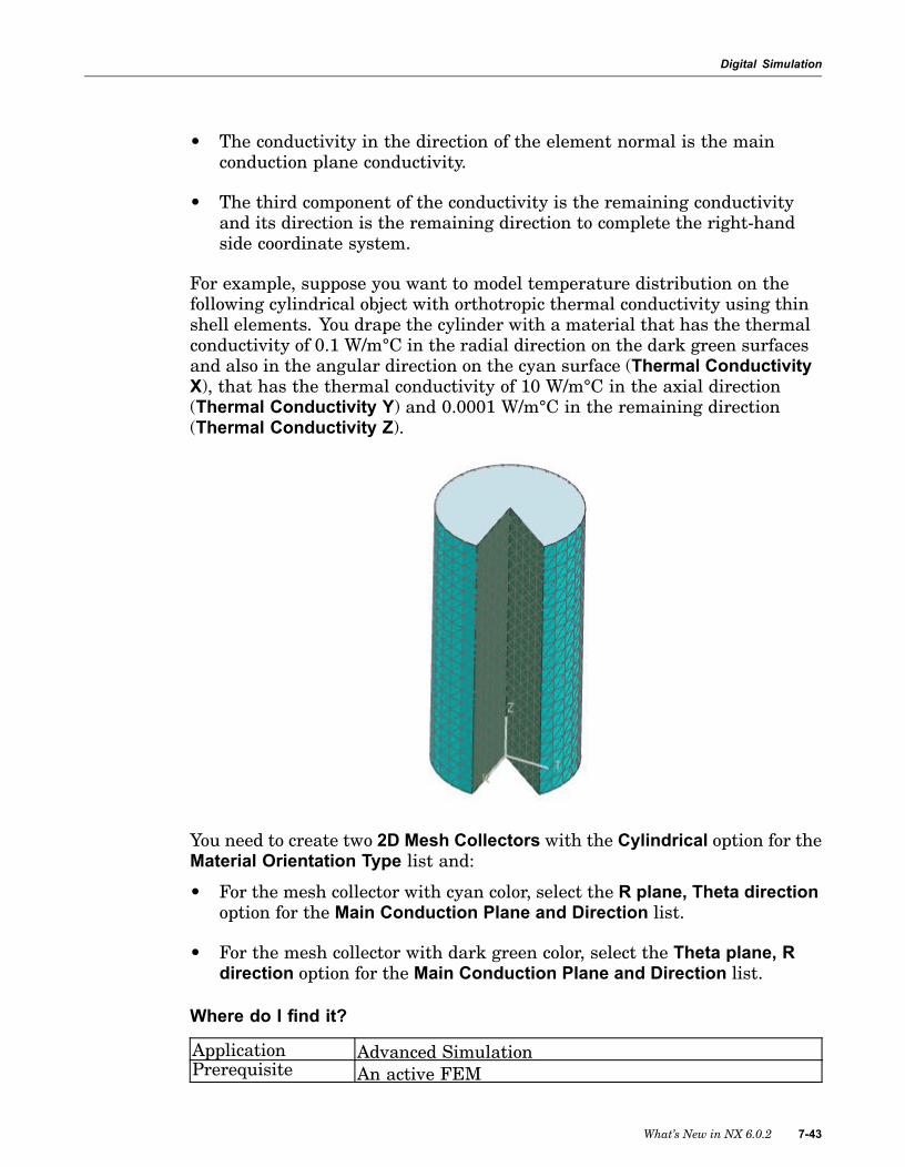
Digital Simulation

• The conductivity in the direction of the element normal is the mainconduction plane conductivity.

• The third component of the conductivity is the remaining conductivityand its direction is the remaining direction to complete the right-handside coordinate system.

For example, suppose you want to model temperature distribution on thefollowing cylindrical object with orthotropic thermal conductivity using thinshell elements. You drape the cylinder with a material that has the thermalconductivity of 0.1 W/m°C in the radial direction on the dark green surfacesand also in the angular direction on the cyan surface (Thermal ConductivityX), that has the thermal conductivity of 10 W/m°C in the axial direction(Thermal Conductivity Y) and 0.0001 W/m°C in the remaining direction(Thermal Conductivity Z).

You need to create two 2D Mesh Collectors with the Cylindrical option for theMaterial Orientation Type list and:

• For the mesh collector with cyan color, select the R plane, Theta directionoption for the Main Conduction Plane and Direction list.

• For the mesh collector with dark green color, select the Theta plane, Rdirection option for the Main Conduction Plane and Direction list.

Where do I find it?

Application Advanced SimulationPrerequisite An active FEM


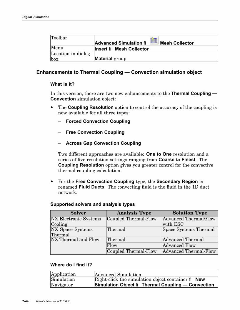
Digital Simulation

ToolbarAdvanced Simulation ® Mesh Collector

Menu Insert ® Mesh CollectorLocation in dialogbox Material group

Enhancements to Thermal Coupling — Convection simulation object

What is it?

In this version, there are two new enhancements to the Thermal Coupling —Convection simulation object:

• The Coupling Resolution option to control the accuracy of the coupling isnow available for all three types:

– Forced Convection Coupling

– Free Convection Coupling

– Across Gap Convection Coupling

Two different approaches are available: One to One resolution and aseries of five resolution settings ranging from Coarse to Finest. TheCoupling Resolution option gives you greater control for the convectivethermal coupling calculation.

• For the Free Convection Coupling type, the Secondary Region isrenamed Fluid Ducts. The convecting fluid is the fluid in the 1D ductnetwork.






Thermal Advanced ThermalFlow Advanced Flow

NX Thermal and Flow

Coupled Thermal-Flow Advanced Thermal-Flow

Where do I find it?


Right-click the simulation object container ® NewSimulation Object ® Thermal Coupling — Convection


Digital Simulation

ToolbarAdvanced Simulation toolbar® Thermal Coupling— Convection

Duct Opening enhancement

What is it?

When you specify external conditions for a Duct Opening type of the DuctFlow Boundary Conditions simulation object, you can now specify onlythe pressure of the fluid or you can also specify the temperature of thefluid. In previous versions, you needed to specify both the pressure and thetemperature at the same time.

A Temperature check box now appears when you select Specify from theExternal Conditions list.

• By selecting the Temperature check box, you specify the TemperatureValue at the duct opening.

• By clearing the Temperature check box, the temperature of the fluid atthe duct opening is the Fluid Temperature value defined in the AmbientConditions page of the Create Solution or the Edit Solution dialog box.

In both cases, you must specify the Total Pressure — Gauge value for thepressure of the fluid at the duct opening.







NX Thermal and Flow


Where do I find it?


Right-click the simulation object container ® NewSimulation Object ® Duct Flow Boundary Conditions

ToolbarAdvanced Simulation toolbar ® Duct FlowBoundary Conditions


Digital Simulation

Density results on duct elements

What is it?

You can now recover density results on duct elements from the analysis byselecting Densities in the Duct Flow group of the Results Options page ofthe Create Solution or Edit Solution dialog box. In the Post ProcessingNavigator after solving, a Fluid Density result type will appear under theSolution results node.







NX Thermal and Flow


Where do I find it?

Application Advanced SimulationSimulationNavigator Right-click the solution node and choose SolveToolbar

Advanced Simulation toolbar ® Solve ® EditSolution Attributes

Radiative Element Subdivision enhancement

What is it?

When selecting elements to which to apply the local Radiative ElementSubdivision settings, the Element Selection Filtering is enhanced. You cannow select from the Filter Type list:• 1D Elements (previously available) — lets you select only 1D elements.

• 2D Elements (previously available) — lets you select only 2D elements.

• Element Edges (new) — lets you select 1D elements and the edges of2D elements.

• Element Faces (new) — lets you select 2D elements and the faces of 3Delements.

You must first set Type Filter on the Selection bar to Element.


Digital Simulation


Use these new options to easily select elements to which you want to applylocal element subdivision for radiation calculations.






Thermal Advanced ThermalNX Thermal and FlowCoupled Thermal-Flow Advanced Thermal-Flow

Where do I find it?


Right-click the simulation object container ® NewSimulation Object ® Radiative Element Subdivision

ToolbarAdvanced Simulation toolbar® Radiative ElementSubdivision

Export flow model boundary conditions to CGNS

What is it?

In addition to nodes and elements, you can now export the following boundarycondition data in the CFD General Notation System (CGNS) format:

• Temperature

• Inlet information: velocity, mass flow, volume flow, or pressure rise

• Outlet information: velocity, mass flow, volume flow, or pressure rise

• Opening information: pressure

For the element on free faces where you apply boundary conditions, thesoftware creates boundary elements with a normal pointing into the fluid.Any pyramid elements are converted to wedge elements.

CGNS export does not support table data. For temperature, velocity, massflow, volume flow, or pressure varying in time, the software exports theboundary condition into the CGNS format with a value equal to 0. Thesoftware does not export any boundary condition values that are definedwith NX spatial fields.


Digital Simulation

CGNS is a standard format for recording computational fluid dynamics(CFD) analysis data.



Coupled Thermal-Flow Electronic SystemsCooling, AdvancedThermal/Flow withESC

Flow Advanced FlowNX Thermal and FlowCoupled Thermal-Flow Advanced Thermal-Flow

Where do I find it?

Application Advanced SimulationMenu File ® Export ® SimulationLocation in dialogbox File Type list ® CGNS

Mapping enhancements

What is it?

All Mapping and Axisymmetric Mapping solutions in NX THERMAL / FLOW,NX SPACE SYSTEMS THERMAL, and NX ELECTRONIC SYSTEMS COOLINGsolvers allow you to automatically create a complete NX solution with allthe appropriate steps, subcases, and loads defined for the Nastran, ANSYS,and Abaqus solvers.

To create complete NX solutions, in the Optional Output page of the CreateSolution or Edit Solution dialog box, select the Create Nastran Solution,Create Ansys Solution, or Create Abaqus Solution check box.The mapping solver creates the following NX solutions:

• SESTATIC 101 — Single Constraint for NX Nastran only

• Linear Statics for ANSYS

• General Analysis for Abaqus

When the Analysis Type is Mapping, the loads the mapping solver createsdepends upon the Source Model Analysis Type and the setting of the Data toMap option (Mapping Details page of the Create Solution and Edit Solutiondialog boxes).

• When the Source Model Analysis Type is Thermal or Coupled and Datato Map is set to Solid Temperatures, the software creates structural NodeID Table Temperature loads.


Digital Simulation

• When the Source Model Analysis Type is Flow or Coupled and Data toMap is set to Flow Values, the software creates structural Node ID TableForce loads.

When the Analysis Type is Axisymmetric Mapping, the software createsstructural Node ID Table Temperature loads.

You can create more than one solution at the same time, such as one for bothNastran and ANSYS. In that case, the mapping solver creates one set of loadsthat are shared between the solutions.

The mapping solver now supports all available Nastran, ANSYS, and Abaquselements which support temperature and pressure data.

You can now map temperature data from axisymmetric model to 3D model.


The automatic creation of mapping solutions for Nastran, ANSYS, andAbaqus simplifies the mapping of transient solutions.



Mapping Thermal-Flow


Mapping Thermal

Mapping Thermal-FlowNX Thermal and FlowAxisymmetric Mapping Thermal

Where do I find it?

Application Advanced SimulationPrerequisite Two FEM with models that are geometrically congruentSimulationNavigator Right-click the simulation file node® New SolutionToolbar

Advanced Simulation toolbar® SolutionMenu Insert ® SolutionLocation in dialogbox Analysis Type ® Mapping or Axisymmetric Mapping


Digital Simulation

NX FE Model Correlation

What is it?

NX FE Model Correlation is a new Advanced Simulation process which youcan use to quantify and visualize the level of agreement between two sets ofmodal results by comparing mode shapes and nodal responses.

NX FE Model Correlation can correlate modal results between structuralfinite element analysis and experimental test modal analysis results(test-analysis) or between two sets of structural finite element analysisresults (analysis-analysis).

7th mode shape of the referencesolution

13th mode shape of the worksolution

You prepare the finite element model for structural analysis by defining themesh and material properties. Then, you solve the following modal analysissolutions:

• NX or MSC Nastran: SEMODES 103

• ANSYS: Modal

• ABAQUS: Frequency Perturbation Substep

With NX FE Model Correlation, you create a solution with the new solverenvironment, MODAL TEST DATA, and the new solution type, Test Solution.You then import the experimental modal results and the test model from NXI-deas Universal (UNV) files into that solution. The test model is disjointfrom the finite element model.

NX FE Model Correlation allows you to:


Digital Simulation

• Setup the correlation process.

• Align test solution with the analysis solution.

• Pair the test modes with the analysis modes.

• Obtain correlation metrics.


NX FE Model Correlation objectively compares mode shapes and nodalresponses to assess the level of agreement between experiments and FEresults in structural dynamics.

Where do I find it?

Application Advanced SimulationPrerequisite An active Simulation file with modal analysis solutionMenu Insert ® Correlation

NX Open

Enhanced NX Open support in CAE

What is it?

Several JA-based NX Open APIs are now available that let you automateAdvanced Simulation operations. The following new functions have beenadded:

NX Open class New function addedBaseFEModel Provides access to the Update Finite

Element Model command.SimSolution Provides access to solve a solution or

write a solver input file.SimSolution Provides access to complete edit

capability for SimSolution propertiesas well as Solver Parameters.

NodeElementManage Creates a NodesRepositionBuilderobject that lets you efficientlyreposition large numbers of nodes.

For details about each new function, see the NX Open Reference Guide for thelanguage you are using (for example, the NX Open C++ Reference Guide).You can find the NX Open reference guides in the NX Help Library underAutomation®NX Open.


Digital Simulation

NX Open support for reading and displaying solver results

What is it?

Using the NX Open interface, you can now write custom automation code forreading and displaying solver results in Advanced Simulation.

Several new NX Open classes have been added to the CAE NameSpace.

• ResultManager

• IResult

• ImportedResult

• ResultAccess

• ResultParameters

• SolutionResult

Use these general steps for working with these new classes:

1. Create a Result object from a solution or by opening a result file.

2. Create a ResultAccess object by providing a Result object and aResultParameters object.

ResultAccess holds a state that can be modified using a ResultParametersobject. ResultParameters is a container of result properties that can bequeried, modified, and set to a ResultAccess object.

3. Query file data from the Result object such as number of nodes, elements,load cases, and so on.

4. Access state data from the ResultAccess object such as minimum andmaximum results values, min-max locations, and so on.

For details about each new class, see the NX Open Reference Guide for thelanguage you are using (for example, the NX Open C++ Reference Guide).You can find the NX Open reference guides in the NX Help Library underAutomation®NX Open.


Digital Simulation

NX Open support for manual creation of all 3D solid element types

What is it?

You can use the new ElemDimTypeAnySolid option in theCAE::ElementCreateBuilder NX Open class to create a 3D element of anysolid topology supported by your solver. In previous versions, you could createonly Penta(6) and Hexa(8) elements.

For details about the new option, see the NX Open Reference Guide for thelanguage you are using (for example, the NX Open C++ Reference Guide).You can find the NX Open reference guides in the NX Help Library underAutomation®NX Open.

Post Processing

Unaveraged results across feature angle boundaries

What is it?

When you analyze elemental or element-nodal results in post-processing andyou use the Averaged results option, you can now choose not to average theresults across nodes at feature angle boundaries in your model.

In the Smooth Plot dialog box, the Averaged option calculates a nodalaverage across all adjacent elements for elemental and element-nodalresults. For this release, a new Feature Angles option has been added tothe averaged-across options.

When the Feature Angles check box is not selected, the software leaves theresults unaveraged across feature angles greater than the angle thresholdyou specify. For example, if you do not want the results averaged acrossfeature angles of 45 degrees or greater, enter 45 in the angle threshold box.

The angle is measured at the free element faces, as shown in the followingexample.


Digital Simulation

Note

The Include Internal Elements option is unavailable when the FeatureAngles check box is not selected.

Example

The following examples illustrate how the stress results remain unaveragedpast the hole and slot features in this disk part.

Stress averaged across feature angles (default setting; FeatureAngles check box selected)


Digital Simulation

Stress unaveraged across feature angles greater than 45 degrees(Feature Angles check box not selected)

About the Identify command

You use the Identify command to probe and display nodal information forthe post view display. When you use the Identify command and the FeatureAngles check box is not selected, you may see multiple values on a singlenode, depending on the number of faces that share this node and the faceyou position the mouse over.


Digital Simulation

Where do I find it?

Application Advanced SimulationPrerequisite Simulation file with elemental or element-nodal results.

The Include Internal Elements option must be turned off.Toolbar

Post Processing®Post ViewLocation in dialogbox

Result (Color Display)®Averaged®Feature Angles

Expanded results support in Post-Processing

You can now display and analyze results in post-processing for severaladditional result types and element types.

NX Nastran results

• Contact gap distance

• Shell element thickness

• Gasket Pressure

• Gasket Closure

• Plastic Gasket Closure

• Gasket Status

• Gasket Yield Stress

• 2D axisymmetric contact results

NX Nastran elements

• Pyramid elements: CPYRAM

• Axisymmetric solid elements: CTRAX3, CQUADX4, CTRAX6, andCQUADX8

NX Response Simulation results

These Response Simulation contour results types are now supported correctly.In previous versions, all possible component results were displayed in theSimulation Navigator even if you had not requested certain components.

• Peak

• RMS


Digital Simulation

• Level Crossing

NX Laminates results

• Ply Failure Indices (ANSYS support added)

• Ply Strength Ratio

• Bond Strength Ratio

NX Flow results

Fluid density is now supported.

Context highlighting in Post Processing Navigator

What is it?

The active results set that is plotted in the graphics window now displays inblue in the Post Processing Navigator.

Von Mises stress result plotted in graphics window and displayed inblue in Post Processing Navigator


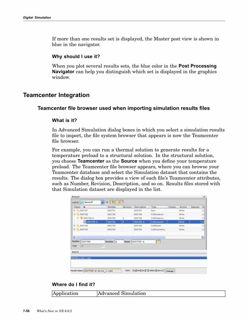
Digital Simulation

If more than one results set is displayed, the Master post view is shown inblue in the navigator.


When you plot several results sets, the blue color in the Post ProcessingNavigator can help you distinguish which set is displayed in the graphicswindow.

Teamcenter Integration

Teamcenter file browser used when importing simulation results files

What is it?

In Advanced Simulation dialog boxes in which you select a simulation resultsfile to import, the file system browser that appears is now the Teamcenterfile browser.

For example, you can run a thermal solution to generate results for atemperature preload to a structural solution. In the structural solution,you choose Teamcenter as the Source when you define your temperaturepreload. The Teamcenter file browser appears, where you can browse yourTeamcenter database and select the Simulation dataset that contains theresults. The dialog box provides a view of each file’s Teamcenter attributes,such as Number, Revision, Description, and so on. Results files stored withthat Simulation dataset are displayed in the list.

Where do I find it?

Application Advanced Simulation


Digital Simulation

SimulationNavigator

For example: edit the solution subcase®chooseNastran Temperatures under Pre-Load Type®choose

Teamcenter under Source. Click Browse.


Chapter

8 Manufacturing

Turning cutter compensation

What is it?

Cutter compensation (cutcom) options control the cutter radius compensationfunction of the machine controller. The software outputs G41 or G42 code toadjust the tool path left or right, measured relative to the tool’s direction ofmotion.

Profile cutting pass without cutter compensation

There are two types of cutter compensation available:

• Fixed tracking point

• Contact contour


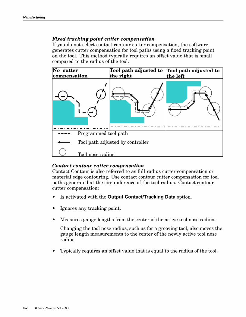
Manufacturing

Fixed tracking point cutter compensationIf you do not select contact contour cutter compensation, the softwaregenerates cutter compensation for tool paths using a fixed tracking pointon the tool. This method typically requires an offset value that is smallcompared to the radius of the tool.

No cuttercompensation

Tool path adjusted tothe right

Tool path adjusted tothe left

Programmed tool path

Tool path adjusted by controller

Tool nose radius

Contact contour cutter compensationContact Contour is also referred to as full radius cutter compensation ormaterial edge contouring. Use contact contour cutter compensation for toolpaths generated at the circumference of the tool radius. Contact contourcutter compensation:

• Is activated with the Output Contact/Tracking Data option.

• Ignores any tracking point.

• Measures gauge lengths from the center of the active tool nose radius.

Changing the tool nose radius, such as for a grooving tool, also moves thegauge length measurements to the center of the newly active tool noseradius.

• Typically requires an offset value that is equal to the radius of the tool.


Manufacturing

Contact contour cutter compensation

No cuttercompensation

Tool path adjustedright to part contour

Tool path adjusted leftto part contour

Programmed tool path

Tool path adjusted by controller

Tool nose radius


If the NC programmer turns on cutter compensation, the machine operatorcan adjust the tool path with the offset value in the cutter compensationregister of the controller. This enables the machine operator to:

• More closely control cutting dimensions of the part.

• Compensate for variation in the tool size.

• Compensate for tool or part deflection.

Where do I find it?

Application ManufacturingAvailable for

Turning finishing operation and profiling passes in aTurning roughing operation

Location in dialogbox Operation dialog box®Non Cutting Moves ®More

page®Cutter Compensation group

Divide by Holder

What is it?

Divide by Holder lets you divide a generated tool path where there are holdercollisions. When the software finds a holder collision, it moves backwards


Manufacturing

along the tool path to the closest transfer, then divides the tool path into twooperations at the transfer. The original operation contains collision free toolpath. The new operation contains the tool path section with holder collisions.

Name Path Edit StatusCAVITY_MILL Repost

Operation Navigator before Divide by Holder

Name Path Edit StatusCAVITY_MILL Repost

CAVITY_MILL_DIV_1 Repost

Operation Navigator after Divide by Holder

You can change the following parameters in the split operation to eliminateholder collisions:

• Tool

The tool shape, diameter, corner radius, and taper angle must be the same.

• Holder

• Program group

• Machine Control options

• Feed rate

Divide by Holder is useful for:

• Level based operations.

• Area milling operations with a Zig or Zig Zag with Lifts cut pattern thatgenerates transfers.

Divide by Holder does not work if the operation does not have transfers.For example, you cannot use Divide by Holder for a Zig Zag cut patternwhere the tool enters the cut, zig-zags everywhere to machine the part,then retracts.


You can:

• Generate operations with holder checking turned off for fasterperformance, then run Divide by Holder to remove holder collisions.


Manufacturing

• Use Divide by Holder when there are changes to the holder information,to correct the tool path without regenerating the operation.

Where do I find it?

Application ManufacturingShortcut menu Operation Navigator®right-click the operation®Tool

Path®Divide by Holder

Post Builder support for Siemens 840 D controller

What is it?

The Siemens Sinumerik 840D controller is now supported. You can:

• Select from a set of template posts that optimally support 5-axis and3-axis postprocessors. Set the post default settings with the customcommand PB_CMD_Sinumerik_default_setting.

• Add a start event for the Sinumerik 840D controller to a single millingoperation, or to the lowest level program group in the Program view of theOperation Navigator. The default parameter settings in the Sinumerik840D start event dialog box are the same as the default settings in theSinumerik 840D template post.

• Set the Sinumerik version with the custom commandPB_CMD_Sinumerik_Version.

Sinumerik version 6 and later support CYCLE832 high speed machiningG code output.

Where do I find it?

Post Builder template posts

Application Post Builder V 6.2 and V 7.0Menu File®NewLocation in dialogbox

Controller group®Library list

Sinumerik 840D start event

Application ManufacturingMenu Insert®OperationLocation in dialogbox

Operation dialog box®Machine Control group®Edit

(Start of Path Events)


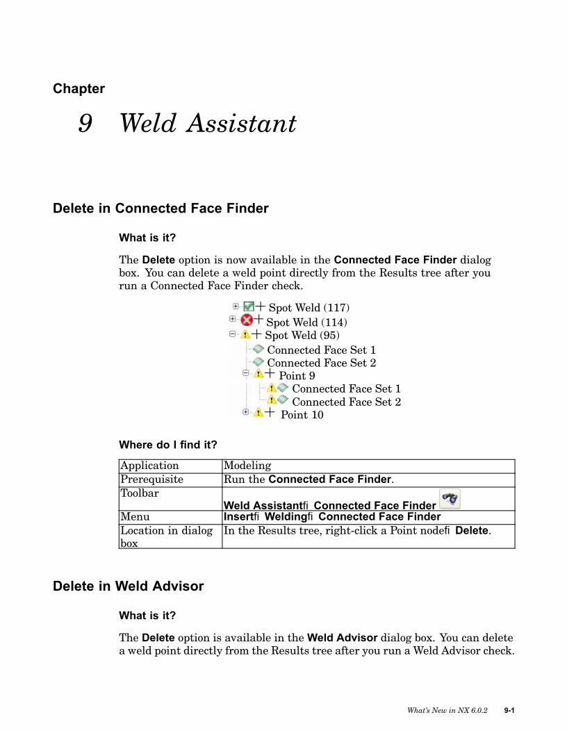
Chapter

9 Weld Assistant

Delete in Connected Face Finder

What is it?

The Delete option is now available in the Connected Face Finder dialogbox. You can delete a weld point directly from the Results tree after yourun a Connected Face Finder check.

Spot Weld (117)Spot Weld (114)Spot Weld (95)Connected Face Set 1Connected Face Set 2Point 9Connected Face Set 1Connected Face Set 2

Point 10

Where do I find it?

Application ModelingPrerequisite Run the Connected Face Finder.Toolbar

Weld Assistant®Connected Face FinderMenu Insert®Welding®Connected Face FinderLocation in dialogbox

In the Results tree, right-click a Point node®Delete.

Delete in Weld Advisor

What is it?

The Delete option is available in theWeld Advisor dialog box. You can deletea weld point directly from the Results tree after you run a Weld Advisor check.


Weld Assistant

Point WLD1Point WLD1Point WLD1Point WLD1Point WLD1Point WLD1

Where do I find it?

Application ModelingPrerequisite Run the Weld Advisor.Toolbar

Weld Assistant®Weld AdvisorMenu Insert®Welding®Weld AdvisorLocation in dialogbox

In the Results tree, right-click a Point node®Delete.

New Auto Point options

What is it?

The Auto Point command has the following new options.

Maximum SingleThickness

Specifies the maximum single metal thickness for all theselected components. If the distance between the topfaces of two panels, or sheets, is greater than the specifiedMaximum Single Thickness plus the specified MaximumFace Gap distance, weld points are not created at thatlocation.

Maximum BendRadius

Specifies the bend radius of a flange. Weld points are notplaced on faces with a radius smaller than this value.

Minimum FlangeWidth

Specifies the minimum flange width. If the opposite sidesof a flange are smaller than the Minimum Flange Width,weld points are not created on that flange.

Where do I find it?

Application ModelingToolbar

Weld Assistant®Auto PointMenu Insert®Welding®Auto PointLocation in dialogbox

Settings group®Maximum Single Thickness/MaximumBend Radius/Minimum Flange Width


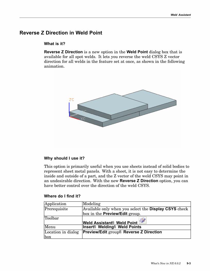
Weld Assistant

Reverse Z Direction in Weld Point

What is it?

Reverse Z Direction is a new option in the Weld Point dialog box that isavailable for all spot welds. It lets you reverse the weld CSYS Z vectordirection for all welds in the feature set at once, as shown in the followinganimation.


This option is primarily useful when you use sheets instead of solid bodies torepresent sheet metal panels. With a sheet, it is not easy to determine theinside and outside of a part, and the Z vector of the weld CSYS may point inan undesirable direction. With the new Reverse Z Direction option, you canhave better control over the direction of the weld CSYS.

Where do I find it?

Application ModelingPrerequisite Available only when you select the Display CSYS check

box in the Preview/Edit group.Toolbar

Weld Assistant®Weld PointMenu Insert®Welding®Weld PointsLocation in dialogbox

Preview/Edit group®Reverse Z Direction


Weld Assistant

Control Direction in Weld Point

What is it?

There are now Control Direction options in the Weld Point dialog box thatyou can use to control the Z-axis direction for spot welds.

Default Specifies the direction of the weld CSYS along the Z-axisusing the default direction.

Opposite Specifies the direction of the weld CSYS along the Z-axisusing the opposite direction.

Note

The default Z direction may be different for different solid types. Forexample, a cylinder’s default Z direction is opposite of the default Zdirection for a measurement vector.


You can use Control Direction options in conjunction with the Reverse ZDirection option for better flexibility in defining connections such as selfpierce rivets.

Where do I find it?

Application ModelingPrerequisite Available only when you create Clinch type weld points

or custom spot welds that use either a cylinder or coneas the display object.

ToolbarWeld Assistant®Weld Point

Menu Insert®Welding®Weld PointLocation in dialogbox

Settings group®Control Directionlist®Default/Opposite


Chapter

10 Ship Design

Manufacturing features

Manufacturing toolbar

Reference Line

What is it?

Reference Line creates a curve lying in a plane parallel to a grid plane at auser-specified offset.

Note

The grid plan is a datum plane created by the Concept module.


Use this line as a point to measure from.

Where do I find it?

Application Ship DesignToolbar

Manufacturing→Reference LineMenu Insert→Manufacturing→Reference Line


Ship Design

Marking Line

What is it?

Marking Line creates curved geometry showing the location of a profile and/orplate on a section of the hull, deck, or bulkhead.


In the context of a section assembly, it is necessary to indicate the location ofprofile and plate parts on a hull section, deck, and/or bulkhead. To accomplishthis, you need to create curved geometry with assigned attributes. Thisgeometry and attributes will be part of the output file for the flame cutter.The flame cutter will scribe this information on the part.

Where do I find it?


Manufacturing→Marking LineMenu Insert→Manufacturing→Marking Line

Plate Preparation

What is it?

Plate Preparation flattens non-planar plates and applies a shrink factor toall plates.


Use Plate Preparation to prepare all plates for manufacturing by flatteningthe plates and/or adding a shrink factor.

Where do I find it?


Manufacturing→Plate PreparationMenu Insert→Manufacturing→Plate Preparation


Ship Design

XML Output

What is it?

This function will outputp flame cutter information used for the cutting ofparts and scribing information on the parts.


Use this functionality to create an XML file, which is used to generate a filethat can be read by the flame cutter to manufacture a part.

Where do I find it?


Manufacturing→XML OutputMenu Insert→Manufacturing→XML Output

Material Allowance

What is it?

Material Allowance creates attributes on the end faces of profiles. Thefunction creates the attribute MK_TYPE and MK_SIZE.


This allowance is needed to compensate for manufacturing and assemblyinaccuracies.

Where do I find it?


Manufacturing→Material AllowanceMenu Insert→Manufacturing→Material Allowance

Vent Hole Marking Sketch

What is it?

Vent Hole Marking Sketch creates a table showing the location of theventilation holes on a part.


Ship Design


Use this function to create a table which shows the X and Y location of eachventilation hole on a part in the flattened state.

Where do I find it?


Manufacturing→Vent Hole Marking SketchMenu Insert→Manufacturing→Vent Hole Marking Sketch

Knuckled Profile

What is it?

Knuckled Profile creates a bend table for profiles that are bent on a brakepress.


In order to manufacture bent profiles from a straight semi-finished material,you need to provide a distance measurement from an edge to the bendcenterline of each bend. Knuckled Profile provides this capability.

Where do I find it?


Manufacturing→Knuckled ProfileMenu Insert→Manufacturing→Knuckled Profile

Inverse Bending

What is it?

Inverse Bending creates curved geometry on a profile.


In order to form curved profiles from a straight semi-finished material, it isnecessary to mark a curve on the profiles. This curve is used as a gaugeduring the bending process. When the curved line becomes straight theprofile is in its formed shape.

Where do I find it?

Application Ship Design


Ship Design

ToolbarManufacturing→Inverse Bending

Menu Insert→Manufacturing→Inverse Bending

Profile List

What is it?

Profile List generates a Bill of Material (BOM) of all the profiles contained ina distributed assembly.


Use this to obtain the information needed for the BOM of the profilescontained in a distributed assembly.

Where do I find it?


Manufacturing→Profile ListMenu Insert→Manufacturing→Profile List

Weld Preparation

What is it?

Weld Preparation adds the needed weld information to a body, by modifyingthe edge of the body for the weld joint type and adding attributes to the body.


Use this function to define the weld joint type and to modify the size and shapeof the body so the flame cutter can cut the body to its proper size and shape.

Where do I find it?


Manufacturing→Weld PreparationMenu Insert→Manufacturing→Weld Preparation


Ship Design

Steel features

Steel Feature toolbar

Profile / Plate

What is it?

The following features are merged in the new Profile / Plate feature:

• Linear Profile

• Non-Linear Profile

• Linear Sheet

• Non-Linear Sheet

You can now choose one feature to create a profile or plate. You do not need toknow if the placement face is planar or non-planar.

Note

The former Sheet feature is now called Plate.


This merger allows you to edit the feature and switch the type from a profileto a plate or from a plate to a profile.

Where do I find it?


Steel Features→Profile / PlateMenu Insert→Steel Features→Profile / Plate


Ship Design

Endcut

What is it?

This option defines an endcut by utilizing the Steel Feature Library function.It also allows you to apply a miter to an endcut feature or to the thicknessface of a solid body.


Use this functionality to modify the end condition of any solid body.

Where do I find it?


Steel Features→EndcutMenu Insert→Steel Features→Endcut

Update Steel Library

What is it?

The reading in of a library part is now a separate step and includes endcuts.


This allows you to read in all of your different library parts before you createa feature and updates the library in a part file if the library changes.

Where do I find it?


Steel Features→Update Steel LibraryMenu Insert→Steel Features→Update Steel Library


Chapter

11 PCB.xchange

PCA import rules

What is it?

You can now setup rules on how NX represents a printed circuit model. Priorto this version, the board was always defined in the master geometry of theprinted circuit assembly (PCA) part. With these new design rules, you canconfigure PCB.xchange so that the board is imported in a separate part andadded as an assembly component to the main PCA part.

On the PCA page of the PCB.xchange Settings dialog box, you can specifyhow to:

• Name the PCA. You can:

– Use the current NX model name.

– Use the ECAD model name.

– Specify a PCA name at import.

• Group PCA entities. This option creates subassemblies in order to classifythe printed circuit entities.

• Import the PCA board, components, and areas. You can import each entityas a master geometry of the main PCA part or an assembly component.


PCA import rules give you more flexibility when importing PCA entities intoNX.

Where do I find it?

Application PCB.xchangeMenu PCB.xchange ® SettingsLocation in dialogbox PCA tab


PCB.xchange

PCB.xchange Settings dialog box enhancements

What is it?

The PCB.xchange Settings dialog box now has the following tabs:

• General

• PCA

• Board

• Holes

• Components

• Keep-ins

• Keep-outs

• Other Areas

• Other Entities

The settings on these different pages let you specify the most commonPCB.xchange work environment variables found in pcbx_ug.ini andpcbx_ug_model.ini initialization files.


Instead of modifying the initialization options in the pcbx_ug.ini andpcbx_ug_model.ini files and then restarting NX in order to have these optionstake effect, you can now set the most common PCB.xchange settings in theimproved PCB.xchange Settings dialog box.

Where do I find it?

Application PCB.xchangeMenu PCB.xchange ® Settings

Import ECAD model in a part file

What is it?

You no longer need to import ECAD models into an NX part file in the NoPart state. For example, if you have a part file with an electronic enclosure,PCB.xchange allows you to directly import a PCA model into this enclosure’spart file.


PCB.xchange

If the part file contains a valid PCB, in order to avoid confusion, it is stronglyrecommended that you design this PCB as a subassembly. To share it withthe imported ECAD model, just make the PCB the work part or the displayedpart.

Where do I find it?

Application PCB.xchangePrerequisite A non empty part fileToolbar

PCB.xchange toolbar® Import ECAD ModelMenu PCB.xchange ® Import ECAD Model

ECAD/NX model comparison enhancement

What is it?

When comparing the current NX model with an existing ECAD model using

the Compare and Update PCA command, you can now preview the

detected changes in the graphics window by selecting Preview Changes .

The following graphic shows the original models and a preview of the detectedchanges.

Original NX model Original ECAD model


PCB.xchange

Detected changes between NX and ECAD models

The following changes are detected:

• Component is not placed at the same location in the NX model andthe ECAD model.

• Component is deleted from the NX model.

• Component is added to the NX model.

If you select one of the changed components from the component list underthe Components Status group, the NX model component and the ECADmodel component are highlighted in the graphics window.


The Preview Changes icon helps you visualize the differences betweenthe NX model and the ECAD model.

Where do I find it?

Application PCB.xchangeToolbar

PCB.xchange toolbar® Compare and Update PCAMenu PCB.xchange ® Compare and Update PCA


PCB.xchange

Filtering enhancements

What is it?

The improved Filters List dialog box contains pre-defined and user-definedfilter rules.

When you import, export, or compare and update ECAD models, you can nowselect the entities to remove in the Filters List dialog box. You can select:

• Different types of holes.

• Different types of components.

• Different types of restriction areas.


The filter rules are now much easier to use with the improved Filters Listdialog box.

Where do I find it?

Application PCB.xchangeToolbar

PCB.xchange toolbar ® Import ECAD Model /

Export ECAD Model / Compare and Update PCA

Menu PCB.xchange® Import ECAD Model / Export ECADModel / Compare and Update PCA


In Import Options, Export Options, or Compare Optionsgroup, select Use Entity Filter / Use Entity Filter on NXmodel / Use Entity Filter on ECAD model ® Filter List


Chapter

12 PCB.xchange + Zuken

What is it?

PCB.xchange + Zuken is a new application that lets you import or export PCBassemblies in the Zuken’s CR5000 native format.

You import or export Zuken format files the same way you import or exportfiles of other supported formats. All functionality previously supported forother file formats is also supported for the Zuken format. In addition, theZuken format supports the import and export of flexible printed circuits,traces, pads, metal, and resist masks.

On the Other Entities page of the PCB.xchange Settings dialog box, youcan specify how to:

• Import traces, pads, masks, and internal layers from Zuken format filesin the Import Rules group.

• Export projection view of the PCB to Zuken format files in the ExportRules group.

By default, PCB.xchange + Zuken imports and exports to version 10 of theCR5000 application. You can change this to version 9 by setting the followingenvironment variable UGII_PCB_CR5000_VERSION to 9.

Where do I find it?

Application PCB.xchange + ZukenPrerequisite An active PCB assemblyToolbar

PCB.xchange toolbar®Export ECAD ModelMenu PCB.xchange®Export ECAD ModelLocation in dialogbox

Export Options®File Format®Zuken bmb or Zuken pcb

Note

For import, file type is automatically detected.


What's New in NX 6.0.2

Documents

Transcript of What's New in NX 6.0.2