BSc(B), 6th. Semester Author:

Thomas Lassen

Advisor:

Philipp Schröder

Bachelor Thesis

What are the economic consequences of the EU's 

CAP on trading with Africa? 

Aarhus School of Business,

University of Aarhus

Spring 2009

Table of Contents 1  Executive Summary ..................................................................................................................... 4 

2  Introduction .................................................................................................................................. 6 

2.1  Problem Statement ................................................................................................................ 7 

2.2  Methodology ......................................................................................................................... 8 

2.3  Delimitations ......................................................................................................................... 8 

3  Africa-EU trade development ...................................................................................................... 9 

4  Agricultural and trade policies ................................................................................................... 11 

4.1  Agriculture in development ................................................................................................. 11 

4.1.1  Infrastructure ................................................................................................................ 12 

4.1.2  Agricultural trade and development ............................................................................. 12 

4.1.3  Liberalization ............................................................................................................... 13 

4.2  The Common Agricultural Policy ....................................................................................... 14 

4.2.1  Reforms of the CAP ..................................................................................................... 15 

4.3  Relationship between the EU and Africa ............................................................................ 19 

4.3.1  ACP-EU agreements .................................................................................................... 19 

4.3.2  The Cotonou Agreement .............................................................................................. 19 

4.3.3  Everything But Arms ................................................................................................... 20 

4.4  Agricultural trade after the 2003 CAP reform ..................................................................... 21 

4.5  WTO agreements ................................................................................................................. 22 

4.5.1  The Uruguay Round ..................................................................................................... 22 

4.5.2  The Doha Round .......................................................................................................... 23 

5  Trade theories ............................................................................................................................. 23 

5.1  Basic trade theory ................................................................................................................ 23 

5.1.1  Tariffs ........................................................................................................................... 24 

5.2  Customs union ..................................................................................................................... 25 

Page | 1

5.3  CAP effects on trade............................................................................................................ 27 

5.3.1  Production subsidies .................................................................................................... 27 

5.3.2  Intervention prices........................................................................................................ 28 

5.3.3  Export subsidies ........................................................................................................... 29 

5.3.4  The 2003 CAP reform .................................................................................................. 29 

5.4  ACP-EU trade agreements .................................................................................................. 29 

5.4.1  Removal of tariffs ........................................................................................................ 30 

5.4.2  Food safety standards ................................................................................................... 31 

5.4.3  The 2003 CAP reform .................................................................................................. 31 

5.5  Theoretical situation today .................................................................................................. 32 

6  Gravity Equation ........................................................................................................................ 33 

6.1  Theory of gravity equation .................................................................................................. 34 

6.2  Determining a model ........................................................................................................... 36 

6.3  Data collection ..................................................................................................................... 37 

7  Gravity equation analysis ........................................................................................................... 38 

7.1  Intra-EU trade ...................................................................................................................... 38 

7.2  Africa-EU trade ................................................................................................................... 40 

7.2.1  Deriving a new model .................................................................................................. 43 

7.3  A new model for Africa-EU trade ....................................................................................... 44 

7.4  Using a control group for Africa-EU trade ......................................................................... 46 

7.5  Difference in import and export of agricultural goods ........................................................ 49 

7.5.1  Import ........................................................................................................................... 49 

7.5.2  Export ........................................................................................................................... 50 

7.6  Conclusions of the gravity equations .................................................................................. 51 

8  Interpretation of results .............................................................................................................. 52 

8.1  Difference in level of agricultural trade .............................................................................. 52 

Page | 2

8.2  Difference in import and export .......................................................................................... 53 

8.3  Impact of FTAs ................................................................................................................... 54 

8.4  Former colonies ................................................................................................................... 54 

8.5  Landlocked countries and islands........................................................................................ 54 

9  Future research steps .................................................................................................................. 54 

9.1  Development aid.................................................................................................................. 54 

9.2  Regions and Free Trade Agreements .................................................................................. 55 

9.3  Policy changes ..................................................................................................................... 55 

9.4  World trade .......................................................................................................................... 55 

10  Conclusion ................................................................................................................................. 56 

11  Bibliography............................................................................................................................... 58 

Appendix A ........................................................................................................................................ 61 

Appendix B ........................................................................................................................................ 62 

Appendix C ........................................................................................................................................ 65 

Appendix D ........................................................................................................................................ 65 

 

Page | 3

1 Executive Summary 

The agricultural sector is crucial for the development and later industrialization of a country. Ac-

cording to several researchers the improvement of productivity in the agricultural sector, and hence

the movement of labor form the agricultural to the production sector, is the base of moving coun-

tries away from poverty. Since the EU, and others, pays a lot in development aid to African coun-

tries, it is interesting to investigate how EUs agricultural support system (CAP) affects the African

countries. The aim of this thesis has been to see what role the CAP has on agricultural trade with

African countries, and therefore also on their economy and development.

Theory suggests that African countries enjoy a comparative advantage in the agricultural sector

compared to the EU. This is due to the development stage of the African countries, as well as the

relative labor and land abundance. Trade figures also show that African countries export more agri-

culture to the EU than they import, but in recent years import have grown relative more than export.

This might suggest some form of distortion in the market.

A look at the EUs CAP shows that it has several trade distorting effects according to theory. In the

beginning the CAP was made up of production subsidies, intervention buying, and export subsidies.

Through several reforms with the aim of creating a more liberalized market, the production subsi-

dies have been changed to a direct subsidies scheme and intervention prices have been lowered a

bit. The production/direct subsidies and the intervention buying both create higher prices in the in-

ternal EU market. This means that two much is produced, and most overproduction is sold to world

market prices with the aid of export subsidies. Through underestimation of the world market prices

the EU has been accused of dumping agricultural products into the African markets.

In the opposite direction several agreements have been made to ensure African producers tariff free

access to the European market. However, very high food safety standards have been set along with

other non-tariff barriers, which prevent many African producers to export to the EU.

Trade theory suggests that a free trade situation would result in the EU importing much of their

agricultural consumption from Africa. However the high minimum prices on the EU market have

resulted in far less consumption and held together with the much higher production, the EU have

gone from being net importer to net exporter of agricultural goods. Due to the tariff free access of

the African producers, all their production would be sold to the EU at the high prices, as no African

consumers are willing to pay these high prices. On the other hand the EU overproduction would be

Page | 4

exported to the African market at world market prices. Several reforms of the CAP and trade

agreements have improved this situation a bit, but it is still the theoretical outcome.

In order to test if theory applies, a quantitative analysis has been conducted of the situation using

the gravity equation. The gravity equation uses trade value as a dependent value and analyses how

several variables, such as GDP, population, and distance, influence bilateral trade between coun-

tries. To see if the CAP affects agricultural trade with Africa, it is important to isolate agricultural

trade from other trade, and see if a difference exists. The results show that Africa trade relative

more in agriculture than non-agriculture with the EU. What is really interesting is that results show

the other EU countries trade more with the EU than Africa does, a result that is contradicting to the

theory of a free market, but is in compliance with the theoretical trade distorting effects of the CAP

and trade agreements.

Besides all the theoretical explanations of subsidies, tariffs, and minimum prices, other reasons can

be found to the situation. Non-tariff barriers presumably play a large role in restricting the African

producers from exporting to the European market, but also supply restraints have a large effect on

the trade outcome. Trade theory is based on unlimited resources, but the small African farmers have

a hard time obtaining more land and thereby expanding production. To make matters worse, the

lack of decent storage facilities often force farmers to sell their harvest right away, sometimes at

very low prices.

Future research into several areas would be interesting, especially into the relation between devel-

opment aid and agricultural support systems. This could show how to help the African agricultural

sector in the best way. Also, it could be interesting to conduct quantitative analysis of the policy

changes made to the CAP and trade agreements, to see what effects these have had in reality.

   

Page | 5

2 Introduction 

Development aid to Africa is one of the big political subjects of today, and many developed coun-

tries pay large sums of monetary aid to these and other developing countries. However, questions

have started to arise if development aid is the right way to help these poor countries. A good and

effective agricultural sector is seen as the cornerstone in developing and industrializing a country.

But how is the developed world, mainly the EU and USA, helping building this foundation? Both

have enormous agricultural support systems domestically, where especially the large Common

Agricultural Policy (CAP) in the EU has dramatic effects on the world market for agricultural

goods. Do these support systems actually undermine the agricultural sector in African countries and

hence hinder their development? If this is the case, we have a quite complex situation. Enormous

sums are paid to help the development of the very same countries, which own support systems in

effect hold down. To find out if there is any ground to these claims, I will try to investigate whether

the EU’s CAP has any effect on agricultural trade with African countries1 and thereby also the

economy and development of these countries.

A quick look at the trade situation today, and how it has developed during recent years, will start off

the investigation. As this in itself does not tell us anything about the CAP’s effect on trade it is

merely to give an overview of the trade development.

To give a better insight into the trade situation, a more detailed description will be made of the EU-

Africa trade relationship. This description will include the roles of agriculture and international

trade in the development of a country, to give a brief glance of what is at stake. Also the CAP and

any trade agreements between the two regions will be assessed and various critique points will be

discussed.

To put the situation into a more theoretical perspective, the described scenarios will be put into the

context of international trade theories. By putting the existing policies and agreements into a theo-

retical framework we will obtain a basis for analyzing how reality is.

A statistical analysis will be conducted on how the CAP affects the agricultural trade between Afri-

ca and the EU. This will be done in order to obtain empirical evidence to answer the questions

asked in the problem statement. As the CAP is not new in any way it will be hard to determine how

a world without the CAP would look like. Therefore any results will be held up against trade theory

1 Because of obvious difference in culture and development stage I will be putting my focus on the sub-Saharan African countries, thus excluding the Northern African Arabic countries. This means that referral to Africa will, unless stated otherwise, be to the sub-Saharan African countries.

Page | 6

of how the world market should look in a free market setting.

The statistical analysis will hopefully show some interesting results of how the trade situation is

between Africa and the EU. Therefore an assessment of the results, and why we obtain these partic-

ular results, will be conducted. This will consist of secondary literature findings as well as reason-

ing between description, theory, and results. At the end of this section a comprehensive overview of

the situation should have emerged.

Before concluding on the findings in the research, a section will be dedicated to suggesting future

research steps, which could be conducted if further knowledge of the area is desired.

2.1 Problem Statement The questions I will aim to answer within this thesis are the following:

How does EU’s CAP affect agricultural trade between sub-Saharan Africa and the EU?

• How does theory suggest the current situation affects trade?

• Can a difference in trade value be found between the two regions due to the CAP?

• How do political agreements between the two regions play into the situation?

In order to asses if the CAP has an influence on agricultural trade it is crucial to look at theory as

well as statistics. If theoretical and statistical analyses complement each other, much stronger con-

clusions can be drawn. Also a look at the influence of other political agreements is important, as

they can alter the effect the CAP might have.

A change in the trade situation will indisputably also have an effect on the economy, which leads to

the next issue:

What are the economic consequences of the EU’s CAP on sub-Saharan Africa?

• Are the African countries better or worse of due to the CAP?

• Does the existence of the CAP hinder development of African countries?

• What are the economical ramifications of the individual components and changes of the

CAP and other policies?

It is important to determine how the economy is affected in order to put the effects into a develop-

ment perspective later on. The development perspective is of course very interesting, as we might

determine if the CAP, and thereby also the EU, is holding back the development of African coun-

tries through protection of own interests.

Page | 7

The individual components and policy changes are quite interesting in order to determine which

parts of the CAP have influence on the economical outcome.

2.2 Methodology This thesis will be based on economical theory which will be supported by research literature of the

subject and data analysis. Quantitative analysis will be used as the main analytical method. An em-

phasis will be put on trustworthy sources for literature and data, which will primarily be collected

from peer reviewed journals and international organizations.

2.3 Delimitations Models for assessing agricultural trade policies such as the Word Agricultural Trade Simulation

(WATSIM) model (von Lampe, 2002) will not be used. This is due to the complex nature of the

model, and the use would simply be without the scope of this thesis.

Some African countries and organizations use French and other non-English languages, and there-

fore available information may be in a language without the reach of my language skills.

Also, due to the low level of development in most African countries, statistics will often be scarce

and the needed statistics may not be available through African countries, but rather international

organizations.

Due to the limited size of this thesis some issues will be left out of the analysis. First of all, no pa-

rallel will be drawn between the agricultural trade and development aid, which was mentioned in

the introduction. This subject is simply too comprehensive. Second, trade between other regions

than the EU and Africa will not be dealt with, as again this will simply be too large a subject for this

thesis. Also, agricultural and other reforms in the individual African countries will not be given any

attention, all though these might in fact affect the trade outcome. The detail in looking at every sin-

gle country is simply too much compared to the presumably limited effect it has on agricultural

trade for the whole region. Finally, the effects of the enlargements of the EU will not be considered,

even though this has changed the competitive situation on the world market, as more countries

where let into the internal EU marketplace, especially since these new countries have a much larger

agricultural sector than the existing EU-15. However it is far too extensive to include this subject

into the limits of this thesis.

 

Page | 8

3 Africa­EU trade development 

Trade in agriculture is the main focus in this paper, so a glance at the trade development should be

interesting, before describing and analyzing the complex trade situation between the EU and Africa.

Descriptive statistics can help to give an overview of what we are dealing with. Theory and analy-

sis, which will be applied later, can tell a lot about how the situation should look, or what lies be-

hind the current situation, but only descriptive statistics give a picture of how the situation actually

is.

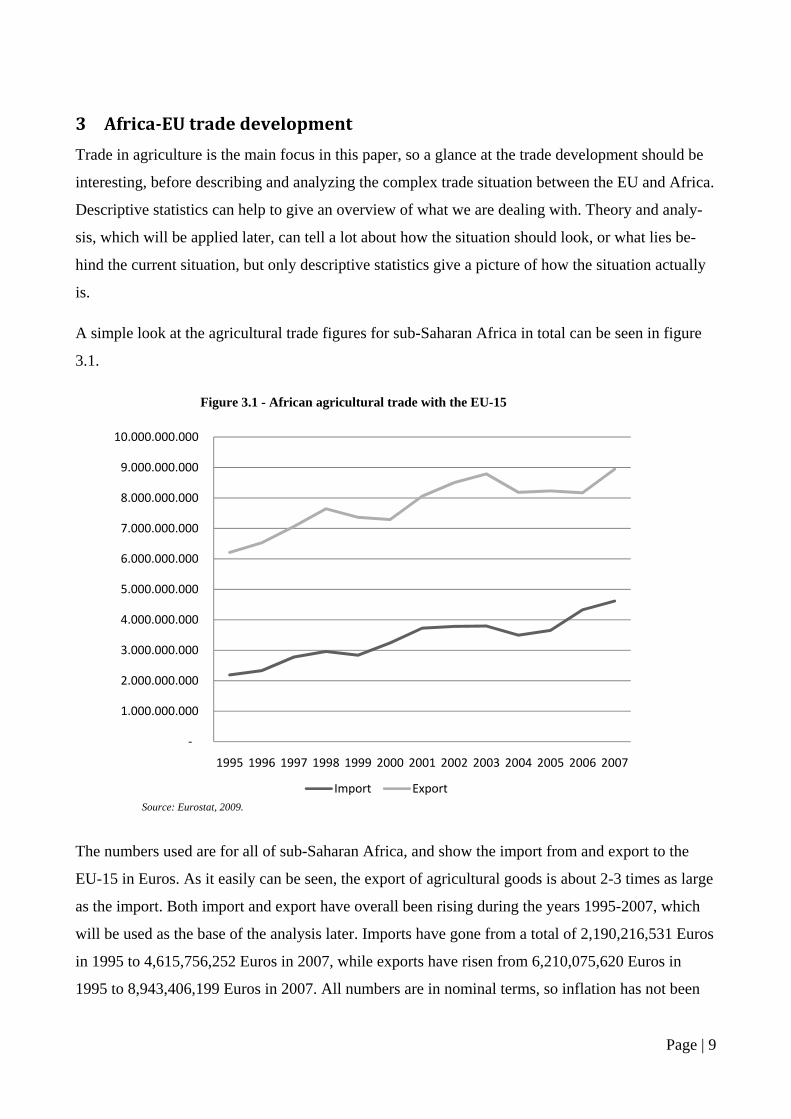
A simple look at the agricultural trade figures for sub-Saharan Africa in total can be seen in figure

3.1.

Figure 3.1 - African agricultural trade with the EU-15

‐

1.000.000.000 

2.000.000.000 

3.000.000.000 

4.000.000.000 

5.000.000.000 

6.000.000.000 

7.000.000.000 

8.000.000.000 

9.000.000.000 

10.000.000.000 

1995 1996 1997 1998 1999 2000 2001 2002 2003 2004 2005 2006 2007

Import ExportSource: Eurostat, 2009.

The numbers used are for all of sub-Saharan Africa, and show the import from and export to the

EU-15 in Euros. As it easily can be seen, the export of agricultural goods is about 2-3 times as large

as the import. Both import and export have overall been rising during the years 1995-2007, which

will be used as the base of the analysis later. Imports have gone from a total of 2,190,216,531 Euros

in 1995 to 4,615,756,252 Euros in 2007, while exports have risen from 6,210,075,620 Euros in

1995 to 8,943,406,199 Euros in 2007. All numbers are in nominal terms, so inflation has not been

Page | 9

taking into account in these figures. However it is clear to see that imports have more than doubled

in the period, while exports have risen less than 50%, so imports have grown relatively more than

exports.

A look at the figures for the individual African countries shows that export figures are a lot more

volatile between countries than import. While countries like Liberia, Djibouti, Guinea, and Sierra

Leone all have exports worth less than one million Euro in 2007, all countries expect Liberia have

imports for more than one million Euros. In general there are far more countries who in the 13 year

period export for less than one million Euros than countries who import below this level. Some of

the export numbers are even extremely low being below 100,000 Euros. It is also notable that a

large country as South Africa in some years has had imports for less than one million Euro, which is

probably due to South Africa’s special status amongst the African countries. The composition of the

trade in individual countries is interesting since export is so much higher than imports, and some

countries apparently are not contributing to this.

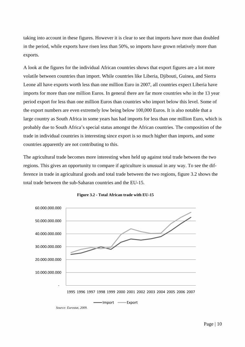
The agricultural trade becomes more interesting when held up against total trade between the two

regions. This gives an opportunity to compare if agriculture is unusual in any way. To see the dif-

ference in trade in agricultural goods and total trade between the two regions, figure 3.2 shows the

total trade between the sub-Saharan countries and the EU-15.

Figure 3.2 - Total African trade with EU-15

‐

10.000.000.000 

20.000.000.000 

30.000.000.000 

40.000.000.000 

50.000.000.000 

60.000.000.000 

1995 1996 1997 1998 1999 2000 2001 2002 2003 2004 2005 2006 2007

Import ExportSource: Eurostat, 2009.

Page | 10

The figure shows that import and export are much closer for total trade than agriculture. However it

might be a surprise that total export is actually larger than total import, considering Africa’s tech-

nological development stage.

Again export figures seem to be a bit more extreme values, as several countries have exports below

10 million Euros, while all import figures are above this level.

Hopefully this paper can help explain some of the reasons lying behind these trade figures, through

the research of the agricultural trade situation.

4 Agricultural and trade policies 

The interest of this thesis is to look at the CAP in terms on economical impact on Africa. This is

interesting because the western world keeps paying a lot of money in development aid, while at the

same time financing an expensive protectionist agricultural sector. Because the consensus in general

is that a good agricultural sector is the basis for industrializing, and hence develops a country, it is

of great concern to many that the CAP is undermining the establishment of a sturdy agricultural

sector in Africa. A quite striking figure to start off with is the OECD countries’ support to agricul-

ture of US$ 311 billion, which is six times the value of official development assistance (Nelson and

Halderman, 2004).

4.1  Agriculture in development The most important commodity group for every country is food, in order to survive. Therefore agri-

culture is at the base of every society, and the concentration of manpower in this sector determines

how much manpower can be employed in other sectors. As Haque (2007) puts it; “Economic devel-

opment implies structural transformation, typically from low productivity to high productivity ac-

tivities, from agriculture and simple manufacturing activities to modern industry”. This really high-

lights the base of this school of development theory. In order to develop, a country must become

more productive. As far most developing countries have large agricultural sectors this is obviously

the sector to enhance productivity in. For African countries the average agricultural percentage of

GDP was 32% (World Bank, 2009) during the years 1995-2007, while the average for EU countries

is 2-3%. Of course there are great deviations between countries, especially in Africa, where the

range is from Botswana with 2-4% in all years to Liberia which had 94% in 1996 but had come

down to 64% in 2007. When agriculture constitutes this much of a countries economy it is easy to

see why it is of such great importance. So in order to develop a country, the thought is to increase

Page | 11

productivity in the agricultural sector, freeing up labor to work in other industries, hence increasing

the size of other industries. This thought is underpinned by the fact that employment in agriculture

is above 60% of the total workforce in African countries (FAO, 2006).

However agricultural growth also has a direct positive effect on growth of other sectors, according

to Thirwall (Morrison and Sarris, 2007). When the agricultural sector starts to grow the demand for

non-agricultural products will increase, as the wealth of the country becomes higher. This increase

in demand will logically lead to growth in the non-agricultural sector, which in time will become

competitive in the international market, and therefore a growth through export will commence.

4.1.1 Infrastructure It is also clear that Africa has the capacity to become a great agricultural contributor. The sub-

Saharan countries in total have 198 million hectares of arable land (FAO, 2006), and much of this is

unused or even unexplored. The main problem seems to lie within the infrastructure of the coun-

tries. Water is not being utilized in an optimal way, which is crucial to fight droughts. Currently

only 1.6% of water is utilized (FAO, 2006). This leads to only 4% of the land being used efficiently.

Therefore a water management system is one of the many measurements that will need to be taken

in the improvement of the infrastructure. Other obvious improvements are within the transport sec-

tor.

Timmer (Morrison and Sarris, 2007) has found that there are three main agricultural development

theories in modern research; one with a free-market approach, one focusing on rural development,

while the last emphasizes the importance of price and marketing in the agricultural sector. What is

interesting, however, is that these three different theories all conclude that government investment

in infrastructure is crucial to further development, although they differ greatly in how to make the

right investments.

Because of the inadequate infrastructure, transport costs and insurance represent more than 25% of

the costs of agricultural goods in 1/3 of the countries (FAO, 2006). These high extra costs are of

course damaging for the international competitiveness of agricultural goods from Africa, which

leads us to the next issue in the subject.

4.1.2 Agricultural trade and development So far I have not mentioned anything about the role in international trade in this issue. This section

will primarily discuss the theories of trade and development, while more specific trade policies and

trade theories will be discussed in depth in a later section. International trade plays a great role in

Page | 12

the whole matter for obvious reasons; if African countries can become more productive in agricul-

ture (or any sector for that matter), they will be more competitive on the international market, which

will lead to an increase in trade and eventually economical growth. Haque (2007) remarks that it is

not as simple as this basic theory describes. The intense focus on low cost production, used in great

parts of Asia, will simply not be applicable today since the world has changed in the direction of a

more globalized world. He adds that a producer now has to be a part of a network or value chain,

and to become this needs to have a proven record of production. If this is in fact the case, African

countries will be put in the bottom of this value chain (if anywhere), where the profit is the lowest.

Looking at agricultural products the far most value addition is in the processing of these into differ-

ent types of food. If African countries are simply selling raw agricultural goods to other countries

for processing, there will be little value added and thereby little growth. To establish oneself as a

producer (or processor of these raw goods), one has to have a proven track record within this area to

compete on the international market, according to Haque (2007). This makes it extremely hard to

get a production culture started, and is of course a great obstacle for development in the African

countries. What is more or less ironical is that these goods may be re-imported to the same coun-

tries, once they have been processed in other countries.

4.1.3 Liberalization The main discussion in international trade communities is to which degree trade should be libera-

lized. Morrison and Sarris (2007) argue that too much liberalization in the crucial agricultural sector

can be hurtful for the development of a country, and that some level of protection can be helpful in

this matter. They go on to argue that in the light of the Doha round (which will be described later),

where agricultural trade liberalization is a great issue, some categories of developing countries

should be allowed flexibility in their protection of the agricultural sector for two main reasons. First

of all, it will help the domestic agricultural sector in competing with imports that might be subsi-

dized, and therefore have an unfair low price (as examples from the EU will show later on). Second,

the flexibility will help to change the tariff structure once the development process is so far along

that agriculture does not play a central role in the economy. However, the developed countries are

anxious to gain easier access to these developing markets, and are pushing hard to lower barriers of

entry (Morrison and Sarris, 2007). This refers directly back to what started my interest in this sub-

ject, why developed countries donate so much money in development aid, while policies might con-

tradict any efforts towards development.

Page | 13

4.2 The Common Agricultural Policy In the beginning the Common Agricultural Policy (CAP) was developed under the Treaty of Rome

to ensure food supply in Europe, after years of war, and maintain a reasonable standard of living for

workers employed in agriculture (Cardwell, 2004). This was mainly done through minimum price

guarantees and subsidies for investments in technology and development of rural areas (European

Commission, 2007). Nelson and Halderman (2004) argue that the CAP was one of the main plat-

forms of the development of what has now become the European Union. Early tools to reach the

guaranteed price levels were to impose taxes on imports and intervention buying when prices within

the EU fell too low. The minimum prices were set to such a level that the least efficient producers

could still survive as producers (Trebilcock and Howse, 2005), which of course meant that more

efficient producers made large profits. Facing a market that guaranteed minimum prices, farmers, of

course, produced as much as possible to earn a maximum profit, as Martin puts it; ‘European far-

mers have demonstrated beyond a shadow of a doubt that they are economically rational’ (Trebil-

cock and Howse, 2005). By the 1980’s this started to lead to enormous surplus stocks of food from

all the intervention buying from the EU. One way to get rid of these surpluses was of course to ex-

port them to other countries by paying the farmers the difference between the guaranteed price and

the lower world price level. According to Trebilcock and Howse (2005), critics have argued that the

EU actually constantly underestimated the world market price; hence effectively selling agricultural

products bellow the world market price. This has in turn resulted in several accusations of dumping,

especially into Africa and other developing countries, and in some cases these accusations have

found to be true. For instance, reports have concluded that the EU dumped beef at unreasonable low

prices into West and South Africa during the 1980’s and 90’s, as well as skimmed milk power into

Jamaica and other countries (Nelson and Halderman, 2004). But dumping is not the only issue con-

cerning the CAPs influence on world markets. By selling enormous volumes of agricultural prod-

ucts, a bias is created in the world market, lowering the price below its natural level. This develop-

ment of the CAP to have a large effect on the international market, has, according to Trebilcock and

Howse (2005), developed the CAP from keeping foreign producers out of the European market, to

making it increasingly harder for them to survive in their domestic markets.

Based on all these forms of subsidies to farmers, the expenditures of the CAP has reached astro-

nomic levels accounting for nearly half of the EU expenditure, even after two of the three reforms

described below. The budget figures for 2000-2006 actually show a rising share of agricultural ex-

penditure. For 2000 agricultural expenditure was set to 40,920 million Euros while total EU ex-

Page | 14

penditure was budgeted at 91,995 million Euros. These budget figures shifted to 41,660 and 90,260

million Euros in 2006 (Cardwell, 2004). This has been the subject of much internal criticism in the

EU from organizations, politicians, and citizens. These, and other, issues have lead to several re-

forms of the CAP system.

4.2.1 Reforms of the CAP There have been three actual reforms of the CAP since it was first implemented. I will be explaining

the first to rather brief in order to understand the movements in the CAP, while the latest reform of

2003 will be discussed in more detail, in order to obtain a picture of the situation today. The main

focus will be on what effects the reforms have on interaction with international markets, and rather

internal policy changes will be described briefly or simply mentioned.

4.2.1.1 The MacSharry Reform 

The first official reform of the CAP came in 1992 with the MacSharry Reform. The reform had two

main concerns to address, and two different communities to please. The first objective was to bring

the market back into balance (Cardwell, 2004). The enormous stocks of agricultural goods that

where being stored in the EU at this time generated large costs on many levels, and the solution of

simply exporting the surplus of goods seemed to be distorting international market. Storage and

handling of agricultural goods in its self generates high costs, along with the transportation costs to

these storage facilities. On top of this, a large overproduction implies that too much is being paid in

subsidies to the farmers, or too much intervention buying is taking place. To further complicate

matters there are also great costs to the consumers, who in the first place pay the taxes to finance the

CAP. Consumers also have to pay higher prices for agricultural goods, as EU prices are artificially

high, while imports from cheaper countries are being taxed to reach the same high price. So the goal

was to find a way to bring down these costs while still maintaining a decent standard of living for

the European farmers.

The second concern was towards the international market. Because of the many accusations of

dumping in developing markets and the general distortion of world market prices, there was in-

creased pressure on the EU to change the CAPs external effects. Especially the United States where

interested in liberalization of world trade (Cardwell, 2004), perhaps so they could gain more access

to the markets where the EU was selling cheap agricultural goods. At the same time as the Mac-

Sharry reforms were conducted the Uruguay Round in the GATT was undergoing, with great focus

on liberalization in world trade, including agriculture. Therefore the GATT, and especially the

Page | 15

USA, had to be satisfied with the reform. Ironically it was not the developing countries, who were

direct affected by the policy, who objected the most, perhaps due to lack of political and economical

power.

The most important measure of the MacSharry reform was the shift from production subsidies to

direct payment of the farmers. The aid to the farmers no longer relied on their level of production,

as such, but were paid on a direct payment scheme (Cardwell, 2004). This also resulted in prices

being lowered, in the best interest for all of the concerns raised earlier. In return for these direct

payments, quotas were imposed on the farmers in order not to reach the same levels of overproduc-

tion.

Other elements of the MacSharry reform was to encourage more environmental friendly agricultural

production, early retirement schemes for farmers, aid for forestry, and a movement away from pay-

ing aid in modules.

4.2.1.2 Agenda 2000 

The document ‘Agenda 2000’ was issued in July 1997. In the preface to the reform the European

Commission made the following statement in the Cork Declaration: “the Common Agricultural Pol-

icy will have to adapt to new realities and challenges in terms of consumer demand and preferences,

international trade developments, and the EU’s next enlargement” (Cardwell, 2004). This declara-

tion was made in March 1998 along with a set of proposed regulations of the initial suggestions of

the July 1997 document. The regulations were seen as less ambitious than the original proposals,

while the final reform differed even further from these proposals.

The basics behind the Agenda 2000 focused on five different areas. First of all a reduction of the

intervention price was proposed, in order to further liberalize the agricultural market. Second and

third areas were to put more focus on rural development and environment. Furthermore the reform

should take a look at the financing of the CAP, and finally, a structural reform should take place, in

order to prepare the CAP for the Eastern enlargement of the EU (Cardwell, 2004).

The final reform was agreed upon at a summit in Berlin in March 1999. All of the focus areas were

touched upon although to different extents. A reduction of intervention prices in three main areas

was agreed, these areas being arable crops, beef and veal, and milk and milk products. Table 4.1

shows the intervention price changes created by the reform for cereals and beef, and as the figures

clearly show the actual price reductions were somewhat lower than initially suggested. Also, the

reduction in intervention prices was implemented in two and three steps, instead of an initial one

Page | 16

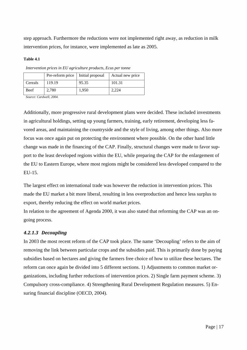
step approach. Furthermore the reductions were not implemented right away, as reduction in milk

intervention prices, for instance, were implemented as late as 2005.

Table 4.1

Intervention prices in EU agriculture products, Ecus per tonne

Pre-reform price Initial proposal Actual new price

Cereals 119.19 95.35 101.31

Beef 2,780 1,950 2,224 Source: Cardwell, 2004.

Additionally, more progressive rural development plans were decided. These included investments

in agricultural holdings, setting up young farmers, training, early retirement, developing less fa-

vored areas, and maintaining the countryside and the style of living, among other things. Also more

focus was once again put on protecting the environment where possible. On the other hand little

change was made in the financing of the CAP. Finally, structural changes were made to favor sup-

port to the least developed regions within the EU, while preparing the CAP for the enlargement of

the EU to Eastern Europe, where most regions might be considered less developed compared to the

EU-15.

The largest effect on international trade was however the reduction in intervention prices. This

made the EU market a bit more liberal, resulting in less overproduction and hence less surplus to

export, thereby reducing the effect on world market prices.

In relation to the agreement of Agenda 2000, it was also stated that reforming the CAP was an on-

going process.

4.2.1.3 Decoupling 

In 2003 the most recent reform of the CAP took place. The name ‘Decoupling’ refers to the aim of

removing the link between particular crops and the subsidies paid. This is primarily done by paying

subsidies based on hectares and giving the farmers free choice of how to utilize these hectares. The

reform can once again be divided into 5 different sections. 1) Adjustments to common market or-

ganizations, including further reductions of intervention prices. 2) Single farm payment scheme. 3)

Compulsory cross-compliance. 4) Strengthening Rural Development Regulation measures. 5) En-

suring financial discipline (OECD, 2004).

Page | 17

First of all, the adjustment of the common market organizations simply changed the amounts and

prices for support and intervention in the existing policy. Many areas were liberalized, and for some

goods, such as rye, intervention was removed completely. These adjustments were also made to

prepare the policy for the new single farm payment scheme by specifying which areas were to be

included into this policy. The adjustments can also be seen as a part of the ongoing process of re-

forming the CAP, so that it always attempts to fit the new market needs and demands.

The next area is the most revolutionary part of the 2003 reforms, namely the single farm payment

scheme (SFP). This is where the decoupling actually takes place, and direct payments are now cal-

culated on the basis of former direct aid and hectares of the individual farm. However, payments are

based more on a regional level, where each region is responsible for determining the level of aid per

hectare, based on other concerns as well. The main idea behind this decoupling is to obtain less di-

rect interference with the individual commodity markets. By letting the farmers chose what to pro-

duce themselves, the agricultural market resembles a free market a bit more, although the existence

of intervention and export subsidies still prevents a normal market behavior. A few restrictions still

exist within fruit, vegetables and table potatoes, as well as certain standards to the agricultural and

environmental condition of the land are set. There are some possibilities in the reform for regions to

promote certain crops over others, along with other exceptions to the strict hectare payment scheme.

The principle of compulsory cross-compliance is closely linked to the SFP. It is in all simplicity a

set of requirements farmers need to fulfill in order to receive the aid from EU. Complementing this

are a set of rules regarding penalties in the situation these requirements are not fulfilled. These set

of rules are a necessity after aid is no longer linked to production, as farmers could simply stop pro-

ducing and still collect aid based on their hectares, if no requirements were set.

More aid schemes exist under the rural development regulations. Examples of these are aid to par-

ticipate in quality improvement programs, in order to improve the quality of agricultural goods. In

addition to this, farmers can also receive aid to meet the stringent standards set by the EU, and to

ensure environment protection and animal welfare. These measures are all a part of ensuring further

development in the agricultural sector, and ensuring the highest standards of agricultural goods,

which also gives an advantage, when trading on the international market, but distorts the market for

foreign producers.

Page | 18

The final measure of the 2003 reforms is a financial control system to ensure that the spending on

CAP does not spin out of control. Already employing such a large post of the EU budget, there is a

public pressure to reduce spending on agricultural support.

4.3 Relationship between the EU and Africa At the heart of the subject of trade between EU and Africa is the political relationship between the

two regions. Again the main focus will naturally be on trade between the two regions, in particular

in the agricultural sector.

4.3.1 ACP­EU agreements Several agreements have been made between the EU and Africa starting with the Yaoundé Agree-

ments from 1959-1974. The Yaoundé Agreements where followed by the Lomé Conventions from

1975 until 2000 where the existing Cotonou Agreements were reached. As of the start of the Lomé

Conventions the organization ACP was founded to represent the developing countries as one. Be-

sides the sub-Saharan African countries the ACP also contains some Caribbean and Pacific coun-

tries, though with the African countries being the dominant force representing 48 of 79 countries in

the ACP. The main aim of the Lomé Conventions was to improve the trade relationship between the

regions, which has been done by slowly liberalizing trade agreements.

However the focus will be on the existing Cotonou Agreement, as to give a picture of the trade rela-

tionship the countries face today.

4.3.2 The Cotonou Agreement The Cotonou Agreement in itself provides free access for the ACP countries into the EU markets,

with some exceptions. This is believed to be achieved in a better way when adopting regional dif-

ferences into the agreement, and therefore negotiations are taken up at a regional level. The main

new part of the Cotonou Agreement compared to the Lomé, is the creation of so called Economic

Partnership Agreements (EPAs). These have a purpose of promoting further regional integration of

the ACP countries, which for Africa concerns the following four regions/unions: CEMAC - Eco-

nomic and Monetary Community of Central Africa, ECOWAS – Economic Community of Western

African States, ESA – Eastern and Southern Africa, and SADC – Southern Africa Development

Community (FOA, 2006). However, they were not to be implemented until 2008, so a further de-

scription of actual effects is still to be seen. The concept behind these EPAs is that a stronger re-

gional relationship between the African countries will strengthen them in the international market.

Page | 19

If we look at a free trade agreement between EU and Africa it should in principle be of great advan-

tage to the agricultural sectors in African countries, however other commodities might become even

harder to compete in. It is almost certain that African countries enjoy a comparative advantage in

the agricultural sector (FOA, 2006), so the removal of trade barriers into the EU should foster more

exports. However there is still the issue of EU export subsidies, which might undermine domestic

producers in Africa. Comparative advantages will be discussed in the trade theory section.

The free market access granted by the Cotonou Agreement primarily works in one direction, name-

ly from Africa into the EU. As negotiations move along the ACP countries can hope to remove the

few remaining exceptions to free access, while the EU would like the ACP countries to (FOA,

2006):

• Remove all quantitative restrictions and reduce tariffs on goods imports over a transition pe-

riod. However tariffs are still allowed on some goods.

• Remove “charges having equivalent effect” immediately.

• Negotiate provisions in other areas, such as services.

Because these negotiations are made between EU and Africa, and not on a global scale (perhaps

WTO), critics say that it will make Africa even more dependent on EU (Goodison, 2007a).

4.3.3 Everything But Arms The initiative Everything But Arms (EBA) was taken in 2001 by the EU Council, and provided full

tariff free entry into the EU market for 49 Least Developed Countries (LCDs). As the title of the

program suggests this is with the exception of trading with armaments, but also bananas (until

2006), sugar, and rice (both until 2009) (FOA, 2006). The idea behind the program is straight for-

ward; to provide easier access to the EU market, and through this, assist with the development of

the countries. However 40 of the 49 countries where already covered by the Cotonou Agreement,

which also pretty much grants free access, so the effects of the EBA are thought to be limited (FOA,

2006). Therefore I will not go any deeper into this subject, but the fact that it runs besides the Coto-

nou Agreement made it worth mentioning.

Page | 20

4.4 Agricultural trade after the 2003 CAP reform Now that the CAP and the trade agreement between the EU and Africa have been briefly described,

it would be interesting to see what impact the 2003 CAP reform had on the Cotonou Agreement of

2000.

The first immediate impact is the reduction of price levels in the EU. By lowering intervention pric-

es, and instead employing direct support of the farmers, the general price level of individual agricul-

tural goods will fall. This might look as a liberalization of the market, which in theory should bene-

fit other participants in the international market. However, due to the Cotonou Agreement and EBA

initiative, African countries enjoy an advantage of selling at the high EU prices without paying tax-

es. Because the prices are lowered with the CAP reform, these African exporters now get a lower

price, while EU farmers still enjoy the same high level of subsidies. This scenery has an adverse

effect on the African exporters (FOA, 2006). Research suggests that even small declines in EU

market prices will force high cost African exporters out of business (FOA, 2006). An example of

the price reduction effects can already be seen in the beef sector, where ACP earnings have fallen

20% since the 2003 CAP reform (Goodison, 2007b). So the initial good intentions of using direct

payments to even out competition actually had the complete opposite effect on the ACP countries,

which the EU is trying to help. Of course the reform also contains an element of defending the CAP

against pressure from the US and WTO, and is not only focused on helping out developing coun-

tries. However, the change in the EU support system will also have an impact on international mar-

ket prices, as the CAP has been undermining these prices, and a small increase in world prices will

occur theoretically (FAO, 2006). The result is a very complex set of winners and losers from the

price changes, which can be quite hard to comprehend.

The next area that is affected by the reform is the food safety standards, already stated as an ob-

stacle earlier. The CAP reform enforces even stricter standards for African exporters to comply

with. Goodison (2007b) suggests that these standards, among other obvious reasons, as health, are

made because EU producers cannot compete against their African counterparts in pure price. There-

fore these high set of standards are set to drive African competitors out, as they face higher costs for

meeting these standards, and can be banned totally if standards are not satisfied. It is estimated by

Technical Center for Rural and Agricultural Cooperation that the costs for meeting these standards

are about 2-10% of a company’s export turnover (Goodison, 2007b). When the African exporters

simultaneously face the lower prices discussed above, it leads to a less profitable business to export

agricultural goods to the EU.

Page | 21

Two more areas, which might be more indirectly affecting African exporters, are differentiation of

products, and an increase in price competitiveness on simple value-added food produced in the EU

(Goodison, 2007b).

The first issue is the increased focus on differencing goods, which is partly a part of the CAP

reform, but is also formed by the market demand for more luxury goods. This constitutes a problem

for the African exporters, as they export in bulks of similar goods. So in order to gain access to the

EU market, marketing will be of great importance to the African exporters.

Another subject, which has not been touched greatly upon so far, is that of simple value-added food

products. These are obviously the easiest products for African companies to produce, or start up

production in, as they have fairly low costs compared to more advanced products. Because of the

change in support to EU farmers, raw materials will become cheaper, hence reducing the production

costs on value-added products. This gives the EU producers a greater competitiveness on the inter-

national markets, including the African.

Both these issues are critical in the sense that they may prevent African countries in moving away

from the simplest production of agricultural goods into a more advanced production society. So

here we might see a direct link between the CAP and the development of African countries.

4.5 WTO agreements In development of trade policies and the CAP reforms, much attention has been paid to fulfilling the

GATT/WTO agreements. The agreement that is in force at the moment is still the Uruguay Round

agreement from 1993, while the Doha Round is still taking place as of today. I will briefly describe

the main context of these two WTO rounds, obviously with main focus on agricultural trade poli-

cies. However, much attention will not be paid to the WTO agreements in this paper, as Africa-EU

agreements have much more influence on the direct trade relations between the two regions. Many

critics (such as Goodison 2007a, Bertow and Schultheis 2007) say that the EU simply aims to

please these WTO agreements when reforming the CAP, or making the ACP trade agreements, so

therefore the WTO agreements form a basis for these policies. A closer look and analysis of the

WTO agreements is simply without the scope of this thesis.

4.5.1 The Uruguay Round The Uruguay Round started in 1986 and reached a final agreement in December 1993. The main

negotiation took place between the two major members, the USA and the EU. These two giants

where so concerned with their own situation that little attention was paid to developing countries

Page | 22

(Trebilcock and Howse, 2005). The agreement on agriculture was by far the most difficult to reach

and the final details where agreed upon in the last week of negotiations. The agreement ended up

containing several reductions in support to farmers; a 20% reduction in domestic support, a 21%

reduction in the volume of export subsidies, and 36% in value of export subsidies (Trebilcock and

Howse, 2005). Another important part of the Uruguay round was the decision to convert all non-

tariff barriers to tariffs (Cardwell, 2004), which by far makes the trade picture more transparent.

For agricultural support it was also decided that direct support to farmers was allowed, which is also

why critics accuse the EU of simply modifying the CAP to fit WTO agreements. But in general it

can be said that the Uruguay round is, what can be achieved, when so many countries, with own

interests in mind, have to agree.

4.5.2 The Doha Round The next attempt to reach a new trade agreement was at the Millennium round in Seattle; however

no agreement could be made. Therefore high hopes are attached to the current round of negotiations

in Doha. In the framework agreement of July 2004, the issues were set to be; the use of monopoly

power and the end of trade distorting practices (Trebilcock and Howse, 2005). As of today, the Do-

ha round is still in negotiation, but much emphasis is put on the highly controversial agricultural

area.

5 Trade theories 

In the following section I will be looking at the key components of the ACP-EU agreements, the

CAP, and EU-Africa agricultural trade in context of traditional trade theories. First of all, I will de-

scribe the basic setting of the trade relationship from classic theory, including tariffs and compara-

tive advantages. Following this I will take a look at how customs unions, like the EU, change the

trade outcome. This will be followed by a more specific look on how the CAP affects the trade out-

come, and finally how the ACP-EU agreements have changed these outcomes, for the better or

worse, which will give us the final picture of the trade outcome, and be the real interesting part of

this analysis.

5.1 Basic trade theory It the context of the basic Ricardian theory of comparative advantages it should be quite clear that

African countries enjoy a comparative advantage towards the EU in the agricultural sector. This can

quite clearly be concluded by the stage of development the two regions are at, but more hard evi-

Page | 23

dence can also be found, simply by looking at how large a role agriculture plays in the economy of

the two regions. In African countries agriculture on average constitutes 35% of the GDP, 35% of

export earnings, and employs 70% of the workforce (Bertow and Schultheis, 2007). The numbers

for the total EU-27 (which include the more agricultural Eastern Europe) in 2007, are: 1.8% of

GDP, and 5.8% of the workforce employed in agriculture (Eurostat, 2009). Africa also has more

natural resources (FAO, 2006) which give them a further comparative advantage towards the EU.

This can be seen by applying the Heckscher-Ohlin theory of relative factor abundance (Salvatore,

2007). Remark that this discussion of comparative advantages is only concerning the relationship

between Africa and EU, as other situations may occur on a global level, where for instance South

Asia is more labor abundant compared to Africa (FAO, 2006). All these factors taken into account,

there should not be any doubt that Africa in fact does have a comparative advantage in agricultural

goods. So in a complete free trade environment, there should be large exports of agricultural goods

from Africa to the EU, and of more advanced products in the opposite direction. However several

distortions exist that give a rather complex trade situation.

5.1.1 Tariffs The starting point is that tariffs existed between the two regions, and as such also between the indi-

vidual countries within the two regions. Traditional trade theory suggests that a tariff on imports

into one country gives a gain to the domestic producers, while the consumers need to pay a higher

price, so they lose from the tariff. On the other side the foreign producers also lose, as less is im-

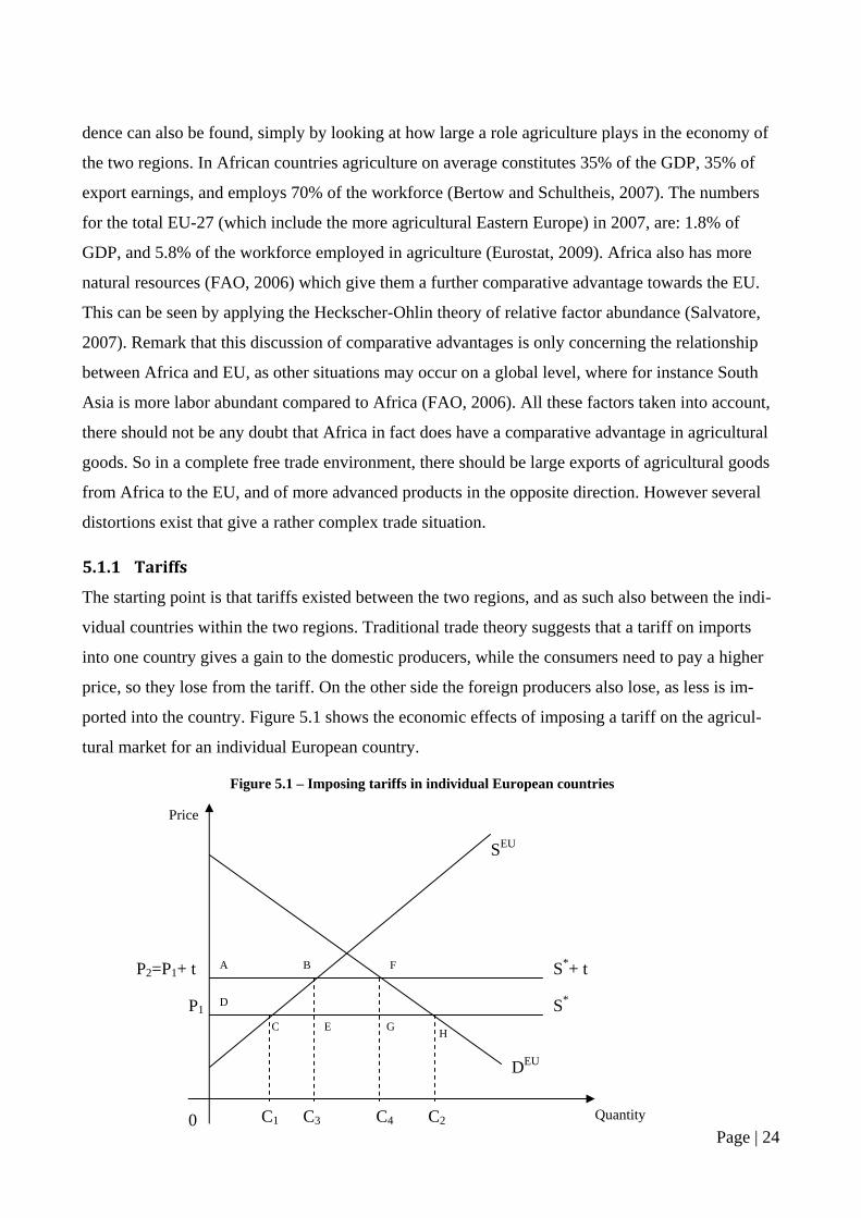
ported into the country. Figure 5.1 shows the economic effects of imposing a tariff on the agricul-

tural market for an individual European country.

Figure 5.1 – Imposing tariffs in individual European countries

0

Price

Quantity

P1

C1 C2

SEU

S*

DEU

C3 C4

P2=P1+ t S*+ tA

D

B F

C E G H

Page | 24

Figure 5.1 simply assumes that Africa has a comparative advantage in agricultural goods. By im-

posing a tariff the price moves to P2, which means that domestic producers move up the supply

curve to C3. A higher price also results in consumers buying less and thereby moving to C4. This

means that the import from Africa has now changed from C2-C1 to C4-C3 and already here we can

conclude that the African producers have lost considerable revenue. On the domestic market of the

European country, the domestic producers gain ABCD while consumers lose AFHD. The EU gains

import tariffs in the amount of BFGE, which means there is a deadweight loss of BCE and FGH.

This means that not only the African producers lose from imposing a tariff, but so does the EU as a

whole. However the main objective of helping the EU farmers has been fulfilled.

This situation is, however, not an issue in the trade between Africa and the EU today, due to the

Cotonou agreement, and therefore I will not go into any debt with the issue, but rather move for-

ward to what is relevant for trade today. From a situation where tariffs existed between all coun-

tries, the EU was formed as a customs union, where member countries over time have ended up not

having any tariffs between each other.

5.2 Customs union The discussion of a customs union in this context is whether the formation of the EU theoretically

has changed the trading partners for the member states and in this light, if it has affected trade with

Africa. The main indicator is whether the EU members would have traded with each other without

the existence of the union. It therefore comes down to who is the cheapest producer and hence has

the comparative advantage in the goods of interest. As the discussion of comparative advantages

concluded, Africa has a clear comparative advantage in agricultural goods, while the EU has in

more advanced products. A simple analysis of these facts give that the EU is trade diverting within

the agricultural sector, but trade creating in nearly all other sectors (in relation to Africa). Figure 5.2

shows the effect of the creation of the EU on agricultural products, while figure 5.3 shows on non-

agricultural goods.

Page | 25

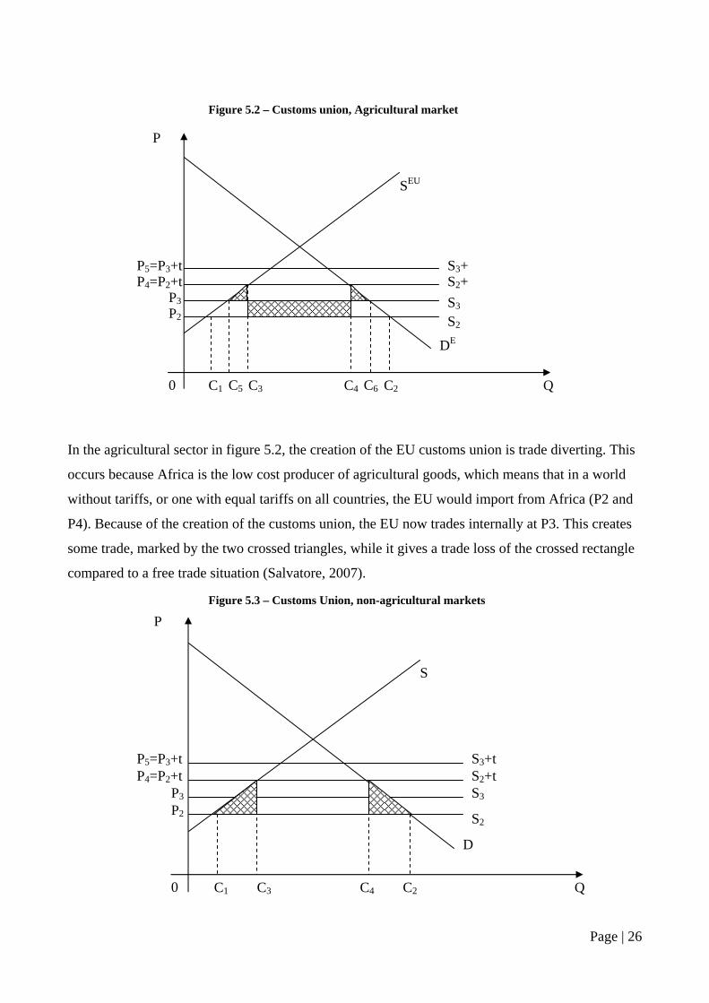
In the agricultural sector in figure 5.2, the creation of the EU customs union is trade diverting. This

occurs because Africa is the low cost producer of agricultural goods, which means that in a world

without tariffs, or one with equal tariffs on all countries, the EU would import from Africa (P2 and

P4). Because of the creation of the customs union, the EU now trades internally at P3. This creates

some trade, marked by the two crossed triangles, while it gives a trade loss of the crossed rectangle

compared to a free trade situation (Salvatore, 2007).

Figure 5.3 – Customs Union, non-agricultural markets

0 Q

P

SEU

DE

P5=P3+t

P2

C1 C2 C4 C3

Figure 5.2 – Customs union, Agricultural market

P3

P4=P2+t S3+S2+S3 S2

C5 C6

0 Q

P

S

D

P5=P3+t

P2

C1 C2 C4 C3

S3+t S2+t S3

S2

P3

P4=P2+t

Page | 26

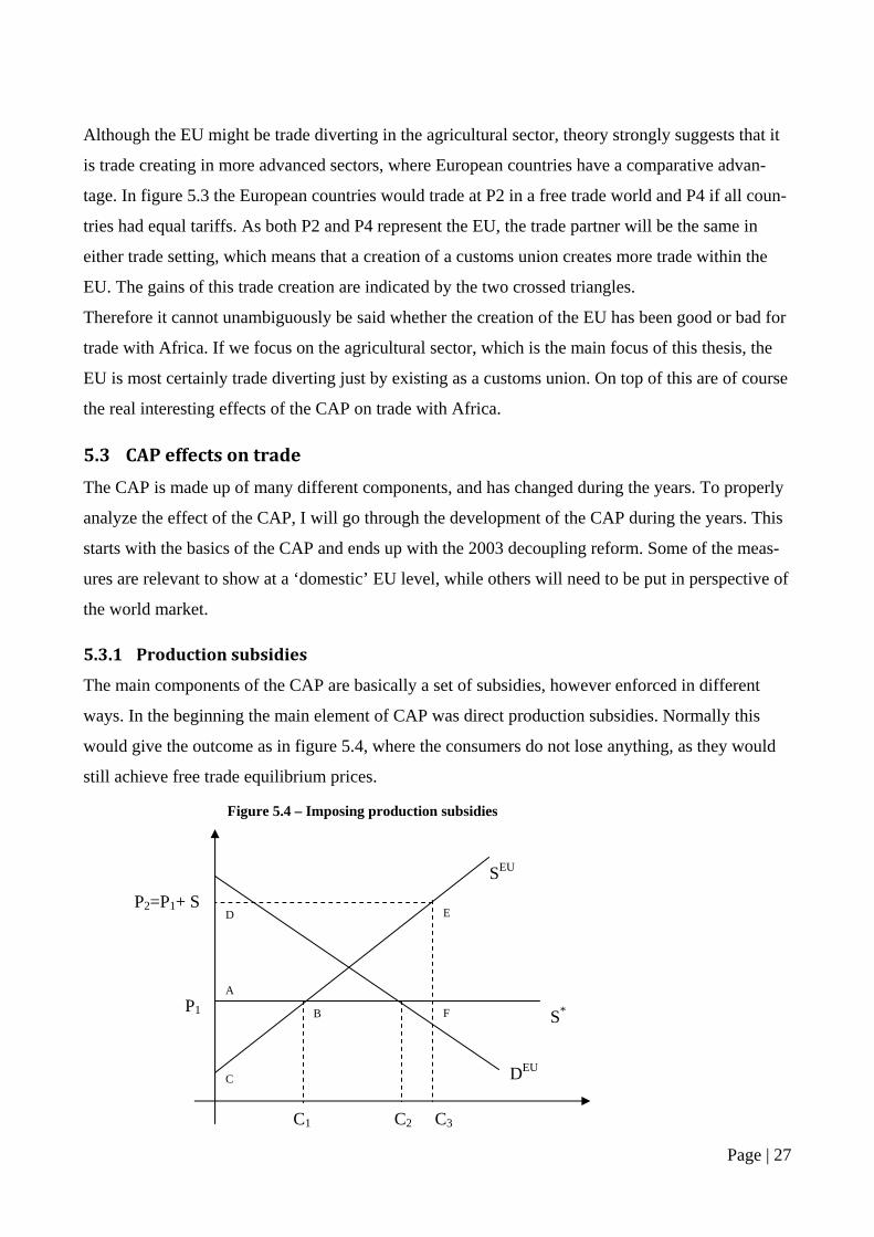
Although the EU might be trade diverting in the agricultural sector, theory strongly suggests that it

is trade creating in more advanced sectors, where European countries have a comparative advan-

tage. In figure 5.3 the European countries would trade at P2 in a free trade world and P4 if all coun-

tries had equal tariffs. As both P2 and P4 represent the EU, the trade partner will be the same in

either trade setting, which means that a creation of a customs union creates more trade within the

EU. The gains of this trade creation are indicated by the two crossed triangles.

Therefore it cannot unambiguously be said whether the creation of the EU has been good or bad for

trade with Africa. If we focus on the agricultural sector, which is the main focus of this thesis, the

EU is most certainly trade diverting just by existing as a customs union. On top of this are of course

the real interesting effects of the CAP on trade with Africa.

5.3 CAP effects on trade The CAP is made up of many different components, and has changed during the years. To properly

analyze the effect of the CAP, I will go through the development of the CAP during the years. This

starts with the basics of the CAP and ends up with the 2003 decoupling reform. Some of the meas-

ures are relevant to show at a ‘domestic’ EU level, while others will need to be put in perspective of

the world market.

5.3.1 Production subsidies The main components of the CAP are basically a set of subsidies, however enforced in different

ways. In the beginning the main element of CAP was direct production subsidies. Normally this

would give the outcome as in figure 5.4, where the consumers do not lose anything, as they would

still achieve free trade equilibrium prices.

Figure 5.4 – Imposing production subsidies

C2

SEU

S

C3

E

P1

P2=P1+ S D

F

C

A

B *

DEU

C1

Page | 27

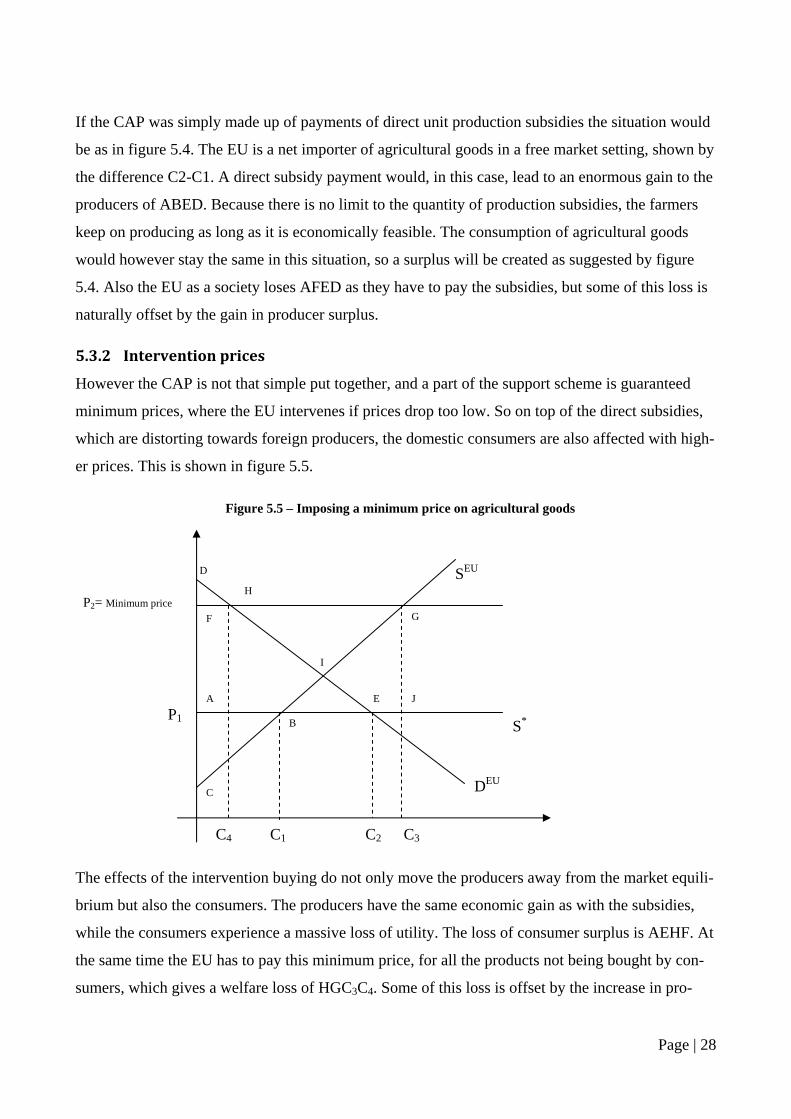
If the CAP was simply made up of payments of direct unit production subsidies the situation would

be as in figure 5.4. The EU is a net importer of agricultural goods in a free market setting, shown by

the difference C2-C1. A direct subsidy payment would, in this case, lead to an enormous gain to the

producers of ABED. Because there is no limit to the quantity of production subsidies, the farmers

keep on producing as long as it is economically feasible. The consumption of agricultural goods

would however stay the same in this situation, so a surplus will be created as suggested by figure

5.4. Also the EU as a society loses AFED as they have to pay the subsidies, but some of this loss is

naturally offset by the gain in producer surplus.

5.3.2 Intervention prices However the CAP is not that simple put together, and a part of the support scheme is guaranteed

minimum prices, where the EU intervenes if prices drop too low. So on top of the direct subsidies,

which are distorting towards foreign producers, the domestic consumers are also affected with high-

er prices. This is shown in figure 5.5.

The effects of the intervention buying do not only move the producers away from the market equili-

brium but also the consumers. The producers have the same economic gain as with the subsidies,

while the consumers experience a massive loss of utility. The loss of consumer surplus is AEHF. At

the same time the EU has to pay this minimum price, for all the products not being bought by con-

sumers, which gives a welfare loss of HGC3C4. Some of this loss is offset by the increase in pro-

Figure 5.5 – Imposing a minimum price on agricultural goods

C2

SEU

S

C1 C3

G

P1

P2= Minimum price F

C

A

B *

DEU

C4

H

E

D

J

I

Page | 28

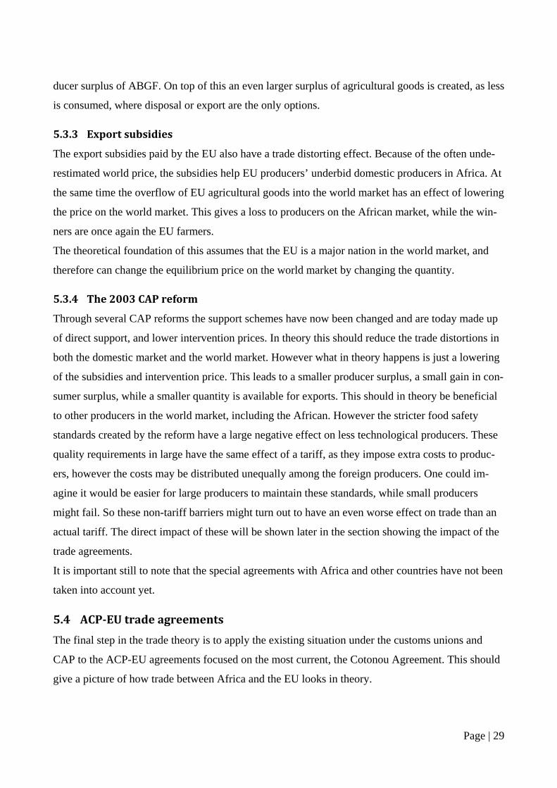
ducer surplus of ABGF. On top of this an even larger surplus of agricultural goods is created, as less

is consumed, where disposal or export are the only options.

5.3.3 Export subsidies The export subsidies paid by the EU also have a trade distorting effect. Because of the often unde-

restimated world price, the subsidies help EU producers’ underbid domestic producers in Africa. At

the same time the overflow of EU agricultural goods into the world market has an effect of lowering

the price on the world market. This gives a loss to producers on the African market, while the win-

ners are once again the EU farmers.

The theoretical foundation of this assumes that the EU is a major nation in the world market, and

therefore can change the equilibrium price on the world market by changing the quantity.

5.3.4 The 2003 CAP reform Through several CAP reforms the support schemes have now been changed and are today made up

of direct support, and lower intervention prices. In theory this should reduce the trade distortions in

both the domestic market and the world market. However what in theory happens is just a lowering

of the subsidies and intervention price. This leads to a smaller producer surplus, a small gain in con-

sumer surplus, while a smaller quantity is available for exports. This should in theory be beneficial

to other producers in the world market, including the African. However the stricter food safety

standards created by the reform have a large negative effect on less technological producers. These

quality requirements in large have the same effect of a tariff, as they impose extra costs to produc-

ers, however the costs may be distributed unequally among the foreign producers. One could im-

agine it would be easier for large producers to maintain these standards, while small producers

might fail. So these non-tariff barriers might turn out to have an even worse effect on trade than an

actual tariff. The direct impact of these will be shown later in the section showing the impact of the

trade agreements.

It is important still to note that the special agreements with Africa and other countries have not been

taken into account yet.

5.4 ACP­EU trade agreements The final step in the trade theory is to apply the existing situation under the customs unions and

CAP to the ACP-EU agreements focused on the most current, the Cotonou Agreement. This should

give a picture of how trade between Africa and the EU looks in theory.

Page | 29

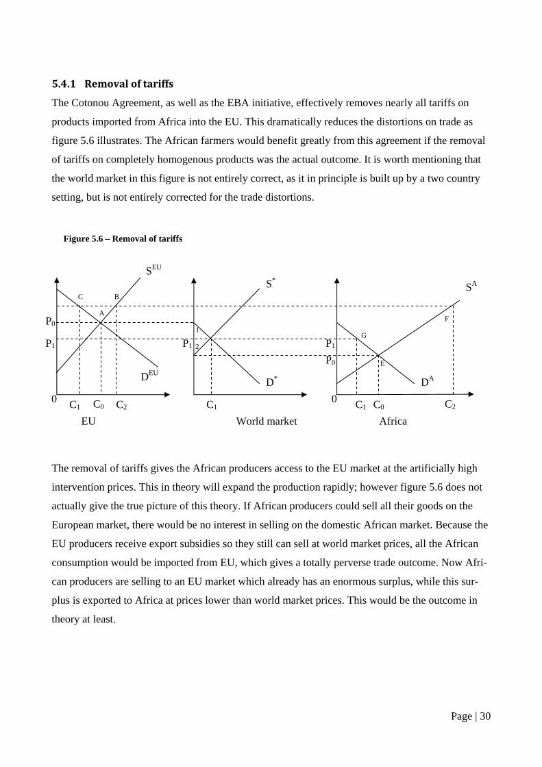
5.4.1 Removal of tariffs The Cotonou Agreement, as well as the EBA initiative, effectively removes nearly all tariffs on

products imported from Africa into the EU. This dramatically reduces the distortions on trade as

figure 5.6 illustrates. The African farmers would benefit greatly from this agreement if the removal

of tariffs on completely homogenous products was the actual outcome. It is worth mentioning that

the world market in this figure is not entirely correct, as it in principle is built up by a two country

setting, but is not entirely corrected for the trade distortions.

Figure 5.6 – Removal of tariffs

2

EU World market Africa

0

P1

P0

C1 C0 C2 C1 C1 C0 C2

S*

D*

SA

DA

SEU

DEU

A

C

1 G

0

B

P1 P1

F

E P0

The removal of tariffs gives the African producers access to the EU market at the artificially high

intervention prices. This in theory will expand the production rapidly; however figure 5.6 does not

actually give the true picture of this theory. If African producers could sell all their goods on the

European market, there would be no interest in selling on the domestic African market. Because the

EU producers receive export subsidies so they still can sell at world market prices, all the African

consumption would be imported from EU, which gives a totally perverse trade outcome. Now Afri-

can producers are selling to an EU market which already has an enormous surplus, while this sur-

plus is exported to Africa at prices lower than world market prices. This would be the outcome in

theory at least.

Page | 30

5.4.2 Food safety standards But unfortunately removal of tariffs is not the only part of the agreement. The existence of non-

tariff restrictions is largely present in the deal between the ACP and the EU. This is especially evi-

dent for the food safety standards imposed by the EU. As described earlier these high standards

induce extra costs for the African producers, reducing their direct competitiveness towards the Eu-

ropean market. Figure 5.7 show how these non-tariff barriers affect the Africa-EU trade for agricul-

tural goods. The same issue with the world market applies to this figure as to figure 5.6

Figure 5.7 – Increasing food safety standards

Page | 31

S*

2

EU World market Africa

0

SASEU

P1

P0

C1 C0 C2 C1 C1 C0 C2

D* DA DEU

A

C

1 G

B

P1 P1

F

E P0

SA’

0 C3

The non-tariff trade barriers, here represented by the food quality standards, increase the costs for

African producers. This is seen by the shift in the supply curve SA to SA’. It is assumed that all

goods are produced at these higher standards, including those for the domestic market. However we

once again see that in this particular diagram, there will be no domestic consumption of goods pro-

duced in Africa. In reality this is not the case, and the high quality standards may not be employed

to domestic markets, giving a totally different situation. The lower costs in selling to the domestic

market will especially be attractive for the small producers in Africa.

5.4.3 The 2003 CAP reform This is however not the end of the theoretical analysis of the trade relationship between Africa and

the EU. The CAP reform in 2003 changed the composition of the trade relations in several ways.

First of all, the intervention prices where reduced, which lead to a further reduction of the profits for

African producers. At the same time food safety standards were increased, imposing further costs to

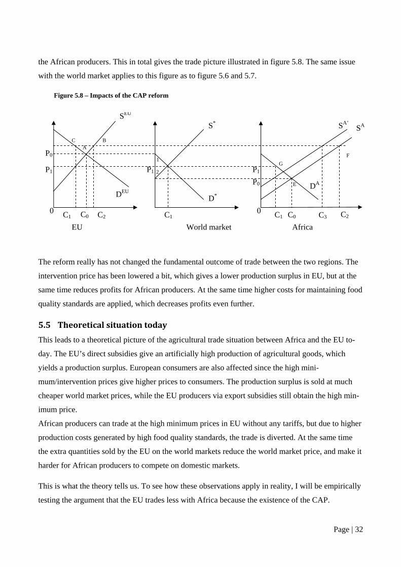
the African producers. This in total gives the trade picture illustrated in figure 5.8. The same issue

with the world market applies to this figure as to figure 5.6 and 5.7.

The reform really has not changed the fundamental outcome of trade between the two regions. The

intervention price has been lowered a bit, which gives a lower production surplus in EU, but at the

same time reduces profits for African producers. At the same time higher costs for maintaining food

quality standards are applied, which decreases profits even further.

5.5 Theoretical situation today This leads to a theoretical picture of the agricultural trade situation between Africa and the EU to-

day. The EU’s direct subsidies give an artificially high production of agricultural goods, which

yields a production surplus. European consumers are also affected since the high mini-

mum/intervention prices give higher prices to consumers. The production surplus is sold at much

cheaper world market prices, while the EU producers via export subsidies still obtain the high min-

imum price.

African producers can trade at the high minimum prices in EU without any tariffs, but due to higher

production costs generated by high food quality standards, the trade is diverted. At the same time

the extra quantities sold by the EU on the world markets reduce the world market price, and make it

harder for African producers to compete on domestic markets.

This is what the theory tells us. To see how these observations apply in reality, I will be empirically

testing the argument that the EU trades less with Africa because the existence of the CAP.

2

EU World market Africa

0

P1

P0

C1 C0 C2 C1 C1 C0 C2

S*

D*

SA

DA

SEU

DEU

A C

1 G

Figure 5.8 – Impacts of the CAP reform

0

B

P1 P1

F

E P0

SA’

C3

Page | 32

6 Gravity Equation 

To analyze if the theory applies, and if the CAP has an influence on trade with Africa, I have cho-

sen to use a gravity equation approach. The approach has gained immense popularity amongst re-

searchers in international trade during the last couple of decades (see e.g. Feenstra et al. 1999, Baier

and Bergstrand 2006, Grant and Lambert 2008).

The origin of gravity equations lies in physics, and explains how gravity is a function of the size of

two objects and the distance between them. For use in economic analysis of international trade this

is changed so that bilateral trade is a function of the size of the two countries’ economy and the dis-

tance between them. Many new variables have been added such as population size (which is also

relevant for the country’s size), and dummies for many factors such as common border, language

and currency.

The starting point in the analysis is to make four different gravity equations, two between the EU

and Africa, one being for all products, and one being for agricultural goods only. This should give a

picture of how trade between the EU and Africa is affected by the CAP. To test if evidence in the

results of these regressions is not just caused by common trade patterns, two control equations will

be made for intra-EU trade, again doing one for all goods and one for agricultural goods only.

When running a standard gravity equation all countries involved in the analysis are included with

their bilateral trade with all other countries in the analysis. This is not optimal for the regression of

African countries’ trade with the EU. Reliable statistics for trade between African countries is near-

ly impossible to obtain. However, the intra-Africa trade is not interesting in this analysis, and there-

fore the gravity equation must be modified to fit the goal of the analysis. This will be done along the

way, as several gravity models are tested until the correct model is reached.

First of all, I will go through some basic gravity equation theory, as many opposing views exist in

the research community. Out from the different theories I will be choosing which parts of each

theory I will be following, making arguments for my decisions along the way. Thereafter I will be

going through the data collection process, and certain decisions made in choosing between different

data. Finally, I will be doing a series of regressions, commenting on these along the way, and con-

cluding with the final model.

Page | 33

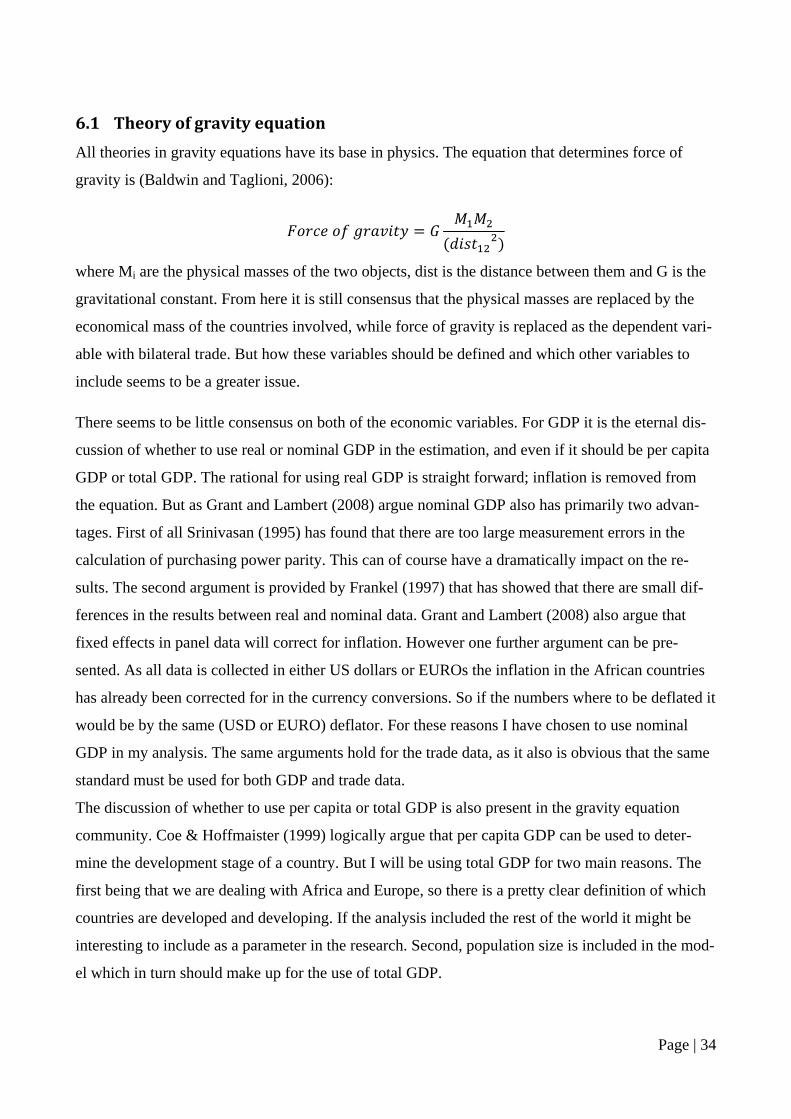
6.1 Theory of gravity equation All theories in gravity equations have its base in physics. The equation that determines force of

gravity is (Baldwin and Taglioni, 2006):

   

where Mi are the physical masses of the two objects, dist is the distance between them and G is the

gravitational constant. From here it is still consensus that the physical masses are replaced by the

economical mass of the countries involved, while force of gravity is replaced as the dependent vari-

able with bilateral trade. But how these variables should be defined and which other variables to

include seems to be a greater issue.

There seems to be little consensus on both of the economic variables. For GDP it is the eternal dis-

cussion of whether to use real or nominal GDP in the estimation, and even if it should be per capita

GDP or total GDP. The rational for using real GDP is straight forward; inflation is removed from

the equation. But as Grant and Lambert (2008) argue nominal GDP also has primarily two advan-

tages. First of all Srinivasan (1995) has found that there are too large measurement errors in the

calculation of purchasing power parity. This can of course have a dramatically impact on the re-

sults. The second argument is provided by Frankel (1997) that has showed that there are small dif-

ferences in the results between real and nominal data. Grant and Lambert (2008) also argue that

fixed effects in panel data will correct for inflation. However one further argument can be pre-

sented. As all data is collected in either US dollars or EUROs the inflation in the African countries

has already been corrected for in the currency conversions. So if the numbers where to be deflated it

would be by the same (USD or EURO) deflator. For these reasons I have chosen to use nominal

GDP in my analysis. The same arguments hold for the trade data, as it also is obvious that the same

standard must be used for both GDP and trade data.

The discussion of whether to use per capita or total GDP is also present in the gravity equation

community. Coe & Hoffmaister (1999) logically argue that per capita GDP can be used to deter-

mine the development stage of a country. But I will be using total GDP for two main reasons. The

first being that we are dealing with Africa and Europe, so there is a pretty clear definition of which

countries are developed and developing. If the analysis included the rest of the world it might be

interesting to include as a parameter in the research. Second, population size is included in the mod-

el which in turn should make up for the use of total GDP.

Page | 34

The other variable which is up for discussion is the value of bilateral trade. Besides the real versus

nominal numbers which has just been discussed, the discussion goes how to estimate the trade vari-

able. The different possible measures are import, export or total trade (import + export) value. Some

also use an average of the import and export. The most common approach seems to be the use of

exports from country i to country j in the model. This method is used by Feenstra et al. (1999),

Grant & Lambert (2008), Roijd (2006), and Baier & Bergstrand (2006), while Kirkpatrick & Wata-

nabe (2004) uses the opposite approach of using imports of country i from country j. By using ei-

ther of these approaches trade flows in both directions are included in the estimation, as they appear

as two separate observations. Baldwin & Taglioni (2006) use the more advanced approach of aver-

aging the trade flow between two countries, which of course reduces the number of observations

and might also have an impact on precision, depending on the goal of the analysis. However it gives

the best picture of actual bilateral trade, and not just export. The final method that can be employed

is used by Coe & Hoffmaister (1999) where the sum of import and export is used. In the big picture

it should not make a big difference which approach is used, and the choices are often chosen with-

out any argumentation of why. I will be employing the last method of the sum of total trade. This is

done because it is expected that there are great differences in the value of trade whether the EU or

African countries are exporters. Further detailed analysis of differences between import and export

can be conducted after the final model has been determined.

The next subject to approach is which dummy variables to use in gravity equations. Some relative

standard variables exist that are used in most models. First of all, variables for common language,

common border, and colonial history can explain the cost of information (Piermartini & Teh, 2005).

These common features can be highly relevant in explaining bilateral trade as the same language

and business practices make trade easier to conduct. In this particular analysis of trade between Eu-

rope and Africa, a dummy variable for colonial history can turn out to be extremely relevant as the

colonial history between these two continents is extensive.

To supplement the distance variable in determining trade costs, two other variables are quite com-

mon to add in the model. These are dummies for if a country is an island or is landlocked, while the

common border dummy also plays a role in the transportation costs alongside the information costs

(Piermartini & Teh, 2005).

Many also use a dummy for whether countries belong to a regional or free trade agreement. This

can be used in several ways, depending on if countries belong to the same agreement or if one of the

countries belongs to one.

Page | 35

I will be using all of these “standard” dummy variables in my model, when they are relevant for the

analysis. One variable that will be irrelevant as the model turns to Africa-EU trade is the border

variable, as none of the observations in the data will be of neighboring countries.

6.2 Determining a model For determining a model to use for the analysis, inspiration has been gathered from several papers

on regional trade agreements and their impact on bilateral trade. This is the research that has been

conducted that resembles my objective the most. Baier & Bergstrand (2006) have examined the

impact of free trade agreements (FTA) on bilateral trade amongst the members, and found that

FTAs double bilateral trade over a 10 year period. For a more Africa specific investigation Gbetn-

kom (2006) has found that trade within the FTA COMESA has changed positively with a policy

change within the member states. Many other examples can be mentioned, but none of these papers

address the problem I am trying to investigate. Therefore these papers have merely been used as

inspiration to give ideas of how to determine a good model for isolating the effect of the CAP on

bilateral trade between Africa and Europe.

The logic behind using FTA investigations as a framework is that the EU and Africa as such can be

determined as two different regions and can be set instead of the FTA dummies. To elaborate a bit

on this, the EU-15 can for logical reasons be directly used as a FTA, while Africa as a whole is a bit

more complicated. Therefore the ACP regions are used as a basic for dividing Africa into FTAs.

However one problem exists with the ACP regions, only two of them are actual FTAs. ECOWAS is

made up by a large group of Western Africa countries where most belong to the same FTA, UE-

MOA. In order to capture the economic differences in trade in belonging to a FTA, I prefer to use

UEMOA rather than ECOWAS as a dummy variable for FTAs. The other problem exists with the

region of Eastern and Southern Africa. This group is not represented by a FTA, although COMESA

covers large parts of the group. One problem in using COMESA is that it over lapses with many

countries in the SADC FTA. Therefore I have chosen to use the FTA of EAC, which only

represents the Eastern Africa countries. All in all it is rather difficult to choose FTAs in Africa, as

relative many exists. Also, some FTAs, such as CEMAC and UEMOA, are more developed than

others, and are actually customs unions with common currencies.

As some African countries belong to the WTO and others do not, I will also include a variable for

this membership, especially as it is interesting for interaction with the EU members, which are all

within the WTO.

As mentioned the colonial ties between Africa and Europe are especially strong, and therefore va-

Page | 36

riables showing these colonial ties are of course essential to the equation. Some African countries

have never had a colonizer, but most have at some point in time. In the research of the African

countries the colonizers have been identified as: United Kingdom, France, Portugal, Spain, Bel-

gium, Germany and Italy. The latter two lost all their colonies after World War II. All of these co-

lonial ties are however included in the model. Some countries have even had several colonizers.

Some of these are due to British and French overtaking after World War II, while others are due to

the many wars and movement of borders between many African countries.

An approach that has been applied in many gravity equations in resent studies is the inclusion of

variables for multilateral resistance. This is for instance done by Baier & Bergstrand (2006) in their

panel data estimation in reference to the research by Anderson & van Wincoop (2003). The purpose

is to account for price differences in reference to the world price. I have chosen not to employ this

method although it seems to be more or less consensus in the research community. My main reason

for not using it is the way my regression will be run. As the data in my model only includes trade

between African countries and the EU-15, price differences are not expected to have a large impact.

The prices for African countries to import from EU are estimated to be more or less the same, while

prices from African countries most likely do not differ a whole lot over the total specter of agricul-

tural (or other) goods.

A brief discussion of some assumption problems when using the gravity equation is found in ap-

pendix A.

6.3 Data collection  The analysis is conducted on the base of all sub-Saharan African countries, which constitutes 48

countries, as well as the 15 European countries that constitute the EU-15. Based on available data

the period has been set from 1995-2007.

Data for bilateral trade flows between the EU-15 and the African countries as well as intra-EU trade

has been obtained from the Eurostat database. The GDP for all countries have been obtained from

the UN statistical database alongside with data from World Development Indicators, which have

complimented each other in filling out missing values. The value of agricultural output has been

obtained from the same two databases. Population numbers for African countries have been col-

lected from World Development Indicators, while the EU population numbers are from the Eurostat

database.

Distances between countries have been calculated out from the numbers in CEPII. Facts about co-

Page | 37

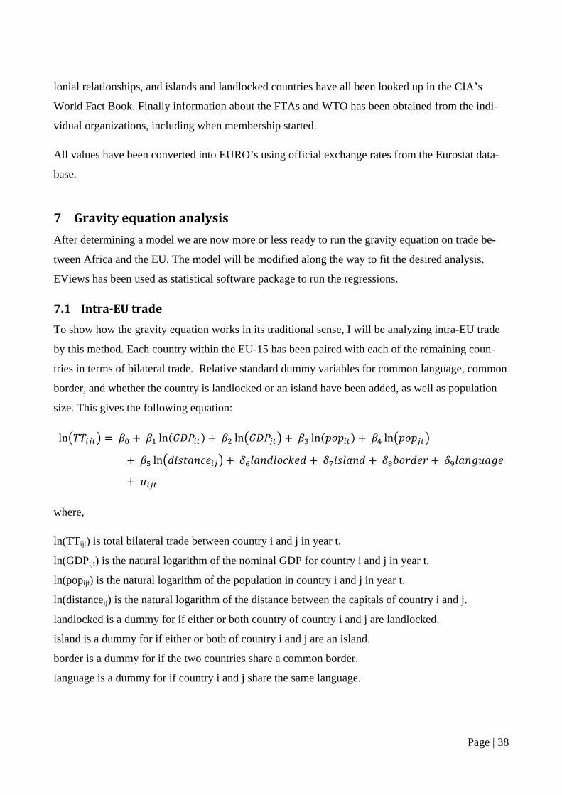
lonial relationships, and islands and landlocked countries have all been looked up in the CIA’s

World Fact Book. Finally information about the FTAs and WTO has been obtained from the indi-

vidual organizations, including when membership started.

All values have been converted into EURO’s using official exchange rates from the Eurostat data-

base.

7 Gravity equation analysis 

After determining a model we are now more or less ready to run the gravity equation on trade be-

tween Africa and the EU. The model will be modified along the way to fit the desired analysis.

EViews has been used as statistical software package to run the regressions.

7.1 Intra­EU trade To show how the gravity equation works in its traditional sense, I will be analyzing intra-EU trade

by this method. Each country within the EU-15 has been paired with each of the remaining coun-

tries in terms of bilateral trade. Relative standard dummy variables for common language, common

border, and whether the country is landlocked or an island have been added, as well as population

size. This gives the following equation:

ln     ln   ln   ln   ln

  ln        

   

where,

ln(TTijt) is total bilateral trade between country i and j in year t.

ln(GDPijt) is the natural logarithm of the nominal GDP for country i and j in year t.

ln(popijt) is the natural logarithm of the population in country i and j in year t.

ln(distanceij) is the natural logarithm of the distance between the capitals of country i and j.

landlocked is a dummy for if either or both country of country i and j are landlocked.

island is a dummy for if either or both of country i and j are an island.

border is a dummy for if the two countries share a common border.

language is a dummy for if country i and j share the same language.

Page | 38

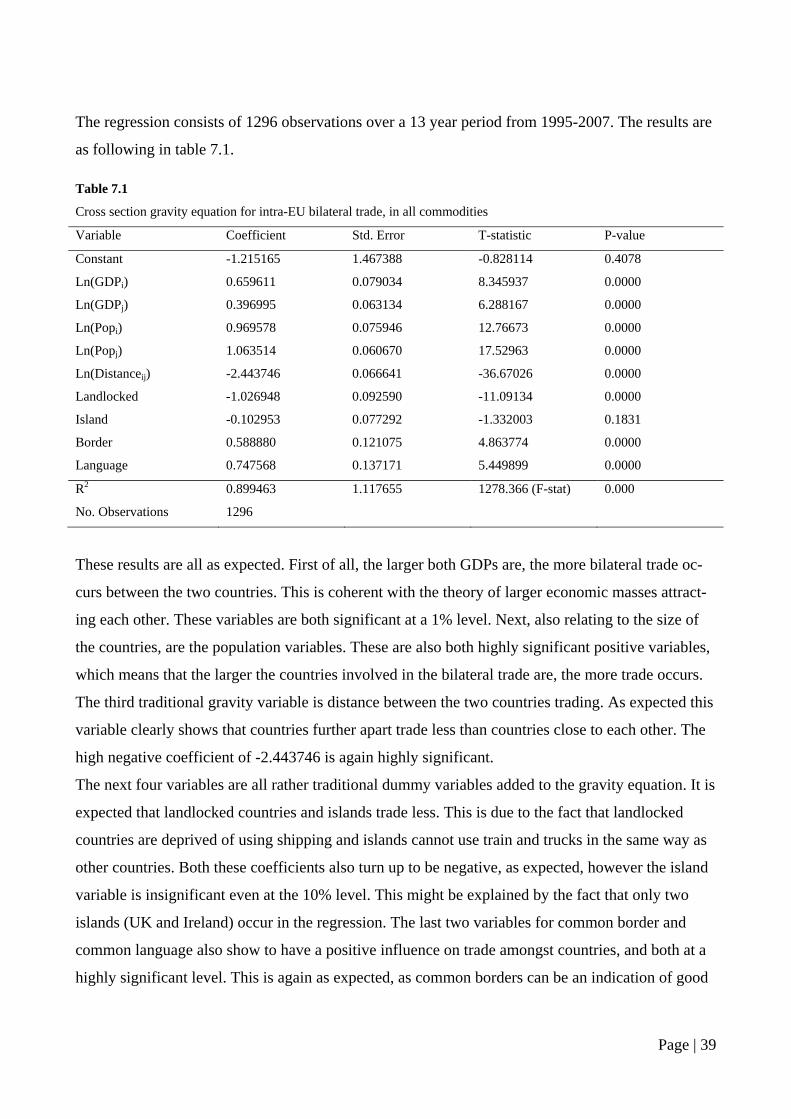
The regression consists of 1296 observations over a 13 year period from 1995-2007. The results are

as following in table 7.1.

Table 7.1

Cross section gravity equation for intra-EU bilateral trade, in all commodities

Variable Coefficient Std. Error T-statistic P-value

Constant -1.215165 1.467388 -0.828114 0.4078

Ln(GDPi) 0.659611 0.079034 8.345937 0.0000

Ln(GDPj) 0.396995 0.063134 6.288167 0.0000

Ln(Popi) 0.969578 0.075946 12.76673 0.0000

Ln(Popj) 1.063514 0.060670 17.52963 0.0000

Ln(Distanceij) -2.443746 0.066641 -36.67026 0.0000

Landlocked -1.026948 0.092590 -11.09134 0.0000

Island -0.102953 0.077292 -1.332003 0.1831

Border 0.588880 0.121075 4.863774 0.0000

Language 0.747568 0.137171 5.449899 0.0000

R2 0.899463 1.117655 1278.366 (F-stat) 0.000

No. Observations 1296

These results are all as expected. First of all, the larger both GDPs are, the more bilateral trade oc-

curs between the two countries. This is coherent with the theory of larger economic masses attract-

ing each other. These variables are both significant at a 1% level. Next, also relating to the size of

the countries, are the population variables. These are also both highly significant positive variables,

which means that the larger the countries involved in the bilateral trade are, the more trade occurs.

The third traditional gravity variable is distance between the two countries trading. As expected this

variable clearly shows that countries further apart trade less than countries close to each other. The

high negative coefficient of -2.443746 is again highly significant.

The next four variables are all rather traditional dummy variables added to the gravity equation. It is

expected that landlocked countries and islands trade less. This is due to the fact that landlocked

countries are deprived of using shipping and islands cannot use train and trucks in the same way as

other countries. Both these coefficients also turn up to be negative, as expected, however the island

variable is insignificant even at the 10% level. This might be explained by the fact that only two

islands (UK and Ireland) occur in the regression. The last two variables for common border and

common language also show to have a positive influence on trade amongst countries, and both at a

highly significant level. This is again as expected, as common borders can be an indication of good

Page | 39

neighbor relationships and common language of course eases the process of trading.

The gravity equation for intra-EU trade has a very high R2 of nearly 0.9. This is well above the tra-

ditional level of gravity equations from previous studies2. There are many possible explanations for

such a high R2 value, the best of them of course being the existence of the internal market in the

EU. The internal market has removed all trade barriers that might exist between all other EU coun-

tries including both tariff and non-tariff barriers.

So to conclude on this first attempt of the gravity equation it seems to work perfect for intra-EU

trade. Now the challenge will be to extend it to Africa-EU trade.

7.2 Africa­EU trade The gravity equation approach used for the intra-EU analysis is not to any use when performing the

next test. In theory it could be quite interesting to include bilateral trade between all African and EU

countries, and this would presumably also yield the best and most precise results. However due to

difficulties of obtaining reliable data for intra-Africa trade this approach has been made impossible

to conduct. Instead the analysis will be looking at each African country’s trade with the EU-15 as a

whole. The argument for using this approach is that intra-Africa trade as such does not explain any-

thing about the influence of the CAP, although these observations would provide excellent control

variables. This problem will be discussed and resolved later in the analysis process. The idea is to

make two gravity equations, one for agricultural goods and one for all commodities, and then com-

pare the results of these regressions.

The variables used in this gravity equation have changed a bit from the traditional variables used in

the intra-EU regression. The GDP of the individual African countries is still used while the GDP for

the trading partner has changed to be that of the EU-15. This means that the GDP for country j in

the regression will remain constant among all the African countries for each year and only change

as the year changes. This might turn up to be a problem, but will most likely just result in an insig-

nificant variable as the values do not change among countries and therefore should have little im-

pact on the level of trade.

The same situation is evident for the population variables, where the EU population again is con-

stant amongst countries for every year. Again the likely outcome is a highly insignificant variable.

Distance between the individual African countries and the EU-15 is measured as the distance from

the capital of the African country to Bruxelles. Bruxelles is chosen for two main reasons. First of

2 See for example Coe and Hoffmaister 1999, Kirkpatrick and Watanebe 2005, Baier and Bergstrand 2006.

Page | 40

all, it is, if any, the capital of the EU. Second, and at least as important, it is located fairly central in

the EU-15 states and therefore works as a good proxy.

Dummy variables for landlocked countries and islands are added as in the intra-EU regression. Fur-

thermore two other sets of dummy variables are added. One set consisting of 7 different variables

and denoting former colonization ties to European countries. One for each of the following coun-

tries: United Kingdom, France, Spain, Portugal, Germany, Italy and Belgium. Obviously some of

these countries have had more colonial activity in Africa than other, and the few colonies Germany

and Italy have had where handed over to other countries after World War II. However, these two

countries set aside; pretty much all former colonies now speak the language of their former coloniz-

er. Therefore these variables are not only an indication of direct colonial influence but also language

ties, and thereby also information costs.

The other set of dummy variables is for which FTA the African countries belong to. As earlier dis-

cussed these are divided into: CEMAC, EAC, SADC and UEMOA. Furthermore a dummy variable

for membership of the WTO is added. As not all African countries are members, and some become

members during the analysis period, it can prove to have a very significant influence on the trade.

A isfter th the model looks as follows:

ln   ln   ln     ln   ln  

  ln        

       

     

 

where all variables are as explained above. This yields the results in table 7.2

Several things come to mind when looking at these results. First of all, the regression has a relative-

ly low R2 of only 0.22. This is very low for a gravity equation, and is as such not acceptable for

explaining trade properly. Furthermore many of the variables are highly insignificant. Therefore this

model can already now be rejected as it does not work as intended. The same regression has been

run for agricultural products only, and obtains a R2 of only 0.27, so a bit higher than for all com-

modities, but still not good enough. Similar gravity estimations have been run for both import and

export individually for both agricultural and all commodities, again without producing useful re-

Page | 41

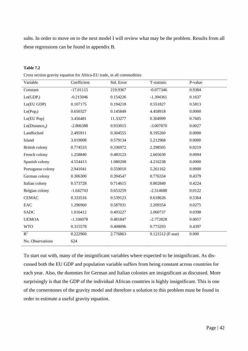
sults. In order to move on to the next model I will review what may be the problem. Results from all

these regressions can be found in appendix B.

Table 7.2

Cross section gravity equation for Africa-EU trade, in all commodities

Variable Coefficient Std. Error T-statistic P-value

Constant -17.01115 219.9367 -0.077346 0.9384

Ln(GDPi) -0.215046 0.154226 -1.394361 0.1637

Ln(EU GDP) 0.107175 0.194218 0.551827 0.5813

Ln(Popi) 0.650327 0.145849 4.458918 0.0000

Ln(EU Pop) 3.456481 11.33277 0.304999 0.7605

Ln(Distanceij) -2.806388 0.933015 -3.007870 0.0027

Landlocked 2.495911 0.304555 8.195260 0.0000

Island 3.019008 0.579134 5.212968 0.0000

British colony 0.774533 0.336972 2.298505 0.0219

French colony 1.258840 0.483123 2.605630 0.0094

Spanish colony 4.554413 1.080208 4.216238 0.0000

Portuguese colony 2.941041 0.559010 5.261162 0.0000

German colony 0.306300 0.394547 0.776334 0.4379

Italian colony 0.573728 0.714615 0.802849 0.4224

Belgian colony -1.642743 0.653259 -2.514688 0.0122

CEMAC 0.333516 0.539123 0.618626 0.5364

EAC 1.296960 0.587031 2.209354 0.0275

SADC 1.016412 0.493227 2.060737 0.0398

UEMOA -1.336078 0.481847 -2.772828 0.0057

WTO 0.315578 0.408096 0.773293 0.4397

R2 0.222960 2.776863 9.121512 (F-stat) 0.000

No. Observations 624

To start out with, many of the insignificant variables where expected to be insignificant. As dis-

cussed both the EU GDP and population variable suffers from being constant across countries for

each year. Also, the dummies for German and Italian colonies are insignificant as discussed. More

surprisingly is that the GDP of the individual African countries is highly insignificant. This is one

of the cornerstones of the gravity model and therefore a solution to this problem must be found in

order to estimate a useful gravity equation.

Page | 42

7.2.1 Deriving a new model For a solution to this problem I have been inspired by Baier and Bergstrand (2006) and Fratianni

(2007) who use the method of scaling the trade to the product of the GDPs. This model actually

comes again in several other papers, and has its base in the basic gravity model from physics. By

dividing the product of the masses on both sides of the equation we reach a scaled version of the

bilateral trade. Although their goal is a completely different than mine, it gave me an idea. By divid-

ing the value of trade with the product of the GDPs we obtain a ratio of how much the trade consti-

tutes of the output of the countries involved. This is in fact an analysis of the trade openness be-

tween the African and European countries. Although this is not the traditional approach to the gravi-

ty equation, it still analyses which variables have an impact on trade, in this instance trade openness

instead of trade in value.

The next problem is that a traditional gravity equation does not isolate the effect of the CAP in any

way. The previous model gave two different equations, one for agriculture and one for total trade.

But it is not as such possible to draw any conclusions about the influence of CAP from comparing

these two gravity equations. In order to solve this problem I had to come up with some way of in-

cluding a variable that shows a coefficient for when CAP has influence on the trade, hence when the

trade is in agriculture. My solution to this problem is to divide each observation for each country

into two observations; one for agriculture and one for non-agriculture. In this way one observation

has data for total trade in agriculture and output of agriculture, and the other observation has data

for total trade in non-agriculture and output in non-agriculture3. Now, in order to include a CAP

variable, a dummy variable is included for all the agriculture observations. This solution works per-

fect with the decision to analyze the trade openness by taking ratio of trade to output, as we can then

see the openness of the agricultural sector compared to all other sectors.

Finally the new approach of using ratios has resulted in a new issue. When calculating the ratios it

became quite apparent that small countries have quite unusual high ratios of trade, often constitut-

ing more trade than output. Because of these unusual numbers, I have filtered out countries of be-

low 1.2 million inhabitants as of 2007. This excludes 9 countries in the equation. Because of these

exclusions the dummy variable for former Spanish colonies has also been dropped, as there no

longer are any in the observations used.

3 An example of this data entry can be seen in appendix C.

Page | 43

7.3 A new model for Africa­EU trade In order to apply the new model, the few mentioned changes are made to the dataset. If the model

works as intended, it should be interesting to see whether agricultural goods are traded relatively

more or less than other goods. In theory Africa has a comparative advantage in the agricultural sec-

tor, but theory of the existing policies also tell us that this sector is distorted in trade between the

two regions.

The model obtained looks as following:

ln  

  ln   ln     ln  

           

     

 

Where the new variables are:

Outputit which is the output of either agricultural sector or non-agriculture depending on the obser-

vation.

EU Outputt which is the EU output of the equivalent sector.

Agriculture is a dummy variable which is 1 if the observation is for the agricultural sector, and 0 if

for non-agricultural.

Table 7.3 shows the results of this regression.

Now we have obtained a model with a sufficient high R2 of 0.69, but several other results of the

model are also interesting and perhaps unexpected. The high R2 tells us that the included variables

explain a great deal of how open the trade is between African countries and the EU. However the

most interesting variable is the newly introduced Agriculture dummy. The dummy turns out to be

highly significant which means that there is a difference in trade with agricultural and non-

agricultural commodities. However this agriculture dummy is positive, which means that there is

more trade openness within the agricultural sector than the non-agricultural sectors. This can per-

haps be explained by using Ricardian theory of comparative advantages. But another explanation

could also be that countries in general trade more in agricultural commodities. This issue will be

part of the next step to the final model.

Page | 44

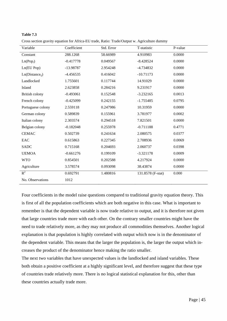
Table 7.3

Cross section gravity equation for Africa-EU trade, Ratio: Trade/Output w. Agriculture dummy

Variable Coefficient Std. Error T-statistic P-value

Constant 288.1268 58.66989 4.910983 0.0000

Ln(Popi) -0.417778 0.049567 -8.428524 0.0000

Ln(EU Pop) -13.98787 2.954248 -4.734832 0.0000

Ln(Distanceij) -4.456535 0.416042 -10.71173 0.0000

Landlocked 1.755601 0.117744 14.91029 0.0000

Island 2.623858 0.284216 9.231917 0.0000

British colony -0.493061 0.152548 -3.232165 0.0013

French colony -0.425099 0.242155 -1.755485 0.0795

Portuguese colony 2.559118 0.247986 10.31959 0.0000

German colony 0.589839 0.155961 3.781977 0.0002

Italian colony 2.303574 0.294518 7.821501 0.0000

Belgian colony -0.182048 0.255978 -0.711188 0.4771

CEMAC 0.502739 0.241634 2.080575 0.0377

EAC 0.615863 0.227345 2.708936 0.0069

SADC 0.715168 0.204693 2.060737 0.0398

UEMOA -0.661276 0.199109 -3.321178 0.0009

WTO 0.854501 0.202588 4.217924 0.0000

Agriculture 3.578574 0.093098 38.43874 0.0000

R2 0.692791 1.480816 131.8578 (F-stat) 0.000

No. Observations 1012

Four coefficients in the model raise questions compared to traditional gravity equation theory. This

is first of all the population coefficients which are both negative in this case. What is important to

remember is that the dependent variable is now trade relative to output, and it is therefore not given

that large countries trade more with each other. On the contrary smaller countries might have the

need to trade relatively more, as they may not produce all commodities themselves. Another logical

explanation is that population is highly correlated with output which now is in the denominator of

the dependent variable. This means that the larger the population is, the larger the output which in-

creases the product of the denominator hence making the ratio smaller.

The next two variables that have unexpected values is the landlocked and island variables. These

both obtain a positive coefficient at a highly significant level, and therefore suggest that these type

of countries trade relatively more. There is no logical statistical explanation for this, other than

these countries actually trade more.

Page | 45

Finally, the coefficients for the colony and trade union dummies can also be discussed. The colony

coefficients surprisingly show the two largest colonial relationships, the United Kingdom and

France, to have negative impact on relative trade, even though the coefficient for France is weakly

significant, while weaker colonial ties as Germany and Italy seem to have a positive effect. The

coefficient for former Belgian colonies is highly insignificant, but this might just be explained by

the fact that Belgium did not have that many colonies in Africa.

The dummies for trade unions show that three of the African trade unions and WTO membership

have positive effect on relative trade, while the last, UEMOA, has a negative impact. This is an in-

teresting observation which will be looked into later in the discussion of the reasons behind the re-

sults.

In general there are quite a few deviations from the traditional gravity equation in the estimation of

this model, and therefore it might be important to stress that this no longer is a traditional gravity

equation, and the abnormalities can simply be a result of this different approach.

7.4 Using a control group for Africa­EU trade In spite of some abnormalities in the results, I feel the model is on the right track to explaining the

difference in agricultural trade, especially due to the agriculture dummy variable. The next goal is

to test whether it is simply normal for countries to trade more in agricultural goods than other com-

modities. This can be done by introducing a control group into the estimation and see if African

agricultural trade is significantly different from agricultural trade in other countries. The original

interest was to examine the effect of CAP on trade with Africa, so in order to make the model show

what is intended, the control group must consist of countries that are not affected by the CAP in

trade. The only set of countries where CAP does not have this effect is the EU countries. Therefore

these will be chosen as control group. Another good approach would be to simply use trade between

African countries and other countries such as Australia and New Zealand, which have liberalized

their agricultural sector. However, I have not had any success in finding reliable data for conducting

this experiment.

To obtain consistency in the estimation each observation for the EU-15 countries will be of each

country’s trade with the remaining 14 countries. In this way the observations are the same as the

African countries. In order to achieve further consistency the distance variable has to be changed.

The new variable is calculated as the average distance to the EU-15 countries, or in the case of the

EU observations to the remaining 14 countries.

Page | 46

Two new dummies are also added to the model, one for EU and one for Africa. Because these off

course are mutually exclusive the Africa dummy will only be used for interaction purposes. On the

basis of these continent specific dummies two interaction terms are created, one for EU and agricul-

ture, and likewise one for Africa and agriculture. This should show the difference in agricultural

trade from non-agricultural trade. Because of these new dummy variables the African trade union

dummies are excluded for time being.

Finally, the colonial dummies are changed as these cannot be used in a sensible way for the EU

countries. The new dummies represent a relationship to the countries that were present in the co-

lonial dummies, and are mostly based on language. This means for instance that both Germany and

Austria obtain the value 1 for the German dummy along with the former German colonies in Africa.

Also the French and Belgian dummies are merged together because of a high degree of common

language.

This gives the following model:

ln  

  ln   ln     ln  

     

   

Before looking at the results a few remarks are necessary. Because of the inclusion of the EU-15

countries, some of the expected values have changed. First of all, the constant is expected to fall

dramatically as the product of the output for the EU countries observations will be much higher than

the African countries. For this reason the EU dummy will most likely become negative, as the de-

pendent variable will become smaller as the product of output becomes smaller, even though the

total trade between the countries most certainly will rise as well.

Otherwise the coefficients are expected to be similar to the previous estimation. The results of the

estimation are shown in table 7.4.

Page | 47

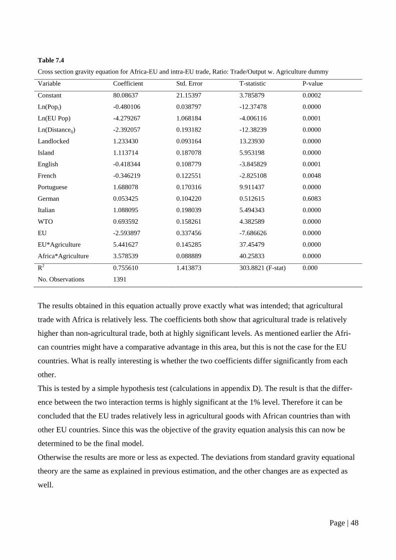
Table 7.4

Cross section gravity equation for Africa-EU and intra-EU trade, Ratio: Trade/Output w. Agriculture dummy

Variable Coefficient Std. Error T-statistic P-value

Constant 80.08637 21.15397 3.785879 0.0002

Ln(Popi) -0.480106 0.038797 -12.37478 0.0000

Ln(EU Pop) -4.279267 1.068184 -4.006116 0.0001

Ln(Distanceij) -2.392057 0.193182 -12.38239 0.0000

Landlocked 1.233430 0.093164 13.23930 0.0000

Island 1.113714 0.187078 5.953198 0.0000

English -0.418344 0.108779 -3.845829 0.0001

French -0.346219 0.122551 -2.825108 0.0048

Portuguese 1.688078 0.170316 9.911437 0.0000

German 0.053425 0.104220 0.512615 0.6083

Italian 1.088095 0.198039 5.494343 0.0000

WTO 0.693592 0.158261 4.382589 0.0000

EU -2.593897 0.337456 -7.686626 0.0000

EU*Agriculture 5.441627 0.145285 37.45479 0.0000

Africa*Agriculture 3.578539 0.088889 40.25833 0.0000

R2 0.755610 1.413873 303.8821 (F-stat) 0.000

No. Observations 1391

The results obtained in this equation actually prove exactly what was intended; that agricultural

trade with Africa is relatively less. The coefficients both show that agricultural trade is relatively

higher than non-agricultural trade, both at highly significant levels. As mentioned earlier the Afri-

can countries might have a comparative advantage in this area, but this is not the case for the EU

countries. What is really interesting is whether the two coefficients differ significantly from each

other.

This is tested by a simple hypothesis test (calculations in appendix D). The result is that the differ-

ence between the two interaction terms is highly significant at the 1% level. Therefore it can be

concluded that the EU trades relatively less in agricultural goods with African countries than with

other EU countries. Since this was the objective of the gravity equation analysis this can now be

determined to be the final model.

Otherwise the results are more or less as expected. The deviations from standard gravity equational

theory are the same as explained in previous estimation, and the other changes are as expected as

well.

Page | 48

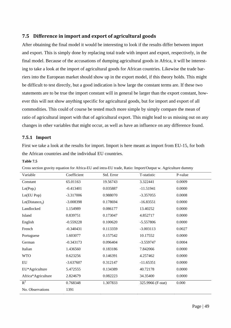
7.5 Difference in import and export of agricultural goods After obtaining the final model it would be interesting to look if the results differ between import

and export. This is simply done by replacing total trade with import and export, respectively, in the

final model. Because of the accusations of dumping agricultural goods in Africa, it will be interest-

ing to take a look at the import of agricultural goods for African countries. Likewise the trade bar-

riers into the European market should show up in the export model, if this theory holds. This might

be difficult to test directly, but a good indication is how large the constant terms are. If these two

statements are to be true the import constant will in general be larger than the export constant, how-

ever this will not show anything specific for agricultural goods, but for import and export of all

commodities. This could of course be tested much more simple by simply compare the mean of

ratio of agricultural import with that of agricultural export. This might lead to us missing out on any

changes in other variables that might occur, as well as have an influence on any difference found.

7.5.1 Import First we take a look at the results for import. Import is here meant as import from EU-15, for both

the African countries and the individual EU countries. Table 7.5

Cross section gravity equation for Africa-EU and intra-EU trade, Ratio: Import/Output w. Agriculture dummy

Variable Coefficient Std. Error T-statistic P-value

Constant 65.01163 19.56743 3.322441 0.0009

Ln(Popi) -0.413401 0.035887 -11.51941 0.0000

Ln(EU Pop) -3.317006 0.988070 -3.357055 0.0008

Ln(Distanceij) -3.008398 0.178694 -16.83551 0.0000

Landlocked 1.154989 0.086177 13.40252 0.0000

Island 0.839751 0.173047 4.852717 0.0000

English -0.559228 0.100620 -5.557806 0.0000

French -0.340431 0.113359 -3.003113 0.0027

Portuguese 1.603077 0.157542 10.17552 0.0000

German -0.343173 0.096404 -3.559747 0.0004

Italian 1.436560 0.183186 7.842066 0.0000

WTO 0.623256 0.146391 4.257462 0.0000

EU -3.637607 0.312147 -11.65351 0.0000

EU*Agriculture 5.472555 0.134389 40.72178 0.0000

Africa*Agriculture 2.824679 0.082223 34.35400 0.0000

R2 0.768348 1.307833 325.9966 (F-stat) 0.000

No. Observations 1391

Page | 49

Many of the coefficients are very similar to the ones for total trade. Therefore we will only take a

look at the interesting ones for the purpose. First of all, the constant has become smaller, but this

can be due to small changes in coefficients with large averages such as EU population. The constant

is not of interest before it can be compared with that of export. Furthermore we see the two interac-

tion variables have moved even further from each other which may indicate that African countries

import even less agricultural goods than EU countries. This is opposite of what might be expected if

dumping of agricultural goods took place.

On the other hand, the theory of comparative advantages and the role agriculture plays in the econ-

omy, suggests that we would expect agricultural goods to be imported relatively less than non-

agricultural goods in Africa. This is not the case, as agricultural imports are still relatively higher.

Finally, the R2 is still quite high, and has actually increased from the total trade regression.

7.5.2 Export The estimation is repeated for exports from the single countries to the EU-15. The results are as

shown in table 7.6. Table 7.6

Cross section gravity equation for Africa-EU and intra-EU trade, Ratio: Export/Output w. Agriculture dummy

Variable Coefficient Std. Error T-statistic P-value

Constant 102.5096 32.53983 3.150281 0.0017

Ln(Popi) -0.530749 0.059679 -8.893361 0.0000

Ln(EU Pop) -5.540167 1.643120 -3.371737 0.0008

Ln(Distanceij) -2.202174 0.297160 -7.410733 0.0000

Landlocked 1.449275 0.143309 10.11296 0.0000

Island 1.437880 0.287771 4.996617 0.0000

English -0.434284 0.167327 -2.595418 0.0095

French -0.495582 0.188512 -2.628917 0.0087

Portuguese 1.927233 0.261987 7.356228 0.0000

German 0.476236 0.160315 2.970619 0.0030

Italian 1.088491 0.304631 3.573144 0.0004

WTO 0.969630 0.243443 3.982991 0.0001

EU -1.866881 0.519087 -3.596469 0.0003

EU*Agriculture 5.337860 0.223483 23.88485 0.0000

Africa*Agriculture 3.514176 0.136733 25.70101 0.0000

R2 0.587399 2.174871 139.9243 (F-stat) 0.000

No. Observations 1391

Page | 50

Again all of the coefficients are not all that different from the total trade estimation without testing

them for significant differences. The constant term has however changed quite a bit from 80.09 in

total trade and 65.01 in imports to 102.51 for exports. Many things can explain this change in the

constant but one of the most likely is an actual change in the value of the dependent value. As ar-

gued, a lower numerator (value of import, export or total trade) will lead to a lower ratio, as the

product of output does not change between the three estimations. Therefore a lower ratio will lead

to a lower constant term. In this case the export constant is higher than the import which suggests

that countries export relatively more than they import. This is of course for all countries and for all

commodities, but is an indication of what lies behind the trade patterns. To support this trend the

two interaction variables have again moved closer to each other.

As with the interaction term for agricultural imports in Africa, we would also expect that the EU

countries export relatively less agricultural goods than other. But the coefficient is still highly sig-

nificant, and higher than the equivalent African coefficient. This is in contradiction to theory of

comparative advantages.

Also, it is worthy of noting that the R2 for the export estimation has dropped a bit to 0.59.

7.6 Conclusions of the gravity equations So to conclude there seems to be a difference between import and export to and from the EU-15.

This difference also appears to be in favor of export, which means more is exported than imported.

Again this might contradict believes of dumping on the African market and high barriers of trade to

the EU market. Many factors can contribute to these results, but it is not unexpected looking back at

the descriptive statistics, especially not if we focus on the agricultural sector. One must keep in

mind that African countries still have a comparative advantage in agricultural goods, so it seems

natural that they export more than they import in this sector. What we still do not know is how these

levels would have been in a totally free trade environment without the CAP.

The most important conclusion to come out of this gravity equation analysis is the evidence that

agricultural trade with Africa is significantly smaller than that of EU countries, despite the theoreti-

cal comparative advantage to the African countries. The next section will investigate the possible

reasons behind this and other results of the gravity equations.

Page | 51

8 Interpretation of results 

The trade situation between Africa and the EU has in many ways been described in the review of

the trade agreements and the CAP. However, I will now take a look at the situation through the

perspective of the results of the gravity equations. First of all, this will of course concern the differ-

ence in the level of agricultural trade with the EU and Africa, which is the main focus of the thesis.

In relation to this it will also be relevant and interesting to look at the difference between import and

export which was found.

Second, I will also look at other interesting findings in the analysis. For one the regression for Afri-

ca still using the FTA dummies show that UEMOA was negatively correlated with trade, while the

three other FTAs where positive. I will figure out if there is a good reason behind this difference.

Another interesting observation is that the former English and French colonies are negatively corre-

lated with trade. Since the UK and France where the two largest colonizers in Africa, it is quite in-

teresting why these countries have less trade than countries with other colonizers. And finally, I will

look for reasons why the variables for landlocked countries and islands are both positive, while

general theory suggest they should be negative.

8.1 Difference in level of agricultural trade Many reasons for distortions in trade have already been presented. The main reasons are most likely

to be the requirements to the agricultural goods imported into the EU market, the export subsidies

paid to the EU farmers, and in general the support schemes to the EU farmers.

Although the Cotonou Agreement practically removes all tariffs, the EU has set up some standards

in the negotiations they would like fulfilled. These relate to competition policy, protection of intel-

lectual property rights, standardization and certification, sanitary and phytosanitary measures, envi-

ronment, labor standards, investment, public procurement, and data protection (Goodison, 2007a).

These all represent some degree of non-tariff restrictions and therefore have a negative effect on

free trade. As Goodison (2007a) notes, meeting the EU food safety standards requires an enormous

effort for ACP countries, including creating new government departments and abnormal invest-

ments. The minimum initial cost to set legislature and establishing the framework is set to €187

million. The EU has even set the standards so high that they will need to invest €250 million to

comply with these standards themselves. As Goodison (2007a) goes on to conclude: “Meeting this

food safety challenge effectively in ACP countries is essential, for any failure in this area could lead

to the closure of EU markets to food-and-agricultural exports from the ACP country concerned”.

This is also remarked by Bertow and Schultheis (2007) that argue that reduction of tariffs have little

Page | 52

impact as long as these non-tariff barriers still exist to such a high degree. So it seems quite obvious

that other challenges than pure tariff barriers play a large role in trade between Africa and EU.

However, it seems quite clear that Goodison and others are negatively biased towards the agree-

ment. This should of course be kept in mind, but since nearly all academic papers seem negative

towards the development prospects of the agreement they may have a point.

As Bertow and Schultheis (2007) also remark, supply restraints for the African producers mean that

the liberalization undergone does not benefit them. Although prices might rise due to the tariff free

import to the EU market, small producers have limited land access, and can therefore not expand

production any further. Other constraints also apply to the African farmers that hinder them in bene-

fiting from the trade liberalization. This includes the lack of storage facilities which means agricul-

tural produce needs to be sold directly after harvest, sometimes at very low prices (Bertow and

Schultheis, 2007).

These are just some of the non-tariff barriers that still exist. So even though tariffs have practically

been removed, many obstacles to trade still exist, and the CAP and Cotonou Agreement seem to be

the main reasons behind these distortions.

8.2 Difference in import and export The results show that countries (both African and EU) in general export more to the EU than they

import from the EU. If more research was done more conclusive evidence might be found that ex-

port is larger than import, but descriptive statistics already suggests that this is true.

One reason already briefly mentioned is the comparative advantage of agriculture in Africa. But as

the EU countries also are represented in the regression, strong conclusions cannot be drawn from

this theory. However it can also be seen as evidence that some of the trade agreements actually do

work in the intended way. To test this it would of course be necessary to test the difference before

and after policy changes, as this might also have been the trade levels before these reforms.

The matter of fact is that even if African countries export more to the EU than they import from

them, the level of exports is presumably still artificially low compared to a free trade setting. In a

free trade setting the EU countries would most likely produce very little agricultural products and

import most of the food needs from Africa, amongst others.

Page | 53

8.3 Impact of FTAs The results in one of the earlier models interestingly show that the UEMOA FTA has a negative

correlation with trade, while the three others have a positive. Secondary literature has offered no

explanation into why this situation could exist, so further research is necessary if this issue is of any

interest. Simple explanations could be a difference in which agricultural goods are produced, the

relative factor endowments, or how resources are utilized. Since negotiations are conducted on an

EU-EPA level, it could also be due to differences in agreements with the EU.

8.4 Former colonies There is no obvious reason for why the former English and French colonies apparently trade less

with EU than other countries. One reason could simply be that their trade is so much focused on

their former colonizers that the rest of the EU countries are neglected. No research has been found

in this area, so therefore further research would need to be conducted to see if this result actually is

significant for trade, and what the reasons are.

8.5 Landlocked countries and islands Again there seems to be no obvious explanation for these results, and further research may be ne-

cessary if the results have any interest in future work with the area. The fact that the final model is

in trade ratio might have an impact, otherwise these types of countries in Africa might have un-

common attributes that contribute to trade.

9 Future research steps 

Evidence has been found that the CAP in fact has an effect on agricultural trade with Africa. But

research into this area is rather scarce, so what can be done if there is an interest of learning more

about the subject?

9.1 Development aid The ultimate goal of this issue will be to put it into the context of development aid paid by the EU.

This will require much research into the area, but will give answer to many interesting questions,

such as if financial resources are being used in the correct way.

In order to conduct such a research it will be relevant to measure the exact economic effects the

CAP has on African countries and their development. This should be held up against how much is

used on financing the CAP and how much is paid out in development aid. This might be a very

Page | 54

comprehensive and difficult task but will most likely yield some very interesting results. If the long

term goal in fact is to help Africa out of poverty, a plan could be made so policies do not contradict

each other, which indications show they might do currently.

9.2 Regions and Free Trade Agreements Many other interesting subjects also deserve further research, some of them have been discovered

within my research, and others have been left out from the start.

One of the unanswered but interesting questions that have arisen during the research is the differ-

ence that may exist between African regions and FTAs. It would be really interesting to discover

what might cause these differences. This could be done be looking closer at the individual agree-

ments that exist with the EU, or policy differences within each regions. Also a comprehensive look

at which agricultural goods are being produced would be relevant. Various crops may be easier to

export than others and factor endowments may also be different between the regions. As a subsec-

tion to this issue, it might also be interesting to look at the differences between former colonizers. If

something is hindering trade for some countries, it might be possible to change in the future.

9.3 Policy changes Another issue that has been more or less ignored in the statistical research is the policy changes

described in the theory sections. It could be interesting to see any significant statistical changes in

the reforms of the CAP and the ACP-EU agreements. It has already been discussed what effects

these changes have in theory, but a quantitative research of how they have actually affected trade

could be quite interesting. As policy changes take some time to have an effect, time-lagged models

will have to be used in the research. Besides showing effects of previous policy changes, it can help

to show which measures had the desired effect and assist in developing future policy changes.

9.4 World trade If the effect of the CAP were to be examined closer it might be relevant to expand the research to a

global scale. This is of course depends on available statistics. If all countries where included in a

gravity equation analysis it would be easier to isolate the CAP effect. Many different approaches

may be used, but it might be relevant to focus on trade with such countries as Australia and New

Zealand, who have recently removed agricultural support systems, and basically employ free trade.

A research with this perspective could also be used in a more global policy development, perhaps in

the Doha Round or future WTO negotiations.

Page | 55

10 Conclusion The research of the trade situation between Africa and the EU has shown several things, theoretical-

ly as well as empirically. It is hard to put numbers on the economic consequences of the CAP, but

theory suggests that African countries are worse off economically due to the CAP. Theory also sug-

gests that African countries have a comparative advantage in agricultural goods, and therefore

should export more of these goods than the EU countries, however empirical research has shown a

different relation, namely that African countries trade relatively less with agricultural goods than

intra-EU trade in these commodities. This is very substantial proof that the CAP has a negative ef-

fect on agricultural trade with Africa.

Although it has not been analyzed to depth, it can be concluded that agriculture does play a large

role in economic development of a country. Therefore the negative effect the CAP has on agricul-

tural trade must also have a negative effect on the development of African countries. Theory says

that if a free trade environment existed between the two regions, the African countries would export

a substantial part of the EU consumption of agricultural goods, while little, if any, would be im-

ported. Trade figures show that more is exported than imported, but not to the degree that might be

expected according to theory. At the same time the import of agricultural goods has increased rela-

tively more than exports in the time period analyzed. A free trade situation would therefore in

theory give an enormous boost to the agricultural sector in Africa, perhaps moving the region closer

to industrialization and away from poverty. This is however something that will need further re-

search in order to be confirmed.

It might look as if several steps have been made in order to move closer to this free trade environ-

ment with reforms of the CAP and agreements between Africa and the EU. However, when theory

is applied to these policy changes it shows that little, if any, effects really come from them. As sug-

gested by some researchers the EU is simply changing the system to fit within the WTO policies,

while the outcome is still more or less the same. The removal of all tariffs on imports into the EU

sounds like a very good initiative, but these tariff boundaries are substituted by non-tariff barriers

that might be even worse for trade. The increased price for meeting the EU standards combined

with the lower selling price on the EU market leads to harder conditions for the African farmers. So

the effects of the CAP are felt both at the micro- and macroeconomic level, as both farmers and

countries as a whole are affected.

Page | 56

Results from the gravity equations show that agricultural goods in general are traded relatively more

than non-agricultural goods in both EU and African countries. If we look at the agricultural share of

GDP in the two regions this relation might not be surprising for exports for African countries and

imports for EU countries. But when both exports and imports for both regions show relative more

trade it is an interesting result. As African countries do not produce as many non-agricultural goods

it might be expected that they would import more of these goods compared to agricultural goods. So

the evidence that agricultural goods are imported relatively more than other goods, suggests that

there might be some form of dumping going on, or at least an unnatural competitive situation.

The most important conclusion of the analysis is that there can be found a statistical significant dif-

ference in agricultural trade with Africa. This clearly suggests that the existence of the CAP in the

EU market has an effect on the trade outcome. However, the research does not give any clear an-

swer to what causes this difference. Several different explanations have been found, but the main

focus has been on explaining it from a CAP perspective. Other external reasons might exist that

give a perhaps natural explanation to the findings. But one thing can be concluded for certain, the

results obtained differ from the theory of a free trade outcome and is pretty much coherent with

theory on trade intervention. So in spite of the effort to remove tariffs, much distortion still exists in

the agricultural trade relationship between Africa and the EU.

These distortions can perhaps be explained by the subsidies paid to the EU farmers both in direct

support and export subsidies, as well as the non-tariff barriers into the EU market, such as high food

quality standards. The first can explain the unnatural high import into the African market, while the

latter can explain the relatively low export to the EU market.

So overall, the combination of theoretical and empirical evidence strongly suggests that the CAP

has a negative economic effect on sub-Saharan African countries, and that the agricultural trade is

different due to the complex trade structure made up by the CAP and trade agreements.

Page | 57

11 Bibliography 

Baier, Scott L. and Bergstrand, Jeffrey H. 2006. Do free trade agreements actually increase mem-

bers’ international trade?. Journal of International Economics 71: 72-95.

Baldwin, Richard and Taglioni, Dario. 2006. Gravity for Dummies and Dummies for Gravity Equa-

tions. Discussion Paper No. 5850 (September 2006). Centre for Economic Policy Research.

Bertow, Kerstin and Schultheis, Antje. 2007. Impact of EU’s agricultural trade policy on smallhold-

ers in Africa. Germanwatch.

Cardwell, Michael. 2004. The European Model of Agriculture. Oxford University Press.

CEMAC. 2009. http://www.cemac.cf/. Accessed: 2/3-2009. Commission De La Communaute Eco-

nomique Et Monetaire De L’Afrique Centrale, Central African Republic.

CEPII Distance Database. 2009. http://www.cepii.fr/anglaisgraph/bdd/distances.htm. Accessed:

4/3-2009. Centre D'Etudes Prospectives et D'Informations Internationales.

CIA. 2008. The 2008 World Fact Book. Central Intelligence Agency.

Coe, David T. and Hoffmaister, Alexander W. 1999. North-South Trade: Is Africa Unusual?. Inter-

national Monetary Fund. Journal of African Economies 8(2): 228-256.

EAC. 2009. http://www.eac.int/. Accessed: 2/3-2009. Eastern African Community, Arusha, Tanza-

nia.

European Commission. 2007. The Common Agricultural Policy Explained. European Communities.

Eurostat. 2009. http://ec.europa.eu/eurostat. Accessed: 19/2-2009. Statistical Office of the European

Communities.

FAO. 2006. The agricultural dimension of the ACP-EU Economic Partnership Agreement. Rome:

Food and Agriculture Organization of the United Nations.

Feenstra, Robert C., Markusen, James A. and Rose, Andrew K. 1999. Using the Gravity Equation to

Differentiate Among Alternative Theories of Trade. Centre for Economic Policy Research.

Page | 58

Fratianni, Michele. 2007. The Gravity Equation in International Trade. Handbook of International

Business, 2nd edition. Oxford University Press.

Gbetnkom, Daniel. 2006. Market Implications of COMESA’s Accession to the Free Trade Area: A

Gravitational Investigation. Journal of African Development 1(1): 133-157.

Goodison, Paul. 2007a. EU trade policy & the future of Africa’s trade relationship with the EU.

Review of African Political Economy 34(112): 247-266.

Goodison, Paul. 2007b. What is the future for EU-Africa trade after CAP reform?. Review of Afri-

can Political Economy 34(112): 279-295.

Grant, Jason H. and Lambert, Dayton M. 2008. Do Regional Trade Agreements Increase Members’

Agricultural Trade?. American Journal of Agricultural Economics 90(3): 765-782.

Haque, Ifran ul. 2007. Rethinking Industrial Policy. Discussion Paper No. 183. United Nations Con-

ference on Trade and Development.

Kirkpatrick, Colin and Watanabe, Matsuo. 2005. Regional Trade in Sub-Saharan Africa: An Analy-

sis of East African Trade Cooperation, 1970-2001. The Manchester School 73(2): 141-164.

Morrison, J. and Sarris, A. 2007. Determining the appropriate level of import protection consistent

with agriculture led development in the advancement of poverty reduction and improved food

security. WTO rules for agriculture compatible with development. Rome: Food and Agricul-

ture Organization of the United Nations.

Nelson, Michael B. and Halderman, Michael. 2004. The EU, CAP, and developing countries: Un-

derstanding the June 2003 CAP Reforms & Their Relation to Developing Country Interests.

American Political Science Association.

OECD. 2004. Analysis of the 2003 CAP Reform. Organisation for Economic Co-Operation and

Development.

Piermartini, Roberta and Teh, Robert. 2005. Demystifying Modelling Methods for Trade Policy.

Discussion Paper No. 10. World Trade Organization. Geneva.

Roijd, Sawkut. 2006. COMESA trade potential: A Gravity Approach. Applied Economic Letters

13: 947-951.

Page | 59

SADC. 2009. http://www.sadc.int/. Accessed: 2/3-2009. Southern African Development Communi-

ty, Gaborone, Botswana.

Salvatore, Dominick. 2007. International Economics 9th edition. John Wiley & Sons Inc.

Trebilcock, Michael J. and Howse, Robert. 2005. The Regulation of International Trade. 3rd Edition.

Routledge.

UEMOA. 2009. http://www.uemoa.int/. Accessed: 2/3-2009. Union Economique et Monétaire

Ouest Africaine, Burkina Faso.

UN Statistical Databases. 2009. http://unstats.un.org/. Accessed: 20/3-2009. United Nations Statis-

tics Division. New York, UN.

von Lampe, Martin. 2002. Modelling Impacts of the Macroeconomic and Political Environment on

Long-Term Prospects for Agricultural World Markets. Agricultural Trade Policies in the New

Millenium. Food Products Press. New York.

World Bank. 2009. World Development Indicators. http://www.worldbank.org/data/. Accessed:

20/3-2009. The World Bank Group.

World Trade Organization. 2009. http://www.wto.org/. Accessed: 2/3-2009. World Trade Organiza-

tion, Geneva, Switzerland.

Page | 60

Appendix A 

Discussion of gravity equation assumptions 

The most common problem in gravity equation is endogeneity bias, especially in regard to omitted

variables. As many different things presumably influence bilateral trade, it is nearly impossible to

include all these variables in the model. This might cause correlation between the independent va-

riables and the omitted variables included in the error term. Baier and Bergstrand (2006) mention

the problem in relation to the FTA dummies, in their paper examining the effects of FTAs. Many

different parameters determine why countries chose to form a FTA, and not all of these are included

in the model. Specific issues regarding to the countries in question may apply, and can be hard to

include in the observed variables. This problem can be generalized to why two specific countries

trade with each other. Politics, special relationships, focused marketing into specific countries, and

so on, can all have great effect on the trade outcome, but are not observed in the gravity equation

model. If these omitted variables are correlated with the independent variables, it will result in bias

in the estimates of the coefficients.

For the specific Africa-EU gravity equation in this thesis, the important independent variables are

the two agriculture variables. Several omitted variables can have a possible biased effect on these

two crucial variables. Examples of omitted variables could be specific policies, the agricultural per-

centage of GDP, or a look at how goods are traded (bulk, differentiated etc.). However this bias is

most likely to influence both of the agricultural variables, and therefore does not pose a large threat

to the results. The main purpose is to investigate if a difference between the two variables exists, so

unless the bias turns out to be very unequal to the variables, the results will be accepted. 

Another problem that has been mentioned is the consistency of the EU GDP and population in the

estimation. These variables only change by year, and are constant across all observations in each

year. However it seems that the only problem to come out of this is insignificant variables. As these

variables are not of any direct interest the insignificant variables are not of any problem to the esti-

mations.

All other standard Multiple Linear Regression assumptions are in general fulfilled in the regres-

sions.

Page | 61

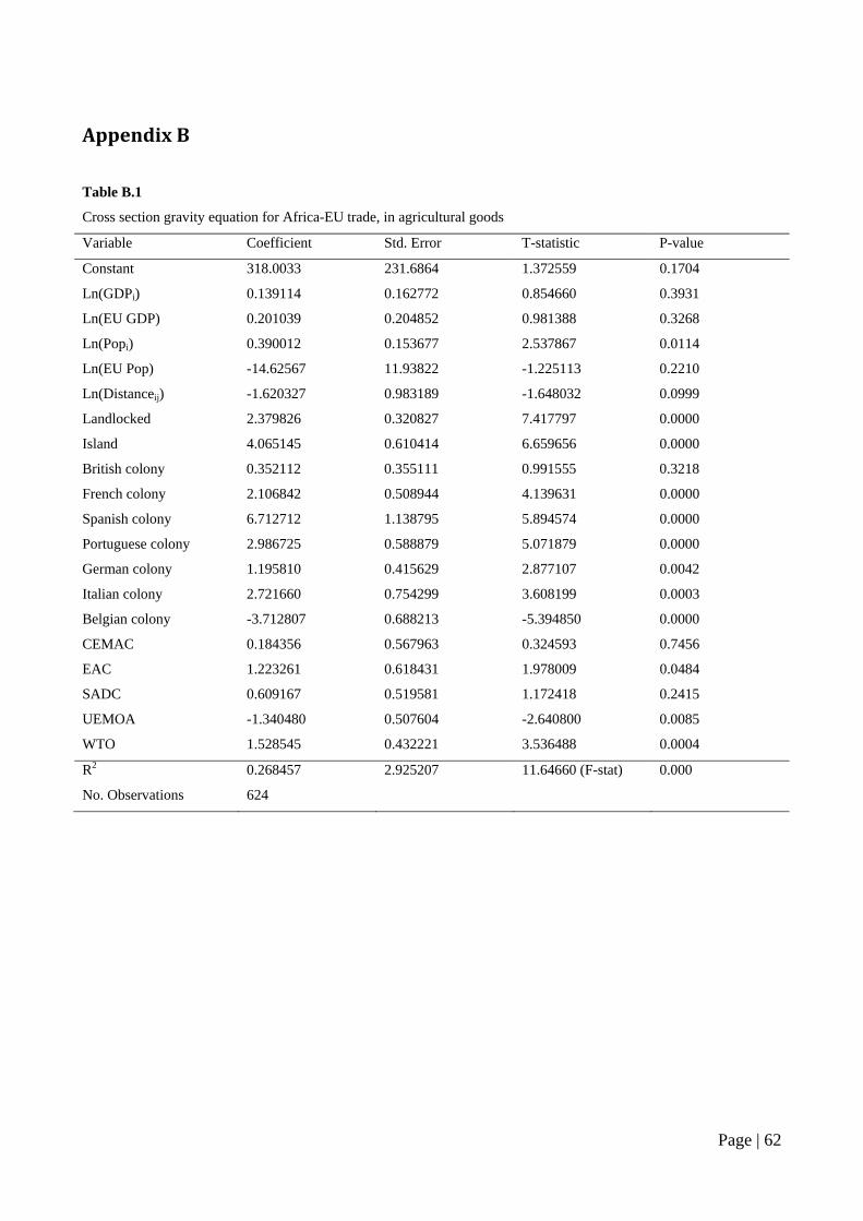
Appendix B 

Table B.1

Cross section gravity equation for Africa-EU trade, in agricultural goods

Variable Coefficient Std. Error T-statistic P-value

Constant 318.0033 231.6864 1.372559 0.1704

Ln(GDPi) 0.139114 0.162772 0.854660 0.3931

Ln(EU GDP) 0.201039 0.204852 0.981388 0.3268

Ln(Popi) 0.390012 0.153677 2.537867 0.0114

Ln(EU Pop) -14.62567 11.93822 -1.225113 0.2210

Ln(Distanceij) -1.620327 0.983189 -1.648032 0.0999

Landlocked 2.379826 0.320827 7.417797 0.0000

Island 4.065145 0.610414 6.659656 0.0000

British colony 0.352112 0.355111 0.991555 0.3218

French colony 2.106842 0.508944 4.139631 0.0000

Spanish colony 6.712712 1.138795 5.894574 0.0000

Portuguese colony 2.986725 0.588879 5.071879 0.0000

German colony 1.195810 0.415629 2.877107 0.0042

Italian colony 2.721660 0.754299 3.608199 0.0003

Belgian colony -3.712807 0.688213 -5.394850 0.0000

CEMAC 0.184356 0.567963 0.324593 0.7456

EAC 1.223261 0.618431 1.978009 0.0484

SADC 0.609167 0.519581 1.172418 0.2415

UEMOA -1.340480 0.507604 -2.640800 0.0085

WTO 1.528545 0.432221 3.536488 0.0004

R2 0.268457 2.925207 11.64660 (F-stat) 0.000

No. Observations 624

Page | 62

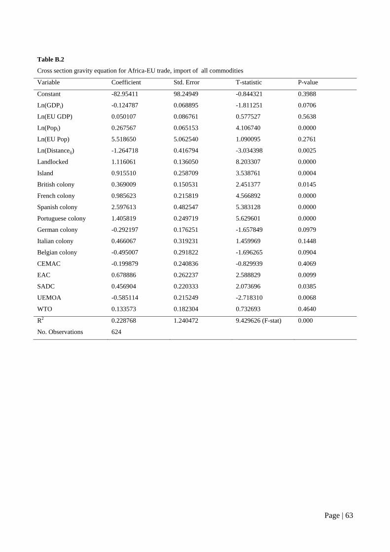
Table B.2

Cross section gravity equation for Africa-EU trade, import of all commodities

Variable Coefficient Std. Error T-statistic P-value

Constant -82.95411 98.24949 -0.844321 0.3988

Ln(GDPi) -0.124787 0.068895 -1.811251 0.0706

Ln(EU GDP) 0.050107 0.086761 0.577527 0.5638

Ln(Popi) 0.267567 0.065153 4.106740 0.0000

Ln(EU Pop) 5.518650 5.062540 1.090095 0.2761

Ln(Distanceij) -1.264718 0.416794 -3.034398 0.0025

Landlocked 1.116061 0.136050 8.203307 0.0000

Island 0.915510 0.258709 3.538761 0.0004

British colony 0.369009 0.150531 2.451377 0.0145

French colony 0.985623 0.215819 4.566892 0.0000

Spanish colony 2.597613 0.482547 5.383128 0.0000

Portuguese colony 1.405819 0.249719 5.629601 0.0000

German colony -0.292197 0.176251 -1.657849 0.0979

Italian colony 0.466067 0.319231 1.459969 0.1448

Belgian colony -0.495007 0.291822 -1.696265 0.0904

CEMAC -0.199879 0.240836 -0.829939 0.4069

EAC 0.678886 0.262237 2.588829 0.0099

SADC 0.456904 0.220333 2.073696 0.0385

UEMOA -0.585114 0.215249 -2.718310 0.0068

WTO 0.133573 0.182304 0.732693 0.4640

R2 0.228768 1.240472 9.429626 (F-stat) 0.000

No. Observations 624

Page | 63

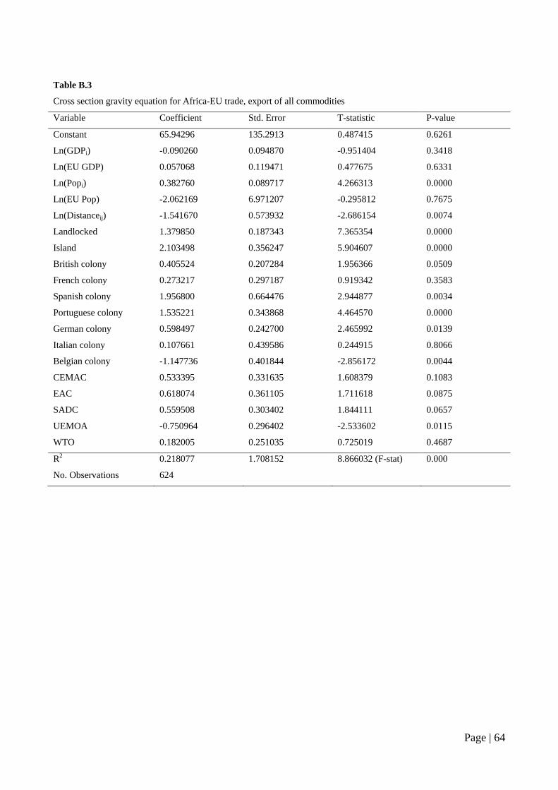
Table B.3

Cross section gravity equation for Africa-EU trade, export of all commodities

Variable Coefficient Std. Error T-statistic P-value

Constant 65.94296 135.2913 0.487415 0.6261

Ln(GDPi) -0.090260 0.094870 -0.951404 0.3418

Ln(EU GDP) 0.057068 0.119471 0.477675 0.6331

Ln(Popi) 0.382760 0.089717 4.266313 0.0000

Ln(EU Pop) -2.062169 6.971207 -0.295812 0.7675

Ln(Distanceij) -1.541670 0.573932 -2.686154 0.0074

Landlocked 1.379850 0.187343 7.365354 0.0000

Island 2.103498 0.356247 5.904607 0.0000

British colony 0.405524 0.207284 1.956366 0.0509

French colony 0.273217 0.297187 0.919342 0.3583

Spanish colony 1.956800 0.664476 2.944877 0.0034

Portuguese colony 1.535221 0.343868 4.464570 0.0000

German colony 0.598497 0.242700 2.465992 0.0139

Italian colony 0.107661 0.439586 0.244915 0.8066

Belgian colony -1.147736 0.401844 -2.856172 0.0044

CEMAC 0.533395 0.331635 1.608379 0.1083

EAC 0.618074 0.361105 1.711618 0.0875

SADC 0.559508 0.303402 1.844111 0.0657

UEMOA -0.750964 0.296402 -2.533602 0.0115

WTO 0.182005 0.251035 0.725019 0.4687

R2 0.218077 1.708152 8.866032 (F-stat) 0.000

No. Observations 624

Page | 64

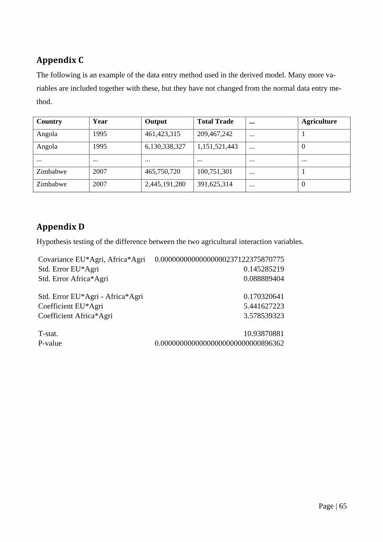
Page | 65

Appendix C 

The following is an example of the data entry method used in the derived model. Many more va-

riables are included together with these, but they have not changed from the normal data entry me-

thod.

Country Year Output Total Trade ... Agriculture

Angola 1995 461,423,315 209,467,242 ... 1

Angola 1995 6,130,338,327 1,151,521,443 ... 0

... ... ... ... ... ...

Zimbabwe 2007 465,750,720 100,751,301 ... 1

Zimbabwe 2007 2,445,191,280 391,625,314 ... 0

Appendix D 

Hypothesis testing of the difference between the two agricultural interaction variables. Covariance EU*Agri, Africa*Agri 0.00000000000000000237122375870775 Std. Error EU*Agri 0.145285219 Std. Error Africa*Agri 0.088889404 Std. Error EU*Agri - Africa*Agri 0.170320641 Coefficient EU*Agri 5.441627223 Coefficient Africa*Agri 3.578539323 T-stat. 10.93870881 P-value 0.00000000000000000000000000896362