1 | P a g e

Welsh waters scallop surveys and stock assessment

Delargy, A., Hold, N., Lambert, G.I., Murray, L.G., Hinz, H., Kaiser, M.J., McCarthy, I.

and Hiddink, J.G.

Please cite as follows: Delargy, A., Hold, N., Lambert, G.I., Murray L.G., Hinz H., Kaiser M.J.,

McCarthy, I., Hiddink J.G. (2019) – Welsh waters scallop surveys and stock assessment. Bangor

University, Fisheries and Conservation Report No. 75. pp 48

2 | P a g e

Funded by:

3 | P a g e

Contents EXECUTIVE SUMMARY........................................................................................................................................ 4

INTRODUCTION .................................................................................................................................................. 7

MATERIALS AND METHODS ............................................................................................................................... 8

Survey design.................................................................................................................................................. 8

Scallop dredging ............................................................................................................................................. 9

Data analyses ................................................................................................................................................ 11

Stock assessment models ............................................................................................................................. 12

Commercial data for stock assessment ........................................................................................................ 13

Survey data for stock assessment ................................................................................................................ 14

RESULTS ............................................................................................................................................................ 14

Survey indices ............................................................................................................................................... 14

Population structure .................................................................................................................................... 16

Growth rates ................................................................................................................................................ 20

Distance from shore analyses ...................................................................................................................... 22

Body part to shell width relationships ......................................................................................................... 24

Maturity stage .............................................................................................................................................. 26

Bycatch ......................................................................................................................................................... 27

Stock assessment results .............................................................................................................................. 29

DISCUSSION ...................................................................................................................................................... 33

Population status from survey results ......................................................................................................... 33

Survey design and data considerations ........................................................................................................ 34

Stock status from stock assessment modelling ............................................................................................ 36

Stock assessment considerations ................................................................................................................. 37

Management recommendations.................................................................................................................. 38

ACKNOWLEDGEMENTS, AUTHORS AND FUNDING .......................................................................................... 46

REFERENCES ..................................................................................................................................................... 47

APPENDIX ......................................................................................................................................................... 48

4 | P a g e

EXECUTIVE SUMMARY

Mean annual survey indices (densities of king scallops caught) were consistently greater in Cardigan

Bay than the other two fishing ground sampled; Liverpool Bay and the waters north of the Llyn

Peninsula, in all years (between 4 to 38 times greater). Mean annual survey indices were also

consistently greater in the area of the special area of conservation (SAC) open to commercial fishing

in Cardigan Bay (Open Box) than Liverpool Bay and the Llyn Peninsula (1.5 to 25 times greater). Mean

annual survey indices in the closed areas of Cardigan Bay were consistently greater than those in the

open areas of Cardigan Bay (Open Box and Open Other) (1.8 to 7.1 times greater).

Mean annual survey indices have been increasing since 2016 in Cardigan Bay (overall). This increase

has been driven by increasing mean annual survey indices in the Experimental Area (closed) and the

Open Box. The indices in the remaining management areas have either remained low or decreased

since 2016. Mean annual survey indices from Liverpool Bay or the Llyn Peninsula remained low

throughout the time series.

The king scallop populations were dominated by larger and older individuals in both Liverpool Bay

and the Llyn Peninsula, although in some years there were relatively high proportions of king scallops

below the minimum landing size (MLS) (110mm shell width) (pre-recruits). In the most recent survey

(April 2019), a relatively high proportion of the population were pre-recruits in Liverpool Bay which

indicated some recruitment to the harvestable portion of the population may occur in the immediate

future. However, the vast majority of the Llyn population were above MLS and therefore recruitment

may be unlikely in the immediate future.

The populations within the West SAC and the Experimental Area (both closed) were dominated by

larger and older individuals in the majority of years, although in 2019 relatively high proportions of

these populations were pre-recruits and therefore this may lead to future recruitment. The

population within the East SAC (closed) was also dominated by larger and older individuals, although

higher proportions of pre-recruits were observed in most years compared to the West SAC or

Experimental Area which may indicate some recruitment was occurring throughout the time series

in the East SAC. The Open Box population was dominated by pre-recruits in many years, including

2019. This indicates recruitment is occurring in the area and that fishing is likely removing large

amounts of individuals above the MLS. The implications by these patterns with respect to

recruitment is discussed further in this report.

The mean annual indices of pre-recruits caught in the queen dredges in the closed parts of Cardigan

Bay (East SAC, West SAC and Experimental Area) were at or below 1 per 100m2 of seabed swept for

the majority of surveys, apart from the most recent survey where the mean index was 3.6 per 100m2.

This increase was largely driven by the Experimental Area, which indicated the potential for

recruitment in the immediate future for this area. The mean annual indices of king scallops ≥ the MLS

caught by king dredges in the open areas of Cardigan Bay were between 0.65 and 0.7 per 100m2 for

5 | P a g e

the years 2012 to 2014, but below 0.35 per 100m2 for all consequent years. This indicated there were

low densities of harvestable king scallops in the areas of Cardigan Bay open to fishing.

There were few differences in growth rates or size-at-age between the fishing grounds and the

management zones of Cardigan Bay, when king scallops from all years were analysed collectively. We

would consider these relationships to be effectively the same for the purposes of management.

There was some evidence of distance to shore affecting the size and age composition of indices,

when data were pooled for all years. Both individual size and size-at-age increased with distance

from shore in the Experimental Area, and fewer younger king scallops were caught with increased

distance from shore. Both size and age decreased with distance from shore in the Open Other area

in Cardigan Bay, but size and age increased with distance from shore in the Open Box in Cardigan

Bay. Other relationships with distance from shore that were identified are discussed in the report,

but these patterns were not consistent across all the relationships examined.

No notable trends were detected in either gonad maturity cycle or the relationship between meat

yield and shell width. Similarly, all shell width to weight of various body parts of the king scallop

relationships were very similar between fishing grounds and management zones of Cardigan Bay.

Mean annual bycatch indices were consistently highest in Liverpool Bay, and were 1.5 to 7.4 times

greater than the indices from Cardigan Bay and 1.9 to 4.1 times greater than the Llyn Peninsula.

Mean annual bycatch indices in Cardigan Bay were less than 0.125 kg per 100m2 swept across all

years, with the highest densities occurring in all areas on the 2018 survey.

The majority of stations in Liverpool Bay and the Llyn Peninsula were dominated by bycatch. Eastern

stations within Cardigan Bay tended to have the highest proportions of bycatch of stations in

Cardigan Bay, however the majority of the indices from Cardigan Bay were dominated by king

scallops.

Natural mortality was estimated at 0.65 yr-1 from catch curve analysis of length-structured survey

indices from the closed areas of the Cardigan Bay SAC. This value is considered relatively high and

further validation is encouraged. However, the high natural mortality rate may explain why indices

have remained low in the East and West SAC despite closure to commercial scallop dredging since

June 2009. Annual fishing mortality rate was estimated using two stock assessment models for the

years 2012 to 2016. The median fishing mortality rate for king scallops ≥ the MLS was approximately

0.1 yr-1 and 0.3 yr-1 from each of the models, through the time series.

Three stock assessment models were implemented in total, and these varied in their simulated stock

structure (length- age- and un-structured). As a consequence, three separate estimates of king

scallop stock size in the fished parts of Cardigan Bay were obtained. The length- and un-structured

models indicated the stock size increased with time between 2012 and 2016, whereas the age-

structured model indicated stock size decreased over the same period. In addition, the magnitude of

estimated stock size, and respective biological reference points, also varied considerably between

6 | P a g e

the three models. The reasons for the variation between models is discussed, along with the need to

extend the data time series to improve model estimates.

In summary, there is strong evidence that king scallop indices in the Experimental Area of Cardigan

Bay are increasing which is driving the overall increase in mean indices for the entire Cardigan Bay

area. Indices remain relatively low in the other closed parts of Cardigan Bay, which may be explained

by a relatively high natural mortality rate. There is no evidence to suggest any improvement in indices

in areas open to fishing in Cardigan Bay, Liverpool Bay or the Llyn Peninsula. There is, however,

evidence of recruitment in the Open Box in the SAC which may explain the increase in survey indices

in this area since 2018. The recruitment is likely a consequence of close proximity to the high density

Experimental Area. The population structures of the open areas in Cardigan Bay appear to be

affected by fishing pressure, with low densities and low relative proportions of king scallops ≥ the

MLS. The populations in Liverpool Bay and the Llyn remain at at low densities, but are dominated by

larger, older individuals with little or highly sporadic recruitment occurring. A longer data time series

is required to better quantify all this information in stock assessment models.

7 | P a g e

INTRODUCTION

Many Welsh scallop fishers operate locally and are dependent on healthy, sustainable, local king scallop

(Pecten maximus) stocks. Scallops (both king and queen scallops (Aequipecten opercularis)) were the most

valuable wild-caught seafood animals landed in to Wales in 2012 (value £7.45 million, MMO 2016). However,

both the amount of landings and their value have decreased since then (value £1.4million in 2017, MMO

2018). Despite this decrease in value, scallops are still highly economically important as the third most

valuable wild-caught seafood animals landed in to Wales in 2017. The local and relative economic importance

of scallops to Wales means it is important that Welsh scallop populations are managed sustainably.

Bangor University has conducted eight scallop research surveys in Welsh waters since 2012, which have

spanned three projects. A European Fisheries Fund (EFF) funded project conducted surveys from 2012 to

2014, a Knowledge Exchange Skills Scholarship 2 (KESS 2) funded PhD project conducted surveys from 2016

to 2018 and a European Maritime and Fisheries Fund (EMFF) funded project conducted a survey in 2019 and

will continue to conduct surveys to 2022. The funders contributing to each project are acknowledged at the

end of this report. The aim of the surveys was to gather information on the distribution, abundance and

population dynamics of king scallop populations in Welsh waters, with the additional aim of conducting stock

assessments to assess stock sizes and provide advice to management on the status of Welsh scallop stocks.

Stock assessments involve the use mathematical and statistical methodology to estimate stock size, and

other useful metrics such as fishing mortality rate and recruitment (Hilborn and Walters 1992). Fishing

mortality rate is a measure of the rate of annual removals from a scallop stock caused by commercial fishing,

and recruitment is the new individuals entering the stock each year (through births). Stock assessments are

also used to estimate biological reference points, which typically indicate an amount of biomass to satisfy

some management criteria. One example would be maximum sustainable yield (MSY), which is the maximum

biomass that could be annually removed from a stock in perpetuity (Maunder 2008). Understanding and

quantification of these metrics are extremely useful for sustainable management of scallop stocks, as they

can be used to guide the implementation of management tools designed to ensure sustainability over the

long term. The KESS 2 project (Delargy 2019) conducted stock assessment modelling using commercial data

and a selection of the survey data reported here, and stock assessment modelling of king scallops will be

continued during the EMFF project.

This report details stock status information for Welsh king scallops as gathered from the research surveys.

Therefore, the report compares the results from the eight surveys. In addition, the report also outlines the

stock assessment model approaches that have been developed and applied for Welsh king scallops. The

results from the stock assessment models are displayed and discussed.

Specifically, the objectives of this report are to:

1. Examine temporal and spatial trends in survey indices of king scallops in Welsh waters

8 | P a g e

2. Examine temporal and spatial trends in survey length- and age-frequency distributions (stock

structure) in Welsh waters

3. Examine temporal and spatial trends in bycatch caught by survey gear in Welsh waters

4. Quantify and examine useful relationships such as growth and length-weight relationships for king

scallops in Welsh waters

5. Implement and analyse stock assessment models to assess stock size, fishing mortality rate,

recruitment and useful biological reference points for a king scallop stock in Cardigan Bay, Wales

MATERIALS AND METHODS

Survey design

Scientific surveys have been conducted by Bangor University from the RV Prince Madog since 2012, over

three projects and encompassed a wide range of researchers. The surveys sampled three main fishing

grounds; Cardigan Bay, Liverpool Bay and north of the Llyn Peninsula (Figure 1). The initial survey also

included Tremadog Bay, but this area was not sampled further due to high densities of static gear. These

fishing grounds were designated after consultation with the fishing industry in 2012. Surveys have been

conducted from 2012 to 2019, with the exception of 2015. In addition, the 2016 survey was conducted in

two parts. The survey timing within each year also varied (Table 1).

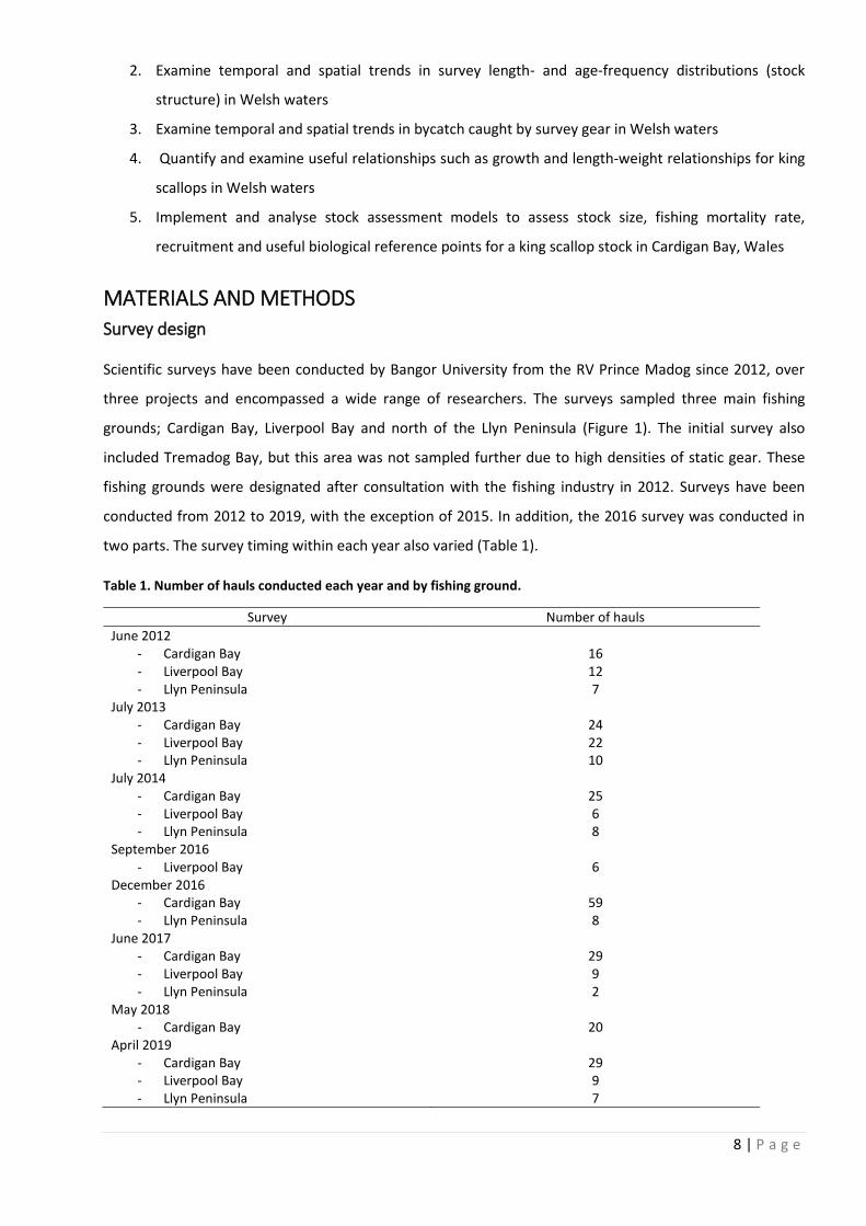
Table 1. Number of hauls conducted each year and by fishing ground.

Survey Number of hauls

June 2012 - Cardigan Bay - Liverpool Bay - Llyn Peninsula

16 12 7

July 2013 - Cardigan Bay - Liverpool Bay - Llyn Peninsula

24 22 10

July 2014 - Cardigan Bay - Liverpool Bay - Llyn Peninsula

25 6 8

September 2016 - Liverpool Bay

6

December 2016 - Cardigan Bay - Llyn Peninsula

59 8

June 2017 - Cardigan Bay - Liverpool Bay - Llyn Peninsula

29 9 2

May 2018 - Cardigan Bay

20

April 2019 - Cardigan Bay - Liverpool Bay - Llyn Peninsula

29 9 7

9 | P a g e

Each survey consisted of stratified-random sampling of each fishing ground, with the number of hauls

conducted in each area dependent on a number of factors including size of fishing ground, importance of

management area, suspected densities of king scallops, temporal length of survey and weather conditions

(Table 1). This stratified-random approach was used to allow for particular areas of interest within Cardigan

Bay to be sampled more or less extensively based on annual objectives and new information (Figure 2).

However, this has the potential to bias annual indices if a greater proportion of sampling effort was

conducted in high density areas. This is indicated in this report when this is suspected to have happened. The

management zones of Cardigan Bay were the Open Box in the Cardigan Bay Special Area of Conservation

(SAC) (open to scallop dredging), the Scientific Experimental Area in the SAC (closed to scallop dredging), the

eastern SAC (East SAC, closed to scallop dredging), the western SAC (West SAC, closed to scallop dredging)

and the remainder of the open fishing area within the Cardigan Bay fishing ground (Open Other). Sampling

was conducted using both dredges and cameras. However, due to a combination of poor weather conditions

restricting camera sampling in some years and the 2019 data not yet processed, camera sampling is not

presented or discussed further in this report. The results and discussion of the camera sampling conducted

during the first project (2012 – 2014) can be found in Lambert et al (2014).

Scallop dredging

Scallop dredging was conducted using four Newhaven dredges. Two dredges had nine teeth, which were

110mm long, and belly ring diameters of 80mm (hereafter referred to as king dredges). The other two

dredges had 10 teeth, which were 60mm long, and belly ring diameters of 60mm (hereafter referred to as

queen dredges). The mouth of each dredge was 0.76m. The king dredges were deployed to simulate

commercial fishing gear, and the queen dredges were deployed to more effectively sample queen scallops

(Aequipecten opercularis) and king scallops below the minimum landing size (MLS) of 110mm in shell width.

Using a gear capable of catching smaller king scallops than commercial gear allowed greater understanding

of the population structure at each fishing ground. The dredges were towed for 20 minutes at each sampling

location at a speed of approximately 2.5 knots. The position of the start and end of each haul were recorded

from the vessel’s navigation system, so that the swept area and midpoint of each haul could be calculated.

The swept area of each haul was used to estimate catch density, and the midpoint was used to explore catch

relationships with distance from shore.

After each haul the total king scallop catch was weighed per dredge, and separately the total queen scallop

catch was weighed by dredge. Total bycatch, defined as all other biota, were also weighed by each dredge.

Total bycatch did not include empty shells, rocks or any other abiotic catch. Bycatch data from the 2019

survey is still being analysed and is not included in this report. In 2012 – 2014, up to 45 king scallops per

dredge were measured to obtain size- and age-frequency distributions. In consequent years this was

increased to up to 90 individuals per dredge. King scallops were measured by shell width to the nearest mm.

10 | P a g e

These king scallops were also aged by counting external growth rings to obtain an age-frequency distribution.

Where there was more than 45 or 90 king scallops per dredge, the total weight of the measured individuals

was recorded. This allowed the size- and age-distributions of the sampled individuals to be raised to the total

weight of the king scallop catch per dredge, under the assumption that the subsampled individuals were

representative of the size- and age-structure of the total king scallop catch from that dredge. The raising of

length- or age-frequency distributions to absolute numbers caught was required for expressing as densities.

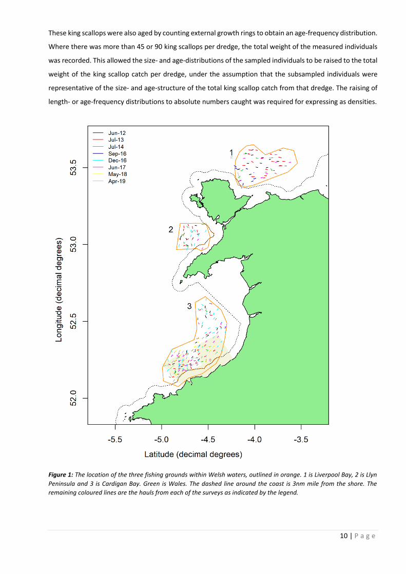
Figure 1: The location of the three fishing grounds within Welsh waters, outlined in orange. 1 is Liverpool Bay, 2 is Llyn

Peninsula and 3 is Cardigan Bay. Green is Wales. The dashed line around the coast is 3nm mile from the shore. The

remaining coloured lines are the hauls from each of the surveys as indicated by the legend.

11 | P a g e

After the 2012, 2013, 2014, (December) 2016 and 2017 surveys, samples of scallops (311, 469, 647, 907 and

565 respectively) were individually weighed (live weight, including shell weight), to allow for estimation of

size-weight and age-weight relationships, and then dissected to obtain shell, meat and gonad weights (±0.01g

in 2012 and 2013 and ±1g in 2014, 2016 and 2017). Quantifying shell, meat and gonad weights allowed

analyses of differences in meat yield (ratio of meat weight to live weight) and differences in the relationships

between various body parts (meat, gonad, shell, live weight) and animal size. The gonad of these scallops

were also classified using the Gonad Observation Index (GOI) as described by Mason (1958). The classification

index has seven stages. Stages 1 and 2 are virgin scallops, stage 3 is the first stage of recovery after spawning,

stages 4 and 5 are stages where the gonad is filling, stage 6 is full and stage 7 is spent (recently released). A

sample of scallops from the 2019 survey is currently being processed in such a manner, but these data were

not available at the time of writing.

Data analyses

King scallop ages were adjusted by prior understanding of expected size-at-age to ensure clear and obvious

outliers or observation errors were corrected. King scallop ages were also adjusted based on survey timing

and prior knowledge of seasonal individual growth rates. For example, because king scallops do not grow

much over the winter and early spring and lay their annual growth ring in the late spring (Chauvaud et al

2012), king scallops caught during the December 2016 and April 2019 surveys (i.e. before the late spring)

were aged one year older than the number of visible rings. This was because the animals would soon lay their

annual growth rings with little increase in body size and could therefore be effectively considered to be a

year older than the number of visible rings.

King scallop subsamples were raised, if required, using the total weight of each subsample relative to the

total weight of king scallops caught in the respective dredge. Raising was required when densities were

expressed as numbers caught per 100m2. Raising was done for each length-, age-structured or total number

density estimates. The swept area of individual hauls were calculated by firstly estimating the length of each

haul from the start and end coordinates, by assuming the vessel had travelled in a straight line as instructed.

Secondly, the length of each haul was then multiplied by the width of a dredge mouth and the number of

dredges to obtain the swept area (100m2).

The von Bertalanffy growth function (VBGF) was used to describe individual king scallop growth estimated

from individual size-at-age (see Kimura (1980) for VBGF equation). The parameters from this equation were

estimated using nonlinear least squares estimation, implemented through the FSA R package (Ogle et al 2019;

R Core Team 2019). All weight-size (live weight or weights of body parts and shell width) relationships were

described by a power law (Eq 1) and the parameters of each relationship (a and b) estimated from the

logarithmic form using a linear model, where W was weight (g) and L was shell width (mm) (Eq 2).

12 | P a g e

𝑊 = 𝑎𝐿𝑏 (1)

ln(𝑊) = 𝑏 ln(𝐿) + ln(𝑎) (2)

The distance from shore of each haul was estimated from the midpoint to the nearest coastline (Wales in all

cases). The midpoint was estimated from the start and end coordinates of each haul, under the assumption

the vessel travelled in a straight line as instructed. Interesting relationships between distance from shore and

different metrics were highlighted with third-order polynomial curves, which were fitted to data as linear

models. The catch composition of each haul was defined as the fraction of each of king scallops, queen

scallops and biotic bycatch of the total weight (kg) of these three things.

Stock assessment models

Three different historical stock reconstruction stock assessment models were implemented. These type of

models use historical data sets to reconstruct the king scallop stock and estimate metrics such as stock size.

These stock assessment models differed in the way they simulated the reconstructed king scallop stock. One

model simulated the stock by grouping king scallops of similar size (shell width), and is referred to as a length-

structured model. The second model grouped king scallops by age, and is referred to as an age-structured

model. The last model did not group the simulated stock in any manner, and is referred to as an unstructured

model. The way a stock is simulated in model calculations has an influence on model estimates and is case-

specific, therefore it was important to test various kinds of models on a Welsh king scallop stock. In addition,

the different model structure results in different data requirements which are important to understand. A

complete description of each model can be found in Chapters 4 and 5 of the KESS 2 PhD thesis (Delargy 2019).

The models were applied to data which corresponded to the areas open to commercial king scallop dredging

in International Council for the Exploration of the Seas (ICES) statistical rectangle 33E5 (hereafter referred to

as the assessment area) (Figure 2). This area did not include the areas of the SAC closed to commercial king

scallop dredging, as no commercial king scallop dredging was assumed to occur in this area and the models

required estimates of commercial fishing data to operate. The assessment area was chosen because the king

scallop landings from this area represented approximately one third of all king scallop landings from all ICES

statistical rectangles partly within Welsh waters (0-12 nautical miles from shore) over the period 2012 to

2016. This made the assessment area an important part of the greater Welsh king scallop fishery. In addition,

as this report demonstrates, the scientific surveys have routinely visited this area and sampled a much larger

number of stations than other areas in the fishery. Other ICES statistical rectangles were not considered as

they either spanned other fisheries (e.g. Isle of Man), or considerable portions had not been sampled by the

surveys. The spatial consistency of commercial and survey data is of paramount importance, to ensure they

accurately reflect the dynamics of the stock. The three models used identical commercial landings and

13 | P a g e

discard data, and survey data came from identical sources but were arranged for each model depending on

simulated stock structure. The stock assessment models were applied to the period 2012 to 2016, as survey

data began in 2012 and complete landings (from all nations, not just UK) from this area were not available

post 2016 as described in the next sub-section. A system is currently being developed to obtain landings for

consequent years, which will then be used to update the stock assessment models and use all available survey

data.

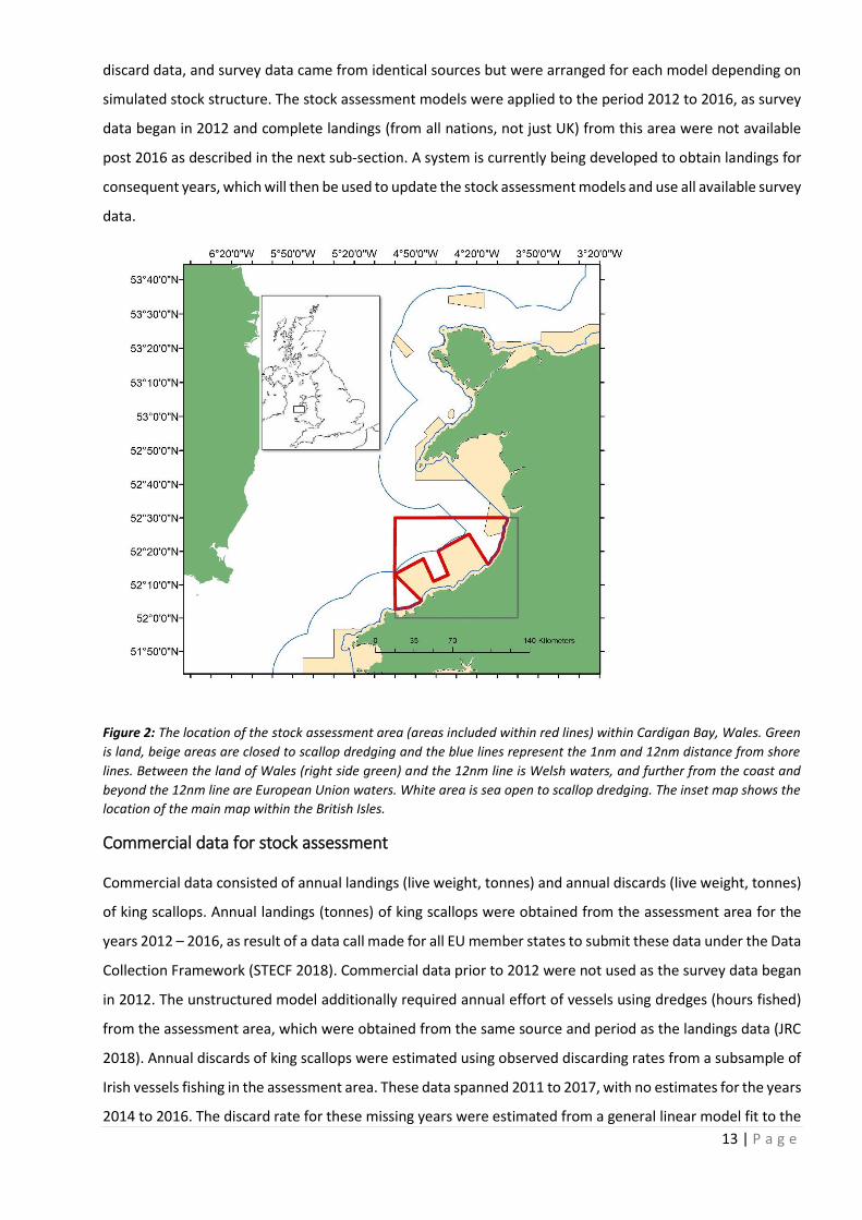
Figure 2: The location of the stock assessment area (areas included within red lines) within Cardigan Bay, Wales. Green

is land, beige areas are closed to scallop dredging and the blue lines represent the 1nm and 12nm distance from shore

lines. Between the land of Wales (right side green) and the 12nm line is Welsh waters, and further from the coast and

beyond the 12nm line are European Union waters. White area is sea open to scallop dredging. The inset map shows the

location of the main map within the British Isles.

Commercial data for stock assessment

Commercial data consisted of annual landings (live weight, tonnes) and annual discards (live weight, tonnes)

of king scallops. Annual landings (tonnes) of king scallops were obtained from the assessment area for the

years 2012 – 2016, as result of a data call made for all EU member states to submit these data under the Data

Collection Framework (STECF 2018). Commercial data prior to 2012 were not used as the survey data began

in 2012. The unstructured model additionally required annual effort of vessels using dredges (hours fished)

from the assessment area, which were obtained from the same source and period as the landings data (JRC

2018). Annual discards of king scallops were estimated using observed discarding rates from a subsample of

Irish vessels fishing in the assessment area. These data spanned 2011 to 2017, with no estimates for the years

2014 to 2016. The discard rate for these missing years were estimated from a general linear model fit to the

14 | P a g e

relationship between known discard rates and years. The discard rates (actual and estimated) for 2012 to

2016 were used to estimate the annual discards from the known amount of annual landings for those years.

Annual discards represented some percentage of the annual catch, and annual landings represented the

remaining percentage of annual catch. Therefore, the annual discards could be determined from the annual

landings.

Survey data for stock assessment

As commercial annual landings were not available later than 2016, survey data were also used from the years

2012 to 2016 in the model (although no survey was conducted in 2015). This ensured the survey data covered

the same timespan as the commercial data. Survey data came directly from the surveys described in this

report. The length-structured model used both annual survey index (total numbers of king scallops caught)

and length-frequency distributions. The age-structured model used both annual survey index and age-

frequency distributions. The unstructured model used only total survey index (total biomass (live weight,

tonnes) of king scallops caught). All three models used an annual proportion of the assessment area sampled

by the survey each year to standardise survey data by the effort applied during each survey. Growth, length-

weight and age-weight parameters were derived as described for the survey data here, but from only king

scallops caught in the assessment area.

A natural mortality rate was estimated for the length- and age-structured stock assessment models by

conducting length-structured catch curve analysis as described in Chapter 4 of the KESS 2 PhD thesis (Delargy

2019). Natural mortality is the annual rate of removals from the stock not attributable to commercial fishing.

Length-structured catch curve analysis provides an estimate of total mortality from declines in catch-at-

length data with increasing scallop size. By applying catch curve analysis to an area closed to commercial

dredging, the estimated total mortality can be assumed to be all natural mortality. Therefore, the catch curve

analysis was applied to king scallops caught in the closed areas of the Cardigan Bay SAC from the surveys

conducted from 2012 to 2016. As the method assumed all king scallops have an equal probability of being

caught by the survey gear, only king scallops with a shell width of 115mm or greater were included for this

analysis.

RESULTS

Survey indices

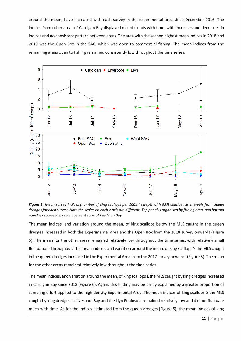
Throughout the survey time series the indices of king scallops caught with the queen dredges were

consistently higher and more variable in Cardigan Bay than either Liverpool Bay or the Llyn Peninsula (Figure

3). The mean indices, and variation around the mean, have increased with each survey in Cardigan Bay since

December 2016. However, this may be partly explained by a greater proportion of sampling effort in the high

density Experimental Area. Within Cardigan Bay, mean indices were consistently higher and more variable in

the Experimental Area than other areas of Cardigan Bay (Figures 3 and 4). The mean indices, and variation

15 | P a g e

around the mean, have increased with each survey in the experimental area since December 2016. The

indices from other areas of Cardigan Bay displayed mixed trends with time, with increases and decreases in

indices and no consistent pattern between areas. The area with the second highest mean indices in 2018 and

2019 was the Open Box in the SAC, which was open to commercial fishing. The mean indices from the

remaining areas open to fishing remained consistently low throughout the time series.

Figure 3: Mean survey indices (number of king scallops per 100m2 swept) with 95% confidence intervals from queen

dredges for each survey. Note the scales on each y-axis are different. Top panel is organised by fishing area, and bottom

panel is organised by management zone of Cardigan Bay.

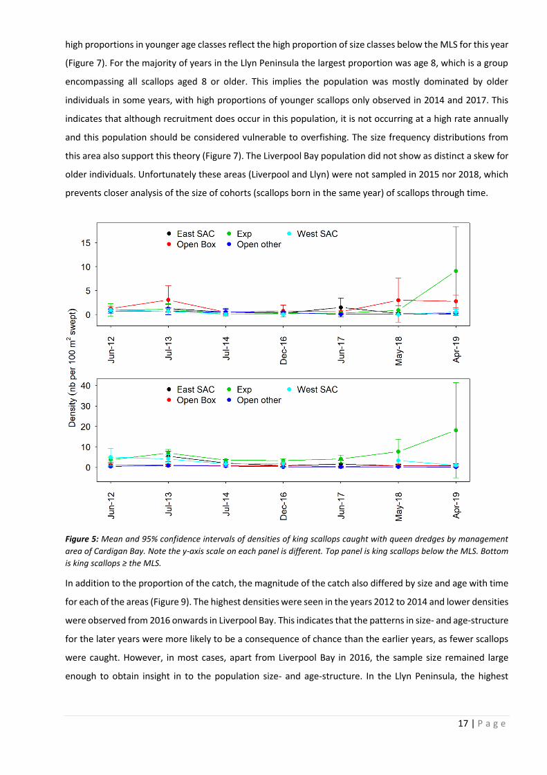
The mean indices, and variation around the mean, of king scallops below the MLS caught in the queen

dredges increased in both the Experimental Area and the Open Box from the 2018 survey onwards (Figure

5). The mean for the other areas remained relatively low throughout the time series, with relatively small

fluctuations throughout. The mean indices, and variation around the mean, of king scallops ≥ the MLS caught

in the queen dredges increased in the Experimental Area from the 2017 survey onwards (Figure 5). The mean

for the other areas remained relatively low throughout the time series.

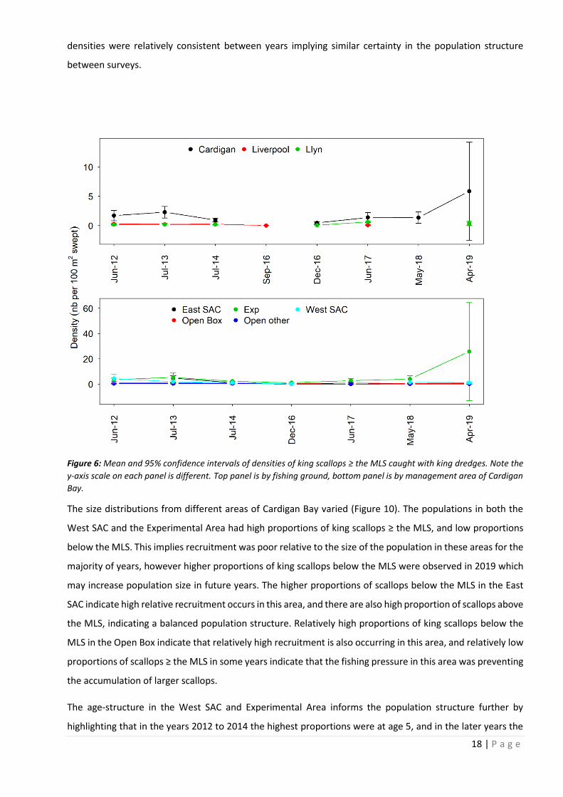
The mean indices, and variation around the mean, of king scallops ≥ the MLS caught by king dredges increased

in Cardigan Bay since 2018 (Figure 6). Again, this finding may be partly explained by a greater proportion of

sampling effort applied to the high density Experimental Area. The mean indices of king scallops ≥ the MLS

caught by king dredges in Liverpool Bay and the Llyn Peninsula remained relatively low and did not fluctuate

much with time. As for the indices estimated from the queen dredges (Figure 5), the mean indices of king

16 | P a g e

scallops ≥ the MLS caught by king dredges increased from 2018 in the Experimental Area. The mean indices

of king scallops ≥ the MLS caught by king dredges in other management areas of Cardigan Bay remained

relatively low and did not fluctuate much through the time series (Figure 6), similar to the indices from the

queen dredges (Figure 5).

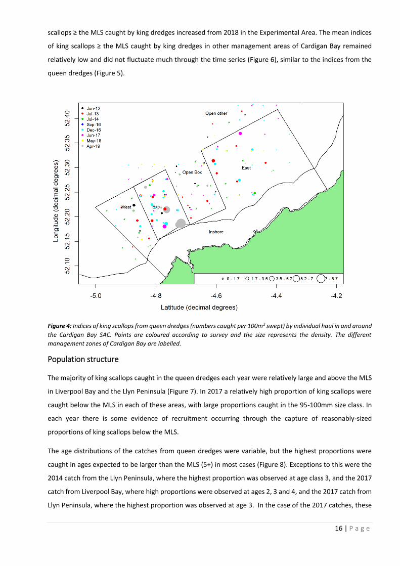
Figure 4: Indices of king scallops from queen dredges (numbers caught per 100m2 swept) by individual haul in and around

the Cardigan Bay SAC. Points are coloured according to survey and the size represents the density. The different

management zones of Cardigan Bay are labelled.

Population structure

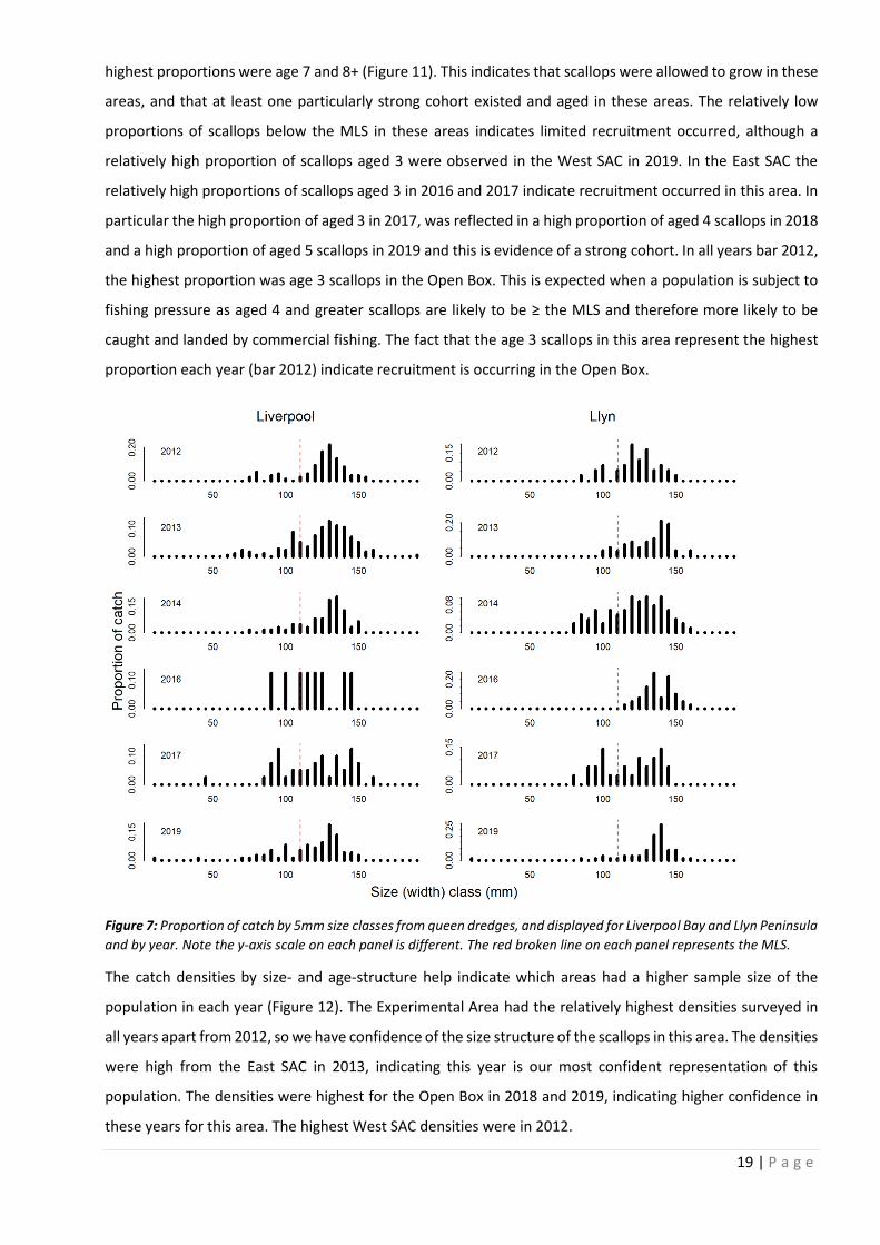
The majority of king scallops caught in the queen dredges each year were relatively large and above the MLS

in Liverpool Bay and the Llyn Peninsula (Figure 7). In 2017 a relatively high proportion of king scallops were

caught below the MLS in each of these areas, with large proportions caught in the 95-100mm size class. In

each year there is some evidence of recruitment occurring through the capture of reasonably-sized

proportions of king scallops below the MLS.

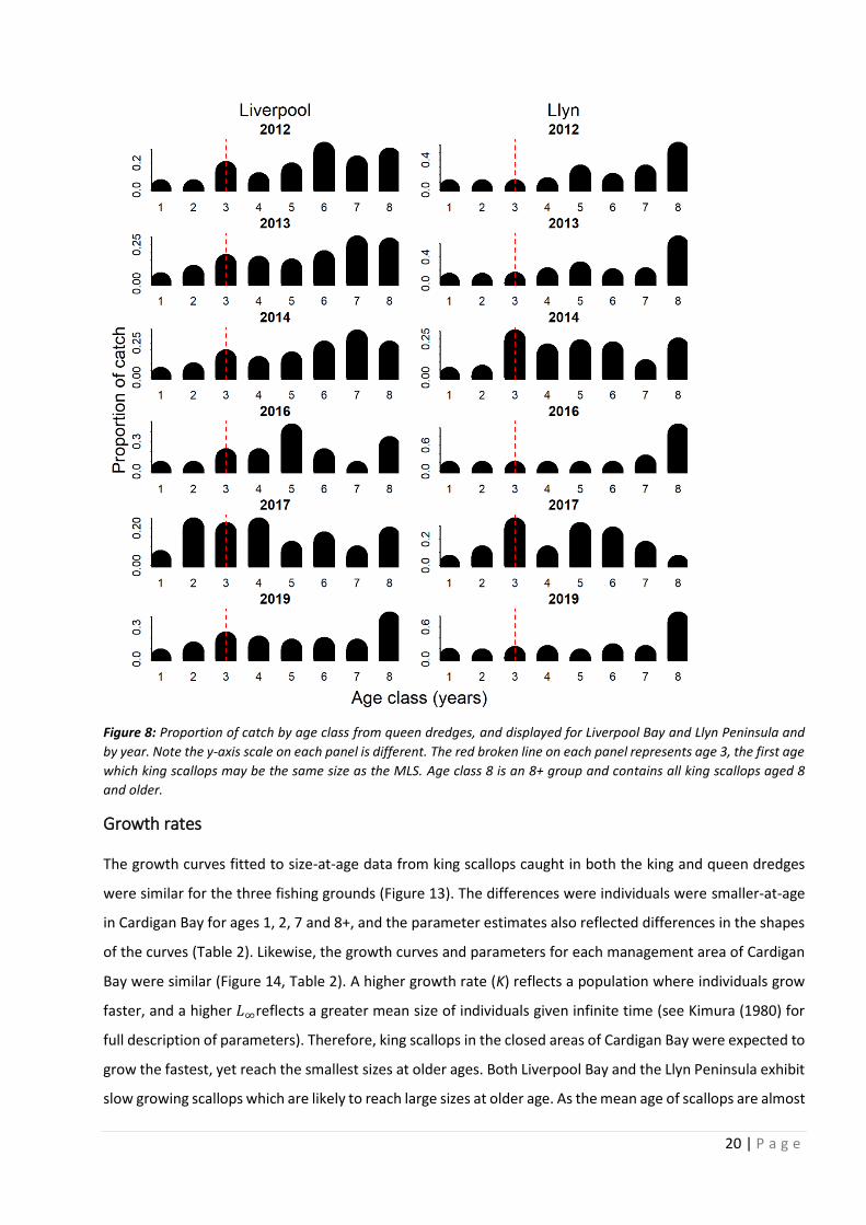
The age distributions of the catches from queen dredges were variable, but the highest proportions were

caught in ages expected to be larger than the MLS (5+) in most cases (Figure 8). Exceptions to this were the

2014 catch from the Llyn Peninsula, where the highest proportion was observed at age class 3, and the 2017

catch from Liverpool Bay, where high proportions were observed at ages 2, 3 and 4, and the 2017 catch from

Llyn Peninsula, where the highest proportion was observed at age 3. In the case of the 2017 catches, these

17 | P a g e

high proportions in younger age classes reflect the high proportion of size classes below the MLS for this year

(Figure 7). For the majority of years in the Llyn Peninsula the largest proportion was age 8, which is a group

encompassing all scallops aged 8 or older. This implies the population was mostly dominated by older

individuals in some years, with high proportions of younger scallops only observed in 2014 and 2017. This

indicates that although recruitment does occur in this population, it is not occurring at a high rate annually

and this population should be considered vulnerable to overfishing. The size frequency distributions from

this area also support this theory (Figure 7). The Liverpool Bay population did not show as distinct a skew for

older individuals. Unfortunately these areas (Liverpool and Llyn) were not sampled in 2015 nor 2018, which

prevents closer analysis of the size of cohorts (scallops born in the same year) of scallops through time.

Figure 5: Mean and 95% confidence intervals of densities of king scallops caught with queen dredges by management

area of Cardigan Bay. Note the y-axis scale on each panel is different. Top panel is king scallops below the MLS. Bottom

is king scallops ≥ the MLS.

In addition to the proportion of the catch, the magnitude of the catch also differed by size and age with time

for each of the areas (Figure 9). The highest densities were seen in the years 2012 to 2014 and lower densities

were observed from 2016 onwards in Liverpool Bay. This indicates that the patterns in size- and age-structure

for the later years were more likely to be a consequence of chance than the earlier years, as fewer scallops

were caught. However, in most cases, apart from Liverpool Bay in 2016, the sample size remained large

enough to obtain insight in to the population size- and age-structure. In the Llyn Peninsula, the highest

18 | P a g e

densities were relatively consistent between years implying similar certainty in the population structure

between surveys.

Figure 6: Mean and 95% confidence intervals of densities of king scallops ≥ the MLS caught with king dredges. Note the

y-axis scale on each panel is different. Top panel is by fishing ground, bottom panel is by management area of Cardigan

Bay.

The size distributions from different areas of Cardigan Bay varied (Figure 10). The populations in both the

West SAC and the Experimental Area had high proportions of king scallops ≥ the MLS, and low proportions

below the MLS. This implies recruitment was poor relative to the size of the population in these areas for the

majority of years, however higher proportions of king scallops below the MLS were observed in 2019 which

may increase population size in future years. The higher proportions of scallops below the MLS in the East

SAC indicate high relative recruitment occurs in this area, and there are also high proportion of scallops above

the MLS, indicating a balanced population structure. Relatively high proportions of king scallops below the

MLS in the Open Box indicate that relatively high recruitment is also occurring in this area, and relatively low

proportions of scallops ≥ the MLS in some years indicate that the fishing pressure in this area was preventing

the accumulation of larger scallops.

The age-structure in the West SAC and Experimental Area informs the population structure further by

highlighting that in the years 2012 to 2014 the highest proportions were at age 5, and in the later years the

19 | P a g e

highest proportions were age 7 and 8+ (Figure 11). This indicates that scallops were allowed to grow in these

areas, and that at least one particularly strong cohort existed and aged in these areas. The relatively low

proportions of scallops below the MLS in these areas indicates limited recruitment occurred, although a

relatively high proportion of scallops aged 3 were observed in the West SAC in 2019. In the East SAC the

relatively high proportions of scallops aged 3 in 2016 and 2017 indicate recruitment occurred in this area. In

particular the high proportion of aged 3 in 2017, was reflected in a high proportion of aged 4 scallops in 2018

and a high proportion of aged 5 scallops in 2019 and this is evidence of a strong cohort. In all years bar 2012,

the highest proportion was age 3 scallops in the Open Box. This is expected when a population is subject to

fishing pressure as aged 4 and greater scallops are likely to be ≥ the MLS and therefore more likely to be

caught and landed by commercial fishing. The fact that the age 3 scallops in this area represent the highest

proportion each year (bar 2012) indicate recruitment is occurring in the Open Box.

Figure 7: Proportion of catch by 5mm size classes from queen dredges, and displayed for Liverpool Bay and Llyn Peninsula

and by year. Note the y-axis scale on each panel is different. The red broken line on each panel represents the MLS.

The catch densities by size- and age-structure help indicate which areas had a higher sample size of the

population in each year (Figure 12). The Experimental Area had the relatively highest densities surveyed in

all years apart from 2012, so we have confidence of the size structure of the scallops in this area. The densities

were high from the East SAC in 2013, indicating this year is our most confident representation of this

population. The densities were highest for the Open Box in 2018 and 2019, indicating higher confidence in

these years for this area. The highest West SAC densities were in 2012.

20 | P a g e

Figure 8: Proportion of catch by age class from queen dredges, and displayed for Liverpool Bay and Llyn Peninsula and

by year. Note the y-axis scale on each panel is different. The red broken line on each panel represents age 3, the first age

which king scallops may be the same size as the MLS. Age class 8 is an 8+ group and contains all king scallops aged 8

and older.

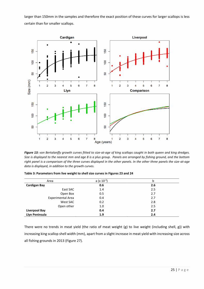
Growth rates

The growth curves fitted to size-at-age data from king scallops caught in both the king and queen dredges

were similar for the three fishing grounds (Figure 13). The differences were individuals were smaller-at-age

in Cardigan Bay for ages 1, 2, 7 and 8+, and the parameter estimates also reflected differences in the shapes

of the curves (Table 2). Likewise, the growth curves and parameters for each management area of Cardigan

Bay were similar (Figure 14, Table 2). A higher growth rate (K) reflects a population where individuals grow

faster, and a higher 𝐿∞reflects a greater mean size of individuals given infinite time (see Kimura (1980) for

full description of parameters). Therefore, king scallops in the closed areas of Cardigan Bay were expected to

grow the fastest, yet reach the smallest sizes at older ages. Both Liverpool Bay and the Llyn Peninsula exhibit

slow growing scallops which are likely to reach large sizes at older age. As the mean age of scallops are almost

21 | P a g e

identical when at the size of the MLS, the differences in growth curves between the grounds is not of

considerable importance for stock assessment or management.

Table 2: Parameters for von Bertalanffy growth curves in Figures 13 and 14x

Area K 𝐿∞(mm) 𝑡0

Cardigan Bay 0.46 137.0 0.19 East SAC 0.49 137.2 0.08

Open Box 0.37 142.0 -0.19 Experimental Area 0.50 135.4 0.40

West SAC 0.48 137.7 0.35 Open other 0.32 146.7 -0.59

Liverpool Bay 0.28 152.9 -0.88 Llyn Peninsula 0.19 168.0 -1.76

Figure 9: Indices by size and age classes from queen dredges. Size classes are 5mm wide. The age 8 class is a plus group.

Indices are expressed as number of king scallops caught per 100m2 of seabed swept by the two queen dredges. Panels

are organised by year, and on each panel the densities for Liverpool Bay and the Llyn Peninsula are denoted with two

different colours.

The median size-at age of king scallops caught in both king dredges and queen dredges showed little

difference between-areas, with higher variation in Cardigan Bay caused by greater sampling in this area

(Figure 15). Slight variation in median size-at-age was observed between the management zones of Cardigan

Bay, with median size marginally greater in the East SAC for all presented ages (Figure 16). The variation in

size-at-age of the king scallops displayed here are generally quite large, which could indicate observation

22 | P a g e

error in aging. Observation error in measuring the size of king scallops is also a possibility, but likely to be less

than aging observation error. Observation error is discussed at the end of this report.

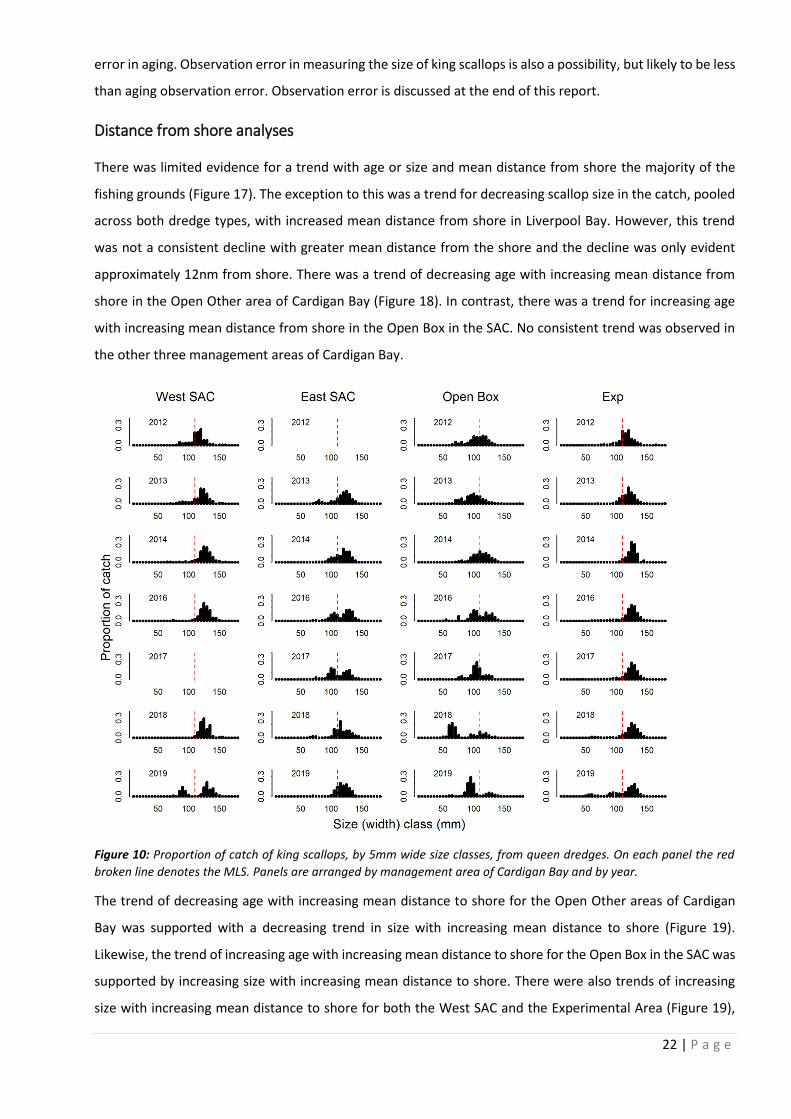
Distance from shore analyses

There was limited evidence for a trend with age or size and mean distance from shore the majority of the

fishing grounds (Figure 17). The exception to this was a trend for decreasing scallop size in the catch, pooled

across both dredge types, with increased mean distance from shore in Liverpool Bay. However, this trend

was not a consistent decline with greater mean distance from the shore and the decline was only evident

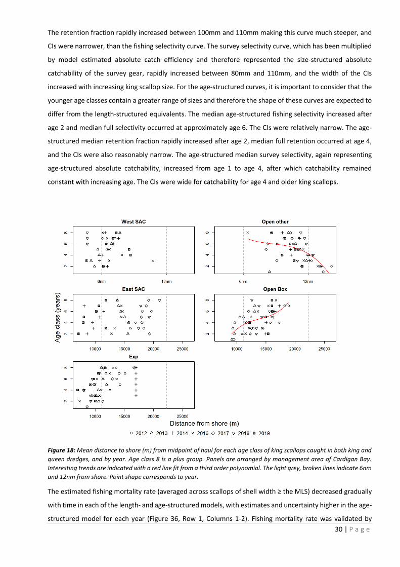
approximately 12nm from shore. There was a trend of decreasing age with increasing mean distance from

shore in the Open Other area of Cardigan Bay (Figure 18). In contrast, there was a trend for increasing age

with increasing mean distance from shore in the Open Box in the SAC. No consistent trend was observed in

the other three management areas of Cardigan Bay.

Figure 10: Proportion of catch of king scallops, by 5mm wide size classes, from queen dredges. On each panel the red

broken line denotes the MLS. Panels are arranged by management area of Cardigan Bay and by year.

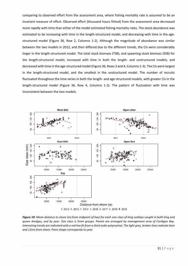
The trend of decreasing age with increasing mean distance to shore for the Open Other areas of Cardigan

Bay was supported with a decreasing trend in size with increasing mean distance to shore (Figure 19).

Likewise, the trend of increasing age with increasing mean distance to shore for the Open Box in the SAC was

supported by increasing size with increasing mean distance to shore. There were also trends of increasing

size with increasing mean distance to shore for both the West SAC and the Experimental Area (Figure 19),

23 | P a g e

although in both cases the trends begin to decrease at sites furthest away from the shore. These trends were

not detected by age class and this could be a result of high observation error in aging or a consequence of

high variation in size-at-age (Figure 16). No trend with size class was observed with increasing mean distance

to shore in the East SAC, which supports the lack of a trend with age class for this area.

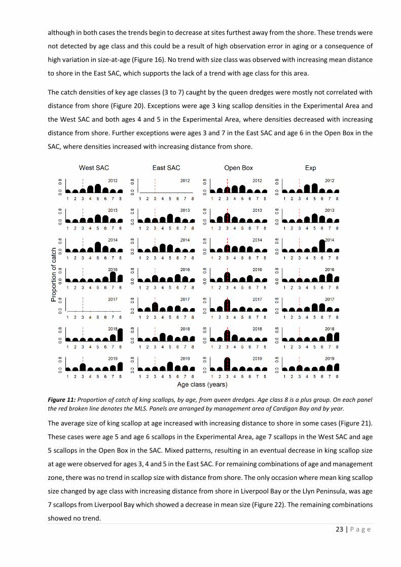
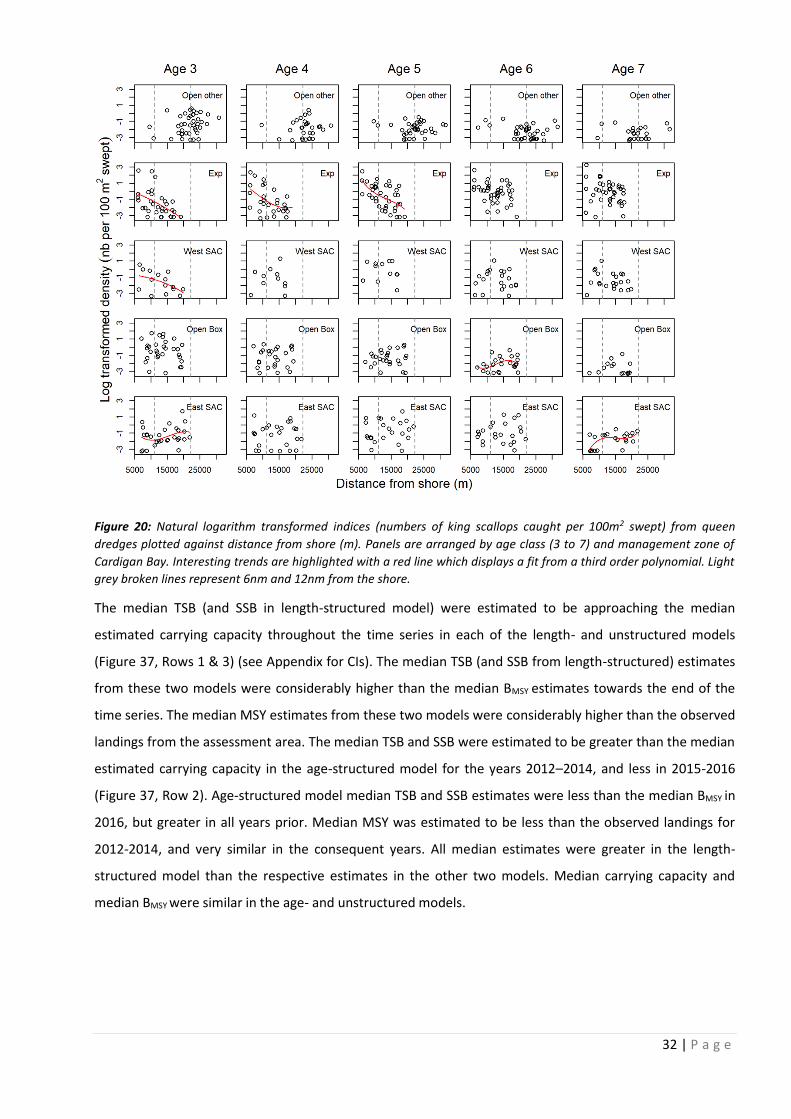
The catch densities of key age classes (3 to 7) caught by the queen dredges were mostly not correlated with

distance from shore (Figure 20). Exceptions were age 3 king scallop densities in the Experimental Area and

the West SAC and both ages 4 and 5 in the Experimental Area, where densities decreased with increasing

distance from shore. Further exceptions were ages 3 and 7 in the East SAC and age 6 in the Open Box in the

SAC, where densities increased with increasing distance from shore.

Figure 11: Proportion of catch of king scallops, by age, from queen dredges. Age class 8 is a plus group. On each panel

the red broken line denotes the MLS. Panels are arranged by management area of Cardigan Bay and by year.

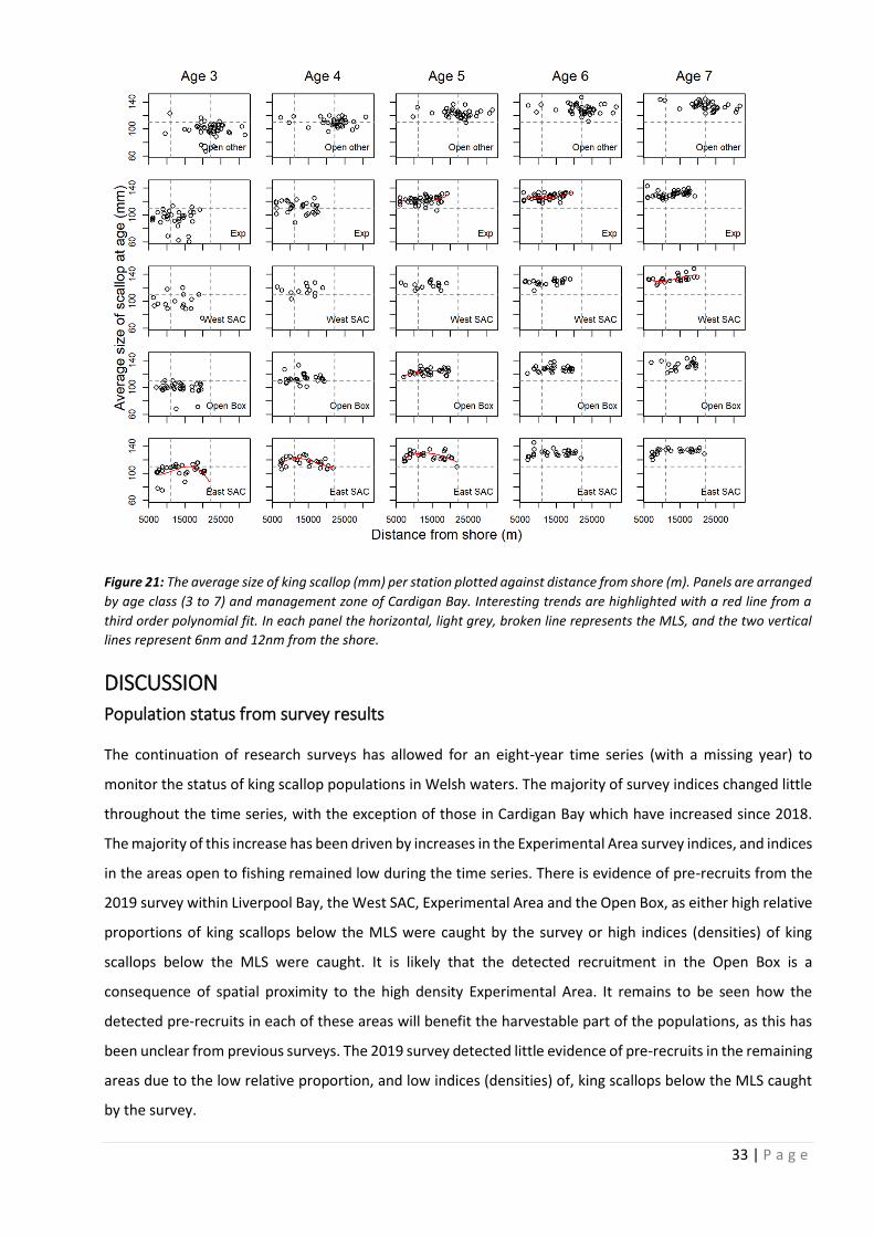
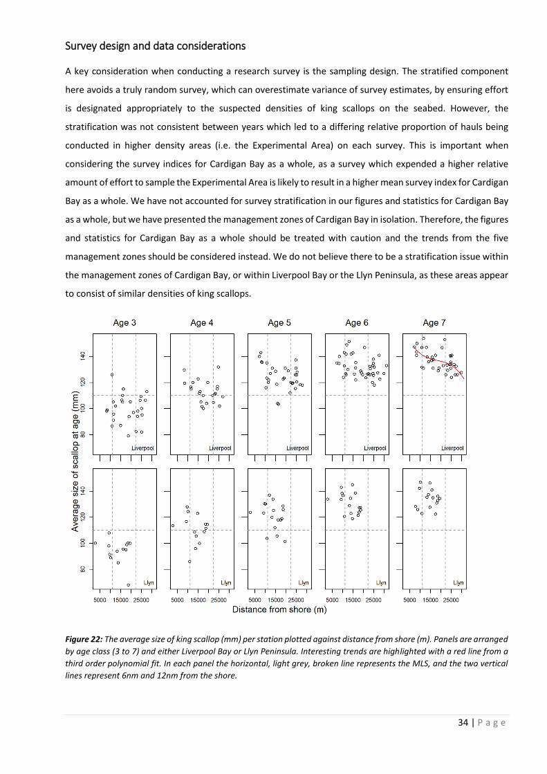
The average size of king scallop at age increased with increasing distance to shore in some cases (Figure 21).

These cases were age 5 and age 6 scallops in the Experimental Area, age 7 scallops in the West SAC and age

5 scallops in the Open Box in the SAC. Mixed patterns, resulting in an eventual decrease in king scallop size

at age were observed for ages 3, 4 and 5 in the East SAC. For remaining combinations of age and management

zone, there was no trend in scallop size with distance from shore. The only occasion where mean king scallop

size changed by age class with increasing distance from shore in Liverpool Bay or the Llyn Peninsula, was age

7 scallops from Liverpool Bay which showed a decrease in mean size (Figure 22). The remaining combinations

showed no trend.

24 | P a g e

Body part to shell width relationships

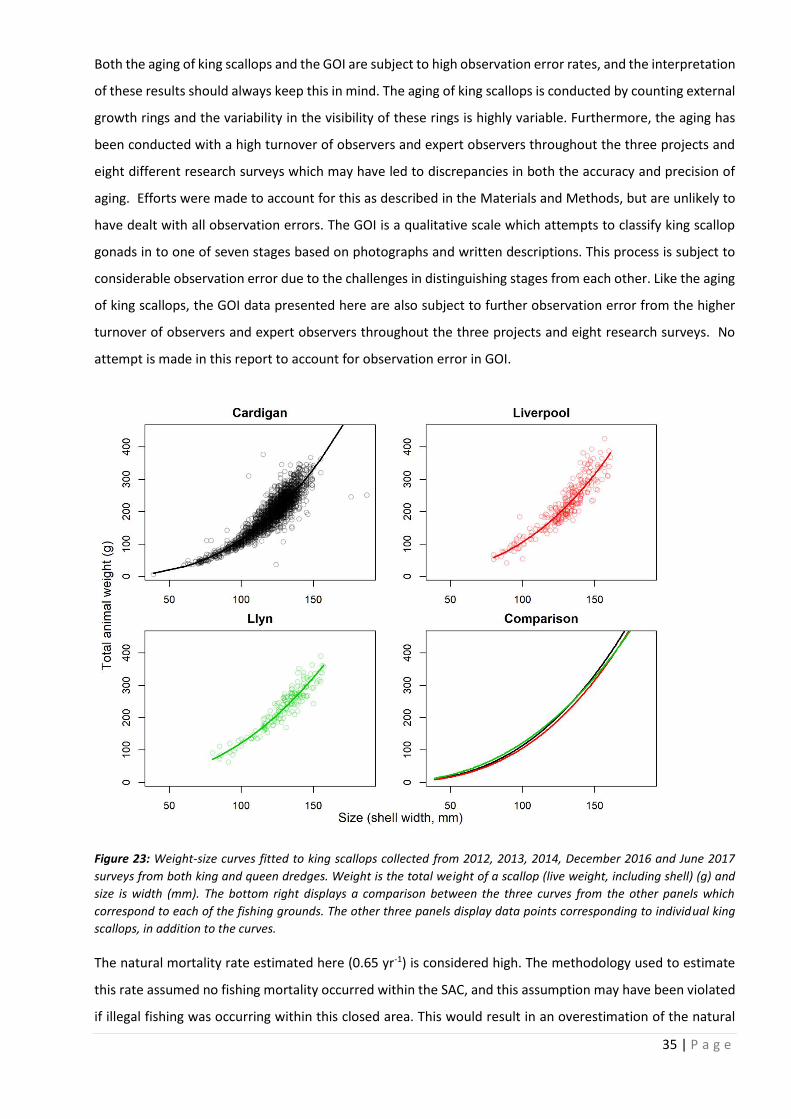
The relationship between total weight (g, live weight) and size (width, mm) of individual king scallops was

extremely similar between each of the fishing grounds (Figure 23) or each of the management zones in

Cardigan Bay (Figure 24). The parameters for these curves are presented in Table 3. There was little difference

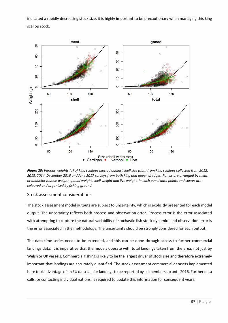
in the relationships between each of meat (or abductor muscle), shell and total weight (all g) with shell width

(mm) between the fishing grounds (Figure 25). There was a slight difference in the relationship between

gonad weight (g) and shell width (mm) between Cardigan Bay and the other two fishing grounds for king

scallops larger than 145mm in shell width, with heavier gonads observed in Cardigan Bay. The relationships

in gonad weight panel (top right) were worse fits than the other three panels (Figure 24) due to increasing

variance in gonad weight with increasing shell width, and therefore the difference in gonad weight in

Cardigan Bay may be driven by outliers.

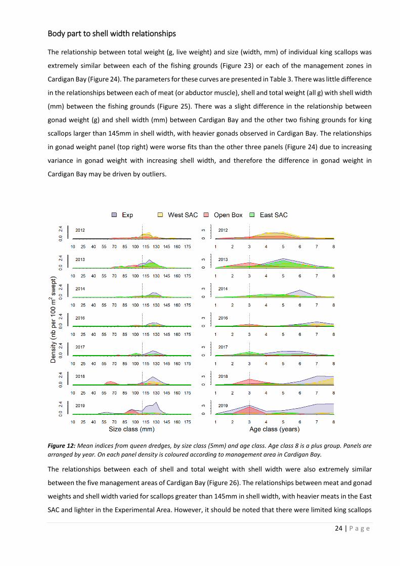
Figure 12: Mean indices from queen dredges, by size class (5mm) and age class. Age class 8 is a plus group. Panels are

arranged by year. On each panel density is coloured according to management area in Cardigan Bay.

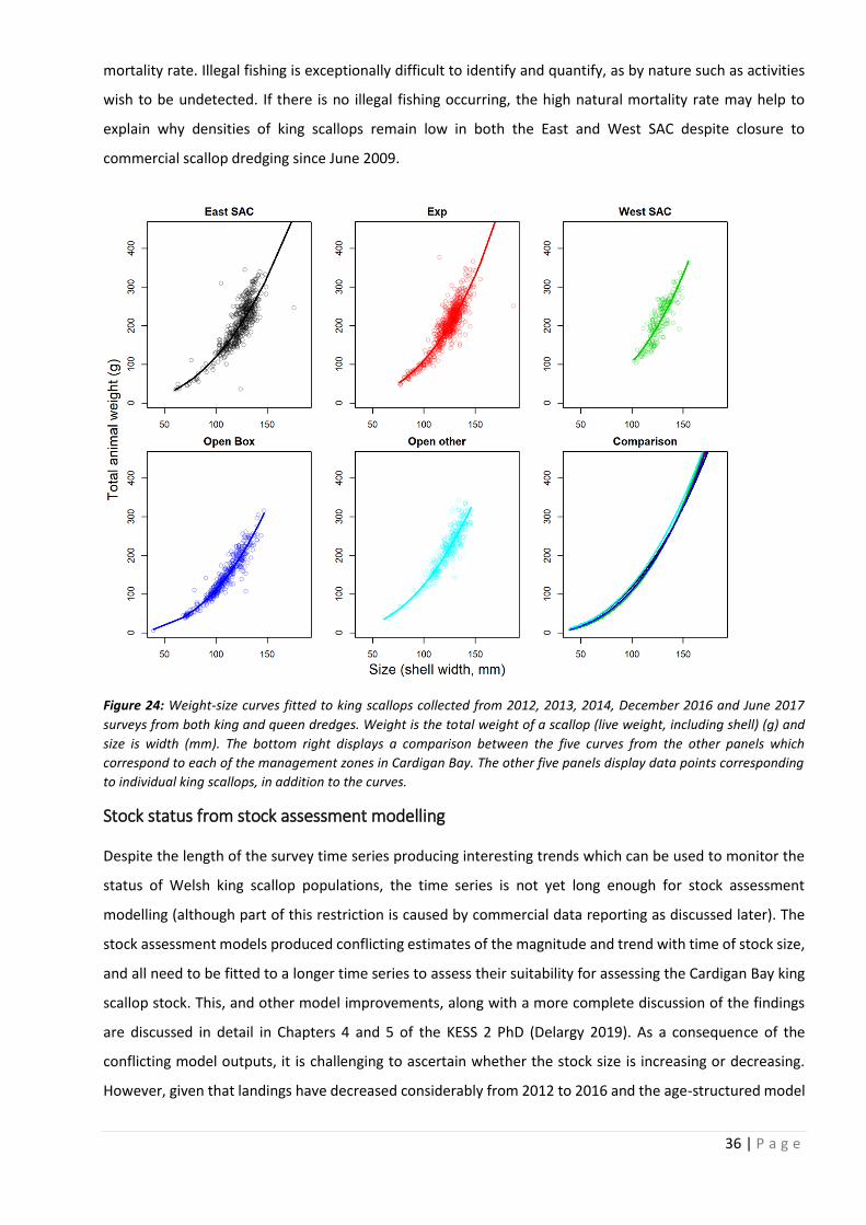
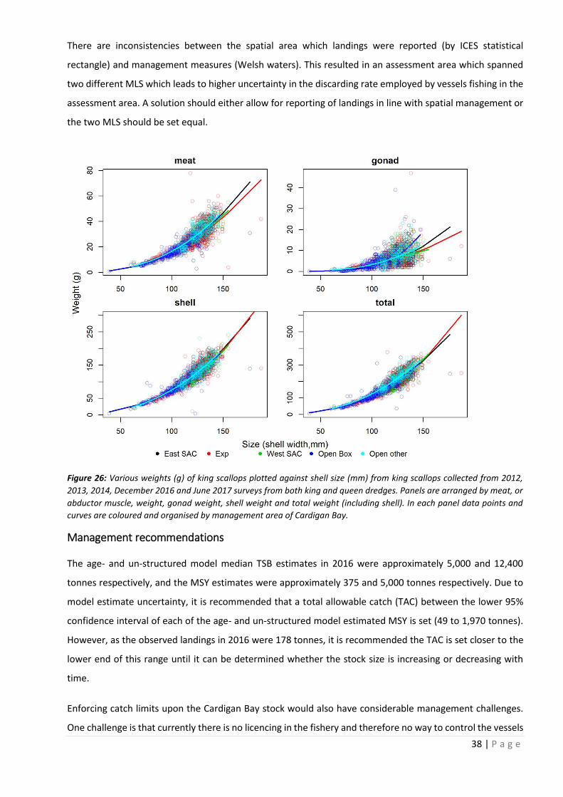
The relationships between each of shell and total weight with shell width were also extremely similar

between the five management areas of Cardigan Bay (Figure 26). The relationships between meat and gonad

weights and shell width varied for scallops greater than 145mm in shell width, with heavier meats in the East

SAC and lighter in the Experimental Area. However, it should be noted that there were limited king scallops

25 | P a g e

larger than 150mm in the samples and therefore the exact position of these curves for larger scallops is less

certain than for smaller scallops.

Figure 13: von Bertalanffy growth curves fitted to size-at-age of king scallops caught in both queen and king dredges.

Size is displayed to the nearest mm and age 8 is a plus group. Panels are arranged by fishing ground, and the bottom

right panel is a comparison of the three curves displayed in the other panels. In the other three panels the size-at-age

data is displayed, in addition to the growth curves.

Table 3: Parameters from live weight to shell size curves in Figures 23 and 24

Area a (x 10-3) b

Cardigan Bay 0.6 2.6 East SAC 1.4 2.5

Open Box 0.5 2.7 Experimental Area 0.4 2.7

West SAC 0.2 2.8 Open other 1.0 2.5

Liverpool Bay 0.4 2.7 Llyn Peninsula 1.9 2.4

There were no trends in meat yield (the ratio of meat weight (g) to live weight (including shell, g)) with

increasing king scallop shell width (mm), apart from a slight increase in meat yield with increasing size across

all fishing grounds in 2013 (Figure 27).

26 | P a g e

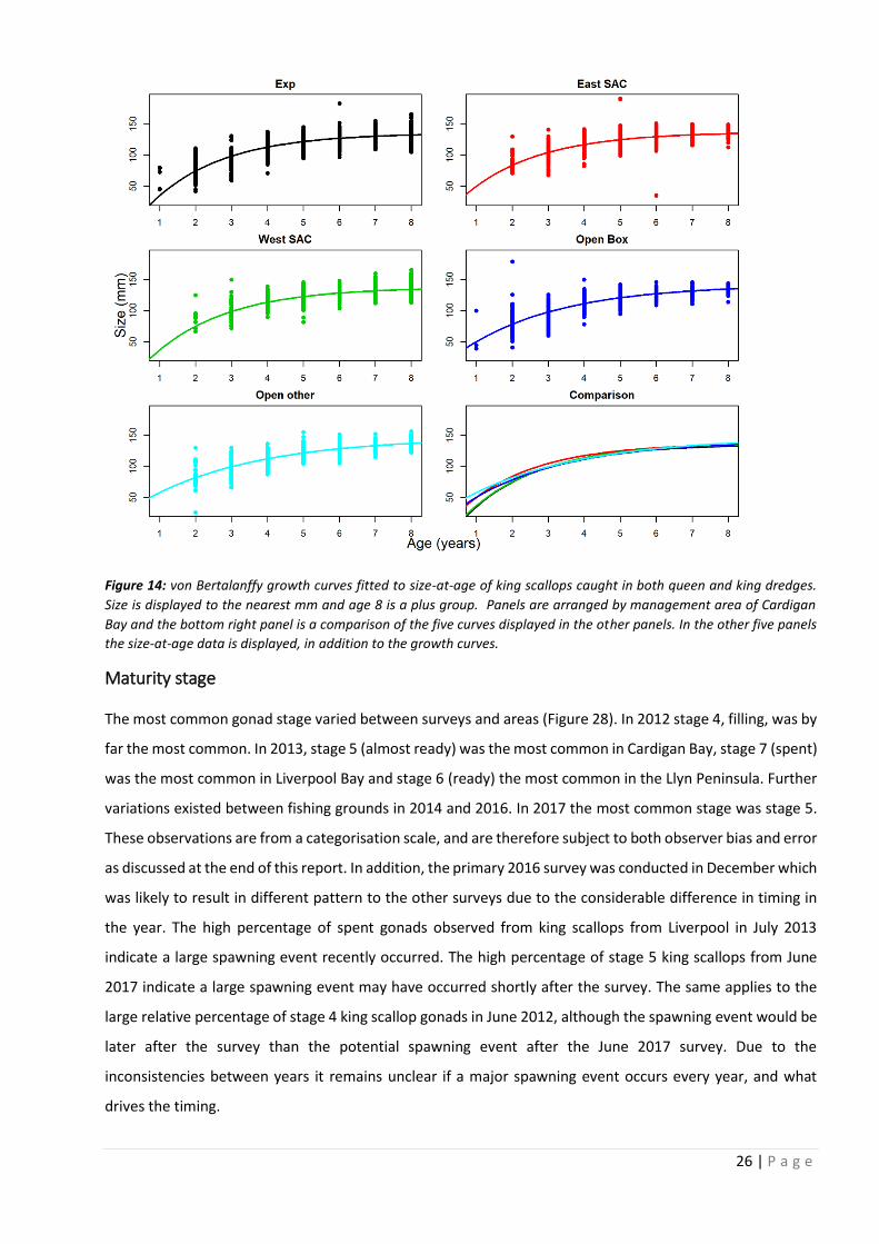
Figure 14: von Bertalanffy growth curves fitted to size-at-age of king scallops caught in both queen and king dredges.

Size is displayed to the nearest mm and age 8 is a plus group. Panels are arranged by management area of Cardigan

Bay and the bottom right panel is a comparison of the five curves displayed in the other panels. In the other five panels

the size-at-age data is displayed, in addition to the growth curves.

Maturity stage

The most common gonad stage varied between surveys and areas (Figure 28). In 2012 stage 4, filling, was by

far the most common. In 2013, stage 5 (almost ready) was the most common in Cardigan Bay, stage 7 (spent)

was the most common in Liverpool Bay and stage 6 (ready) the most common in the Llyn Peninsula. Further

variations existed between fishing grounds in 2014 and 2016. In 2017 the most common stage was stage 5.

These observations are from a categorisation scale, and are therefore subject to both observer bias and error

as discussed at the end of this report. In addition, the primary 2016 survey was conducted in December which

was likely to result in different pattern to the other surveys due to the considerable difference in timing in

the year. The high percentage of spent gonads observed from king scallops from Liverpool in July 2013

indicate a large spawning event recently occurred. The high percentage of stage 5 king scallops from June

2017 indicate a large spawning event may have occurred shortly after the survey. The same applies to the

large relative percentage of stage 4 king scallop gonads in June 2012, although the spawning event would be

later after the survey than the potential spawning event after the June 2017 survey. Due to the

inconsistencies between years it remains unclear if a major spawning event occurs every year, and what

drives the timing.

27 | P a g e

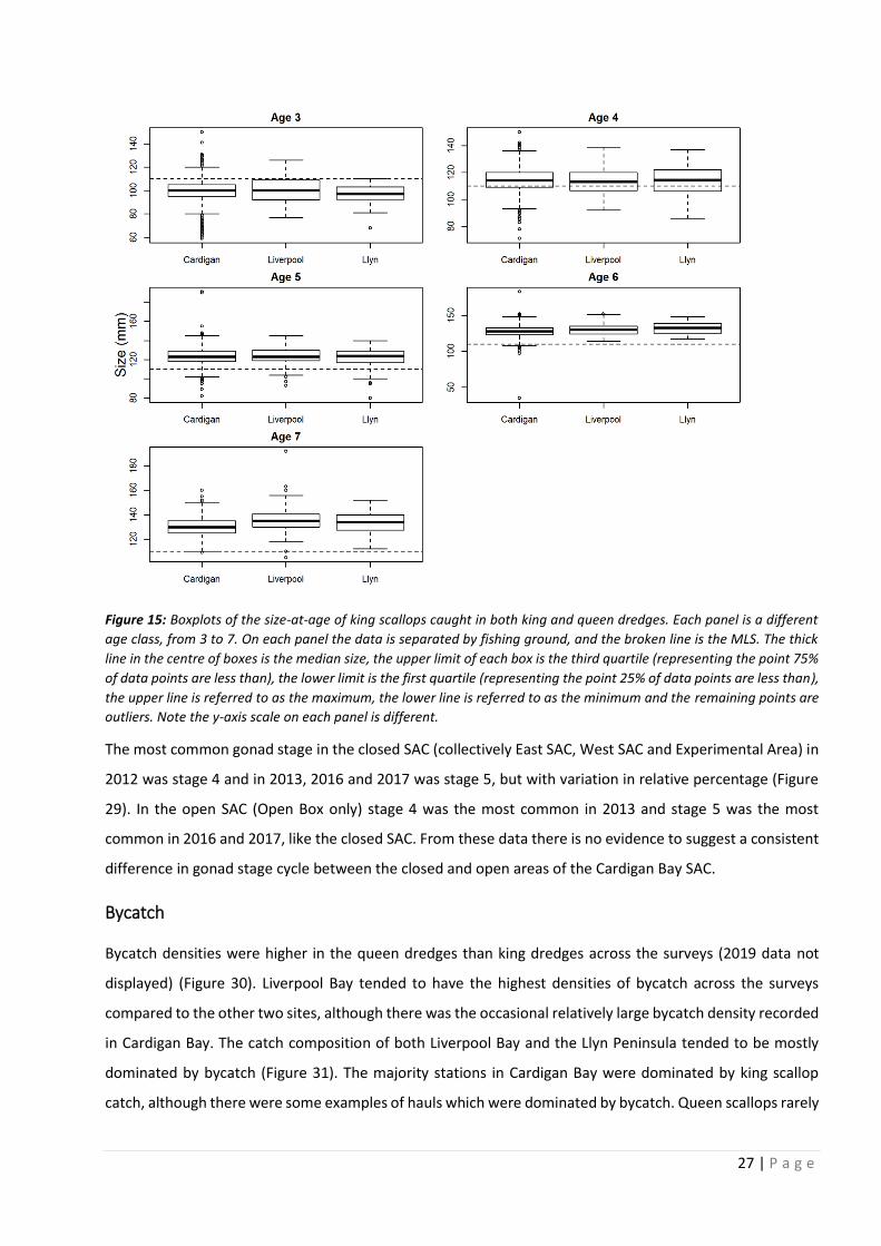
Figure 15: Boxplots of the size-at-age of king scallops caught in both king and queen dredges. Each panel is a different

age class, from 3 to 7. On each panel the data is separated by fishing ground, and the broken line is the MLS. The thick

line in the centre of boxes is the median size, the upper limit of each box is the third quartile (representing the point 75%

of data points are less than), the lower limit is the first quartile (representing the point 25% of data points are less than),

the upper line is referred to as the maximum, the lower line is referred to as the minimum and the remaining points are

outliers. Note the y-axis scale on each panel is different.

The most common gonad stage in the closed SAC (collectively East SAC, West SAC and Experimental Area) in

2012 was stage 4 and in 2013, 2016 and 2017 was stage 5, but with variation in relative percentage (Figure

29). In the open SAC (Open Box only) stage 4 was the most common in 2013 and stage 5 was the most

common in 2016 and 2017, like the closed SAC. From these data there is no evidence to suggest a consistent

difference in gonad stage cycle between the closed and open areas of the Cardigan Bay SAC.

Bycatch

Bycatch densities were higher in the queen dredges than king dredges across the surveys (2019 data not

displayed) (Figure 30). Liverpool Bay tended to have the highest densities of bycatch across the surveys

compared to the other two sites, although there was the occasional relatively large bycatch density recorded

in Cardigan Bay. The catch composition of both Liverpool Bay and the Llyn Peninsula tended to be mostly

dominated by bycatch (Figure 31). The majority stations in Cardigan Bay were dominated by king scallop

catch, although there were some examples of hauls which were dominated by bycatch. Queen scallops rarely

28 | P a g e

contributed to any notable proportion of catch composition. There was no pattern in catch composition

within Cardigan Bay (Figure 32).

Mean bycatch density was highest in Liverpool Bay for all years (Figure 33). Mean bycatch density was similar

between Cardigan Bay and the Llyn Peninsula in most years. Mean bycatch density was highest in the parts

of Cardigan Bay outside the SAC (Open Other) compared to those in the SAC in 2012, but mean bycatch

densities were similar between the management zones of Cardigan Bay in all other years (Figure 33). Bycatch

densities from the queen dredges did not show a trend with time for any area.

The mean bycatch density in the king dredges was highest in Liverpool Bay for all comparable surveys (Figure

34). Mean bycatch density caught in these dredges decreased from 2012 to 2016 in Liverpool Bay, but was

recorded at a similar level to 2012 and 2013 in 2017. Mean density of bycatch from the king dredges in

Cardigan Bay increased from 2017 to 2018. The mean density of bycatch from the king dredges in the

different management zones of Cardigan Bay fluctuated considerably and displayed no clear trend with time.

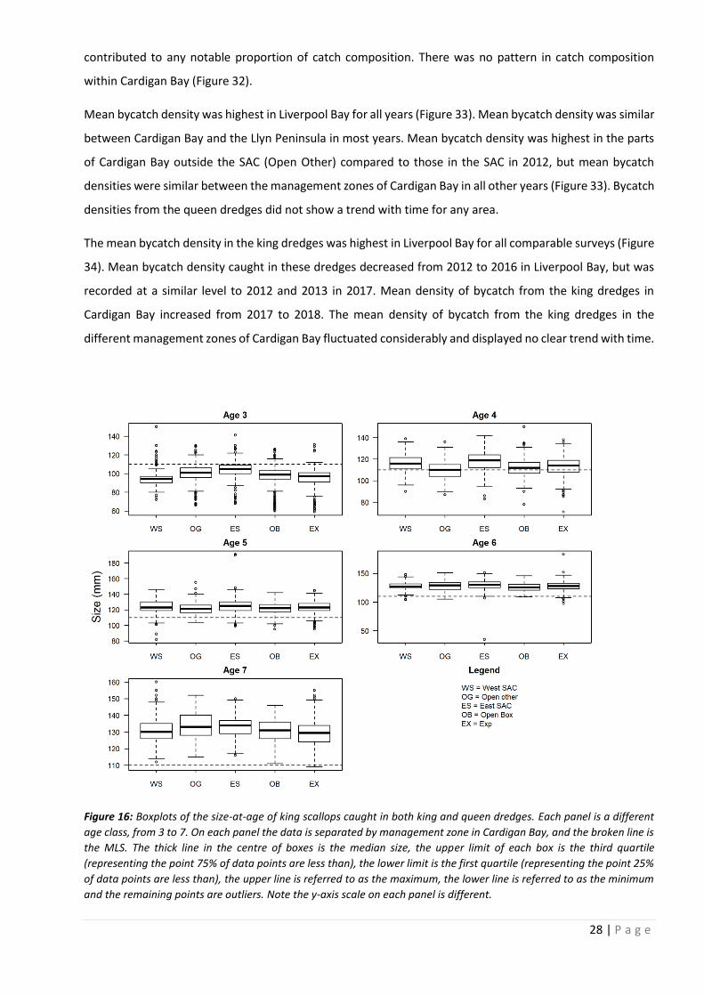
Figure 16: Boxplots of the size-at-age of king scallops caught in both king and queen dredges. Each panel is a different

age class, from 3 to 7. On each panel the data is separated by management zone in Cardigan Bay, and the broken line is

the MLS. The thick line in the centre of boxes is the median size, the upper limit of each box is the third quartile

(representing the point 75% of data points are less than), the lower limit is the first quartile (representing the point 25%

of data points are less than), the upper line is referred to as the maximum, the lower line is referred to as the minimum

and the remaining points are outliers. Note the y-axis scale on each panel is different.

29 | P a g e

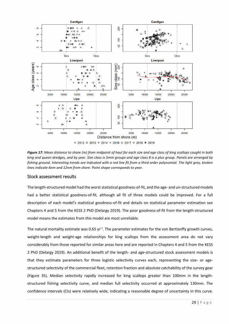
Figure 17: Mean distance to shore (m) from midpoint of haul for each size and age class of king scallops caught in both

king and queen dredges, and by year. Size class is 5mm groups and age class 8 is a plus group. Panels are arranged by

fishing ground. Interesting trends are indicated with a red line fit from a third order polynomial. The light grey, broken

lines indicate 6nm and 12nm from shore. Point shape corresponds to year.

Stock assessment results

The length-structured model had the worst statistical goodness-of-fit, and the age- and un-structured models

had a better statistical goodness-of-fit, although all fit of three models could be improved. For a full

description of each model’s statistical goodness-of-fit and details on statistical parameter estimation see

Chapters 4 and 5 from the KESS 2 PhD (Delargy 2019). The poor goodness-of-fit from the length-structured

model means the estimates from this model are most unreliable.

The natural mortality estimate was 0.65 yr-1. The parameter estimates for the von Bertlanffy growth curves,

weight-length and weight-age relationships for king scallops from the assessment area do not vary

considerably from those reported for similar areas here and are reported in Chapters 4 and 5 from the KESS

2 PhD (Delargy 2019). An additional benefit of the length- and age-structured stock assessment models is

that they estimate parameters for three logistic selectivity curves each, representing the size- or age-

structured selectivity of the commercial fleet, retention fraction and absolute catchability of the survey gear

(Figure 35). Median selectivity rapidly increased for king scallops greater than 100mm in the length-

structured fishing selectivity curve, and median full selectivity occurred at approximately 130mm. The

confidence intervals (CIs) were relatively wide, indicating a reasonable degree of uncertainty in this curve.

30 | P a g e

The retention fraction rapidly increased between 100mm and 110mm making this curve much steeper, and

CIs were narrower, than the fishing selectivity curve. The survey selectivity curve, which has been multiplied

by model estimated absolute catch efficiency and therefore represented the size-structured absolute

catchability of the survey gear, rapidly increased between 80mm and 110mm, and the width of the CIs

increased with increasing king scallop size. For the age-structured curves, it is important to consider that the

younger age classes contain a greater range of sizes and therefore the shape of these curves are expected to

differ from the length-structured equivalents. The median age-structured fishing selectivity increased after

age 2 and median full selectivity occurred at approximately age 6. The CIs were relatively narrow. The age-

structured median retention fraction rapidly increased after age 2, median full retention occurred at age 4,

and the CIs were also reasonably narrow. The age-structured median survey selectivity, again representing

age-structured absolute catchability, increased from age 1 to age 4, after which catchability remained

constant with increasing age. The CIs were wide for catchability for age 4 and older king scallops.

Figure 18: Mean distance to shore (m) from midpoint of haul for each age class of king scallops caught in both king and

queen dredges, and by year. Age class 8 is a plus group. Panels are arranged by management area of Cardigan Bay.

Interesting trends are indicated with a red line fit from a third order polynomial. The light grey, broken lines indicate 6nm

and 12nm from shore. Point shape corresponds to year.

The estimated fishing mortality rate (averaged across scallops of shell width ≥ the MLS) decreased gradually

with time in each of the length- and age-structured models, with estimates and uncertainty higher in the age-

structured model for each year (Figure 36, Row 1, Columns 1-2). Fishing mortality rate was validated by

31 | P a g e

comparing to observed effort from the assessment area, where fishing mortality rate is assumed to be an

invariant measure of effort. Observed effort (thousand hours fished) from the assessment area decreased

more rapidly with time than either of the model estimated fishing mortality rates. The stock abundance was

estimated to be increasing with time in the length-structured model, and decreasing with time in the age-

structured model (Figure 36, Row 2, Columns 1-2). Although the magnitude of abundance was similar

between the two models in 2012, and then differed due to the different trends, the CIs were considerably

larger in the length-structured model. The total stock biomass (TSB), and spawning stock biomass (SSB) for

the length-structured model, increased with time in both the length- and unstructured models, and

decreased with time in the age-structured model (Figure 36, Rows 3 and 4, Columns 1-3). The CIs were largest

in the length-structured model, and the smallest in the unstructured model. The number of recruits

fluctuated throughout the time series in both the length- and age-structured models, with greater CIs in the

length-structured model (Figure 36, Row 4, Columns 1-2). The pattern of fluctuation with time was

inconsistent between the two models.

Figure 19: Mean distance to shore (m) from midpoint of haul for each size class of king scallops caught in both king and

queen dredges, and by year. Size class is 5mm groups. Panels are arranged by management area of Cardigan Bay.

Interesting trends are indicated with a red line fit from a third order polynomial. The light grey, broken lines indicate 6nm

and 12nm from shore. Point shape corresponds to year.

32 | P a g e

Figure 20: Natural logarithm transformed indices (numbers of king scallops caught per 100m2 swept) from queen

dredges plotted against distance from shore (m). Panels are arranged by age class (3 to 7) and management zone of

Cardigan Bay. Interesting trends are highlighted with a red line which displays a fit from a third order polynomial. Light

grey broken lines represent 6nm and 12nm from the shore.

The median TSB (and SSB in length-structured model) were estimated to be approaching the median

estimated carrying capacity throughout the time series in each of the length- and unstructured models

(Figure 37, Rows 1 & 3) (see Appendix for CIs). The median TSB (and SSB from length-structured) estimates

from these two models were considerably higher than the median BMSY estimates towards the end of the

time series. The median MSY estimates from these two models were considerably higher than the observed

landings from the assessment area. The median TSB and SSB were estimated to be greater than the median

estimated carrying capacity in the age-structured model for the years 2012–2014, and less in 2015-2016

(Figure 37, Row 2). Age-structured model median TSB and SSB estimates were less than the median BMSY in

2016, but greater in all years prior. Median MSY was estimated to be less than the observed landings for

2012-2014, and very similar in the consequent years. All median estimates were greater in the length-

structured model than the respective estimates in the other two models. Median carrying capacity and

median BMSY were similar in the age- and unstructured models.

33 | P a g e

Figure 21: The average size of king scallop (mm) per station plotted against distance from shore (m). Panels are arranged

by age class (3 to 7) and management zone of Cardigan Bay. Interesting trends are highlighted with a red line from a

third order polynomial fit. In each panel the horizontal, light grey, broken line represents the MLS, and the two vertical

lines represent 6nm and 12nm from the shore.

DISCUSSION

Population status from survey results

The continuation of research surveys has allowed for an eight-year time series (with a missing year) to

monitor the status of king scallop populations in Welsh waters. The majority of survey indices changed little

throughout the time series, with the exception of those in Cardigan Bay which have increased since 2018.

The majority of this increase has been driven by increases in the Experimental Area survey indices, and indices

in the areas open to fishing remained low during the time series. There is evidence of pre-recruits from the

2019 survey within Liverpool Bay, the West SAC, Experimental Area and the Open Box, as either high relative

proportions of king scallops below the MLS were caught by the survey or high indices (densities) of king

scallops below the MLS were caught. It is likely that the detected recruitment in the Open Box is a

consequence of spatial proximity to the high density Experimental Area. It remains to be seen how the

detected pre-recruits in each of these areas will benefit the harvestable part of the populations, as this has

been unclear from previous surveys. The 2019 survey detected little evidence of pre-recruits in the remaining

areas due to the low relative proportion, and low indices (densities) of, king scallops below the MLS caught

by the survey.

34 | P a g e

Survey design and data considerations

A key consideration when conducting a research survey is the sampling design. The stratified component

here avoids a truly random survey, which can overestimate variance of survey estimates, by ensuring effort

is designated appropriately to the suspected densities of king scallops on the seabed. However, the

stratification was not consistent between years which led to a differing relative proportion of hauls being

conducted in higher density areas (i.e. the Experimental Area) on each survey. This is important when

considering the survey indices for Cardigan Bay as a whole, as a survey which expended a higher relative

amount of effort to sample the Experimental Area is likely to result in a higher mean survey index for Cardigan

Bay as a whole. We have not accounted for survey stratification in our figures and statistics for Cardigan Bay

as a whole, but we have presented the management zones of Cardigan Bay in isolation. Therefore, the figures

and statistics for Cardigan Bay as a whole should be treated with caution and the trends from the five

management zones should be considered instead. We do not believe there to be a stratification issue within

the management zones of Cardigan Bay, or within Liverpool Bay or the Llyn Peninsula, as these areas appear

to consist of similar densities of king scallops.

Figure 22: The average size of king scallop (mm) per station plotted against distance from shore (m). Panels are arranged

by age class (3 to 7) and either Liverpool Bay or Llyn Peninsula. Interesting trends are highlighted with a red line from a

third order polynomial fit. In each panel the horizontal, light grey, broken line represents the MLS, and the two vertical

lines represent 6nm and 12nm from the shore.

35 | P a g e

Both the aging of king scallops and the GOI are subject to high observation error rates, and the interpretation

of these results should always keep this in mind. The aging of king scallops is conducted by counting external

growth rings and the variability in the visibility of these rings is highly variable. Furthermore, the aging has

been conducted with a high turnover of observers and expert observers throughout the three projects and

eight different research surveys which may have led to discrepancies in both the accuracy and precision of

aging. Efforts were made to account for this as described in the Materials and Methods, but are unlikely to

have dealt with all observation errors. The GOI is a qualitative scale which attempts to classify king scallop

gonads in to one of seven stages based on photographs and written descriptions. This process is subject to

considerable observation error due to the challenges in distinguishing stages from each other. Like the aging

of king scallops, the GOI data presented here are also subject to further observation error from the higher

turnover of observers and expert observers throughout the three projects and eight research surveys. No

attempt is made in this report to account for observation error in GOI.

Figure 23: Weight-size curves fitted to king scallops collected from 2012, 2013, 2014, December 2016 and June 2017

surveys from both king and queen dredges. Weight is the total weight of a scallop (live weight, including shell) (g) and

size is width (mm). The bottom right displays a comparison between the three curves from the other panels which

correspond to each of the fishing grounds. The other three panels display data points corresponding to individual king

scallops, in addition to the curves.

The natural mortality rate estimated here (0.65 yr-1) is considered high. The methodology used to estimate

this rate assumed no fishing mortality occurred within the SAC, and this assumption may have been violated

if illegal fishing was occurring within this closed area. This would result in an overestimation of the natural

36 | P a g e

mortality rate. Illegal fishing is exceptionally difficult to identify and quantify, as by nature such as activities

wish to be undetected. If there is no illegal fishing occurring, the high natural mortality rate may help to

explain why densities of king scallops remain low in both the East and West SAC despite closure to

commercial scallop dredging since June 2009.

Figure 24: Weight-size curves fitted to king scallops collected from 2012, 2013, 2014, December 2016 and June 2017

surveys from both king and queen dredges. Weight is the total weight of a scallop (live weight, including shell) (g) and

size is width (mm). The bottom right displays a comparison between the five curves from the other panels which

correspond to each of the management zones in Cardigan Bay. The other five panels display data points corresponding

to individual king scallops, in addition to the curves.

Stock status from stock assessment modelling

Despite the length of the survey time series producing interesting trends which can be used to monitor the

status of Welsh king scallop populations, the time series is not yet long enough for stock assessment

modelling (although part of this restriction is caused by commercial data reporting as discussed later). The

stock assessment models produced conflicting estimates of the magnitude and trend with time of stock size,

and all need to be fitted to a longer time series to assess their suitability for assessing the Cardigan Bay king

scallop stock. This, and other model improvements, along with a more complete discussion of the findings

are discussed in detail in Chapters 4 and 5 of the KESS 2 PhD (Delargy 2019). As a consequence of the

conflicting model outputs, it is challenging to ascertain whether the stock size is increasing or decreasing.

However, given that landings have decreased considerably from 2012 to 2016 and the age-structured model

37 | P a g e

indicated a rapidly decreasing stock size, it is highly important to be precautionary when managing this king

scallop stock.

Figure 25: Various weights (g) of king scallops plotted against shell size (mm) from king scallops collected from 2012,

2013, 2014, December 2016 and June 2017 surveys from both king and queen dredges. Panels are arranged by meat,

or abductor muscle weight, gonad weight, shell weight and live weight. In each panel data points and curves are

coloured and organised by fishing ground.

Stock assessment considerations

The stock assessment model outputs are subject to uncertainty, which is explicitly presented for each model

output. The uncertainty reflects both process and observation error. Process error is the error associated

with attempting to capture the natural variability of stochastic fish stock dynamics and observation error is

the error associated in the methodology. The uncertainty should be strongly considered for each output.

The data time series needs to be extended, and this can be done through access to further commercial

landings data. It is imperative that the models operate with total landings taken from the area, not just by

Welsh or UK vessels. Commercial fishing is likely to be the largest driver of stock size and therefore extremely

important that landings are accurately quantified. The stock assessment commercial datasets implemented

here took advantage of an EU data call for landings to be reported by all members up until 2016. Further data

calls, or contacting individual nations, is required to update this information for consequent years.

38 | P a g e

There are inconsistencies between the spatial area which landings were reported (by ICES statistical

rectangle) and management measures (Welsh waters). This resulted in an assessment area which spanned

two different MLS which leads to higher uncertainty in the discarding rate employed by vessels fishing in the

assessment area. A solution should either allow for reporting of landings in line with spatial management or

the two MLS should be set equal.

Figure 26: Various weights (g) of king scallops plotted against shell size (mm) from king scallops collected from 2012,

2013, 2014, December 2016 and June 2017 surveys from both king and queen dredges. Panels are arranged by meat, or

abductor muscle, weight, gonad weight, shell weight and total weight (including shell). In each panel data points and

curves are coloured and organised by management area of Cardigan Bay.

Management recommendations

The age- and un-structured model median TSB estimates in 2016 were approximately 5,000 and 12,400

tonnes respectively, and the MSY estimates were approximately 375 and 5,000 tonnes respectively. Due to

model estimate uncertainty, it is recommended that a total allowable catch (TAC) between the lower 95%

confidence interval of each of the age- and un-structured model estimated MSY is set (49 to 1,970 tonnes).

However, as the observed landings in 2016 were 178 tonnes, it is recommended the TAC is set closer to the

lower end of this range until it can be determined whether the stock size is increasing or decreasing with

time.

Enforcing catch limits upon the Cardigan Bay stock would also have considerable management challenges.

One challenge is that currently there is no licencing in the fishery and therefore no way to control the vessels

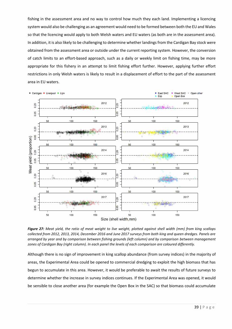
39 | P a g e

fishing in the assessment area and no way to control how much they each land. Implementing a licencing

system would also be challenging as an agreement would need to be formed between both the EU and Wales

so that the licencing would apply to both Welsh waters and EU waters (as both are in the assessment area).

In addition, it is also likely to be challenging to determine whether landings from the Cardigan Bay stock were

obtained from the assessment area or outside under the current reporting system. However, the conversion

of catch limits to an effort-based approach, such as a daily or weekly limit on fishing time, may be more

appropriate for this fishery in an attempt to limit fishing effort further. However, applying further effort

restrictions in only Welsh waters is likely to result in a displacement of effort to the part of the assessment

area in EU waters.

Figure 27: Meat yield, the ratio of meat weight to live weight, plotted against shell width (mm) from king scallops

collected from 2012, 2013, 2014, December 2016 and June 2017 surveys from both king and queen dredges. Panels are

arranged by year and by comparison between fishing grounds (left column) and by comparison between management

zones of Cardigan Bay (right column). In each panel the levels of each comparison are coloured differently.

Although there is no sign of improvement in king scallop abundance (from survey indices) in the majority of

areas, the Experimental Area could be opened to commercial dredging to exploit the high biomass that has

begun to accumulate in this area. However, it would be preferable to await the results of future surveys to

determine whether the increase in survey indices continues. If the Experimental Area was opened, it would

be sensible to close another area (for example the Open Box in the SAC) so that biomass could accumulate

40 | P a g e

in this area (especially as there is indication from the population structure that recruitment occurs regularly

in this area).

It is essential for stock assessment that the survey data series is continued. The EMFF project will continue

to collect survey data for stock assessment to 2022, and it is imperative surveys are conducted beyond then

if stock assessment modelling is to be implemented in the future. Other methods for a stock assessment,

such as quantification of vessel catch efficiencies or data-limited tools, represent other avenues for

estimating stock size, but do not estimate many other useful pieces of management information that come

from the stock assessment models implemented here. Quantification of vessel catch efficiencies will also be

a focus of research on the EMFF project, as an alternative to stock assessment modelling.

Figure 28: Relative percentage of gonad stage from king scallops collected from 2012, 2013, 2014, December 2016 and

June 2017 surveys from both king and queen dredges. Panels are arranged by survey and by fishing ground. The bars in

each panel correspond to stages from the GOI and are coloured accordingly. Blank panels reflect areas which were not

surveyed during that survey.

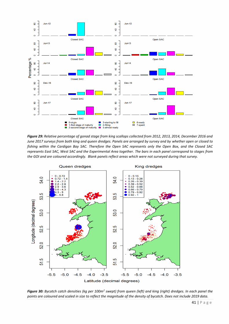
41 | P a g e

Figure 29: Relative percentage of gonad stage from king scallops collected from 2012, 2013, 2014, December 2016 and

June 2017 surveys from both king and queen dredges. Panels are arranged by survey and by whether open or closed to

fishing within the Cardigan Bay SAC. Therefore the Open SAC represents only the Open Box, and the Closed SAC

represents East SAC, West SAC and the Experimental Area together. The bars in each panel correspond to stages from

the GOI and are coloured accordingly. Blank panels reflect areas which were not surveyed during that survey.

Figure 30: Bycatch catch densities (kg per 100m2 swept) from queen (left) and king (right) dredges. In each panel the

points are coloured and scaled in size to reflect the magnitude of the density of bycatch. Does not include 2019 data.

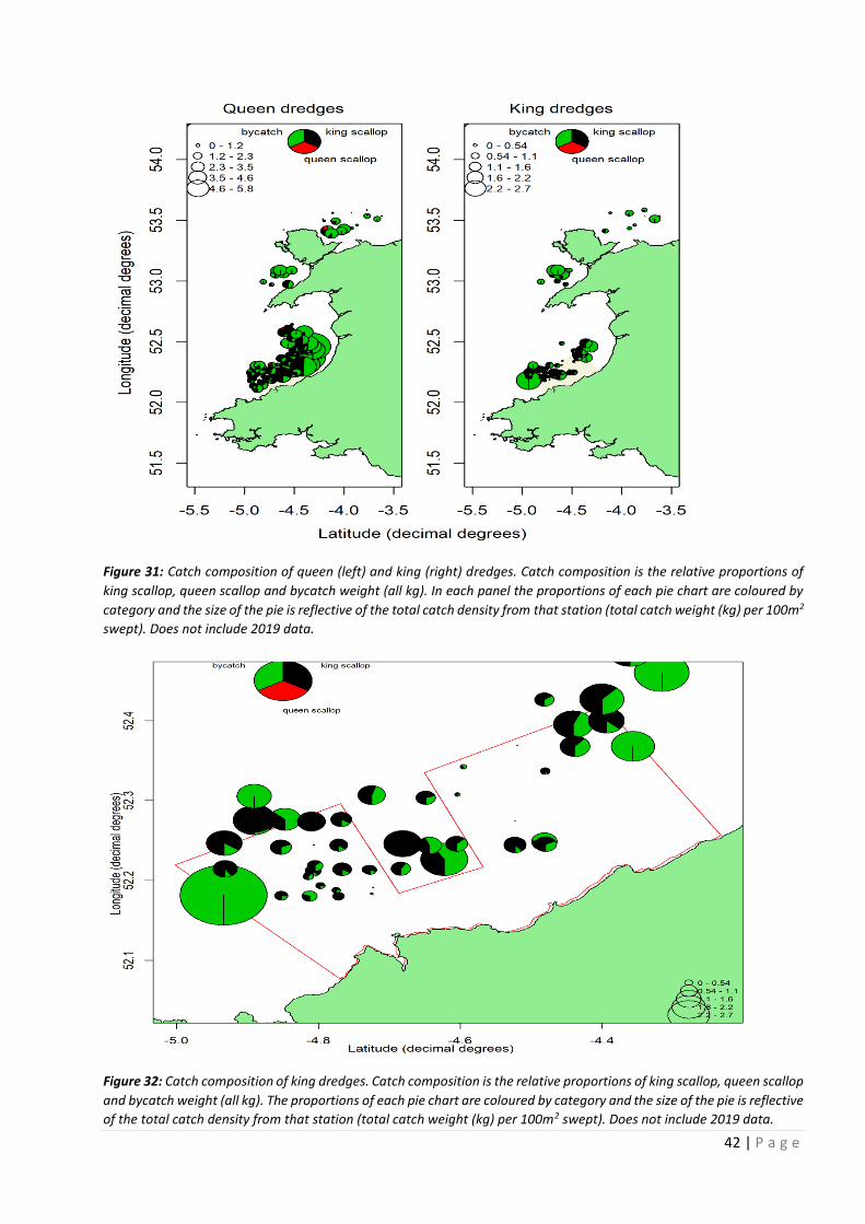
42 | P a g e

Figure 31: Catch composition of queen (left) and king (right) dredges. Catch composition is the relative proportions of

king scallop, queen scallop and bycatch weight (all kg). In each panel the proportions of each pie chart are coloured by

category and the size of the pie is reflective of the total catch density from that station (total catch weight (kg) per 100m2

swept). Does not include 2019 data.

Figure 32: Catch composition of king dredges. Catch composition is the relative proportions of king scallop, queen scallop

and bycatch weight (all kg). The proportions of each pie chart are coloured by category and the size of the pie is reflective

of the total catch density from that station (total catch weight (kg) per 100m2 swept). Does not include 2019 data.

43 | P a g e

Figure 33: Mean densities, and 95% confidence intervals, of bycatch (kg per 100m2 swept) from queen dredges from

each survey. Top panel is separated by fishing ground, and bottom panel is separated by management area of Cardigan

Bay. Note the y-axis scale on each panel is different.

Figure 34: Mean densities, and 95% confidence intervals, of bycatch (kg per 100m2 swept) from king dredges from each

survey. Top panel is separated by fishing ground, and bottom panel is separated by management area of Cardigan Bay.

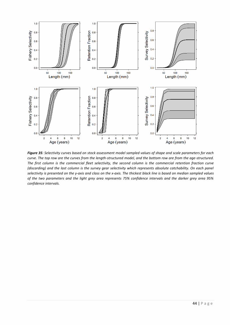
44 | P a g e

Figure 35: Selectivity curves based on stock assessment model sampled values of shape and scale parameters for each

curve. The top row are the curves from the length-structured model, and the bottom row are from the age-structured.

The first column is the commercial fleet selectivity, the second column is the commercial retention fraction curve

(discarding) and the last column is the survey gear selectivity which represents absolute catchability. On each panel

selectivity is presented on the y-axis and class on the x-axis. The thickest black line is based on median sampled values

of the two parameters and the light grey area represents 75% confidence intervals and the darker grey area 95%

confidence intervals.

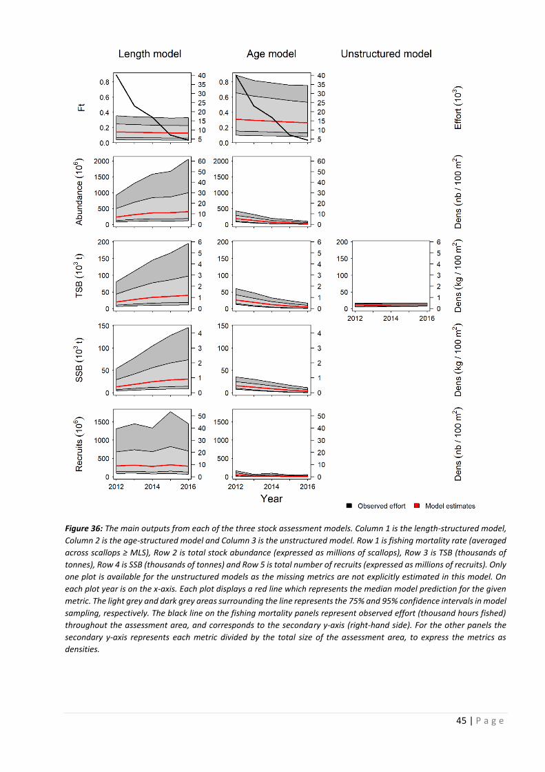
45 | P a g e

Figure 36: The main outputs from each of the three stock assessment models. Column 1 is the length-structured model,

Column 2 is the age-structured model and Column 3 is the unstructured model. Row 1 is fishing mortality rate (averaged

across scallops ≥ MLS), Row 2 is total stock abundance (expressed as millions of scallops), Row 3 is TSB (thousands of

tonnes), Row 4 is SSB (thousands of tonnes) and Row 5 is total number of recruits (expressed as millions of recruits). Only

one plot is available for the unstructured models as the missing metrics are not explicitly estimated in this model. On

each plot year is on the x-axis. Each plot displays a red line which represents the median model prediction for the given

metric. The light grey and dark grey areas surrounding the line represents the 75% and 95% confidence intervals in model

sampling, respectively. The black line on the fishing mortality panels represent observed effort (thousand hours fished)

throughout the assessment area, and corresponds to the secondary y-axis (right-hand side). For the other panels the

secondary y-axis represents each metric divided by the total size of the assessment area, to express the metrics as

densities.

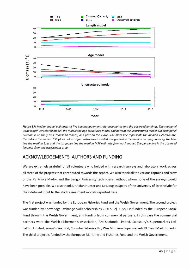
46 | P a g e

Figure 37: Median model estimates of five key management reference points and the observed landings. The top panel

is the length-structured model, the middle the age-structured model and bottom the unstructured model. On each panel

biomass is on the y-axis (thousand tonnes) and year on the x-axis. The black line represents the median TSB estimate,

the red line the median SSB (does not exist for unstructured model), the green line the median carrying capacity, the blue

line the median BMSY and the turquoise line the median MSY estimate from each model. The purple line is the observed

landings from the assessment area.

ACKNOWLEDGEMENTS, AUTHORS AND FUNDING

We are extremely grateful for all volunteers who helped with research surveys and laboratory work across

all three of the projects that contributed towards this report. We also thank all the various captains and crew

of the RV Prince Madog and the Bangor University technicians, without whom none of the surveys would

have been possible. We also thank Dr Aidan Hunter and Dr Douglas Speirs of the University of Strathclyde for

their detailed input to the stock assessment models reported here.

The first project was funded by the European Fisheries Fund and the Welsh Government. The second project

was funded by Knowledge Exchange Skills Scholarships 2 (KESS 2). KESS 2 is funded by the European Social

Fund through the Welsh Government, and funding from commercial partners. In this case the commercial

partners were the Welsh Fishermen’s Association, AM Seafoods Limited, Sainsbury’s Supermarkets Ltd,

FalFish Limited, Young’s Seafood, Coombe Fisheries Ltd, Wm Morrison Supermarkets PLC and Mark Roberts.

The third project is funded by the European Maritime and Fisheries Fund and the Welsh Government.

47 | P a g e

Adam Delargy analysed all data, conducted the stock assessments and wrote the report. Adam also designed

and led four of the surveys (2016 to 2018). Michel Kaiser obtained the funding the supervised the EFF and

KESS 2 projects. Michel also contributed to obtaining the funding for the EMFF project. Jan Hiddink

supervised the KESS 2 project and is a supervisor on the EMFF project. Gwladys Lambert designed and led

the 2013 and 2014 research surveys, and conducted a considerable amount of data processing from all three

surveys from the initial project (2012 to 2014). Hilmar Hinz designed and led the 2012 survey, and along with

Lee Murray, was also heavily involved in the surveys from the initial project and consequent data processing.

Natalie Hold contributed towards obtaining the funding for the EMFF project and designed and led the 2019

survey. Ian McCarthy is the Principal Investigator on the EMFF project.

REFERENCES

Chauvaud, L., Patry, Y., Jolivet, A., Cam, E., Le Goff, C., Strand, Ø., Charrier, G., Thébault, J., Lazure, P., Gotthard, K. and

Clavier, J., 2012. Variation in size and growth of the great scallop Pecten maximus along a latitudinal gradient. PloS

one, 7(5), p.e37717.

Delargy, A., 2019. Quantitative Methods for Producing Evidence to Support Sustainable King Scallop Fishing. PhD thesis,

Bangor University.

Hilborn, R. and Walters, C.J., 1992. Quantitative fisheries stock assessment: choice dynamics and uncertainty–Chapman

and Hall. New York.

Kimura, D.K., 1980. Likelihood methods for the von Bertalanffy growth curve. Fishery bulletin, 77(4), pp.765-776.

Lambert, G.I., Murray L.G., Hinz H., Kaiser M.J., 2014. Status of scallop populations in Welsh waters. Bangor University,

Fisheries and Conservation Report No. 41. pp 61

Mason, J., 1958. The breeding of the scallop, Pecten maximus (L.), in Manx waters. Journal of the Marine Biological

Association of the United Kingdom, 37(3), pp.653-671.

Maunder, M. N., 2008. Maximum Sustainable Yield. In Encyclopedia of Ecology, S.E. Jørgensen and B.D. Fath, eds.

(Oxford: Academic Press), pp. 2292–2296.

Ogle, D.H., P. Wheeler, and A. Dinno. 2019. FSA: Fisheries Stock Analysis. R package version 0.8.25,

https://github.com/droglenc/FSA

R Core Team. 2019. R: A language and environment for statistical computing. Vienna.

STECF (Scientific, Technical and Economic Committee for Fisheries) 2018 – Fisheries Dependent Information – New FDI

(STECF-18-11). Publications Office of the European Union, Luxembourg, 2018, ISBN 978-92-79-79394-3,

doi:10.2760/696153, JRC114717

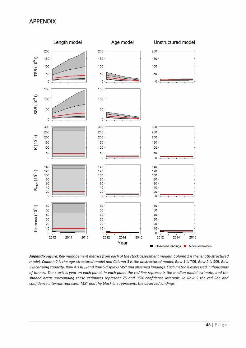
48 | P a g e

APPENDIX

Appendix Figure: Key management metrics from each of the stock assessment models. Column 1 is the length-structured

model, Column 2 is the age-structured model and Column 3 is the unstructured model. Row 1 is TSB, Row 2 is SSB, Row

3 is carrying capacity, Row 4 is BMSY and Row 5 displays MSY and observed landings. Each metric is expressed in thousands

of tonnes. The x-axis is year on each panel. In each panel the red line represents the median model estimate, and the

shaded areas surrounding these estimates represent 75 and 95% confidence intervals. In Row 5 the red line and

confidence intervals represent MSY and the black line represents the observed landings.