WELL IMPAIRMENT UPSCALING APPLIED TO WATER INJECTION ABOVE FRACTURE PRESSURE SIMULATION

Juan Manuel Montoya Moreno Eduin Orlando Muñoz Mazo Eliana Luci Ligero Denis José Schiozer moreno@dep.fem.unicamp.br eduin@dep.fem.unicamp.br eligero@dep.fem.unicamp.br denis@dep.fem.unicamp.br Departamento de Engenharia de Petróleo Centro de Estudos do Petróleo Universidade Estadual de Campinas – Unicamp Caixa Postal 6052 – CEP 13083-970 Campinas – SP - Brasil Abstract. Water injection into reservoirs is used to increase oil recovery and to maintain reservoir pressure above the bubble point. In spite of the water injection advantages, there is a technical problem: well impairment or injectivity loss associated to this recovery method. Well impairment results from deposition of different types of particles as solid rock fines; insoluble carbonates from seawater, oil droplets and bacteria. To avoid injectivity loss and to minimize the strong economic impact, different actions must be taken in reservoir development projects, especially in offshore fields. An important option is to inject water above the fracture pressure in order to create high conductivity channels in the reservoir. In this work, a mathematical model is used to represent well impairment in a commercial numerical flow simulator with a refined grid, and different upscaling methods are used to transfer the behavior of well impairment into a coarse grid (full field simulations). Furthermore, a fracture model with transmissibility modifiers is used together with a virtual horizontal well model as a new proposal to model fractures induced by water injection in commercial simulators. Results show that it is important to define a suitable method to upscale the refined well block permeability to the coarse well block. Moreover, results indicate that it is appropriate to use virtual horizontal wells as fracture modeling method. Keywords: Water injection, Well impairment, Hydraulic fracture, Upscaling,

Reservoir simulation.

1. INTRODUCTION

Waterflooding is the most common method for additional oil recovery used worldwide, representing about 80% of all recovery methods. Natural oil production is known as primary production, and generally under this condition, reservoirs have recovery factors among 5 and 20% (Gomes, 2003). When the reservoir energy is not sufficient to maintain an economic oil rate, different recovery methods can be employed to maintain the reservoir pressure and oil rates. Water injection is a recovery method capable to introduce energy into reservoir, increasing its pressure and the final recovery factor from 15% to 60% values (Rosa et al., 2006).

According to Sigh (1982), water injection involves different criteria: geological, that influence the flood performance; technical, such as injection pressure, water quality and water processing systems; and economic such as injection and processing costs. In spite of the water injection advantages, a technical problem, the injectivity loss, has a significant economic impact. Sharma et al. (2000) described the injectivity loss as one of the most important problems in the waterflooding process and it is more critical in offshore operations.

Injectivity loss is related to well loss capacity to maintain a constant water injection rate and it is directly related to the water quality. Water for injection has different sources: seawater, rivers, lakes and, production water, as in many fields. Oort et al. (1992) describe the different type of particles and their source: solid particles (sand, fines and clay) come from formation or sea water, oil droplets (disperse phase) from production water, bacteria, microscopic algae, dissolved salts, carbonates, sulfates and some iron compounds come from sea water. When water flows in the porous media, these particles are retained in the throats, reducing the permeability around the injector well (Bedrikovetsky et al. 2001) and the injectivity is declined. Independent of its origin, water always contains different kind of suspended particles and requires special treatments to eliminate dissolved oxygen, to kill bacteria and to remove solid particles through filtration. As a result the companies have to invest in processing and treatment systems.

Some works available in literature are concerned about the impact of the injectivity loss. Gadde and Sharma (2001) developed an analytical model to study the decline caused by injection of fines and the impact on the injector performance. A model was used to determine the parameters of quality for injection water. Bedrikovetsky et al. (2001) developed a mathematical model with two parameters (damage and filtration coefficients) to calculate the information necessary to determine the injector well impairment from laboratory and field tests. On the other hand, injectivity loss in numerical reservoir simulator is not commented and treated. Souza et al. (2005) represented the injectivity loss considering that water rate injection decreases as a time step function, but the bottom-hole pressure behavior was not considered. Additionally, simulators have multipliers to fix the injectivity index but there are not studies that show these utilities for injectivity loss modeling.

To avoid the injectivity loss, different procedures may be used. The best choice depends on technical, economic and environmental conditions. Palsson et al. (2003) discussed, using a decision tree, the different options and their economic impact: the first option involved drilling costs, the second option implicated in the reservoir depressurization and stimulation costs when is required, and the third option considered the investment in processing systems which were neither simple nor cheap. Furtado et al. (2005) commented that injectivity loss increases the operational cost because it involves continuous water filtration, addition of chemical agents to kill bacteria, scale inhibitors and sometimes requires changing parts of the injection system.

Injectivity loss implicates continuously to elevate the bottom-hole pressure in order to maintain constant the water rate. Typically, the operational limit for injector bottom-hole

pressure is the fracture pressure. Actually, other option to combat injectivity loss is to increase the injection pressure above formation fracturing pressure, breaking the formation and creating high conductivity channels. Ovens et al. (1998) reported a field case in Denmark (Dan field), where water injection under fracturing conditions was used to improve the injectivity. Another case was commented by Ali et al. (1994) in Valhall field. This field presented low injectivity and water fracturing was implemented to inject water in economic conditions. Some authors comment about the correct well location to avoid water re-cycling when the fracture is aligned with the producer well, dismissing the areal sweep efficiency.

Considering the previous situation, geomechanical simulators are the best tools to analyze and study fracture behavior under water injection conditions. However, this kind of software shows a high time consumption and is normally non-commercial. Van den Hoek et al. (2004) developed a decoupled geomechanical simulator to study water disposal water in Oman. Gadde and Sharma (2001) coupled both geomechanical and flow simulator to study only one well located at the center of drainage area and Rewis (1999) presented a coupled model but it only works with simple geometries. Finally, some commercial simulators have incorporated geomechanical applications, but they have some numerical instability. Additionally, there are a few approximations to model fracture in commercial numerical reservoir simulators as was described by Wan (1999): (1) using local grid refinements in grid blocks with high permeability and low porosity, (2) using transmissibility modifiers or (3) using an effective radius to represent the fracture. Also a method to calculate well injectivity index for non-conventional wells (vertical or horizontal wells with fractures) was presented.

The above options have high time consumption and require local grid refinements and, for full field studies, sometimes, can be hard to implement or not have practical use. It is important to outline that available numerical simulators for fracture modeling always are related with hydraulic and natural fracture modeling, and most of the times, they are not related to fractures induced by water injection.

The goals of this work are to study methods to calculate well block permeability when a formation damage region has been developed around the injector well, to study the impact of injectivity loss in reservoir performance, and to model the fracture propagation induced by the water in order to avoid injectivity loss. Two alternatives are considered to model the fracture propagation: (1) to use transmissibility modifiers, as proposed by Souza et al. (2005), but in addition to their methodology, it is calculated the well injectivity decline and (2) to use a virtual horizontal well to represent the fracture behavior without grid refinement. 2. APPLICATION

The base model is an extension of Souza et al. (2005) model: one-fourth direct line and five spot injection models. This was adopted in this work because one-fourth models require well index, injection rate, porosity and permeability well block modifications that may mask loss injectivity and fracture effects.

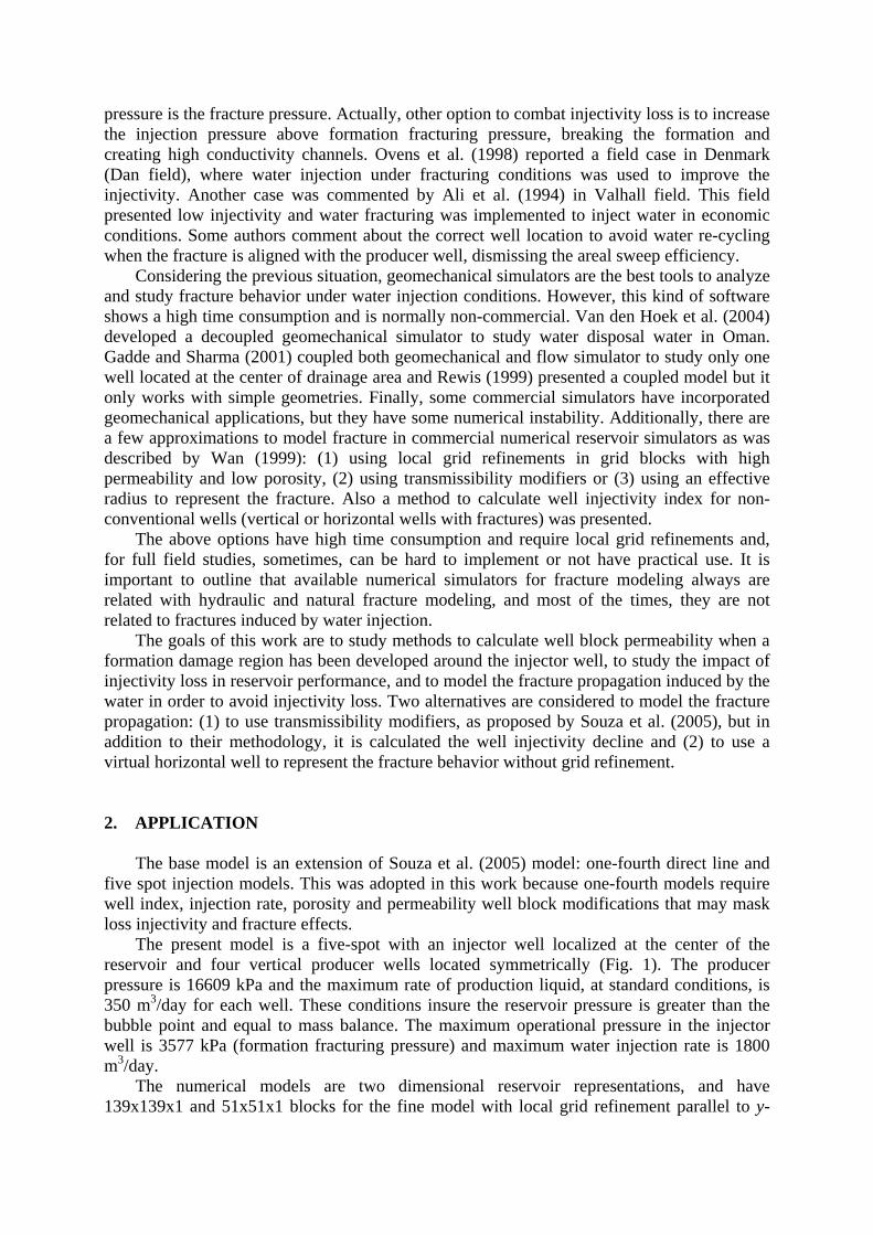
The present model is a five-spot with an injector well localized at the center of the reservoir and four vertical producer wells located symmetrically (Fig. 1). The producer pressure is 16609 kPa and the maximum rate of production liquid, at standard conditions, is 350 m3/day for each well. These conditions insure the reservoir pressure is greater than the bubble point and equal to mass balance. The maximum operational pressure in the injector well is 3577 kPa (formation fracturing pressure) and maximum water injection rate is 1800 m3/day.

The numerical models are two dimensional reservoir representations, and have 139x139x1 and 51x51x1 blocks for the fine model with local grid refinement parallel to y-

axis and coarse Cartesian grid, respectively. The distance between injector well and any producer well is 765 m. The fine model is used to represent the fracture with transmissibility modifiers and virtual horizontal well. The coarse model is used to adjust the behavior of the refined model to represent the field scenarios.

The petrophysical properties (Table 1) are assumed as constant throughout the reservoir, the net to gross ratio is equal to the unit and the gravitatory and capillary effects are neglected.

Figure 1. Base models. Inverted five-spot arrangement of wells.

Table 1. Reservoir properties

Property Nomenclature Value Porosity φ 25% Horizontal permeability kx = ky 500 mD Vertical permeability kz 200 mD Rock compressibility cr 4.4967x10-7 kPa-1

Initial pressure pi 27579 kPa Depth hr 2680 m

The fluid used is 40o API and its viscosity varies among 0.7 – 0.2 cP at reservoir

conditions. Other fluid properties are listed in Table 2. These fluid properties make the system behaves as a “piston-like system”. The simulation model is Black-Oil, a commercial simulator is used to execute the simulations and the simulation total time is 6205 days.

Table 2. Fluid properties

Property Nomenclature Value Reservoir temperature Tr 91.1 oC Bubble point pressure pb 16609 kPa Initial water saturation Swi 17 % Water viscosity μw 0.9 cP Water formation volume BBw 1.0

3. PROCEDURE

Three scenarios are focus of study, each one with two different grid types (fine and coarse). The first scenario represents the base model, an ideal reservoir with homogeneous petrophysical properties. Its principal characteristic is that there is not injectivity loss in the

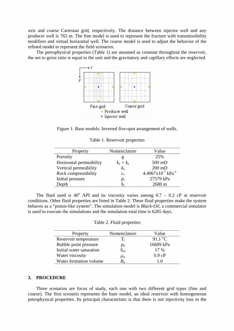
injector well. In this case, refined and coarse grids are adjusted until the simulation responses in water injection rates, bottom-hole pressure and produced oil rates are equal. The second model presents injectivity loss in the injector well during the simulation time. Injectivity loss is modeled with an analytical expression that represents permeability variation near the well and using up-scaling method, the equivalent injector well permeability block is calculated. The third model includes injectivity loss during the initial time until the bottom-hole pressure reaches the fracture pressure. After that, a fracture is induced into the reservoir and it is represented by two models (Fig. 2): transmissibility modifiers according to Souza et al. (2005) model and by a new proposal, using a virtual horizontal well. The fine model has refined blocks parallel to y-axis, representing the growing fracture direction. Nevertheless, for a full field application, it is necessary to know the reservoir stress state in order to determine the correct fracture direction. Different parameters are analyzed for each model: water injection rate, bottom-hole pressure, produced oil and water rate and cumulative oil and water.

Figure 2. Fracture models. 3.1 Injectivity decline modeling and well block permeability calculation.

The water injection rate is calculated using the Eq. 1 under conditions of single-phase and steady state flow (Rosa et al., 2006):

( )

⎟⎟⎠

⎞⎜⎜⎝

⎛+

−=

srr

LnB

pphkkq

w

eww

wfww

μ

π2 (1)

where qw is the water rate at standard conditions, h is reservoir thickness, k is the absolute permeability, kw is the effective permeability, p is the drainage area mean pressure, pwf is the bottom-hole pressure, μw is the water viscosity, BBw is the water formation volume factor, re and rw are the external and well radius, respectively and s is the well damage factor (skin).

The injectivity index equation, IIw, for an injection well is obtained from Eq. (1) according to definition of Rosa et al. (2006):

( )⎟⎟⎠

⎞⎜⎜⎝

⎛+

=−

=s

rr

LnB

hkkpp

qII

w

eww

w

wf

ww

μ

π2 (2)

Applying the Eq. (2) in the injector well grid block and following the representation of Ertekin et al. (2001), the injectivity index may be represented as a product of both, water mobility and geometric terms as is shown in Eq. (3):

www GII λ= (3)

where the water mobility, λw, is defined by Eq. (4):

ww

ww B

kμ

λ = (4)

and the geometric factor, Gw, is defined by Eq. (5):

⎟⎟⎠

⎞⎜⎜⎝

⎛+

=

srr

Ln

khG

w

eq

bbw

π2 (5)

where req is defined as equivalent radius and it is a grid geometrical parameters function (Peaceman, 1978). For homogeneous and heterogeneous systems, kb is the block permeability and is calculated as a geometric mean of kx and ky and hb is the well block thickness.

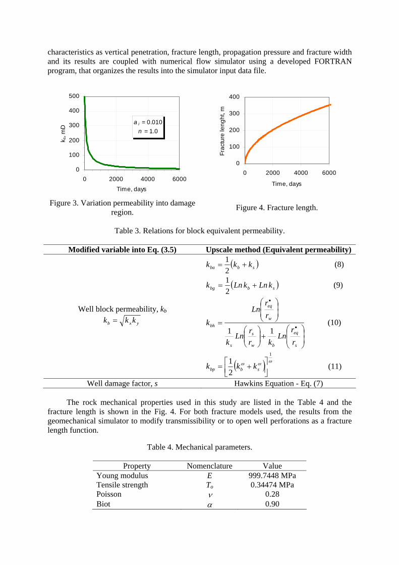
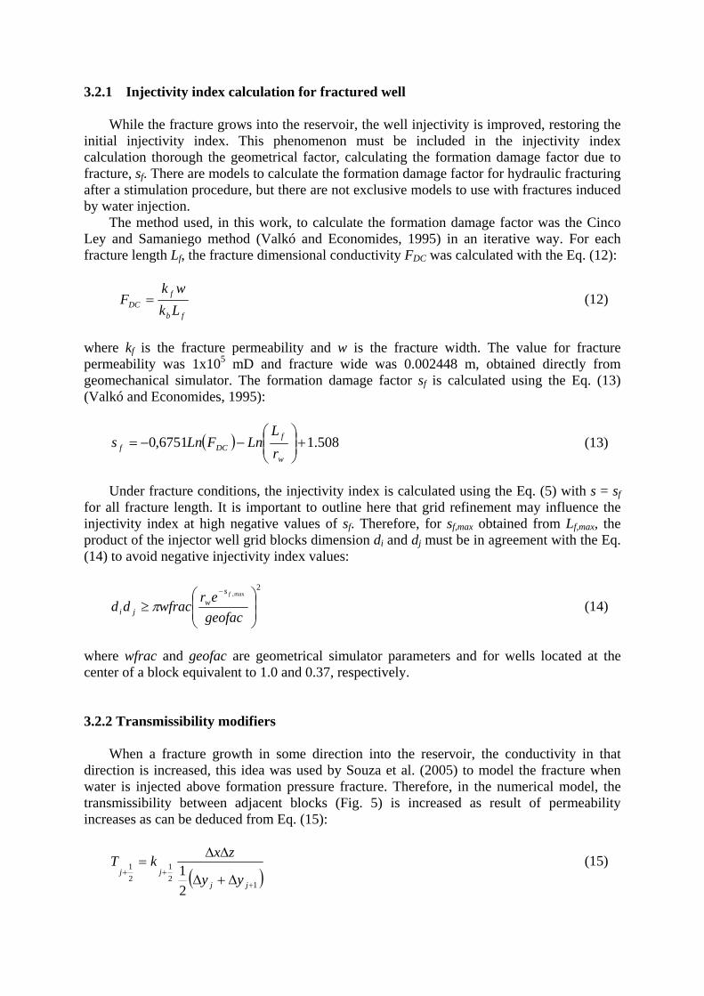
In order to model the well impairment, the injectivity index, IIw, is varied as a result to consider the Gw as a time function. The varied parameters were the well factor damage and the well block permeability. The permeability variation around the injector well, which is related with factor damage, was modeled by an analytical expression:

( ) ni

snta

kk 1.1 +

= (6)

where ks is the well damaged region permeability, ai and n are constants that define the curve shape (Fig. 3) and k is initial block permeability. The permeability values obtained form Eq. (6) were employed to calculate the well bore damage factor, according to the Eq. (7) presented by Craft and Hawkins (1959):

w

s

s

sb

rr

Lnk

kks ⎟⎟

⎠

⎞⎜⎜⎝

⎛ −= (7)

where rs is the damaged zone radius and it was assumed equal to rs=1.5 m. As the damage region have permeability variation, different upscaling techniques were used to obtain an equivalent well block permeability to be used in Eq. (5).

The Table 3 presents the equations for arithmetic kba, geometric kbg, power-law kbp and radial-harmonic kbh means used to upscale and the possible combinations used in this work. The area of the block of injector well is related to a circle of equal area by the radius defined as r*

eq in the Eq. (10) and ω is a parameter that can take values between zero and one. 3.2 Fracture modeling

The fracture generated by water injection were modeled by two methods: the first one, it

is similar to the model used by Souza et al. (2005) including injectivity loss at initial times and the second one is a new proposal to model the fracture using a virtual horizontal well. An non-commercial geomechanical simulator is used to study the fracture geometric

characteristics as vertical penetration, fracture length, propagation pressure and fracture width and its results are coupled with numerical flow simulator using a developed FORTRAN program, that organizes the results into the simulator input data file.

a i = 0.010n = 1.0

0

100

200

300

400

500

0 2000 4000 600

Time, days

k s, m

D

0

0

100

200

300

400

0 2000 4000 6000

Time, days

Frac

ture

leng

ht, m

Figure 3. Variation permeability into damage

region. Figure 4. Fracture length.

Table 3. Relations for block equivalent permeability.

Modified variable into Eq. (3.5) Upscale method (Equivalent permeability)

( sbba kkk +=21 ) (8)

( sbbg kLnkLnk +=21 ) (9)

⎟⎟⎠

⎞⎜⎜⎝

⎛+⎟⎟

⎠

⎞⎜⎜⎝

⎛

⎟⎟⎠

⎞⎜⎜⎝

⎛

=•

•

s

eq

bw

s

s

w

eq

bh

rr

Lnkr

rLn

k

rr

Ln

k11

(10)

Well block permeability, kb

yxb kkk =

( ) ωωω

1

21

⎥⎦⎤

⎢⎣⎡ += sbbp kkk (11)

Well damage factor, s Hawkins Equation - Eq. (7)

The rock mechanical properties used in this study are listed in the Table 4 and the fracture length is shown in the Fig. 4. For both fracture models used, the results from the geomechanical simulator to modify transmissibility or to open well perforations as a fracture length function.

Table 4. Mechanical parameters.

Property Nomenclature Value Young modulus E 999.7448 MPa Tensile strength To 0.34474 MPa Poisson ν 0.28 Biot α 0.90

3.2.1 Injectivity index calculation for fractured well

While the fracture grows into the reservoir, the well injectivity is improved, restoring the initial injectivity index. This phenomenon must be included in the injectivity index calculation thorough the geometrical factor, calculating the formation damage factor due to fracture, sf. There are models to calculate the formation damage factor for hydraulic fracturing after a stimulation procedure, but there are not exclusive models to use with fractures induced by water injection.

The method used, in this work, to calculate the formation damage factor was the Cinco Ley and Samaniego method (Valkó and Economides, 1995) in an iterative way. For each fracture length Lf, the fracture dimensional conductivity FDC was calculated with the Eq. (12):

fb

fDC Lk

wkF = (12)

where kf is the fracture permeability and w is the fracture width. The value for fracture permeability was 1x105 mD and fracture wide was 0.002448 m, obtained directly from geomechanical simulator. The formation damage factor sf is calculated using the Eq. (13) (Valkó and Economides, 1995):

( ) 508.16751,0 +⎟⎟⎠

⎞⎜⎜⎝

⎛−−=

w

fDCf r

LLnFLns (13)

Under fracture conditions, the injectivity index is calculated using the Eq. (5) with s = sf

for all fracture length. It is important to outline here that grid refinement may influence the injectivity index at high negative values of sf. Therefore, for sf,max obtained from Lf,max, the product of the injector well grid blocks dimension di and dj must be in agreement with the Eq. (14) to avoid negative injectivity index values:

2

max,

⎟⎟⎠

⎞⎜⎜⎝

⎛≥

−

geofacer

wfracddfs

wji π (14)

where wfrac and geofac are geometrical simulator parameters and for wells located at the center of a block equivalent to 1.0 and 0.37, respectively. 3.2.2 Transmissibility modifiers

When a fracture growth in some direction into the reservoir, the conductivity in that direction is increased, this idea was used by Souza et al. (2005) to model the fracture when water is injected above formation pressure fracture. Therefore, in the numerical model, the transmissibility between adjacent blocks (Fig. 5) is increased as result of permeability increases as can be deduced from Eq. (15):

( )121

21

21

+

++Δ+Δ

ΔΔ=

jjjj

yy

zxkT (15)

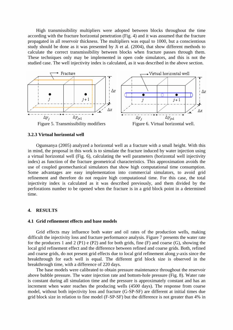
High transmissibility multipliers were adopted between blocks throughout the time according with the fracture horizontal penetration (Fig. 4) and it was assumed that the fracture propagated in all reservoir thickness. The multipliers was equal to 1000, but a conscientious study should be done as it was presented by Ji et al. (2004), that show different methods to calculate the correct transmissibility between blocks when fracture passes through them. These techniques only may be implemented in open code simulators, and this is not the studied case. The well injectivity index is calculated, as it was described in the above section.

Figure 5. Transmissibility modifiers Figure 6. Virtual horizontal well. 3.2.3 Virtual horizontal well

Ogunsanya (2005) analyzed a horizontal well as a fracture with a small height. With this in mind, the proposal in this work is to simulate the fracture induced by water injection using a virtual horizontal well (Fig. 6), calculating the well parameters (horizontal well injectivity index) as function of the fracture geometrical characteristics. This approximation avoids the use of coupled geomechanical simulators that show high computational time consumption. Some advantages are easy implementation into commercial simulators, to avoid grid refinement and therefore do not require high computational time. For this case, the total injectivity index is calculated as it was described previously, and them divided by the perforations number to be opened when the fracture is in a grid block point in a determined time. 4. RESULTS 4.1 Grid refinement effects and base models

Grid effects may influence both water and oil rates of the production wells, making difficult the injectivity loss and fracture performance analysis. Figure 7 presents the water rate for the producers 1 and 2 (P1) e (P2) and for both grids, fine (F) and coarse (G), showing the local grid refinement effect and the difference between refined and coarse grids. Both, refined and coarse grids, do not present grid effects due to local grid refinement along y-axis since the breakthrough for each well is equal. The different grid block size is observed in the breakthrough time, with a difference of 220 days.

The base models were calibrated to obtain pressure maintenance throughout the reservoir above bubble pressure. The water injection rate and bottom-hole pressure (Fig. 8). Water rate is constant during all simulation time and the pressure is approximately constant and has an increment when water reaches the producing wells (4500 days). The response from coarse model, without both injectivity loss and fracture (G-SP-SF) are different at initial times due grid block size in relation to fine model (F-SP-SF) but the difference is not greater than 4% in

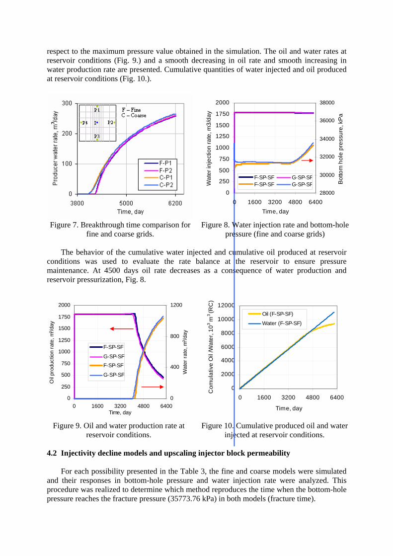
respect to the maximum pressure value obtained in the simulation. The oil and water rates at reservoir conditions (Fig. 9.) and a smooth decreasing in oil rate and smooth increasing in water production rate are presented. Cumulative quantities of water injected and oil produced at reservoir conditions (Fig. 10.).

The behavior of the cumulative water injected and cumulative oil produced at reservoir

conditions was used to evaluate the rate balance at the reservoir to ensure pressure maintenance. At 4500 days oil rate decreases as a consequence of water production and reservoir pressurization, Fig. 8.

0

250

500

750

1000

1250

1500

1750

2000

0 1600 3200 4800 6400Time, day

Oil p

rodu

ctio

n ra

te, m

3 /day

0

400

800

1200

Wat

er ra

te, m

3 /day

F-SP-SF

G-SP-SFF-SP-SF

G-SP-SF

0

2000

4000

6000

8000

10000

12000

0 1600 3200 4800 6400

Time, day

Com

ulat

ive

Oil

/Wat

er, 1

03 m3 (R

C)

Oil (F-SP-SF)

Water (F-SP-SF)

Figure 9. Oil and water production rate at reservoir conditions.

Figure 10. Cumulative produced oil and water injected at reservoir conditions.

4.2 Injectivity decline models and upscaling injector block permeability

0

250

500

750

1000

1250

1500

1750

2000

0 1600 3200 4800 6400Time, day

Wat

er in

ject

ion

rate

, m3/

day

28000

30000

32000

34000

36000

38000

Bot

tom

hol

e pr

essu

re, k

Pa

F-SP-SF G-SP-SFF-SP-SF G-SP-SF

Figure 7. Breakthrough time comparison for fine and coarse grids.

Figure 8. Water injection rate and bottom-hole pressure (fine and coarse grids)

For each possibility presented in the Table 3, the fine and coarse models were simulated

and their responses in bottom-hole pressure and water injection rate were analyzed. This procedure was realized to determine which method reproduces the time when the bottom-hole pressure reaches the fracture pressure (35773.76 kPa) in both models (fracture time).

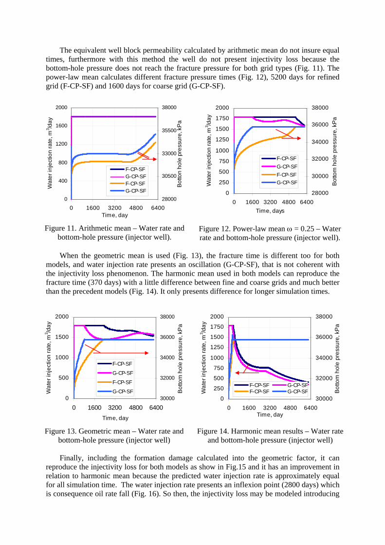
The equivalent well block permeability calculated by arithmetic mean do not insure equal times, furthermore with this method the well do not present injectivity loss because the bottom-hole pressure does not reach the fracture pressure for both grid types (Fig. 11). The power-law mean calculates different fracture pressure times (Fig. 12), 5200 days for refined grid (F-CP-SF) and 1600 days for coarse grid (G-CP-SF).

0

400

800

1200

1600

2000

0 1600 3200 4800 6400Time, day

Wat

er in

ject

ion

rate

, m3 /d

ay

28000

30500

33000

35500

38000

Bot

ton

hole

pre

ssur

e, k

Pa

F-CP-SFG-CP-SFF-CP-SFG-CP-SF

0

250

500

750

1000

1250

1500

1750

2000

0 1600 3200 4800 6400Time, days

Wat

er in

ject

ion

rate

, m3 /d

ay

28000

30000

32000

34000

36000

38000

Bot

tom

hol

e pr

essu

re, k

Pa

F-CP-SFG-CP-SFF-CP-SFG-CP-SF

Figure 11. Arithmetic mean – Water rate and

bottom-hole pressure (injector well). Figure 12. Power-law mean ω = 0.25 – Water rate and bottom-hole pressure (injector well).

When the geometric mean is used (Fig. 13), the fracture time is different too for both

models, and water injection rate presents an oscillation (G-CP-SF), that is not coherent with the injectivity loss phenomenon. The harmonic mean used in both models can reproduce the fracture time (370 days) with a little difference between fine and coarse grids and much better than the precedent models (Fig. 14). It only presents difference for longer simulation times.

0

500

1000

1500

2000

0 1600 3200 4800 6400Time, day

Wat

er in

ject

ion

rate

, m3 /d

ay

30000

32000

34000

36000

38000

Bot

tom

hol

e pr

essu

re, k

Pa

F-CP-SF

G-CP-SF

F-CP-SF

G-CP-SF0

250

500

750

1000

1250

1500

1750

2000

0 1600 3200 4800 6400Time, day

Wat

er in

ject

ion

rate

, m3 /d

ay

30000

32000

34000

36000

38000

Bot

tom

hol

e pr

essu

re, k

Pa

F-CP-SF G-CP-SFF-CP-SF G-CP-SF

Figure 13. Geometric mean – Water rate and bottom-hole pressure (injector well)

Figure 14. Harmonic mean results – Water rate and bottom-hole pressure (injector well)

Finally, including the formation damage calculated into the geometric factor, it can

reproduce the injectivity loss for both models as show in Fig.15 and it has an improvement in relation to harmonic mean because the predicted water injection rate is approximately equal for all simulation time. The water injection rate presents an inflexion point (2800 days) which is consequence oil rate fall (Fig. 16). So then, the injectivity loss may be modeled introducing

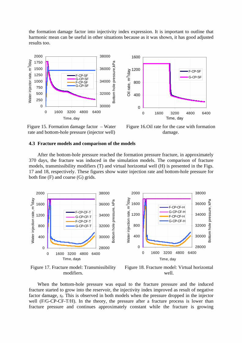
the formation damage factor into injectivity index expression. It is important to outline that harmonic mean can be useful in other situations because as it was shown, it has good adjusted results too.

0

250

500

750

1000

1250

1500

1750

2000

0 1600 3200 4800 6400

Time, day

Wat

er in

ject

or ra

te, m

3 /day

30000

32000

34000

36000

38000

Bot

tom

hol

e pr

essu

re,k

Pa

F-CP-SFG-CP-SFF-CP-SFG-CP-SF

0

400

800

1200

1600

0 1600 3200 4800 6400Time, day

Oil

rate

, m3 /d

ay F-CP-SF

G-CP-SF

Figure 15. Formation damage factor – Water rate and bottom-hole pressure (injector well)

Figure 16.Oil rate for the case with formation damage.

4.3 Fracture models and comparison of the models

After the bottom-hole pressure reached the formation pressure fracture, in approximately 370 days, the fracture was induced in the simulation models. The comparison of fracture models, transmissibility modifiers (T) and virtual horizontal well (H) is presented in the Figs. 17 and 18, respectively. These figures show water injection rate and bottom-hole pressure for both fine (F) and coarse (G) grids.

0

400

800

1200

1600

2000

0 1600 3200 4800 6400Time, days

Wat

er in

ject

ion

rate

, m3 /d

ay

28000

30000

32000

34000

36000

38000

Bot

tom

hol

e pr

essu

re, k

Pa

F-CP-CF-TG-CP-CF-TF-CP-CF-TG-CP-CF-T

0

400

800

1200

1600

2000

0 1600 3200 4800 6400

Time, day

Wat

er in

ject

ion

rate

, m3 /d

ay

28000

30000

32000

34000

36000

38000

Bot

tom

hol

e pr

essu

re, k

Pa

F-CP-CF-HG-CP-CF-HF-CP-CF-HG-CP-CF-H

Figure 17. Fracture model: Transmissibility modifiers.

Figure 18. Fracture model: Virtual horizontal well.

When the bottom-hole pressure was equal to the fracture pressure and the induced

fracture started to grow into the reservoir, the injectivity index improved as result of negative factor damage, sf. This is observed in both models when the pressure dropped in the injector well (F/G-CP-CF-T/H). In the theory, the pressure after a fracture process is lower than fracture pressure and continues approximately constant while the fracture is growing

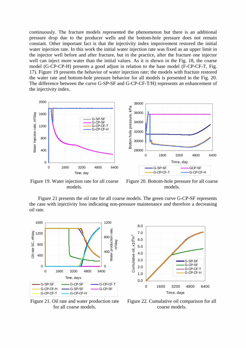
continuously. The fracture models represented the phenomenon but there is an additional pressure drop due to the producer wells and the bottom-hole pressure does not remain constant. Other important fact is that the injectivity index improvement restored the initial water injection rate. In this work the initial water injection rate was fixed as an upper limit in the injector well before and after fracture, but in the practice, after the fracture one injector well can inject more water than the initial values. As it is shown in the Fig. 18, the coarse model (G-CP-CP-H) presents a good adjust in relation to the base model (F-CP-CF-T, Fig. 17). Figure 19 presents the behavior of water injection rate; the models with fracture restored the water rate and bottom-hole pressure behavior for all models is presented in the Fig. 20. The difference between the curve G-SP-SF and G-CP-CF-T/H) represents an enhancement of the injectivity index.

0

400

800

1200

1600

2000

0 1600 3200 4800 6400Time, day

Wat

er in

ject

ion

rate

, m3 /d

ay

G-SP-SFG-CP-SFG-CP-CF-TG-CP-CF-H

28000

30000

32000

34000

36000

38000

0 1600 3200 4800 6400

Time, day

Bot

ton

hole

pre

ssur

e, k

Pa

G-SP-SF GCP-SFG-CP-CF-T G-CP-CF-H

Figure 19. Water injection rate for all coarse models.

Figure 20. Bottom-hole pressure for all coarse models.

Figure 21 presents the oil rate for all coarse models. The green curve G-CP-SF represents

the case with injectivity loss indicating non-pressure maintenance and therefore a decreasing oil rate.

0

400

800

1200

1600

0 1600 3200 4800 6400

Time, days

Oil r

ate

SC, m

3 /day

0

400

800

1200

Wat

er p

rodu

ctio

n ra

te,

m3 /d

ay

G-SP-SF G-CP-SF G-CP-CF-TG-CP-CF-H G-SP-SF G-CP-SFG-CP-CF-T G-CP-CF-H

0.0

1.0

2.0

3.0

4.0

5.0

6.0

7.0

8.0

0 1600 3200 4800 6400

Time, days

Cum

ulat

ive

oil,

x106 m

3

G-SP-SFG-CP-SFG-CP-CF-TG-CP-CF-H

Figure 21. Oil rate and water production rate for all coarse models.

Figure 22. Cumulative oil comparison for all coarse models.

That effect represents the injectivity loss impact in reservoir performance and it is the worst situation because the fracture is aligned with two production wells as it can be observed in the Fig. 21. This fact is important for the correct well allocation for reservoir development. The models with fracture (G-CP-CF-T/H) restore the oil rate, but accelerate the water breakthrough in the production wells. Figure 22 shows the cumulative oil production for all coarse models. The fact to outline is the injectivity loss impact as is show the green curve (G-CP-SF). In this model, the difference between models without injectivity loss, fracture models and with injectivity loss is about 2.3x106 m3 of oil and that value has an economic impact. 5. CONCLUSIONS

The objective of this paper was to discuss some aspects related to well block permeability calculations when a damaged region is presented around injector well for refined and coarse grids and fracture models for commercial simulators.

The harmonic mean and formation damage into geometrical factor methods presented good results to predict the fracture time in both models. Arithmetic, geometrical and power-law means could not reproduce the injectivity loss phenomenon in refined and coarse grids.

The transmissibility between grid blocks was discussed and it was presented as a method to represent a fracture in numerical reservoir models. An improvement of a fracture transmissibility model previously presented in the literature was presented including injectivity loss during initial times.

A new method to represent an induced fracture induce by water injection was presented, including a method to consider results from geomechanical simulators into commercial numerical simulators. A virtual horizontal well can reproduce the behavior of the fracture growth using a coarse grid, but future adjust must be done to calculate the correct injector well bottom-hole pressure. The advantages of this method are that it is not necessary refine grids to model the behavior fracture and the possibility to include geomechanical results into flow model. Acknowledgements

The authors wish to thank to CAPES, CNPq (Proset), CEPETRO, Finep (CTPETRO) and Petrobras. The authors would like to thank Sérgio Iatchuk for his opportune comments and suggestions. Responsibility notice

The authors are the only responsible for the printed material included in this paper. REFERENCES Ali, N., Singh, P. K., Peng, C. P., Shiralkar, G. S., Moschovidis, Z. A., Baack, W. L., 1994.

Injection-Above-Parting-Pressure Waterflood Pilot, Valhall Field, Norway. SPE Reservoir Engineering, vol. 9, n. 1, pp 22-28.

Bedrikovetsky, P.., Marchesin, D., Secaira, F., Serra, A. L., Marchesin, A., Rezende, E., &

Hime, H., 2001. Well Impairment During Sea/Produced Water Flooding: Treatment of

Laboratory Data. SPE 69546, SPE Latim Americam and Caribbean Petroleum Engineering Conference. Buenos Aires.

Craft, B. C. Hawkins, M. F., 1959. Applied Petroleum Reservoir Engineering. pp. 292-293. Prentice-Hall Inc.

Ertekin, T., Abou-kassem, J. H., King, G. R., 2001. Basic Applied Reservoir Simulation. pp.

105-107. SPE textbook Series, vol. 7. Furtado, C. J. A., Siqueira, A. G., Souza, A. L. S., Correa, A. C. F., Mendes, R. A., 2005

Produced Water Reinjection in Petrobras Fields: Challenges and Perspectives. SPE 94705. SPE Latin American and Caribbean Petroleum Engineering Conference. Rio de Janeiro, Brazil.

Gadde, P. B., Sharma, M. M., 2001. Growing Injection Well Fractures and Their Impact on

Waterflood Performance. SPE 71614. SPE Annual Technical Conference and Exhibition. New Orleans, Louisiana.

Gomes, A. C. de A., 2003. Efeitos do Fluxo Bifásico e da Compressibilidade no Declínio da

Injetividade nos Poços Injetores de Água. MSc thesis, Universidade Estadual do Norte Fluminense.

Ji, L., Settari, A., Sullivan, R. B., Orr, D., 2004. Methods for Modeling Dynamic Fractures in

Coupled Reservoir and Geomechanics Simulation. SPE 90874. SPE Annual Technical Conference and Exhibition. Houston, Texas.

Ogunsanya, B. O., 2005. A Physically Consistent Solution for Describing the Transient

Response of Hydraulically Fractured and Horizontal Wells. PhD thesis, Texas Tech University.

Oort, van E., Velzem, van J. F. G., Leerlooijer, K., 1992. Impairment by Suspended Solids

Invasion: Testing and Prediction. SPE 23822. SPE Formation Damage Symposium, Lafayette, Louisiana.

Ovens, J. E. V., Larsen, F. P., Cowie, D. R., 1998. Making Sense of Water Injection

Fractures in the Dan Field. SPE Reservoir Evaluation & Engineering, vol. 1, n.6, pp. 556-566.

Palsson, B., Davies, D. R., Todd, A. C., Somerville, J. M., 2003. A Holistic Review of the

Water Injection Process. SPE 82224, SPE European Formation Damage Conference, The Hague.

Peaceman, D., 1978. Interpretation of Well Block Pressures in Numerical Reservoir

Simulation. SPE Journal, pp. 183-194. Rosa, A. J., Carvalho, R S., Xavier, J. A D., 2006. Engenharia de Reservatórios de Petróleo.

pp. 660-661. Interciência. Rewis, A., 1999. Coupled Thermal/Fluid-Flow/Geomechanical Simulation of Waterflood

Under Fracturing Conditions. PhD thesis, New Mexico Tech.

Sharma, M. M., Pang, S., Wennberg, K. E., Morgenthaler, L. N., 2000. Injectivity Decline in Water-Injection Wells: An Offshore Gulf of Mexico Case Study. SPE Production and Facilities Vol. 15, No. 1, pp 6-13.

Singh, S. P., Kiel, O. G., 1982. Waterflood Design (Pattern, Rate, and Timing). SPE 10024,

SPE International Petroleum Exhibition and Technical Symposium. Beijing, China. Souza, A. L. S., Fernandez, P. D., Mendes, Rosa, A. J., Furtado, C. J. A., 2005. The Impact of

Injection with Fracture Propagation during Waterflooding Process. SPE 94704. SPE Latin Americam and Caribbean Petroleum Engineering Conference. Rio de Janeiro, Brazil.

Valkó, P., Economides, M. 1996. Hydraulic Fracture Mechanics, John Willey and Songs,

1995. 22 – 29 p. Van den Hoek, P. J. et al., 2004. Impact of Induced Fractures on Sweep and Reservoir

Management in Pattern Floods. SPE 90968, SPE Annual Technical Conference and Exhibition, Houston.

Wan, J. 1999. Models for hydraulically Fractured Horizontal Wells. MSc thesis, Stanford

University.