Welfare Gains of Aid Indexation in Small Open Economies

Anubha Dhasmana

WP/08/101

© 2008 International Monetary Fund WP/08/101 IMF Working Paper African Department

Welfare Gains of Aid Indexation in Small Open Economies

Prepared by Anubha Dhasmana

Authorized for distribution by Andrew Berg

April 2008

Abstract

This Working Paper should not be reported as representing the views of the IMF. The views expressed in this Working Paper are those of the author(s) and do not necessarily represent those of the IMF or IMF policy. Working Papers describe research in progress by the author(s) and are published to elicit comments and to further debate.

Foreign aid flows to poor, aid-dependent economies are highly volatile and pro-cyclical. Shortfalls in aid coincide with shortfalls in GDP and government revenues. This increases the consumption volatility in aid dependent countries, thereby causing substantial welfare losses. This paper finds that indexing aid flows to exogenous shocks like a change in the terms of trade can significantly improve the welfare of aid-dependent country by lowering its output and consumption volatility. Compared to the benchmark specification with stochastic aid flows, indexation of aid flows to terms of trade shocks can reduce the cost of business cycle fluctuations in the recipient country by four percent of permanent consumption. Moreover, use of indexed aid can allow donors to reduce the aid flows by three percent without lowering the level of welfare in the recipient country. JEL Classification Numbers: F30, F32, F34, F35, F37, F41, F42, F43, F47 Keywords: Aid, Volatility, Welfare, Terms of Trade, Business Cycle. Author’s E-Mail Address: adhasmana@imf.org

2 Contents Page

I. Introduction ............................................................................................................................2

II. Primary Commodity Exports and Price Volatility ................................................................5

III. The Benchmark Model ........................................................................................................8

IV. Model Calibration and Comparative Statics......................................................................13

V. Dynamics ............................................................................................................................14

VI. Results................................................................................................................................19

VII. Conclusion........................................................................................................................22 Tables 1. Dynamic behavior of Aid.....................................................................................................24 2. Share of the leading primary commodity export (97–99)....................................................25 3. Share of the Top Three Primary Commodities, (1997–99) .................................................26 4. Instability indices of prices of major primary commodities during 1957-1999 ..................27 6. Welfare cost under alternative model specifications ...........................................................31 7. Welfare gains from indexed Aid..........................................................................................31 8. Welfare gains from indexed Aid..........................................................................................34 9. Welfare gains from indexed Aid..........................................................................................35 Figures 1. Resource flow as a percentage of GDP................................................................................23 2. Steady state values ...............................................................................................................29 3. Sensitivity analysis...............................................................................................................30 4. Stationary capital distribution..............................................................................................33 References References................................................................................................................................36

3

I. INTRODUCTION

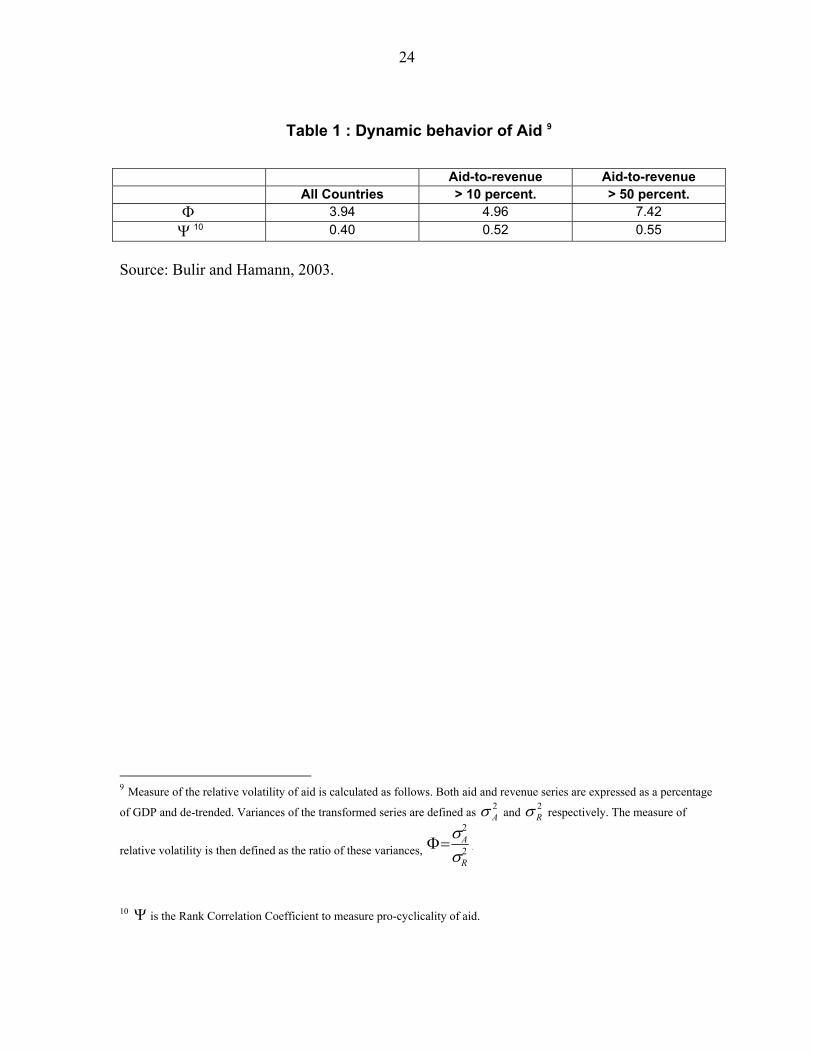
Aid flows to poor, aid dependent countries are highly volatile and pro-cyclical1. Table 1. gives an idea of the volatility (relative to the volatility of government revenues) and pro- cyclicality of aid flows for a group of 72 aid-dependent countries. The first row gives the measure of relative volatility of aid flows for the period 1975-1997. For the entire sample, the average of this measure is close to 4 which implies that, on an average, aid flows to these countries are four times more volatile than the fiscal revenues of the government (where both aid flows and revenues are normalized by the level of GDP). For countries with the average ratio of aid to revenue greater than 10 percent over the entire time period, relative aid volatility is 4.96 and it increases further to 7.4 in countries where average ratio of aid to revenue is above 50 percent. Thus, aid flows are vastly more volatile than government revenues and the relative volatility of aid flows increases with the level of aid dependency of the recipient country. The second row gives the average correlation coefficient between de-trended aid and revenue series. The average correlation coefficient is positive for all the groups, with the size of the correlation coefficient increasing with the ratio of aid to government revenues. Given that these countries have little or no access to international capital markets and that they are dependent on one or two primary commodities with highly volatile prices for their export revenues, volatility and pro-cyclicality of aid flows have important implications for their growth and welfare. On the other hand, adjusting aid flows to cushion the exogenous shocks faced by these countries has the potential to reduce their income and consumption volatility and hence improve their welfare. This paper studies the potential for innovative aid indexation schemes to reduce the macroeconomic volatility and the resultant welfare loss in aid-dependent countries. To give a brief overview of the model and the key results, I study the problem of an aid-dependent country using a three sector, dynamic general equilibrium model of a small open economy (SOE hereafter) with no access to international capital markets. The SOE faces productivity and terms of trade shocks and receives an exogenous stochastic transfer of tradable goods known as aid every period. As observed in the data, aid flows are assumed to be more volatile than the output and mildly pro-cyclical. The SOE can not borrow abroad to smooth consumption but it can invest in the domestic capital stock. The representative household engages in precautionary saving through accumulation of capital stock. However, capital is not a perfect means of consumption smoothing in the face of exogenous shocks as it is subject to diminishing marginal product which implies that as the SOE builds up its capital stock to buffer itself against exogenous shocks, returns to the incremental capital stock

1 See Bulir and Hamann (2003).

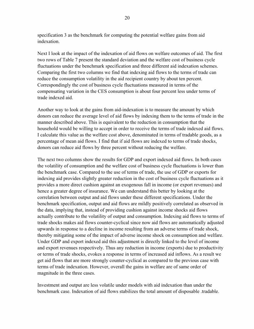
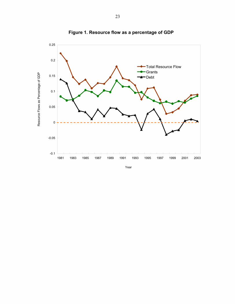
4 decline at the margin, making it costlier for the SOE to protect its income against exogenous decline by accumulating more and more capital. In this set-up, presence of capital adjustment costs increases the welfare cost of aid volatility substantially (about four times)2. Indexing aid flows to temporary terms of trade shocks, while keeping the average level of aid constant, significantly reduces the volatility of disposable income and consumption and hence, lowers the cost of business cycle fluctuations, in the aid recipient country. Compared to the benchmark case with stochastic aid flows, the reduction in the cost of business cycle fluctuations due to the use of indexed aid is about four percent of the permanent consumption. Alternatively, compared to the benchmark, the same level of welfare can be provided to the recipient country with three percent less aid by indexing aid to terms of trade shocks. These results are noteworthy for several reasons. First, in the absence of access to international financial markets, aid has become the main source of foreign capital for many of these countries, replacing official debt. As can be seen from Figure 1, since the mid 1990s real resource transfers on debt (as a percentage of GDP) have been close to zero or negative, with outright grants gaining in relative importance3. Aid is also a major source of disposable income for these countries (accounting for 12.5 percent of disposable income on average in Africa). Highly volatile and unreliable aid flows can therefore deter investment and make fiscal planning difficult in the aid-dependent countries, affecting their growth adversely. Second, pro-cyclical aid flows imply that poor countries are forced to raise taxes or curb their expenditures at the time when these economies are going through recession, thereby dampening their growth even further4. Pro-cyclicality of aid flows by itself may not be completely undesirable and could, in fact, be an optimal outcome in the presence of asymmetric information and divergent preferences amongst benevolent donor and recipient countries (Pallage and Robe, 2003). However there is no empirical evidence to suggest that this is indeed the case. On the contrary, the evidence shows that aid flows are dictated by political and strategic considerations much more than by economic prudence and policy performance of the recipients (Alesina and Dollar, 2003). Finally, these results show that in the presence of terms of trade shocks and capital adjustment costs the direct impact of aid volatility on the welfare of aid-dependent countries through higher consumption volatility can be substantial and should therefore be taken in to account while designing aid programs.

2 Welfare cost of aid volatility is defined as the percentage increase in consumption at all dates that is required to compensate the representative household for the resulting higher volatility in consumption. 3 Net resource transfers on debt are defined as disbursements of loans to the developing countries less debt service payments and debt amortization.

4 Gemmell and McGillivray (1998) record that shortfalls in aid are often followed by reductions in government spending indicating that the recipient countries are not able to make up for the reduction in aid flows by higher revenues.

5 My paper is closely related to Arellano et.al (2005) who examine the effects of aid volatility on consumption, investment, and welfare in a two-sector general equilibrium model and find that aid volatility can result in substantial welfare losses for a country with limited access to international capital markets (though not large enough to completely offset the effect of aid itself). However, their analysis ignores two important factors that are likely to affect the welfare costs of aid volatility in poor countries–volatility in the relative price of their main exports and capital adjustment costs. This paper takes the analysis of Arellano et.al. (2005) a step further by looking at the welfare cost of aid volatility in the presence of terms of trade shocks and capital adjustment costs. It then explores the potential of using aid flows to provide insurance to SOE against temporary terms of trade shocks by indexing aid flows to exogenous terms of trade shocks5.

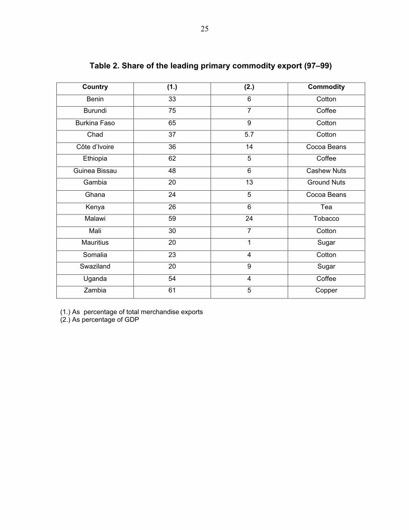
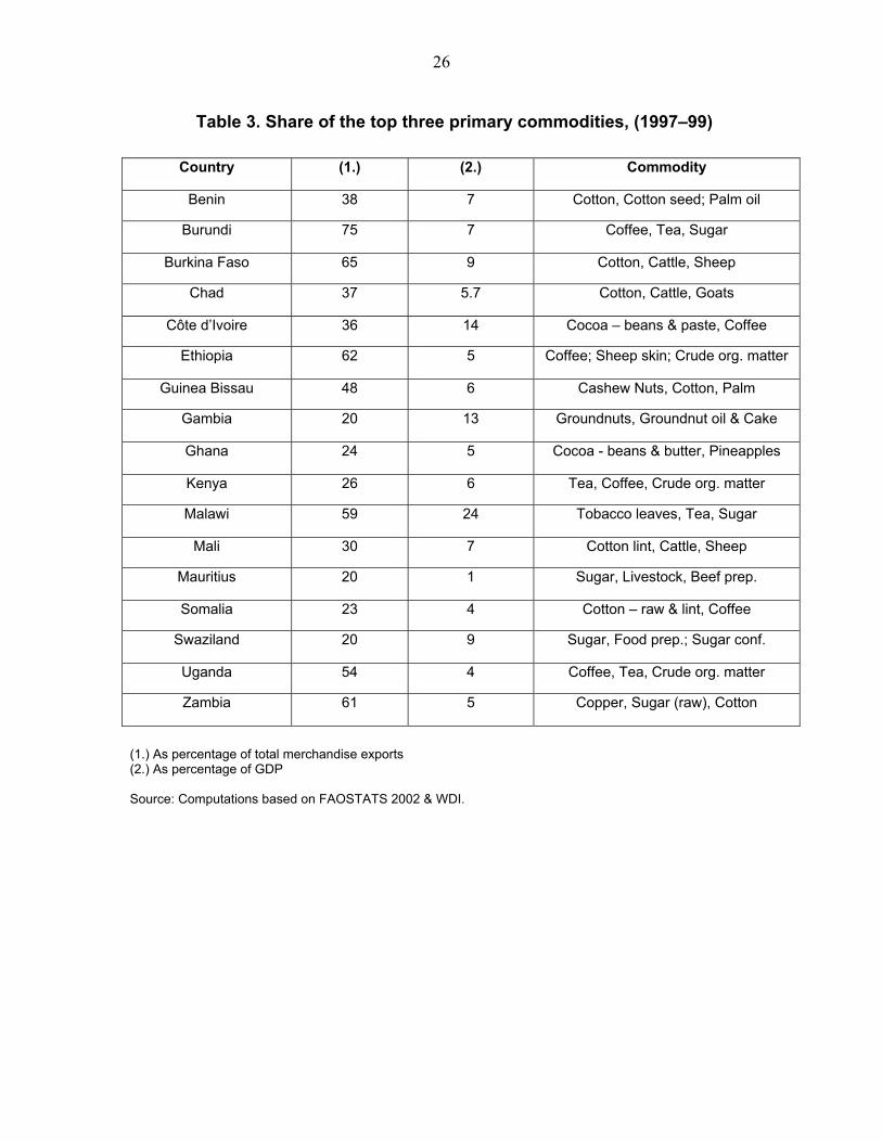
II. PRIMARY COMMODITY EXPORTS AND PRICE VOLATILITY The problem of aid volatility in poor countries is compounded by the fact that the majority of these countries are heavily dependent on one or two primary commodities for their export evenues and the prices of those primary commodities are highly volatile. As a result their export revenues, which are the only other source of financing tradable consumption and purchase of imported inputs besides aid, are very volatile too. Tables 2 and 3 give an idea of the extent of this primary export dependence. Table 2 lists average shares of the main primary commodity export in total exports and GDP of the country between 1997-99 for 17 Highly Indebted Poor Countries (HIPC’s), which are also major recipients of aid. Table 3 does the same for the top three primary commodity exports. Of the 17 countries under consideration, 14 have more than 20 percent of their export revenues coming from a single commodity while 15 countries earn more than 30 percent of their export revenue from just three commodities. For 16 out of the 17 countries, export revenues from the top 3 commodities constitute more than 5 percent of their total GDP. To give an idea of the relative price volatility of the key primary commodities exported by these countries I calculate instability indices for individual commodities over the period 1957–1999. The instability index for each commodity is defined as the percentage standard deviation of the natural logarithm of its price (which is deflated by The Economist’s Manufactured Unit Value Index6 to get the real value) around the Hodrick-Prescott filtered 5 The idea of using concessional resource flows as an insurance mechanism has been discussed before in several papers. Starting from Bailey (1983), Shiller (1993), Borensztein and Mauro (2004) and Tabova (2005) suggest indexing concessional debt service of HIPCs to some measure of countries ability to pay such as, GDP, consumption or price of their primary exports. Berube et.al., 2004 suggest using aid flows to insure developing countries against adverse shocks.

6 M.V.I is calculated as the nominal industrial commodity price index (dollar based, weighted by the value of developed country imports), deflated by the G.D.P deflator of the US.

(continued…)

6 trend. The indices thus calculated give an idea of the volatility of primary commodity export prices relative to the volatility of manufactured goods imported by these countries. Results from this exercise are presented in Table 4. The price for sugar seems to be the most volatile (average annual percentage deviation of around 40 percent) followed by the price of cashew nuts. The average annual percentage deviation for all the primary commodity prices is around 20 percent with 10 out of the 14 commodities having volatility above 15 percent. Given that the average share of the leading primary commodity in total exports is about 40 percent for countries in the sample, commodity price volatility on its own would result in an annual volatility of 4 to 16 percent (depending upon the commodity in question) in export revenues. Thus, fluctuations in commodity prices are an important source of macroeconomic volatility in these developing countries. This volatility in primary commodity prices is reflected in the volatile terms of trade for developing countries (Bidrakota and Crucini, 2000). In the discussion that follows I use the words terms of trade to denote the Net Barter Terms of Trade which measures the number of units of exports that can be exchanged for a unit of imports.

A. Case Study: Cotton

In the face of such volatile commodity export prices and revenues one obvious question to ask against exogenous income shocks such as adverse terms of trade. I look at the case of Burkina Faso to examine this point. The choice of Burkina Faso was dictated by the availability of data and the nature of its primary export cotton. It is a small open economy dependent on primary commodity exports, with cotton exports accounting for 65 of its total merchandise exports and nine percent of its total GDP. It s also a price taker in the world market for cotton. The table below describes some important features of the relationship between aid flows, government revenues (excluding O.D.A.) and world cotton prices for Burkina Faso. As we can see from the first row, aid flows are about five times more volatile than the government revenues in line with the overall results for aid dependent economies. Second row gives the rank correlation coefficient between aid and government revenue. Again, in line with the overall results this correlation coefficient is positive. Next two rows give the correlation between world cotton price on the one hand and aid and government revenue on the other. Government revenue is positively correlated with the level of cotton prices. This reflects the fact that for many developing country governments, tax on commodity exports is a major source of revenue. As the price of their major commodity export goes down so does the revenue, and vice versa. Clearly, if aid flows to Burkina Faso

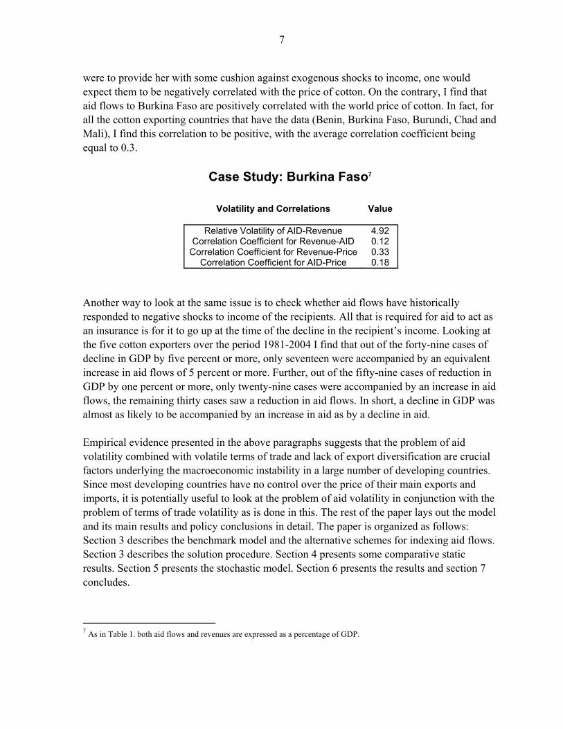
7 were to provide her with some cushion against exogenous shocks to income, one would expect them to be negatively correlated with the price of cotton. On the contrary, I find that aid flows to Burkina Faso are positively correlated with the world price of cotton. In fact, for all the cotton exporting countries that have the data (Benin, Burkina Faso, Burundi, Chad and Mali), I find this correlation to be positive, with the average correlation coefficient being equal to 0.3.

Case Study: Burkina Faso7

Another way to look at the same issue is to check whether aid flows have historically responded to negative shocks to income of the recipients. All that is required for aid to act as an insurance is for it to go up at the time of the decline in the recipient’s income. Looking at the five cotton exporters over the period 1981-2004 I find that out of the forty-nine cases of decline in GDP by five percent or more, only seventeen were accompanied by an equivalent increase in aid flows of 5 percent or more. Further, out of the fifty-nine cases of reduction in GDP by one percent or more, only twenty-nine cases were accompanied by an increase in aid flows, the remaining thirty cases saw a reduction in aid flows. In short, a decline in GDP was almost as likely to be accompanied by an increase in aid as by a decline in aid. Empirical evidence presented in the above paragraphs suggests that the problem of aid volatility combined with volatile terms of trade and lack of export diversification are crucial factors underlying the macroeconomic instability in a large number of developing countries. Since most developing countries have no control over the price of their main exports and imports, it is potentially useful to look at the problem of aid volatility in conjunction with the problem of terms of trade volatility as is done in this. The rest of the paper lays out the model and its main results and policy conclusions in detail. The paper is organized as follows: Section 3 describes the benchmark model and the alternative schemes for indexing aid flows. Section 3 describes the solution procedure. Section 4 presents some comparative static results. Section 5 presents the stochastic model. Section 6 presents the results and section 7 concludes.

7 As in Table 1. both aid flows and revenues are expressed as a percentage of GDP.

Volatility and Correlations

Value

Relative Volatility of AID-Revenue 4.92

Correlation Coefficient for Revenue-AID 0.12 Correlation Coefficient for Revenue-Price 0.33

Correlation Coefficient for AID-Price 0.18

8

III. THE BENCHMARK MODEL

The model used in this paper is based on the SOE real business cycle model developed by Mendoza (1995). The economy is inhabited by an infinitely lived representative household that derives utility from consuming three different types of goods: exportable goods, importable goods and non-tradable goods. The household sells its labor to firms and invests in capital in return for wages and rental income, respectively. Firms produce exportable and non-tradable goods. Capital is sector specific and is the only asset available for investing savings in the economy. Total amount of labor in the economy is normalized to one and it is freely substitutable across sectors. To model the behavior of aid in the economy I follow the method used in Arellano et.al (2005). Besides domestic production, the economy gets a stochastic transfer of foreign resources labeled as aid in every period. There are three sources of uncertainty in the economy, productivity shocks, aid shocks and terms of trade shocks. These shocks motivate rational individuals to adjust their savings and investment in order to smooth consumption and to adjust sectorial employment in response to changes in real wage rate. In the following sections I describe the model in detail. Unlike Mendoza (1995), the economy in my paper does not have access to any other foreign asset. Imports are used as numeraire good throughout the paper.

A. Household

The infinitely lived representative household in the economy maximizes its expected lifetime utility which depends on the aggregate consumption level Ct :

( )∑∞

=

−

−=

0

1

0 1t

tt CEUσ

βσ

(III-1)

where σ is the coefficient of risk aversion and β denotes the subjective discount factor.

The aggregate consumption function tC is of constant elasticity of substitution form given by:

( ) ( )( )[ ]μμμ ϖϖ1

1−

−−−+= N

tTtt CCC (III-2)

Where ( ) ( )1T EX IMt t tC C C

ς ς−= is the composite tradable good, EX

tC is the consumption of

exportable goods, IMtC is the consumption of importable goods and ς is the share of

exportable goods in tradable goods expenditure. The household rents capital and provides labor to the firms. In return it earns rental income tr and wage tw . Besides wage and rental

9 income, it receive a stochastic transfer of tradable goods from abroad. The price of exports is exogenously given to the SOE. The overall resource constraint of the household is therefore: EX EX N N IM

t t t t t t t t t tp C p C C w r k AID s+ + = + + − (III-3) where ts is the household saving, tk is the amount of capital stock, EX

tp is the stochastic terms of trade (relative price of export in terms of imports) which is subject to exogenous shocks. While these shocks might be short lived for some countries, they may have permanent effects in case of other countries. In the discussion that follows, I assume that shocks to the terms of trade are persistent but temporary, i.e., their effect dies down after a finite number of time periods. N

tp is the price of non-tradable goods, also expressed in terms of imports, and tAID is the exogenous stochastic transfer of tradable good. The household can invest its savings only in the domestic capital stock as the SOE lacks access to international capital markets.

B. Firms

Firms produce non-tradable and exportable goods using capital and labor services (they do not produce importable goods but the exportable goods can, in principle, also be imported). Both the sectors face Cobb-Douglas production technology

( ) ( )1N N Nt tY A k L

η η−= (III-4)

( ) ( )1EX EX EXt tY A k L

α α−= (III-5)

where tA is the common productivity shock affecting both the non-tradable and the exportable sector, and α and η are shares of capital in exportable and non-tradable sectors respectively. Firms and households have the same information set; both know the distribution of shocks. Labor is perfectly mobile across sectors. The total amount of labor is divided between the two sectors as follows 1N EX

t tL L+ = (III-6) Capital, however, is assumed to be somewhat sector-specific implying that shifting capital from one sector to another involves a transformation cost which is captured by the factor transformation curve given below (see Mendoza and Urine, 2000):

10

( )1

,EX N EX Nt t t t tk k k k k

υ υ υκ− −

−

⎡ ⎤= = +⎣ ⎦ (III-7)

Where, tk is the aggregate capital stock in the economy, EXtk is the capital used in exportable

sector, Ntk is the stock of capital in non-tradable sector and ( )1/ 1 υ+ is the elasticity of

substitution between EXtk and N

tk . Perfectly homogenous capital is the special case where 1υ = − . The assumption of sector specific capital is in line with the specific-factors models

developed in the trade literature and it allows us to replicate the large changes in the relative price of non-tradable goods resulting from changes in the inflow of aid, as witnessed in the data. Firms face quadratic capital adjustment costs. The assumption of quadratic adjustment cost is necessary to match the volatility of investment observed in the data with that produced by the model. The capital accumulation equation is therefore given by:

( ) ( )21 11

2t t t t tk k i k kφδ+ +⎛ ⎞= − + − −⎜ ⎟⎝ ⎠

(III-8)

where ti is aggregate investment and φ is the adjustment cost parameter. Investment in this model takes place only using imported goods which can be purchased either by using aid inflows or by using export revenues. This is a simplifying assumption that captures the fact that imported capital goods and intermediate inputs are important ingredients in the developing country's production process that can not be substituted by domestic capital stock (Lee, 1994). In fact, capital goods and intermediate inputs form the majority of imports for these countries. This assumption gives us the following equation :

( )EX EX EX IM

t t t t t ti p Y C AID C= − + − (III-9) Thus, investment gets affected by fluctuations in both, the relative price of exports and the aid flows. Market clearing conditions in the non tradable and tradable sectors ensure that saving is equal to investment in this SOE. The market clearing conditions for the two sectors are:

N Nt tC Y= (III-10)

EX EX N N IMt t t t t t t t t tp C p C C w r k AID s+ + = + + − (III-11)

In equilibrium, marginal productivity of both the factors are equalized across sectors. First order optimization conditions give us the following equations:

11

( ) ( ) ( ) ( ) ( ) ( )1 1EX EX EX N N Nt t t t t t t t tw p A k L p A k L

α α η ηα η

− −= − = − (III-12)

( )( )

( )( )

1 1

1 2

/ /

, ,

EX EX EX N Nt t t t t t tN

t tEX N EX Nt t t t

p A k L A k Lr p

k k k k

α ηα η

κ κ

− −

= = (III-13)

Equations (III-12) and (III-13) say that the wage rate of labor is equal to the marginal product of labor in the two sectors and similarly the rental rate of capital is equal to the marginal product of capital in the two sectors. Combining the first order optimization conditions of the household and firms we get the following inter-temporal Euler equation:

( )( )

1

1

1 1

/1

,

EX EX EXt t t tt t

tC C EX Nt t t t

p A k LC CEp p k k

ασ σ α

β δκ

−− −

+

+

⎛ ⎞⎜ ⎟= + −⎜ ⎟⎝ ⎠

(III-14)

Here Ctp is the CES price index for aggregate consumption:

( )( ) ( )( ) ( )( )( ) ( )

( )1 // 1 / 111 1C EX Nt t tp p p

μ μμ μς μ μςςως ς ϖ++ +−−⎛ ⎞

= − + −⎜ ⎟⎝ ⎠

(III-15)

Equation (III-14) equalizes the marginal cost of sacrificing current consumption with the marginal benefit of allocating the resulting extra savings into the aggregate capital. Equation (III-15) is a function of elasticity’s of substitution, the terms of trade EX

tp as well as the price

of non-tradable goods Ntp .

C. The Steady State

The following paragraphs describe the steady state of this economy. Profit maximization by firms implies that in the equilibrium, wage rate equals the marginal product of labor and rental rate equals the marginal product of capital in the two sectors. Since capital is sector-specific, the effective rate of return in each sector incorporates the degree of factor substitutability between the two sectors given by the derivative of κ with respect to the sectorial capital.

( )( )

( )( )

1 1

1 2

/ /

, ,

EX EX N NN

EX N EX N

k L k Lp

k k k k

α ηα η

κ κ

− −

= (III-16)

( )( ) ( )( )1 / 1 /EX EX N N Nk L p k Lα η

α η− = − (III-17)

12 The inter-temporal equilibrium condition implies that the steady state return on capital stock, which is the marginal product of capital net of depreciation, is equal to the discount factor β . This can be written as:

( )( )

1

1

/1,

EX EX

EX N

k L

k k

αα

β κ

−⎡ ⎤⎢ ⎥=⎢ ⎥⎣ ⎦

(III-18)

Utility maximization by consumers gives us a set of first order conditions which, after slight algebraic manipulation, can be rewritten as follows:

11

IM

EX

CC

ςς

⎛ ⎞=⎜ ⎟−⎝ ⎠

(III-19)

( )( )( ) ( )( )( ) ( )( ) ( )

1

11

1

1

NN

EX IM EX IM

Cp

C C C C

μ

μς ς ς ς

ϖ

ϖ ς

− −

− −− −

−=

⎛ ⎞−⎜ ⎟

⎝ ⎠

(III-20)

Equation (III-19) equates the marginal rate of substitution between importable and exportable goods to their relative price or the terms of trade, which we assume to be equal to 1 in the steady state for simplicity. Equation (III-20), similarly, equates the marginal rate of substitution between non-tradable and importable goods with the relative price of non-tradable goods in terms of importable goods. Goods market clearing conditions are given by the following equations: ( )1NN NC k L ηη −= (III-21) ( )1EXIM EX EXC C k L AID iαα −+ = + − (III-22) Consumption of the non-tradable good is equal to its output in every period reflecting the assumption that investment and saving in the economy can only take place in terms of tradable goods. Total expenditure on tradable consumption is equal to exportable output plus aid flows less the investment in domestic capital. Steady state investment is equal to the steady state capital stock times the rate of depreciation. i kδ= (III-23) Equations (III-24) and (III-29) give the input market clearing conditions.

( ),EX Nk k kκ= (III-24)

13

1N EXL L+ = (III-25)

IV. MODEL CALIBRATION AND COMPARATIVE STATICS

Parameters of the baseline specification are chosen to mimic some of the characteristics of poor aid-dependent countries or taken from other developing country business cycle studies. The model is then solved numerically, using value function iteration. The elasticity of substitution between exportable and non-tradable consumption, ( )1/ 1 μ+ , is 1.279 which is equal to the GMM estimate from the panel study of 13 developing countries by Ostry and Reinhart (1992). This determines the responsiveness of non-tradable consumption to relative price (real exchange rate) changes. Share of exports in tradable consumption ( )ς is set equal to 0.15, same as in the developing country benchmark in Mendoza (1995). The value of the risk aversion coefficient ( )σ has an important bearing on the measure of welfare cost of aid and consumption volatility and hence on the magnitude of gains from aid indexation. It determines the ease with which consumers can trade current consumption for future consumption: the smaller the risk aversion coefficient, the greater the ease of inter-temporal substitution of consumption and hence the smaller the welfare cost of consumption volatility due to exogenous shocks. In the real business cycle as well as the consumption literature, the value of this parameter is widely believed to lie between 2 and 5. I therefore use two different values of this parameter in the simulations - 2.61 and 5. The first value is the GMM estimate in Ostry and Reinhart (1992) and the second value is the one estimated by Reinhart and Vegh (1995). I present both sets of results in the paper. The non-tradable sector is assumed to be more capital intensive than the exportable sector which is in line with other developing country studies such as Mendoza (1995) and Arellano et.al. (2003). This reflects the fact that for these developing countries production of primary agricultural commodities (which are their key exports) such as sugar involves relatively large amounts of labor and little capital while opposite is true for their non-tradable goods production which mainly includes physical and social infrastructure. Capital shares in exportable and non-tradable sectors, α and η , are therefore set equal to 0.3 and 0.4 respectively. The elasticity of substitution between capital used in exportable and non-tradable sectors, ( )1/ 1 υ+ is set equal to -10, same as in Mendoza and Urine (2000). The rate of depreciation of capital δ is set equal to 0.09 so that in steady state the investment rate is set equal to 18 percent of GDP, an average of long-term investment rates taken from the World Economic Outlook. Table 5 lists the parameter values used in the benchmark model.

A. Sensitivity Analysis

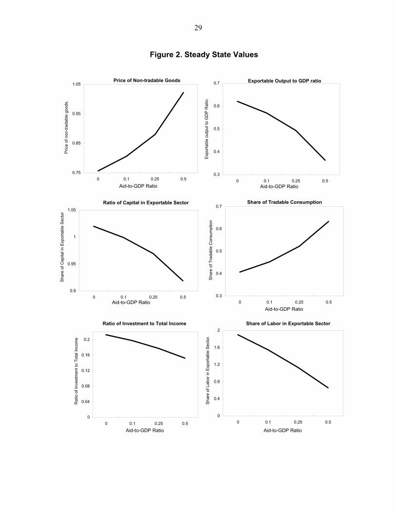
In this section I do some sensitivity analysis to see how steady state variables change with different levels of aid and parameter values. Figure 2 plots the steady state values of endogenous variables for four different levels of aid to GDP ratio - 0, 1/10, 1/4 and 1/2. More

14 aid increases the relative price of the non tradable good (the real exchange rate) lowers the share of labor and capital employed in the exportable sector and lowers the share of exportable output in total GDP. It lowers investment as a share of total income (defined as the sum of GDP and exogenous aid flows) and increases the share of tradable goods in total consumption. The decline of exportable goods sector as a result of increased aid reflects the problem of the ‘Dutch` disease whereby increased inflows of foreign resources cause real appreciation and hence hurt the export producing sector. The share of tradable goods consumption in total consumption goes up because aid pushes the relative price of non-tradable goods upwards. This happens because aid increases the availability of tradable goods relative to the availability of the non-tradable good. Also, due to the sector specificity of capital, shifting capital from exportable to non-tradable sector pushes up the return on capital, and hence raises the relative price of the good using capital more intensively (i.e. the non-tradable good). Lower relative price of tradable goods also explains the increase in their share in total consumption. The reduction in the ratio of investment to total income in response to the increase in aid shows that in the long run a permanent increase in aid will only lead to a permanently higher level of consumption with no change in the level of saving or investment. This is because the steady state capital stock is determined by the time preference parameter and the rate of depreciation and is thus independent of the level of aid. I check the sensitivity of these results to different values of capital intensity and capital substitution elasticity parameters. As can be seen from Figure 3, one key result—the decline in the output of exportable goods, remains intact in all the models, while the other—the increase in the relative price of non-tradable goods, remains intact as long as capital is sector specific. Specificity of capital is necessary for real appreciation because if capital was perfectly substitutable then shifting capital towards the non-tradable sector in response to increased supply of tradable goods will involve no ‘transformation costs. As for the decline in exportable output, it occurs even in the absence of real appreciation since aid, which is a transfer of tradable goods, substitutes for domestic production of tradable goods. The magnitude of decline in the ratio of capital employed in the exportable sector, in response to an exogenous increase in aid, depends on the elasticity of substitution of capital between the two sectors. The more sector-specific the capital, the costlier it is to shift capital stock from the exportable to the non-tradable sector and hence the smaller is the decline in the share of capital used in the exportable sector. The ratio of labor in the exportable sector goes down in all the models with the size of decline once again determined by the elasticity of substitution of capital between the two sectors. Finally, the ratio of investment to total income (defined as the sum of domestic output and aid transfers) declines in all the models indicating that additional aid gets consumed instead of being saved.

V. DYNAMICS

In this section I describe the properties of the shocks facing the SOE and lay down the solution procedure for the dynamic model in detail. The benchmark model sets the productivity, terms of trade and aid shocks to match the volatility and persistence of output

15 and aid flows in the aid-dependent economies. It is assumed that productivity shocks affect exportable and non-tradable sectors equally, with a standard deviation of 4 percent and a first order auto-correlation coefficient of 0.4. This setup implies that 60 percent of any deviation of productivity from its mean level dissipates in each period. Volatility of aid shocks is set to be five times the volatility of productivity shocks as found by Bulir and Hamann (2003). The correlation coefficient between productivity and aid shocks is set equal to 0.4 to capture the pro-cyclicality of aid flows observed in the data. Terms of trade shocks have a standard deviation of 11 percent and persistence of 0.4 (Mendoza, 1995). Steady state aid to GDP ratio is set equal to 12.5 percent for benchmark simulations. This is equal to the average aid to GDP ratio for the seventeen countries listed below. The recursive nature of the problem allows us to rewrite it in the form of a Bellman equation as follows:

( ) ( ) ( )( )

( ) ( )( )

( )

10 1 1

1

1

, max , ,

s.t.

1 and ,

tt t t t t tk

NN Nt t t

EX EX IM EX EX EXt t t t t t t t

N EX EX Nt t t t t

V k s U k s E V k s

C k L

p C C i p A k L AID

L L k k k

ηη

α α

β

κ

++ +

−

−

= + ⎡ ⎤⎣ ⎦

=

+ + = +

+ = =

(V-1)

Utility in each period depends on the stock of capital, and the state of nature ( ts ) which denotes the set of shocks to productivity, aid and terms of trade. Solving this equation under the household’s resource constraint gives the optimal path for capital stock and consumption. This optimization problem does not have an analytical solution. Hence I use numerical techniques to obtain the value function and the policy function for the problem. Indexation of aid flows to the terms of trade or GDP introduces kinks in the household’s budget constraint which makes the use of linear approximation methods widely used in the RBC literature inappropriate. I therefore follow an exact-solution procedure based on value function and transition probability iterations using discrete grids to approximate the state space.

A. Indexed Aid As explained earlier, the idea behind indexing aid flows to some macroeconomic indicator of the recipient country’s income is to provide it (the recipient country) a cushion against an exogenous fall in income. Use of such schemes has the potential to improve the welfare of poor aid recipient countries by reducing their macroeconomic volatility. In the following paragraphs I describe three different methods of indexing aid flows in detail and discuss their pros and cons.

16 Terms of Trade Indexed Aid Empirical evidence presented in the beginning of the paper showed that highly volatile terms of trade are a major cause of macroeconomic instability in developing countries. Increasing aid flows in response to an adverse terms of trade shock so as to cushion the exogenous fall in the income and export revenue of the SOE can lower this macroeconomic stability. Use of terms of trade for indexing aid flows has several advantages. To list a couple of them - few developing countries have significant market power to affect the prices of their major exports or imports and so there are no moral hazard problems of the sort which arise when governments have some control over the variable which determines aid flows. Also, world prices are known without any lag and hence a scheme based on such prices would potentially be able to moderate aid flows in a more timely manner as compared to schemes based on other macroeconomic variables such as GDP or exports, data for which are subject to significant lags and frequent revisions. At the same time, using an index based on terms of trade may not provide complete coverage against price volatility because transport costs and grade differentials may result in significant divergence between the prices at which a country exports or imports goods and the international prices of those goods. Further, quantity variation may be as important a determinant of a country’s export revenue as price variation and a scheme based on terms of trade alone does not take that in to account. Finally, reliance on a terms of trade trigger limits applicability of the scheme to countries with high commodity concentration in exports and imports. The first two limitations can be overcome if we index the aid flows to export revenues instead of terms of trade while the use of a more general macroeconomic indicator such as consumption or income growth can allow inclusion of a wider group of countries in the indexing scheme. However, as mentioned above, both these alternatives involve significant moral hazard risks. The actual choice of the variable for aid indexation, therefore, involves a trade-off between the extent of insurance provided against negative income shocks and the potential cost of associated moral hazard problems. It is therefore useful to compare the potential welfare gains from using the three alternative forms of indexation. When talking about providing insurance against the terms of trade shocks one has to distinguish between temporary and permanent shocks to the terms of trade. While it might be worthwhile to try and smooth over temporary fluctuations in the terms of trade it would be inadvisable to shield developing countries against secular decline in the relative price of their exports. If the latter describes the behavior of the terms of trade facing a particular country then fundamental shifts in the structure of production and exports might be the only feasible solution in the long run. Cashin and Pattillo (2000) analyze the terms of trade shocks for a group of 42 countries over the period 1960-1996 and provide median-unbiased estimates of their half life. They find that out of the 42 countries in their sample, 11 have terms of trade shocks that do not dissipate at all or are permanent. These include Côte d’Ivoire, Kenya, Uganda and Zambia. Hence, out of the 17 countries listed below, these four are not suitable

17 candidates for insurance schemes trying to stabilize their income against terms of trade shocks but the remaining 13 countries can potentially benefit from such insurance schemes. Details of the way indexation of aid flows to the terms of trade works are as follows. A particular period may be classified as either normal (N), adverse (A) or propitious (P) on the basis of a previously agreed upon criterion based on the country’s terms of trade. In this paper the criterion is based on the actual size of the shock in any given period. For the purposes of implementation this terms of trade shock can be calculated as the percentage deviation from a moving average trend calculated over last four or five years. If the shock is are less than 0.5 standard deviation (hereafter s.d.) in size then the period is defined as N and aid flows are kept at their mean level. The use of a normal period defined within a band is based on the principle that any scheme should aim to cope with only exceptional price movements and not normal price movements. In the case of a shock lying between 0.5 s.d. and 1 s.d., the period is denoted as A (P when the shock is positive) and the aid flows are increased (decreased) by 5 percent. If the shock is larger than 1 s.d. in size, the period is denoted as A* (P* when the shock is positive) and the aid flows are increased (decreased) by 10 percent. Aid flows under this scheme can therefore be described as follows:

1.1 if 1 . .

1.05 if - 0.5 . . -1 . .

if 0.5 . . 0.5 . .

0.95 if 1 . 0.5 .

0.9 if 1 . .

aid s s d

aid s d s s d

aid aid s d s s d

aid s d s s d

aid s s d

⎡ ⎤× ≤ −⎢ ⎥

× ≥ ≥⎢ ⎥⎢ ⎥= > > −⎢ ⎥⎢ ⎥× > ≥⎢ ⎥⎢ ⎥× ≥⎣ ⎦

(V-2)

The choice of one standard deviation shock for the outer limit of the second terms of trade band roughly corresponds to a direct change of 0.5 percent in the GDP. The limit of 0.5 percent of GDP is in turn commensurate with the I.M.F.’s definition of a ‘large` disaster8. Translated into export revenues, a one standard deviation decline in terms of trade is roughly equal to a direct loss of 3 percent. For the purposes of comparison, I therefore use a cut-off point of 0.5 percent and 3 percent respectively for GDP and export indexed aid. Export-Indexed Aid Export indexed aid can be seen as a combination of a bond and an insurance contract whose payments are linked to the value of exportable good output in terms of importable goods. When the value of exports falls (goes up) by more than 3 percent below (above) the steady 8 IMF classifies a disaster as large if it caused a direct damage of at least 0.5 percent of G.D.P.

18 state level, aid flows to the recipient country are adjusted upwards (downwards), proportionately. Hence, aid flows to the recipient country are given by: ( )1t x EXtaid aid gλ= × + (V-3) Where:

( ) ( )( )1

max 0, 0.03EX EX EX EX

EX t t t

EXtEX

Y p A k Lg

Y

α α−⎡ ⎤−⎢ ⎥= −⎢ ⎥⎢ ⎥⎣ ⎦

(V-4)

aid is the mean level of aid, EXY is the steady state level of exportable output and EXtg is what I call exports gap - the difference between the exportable output in period t and its steady state level. xλ < 1 is the adjustment coefficient that determines the degree of aid indexation. The underlying idea behind this indexation is to stabilize the disposable tradable income of the SOE around its long run value. GDP Indexed Aid As in the case of export-indexed aid, the idea underlying the GDP indexed aid is to adjust aid flows, when the GDP falls below (rises above) its steady state level by more than a pre-specified level (0.5 percent in this case). The GDP indexed aid is therefore given by :

( )1t Y Ytaid aid gλ= × + (V-5)

Where:

( )max 0, 0.005t

Yt

Y Yg

Y

⎡ ⎤−⎢ ⎥= −⎢ ⎥⎣ ⎦

(V-6)

Y is the steady state level of GDP, and tY is the current level of GDP. Welfare Costs The metric used for the welfare cost in this paper is the CES consumption. Following Lucas (1987), the welfare cost of consumption volatility is defined as the minimum percentage increase in the level of consumption in every period, needed to render the agent indifferent between the stochastic consumption stream and a deterministic one with the same mean. In

19 these computations, I focus solely on business cycle fluctuations, defined as the cyclical component of Hodrick-Presscott (HP) filtered series. Again, as shown in Lucas (1987), under the assumptions of CRRA utility and i.i.d shocks to consumption, the welfare cost of consumption volatility has a closed form solution that can be approximated by:

( )12

W V Cσ=

where σ is the coefficient of relative risk aversion and ( )V C is the variance of the CES consumption aggregator around the Hodrick-Prescott filtered trend. Clearly, the welfare cost of business cycle fluctuations increases proportionately with the level of risk aversion and the variance of consumption. For any given level of risk aversion, a lower level of consumption volatility would therefore imply a higher level of welfare ceteris paribus. One caveat in interpreting the results presented below is that aid volatility not only changes the volatility of consumption, but also changes the level of consumption in the long run as a result of precautionary savings that enlarge the capital stock. Given my focus on the cost of business cycle fluctuations the welfare calculations in this paper are solely based on consumption volatility, ignoring changes in levels.

VI. RESULTS

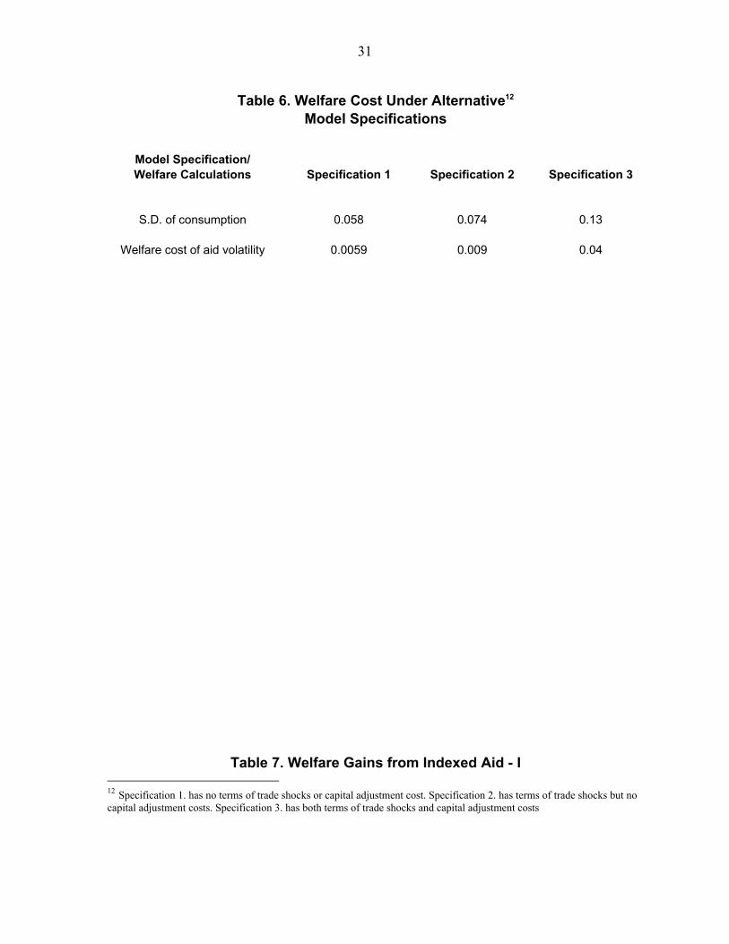
This section presents the main results of the paper along with some sensitivity analysis. First I compare three different specifications for the benchmark model, looking at their implications for the welfare cost of aid volatility. For calculating the cost of aid volatility, I compare each specification to the case with a constant aid flow (equal to the mean) and productivity shocks. The first specification has no terms of trade shocks and no capital adjustment costs. This is similar to the case studied by Arrelano et.al. (2005) The second specification has terms of trade shocks but no capital adjustment cost. The third and final specification has both terms of trade shocks and capital adjustment costs. Table 6 presents the results for the three specifications. Looking at the first row we can see that the standard deviation of consumption is the lowest for the specification with no terms of trade shocks and capital adjustment costs and it is the highest in the case when we have both capital adjustment cost and terms of trade shocks. While the difference is relatively small for specifications 1 and 2, it is very large for specifications 1 and 3. Larger consumption volatility translates into higher welfare losses for the risk averse households, as shown by the second row of Table 6. Compared to the estimates in Arellano et.al. (2005) the welfare loss of aid volatility in the presence of terms of trade shocks and capital adjustment costs are more that twenty times larger. This shows that ignoring capital adjustment costs can lead to substantial underestimation of welfare losses due to aid volatility. As explained in the beginning, the intuition for this is that capital adjustment cost makes domestic capital a less effective means of consumption smoothing and hence raises the level of consumption volatility which, in turn, translates in to a higher cost of aid volatility. I therefore choose

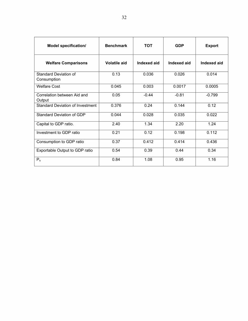
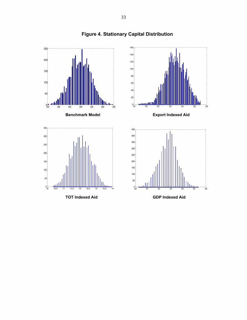
20 specification 3 as the benchmark for computing the potential welfare gains from aid indexation. Next I look at the impact of the indexation of aid flows on welfare outcomes of aid. The first two rows of Table 7 present the standard deviation and the welfare cost of business cycle fluctuations under the benchmark specification and three different aid indexation schemes. Comparing the first two columns we find that indexing aid flows to the terms of trade can reduce the consumption volatility in the aid recipient country by about ten percent. Correspondingly the cost of business cycle fluctuations measured in terms of the compensating variation in the CES consumption is about four percent less under terms of trade indexed aid. Another way to look at the gains from aid-indexation is to measure the amount by which donors can reduce the average level of aid flows by indexing them to the terms of trade in the manner described above. This is equivalent to the reduction in consumption that the household would be willing to accept in order to receive the terms of trade indexed aid flows. I calculate this value as the welfare cost above, denominated in terms of tradable goods, as a percentage of mean aid flows. I find that if aid flows are indexed to terms of trade shocks, donors can reduce aid flows by three percent without reducing the welfare. The next two columns show the results for GDP and export indexed aid flows. In both cases the volatility of consumption and the welfare cost of business cycle fluctuations is lower than the benchmark case. Compared to the use of terms of trade, the use of GDP or exports for indexing aid provides slightly greater reduction in the cost of business cycle fluctuations as it provides a more direct cushion against an exogenous fall in income (or export revenues) and hence a greater degree of insurance. We can understand this better by looking at the correlation between output and aid flows under these different specifications. Under the benchmark specification, output and aid flows are mildly positively correlated as observed in the data, implying that, instead of providing cushion against income shocks aid flows actually contribute to the volatility of output and consumption. Indexing aid flows to terms of trade shocks makes aid flows counter-cyclical since now aid flows are automatically adjusted upwards in response to a decline in income resulting from an adverse terms of trade shock, thereby mitigating some of the impact of adverse income shock on consumption and welfare. Under GDP and export indexed aid this adjustment is directly linked to the level of income and export revenues respectively. Thus any reduction in income (exports) due to productivity or terms of trade shocks, evokes a response in terms of increased aid inflows. As a result we get aid flows that are more strongly counter-cyclical as compared to the previous case with terms of trade indexation. However, overall the gains in welfare are of same order of magnitude in the three cases. Investment and output are less volatile under models with aid indexation than under the benchmark case. Indexation of aid flows stabilizes the total amount of disposable .tradable.

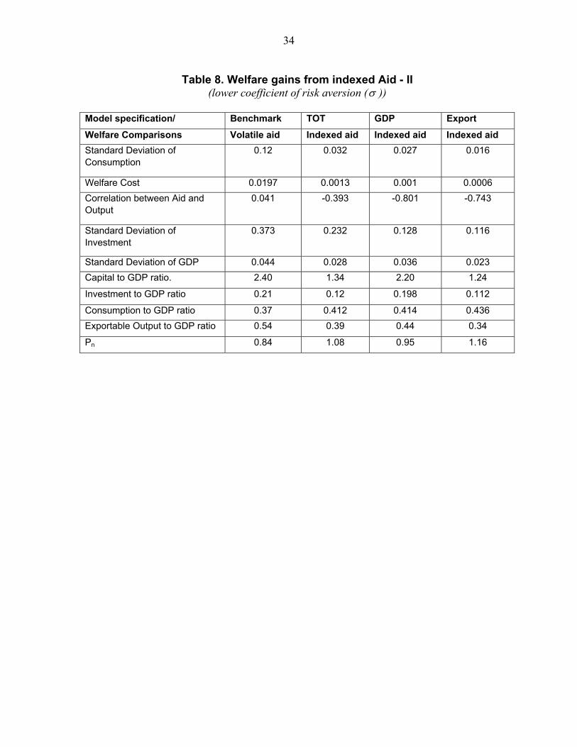
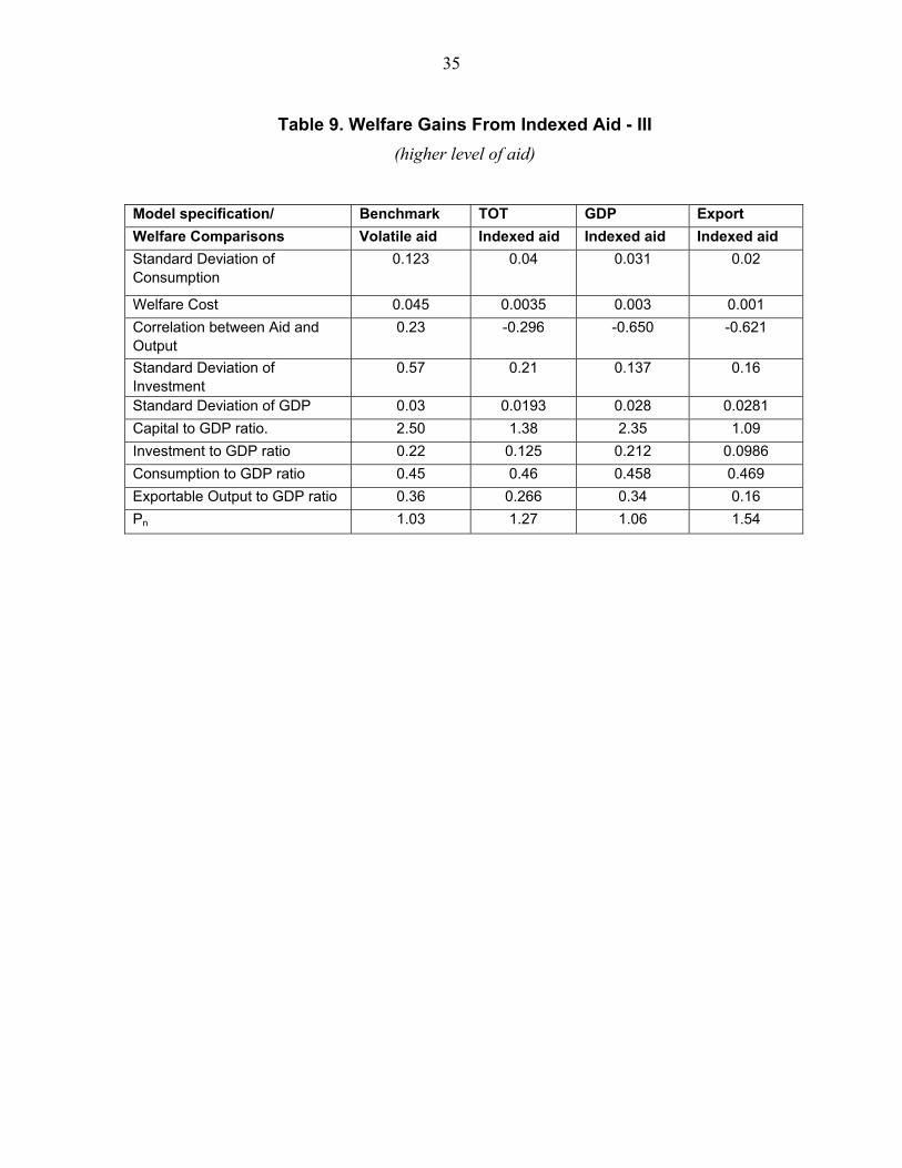
21 income of the SOE and thus reduces the volatility of investment which, by assumption, can only be done by using tradable goods. Less volatile investment in turn leads to less volatile output. The insurance against an exogenous fall in income provided by aid indexation schemes reduces the need for precautionary capital accumulation and thus leads to a smaller long run capital to GDP ratio, as recorded in the sixth row of Table 7. Figure 4 shows the stationary or long run distribution of the capital stock for the four specifications. We can see that the long run distribution of capital stock shifts to the left when aid is indexed to income shocks, indicating a decline in the precautionary capital accumulation. Correspondingly, the long run investment to GDP ratio is also lower with indexation of aid than without it. The long run consumption to GDP ratio is higher with aid indexation than without it. This reflects the fact that with insurance the representative household devotes a greater proportion of its output to consumption than to saving and investment for consumption smoothing. The share of exportable goods in the GDP falls in the presence of aid indexation when compared with the benchmark case. This reflects the assumption that investment in the SOE can only be done by using tradable goods. Insurance through aid indexation reduces the level of long run investment and hence the demand for tradable goods. Reduction in the demand for tradable goods results in an increase in the relative price of non-tradable goods prompting an increase in the share of labor and capital employed in the non tradable sector. This in turn reduces the share of exportable output in the GDP. To check the robustness of my results I do a couple of sensitivity tests on the benchmark model. The first test involves using a smaller coefficient of risk aversion (equal to 2.61). Table 8 presents the results from this experiment. A lower coefficient of risk aversion implies a smaller welfare loss for any given level of consumption volatility. This can be seen by comparing the second rows of Table 8 and Table 7. While the level of consumption volatility is roughly the same as before, the welfare loss under the benchmark case is now about 2 percent (half the previous size). Correspondingly, the gains from indexing aid flows are also smaller but roughly of the same magnitude for all three specifications. In all other aspects such as correlations and ratios between key macroeconomic variables, there is no significant change from the benchmark case. On the whole, gains form using indexed aid are still substantial, though not as large as before. The second experiment involves doubling the average level of aid flows. Since several policy makers have emphasized the need for doubling the aid flows to poor countries in order to achieve the Millennium Development Goals, it would be interesting to see the impact of such a policy in a dynamic framework. Comparing the results in Tables 9 and 7 we find that for all specifications, the volatility of consumption and the welfare cost of business cycles as a percentage of permanent consumption remain relatively unchanged when aid flows are doubled. Indexing aid flows still provides substantial welfare gains and, since a permanent

22 increase in aid leads to a permanent increase in the level of consumption, the gains in absolute terms are potentially larger. The ratio of exportable output to GDP falls and the relative price of non tradable goods rises with an increase in the average level of aid flows under all specifications. Thus, the phenomenon of .Dutch disease. carries over from the static model presented in section 4 to the dynamic model. Consumption to GDP ratio goes up in response to increased aid flows reflecting the fact that a permanent increase in aid flows raises the level of consumption permanently.

VII. CONCLUSION

Volatility and pro-cyclicality of aid flows results in substantial welfare losses for aid-dependent economies lacking access to international capital markets. Welfare costs of aid volatility are significantly higher in the presence of capital adjustment cost and terms of trade shocks. Rearranging aid flows so as to insure aid-dependent economies against exogenous terms of trade shocks can substantially improve welfare by lowering the consumption volatility in these countries. For reasonable values of the risk aversion coefficient, gains in welfare are between 2 to 4 percent of permanent consumption. Alternatively, donors can reduce the average level of aid by 1.5 to 3 percent without lowering the welfare of the recipient country, by indexing aid to exogenous shocks. The model used in this paper is simplified in several respects. It does not take into account the conditionality and fungibility of aid flows. It also ignores the absorption capacity constraints and productivity spillover associated with the expansion of the exportable sector. It assumes a simplified consumption behavior, with a representative household maximizing an inter-temporal utility function characterized by constant relative risk aversion. Most of these factors are however likely to increase the measured welfare gain from indexing and hence my calculations of welfare gains in the paper can be regarded as a lower bound for the potential gains from indexing. To sum up, while donor countries move towards increasing the aid flows to poor countries in order to achieve the millennium development goals, it is important to ensure effectiveness of these increased flows in raising welfare. One aspect of that should be designing aid flow structures that promote growth and minimize volatility.

23

Figure 1. Resource flow as a percentage of GDP

-0.1

-0.05

0

0.05

0.1

0.15

0.2

0.25

1981 1983 1985 1987 1989 1991 1993 1995 1997 1999 2001 2003

Year

Res

ourc

e Fl

ows

as P

erce

ntag

e of

GD

P

Total Resource FlowGrantsDebt

24

Table 1 : Dynamic behavior of Aid 9

Aid-to-revenue Aid-to-revenue All Countries > 10 percent. > 50 percent. Φ 3.94 4.96 7.42 Ψ 10 0.40 0.52 0.55

Source: Bulir and Hamann, 2003.

9 Measure of the relative volatility of aid is calculated as follows. Both aid and revenue series are expressed as a percentage

of GDP and de-trended. Variances of the transformed series are defined as 2Aσ and 2

Rσ respectively. The measure of

relative volatility is then defined as the ratio of these variances,

2

2A

R

σσ

Φ= .

10 Ψ is the Rank Correlation Coefficient to measure pro-cyclicality of aid.

25

Table 2. Share of the leading primary commodity export (97–99)

Country (1.) (2.) Commodity

Benin 33 6 Cotton

Burundi 75 7 Coffee

Burkina Faso 65 9 Cotton

Chad 37 5.7 Cotton

Côte d’Ivoire 36 14 Cocoa Beans

Ethiopia 62 5 Coffee

Guinea Bissau 48 6 Cashew Nuts

Gambia 20 13 Ground Nuts

Ghana 24 5 Cocoa Beans

Kenya 26 6 Tea

Malawi 59 24 Tobacco

Mali 30 7 Cotton

Mauritius 20 1 Sugar

Somalia 23 4 Cotton

Swaziland 20 9 Sugar

Uganda 54 4 Coffee

Zambia 61 5 Copper

(1.) As percentage of total merchandise exports (2.) As percentage of GDP

26

Table 3. Share of the top three primary commodities, (1997–99)

Country (1.) (2.) Commodity

Benin 38 7 Cotton, Cotton seed; Palm oil

Burundi 75 7 Coffee, Tea, Sugar

Burkina Faso 65 9 Cotton, Cattle, Sheep

Chad 37 5.7 Cotton, Cattle, Goats

Côte d’Ivoire 36 14 Cocoa – beans & paste, Coffee

Ethiopia 62 5 Coffee; Sheep skin; Crude org. matter

Guinea Bissau 48 6 Cashew Nuts, Cotton, Palm

Gambia 20 13 Groundnuts, Groundnut oil & Cake

Ghana 24 5 Cocoa - beans & butter, Pineapples

Kenya 26 6 Tea, Coffee, Crude org. matter

Malawi 59 24 Tobacco leaves, Tea, Sugar

Mali 30 7 Cotton lint, Cattle, Sheep

Mauritius 20 1 Sugar, Livestock, Beef prep.

Somalia 23 4 Cotton – raw & lint, Coffee

Swaziland 20 9 Sugar, Food prep.; Sugar conf.

Uganda 54 4 Coffee, Tea, Crude org. matter

Zambia 61 5 Copper, Sugar (raw), Cotton

(1.) As percentage of total merchandise exports (2.) As percentage of GDP Source: Computations based on FAOSTATS 2002 & WDI.

27

Table 4. Instability indices of prices of major primary commodities during 1957–1999

Commodity Index11

Sugar 39.2

Cashew Nuts 30.5

Coffee (Brazil) 28.4

Coffee (Uganda) 25.5

Cocoa 22.8

Jute 20.2

Ground Nuts 19.6

Tea 19.2

Rubber 17.0

Copper 16.3

Soy Beans 13.8

Cotton 13.4

Bananas 11.9

Tobacco 11.7

Source: Computations based on data from UNSTAD (COMTRADE) and FAO, January 2004.

11 The instability index is measured as percentage standard deviation of log prices (deflated by Economist’s MUV index) from a Hodrick-Prescott filtered trend.

28

Table 5. Benchmark Parameter Values

Parameter Symbol Value

Time Preference β 0.95

Share of tradable Consumption ϖ 0.50

Share of Exportable good in tradable good consumption. ς 0.15

Elasticity of substitution between tradable and non-tradable consumption

( )1/ 1 μ+ 1.279

Depreciation Rate δ 0.09

Capital Share in Exportable Sector α 0.30

Capital Share in Non-tradable sector η 0.40

Risk Aversion Coefficient σ 5.00

Elasticity of substitution between tradable and non-tradable capital ( )1/ 1 ν+ -10

Productivity T NA A= 1

Capital Adjustment Cost φ 0.028

29

Figure 2. Steady State Values

Price of Non-tradable Goods

0.75

0.85

0.95

1.05

0 0.1 0.25 0.5

Aid-to-GDP Ratio

Pric

e of

non

-trad

able

goo

ds.

Exportable Output to GDP ratio

0.3

0.4

0.5

0.6

0.7

0 0.1 0.25 0.5Aid-to-GDP Ratio

Exp

orta

ble

outp

ut to

GD

P R

atio

. Ratio of Capital in Exportable Sector

0.9

0.95

1

1.05

0 0.1 0.25 0.5Aid-to-GDP Ratio

Sha

re o

f Cap

ital i

n E

xpor

tabl

e S

ecto

r

Share of Tradable Consumption

0.3

0.4

0.5

0.6

0.7

0 0.1 0.25 0.5

Aid-to-GDP Ratio

Sha

re o

f Tra

dabl

e C

onsu

mpt

ion

Ratio of Investment to Total Income

0

0.04

0.08

0.12

0.16

0.2

0 0.1 0.25 0.5

Aid-to-GDP Ratio

Rat

io o

f Inv

estm

ent t

o To

tal I

ncom

e

Share of Labor in Exportable Sector

0

0.4

0.8

1.2

1.6

2

0 0.1 0.25 0.5

Aid-to-GDP Ratio

Sha

re o

f Lab

or in

Exp

orta

ble

Sect

or.

30

Figure 3. Sensitivity Analysis

Price of Non-Tradable Goods

0.75

0.8

0.85

0.9

0.95

1

1.05

1.1

1.15

1.2

1.25

0 0.1 0.25 0.5

Aid-to-GDP Ratio

Pric

e of

Non

-Tra

dabl

e G

oods

.

Model 1Model 2Model 3Model 4

Capital in Exportable Sector

0.4

0.6

0.8

1

1.2

1.4

1.6

0 0.1 0.25 0.5

Aid-to-GDP Ratio

Sha

re o

f Cap

ital i

n E

xpor

tabl

e S

ecto

r.

Model 1Model 2Model 3Model 4

Share of Tradable Consumption

0.3

0.35

0.4

0.45

0.5

0.55

0.6

0.65

0.7

0 0.1 0.25 0.5

Aid-to-GDP Ratio

Sha

re o

f Tra

dabl

e C

onsu

mpt

ion.

Model 1

Model 2

Model 3

Model 4

Share of Exportable Good in GDP

0.3

0.35

0.4

0.45

0.5

0.55

0.6

0.65

0.7

0 0.1 0.25 0.5Aid-to-GDP Ratio.

Sha

re o

f Exp

orta

ble

Out

put i

n G

DP

. Model 1

Model 2

Model 3

Model 4

Ratio of Investment to Total Income

0.12

0.14

0.16

0.18

0.2

0.22

0.24

0 0.1 0.25 0.5

Aid-to-GDP Ratio

Rat

io o

f Inv

estm

ent t

o To

tal I

ncom

e. Models 1 & 4

Models 2 & 3

Share of Labor in Exportable Goods

0

0.5

1

1.5

2

0 0.1 0.25 0.5

Aid-to-GDP Ratio

Sha

re o

f Lab

or in

Exp

orts

.

Model 1

Model 2

Model 3

Model 4

31

Table 6. Welfare Cost Under Alternative12 Model Specifications

Model Specification/ Welfare Calculations

Specification 1 Specification 2 Specification 3

S.D. of consumption 0.058 0.074 0.13

Welfare cost of aid volatility 0.0059 0.009 0.04

Table 7. Welfare Gains from Indexed Aid - I 12 Specification 1. has no terms of trade shocks or capital adjustment cost. Specification 2. has terms of trade shocks but no capital adjustment costs. Specification 3. has both terms of trade shocks and capital adjustment costs

32

Model specification/ Benchmark TOT GDP Export

Welfare Comparisons Volatile aid Indexed aid Indexed aid Indexed aid

Standard Deviation of Consumption

0.13 0.036 0.026 0.014

Welfare Cost 0.045 0.003 0.0017 0.0005

Correlation between Aid and Output

0.05 -0.44 -0.81 -0.799

Standard Deviation of Investment 0.376 0.24 0.144 0.12

Standard Deviation of GDP 0.044 0.028 0.035 0.022

Capital to GDP ratio. 2.40 1.34 2.20 1.24

Investment to GDP ratio 0.21 0.12 0.198 0.112

Consumption to GDP ratio 0.37 0.412 0.414 0.436

Exportable Output to GDP ratio 0.54 0.39 0.44 0.34

Pn 0.84 1.08 0.95 1.16

33

Figure 4. Stationary Capital Distribution

35 40 45 50 55 60 650

50

100

150

200

250

16 18 20 22 24 26 280

20

40

60

80

100

120

140

160

Benchmark Model Export Indexed Aid

10 10.5 11 11.5 12 12.5 13 13.5 140

50

100

150

200

250

300

350

20 21 22 23 24 25 26

0

50

100

150

200

250

300

350

400

450

TOT Indexed Aid GDP Indexed Aid

34

Table 8. Welfare gains from indexed Aid - II (lower coefficient of risk aversion (σ ))

Model specification/ Benchmark TOT GDP Export

Welfare Comparisons Volatile aid Indexed aid Indexed aid Indexed aid Standard Deviation of Consumption

0.12 0.032 0.027 0.016

Welfare Cost 0.0197 0.0013 0.001 0.0006 Correlation between Aid and Output

0.041 -0.393 -0.801 -0.743

Standard Deviation of Investment

0.373 0.232 0.128 0.116

Standard Deviation of GDP 0.044 0.028 0.036 0.023 Capital to GDP ratio. 2.40 1.34 2.20 1.24

Investment to GDP ratio 0.21 0.12 0.198 0.112

Consumption to GDP ratio 0.37 0.412 0.414 0.436 Exportable Output to GDP ratio 0.54 0.39 0.44 0.34

Pn 0.84 1.08 0.95 1.16

35

Table 9. Welfare Gains From Indexed Aid - III (higher level of aid)

Model specification/ Benchmark TOT GDP Export Welfare Comparisons Volatile aid Indexed aid Indexed aid Indexed aid Standard Deviation of Consumption

0.123 0.04 0.031 0.02

Welfare Cost 0.045 0.0035 0.003 0.001 Correlation between Aid and Output

0.23 -0.296 -0.650 -0.621

Standard Deviation of Investment

0.57 0.21 0.137 0.16

Standard Deviation of GDP 0.03 0.0193 0.028 0.0281 Capital to GDP ratio. 2.50 1.38 2.35 1.09 Investment to GDP ratio 0.22 0.125 0.212 0.0986 Consumption to GDP ratio 0.45 0.46 0.458 0.469 Exportable Output to GDP ratio 0.36 0.266 0.34 0.16 Pn 1.03 1.27 1.06 1.54

36

References

Athanasoulis,S. and E. van Wincoop, 1997, "Growth uncertainty and risk-sharing", Economic report series, No. 41, (February 1997)

Athanasoulis, S., R.J. Shiller, and E. van Wincoop, 1999, "Macro markets and financial security",

Economic policy review, (April 1999), Federal Reserve Bank of New York Arellano, C., Bulir, A., L. Lipshitz, and Timothy, L., 2005, "The Dynamic Implications of Foreign

Aid and Its Variability", Journal of Development Economics (forthcoming), Available at http://dx.doi.org/10.1016/j.jdeveco.2008.01.005

Atta-Mensah, J., 2004,. "Commodity Linked Bonds: A Potential Means for Less Developed Countries

to Raise Foreign Capital", Bank of Canada Working Paper, 2004-20, (June 2004) Bailey, N., 1983, "A safety Net for Foreign Lending", Business Week, (January 10) Barro, R., 1995, "Optimal Debt Management", NBER Working Paper 5327 Berlage, L., Cassimon, D., Dreze, J. and Reding P., 2000, "Prospective Aid and Indebtedness Relief:

A Proposal", CORE Discussion Paper, 2000/32 Birdsall, N., 2005, "Seven Deadly Sins: Reflections on Donor Failings", Center for Global

Development, Working Paper No. 50 Borzentine, E. and P. Mauro, 2004, "The case for GDP-indexed bonds", Economic Policy, (April

2004), pp. 165-216 Bulir, A. and A.J., Hamann, 2003, "Aid Volatility: An Empirical Assessment", IMF Staff Papers,

Vol. 50, No. 1, pp. 64-89 Bulir, A. and A.J., Hamann, 2006, "Volatility of Development Aid: From the Frying Pan into the

Fire", March 2006, IMF Staff Paper, Vol. 54, No. 07/04 Burnside, C. and Dollar, D, 2000, "AID, Policies and Growth", American Economic Review,

September 2000, Vol. 90, No. 4, pp. 847-68 Berube, C., Pallage, S. and M.A. Robe, 2004, "On Potential of Foreign Aid as Insurance", CIRPEE

Working Paper 04-40 Cashin, P., Liang, H. and McDermott, C., 2000, "How Persistent Are Shocks to World Commodity

Prices?", IMF Staff Papers, Vol. 47, No. 2 Cashin, P. and McDermott, C., 2002, "The Long Run Behavior of Commodity Prices: Small Trends

and Big Variability", IMF Staff Papers, Vol. 49, No. 2 Cuddington, John T., 1992, "Long-Run Trends in 26 Primary Commodity Prices", Journal of

Development Economics, Vol. 39, pp. 207-27

37 Gemmell, N. and M. McGillivray, 1998, "Aid and Tax Instability and the Government Budget

Constraints in Developing Countries", CREDIT Working Paper No. 98/1 (Nottingham, England: University of Nottingham Center for Research in Economic Development and International Trade)

Gilbert, C.L. and A. Tabova, 2003, "Realignment of debt service obligations and ability to pay in

concessional lending", World Bank, HIPC debt sustainability progress report Gilbert, C.L. and A. Tabova, 2004, "Commodity Prices and Debt Sustainability", Discussion Paper 4,

Economica, University of Trento Hamilton, J.D., 1989, "A New Approach to the Economic Analysis of Non-stationary Time Series

and the Business Cycle", Econometrica, Vol. 57, No. 2., pp. 357-384 Hausmann, R. and R. Rigobon, 2003, "IDA in UF: On the Benefits of Changing the Currency

Denomination of Concessional Lending to Low-Income Countries", World Bank Policy Paper

International Monetary Fund, 2004, "Sovereign Debt Structure for Crisis prevention", July 2004 Pallage, S. and M.A. Robe, 2001, "Foreign Aid and Business Cycle", Review of International

Economics, Vol. 9, No. 4, pp. 641-672 Pallage, S. and M.A. Robe, 2003, "On Welfare Cost of Economic Fluctuations in Developing

Countries", International Economic Review, Vol. 44, No. 2, pp. 677-698 Ramey, G. and V.A. Ramey, 1994, "Cross-country Evidence on the Link Between Volatility and Growth", NBER Working Paper No. W4959 Reinhart, Carmen M. and Wickham, P., 1994, "Commodity Prices: Cyclical Weakness or Secular

Decline?", IMF Staff Papers, Vol. 41 (June), pp. 175-213 Reinhart, Carmen M. and Vegh, C.A., 1995, "Real Effects of Exchange-Rate Based Stabilization: An

Analysis of Competing Theories", in B.S. Bernanke and J. Rotemberg (eds.) NBER Macroeconomics Annual, (MIT Press, Cambridge), 125-174.

Sevensson, J., 2000, "When is Foreign Aid Policy Credible? Aid Dependence and Conditionality",

Journal of Development Economics, Vol. 61, pp. 61-84 Shiller, R.J., 1993, "Macro Markets: Creating Institutions for Managing Society’s Largest Economic

Risks", Clarendon Press, Oxford Shiller, R.J., 2003, "The New Financial Order: Risk in the 21st century", Princeton University Press,

Princeton, N.J. Shiller, R.J., 2004, "Radical Financial Innovation", Cowles foundation discussion paper No. 1461,

April 2004 Lucas, R., 1987, "Models of Business Cycles", (New York: Basil Blackwell).

38 Mendoza, E.G., 1991, " Real Business Cycles in a Small Open Economy", American Economic

Review, Vol. 81, pp. 797-818 Mendoza, E.G., 1995, "The Terms of Trade, The Real Exchange Rate, and Economic Fluctuations",

International Economic Review, Vol. 36, No.1, pp. 101-137 Mendoza, E.G. and Urine, M., 2000, "Devaluation Risk and The Business-Cycle Implications of

Exchange Rate Management", Carnegie-Rochester Conference Series on Public Policy 53, Vol. 53, pp. 239-296.

Vostroknutova, E., 2005, "Concessional Loans Indexed to GDP Growth: Costs, Benefits and

International Risk Sharing", Background Paper, Washington D.C., World Bank Vostroknutova, E. and S. Yi, 2005, "On Costs and Benefits of Indexing Concessional Loans to Low

Income Countries on Changes in Real Exchange Rates", Background Paper, Washington D.C., World Bank

World Bank, 2005, "Managing the Debt Risk of Exogenous Shocks in Low Income Countries",

Washington D.C., World Bank