Wei Liu Michael RЎckner
267
Universitext Wei Liu Michael Röckner Stochastic Partial Differential Equations: An Introduction
-
Upload
khangminh22 -
Category
Documents
-
view
0 -
download
0
Transcript of Wei Liu Michael RЎckner

Universitext
Wei LiuMichael Röckner
Stochastic Partial Differential Equations: An Introduction

Universitext

Universitext
Series Editors
Sheldon AxlerSan Francisco State University
Vincenzo CapassoADAMSS (Interdisciplinary Centre for Adv)
Carles CasacubertaUniversitat de Barcelona
Angus MacIntyreQueen Mary University of London
Kenneth RibetUniversity of California, Berkeley
Claude SabbahCNRS, Ecole polytechnique Centre de mathématiques
Endre SüliUniversity of Oxford
Wojbor A. WoyczynskiCase Western Reserve University, Cleveland, OH
Universitext is a series of textbooks that presents material from a wide variety of mathe-matical disciplines at master’s level and beyond. The books, often well class-tested by theirauthor, may have an informal, personal even experimental approach to their subject matter.Some of the most successful and established books in the series have evolved through severaleditions, always following the evolution of teaching curricula, to very polished texts.
Thus as research topics trickle down into graduate-level teaching, first textbooks written fornew, cutting-edge courses may make their way into Universitext.
More information about this series at http://www.springer.com/series/223

Wei Liu • Michael RRockner
Stochastic Partial DifferentialEquations: An Introduction
123

Wei LiuSchool of Mathematics and StatisticsJiangsu Normal UniversityXuzhou, China
Michael RRocknerFaculty of MathematicsBielefeld UniversityBielefeld, Germany
ISSN 0172-5939 ISSN 2191-6675 (electronic)UniversitextISBN 978-3-319-22353-7 ISBN 978-3-319-22354-4 (eBook)DOI 10.1007/978-3-319-22354-4
Library of Congress Control Number: 2015953013
Mathematics Subject Classification (2010): 60-XX, 60H15, 60H10, 60H05, 60J60, 60J25, 35-XX,35K58, 35K59, 35Q35, 34-XX, 34F05, 34G20, 47-XX,47J35
Springer Cham Heidelberg New York Dordrecht London© Springer International Publishing Switzerland 2015This work is subject to copyright. All rights are reserved by the Publisher, whether the whole or part ofthe material is concerned, specifically the rights of translation, reprinting, reuse of illustrations, recitation,broadcasting, reproduction on microfilms or in any other physical way, and transmission or informationstorage and retrieval, electronic adaptation, computer software, or by similar or dissimilar methodologynow known or hereafter developed.The use of general descriptive names, registered names, trademarks, service marks, etc. in this publicationdoes not imply, even in the absence of a specific statement, that such names are exempt from the relevantprotective laws and regulations and therefore free for general use.The publisher, the authors and the editors are safe to assume that the advice and information in this bookare believed to be true and accurate at the date of publication. Neither the publisher nor the authors orthe editors give a warranty, express or implied, with respect to the material contained herein or for anyerrors or omissions that may have been made.
Printed on acid-free paper
Springer International Publishing AG Switzerland is part of Springer Science+Business Media(www.springer.com)

Contents
1 Motivation, Aims and Examples . . . . . . . . . . . . . . . . . . . . . . . . . . . . . . . . . . . . . . . . . . . 11.1 Motivation and Aims . . . . . . . . . . . . . . . . . . . . . . . . . . . . . . . . . . . . . . . . . . . . . . . . . . . 11.2 General Philosophy and Examples . . . . . . . . . . . . . . . . . . . . . . . . . . . . . . . . . . . . 3
2 The Stochastic Integral in General Hilbert Spaces(w.r.t. Brownian Motion) . . . . . . . . . . . . . . . . . . . . . . . . . . . . . . . . . . . . . . . . . . . . . . . . . . . . 92.1 Infinite-Dimensional Wiener Processes . . . . . . . . . . . . . . . . . . . . . . . . . . . . . . . 92.2 Martingales in General Banach Spaces. . . . . . . . . . . . . . . . . . . . . . . . . . . . . . . . 232.3 The Definition of the Stochastic Integral . . . . . . . . . . . . . . . . . . . . . . . . . . . . . . 27
2.3.1 Scheme of the Construction of the Stochastic Integral . . . . . . . 272.3.2 The Construction of the Stochastic Integral in Detail . . . . . . . . 27
2.4 Properties of the Stochastic Integral . . . . . . . . . . . . . . . . . . . . . . . . . . . . . . . . . . . 422.5 The Stochastic Integral for Cylindrical Wiener Processes . . . . . . . . . . . 49
2.5.1 Cylindrical Wiener Processes. . . . . . . . . . . . . . . . . . . . . . . . . . . . . . . . . . 492.5.2 The Definition of the Stochastic Integral
for Cylindrical Wiener Processes . . . . . . . . . . . . . . . . . . . . . . . . . . . . . . 52
3 SDEs in Finite Dimensions . . . . . . . . . . . . . . . . . . . . . . . . . . . . . . . . . . . . . . . . . . . . . . . . . . 553.1 Main Result and A Localization Lemma .. . . . . . . . . . . . . . . . . . . . . . . . . . . . . 553.2 Proof of Existence and Uniqueness. . . . . . . . . . . . . . . . . . . . . . . . . . . . . . . . . . . . 62
4 SDEs in Infinite Dimensions and Applications to SPDEs . . . . . . . . . . . . . . . . 694.1 Gelfand Triples, Conditions on the Coefficients and Examples . . . . . . 694.2 The Main Result and An Itô Formula . . . . . . . . . . . . . . . . . . . . . . . . . . . . . . . . . 894.3 Markov Property and Invariant Measures . . . . . . . . . . . . . . . . . . . . . . . . . . . . . 109
5 SPDEs with Locally Monotone Coefficients . . . . . . . . . . . . . . . . . . . . . . . . . . . . . . . 1235.1 Local Monotonicity . . . . . . . . . . . . . . . . . . . . . . . . . . . . . . . . . . . . . . . . . . . . . . . . . . . . 123
5.1.1 Main Result. . . . . . . . . . . . . . . . . . . . . . . . . . . . . . . . . . . . . . . . . . . . . . . . . . . . . 1235.1.2 Proof of the Main Theorem .. . . . . . . . . . . . . . . . . . . . . . . . . . . . . . . . . . . 1265.1.3 Application to Examples . . . . . . . . . . . . . . . . . . . . . . . . . . . . . . . . . . . . . . . 133
v

vi Contents
5.2 Generalized Coercivity . . . . . . . . . . . . . . . . . . . . . . . . . . . . . . . . . . . . . . . . . . . . . . . . . 1455.2.1 Main Results . . . . . . . . . . . . . . . . . . . . . . . . . . . . . . . . . . . . . . . . . . . . . . . . . . . 1455.2.2 Proofs of the Main Theorems. . . . . . . . . . . . . . . . . . . . . . . . . . . . . . . . . . 1495.2.3 Application to Examples . . . . . . . . . . . . . . . . . . . . . . . . . . . . . . . . . . . . . . . 165
6 Mild Solutions . . . . . . . . . . . . . . . . . . . . . . . . . . . . . . . . . . . . . . . . . . . . . . . . . . . . . . . . . . . . . . . . 1796.1 Prerequisites for This Chapter . . . . . . . . . . . . . . . . . . . . . . . . . . . . . . . . . . . . . . . . . 179
6.1.1 The Itô Formula . . . . . . . . . . . . . . . . . . . . . . . . . . . . . . . . . . . . . . . . . . . . . . . . 1796.1.2 A Burkholder–Davis–Gundy Type Inequality . . . . . . . . . . . . . . . . 1806.1.3 Stochastic Fubini Theorem . . . . . . . . . . . . . . . . . . . . . . . . . . . . . . . . . . . . 181
6.2 Existence, Uniqueness and Continuity with Respectto the Initial Data . . . . . . . . . . . . . . . . . . . . . . . . . . . . . . . . . . . . . . . . . . . . . . . . . . . . . . . 181
6.3 Smoothing Property of the Semigroup: PathwiseContinuity of the Mild Solution . . . . . . . . . . . . . . . . . . . . . . . . . . . . . . . . . . . . . . . 201
A The Bochner Integral . . . . . . . . . . . . . . . . . . . . . . . . . . . . . . . . . . . . . . . . . . . . . . . . . . . . . . . . 209A.1 Definition of the Bochner Integral . . . . . . . . . . . . . . . . . . . . . . . . . . . . . . . . . . . . . 209A.2 Properties of the Bochner Integral . . . . . . . . . . . . . . . . . . . . . . . . . . . . . . . . . . . . . 211
B Nuclear and Hilbert–Schmidt Operators . . . . . . . . . . . . . . . . . . . . . . . . . . . . . . . . . 215
C The Pseudo Inverse of Linear Operators . . . . . . . . . . . . . . . . . . . . . . . . . . . . . . . . . . 221
D Some Tools from Real Martingale Theory . . . . . . . . . . . . . . . . . . . . . . . . . . . . . . . . 225
E Weak and Strong Solutions: The Yamada–Watanabe Theorem . . . . . . . . 227
F Continuous Dependence of Implicit Functions on a Parameter . . . . . . . . 241
G Strong, Mild and Weak Solutions . . . . . . . . . . . . . . . . . . . . . . . . . . . . . . . . . . . . . . . . . . 243
H Some Interpolation Inequalities . . . . . . . . . . . . . . . . . . . . . . . . . . . . . . . . . . . . . . . . . . . . 247
I Girsanov’s Theorem in Infinite Dimensions with Respectto a Cylindrical Wiener Process . . . . . . . . . . . . . . . . . . . . . . . . . . . . . . . . . . . . . . . . . . . . 251
References . . . . . . . . . . . . . . . . . . . . . . . . . . . . . . . . . . . . . . . . . . . . . . . . . . . . . . . . . . . . . . . . . . . . . . . . . 261
Index . . . . . . . . . . . . . . . . . . . . . . . . . . . . . . . . . . . . . . . . . . . . . . . . . . . . . . . . . . . . . . . . . . . . . . . . . . . . . . . 265

Chapter 1Motivation, Aims and Examples
1.1 Motivation and Aims
In this course we will concentrate on (nonlinear) stochastic partial differentialequations (SPDEs) of evolutionary type. All kinds of dynamics with stochasticinfluence in nature or man-made complex systems can be modeled by suchequations. As we shall see from the examples at the end of this section, the statespaces of their solutions are necessarily infinite dimensional, such as spaces of(generalized) functions. In this course the state spaces, denoted by H, will be mostlyseparable Hilbert spaces, sometimes separable Banach spaces.
There is also enormous research activity on SPDEs where the state spaces arenot linear, but rather spaces of measures (particle systems, dynamics in populationgenetics) or infinite-dimensional manifolds (path or loop spaces over Riemannianmanifolds).
There are basically three approaches to analyzing SPDEs: the “martingale(or martingale measure) approach” (cf. [80]), the “semigroup (or mild solution)approach” (cf. [26, 27]) and the “variational approach” (cf. [75]). There is anenormously rich literature on all three approaches which cannot be listed here.We refer instead to the above and the following other monographs on SPDEs:[6, 13, 16, 19, 20, 26–28, 37, 46, 48, 50, 53, 66] and the references therein.
The purpose of this course is to give an introduction to the “variationalapproach”, as self-contained as possible, including the “local case”, i.e. where, e.g.the standard (weak) monotonicity conditions only hold locally. In the “global case”this approach was initiated in the pioneering work of E. Pardoux [64, 65] and furtherdeveloped by N. Krylov and B. Rozovskiı in [54] for continuous martingales asintegrators in the noise term and later by I. Gyöngy and N. Krylov in [40–42] fornot necessarily continuous martingales.
The predecessor [67] of this monograph grew out of a two-semester graduatecourse given by the second-named author at Purdue University in 2005/2006. Thisextended edition of [67] is the outcome of a two semester graduate course held at the
© Springer International Publishing Switzerland 2015W. Liu, M. Röckner, Stochastic Partial Differential Equations: An Introduction,Universitext, DOI 10.1007/978-3-319-22354-4_1
1

2 1 Motivation, Aims and Examples
University of Bielefeld in 2012/2013. Prerequisites would be an advanced course inprobability theory, covering standard martingale theory, stochastic processes in R
d
and maybe basic stochastic integration, though the latter is not formally required.Since graduate students in probability theory are usually not familiar with the theoryof Hilbert spaces or basic linear operator theory, all required material from theseareas is included in the text, most of it in the appendices. For the same reason weminimize the general theory of martingales on Hilbert spaces, paying, however, theprice that some proofs concerning stochastic integration on Hilbert space are a bitlengthy, since they have to be done “with bare hands”.
For simplicity we specialize to the case where the integrator in the noise termis just a cylindrical Wiener process, but everything is spelt out in such a way thatit generalizes directly to continuous local martingales. In particular, integrands arealways assumed to be predictable rather than just adapted and product measurable.The existence and uniqueness proof (cf. Sect. 4.2) is our personal version of theproof in [54, 75] and is largely taken from [69] presented there in a more generalframework. The results on invariant measures (cf. Sect. 4.3) we could not find in theliterature for the “variational approach”. They are, however, quite straightforwardmodifications of those in the “semigroup approach” in [27].
To keep this course reasonably self-contained we also include a complete proofof the finite-dimensional case in Chap. 3, which is based on the very focussed andbeautiful exposition in [52], which uses the Euler approximation. Among othercomplementing topics such as Chap. 6, which contains a concise introduction tothe “semigroup (or mild solution) approach”, the appendices contain a detailedaccount of the Yamada–Watanabe Theorem on the relation between weak and strongsolutions (cf. Appendix E), and a detailed proof of Girsanov’s Theorem in infinitedimensions (cf. Appendix I).
The structure of this monograph is, we hope, obvious from the list of contents.Here, we only mention that a substantial part consists of a very detailed introductionto stochastic integration on Hilbert spaces (see Chap. 2), major parts of which (aswell as Appendices A–C) are taken from the Diploma thesis of Claudia Prévôt(née Knoche) and Katja Frieler (see [34]), which in turn was based on [26] andsupervised by the second named author of this monograph. We would like to thankboth of them at this point for their permission to do this. We thank all coauthors ofthose joint papers which form another component for the basis of this monograph. Itwas really a pleasure working with them in this exciting area of probability theory.We would also like to thank Nelli Schmelzer, Matthias Stephan, Sven Wiesingerand Lukas Wresch for the excellent type job, as well as the participants of thegraduate courses at Purdue and Bielefeld University for checking large parts of thetext carefully. Special thanks go to Michael Scheutzow and Byron Schmuland forspotting a number of misprints and small errors in [67]. We also thank ClaudiaPrévôt for giving permission for this extension of [67]. Furthermore, the first namedauthor acknowledges the financial support from NSFC (No. 11201234, 11571147)and a project funded by PAPD of Jiangsu Higher Education Institutions. The lastnamed author would like to thank the German Science Foundation (DFG) for itsfinancial support through SFB 701 and also Jose Luis da Silva for his hospitality

1.2 General Philosophy and Examples 3
during a very pleasant stay at the University of Madeira where the final proofreadingof this monograph was done.
1.2 General Philosophy and Examples
Before starting with the main body of this course, let us briefly recall the generalphilosophy of describing stochastic dynamics by stochastic differential equations(SDE) in a more heuristic and intuitive way. These usually take values in a spaceH of (generalized) functions, e.g. on a domain ƒ � R
d, or a differential manifold,a fractal or even merely in an arbitrary measurable space .ƒ;B/. Abstractly, H is aseparable Hilbert or Banach space. Then given a map F W Œ0;T��H�U ! H, whereT 2�0;1Œ and U is another separable Hilbert space, one considers the differentialequations
dX.t/
dtD F.t;X.t/; PW.t// (1.1)
on H. Here PW.t/; t 2 Œ0;T�, is a U-valued white noise in time, more precisely,the generalised time derivative of a U-valued cylindrical Brownian motion W.t/ D.Wk.t//k2N; t 2 Œ0;T�, on some probability space .�;F ;P/. Hence PW.t/; t 2 Œ0;T�,are independent centred Gaussian variables with infinite variance, hence in regard to(1.1) the “worst” (Gaussian) random perturbation that can occur in (1.1). Employinga Taylor expansion for F around 0 2 U and, neglecting terms of order 2 and higher,turns (1.1) into
dX.t/
dtD F.t;X.t/; 0/C D3F.t;X.t/; 0/ PW.t/; (1.2)
where D3F denotes the derivative of F with respect to its third coordinate. Setting
A.t; x/ WD F.t; x; 0/; B.t; x/ WD D3F.t; x; 0/
and taking into account the non-differentiability of W.t/ in t, (1.2) turns into
dX.t/ D A.t;X.t//dt C B.t;X.t//dW.t/; (1.3)
to be rigorously understood in integral form. We mention here that the stochasticterm in (1.3) is often called or interpreted as a “stochastic force”, though the equa-tion is first order. This can, however, be justified by the Kramers–Smoluchowskiapproximation (see [14, 15, 33, 51, 76]). Furthermore, A is called the drift of theequation.
We briefly recall here that the linear pendant of (1.3) is given by the associ-ated Fokker–Planck–Kolmogorov equations obtained as a linearization of (1.3) as

4 1 Motivation, Aims and Examples
follows: Let FC2b;T denote the set of all functions f W Œ0;T��H ! R; C1 in t 2 Œ0;T�
and C2b in x 2 H, depending only on finitely many coordinates of x (with respect to
a fixed orthonormal basis of H). Take f 2 FC2b;T and compose it with the solution of
(1.3) for t > s with initial datum x 2 H at times s, denoted by X.t; s; x/, i.e. considerf .t;X.t; s; x//. Subsequently, take the expectation (with respect to P) to get
ps;t. f .t; �//.x/ WD E Œ f .t;X.t; s; x//� ; s < t:
Then apply Itô’s formula to find that
@
@tps;t. f .t; �//.x/ D ps;t.Lf .t; �//.x/; s < t; x 2 H; (1.4)
with L being the corresponding Kolmogorov operator given by
Lf .t; x/ D @
@tf .t; x/C 1
2Tr.B�.t; x/B.t; x/D2
x f .t; x//C A.t; x/Dx f .t; x/; x 2 H;
(1.5)
where Dx;D2x are the Fréchet derivatives of f .t; �/ W H ! R. We note that (1.5)
is well-defined (in particular the trace exists) for f 2 FC2b;T . We emphasize that
the less B�.t; x/;B.t; x/ is degenerate, the less degenerate is the second order partof the operator L. In this sense the noise part in (1.3) makes the equation better(“regularization by noise”). In this course, however, we shall concentrate on infinitedimensional stochastic differential equations as (1.3) which in applications areSPDEs. For a detailed analysis of the corresponding Fokker–Planck–Kolmogorovequations (1.4) we refer to the recent monograph [10].
Now we would like to give a few examples of SPDEs that appear in fundamentalapplications. We present them in a very brief way and refer to the above-mentionedliterature for a more elaborate discussion of these and many more examples and theirrôle in the applied sciences. Below we use standard notation, in particular Hm;2
0 .ƒ/
denotes the Sobolev space of order m in L2.ƒ/ with Dirichlet boundary conditionfor an open set ƒ � R
d.
Example 1.2.1 (Stochastic Quantization of the Free Euclidean Quantum Field)
dX.t/ D .� � m2/X.t/ dt C dW.t/
on H � S 0.Rd/.
• m 2 Œ0;1/ denotes “mass”,• .W.t//t>0 is a cylindrical Wiener process on L2.Rd/ � H (with the inclusion
being a Hilbert–Schmidt embedding).

1.2 General Philosophy and Examples 5
Example 1.2.2 (Stochastic Reaction Diffusion Equations)
dX.t/ D Œ�X.t/� g.X.t//� dt C B.t;X.t// dWt
on H WD L2.ƒ/;ƒ � Rd; ƒ open, d 6 3,
• B.t; x/ W H ! H is Hilbert–Schmidt 8x 2 H; t > 0.• g W R ! R is a “locally weakly monotone” function of at most polynomial
growth (depending on d),• W D .W.t//t>0 is a cylindrical Wiener process on H.
Example 1.2.3 (Stochastic Generalized Burgers Equation)
dX.t/ D�
d2
d�2X.t/� f .X.t//
d
d�X.t/C g.X.t//
�dt C B.t;X.t// dW.t/
on H WD L2��0; 1Œ
�.
• � 2�0; 1Œ,• f W R ! R is a Lipschitz function,• g W R ! R is as above, of at most cubic growth,• B and W are as above.
Example 1.2.4 (2D Stochastic Navier–Stokes Equation)
dX.t/ D PH���sX.t/� hX.t/;riX.t/
�dt C B.t;X.t// dW.t/
on H WD ˚u 2 L2.ƒ ! R
2; d�/ˇ
div u D 0�, ƒ � R
2, ƒ open, @ƒ smooth.
• � denotes viscosity,• �s denotes the Stokes Laplacian,• div is taken in the sense of distributions,• PH denotes the Helmholtz–Leray projection,• B and W are as above.
Example 1.2.5 (3D Stochastic Navier–Stokes Equation)
dX.t/ D PH Œ��sX.t/� hX.t/;riX.t/� dt C B.t/ dW.t/
on H WD ˚u 2 H1
0.ƒ ! R3I d�/j div u D 0
�; ƒ � R
3;ƒ open ; @ƒ smooth :
• B and W are as above (but B is independent of X.t/).
Example 1.2.6 (Stochastic p-Laplace Equation)
dX.t/ D div�jrX.t/jp�2rX.t/
�dt C B.t;X.t// dW.t/
on H WD L2.ƒ/;ƒ � Rd; ƒ open,

6 1 Motivation, Aims and Examples
• B and W are as above.
Example 1.2.7 (Stochastic Porous Media Equation)
dX.t/ D �‰.X.t// dt C B.t;X.t// dW.t/
on H WD dual of H10.ƒ/, ƒ as above.
• ‰ W R ! R is “monotone”,• B and W are as above.
Example 1.2.8 (Stochastic Cahn–Hilliard Equation)
dX.t/ D Œ��2X.t/C�'.X.t//� dt C B.t/ dW.t/
rX.t/ � n D r.�X.t// � n D 0 on @ƒ
on H WD L2.ƒ/;ƒ as above.
• n denotes the outward unit normal on @ƒ,• ' W R ! R is C1, is locally weakly monotone and of at most polynomial growth
p 2 Œ2; dC4d �,
• B and W are as above.
Example 1.2.9 (Stochastic Surface Growth Model)
dX.t/ D Œ� @4
@�4X.t/� @2
@�2X.t/C @2
@�2.@
@�X.t//2� dt C B.t/ dW.t/
X.t/ �@ƒD 0
on H D H2;20 .ƒ/ with ƒ WD�0;LŒ,
• � 2�0;LŒ;• B and W are as above.
The general form of these equations with state spaces consisting of functions� 7! x.�/, where � is a spatial variable, e.g. from a subset of Rd, is as follows:
dX.t/.�/ D A
t;X.t/.�/;D�X.t/.�/;D2�
�X.t/.�/
�dt
C B
t;X.t/.�/;D�Xt.�/;D2�
�X.t/.�/
�dW.t/ :
Here D� and D2� mean first and second total derivatives, respectively. The stochastic
term can be considered as a “perturbation by noise”. So, clearly one motivationfor studying SPDEs is to get information about the corresponding (unperturbed)deterministic PDE by letting the noise go to zero (e.g. replace B by " � B and let" ! 0) or to understand the different features occurring if one adds the noise term.

1.2 General Philosophy and Examples 7
If we drop the stochastic term in these equations we get a deterministic PDE of“evolutionary type”. Roughly speaking this means we have that the time derivativeof the desired solution (on the left) is equal to a non-linear functional of its spatialderivatives (on the right).
For a detailed analysis of Example 1.2.1 and for the non-linear much harderstochastic quantization equations for interacting Euclidean quantum fields we referto [2] and the recent survey [1] (including the references therein). All other examplesabove under the respective appropriate conditions are covered by the theorypresented in this course and all of them are analyzed in detail here. This is in contrastto [67], where Examples 1.2.2–1.2.5, 1.2.8 and 1.2.9, were not covered, sincethey only satisfy “local monotonicity conditions” and/or weaker growth conditionsand/or “generalized coercivity conditions”. All these latter examples are includedonly in this extended version, more precisely, in the newly added Chap. 5, whereglobal solutions for Examples 1.2.2–1.2.4 are constructed in Sect. 5.1 and localsolutions for Examples 1.2.5, 1.2.8 and 1.2.9 in Sect. 5.2 (see also Remark 5.1.11(4)for a number of further examples which, in order to keep it within a reasonablesize, have not been included in this course). We would like to stress that Sect. 5.2in particular contains the presentation of a general technique to construct localsolutions to SPDEs on the basis of a classical inequality due to Bihari. Furthermore,we include a study of a “tamed version” of Example 1.2.5 (see Example 5.2.25), forwhich global solutions exist (at least in the deterministic case), and we show thatthe solutions in Example 1.2.8 are global, if B � 0 or p 6 2.
After having discussed a number of typical examples of nonlinear SPDEs, wewould like to address a genuine problem of the theory of SPDEs, namely thatin some cases one is interested in perturbing the deterministic PDE by a veryrough noise, meaning a noise which is itself no longer function-valued, but onlytakes values in a space of generalized functions, i.e. in a subspace of the space ofSchwarz distributions. One way out is to go to the mild formulation of the SPDE(see Chap. 6) and use the smoothing property of a hopefully “strong enough” linearpart of the drift. But if one focuses on the Laplacian, “strong enough” requires thatthe underlying domain is one dimensional. So, already in two dimensions one canonly expect Schwarz distribution-valued solutions to the SPDE, hence the simplestnon-linear parts of the drift, as e.g. a power of the solution, have to be definedby renormalization techniques (see [2] and also [1]). Recently, a breakthrough hasbeen achieved in this direction by Martin Hairer in [44] (for which, together withhis work on the KPZ-equation [43] and other beautiful results in the field, he wasawarded the Fields Medal in 2014). In [44] he develops a whole theory to define and(locally) solve nonlinear SPDEs in a reformulated framework. This theory applies toa number of important (nonlinear) SPDEs with distribution-valued solutions on two-or three-dimensional underlying domains. We refer to [35] for a detailed expositionof this theory.
To conclude this introduction, let us summarize the new parts of this monographin comparison to [67], adding the references of their respective origin, which are allquite recent papers, except for the new Chap. 6 and the new Appendix F. The newChap. 5, whose contents has already been summarized in the previous paragraph,

8 1 Motivation, Aims and Examples
is an extended version of [57–59]. Chapter 6 contains a concise introduction to the“semigroup (or mild solution) approach”, in particular, addressing the measurabilityissues occurring in this context and (through the famous “factorization method”in [26]) also the question of when the solutions have continuous sample paths.To complement Chap. 6 we also include Appendix F which is needed there. BothChap. 6 and Appendix F are elaborations of the corresponding sections in [34],which in turn are based on [26]. Appendix E is a more detailed version of [71] and itcontains a complete proof of the Yamada–Watanabe Theorem in infinite dimensions,whereas [67] only contains the finite dimensional case. The new Appendix Hcontains two elementary proofs for well-known interpolation inequalities whichare essential for analyzing the (stochastic) Navier–Stokes equations. The proofs areessentially taken from [61]. Finally, the new Appendix I on Girsanov’s Theorem ininfinite dimensions is an extended version of Appendix A.1 in [22].

Chapter 2The Stochastic Integral in General HilbertSpaces (w.r.t. Brownian Motion)
We fix two separable Hilbert spaces�U; h ; iU
�and
�H; h ; i� with norms k kU
and k kH , respectively, where we drop the subscript H in the latter if there is noconfusion possible. The first part of this chapter is devoted to the construction of thestochastic Itô integral
Z t
0
ˆ.s/ dW.s/ ; t 2 Œ0;T�;
where W.t/, t 2 Œ0;T�, is a Wiener process on U and ˆ is a process with values thatare linear but not necessarily bounded operators from U to H.
For that we will first have to introduce the notion of the standard Wienerprocess in infinite dimensions. Then there will be a short section on martingalesin general Hilbert spaces. These two concepts are important for the construction ofthe stochastic integral, which will be explained in the following section.
Following this, we shall collect and prove a number of properties of the stochasticintegral, which are necessary for the later chapters.
Finally, we will describe how to transfer the definition of the stochastic integralto the case when W.t/, t 2 Œ0;T�, is a cylindrical Wiener process. For simplicity weassume that U and H are real Hilbert spaces.
2.1 Infinite-Dimensional Wiener Processes
For a topological space X we denote its Borel �-algebra by B.X/.Definition 2.1.1 A probability measure � on
�U;B.U/� is called Gaussian if for
all v 2 U the bounded linear mapping
v0 WU ! R
© Springer International Publishing Switzerland 2015W. Liu, M. Röckner, Stochastic Partial Differential Equations: An Introduction,Universitext, DOI 10.1007/978-3-319-22354-4_2
9

10 2 Stochastic Integral in Hilbert Spaces
defined by
u 7! hu; viU ; u 2 U;
has a Gaussian law, i.e. for all v 2 U there exist m WD m.v/ 2 R and � WD �.v/ 2Œ0;1Œ such that, if �.v/ > 0,
�� ı .v0/�1
�.A/ D�.v0 2 A/ D 1p
2�2
ZA
e� .x�m/2
2�2 dx for all A 2 B.R/;
and, if �.v/ D 0,
� ı .v0/�1 D ım.v/:
Theorem 2.1.2 A measure � on�U;B.U/� is Gaussian if and only if
O�.u/ WDZ
Ueihu;viU �.dv/ D eihm;uiU� 1
2 hQu;uiU ; u 2 U;
where m 2 U and Q 2 L.U/ is nonnegative, symmetric, with finite trace (seeDefinition B.0.3; here L.U/ denotes the set of all bounded linear operators on U).
In this case � will be denoted by N.m;Q/ where m is called the mean and Qis called the covariance (operator). The measure � is uniquely determined by mand Q.
Furthermore, for all h; g 2 U
Zhx; hiU �.dx/ D hm; hiU;
Z �hx; hiU � hm; hiU��hx; giU � hm; giU
��.dx/ D hQh; giU;
Zkx � mk2U �.dx/ D tr Q:
Proof (Cf. [26]) Obviously, a probability measure with this Fourier transform isGaussian. Now let us conversely assume that � is Gaussian. We need the following:
Lemma 2.1.3 Let � be a probability measure on .U;B.U//. Let k 2 N be such that
ZU
ˇhz; xiU
ˇk�.dx/ < 1 8 z 2 U:
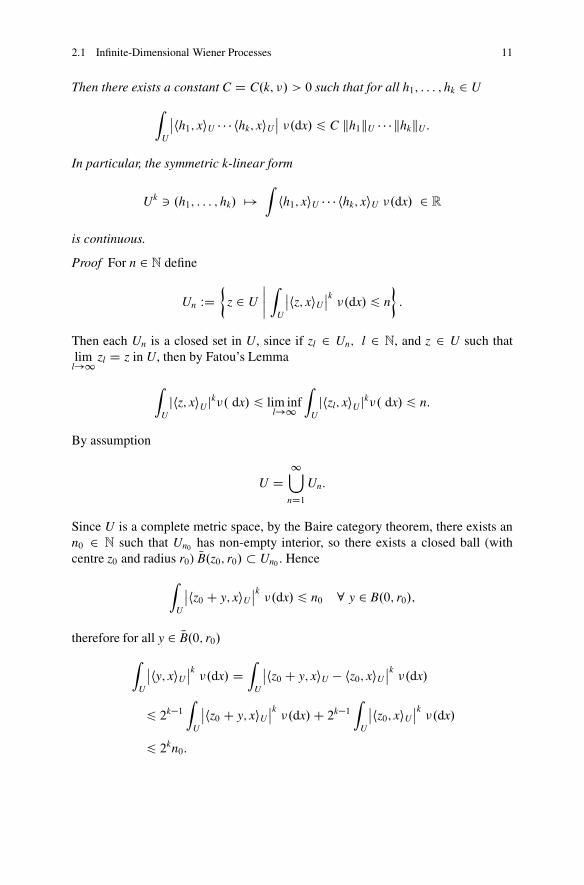
2.1 Infinite-Dimensional Wiener Processes 11
Then there exists a constant C D C.k; �/ > 0 such that for all h1; : : : ; hk 2 U
ZU
ˇhh1; xiU � � � hhk; xiU
ˇ�.dx/ 6 C kh1kU � � � khkkU :
In particular, the symmetric k-linear form
Uk 3 .h1; : : : ; hk/ 7!Z
hh1; xiU � � � hhk; xiU �.dx/ 2 R
is continuous.
Proof For n 2 N define
Un WD�
z 2 U
ˇˇZ
U
ˇhz; xiU
ˇk�.dx/ 6 n
�:
Then each Un is a closed set in U, since if zl 2 Un; l 2 N, and z 2 U such thatlim
l!1 zl D z in U, then by Fatou’s Lemma
ZU
jhz; xiUjk�. dx/ 6 lim infl!1
ZU
jhzl; xiUjk�. dx/ 6 n:
By assumption
U D1[
nD1Un:
Since U is a complete metric space, by the Baire category theorem, there exists ann0 2 N such that Un0 has non-empty interior, so there exists a closed ball (withcentre z0 and radius r0) NB.z0; r0/ � Un0 . Hence
ZU
ˇhz0 C y; xiU
ˇk�.dx/ 6 n0 8 y 2 B.0; r0/;
therefore for all y 2 NB.0; r0/Z
U
ˇhy; xiU
ˇk�.dx/ D
ZU
ˇhz0 C y; xiU � hz0; xiU
ˇk�.dx/
6 2k�1Z
U
ˇhz0 C y; xiU
ˇk�.dx/C 2k�1
ZU
ˇhz0; xiU
ˇk�.dx/
6 2kn0:

12 2 Stochastic Integral in Hilbert Spaces
Applying this for y WD r0z, z 2 U with kzkU D 1, we obtain
ZU
ˇhz; xiU
ˇk�.dx/ 6 2kn0r
�k0 :
Hence, if h1; : : : ; hk 2 U n f0g, then by the generalized Hölder inequality
ZU
ˇˇˇ
h1kh1kU
; x
�U
� � �
hk
khkkU; x
�U
ˇˇˇ �.dx/
6 Z
U
ˇˇ
h1kh1kU
; x
�U
ˇˇk
�.dx/
!1=k
: : :
ZU
ˇˇ
hk
khkkU; x
�U
ˇˇk
�.dx/
!1=k
6 2kn0r�k0 ;
and the assertion follows. utApplying Lemma 2.1.3 for k D 1 and � WD � we obtain that
U 3 h 7!Z
hh; xiU �.dx/ 2 R
is a continuous linear map, hence there exists an m 2 U such that
ZU
hx; hiU �.dx/ D hm; hi 8 h 2 U:
Applying Lemma 2.1.3 for k D 2 and � WD � we obtain that
U2 3 .h1; h2/ 7!Z
hx; h1iUhx; h2iU �.dx/� hm; h1iUhm; h2iU
is a continuous symmetric bilinear map, hence there exists a symmetric Q 2 L.U/such that this map is equal to
U2 3 .h1; h2/ 7! hQh1; h2iU:
Since for all h 2 U
hQh; hiU DZ
hx; hi2U �.dx/��Z
hx; hiU �.dx/
�2> 0;

2.1 Infinite-Dimensional Wiener Processes 13
Q is positive definite. It remains to prove that Q is trace class (i.e.
tr Q WD1X
iD1hQei; eiiU < 1
for one (hence every) orthonormal basis fei j i 2 Ng of U, cf. Appendix B). We mayassume without loss of generality that � has mean zero, i.e. m D 0 (2 U), sincethe image measure of � under the translation U 3 x 7! x � m is again Gaussianwith mean zero and the same covariance Q. Then we have for all h 2 U and allc 2 .0;1/
1 � e� 12 hQh;hiU D
ZU
�1 � coshh; xiU
��.dx/
6Z
fk�kU6cg�1 � coshh; xiU
��.dx/C 2�
�˚x 2 U
ˇ kxkU > c��
6 1
2
Zfk�kU6cg
ˇhh; xiU
ˇ2�.dx/C 2�
�˚x 2 U
ˇ kxkU > c��
(2.1)
(since 1 � cos x 6 12x2). Defining a positive definite symmetric linear operator Qc
on U by
hQch1; h2iU WDZ
fk�kU6cghh1; xiU � hh2; xiU �.dx/; h1; h2 2 U;
we even have that Qc is trace class because for every orthonormal basis fek j k 2 Ngof U we have (by monotone convergence)
1XkD1
hQcek; ekiU DZ
fk�kU6cg
1XkD1
hek; xi2U �.dx/ DZ
fk�kU6cgkxk2U �.dx/
6 c2 < 1:
Claim There exists a c0 2 .0;1/ (large enough) so that Q 6 2 log 4 Qc0 (meaningthat hQh; hiU 6 2 log 4 hQc0h; hiU for all h 2 U).
To prove the claim let c0 be so big that ��˚
x 2 Uˇ kxkU > c0
��6 1
8. Let h 2 U
such that hQc0h; hiU 6 1. Then (2.1) implies
1 � e� 12 hQh;hiU 6 1
2C 1
4D 3
4;
hence 4 > e12 hQh;hiU , so hQh; hiU 6 2 log 4. If h 2 U is arbitrary, but hQc0h; hiU 6D 0,
then we apply what we have just proved to h=hQc0h; hi 12U and the claim follows forsuch h. If, however, hQc0h; hiU D 0, then for all n 2 N, hQc0nh; nhiU D 0 6 1,

14 2 Stochastic Integral in Hilbert Spaces
hence by the above hQh; hiU 6 n�22 log 4. Therefore, hQh; hiU D 0 and the claimis proved, also for such h.
Since Qc0 has finite trace, so has Q by the claim and the theorem is proved, sincethe uniqueness part follows from the fact that the Fourier transform is one-to-one.
utThe following result is then obvious.
Proposition 2.1.4 Let X be a U-valued Gaussian random variable on a probabilityspace .�;F ;P/, i.e. there exist m 2 U and Q 2 L.U/ nonnegative, symmetric, withfinite trace such that P ı X�1 D N.m;Q/.
Then hX; uiU is normally distributed for all u 2 U and the following statementshold:
• E�hX; uiU
� D hm; uiU for all u 2 U,• E
�hX � m; uiU � hX � m; viU� D hQu; viU for all u; v 2 U,
• E�kX � mk2U
� D tr Q.
The following proposition will lead to a representation of a U-valued Gaussianrandom variable in terms of real-valued Gaussian random variables.
Proposition 2.1.5 If Q 2 L.U/ is nonnegative, symmetric, with finite trace thenthere exists an orthonormal basis ek, k 2 N, of U such that
Qek D kek; k > 0; k 2 N;
and 0 is the only accumulation point of the sequence .k/k2N.
Proof See [68, Theorem VI.21; Theorem VI.16 (Hilbert–Schmidt theorem)]. utProposition 2.1.6 (Representation of a Gaussian Random Variable) Let m 2 Uand Q 2 L.U/ be nonnegative, symmetric, with tr Q < 1. In addition, we assumethat ek, k 2 N, is an orthonormal basis of U consisting of eigenvectors of Qwith corresponding eigenvalues k, k 2 N, as in Proposition 2.1.5, numbered indecreasing order.
Then a U-valued random variable X on a probability space .�;F ;P/ isGaussian with P ı X�1 D N.m;Q/ if and only if
X DXk2N
pkˇkek C m (as objects in L2.�;F ;PI U/),
where ˇk, k 2 N, are independent real-valued random variables with P ı ˇk�1 D
N.0; 1/ for all k 2 N with k > 0. The series converges in L2.�;F ;PI U/.
Proof
1. Let X be a Gaussian random variable with mean m and covariance Q. Below weset h ; i WD h ; iU.

2.1 Infinite-Dimensional Wiener Processes 15
Then X D Pk2NhX; ekiek in U where hX; eki is normally distributed with
mean hm; eki and variance k, k 2 N, by Proposition 2.1.4. If we now define
ˇk W(
D hX;eki�hm;ekipk
if k 2 N with k > 0
� 0 2 R else,
then we get that P ı ˇ�1k D N.0; 1/ and X D P
k2Npkˇkek C m. To prove the
independence of ˇk, k 2 N, we take an arbitrary n 2 N and ak 2 R, 1 6 k 6 n,and obtain that for c WD �Pn
kD1; k¤0akpk
hm; eki
nXkD1
akˇk DnX
kD1;k 6D0
akpk
hX; eki C c D X;
nXkD1;k 6D0
akpk
ek
�C c
which is normally distributed since X is a Gaussian random variable. Thereforewe have that ˇk, k 2 N, form a Gaussian family. Hence, to get the independence,we only have to check that the covariance of ˇi and ˇj, i; j 2 N, i 6D j, withi 6D 0 6D j, is equal to zero. But this is clear since
E.ˇiˇj/ D 1pij
E�hX � m; eiihX � m; eji
� D 1pij
hQei; eji
D ipij
hei; eji D 0
for i 6D j.Furthermore, the series
PnkD1
pkˇkek, n 2 N, converges in L2.�;F ;PI U/
since the space is complete and
E
����nX
kDm
pkˇkek
���2U
�D
nXkDm
kE�jˇkj2
� DnX
kDm
k:
SinceP
k2N k D tr Q < 1 this expression becomes arbitrarily small for m andn large enough.
2. Let ek, k 2 N, be an orthonormal basis of U such that Qek D kek, k 2 N, andlet ˇk, k 2 N, be a family of independent real-valued Gaussian random variableswith mean 0 and variance 1. Then it is clear that the series
PnkD1
pkˇkek C m,
n 2 N, converges to X WD Pk2N
pkˇkek C m in L2.�;F ;PI U/ (see part 1).
Now we fix u 2 U and get that
D nXkD1
pkˇkek C m; u
ED
nXkD1
pkˇkhek; ui C hm; ui

16 2 Stochastic Integral in Hilbert Spaces
is normally distributed for all n 2 N and the sequence converges inL2.�;F ;P/. This implies that the limit hX; ui is also normally distributedwhere
E�hX; ui� D E
Xk2N
pkˇkhek; ui C hm; ui
D limn!1 E
nXkD1
pkˇkhek; ui
C hm; ui D hm; ui
and concerning the covariance we obtain that
E�hX; ui � hm; ui��hX; vi � hm; vi�
D limn!1 E
nXkD1
pkˇkhek; ui
nXkD1
pkˇkhek; vi
DXk2N
khek; uihek; vi DXk2N
hQek; uihek; vi
DXk2N
hek;Quihek; vi D hQu; vi
for all u; v 2 U. utBy part 2 of this proof we finally get the following existence result.
Corollary 2.1.7 Let Q be a nonnegative and symmetric operator in L.U/ with finitetrace and let m 2 U. Then there exists a Gaussian measure � D N.m;Q/ on�U;B.U/�.
Let us give an alternative, more direct proof of Corollary 2.1.7 without usingProposition 2.1.6. For the proof we need the following exercise.
Exercise 2.1.8 Consider R1 with the product topology. Let B.R1/ denote its
Borel �-algebra. Prove:
(i) B.R1/ D �.k j k 2 N/, where k W R1 ! R denotes the projection on thek-th coordinate.
(ii) l2.R/WDn.xk/k2N 2 R
1ˇ 1X
kD1x2k < 1
o2 B.R1/:
(iii) B.R1/ \ l2.R/ D ��k jl2
ˇk 2 N
�:
(iv) Let l2.R/ be equipped with its natural norm
kxkl2 WD 1X
kD1x2k 12; x D .xk/k2N 2 l2.R/;
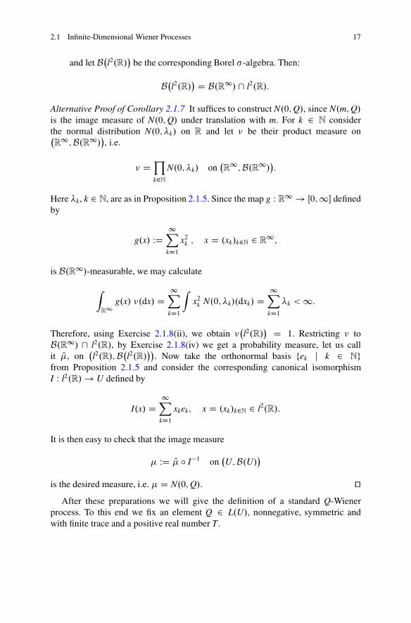
2.1 Infinite-Dimensional Wiener Processes 17
and let B�l2.R/� be the corresponding Borel �-algebra. Then:
B�l2.R/� D B.R1/\ l2.R/:
Alternative Proof of Corollary 2.1.7 It suffices to construct N.0;Q/, since N.m;Q/is the image measure of N.0;Q/ under translation with m. For k 2 N considerthe normal distribution N.0; k/ on R and let � be their product measure on�R
1;B.R1/�, i.e.
� DYk2N
N.0; k/ on�R
1;B.R1/�.
Here k, k 2 N, are as in Proposition 2.1.5. Since the map g W R1 ! Œ0;1� definedby
g.x/ WD1X
kD1x2k ; x D .xk/k2N 2 R
1;
is B.R1/-measurable, we may calculate
ZR1
g.x/ �.dx/ D1X
kD1
Zx2k N.0; k/.dxk/ D
1XkD1
k < 1:
Therefore, using Exercise 2.1.8(ii), we obtain ��l2.R/
� D 1. Restricting � toB.R1/ \ l2.R/, by Exercise 2.1.8(iv) we get a probability measure, let us callit Q�, on
�l2.R/;B�l2.R/��. Now take the orthonormal basis fek j k 2 Ng
from Proposition 2.1.5 and consider the corresponding canonical isomorphismI W l2.R/ ! U defined by
I.x/ D1X
kD1xkek; x D .xk/k2N 2 l2.R/:
It is then easy to check that the image measure
� WD Q� ı I�1 on�U;B.U/�
is the desired measure, i.e. � D N.0;Q/. utAfter these preparations we will give the definition of a standard Q-Wiener
process. To this end we fix an element Q 2 L.U/, nonnegative, symmetric andwith finite trace and a positive real number T.

18 2 Stochastic Integral in Hilbert Spaces
Definition 2.1.9 A U-valued stochastic process W.t/, t 2 Œ0;T�, on a probabilityspace .�;F ;P/ is called a (standard) Q-Wiener process if:
• W.0/ D 0,• W has P-a.s. continuous trajectories,• the increments of W are independent, i.e. the random variables
W.t1/; W.t2/ � W.t1/; : : : ; W.tn/� W.tn�1/
are independent for all 0 6 t1 < � � � < tn 6 T, n 2 N,• the increments have the following Gaussian laws:
P ı �W.t/ � W.s/��1 D N
�0; .t � s/Q
�for all 0 6 s 6 t 6 T:
Similarly to the existence of Gaussian measures the existence of a Q-Wienerprocess in U can be reduced to the real-valued case. This is the content of thefollowing proposition.
Proposition 2.1.10 (Representation of the Q-Wiener Process) Let ek, k 2 N,be an orthonormal basis of U consisting of eigenvectors of Q with correspondingeigenvalues k, k 2 N. Then a U-valued stochastic process W.t/, t 2 Œ0;T�, is aQ-Wiener process if and only if
W.t/ DXk2N
pkˇk.t/ek; t 2 Œ0;T�; (2.2)
where ˇk, k 2 fn 2 N j n > 0g, are independent real-valued Brow-nian motions on a probability space .�;F ;P/. The series even converges inL2��;F ;PI C.Œ0;T�;U/
�, and thus always has a P-a.s. continuous version. (Here
the space C�Œ0;T�;U
�is equipped with the sup norm.) In particular, for any Q as
above there exists a Q-Wiener process on U.
Proof
1. Let W.t/, t 2 Œ0;T�, be a Q-Wiener process in U.Since P ı W.t/�1 D N.0; tQ/, we see as in the proof of Proposition 2.1.6 that
W.t/ DXk2N
pkˇk.t/ek; t 2 Œ0;T�;
with
ˇk.t/ W(
D hW.t/;ekipk
if k 2 N with k > 0
� 0 else,

2.1 Infinite-Dimensional Wiener Processes 19
for all t 2 Œ0;T�. Furthermore, P ı ˇ�1k .t/ D N.0; t/, k 2 N, and ˇk.t/, k 2 N, are
independent for each fixed t 2 Œ0;T�.Now we fix k 2 N. First we show that ˇk.t/, t 2 Œ0;T�, is a Brownian motion:If we take an arbitrary partition 0 D t0 6 t1 < � � � < tn 6 T, n 2 N, of Œ0;T�
we get that
ˇk.t1/; ˇk.t2/ � ˇk.t1/; : : : ; ˇk.tn/� ˇk.tn�1/
are independent for each k 2 N since for 1 6 j 6 n
ˇk.tj/ � ˇk.tj�1/ D(
1pk
˝W.tj/ � W.tj�1/; ek
˛if k > 0,
0 else.
Moreover, we obtain that for the same reason P ı �ˇk.t/�ˇk.s/��1 D N.0; t � s/
for 0 6 s 6 t 6 T.In addition,
t 7! 1pk
˝W.t/; ek
˛ D ˇk.t/
is P-a.s. continuous for all k 2 N.Secondly, it remains to prove that ˇk, k 2 N, are independent.We take k1; : : : ; kn 2 N, n 2 N, ki 6D kj if i 6D j and an arbitrary partition
0 D t0 6 t1 6 : : : 6 tm 6 T, m 2 N.Then we have to show that
��ˇk1 .t1/; : : : ; ˇk1 .tm/
�; : : : ; �
�ˇkn.t1/; : : : ; ˇkn.tm/
�
are independent.We will prove this by induction with respect to m:If m D 1 it is clear that ˇk1 .t1/; : : : ; ˇkn.t1/ are independent as observed above.
Thus, we now take a partition 0 D t0 6 t1 6 : : : 6 tmC1 6 T and assume that
��ˇk1 .t1/; : : : ; ˇk1 .tm/
�; : : : ; �
�ˇkn.t1/; : : : ; ˇkn.tm/
�
are independent. We note that
��ˇki.t1/; : : : ; ˇki.tm/; ˇki.tmC1/
�D �
�ˇki.t1/; : : : ; ˇki.tm/; ˇki.tmC1/� ˇki.tm/
�; 1 6 i 6 n;

20 2 Stochastic Integral in Hilbert Spaces
and that
ˇki.tmC1/ � ˇki.tm/ D8<:
1pki
˝W.tmC1/� W.tm/; eki
˛U
if k > 0,
0 else,
1 6 i 6 n, are independent since they are pairwise orthogonal inL2.�;F ;PIR/ and since W.tmC1/ � W.tm/ is a Gaussian random variable.If we take Ai;j 2 B.R/, 1 6 i 6 n, 1 6 j 6 m C 1, then because of theindependence of �
�W.s/
ˇs 6 tm
�and �
�W.tmC1/� W.tm/
�we get that
P n\
iD1
˚ˇki.t1/ 2 Ai;1; : : : ; ˇki.tm/ 2 Ai;m;
ˇki.tmC1/ � ˇki.tm/ 2 Ai;mC1�
DP n\
iD1
m\jD1
˚ˇki.tj/ 2 Ai;j
�„ ƒ‚ …2 ��W.s/ ˇ s 6 tm
�\
n\iD1
˚ˇki.tmC1/ � ˇki.tm/ 2 Ai;mC1
�„ ƒ‚ …
2 ��W.tmC1/� W.tm/�
DP n\
iD1
m\jD1
˚ˇki.tj/ 2 Ai;j
� � P n\
iD1
˚ˇki.tmC1/ � ˇki.tm/ 2 Ai;mC1
�
D� nY
iD1P m\
jD1
˚ˇki.tj/ 2 Ai;j
��
� nY
iD1P˚ˇki.tmC1/� ˇki.tm/ 2 Ai;mC1
�
DnY
iD1P m\
jD1
˚ˇki.tj/ 2 Ai;j
�\ ˚ˇki.tmC1/� ˇki.tm/ 2 Ai;mC1
�
and therefore the assertion follows.2. If we define
W.t/ WDXk2N
pkˇk.t/ek; t 2 Œ0;T�;
where ˇk, k 2 N, are independent real-valued continuous Brownian motions thenit is clear that W.t/, t 2 Œ0;T�, is well-defined in L2.�;F ;PI U/. Besides, it is

2.1 Infinite-Dimensional Wiener Processes 21
obvious that the process W.t/, t 2 Œ0;T�, starts at zero and that
P ı �W.t/ � W.s/��1 D N
�0; .t � s/Q
�; 0 6 s < t 6 T;
by Proposition 2.1.6. It is also clear that the increments are independent.Thus it remains to show that the above series converges in
L2��;F ;PI C.Œ0;T�;U/
�. To this end we set
WN.t; !/ WDNX
kD1
pkˇk.t; !/ek
for all .t; !/ 2 �T WD Œ0;T� � � and N 2 N. Then WN , N 2 N, is P-a.s.continuous and we have that for M < N
E
supt2Œ0;T�
��WN.t/ � WM.t/��2
U
D E
sup
t2Œ0;T�
NXkDMC1
kˇ2k .t/
6NX
kDMC1kE
�sup
t2Œ0;T�ˇ2k .t/
�6 4
NXkDMC1
k supt2Œ0;T�
E�ˇk.t/
2�
6 4TNX
kDMC1k
because of Doob’s maximal inequality for nonnegative real-valued submartin-gales. As
Xk2N
k D tr Q < 1, the assertion follows. ut
Definition 2.1.11 (Normal Filtration) A filtration Ft, t 2 Œ0;T�, on a probabilityspace .�;F ;P/ is called normal if:
• F0 contains all elements A 2 F with P.A/ D 0 and• Ft D FtC D
\s>t
Fs for all t 2 Œ0;TŒ .
Definition 2.1.12 (Q-Wiener Process with Respect to a Filtration) A Q-Wienerprocess W.t/, t 2 Œ0;T�, is called a Q-Wiener process with respect to a filtration Ft,t 2 Œ0;T�, if:
• W.t/, t 2 Œ0;T�, is adapted to Ft, t 2 Œ0;T�, and• W.t/ � W.s/ is independent of Fs for all 0 6 s 6 t 6 T.
In fact it is possible to show that any U-valued Q-Wiener process W.t/, t 2 Œ0;T�,is a Q-Wiener process with respect to a normal filtration:
We define
N WD ˚A 2 F ˇ
P.A/ D 0�; F0
t WD ��W.s/
ˇs 6 t
�and QF0
t WD �.F0t [ N /:

22 2 Stochastic Integral in Hilbert Spaces
Then it is clear that
Ft WD\s>t
QF0s ; t 2 Œ0;TŒ; FT WD QF0
T ; (2.3)
is a normal filtration, called the normal filtration associated to W.t/; t 2 Œ0;T�, andwe get:
Proposition 2.1.13 Let W.t/, t 2 Œ0;T�, be an arbitrary U-valued Q-Wienerprocess on a probability space .�;F ;P/. Then it is a Q-Wiener process with respectto the normal filtration Ft, t 2 Œ0;T�, given by (2.3).
Proof It is clear that W.t/, t 2 Œ0;T�, is adapted to Ft, t 2 Œ0;T�. Hence we onlyhave to verify that W.t/ � W.s/ is independent of Fs, 0 6 s < t 6 T. But if we fix0 6 s < t 6 T it is clear that W.t/ � W.s/ is independent of QFs since
��W.t1/; W.t2/; : : : ; W.tn/
�D �
�W.t1/; W.t2/� W.t1/; : : : ; W.tn/� W.tn�1/
�
for all 0 6 t1 < t2 < � � � < tn 6 s. Of course, W.t/ � W.s/ is then also independentof QF0
s . To prove now that W.t/�W.s/ is independent of Fs it is enough to show that
P˚
W.t/ � W.s/ 2 A�\ B
D P
�W.t/ � W.s/ 2 A
� � P.B/
for any B 2 Fs and any closed subset A � U as E WD fA � U j A closedg generatesB.U/ and is stable under finite intersections. But we have
P˚
W.t/ � W.s/ 2 A�\ B
D E1A ı �W.t/ � W.s/
� � 1B
D limn!1 E
�h1 � n dist
�W.t/ � W.s/;A
� _ 0i1B
�
D limn!1 lim
m!1 E
�h1 � n dist
�W.t/ � W.s C 1
m/;A� _ 0
i1B
�
D limn!1 lim
m!1 E
�1 � n dist
�W.t/ � W.s C 1
m /;A� _ 0
�� P.B/
D P�W.t/ � W.s/ 2 A
� � P.B/;
since W.t/ � W.s C 1m / is independent of QF0
sC 1m
� Fs for all m 2 N. ut

2.2 Martingales in General Banach Spaces 23
2.2 Martingales in General Banach Spaces
Analogously to the real-valued case it is possible to define the conditional expecta-tion of any Bochner integrable random variable with values in an arbitrary separableBanach space
�E; k k�. This result is formulated in the following proposition.
Proposition 2.2.1 (Existence of the Conditional Expectation) Assume that E isa separable real Banach space. Let X be a Bochner integrable E-valued randomvariable defined on a probability space .�;F ;P/ and let G be a �-field containedin F .
Then there exists a unique, up to a set of P-probability zero, Bochner integrableE-valued random variable Z, measurable with respect to G, such that
ZA
X dP DZ
AZ dP for all A 2 G: (2.4)
The random variable Z is denoted by E.X j G/ and is called the conditionalexpectation of X given G. Furthermore,
��E.X j G/�� 6 E�kXk ˇ G�:
Proof (Cf. [26, Proposition 1.10, p. 27]) Let us first show the uniqueness.Since E is a separable Banach space, there exist ln 2 E�, n 2 N, separating the
points of E. Suppose that Z1;Z2 are Bochner integrable, G-measurable mappingsfrom� to E such that
ZA
X dP DZ
AZ1 dP D
ZA
Z2 dP for all A 2 G.
Then for n 2 N by Proposition A.2.2
ZA
�ln.Z1/� ln.Z2/
�dP D 0 for all A 2 G.
Applying this with A WD ˚ln.Z1/ > ln.Z2/
�and A WD ˚
ln.Z1/ < ln.Z2/�
it followsthat ln.Z1/ D ln.Z2/ P-a.s., so
�0 WD\n2N
˚ln.Z1/ D ln.Z2/
�
has P-measure one. Since ln, n 2 N, separate the points of E; it follows that Z1 D Z2on �0.

24 2 Stochastic Integral in Hilbert Spaces
To show the existence we first assume that X is a simple function. So, there existx1; : : : ; xN 2 E and pairwise disjoint sets A1; : : : ;AN 2 F such that
X DNX
kD1xk1Ak :
Define
Z WDNX
kD1xkE.1Ak j G/:
Then obviously Z is G-measurable and satisfies (2.4). Furthermore,
kZk 6NX
kD1kxkkE.1Ak j G/ D E
NXkD1
kxkk1Ak
ˇG
D E�kXk ˇ G�: (2.5)
Taking the expectation we get
E�kZk� 6 E
�kXk�: (2.6)
For general X take simple functions Xn, n 2 N, as in Lemma A.1.4 and define Zn
as above with Xn replacing X. Then by (2.6) for all n;m 2 N
E�kZn � Zmk� 6 E
�kXn � Xmk�;so Z WD limn!1 Zn exists in L1.�;F ;PI E/. Therefore, for all A 2 G
ZA
X dP D limn!1
ZA
Xn dP D limn!1
ZA
Zn dP DZ
AZ dP:
Clearly, Z can be chosen G-measurable, since so are the Zn. Furthermore, by (2.5)
��E.X j G/�� D kZk D limn!1kZnk 6 lim
n!1 E�kXnk ˇ G� D E
�kXk ˇ G�;where the limits are taken in L1.P/. ut
Later we will need the following result:
Proposition 2.2.2 Let .E1; E1/ and .E2; E2/ be two measurable spaces and‰ W E1�E2 ! R be a bounded measurable function. Let X1 and X2 be two random variableson .�;F ;P/ with values in .E1; E1/ and .E2; E2/ respectively, and let G � F be afixed �-field.

2.2 Martingales in General Banach Spaces 25
Assume that X1 is G-measurable and X2 is independent of G, then for P-a.e.! 2 �
E�‰.X1;X2/
ˇ G�.!/ D E Œ‰.X1.!/;X2/� :
Proof A simple exercise or see [26, Proposition 1.12, p. 29]. utRemark 2.2.3 The previous proposition can be easily extended to the case wherethe function‰ is not necessarily bounded but nonnegative.
Definition 2.2.4 Let M.t/, t > 0, be a stochastic process on .�;F ;P/ with valuesin a separable Banach space E, and let Ft, t > 0, be a filtration on .�;F ;P/.
The process M is called an Ft-martingale, if:
• E�kM.t/k� < 1 for all t > 0,
• M.t/ is Ft-measurable for all t > 0,• E
�M.t/
ˇ Fs� D M.s/ P-a.s. for all 0 6 s 6 t < 1.
Remark 2.2.5 Let M be as above such that E.kM.t/k/ < 1 for all t 2 Œ0;T�. ThenM is an Ft-martingale if and only if l.M/ is an Ft-martingale for all l 2 E�. Inparticular, results like optional stopping etc. extend to E-valued martingales.
There is the following connection to real-valued submartingales.
Proposition 2.2.6 If M.t/, t > 0, is an E-valued Ft-martingale and p 2 Œ1;1/,then
��M.t/��p
, t > 0, is a real-valued Ft-submartingale.
Proof Since E is separable there exist lk 2 E�, k 2 N, such that kzk D supk2N
lk.z/ for
all z 2 E. Then by Proposition A.2.2 for s < t
E�kMtk
ˇ Fs�
> supk
E�lk.Mt/
ˇ Fs�
D supk
lk�E.Mt j Fs/
�
D supk
lk.Ms/ D kMsk:
This proves the assertion for p D 1. Then Jensen’s inequality implies the assertionfor all p 2 Œ1;1/. utTheorem 2.2.7 (Maximal Inequality) Let p > 1 and let E be a separable Banachspace.
If M.t/, t 2 Œ0;T�, is a right-continuous E-valued Ft-martingale, then
�E
supt2Œ0;T�
��M.t/��p� 1
p
6 p
p � 1 supt2Œ0;T�
E�kM.t/kp
� 1p
D p
p � 1
E�kM.T/kp
� 1p:

26 2 Stochastic Integral in Hilbert Spaces
Proof The inequality is a consequence of the previous proposition and Doob’smaximal inequality for nonnegative real-valued submartingales. utRemark 2.2.8 We note that in the inequality in Theorem 2.2.7 the first normis the standard norm on Lp
��;F ;PI L1.Œ0;T�I E/
�, whereas the second is the
standard norm on L1�Œ0;T�I Lp.�;F ;PI E/�. So, for right-continuous E-valued Ft-
martingales these two norms are equivalent.
Now we fix 0 < T < 1 and denote by M2T.E/ the space of all E-valued
continuous, square integrable martingales M.t/, t 2 Œ0;T�. This space will playan important role with regard to the definition of the stochastic integral. We willespecially use the following fact.
Proposition 2.2.9 The space M2T.E/ equipped with the norm
kMkM2T
WD supt2Œ0;T�
E�kM.t/k2� 1
2 D
E�kM.T/k2� 1
2
6
E�
supt2Œ0;T�
kM.t/k2� 12 6 2 � E
�kM.T/k2� 12
is a Banach space.
Proof By the Riesz–Fischer theorem the space L2��;F ;PI L1�Œ0;T�;E�� is com-
plete. So, we only have to show that M2T is closed. But this is obvious since even
L1.�;F ;PI E/-limits of martingales are martingales. utProposition 2.2.10 Let T > 0 and W.t/, t 2 Œ0;T�, be a U-valued Q-Wienerprocess with respect to a normal filtration Ft, t 2 Œ0;T�, on a probability space.�;F ;P/. Then W.t/, t 2 Œ0;T�, is a continuous square integrable Ft-martingale,i.e. W 2 M2
T.U/.
Proof The continuity is clear by definition and for each t 2 Œ0;T� we have thatE�kW.t/k2U
� D t tr Q < 1 (see Proposition 2.1.4). Hence let 0 6 s 6 t 6 T andA 2 Fs. Then we get by Proposition A.2.2 that
ZA
W.t/ � W.s/ dP; u
�U
DZ
A
˝W.t/ � W.s/; u
˛U
dP
D P.A/Z ˝
W.t/ � W.s/; u˛U dP D 0
for all u 2 U as Fs is independent of W.t/ � W.s/ and E�hW.t/ � W.s/; uiU
� D 0
for all u 2 U. Therefore,
ZA
W.t/ dP DZ
AW.s/ dP; for all A 2 Fs:
ut

2.3 The Definition of the Stochastic Integral 27
2.3 The Definition of the Stochastic Integral
For the whole section we fix a positive real number T and a probability space.�;F ;P/ and we define �T WD Œ0;T� � � and PT WD dt ˝ P where dx is theLebesgue measure.
Moreover, we let Q 2 L.U/ be symmetric, nonnegative and with finite trace andconsider a Q-Wiener process W.t/, t 2 Œ0;T�, with respect to a normal filtration Ft,t 2 Œ0;T�.
2.3.1 Scheme of the Construction of the Stochastic Integral
Step 1: First we consider a certain class E of elementary L.U;H/-valued pro-cesses and define the mapping
Int W E ! M2T.H/ DW M2
T
ˆ 7! R t0ˆ.s/ dW.s/; t 2 Œ0;T�:
Step 2: We prove that there is a certain norm on E such that
Int W E ! M2T
is an isometry. Since M2T is a Banach space this implies that Int can be extended
to the abstract completion NE of E . This extension remains isometric and it isunique.
Step 3: We give an explicit representation of NE .Step 4: We show how the definition of the stochastic integral can be extended by
localization.
2.3.2 The Construction of the Stochastic Integral in Detail
Step 1: First we define the class E of all elementary processes as follows.
Definition 2.3.1 (Elementary Process) An L D L.U;H/-valued process ˆ.t/, t 2Œ0;T�, on .�;F ;P/ with normal filtration Ft, t 2 Œ0;T�, is said to be elementary ifthere exist 0 D t0 < � � � < tk D T, k 2 N, such that
ˆ.t/ Dk�1XmD0
ˆm1�tm;tmC1�.t/; t 2 Œ0;T�;

28 2 Stochastic Integral in Hilbert Spaces
where:
• ˆm W � ! L.U;H/ is Ftm-measurable, w.r.t. the strong Borel �-algebra onL.U;H/, 0 6 m 6 k � 1,
• ˆm takes only a finite number of values in L.U;H/, 0 6 m 6 k � 1.
We now define
Int.ˆ/.t/ WDZ t
0
ˆ.s/ dW.s/ WDk�1XmD0
ˆm�W.tmC1 ^ t/ � W.tm ^ t/
�; t 2 Œ0;T�;
(this is obviously independent of the representation) for all ˆ 2 E .
Proposition 2.3.2 Let ˆ 2 E . Then the stochastic integralZ t
0
ˆ.s/ dW.s/, t 2Œ0;T�, defined above, is a continuous square integrable martingale with respect toFt, t 2 Œ0;T�, i.e.
Int W E ! M2T :
Proof Let ˆ 2 E be given by
ˆ.t/ Dk�1XmD0
ˆm1�tm;tmC1�.t/; t 2 Œ0;T�;
as in Definition 2.3.1. Then it is clear that
t 7!Z t
0
ˆ.s/ dW.s/ Dk�1XmD0
ˆm�W.tmC1 ^ t/ � W.tm ^ t/
�
is P-a.s. continuous because of the continuity of the Wiener process and thecontinuity of ˆm.!/ W U ! H, 0 6 m 6 k � 1, ! 2 �. In addition, we getfor each summand that
���ˆm�W.tmC1 ^ t/ � W.tm ^ t/
����6kˆmkL.U;H/
��W.tmC1 ^ t/� W.tm ^ t/��
U:
Since W.t/, t 2 Œ0;T�, is square integrable and ! ! kˆm.!/kL.U;H/ is bounded
(because ˆm.�/ is finite), this implies thatZ t
0
ˆ.s/ dW.s/ is square integrable for
each t 2 Œ0;T�.

2.3 The Definition of the Stochastic Integral 29
To prove the martingale property we take 0 6 s 6 t 6 T and a set A from Fs.If˚ˆm.!/
ˇ! 2 �
� WD fLm1 ; : : : ;L
mkm
g, we obtain by Proposition A.2.2 and themartingale property of the Wiener process that
ZA
k�1XmD0
ˆm�W.tmC1 ^ t/ � W.tm ^ t/
�dP
DX
06m6k�1;tmC1<s
ZAˆm�W.tmC1 ^ s/ � W.tm ^ s/
�dP
CX
06m6k�1;s6tmC1
kmXjD1
ZA\fˆmDLm
j gLm
j
�W.tmC1 ^ t/ � W.tm ^ t/
�dP
DX
06m6k�1;tmC1<s
ZAˆm�W.tmC1 ^ s/ � W.tm ^ s/
�dP
CX
06m6k�1;s6tmC1
kmXjD1
Lmj
ZA\fˆmDLm
j g„ ƒ‚ …2Fs_tm
�W.tmC1 ^ t/ � W.tm ^ t/
�dP
DX
06m6k�1;tmC1<s
ZAˆm�W.tmC1 ^ s/ � W.tm ^ s/
�dP
CX
06m6k�1;tm<s6tmC1
kmXjD1
Lmj
ZA\fˆmDLm
j g�W.tmC1 ^ s/ � W.tm ^ s/
�dP
DZ
A
k�1XmD0
ˆm�W.tmC1 ^ s/ � W.tm ^ s/
�dP:
utStep 2: To verify the assertion that there is a norm on E such that Int W E ! M2
Tis an isometry, we have to introduce the following notion.
Definition 2.3.3 (Hilbert–Schmidt Operator) Let ek, k 2 N, be an orthonormalbasis of U. An operator A 2 L.U;H/ is called Hilbert–Schmidt if
Xk2N
hAek;Aeki < 1:
In Appendix B we take a close look at this notion. So here we only summarizethe results which are important for the construction of the stochastic integral.

30 2 Stochastic Integral in Hilbert Spaces
The definition of a Hilbert–Schmidt operator and the number
kAkL2 WDX
k2NkAekk2
12
are independent of the choice of the basis (see Remark B.0.6(i)). Moreover, thespace L2.U;H/ of all Hilbert–Schmidt operators from U to H equipped with theinner product
hA;BiL2 WDXk2N
hAek;Beki
is a separable Hilbert space (see Proposition B.0.7). Later, we will use the factthat kAkL2.U;H/ D kA�kL2.H;U/, where A� is the adjoint operator of A (seeRemark B.0.6(i)). Furthermore, the composition of a Hilbert–Schmidt operator witha bounded linear operator is again Hilbert–Schmidt.
Besides we recall the following fact.
Proposition 2.3.4 If Q 2 L.U/ is nonnegative and symmetric then there existsexactly one element Q
12 2 L.U/ nonnegative and symmetric such that Q
12 ıQ
12 D Q.
If, in addition, tr Q < 1 we have that Q12 2 L2.U/, kQ
12 k2L2 D tr Q and that
L ı Q12 2 L2.U;H/ for all L 2 L.U;H/.
Proof [68, Theorem VI.9, p. 196]. utAfter these preparations we simply calculate the M2
T -norm of
Z t
0
ˆ.s/ dW.s/; t 2 Œ0;T�;
and get the following result.
Proposition 2.3.5 If ˆ D Pk�1mD0 ˆm1�tm;tmC1� is an elementary L.U;H/-valued
process then
����Z �
0
ˆ.s/ dW.s/
����2
M2T
D E
�Z T
0
��ˆ.s/ ı Q12
��2L2
ds
�DW kˆk2T (“Itô-isometry”):
Proof If we set �m WD W.tmC1/ � W.tm/ then we get that
����Z �
0
ˆ.s/ dW.s/
����2
M2T
D E
����Z T
0
ˆ.s/ dW.s/
����2
H
!D E
����k�1XmD0
ˆm�m
���2H
�
D E k�1X
mD0kˆm�mk2H
C 2E
X06m<n6k�1
hˆm�m; ˆn�niH
:

2.3 The Definition of the Stochastic Integral 31
Claim 1:
E k�1X
mD0kˆm�mk2H
D
k�1XmD0
.tmC1 � tm/E�kˆm ı Q
12 k2L2
�
DZ T
0
E��ˆ.s/ ı Q
12
��2L2
ds:
To prove this we take an orthonormal basis fk, k 2 N, of H and get by the Parsevalidentity and Levi’s monotone convergence theorem that
E�kˆm�mk2H
� DXl2N
E�hˆm�m; fli2H
� DXl2N
E
E�h�m; ˆ
�m fli2U
ˇ Ftm
�:
Taking an orthonormal basis ek, k 2 N, of U we obtain that
ˆ�m fl D
Xk2N
h fl; ˆmekiHek:
Since h fl; ˆmekiH is Ftm-measurable, this implies thatˆ�m fl is Ftm-measurable by
Proposition A.1.3. Using the fact that �.�m/ is independent of Ftm we obtain byProposition 2.2.2 that for P-a.e. ! 2 �
E�h�m; ˆ
�m fli2U
ˇ Ftm
�.!/ D E
˝�m; ˆ
�m.!/fl
˛2U
D .tmC1 � tm/DQ�ˆ�
m.!/fl�; ˆ�
m.!/flEU;
since E�h�m; ui2U
� D .tmC1 � tm/hQu; uiU for all u 2 U. Thus, the symmetry of
Q12 finally implies that
E�kˆm�mk2H
� DXl2N
E
E�h�m; ˆ
�m fli2U
ˇ Ftm
�
D .tmC1 � tm/Xl2N
E�hQˆ�
m fl; ˆ�m fliU
�
D .tmC1 � tm/Xl2N
E��Q
12 ˆ�
m fl��2
U
D .tmC1 � tm/E
�����ˆm ı Q12�����2
L2.H;U/
�
D .tmC1 � tm/E��ˆm ı Q
12
��2L2.U;H/
:

32 2 Stochastic Integral in Hilbert Spaces
Hence the first assertion is proved and it only remains to verify the followingclaim.
Claim 2:
E�hˆm�m; ˆn�niH
� D 0 ; 0 6 m < n 6 k � 1:
But this can be proved in a similar way to Claim 1:
E�hˆm�m; ˆn�niH
� D E
E�hˆ�
nˆm�m; �niU
ˇ Ftn
�
DZ
E˝ˆ�
n .!/ˆm.!/�m.!/;�n˛U
P.d!/ D 0;
since E�hu; �niU
� D 0 for all u 2 U (see Proposition 2.2.2). Hence the assertionfollows. utHence the right norm on E has been identified. But strictly speaking k kT is only
a seminorm on E . Therefore, we have to consider equivalence classes of elementaryprocesses with respect to k kT to get a norm on E . For simplicity we will not changethe notation but stress the following fact.
Remark 2.3.6 If two elementary processesˆ and Q belong to one equivalence classwith respect to k kT it does not follow that they are equal PT -a.e. because their valuesonly have to correspond on Q
12 .U/ PT-a.e.
Thus we have finally shown that
Int W �E ; k kT� ! �M2
T ; k kM2T
�
is an isometric transformation. Since E is dense in the abstract completion NE of Ewith respect to k kT it is clear that there is a unique isometric extension of Int to NE .
Step 3: To give an explicit representation of NE it is useful, at this moment, tointroduce the subspace U0 WD Q
12 .U/ with the inner product given by
hu0; v0i0 WD ˝Q� 1
2 u0;Q� 12 v0˛U;
u0; v0 2 U0, where Q� 12 is the pseudo inverse of Q
12 in the case that Q is not one-
to-one. Then we get by Proposition C.0.3(i) that .U0; h ; i0/ is again a separableHilbert space.The separable Hilbert space L2.U0;H/ is called L02. By Proposition C.0.3(ii) we
know that Q12 gk, k 2 N, is an orthonormal basis of
�U0; h ; i0
�if gk, k 2 N, is an
orthonormal basis of�Ker Q
12
�?. This basis can be supplemented to a basis of U

2.3 The Definition of the Stochastic Integral 33
by elements of Ker Q12 . Thus we obtain that
kLkL02D ��L ı Q
12
��L2
for each L 2 L02:
Define L.U;H/0 WD ˚T jU0
ˇT 2 L.U;H/
�. Since Q
12 2 L2.U/ it is clear that
L.U;H/0 � L02 and that the k kT -norm of ˆ 2 E can be written in the followingway:
kˆkT D
E
�Z T
0
kˆ.s/k2L02
ds
�! 12
:
We also need the following �-field:
PT WD �˚�s; t� � Fs
ˇ0 6 s < t 6 T; Fs 2 Fs
� [ ˚f0g � F0ˇ
F0 2 F0�
D ��Y W �T ! R
ˇY is left-continuous and adapted to
Ft; t 2 Œ0;T��:Let QH be an arbitrary separable Hilbert space. If Y W �T ! QH is PT=B. QH/-measurable it is called ( QH-)predictable.If, for example, the process Y itself is continuous and adapted to Ft, t 2 Œ0;T�,then it is predictable.So, we are now able to characterize NE .
Claim There is an explicit representation of NE and it is given by
N 2W.0;TI H/ WD ˚
ˆ W Œ0;T� �� ! L02ˇˆ is predictable and kˆkT < 1�
D L2�Œ0;T� ��;PT ; dt ˝ PI L02
�:
For simplicity we also write N 2W.0;T/ or N 2
W instead of N 2W.0;TI H/.
To prove this claim we first notice the following facts:
1. Since L.U;H/0 � L02 and since any ˆ 2 E is L02-predictable by construction wehave that E � N 2
W .2. Because of the completeness of L02 we get by Appendix A that
N 2W D L2.�T ;PT ;PT I L02/
is also complete.
Therefore N 2W is at least a candidate for a representation of NE . Thus it only remains
to show that E is a dense subset of N 2W . But this is formulated in Proposition 2.3.8
below, which can be proved with the help of the following lemma.

34 2 Stochastic Integral in Hilbert Spaces
Lemma 2.3.7 There is an orthonormal basis of L02 consisting of elements ofL.U;H/0. This especially implies that L.U;H/0 is a dense subset of L02.
Proof Since Q is symmetric, nonnegative and tr Q < 1 we know byLemma 2.1.5 that there exists an orthonormal basis ek, k 2 N, of U such thatQek D kek, k > 0, k 2 N. In this case Q
12 ek D p
kek, k 2 N with k > 0, is anorthonormal basis of U0 (see Proposition C.0.3(ii)).
If fk, k 2 N, is an orthonormal basis of H then by Proposition B.0.7 we know that
fj ˝pkek D fjh
pkek; �iU0 D 1p
kfjhek; �iU; j; k 2 N; k > 0;
form an orthonormal basis of L20 consisting of operators in L.U;H/0. utProposition 2.3.8 If ˆ 2 N 2
W then there exists a sequenceˆn, n 2 N, of L.U;H/0-valued elementary processes such that
kˆ �ˆnkT �! 0 as n ! 1:
Proof
Step 1: If ˆ 2 N 2W there exists a sequence of simple random variables ˆn DPMn
kD1 Lnk1An
k, An
k 2 PT and Lnk 2 L02, n 2 N, such that
kˆ �ˆnkT �! 0 as n ! 1:
As L02 is a separable Hilbert space, this is a simple consequence of Lemma A.1.4and Lebesgue’s dominated convergence theorem.Thus the assertion is reduced to the case thatˆ D L1A where L 2 L02 and A 2 PT .
Step 2: Let A 2 PT and L 2 L02. Then there exists a sequence Ln, n 2 N, inL.U;H/0 such that
kL1A � Ln1AkT �! 0 as n ! 1:
This result is obvious by Lemma 2.3.7 and thus now we only have to considerthe case when ˆ D L1A, L 2 L.U;H/0 and A 2 PT .
Step 3: If ˆ D L1A, L 2 L.U;H/0, A 2 PT , then there is a sequence ˆn, n 2 N,of elementary L.U;H/0-valued processes in the sense of Definition 2.3.1 suchthat
kL1A �ˆnkT �! 0 as n �! 1:
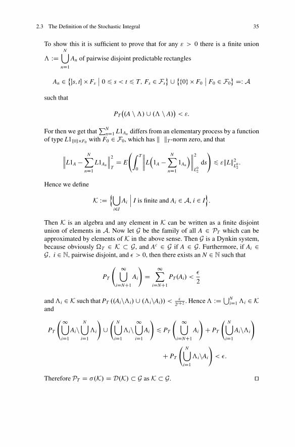
2.3 The Definition of the Stochastic Integral 35
To show this it is sufficient to prove that for any " > 0 there is a finite union
ƒ WDN[
nD1An of pairwise disjoint predictable rectangles
An 2 ˚�s; t� � Fs
ˇ0 6 s < t 6 T; Fs 2 Fs
� [ ˚f0g � F0ˇ
F0 2 F0� DW A
such that
PT�.A nƒ/ [ .ƒ n A/
�< ":
For then we get thatPN
nD1 L1An differs from an elementary process by a functionof type L1f0g�F0 with F0 2 F0, which has k kT -norm zero, and that
���L1A �NX
nD1L1An
���2T
D E
Z T
0
����L1A �
NXnD1
1An
����2
L02
ds
!6 "kLk2
L02:
Hence we define
K WDn[
i2I
Ai
ˇˇ I is finite and Ai 2 A, i 2 I
o:
Then K is an algebra and any element in K can be written as a finite disjointunion of elements in A. Now let G be the family of all A 2 PT which can beapproximated by elements of K in the above sense. Then G is a Dynkin system,because obviously �T 2 K � G, and Ac 2 G if A 2 G. Furthermore, if Ai 2G; i 2 N, pairwise disjoint, and � > 0, then there exists an N 2 N such that
PT
1[iDNC1
Ai
!D
1XiDNC1
PT.Ai/ <�
2
andƒi 2 K such that PT ..Ainƒi/[ .ƒinAi// <�
2iC2 . Henceƒ WD SNiD1 ƒi 2 K
and
PT
1[iD1
AinN[
iD1ƒi

36 2 Stochastic Integral in Hilbert Spaces
Step 4: Finally, by the so-called localization procedure we shall extend thedefinition of the stochastic integral to the linear space
NW.0;TI H/ WD(ˆ W �T ! L02
ˇˇˆ is predictable with
P
�Z T
0
kˆ.s/k2L02
ds < 1�
D 1
):
For simplicity we also write NW.0;T/ or NW instead of NW.0;TI H/ and NW iscalled the class of stochastically integrable processes on Œ0;T�.The extension is done in the following way:For ˆ 2 NW we define
�n WD inf
�t 2 Œ0;T�
ˇˇ Z t
0
kˆ.s/k2L02
ds > n
�^ T: (2.7)
Then by the right-continuity of the filtration Ft, t 2 Œ0;T�, we get that
f�n 6 tg D\m2N
��n < t C 1
m
�
D\m2N
[q2Œ0;tC 1
m Œ\Q
�Z q
0
kˆ.s/k2L02
ds > n
�„ ƒ‚ …2Fq by the real Fubini theorem„ ƒ‚ …
2FtC 1
mand decreasing in m
2 Ft:
Therefore �n, n 2 N, is an increasing sequence of stopping times with respect toFt, t 2 Œ0;T�, such that
E
�Z T
0
k1�0;�n �.s/ˆ.s/k2L02 ds
�6 n < 1:
In addition, the processes 1�0;�n�ˆ, n 2 N, are still L02-predictable since 1�0;�n� isleft-continuous and .Ft/-adapted or since
�0; �n� WD ˚.s; !/ 2 �T
ˇ0 < s 6 �n.!/
�
D˚.s; !/ 2 �T
ˇ�n.!/ < s 6 T
� [ f0g ��c
D[
q2Q
��q;T� � f�n 6 qg„ ƒ‚ …
2Fq
�
„ ƒ‚ …2PT
[ f0g ��c 2 PT :

2.3 The Definition of the Stochastic Integral 37
Thus we get that the stochastic integrals
Z t
0
1�0;�n �.s/ˆ.s/ dW.s/; t 2 Œ0;T�;
are well-defined for all n 2 N. For arbitrary t 2 Œ0;T� we set
Z t
0
ˆ.s/ dW.s/ WDZ t
0
1�0;�n�.s/ˆ.s/ dW.s/ on f�n � tg: (2.8)
(Note that the sequence �n, n 2 N, even reaches T P-a.s., in the sense that forP-a.e. ! 2 � there exists an n.!/ 2 N such that �n.!/ D T for all n > n.!/.)To show that this definition is consistent we have to prove that for arbitrarynatural numbers m < n and t 2 Œ0;T�
Z t
0
1�0;�m�.s/ˆ.s/ dW.s/ DZ t
0
1�0;�n �.s/ˆ.s/ dW.s/ P-a.s.
on f�m > tg � f�n > tg. This result follows from the following lemma, whichalso implies that the process in (2.8) is a continuous H-valued local martingale.
Lemma 2.3.9 Assume that ˆ 2 N 2W and that � is an Ft-stopping time such that
P.� 6 T/ D 1. Then there exists a P-null set N 2 F independent of t 2 Œ0;T� suchthat
Z t
0
1�0;��.s/ˆ.s/ dW.s/ D Int�1�0;��ˆ
�.t/ D Int.ˆ/.� ^ t/
DZ �^t
0
ˆ.s/ dW.s/ on Nc for all t 2 Œ0;T�:
Proof Since both integrals which appear in the equation are P-a.s. continuous weonly have to prove that they are equal P-a.s. at any fixed time t 2 Œ0;T�.Step 1: We first consider the case that ˆ 2 E and that � is a simple stopping time
which means that it takes only a finite number of values.Let 0 D t0 < t1 < � � � < tk 6 T, k 2 N, and
ˆ Dk�1XmD0
ˆm1�tm;tmC1�
where ˆm W � ! L.U;H/ is Ftm -measurable and only takes a finite number ofvalues for all 0 6 m 6 k � 1.

38 2 Stochastic Integral in Hilbert Spaces
If � is a simple stopping time, there exists an n 2 N such that �.�/D fa0; : : : ; angand
� DnX
jD0aj1Aj ;
where 0 6 aj < ajC1 6 T and Aj D f� D ajg 2 Faj . Then we get that 1��;T�ˆ isan elementary process since
1��;T�.s/ˆ.s/ Dk�1XmD0
ˆm1�tm;tmC1�\��;T�.s/
Dk�1XmD0
nXjD0
1Ajˆm1�tm ;tmC1�\�aj ;T�.s/
Dk�1XmD0
nXjD0
1Ajˆm„ƒ‚…Ftm_aj -measurable
1�tm_aj;tmC1_aj�.s/
and concerning the integral we are interested in, we obtain that
Z t
0
1�0;��.s/ˆ.s/ dW.s/ DZ t
0
ˆ.s/ dW.s/�Z t
0
1��;T�.s/ˆ.s/ dW.s/
Dk�1XmD0
ˆm�W.tmC1 ^ t/ � W.tm ^ t/
�
�k�1XmD0
nXjD0
1Ajˆm
W�.tmC1 _ aj/ ^ t
� � W�.tm _ aj/ ^ t
�
Dk�1XmD0
ˆm�W.tmC1 ^ t/ � W.tm ^ t/
�
�k�1XmD0
nXjD0
1Ajˆm
W�.tmC1 _ �/ ^ t
� � W�.tm _ �/ ^ t
�
Dk�1XmD0
ˆm�W.tmC1 ^ t/ � W.tm ^ t/
�
�k�1XmD0
ˆm
W�.tmC1 _ �/ ^ t
� � W�.tm _ �/ ^ t
�

2.3 The Definition of the Stochastic Integral 39
Dk�1XmD0
ˆm
W.tmC1 ^ t/ � W.tm ^ t/
� W�.tmC1 _ �/ ^ t
�C W�.tm _ �/ ^ t
�
Dk�1XmD0
ˆm
W.tmC1 ^ � ^ t/ � W.tm ^ � ^ t/
DZ t^�
0
ˆ.s/ dW.s/:
Step 2: Now we consider the case when ˆ is still an elementary process while �is an arbitrary stopping time with P.� 6 T/ D 1.Then there exists a sequence
�n D2n�1XkD0
T.k C 1/2�n1�Tk2�n;T.kC1/2�n � ı �; n 2 N;
of simple stopping times such that �n # � as n ! 1 and because of thecontinuity of the stochastic integral we get that
Z �n^t
0
ˆ.s/ dW.s/n!1���!
Z �^t
0
ˆ.s/ dW.s/ P-a.s.
Besides, we obtain (even for non-elementary processes ˆ) that
��1�0;�n�ˆ� 1�0;��ˆ��2
TD E
�Z T
0
1��;�n�.s/kˆ.s/k2L02 ds
�n!1���! 0;
which by the definition of the integral implies that
E
����Z t
0
1�0;�n�.s/ˆ.s/ dW.s/�Z t
0
1�0;��.s/ˆ.s/ dW.s/
����2!
n!1���! 0
for all t 2 Œ0;T�. As by Step 1
Z t
0
1�0;�n�.s/ˆ.s/ dW.s/ DZ �n^t
0
ˆ.s/ dW.s/; n 2 N; t 2 Œ0;T�;
the assertion follows.Step 3: Finally we generalize the statement to arbitraryˆ 2 N 2
W.0;T/:Ifˆ 2 N 2
W.0;T/, then there exists a sequence of elementary processesˆn, n 2 N,such that
kˆn �ˆkTn!1���! 0 :

40 2 Stochastic Integral in Hilbert Spaces
By the definition of the stochastic integral this means that
Z �
0
ˆn.s/ dW.s/n!1���!
Z �
0
ˆ.s/ dW.s/ in M2T :
Hence it follows that there is a subsequence nk, k 2 N, and a P-null set N 2 Findependent of t 2 Œ0;T� such that
Z t
0
ˆnk .s/ dW.s/k!1���!
Z t
0
ˆ.s/ dW.s/ on Nc
for all t 2 Œ0;T� and therefore we get for all t 2 Œ0;T� that
Z �^t
0
ˆnk.s/ dW.s/k!1���!
Z �^t
0
ˆ.s/ dW.s/ P-a.s.
In addition, it is clear that
k1�0;��ˆn � 1�0;��ˆkT �!n!1 0
which implies that for all t 2 Œ0;T�
E
����Z t
0
1�0;��.s/ˆn.s/ dW.s/ �Z t
0
1�0;��.s/ˆ.s/ dW.s/
����2!
n!1���! 0:
As by Step 2
Z t
0
1�0;��.s/ˆnk .s/ dW.s/ DZ �^t
0
ˆnk.s/ dW.s/ P-a.s.
for all k 2 N the assertion follows. utTherefore, for m < n on f�m > tg � f�n > tgZ t
0
1�0;�n�.s/ˆ.s/ dW.s/ DZ �m^t
0
1�0;�n �.s/ˆ.s/ dW.s/
DZ t
0
1�0;�m�.s/1�0;�n �.s/ˆ.s/ dW.s/ DZ t
0
1�0;�m�.s/ˆ.s/ dW.s/ P-a.s.,
where we used Lemma 2.3.9 for the second equality. Hence the definition isconsistent.
Remark 2.3.10 Let ˆ 2 NW and �n; n 2 N, as in 2.3.1. In fact it is easy to see thatthe definition of the stochastic integral for ˆ 2 NW does not depend on the choiceof �n, n 2 N. We shall show this in several steps. So, let if �n, n 2 N, be another

2.3 The Definition of the Stochastic Integral 41
sequence of stopping times such that �n " T as n ! 1 and 1�0;�n�ˆ 2 N 2W for all
n 2 N. Then:
(i)
Z t
0
ˆ.s/ dW.s/ D limn!1
Z t
0
1�0;�n �.s/ˆ.s/ dW.s/ for all t 2 Œ0;T�P-a.s.
(ii) Lemma 2.3.9 holds for all ˆ 2 NW .(iii)
Z t
0
ˆ.s/ dW.s/ DZ t
0
1�0;�n�.s/ˆ.s/ dW.s/ on f�n � tgP-a.s.
Proof
(i) Let t 2 Œ0;T�. Then we get that on the set f�m > tgZ t
0
ˆ.s/ dW.s/ DZ t
0
1�0;�m�.s/ˆ.s/ dW.s/
D limn!1
Z t^�n
0
1�0;�m�.s/ˆ.s/ dW.s/
D limn!1
Z t^�m
0
1�0;�n�.s/ˆ.s/ dW.s/
D limn!1
Z t
0
1�0;�n �.s/ˆ.s/ dW.s/ P-a.s.;
utwhere we used Lemma 2.3.9 twice for the third equality. Letting m ! 1assertion (i) follows.
(ii) Let � be as in Lemma 2.3.9. Then P-a.s. for all t 2�0;T�Z �^t
0
ˆ.s/ dW.s/ D limn!1
Z �^t
0
1�0;�n�.s/ˆ.s/ dW.s/
D limn!1
Z t
0
1�0;��.s/1�0;�n �.s/ˆ.s/ dW.s/
DZ t
0
1�0;��.s/ˆ.s/ dW.s/;
where we used (i) for the first and last equality and Lemma 2.3.9 for the second.

42 2 Stochastic Integral in Hilbert Spaces
(iii) By (ii) we have P-a.s. on f�n � tgZ t
0
ˆ.s/ dW.s/ DZ �n^t
0
ˆ.s/ dW.s/
DZ t
0
1�0;�n �.s/ˆ.s/ dW.s/:
2.4 Properties of the Stochastic Integral
Let T be a positive real number and W.t/, t 2 Œ0;T�, a Q-Wiener process as describedat the beginning of the previous section.
Lemma 2.4.1 Let ˆ be a L02-valued stochastically integrable process,. QH; k k QH/ a further separable Hilbert space and L 2 L.H; QH/.
Then the process L�ˆ.t/
�, t 2 Œ0;T�, is an element of NW.0;TI QH/ and
L
�Z T
0
ˆ.t/ dW.t/
�DZ T
0
L�ˆ.t/
�dW.t/ P-a.s.
Proof Since ˆ is a stochastically integrable process and
���L�ˆ.t/
����L2.U0; QH/
6 kLkL.H; QH/kˆ.t/kL02;
it is obvious that L�ˆ.t/
�, t 2 Œ0;T�, is L2.U0; QH/-predictable and
P
�Z T
0
���L�ˆ.t/
����2L2.U0; QH/
dt < 1�
D 1:
Step 1: As the first step we consider the case thatˆ is an elementary process, i.e.
ˆ.t/ Dk�1XmD0
ˆm1�tm;tmC1�.t/; t 2 Œ0;T�;
where 0 D t0 < t1 < � � � < tk D T, ˆm W � ! L.U;H/ Ftm-measurable withˇˆm.�/
ˇ< 1 for 0 6 m 6 k. Then
L
�Z T
0
ˆ.t/ dW.t/
�D L
k�1XmD0
ˆm�W.tmC1/� W.tm/
�
Dk�1XmD0
Lˆm�W.tmC1/� W.tm/
� DZ T
0
L�ˆ.t/
�dW.t/:

2.4 Properties of the Stochastic Integral 43
Step 2: Now let ˆ 2 N 2W.0;T/. Then there exists a sequence ˆn, n 2 N, of
elementary processes with values in L.U;H/0 such that
kˆn �ˆkT D
E
�Z T
0
kˆn.t/ �ˆ.t/k2L02
dt
�! 12
n!1���! 0:
Then L.ˆn/, n 2 N, is a sequence of elementary processes with values inL.U; QH/0 and
��L.ˆn/ � L.ˆ/��
T6 kLkL.H; QH/kˆn �ˆkT
n!1���! 0:
By the definition of the stochastic integral, Step 1 and the continuity of L we getthat there is a subsequence nk, k 2 N, such that
Z T
0
L�ˆ.t/
�dW.t/ D lim
k!1
Z T
0
L�ˆnk.t/
�dW.t/
D limk!1 L
�Z T
0
ˆnk.t/ dW.t/
�D L
�lim
k!1
Z T
0
ˆnk .t/ dW.t/
�
D L
�Z T
0
ˆ.t/ dW.t/
�P-a.s.
Step 3: Finally let ˆ 2 NW.0;T/.Let �n, n 2 N, be a sequence of stopping times as in (2.7). Then 1�0;�n�L.ˆ/ 2N 2
W.0;T; QH/ for all n 2 N and we obtain by Remark 2.3.10 and Step 2 (selectinga subsequence if necessary)
Z T
0
L�ˆ.t/
�dW.t/ D lim
n!1
Z T
0
1�0;�n�.t/L�ˆ.t/
�dW.t/
D limn!1 L
�Z T
0
1�0;�n �.t/ˆ.t/ dW.t/
�D L
�lim
n!1
Z T
0
1�0;�n �.t/ˆ.t/ dW.t/
�
D L
�Z T
0
ˆ.t/ dW.t/
�P-a.s.
utBelow Bs.L.U0;H// denotes the Borel �-algebra generated by the strong
topology on L.U0;H/.
Lemma 2.4.2 Let ˆ W �T ! L.U0;H/ be PTnBs.L.U0;H//-measurable and f W�T ! H be PTnB.H/-measurable such that
Z T
0
kˆ�.t; !/f .t; !/k2U0 dt < 1 P-a.s.

44 2 Stochastic Integral in Hilbert Spaces
Set
Z T
0
˝f .t/; ˆ.t/ dW.t/
˛ WDZ T
0
Q f .t/ dW.t/ (2.9)
with
Q f .t/.u/ WD ˝f .t/; ˆ.t/u
˛; u 2 U0:
Then the stochastic integral in (2.9) is well-defined as a continuous R-valuedstochastic process. More precisely, Q f is a PT=B.L2.U0;R//-measurable map fromŒ0;T� �� to L2.U0;R/, and
k Q f .t; !/kL2.U0;R/ D kˆ�.t; !/f .t; !/kU0 :
Proof Let ek; k 2 N, be an orthonormal basis of U0. Then for all .t; !/ 2 Œ0;T���
k Q f .t; !/k2L2.U0;R/ D1X
kD1h f .t; !/;ˆ.t; !/eki2
D1X
kD1hˆ�.t; !/f .t; !/; eki2U0
D kˆ�.t; !/f .t; !/k2U0 :
Now all assertions follow. utLemma 2.4.3 Let ˆ 2 NW.0;T/ and n, n 2 N, a sequence in C.Œ0;T�;H/ whichconverges uniformly to . Then there exists a subsequence nk , k 2 N, such that
Z T
0
˝ nk.t/; ˆ.t/ dW.t/
˛ k!1���!Z T
0
˝ .t/; ˆ.t/ dW.t/
˛P-a.s.
Proof
Step 1: Let ˆ 2 N 2W.0;T/.
Then we get that
�� Q n � Q
��T
6 supt2Œ0;T�
�� n.t/ � .t/�� kˆkT
and therefore we get by the isometry that
Z T
0
Q n.t/ dW.t/
n!1���!Z T
0
Q .t/ dW.t/

2.4 Properties of the Stochastic Integral 45
in L2.�;F ;PIR/ which implies that there is a subsequence nk, k 2 N, such that
Z T
0
˝ nk.t/; ˆ.t/ dW.t/
˛ k!1���!Z T
0
˝ .t/; ˆ.t/ dW.t/
˛P-a.s.
Step 2: Let ˆ 2 NW.0;T/.As in Step 4 of the definition of the stochastic integral we define the stoppingtimes
�m WD inf
�t 2 Œ0;T�
ˇˇ Z t
0
��ˆ.s/��2L2
ds > m
�^ T:
Then the process 1�0;�m �ˆ is in N 2W.0;TI H/ for all m 2 N. By Step 1 and a
diagonal argument we get the existence of a subsequence nk, k 2 N, such that
Z T
0
˝ nk.t/; 1�0;�m �.t/ˆ.t/ dW.t/
˛ k!1���!Z T
0
˝ .t/; 1�0;�m�.t/ˆ.t/ dW.t/
˛P-a.s.
for all m 2 N. Hence, by the definition of the stochastic integral, we obtain byLemma 2.3.9 that
Z T
0
˝ .t/; ˆ.t/ dW.t/
˛ D 1 1SmD1
f�m�1<T6�mg
Z T
0
˝ .t/; ˆ.t/ dW.t/
˛
D1X
mD11f�m�1<T6�mg
Z T^�m
0
˝ .t/; ˆ.t/ dW.t/
˛
D1X
mD11f�m�1<T6�mg
Z T
0
˝ .t/; 1�0;�m �.t/ˆ.t/ dW.t/
˛
D1X
mD11f�m�1<T6�mg lim
k!1
Z T
0
˝ nk .t/; 1�0;�m �.t/ˆ.t/ dW.t/
˛
D limk!1
1XmD1
1f�m�1<T6�mgZ T
0
˝ nk .t/; 1�0;�m �.t/ˆ.t/ dW.t/
˛
D limk!1
Z T
0
˝ nk.t/; ˆ.t/ dW.t/
˛P-a.s.
utLemma 2.4.4 Letˆ 2 NW.0;TI H/ and M.t/ WD R t
0ˆ.s/ dW.s/; t 2 Œ0;T�. Define
hMit WDZ t
0
kˆ.s/k2L02
ds; t 2 Œ0;T�:

46 2 Stochastic Integral in Hilbert Spaces
Then hMi is the unique continuous increasing .Ft/-adapted process starting at zerosuch that kM.t/k2 � hMit; t 2 Œ0;T�, is a local martingale. If ˆ 2 N 2
W.0;T/, thenfor any sequence
Il WD f0 D tl0 < tl
1 < : : : < tlkl
D Tg; l 2 N;
of partitions with
maxi.tl
i � tli�1/ ! 0 as l ! 1
liml!1 E
0B@ˇˇˇX
tljC16t
kM.tljC1/ � M.tl
j/k2 � hMit
ˇˇˇ1CA D 0 for all t 2 Œ0;T�:
Proof For n 2 N let �n be as in (2.7) and � an Ft-stopping time with PŒ� 6 T� D 1.Then by Remark 2.3.10 for � WD � ^ �n;
E
����Z �
0
ˆ.s/ dW.s/
����2!
D E
����Z T
0
1�0;��ˆ.s/ dW.s/
����2!
D E
�Z T
0
k1�0;��ˆ.s/k2L02 ds
�
D E
�Z �
0
kˆ.s/k2L02
ds
�;
and the first assertion follows, because the uniqueness is obvious, since any real-valued local martingale of bounded variation is constant.
To prove the second assertion we fix an orthonormal basis feiji 2 Ng of H andnote that by the theory of real-valued martingales we have for each i 2 N
liml!1 E
0B@ˇ X
tljC16t
hei;M.tljC1/ � M.tl
j/i2H �Z t
0
kˆ.s/�eik2U0 dsˇ1CA D 0; (2.10)
since by the first part of the assertion and Lemmas 2.4.1 and 2.4.2
Z �
0
hei; ˆ.s/ dW.s/iH
�t
DZ t
0
kˆ.s/�eik2U0 ds; t 2 Œ0;T�:

2.4 Properties of the Stochastic Integral 47
Furthermore, for all i; l 2 N
E
0B@ˇˇˇX
tljC16t
hei;M.tljC1/� M.tl
j/i2H �Z t
0
kˆ.s/�eik2U0 ds
ˇˇˇ1CA
6X
tljC16t
E
24 Z tljC1
tlj
hei; ˆ.s/ dW.s/iH
!235C E
�Z t
0
kˆ.s/�eik2U0 ds
�
DX
tljC16t
E
Z tljC1
tlj
kˆ.s/�eik2U0 ds
!C E
�Z t
0
kˆ.s/�eik2U0 ds
�
6 2E
�Z t
0
kˆ.s/�eik2U0 ds
�(2.11)
which is summable over i 2 N. Here we used the isometry property of Int in thesecond to last step. But
E
0B@ˇˇˇX
tljC16t
kM.tljC1/� M.tl
j/k2 �Z t
0
kˆ.s/k2L02
ds
ˇˇˇ1CA
D E
0B@ˇˇˇ
1XiD1
0B@X
tljC16t
hei;M.tljC1/� M.tl
j/i2H �Z t
0
kˆ.s/�eik2U0 ds
1CAˇˇˇ1CA
61X
iD1E
0B@ˇˇˇX
tljC16t
hei;M.tljC1/ � M.tl
j/i2H �Z t
0
kˆ.s/�eik2U0 ds
ˇˇˇ1CA
where we used Remark B.0.6(i) in the first step. Hence the second assertion followsby the Lebesgue dominated convergence theorem from (2.10) and (2.11). ut
We conclude this section with the following useful result:
Proposition 2.4.5 Let ˆ 2 N 2W.0;TI H/. Then P-a.s.
Z t
0
ˆ.s/ dW.s/ D1X
kD1
pk
Z t
0
ˆ.s/.ek/ dˇk.s/; t 2 Œ0;T�;
where k; ek; ˇk; k 2 N, are as in the representation (2.2) of Proposition 2.1.10 forour Q-Wiener process W.t/; t 2 Œ0;T�, on U and the sum on the right-hand sideconverges in L2.�;F ;PI C.Œ0;T�I H//:

48 2 Stochastic Integral in Hilbert Spaces
Proof For n 2 N define
Q6n WDnX
kD1k hek; �iU ek;
Q>n WD1X
kDnC1k hek; �iU ek;
W6n WDnX
kD1
pkˇk.t/ek; t 2 Œ0;T�;
W>n.t/ WD1X
kDnC1
pkˇk.t/ek; t 2 Œ0;T�:
Then Q6n;Q>n are symmetric, nonnegative definite operators on U with finitetrace and W6n.t/;W>n.t/; t 2 Œ0;T�, are Q6n- and Q>n-Wiener processes on Urespectively. Furthermore, since by construction our H-valued stochastic integralsare linear in the integrators, it then follows by Proposition 2.2.9 that
EŒ supt2Œ0;T�
����Z t
0
ˆ.s/ dW.s/ �Z t
0
ˆ.s/ dW6n.s/
����2
�
6 2 E Œ
����Z T
0
ˆ.s/ dW>n.s/
����2
�
D 2 E Œ
Z T
0
kˆ.s/k2L2.Q
1=2>n .U/;H/
ds�
D 2 E Œ
Z T
0
1XkDnC1
kkˆ.s/.ek/k2H ds�;
which converges to zero as n �! 1 by Lebesgue’s dominated convergencetheorem, since ˆ 2 N 2
W.0;TI H/. But clearly for t 2 Œ0;T�Z t
0
ˆ.s/ dW6n.s/ DnX
kD1
pk
Z t
0
ˆ.s/.ek/ dˇk.s/
by construction of our H-valued stochastic integrals. Hence the assertion is proved.ut

2.5 The Stochastic Integral for Cylindrical Wiener Processes 49
2.5 The Stochastic Integral for Cylindrical Wiener Processes
Until now we have considered the case that W.t/, t 2 Œ0;T�, was a standard Q-Wiener process where Q 2 L.U/ was nonnegative, symmetric and with finite trace.We could integrate processes in
NW WD�ˆ W �T ! L2.Q
12 .U/;H/ j ˆ is predictable and
P
�Z T
0
kˆ.s/k2L02
ds < 1�
D 1
�:
In fact it is possible to extend the definition of the stochastic integral to the casewhen Q is not necessarily of finite trace. To this end we first have to introduce theconcept of cylindrical Wiener processes.
2.5.1 Cylindrical Wiener Processes
Let Q 2 L.U/ be nonnegative definite and symmetric. We recall that in the casewhen Q is of finite trace, a Q-Wiener process has the following representation:
W.t/ DXk2N
ˇk.t/ek; t 2 Œ0;T�;
where ek, k 2 N, is an orthonormal basis of Q12 .U/ D U0 and ˇk, k 2 N,
is a family of independent real-valued Brownian motions. The series convergesin L2.�;F ;PI U/, because the inclusion U0 � U defines a Hilbert–Schmidtembedding from .U0; h ; i0/ to .U; h ; i/. In the case when Q is no longer of finitetrace one loses this convergence. Nevertheless, it is possible to define the Wienerprocess.
To this end we need a further Hilbert space .U1; h ; i1/ and a Hilbert–Schmidtembedding
J W .U0; h ; i0/ ! .U1; h ; i1/:
Remark 2.5.1 .U1; h ; i1// and J as above always exist; e.g. choose U1 WD U and˛k 2�0;1Œ; k 2 N; such that
P1kD1 ˛2k < 1. Define J W U0 ! U by
J.u/ WD1X
kD1˛khu; eki0 ek; u 2 U0:
Then J is one-to-one and Hilbert–Schmidt.

50 2 Stochastic Integral in Hilbert Spaces
Then the process given by the following proposition is called a cylindrical Q-Wiener process in U.
Proposition 2.5.2 Let ek, k 2 N be an orthonormal basis of U0 D Q12 .U/ and ˇk,
k 2 N, a family of independent real-valued Brownian motions. Define Q1 WD JJ�:Then Q1 2 L.U1/, Q1 is nonnegative definite and symmetric with finite trace andthe series
W.t/ D1X
kD1ˇk.t/Jek; t 2 Œ0;T�; (2.12)
converges in M2T.U1/ and defines a Q1-Wiener process on U1. Moreover, we have
that Q12
1 .U1/ D J.U0/ and for all u0 2 U0
ku0k0 D kQ� 12
1 Ju0k1 D kJu0kQ121 .U1/
;
i.e. J W U0 ! Q12
1 .U1/ is an isometry.
Proof
Step 1: We prove that W.t/, t 2 Œ0;T�, defined in (2.12) is a Q1-Wiener processin U1.If we set �j.t/ WD ˇj.t/J.ej/, j 2 N, we obtain that �j.t/, t 2 Œ0;T�, is a continuousU1-valued martingale with respect to
Gt WD �
�[j2N�.ˇj.s/js 6 t/
�;
t 2 Œ0;T�, since
E.ˇj.t/ j Gs/ D E.ˇj.t/ j �.ˇj.u/ju 6 s// D ˇj.s/ for all 0 6 s < t 6 T
as ���.ˇj.u/ju 6 s/ [ �.ˇj.t//
�is independent of
�
�[k2Nk 6Dj
�.ˇk.u/ju 6 s/
�:
Then it is clear that
Wn.t/ WDnX
jD1ˇj.t/J.ej/; t 2 Œ0;T�;

2.5 The Stochastic Integral for Cylindrical Wiener Processes 51
is also a continuous U1-valued martingale with respect to Gt, t 2 Œ0;T�. Inaddition, we obtain that
E
0@ sup
t2Œ0;T�k
mXjDn
ˇj.t/J.ej/k21
1A 6 4 sup
t2Œ0;T�E
0@k
mXjDn
ˇj.t/J.ej/k21
1A
D 4TmX
jDn
kJ.ej/k21; m > n > 1:
Note that kJk2L2.U0;U1/ DXj2N
kJ.ej/k21 < 1. Therefore, we get the convergence
of Wn.t/, t 2 Œ0;T�, in M2T.U1/, hence the limit W.t/, t 2 Œ0;T�, is P-a.s.
continuous.Now we want to show that P ı .W.t/�W.s//�1 D N.0; .t � s/JJ�/. Analogouslyto the second part of the proof of Proposition 2.1.6 we get that hW.t/ � W.s/; u1i1is normally distributed for all 0 6 s < t 6 T and u1 2 U1. It is easy to see thatthe mean is equal to zero and concerning the covariance of hW.t/ � W.s/; u1i1and hW.t/ � W.s/; v1i1, u1; v1 2 U1, we obtain that
E.hW.t/ � W.s/; u1i1hW.t/ � W.s/; v1i1/DXk2N.t � s/hJek; u1i1hJek; v1i1
D .t � s/Xk2N
hek; J�u1i0hek; J
�v1i0
D .t � s/hJ�u1; J�v1i0 D .t � s/hJJ�u1; v1i1:
Thus, it only remains to show that the increments of W.t/, t 2 Œ0;T�, are indepen-dent but this can be done in the same way as in the proof of Proposition 2.1.10.
Step 2: We prove that Im Q12
1 D J.U0/ and that ku0k0 D kQ� 12
1 Ju0k1 for allu0 2 U0.
Since Q1 D JJ�, by Corollary C.0.6 we obtain that Q12
1 .U1/ D J.U0/ and that
kQ� 12
1 u1k1 D kJ�1u1k0 for all u1 2 J.U0/. We now replace u1 by J.u0/, u0 2 U0,to get the last assertion, because J W U0 ! U1 is one-to-one. ut

52 2 Stochastic Integral in Hilbert Spaces
2.5.2 The Definition of the Stochastic Integral for CylindricalWiener Processes
We fix Q 2 L.U/ nonnegative, symmetric but not necessarily of finite trace. Afterthe preparations of the previous section we are now able to define the stochasticintegral with respect to a cylindrical Q-Wiener process W.t/, t 2 Œ0;T�.
Basically we integrate with respect to the standard U1-valued Q1-Wiener processgiven by Proposition 2.5.2. In this sense we first get that a process ˆ.t/, t 2 Œ0;T�,
is integrable with respect to W.t/, t 2 Œ0;T�, if it takes values in L2.Q12
1 .U1/;H/, ispredictable and if
P
Z T
0
kˆ.s/k2L2.Q
121 .U1/;H/
ds < 1!
D 1:
But in addition, we have by Proposition 2.5.2 that Q12
1 .U1/ D J.U0/ and that
hJu0; Jv0iQ121 .U1/
D hQ� 12
1 Ju0;Q� 12
1 Jv0i1 D hu0; v0i0
for all u0; v0 2 U0 (by polarization). In particular, it follows that Jek, k 2 N, is an
orthonormal basis of Q12
1 .U1/. Hence we get that
ˆ 2 L02 D L2.Q12 .U/;H/ ” ˆ ı J�1 2 L2.Q
12
1 .U1/;H/
since
kˆk2L02
DXk2N
hˆek; ˆeki
DXk2N
hˆ ı J�1.Jek/; ˆ ı J�1.Jek/i D kˆ ı J�1k2L2.Q
121 .U1/;H/
:
Now we define
Z t
0
ˆ.s/ dW.s/ WDZ t
0
ˆ.s/ ı J�1 dW.s/; t 2 Œ0;T�: (2.13)
Then the class of all integrable processes is given by
NW Dnˆ W �T ! L02 j ˆ predictable and P
Z T
0
kˆ.s/k2L02
ds < 1
D 1o
as in the case where W.t/, t 2 Œ0;T�, is a standard Q-Wiener process in U.

2.5 The Stochastic Integral for Cylindrical Wiener Processes 53
Remark 2.5.3
1. We note that the stochastic integral defined in (2.13) is independent of the choiceof .U1; h ; i1/ and J. This follows by construction, since by (2.12) for elementaryprocesses (2.13) does not depend on J.
2. If Q 2 L.U/ is nonnegative, symmetric and with finite trace the standard Q-Wiener process can also be considered as a cylindrical Q-Wiener process bysetting J D I W U0 ! U where I is the identity map. In this case both definitionsof the stochastic integral coincide.
Exercise 2.5.4 Prove the analogue of Proposition 2.4.5, when W.t/; t 2 Œ0;T�, is acylindrical Wiener process.
Finally, we note that since the stochastic integrals in this chapter all have astandard Wiener process as integrator, we can drop the predictability assumptionon ˆ 2 NW and (as we shall do in subsequent chapters) just assume progressivemeasurability, i.e. ˆjŒ0;t��� is B.Œ0; t�/ ˝ Ft=B.L02/-measurable for all t 2 Œ0;T�,at least if .�;F ;P/ is complete (otherwise we consider its completion) (cf. [81,Theorem 6.3.1]). We used the above framework so that it easily extends tomore general Hilbert-space-valued martingales as integrators replacing the standardWiener process. The details are left to the reader.

Chapter 3SDEs in Finite Dimensions
This chapter is an extended version of [52, Sect. 1].
3.1 Main Result and A Localization Lemma
Let .�;F ;P/ be a complete probability space and Ft; t 2 Œ0;1Œ, a normalfiltration. Let .Wt/t>0 be a standard Wiener process on R
d1 , d1 2 N, with respectto Ft; t 2 Œ0;1Œ. So, in the terminology of the previous section U WD R
d1 , Q WD I.The role of the Hilbert space H there will be taken by R
d; d 2 N.Let M.d�d1;R/ denote the set of all real d�d1-matrices. Let the following maps
� D �.t; x; !/; b D b.t; x; !/ be given:
� WŒ0;1Œ�Rd �� ! M.d � d1;R/;
b WŒ0;1Œ�Rd �� ! Rd
such that both are continuous in x 2 Rd for each fixed t 2 Œ0;1Œ, w 2 �, and
progressively measurable, i.e. for each t their restriction to Œ0; t��� is B.Œ0; t�/˝Ft-measurable, for each fixed x 2 R
d. We note that then both � and b restricted toŒ0; t� � R
d � � are B.Œ0; t�/ ˝ B.Rd/ ˝ Ft-measurable for every t 2 Œ0;1Œ. Inparticular, for every x 2 R
d; t 2 Œ0;1Œ both are Ft-measurable. We also assumethat the following integrability conditions hold:
Z T
0
supjxj6R
fk�.t; x/k2 C jb.t; x/jg dt < 1 on �; (3.1)
© Springer International Publishing Switzerland 2015W. Liu, M. Röckner, Stochastic Partial Differential Equations: An Introduction,Universitext, DOI 10.1007/978-3-319-22354-4_3
55

56 3 SDEs in Finite Dimensions
for all T;R 2 Œ0;1Œ. Here j j denotes the Euclidean distance on Rd and
k�k2 WDdX
iD1
d1XjD1
j�ijj2: (3.2)
h ; i below denotes the Euclidean inner product on Rd.
Theorem 3.1.1 Let b; � be as above satisfying (3.1). Assume that on� for all t;R 2Œ0;1Œ; x; y 2 R
d; jxj; jyj 6 R
2hx � y; b.t; x/ � b.t; y/i C k�.t; x/ � �.t; y/k2(local weak monotonicity) (3.3)6 Kt.R/jx � yj2
and
2hx; b.t; x/i C k�.t; x/k2 6 Kt.1/.1C jxj2/; (weak coercivity) (3.4)
where for R 2 Œ0;1Œ, Kt.R/ is an RC-valued .Ft/-adapted process satisfying on �for all R;T 2 Œ0;1Œ
˛T.R/ WDZ T
0
Kt.R/ dt < 1: (3.5)
Then for any F0-measurable map X0 W � ! Rd there exists a (up to P-
indistinguishability) unique solution to the stochastic differential equation
dX.t/ D b.t;X.t// dt C �.t;X.t// dW.t/: (3.6)
Here solution means that .X.t//t>0 is a P-a.s. continuous Rd-valued .Ft/-adaptedprocess such that P-a.s. for all t 2 Œ0;1Œ
X.t/ D X0 CZ t
0
b.s;X.s// ds CZ t
0
�.s;X.s// dW.s/: (3.7)
Furthermore, for all t 2 Œ0;1Œ
E.jX.t/j2e�˛t.1// 6 E.jX0j2/C 1: (3.8)
Remark 3.1.2 We note that by (3.1) the integrals on the right-hand side of (3.7) arewell-defined.
For the proof of the above theorem we need two lemmas.

3.1 Main Result and A Localization Lemma 57
Lemma 3.1.3 Let Y.t/; t 2 Œ0;1Œ, be a continuous, RC-valued, .Ft/-adaptedprocess on .�;F ;P/ and � an .Ft/-stopping time, and let " 2�0;1Œ. Set
�" WD � ^ infft > 0jY.t/ > "g
(where as usual we set inf ; D C1). Then
P.f supt2Œ0;��
Y.t/ > "; � < 1g/ 6 1
"E.1f�<1gY.�"//:
Proof We have
f supt2Œ0;��
Y.t/ > "g \ f� < 1g D fY.�"/ > "g \ f� < 1g:
Hence the assertion follows by Chebyshev’s inequality. utThe following general “localization lemma” will be crucial.
Lemma 3.1.4 Let n 2 N and X.n/.t/; t 2 Œ0;1Œ; be a continuous, Rd-valued,.Ft/-adapted process on .�;F ;P/ such that X.n/.0/ D X0 for some F0-measurablefunction X0 W � ! R
d and
dX.n/.t/ D b.t;X.n/.t/C p.n/.t// dt C �.t;X.n/.t/C p.n/.t// dW.t/; t 2 Œ0;1Œ
for some progressively measurable process p.n/.t/; t 2 Œ0;1Œ. For n 2 N and R 2Œ0;1Œ let �.n/.R/ be .Ft/-stopping times such that
(i)
jX.n/.t/j C jp.n/.t/j 6 R if t 2 �0; � .n/.R/� P-a.e.
(ii)
limn!1 E
Z T^�.n/.R/
0
jp.n/.t/j dt D 0 for all T 2 Œ0;1Œ:
(iii) There exists a function r W Œ0;1Œ! Œ0;1Œ such that limR!1 r.R/ D 1 and
limR!1 lim
n!1Pn�.n/.R/ 6 T; sup
t2Œ0;�.n/.R/�jX.n/.t/j 6 r.R/
o
D 0 for all T 2 Œ0;1Œ:

58 3 SDEs in Finite Dimensions
Then for every T 2 Œ0;1Œ we have
supt2Œ0;T�
jX.n/.t/ � X.m/.t/j ! 0 in probability as n;m ! 1:
Proof By (3.1) we may assume that
supjxj6R
jb.t; x/j 6 Kt.R/ for all R; t 2 Œ0;1Œ: (3.9)
(Otherwise, we replace Kt.R/ by the maximum of Kt.R/ and the integrand in (3.1).)Fix R 2 Œ0;1Œ and define the .Ft/-stopping times
�.R; u/ WD infft > 0j˛t.R/ > ug; u 2 Œ0;1Œ:
Since t 7! ˛t.R/ is locally bounded, we have that �.R; u/ " 1 as u ! 1. Inparticular, there exists a u.R/ 2 Œ0;1Œ such that
P.f�.R; u.R// 6 Rg/ 6 1
R:
Setting �.R/ WD �.R; u.R// we have �.R/ ! 1 in probability as R ! 1 and˛t^�.R/.R/ 6 u.R/ for all t;R 2 Œ0;1Œ.
Furthermore, if we replace �.n/.R/ by �.n/.R/^ �.R/ for n 2 N, R 2 Œ0;1Œ, thenclearly assumptions (i) and (ii) above still hold. But
P
(�.n/.R/ ^ �.R/ 6 T; sup
t2Œ0;�.n/ .R/^�.R/�jX.n/.t/j 6 r.R/
)!
6 P
(�.n/.R/ 6 T; sup
t2Œ0;�.n/ .R/�jX.n/.t/j 6 r.R/; � .n/.R/ 6 �.R/
)!
C P.f�.R/ 6 T; � .n/.R/ > �.R/g/
and limR!1 P.f�.R/ 6 Tg/ D 0. So, assumption (iii) also holds when �.n/.R/ isreplaced by �.n/.R/ ^ �.R/. We may thus assume that �.n/.R/ 6 �.R/, hence
˛t^�.n/.R/.R/ 6 u.R/ for all t;R 2 Œ0;1Œ; n 2 N: (3.10)
Fix R 2 Œ0;1Œ and define
.n/t .R/ WD
Z t
0
jp.n/.s/j Ks.R/ ds; t 2 �0;1Œ; n 2 N: (3.11)

3.1 Main Result and A Localization Lemma 59
By (3.10) it follows that
limn!1 E
.n/T^�.n/.R/.R/
D 0 for all R;T 2 Œ0;1Œ: (3.12)
Indeed, for all m; n 2 N
Z T^�.n/.R/
0
jp.n/.t/j Kt.R/ dt
6 mZ T^�.n/.R/
0
jp.n/.t/j dt C RZ T^�.R/
0
1�m;1Œ.Kt.R//Kt.R/ dt:
By assumption (ii) we know that as n ! 1 this converges in L1.�;F ;P/ to
RZ T^�.R/
0
1�m;1Œ.Kt.R//Kt.R/ dt;
which in turn is dominated by R ˛T^�.R/ 6 R u.R/ and converges P-a.e. to zeroas m ! 1 by (3.5). So, (3.12) follows by Lebesgue’s dominated convergencetheorem. Let n;m 2 N and set
t.R/ WD exp.�2˛t.R/� jX0j/; t 2 Œ0;1Œ: (3.13)
Then by Itô’s formula we have P-a.e. for all t 2 Œ0;1Œ
jX.n/.t/ � X.m/.t/j2 t.R/
DZ t
0
s.R/
�2hX.n/.s/ � X.m/.s/; b.s;X.n/.s/C p.n/.s//
� b.s;X.m/.s/C p.m/.s//iC k�.s;X.n/.s/C p.n/.s// � �.s;X.m/.s/C p.m/.s//k2
� 2Ks.R/jX.n/.s/ � X.m/.s/j2�
ds C M.n;m/R .t/; (3.14)
where M.n;m/R .t/; t 2 Œ0;1Œ, is a continuous local .Ft/-martingale with
M.n;m/R .0/ D 0. Writing
X.n/.s/ � X.m/.s/ D .X.n/.s/C p.n/.s//� .X.m/.s/C p.m/.s// � p.n/.s/C p.m/.s/

60 3 SDEs in Finite Dimensions
and by the weak monotonicity assumption (3.3), for t 2 Œ0; �n.R/ ^ �m.R/� theright-hand side of (3.14) is P-a.e. dominated by
Z t
0
s.R/
�2hp.m/.s/� p.n/.s/; b.s;X.n/.s/C p.n/.s//
� b.s;X.m/.s/C p.m/.s//iC Ks.R/j.X.n/.s/ � X.m/.s//C .p.n/.s/ � p.m/.s//j2
� 2Ks.R/jX.n/.s/� X.m/.s/j2�
ds C M.n;m/R .t/
6 2
Z t
0
s.R/Ks.R/�2jp.m/.s/� p.n/.s/j C jp.m/.s/ � p.n/.s/j2� ds
C M.n;m/R .t/;
where we used (3.9) and assumption (i) in the last step. Since s.R/ 6 1 for alls 2 Œ0;1Œ and since for s 2�0; �.n/.R/ ^ �.m/.R/�
jp.m/.s/ � p.n/.s/j2 6 2R.jp.m/.s/j C jp.n/.s/j/ P-a.e.;
the above implies that for T 2 Œ0;1Œ fixed and �.n;m/.R/ WD T ^ �.n/.R/ ^ �.m/.R/we have P-a.e. for t 2 Œ0; �.n;m/.R/�
jX.n/.t/ � X.m/.t/j2 t.R/ 6 4.1C R/..n/t .R/C .m/t .R//C M.n;m/
R .t/: (3.15)
Hence for any .Ft/-stopping time � 6 �.n;m/.R/ and .Ft/-stopping times �k " 1 ask ! 1 so that M.n;m/
R .t ^ �k/, t 2 Œ0;1Œ, is a martingale for all k 2 N, we have
E.jX.n/.� ^ �k/ � X.m/.� ^ �k/j2 �^�k .R//
6 4.1C R/E..n/T^�.n/.R/.R/C
.m/T^�.m/.R/.R//:
First letting k ! 1 and applying Fatou’s lemma, and then using Lemma 3.1.3 weobtain that for every " 2 �0;1Œ
P.f supt2Œ0;�.n;m/.R/�
.jX.n/.t/ � X.m/.t/j2 t.R// > "g/
6 4.1C R/
"E..n/
T^�.n/.R/.R/C .m/T^�.m/.R/.R//:

3.1 Main Result and A Localization Lemma 61
Since Œ0;1Œ3 t 7! t.R/.!/ is strictly positive, independent of n;m 2 N, andcontinuous, the above inequality and (3.12) imply that
supt2Œ0;�.n;m/.R/�
jX.n/.t/ � X.m/.t/j ! 0 as n;m ! 1
in P-measure. So, to prove the assertion it remains to show that given T 2 Œ0;1Œ,
limR!1 lim
n!1 P.f�.n/.R/ 6 Tg/ D 0: (3.16)
We first observe that replacing Kt.R/ by max.Kt.R/;Kt.1// we may assume that
Kt.1/ 6 Kt.R/ for all t 2 Œ0;1Œ; R 2 Œ1;1Œ: (3.17)
Now we proceed similarly as above, but use the assumption of weak coercivity(3.4) instead of weak monotonicity (3.3). Let n 2 N and R 2 Œ1;1Œ. Then by Itô’sformula P-a.e. for all t 2 Œ0;1Œ we have
jX.n/.t/j2 t.1/
DjX0j2e�jX0j CZ t
0
s.1/�2hX.n/.s/; b.s;X.n/.s/C p.n/.s//i
C k�.s;X.n/.s/C p.n/.s//k2 � 2Ks.1/jX.n/.s/j2�
ds C M.n/R .t/; (3.18)
where M.n/R .t/; t 2 Œ0;1Œ; is a continuous local .Ft/-martingale with
M.n/R .0/ D 0: By (3.4) and (3.9) and since s.1/ 6 1 for all s 2 Œ0;1Œ the
second summand of the right-hand side of (3.18) is P-a.e. for all t 2 Œ0;T ^ �.n/.R/�dominated by
Z t
0
s.1/�2h�p.n/.s/; b.s;X.n/.s/C p.n/.s//i
C Ks.1/jX.n/.s/C p.n/.s/j2 C Ks.1/� 2Ks.1/ jX.n/.s/j2� ds
6 2Z t
0
Ks.R/ jp.n/.s/j.1C jp.n/.s/j/ ds CZ t
0
e�2˛s.1/Ks.1/ ds
6 2.1C R/.n/t .R/CZ ˛t.1/
0
e�2s ds; (3.19)
where we used (3.17) and assumption (i).

62 3 SDEs in Finite Dimensions
Again localizing M.n/R .t/; t 2 Œ0;1Œ, from (3.18) and (3.19) we deduce that for
every .Ft/-stopping time � 6 T ^ �.n/.R/
E.jX.n/.�/j2 � .1// 6 E.jX0j2e�jX0j/C 1
2C 2.1C R/E..n/
T^�.n/.R/.R//:
Hence by Lemma 3.1.3 and (3.12) we obtain
limc!1 sup
R2Œ0;1Œ
limn!1
P.f supt2Œ0;T^�.n/.R/�
.jX.n/.t/j2 t.1// > cg/ D 0:
Since Œ0;1Œ3 t 7! t.1/ is strictly positive, independent of n 2 N and continuous,and since r.R/ ! 1 as R ! 1, we conclude that
limR!1 lim
n!1 P.f supt2Œ0;�.n/.R/�
jX.n/.t/j > r.R/; � .n/.R/ 6 Tg/
6 limR!1 sup
QR2Œ0;1Œ
limn!1 P.f sup
t2Œ0;T^�.n/.QR/�jX.n/.t/j > r.R/g/ D 0:
Hence (3.16) follows from assumption (iii). utRemark 3.1.5 In our application of Lemma 3.1.4 below, assumption (iii) will befulfilled, since the event under P will be empty for all n 2 N; R 2 Œ0;1Œ. For a casewhere assumption (iii) is more difficult to check, we refer to [52, Sect. 1].
3.2 Proof of Existence and Uniqueness
Proof of Theorem 3.1.1 The proof is based on Euler’s method. Fix n 2 N and definethe processes X.n/.t/; t 2 Œ0;1Œ, iteratively by setting
X.n/.0/ WD X0
and for k 2 N [ f0g and t 2 � kn ;
kC1n
�by
X.n/.t/
DX.n/�
k
n
�CZ t
kn
b
�s;X.n/
�k
n
��ds C
Z t
kn
�
�s;X.n/
�k
n
��dW.s/:

3.2 Proof of Existence and Uniqueness 63
This is equivalent to
X.n/.t/ D X0 CZ t
0
b.s;X.n/.�.n; s/// ds
CZ t
0
�.s;X.n/.�.n; s/// dW.s/; t 2 Œ0;1Œ; (3.20)
where �.n; t/ WD Œtn�=n. t/; and also to
X.n/.t/ D X0 CZ t
0
b.s;X.n/.s/C p.n/.s// ds
CZ t
0
�.s;X.n/.s/C p.n/.s// dW.s/; t 2 Œ0;1Œ;
where
p.n/.t/ WDX.n/.�.n; t//� X.n/.t/
D �Z t
�.n;t/b.s;X.n/.�.n; s/// ds
�Z t
�.n;t/�.s;X.n/.�.n; s/// dW.s/; t 2 Œ0;1Œ:
Now fix R 2 Œ0;1Œ and define
�.n/.R/ WD inf
�t > 0
ˇjX.n/.t/j > R
3
�
and
r.R/ WD R
4:
Then clearly,
jp.n/.t/j 6 2R
3and jX.n/.t/j 6 R
3if t 2 �0; � .n/.R/�:
In particular, condition (i) in Lemma 3.1.4 holds. Since X.�.n/.R// > R3
onf�.n/.R/ < 1g, the event in Lemma 3.1.4(iii) is empty for all n 2 N, R 2 Œ0;1Œ, sothis condition is also satisfied. Let ei; 1 6 i 6 d; be the canonical basis of Rd and

64 3 SDEs in Finite Dimensions
T 2 Œ0;1Œ. Since for t 2 Œ0;T�
� hei; p.n/.t/i
DZ t
�.n;t/hei; b.s;X
.n/.�.n; s///i ds CZ t
�.n;t/hei; �.s;X
.n/.�.n; s/// dW.s/i;
it follows that for " 2 �0;1Œ and 1 6 i 6 d; t 2 Œ0;1Œ
P.fjhei; p.n/.t/ij > 2"; t 6 �.n/.R/g/
6 P
(Z t
�.n;t/supjxj6R
jb.s; x/j ds > "
)!
C P
��sup
Qt2Œ0;t�
ˇˇ Z Qt^�.n/.R/
0
1Œ�.n;t/;T�.s/
hei; �.s;X.n/.�.n; s/// dW.s/i
ˇˇ > "
��
and by Corollary D.0.2 the second summand is bounded by
3ı
"C P
(Z t
�.n;t/supjxj6R
k�.s; x/k2 ds > ı2)!
:
Altogether, first letting n ! 1 and using (3.1), and then letting ı ! 0 we obtainthat for all t 2 Œ0;1Œ
1Œ0:�n.R/�.t/ p.n/.t/ ! 0 as n ! 1
in P-measure. Since
1Œ0:�n.R/�.t/ˇp.n/.t/
ˇ6 2R
3; t 2 Œ0;1Œ;
it follows by Lebesgue’s dominated convergence theorem and Fubini’s theoremthat condition (ii) in Lemma 3.1.4 is also fulfilled. Now Lemma 3.1.4 and thefact that the space of continuous processes is complete with respect to locally (int 2 Œ0;1Œ) uniform convergence in probability imply that there exists a continuous,.Ft/-adapted, Rd-valued process X.t/; t 2 Œ0;1Œ, such that for all T 2 Œ0;1Œ
supt2Œ0;T�
jX.n/.t/ � X.t/j ! 0 in P-measure as n ! 1: (3.21)
To prove that X satisfies (3.6) we are going to take the limit in (3.20). To this end,fix T 2 Œ0;1Œ and t 2 Œ0;T�. By (3.21) and because of the path continuity we only

3.2 Proof of Existence and Uniqueness 65
have to show that the right-hand side of (3.20) converges in P-measure to
X0 CZ t
0
b.s;X.s// ds CZ t
0
�.s;X.s// dW.s/:
Since the convergence in (3.21) is uniform on Œ0;T�, by equicontinuity we also havethat
supt2Œ0;T�
jX.n/.�.n; t//� X.t/j ! 0 in P-measure as n ! 1:
Hence for Y.n/.t/ WD X.n/.�.n; t// and a subsequence .nk/k2N
supt2Œ0;T�
jY.nk/.t/ � X.t/j ! 0 P-a.e. as k ! 1:
In particular, for S.t/ WD supk2N jY.nk/.t/j
supt2Œ0;T�
S.t/ < 1 P-a.e. (3.22)
For R 2 Œ0;1Œ define the .Ft/-stopping time
�.R/ WD infft 2 Œ0;T�jS.t/ > Rg ^ T:
By the continuity of b in x 2 Rd and by (3.1)
limk!1
Z t
0
b.s;X.nk/.�.nk; s/// ds DZ t
0
b.s;X.s// ds P-a.e. on ft 6 �.R/g:(3.23)
To handle the stochastic integrals we need another sequence of stopping times. ForR;N 2 Œ0;1Œ define the .Ft/-stopping time
�N.R/ WD infft 2 Œ0;T�jZ t
0
supjxj6R
k�.s; x/k2 ds > Ng ^ �.R/:
Then by the continuity of � in x 2 Rd, (3.1), and Lebesgue’s dominated convergence
theorem
limk!1 E
Z �N .R/
0
k�.s;X.nk/.�.nk; s/// � �.s;X.s//k2 ds
!D 0;

66 3 SDEs in Finite Dimensions
hence
Z t
0
�.s;X.nk/.�.nk; s// dW.s/ !Z t
0
�.s;X.s// dW.s/ (3.24)
in P-measure on ft 6 �N.R/g as k ! 1. By (3.1), for every ! 2 � there exists anN.!/ 2 Œ0;1Œ such that �N.R/ D �.R/ for all N > N.!/; so
[N2N
ft 6 �N.R/g D ft 6 �.R/g:
Therefore, (3.24) holds in P-measure on ft 6 �.R/g. But by (3.22) for P-a.e. ! 2 �there exists an R.!/ 2 Œ0;1Œ such that �.R/ D T for all R > R.!/. So, as above weconclude that (3.23) and (3.24) hold in P-measure on �. This completes the proofof existence.
The uniqueness is a special case of the next proposition. So, let us prove the finalstatement. We have by Itô’s formula for our solution X that P-a.e. for all t 2 Œ0;1Œ
jX.t/j2e�˛t.1/ D jX0j2 CZ t
0
e�˛s.1/�2hX.s/; b.s;X.s//i C k�.s;X.s//k2
� Ks.1/jX.s/j2�
ds C M.t/;
where M.t/; t 2 Œ0;1Œ; is a continuous local martingale with M.0/ D 0. Bythe weak coercivity assumption (3.4) the right-hand side of the above equation isdominated by
jX0j2 CZ ˛t.1/
0
e�s ds C M.t/:
So, again by localizing M.t/; t 2 Œ0;1Œ, and Fatou’s lemma we get
E.jX.t/j2e�˛t.1// 6 E.jX0j2/C 1; t 2 Œ0;1Œ:
utProposition 3.2.1 Let the assumptions of Theorem 3.1.1 apart from (3.4) besatisfied. Let X0;X
.n/0 W � ! R
d; n 2 N, be F0-measurable such that
P � limn!1 X.n/0 D X0:

3.2 Proof of Existence and Uniqueness 67
Let T 2 Œ0;1Œ and assume that X.t/;X.n/.t/; t 2 Œ0;T�; n 2 N, be solutions of (3.6)(up to time T) such that X.0/ D X0 and X.n/.0/ D X.n/0 P-a.e. for all n 2 N. Then
P � limn!1 sup
t2Œ0;T�jX.n/.t/ � X.t/j D 0: (3.25)
Proof By the characterization of convergence in P-measure in terms of P-a.e.convergent subsequences (cf. e.g. [5]), we may assume that X.n/0 ! X0 as n ! 1P-a.e.
Fix R 2 Œ0;1Œ and define
�t.R/ WD exp.�˛t.R/ � supn
jX.n/0 j/; t 2 Œ0;1Œ:
We note that since jX0j < 1, we have �t.R/ > 0 P-a.e. for all t 2 Œ0;1Œ. Define
�.n/.R/ WD infft > 0jjX.n/.t/j C jX.t/j > Rg ^ T:
Analogously to deriving (3.15) in the proof of Lemma 3.1.4 using the weakmonotonicity assumption (3.3), we obtain that P-a.e. for all t 2 Œ0;T� and all n 2 N
jX.n/.t ^ �.n/.R//� X.t ^ �.n/.R//j2�t^�.n/.R/.R/
6 jX.n/0 � X0j2e� supn jX.n/0 j C m.n/R .t/;
where m.n/R .t/; t 2 Œ0;T�, are continuous local .Ft/-martingales such that m.n/
R .0/ D0. Hence localizing m.n/
R .t/; t 2 Œ0;T�, for any .Ft/-stopping time � 6 �.n/.R/ weobtain that
E.jX.n/.�/ � X.�/j2�� .R// 6 E.jX.n/0 � X0j2e� supn jX.n/0 j/: (3.26)
Since the right-hand side of (3.26) converges to zero, by Lemma 3.1.3 we concludethat
P � limn!1 sup
t2Œ0;T��jXn/.t ^ �.n/.R//� X.t ^ �.n/.R//j2�t^�.n/.R/.R/
� D 0: (3.27)
Since P-a.e. the function Œ0;1Œ3 t 7! �t.R/ is continuous and strictly positive,(3.27) implies
P � limn!1 sup
t2Œ0;T�jX.n/.t ^ �.n/.R// � X.t ^ �.n/.R//j D 0: (3.28)

68 3 SDEs in Finite Dimensions
But
P.f�.n/.R/ < Tg/6 P.f sup
t2Œ0;T�.jX.n/.t ^ �.n/.R//j C jX.t ^ �.n/.R//j/ > Rg/
6 P.f supt2Œ0;T�
.jX.n/.t ^ �.n/.R//� X.t ^ �.n/.R//j/ > 1g/
C P.f2 supt2Œ0;T�
jX.t/j > R � 1g/:
This together with (3.28) implies that
limR!1 lim
n!1 P.f�.n/.R/ < Tg/ D 0: (3.29)
(3.28) and (3.29) imply (3.25). ut

Chapter 4SDEs in Infinite Dimensions and Applicationsto SPDEs
In this chapter we will present one specific method to solve stochastic differentialequations in infinite dimensional spaces, known as the variational approach. Themain criterion for this approach to work is that the coefficients satisfy certainmonotonicity assumptions. As the main references for Sect. 4.2 we mention [54, 69],but one should also check the references therein, in particular the pioneering work[65]. Section 4.1 is devoted to formulating the necessary conditions and a numberof key applications. In the last section we study the Markov property and invariantmeasures.
4.1 Gelfand Triples, Conditions on the Coefficientsand Examples
Let H be a separable Hilbert space with inner product h ; iH and H� its dual. Let Vbe a reflexive Banach space, such that V � H continuously and densely. Then forits dual space V� it follows that H� � V� continuously and densely. Identifying Hand H� via the Riesz isomorphism we have that
V � H � V� (4.1)
continuously and densely and if V�
h ; iV denotes the dualization between V� and V(i.e. V�
hz; viV WD z.v/ for z 2 V�; v 2 V), it follows that
V�
hz; viV D hz; viH for all z 2 H; v 2 V: (4.2)
.V;H;V�/ is called a Gelfand triple. Note that since H � V� continuously anddensely, V� is also separable, hence so is V . Furthermore, B.V/ is generated by
© Springer International Publishing Switzerland 2015W. Liu, M. Röckner, Stochastic Partial Differential Equations: An Introduction,Universitext, DOI 10.1007/978-3-319-22354-4_4
69

70 4 SDEs in Infinite Dimensions and Applications to SPDEs
V� and B.H/ by H�. We also have by Kuratowski’s theorem that V 2 B.H/; H 2B.V�/ and B.V/ D B.H/\ V; B.H/ D B.V�/ \ H:
Below we want to study stochastic differential equations on H of type
dX.t/ D A.t;X.t// dt C B.t;X.t// dW.t/ (4.3)
with W.t/; t 2 Œ0;T�, a cylindrical Q-Wiener process with Q D I on anotherseparable Hilbert space .U; h ; iU/ and with B taking values in L2.U;H/ as inChap. 2, but with A taking values in the larger space V�.
The solution X will, however, take values in H again. In this section we giveprecise conditions on A and B.
Let T 2 Œ0;1Œ be fixed and let .�;F ;P/ be a complete probability space withnormal filtration Ft; t 2 Œ0;1Œ. Let
A W Œ0;T� � V �� ! V�; B W Œ0;T� � V �� ! L2.U;H/
be progressively measurable, i.e. for every t 2 Œ0;T�, these maps restricted to Œ0; t��V �� are B.Œ0; t�/˝B.V/˝Ft-measurable. As usual by writing A.t; v/ we mean themap ! 7! A.t; v; !/. Analogously for B.t; v/. We impose the following conditionson A and B:
(H1) (Hemicontinuity) For all u; v;w 2 V; ! 2 � and t 2 Œ0;T� the map
R 3 7! V�
hA.t; u C v; !/;wiV
is continuous.(H2) (Weak monotonicity) There exists a c 2 R such that for all u; v 2 V
2 V�
hA.�; u/� A.�; v/; u � viV C kB.�; u/� B.�; v/k2L2.U;H/6 cku � vk2H on Œ0;T� ��:
(H3) (Coercivity) There exist ˛ 2 �1;1Œ; c1 2 R; c2 2 �0;1Œ and an .Ft/-adaptedprocess f 2 L1.Œ0;T� ��; dt ˝ P/ such that for all v 2 V; t 2 Œ0;T�
2 V�
hA.t; v/; viV CkB.t; v/k2L2.U;H/ 6 c1kvk2H � c2kvk˛V C f .t/ on �:
(H4) (Boundedness) There exist c3 2 Œ0;1Œ and an .Ft/-adapted processg 2 L
˛˛�1 .Œ0;T� ��; dt ˝ P/ such that for all v 2 V; t 2 Œ0;T�
kA.t; v/kV� 6 g.t/C c3kvk˛�1V on �;
where ˛ is as in (H3).

4.1 Gelfand Triples, Conditions on the Coefficients and Examples 71
Remark 4.1.1
1. By (H3) and (H4) it follows that for all v 2 V; t 2 Œ0;T�
kB.t; v/k2L2.U;H/ 6 c1kvk2H C f .t/C 2kvkV g.t/C .2c3 � c2/kvk˛V on �:
2. Fix .t; !/ 2 Œ0;T� �� and set for u 2 V
A.u/ WD A.t; u; !/:
Analogously to the finite dimensional case (see 3.1.3) we introduce:
.H2loc/ For every R 2 �0;1Œ there exists a CR such that for all u; v 2 Vwith kukV ; kvkV 6 R
2 V�
hA.u/� A.v/; u � viV 6 CRku � vk2H :
Then the following holds:(H1) and .H2loc/ imply that A is demicontinuous, i.e.
un ! u as n ! 1 (strongly) in V
implies
A.un/ ! A.u/ as n ! 1 weakly in V�
(cf. [82, Proposition 26.4]).In particular, if H D R
d; d 2 N; hence V D V� D Rd, then (H1) and .H2loc/
imply that u 7! A.t; u; !/ is continuous from Rd to R
d.
Proof Set for u 2 V;R 2 �0;1Œ
AR.u/ WD A.u/� CR u:
The proof will be done in four steps. utClaim 1: A is locally bounded, i.e. for all u 2 V there exists a neighborhood U.u/
such that A.U.u// is a bounded subset of V�.
Proof of Claim 1 First consider u D 0. Suppose A.U.0// is unbounded for allneighborhoods U.0/ of 0. Then there exist un 2 V , n 2 N, such that
kunkV ! 0 and kA.un/kV� ! 1 as n ! 1:
Then there exists an R 2 �0;1Œ such that kunkV 6 R for all n 2 N. Set
an WD .1C kAR.un/kV�kunkV /�1:

72 4 SDEs in Infinite Dimensions and Applications to SPDEs
Then by (H2loc) for all v 2 Vnf0g and vR WD R vkvkV
an V�
hAR.un/; un � .˙vR/iV �an V�
hAR.˙vR/; un � .˙vR/iV 6 0;
hence
an V�
hAR.un/; vRiV 6 �an V�
hAR.un/; uniV Can V�
hAR.˙vR/; un vRiV
6 ankAR.un/kV�kunkV C kAR.˙vR/kV�kun vRkV
6 1C kAR.˙vR/kV� .R C kvRkV/:
Consequently,
supn
j V�
hanAR.un/; viV j < 1 for all v 2 V:
Therefore, by the Banach–Steinhaus theorem
N WD supn
kanAR.un/kV� < 1;
and thus for n0 2 N so large that kunk 6 12N for all n > n0 we obtain
kAR.un/kV� 6 a�1n N 6 N C 1
2kAR.un/kV� ;
i.e.
kAR.un/kV� 6 2N for all n > n0:
Hence also supnkA.un/kV� < 1, which is a contradiction. So, A.U.0// is boundedfor some neighborhood U.0/ of 0.
For arbitrary u 2 V we apply the above argument to the operator
Au.v/ WD A.u C v/; v 2 V
which obviously also satisfies (H1) and .H2loc/. So, Claim 1 is proved. utClaim 2: Let u 2 V; b 2 V� such that there exist R 2 ŒkukV ;1Œ; � 2�0;1Œ such
that
V�
hb � A.v/; u � viV 6 �ku � vk2H for all v 2 V with kvkV 6 R C 1:
Then A.u/ D b.

4.1 Gelfand Triples, Conditions on the Coefficients and Examples 73
Proof of Claim 2 Let w 2 V; kwkV 6 1; t 2 �0; 1Œ and set v WD u � tw. Then byassumption
V�
hb � A.u � tw/; twiV D V�
hb � A.v/; u � viV 6 � t2kwk2H :
Dividing first by t and then letting t ! 0, by (H1) we obtain
V�
hb � A.u/;wiV 6 0 for all w 2 V:
So, replacing w by �w, w 2 V , we get
V�
hb � A.u/;wiV D 0 for all w 2 V;
hence A.u/ D b. utClaim 3: (“monotonicity trick”). Let un; u 2 V; n 2 N; and b 2 V� such that
un ! u as n ! 1 weakly in V;
un ! u as n ! 1 strongly in H;
A.un/ ! b as n ! 1 weakly in V�
and
lim supn!1 V�
hA.un/; uniV > V�
hb; uiV :
Then A.u/ D b.
Proof of Claim 3 Let R WD kukV C supn kunkV : We have for all v 2 V with kvkV 6R C 1
V�
hA.un/; uniV � V�
hA.v/; uniV � V�
hA.un/� A.v/; viV
D V�
hA.un/� A.v/; un � viV 6 CRC1kun � vk2Hby .H2loc/. Taking lim sup
n!1we obtain
V�
hb; uiV � V�
hA.v/; uiV � V�
hb � A.v/; viV 6 CRC1ku � vk2H ;
so
V�
hb � A.v/; u � viV 6 CRC1ku � vk2H for all v 2 V with kvkV 6 R C 1:
Hence Claim 2 implies that A.u/ D b. ut

74 4 SDEs in Infinite Dimensions and Applications to SPDEs
Claim 4: Let un; u 2 V; n 2 N, such that
un ! u as n ! 1 (strongly) in V:
Then
A.un/ ! A.u/ as n ! 1 weakly in V�:
Proof of Claim 4 Since un ! u as n ! 1 in V , by Claim 1 fA.un/jn 2 Ngis bounded in V�. Since V is separable, closed bounded sets in V� are weaklysequentially compact. Hence there exists a subsequence .nk/k2N and b 2 V� suchthat A.unk/ ! b as k ! 1 weakly in V�. Since unk ! u strongly in V as k ! 1;
we get
limk!1 V�
hA.unk/; unk iV D V�
hb; uiV :
Therefore, since V � H continuously, all conditions in Claim 3 are fulfilled and wecan conclude that A.u/ D b. So, for all such subsequences their weak limit is A.u/,hence A.un/ ! A.u/ as n ! 1 weakly in V�. ut
Let us now discuss the above conditions. We shall solely concentrate on A andtake B � 0. The latter we do because of the following:
Exercise 4.1.2
1. Suppose A;B satisfy (H2), (H3) above and QA is another map satisfying (H2),(H3). Then A C QA; B satisfy (H2),(H3). Likewise, if A and QA both satisfy (H1),(H4) then so does A C QA.
2. If A satisfies (H2), (H3) (with B � 0) and for all t 2 Œ0;T�; ! 2 �; the map u 7!B.t; u; !/ is Lipschitz with respect to k kH with Lipschitz constant independentof t 2 Œ0;T�; ! 2 �, then A;B satisfy (H2), (H3).
Below, we only look at A independent of t 2 Œ0;T�; ! 2 �. From here examplesfor A dependent on .t; !/ are then immediate.
Example 4.1.3 V D H D V� (which includes the case H D Rd).
Clearly, since for all v 2 V
2 V�
hA.v/; viV 6 2 V�
hA.v/ � A.0/; viV CkA.0/k2V�
C kvk2Vin the present case where V D H D V�, (H2) implies (H3) with c1 > c2 and ˛ WD2. Furthermore, obviously, if A is Lipschitz in u, then (H1)–(H4) are immediatelysatisfied. But for (H1)–(H3) to hold, conditions (with respect to u) on A, which canbe checked locally, can be sufficient, as the following proposition shows.
Proposition 4.1.4 Suppose A W H ! H is Fréchet differentiable such that for somec 2 Œ0;1Œ the operator DA.x/�cI .2 L.H// is negative definite for all x 2 H. ThenA satisfies (H1)–(H3) (with B � 0).

4.1 Gelfand Triples, Conditions on the Coefficients and Examples 75
Proof Since A is Fréchet differentiable, it is continuous, so, in particular, (H1) holds.Furthermore, for x; y 2 H we have
A.x/� A.y/ DZ 1
0
d
dsA.y C s.x � y// ds
DZ 1
0
DA.y C s.x � y//.x � y/ ds:
Hence by assumption
hA.x/� A.y/; x � yiH DZ 1
0
hDA.y C s.x � y//.x � y/; x � yiH ds
6 cZ 1
0
hx � y; x � yiH ds
D ckx � yk2H ;
and so (H2) holds and hence (H3), as shown above. utWe again note that Proposition 4.1.4 shows that locally checkable conditions on
A can already imply (H1)–(H3), if (V D H D V� and) ˛ D 2. However, the globalcondition (H4) then requires that A is of at most linear growth since ˛ � 1 D 1 if˛ D 2. We also note that for H D R
1 the conditions in Proposition 4.1.4 just meanthat A is differentiable and decreasing.
If H is a space of functions, a possible and easy choice for A would be, forexample, Au D �u3. But then we cannot choose H D L2 because A would not leaveL2 invariant. This is one motivation to look at triples V � H � V� because then wecan take V D L p and H D L2 and define A from V to V� D Lp=.p�1/. Let us look atthis case more precisely.
Example 4.1.5 (L p � L2 � Lp=.p�1/ and A.u/ WD �ujujp�2) Hence the stochasticdifferential equation (4.3) becomes
dX.t/ D �X.t/jX.t/jp�2 dt C B.t;X.t// dW.t/:
Let p 2 Œ2;1Œ; ƒ � Rd; ƒ open. Let
V WD L p.ƒ/ WD L p.ƒ; d�/;
equipped with its usual norm k kp; and
H WD L2.ƒ/ WD L2.ƒ; d�/;

76 4 SDEs in Infinite Dimensions and Applications to SPDEs
where d� denotes Lebesgue measure on ƒ. Then
V� D Lp=.p�1/.ƒ/:
If p > 2 we assume that
jƒj WDZRd
Iƒ.�/ d� < 1: (4.4)
Then
V � H � V�;
or concretely
L p.ƒ/ � L2.ƒ/ � Lp=.p�1/.ƒ/
continuously and densely. Recall that since p > 1, L p.ƒ/ is reflexive.Define A W V ! V� by
Au WD �ujujp�2; u 2 V D L p.ƒ/:
Indeed, A takes values in V� D Lp=.p�1/.ƒ/, since
ZjAu.�/jp=.p�1/ d� D
Zju.�/jp d� < 1
for all u 2 L p.ƒ/.
Claim A satisfies (H1)–(H4).
Proof Let u; v; x 2 V . Then for 2 R
V�
hA.u C v/ � A.u/; xiV
DZ.u.�/ju.�/jp�2 � .u.�/C v.�//ju.�/C v.�/jp�2/x.�/ d�
6��ujujp�2 � .u C v/ju C vjp�2��
V�
kxkV
which converges to zero as ! 0 by Lebesgue’s dominated convergence theorem.So, (H1) holds.
Furthermore,
V�
hA.u/� A.v/; u � viV
DZ.v.�/jv.�/jp�2 � u.�/ju.�/jp�2/.u.�/ � v.�// d� 6 0;

4.1 Gelfand Triples, Conditions on the Coefficients and Examples 77
since the map s 7! sjsjp�2 is increasing on R. Thus (H2) holds, with c WD 0.We also have that
V�
hA.v/; viV D �Z
jv.�/jp d� D �kvkpV ;
so (H3) holds with ˛ WD p. In addition,
kA.v/kV� D�Z
jv.�/jp d�
� p�1p
D kvkp�1V
so (H4) holds with ˛ WD p as required. utRemark 4.1.6 In the example above we may take A W V WD L p.ƒ/ ! L
pp�1 .ƒ/ D
V� defined by
A.v/ WD �‰.v/; v 2 L p.ƒ/;
where ‰ W R ! R is a fixed function satisfying properties .‰1/� .‰4/ specified inExample 4.1.11 below.
Now we turn to cases where A is given by a (possibly nonlinear) partialdifferential operator. We shall start with the linear case; more concretely, A willbe given by the classical Laplace operator
� DdX
iD1
@2
@�2i
with initial domain given by C10 .ƒ/. We want to take A to be an extension of � to
a properly chosen Banach space V so that A W V ! V� is (defined on all of V and)continuous with respect to k kV and k kV� . The right choice for V is the classicalSobolev space H1;p
0 .ƒ/ for p 2 Œ2;1Œ with Dirichlet boundary conditions. So, as apreparation we need to introduce (first-order) Sobolev spaces.
Again let ƒ � Rd, ƒ open, and let C1
0 .ƒ/ denote the set of all infinitelydifferentiable real-valued functions on ƒ with compact support. Let p 2 Œ1;1Œ
and for u 2 C10 .ƒ/ define
kuk1;p WD�Z
.ju.�/jp C jru.�/jp/ d�
�1=p
: (4.5)
Then define
H1;p0 .ƒ/ WD completion of C1
0 .ƒ/ with respect to k k1;p: (4.6)
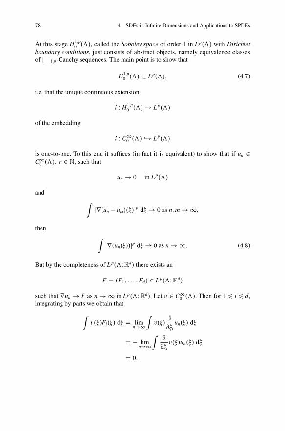
78 4 SDEs in Infinite Dimensions and Applications to SPDEs
At this stage H1;p0 .ƒ/, called the Sobolev space of order 1 in L p.ƒ/ with Dirichlet
boundary conditions, just consists of abstract objects, namely equivalence classesof k k1;p-Cauchy sequences. The main point is to show that
H1;p0 .ƒ/ � L p.ƒ/; (4.7)
i.e. that the unique continuous extension
Ni W H1;p0 .ƒ/ ! L p.ƒ/
of the embedding
i W C10 .ƒ/ ,! L p.ƒ/
is one-to-one. To this end it suffices (in fact it is equivalent) to show that if un 2C10 .ƒ/; n 2 N; such that
un ! 0 in L p.ƒ/
andZ
jr.un � um/.�/jp d� ! 0 as n;m ! 1;
thenZ
jr.un.�//jp d� ! 0 as n ! 1: (4.8)
But by the completeness of L p.ƒIRd/ there exists an
F D .F1; : : : ;Fd/ 2 L p.ƒIRd/
such that run ! F as n ! 1 in L p.ƒIRd/. Let v 2 C10 .ƒ/. Then for 1 6 i 6 d,
integrating by parts we obtain that
Zv.�/Fi.�/ d� D lim
n!1
Zv.�/
@
@�iun.�/ d�
D � limn!1
Z@
@�iv.�/un.�/ d�
D 0:

4.1 Gelfand Triples, Conditions on the Coefficients and Examples 79
Hence Fi D 0 d�-a.e. for all 1 6 i 6 d, so (4.8) holds.Consider the operator
r W C10 .ƒ/ � L p.ƒ/ ! L p.ƒIRd/:
By what we have shown above, we can extend r to all of H1;p0 .ƒ/ as follows. Let
u 2 H1;p0 .ƒ/ and let un 2 C1
0 .ƒ/ such that limn!1ku � unk1;p D 0. In particular,.run/n2N is a Cauchy sequence in L p.ƒIRd/, hence has a limit there. So, define
ru WD limn!1 run in L p.ƒIRd/: (4.9)
By what we have shown above this limit only depends on u and not on the chosensequence. We recall the fact that H1;p
0 .ƒ/ is reflexive for all p 2 �1;1Œ (cf. [82]).
Example 4.1.7 (H1;20 � L2 � .H1;2
0 /�; A D �) Though later we shall see that to
have (H3) we have to take p D 2, we shall first consider p 2 Œ2;1Œ and define
V WD H1;p0 .ƒ/;H WD L2.ƒ/;
so
V� WD H1;p0 .ƒ/
�:
Again we assume (4.4) to hold if p > 2. Since then V � L p.ƒ/ � H, continuouslyand densely, identifying H with its dual we obtain the continuous and denseembeddings
V � H � V�
or concretely
H1;p0 .ƒ/ � L2.ƒ/ � H1;p
0 .ƒ/�: (4.10)
Now we are going to extend � with initial domain C10 .ƒ/ to a bounded linear
operator A W V ! V�. First of all we can consider� as an operator taking values inV� since
� W C10 .ƒ/ ! C1
0 .ƒ/ � L2.ƒ/ � V�:
Furthermore, for u; v 2 C10 .ƒ/ again integrating by parts we obtain
ˇV�
h�u; viV
ˇ D jh�u; viHj
Dˇˇ�Z
hru.�/;rv.�/i d�
ˇˇ

80 4 SDEs in Infinite Dimensions and Applications to SPDEs
6�Z
jru.�/j pp�1 d�
� p�1p�Z
jrv.�/jp d�
� 1p
6�Z
jru.�/j pp�1 d�
� p�1p
kvk1;p:
Hence for all u 2 C10 .ƒ/
k�ukV� 6 kjrujk pp�1: (4.11)
So, by (4.4) and since pp�1 6 2 6 p, we get by Hölder’s inequality
k�ukV� 6 jƒj p�2p kuk1;p for all u 2 C1
0 .ƒ/; (4.12)
where for p D 2 the factor on the right is just equal to 1.So, � with domain C1
0 .ƒ/ extends (uniquely) to a bounded linear operator A WV ! V� (with domain all of V), also denoted by�.
Now let us check (H1)–(H4) for A.
Claim
A.D �/ W H1;p0 .ƒ/ !
H1;p0 .ƒ/
�
satisfies (H1),(H2),(H4) and provided p D 2, also (H3).
Proof Since A W V ! V� is linear, (H1) is obviously satisfied. Furthermore, ifu; v 2 V then there exist un; vn 2 C1
0 .ƒ/; n 2 N; such that un ! u; vn ! v asn ! 1 in V . Hence, integrating by parts, we get
V�
hA.u/� A.v/; u � viV D limn!1 V�
h�un ��vn; un � vniV
D limn!1h�.un � vn/; un � vniH
D � limn!1
Zjr.un � vn/.�/j2 d� 6 0:
So (H2) is satisfied. Furthermore,
2 V�
hA.v/; viV D limn!1 2h�vn; vniH
D � limn!1 2
Zjrvn.�/j2 d�
D �2Z
jrv.�/j2 d�
D 2�kvk2H � kvk21;2
�:

4.1 Gelfand Triples, Conditions on the Coefficients and Examples 81
So (H3) is satisfied if p D 2 with ˛ D 2. Furthermore, (H4), with ˛ D 2, is clear by(4.12). utRemark 4.1.8 The corresponding SDE (4.3) then reads
dX.t/ D �X.t/ dt C B.t;X.t// dW.t/:
If B � 0, this is just the classical heat equation. If B 6� 0, but constant, the solutionis an Ornstein–Uhlenbeck process on H.
Example 4.1.9 (H1;p0 � L2 � .H1;p
0 /�, A D p-Laplacian) Hence the stochastic
differential equation (4.3) becomes
dX.t/ D div�jrX.t/jp�2rX.t/
�dt C B.t;X.t// dW.t/:
Again we take p 2 Œ2;1Œ, ƒ � Rd, ƒ open and bounded, and V WD H1;p
0 .ƒ/,H WD L2.ƒ/, so V� D .H1;p
0 .ƒ//�. Define A W H1;p
0 .ƒ/ ! H1;p0 .ƒ/
� by
A.u/ WD div.jrujp�2ru/; u 2 H1;p0 .ƒ/I
more precisely, given u 2 H1;p0 .ƒ/ for all v 2 H1;p
0 .ƒ/
V�
hA.u/; viV WD �Z
jru.�/jp�2hru.�/;rv.�/i d� for all v 2 H1;p0 .ƒ/:
(4.13)
A is called the p-Laplacian, also denoted by �p. Note that �2 D �. To show thatA W V ! V� is well-defined we have to show that the right-hand side of (4.13)defines a linear functional in v 2 V which is continuous with respect to k kV Dk k1;p. First we recall that by (4.9) ru 2 L p.ƒIRd/ for all u 2 H1;p
0 .ƒ/. Hence byHölder’s inequality
Zjru.�/jp�1jrv.�/j d� 6
�Zjru.�/jp d�
� p�1p�Z
jrv.�/jp d�
� 1p
6 kukp�11;p kvk1;p:
Since this dominates the absolute value of the right-hand side of (4.13) for all u 2H1;p0 .ƒ/ we have that A.u/ is a well-defined element of .H1;p
0 .ƒ//� and that
kA.u/kV� 6 kukp�1V : (4.14)
Now we are going to check that A satisfies (H1)–(H4).

82 4 SDEs in Infinite Dimensions and Applications to SPDEs
(H1) Let u; v; x 2 H1;p0 .ƒ/, then by (4.13) we have to show for 2 R; jj 6 1
lim!0
Z jr.u C v/.�/jp�2hr.u C v/.�/;rx.�/i
� jru.�/jp�2hru.�/;rx.�/i
d� D 0:
Since obviously the integrands converge to zero as ! 0 d�-a.e., weonly have to find a dominating function to apply Lebesgue’s dominatedconvergence theorem. But obviously, since jj 6 1
jr.u C v/.�/jp�2jhr.u C v/.�/;rx.�/ij62p�2 �jru.�/jp�1 C jrv.�/jp�1� jrx.�/j
and the right-hand side is in L1.ƒ/ by Hölder’s inequality as we have seenabove.
(H2) Let u; v 2 H1;p0 .ƒ/. Then by (4.13)
� V�
hA.u/� A.v/; u � viV
DZ
hjru.�/jp�2ru.�/ � jrv.�/jp�2rv.�/;ru.�/ � rv.�/i d�
DZ.jru.�/jp C jrv.�/jp � jru.�/jp�2hru.�/;rv.�/i
� jrv.�/jp�2hru.�/;rv.�/i/ d�
>Z.jru.�/jp C jrv.�/jp � jru.�/jp�1jrv.�/j
� jrv.�/jp�1jru.�/j/ d�
DZ.jru.�/jp�1 � jrv.�/jp�1/.jru.�/j � jrv.�/j/ d�
> 0;
since the map RC 3 s 7! sp�1 is increasing. Hence (H2) is shown with c D 0.(H3) Because ƒ is bounded by Poincaré’s inequality (cf. [39]) there exists a
constant c D c.p; d; jƒj/ 2�0;1Œ such that
Zjru.�/jp d� > c
Zju.�/jp d� for all u 2 H1;p
0 .ƒ/: (4.15)

4.1 Gelfand Triples, Conditions on the Coefficients and Examples 83
Hence by (4.13) for all u 2 H1;p0 .ƒ/
V�
hA.u/; uiV D �Z
jru.�/jp d� 6 �min.1; c/
2kukp
1;p:
So, (H3) holds with ˛ D p and c1 D 0. (We note that only for (H3) have weused that ƒ is bounded.)
(H4) This condition holds for A by (4.14) with ˛ D p.
Before we go on to our last example, which will include the case of the porousmedium equation, we would like to stress the following:
Remark 4.1.10
1. If one is given V � H � V� and A W V ! V� (e.g. as in the above examples)satisfying (H1)–(H4) (with B � 0) one can consider a “smaller” space V0, i.e.another reflexive separable Banach space such that
V0 � V
continuously and densely, hence (by restricting the linear functionals to V0)
V� � V�0
continuously and densely, so altogether
V0 � V � H � V� � V�0 :
Restricting A to V0 we see that A satisfies (H1),(H2) and (H4) with respect to theGelfand triple
V0 � H � V�0 :
However, since k kV0 is up to a multiplicative constant larger than k kV , property(H3) might no longer hold. Therefore, e.g. if one considers a map A whichis given by a sum of the Laplacian (cf. Example 4.1.7) and a monomial (cf.Example 4.1.5) one cannot just take any V0 � H1;2
0 .ƒ/ \ L p.ƒ/, since (H3)might get lost.
In the case of the p-Laplacian, p 2 Œ2;1Œ, it is possible to add monomials oforder p, since H1;p
0 .ƒ/ � L p.ƒ/ continuously and densely, so
A.u/ WD div.jrujp�2ru/� ujujp�2; u 2 H1;p0 .ƒ/;
satisfies (H1)–(H4), if ƒ is bounded, with respect to the Gelfand triple
H1;p0 .ƒ/ � L2.ƒ/ � .H1;p
0 .ƒ//�:

84 4 SDEs in Infinite Dimensions and Applications to SPDEs
But generally, taking sums of A as above requires some care and is not alwayspossible.
2. In all our analysis the space V� is only used as a tool. Eventually, since thesolutions to our SDE (4.3) will take values in H; V� will be of no relevance.Therefore, no further information about V� such as its explicit representation(e.g. as a space of Schwartz distributions) is necessary.
Example 4.1.11 [L p � .H1;20 /
� � .L p/�, A D porous medium operator] Thestochastic differential equation (4.3) becomes
dX.t/ D �‰.X.t// dt C B.t;X.t// dW.t/:
As references for this example we refer to [4, 25, 69].Let ƒ � R
d, ƒ open and bounded, p 2 Œ2;1Œ and
V WD L p.ƒ/; H WD .H1;20 .ƒ//
�:
Since ƒ is bounded we have by Poincaré’s inequality (4.15) that for some constantc D c.2; d; jƒj/ > 0
kuk1;2 > kukH1;20
WD�Z
jru.�/j2 d�
� 12
>�
min.1; c/
2
� 12
kuk1;2 for all u 2 H1;20 .ƒ/: (4.16)
So, we can (and will do so below) consider H1;20 .ƒ/ with norm k kH1;2
0and
corresponding scalar product
hu; viH1;20
WDZ
hru.�/;rv.�/i d�; u; v 2 H1;20 .ƒ/:
Since H1;20 .ƒ/ � L2.ƒ/ continuously and densely, so is
H1;20 .ƒ/ � L
pp�1 .ƒ/:
Hence
L p.ƒ/ �
Lp
p�1 .ƒ/� � .H1;2
0 .ƒ//� D H;
continuously and densely. Now we would like to identify H with its dual H� DH1;20 .ƒ/ via the corresponding Riesz isomorphism R W H ! H� defined by Rx WD
hx; �iH; x 2 H: Let us calculate the latter.

4.1 Gelfand Triples, Conditions on the Coefficients and Examples 85
Lemma 4.1.12 The map � W H1;20 .ƒ/ ! .H1;2
0 .ƒ//� D H (defined by (4.13) for
p D 2) is an isometric isomorphism. In particular,
h�u; �viH D hu; viH1;20
for all u; v 2 H1;20 .ƒ/: (4.17)
Furthermore, .��/�1 W H ! H� D H1;20 .ƒ/ is the Riesz isomorphism for H, i.e.
for every x 2 H
hx; �iH D H1;20
h.��/�1x; �iH : (4.18)
Proof Let u 2 H1;20 .ƒ/. Since by (4.13) for all v 2 H1;2
0 .ƒ/
Hh��u; viH1;20
DZ
hru.�/;rv.�/i d� D hu; viH1;20; (4.19)
it follows that �� W H1;20 .ƒ/ ! H is just the Riesz isomorphism for H1;2
0 .ƒ/ andthe first part of the assertion including (4.17) follows. To prove the last part, fixx 2 H. Then by (4.17) and (4.19) for all y 2 H
hx; yiH D h.��/�1x; .��/�1yiH1;20
D Hhx; .��/�1yiH1;20:
utNow we identify H with its dual H� by the Riesz map .��/�1 W H ! H�, so
H � H� in this sense, hence
V D L p.ƒ/ � H � .L p.ƒ//� D V� (4.20)
continuously and densely.
Lemma 4.1.13 The map
� W H1;20 .ƒ/ ! .L p.ƒ//�
extends to a linear isometry
� W Lp
p�1 .ƒ/ ! .L p.ƒ//� D V�
and for all u 2 Lp
p�1 .ƒ/; v 2 L p.ƒ/
V�
h��u; viV DL
pp�1
hu; viL p DZ
u.�/v.�/ d�: (4.21)
Remark 4.1.14 One can prove that this isometry is in fact surjective, hence
.L p.ƒ//� D �.Lp
p�1 / ¤ Lp
p�1 :

86 4 SDEs in Infinite Dimensions and Applications to SPDEs
We shall not use this below, but it shows that the embedding (4.20) has to be handledwith care, always taking into account that H is identified with H� by .��/�1 W H !H�, giving rise to a different dualization between L p.ƒ/ and .L p.ƒ//�. In particular,for all x 2 H; v 2 L p.ƒ/
.L p/�hx; viL p D hx; viH
�¤
Lp
p�1hx; viL p D
Zx.�/v.�/ d� provided x 2 L
pp�1
�:
Proof of Lemma 4.1.13 Let u 2 H1;20 .ƒ/. Then since �u 2 H, by (4.2) and (4.18)
we obtain that for all v 2 V
V�
h�u; viV D h�u; viH D �H1;20
hu; viH D �hu; viL2 (4.22)
since v 2 V � L2.ƒ/. Therefore,
k�ukV� 6 kuk pp�1:
So, � extends to a continuous linear map
� W Lp
p�1 .ƒ/ ! V�
such that (4.22) holds for all u 2 Lp
p�1 .ƒ/, i.e. (4.21) is proved.So, applying it to u 2 L
pp�1 .ƒ/ and
v WD �kuk� qp
q ujujq�2 2 L p.ƒ/;
where q WD pp�1 , by (4.21) we obtain that
V�
h�u; viV D kuk pp�1
and kvkp D 1, so k�ukV� D kuk pp�1
and the assertion is completely proved.ut
Now we want to define the “porous medium operator A”. So, let ‰ W R ! R bea function having the following properties:
.‰1/ ‰ is continuous.
.‰2/ For all s; t 2 R
.t � s/.‰.t/ �‰.s// > 0:

4.1 Gelfand Triples, Conditions on the Coefficients and Examples 87
.‰3/ There exist p 2 Œ2;1Œ; a 2 �0;1Œ; c 2 Œ0;1Œ such that for all s 2 R
s‰.s/ > ajsjp � c:
.‰4/ There exist c3; c4 2 �0;1Œ such that for all s 2 R
j‰.s/j 6 c4 C c3jsjp�1;
where p is as in .‰3/.
We note that .‰4/ implies that
‰.v/ 2 Lp
p�1 .ƒ/ for all v 2 L p.ƒ/: (4.23)
Now we can define the porous medium operator A W L p.ƒ/ D V ! V� D .L p.ƒ//�by
A.u/ WD �‰.u/; u 2 L p.ƒ/: (4.24)
Note that by Lemma 4.1.13 the operator A is well-defined. Now let us check (H1)–(H4).
(H1) Let u; v; x 2 V D L p.ƒ/ and 2 R. Then by (4.21)
V�
hA.u C v/; xiV D V�
h�‰.u C v/; xiV
D �Z‰.u.�/C v.�//x.�/ d�: (4.25)
By .‰4/ for jj 6 1 the integrand in the right-hand side of (4.25) is boundedby
Œc4 C c32p�2.jujp�1 C jvjp�1/�jxj
which by Hölder’s inequality is in L1.ƒ/. So, (H1) follows by (‰1) andLebesgue’s dominated convergence theorem.
(H2) Let u; v 2 V D L p.ƒ/. Then by (4.21)
V�
hA.u/� A.v/; u � v/iV D V�h�.‰.u/�‰.v//; u � viV
D �ZŒ‰.u.�// �‰.v.�//�.u.�/ � v.�// d�
6 0;
where we used .‰2/ in the last step.

88 4 SDEs in Infinite Dimensions and Applications to SPDEs
(H3) Let v 2 L p.ƒ/ D V . Then by (4.21) and .‰3/
V�
hA.v/; viV D �Z‰.v.�//v.�/ d�
6Z.�ajv.�/jp C c/ d�:
Hence (H3) is satisfied with c1 WD 0; c2 WD 2a; ˛ D p and f .t/ D 2cjƒj.(H4) Let v 2 L p.ƒ/ D V . Then by Lemma 4.1.13 and .‰4/
kA.v/kV� D k�‰.v/kV�
D k‰.v/kL
pp�1
6 c4jƒj p�1p C c3
�Zjv.�/jp d�
� p�1p
D c4jƒj p�1p C c3kvkp�1
V ;
so (H4) holds with ˛ D p.
Remark 4.1.15
1. For p 2 Œ2;1Œ and ‰.s/ WD sjsjp�2 we have
A.v/ D �.vjvjp�2/; v 2 L p.ƒ/;
which is the non-linear operator appearing in the classical porous mediumequation, i.e.
@X.t/
@tD �.X.t/jX.t/jp�2/; X.0; �/ D X0;
whose solution describes the time evolution of the density X.t/ of a substance ina porous medium (cf. e.g. [4]).
2. Let ‰ W R ! R be given such that .‰1/–.‰4/ are satisfied with some p 2 �1;1Œ
(in .‰3/, .‰4/). One can see that the above assumptions that ƒ is bounded andp > 2, can be avoided. But p then depends on the dimension of the underlyingspace R
d. Let us assume first that d > 3. We distinguish two cases:
Case 1. jƒj D 1 and p WD 2ddC2 , c D c4 D 0, where c; c4 are the constants in
.‰3/ and in .‰4/ respectively.Case 2. jƒj < 1 and p 2 � 2d
dC2 ;1�.
By the Sobolev embedding theorem (cf. [39, Theorem 7.10]) we have
H1;20 .ƒ/ � L
2dd�2 .ƒ/

4.2 The Main Result and An Itô Formula 89
continuously and densely, and
kuk 2dd�2
6 2.d � 1/pd.d � 2/
kukH1;20
for all u 2 H1;20 .ƒ/:
In Case 1 we have 2dd�2 D p
p�1 and in Case 2 (hence in both cases)
2d
d � 2> p
p � 1and thus
H1;20 .ƒ/ � L
pp�1 .ƒ/
densely and for some c0 2�0;1Œ
kuk pp�1
6 c0kukH1;20
for all u 2 H1;20 .ƒ/:
Now the above arguments generalize to both Cases 1 and 2, i.e. for the Gelfandtriple
V WD L p.ƒ/ � H WD .H1;20 .ƒ//
� � .L p.ƒ//�
the operator
A W L p.ƒ/ DW V ! V� D .L p.ƒ//�
defined in (4.24), satisfies (H1)–(H4).We note that in Case 1 the norm k kH1;2
0defined in (4.16) is in general not
equivalent to k k1;2, because the Poincaré inequality does not hold. In Case 1, ifd D 6, or in Case 2, if .3 6/d 6 6, we may take p D 3
2and
‰.s/ WD sign.s/p
jsj; s 2 R:
In this case the equation in Remark 4.1.15 is called fast diffusion equation. Forƒ bounded the above extends, of course, also to the case d D 1; 2 where evenstronger Sobolev embeddings hold (cf. [39, Theorems 7.10 and 7.15]).
4.2 The Main Result and An Itô Formula
Consider the general situation described at the beginning of the previous section.So, we have a Gelfand triple
V � H � V�

90 4 SDEs in Infinite Dimensions and Applications to SPDEs
and maps
A W Œ0;T� � V �� ! V�; B W Œ0;T� � V �� ! L2.U;H/
as specified there, satisfying (H1)–(H4), and consider the stochastic differentialequation
dX.t/ D A.t;X.t// dt C B.t;X.t// dW.t/ (4.26)
on H with W.t/; t 2 Œ0;T�, a cylindrical Q-Wiener process with Q WD I takingvalues in another separable Hilbert space .U; h ; iU/ and being defined on acomplete probability space .�;F ;P/ with normal filtration Ft; t 2 Œ0;T�.
Before we formulate our main existence and uniqueness result for solutions of(4.26) we have to define what we mean by “solution”.
Definition 4.2.1 A continuous H-valued (Ft)-adapted process .X.t//t2Œ0;T� is calleda solution of (4.26), if for its dt ˝ P-equivalence class OX we have OX 2 L˛.Œ0;T� ��; dt ˝ PI V/\ L2.Œ0;T� ��; dt ˝ PI H/ with ˛ as in (H3) and P-a.s.
X.t/ D X.0/CZ t
0
A.s; NX.s// ds CZ t
0
B.s; NX.s// dW.s/; t 2 Œ0;T�; (4.27)
where NX is any V-valued progressively measurable dt ˝ P-version of OX.
Remark 4.2.2
1. The existence of the special version NX above follows from Exercise 4.2.3 below.Furthermore, for technical reasons in Definition 4.2.1 and below we consider allprocesses initially as V�-valued, hence by dt ˝P-equivalence classes we alwaysmean classes of V�-valued processes.
2. The integral with respect to ds in (4.27) is initially a V�-valued Bochner integralwhich turns out to be in fact H-valued.
3. Solutions in the sense of Definition 4.2.1 are often called variational solutions inthe literature. There are various other notions of solutions for stochastic (partial)differential equations. We recall the definition of (probabilistically) weak andstrong solutions in Appendix E below. The notions of analytically weak andstrong solutions as well as the notion of mild solutions and their relations arerecalled in Appendix G below.
4. We stress that the solution .X.t//t2Œ0;T� from Definition 4.2.1 is in general not anH-valued semimartingale, since the first integral in the right-hand side of (4.27)is not necessarily of bounded variation in H. Therefore, the classical Itô-formulaon Hilbert spaces (see Sect. 6.1 below) does not apply to .X.t//t2Œ0;T�.
Exercise 4.2.3
1. Let BV�
1 denote the closed unit ball in V�. Since BV�
1 \ H ¤ ;, it has a countablesubset fliji 2 Ng, which is dense in BV�
1 \ H with respect to H-norm. Define

4.2 The Main Result and An Itô Formula 91
‚ W H ! Œ0;1� by
‚.h/ WD supi2N
jhli; hiHj; h 2 H:
Then ‚ is lower semicontinuous on H, hence B.H/-measurable. Since
V�
hli; viV D hli; viH ; i 2 N; v 2 V , we have
‚.v/ D kvkV for all v 2 V;
and furthermore (by the reflexivity of V)
f‚ < 1g D V:
2. Let X W Œ0;T��� ! H be any progressively measurable (i.e. B.Œ0; t�/˝Ft=B.H/-measurable for all t 2 Œ0;T�/ dt ˝ P-version of OX 2 L˛.Œ0;T� � �; dt ˝PI V/; ˛ 2�0;1Œ. Then
NX WD If‚ıX<1gX
is a V-valued progressively measurable (i.e. B.Œ0; t�/ ˝ Ft=B.V/-measurable)dt ˝ P-version of OX.
3. Both A.�; NX/ and B.�; NX/ are V�-valued respectively L2.U;H/-valued progres-sively measurable processes.
Now the main result (cf. [54]):
Theorem 4.2.4 Let A;B be as above satisfying (H1)–(H4) and letX0 2 L2.�;F0;PI H/. Then there exists a unique solution X to (4.26) in thesense of Definition 4.2.1. Moreover,
E. supt2Œ0;T�
kX.t/k2H/ < 1: (4.28)
The proof of Theorem 4.2.4 strongly depends on the following Itô formula, from[54, Theorem I.3.1], which we shall prove here first. The presentation of its proofand that of Theorem 4.2.4 is an extended adaptation of those in [69].
Theorem 4.2.5 Let ˛ 2�1;1Œ; X0 2 L2.�;F0;PI H/ and Y 2 L˛
˛�1 .Œ0;T� ��; dt ˝ PI V�/; Z 2 L2.Œ0;T� � �; dt ˝ PI L2.U;H//; both progressivelymeasurable. Define the continuous V�-valued process
X.t/ WD X0 CZ t
0
Y.s/ ds CZ t
0
Z.s/ dW.s/; t 2 Œ0;T�:
If for its dt ˝ P-equivalence class OX we have OX 2 L˛.Œ0;T� ��; dt ˝ PI V/ and ifE.kX.t/k2H/ < 1 for dt-a.e. t 2 Œ0;T� (which is automatically the case if ˛ > 2),

92 4 SDEs in Infinite Dimensions and Applications to SPDEs
then X is a continuous H-valued .Ft/-adapted process,
E
sup
t2Œ0;T�kX.t/k2H
!6 4
�E�kX.0/k2H
�C kYkK� .kXkK C 1/
C 10 E
�Z T
0
kZ.s/k2L2.U;H/ ds
��(4.29)
and the following Itô-formula holds for the square of its H-norm P-a.s.
kX.t/k2H D kX0k2H CZ t
0
2 V�
hY.s/; NX.s/iV CkZ.s/k2L2.U;H/
ds
C 2
Z t
0
hX.s/;Z.s/ dW.s/iH for all t 2 Œ0;T� (4.30)
for any V-valued progressively measurable dt ˝ P-version NX of OX.
As in [54] for the proof of Theorem 4.2.5 we need the following lemmaabout piecewise constant approximations based on an argument due to [29]. Forabbreviation below we set
K WD L˛.Œ0;T� ��; dt ˝ PI V/: (4.31)
Lemma 4.2.6 Let X W Œ0;T� �� ! V� be B.Œ0;T�/˝ F=B.V�/-measurable suchthat for its dt ˝P-equivalence class OX we have OX 2 K. Then there exists a sequenceof partitions Il WD f0 D tl
0 < tl1 < � � � < tl
klD Tg such that Il � IlC1 and
ı.Il/ WD maxi.tli �tl
i�1/ ! 0 as l ! 1, X.tli/ 2 V P-a.e. for all l 2 N; 1 i kl�1;
and for
NXl WDklX
iD21Œtli�1;t
li ŒX.tl
i�1/; QXl WDkl�1XiD1
1Œtli�1;tli ŒX.tl
i/; l 2 N;
we have that NXl; QXl are ( dt ˝ P-versions of elements) in K such that
liml!1
˚k OX � NXlkK C k OX � QXlkK� D 0:
Proof For simplicity we assume that T D 1 and let NX W Œ0; 1��� ! V be a dt ˝ P-version of OX such that
R 10 k NX.t/k˛V dt < 1 P-a.s. We extend NX to R � � by setting
NX D 0 on Œ0; 1�c � �. There exists an �0 2 F with full probability such that forevery ! 2 �0 there exists a sequence . fn/n2N � C.RI V/ with compact support suchthat
ZR
k fn.s/ � NX.s; !/k˛V ds 1
2n; n 2 N:

4.2 The Main Result and An Itô Formula 93
Thus, for every n 2 N;
lim supı!0
ZR
k NX.ı C s; !/ � NX.s; !/k˛V ds
3˛�1 lim supı!0
ZR
�k NX.ı C s; !/ � fn.ı C s/k˛V C k NX.s; !/ � fn.s/k˛V�
ds
3˛�1
n; n 2 N:
Here we used that since each fn is uniformly continuous, by Lebesgue’s dominatedconvergence theorem we have that for all n 2 N
limı!0
ZR
kfn.ı C s/� fn.s/k˛V ds D 0:
Letting n ! 1 we obtain
limı!0
ZR
k NX.ı C s; !/ � NX.s; !/k˛V ds D 0; ! 2 �0: (4.32)
Now, given t 2 R, let Œt� denote the largest integer t. Let �n.t/ WD 2�nŒ2nt�; n 2 N;
that is, �n.t/ is the largest number of the form k2n ; k 2 Z, less or equal to t. Shifting
the integral in (4.32) by t and taking ı D �n.t/ � t we obtain
limn!1
ZR
k NX.�n.t/C s/ � NX.t C s/k˛V ds D 0 on �0:
Moreover, since NX.r/ D 0 for all r 2 RnŒ0; 1�,Z 1
0
k NX.�n.t/C s/ � NX.t C s/k˛V ds
1Œ�2;2�.t/2˛�1ZR
�k NX.�n.t/C s/k˛V C k NX.t C s/k˛V�
ds
D 2˛1Œ�2;2�.t/Z 1
0
k NX.s/k˛V ds on �0:
So, by Lebesgue’s dominated convergence theorem, we obtain that
0 D limn!1 E
ZR
dtZ 1
0
k NX.�n.t/C s/ � NX.t C s/k˛V ds
� limn!1 E
Z 1
0
dsZ 1
0
k NX.�n.t � s/C s/� NX.t/k˛V dt: (4.33)

94 4 SDEs in Infinite Dimensions and Applications to SPDEs
Given s 2 Œ0; 1Œ and n 2 N, let the partition In.s/ be defined by
tn0.s/ WD 0; tn
i .s/ WD
s � Œ2ns�
2n
C i � 1
2n; 1 i 2n; tn
2nC1.s/ WD 1:
Then, for t 2 Œtni�1.s/; tn
i .s/Œ, 2 6 i 6 2n C 1, one has t � s 2 Œ2�n.i � Œ2ns� �2/; 2�n.i � Œ2ns� � 1/Œ and hence,
�n.t � s/C s D 2�n.i � Œ2ns� � 2/C s D tni�1.s/; 2 i 2n C 1:
Therefore, (4.33) implies
limn!1 E
Z 1
0
dsZ 1
0
k NX.t/ � NXn;s.t/k˛V dt D 0;
where NXn;s is the process defined as NXl for the partition In.s/ but with X.tli�1.s//
replaced by NX.tli�1.s//. Similarly, the same holds for QXn;s in place of NXn;s by using
Q�n WD �n C 2�n instead of �n, where QXn;s is defined as QXl for the partition In.s/ butwith X.tl
i.s// replaced by NX.tli.s//. Hence, there exist a subsequence nk ! 1 and a
ds-zero set N1 2 B.Œ0; 1�/ such that
limk!1 E
Z 1
0
�k NX.t/ � NXnk ;s.t/k˛V C k NX.t/ � QXnk;s.t/k˛V�
dt D 0; s 2 Œ0; 1� n N1:
In particular, NXnk;s and QXnk;s are ( dt ˝ P-versions of elements) in K. Since for1 i 2n the maps s 7! tn
i .s/ are piecewise C1-diffeomorphisms, the imagemeasures of ds under these maps are absolutely continuous with respect to ds.Therefore, since NX D X ds ˝ P-a.e., there exists a ds-zero set N2 2 B.Œ0; 1�/ suchthat
NX.tni .s// D X.tn
i .s// P-a.e. for all s 2 Œ0; 1� n N2; 1 i 2n:
Therefore, fixing s 2 Œ0; 1Œn.N1 [ N2/, the sequence of the corresponding partitionsInl.s/; l � 1, has all properties of the assertion. utRemark 4.2.7
(i) As follows from the above proof all the partition points tli; l � 1; 1 i
kl � 1; in the assertion of Lemma 4.2.6 can be chosen outside an a priori givenLebesgue zero set in Œ0;T� instead of N2 above.
(ii) Tracing through the proof of Lemma 4.2.6 one sees that it also holds if wereplace K by the following space
K0 WD L˛W.Œ0;T� ��; dt ˝ PI V/ \ L2W.Œ0;T� ��; dt ˝ PI H/;

4.2 The Main Result and An Itô Formula 95
equipped with the sum of the two respective norms, where we adopt thestandard notation of a subscript W for the subspace of those elements whichpossess an .Ft/-adapted dt ˝ P-version.
Proof of Theorem 4.2.5 Since M.t/ WD R t0
Z.s/ dW.s/, t 2 Œ0;T�, is already acontinuous martingale on H and since Y 2 K� D L˛=.˛�1/.Œ0;T��� ! V�I dt˝P/is progressively measurable,
R t0
Y.s/ ds is a continuous adapted process on V�. Thus,X is a continuous adapted process on V�, hence B.Œ0;T�/˝ F=B.V�/-measurable.
Claim (a):
kX.t/k2H DkX.s/k2H C 2
Z t
sV�
hY.r/;X.t/iV dr C 2hX.s/;M.t/� M.s/iH
C kM.t/ � M.s/k2H � kX.t/ � X.s/� M.t/C M.s/k2H (4.34)
holds for all t > s such that X.t/;X.s/ 2 V:Indeed, this follows immediately by noting that
kM.t/ � M.s/k2H � kX.t/� X.s/� M.t/C M.s/k2HC 2hX.s/;M.t/� M.s/iH
D 2hX.t/;M.t/� M.s/iH � kX.t/ � X.s/k2HD 2hX.t/;X.t/� X.s/iH � 2
Z t
sV�hY.r/;X.t/iV dr
� kX.t/k2H � kX.s/k2H C 2hX.t/;X.s/iH
D kX.t/k2H � kX.s/k2H � 2Z t
sV�hY.r/;X.t/iV dr:
Claim (b): We have
E
�sup
t2Œ0;T�kX.t/k2H
�< 1: (4.35)
To prove the claim let Il; l 2 N, be a sequence of partitions as in Lemma 4.2.6. ByRemark 4.2.7(i) and the assumption that E.kX.t/k2H/ < 1 for dt-a.e. t 2 Œ0;T�we may choose Il such that
E.kX.t/k2H/ < 1 for all t 2[l2N
Il: (4.36)
Then by (4.34), for any t D tli 2 Il n f0;Tg
kX.t/k2H � kX0k2H

96 4 SDEs in Infinite Dimensions and Applications to SPDEs
Di�1XjD0.kX.tl
jC1/k2H � kX.tlj/k2H/
D 2
Z t
0V�
hY.s/; QXl.s/iV ds
C 2
Z t
0
h NXl.s/;Z.s/ dW.s/iH C 2hX.0/;Z tl1
0
Z.s/ dW.s/iH
Ci�1XjD0
�kM.tljC1/� M.tl
j/k2H � kX.tljC1/ � X.tl
j/ � M.tljC1/C M.tl
j/k2H�;
(4.37)
where NXl and QXl are defined as in Lemma 4.2.6. We note that since NXl is .Ft/-adapted and pathwise bounded the stochastic integral involving NXl above is well-defined. By Lemma 4.2.6
E
�Z T
0
j V�
hY.s/; QXl.s/iV j ds
� kYkK� k QXlkK c1 (4.38)
for some constant c1 > 0 independent of l: Moreover, by the Burkholder–Davisinequality (cf. Proposition D.0.1), Lemmas 2.4.2 and 2.4.4,
E
sup
t2Œ0;T�
ˇˇZ t
0
h NXl.s/;Z.s/ dW.s/iH
ˇˇ!
63E
�Z T
0
kZ.s/� NXl.s/k2U ds
�1=2!
63E
�Z T
0
k NXl.s/k2HkZ.s/k2L2.U;H/ ds
�1=2!
D3E
�Z T
0
k NXl.s/k2H dhMis
�1=2!
14
E
�sup
1�j�kl�1kX.tl
j/k2H�
C 9E�hMiT
�; (4.39)
since hMit D R t0
kZ.s/k2L2.U;H/ ds and we used that
ab 6 1
12a2 C 3b2; a; b > 0:

4.2 The Main Result and An Itô Formula 97
Here we note that by (4.36)
E
sup
1�j�kl�1kX.tl
j/k2H!< 1:
Finally, by Lemma 2.4.4
E
0@ i�1X
jD0kM.tl
jC1/� M.tlj/k2H
1A D
i�1XjD0
E
Z tljC1
tlj
kZ.s/k2L2.U;H/ ds
!
D E
Z tli
0
kZ.s/k2L2.U;H/ ds
!
D EhMitli
: (4.40)
Combining (4.37)–(4.40), we obtain
E
sup
t2IlnfTgkX.t/k2H
! c2
with c2 WD 4hE.kX.0/k2H/C kYkK� .kXkK C 1/C 10E.
R T0
kZ.s/k2L2.U;H/ ds/i.
Therefore, letting l " 1 and setting I WD [l�1Il nfTg;with Il as in Lemma 4.2.6,we obtain
E
�supt2I
kX.t/k2H�
6 c2;
since Il � IlC1 for all l 2 N. Since for all t 2 Œ0;T�NX
jD1V�
hX.t/; eji2V " kX.t/k2H as N " 1;
where fej
ˇj 2 Ng � V is an orthonormal basis of H and as usual for x 2 V� n H
we set kxkH WD 1, it follows that t 7! kX.t/kH is lower semicontinuous P-a.s.Since I is dense in Œ0;T�, we have supt2Œ0;T� kX.t/k2H D supt2I kX.t/k2H : Thus,(4.35) holds.
Claim (c):
liml!1 sup
t2Œ0;T�
ˇˇ Z t
0
hX.s/� NXl.s/;Z.s/ dW.s/iH
ˇˇ D 0 in probability. (4.41)

98 4 SDEs in Infinite Dimensions and Applications to SPDEs
We first note that because of (b) X is H-valued P-a.s. and by (b) and its continuityin V� the process X is weakly continuous in H P-a.s. and, therefore, since B.H/is generated by H�, progressively measurable as an H-valued process. Hence, forany n 2 N the process PnX is continuous in H so that
liml!1
Z T
0
kPn.X.s/� NXl.s//k2H dhMis D 0; P-a.s.
Here Pn denotes the orthogonal projection onto spanfe1; : : : ; eng in H. Therefore,applying Corollary D.0.2 we see that it suffices to show that for any " > 0;
limn!1 sup
l2NP
�sup
t2Œ0;T�
ˇˇ Z t
0
h.1� Pn/ NXl.s/;Z.s/ dW.s/iH
ˇˇ > "
�D 0;
limn!1 P
�sup
t2Œ0;T�
ˇˇ Z t
0
h.1� Pn/X.s/;Z.s/ dW.s/iH
ˇˇ > "
�D 0: (4.42)
For any n 2 N, ı 2 .0; 1/ and N > 1 by Lemma 2.4.2 and Corollary D.0.2 wehave that
P
�sup
t2Œ0;T�
ˇˇ Z t
0
h.1 � Pn/ NXl.s/;Z.s/ dW.s/iH
ˇˇ > "
�
3ı
"C P
�Z T
0
kZ.s/�.1 � Pn/. NXl.s//k2U ds > ı2�
3ı
"C P
sup
t2Œ0;T�kX.t/kH > N
C N2
ı2
Z T
0
k.1 � Pn/Z.s/k2L2.U;H/ ds:
By first letting n ! 1, and using Lebesgue’s dominated convergence theorem,and then letting N ! 1, and using Claim (b), and finally letting ı ! 0, weprove the first equality in (4.42). Similarly, the second equality is proved.
Claim (d): (4.30) holds for t 2 I:Fix t 2 I. We may assume that t ¤ 0: In this case for each sufficiently largel 2 N there exists a unique 0 < i < kl such that t D tl
i: We have X.tlj/ 2 V
a.s. for all j. By Lemma 4.2.6 and (4.41) the sum of the first three terms in theright-hand side of (4.37) converges in probability to 2
R t0 V�hY.s/; NX.s/iV ds C
2R t0hX.s/;Z.s/ dW.s/iH; as l ! 1. Hence by Lemma 2.4.4
kX.t/k2H � kX.0/k2HD2
Z t
0V�
hY.s/; NX.s/iV ds C 2
Z t
0
hX.s/;Z.s/ dW.s/iH C hMit � "0;

4.2 The Main Result and An Itô Formula 99
where
"0 WD P � liml!1
i�1XjD0
kX.tljC1/ � X.tl
j/� M.tljC1/C M.tl
j/k2H
exists and “P � lim” denotes limit in probability. So, to prove (4.30) for t asabove, it suffices to show that "0 D 0: Since for any ' 2 V ,
hX.tljC1/ � X.tl
j/� M.tljC1/C M.tl
j/; 'iH DZ tljC1
tlj
V�hY.s/; 'iV ds;
letting QMl and NMl be defined as QXl and NXl respectively, for M replacing X, weobtain for every n 2 N
"0 D P � liml!1
�Z t
0V�
hY.s/; QXl.s/ � NXl.s/ � Pn. QMl.s/ � NMl.s//iV ds
C hZ tl1
0
Y.s/ ds; X.0/iH �i�1XjD0
hX.tljC1/� X.tl
j/ � M.tljC1/
C M.tlj/; .1 � Pn/.M.t
ljC1/ � M.tl
j//iH
�:
The weak continuity of X in H implies that t 7! R t0
Y.s/ds is weakly continuousin H, since M is continuous in H. Hence the second term converges to zeroas l ! 1. Lemma 4.2.6 implies that
R t0 V�
hY.s/; QXl.s/ � NXl.s/iV ds ! 0
in probability as l ! 1. Moreover, since PnM.s/ is a continuous process inV ,R t0 V�
hY.s/;Pn. QMl.s/ � NMl.s//iV ds ! 0 P-a.s. as l ! 1. Thus, by theCauchy–Schwarz inequality, Lemmas 2.4.1 and 2.4.4
"0 P- liml!1
i�1XjD0
kX.tljC1/ � X.tl
j/ � M.tljC1/C M.tl
j/k2H 12
� i�1X
jD0k.1 � Pn/.M.t
ljC1/� M.tl
j//k2H 12
D "1=20
Z t
0
k.1 � Pn/Z.s/k2L2.U;H/ ds;
which goes to zero as n ! 1 again by Lebesgue’s dominated convergencetheorem. Therefore, "0 D 0:
Claim (e): (4.30) holds for all t 2 Œ0;T�nI.

100 4 SDEs in Infinite Dimensions and Applications to SPDEs
Take �0 2 F with full probability such that the limit in (4.41) is a pointwiselimit on �0 for some subsequence (denoted again by l ! 1) and (4.30) holdsfor all t 2 I on �0. If t … I, for any l 2 N there exists a unique j.l/ < kl suchthat t 2�tl
j.l/; tlj.l/C1�: Letting t.l/ WD tl
j.l/; we have t.l/ " t as l " 1: Using that
ku � vk2H D kuk2H � kvk2H � 2 V�
hu � v; viV for all u; v 2 V , by (4.30) for t 2 I,for all l > m we have on�0
kX.t.l// � X.t.m//k2H D kX.t.l//k2H � kX.t.m//k2H
� 2V�
hZ t.l/
t.m/Y.s/ ds C
Z t.l/
t.m/Z.s/ dW.s/; X.t.m//i
V
D 2
Z t.l/
t.m/V�
hY.s/; NX.s/� X.t.m//iV ds
C 2
Z t.l/
t.m/hX.s/�X.t.m//;Z.s/ dW.s/iHChMit.l/�hMit.m/
D 2
Z t.l/
t.m/V�
hY.s/; NX.s/� NXm.s/iV ds
C 2
Z t.l/
t.m/hX.s/� NXm.s/;Z.s/ dW.s/iHChMit.l/�hMit.m/;
(4.43)
where in the second equality we tacitly assumed that m is so big that t.m/ > 0.The second summand is dominated by
4 supt2Œ0;T�
ˇˇZ t
0
hX.s/� NXm.s/;Z.s/ dW.s/iH
ˇˇ :
Thus, by the continuity of hMit and (4.41) (holding pointwise on �0), we havethat
limm!1 sup
l>m
�2
ˇˇ Z T
0
1Œt.m/;t.l/�.s/h X.s/� NXm.s/;Z.s/ dW.s/iH
ˇˇ
C jhMit.l/ � hMit.m/j�
D 0 (4.44)
holding on �0. Furthermore, by Lemma 4.2.6, selecting another subsequence ifnecessary, we have for some �00 2 F with full probability and�00 � �0; that on�00
limm!1
Z T
0
j V�
hY.s/; NX.s/ � NXm.s/iV j ds D 0:

4.2 The Main Result and An Itô Formula 101
Since
supl>m
Z t.l/
t.m/j V�
hY.s/; NX.s/ � NXm.s/iV j ds
Z T
0
j V�
hY.s/; NX.s/ � NXm.s/iV j ds;
we have that on �00
limm!1 sup
l>m
Z t.l/
t.m/V�
hY.s/; NX.s/ � NXm.s/iV ds D 0:
Combining this with (4.43) and (4.44), we conclude that
limm!1 sup
l�mkX.t.l// � X.t.m//k2H D 0
holds on �00: Thus, .X.t.l///l2N converges in H on �00. Since we know thatX.t.l// ! X.t/ in V�, it converges to X.t/ strongly in H on �00. Therefore, since(4.30) holds on �00 for t.l/, letting l ! 1, we obtain (4.30) on �00 also for allt … I:
Claim (f): X is strongly continuous in H.Since the right-hand side of (4.30) is on �00 continuous in t 2 Œ0;T�; so must beits left-hand side, i.e. t 7! kX.t/kH is continuous on Œ0;T�: Therefore, the weakcontinuity of X.t/ in H implies its strong continuity in H. ut
Remark 4.2.8
(i) In the situation of Theorem 4.2.5 we have
E.kX.t/k2H/
DE.kX0k2H/CZ t
0
E.2 V�
hY.s/; NX.s/iV CkZ.s/k2L2.U;H// ds; t 2 Œ0;T�:(4.45)
Proof Let M.t/; t 2 Œ0;T�, denote the real valued local martingale in (4.30) and let�l; l 2 N, be .Ft/-stopping times such that M.t ^ �l/; t 2 Œ0;T�, is a martingale and�l " T as l ! 1. Then for all l 2 N; t 2 Œ0;T�, we have
E.kX.t ^ �l/k2H/
DE.kX0k2H/CZ t
0
E.1Œ0;�l�.s/Œ2 V�
hY.s/; NX.s/iV CkZ.s/k2L2.U;H/�/ ds: (4.46)

102 4 SDEs in Infinite Dimensions and Applications to SPDEs
Using Claim (b) from the proof of Theorem 4.2.5 and the fact that the integrandson the right-hand side of (4.45) are dt ˝ P-integrable we can apply Lebesgue’sdominated convergence theorem to obtain the assertion. ut(ii) We note that in (4.30) the stochastic integral is always a (global) martingale.
This immediately follows from Proposition D.01(ii), since
E. supt2Œ0;T�
kX.t/k2H/ < 1:
(iii) Suppose ˛ 2 .1; 2/. Then by Remark 4.2.7(ii) and by tracing through the proofof Theorem 4.2.5 one sees that the latter remains valid if we replace K by thespace K0 defined Remark 4.2.7(ii) and K� by K�
0 . The reason is that clearly
K�0 D L
˛˛�1
W .Œ0;T� ��; dt ˝ PI V�/C L2W.Œ0;T� ��I dt ˝ PI H/
� LqW.Œ0;T� ��; dt ˝ PI V�/ with q WD min.2;
˛
˛ � 1/:
Now we turn to the proof of Theorem 4.2.4. We first need some preparations. Letfeiji 2 Ng � V be an orthonormal basis of H and let Hn WD spanfe1; : : : ; eng suchthat spanfeiji 2 Ng is dense in V . Let Pn W V� ! Hn be defined by
Pny WDnX
iD1V�hy; eiiVei; y 2 V�: (4.47)
By (4.1.2), PnjH is just the orthogonal projection onto Hn in H. Furthermore,
V�
hz; PnyiV D V�
hy; PnziV for all y; z 2 V�,
and
V�
hPny; viV D V�
hy;PnviV for all y 2 V�; v 2 V .
Let fgiji 2 Ng be an orthonormal basis of U and set
W.n/.t/ WDnX
iD1hW.t/; giiU gi :
Here for g 2 U we define
hW.t/; giU WDtZ
0
hg; �iU dW.s/; t 2 Œ0;T�;

4.2 The Main Result and An Itô Formula 103
where the stochastic integral is well-defined by Sect. 2.5.2 with H WD R, since themap u 7! hg; uiU , u 2 U, is in L2.U;R/.
For each finite n 2 N we consider the following stochastic equation on Hn W
dX.n/.t/
DPnA.t;X.n/.t// dt C PnB.t;X.n/.t// dW.n/.t/; (4.48)
where X.n/.0/ WD PnX0: It is easily seen (cf. in particular Remark 4.1.1) that we arein the situation of Theorem 3.1.1 which implies that (4.48) has a unique continuousstrong solution. Let
J WD L2.Œ0;T� ��; dt ˝ PI L2.U;H//: (4.49)
To construct the solution to (4.26), we need the following lemma.
Lemma 4.2.9 Under the assumptions in Theorem 4.2.4, there exists a C 2 �0;1Œ
such that
kX.n/kK C kA.�;X.n//kK� C supt2Œ0;T�
EkX.n/.t/k2H C (4.50)
for all n 2 N.
Proof By the finite-dimensional Itô formula we have P-a.s.
kX.n/.t/k2H D kX.n/0 k2H CZ t
0
�2 V�
hA.s;X.n/.s//;X.n/.s/iV
C kZ.n/.s/k2L2.Un;H/
�ds C M.n/.t/; t 2 Œ0;T�;
where Z.n/.s/ WD PnB.s;X.n/.s//; Un WD span fe1; : : : ; eng and
M.n/.t/ WD 2
Z t
0
hX.n/.s/;PnB.s;X.n/.s// dW.n/.s/iH; t 2 Œ0;T�;
is a local martingale. Let �l; l 2 N; be .Ft/-stopping times such that kX.n/.t ^�l/.!/kV is bounded uniformly in .t; !/ 2 Œ0;T� � �, M.n/.t ^ �l/; t 2 Œ0;T�; is amartingale for each l 2 N and �l " T as l ! 1. Then for all l 2 N; t 2 Œ0;T�
E�kX.n/.t ^ �l/k2H
�
DE.kX.n/0 k2H/CZ t
0
E1Œ0;�l�.s/.2 V�
hA.s;X.n/.s//;X.n/.s/iV
C kZ.n/.s/k2L2.Un;H//
ds:

104 4 SDEs in Infinite Dimensions and Applications to SPDEs
Hence using the product rule we obtain
E.e�c1tkX.n/.t ^ �l/k2H/
D E.kX.n/0 k2H/CZ t
0
E.kX.n/.s ^ �l/k2H/ d.e�c1s/
CZ t
0
e�c1s d.E.kX.n/.s ^ �l/k2H//
D E.kX.n/0 k2H/ �Z t
0
c1E.kX.n/.s ^ �l/k2H/e�c1s ds
CZ t
0
e�c1sE1Œ0;�l �.s/.2 V�
hA.s;X.n/.s//;X.n/.s/iV
C kZ.n/.s/k2L2.Un;H//
ds: (4.51)
Applying (H3) we arrive at
E.e�c1tkX.n/.t ^ �l/k2H/CZ t
0
c1E.kX.n/.s ^ �l/k2H/e�c1s ds
C c2
Z t
0
E.1Œ0;�l�.s/kX.n/.s ^ �l/k˛V /e�c1s ds
6 E.kX.n/0 k2H/CZ t
0
c1E.kX.n/.s/k2H/e�c1s ds CZ T
0
E.jf .s/j/ ds;
where by the definition of �l; l 2 N, all terms are finite. Now taking l ! 1 andapplying Fatou’s lemma we get
E.e�c1tkX.n/.t/k2H/C c2E
�Z t
0
kX.n/.s/k˛V e�c1s ds
�
6E.kX.n/0 k2H/C E
�Z T
0
jf .s/j ds
�
for all t 2 Œ0;T�. Here we used that by (3.8) the subtracted term is finite. SincekX.n/0 kH 6 kX0kH , now the assertion follows for the first and third summand in(4.50). For the remaining summand the assertion then follows by (H4). utProof of Theorem 4.2.4 By the reflexivity of K, Lemma 4.2.9 and Remark 4.1.1,part 1, we have, for a subsequence nk ! 1:
(i) X.nk/ ! NX weakly in K and weakly in L2.Œ0;T� ��I dt ˝ PI H/:(ii) Y.nk/ WD A.�;X.nk// ! Y weakly in K�.

4.2 The Main Result and An Itô Formula 105
(iii) Z.nk/ WD B.�;X.nk// ! Z weakly in J and hence
Z �
0
Pnk B.s;X.nk/.s// dW.nk/.s/ !Z �
0
Z.s/ dW.s/
in M2T.H/ and, therefore, also weakly� in L1.Œ0;T�; dtI L2.�;PI H//
(equipped with the supremum norm).
Here the second part in (iii) follows since also Pnk B.�;X.nk// QPnk ! Z weakly in J,where QPn is the orthogonal projection onto spanfg1; � � � ; gng in U, since
Z �
0
Pnk B.s;X.nk/.s// dW.nk/.s/ DZ �
0
Pnk B.s;Xnk.s// QPnk dW.s/
and since a bounded linear operator between two Banach spaces is trivially weaklycontinuous. Since the approximants are progressively measurable, so are (the dt ˝P-versions) NX;Y and Z.
Thus from (4.48) for all v 2 Sn>1 Hn.� V/; ' 2 L1.Œ0;T� � �/ by Fubini’s
theorem we get
E
�Z T
0V�
h NX.t/; '.t/viV dt
�
D limk!1 E
�Z T
0V�
hX.nk/.t/; '.t/viV dt
�
D limk!1 E
�Z T
0V�
hX.nk/0 ; '.t/viV dt
CZ T
0
Z t
0V�
hPnk Y.nk/.s/; '.t/viV ds dt
CZ T
0
Z t
0
Pnk Z.nk/.s/ dW.nk/.s/; '.t/v
�H
dt
�
D limk!1
�E
�hX.nk/
0 ; viH
Z T
0
'.t/ dt
�
C E
�Z T
0 V�
hY.nk/.s/;Z T
s'.t/ dt vi
Vds
�
CZ T
0
E
� Z t
0
Z.nk/.s/ dW.nk/.s/; '.t/v
�H
�dt
�
D E
�Z T
0 V�
hX0 CZ t
0
Y.s/ ds CZ t
0
Z.s/ dW.s/; '.t/viV
dt
�:

106 4 SDEs in Infinite Dimensions and Applications to SPDEs
Therefore, defining
X.t/ WD X0 CZ t
0
Y.s/ ds CZ t
0
Z.s/ dW.s/; t 2 Œ0;T�; (4.52)
we have X D NX dt ˝ P-a.e.Now Theorem 4.2.5 applies to X in (4.52), so X is continuous in H and
E
�supt�T
kX.t/k2H�< 1:
Thus, it remains to verify that
B.�; NX/ D Z; A.�; NX/ D Y; dt ˝ P-a.e. (4.53)
To this end, we first note that for any nonnegative 2 L1.Œ0;T�; dtIR/ it followsfrom (i) that
E
�Z T
0
.t/k NX.t/k2H dt
�
D limk!1 E
�Z T
0
h .t/ NX.t/;X.nk/.t/iH dt
�
�
EZ T
0
.t/k NX.t/k2H dt
�1=2lim infk!1
�EZ T
0
.t/kX.nk/.t/k2H dt
�1=2< 1:
Since X D NX dt ˝ P-a.e., this implies
E
�Z T
0
.t/kX.t/k2H dt
� lim inf
k!1 E
�Z T
0
.t/kX.nk/.t/k2H dt
�: (4.54)
By (4.52) using Remark 4.2.8, the product rule and Fubini’s theorem we obtain that
E�e�ctkX.t/k2H
� � E�kX0k2H
�
D E
�Z t
0
e�cs�2 V�hY.s/; NX.s/iV C kZ.s/k2L2.U;H/ � ckX.s/k2H
�ds
�: (4.55)
Furthermore, for any � 2 K \ L2.Œ0;T� � �; dt ˝ PI H/, taking l ! 1 in (4.51)with c1 replaced by c and t ^ �l replaced by t, we obtain
E�e�ctkX.nk/.t/k2H
� � EkX.nk/
0 k2H
D E
�Z t
0
e�cs�2 V�hA.s;X.nk/.s//;X.nk/.s/iV

4.2 The Main Result and An Itô Formula 107
C kPnk B.s;X.nk/.s// QPnk k2L2.U;H/ � ckX.nk/.s/k2H�
ds
�
E
�Z t
0
e�cs�2 V�hA.s;X.nk/.s//;X.nk/.s/iV
C kB.s;X.nk/.s//k2L2.U;H/ � ckX.nk/.s/k2H�
ds
�
D E
�Z t
0
e�cs2 V�hA.s;X.nk/.s//� A.s; �.s//;X.nk/.s/ � �.s/iV
C kB.s;X.nk/.s//� B.s; �.s//k2L2.U;H/ � ckX.nk/.s/ � �.s/k2H
ds
C E
�Z t
0
e�cs2 V�hA.s; �.s//;X.nk/.s/iV
C 2 V�hA.s;X.nk/.s// � A.s; �.s//; �.s/iV
� kB.s; �.s//k2L2.U;H/ C 2hB.s;X.nk/.s//;B.s; �.s//iL2.U;H/
� 2chX.nk/.s/; �.s/iH C ck�.s/k2H
ds
�: (4.56)
Note that by (H2) the first of the two summands above is negative. Hence byletting k ! 1 we conclude by (i)–(iii), Fubini’s theorem, and (4.54) that for everynonnegative 2 L1.Œ0;T�; dtIR/
E
�Z T
0
.t/.e�ctkX.t/k2H � kX0k2H/ dt
�
E
�Z T
0
.t/
� Z t
0
e�csh2 V�hA.s; �.s//; NX.s/iV C 2 V�hY.s/
� A.s; �.s//; �.s/iV � kB.s; �.s//k2L2.U;H/ C 2hZ.s/;B.s; �.s//iL2.U;H/
� 2chX.s/; �.s/iH C ck�.s/k2Hi
ds
�dt
�:
Inserting (4.55) for the left-hand side and rearranging we arrive at
0 �E
�Z T
0
.t/
� Z t
0
e�cs�2 V�hY.s/ � A.s; �.s//; NX.s/ � �.s/iV
C kB.s; �.s//� Z.s/k2L2.U;H/ � ckX.s/� �.s/k2H�
ds
�dt
�: (4.57)
Taking � D NX we obtain from (4.57) that Z D B.�; NX/. Finally, first applying (4.57)to � D NX � " Q� v for " > 0 and Q� 2 L1.Œ0;T���; dt ˝ PIR/; v 2 V , then dividing

108 4 SDEs in Infinite Dimensions and Applications to SPDEs
both sides by " and letting " ! 0, by Lebesgue’s dominated convergence theorem,(H1) and (H4), we obtain
0 � E
�Z T
0
.t/
�Z t
0
e�cs Q�.s/ V�hY.s/ � A.s; NX.s//; viV ds
�dt
�:
By the arbitrariness of , Q� and v, we conclude that Y D A.�; NX/: This completesthe existence proof.
The uniqueness is a consequence of the following proposition. utProposition 4.2.10 Consider the situation of Theorem 4.2.4 and let X;Y be twosolutions. Then for c 2 R as in (H2)
E.kX.t/ � Y.t/k2H/ 6 ectE.kX.0/� Y.0/k2H/ for all t 2 Œ0;T�: (4.58)
Proof We first note that by our definition of solution (cf. Definition 4.2.1) and byRemark 4.1.1, part 1 we can apply Remark 4.2.8 to X � Y and the product rule toobtain for t 2 Œ0;T�
E.e�ctkX.t/ � Y.t/k2H/ D E.kX0 � Y0k2H/
CZ t
0
.E.2 V�
hA.s; NX.s// � A.s; NY.s//; NX.s/ � NY.s/iV
C kB.s; NX.s//� B.s; NY.s//k2L2.U;H/� cE.kX.s/� Y.s/k2H//e�cs ds
6 E.kX.0/� Y.0/k2H/;
where we used (H2) in the last step. Applying Gronwall’s lemma we obtain theassertion. utRemark 4.2.11 Let s 2 Œ0;T� and Xs 2 L2.�;Fs;PI H/. Consider the equation
X.t/ D Xs CZ t
sA.u; NX.u// du C
Z t
sB.u; NX.u// dW.u/; t 2 Œs;T� (4.59)
with underlying Wiener process W.t/ � W.s/; t 2 Œs;T�, and filtration .Ft/t>s, i.e.we just start our time at s. We define the notion of solution for (4.59) analogouslyto Definition 4.2.1. Then all results above in the case s D 0 carry over to this moregeneral case. In particular, there exists a unique solution with initial condition Xs
denoted by X.t; s;Xs/; t 2 Œs;T�. Let 0 6 r 6 s 6 T. Then for Xr 2 L2.�;Fr;PI H/
X.t; r;Xr/ D X.t; s;X.s; r;Xr//; t 2 Œs;T� P-a.e. (4.60)

4.3 Markov Property and Invariant Measures 109
Indeed, we have
X.t; r;Xr/ D Xr CZ t
rA.u; NX.u; r;Xr// du C
Z t
rB.u; NX.u; r;Xr// dW.u/
D X.s; r;Xr/CZ t
sA.u; NX.u; r;Xr// du
CZ t
sB.u; NX.u; r;Xr// dW.u/; t 2 Œs;T�:
But by definition X.t; s;X.s; r;Xr//; t 2 Œs;T�; satisfies the same equation. So, (4.60)follows by uniqueness. Furthermore, if for s 2 Œ0;T�; Xs D x for some x 2 Hand A and B are independent of ! 2 �, then by construction X.t; s; x/ obviouslyis independent of Fs for all t 2 Œs;T�, since so are collections of increments ofW.t/; t 2 Œs;T�.
4.3 Markov Property and Invariant Measures
Now we are going to prove some qualitative results about the solutions of (4.2.1) or(4.59) and about their transition probabilities, i.e. about
ps;t.x; dy/ WD P ı .X.t; s; x//�1. dy/; 0 6 s 6 t 6 T; x 2 H: (4.61)
As usual we set for B.H/-measurable F W H ! R, and t 2 Œs;T�; x 2 H
ps;tF.x/ WDZ
F.y/ps;t.x; dy/;
provided F is ps;t.x; dy/-integrable.
Remark 4.3.1 The measures ps;t.x; dy/; 0 6 s 6 t 6 T; x 2 H, could in principledepend on the chosen Wiener process and the respective filtration. However, theconstruction of our solutions X.t; s; x/; t 2 Œs;T�, suggests that this is not the case.This can be rigorously proved in several ways. It is, for example, a consequence ofthe famous Yamada–Watanabe theorem which is included in Appendix E below.
Proposition 4.3.2 Consider the situation of Theorem 4.2.4. Let F W H ! R beLipschitz with
Lip.F/ WD supx;y2H;x¤y
jF.x/� F.y/jkx � ykH
.< 1/

110 4 SDEs in Infinite Dimensions and Applications to SPDEs
denoting its Lipschitz constant. Then for all 0 6 s 6 t 6 T
ps;tjFj.x/ < 1 for all x 2 H
and for all x; y 2 H
jps;tF.x/� ps;tF.y/j 6 ec2 .t�s/Lip.F/ kx � ykH ; (4.62)
where c is as in (H2).
Proof Clearly, for all x 2 H
jF.x/j 6 jF.0/j C Lip.F/ kxkH ;
and thus for all 0 6 s 6 t 6 T
ps;tjFj.x/ D E.jFj.X.t; s; x///6 jF.0/j C Lip.F/ E.kX.t; s; x/kH/
6 jF.0/j C Lip.F/
E
sup
t2Œs;T�kX.t; s; x/k2H
!!1=2
< 1:
Furthermore, for x; y 2 H by (the “started at s” analogue of) (4.58)
jps;tF.x/� ps;tF.y/j 6 E.jF.X.t; s; x//� F.X.t; s; y///j/6 Lip.F/ E.kX.t; s; x/� X.t; s; y/kH/
6 Lip.F/ ec2 .t�s/kx � ykH :
utProposition 4.3.3 Consider the situation of Theorem 4.2.4 and, in addition, assumethat both A and B as well as f and g in (H3),(H4) respectively, are independent of! 2 �. Then any solution X.t/; t 2 Œr;T�, of (4.59) (with r replacing s) is Markovin the following sense:for every bounded, B.H/-measurable G W H ! R, and all s; t 2 Œr;T�; s 6 t
E.G.X.t//jFs/.!/ D E.G.X.t; s;X.s/.!//// for P-a.e. ! 2 �: (4.63)
Proof Let s; t 2 Œr;T�; s t. Then by Theorem E.0.8 in Appendix E there exists anF 2 OE as in Definition E.0.5 such that for P-a.e. ! 2 �
X.t/.!/ D FPıX.s/�1.X.s/.!/; QW.!//.t/

4.3 Markov Property and Invariant Measures 111
with QW WD W � W.s/ and W is defined by (2.12) as a Q1-Wiener process on U1.Then for every bounded, B.H/-measurable G W H ! R and P-a.e. ! 2 �
EŒG.X.t//jFs�.!/
DEŒG.FPıX.s/�1.X.s/.!/; QW/.t//�DEŒG.FıX.s/.!/.X.s/.!/; QW/.t//�DEŒG.X.t; s;X.s/.!///�;
where in the last equality we applied Theorem E.0.8 again and in the third equalitywe used the fact that by the definition of OE , for P ı X.s/�1-a.e. x 2 H
F�.x; � / D F.x; � / D Fıx.x; � / D PQ1-a.e.
utCorollary 4.3.4 Consider the situation of Proposition 4.3.3 and let 0 6 r 6 s 6t 6 T. Then we have (“Chapman–Kolmogorov equations”)
pr;sps;t D pr;t; (4.64)
i.e. for F W H ! R; bounded and B.H/-measurable, x 2 H,
pr;s.ps;tF/.x/ D pr;tF.x/:
Proof For F W H ! R as above and x 2 H by Proposition 4.3.3 we have
pr;s. ps;tF/.x/ D E.ps;tF.X.s; r; x/// DZ
E.F.X.t; s;X.s; r; x/.!////P. d!/
DZ
E.F.X.t; r; x//jFs/.!/P. d!/
D E.F.X.t; r; x/// D pr;tF.x/:
utNow let us assume that in the situation of Theorem 4.2.4 both A and B as well as
f and g in (H3), (H4) respectively are independent of .t; !/ 2 Œ0;T� � � (so theyparticularly hold for all T 2 Œ0;1Œ). Then again using the notation introduced inRemark 4.2.11 for 0 6 s 6 t < 1 and x 2 H we have
X.t; s; x/ D X QW.t � s; 0; x/ P-a.e., (4.65)

112 4 SDEs in Infinite Dimensions and Applications to SPDEs
where X QW.t; 0; x/; t 2 Œ0;1Œ; is the solution of
X.t/ D x CZ t
0
A. NX.u// du CZ t
0
B. NX.u// d QW.u/
and QW WD W.�C s/�W.s/ with filtration FsCu, u 2 Œ0;1Œ, which is again a Wienerprocess. To show this let us express the dependence of the solution X.t; s; x/; t 2Œs;1/ of (4.59) with Xs WD x on the Wiener process W by writing XW.t; s; x/ insteadof X.t; s; x/ and similarly, pW
s;t.s; dy/ instead of ps;t.x; dy/. Then, for all s; u 2 Œ0;1Œ
XW.u C s; s; x/
Dx CZ uCs
sA. NXW.u0; s; x// du0 C
Z t
sB. NXW.u0; s; x// dW.u0/
Dx CZ u
0
A. NXW.u0 C s; s; x// du0 CZ u
0
B. NXW.u0 C s; s; x// d QW.u0/:
So, by uniqueness the process XW.uCs; s; x/; u 2 Œ0;1Œ, must P-a.e. coincide withX QW.u; 0; x/; u 2 Œ0;1Œ, and (4.65) follows with u WD t � s. In particular, it followsthat
pWs;t.x; dy/ D P ı .X QW.t � s; 0; x//�1. dy/ D p QW
0;t�s.x; dy/ D pW0;t�s.x; dy/ (4.66)
(“time homogeneity”), where we used Remark 4.3.1 for the last equality.Defining
pt WD pW0;t; t 2 Œ0;1Œ;
equality (4.64) for r D 0 and s C t replacing t by (4.66) turns into
psCt D pspt for s; t 2 Œ0;1Œ: (4.67)
For x 2 H we define
Px WD P ı .X.�; 0; x//�1; (4.68)
i.e. Px is the distribution of the solution to (4.2.1) with initial condition x 2 H,defined as a measure on C.Œ0;1Œ;H/. We equip C.Œ0;1Œ;H/ with the �-algebra
G WD �.sjs 2 Œ0;1Œ/
and filtration
Gt WD �.sjs 2 Œ0; t�/; t 2 Œ0;1Œ;

4.3 Markov Property and Invariant Measures 113
where t.w/ WD w.t/ for w 2 C.Œ0;1Œ;H/; t 2 Œ0;1Œ.
Proposition 4.3.5 Consider the situation of Theorem 4.2.4 and, in addition, assumethat both A and B as well as f and g in (H3),(H4) respectively, are independent of.t; !/ 2 Œ0;T��� (so they particularly hold for all T 2 Œ0;1Œ). Then the followingassertions hold:
1. Px; x 2 H, form a time-homogenous Markov process on C.Œ0;1/;H/ withrespect to the filtration Gt; t 2 Œ0;1Œ, i.e. for all s; t 2 Œ0;1Œ; and all bounded,B.H/-measurable F W H ! R
Ex.F.tCs/jGs/ D Es.F.t// Px � a.e.; (4.69)
where Ex and Ex.�jGs/ denote expectation and conditional expectation withrespect to Px, respectively.
2. Suppose dim H < 1. If there exist �; f 2 �0;1Œ such that
2 V�
hA.v/; viV CkB.v/k2L2.U;H/ 6 ��kvk2H C f for all v 2 V; (4.70)
(“strict coercivity”) then there exists an invariant measure � for .pt/t>0, i.e. � isa probability measure on .H;B.H// such that
ZptF d� D
ZF d� for all t 2 Œ0;1Œ (4.71)
and all bounded, B.H/-measurable F W H ! R.
Proof
1. The right-hand side of (4.69) is Gs-measurable by Proposition 4.3.2 and amonotone class argument. So, let 0 6 t1 < t2 < : : : < tn 6 s and let G W Hn ! R
be bounded and ˝niD1B.H/-measurable. Then by (4.63) and (4.66)
Ex.G.t1 ; : : : ; tn/F.tCs//
D E.G.X.t1; 0; x/; : : : ;X.tn; 0; x//F.X.t C s; 0; x//
D E.G.X.t1; 0; x/; : : : ;X.tn; 0; x//E.F.X.t C s; 0; x//jFs//
DZ
G.X.t1; 0; x/.!/; : : : ;X.tn; 0; x/.!//
E.F.X.t C s; s;X.s; 0; x/.!////P.d!/
DZ
G.X.t1; 0; x/.!/; : : : ;X.tn; 0; x/.!//
E.F.X.t; 0;X.s; 0; x/.!////P. d!/
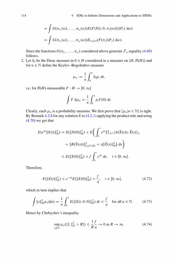
114 4 SDEs in Infinite Dimensions and Applications to SPDEs
DZ
G.t1 .!/; : : : ; tn.!//E.F.X.t; 0; s.!////Px. d!/
DZ
G.t1 .!/; : : : ; tn.!//Es.!/.F.t//Px. d!/:
Since the functions G.t1 ; : : : ; tn/ considered above generateFs, equality (4.69)follows.
2. Let ı0 be the Dirac measure in 0 2 H considered as a measure on .H;B.H// andfor n 2 N define the Krylov–Bogoliubov measure
�n WD 1
n
Z n
0
ı0pt dt;
i.e. for B.H/-measurable F W H ! Œ0;1Œ
ZF d�n D 1
n
Z n
0
ptF.0/ dt:
Clearly, each �n is a probability measure. We first prove that f�njn 2 Ng is tight.By Remark 4.2.8 for any solution X to (4.2.1) applying the product rule and using(4.70) we get that
E.e�tkX.t/k2H/ D E.kX.0/k2H/C E
�Z t
0
e�s�2 V�
hA. NX.s//; NX.s/iV
C kB. NX.s//k2L2.U;H/ C �k NX.s/k2H�
ds
�
6 E.kX.0/k2H/C fZ t
0
e�s ds; t 2 Œ0;1Œ:
Therefore,
E.kX.t/k2H/ 6 e��tE.kX.0/k2H/C f
�; t 2 Œ0;1Œ; (4.72)
which in turn implies that
Zkxk2H�n.dx/ D 1
n
Z n
0
E.kX.t; 0; 0/k2H/ dt 6 f
�for all n 2 N: (4.73)
Hence by Chebychev’s inequality
supn2N
�n.fk k2H > Rg/ 6 1
R
f
�! 0 as R ! 1: (4.74)

4.3 Markov Property and Invariant Measures 115
Since dim H < 1, the closed balls fk k2H 6 Rg; R 2 �0;1Œ, are compact. Henceby Prohorov’s theorem there exists a probability measure � and a subsequence.�nk /k2N such that �nk ! � weakly as k ! 1.
Now let us prove that � is invariant for .pt/t>0. So, let t 2 Œ0;1Œ and let F WH ! R be bounded and B.H/-measurable. By a monotone class argument wemay assume that F is Lipschitz continuous. Then ptF is bounded and (Lipschitz)continuous by Proposition 4.3.2. Hence using (4.67) for the third equality below,we obtain
ZptF d�
D limk!1
ZptF d�nk
D limk!1
1
nk
Z nk
0
ps.ptF/.0/ ds
D limk!1
1
nk
Z nk
0
psCtF.0/ ds
D limk!1
ZF d�nk C lim
k!11
nk
Z nkCt
nk
psF.0/ ds � limk!1
1
nk
Z t
0
psF.0/ ds
DZ
F d�; (4.75)
since jpsF.0/j 6 supx2H jF.x/j, so the second and third limits above are equal tozero. ut
Remark 4.3.6 If dim H D 1, the above proof of Proposition 4.3.5, part 2 works upto and including (4.74). However, since closed balls are no longer compact, one canapply Prohorov’s theorem only on a Hilbert space H1 into which H is compactlyembedded. So, let H1 be a separable Hilbert space such that H � H1 compactly anddensely (e.g. take H1 to be the completion of H in the norm
kxk1 WD" 1X
iD1˛ihx; eii2H
#1=2; x 2 H;
where ˛i 2 �0;1Œ;P1
iD1 ˛i < 1, and feiji 2 Ng is an orthonormal basis of H);extending the measures �n by zero to B.H1/ we obtain that f�njn 2 Ng is tighton H1. This extension of the measures is possible, since by Kuratowski’s theoremH 2 B.H1/ and B.H1/ \ H D B.H/. Hence by Prohorov’s theorem there exists aprobability measure N� on .H1;B.H1// and a subsequence .�nk /k2N such that �nk !N� weakly on H1 as k ! 1. As in Exercise 4.2.3, part 1 one constructs a lower

116 4 SDEs in Infinite Dimensions and Applications to SPDEs
semicontinuous function‚ W H1 ! Œ0;1� such that
‚ WD� k kH on H
C1 on H1nH:
Then (4.73) implies that for li; i 2 N, as in Example 4.2.3, part 1,
ZH1
‚2.x/ N�. dx/ D limN!1 lim
M!1
Zsupi6N
hli; xi2H1 ^ M N�. dx/
D supM;N2N
limk!1
Zsupi6N
hli; xi2H1 ^ M�nk . dx/
6 lim infk!1 sup
N;M2N
Zsupi6N
hli; xi2H1 ^ M �nk. dx/
D lim infk!1
ZH
kxk2H �nk . dx/
6 f
�:
Hence ‚ < 1 N�-a.e., so N�.H/ D 1. Therefore, � WD N�ˇB.H/ is a probabilitymeasure on .H;B.H//.
Unfortunately, the last part of the proof of Proposition 4.3.5, which shows that� is invariant, does not work. More precisely, for the first equality in (4.75) weneed that ptF is continuous with respect to the same topology with respect to which.�nk /k2N converges weakly, i.e. the topology on H1. This is, however, weaker thanthat on H. So, unless we can construct H1 in such a way that ptF has a continuousextension to H1, the first equality in (4.75) may not hold.
So far, we have taken a positive time s as the starting time for our SDE (seeRemark 4.2.11). In the case of coefficients independent of t and !, it is also possibleand convenient to consider negative starting times. For this, however, we need aWiener process with negative time. To this end we recall that we can run a cylindricalWiener process W.t/; t 2 Œ0;1Œ on H (with positive time) backwards in time andagain get a Wiener process. More precisely, for fixed T 2 Œ0;1Œ we have thatW.T � t/ � W.T/, t 2 Œ0;T� is again a cylindrical Wiener process with respect tothe filtration �.fW.T � s/ � W.T/js 2 Œ0; t�g/; t 2 Œ0;T�, and also with respect tothe filtration �.fW.r2/ � W.r1/jr1; r2 2 ŒT � t;1Œ; r2 6 r1g/, t 2 Œ0;T�, where thelatter will be more convenient for us.
So, let A;B be independent of .t; !/ 2 Œ0;T� �� and let W.1/.t/; t 2 Œ0;1Œ, beanother cylindrical Wiener process on .�;F ;P/ with covariance operator Q D I,independent of W.t/; t 2 Œ0;1Œ: Define
NW.t/ WD�
W.t/; if t 2 Œ0;1Œ;
W.1/.�t/; if t 2� � 1; 0�(4.76)

4.3 Markov Property and Invariant Measures 117
with filtration
NFt WD\s>t
NFıs ; t 2 R; (4.77)
where NFıs WD �.f NW.r2/ � NW.r1/jr1; r2 2� � 1; s�; r2 > r1g;N / and N WD fA 2
F jP.A/ D 0g. As in the proof of Proposition 2.1.13 one shows that if �1 < s <t < 1, then NW.t/ � NW.s/ is independent of NFs. Now for s 2 R fixed consider theSDE
dX.t/ D A.X.t// dt C B.X.t// d NW.t/; t 2 Œs;1Œ: (4.78)
Remark 4.3.7 Let s 2 R and Xs 2 L2.�; NFs;PI H/ and consider the integral versionof (4.78)
X.t/ D Xs CZ t
sA. NX.u// du C
Z t
sB. NX.u// d NW.u/; t 2 Œs;1Œ; (4.79)
with underlying Wiener process NW.t/ � NW.s/; t 2 Œs;1Œ and filtration . NFt/t>s
(cf. Remark 4.2.11). We define the notion of solution for (4.79) analogously toDefinition 4.2.1. Then again all results above for s D 0 (respectively for s 2 Œ0;1Œ;
see Remark 4.2.11) carry over to this more general case. In particular, we have theanalogue of (4.64), namely
pr;sps;t D pr;t for all � 1 < r 6 s 6 t < 1; (4.80)
where for s; t 2 R; s 6 t; x 2 H
ps;t.x; dy/ WD P ı .X.t; s; x//�1. dy/;
and analogously to (4.66) one shows that
ps;t.x; dy/ D p0;t�s.x; dy/:
In particular, for t D 0 we have
p�s;0.x; dy/ D p0;s.x; dy/ for all x 2 H; s 2 Œ0;1Œ: (4.81)
Furthermore, for every s 2 R there exists a unique solution with initial conditionXs denoted by X.t; s;Xs/; t 2 Œs;1Œ, and (4.60) as well as the final part ofRemark 4.2.11 also hold in this case.
Our next main aim (cf. Theorem 4.3.9 below) is to prove the existence of a uniqueinvariant measure for (4.78) if the constant c in (H2) is strictly negative (“strictmonotonicity”). The method of the proof is an adaptation from [27, Sect. 6.3.1]. Weshall need the following:

118 4 SDEs in Infinite Dimensions and Applications to SPDEs
Lemma 4.3.8 Suppose (H3), (H4) hold and that (H2) holds for c WD � for some 2�0;1Œ. Let � 2�0; Œ. Then there exists a ı� 2�0;1Œ such that for all v 2 V
2 V�
hA.v/; viV CkB.v/k2L2.U;H/ 6 ��kvk2H C ı�: (4.82)
Proof Let v 2 V and " 2�0; 1Œ. Then first using (H2) (with c D � according to ourassumption), then Remark 4.1.1, part 1, and finally (H3) we obtain
2 V�
hA.v/; viV CkB.v/k2L2.U;H/D 2 V�
hA.v/� A.0/; viV C2 V�
hA.0/; viV CkB.v/ � B.0/k2L2.U;H/� kB.0/k2L2.U;H/ C 2hB.v/;B.0/iL2.U;H/
6 �kvk2H C 2"kvk˛V C 2"� 1˛�1 .˛ � 1/˛
�˛˛�1 kA.0/k ˛
˛�1
V�
C "�1kB.0/k2L2.U;H/C "kB.v/k2L2.U;H/
6 �kvk2H C 2"kvk˛V C ˇ"
C "
�c1kvk2H C f C 2
˛kvk˛V C 2
˛ � 1
˛g
˛˛�1 C 2c3kvk˛V
�
6��C "c1
�1C 2
c2.1C ˛�1 C c3/
��kvk2H C Q
" C 2
c2".1C ˛�1 C c3/f
� 2
c2".1C ˛�1 C c3/.2 V�
hA.v/; viV CkB.v/k2L2.U;H//
with ˇ"; Q" 2 �0;1Œ independent of v and where we applied Young’s inequality in
the form
ab D Œ.˛"/�1=˛a�Œ.˛"/1=˛b� 6 .˛"/�1=.˛�1/
˛=.˛ � 1/a˛=.˛�1/ C "b˛;
a; b 2 Œ0;1Œ in the second step. Hence taking " small enough we can find ı� 2�0;1Œ such that for all v 2 V
2 V�
hA.v/; viV CkB.v/k2L2.U;H/ 6 ��kvk2H C ı�:
utTheorem 4.3.9 Consider the situation of Proposition 4.3.5 and, in addition,assume that c 2 R in (H2) is strictly negative, i.e. c D �; 2�0;1Œ (“strictmonotonicity”). Then there exists an invariant measure � for .pt/t>0 such that
Zkyk2H �. dy/ < 1:

4.3 Markov Property and Invariant Measures 119
Moreover, for F W H ! R Lipschitz, x 2 H and any invariant measure � for .pt/t>0
jptF.x/�Z
F d�j 6 e� 2 tLip.F/
Zkx � ykH �. dy/ for all t 2 Œ0;1Œ: (4.83)
In particular, there exists exactly one invariant measure for .pt/t>0.
Remark 4.3.10 (4.83) is referred to as “exponential convergence of .pt/t>0 toequilibrium” (uniformly with respect to x in balls in H).
For the proof of Theorem 4.3.9 we need one lemma.
Lemma 4.3.11 Consider the situation of Theorem 4.3.9. Let t 2 R. Then thereexists an �t 2 L2.�;F ;PI H/, such that for all x 2 H
lims!�1 X.t; s; x/ D �t in L2.�;F ;PI H/:
Moreover, there exists a C 2 Œ0;1Œ such that for all s 2 � � 1; t�
E.kX.t; s; x/ � �tk2H/ 6 Ce.s�t/.1C kxk2H/:
Proof For s1; s2 2 � � 1; t�; s1 6 s2, and x 2 H
X.t; s1; x/� X.t; s2; x/
DZ t
s2
ŒA. NX.u; s1; x//� A. NX.u; s2; x//� ds
CZ t
s2
ŒB. NX.u; s1; x// � B. NX.u; s2; x//� d NW.u/C X.s2; s1; x/ � x;
since
X.s2; s1; x/ D x CZ s2
s1
A. NX.u; s1; x// du CZ s2
s1
B. NX.u; s1; x// d NW.u/: (4.84)
Since Remark 4.2.8 extends to our present case we can use the product rule and(H2) with c D � to obtain
E.etkX.t; s1; x/� X.t; s2; x/k2H/ D E.es2kX.s2; s1; x/ � xk2H/
CtZ
s2
euE2 V�
hA. NX.u; s1; x// � A. NX.u; s2; x//; NX.u; s1; x/ � NX.u; s2; x/iV
C kB. NX.u; s1; x//� B. NX.u; s2; x//k2L2.U;H/
du
120 4 SDEs in Infinite Dimensions and Applications to SPDEs
CtZ
s2
euE�kX.u; s1; x/ � X.u; s2; x/k2H
�du
6 2es2 ŒE�kX.s2; s1; x/k2H/C kxk2H
�: (4.85)
But again by Remark 4.2.8 extended to the present case, the product rule and (4.82)imply
E.e�s2kX.s2; s1; x/k2H/
D es1�kxk2H CZ s2
s1
e�uE2 V�
hA. NX.u; s1; x//; NX.u; s1; x/iV
C kB. NX.u; s1; x//k2L2.U;H/
du CZ s2
s1
e�u�E.kX.u; s1; x/k2H/ du
6 es1�kxk2H C ı�
Z s2
s1
e�u du 6 es1�kxk2H C ı�
�es2�: (4.86)
Combining (4.85) and (4.86) we obtain
E.kX.t; s1; x/ � X.t; s2; x/k2H/ 6 2
�ı�
�C 2kxk2H
�e.s2�t/: (4.87)
Letting s2 (hence s1) tend to �1, it follows that there exists an�t.x/ 2 L2.�;F ;PI H/ such that
lims!�1 X.t; s; x/ D �t.x/ in L2.�;F ;PI H/;
and letting s1 ! �1 in (4.87) the last part of the assertion also follows, providedwe can prove that �t.x/ is independent of x 2 H. To this end let x; y 2 H ands 2 � � 1; t�. Then
X.t; s; x/ � X.t; s; y/
Dx � y CZ t
s.A. NX.u; s; x//� A. NX.u; s; y// du
CZ t
s.B. NX.u; s; x//� B. NX.u; s; y// d NW.u/:
Hence by the same arguments to derive (4.85) we get
E.etkX.t; s; x/ � X.t; s; y/k2H/ 6 eskx � yk2H ;

4.3 Markov Property and Invariant Measures 121
so
lims!�1 .X.t; s; x/� X.t; s; y// D 0 in L2.�;F ;PI H/:
Hence both assertions are completely proved. utProof of Theorem 4.3.9 Define
� WD P ı ��10
with �0 as in Lemma 4.3.11. Since �0 2 L2.�;F ;PI H/ we have that
Zkyk2H �. dy/ < 1:
Let t 2 Œ0;1Œ. We note that by (4.80) and (4.81) for all s 2 Œ0;1Œ
p�s;0p0;t D p�s;t D p0;tCs D p�.tCs/;0: (4.88)
Let F W H ! R, F bounded and Lipschitz. Then by Proposition 4.3.2 we have thatp0;tF is (bounded and) Lipschitz. Furthermore, by Lemma 4.3.11 for all x 2 H
p�s;0.x; dy/ ! � weakly as s ! 1:
Hence by (4.88) for all x 2 H
Zp0;tF d� D lim
s!1 p�s;0.p0;tF/.x/ D lims!1 p�.tCs/;0F.x/ D
ZF d�:
Recalling that by definition pt D p0;t, it follows that � is an invariant measurefor .pt/t>0. Furthermore, if � is an invariant measure for .pt/t>0; then by Proposi-tion 4.3.2 for all t 2 Œ0;1Œ
ˇˇptF.x/�
ZF d�
ˇˇ D
ˇˇZ.ptF.x/� ptF.y//�.dy/
ˇˇ
6Z.e�
2 tLip.F/kx � yk/ ^ 2kFk1 �.dy/;
which implies (4.83) and by letting t ! 1 also that all such invariant measures �coincide. ut

Chapter 5SPDEs with Locally Monotone Coefficients
In this chapter we will present more general results on the existence and uniquenessof solutions to SPDEs. More precisely, we will replace the standard monotonicitycondition and coercivity condition in Chap. 4 by a local monotonicity condition andgeneralized coercivity condition respectively. The main references for this chapterare [57–59].
In the applications we make a slight change of notation by writing for thestandard Lp-norms k�kLp instead of k�kp; p 2 Œ1;1�, as in previous chapters tobe more consistent with the notation for norms in Sobolev spaces, used below.
5.1 Local Monotonicity
5.1.1 Main Result
Let
V � H � H� � V�
be a Gelfand triple and for T > 0 let W.t/; t 2 Œ0;T�, be a cylindrical Wienerprocess in a separable Hilbert space U on a probability space .�;F ;P/with normalfiltration Ft; t 2 Œ0;T�. We consider the following stochastic differential equationon H
dX.t/ D A.t;X.t// dt C B.t;X.t// dW.t/; (5.1)
where for some fixed time T > 0
A W Œ0;T� � V �� ! V�I B W Œ0;T� � V �� ! L2.U;H/
are progressively measurable.
© Springer International Publishing Switzerland 2015W. Liu, M. Röckner, Stochastic Partial Differential Equations: An Introduction,Universitext, DOI 10.1007/978-3-319-22354-4_5
123

124 5 SPDEs with Locally Monotone Coefficients
In Chap. 4 we have shown that (5.1) has a unique solution if A;B satisfy theclassical monotonicity and coercivity conditions. The main aim of this section is toprovide a more general framework for the variational approach, being conceptuallynot more complicated than the classical one (cf. Chap. 4 or [54] ), but includinga large number of new applications, for example, fundamental SPDEs such as thestochastic 2-D Navier–Stokes equation and stochastic Burgers type equations. Themain changes consist of localizing the monotonicity condition and relaxing thegrowth condition. Let us now state the precise conditions on the coefficients of (5.1):
Suppose that there exist constants ˛ 2�1;1Œ, ˇ 2 Œ0;1Œ, � 2�0;1Œ, C0 2 R anda nonnegative adapted process f 2 L1.Œ0;T� � �I dt ˝ P/ such that the followingconditions hold for all u; v;w 2 V and .t; !/ 2 Œ0;T� ��:
.H1/ (Hemicontinuity) The map 7! V�hA.t; u C v/;wiV is continuous on R..H20/ (Local monotonicity)
2V�hA.t; u/� A.t; v/; u � viV C kB.t; u/� B.t; v/k2L2.U;H/ .f .t/C �.v// ku � vk2H ;
where � W V ! Œ0;C1Œ is a measurable hemicontinuous function andlocally bounded in V .
.H3/ (Coercivity)
2V�hA.t; v/; viV C kB.t; v/k2L2.U;H/ C0kvk2H � �kvk˛V C f .t/:
.H40/ (Growth)
kA.t; v/k ˛˛�1
V�
.f .t/C C0kvk˛V /.1C kvkˇH/:
Remark 5.1.1
(1) .H20/ is significantly weaker than the standard monotonicity condition .H2/(i.e. � � 0) in Chap. 4. One typical choice of � in applications is
�.v/ D Ckvk�V ;
where C and � are some nonnegative constants.One important example is the stochastic 2-D Navier–Stokes equation on a
bounded or unbounded domain. It satisfies .H20/, but not .H2/ (see Sect. 5.1.3below).
(2) .H40/ is also weaker than the standard growth condition .H4/ in Chap. 4. Theadvantage of .H40/ is, e.g. that it allows the inclusion of many semilinear typeequations with nonlinear perturbation terms. For example, if we consider areaction-diffusion type equation, i.e. A.u/ D �u C F.u/, then for .H3/ tohold we need ˛ D 2. Hence .H4/ would imply that F has at most linear

5.1 Local Monotonicity 125
growth. However, for the weaker condition .H40/ we can allow F to have somepolynomial growth. We refer to Sect. 5.1.3 for more details.
(3) By .H3/, .H40/ and Young’s inequality it easily follows that
kB.t; v/k2L2.U;H/ f .t/C C0kvk2H C 2.˛ � 1/
˛f .t/
1C kvkˇH
C 2
˛
hC0.˛ � 1/.1C kvkˇH/C 1 � ˛
2�i
kvk˛V :
(4) Since � is locally bounded, .H20/ implies that for fixed ! 2 �; t 2 Œ0;T�,A.t; �; !/ satisfies .H2loc/ in Remark 4.1.1,2. Hence .H1/ and .H20/ imply thatA.t; �; !/ W V ! V� is demicontinuous for all .t; !/ 2 Œ0;T� ��.
Definition 5.1.2 A continuous H-valued .Ft/-adapted process .X.t//t2Œ0;T� is calleda solution of (5.1), if for its dt ˝ P-equivalence class OX we have
OX 2 L˛.Œ0;T� ��; dt ˝ PI V/\ L2.Œ0;T� ��; dt ˝ PI H/
with ˛ in .H3/ and P-a:s:
X.t/ D X.0/CZ t
0
A.s; NX.s// ds CZ t
0
B.s; NX.s// dW.s/; t 2 Œ0;T�;
where NX is any V-valued progressively measurable dt ˝ P-version of OX (whichexists by Exercise 4.2.3).
Theorem 5.1.3 Suppose .H1/; .H20/; .H3/; .H40/ hold for some f 2 Lp=2.Œ0;T� ��I dt ˝ P/ with some p � ˇ C 2, and there exists a constant C such that
kB.t; v/k2L2.U;H/ C.f .t/C kvk2H/; t 2 Œ0;T�; v 2 VI�.v/ C.1C kvk˛V /.1C kvkˇH/; v 2 V: (5.2)
Then for any X0 2 Lp.�;F0;PI H/, (5.1) has a unique solution .X.t//t2Œ0;T� suchthat X.0/ D X0 and it satisfies
E
sup
t2Œ0;T�kX.t/kp
H
!< 1:
Moreover, if A.t; �/.!/;B.t; �/.!/ are independent of t 2 Œ0;T� and ! 2 �, then thesolution .X.t//t2Œ0;T� of (5.1) is a Markov process.

126 5 SPDEs with Locally Monotone Coefficients
5.1.2 Proof of the Main Theorem
The first step of the proof is mainly based on the Galerkin approximation. Let
fe1; e2; � � � g � V
be an orthonormal basis of H and let Hn WD spanfe1; � � � ; eng such thatspanfe1; e2; � � � g is dense in V . Let Pn W V� ! Hn be defined by
Pny WDnX
iD1V�hy; eiiVei; y 2 V�:
Recall that Pn �H is just the orthogonal projection onto Hn in H and we have
V�hPnA.t; u/; viV D hPnA.t; u/; viH D V�hA.t; u/; viV ; u 2 V; v 2 Hn:
Let fg1; g2; � � � g be an orthonormal basis of U and
W.n/.t/ WDnX
iD1hW.t/; giiUgi D QPnW.t/;
where QPn is the orthogonal projection onto spanfg1; � � � ; gng in U.Then for each finite n 2 N we consider the following stochastic equation on Hn
dX.n/.t/ D PnA.t;X.n/.t// dt C PnB.t;X.n/.t// dW.n/.t/; X.n/.0/ D PnX0: (5.3)
By Remark 5.1.1, (3) and (4) it is easy to check that all assumptions of Theo-rem 3.1.1 hold, which hence implies that (5.3) has a unique strong solution.
In order to construct the solution of (5.1), we need some a priori estimates forX.n/. As in Chap. 4 we use the following notations:
K WD L˛.Œ0;T� ��; dt ˝ PI V/IJ WD L2.Œ0;T� ��; dt ˝ PI L2.U;H//:
Lemma 5.1.4 Under the assumptions in Theorem 5.1.3, there exists a C > 0 suchthat for all n 2 N
kX.n/kK C supt2Œ0;T�
EkX.n/.t/k2H C:
Proof The assertion follows from .H3/ as in the proof of Lemma 4.2.9. ut

5.1 Local Monotonicity 127
Lemma 5.1.5 Under the assumptions in Theorem 5.1.3, there exists a C > 0 suchthat for all n 2 N we have
E
sup
t2Œ0;T�kX.n/.t/kp
H
!C E
Z T
0
kX.n/.t/kp�2H kX.n/.t/k˛V dt
C
�EkX0kp
H C EZ T
0
f p=2.t/ dt
�: (5.4)
In particular, there exists a C > 0 such that for all n 2 N
kA.�;X.n//kK� C:
Proof By Itô’s formula (for Rn-valued semimartingales)
kX.n/.t/kpH
DkX.n/.0/kpH C p.p � 2/
Z t
0
kX.n/.s/kp�4H k.PnB.s;X.n/.s// QPn/
�X.n/.s/k2H ds
C p
2
Z t
0
kX.n/.s/kp�2H
2V�hA.s;X.n/.s//;X.n/.s/iVCkPnB.s;X.n/.s// QPnk2L2.U;Hn/
ds
C pZ t
0
kX.n/.s/kp�2H hX.n/.s/;PnB.s;X.n/.s// dW.n/.s/iH:
Hence by (H3), (5.1.3) and Young’s inequality
kX.n/.t/kpH C p�
2
Z t
0
kX.n/.s/kp�2H kX.n/.s/k˛V ds
kX.n/.0/kH C CZ t
0
kX.n/.s/kp
H C f .s/ � kX.n/.s/kp�2H
ds
C pZ t
0
kX.n/.s/kp�2H hX.n/.s/;PnB.s;X.n/.s// dW.n/.s/iH
kX0kpH C C
Z t
0
�kX.n/.s/kpH C f p=2.s/
�ds
C pZ t
0
kX.n/.s/kp�2H hX.n/.s/;PnB.s;X.n/.s// dW.n/.s/iH ; t 2 Œ0;T�; (5.5)
where C is a constant (independent of n) and may change from line to line.For n 2 N we define the stopping time
�.n/R WD infft 2 Œ0;T� W kX.n/.t/kH > Rg ^ T; R > 0:

128 5 SPDEs with Locally Monotone Coefficients
Here, as usual, inf ; WD 1. It is obvious that
limR!1 �
.n/R D T; P-a:s:; n 2 N:
Then by Proposition D.0.1(i), (5.2) and Young’s inequality we have for all t 2Œ0;T�
E supr2Œ0;�.n/R ^t�
ˇˇZ r
0
kX.n/.s/kp�2H hX.n/.s/;PnB.s;X.n/.s// dW.n/.s/iH
ˇˇ
3E
Z �.n/R ^t
0
kX.n/.s/k2p�2H kB.s;X.n/.s//k2L2.U;H/ ds
!1=2
3E
0@ sup
s2Œ0;�.n/R ^t�
kX.s/.n//k2p�2H � C
Z �.n/R ^t
0
�kX.s/.n//k2H C f .s/�
ds
1A1=2
3E
264" sup
s2Œ0;�.n/R ^t�
kX.n/.s/kpH C C"
0@Z t
0
. supr2Œ0;�.n/R ^t�
kX.n/.r/k2H C f .s// ds
1A
p=2375
3"E. sups2Œ0;�.n/R ^t�
kX.n/.s/kpH/C 3 � .2T/p=2�1C"
Z t
0
E supr2Œ0;�.n/R ^t�
�kX.n/.r/k2H C f p=2.s/�
ds;
(5.6)
where " > 0 is a small constant.Then by (5.5), (5.6) and Gronwall’s lemma we have
E. supt2Œ0;�.n/R �
kX.n/.t/kpH/C E
Z �.n/R
0
kX.n/.s/kp�2H kX.n/.s/k˛V ds
C
�EkX0kp
H C EZ T
0
f p=2.s/ ds
�; n 2 N;
where C is a constant independent of n.Letting R ! 1, (5.4) follows from the monotone convergence theorem.Moreover, by .H40/ and because p � ˇ C 2, we deduce from (5.4) and
Lemma 5.1.4 that
kA.�;X.n//kK� C; n � 1;
where C is a constant independent of n. ut

5.1 Local Monotonicity 129
Proof of Theorem 5.1.3
(1) Existence: By Lemmas 5.1.4, 5.1.5 and (5.2) there exists a subsequence nk !1 such that
(i) X.nk/ ! NX weakly in K and weakly� in Lp.�I L1.Œ0;T�I H//.(ii) Y.nk/ WD A.�;X.nk// ! Y weakly in K�.
(iii) Z.nk/ WD Pnk B.�;X.nk// ! Z weakly in J and hence
Z �
0
Pnk B.s;X.nk/.s// dW.nk/.s/ !Z �
0
Z.s/ dW.s/
weakly in M2T.H/ and, therefore, also weakly� in L1.Œ0;T�; dtI L2.�;
PI H//.
Now we define
X.t/ WD X0 CZ t
0
Y.s/ ds CZ t
0
Z.s/ dW.s/; t 2 Œ0;T�: (5.7)
As in the proof of Theorem 4.2.4 one shows that X D NX dt ˝ P-a:e:Then by Theorem 4.2.5 we know that X is an H-valued continuous
.Ft/-adapted process. Since X.nk/; k 2 N, converges weakly to X inLp .�I L1.Œ0;T�I H//, it follows by Lemma 5.1.5 that
E
sup
t2Œ0;T�kX.t/kp
H
!< 1: (5.8)
Therefore, it remains to verify that
A.�; NX/ D Y; B.�; NX/ D Z dt ˝ P-a:e:
Define
M WD K \ Lp .�I L1.Œ0;T�I H// :
Let � be a V-valued progressively measurable version of an element in M andlet �� W � ! Œ0;T� be a stopping time such that
c� WD P-ess sup�
Z ��
0
�f .s/C k�.s/k˛V
�ds < 1:

130 5 SPDEs with Locally Monotone Coefficients
Applying the Itô-formula (4.30) together with Itô’s product rule we obtain fort 2 Œ0;T�
E
�e� R t^��
0 .f .s/C�.�.s/// dskX.nk/.t ^ ��/k2H�
� E�kX.nk/.0/k2H
�
DE
�Z t^��
0
e� R s0 .f .r/C�.�.r/// dr
�2V�hA.s;X.nk/.s//;X.nk/.s/iV
C kPnk B.s;X.nk/.s// QPnk k2L2.U;Hn/ � .f .s/C �.�.s///kX.nk/.s/k2H�
ds
�
E
�Z t^��
0
e� R s0 .f .r/C�.�.r/// dr
�2V�hA.s;X.nk/.s//;X.nk/.s/iV
C kB.s;X.nk/.s//k2L2.U;H/ � .f .s/C �.�.s///kX.nk/.s/k2H�
ds
�
DE
�Z t^��
0
e� R s0 .f .r/C�.�.r/// dr
�2V�hA.s;X.nk/.s//� A.s; �s/;X
.nk/.s/ � �.s/iV
C kB.s;X.nk/.s//� B.s; �.s//k2L2.U;H/
� .f .s/C �.�.s///kX.nk/.s/ � �.s/k2H�
ds
�
C E
� Z t^��
0
e� R s0 .f .r/C�.�.r/// dr
�2V�hA.s;X.nk/.s// � A.s; �.s//; �.s/iViV
C 2V�hA.s; �.s//;X.nk/.s/�kB.s; �.s//k2L2.U;H/C 2hB.s;X.nk/.s//;B.s; �.s//iL2.U;H/
� 2.f .s/C �.�.s///hX.nk/.s/; �.s/iH C .f .s/C �.�.s///k�.s/k2H�
ds
�:
(5.9)
Above in (5.9) we used that by Proposition D.0.1(ii), (5.2) and Lemma 5.1.5(used for fixed n) the local martingale appearing after applying Itô’s formula isa martingale, hence has expectation zero. Furthermore, by the definition of M,the property of �� , (5.2), (H40) and because of Lemma 5.1.5 (used for fixed k)it is easy to check that all integrals in (5.9) are well-defined. Letting k ! 1, by.H20/, (i)-(iii) and the same argument as in (4.53) we have for every nonnegative

5.1 Local Monotonicity 131
2 L1.Œ0;T�I dt/,
E
�Z T
0
.t/
�e� R t^��
0 .f .s/C�.�.s/// dskX.t/k2H � kX0k2H�
dt
�
lim infk!1 E
�Z T
0
.t/
�e� R t^��
0 .f .s/C�.�.s/// dskX.nk/.t/k2H � kX.nk/.0/k2H�
dt
�
E
� Z T
0
.t/
�Z t^��
0
e� R s0 .f .r/C�.�.r/// dr
�2V�hY.s/� A.s; �.s//; �.s/iV
C 2V�hA.s; �.s//; NX.s/iV � kB.s; �.s//k2L2.U;H/ C 2hZ.s/;B.s; �.s//iL2.U;H/
� 2.f .s/C �.�.s///hX.s/; �.s/iH C .f .s/C �.�.s///k�.s/k2H�
ds
�dt
�:
(5.10)
By Itô’s formula and Proposition D.0.1(iii) we have
E
�e� R t^��
0 .f .s/C�.�.s/// dskX.t/k2H�
� E�kX0k2H
�
DE
� Z t^��
0
e� R s0 .f .r/C�.�.r/// dr
�2V�hY.s/; NX.s/iV
C kZ.s/k2L2.U;H/ � .f .s/C �.�.s///kX.s/k2H�
ds
�: (5.11)
By inserting (5.11) into (5.10) we obtain
0 �E
� Z T
0
.t/
�Z t^��
0
e� R s0 .f .r/C�.�.r/// dr.2V�hY.s/ � A.s; �.s//; NX.s/ � �.s/iV
C kB.s; �.s//� Z.s/k2L2.U;H/ � .f .s/C �.�.s///kX.s/� �.s/k2H/ ds
�dt
�:
(5.12)
Note that (5.2), Lemmas 5.1.4 and 5.1.5 imply that
NX 2 M:
Taking � D NX and for R > 0
�� WD �XR WD inf
�t 2 Œ0;T� W
Z t
0
�f .s/C k NX.s/k˛V
�ds > R˛
�^ T;

132 5 SPDEs with Locally Monotone Coefficients
and then letting R ! 1, we obtain that Z D B.�; NX/. Next, we take � D NX�" Q�vfor Q� 2 L1.Œ0;T� � �I dt ˝ PIR/, v 2 V and �� WD �X
R ; R > 0: Then wedivide by " and let " ! 0 to derive by .H1/ and the hemicontinuity of � that
0 � E
�Z T
0
.t/
� Z t^��
0
e� R s0 .f .r/C�. NX.r/// dr Q�.s/V�hY.s/�A.s; NX.s//; viV ds
�dt
�:
(5.13)
We note that interchanging the limit " ! 0 with the integrals is indeed justifiedby (5.2), (H40) and the definition of �X
R . By the arbitrariness of and Q�, weconclude that Y D A.�; NX/ on Œ0; �X
R �. Letting R ! 1 we obtain that Y DA.�; NX/.
Hence X is a solution of (5.1).(2) Uniqueness: Suppose X;Y are solutions of (5.1) with initial conditions X0;Y0
respectively, i.e.
X.t/ D X0 CZ t
0
A.s; NX.s// ds CZ t
0
B.s; NX.s// dW.s/; t 2 Œ0;T�I
Y.t/ D Y0 CZ t
0
A.s; NY.s// ds CZ t
0
B.s; NY.s// dW.s/; t 2 Œ0;T�:
Then by the product rule, Itô’s formula from Theorem 4.2.5 and .H20/ we havefor t 2 Œ0;T�
e� R t0.f .s/C�. NY.s/// dskX.t/� Y.t/k2H kX0 � Y0k2HC 2
Z t
0
e� R s0 .f .r/C�. NY.r/// drhX.s/� Y.s/;
�B.s; NX.s//� B.s; NY.s//� dW.s/iH:
By Proposition D.0.1(ii) the real-valued local martingale on the right-hand sideis a martingale. So, taking expectation we arrive at
Ehe� R t
0.f .s/C�. NY.s/// dskX.t/ � Y.t/k2Hi
EkX0 � Y0k2H ; t 2 Œ0;T�:
If X0 D Y0, then
Ehe� R t
0.f .s/C�. NY.s/// dskX.t/ � Y.t/k2Hi
D 0; t 2 Œ0;T�:
Since Y 2 M, (5.2) implies that
Z T
0
.f .s/C �. NY.s/// ds < 1 P-a:s:

5.1 Local Monotonicity 133
Consequently, for every t 2 Œ0;T�
X.t/ D Y.t/ P-a:s:
Therefore, the pathwise uniqueness follows from the path continuity of X;Yin H.
(3) The proof of the Markov property is similar to the proof of Proposition 4.3.5,1.ut
5.1.3 Application to Examples
Below we present some examples where the coefficients are only locally monotone,hence the classical result of monotone operators cannot be applied.
In this section we use the notation Di to denote the spatial derivative @@xi
andƒ �R
d is an open bounded domain. For the standard Sobolev space H1;p0 .ƒ/; p � 1, as
before we always use the following Sobolev norm:
kuk1;p WD�Z
ƒ
jru.�/jp d�
�1=p
:
For simplicity we only consider examples where the coefficients are time indepen-dent, but one can easily adapt those examples to the time dependent case.
Lemma 5.1.6 Consider the Gelfand triple
V WD H1;20 .ƒ/ � H WD L2.ƒ/ �
H1;20 .ƒ/
� D V�
and the operator
A.u/ WD �u C hf .u/;rui;
where f D .f1; : : : ; fd/ W R ! Rd is a Lipschitz function and h ; i denotes the inner
product in Rd. Let Lip.f / denote the corresponding Lipschitz constant.
.0/ If d 4, there exists a C 2�0;1Œ such that for all u; v;w 2 V
Zƒ
jujjrwjjvj d� CkukVkwkV kvkV :
In particular A W V ! V�. Furthermore, if d D 1 or f is bounded, A satisfies.H40/ with ˛ D 1 and ˇ D 2; ˇ D 0 respectively.

134 5 SPDEs with Locally Monotone Coefficients
.1/ If d D 1 or if each fi is bounded and d D 2, then there exists a C 2 .0;1/ suchthat
2V�hA.u/� A.v/; u � viV �ku � vk2V C �C C Ckvk2V
� ku � vk2H ; u; v 2 V:
.2/ If d D 3, then there exists a C 2 .0;1/ such, that
2V�hA.u/� A.v/; u � viV �ku � vk2V C �C C Ckvk4V
� ku � vk2H ; u; v 2 V:
.3/ Let ƒ be possibly unbounded and let bi 2 Ld.ƒ/ C L1.ƒ/; 1 i d,b WD .b1; : : : ; bd/ and
A.u/ WD �u C hb;rui:
Then for d � 3 there exists a C 2 .0;1/ such that
2V�hA.u/� A.v/; u � viV �ku � vk2V C Cku � vk2H ; u; v 2 V;
(i.e. in this case .H2/ holds).
Proof
(0): We have for all u; v 2 V
Zƒ
jhf .u/;ruij jvj d� Zƒ
.jf .0/j C Lip.f /juj/ jrujjvj d�:
Hence the second part of the assertion follows from the first and Example 4.1.7.To prove the first part, we note that for all u; v;w 2 V
Zƒ
jujjrwjjvj d� kuvkL2kwkV ;
and by the generalized Hölder inequality the right-hand side is dominated by
(a) kukL2kvkL1 kwkV ;
(b) kukL4kvkL4kwkV ;
(c) kukLd kvkL
2dd�2
kwkV :
In case d D 1; H1;20 .ƒ/ � L1.ƒ/ continuously. Hence assertion (0) follows
from (a) if d D 1.In case d D 2; H1;2
0 .ƒ/ � Lp.ƒ/ continuously for all p 2 Œ1;1Œ. Henceassertion (0) follows from (b) if d D 2.In case d 3;H1;2
0 .ƒ/ � L2d
d�2 .ƒ/ continuously, and L2d
d�2 .ƒ/ � Ld.ƒ/
continuously if d 4. Hence assertion (0) follows from (c) if d D 3 or 4.
5.1 Local Monotonicity 135
To prove the last part of the assertion we note that this is trivially true if f isbounded. If d D 1 and if f is merely Lipschitz continuous it follows immediatelyfrom (a).
(1) and (2): We have
V�hA.u/� A.v/; u � viV
D �ku � vk2V CdX
iD1
Zƒ
.fi.u/Diu � fi.v/Div/ .u � v/ d�:
To estimate the second term on the right-hand side, let Fi W R ! R be such thatFi.0/ D 0 and F0
i D fi and Gi W R ! R be such that Gi.0/ D 0 and G0i D Fi.
ThenZƒ
.fi.u/Diu � fi.v/Div/.u � v/ d�
DZƒ
.fi.u/Di.u � v/C .fi.u/� fi.v//Div/ .u � v/ d�
�Zƒ
fi.u � v/Di.u � v/.u � v/ d�
CZƒ
Di .Fi.u � v// .u � v/ d�;
where integrating by parts and using that u � v 2 H1;20 .ƒ/ we see that the last
term on the right-hand side is equal to
�Zƒ
Di .Gi.u � v// d�;
which in turn after summation from i D 1 to d by Gauss’s divergence theorem iszero, since Gi.u � v/ D 0 on @ƒ for all 1 i d, because u; v 2 H1;2
0 .ƒ/.Hence altogether we obtain
V�hA.u/� A.v/; u � viV
� ku � vk2V CZƒ
hf .u/� f .u � v/; r.u � v/i.u � v/ d�
CZƒ
hf .u/� f .v/; rvi.u � v/ d�: (5.14)

136 5 SPDEs with Locally Monotone Coefficients
Now let us first consider the case d D 1. Then using that f is Lipschitz andapplying the Cauchy–Schwarz and Young inequalities, we estimate the right-hand side of (5.14) by
�ku � vk2V C Lip.f /�ku � vkV kvkL1 ku � vkL2 C kvkV ku � vk2L4
�
�34
ku � vk2V C C�kvk2V ku � vk2L2 C kvkV ku � vk2L4
�; (5.15)
where C 2 .0;1/ is independent of u; v and we used that H1;20 .ƒ/ � L1.ƒ/
continuously, since d D 1.In case d D 2; 3 and f is bounded, we similarly obtain that the right-hand side of(5.14) is dominated by
�ku � vk2V C 2kf kL1 ku � vkV ku � vkL2 C Lip.f /kvkV ku � vk2L4
�34
ku � vk2V C C�ku � vk2L2 C kvkV ku � vk2L4
�; (5.16)
where C 2 .0;1/ is independent of u; v.For d D 2, we have the following well-known interpolation inequality:
kuk2L4 2kukL2krukL2 ; u 2 H1;20 .ƒ/; (5.17)
(see Lemma H.0.1 (i) in Appendix H).Hence combining this with (5.15), (5.16) and using Young’s inequality wededuce that for some C 2 .0;1/
V�hA.u/�A.v/; u�viV �12
ku�vk2V C�C C Ckvk2V� ku�vk2H for all u; v 2 V;
and assertion (1) is proved.For d D 3 we use the following interpolation inequality
kuk2L4 2p2kuk 1
2
L2kruk 3
2
L2; u 2 H1;2
0 .ƒ/; (5.18)
(see Lemma H.0.1 (ii) in Appendix H).Then assertion (2) can be derived similarly from (5.16) and Young’s inequality.
(3): In this case A is linear and the assertion follows from the following lemma.ut
Lemma 5.1.7 Let g 2 Ld.ƒ/C L1.ƒ/ and " 2�0;1Œ.Define
˛ WD ˛."/ WD "�1 infnˇ 2 .0;1/jk1fjgj2>ˇggkLd "
o;

5.1 Local Monotonicity 137
where is the constant of the Sobolev embedding H1;20 .ƒ/ � L
2dd�2 .ƒ/, i.e.
kukL2d
d�2
�Zƒ
jruj2 d�
� 12
for all u 2 H1;20 .ƒ/:
Then ˛ < 1 and for all u; v 2 H1;20 .ƒ/ we have
Zƒ
jgjjujjrvj d� �"
Zƒ
jruj2 d� C ˛kuk2L2� 1
2�"
Zƒ
jrvj2 d� C ˛kvk2L2� 1
2
:
Proof Since g 2 Ld.ƒ/ C L1.ƒ/, we have that ˛ < 1. Furthermore, by theCauchy–Schwarz inequality
Zƒ
jgjjujjrvj d� �Z
ƒ
jgj2u2 d�
� 12�Z
ƒ
jrvj2 d�
� 12
: (5.19)
The first factor on the right-hand side can be estimated by
�Z1fjgj2>˛"gjgj2u2 d� C ˛"kuk2L2
� 12
k1fjgj2>˛"ggk2Ld kuk2
L2d
d�2C ˛"kuk2L2
12
�"2Zƒ
jruj2 d� C ˛"kuk2L2� 1
2
;
where we used Hölder’s inequality and the definitions of ; ˛ respectively. There-fore, the right-hand side of (5.19) is dominated by
"
�Zƒ
jruj2 d� C ˛
"kuk2L2
� 12�Z
ƒ
jrvj2 d� C ˛
"kvk2L2
� 12
which implies the assertion. utExample 5.1.8 (Semilinear Stochastic Equations) Let d 3 and consider thesituation of Lemma 5.1.6, (1), (3) with the operator A as defined there and thesemilinear stochastic equation
dX.t/ D .A.X.t//C g.X.t/// dt C B.X.t// dW.t/; (5.20)
where W is a cylindrical Wiener process in L2.ƒ/ defined on a probability space.�;F ;P/ with normal filtration Ft; t 2 Œ0;T�. Let g;B satisfy the following

138 5 SPDEs with Locally Monotone Coefficients
conditions:
(i) g W R ! R is a continuous function with g.0/ D 0 and such that for someC; r; s 2 Œ0;1Œ
jg.x/j C.jxjr C 1/; x 2 RI (5.21)
.g.x/� g.y//.x � y/ C.1C jyjs/.x � y/2; x; y 2 R: (5.22)
(ii) B W Œ0;T� � V �� ! L2.L2.ƒ// is as in Theorem 5.1.3.
Then the following holds:
(1) If d D 1; r D 3; s D 2, then for any p 2 Œ6;1Œ and X0 2 Lp.�;F0;PI H/,(5.20) has a unique solution .X.t//t2Œ0;T� and this solution satisfies
E
sup
t2Œ0;T�kX.t/kp
H CZ T
0
kX.t/k2V dt
!< 1: (5.23)
(2) If d D 2; r < 3; s D 2, then for p � max.2r; 4/ and any X0 2 Lp.�;F0;PI H/,(5.20) has a unique solution .X.t//t2Œ0;T� and this solution satisfies (5.23).
(3) If d D 3; r D 73; s D 4
3, then for p � 16
3and any X0 2 Lp.�;F0;PI H/, (5.20)
has a unique solution .X.t//t2Œ0;T� and this solution satisfies (5.23).
Proof We define the operator
Ag.u/ D A.u/C g.u/; u 2 V:
Since d 3, by Sobolev embedding (cf. the proof of Lemma 5.1.6,(0)) we haveV � L6.ƒ/, hence g.u/ 2 L2.ƒ/ � V� for all u 2 V , and, therefore, Ag W V !V�. The hemicontinuity .H1/ follows easily from the conditions on f , g and byLemma 5.1.6, (0) in case (1) and (2), respectively the linearity of A in case (3).
(1): Let d D 1. Then by (5.22) for all u; v 2 V
V�hg.u/� g.v/; u � viV DZƒ
.g.u/� g.v// .u � v/ d�
C�1C kvks1
� ku � vk2H :
Since s D 2 and H1;20 .ƒ/ � L1.ƒ/ continuously, it follows from
Lemma 5.1.6,(1) that Ag satisfies (H20) with �.v/ WD C.1 C kvk2V / for someconstant C 2�0;1Œ. Likewise .H3/ then follows with ˛ D 2, since g.0/ D 0.

5.1 Local Monotonicity 139
Furthermore, for all u 2 V by (5.21), because r D 3,
jV�hg.u/; viV j CZƒ
.1C jujr/jvj d�
C�kvkL1 C kvkL1 kukL1 kuk2L2
�;
which by the above embedding is up to a constant dominated by
kvkV�1C kukVkuk2H
�:
Hence Lemma 5.1.6, (0) implies that .H40/ and hence (5.2) holds (with ˛ D 2)and ˇ D 4. So, Theorem 5.1.3 applies, with p � 6.
(2): Let d D 2. We recall that in this case we assume that f is bounded. We havefor all u; v 2 V by (5.22)
V�hg.u/� g.v/; u � viV CZƒ
.1C jvjs/ .u � v/2 d�
Cku � vk2H C CkvksL2s ku � vk2L4
Cku � vk2H C 2CkvksL2s ku � vkHku � vkV ;
where we used (5.17) in the last step. Applying Young’s inequality we obtainthat for some constant QC 2�0;1Œ the right-hand side of the above inequality isbounded by
1
4ku � vk2V C Cku � vk2H C QCkvk2s
L2s ku � vk2H :
Since s D 2, we can use (5.17) again to conclude by Lemma 5.1.6,(1) that Ag
satisfies .H20/ with
�.v/ WD C�1C kvk2V
� �1C kvk2H
�
for some constant C 2�0;1Œ. And again since g.0/ D 0, .H3/ also holds with˛ D 2. Furthermore, for all u 2 V by (5.21) for " 2�0; 1Œ
jV�hg.u/; viV j CZƒ
.1C jujr/jvj d�
C�kvkL1 C kukr
Lr.1C"/kvkL.1C"/="
�;
which (since d D 2) up to a constant is dominated by
�1C kukr
Lq
� kvkV

140 5 SPDEs with Locally Monotone Coefficients
with q WD r.1 C "/. Now since r < 3 we can choose " so small that r < 1 C2.1C "/�1, hence
p WD 2
2 � .r � 1/.1C "/2�1;1Œ:
Let p0 WD pp�1 D 2
.r�1/.1C"/ and 2�0; 1Œ. Then by interpolation and choosing
WD r�1 (assuming without loss of generality that r > 1) we obtain
kukrLq kukr
Lqp kuk.1�/rL.1�/qp0
kukL.1C"/p kukr�1L2 ;
which is up to a constant dominated by kukVkukr�1H . Hence Lemma 5.1.6, (0)
implies that .H40/ holds (with ˛ D 2) and ˇ D 2.r � 1/. So, (5.2) holds with˛ D 2; ˇ D 2 max.r � 1; 1/ and Theorem 5.1.3 applies with p � max.2r; 4/.
(3): Let d D 3. We recall that in this case as in Lemma 5.1.6,(3) we assume thatA D �C hb;ri with b as given there. We have for all u; v 2 V by (5.22) as inthe proof of assertion (2) that
V�hg.u/� g.v/; u � viV Cku � vk2H C CkvksL2s ku � vk2L4
Cku � vk2H C 2p2Ckvks
L2s ku � vk 12
L2ku � vk 3
2
V ;
where we used (5.18) in the last step. So, by Young’s inequality for some QC 2�0;1Œ the right-hand side is bounded by
1
4ku � vk2V C Cku � vk2H C QCkvk4s
L2s ku � vk2H :
By interpolation for WD 12s 2�0; 1Œ and p WD 6; p0 WD 6
5we have, because
s D 43,
kvk4sL2s kvk4s
L2sp kvk4.1�/sL2.1�/sp0
D kvk2L6kvk2.2s�1/L.2s�1/ 65
D kvk2L6kvk 103
H ;
which is up to a constant dominated by kvk2V kvk 103
H . Hence Lemma 5.1.7 impliesthat Ag satisfies .H20/ with
�.v/ WD C�1C kvk2V
� �1C kvk 10
3
H
�

5.1 Local Monotonicity 141
for some constant C 2�0;1Œ. And, since g.0/ D 0, .H3/ also holds with ˛ D 2.Furthermore, for all u 2 V by (5.21)
jV�hg.u/; viVj CZƒ
.1C jujr/jvj d�
CkvkL1 C kukr
Lq kvkL
2dd�2
with q WD 2drdC2 , which, since H1;2
0 .ƒ/ � L2d
d�2 .ƒ/ continuously, is up to a constantdominated by
�1C kukr
Lq
� kvkV :
For WD 1r 2�0; 1Œ by interpolation we have
kukrLq kukr
Lqpkuk.1�/rL.1�/qp0
kukL
2dp.dC2/
kukr�1L.r�1/qp0
r
:
Choosing p WD dC2d�2 and p0 D p
p�1 D dC24
, the right-hand side is equal to
kukL2d
d�2kukr�1
L.r�1/d2
;
which for r D 1 C 4d D 7
3, since d D 3, is up to a constant dominated by
kukV kuk 4dH D kukVkuk 4
3
H . Hence Lemma 5.1.7 implies that .H40/ holds (with˛ D 2) and ˇ D 8
3. So, (5.2) holds with ˛ D 2, ˇ D 10
3and Theorem 5.1.3
applies with p � 163
. utRemark 5.1.9
(i) Equation (5.20), in particular for g � 0, is often called the stochasticgeneralized Burgers equation. In the case where d D 1 and f .r/ D r; r 2 R,(5.20) is called the stochastic Burgers equation.
(ii) One obvious generalization is that one can replace� in (5.20) by the p-Laplaceoperator div.jrujp�2ru/ or the more general quasi-linear differential operator
Xj˛j�m
.�1/j˛jD˛A˛.Du/;
where Du D .Dˇu/jˇj�m. Under certain assumptions (cf. [82, Proposition30.10]) this operator satisfies the monotonicity and coercivity condition. Then,according to Theorem 5.1.3, we can obtain the existence and uniqueness ofsolutions to this type of quasi-linear SPDE with non-monotone perturbations(e:g: some locally Lipschitz lower order terms).

142 5 SPDEs with Locally Monotone Coefficients
Example 5.1.10 (Stochastic 2 D Navier–Stokes Equation) Let ƒ be a boundeddomain in R
2 with smooth boundary. Define
V WDnv 2 H1;2
0 .ƒI R2/ W r � v D 0 a:e: in ƒ
o; kvkV WD
�Zƒ
jrvj2 d�
�1=2;
and let H be the closure of V in L2.ƒI R2/. The linear operator PH (Helmholtz–
Leray projection) and A (Stokes operator with viscosity constant �) are defined by
PH W L2.ƒIR2/ ! H orthogonal projectionI
A W H2;2.ƒIR2/ \ V ! H; Au D �PH�u;
where H2;2.ƒIR2/ is the standard Sobolev space of order 2 in L2.ƒIR2/ (see e.g.[77, Chap. I, 3.6]) Then the Navier–Stokes equation can be formulated as follows
u0 D Au C F.u/C f ; u.0/ D u0 2 H; (5.24)
where f 2 L2.Œ0;T�I V�/ denotes some external force and
F W V � V ! V�; F.u; v/ WD �PH Œ.u � r/ v� ;F.u/ WD F.u; u/;
where u � r D P2iD1 ui@i and u D .u1; u2/: That F W V � V ! V� is indeed well-
defined and even continuous follows by Lemma 5.1.6, (0). Using the Gelfand triple
V � H � H� � V�;
as in Example 4.1.7, one sees that A extends by continuity to a map
A W V ! V�;
so that for some C 2�0;1Œ; kAukV� CkukV ; u 2 V . In particular, we have
V�hF.u; v/;wiV D �V�hF.u;w/; viV ; V�hF.u; v/; viV D 0; u; v;w 2 V: (5.25)
Now we consider the stochastic 2-D Navier–Stokes equation
dX.t/ D .AX.t/C F.X.t//C f .t// dt C B.X.t// dW.t/; X.0/ D X0; (5.26)
where W is a cylindrical Wiener process in H on a probability space .�;F ;P/ withnormal filtration Ft; t 2 Œ0;T�.

5.1 Local Monotonicity 143
Claim Suppose that p � 4, X0 2 Lp.�;F0;PI H/ and B W Œ0;T� � V � � is asin Theorem 5.1.3. Then (5.26) has a unique solution .X.t//t2Œ0;T� and this solutionsatisfies
E
sup
t2Œ0;T�kX.t/kp
H CZ T
0
kX.t/k2V dt
!< 1:
Proof The hemicontinuity .H1/ is obvious since A is a linear and F is a bilinearmap.
By (5.25) and (5.17), respectively, it follows that for some constant C 2�0;1Œ
jV�hF.w/; viV j Ckwk2L4.ƒIR2/kvkV IjV�hF.w/; viV j Ckwk3=2V kwk1=2H kvkL4.ƒIR2/; v;w 2 V: (5.27)
Then by (5.25) and (5.27) it follows that for some C; QC 2�0;1Œ
V�hF.u/� F.v/; u � viV D �V�hF.u; u � v/; viV C V�hF.v; u � v/; viV
D �V�hF.u � v/; viV
Cku � vk3=2V ku � vk1=2H kvkL4.ƒIR2/
�
2ku � vk2V C QC
�3kvk4L4.ƒIR2/ku � vk2H ; u; v 2 V:
(5.28)
Hence
V�hAu C F.u/� Av � F.v/; u � viV ��2
ku � vk2V CQC�3
kvk4L4.ƒIR2/ku � vk2H
and (H20) holds with �.v/ WD QC�3
kvk4L4.ƒI R2/ which by (5.17) is up to a constant
dominated by kuk2Hkuk2V . By (5.25) it is also easy to show .H3/ with ˛ D 2. Indeed,for some C 2�0;1Œ
V�hAv C F.v/C f .t/; viV ��kvk2V C kf .t/kV� kvkV
��2
kvk2V C Ckf .t/k2V�
; v 2 V;
kB.v/k2L2 2Ckvk2H C 2kB.0/k2L2 ; v 2 V:
(5.27) and (5.17) imply that .H40/ and (5.2) hold with ˇ D 2.Therefore, the existence and uniqueness of solutions to (5.26) follow from
Theorem 5.1.3 by taking p � 4. ut

144 5 SPDEs with Locally Monotone Coefficients
Remark 5.1.11
(1) Let us now consider the 3D Navier–Stokes equation. We note that (5.25) stillholds, since it is dimension independent. Hence using (5.18) (instead of (5.17)),as above we obtain for some C; QC 2�0;1Œ
V�hF.u/� F.v/; u � viV D �V�hF.u � v/; viV
Cku � vk7=4V ku � vk1=4H kvkL4.ƒIR3/
�
2ku � vk2V C
QC�7
kvk8L4.ƒIR3/ku � vk2H ; u; v 2 V:
Hence we have the following local monotonicity .H20/:
V�hAu C F.u/� Av� F.v/; u � viV ��2
ku � vk2V CQC�7
kvk8L4.ƒIR3/ku � vk2H :
Using an interpolation formula for the norm k kL3 (see [78, Theorem 2.1]),another form of local monotonicity can be derived similarly:
V�hF.u/� F.v/; u � viV D �V�hF.u � v/; viV
Cku � vk3=2V ku � vk1=2H kvkL6.ƒIR3/
�
2ku � vk2V C QC
�3kvk4L6.ƒIR3/ku � vk2H ; u; v 2 V:
(2) Clearly, (H3) holds with ˛ D 2 by (5.25). However, concerning the growthcondition, by (5.18) we have in the 3D case that for some C; QC 2�0;1Œ
kF.u/kV� Ckuk2L4.ƒIR3/ QCkuk1=2H kuk3=2V ; u 2 V:
Unfortunately, this is not enough to verify .H40/, since ˛ D 2.(3) By similar arguments as in the case of the 2D Navier–Stokes equation it can
be shown that Theorem 5.1.3 applies to incompressible non-Newtonian fluidssubject to random forces. For details we refer to [59, Sect. 3.5].
(4) Besides the stochastic 2D Navier–Stokes equation, many other hydrodynamicalsystems also satisfy the local monotonicity condition .H20/ and the coercivitycondition .H3/. For example, in [17] the authors have studied the well-posedness and large deviation principle for an abstract stochastic semilinearequation which covers a wide class of fluid dynamical models. In fact, the Con-ditions .C1/ and .C2/ in [17] imply that the assumptions in Theorem 5.1.3 hold.More precisely, .2:2/ in [17] implies .H3/ and the local monotonicity .H20/follows from .2:4/ (or .2:8/) in [17]. The other assumptions in Theorem 5.1.3can also be verified easily. Therefore, Theorem 5.1.3 can be applied to showthe well-posedness of all stochastic hydrodynamical models in [17] such as the

5.2 Generalized Coercivity 145
stochastic magneto-hydrodynamic equations, the stochastic Boussinesq modelfor the Bénard convection, the stochastic 2D magnetic Bénard problem, thestochastic 3D Leray-˛ model and some stochastic shell models of turbulence.
5.2 Generalized Coercivity
5.2.1 Main Results
Let
V � H � H� � V�
be a Gelfand triple as in Sect. 4.1 and consider the general nonlinear evolutionequation
u0.t/ D A.t; u.t//; t 2�0;TŒ; u.0/ D u0 (5.29)
in H, where T > 0 and A W Œ0;T� � V ! V� is B.Œ0;T� � V/=B.V�/-measurable.In this section we establish the existence, uniqueness and continuous dependence
on initial conditions of solutions to (5.29) (see Theorems 5.2.2 and 5.2.4 below),replacing the local monotonicity condition .H20/ from the previous section by aneven weaker condition (see .H200/ below) and also relaxing the coercivity condition.H3/ (see .H30/ below). An analogous result for stochastic PDEs with generaladditive noise is also obtained (see Theorem 5.2.6 below). In Sect. 5.2.3 below themain result will then be applied to establish local/global existence and uniqueness ofsolutions for a large class of classical (stochastic) nonlinear evolution equations suchas the stochastic 2D and 3D Navier–Stokes equations, the tamed 3D Navier–Stokesequation and the Cahn–Hilliard equation. Through our generalized framework wegive new and significantly simpler proofs for all these well known results. Moreover,the main result is also applied to less well-studied stochastic surface growth PDEsand stochastic power law fluids to obtain existence and uniqueness results also forthese models (see Sect. 5.2.3 for details). We emphasize that by applying our mainresults (see Theorems 5.2.2 and 5.2.6) we obtain both the classical local existenceand uniqueness of strong solutions to the stochastic 3D Navier–Stokes equation andquite recent local existence and uniqueness results for stochastic surface growthPDE (see [59]). Here the meaning of strong solution is in the sense of both PDE andprobability theory.
Let us now formulate the precise conditions on the coefficients in (5.29).Suppose that there exist constants ˛ 2�1;1Œ, ˇ;C 2 Œ0;1Œ, � 2�0;1Œ and
nonnegative functions f ; h 2 L1.Œ0;T�IR/ such that the following conditions holdfor all t 2 Œ0;T� and u; v;w 2 V:

146 5 SPDEs with Locally Monotone Coefficients
.H1/ (Hemicontinuity) The map 7! V�hA.t; u C v/;wiV is continuous on R..H200/ (Local monotonicity)
V�hA.t; u/� A.t; v/; u � viV .f .t/C �.u/C �.v// ku � vk2H ;
where �; � W V ! Œ0;C1Œ are measurable and locally bounded functionson V .
.H30/ (Generalized coercivity)
2 V�hA.t; v/; viV h.t/ g.kvk2H/� �kvk˛V C f .t/;
where g W Œ0;1Œ! Œ0;1Œ is a non-decreasing continuous function such thatg.�0;1Œ/ ��0;1Œ.
.H40/ (Growth)
kA.t; v/kV� �
f .t/˛�1˛ C Ckvk˛�1
V
��1C kvkˇH
�:
Remark 5.2.1 Since � and � are locally bounded on V , Remark 5.1.1,(4) holds cor-respondingly. Hence .H1/ and .H200/ imply that A.t; �/ W V ! V� is demicontinuousfor every t 2 Œ0;T�.
Define
L.t/ WDZ t
0
h.s/ ds C G
�ku0k2H C
Z t
0
f .s/ ds
�; t 2 Œ0;T�; (5.30)
where f ; g; h are as in .H30/ and G.x/ WD R xx0
1g.s/ ds; x 2�0;1Œ; for some fixed
x0 2�0;1Œ. Note that since G.x/ is not defined for x D 0, we have to make sure thatthe argument of G in (5.30) is not zero. But we may always replace f in .H3/0 bya bigger function, so that
R t0 f .s/ ds > 0 for all t 2�0;T�, which we shall tacitly do
below.Now we can state the first main result of this section, which provides a more
general framework to analyze various classes of nonlinear evolution equations.
Theorem 5.2.2 Suppose that V � H is compact and that .H1/; .H200/; .H30/; .H40/hold.
(i) For every u0 2 H and every T0 2�0;T� such that
L.T0/ < supx2�0;1Œ
G.x/; (5.31)
(5.29) has a solution on Œ0;T0�, i.e.
u 2 L˛.Œ0;T0�I V/ \ C.Œ0;T0�I H/;

5.2 Generalized Coercivity 147
and
u.t/ D u0 CZ t
0
A.s; u.s// ds; t 2 Œ0;T0�;
where the integral is a V�-valued Bochnel integral.(ii) If .H30/ holds with g.x/ D Cx; x � 0; for some constant C, then one can take
T0 D T in (i).
Remark 5.2.3 If h � 1 and g.x/ D C0jxj� .� > 1/, then for T0 2�0;T� we haveL.T0/ < sup
x2�0;1Œ
G.x/ if and only if
T0 <C0
.� � 1/ku0k2H C R T0
0f .s/ ds
��1 ;
where the right-hand side tends to C1 if � # 1, proving that (ii) follows from (i) inTheorem 5.2.2.
The next result shows the continuous dependence of solutions to (5.29) on theinitial condition u0.
Theorem 5.2.4 Suppose that V � H is compact and that .H1/; .H200/; .H30/; .H40/hold.
(i) Let T0 2�0;T� and let ui be solutions of (5.29) on Œ0;T0� for initial conditionsui;0 2 H, i D 1; 2 respectively. Then there exists a C 2 Œ0;1Œ such that
ku1.t/ � u2.t/k2H ku1;0 � u2;0k2H exp
�CZ t
0
�f .s/C �.u1.s//C �.u2.s//
�ds
�;
t 2 Œ0;T0�: (5.32)
In particular, u1;0 D u2;0 implies u1 D u2 provided the integral in (5.32) is finitefor t D T0, which in turn holds if there exist C; � 2 Œ0;1Œ such that
�.v/C �.v/ C.1C kvk˛V /.1C kvk�H/; v 2 V: (5.33)
(ii) Suppose (5.33) holds. If u; u.n/; n 2 N; are solutions of (5.29) on Œ0;T0� suchthat u.n/.0/ ! u.0/ in H as n ! 1, then
limn!1 sup
t2Œ0;T0�ku.n/.t/ � u.t/kH D 0:
Now we formulate the analogous result for SPDEs on Hilbert spaces withadditive type noise. Suppose that U is another Hilbert space and W.t/ is a U-valuedcylindrical Wiener process defined on a probability space .�;F ;P/ with normal

148 5 SPDEs with Locally Monotone Coefficients
filtration Ft; t 2 Œ0;T�. We consider the following type of stochastic evolutionequations on H,
dX.t/ D ŒA1.t;X.t//C A2.t;X.t//� dt C B.t/ dW.t/; t 2 Œ0;T�; X.0/ D X0;(5.34)
where A1;A2 W Œ0;T� � V ! V� and B W Œ0;T� ! L2.U;H/ are measurable.Now we give the definition of a local solution to (5.34).
Definition 5.2.5
(i) For an .Ft/-stopping time � W � 7! Œ0;T� a process .X.t//t2Œ0;� � is called .Ft/-adapted if the process .X.t//t2Œ0;T� defined by
eX.t/ WD(
X.t/ ; t 2 Œ0; ��X.�/ ; t 2 ��;T�
is .Ft/-adapted.
(ii) An H-valued .Ft/-adapted process .X.t//t2Œ0;� � is called a local solution of(5.34) if X.�; !/ 2 L1.Œ0; �.!/�I V/ \ C.Œ0; �.!/�I H/ and P-a:s: ! 2 �,
X.t/ D X0CZ t
0
ŒA1.s;X.s//C A2.s;X.s//� dsCZ t
0
B.s/ dW.s/; t 2 Œ0; �.!/�;
where � is an .Ft/- stopping time satisfying �.!/ > 0 for P-a:e: ! 2 � andX0 2 L2.�;F0;PI H/.
(iii) A local solution .X.t//t2Œ0;�X � is called unique if for any other local solution.Y.t//t2Œ0;�Y � we have
P�X.t/ D Y.t/; t 2 Œ0; �X ^ �Y �g� D 1:
Theorem 5.2.6 Suppose that V � H is compact, A1 satisfies .H1/; .H200/; .H30/;.H40/ with � � 0, ˇ D 0, h � 1 and g.x/ D Cx, A2 satisfies .H1/; .H200/;.H30/; .H40/ with the same ˛ 2�1;1Œ in .H30/; .H40/ as A1. Furthermore, supposethat B 2 L2.Œ0;T�I L2.U;H//, and that there exist C; � 2 Œ0;1Œ such that
g.x C y/ C.g.x/C g.y//; x; y 2 Œ0;1ŒI�.u C v/ C.�.u/C �.v//; u; v 2 VI�.u C v/ C.�.u/C �.v//; u; v 2 VI�.v/C �.v/ C.1C kvk˛V /.1C kvk�H/; v 2 V:

5.2 Generalized Coercivity 149
Then for any X0 2 L2.�;F0;PI H/, there exists a unique local solution .X.t//t2Œ0;� �to (5.34) satisfying
X.�/ 2 L˛.Œ0; ��I V/ P-a:s:
Moreover, if A2 also satisfies .H30/ with g.x/ D Cx and if ˛ˇ 2, then all assertionsabove hold for � � T.
Remark 5.2.7
(1) The main idea of the proof is to use a shift transformation to reduce (5.34) to adeterministic evolution equation (with random parameter) which Theorem 5.2.2can be applied to. More precisely, we consider the process Y which solves thefollowing stochastic differential equation:
dY.t/ D A1.t;Y.t// dt C B.t/ dW.t/; t 2 Œ0;T�; Y.0/ D 0: (5.35)
Since A1 satisfies .H1/; .H200/; .H30/; .H40/ with � � 0, ˇ D 0, h � 1 andg.x/ D Cx, the existence and uniqueness of Y.t/ follows from Theorem 5.1.3with p D 2. Let u WD X � Y. Then it is easy to show that u satisfies adeterministic evolution equation of type (5.29) for each fixed ! 2 �.
(2) Unlike in [38], here we do not need to assume the noise to take values in V (i.e.B 2 L2.Œ0;T�I L2.UI V//). The reason is that here we use the auxiliary process Yinstead of subtracting the noise part directly as in [38] and that A1 ¤ 0 becauseit satisfies .H30/.
5.2.2 Proofs of the Main Theorems
The proof of Theorem 5.2.2 is split into several lemmas. First, however, weneed some preparations. We shall start with the Galerkin approximation to (5.29).However, even in the finite dimensional case, existence and uniqueness of solutionsto (5.29) do not immediately follow from the standard results because of thegeneralized coercivity condition .H30/. We shall prove existence below by usinga classical theorem of Carathéodory for ordinary differential equations. Anotherdifficulty is that we cannot apply Gronwall’s lemma directly for .H30/. Instead, wewill use Bihari’s inequality, which is a generalized version of Gronwall’s lemma.
Lemma 5.2.8 (Bihari’s Inequality) Let g W Œ0;1Œ! Œ0;1Œ be a non-decreasingcontinuous function such that g.�0;1Œ/ ��0;1Œ. If p, h W Œ0;1Œ! Œ0;1Œ aremeasurable functions with h 2 L1loc.Œ0;1Œ/ and K0 2�0;1Œ such that
p.t/ K0 CZ t
0
h.s/ g.p.s// ds; t � 0:

150 5 SPDEs with Locally Monotone Coefficients
Then we have
p.t/ G�1�
G .K0/CZ t
0
h.s/ ds
�; 0 t T0; (5.36)
where G.x/ WD R xx0
1g.s/ ds < 1 for all x 2�0;1Œ and some fixed x0 2�0;1Œ; G�1 W
G.�0;1Œ/ !�0;1Œ is the inverse function of G and T0 2�0;1Œ such that G.K0/CR T00
h.s/ ds belongs to the domain of G�1.
Remark 5.2.9 G is continuous and strictly increasing, hence
G.�0;1Œ/ D� infx2�0;1Œ
G.x/; supx2�0;1Œ
G.x/Œ:
In particular, G.K0/ < supx2�0;1Œ
G.x/ and the interval ŒG.K0/; supx2�0;1Œ
G.x/Πis contained
in G.�0;1Œ/, i.e. in the domain of G�1. Hence (5.36) holds for t 2 Œ0;T0�, whereT0 2�0;1Œ satisfies
Z T0
0
h.s/ ds C G.K0/ < supx2�0;1Œ
G.x/:
In particular, if h � 1 and g.x/ D C0x� for some constants C0 > 0 and � > 1, then
G.x/D C0� � 1
x1��0 � x1��
I G�1.x/D
ˇˇx1��0 � � � 1
C0x
ˇˇ
11��
sign
�x1��0 � � � 1
C0x
�:
Hence (5.36) holds on Œ0;T0� for any T0 2 Œ0; C0��1K1��
0 Œ (in particular, for any T0 2Œ0;1Œ if � D 1).
We first recall the definition of pseudo-monotone operators, which is a veryuseful generalization of monotone operators and was first introduced by Brézis in[11]. It will be crucial for us below. For abbreviation we use the notation “*” forweak convergence in a Banach space.
Definition 5.2.10 The operator A W V ! V� is called pseudo-monotone if un * uin V and
lim infn!1 V�hA.un/; un � uiV � 0
implies that for all v 2 V
V�hA.u/; u � viV � lim supn!1 V�hA.un/; un � viV :

5.2 Generalized Coercivity 151
Lemma 5.2.11 Let A be pseudo-monotone and un * u in V. Then
lim supn!1 V�hA.un/; un � uiV 0:
Proof If the conclusion is not true, then we can extract a subsequence such thatunk * u in V and
lim infk!1 V�hA.unk/; unk � uiV > 0:
Since A is pseudo-monotone, this implies that
0 D V�hA.u/; u � uiV
� lim supk!1
V�hA.unk/; unk � uiV
� lim infk!1 V�hA.unk/; unk � uiV :
This contradiction proves the assertion. utRemark 5.2.12 In [12] Browder introduced a different definition of pseudo-monotone operators: An operator A W V ! V� is called pseudo-monotone ifun * u in V and
lim infn!1 V�hA.un/; un � uiV � 0
implies
A.un/ * A.u/ in V� and limn!1 V�hA.un/; uniV D V�hA.u/; uiV:
This definition, however, turns out to be equivalent to Definition 5.2.10. Indeed,obviously the above definition implies that the operator A is pseudo-monotone inthe sense of Definition 5.2.10. Conversely, if A is as in Definition 5.2.10 and un * uin V such that
lim infn!1 V�hA.un/; un � uiV � 0;
then by Lemma 5.2.11
limn!1 V�hA.un/; un � uiV D 0:

152 5 SPDEs with Locally Monotone Coefficients
Hence for all v 2 V
lim supn!1 V�hA.un/; u � viV
D lim supn!1 V�hA.un/; u � viV C lim
n!1 V�hA.un/; un � uiV
D lim supn!1 V�hA.un/; un � viV
V�hA.u/; u � viV :
Hence for all w 2 V
lim supn!1 V�hA.un/;wiV V�hA.u/;wiV :
Replacing w by �w we deduce that A.un/ * A.u/ in V�. Likewise, then we alsoobtain that
limn!1 V�hA.un/; uniV D lim
n!1 V�hA.un/; un�uiVC limn!1 V�hA.un/; uiV D V�hA.u/; uiV:
Lemma 5.2.13 If the embedding V � H is compact, then .H1/ and .H200/ implythat A.t; �/ is pseudo-monotone for any t 2 Œ0;T�.Proof We fix t 2 Œ0;T� and denote A.t; �/ by A.�/.
Suppose un * u in V and
lim infn!1 V�hA.un/; un � uiV � 0; (5.37)
then for any v 2 V we have to show
V�hA.u/; u � viV � lim supn!1 V�hA.un/; un � viV : (5.38)
Let v 2 V . We set
C0 WD kukV C kvkV C supn
kvnkV I
C1 WD sup ff .t/C �.v/C �.v/ W v 2 V; kvkV 2C0g .< 1/:
Since the embedding V � H is compact, we have un ! u in V� and
V�hC1u; u � viV D limn!1 V�hC1un; un � viV :

5.2 Generalized Coercivity 153
Hence for proving (5.38) it is sufficient to show that
V�hA0.u/; u � viV � lim supn!1 V�hA0.un/; un � viV ;
where A0 D A � C1I and I is the identity operator.Then .H200/ implies that
lim supn!1 V�hA0.un/; un � uiV lim sup
n!1 V�hA0.u/; un � uiV D 0:
By (5.37) we obtain
limn!1 V�hA0.un/; un � uiV D 0: (5.39)
Let z D u C t.v � u/ with t 2 .0; 12/, then the local monotonicity .H200/ implies that
V�hA0.un/� A0.z/; un � ziV 0;
i:e:
tV�hA0.z/; u � viV � .1 � t/V�hA0.un/; un � uiV
�tV�hA0.un/; un � viV � V�hA0.z/; un � uiV :
By taking lim sup on both sides and using (5.39) we have
V�hA0.z/; u � viV � lim supn!1 V�hA0.un/; un � viV :
Then letting t ! 0, by the hemicontinuity .H1/ we obtain
V�hA0.u/; u � viV � lim supn!1 V�hA0.un/; un � viV :
Therefore, A is pseudo-monotone. utRemark 5.2.14 As we shall see in Sect. 5.2.3 below, for some concrete operators, itis easier to check the local monotonicity .H200/ instead of the definition of pseudo-monotonicity itself.
Let en 2 V; n 2 N; be an orthonormal basis in H such that spanfen W n 2 Ng isdense in V . Let Hn WD spanfe1; � � � ; eng and let Pn W V� ! Hn be defined by
Pny WDnX
iD1V�hy; eiiVei; y 2 V�:

154 5 SPDEs with Locally Monotone Coefficients
For each finite n 2 N we consider the following evolution equation on Hn:
un.t/ D Pnu0 CZ t
0
PnA.s; un.s// ds; t 2 Œ0;T�: (5.40)
From now on, we fix T0 2�0;T� as in the assertion of Theorem 5.2.2, i.e. suchthat L.T0/ < sup
x2�0;1Œ
G.x/ with L as defined in (5.30).
Set X WD L˛.Œ0;T0�I V/ and k kX WD k kL˛.Œ0;T0�IV/. Then X� D L˛
˛�1 .Œ0;T0�I V�/with norm k kX� WD k k
L˛
˛�1 .Œ0;T0�IV�/.
Lemma 5.2.15 Suppose that V � H is compact and that .H1/; .H200/; .H30/; .H40/hold. Then for every solution un to (5.40) on Œ0;T0� we have
kun.t/k2H C �
Z t
0
kun.s/k˛V ds G�1�
G
�ku0k2H C
Z T0
0
f .s/ ds
�CZ t
0
h.s/ ds
�;
t 2 Œ0;T0�: (5.41)
In particular, there exists a C0 2�0;1Œ such that
kunkX C supt2Œ0;T0�
kun.t/kH C kA.�; un/kX� C0 for all n 2 N: (5.42)
Proof By the Itô formula (4.29), (4.30) (with Z � 0) and .H30/ we have
kun.t/k2H � kun.0/k2HD 2
Z t
0V�hu0
n.s/; un.s/iV ds
D 2
Z t
0V�hPnA.s; un.s//; un.s/iV ds
D 2
Z t
0V�hA.s; un.s//; un.s/iV ds
Z t
0
���kun.s/k˛V C h.s/ g�kun.s/k2H
�C f .s/�
ds: (5.43)
Hence we have for t 2 Œ0;T0�,
kun.t/k2H C �
Z t
0
kun.s/k˛V ds ku0k2H CZ T0
0
f .s/ ds CZ t
0
h.s/ g.kun.s/k2H/ ds:
Then by Lemma 5.2.8 and Remark 5.2.9 we know that (5.41) holds.

5.2 Generalized Coercivity 155
Therefore, there exists a constant C2 such that
kunkX C supt2Œ0;T0 �
kun.t/kH C2; n � 1:
Then by .H40/ there exists a constant C3 such that
kA.�; un/kX� C3; n � 1:
Hence the proof is complete. utLemma 5.2.16 Suppose that V � H is compact and that .H1/; .H200/; .H30/; .H40/hold. Then (5.40) has a solution un on Œ0;T0�.
Proof For any t 2 Œ0;T�, by Remark 5.2.1 we know that A.t; �/ is demicontinuous,i.e.
un ! u (strongly) in V as n ! 1
implies that
A.t; un/ * A.t; u/ in V� as n ! 1:
The demicontinuity implies that PnA.t; �/ W Hn ! Hn is continuous. If u W Œ0;T0� !Hn is a solution of (5.40), then by Lemma 5.2.15 for some R 2�0;1Œ
ku.t/kH R for all t 2 Œ0;T0�: (5.44)
Hence we may replace PnA.t; �/ by �n;RPnA.t; �/ with �n;R 2 C10 .Hn/, which is
identically equal to 1 on a ball in Hn, large enough in comparison with R from (5.44).Then obviously (3.1) and (3.4) from Chap. 3 are fulfilled with � � 0 and b WD�n;RPnA.t; �/ by .H40/. Also (3.3) follows from .H200/. Hence by Theorem 3.1.1there exists a un W Œ0;T� �! Hn such that un is the unique solution to (5.40) onŒ0;T0�. utRemark 5.2.17 In the proof of Theorem 5.2.6 below we shall use Lemma 5.2.16in the case where b WD �n;RPnA.t; �/ also depends on ! 2 � in a progressivelymeasurable way and T0 is an .Ft/-stopping time. Then by Theorem 3.1.1 everyun W Œ0;T� ! Hn from the proof of Lemma 5.2.16 above will be .Ft/-adaptedand so will beeun WD un.� ^ T0/. This and (5.45) below implies that for u definedin Lemma 5.2.18 below we have that .u.t//t2Œ0;T0� is .Ft/-adapted in the sense ofDefinition 5.2.5 (i).
Note that X and X� are reflexive Banach spaces. Hence by Lemma 5.2.15 thereexists a subsequence of un; n 2 N; from Lemma 5.2.16, again denoted by un, such

156 5 SPDEs with Locally Monotone Coefficients
that as n ! 1
un ! Nu weakly in X and weakly� in L1.Œ0;T0�I H/IA.�; un/ ! w weakly in X�: (5.45)
Recall that un.0/ D Pnu0 ! u0 in H as n ! 1.
Lemma 5.2.18 Suppose that V � H is compact and that .H1/; .H200/; .H30/; .H40/hold. Define
u.t/ WD u0 CZ t
0
w.s/ ds; t 2 Œ0;T0�: (5.46)
Then u 2 C.Œ0;T0�I H/ and u D Nu dt-a:e:
Proof (Cf. the proof of Theorem 4.2.4) From (5.40) for all v 2 Sn2N Hn.� V/,
' 2 L1.Œ0;T0�/ by Fubini’s theorem we obtain
Z T0
0V�hNu.t/; '.t/viV dt
D limn!1
Z T0
0V�hun.t/; '.t/viV dt
D limn!1
�Z T0
0V�hPnu0; '.t/viV dt C
Z T0
0
Z t
0V�hPnA.s; un.s//; '.t/viV ds dt
�
D limn!1
�V�hPnu0; viV
Z T0
0
'.t/ dt CZ T0
0V�hA.s; un.s//;
Z T0
s'.t/ dt viV ds
�
DZ T0
0V�hu0 C
Z t
0
w.s/ ds; '.t/viV dt:
Therefore, we have u D Nu dt-a:e:, and applying Theorem 4.2.5 (with Z � 0), weobtain that u 2 C.Œ0;T0�I H/ . utRemark 5.2.19 We would like to emphasize that below we shall always work withthis fixed version u of Nu defined in (5.46). Furthermore, since A.�; un/ * w in X�,(5.46) implies that
un.t/ * u.t/ in V� for all t 2 Œ0;T0�:
Since supn kun.t/kH < 1, it follows that also
un.t/ * u.t/ in H for all t 2 Œ0;T0�: (5.47)

5.2 Generalized Coercivity 157
Hence, by (5.45) and the lower sequence semicontinuity of the norm in a Banachspace with respect to weak convergence it follows that
supt2Œ0;T0�
ku.t/k2H C �
Z T0
0
ku.s/k˛V ds G�1�
G
�ku0k2H C
Z T0
0
f .s/ ds
�CZ T0
0
h.s/ ds
�:
(5.48)
The next crucial step in the proof of Theorem 5.2.2 is to verify that w D A.u/.In the case of monotone operators, this is the well known Minty’s lemma ormonotonicity trick (cf. [82, Lemma 30.6] or Claim 3 in the proof of Remark 4.1.1).In the case of locally monotone operators, we use the following integrated versionof Minty’s lemma which holds due to pseudo-monotonicity.
Lemma 5.2.20 Suppose that V � H is compact and .H1/; .H200/; .H30/; .H40/hold, and assume that
lim infn!1
Z T0
0V�hA.t; un.t//; un.t/ � u.t/iV dt � 0: (5.49)
Then for every v 2 X we have
Z T0
0V�hA.t; u.t//; u.t/ � v.t/iV dt � lim sup
n!1
Z T0
0V�hA.t; un.t//; un.t/ � v.t/iV dt:
(5.50)
In particular, the limit inferior in (5.49) and the limit superior in (5.50) are in factlimits and thus A.t; u.t// D w.t/ for dt-a:e: t 2 Œ0;T0�.Proof
Claim 1: For all t 2 Œ0;T0� such that u.t/ 2 V , we have
lim supn!1 V�hA.t; un.t//; un.t/ � u.t/iV 0: (5.51)
Indeed, suppose there exist t0 2 Œ0;T0� such that u.t0/ 2 V and a subsequencesuch that
limi!1 V�hA.t0; uni.t0//; uni.t0/� u.t0/iV > 0:
By .H30/ and .H40/ there exists a C0 2�0;1Œ such that after applying Young’sinequality we obtain
2V�hA.t0; uni.t0//; uni.t0/� u.t0/iV � �
2kuni.t0/k˛V
C C0�f .t0/C h.t0/ g.kuni.t0/k2H/
�
C C01C kuni.t0/k˛ˇH
ku.t0/k˛V :
(5.52)

158 5 SPDEs with Locally Monotone Coefficients
Hence by (5.47) we conclude that uni.t0/; i 2 N; is a bounded sequence in V(w.r.t. k kV ), which again by (5.47) then converges to u.t0/ weakly in V . SinceA.t0; �/ is pseudo-monotone, by Lemma 5.2.11 this, however, implies that
lim supi!1
V�hA.t0; uni.t0//; uni.t0/� u.t0/iV 0;
which is a contradiction to the definition of the subsequence uni.t0/; i 2 N.Hence (5.51) holds.As above, by .H30/ and .H40/ there exists a C0 2�0;1Œ such that for every v 2 X
2V�hA.t; un.t//; un.t/ � v.t/iV
� �
2kun.t/k˛V C C0
�f .t/C h.t/ g.kun.t/k2H/
�
CC01C kun.t/k˛ˇH
kv.t/k˛V for dt-a:e: t 2 Œ0;T0�: (5.53)
Hence by Lemma 5.2.15, Fatou’s lemma and (5.49) we have
0 lim infn!1
Z T0
0V�hA.t; un.t//; un.t/ � u.t/iV dt
lim supn!1
Z T0
0V�hA.t; un.t//; un.t/ � u.t/iV dt
Z T0
0
lim supn!1 V�hA.t; un.t//; un.t/ � u.t/iV dt (5.54)
which by (5.51) is negative.Hence
limn!1
Z T0
0V�hA.t; un.t//; un.t/ � u.t/iV dt D 0; (5.55)
and, therefore, for every v 2 X
limn!1
Z T0
0V�hA.t; un.t//; un.t/ � v.t/iV dt D
Z T0
0V�hw.t/; u.t/ � v.t/iV dt:
(5.56)Claim 2: There exists a subsequence uni ; i 2 N; such that
limi!1 V�hA.t; uni.t//; uni.t/ � u.t/iV D 0 for dt-a:e: t 2 Œ0;T0�: (5.57)

5.2 Generalized Coercivity 159
Define gn.t/ WD 1fu2Vg.t/ V�hA.t; un.t//; un.t/�u.t/iV ; t 2 Œ0;T�. Then by (5.55),(5.51) respectively
limn!1
Z T0
0
gn.t/ dt D 0; lim supn!1
gn.t/ 0 for dt-a:e: t 2 Œ0;T0�:
The latter clearly implies that limn!1 gCn .t/ D 0 for dt-a:e: t 2 Œ0;T0�, where
gCn .t/ WD maxfgn.t/; 0g.
Furthermore, (5.53) (with v WD u) and (5.42) imply that for some C 2�0;1Œ andall n 2 N
gn.t/ C�f .t/C h.t/C ku.t/k˛V
�for dt-a:e: t 2 Œ0;T0�:
Hence by Lebesgue’s dominated convergence theorem we have
limn!1
Z T0
0
gCn .t/ dt D 0:
Note that jgn.t/j D 2gCn .t/ � gn.t/. Hence we have
limn!1
Z T0
0
jgn.t/j dt D 0:
Therefore, we can take a subsequence gni.t/; i 2 N; such that
limi!1 gni.t/ D 0 for dt-a:e: t 2 Œ0;T0�;
i:e: (5.57) holds.Let t 2 fs 2 Œ0;T0� W u.s/ 2 Vg such that the convergence in (5.57) holds. Thenby (5.53) (with v WD u), funi.t/ W i 2 Ng is bounded in V , hence by (5.47)uni.t/ * u.t/ in V . Since A is pseudo-monotone, (5.57) implies that for all v 2 X
V�hA.t; u.t//; u.t/ � v.t/iV � lim supi!1
V�hA.t; uni.t//; uni.t/ � v.t/iV :
By (5.53) and Fatou’s lemma it follows for every v 2 X that
Z T0
0V�hA.t; u.t//; u.t/ � v.t/iV dt
�Z T0
0
lim supi!1
V�hA.t; uni.t//; uni.t/ � v.t/iV dt
� lim supi!1
Z T0
0V�hA.t; uni.t//; uni.t/ � v.t/iV dt
160 5 SPDEs with Locally Monotone Coefficients
D limn!1
Z T0
0V�hA.t; un.t//; un.t/ � v.t/iV dt
DZ T0
0V�hw.t/; u.t/ � v.t/iV dt; (5.58)
where we used (5.56) in the last two steps.Hence (5.50) is proved. But since v 2 X was arbitrary, (5.58) implies thatA.�; u/ D w as elements in X�, which completes the proof. utNow we can give the complete proof of Theorem 5.2.2.
Proof of Theorem 5.2.2 Since (ii) was already proved in Remark 5.2.3 it remainsto prove (i). Using the Itô formula (4.29) (with Z � 0) we conclude fromLemmas 5.2.16 and 5.2.18 that
kun.T0/k2H � kun.0/k2H D 2
Z T0
0V�hA.t; un.t//; un.t/iV dt
and
ku.T0/k2H � ku0k2H D 2
Z T0
0V�hw.t/; u.t/iV dt;
respectively. Since by (5.47), un.T0/ * u.T0/ in H, by the lower semicontinuity ofk kH we have
lim infn!1 kun.T0/k2H � ku.T0/k2H :
Hence we have by (5.45)
lim infn!1
Z T0
0V�hA.t; un.t//; un.t/iV dt
�12
�ku.T0/k2H � ku.0/k2H�
DZ T0
0V�hw.t/; u.t/iV dt
D limn!1
Z T0
0V�hA.t; un.t//; u.t/iV dt:
By Lemma 5.2.20 it now follows that u is a solution to (5.29). ut

5.2 Generalized Coercivity 161
Proof of Theorem 5.2.4
.i/ Let
a.s/ WD f .s/C �.u1.s//C �.u2.s//; s 2 Œ0;T0�:
Since, otherwise, (5.32) is trivially true, we may assume that a 2 L1.Œ0;T0�/.Then again by (4.29) with Z � 0 and the product rule we have for t 2 Œ0;T0�
e� R t0 a.s/ dsku1.t/ � u2.t/k2H
Dku1;0 � u2;0k2H C 2
Z t
0
e� R s0 a.r/ dr
V�hA.s; u1.s//� A.s; u2.s//; u1.s/� u2.s/iV ds
�Z t
0
e� R s0 a.r/ dra.s/ku1.s/� u2.s/k2H ds;
which by .H200/ is dominated by ku1;0 � u2;0k2H .Hence (5.32) follows. The remaining parts of the assertion then follow
immediately..ii/ The assertion is an immediate consequence of (i), (5.48) and (5.33). utProof of Theorem 5.2.6 We first consider the process Y which solves the followingSPDE:
dY.t/ D A1.t;Y.t// dt C B.t/ dW.t/; t 2 Œ0;T�; Y.0/ D 0:
By Theorem 5.1.3 we know that there exists a unique solution Y to the aboveequation in the sense of Definition 5.1.2 and it satisfies
Y 2 L˛.Œ0;T�I V/ \ C.Œ0;T�I H/; P-a.s.
Fix ! 2 � and consider the transformed equation:
u.t/ D u0 CZ t
0
QA.s; u.s// ds; t 2 Œ0;T�; (5.59)
where � D �.!/ 2�0;T� will be determined later, u0 WD X0.!/ and
QA.t; v/ WD A1.t; vC NY.t; !//� A1.t; NY.t; !//C A2.t; vC NY.t; !//; v 2 V; t 2 0;T�:
Here NY is a fixed V-valued progressively measurable dt ˝ P-version of Y (seeDefinition 5.1.2). Clearly, if u.D u.!// satisfies (5.59) up to some time �.D �.!//,then X WD u C Y is a solution to (5.34) on Œ0; �� in the sense of Definition 5.2.5.

162 5 SPDEs with Locally Monotone Coefficients
To obtain the existence (and uniqueness) of a solution to (5.59) we only need toshow that QA satisfies all the assumptions of Theorem 5.2.2 for some properly chosen� D �.!/ replacing T0.
Clearly, QA is B.Œ0;T��V/=B.V�/-measurable. Furthermore, QA is hemicontinuoussince .H1/ holds for both A1 and A2.
For u; v 2 V and t 2 Œ0;T� by our assumptions on �; � (writing Y.t/ instead ofNY.t; !/ for simplicity) we have
V�h QA.t; u/� QA.t; v/; u � viV
DV�hA1.t; u C Y.t// � A1.t; v C Y.t//; u � viV
C V�hA2.t; u C Y.t// � A2.t; v C Y.t//; u � viV
.f .t/C �.v C Y.t/// ku � vk2HC .f .t/C �.v C Y.t//C �.v C Y.t/// ku � vk2H
C Œf .t/C �.Y.t//C �.Y.t//C �.v/C �.v/� ku � vk2H ;
i.e. .H200/ holds for QA with
Qf .t/ WD C Œf .t/C �.Y.t//C �.Y.t//� 2 L1.Œ0;T�/:
Since A2 satisfies .H30/ and .H40/, by Young’s inequality we have for v 2 V; t 2Œ0;T�
2V�hA2.t; v C Y.t//; viV D 2V�hA2.t; v C Y.t//; v C Y.t/ � Y.t/iV
� �kv C Y.t/k˛V C h.t/ g.kv C Y.t/k2H/C f .t/ � 2V�hA2.t; v C Y.t//;Y.t/iV
� �kv C Y.t/k˛V C h.t/ g.kv C Y.t/k2H/C f .t/
C C
f .t/˛�1˛ C kv C Y.t/k˛�1
V
1C kv C Y.t/kˇH
kY.t/kV
� �
2kv C Y.t/k˛V C h.t/ g.kv C Y.t/k2H/C .1C �
2/f .t/
C CkY.t/k˛V1C kv C Y.t/k˛ˇH
� �
2
�21�˛kvk˛V � kY.t/k˛V
�C h.t/ g.2kvk2H C 2kY.t/k2H/
C .1C �
2/f .t/C CkY.t/k˛V
1C kvk˛ˇH C kY.t/k˛ˇH
� 2�˛�kvk˛V C Ch.t/�g.kvk2H/C g.kY.t/k2H/
�C CkY.t/k˛V kvk˛ˇH
C .1C �
2/f .t/C CkY.t/k˛V
1C kY.t/k˛ˇH
; v 2 V;

5.2 Generalized Coercivity 163
where C is some constant changing from line to line (but independent of t and !).Similarly, we have v 2 V; t 2 Œ0;T�
2V�hA1.t; v C Y.t// � A1.t;Y.t//; viV
D2V�hA1.t; v C Y.t//; v C Y.t/ � Y.t/iV � 2V�hA1.t;Y.t//; viV
� �kv C Y.t/k˛V C Ckv C Y.t/k2H C f .t/
C 2kY.t/kV
f .t/
˛�1˛ C Ckv C Y.t/k˛�1
V
C 2kvkV kA1.t;Y.t//kV�
� �
2kv C Y.t/k˛V C Ckv C Y.t/k2H C .1C �
2/f .t/
C CkY.t/k˛V C 2kvkV kA1.t;Y.t//kV�
� �
2
�21�˛kvk˛V � kY.t/k˛V
�C C�kvk2H C kY.t/k2H
�
C C.f .t/C kY.t/k˛V /C kvkV
f .t/
˛�1˛ C CkY.t/k˛�1
V
� 2�˛�1�kvk˛V C Ckvk2H C C�f .t/C kY.t/k˛V C kY.t/k2H
�; v 2 V:
Since Y 2 L˛.Œ0;T�I V/ \ C.Œ0;T�I H/, we conclude that QA satisfies .H30/ with
Qf .t; !/ WD C
f .t/C kY.t; !/k˛V C kY.t; !/k2H C kY.t; !/k˛V kY.t; !/k˛ˇH
C h.t/ g.kY.t; !/k2H/; t 2 Œ0;T�;
Qg.x/ WD g.x/C x˛ˇ=2 C x; x 2 Œ0;1Œ;
Qh.t; !/ WD C�h.t/C kY.t; !/k˛V C 1
�; t 2 Œ0;T�;
replacing f ; g; h.The growth condition .H40/ also holds for QA, since for some C 2�0;1Œ
independent of ! and t (which may change from line to line) we have for allv 2 V; t 2 Œ0;T�
k QA.t; v/kV� kA1.t; v C Y.t//kV� C kA1.t;Y.t//kV� C kA2.t; v C Y.t//kV�
C
f .t/˛�1˛ C kv C Y.t/k˛�1
V
1C kv C Y.t/kˇH
C f .t/˛�1˛ C CkY.t/k˛�1
V
Cf .t/˛�1˛ C CkY.t/k˛�1
V C Ckvk˛�1V
1C kY.t/kˇH C kvkˇH
C
1C sup
t2Œ0;T�kY.t/kˇH
!Qf .t/ ˛�1˛ C Ckvk˛�1
V
1C kvkˇH
:

164 5 SPDEs with Locally Monotone Coefficients
Now for " 2�0; supx2�0;1Œ
QG.x/ � QG.ku0k2H/Œ we define
�".!/ WD inf
(t 2 Œ0;T� W QL.t; !/ � sup
x2�0;1Œ
QG.x/� "
)^ T;
where QL.�; !/ is as defined in (5.30) with Qf .�; !/; Qg; Qh.�; !/; QG replacing f ; g; h;Grespectively and QG.x/ WD R x
x01
Qg.s/ ds; x 2�0;1Œ; with x0 2�0;1Œ fixed.
Since Qf and Qh are .Ft/-adapted processes, the continuous real-valued processQL.t/; t 2 Œ0;T�; is also .Ft/-adapted. Hence �" is an .Ft/-stopping time.
Clearly,
QL.�"/ supx2�0;1Œ
QG.x/ � " on f�" > 0g:
But by the choice of ", obviously f�" > 0g D �. So,
QL.�"/ < supx2�0;1Œ
QG.x/;
i.e. (5.31) holds for QL.�; !/ with �".!/ replacing T0.Therefore, according to Theorems 5.2.2, (5.59) has a solution u on Œ0; �".!/� for
P-a:e: ! 2 �.Define
X.t/ WD u.t/C Y.t/; t 2 Œ0; �"�:
By Remark 5.2.17 .u.t//t2Œ0;�"� and hence .X.t//t2Œ0;�"� is .Ft/-adapted. Furthermore,obviously .X.t//t2Œ0;�"� is a local solution to (5.34).
To prove uniqueness let .Xi.t//t2Œ0;�.i/�; i D 1; 2, be two local solutions to (5.34).Define
ui.t/ WD Xi.t/ � Y.t/; t 2 Œ0; � .i/�:
Then obviously each ui solves (5.59) on Œ0; � .i/�. Hence it follows by Theorem 5.2.4(i) that u1 D u2 on Œ0; � .1/ ^ �.2/�, i. e. X1 D X2 on Œ0; � .1/ ^ �.2/�. The last part ofthe assertion follows by the definition of Qg above, since it implies that (5.59) has a(global) solution on Œ0;T�.
Now the proof is complete. utRemark 5.2.21 It follows from the above proof that, of course, we have a uniquesolution to (5.34) on Œ0; sup
">0
�"Œ.

5.2 Generalized Coercivity 165
5.2.3 Application to Examples
In this section we will first apply our general results to some classical examples(see the first three examples below), but which have not been covered by the morerestricted framework in Sect. 5.1 and Chap. 4. Subsequently, in the last example ofthis section we apply our results to an example, which, at least in such generality,for the first time was solved in [57, 59] in the deterministic and stochastic caserespectively. Recall that in this section we use C to denote a generic constant whichmay change from line to line.
3D Navier–Stokes Equation
First we want to apply Theorems 5.2.2 and 5.2.4 to the 3D Navier–Stokes equation,which is a classical model to describe the time evolution of an incompressible fluid,given as follows:
@
@tu.t/ D ��u.t/� .u.t/ � r/u.t/C rp.t/C f .t/;
div.u/ D 0; uj@ƒ D 0; u.0/ D u0; (5.60)
where ƒ is a bounded open domain in R3 with smooth boundary, u.t; �/ D
.u1.t; �/; u2.t; �/; u3.t; �//; � 2 ƒ, represents the velocity field of the fluid, � isthe viscosity constant, the pressure p.t; �/ is an unknown scalar function and f is a(known) external force field acting on the fluid. In the pioneering work [55] Lerayproved the existence of a weak solution for the 3D Navier–Stokes equation in thewhole space. However, up to now, the uniqueness and regularity of weak solutionsare still open problems (cf. e.g. [79]).
Let C10;� .ƒIR3/ denote the set of all divergence free smooth vector fields from
ƒ to R3 with compact support equipped with the following norms respectively:
kukH1;2 WD�Z
ƒ
jruj2 d�
�1=2I kukH2;2 WD
�Zƒ
j�uj2 d�
�1=2:
For p � 1, let Lp WD Lp.ƒIR3/ be the vector valued Lp-space with the usual normk kLp . We note that by Poincaré’s inequality there exists a C 2 �0;1Œ such that forall u 2 C1
0;� .ƒIR3/
kuk2H1;2 D3X
i;jD1
Zƒ
�@iu
j�2
d� D �3X
i;jD1
Zƒ
uj@2i uj d�

166 5 SPDEs with Locally Monotone Coefficients
0@ 3X
jD1
Zƒ
�uj�2
d�
1A
12
kukH2;2
C
0@ 3X
jD1
Zƒ
jrujj2 d�
1A
12
kukH2;2 D CkukH1;2kukH2;2 ;
hence
kukH1;2 CkukH2;2 :
Now we define
L2� WD completion of C10;� .ƒIR3/ w:r:t: k kL2 I
H WD completion of C10;� .ƒIR3/ w:r:t: k kH1;2 I
V WD completion of C10;� .ƒIR3/ w:r:t: k kH2;2 :
Here the norm k kH2;2 (resp. k kH1;2) restricted to V (resp. H) will be also denotedby k kV (resp. k kH).
In the literature it is standard to use the Gelfand triple H � L2� � H� toanalyze the Navier–Stokes equation and it works very well in the 2D case evenwith general stochastic perturbations (cf. Example 5.1.10). However, as pointed outin Remark 5.1.11(2), the growth condition .H40/ fails to hold on this triple for the3D Navier–Stokes equation.
Motivated by some recent works on the (stochastic) tamed 3D Navier–Stokesequation (see the next section and the references mentioned there), we will use thenew Gelfand triple V � H � V� defined above to verify the growth condition .H40/.One further ingredient is to use the following inequality in the 3D case (see e.g. [45,Theorem 2.1]):
supƒ
juj2 Ck�ukL2krukL2 ; u 2 V: (5.61)
Before we proceed, we note that for v 2 V , ' 2 C10;� .ƒIR3/
V�hv; 'iV D hv; 'iH D hv;��'iL2 ;
hence
jV�hv; 'iV j kvkL2�k'kV ;

5.2 Generalized Coercivity 167
so the linear map v 7! V�hv; � iV from V into V� extends by continuity to acontinuous linear map from L2� to V�, which we also denote by f . We have forall f 2 L2�
V�hf ; 'iV D hf ;��'iL2�for all ' 2 C1
0;� .ƒIR3/ (5.62)
and
kf kV� kf kL2�: (5.63)
Let PH be the orthogonal (Helmholtz–Leray) projection from L2.ƒIR3/ to L2� .Then by means of the divergence free Hilbert spaces V;H and the orthogonalprojection PH , the classical 3D Navier–Stokes equation (5.60) can be reformulatedin the following abstract form:
u0 D Au C F.u/C Qf ; u.0/ D u0 2 H; (5.64)
where
F.u/ WD F.u; u/;
Qf W Œ0;T� ! L2� ; Qf WD PHf
and A W V ! V�; F W V � V ! V are defined as follows:For u; v 2 C1
0;� .ƒIR3/ set
Au WD �PH�u and F.u; v/ WD PHŒ.u � r/v�:
We note that for u 2 C10;� .ƒIR3/ also �u 2 C1
0;� .ƒIR3/, so Au D ��u. Then
jV�hAu; viV j D jhAu; viHj D jhAu; .��/viL2 j kukV kvkV ; u; v 2 C10;� .ƒ/:
Hence, A can be extended by continuity to a linear map from V to V� such that
kAukV� kukV ; u 2 V:
Furthermore, for all u; v; ' 2 C10;� .ƒIR3/ by (5.63)
kF.u; v/kV� kF.u; v/kL2�:
But for some C 2�0;1Œ (independent of u; v)
Zƒ
jF.u; v/j2 d� Zƒ
j.u � r/vj2 d� Ckuk2L1
kvk2V ;

168 5 SPDEs with Locally Monotone Coefficients
which by (5.61) is up to a constant dominated by kukV kukHkvk2V . So, altogetherthere exist C1;C2;C3 2�0;1Œ such that
kF.u; v/kV� C1kukL1kvkH C2kuk1=2V kuk1=2H kvkH
C3kukVkvkH for all u; v 2 C10;� .ƒIR3/: (5.65)
Hence, since F W C10;� .ƒIR3/ � C1
0;� .ƒIR3/ ! V� is bilinear, F has a uniquecontinuous bilinear extensions from V � V ! V� such that (5.65) holds for allu; v 2 V .
Remark 5.2.22 We note in contrast to (5.25) under the current Gelfand triple
V�hF.u; v/; viV D hF.u; v/; .��/viL2 ; u; v;w 2 V;
which might not be equal to 0 in general.
For simplicity we only apply Theorems 5.2.2 and 5.2.4 to the deterministic 3DNavier–Stokes equation and give a simple proof for this well known result. Butwe can also add an additive noise to (5.64) and obtain the corresponding result inthe stochastic case by applying Theorem 5.2.6. We refer to [77, 79] for historicalremarks and references on the classical local existence and uniqueness results forthe 3D Navier–Stokes equation.
Example 5.2.23 (3D Navier–Stokes Equation) If Qf 2 L2.0;TI L2� / and u0 2 H, thenthere exists a constant T0 2 .0;T� such that (5.64) has a unique strong solutionu 2 L2.Œ0;T0�I V/ \ C.Œ0;T0�I H/.
Proof For simplicity, let us assume that � D 1.The hemicontinuity .H1/ is obvious since A is linear and F is bilinear. Below
we prove .H200/; .H30/; .H40/ for u; v 2 C10;� .ƒIR3/ which by the continuity of
A W V ! V� and F W V � V ! V� is sufficient. Furthermore, C will denote aconstant that may change from line to line. We have
V�hAu � Av; u � viV DhA.u � v/; .��/.u � v/iL2
D � ku � vk2V :
By (5.65) and Young’s inequality we have
V�hF.u/� F.v/; u � viV
DV�hF.u; u � v/; u � viV C V�hF.u � v; v/; u � viV
Cku � vkV �kukL1 ku � vkH C ku � vk1=2V ku � vk1=2H kvkH
12
ku � vk2V C C�kuk2L1
C kvk4H� ku � vk2H : (5.66)

5.2 Generalized Coercivity 169
Combining these two estimates we obtain
V�hAu C F.u/� Av � F.v/; u � viV
� 1
2ku � vk2V C C
�kuk2L1
C kvk4H� ku � vk2H : (5.67)
Hence .H200/ follows with �.u/ WD Ckuk2L1
and �.v/ WD Ckvk4H . In particular,taking u D 0 we obtain that
V�hAv C F.v/; viV �12
kvk2V C Ckvk6H :
Therefore, .H30/ holds with g.x/ D Cx3 and h � 1, because
V�hAv C F.v/C Qf ; viV �12
kvk2V C Ckvk6H C kQf kV�kvkV
�14
kvk2V C Ckvk6H C CkQf k2L2 ; v 2 V:
Moreover, by (5.63) and (5.65)
kA.v/C F.v/C Qf kV� kvkV C CkvkV kvkH C kQf kL2
�kQf kL2 C CkvkV�.1C kvkH/ ; v 2 V; (5.68)
i.e. .H40/ holds with ˇ D 1.Finally, we note that � C � satisfies (5.33) by (5.61) and both � and � are
subadditive up to a constant. Therefore, the local existence and uniqueness ofsolutions to (5.64) on Œ0;T0� with T0 satisfying (5.31) follows from Theorems 5.2.2and 5.2.4. utRemark 5.2.24
(1) By Remark 5.2.3 we can take any T0 2 .0;T� such that
T0 <C
.ku0k2H C R T00.1C kQf .t/k2
L2/ dt/2
;
for a suitable C 2�0;1Œ.(2) Note that the solution here is a strong solution in the sense of PDEs. It is obvious
that we can also allow Qf in (5.64) to depend on the unknown solution u providedQf satisfies some local monotonicity condition.

170 5 SPDEs with Locally Monotone Coefficients
A Tamed 3D Navier–Stokes Equation
In the case of the 3D Navier–Stokes equation we have seen that the generalizedcoercivity condition .H30/ holds with g.x/ D Cx3, hence we only get local existenceand uniqueness of solutions. In this section we consider a tamed version of the 3DNavier–Stokes equation, which was proposed in [73, 74, 83]. The main feature ofthis tamed equation is that if there is a bounded strong solution to the classical3D Navier–Stokes equation (5.60), then this smooth solution must also satisfy thefollowing tamed equation (for N large enough):
@tu.t/ D ��u.t/� .u.t/ � r/u.t/C rp.t/ � gN�ku.t/k2L1
�u.t/C f .t/;
div.u/ D 0; uj@ƒ D 0; u.0/ D u0; (5.69)
where the taming function gN W RC ! RC is smooth and satisfies for some N > 0,
8<ˆ:
gN.r/ D 0; if r N;
gN.r/ D .r � N/=�; if r � N C 1;
0 g0N.r/ C; r � 0:
We note that our “taming term” gN
ku.t/k2L1
u.t/ is slightly different and, in fact,
simpler than the one used in [73, 74, 83].We will use the same Gelfand triple as for the 3D Navier–Stokes equation, i.e.,
H WD completion of C10;� .ƒ;R
3/ w:r:t: k kH1;2 IV WD completion of C1
0;� .ƒ;R3/ w:r:t: k kH2;2 :
Example 5.2.25 (Tamed 3D Navier–Stokes Equation) For f 2 L2.0;TI L2� / and u0 2H, (5.69) has a unique strong solution u 2 L2.Œ0;T�I V/ \ C.Œ0;T�I H/.
Proof We assume � D 1 for simplicity.Similarly as in (5.64), using the Gelfand triple
V � H � V�
(5.69) can be rewritten in the following abstract form (a priori as an equation in V�):
u.t/ DZ t
0
�Au.s/C F.u/.s/� gN.ku.s/k2L1
/u.s/C Qf .s/� ds; t 2 Œ0;T0�; u0 2 H:
Again .H1/ is easy to check since we already know that A C F C Qf ishemicontinuous and because gN is Lipschitz continuous. By (5.61) and Young’s

5.2 Generalized Coercivity 171
inequality we also have for all u; v 2 C10;� .ƒIR3/
� V�hgN.kuk2L1
/u � gN.kvk2L1
/v; u � viV
D � hgN.kuk2L1
/u � gN.kvk2L1
/v; .��/.u � v/iL2
D � hgN.kuk2L1
/ru � gN.kvk2L1
/rv;r.u � v/iL2
D � gN.kuk2L1
/ku � vk2H � h�gN.kuk2L1
/� gN.kvk2L1
/�rv;r.u � v/iL2
jgN.kuk2L1
/ � gN.kvk2L1
/j � kvkH � ku � vkH
Cku � vkL1 .kukL1 C kvkL1 / kvkHku � vkH
Cku � vkL1
�kuk2L1
C kvk2H C kvkL1 kvkH� ku � vkH
Cku � vkV�kuk2L1
C kvk2H C kvkL1 kvkH� ku � vkH
14
ku � vk2V C C�kuk4L1
C kvk4H C kvk2L1
kvk2H� ku � vk2H ;
where we have used that gN � 0 and 0 g0N C in the above estimates.
Hence by (5.67) we have the following estimate for all u; v 2 C10;� .ƒIR3/
V�hAu C F.u/� gN.kuk2L1
/u � Av � F.v/C gN.kvk2L1
/v; u � viV
� 1
4ku � vk2V C C
�1C kuk4L1
C kvk4H C kvk2L1
kvk2H� ku � vk2H
� 1
4ku � vk2V C C
�1C kuk4L1
C kvk4H C kvk4L1
� ku � vk2H ;
i.e. .H200/ holds with �.u/ D Ckuk4L1
and �.v/ D C�kvk4H C kvk4L1
�.
For all v 2 C0;� .ƒIRd/ we have
V�hAv; viV D hPH�v; .��/viL2 D �kvk2Vand by (5.65)
V�hF.v/; viV kF.v/kV�kvkV 1
4kvk2V C kvk2L1
kvk2H :
Furthermore,
�V�hgN.kvk2L1
/v; viV D �gN.kvk2L1
/hv; .��/viL2
D �gN.kvk2L1
/ �Zƒ
jrvj2 dx
�kvk2L1
kvk2H C .N C 1/kvk2H ;where we used that gN.r/ � r � .N C 1/ in the last inequality.

172 5 SPDEs with Locally Monotone Coefficients
Adding these three inequalities we obtain
V�hAv C F.v/ � gN.kvk2L1
/v C Qf ; viV
� 3
4kvk2V C .N C 1/kvk2H C kQf kL2kvkV
� 1
2kvk2V C .N C 1/kvk2H C CkQf k2L2 ; v 2 V;
where we used Young’s inequality in the last step. This implies .H30/ with g.x/ DNx and h � 1.
By (5.61) it easily follows that
kgN.kvk2L1
/vkV� kgN.kvk2L1
/vkL2 Ckvk2L1
kvkL2 CkvkV kvk2H ; v 2 V:
Then, combining this with (5.68), we obtain that .H40/ holds with ˛ D 2; ˇ D 2.Equation (5.61) implies that kuk4L1
Ckuk2Hkuk2V , hence �C � satisfies (5.33).Clearly, both � and � are subadditive up to a constant. Hence the global existenceand uniqueness of solutions to (5.69) follows from Theorems 5.2.2 and 5.2.4. utRemark 5.2.26 As for the classical 3D Navier–Stokes equation we can also addan additive noise and apply Theorem 5.2.6 to get a unique local solution for itsstochastic version. However, since as shown above, ˛ D 2 and ˇ D 2 in thiscase, the last part of Theorem 5.2.6 does not apply to get global solutions by ourtechniques. It is, however, true that a unique global solution exists in the stochasticcase. This can be proved by different methods (see [72, 73]).
The Cahn–Hilliard Equation
The Cahn–Hilliard equation is a classical model to describe phase separation in abinary alloy and some other media, we refer to [62] for a survey on this model (seealso [21, 30] for the stochastic case). Let ƒ be a bounded open domain in R
d withd 3 with smooth boundary. The Cahn–Hilliard equation has the following form:
@tu D ��2u C�'.u/; u.0/ D u0;
ru � n D r.�u/ � n D 0 on @ƒ; (5.70)
where� is the Laplace operator and r is the gradient, n is the outward unit normalvector on the boundary @ƒ and the nonlinear term ' is some function which will bespecified below.

5.2 Generalized Coercivity 173
Let C4. Nƒ/ denote the set of all real valued functions onƒ, which are restrictionsof functions in C4.Rd/. Define
V0 WD fu 2 C4. Nƒ/ W ru � n D r.�u/ � n D 0 on @ƒg:
Now we consider the following Gelfand triple
V � H WD L2.ƒ/ � V�;
where
V WD closure of V0 in H2;2.ƒ/
and
kukH2;2 WD�Z
ƒ
j�uj2 dx
�1=2:
For the reader’s convenience, we recall the following Gagliardo–Nirenberg inter-polation inequality (cf. [78, Theorems 2.25 and 2.21]) for bounded open ƒ � R
d,d � 1, with smooth boundary.
If m; j 2 Z such that m > j � 0 and q 2 Œ1;1� such that
1
qD 1
2C j
d� ma
d;
j
m a 1;
with a ¤ 1, if m � j � d2
D 0; then there exists a C 2�0;1Œ such that
kukHj;q CkukaHm;2kuk1�a
L2 ; u 2 Hm;2.ƒ/: (5.71)
Here, for nonnegative integers j; q, the space Hj;q.ƒ/ denotes the classical Sobolevspace of order j in Lq.ƒ/.
For j WD 0; q WD 0;m WD 2 and hence a WD d4, this implies, since d 3 the
classical Sobolev embedding
H2;2.ƒ/ � L1.ƒ/ continuously: (5.72)
Then we get the following existence and uniqueness result for (5.70).
Example 5.2.27 Suppose that ' 2 C1.R/ and that there exist C 2 �0;1Œ ; p 2�2; dC4
d
�such that
' 0.x/ � �C; j'.x/j C.1C jxjp/; x 2 RIj'.x/ � '.y/j C.1C jxjp�1 C jyjp�1/jx � yj; x; y 2 R:

174 5 SPDEs with Locally Monotone Coefficients
Then for every u0 2 L2.ƒ/, there exists a unique global solution to (5.70).
Proof Let
A.u/ WD A1u C A2u; u 2 V0;
where
A1.u/ WD ��2u and A2.u/ WD �'.u/; u 2 V0:
Note that for u 2 V0 by the boundary conditions imposed on the elements of V0 wehave for v 2 V0
jV�hA1.u/; viV j D jh��u; �viL2 j kvkV kukV :
Hence A1 extends to a linear continuous map from V to V� such that
kA1.u/kV� kukV for all u 2 V0: (5.73)
Furthermore, again by the boundary conditions on elements in V0, by the localLipschitz property of ' and by (5.71) we obtain for all u1; u2 2 V0
V�hA2.u1/ � A2.u2/; viV D h'.u1/� '.u2/;�viL2
kvkV Ck.1C ju1jp�1 C ju2jp�1/ ju1 � u2jkL2
kvkV C.1C ku1kp�1L1
C ku2kp�1L1
/ku1 � u2kL2
kvkV ku1 � u2kVC.1C ku1kp�1V C ku2kp�1
V /: (5.74)
Therefore, by uniform continuity A2 extends to a continuous map from V to V�. Inparticular, .H1/ holds and .H200/, .H30/ and .H40/ only have to be checked for allu; v 2 V0.
For all u; v 2 V0, we have
�V�h�2u ��2v; u � viV D �ku � vk2V :
In addition, as in (5.73) and using Young’s inequality we get
V�h�'.u/��'.v/; u � viV
ku � vkV k'.u/� '.v/kL2
12
ku � vk2V C C1C kuk2p�2
L1
C kvk2p�2L1
ku � vk2H ; u; v 2 V0:

5.2 Generalized Coercivity 175
Hence .H200/ holds with �.v/ D �.v/ D Ckvk2p�2L1
.Similarly, since ' 0 is lower bounded we have for all v 2 V0,
V�h�'.v/; viV D �Zƒ
' 0.v/jrvj2 d� Ckvk2H1;2
D �CZƒ
�vv d� 1
2kvk2V C Ckvk2H :
It follows that .H30/ holds with ˛ D 2, h � 1 and g.x/ D Cx.By (5.71) with j WD 0; q WD 2p;m WD 2 and thus a WD .p�1/d
4p it follows that forall v 2 V0
k�'.v/kV� k'.v/kH
C�1C kvkp
L2p
�
C1C kvkap
V kvk.1�a/pH
D C1C kvkap
V kvk1�apH kvkp�1
H
:
Since p 4d C 1 (i.e. ap D .p�1/d
4 1) and kvkH CkvkV , this implies that
k�'.v/kV� C .1C kvkV /1C kvkp�1
H
for all v 2 V0:
Hence by (5.73) .H40/ follows with ˇ D p � 1.Furthermore, (5.71) with j D 0; q D 1;m D 2, and thus a D d
4implies that for
all v 2 V
�.v/C�.v/D Ckvk2p�2L1
Ckvk2a.p�1/V kvk2.1�a.p�1//
H kvk2.p�1/�2H Ckvk2V kvk2p�4
H ;
because a.p � 1/ D d4.p � 1/ 1 and kvkH CkvkV . Hence (5.33) also holds and
both � and � are subadditive up to a constant.Therefore, the assertion follows from Theorems 5.2.2 and 5.2.4. ut
Remark 5.2.28 Again we can apply Theorem 5.2.6 to obtain local existence anduniqueness of solutions for (5.70) perturbed by additive noise. These solutions areglobal if p 6 2, since, as shown above ˛ D 2; ˇ D p � 1 in this case. So, the lastpart of Theorem 5.2.6 applies, because then ˛ˇ 6 2.

176 5 SPDEs with Locally Monotone Coefficients
Surface Growth PDE with Noise
We consider a model which appears in the theory of growth of surfaces, whichdescribes an amorphous material deposited on an initially flat surface in highvacuum (cf. [7] and the references therein). Taking into account random noises theequation is formulated on the intervalƒ WD�0;LŒ as follows:
dX.t/ Dh�@4�X.t/� @2�X.t/C @2� .@�X.t//
2i
dt C B.t/ dW.t/;
X.t/j@ƒ D 0; X.0/ D x0; t 2 Œ0;T�; (5.75)
where @�; @2� ; @4� denote the first, second and fourth spatial derivatives in � 2�0;LŒ
respectively.Recall that W.t/; t 2 Œ0;T�, is a U-valued cylindrical Wiener process defined on
a probability space .�;F ;P/ with normal filtration Ft; t 2 Œ0;T�. We shall use thefollowing Gelfand triple
V WD H4;20 .�0;LŒ/ � H WD H2;2
0 .�0;LŒ/ � V�;
where as usual for nonnegative integers j; q the space Hj;q0 .�0;LŒ/ denotes the closure
of C10 .�0;LŒ/ in Hj;q.�0;LŒ/. We obtain the following local existence and uniqueness
of strong solutions for (5.75).
Example 5.2.29 Suppose that B 2 L2.Œ0;T�I L2.UI H//. For any X0 2 L2.�;F0;PI H/, there exists a unique local solution .X.t//t2Œ0;� � to (5.75) satisfying
X.�/ 2 L2.Œ0; ��I V/ \ C.Œ0; ��I H/;P-a:s:
Proof It is sufficient to verify .H1/; .H200/; .H30/; .H40/ for (5.75). Then theassertion follows from Theorem 5.2.6. For u 2 C1
0 .�0;LŒ/ we have for all v 2C40.�0;LŒ/
ˇˇV�h�.@4�u C @2�u/; viV
ˇˇ D
ˇˇh@6�u C @4�u; @
2�viL2
ˇˇ
Dˇˇh@4�u C @2�u; @
4�viL2
ˇˇ
.kukV C kukH/kvkV ;
hence �.@4� C @2� / extends to a continuous linear map from V to V� such that
k � .@4� C @2�/ukV� kukV C kukH for all u 2 V:
Furthermore, recalling that
H1;20 .�0;LŒ/ � L1.�0;LŒ/

5.2 Generalized Coercivity 177
continuously for u1; u2 2 C10 .�0;LŒ/ by the Leibnitz rule we have for all v 2
C10 .�0;LŒ/
V�h@2�.@xu1/2 � @2� .@�u2/2; viV
Dh@2�.@�u1/2 � @2�.@�u2/2; @4�viL2
kvkV k@2� .@�u1/2 � @2�.@�u2/2kL2
2kvkV
hk.@2�u1/2 � .@2�u2/2kL2 C k@�u1@3�u1 � @�u2@
3�u2kL2
i
2kvkV�.k@2�u1kL1 C k@2�u2kL1/ku1 � u2kH
C k@�u1kL1 k@3�u1 � @3�u2kL2 C k@3�u2kL2k@�u1 � @�u2kL1
�CkvkV
�.k@3�u1kL2 C k@3�u2kL2 /ku1 � u2kH C ku1kHk@3� .u1 � u2/kL2
�DCkvkV
�.k@2�u1kH1;2 C k@2�u2kH1;2 /ku1 � u2kH C ku1kHk@2� .u1 � u2/kH1;2
�CkvkV
�.k@2�u1k1=2H2;2ku1k1=2H C k@2�u2k1=2H2;2ku2k1=2H /ku1 � u2kH
C ku1kHk@2� .u1 � u2/k1=2H2;2ku1 � u2k1=2H
�DCkvkH
�.ku1k1=2V ku1k1=2H C ku2k1=2V ku2k1=2H /ku1 � u2kH
C ku1kHku1 � u2k1=2V ku1 � u2k1=2H
�; (5.76)
where we used (5.71) in the second to last step and C 2�0;1Œ, independentof u1; u2; v, but possibly changing from line to line. This implies local uniformcontinuity and hence extendability of @2� .@� �/2 to a continuous map from V to V�.
We define the maps A1;A2 W V ! V� by
A1.u/ WD �12.@4�u C @2�u/; A2.u/ WD �1
2.@4�u C @2�u/C @2� .@�u/
2; u 2 V;
which by continuity satisfy .H1/. It is also easy to check that A1 satisfies allassumptions in Theorem 5.2.6. Furthermore, it suffices to check that A2 satisfies.H200/; .H30/ and .H40/ for u; v 2 C1
0 .�0;LŒ/By (5.76) and Young’s inequality there exists a C 2�0;1Œ such that for all u; v 2
C10 .�0;LŒ/
V�h@2� .@�u/2 � @2�.@�v/2; u � viV
14
ku � vk2V C C.kukV kukH C kvkV kvkH C kuk4H/ku � vk2H : (5.77)
178 5 SPDEs with Locally Monotone Coefficients
Furthermore, for all u; v 2 C10 .�0;LŒ/
1
2V�h�@4�u � @2�u C @4�v C @2�v; u � viV
� 1
2ku � vk2V C 1
2ku � vkV ku � vkH
� 3
8ku � vk2V C 8ku � vk2H : (5.78)
(5.77) and (5.78) imply that .H200/ holds for A2 with
�.u/ WD C�kuk2V C kuk4H
�; �.v/ WD Ckvk2V :
Taking u D 0 in (5.77), (5.78) and applying Young’s inequality we obtain that forsome C 2�0;1Œ
2V�hA2v; viV � 1
10kvk2V C Ckvk6H C C for all u 2 C1
0 .�0;LŒ/;
which implies that .H30/ holds for A2 with ˛ D 2; g.x/ D Cx3 and h � 1.Furthermore, (5.76) implies that .H40/ holds for A2 with ˛ D 2 and ˇ D 1.
Now the proof is complete. utRemark 5.2.30
(1) It is known in the literature that the surface growth model has some similarfeatures of difficulty as the 3D Navier–Stokes equation. The uniqueness ofanalytically weak solutions for this model is still an open problem in both thedeterministic and stochastic cases.
(2) The solution obtained here for the stochastic surface growth model is a strongsolution both in the analytic and probabilistic sense. For the space-time whitenoise case, i.e. B � I, the existence of a martingale solution was obtained in [7]for this model, and the existence of a Markov selection and ergodicity propertieswere also proved there.
(3) In [8, 9] the authors established local existence and uniqueness of solutions forthe surface growth model with more general initial conditions in the criticalHilbert space H1=2 or some Besov space (the largest possible critical spacewhere weak solutions make sense). They used fixed point arguments and atechnique introduced by H. Koch and D. Tataru for the Navier–Stokes equation(cf. [9] and the references therein).

Chapter 6Mild Solutions
This chapter contains a concise introduction to the “semigroup (or mild solution)approach”. One difference to the variational approach is that we do not use a Gelfandtriple, but just our Hilbert space H. The main idea is to use the linear part (if thereis one) of the drift as a “smoothing device”.
6.1 Prerequisites for This Chapter
As said before, this course is mainly concentrated on the “variational approach” andthis chapter is meant to be merely complementary, presenting another importantapproach to stochastic partial differential equations. Therefore, and since theseprerequisites are only used in this chapter, in contrast to the other parts of thismonograph, in this section we do not include proofs, but refer instead to [26].
6.1.1 The Itô Formula
We assume that
• ˆ 2 NW.0;TI H/• 'W�T ! H is a predictable and P-a.s. Bochner integrable process on Œ0;T�• X.0/W� ! H is F0-measurable
© Springer International Publishing Switzerland 2015W. Liu, M. Röckner, Stochastic Partial Differential Equations: An Introduction,Universitext, DOI 10.1007/978-3-319-22354-4_6
179

180 6 Mild Solutions
• FW Œ0;T� � H ! R is twice Fréchet differentiable with derivatives
@F
@tWD D1FW Œ0;T� � H ! R
DF WD D2FW Œ0;T� � H ! L.H;R/ Š H
D2F WD D22FW Œ0;T� � H ! L.H/;
which are uniformly continuous on bounded subsets of Œ0;T� � H.
Under theses assumptions the process
X.t/ WD X.0/CZ t
0
'.s/ ds CZ t
0
ˆ.s/ dW.s/; t 2 Œ0;T�;
is well defined and we get the following result.
Theorem 6.1.1 (Itô Formula) There exists a P-null set N 2 F such that thefollowing formula is fulfilled on Nc for all t 2 Œ0;T�:
F.t;X.t// D F.0;X.0//CZ t
0
hDF.s;X.s//; ˆ.s/ dW.s/i
CZ t
0
@F
@t.s;X.s//C hDF.s;X.s//; '.s/i
C 1
2trhD2F.s;X.s//.ˆ.s/Q
12 /.ˆ.s/Q
12 /�i
ds:
Proof [26, Theorem 4.17, p. 105]. Note that by Proposition B.0.10 the terminvolving the trace is indeed finite and is equal to
1
2trh.ˆ.s/Q
12 /�D2F.s;X.s//.ˆ.s/Q
12 /i:
ut
6.1.2 A Burkholder–Davis–Gundy Type Inequality
Theorem 6.1.2 (Burkholder–Davis–Gundy Type Inequality) Let p > 2 andˆ 2NW.0;TI H/. Then
E
sup
t2Œ0;T�
����Z t
0
ˆ.s/ dW.s/
����p!! 1
p
6 p
�p
2.p � 1/
� 12�Z T
0
Ekˆ.s/kp
L02
2p
ds
� 12
:

6.2 Existence, Uniqueness and Continuity with Respect to the Initial Data 181
Proof [26, Lemma 7.2, p. 182]. utRemark 6.1.3 If ˆ 2 N 2
W.0;T/ we get thatR t0ˆ.s/ dW.s/, t 2 Œ0;T�, is a
martingale and therefore
supt2Œ0;T�
E
����Z t
0
ˆ.s/ dW.s/
����2!
D E
����Z T
0
ˆ.s/ dW.s/
����2!:
6.1.3 Stochastic Fubini Theorem
We assume that
1. .E; E ; �/ is a measure space where � is finite.2. ˆW�T � E ! L02, .t; !; x/ 7! ˆ.t; !; x/ is PT ˝ E=B.L02/-measurable, thus in
particular ˆ.�; �; x/ is a predictable L02-valued process for all x 2 E.
Theorem 6.1.4 (Stochastic Fubini Theorem) Assume 1., 2. and that
ZE
kˆ.�; �; x/kt �.dx/ DZ
E
�E
�Z T
0
kˆ.t; �; x/k2L02
dt
�� 12
�.dx/ < 1:
Then
ZE
�Z T
0
ˆ.t; x/ dW.t/
��.dx/ D
Z T
0
�ZEˆ.t; x/ �.dx/
�dW.t/ P-a.s.
Proof [26, Theorem 4.18, p. 109] ut
6.2 Existence, Uniqueness and Continuity with Respectto the Initial Data
As in previous chapters let .U; k kU/ and .H; k k/ be separable Hilbert spaces. Wetake Q D I and fix a cylindrical Q-Wiener process W.t/, t > 0, in U on a probabilityspace .�;F ;P/ with a normal filtration Ft, t > 0. Moreover, we fix T > 0 andconsider the following type of stochastic differential equations in H
(dX.t/ D ŒAX.t/C F.X.t//� dt C B.X.t// dW.t/; t 2 Œ0;T�
X.0/ D �;(6.1)
where

182 6 Mild Solutions
• A W D.A/ ! H is the infinitesimal generator of a C0-semigroup S.t/, t > 0, oflinear operators on H,
• F W H ! H is B.H/=B.H/-measurable,• B W H ! L.U;H/,• � is an H-valued, F0-measurable random variable.
To motivate the definition of a mild solution below we first note that only invery special cases can one find a solution to (6.1) such that X 2 D.A/ dt ˝ P-a.s.Therefore, one reformulates the equation on the basis of the following heuristics:
Consider the integral form of (6.1) and apply the (not-defined!) operator e�tA fort 2 Œ0;T� to this equation. Applying Itô’s product rule (again heuristically), we find
e�AtX.t/ D � CZ t
0
e�As.AX.s//C F.X.s// ds CZ t
0
e�AsB.X.s// dW.s/
�Z t
0
e�AsAX.s/ ds
) X.t/ DS.t/� CZ t
0
S.t � s/F.X.s// ds CZ t
0
S.t � s/B.X.s// dW.s/:
Definition 6.2.1 (Mild Solution) An H-valued predictable process X.t/, t 2 Œ0;T�,is called a mild solution of problem (6.1) if
X.t/ D S.t/� CZ t
0
S.t � s/F.X.s// ds
CZ t
0
S.t � s/B.X.s// dW.s/ P-a.s. (6.2)
for each t 2 Œ0;T� (i.e. the P-zero set, where (6.2) does not hold, may depend on t).In particular, the appearing integrals have to be well defined.
To prove the existence of a mild solution on Œ0;T� we make the following usualassumptions (see [27, Hypothesis 5.1, p. 65]).
Hypothesis M.0
• A W D.A/ ! H is the infinitesimal generator of a C0-semigroup S.t/, t > 0, on H.• F W H ! H is Lipschitz continuous, i.e. that there exists a constant C > 0 such
that
kF.x/ � F.y/k 6 Ckx � yk for all x; y 2 H:
• B W H ! L.U;H/ is strongly continuous, i.e. the mapping
x 7! B.x/u
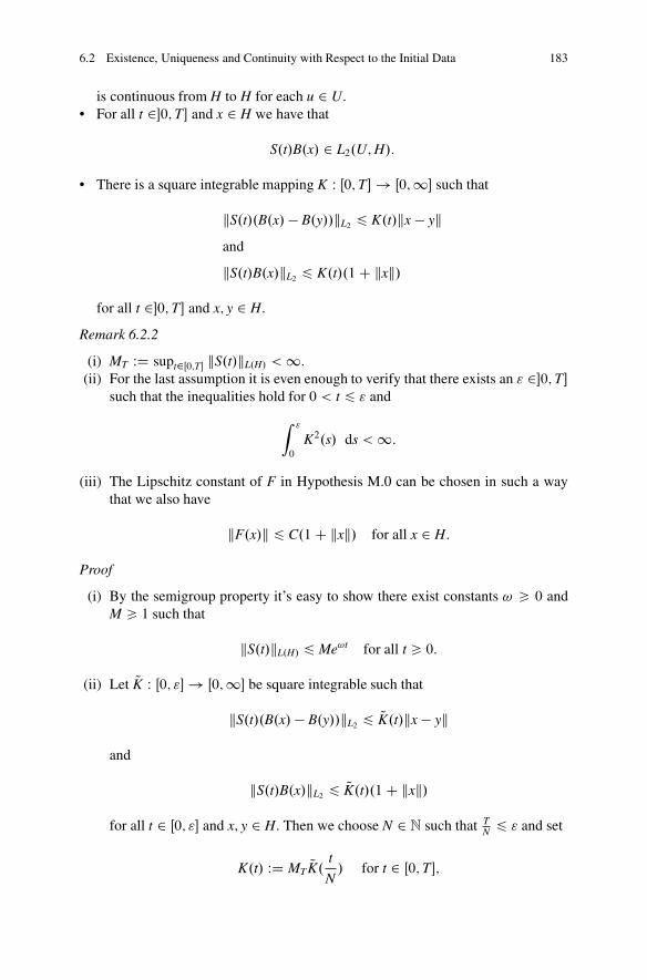
6.2 Existence, Uniqueness and Continuity with Respect to the Initial Data 183
is continuous from H to H for each u 2 U.• For all t 2�0;T� and x 2 H we have that
S.t/B.x/ 2 L2.U;H/:
• There is a square integrable mapping K W Œ0;T� ! Œ0;1� such that
kS.t/.B.x/� B.y//kL2 6 K.t/kx � ykand
kS.t/B.x/kL2 6 K.t/.1C kxk/
for all t 2�0;T� and x; y 2 H.
Remark 6.2.2
(i) MT WD supt2Œ0;T� kS.t/kL.H/ < 1.(ii) For the last assumption it is even enough to verify that there exists an " 2�0;T�
such that the inequalities hold for 0 < t 6 " and
Z "
0
K2.s/ ds < 1:
(iii) The Lipschitz constant of F in Hypothesis M.0 can be chosen in such a waythat we also have
kF.x/k 6 C.1C kxk/ for all x 2 H:
Proof
(i) By the semigroup property it’s easy to show there exist constants ! > 0 andM > 1 such that
kS.t/kL.H/ 6 Me!t for all t > 0:
(ii) Let QK W Œ0; "� ! Œ0;1� be square integrable such that
kS.t/.B.x/� B.y//kL2 6 QK.t/kx � yk
and
kS.t/B.x/kL2 6 QK.t/.1C kxk/
for all t 2 Œ0; "� and x; y 2 H. Then we choose N 2 N such that TN 6 " and set
K.t/ WD MT QK. t
N/ for t 2 Œ0;T�;

184 6 Mild Solutions
where MT D supt2Œ0;T� kS.t/kL.H/. Then it is clear that K W Œ0;T� ! Œ0;1Œ
is square integrable and for all x; y 2 H, t 2�0;T� we get by the semigroupproperty that
kS.t/.B.x/ � B.y//kL2 D kS.Nt � t
N/S.
t
N/.B.x/ � B.y//kL2
6 MTkS.t
N/.B.x/� B.y//kL2
6 MT QK. t
N/kx � yk D K.t/kx � yk
and
kS.t/B.x/kL2 6 MTkS.t
N/B.x/kL2
6 MT QK. t
N/.1C kxk/ D K.t/.1C kxk/:
(iii) For all x 2 H we have that
kF.x/k 6 kF.x/ � F.0/k C kF.0/k6 Ckxk C kF.0/k6 .C _ kF.0/k/ .1C kxk/
and, of course, we still have that
kF.x/ � F.y/k 6 .C _ kF.0/k/ kx � yk for all x; y 2 H:
utNow we introduce the spaces in which we want to find the mild solution of the aboveproblem:
For each T > 0 and p > 2 we define Hp.T;H/ to be the space of all H-valuedpredictable processes Y such that
kYkHp WD supt2Œ0;T�
�E.kY.t/kp/
� 1p < 1:
Then (Hp.T;H/, k kHp ) is a Banach space (after going over to the usual equivalenceclasses of processes).
For technical reasons we also consider the norms k kp;;T , > 0, on Hp.T;H/given by
kYkp;;T WD supt2Œ0;T�
e�t�E.kY.t/kp/
� 1p :

6.2 Existence, Uniqueness and Continuity with Respect to the Initial Data 185
Then k kHp D k kp;0;T and for all > 0, Y 2 Hp.T;H/ we get that
kYkp;;T 6 kYkHp 6 eTkYkp;;T ;
which means that all norms k kp;;T , > 0, are equivalent. For simplicity weintroduce the following notations
Hp.T;H/ WD .Hp.T;H/; k kHp/
and
Hp;.T;H/ WD .Hp.T;H/; k kp;;T /:
Theorem 6.2.3 Under Hypothesis M.0 there exists a unique mild solution X.�/ 2Hp.T;H/ of problem (6.1) with initial condition
� 2 Lp.�;F0;PI H/ DW Lp0:
In addition we even obtain that the mapping
X W Lp0 ! Hp.T;H/
� 7! X.�/
is Lipschitz continuous with Lipschitz constant LT;p.
Remark 6.2.4
1. The above result can be found in [27, Theorem 5.3.1, p. 66]. The proof is basedon the abstract implicit function Theorem F.0.1. In particular, one has to verifythat there is a predictable version of
Z t
0
S.t � s/B.Y.s// dW.s/; t 2 Œ0;T�;
for all Y 2 Hp.T;H/. In [27, Proposition 6.2, p. 153] this is solved in the casewhere B.Y/ 2 NW . We, however, do not assume that B itself takes values inL2.U;H/.
2. It follows from the Lipschitz continuity of X that there exists a constant CT;p
independent of � 2 Lp0 such that
kX.�/kHp 6 CT;p.1C k�kLp /:
Before giving a proof of the theorem we need the following lemmas.
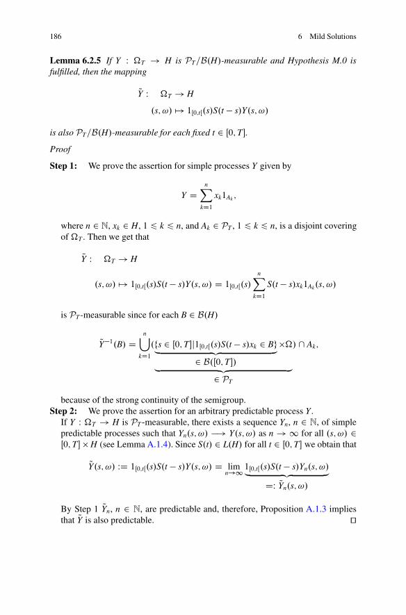
186 6 Mild Solutions
Lemma 6.2.5 If Y W �T ! H is PT=B.H/-measurable and Hypothesis M.0 isfulfilled, then the mapping
QY W �T ! H
.s; !/ 7! 1Œ0;tŒ.s/S.t � s/Y.s; !/
is also PT=B.H/-measurable for each fixed t 2 Œ0;T�.Proof
Step 1: We prove the assertion for simple processes Y given by
Y DnX
kD1xk1Ak ;
where n 2 N, xk 2 H, 1 6 k 6 n, and Ak 2 PT , 1 6 k 6 n, is a disjoint coveringof �T . Then we get that
QY W �T ! H
.s; !/ 7! 1Œ0;tŒ.s/S.t � s/Y.s; !/ D 1Œ0;tŒ.s/nX
kD1S.t � s/xk1Ak.s; !/
is PT-measurable since for each B 2 B.H/
QY�1.B/ Dn[
kD1.fs 2 Œ0;T�j1Œ0;tŒ.s/S.t � s/xk 2 Bg„ ƒ‚ …
2 B.Œ0;T�/��
„ ƒ‚ …2 PT
/ \ Ak;
because of the strong continuity of the semigroup.Step 2: We prove the assertion for an arbitrary predictable process Y.
If Y W �T ! H is PT -measurable, there exists a sequence Yn, n 2 N, of simplepredictable processes such that Yn.s; !/ �! Y.s; !/ as n ! 1 for all .s; !/ 2Œ0;T�� H (see Lemma A.1.4). Since S.t/ 2 L.H/ for all t 2 Œ0;T� we obtain that
QY.s; !/ WD 1Œ0;tŒ.s/S.t � s/Y.s; !/ D limn!1 1Œ0;tŒ.s/S.t � s/Yn.s; !/„ ƒ‚ …
DW QYn.s; !/
By Step 1 QYn, n 2 N, are predictable and, therefore, Proposition A.1.3 impliesthat QY is also predictable. ut

6.2 Existence, Uniqueness and Continuity with Respect to the Initial Data 187
Lemma 6.2.6 If Y is a predictable H-valued process and Hypothesis M.0 is fulfilledthen the mapping
.s; !/ 7! 1Œ0;tŒ.s/S.t � s/B.Y.s; !//
is PT=B.L2.U;H//-measurable.
Proof Let fk, k 2 N, be an orthonormal basis of H and ek, k 2 N, an orthonormalbasis of U. Then fk ˝ ej D fkhej; �iU, k; j 2 N, is an orthonormal basis of L2.U;H/(see Proposition B.0.7). Because of the strong continuity of B we obtain that
.s; !/ 7! B.Y.s; !//ej
is predictable for all j 2 N. Hence the previous lemma implies that
.s; !/ 7!hfk ˝ ej; 1Œ0;tŒ.s/S.t � s/B.Y.s; !//iL2
D hfk; 1Œ0;tŒ.s/S.t � s/B.Y.s; !//eji
is predictable for all j; k 2 N. This is enough to conclude that
.s; !/ 7! 1Œ0;tŒ.s/S.t � s/B.Y.s; !//
is predictable. utLemma 6.2.7 If a mapping g W �T ! H is PT=B.H/-measurable then the mapping
QY W �T ! H
.s; !/ 7! 1Œ0;tŒ.s/g.s; !/
is B.Œ0;T�/˝ Ft=B.H/-measurable for each t 2 Œ0;T�.Proof We have to show that .Œ0; tŒ��/ \ PT � B.Œ0;T�/˝ Ft.Let t 2 Œ0;T�. If we set
A WD fA 2 PT j A \ .Œ0; tŒ��/ 2 B.Œ0;T�/˝ Ftg
it is clear that A is a �-field which contains the predictable rectangles �s; u� � Fs,Fs 2 Fs, 0 6 s 6 u 6 T and f0g � F0, F0 2 F0. Therefore A D PT . utLemma 6.2.8 If a process ˆ is adapted to Ft, t 2 Œ0;T�, and stochasticallycontinuous with values in a Banach space E, then there exists a predictable versionof ˆ.
Proof [26, Proposition 3.6 (ii), p. 76] ut

188 6 Mild Solutions
Lemma 6.2.9 Let ˆ be a predictable H-valued process which is P-a.s. Bochnerintegrable. Then the process given by
Z t
0
S.t � s/ˆ.s; !/ ds; ! 2 �; t 2 Œ0;T�;
is P-a.s. continuous and adapted to Ft, t 2 Œ0;T�. This especially implies that it ispredictable (more precisely, has a predictable version).
Proof By Lemma 6.2.5 the process 1Œ0;tŒ.s/S.t � s/ˆ.s/, s 2 Œ0;T�, is predictableand in addition k1Œ0;tŒ.s/S.t � s/ˆ.s/k 6 MTkˆ.s/k, s 2 Œ0;T�.
Hence the integralsZ t
0
S.t � s/ˆ.s/ ds, t 2 Œ0;T�, are well defined.
First we want to prove the continuity. To this end let 0 6 s 6 t 6 T. Then we getthat
kZ s
0
S.s � u/ˆ.u/ du �Z t
0
S.t � u/ˆ.u/ duk
6 kZ s
0
ŒS.s � u/� S.t � u/�ˆ.u/ duk C kZ t
sS.t � u/ˆ.u/ duk
6Z s
0
kŒS.s � u/� S.t � u/�ˆ.u/k du CZ t
skS.t � u/ˆ.u/k du;
where the first summand converges to zero as s " t or t # s because by Lebesgue’sdominated convergence theorem:
k1Œ0;sŒ.u/ŒS.s � u/� S.t � u/�ˆ.u/k ! 0 as s " t or t # s
for all u 2 Œ0;T� because of the strong continuity of the semigroup S.u/, u 2 Œ0;T�.Moreover
k1Œ0;sŒ.u/ŒS.s � u/� S.t � u/�ˆ.u/k6 1Œ0;sŒ.u/.kS.s � u/kL.H/ C kS.t � u/kL.H//kˆ.u/k6 2MTkˆ.u/k;
where kˆk 2 L1.Œ0;T�; dx/ WD L1.Œ0;T�;B.Œ0;T�/; dxIR/ P-a.s.Concerning the second summand we get the same result since
Z t
skS.t � u/ˆ.u/k du
6Z t
sMTkˆ.u/k du �! 0 as s " t or t # s

6.2 Existence, Uniqueness and Continuity with Respect to the Initial Data 189
P-a.s. by Lebesgue’s dominated convergence theorem.In order to prove that the process given by the integrals is adapted, we fix t 2
Œ0;T�. By Lemma 6.2.7 the mapping
.s; !/ 7! 1Œ0;tŒ.s/S.t � s/ˆ.s; !/
is B.Œ0;T�/˝ Ft-measurable. Hence, by Proposition A.2.2, we get for each x 2 Hthat the mapping
! 7!hZ t
0
S.t � s/ˆ.s; !/ ds; xi
DZ t
0
hS.t � s/ˆ.s; !/; xi ds
DZ T
0
h1Œ0;tŒ.s/S.t � s/ˆ.s; !/; xi ds
is Ft-measurable by the real Fubini theorem and, therefore, the integral itself is Ft-measurable. utLemma 6.2.10 Let .xn;m/m2N, n 2 N, be sequences of real numbers such that foreach n 2 N there exists an xn 2 R with
xn;m �! xn as m ! 1:
If there exists a further sequence yn, n 2 N, such that jxn;mj 6 yn for all m 2 N andPn2N yn < 1 then
Xn2N
xn;m �!Xn2N
xn as m ! 1:
Proof The assertion is a simple consequence of Lebesgue’s dominated convergencetheorem with respect to the measure � WD P
n2N ın where ın is the Dirac measurein n. utProof of Theorem 6.2.3
Idea: Let p > 2. For t 2 Œ0;T�, � 2 Lp0 and Y 2 Hp.T;H/ we define
F.�;Y/.t/ WD S.t/� CZ t
0
S.t � s/F.Y.s// ds CZ t
0
S.t � s/B.Y.s// dW.s/
and prove that
F W Lp0 � Hp.T;H/ ! Hp.T;H/:

190 6 Mild Solutions
Since X.�/ 2 Hp.T;H/ is a mild solution of problem (6.1) if and only ifF.�;X.�// D X.�/ we have to look for an implicit function X W Lp
0 ! Hp.T;H/such that the previous equation holds for arbitrary � 2 Lp
0. To this end we showthat there exists a D .p/ > 0 such that
F W Lp0 � Hp;;T .T;H/ ! Hp;;T .T;H/
is a contraction with respect to the second variable, i.e. that there exists an ˛.p/ <1 such that for all � 2 Lp
0 and Y, QY 2 Hp.T;H/
kF.�;Y/ � F.�; QY/kp;;T 6 ˛.p/kY � QYkp;;T :
Setting G WD F , ƒ WD Lp0 and E WD Hp.T;H/ we are hence in the situation
described at the beginning of Appendix F. Therefore, it is clear that the implicitfunction X D ' exists and that it is unique.To get the Lipschitz continuity of the mapping X W Lp
0 ! Hp.T;H/ we verifythat the condition of Theorem F.0.1 (ii) is fulfilled. Because of the equivalence ofthe norms k kp;;T and k kHp that means that it is enough to show the existenceof a constant LT;p > 0 such that
kF.�;Y/ � F. Q�;Y/kHp 6 LT;pk� � Q�kLp
for all �, Q� 2 Lp0 and Y 2 Hp.T;H/.
Step 1: We prove that the mapping F is well defined.Let � 2 Lp
0 and Y 2 Hp.T;H/.
1. The Bochner integralZ t
0
S.t � s/F.Y.s// ds, t 2 Œ0;T�, is well defined by
Lemma 6.2.9:
(i) Because of the continuity of F W H ! H it is clear that F.Y.t//, t 2 Œ0;T�,is predictable.
(ii) In addition the process F.Y.t//, t 2 Œ0;T�, is P-a.s. Bochner integrablesince
E.Z t
0
kF.Y.s//k ds/6Z t
0
E.C.1C kY.s/k// ds 6 CT.1C kYkHp/<1:
2. The stochastic integralsZ t
0
S.t � s/B.Y.s// dW.s/, t 2 Œ0;T�, are well
defined since the processes 1Œ0;tŒ.s/S.t � s/B.Y.s//, s 2 Œ0;T�, are in N 2W.0;T/
for all t 2 Œ0;T�:(i) The mapping
.s; !/ 7! 1Œ0;tŒ.s/S.t � s/B.Y.s; !//

6.2 Existence, Uniqueness and Continuity with Respect to the Initial Data 191
is PT=B.L2.U;H//-measurable by Lemma 6.2.6.(ii) For the norm we obtain that
k1Œ0;tŒS.t � �/B.Y/k2T D E.Z t
0
kS.t � s/B.Y.s//k2L2 ds/
DZ t
0
E.kS.t � s/B.Y.s//k2L2 / ds
6Z t
0
K2.t � s/E�.1C kY.s/k/2� ds
6 2
Z t
0
K2.t � s/E.1C kY.s/k2/ ds
6 2 .1C sups2Œ0;T�
E.kY.s/k2/Z t
0
K2.t � s/ ds
6 2 .1C kYk2Hp/
Z t
0
K2.s/ ds < 1:
Step 2: We prove that F.�;Y/ 2 Hp.T;H/ for all � 2 Lp0 and Y 2 Hp.T;H/.
Let � 2 Lp0 and Y 2 Hp.T;H/.
1. The first summand S.t/�, t 2 Œ0;T�, is an element of Hp.T;H/:
(i) The mapping
.s; !/ 7! S.t/�.!/
is predictable since for fixed ! 2 �
t 7! S.t/�.!/
is a continuous mapping from Œ0;T� to H and for fixed t 2 Œ0;T�
! 7! S.t/�.!/
is not only Ft- but even F0-measurable.(ii) For the norm we obtain that
kS.�/�kHp D supt2Œ0;T�
.E.kS.t/�kp//1p 6 MTk�kLp < 1:
2. There is a version of the second summandZ t
0
S.t � s/F.Y.s// ds, t 2 Œ0;T�,
which is an element of Hp.T;H/:

192 6 Mild Solutions
(i) First we notice that the mapping
.s; !/ 7!Z t
0
S.t � s/F.Y.s; !// ds
has a predictable version because the assumptions of Lemma 6.2.9 arefulfilled.
(ii) Concerning the norm we prove that
kZ �
0
S.� � s/F.Y.s// dskHp 6 CTMT .1C kYkHp /:
To verify the assertion we take t from Œ0;T� and show that the Lp-norm of
kZ t
0
S.t � s/F.Y.s// dsk
can be estimated independently of t 2 Œ0;T�:
kZ t
0
S.t � s/F.Y.s// dskp 6 CpTp�1MpT
Z t
0
.1C kY.s/k/p ds P-a.s.
Taking the expectation we get that
�E.k
Z t
0
S.t � s/F.Y.s// dskp/� 1
p
6 CTp�1
p MT�E.Z t
0
.1C kY.s/k/p ds� 1
p
6 CTp�1
p MT��
E.Z T
0
1 ds/� 1
p C � Z T
0
E.kY.s/kp/ ds� 1
p�
6 CTMT.1C kYkHp/ < 1
and the claimed inequality follows.
3. There is a version ofZ t
0
S.t � s/B.Y.s// dW.s/, t 2 Œ0;T�, which is in
Hp.T;H/: (i) First we show that there is a predictable version of the process.To do so we proceed in several steps.
Claim 1: If ˛ > 1 the processZ t
˛
0
S.t � s/B.Y.s// dW.s/, t 2 Œ0;T�, has a
predictable version.

6.2 Existence, Uniqueness and Continuity with Respect to the Initial Data 193
To prove this we first use the semigroup property and get that
Z t˛
0
S.t � s/B.Y.s// dW.s/
DZ t
˛
0
S.t � ˛s/S..˛ � 1/s/B.Y.s// dW.s/; t 2 Œ0;T�:
We set
ˆ˛.s/ WD .s/1�0;T�.s/S..˛ � 1/s/B.Y.s//:
Then it is clear that ˆ˛.t/, t 2 Œ0;T�, is an element of N 2W.0;T/:
The fact that there is a predictable version of
.s; !/ 7! 1�0;T�.s/S..˛ � 1/s/B.Y.s; !//
can be proved in the same way as Lemma 6.2.6 and, of course, by HypothesisM.0
E.Z T
0
kS..˛ � 1/s/B.Y.s//k2L2 ds/
6Z T
0
E�K2..˛ � 1/s/.1C kY.s/k/2� ds
6 2
Z T
0
K2..˛ � 1/s/.1C sups2Œ0;T�
E.kY.s/k2// ds
D 2.1C kYk2H2.T;H//
Z .˛�1/T
0
1
˛ � 1K2.s/ ds < 1:
Therefore, we now have to prove that the process
Z t˛
0
S.t � ˛s/ Q .s/ dW.s/; t 2 Œ0;T�;
has a predictable version for each ˛ > 1 and Q 2 N 2W.0;T/.
(a) We first consider the case where Q .t/, t 2 Œ0;T�, is a simple process of theform
Q DmX
kD1Lk1Ak

194 6 Mild Solutions
where m 2 N, Lk 2 L2.U;H/ and Ak 2 PT , 1 6 k 6 m. To get the requiredmeasurability we check the conditions of Lemma 6.2.8.At first it is clear that
Z t˛
0
S.t � ˛s/ Q .s/ dW.s/
is F t˛
- and therefore also Ft-measurable for each t 2 Œ0;T� since the process
1Œ0; t˛ Œ.s/S.t � ˛s/ Q .s/; s 2 Œ0;T�;
lies in N 2W.0;T/ (see the proof of Lemma 6.2.6) and therefore the process
Z u
0
1Œ0; t˛ Œ.s/S.t � ˛s/ Q .s/ dW.s/; u 2 Œ0;T�;
is an H-valued martingale with respect to Fu, u 2 Œ0;T�. Now we show that
t 7!Z t
˛
0
S.t � ˛s/ Q .s/ dW.s/
is continuous in mean square and, therefore, stochastically continuous.To this end we take arbitrary 0 6 t < u 6 T and get that
�E.k
Z u˛
0
S.u � ˛s/ Q .s/ dW.s/ �Z t
˛
0
S.t � ˛s/ Q .s/ dW.s/k2/� 12
6�E.k
Z t˛
0
ŒS.u � ˛s/ � S.t � ˛s/� Q .s/ dW.s/k2/� 12
C �E.k
Z u˛
0
1Œ t˛ ;
u˛ Œ.s/S.u � ˛s/ Q .s/ dW.s/k2/� 12
D �E.Z t
˛
0
kŒS.u � ˛s/ � S.t � ˛s/� Q .s/k2L2 ds/� 12
C �E.Z u
˛
t˛
kS.u � ˛s/ Q .s/k2L2 ds/� 12
6mX
kD1
�E.Z t
˛
0
1Ak.s; �/kŒS.u � ˛s/ � S.t � ˛s/�Lkk2L2 ds/� 12
CmX
kD1
�E.Z u
˛
t˛
1Ak.s; �/kS.u � ˛s/Lkk2L2 ds/� 12

6.2 Existence, Uniqueness and Continuity with Respect to the Initial Data 195
6mX
kD1
� Z t˛
0
kŒS.u � ˛s/ � S.t � ˛s/�Lkk2L2 ds� 12
CmX
kD1
� Z u˛
t˛
kS.u � ˛s/Lkk2L2 ds� 12 ; (6.3)
where the first summand in the right-hand side of (6.3) converges to zero ast " u or u # t for the following reason:Let en, n 2 N, be an orthonormal basis of U. Then we get for each s 2 Œ0;T�and 1 6 k 6 m that
1Œ0; t˛ Œ.s/kŒS.u � ˛s/ � S.t � ˛s/�Lkk2L2
DXn2N
1Œ0; t˛ Œ.s/kŒS.u � ˛s/ � S.t � ˛s/�Lkenk2;
where
1Œ0; t˛ Œ.s/kŒS.u � ˛s/ � S.t � ˛s/�Lkenk2 �! 0 as t " u or u # t
and at the same time
1Œ0; t˛ Œ.s/kŒS.u � ˛s/ � S.t � ˛s/�Lkenk2 6 4M2
TkLkenk2
for all n 2 N, 1 6 k 6 m. By Lemma 6.2.10 this result implies the pointwiseconvergence
1Œ0; t˛ Œ.s/kŒS.u � ˛s/ � S.t � ˛s/�Lkk2L2 �! 0 as t " u or u # t:
Since there is the following upper bound
1Œ0; t˛ Œ.s/kŒS.u � ˛s/ � S.t � ˛s/�Lkk2L2 6 4M2
TkLkk2L2 2 L1.Œ0;T�; dx/
for all s 2 Œ0;T�, 0 6 t < u 6 T, we get the required convergence of the
integralsZ t
˛
0
kŒS.u � ˛s/ � S.t � ˛s/�Lkk2L2 ds, 1 6 k 6 m, by Lebesgue’s
dominated convergence theorem.The second summand in the right side of (6.3) of the above equation alsoconverges to zero since for each 1 6 k 6 m
Z u˛
t˛
kS.u � ˛s/Lkk2L2 ds 6 u � t
˛M2
TkLkk2L2 �! 0 as u # t or t " u:

196 6 Mild Solutions
Hence Lemma 6.2.8 implies that there is a predictable version of
Z t˛
0
S.t � ˛s/ Q .s/ dW.s/; t 2 Œ0;T�;
if Q is elementary.(b) Now we generalize this result to arbitrary Q 2 N 2
W :If Q is an arbitrary process in N 2
W.0;T/ there exists a sequence Q n, n 2 N,of simple processes of the form we considered in (a) such that
E.Z T
0
k Q .s/ � Q n.s/k2L2 ds/ �!n!1 0
(see Lemma A.1.4). Hence let ‰n.t/, t 2 Œ0;T�, n 2 N, be a predictable
version ofZ t
˛
0
S.t � ˛s/ Q n.s/ dW.s/, t 2 Œ0;T�, n 2 N, which exists by
step (a). To get the predictability ofZ t
˛
0
S.t � ˛s/ˆ.s/ dW.s/ we prove that
there is a subsequence nk, k 2 N, such that
‰nk.t/ �!k!1
Z t˛
0
S.t � ˛s/ Q .s/ dW.s/ P-a.s. for all t 2 Œ0;T�:
To this end we take c > 0, t 2 Œ0;T� and obtain that
P.kZ t
˛
0
S.t � ˛s/ Q .s/ dW.s/ �‰n.t/k > c/
6 1
c2E.k
Z t˛
0
S.t � ˛s/Œ Q .s/ � Q n.s/� dW.s/k2/
D 1
c2E.Z t
˛
0
kS.t � ˛s/Œ Q .s/ � Q n.s/�k2L2 ds/
6 M2T
c2E.Z t
˛
0
k Q .s/ � Q n.s/k2L2 ds/ 6 M2T
c2E.Z T
0
k Q .s/� Q n.s/k2L2 ds/:
As this upper bound is independent of t 2 Œ0;T� this implies that
supt2Œ0;T�
P.kZ t
˛
0
S.t � ˛s/ Q .s/ dW.s/�‰n.t/k > c/
6 M2T
c2E.Z T
0
k Q .s/ � Q n.s/k2L2 ds/ �!n!1 0:
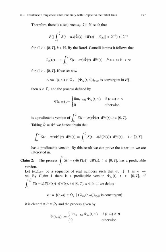
6.2 Existence, Uniqueness and Continuity with Respect to the Initial Data 197
Therefore, there is a sequence nk, k 2 N, such that
P.kZ t
˛
0
S.t � ˛s/ Q .s/ dW.s/ �‰nk k > 2�k/ 6 2�k
for all t 2 Œ0;T�, k 2 N. By the Borel–Cantelli lemma it follows that
‰nk.t/ �!Z t
˛
0
S.t � ˛s/ Q .s/ dW.s/ P-a.s. as k ! 1
for all t 2 Œ0;T�. If we set now
A WD f.t; !/ 2 �T j .‰nk.t; !//k2N is convergent in Hg;
then A 2 PT and the process defined by
‰.t; !/ WD(
limk!1‰nk.t; !/ if .t; !/ 2 A
0 otherwise
is a predictable version ofZ t
˛
0
S.t � ˛s/ Q .s/ dW.s/, t 2 Œ0;T�.Taking Q D ˆ˛ we hence obtain that
Z t˛
0
S.t � ˛s/ˆ˛.s/ dW.s/ DZ t
˛
0
S.t � s/B.Y.s// dW.s/; t 2 Œ0;T�;
has a predictable version. By this result we can prove the assertion we areinterested in.
Claim 2: The processZ t
0
S.t � s/B.Y.s// dW.s/, t 2 Œ0;T�, has a predictable
version.Let .˛n/n2N be a sequence of real numbers such that ˛n # 1 as n !1. By Claim 1 there is a predictable version ‰˛n.t/, t 2 Œ0;T�, ofZ t
˛n
0
S.t � s/B.Y.s// dW.s/, t 2 Œ0;T�, n 2 N. If we define
B WD f.t; !/ 2 �T j .‰˛n.t; !//n2N is convergentg;
it is clear that B 2 PT and the process given by
‰.t; !/ WD(
limn!1‰˛n.t; !/ if .t; !/ 2 B
0 otherwise

198 6 Mild Solutions
is predictable. Besides we get that for each t 2 Œ0;T�
‰.t/ DZ t
0
S.t � s/B.Y.s// dW.s/ P-a.s.;
since P-a.s.
‰˛n.t/ DZ t
˛n
0
S.t � s/B.Y.s// dW.s/ �!n!1
Z t
0
S.t � s/B.Y.s// dW.s/;
because of the continuity of the stochastic integrals
Z u
0
1Œ0;tŒ.s/S.t � s/B.Y.s// dW.s/; u 2 Œ0;T�:
Therefore the predictable version is found.(ii) Concerning the norm we get that
kZ �
0
S.� � s/B.Y.s// dW.s/kHp
6 .p
2.p � 1// 12
Z T
0
K2.s/ ds 12.1C kYkHp/;
since we obtain by Theorem 6.1.2 (Burkholder–Davis–Gundy type inequality)that
E.k
Z t
0
S.t � s/B.Y.s// dW.s/kp/ 1
p
6 .p
2.p � 1// 12
Z t
0
�E.kS.t � s/B.Y.s//kp
L2/� 2
p ds 12
6 .p
2.p � 1// 12
Z t
0
K2.t � s/�E..1C kY.s/k/p/� 2p ds
12
6 .p
2.p � 1// 12
Z t
0
K2.t � s/.1C kY.s/kLp /2 ds 12
6 .p
2.p � 1// 12
Z T
0
K2.s/ ds 12.1C kYkHp /:
Therefore, we have finally proved that
F W Lp0 � Hp.T;H/ ! Hp.T;H/:

6.2 Existence, Uniqueness and Continuity with Respect to the Initial Data 199
Step 3: For each p > 2 there is a .p/ DW such that
F.�; �/ W Hp;.T;H/ ! Hp;.T;H/
is a contraction for all � 2 Lp0 where the contraction constant ˛./ < 1 does not
depend on �:Let Y, QY 2 Hp.T;H/, � 2 Lp
0 and t 2 Œ0;T�. Then we get that
kŒF.�;Y/ � F.�; QY/�.t/kLp
6 kZ t
0
S.t � s/ŒF.Y.s// � F. QY.s//� dskLp
C kZ t
0
S.t � s/ŒB.Y.s// � B. QY.s//� dW.s/kLp ;
where the first summand can be estimated in the following way:
kZ t
0
S.t � s/ŒF.Y.s// � F. QY.s//� dskp 6 MpTCpTp�1
Z t
0
kY.s/ � QY.s/kp ds P-a.s.,
which implies that
�E.k
Z t
0
S.t � s/ŒF.Y.s// � F. QY.s//� dskp/� 1
p
6 MTCTp�1
p .
Z t
0
E.kY.s/ � QY.s/kp/ ds/1p
D MTCTp�1
p .
Z t
0
eps e�psE.kY.s/ � QY.s/kp/„ ƒ‚ …6 kY � QYkp
p;;T
ds/1p
6 MTCTp�1
p .
Z t
0
eps ds/1p kY � QYkp;;T
6 MTCTp�1
p et.1
p/1p kY � QYkp;;T :
Dividing by et yields
kZ �
0
S.� � s/ŒF.Y.s// � F. QY.s//� dskp;;T 6 MTCTp�1
p .1
p/1p
„ ƒ‚ …�! 0 as ! 1
kY � QYkp;;T :
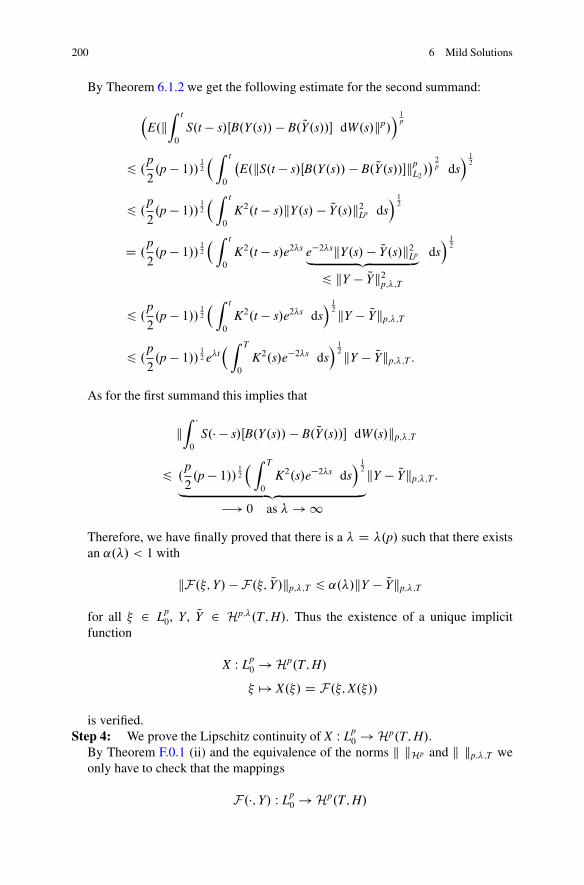
200 6 Mild Solutions
By Theorem 6.1.2 we get the following estimate for the second summand:
E.k
Z t
0
S.t � s/ŒB.Y.s// � B. QY.s//� dW.s/kp/ 1
p
6 .p
2.p � 1//
12
Z t
0
�E.kS.t � s/ŒB.Y.s// � B. QY.s//�kp
L2/� 2
p ds 12
6 .p
2.p � 1//
12
Z t
0
K2.t � s/kY.s/ � QY.s/k2Lp ds 12
D .p
2.p � 1//
12
Z t
0
K2.t � s/e2s e�2skY.s/ � QY.s/k2Lp„ ƒ‚ …6 kY � QYk2p;;T
ds 12
6 .p
2.p � 1//
12
Z t
0
K2.t � s/e2s ds 12 kY � QYkp;;T
6 .p
2.p � 1//
12 et
Z T
0
K2.s/e�2s ds 12 kY � QYkp;;T :
As for the first summand this implies that
kZ �
0
S.� � s/ŒB.Y.s// � B. QY.s//� dW.s/kp;;T
6 .p
2.p � 1// 12
Z T
0
K2.s/e�2s ds 12
„ ƒ‚ …�! 0 as ! 1
kY � QYkp;;T :
Therefore, we have finally proved that there is a D .p/ such that there existsan ˛./ < 1 with
kF.�;Y/ � F.�; QY/kp;;T 6 ˛./kY � QYkp;;T
for all � 2 Lp0, Y, QY 2 Hp;.T;H/. Thus the existence of a unique implicit
function
X W Lp0 ! Hp.T;H/
� 7! X.�/ D F.�;X.�//
is verified.Step 4: We prove the Lipschitz continuity of X W Lp
0 ! Hp.T;H/.By Theorem F.0.1 (ii) and the equivalence of the norms k kHp and k kp;;T weonly have to check that the mappings
F.�;Y/ W Lp0 ! Hp.T;H/
6.3 Smoothing Property of the Semigroup: Pathwise Continuity of the Mild. . . 201
are Lipschitz continuous for all Y 2 Hp.T;H/ where the Lipschitz constant doesnot depend on Y.But this assertion holds as for all �, 2 Lp
0 and Y 2 Hp.T;H/
kF.�;Y/ � F. ;Y/kHp D kS.�/.� � /kHp 6 MTk� � kLp :
ut
6.3 Smoothing Property of the Semigroup: PathwiseContinuity of the Mild Solution
Let X.�/ be the mild solution of problem (6.1) with initial condition � 2 Lp0. The aim
of this section is to prove that the mapping t 7! X.�/.t/ has a continuous version.Because of Lemma 6.2.9 we already know that the process of the Bochner integrals
Z t
0
S.t � s/F.X.�/.s// ds; t 2 Œ0;T�;
is P-a.s. continuous. Hence it only remains to show that the process
Z t
0
S.t � s/B.X.�/.s// dW.s/; t 2 Œ0;T�;
has a continuous version. To this end we use the method which is presented in[27, Theorem 5.2.6, p. 59; Proposition A.1.1, p. 307]. In contrast to [27] we do notdemand that the semigroup is analytic and therefore we only get continuity insteadof Hölder continuity as in [27].
First, we have to introduce the general concept of the stochastic convolution.
Definition 6.3.1 (Stochastic Convolution) If ˆ.t/, t 2 Œ0;T�, is a L.U;H/-valuedpredictable process such that the stochastic integrals
WˆA .t/ WD
Z t
0
S.t � s/ˆ.s/ dW.s/; t 2 Œ0;T�;
are well defined, then the process WˆA .t/, t 2 Œ0;T�, is called stochastic convolution.
The following result (see [27, Theorem 5.2.5, p. 58]) is a corollary of the stochasticFubini Theorem (i.e. Theorem 6.1.4 above).
Theorem 6.3.2 (Factorization Formula) Let ˛ 2�0; 1Œ and ˆ be an L.U;H/-valued predictable process. Assume that
1. S.t � s/ˆ.s/ is L2.U;H/-valued for all s 2 Œ0; tŒ, t 2 Œ0;T�.2.Z s
0
.s � u/�2˛E�kS.s � u/ˆ.u/k2L2
�du < 1 for all s 2 Œ0;T�.

202 6 Mild Solutions
3.Z t
0
.t � s/˛�1hZ s
0
.s�u/�2˛E�kS.s�u/ˆ.u/k2L2
�dui 12
ds < 1 for all t 2 Œ0;T�.Then we have the following representation of the stochastic convolution.
Z t
0
S.t � s/ˆ.s/ dW.s/ D sin˛
Z t
0
.t � s/˛�1S.t � s/Yˆ˛ .s/ ds (6.4)
P-a.s. for all t 2 Œ0;T�, where Yˆ˛ .s/, s 2 Œ0;T�, is an B.Œ0;T�/ ˝ FT-measurableversion of
Z s
0
.s � u/�˛S.s � u/ˆ.u/ dW.u/; s 2 Œ0;T�: (6.5)
Proof First we check thatZ s
0
.s � u/�˛S.s � u/ˆ.u/ dW.u/; s 2 Œ0;T�, is well
defined and has an B.Œ0;T�/˝ FT-measurable version Yˆ˛ .s/; s 2 Œ0;T�. But this istrue since first we have that the mapping
' W .u; !; s/ 7! 1Œ0;sŒ.u/.s � u/�˛S.s � u/ˆ.u/; u 2 Œ0;T�;
is PT ˝ B.Œ0;T�/=B.L2/-measurable by assumption 1. (The proof can be done in asimilar way as the proof of Lemma 6.2.5 and the proof of Lemma 6.2.6). Secondly,by assumption 2., we obtain that
E�Z T
0
k1Œ0;sŒ.u/.s � u/�˛S.s � u/ˆ.u/k2L2 du�
DZ s
0
.s � u/�2˛E�kS.s � u/ˆ.u/k2L2
�du < 1;
by assumption 2.Therefore the mapping ' W �T � Œ0;T� ! L2.U;H/ fulfills the conditions
of Theorem 6.1.4 and thus the process in (6.5) is well defined and has a productmeasurable version Yˆ˛ (see the proof of [26, Theorem 4.18, p. 109]). In addition,for fixed t 2 Œ0;T� the mapping 't given by
't W �T � Œ0;T� ! L2.U;H/
.u; !; s/ 7! 1Œ0;tŒ.s/.t � s/˛�11Œ0;sŒ.u/.s � u/�˛S.t � u/ˆ.u; !/
also fulfills the conditions of Theorem 6.1.4 for the following reasons:Now fix t 2 Œ0;T�. We have that the mapping
't W �T � Œ0;T� ! L2.U;H/

6.3 Smoothing Property of the Semigroup: Pathwise Continuity of the Mild. . . 203
is PT ˝ B.Œ0;T�/=B.L2/-measurable. Moreover, we get by assumption 3 that
Z T
0
E�Z T
0
1Œ0;tŒ.s/1Œ0;sŒ.u/.t � s/2.˛�1/.s � u/�2˛
kS.t � u/ˆ.u/k2L2 du� 1
2ds
DZ T
0
1Œ0;tŒ.s/.t � s/˛�1Z T
0
1Œ0;sŒ.u/.s � u/�2˛
E�kS.t � u/ˆ.u/k2L2
�du 12
ds
(by Fubini’s theorem)
6 MT
Z T
0
1Œ0;tŒ.s/.t � s/˛�1Z T
0
1Œ0;sŒ.u/.s � u/�2˛
E�kS.s � u/ˆ.u/k2L2
�du 12
ds < 1(by the semigroup property).
Therefore, there exists a product measurable version of
Z s
0
1Œ0;tŒ.s/.t � s/˛�1.s � u/�˛S.t � u/ˆ.u/ dW.u/; s 2 Œ0;T�:
Since by Lemma 2.4.1 for each s 2 Œ0;T�Z s
0
1Œ0;tŒ.s/.t � s/˛�1.s � u/�˛S.t � u/ˆ.u/ dW.u/
D1Œ0;tŒ.s/.t � s/˛�1S.t � s/Yˆ˛ .s/ P-a.s.,
for this version again by Fubini’s theorem we get that
EkZ t
0
.t � s/˛�1S.t � s/Yˆ˛ .s/ ds
�Z T
0
Z s
0
1Œ0;tŒ.s/.t � s/˛�1.s � u/�˛S.t � u/ˆ.u/ dW.u/ dsk
Z T
0
Ek1Œ0;tŒ.s/.t � s/˛�1S.t � s/Yˆ˛ .s/
�Z S
0
1Œ0;tŒ.s/.t � s/˛�1.s � u/�˛S.t � u/ˆ.u/ dW.u/k
ds
D 0:

204 6 Mild Solutions
Furthermore, we can use Theorem 6.1.4 to exchange the integration and thus wefinally obtain that
Z t
0
.t � s/˛�1S.t � s/Yˆ˛ .s/ ds
DZ t
0
Z s
0
.t � s/˛�1.s � u/�˛S.t � u/ˆ.u/ dW.u/ ds
DZ t
0
Z t
u.t � s/˛�1.s � u/�˛S.t � u/ˆ.u/ ds dW.u/
DZ t
0
Z t
u.t � s/˛�1.s � u/�˛ ds
S.t � u/ˆ.u/ dW.u/
D
sin ˛
Z t
0
S.t � u/ˆ.u/ dW.u/ P-a.s.
sinceZ t
u.t � s/˛�1.s � u/�˛ ds D
sin ˛(keyword: Euler’s beta function). ut
Using this representation of the stochastic convolution we are now able to provethe desired pathwise continuity.
Let p � 2 and ˛ 2� 1p ; 1Œ. For ' 2 Lp.Œ0;T�I H/ WD Lp.Œ0;T�;B.Œ0;T�/; dtI H/ wedefine
R˛'.t/ WDZ t
0
.t � s/˛�1S.t � s/'.s/ ds; t 2 Œ0;T�:
Then R˛' is well defined since
Z t
0
k.t � s/˛�1S.t � s/'.s/k ds 6�Z t
0
s.˛�1/ pp�1 ds
� p�1p MTk'kLp < 1;
since ˛ > 1p and therefore .˛ � 1/ p
p�1 > �1.
Proposition 6.3.3 Let ˛ 2�0; 1Œ and p > 1˛
. Then
R˛ W Lp.Œ0;T�I H/ ! C.Œ0;T�I H/:
Remark 6.3.4 If one assumes that the semigroup S.t/, t 2 Œ0;T�, is analytic one evengets that R˛' is Hölder continuous for all ' 2 Lp.Œ0;T�I H/ (see [27, PropositionA.1.1, p. 307]).

6.3 Smoothing Property of the Semigroup: Pathwise Continuity of the Mild. . . 205
Proof of 6.3.3 Let ' 2 Lp.Œ0;T�I H/, t 2 Œ0;T�, and let tn, n 2 N, be a sequence inŒ0;T� such that tn �!
n!1 t. Then
kR˛'.tn/� R˛'.t/k
D kZ tn
0
.tn � s/˛�1S.tn � s/'.s/ ds �Z t
0
.t � s/˛�1S.t � s/'.s/ dsk
6Z T
0
k1Œ0;tn Œ.s/.tn � s/˛�1S.tn � s/'.s/ � 1Œ0;tŒ.s/.t � s/˛�1S.t � s/'.s/k ds:
Concerning the inner term we obtain that
k1Œ0;tnŒ.s/.tn � s/˛�1S.tn � s/'.s/ � 1Œ0;tŒ.s/.t � s/˛�1S.t � s/'.s/k �!n!1 0
for ds-a.e. s 2 Œ0;T�. Moreover, the family
.k1Œ0;tn Œ.tn � �/˛�1S.tn � �/'.�/� 1Œ0;tŒ.t � �/˛�1S.t � �/'.�/k/n2N
is uniformly integrable :For t 2 Œ0;T� we set
Ft.s/ WD 1Œ0;tŒ.s/.t � s/˛�1kS.t � s/'.s/k; s 2 Œ0;T�:
Since .˛ � 1/ pp�1 > �1, there exists an " > 0 such that
.˛ � 1/.1C "/p
p � 1 � "> �1 and p > 1C ":
Then
Z T
0
F1C"t .s/ ds 6�Z t
0
.t � s/.˛�1/.1C"/ pp�1�" ds
� p�1�"p M1C"
T k'k1C"Lp
6�Z T
0
s.˛�1/.1C"/ pp�1�" ds
� p�1�"p M1C"
T k'k1C"Lp
< 1:
Therefore, supt2Œ0;T�
Z T
0
F1C"t .s/ ds < 1 and hence Ft, t 2 Œ0;T�, is uniformly
integrable. Since
k1Œ0;tnŒ.s/.tn � s/˛�1S.tn � s/'.s/ � 1Œ0;tŒ.s/.t � s/˛�1S.t � s/'.s/k6 Ftn.s/C Ft.s/

206 6 Mild Solutions
for all s 2 Œ0;T� the assertion follows. utThus we have found a tool to check whether the process
Z t
0
S.t � s/B.X.�/.s// dW.s/; t 2 Œ0;T�;
has a P-a.s. continuous version.
Proposition 6.3.5 Assume that the mappings A, F and B satisfy Hypothesis M.0,and let p � 2. If there exists an ˛ 2� 1p ;1Œ such that
Z T
0
s�2˛K2.s/ ds < 1;
then the mild solution X.�/ of problem (6.1) has a continuous version for all initialconditions � 2 Lp
0.
Proof Without loss of generality we may assume that ˛ 2�0; 1Œ. S.�/� is P-a.s.continuous because of the strong continuity of the semigroup.
In Step 2, 2. (i) of the proof of Theorem 6.2.3 we have already shown that theprocess of the Bochner integrals
Z t
0
S.t � s/F.X.�/.s// ds; t 2 Œ0;T�;
has P-a.s. continuous trajectories.Thus, in fact, it only remains to prove that the process
Z t
0
S.t � s/B.X.�/.s// dW.s/; t 2 Œ0;T�;
has a continuous version:Since
Z t
0
.t � s/˛�1�Z s
0
.s � u/�2˛E�kS.s � u/B.X.�/.u//k2L2
�du� 12 ds
6Z t
0
.t � s/˛�1�Z s
0
.s � u/�2˛K2.s � u/E�.1C kX.�/.u/k/2� du
� 12 ds
6 .1C kX.�/kH2 /
Z t
0
.t � s/˛�1�Z s
0
.s � u/�2˛K2.s � u/ du� 12 ds
6 .1C kX.�/kH2 / Z T
0
u�2˛K2.u/ du 12
Z T
0
s˛�1 ds < 1;

6.3 Smoothing Property of the Semigroup: Pathwise Continuity of the Mild. . . 207
we have by Theorem 6.3.2 (factorization formula) that P-a.s.
Z t
0
S.t � s/B.X.�/.s// dW.s/
D sin˛
Z t
0
.t � s/˛�1S.t � s/Z s
0
.s � u/�˛S.s � u/B.X.�/.u// dW.u/ ds
D sin˛
R˛� Z �
0
.� � u/�˛S.� � u/B.X.�/.u// dW.u/„ ƒ‚ …
DW Y˛
�.t/:
Since the mapping ' W �T � Œ0;T� ! L2.U;H/ given by
'.u; !; s/ WD 1Œ0;sŒ.u/.s � u/�˛S.s � u/B.X.�/.u; !//
fulfills the conditions of Theorem 6.1.4, the process Y˛ can be understood as a
B.Œ0;T�/ ˝ FT -measurable version ofZ t
0
.t � u/�˛S.t � u/B.X.�/.u// dW.u/,
t 2 Œ0;T� (see the proof of [26, Theorem 4.18, p. 109]).To get the P-a.s. continuity of the stochastic integral we have to show that P-a.s.
Y˛ 2 Lp.Œ0;T�I H/:
By Theorem 6.1.2 we can estimate E�kY˛.t/kp
�independently of t 2 Œ0;T� in the
following way
E�kY˛.t/kp
�
6�p
2.p � 1/� p
2
Z t
0
.t � s/�2˛�E.kS.t � s/B.X.�/.s//kp
L2/� 2
p ds p2
6�p
2.p � 1/� p
2
Z t
0
.t � s/�2˛K2.t � s/�E..1C kX.�/.s/k/p/� 2p ds
p2
6�p
2.p � 1/� p
2
Z t
0
.t � s/�2˛K2.t � s/.1C kX.�/kHp/2 ds p2
6�p
2.p � 1/� p
2 .1C kX.�/kHp/pZ T
0
s�2˛K2.s/ ds p2< 1:
Finally, we obtain by the real Fubini theorem that
E�Z T
0
kY˛.t/kp dt� D
Z T
0
E�kY˛.t/kp
�dt < 1:
ut

Appendix AThe Bochner Integral
Let�X; k k� be a Banach space, B.X/ the Borel �-field of X and .�;F ; �/ a measure
space with finite measure �.
A.1 Definition of the Bochner Integral
Step 1: As a first step we want to define the integral for simple functions whichare defined as follows. Set
E WDnf W � ! X
ˇf D
nXkD1
xk1Ak ; xk 2 X; Ak 2 F ; 1 6 k 6 n; n 2 N
o
and define a semi-norm k kE on the vector space E by
kf kE WDZ
kf k d�; f 2 E :
To get that�E ; k kE
�is a normed vector space we consider equivalence classes
with respect to k kE . For simplicity we will not change the notation.For f 2 E , f D Pn
kD1 xk1Ak , Ak’s pairwise disjoint (such a representation is callednormal and always exists, because f D Pn
kD1 xk1Ak , where f .�/ D fx1; : : : ; xkg,xi 6D xj, and Ak WD ff D xkg) and we now define the Bochner integral to be
Zf d� WD
nXkD1
xk�.Ak/:
© Springer International Publishing Switzerland 2015W. Liu, M. Röckner, Stochastic Partial Differential Equations: An Introduction,Universitext, DOI 10.1007/978-3-319-22354-4
209

210 Appendix A
(Exercise: This definition is independent of representations, and hence linear.) Inthis way we get a mapping
int W �E ; k kE� ! �
X; k k�f 7!
Zf d�
which is linear and uniformly continuous since��R f d�
�� 6R kf k d� for all
f 2 E .Therefore we can extend the mapping int to the abstract completion of E withrespect to k kE which we denote by E .
Step 2: We give an explicit representation of E .
Definition A.1.1 A function f W � ! X is called strongly measurable if it isF=B.X/-measurable and f .�/ � X is separable.
Definition A.1.2 Let 1 6 p < 1. Then we define
Lp.�;F ; �I X/ WD Lp.�I X/
WD�
f W � ! X
ˇˇ f is strongly measurable with
respect to F ; andZ
kf kp d� < 1�
and the semi-norm
kf kLp WD�Z
kf kp d�
� 1p
; f 2 Lp.�;F ; �I X/:
The space of all equivalence classes in Lp.�;F ; �I X/ with respect to k kLp isdenoted by Lp.�;F ; �I X/ WD Lp.�I X/.
Claim L1.�;F ; �I X/ D E .
Step 2.a:�L1.�;F ; �I X/; k kL1
�is complete.
The proof is just a modification of the proof of the Fischer–Riesz theorem by thefollowing proposition.
Proposition A.1.3 Let .�;F/ be a measurable space and let X be a Banach space.Then:
(i) the set of F=B.X/-measurable functions from � to X is closed under theformation of pointwise limits, and
(ii) the set of strongly measurable functions from � to X is closed under theformation of pointwise limits.

A.2 Properties of the Bochner Integral 211
Proof Simple exercise or see [18, Proposition E.1, p. 350]. utStep 2.b E is a dense subset of L1.�;F ; �I X/ with respect to k kL1 .
This will follow from the following lemma.
Lemma A.1.4 Let E be a metric space with metric d and let f W � ! E be stronglymeasurable. Then there exists a sequence fn, n 2 N, of simple E-valued functions(i.e. fn is F=B.E/-measurable and takes only a finite number of values) such thatfor arbitrary ! 2 � the sequence d
�fn.!/; f .!/
�, n 2 N, is monotonely decreasing
to zero.
Proof ([26, Lemma 1.1, p. 16]) Let fek j k 2 Ng be a countable dense subset off .�/. For m 2 N and ! 2 � define
dm.!/ WD min˚d�f .!/; ek
� ˇk 6 m
� � D dist.f .!/; fek; k 6 mg/�;km.!/ WD min
˚k 6 m
ˇdm.!/ D d
�f .!/; ek
��;
fm.!/ WD ekm.!/:
Obviously fm, m 2 N, are simple functions since they are F=B.E/-measurable(exercise) and
fm.�/ � fe1; e2; : : : ; emg:
Moreover, by the density of fek j k 2 Ng, the sequence dm.!/, m 2 N, ismonotonically decreasing to zero for arbitrary ! 2 �. Since d
�fm.!/; f .!/
� Ddm.!/ the assertion follows. ut
Let now f 2 L1.�;F ; �I X/. By Lemma A.1.4 above we get the existence of asequence of simple functions fn, n 2 N, such that
��fn.!/ � f .!/�� # 0 for all ! 2 � as n ! 1:
Hence fnn!1���! f in k kL1 by Lebesgue’s dominated convergence theorem.
A.2 Properties of the Bochner Integral
Proposition A.2.1 (Bochner Inequality) Let f 2 L1.�;F ; �I X/. Then
kZ
f d�k 6Z
kf k d�:

212 Appendix A
Proof We know the assertion is true for f 2 E , i.e. int W E ! X is linear, continuouswith kint f k 6 kf kE for all f 2 E , so the same is true for its unique continuousextension int W E D L1.�I X/ ! X, i.e. for all f 2 L1.X; �/
kZ
f d�k D ��int f�� 6 kf kE D
Zkf k d�:
utProposition A.2.2 Let f 2 L1.�;F ; �I X/. Then
ZL ı f d� D L
�Zf d�
�
holds for all L 2 L.X;Y/, where Y is another Banach space.
Proof Simple exercise or see [18, Proposition E.11, p. 356]. utProposition A.2.3 (Fundamental Theorem of Calculus) Let �1 < a < b < 1and f 2 C1
�Œa; b�I X
�. Then
f .t/ � f .s/ DZ t
sf 0.u/ du WD
( R1Œs;t�.u/f 0.u/ du if s 6 t
� R 1Œt;s�.u/f 0.u/ du otherwise
for all s; t 2 Œa; b� where du denotes the Lebesgue measure on B.R/.Proof
Claim 1: If we set F.t/ WD R ts f 0.u/ du, t 2 Œa; b�, we get that F0.t/ D f 0.t/ for all
t 2 Œa; b�.For that we have to prove that
k1h
�F.t C h/� F.t/
� � f 0.t/kXh!0���! 0:
To this end we fix t 2 Œa; b� and take an arbitrary " > 0. Since f 0 is continuouson Œa; b� there exists a ı > 0 such that
��f 0.u/� f 0.t/��
X< " for all u 2 Œa; b� with
ju � tj < ı. Then we obtain that
k1h
�F.t C h/� F.t/
�� f 0.t/kX D k1h
Z tCh
t
�f 0.u/� f 0.t/
�dukX
6 1
jhjZ t_.tCh/
t^.tCh/
��f 0.u/� f 0.t/��
Xdu < "
if t C h 2 Œa; b� and jhj < ı.

A.2 Properties of the Bochner Integral 213
Claim 2: If QF 2 C1�Œa; b�I X
�is a further function with QF0 D F0 D f 0 then there
exists a constant c 2 X such that F � QF D c.Let us first assume that F.a/ D 0 D QF.a/. Then for all L 2 X� D L.X;R/we define gL WD L.F � QF/. Then g0
L D 0 and therefore gL is constant cL. ButgL.a/ D L.F.a/ � QF.a// D 0, so cL D 0. Since X� separates the points of X, bythe Hahn–Banach theorem (see [3, Satz 4.2, p. 114]) this implies that F � QF D 0.In the general case we apply the above to F � F.a/ and QF � QF.a/ to obtain theassertion. ut

Appendix BNuclear and Hilbert–Schmidt Operators
Let�U; h ; iU
�and
�H; h ; i� be two separable Hilbert spaces. The space of all
bounded linear operators from U to H is denoted by L.U;H/; for simplicity we writeL.U/ instead of L.U;U/. If we speak of the adjoint operator of L 2 L.U;H/we writeL� 2 L.H;U/. An element L 2 L.U/ is called symmetric if hLu; viU D hu;LviU
for all u; v 2 U. In addition, L 2 L.U/ is called nonnegative if hLu; ui > 0 for allu 2 U.
Definition B.0.1 (Nuclear Operator) An element T 2 L.U;H/ is said to be anuclear operator if there exists a sequence .aj/j2N in H and a sequence .bj/j2N in Usuch that
Tx D1X
jD1ajhbj; xiU for all x 2 U
and
Xj2N
kajk � kbjkU < 1:
The space of all nuclear operators from U to H is denoted by L1.U;H/.If U D H and T 2 L1.U;H/ is nonnegative and symmetric, then T is called trace
class.
Proposition B.0.2 The space L1.U;H/ endowed with the norm
kTkL1.U;H/ WD infnX
j2Nkajk � kbjkU
ˇˇ Tx D
1XjD1
ajhbj; xiU; x 2 Uo
is a Banach space.
© Springer International Publishing Switzerland 2015W. Liu, M. Röckner, Stochastic Partial Differential Equations: An Introduction,Universitext, DOI 10.1007/978-3-319-22354-4
215

216 Appendix B
Proof [60, Corollary 16.25, p. 154]. utDefinition B.0.3 Let T 2 L.U/ and let ek, k 2 N, be an orthonormal basis of U.Then we define
tr T WDXk2N
hTek; ekiU
if the series is convergent.
One has to notice that this definition could depend on the choice of theorthonormal basis. But there is the following result concerning nuclear operators.
Remark B.0.4 If T 2 L1.U/ then tr T is well-defined independently of the choice ofthe orthonormal basis ek, k 2 N. Moreover we have that
jtr Tj 6 kTkL1.U/:
Proof Let .aj/j2N and .bj/j2N be sequences in U such that
Tx DXj2N
ajhbj; xiU
for all x 2 U andXj2N
kajkU � kbjkU < 1.
Then we get for any orthonormal basis ek, k 2 N, of U that
hTek; ekiU DXj2N
hek; ajiU � hek; bjiU
and therefore
Xk2N
ˇhTek; ekiU
ˇ6Xj2N
Xk2N
ˇhek; ajiU � hek; bjiU
ˇ
6Xj2N
Xk2N
ˇhek; ajiU
ˇ2 12 �X
k2N
ˇhek; bjiU
ˇ2 12
DXj2N
kajkU � kbjkU < 1:
This implies that we can exchange the summation to get that
Xk2N
hTek; ekiU DXj2N
Xk2N
hek; ajiU � hek; bjiU DXj2N
haj; bjiU;
and the assertion follows. ut

B Nuclear and Hilbert–Schmidt Operators 217
Definition B.0.5 (Hilbert–Schmidt Operator) A bounded linear operator T WU ! H is called Hilbert–Schmidt if
Xk2N
kTekk2 < 1
where ek, k 2 N, is an orthonormal basis of U.The space of all Hilbert–Schmidt operators from U to H is denoted by L2.U;H/.
Remark B.0.6
(i) The definition of Hilbert–Schmidt operator and the number
kTk2L2.U;H/ WDXk2N
kTekk2
does not depend on the choice of the orthonormal basis ek, k 2 N, and we havethat kTkL2.U;H/ D kT�kL2.H;U/. For simplicity we also write kTkL2 instead ofkTkL2.U;H/.
(ii) kTkL.U;H/ 6 kTkL2.U;H/.(iii) Let G be another Hilbert space and S1 2 L.H;G/; S2 2 L.G;U/; T 2
L2.U;H/. Then S1T 2 L2.U;G/ and TS2 2 L2.G;H/ and
kS1TkL2.U;G/ 6 kS1kL.H;G/kTkL2.U;H/;
kTS2kL2.G;H/ 6 kTkL2.U;H/kS2kL.G;U/:
Proof
(i) If ek, k 2 N, is an orthonormal basis of U and fk, k 2 N, is an orthonormalbasis of H we obtain by the Parseval identity that
Xk2N
kTekk2 DXk2N
Xj2N
ˇhTek; fjiˇ2 D
Xj2N
kT�fjk2U
and therefore the assertion follows.(ii) Let x 2 U and fk, k 2 N, be an orthonormal basis of H. Then we get that
kTxk2 DXk2N
hTx; fki2 6 kxk2UXk2N
kT�fkk2U D kTk2L2.U;H/ � kxk2U :
(iii) Let ek; k 2 N be an orthonormal basis of U. Then
Xk2N
kS1Tekk2G 6 kS1k2L.H;G/kTk2L2.U;H/:

218 Appendix B
Furthermore, since .TS2/� D S�2T�, it follows by the above and (i) that TS2 2
L2.G;H/ and
kTS2kL2.G;H/ D k.TS2/�kL2.H;G/
D kS�2T�kL2.H;G/
6 kS2kL.G;U/ � kTkL2.U;H/;
since a bounded operator has the same norm as its adjoint. utProposition B.0.7 Let S;T 2 L2.U;H/ and let ek, k 2 N, be an orthonormal basisof U. If we define
hT; SiL2 WDXk2N
hSek;Teki
we obtain that�L2.U;H/; h ; iL2
�is a separable Hilbert space.
If fk, k 2 N, is an orthonormal basis of H we get that fj ˝ ek WD fjhek; � iU,j; k 2 N, is an orthonormal basis of L2.U;H/.
Proof We have to prove the completeness and the separability.
1. L2.U;H/ is complete:Let Tn, n 2 N, be a Cauchy sequence in L2.U;H/. Then it is clear that it
is also a Cauchy sequence in L.U;H/. Because of the completeness of L.U;H/there exists an element T 2 L.U;H/ such that kTn � TkL.U;H/ �! 0 as n ! 1.But by Fatou’s lemma we also have for any orthonormal basis ek, k 2 N, of Uthat
kTn � Tk2L2 DXk2N
˝.Tn � T/ek; .Tn � T/ek
˛
DXk2N
lim infm!1
��.Tn � Tm/ek
��2
6 lim infm!1
Xk2N
��.Tn � Tm/ek
��2 D lim infm!1 kTn � Tmk2L2 < "
for all n 2 N big enough. Therefore the assertion follows.2. L2.U;H/ is separable:
If we define fj˝ek WD fjhek; � iU , j; k 2 N, then it is clear that fj˝ek 2 L2.U;H/for all j; k 2 N and for arbitrary T 2 L2.U;H/ we get that
hfj ˝ ek;TiL2 DXn2N
hek; eniU � hfj;Teni D hfj;Teki:

B Nuclear and Hilbert–Schmidt Operators 219
Therefore it is obvious that fj˝ek, j; k 2 N, is an orthonormal system. In addition,T D 0 if hfj ˝ ek;TiL2 D 0 for all j; k 2 N, and therefore span.fj ˝ ek j j; k 2 N/
is a dense subspace of L2.U;H/. utProposition B.0.8 Let
�G; h ; iG
�be a further separable Hilbert space. If T 2
L2.U;H/ and S 2 L2.H;G/ then ST 2 L1.U;G/ and
kSTkL1.U;G/ 6 kSkL2 � kTkL2 :
Proof Let fk, k 2 N, be an orthonormal basis of H. Then we have that
STx DXk2N
hTx; fkiSfk; x 2 U
and therefore
kSTkL1.U;G/ 6Xk2N
kT�fkkU � kSfkkG
6X
k2NkT�fkk2U
12 �X
k2NkSfkk2G
12 D kSkL2 � kTkL2 :
utRemark B.0.9 Let ek, k 2 N, be an orthonormal basis of U. If T 2 L.U/ issymmetric and nonnegative with
Pk2NhTek; ekiU < 1 then T 2 L1.U/.
Proof The result is obvious by the previous proposition and the fact that thereexists a nonnegative and symmetric T
12 2 L.U/ such that T D T
12 T
12 (see
Proposition 2.3.4). Then T12 2 L2.U/. ut
Proposition B.0.10 Let L 2 L.H/ and B 2 L2.U;H/. Then LBB� 2 L1.H/, B�LB 2L1.U/ and we have that
tr LBB� D tr B�LB:
Proof We know by Remark B.0.6(iii) and Proposition B.0.8 that LBB� 2 L1.H/ andB�LB 2 L1.U/. Let ek, k 2 N, be an orthonormal basis of U and let fk, k 2 N, be anorthonormal basis of H. Then the Parseval identity implies that
Xk2N
Xn2N
ˇhfk;Beni � hfk;LBeniˇ
6Xn2N
Xk2N
ˇhfk;Beniˇ2 12 �X
k2N
ˇhfk;LBeniˇ2 12
DXn2N
kBenk � kLBenk 6 kLkL.H/ � kBk2L2 :

220 Appendix B
Therefore, below it is allowed to interchange the sums to obtain that
tr LBB� DXk2N
hLBB�fk; fki DXk2N
hB�fk;B�L�fkiU
DXk2N
Xn2N
hB�fk; eniU � hB�L�fk; eniU DXn2N
Xk2N
hfk;Beni � hfk;LBeni
DXn2N
hBen;LBeni DXn2N
hen;B�LBeniU D tr B�LB:
ut

Appendix CThe Pseudo Inverse of Linear Operators
Let�U; h ; iU
�and
�H; h ; i� be two Hilbert spaces.
Definition C.0.1 (Pseudo Inverse) Let T 2 L.U;H/ and Ker.T/ WD fx 2 U jTx D 0g. The pseudo inverse of T is defined as
T�1 WD �T jKer.T/?
��1 W T�Ker.T/?
� D T.U/ ! Ker.T/?:
(Note that T is one-to-one on Ker.T/?.)
Remark C.0.2
(i) There is an equivalent way of defining the pseudo inverse of a linear operatorT 2 L.U;H/. For x 2 T.U/ one sets T�1x 2 U to be the solution of minimalnorm of the equation Ty D x, y 2 U.
(ii) If T 2 L.U;H/ then T�1 W T.U/ ! Ker.T/? is linear and bijective.
Proposition C.0.3 Let T 2 L.U/ and T�1 be the pseudo inverse of T.
(i) If we define an inner product on T.U/ by
hx; yiT.U/ WD hT�1x;T�1yiU for all x; y 2 T.U/;
then�T.U/; h ; iT.U/
�is a Hilbert space.
(ii) Let ek, k 2 N, be an orthonormal basis of .Ker T/?. Then Tek, k 2 N, is anorthonormal basis of
�T.U/; h ; iT.U/
�.
Proof T W .Ker T/? ! T.U/ is bijective and an isometry if .Ker T/? is equippedwith h ; iU and T.U/ with h ; iT.U/. ut
Now we want to present a result about the images of linear operators. To this endwe need the following lemma.
© Springer International Publishing Switzerland 2015W. Liu, M. Röckner, Stochastic Partial Differential Equations: An Introduction,Universitext, DOI 10.1007/978-3-319-22354-4
221

222 Appendix C
Lemma C.0.4 Let T 2 L.U;H/. Then the set TBc.0/ (D ˚Tuˇ
u 2 U; kukU 6 c�),
c > 0, is convex and closed.
Proof Since T is linear it is obvious that the set is convex.Since a convex subset of a Hilbert space is closed (with respect to the norm)
if and only if it is weakly closed, it suffices to show that TBc.0/ is weaklyclosed. Since T W U ! H is linear and continuous (with respect to the normson U;H respectively) it is also obviously continuous with respect to the weaktopologies on U;H respectively. But by the Banach–Alaoglu theorem (see e.g. [68,Theorem IV.21, p. 115]) closed balls in a Hilbert space are weakly compact. HenceBc.0/ is weakly compact, and so is its continuous image, i.e. TBc.0/ is weaklycompact, therefore weakly closed. utProposition C.0.5 Let
�U1; h ; i1
�and
�U2; h ; i2
�be two Hilbert spaces. In
addition, let T1 2 L.U1;H/ and T2 2 L.U2;H/. Then the following statementshold.
(i) If there exists a constant c > 0 such that kT�1 xk1 6 ckT�
2 xk2 for all x 2 H then˚T1u
ˇu 2 U1; kuk1 6 1
� � ˚T2v
ˇv 2 U2; kvk2 6 c
�. In particular, this
implies that Im T1 � Im T2.(ii) If kT�
1 xk1 D kT�2 xk2 for all x 2 H then Im T1 D Im T2 and kT�1
1 xk1 D kT�12 xk2
for all x 2 Im T1, where T�1i is the pseudo inverse of Ti; i D 1; 2.
Proof [26, Proposition B.1, p. 407]
(i) Assume that there exists a u0 2 U1 such that
ku0k1 6 1 and T1u0 … ˚T2v ˇ v 2 U2; kvk2 6 c�:
By Lemma C.0.4 we know that the set˚T2v
ˇv 2 U2; kvk2 6 c
�is
closed and convex. Therefore, we get by the separation theorem (see [3,5.11 Trennungssatz, p. 166]) that there exists an x 2 H, x 6D 0, such that
1 < hx;T1u0i and hx;T2vi 6 1 for all v 2 U2 with kvk2 6 c:
Thus kT�1 xk1 > 1 and ckT�
2 xk2 D supkvk26c
ˇhT�2 x; vi2
ˇ6 1, a contradiction.
(ii) By (i) we know that Im T1 D Im T2. It remains to verify that
kT�11 xk1 D kT�1
2 xk2 for all x 2 Im T1:
If x D 0 then kT�11 0k1 D 0 D kT�1
2 0k2.If x 2 Im T1 n f0g then there exist u1 2 .Ker T1/? and u2 2 .Ker T2/? such
that x D T1u1 D T2u2. We have to show that ku1k1 D ku2k2.

C The Pseudo Inverse of Linear Operators 223
Assume that ku1k1 > ku2k2.> 0/. Then (i) implies that
x
ku2k2 D T2
�u2
ku2k2�
2 ˚T2v
ˇv 2 U2; kvk2 6 1
� D ˚T1u
ˇu 2 U1; kuk1 6 1
�:
Furthermore,
x
ku2k2 D T1
�u1
ku2k2�
and
���� u1ku2k2
����1
> 1:
Both together imply that there exists a Qu1 2 U1, kQu1k1 6 1, so that for Qu2 WDu1ku2k2 2 .Ker T1/? we have
T1 Qu1 D x
ku2k2 D T1 Qu2 ; i.e. Qu1 � Qu2 2 Ker T1:
Therefore,
0 D hQu1 � Qu2; Qu2i1 D hQu1; Qu2i1 � kQu2k21 kQu1k1kQu2k1 � kQu2k21 �
1 � kQu2k1�kQu2k1 < 0:
This is a contradiction. utCorollary C.0.6 Let T 2 L.U;H/ and set Q WD TT� 2 L.H/. Then we have
Im Q12 D Im T and
��Q� 12 x�� D kT�1xkU for all x 2 Im T;
where Q� 12 is the pseudo inverse of Q
12 .
Proof Since by Lemma 2.3.4 Q12 is symmetric we have for all x 2 H that
����Q 12��
x���2 D ��Q
12 x��2 D hQx; xi D hTT�x; xi D kT�xk2U :
Therefore the assertion follows by Proposition C.0.5. ut

Appendix DSome Tools from Real Martingale Theory
We need the following Burkholder–Davis inequality for real-valued continuouslocal martingales.
Proposition D.0.1 Let .Nt/t2Œ0;T� be a real-valued continuous local martingale ona probability space .�;F ;P/ with respect to a normal filtration .Ft/t2Œ0;T� withN0 D 0.
(i) Then for all stopping times �.6 T/
E. supt2Œ0;� �
jNtj/ 6 3E.hNi1=2� /:
(ii) If E.hNi1=2T / < 1, then .Nt/t2Œ0;T� is a martingale.
Proof See e.g. [56, p. 75, line 1] for .i/. Now we prove .ii/.Let �N W � ! Œ0;T�; N 2 N, be stopping times such that .Nt^�N /t2Œ0;T� is a
martingale and limN!1 �N D T. Then for each t 2 Œ0;T�
limN!1 Nt^�N D Nt P-a.s.
and by (i)
supN2N
jNt^�N j sups2Œ0;T�
jNsj 2 L1.�I R/:
Hence by Lebesgue’s dominated convergence theorem for each t 2 Œ0;T�
limN!1 Nt^�N D Nt in L1.�I R/
and assertion (ii) follows. ut
© Springer International Publishing Switzerland 2015W. Liu, M. Röckner, Stochastic Partial Differential Equations: An Introduction,Universitext, DOI 10.1007/978-3-319-22354-4
225

226 Appendix D
Corollary D.0.2 Let "; ı 2�0;1Œ. Then for N as in Proposition D.0.1
P. supt2Œ0;T�
jNtj > "/ 6 3
"E.hNi1=2T ^ ı/C P.hNi1=2T > ı/:
Proof Let
� WD infft > 0j hNi1=2t > ıg ^ T:
Then �.6 T/ is an Ft-stopping time. Hence by Proposition D.0.1
P
sup
t2Œ0;T�jNtj > "
!
DP
�sup
t2Œ0;T�jNtj > "; � D T
�C P
�sup
t2Œ0;T�jNtj > "; � < T
�
63"
E.hNi1=2� /C P
�sup
t2Œ0;T�jNtj > "; hNi1=2T > ı
�
63"
E.hNi1=2T ^ ı/C P.hNi1=2T > ı/:
ut

Appendix EWeak and Strong Solutions:The Yamada–Watanabe Theorem
The main reference for this chapter is [71].Let H be a separable Hilbert space, with inner product h�; �iH and norm k kH . Let
V;E be separable Banach spaces with norms k kV and k kE , such that
V � H � E
continuously and densely. For a topological space X let B.X/ denote its Borel �-algebra. By Kuratowski’s theorem we have that V 2 B.H/, H 2 B.E/ and B.V/ DB.H/\ V , B.H/ D B.E/\ H.
Setting kxkV WD 1 if x 2 H n V , we extend k kV to a function on H. We recallthat by Exercise 4.2.3 this extension is B.H/-measurable and lower semicontinuous.Hence the following path space is well-defined:
B WD�
w 2 C.RCI H/
ˇˇZ T
0
kw.t/kV dt < 1 for all T 2 Œ0;1/
�;
equipped with the metric
�.w1;w2/ WD1X
kD12�k
��Z k
0
kw1.t/ � w2.t/kV dt C supt2Œ0;k�
kw1.t/ � w2.t/kH
�^1�:
Obviously, .B; �/ is a complete separable metric space. Let Bt.B/ denote the �-algebra generated by all maps s W B ! H, s 2 Œ0; t�, where s.w/ WD w.s/, w 2 B.
Let .U; h ; iU/ be another separable Hilbert space and let L2.U;H/ denote thespace of all Hilbert–Schmidt operators from U to H equipped with the usual Hilbert–Schmidt norm k kL2 .
Let b W RC � B ! E and � W RC � B ! L2.U;H/ be B.RC/˝ B.B/=B.E/ andB.RC/˝ B.B/=B.L2.U;H//-measurable respectively such that for each t 2 RC
b.t; �/ is Bt.B/=B.E/-measurable
© Springer International Publishing Switzerland 2015W. Liu, M. Röckner, Stochastic Partial Differential Equations: An Introduction,Universitext, DOI 10.1007/978-3-319-22354-4
227

228 Appendix E
and
�.t; �/ is Bt.B/=B.L2.U;H//-measurable.
As usual we call .�;F ;P; .Ft// a stochastic basis if .�;F ;P/ is a completeprobability space and .Ft/ is a right continuous filtration on � augmented by theP-zero sets. Let ˇk; k 2 N, be independent .Ft/-Brownian motions on a stochasticbasis .�;F ;P; .Ft// and define the sequence
W.t/ WD .ˇk.t//k2N; t 2 Œ0;1/:
Below we refer to such a process W on R1 as a standard R
1-Wiener process.We fix an orthonormal basis fek; k 2 Ng of U and consider W as a cylindrical Wienerprocess on U, that is, we informally have
W.t/ D1X
kD1ˇk.t/ek; t 2 Œ0;1/:
We consider the following stochastic evolution equation:
dX.t/ D b.t;X/dt C �.t;X/dW.t/; t 2 Œ0;1/: (E.1)
Definition E.0.1 A pair .X;W/, where X D .X.t//t2Œ0;1/ is an .Ft/-adapted processwith paths in B and W is a standard R
1-Wiener process on a stochastic basis.�;F ;P; .Ft//, is called a weak solution of (E.1) if
(i) For any T 2 Œ0;1/
Z T
0
kb.s;X/kEds CZ T
0
k�.s;X/k2L2.U;H/ds < 1 P-a.e.
(ii) As a stochastic equation on E we have
X.t/ D X.0/CZ t
0
b.s;X/ds CZ t
0
�.s;X/dW.s/; t 2 Œ0;1/ P-a.e.
Remark E.0.2
(i) By the measurability assumptions on b and � , it follows that if X is as inDefinition E.0.1 then both processes b.�;X/ and �.�;X/ are .Ft/-adapted.
(ii) We recall that by definition of the H-valued stochastic integral in (ii) we have
Z t
0
�.s;X/dW.s/ WDZ t
0
�.s;X/ ı J�1d NW.s/; t 2 Œ0;1/;

E Weak and Strong Solutions: The Yamada–Watanabe Theorem 229
where J is any one-to-one Hilbert–Schmidt operator from U into anotherHilbert space . NUh ; i NU/ and
NW.t/ WD1X
kD1ˇk.t/Jek; t 2 Œ0;1/: (E.2)
By Sect. 2.5 this definition of the stochastic integral is independent of the choiceof J and . NU; h ; i NU/. We recall that for s 2 Œ0;1/, w 2 B
�.s;w/ ı J�1 2 L2.Q1=2. NU/;H/
with k�.s;w/ ı J�1kL2.Q1=2. NU/;H/ D k�.s;w/kL2 .U;H/;
where Q WD JJ�, and that NW is a Q-Wiener process on NU.
Below we shall fix one such J and . NU; h ; i NU/ as in Remark E.0.2(ii) and set
N�.s;w/ WD �.s;w/ ı J�1; s 2 Œ0;1/;w 2 B;
and for any standard R1-Wiener process W we define NW as in (E.2) for the fixed J.
Furthermore we define
W0 WD fw 2 C.RC; NU/jw.0/ D 0g
equipped with the supremum norm and Borel �-algebra B.W0/. For t 2 RC letBt.W0/ be the �-algebra generated by s W W0 ! NU, 0 s t, s.w/ WD w.s/.
Definition E.0.3 We say that weak uniqueness holds for (E.1) if whenever .X;W/and .X0;W 0/ are two weak solutions with stochastic bases (�;F ;P; .Ft// and.�0;F 0;P0; .F 0
t // such that
P ı X.0/�1 D P0 ı X0.0/�1;
(as measures on .H;B.H//), then
P ı X�1 D P0 ı .X0/�1
(as measures on .B;B.B//).Definition E.0.4 We say that pathwise uniqueness holds for (E.1), if whenever.X;W/, .X0;W/ are two weak solutions on the same stochastic basis .�;F ;P; .Ft//
and with the same standard-R1-Wiener process W on .�;F ;P/ such that X.0/ DX0.0/ P-a.e., then P-a.e.
X.t/ D X0.t/; t 2 Œ0;1/:

230 Appendix E
To define strong solutions we need to introduce the following class OE of maps:Let OE denote the set of all maps F W H � W0 ! B such that for every probability
measure � on .H;B.H// there exists a B.H/˝ B.W0/�˝PQ
=B.B/-measurable mapF� W H � W0 ! B such that for �-a.e. x 2 H
F.x;w/ D F�.x;w/ for PQ-a.e. w 2 W0:
Here B.H/˝ B.W0/�˝PQ
denotes the completion of B.H/˝ B.W0/ with respectto � ˝ PQ, and PQ denotes the distribution of the Q-Wiener process on NU on.W0;B.W0//: Of course, F� is uniquely determined �˝ PQ-a.e.
Definition E.0.5 A weak solution .X;W/ to (E.1) on .�;F ;P; .Ft// is called astrong solution if there exists an F 2 OE such that for x 2 H, w 7! F.x;w/ is
Bt.W0/PQ
=Bt.B/-measurable for every t 2 Œ0;1/ and
X D FPıX.0/�1.X.0/; NW/ P-a.e.;
where Bt.W0/PQ
denotes the completion with respect to PQ in B.W0/.
Definition E.0.6 Equation (E.1) is said to have a unique strong solution if thereexists an F 2 OE satisfying the adaptiveness condition in Definition E.0.5 and suchthat:
1. For every standard R1-Wiener process on a stochastic basis .�;F ;P; .Ft// and
any F0=B.H/-measurable � W � ! H the B-valued process
X WD FPı��1 .�; NW/
is .Ft/-adapted and satisfies (i), (ii) in Definition E.0.1, i.e. .F.�; NW/;W/ is aweak solution to (E.1), and in addition X.0/ D � P-a.e.
2. For any weak solution .X;W/ to (E.1) we have
X D FPıX.0/�1.X.0/; NW/ P-a.e.
Remark E.0.7 Since X.0/ of a weak solution is P-independent of NW , thus
P ı .X.0/; NW/�1 D �˝ PQ;
we have that the existence of a unique strong solution for (E.1) implies that weakuniqueness also holds.

E Weak and Strong Solutions: The Yamada–Watanabe Theorem 231
Now we can formulate the main result of this section.
Theorem E.0.8 Let � and b be as above. Then Eq. (E.1) has a unique strongsolution if and only if both of the following properties hold:
(i) For every probability measure � on .H;B.H// there exists a weak solution.X;W/ of (E.1) such that � is the distribution of X.0/.
(ii) Pathwise uniqueness holds for (E.1).
Proof Suppose (E.1) has a unique strong solution. Then (ii) obviously holds. Toshow (i) one only has to take the probability space .W0;B.W0/;PQ/ and consider
.H � W0;B.H/˝ B.W0/�˝PQ
; �˝ PQ/ with filtration
\">0
�.B.H/˝ BtC".W0/;N /; t > 0;
where N denotes all �˝PQ-zero sets in B.H/˝ B.W0/�˝PQ
. Let � W H �W0 ! Hand W W H � W0 ! W0 be the canonical projections. Then X WD FPı��1.�;W/ isthe desired weak solution in (i). ut
Now let us suppose that (i) and (ii) hold. The proof that then there exists aunique strong solution for (E.1) is quite technical. We structure it through a seriesof lemmas.
Lemma E.0.9 Let .�;F/ be a measurable space such that f!g 2 F for all ! 2 �and such that
D WD f.!; !/j! 2 �g 2 F ˝ F
(which is the case, e.g. if � is a Polish space and F its Borel �-algebra). Let P1;P2be probability measures on .�;F/ such that P1 ˝ P2.D/ D 1. Then P1 D P2 D ı!0for some !0 2 �.
Proof Let f W � ! Œ0;1/ be F -measurable. Then
Zf .!1/P1.d!1/ D
“f .!1/P1.d!1/P2.d!2/
D“
1D.!1; !2/f .!1/P1.d!1/P2.d!2/
D“
1D.!1; !2/f .!2/P1.d!1/P2.d!2/ DZ
f .!2/P2.d!2/;

232 Appendix E
so P1 D P2. Furthermore,
1 D“
1D.!1; !2/P1.d!1/P2.d!2/ DZ
P1.f!2g/P2.d!2/;
hence 1 D P1.f!2g/ for P2-a.e. !2 2 �. Therefore, P1 D ı!0 for some !0 2 �. utFix a probability measure � on .H;B.H// and let .X;W/ with stochastic basis
.�;F ;P; .Ft// be a weak solution to (E.1) with initial distribution �. Define aprobability measure P� on .H � B � W0;B.H/˝ B.B/˝ B.W0// by
P� WD P ı .X.0/;X; NW/�1:
Lemma E.0.10 There exists a family K�..x;w/; dw1/; x 2 H;w 2 W0, ofprobability measures on .B;B.B// having the following properties:
(i) For every A 2 B.B/ the map
H � W0 3 .x;w/ 7! K�..x;w/;A/
is B.H/˝ B.W0/-measurable.(ii) For every B.H/˝B.B/˝B.W0/-measurable map f W H �B �W0 ! Œ0;1/
we haveZ
H�B�W0
f .x;w1;w/P�.dx; dw1; dw/
DZ
H
ZW0
ZB
f .x;w1;w/K�..x;w/; dw1/PQ.dw/�.dx/:
(iii) If t 2 Œ0;1/ and f W B ! Œ0;1/ is Bt.B/-measurable, then
H � W0 3 .x;w/ 7!ZB
f .w1/K�..x;w/; dw1/
is B.H/˝ Bt.W0/�˝PQ
-measurable, where B.H/˝ Bt.W0/�˝PQ
denotes thecompletion with respect to �˝ PQ in B.H/˝ B.W0/.
Proof Let … W H � B � W0 ! H � W0 be the canonical projection. Since X.0/ isF0-measurable, hence P-independent of NW, it follows that
P� ı…�1 D P ı .X.0/; NW/�1 D �˝ PQ:
Hence by the existence result on regular conditional distributions (cf. e.g. [47,Corollary to Theorem 3.3 on p. 15]), the existence of the family K�..x;w/; dw1/; x 2H; w 2 W0, satisfying (i) and (ii) follows.

E Weak and Strong Solutions: The Yamada–Watanabe Theorem 233
To prove (iii) it suffices to show that for t 2 Œ0;1/ and for all A0 2 B.H/,A1 2 Bt.B/, A 2 Bt.W0/ and
A0 WD fr1 � t 2 B1; r2 � r1 2 B2; : : : ; rk � rk�1 2 Bkg .� W0/ ;
t 6 r1 < : : : < rk; B1; : : : ;Bk 2 B. NU/;
ZA0
ZW0
1A\A0.w/K�..x;w/;A1/PQ.dw/�.dx/
DZ
A0
ZW0
1A\A0.w/E�˝PQ.K�.�;A1/jB.H/˝ Bt.W0//PQ.dw/�.dx/; (E.3)
since the system of all A \ A0; A 2 Bt.W0/; A0 as above generates B.W0/. But bypart (ii) above, the left-hand side of (E.3) is equal to
ZH�B�W0
1A0.x/1A\A0.w/1A1 .w1/P�.dx; dw1; dw/
DZ�
1A0.X.0//1A1.X/1A. NW/1A0. NW/dP: (E.4)
But 1A0. NW/ is P-independent of Ft, since W is a standard R1-Wiener process on
.�;F ;P;Ft/, so the right-hand side of (E.4) is equal to
Z�
1A0. NW/dP �Z�
1A0.X.0//1A1.X/1A. NW/dP
D PQ.A0/Z
H�B�W0
1A0.x/1A.w/1A1.w1/P�.dx; dw1; dw/
D PQ.A0/Z
A0
ZA
K�..x;w/;A1/PQ.dw/�.dx/
D PQ.A0/Z
A0
ZAE�˝PQ.K�.�;A1/jB.H/˝ Bt.W0//..x;w//P
Q.dw/�.dx/
DZ
A0
ZW0
1A\A0.w/E�˝PQ.K�.�;A1/jB.H/˝ Bt.W0//..x;w//PQ.dw/�.dx/;
since A0 is PQ-independent of Bt.W0/. utFor convenient labelling subsequently, up to and including the proof of
Lemma E.0.14, we rename our weak solution as .X.1/;W.1// WD .X;W/ and define.�.1/;F .1/;P.1/; .F .1/
t //; NW.1/;P.1/� ;K.1/� correspondingly. Now take another weak
solution .X.2/;W.2// of (E.1) with the same initial distribution � on a stochastic

234 Appendix E
basis .�.2/;F .2/;P.2/; .F .2/t //. Define NW.2/;P.2/� correspondingly and let K.2/
� beconstructed correspondingly as in Lemma E.10. For x 2 H define a measure Qx
on
.H � B � B � W0;B.H/˝ B.B/˝ B.B/˝ B.W0//
by
Qx.A/ WDZ
H
ZB
ZB
ZW0
1A.z;w1;w2;w/
K.1/� ..z;w/; dw1/K
.2/� ..z;w/; dw2/P
Q.dw/ıx.dz/:
Define the stochastic basis
Q� WD H � B � B � W0
QF x WD B.H/˝ B.B/˝ B.B/˝ B.W0/Qx
QF xt WD
\">0
�.B.H/˝ BtC".B/˝ BtC".B/˝ BtC".W0/;Nx/;
where
Nx WD fN 2 QF xjQx.N/ D 0g;
and define maps
…0 W Q� ! H; .x;w1;w2;w/ 7! x;
…i W Q� ! B; .x;w1;w2;w/ 7! wi 2 B; i D 1; 2;
…3 W Q� ! W0; .x;w1;w2;w/ 7! w 2 W0:
Then, obviously,
Qx ı…�10 D ıx (E.5)
and for i D 1; 2
Qx ı…�13 D PQ.D P ı . NW.i//�1/: (E.6)
Lemma E.0.11 There exists an N0 2 B.H/with �.N0/ D 0 such that for all x 2 Nc0
we have that …3 is an . QF xt /-Wiener process on . Q�; QF x;Qx/ taking values in NU.
E Weak and Strong Solutions: The Yamada–Watanabe Theorem 235
Proof By definition…3 is . QF xt /-adapted for every x 2 H. Furthermore, for 0 6 s <
t; y 2 H, and A0; QA0 2 B.H/; Ai 2 Bs.B/; i D 1; 2; A3 2 Bs.W0/,
ZQA0EQx.exp.ihy;…3.t/ �…3.s/i NU/1A0�A1�A2�A3 /�.dx/
DZ
QA0
ZW0
exp.ihy;w.t/ � w.s/i NU/1A0.x/1A3.w/
K.1/� ..x;w/;A1/K
.2/� ..x;w/;A2/P
Q.dw/�.dx/
DZ
QA0
ZW0
exp.ihy;w.t/ � w.s/i NU/PQ.dw/Qx.A0 � A1 � A2 � A3/�.dx/;
where we used Lemma E.0.10(iii) in the last step. Now the assertion followsby (E.6), a monotone class argument and the same reasoning as in the proofof Proposition 2.1.13. utLemma E.0.12 There exists an N1 2 B.H/, N0 � N1, with �.N1/ D 0 such thatfor all x 2 Nc
1; .…1;…3/ and .…2;…3/ with stochastic basis . Q�; QF x;Qx; . QF xt // are
weak solutions of (E.1) such that
…1.0/ D …2.0/ D x Qx-a.e.;
therefore, …1 D …2 Qx-a.e.
Proof ([26, Theorem 4.18, p. 109]) For i D 1; 2 consider the set Ai 2 QF x defined by
Ai WDn…i.t/ �…0 D
Z t
0
b.s;…i/ds CZ t
0
N�.s;…i/d…3.s/ 8 t 2 Œ0;1/o
\�Z T
0
kb.t;…i/kEdt CZ T
0
k�.t;…i/k2L2.U;H/dt < 1 8 T 2 Œ0;1/
�:
Define A 2 B.H/˝ B.B/˝ B.W0/ analogously with …i replaced by the canonicalprojection from H �B�W0 onto the second and…0;…3 by the canonical projectiononto the first and third coordinate respectively. Then by Lemma E.0.10(ii) for i D1; 2
ZH
Qx.Ai/ �.dx/
DZ
H
ZW0
ZB
ZB
1Ai.x;w1;w2;w/K.1/� ..x;w/; dw1/K
.2/� ..x;w/; dw2/P
Q.dw/�.dx/
D P.i/� .A/ D P.i/.f.X.i/.0/;X.i/; NW.i// 2 Ag/ D 1: (E.7)

236 Appendix E
Since all measures in the left-hand side of (E.7) are probability measures, it followsthat for �-a.e. x 2 H
1 D Qx.Ai/ D Qx.Ai;x/;
where for i D 1; 2
Ai;x WD�…i.t/ � x D
Z t
0
b.s;…i/ds CZ t
0
N�.s;…i/d…3.s/8t 2 Œ0;1/
�
\�Z T
0
kb.t;…i/kE C k�.t;…i/k2L2.U;H/dt < 1 8T 2 Œ0;1/
�:
Hence the first assertion follows. The second then follows by the pathwise unique-ness assumption in condition (ii) of the theorem. utLemma E.0.13 There exists a B.H/˝ B.W0/
�˝PQ
=B.B/-measurable map
F� W H � W0 ! B
such that
K.1/� ..x;w/; �/ D K.2/
� ..x;w/; �/ D ıF�.x;w/
(= Dirac measure on B.B/ with mass in F�.x;w//
for � ˝ PQ-a.e. .x;w/ 2 H � W0. Furthermore, F� is B.H/˝ Bt.W0/�˝PQ
=Bt.B/-
measurable for all t 2 Œ0;1/, where B.H/˝ Bt.W0/�˝PQ
denotes the completionwith respect to �˝ PQ in B.H/˝ B.W0/.
Proof By Lemma E.0.12 for all x 2 Nc1, we have
1 D Qx.f…1 D …2g/
DZW0
ZB
ZB
1D.w1;w2/K.1/� ..x;w/; dw1/K
.2/� ..x;w/; dw2/P
Q.dw/;
where D WD f.w1;w1/ 2 B � Bjw1 2 Bg. Hence by Lemma E.0.9 there exists anN 2 B.H/˝ B.W0/ such that �˝ PQ.N/ D 0 and for all .x;w/ 2 Nc there existsan F�.x;w/ 2 B such that
K.1/� ..x;w/; dw1/ D K.2/
� ..x;w/; dw1/ D ıF�.x;w/.dw1/:

E Weak and Strong Solutions: The Yamada–Watanabe Theorem 237
Set F�.x;w/ WD 0, if .x;w/ 2 N. Let A 2 B.B/. Then for i D 1; 2
fF� 2 Ag D .fF� 2 Ag \ N/ [ .fK.i/� .�;A/ D 1g \ Nc/
and the measurability properties of F� follow from Lemma E.0.10. utWe note here that, of course, F� depends on the two weak solutions .X.1/;W.1//
and .X.2/;W.2// chosen(!) above.
Lemma E.0.14 We have
X.i/ D F�.X.i/.0/; NW.i// P.i/-a.e. for both i D 1 and i D 2:
In particular, any two weak solutions with initial law � have the same distributionon B.
Proof By Lemmas E.0.10 and E.0.13 for both i D 1 and i D 2 we have
P.i/.fX.i/ D F�.X.i/.0/; NW.i//g/
DZH
ZW0
ZB
1fw1DF�.x;w/g.x;w1;w/ıF�.x;w/.dw1/PQ.dw/�.dx/
D1:ut
Let W 0 be another standard R1-Wiener process on a stochastic basis
.�0;F 0;P0; .F 0t // and � W �0 ! H an F 0
0=B.H/-measurable map such that� D P0 ı ��1. Set
X0 WD F�.�; NW 0/:
Lemma E.0.15 .X0;W 0/ is a weak solution to (E.1) with X0.0/ D � P0-a.s. Inparticular, if . QX;W 0/ is a weak solution to (E.1) on .�0;F 0;P0; .F 0
t // with QX.0/ D �
P0-a.e., then
QX D F�.�; NW 0/ P0-a.e.
Proof By the measurability properties of F� (cf. Lemma E.0.13) it follows that X0is adapted. We have
P0.f� D X0.0/g/ D P0.f� D F�.�; NW 0/.0/g/D �˝ PQ.f.x;w/ 2 H � W0jx D F�.x;w/.0/g/D P.fX.0/ D F�.X.0/; NW/.0/g/ D 1;
where we used Lemma E.0.14 in the last step.

238 Appendix E
To see that .X0;W 0/ is a weak solution we consider the set A 2 B.H/˝ B.B/˝B.W0/ defined in the proof of Lemma E.0.12. We have to show that
P0.f.X0.0/;X0; NW 0/ 2 Ag/ D 1:
But since X0.0/ D � is P0-independent of NW 0, we have
Z1A.X
0.0/;F�.X0.0/; NW 0/; NW 0/dP0
DZ
H
ZW0
1A.x;F�.x;w/;w/PQ.dw/�.dx/
DZ
H
ZW0
ZB
1A.x;w1;w/ıF�.x;w/.dw1/PQ.dw/�.dx/
DZ1A.x;w1;w/P�.dx; dw1; dw/
DP.f.X.0/;X; NW/ 2 Ag/ D 1;
where we used Lemmas E.0.10 and E.0.13 in the second to last step. The last partof the assertion now follows from condition (ii) in Theorem E.0.8. utRemark E.0.16 We stress that so far we have only used that we have (at least)one weak solution to (E.1) with the fixed initial distribution �, and that pathwiseuniqueness holds for all solutions with initial distribution � or with a deterministicstarting point in a set of full �-measure.
To complete the proof we still have to construct F 2 OE (for which we shall use ourassumption (i) in Theorem E.0.8 in full strength, i.e. that we have a weak solutionfor every initial distribution) and to check the adaptiveness conditions on it. Belowwe shall also apply what we have just obtained above to ıx replacing �. So, for eachx 2 H we have a function Fıx W H � W0 ! B. Now define
F.x;w/ WD Fıx.x;w/; x 2 H; w 2 W0: (E.8)
The proof of Theorem E.0.8 is then completed by the following lemma.
Lemma E.0.17 Let � be a probability measure on .H;B.H// and F� W H �W0 !B as constructed in Lemma E.0.13. Then for �-a.e. x 2 H
F.x; �/ D F�.x; �/ PQ � a:e:
Furthermore, F.x; �/ is Bt.W0/PQ
=Bt.B/-measurable for all x 2 H; t 2 Œ0;1/, where
Bt.W0/PQ
denotes the completion of Bt.W0/ with respect to PQ in B.W0/.

E Weak and Strong Solutions: The Yamada–Watanabe Theorem 239
In particular, (by Lemmas E.0.13 and E.0.15) Condition 1 and (by the last partof Lemma E.0.15) Condition 2 in Definition E.0.6 hold.
Proof Let
N� WD H � B � W0
NF WD B.H/˝ B.B/˝ B.W0/
and let x 2 H. Define a measure NQx on . N�; NF/ by
NQx.A/ WDZ
H
ZW0
ZB
1A.z;w1;w/K�..z;w/; dw1/PQ.dw/ıx.dz/
with K� as in Lemma E.0.10. Consider the stochastic basis . N�; NF x; NQx; . NF xt // where
NF x WD B.H/˝ B.B/˝ B.W0/NQx;
NF xt WD
\">0
�.B.H/˝ BtC".B/˝ BtC".W0/; NNx/;
where NNx WD fN 2 NF xj NQx.N/ D 0g. As in the proof of Lemma E.0.12 one showsthat for x outside a �-zero set N1 2 B.H/, .…;…3/ on . N�; NF x; NQx; . NF x
t // is a weaksolution to (E.1) with ….0/ D x NQx-a.e. Here
…0 W H � B � W0 ! H; .x;w1;w/ 7! x;
… W H � B � W0 ! B; .x;w1;w/ 7! w1;
…3 W H � B � W0 ! W0; .x;w1;w/ 7! w:
By Lemma E.0.15 .Fıx.x;…3/;…3/ on the stochastic basis . N�; NF x; NQx; . NF xt // is a
weak solution to (E.1) with
Fıx.x;…3/.0/ D x NQx � a:s:
for every x 2 H. Hence by our pathwise uniqueness assumption (ii), it follows thatfor all x 2 Nc
1
Fıx.x;…3/ D … NQx � a:s: (E.9)
For all A 2 B.H/˝ B.B/˝ B.W0/ by Lemma E.0.13
ZH
ZW0
ZB
1A.x;w1;w/ıF�.x;w/.dw1/PQ.dw/�.dx/ D
ZH
NQx.A/�.dx/:

240 Appendix E
But for each x 2 Nc1 by (E.9)
NQx.A/ DZ
N�1A.…0;Fıx.x;…3/;…3/d NQx
DZW0
1A.x;Fıx.x;w/;w/PQ.dw/
DZW0
ZB
1A.x;w1;w/ıFıx .x;w/.dw1/PQ.dw/: (E.10)
Since x 7! NQx.A/ D RW0
RB1A.x;w1;w/K�..x;w/; dw1/PQ.dw/ is B.H/�-
measurable, so is the right-hand side of (E.10). Therefore, we can integrate withrespect to � and obtain
ZH
ZW0
ZB
1A.x;w1;w/ıF�.x;w/.dw1/PQ.dw/�.dx/
DZ
H
ZW0
ZB
1A.x;w1;w/ıFıx .x;w/.dw1/PQ.dw/�.dx/;
which implies the first assertion.Let x 2 H; t 2 Œ0;1/; A 2 Bt.B/, and define
NFıx WD 1fxg�W0Fıx :
Then
NFıx D Fıx ıx ˝ PQ � a:e:;
hence by the last part of Lemma E.0.13.
f NFıx 2 Ag 2 B.H/˝ Bt.W0/ıx˝PQ
: (E.11)
But
f NFıx 2 Ag D fxg � fFıx.x; �/ 2 Ag [ .Hnfxg/� f0 2 Ag;
so by (E.11) it follows that
fFıx.x; �/ 2 Ag 2 Bt.W0/PQ
:
utRemark E.0.18 For a detailed proof of the Yamada–Watanabe Theorem in theframework of the “semigroup (or mild solution) approach” to SPDEs, we refer to[63].

Appendix FContinuous Dependence of Implicit Functionson a Parameter
In this section we fix two Banach spaces .E; k kE/ and .ƒ; k kƒ/. For the wholesection we consider a mapping G W ƒ � E ! E with the following property:
There exists an ˛ 2 Œ0; 1Œ such that
kG.; x/ � G.; y/kE 6 ˛kx � ykE for all 2 ƒ and all
x; y 2 E:
Then we get by the contraction theorem that there exists exactly one mapping ' Wƒ ! E such that './ D G.; '.// for all 2 ƒ.
Theorem F.0.1 (Continuity of the Implicit Function)
(i) If we assume in addition that the mapping 7! G.; x/ is continuous from ƒ
to E for all x 2 E we get that ' W ƒ ! E is continuous.(ii) If there exists an L > 0 such that
kG.; x/ � G. Q; x/kE 6 Lk � Qkƒ for all x 2 Ethen the mapping ' W ƒ ! E is Lipschitz continuous.
Proof
(i) We fix 0 2 ƒ. Then for any other 2 ƒ
'./� '.0/ D G.; '.// � G.0; '.0//
D ŒG.; '.// � G.; '.0//�C ŒG.; '.0// � G.0; '.0//�:
Because of the contraction property we obtain that
k'./ � '.0/kE 6 ˛k'./ � '.0/kE C kG.; '.0// � G.0; '.0//kE
© Springer International Publishing Switzerland 2015W. Liu, M. Röckner, Stochastic Partial Differential Equations: An Introduction,Universitext, DOI 10.1007/978-3-319-22354-4
241

242 Appendix F
and hence
k'./ � '.0/kE 6 1
1 � ˛ kG.; '.0// � G.0; '.0//kE:
Therefore we get the result (i).(ii) In the same way as in (i) we obtain that for arbitrary and Q 2 ƒ
k'./� '. Q/kE 6 1
1 � ˛ kG.; '. Q//� G. Q; '. Q//kE 6 L
1 � ˛ k � Qkƒ;
where we used the additional Lipschitz property of the mapping G in the laststep. ut

Appendix GStrong, Mild and Weak Solutions
In this chapter we only state the results and refer to [26, 34] for the proofs.As in previous chapters let .U; k kU/ and .H; k k/ be separable Hilbert spaces.
We take Q D I and fix a cylindrical Q-Wiener process W.t/, t > 0, in U ona probability space .�;F ;P/ with a normal filtration Ft, t > 0. Moreover, wefix T > 0 and consider the following type of stochastic differential equationsin H:
dX.t/ D ŒCX.t/C F.X.t//� dt C B.X.t// dW.t/; t 2 Œ0;T�;X.0/ D �; (G.1)
where:
• C W D.C/ ! H is the infinitesimal generator of a C0-semigroup S.t/, t > 0, oflinear operators on H,
• F W H ! H is B.H/=B.H/-measurable,• B W H ! L.U;H/,• � is a H-valued, F0-measurable random variable.
Definition G.0.1 (Mild Solution) An H-valued predictable process X.t/,t 2 Œ0;T�, is called a mild solution of (G.1) if
X.t/ D S.t/� CZ t
0
S.t � s/F.X.s// ds
CZ t
0
S.t � s/B.X.s// dW.s/ P-a.s. (G.2)
for each t 2 Œ0;T�. In particular, the appearing integrals have to be well-defined.
© Springer International Publishing Switzerland 2015W. Liu, M. Röckner, Stochastic Partial Differential Equations: An Introduction,Universitext, DOI 10.1007/978-3-319-22354-4
243
244 Appendix G
Definition G.0.2 (Analytically Strong Solutions) A D.C/-valued predictableprocess X.t/, t 2 Œ0;T�, (i.e. .s; !/ 7! X.s; !/ is PT=B.H/- measurable) is calledan analytically strong solution of (G.1) if
X.t/ D � CZ t
0
CX.s/C F.X.s// ds CZ t
0
B.X.s// dW.s/ P-a.s. (G.3)
for each t 2 Œ0;T�. In particular, the integrals on the right-hand side have to bewell-defined, that is, CX.t/, F.X.t//, t 2 Œ0;T�, are P-a.s. Bochner integrable andB.X/ 2 NW .
Definition G.0.3 (Analytically Weak Solution) An H-valued predictableprocess X.t/, t 2 Œ0;T�, is called an analytically weak solution of (G.1)if
hX.t/; i D h�; i CZ t
0
hX.s/;C� i C hF.X.s//; i ds
CZ t
0
h ;B.X.s//dW.s/i P-a.s. (G.4)
for each t 2 Œ0;T� and 2 D.C�/. Here .C�;D.C�/ is the adjoint of .C;D.C//on H. In particular, as in Definitions G.0.2 and G.0.1, the appearing integrals haveto be well-defined.
Proposition G.0.4 (Analytically Weak Versus Analytically Strong Solutions)
(i) Every analytically strong solution of (G.1) is also an analytically weaksolution.
(ii) Let X.t/, t 2 Œ0;T�, be an analytically weak solution of (G.1) with values inD.C/ such that B.X.t// takes values in L2.U;H/ for all t 2 Œ0;T�. We furtherassume that
P
�Z T
0
kCX.t/k dt < 1�
D 1
P
�Z T
0
kF.X.t//k dt < 1�
D 1
P
�Z T
0
kB.X.t//k2L2 dt < 1�
D 1:
Then the process is also an analytically strong solution.

G Strong, Mild and Weak Solutions 245
Proposition G.0.5 (Analytically Weak Versus Mild Solutions)
(i) Let X.t/, t 2 Œ0;T�, be an analytically weak solution of (G.1) such thatB.X.t// takes values in L2.U;H/ for all t 2 Œ0;T�. Besides we assumethat
P
�Z T
0
kX.t/k dt < 1�
D 1
P
�Z T
0
kF.X.t//k dt < 1�
D 1
P
�Z T
0
kB.X.t//k2L2 dt < 1�
D 1:
Then the process is also a mild solution.(ii) Let X.t/, t 2 Œ0;T�, be a mild solution of (G.1) such that the map-
pings
.t; !/ 7!Z t
0
S.t � s/F.X.s; !// ds
.t; !/ 7!Z t
0
S.t � s/B.X.s// dW.s/.!/
have predictable versions. In addition, we require that
P.Z T
0
kF.X.t//k dt < 1/ D 1
Z T
0
E.Z t
0
khS.t � s/B.X.s//;C� ik2L2.U;R/ ds/ dt < 1
for all 2 D.C�/.Then the process is also an analytically weak solution.
Remark G.0.6 The precise relation of mild and analytically weak solutions withthe variational solutions from Definition 4.2.1 is obviously more difficult todescribe in general. We shall concentrate just on the following quite typical specialcase:Consider the situation of Sect. 4.2, but with A and B independent of t and !. Assumethat there exist a self-adjoint operator .C;D.C// on H such that �C > const. > 0
and F W H ! H B.H/=B.H/-measurable such that
A.x/ D Cx C F.x/; x 2 V;

246 Appendix G
and
V WD D..�C/12 /;
equipped with the graph norm of .�C/12 . Then it is easy to see that C extends to a
continuous linear operator form V to V�, again denoted by C such that for x 2 V ,y 2 D.C/
V�
hCx; yiV D hx;Cyi: (G.5)
Now let X be a (variational) solution in the sense of Definition 4.2.1, then it followsimmediately from (G.5) that X is an analytically weak solution in the sense ofDefinition G.0.3.

Appendix HSome Interpolation Inequalities
For the following see [61, Lemma 2.1 and the subsequent remark].
Lemma H.0.1 Let ƒ � Rd be open, d 2 N and Lp WD Lp.ƒ/ for p 2 Œ1;1/.
(i) If d D 2, then k'k4L4
6 4k'k2L2
kr'k2L2
for all ' 2 H1;20 .ƒ/:
(ii) If d D 3, then k'k4L4
6 8k'kL2kr'k3L2
for all ' 2 H1;20 .ƒ/:
(iii) If d D 2, then k' kL1 6 kD1'kL1kD2 kL1 for all '; 2 L2.ƒ/ \ H1;10 .ƒ/,
where Di WD @@xi
.
Proof Obviously, by a density argument it suffices to show assertions .i/–.iii/ for' 2 C1
0.ƒ/, since by Sobolev embedding H1;20 � Lp.ƒ/ for all p 2 Œ1;1Œ if d D 2,
and H1;20 .ƒ/ � L
2dd�2 .ƒ/ if d > 3. Therefore, fix ' 2 C1
0.ƒ/.
(i) Using the chain rule and the fundamental theorem of calculus we obtain
'2 .x; y/ DZ x
�1D1
�'2 .s; y/
�ds D
Z x
�12'.s; y/D1'.s; y/ds
and henceZ Z
'4 .x; y/ dx dy DZ Z
'2 .x; y/ '2 .x; y/ dx dy
6 4
Z Z �Zj' .s; y/j jD1' .s; y/j ds
�
��Z
j' .x; t/j jD2' .x; t/j dt
�dx dy
© Springer International Publishing Switzerland 2015W. Liu, M. Röckner, Stochastic Partial Differential Equations: An Introduction,Universitext, DOI 10.1007/978-3-319-22354-4
247

248 Appendix H
D 4
Z Zj' .s; y/j jD1' .s; y/j ds dy
�Z Z
j' .x; t/j jD2' .x; t/j dt dx
6 4k'kL2 kD1'kL2„ ƒ‚ …6kr'kL2
k'kL2 kD2'kL2„ ƒ‚ …6kr'kL2
6 4k'k2L2kr'k2L2 ;
where we used Fubini’s theorem and the Cauchy–Schwarz inequality.(ii) Fix z 2 R. Again by the chain rule and the fundamental theorem of calculus
we have
'2 .x; y; z/ DZ z
�1D3'
2 .x; y; s/ ds 6 2
ZR
j' .x; y; s/j jD3' .x; y; s/j ds:
Hence by (i)
Z Z'4 .x; y; z/ dx dy 6 4
Z Z'2 .x; y; z/ dx dy
Z Z ˇrx;y' .x; y; z/ˇ2
dx dy
6 4
Z Z Z2 j' .x; y; s/j jD3' .x; y; s/j dsdxdy
�Z Z ˇrx;y' .x; y; z/
ˇ2dx dy:
Integrating over z 2 R implies
k'k4L4 6 8
Z Z Zj' .x; y; z/j jD3' .x; y; z/j dx dy dz
„ ƒ‚ …6k'kL2kD3'kL26k'kL2kr'kL2
�Z Z Z ˇrx;y' .x; y; z/
ˇ2dx dy dz
„ ƒ‚ …6kr'k2
L2
6 8k'kL2kr'k3L2 :
(iii) By the fundamental theorem of calculus we have
' .x; y/ DZ x
�1D1' .s; y/ ds D
Z y
�1D2' .x; t/ dt

H Some Interpolation Inequalities 249
and by Fubini’s theorem we get for all 2 C10.ƒ/
Z Z' .x; y/ .x; y/ dx dy
6Z Z �Z
jD1' .s; y/j ds
� �ZjD2 .x; t/j dt
�dx dy
DZ Z
jD1' .s; y/j ds dyZ Z
jD2 .x; t/j dt dx
D kD1'kL1kD2 kL1 :
ut

Appendix IGirsanov’s Theorem in Infinite Dimensionswith Respect to a Cylindrical Wiener Process
In this section, which is an extended version of [23, Appendix A.1], we consider theGirsanov theorem for stochastic differential equations on Hilbert spaces of type (I.2)below with cylindrical Wiener noise. We shall give a complete and reasonably self-contained proof of this well-known folklore result (see, for instance, [26, 32, 36]).The proof is reduced to the Girsanov theorem of general real-valued continuouslocal martingales (see [70, (1.7) Theorem, page 329]).
We consider the following situation: We are given a negative definite self-adjointoperator A W D.A/ � H ! H on a separable Hilbert space .H; h�; �i/ with .�A/�1Cıbeing of trace class, for some ı 2�0; 1Œ, a measurable map F W H ! H of atmost linear growth and W a cylindrical Wiener process over H defined on a filteredprobability space .�;F ; .Ft/;P/ represented in terms of the eigenbasis .ek/k2N of.A;D.A// through a sequence
W.t/ D .Wk.t/ek/k2N; t � 0; (I.1)
where Wk, k 2 N, are independent real-valued Brownian motions starting at zero on.�;F ; .Ft/;P/. Consider the stochastic equations
dX.t/ D .AX.t/C F.X.t///dt C dW.t/; t 2 Œ0;T�; X.0/ D x; (I.2)
and
dZ.t/ D AZ.t/dt C dW.t/; t 2 Œ0;T�; Z.0/ D x; (I.3)
for some T > 0.
Theorem I.0.2 Let x 2 H. Then (I.2) has a unique weak mild solution and its lawPx on C.Œ0;T�I H/ is equivalent to the law Qx of the solution to (I.3) (which is justthe classical Ornstein–Uhlenbeck process). If F is bounded x may be replaced by anF0-measurable H-valued random variable.
© Springer International Publishing Switzerland 2015W. Liu, M. Röckner, Stochastic Partial Differential Equations: An Introduction,Universitext, DOI 10.1007/978-3-319-22354-4
251

252 Appendix I
The rest of this section is devoted to the proof of this theorem. We first needsome preparation and start by recalling that because TrŒ.�A/�1Cı� < 1, ı 2�0; 1Œ,the stochastic convolution
WA.t/ WDZ t
0
e.t�s/A dW.s/; t � 0; (I.4)
is a well defined Ft-adapted stochastic process (“OU process”) with continuouspaths in H and
Z.t; x/ WD etAx C WA.t/; t 2 Œ0;T�; (I.5)
is the unique mild solution of (I.2). Let
Qx WD P ı Z.�; x/�1; (I.6)
and b.t/, t � 0, be a progressively measurable H-valued process on .�;F ; .Ft/;P/such that
E
�Z T
0
jb.s/j2ds
�< 1: (I.7)
Define
Y.t/ WDZ t
0
hb.s/; dW.s/i WDXk�1
Z t
0
hb.s/; eki dWk.s/; t 2 Œ0;T�: (I.8)
Lemma I.0.3 The series on the r.h.s. of (I.8) converges in L2.�;PI C.Œ0;T�IR//.Hence the stochastic integral Y.t/ is well defined and a continuous real-valuedmartingale, which is square integrable.
Proof We have for all n;m 2 N, n > m, by Doob’s inequality
Eh
supt2Œ0;T�
ˇ nXkDm
Z t
0
hek; b.s/i dWk.s/ˇ2i 2E
hˇ nXkDm
Z T
0
hek; b.s/i dWk.s/ˇ2i
D 2
nXk;lDm
Eh Z T
0
hek; b.s/i dWk.s/Z T
0
hel; b.s/i dWl.s/i
D 2
nXkDm
E
�Z T
0
hek; b.s/i2 ds
�! 0;
as m; n ! 1 because of (I.7). Hence the series on the right-hand side of (I.8)converges in L2.�;PI C.Œ0;T�IR// and the assertion follows. ut

I Girsanov’s Theorem in Infinite Dimensions with Respect to a Cylindrical. . . 253
Remark I.0.4 It can be shown that ifR t0hb.s/; dW.s/i; t 2 Œ0;T�; is defined as usual,
using approximations by elementary functions (see [67, Lemma 2.4.2]) the resultingprocess is the same.
It is now easy to calculate the corresponding variation process˝R �0hb.s/; dW.s/i˛
t;
t 2 Œ0;T�:Lemma I.0.5 We have
hYit D Z �
0
hb.s/; dW.s/i�
t
DZ t
0
jb.s/j2 ds; t 2 Œ0;T�:
Proof We have to show that
Y2.t/ �Z t
0
jb.s/j2ds; t 2 Œ0;T�;
is a martingale, i.e. for all bounded Ft-stopping times � we have
EŒY2.�/� D E
�Z �
0
jb.s/j2 ds
�;
which follows immediately as in the proof of Lemma I.0.3. utDefine the measure
eP WD eY.T/� 12 hYiT � P; (I.9)
on .�;F/, which is equivalent to P. Since E.t/ WD eY.t/� 12 hYit ; t 2 Œ0;T�;
is a nonnegative local martingale, it follows by Fatou’s Lemma that E is asupermartingale, and since E.0/ D 1, we have
EŒE.t/� EŒE.0/� D 1:
HenceeP is a sub-probability measure.
Proposition I.0.6 Suppose thateP is a probability measure i.e.
EŒE.T/� D 1: (I.10)
Then
eWk.t/ WD Wk.t/ �Z t
0
hek; b.s/i ds; t 2 Œ0;T�; k 2 N;

254 Appendix I
are independent real-valued Brownian motions starting at 0 on .�;F ; .Ft/;eP/ i.e.
eW.t/ WD .eWk.t/ek/k2N; t 2 Œ0;T�;
is a cylindrical Wiener process over H on .�;F ; .Ft/;eP/.Proof By the classical Girsanov Theorem (for general real-valued martingales, see[70, (1.7) Theorem, page 329]) it follows that for every k 2 N
Wk.t/ � hWk;Yit; t 2 Œ0;T�;
is a local martingale undereP. Set
Yn.t/ WDnX
kD1
Z t
0
hek; b.s/i dWk.s/; t 2 Œ0;T�; n 2 N:
Then, because by Cauchy–Schwartz’s inequality
jhWk;Y � Ynitj 6 hWki1=2t hY � Yni1=2t ; t 2 Œ0;T�; n 2 N;
and since
EŒhY � Ynit� D EŒ.Y.t/ � Yn.t//2� ! 0 as n ! 1;
by Lemma I.0.3, we conclude that (selecting a subsequence if necessary) P-a.s. forall t 2 Œ0;T�
hWk;Yit D limn!1hWk;Ynit D
Z t
0
hek; b.s/i ds;
since hWk;Wlit D 0 if k ¤ l, by independence. Hence each eWk is a local martingaleundereP:
It remains to show that for every n 2 N; .eW1; :::; eWn/ is, under eP, an n-dimensional Brownian motion. But P-a.s. for l ¤ k
heWl; eWkit D hWl;Wkit D ıl;k t; t 2 Œ0;T�:
Since P is equivalent to eP, this also holdseP-a.s. Hence by Lèvy’s CharacterizationTheorem [70, (3.6) Theorem, page 150] it follows that .eW1; :::; eWn/ is an n-dimensional Brownian motion in R
n for all n, undereP. ut

I Girsanov’s Theorem in Infinite Dimensions with Respect to a Cylindrical. . . 255
Proposition I.0.7 Let WA.t/; t 2 Œ0;T�; be defined as in (I.4). Then there exists an� > 0 such that
E
24exp
(� sup
t2Œ0;T�jWA.t/j
) 235 < 1:
Proof Consider the distribution Q0 WD PıW�1A of WA on E WD C.Œ0;T�I H/. If Q0 is
a Gaussian measure on E, the assertion follows by Fernique’s Theorem (see [31]).To show that Q0 is a Gaussian measure on E we have to show that for each l in thedual space E0 of E we have that Q0 ı l�1 is Gaussian on R. We prove this in twosteps.
Step 1. Let t0 2 Œ0;T�, h 2 H and `.!/ WD hh; !.t0/i for ! 2 E. To see thatQ0 ı `�1 is Gaussian on R; consider a sequence ık 2 C.Œ0;T�IR/; k 2 N; suchthat ık.t/dt converges weakly to the Dirac measure �t0 : Then for all ! 2 E
`.!/ D limk!1
Z T
0
hh; !.s/i ık.s/ ds D limk!1
Z T
0
hhık.s/; !.s/i ds
D limk!1 hhık; !iL2.Œ0;T�IH/ :
Since (e.g. by Da Prato [19, Proposition 2.15]) the law of WA in L2.Œ0;T�I H/ isGaussian, it follows that the distribution of ` is Gaussian.
Step 2. Let ` 2 E0 be arbitrary. The following argument is taken from [24,Proposition A.2]. Let ! 2 E, then we can consider its Bernstein approximation
ˇn.!/.t/ WDnX
kD1
n
k
!'k;n.t/!.Tk=n/; n 2 N; t 2 Œ0;T�;
where 'k;n.t/ WD .tT/k.1 � tT/n�k: But the linear map
H 3 x ! `.x'k;n/ 2 R
is continuous on H, hence there exists an hk;n 2 H such that
`.x'k;n/ D hhk;n; xi; x 2 H:
Since ˇn.!/ ! ! uniformly for all ! 2 E as n ! 1, it follows that for all! 2 E
`.!/ D limn!1 `.ˇn.!// D lim
n!1
nXkD1
n
k
!hhk;n; !.Tk=n/i:
Hence it follows by Step 1 that Q0 ı `�1 is Gaussian. ut

256 Appendix I
Now we turn to SDE (I.2). We are going to apply the above with
b.t/ WD 1
2F.etAx C WA.t//; t 2 Œ0;T�;
and define
M WD eR T0 hF.etAxCWA.t//;dW.t/i� 1
2
R T0 jF.etAxCWA.t//j2dt;
ePx WD MP:
(I.11)
Proposition I.0.8 ePx is a probability measure on .�;F/, i.e. E.M/ D 1.
Proof As before we set Z.t; x/ WD etAx C WA.t/; t 2 Œ0;T�. By Proposition I.0.7the arguments below are standard, (see e.g. [49, Corollaries 5.14 and 5.16, pages199/200]). Since F is of at most linear growth, by Proposition I.0.7 we can findN 2 N large enough such that for all 0 i N and ti WD iT
N
Ehe12
R titi�1
jF.etAxCWA.t//j2dti< 1:
Defining Fi.etAx C WA.t// WD 1.ti�1;ti�.t/F.etAx C WA.t// it follows from Novikov’s
criterion [70, (1.16) Corollary, page 333] that for all 1 i N
Ei.t/ WD eR t0hFi.esAxCWA.s//;dW.s/i� 1
2
R t0 jFi.esAxCWA.s/j2ds; t 2 Œ0;T�;
is an Ft-martingale under P. But then since Ei.ti�1/ D 1, by the martingale propertyof each Ei we can conclude that
EheR t0hF.esAxCWA.s//;dW.s/i� 1
2
R t0 jF.esAxCWA.s/j2ds
i
D E ŒEN.tN/EN�1.tN�1/ � � �E1.t1/�
D E ŒEN.tN�1/EN�1.tN�1/ � � �E1.t1/�
D E ŒEN�1.tN�1/ � � �E1.t1/�
� � �
D EŒE1.t1/� D EŒE1.t0/� D 1:
utRemark I.0.9 It is obvious from the previous proof that x may always be replacedby an F0-measurable H-valued map which is exponentially integrable, and by any

I Girsanov’s Theorem in Infinite Dimensions with Respect to a Cylindrical. . . 257
F0-measurable H-valued map if F is bounded. The same holds for the rest of theproof of Theorem I.0.2, i.e., the following two propositions.
Proposition I.0.10 We haveePx-a.s.
Z.t; x/ D etAx CZ t
0
e.t�s/AF.Z.s; x// ds CZ t
0
e.t�s/A deW.s/; t 2 Œ0;T�; (I.12)
where eW is the cylindrical Wiener process underePx introduced in Proposition I.0.6with b.s/ WD F.Z.s; x//, which applies because of Proposition I.0.8, i.e. under ePx,Z.�; x/ is a mild solution of
dZ.t/ D .AZ.t/C F.Z.t///dt C deW.t/; t 2 Œ0;T�; Z.0/ D x:
Proof Since F is of at most linear growth and because of Proposition I.0.7, to prove(I.12) it is enough to show that for all k 2 N and Fk WD hek;Fi ; Zk WD hek;Zi ; xk WDhek; xi for x 2 H we have, since Aek D �kek, that
dZk.t; x/ D .�kZk.t; x/C Fk.Z.t; x///dt C deWk.t/; t 2 Œ0;T�; Zk.0/ D xk:
But this is obvious by the definition of eWk: utProposition I.0.10 settles the existence part of Theorem I.0.2. Now let us turn to
the uniqueness part and complete the proof of Theorem I.0.2.
Proposition I.0.11 The weak solution to (I.2) constructed above is unique and itslaw is equivalent to Qx.
Proof Let X.t; x/; t 2 Œ0;T�; be a weak mild solution to (I.2) on a filteredprobability space .�;F ; .Ft/;P/ for a cylindrical process of type (I.1). Hence
X.t; x/ D etAx C WA.t/CZ t
0
e.t�s/AF.X.s; x// ds;
for some cylindrical Wiener process W.t/ D .Wk.t/ ek/k2N; t 2 Œ0;T�, on somefiltered probability space .�;F ; .Ft/;P/. Since F is at most of linear growth, itfollows from Gronwall’s inequality that for some constant C � 0
supt2Œ0;T�
jX.t; x/j C1
1C sup
t2Œ0;T�jetAx C WA.t/j
!:
Hence by Proposition I.0.7
E
24exp
(� sup
t2Œ0;T�jX.t; x/j
) 235 < 1: (I.13)

258 Appendix I
Define
M WD e� R T0 hF.X.s;x//;dW.s/i� 1
2
R T0 jF.X.s;x//j2ds
and
eP WD M � P:
Then by exactly the same arguments as above
EŒM� D 1:
Hence by Proposition I.0.6 defining
eWk.t/ WD Wk.t/CZ t
0
hek;F.X.s; x//i ds; t 2 Œ0;T�; k 2 N;
we obtain that eW.t/ WD .eWk.t/ek/k2N is a cylindrical Wiener process under eP andthus
eWA.t/ WDZ t
0
e.t�s/A deW.s/ D WA.t/CZ t
0
e.t�s/AF.X.s; x// ds; t 2 Œ0;T�;
and therefore,
X.t; x/ D etAx C eWA.t/; t 2 Œ0;T�;
is an Ornstein–Uhlenbeck process undereP starting at x. Consequently,
eP ı X.�; x/�1 D Qx: (I.14)
But since it is easy to see that,
Z T
0
hF.X.s; x//; dW.s/i DZ T
0
hF.X.s; x//; deW.s/i �Z T
0
jF.X.s; x//j2 ds;
it follows that
P D eR T0 hF.X.s;x//;deW.s/i� 1
2
R T0 jF.X.s;x//j2ds �eP:
For k 2 N define bWk W C.Œ0;T�I H/ ! R by
bWk.w/.t/WD˝ek; etAx � w.t/
˛Ck
Z t
0
˝ek; e
sAx � w.s/˛ds; w 2 C.Œ0;T�I H/; t 2 Œ0;T�:

I Girsanov’s Theorem in Infinite Dimensions with Respect to a Cylindrical. . . 259
Then, since for k 2 N; t 2 Œ0;T�
eWk.t/ D ˝ek; eWA.t/
˛ C k
Z t
0
˝ek; eWA.s/
˛ds
and
X.t; x/ D etAx C eWA.t/;
it follows that
bWk.X.�; x/.!//.t/ D eWk.!/.t/; k 2 N; t 2 Œ0;T�; ! 2 �: (I.15)
Hence .bWk.t//t2Œ0;T� ; k 2 N, are independent Brownian motions on .C.Œ0;T�I H/;FX; .FX
t /;Qx/, where FX;FXt are the image �-algebras under X.�; x/ of F and Ft
respectively. It is easy to check that FXt ; t 2 Œ0;T�, is a normal filtration and that
Ft � FX
t for all t 2 Œ0;T�; (I.16)
where Ft is the normal filtration associated to the process .t/ W C.Œ0;T�I H/ ! H
defined by
.t/.w/ WD w.t/; t 2 Œ0;T�; w 2 C.Œ0;T�I H/;
with respect to the measure Qx on C.Œ0;T�I H/ equipped with its Borel �-algebraF
T .D �.f.t/jt 2 Œ0;T�g//, i.e. for t 2 Œ0;T�
Ft WD
\s>t
�.�..r/jr 6 s/ [ NQx/;
where NQx WD fN 2 FT jQx.N/ D 0g.
Since each bWk.t/; t 2 Œ0;T�; is .�..r/jr 6 t//t2Œ0;T� adapted, it is an .Ft /-
Brownian motion due to (I.16). Hence the stochastic integral in the followingdefinition is well-defined:
�x.w/ WD eR T0
DF..s//; dbW.s/E.w/� 1
2
R T0 jF.w.s//j2ds
; w 2 C.Œ0;T�I H/; (I.17)
where
bW.t/ WD .bWk.t/ek/k2N; t 2 Œ0;T�;
is the cylindrical Wiener process on H corresponding to bWk.t/; t 2 Œ0;T�; k 2 N.We emphasize that thus �x W C.Œ0;T�I H/ !�0;1Œ is an F
T .� FXT /-measurable
function which is defined independently of X.�; x/; .�;F ; .Ft/;P/ and W. The

260 Appendix I
definition of the stochastic integral in (I.17) is analogous to (I.8). Hence, due tothe general construction of R-valued stochastic integrals, it follows thateP-a.s.
�x.X.�; x// D eR T0 hF.X.s;x//; dW.s/i� 1
2
R T0 jF.X.s;x//j2ds :
Since, therefore, P D �x.X.�; x//eP, we deduce from (I.14) that
P ı X.�; x/�1 D �xQx :
ut

References
1. Alberverio, S., Ma, Z.M., Röckner, M.: Quasi regular Dirichlet forms and the stochasticquantization problem. In: A Festschrift in Honor of Masatoshi Fukushima. InterdisciplinaryMathematical Sciences, vol. 17, pp. 27–58. World Scientific, Singapore (2015)
2. Albeverio, S., Röckner, M.: Stochastic differential equations in infinite dimensions: solutionsvia Dirichlet forms. Probab. Theor. Relat. Fields 89, 347–386 (1991)
3. Alt, H.W.: Lineare Funktionalanalysis. Springer, Berlin (1992)4. Aronson, D.G.: The porous medium equation. In: Nonlinear Diffusion Problems (Montecatini
Terme, 1985). Lecture Notes in Mathematics, vol. 1224, pp. 1–46. Springer, Berlin (1986)5. Bauer, H.: Measure and Integration Theory. de Gruyter Studies in Mathematics, vol. 26. Walter
de Gruyter & Co., Berlin (2001)6. Blömker, D.: Amplitude Equations for Stochastic Partial Differential Equations. Interdisci-
plinary Mathematical Sciences, vol. 3. World Scientific, Hackensack (2007)7. Blömker, D., Flandoli, F., Romito, M.: Markovianity and ergodicity for a surface growth PDE.
Ann. Probab. 37, 275–313 (2009)8. Blömker, D., Romito, M.: Regularity and blow up in a surface growth model. Dyn. Partial
Differ. Equ. 6, 227–252 (2009)9. Blömker, D., Romito, M.: Local existence and uniqueness in the largest critical space for a
surface growth model. Nonlinear Differ. Equ. Appl. 19, 365–381 (2012)10. Bogachev, V.I., Krylov, N.V., Röckner, M., Shaposhnikov, S.: Fokker-Planck Kolmogorov
equations. Regular and Chaotic Dynamics, Moscow-Izhevsk (2013, in Russian)11. Brezis, H.: Équations et inéquations non linéaires dans les espaces vectoriels en dualité. Ann.
Inst. Fourier (Grenoble) 18, 115–175 (1968)12. Browder, F.E.: Pseudo-monotone operators and nonlinear elliptic boundary value problems on
unbounded domains. Proc. Nat. Acad. Sci. USA 74, 2659–2661 (1977)13. Carmona, R., Rozovskiı, B.: Stochastic Partial Differential Equations: Six Perspectives.
Mathematical Surveys and Monographs, vol. 64. American Mathematical Society, Providence(1999)
14. Cerrai, S., Freidlin, M.: On the Smoluchowski-Kramers approximation for a system with aninfinite number of degrees of freedom. Probab. Theor. Relat. Fields 135, 363–394 (2006)
15. Cerrai, S., Freidlin, M.: Smoluchowski-Kramers approximation for a general class of SPDEs.Probab. Theor. Relat. Fields 135, 363–394 (2006)
16. Chow, P.-L.: Stochastic Partial Differential Equations. Chapman & Hall/CRC Applied Mathe-matics and Nonlinear Science Series. Chapman & Hall/CRC, Boca Raton (2007)
17. Chueshov, I., Millet, A.: Stochastic 2D hydrodynamical type systems: well posedness and largedeviations. Appl. Math. Optim. 61, 379–420 (2010)
© Springer International Publishing Switzerland 2015W. Liu, M. Röckner, Stochastic Partial Differential Equations: An Introduction,Universitext, DOI 10.1007/978-3-319-22354-4
261

262 References
18. Cohn, D.L.: Measure Theory. Birkhäuser, Boston (1980)19. Da Prato, G.: Kolmogorov Equations for Stochastic PDEs. Advanced Courses in Mathematics
– CRM Barcelona. Birkhaeuser, Basel (2004)20. Da Prato, G.: Introduction to Stochastic Analysis and Malliavin Calculus, 2nd edn. Appunti.
Scuola Normale Superiore di Pisa (Nuova Serie), vol. 7. Edizioni della Normale, Pisa (2008)21. Da Prato, G., Debussche, A.: Stochastic Cahn-Hilliard equation. Nonlinear Anal. 26, 241–263
(1996)22. Da Prato, G., Flandoli, F., Priola, E., Röckner, M.: Strong uniqueness for stochastic evolution
equations in Hilbert spaces with bounded measurable drift. Ann. Prob. 41, 3306–3344 (2013)23. Da Prato, G., Flandoli, F., Priola, E., Röckner, M.: Strong uniqueness for stochastic evolution
equations with unbounded measurable drift term. J. Theor. Probab. (to appear, 2014)24. Da Prato, G., Lunardi, A.: Maximal L2-regularity for Dirichlet problems in Hilbert spaces. J.
Math. Pures Appl. 99(9), 741–765 (2013)25. Da Prato, G., Röckner, M., Rozovskiı, B.L., Wang, F.-Y.: Strong solutions of stochastic
generalized porous media equations: existence, uniqueness, and ergodicity. Commun. PartialDiffer. Equ. 31, 277–291 (2006)
26. Da Prato, G., Zabczyk, J.: Stochastic Equations in Infinite Dimensions. Encyclopedia ofMathematics and Applications. Cambridge University Press, Cambridge (1992) [see alsoSecond Edition 2014]
27. Da Prato, G., Zabczyk, J.: Ergodicity for Infinite-Dimensional Systems. London MathematicalSociety Lecture Note Series, vol. 229. Cambridge University Press, Cambridge (1996)
28. Dalang, R., Khoshnevisan, D., Müller, C., Nualart, D., Xiao, Y.: A Minicourse on StochasticPartial Differential Equations. Lecture Notes in Mathematics, 1962. Springer, Berlin (2009)
29. Doob, J.L.: Stochastic Processes. A Wiley-Interscience Publication, New York (1953)30. Elezovic, N., Mikelic, A.: On the stochastic Cahn-Hilliard equation. Nonlinear Anal. 16, 1169–
1200 (1991)31. Fernique, X.: Régularité des Trajectoires des Fonctions Aleátoires Gaussiennes. In: Hennequin,
P.L. (ed.) Ecoles d’Eté de Probabilités de Saint-Flour IV-1975. Lecture Notes in Mathematics,vol. 480, pp. 1–97. Springer, Berlin (1975)
32. Ferrario, B.: Uniqueness and absolute continuity for semilinear SPDE’s. In: Dalang, R.C.,Dozzi, M., Russo, F. (eds.) Seminar on Stochastic Analysis, Random Fields and ApplicationsVII. Progress in Probability, vol. 87, Birkhäuser/Springer Basel AG, Basel (2013)
33. Freidlin, M.: Some remarks on the Smoluchowski-Kramers approximation. J. Stat. Phys. 117,617–634 (2004)
34. Frieler, K., Knoche, C.: Solutions of stochastic differential equations in infinite dimensionalHilbert spaces and their dependence on initial data. Diploma Thesis, Bielefeld University,BiBoS-Preprint E02-04-083 (2001)
35. Fritz, P., Hairer, M.: A Course on Rough Paths, with an Introduction to Regularity Structures.Springer, New York (2014)
36. Gatarek, D., Goldys, B.: On solving stochastic evolution equations by the change of drift withapplication to optimal control. In: Stochastic Partial Differential Equations and Applications(Trento, 1990). Pitman Research Notes in Mathematics Series, vol. 268, pp. 180–190.Longman Sci. Tech., Harlow (1992)
37. Gawarecki, L., Mandrekar, V.: Stochastic differential equations in infinite dimensions withapplications to stochastic partial differential equations. In: Probability and Its Applications(New York). Springer, Heidelberg (2011)
38. Gess, B., Liu, W., Röckner, M.: Random attractors for a class of stochastic partial differentialequations driven by general additive noise. J. Differ. Equ. 251, 1225–1253 (2011)
39. Gilbarg, D., Trudinger, N.S.: Elliptic Partial Differential Equations of Second Order, 2nd edn.Grundlehren der Mathematischen Wissenschaften [Fundamental Principles of MathematicalSciences], vol. 224. Springer, Berlin (1983)
40. Gyöngy, I.: On stochastic equations with respect to semimartingales, III. Stochastics 7, 231–254 (1982)
References 263
41. Gyöngy, I., Krylov, N.V.: On stochastic equations with respect to semimartingales, I. Stochas-tics 4, 1–21 (1980/1981)
42. Gyöngy, I., Krylov, N.V.: On stochastics equations with respect to semimartingales, II. Itôformula in Banach spaces. Stochastics 6, 153–173 (1981/1982)
43. Hairer, M.: Solving the KPZ equation. Ann. Math. 2, 559–664 (2013)44. Hairer, M.: A theory of regularity structures. Invent. Math. 198, 269–504 (2014)45. Heywood, J.: On a conjecture concerning the Stokes problem in nonsmooth domains. In:
Mathematical Fluid Mechanics. Advances in Mathematical Fluid Mechanics, pp. 195–205.Birkhäuser, Basel (2001)
46. Holden, H., Øksendal, B., Ubøe, J., Zhang, T.: Stochastic partial differential equations. In: AModeling, White Noise Functional Approach, 2nd edn. Springer, New York (2010)
47. Ikeda, N., Watanabe, S.: Stochastic Differential Equations and Diffusion Processes. North-Holland Mathematical Library, vol. 24. North-Holland, Amsterdam (1981)
48. Kallianpur, G., Xiong, J.: Stochastic Differential Equations in Infinite-Dimensional Spaces.Institute of Mathematical Statistics Lecture Notes-Monograph Series, vol. 26. Institute ofMathematical Statistics, Hayward (1995)
49. Karatzas, I., Shreve, S.E.: Brownian Motion and Stochastic Calculus. Graduate Texts inMathematics, vol. 113. Springer, New York (1988)
50. Kotelenez, P.: Stochastic ordinary and stochastic partial differential equations. Transition frommicroscopic to macroscopic equations. In: Stochastic Modelling and Applied Probability,vol. 58. Springer, New York (2008)
51. Kramers, H.: Brownian motion in a field of force and the diffusion model of chemical reactions.Physica 7, 284–304 (1940)
52. Krylov, N.V.: On Kolmogorov’s equations for finite-dimensional diffusions. In: StochasticPDE’s and Kolmogorov Equations in Infinite Dimensions (Cetraro, 1998). Lecture Notes inMathematics, vol. 1715, pp. 1–63. Springer, Berlin (1999)
53. Krylov, N.V., Röckner, M., Zabczyk, J.: Stochastic PDE’s and Kolmogorov Equations inInfinite Dimensions. Lecture Notes in Mathematics, vol. 1715. Springer, Berlin (1999)
54. Krylov, N.V., Rozovskiı, B.L.: Stochastic evolution equations. In: Current Problems inMathematics. Akad. Nauk SSSR, vol. 14 (Russian), pp. 71–147, 256. Vsesoyuz. Inst. Nauchn.i Tekhn. Informatsii, Moscow (1979)
55. Leray, J.: Sur le mouvement d’un liquide visqueux emplissant l’espace. Acta Math. 63, 193–248 (1934)
56. Lipster, R., Shiryaev, A.: Theory of Martingales. Kluwer Academic, Dordrecht (1989)57. Liu, W.: Existence and uniqueness of solutions to nonlinear evolution equations with locally
monotone operators. Nonlinear Anal. 74, 7543–7561 (2011)58. Liu, W., Röckner, M.: SPDE in Hilbert space with locally monotone coefficients. J. Funct.
Anal. 259, 2902–2922 (2010)59. Liu, W., Röckner, M.: Local and global well-posedness of SPDE with generalized coercivity
conditions. J. Differ. Equ. 254, 725–755 (2013)60. Meise, R., Vogt, D.: Einführung in die Funktionalanalysis. Vieweg, New York (1992)61. Menaldi, J.-L., Sritharan, S.: Stochastic 2D Navier-Stokes equation. Appl. Math. Optim. 46,
31–53 (2002)62. Novick-Cohen, A.: The Cahn-Hilliard equation: mathematical and modeling perspectives. Adv.
Math. Sci. Appl. 8, 965–985 (1998)63. Ondreját, M.: Uniqueness for stochastic evolution equations in Banach spaces. Dissertationes
Math. (Rozprawy Mat.) 426, 1–63 (2004)64. Pardoux, É.: Sur des équations aux dérivées partielles stochastiques monotones. C. R. Acad.
Sci. Paris Sér. A-B 275, A101–A103 (1972)65. Pardoux, É.: Équations aux dérivées partielles stochastiques de type monotone. In: Séminaire
sur les Équations aux Dérivées Partielles (1974–1975), III, Exp. No. 2, p. 10. Collège de France,Paris (1975)

264 References
66. Peszat, S., Zabczyk, J.: Stochastic Partial Differential Equations with Lévy Noise. AnEvolution Equation.. Encyclopedia of Mathematics and Its Applications, vol. 113. CambridgeUniversity Press, Cambridge (2007)
67. Prévôt, C., Röckner, M.: A Concise Course on Stochastic Partial Differential Equations.Lecture Notes in Mathematics, vol. 1905. Springer, Berlin (2007)
68. Reed, M., Simon, B.: Methods of Modern Mathematical Physics. Academic, London (1972)69. Ren, J., Röckner, M., Wang, F.: Stochastic generalized porous media and fast diffusion
equations. J. Differ. Equ. 238, 118–152 (2007)70. Revuz, D., Yor, M.: Continuous Martingales and Brownian Motion. Grundlehren der Math-
ematischen Wissenschaften [Fundamental Principles of Mathematical Sciences], vol. 293.Springer, Berlin (1999)
71. Röckner, M., Schmuland, B., Zhang, X.: Yamada-Watanabe Theorem for stochastic evolutionequations in infinite dimensions. Cond. Matt. Phys. 11, 247–259 (2008)
72. Röckner, M., Zhang, T.-S.: Stochastic 3D tamed Navier-Stokes equation: existence, uniquenessand small time large deviation principles. J. Differ. Equ. 252, 716–744 (2012)
73. Röckner, M., Zhang, X.: Stochastic tamed 3D Navier-Stokes equations: existence, uniquenessand ergodicity. Probab. Theor. Relat. Fields 145, 211–267 (2009)
74. Röckner, M., Zhang, X.: Tamed 3D Navier-Stokes equation: existence, uniqueness andregularity. Infin. Dimens. Anal. Quantum Probab. Relat. Top. 12, 525–549 (2009)
75. Rozovskiı, B.: Stochastic Evolution Systems. Mathematics and Its Applications, vol. 35.Kluwer Academic, Dordrecht (1990)
76. Smoluchowski, M.: Drei Vorträge über Diffusion Brownsche Bewegung und Koagulation vonKolloidteilchen. Physik Zeit. 17, 557–585 (1916)
77. Sohr, H.: The Navier-Stokes Equations. Birkhäuser Advanced Texts: Basler Lehrbücher[Birkhäuser Advanced Texts: Basel Textbooks], An Elementary Functional Analytic Approach.Birkhäuser, Basel (2001)
78. Taira, K.: Analytic Semigroups and Semilinear Initial Boundary Value Problems. CambridgeUniversity Press, Cambridge (1995)
79. Temam, R.: Navier-Stokes Equations. Theory and Numerical Analysis AMS Chelsea Publish-ing, Providence (2001) [Reprint of the 1984 edition]
80. Walsh, J.B.: An introduction to stochastic partial differential equations. In: École d’été deProbabilités de Saint-Flour, XIV—1984. Lecture Notes in Mathematics, vol. 1180, pp. 265–439. Springer, Berlin (1986)
81. Weizsäcker, H., Winkler, G.: Stochastic Integrals: An Introduction. Vieweg, New York (1990)82. Zeidler, E.: Nonlinear Functional Analysis and Its Applications, II/B. Nonlinear Monotone
Operators. Springer, New York (1990) [Translated from the German by the author and Leo F.Boron]
83. Zhang, X.: A tamed 3D Navier-Stokes equation in uniform C2-domains. Nonlinear Anal. 71,3093–3112 (2009)

Index
Bihari’s inequality, 149Bochner inequality, 211Bochner integral, 209Burkholder–Davis–Gundy type inequality,
180Burkholder–Davis inequality, 225
Coercivity, 70weak, 56
Conditional expectation, 23Covariance operator, 10
Demicontinuity, 71
Elementary process, 27Euler method, 62
Factorization formula, 201Fundamental theorem of calculus, 212
Gaussian- law, 10- measure, 9random variable, 14
Gelfand triple, 69Girsanov’s Theorem in infinite dimensions,
251
Heat equation, 81Hemicontinuity, 70Hilbert–Schmidt norm, 217
Interpolation inequalities, 247Invariant measure, 109Itô formula, 92, 180Itô isometry, 30
Localization procedure, 36
Markov property, 109Martingale, 25Maximal inequality, 25Mild solution, 182Monotonicity
local, 124local weak, 56trick, 73weak, 70
Normal filtration, 21
OperatorHilbert–Schmidt -, 217nonnegative -, 215nuclear -, 215
© Springer International Publishing Switzerland 2015W. Liu, M. Röckner, Stochastic Partial Differential Equations: An Introduction,Universitext, DOI 10.1007/978-3-319-22354-4
265

266 Index
p-Laplace, 81porous medium, 84pseudo monotone, 150symmetric -, 215trace class -, 215
Ornstein–Uhlenbeck process, 81
Predictable process, 33Predictable � -field, 33Pseudo inverse, 221
Quadratic variation, 45
Sobolev space, 78Solution
analytically strong -, 244analytically weak -, 244mild -, 243strong -, 230weak -, 228
Stochastically integrable process, 36Stochastic convolution, 201Stochastic differential equation
Burgers equation, 5Cahn–Hilliard equation, 6, 172heat equation, 81- in finite dimensions, 56
- in infinite dimensions, 702D Navier–Stokes equation, 5, 1423D Navier–Stokes equation, 5, 165p-Laplace equation, 5, 81porous media equation, 6reaction diffusion equation, 5semilinear, 137surface growth model, 6, 176tamed 3D Navier–Stokes equation, 170
Stochastic Fubini Theorem, 181Stochastic integral, 27Strong measurability, 210
Trace, 215
Uniquenesspathwise -, 229strong -, 230weak -, 229
Wiener processCylindrical, 49Q, 18
Yamada–Watanabe Theorem, 231