ecp17131.pdf - LiU Electronic Press

22-24 MAY 2017GOTHENBURG SWEDEN

CONFERENCE CENTRE WALLENBERG

Editor: Jörg Tiedemann

NEALTNorthern European Association for

Language Technology

NEALT Proceedings Series Vol. 29

Proceedings of the 21st Nordic Conference on Computational Linguistics

NoDaLiDa 2017

21st Nordic Conference ofComputational Linguistics

Proceedings of the Conference

23 – 24 May 2017Wallenberg Conference Center

Gothenburg, Sweden

Cover photo: Kjell Holmner/Goteborg & Co

c©2017 Linkoping University Electronic Press

The proceedings are published by:

Linkoping University Electronic PressLinkping Electronic Conference Proceedings No. 131http://www.ep.liu.se/ecp/contents.asp?issue=131

ACL Anthologyhttp://aclweb.org/anthology/W/W17/#0200

ISSN: 1650-3686eISSN: 1650-3740ISBN: 978-91-7685-601-7

iii

Introduction

On behalf of the program committee, I am pleased to welcome you to the 21st Nordic Conference onComputational Linguistics (NoDaLiDa 2017), held at the Wallenberg Conference Center in the beautifulcity of Gothenburg in Sweden, on May 22–24, 2017. The proceedings are published as part of theNEALT Proceedings Series by Linkoping University Electronic Press and they will also be availablefrom the ACL Anthology together with the proceedings of the co-located workshops. The NoDaLiDaconference has been organized bi-annually since 1977 and returns to this anniversary event after 40 yearsback to Gothenburg, where it started as a friendly gathering to discuss on-going research in the fieldof computational linguistics in the Nordic countries. The Northern European Association for LanguageTechnology (NEALT) was founded later in 2006, which is now responsible for organizing NoDaLiDaamong other events in the Nordic countries, the Baltic states and Northwest Russia. Since the early days,NoDaLiDa has grown into a recognized international conference and the tradition continues with theprogram of this year’s conference. It is a great honor for me to serve as the general chair of NoDaLiDa2017 and I am grateful for all the support during the progress.

Before diving deeper into the acknowledgements, please, let me first briefly introduce the setup of theconference. Similar to the last edition, we included different paper categories to be presented: Regularlong papers, student papers, short papers and system demonstration papers. Regular papers are presentedorally during the conference and short papers received a slot in one of the two poster sessions. Systemdemonstrations are given at the same time as the posters. We selected two student papers for an oralpresentation and three student papers for poster presentations. In total, we received 78 submissions andaccepted 49. The submissions included 32 regular papers (21 accepted, 65.6% acceptance rate), 8 studentpapers (5 accepted, 62.5% acceptance rate), 27 short papers (12 accepted, 44.4% acceptance rate) and 11system demonstration papers (which we accepted all).

In addition to the submitted papers, NoDaLiDa 2017 also features invited keynote speakers – threedistinguished international researchers: Kyunghyun Cho from New York University, Sharon Goldwaterfrom the University of Edinburgh and Rada Mihalcea from the University of Michigan. We are excitedabout their contributions and grateful for their participation in the conference.

Furthermore, four workshops are connected to NoDaLiDa 2017: The First Workshop on UniversalDependencies (UDW 2017), the Joint 6th Workshop on NLP for CALL and 2nd Workshop on NLPfor Research on Language Acquisition (NLP4CALL & LA), the Workshop on Processing HistoricalLanguage and the Workshop on Constraint Grammar - Methods, Tools, and Applications. We would liketo thank the workshop organizers for their efforts in making these events happen enriching the wholeconference and its scientific coverage.

Finally, I would also like to thank the entire team behind the conference. Organizing such an event is acomplex process and would not be possible without the help of many people. I would like to thank allmembers of the program committee, especially Beata Megyesi for a smooth transition from the previousNoDaLiDa and all her valuable input coming from the organization of that event, Inguna Skadina fortaking care of the submission system EasyChair, Lilja Øvrelid for the publicity and calls that we needto send out. My greatest relieve from organisational pain came from the professional local committeein Gothenburg. It is a pleasure to work together with their team and without the hard work of the localorganizers we could not run the event in any way. Thank you very much and especially thanks to NinaTahmasebi for leading the local team. All names are properly listed below and I am grateful to all ofyou and your efforts. I would also like to acknowledge the large number of reviewers and sub-reviewersfor their assessment of the submissions, NEALT for backing up the conference, Linkoping UniversityPress for publishing the proceedings as well as people behind the ACL Anthology for offering the spacefor storing our publications. And, last but not least, I would also thank our sponsors for all the financial

v

support, which really helped us to organize a pleasant and affordable meeting.

With all of these acknowledgments, and with my apologies for forgetting to mention many names thatshould be listed here, I would like to wish you all, once again, a fruitful conference and a nice stay inGothenburg. And I wish you a lot of pleasure with reading the contributions in this volume especially ifyou, for whatever reason, happen to read this welcome address after the conference has already ended.

Jorg Tiedemann (general chair of NoDaLiDa 2017)

Welcome Message by the Local Organizers

40 years ago, the first NoDaLiDa conference took place here in Gothenburg, arranged by what isnow Sprakbanken, the Swedish Language Bank. The aim of the conference was to bring togetherresearchers from the five Nordic countries to discuss all aspects of language technology. Experiences andresults with respect to the Nordic languages would benefit from being shared, compared and discussed.The community has grown and expanded since; today, NoDaLiDa brings together researchers andpractitioners from 23 countries and a diverse field of studies. The first meeting attracted over 60 peopleand the current installment has more than doubled that amount. Though the field has developed, manyof the topics raised in 1977 are still highly relevant and interesting today. For example, the creation oflexical resources, sense disambiguation and syntactic analysis, and analysis of large amounts of text. Tocelebrate the 40th anniversary of NoDaLiDa, we are happy to welcome you back to Gothenburg and this21st edition of the conference. We hope that Gothenburg will show its most beautiful side, offering yousunshine, vast views of the sea and good food. We hope that you will enjoy interesting talks, posters andworkshops during these three days of NoDaLiDa, which will provide inspiration in the 40 years to come.Welcome!

Nina TahmasebiYvonne AdesamMartin Kasaon behalf of the local organizers

vi

General Chair:

Jörg Tiedemann, University of Helsinki, Finland

Program Committee:

Jón Guðnason, Reykjavik University, IcelandBeáta Megyesi, Uppsala University, SwedenKadri Muischnek, University of Tartu, EstoniaInguna Skadina, University of Latvia, LatviaAnders Søgaard, University of Copenhagen, DenmarkAndrius Utka, Vytautas Magnus University, LithuaniaLilja Øvrelid, University of Oslo, Norway

Organizing Committee:

Nina Tahmasebi (chair), University of Gothenburg, SwedenYvonne Adesam (co-chair), University of Gothenburg, SwedenMartin Kaså (co-chair), University of Gothenburg, SwedenSven Lindström (publication chair), University of Gothenburg, SwedenElena Volodina (sponsor chair), University of Gothenburg, SwedenLars Borin, University of Gothenburg, SwedenDana Dannélls, University of Gothenburg, SwedenIldikó Pilán, University of Gothenburg, Sweden

Invited Speaker:

Rada Mihalcea, University of MichiganKyunghyun Cho, New York UniversitySharon Goldwater, University of Edinburgh

vii

Reviewers:

Lars Ahrenberg, Linköping UniversityTanel Alumäe, Tallinn University of TechnologyIsabelle Augenstein, University College LondonIlze Auzina, University of LatviaJoachim Bingel, University of CopenhagenJohannes Bjerva, University of GroningenBernd Bohnet, GoogleChloé Braud, University of CopenhagenLin Chen, UICKoenraad De Smedt, University of BergenRodolfo Delmonte, Universita’ Ca’ FoscariLeon Derczynski, University of SheffieldJens Edlund, Royal Technical Institute (KTH), StockholmMurhaf Fares, University of OsloBjörn Gambäck, Norwegian University of Science and TechnologyFilip Ginter, University of TurkuGintare Grigonyte, University of StockholmNormunds Gruzıtis, University of LatviaAngelina Ivanova, University of OsloRichard Johansson, University of GothenburgSofie Johansson, Institutionen för svenska språketArne Jönsson, Linöping UniversityHeiki-Jaan Kaalep, University of TartuJussi Karlgren, Gavagai & KTH StockholmSigrid Klerke, University of CopenhagenMare Koit, University of TartuAndrey Kutuzov, University of OsloOphélie Lacroix, University of CopenhagenEmanuele Lapponi, University of OsloKrister Lindén, University of HelsinkiPierre Lison, Norwegian Computing CenterKaili Müürisep, University of TartuCostanza Navarretta, University of CopenhagenJoakim Nivre, Uppsala UniversityPierre Nugues, Lund UniversityStephan Oepen, Universitetet i OsloHeili Orav, University of TartuPatrizia Paggio, University of CopenhagenEva Pettersson, Uppsala UniversityMarcis Pinnis, TildeTommi Pirinen, Universität HamburgFabio Rinaldi, IFI, University of ZurichEiríkur Rögnvaldsson, University of IcelandMarina Santini, SICS East ICTKairit Sirts, Tallinn University of TechnologyRaivis Skadinš, TildeSara Stymne, Uppsala UniversityTorbjørn Svendsen, Norwegian University of Science and TechnologyAndrius Utka, Vytautas Magnus UniversityErik Velldal, University of Oslo

viii

Sumithra Velupillai, KTH Royal Institute of Technology, StockholmMartin Volk, University of ZurichJürgen Wedekind, University of CopenhagenMats Wirén, Stockholm UniversityRoman Yangarber, University of HelsinkiGustaf Öqvist Seimyr, Karolinska InstitutetRobert Östling, Stockholm University

Additional Reviewers:

Amrhein, ChantalFahlborg, DanielKlang, MarcusMascarell, LauraMitchell, JeffPretkalnina, LaumaVare, KadriWaseem, Zeerak

ix

Table of Contents

Regular Papers

Joint UD Parsing of Norwegian Bokmål and NynorskErik Velldal, Lilja Øvrelid and Petter Hohle . . . . . . . . . . . . . . . . . . . . . . . . . . . . . . . . . . . . . . . . . . . . . . . . 1

Replacing OOV Words For Dependency Parsing With Distributional SemanticsPrasanth Kolachina, Martin Riedl and Chris Biemann . . . . . . . . . . . . . . . . . . . . . . . . . . . . . . . . . . . . . . 11

Real-valued Syntactic Word Vectors (RSV) for Greedy Neural Dependency ParsingAli Basirat and Joakim Nivre . . . . . . . . . . . . . . . . . . . . . . . . . . . . . . . . . . . . . . . . . . . . . . . . . . . . . . . . . . . . 20

Tagging Named Entities in 19th Century and Modern Finnish Newspaper Material with a Finnish Se-mantic Tagger

Kimmo Kettunen and Laura Löfberg . . . . . . . . . . . . . . . . . . . . . . . . . . . . . . . . . . . . . . . . . . . . . . . . . . . . . . 29

Machine Learning for Rhetorical Figure Detection: More Chiasmus with Less AnnotationMarie Dubremetz and Joakim Nivre . . . . . . . . . . . . . . . . . . . . . . . . . . . . . . . . . . . . . . . . . . . . . . . . . . . . . . 37

Coreference Resolution for Swedish and German using Distant SupervisionAlexander Wallin and Pierre Nugues . . . . . . . . . . . . . . . . . . . . . . . . . . . . . . . . . . . . . . . . . . . . . . . . . . . . . . 46

Aligning phonemes using finte-state methodsKimmo Koskenniemi . . . . . . . . . . . . . . . . . . . . . . . . . . . . . . . . . . . . . . . . . . . . . . . . . . . . . . . . . . . . . . . . . . . 56

Twitter Topic Modeling by Tweet AggregationAsbjørn Steinskog, Jonas Therkelsen and Björn Gambäck . . . . . . . . . . . . . . . . . . . . . . . . . . . . . . . . . . 77

A Multilingual Entity Linker Using PageRank and Semantic GraphsAnton Södergren and Pierre Nugues . . . . . . . . . . . . . . . . . . . . . . . . . . . . . . . . . . . . . . . . . . . . . . . . . . . . . . 87

Linear Ensembles of Word Embedding ModelsAvo Muromägi, Kairit Sirts and Sven Laur . . . . . . . . . . . . . . . . . . . . . . . . . . . . . . . . . . . . . . . . . . . . . . . . 96

Using Pseudowords for Algorithm Comparison: An Evaluation Framework for Graph-based Word SenseInduction

Flavio Massimiliano Cecchini, Chris Biemann and Martin Riedl . . . . . . . . . . . . . . . . . . . . . . . . . . . . 105

North-Sámi to Finnish rule-based machine translation systemTommi Pirinen, Francis M. Tyers, Trond Trosterud, Ryan Johnson, Kevin Unhammer and Tiina

Puolakainen . . . . . . . . . . . . . . . . . . . . . . . . . . . . . . . . . . . . . . . . . . . . . . . . . . . . . . . . . . . . . . . . . . . . . . . . . . . . . . . 115

Machine translation with North Saami as a pivot languageLene Antonsen, Ciprian Gerstenberger, Maja Kappfjell, Sandra Nystø Ráhka, Marja-Liisa Olthuis,

Trond Trosterud and Francis M. Tyers . . . . . . . . . . . . . . . . . . . . . . . . . . . . . . . . . . . . . . . . . . . . . . . . . . . . . . . . 123

SWEGRAM –A Web-Based Tool for Automatic Annotation and Analysis of Swedish TextsJesper Näsman, Beáta Megyesi and Anne Palmér . . . . . . . . . . . . . . . . . . . . . . . . . . . . . . . . . . . . . . . . . 132

Optimizing a PoS Tagset for Norwegian Dependency ParsingPetter Hohle, Lilja Øvrelid and Erik Velldal . . . . . . . . . . . . . . . . . . . . . . . . . . . . . . . . . . . . . . . . . . . . . . 142

xi

Creating register sub-corpora for the Finnish Internet ParsebankVeronika Laippala, Juhani Luotolahti, Aki-Juhani Kyröläinen, Tapio Salakoski and Filip Ginter152

KILLE: a Framework for Situated Agents for Learning Language Through InteractionSimon Dobnik and Erik de Graaf . . . . . . . . . . . . . . . . . . . . . . . . . . . . . . . . . . . . . . . . . . . . . . . . . . . . . . . . 162

Data Collection from Persons with Mild Forms of Cognitive Impairment and Healthy Controls - Infras-tructure for Classification and Prediction of Dementia

Dimitrios Kokkinakis, Kristina Lundholm Fors, Eva Björkner and Arto Nordlund . . . . . . . . . . . . 172

Evaluation of language identification methods using 285 languagesTommi Jauhiainen, Krister Lindén and Heidi Jauhiainen . . . . . . . . . . . . . . . . . . . . . . . . . . . . . . . . . . . 183

Can We Create a Tool for General Domain Event Analysis?Siim Orasmaa and Heiki-Jaan Kaalep . . . . . . . . . . . . . . . . . . . . . . . . . . . . . . . . . . . . . . . . . . . . . . . . . . . . 192

From Treebank to Propbank: A Semantic-Role and VerbNet Corpus for DanishEckhard Bick . . . . . . . . . . . . . . . . . . . . . . . . . . . . . . . . . . . . . . . . . . . . . . . . . . . . . . . . . . . . . . . . . . . . . . . . . 202

Student Papers

Acoustic Model Compression with MAP adaptationKatri Leino and Mikko Kurimo . . . . . . . . . . . . . . . . . . . . . . . . . . . . . . . . . . . . . . . . . . . . . . . . . . . . . . . . . . 65

OCR and post-correction of historical Finnish textsSenka Drobac, Pekka Kauppinen and Krister Lindén . . . . . . . . . . . . . . . . . . . . . . . . . . . . . . . . . . . . . . . 70

Mainstreaming August Strindberg with Text NormalizationAdam Ek and Sofia Knuutinen . . . . . . . . . . . . . . . . . . . . . . . . . . . . . . . . . . . . . . . . . . . . . . . . . . . . . . . . . . 266

Improving Optical Character Recognition of Finnish Historical Newspapers with a Combination of Frak-tur & Antiqua Models and Image Preprocessing

Mika Koistinen, Kimmo Kettunen and Tuula Pääkkönen . . . . . . . . . . . . . . . . . . . . . . . . . . . . . . . . . . . 277

The Effect of Excluding Out of Domain Training Data from Supervised Named-Entity RecognitionAdam Persson . . . . . . . . . . . . . . . . . . . . . . . . . . . . . . . . . . . . . . . . . . . . . . . . . . . . . . . . . . . . . . . . . . . . . . . . . 289

Short Papers

Cross-lingual Learning of Semantic Textual Similarity with Multilingual Word RepresentationsJohannes Bjerva and Robert Östling . . . . . . . . . . . . . . . . . . . . . . . . . . . . . . . . . . . . . . . . . . . . . . . . . . . . . 211

Will my auxiliary tagging task help? Estimating Auxiliary Tasks Effectivity in Multi-Task LearningJohannes Bjerva . . . . . . . . . . . . . . . . . . . . . . . . . . . . . . . . . . . . . . . . . . . . . . . . . . . . . . . . . . . . . . . . . . . . . . . 216

Iconic Locations in Swedish Sign Language: Mapping Form to Meaning with Lexical DatabasesCarl Börstell and Robert Östling . . . . . . . . . . . . . . . . . . . . . . . . . . . . . . . . . . . . . . . . . . . . . . . . . . . . . . . . 221

Docforia: A Multilayer Document ModelMarcus Klang and Pierre Nugues . . . . . . . . . . . . . . . . . . . . . . . . . . . . . . . . . . . . . . . . . . . . . . . . . . . . . . . . 226

xii

Finnish resources for evaluating language model semanticsViljami Venekoski and Jouko Vankka . . . . . . . . . . . . . . . . . . . . . . . . . . . . . . . . . . . . . . . . . . . . . . . . . . . . 231

Málrómur: A Manually Verified Corpus of Recorded Icelandic SpeechSteinþór Steingrímsson, Jón Guðnason, Sigrún Helgadóttir and Eiríkur Rögnvaldsson . . . . . . . . 237

The Effect of Translationese on Tuning for Statistical Machine TranslationSara Stymne . . . . . . . . . . . . . . . . . . . . . . . . . . . . . . . . . . . . . . . . . . . . . . . . . . . . . . . . . . . . . . . . . . . . . . . . . . 241

Word vectors, reuse, and replicability: Towards a community repository of large-text resourcesMurhaf Fares, Andrey Kutuzov, Stephan Oepen and Erik Velldal . . . . . . . . . . . . . . . . . . . . . . . . . . . 271

Redefining Context Windows for Word Embedding Models: An Experimental StudyPierre Lison and Andrey Kutuzov . . . . . . . . . . . . . . . . . . . . . . . . . . . . . . . . . . . . . . . . . . . . . . . . . . . . . . . 284

Quote Extraction and Attribution from Norwegian NewspapersAndrew Salway, Paul Meurer, Knut Hofland and Øystein Reigem. . . . . . . . . . . . . . . . . . . . . . . . . . .293

Wordnet extension via word embeddings: Experiments on the Norwegian WordnetHeidi Sand, Erik Velldal and Lilja Øvrelid . . . . . . . . . . . . . . . . . . . . . . . . . . . . . . . . . . . . . . . . . . . . . . . 298

Universal Dependencies for Swedish Sign LanguageRobert Östling, Carl Börstell, Moa Gärdenfors and Mats Wirén . . . . . . . . . . . . . . . . . . . . . . . . . . . . 303

System Demonstration Papers

Multilingwis2 –Explore Your Parallel CorpusJohannes Graën, Dominique Sandoz and Martin Volk . . . . . . . . . . . . . . . . . . . . . . . . . . . . . . . . . . . . . 247

A modernised version of the Glossa corpus search systemAnders Nøklestad, Kristin Hagen, Janne Bondi Johannessen, Michał Kosek and Joel Priestley . 251

Dep_search: Efficient Search Tool for Large Dependency ParsebanksJuhani Luotolahti, Jenna Kanerva and Filip Ginter . . . . . . . . . . . . . . . . . . . . . . . . . . . . . . . . . . . . . . . . 255

Proto-Indo-European Lexicon: The Generative Etymological Dictionary of Indo-European LanguagesJouna Pyysalo . . . . . . . . . . . . . . . . . . . . . . . . . . . . . . . . . . . . . . . . . . . . . . . . . . . . . . . . . . . . . . . . . . . . . . . . . 259

Tilde MODEL - Multilingual Open Data for EU LanguagesRoberts Rozis and Raivis Skadinš . . . . . . . . . . . . . . . . . . . . . . . . . . . . . . . . . . . . . . . . . . . . . . . . . . . . . . . 263

Services for text simplification and analysisJohan Falkenjack, Evelina Rennes, Daniel Fahlborg, Vida Johansson and Arne Jönsson . . . . . . . 309

Exploring Properties of Intralingual and Interlingual Association Measures VisuallyJohannes Graën and Christof Bless . . . . . . . . . . . . . . . . . . . . . . . . . . . . . . . . . . . . . . . . . . . . . . . . . . . . . . 314

TALERUM - Learning Danish by Doing DanishPeter Juel Henrichsen . . . . . . . . . . . . . . . . . . . . . . . . . . . . . . . . . . . . . . . . . . . . . . . . . . . . . . . . . . . . . . . . . . 318

Cross-Lingual Syntax: Relating Grammatical Framework with Universal DependenciesAarne Ranta, Prasanth Kolachina and Thomas Hallgren . . . . . . . . . . . . . . . . . . . . . . . . . . . . . . . . . . . 322

xiii

Exploring Treebanks with INESS SearchVictoria Rosén, Helge Dyvik, Paul Meurer and Koenraad De Smedt . . . . . . . . . . . . . . . . . . . . . . . . 326

A System for Identifying and Exploring Text Repetition in Large Historical Document CorporaAleksi Vesanto, Filip Ginter, Hannu Salmi, Asko Nivala and Tapio Salakoski . . . . . . . . . . . . . . . . 330

xiv

Conference Program

Tuesday, May 23, 2017

9:10–9:30 Opening Remarks

9:30–10:30 Invited Talk by Kyunghyun Cho

Session 1: Syntax

11:00–11:30 Joint UD Parsing of Norwegian Bokmål and NynorskErik Velldal, Lilja Øvrelid and Petter Hohle

11:30–12:00 Replacing OOV Words For Dependency Parsing With Distributional SemanticsPrasanth Kolachina, Martin Riedl and Chris Biemann

12:00–12:30 Real-valued Syntactic Word Vectors (RSV) for Greedy Neural Dependency ParsingAli Basirat and Joakim Nivre

Session 2: Semantics and Discourse

11:00–11:30 Tagging Named Entities in 19th Century and Modern Finnish Newspaper Materialwith a Finnish Semantic TaggerKimmo Kettunen and Laura Löfberg

11:30–12:00 Machine Learning for Rhetorical Figure Detection: More Chiasmus with Less An-notationMarie Dubremetz and Joakim Nivre

12:00–12:30 Coreference Resolution for Swedish and German using Distant SupervisionAlexander Wallin and Pierre Nugues

xv

Tuesday, May 23, 2017 (continued)

Session 3: Mixed Topics

11:00–11:30 Aligning phonemes using finte-state methodsKimmo Koskenniemi

11:30–12:00 Acoustic Model Compression with MAP adaptationKatri Leino and Mikko Kurimo

12:00–12:30 OCR and post-correction of historical Finnish textsSenka Drobac, Pekka Kauppinen and Krister Lindén

12:30–13:30 Lunch

Session 4: Social Media

13:30–14:00 Twitter Topic Modeling by Tweet AggregationAsbjørn Steinskog, Jonas Therkelsen and Björn Gambäck

14:00–14:30 A Multilingual Entity Linker Using PageRank and Semantic GraphsAnton Södergren and Pierre Nugues

Session 5: Lexical Semantics

13:30–14:00 Linear Ensembles of Word Embedding ModelsAvo Muromägi, Kairit Sirts and Sven Laur

14:00–14:30 Using Pseudowords for Algorithm Comparison: An Evaluation Framework for Graph-based Word Sense InductionFlavio Massimiliano Cecchini, Chris Biemann and Martin Riedl

xvi


Session 6: Machine Translation

13:30–14:00 North-Sámi to Finnish rule-based machine translation systemTommi Pirinen, Francis M. Tyers, Trond Trosterud, Ryan Johnson, Kevin Unhammer andTiina Puolakainen

14:00–14:30 Machine translation with North Saami as a pivot languageLene Antonsen, Ciprian Gerstenberger, Maja Kappfjell, Sandra Nystø Ráhka, Marja-LiisaOlthuis, Trond Trosterud and Francis M. Tyers

14:30–15:00 Lightning Talks

15:30–16:30 Posters and System Demonstrations

16:30–17:15 Tutorial on Swedish, Maia Andreasson

17:15–18:00 SIG Meetings

Wednesday, May 24, 2017

9:00–10:00 Invited Talk by Sharon Goldwater

10:00–10:30 Lightning Talks

10:30–11:30 Posters and System Demonstrations

11:30–12:30 NEALT Business Meeting

12:30–13:30 Lunch

xvii

Wednesday, May 24, 2017 (continued)

Session 7: Syntax

13:30–14:00 SWEGRAM –A Web-Based Tool for Automatic Annotation and Analysis of Swedish TextsJesper Näsman, Beáta Megyesi and Anne Palmér

14:00–14:30 Optimizing a PoS Tagset for Norwegian Dependency ParsingPetter Hohle, Lilja Øvrelid and Erik Velldal

14:30–15:00 Creating register sub-corpora for the Finnish Internet ParsebankVeronika Laippala, Juhani Luotolahti, Aki-Juhani Kyröläinen, Tapio Salakoski and FilipGinter

Session 8: NLP Applications

13:30–14:00 KILLE: a Framework for Situated Agents for Learning Language Through InteractionSimon Dobnik and Erik de Graaf

14:00–14:30 Data Collection from Persons with Mild Forms of Cognitive Impairment and Healthy Con-trols - Infrastructure for Classification and Prediction of DementiaDimitrios Kokkinakis, Kristina Lundholm Fors, Eva Björkner and Arto Nordlund

14:30–15:00 Evaluation of language identification methods using 285 languagesTommi Jauhiainen, Krister Lindén and Heidi Jauhiainen

Session 9: NLP Applications

13:30–14:00 Can We Create a Tool for General Domain Event Analysis?Siim Orasmaa and Heiki-Jaan Kaalep

14:00–14:30 From Treebank to Propbank: A Semantic-Role and VerbNet Corpus for DanishEckhard Bick

15:30–16:30 Invited Talk by Rada Mihalcea

16:30–17:00 Best Paper Awards and Closing Remarks

xviii

Tuesday, May 23, 2017

Poster Session 1

15:30–16:30 Cross-lingual Learning of Semantic Textual Similarity with Multilingual Word Represen-tationsJohannes Bjerva and Robert Östling

15:30–16:30 Will my auxiliary tagging task help? Estimating Auxiliary Tasks Effectivity in Multi-TaskLearningJohannes Bjerva

15:30–16:30 Iconic Locations in Swedish Sign Language: Mapping Form to Meaning with LexicalDatabasesCarl Börstell and Robert Östling

15:30–16:30 Docforia: A Multilayer Document ModelMarcus Klang and Pierre Nugues

15:30–16:30 Finnish resources for evaluating language model semanticsViljami Venekoski and Jouko Vankka

15:30–16:30 Málrómur: A Manually Verified Corpus of Recorded Icelandic SpeechSteinþór Steingrímsson, Jón Guðnason, Sigrún Helgadóttir and Eiríkur Rögnvaldsson

15:30–16:30 The Effect of Translationese on Tuning for Statistical Machine TranslationSara Stymne

System Demonstrations 1

15:30–16:30 Multilingwis2 –Explore Your Parallel CorpusJohannes Graën, Dominique Sandoz and Martin Volk

15:30–16:30 A modernised version of the Glossa corpus search systemAnders Nøklestad, Kristin Hagen, Janne Bondi Johannessen, Michał Kosek and JoelPriestley

15:30–16:30 Dep_search: Efficient Search Tool for Large Dependency ParsebanksJuhani Luotolahti, Jenna Kanerva and Filip Ginter

xix


15:30–16:30 Proto-Indo-European Lexicon: The Generative Etymological Dictionary of Indo-European LanguagesJouna Pyysalo

15:30–16:30 Tilde MODEL - Multilingual Open Data for EU LanguagesRoberts Rozis and Raivis Skadinš

Wednesday, May 24, 2017

Poster Session 2

10:30–11:30 Mainstreaming August Strindberg with Text NormalizationAdam Ek and Sofia Knuutinen

10:30–11:30 Word vectors, reuse, and replicability: Towards a community repository of large-text re-sourcesMurhaf Fares, Andrey Kutuzov, Stephan Oepen and Erik Velldal

10:30–11:30 Improving Optical Character Recognition of Finnish Historical Newspapers with a Com-bination of Fraktur & Antiqua Models and Image PreprocessingMika Koistinen, Kimmo Kettunen and Tuula Pääkkönen

10:30–11:30 Redefining Context Windows for Word Embedding Models: An Experimental StudyPierre Lison and Andrey Kutuzov

10:30–11:30 The Effect of Excluding Out of Domain Training Data from Supervised Named-EntityRecognitionAdam Persson

10:30–11:30 Quote Extraction and Attribution from Norwegian NewspapersAndrew Salway, Paul Meurer, Knut Hofland and Øystein Reigem

10:30–11:30 Wordnet extension via word embeddings: Experiments on the Norwegian WordnetHeidi Sand, Erik Velldal and Lilja Øvrelid

10:30–11:30 Universal Dependencies for Swedish Sign LanguageRobert Östling, Carl Börstell, Moa Gärdenfors and Mats Wirén

xx

Wednesday, May 24, 2017 (continued)

System Demonstrations 2

10:30–11:30 Services for text simplification and analysisJohan Falkenjack, Evelina Rennes, Daniel Fahlborg, Vida Johansson and Arne Jönsson

10:30–11:30 Exploring Properties of Intralingual and Interlingual Association Measures VisuallyJohannes Graën and Christof Bless

10:30–11:30 TALERUM - Learning Danish by Doing DanishPeter Juel Henrichsen

10:30–11:30 Cross-Lingual Syntax: Relating Grammatical Framework with Universal DependenciesAarne Ranta, Prasanth Kolachina and Thomas Hallgren

10:30–11:30 Exploring Treebanks with INESS SearchVictoria Rosén, Helge Dyvik, Paul Meurer and Koenraad De Smedt

10:30–11:30 A System for Identifying and Exploring Text Repetition in Large Historical Document Cor-poraAleksi Vesanto, Filip Ginter, Hannu Salmi, Asko Nivala and Tapio Salakoski

xxi

Proceedings of the 21st Nordic Conference of Computational Linguistics, pages 1–10,Gothenburg, Sweden, 23-24 May 2017. c©2017 Linköping University Electronic Press

Joint UD Parsing of Norwegian Bokmål and Nynorsk

Erik Velldal and Lilja Øvrelid and Petter HohleUniversity of Oslo

Department of Informatics{erikve,liljao,pettehoh}@ifi.uio.no

Abstract

This paper investigates interactions inparser performance for the two officialstandards for written Norwegian: Bokmåland Nynorsk. We demonstrate that whileapplying models across standards yieldspoor performance, combining the trainingdata for both standards yields better resultsthan previously achieved for each of themin isolation. This has immediate practi-cal value for processing Norwegian, as itmeans that a single parsing pipeline is suf-ficient to cover both varieties, with no lossin accuracy. Based on the Norwegian Uni-versal Dependencies treebank we presentresults for multiple taggers and parsers,experimenting with different ways of vary-ing the training data given to the learners,including the use of machine translation.

1 Introduction

There are two official written standards of theNorwegian language; Bokmål (literally ‘booktongue’) and Nynorsk (literally ‘new Norwegian’).While Bokmål is the main variety, roughly 15%of the Norwegian population uses Nynorsk. How-ever, language legislation specifies that minimally25% of the written public service informationshould be in Nynorsk. The same minimum ratioapplies to the programming of the Norwegian Pub-lic Broadcasting Corporation (NRK).

The two varieties are so closely related that theymay in practice be regarded as ‘written dialects’.However, lexically there can be relatively largedifferences. Figure 1 shows an example sentencein both Bokmål and Nynorsk. While the word or-der is identical and many of the words are clearlyrelated, we see that only 2 out of 9 word formsare identical. When quantifying the degree of lex-ical overlap with respect to the treebank data we

will be using, (Section 3) we find that out of the6741 non-punctuation word forms in the Nynorskdevelopment set, 4152, or 61.6%, of these are un-known when measured against the Bokmål train-ing set. For comparison, the corresponding pro-portion of unknown word forms in the Bokmål de-velopment set is 36.3%. These lexical differencesare largely caused by differences in productive in-flectional forms, as well as highly frequent func-tional words like pronouns and determiners.

In this paper we demonstrate that Bokmål andNynorsk are different enough that parsers trainedon data for a given standard alone can not be ap-plied to the other standard without a vast drop inaccuracy. At the same time, we demonstrate thatthey are similar enough that mixing the trainingdata for both standards yields better performance.This also reduces the complexity required for pars-ing Norwegian, in that a single pipeline is enough.When processing mixed texts (as is typically thecase in any real-world setting), the alternatives areto either (a) maintain two distinct pipelines and se-lect the right one by applying an initial step of lan-guage identification (for each document, say), or(b) use a single-standard pipeline only and accepta substantial loss in accuracy (on the order of 20–25 percentage points in LAS and 15 points in tag-ger accuracy) whenever text of the non-matchedstandard is encountered.

In addition to simply combining the labeledtraining data as is, we also assess the feasibil-ity of applying machine translation to increase theamount of available data for each variety. All finalmodels and data sets used in this paper are madeavailable online.1

2 Previous Work

Cross-lingual parsing has previously been pro-posed both for closely related source-target lan-

1https://github.com/erikve/bm-nn-parsing

1

Ein får ikkje noko tilfredsstillande fleirbrukshus med dei penganeMan får ikke noe tilfredsstillende flerbrukshus med de pengeneOne gets not any satisfactory multiuse-house with those money

PRON VERB ADV DET ADJ NOUN ADP DET NOUN

nsubj neg

dobjdet

amod

nmod

case

det

Figure 1: Example sentence in Nynorsk (top row) and Bokmål (second row) with corresponding Englishgloss, UD PoS and dependency analysis.

guage pairs and less related languages. Thistask has been approached via so-called ’annotationprojection’, where parallel data is used to inducestructure from source to target language (Hwa etal., 2005; Spreyer et al., 2010; Agic et al., 2016)and as delexicalized model transfer (Zeman andResnik, 2008; Søgaard, 2011; Täckström et al.,2012). The basic procedure in the latter workhas relied on a simple conversion procedure tomap part-of-speech tags of the source and targetlanguages into a common tagset and subsequenttraining of a delexicalized parser on (a possiblyfiltered version of) the source treebank. Zemanand Resnik (2008) applied this approach to thehighly related language pair of Swedish and Dan-ish, and Skjærholt and Øvrelid (2012) extendedthe language inventory to also include Norwegian,and showed that parser lexicalization actually im-proved parsing results between these languages.

The release of universal representations for PoStags (Petrov et al., 2012) and dependency syntax(Nivre et al., 2016) has enabled research in cross-lingual parsing that does not require a language-specific conversion procedure. Tiedemann et al.(2014) utilize statistical MT for treebank transla-tion in order to train cross-lingual parsers for arange of language pairs. Ammar et al. (2016) em-ploy a combination of cross-lingual word clustersand embeddings, language-specific features andtypological information in a neural network archi-tecture where one and the same parser is used toparse many languages.

In this work the focus is on cross-standard,rather than cross-lingual, parsing. The two stan-dards of Norwegian can be viewed as two highlyrelated languages, which share quite a few lexicalitems, hence we assume that parser lexicalizationwill be beneficial. Like Tiedemann et al. (2014),we experiment with machine translation of train-

ing data, albeit using a rule-based MT system withno word alignments. Our main goal is to arrive atthe best joint model that may be applied to bothNorwegian standards.

3 The Norwegian UD Treebank

Universal Dependencies (UD) (de Marneffe et al.,2014; Nivre, 2015) is a community-driven effortto create cross-linguistically consistent syntacticannotation. Our experiments are based on theUniversal Dependency conversion (Øvrelid andHohle, 2016) of the Norwegian Dependency Tree-bank (NDT) (Solberg et al., 2014).

NDT contains manually annotated syntacticand morphological information for both varietiesof Norwegian; 311,000 tokens of Bokmål and303,000 tokens of Nynorsk. The treebanked mate-rial mostly comprises newspaper text, but also in-cludes government reports, parliament transcriptsand blog excerpts. The UD version of NDT hasuntil now been limited to the Bokmål sections ofthe treebank. For the purpose of the current work,the Nynorsk section has also been automaticallyconverted to Universal Dependencies, making useof the conversion software described in Øvrelidand Hohle (2016) with minor modifications.2

UD conversion of NDT Nynorsk Figure 1 pro-vides the UD graph for our Nynorsk example sen-tence. The NDT and UD schemes differ in termsof both PoS tagset and morphological features, aswell as structural analyses. The conversion there-fore requires non-trivial transformations of the de-pendency trees, in addition to mappings of tagsand labels that make reference to a combination

2The data used for these experiments follows the UD v1.4guidelines, but its first release as a UD treebank will be inv2.0. For replicability we therefore make our data availablefrom the companion Git repository.

2

of various kinds of linguistic information. For in-stance, in terms of PoS tags, the UD scheme of-fers a dedicated tag for proper nouns (PROPN),where NDT contains information about noun typeamong its morphological features. UD further dis-tinguishes auxiliary verbs (AUX) from main verbs(VERB). This distinction is not explicitly made inNDT, hence the conversion procedure makes useof the syntactic context of a verb; verbs that havea non-finite dependent are marked as auxiliaries.

Among the main tenets of UD is the primacyof content-words. This means that content words,as opposed to function words, are syntactic headswherever possible, e.g., choosing main verbs asheads, instead of auxiliary verbs and promot-ing prepositional complements to head status in-stead of the preposition (which is annotated as acase marker, see Figure 1). The NDT annotationscheme, on the other hand, largely favors func-tional heads and in this respect differs structurallyfrom the UD scheme in a number of importantways. The structural conversion is implementedas a cascade of rules that employ a small set ofgraph operations that reverse, reattach, delete andadd arcs, followed by a relation conversion pro-cedure over the modified graph structures (Øvre-lid and Hohle, 2016). It involves the conversionof verbal groups, copula constructions, preposi-tions and their complements, predicative construc-tions and coordination, as well as the introductionof specialized dependency labels for passive argu-ments, particles and relative clauses.

Since the annotation found in the Bokmål andNynorsk sections of NDT follow the same setof guidelines, the conversion requires only minormodifications of the conversion code described inØvrelid and Hohle (2016). These modificationstarget (a) a small set of morphological features thathave differing naming conventions, e.g., ent vseint for singular number, and be vs bu for definite-ness, and (b) rules that make reference to closedclass lemmas, such as quantificational pronounsand possessive pronouns.

4 Experimental Setup

This section briefly outlines some key componentsof our experimental setup. We will be reporting re-sults of two pipelines for tagging and parsing – onebased on TnT and Mate and one based on UDPipe– described in the following.

TnT & Mate The widely used TnT tagger(Brants, 2000), implementing a 2nd order Markovmodel, achieves high accuracy as well as veryhigh speed. TnT was used by Petrov et al. (2012)when evaluating the proposed universal tag set.Solberg et al. (2014) found the Mate dependencyparser (Bohnet, 2010) to have the best perfor-mance for parsing of NDT, and recent dependencyparser comparisons (Choi et al., 2015) have alsofound Mate to perform very well for English. Thefast training time of Mate also facilitates rapidexperimentation. Mate implements the second-order maximum spanning tree dependency pars-ing algorithm of Carreras (2007) with the passive-aggressive perceptron algorithm of Crammer et al.(2006) implemented with a hash kernel for fasterprocessing times (Bohnet, 2010).

UDPipe UDPipe (Straka et al., 2016) providesan open-source C++ implementation of an entireend-to-end pipeline for dependency parsing. Allcomponents are trainable and default settings areprovided based on tuning towards the UD tree-banks. The two components of UDPipe used inour experiments comprise the MorphoDiTa tag-ger (Straková et al., 2014) and the Parsito parser(Straka et al., 2015).

MorphoDiTa implements an averaged percep-tron algorithm (Collins, 2002) while Parsito is agreedy transition-based parser based on the neu-ral network classifier described by Chen and Man-ning (2014). When training the components, weuse the same parametrization as reported in Strakaet al. (2016) after tuning the parser for version1.2 of the Bokmål UD data. For the parser, thisincludes form embeddings of dimension 50, PoStag, FEATS and arc label embeddings of dimen-sion 20, and a 200-node hidden layer. For eachexperiment, we pre-train the form embeddings onthe training data (i.e., the raw text of whateverportion of the labeled training data is used for agiven experiment) using word2vec (Mikolov et al.,2013), again with the same parameters as reportedby Straka et al. (2015) for a skipgram model witha window of ten context words.

Parser training on predicted tags All parsersevaluated in this paper are both tested and trainedusing PoS tags predicted by a tagger rather thangold tags. Training on predicted tags makes thetraining set-up correspond more closely to a realis-tic test setting and makes it possible for the parser

3

to adapt to errors made by the tagger. While thisis often achieved using jackknifing (n-fold train-ing and tagging of the labeled training data), wehere simply apply the taggers to the very same datathey have been trained on, reflecting the ‘trainingerror’ of the taggers. We have found that train-ing on such ‘silver-standard’ tags improves pars-ing scores substantially compared to training ongold tags (Hohle et al., 2017). In fact, Straka et al.(2016) also found that this set-up actually yieldshigher parsing scores compared to 10-fold taggingof the training data. Of course, the test sets forwhich we evaluate the performance is still unseendata for the taggers.

Data split For Bokmål we use the same split fortraining, development and testing as defined forNDT by Hohle et al. (2017). As no pre-definedsplit was established for Nynorsk we defined thisourselves, following the same 80-10-10 propor-tions and also taking care to preserve contiguoustexts in the various sections while also keepingthem balanced in terms of genre.

Evaluation The taggers are evaluated in termsof tagging accuracy (Acc in the following ta-bles) while the parsers are evaluated by labeledand unlabeled attachment score (LAS and UAS).For the TnT tagger, accuracy is computed withthe tnt-diff script of the TnT-distribution, andscores are computed over the base PoS tags, dis-regarding morphological features. Mate is evalu-ated using the MaltEval tool (Nilsson and Nivre,2008). For the second pipeline, we rely on UD-Pipe’s built-in evaluation support, which also im-plements MaltEval.

5 Initial experiments

5.1 ‘Cross-standard’ parsing

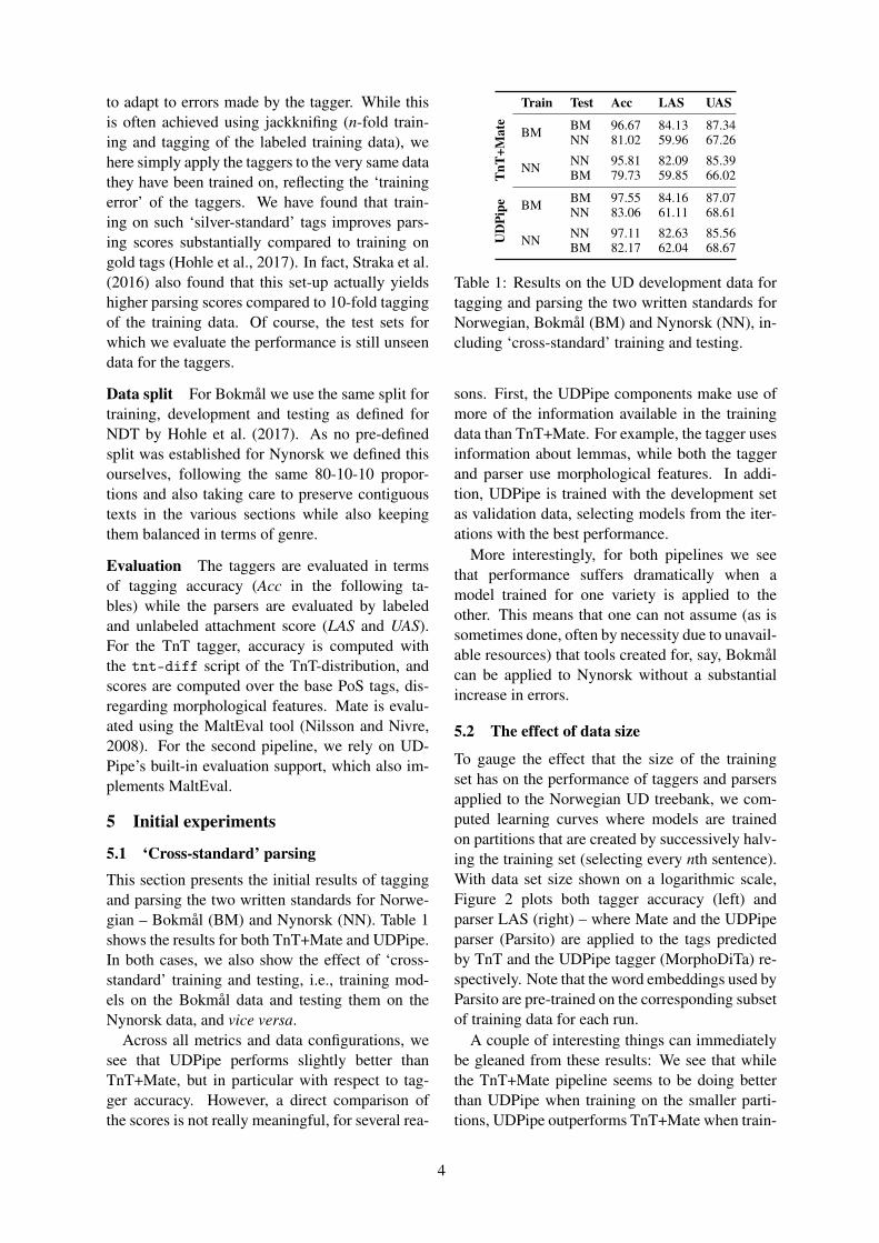
This section presents the initial results of taggingand parsing the two written standards for Norwe-gian – Bokmål (BM) and Nynorsk (NN). Table 1shows the results for both TnT+Mate and UDPipe.In both cases, we also show the effect of ‘cross-standard’ training and testing, i.e., training mod-els on the Bokmål data and testing them on theNynorsk data, and vice versa.

Across all metrics and data configurations, wesee that UDPipe performs slightly better thanTnT+Mate, but in particular with respect to tag-ger accuracy. However, a direct comparison ofthe scores is not really meaningful, for several rea-

Train Test Acc LAS UAS

TnT

+Mat

e

BM BM 96.67 84.13 87.34NN 81.02 59.96 67.26

NN NN 95.81 82.09 85.39BM 79.73 59.85 66.02

UD

Pipe BM BM 97.55 84.16 87.07

NN 83.06 61.11 68.61

NN NN 97.11 82.63 85.56BM 82.17 62.04 68.67

Table 1: Results on the UD development data fortagging and parsing the two written standards forNorwegian, Bokmål (BM) and Nynorsk (NN), in-cluding ‘cross-standard’ training and testing.

sons. First, the UDPipe components make use ofmore of the information available in the trainingdata than TnT+Mate. For example, the tagger usesinformation about lemmas, while both the taggerand parser use morphological features. In addi-tion, UDPipe is trained with the development setas validation data, selecting models from the iter-ations with the best performance.

More interestingly, for both pipelines we seethat performance suffers dramatically when amodel trained for one variety is applied to theother. This means that one can not assume (as issometimes done, often by necessity due to unavail-able resources) that tools created for, say, Bokmålcan be applied to Nynorsk without a substantialincrease in errors.

5.2 The effect of data size

To gauge the effect that the size of the trainingset has on the performance of taggers and parsersapplied to the Norwegian UD treebank, we com-puted learning curves where models are trainedon partitions that are created by successively halv-ing the training set (selecting every nth sentence).With data set size shown on a logarithmic scale,Figure 2 plots both tagger accuracy (left) andparser LAS (right) – where Mate and the UDPipeparser (Parsito) are applied to the tags predictedby TnT and the UDPipe tagger (MorphoDiTa) re-spectively. Note that the word embeddings used byParsito are pre-trained on the corresponding subsetof training data for each run.

A couple of interesting things can immediatelybe gleaned from these results: We see that whilethe TnT+Mate pipeline seems to be doing betterthan UDPipe when training on the smaller parti-tions, UDPipe outperforms TnT+Mate when train-

4

90

95

100

6.25 12.5 25 50 100

Acc

urac

y

% of training data

TnT

UDPipe

65

70

75

80

85

90

6.25 12.5 25 50 100

LAS

% of training data

TnT+Mate

UDPipe

Figure 2: Learning curves when training the two pipelines TnT+Mate and UDPipe on successively halvedpartitions of the Norwegian Bokmål training set (using a log scale), while testing on the developmentset. UPoS tagging accuracy to the left; labeled attachment score to the right.

ing on the full training set. Moreover, in all cases,we observe a roughly log-linear trend where im-provements are close to being constant for eachn-fold increase of data. The trends also seem toindicate that having access to even more labeleddata could improve performance further.

5.3 Motivating the further experiments

The ‘cross-standard’ experiments in Section 5.1showed that models trained on labeled data for oneof the two varieties of written Norwegian performpoorly when applied to the other. For all testedconfigurations, we observe a loss of between 20and 25 percentage points in labeled attachmentscore compared to training and testing on one andthe same variety. At the same time, it is impor-tant to realize that the results for ‘within-standard’processing of either the Bokmål or Nynorsk tree-bank data in isolation, correspond to an idealizedsetting that is not representative of how writtenNorwegian is encountered ‘in the wild’. In thenews sources, blogs, government reports and par-liament transcripts that form the basis for the tree-bank, both varieties of Norwegian will occur, in-termixed. In practice, this means that the actualparsing results can be expected to lie somewherein between the extremes reported in Table 1. Ofcourse, a language identification module could betrained and applied as a pre-processing step forselecting the appropriate model, but in practice itwould be much more convenient if we were ableto have a single model that could process both va-rieties equally well.

In the next section, we look into various ways ofmixing training data for the two written standardsof Norwegian in order to create improved mod-els for cross-standard joint processing. Moreover,given the empirical indications in Section 5.2 thatmore labeled training data could benefit the tag-gers and parsers, this strategy is also motivated bywanting to improve the absolute results for eachstandard in isolation.

6 Joint models

In this section we test the effects of combining thetraining data for Bokmål and Nynorsk, as well asextending it through machine translation.

6.1 Mixed training dataIn a first round of experiments we simply con-catenate the training sections for Bokmål andNynorsk. The results can be seen in the row‘BM+NN’ in Table 2. For both pipelines and bothlanguage varieties we observe the same trend: De-spite a loss in tagging accuracy, parsing perfor-mance improves when compared to training onjust a single variety (rows ‘BM’ or ‘NN’). Whileeffectively doubling the size of the training data,we do not see the same factor of improvementas for the learning curves in Figure 2, but wenonetheless see an increase in LAS of up to oneadditional percentage point. It is important tonote that the results for ‘BM+NN’ represents us-ing joint tagging and parsing pipelines across bothwritten standards: For each set-up (TnT+Mate andUDPipe) we train a single pipeline, and then apply

5

Bokmål Nynorsk

Train Acc LAS UAS Train Acc LAS UAS

Mat

e BM 96.67 84.13 87.34 NN 95.81 82.09 85.39BM+NN 96.29 84.97 88.04 BM+NN 95.18 83.13 86.22BM+MT 96.32 85.45 88.47 NN+MT 94.98 83.63 86.82BM+NN+MT 96.30 85.05 88.12 BM+NN+MT 94.97 83.47 86.65

UD

Pipe BM 97.55 84.16 87.07 NN 97.11 82.63 85.56

BM+NN 97.01 84.65 87.42 BM+NN 96.43 82.81 85.84BM+MT 97.17 85.03 87.97 NN+MT 96.16 82.47 85.57BM+NN+MT 96.83 85.10 88.01 BM+NN+MT 96.15 83.20 86.28

Table 2: Development results for Bokmål and Nynorsk tagged and parsed with TnT+Mate and UDPipe,training on Bokmål or Nynorsk alone (rows BM or NN), mixed (BM+NN), or each combined withmachine-translated data (BM+MT or NN+MT), or everything combined, i.e., the original and translatedversions of both the Bokmål and Nynorsk training data (BM+NN+MT).

the same pipeline to both the Nynorsk and Bokmåldevelopment sets.

As a control experiment, to better understandto what extent the improvements are due only tolarger training sets or also to the use of mixeddata, we ran the same experiments after down-sampling the combined training set to the samesize as the originals (simply discarding every sec-ond sentence). For TnT+Mate and UDPipe re-spectively, this gave a LAS of 82.81 and 82.77for Bokmål, and 81.47 and 80.86 for Nynorsk.We see that while training joint models on thedown-sampled mixed data gives slightly lower re-sults than when using the full concatenation (orusing dedicated single-standard models), it stillprovides a robust alternative for processing mixeddata, given the dramatically lower results we ob-served for cross-standard testing in Section 5.1.

6.2 Machine-translated training data

The results above show that combining trainingdata across standards can improve parsing perfor-mance. As mentioned in the introduction, though,there is a large degree of lexical divergence be-tween the two standards. In our next suite of ex-periments, we therefore attempt to further improvethe results by automatically machine-translatingthe training texts. Given the strong degree ofstructural equivalence between Norwegian Bok-mål and Nynorsk, we can expect MT to yield rel-atively accurate translations. For this, we use thetwo-way Bokmål–Nynorsk MT system of Unham-mer and Trosterud (2009), a rule-based shallow-transfer system built on the open-source MT plat-form Apertium (Forcada et al., 2011).

The raw text passed to Apertium is extracted

from the full-form column of the UD CoNLLtraining data (translating the lemmas does not giveadequate results). The only sanity-checking weperform on the result is ensuring that the numberof tokens in the target translation matches that ofthe source. In cases where the token counts di-verge – for example when the Bokmål form fort-sette (‘continue’) is translated to Nynorsk as haldefram (‘keep on’) – the sentence is left in its originalsource form. For the NN→BM translation, this isthe case for almost 4% of the sentences. The direc-tion BM→NN appears to be slightly harder, wherealmost 13% of the sentences are left untranslated.

We tested the translated training data in twoways: 1) Training single-standard pipelines, forexample training on the original Bokmål data andthe Nynorsk data translated to Bokmål, and 2)training on all the available training data com-bined, i.e., both of the original versions and bothof the translated versions, in effect increasing theamount of training data by a factor of four.

The results for the development data are shownin Table 2. Adding the MT data reinforces thetrend observed for mixing the original trainingsets: Despite that PoS tagging accuracy typically(though not always) decreases when adding data,parsing accuracy improves. For the TnT+Matepipeline, we see that the best parser performance isobtained with the single-standard models includ-ing the MT data, while UDPipe achieves the bestresults when using the maximal amount of train-ing data. Coupled with the parser learning curvesin Figure 2, this observation is in line with theexpectation that neural network architectures bothrequire and benefit more from larger training sam-ples, but recall the caveat noted in Section 5.1

6

about how the scores are not directly compara-ble. Finally, note that this latter configuration, i.e.,combining both of the original training sets withboth of the translated versions, again correspondsto having a single joint model for both Bokmål andNynorsk. Also for TnT+Mate, we see that thisconfiguration yields better results than our previ-ous joint model without the MT data.

6.3 Caveat on morphology

Although the development results demonstratethat the various ways of combining the trainingdata lead to increased parser performance, we sawthat the tagging accuracy was slightly reduced.However, the UDPipe tagging component, Mor-phoDiTa, performs additional morphological anal-ysis beyond assigning UPoS tags. It also per-forms lemmatization and assigns morphologicalfeatures, and in particular for the first of thesetasks the drop in performance for the joint mod-els is more pronounced. For example, when com-paring the Bokmål development results for theUDPipe model trained on the original Bokmåldata alone versus Bokmål and Nynorsk combined,the lemmatization accuracy drops from 97.29% to95.18% (and the morphological feature accuracydrops from 96.03% to 95.39%). This is not sur-prising. Given the close similarities of Bokmåland Nynorsk, several words in the two variantswill have identical inflected forms but differentlemmas, introducing a lot of additional ambiguityfor the lemmatizer. The drop in lemma accuracyis mostly due to a handful of high-frequent wordshaving this effect, for example the verb forms var(‘was’) or er (‘is’) which should be lemmatized asvære in Bokmål and vere in Nynorsk. However,for the taggers trained on the maximal trainingdata where we include the machine-translated ver-sions of both varieties, the lemma accuracy reallyplummets, dropping to 86.19% (and morphologi-cal feature accuracy dropping to 93.79%). Again,this is as expected, given that only the full-formsof training data were translated.

In our parsing pipeline, lemmas are not usedand so this drop in accuracy does not affect down-stream performance. However, for applicationswhere lemmatization plays an important role, ajoint tagger should either be trained without theuse of the MT data (or an initial single-standardlemmatizer should be used to lemmatize this dataafter translation), and ideally should be made to

take more context into consideration to be able tomake more accurate predictions.

7 Held-out results

For the held-out results, we focus on testing thetwo joint models, i.e., (1) estimating models fromthe original training sets for Nynorsk and Bokmålcombined, as well as (2) augmenting this furtherwith the their MT versions (translating each vari-ety into the other). We contrast the performance ofthese joint models with the results from training oneither of the original single-standard training setsin isolation, including cross-standard testing. Ta-ble 3 summarizes the results for both pipelines –TnT+Mate and UDPipe – for the held-out sectionsof the treebanks for both of the Norwegian writtenvarieties – Bokmål (BM) and Nynorsk (NN).

In terms of relative performance, the outcomeis the same as for the development data: The jointmodels give better parsing performance across allconfigurations, compared to the dedicated single-standard models, despite reduced tagger accuracy.In terms of absolute figures, we see that UDPipehas the best performance.

It is also interesting to note that the UDPipeparser appears to be more robust to the noise in-troduced with MT data, and that this may evenhave had the effect of mitigating overfitting: Whilewe observe a slight drop in performance for thesingle-variety models when moving from develop-ment to held-out results, the effect is the oppositefor the joint model trained on the MT data. Thiseffect is most pronounced for the Nynorsk data,which is also known to have the most translationerrors in the training data.

Finally, note that while our parser scores arestronger than those previously reported for UD-Pipe on Norwegian (Bokmål only) (Straka et al.,2016), there are several reasons why the results arenot directly comparable. First, we here use version1.4 of the UD treebank as opposed to version 1.2for the results of Straka et al. (2016), and secondly,the embeddings generated by word2vec are non-deterministic, meaning that strictly speaking, dif-ferent UDPipe models for the same training datacan only be directly compared if reusing the sameembeddings.

8 Future work

Immediate follow-up work will include using alarger unlabeled corpus for pre-training the word

7

BM NN

Training Acc LAS UAS Acc LAS UAS

Mat

e BM 96.31 83.80 87.04 81.66 60.51 67.55NN 80.32 60.64 67.13 95.55 81.51 85.06BM+NN 95.98 84.74 87.83 95.06 83.11 86.42BM+NN+MT 95.79 84.88 87.89 94.78 83.87 87.16

UD

Pipe BM 97.07 83.42 86.28 83.35 60.95 68.15

NN 82.92 62.85 69.66 96.80 82.40 85.38BM+NN 96.49 84.20 86.90 96.27 83.46 86.24BM+NN+MT 96.48 85.31 88.04 96.05 84.17 87.18

Table 3: Held-out test results for Norwegian Bokmål and Nynorsk tagged and parsed with TnT+Mateand UDPipe, using either the Bokmål or Nynorsk training data alone (rows BM or NN), Bokmål andNynorsk mixed (BM+NN), or Bokmål and Nynorsk combined with machine-translated data, i.e., theoriginal versions of both varieties as well as the translations of each into the other (BM+NN+MT).

embeddings used by UDPipe’s Parsito parser. Forthis, we will use the Norwegian Newspaper Cor-pus which consists of texts collected from a rangeof major Norwegian news sources for the years1998–2014, and importantly comprising both theBokmål and the Nynorsk variety. Another di-rection for optimizing the performance of thepipelines is to use different training data for thedifferent components. This is perhaps most impor-tant for the UDPipe model. While the parser ben-efits from including the machine-translated data intraining, the tagger performs better when using thecombination of the original training data. This ismostly noticeable when considering not just theaccuracy of the UPoS tags but also the morpho-logical features, which are also used by the parser.Finally, while the experimental results in this pa-per are based on the UD conversion of the Norwe-gian Dependency Treebank, there is of course noreason to expect that the effects will be differenton the original NDT data. We plan to also repli-cate the experiments for NDT, and make availableboth pre-trained joint and single-standard modelsfor this data set as well.

9 Conclusion

This paper has tackled the problem of creating asingle pipeline for dependency parsing that givesaccurate results across both of the official vari-eties for written Norwegian language – Bokmåland Nynorsk. Although the two varieties are veryclosely related and have few syntactic differences,they can be very different lexically. To the best ofour knowledge, this is the first study to attempt tobuild a uniform tool-chain for both language stan-dards, and also to quantify cross-standard perfor-

mance of Norwegian NLP tools in the first place.

The basis of our experiments is the NorwegianDependency Treebank, converted to Universal De-pendencies. For Bokmål, this treebank conversionwas already in place (Øvrelid and Hohle, 2016),while for the Nynorsk data, the conversion hasbeen done as part of the current study. To makeour results more robust, we have evaluated andcompared pipelines created with two distinct setof tools, each based on different learning schemes;one based on the TnT tagger and the Mate parser,and one based on UDPipe.

To date, the common practice has been to builddedicated models for a single language variantonly. Quantifying the performance of modelstrained on labeled data for a single variety (e.g.,the majority variety Bokmål) when applied to datafrom the other (Nynorsk), we found that parsingaccuracy dramatically degrades, with LAS drop-ping by 20–25 percentage points. At the sametime, we found that when combining the trainingdata for both varieties, parsing performance in factincreases for both. Importantly, this also elimi-nates the issue of cross-standard performance, asonly a single model is used. Finally, we haveshown that the joint parsers can be improved evenfurther by also including machine-translated ver-sions of the training data for each variety.

In terms of relative differences, the trends forall observed results are consistent across both ofour tool chains, TnT+Mate and UDPipe, althoughwe find the latter to have the best absolute perfor-mance. Our results have immediate practical valuefor processing Norwegian, as it means that a singleparsing pipeline is sufficient to cover both officialwritten standards, with no loss in accuracy.

8

ReferencesŽeljko Agic, Anders Johannsen, Barbara Plank, Héc-

tor Alonso Martínez, Natalie Schluter, and AndersSøgaard. 2016. Multilingual projection for parsingtruly low-resource languages. Transactions of theAssociation for Computational Linguistics, 4:301–312.

Waleed Ammar, George Mulcaire, Miguel Ballesteros,Chris Dyer, and Noah A. Smith. 2016. One parser,many languages. arXiv preprint arXiv:1602.01595.

Bernd Bohnet. 2010. Very High Accuracy and FastDependency Parsing is not a Contradiction. In Pro-ceedings of the 23rd International Conference onComputational Linguistics, pages 89–97, Beijing,China.

Thorsten Brants. 2000. TnT - A Statistical Part-of-Speech Tagger. In Proceedings of the Sixth AppliedNatural Language Processing Conference, Seattle,WA, USA.

Xavier Carreras. 2007. Experiments with a higher-order projective dependency parser. In Proceed-ings of the Joint Conference on Empirical Methodsin Natural Language Processing and Conference onComputational Natural Language Learning, pages957–961, Prague, Czech Republic.

Danqi Chen and Christopher Manning. 2014. A fastand accurate dependency parser using neural net-works. In Proceedings of the 2014 Conference onEmpirical Methods in Natural Language Process-ing, pages 740–750, Doha, Qatar.

Jinho D. Choi, Joel Tetreault, and Amanda Stent. 2015.It Depends: Dependency Parser Comparison Us-ing A Web-Based Evaluation Tool. In Proceedingsof the 53rd Annual Meeting of the Association forComputational Linguistics, pages 387–396, Beijing,China.

Michael Collins. 2002. Discriminative training meth-ods for hidden markov models: Theory and experi-ments with perceptron algorithms. In Proceedingsof the 2002 Conference on Empirical Methods inNatural Language Processing, pages 1–8, PA, USA.

Koby Crammer, Ofer Dekel, Joseph Keshet, ShaiShalev-Shwartz, and Yoram Singe. 2006. Onlinepassive-aggressive algorithms. Journal of MachineLearning Research, 7:551–585.

Marie-Catherine de Marneffe, Timothy Dozat, Na-talia Silveira, Katri Haverinen, Filip Ginter, JoakimNivre, and Christopher D. Manning. 2014. Uni-versal Stanford dependencies. A cross-linguistic ty-pology. In Proceedings of the International Confer-ence on Language Resources and Evaluation, pages4585–4592, Reykjavik, Iceland.

Mikel L. Forcada, Mireia Ginestí-Rosell, Jacob Nord-falk, Jim O’Regan, Sergio Ortiz-Rojas, Juan An-tonio Pérez-Ortiz, Felipe Sánchez-Martínez, Gema

Ramírez-Sánchez, and Francis M. Tyers. 2011.Apertium: a free/open-source platform for rule-based machine translation. Machine Translation,25(2):127–144.

Petter Hohle, Lilja Øvrelid, and Erik Velldal. 2017.Optimizing a PoS tagset for Norwegian dependencyparsing. In Proceedings of the 21st Nordic Con-ference of Computational Linguistics, Gothenburg,Sweden.

Rebecca Hwa, Philip Resnik, Amy Weinberg, ClaraCabezas, and Okan Kolak. 2005. Bootstrappingparsers via syntactic projection across parallel texts.Natural Language Engineering, 11(3).

Tomas Mikolov, Kai Chen, Greg Corrado, and Jef-frey Dean. 2013. Efficient estimation of wordrepresentations in vector space. arXiv preprintarXiv:1301.3781.

Jens Nilsson and Joakim Nivre. 2008. MaltEval:An evaluation and visualization tool for dependencyparsing. In Proceedings of the Sixth InternationalConference on Language Resources and Evaluation,pages 161–166, Marrakech, Morocco.

Joakim Nivre, Marie-Catherine de Marneffe, Filip Gin-ter, Yoav Goldberg, Jan Hajic, Christopher D. Man-ning, Ryan McDonald, Slav Petrov, Sampo Pyysalo,Natalia Silveira, Reut Tsarfaty, and Daniel Zeman.2016. Universal dependencies v1: A multilingualtreebank collection. In Proceedings of the Interna-tional Conference on Language Resources and Eval-uation, Portorož, Slovenia.

Joakim Nivre. 2015. Towards a Universal Grammarfor Natural Language Processing. In ComputationalLinguistics and Intelligent Text Processing, volume9041 of Lecture Notes in Computer Science, pages3–16. Springer International Publishing.

Lilja Øvrelid and Petter Hohle. 2016. Universal De-pendencies for Norwegian. In Proceedings of theTenth International Conference on Language Re-sources and Evaluation, Portorož, Slovenia.

Slav Petrov, Dipanjan Das, and Ryan McDonald. 2012.A Universal Part-of-Speech Tagset. In Proceedingsof the Eighth International Conference on LanguageResources and Evaluation, pages 2089–2096, Istan-bul, Turkey.

Arne Skjærholt and Lilja Øvrelid. 2012. Impactof treebank characteristics on cross-lingual parseradaptation. In Proceedings of the Eleventh Interna-tional Workshop on Treebanks and Linguistic Theo-ries, pages 187–198, Lisbon, Portugal.

Anders Søgaard. 2011. Data point selection for cross-language adaptation of dependency parsers. In Pro-ceedings of the 49th Annual Meeting of the Associ-ation for Computational Linguistics, pages 682—-686, Portland, Oregon.

9

Per Erik Solberg, Arne Skjærholt, Lilja Øvrelid, KristinHagen, and Janne Bondi Johannessen. 2014. TheNorwegian Dependency Treebank. In Proceedingsof the Ninth International Conference on LanguageResources and Evaluation, pages 789–795, Reyk-javik, Iceland.

Kathrin Spreyer, Lilja Øvrelid, and Jonas Kuhn. 2010.Training parsers on partial trees: A cross-languagecomparison. In Proceedings of the InternationalConference on Language Resources and Evaluation(LREC).

Milan Straka, Jan Hajic, Jana Straková, and Jan Ha-jic jr. 2015. Parsing universal dependency tree-banks using neural networks and search-based or-acle. In Proceedings of Fourteenth InternationalWorkshop on Treebanks and Linguistic Theories,Warsaw, Poland.

Milan Straka, Jan Hajic, and Jana Straková. 2016. UD-Pipe: trainable pipeline for processing CoNLL-Ufiles performing tokenization, morphological anal-ysis, pos tagging and parsing. In Proceedings ofthe Tenth International Conference on Language Re-sources and Evaluation, Portorož, Slovenia.

Jana Straková, Milan Straka, and Jan Hajic. 2014.Open-Source Tools for Morphology, Lemmatiza-tion, POS Tagging and Named Entity Recognition.In Proceedings of 52nd Annual Meeting of the As-sociation for Computational Linguistics: SystemDemonstrations, pages 13–18, Baltimore, Mary-land.

Oscar Täckström, Ryan McDonald, and Jakob Uszko-reit. 2012. Cross-lingual word clusters for directtransfer of linguistic structure. In Proceedings ofthe 2012 Conference of the North American Chap-ter of the Association for Computational Linguistics,Montreal, Canada.

Jörg Tiedemann, Željko AgicZeljko, and Joakim Nivre.2014. Treebank translation for cross-lingual parserinduction. In Proceedings of the Eighteenth Confer-ence on Computational Natural Language Learning,pages 130–140.

Kevin Brubeck Unhammer and Trond Trosterud. 2009.Reuse of Free Resources in Machine Translation be-tween Nynorsk and Bokmål. In Proceedings of theFirst International Workshop on Free/Open-SourceRule-Based Machine Translation, pages 35–42, Ali-cante.

Dan Zeman and Philip Resnik. 2008. Cross-languageparser adaptation between related languages. InProceedings of the IJCNLP-08 Workshop on NLPfor Less Privileged Languages, Hyderabad, India.

10


Replacing OOV Words For Dependency ParsingWith Distributional Semantics

Prasanth Kolachina 4 and Martin Riedl ♦ and Chris Biemann ♦4 Department of Computer Science and Engineering, University of Gothenburg, Sweden

♦ Language Technology Group, Universitat Hamburg, [email protected]

{riedl,biemann}@informatik.uni-hamburg.de

Abstract

Lexical information is an important fea-ture in syntactic processing like part-of-speech (POS) tagging and dependencyparsing. However, there is no such in-formation available for out-of-vocabulary(OOV) words, which causes many clas-sification errors. We propose to replaceOOV words with in-vocabulary words thatare semantically similar according to dis-tributional similar words computed from alarge background corpus, as well as mor-phologically similar according to commonsuffixes. We show performance differ-ences both for count-based and dense neu-ral vector-based semantic models. Fur-ther, we discuss the interplay of POS andlexical information for dependency pars-ing and provide a detailed analysis and adiscussion of results: while we observesignificant improvements for count-basedmethods, neural vectors do not increasethe overall accuracy.

1 Introduction

Due to the high expense of creating treebanks,there is a notorious scarcity of training data fordependency parsing. The quality of dependencyparsing crucially hinges on the quality of part-of-speech (POS) tagging as a preprocessing step;many dependency parsers also utilize lexicalizedinformation, which is only available for the train-ing vocabulary. Thus errors in dependency parsersoften relate to OOV (out of vocabulary, i.e. notseen in the training data) words.

While there has been a considerable amount ofwork to address the OOV problem with continuous

word representations (see Section 2), this requiresa more complex model and hence, increases train-ing and execution complexity.

In this paper, we present a very simple yet effec-tive way of alleviating the OOV problem to someextent: we use two flavors of distributional sim-ilarity, computed on a large background corpus,to replace OOV words in the input with semanti-cally or morphologically similar words that havebeen seen in the training, and project parse labelsback to the original sequence. If we succeed inreplacing OOV words with in-vocabulary wordsof the same syntactic behavior, we expect the tag-ging and parsing process to be less prone to errorscaused by the absence of lexical information.

We show consistent significant improvementsboth for POS tagging accuracy as well as for La-beled Attachment Scores (LAS) for graph-basedsemantic similarities. The successful strategiesmostly improve POS accuracy on open classwords, which results in better dependency parses.Beyond improving POS tagging, the strategy alsocontributes to parsing accuracy. Through exten-sive experiments – we show results for seven dif-ferent languages – we are able to recommend oneparticular strategy in the conclusion and show theimpact of using different similarity sources.

Since our method manipulates the input datarather than the model, it can be used with anyexisting dependency parser without re-training,which makes it very applicable in existing envi-ronments.

2 Related Work

While part-of-speech (POS) tags play a major rolein detecting syntactic structure, it is well known(Kaplan and Bresnan (1982) inter al.) that lexicalinformation helps for parsing in general and for

11

dependency parsing in particular, see e.g. Wang etal. (2005).

In order to transfer lexical knowledge from thetraining data to unseen words in the test data, Kooet al. (2008) improve dependency parsing withfeatures based on Brown Clusters (Brown et al.,1992), which are known to be drawing syntactic-semantic distinctions. Bansal et al. (2014) showslight improvements over Koo et al. (2008)’smethod by tailoring word embeddings for depen-dency parsing by inducing them on syntactic con-texts, which presupposes the existence of a depen-dency parser. In more principled fashion, Socheret al. (2013) directly operate on vector representa-tions. Chen et al. (2014) address the lexical gapby generalizing over OOV and other words in afeature role via feature embeddings. Another ap-proach for replacing OOV words by known onesusing word embeddings is introduced by Andreasand Klein (2014).

All these approaches, however, require re-training the parser with these additional featuresand make the model more complex. We present amuch simpler setup of replacing OOV words withsimilar words from the training set, which allowsretrofitting any parser with our method.

This work is related to Biemann and Riedl(2013), where OOV performance of fine-grainedPOS tagging has been improved in a similar fash-ion. Another similar work to ours is proposedby Huang et al. (2014), who replace OOV namedentities with named entities from the same (fine-grained) class for improving Chinese dependencyparsing, which largely depends on the quality ofthe employed NER tagger and is restricted tonamed entities only. In contrast, we operate onall OOV words, and try to improve prediction oncoarse universal POS classes and universal depen-dencies.

On a related note, examples for a successful ap-plication of OOV replacements is demonstratedfor Machine Translation (Gangadharaiah et al.,2010; Zhang et al., 2012).

3 Methodology

For replacing OOV words we propose three strate-gies: replace OOV words by most similar ones us-ing distributional semantic methods, replace OOVwords with words with the most common suffixand replacing OOV words before or after POS tag-ging to observe the effect on dependency parsing.

The influence of all components is evaluated sepa-rately for POS tagging and dependency parsing inSection 5.

3.1 Semantic SimilaritiesIn order to replace an OOV word by a similar in-vocabulary word, we use models that are based onthe distributional hypothesis (Harris, 1951). Forshowing the impact of different models we use agraph-based approach that uses the left- and right-neighbored word as context, represented by themethod proposed by Biemann and Riedl (2013),and is called distributional thesaurus (DT). Fur-thermore, we apply two dense numeric vector-space approaches, using the skip-gram model(SKG) and CBOW model of the word2vec im-plementation of Mikolov et al. (2013).

3.2 Suffix SourceIn addition, we explore replacing OOVs withwords from the similarity source that are containedin the training set and share the longest suffix.This might be beneficial as suffixes reflect mor-phological markers and carry word class informa-tion in many languages. The assumption here isthat for syntactic dependencies, it is more crucialthat the replacement comes from the same wordclass than its semantic similarity. This also servesas a comparison to gauge the benefits of the simi-larity source alone. Below, these experiments aremarked with suffix, whereas the highest-ranked re-placement from the similarity sources are markedas sim. As a suffix-only baseline, we replace OOVswith its most suffix-similar word from the train-ing data, irrespective of its distributional similar-ity. This serves as a sanity check whether semanticsimilarities are helpful at all.

3.3 Replacement Strategies regarding POSWe explore two different settings for dependencyparsing that differ in the use of POS tags:

(1) oTAG: POS-tag original sequence, then re-place OOV words, retaining original tags forparsing;

(2) reTAG: replace OOV word, then POS-tag thenew sequence and use the new tags for pars-ing.

The oTAG experiments primarily quantify thesensitivity of the parsing model to word forms,whereas reTag assess the potential improvementsin the POS tagging.

12

3.4 Replacement ExampleAs an example, consider the automatically POS-tagged input sentence “We/P went/V to/P the/Daquatic/N park/N” where “aquatic” is an OOVword. Strategy oTAG sim replaces “aquatic” with“marine” since it is the most similar in-vocabularyword of “aquatic”. Strategy oTAG suffix replacesit with “exotic” because of the suffix “tic” and itssimilarity with “aquatic”. The suffix-only baselinewould replace with “automatic” since it shares thelongest suffix of all in-vocabulary words. The re-TAG strategy would then re-tag the sentence, sothe parser will e.g. operate on “We/P went/V to/Pthe/D marine/ADJ park/N”. Table 1 shows an ex-ample for different similarity-based strategies forEnglish and German1. We observe that the simstrategy returns semantically similar words that donot necessarily have the same syntactic function asthe OOV target.

sim sim&suffixEnglish OOV: upgraded

Suffix-only paradedCBOW upgrade downloadedSKG upgrade expandedDT expanded updated

German OOV: NachtzeitSuffix-only PachtzeitCBOW tagsuber RuhezeitSKG tagsuber EchtzeitDT Jahreswende Zeit

Table 1: Here we show replacements for differentmethods using different strategies.

4 Experimental Settings

Here we describe the methods, background cor-pora used for computing similarities and all furthertools used for the experiments. With our experi-ments, we target to address the following researchquestions:

• Can syntactic processing benefit from OOVreplacement, and if so, under what strategiesand conditions?

• Is there a qualitative difference between sim-ilarity sources with respect to tagger/parserperformance?

1Translations: Nachtzeit = night time; tagsuber = duringthe day; Pachtzeit = length of lease; Ruhezeit = downtime;Echtzeit = real time; Jahreswende = turn of the year

• Are there differences in the sensitivity ofparsing inference methods to OOV replace-ment?

4.1 Similarity ComputationsWe are using two different approaches to deter-mine semantic similarity: a symbolic, graph-basedframework for distributional similarity and a neu-ral language model that encodes words in a densevector space.

Graph-based Semantic SimilarityThe computation of a corpus-based distributionalthesaurus (marked as DT below) is performed fol-lowing the approach by Biemann and Riedl (2013)as implemented in the JoBimText2 software. Forcomputing similarities between words from largeunlabeled corpora, we extract as word-contextthe left and right neighboring words, not usinglanguage-specific syntactic preprocessing. Wordsare more similar if they share more of their mostsalient 1000 context features, where salient con-text features are ranked by Lexicographer’s Mu-tual Information (LMI), (Evert, 2005). Word sim-ilarity in the DT is defined as the count of overlap-ping salient context features. In addition we prunesimilar words3 below a similarity threshold of 5.

In order to use such a DT to replace an OOVword, we look up the most similar terms for theOOV word and choose the highest-ranked wordfrom the training data vocabulary, respectively themost similar word with the longest common suf-fix.

Neural Semantic SimilarityAs an alternative similarity we run word2vecwith default parameters (marked as w2v below)(Mikolov et al., 2013) on our background corpora,obtaining 200-dimensional dense vector embed-dings for all words with a corpus frequency largerthan 5. We conduct this for both flavors of w2v:skipgram, marked as SKG below (based on posi-tional windows) and CBOW (based on bag of wordsentential contexts).

Following the standard approach, we use the co-sine between word vectors as a similarity measure:for each OOV, we compare vectors from all wordsin the training set and pick the word that corre-spond to the most similar vector as a replacement,

2http://www.jobimtext.org3we have tried a few thresholds in preliminary experi-

ments and did not find results to be very sensitive in the rangeof 2 – 20

13

respectively the most similar word of those withthe longest common suffix.

4.2 Corpora for Similarity ComputationAs we perform the experiments on various lan-guages, we will compute similarities for each lan-guage separately. The English similarities arecomputed based on 105M sentences from theLeipzig corpora collection (LCC) (Richter et al.,2006) and the Gigaword corpus (Parker et al.,2011). The German (70M) and the Hindi (2M)corpora are extracted from the LCC as well. Wecompute similarities on 19.7M sentences of Ara-bic, 259.7M sentences of French and 128.1M sen-tences of Spanish extracted from web corpora4

provided by Schafer and Bildhauer (2013). For thecomputation of the Swedish similarities we use a60M-sentence news corpus from Spraakbanken.5

In summary, all background corpora are in the or-der of about 1 Gigaword, except the Hindi corpus,which is considerably smaller.

4.3 Dependency Parser and POS TaggerFor the dependency parsing we use the implemen-tation of the graph-based dependency parser pro-vided in Mate-tools (Bohnet, 2010, version 3.6)and the transition-based Malt parser (Nivre, 2009,version 1.8.1). Graph-based parsers use global in-ference to construct the maximum spanning de-pendency tree for the input sequences. Contrary,the greedy algorithm in the transition-based parseruses local inference to predict the dependencytree. The parsing models for both parsers, Mate-tools and Malt parser, are optimized using cross-validation on the training section of the treebank6.We train the dependency parsers using POS tags(from the Mate-tools tagger) predicted using a 5-fold cross-validation. The evaluation of the parseraccuracies is carried out using MaltEval. We re-port labeled attachment score (LAS) for both over-all and on OOV token positions.

4.4 TreebanksFor training and testing we apply the treebanks(train/dev/test size in tokens in parentheses) fromthe Universal Dependencies project (Nivre et al.,

4http://corporafromtheweb.org/5http://spraakbanken.gu.se6Using Malt Optimizer (Ballesteros and Nivre, 2016) for

the Malt parser; for Mate-tools, we tuned the parameter thatrepresents the percentage of non-projective edges in a lan-guage, which matches the parameters suggested by Bohnet(2010).

2016, version 1.2 released November 15th, 2015)for Arabic, English, French, German, Hindi, Span-ish and Swedish. Tagset definitions are availableonline.7

5 Results

In this section, we report experimental results andcompare them to the baseline without OOV re-placement. All statistical significance tests aredone using McNemar’s test. Significant improve-ments (p < 0.05) over the baseline without OOVreplacement are marked with an asterisk (∗), sig-nificant performance drops with a hashmark (#)and the best result per experiment is marked inbold.

5.1 Results for POS Tagging

In Table 2 we show overall and OOV-only POStagging accuracies on the respective test set forseven languages using similarities extracted fromthe DT.

LANG OOV baseline suffix only DT sim DT suffix% all OOV all OOV all OOV all OOV

Arabic 10.3 98.53 94.01 97.82# 87.44# 98.49# 93.67# 98.52 93.91English 8.0 93.43 75.39 93.09# 72.03# 93.82* 78.67* 93.61* 76.75French 5.3 95.47 83.29 95.17# 78.30# 95.68* 86.28* 95.73* 86.78*German 11.5 91.92 85.63 90.88# 77.70# 91.84 85.32 91.92 85.68Hindi 4.4 95.35 76.41 95.07# 71.27# 95.41 77.57 95.44* 78.00*Spanish 6.9 94.82 79.62 95.00 81.17 95.45* 86.36* 95.49* 85.84*Swedish 14.3 95.34 89.80 94.78# 86.04 # 95.57* 90.88* 95.82* 92.40*

Table 2: Test set overall OOV rates, POS accuracyin % for baseline, suffix-only baseline, DT simi-larity and suffix replacement strategies for sevenlanguages.

Unsurprisingly, we observe consistent perfor-mance drops, mostly significant, for the suffix-only baseline. For all languages except German,the DT-based replacement strategies result in sig-nificant improvements of either overall accuracy,OOV accuracy or both. In most experiments,the DT suffix replacement strategy scores slightlyhigher than the DT sim strategy.

Table 3 lists POS accuracies for three lan-guages for similarities from the w2v neural lan-guage model in its SKG and CBOW flavors us-ing the cosine similarity. In contrast to the DT-based replacements, there are no improvementsover the baseline, and some performance drops areeven significant. Also replacing the cosine similar-ity with the Euclidian distance did not change this

7http://universaldependencies.org/

14

SKG CBOWLANG sim suffix sim suffix

all OOV all OOV all OOV all OOVArabic 98.46# 93.39# 98.50# 93.73# 98.48# 93.60# 98.52 93.94English 93.10# 72.29# 93.57 76.31 93.24# 73.91 93.52 75.70German 90.99# 77.65# 91.62# 83.61# 91.78 83.92# 91.91 85.43

Table 3: Test set POS accuracies for w2v-basedmodel’s similarity and suffix replacement strate-gies for three languages.

observation. The suffix-based strategy seems towork better than the similarity-based strategy alsofor the w2v-based replacement.

It seems that count-based similarities performbetter for the replacement. Thus, we did not ex-tend the experiments with w2v to other languages.

5.2 Results for Dependency Parsing

As a general trend for all languages (see Ta-ble 4), we observe that the graph-based parserachieves higher LAS scores than the transition-based parser.

However, the optimal replacement strategy de-pends on the language for both parsers. Only forSwedish (reTAG DT suffix) and Spanish (reTAGDT sim), the same replacements yield the highestscores both on all words and OOV words for bothparsers. Using the modified POS tags (reTAG)results in improvements for the transitions-basedparser for 4 languages and for 5 languages usingthe graph-based parser. Whereas the results im-prove only marginal when using the reTAG strat-egy as can be observed from Table 4, most im-provements are significant.

Using word embeddings for the reTAG strat-egy (see Table 5), we again observe performancedrops, except for Arabic.

Following the oTAG strategy, we observe signif-icant improvements on German and Arabic for theCBOW method. For German the best performanceis obtained with the SKG model (74.47*) whichis slightly higher then the suffix only replacement,which achieves high scores in the oTAG setting.Whereas for POS tagging the suffix-based DT re-placement mostly results in the highest scores,there is no clear recommendation for a replace-ment strategy for parsing all languages. Lookingat the average delta (∆) values for all languages(see Tables 4 and 5) in comparison to the baseline,the picture is clearer: here, for both parser the re-TAG DT suffix strategy yields the highest improve-ments and the CBOW and SKG methods only

result in consistent improvements for the oTAGstrategy. Further average performance gains areobserved for the CBOW suffix-based method us-ing the reTAG strategy.

To sum up, we have noted that the DT-basedstrategies seem more advantageous than the w2v-strategies across languages. Comparing the differ-ent strategies for using DTs, we observe an advan-tage of reTAG over oTAG and a slight advantageover suffix vs. sim. Most notably, DT reTAG suf-fix is the only strategy that never resulted in a sig-nificant performance drop on all datasets for bothparsers and yields the highest average ∆ improve-ment of 1.50. Given its winning performance onthe POS evaluation, we recommend to use thisstrategy.

6 Data Analysis

6.1 Analysis of POS Accuracy

Since POS quality has a direct influence on parseraccuracy, we have analyzed the two reTag strate-gies suffix and sim for our three similarity sources(DT, SKG, CBOW) in more detail for German andEnglish by comparing them to the oTAG baselines.In general, differences are mostly found for openword classes such as ADJ, ADV, NOUN, PROPNand VERB, which naturally have the highest OOVrates in the test data. In both languages, the DT-based strategies supply about 84% of the replace-ments of the w2v strategies.

For German, only the DT suffix-based replace-ments led to a slight overall POS improvement.All similarity sources improved the tagging ofNOUN for suffix, but not for sim. All replacementsled to some losses in VERBs, with SKG losing themost. Both w2v sources lost more on ADJ than theDT, which also showed the largest improvementson ADV. In addition, we analyzed the POS classifi-cation only for tokens that could be replaced bothby the DT and the w2v-methods. For these tokens,the SKG method can not surpass the oTAG perfor-mance. Furthermore, for DT and CBOW, the suffixstrategies achieve slightly lower scores than sim(0.18%-0.63%). On the tokens where all methodspropose replacements, the DT results in better ac-curacy (86.00%) than CBOW (85.82%).

For English, the picture is similar but in gen-eral the improvement of the scores is larger: whilethe DT sim led to the largest and the DT suffixto the second-largest overall improvements, thesuffix-based w2v-strategies can also improve POS

15

oTAG reTAGbaseline suffix only DT sim DT suffix suffix only DT sim DT suffix

Language all OOV all OOV all OOV all OOV all OOV all OOV all OOVGraph-based Parser

Arabic 75.60 56.90 75.61 57.76* 75.74* 58.18* 75.71* 58.31* 74.54# 52.84# 75.75* 58.18* 75.72* 58.31*English 79.57 63.64 79.55 63.77 79.64 64.38* 79.54 64.20 79.24# 62.37 79.95* 66.17* 79.78* 65.30*French 77.76 64.59 77.91 65.34 77.61 64.09 77.79 64.84 77.59 64.59 77.59 64.09 77.97 65.84German 74.24 68.93 74.43* 69.66* 74.27 69.14 74.21 69.24 72.26# 63.43# 74.13 68.10 74.22 69.09Hindi 87.67 72.00 87.76* 72.74 87.78* 72.80* 87.71 72.86* 87.49# 70.60 87.67 72.62 87.69 72.74Spanish 80.02 63.56 80.07 65.28* 80.32* 67.18* 80.30* 66.84* 79.38# 64.59 80.41* 68.91* 80.27 68.05*Swedish 77.13 70.70 77.16 70.87 77.44* 71.07 77.31* 71.03 76.55# 69.12# 77.62* 71.96* 77.65* 72.05*∆ all 0.00 0.00 0.10 0.72 0.10 0.89 0.08 0.93 -0.79 -1.89 0.02 0.95 0.12 1.35

Transition-based ParserArabic 72.63 52.81 72.71 53.67 72.79* 53.94* 72.75* 53.91* 71.75# 48.61# 72.77* 53.84* 72.74* 53.84*English 77.26 61.84 77.15# 61.67 77.16 61.84 77.30 62.41 76.85# 60.14# 77.32 62.33 77.53* 63.29*French 74.25 63.09 74.37 63.84 74.38 64.09 74.24 62.84 74.14 62.34 74.59* 64.59 74.69* 64.09German 70.29 63.02 70.24 62.97 70.22 62.76 70.29 63.07 67.97# 56.38# 70.21 62.19 70.16 62.34Hindi 84.08 66.14 83.99# 65.16 84.16* 67.24* 84.14* 67.05* 83.78# 63.08# 84.10 66.99 84.14 66.99Spanish 75.39 57.86 75.52 59.59* 75.67* 59.93* 75.38 59.07 75.19 60.10 76.10* 63.90* 75.68 62.52*Swedish 73.45 66.59 73.48 66.46 73.52 66.66 73.60* 67.02 72.91# 64.61# 74.01* 68.27* 74.09* 68.53*∆ all 0.00 0.00 0.02 0.36 0.11 0.70 0.02 0.53 -0.76 -2.10 0.12 1.01 0.20 1.50

Table 4: LAS scores for the parsing performance on the test sets when replacing OOV words with a DT.Additionally, we present ∆ values for all languages.

oTAG reTAGsimilarity suffix similarity suffix

SKG CBOW SKG CBOW SKG CBOW SKG CBOWLanguage all OOV all OOV all OOV all OOV all OOV all OOV all OOV all OOV

Graph-based ParserArabic 75.62 58.00* 75.71* 57.97* 75.67 58.62* 75.73* 58.49* 75.54 57.66* 75.69 57.83* 75.65 58.42* 75.73* 58.49*English 79.55 63.85 79.57 64.16 79.58 63.99 79.61 64.03 78.86# 59.97# 79.64 64.12 79.38 62.81 79.57 64.03German 74.47* 69.55* 74.39 69.29 74.39* 69.35 74.40* 69.24 72.82# 64.26# 73.70# 66.60# 74.06 67.95 74.14 68.41∆ all 0.08 0.64 0.08 0.83 0.09 0.65 0.11 0.76 -0.73 -2.53 -0.11 -0.10 -0.13 -0.31 0.01 0.49

Transition-based ParserArabic 72.62 53.67* 72.65 53.60* 72.88* 54.80* 72.72 53.67* 72.60 53.46 72.64 53.49* 72.85* 54.53* 72.71 53.63*English 77.10# 61.49 77.24 62.06 77.17 62.28 77.28 62.46* 76.54# 57.78# 77.22 61.84 77.07 60.58 77.24 62.37German 70.19 63.07 70.22 63.38 70.17 63.54 70.36 63.49 68.90# 57.62# 69.48# 60.68# 69.98# 62.09 70.06 62.60∆ all -0.09 0.19 0.01 0.98 -0.02 0.46 0.06 0.65 -0.71 -2.94 -0.09 -0.16 -0.28 -0.55 0.06 0.31

Table 5: LAS scores for the parsing performance replacing OOV words with w2v and ∆ values.

tagging quality, whereas the sim w2v-strategies de-crease POS accuracy. Here, we see improvementsfor ADJ for all but the sim-based w2v-strategies,improvements on NOUN for all but SKG suffix,and for all suffix strategies for VERB. Inspectingagain the words that can be replaced by all re-placement strategies we observe the highest accu-racy improvement using the suffix strategies: herethe scores outperform the baseline (78.07%) upto 84.00% using the DT and up to 80.90% withCBOW.

The largest difference and the decisive factorfor English and German happens on the PROPNtag: Whereas DT sim and SKG suffix only resultin small positive changes, all other strategies fre-quently mis-tag PROPN as NOUN, increasing thiserror class by a relative 15% – 45%. These aremostly replacements of rare proper names withrare nouns, which are less found in DT replace-

ments due to the similarity threshold. Regardingthe other languages, we found largest improve-ments in French for NOUN for the DT sim replace-ment, coupled with losses on PROPN. Both DTstrategies improved VERB. For Spanish largest im-provements were found in ADJ, NOUN and PRONfor both DT strategies. Small but significant im-provements for Hindi were distributed across partsof speech, and for Arabic, no sizeable improve-ments were observed.

Only for Arabic we observe a general perfor-mance drop when replacing OOV words. Inspect-ing the OOV words, we detect that around 97%of these words have been annotated as X (other).Overall, the test set contains 8.4% of such anno-tations, whereas X is rarely encountered in ourother languages. Since the baseline performancefor Arabic POS is very high, there is not much toimprove with replacements.

16

6.2 Analysis of Parsing Accuracy by RelationLabel

We have conducted a differential analysis compar-ing LAS F-scores on all our languages betweenthe baseline and the different replacement options,specifically for understanding the effects of DT re-TAG strategies. Focusing on frequent dependencylabels (average occurrence: 4% – 14%), we gainimprovements for the relations conj, amod andcase across all test sets. Except for Hindi, theLAS F1 score increases up to 0.6% F1 for caserelations, which is the relation between preposi-tion (or post-positions) and the head noun of theprepositional phrase. For the amod relation thatconnects modifying adjectives to nouns, we ob-serve a +0.5% – +1% improvement in F-scorefor all languages except Hindi and French, cor-responding largely to the increased POS accuracyfor nouns and adjectives.

For English, we found most improvements inthe relations compound (about +1 F1) and name(+0.5 – +5.0 F1) for both parsers, while rela-tions cop and xcomp were recognized less pre-cisely (-0.2 – -0.9 F1). The graph-based parseralso improves largely in appos (+3.5 – +4.2F1) and nmod:npmod (+5.2 – +6.5 F1), whilethe transition-based parser sees improvements iniobj (+3.8 – +5.1 F1) and neg (+1.0 F1). ForGerman, the case relation improves for bothparsers with +0.2 – +0.6 F1. The graph-basedparser improves on auxpass (+1.1 – 1.4 F1)and conj (+0.4 – +0.9 F1). Whereas pinpointingsystematic differences between the two parsers ishardly possible, we often observe that the graph-based parser seems to perform better on rare re-lations, whereas the transition-based parser dealsbetter with frequent relations.

As with the overall evaluation, there is no cleartrend for the suffix vs. the sim strategy for singlerelations, except for graph-based German dobjand iobj, which stayed the same or performedworse for the DT suffix reTAG (0 – -0.9 F1), butimproved greatly for DT sim reTAG (+0.9 – +2.4F1).

In summary, OOV replacement seems to ben-efit dependency parsing mostly on relations thatinvolve open class words, as well as relationsthat need semantic information for disambigua-tion, e.g. case, dobj and iobj.

Figure 1: Learning curve of LAS for OOV wordsfor English development set.

7 Discussion

In the following we want to discuss about select-ing a recommendation for the OOV replacementand will highlight the differences we observed inour experiments between graph-based and dense-vector-based similarities.

7.1 Recommendations for OOV ReplacementOur experiments show that a simple OOV replace-ment strategy can lead to significant improvementsfor dependency parsing across typologically dif-ferent languages. Improvements can be partiallyattributed to gains in the POS tagging quality espe-cially with the suffix-based replacement strategy,and partially attributed to improved use of lexical-ized information from semantic similarity.

Overall, the strategy of replacing OOV wordsfirst and POS-tagging the sequence on the basis ofthe replacements (reTAG) shows to be more effec-tive than the other way around. While improve-ments are generally small yet significant, we stillbelieve that OOV replacement is a viable strat-egy, especially given its simplicity. In learningcurve experiments, as exemplified in Figure 1, wefound the relative effect to be more pronounced forsmaller amounts of training, despite having lessin-vocabulary material to choose from. Thus, ourapproach seems especially suited for low-resourcelanguages where labeled training material is noto-riously scarce.

The question whether to use DT suffix or DT simas replacement strategy for dependency parsing isnot easily answered – while DT suffix shows thebest overall improvements across the datasets, DT

17

sim performs slightly better on Arabic and Englishgraph-based parsing and English POS tagging.

7.2 On Differences between Graph-Basedand Dense-Vector Similarity

What would be needed to fruitfully utilize the pop-ular neural language model w2v as a similaritysource, and why does the graph-based DT seemsto be so much more suited for OOV replacement?From above analysis and from data inspection, weattribute the advantage of DT to its capability ofNOT returning replacements when it has too lowconfidence, i.e. no in-vocabulary word is foundwith a similarity score of 5 or more. In contrast,vector spaces do not provide an interpretable no-tion of similarity/closeness that can be uniformlyapplied as a similarity threshold: we have com-pared cosine similarities of token replacementsthat lead to improvements, no changes and drops,and found no differences between their averagevalues. A further difference is the structure ofthe vector space and the DT similarity rankings:Whereas the DT returns similar words with a fre-quency bias, i.e. rather frequent words are foundin the most similar words per OOV target, the vec-tor space does not have such frequency bias and,since there are more rare than frequent words inlanguage, returns many rare words from the back-ground corpus8. This effect can be alleviated tosome extent when applying frequency thresholds,but is in turn aggravated when scaling up the back-ground corpus. Thus, a condition that would onlytake the top-N most similar words from the back-ground collection into account for expansions isalso bound to fail for w2v. The only reason-able mechanism seems to be a background corpusfrequency threshold on the in-vocabulary word.However, even when comparing only on the po-sitions where both DT and w2v returned replace-ments, we still find DT replacements more advan-tageous. Inspection revealed that while many re-placements are the same for the similarity sources,the DT replacements more often stay in the sameword class (cf. Table 1), e.g. regarding conjuga-tive forms of verbs and regarding the distinctionbetween common and proper nouns.

8we have seen this effect repeatedly and consistentlyacross corpora, languages and parameters

8 Conclusion

In this paper, we have shown that syntactic prepro-cessing, both POS tagging and dependency pars-ing, can benefit from OOV replacement. We havedevised a simple yet effective strategy (DT suffixreTAG) to improve the quality of universal depen-dency parsing by replacing OOV words via se-mantically similar words that share a suffix, sub-sequently run the POS tagger and the dependencyparser over the altered sequence, and projectingthe labels back to the original sequence. In theseexperiments similar words from a count-based dis-tributional thesaurus are more effective than thedense numeric w2v approach.

In future work, we will apply our method forother types of lexicalized parsers, such as con-stituency grammar and combinatory categorialgrammar parsers, as well as examine the influenceof OOVs on semantic tasks like semantic role la-beling or frame-semantic parsing.

ReferencesJacob Andreas and Dan Klein. 2014. How much do

word embeddings encode about syntax? In Pro-ceedings of the 52nd Annual Meeting of the Associa-tion for Computational Linguistics (Volume 2: ShortPapers), pages 822–827, Baltimore, Maryland.

Miguel Ballesteros and Joakim Nivre. 2016. Maltopti-mizer: Fast and effective parser optimization. Natu-ral Language Engineering, 22:187–213, 3.

Mohit Bansal, Kevin Gimpel, and Karen Livescu.2014. Tailoring Continuous Word Representationsfor Dependency Parsing. In Proceedings of the 52ndAnnual Meeting of the Association for Computa-tional Linguistics, ACL ’14, pages 809–815, Balti-more, MA, USA.

Chris Biemann and Martin Riedl. 2013. Text: Now in2D! A Framework for Lexical Expansion with Con-textual Similarity. Journal of Language Modelling,1(1):55–95.

Bernd Bohnet. 2010. Very High Accuracy and FastDependency Parsing is Not a Contradiction. In Pro-ceedings of the 23rd International Conference onComputational Linguistics, COLING ’10, pages 89–97, Beijing, China.

Peter F. Brown, Peter V. deSouza, Robert L. Mercer,Vincent J. Della Pietra, and Jenifer C. Lai. 1992.Class-based N-gram Models of Natural Language.Computational Linguistics, 18(4):467–479.

Wenliang Chen, Yue Zhang, and Min Zhang. 2014.Feature Embedding for Dependency Parsing. InProceedings of the 25th International Conference on

18

Computational Linguistics, COLING 2014, pages816–826, Dublin, Ireland.

Stefan Evert. 2005. The Statistics of Word Cooccur-rences: Word Pairs and Collocations. Ph.D. thesis,Institut fur maschinelle Sprachverarbeitung, Univer-sity of Stuttgart.

Rashmi Gangadharaiah, Ralf D. Brown, and Jaime Car-bonell. 2010. Monolingual Distributional Profilesfor Word Substitution in Machine Translation. InProceedings of the 23rd International Conference onComputational Linguistics, COLING 2010, pages320–328, Beijing, China.

Zellig Sabbetai Harris. 1951. Methods in StructuralLinguistics. University of Chicago Press, Chicago.

Hen-Hsen Huang, Huan-Yuan Chen, Chang-ShengYu, Hsin-Hsi Chen, Po-Ching Lee, and Chun-HsunChen. 2014. Sentence Rephrasing for Parsing Sen-tences with OOV Words. In Proceedings of theNinth International Conference on Language Re-sources and Evaluation (LREC’14), pages 26–31,Reykjavik, Iceland.

Ronald M. Kaplan and Joan Bresnan. 1982. Lexical-Functional Grammar: A Formal System for Gram-matical Representation. In The Mental Representa-tion of Grammatical Relations, pages 173–281. MITPress, Cambridge, MA.

Terry Koo, Xavier Carreras, and Michael Collins.2008. Simple Semi-supervised Dependency Pars-ing. In Proceedings of the Annual Meeting of the As-sociation for Computational Linguistics, ACL ’08,pages 595–603, Columbus, OH, USA.

Tomas Mikolov, Kai Chen, Greg Corrado, and JeffreyDean. 2013. Efficient Estimation of Word Repre-sentations in Vector Space. In Proceedings of the In-ternational Conference on Machine Learning, ICLR2013, pages 1310–1318, Scottsdale, AZ, USA.

Joakim Nivre, Marie-Catherine de Marneffe, Filip Gin-ter, Yoav Goldberg, Jan Hajic, Christopher D. Man-ning, Ryan McDonald, Slav Petrov, Sampo Pyysalo,Natalia Silveira, Reut Tsarfaty, and Daniel Zeman.2016. Universal dependencies v1: A multilingualtreebank collection. In Proceedings of the Tenth In-ternational Conference on Language Resources andEvaluation (LREC 2016), Portoroz, Slovenia.

Joakim Nivre. 2009. Non-projective dependency pars-ing in expected linear time. In Proceedings of theJoint Conference of the 47th Annual Meeting of theACL and the 4th International Joint Conference onNatural Language Processing of the AFNLP, ACL’09, pages 351–359, Suntec, Singapore.

Robert Parker, David Graff, Junbo Kong, Ke Chen, andKazuaki Maeda. 2011. English Gigaword Fifth Edi-tion. Linguistic Data Consortium, Philadelphia.

Matthias Richter, Uwe Quasthoff, Erla Hallsteinsdottir,and Chris Biemann. 2006. Exploiting the LeipzigCorpora Collection. In Proceedings of the IS-LTC2006, pages 68–73, Ljubljana, Slovenia.

Roland Schafer and Felix Bildhauer. 2013. Web Cor-pus Construction. Synthesis Lectures on HumanLanguage Technologies. Morgan and Claypool.

Richard Socher, John Bauer, Christopher D. Manning,and Andrew Y. Ng. 2013. Parsing with Compo-sitional Vector Grammars. In Proceedings of the51st Annual Meeting of the Association for Compu-tational Linguistics, ACL ’13, pages 455–465, Sofia,Bulgaria.

Qin Iris Wang, Dale Schuurmans, and Dekang Lin.2005. Strictly Lexical Dependency Parsing. InProceedings of the Ninth International Workshop onParsing Technology, Parsing ’05, pages 152–159,Vancouver, BC, Canada.

Jiajun Zhang, Feifei Zhai, and Chengqing Zong. 2012.Handling Unknown Words in Statistical MachineTranslation from a New Perspective. In Proceedingsof the 1st Conference on Natural Language Process-ing and Chinese Computing, NLP&CC ’12, pages176–187, Beijing, China.

19


Real-valued Syntactic Word Vectors (RSV) for Greedy NeuralDependency Parsing

Ali Basirat and Joakim NivreDepartment of Linguistics and Philology

Uppsala University{ali.basirat,joakim.nivre}@lingfil.uu.se

Abstract

We show that a set of real-valued wordvectors formed by right singular vectorsof a transformed co-occurrence matrix aremeaningful for determining different typesof dependency relations between words.Our experimental results on the task of de-pendency parsing confirm the superiorityof the word vectors to the other sets ofword vectors generated by popular meth-ods of word embedding. We also studythe effect of using these vectors on theaccuracy of dependency parsing in differ-ent languages versus using more complexparsing architectures.

1 Introduction

Greedy transition-based dependency parsing is ap-pealing thanks to its efficiency, deriving a parsetree for a sentence in linear time using a discrimi-native classifier. Among different methods of clas-sification used in a greedy dependency parser, neu-ral network models capable of using real-valuedvector representations of words, called word vec-tors, have shown significant improvements in bothaccuracy and speed of parsing. It was first pro-posed by Chen and Manning (2014) to use wordvectors in a 3-layered feed-forward neural networkas the core classifier in a transition-based depen-dency parser. The classifier is trained by the stan-dard back-propagation algorithm. Using a limitednumber of features defined over a certain numberof elements in a parser configuration, they couldbuild an efficient and accurate parser, called theStanford neural dependency parser. This archi-tecture then was extended by Straka et al. (2015)and Straka et al. (2016). Parsito (Straka et al.,2015) adds a search-based oracle and a set of mor-phological features to the original architecture inorder to make it capable of parsing the corpus of

universal dependencies. UDPipe (Straka et al.,2016) adds a beam search decoding to Parsitoin order to improve the parsing accuracy at the costof decreasing the parsing speed.

We propose to improve the parsing accuracyin the architecture introduced by Chen and Man-ning (2014) through using more informative wordvectors. The idea is based on the greedy natureof the back-propagation algorithm which makesit highly sensitive to the initial state of the algo-rithm. Thus, it is expected that more qualifiedword vectors positively affect the parsing accu-racy. The word vectors in our approach are formedby right singular vectors of a matrix returned bya transformation function that takes a probabilityco-occurrence matrix as input and expand the datamassed around zero. We show how the proposedmethod is related to HPCA (Lebret and Collobert,2014) and GloVe (Pennington et al., 2014).

Using these word vectors with the Stanfordparser we could obtain the parsing accuracy of93.0% UAS and 91.7% LAS on Wall Street Jour-nal (Marcus et al., 1993). The word vectors con-sistently improve the parsing models trained withdifferent types of dependencies in different lan-guages. Our experimental results show that pars-ing models trained with Stanford parser can be asaccurate or in some cases more accurate than otherparsers such as Parsito, and UDPipe.

2 Transition-Based Dependency Parsing

A greedy transition-based dependency parser de-rives a parse tree from a sentence by predicting asequence of transitions between a set of configu-rations characterized by a triple c = (Σ, B,A),where Σ is a stack that stores partially processednodes, B is a buffer that stores unprocessed nodesin the input sentence, and A is a set of partialparse trees assigned to the processed nodes. Nodesare positive integers corresponding to linear posi-tions of words in the input sentence. The process

20

of parsing starts from an initial configuration andends with some terminal configuration. The tran-sitions between configurations are controlled by aclassifier trained on a history-based feature modelwhich combines features of the partially built de-pendency tree and attributes of input tokens.

The arc-standard algorithm (Nivre, 2004) isamong the many different algorithms proposed formoving between configurations. The algorithmstarts with the initial configuration in which allwords are in B, Σ is empty, and A holds an ar-tificial node 0. It uses three actions Shift, Right-Arc, and Left-Arc to transition between the config-urations and build the parse tree. Shift pushes thehead node in the buffer into the stack uncondition-ally. The two actions Left-Arc and Right-Arc areused to build left and right dependencies, respec-tively, and are restricted by the fact that the finaldependency tree has to be rooted at node 0.

3 Stanford Dependency Parser

The Stanford dependency parser can be consid-ered as a turning point in the history of greedytransition-based dependency parsing. The parsercould significantly improve both the accuracy andspeed of dependency parsing. The key success ofthe parser can be summarized in two points: 1) ac-curacy is improved by using a neural network withpre-trained word vectors, and 2) efficiency is im-proved by pre-computation to keep the most fre-quent computations in the memory.

The parser is an arc-standard system with afeed-forward neural-network as its classifier. Theneural network consists of three layers: An in-put layer connects the network to a configurationthrough 3 real-valued vectors representing words,POS tags, and dependency relations. The vec-tors that represent POS-tags and dependency re-lations are initialized randomly but those that rep-resent words are initialized by word vectors sys-tematically extracted from a corpus. Each of thesevectors are independently connected to the hiddenlayer of the network through three distinct weightmatrices. A cube activation function is used inthe hidden layer to model the interactions betweenthe elements of the vectors. The activation func-tion resembles a third degree polynomial kernelthat enables the network to take different combi-nations of vector elements into consideration. Theoutput layer generates probabilities for decisionsbetween different actions in the arc-standard sys-

tem. The network is trained by the standard back-propagation algorithm that updates both networkweights and vectors used in the input layer.

4 Word Vectors

Dense vector representations of words, in this pa-per known as word vectors, have shown great im-provements in natural language processing tasks.An advantage of this representation compared tothe traditional one-hot representation is that theword vectors are enriched with information aboutthe distribution of words in different contexts.

Following Lebret and Collobert (2014), we pro-pose to extract word vectors from a co-occurrencematrix as follows: First we build a co-occurrencematrix C from a text. The element Ci,j is a max-imum likelihood estimation of the probability ofseeing word wj in the context of word wi, (i.e.,Ci,j = p(wj |wi). It results in a sparse matrixwhose data are massed around zero because of thedisproportional contribution of the high frequencywords in estimating the co-occurrence probabili-ties. Each column of C can be seen as a vector ina high-dimensional space whose dimensions cor-respond to the context words. In practice, we needto reduce the dimensionality of these vectors. Thiscan be done by standard methods of dimensional-ity reduction such as principal component analy-sis. However, the high density of data around zeroand the presence of a small number of data pointsfar from the data mass can lead to some meaning-less discrepancies between word vectors.

In order to have a better representation of thedata we expand the probability values in C byskewing the data mass from zero toward one. Thiscan be done by any monotonically increasing con-cave function that magnifies small numbers in itsdomain while preserving the given order. Com-monly used transformation functions with thesecharacteristics are the logarithm function, the hy-perbolic tangent, the power transformation, andthe Box-cox transformation with some specificparameters. Fig. 1 shows how a transformationfunction expands high-dimensional word vectorsmassed around zero.

After applying f on C, we centre the columnvectors in f(C) around their mean and build theword vectors as below:

Υ = γVTn,k (1)

where Υ is a matrix of k dimensional word vec-tors associated with n words, VT

n,k is the top k

21

-10 -8 -6 -4 -2 0 2-10

-8

-6

-4

-2

0

2

4

the

,

.

of

NUMBER

to

and inafor

''for

'' ‘‘that ison's

was-lrb--rrb-with

asby

itheat saidfrom hisbeare an

(a)

-70 -60 -50 -40 -30 -20 -10 0 10-20

-15

-10

-5

0

5

10

the

, .of

NUMBER

toandin

a

for''

‘‘

that

ison's

was

-lrb--rrb-with

as by

it

heat

saidfrom

his

be

are

an

are

an

;

have

:

has

but

this

not i

were

they

had

who

or

which

their

will

--

its

new

one

after

been

also

we

more

would

about

-

you

first

two

up

when

n't

'

all

there

her

she

other

out

people

can

than

year

into

some

over

percent

do

if

time

$

last

no

years

_

government

world

only

what

could

most

so

them

may

him

president

three

million

u.s.

state

united

many

against

like

duringbefore

where

now

did

just

because

while

us

states

between

since

made

city

such

then

national

throughunder

any

my

down

these

being

group

company

back

country

day

‘

news

american

even

york

both

second

southour those

including

part

well

getstill make

war

school

work

off...

international

team

used

how

very

week

much

way

here

four

%

=

end

later

should

china

minister

see

home

house

another

?

billion

NUMBERth

take

formerpolice

around

high

next

times

told

officials

meparty

north

tuesday

called

use

same

say

wednesday

public market

fridaythursdaymonday

several

game

until

bank

going

good

think

says

your

military

early

number

each

season

reuters

however

family

set

go

according

university

does

five

long

following

political

found

public market

fridaythursdaymonday

several

game

until

bank

going

good

think

says

your

military

early

number

each

season

reuters

however

family

set

go

according

university

does

five

long

following

political

found

known

lifesecurity

left

service

major

know

own

general

place

top

foreign

right

court

area

points

-rsb-

took

-lsb-

local

won

john days

members

among

business

economic

best

system

help

washington

women

serieswest

want

march

came

report

children

show

sunday

without

nameofficial

power

months

/

support

fewlittle

becameheld

come

monthman

countries

film

oil

dollars

|

never

menwhite companies

law

third

june

six

expected

moved

iraq

de

central

NUMBERs

european

killed

too

began

british

reported

lateevery

games

play

office

saturday

july

east

put

leaguegreat

case

money bush

today

town

center

finalsmall

financial

played

open

april

added

chief

NUMBER.NUMBER

least

trade

released

meeting

line

within &

got

need

again

information

air

past

musiccounty

're

federal

program

along

head

big

although

death

went

must

history

point

capital

might

side

become

night

army

order

japan

born

due

force

health

far

near

close

ago

forces

french

prime

earlier away

old

though

union

win

saying

.NUMBER

january

districtleader

based

priceslargedevelopment

department

often

september

region

move

record

lost

lead

france

water

israelmain

whether

led

director

member

less

others

plan

chinese

age

already

recent

different

run

storydecembercup

once

economy

control

category

NUMBER-NUMBER

given

better

rightsamerica

october

peace

statementcouncil

give

youngprice

per

totalhalf

deal

november

died

making

important

indialondon

campaign

leadersrussiastock

shares

press

building

further

populationelection

hit

having

station

change

august

lot

club

college

talks

research

book

studentssalesblack

seenreally

television

include

conference

human

NUMBER-NUMBER:NUMBER

communitystreet

industrytroops

start

call

issue

find

taken

agencyrate

look

announced

asked

something

defense

bill

clinton

free

attack

committee

across

current

working

church

rose

interest

media

europe

services

received

album

germany

results

started

-NUMBER

realsan

february

list

special

index

decision

things

spokesman

players

growthsouthern

administration

keep

enough

fell

periodpolicy

site

named

despiteusing

possible

groups

role

board

averageprocess

together

weeks

almost

seven

level

return

'm

german

nations

cut

behind

football

words

father

've

NUMBER-year-old

yet

whose

strong

england

plans

israeli

northern

roadaustralia

share

social

higher

full

russian

live

westernenergyfood future

trying

david

always

outside

land

form

car

single

island

able

george

nearly

nation

issues

river

park

production

largest

likely

taking

global

datacentury

himself

why

round

race

nuclear

kingfield

hours

education

son

areas

visit

attacks

california

fire

workerskey

playeraction

!

face

japanese

leading

eight

exchange

ever

agreement

included

voteminutes

career africa

gave

redcongress

lowersenior

available

korea

palestinian

markets

match

association

democratic

built

problemsexecutive

village

located

english

art

result

pay

similar

thought

secretary

job

ministry

believe

front

continue

private

band

file

position

sent

radio

clear

project

body

love

published

living

increase

short

previous

done

authorities

reports

middle

*

hard

dollar

wanted

title

>

course

opposition

ca

iranelections

coach

milesproblem

commission

served

act

province

playing

los

daily

mother

release

shot

wifelow

soon

division

ii

woman

factcanada

michaelstudy

rates

meet

means

fall

britain

post

song thing

provide

victory

workedsaw

(b)

Figure 1: PCA visualization of the high-dimensionalcolumn-vectors of a co-occurrence matrix (a) before and (b)after applying the transformation function 10

√x

right singular vectors of f(C), and γ = λ√n is a

constant factor to scale the unbounded data in theword vectors. In the following, we will refer to ourmodel as RSV, standing for Right Singular wordVector or Real-valued Syntactic word Vectors as itis mentioned in the title of this paper.

5 Experimental Setting

We restrict our experiments to three languages,English, Swedish, and Persian. Our experimentson English are organized as follows: Using dif-ferent types of transformation functions, we firstextract a set of word vectors that gives the bestparsing accuracy on our development set. Then westudy the effect of dimensionality on parsing per-formance. Finally, we give a comparison betweenour best results and the results obtained from othersets of word vectors generated with popular meth-ods of word embedding. Using the best transfor-mation function obtained for English, we extractword vectors for Swedish and Persian. These wordvectors are then used to train parsing models onthe corpus of universal dependencies.

The English word vectors are extracted froma corpus consisting of raw sentences in WallStreet Journal (WSJ) (Marcus et al., 1993), En-glish Wikicorpus,1 Thomson Reuters Text Re-

1http://www.cs.upc.edu/˜nlp/wikicorpus/

search Collection (TRC2), English Wikipedia cor-pus,2, and the Linguistic Data Consortium (LDC)corpus. We concatenate all the corpora and splitthe sentences by the OpenNLP sentence splittingtool.The Stanford tokenizer is used for tokeniza-tion. Word vectors for Persian are extracted fromthe Hamshahri Corpus (AleAhmad et al., 2009),Tehran Monolingual Corpus,3and Farsi Wikipediadownload from Wikipedia Monolingual Corpora.4

The Persian text normalizer tool (Seraji, 2015) isused for sentence splitting and tokenization.5Wordvectors for Swedish are extracted from SwedishWikipedia available at Wikipedia MonolingualCorpora, Swedish web news corpora (2001-2013)and Swedish Wikipedia corpus collected by Sprk-banken. 6 The OpenNLP sentence splitter and to-kenizer are used for normalizing the corpora.

We replace all numbers with a special tokenNUMBER and convert uppercase letters to lower-case forms in English and Swedish. Word vectorsare extracted only for the unique words appearingat least 100 times. We choose the cut-off wordfrequency of 100 because it is commonly used asa standard threshold in the other references. The10 000 most frequent words are used as contextwords in the co-occurrence matrix. Table 1 rep-resents some statistics of the corpora.

#Tokens #W ≥ 1 #W ≥ 100 #SentsEnglish 8 × 109 14 462 600 404 427 4 × 108

Persian 4 × 108 1 926 233 60 718 1 × 107

Swedish 6 × 108 5 437 176 174 538 5 × 107

Table 1: Size of the corpora from which word vectors areextracted; #Tokens: total number of tokens; #W≥k: numberof unique words appearing at least k times in the corpora;#Sents: number of sentences.

The word vectors are evaluated with respectto the accuracy of parsing models trained withthem using the Stanford neural dependency parser(Chen and Manning, 2014). The English parsingmodels are trained and evaluated on the corpus ofuniversal dependencies (Nivre et al., 2016) version1.2 (UD) and Wall Street Journal (WSJ) (Marcuset al., 1993) annotated with Stanford typed depen-dencies (SD) (De Marneffe and Manning, 2010)and CoNLL syntactic dependencies (CD) (Johans-

2https://dumps.wikimedia.org/enwiki/latest/

enwiki-latest-pages-articles.xml.bz2-rss.xml3http://ece.ut.ac.ir/system/files/NLP/Resources/

4http://linguatools.org/tools/corpora/

wikipedia-monolingual-corpora5http://stp.lingfil.uu.se/˜mojgan

6https://spraakbanken.gu.se/eng/resources/corpus

22

son and Nugues, 2007). We split WSJ as follow:sections 02–21 for training, section 22 for devel-opment, and section 23 as test set. The Stanfordconversion tool (De Marneffe et al., 2006) and theLTH conversion tool7 are used for converting con-stituency trees in WSJ to SD and CD. The Swedishand Persian parsing models are trained on the cor-pus of universal dependencies. All the parsingmodels are trained with gold POS tags unless weclearly mention that predicted POS tags are used.

6 Results

In the following we study how word vectors gener-ated by RSV influence parsing performance. RSVhas four main tuning parameters: 1) the contextwindow, 2) the transformation function f , 3) theparameter λ used in the normalization step, and4) the number of dimensions. The context win-dow can be symmetric or asymmetric with dif-ferent length. We choose the asymmetric contextwindow with length 1 i.e., the first preceding word,as it is suggested by Lebret and Collobert (2015)for syntactic tasks. λ is a task dependent param-eter that controls the variance of word vectors. Inorder to find the best value of λ, we train the parserwith different sets of word vectors generated ran-domly by Gaussian distributions with zero meanand isotropic covariance matrices λI with valuesof λ ∈ (0, 1]. Fig. 2a shows the parsing accura-cies obtained from these word vectors. The bestresults are obtained from word vectors generatedby λ = 0.1 and λ = 0.01. The variation in the re-sults shows the importance of the variance of wordvectors on the accuracy of parser. Regarding thisargument, we set the normalization parameter λ inEq. 1 equal to 0.1. The two remaining parametersare explored in the following subsections.

6.1 Transformation FunctionWe have tested four sets of transformation func-tions on the co-occurrence matrix:

• f1 = tanh(nx)

• f2 = n√x

• f3 = n( n√x − 1)

• f4 = log(2n+1x+1)log(2n+1+1)

where x ∈ [0, 1] is an element of the matrix andn is a natural number that controls the degree ofskewness, the higher the value of n is, the more

7http://nlp.cs.lth.se/software/

treebank-converter/

the data will be skewed. Fig. 2b shows the effectof using these transformation functions on parsingaccuracy. Best results are obtained from nth-rootand Box-cox transformation functions with n = 7,which are closely related to each other. Denotingthe set of word vectors obtained from the transfor-mation function f as Υ(f), it can be shown thatΥ(f3) = Υ(f2) −n, since the effect of coefficientn in the first term of f3 is cancelled out by the rightsingular vectors in Eq. 1.

Fig. 2c visualizes best transformation functionsin each of the function sets. All the functionsshare the same property of having relatively highderivatives around 0 which allows of skewing datain the co-occurrence matrix to right (i.e., close toone) and making a clear gap between the syntacticstructures that can happen (i.e., non-zeros proba-bilities in the co-occurrence matrix) and those thatcannot happen (i.e., zero probabilities in the co-occurrence matrix. This movement from zero toone, however, can lead to disproportional expan-sions between the data close to zero and those thatare close to one. It is because the limit of the ra-tio of the derivative of fi(x) i = 1, 2, 3, 4 to thederivative of fi(y) as x approaches to 0 and y ap-proaches to 1 is infinity i.e., limx→0,y→1

f ′i(x)f ′i(y)

=

∞. The almost uniform behaviour of f1(x) forx > 0.4 results in a small variance in the generateddata that will be ignored by the subsequent sin-gular value decomposition step and consequentlyloses the information provided with the most prob-able context words. Our solution to these prob-lems is to use the following piecewise transforma-tion function f :

f =

{tanh(7x) x ≤ θ7√x x > θ

(2)

where θ = 10−n and n ∈ N. This function ex-pands the data in a more controlled manner (i.e.,limx→0,y→1

f ′(x)f ′(y) = 49) with less lost in informa-

tion provided with the variance of data. Using thisfunction with θ = 10−7, we could get UAS of 92.3and LAS of 90.9 on WSJ development set anno-tated with Stanford typed dependencies, which isslightly better than other transformation functions(see Fig. 2b). We obtain UAS of 92.0 and LAS of90.6 on the WSJ test set with the same setting.

6.2 DimensionalityThe dimensionality of word vectors is determinedby the number of singular vectors used in Eq. 1.

23

1e-0

5

0.00

01

0.00

1

0.01

0.

1

0.2

1

90.2

90.4

90.6

90.8

91

91.2

91.4

91.6

(a)

1 2 3 4 5 6 7 8 9 1091

91.2

91.4

91.6

91.8

92

92.2

92.4

f1f2f3f4f

(b)0 0.1 0.2 0.3 0.4 0.5 0.6 0.7 0.8 0.9 1

0

0.1

0.2

0.3

0.4

0.5

0.6

0.7

0.8

0.9

1

f1 = tanh(7x)

f2 = 7√

x17(f3 + 7) = 7

√

x

f4 =log(29x+1)

29+1

(c)

Figure 2: Unlabelled attachment score of parsing models trained with (a) the randomly generated word vectors, and (b)the systematically extracted word vectors using different transformation functions. The experiments are carried out with 50dimensional word vectors. Parsing models are evaluated on the development set in Wall Street Journal annotated with Satnfordtyped dependencies (SD). f in (b) is the piecewise transformation function shown in Eq. 2. c: the transformation functions ineach function set resulting in the best parsing models. The vertical axis shows the data in a probability co-occurrence matrixand the vertical axis shows their projection after transformation. For better visualization, the range of f3 is scaled to [0, 1].

High dimensional word vectors are expected toresult in higher parsing accuracies. It is becausethey can capture more information from the origi-nal data, i.e., the Frobenius norm of the deferencebetween the original matrix and its truncated es-timation depends on the number of top singularvectors used for constructing the truncated ma-trix. This achievement, however, is at the costof more computational resources a) to extract theword vectors, and b) to process the word vectorsby parser. The most expensive step to extract theword vectors is the singular value decompositionof the transformed co-occurrence matrix. Usingthe randomized SVD method described by Troppet al. (2009), the extraction of k top singular vec-tors of an m × n matrix requires O(mn log(k))floating point operations. It shows that the cost forhaving larger word vectors grows logarithmicallywith the number of dimensions.

The parsing performance is affected by the di-mensionality of the word vectors, fed into the in-put layer of the neural network, in two ways: First,higher number of dimensions in the input layerlead to a larger weight matrix between the inputlayer and the hidden layer. Second, larger hid-den layer is needed to capture the dependenciesbetween the elements in the input layer. Givena set of word vectors with k dimensions con-nected to the hidden layer with h hidden units, theweight matrix between the input layer and the hid-den layer grows with the scale of O(kh), and theweight matrix between the hidden layer and theoutput layer grows with the scale of O(h). Foreach input vector, the back-propagation algorithmpasses the weight matrices three times per iteration1) to forward each input vector through the net-

work, 2) to back propagate the errors, generatedby the inputs, and 3) to update the network param-eters. So, each input vector needs O(3(kh + h)))time to be processed by the algorithm. Given thetrained model, the output signals are generatedthrough only one forward pass.

Table 2 shows how high dimensional word vec-tors affect the parsing performance. In general,increasing the number of hidden units leads to amore accurate parsing model at a linear cost ofparsing speed. Increasing the dimensionality ofword vectors to 200 dimensions consistently in-creases the parsing accuracy at again the lineartime of parsing speed. However, increasing boththe dimensionality of word vectors and the size ofthe hidden layer leads to a quadratic decrease inparsing speed. The best results are obtained fromthe parsing model trained with 100-dimensionalword vectors and 400 hidden units, resulting in theparsing accuracy of 93.0 UAS and 91.7 LAS onour test set, +1.0 UAS and +1.1 LAS improve-ment over what we obtained with 50 dimensionalword vectors. It is obtained at the cost of 47% re-duction in the parsing speed.

6.3 Comparison and Consistency

We evaluate the RSV word vectors on differenttypes of dependency representations and differ-ent languages. Table 3 gives a comparison be-tween RSV and different methods of word embed-ding with respect to their contributions to depen-dency parsing and the time required to generateword vectors for English. All the parsing mod-els are trained with 400 hidden units and 100-dimensional word vectors extracted from Englishraw corpus described in Sec. 5. The word vec-

24

h→ 200 300 400↓k UAS LAS P UAS LAS P UAS LAS P50 92.3 90.9 392 92.9 91.5 307 93.0 91.6 237

100 92.6 91.2 365 92.9 91.5 263 93.1 91.8 206150 92.6 91.2 321 92.9 91.5 236 93.1 91.8 186200 92.7 91.3 310 93.1 91.7 212 93.1 91.8 165250 92.7 91.2 286 92.9 91.5 201 93.0 91.7 146300 92.6 91.2 265 92.9 91.6 180 92.9 91.5 119350 92.7 91.2 238 92.8 91.4 174 92.9 91.5 111400 92.6 91.2 235 92.8 91.3 141 93.0 91.5 97

Table 2: The performance of parsing models trained withk-dimensional word vectors and h hidden units. The pars-ing accuracies (UAS, LAS) are for the development set. P:parsing speed (sentence/second).

tors are extracted by a Linux machine running on12 CPU cores. The free parameters of the wordembedding methods, i.e., context type and con-text size, have been tuned on the developmentset and the best settings, resulting in the high-est parsing accuracies, were then chosen for com-parison. It leads us to asymmetric window oflength 1 for RSV, GloVe and HPCA, and sym-metric window of length 1 for word2vec mod-els, CBOW and SkipGram. The GloVe word vec-tors are extracted by available implementation ofGloVe (Pennington et al., 2014) running for 50iterations. The HPCA word vectors are extractedby our implementation of the method (Lebret andCollobert, 2014). CBOW and SkipGram wordvectors are extracted by available implementationof word2vec (Mikolov et al., 2013) running for10 iterations, and a negative sampling value of 5.In order to show the validity of the results, we per-form a bootstrap statistical significance test (Berg-Kirkpatrick et al., 2012) on the results obtainedfrom each parsing experiment and RSV with thenull hypothesis H0: RSV is no better than themodel B, where B can be any of the word embed-ding methods. The resulting p-values are reportedtogether with the parsing accuracies.

The empirical results show that HPCA,RSV, andGloVe are ranked as fastest methods of word em-bedding in order of time. The reason why thesemethods are faster than word2vec is becausethey scan the corpus only one time and then storeit as a co-occurrence matrix in memory. The rea-son why HPCA is faster than RSV is because HPCAstores the co-occurrence matrix as a sparse matrixbut RSV stores it as a full matrix. This expensemakes RSV more qualified than HPCA when theyare used in the task of dependency parsing.

The results obtained from RSVword vectors are

Model TimeSD CD UD

UAS LAS UAS LAS UAS LASp-val p-val p-val p-val p-val p-val

CBOW 874193.0 91.5 93.4 92.6 88.0 85.40.00 0.00 0.02 0.00 0.00 0.00

SGram 1111393.0 91.6 93.4 92.5 87.4 84.90.06 0.02 0.00 0.00 0.00 0.00

GloVe 315092.9 91.6 93.5 92.6 88.4 85.80.02 0.02 0.04 0.06 0.54 0.38

HPCA 2749 92.1 90.8 92.5 91.7 86.6 84.00.00 0.00 0.00 0.00 0.00 0.00

RSV 2859 93.1 91.8 93.6 92.8 88.4 85.9

Table 3: Performance of word embedding methods: Qual-ity of word vectors are measured with respect to parsing mod-els trained with them. The efficiency of models is measuredwith respect to the time (seconds) required to extract a set ofword vectors. Parsing models are evaluated on our Englishdevelopment set; SGram: SkipGram, SD: Stanford typed De-pendencies, CD: CoNLL Dependencies, UD: Universal De-pendencies, and p-val: p-value of the null hypothesis: RSV isno better than the word embedding method corresponding toeach cell of the table.

comparable and slightly better than other sets ofword vectors. The difference between RSV andother methods is more clear when one looks at thedifference between the labelled attachment scores.Apart from the parsing experiment with GloVe onthe universal dependencies, the relatively smallp-values reject our null hypothesis and confirmsthat RSV can result in more qualified word vectorsfor the task of dependency parsing. In additionto this, the constant superiority of the results ob-tained from RSV on different dependency styles isan evidence that the results are statistically signif-icant, i.e., the victory of RSV is not due merelyto chance. Among the methods of word embed-ding, we see that the results obtained from GloVeare more close to RSV, especially when they comewith universal dependencies. We show in Sec. 8how these methods are connected to each other.

Table 4 shows the results obtained from Stan-ford parser trained with RSV vectors and twoother greedy transition-based dependency parsersMaltParser (Nivre et al., 2006) and Parsito(Straka et al., 2015). All the parsing models aretrained with the arc-standard system on the corpusof universal dependencies. Par-St and Par-Sr referto the results reported for Parsito trained withstatic oracle and search-based oracle. As shown,in all cases, the parsing models trained with Stan-ford parser and RSV (St-RSV) are more accuratethan other parsing models. The superiority of theresults obtained from St-RSV to Par-Sr shows theimportance of word vectors in dependency pars-ing in comparison with adding more features to

25

the parser or performing the search-based oracle.

Par-St Par-Sr Malt St-RSVUAS UAS UAS UASLAS LAS LAS LAS

English 86.7 87.4 86.3 87.684.2 84.7 82.9 84.9

Persian 83.8 84.5 80.8 85.480.2 81.1 77.2 82.4

Swedish 85.3 85.9 84.7 86.281.4 82.3 80.3 82.5

Table 4: Accuracy of dependency parsing. Par-St and Par-Sr refer to the Parsito models trained with static oracleand search-based oracle. St-RSV refers to the Stanford parsertrained with RSV vectors.

The results obtained from Stanford parser andUDPipe (Straka et al., 2016) are summarized inTable 5. The results are reported for both predictedand gold POS tags. UDPipe sacrifice the greedynature of Parsito through adding a beam searchdecoder to it. In general, one can argue thatUDPipe adds the following items to the Stan-ford parser: 1) a search-based oracle, 2) a set ofmorphological features, and 3) a beam search de-coder. The almost similar results obtained fromboth parsers for English show that a set of infor-mative word vectors can be as influential as thethree extra items added by UDPipe. However,the higher accuracies obtained from UDPipe forSwedish and Persian, and the fact that the trainingdata for these languages are considerably smallerthan English, show the importance of these ex-tra items on the accuracy of parsing model whenenough training data is not provided.

Predicted tags Gold tagsUDPipe St-RSV UDPipe St-RSV

UAS UAS UAS UASLAS LAS LAS LAS

English 84.0 84.6 87.5 87.680.2 80.9 85.0 84.9

Swedish 81.2 80.4 86.2 86.277.0 76.6 83.2 82.5

Persian 84.1 82.4 86.3 85.479.7 78.1 83.0 82.4

Table 5: Accuracy of dependency parsing on the corpus ofuniversal dependencies. St-RSV refers to the Stanford parsertrained with RSV vectors.

7 Nature of Dimensions

In this section, we study the nature of dimensionsformed by RSV. Starting from high-dimensionalspace formed by the transformed co-occurrencematrix f(C), word similarities can be measured

by a similarity matrix K = f(CT )f(C) whoseleading eigenvectors, corresponding to the leadingright singular vectors of f(C), form the RSV wordvectors. It suggests that RSV dimensions measurea typical kind of word similarity on the basis ofvariability of word’s contexts, since the eigenvec-tors of K account for the directions of largest vari-ance in the word vectors defined by f(C).

To assess the validity of this statement, we studythe dimensions individually. For each dimension,we first project all unit-sized word vectors onto itand then sort the resulting data in ascending orderto see if any syntactic or semantic regularities canbe seen. Table 6 shows 10 words appearing in thehead of ordered lists related to the first 10 dimen-sions. The dimensions are indexed according totheir related singular vectors. The table shows thatto some extent the dimensions match syntactic andsemantic word categories discussed in linguistics.There is a direct relation between the indices andthe variability of word’s contexts. The regulari-ties between the words appearing in highly vari-able contexts, mostly the high frequency words,are captured by the leading dimensions.

To a large extent, the first dimension accountsfor the degree of variability of word’s contexts.Lower numbers are given to words that appearin highly flexible contexts (i.e., high frequencywords such as as, but, in and ...). Dimensions 2–5 are informative for determining syntactic cate-gories such as adjectives, proper nouns, functionwords, and verbs. Dimensions 2 and 8 give lowernumbers to proper names (interestingly, mostlylast names in 2 and male first names in 8). Somekind of semantic regularity can also be seen inmost dimensions. For example, adjectives in di-mension 2 are mostly connected with society,nouns in dimension 6 denote humans, nouns in di-mension 7 are abstract, and words in dimension 9are mostly connected to affective emotions.

8 Related Work on Word Vectors

The two dominant approaches to creating wordvectors (or word embeddings) are: 1) incrementalmethods that update a set of randomly initializedword vectors while scanning a corpus (Mikolovet al., 2013; Collobert et al., 2011), and 2) batchmethods that extract a set of word vectors from aco-occurrence matrix (Pennington et al., 2014; Le-bret and Collobert, 2014). Pennington et al. (2014)show that both approaches are closely related to

26

Dim Top 10 words1 . – , is as but in ... so2 domestic religious civilian russian physical social iraqi

japanese mexican scientific3 mitchell reid evans allen lawrence palmer duncan rus-

sell bennett owen4 . but in – the and or as at ,5 ’s believes thinks asks wants replied tries says v. agrees6 citizens politicians officials deputy businessmen law-

makers former elected lawyers politician7 cooperation policy reforms policies funding reform ap-

proval compliance oversight assistance8 geoff ron doug erik brendan kurt jeremy brad ronnie

yuri9 love feeling sense answer manner desire romantic emo-

tional but ...10 have were are but – . and may will

Table 6: Top 10 words projected on the top 10 dimensions

each other. Here, we elaborate the connectionsbetween RSV and HPCA (Lebret and Collobert,2014) and GloVe (Pennington et al., 2014).HPCA performs Hellinger transformation fol-

lowed by principal component analysis on co-occurrence matrix C as below:

Y = SV T (3)

where Y is the matrix of word vecors, and S andV are matrices of top singular values and right sin-gular vectors of 2

√C. Since the word vectors are to

be used by a neural network, Lebret and Collobert(2014) recommend to normalize them to avoid thesaturation problem in the network weights (Le-Cun et al., 2012). Denoting Y as the empiricalmean of the column vectors in Y and σ(Y ) as theirstandard deviation, Eq. 4 suggested by Lebret andCollobert (2014) normalizes the elements of wordvectors to have zero mean and a fixed standard de-viation of λ ≤ 1.

Υ =λ(Y − Y )

σ(Y )(4)

Y is 0 if one centres the column vectors in 2√C

around their mean before performing PCA. Sub-stituting Eq. 3 into Eq. 4 and the facts that Y = 0and σ(Y ) = 1√

n−1S, where n is the number of

words, we reach Eq. 1.In general, one can argue that RSV generalises

the idea of Hellinger transformation used in HPCAthrough a set of more general transformation func-tions. Other differences between RSV and HPCAare in 1) how they form the co-occurrence matrixC, and 2) when they centre the data. For eachword wi and each context word wj , Ci,j in RSVis p(wj |wi), but p(wi|wj) in HPCA. In RSV, the

column vectors of f(C) are centred around theirmeans before performing SVD, but in HPCA, thedata are centred after performing PCA. In Sec. 6,we showed that these changes result in significantimprovement in the quality of word vectors.

The connections between RSV and GloVe is asfollows. GloVe extracts word vectors from a co-occurrence matrix transformed by logarithm func-tion. Using a global regression model, Penningtonet al. (2014) argue that linear directions of mean-ings is captured by the matrix of word vectors Υn,k

with following property:

ΥTΥ = log(C) + b1 (5)

where, Cn,n is the co-occurrence matrix, bn,1 is abias vector, and 11,n is a vector of ones. DenotingΥi as ith column of Υ and assuming ‖Υi‖ = 1 fori = 1 . . . n, the left-hand side of Eq. 5 measuresthe cosine similarity between unit-sized word vec-tors Υi in a kernel space and the right-hand sideis the corresponding kernel matrix. Using ker-nel principal component analysis (Scholkopf et al.,1998), a k-dimensional estimation of Υ in Eq. 5 is

Υ =√SV T (6)

where S and V are the matrices of top singularvalues and singular vectors of K . Replacing thekernel matrix in Eq. 5 with the second degree poly-nomial kernel K = f(CT )f(C), which measuresthe similarities on the basis of the column vectorsdefined by the co-occurrence matrix, the word vec-tors generated by Eq. 6 and Eq. 1 are distributed inthe same directions but with different variances. Itshows that the main difference between RSV andGloVe is in the kernel matrices they are using.

9 Conclusion

In this paper, we have proposed to form a set ofword vectors from the right singular vectors of aco-occurrence matrix that is transformed by a 7th-root transformation function. It has been shownthat the proposed method is closely related to pre-vious methods of word embedding such as HPCAand GloVe. Our experiments on the task of de-pendency parsing show that the parsing modelstrained with our word vectors are more accuratethan the parsing models trained with other popularmethods of word embedding.

27

ReferencesAbolfazl AleAhmad, Hadi Amiri, Ehsan Darrudi, Ma-

soud Rahgozar, and Farhad Oroumchian. 2009.Hamshahri: A standard persian text collection.Knowledge-Based Systems, 22(5):382–387.

Taylor Berg-Kirkpatrick, David Burkett, and DanKlein. 2012. An empirical investigation of statis-tical significance in nlp. In Proceedings of the 2012Joint Conference on Empirical Methods in Natu-ral Language Processing and Computational Natu-ral Language Learning, EMNLP-CoNLL ’12, pages995–1005, Stroudsburg, PA, USA. Association forComputational Linguistics.

Danqi Chen and Christopher Manning. 2014. A fastand accurate dependency parser using neural net-works. In Proceedings of the 2014 Conference onEmpirical Methods in Natural Language Processing(EMNLP), pages 740–750.

Ronan Collobert, Jason Weston, Leon Bottou, MichaelKarlen, Koray Kavukcuoglu, and Pavel Kuksa.2011. Natural language processing (almost) fromscratch. The Journal of Machine Learning Re-search, 12:2493–2537.

Marie-Catherine De Marneffe and Christopher D Man-ning. 2010. Stanford typed dependencies manual(2008). URL: http://nlp.stanford.edu/software/dependencies_manual.pdf.

Marie-Catherine De Marneffe, Bill MacCartney,Christopher D Manning, et al. 2006. Generat-ing typed dependency parses from phrase structureparses. In Proceedings of LREC, volume 6, pages449–454.

Richard Johansson and Pierre Nugues. 2007. Ex-tended constituent-to-dependency conversion for en-glish. In 16th Nordic Conference of ComputationalLinguistics, pages 105–112. University of Tartu.

Remi Lebret and Ronan Collobert. 2014. Word em-beddings through hellinger pca. In Proceedings ofthe 14th Conference of the European Chapter of theAssociation for Computational Linguistics, pages482–490, Gothenburg, Sweden, April. Associationfor Computational Linguistics.

Remi Lebret and Ronan Collobert. 2015. Rehabilita-tion of count-based models for word vector repre-sentations. In Computational Linguistics and Intel-ligent Text Processing, pages 417–429. Springer.

Yann A LeCun, Leon Bottou, Genevieve B Orr, andKlaus-Robert Muller. 2012. Efficient backprop. InNeural networks: Tricks of the trade, pages 9–48.Springer.

Mitchell P. Marcus, Beatrice Santorini, and Mary AnnMarcinkiewicz. 1993. Building a large annotatedcorpus of English: The Penn treebank. Computa-tional Linguistics - Special issue on using large cor-pora, 19(2):313 – 330, June.

Tomas Mikolov, Kai Chen, Greg Corrado, and JeffreyDean. 2013. Efficient estimation of word represen-tations in vector space. In Proceedings of Workshopat ICLR.

Joakim Nivre, Johan Hall, and Jens Nilsson. 2006.Maltparser: A data-driven parser-generator for de-pendency parsing. In Proceedings of the 5th In-ternational Conference on Language Resources andEvaluation (LREC), pages 2216–2219.

Joakim Nivre, Marie-Catherine de Marneffe, Filip Gin-ter, Yoav Goldberg, Jan Hajic, Christopher D Man-ning, Ryan McDonald, Slav Petrov, Sampo Pyysalo,Natalia Silveira, et al. 2016. Universal dependen-cies v1: A multilingual treebank collection. In Pro-ceedings of the 10th International Conference onLanguage Resources and Evaluation (LREC 2016).

Joakim Nivre. 2004. Incrementality in deterministicdependency parsing. In Proceedings of the Work-shop on Incremental Parsing: Bringing Engineeringand Cognition Together, pages 50–57. Associationfor Computational Linguistics.

Jeffrey Pennington, Richard Socher, and Christopher DManning. 2014. Glove: Global vectors for wordrepresentation. In EMNLP, volume 14, pages 1532–1543.

Bernhard Scholkopf, Alexander Smola, and Klaus-Robert Muller. 1998. Nonlinear component anal-ysis as a kernel eigenvalue problem. Neural compu-tation, 10(5):1299–1319.

Mojgan Seraji. 2015. Morphosyntactic Corpora andTools for Persian. Ph.D. thesis, Uppsala University.

Milan Straka, Jan Hajic, Jana Strakova, and Jan Ha-jic jr. 2015. Parsing universal dependency treebanksusing neural networks and search-based oracle. InInternational Workshop on Treebanks and Linguis-tic Theories (TLT14), pages 208–220.

Milan Straka, Jan Hajic, and Jana Strakov. 2016.Udpipe: Trainable pipeline for processing conll-ufiles performing tokenization, morphological anal-ysis, pos tagging and parsing. In Nicoletta Cal-zolari (Conference Chair), Khalid Choukri, ThierryDeclerck, Sara Goggi, Marko Grobelnik, BenteMaegaard, Joseph Mariani, Helene Mazo, Asun-cion Moreno, Jan Odijk, and Stelios Piperidis, edi-tors, Proceedings of the Tenth International Confer-ence on Language Resources and Evaluation (LREC2016), Paris, France, may. European Language Re-sources Association (ELRA).

A Tropp, N Halko, and PG Martinsson. 2009. Find-ing structure with randomness: Stochastic algo-rithms for constructing approximate matrix decom-positions. Technical report, Applied & Computa-tional Mmathematics, California Institute of Tech-nology.

28


Tagging Named Entities in 19th Century and Modern Finnish

Newspaper Material with a Finnish Semantic Tagger

Kimmo Kettunen

The National Library of Finland

Saimaankatu 6, Mikkeli FI-50100

[email protected]

Laura Löfberg

Department of Linguistics and English

Language, Lancaster University, UK

[email protected]

Abstract

Named Entity Recognition (NER),

search, classification and tagging of

names and name like informational

elements in texts, has become a standard

information extraction procedure for

textual data during the last two decades.

NER has been applied to many types of

texts and different types of entities:

newspapers, fiction, historical records,

persons, locations, chemical compounds,

protein families, animals etc. In general a

NER system’s performance is genre and

domain dependent. Also used entity

categories vary a lot (Nadeau and Sekine,

2007). The most general set of named

entities is usually some version of three

part categorization of locations, persons

and corporations.

In this paper we report evaluation

results of NER with two different data:

digitized Finnish historical newspaper

collection Digi and modern Finnish

technology news, Digitoday. Historical

newspaper collection Digi contains

1,960,921 pages of newspaper material

from years 1771–1910 both in Finnish

and Swedish. We use only material of

Finnish documents in our evaluation. The

OCRed newspaper collection has lots of

OCR errors; its estimated word level

correctness is about 70–75%, and its

NER evaluation collection consists of

75 931 words (Kettunen and Pääkkönen,

2016; Kettunen et al., 2016). Digitoday’s

annotated collection consists of 240

articles in six different sections of the

newspaper.

Our new evaluated tool for NER

tagging is non-conventional: it is a rule-

based Finnish Semantic Tagger, the FST

(Löfberg et al., 2005), and its results are

compared to those of a standard rule-

based NE tagger, FiNER.

1 Introduction

Digital newspapers and journals, either OCRed

or born digital, form a growing global network of

data that is available 24/7, and as such they are

an important source of information. As the

amount of digitized journalistic data grows, also

tools for harvesting the data are needed to gather

information. Named Entity Recognition has

become one of the basic techniques for

information extraction of texts since the mid-

1990s (Nadeau and Sekine, 2007). In its initial

form NER was used to find and mark semantic

entities like person, location and organization in

texts to enable information extraction related to

this kind of material. Later on other types of

extractable entities, like time, artefact, event and

measure/numerical, have been added to the

repertoires of NER software (Nadeau and Sekine,

2007). In this paper we report evaluation results

of NER for both historical 19th century Finnish

and modern Finnish. Our historical data consists

of an evaluation collection out of an OCRed

Finnish historical newspaper collection 1771–

1910 (Kettunen et al., 2016). Our present day

29

Finnish evaluation collection is from a Finnish

technology newspaper Digitoday1.

Kettunen et al. (2016) have reported NER

evaluation results of the historical Finnish data

with two tools, FiNER and ARPA (Mäkelä,

2014). Both tools achieved maximal F-scores of

about 60 at best, but with many categories the

results were much weaker. Word level accuracy

of the evaluation collection was about 73%, and

thus the data can be considered very noisy.

Results for modern Finnish NER have not been

reported extensively so far. Silfverberg (2015)

mentions a few results in his description of

transferring an older version of FiNER to a new

version. With modern Finnish data F-scores

round 90 are achieved. We use an older version

of FiNER in this evaluation as a baseline NE

tagger. FiNER is described more in Kettunen et

al. (2016). Shortly described it is a rule-based

NER tagger that uses morphological recognition,

morphological disambiguation, gazetteers (name

lists), as well as pattern and context rules for

name tagging.

Along with FiNER we use a non-standard

NER tool, a semantic tagger for Finnish, the FST

(Löfberg et al., 2005). The FST is not a NER tool

as such; it has first and foremost been developed

for semantic analysis of full text. The FST

assigns a semantic category to each word in text

employing a comprehensive semantic category

scheme (USAS Semantic Tagset, available in

English2

and also in Finnish3

). The Finnish

Semantic Tagger (the FST) has its origins in

Benedict, the EU-funded language technology

project from the early 2000s, the aim of which

was to discover an optimal way of catering for

the needs of dictionary users in modern

electronic dictionaries by utilizing state-of-the-

art language technology of the early 2000s.

The FST was developed using the English

Semantic Tagger as a model. This semantic

tagger was developed at the University Centre

for Corpus Research on Language (UCREL) at

1https://github.com/mpsilfve/finer-

data/tree/master/digitoday/ner_test_data

_annotatated 2

http://ucrel.lancs.ac.uk/usas/USASSemant

icTagset.pdf 3 https://github.com/UCREL/Multilingual-

USAS/raw/master/Finnish/USASSemanticTags

et-Finnish.pdf

Lancaster University as part of the UCREL

Semantic Analysis System (USAS4) framework,

and both these equivalent semantic taggers were

utilized in the Benedict project in the creation of

a context-sensitive search tool for a new

intelligent dictionary. The overall architecture of

the FST is described in Löfberg et al. (2005) and

the intelligent dictionary application in Löfberg

et al. (2004).

In different evaluations the FST has been

shown to be capable of dealing with most general

domains which appear in a modern standard

Finnish text. Furthermore, although the semantic

lexical resources of the tagger were originally

developed for the analysis of general modern

standard Finnish, evaluation results have shown

that the lexical resources are also applicable to

the analysis of both older Finnish text and the

more informal type of writing found on the Web.

In addition, the semantic lexical resources can be

tailored for various domain-specific tasks thanks

to the flexible USAS category system.

Lexical resources used by the FST consist of

two separate lexicons: the semantically

categorized single word lexicon contains 45,871

entries and the multiword expression lexicon

contains 6,113 entries, representing all parts of

speech.

Our aim in the paper is twofold: first we want

to evaluate whether a general computational

semantic tool like the FST is able to perform a

limited semantic task like NER as well as

dedicated NER taggers. Secondly, we try to

establish the gap on NER performance of a

modern Finnish tool with 19th century low

quality OCRed text and good quality modern

newspaper text. These two tasks will inform us

about the adaptability of the FST to NER in

general and also its adaptability to tagging of 19th

century Finnish that has lots of errors.

2 Results for the Historical Data

Our historical Finnish evaluation data consists of

75 931 lines of manually annotated newspaper

text. Most of the data is from the last decades of

19th century. Our earlier NER evaluations with

this data have achieved at best F-scores of 50–60

in some name categories (Kettunen et al., 2016).

4 http://ucrel.lancs.ac.uk/usas/

30

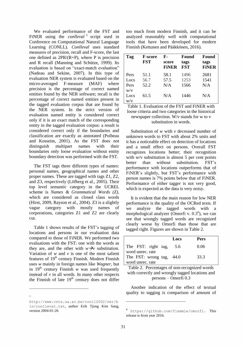
We evaluated performance of the FST and

FiNER using the conlleval5

script used in

Conference on Computational Natural Language

Learning (CONLL). Conlleval uses standard

measures of precision, recall and F-score, the last

one defined as 2PR/(R+P), where P is precision

and R recall (Manning and Schütze, 1999). Its

evaluation is based on “exact-match evaluation”

(Nadeau and Sekine, 2007). In this type of

evaluation NER system is evaluated based on the

micro-averaged F-measure (MAF) where

precision is the percentage of correct named

entities found by the NER software; recall is the

percentage of correct named entities present in

the tagged evaluation corpus that are found by

the NER system. In the strict version of

evaluation named entity is considered correct

only if it is an exact match of the corresponding

entity in the tagged evaluation corpus: a result is

considered correct only if the boundaries and

classification are exactly as annotated (Poibeau

and Kosseim, 2001). As the FST does not

distinguish multipart names with their

boundaries only loose evaluation without entity

boundary detection was performed with the FST.

The FST tags three different types of names:

personal names, geographical names and other

proper names. These are tagged with tags Z1, Z2,

and Z3, respectively (Löfberg et al., 2005). Their

top level semantic category in the UCREL

scheme is Names & Grammatical Words (Z),

which are considered as closed class words

(Hirst, 2009, Rayson et al., 2004). Z3 is a slightly

vague category with mostly names of

corporations, categories Z1 and Z2 are clearly

cut.

Table 1 shows results of the FST’s tagging of

locations and persons in our evaluation data

compared to those of FiNER. We performed two

evaluations with the FST: one with the words as

they are, and the other with wv substitution.

Variation of w and v is one of the most salient

features of 19th century Finnish. Modern Finnish

uses w mainly in foreign names like Wagner, but

in 19th century Finnish w was used frequently

instead of v in all words. In many other respects

the Finnish of late 19th century does not differ

5 http://www.cnts.ua.ac.be/conll2002/ner/b

in/conlleval.txt, author Erik Tjong Kim Sang,

version 2004-01-26

too much from modern Finnish, and it can be

analyzed reasonably well with computational

tools that have been developed for modern

Finnish (Kettunen and Pääkkönen, 2016).

Tag F-score

FST

F-

score

FiNER

Found

tags

FST

Found

tags

FiNER

Pers 51.1 58.1 1496 2681

Locs 56.7 57.5 1253 1541

Pers

w/v

52.2 N/A 1566 N/A

Locs

w/v

61.5 N/A 1446 N/A

Table 1. Evaluation of the FST and FiNER with

loose criteria and two categories in the historical

newspaper collection. W/v stands for w to v

substitution in words.

Substitution of w with v decreased number of

unknown words to FST with about 2% units and

it has a noticeable effect on detection of locations

and a small effect on persons. Overall FST

recognizes locations better; their recognition

with w/v substitution is almost 5 per cent points

better than without substitution. FST’s

performance with locations outperforms that of

FiNER’s slightly, but FST’s performance with

person names is 7% points below that of FiNER.

Performance of either tagger is not very good,

which is expected as the data is very noisy.

It is evident that the main reason for low NER

performance is the quality of the OCRed texts. If

we analyze the tagged words with a

morphological analyzer (Omorfi v. 0.36), we can

see that wrongly tagged words are recognized

clearly worse by Omorfi than those that are

tagged right. Figures are shown in Table 2.

Locs Pers

The FST: right tag,

word unrec. rate

5.6 0.06

The FST: wrong tag,

word unrec. rate

44.0 33.3

Table 2. Percentages of non-recognized words

with correctly and wrongly tagged locations and

persons – Omorfi 0.3

Another indication of the effect of textual

quality to tagging is comparison of amount of

6 https://github.com/flammie/omorfi. This

release is from year 2016.

31

tags with equal texts of different quality. We

made tests with three versions of a 100,000 word

text material that is different from our historical

NER evaluation material but derives from the

19th century newspaper collection as well. One

text version was old OCR, another manually

corrected OCR version and third a new OCRed

version. Besides character level errors also word

order errors have been corrected in the two new

versions. For these texts we did not have a gold

standard NE tagged version, and thus we could

only count number of NER tags in different texts.

Results are shown in Table 3.

Locs Gain Pers Gain

Old OCR 1866 2562

Manually

corrected

OCR

1986 +6.4% 2694 +5.2%

New OCR 2011 +7.8% 2879 +12.4%

Table 3. Number of the FST tags in different

quality OCR texts

As the figures show, there is a 5–12% unit

increase in the number of tags, when the quality

of the texts is better. Although all of the tags are

obviously not right, the increase is still

noticeable and suggests that improvement in text

quality will also improve finding of NEs. Same

kind of results were achieved in Kettunen et al.

(2016) with FiNER and ARPA.

NER experiments with OCRed data in other

languages show usually improvement of NER

when the quality of the OCRed data has been

improved from very poor to somehow better

(Lopresti, 2009). Results of Alex and Burns

(2014) imply that with lower level OCR quality

(below 70% word level correctness) name

recognition is harmed clearly. Packer et al. (2010)

report partial correlation of Word Error Rate of

the text and achieved NER result; their

experiments imply that word order errors are

more significant than character level errors.

Miller et al. (2000) show that rate of achieved

NER performance of a statistical trainable tagger

degraded linearly as a function of word error

rates. On the other hand, results of Rodriquez et

al. (2012) show that manual correction of OCRed

material that has 88–92% word accuracy does

not increase performance of four different NER

tools significantly.

As the word accuracy of the historical

newspaper material is low, it would be

expectable, that somehow better recognition

results would be achieved, if the word accuracy

was round 80–90% instead of 70–75%. Our

informal tests with different quality texts suggest

this, too, as do the distinctly different

unrecognition rates with rightly and wrongly

tagged words.

Ehrmann et al. (2016) suggest that application

of NE tools on historical texts faces three

challenges: i) noisy input texts, ii) lack of

coverage in linguistic resources, and iii)

dynamics of language. In our case the first

obstacle is the most obvious, as was shown. Lack

of coverage in linguistic resources e.g. in the

form of missing old names in the lexicons of the

NE tools is also a considerable source of errors

in our case, as our tools are made for modern

Finnish. With dynamics of language Ehrmann et

al. refer to different rules and conventions for the

use of written language in different times. In this

respect late 19th century Finnish is not that

different from current Finnish, but obviously also

this can affect the results and should be studied

more thoroughly.

3 Results of the FST and FiNER for the

Digitoday Data

Our second evaluation data is modern Finnish,

texts of a technology and business oriented web

newspaper, Digitoday. NE tagged Digitoday

data7

has been classified to eight different

content sections according to the web publication

(http://www.digitoday.fi/). Two sections,

Opinion and Entertainment, have been left out of

the tagged data. Each content section has 15–40

tagged files (altogether 240 files) that comprise

of articles, one article in each file. The content

sections are yhteiskunta (Society), bisnes

(Business), tiede ja teknologia (Science and

technology), data, mobiili (Mobile), tietoturva

(Data security), työ ja ura (Job and career) and

vimpaimet (Gadgets) We included first 20

articles of each category’s tagged data in the

evaluation. Vimpaimet had only 15 files, which

were all included in the data. Each evaluation

data set includes about 2700–4100 lines of text,

7https://github.com/mpsilfve/finer-

data/tree/master/digitoday/ner_test_data

_annotatated.

Data was collected on the first week of October and

November 2016 in two parts.

32

altogether 31 100 lines with punctuation. About

64% of the evaluation data available in the

Github repository was utilized in our evaluation

– 155 files out of 240. Structure of the tagged

files was simple; they contained one word per

line and possibly a NER tag. Punctuation marks

were tokenized on lines of their own. The

resulting individual files had a few tags like

<paragraph> and <headline>, which were

removed. Also dates of publishing were removed.

Table 4 shows evaluation results of the eight

sections of the Digitoday data with the FST and

FiNER section-by-section. Table 5 shows

combined results of the eight sections and Figure

1 shows combined results graphically.

F-score

FST

F-score

FiNER

Diff. FiNER

vs. the FST’s

F-scores

Found

tags FST

Found

Tags FiNER

Business

Persons 50.00 58.93 +8,93 39 67

Locations 67.14 76.47 +9,33 82 78

Corporations 31.27 65.89 +34,62 69 214

Society

Persons 50.00 59.86 +9,86 40 79

Locations 78.26 81.63 +3,37 146 138

Corporations 34.65 62.56 +27,91 57 166

Scitech

Persons 56.67 43.96 -12,71 32 63

Locations 57.14 57.41 +0,27 41 51

Corporations 42.49 61.93 +19,44 88 167

Data

Persons 56.00 32.26 -23,74 29 72

Locations 64.58 67.42 +2,84 58 51

Corporations 23.85 59.21 +35,36 60 119

Mobile

Persons 40.00 52.78 +12,78 20 52

Locations 70.77 68.49 -2,28 38 46

Corporations 50.73 62.07 +11,34 139 231

Work and career

Persons 71.00 72.65 +1,65 79 113

Locations 68.09 76.09 +8,00 51 49

Corporations 48.67 74.64 +25,97 71 151

Data security

Persons 40.65 46.71 +6,06 47 91

Locations 83.05 83.93 +0,88 66 60

Corporations 29.70 39.08 +9,38 60 119

Gadgets

Persons 84.62 50.00 -34,62 13 35

Locations 48.28 66.67 +18,39 19 20

Corporations 57.87 68.29 +10,42 90 142

Table 4. Results of FiNER and the FST with Digitoday’s data section-by-section

Sections combined F-score FST F-score

FiNER

Diff. FiNER vs.

FST’s F-scores

Found

tags FST

Found

tags FiNER

Persons 56.15 55.39 -0.76 299 572

Locations 70.77 74.58 +3.81 501 493

Corporations 40.11 62.56 +22.45 634 1309

Total for the eight

sections

1434 2374

Table 5. Combined results of all Digitoday’s sections

33

Figure 1. Combined results of all Digitoday’s sections

FiNER achieves best F-scores in most of

Digitoday’s sections. Out of all the 24 cases,

FiNER performs better in 20 cases and the FST

in four. The FST performs worst with

corporations, but differences with locations

compared to FiNER are small. Performance

differences with persons between FiNER and the

FST are also not that great, and the FST performs

better than FiNER in three of the sections.

Both taggers find locations best and quite

evenly in all the Digitoday’s sections. Persons

are found varyingly by both taggers, and section

wise performance is uneven. Especially bad they

are found in the Data and Data security sections.

One reason for FiNER’s bad performance in this

section is that many products are confused to

persons. In Business and Society sections,

persons are found more reliably. One reason for

the FST’s varying performance with persons is

variance of section-by-section usage of Finnish

and non-Finnish person names. In some sections

mainly Finnish persons are discussed and in

some sections mainly foreign persons. The FST

recognizes Finnish names relatively well, but it

does not cover foreign names as well. The

morphological analyzer’s components in the FST

are also lexically quite old, which shows in some

lacking name analyses, such as Google,

Facebook, Obama, Twitter, if the words are in

inflected forms.

4 Discussion

We have shown in this paper results of NE

tagging of both historical OCRed Finnish and

modern digital born Finnish with two tools,

FiNER and a Finnish Semantic Tagger, the FST.

FiNER is a dedicated rule-based NER tool for

Finnish, but the FST is a general lexicon-based

semantic tagger.

We set a twofold task for our evaluation.

Firstly we wanted to compare a general

computational semantics tool the FST to a

dedicated NE tagger in named entity search.

Secondly we wanted to see, what is the

approximate decrease in NER performance of

modern Finnish taggers, when they are used with

noisy historical Finnish data. Answer to the first

question is clear: the FST performs mostly as

well as FiNER with persons and locations in

modern data. With historical data FiNER

outperforms the FST with persons; with locations

both taggers perform equally. Corporations were

not evaluated in the historical data. In

Digitoday’s data FiNER was clearly better than

FST with corporations.

Answer to our second question is more

ambiguous. With historical data both taggers

achieve F-scores round 57 with locations, the

FST 61.5 with w/v substitution. With

Digitoday’s data F-scores of 70–74.5 are

achieved, and thus there is 9–16% point

difference in the performance. With persons

FiNER’s score with both data are quite even in

average. It would be expectable, that FiNER

performed better with modern data. Some

sections of Digitoday data (Scitech, Data, Data

Security) are performing clearly worse than

others, and FiNER’s performance only in Work

and Career is on expectable level. It is possible

that section wise topical content has some effect

in the results. The FST’s performance with

persons is worst with historical data, but with

Digitoday’s data it performs much better.

Technology behind FST is relatively old, but it

has a sound basis and a long history. Since the

beginning of the 1990s and within the framework

of several different projects, the UCREL team

has been developing an English semantic tagger,

the EST, for the annotation of both spoken and

written data with the emphasis on general

language. The EST has also been redesigned to

create a historical semantic tagger for English.

34

To show versatility of the UCREL semantic

tagger approach, we list a few other

computational analyses where the EST has been

applied to:

- stylistic analysis of written and spoken

English

- analysis and standardization of SMS spelling

variation,

- analysis of the semantic content and

persuasive composition of extremist media,

- corpus stylistics,

- discourse analysis,

- ontology learning,

- phraseology,

- political science research,

- sentiment analysis, and

- deception detection.

More applications are referenced on UCREL’s

web pages (http://ucrel.lancs.ac.uk/usas/;

http://ucrel.lancs.ac.uk/wmatrix/#apps).

As can be seen from the list, the approach

taken in UCREL that is also behind the FST is

robust with regards to linguistic applications.

Based on our results with both historical and

modern Finnish data, we believe that the EST

based FST is also a relevant tool for named

entity recognition. It is not optimal for the task in

its present form, as it lacks e.g. disambiguation

of ambiguous name tags at this stage8. On the

other hand, the FST’s open and well documented

semantic lexicons are adaptable to different tasks

as they can be updated relatively easily. The FST

would also benefit from an updated open source

morphological analyzer. Omorfi9, for example,

would be suitable for use, as it has a

comprehensive lexicon of over 400 000 base

forms. With an up-to-date Finnish morphological

analyzer and disambiguation tool the FST would

yield better NER results and in the same time it

would be a versatile multipurpose semantical

analyzer of Finnish.

Overall our results show that a general

semantic tool like the FST is able to perform in a

restricted semantic task of name recognition

almost as well as a dedicated NE tagger. As NER

8 Many lexicon entries contain more senses than one,

and these are arranged in perceived frequency order.

For example, it is common in Finnish that a name of

location is also a family name. 9 https://github.com/flammie/omorfi

is a popular task in information extraction and

retrieval, our results show that NE tagging does

not need to be only a task of dedicated NE

taggers, but it can be performed equally well

with more general multipurpose semantic tools.

Acknowledgments

Work of the first author is funded by the EU

Commission through its European Regional

Development Fund, and the program Leverage

from the EU 2014–2020.

References

Maud Ehrmann, Giovanni Colavizz, Yannick

Rochat, and Frédéric Kaplan. 2016.

Diachronic Evaluation of NER Systems on

Old Newspapers. In Proceedings of the 13th

Conference on Natural Language Processing

(KONVENS 2016), 97–107. https://www.linguistics.rub.de/

konvens16/pub/13_konvensproc.pd

f

Graeme Hirst. 2009. Ontology and the Lexicon.

ftp://ftp.cs.toronto.edu/pub/gh/Hirst-Ontol-

2009.pdf

Kimmo Kettunen and Tuula Pääkkönen. 2016.

Measuring Lexical Quality of a Historical

Finnish Newspaper Collection – Analysis of

Garbled OCR Data with Basic Language

Technology Tools and Means. LREC 2016,

Tenth International Conference on Language

Resources and Evaluation. http://www.lrec-

conf.org/proceedings/lrec2016/p

df/17_Paper.pdf.

Kimmo Kettunen, Eetu Mäkelä, Juha Kuokkala,

Teemu Ruokolainen and Jyrki Niemi. 2016.

Modern Tools for Old Content - in Search of

Named Entities in a Finnish OCRed Historical

Newspaper Collection 1771-1910. Krestel, R.,

Mottin, D. and Müller, E. (eds.), Proceedings

of Conference "Lernen, Wissen, Daten,

Analysen", LWDA 2016, http://ceur-ws.org/Vol-1670/

Laura Löfberg, Jukka-Pekka Juntunen, Asko

Nykänen, Krista Varantola, Paul Rayson and

Dawn Archer. 2004. Using a semantic tagger

as dictionary search tool. In 11th EURALEX

(European Association for Lexicography)

International Congress Euralex 2004: 127–

134.

35

Laura Löfberg, Scott Piao, Paul Rayson, Jukka-

Pekka Juntunen, Asko Nykänen and Krista

Varantola. 2005. A semantic tagger for the

Finnish language. http://eprints.lancs.ac.uk/1268

5/1/cl2005_fst.pdf

Daniel Lopresti. 2009. Optical character

recognition errors and their effects on natural

language processing. International Journal on

Document Analysis and Recognition, 12(3):

141–151.

Eetu Mäkelä. 2014. Combining a REST Lexical

Analysis Web Service with SPARQL for

Mashup Semantic Annotation from Text.

Presutti, V. et al. (Eds.), The Semantic Web:

ESWC 2014 Satellite Events. Lecture Notes in

Computer Science, vol. 8798, Springer: 424–

428.

Christopher D. Manning and Hinrich Schütze.

1999. Foundations of Statistical Language

Processing. The MIT Press, Cambridge,

Massachusetts.

Mónica Marrero, Julián Urbano , Sonia Sánchez-

Cuadrado , Jorge Morato and Juan Miguel

Gómez-Berbís. 2013. Named Entity

Recognition: Fallacies, challenges and

opportunities. Computer Standards &

Interfaces 35(5): 482–489.

David Miller, Sean Boisen, Richard Schwartz,

Rebecca Stone and Ralph Weischedel. 2000.

Named entity extraction from noisy input:

Speech and OCR. Proceedings of the 6th

Applied Natural Language Processing

Conference: 316–324, Seattle, WA. http://www.anthology.aclweb.org

/A/A00/A00-1044.pdf

David Nadeau and Satoshi Sekine. 2007. A

Survey of Named Entity Recognition and

Classification. Linguisticae

Investigationes 30(1):3–26.

Thomas L. Packer, Joshua F. Lutes, Aaron P.

Stewart, David W. Embley, Eric K. Ringger,

Kevin D. Seppi and Lee S. Jensen. 2010.

Extracting Person Names from Diverse and

Noisy OCR Tex. Proceedings of the fourth

workshop on Analytics for noisy unstructured

text data. Toronto, ON, Canada: ACM. http://dl.acm.org/citation.cfm?

id=1871845.

Scott Piao, Paul Rayson, Dawn Archer,

Francesca Bianchi, Carmen Dayrell,

Mahmoud El-Haj, Ricardo-María Jiménez,

Dawn Knight, Michal Kren, Laura Löfberg,

Rao Muhammad Adeel Nawab, Jawad Shafi,

Phoey Lee Teh and Olga Mudraya. 2016.

Lexical Coverage Evaluation of Large-scale

Multilingual Semantic Lexicons for Twelve

Languages. Proceedings of LREC. http://www.lrec-

conf.org/proceedings/lrec2016/p

df/257_Paper.pdf.

Thierry Poibeau and Leila Kosseim. 2001.

Proper Name Extraction from Non-

Journalistic Texts. Language and Computers,

37: 144–157.

Paul Rayson, Dawn Archer, Scott Piao and Tony

McEnery. 2004. The UCREL semantic

analysis system. Proceedings of the workshop

on Beyond Named Entity Recognition

Semantic labelling for NLP tasks in

association with 4th International Conference

on Language Resources and Evaluation

(LREC 2004): 7–12. http://www.lancaster.ac.uk/staf

f/rayson/publications/usas_lrec

04ws.pdf

Kepa Joseba Rodriquez, Mike Bryant, Tobias

Blanke and Magdalena Luszczynska. 2012.

Comparison of Named Entity Recognition

Tools for raw OCR text. Proceedings of

KONVENS 2012 (LThist 2012 wordshop),

Vienna September 21: 410–414.

Miikka Silfverberg. 2015. Reverse Engineering a

Rule-Based Finnish Named Entity Recognizer. https://kitwiki.csc.fi/twiki/pu

b/FinCLARIN/KielipankkiEventNER

Workshop2015/Silfverberg_presen

tation.pdf.

36


Machine Learning for Rhetorical Figure Detection:More Chiasmus with Less Annotation

Marie DubremetzUppsala University

Dept. of Linguistics and PhilologyUppsala, Sweden

[email protected]

Joakim NivreUppsala University

Dept. of Linguistics and PhilologyUppsala, Sweden

[email protected]

Abstract

Figurative language identification is a hardproblem for computers. In this paper wehandle a subproblem: chiasmus detection.By chiasmus we understand a rhetoricalfigure that consists in repeating two el-ements in reverse order: “First shall belast, last shall be first”. Chiasmus detec-tion is a needle-in-the-haystack problemwith a couple of true positives for millionsof false positives. Due to a lack of anno-tated data, prior work on detecting chias-mus in running text has only consideredhand-tuned systems. In this paper, we ex-plore the use of machine learning on apartially annotated corpus. With only 31positive instances and partial annotation ofnegative instances, we manage to build asystem that improves both precision andrecall compared to a hand-tuned systemusing the same features. Comparing thefeature weights learned by the machineto those give by the human, we discovercommon characteristics of chiasmus.

1 Introduction

Recent research shows a growing interest in thecomputational analysis of style and rhetorics.Works like Bendersky and Smith (2012) andBooten and Hearst (2016) demonstrate that, withsufficient amounts of data, one can even train asystem to recognize quotable sentences. Classicalmachine learning techniques applied to text canhelp discover much more than just linguistic struc-ture or semantic content. The techniques appliedso far use a lot of data already annotated by in-ternet users, for instance, tumblr sentences with

the label #quotation (Booten and Hearst, 2016). Itis a clever reuse of the web as an annotated cor-pus, but what happens if the stylistic phenomenonwe want to discover is not as popular on the web?When there is no available corpus and when thestylistic phenomenon is rare, collecting a substan-tial amount of annotated data seems unreachableand the computational linguist faces the limits ofwhat is feasible.

This study is a contribution which aims at push-ing this limit. We focus on the task of automat-ically identifying a playful and interesting studycase that is rather unknown in computational lin-guistics: the chiasmus. The chiasmus is a fig-ure that consists in repeating a pair of identicalwords in reverse order. The identity criterion forwords can be based on different linguistic prop-erties, such as synonymy or morphological form.Here we focus on chiasmi that have words withidentical lemmas, sometimes referred to as an-timetabole, and illustrated in Example 1. Fromnow on, we will refer to this case as simply chi-asmus.

(1) User services management: changing abreed or breeding a change?

Chiasmus is named after the greek letter χ becausethe pattern of repetition is often represented as an‘X’ or a cross like in Figure 1.

There are several reasons why NLP should payattention to chiasmi. First it is a widespread lin-guistic phenomenon across culture and ages. Be-cause of the Greek etymology of its name, onemight believe that chiasmus belongs only to therhetoricians of the classical period. It is actuallya much more ancient and universal figure. Welch(1981) observes it in Talmudic, Ugaritic and evenSumero-Akkadian literature. Contrary to what one

37

Figure 1: Schema of a chiasmus

may think, chiasmus is not an archaic ornament oflanguage and it is used far beyond advertisementor political discourses. It is relevant for good writ-ers of any century. Even scientists use it. For in-stance, currently, a small community of linguistsgives a monthly ‘Chiasmus Award’ which eachtime reveals a new chiasmus produced recently bythe scientific community.1 Thus, we come to thesame conclusion as Nordahl (1971). If the chias-mus has for a long time seemed to be dying, thisis only true with respect to the interest devoted toit by linguists. In reality, the chiasmus, rhetoricalor functional, is doing well (Nordahl, 1971). Suchuniversality and modernity makes chiasmus detec-tion a fruitful task to perform on many genres, onold text as on new texts.

Second, we can assume that the presence ofchiasmus is a sign of writing quality because theauthor took the time to create it or to quote it.Nowadays the production of texts on the web isa huge industry where authors’ compensation isoften based on the number of words produced,which does not increase the quality. Thus, detect-ing such figures of speech is one clue (among oth-ers) that may help distinguish masterpieces frompoorly written texts.

Finally, an additional reason for studying chi-asmus, which is the focus of this paper, is its rar-ity. To see just how rare it is, consider WinstonChurchill’s River War, a historical narrative count-ing more than one hundred thousand words. De-spite the author’s well-known rhetorical skills, wecould only find a single chiasmus in the book:

(2) Ambition stirs imagination nearly as muchas imagination excites ambition.

Such rareness is a challenge for our discipline. Itis well known that the statistical methods domi-nant in NLP work best for commonly occurring

1http://specgram.com/psammeticuspress/chiasmus.html

linguistic phenomena and that accuracy often de-clines drastically for the long tail of low-frequencyevents typical of language. Detecting chiasmusis a needle-in-the-haystack problem where all theinteresting instances are in the long tail. Simplyidentifying word pairs repeated in reverse orderis trivial, but identifying the tiny fraction of thesethat have a rhetorical purpose is not.

Because of its rarity, the chiasmus is not wellsuited for large-scale annotation efforts. Previousefforts aimed at chiasmus detection have there-fore not been able to use (supervised) machinelearning for the simple reason that there has beenno training data available. These efforts havetherefore mainly been based on hand-crafted rulesdefining categorical distinctions and typically suf-fering from either low precision or low recall.Dubremetz and Nivre (2015; 2016) proposed afeature-based ranking approach instead, but be-cause they had no annotated data to use for train-ing, they had to resort to tuning feature weights byhand on the training set. However, an importantside effect of their work was the release of a smallannotated corpus of chiasmi, containing 31 pos-itive instances, a few hundred (annotated) nega-tive instances, and several million unannotated in-stances assumed to be negative.

This paper presents the first attempt to use ma-chine learning to tune the weights of a model forchiasmus detection, using the corpus released byDubremetz and Nivre (2016). To see whether it ispossible to learn from this type of corpus at all, wetrain a log-linear model with the same features asDubremetz and Nivre (2015) and Dubremetz andNivre (2016). The results show that the machine-learned model, despite the small number of pos-itive training instances, improves both precisionand recall over the hand-tuned system, which isvery encouraging. A comparison between the twotypes of systems reveals that they agree almostperfectly about which features are positive andnegative, respectively, and that the difference inperformance is therefore due simply to more well-calibrated weights. From a more general perspec-tive, this shows that using a hand-tuned system tobootstrap a small seed corpus for machine learn-ing may be a viable strategy for tackling needle-in-the-haystack problems like chiasmus detection.

38

2 Related Work

When documenting chiasmus, the computationallinguist ends up in a paradox: linguists have de-veloped reflections on this rhetorical figure butthose reflections are not the most helpful. Indeed,they never question the concept of criss-cross pat-terns as an insufficient condition for producing arhetorical effect. Typically dictionaries and stylis-tic books (Fontanier, 1827; Dupriez, 2003) willexplain why chiasmus should belong to the cate-gory of scheme and not of trope. Rabatel (2008)argues why chiasmus has different functions andshould therefore be divided into subcategories. Onthe other side, Horvei (1985) demonstrates thatchiasmus should not be considered as a simplesubcategory of parallelism but rather as a figureon its own. All those reflections are interestingbut they all focus on placing chiasmus into thevast family of rhetorical figures. Following thislinguistics tradition, the first computational lin-guists (Gawryjolek, 2009; Hromada, 2011) work-ing on chiasmus perform multiple figure detec-tions. They focus on making detectors that canperform both the classification and detection of allkinds of repetitive figures such as epanaphora,2

epiphora, 3 anadiplosis.4 To some extent, theirsystems are a success in that they correctly dis-tinguish figures from each other. Thus they provethat computers are excellent at extracting each rep-etition type with the right label (epiphora versusepanaphora versus chiasmus). However, they donot evaluate their systems on real corpora, usingprecision and recall, and therefore do not reallyconfront the problem of false positives and acci-dental repetitions.

It is only a couple of years later that compu-tational linguists dare to break with the pure lin-guistic tradition of handling all rhetorical figurestogether. With computational linguists like Strom-mer (2011; Dubremetz (2013) we observe the firstof two important methodological shifts in how theproblem is approached. For the first time compu-tational linguists decide to focus on only one fig-ure (epanaphora for Strommer (2011), chiasmusfor Dubremetz (2013)) and provide some insight

2“We shall not flag or fail. We shall go on to the end.We shall fight in France, we shall fight on the seas andoceans[...]”

3“When I was a child, I spoke as a child, I understood asa child, I thought as a child. ”

4“Mutual recognition requires trust, trust requires com-mon standards, and common standards requires solidarity.”

into precision/recall. By doing so, they come backto an essential question: When should we considera repetition as accidental instead of rhetoric?

This question seems at first simpler than thequestion of categorising chiasmus against its alter-native figures. But answering it leads to more uni-versal and interesting answers for computationallinguistics research. Indeed, repetition in languageis extremely banal and viewing every repetition ina text as being rhetorical would be absurd. Thevery first problem in repetitive figure detection ingeneral, in chiasmus detection in particular, is thedisproportional number of false positives that thetask generates. Dubremetz and Nivre (2015) pointout that in 300 pages of historical tale the previousdetector (Gawryjolek, 2009) extracts up to 66,000of the criss-cross patterns (for only one true pos-itive chiasmus to be found). At the opposite end,the more strict detector of Hromada (2011) endsup giving a completely empty output on the samebook. The pattern that we have to work on, a pairof repetitions in reverse order, is so frequent andthe true positive cases are so rare that it makes itimpossible to annotate a corpus for a traditionalclassification task.

Dubremetz and Nivre (2015; 2016) introducethe second shift in the approach to chiasmus de-tection. Their observation is the same as the onemade by Dunn (2013) on metaphora:

One problem with the systems described[...] is that they are forced to draw an ar-bitrary line between two classes to rep-resent a gradient phenomenon. (Dunn,2013)

Like Dunn (2013) claims for metaphora,Dubremetz and Nivre (2015) claim that chi-asmus detection is not a binary detection task.It is rather a ranking task similar to informationretrieval. As documents are more or less relevantto a query, some chiasmi are more prototypicalthan others. There are extremely relevant caseslike Sentence 3, some completely irrelevantrepetitions like Sentence 4 and there are those inbetween or borderline cases like Sentence 5.

(3) How to talk so business will listen ... Andlisten so business will talk?

(4) Let me show you the Disease Ontology up-date: take a look at the expanded and up-dated database of human diseases, as we cansee, it grew since 2014.

39

(5) It is just as contrived to automatically allo-cate Taiwan to China as it was to allocateChina’s territory to Taiwan in the past.

Consequently, they decide to convert the detec-tion into a ranking task where prototypical chiasmiwould be ranked at the top and less relevant in-stances would be gradually ranked lower. By do-ing so, they allow a new type of evaluation. Beforeevaluation was impossible due to the too big num-ber of false instances to annotate (about 66,000 ofthem for only one true positive in 150,000 words).But instead of annotating the millions of instancesin their training and test set, they decide to anno-tate only the top two hundred given by the ma-chine. And by trying several systems and keep-ing trace of the previous annotations they grad-ually augment the number of true instances theycan evaluate on (Clarke and Willett, 1997). Thusthey make a needle-in-the-haystack problem a fea-sible task by reusing the data on which a sys-tem of detection is confident to improve evalua-tion and learning progressively. At the end of theirstudy they show that chiasmi can be ranked using acombination of features like punctuation position,stopwords, similarity of n-gram context, conjunc-tion detection, and syntax.

Because of lack of data, Dubremetz andNivre (2015; 2016) tuned their features manually.They give average precision5 results which is agood start. But they could not train a proper clas-sifier. Thus, we have no idea if a computer canlearn the patterns associated with rhetorical chi-asmi and if a binary system would properly dis-tinguish some true positives and not just throwall true instances in the overwhelming majorityof false positives. This is the issue tackled inthis paper. Using a partially annotated corpus wetrain a model automatically and compare the per-formance to the hand-tuned system. We evaluatethe system using both average precision and F1-scores.

3 Corpus

We use the corpus from Dubremetz and Nivre(2015) as our training corpus (used to learn

5Average precision is a common evaluation used in infor-mation retrieval. It considers the order in which each can-didates is returned by making the average of the precisionat each positive instance retrieved by the machine. Thusthis measure gives more information on the performance ofa ranking system than a single recall/precision value (Croft etal., 2010).

weights for a fixed set of features) and a new cor-pus as our final test corpus. The training corpusconsists of four million words from the Europarlcorpus, containing about two million instances ofcriss-cross patterns. Through the previous effortsof Dubremetz and Nivre (2015; 2016), 3096 ofthese have been annotated by one annotator asTrue, False, Borderline or Duplicate.6 The True,Borderline and Duplicate instances were then re-annotated by a second annotator. Only instanceslabeled True by both annotators will be consid-ered as true positives in our experiments (at bothtraining and test time). This makes sure that bothtraining and evaluation is based on the most pro-totypical true examples. The test set is an unseenfurther extract of the Europarl corpus of 2 millionwords. For the test phase, two annotators wereasked to annotate the top 200 instances of eachsystem. In total, this produced 457 doubly anno-tated instances in our test set containing one mil-lion instances in total.

4 Features

Dubremetz and Nivre (2015) proposed a standardlinear model to rank candidate instances:

f (r) =n

∑i=1

xi ·wi

where r is a string containing a pair of invertedwords, xi is a set of feature values, and wi is theweight associated with each features. Given twoinversions r1 and r2, f (r1)> f (r2) means that theinversion r1 is more likely to be a chiasmus thanr2 according to the model.

The features used are listed in Table 1, usingthe notation defined in Figure 2. The featuregroups Basic, Size, Similarity and Lexical cluescome from Dubremetz and Nivre (2015), while thegroup Syntactic features was added in Dubremetzand Nivre (2016). We use the same features inour machine learning experiments but only traintwo systems, one corresponding to Dubremetz andNivre (2015) (called Base) and one correspond-ing to Dubremetz and Nivre (2016) (called Allfeatures). This allows us to make a head-to-headcomparison between the systems, where the onlydifference is whether feature weights have beentuned manually or using machine learning.

6For example, if the machine extracts both “All for one,one for all” and “All for one, one for all”, the first is labeledTrue and the second Duplicate, even if both extracts cover atrue chiasmus.

40

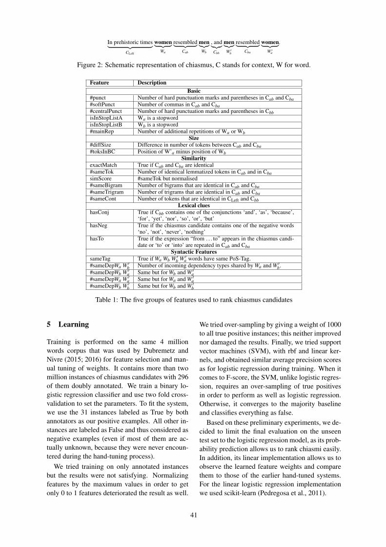
In prehistoric times︸︷︷︸CLeft

women︸︷︷︸Wa

resembled︸︷︷︸Cab

men︸︷︷︸Wb

, and︸︷︷︸Cbb

men︸︷︷︸W ′

b

resembled︸︷︷︸Cba

women︸︷︷︸W ′

a

.

Figure 2: Schematic representation of chiasmus, C stands for context, W for word.

Feature DescriptionBasic

#punct Number of hard punctuation marks and parentheses in Cab and Cba#softPunct Number of commas in Cab and Cba#centralPunct Number of hard punctuation marks and parentheses in CbbisInStopListA Wa is a stopwordisInStopListB Wb is a stopword#mainRep Number of additional repetitions of Wa or Wb

Size#diffSize Difference in number of tokens between Cab and Cba#toksInBC Position of W’a minus position of Wb

SimilarityexactMatch True if Cab and Cba are identical#sameTok Number of identical lemmatized tokens in Cab and in CbasimScore #sameTok but normalised#sameBigram Number of bigrams that are identical in Cab and Cba#sameTrigram Number of trigrams that are identical in Cab and Cba#sameCont Number of tokens that are identical in CLeft and Cbb

Lexical clueshasConj True if Cbb contains one of the conjunctions ‘and’, ‘as’, ‘because’,

‘for’, ‘yet’, ‘nor’, ‘so’, ‘or’, ‘but’hasNeg True if the chiasmus candidate contains one of the negative words

‘no’, ‘not’, ‘never’, ‘nothing’hasTo True if the expression “from . . . to” appears in the chiasmus candi-

date or ‘to’ or ‘into’ are repeated in Cab and CbaSyntactic Features

sameTag True if Wa Wb W ′b W ′a words have same PoS-Tag.#sameDepWa W ′b Number of incoming dependency types shared by Wa and W ′b.#sameDepWb W ′a Same but for Wb and W ′a#sameDepWa W ′a Same but for Wa and W ′a#sameDepWb W ′b Same but for Wb and W ′b

Table 1: The five groups of features used to rank chiasmus candidates

5 Learning

Training is performed on the same 4 millionwords corpus that was used by Dubremetz andNivre (2015; 2016) for feature selection and man-ual tuning of weights. It contains more than twomillion instances of chiasmus candidates with 296of them doubly annotated. We train a binary lo-gistic regression classifier and use two fold cross-validation to set the parameters. To fit the system,we use the 31 instances labeled as True by bothannotators as our positive examples. All other in-stances are labeled as False and thus considered asnegative examples (even if most of them are ac-tually unknown, because they were never encoun-tered during the hand-tuning process).

We tried training on only annotated instancesbut the results were not satisfying. Normalizingfeatures by the maximum values in order to getonly 0 to 1 features deteriorated the result as well.

We tried over-sampling by giving a weight of 1000to all true positive instances; this neither improvednor damaged the results. Finally, we tried supportvector machines (SVM), with rbf and linear ker-nels, and obtained similar average precision scoresas for logistic regression during training. When itcomes to F-score, the SVM, unlike logistic regres-sion, requires an over-sampling of true positivesin order to perform as well as logistic regression.Otherwise, it converges to the majority baselineand classifies everything as false.

Based on these preliminary experiments, we de-cided to limit the final evaluation on the unseentest set to the logistic regression model, as its prob-ability prediction allows us to rank chiasmi easily.In addition, its linear implementation allows us toobserve the learned feature weights and comparethem to those of the earlier hand-tuned systems.For the linear logistic regression implementationwe used scikit-learn (Pedregosa et al., 2011).

41

Model Avg Precision Precision Recall F1-scoreMachine Base 57.1 80.0 30.8 44.4Machine All features 70.8 90 69.2 78.3Human Base 42.5 – – –Human All features 67.7 – – –

Table 2: Results for logistic regression model (Machine) with comparison to the hand-tuned models ofDubremetz and Nivre (2015; 2016) (Human). Inter annotator agreement κ = 0.69

6 Evaluation

Table 2 shows that the systems based on machinelearning give better performance than the hand-tuned systems. With only base features, the aver-age precision improves by as much as 15%. Withsyntactic features added, the difference is smallerbut nevertheless 3%. The performance is mea-sured on the 13 instances in the test set judged asTrue by both annotators. For the machine learn-ing system, we also report precision, recall andF1-score. Again, we see that syntactic featureshelp a lot, especially by improving recall fromabout 30% to over 69%. The F1-score of about78% is surprisingly good given how imbalancedthe classes are (13 positive instances to one mil-lion negative instances). The most impressive re-sult is the precision score of 90% obtained by themachine when using all features. This means that9 out of 10 instances classified as True were actu-ally real positive instances.

7 Error Analysis

To cast further lights on the results, we performedan error analysis on the cross-validation experi-ments (run on the training set). In the all-featuresexperiment, we encountered 4 false positives. Ofthese, 3 were actually annotated as Borderline byboth annotators, and 1 was annotated as Border-line by one annotator and False by the other, whichmeans that none of the false positives were consid-ered False by both annotators. To illustrate someof the difficulties involved, we list 5 of the 31 pos-itive instances in the training set (6–10), followedby the 3 borderline cases (11–13) and the 1 case ofannotator disagreement (14).

Positive

(6) We do not believe that the end justifies themeans but that the means prefigure the end.

(7) Do not pick the winners and let the winnerspick.

(8) Europe has no problem converting euros intoresearch, but has far greater difficulty con-verting research into euros.

(9) That it is not the beginning of the end but theend of the beginning for Parliament’s rights.

(10) It is much better to bring work to peoplethan to take people to work.

Borderline

(11) In parallel with the work on these practicalaspects, a discussion is ongoing within theEuropean Union on determining the mecha-nisms for participation both by EU MemberStates which are not members of NATO andby NATO countries which are not EU Mem-ber States.

(12) In that way, they of course become the EU’ srepresentatives in the Member States insteadof the Member States’ representatives in theEU.

(13) If there is discrimination between a blackperson and a white person, or vice versa, forexample if someone discriminates against awhite Portuguese in favour of a black Por-tuguese, or against a black Portuguese infavour of a white Portuguese, this is clearlyunlawful racism and should result in prose-cution.

Disagreement

(14) European consciousness is that which mustcontribute to the development of mutual re-spect [...] and which must ensure that toler-ance is not confused with laxity and an ab-sence of rules and laws and that laws andrules are not made with the intention of pro-tecting some and not others.

42

How can the classifier achieve such good resultson both recall and precision with only 31 positiveinstances to learn from? We believe an importantpart of the explanation lies in the way the train-ing set was constructed through repeated testingof hand-crafted features and weights. This processresulted in the annotation of more than 3 000 obvi-ous false positive cases that were recurrently com-ing up in the hand-tuning experiments. The humanstarted tuning and annotating with the most simplefeatures like stop words to start filtering out falsepositives. This is in fact a necessary requirement.Without stop word filtering, the chance of finding atrue positive in the top 200 instances is extremelysmall. Thus, if a false negative is hidden some-where in the training set, it is likely to be one in-volving stop words. To the best of our knowledge,there is only one existing chiasmus ever reportedin the history of rhetorics that relies exclusively onstopwords:

(15) All for one, one for all

Given this, we cannot guarantee that there are nofalse negatives in the training set, but we can defi-nitely say that they are unlikely to be prototypicalchiasmi. Thanks to this quality of the annotation,the machine had the maximum of information wecould possibly give about false positives which isby far the most important class. In addition, theperformance observed with only 31 positive train-ing instances might be revealing something aboutchiasmus: the linguistic variation is limited. Thus,within 31 examples the patterns are repeated oftenenough so that a machine can learn to detect them.

8 Weights

Figure 3 shows the weights assigned to differ-ent features in the hand-tuning experiments ofDubremetz and Nivre (2015; 2016) and in the ma-chine learning experiments reported in this paper.All weights have been normalized to the interval[0, 1] through division by the largest weight ineach set.

The comparison gives rise to several interestingobservations. The most striking one is that the ma-chine and the human agree on which features arenegative versus positive. The only exception is the#sameTrigram feature (cf. Table 1, group Simi-larity). This feature counts the number of trigramsthat are identical in the two different parts of the

Figure 3: Feature weights from machine learningand hand-tuning, normalized to the interval [0, 1]

chiasmus. For instance, in the Kennedy quote (ex-ample 16), there is one identical trigram: can dofor. However, we can easily explain this disagree-ment: this feature is one out of four that expressthe similarity between chiasmus propositions andmay thus be redundant.

(16) Ask not what your country can do for you;ask what you can do for your country.

The machine assigned the largest weights tothe stop word features, namely isInStopListA andisInStopListB (cf. Table 1), which agrees withhuman logic. Note, however, that the humangave the maximum weight to several other fea-tures as well, like features related to punctuation(negative) and part-of-speech tag identity (posi-tive). Finally, we observe that the human gives

43

the same absolute value to all the syntactic de-pendency features, while the machine tuned themslightly differently. It put a smaller weight onthe negative feature #sameDepWbW ′b but not on#sameDepWaW ′a. These two negative features areof the same nature: they target the elimination offalse positives based on enumerations. In proto-typical chiasmi, like the one from Hippocrates (ex-ample 17), the two occurrences of a and b in theabba pattern have different syntactic roles becausethey switch positions in a repeated syntactic struc-ture.

(17) Hippocrates said that food should be ourmedicine and medicine our food.

Therefore, both #sameDepWaW ′a and#sameDepWbW ′b penalize instances wherethe pairwise occurrences have the same role. Tothe human it was not obvious that they shouldbe differentiated, but apparently this constraint isstatistically stronger for the outermost a words.

9 Limitations and Future Work

An obvious limitation of our study is the small setof true positives on which we base the evaluation.As explained earlier, it is normal to have very fewtrue examples even out of 2 million words of text.The Europarl corpus (Koehn, 2005), being large,consistent, but sometimes noisy, seemed to us con-venient by its size and the robustness challenge itrepresented. Above all, it has a style that is nottoo specific, like poetry would be. Thus, we canhope that models tuned on this corpus would gen-eralise to other genres (novels, for instance). Agood follow-up experiment would therefore be toexplore other genres and in this way test the gen-erality of the system. This will be done in futureresearch.

Another line of future research is to extend theapproach to other (repetitive) rhetorical figures,such as anadiplosis (the repetition of the last wordof one clause or sentence at the beginning of thenext) or anaphora (the repetition of the same wordor group of words at the beginning of successiveclauses, sentences, or lines). It would be interest-ing to see, first, whether the same types of featureswould be useful and, secondly, how easy or diffi-cult it is to discriminate between different figures.

10 Conclusion

In this paper, we target a task outside the NLPcomfort zone: chiasmus detection. The challengeconsists in training a model for an extremely rarestylistic phenomenon, with a corpus that is onlyvery partially annotated. Previously, only handtuned systems existed and we had no idea howmany examples were needed to train an effectivemodel. We trained a log-linear classifier on a fourmillion word corpus of political debates. This cor-pus contained only 31 true examples, a few hun-dred instances explicitly annotated as false, andmillions of unknown instances labeled as false bydefault. This method gives good recall and preci-sion and even gives slightly higher accuracy thanthe hand-tuned system when it comes to ranking.

We observed strong similarities in the assign-ment of feature weights by human and machine,with almost total agreement on which featuresshould be positive or not, although the machinecould fine-tune the weights, for example, to ac-count for differential syntactic patterns. An erroranalysis revealed that false positives were morelikely than not to be cases that were consid-ered borderline (or unclear) by human annotators.Taken together, these results indicate that we havecreated a system coherent with the human percep-tion of rhetoric.

Our research is transforming a difficult needle-in-the-haystack problem into a feasible task andthe only concession to do is to accept partial recall.As in old traditional methods (Blum and Mitchell,1998; Yarowsky, 1995), we wielded the full po-tential of labeled and unlabeled data. We adaptedit to the domain of style and creative language.Detecting chiasmus is a creative manipulation oftexts that has potential applications in figurativelanguage processing (Veale, 2011), where infor-mation retrieval becomes creative text retrieval.

References

Michael Bendersky and David Smith. 2012. A Dic-tionary of Wisdom and Wit: Learning to ExtractQuotable Phrases. In Proceedings of the NAACL-HLT 2012 Workshop on Computational Linguisticsfor Literature, pages 69–77, Montreal, Canada. As-sociation for Computational Linguistics.

Steven Bird, Ewan Klein, and Edward Loper. 2009.Natural Language Processing with Python. O’reillyedition.

44

Avrim Blum and Tom Mitchell. 1998. Combin-ing Labeled and Unlabeled Data with Co-training.In Proceedings of the Eleventh Annual Conferenceon Computational Learning Theory, pages 92–100,New York, NY, USA. ACM.

Kyle Booten and Marti A Hearst. 2016. Patterns ofWisdom: Discourse-Level Style in Multi-SentenceQuotations. In Proceedings of the 2016 Conferenceof the North American Chapter of the Associationfor Computational Linguistics: Human LanguageTechnologies, pages 1139–1144, San Diego, Califor-nia, jun. Association for Computational Linguistics.

Sarah J. Clarke and Peter Willett. 1997. Estimating therecall performance of Web search engines. Proceed-ings of Aslib, 49(7):184–189.

Bruce Croft, Donald Metzler, and Trevor Strohman.2010. Search Engines: Information Retrieval inPractice: International Edition, volume 54. Pear-son Education.

Marie Dubremetz and Joakim Nivre. 2015. Rhetor-ical Figure Detection: the Case of Chiasmus. InProceedings of the Fourth Workshop on Computa-tional Linguistics for Literature, pages 23–31, Den-ver, Colorado, USA. Association for ComputationalLinguistics.

Marie Dubremetz and Joakim Nivre. 2016. SyntaxMatters for Rhetorical Structure: The Case of Chias-mus. In Proceedings of the Fifth Workshop on Com-putational Linguistics for Literature, pages pages47–53, San Diego, California,USA. Association forComputational Linguistics.

Marie Dubremetz. 2013. Vers une identifica-tion automatique du chiasme de mots. In Actesde la 15e Rencontres des Etudiants Chercheursen Informatique pour le Traitement Automatiquedes Langues (RECITAL’2013), pages 150–163, LesSables d’Olonne, France.

Jonathan Dunn. 2013. What metaphor identificationsystems can tell us about metaphor-in-language. InProceedings of the First Workshop on Metaphor inNLP, pages 1–10, Atlanta, Georgia. Association forComputational Linguistics.

Bernard Dupriez. 2003. Gradus, les procedeslitteraires. Union Generale d’Editions 10/18.

Pierre Fontanier. 1827. Les Figures du discours.Flammarion, 1977 edition.

Jakub J. Gawryjolek. 2009. Automated Annotationand Visualization of Rhetorical Figures. Master the-sis, Universty of Waterloo.

Harald Horvei. 1985. The Changing Fortunes of aRhetorical Term: The History of the Chiasmus. TheAuthor.

Daniel Devatman Hromada. 2011. Initial Experimentswith Multilingual Extraction of Rhetoric Figures bymeans of PERL-compatible Regular Expressions. InProceedings of the Second Student Research Work-shop associated with RANLP 2011, pages 85–90,Hissar, Bulgaria.

Philipp Koehn. 2005. Europarl: A Parallel Corpusfor Statistical Machine Translation. In The TenthMachine Translation Summit, pages 79–86, Phuket,Thailand.

Christopher D Manning, Mihai Surdeanu, John Bauer,Jenny Finkel, Steven J Bethard, and David Mc-Closky. 2014. The Stanford CoreNLP NaturalLanguage Processing Toolkit. In Association forComputational Linguistics (ACL) System Demon-strations, pages 55–60.

Helge Nordahl. 1971. Variantes chiasmiques. Essai dedescription formelle. Revue Romane, 6:219–232.

Fabian Pedregosa, Gael Varoquaux, Alexandre Gram-fort, Vincent Michel, Bertrand Thirion, OlivierGrisel, Mathieu Blondel, Peter Prettenhofer, RonWeiss, Vincent Dubourg, Jake Vanderplas, Alexan-dre Passos, David Cournapeau, Matthieu Brucher,Matthieu Perrot, and Edouard Duchesnay. 2011.Scikit-learn: Machine Learning in Python. Journalof Machine Learning Research, 12:2825–2830.

Alain Rabatel. 2008. Points de vue en confrontationdans les antimetaboles PLUS et MOINS. Languefrancaise, 160(4):21–36.

Claus Walter Strommer. 2011. Using Rhetorical Fig-ures and Shallow Attributes as a Metric of Intent inText. Ph.D. thesis, University of Waterloo.

Tony Veale. 2011. Creative Language Retrieval: ARobust Hybrid of Information Retrieval and Lin-guistic Creativity. In The 49th Annual Meeting of theAssociation for Computational Linguistics: HumanLanguage Technologies, Proceedings of the Con-ference, 19-24, pages 278–287, Portland, Oregon,USA. Association for Computational Linguistics.

John Woodland Welch. 1981. Chiasmus in Antiquity:Structures, Analyses, Exegesis. Reprint Series. Re-search Press.

David Yarowsky. 1995. Unsupervised Word SenseDisambiguation Rivaling Supervised Methods. InProceedings of the 33rd Annual Meeting on Asso-ciation for Computational Linguistics, pages 189–196, Stroudsburg, PA, USA. Association for Com-putational Linguistics.

45


Coreference Resolution for Swedish and German using DistantSupervision

Alexander WallinLund University

Department of Computer ScienceLund, Sweden

[email protected]

Pierre NuguesLund University

Department of Computer ScienceLund, Sweden

[email protected]

Abstract

Coreference resolution is the identificationof phrases that refer to the same entity ina text. Current techniques to solve coref-erences use machine-learning algorithms,which require large annotated data sets.Such annotated resources are not availablefor most languages today. In this paper, wedescribe a method for solving coreferencesfor Swedish and German using distant su-pervision that does not use manually anno-tated texts.

We generate a weakly labelled training setusing parallel corpora, English-Swedishand English-German, where we solve thecoreference for English using CoreNLPand transfer it to Swedish and Germanusing word alignments. To carry thisout, we identify mentions from depen-dency graphs in both target languages us-ing hand-written rules. Finally, we evalu-ate the end-to-end results using the evalu-ation script from the CoNLL 2012 sharedtask for which we obtain a score of 34.98for Swedish and 13.16 for German and,respectively, 46.73 and 36.98 using goldmentions.

1 Introduction

Coreference resolution is the process of determin-ing whether two expressions refer to the same en-tity and linking them in a body of text. The refer-ring words and phrases are generally called men-tions. Coreference resolution is instrumental inmany language processing applications such as in-formation extraction, the construction of knowl-edge graphs, text summarizing, question answer-ing, etc.

As most current high-performance coreferencesolvers use machine-learning techniques and su-

pervised training (Clark and Manning, 2016),building solvers requires large amounts of texts,hand-annotated with coreference chains. Unfortu-nately, such corpora are expensive to produce andare far from being available for all the languages,including the Nordic languages.

In the case of Swedish, there seems to be onlyone available corpus annotated with coreferences:SUC-Core (Nilsson Bjorkenstam, 2013), whichconsists of 20,000 words and 2,758 coreferringmentions. In comparison, the CoNLL 2012 sharedtask (Pradhan et al., 2012) uses a training set ofmore than a million word and 155,560 coreferringmentions for the English language alone.

Although models trained on large corpora donot automatically result in better solver accura-cies, the two orders of magnitude difference be-tween the English CoNLL 2012 corpus and SUC-Core has certainly consequences on the modelquality for English. Pradhan et al. (2012) positedthat larger and more consistent corpora as wellas a standardized evaluation scenario would be away to improve the results in coreference resolu-tion. The same should apply to Swedish. Unfor-tunately, annotating 1,000,000 words by hand re-quires seems to be out of reach for this languagefor now.

In this paper, we describe a distant supervisiontechnique to train a coreference solver for Swedishand other languages lacking large annotated cor-pora. Instead of using SUC-Core to train a model,we used it for evaluation.

2 Distant Supervision

Distant supervision is a form of supervised learn-ing, though the term is sometimes used inter-changeably with weak supervision and self train-ing depending on the source (Mintz et al., 2009;Yao et al., 2010). The primary difference betweendistant supervision and supervised learning liesin the annotation procedure of the training data;

46

supervised learning uses labelled data, often ob-tained through a manual annotation, whereas inthe case of distant supervision, the annotation isautomatically generated from another source thanthe training data itself.

Training data can be generated using variousmethods, such as simple heuristics or from the out-put of another model. Distant supervision will of-ten yield models that perform less well than mod-els using other forms of supervised learning (Yaoet al., 2010). The advantage of distant supervisionis that the training set does not need an initial an-notation. Distant supervision covers a wide rangeof methods. In this paper, we used an annotationprojection, where the output of a coreference re-solver is transferred across a parallel corpus, fromEnglish to Swedish and English to German, andused as input for training a solver in the target lan-guage (Martins, 2015; Exner et al., 2015).

3 Previous Work

Parallel corpora have been used to transfer syntac-tic annotation. Hwa et al. (2005) is an example ofthis. In the case of coreference, Rahman and Ng(2012) used statistical machine translation to alignwords and sentences and transfer annotated dataand other entities from one language to another.They collected a large corpus of text in Spanishand Italian, translating each sentence using ma-chine translation, applying a coreference solver onthe generated text, and aligning the sentences us-ing unsupervised machine translation methods.

Martins (2015) developed a coreference solverfor Spanish and Portuguese using distant su-pervision, where he transferred entity mentionsfrom English to a target language using machine-learning techniques.

In this paper, we describe a new projectionmethod, where we use a parallel corpus similarlyto Hwa et al. (2005) and, where we follow themethods and metrics described by Rahman andNg (2012). We also reused the maximum spanheuristic in Martins (2015) and the pruning of doc-uments according to the ratio between correct andincorrect entity alignments.

4 Approach

4.1 OverviewOur goal was to create a coreference solver forSwedish and German with no labelled data to trainthe model. Swedish has no corpora of sufficient

size to train a general coreference solver, whereasGerman has a large labelled corpus in the form ofTuba D/Z (Henrich and Hinrichs, 2014). Althoughwe could have trained a solver from the Tuba D/Zdataset, we applied the same projection methodsto German to determine if our method would gen-eralize beyond Swedish.

We generated weakly labelled data using a par-allel corpus consisting of sentence-aligned textwith a sentence mapping from English to Swedishand English to German. We annotated the En-glish text using a coreference solver for Englishand we transferred the coreference chains to thetarget language by word alignment. We then usedthe transferred coreference chains to train corefer-ence solvers for the target languages.

4.2 Processing PipelinesWe used three language-dependent processingpipelines:

• We applied Stanford’s CoreNLP (Manning etal., 2014) to annotate the English part. Weused the parts of speech, dependency graphs,and coreference chains;

• Mate Tools (Bjorkelund et al., 2010) for Ger-man;

• For Swedish, we used Stagger (Ostling,2013) for the parts of speech and MaltParserfor the dependencies (Nivre et al., 2007).

4.3 EvaluationAs annotation and evaluation framework, we fol-lowed the CoNLL 2011 and 2012 shared tasks(Pradhan et al., 2011; Pradhan et al., 2012). Thesetasks evaluated coreference resolution systems forthree languages: English, Arabic, and Chinese. Toscore the systems, they defined a set of metrics aswell as a script that serves as standard in the field.

We carried out the evaluation for both Swedishand German with this CoNLL script. For Swedish,we used SUC-Core (Nilsson Bjorkenstam, 2013)as a test set, while for German, we used the Tuba-D/Z corpus in the same manner as with SUC-Core(Henrich and Hinrichs, 2013; Henrich and Hin-richs, 2014).

5 Parallel Corpora

5.1 EuroparlAs parallel corpora, we used the Europarl corpus(Koehn, 2005), consisting of protocols and articles

47

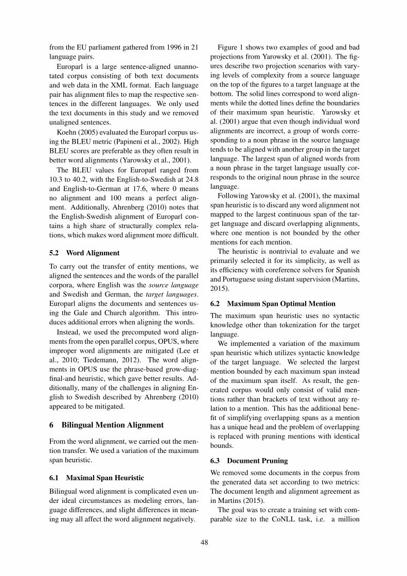
from the EU parliament gathered from 1996 in 21language pairs.

Europarl is a large sentence-aligned unanno-tated corpus consisting of both text documentsand web data in the XML format. Each languagepair has alignment files to map the respective sen-tences in the different languages. We only usedthe text documents in this study and we removedunaligned sentences.

Koehn (2005) evaluated the Europarl corpus us-ing the BLEU metric (Papineni et al., 2002). HighBLEU scores are preferable as they often result inbetter word alignments (Yarowsky et al., 2001).

The BLEU values for Europarl ranged from10.3 to 40.2, with the English-to-Swedish at 24.8and English-to-German at 17.6, where 0 meansno alignment and 100 means a perfect align-ment. Additionally, Ahrenberg (2010) notes thatthe English-Swedish alignment of Europarl con-tains a high share of structurally complex rela-tions, which makes word alignment more difficult.

5.2 Word Alignment

To carry out the transfer of entity mentions, wealigned the sentences and the words of the parallelcorpora, where English was the source languageand Swedish and German, the target languages.Europarl aligns the documents and sentences us-ing the Gale and Church algorithm. This intro-duces additional errors when aligning the words.

Instead, we used the precomputed word align-ments from the open parallel corpus, OPUS, whereimproper word alignments are mitigated (Lee etal., 2010; Tiedemann, 2012). The word align-ments in OPUS use the phrase-based grow-diag-final-and heuristic, which gave better results. Ad-ditionally, many of the challenges in aligning En-glish to Swedish described by Ahrenberg (2010)appeared to be mitigated.

6 Bilingual Mention Alignment

From the word alignment, we carried out the men-tion transfer. We used a variation of the maximumspan heuristic.

6.1 Maximal Span Heuristic

Bilingual word alignment is complicated even un-der ideal circumstances as modeling errors, lan-guage differences, and slight differences in mean-ing may all affect the word alignment negatively.

Figure 1 shows two examples of good and badprojections from Yarowsky et al. (2001). The fig-ures describe two projection scenarios with vary-ing levels of complexity from a source languageon the top of the figures to a target language at thebottom. The solid lines correspond to word align-ments while the dotted lines define the boundariesof their maximum span heuristic. Yarowsky etal. (2001) argue that even though individual wordalignments are incorrect, a group of words corre-sponding to a noun phrase in the source languagetends to be aligned with another group in the targetlanguage. The largest span of aligned words froma noun phrase in the target language usually cor-responds to the original noun phrase in the sourcelanguage.

Following Yarowsky et al. (2001), the maximalspan heuristic is to discard any word alignment notmapped to the largest continuous span of the tar-get language and discard overlapping alignments,where one mention is not bounded by the othermentions for each mention.

The heuristic is nontrivial to evaluate and weprimarily selected it for its simplicity, as well asits efficiency with coreference solvers for Spanishand Portuguese using distant supervision (Martins,2015).

6.2 Maximum Span Optimal MentionThe maximum span heuristic uses no syntacticknowledge other than tokenization for the targetlanguage.

We implemented a variation of the maximumspan heuristic which utilizes syntactic knowledgeof the target language. We selected the largestmention bounded by each maximum span insteadof the maximum span itself. As result, the gen-erated corpus would only consist of valid men-tions rather than brackets of text without any re-lation to a mention. This has the additional bene-fit of simplifying overlapping spans as a mentionhas a unique head and the problem of overlappingis replaced with pruning mentions with identicalbounds.

6.3 Document PruningWe removed some documents in the corpus fromthe generated data set according to two metrics:The document length and alignment agreement asin Martins (2015).

The goal was to create a training set with com-parable size to the CoNLL task, i.e. a million

48

[J1 N1] VBD [N2 N2] IN [N3]

[DT(1) N(1) J(1)] VBD [N(2) de N(2)] DT [N(3)]

/0

[DT1 J1 N1] VBD [N2 N2]

[DT(1) N(1)] VBD [N(2)} J(1){ de N(2)]

/0

Figure 1: Left: Standard projection scenario according to Yarowsky et al. (2001); Right: Problematicprojection scenario

words or more. To this effect, we aligned all thedocuments using the maximum span variant andwe measured the alignment accuracy defined asthe number of accepted alignments divided by thesum of all alignments.

We removed all the documents with lower thanaverage alignment accuracy. Additionally, largerdocuments were removed until we could generatea total training set consisting of approximately amillion words in total.

7 Evaluation

7.1 MetricsThere are multiple metrics to evaluate coreferenceresolution. We used the CoNLL 2012 score as itconsists of a single value (Pradhan et al., 2012).This score is the mean of three other metrics:MUC6 (Vilain et al., 1995), B3 (Bagga and Bald-win, 1998), and CEAFE (Luo, 2005). We alsoreport the values we obtained with CEAFM, andBLANC (Recasens and Hovy, 2011).

7.2 Test SetsSwedish: SUC-Core. The SUC-Core corpus(Nilsson Bjorkenstam, 2013) consists of 20,000words and tokens in 10 documents with 2,758coreferring mentions. The corpus is a subset ofthe SUC 2.0 corpus, annotated with noun phrasecoreferential links (Gustafson-Capkova and Hart-mann, 2006).

The corpus is much too small to train a corefer-ence solver, but it is more than sufficient to eval-uate solvers trained on some different source ma-terial. As a preparatory step to evaluate corefer-ence resolution in Swedish, the information fromSUC-Core was merged with SUC 2.0 and SUC3.0 to have a CoNLL 2012 compatible file format.Additionally, we removed the singletons from themerged data files.

German: Tuba D/Z. The Tuba D/Z corpus(Henrich and Hinrichs, 2013; Henrich and Hin-richs, 2014) consists of 1,787,801 words and to-kens organized in 3,644 files annotated with bothpart of speech and dependency graph information.

Although the corpus would be sufficient in sizeto train a coreference solver, we only used it forevaluation in this work. As with SUC-Core, weremoved all the singletons. Due to time and mem-ory constraints, we only used a subset of the TubaD/Z corpus for evaluation.

7.3 End-to-End EvaluationSimilarly to the CoNLL 2011 and 2012 sharedtasks, we evaluated our system using gold and pre-dicted mention boundaries. When given the goldmentions, the solver knows the boundaries of allnonsingleton mentions in the test set, while withpredicted mention boundaries, the solver has noprior knowledge about the test set. We also fol-lowed the shared tasks in only using machine-annotated parses as input.

The rationale for using gold mention bound-aries is that they correspond to the use of an idealmethod for mention identification, where the re-sults are an upper bound for the solver as it doesnot consider singleton mentions (Pradhan et al.,2011).


8.1 Selection of Training SetsFor Swedish, we restricted the training set to theshortest documents containing at least one coref-erence chain. After selection and pruning, thisset consisted of 4,366,897 words and 183,207 sen-tences in 1,717 documents.

For German, we extracted a training set consist-ing of randomly selected documents containing atleast one coreference chain. After selection and

49

pruning, the set consisted of 9,028,208 words and342,852 sentences in 1,717 documents.

8.2 Mention Identification

Swedish. The mentions in SUC-Core corre-spond to noun phrases. We identified them auto-matically from the dependency graphs producedby Maltparser using a set of rules based on themention headwords. Table 1 shows these rules thatconsist of a part of speech and an additional con-straint. When a rule matches the part of speech ofa word, we create the mention from its yield.

As SUC-Core does not explicitly define themention bracketing rules, we had to further ana-lyze this corpus to discern basic patterns and ad-just the rules to better map the mention boundaries(Table 2).

German. The identification of noun phrasesin German proved more complicated than inSwedish, especially due to the split antecedentslinked by a coordinating conjunction. Considerthe phrase Anna and Paul. Anna, Paul, as wellas the whole phrase are mentions of entities. InSwedish, the corresponding phrase would be Annaoch Paul with the conjunction och as the headword. The annotation scheme used for the TIGERcorpus does not have the conjunction as head forcoordinated noun phrases (Albert et al., 2003). InSwedish, the rule for identifying the same kind ofsplit antecedents only needs to check whether aconjunction has children that were noun phrases,whereas in German the same rule required moreanalysis.

Table 3 shows the rules for the identification ofnoun phrases in German, and Table 4, the post-processing rules.

9 Algorithms

9.1 Generating a Training Set

To solve coreference, we used a variation of theclosest antecedent approach described in Soon etal. (2001). This approach models chains as a pro-jected graph with mentions as vertices, where ev-ery mention has at most one antecedent and oneanaphora. The modeling assumptions relaxes thecomplex relationship between coreferring men-tions by only considering the relationship betweena mention and its closest antecedent.

The problem is framed as a binary classificationproblem, where the system only needs to decide

POS Additional rule NPUO Dependency head has POS PM No

Otherwise YesPM Dependency head has POS PM

but different grammatical caseYes

Dependency head has POS PM NoOtherwise Yes

PS YesPN YesNN YesKN The head word is och and has at

least one child who is a mentionYes

Otherwise NoDT The head word is den Yes

Otherwise NoJJ The head word is sjalv Yes

Otherwise No

Table 1: Hand-written rules for noun phrase iden-tification for Swedish based on SUC-Core. Therules are ordered by precedence from top to bot-tom

# Description1 Remove words from the beginning or the

end of the phrase if they have the POS tagsET, EF or VB.

2 The first and last words closest to the men-tion head with the HP POS tag and allwords further from the mention head is re-moved from the phrase.

3 Remove words from the beginning or theend of the phrase if they have the POS tagsAB or MAD.

4 The first and last words closest to the men-tion head with the HP POS tag and withthe dependency arch SS and all words fur-ther from the mention head is removedfrom the phrase.

5 Remove words from the end of the phraseif they have the POS tag PP.

6 Remove words from the beginning or theend of the phrase if they have the POS tagPAD.

Table 2: Additional hand-written rules for postprocessing the identified noun phrases

whether a mention and its closest antecedent core-fer (Soon et al., 2001). When generating a trainingset, the negative examples are more frequent than

50

POS Additional rule NPNN Depend. head has POS NN No

Otherwise YesNE Depend. head has POS NE No

Otherwise YesPRELS YesPRF YesPPOSAT YesPRELAT YesPIS YesPDAT YesPDS YesFM YesCARD Yes

Table 3: Hand-written rules for noun phrase iden-tification for German based on Tuba-D/Z

the positive ones, which may skew the model. Welimited the ratio at somewhere between 4 and 5 %and randomizing which negative samples becomepart of the final training set.

9.2 Machine-Learning Algorithms

We used the C4.5, random forest, and logistic re-gression algorithms from the Weka Toolkit andLibLinear to train the models (Witten and Frank,2005; Hall et al., 2009; Fan et al., 2008).

9.3 Features

Swedish. As features, we used a subset Stam-borg et al. (2012) and Soon et al. (2001). Table 5shows the complete list.

German. The feature set for German is de-scribed in Table 5. The primary difference be-tween German and Swedish is the addition of gen-der classified names. We used the lists of namesand job titles from IMS Hotcoref DE (Rosiger andKuhn, 2016) to train the German model.

The morphological information from bothCoreNLP and Mate Tools appeared to be limitedwhen compared with Swedish, which is reflectedin the feature set.

10 Results

10.1 Mention Alignment

Swedish. The Swedish EuroParl corpus consistsof 8,445 documents. From these documents, weselected a subset consisting of 3,445 documents

# Rule1 Remove words from the start or the

end of the phrase if they have thePOS tags $. $( PROP KON.

2 If there is a word with the POS tagVVPP after the head word the wordprior to this word becomes the lastword in the phrase.

3 If there is a dependant word with thePOS tag KON and its string equalsund create additional mentions fromthe phrases left and right of thisword.

4 If there is a word with the POS tagAPPRART after the head word theword prior to this word becomes thelast word in the phrase.

Table 4: Additional hand-written rules for postprocessing the identified noun phrases in German

based on the size, where we preferred the smallerdocuments.

The selected documents contained in total1,189,557 mentions that were successfully trans-ferred and 541,608 rejected mentions.

We removed the documents with less than 70%successfully transferred mentions, which yieldeda final tally of 515,777 successfully transferredmentions and 198,675 rejected mentions in 1,717documents.

German. The German EuroParl corpus consistsof 8,446 documents. From these documents, werandomly selected a subset consisting of 2,568documents.

The selected documents contained in total992,734 successfully transferred and 503,690 re-jected mentions.

We removed the documents with less than 60%successfully transferred mentions, which yieldeda final tally of 975,539 successfully transferredmentions and 491,009 rejected mentions in 964documents.

10.2 Mention Identification

Swedish. Using the rules described in Table 1,we identified 91.35% of the mentions in SUC-Core. We could improve the results to 95.82%with the additional post processing rules describedin Table 2.

51

Rule Type sv deMentions are identical Boolean ! !

Mention head words are identical Boolean ! !

POS of anaphora head word is PN Boolean !

POS of antecedent head word is PN Boolean !

POS of anaphora head word is PM Boolean !

POS of antecedent head word is PM Boolean !

Anaphora head word has the morphological feat DT Boolean !

Antecedent head grammatical article Enum !

Anaphora head grammatical article Enum !

Antecedent grammatical number Enum !

Anaphora grammatical number Enum !

Checks if mention contains a word which is a malefirst name

Boolean !

Checks if mention contains a word which is a femalefirst name

Boolean !

Checks if mention contains a word which is a jobtitle

Boolean !

Checks if mention contains a word which is a malefirst name

Boolean !

Checks if mention contains a word which is a femalefirst name

Boolean !

Checks if mention contains a word which is a jobtitle

Boolean !

Number of intervening sentences between the twomentions. Max. 10.

Integer !

Grammatical gender of antecedent head word Enum ! !

Grammatical gender of anaphora head word Enum ! !

Anaphora head is subject Enum !

Antecedent head is subject Enum !

Anaphora has the morphological feature gen Enum !

Antecedent has the morphological feature gen Enum !

Anaphora has the morphological feature ind Enum !

Antecedent has the morphological feature ind Enum !

Anaphora has the morphological feature nom Enum !

Antecedent has the morphological feature nom Enum !

Anaphora has the morphological feature sg Enum !

Antecedent has the morphological feature sg Enum !

Table 5: The feature set used for Swedish (sv) and German (de)

German. Using the rules described in Table 3,we identified 65.90% of the mentions in TubaD/Z. With the additional post processing rules de-scribed in Table 4, we reached a percentage of82.08%.

10.3 Coreference Resolution

Table 6 shows the end-to-end results when usingpredicted mentions and Table 7 shows the resultswith the same pipeline with gold mentions. Theselatter results correspond to the upper bound figureswe could obtain with this technique with a same

52

Language Method MUC6 B3 CEAFE CEAFM BLANC MELACoNLL

Swedish J48 46.72 29.11 28.32 32.67 29.94 34.98Random forest 46.29 28.87 27.68 32.21 29.41 34.28Logistic regression 39.18 2.4 1.01 8.88 5.46 14.19

German J48 34.29 2.63 2.55 12.81 4.67 13.16Random forest 33.51 2.54 2.4 11.82 5.46 12.81Logistic regression 33.97 2.36 1.35 12.5 4.58 12.56

Table 6: End-to-end results using predicted mentions

Language Method MUC6 B3 CEAFE CEAFM BLANC MELACoNLL

Swedish J48 61.43 37.78 40.97 42.36 41.51 46.73Random forest 61.37 37.72 41.03 42.46 41.22 46.71Logistic regression 84.77 13.37 1.95 16.68 15.5 33.37

German J48 82.69 19.74 5.86 26.75 19.56 36.1Random forest 77.24 24.16 9.53 26.94 32.72 36.98Logistic regression 83.71 17.6 4.5 25.58 16.61 35.27

Table 7: End-to-end results using gold mention boundaries

feature set.

11 Conclusion

In this paper, we have described end-to-end coref-erence solvers for Swedish and German that usedno annotated data. We used feature sets limited tosimple linguistic features easily extracted from theSwedish treebank and the German Tiger corpus,respectively. A large subset of the feature set ofStamborg et al. (2012) would very likely improvethe results in this work.

The results in Tables 6 and 7 show that eventhough the dependency grammar based approachfor identifying mentions yields a decent perfor-mance compared with CoNLL 2011 and 2012, abetter identification and pruning procedure wouldprobably significantly improve the results. This ismanifest in German, where using the gold men-tions results in a considerable increase of thescores: Table 7 shows a difference of more than23 points compared with those in Table 6. Thisdemonstrates that the large difference in scoresbetween Swedish and German has its source inthe methods used for mention identification ratherthan in the different feature sets or the correctnessof the training set. This can be explained by thedifficulty to predict mentions for German, possi-bly because of the differences in the dependencygrammar format, as relatively few mentions wereidentified using their head elements.

The final results also show that classifiers based

on J48 and random forests produced better scoresthan logistic regression.

Coreference resolution using weak labelledtraining data from distant supervision enabled usto create coreference solvers for Swedish and Ger-man, even though the mention alignment in theparallel corpora was far from perfect. It is diffi-cult to compare results we obtained in this articlewith those presented in CoNLL, as the languagesand test sets are different. Despite this, we ob-serve that when using gold mention boundaries,we reach a MELACoNLL score for Swedish that iscomparable with results obtained for Arabic in theCoNLL-2012 shared task using the similar pre-conditions. We believe this shows the method weproposed is viable. Our results are, however, lowerthan those obtained for English and Chinese in thesame task and could probably be improved with abetter mention detection.

Acknowledgments

This research was supported by Vetenskapsradet,the Swedish research council, under the Det digi-taliserade samhallet program.

ReferencesLars Ahrenberg. 2010. Alignment-based profiling of

Europarl data in an English-Swedish parallel corpus.In Nicoletta Calzolari (Conference Chair), KhalidChoukri, Bente Maegaard, Joseph Mariani, JanOdijk, Stelios Piperidis, Mike Rosner, and Daniel

53

Tapias, editors, Proceedings of the Seventh Interna-tional Conference on Language Resources and Eval-uation (LREC’10), Valletta, Malta, may. EuropeanLanguage Resources Association (ELRA).

Stefanie Albert, Jan Anderssen, Regine Bader,Stephanie Becker, Tobias Bracht, Sabine Brants,Thorsten Brants, Vera Demberg, Stefanie Dipper,Peter Eisenberg, et al. 2003. Tiger annotationss-chema. Technical report, Universitat des Saarlan-des.

Amit Bagga and Breck Baldwin. 1998. Entity-based cross-document coreferencing using the vec-tor space model. In Proceedings of the 36th An-nual Meeting of the Association for ComputationalLinguistics and 17th International Conference onComputational Linguistics - Volume 1, ACL ’98,pages 79–85, Stroudsburg, PA, USA. Associationfor Computational Linguistics.

Anders Bjorkelund, Bernd Bohnet, Love Hafdell, andPierre Nugues. 2010. A high-performance syntac-tic and semantic dependency parser. In Proceedingsof the 23rd International Conference on Computa-tional Linguistics: Demonstrations, pages 33–36.Association for Computational Linguistics.

Kevin Clark and Christopher D. Manning. 2016. Im-proving coreference resolution by learning entity-level distributed representations. In Proceedings ofthe 54th Annual Meeting of the Association for Com-putational Linguistics (Volume 1: Long Papers),pages 643–653, Berlin, Germany, August. Associ-ation for Computational Linguistics.

Peter Exner, Marcus Klang, and Pierre Nugues. 2015.A distant supervision approach to semantic role la-beling. In Fourth Joint Conference on Lexical andComputational Semantics (* SEM 2015).

Rong-En Fan, Kai-Wei Chang, Cho-Jui Hsieh, Xiang-Rui Wang, and Chih-Jen Lin. 2008. LIBLINEAR:A library for large linear classification. Journal ofmachine learning research, 9(Aug):1871–1874.

Sofia Gustafson-Capkova and Britt Hartmann. 2006.Manual of the Stockholm Umea corpus version 2.0.Technical report, Stockholm University.

Mark Hall, Eibe Frank, Geoffrey Holmes, BernhardPfahringer, Peter Reutemann, and Ian H Witten.2009. The WEKA data mining software: an update.ACM SIGKDD explorations newsletter, 11(1):10–18.

Verena Henrich and Erhard Hinrichs. 2013. Extendingthe TuBa-D/Z treebank with GermaNet sense anno-tation. In Language Processing and Knowledge inthe Web, pages 89–96. Springer Berlin Heidelberg.

Verena Henrich and Erhard Hinrichs. 2014. Con-sistency of manual sense annotation and integrationinto the TuBa-D/Z treebank. In Proceedings of the13th International Workshop on Treebanks and Lin-guistic Theories (TLT13).

Rebecca Hwa, Philip Resnik, Amy Weinberg, ClaraCabezas, and Okan Kolak. 2005. Bootstrappingparsers via syntactic projection across parallel texts.Natural language engineering, 11(03):311–325.

Philipp Koehn. 2005. Europarl: A parallel corpus forstatistical machine translation. In MT summit, vol-ume 5, pages 79–86.

Jae-Hee Lee, Seung-Wook Lee, Gumwon Hong,Young-Sook Hwang, Sang-Bum Kim, and Hae-Chang Rim. 2010. A post-processing approach tostatistical word alignment reflecting alignment ten-dency between part-of-speeches. In Proceedingsof the 23rd International Conference on Computa-tional Linguistics: Posters, pages 623–629. Associ-ation for Computational Linguistics.

Xiaoqiang Luo. 2005. On coreference resolution per-formance metrics. In Proceedings of the confer-ence on Human Language Technology and Empiri-cal Methods in Natural Language Processing, pages25–32. Association for Computational Linguistics.

Christopher D. Manning, Mihai Surdeanu, John Bauer,Jenny Finkel, Steven J. Bethard, and David Mc-Closky. 2014. The Stanford CoreNLP natural lan-guage processing toolkit. In Association for Compu-tational Linguistics (ACL) System Demonstrations,pages 55–60.

Andre F. T. Martins. 2015. Transferring coreferenceresolvers with posterior regularization. In Proceed-ings of the 53rd Annual Meeting of the Associationfor Computational Linguistics and the 7th Interna-tional Joint Conference on Natural Language Pro-cessing (Volume 1: Long Papers), pages 1427–1437,Beijing, China, July. Association for ComputationalLinguistics.

Mike Mintz, Steven Bills, Rion Snow, and Dan Ju-rafsky. 2009. Distant supervision for relation ex-traction without labeled data. In Proceedings of theJoint Conference of the 47th Annual Meeting of theACL and the 4th International Joint Conference onNatural Language Processing of the AFNLP: Vol-ume 2-Volume 2, pages 1003–1011. Association forComputational Linguistics.

Kristina Nilsson Bjorkenstam. 2013. SUC-CORE: Abalanced corpus annotated with noun phrase coref-erence. Northern European Journal of LanguageTechnology (NEJLT), 3:19–39.

Joakim Nivre, Johan Hall, Jens Nilsson, AtanasChanev, Gulsen Eryigit, Sandra Kubler, SvetoslavMarinov, and Erwin Marsi. 2007. MaltParser:A language-independent system for data-driven de-pendency parsing. Natural Language Engineering,13(02):95–135.

Robert Ostling. 2013. Stagger: An open-source partof speech tagger for Swedish. Northern EuropeanJournal of Language Technology (NEJLT), 3:1–18.

54

Kishore Papineni, Salim Roukos, Todd Ward, and Wei-Jing Zhu. 2002. BLEU: a method for automaticevaluation of machine translation. In Proceedings ofthe 40th annual meeting on association for compu-tational linguistics, pages 311–318. Association forComputational Linguistics.

Sameer Pradhan, Lance Ramshaw, Mitchell Marcus,Martha Palmer, Ralph Weischedel, and NianwenXue. 2011. CoNLL-2011 shared task: Modelingunrestricted coreference in ontonotes. In Proceed-ings of the Fifteenth Conference on ComputationalNatural Language Learning: Shared Task, pages 1–27. Association for Computational Linguistics.

Sameer Pradhan, Alessandro Moschitti, Nianwen Xue,Olga Uryupina, and Yuchen Zhang. 2012. CoNLL-2012 shared task: Modeling multilingual unre-stricted coreference in ontonotes. In Joint Confer-ence on EMNLP and CoNLL-Shared Task, pages 1–40. Association for Computational Linguistics.

Altaf Rahman and Vincent Ng. 2012. Translation-based projection for multilingual coreference reso-lution. In Proceedings of the 2012 Conference ofthe North American Chapter of the Association forComputational Linguistics: Human Language Tech-nologies, pages 720–730. Association for Computa-tional Linguistics.

Marta Recasens and Eduard Hovy. 2011. BLANC:Implementing the rand index for coreference evalu-ation. Natural Language Engineering, 17(04):485–510.

Ina Rosiger and Jonas Kuhn. 2016. IMS HotCoref DE:A data-driven co-reference resolver for German. InLREC.

Wee Meng Soon, Hwee Tou Ng, and DanielChung Yong Lim. 2001. A machine learning ap-proach to coreference resolution of noun phrases.Computational linguistics, 27(4):521–544.

Marcus Stamborg, Dennis Medved, Peter Exner, andPierre Nugues. 2012. Using syntactic dependen-cies to solve coreferences. In Joint Conference onEMNLP and CoNLL-Shared Task, pages 64–70. As-sociation for Computational Linguistics.

Jorg Tiedemann. 2012. Parallel data, tools and in-terfaces in OPUS. In Nicoletta Calzolari (Con-ference Chair), Khalid Choukri, Thierry Declerck,Mehmet Ugur Dogan, Bente Maegaard, Joseph Mar-iani, Jan Odijk, and Stelios Piperidis, editors, Pro-ceedings of the Eight International Conference onLanguage Resources and Evaluation (LREC’12), Is-tanbul, Turkey, may. European Language ResourcesAssociation (ELRA).

Marc Vilain, John Burger, John Aberdeen, Dennis Con-nolly, and Lynette Hirschman. 1995. A model-theoretic coreference scoring scheme. In Proceed-ings of the 6th conference on Message understand-ing, pages 45–52. Association for ComputationalLinguistics.

Ian H Witten and Eibe Frank. 2005. Data Mining:Practical machine learning tools and techniques.Morgan Kaufmann.

Limin Yao, Sebastian Riedel, and Andrew McCallum.2010. Collective cross-document relation extrac-tion without labelled data. In Proceedings of the2010 Conference on Empirical Methods in NaturalLanguage Processing, pages 1013–1023. Associa-tion for Computational Linguistics.

David Yarowsky, Grace Ngai, and Richard Wicen-towski. 2001. Inducing multilingual text analysistools via robust projection across aligned corpora.In Proceedings of the first international conferenceon Human language technology research, pages 1–8. Association for Computational Linguistics.

55


Aligning phonemes using finte-state methods

Kimmo KoskenniemiUniversity of Helsinki

Helsinki, [email protected]

Abstract

The paper presents two finite-state meth-ods which can be used for aligning pairsof cognate words or sets of different al-lomorphs of stems. Both methods useweighted finite-state machines for choos-ing the best alternative. Individual let-ter or phoneme correspondences can beweighted according to various principles,e.g. using distinctive features. The com-parison of just two forms at a time is sim-ple, so that method is easier to refine toinclude context conditions. Both meth-ods are language independent and couldbe tuned for and applied to several typesof languages for producing gold standarddata.

The algorithms were implemented usingthe HFST finite-state library from shortPython programs. The paper demonstratesthat the solving of some non-trivial prob-lems has become easier and accessible fora wider range of scholars.

1 Background

In this paper, finite-state automata (FSA) andfinite-state transducers (FST) are used as the basictools. In particular, the utility of weighted finite-state transducers (WFST) and automata (WFSA)is demonstrated.

Finite-state toolboxes have been freely avail-able for some time, e.g. OpenFST (Mohri etal., 2002), Xerox XFST (Beesley and Karttunen,2003), HFST – Helsinki Finite-State TransducerTechnology (Linden et al., 2011), SFST (Schmid,2005) and Foma (Hulden, 2009). These imple-mentations have been accessible as libraries forC or C++ programmers, some also as commandline programs which can be pipelined (HFST), andsome as scripting languages (XFST, SFST, Foma,

HFST). Combining independent programs usingshell commands is easy and suitable for manykinds of tasks, but certain combinations of oper-ations are difficult or impossible to achieve thisway. Even the XFST and SFST scripting lan-guages have their restrictions, especially for loop-ing, testing and input/output. It seems that none ofthe tasks discussed in this paper could be conve-niently solved using the XFST or SFST scriptinglanguage.

More recently, most finite-state packages havebeen also available through Python in one wayor the other. The HFST Python embedding wasused here for a few reasons: it is implemented forPython 3 which uses Unicode as its native code,one could use weighted transducers, and HFSTcontained the kinds of functions that were needed.

2 Previous work on alignment

Automatic alignment of letters or phonemes is rel-evant in several areas, e.g. finding the pronun-ciation of unknown words or names in speechsynthesis, see e.g. (Jiampojamarn et al., 2007),phonetically based spelling correction, see e.g.(Toutanova and Moore, 2002), in comparing cog-nate words in historical linguistics, see e.g. (Cov-ington, 1998; Kondrak, 2000) , reconstructingproto-languages, e.g. (Bouchard-Cote et al., 2009)and in many other areas of linguistics. Characterby character alignment can be approached as a ma-chine learning problem, as in (Ciobanu and Dinu,2014) or as a linguistic task as is done in this paper.The methods presented here make use of generalproperties of phonology. Still, more specific rulescan be included where needed.

Covington (1998) used a special six step mea-sure for phoneme distances and (Nerbonne andHeeringa, 1997) used phonetic features and theplain Levenshtein distance between sequences offeatures in order to estimate differences betweenDutch dialects. (Somers, 1999) used distinctive

56

features in the comparison and his algorithm usedthe (manually marked) stressed vowels as the start-ing point whereas other approaches progressedfrom left to right. All these approaches were lo-cal in the sense that they measure each pair ofphonemes separately and the sum of the mea-sures was the measure of the whole alignment.Their methods appear to depend on this assump-tion and therefore exclude the inclusion of contextdependent phenomena e.g. assimilation, metathe-sis, constraints of syllable structure etc.

The work presented here separates the defini-tion of the measure from the algorithm for findingthe best alignment. Measures are represented asWFSTs and they are built by producing weightedregular expressions using simple Python scripts.The algorithms used here utilize the efficient algo-rithms already available in the finite-state calculusfor finding the best paths from weighted acyclicautomata (Mohri, 2009).

3 Weighting the correspondences ofphonemes

Simple phoneme by phoneme (or letter by letter)alignment is needed when relating cognate wordsof related languages or e.g. relating the writtenwords in old texts with their present day forms.The process of alignment consists here of makingphonetically similar phonemes correspond to eachother and adding zeroes Ø where necessary (dueto epenthesis or elision). E.g. Estonian leem andFinnish liemi would be aligned by adding one zeroat the end of the Estonian form:

l e e m Øl i e m i

In general, consonants may not correspond tovowels or vice versa, except for glides, approx-imants or semivowels which may correspond tocertain vowels and certain consonants. In thispaper, many-to-one, and one-to-many correspon-dences are simply expressed by using combina-tions of phoneme to phoneme correspondences,phoneme to zero and zero to phoneme correspon-dences.

Vowels can be described by using distinctivefeatures such as the height of the tongue, front-ness/backness and rounding/unrounding, see Fig-ure 1. Using such features, one may compute dis-tances between different vowels. Similarly, conso-nants can be characterized by their place of articu-lation, voicing and the manner of articulation, see

Figure 2. The measure used here is not intendedto be an absolute or universal measure, it is justan ad hoc approximation suitable for Estonian andFinnish.

vowels = {’i’:(’Close’,’Front’,’Unrounded’),’y’:(’Close’,’Front’,’Rounded’),’u’:(’Close’,’Front’,’Rounded’),’u’:(’Close’,’Back’,’Rounded’),’e’:(’Mid’,’Front’,’Unrounded’),’o’:(’Mid’,’Front’,’Rounded’),’~o’:(’Mid’,’Back’,’Unrounded’),’o’:(’Mid’,’Back’,’Rounded’),’a’:(’Open’,’Front’,’Unrounded’),’a’:(’Open’,’Back’,’Unrounded’)}

Figure 1: Description of some Finnish and Es-tonian orthographic vowels using distinctive fea-tures. IPA symbol for letters for which they arenot the letter itself: u = y, o = ø, o = 7, a = æ, a = A

The work described here permits different kindsof definitions for measuring the distances, includ-ing those used in (Covington, 1998; Kondrak,2000; Nerbonne and Heeringa, 1997; Somers,1999). Any measure which can reasonably be ex-pressed as a WFST can be used by the algorithmpresented in Section 4.

From the phoneme descriptions shown in Fig-ure 1, one can compute simple distances betweenany two vowels or any two consonants. The for-mula chosen in this study was heuristic. Tongueheight had three steps corresponding to values 1,2, 3 and the distance was taken to be the differ-ence of those values. The distance between frontand back was taken to be 1 as was the distance be-tween rounding and unrounding. The distance be-tween any two vowels was defined to be the sumof these three numbers.1

A similar formula was used for consonantswhere the positions of articulation was numberedfrom 1 to 5 and their difference was the distance,see Figure 2. Different voicing counted as 1, andso did the manner of articulation. Again, the totaldistance was the sum of these three numbers.

A double loop through vowels and anotherthrough consonants produced a list of feasiblecombinations of phonemes and the computedmeasure for their difference. These triplets werethen formatted as strings and glued together intoa long regular expression, see some samples of it

1This is sometimes called Manhattan distance as opposedto the Euclidean distance which would be the square root ofthe sum of squares.

57

consonants = {’m’:(’Bilab’,’Voiced’,’Nasal’),’p’:(’Bilab’,’Unvoiced’,’Stop’),’b’:(’Bilab’,’Voiced’,’Stop’),’v’:(’Labdent’,’Voiced’,’Fricative’),’f’:(’Labdent’,’Unvoiced’,’Fricative’),’n’:(’Alveolar’,’Voiced’,’Nasal’),’t’:(’Alveolar’,’Unvoiced’,’Stop’),’d’:(’Alveolar’,’Voiced’,’Stop’),’s’:(’Alveolar’,’Unvoiced’,’Sibilant’),’l’:(’Alveolar’,’Voiced’,’Lateral’),’r’:(’Alveolar’,’Voiced’,’Tremulant’),’j’:(’Velar’,’Voiced’,’Approximant’),’k’:(’Velar’,’Unvoiced’,’Stop’),’g’:(’Velar’,’Voiced’,’Stop’),’h’:(’Glottal’,’Unvoiced’,’Fricative’)}

Figure 2: Description of some Finnish an Estonianconsonants

below:... | u:u::0 | u:y::1 | u:a::4 | u:o::2 ...| k:g::1 | k:h::2 | k:j::2 | k:k::0 ...

Note that the weight is after a double colon ac-cording to the extended notation for weighted reg-ular expressions used in HFST. Thus, in the aboveformula, u may correspond to u at null cost, and kmay correspond to g at a cost of 1.

Any phoneme could be deleted or inserted at acost. A simple loop produced the additional corre-spondences and their weights:

... | o:Ø::3 | p:Ø::3 | r:Ø::3 | ...| Ø:o::3 | Ø:p::3 | Ø:r::3 | ...

In Finnish and in Estonian, long vowels arerepresented as two successive vowels. The de-fault correspondences and weights clearly allowshortening of long vowels (or double consonants),but there would be two ways to express it withequal weights: one where the first of the two cor-responds to zero, and the other where the sec-ond component corresponds to zero. In order toavoid this ambiguity, there was yet another loopwhich produced the necessary pieces of expres-sions which had a slightly smaller weight than thedeletion alone. Note that e.g. p:Ø p will remainacceptable, but the expression below gives a lowerweight for the combination where the latter com-ponent corresponds to zero.

... | o Ø:o::2 | p Ø:p::2 | r Ø:r::2 ...| o o:Ø::2 | p p:Ø::2 | r r:Ø::2 ...

One can use the same technique for handling or-thographic conventions. One language might usekk and the other ck for a geminate k, similarly ksinstead of x and ts instead of z. One can make suchcorrespondences to have a zero distance by listing

them with an explicit zero weight, e.g.:k:c::0 k::0 | k:x s:Ø::0 | t:z s:Ø::0

One could use the same mechanism for giv-ing some phoneme relations a lower weight. Onecould e.g. prefer assimilations over arbitrary com-binations by imposing a lower weight for a variantif preceded or followed by phoneme which artic-ulated in the same place. Local metathesis affect-ing two consecutive phonemes could also be ex-pressed fairly neatly.

When all expressions are glued together, en-closed in brackets and followed by a Kleene star,the regular expression is ready to be compiledinto a WFST. After compilation, the WFST whichholds the distances as weights, can be stored as afile to be used later by the aligning algorithm.

4 Aligning pairs of words

Now, we are ready to write a small but generalPython script which reads in the similarity WFSTdescribed in Section 3 and (1) reads in a pair ofcognate words from the standard input and (2)converts them into FSTs W1 and W2, (3) adds ex-plicit zero symbols freely to each, (4) comparesthe zero-filled expressions using the weighed dis-tance transducer ALIGN and produces in this wayall possible alignments and their total weights as aweighted transducer RES. Of these many possiblealignments accepted by RES, (5) the best one ischosen and (6) printed, see Figure 3.

import sys, hfstalgfile = hfst.HfstInputStream("d.fst")ALIGN = algfile.read()for line in sys.stdin: # (1)

F1,F2 = line.strip().split(sep=":") # (1)W1 = hfst.fst(F1) # (2)W1.insert_freely(("Ø","Ø")) # (3)W2 = hfst.fst(F2) # (2)W2.insert_freely(("Ø","Ø")) # (3)W1.compose(ALIGN) # (4)W1.compose(W2) # (4)RES = W1.n_best(1).minimize() # (5)paths = # (6)

res.extract_paths(output=’text’) # (6)print(paths.strip()) # (6)

Figure 3: Python program for aligning pairs ofcognate words

The algorithm in Figure 3 considers all possibleways to add zero symbols to the cognates. It evenadds an indefinite number of zeros to each cog-nate word. For Estonian leem and Finnish liemithe adding of the zeros would result in strings cov-ered by the following expressions.

58

W1: Ø* l Ø* e Ø* e Ø* m Ø*W2: Ø* l Ø* i Ø* e Ø* m Ø* i Ø*

The key idea is in the composition of thesetwo FSAs so that the distance metric transducerALIGN is in the middle:

W1 .o. ALIGN .o. W2

Transducers W1, W2 and the ALIGN are allepsilon-free, so the composition accepts onlysame length string pairs. Note that the distancemetric ALIGN does not allow a zero to correspondto another zero, so the zero filled strings may onlybe at most twice so long as the longer cognate was.There would still be quite a few comparisons to do,if one would compare and evaluate them one pairat a time.

The HFST function n best(1) finds the pair ofstrings which would have the least weight. Thisis one of the operations that are efficient for WF-STs. The operation produces a FST which acceptsexactly the best string pair. Another function isneeded for extracting the transition labels whichconstitute the strings themselves.

The aligner was used among other things, for re-lating word forms of Modern Finnish and Finnishof a Bible translation of year 1642. With slighttuning of the WFST, the aligner worked as the pri-mary tool for aligning further pairs of old and newwords which were used for writing and testing therules which related the two forms of Finnish. Theold orthography was less phonemic than the mod-ern one and there was more orthographic variationin the old texts. After the initial adjusting to the or-thography of the old texts, only a little tuning wasneeded to modify the computation of the similari-ties until the formula appeared to be stable.

As an informal check, the manually edited andchecked set of 203 pairs of old and new wordforms was cleaned from the added zeros and re-aligned using the aligner. Only one difference wasobserved in the result as compared with the origi-nal.2

5 Other uses for the distance WFSTs

The aligner was developed for aligning pairs ofcognate words given to it. In this task, the alignercan and perhaps must be quite general. When we

2The manually aligned lepaØsivat:lewaisiØØt was prob-lematic because Old Finnish had a different morpheme forthe third person past tense -it whereas the Modern Finnishhas -ivat. Thus, no ‘correct’ alignment actually exists. Thepair to be aligned ought to be lepaisit:lewaisit.

are studying the relation between two languages,we ought not commit ourselves to certain soundchanges (or sound laws) when we start by prepar-ing the source data for analyzing the relation itself.

One might speculate that the aligner could alsobe used as a predictor of the likely shapes of themissing half of a cognate pair. The WFST alone is,however, not useful for such because it generatestoo many candidates, not only those which wouldfollow from the sound changes which govern therelation of the languages. The correct candidatewould be buried under a heap of incorrect ones.

Instead of proposing the missing halves of cog-nate pairs from scratch, one can get useful resultsif one has a word list of the other language. Prepar-ing for the processing, one first converts the wordlist into a FSA, say words-et.fst.

Then, one types in a known word from the firstlanguage. The script (1) converts it into a FSA, (2)shuffles it freely with zeros, (3) composes it withthe distance WFST, (4) deletes all zeros from theresult and then (5) composes it with a FSA con-taining the word list. From the result of this chain,(6) the best word pairs are retrieved and printedfor the user. Using HFST command line tools, thechain of programs looks like:

$ hfst-strings2fst |hfst-shuffle -2 zeros.fst |hfst-compose -2 chardist.fst |hfst-compose -2 del-zeros.fst |hfst-compose -2 words-et.fst |hfst-fst2strings -N 5 -w

This is a pipeline of programs which expects theuser to feed words of the first language. For eachword typed in, the programs do the operations, andfrom the resulting WFST, the last program printsfive best matches, e.g. for the Finnish word ajo(’driving’, ’trip’) it produces:

> ajoajo:aju 1ajo:aje 2ajo:aie 3ajo:aiu 3ajo:agu 3

The pipeline computes five best guesses as pairsof the Finnish and the Estonian words, and showstheir weights. In this case, the first guess Estonianaju happens to be the correct one. In other cases,the correct one may not the best scored candidate,as for vierastus, the correct candidate voorastus isthe third in the list. Some short words may havemany similar words in the word list. For them, thedesired candidate is often too far down in the list

59

of best ranking candidates and will not be foundthis way.

Using the aligner is of course less precise thanbuilding a realistic model of sound changes as wasdone in (Koskenniemi, 2013a) where two-levelrules were used for this purpose.

6 Aligning a set of stems or other morphs

Comparing several words is needed when relatingmore than two historically connected languagesbut also when relating e.g. different stems of aword in order to build lexical entries which can beused in morphological analysis. The reason for re-lating stems is usually to construct one commonmorphophonemic representation for all stems of aword.

In a simplified version of the two-level morpho-logical analysis, one does not postulate underly-ing forms which are plain sequences of phonemes.Instead, one uses alternations of phonemes (mor-phophonemes) when different phonemes alternatewith each other, cf. (Koskenniemi, 2013b). Theproblem of aligning three or more different wordsis similar to the one discussed above but somewhatdifferent methods are needed.

Let us look at the Estonian word pagu (’an es-cape’) which inflects in forms like pagu, paos,pakku. Traditional generative phonology wouldprefer an underlying stem like paku and derive theother forms from that using a sequence of rewrit-ing rules. In contrast to this, the linguist followingthe methods of the simplified two-level morphol-ogy, would first locate the boundaries between thestem morphs and the suffix morphs, i.e. pagu+,pao+s and pakku+, then take the stems pagu, pao,and pakku, then insert a few zeros in order tomake the stem morphs same length, i.e. pagØu,paØØo, pakku. Thus, the linguist would arriveat the morphophonemic representation p a {gØk}{ØØk} {uou} by merging the corresponding let-ters of each stem morph.

Let us see, how an algorithm could simulate thelinguist when it starts from the point where theboundaries have already been located. The task ofthe algorithm is (1) to produce all alignments, in-cluding lots of nonsense alignments, (2) filter outinfeasible alignments, and (3) to evaluate the fea-sible alignments and choose the best among them.

In order to carry out the first task, the algo-rithm blindly inserts some (or no) zero symbolsinto each stem in order to make all stem candi-

dates same length. Thus, some stems are expandedto a number of alternatives where the zeros are atall different places. Assuming that five letters suf-fice for our example word, the first stem needs onezero, the second stem needs two zeros, and thethird stem does not need any.3 The insertion ofthe zeros to the first stem pagu would produce thestrings Øpagu, pØagu, paØgu, pagØu and paguØ.Only one of these five will turn out to be useful butthe algorithm does not know yet which. It does notactually produce the set of strings with zeros, butinstead, it produces an automaton which acceptsall of them.

The feasibility of an alignment is evaluated us-ing the phoneme (or letter) correspondences whichare caused by the insertion of zeros. AligningØpagu, paØØo and pakku would imply corre-spondences Ø-p-p, p-a-a, a-Ø-k, g-Ø-k and u-o-u. Such an alignment is infeasible, as it includestwo forbidden correspondences: the second andthe third phoneme correspondences p-a-a and a-Ø-k are both infeasible because they contain botha consonant and a vowel (the dashes of the cor-respondences will be omitted hereafter). Anotheralignment, e.g. pagØu, paØØ and pakku wouldimply the correspondences ppp, aaa, gØk, ØØkand uou which all seem phonologically feasiblecontaining only identical or closely related soundsand zeros.

Each phoneme correspondence is evaluated sep-arately and assigned a weight according to thesimilarity of the participating phonemes. Thegoodness of an alignment is computed as a sumof all weights for the phoneme correspondences inthe alignment. In the same manner as when com-paring two words, a correspondence consisting ofidentical phonemes e.g. ppp has a zero weight.

Two different distance measures were used. Forvowels, the number of distinct vowels participat-ing the correspondence was used as the measure.If the zero was also a member of the correspon-dence, 0.4 was added. For consonants, the differ-ences of their features was counted. If there wereboth voiced and unvoiced, then 1 was added, ifthere were different manners of articulation, thenone less than the number of manners was added.The positions of articulation were numbered from

3One may start with the shortest possible stems. If noresults are produced (because one would have to match someconsonant to a vowel), one may add one more zero and tryagain, and repeat this until the matching succeeds, and thenstill try with adding one more zero.

60

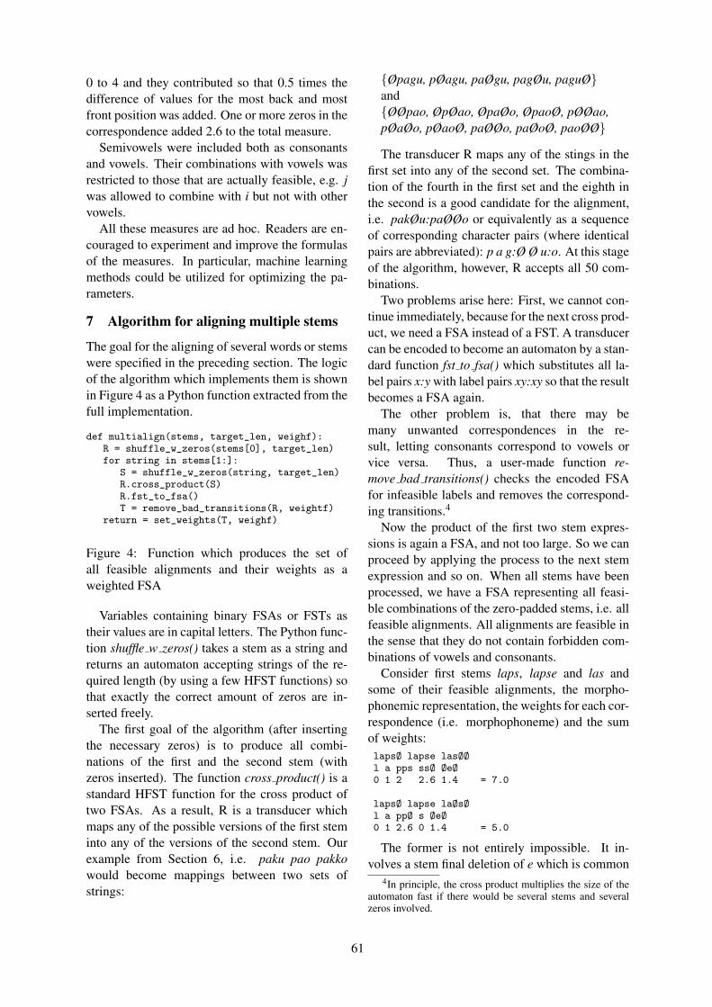
0 to 4 and they contributed so that 0.5 times thedifference of values for the most back and mostfront position was added. One or more zeros in thecorrespondence added 2.6 to the total measure.

Semivowels were included both as consonantsand vowels. Their combinations with vowels wasrestricted to those that are actually feasible, e.g. jwas allowed to combine with i but not with othervowels.

All these measures are ad hoc. Readers are en-couraged to experiment and improve the formulasof the measures. In particular, machine learningmethods could be utilized for optimizing the pa-rameters.

7 Algorithm for aligning multiple stems

The goal for the aligning of several words or stemswere specified in the preceding section. The logicof the algorithm which implements them is shownin Figure 4 as a Python function extracted from thefull implementation.

def multialign(stems, target_len, weighf):R = shuffle_w_zeros(stems[0], target_len)for string in stems[1:]:

S = shuffle_w_zeros(string, target_len)R.cross_product(S)R.fst_to_fsa()T = remove_bad_transitions(R, weightf)

return = set_weights(T, weighf)

Figure 4: Function which produces the set ofall feasible alignments and their weights as aweighted FSA

Variables containing binary FSAs or FSTs astheir values are in capital letters. The Python func-tion shuffle w zeros() takes a stem as a string andreturns an automaton accepting strings of the re-quired length (by using a few HFST functions) sothat exactly the correct amount of zeros are in-serted freely.

The first goal of the algorithm (after insertingthe necessary zeros) is to produce all combi-nations of the first and the second stem (withzeros inserted). The function cross product() is astandard HFST function for the cross product oftwo FSAs. As a result, R is a transducer whichmaps any of the possible versions of the first steminto any of the versions of the second stem. Ourexample from Section 6, i.e. paku pao pakkowould become mappings between two sets ofstrings:

{Øpagu, pØagu, paØgu, pagØu, paguØ}and{ØØpao, ØpØao, ØpaØo, ØpaoØ, pØØao,pØaØo, pØaoØ, paØØo, paØoØ, paoØØ}

The transducer R maps any of the stings in thefirst set into any of the second set. The combina-tion of the fourth in the first set and the eighth inthe second is a good candidate for the alignment,i.e. pakØu:paØØo or equivalently as a sequenceof corresponding character pairs (where identicalpairs are abbreviated): p a g:Ø Ø u:o. At this stageof the algorithm, however, R accepts all 50 com-binations.

Two problems arise here: First, we cannot con-tinue immediately, because for the next cross prod-uct, we need a FSA instead of a FST. A transducercan be encoded to become an automaton by a stan-dard function fst to fsa() which substitutes all la-bel pairs x:y with label pairs xy:xy so that the resultbecomes a FSA again.

The other problem is, that there may bemany unwanted correspondences in the re-sult, letting consonants correspond to vowels orvice versa. Thus, a user-made function re-move bad transitions() checks the encoded FSAfor infeasible labels and removes the correspond-ing transitions.4

Now the product of the first two stem expres-sions is again a FSA, and not too large. So we canproceed by applying the process to the next stemexpression and so on. When all stems have beenprocessed, we have a FSA representing all feasi-ble combinations of the zero-padded stems, i.e. allfeasible alignments. All alignments are feasible inthe sense that they do not contain forbidden com-binations of vowels and consonants.

Consider first stems laps, lapse and las andsome of their feasible alignments, the morpho-phonemic representation, the weights for each cor-respondence (i.e. morphophoneme) and the sumof weights:lapsØ lapse lasØØl a pps ssØ ØeØ0 1 2 2.6 1.4 = 7.0

lapsØ lapse laØsØl a ppØ s ØeØ0 1 2.6 0 1.4 = 5.0

The former is not entirely impossible. It in-volves a stem final deletion of e which is common

4In principle, the cross product multiplies the size of theautomaton fast if there would be several stems and severalzeros involved.

61

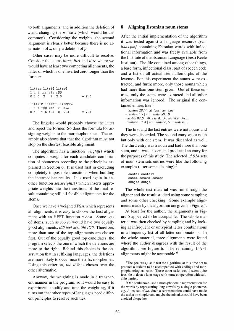
to both alignments, and in addition the deletion ofs and changing the p into s (which would be un-common). Considering the weights, the secondalignment is clearly better because there is no al-ternation of s, only a deletion of p.

Other cases may be more difficult to resolve.Consider the stems litter, litri and litre where wewould have at least two competing alignments, thelatter of which is one inserted zero longer than theformer:

litter litriØ litreØl i t trr eie rØØ0 1 0 2 2 2.6 = 7.6

litterØ litØØri litØØrel i t tØØ eØØ r Øie0 1 0 2.6 1.4 0 2.4 = 7.4

The linguist would probably choose the latterand reject the former. So does the formula for as-signing weights to the morphophonemes. The ex-ample also shows that that the algorithm must notstop on the shortest feasible alignment.

The algorithm has a function weightf() whichcomputes a weight for each candidate combina-tion of phonemes according to the principles ex-plained in Section 6. It is used first in excludingcompletely impossible transitions when buildingthe intermediate results. It is used again in an-other function set weights() which inserts appro-priate weights into the transitions of the final re-sult containing still all feasible alignments for thestems.

Once we have a weighted FSA which representsall alignments, it is easy to choose the best align-ment with an HFST function n best. Some setsof stems, such as too to would have two equallygood alignments, too toØ and too tØo. Therefore,more than one of the top alignments are chosenfirst. Out of the equally good top candidates, theprogram selects the one in which the deletions aremore to the right. Behind this choice is the ob-servation that in suffixing languages, the deletionsare more likely to occur near the affix morphemes.Using this criterion, too toØ is chosen over theother alternative.

Anyway, the weighting is made in a transpar-ent manner in the program, so it would be easy toexperiment, modify and tune the weighting, if itturns out that other types of languages need differ-ent principles to resolve such ties.

8 Aligning Estonian noun stems

After the initial implementation of the algorithmit was tested against a language resource tyve-baas.pmf containing Estonian words with inflec-tional information and was freely available fromthe Institute of the Estonian Language (Eesti KeeleInstituut). The file contained among other things,a base form, inflectional class, part of speech codeand a list of all actual stem allomorphs of thelexeme. For this experiment the nouns were ex-tracted, and furthermore, only those nouns whichhad more than one stem given. Out of these en-tries, only the stems were extracted and all otherinformation was ignored. The original file con-tained entries like:

=’aasima 28 V | at: ’aasi, an: aasi=’aasta 01 S | a0: ’aasta, a0r: 0=aastak 02 S | a0: aastak, b0: aastaku, b0r:...˜’aastane 10 A | a0: ’aastane, b0: ’aastase,...

The first and the last entries were not nouns andthey were discarded. The second entry was a nounbut only with one stem. It was discarded as well.The third entry was a noun and had more than onestem, and it was chosen and produced an entry forthe purposes of this study. The selected 15 934 setsof noun stem sets entries were like the followingexamples (after some cleaning):5

aastak aastakuaatom aatomi aatomeabajas abaja

The whole test material was run through thealigner and the result studied using some samplingand some other checking. Some example align-ments made by the algorithm are given in Figure 5.

At least for the author, the alignments in Fig-ure 5 appeared to be acceptable. The whole ma-terial was then checked by sampling and by look-ing at infrequent or untypical letter combinationsin a frequency list of all letter combinations. Inthe whole material, three alignments were foundwhere the author disagrees with the result of thealgorithm, see Figure 6. The remaining 15 931alignments might be acceptable.6

5The goal was just to test the algorithm, at this time not toproduce a lexicon to be accompanied with endings and mor-phophonological rules. Those other tasks would seem quitefeasible to do at a later stage with some cooperation with suit-able parties.

6One could have used a more phonemic representation forthe words by representing long vowels by a single phoneme,e.g. A instead of aa. Such a representation could have madethe task a bit simpler and maybe the mistakes could have beenavoided altogether.

62

birmalane birmalase birmalas birmalasib i r m a l a nsss eeØi

faktuur faktuuri faktuuref a k t u u r Øie

hamarik hamarikku hamariku hamarikkehamarike

h a m a r i k ØkØkØ Øuueekoger kogre kokre kogri kokri

k o ggkgk eØØØØ r Øeeiikuusk kuuske kuuse kuuski kuusi

k u u s kkØkØ Øeeiiliud liuda liua liudu

l i u ddØd Øaaumutter mutri mutre

m u t tØØ eØØ r Øiepagu pao pakku

p a gØk ØØk uoupugu pukku

p u gk Øk uruga roa ruge rukka

r uouu gØgk ØØØk aaeasugu soo sukku

s uou gØk ØØk uoutoht tohtu tohu tohte tohe

t o h ttØtØ Øuueevahk vahku vahu vahke vahe

v a h kkØkØ Øuueeaie aige

a i Øg e

Figure 5: Some example stem sets and their align-ments

raag raagu rao raageraagØ raagu raoØØ raager a aaoa ggØg ØuØe

saad saadu sao saadesaadØ saadu saoØØ saades a aaoa ddØd ØuØe

sae saaja saajusaeØØ saaja saajus a eaa Øjj Øau

Figure 6: The three questionable alignments foundin the Estonian word list of nouns

9 Tasks for the future

Distances between phonemes as described in Sec-tion 4 seems like a challenge for further research.In essence, the relation looks like a two-level rulerelation with weights. No present compiler fortwo-level rules can directly assign weights to cor-respondences. It appears to be possible to includesome form of weighting to the rule formalism andwrite a compiler.

A two-level compiler dedicated for alignmenttasks could express the language specific pat-terns of phoneme alternations. A clear case forsuch rules would be the proper handling of vowellengthening and gemination. Furthermore, oneguiding the insertions and deletions could be made

more transparent and robust using rules.Writing dedicated compilers for two-level rules

has now become much easier. It would be a rea-sonable project to write a compiler which is ori-ented towards alignment. In this way, one couldimplement suitable context constraints for the tar-get language(s) and integrate it into the process ofalignment.

The algorithm with the weights made for Esto-nian stems, was tested also for the alignment ofFinnish noun stems. The result appeared to befully clean, but only model words for different in-flectional classes were tested. The same weightswere also tested for some cognate word sets forUralic languages found in en.wictionary.org as faras the symbols were available. The alignments forthose seemed to be OK. Extensive tests are neededto evaluate the performance on those areas.

All programs made and the testing data usedin this project is in the open source and has beenmade accessible to all7. Even without a nicer com-piler, the modification of the weighting schemesis easy for anybody who has slight command ofPython programming. In particular, researchersinterested in statistical or machine learning meth-ods are encouraged to apply their methods forfinding optimal weightings for phoneme combi-nations or using the material as a gold standardfor other types of solutions. Even linguists whohave better command of Estonian than the author,are encouraged to report mistakes in the alignedmaterial or critique on what the optimal alignmentought to be.

Using the Python programs with the finite statetools requires the availability of Python3, theHFST library and the SWIG interface for using thelibrary from Python.8

10 Credits

The FIN-CLARIN language infrastructure projecthas developed and maintains the HFST software.The author is grateful for their technical supportand assistance. Particular thanks are due to ErikAxelsson.

7See https://github.com/koskenni/alignment for the pro-grams and for the test data

8See https://hfst.github.io/ for the documentation and in-structions for downloading, installing and using the PythonHFST

63

ReferencesKenneth R. Beesley and Lauri Karttunen. 2003. Fi-

nite State Morphology. Studies in ComputationalLinguistics, 3. University of Chicago Press. Ad-ditional info, see: www.stanford.edu/~laurik/fsmbook/home.html.

Alexandre Bouchard-Cote, Thomas L. Griffiths, andDan Klein. 2009. Improved reconstruction of pro-tolanguage word forms. In Proceedings of HumanLanguage Technologies: The 2009 Annual Confer-ence of the North American Chapter of the Associ-ation for Computational Linguistics, pages 65–73,Boulder, Colorado, June. Association for Computa-tional Linguistics.

Alina Maria Ciobanu and Liviu P. Dinu. 2014. Au-tomatic detection of cognates using orthographicalignment. In Proceedings of the 52nd Annual Meet-ing of the Association for Computational Linguistics(Volume 2: Short Papers), pages 99–105, Baltimore,Maryland, June. Association for Computational Lin-guistics.

Michael A. Covington. 1998. Alignment of multiplelanguages for historical comparison. In Proceedingsof the 36th Annual Meeting of the Association forComputational Linguistics and 17th InternationalConference on Computational Linguistics, Volume1, pages 275–279, Montreal, Quebec, Canada, Au-gust. Association for Computational Linguistics.

Mans Hulden. 2009. Foma: a finite-state compiler andlibrary. In Proceedings of the Demonstrations Ses-sion at EACL 2009, pages 29–32, Stroudsburg, PA,USA, April. Association for Computational Linguis-tics.

Sittichai Jiampojamarn, Grzegorz Kondrak, and TarekSherif. 2007. Applying many-to-many alignmentsand hidden markov models to letter-to-phonemeconversion. In Human Language Technologies2007: The Conference of the North American Chap-ter of the Association for Computational Linguistics;Proceedings of the Main Conference, pages 372–379, Stroudsburg, PA, USA, April. Association forComputational Linguistics.

Grzegorz Kondrak. 2000. A new algorithm for thealignment of phonetic sequences. In 1st Meetingof the North American Chapter of the Associationfor Computational Linguistics, Proceedings. Asso-ciation for Computational Linguistics.

Kimmo Koskenniemi. 2013a. Finite-state relations be-tween two historically closely related languages. InProceedings of the workshop on computational his-torical linguistics at NODALIDA 2013; May 22-24;2013; Oslo; Norway, number 87 in NEALT Pro-ceedings Series 18, pages 53–53. Linkoping Univer-sity Electronic Press; Linkopings universitet.

Kimmo Koskenniemi. 2013b. An informal discoveryprocedure for two-level rules. Journal of LanguageModelling, 1(1):155–188.

Krister Linden, Erik Axelson, Sam Hardwick,Tommi A. Pirinen, and Miikka Silfverberg. 2011.Hfst – framework for compiling and applying mor-phologies. In Cerstin Mahlow and Michael Pi-otrowski, editors, Systems and Frameworks forComputational Morphology 2011 (SFCM-2011),volume 100 of Communications in Computer andInformation Science, pages 67–85. Springer-Verlag.

Mehryar Mohri, Fernando C. N. Pereira, and MichaelRiley. 2002. Weighted finite-state transducers inspeech recognition. Computer Speech and Lan-guage, 16(1):69–88.

Mehryar Mohri. 2009. Weighted automata algo-rithms. In Manfred Droste, Werner Kuich, andHeiko Vogler, editors, Handbook of Weighted Au-tomata. Springer.

John Nerbonne and Wilbert Heeringa. 1997. Measur-ing dialect distance phonetically. In ComputationalPhonology: Third Meeting of the ACL Special Inter-est Group in Computational Phonology, pages 11–18. SigPHON, Association for Computational Lin-guistics.

Helmut Schmid. 2005. A programming languagefor finite state transducers. In Proceedings of the5th International Workshop on Finite State Methodsin Natural Language Processing (FSMNLP 2005),Helsinki, Finland.

Harold L. Somers. 1999. Aligning phonetic segmentsfor children’s articulation assessment. Computa-tional Linguistics, 25(2):267–275, June.

Kristina Toutanova and Robert Moore. 2002. Pronun-ciation modeling for improved spelling correction.In Proceedings of 40th Annual Meeting of the Asso-ciation for Computational Linguistics, pages 144–151, Philadelphia, Pennsylvania, USA, July. Asso-ciation for Computational Linguistics.

64


Acoustic Model Compression with MAP adaptation

Katri Leino and Mikko KurimoDepartment of Signal Processing and Acoustics

Aalto University, [email protected]

[email protected]

Abstract

Speaker adaptation is an important stepin optimization and personalization of theperformance of automatic speech recog-nition (ASR) for individual users. Whilemany applications target in rapid adap-tation by various global transformations,slower adaptation to obtain a higher levelof personalization would be useful formany active ASR users, especially forthose whose speech is not recognized well.This paper studies the outcome of com-binations of maximum a posterior (MAP)adaptation and compression of Gaussianmixture models. An important result thathas not received much previous attentionis how MAP adaptation can be utilized toradically decrease the size of the modelsas they get tuned to a particular speaker.This is particularly relevant for small per-sonal devices which should provide accu-rate recognition in real-time despite a lowmemory, computation, and electricity con-sumption. With our method we are able todecrease the model complexity with MAPadaptation while increasing the accuracy.

1 Introduction

Speaker adaptation is one of the most importanttechniques to improve automatic speech recog-nition (ASR) performance. While today manyout-of-the-box ASR systems work fairly well,in noisy real-world conditions the accuracy andspeed are often insufficient for large-vocabularyopen-domain dictation. This is particularly annoy-ing for people who have temporary or permanentmobility limitations and cannot utilize other in-put modalities. A feasible solution to improve therecognition performance is to personalize the sys-tem by recording adaptation data.

Speech recognition systems require high com-putational capacity and the recognition is typi-cally run in the cloud instead of locally in thedevice. Computation requirements are due tolarge speaker independent (SI) acoustic and lan-guage models which slow the recognition process.Transferring data between the user end device andthe cloud causes latency, particularly, when fastnetwork is unavailable, hence it would be betterif models were small enough to run the recogni-tion locally. Speech recognition is typically usedon devices which have only a single user, hence alarge SI model contains a lot of unnecessary in-formation. Speaker dependent (SD) models re-quire only a fraction of the SI model size and aremore accurate (Huang and Lee, 1993), hence theywould be an ideal solution for smaller systems. ASD model, however, needs several hours of tran-scribed training data from the user which is oftennot possible in practice. Therefore, the large SImodels are more commonly used.

There are many compression methods for theacoustic models. Popular approaches are vectorquantization (Bocchieri and Mak, 2001) and com-pression of Hidden Markov model (HMM) pa-rameters. The HMM parameters can be clusteredby sharing parameters between the states. Typi-cal clustering methods are subspace compression(Bocchieri and Mak, 2001), tying (Hwang andHuang, 1993) and clustering the Gaussian mixturemodels (GMMs) (Crouse et al., 2011). The com-pression methods, however, do not aim to improvethe accuracy, as they have been developed to savememory and boost the recognition speed.

The accuracy of the SI model can be improvedby speaker adaptation. Adaptation is a commontechnique for adjusting parameters of a generalacoustic model for a specific acoustic situation. Itcan significantly improve performance for speak-ers that are not well represented in the trainingdata. However, the conventional adaptation meth-

65

ods do not resolve the issue with the model size.In this paper we introduce speaker adaptation forGMM-HMM ASR system which also reduces themodel size.

MAP adaptation (Gauvain and Lee, 1994) is oneof the most common supervised speaker adapta-tion methods. The MAP adaptation requires atleast several minutes of adaptation data, but asthe amount of data increases, the MAP estima-tion converges towards the ML estimation of aSD model. An advantage in MAP adaptation isthat it can be applied along with the compressionmethods and even with other adaptation methodssuch as the maximum likelihood linear regression(MLLR) (Leggetter and Woodland, 1995).

In this paper we propose a modification to theMAP adaptation that also reduces the model com-plexity. The acoustic model is simplified by merg-ing Gaussian components that are the least rele-vant in the adaptation and improved by adaptingthe means of the components. Merging preservessome of the information merged Gaussians hadwhich would be lost if the least relevant Gaussiancomponents were simply removed.

Recently, it has been shown that deep neuralnetwork (DNN) acoustic models can clearly out-perform GMMs in ASR (Hinton et al., 2012). Intheory, a corresponding adaptation procedure as inthis work could also be applied to DNNs to cutoff connections and units that are the least rele-vant in the adaptation data and re-train the remain-ing network. However, it is much more compli-cated to re-train and to analyze the modified DNNmodel than a GMM. This is the reason we startedto develop this new version of the MAP adapta-tion combined with model reduction using first thesimple GMMs. If it is successful, the next step isto see how much it can benefit the DNNs.

This paper introduces a modified MAP adapta-tion. In the following section the MAP adapta-tion and the Gaussian split and merge operationsare described. Initial experimental results are pre-sented in Section 3 to show effectiveness of themethod in our Finnish large vocabulary continu-ous speech recognition (LVCSR) system. The re-sults are discussed in Section 4, and the final con-clusions are drawn in Section 5.

2 Methods

In the MAP adaptation of Gaussian mixtureHMMs, the mean of a single mixture component

is updated as following (Young et al., 1997)

µµµmap =γ

γ + τµµµml +

τγ + τ

µµµ prior, (1)

where µµµml is a maximum likelihood (ML)-estimate for the mean over the adaptation data andµµµ prior is the mean of the initial model. The weightof prior knowledge is adjusted empirically withthe hyperparameter τ . The occupancy of likeli-hood γ is defined as

γ =R

∑r=1

Tr

∑t=1

Lr(t), (2)

where L defines the likelihood probability in thesentence r at the time instant t. Other HMM pa-rameters can be updated with MAP as well, but inthis paper only the mean update was used.

As can be seen from Equation (1), if the occu-pancy of the components is small, i.e. the triphonedoes not frequently occur in the adaptation data,the MAP estimate will remain close to the meanof the initial model. On the other hand, if the tri-phone is well presented in the data, thus the occu-pancy is large, the MAP estimate is shifted moretowards the ML estimate over the adaptation data.The shifting can be constrained with a weight pa-rameter τ . The optimal τ depends on the initialmodel and data, and there is no closed form so-lution of finding the optimal value. Hence τ hasto be determined empirically for each adaptationinstances.

Split and merge operations are a practicalmethod to control the model complexity duringthe Baum-Welch based training procedure whichis commonly used training algorithm in ML train-ing of acoustic models. In the training, for eachGaussian mixture component, the occupancy, i.e.probability mass, is accumulated in each train-ing iteration. When the occupancy of the mix-ture component reaches a certain pre-determinedthreshold, the Gaussian distribution is split intotwo Gaussian distributions, and the mixture gainsanother component. On the other hand, if any pairof Gaussians in the mixture remain below a min-imum occupancy level, the Gaussians are mergedinto a single component. The resulting Gaussianwill be given parameters which are the average ofthe two merged Gaussians. The split and mergeoperations during the training cause the size of thetraining data set to determine the complexity of themodel. As each HMM model accumulate different

66

amount of occupancy, the number of componentsalso varies for each mixture. (Huang et al., 2001)

The conventional MAP adaptation tunes the pa-rameters of the SI acoustic model to correspondbetter to the adaptation data. As only parametersare changed, the size of the model does not changeduring the adaptation. However, if there is no needto keep a large SI model in the background, e.g.,available for other users, the complexity controlsimilar to the split and merge operations in the MLtraining can be included to the MAP adaptation aswell. Because the adaptation data is only from asingle target speaker, a much lower complexity isusually sufficient to model the data.

With our method, the model shrinks during theMAP adaptation because the initial model has toomany components compared to the size of theadaptation set, thus enough occupancy is not ac-cumulated to all components. Components that donot accumulate occupancy over the minimum oc-cupancy threshold are merged together with theirnearest neighbor. Because pairs of Gaussians arealways merged, the model can compress by half ineach iteration at maximum. How much the modelis actually compressed depends on how the occu-pancy is divided between the components. It is ex-pected that the components are reduced rapidly asthe adaptation set is small compared to the train-ing data. After merging, the Gaussians are re-estimated to maximize the fit to the new set of ob-servations associated to them.

3 Experiments

The modified MAP adatation is evaluated in aspeaker adaptation task. The corpus for the taskincluded three Finnish audio books each recordedby a different speaker. In addition to the vari-able readers also the style of reading varied signif-icantly between the books. For example, the taskof the first reader ”Speaker1” was to avoid any in-terpretation of the text, because the book was in-tended for the blind audience. The two other read-ers ”Speaker2” and ” Speaker3” described every-day matters in a very lively reading style.

The same value for the MAP hyperparameter τwas used for all speakers with no speaker-specificoptimization. The length of the adaptation setswas 25 minutes for all speakers. The evaluation setwas 90 minutes long for ”Speaker1” and 30 min-utes for ”Speaker2” and ”Speaker3”. The trainingset for an SD reference model for ”Speaker1” had

90 minutes of speech, and the resulting Gaussianmixture model had 4500 Gaussian components.

The baseline SI model with 40 032 Gaussianswas ML trained with Finnish Speecon corpus(Iskra et al., 2002) including 90 hours of speech.This model was also used as the initial model to beadapted in the experiments. The language modelused for all experiment was trained with Finnishnews texts. Because Finnish is an agglutinativelanguage, the n-gram language model was basedon statistical morphs instead of words to avoid out-of-vocabulary words (Hirsimaki et al., 2009).

The experiments were conducted by the morph-based LVCSR system, AaltoASR (Hirsimaki etal., 2009) developed at Aalto University. Thesource codes of the recognizer were recently pub-lished as open source1. The acoustic features were39 dimensional MFCCs normalized by cepstralmean subtraction. The Gaussians had diagonalcovariances and a global diagonalising transformwas used. The acoustic models were based ondecision-tree-tied triphones with GMMs.

In this paper the recognition accuracy is mea-sured by using the word error rate (WER). It isnoteworthy that in agglutinative languages, suchas Finnish, words are often quite long. It meansthat sometimes one misrecognized phoneme in aword such as ”kahvinjuojallekin” leads to 100%WER, whereas the same mistake in English ”alsofor a coffee drinker” gives only 20%. Thus, theWER numbers in Finnish are typically high and10% WER means already very good ASR.

Because the adaptation set is much smaller thanthe training set for the initial SI model, the oc-cupancy will not accumulate for every Gaussiancomponent. Whenever a Gaussian does not gainsufficient occupancy, it is merged into anotherGaussian distribution as explained in the previoussection. In the experiments for ”Speaker1”, for ex-ample, this extended MAP adaptation reduced themodel size from 40 032 to the 26 224 Gaussiancomponents after one iteration.

The results in Figure 1 show that the MAPadaptation improves the SI model for ”Speaker1”,even if the model size is also reduced. The bluebars represent WER after the normal MAP adap-tation when the model size remains unchanged.The red bars show WER when the model is com-pressed during the adaptation. The purple hori-zontal line represents the performance of the base-

1https://github.com/aalto-speech/AaltoASR

67

Figure 1: WER comparison of the normally MAPadapted (40k) and compressed model (20k) for”Speaker 1”, where the numbers indicate the num-ber of Gaussian components.

line SI model without any adaptations. The WERfor the baseline was 19.93%. Figure 1 shows thatas the adaptation set increases the accuracy im-proves with both methods and the difference inWER between the compressed and the uncom-pressed model reduces. The results were similarwith the other speakers as well, as can be seenfrom the tables 1 and 2.

The improvement of the compressed modelscould be explained by the MAP estimates converg-ing towards the SD model estimates as the adapta-tion data increases. The WER for ”Speaker1” withthe SD model was 10.02%. The results also implythat all the SI model components are not necessaryfor all users.

It was also experimented with the ”Speaker1” ifsimilar results could be achieved by using the MLestimates instead of the MAP estimates in com-pression. However, as can be seen from Table 3,the ML estimates do not improve the accuracy ofthe SI model, which had WER 19.93%, until theadaptation data has reached 25 minutes.

Table 1: Uncompressed MAP (WER).

Adaption set

SI 2 min 7 min 15 min 25 min

Speaker1 19.93 19.58 17.00 16.42 15.28

Speaker2 27.40 23.30 22.80 23.30 22.20

Speaker3 29.7 30.20 28.90 28.00 27.30

Table 2: Compressed MAP (WER).

Adaption set

SI 2 min 7 min 15 min 25 min

Speaker1 19.93 19.94 19.30 17.84 15.95

Speaker2 27.40 24.10 21.00 21.00 18.90

Speaker3 29.7 34.70 30.00 27.80 26.30

Table 3: WER for ”Speaker1” after adapting withML estimates.

Adaption set

SI SD 2 min 7 min 15 min 25 min

WER 19.93 10.02 25.19 21.40 20.55 19.76

4 Discussion

While the initial experiments were repeated forthree quite different speakers and texts, trying evenmore speakers will be the obvious way to verifythe conclusions. Non-standard test speakers, suchas non-natives, elderly, children and those havingspeaking disorders will be particularly interestingto observe.

The initial acoustic model was a relatively largeand robust SI model. With a smaller SI model, thebehavior of the method could be different. Smallermodels should compress more moderately thanlarger models, since the occupancy of the adap-tation set is allocated to fewer model componentsand relatively more components achieve the mini-mum occupancy value.

The models were compressed by half in the ex-periments after a single iteration. It is howeverpossible to use multiple iterations to reduce thesize further. However, compressing the model toomuch without a sufficient amount of adaptationdata could result a loss of important componentsand the accuracy would decrease. At the moment,the only way to control the amount of compres-sion is to adjust the minimum occupancy thresholdfor merging. Unfortunately, this approach is lim-ited as after the adaptation many components willhave zero occupancy. The next step is to explorethe optimal amount of compression and if differentmerging algorithms could provide better results.

The mean of each Gaussian has so far been theonly parameter adapted in the experiments. TheWER could be improved more rapidly by updatingthe other HMM parameters as well (Sharma andHasegawa-Johnson, 2010).

The advantage in the MAP adaptation is that it

68

can be used in combination with other compres-sion and adaptation methods, because it directlymodifies the Gaussian parameters. We success-fully adapted a discriminatively trained SI modelwith our method, as well. The results were simi-lar with the ML SI model we presented in this pa-per. This implies that compressing MAP adapta-tion can be combined with a variety of techniques.

The usability of the speech recognition applica-tion depends on the accuracy and latency of theASR system. Hence, the model size is crucial,since high complexity causes latency to the ASRsystem. Currently, large SI models dominate inthe applications as they suit for many acoustic en-vironments. However, it is easier to accomplishhigher accuracy with an ASR system trained for alimited acoustic environment. With small personaldevices there is no need for a large SI model, asthey typically have a single user. If the models aresmall enough, it is possible to run the ASR systemand store the model locally in the device. Utilizingthe memory of the device would reduce the mem-ory demand on the server. One possible applica-tion for our method would be to adapt and com-press the SI model during the use and to move themodels completely into the user’s device, whenthe models are small enough.

5 Conclusions

The MAP adaptation was expanded with split andmerge operations which are used in ML training.The initial results indicate that the method cancompresses the SI model by a half while still im-proving the performance with the speaker adapta-tion. While the results are promising, more ex-periments are required to confirm that our methodis suitable for the personalization of the acousticmodel.

Acknowledgments

This work was supported by Academy of Finlandwith the grant 251170, Nokia Inc. and the Founda-tion for Aalto University Science and Technologywith the post-graduate grant, and Aalto Science-ITproject by providing the computational resources.

ReferencesEnrico Bocchieri and Brian Kan-Wing Mak. 2001.

Subspace Distribution Clustering Hidden MarkovModel. Speech and Audio Processing, IEEE Trans-actions on, 9(3):264–275.

David F. Crouse, Peter Willett, Krishna Pattipati, andLennart Svensson. 2011. A look at Gaussian mix-ture reduction algorithms. In Information Fusion(FUSION), 2011 Proceedings of the 14th Interna-tional Conference.

Jean-Luc Gauvain and Chin-Hui Lee. 1994. Max-imum a posteriori estimation for multivariateGaussian mixture observations of Markov chains.Speech and audio processing, ieee transactions on,2(2):291–298.

Geoffrey Hinton, Li Deng, Dong Yu, George E Dahl,Abdel-rahman Mohamed, Navdeep Jaitly, AndrewSenior, Vincent Vanhoucke, Patrick Nguyen, Tara NSainath, et al. 2012. Deep Neural Networks foracoustic modeling in speech recognition: The sharedviews of four research groups. Signal ProcessingMagazine, IEEE, 29(6):82–97.

Teemu Hirsimaki, Janne Pylkkonen, and Mikko Ku-rimo. 2009. Importance of high-order n-grammodels in morph-based speech recognition. Audio,Speech, and Language Processing, IEEE Transac-tions on, 17(4):724–732.

Xuedong Huang and Kai-Fu Lee. 1993. On speaker-independent, speaker-dependent, and speaker-adaptive speech recognition. IEEE Transactions onSpeech and Audio processing, 1(2):150–157.

Xuedong Huang, Alex Acero, Hsiao-Wuen Hon, andRaj Foreword By-Reddy. 2001. Spoken languageprocessing: A guide to theory, algorithm, and systemdevelopment. Prentice Hall PTR.

Mei-Yuh Hwang and Xuedong Huang. 1993. Shared-distribution Hidden Markov Models for speechrecognition. Speech and Audio Processing, IEEETransactions on, 1(4):414–420.

Dorota J Iskra, Beate Grosskopf, Krzysztof Marasek,Henk van den Heuvel, Frank Diehl, and AndreasKiessling. 2002. SPEECON-Speech databases forconsumer devices: Database specification and vali-dation. In LREC.

Christopher J Leggetter and Philip C Woodland. 1995.Maximum Likelihood Linear Regression for speakeradaptation of continuous density Hidden MarkovModels. Computer Speech & Language, 9(2):171–185.

Harsh Vardhan Sharma and Mark Hasegawa-Johnson.2010. State-transition interpolation and MAP adap-tation for HMM-based dysarthric speech recogni-tion. In Proceedings of the NAACL HLT 2010 Work-shop on Speech and Language Processing for As-sistive Technologies, pages 72–79. Association forComputational Linguistics.

Steve Young, Gunnar Evermann, Mark Gales, ThomasHain, Dan Kershaw, Xunying Liu, Gareth Moore,Julian Odell, Dave Ollason, Dan Povey, et al. 1997.The HTK book, volume 2. Entropic Cambridge Re-search Laboratory Cambridge.

69


OCR and post-correction of historical Finnish texts

Senka Drobac and Pekka Kauppinen and Krister LindenUniversity of Helsinki

Department of Modern Languages{senka.drobac, pekka.kauppinen, krister.linden}@helsinki.fi

Abstract

This paper presents experiments on Op-tical character recognition (OCR) as acombination of Ocropy software anddata-driven spelling correction that usesWeighted Finite-State Methods. Bothmodel training and testing were done onFinnish corpora of historical newspapertext and the best combination of OCR andpost-processing models give 95.21% char-acter recognition accuracy.

1 Introduction

In recent years, optical character recognition ofprinted text has reached high accuracy rates formodern fonts. However, historical documents stillpose a challenge for character recognition andOCR of those documents still does not yield satis-fying results. This is a problem for all researcherswho would like to use those documents as a partof their research.

The main reasons why historical documentsstill pose a challenge for OCR are: fonts differin different materials, lack of orthographic stan-dard (same words spelled differently), materialquality (some documents can have deformations)and a lexicon of known historical spelling vari-ants is not available (although if they were, theymight not give any OCR advantage for morpho-logically rich languages as noted by Silfverbergand Rueter (2015), but they can be useful in thepost-processing phase).

The leading software frameworks for OCR arecommercial ABBYY FineReader1 and two opensource frameworks: Ocropy2 (previously knownas OCRopus) and Tesseract3. Springmann et al.(2014) experiment with these three and compare

1https://www.abbyy.com2https://github.com/tmbdev/ocropy3https://github.com/tesseract-ocr

their performance on five pages of historical print-ings of Latin texts. The mean character accuracythey achieve is 81.66% for Ocropy, 80.57% forABBYY FineReader, and 78.77% for Tesseract.

However, Finnish historical documents aremainly written in Gothic (Fraktur) font, whichis harder to recognize. The National Library ofFinland has scanned, segmented and performedOCR on their historical newspaper corpus withABBYY FineReader. On a test set that is repre-sentative of the bulk of the Finnish material, AB-BYY FineReader’s recognition accuracy is only90.16%.

In this work we test how Ocropy performs op-tical character recognition on historical Finnishdocuments. We achieve a character accuracy of93.50% with Ocropy when training with Finnishhistorical data. Additionally, we also wanted tofind out whether any further improvement in theOCR quality could be achieved by performingOCR post-correction with an unstructured classi-fier and a lexicon on the Ocropy output.

Our experiments show that already with a rel-atively small training set (around 10,000 lines)we can get over 93% accuracy with Ocropy andwith additional post-correction, the accuracy goesbeyond 94%. With two training sets combined(around 60,000 lines), we get accuracy even over95%.

1.1 Related work

In Springmann et al. (2014), they apply differentOCR methods to historical printings of Latin textand get the highest accuracies when using Ocropy.Some work on Fraktur fonts has been reportedin Breuel et al. (2013) where models were trainedon artificial training data and got high accuracieswhen tested on scanned books with Fraktur text.

In Shafait (2009), alongside with the overviewof different OCR methods, they present the archi-tecture of Ocropy and explain different steps of a

70

typical OCR process.Approaches to OCR post-processing are numer-

ous and commonly rely on an error model for gen-erating correction candidates. A language modelmay be incorporated to model output-level char-acter dependencies. A lexicon can be used to de-termine which suggestions are valid words of thelanguage – historical OCR may pose a challengehere if lexical resources are scarce. The post-processing method used in our work is describedby Silfverberg et al. (2016) and can be describedas an unstructured classifier. While the method isrelatively simple from both a theoretical and com-putational points of view as it lacks a languagemodel and a segmentation model found in manyrecently proposed approaches (see e.g. Eger et al.(2016), Llobet et al. (2010)) the classifier never-theless captures the regularities of character-levelerrors occurring in OCR output and demonstra-bly improves the quality of the processed text. Amore detailed comparison with other OCR-postprocessing methods can be found in Silfverberg etal. (2016).

2 Data and resources

2.1 Data

In our experiments, we use two data sets hereafterreferred to as DIGI and NATLIB. Both are part ofa larger corpus of historical newspapers and mag-azines that has been digitized by the National Li-brary of Finland and consists of image files of in-dividual lines of printed text as well the contentsof said lines as plain text.

We created the DIGI data set as follows: first,a total of approximately 12,000 non-punctuationaltokens were picked at random from the entire cor-pus. For each token, a random sentence contain-ing said token was retrieved from the corpus to-gether with information pertaining to the publi-cation as well as as the page on which the sen-tence appears. The ABBYY METS/ALTO fileand the corresponding image file of the scannedpage on which the sentence appeared were re-trieved from a repository, and the latter was sub-sequently cropped to only contain the line(s) onwhich the sentence occurred (i.e. the line segmen-tation was done by ABBYY FineReader). Thecontents of the lines were then manually writteninto a plain text file, which serves as the groundtruth for training and testing our methods. Imageswhose contents could not be made out were ex-

cluded from the final data set, which consists of atotal of over 12,000 image files and lines of man-ually edited ground truth data. This also gave usan fairly good idea of the overall quality of the cor-pus: we compared the ABBYY FineReader outputwith the manually edited ground truth and calcu-lated a character error rate of 90.16%.

The NATLIB data set contains 54,087 line im-ages and corresponding ground truth texts seg-mented from 225 pages of historical documents.The data was provided to us by the National Li-brary of Finland.

2.2 Ocropy

Ocropy (previously known as OCRopus - Breuel(2008), Breuel (2009), Breuel et al. (2013)) isa leading open source software toolkit for train-ing OCR models using long short term memorynetworks. In addition to character recognition,Ocropy offers tools for pre-processing documents(line segmentation, binzarization/normalization),tools for creation and correction of ground truthand evaluation tools.

2.3 Unstructured Classifier and Lexicon

We chose to perform OCR post-correction by us-ing the unstructured classifier described by Sil-fverberg et al. (2016), as it was fast and easy toimplement. The system is originally designed forcorrecting individual input strings and makes useof an error model that can be formulated as a se-ries of weighted context-sensitive parallel replacerules implemented as a weighted finite-state trans-ducer. Lexical lookup is used to validate or discardsuggestions generated by the error model.

For validation, we used a modified version ofthe lexicon also used by Silfverberg et al. (2016),which in turn is a modified and extended versionof a finite-state morphology of modern Finnishthat has been specifically tailored to accept formsand spellings found in 19th century Finnish. Wefurther modified this lexicon to accept strings withleading and trailing punctuation, as we found thatpunctuation often provides important clues forfinding the correct substitution, which could belost if the data was tokenized and the punctuationremoved.

3https://github.com/tmbdev/ocropy

71

3 Method

In this section we describe the OCR process inits entirety. The method consists of three majorparts: Data preparation, OCR and finally post-processing.

1. Preparing the data

We divided the DIGI data set into three parts:9,345 images and lines were allocated totraining, 1,038 served as development dataand the remaining 2,046 lines were reservedfor testing. The motivation for splitting thedata this way comes from practical reasons:we initially had separate sets of 10,383 and2,046 lines, so we decided to take 10% fromthe bigger set as the development data, 90%as the training data and to use the smaller setfor testing.

The NATLIB data was on the other handcompletely randomly split into three parts:43,704 lines was used for training, 100 wasused as development set and 5,308 as test set.In this case we used a very small develop-ment set because from our previous experi-ence with DIGI data, we learned that recog-nition of large amount of lines can be quiteslow. And since we had to do recognition forall saved models to find the best one, we de-cided to save time by reducing the size of thedevelopment set.

2. OCR

(a) Since Ocropy works with black andwhite images files, the first step was tobinarize our data. For this, we usedthe ocropus-nlib program with de-fault settings, which alongside with bi-narization performs vertical normaliza-tion of the text. Example line imagesbefore and after binarization are shownin Figure 1.

(b) Once the images were binarized, weused them together with ground truthtexts to train neural network mod-els. Training was performed with theocropus-rtrain program which saveda model after every 1,000 iterations. Wetested all those models on the develop-ment set and when the recognition accu-racy stopped improving, we stopped thetraining. The model that achieved the

tivat tuota poloista, joka on jou-

(a)

osa saatyluokkaamme ruotsalaistunut.

(b)

tuntoasi. Tunne ja tunnusta Juma-

(c)

Figure 1: Example lines from DIGI test set. Thefirst line shows the original scanned line, the sec-ond one is the binarized version, and the last oneis the ground truth text.

highest accuracy on the development setwas used for testing on the test sets.

(c) Finally, prediction was done with theocropus-rpred function. We testedthe best model from both data sets on alltest sets.

3. Post-processing

(a) In order to train the error models usedin post-correction, we ran the best OCRmodels on their respective training datasets and aligned the output with the cor-responding ground truth data at the char-acter level. The alignment was per-formed iteratively, with each iterationyielding a better alignment comparedwith the previous one.

(b) The aligned data was then used to traina number of error models of varyingsizes. The different models were ob-tained by varying the value of the thresh-old (T) i.e. the number of times a sub-stitution must occur in a given contextin the aligned training data in order tobe included in the rule set and the finalmodel. The resulting models were thentested on the development data set in or-der to determine the optimal value of T.

(c) Finally, the training data sets and thedevelopment data sets were combined.

72

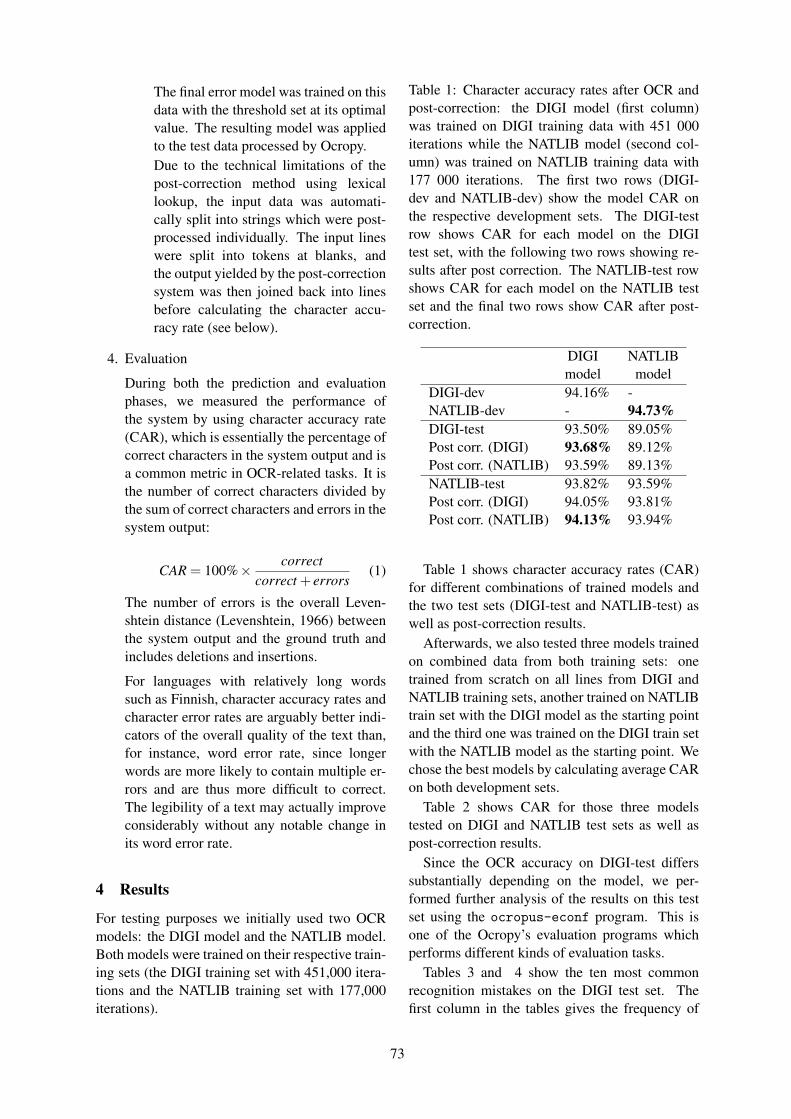
The final error model was trained on thisdata with the threshold set at its optimalvalue. The resulting model was appliedto the test data processed by Ocropy.Due to the technical limitations of thepost-correction method using lexicallookup, the input data was automati-cally split into strings which were post-processed individually. The input lineswere split into tokens at blanks, andthe output yielded by the post-correctionsystem was then joined back into linesbefore calculating the character accu-racy rate (see below).

4. Evaluation

During both the prediction and evaluationphases, we measured the performance ofthe system by using character accuracy rate(CAR), which is essentially the percentage ofcorrect characters in the system output and isa common metric in OCR-related tasks. It isthe number of correct characters divided bythe sum of correct characters and errors in thesystem output:

CAR = 100%× correctcorrect + errors

(1)

The number of errors is the overall Leven-shtein distance (Levenshtein, 1966) betweenthe system output and the ground truth andincludes deletions and insertions.

For languages with relatively long wordssuch as Finnish, character accuracy rates andcharacter error rates are arguably better indi-cators of the overall quality of the text than,for instance, word error rate, since longerwords are more likely to contain multiple er-rors and are thus more difficult to correct.The legibility of a text may actually improveconsiderably without any notable change inits word error rate.

4 Results

For testing purposes we initially used two OCRmodels: the DIGI model and the NATLIB model.Both models were trained on their respective train-ing sets (the DIGI training set with 451,000 itera-tions and the NATLIB training set with 177,000iterations).

Table 1: Character accuracy rates after OCR andpost-correction: the DIGI model (first column)was trained on DIGI training data with 451 000iterations while the NATLIB model (second col-umn) was trained on NATLIB training data with177 000 iterations. The first two rows (DIGI-dev and NATLIB-dev) show the model CAR onthe respective development sets. The DIGI-testrow shows CAR for each model on the DIGItest set, with the following two rows showing re-sults after post correction. The NATLIB-test rowshows CAR for each model on the NATLIB testset and the final two rows show CAR after post-correction.

DIGImodel

NATLIBmodel

DIGI-dev 94.16% -NATLIB-dev - 94.73%DIGI-test 93.50% 89.05%Post corr. (DIGI) 93.68% 89.12%Post corr. (NATLIB) 93.59% 89.13%NATLIB-test 93.82% 93.59%Post corr. (DIGI) 94.05% 93.81%Post corr. (NATLIB) 94.13% 93.94%

Table 1 shows character accuracy rates (CAR)for different combinations of trained models andthe two test sets (DIGI-test and NATLIB-test) aswell as post-correction results.

Afterwards, we also tested three models trainedon combined data from both training sets: onetrained from scratch on all lines from DIGI andNATLIB training sets, another trained on NATLIBtrain set with the DIGI model as the starting pointand the third one was trained on the DIGI train setwith the NATLIB model as the starting point. Wechose the best models by calculating average CARon both development sets.

Table 2 shows CAR for those three modelstested on DIGI and NATLIB test sets as well aspost-correction results.

Since the OCR accuracy on DIGI-test differssubstantially depending on the model, we per-formed further analysis of the results on this testset using the ocropus-econf program. This isone of the Ocropy’s evaluation programs whichperforms different kinds of evaluation tasks.

Tables 3 and 4 show the ten most commonrecognition mistakes on the DIGI test set. Thefirst column in the tables gives the frequency of

73

Table 2: Character accuracy rates after OCR andpost-correction of models with combined trainingdata: (1) the model was trained from the beginningon both training data combined, (2) model wastrained on NATLIB data with the DIGI model asstarting point, (3) model was trained on DIGI datawith the NATLIB model as starting point. The firstrow show the average character accuracy rate thatthe models scored on the two development sets.The following two rows show CAR on the DIGItest set before and after post correction. The lasttwo rows show CAR on the NATLIB test set be-fore and after post correction.

(1) (2) (3)Dev (avg) 94.47% 93.62% 93.62%DIGI-test 93% 91.88% 92.32%Post corr. 93.27% 92% 92.57%

NATLIB-test 94.83% 94.25% 93.68%Post corr. 95.21% 94.56% 94.01%

the mistakes, the second column the recognitionresult and the third one the ground truth. Deletionsare marked with ” ” in the OCR column whileinsertions with ” ” in the ground truth column.The most common mistake the DIGI model makeson the DIGI test set is insertion of spaces, whichhappened 122 times. Similarly, the most frequentmistake the NATLIB model made on the same testwas deleting a hyphen symbol ”-”, which hap-pened 663 times. One example when the hyphenwas not recognized and simply left out is shown inFigure 1c. To better understand the severity of themistakes, it is good to know that the DIGI test sethas in total 78,116 characters.

Table 5 shows the frequency of Ocropy recog-nition mistakes per line for each model. The testset in both cases was DIGI-test. The DIGI-modeldoes 100% correct OCR on 758 lines (37%) andthe NATLIB-model on 351 lines (17%).

The best post-correction results were, due to thesparsity of the data, achieved by error models thatwere trained with high thresholds. This was es-pecially the case with the NATLIB dataset, withthreshold values between 60 and 70 yielding thebest results for the development and test data sets.The resulting models could easily correct the mostobvious cases without corrupting strings that werecorrect to begin with.

Table 3: A confusion matrix for the DIGI testset after recognition with the DIGI model (beforepost-correction)

Freq. OCR Ground truth12299 i8778 u n60 i43 -41 t41 . ,36 l i31 e o

Table 4: A confusion matrix for the DIGI test setafter recognition with the NATLIB model (beforepost-correction)

Freq. OCR Ground truth663 -324109 i76 a74 s e67 a n65 v63 r v62 t61 y

Table 5: Number of mistakes per line after recog-nition on DIGI test set (before post correction)with both models. The first column shows thenumber of mistakes per line, the second columnthe frequency of lines after recognition with theDIGI-model and the third column the frequencyof lines after recognition with the NATLIB-model

Mistakesper line

DIGI-modeln.◦ lines

NATLIB-modeln.◦ lines

0 758 (37%) 351 (17%)1 427 (21%) 509 (25%)2 273 (13%) 292 (14%)3 160 (8%) 180 (9%)4 119 (6%) 162 (8%)

. . . . . . . . .

74

GT: musta, nelisolkinen naisen nahkawyo

DIGI: ew.O:NATLIB: e.”:.:s’

(a)

GT: Ruusua ja kaikellaista sarkya parantaa hie-DIGI: ,:NATLIB: ::,:

(b)

GT: GIN LEIPURI- & KONDIITORIDIGI: .tt 1h110 Ml. t 00khronNATLIB: u 1.kL10Ml. K0tte4

(c)

Figure 2: Example lines with a large number ofmistakes for both models

5 Discussion

A surprising result was that the NATLIB modelperformed poorly on the DIGI test set. Since theNATLIB model was trained on approximately fivetimes more data than the DIGI model, we expectedto get better results with this model. The main rea-son for the lower recognition rate was a large num-ber of unrecognized hyphens, as shown in Table 4.Although both training sets were picked up fromthe same corpora, the reason for this phenomenacould be that the NATLIB model represents 225pages of consecutive text, while the DIGI modelhas a better distribution over the entire corpus.

After combining the two training data sets, wegot significantly better results for the NATLIB testset, however the best results for the DIGI test setwere still gained by the model trained on the DIGIdata solely.

Since the models are trained on lines, a ma-jor problem for OCR is incorrect line segmenta-tion. For example, Figure 2 shows three examplelines on which both models performed extremelypoorly. The first two images Figure 2a and Fig-ure 2b have been incorrectly segmented - thereis too much information from the following linecaused by a large starting letter. Our future workis to put more focus on segmentation and prepara-tion of representative data. We should use a neuralnetwork model that is trained on both artificial as

well as real data to see if a bigger data set couldincorporate correct artificial data for currently ob-served problems.

The other big problem are images with rarefonts (rare in the sense that they are not well rep-resented in the training data). In the third image(Figure 2c), part of the text has been cut off by theincorrect segmentation, but since visible charac-ters were not recognized, we believe that the mainreason for the poor OCR result is the font. Thiskind of font is not very common in Finnish histor-ical documents that the models have been trainedon, so it is not recognized. This problem could besolved by adding more fonts to the training data.

The unstructured post-correction method gavea small improvement, which was interesting andby no means self-evident: it could have turned outthat the remaining errors were so spurious that nofurther regularities could be extracted. This sug-gests that there is room for improving the neuralnetwork to incorporate the benefits provided bythe post-correction method.

The biggest problem for our current post-correction is that it cannot influence spaces andword boundaries and they seem to be a majorsource of errors. A task for future work is there-fore testing a structured post-correction methodusing more advanced line-oriented post correction.

6 Conclusions

Our experiments show that already with a rela-tively small but well-chosen training set (around10,000 lines), we can get a character accuracy rateof more than 93% with Ocropy and with addi-tional unstructured post-correction, the accuracygoes beyond 94%. With combination of the twotraining sets and with additional unstructured post-correction, the accuracy reaches 95.21%.

References

Thomas M Breuel, Adnan Ul-Hasan, Mayce Ali Al-Azawi, and Faisal Shafait. 2013. High-performanceOCR for printed English and Fraktur using LSTMnetworks. In 2013 12th International Conferenceon Document Analysis and Recognition, pages 683–687. IEEE.

Thomas M Breuel. 2008. The OCRopus open sourceOCR system. In Electronic Imaging 2008, pages68150F–68150F. International Society for Opticsand Photonics.

75

Thomas Breuel. 2009. Recent progress on the OCRo-pus OCR system. In Proceedings of the Inter-national Workshop on Multilingual OCR, page 2.ACM.

Steffen Eger, Tim vor der Brck, and Alexander Mehler.2016. A comparison of four character-level string-to-string translation models for (OCR) spelling er-ror correction. The Prague Bulletin of MathematicalLinguistics, 105:77–99.

Vladimir I. Levenshtein. 1966. Binary codes capableof correcting deletions, insertions and reversals. So-viet Physics Doklady, 10:707.

R. Llobet, J. R. Cerdan-Navarro, J. C. Perez-Cortes,and J. Arlandis. 2010. OCR post-processing us-ing weighted finite-state transducers. In 2010 20thInternational Conference on Pattern Recognition,pages 2021–2024, Aug.

Faisal Shafait. 2009. Document image analysis withOCRopus. In Multitopic Conference, 2009. INMIC2009. IEEE 13th International, pages 1–6. IEEE.

Miikka Silfverberg and Jack Rueter. 2015. Can mor-phological analyzers improve the quality of opticalcharacter recognition? In Septentrio Conference Se-ries, number 2, pages 45–56.

Miikka Silfverberg, Pekka Kauppinen, and KristerLinden. 2016. Data-driven spelling correction usingweighted finite-state methods. In Proceedings of theSIGFSM Workshop on Statistical NLP and WeightedAutomata, pages 51–59, Berlin, Germany, August.Association for Computational Linguistics.

Uwe Springmann, Dietmar Najock, Hermann Morgen-roth, Helmut Schmid, Annette Gotscharek, and Flo-rian Fink. 2014. OCR of historical printings of latintexts: problems, prospects, progress. In Proceed-ings of the First International Conference on DigitalAccess to Textual Cultural Heritage, pages 71–75.ACM.

76


Twitter Topic Modeling by Tweet Aggregation

Asbjørn Ottesen Steinskog Jonas Foyn Therkelsen Björn GambäckDepartment of Computer Science

Norwegian University of Science and TechnologyNO–7491 Trondheim, Norway

[email protected] [email protected] [email protected]

Abstract

Conventional topic modelingschemes, such as Latent Dirich-let Allocation, are known to performinadequately when applied to tweets,due to the sparsity of short documents.To alleviate these disadvantages, weapply several pooling techniques,aggregating similar tweets into indi-vidual documents, and specificallystudy the aggregation of tweets shar-ing authors or hashtags. The resultsshow that aggregating similar tweetsinto individual documents signifi-cantly increases topic coherence.

1 Introduction

Due to the tremendous amount of data broad-casted on microblog sites like Twitter, extract-ing information from microblogs has turnedout to be useful for establishing the publicopinion on different issues. O’Connor et al.(2010) found a correlation between word fre-quencies in Twitter and public opinion sur-veys in politics. Analyzing tweets (Twittermessages) over a timespan can give great in-sights into what happened during that time,as people tend to tweet about what concernsthem and their surroundings. Many influentialpeople post messages on Twitter, and inves-tigating the relation between the underlyingtopics of different authors’ messages could

yield interesting results about people’s inter-ests. One could for example compare the top-ics different politicians tend to talk about toobtain a greater understanding of their simi-larities and differences. Twitter has an abun-dance of messages, and the enormous amountof tweets posted every second makes Twittersuitable for such tasks. However, detectingtopics in tweets can be a challenging task dueto their informal type of language and sincetweets usually are more incoherent than tra-ditional documents. The community has alsospawned user-generated metatags, like hash-tags and mentions, that have analytical valuefor opinion mining.

The paper describes a system aimed at dis-covering trending topics and events in a cor-pus of tweets, as well as exploring the top-ics of different Twitter users and how theyrelate to each other. Utilizing Twitter meta-data mitigates the disadvantages tweets typi-cally have when using standard topic model-ing methods; user information as well as hash-tag co-occurrences can give a lot of insightinto what topics are currently trending.

The rest of the text is outlined as follows:Section 2 describes the topic modeling taskand some previous work in the field, whileSection 3 outlines our topic modeling strate-gies, and Section 4 details a set of experi-ments using these. Section 5 then discussesand sums up the results, before pointing tosome directions for future research.

77

2 Topic modeling

Topic models are statistical methods used torepresent latent topics in document collec-tions. These probabilistic models usuallypresent topics as multinomial distributionsover words, assuming that each document ina collection can be described as a mixture oftopics. The language used in tweets is of-ten informal, containing grammatically cre-ative text, slang, emoticons and abbreviations,making it more difficult to extract topics fromtweets than from more formal text.

The 2015 International Workshop on Se-mantic Evaluation (SemEval) presented a taskon Topic-Based Message Polarity Classifica-tion, similar to the topic of this paper. Themost successful systems used text preprocess-ing and standard methods: Boag et al. (2015)took a supervised learning approach using lin-ear SVM (Support Vector Machines), heav-ily focused on feature engineering, to reachthe best performance of all. Plotnikova et al.(2015) came in second utilizing another super-vised method, Maximum Entropy, with lexi-con and emoticon scores and trigrams, whileessentially ignoring topics, which is interest-ing given the task. Zhang et al. (2015) differedfrom the other techniques by focusing on wordembedding features, as well as the traditionaltextual features, but argued that to only extendthe model with the word embeddings did notnecessarily significantly improve results.

Although the informal language and sparsetext make it difficult to retrieve the underly-ing topics in tweets, Weng et al. (2010) pre-viously found that Latent Dirichlet Alloca-tion (LDA) produced decent results on tweets.LDA (Blei et al., 2003) is an unsupervisedprobabilistic model which generates mixturesof latent topics from a collection of docu-ments, where each mixture of topics produceswords from the collection’s vocabulary withcertain probabilities. A distribution over top-

ics is first sampled from a Dirichlet distribu-tion, and a topic is chosen based on this distri-bution. Each document is modeled as a distri-bution over topics, with topics represented asdistributions over words (Blei, 2012).

Koltsova and Koltcov (2013) used LDAmainly on topics regarding Russian presiden-tial elections, but also on recreational andother topics, with a dataset of all posts by2,000 LiveJournal bloggers. Despite the broadcategories, LDA showed its robustness bycorrectly identifying 30–40% of the topics.Sotiropoulos et al. (2014) obtained similarresults on targeted sentiment towards topicsrelated to two US telecommunication firms,while Waila et al. (2013) identified socio-political events and entities during the ArabSpring, to find global sentiment towards these.

The Author-topic model (Rosen-Zvi et al.,2004) is an LDA extension taking informationabout an author into account: for each wordin a document d, an author from the docu-ment’s set of authors is chosen at random. Atopic t is then chosen from a distribution overtopics specific to the author, and the word isgenerated from that topic. The model givesinformation about the diversity of the topicscovered by an author, and makes it possible tocalculate the distance between the topics cov-ered by different authors, to see how similarthey are in their themes and topics.

Topic modeling algorithms have gained in-creased attention in modeling tweets. How-ever, tweets pose some difficulties becauseof their sparseness, as the short documentsmight not contain sufficient data to establishsatisfactory term co-occurrences. Therefore,pooling techniques (which involve aggregat-ing related tweets into individual documents)might improve the results produced by stan-dard topic model methods. Pooling tech-niques include, among others, aggregation oftweets that share hashtags and aggregation of

78

tweets that share author. Hong and Davison(2010) compare the LDA topic model withan Author-topic model for tweets, finding thatthe topics learned from these methods differfrom each other. By aggregating tweets writ-ten by an author into one individual document,they mitigate the disadvantages caused by thesparse nature of tweets. Moreover, Quan etal. (2015) present a solution for topic model-ing for sparse documents, finding that auto-matic text aggregation during topic modelingis able to produce more interpretable topicsfrom short texts than standard topic models.

3 Extracting topic models

Topic models can be extracted in severalways, in addition to the LDA-based meth-ods and SemEval methods outlined above.Specifically, here three sources of informationare singled out for this purpose: topic modelscores, topic clustering, and hashtags.

3.1 Topic model scoring

The unsupervised nature of topic discoverymakes the assessment of topic models chal-lenging. Quantitative metrics do not necessar-ily provide accurate reflections of a human’sperception of a topic model, and hence a vari-ety of evaluation metrics have been proposed.

The UMass coherence metric (Mimno etal., 2011) measures topic coherence: C =

∑Mm=2 ∑m−1

l=1 log D(wm,wl)+1D(wl)

with (w1, ...,wM)being the M most probable words in the topic,D(w) the number of documents that containword w, and D(wm,wl) the number of doc-uments that contain both words wm and wl .The metric utilizes word co-occurrence statis-tics gathered from the corpus, which ideallyalready should be accounted for in the topicmodel. Mimno et al. (2011) achieved reason-able results when comparing the scores ob-tained by this measure with human scoring ona corpus of 300,000 health journal abstracts.

However, statistical methods cannot modela human’s perception of the coherence in atopic model perfectly, so human judgementis commonly used to evaluate topic models.Chang et al. (2009) propose two tasks wherehumans can evaluate topic models: Word in-trusion lets humans measure the coherence ofthe topics in a model by evaluating the la-tent space in the topics. The human subjectis presented with six words, and the task isto find the intruder, which is the one wordthat does not belong with the others. The ideais that the subject should easily identify thatword when the set of words minus the intrudermakes sense together. In topic intrusion, sub-jects are shown a document’s title along withthe first few words of the document and fourtopics. Three of those are the highest proba-bility topics assigned to the document, whilethe intruder topic is chosen randomly.

In addition to these methods, we introducea way to evaluate author-topic models, specif-ically with the Twitter domain in mind. Atopic mixture for each author is obtained fromthe model. The human subjects should knowthe authors in advance, and have a fair under-standing of which topics the authors are gen-erally interested in. The subjects are then pre-sented a list of authors, along with topic distri-butions for each author (represented by the 10most probable topics, with each topic given byits 10 most probable words). The task of thesubject is to deduce which topic distributionbelongs to which author. The idea is that co-herent topics would make it easy to recognizeauthors from a topic mixture, as author inter-ests would be reflected by topic probabilities.

3.2 Clustering tweets

An important task related to topic modelingis determining the number of clusters, k, touse for the model. There is usually not asingle correct optimal value: too few clus-

79

ters will produce topics that are overly broadand too many clusters will result in overlap-ping or too similar topics. The Elbow methodcan be used to estimate the optimal numberof clusters, by running k-means clustering onthe dataset for different values of k, and thencalculating the sum of squared error (SSE =

∑ni=1[yi− f (xi)]

2) for each value.For text datasets, Can and Ozkarahan

(1990) propose that the number of clusters canbe expressed by the formula mn

t , where m isthe number of documents, n the number ofterms, and t the number of non-zero entriesin the document by term matrix. Greene et al.(2014) introduce a term-centric stability anal-ysis strategy, assuming that a topic model withan optimal number of clusters is more robustto deviations in the dataset. However, theyvalidated the method on news articles, that aremuch longer and usually more coherent thantweets. Greene et al. (2014) released a Pythonimplementation1 of the stability analysis ap-proach, which we used to predict the optimalnumber of clusters for a Twitter dataset.

To estimate the number of topics in atweet corpus, stability analysis was applied to10,000 tweets posted on January 27, 2016, us-ing a [2,10] k range for the number of top-ics. An initial topic model was generated fromthe whole dataset. Proceedingly, τ randomsubsets of the dataset were generated, withone topic model per k value for each subsetS1, ...,Sτ . The stability score for a k valueis generated by computing the mean agree-ment score between a reference set S0 and asample ranking set Si for k: ∑τ

i=1 agree(S0,Si)(Greene et al., 2014). The number of termsto consider, t, also affects the agreement. At value of 20 indicates that the top 10 termsfor each topic were used. The stability scoreswere overall low, e.g., t = 20 ranging from0.43 at k = 2 to 0.31 at k = 10. The low scores

1https://github.com/derekgreene/topic-stability

are likely caused by the sparse and noisy datain tweets, as this method was originally usedfor longer, more coherent documents. Themethod’s estimation of number of topics istherefore not a good indication of the numberof underlying topics in Twitter corpora.

Good results have been achieved by using ahigher number of topics for tweets than whatis needed for larger, more coherent corpora,since short messages and the diverse themes intweets require more topics. Hong and Davison(2010) use a range of topics for tweets from 20to 150, obtaining the best results for t = 50, al-though the chance of duplicate or overlappingtopics increase with the amount of topics.

3.3 Hashtags

Tweets have user-generated metatags that canaid the topic and sentiment analysis. A hash-tag is a term or an abbreviation preceded bythe hash mark (#). Being labels that users tagtheir messages with, they serve as indicatorsof which underlying topics are contained in atweet. Moreover, hashtags can help discoveremerging events and breaking news, by look-ing at new or uncommon hashtags that sud-denly rise in attention. We here present the us-age of hashtag co-occurrences to divulge thehidden thematic structure in a corpus, using acollection of 3 million tweets retrieved duringthe Super Bowl game, February 7th, 2016.

Hashtag co-occurrences show how hash-tags appear together in tweets. Since dif-ferent hashtags appearing in the same tweetusually share the underlying topics, a hashtagco-occurence graph might give interesting in-formation regarding the topics central to thetweet. Looking at which hashtags co-occurwith the hashtag #SuperBowl gives us moreinformation about other important themes andtopics related to Super Bowl. Table 1 showsthe 10 most popular hashtags from the Su-per Bowl corpus, about half of them being re-

80

Hashtag Freq.

SB50 10,234KCA 3,624SuperBowl 2,985FollowMeCameronDallas 1,899Broncos 1,290EsuranceSweepstakes 1,079followmecaniff 995FollowMeCarterReynolds 938KeepPounding 794SuperBowl50 783

Table 1: Hashtags during Super Bowl 2016

lated to the Super Bowl. Interestingly, (Den-ver) Broncos, the winning team of the match,was the 5th most mentioned hashtag, while thelosing team (Carolina) Panthers only was the17th most popular hashtag that day.

Some hashtags are related to a topic with-out it being apparent, since it requires furtherknowledge to understand how they are related:“Keep Pounding” is a quote by the late Car-olina Panthers player and coach Sam Mills.

Hashtag co-occurrences help reveal suchrelated hashtags, and hashtag-graph basedtopic models have been found to enhance thesemantic relations displayed by standard topicmodel techniques (Wang et al., 2014). Fig-ure 1 displays the 20 most co-occurring hash-tags in a co-occurrence network for the Su-per Bowl corpus. Three clusters of hash-tags emerge, with Super Bowl related hash-tags forming the largest. Related topics andterms become more apparent when displayedin a co-occurrence graph like this, with Keep-Pounding and SB50 being the 8th most co-occurring hashtag pair, and the artists Be-yonce and Coldplay appearing in the Su-per Bowl cluster since they performed duringthe halftime show. The graph also indicatesEsuranceSweepstakes to be related to SuperBowl, and indeed the company Esurance runan ad during the match, encouraging people totweet using the hashtag EsuranceSpeestakes.

Another cluster consists of the three hash-

Figure 1: Hashtag co-occurrence network

tags votelauramarano, KCA and VoteAriana-Grande. KCA is an abbreviation of Kid’sChoice Awards, an annual award show wherepeople can vote for their favorite television,movie and music acts, by tweeting the hash-tag KCA with a specific nominee-specific vot-ing hashtag (e.g., VoteArianaGrande).

4 Topic Modeling Experiments

Extending the studies of the previous section,a set of experiments related to topic modelingwere conducted, comparing a standard LDAtopic model to a hashtag-aggregated model,and comparing two author-topic models.

4.1 Hashtag-aggregated topic modelA pooling technique that involves aggregatingtweets sharing hashtags was applied, the as-sumption being that tweets that share hashtagsalso share underlying topics. The main goal ofthis method is the same as for the Author-topicmodel and other pooling techniques; alleviat-ing the disadvantages of short documents byaggregating documents that are likely to sharelatent topics. Some restrictions were intro-duced: only single-hashtag tweets were used,and only hashtags that appeared in at least 20of the documents in the corpus.

Table 2 shows a sample of the resulting top-ics. They appear more coherent than the top-ics generated on tweets as individual docu-ments, even though many of the less proba-ble words in each topic might seem somewhatrandom. It is, however, easier to get an un-

81

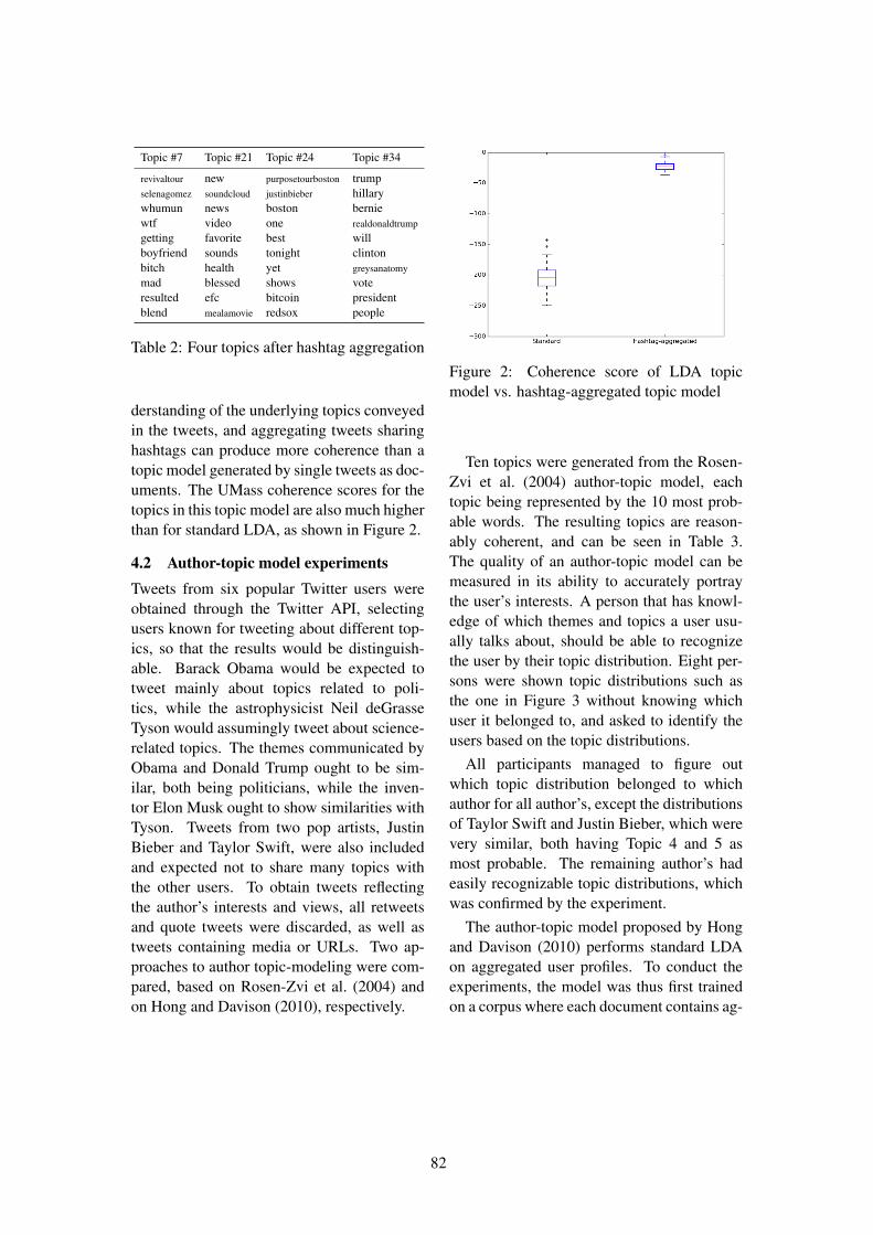
Topic #7 Topic #21 Topic #24 Topic #34

revivaltour new purposetourboston trumpselenagomez soundcloud justinbieber hillarywhumun news boston berniewtf video one realdonaldtrump

getting favorite best willboyfriend sounds tonight clintonbitch health yet greysanatomy

mad blessed shows voteresulted efc bitcoin presidentblend mealamovie redsox people

Table 2: Four topics after hashtag aggregation

derstanding of the underlying topics conveyedin the tweets, and aggregating tweets sharinghashtags can produce more coherence than atopic model generated by single tweets as doc-uments. The UMass coherence scores for thetopics in this topic model are also much higherthan for standard LDA, as shown in Figure 2.

4.2 Author-topic model experimentsTweets from six popular Twitter users wereobtained through the Twitter API, selectingusers known for tweeting about different top-ics, so that the results would be distinguish-able. Barack Obama would be expected totweet mainly about topics related to poli-tics, while the astrophysicist Neil deGrasseTyson would assumingly tweet about science-related topics. The themes communicated byObama and Donald Trump ought to be sim-ilar, both being politicians, while the inven-tor Elon Musk ought to show similarities withTyson. Tweets from two pop artists, JustinBieber and Taylor Swift, were also includedand expected not to share many topics withthe other users. To obtain tweets reflectingthe author’s interests and views, all retweetsand quote tweets were discarded, as well astweets containing media or URLs. Two ap-proaches to author topic-modeling were com-pared, based on Rosen-Zvi et al. (2004) andon Hong and Davison (2010), respectively.

Figure 2: Coherence score of LDA topicmodel vs. hashtag-aggregated topic model

Ten topics were generated from the Rosen-Zvi et al. (2004) author-topic model, eachtopic being represented by the 10 most prob-able words. The resulting topics are reason-ably coherent, and can be seen in Table 3.The quality of an author-topic model can bemeasured in its ability to accurately portraythe user’s interests. A person that has knowl-edge of which themes and topics a user usu-ally talks about, should be able to recognizethe user by their topic distribution. Eight per-sons were shown topic distributions such asthe one in Figure 3 without knowing whichuser it belonged to, and asked to identify theusers based on the topic distributions.

All participants managed to figure outwhich topic distribution belonged to whichauthor for all author’s, except the distributionsof Taylor Swift and Justin Bieber, which werevery similar, both having Topic 4 and 5 asmost probable. The remaining author’s hadeasily recognizable topic distributions, whichwas confirmed by the experiment.

The author-topic model proposed by Hongand Davison (2010) performs standard LDAon aggregated user profiles. To conduct theexperiments, the model was thus first trainedon a corpus where each document contains ag-

82

#1 #2 #3 #4 #5 #6 #7 #8 #9 #10

will just earth night tonight just people great president donnew like moon today love one much thank obama fyinow will day get thank know time trump2016 america timeget now sun new thanks orbit won will sotu tesla

america good world happy ts1989 two tonight cruz actonclimate firstmake think ask back taylurking might way hillary economy rocketpoll also universe time show long bad makeamericagreatagain work science

many around full see got planet show big change spacetrump live space one crowd star morning cnn americans launchdon landing year good tomorrow instead really said jobs model

Table 3: The ten topics generated for the Rosen-Zvi et al. (2004) author-topic model

Figure 3: Topic distribution for Obama

gregated tweets for each user. Furthermore,new tweets for each author (which were notpart of the training data) were downloaded,and the topic distribution inferred for each ofthe new tweets. Finally, the topic distributionfor each user was calculated as the averagetopic distribution over all new tweets writtenby that user. Since a low number of topicsproduces too many topics containing the samepopular words, 50 topics were used instead ofthe 10 in the previous experiments.

An example of the resulting topic mixturesfor the authors can be seen in Figure 4, withthe most probable topics for each of the au-thors tabulated in Table 4. As opposed to theprevious topic mixtures, these topic mixturesgenerally had one topic that was much moreprobable than the remaining topics. There-fore, the diversity in the language by eachauthor might not be captured as well by thismodel. On the other hand, the most probable

Figure 4: Obama’s aggregated topics

topic for each author generally describes theauthor with a high precision. It is thereforeeasier to distinguish Justin Bieber from TaylorSwift than it was in the previous experiment.

5 Discussion and conclusion

A topic modeling system for modeling tweetcorpora was created, utilizing pooling tech-niques to improve the coherence and inter-pretability of standard topic models. The re-sults indicate that techniques such as authoraggregating and hashtag aggregation generatemore coherent topics.

Various methods for estimating the optimalnumber of topics for tweets were tested. TheElbow method almost exclusively suggesteda k value between 3 and 5, no matter howlarge or diverse the corpus was. The stabil-ity score (Greene et al., 2014) also producedrather poor estimates for a number of topicswhen applied to a tweet corpus. The spar-

83

#0 (Obama) #20 (Musk) #26 (Tyson) #35 (Trump) #43 (Bieber) #19 (Swift)

president tesla earth will thanks tonightobama will moon great love ts1989america rocket just thank whatdoyoumean taylurking

sotu just day trump2016 mean justactonclimate model one just purpose love

time launch time cruz thank thankwork good sun hillary lol crowd

economy dragon people new good nightamericans falcon space people great now

change now will makeamericagreatagain see show

Table 4: The most probable topic for the six authors inferred from aggregated topic distribution

sity of tweets is likely the cause of this; thedocuments do not contain enough words toproduce sufficient term co-occurrences. Hongand Davison (2010) found that 50 topics pro-duced the optimal results for their author-topicmodel, although the optimal number of top-ics dependents on the diversity of the cor-pora. Thus k values of 10 and 50 were usedin the experiments, with 50 for large corporawhere a diverse collection of documents wasexpected.

Hashtag co-occurrences were used to di-vulge latent networks of topics and events ina collection of tweets. A hashtag aggregat-ing technique was shown to mitigate the neg-ative impacts sparse texts have on the coher-ence of a topic model. Hashtag aggregationtechnique is especially interesting, as it uti-lizes a specific metadata tag that is not presentin standard documents. A hashtag aggregatedtopic model produced a much better coher-ence than the standard LDA variation for thesame corpus; this is also consistent with recentresearch on topic models for microblogs. TwoAuthor-topic models were used in our exper-iments, one using the Rosen-Zvi et al. (2004)topic model and the aggregated author-topicmodel proposed by Hong and Davison (2010),both seeming to produce interpretable topics.It is worth noting that there is no standard-ized methods for evaluating topic models, as

most quantitative ways try to estimate humanjudgement. Moreover, there is no precise def-inition of a gold standard for topic models,which makes the task of comparing and rank-ing topic models difficult. A combination of acomputational method and human judgementwas therefore used in the evaluations.

One way to extend the topic modeling sys-tem would be to apply online analysis byimplementing automatic updates of a topicmodel, continuously extended by new tweetsretrieved from the Twitter Streaming API.This would help in detect emerging events, ina fashion similar to Lau et al. (2012). More-over, Dynamic Topic Models could be consid-ered to provide better temporal modeling ofTwitter data. A limitation to topic modeling ingeneral is the difficulties in evaluating the ac-curacy of the models. Computational methodstry to simulate human judgement, which posesdifficulties, as human judgement is not clearlydefined. Further research could help providebetter methods for evaluating topic models. Inthis paper, we aggregated tweets sharing au-thors and hashtags. Further work should lookinto other pooling schemes, and see how theycompare to author and hashtag aggregation.One example would be to aggregate conver-sations on Twitter into individual documents.Tweets contain a lot of metadata that can aidthe aggregation process.

84

ReferencesDavid M Blei, Andrew Y Ng, and Michael I Jor-

dan. 2003. Latent Dirichlet Allocation. Inthe Journal of Machine Learning Research, vol-ume 3, pages 993–1022, MIT, Massachusetts,USA. JMLR. org.

David M. Blei. 2012. Probabilistic Topic Models.In Communications of Association for Com-puter Machinery, volume 55, New York, NY,USA, April. ACM.

William Boag, Peter Potash, and Anna Rumshisky.2015. TwitterHawk: A Feature Bucket BasedApproach to Sentiment Analysis. In Proceed-ings of the 9th International Workshop on Se-mantic Evaluation (SemEval 2015), pages 640–646, Denver, Colorado, June. Association forComputational Linguistics.

Fazli Can and Esen A. Ozkarahan. 1990.Concepts and Effectiveness of the Cover-coefficient-based Clustering Methodology forText Databases. In ACM Transitional DatabaseSystems, volume 15, pages 483–517, New York,NY, USA, December. Association for ComputerMachinery.

Jonathan Chang, Sean Gerrish, Chong Wang, Jor-dan L Boyd-Graber, and David M Blei. 2009.Reading tea leaves: How humans interpret topicmodels. In Advances in neural informationprocessing systems, pages 288–296, Vancouver,British Columbia.

Derek Greene, Derek O’Callaghan, edi-tor="Calders Toon Cunningham, Pádraig",Floriana Esposito, Eyke Hüllermeier, and RosaMeo, 2014. How Many Topics? StabilityAnalysis for Topic Models, pages 498–513.Springer Berlin Heidelberg, Berlin, Heidelberg.

Liangjie Hong and Brian D. Davison. 2010. Em-pirical Study of Topic Modeling in Twitter.In Proceedings of the First Workshop on So-cial Media Analytics, SOMA ’10, pages 80–88,New York, NY, USA. ACM.

Olessia Koltsova and Sergei Koltcov. 2013. Map-ping the public agenda with topic modeling:The case of the Russian LiveJournal. In Policy& Internet, volume 5, pages 207–227, Russia.

Jey Han Lau, Nigel Collier, and Timothy Bald-win. 2012. On-line Trend Analysis with Topic

Models:\# Twitter Trends Detection TopicModel Online. In Proceedings of COLING2012: Technical Papers, pages 1519–1534,pages 1519–1534, Mumbai, India.

David Mimno, Hanna M. Wallach, Edmund Tal-ley, Miriam Leenders, and Andrew McCallum.2011. Optimizing semantic coherence in topicmodels. In Proceedings of the Conference onEmpirical Methods in Natural Language Pro-cessing, EMNLP ’11, pages 262–272, Strouds-burg, PA, USA. Association for ComputationalLinguistics.

Brendan O’Connor, Ramnath Balasubramanyan,Bryan R Routledge, and Noah A Smith. 2010.From Tweets to Polls: Linking Text Sentimentto Public Opinion Time Series. In Interna-tional Conference on Web and Social Media,volume 11, pages 1–2, Washington DC, USA.

Nataliia Plotnikova, Micha Kohl, Kevin Volkert,Andreas Lerner, Natalie Dykes, Heiko Emer,and Stefan Evert. 2015. KLUEless: Po-larity Classification and Association. In Pro-ceedings of the 9th International Workshop onSemantic Evaluation (SemEval 2015), Erlan-gen, Germany. Friedrich-Alexander-UniversitatErlangen-Nurnberg.

Xiaojun Quan, Chunyu Kit, Yong Ge, andSinno Jialin Pan. 2015. Short and sparsetext topic modeling via self-aggregation. InProceedings of the 24th International Confer-ence on Artificial Intelligence, IJCAI’15, pages2270–2276. AAAI Press.

Michal Rosen-Zvi, Thomas Griffiths, MarkSteyvers, and Padhraic Smyth. 2004. TheAuthor-topic Model for Authors and Docu-ments. In Proceedings of the 20th Confer-ence on Uncertainty in Artificial Intelligence,UAI ’04, pages 487–494, Arlington, Virginia,United States. AUAI Press.

Dionisios N Sotiropoulos, Chris D Kounavis,Panos Kourouthanassis, and George M Giaglis.2014. What drives social sentiment? An en-tropic measure-based clustering approach to-wards identifying factors that influence socialsentiment polarity. In Information, Intelligence,Systems and Applications, IISA 2014, The 5thInternational Conference, pages 361–373, Cha-nia Crete, Greece. IEEE.

85

Pranav Waila, VK Singh, and Manish K Singh.2013. Blog text analysis using topic modeling,named entity recognition and sentiment classi-fier combine. In Advances in Computing, Com-munications and Informatics (ICACCI), 2013International Conference on, pages 1166–1171,Mysore, India. IEEE.

Y. Wang, J. Liu, J. Qu, Y. Huang, J. Chen, andX. Feng. 2014. Hashtag Graph Based TopicModel for Tweet Mining. In 2014 IEEE In-ternational Conference on Data Mining, pages1025–1030, Shenzhen, China, Dec.

Jianshu Weng, Ee-Peng Lim, Jing Jiang, and

Qi He. 2010. TwitterRank: Finding Topic-sensitive Influential Twitterers. In Proceed-ings of the Third ACM International Conferenceon Web Search and Data Mining, WSDM ’10,pages 261–270, New York, NY, USA. ACM.

Zhihua Zhang, Guoshun Wu, and Man Lan. 2015.East China Normal University, ECNU: Multi-level Sentiment Analysis on Twitter Using Tra-ditional Linguistic Features and Word Embed-ding Features. In Proceedings of the 9th In-ternational Workshop on Semantic Evaluation(SemEval 2015), Shanghai, China. East ChinaNormal University Shanghai.

86


A Multilingual Entity Linker Using PageRank and Semantic Graphs

Anton SodergrenDepartment of computer science

Lund University, [email protected]

Pierre NuguesDepartment of computer science


Abstract

This paper describes HERD, a multilin-gual named entity recognizer and linker.HERD is based on the links in Wikipediato resolve mappings between the entitiesand their different names, and Wikidataas a language-agnostic reference of entityidentifiers.

HERD extracts the mentions from text us-ing a string matching engine and linksthem to entities with a combination ofrules, PageRank, and feature vectors basedon the Wikipedia categories. We evalu-ated HERD with the evaluation protocolof ERD’14 (Carmel et al., 2014) and wereached the competitive F1-score of 0.746on the development set. HERD is de-signed to be multilingual and has versionsin English, French, and Swedish.

1 Introduction

Named entity recognition (NER) refers to the pro-cess of finding mentions of persons, locations,and organizations in text, while entity linking (ordisambiguation) associates these mentions withunique identifiers. Figure 1 shows an example ofentity linking with the mention Michael Jackson,an ambiguous name that may refer to thousands ofpeople and where 21 are famous enough to havea Wikipedia page (Wikipedia, 2016). In Fig. 1,the search engine selected the most popular entity(top) and used the cue word footballer (bottom) tolink the phrase Michael Jackson footballer to theEnglish defender born in 1973.

Entity recognition and linking has become acrucial component to many language process-ing applications: Search engines (Singhal, 2012),question answering (Ferrucci, 2012), or dialogueagents. This importance is reflected by a growingnumber of available systems; see TAC-KBP2015

(Ji et al., 2015), for instance, with 10 participatingteams.

Although many applications include entity link-ers, the diversity of the input texts, which can in-clude tweets, search queries, news wires, or en-cyclopedic articles, makes their evaluation prob-lematic. While some evaluations consider entitylinking in isolation and mark the mentions in theinput, end-to-end pipelines, where the input con-sists of raw text, need to combine entity recogni-tion and linking. The ERD’14 challenge (Carmelet al., 2014) is an example of the latter.

2 Previous Work

Entity linking has spurred a considerable amountof work over the last 10 years. Bunescu andPasca (2006), Mihalcea and Csomai (2007), andCucerzan (2007) used Wikipedia as a knowledgesource and its articles to define the entities, its hy-perlinks to find the mentions, and semantic knowl-edge from redirect pages and categories, to carryout disambiguation. Milne and Witten (2008) usedthe likelihood of an entity given a mention M,P(E|M), and a relatedness metric between twoentities computed from the links to their corre-sponding pages to improve both recall and pre-cision. Ferragina and Scaiella (2010) addressedshorter pieces of text with the idea to use a collec-tive agreement between all the entities.

The Entity Recognition and DisambiguationChallenge (ERD’14) (Carmel et al., 2014) is a re-cent evaluation, where competitors were given aset of entities to recognize and link in a corpus ofunlabelled text. This setting is closer to real worldapplication than TAC (Ji et al., 2015), where par-ticipants have to link already bracketed mentions.The evaluation included two tracks: one with longdocuments of an average size of 600 words and ashort track consisting of search query.

Finally, the CoNLL-2003 shared task (TjongKim Sang and De Meulder, 2003) is an influen-

87

Figure 1: Search results for the queries Michael Jackson and Michael Jackson footballer. The enginereturns the most popular entity (top) and uses the minimal context given in the query, footballer, topropose a less popular entity (bottom)

tial evaluation of language independent named en-tity recognition, with a focus on German and En-glish. Hoffart et al. (2011) linked the names inthe English corpus to Wikipedia pages making thisdataset a useful corpus for entity linking.

In this paper, we used the ERD’14 developmentset as well as the CoNLL-2003 dataset with Wiki-data links.

3 Building the Entity Knowledge Base

3.1 Mention-Entity Pairs

Following Mihalcea and Csomai (2007) andBunescu and Pasca (2006), we collected themention-entity pairs from the Wikipedia links(wikilinks). We built the entity base from the fromthree versions of Wikipedia: English, French, andSwedish, and the frequency of the wikilinks ineach version. Figure 2 shows an example of a pairwith the mention Swedish Parliament. This givessuggestions of how an entity is commonly referredto: i.e. its name or aliases.

Figure 2: The structure of wikilinks in Wikipedia.

3.2 Entity Nomenclature

As nomenclature for the entities, we used Wiki-data, the linked database of Wikimedia. Wikidataconnects the different language versions of eacharticle in Wikipedia with a unique identifier calledthe Q-number. In addition to being a cross-lingualrepository, Wikidata also links a large number ofentities to structured information such as the datesof birth and death for persons.

In order to use a language-agnostic identifier,we translated the wikilinks into Q-numbers. Weextracted the pairs of Q-numbers and article namesfrom a Wikidata dump for each language. Sincethe dump does not contain any URL, the algo-

88

rithm must recreate the address from the titles. Wecould reach a coverage of about 90%. The re-maining 10% corresponds to redirect pages thatact as alternative names or to cover common mis-spellings. We used the Wikipedia dump to identifythese redirects and we improved the coverage rateto 99.1%.

3.3 Annotating the MentionsWe annotated the mention-entity pairs in ourknowledge base with a set of features that we usedin the subsequent processing:

1. The Frequency of the mention-entity pairs.Table 1 shows an example for the city of Hon-olulu.

2. We used dictionaries of common nouns, verb,and adjectives for each language. If a men-tion only consists of words in the dictionary,we mark it as only-dictionary. An exam-ple of this is the artist Prince in English andFrench.

3. We computed a list of the most frequentwords (stop words) from Wikipedia for eachlanguage. They include the, in, and, and a, inEnglish. If all the words in a mention are stopwords, we mark it as only-stop-words.

4. The system marks the mentions with a highnumber of links as highly-ambiguous,such as John or details with almost 5,000 dif-ferent entities linked to each.

5. Mentions without uppercase letters aremarked as lower-case.

6. Family names and surnames. If the mostcommon mention of a person has more thantwo words, we mark each mention of oneword as generic, such as the mention Bushreferring to the former president George W.Bush.

7. We also annotate the entities with their fre-quency (total-frequency). It correspondsto the sum of all their mentions frequencies.

3.4 Pruning the Knowledge BaseAlthough Wikipedia is reviewed by scores of vol-unteers, there are plenty of misleading mentions inthe collected knowledge base. We removed a partof them using the following rules:

1. The mention is marked as lower-case

and either only-dictionary oronly-stop-words

2. The frequency of the entity-mention is ex-actly 1, while the total-frequency of thatentity is above a threshold parameter that wasempirically obtained.

3. The mention consists of two or more words,and starts with a lower-case stop word, thatis not a definite article. This will filter outanchors of the type a city in Sweden.

We also clustered the mentions with a normal-ized Levenshtein distance (Levenshtein, 1966). Ifthe distance was less than 0.2 to any element, theywere considered to be in the same group. We ap-plied the clustering to all the surface forms and wediscarded the mentions without a group.

4 System Components and Pipeline

The system consists of three main components: aspotter that identifies the mentions, a set of rulesthat prunes the results, and an improver that usescontextual clues for entity recognition (Fig. 3).

The spotter outputs a match for every conceiv-able mention of an entity, leaving us with a doc-ument where almost every word is tagged as anentity. This output has a very high recall, but avery low precision.

The filtering that comes after that tries to re-move the most unlikely of the alternatives from thespotter and raises the precision to a modest levelwhile trying to have a minimal impact on the re-call. If the input data to the next step is completelyunfiltered the Contextual Improver is unable to af-fect the results in a positive way.

The Contextual Improver is the final step anduses contextual clues, such as which categories theentities belong to and which entities are commonlyseen together, to improve the result.

4.1 Mention Spotting

We use the mention-entity knowledge base to spotthe mentions in raw text and associate them withall their possible entities. Following Lipczak etal. (2014), we applied the Solr Text Tagger (Smi-ley, 2013) based on finite-state transducers and theLucene indexer. Solr Text Tagger was chosen asit is a highly effective way of marking up possiblematches of a database in a text. It is based on the

89

Mention Entity Frequency Mention Entity FrequencyHonolulu Q18094 5117 Hawaii Q18094 11Honolulu, Hawaii Q18094 2281 Honolulu, HI MSA Q18094 7Honolulu, HI Q18094 600 HONOLULU Q18094 7Honolulu, Hawaii, USA Q18094 67 city of Honolulu Q18094 7Honolulu, Hawai’i Q18094 47 honolulu Q18094 5Honolulu, Hawai’i Q18094 21 Honululu Q18094 5Honolulu CPD Q18094 21

Table 1: An example of the mention-entity counts for the entity Q18094, most commonly called Hon-olulu

Figure 3: The system architecture, where the knowledge base contains the mention-entity pairs

Lucene open-source software and its implementa-tion of finite-state transducers.

As a preprocessing step, Solr Text Tagger com-piles all the mentions in the knowledge base,where the input labels are the letters and symbolsof mentions and the output labels are the entityidentifiers. Then, given an untagged text, the tag-ger marks all the occurrences, possibly overlap-ping, of all the names in the database. See Fig. 4.

4.2 Filtering and Expansion

The output of the Spotter is usually very noisyas most words can match some mention in theknowledge base. Examples include It, a novelby Stephen King, or Is This It, an album by TheStrokes. The result is a high mention recall, but alow precision. We applied filters to remove somematches and improve the precision while preserv-ing the recall.

The system uses a set of manually-written rulesand empirically obtained hyper parameters to im-prove precision with a minimal effect on recall.We describe them in the sections below. The com-plete list of parameter values is provided in the

HERD source code available from GitHub1.

4.2.1 Mention ProbabilityWe computed the probability for a term or aphrase to be a link over the whole Wikipedia(Eckhardt et al., 2014) using the formula:Mention probability = link(mention)

f req(mention) . This gives ahint at whether a word sequence is more com-monly used as a mention of entities or just aswords.

Medical Center, for example, is linked 1.0% ofthe times used, while Medical Center of CentralGeorgia has a mention probability of 73.7%.

Any candidate that had less than 0.5% mentionprobability was immediately pruned.

4.2.2 Filters to Improve PrecisionFilters are rules based on syntactical clues and theflags defined in Sect. 3.3. Each matching rule re-turns a suspicion score and we compute the sumof the scores. The most significant rules are:

1. Capitalization: Add suspicion to any mentionthat does not contain a capital letter. Thisloses some recall, but increases the precision

1https://github.com/AAAton/herd

90

dramatically. We improved it with a func-tion that takes into consideration the numberof capital letters, whether the mention is thestart of a new sentence and whether the men-tion has the only-dictionary tag. Head-lines also use capitalized words. We recog-nize fully capitalized sentences with regularexpressions. Mentions in headlines with theonly-dictionary, or only-stop-words

tags, generate suspicion.

2. Generic names: We apply a two-pass analy-sis for generic mentions. We remove themfrom the first pass. In a second pass, thegeneric names are restored if a mention of thesame entity that is not generic shows in thetext i.e. the Bush mention is kept only whenthere is a full mention of George W. Bush inthe text. This is to avoid the tagging of themention Bush with every entity having thisname as a generic name.

3. Colliding names: If two tags are immediateneighbors, with the exception of a space, theygenerate suspicion. The system considers allthe candidate entities for a surface form, andonly triggers suspicion if at least one of theentities is a generic name. This is a methodto detect and avoid tagging a multiword namewhich does not exist in our knowledge basewith multiple other candidates.

4.2.3 Extender to Improve RecallWe extended the detected mentions following thework of Eckhardt et al. (2014). Once we recog-nize a mention consisting of two words or morethat passed the filter, we create new mentions withacronyms and generic version of the item by split-ting it into multiple parts.

Given the text a division of First Citizens Banc-Shares Inc. of Raleigh, N.C., where the systemrecognizes the mention First Citizens BancSharesInc, the extender creates possible acronyms, suchas FCBI and F.C.B.I. It also looks for parentheses,immediately following a mention, giving a sug-gestion of how it is meant to be abbreviated.

The extender also splits the mention into partsof 1, 2, and 3 words. The mention above generatesFirst, Citizens, BankShares and Inc., as well asFirst Citizens, Citizens BankShares, BankSharesInc, and so forth. We associate the generated men-tions with the set of entities of the original men-

tion. The tagged extensions are filtered in the samemanner as all the other tags.

4.3 Contextual Improver

For each document, the Improver uses PageR-ank to determine which candidates commonly oc-cur together, and prunes the unseen combinations.This produces a result with a very high precision.We use this high precision output as the modelledcontext of the document. A weighted categorygraph is calculated for this modelled context. Thenamed entity recognition is then widened by con-sidering the similarity of all the candidates to themodelled context.

Once the improver has been applied, we carryout a final clean-up step, where we eliminate allthe overlap and rank the remaining candidates foreach mention.

4.3.1 PageRankWe apply a modified version of PageRank (Brinand Page, 1998) to the tagged mentions. Follow-ing Eckhardt et al. (2014), we create a node for ev-ery mention-entity pair that is detected in the text,and run three iterations of PageRank. We analyzethe internal links of Wikipedia to determine whichentities appear in the same context. Two entitiesare considered linked if the article of Entity A linksto the article of Entity B or a link to both the articleof Entity A and the article of Entity B occurs in thesame paragraph.

The links calculated on Wikipedia are trans-ferred to the tagged document and produce a graphof linked entities. Unlike the work of Eckhardt etal. (2014), we initialize each node with the stan-dard value 1/N, and the ratio between the initialvalue and the final value is used to modify the sus-picion for a candidate.

After applying PageRank, some entities will behigher ranked than others which we take as an in-put to another round of filtering. The candidateswith high suspicion are removed. This producesa high precision output, with a slight drop of therecall.

4.3.2 Weighted Category GraphWe use a weighted category graph (WCG) derivedfrom the user-annotated categories of Wikipediaarticles (Lipczak et al., 2014). For each article, wecreated this graph from all the languages in whichthe article is available. If an article has the samecategory in all the languages, this category is as-

91

Figure 4: The Solr Text Tagger processing scheme, where the operations are carried out through POSTrequests.

signed the maximum weight of 1.0. The weight isthen decreased as a linear function of the numberof languages. The categories need to be weightedto avoid rare or incorrect categories assigned to ar-ticles.

Wikipedia categories are themselves catego-rized into parent categories. The category of Swe-den has a parent category of Countries in Europefor example. A tree of categories is derived fromeach article by getting the top k categories of an ar-ticle, and expanding those categories with the topk parents for each category. This process is re-peated d times. This generalizes the categories ofthe article, which makes them easier to compare toadjacent articles.

The value k is set to 5, and the value d is set to3, as proposed by Lipczak et al. (2014).

Table 2 shows an example of the categories weobtain from the article about Sweden.

The weighted category graph is used in the fol-lowing way:

1. We input a set of core entities with high pre-cision. The improver calculates a weightedcategory vector for each entity and creates atopic centroid as the linear combinationof these vectors. This is meant to function asthe general topic of the analyzed document.

2. We improve the precision of the core entitiesby comparing each of the high-precision en-tities to the topic centroid with a cosine sim-ilarity. If the score of an entity is under athreshold value of 0.6, it is removed. Finally,the topic centroid is recalculated.

3. We then compare each entity in the unfilteredoutput of Solr Text Tagger to the topic cen-troid with a cosine similarity. We keep theentities that are above a threshold value of0.2.

Category RatioSweden 1.00Countries in Europe 0.38Member states of the European Union 0.30Constitutional monarchies 0.20Scandinavia 0.20

Table 2: Top 5 categories for Sweden, Q34

This procedure widens the scope of the en-tity selection and improves the recall in a contextaware manner. Since the output of the weightedcategory graphs is similar to the input constraintsof PageRank, and the output of PageRank is simi-lar to the input requirements of the weighted cate-gory graph, we have set them into an iteration cy-cle in order to achieve higher results.

4.3.3 Clean-upAs a final step, we eliminate overlapping men-tions: When two mentions overlap, we keep thelongest. If the mentions are of equal length, wekeep the rightmost.

The remaining candidates for each mention arethen ranked by their wikilink frequency, and themost frequent candidate is selected as the correctdisambiguation.

5 Experimental Setup and Results

We evaluated the system with two different datasets for English: ERD-51 and AIDA/YAGO andwe used the evaluation metrics of ERD’14 Carmelet al. (2014). We did not have access to evaluationsets for the other languages.

ERD-51 is the development set of Carmel etal. (2014). It consists of 51 documents that havebeen scraped from a variety of sources with 1,169human-annotated mentions. Each annotation has astart, an end, and a Freebase identifier (Bollackeret al., 2008). In the competition, a set of enti-ties, slightly over 2 million, was given, and thus

92

the problem of defining what a named entity ac-tually is was avoided. We filtered our knowledgebase to only contain mentions of entities from thegiven set.

AIDA/YAGO is derived from the CoNLL-2003shared task (Tjong Kim Sang and De Meulder,2003). It is a collection of 1393 news articles with34,587 human-annotated names. 27,632 of thosenames have been disambiguated with a link to thecorresponding Wikipedia site using a dump from2010-08-17 (Hoffart et al., 2011).

Tables 4 and 3 show the results evolving overdifferent versions of the system. The executiontime is normalized to the time spent to process5,000 characters. It should not be considered anabsolute value, but can be used to compare the dif-ferent algorithms.

Lipczak et al. (2014) and Eckhardt et al. (2014),respectively second and third of ERD’14, reportedresults of 0.735 and 0.72 on the test set. Our re-sults are not exactly comparable as we used thedevelopment set. Nonetheless we believe our sys-tem competitive. The highest scoring participant(Cucerzan, 2014) with a score of 0.76 was one ofthe organizers and was not part of the competition.The reason for the difference in recognition scorebetween the ERD-51 and the AIDA/YAGO datasetlies in the text genres. AIDA/YAGO is collectedfrom well written news wires, mainly written byprofessionals with proper punctuation and capi-talization, while ERD-51 is a collection of morepoorly written texts collected from a wider vari-ety of sources, spanning from blogs to eBay salessites.

For the score of the linked systems, the resultsare the opposite. ERD-51 has been annotated andlinked by humans from a predefined set of 2 mil-lion entities, while the linking in AIDA/YAGO hasbeen done from an older dump of Wikipedia. Thedump contains around 3 million different sites, un-like the dump we used that has around 5 millionentities. Both the mismatch in the entities that arepossible to use and the larger size of the knowl-edge base lead to a larger gap between recognitionand linking.

With a latency of around 200 ms per 5,000 char-acters, the system should be able to tag the en-tire of the English Wikipedia under a day with aheavy duty computer. We estimate that the averagelength of a Wikipedia article is around 2,000 char-acters, that there are 5 million articles, 24 available

cores and 100% run time.We implemented the entity linker as an interac-

tive demonstration. The user can paste a text andvisualize the results in the form of a text annotatedwith entity labels. Once the user hovers over thelabel, the ranked candidates are displayed with alink to the Wikidata page for that entity. Figure 5shows an output of the system.

6 Conclusions and Future Work

We explored different methods to carry outlanguage-independent entity linking from raw textand we presented evaluations on English. The ver-sion of the system that had the highest score useda 4-step pipeline, ending with an iteration cyclebetween a personalized version of PageRank andthe usage of weighted category graphs. The sys-tem reached a weighted F1-score of 0.746 on theERD-51 dataset.

The paper takes an unusual approach to namedentity recognition and disambiguation as it doesnot separate the tasks, but treats every candidateto every mention as a separate possibility. Theiteration between two context-aware algorithmswith different precision/recall characteristics im-proved the results dramatically and is, to the bestof our knowledge, a novel, language-independentapproach to entity recognition and disambigua-tion. We also exposed a way of pruning unsatis-fying links in a collected knowledge base by clus-tering.

The system and its approach can be improved ina number of ways. Firstly, the usage of manuallywritten rules is suboptimal, as the rules may be de-pendent on the language. A method that only usesWikipedia, or some other multilingual resource,and avoids syntactical clues altogether, would bea better solution. An approach like that would bemore robust to the differences between languages.

We have also introduced a number of thresholdvalues in different parts of the system, such as thesuspicion cutoff in the manual rules and the simi-larity threshold in the WCG. These are difficult tooptimize without an automated method. We thinkHERD would benefit from finding an alternativeapproach that avoids cutoff values or automatestheir optimization.

The approach would also benefit from a deeperevaluation on a wider variety of datasets, spanningover several languages, as well as the two Englishdatasets used in this article.

93

Exec. Recognition LinkingVersion (ms) Precision Recall F Precision Recall Fv0.1 Baseline - 0.745 0.686 0.714 0.551 0.521 0.535v0.2 With extender - 0.673 0.762 0.715 0.520 0.581 0.549v0.3 Remove colliding men-tions

- 0.698 0.730 0.714 0.536 0.572 0.554

v0.4 Simplified filtering - 0.723 0.720 0.721 0.613 0.610 0.611v0.5 Relaxed filtering - 0.642 0.859 0.734 0.522 0.720 0.605v0.6 Part of headline - 0.691 0.796 0.740 0.593 0.684 0.635v0.7 Filter out candidateswith low frequency

250 0.718 0.785 0.750 0.612 0.672 0.640

v0.8 PageRank 246 0.865 0.765 0.812 0.747 0.661 0.701v1.0 PageRank & WCG 608 0.843 0.848 0.845 0.744 0.749 0.746

Table 3: Results on the ERD51 dataset

Exec. Recognition LinkingVersion (ms) Precision Recall F Precision Recall Fv0.1 Baseline - 0.940 0.630 0.755v0.2 With extender - 0.889 0.684 0.773v0.3 Remove colliding nodes - 0.923 0.678 0.782v0.4 Simplified filtering - 0.934 0.705 0.803v0.5 Relaxed filtering - 0.912 0.769 0.835v0.7 Filtered out candidateswith low frequency

1088 0.888 0.789 0.835

v0.8 PageRank 3325 0.935 0.819 0.873 0.732 0.631 0.678v1.0 PageRank & WCG 4415 0.932 0.827 0.876 0.740 0.647 0.690

Table 4: Results on the AIDA/YAGO dataset

Figure 5: Visualizer

The HERD source code is available fromGitHub at this repository: https://github.

com/AAAton/herd. A demonstration of HERD aspart of the Langforia processing pipelines (Klangand Nugues, 2016) is available at this location:http://vilde.cs.lth.se:9000.

Acknowledgements


94

References

Kurt Bollacker, Colin Evans, Praveen Paritosh, TimSturge, and Jamie Taylor. 2008. Freebase: Acollaboratively created graph database for structur-ing human knowledge. In Proceedings of the 2008ACM SIGMOD International Conference on Man-agement of Data, SIGMOD ’08, pages 1247–1250,New York, NY, USA. ACM.

Sergey Brin and Lawrence Page. 1998. Theanatomy of a large-scale hypertextual web searchengine. Computer Networks and ISDN Systems,30(1-7):107–117, April.

Razvan C Bunescu and Marius Pasca. 2006. Using en-cyclopedic knowledge for named entity disambigua-tion. In European Chapter of the Association forComputational Linguistics, volume 6, pages 9–16.

David Carmel, Ming-Wei Chang, Evgeniy Gabrilovich,Bo-June Paul Hsu, and Kuansan Wang. 2014.ERD’14: Entity recognition and disambiguationchallenge. In ACM SIGIR Forum, volume 48, pages63–77. ACM.

Silviu Cucerzan. 2007. Large-scale named entity dis-ambiguation based on wikipedia data. In EmpiricalMethods in Natural Language Processing and Com-putational Natural Language Learning, volume 7,pages 708–716.

Silviu Cucerzan. 2014. Name Entities Made Obvi-ous: The Participation in the ERD 2014 Evaluation.In Proceedings of the First International Workshopon Entity Recognition & Disambiguation, ERD ’14,pages 95–100, New York, NY, USA. ACM.

Alan Eckhardt, Juraj Hresko, Jan Prochazka, andOtakar Smri;. 2014. Entity linking based on theco-occurrence graph and entity probability. In Pro-ceedings of the First International Workshop on En-tity Recognition & Disambiguation, ERD ’14, pages37–44, New York, NY, USA. ACM.

Paolo Ferragina and Ugo Scaiella. 2010. Tagme:On-the-fly annotation of short text fragments (bywikipedia entities). In Proceedings of the 19thACM International Conference on Information andKnowledge Management, CIKM ’10, pages 1625–1628, New York, NY, USA. ACM.

David Angelo Ferrucci. 2012. Introduction to “Thisis Watson”. IBM Journal of Research and Develop-ment, 56(3.4):1:1 –1:15, May-June.

Johannes Hoffart, Mohamed Amir Yosef, Ilaria Bor-dino, Hagen Furstenau, Manfred Pinkal, Marc Span-iol, Bilyana Taneva, Stefan Thater, and GerhardWeikum. 2011. Robust disambiguation of namedentities in text. In Proceedings of the 2011 Con-ference on Empirical Methods in Natural LanguageProcessing, pages 782–792, Edinburgh.

Heng Ji, Joel Nothman, Ben Hachey, and Radu Florian.2015. Overview of tac-kbp2015 trilingual entity dis-covery and linking. In Proceedings of the EighthText Analysis Conference (TAC2015).

Marcus Klang and Pierre Nugues. 2016. Langforia:Language pipelines for annotating large collectionsof documents. In Proceedings of COLING 2016,the 26th International Conference on ComputationalLinguistics: System Demonstrations, pages 74–78,Osaka, Japan, December. The COLING 2016 Orga-nizing Committee.

V. I. Levenshtein. 1966. Binary Codes Capable of Cor-recting Deletions, Insertions and Reversals. SovietPhysics Doklady, 10:707, February.

Marek Lipczak, Arash Koushkestani, and EvangelosMilios. 2014. Tulip: Lightweight entity recog-nition and disambiguation using wikipedia-basedtopic centroids. In Proceedings of the First Inter-national Workshop on Entity Recognition & Disam-biguation, ERD ’14, pages 31–36, New York, NY,USA. ACM.

Rada Mihalcea and Andras Csomai. 2007. Wikify!:Linking documents to encyclopedic knowledge. InProceedings of the Sixteenth ACM Conference onConference on Information and Knowledge Man-agement, CIKM ’07, pages 233–242, New York,NY, USA. ACM.

David Milne and Ian H. Witten. 2008. Learning to linkwith wikipedia. In Proceedings of the 17th ACMConference on Information and Knowledge Man-agement, CIKM ’08, pages 509–518, New York,NY, USA. ACM.

Amit Singhal. 2012. Introducing the knowledgegraph: things, not strings. Official Google Blog.http://googleblog.blogspot.com/2012/05/introducing-knowledge-graph-things-not.html. Retrieved 7 November 2013, May.

David Smiley. 2013. Solr text tagger, text taggingwith finite state transducers. https://github.com/OpenSextant/SolrTextTagger.

Erik F. Tjong Kim Sang and Fien De Meulder.2003. Introduction to the conll-2003 shared task:Language-independent named entity recognition. InProceedings of the Seventh Conference on NaturalLanguage Learning at HLT-NAACL 2003 - Volume4, CONLL ’03, pages 142–147, Stroudsburg, PA,USA. Association for Computational Linguistics.

Wikipedia. 2016. Michael Jackson (disam-biguation) – Wikipedia, the free encyclopedia.https://en.wikipedia.org/wiki/Michael_Jackson_(disambiguation).

95


Linear Ensembles of Word Embedding Models

Avo MuromagiUniversity of Tartu

Tartu, [email protected]

Kairit SirtsUniversity of Tartu


Sven LaurUniversity of Tartu


Abstract

This paper explores linear methods forcombining several word embedding mod-els into an ensemble. We constructthe combined models using an iterativemethod based on either ordinary leastsquares regression or the solution to the or-thogonal Procrustes problem.

We evaluate the proposed approacheson Estonian—a morphologically complexlanguage, for which the available corporafor training word embeddings are rela-tively small. We compare both com-bined models with each other and withthe input word embedding models usingsynonym and analogy tests. The resultsshow that while using the ordinary leastsquares regression performs poorly in ourexperiments, using orthogonal Procrustesto combine several word embedding mod-els into an ensemble model leads to 7-10%relative improvements over the mean re-sult of the initial models in synonym testsand 19-47% in analogy tests.

1 Introduction

Word embeddings—dense low-dimensional vec-tor representations of words—have become verypopular in recent years in the field of natu-ral language processing (NLP). Various meth-ods have been proposed to train word embed-dings from unannoted text corpora (Mikolov etal., 2013b; Pennington et al., 2014; Al-Rfou etal., 2013; Turian et al., 2010; Levy and Gold-berg, 2014), most well-known of them being per-haps Word2Vec (Mikolov et al., 2013b). Embed-ding learning systems essentially train a modelfrom a corpus of text and the word embeddingsare the model parameters. These systems con-tain a randomized component and so the trained

models are not directly comparable, even whenthey have been trained on exactly the same data.This random behaviour provides an opportunityto combine several embedding models into an en-semble which, hopefully, results in a better setof word embeddings. Although model ensembleshave been often used in various NLP systems toimprove the overall accuracy, the idea of combin-ing several word embedding models into an en-semble has not been explored before.

The main contribution of this paper is to showthat word embeddings can benefit from ensemblelearning, too. We study two methods for com-bining word embedding models into an ensem-ble. Both methods use a simple linear transforma-tion. First of them is based on the standard ordi-nary least squares solution (OLS) for linear regres-sion, the second uses the solution to the orthogonalProcrustes problem (OPP) (Schonemann, 1966),which essentially also solves the OLS but adds theorthogonality constraint that keeps the angles be-tween vectors and their distances unchanged.

There are several reasons why using an ensem-ble of word embedding models could be useful.First is the typical ensemble learning argument—the ensemble simply is better because it enables tocancel out random noise of individual models andreinforce the useful patterns expressed by severalinput models. Secondly, word embedding systemsrequire a lot of training data to learn reliable wordrepresentations. While there is a lot of textualdata available for English, there are many smallerlanguages for which even obtaining enough plainunannotated text for training reliable embeddingsis a problem. Thus, an ensemble approach thatwould enable to use the available data more effec-tively would be beneficial.

According to our knowledge, this is the firstwork that attempts to leverage the data by com-bining several word embedding models into a newimproved model. Linear methods for combin-

96

ing two embedding models for some task-specificpurpose have been used previously. Mikolov etal. (2013a) optimized the linear regression withstochastic gradient descent to learn linear transfor-mations between the embeddings in two languagesfor machine translation. Mogadala and Rettinger(2016) used OPP to translate embeddings betweentwo languages to perform cross-lingual documentclassification. Hamilton et al. (2016) aligned aseries of embedding models with OPP to detectchanges in word meanings over time. The sameproblem was addressed by Kulkarni et al. (2015)who aligned the embedding models using piece-wise linear regression based on a set of nearestneighboring words for each word.

Recently, Yin and Schutze (2016) experimentedwith several methods to learn meta-embeddings bycombining different word embedding sets. Ourwork differs from theirs in two important aspects.First, in their work each initial model is trainedwith a different word embedding system and on adifferent data set, while we propose to combine themodels trained with the same system and on thesame dataset, albeit using different random initial-isation. Secondly, although the 1toN model pro-posed in (Yin and Schutze, 2016) is very similar tothe linear models studied in this paper, it doesn’tinvolve the orthogonality constraint included inthe OPP method, which in our experiments, asshown later, proves to be crucial.

We conduct experiments on Estonian and con-struct ensembles from ten different embeddingmodels trained with Word2Vec. We compare theinitial and combined models in synonym and anal-ogy tests and find that the ensemble embeddingscombined with orthogonal Procrustes method in-deed perform significantly better in both tests,leading to a relative improvement of 7-10% overthe mean result of the initial models in synonymtests and 19-47% in analogy tests.

2 Combining word embedding models

A word embedding model is a matrix W ∈R|V |×d ,where |V | is the number of words in the model lex-icon and d is the dimensionality of the vectors.Each row in the matrix W is the continuous rep-resentation of a word in a vector space.

Given r embedding models W1, . . . ,Wr we wantto combine them into a target model Y . We de-fine a linear objective function that is the sum of r

linear regression optimization goals:

J =r

∑i=1‖Y −WiPi‖2 , (1)

where P1, . . . ,Pr are transformation matrices thattranslate W1, . . . ,Wr, respectively, into the com-mon vector space containing Y .

We use an iterative algorithm to find matricesP1, . . . ,Pr and Y . During each iteration the algo-rithm performs two steps:

1. Solve r linear regression problems with re-spect to the current target model Y , which re-sults in updated values for matrices P1, . . .Pr;

2. Update Y to be the mean of the translationsof all r models:

Y =1r

r

∑i=1

WiPi. (2)

This procedure is continued until the change inthe average normalised residual error, computed as

1r

r

∑i=0

‖Y −WiPi‖√|V | ·d

, (3)

will become smaller than a predefined thresholdvalue.

We experiment with two different methods forcomputing the translation matrices P1, . . . ,Pr. Thefirst is based on the standard least squares solu-tion to the linear regression problem, the secondmethod is known as solution to the OrthogonalProcrustes problem (Schonemann, 1966).

2.1 Solution with the ordinary least squares(SOLS)

The analytical solution for a linear regressionproblem Y = PW for finding the transformationmatrix P, given the input data matrix W and theresult Y is:

P = (W TW )−1W TY (4)

We can use this formula to update all matrices Pi

at each iteration. The problem with this approachis that because Y is also unknown and will be up-dated repeatedly in the second step of the iterativealgorithm, the OLS might lead to solutions whereboth WiPi and Y are optimized towards 0 which isnot a useful solution. In order to counteract thiseffect we rescale Y at the start of each iteration.This is done by scaling the elements of Y so thatthe variance of each column of Y would be equalto 1.

97

SOLS SOPPDim Error # Iter Error # Iter50 0.162828 33 0.200994 5100 0.168316 38 0.183933 5150 0.169554 41 0.171266 4200 0.172987 40 0.167554 4250 0.175723 40 0.164493 4300 0.177082 40 0.160988 4

Table 1: Final errors and the number of iterationsuntil convergence for both SOLS and SOPP. Thefirst column shows the embedding size.

.

2.2 Solution to the Orthogonal Procrustesproblem (SOPP)

Orthogonal Procrustes is a linear regression prob-lem of transforming the input matrix W to the out-put matrix Y using an orthogonal transformationmatrix P (Schonemann, 1966). The orthogonalityconstraint is specified as

PPT = PT P = I

The solution to the Orthogonal Procrustes canbe computed analytically using singular value de-composition (SVD). First compute:

S =W TY

Then diagonalize using SVD:

ST S =V DSV T

SST =UDSUT

Finally compute:

P =UV T

This has to be done for each Pi during each itera-tion.

This approach is very similar to SOLS. Theonly difference is the additional orthogonality con-straint that gives a potential advantage to thismethod as in the translated word embeddings WiPi

the lengths of the vectors and the angles betweenthe vectors are preserved. Additionally, we nolonger need to worry about the trivial solutionwhere P1, . . . ,Pr and Y all converge towards 0.

3 Experiments

We tested both methods on a number of Word2Vecmodels (Mikolov et al., 2013b) trained on the Es-tonian Reference Corpus.1 Estonian Reference

1http://www.cl.ut.ee/korpused/segakorpus

Dim SOLS SOPP Mean W50 70098 38998 41933

100 68175 32485 35986150 73182 30249 33564200 73946 29310 32865250 75884 28469 32194300 77098 28906 32729Avg 73064 31403 34879

Table 2: Average mean ranks of the synonym test,smaller values are better. The best result in eachrow is in bold. All differences are statistically sig-nificant: with p < 2.2 ·10−16 for all cases.

Corpus is the largest text corpus available for Es-tonian. Its size is approximately 240M word to-kens, which may seem like a lot but compared tofor instance English Gigaword corpus, which isoften used to train word embeddings for Englishwords and which contains more than 4B words,it is quite small. All models were trained usinga window size 10 and the skip-gram architecture.We experimented with models of 6 different em-bedding sizes: 50, 100, 150, 200, 250 and 300.For each dimensionality we had 10 models avail-able. The number of distinct words in each modelis 816757.

During training the iterative algorithm was rununtil the convergence threshold th = 0.001 wasreached. The number of iterations needed forconvergence for both methods and for modelswith different embedding size are given in Ta-ble 1. It can be seen that the convergence withSOPP took significantly fewer iterations than withSOLS. This difference is probably due to two as-pects: 1) SOPP has the additional orthogonalityconstraint which reduces the space of feasible so-lutions; 2) although SOLS uses the exact analyti-cal solutions for the least squares problem, the fi-nal solution for Y does not move directly to the di-rection pointed to by the analytical solutions dueto the variance rescaling.

4 Results

We evaluate the goodness of the combined modelsusing synonym and analogy tests.

4.1 Synonym ranks

One of the common ways to evaluate word embed-dings is to use relatedness datasets to measure thecorrelation between the human and model judge-

98

Figure 1: Histogram of the synonym ranks of the 100 dimensional vectors. Dark left columns show therank frequencies of the SOPP model, light right columns present the rank frequencies of one of the initialmodels.

ments (Schnabel et al., 2015). In those datasets,there are word pairs and each pair is human an-notated with a relatedness score. The evaluationis then performed by correlating the cosine sim-ilarities between word pairs with the relatednessscores. As there are no annotated relatednessdatasets for Estonian, we opted to use a synonymtest instead. We rely on the assumption that the re-latedness between a pair of synonyms is high andthus we expect the cosine similarity between thesynonymous words to be high as well.

We obtained the synonyms from the Estoniansynonym dictionary.2 We queried each word inour vocabulary and when the exact match for thisword was found then we looked at the first syn-onym offered by the dictionary. If this synonymwas present in our vocabulary then the synonympair was stored. In this manner we obtained a to-tal of 7579 synonym pairs. We ordered those pairsaccording to the frequency of the first word in thepair and chose the 1000 most frequent words withtheir synonyms for the synonym test.

For each first word in the synonym pair, wecomputed its cosine similarity with every otherword in the vocabulary, ordered those similaritiesin the descending order and found the rank of thesecond word of the synonym pair in this resultinglist. Then we computed the mean rank over all1000 synonym pairs. We performed these stepson both types of combined models— YSOLS andYSOPP— and also on all input models Wi. Finallywe also computed the mean of the mean ranks ofall 10 input models.

The results as shown in Table 2 reveal that the

2The Institute of the Estonian Language, http://www.eki.ee/dict/sys/

synonym similarities tend to be ranked lower inthe combined model obtained with SOLS whencompared to the input models. SOPP, on the otherhand, produces a combined model where the syn-onym similarities are ranked higher than in ini-tial models. This means that the SOPP combinedmodels pull the synonymous words closer togetherthan they were in the initial models. The dif-ferences in mean ranks were tested using pairedWilcoxon signed-rank test at 95% confidence leveland the differences were statistically significantwith p-value being less than 2.2 ·10−16 in all cases.In overall, the SOPP ranks are on average 10%lower than the mean ranks of the initial models.The absolute improvement on average betweenSOPP and mean of W is 3476.

Although we assumed that the automatically ex-tracted synonym pairs should be ranked closely to-gether, looking at the average mean ranks in Ta-ble 2 reveals that it is not necessarily the case—the average rank of the best-performing SOPPmodel is over 31K. In order to understand those re-sults better we looked at the rank histogram of theSOPP model and one of the initial models, shownon Figure 1. Although the first bin covering therank range from 1 to 10 contains the most wordsfor both models and the number of synonym pairsfalling to further rank bins decreases the curve isnot steep and close to 100 words (87 in case ofSOPP and 94 in case of the initial model) belongto the last bin counting ranks higher than 100000.Looking at the farthest synonym pairs revealedthat one word in these pairs is typically polyse-mous and its sense in the synonym pair is a rela-tively rarely used sense of this word, while thereare other more common senses of this word with a

99

Hit@1 Hit@10Dim SOLS SOPP Mean W Min W Max W SOLS SOPP Mean W Min W Max W

50 0.058 0.193 0.144 0.124 0.170 0.158 0.390 0.329 0.305 0.347100 0.116 0.255 0.185 0.170 0.197 0.239 0.475 0.388 0.371 0.409150 0.085 0.278 0.198 0.170 0.228 0.224 0.502 0.398 0.378 0.417200 0.066 0.290 0.197 0.178 0.224 0.205 0.541 0.408 0.390 0.425250 0.093 0.282 0.200 0.181 0.224 0.193 0.517 0.406 0.394 0.421300 0.069 0.286 0.197 0.162 0.228 0.212 0.533 0.401 0.359 0.440Avg 0.081 0.264 0.187 0.205 0.493 0.388

Table 3: Hit@1 and Hit@10 accuracies of the analogy test. SOLS and SOPP columns show the accu-racies of the combined models. Mean W , Min W and Max W show the mean, minimum and maximumaccuracies of the initial models Wi, respectively. The best accuracy among the combined models and themean of the initial models is given in bold. The last row shows the average accuracies over all embeddingsizes.

completely different meaning. We give some ex-amples of such synonym pairs:

• kaks (two) - puudulik (insufficient): thesense of this pair is the insufficient grade inhigh school, while the most common senseof the word kaks is the number two;

• ida (east) - ost (loan word from German alsomeaning east): the most common sense of theword ost is purchase;

• rubla (rouble) - kull (bank note in slang): themost common sense of the word kull is hawk.

4.2 Analogy testsAnalogy tests are another common intrinsicmethod for evaluating word embeddings (Mikolovet al., 2013c). A famous and typical example ofan analogy question is “a man is to a king like awoman is to a ?”. The correct answer to thisquestion is “queen”.

For an analogy tuple a : b,x : y (a is to b as xis to y) the following is expected in an embeddingspace to hold:

wb−wa +wx ≈ wy,

where the vectors w are word embeddings. For theabove example with “man”, “king”, “woman” and“queen” this would be computed as:

wking−wman +wwoman ≈ wqueen

Given the vector representations for the threewords in the analogy question—wa, wb and wx—the goal is to maximize (Mikolov et al., 2013b)

cos(wy,wb−wa +wx) (5)

over all words y in the vocabulary.We used an Estonian analogy data set with 259

word quartets. Each quartet contains two pairs ofwords. The word pairs in the data set belong intothree different groups where the two pairs containeither:

• a positive and a comparative adjective form,e.g. pime : pimedam, joukas : joukam (inEnglish dark : darker, wealthy : wealthier);

• the nominative singular and plural forms ofa noun, e.g. vajadus : vajadused, voistlus :voistlused (in English need : needs , compe-tition : competitions);

• The lemma and the 3rd person past form of averb, e.g. aitama : aitas, katsuma : katsus (inEnglish help : helped, touch : touched).

We evaluate the results of the analogy test usingprediction accuracy. A prediction is consideredcorrect if and only if the vector wy that maximizes(5) represents the word expected by the test case.We call this accuracy Hit@1. Hit@1 can be quite anoisy measurement as there could be several wordvectors in a very close range to each other compet-ing for the highest rank. Therefore, we also com-pute Hit@10, which considers the prediction cor-rect if the word expected by the test case is amongthe ten closest words. As a common practice, thequestion words represented by the vectors wa, wband wx were excluded from the set of possible pre-dictions.

The Hit@1 and Hit@10 results in Table 3 showsimilar dynamics: combining models with SOPPis much better than SOLS in all cases. The SOPP

100

Figure 2: Mean squared distances describingthe scattering of the translated word embeddingsaround the combined model embedding for everyword in the vocabulary. The words in the horizon-tal axis are ordered by the frequency with mostfrequent words plotted first.

combined model is better than the mean of theinitial models in all six cases. Furthermore, it isconsistently above the maximum of the best initialmodels. The average accuracy of SOPP is betterthan the average of the mean accuracies of initialmodels by 41%, relatively (7.7% in absolute) interms of Hit@1 and 27% relatively (10.5% in ab-solute) in terms of Hit@10.

5 Analysis

In order to gain more understanding how thewords are located in the combined model spacein comparison to the initial models we performedtwo additional analyses. First, we computed thedistribution of mean squared errors of the words tosee how the translated embeddings scatter aroundthe word embedding of the combined model. Sec-ondly, we looked at how both of the methods affectthe pairwise similarities of words.

5.1 Distribution of mean squared distances

We computed the squared Euclidean distance foreach word in vocabulary between the combinedmodel Y and all the input embedding models. Thedistance ei j for a jth word and the ith input modelis:

di j = ‖Yj−Ti j‖2,

where Ti = WiPi is the ith translated embeddingmodel. Then we found the mean squared distance

Figure 3: Mean squared distances describingthe scattering of the translated word embeddingsaround the combined model embedding for a ran-dom sample of 1000 words. The words in the hori-zontal axis are ordered by the frequency with mostfrequent words plotted first.

for the jth word by calculating:

d j =1r

r

∑i=0

di j

These distances are plotted on Figure 2. Thewords on the horizontal axis are ordered by theirfrequency—the most frequent words coming first.We show these results for models with 100 dimen-sions but the results with other embedding sizeswere similar.

Notice that the distances for less frequent wordsare similarly small for both SOLS and SOPPmethods. However, the distribution of distancesfor frequent words is quite different—while thedistances go up with both methods, the frequentwords are much more scattered when using theSOPP approach.

Figure 3 shows the mean squared distances of arandom sample of 1000 words. These plots revealanother difference between the SOLS and SOPPmethods. While for SOPP, the distances tend todecrease monotonically with the increase in wordfrequency rank, with SOLS the distances first in-crease and only then they start to get smaller.

Our vocabulary also includes punctuationmarks and function words, which are among themost frequent tokens and which occur in manydifferent contexts. Thus, the individual modelshave a lot of freedom to position them in the wordembedding space. The SOLS combined model isable to bring those words more close to each other

101

Figure 4: Cosine similarities of 1000 randomly chosen word pairs ordered by their similarity in thecombined model Y . Red, blue and green bands represent the maximum, mean and minimum similaritiesin the initial models, respectively.

in the aligned space, while SOPP has less free-dom to do that because of the orthogonality con-straint. When looking at the words with largestdistances under SOPP in the 1000 word randomsample then we see that the word with the highestmean squared distance refers to the proper nameof a well-known Estonian politician who has beenprobably mentioned often and in various contextsin the training corpus. Other words with a largedistance in this sample include for instance a nameof a month and a few quantifying modifiers.

5.2 Word pair similarities

In this analysis we looked at how the cosine simi-larities between pairs of words change in the com-bined model compared to their similarities in theinput embedding models. For that, we chose a to-tal of 1000 word pairs randomly from the vocab-ulary. For each pair we calculated the followingvalues:

• cosine similarity under the combined model;

• maximum and minimum cosine similarity inthe initial models Wi;

• mean cosine similarity over the initial mod-els Wi.

The results are plotted in Figure 4. These resultsare obtained using the word embeddings with size100, using different embedding sizes revealed the

same patterns. In figures, the word pairs are or-dered on the horizontal axis in the ascending orderof their similarities in the combined model Y .

The plots reveal that 1) the words that are sim-ilar in initial models Wi are even more similar inthe combined model Y ; and 2) distant words in ini-tial models become even more distant in the com-bined model. Although these trends are visible incases of both SOLS and SOPP, this behaviour ofthe combined models to bring more similar wordscloser together and place less similar words fartheraway is more emphasized in the combined modelobtained with SOLS.

In Figure 4, the red, green and blue “bands”,representing the maximum, mean and minimumsimilarities of the initial models, respectively, arewider on the SOLS plot. This indicates that SOPPpreserves more the original order of word pairsin terms of their similarities. However, some ofthis difference may be explained by the fact thatSOPP has an overall smaller effect on the similar-ity compared to SOLS, which is due to the prop-erty of SOPP to preserve the angles and distancesbetween the vectors during the transformation.

6 Discussion and future work

From the two linear methods used to combine themodels, SOPP was performing consistently betterin both synonym and analogy tests. Although, asshown in Figures 2 and 3, the word embeddings ofthe aligned initial models were more closely clus-

102

tered around the embeddings of the SOLS com-bined model, this seemingly better fit is obtainedat the cost of distorting the relations between theindividual word embeddings. Thus, we have pro-vided evidence that adding the orthogonality con-straint to the linear transformation objective is im-portant to retain the quality of the translated wordembeddings. This observation is relevant both inthe context of producing model ensembles as wellas in other contexts where translating one embed-ding space to another could be relevant, such aswhen working with semantic time series or multi-lingual embeddings.

In addition to combining several models trainedon the same dataset with the same configuration asdemonstrated in this paper, there are other possibleuse cases for the model ensembles which could beexplored in future work. For instance, currentlyall our input models had the same dimensionalityand the same embedding size was also used in thecombined model. In future it would be interestingto experiment with combining models with differ-ent dimensionality, in this way marginalising outthe embedding size hyperparameter.

Our experiments showed that the SOPP ap-proach performs well in both synonym and anal-ogy tests when combining the models trained onthe relatively small Estonian corpus. In future weplan to conduct similar experiments on more lan-guages that, similar to Estonian, have limited re-sources for training reliable word embeddings.

Another idea would be to combine embeddingstrained with different models. As all word embed-ding systems learn slightly different embeddings,combining for instance Word2Vec (Mikolov etal., 2013b), Glove (Pennington et al., 2014) anddependency based vectors (Levy and Goldberg,2014) could lead to a model that combines thestrengths of all the input models. Yin and Schutze(2016) demonstrated that the combination of dif-ferent word embeddings can be useful. However,their results showed that the model combinationis less beneficial when one of the input models(Glove vectors in their example) is trained on ahuge text corpus. Thus, we predict that the ensem-ble of word embeddings constructed based on dif-ferent embedding models also has the most effectin the setting of limited training resources.

Finally, it would be interesting to explore thedomain adaptation approach by combining for in-stance the embeddings learned from the large gen-

eral domain with the embeddings trained on asmaller domain specific corpus. This could be ofinterest because there are many pretrained wordembedding sets available for English that can befreely downloaded from the internet, while thecorpora they were trained on (English Gigaword,for instance) are not freely available. The modelcombination approach would enable to adapt thoseembeddings to the domain data by making use ofthe pretrained models.

7 Conclusions

Although model ensembles have been often usedto improve the results of various natural languageprocessing tasks, the ensembles of word embed-ding models have been rarely studied so far. Ourmain contribution in this paper was to combineseveral word embedding models trained on thesame dataset via linear transformation into an en-semble and demonstrate the usefulness of this ap-proach experimentally.

We experimented with two linear methods tocombine the input embedding models—the ordi-nary least squares solution to the linear regressionproblem and the orthogonal Procrustes which addsan additional orthogonality constraint to the leastsquares objective function. Experiments on syn-onym and analogy tests on Estonian showed thatthe combination with orthogonal Procrustes wasconsistently better than the ordinary least squares,meaning that preserving the distances and anglesbetween vectors with the orthogonality constraintis crucial for model combination. Also, the or-thogonal Procrustes combined model performedbetter than the average of the individual initialmodels in all synonym tests and analogy tests sug-gesting that combining several embedding modelsis a simple and useful approach for improving thequality of the word embeddings.

Acknowledgments

We thank Alexander Tkachenko for providing thepretrained input models and the analogy test ques-tions. We also thank the anonymous reviewers fortheir helpful suggestions and comments.

ReferencesRami Al-Rfou, Bryan Perozzi, and Steven Skiena.

2013. Polyglot: Distributed word representationsfor multilingual NLP. In Proceedings of the Seven-

103

teenth Conference on Computational Natural Lan-guage Learning, pages 183–192.

William L. Hamilton, Jure Leskovec, and Dan Jurafsky.2016. Diachronic word embeddings reveal statisti-cal laws of semantic change. In Proceedings of the54th Annual Meeting of the Association for Compu-tational Linguistics (Volume 1: Long Papers), pages1489–1501.

Vivek Kulkarni, Rami Al-Rfou, Bryan Perozzi, andSteven Skiena. 2015. Statistically significant de-tection of linguistic change. In Proceedings of the24th International Conference on World Wide Web,pages 625–635.

Omer Levy and Yoav Goldberg. 2014. Dependency-based word embeddings. In Proceedings of the 52ndAnnual Meeting of the Association for Computa-tional Linguistics (Volume 2: Short Papers), pages302–308.

Tomas Mikolov, Quoc V. Le, and Ilya Sutskever.2013a. Exploiting similarities among languages formachine translation. CoRR, abs/1309.4168.

Tomas Mikolov, Ilya Sutskever, Kai Chen, Greg S Cor-rado, and Jeff Dean. 2013b. Distributed representa-tions of words and phrases and their compositional-ity. In Advances in Neural Information ProcessingSystems 26, pages 3111–3119.

Tomas Mikolov, Scott Wen-tau Yih, and GeoffreyZweig. 2013c. Linguistic regularities in continuousspace word representations. In Proceedings of the2013 Conference of the North American Chapter ofthe Association for Computational Linguistics: Hu-man Language Technologies, pages 746–751.

Aditya Mogadala and Achim Rettinger. 2016. Bilin-gual word embeddings from parallel and non-parallel corpora for cross-language text classifica-tion. In Proceedings of the 2016 Conference ofthe North American Chapter of the Association forComputational Linguistics: Human Language Tech-nologies, pages 692–702.

Jeffrey Pennington, Richard Socher, and Christo-pher D. Manning. 2014. Glove: Global vectorsfor word representation. In Proceedings of the 2014Conference on Empirical Methods in Natural Lan-guage Processing, pages 1532–1543.

Tobias Schnabel, Igor Labutov, David Mimno, andThorsten Joachims. 2015. Evaluation methods forunsupervised word embeddings. In Proceedings ofthe 2015 Conference on Empirical Methods in Nat-ural Language Processing, pages 298–307.

Peter H. Schonemann. 1966. A generalized solution ofthe orthogonal procrustes problem. Psychometrika,31(1):1–10.

Joseph Turian, Lev Ratinov, and Yoshua Bengio. 2010.Word representations: A simple and general methodfor semi-supervised learning. In Proceedings of the

48th Annual Meeting of the Association for Compu-tational Linguistics, pages 384–394.

Wenpeng Yin and Hinrich Schutze. 2016. Learn-ing Word Meta-Embeddings. In Proceedings of the54th Annual Meeting of the Association for Compu-tational Linguistics, pages 1351–1360.

104


Using Pseudowords for Algorithm Comparison:An Evaluation Framework for Graph-based Word Sense Induction

Flavio Massimiliano CecchiniDISCo

Universita degli Studi di [email protected]

Martin Riedl, Chris BiemannLanguage Technology Group

Universitat [email protected]@informatik.uni-hamburg.de

Abstract

In this paper we define two parallel datasets based on pseudowords, extracted fromthe same corpus. They both consist ofword-centered graphs for each of 1225 dif-ferent pseudowords, and use respectivelyfirst-order co-occurrences and second-order semantic similarities. We proposean evaluation framework on these datasets for graph-based Word Sense Induc-tion (WSI) focused on the case of coarse-grained homonymy: We compare differ-ent WSI clustering algorithms by measur-ing how well their outputs agree with the apriori known ground-truth decompositionof a pseudoword. We perform this eval-uation for four different clustering algo-rithms: the Markov cluster algorithm, Chi-nese Whispers, MaxMax and a gangplank-based clustering algorithm. To further im-prove the comparison between these algo-rithms and the analysis of their behaviours,we also define a new specific evaluationmeasure. As far as we know, this is the firstlarge-scale systematic pseudoword evalu-ation dedicated to the induction of coarse-grained homonymous word senses.

1 Introduction and Related Work

Word Sense Induction (WSI) is the branch of Natu-ral Language Processing (NLP) concerned with theunsupervised detection of all the possible sensesthat a term can assume in a text document. It couldalso be described as “unsupervised Word SenseDisambiguation” (Navigli, 2009). Since ambigu-ity and arbitrariness are constantly present in nat-ural languages, WSI can help improve the analysisand understanding of text or speech (Martin andJurafsky, 2000). At its core we find the notion ofdistributional semantics, exemplified by the state-

ment by Harris (1954): “Difference of meaningcorrelates with difference of distribution.”

In this paper, we focus on graph-based methods.Graphs provide an intuitive mathematical repre-sentation of relations between words. A graph canbe defined and built in a straightforward way, butallows for a very deep analysis of its structuralproperties. This and their discrete nature (contraryto the continuous generalizations represented byvector spaces of semantics, cf. Turney and Pan-tel (2010)) favour the identification of significa-tive patterns and subregions, among other thingsallowing the final number of clusters to be left un-predetermined, an ideal condition for WSI.

The main contribution of this paper is three-fold: We present two parallel word graph data setsbased on the concept of pseudowords, both for thecase of semantic similarities and co-occurrences;on them, we compare the performances of fourWSI clustering algorithms; and we define a newad hoc evaluation measure for this task, calledTOP2.

Pseudowords were first proposed by Gale etal. (1992) and Schutze (1992) as a way to cre-ate artificial ambiguous words by merging two (ormore) random words. A pseudoword simulateshomonymy, i.e. a word which possesses two (ormore) semantically and etymologically unrelatedsenses, such as count as “nobleman” as opposed to“the action of enumerating”. The study of Nakovand Hearst (2003) shows that the performancesof WSI algorithms on random pseudowords mightrepresent an optimistic upper bound with respectto true polysemous words, as generic polysemyimplies some kind of correlation between the cate-gories and the distributions of the different sensesof a word, which is absent from randomly gener-ated ones. We are aware of the approaches pro-posed in (Otrusina and Smrz, 2010) and (Pile-hvar and Navigli, 2013), used e.g. in (Baskaya

105

and Jurgens, 2016), for a pseudoword generationthat better models polysemous words with an ar-bitrary degree of polysemy. Both works implythe emulation of existing polysemous words, fol-lowing the semantic structure of WordNet (Miller,1995): pseudosenses (the components of a pseu-doword) corresponding to the synsets of a wordare represented by the closest monosemous termson the WordNet graph, according to Personal-ized PageRank (Haveliwala, 2002) applied to theWordNet graph. However, we want to remark thedifferent nature of our paper. Here we comparethe behaviours of different clustering algorithmson two data sets of pseudowords built to emu-late homonymy, and relate these behaviours to thestructure of the word graphs relative to these pseu-dowords. As homonymy is more clear-cut thangeneric polysemy, we deem that the efficacy of aWSI algorithm should be first measured in this casebefore being tested in a more fine-grained and am-biguous situation. Also, the task we defined doesnot depend on the arbitrary granularity of an ex-ternal lexical resource1, which might be too fine-grained for our purpose. Further, the sense distinc-tions e.g. in WordNet might not be mirrored in thecorpus, and conversely, some unforeseen sensesmight be observed. Instead, our work can be seenas an expansion of the pseudoword evaluation pre-sented in (Bordag, 2006), albeit more focused inits goal and implementation.

In our opinion, current WSI tasks presentsome shortcomings. A fundamental problem isthe vagueness regarding the granularity (fine orcoarse) of the senses that have to be determined.As a consequence, the definition of an adequateevaluation measure becomes difficult, as many ofthem have been showed to be biased towards fewor many clusters2. Further, small data sets oftendo not allow obtaining significant results. Pseu-doword evaluation, on the contrary, presents anobjective and self-contained framework where theclassification task is well characterized and givesthe opportunity to define an ad hoc evaluationmeasure, at the same time automating the dataset creation. Therefore, we tackle the followingresearch questions: What are the limitations of a

1As was also the case for task 13 of SemEval 2013, cf.(Jurgens and Klapaftis, 2013)

2See for example the results at task 14 of SemEval 2010(Manandhar et al., 2010), where adjusted mutual informationwas introduced to correct the bias: https://www.cs.york.ac.uk/semeval2010_WSI/task_14_ranking.html.

pseudoword evaluation for homonymy detection?How does the structure of a pseudoword’s wordgraph depend on its components? How do dif-ferent clustering strategies compare on the samedata set, and what are the most suited measures toevaluate their performances?

The paper is structured as follows. In Section 2we give a definition of the ego word graph of aword and present our starting corpus. Section 3details our evaluation setting and describes ourproposed measure TOP2. Section 4 introduces thefour graph clustering algorithms chosen for eval-uation. Lastly, Section 5 comments the results ofthe comparisons, and Section 6 concludes the pa-per.

2 Word Graphs and Data Set

For our evaluation we will use word graphsbased both on semantic similarities (SSIM) andon co-occurrences. We define both as undirected,weighted graphs G = (V,E) whose nodes corre-spond to a given subset V of the vocabulary ofthe considered corpus, and where two nodes v, ware connected by an edge if and only if v and wco-occur in the same sentence (co-occurrences) orshare some kind of context (semantic similarities).In either case, we express the strength of the con-nection between two words through a weight map-ping p : E −→ R+, for which we can take indica-tors such as raw frequency or pointwise mutual in-formation. The higher the value on an edge, themore significant we deem their connection.We will consider word-centered graphs, called egoword graphs. Both kinds of ego word graphswill be induced by the distributional thesauri com-puted on a corpus consisting of 105 million En-glish newspaper sentences3, using the JoBimText(Biemann and Riedl, 2013) implementation. In thecase of co-occurrences, for a given word v we usea frequency-weighted version of pointwise mutualinformation called lexicographer’s mutual infor-mation (LMI) (Kilgarriff et al., 2004; Evert, 2004)to rank all the terms co-occurring with v in a sen-tence and to select those that will appear in its egoword graph. Edge weights are defined by LMI andthe possible edge between two nodes u and w willbe determined by the presence of u in the distribu-

3A combination of the Leipzig Corpora Collection (LCC),http://corpora.uni-leipzig.de (Richter et al., 2006)and the Gigaword corpus (Parker et al., 2011).

106

tional thesaurus of w, or viceversa.The process is similar in the case of SSIMs,

but here LMI is computed on term-context co-occurrences based on syntactic dependencies ex-tracted from the corpus by means of the StanfordParser (De Marneffe et al., 2006).

In both cases, the word v itself is removed fromG, since we are interested just in the relationsbetween the words more similar to it, following(Widdows and Dorow, 2002). The clusters inwhich the node set of G will be subdivided willrepresent the possible senses of v. We remark thatco-occurrences are first-order relations (i.e. in-ferred directly by data), whereas SSIMs are of sec-ond order, as they are computed on the base of co-occurrences4. For this reason, two different kindsof distributional thesauri might have quite differ-ent entries even if they pertain to the same word.Further, the ensuing word graphs will show a com-plementary correlation: co-occurrences representsyntagmatic relations with the central word, whileSSIMs paradigmatic ones5, and this also deter-mines different structures, as e.g. co-occurrencesare denser than SSIMs.

3 Pseudoword Evaluation Framework

The method of pseudoword evaluation was firstindependently proposed in (Gale et al., 1992) and(Schutze, 1992). Given two words appearing in acorpus, e.g. cat and window, we replace all theiroccurrences therein with an artificial term formedby their combination (represented in our exampleas cat window), a so-called pseudoword thatmerges the contexts of its components (also calledpseudosenses). The original application of thisevaluation assumes that all the components of apseudoword are monosemous words, i.e. possessonly one sense. Ideally, an algorithm trying toinduce the senses of a monosemous word fromthe corresponding word graph should return onlyone cluster, and we would expect it to find exactlytwo clusters in the case of a pseudoword withtwo components. This makes evaluation moretransparent, and we are restricting ourselves tomonosemous words for this reason.

For the purpose of our evaluation, we ex-tract monosemous nouns from the 105 million

4About relations of second and higher orders, cf. (Bie-mann and Quasthoff, 2009).

5A fundamental source on this topic is (De Saussure, 19951916).

sentences of the corpus described in Section2, over which we compute all SSIM- and co-occurrence-based distributional thesauri. Wedivide all the nouns into 5 logarithmic frequencyclasses identified with respect to the frequency ofthe most common noun in the corpus. For eachclass, we extract random candidates: We retainonly those that possess one single meaning, i.e.for which Chinese Whispers (see Section 4.2)6

yields one single cluster, additionally checkingthat they have only one synset in WordNet (whichis commonly accepted to be fine-grained). Werepeat this process until we obtain 10 suitablecandidates per frequency class. In the end, weobtain a total of 50 words whose combinationsgive rise to 1225 different pseudowords. We thenproceed to create two kinds of pseudoword egoword graph data sets, as described in Section2: one for co-occurrences and one for semanticsimilarities. In both cases we limit the graphs tothe topmost 500 terms, ranked by LMI.The evaluation consists in running the clusteringalgorithms on the ego word graphs: since weknow the underlying (pseudo)senses of each pseu-doword A B, we also know for each node in itsego word graph if it belongs to the distributionalthesaurus, and thus to the subgraph relative to A,B or both, and thus we already know our groundtruth clustering T = (TA,TB). Clearly, the propor-tion between TA and TB might be very skewed,especially if A and B belong to very differentfrequency classes. Despite the criticism of thepseudoword evaluation for being too artificial andits senses not obeying the true sense distributionof a proper polysemic word, we note that this is avery realistic situation for homonymy, since sensedistributions tend to be skewed and dominated bya most frequent sense (MFS). In coarse-grainedWord Sense Disambiguation evaluations, theMFS baseline is often in the range of 70% - 80%(Navigli et al., 2007).Our starting assumption for very skewed cases isthat a clustering algorithm will be biased towardsthe more frequent term of the two, that is, it willtendentially erroneously find only one cluster. Itcould also be possible that all nodes relative to Aat the same time also appear in the distributionalthesaurus of B, so that the word A is overshadowedby B. We call this a collapsed pseudoword. We

6We use the implementation from https://sourceforge.net/projects/jobimtext/ with pa-rameters: -n 200 -N 200.

107

decided not to take collapsed pseudowords intoaccount for evaluation, since in this case the initialpurpose of simulating a polysemous does nothold: we are left with an actually monosemouspseudoword.

We measure the quality of the clustering of apseudoword ego graph in terms of the F-score ofthe BCubed metric (Bagga and Baldwin, 1998;Amigo et al., 2009), alongside with normalizedmutual information7 (NMI) (Strehl, 2002) and ameasure developed by us, TOP2, loosely inspiredby NMI. We define TOP2 as the average of the har-monic means of homogeneity and completeness ofthe two clusters that better represent the two com-ponents of the pseudoword.More formally, suppose that the pseudoword A Bis the combination of the words A and B. We de-note the topmost 500 entries in the distributionalthesauri of A and B respectively as DA and DB, andwe write D′A = DA∩V and D′B = DB∩V , where Vis the node set of GAB, the pseudoword’s ego wordgraph. We can express V as

V = α∪β∪ γ∪δ, (1)

where α = D′A\D′B, β = D′B\D′A, γ = D′A ∩D′B,δ = V\(D′A ∪D′B). So, elements in α and β arenodes in V that relate respectively only to A orB, elements of γ are nodes of V that appear inboth distributional thesauri and elements in δ arenot among the topmost 500 entries in the distribu-tional thesauri of either A or B, but happened tohave a significant enough relation with the pseu-doword to appear in V . We note that we will notconsider nodes in δ, and we will neither considernodes of γ, since they act as neutral terms. Con-sequently, we take TA = α, TB = β as the groundtruth clusters of V\(γ∪ δ), which we will com-pare with C\(γ∪δ) = {C\(γ∪δ) |C ∈ C}, whereC = {C1, . . . ,Cn} is any clustering of V . It is pos-sible that either α = /0 or β = /0, which means thatin GAB the relation D′A ⊂ D′B or D′B ⊂ D′A holds.In this case one word is totally dominant over theother, and the pseudoword actually collapses ontoone sense. As already mentioned, we decided toexclude collapsed pseudowords from evaluation.To compute the BCubed F-score and NMI, wecompare the ground truth clustering T = {α,β} tothe clustering C\(γ∪ δ) that we obtain from any

7NMI is equivalent to V-measure, as shown by Remus andBiemann (2013).

algorithm under consideration. However, for theTOP2 score we want to look only at the two clus-ters CA and CB that better represent component Aand B respectively. We define them as:

CA = argmaxC∈C

|C∩α| , CB = argmaxC∈C

|C∩β| .

For CA (respectively CB) we define its precisionor purity pA (pB) and its recall or completeness cA

(cB) with respect to α (β) as

pA =|CA∩α||CA|

, cA =|CA∩α||α| .

We take the respective harmonic means h(pA,cA)and h(pB,cB) and define the TOP2 score as theirmacro-average:

TOP2 =h(pA,cA)+h(pB,cB)

2.

If it happens that CA =CB, we keep the best clus-ter for one component and take the second best forthe other, according to which choice maximizesTOP2. If the clustering consists of only one clus-ter, we define either CA = /0 or CB = /0 and putthe harmonic mean of its purity and completenessequal to 0. Therefore, in such case the TOP2 willnever be greater than 1

2 . The motivation for theTOP2 score is that we know what we are look-ing for: namely, for two clusters that represent Aand B. The TOP2 score then gives us a measureof how well the clustering algorithm succeeds incorrectly concentrating all the information in ex-actly two clusters with the least dispersion; thiscan be generalized to the case of more than twopseudosenses.

4 The Algorithms

In our experimental setting we will compare fourgraph-based clustering algorithms commonly ap-plied in, or especially developed for, the task ofWSI. They are: the Markov cluster algorithm(MCL) (van Dongen, 2000); Chinese Whispers(CW) (Biemann, 2006); MaxMax (MM) (Hope andKeller, 2013); and the gangplank clustering al-gorithm (GP) (Cecchini and Fersini, 2015). Theyare detailed in the following subsections. We re-mark that none of these algorithms sets a prede-fined number of clusters to be found. This is acritical property of WSI algorithms, since it is notknown a priori whether a word is ambiguous in theunderlying data collection and how many senses itmight have.

108

4.1 Markov Cluster Algorithm

The Markov cluster algorithm (van Dongen, 2000)uses the concept of random walk on a graph, orMarkov chain: the more densely intra-connecteda region in the graph, the higher the probability toremain inside it starting from one of its nodes andmoving randomly to another one. The strategy ofthe algorithm is then to perform a given numbern of steps of the random walk, equivalent to tak-ing the n-th power of the graph’s adjacency matrix.Subsequently, entries of the matrix are raised toa given power to further increase strong connec-tions and weaken less significant ones. This cy-cle is repeated an arbitrary number of times, and,as weaker connections tend to disappear, the re-sulting matrix is interpretable as a graph cluster-ing. Not rooted in the NLP community, MCL wasused for the task of WSI on co-occurrence graphsin (Widdows and Dorow, 2002). Our implementa-tion uses an expansion factor of 2 and an inflationfactor of 1.4, which yielded the best results.

4.2 Chinese Whispers

The Chinese Whispers algorithm was first de-scribed in (Biemann, 2006). It is inspired by MCL

as a simplified version of it and similarly simulatesthe flow of information in a graph. Initially, everynode in the graph starts as a member of its ownclass; then, at each iteration every node assumesthe prevalent class among those of its neighbours,measured by the weights on the edges incident toit. This algorithm is not deterministic and maynot stabilize, as nodes are accessed in random or-der. However, it is extremely fast and quite suc-cessful at distinguishing denser subgraphs. Theresulting clustering is generally relatively coarse.Besides its use for word sense induction, in (Bie-mann, 2006) CW was also used for the tasks oflanguage separation and word class induction.

4.3 MaxMax

MaxMax was originally described in (Hope andKeller, 2013) and applied to the task of WSI onweighted word co-occurrence graphs. It is a soft-clustering algorithm that rewrites the word graphG as an unweighted, directed graph, where edgesare oriented by the principle of maximal affinity:the node u dominates v if the weight of (u,v) ismaximal among all edges departing from v. Clus-ters are then defined as all the maximal quasi-strongly connected subgraphs of G (Ruohonen,

2013), each of which is represented by its root.Clusters can overlap because a node could be thedescendant of two roots at the same time. The al-gorithm’s complexity is linear in the number of theedges and its results are uniquely determined.

4.4 Gangplanks

The gangplank clustering algorithm was intro-duced in (Cecchini and Fersini, 2015), where itsuse for the task of WSI on co-occurrence graphsis shown. There, the concept of gangplank edgesis introduced: they are edges that can be seen asweak links between nodes belonging to different,highly intra-connected subgraphs of a graph, andthus help deduce a cluster partitioning of the nodeset. In its proposed implementation, the computa-tion of gangplank edges and the subsequent clus-tering of G is actually performed on a second-order graph of G, a distance graph DG whichrepresents the distances between nodes of G ac-cording to a weighted version of Jaccard distanceadapted to node neighbourhoods. The gangplankalgorithm is deterministic and behaves stably alsoon very dense or scale-free graphs. The resultingclustering tends to be relatively fine-grained.

5 Results and Data Set Analysis

Table 2 summarizes the scores of BCubed F-measure (BC-F), NMI and TOP2 as mean scoresover each possible pseudoword class, and Table1 the overall mean scores per algorithm for theSSIM- and the co-occurrence-based data sets. Theclass of a pseudoword is the combination of thefrequency classes of its two components, labelledfrom 1, comprising the least frequent words, to 5,comprising the most frequent words in the corpus.A total of 15 combinations are possible. Eachhas 45 pseudowords if the two words are of thesame frequency class, and 100 otherwise. Thecase of having a collapsed pseudoword, discussedin Section 3, is more frequent for SSIMs thanfor co-occurrences. Formally, in the notation of(1), we say that one component of a pseudowordtotally dominates the other one when either α = /0or β = /0. This happens 249 times for SSIM-basedgraphs and 143 times for co-occurrence-basedones. We excluded all such pseudowords fromevaluation, since they actually possess only onesense and thus can not really be disambiguated.There is a clear and expected tendency for col-lapsed pseudowords to appear for very uneven

109

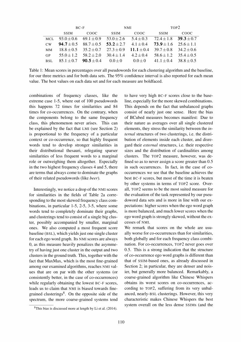
BC-F NMI TOP2SSIM COOC SSIM COOC SSIM COOC

MCL 93.0±0.6 69.1±0.9 53.0±2.6 5.4±0.3 72.4±1.8 333999...333±0.7CW 999444...777±0.5 88.7±0.5 555333...222±2.7 4.1±0.4 777333...999±1.6 25.6±1.1MM 18.8±0.5 35.2±0.7 27.3±0.9 111111...111±0.4 39.7±0.8 34.2±0.6GP 55.0±1.2 58.2±2.0 30.4±1.4 4.2±0.4 58.6±1.2 35.4±0.5BSL 85.1±0.7 999000...555±0.4 0.0±0 0.0±0 41.1±0.4 38.8±0.5

Table 1: Mean scores in percentages over all pseudowords for each clustering algorithm and the baseline,for our three metrics and for both data sets. The 95% confidence interval is also reported for each meanvalue. The best values on each data set and for each measure are boldfaced.

combinations of frequency classes, like theextreme case 1-5, where out of 100 pseudowordsthis happens 72 times for similarities and 84times for co-occurrences. On the contrary, whenthe components belong to the same frequencyclass, this phenomenon never arises. This canbe explained by the fact that LMI (see Section 2)is proportional to the frequency of a particularcontext or co-occurrence, so that highly frequentwords tend to develop stronger similarities intheir distributional thesauri, relegating sparsersimilarities of less frequent words to a marginalrole or outweighing them altogether. Especiallyin the two highest frequency classes 4 and 5, thereare terms that always come to dominate the graphsof their related pseudowords (like beer).

Interestingly, we notice a drop of the NMI scoresfor similarities in the fields of Table 2a corre-sponding to the most skewed frequency class com-binations, in particular 1-5, 2-5, 3-5, where somewords tend to completely dominate their graphs,and clusterings tend to consist of a single big clus-ter, possibly accompanied by smaller, marginalones. We also computed a most frequent scorebaseline (BSL), which yields just one single clusterfor each ego word graph. Its NMI scores are always0, as this measure heavily penalizes the asymme-try of having just one cluster in the output and twoclusters in the ground truth. This, together with thefact that MaxMax, which is the most fine-grainedamong our examined algorithms, reaches NMI val-ues that are on par with the other systems (orconsistently better, in the case of co-occurrences)while regularly obtaining the lowest BC-F scores,leads us to claim that NMI is biased towards fine-grained clusterings8. On the opposite side of thespectrum, the more coarse-grained systems tend

8This bias is discussed more at length by Li et al. (2014).

to have very high BC-F scores close to the base-line, especially for the more skewed combinations.This depends on the fact that unbalanced graphsconsist of nearly just one sense. Here the biasof BCubed measures becomes manifest: Due totheir nature as averages over all single clusteredelements, they stress the similarity between the in-ternal structures of two clusterings, i.e. the distri-bution of elements inside each cluster, and disre-gard their external structures, i.e. their respectivesizes and the distribution of cardinalities amongclusters. The TOP2 measure, however, was de-fined so as to never assign a score greater than 0.5in such occurrences. In fact, in the case of co-occurrences we see that the baseline achieves thebest BC-F scores, but most of the time it is beatenby other systems in terms of TOP2 score. Over-all, TOP2 seems to be the most suited measure forthe evaluation of the task represented by our pseu-doword data sets and is more in line with our ex-pectations: higher scores when the ego word graphis more balanced, and much lower scores when theego word graph is strongly skewed, without the ex-cesses of NMI.We remark that scores on the whole are usu-ally worse for co-occurrences than for similarities,both globally and for each frequency class combi-nation. For co-occurrences, TOP2 never goes over0.5. This is a strong indication that the structureof co-occurrence ego word graphs is different thanthat of SSIM-based ones, as already discussed inSection 2; in particular, they are denser and nois-ier, but generally more balanced. Remarkably, acoarse-grained algorithm like Chinese Whispersobtains its worst scores on co-occurrences, ac-cording to TOP2, suffering from its very unbal-anced, nearly-BSL clusterings. However, this verycharacteristic makes Chinese Whispers the bestsystem overall on the less dense SSIMs (and the

110

1 2 3 4 5BC-F NMI TOP2 BC-F NMI TOP2 BC-F NMI TOP2 BC-F NMI TOP2 BC-F NMI TOP2

MCL 92.6 71.9 79.7 89.7 67.6 81.1 87.4 64.0 83.4 99.0 35.9 65.5 98.0 26.3 55.0CW 94.7 79.6 85.6 94.2 78.4 87.0 91.8 73.0 86.8 98.9 30.6 63.6 99.4 29.7 61.4MM 37.0 45.5 50.8 26.8 39.7 46.4 17.6 32.5 40.2 17.0 11.2 42.5 13.2 10.3 37.7 1GP 70.6 57.5 76.4 62.3 46.4 71.7 50.8 34.9 62.4 49.8 8.4 43.2 46.9 7.5 36.9BSL 72.5 0.0 35.5 75.8 0.0 38.2 81.5 0.0 41.6 98.4 0.0 47.9 98.3 0.0 44.1

MCL 88.2 63.5 80.4 85.4 58.3 79.0 98.2 43.2 68.4 97.8 12.9 38.5CW 92.4 74.5 86.8 87.5 59.6 78.8 98.2 27.2 60.9 98.5 10.9 49.6MM 22.7 38.9 40.8 16.3 33.6 34.8 16.9 13.1 45.3 12.5 9.0 28.6 2GP 60.4 47.3 72.7 55.5 40.4 67.0 51.6 9.7 45.2 48.1 6.8 35.7BSL 73.8 0.0 37.2 76.4 0.0 38.0 97.4 0.0 46.4 98.0 0.0 43.7

MCL 83.5 49.9 75.0 97.7 41.8 66.1 97.3 13.2 44.1CW 84.3 43.4 69.9 97.5 25.8 59.3 97.7 9.1 49.4MM 12.7 31.0 28.4 17.8 15.4 43.1 12.4 9.6 29.3 3GP 53.2 36.1 65.8 46.3 13.3 47.9 43.4 7.8 36.5BSL 76.6 0.0 38.1 96.5 0.0 45.4 97.5 0.0 43.3

MCL 93.9 69.3 78.0 96.3 68.9 79.1CW 96.0 81.9 86.4 96.8 69.5 80.5MM 21.4 40.0 41.7 18.2 33.1 39.6 4GP 69.2 48.2 69.5 59.8 37.8 64.3BSL 77.2 0.0 36.6 82.8 0.0 39.6

MCL 96.6 78.9 86.5CW 96.9 76.9 85.5MM 17.6 35.7 38.8 5GP 59.4 43.7 70.1BSL 81.0 0.0 40.2

(a) Scores on the SSIM-based data set.1 2 3 4 5

BC-F NMI TOP2 BC-F NMI TOP2 BC-F NMI TOP2 BC-F NMI TOP2 BC-F NMI TOP2MCL 61.3 6.3 41.1 63.2 5.0 45.8 74.4 4.0 46.4 70.9 2.2 30.2 76.8 5.1 37.1CW 69.9 7.1 38.3 80.5 4.4 34.4 92.5 3.2 25.9 95.8 0.3 7.3 98.7 0.1 12.8MM 49.6 17.1 42.2 40.7 13.4 39.7 38.3 7.3 39.2 34.7 3.7 28.0 36.9 3.7 32.7 1GP 48.1 5.3 40.9 45.0 5.0 37.1 27.7 4.5 28.0 57.3 2.5 34.7 73.7 0.7 37.9BSL 71.9 0.0 34.4 83.5 0.0 42.0 94.4 0.0 46.7 98.9 0.0 47.9 99.7 0.0 48.9

MCL 60.5 4.8 43.3 67.5 5.0 40.5 65.8 4.6 38.8 77.6 4.6 34.0CW 81.8 3.1 32.5 87.1 3.4 30.4 92.7 2.8 20.2 97.0 5.7 22.6MM 35.0 13.8 35.6 34.6 11.8 33.5 34.2 8.7 34.5 36.2 5.1 30.3 2GP 49.6 5.7 36.9 29.2 7.2 31.0 62.7 5.1 38.2 86.0 0.7 41.1BSL 83.0 0.0 38.2 88.3 0.0 36.8 94.7 0.0 41.9 98.0 0.0 44.0

MCL 69.6 5.4 34.0 66.4 6.4 37.1 77.2 6.8 43.1CW 85.6 3.3 25.1 88.4 3.3 23.2 94.6 5.7 24.4MM 32.7 13.7 27.9 31.7 13.2 30.6 33.4 8.1 34.5 3GP 38.5 5.8 28.5 63.5 6.2 36.6 88.3 0.9 39.9BSL 86.7 0.0 28.3 89.6 0.0 32.9 95.8 0.0 40.3

MCL 59.2 8.5 35.1 71.9 7.7 39.8CW 84.7 5.0 26.7 89.1 7.7 31.5MM 31.1 18.5 32.9 31.6 14.3 35.6 4GP 60.7 7.1 34.5 81.0 2.5 36.7BSL 86.8 0.0 27.3 90.5 0.0 35.5

MCL 73.0 7.8 33.7CW 85.1 4.3 27.2MM 30.5 19.2 32.4 5GP 81.9 1.4 29.5BSL 86.8 0.0 27.6

(b) Scores on the co-occurrence-based data set.

Table 2: Mean scores per frequency class combination over both SSIM-based and the co-occurrence-based ego word graph data sets. The best values for each frequency class combination are highlighted.

111

other evaluation measures agree). At the sametime, the more fine-grained GP and MCL seemto better adapt to the structure of co-occurrencegraphs, while GP’s performances clearly deterio-rate on more unbalanced pseudowords for SSIMs.On the lower end of the spectrum, MaxMax showsa very constant but too divisive nature for our taskof homonymy detection.

5.1 Example of Clusterings

We briefly want to show the differences betweenthe clusterings of our four systems (CW, MCL,MaxMax, GP) on the SSIM ego word graph of asame pseudoword. We chose catsup bufflehead:catsup (variant of ketchup) belongs to frequencyclass 2 and bufflehead (a kind of duck) to fre-quency class 1. Their graph has 488 nodes and adensity of 0.548, above the global mean of 0.45.The node ratio is in favour of catsup at 3.05 : 1against bufflehead, with respectively 111 against339 exclusive terms, still being a quite balancedego graph.Chinese Whispers finds two clusters which seemto cover correctly the two senses of bird or animalon one side, {hummingbird, woodpecker,dove, merganser,...}, and food on theother side: {polenta, egg, baguette,squab,...}. Its scores are very high, respec-tively 0.95 for BC-F, 0.80 for NMI and 0.93 forTOP2.The gangplank algorithm yields 5 clusters. Oneis clearly about the bird: {goldeneye, condor,peacock,...}. The other four have high pre-cision, but lose recall for splitting the sense offood, e.g. in {puree, clove, dill,...} and{jelly, tablespoon, dripping,...}, andthe distinction between them is not always clear.We obtain a BC-F of 0.66, a NMI of 0.51 and aTOP2 of 0.78.The Markov cluster algorithm with an inflationfactor of 1.4 fails to make a distinction andfinds only one cluster: {raptor, Parmesan,coffee, stork,...}. Its scores are the same ofour trivial baseline: BC-F 0.77, NMI 0.0 and TOP20.41 (< 0.5, see section 3).MaxMax confirms its tendency of very fine-grained clusterings and produces 22 clusters.Each has a very high precision, but some consistof only two or three elements, such as {gin,rum, brandy} and {cashmere, denim} andin general they make very narrow distinctions.

The biggest cluster {chili, chily, ginger,shallot,...} has 89 elements. We also find acluster with bird names, but the overall scores arelow: BC-F 0.27, NMI 0.38 and TOP2 0.45.

6 Conclusions

The major contribution of this work is to presenttwo new pseudoword ego word graph data sets forgraph-based homonymy detection: one for contextsemantic similarities and one for co-occurrences.The data sets are modelled around 1225 pseu-dowords, each representing the combination oftwo monosemous words. We show that many egoword graphs are too skewed when the two compo-nents come from very different frequency classes,up to the point of actually collapsing on just onesense, but in general they represent a good approx-imation of homonymy. We evidence the biases ofBCubed measures and NMI, respectively towardsbaseline-like clusterings (and BSL is the best per-forming system for co-occurrences in this sense)and finer clusterings. On the contrary, our pro-posed TOP2 metric seems to strike the right bal-ance and to provide the most meaningful scoresfor interpretation. Chinese Whispers, which yieldstendentially coarse clusterings, emerges as the bestsystem overall for this task with regard to SSIM,and is closely followed by MCL, which is in turnthe best system for co-occurrences, according toTOP2. The more fine-grained GP approach fallsin-between. MaxMax systematically has the low-est scores, as its clusterings prove to be too frag-mented for our task, and only achieves good NMI

values, which are however biased.These considerations lead us to identify Word

Sense Discrimination9 (WSD), commonly used asa synonym for Word Sense Induction, as an actu-ally different, yet complementary task which ne-cessitates different instruments, as exemplified byour double data set: whereas WSI is paradigmatic,WSD is syntagmatic. We deem that this distinctiondeserves further investigation. As a future work,beyond expanding our data sets we envision theimplementation of consensus clustering (Ghaemiet al., 2009) and re-clustering techniques to im-prove results, and a more accurate analysis of therelation between creation of word graphs and al-gorithms’ outputs.

9Defined as “determining for any two occurrences [of aword] whether they belong to the same sense or not”, afterSchutze (1998).

112

ReferencesEnrique Amigo, Julio Gonzalo, Javier Artiles, and Fe-

lisa Verdejo. 2009. A comparison of extrinsicclustering evaluation metrics based on formal con-straints. Information retrieval, 12(4):461–486.

Amit Bagga and Breck Baldwin. 1998. Algorithmsfor scoring coreference chains. In Proceedingsof the first international Conference on LanguageResources and Evaluation (LREC’98), workshopon linguistic coreference, pages 563–566, Granada,Spain. European Language Resources Association.

Osman Baskaya and David Jurgens. 2016. Semi-supervised learning with induced word senses forstate of the art word sense disambiguation. Journalof Artificial Intelligence Research, 55:1025–1058.

Chris Biemann and Uwe Quasthoff. 2009. Networksgenerated from natural language text. In Dynam-ics on and of complex networks, pages 167–185.Springer.

Chris Biemann and Martin Riedl. 2013. Text: Nowin 2D! a framework for lexical expansion with con-textual similarity. Journal of Language Modelling,1(1):55–95.

Chris Biemann. 2006. Chinese whispers: an effi-cient graph clustering algorithm and its applicationto natural language processing problems. In Pro-ceedings of the first workshop on graph based meth-ods for natural language processing, pages 73–80,New York, New York, USA.

Stefan Bordag. 2006. Word sense induction: Triplet-based clustering and automatic evaluation. In Pro-ceedings of the 11th Conference of the EuropeanChapter of the Association for Computational Lin-guistics, pages 137–144, Trento, Italy. EACL.

Flavio Massimiliano Cecchini and Elisabetta Fersini.2015. Word sense discrimination: A gangplank al-gorithm. In Proceedings of the Second Italian Con-ference on Computational Linguistics CLiC-it 2015,pages 77–81, Trento, Italy.

Marie-Catherine De Marneffe, Bill MacCartney, andChristopher Manning. 2006. Generating typed de-pendency parses from phrase structure parses. InProceedings of the fifth international Conferenceon Language Resources and Evaluation (LREC’06),pages 449–454, Genoa, Italy. European LanguageResources Association.

Ferdinand De Saussure. 1995 [1916]. Cours de lin-guistique generale. Payot&Rivage, Paris, France.Critical edition of 1st 1916 edition.

Stefan Evert. 2004. The statistics of word cooccur-rences: word pairs and collocations. Ph.D. thesis,Universitat Stuttgart, August.

William Gale, Kenneth Church, and David Yarowsky.1992. Work on statistical methods for word sense

disambiguation. In Technical Report of 1992 FallSymposium - Probabilistic Approaches to NaturalLanguage, pages 54–60, Cambridge, Massachusetts,USA. AAAI.

Reza Ghaemi, Md Nasir Sulaiman, Hamidah Ibrahim,Norwati Mustapha, et al. 2009. A survey: clusteringensembles techniques. World Academy of Science,Engineering and Technology, 50:636–645.

Zellig Harris. 1954. Distributional structure. Word,10(2-3):146–162.

Taher Haveliwala. 2002. Topic-sensitive pagerank. InProceedings of the 11th international conference onWorld Wide Web, pages 517–526, Honolulu, Hawaii,USA. ACM.

David Hope and Bill Keller. 2013. MaxMax: a graph-based soft clustering algorithm applied to wordsense induction. In Proceedings of the 14th Interna-tional Conference on Computational Linguistics andIntelligent Text Processing, pages 368–381, Samos,Greece.

David Jurgens and Ioannis Klapaftis. 2013. SemEval-2013 task 13: Word sense induction for graded andnon-graded senses. In *SEM 2013: The SecondJoint Conference on Lexical and Computational Se-mantics, volume 2, pages 290–299, Atlanta, Geor-gia, USA. ACL.

Adam Kilgarriff, Pavel Rychly, Pavel Smrz, and DavidTugwell. 2004. The sketch engine. In Proceedingsof the Eleventh Euralex Conference, pages 105–116,Lorient, France.

Linlin Li, Ivan Titov, and Caroline Sporleder. 2014.Improved estimation of entropy for evaluation ofword sense induction. Computational Linguistics,40(3):671–685.

Suresh Manandhar, Ioannis Klapaftis, Dmitriy Dligach,and Sameer Pradhan. 2010. Semeval-2010 task 14:Word sense induction & disambiguation. In Pro-ceedings of the 5th international workshop on se-mantic evaluation, pages 63–68, Los Angeles, Cal-ifornia, USA. Association for Computational Lin-guistics.

James Martin and Daniel Jurafsky. 2000. Speech andlanguage processing. Pearson, Upper Saddle River,New Jersey, USA.

George Miller. 1995. WordNet: a lexical database forEnglish. Communications of the ACM, 38(11):39–41.

Preslav Nakov and Marti Hearst. 2003. Category-based pseudowords. In Companion Volume of theProceedings of the Human Language TechnologyConference of the North American Chapter of theAssociation for Computational Linguistics (HTL-NAACL) 2003 - Short Papers, pages 70–72, Ed-monton, Alberta, Canada. Association for Compu-tational Linguistics.

113

Roberto Navigli, Kenneth Litkowski, and Orin Har-graves. 2007. SemEval-2007 task 07: Coarse-grained English all-words task. In Proceedings ofthe 4th International Workshop on Semantic Evalu-ations, pages 30–35, Prague, Czech Republic. Asso-ciation for Computational Linguistics.

Roberto Navigli. 2009. Word sense disambiguation: Asurvey. ACM Computing Surveys (CSUR), 41(2):10.

Lubomır Otrusina and Pavel Smrz. 2010. A new ap-proach to pseudoword generation. In Proceedings ofthe seventh international Conference on LanguageResources and Evaluation (LREC’10), pages 1195–1199. European Language Resources Association.

Robert Parker, David Graff, Junbo Kong, Ke Chen, andKazuaki Maeda. 2011. English Gigaword FifthEdition. Linguistic Data Consortium, Philadelphia,Pennsylvania, USA.

Mohammad Taher Pilehvar and Roberto Navigli. 2013.Paving the way to a large-scale pseudosense-annotated dataset. In Proceedings of the 2013 Con-ference of the North American Chapter of the Asso-ciation for Computational Linguistics: Human Lan-guage Technologies (HTL-NAACL), pages 1100–1109, Atlanta, Georgia, USA. Association for Com-putational Linguistics.

Steffen Remus and Chris Biemann. 2013. Threeknowledge-free methods for automatic lexical chainextraction. In Proceedings of the 2013 Confer-ence of the North American Chapter of the Associ-ation for Computational Linguistics: Human Lan-guage Technologies (HTL-NAACL), pages 989–999,Atlanta, Georgia, USA. Association for Computa-tional Linguistics.

Matthias Richter, Uwe Quasthoff, Erla Hallsteinsdottir,and Chris Biemann. 2006. Exploiting the LeipzigCorpora Collection. In Proceedings of the FifthSlovenian and First International Language Tech-nologies Conference, IS-LTC ’06, pages 68–73,Ljubljana, Slovenia. Slovenian Language Technolo-gies Society.

Keijo Ruohonen. 2013. Graph Theory. Tampereenteknillinen yliopisto. Originally titled Graafiteoria,lecture notes translated by Tamminen, J., Lee, K.-C.and Piche, R.

Hinrich Schutze. 1992. Dimensions of meaning. InProceedings of Supercomputing’92, pages 787–796,Minneapolis, Minnesota, USA. ACM/IEEE.

Hinrich Schutze. 1998. Automatic word sense dis-crimination. Computational linguistics, 24(1):97–123.

Alexander Strehl. 2002. Relationship-based cluster-ing and cluster ensembles for high-dimensional datamining. Ph.D. thesis, The University of Texas atAustin, May.

Peter Turney and Patrick Pantel. 2010. From fre-quency to meaning: Vector space models of se-mantics. Journal of artificial intelligence research,37(1):141–188.

Stijn van Dongen. 2000. Graph clustering by flow sim-ulation. Ph.D. thesis, Universiteit Utrecht, May.

Dominic Widdows and Beate Dorow. 2002. A graphmodel for unsupervised lexical acquisition. In Pro-ceedings of the 19th international conference onComputational Linguistics, volume 1, pages 1–7,Taipei, Taiwan. Association for Computational Lin-guistics.

114


North Sámi to Finnish rule-based machine translation systemRyan Johnson¹ and Tommi A Pirinen² and Tiina Puolakainen³Francis Tyers¹ and Trond Trosterud¹ and Kevin Unhammer¹

¹ UiT Norgga Árktalaš universitehta, Giela ja kultuvrra instituhtta, Romssa, Norga² Universität Hamburg, Hamburger Zentrum für Sprachkorpora, Deutschland

³ Institute of the Estonian Language, [email protected], [email protected],[email protected], {francis.tyers, trond.trosterud}@uit.no

[email protected]

Abstract

This paper presents a machine translationsystem between Finnish and North Sámi,two Uralic languages. In this paper weconcentrate on the translation direction toFinnish. As a background, the differ-ences between the two languages is pre-sented, followed by how the system wasdesigned to handle some of these differ-ences. We then provide an evaluation ofthe system’s performance and directionsfor future work.

1 Introduction0

This paper presents a prototype shallow-transferrule-based machine translation system betweenFinnish and North Sámi. The paper will be laid outas follows: Section 2 gives a short review of someprevious work in the area of Uralic-Uralic lan-guage machine translation; Section 3 introducesFinnish and North Sámi and compares their gram-mar; Section 4 describes the system and the toolsused to construct it; Section 5 gives a preliminaryevaluation of the system; and finally Section 6 de-scribes our aims for futurework and some conclud-ing remarks.

2 Previous work

Within the Apertium platform, work on severalMT systems from North Sámi to Norwegian andto other Sámi languages have been developed (Ty-ers et al., 2009; Wiechetek et al., 2010; Trosterudand Unhammer, 2013; Antonsen et al., 2016)).Besides these systems, several previous workson making machine translation systems betweenUralic languages exist, although to our knowledgenone are publicly available, except for North Sámi

0Authors are listed here alphabetically

to Norwegian1, and the translation between Esto-nian, Finnish and Hungarian being available viaEnglish as a pivot language in Google Translate.2For non-Uralic pairs there are also numerous sim-ilarly laid out systems e.g. in Apertium’s Turkicpairs, e.g. (Salimzyanov et al., 2013), that can of-fer insights on how the pair is implemented, whichare detailed later in the article but the main partsare the same.

3 The languages

North Sámi and Finnish belong to the Sámi andFinnic branches of the Uralic languages, respec-tively. The languages are mutually unintelligi-ble, but grammatically quite similar. The ortho-graphical conventions between Finnish and NorthSámi written in Finland were quite similar until1979, when an unified North Sámi orthographywidened the distance to Finnish. Finnish is pri-marily spoken in Finland, where it is the nationallanguage, sharing status with Swedish as an offi-cial language. The total number of speakers is atleast 6 million people. North Sámi is spoken inthe Northern parts of Norway, Sweden and Fin-land by approximately 24.700 people, and it has,alongside the national language, some official sta-tus in the municipalities and counties where it isspoken. North Sámi speakers are bilingual in theirmother tongue and in their respective national lan-guage, many also speak the neighbouring officiallanguage. An MT system between North Sámiand Finnish is potentially of great use to the lan-guage communities, although fulfilling differentfunctions. In Finland, it may be used to understandSámi text, and in Norway and Sweden, it may beused byNorth Sámi speakers to understand Finnishtext. In principle, the system may also be used forNorth Sámi text production, although further de-

1https://gtweb.uit.no/jorgal2https://translate.google.com

115

velopment will be needed to fulfil such a function.

3.1 Phonological differencesAs related languages, Finnish and North Sámishare several phonological processes, the mostimportant one being consonant gradation. How-ever, North Sámi consonant gradation involves thevast majority of stem-internal consonant clusters,whereas the Finnish counterpart involves only thestops p, t, k. Vowel length has a more central rolein Finnish than in North Sámi, Several instancesof final vowel apocopy in North Sámi, as well asa neutralisation of p, t, k in word-final position,has also resulted in quite extensive morphologicalhomonymy. A richer inventory of affricates andfricatives in North Sámi, as well as preaspiration,also add to the difference.

3.2 Orthographic differencesIn the native vocabulary, neither Finnish nor NorthSámi distinguish between voiced and unvoicedplosives, but whereas Finnish writes them as p,t, k, North Sámi writes b, d, g, as in kirja : girji“book”. Finnish marks vowel length with doubleletter symbols. In North Sámi this distinction ismarked for one vowel only, a, and with acute ac-cent. Apart from this the orthographic principles ofthe two languages is quite similar, the almost totallack of free rides is a result of different phonology.

3.3 Morphological differencesThere are a number of examples where the mor-phologies of Finnish and North Sámi are rather dif-ferent.North Sámi has a separate dual number, whereas

Finnish has not. Otherwise the North Sámi andFinnish finite verb morphology is almost identi-cal. The infinite verb conjugation is more differ-ent, though: Finnish has a rich array of infinitivesthat are inflected in different subsets of the casesystem.Finnish has more than twice the number of cases

as North Sámi has. Where North Sámi only hasone case for the direct object (accusative), Finnishhas two (accusative and partitive). The Finnishsystem of adverbial cases consist of a 2x3matrix ofinner/outer to/in/from cases, North Sámi has onlyone of these distinctions (to/in˜from), thus the 6Finnish cases corresponds to 2 North Sámi ones.In principle, Finnish andNorth Sámi have the samesystem of possessive suffixes, but in North Sámi itsuse is far more restricted than in Finnish.

3.4 Syntactic differences

Syntactically speaking, there are two varieties ofNorth Sámi, one used within and one outside ofFinland. The Finnish variety is much closer toFinnish than the Scandinavian one. ComparingFinnish with the Scandinavian variety of NorthSámi, themost striking difference is participle con-structions vs. relative clauses. Where North Sámiuses subordinate clauses, written Finnish often usehead-final participle constructions instead. Sinceboth varieties are found in Finnish, at least to somedegree, we at the moment let most “Scandinavian”varieties of North Sámi through, thereby givingNorth Sámi from Norway and Finland a differentstylistic flavour in the Finnish output.The North Sámi passive is a derivational pro-

cess, whereas it for Finnish is an inflectional one,resulting in quite different syntactic patterns forpassive. Finnish has a richer array of indefiniteverb forms.Finnish adjectives agree with their head noun in

case and number, whereas North Sámi has an in-variant attribute form for all but one adjective, theadjective buorre ‘good’, and partial agreement fordeterminers.Existential and habitive clauses have the same

structure in the two languages, possessor.local-case copula possessed and adverbial copula e-subject (on me / in street is car ‘I have a car/Thereis a car in the street’). except that in Finnish, thepossessed/e-subject behaves like objects, whereasit in North Sámi they behave like subjects. Thus, inNorth Sámi, the copula agrees with the possessed/ e-subject, whereas in Finnish, it does not.

4 System

The system is based on the Apertium3 machinetranslation platform (Forcada et al., 2011). Theplatform was originally aimed at the Romance lan-guages of the Iberian peninsula, but has also beenadapted for other, more distantly related, languagepairs. The whole platform, both programs anddata, are licensed under the Free Software Foun-dation’s General Public Licence4 (GPL) and allthe software and data for the 30 released languagepairs (and the other pairs beingworked on) is avail-able for download from the project website.

3http://apertium.sf.net4https://www.gnu.org/licenses/gpl-3.0.en.

html

116

4.1 Architecture of the system

The Apertium translation engine consists of aUnix-style pipeline or assembly line with the fol-lowing modules (see Figure 1):

• A deformatter which encapsulates the formatinformation in the input as superblanks thatwill then be seen as blanks between words bythe other modules.

• A morphological analyser which segmentsthe text in surface forms (SF) (words, or,where detected, multiword lexical units orMWLUs) and for each, delivers one or morelexical forms (LF) consisting of lemma, lexi-cal category and morphological information.

• A morphological disambiguator (CG) whichchooses, using linguistic rules the most ade-quate sequence of morphological analyses foran ambiguous sentence.

• A lexical transfer module which reads eachSL LF and delivers the corresponding target-language (TL) LF by looking it up in a bilin-gual dictionary encoded as an FST compiledfrom the corresponding XML file. The lexi-cal transfer module may return more than oneTL LF for a single SL LF.

• A lexical selection module (Tyers et al.,2012b) which chooses, based on contextrules, the most adequate translation of am-biguous source language LFs.

• A structural transfer module, which performslocal syntactic operations, is compiled fromXML files containing rules that associate anaction to each defined LF pattern. Patterns areapplied left-to-right, and the longest matchingpattern is always selected.

• A morphological generator which delivers aTL SF for each TL LF, by suitably inflectingit.

• A reformatter which de-encapsulates any for-mat information.

Table 1 provides an example of a single phraseas it moves through the pipeline.

4.2 Morphological transducersThe morphological transducers are compiled withthe Helsinki Finite State Technology (Lindén etal., 2009),5 a free/open-source reimplementationof the Xerox finite-state tool-chain, popular in thefield of morphological analysis. It implementsboth the lexc morphology description language fordefining lexicons, and the twol and xfst script-ing languages for modeling morphophonologicalrules. This toolkit has been chosen as it—or theequivalent XFST—has been widely used for otherUralic languages (Koskenniemi, 1983; Pirinen,2015; Moshagen et al., 2013), and is available un-der a free/open-source licence. The morphologiesof both languages are implemented in lexc, and themorphophonologies of both languages are imple-mented in twolc.The same morphological description is used for

both analysis and generation. To avoid overgener-ation, any alternative forms are marked with one oftwomarks, LR (only analyser) or RL (only genera-tor). Instead of the usual compile/invert to compilethe transducers, we compile twice, once the gen-erator, without the LR paths, and then again theanalyser without the RL paths.

4.3 Bilingual lexiconThe bilingual lexicon currently contains 19,415stem-to-stem correspondences (of which 8044proper nouns) and was built partly upon an avail-able North Sámi—Finnish dictionary6, and partlyby hand (i.e., by translating North Sámi stemsunrecognised by the morphological analyser intoFinnish). The proper nouns were taken from ex-isting lexical resources. Entries consist largelyof one-to-one stem-to-stem correspondences withpart of speech, but also include some entries withambiguous translations (see e.g., Figure 2).

4.4 Disambiguation rulesThe system has a morphological disambiguationmodule in the form of a Constraint Grammar(Karlsson et al., 1995). The version of the formal-ism used is vislcg3.7 The output of each morpho-logical analyser is highly ambiguous, measured ataround 2.4 morphological analyses per form forFinnish and 2.6 for North Sámi8. The goal of

5https://hfst.github.io6https://gtweb.uit.no/langtech/trunk/words/

dicts/smefin/src/7http://visl.cg.sdu.dk8Cf. (Trosterud and Wiechetek, 2007)

117

Figure 1: Apertium structure (Image from apertium wiki by user Rcrowther) http://wiki.apertium.org/wiki/Workflow_diagram

118

North Sámi input: Sámegielat leat gielat maid sámit hállet.Morphological analysis:ˆSámegielat/ sámegielat<adj> <attr>/ sámegielat<adj> <sg><nom>/sámegiella<n> <pl><nom>/ sámegiella<n> <sg><acc><px2sg>/sámegiella<n> <sg><gen><px2sg>/ sámegiella<n> <sg><acc><px2sg>/sámegiella<n> <sg><gen><px2sg>$

ˆleat/ leat<vblex><iv> <indic><pres><conneg>/leat<vblex><iv> <indic><pres><p1><pl>/ leat<vblex><iv> <indic><pres><p2><sg>/leat<vblex><iv> <indic><pres><p3><pl>/ leat<vblex><iv> <inf>$ˆgielat/ giella<n> <pl><nom>/ giella<n> <sg><acc><px2sg>/

giella<n> <sg><gen><px2sg>/ giella<n> <sg><acc><px2sg>/giella<n> <sg><gen><px2sg>$ ˆmaid/ maid<adv>/ mii<prn><itg> <pl><acc>/

mii<prn><itg> <pl><gen>/ mii<prn><itg> <sg><acc>/ mii<prn><rel> <pl><acc>/mii<prn><rel> <pl><gen>/ mii<prn><rel> <sg><acc>$

ˆsámit/ sápmi<n> <pl><nom>/ sápmi<n> <pl><nom>$

ˆhállet/ hállat<vblex><tv> <imp><p2><pl>/hállat<vblex><tv> <indic><pres><p3><pl>/ hállat<vblex><tv> <indic><pret><p2><sg>$ˆ./.<sent>$Morphological disambiguation:ˆSámegielat/sámegiella<n> <pl><nom> <@SUBJ→>$ˆleat/leat<vblex><iv> <indic><pres><p3><pl> <@+FMAINV>$ˆgielat/giella<n> <pl><nom> <@←SPRED>$ˆmaid/mii<prn><rel> <pl><acc> <@OBJ→>$ˆsámit/sápmi<n> <pl><nom> <@SUBJ→>$ˆhállet/hállat<vblex><tv> <indic><pres><p3><pl> <@+FMAINV>$ ˆ./.<sent>$Lexical translation:ˆSámegiella<n> <pl><nom> <@SUBJ→>/ Saamekieli<n> <pl><nom> <@SUBJ→>/Saame<n> <pl><nom> <@SUBJ→>$

ˆleat<vblex><iv> <indic><pres><p3><pl> <@+FMAINV>/olla<vblex> <actv><indic><pres><p3><pl> <@+FMAINV>/sijaita<vblex> <actv><indic><pres><p3><pl> <@+FMAINV>$

ˆgiella<n> <pl><nom> <@←SPRED>/ kieli<n> <pl><nom> <@←SPRED>/ansa<n> <pl><nom> <@←SPRED>$

ˆmii<prn><rel> <pl><acc> <@OBJ→>/ mikä<prn><rel> <pl><acc> <@OBJ→>$

ˆsápmi<n> <pl><nom> <@SUBJ→>/ saame<n> <pl><nom> <@SUBJ→>$

ˆhállat<vblex><tv> <indic><pres><p3><pl> <@+FMAINV>/puhua<vblex> <actv><indic><pres><p3><pl> <@+FMAINV>/mekastaa<vblex> <actv><indic><pres><p3><pl> <@+FMAINV>$ˆ.<sent>/.<sent>$Structural transfer:ˆSaamekieli<n> <pl><nom>$ ˆolla<vblex> <actv><indic><pres><p3><pl>$ˆkieli<n> <pl><nom>$ ˆmikä<prn><rel> <pl><par>$ˆsaame<n> <pl><nom>$ ˆpuhua<vblex> <actv><indic><pres><p3><pl>$ˆ.<sent>$Finnish translation:Saamekielet ovat kielet #mikä saamet puhuvat

Table 1: Translation process for the North Sámi phrase Sámegielat leat gielat maid sámit hállet (TheSámi languages are the languages that the Sámis speak)

119

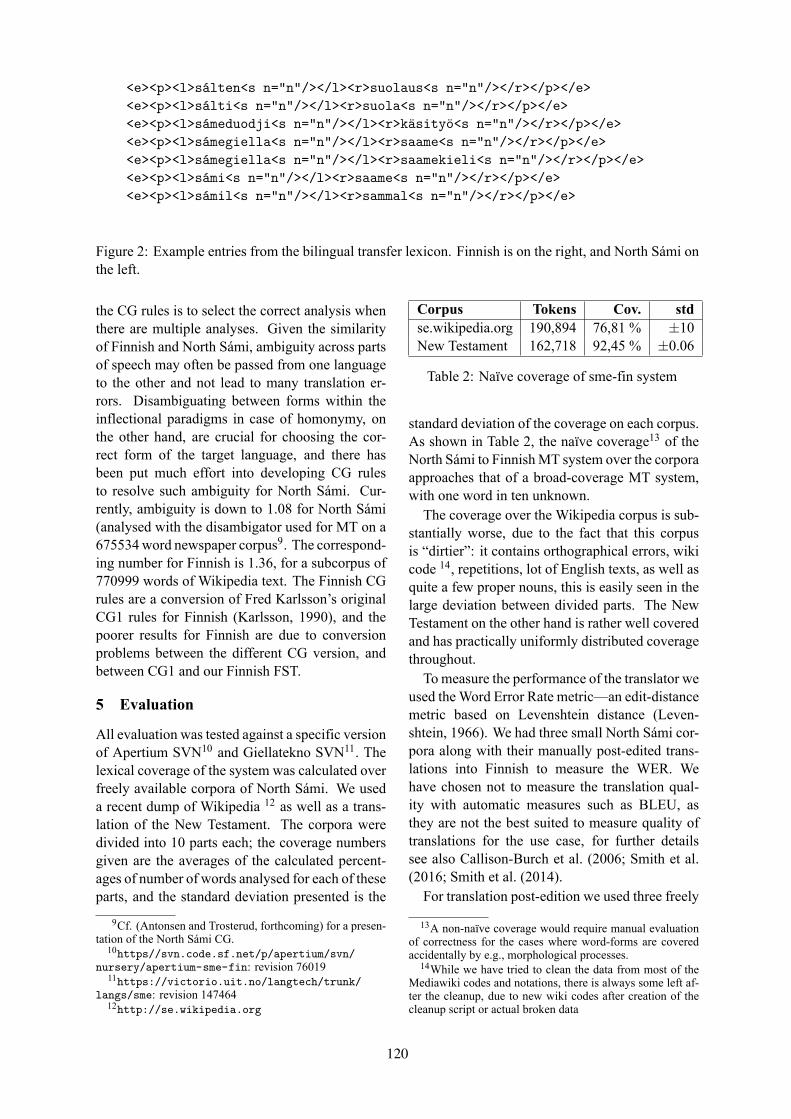
<e><l>sálten<s n="n"/></l><r>suolaus<s n="n"/></r></e><e><l>sálti<s n="n"/></l><r>suola<s n="n"/></r></e><e><l>sámeduodji<s n="n"/></l><r>käsityö<s n="n"/></r></e><e><l>sámegiella<s n="n"/></l><r>saame<s n="n"/></r></e><e><l>sámegiella<s n="n"/></l><r>saamekieli<s n="n"/></r></e><e><l>sámi<s n="n"/></l><r>saame<s n="n"/></r></e><e><l>sámil<s n="n"/></l><r>sammal<s n="n"/></r></e>

Figure 2: Example entries from the bilingual transfer lexicon. Finnish is on the right, and North Sámi onthe left.

the CG rules is to select the correct analysis whenthere are multiple analyses. Given the similarityof Finnish and North Sámi, ambiguity across partsof speech may often be passed from one languageto the other and not lead to many translation er-rors. Disambiguating between forms within theinflectional paradigms in case of homonymy, onthe other hand, are crucial for choosing the cor-rect form of the target language, and there hasbeen put much effort into developing CG rulesto resolve such ambiguity for North Sámi. Cur-rently, ambiguity is down to 1.08 for North Sámi(analysed with the disambigator used for MT on a675534word newspaper corpus9. The correspond-ing number for Finnish is 1.36, for a subcorpus of770999 words of Wikipedia text. The Finnish CGrules are a conversion of Fred Karlsson’s originalCG1 rules for Finnish (Karlsson, 1990), and thepoorer results for Finnish are due to conversionproblems between the different CG version, andbetween CG1 and our Finnish FST.

5 Evaluation

All evaluation was tested against a specific versionof Apertium SVN10 and Giellatekno SVN11. Thelexical coverage of the system was calculated overfreely available corpora of North Sámi. We useda recent dump of Wikipedia 12 as well as a trans-lation of the New Testament. The corpora weredivided into 10 parts each; the coverage numbersgiven are the averages of the calculated percent-ages of number of words analysed for each of theseparts, and the standard deviation presented is the

9Cf. (Antonsen and Trosterud, forthcoming) for a presen-tation of the North Sámi CG.

10https//svn.code.sf.net/p/apertium/svn/nursery/apertium-sme-fin: revision 76019

11https://victorio.uit.no/langtech/trunk/langs/sme: revision 147464

12http://se.wikipedia.org

Corpus Tokens Cov. stdse.wikipedia.org 190,894 76,81 % ±10New Testament 162,718 92,45 % ±0.06

Table 2: Naïve coverage of sme-fin system

standard deviation of the coverage on each corpus.As shown in Table 2, the naïve coverage13 of theNorth Sámi to FinnishMT system over the corporaapproaches that of a broad-coverage MT system,with one word in ten unknown.The coverage over the Wikipedia corpus is sub-

stantially worse, due to the fact that this corpusis “dirtier”: it contains orthographical errors, wikicode 14, repetitions, lot of English texts, as well asquite a few proper nouns, this is easily seen in thelarge deviation between divided parts. The NewTestament on the other hand is rather well coveredand has practically uniformly distributed coveragethroughout.To measure the performance of the translator we

used theWord Error Rate metric—an edit-distancemetric based on Levenshtein distance (Leven-shtein, 1966). We had three small North Sámi cor-pora along with their manually post-edited trans-lations into Finnish to measure the WER. Wehave chosen not to measure the translation qual-ity with automatic measures such as BLEU, asthey are not the best suited to measure quality oftranslations for the use case, for further detailssee also Callison-Burch et al. (2006; Smith et al.(2016; Smith et al. (2014).For translation post-edition we used three freely

13A non-naïve coverage would require manual evaluationof correctness for the cases where word-forms are coveredaccidentally by e.g., morphological processes.

14While we have tried to clean the data from most of theMediawiki codes and notations, there is always some left af-ter the cleanup, due to new wiki codes after creation of thecleanup script or actual broken data

120

Corpus Tokens OOV WERRedigering.se 1,070 95 34.24Samediggi.fi 570 33 36.32The Story 361 0 19.94

Table 3: Word error rate over the corpora; OOVis the number of out-of-vocabulary (unknown)words.

available parallel texts from the internet: one fromthe Finnish Sámi parliament site15, one from aSwedish regulation of minority people and lan-guages and the story that is used with all Apertiumlanguage pairs as initial development set (“Whereis James?”). Table 3 presents the WER for the cor-pora.Analysing the changes in post-edition, a few

classes of actual errors can be identified. Onecommon example arises from the grammatical dif-ferences in the case system systems, in particularthe remaining adpositions are often turned into acase suffix for the dependent noun phrase, e.g.,the North Sámi “birra” has been turned into theFinnish adposition “ympäri” (around), where el-ative case is required, similarly for the transla-tion “seassa” (among) instead of inessive case.Also visible, especially in the story text is thelack of possessive suffix agreement e.g. “heidänäiti” (their mother n sg nom) instead of “heidänäitinsä” (their mother n sp nom/gen pxsp3), whilethe former is perfectly acceptable in standard spo-ken Finnish it is not accepted as formal written lan-guage form. Another issue that appeared a num-ber of times, maybe partially due to the genre ofthe texts selected, i.e. law texts, was the selectionof adverb (form), e.g. the word-form “mukana”(with) was corrected to “mukaan” (according to).A large amount of simple lexical problems is dueto the vocabulary of the selected texts as well:“hallintoalue” (governmental area), “seurantavas-tuu” (responsibility of surveillance), “itsehallinto”(autonomy), and their compounds, are all eithermissing or partially wrong due to lexical selec-tions.

6 Concluding remarks

We have presented the first MT system fromFinnish to North Sámi. With a WER of above30%, it still is far from production-level perfor-mance, and it is also at the prototype-level in

15http://samediggi.fi

terms of the number of rules. Although the im-pact of this relatively low number of rules on thequality of translation is extensive (cf., the differ-ence in WER between the development and test-ing corpora), the outlook is promising and the cur-rent results suggest that a high quality translationbetween morphologically-rich agglutinative lan-guages is possible. We plan to continue develop-ment on the pair; the coverage of the system is al-ready quite high, although we intend to increaseit to 95 % on the corpora we have we estimatethat this will mean adding around 5,000 new stemsand take 1–2 months. The remaining work willbe improving the quality of translation by addingmore rules, starting with the transfer component.The long-term plan is to integrate the data createdwith other open-source data for Uralic languagesin order to make transfer systems between all theUralic language pairs. Related work is currentlyongoing from North Sámi to South, Lule and InariSámi, from North Sámi to Norwegian, and be-tween Finnish and Estonian. The system presentedhere is available as free/open-source software un-der the GNU GPL and the whole system may bedownloaded from Sourceforge and the open repos-itory of Giellatekno.

Acknowledgements

The work on this North Sámi-Finnish machinetranslation system was partially funded by theGoogle Summer of Code and Google Code-In pro-grammes, and partly by a Norsk forsingsråd grant(234299) on machine translation between Sámilanguages.

ReferencesLeneAntonsen and Trond Trosterud. forthcoming. Ord

sett innafra og utafra – en datalingvistisk analyse avnordsamisk. Norsk Lingvistisk Tidsskrift.

Lene Antonsen, Trond Trosterud, and Francis Tyers.2016. A North Saami to South Saami machine trans-lation prototype. 4:11—27.

Chris Callison-Burch, Miles Osborne, and PhilippKoehn. 2006. Re-evaluation the role of bleu inmachine translation research. In EACL, volume 6,pages 249–256.

Mikel L Forcada, Mireia Ginestí-Rosell, Jacob Nord-falk, Jim O’Regan, Sergio Ortiz-Rojas, Juan An-tonio Pérez-Ortiz, Felipe Sánchez-Martínez, GemaRamírez-Sánchez, and Francis M Tyers. 2011.

121

Apertium: a free/open-source platform for rule-based machine translation. Machine translation,25(2):127–144.

Fred Karlsson, Atro Voutilainen, Juha Heikkilae, andArto Anttila. 1995. Constraint Grammar:a language-independent system for parsing unre-stricted text, volume 4. Walter de Gruyter.

Fred Karlsson. 1990. Constraint grammar as a frame-work for parsing running text. In Proceedings ofthe 13th conference on Computational linguistics-Volume 3, pages 168–173. Association for Compu-tational Linguistics.

Kimmo Koskenniemi. 1983. Two-level morphology—A General Computational Model for Word-FormRecognition and Production. Ph.D. thesis, Depart-ment of General Linguistics. University of Helsinki,Finland.

Vladimir I Levenshtein. 1966. Binary codes capableof correcting deletions, insertions, and reversals. InSoviet physics doklady, volume 10, pages 707–710.

Krister Lindén, Miikka Silfverberg, and Tommi Piri-nen. 2009. Hfst tools for morphology–an efficientopen-source package for construction of morpholog-ical analyzers. In International Workshop on Sys-tems and Frameworks for Computational Morphol-ogy, pages 28–47. Springer.

Sjur N Moshagen, Tommi A Pirinen, and TrondTrosterud. 2013. Building an open-source de-velopment infrastructure for language technologyprojects. In Proceedings of the 19th Nordic Con-ference of Computational Linguistics (NODALIDA2013); May 22-24; 2013; Oslo University; Norway.NEALT Proceedings Series 16, number 085, pages343–352. Linköping University Electronic Press.

Tommi A Pirinen. 2015. Development and use of com-putational morphology of finnish in the open sourceand open science era: Notes on experiences withomorfi development. SKY Journal of Linguistics,28:381–393.

Ilnar Salimzyanov, J Washington, and F Tyers. 2013.A free/open-source kazakh-tatar machine translationsystem. Machine Translation Summit XIV.

Aaron Smith, Christian Hardmeier, and Jörg Tiede-mann. 2014. Bleu is not the colour: How optimisingbleu reduces translation quality.

Aaron Smith, Christian Hardmeier, and Jörg Tiede-mann. 2016. Climbing mount bleu: The strangeworld of reachable high-bleu translations. BalticJournal of Modern Computing, 4(2):269.

Trond Trosterud and Kevin Brubeck Unhammer. 2013.Evaluating North Sámi to Norwegian assimilationRBMT. In Proceedings of the Third InternationalWorkshop on Free/Open-Source Rule-Based Ma-chine Translation (FreeRBMT 2012), volume 3 of

Technical report, pages 13–26. Department of Com-puter Science and Engineering, Chalmers Universityof Technology and University of Gothenburg.

Trond Trosterud and Linda Wiechetek. 2007. Dis-ambiguering av homonymi i Nord- og Lulesamisk.Suomalais-Ugrilaisen Seuran Toimituksia = Mé-moires de la Société Fi nno-Ougrienne. Sámit,sánit, sátnehámit. Riepmočála Pekka Sammallahtiimiessemánu 21. beaivve 2007, 253:375–395.

Francis Tyers, Linda Wiechetek, and Trond Trosterud.2009. Developing prototypes for machine transla-tion between two Sámi languages. In Proceedingsof the 13th Annual Conference of the European As-sociation for Machine Translation, EAMT09, pages120–128.

Linda Wiechetek, Francis Tyers, and Thomas Omma.2010. Shooting at flies in the dark: Rule-based lex-ical selection for a minority language pair. LectureNotes in Artificial Intelligence, 6233:418–429.

122


Machine translation with North Saami as a pivot language

Lene Antonsen and Ciprian Gerstenberger and Maja KappfjellSandra Nystø Rahka and Marja-Liisa Olthuis

Trond Trosterud and Francis M. TyersDepartment of Language and CultureUiT The Arctic University of Norway

[email protected]

Abstract

Translating from a majority language intoseveral minority languages implies dupli-cating both translation and terminologywork. Our assumption is that a manualtranslation into one of the languages, andmachine translation from this one into theother ones, will both cut translation timeand be beneficial for work on terminology.We test the functionality of North Saamias a pivot language, with subsequent ma-chine translation into South, Lule and InariSaami.

1 Introduction

In this paper, we present a workflow with manualtranslation from the majority languages Finnish,Norwegian (and Swedish) into North Saami andsubsequent rule-based machine translation (here-after MT) into the target languages (hereafter TL)South, Lule and Inari Saami. Thus North Saamiis source language (SL) for the MT system andpivot language for the overall evaluation1. Thesystem is based upon grammatical analysis of smetransfer lexica, lexical-selection rules, and trans-fer rules for the syntactic differences between thelanguages. We deemed the rule-based approach agood fit for closely related languages with complexmorphology and very few parallel texts.

In the remainder of the paper we delineate thelinguistic and theoretical background of the project(Section 2), give an overview of the project (Sec-tion 3), describe the evaluation method of the sys-tems (Section 4) and discuss different aspects ofthe evaluation method (Section 5). Finally, wepoint out the importance of such systems both forresearch and for society (Section 6).

1We will refer to the working languages by their languagecode: sma, sme, smj and smn for South, North, Lule andInari Saami, as well as nob and fin for Norwegian Bokmåland Finnish.

2 Background

The Saami branch of the Uralic language familyconsists of 6 literary languages, 4 are included inthe present article. sme is the largest one, it has25,700 speakers in Norway, Sweden and Finland.The smaller languages, smn, sma and smj, eachcount 450–2000 speakers.2 With the exceptionof sma, the neighbouring Saami languages are tosome extent mutually intelligible.

All Saami languages are endangered minoritylanguages, having a limited position as an offi-cial language in some domains in modern soci-ety. There is a continuous shortage of texts, andthe lack of both writers and translators is a bot-tleneck to building full literacy. sme is in a bet-ter position than the other languages, especially inNorway, where the imbalance in speaker base islargest, i.e. the proportion of sme speakers to smaand smj speakers is the highest.

Our goal is to explore the use of MT betweenclosely-related languages, for easing the transla-tion bottleneck, by a setup with manual translationto one Saami language and then MT to other Saamilanguages, instead of manual translation from thethree majority languages into several Saami lan-guages (given the lack of MT systems into Saami).

2.1 Previous workThe literature on Saami MT includes severalworks. Relevant here is an article about an earlyversion of an MT system sme → sma on a lim-ited domain, where sme is used as pivot languagefor nob to sma translation (Antonsen et al., 2016)3.In a study on pivot translation for under-resourcedlanguages, (Babych et al., 2007) a Ukrainian–English RBMT system performes better with the

2http://www.ethnologue.com and Pasanen (2015)3The other works are (Tyers et al., 2009) on an early

sme → smj system, comparing rule-based and statistical MT,(Wiechetek et al., 2010) on lexical selection rules for the samelanguage pair, and (Trosterud and Unhammer, 2013) on anevaluation of a sme → nob system.

123

aid of Russian as a pivot language than one with-out.

Using Spanish as a pivot language between En-glish and Brazilian Portuguese, (Masselot et al.,2010) shows translators only English original andBrazilian Portuguese MT output. This is a similarapproach to ours: the evaluators were shown thefin or nob original and the target language MT out-put made by translating from the manually trans-lated output in sme.

3 The project

The MT systems were implemented with Apertium(Forcada et al., 2011), which is a highly modularset of tools for building rule-based MT systems.For each language pair, the pipeline consists of thefollowing modules4:

• morphological analysis of the SL by means ofa Finite-State Transducer (hereafter FST)

• disambiguation and syntactic analysis withConstraint Grammar (hereafter CG)

• lexical transfer (word translation of the dis-ambiguated source)

• lexical selection (choice of contextually ap-propriate lemma)

• one or more levels of FST-based structuraltransfer (reordering and changes to morpho-logical features)

• generation of TL by means of FST

Figure 1 offers an overview of the modules andshows the output on each processing step.

3.1 Resource challengesThe backbone of the MT system is the lexical map-ping, which is implemented as a dictionary be-tween SL and TL. The described MT project dealswith pairs of minority languages. As before theproject there were no dictionaries between Saamilanguages, the resources had to be compiled in var-ious ways.

Due to the proximity between sme and smj, itwas possible to map the sme lexical entries into smjby means of a transliteration FST. The output wasthen post-edited by a native speaker of smj. Thissimple yet effective method ensured that the SLlexicon was congruent with the TL lexicon. How-ever, this shallow lexical mapping is not possiblefor Saami languages that are by far more differentthan sme, as it is the case with sma and smn.

4For a presentation of the grammatical analysers andgenerators, see Antonsen et al. (2010) and Antonsen andTrosterud (forthcoming).

The dictionary between sme and sma was builtby crossing the sme–nob with the nob–sma dictio-nary, both compiled at Giellatekno. The coverageof the resulting sme–sma dictionary has been in-crementally extended during the system develop-ment work

The most difficult case was the compilation ofthe sme–smn lexical resource. The candidate wordpairs were created by mapping sme–fin onto thefin–smn, and since the fin–smn dictionary gaveseveral smn translations for each entry, the re-sulting sme–smn had about 3.62 translations foreach smn. Since cognates were in most cases thebest candidates, we calculated the Levenshtein dis-tance (Levenshtein, 1965) between the sme formand a version of the smn candidate that was ortho-graphically adjusted to sme, and sent the highestscoring candidate(s) to be manually corrected. Asan illustration, for the sme entry bahčit ‘to milk’there were two smn candidates: paččeeđ ‘to milk’and cuskâdiđ ‘to stop a milk-feeding animal fromgiving milk’. After adjusting for regular soundchanges, paččeeđ gave a Levenshtein distance of3, and cuskâdiđ of 6, and thus paččeeđ was cho-sen. In the Saami languages, proper nouns are in-flected for case, and heuristic recognition of namesis thus not sufficient. Therefore, 80-90% of thebilingual dictionaries were devoted to proper nounpairs.

After a manual check, the sme–smn dictionarywas ready for use in MT. All three dictionarieshave been incrementally extended and refined dur-ing the system development.

3.2 Linguistic challenges3.2.1 Linguistic differencesGenerally, the grammatical differences betweenthe Saami languages are minor. However, withonly 7 cases, the pivot language, sme, is the onewith the smallest case inventory. Of these, nounsand pronouns in accusative share forms with thegenitive, and numerals in accusative share formswith the nominative. smn shares the system ofgrammatical and local cases with sme, but has twoextra cases: partitive and abessive (correspondingto the sme postpositional phrase N haga (‘with-out N’)). smn also makes a distinction between ac-cusative and genitive, most notably in the plural.sma and smj have a richer case system than sme:their genitive and accusative forms are always dis-tinct from each other. Moreover, unlike the loca-tive case syncretism in sme for in and from spatialrelations, these languages encode the two different

124

Figure 1: Translation pipeline and processing example for Son bargá vuođđoeláhusas ‘He works in-the-primary-sector’ fromsme to sma

relations by inessive and elative case, respectively.Hence, given the case syncretism of the SL, one ofthe challenges for the MT system is to make thecontextually correct case distinction in the targetlanguage.

In NP-internal agreement in sme, the adjectivedoes not agree with its head noun, but gets a sep-arate attributive form, invariant in the differentcases, but marking membership in the NP. In prin-ciple, all the other Saami languages have the samesystem, but there are some differences. smn, on theone hand, has a richer system of semi-agreementfor large sub-parts of its adjectives, whereas smaoften replaces adjective loanwords with genitivenouns. smj is here closer to sme.

As in fin, negation is expressed by a negationverb in the Saami languages. smn and sme havethe same system as fin: in the present tense, thenegation verb combines with a form identical to theimperative, while in past tense, it combines with aform identical to the perfect participle. In contrast,smj and sma have an older system, where the nega-tion verb itself is inflected for tense while the mainverb is identical to the imperative irrespective oftense.

Regarding syntax, sme and smn are quite simi-lar, whereas in smj and especially in sma there is astrong tendency towards SOV word order, wheresme and smn have SVO. With a verb complex aux-iliary + verb (AV), the sme and smn may also have

SAOV in addition to SAVO, which is dependentupon the information structure of the sentence.

For NP structure and treatment of given and newinformation, sma also differs most from the rest.As for verbs, despite minor differences betweenSL and TL, the inventories of non-finite verbs arerather similar, which enabled a one-to-one map-ping of verb forms.

3.2.2 Analysis of the pivot languageIn order to cope with as many of the above-mentioned challenges, we enriched the input in theSL with pieces of information needed for the ap-propriate choice in the specific TL.

This has been realised partly by adding extratags in the CG (the syntactic module), and partly byadding parallel paths to the FST (the morpholog-ical module). The sme accusative–genitive syn-cretism may exemplify this: this ambiguity is dis-ambiguated in the syntactic analysis.

The issue of one-to-many mapping of the smelocative case, which should be translated either asinessive or elative into sma and smj, was solved byadding an extra tag to the adverbials in the syntac-tic analysis, marking the ambiguity between ines-sive and elative. This way eased the choice of thecontextually appropriate case in the TL output.

Additionally, locative was also marked forhabitive5 in the syntactic module. Correct mark-

5The possessive construction as in ‘I have a book.’

125

ing of habitive versus other adverbials is only rel-evant for sma, which uses genitive instead of thesme locative. In smj the habitive case is inessive,which is the default translation for the locative ifit does not have a tag for elative in the syntacticanalysis.

Adding extra tags was also the solution for thefrequent sme particle ge, which is used for bothnegative and positive polarity. This extra markingeased the choice of the appropriate forms in smnand sma because these two TLs feature differentclitics for polarity marking.

Other case assignment differences between SLand TLs such as time and path expressions weresolved by enriching the SL analysis with tags in-dicating semantic category (e.g. Sem/Time). Se-mantic tags were used also for structural transferof sme adposition phrases into sma.

3.2.3 Transfer rulesIn a transfer-based MT system, the transfer mod-ule takes care not only of the simple lexical trans-fer but also of any structural discrepancy betweensource and target language by, e.g., changing mor-phological attributes, deleting or adding words, orchanging word order. Table 1 shows some exam-ples of structural mapping of grammatical patternsbetween source and target language.

The rules for transforming the word order, e.g.,from VX in sme to XV in sma, have to cover all dif-ferent syntactic constructions that VX is a part of,such as subject ellipsis, progressive constructions,complex objects, and verb phrases as complementto nouns or adjectives. By means of syntactic tagsin the sme analysis, the transfer rules build chunksof syntactic phrases, and then the verb is movedpast these chunks. Compared to earlier Apertiumsystems as described in (Antonsen et al., 2016),this is new, and a significant improvement. Un-like the MT systems for smn and smj that containa similar amount of rules, the sma MT system hasthree times as many rules. This is due to the syn-tactic differences between sma and the other Saamilanguages.

4 Evaluation

We evaluated the output of the MT systems inthree steps. First, we estimated the lexical cover-age, then we analysed and evaluated the amounton editing on the the MT output text via the pivotlanguage. Finally, the evaluators were asked tocompare post-editing to translation of a similar textfrom the majority language, yet without access to

rule type sme→smn →smj →sma

modifying/ 63 75 171chunkingword order 7 24 37macro rules 38 12 96total 108 111 304

Table 1: Transfer rules for each of the language pairs. Macrorules modify morphological attributes, as a part of ordinaryrules.

any MT output text.

4.1 Word coverageTo measure the system coverage, we used a cor-pus of 8.9 million words, consisting of texts on theSaami school system in Finland as well as admin-istrative texts from the Saami Parliament of Nor-way. As Table 2 shows, the difference in coveragebetween the three language pairs is minimal6.

dynamic dynamiccoverage comp. deriv.

sme–sma 0.938 0.557 15 typessme–smj 0.940 0.558 22 typessme–smn 0.944 0.822 26 typesAverage 0.941 0.670

Table 2: Coverage of text corpus (1.0 = 100%)In Table 2, dynamic compounding means that

the system translates any N + N compound. Thismakes up more than 8% points in coverage for smnand a little more than 5% for the other languages.Another significant difference is in how many dy-namic derivations (= all stems are optionally di-rected to a set of derivational affixes) are trans-ferred from SL to each TL: 26 dynamic derivationtypes to smn, 22 types to smj and only 15 types tosma.

As indicated by the amount of similarity indynamic word formation, sme–smn is the mostsimilar language pair both for compounding andderivations, while the largest differences are foundbetween sme and sma.

6Note that for sme–sma, this is an improvement over the87.4% reported in (Antonsen et al., 2016).

126

sma smj smn TotalWER 0.57 0.46 0.37 0.42PER 0.45 0.39 0.32 0.35PER/WER 0.79 0.85 0.86 0.83

Table 3: WER - all languages

4.2 Word Error Rate4.2.1 Evaluation setupFor the quantitative evaluation, we selected onetext in nob and one in fin that had already beenmanually translated into sme. Since the coveragewas measured in a separate test (see Section 4.1),we added the missing sme words into each of thesystems. Using the MT systems, we translated thesme text with a nob original into sma and smj, andthe sme text with a fin original into smn.

For each language pair, we had three evaluators,who were all professional translators. Each eval-uator received both the nob or fin original and theMT output. The task was then to produce a goodtarget language text, either by correcting the MTversion or by translating the original. As two eval-uators did not post-edit they are treated separatelyin Section 4.4.

For each evaluator, we calculated Word ErrorRate and Position-independent Word Error Rate(hereafter WER and PER) of the MT version ascompared to the post-edited text. WER is definedas the number of words being corrected, inserted,or deleted in the post-edited text. PER differs fromWER in ignoring word-order changes. Thus, aWER of 10% means that every tenth word has beenchanged in one way or another in the post-editedtext. Average WER and PER values for all evalua-tors for the different languages are shown in Table3.

The best values were found for smn, which wasalso the language with the smallest WER/PER dif-ference. sma had the highest values (i.e. worseresults). sma is also the language with the largestWER/PER difference. Given the word order dif-ferences between sma and the other Saami lan-guages, these values were as expected.

In order to get a better picture of the challenges,we looked at five different categories for each lan-guage pair. This gave the picture in Table 4.

sma stands out with word order being the largestcategory, for the two others lexical selection islargest, whereas word generation is problematic

sma smj smnLexical selection 0.33 0.42 0.38Word form correction 0.18 0.17 0.28Word generation correction 0.01 0.11 0.03Insert/delete/move word 0.43 0.26 0.26Punctuation 0.04 0.04 0.03Total 1.00 1.00 1.00

Table 4: Distribution of correction types

for smj. We comment on the different types be-low.

4.2.2 Lexical selectionsme–sma had more lexical selection changes thanthe other pairs and there was also less consensusamong the evaluators as to what to change to. Inno instances did the every evaluator agree whatto replace the MT suggestion with. Either theydisagreed on whether to replace the MT sugges-tion, or they differed as to what to replace it with.An example of the former is where one evalua-tor accepted evtiedimmienuepieh for utviklingsmu-ligheter (‘development possibilities’), where theother one wanted evtiedimmiehille (nuepie, hillemeaning ‘possibility’, nuepie also ‘offer’). An ex-ample of the latter type was bærekraftig ‘sustain-able’, where the MT gaarsje was replaced, eitherwith nænnoes ‘solid’ or with jïjtjeguedteldh ‘selfcarrying’. Similar examples were also found forsme–smn and sme–smj.

A closer investigation of lexical choice by theevaluators shows that usually the lexemes foundin the MT output were retained, indicating that thebilingual dictionary is solid. In the cases wherethe correct lexeme was not chosen by the system,evaluators did not agree on which was most appro-priate.

4.2.3 Word form correctionThe choice of wrong forms in the TL output hadseveral causes. Often, the correcting of word formwas due to lexical selection, replacing a verb may,for instance, result in changing case for the adver-bial as well.

Another reason was difficulties in the SL in-put analysis, i.e., mistakenly resolved ambiguities.sme features a series of systematic homonymiessuch as gen vs. acc, inf vs. prs.pl1 as well assg.com vs. pl.loc. These homonymies can not bepreserved into any of TLs: the one–to–many map-

127

nob De siste fem årene ...sme Maŋimus viđa jagis ...

sma-mt Minngebe vïjhtene jaepesne...sma-e1 Minngemes vïjhte jaepie ...sma-e2 Minngemes vïjhte jaepesne...sma-e3 Daah minngemes vïjhte jaepieh...smj-mt Maŋemus vidán jagen...smj-e1 Maŋemus vidán jagen ...smj-e2 Maŋemus vidá jage ...smj-e3 Maŋemus vihtta jage ...

The last five years...

Table 5: Translation of the phrase de siste fem årene ‘the lastfive years’

ping problem. As sme input, the nom–acc am-biguous form dieđusge ‘of course’ in the contextof the gen–acc ambiguous form bohccuid ‘rein-deers’ as in Ailu lea maiddái oaidnán luonddusmáŋggaid ealliid, bohccuid dieđusge (‘Ailu hasalso seen in-the-nature many animals, reindeers ofcourse’), triggers the wrong gen form poccui insmn, instead of the correct acc form poccuid. Sim-ilar errors were found for the other language pairsas well.

An example of the amount of variation is thetranslation of the phrase de siste fem årene ‘the lastfive years’ into sma and smj. As presented in Ta-ble 5, all six evaluators gave different versions ofthe phrase, and only one of them agreed with theMT output (for smj) . This demonstrates that thelanguages involved have weak norms.

4.2.4 Word generation correctionWord form generation correction occurs whenthere is a correct analysis of the input, there isa correct mapping in the bilingual dictionary, butsome word forms in the TL are not generated prop-erly or the evaluator prefers another possible nor-mative form. Generation corrections constitutedthe smallest type of the post-editing corrections.This indicates that each transducer is an accuraterepresentation of the grammar of the language itmodels. The FST use for the proofing tools of thedifferent Saami languages also supports this obser-vation. smj stands out with the worst results here,this is partly due to different orthographic conven-tions for smj in Norway and Sweden.

4.2.5 Reordering, addition, and deletionA common type of word addition is the addi-tion of grammatical words. Thus, for the original

stimulere til etablering av nye næringer innenfornye bransjer (‘stimulate the establishing of newbusinesses within new industries’) the sme ođđasurggiin ‘new industry.loc’ (from nob innenfor nyebransjer (‘within new industries’) was renderedwith inessive orre suerkine by the system. One ofthe evaluators accepted this, and the other one in-serted a postposition instead (orre suerkiej sistie‘new industry.pl.gen within.po’).

There is no norm for how to write year-numeralsin sma and smj, and two of the evaluators for smjand one for sma had added the word ‘year’ for thecase marking, e.g. inessive in front of postposi-tion in smj: jagen 2000 rájes ‘year-ine 2000 from’‘from 2000’.

In all three Saami languages pro-drop is com-mon, but the pronouns tend to be kept in transla-tions from languages without pro-drop. Both forsma and smj two of the evaluators deleted the thirdperson singular pronominal subject in the samesentence in the MT text.

Word order change was an issue sma and smj.smn sentences, however, kept the sme word order.This was accepted by the evaluators, as expected,given the high degree of syntactic similarity be-tween the two languages.

4.3 Qualitative evaluationIn addition to the text discussed in the previ-ous section (Text B), the evaluators got another,equally-sized text (Text A) in the original language(nob/fin), without a machine-translated version.The level of difficulty of Text A was estimated tobe similar to that of Text B. In addition to post-editing or translating Text B to the target language,the evaluators were asked to translate Text A. Thesecond part of the evaluation consisted in compar-ing the two tasks: translation with and without thehelp of a pivot language. This step was carriedout via a questionnaire7 containing three multiplechoice questions (cf. Table 6):

1. Compare the time you spent on the two texts,Text A (translating from scratch) and Text B(using the MT version).

2. How did you use the MT version?3. Do you think that such an MT program will

be useful for you as a translator?

In addition, there were two open questions: Theevaluators were asked to comment upon the termssuggested by the MT system that cannot be found

7The URL to the original texts sent out will be providedafter review.

128

Time spent sma smj smn Σmore time on A than B 0 3 1 4same amount of time on both 2 0 2 4more time on B than A 0 0 0 0How did you usethe MT version? sma smj smn ΣI used it for post-editing 2 2 3 7I translated from scratch ...... but used it to find terms 0 1 0 1... but it was of some help 1 0 0 1It is so bad that I cannot use it 0 0 0 0Is this MT program useful? sma smj smn ΣYes, ...even as it is now 3 3 3 9only after much improvement 0 0 0 0only when almost perfect 0 0 0 0No, I do not think so 0 0 0 0

Table 6: Answers to multiple choice questions

in relevant term collections, and they were invitedto comment freely upon their experience with us-ing the MT program.

Both the sma and smj evaluators appreciated thenew terms suggested by the MT system, although,in several instances, they would not have used theterms proposed.

Except for one smn evaluator, who had no com-ments, all others had positive overall comments tothe program. It was of ‘great help’, it did the jobof looking up all unknown words, and it was ableto consistently give a good translation, where a hu-man translator might get bored and fall back to justcopying the nob syntax.

4.4 Translating from scratchOne sma and one smj evaluator did not post-edit,instead, they translated the text from scratch, yetusing the MT output as a reference. Both had con-siderably higher WER results that the evaluatorswho have post-edited the MT output. It seems thatMT output post-editing in itself gives rise to so-lutions closer to the MT output, thus closer to thepivot language sme.

A case in point is when the nob original writesabout en analyse som Telemarksforskning hargjennomført for Sametinget, ‘an analysis which T.has conducted for the Saami parliament’. Boththe MT and the two evaluators post-editing theoutput write mej Telemarksforskning tjïrrehtammeSaemiedigkien åvteste, on a par with the sme leačađahan Sámedikki ovddas. The third evaluator,writing from scratch, finds a drastically differentsolution. In this translation, Telemarksforsking

conducts an analysis which the Saami parliamentsupports (maam Saemiedægkan dorjeme). Again,for the wording choices of the translated text, thereis a difference between post-editing an MT outputand translating from scratch.

5 Using a pivot language

The first manual step in the translation process,from the original to the pivot language, has clearlyhad an influence on the result. To investigate theimpact of this influence on the current translationprocess, we compare the WER results in Section4.2 from a parallel evaluation from sme to smn,yet, this time measured not against the fin original,but against the MT source language itself. Wherethe two-step translation process gave WER andPER values of 0.37 and 0.32, respectively (cf. Ta-ble 3), the corresponding values for a similar trans-lation from North Saami as SL were 0.11 and 0.11,more than three times as good.

In retrospect, we see the following as a weak-ness in the evaluation. In the first step, from noband fin to sme, we deliberately chose actual trans-lations, in order to make what we saw as a realisticsetup. The next step, from sme to the target Saamilanguage, we conducted as described in 4.2.1. Theresult was that the two translation steps served dif-ferent functions: The first step made a sme textfor a concrete set of readers in a concrete setting,whereas the last step was part of a decontextualisedevaluation process. Rather than aiming at a real-istic case only for the first step, we should haveensured the same function across the whole trans-lation chain, either by having translators translate(accurately) from nob/fin to sme, or by correctingthe sme translation ourselves.

The syntactic analysis of the pivot languageis crucial for the generation or the correct targetlanguage sentence and the importance of a cor-rect syntactic analysis increases with larger syntac-tic differences between pivot and target language.The smj and sma evaluation texts were the same,and nine bad suggestions in the sma MT outputtext were due to incorrect analysis: five becauseof incorrect or deficient disambiguation and fourbecause of incorrect syntactic tag. Due to syntac-tic similarities between sme and smj, the same nineerrors in the input analysis caused only three errorsin the smj MT output text.

The target languages of this study are continu-ously suffering from the lack of adequate termi-nology, especially concerning the modern societyand special fields. For example ‘archery’, fin jou-

129

siammunta, was translated into sme with dávgebis-suin báhčin ‘shooting with bow gun’, wherefrom itcan be taken into smn with tävgipissoin pääččim.

Secondly, also some idiomatic expressionscould be created using MT. The fin expres-sion toiminnallisilla rasteilla ‘at functional posts’(along the trail) can not be literally translated. Thesme translator has chosen for doaimmálaš bargob-ádji ’functional workshop’. The same expressiontoimâlâš pargopääji can also be used for smn:

fin toiminnallisilla rasteilla tutustutaan muun muassa riis-tanhoitoon.

sme Doaimmalaš bargobájiid áigge mánát besset oahpás-muvvat fuođđodikšumii.

mt Toimâlij [pargopáájái ääigi] párnááh peesih uápásmuđpivdoelleetipšomân.

e12 Toimâlij pargopáájáin párnááh peesih uápásmuđ piv-doelleetipšomân.

e3 Toimâlij pargopáájái ääigi párnááh peesih uápásmuđpivdoelleetipšomân.

tr During the workshops the children get to know how thewild animals are treated.

Offering literal translations, dynamic com-pounding and derivation from sme, the programsuccessfully suggests adequate terms or othertranslation solutions. This is possible while a per-fect equivalence at word level between the pivotlanguage and the TL exists. This phenomenon waspointed out by several evaluators, especially thesma ones, as a positive experience with MT trans-lations.

6 Conclusion

We have presented a project in which we built threerule-based MT systems to translate from sme tosma, smj and smn, respectively. Each of the sys-tems was tested for coverage and three evaluatorspost-edited the MT translations and gave feebackon the system quality via a questionnaire.

All the MT systems were judged as useful bythe evaluators, especially with respect to terminol-ogy. All but two evaluators used the MT output asa basis for post-editing, rather than writing fromscratch. Half of the evaluators found post-editingtime-saving, the rest found it equally fast as man-ual transtion.

A central problem was the lack of a stable normin the target languages, both with respect to ter-minology, orthography and syntax, which made ithard to present a translation that could gather con-sensus among the evaluators. The lion’s share ofthe errors still came from the pivot translation notfollowing the original. With manual translations

into the pivot language being closer to the origi-nal text, we anticipate the present setup to improveconsiderably.

Acknowledgments

This work was financed by Norsk forskingsråd(grant No. 234299), the Kone Foundation as wellas our university. Thanks to Erika Sarivaara forwork with the smn transducer.

ReferencesLene Antonsen and Trond Trosterud. forthcoming. Ord

sett innafra og utafra – en datalingvistisk analyse avnordsamisk. Norsk Lingvistisk Tidsskrift.

Lene Antonsen, Trond Trosterud, and Linda Wiechetek.2010. Reusing grammatical resources for new lan-guages. In Proceedings of LREC-2010, Valetta,Malta. ELRA.

Lene Antonsen, Trond Trosterud, and Francis Tyers.2016. A North Saami to South Saami machine trans-lation prototype. Northern Europe Journal of Lan-guage Technology, 4.

Bogdan Babych, Tony Hartley, and Serge Sharoff.2007. Translating from under-resourced languages:comparing direct transfer against pivot translation.In Proceedings of the MT Summit XI, pages 29–35.

Mikel L. Forcada, Mireia Ginestí-Rosell, Jacob Nord-falk, Jim O’Regan, Sergio Ortiz-Rojas, Juan An-tonio Pérez-Ortiz, Felipe Sánchez-Martínez, GemaRamírez-Sánchez, and Francis M. Tyers. 2011.Apertium: a free/open-source platform for rule-based machine translation. Machine Translation,25(2):127–144.

V. I. Levenshtein. 1965. Binary codes capable of cor-recting deletions, insertions and reversals. SovietPhysics Doklady 10, 707–710, trans. from DokladyAkademii Nauk SSSR, 163:845–848.

Francois Masselot, Petra Ribiczey, and Gema Ramírez-Sánchez. 2010. Using the apertium spanish-brazilian portuguese machine translation system forlocalization. InProceedings of the 14th Annual Con-ference of the European Association for MachineTranslation, EAMT10.

Annika Pasanen. 2015. Kuávsui já peeivičuovâ.’Sarastus ja päivänvalo’ : Inarinsaamen kielen re-vitalisaatio. Uralica Helsingiensia, Helsinki.

Trond Trosterud and Kevin Brubeck Unhammer. 2013.Evaluating North Sámi to Norwegian assimilationRBMT. In Proceedings of the Third InternationalWorkshop on Free/Open-Source Rule-Based Ma-chine Translation (FreeRBMT 2012), volume 3 ofTechnical report, pages 13–26. Department of Com-puter Science and Engineering, Chalmers Universityof Technology and University of Gothenburg.

130

Francis Tyers, Linda Wiechetek, and Trond Trosterud.2009. Developing prototypes for machine transla-tion between two Sámi languages. In Proceedingsof the 13th Annual Conference of the European As-sociation for Machine Translation, EAMT09, pages120–128.

Linda Wiechetek, Francis Tyers, and Thomas Omma.2010. Shooting at flies in the dark: Rule-based lex-ical selection for a minority language pair. LectureNotes in Artificial Intelligence, 6233:418–429.

131


SWEGRAM – A Web-Based Tool for Automatic Annotation and Analysisof Swedish Texts

Jesper NasmanLinguistics and Philology

Uppsala [email protected]

Beata MegyesiLinguistics and Philology


Anne PalmerScandinavian Languages


AbstractWe present SWEGRAM, a web-based toolfor the automatic linguistic annotation andquantitative analysis of Swedish text, en-abling researchers in the humanities andsocial sciences to annotate their own textand produce statistics on linguistic andother text-related features on the basis ofthis annotation. The tool allows users toupload one or several documents, whichare automatically fed into a pipeline oftools for tokenization and sentence seg-mentation, spell checking, part-of-speechtagging and morpho-syntactic analysis aswell as dependency parsing for syntacticannotation of sentences. The analyzer pro-vides statistics on the number of tokens,words and sentences, the number of partsof speech (PoS), readability measures, theaverage length of various units, and fre-quency lists of tokens, lemmas, PoS, andspelling errors. SWEGRAM allows usersto create their own corpus or compare textson various linguistic levels.

1 Introduction

Although researchers in natural language process-ing have focused for decades on the developmentof tools for the automatic linguistic analysis oflanguages and state-of-the-art systems for linguis-tic analysis have achieved a high degree of accu-racy today, these tools are still not widely usedby scholars in the humanities and social sciences.The main reason is that many of the tools re-quire programming skills to prepare and processtexts. Furthermore, these tools are not linked ina straightforward way to allow the annotation andanalysis on different linguistic levels that could beused easily in data-driven text research.

In this paper, we present SWEGRAM, a web-based tool for the automatic linguistic annotation

and quantitative analysis of Swedish text, whichallows researchers in the humanities and socialsciences to annotate their own text or create theirown corpus and produce statistics on linguistic andother text-related features based on the annota-tion. SWEGRAM requires no previous knowledgeof text processing or any computer skills, and isavailable online for anyone to use.1

We start with a brief overview of some impor-tant infrastructural tools for processing languagedata. In Section 3 we give an introduction to SWE-GRAM along with our goals and considerationsin developing the web-based tool. Following thisintroductory section, we present the componentsused for the linguistic annotation on several levels,and the format of the data representation. We thengive an overview of quantitative linguistic analy-sis, providing statistics on various linguistic fea-tures for text analysis. In Section 4 we describe alinguistic study of student essays to illustrate howSWEGRAM can be used by scholars in the hu-manities. Finally, in Section 5, we conclude thepaper and identify some future challenges.

2 Background

To make language technology applications avail-able and useful to scholars of all disciplines, inparticular researchers in the humanities and so-cial sciences has attracted great attention in thelanguage technology community in the past years.One aim is to create language resources and toolsthat are readily available for automatic linguisticanalysis and can help in quantitative text analy-sis. Important resources are corpora and lexiconsof various kinds. Basic tools usually include a to-kenizer for the automatic segmentation of tokensand sentences, a lemmatizer for finding the baseform of words, a part-of-speech (PoS) tagger toannotate the words with their PoS and morpholog-

1http://stp.lingfil.uu.se/swegram/

132

ical features, and a syntactic parser to annotate thesyntactic structure of the sentence.

Creating infrastructure for language analyis isnot new and several projects have been focus-ing on developing on-line services for collection,annotation and/or analysis of language data withjoint effort from the LT community. One of theimportant projects is the European Research In-frastructure for Language Resources and Tech-nology CLARIN2 with nodes in various coun-tries, such as the Swedish SWE-CLARIN3. Dur-ing the past years, we have seen a noticable in-crease in web-services allowing storage, annota-tion and/or analysis of data for various languages.Such example include LAP: The CLARINO Lan-guage Analysis Portal that was developed to al-low large-scale processing service for many Eu-ropean languages (Kouylekov et al., 2014; Lap-poni et al., 2014); WebLicht, a web-based toolfor semi-annotation and visualization of languagedata (Hinrichs et al., 2010; CLARIN-D/SfS-Uni. Tubingen, 2012); The Australian projectAlveo: Above and Beyond Speech, Language andMusic infrastructure, a virtual lab for human com-munication science, for easy access to languageresources that can be shared with workflow toolsfor data processing (Estival and Cassidy, 2016).

Many language technology tools are readilyavailable as off-the-shelf packages and achieve ahigh degree of accuracy, including the analysis ofSwedish text. A pipeline in which standard anno-tation tools can be run on-line was recently estab-lished through SPARV (Borin et al., 2016) at theSwedish Language Bank (Sprakbanken),4 for thelinguistic analysis of uploaded text, including tok-enization, lemmatization, word senses, compoundanalysis, named-entity recognition, PoS and syn-tactic analysis using dependency structures. Userscan access the annotation directly online, or down-load the results as an XML document. The goal isto provide linguistic annotation and allow furtheranalysis using Sprakbanken’s own corpus searchtool, Korp (Borin et al., 2012).5

Many tools are available for various types oftext analysis. These include search programs foranalyzing specific resources or corpora. Exam-ples include Xaira,6 an open source software pack-

2https://www.clarin.eu/3https://sweclarin.se/eng/about4https://spraakbanken.gu.se/sparv/5https://spraakbanken.gu.se/korp/6http://projects.oucs.ox.ac.uk/xaira/Doc/refman.xml

age that supports indexing and analysis of corporausing XML, which was originally developed forthe British National Corpus; the BNCWeb (Hoff-mann et al., 2008), a web-based interface for theBritish National Corpus; or Korp (Borin et al.,2012), for searches of Swedish corpora. Otherpopular tools are concordance programs, such asAntConc,7 Webcorp8 and ProtAnt (Anthony andBaker, 2015), which also displays other text re-lated features such as frequencies, collocationsand keywords. WordSmith Tools (Scott, 2016)is also commonly used for text analysis, allowingthe creation of word lists with frequencies, concor-dance lists, clusters, collocations and keywords.

Next, we describe SWEGRAM, a publiclyavailable on-line tool for corpus creation, annota-tion and data-driven analysis of Swedish text.

3 SWEGRAM

The main goal of SWEGRAM is to provide asimple web-based tool that allows linguistic an-notation and quantitative analysis of Swedish textwithout any expert knowledge in natural languageprocessing. SWEGRAM consists of two separateweb-based applications: annotation and analysis.In the web-based interface, users can upload oneor several text files of their choice and receive theannotated text(s), which can be sent for further textanalysis, as specified by the user.

The annotation includes tokenization and sen-tence segmentation, normalization in terms ofspelling correction, PoS tagging including mor-phological features, and dependency parsing torepresent the syntactic structure of the sentence.The annotation tool can be used to annotate indi-vidual texts or create a large collection of anno-tated texts, a corpus.

Once the data set is uploaded and annotated, theanalyzer provides information about the numberof tokens, words, and sentences; the distributionof PoS and morphological features; various read-ability measures; average length of different units(such as words, tokens, sentences); frequency listsand spelling errors.

In developing SWEGRAM, we wanted to cre-ate a tool with open source components that wasfreely accessible, where users can upload any textwithout it being saved by the system. Anotherimportant goal was to build a modular system

7http://www.laurenceanthony.net/software.html8http://www.webcorp.org.uk/live/

133

in which the components involved can be easilychanged as better models are developed, while in-dividual components can be built on one anotherwith a simple representation format that is easy tounderstand.

The pipeline handling linguistic annotation iswritten mainly in Python, and the user interfacewas developed using regular HTML, CSS andJavaScript. The backend of the web interfacewas developed using the Django web framework.Next, we will describe the components includedfor annotation and analysis in more detail.

3.1 Automatic AnnotationIn order to automatically process and annotatetexts, we use state-of-the-art natural language pro-cessing tools trained on Swedish standard textswith a documented high degree of performance.The annotation pipeline is illustrated in Figure 1.When a file is uploaded, the document is prepro-cessed by converting the file into a plain text for-mat. The text is segmented into sentences andtokens by a tokenizer and misspelled tokens arecorrected for spelling errors by a normalizer. Thecorrected text is run through a PoS tagger and lem-matizer to get the base form of the words and theircorrect PoS and morphological annotation giventhe context. Finally, the sentences are syntacti-cally analyzed by a parsing module using depen-dency analysis. The following subsections containdescriptions of each of these modules.

3.1.1 PreprocessingIn many cases, SWEGRAM does not require anypreprocessing of documents. Users can uploaddocuments in formats such as DOC, DOCX andRTF and the document is automatically convertedinto a plain text file encoded in UTF-8, which iswhat the annotation pipeline requires as input. Thetext is converted using unoconv,9 which can han-dle any format that LibreOffice is able to import.

3.1.2 TokenizationTokenization is used to separate the words frompunctuation marks and segment the sentences.Two tokenizers were considered for SWEGRAM:the tokenizer written in Java and used in the PoStagger Stagger (Ostling, 2013) and the Svannotatetokenizer, originally developed for the SwedishTreebank (Nivre et al., 2008). A comparisonwas made between these tokenizers, and only a

9https://github.com/dagwieers/unoconv

few differences were found, since both tokenizersachieved similar results. However, while Svanno-tate is an independent, rule-based tokenizer writ-ten in Python, Stagger’s tokenizer is built into thePoS tagger. We chose to include Svannotate formodularity and consistency in the pipeline since itis written in Python, like the rest of SWEGRAM.

In evaluating Svannotate to tokenize studentwritings (Megyesi et al., 2016), errors that oc-curred were due in part to the inconsistent use ofpunctuation marks – for example, when a sentencedoes not always end with an appropriate punctua-tion mark, either because abbreviations are not al-ways spelled correctly or a new sentence does notalways begin with a capital letter.

Since the annotation pipeline is modular, usershave the option of tokenizing a text, manually cor-recting it and then using the corrected version forthe remaining steps.

3.1.3 NormalizationAfter tokenization and sentence segmentation,normalization is carried out in the form of spellingcorrection, including correction of erroneouslysplit compounds. Since there is no open source,state-of-the-art normalizer that is readily availablefor Swedish, we used a modified version of Hist-Norm (Pettersson et al., 2013) for spelling correc-tion. HistNorm was originally developed to trans-form words in historical texts that had substan-tial variation in possible spellings of their mod-ern variant using either Levenshtein-based nor-malization or normalization based on statisticalmachine translation (SMT). When used on histori-cal data, HistNorm achieves accuracy of 92.9% onSwedish text, based on SMT. For texts written bystudents, however, we found that the Levenshtein-based normalization gave better results.

One type of spelling error that occurs frequentlyin Swedish is erroneously split compounds, that is,compounds that are split into two or more wordsinstead of written as one word. If we consider theSwedish compound kycklinglever (chicken liver),erroneously splitting the words would form thetwo words kyckling (chicken) and lever (is alive).This significantly alters the meaning of the phraseand will affect the final output of the annota-tion, making the statistical analysis less accu-rate. Addressing these errors can lead to an im-proved annotation performance. This problem isaddressed using a rule-based system as describedby (Ohrman, 1998). Because of the PoS tags

134

Figure 1: Screenshot of the web-based annotation interface.

rules for identifying split compounds for each to-ken, PoS tagging has to be performed prior tocorrecting compounds. The text is then taggedagain using the corrected compounds. We willreturn to how these types of corrections are rep-resented while still keeping the original tokens inSection 3.1.6.

Further analysis and improvement are needed toadapt this normalization tool to texts written in lessstandard Swedish for a higher degree of accuracy.

3.1.4 Morpho-Syntactic AnnotationFor the PoS and morphological annotation of thenormalized texts, we use two types of annota-tion. One is based on the universal PoS tagset,10

which consists of 17 main PoS categories: ad-jective, adposition, adverb, auxiliary, coordinat-ing conjunction, determiner, interjection, noun,numeral, particle, pronoun, proper noun, punc-tuation, subordinating conjunction, symbol, verband others with their morphological features. Theother tagset used is the Stockholm-Umea Corpustagset (Gustafson-Capkova and Hartmann, 2006),which contains 23 main PoS categories.

We compared two commonly used PoS taggersfor Swedish, HunPos (Halacsy et al., 2007) andStagger (Ostling, 2013), and evaluated their per-formance on our test data. Both taggers used mod-els trained on what is normally used as a standardcorpus for Swedish, the Stockholm Umea Cor-pus (Gustafson-Capkova and Hartmann, 2006).The accuracy of these taggers when trained andevaluated on SUC 2.0 is very similar, 95.9% forHunPos (Megyesi, 2008) and 96.6% for Stag-ger (Ostling, 2013). Testing these taggers on theUppsala Corpus of Student Writings (Megyesi etal., 2016) using SUC models, Stagger performedslightly better. Another advantage of Stagger isthat it can also perform lemmatization.

However, we ultimately decided to use a re-implementation of Stagger, the tagger called Effi-cient Sequence Labeler (efselab),11 as the defaulttagger. This, like Stagger, uses an averaged per-ceptron learning algorithm, but Efselab has the ad-

10http://universaldependencies.org/u/pos/11https://github.com/robertostling/efselab

vantage that it performs PoS tagging significantlyfaster (about one million tokens a second) whileachieving similar performance results as Stagger.

3.1.5 Syntactic AnnotationThe final step in the annotation pipeline is the syn-tactic annotation in terms of dependency structure.We apply universal dependencies (UD) (Nivre etal., 2016) to mark syntactic structures and rela-tions where one word is the head of the sentence,attached to a ROOT, and all other words are depen-dent on another word in a sentence. Dependencyrelations are marked between content words whilefunction words are direct dependents of the mostclosely related content word. Punctuation marksare attached to the head of the clause or phraseto which they belong. The UD taxonomy distin-guishes between core arguments such as subjects,direct and indirect objects, clausal complements,and other non-core or nominal dependents. Fora detailed description of the dependency structureand annotation, we refer readers to the UD web-site.12

To annotate the sentences with UD, we useMaltParser 1.8.1 (Nivre et al., 2006), along witha model trained on the Swedish data with Univer-sal Dependencies (UD). Since parser input needsto be in the form of the universal tagset, the tagsneed to be converted. This conversion is carriedout using a script that comes with efselab, whichconverts SUC to UD.

Since UD was developed in our field of naturallanguage processing only recently, it has not beenused widely by scholars outside our community.In the near future, we will experiment with varioustypes of syntactic representation.

3.1.6 FormatIn order to make it easy for scholars in the hu-manities to interpret the annotated texts, we chosethe CoNLL-U tab-separated format13 instead of anXML-based representation. Sentences consist ofone or more lines of words where each line repre-sents a single word/token with a series of 11 fields

12http://universaldependencies.org/13http://universaldependencies.org/format.html

135

with separate tabs for various annotation types.Table 1 describes the fields that represent the anal-ysis of each token. New sentences are precededby a blank line, which marks sentence boundaries.Comment lines starting with hash (#) are also al-lowed and may be used for metadata information(such as sentence numbering) for the sentence fol-lowing immediately. All annotations are encodedin plain text files in UTF-8.

In Table 2 an example is provided of an anno-tated text in the CoNLL-U format. In this exam-ple, the original text contains a spelling mistake,vekan, corrected as veckan in the column NORM,where the corrected form is analyzed. The ex-ample sentence also contains an erroneously splitcompound – Syd Korea which should be written asone word, Sydkorea. The corrected word is giventhe index numbers of the two original words, inthis case 4-5, where the corrected version is an-alyzed linguistically while the original forms areleft as they are without any further analysis.

Text containing metadata has been an importantfactor in the development of SWEGRAM. Meta-data containing information about the text such asthe author’s age, gender, geographic area or typeof text can be parsed and used during analysis, al-lowing users to filter their texts based on the meta-data provided, and produce statistics on the fea-tures of the particular text(s). The metadata shouldbe represented in the format <feature1, feature2 ...featureN>. Development is currently under wayto allow metadata of any type (defined by the user)to be used in annotation and analysis.

3.1.7 Web-based Annotation ToolThe web-based annotation tool is illustrated inFigure 2. Users can upload one or several textsand annotate them.

Figure 2: Screenshot of the web-based annotationinterface.

Modularity has been an important factor in de-veloping the annotation tool. Any module can be

deactivated, which enables users to exclude somepart of the annotation if they wish and use theirown annotation instead. For example, users canupload a text that is already tokenized in order toannotate it with PoS and syntactic features. Af-ter tokenization, normalization can also be carriedout in the form of spell checking and correctionof erroneously split compound words, or a textthat is already corrected can be uploaded. Simi-larly, users could correct the PoS annotation givenby the tool and run the syntactic analyzer on thecorrected PoS tagged data. Users are thus free todecide which particular tools are needed, and thesubsequent linguistic annotation is based on cor-rected, normalized forms, which could help im-prove the performance of subsequent steps sincecorrected data are used.

Each module may include several algorithmsand models depending on the corpus data the mod-els were trained on. We include the most fre-quently used models with the highest accuracy onstandard Swedish, which were evaluated and pub-lished previously.

Moreover, the pipeline is built in such a waythat new, better analyzers can be plugged intothe system. It is also possible to select differ-ent models for the PoS tagger and the syntac-tic parser, but currently only one model is pro-vided for each, both based on Stockholm-UmeaCorpus (SUC) 3.0 (Gustafson-Capkova and Hart-mann, 2006) and previously evaluated with a doc-umented high degree of accuracy. However, onerestriction in choosing syntactic annotation (theparser and parser model) is that only the PoSmodel that the parser was trained on may be runduring the PoS tagging module to get consistentannotation.

Another important factor was that the formatshould be readable and easy to understand so thatusers can manually examine the data annotated.The results are made available to users in the formof a downloadable plain text file encoded in UTF-8 or shown directly on the web-page. In contrastto formats like SGML or XML, the CoNLL-U for-mat, which is tab-separated with one token per lineand has various linguistic fields represented in var-ious columns, is well suited for our purposes. Theformat with fields separated by tabs allows usersto import their file in Excel or another tool of theirchoice to carry out further quantitative analysis.

Since the corpus format allows several types of

136

FEATURE DescriptionTEXT ID Paragraph-sentence index, integer starting at 1 for each new paragraph and sentenceTOKEN ID Token index, integer starting at 1 for each new sentence; may be a range for tokens with multiple wordsFORM Word form or punctuation symbolNORM Corrected/normalized token (e.g. in case of spelling error)LEMMA Lemma or stem of word formUPOS Part-of-speech tag based on universal part-of-speech tagXPOS Part-of-speech tag based on the Stockholm-Umea Corpus; underscore if not availableXFEATS List of morphological features for XPOS; underscore if not availableUFEATS List of morphological features for UPOS; underscore if not availableHEAD Head of the current token, which is either a value of ID or zero (0)DEPREL Dependency relation to the HEAD (root iff HEAD = 0) based on the Swedish Treebank annotationDEPS List of secondary dependencies (head-deprel pairs)MISC Any other annotation

Table 1: Annotation representation format for each token and field.

TEXT ID ID FORM NORM LEMMA UPOS XPOS XFEATS UFEATS HEAD DEPREL DEPS MISC2.4 1 Jag Jag jag PRON PN UTR |SIN |DEF |SUB Case=Nom|Definite=Def|Gender=Com|Number=Sing 0 root I2.4 2 var var vara VERB VB PRT |AKT Mood=Ind|Tense=Past|VerbForm=Fin|Voice=Act 1 acl was2.4 3 i i i ADP PP 4-5 case in2.4 4-5 Sydkorea Sydkorea PROPN PM NOM Case=Nom 2 nmod South Korea2.4 4 Syd Syd South2.4 5 Korea Korea Korea2.4 6 forra forra forra ADJ JJ POS |UTR/NEU |SIN |DEF |NOM Case=Nom|Definite=Def|Degree=Pos|Number=Sing 7 det last2.4 7 vekan veckan vecka NOUN NN UTR |SIN |DEF |NOM Case=Nom|Definite=Def|Gender=Com|Number=Sing 4-5 nmod week2.4 8 . . . PUNCT MAD 1 punct .

Table 2: Example of the extended CoNLL-U shared task format for the sentence Jag var i Syd Korea forravekan (I was in South Korea last week). It contains one misspelled word, veckan, and one erroneouslysplit compound, Syd Korea – South Korea, which should be a single compound word in Swedish. Notethat the MISC column here is used to provide English translations for this table.

annotation by including additional columns, userscan easily choose between them based on their de-sires or choose to have all annotations available.

3.2 Automatic Quantitative AnalysisUsers can upload one or several annotated textsfor further quantitative analysis. Statistics are cal-culated and shown on several levels: for all texts,and if the text file is divided into several subtexts,for each of these. Figure 3 illustrates the start pageof the quantitative analysis where information isgiven about the number of uploaded texts, words,tokens and sentences.

Figure 3: Automatic quantitative analysis.

The following features can be extracted auto-matically: number of tokens, words, sentences,texts and PoS; readability measures; average

length of words, tokens, sentences, paragraphs andtexts; frequency lists of tokens, lemmas and PoS;and spelling errors.

The statistical calculations are divided intothree sections: general statistics, frequencies andspelling errors. General statistics provide userswith the option of including statistics for all PoSor for specific ones, readability metrics in termsof LIX, OVIX and the nominal ratio, and frequen-cies of word length above, below or at a specificthreshold value.

The frequencies section can provide users withfrequency lists for all texts and for individual texts.These can be based on lemmas or tokens, withor without delimiters. In addition, the frequencylists can be sorted based on frequencies or words(lemmas or tokens) in alphabetical order. The fre-quency lists can also be limited to specific parts ofspeech.

The spelling errors section provides a list ofspelling errors sorted by frequency, for all up-loaded texts and for individual texts.

In addition, users can generate statistics by fil-tering the texts using metadata information. In or-der to do so, the uploaded texts have to be markedup with metadata as described in Section 3.1.6.

137

Given each field, the texts can be filtered based onthe properties of the metadata. Examples of anal-yses are provided in the next section.

Users can also specify whether the outputshould be delivered as a downloadable file sepa-rated by tabs, which can be imported into otherprograms such as Excel for further analysis, orshown directly in the browser.

Separately from the statistics, users can alsoview the uploaded texts in their entirety and per-form different types of searches in the annotatedtext. This includes searching for words, lemmasand PoS tags that either start with, end with, con-tain or exactly match a user-defined search query.The results are then printed and sorted accordingto what texts they appear in.

4 User Study

In this section we will demonstrate some of thepossibilities of using SWEGRAM to analyze stu-dent writing as part of the national test carried outby school children in Sweden. We concentrate ontwo texts which are interesting to compare becausethey have some features in common but also differin terms of the age of the writers, with the differ-ence being three school years. Without makinguse of SWEGRAMs capacity to analyze extensivedata, we simply want to demonstrate some fea-tures included in the tool and what they can showabout the characteristics of the two texts.

Essay D245, from the last year of compulsoryschool, and essay C381, from the final year of up-per secondary school, both represent the exposi-tory genre. Both essays have also been used as ex-amples, benchmarks, of essays receiving the high-est grade in the guide for assessing national tests.Therefore these two essays are both considered tobe good writing for their respective school year.However, there is a three-year difference in agebetween the students, and the writing assignmentsgiven in the tests are different. Text D245 dis-cusses a general subject, love. The introductionof the essay, translated into English, is: Would yourisk sacrificing your life for love, would you riskturning your entire existence upside down? Thequestion is not easy to answer. Text C381 is anexpository essay on the fairytale Sleeping Beauty,which makes the subject more specific. The in-troduction to this essay is translated into Englishas: Folk tales – anonymous stories that have beenpassed down from one generation to the next no

matter where humans have lived /.../ Why is thisold fairytale still widely read in society today?.

We compare the documents in terms of differ-ent features that can give information relevant totext quality and writing development, such as lex-ical variation and specification, word frequencies,nominal ratio and distribution of parts-of speech.

Looking at the lexical variation, the two textsare about the same length; D245 has 790 wordsand C381 has 713 words. But the average wordlength of the text from upper secondary schoolis higher than that of the text from compulsoryschool, as shown in Table 3.

D245 C381Word length 4.70 5.66Ovix 52.87 81.70Nominal ratio 0.55 1.35Sentence length 20.27 25.73

Table 3: Some measures from SWEGRAM.

These results indicate that C381 may be morespecified and lexically varied than D245, sincelonger words correlate with specification and vari-ation in a text (Hultman and Westman, 1977; Va-gle, 2005). Lexical variation in a text can also bemeasured by Ovix, a word variation index (Hult-man and Westman, 1977). This measure shows thesame tendencies: more variation in the text fromupper secondary school.

The lexicon can further be studied using SWE-GRAMs word frequency lists. In the list of nounswe look for long, compound nouns, since this isconsidered one feature of Swedish academic lan-guage. We find a number of these long words, sev-eral with more than 12 letters, in C 381. In D 245there are a few compound nouns but none as longas this, which makes the lexicon of this text lessspecified and dense.

Nominal ratio is used to measure the nominal-ity of the text. A high nominal ratio indicates highinformation load, whereas a low nominal ratio in-dicates a less dense text (Magnusson and Johans-son Kokkinakis, 2011). Texts with high nominal-ity are often conceived as having more of a writtenstyle, whereas lower values tend to give the text amore colloquial character. The difference in thenominal ratio for the two texts is substantial, 0.55in D245 and as high as 1.35 in C381, as shownin Table 3. As a result, the essay from upper sec-ondary school is considerably more nominal, has a

138

higher information load and presumably has moreof a written style than the essay from compulsoryschool. The surprisingly high value of the nominalratio in C381 could partly be explained by the factthat there are several references to other works inthis text, and these include long nominal phrases.

D245 C381VB (17.38%) NN (19.82%)NN (12.33%) VB (13.34%)PN (11.66%) PP (11.27%)AB (10.87%) AB (7.12%)PP (8.30%) JJ (6.99%)

Table 4: The five most frequently occurring partsof speech.

A look at the parts of speech used most fre-quently shows that D245 is rich in verbs and pro-nouns, parts of speech that characterize a collo-quial style; see Table 4. C381, on the other hand,has high proportions of nouns and prepositions,which are important words in forming nominalphrases.

Table 3 shows that there is a difference in theaverage sentence length in the two essays: 20.27words in D245 and 25.73 in C381. Since longersentences may contain more clauses than shorterones, this result indicates that the syntax of theessay from upper secondary school may be morecomplex that in D 245. The hypothesis can becontrolled by a frequency list of conjunctions andsubjunctions, words that connect clauses. In D245there are six different conjunctions and three dif-ferent subjunctions, a total of nine connectives ofthis kind. In C381 there are eight different con-junctions and four subjunctions, a total of twelvedifferent words. So the variation in connectivesis more important in C381. The distribution ofparts of speech also shows that conjunctions andsubjunctions occur more frequently in C381 (KN+ SN 7.12 %) than in D245 (KN + SN 5.54 %),which supports the hypothesis.

In summary, the analysis shows considerabledifferences between the two essays, as regards thelexicon, distribution of PoS and syntax. However,the result should not be interpreted in relation tothe writing competence or writing developmentshown in the student texts. The purpose is to showthe potential of analyses made with SWEGRAMwithout using the appropriate amount of data.

5 Conclusion

We presented a web-based interface for the au-tomatic annotation and quantitative analysis ofSwedish. The web-based tool enables users toupload a file, which is then automatically fedinto a pipeline of tools for tokenization and sen-tence segmentation, spell checking, PoS taggingand morpho-syntactic analysis as well as depen-dency parsing for syntactic annotation of sen-tences. Users can then send the annotated filefor further quantitative analysis of the linguis-tically annotated data. The analyzer providesstatistics about the number of tokens, words, sen-tences, number of PoS, readability measures, aver-age length of various units (such as words, tokensand sentences), frequency lists of tokens, lemmasand PoS, and spelling errors. Statistics can be alsoextracted based on metadata, given that metadataare defined by the user.

The tool can be easily used for the analysisof a single text, for the comparison of severaltexts, or for the creation of an entire corpus of theuser’s choice by uploading a number of text doc-uments. The tool has been used succesfully in thecreation of the Uppsala Corpus of Student Writ-ings (Megyesi et al., 2016). Since SWEGRAMwill be used to create corpora, the possibility ofcustomizing the content and format of metadatais something that could be beneficial to users andwill be implemented in the near future.

The tools are readily available and can be usedby anyone who is interested in the linguistic an-notation of Swedish text. As better models forstandard Swedish are presented, our intention isto include them in the interface along with the oldmodels to allow comparative studies. Our priorityfor further improvement is the normalization toolsince there is no readily available open source toolfor automatic spelling and grammar correction ofSwedish. In addition, we would like to implementa visualization tool of the linguistic analysis, es-pecially syntax, which will also facilitate syntacticsearches.

Acknowledgments

This project was supported by SWE-CLARIN, aSwedish consortium in Common Language Re-sources and Technology Infrastructure (CLARIN)financed by the Swedish Research Council for theperiod 2014–2018.

139

ReferencesLaurence Anthony and Paul Baker. 2015. ProtAnt: A

tool for analysing the prototypicality of texts. Inter-national Journal of Corpus Linguistics, 20(3):273–292.

Lars Borin, Markus Forsberg, and Johan Roxen-dal. 2012. Korp – the corpus infrastructure ofSprakbanken. In Proceedings of the 8th Interna-tional Conference on Language Resources and Eval-uation, LREC 2012, page 474478.

Lars Borin, Markus Forsberg, Martin Hammarstedt,Dan Rosen, Anne Schumacher, and Roland Schafer.2016. Sparv: Sprakbanken’s corpus annotationpipeline infrastructure. In SLTC 2016.

CLARIN-D/SfS-Uni. Tubingen. 2012. We-bLicht: Web-Based Linguistic Chaining Tool. On-line. Date Accessed: 28 Mar 2017. URLhttps://weblicht.sfs.uni-tuebingen.de/ .

Dominique Estival and Steve Cassidy. 2016. Alveo:Above and beyond speech, language and music,a virtual lab for human communication science.Online. Date Accessed: 28 Mar 2017. URLhttp://alveo.edu.au/about/.

Sofia Gustafson-Capkova and Britt Hartmann, 2006.Documentation of the Stockholm - Umea Corpus.Stockholm University: Department of Linguistics.

Peter Halacsy, Andras Kornai, and Csaba Oravecz.2007. Hunpos: An open source trigram tagger. InProceedings of the 45th Annual Meeting of the ACLon Interactive Poster and Demonstration Sessions,ACL ’07, pages 209–212, Stroudsburg, PA, USA.Association for Computational Linguistics.

Erhard W. Hinrichs, Marie Hinrichs, and Thomas Zas-trow. 2010. Weblicht: Web-based LRT services forGerman. In Proceedings of the ACL 2010 SystemDemonstrations, pages 25–29.

Sebastian Hoffmann, Stefan Evert, Nicholas Smith,David Lee, and Ylva Berglund Prytz. 2008. Cor-pus Linguistics with BNCweb – A Practical Guide.Frankfurt am Main: Peter Lang.

Tor G. Hultman and Margareta Westman. 1977. Gym-nasistsvenska. LiberLaromedel, Lund.

Milen Kouylekov, Emanuele Lapponi, StephanOepen, Erik Velldal, and Nikolay AleksandrovVazov. 2014. LAP: The language analysis portal.Online. Date Accessed: 28 Mar 2017. URLhttp://www.mn.uio.no/ifi/english/research/projects/-clarino/.

Emanuele Lapponi, Erik Velldal, Stephan Oepen, andRune Lain Knudsen. 2014. Off-road laf: Encodingand processing annotations in nlp workflows. In 9thedition of the Language Resources and EvaluationConference (LREC).

Ulrika Magnusson and Sofie Johansson Kokkinakis.2011. Computer-Based Quantitative Methods Ap-plied to First and Second Language Student Writ-ing. In Inger Kallstrom and Inger Lindberg, editors,Young Urban Swedish. Variation and change in mul-tilingual settings, pages 105–124. Goteborgsstudieri nordisk sprakvetenskap 14. University of Gothen-burg.

Beata Megyesi, Jesper Nasman, and Anne Palmer.2016. The Uppsala corpus of student writings: Cor-pus creation, annotation, and analysis. In Nico-letta Calzolari (Conference Chair), Khalid Choukri,Thierry Declerck, Sara Goggi, Marko Grobelnik,Bente Maegaard, Joseph Mariani, Helene Mazo,Asuncion Moreno, Jan Odijk, and Stelios Piperidis,editors, Proceedings of the Tenth International Con-ference on Language Resources and Evaluation(LREC 2016), pages 3192–3199, Paris, France. Eu-ropean Language Resources Association (ELRA).

Beata Megyesi. 2008. The Open Source Tagger Hun-PoS for Swedish. Uppsala University: Departmentof Linguistics and Philology.

Joakim Nivre, Johan Hall, and Jens Nilsson. 2006.Maltparser. In Proceedings of the 5th InternationalConference on Language Resources and Evaluation,LREC ’06, pages 2216–2219.

Joakim Nivre, Beata Megyesi, Sofia Gustafson-Capkova, Filip Salomonsson, and Bengt Dahlqvist.2008. Cultivating a Swedish treebank. In JoakimNivre, Mats Dahllof, and Beata Megyesi, editors,Resourceful Language Technology: A Festschrift inHonor of Anna Sagvall Hein, pages 111–120.

Joakim Nivre, Zeljko Agic, Lars Ahrenberg, Maria Je-sus Aranzabe, Masayuki Asahara, Aitziber Atutxa,Miguel Ballesteros, John Bauer, Kepa Ben-goetxea, Yevgeni Berzak, Riyaz Ahmad Bhat, Eck-hard Bick, Carl Borstell, Cristina Bosco, GosseBouma, Sam Bowman, Gulsen Cebirolu Eryiit,Giuseppe G. A. Celano, Fabricio Chalub, CarColtekin, Miriam Connor, Elizabeth Davidson,Marie-Catherine de Marneffe, Arantza Diaz deIlarraza, Kaja Dobrovoljc, Timothy Dozat, KiraDroganova, Puneet Dwivedi, Marhaba Eli, TomazErjavec, Richard Farkas, Jennifer Foster, ClaudiaFreitas, Katarına Gajdosova, Daniel Galbraith, Mar-cos Garcia, Moa Gardenfors, Sebastian Garza, FilipGinter, Iakes Goenaga, Koldo Gojenola, MemduhGokrmak, Yoav Goldberg, Xavier Gomez Guino-vart, Berta Gonzales Saavedra, Matias Grioni, Nor-munds Gruzitis, Bruno Guillaume, Jan Hajic, LinhHa M, Dag Haug, Barbora Hladka, Radu Ion,Elena Irimia, Anders Johannsen, Fredrik Jørgensen,Huner Kaskara, Hiroshi Kanayama, Jenna Kanerva,Boris Katz, Jessica Kenney, Natalia Kotsyba, Si-mon Krek, Veronika Laippala, Lucia Lam, PhngLe Hng, Alessandro Lenci, Nikola Ljubesic, OlgaLyashevskaya, Teresa Lynn, Aibek Makazhanov,Christopher Manning, Catalina Maranduc, DavidMarecek, Hector Martınez Alonso, Andre Martins,Jan Masek, Yuji Matsumoto, Ryan McDonald, Anna

140

Missila, Verginica Mititelu, Yusuke Miyao, Simon-etta Montemagni, Keiko Sophie Mori, ShunsukeMori, Bohdan Moskalevskyi, Kadri Muischnek,Nina Mustafina, Kaili Muurisep, Lng Nguyn Th,Huyn Nguyn Th Minh, Vitaly Nikolaev, HannaNurmi, Petya Osenova, Robert Ostling, Lilja Øvre-lid, Valeria Paiva, Elena Pascual, Marco Passarotti,Cenel-Augusto Perez, Slav Petrov, Jussi Piitulainen,Barbara Plank, Martin Popel, Lauma Pretkalnia,Prokopis Prokopidis, Tiina Puolakainen, SampoPyysalo, Alexandre Rademaker, Loganathan Ra-masamy, Livy Real, Laura Rituma, Rudolf Rosa,Shadi Saleh, Baiba Saulite, Sebastian Schuster,Wolfgang Seeker, Mojgan Seraji, Lena Shakurova,Mo Shen, Natalia Silveira, Maria Simi, RaduSimionescu, Katalin Simko, Maria Simkova, KirilSimov, Aaron Smith, Carolyn Spadine, Alane Suhr,Umut Sulubacak, Zsolt Szanto, Takaaki Tanaka,Reut Tsarfaty, Francis Tyers, Sumire Uematsu,Larraitz Uria, Gertjan van Noord, Viktor Varga,Veronika Vincze, Lars Wallin, Jing Xian Wang,Jonathan North Washington, Mats Wiren, ZdenekZabokrtsky, Amir Zeldes, Daniel Zeman, andHanzhi Zhu. 2016. Universal dependencies 1.4.LINDAT/CLARIN digital library at the Institute ofFormal and Applied Linguistics, Charles Universityin Prague.

Lena Ohrman, 1998. Felaktigt sarskrivna sam-mansattningar. Stockholm University, Departmentof Linguistics.

Robert Ostling. 2013. Stagger: An open-source partof speech tagger for Swedish. Northern EuropeanJournal of Language Technology, 3:1–18.

Eva Pettersson, Beata Megyesi, and Joakim Nivre.2013. Normalisation of historical text using context-sensitive weighted Levenshtein distance and com-pound splitting. In Proceedings of the 19th NordicConference of Computational Linguistics, NODAL-IDA ’13.

Mike Scott, 2016. WordSmith Tools Version 7. Stroud:Lexical Analysis Software.

Wenche Vagle. 2005. Tekstlengde + ordlengdesnitt= kvalitet? Hva kvantitative kriterier forteller omavgangselevenas skriveprestasjoner. In Kjell LarsBerge, Siegfred Evensen, Frydis Hertzberg, andWenche. Vagle, editors, Ungdommers skrivekom-petanse, Bind 2. Norskexamen som tekst. Univer-sitetsforlaget.

141


Optimizing a PoS Tagset for Norwegian Dependency Parsing

Petter Hohle and Lilja Øvrelid and Erik VelldalUniversity of Oslo

Department of Informatics{pettehoh,liljao,erikve}@ifi.uio.no

Abstract

This paper reports on a suite of exper-iments that evaluates how the linguisticgranularity of part-of-speech tagsets im-pacts the performance of tagging and syn-tactic dependency parsing. Our resultsshow that parsing accuracy can be signifi-cantly improved by introducing more fine-grained morphological information in thetagset, even if tagger accuracy is compro-mised. Our taggers and parsers are trainedand tested using the annotations of theNorwegian Dependency Treebank.

1 Introduction

Part-of-speech (PoS) tagging is an important pre-processing step for many NLP tasks, such as de-pendency parsing (Nivre et al., 2007; Hajic et al.,2009), named entity recognition (Sang and Meul-der, 2003) and sentiment analysis (Wilson et al.,2009). Whereas much effort has gone into thedevelopment of PoS taggers – to the effect thatthis task is often considered more or less a solvedtask – considerably less effort has been devoted tothe empirical evaluation of the PoS tagsets them-selves. Error analysis of PoS taggers indicate that,whereas tagging improvement through means oflearning algorithm or feature engineering seemsto have reached something of a plateau, linguisticand empirical assessment of the distinctions madein the PoS tagsets may be an avenue worth investi-gating further (Manning, 2011). Clearly, the utilityof a PoS tagset is tightly coupled with the down-stream task for which it is performed. Even so,PoS tagsets are usually employed in a “one size fitsall” fashion, regardless of the requirements posedby the task making use of this information.

It is well known that syntactic parsing oftenbenefits from quite fine-grained morphologicaldistinctions (Zhang and Nivre, 2011; Seeker and

Kuhn, 2013; Seddah et al., 2013). Morphologyinteracts with syntax through phenomena such asagreement and case marking, and incorporating in-formation on morphological properties of wordscan therefore often improve parsing performance.However, in a realistic setting where the aim isto automatically parse raw text, the generationof morphological information will often require aseparate step of morphological analysis that can bequite costly.

In this paper, we optimize a PoS tagset for thetask of dependency parsing of Norwegian Bokmål.We report on a set of experiments where PoS tagsare extended with various morphological proper-ties and evaluated in terms of both tagging accu-racy and syntactic parsing accuracy. Our resultsshow that the introduction of morphological dis-tinctions not present in the original tagset, whilstcompromising tagger accuracy, actually leads tosignificantly improved parsing accuracy. This op-timization also allows us to bypass the additionalstep of morphological analysis, framing the wholepre-processing problem as a simple tagging task.The impact on parser performance is also morepronounced in this study than in similar previouswork, as surveyed in Section 2 next.

For the remainder of the paper, Section 3 de-tails the treebank that provides the basis for ourexperiments, while Section 4 describes the exper-imental setup. Section 5 goes on to provide theresults from our tagset optimization, before wefinally summarize our main findings and discusssome directions for future work in Section 6.

2 Previous Work

This section reviews some of the previous workdocumenting the impact that PoS tagsets has onthe performance of taggers and parsers.

Megyesi (2002) trained and evaluated a rangeof PoS taggers on the Stockholm-Umeå Corpus(SUC) (Gustafson-Capková and Hartmann, 2006),

142

annotated with a tagset based on a Swedish versionof PAROLE tags totaling 139 tags. Furthermore,the effects of tagset size on tagging was investi-gated by mapping the original tagset into smallersubsets designed for parsing. Megyesi (2002) ar-gues that a tag set with complete morphologicaltags may not be necessary for all NLP applica-tions, for instance syntactic parsing. The studyfound that the smallest tagset comprising 26 tagsyields the lowest tagger error rate. However, forsome of the taggers, augmenting the tagset withmore linguistically informative tags may actuallylead to a drop in error rate (Megyesi, 2002). Un-fortunately, results for parsing with the variousPoS tagsets are not reported.

In a similar study, MacKinlay (2005) investi-gated the effects of PoS tagsets on tagger per-formance in English, specifically the Wall StreetJournal portion of the Penn Treebank (PTB) (Mar-cus et al., 1993). Based on linguistic considera-tions, MacKinlay (2005) mapped the 45 tags of theoriginal PTB tagset to more fine-grained tagsets toinvestigate whether additional linguistic informa-tion could assist the tagger. Experimenting withboth lexically and syntactically conditioned mod-ifications, they did not find any statistically sig-nificant improvements, arguing that their resultsdo not support the hypothesis that it is possible toachieve significant performance improvements inPoS tagging by utilizing a finer-grained tagset.

Moving beyond tagging, Seddah et al. (2009)focus on syntactic constituent parsing for Frenchand show that extending the PoS tagset with infor-mation about mood and finiteness for verbs is in-deed beneficial. Similarly, the recent shared taskson parsing morphologically rich languages hasseen quite a bit of work focused on evaluating theeffect of various types of morphological informa-tion on syntactic parsing (both constituent-basedand dependency-based) (Tsarfaty et al., 2010;Seddah et al., 2013). They find that the type ofmorphological information which is beneficial forparsing varies across languages and the quality ofthis information (i.e. whether it is gold standard orpredicted) will also influence the results.

Rehbein and Hirschmann (2013) report onexperiments for parsing German, demonstratingsmall but significant improvements when intro-ducing more fine-grained and syntactically mo-tivated distinctions in the tagset, based on theStuttgard-Tübingen Tagset (STTS). However, the

scope of the changes are limited to modifier dis-tinctions and the new tagset only includes fournew PoS tags, changing two of the original STTScategories. The setup also introduces some addi-tional complexity in the parsing pipeline in thattwo taggers are used; a first pass of tagging withthe original STTS tagset provides context featuresused in a second pass of tagging using the modi-fied tagset. When training and testing on predictedtags using the Mate dependency parser (Bohnet,2010), Rehbein and Hirschmann (2013) report amodest increase in LAS from 86.94 using STTS to87.13 for the modified double-tagger setup. Usingthe Berkeley constituent parser, there is a corre-sponding increase in F-score from 75.45 to 75.55(Rehbein and Hirschmann, 2013).

Maier et al. (2014) also experiment with apply-ing the Berkeley constituency parser to Germanusing tagsets of varying granularity; the 12 tags ofthe Universal Tagset (UTS) (Petrov et al., 2012),the 54 tags of STTS and an extended version ofSTTS including all the morphological informationfrom the treebanks used for training, resulting inup to 783 tags. Maier et al. (2014) experimentedwith six different PoS taggers, but found TnT tohave the most consistent performance across dif-ferent tagsets and settings. Predictably, taggeraccuracy drops as granularity increases, but thebest parsing performance was observed for themedium-sized tagset, i.e., the original STTS.

Müller et al. (2014) attempt to improve depen-dency parsing with Mate by automatically defin-ing a more fine-grained tagset using so-calledsplit-merge training to create Hidden Markovmodels with latent annotations (HMM-LA). Thisentails iteratively splitting every tag into two sub-tags, but reverting to the original tag unless a cer-tain improvement in the likelihood function is ob-served. Müller et al. (2014) argue that the result-ing annotations “are to a considerable extent lin-guistically interpretable”. Similarly to the setupof Rehbein and Hirschmann (2013), two layers oftaggers are used. While the modifications of thetagset are optimized towards tagger performancerather than parsing performance, the parser’s LASon the test set improves from 90.34 to 90.57 forEnglish (using a HMM-LA tagset of 115 tags) andfrom 87.92 to 88.24 for German (using 107 tags).

In the current paper, we introduce linguisti-cally motivated modifications across a range ofPoS tags in the Norwegian Dependency Treebank

143

Tag Description

adj Adjectiveadv Adverbdet Determinerinf-merke Infinitive markerinterj Interjectionkonj Conjunctionprep Prepositionpron Pronounsbu Subordinate conjunctionsubst Nounukjent Unknown (foreign word)verb Verb

Table 1: Overview of the original PoS tagset ofNDT (excluding punctuation tags).

and demonstrate significant – and substantial – im-provements in parser performance.

3 The Norwegian Dependency Treebank

Our experiments are based on the newly developedNorwegian Dependency Treebank (NDT) (Sol-berg et al., 2014), the first publicly available tree-bank for Norwegian. It was developed at the Na-tional Library of Norway in collaboration with theUniversity of Oslo, and contains manually codedsyntactic and morphological annotation for bothBokmål and Nynorsk, the two official written stan-dards of the Norwegian language. This paper onlyreports results for Bokmål, the main variety. Thetreebanked material mostly comprises newspapertext, but also include government reports, parlia-ment transcripts and blog excerpts, totaling 311000 tokens for Norwegian Bokmål. The annota-tion process was supported by the rule-based Oslo-Bergen Tagger (Hagen et al., 2000) and then man-ually corrected by human annotators, also addingsyntactic dependency analyses to the morphosyn-tactic annotation.

Morphological Annotation The morphologicalannotation and PoS tagset of NDT is based on thesame inventory as used by the Oslo-Bergen Tag-ger (Hagen et al., 2000; Solberg, 2013), which inturn is largely based on the work of Faarlund et al.(1997). The tagset consists of 12 morphosyntacticPoS tags outlined in Table 1, with 7 additional tagsfor punctuation and symbols. The tagset is thusrather coarse-grained, with broad categories suchas subst (noun) and verb (verb). The PoS tagsare complemented by a large set of morphologicalfeatures, providing information about morpholog-ical properties such as definiteness, number and

Head Dependent

Preposition Prepositional complementFinite verb ComplementizerFirst conjunct Subsequent conjunctsFinite auxiliary Lexical/main verbNoun Determiner

Table 2: Central head-dependent annotationchoices in NDT.

tense. Selected subsets of these features are usedin our tagset modifications, where the coarse PoStag of relevant tokens is concatenated with one ormore features to include more linguistic informa-tion in the tags.

Syntactic Annotation The syntactic annotationchoices in NDT are largely based on the Norwe-gian Reference Grammar (Faarlund et al., 1997).Some central annotation choices are outlined inTable 2, taken from Solberg et al. (2014), provid-ing overview of the analyses of syntactic construc-tions that often distinguish dependency treebanks,such as coordination and the treatment of auxil-iary and main verbs. The annotations comprise 29dependency relations, including ADV (adverbial),SUBJ (subject) and KOORD (coordination).


This section briefly outlines some key componentsof our experimental setup.

Data Set Split As there was no existing stan-dardized data set split of NDT due to its recent de-velopment, we first needed to define separate sec-tions for training, development and testing.1 Ourproposed sectioning of the treebank follows a stan-dard 80-10-10 split. In establishing the split, carehas been taken to preserve contiguous texts in thevarious sections while also keeping them balancedin terms of genre.

Tagger As our experiments during developmentrequired many repeated cycles of training and test-ing for the various modified tagsets, we sought aPoS tagger that is both reasonably fast and accu-rate. There is often a considerable trade-off be-tween the two factors, as the most accurate tag-gers tend to suffer in terms of speed due to theircomplexity. However, a widely used tagger thatachieves both close to state-of-the-art accuracy as

1Our defined train/dev./test split is available for down-load at http://github.com/petterhh/ndt-tools andwill be distributed with future releases of the treebank.

144

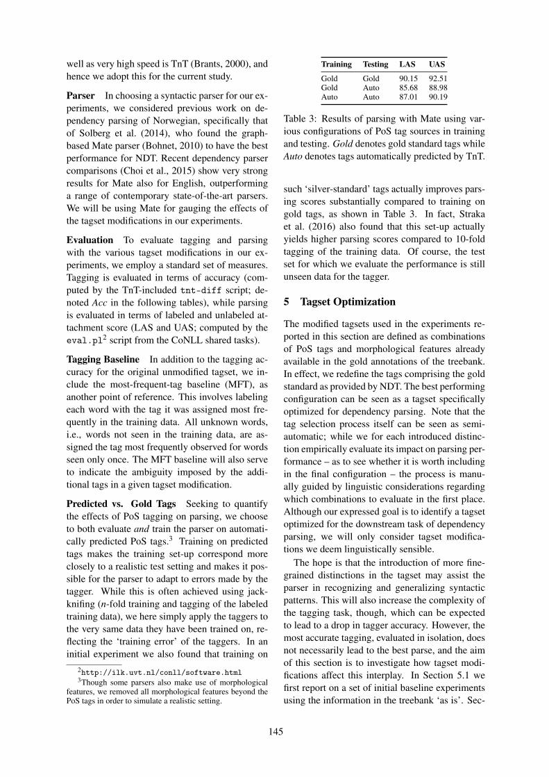
well as very high speed is TnT (Brants, 2000), andhence we adopt this for the current study.

Parser In choosing a syntactic parser for our ex-periments, we considered previous work on de-pendency parsing of Norwegian, specifically thatof Solberg et al. (2014), who found the graph-based Mate parser (Bohnet, 2010) to have the bestperformance for NDT. Recent dependency parsercomparisons (Choi et al., 2015) show very strongresults for Mate also for English, outperforminga range of contemporary state-of-the-art parsers.We will be using Mate for gauging the effects ofthe tagset modifications in our experiments.

Evaluation To evaluate tagging and parsingwith the various tagset modifications in our ex-periments, we employ a standard set of measures.Tagging is evaluated in terms of accuracy (com-puted by the TnT-included tnt-diff script; de-noted Acc in the following tables), while parsingis evaluated in terms of labeled and unlabeled at-tachment score (LAS and UAS; computed by theeval.pl2 script from the CoNLL shared tasks).

Tagging Baseline In addition to the tagging ac-curacy for the original unmodified tagset, we in-clude the most-frequent-tag baseline (MFT), asanother point of reference. This involves labelingeach word with the tag it was assigned most fre-quently in the training data. All unknown words,i.e., words not seen in the training data, are as-signed the tag most frequently observed for wordsseen only once. The MFT baseline will also serveto indicate the ambiguity imposed by the addi-tional tags in a given tagset modification.

Predicted vs. Gold Tags Seeking to quantifythe effects of PoS tagging on parsing, we chooseto both evaluate and train the parser on automati-cally predicted PoS tags.3 Training on predictedtags makes the training set-up correspond moreclosely to a realistic test setting and makes it pos-sible for the parser to adapt to errors made by thetagger. While this is often achieved using jack-knifing (n-fold training and tagging of the labeledtraining data), we here simply apply the taggers tothe very same data they have been trained on, re-flecting the ‘training error’ of the taggers. In aninitial experiment we also found that training on

2http://ilk.uvt.nl/conll/software.html3Though some parsers also make use of morphological

features, we removed all morphological features beyond thePoS tags in order to simulate a realistic setting.

Training Testing LAS UAS

Gold Gold 90.15 92.51Gold Auto 85.68 88.98Auto Auto 87.01 90.19

Table 3: Results of parsing with Mate using var-ious configurations of PoS tag sources in trainingand testing. Gold denotes gold standard tags whileAuto denotes tags automatically predicted by TnT.

such ‘silver-standard’ tags actually improves pars-ing scores substantially compared to training ongold tags, as shown in Table 3. In fact, Strakaet al. (2016) also found that this set-up actuallyyields higher parsing scores compared to 10-foldtagging of the training data. Of course, the testset for which we evaluate the performance is stillunseen data for the tagger.

5 Tagset Optimization

The modified tagsets used in the experiments re-ported in this section are defined as combinationsof PoS tags and morphological features alreadyavailable in the gold annotations of the treebank.In effect, we redefine the tags comprising the goldstandard as provided by NDT. The best performingconfiguration can be seen as a tagset specificallyoptimized for dependency parsing. Note that thetag selection process itself can be seen as semi-automatic; while we for each introduced distinc-tion empirically evaluate its impact on parsing per-formance – as to see whether it is worth includingin the final configuration – the process is manu-ally guided by linguistic considerations regardingwhich combinations to evaluate in the first place.Although our expressed goal is to identify a tagsetoptimized for the downstream task of dependencyparsing, we will only consider tagset modifica-tions we deem linguistically sensible.

The hope is that the introduction of more fine-grained distinctions in the tagset may assist theparser in recognizing and generalizing syntacticpatterns. This will also increase the complexity ofthe tagging task, though, which can be expectedto lead to a drop in tagger accuracy. However, themost accurate tagging, evaluated in isolation, doesnot necessarily lead to the best parse, and the aimof this section is to investigate how tagset modi-fications affect this interplay. In Section 5.1 wefirst report on a set of initial baseline experimentsusing the information in the treebank ‘as is’. Sec-

145

Tagset MFT Acc LAS UAS

Original 94.14 97.47 87.01 90.19Full 85.15 93.48 87.15 90.39

Table 4: Tagging and parsing our developmentsection of NDT with the two initial tagsets. Fromleft to right, we report the tagger accuracy of themost-frequent-tag baseline, the tagger accuracy ofTnT, and the labeled and unlabeled attachmentscore for the Mate parser.

tion 5.2 then details the results of tuning the selec-tion of tags for each word class in isolation, beforefinally discussing overall results for the completeoptimized tagset in Section 5.3.

5.1 Baseline Experiments

In an initial round of experiments, we concate-nated the tag of each token with its full set ofmorphological features, thereby mapping the orig-inal tagset to a new maximally fine-grained tagset,given the annotations available in the treebank.This resulted in a total of 368 tags, hereafter re-ferred to as the full tagset. The two initial tagsets,i.e., the original tagset comprising 19 tags andthe full tagset comprising 368 tags, thus repre-sent two extremes in terms of granularity. To es-tablish some initial points of reference for howtagset granularity affects the performance of tag-ging and parsing on NDT, we trained and tested afull pipeline with both of these initial tagsets. Theresults are reported in Table 4. Unsurprisingly, wesee that the tagger accuracy plummets when wemove from the original to the full tagset. Whilethe MFT baseline for the original tagset is 94.14%,it drops by almost 9 percentage points to 85.15%for the full tagset. Correspondingly, TnT achieves97.47% and 93.48% accuracy for the original andfull tagset, respectively. These results confirm ourhypothesis that the high level of linguistic infor-mation in the full, fine-grained tagset comes at theexpense of reduced tagger performance. In spiteof this drop, however, we see that the additionalinformation in the full tagset still improves theparser performance. With the original tagset, Mateachieves 87.01% LAS and 90.19% UAS, whichfor the full tagset increases to 87.15% and 90.39%,respectively. These preliminary results are encour-aging in indicating that the additional linguistic in-formation assists the syntactic parser, motivatingfurther optimization of the tagset.

5.2 Tagset ExperimentsWe modify the tags for nouns (subst), verbs(verb), adjectives (adj), determiners (det) andpronouns (pron) in NDT by appending selectedsets of morphological features to each tag in orderto increase the linguistic information expressed bythe tags. For each tag, we in turn first experi-ment with each of the available features in isola-tion before testing various combinations. We baseour choices of combinations on how promising thefeatures are in isolation and what we deem worthinvestigating in terms of linguistic utility.

The morphological properties of the variousparts-of-speech are reflected in the morphologicalfeatures associated with the respective PoS tags.For instance, as nouns in Norwegian inflect forgender, definiteness and number, the treebank op-erates with additional features for these properties.In addition to morphological properties such asdefiniteness, tense and number, all classes exceptfor verbs have a type feature that provides infor-mation about the subtype of the PoS, e.g., whethera noun is common or proper.

Nouns In Norwegian, nouns are assigned gen-der (feminine, masculine or neuter), definiteness(definite or indefinite) and number (singular orplural). There is agreement in gender, definite-ness and number between nouns and their modi-fiers (i.e., adjectives and determiners). Addition-ally, NDT has a separate case feature for distin-guishing nouns in genitive case. Genitive casemarks possession, hence nouns marked with geni-tive case are quite different from other nouns, tak-ing a noun phrase as complement. Distinguishingon type can be useful, as evident by the presenceof separate tags for proper and common nouns inmany tagsets, such as those of Penn Treebank andStockholm-Umeå corpus.

The results for tagset modifications for nounsare shown in Table 5 and reveal that, apart fromcase, none of the tagset modifications improvetagging. However, they all result in increases inparser accuracy. The most informative featuresare definiteness, with an increase in LAS of 1.26percentage points to 88.27%, and type, yieldingan LAS of 88.07%. Turning to combinations offeatures, we found that the combination of typeand case, as well as type and definiteness, werethe most promising, which led us to combine type,case and definiteness in a final experiment, result-ing in LAS of 88.81% and UAS of 91.73%. This

146

Feature(s) Acc LAS UAS

— 97.47 87.01 90.19Case 97.48 87.63 90.72Definiteness 97.00 88.27 91.42Gender 96.09 87.21 90.36Number 96.37 87.97 91.00Type 96.92 88.07 91.11Case & definiteness 97.03 88.39 91.44Type & case 96.92 88.46 91.51Type & definiteness 96.99 88.44 91.48Type, case & definiteness 97.05 88.81 91.73

Table 5: Tagging and parsing with modified PoStags for nouns. The first row corresponds to usingthe original tagset unmodified.

constitutes an improvement of 1.80 percentagepoints and 1.54 percentage points, respectively.

Verbs Verbs are inflected for tense (infinitive,present, preterite or past perfect) in Norwegianand additionally exhibit mood (imperative or in-dicative) and voice (active or passive). Note thatboth voice and mood have only a single value inthe treebank; pass (passive) and imp (imperative),respectively. Verbs which are not passive are im-plicitly active, and verbs which are not imperativeare in indicative mood.

Table 6 presents the results from tagging andparsing with modified verb tags. Imperativeclauses are fundamentally different from indica-tive clauses as they lack an overt subject, whichis reflected in the fact that mood is the only fea-ture leading to an increase in LAS, with a reportedLAS of 87.04%. Although voice is a very distin-guishing property for verbs, and passive clausesare very different from active clauses, introduc-ing this distinction in the tagset leads to a dropin LAS of 0.05 percentage points, while distin-guishing between the various tenses yields an LASof 86.97%. Combining the two most promisingfeatures of mood and tense resulted in an LAS of87.12% and UAS of 90.31%.

In an additional experiment, we mapped theverb tenses (and mood, in the case of imperative)to finiteness. All verbs have finiteness, hence thisdistinction has broad coverage. This mapping issyntactically grounded as finite verbs and nonfi-nite verbs appear in very different syntactic con-structions, and proved to improve parsing witha 0.29 and 0.24 percentage points improvementover the baseline, for LAS and UAS, respectively.This coincides with the previous observations for


— 97.47 87.01 90.19Mood 97.43 87.04 90.19Tense 97.30 86.97 90.18Voice 97.45 86.96 90.09Mood & tense 97.31 87.12 90.31Voice & tense 97.28 86.99 90.15Mood, tense & voice 97.27 86.83 90.05Finiteness 97.35 87.30 90.43

Table 6: Tagging and parsing with modified PoStags for verbs.


— 97.47 87.01 90.19Definiteness 96.84 87.14 90.29Degree 97.41 87.29 90.44Gender 96.89 87.10 90.25Number 96.71 86.99 90.10Type 97.40 87.11 90.25Definiteness & degree 96.81 87.23 90.39Definiteness & gender 96.31 87.18 90.39Definiteness & number 96.78 87.27 90.44

Table 7: Tagging and parsing with modified PoStags for adjectives.

Swedish in Øvrelid (2008), where finiteness wasfound to be a very beneficial feature for parsing.

Adjectives Adjectives agree with the noun theymodify in terms of gender, number and definite-ness. Furthermore, adjectives are inflected for de-gree (positive, comparative or superlative).

Table 7 shows the results of modifying the prontag in NDT. All features except for number lead toincreases in parser accuracy scores, the most suc-cessful of which is degree with a reported LAS of87.29%, while distinguishing adjectives on defi-niteness yields an LAS of 87.14% and introducingthe distinction of gender leads to LAS of 87.10%.

Turning to combinations of features, definite-ness and number achieve the best parser accuracyscores, very close to those of degree. Adjectivesagree with their head noun and determiner in defi-niteness and number, making this an expected im-provement. The combination of definiteness anddegree is also quite promising, obtaining LAS of87.23% and UAS of 90.39%. It is interesting thatnone of the combinations surpass the experimentwith degree in isolation, which indicates that de-gree does not interact with the other features inany syntactically significant way.

Determiners Like adjectives, determiners inNorwegian agree with the noun they modify in

147

Feature Acc LAS UAS

— 97.47 87.01 90.19Definiteness 97.49 87.30 90.42Gender 97.28 87.09 90.31Number 97.49 87.04 90.18Type 97.61 87.00 90.11

Table 8: Tagging and parsing with modified PoStags for determiners.

terms of gender, number and definiteness.The results from the experiments with determin-

ers are shown in Table 8. Introducing the dis-tinction of type (demonstrative, amplifier, quanti-fier, possessive or interrogative) led to an increasein tagger accuracy of 0.14 percentage points to97.61%, while marginally impacting the parsing,with LAS of 87.00%, 0.01 percentage points be-low that of the original tagset. The increase in tag-ger accuracy when introducing the distinction oftype is noteworthy, as we expected the finer granu-larity to lead to a decrease in accuracy. This servesto indicate that more fine-grained distinctions fordeterminers, which is a quite disparate category inthe treebank, may be quite useful for tagging.

Gender, on the other hand, improved parsing(87.09% LAS), but complicated tagging, as thevarious genders are often difficult to differenti-ate, in particular masculine and feminine, whichshare many of the same forms. The number ofa determiner, i.e., singular or plural, led to asmall increase in tagger accuracy and LAS, whilemarginally lower UAS. The introduction of def-initeness gave the best parsing results, LAS of87.30% and UAS of 90.42%, and additionally in-creased tagger accuracy slightly. The increase inLAS and UAS is rather interesting, as there areonly 121 determiner tokens with marked definite-ness in the development data. As this accounts fora very small number of tokens, we did not con-sider further fine-grained modifications with defi-niteness. This result further underlines the impor-tance of definiteness for parsing of Norwegian.

Pronouns Pronouns in Norwegian include per-sonal, reciprocal, reflexive and interrogative. Theycan furthermore exhibit gender, number and per-son, while personal pronouns can be distinguishedby case (either accusative or nominative).

The results in Table 9 show that number, per-son and type are the most useful features for pars-ing, with LAS of 87.21%, 87.22% and 87.19%,respectively. However, when combining number


— 97.47 87.01 90.19Case 97.50 87.08 90.21Gender 97.48 87.06 90.23Number 97.49 87.21 90.33Person 97.49 87.22 90.32Type 97.48 87.19 90.40Number & person 97.49 96.98 90.16Type & case 97.51 87.30 90.41Type & number 97.49 87.27 90.41Type & person 97.49 87.00 90.14Type, case & number 97.52 87.11 90.36

Table 9: Tagging and parsing with modified PoStags for pronouns.

and person, we observe a drop of more than 0.2percentage points, indicating that these features donot interact in any syntactically distinctive way.The most interesting observation is that all resultsexceed the tagging accuracy of the original tagset,with the most fine-grained distinction (type, caseand number combined) provides the largest im-provement (accuracy of 97.52%). This shows thatthe introduction of more fine-grained distinctionsfor pronouns aids the PoS tagger in disambiguat-ing ambiguous words. While case alone yields anLAS of 87.08%, we found that the combination oftype and case yields the second highest tagging ac-curacy of 97.51%. Pronouns of different type andpersonal pronouns of different case exhibit quitedifferent properties and appear in different con-structions. Pronouns in nominative case (i.e., sub-jects) primarily occur before the main verb, whilepronouns in accusative case (i.e., objects) occur af-ter the main verb, as Norwegian exhibits so-calledV2 word order, requiring that the finite verb of adeclarative clause appears in the second position.

5.3 Optimized Tagset

Category Feature(s) MFT Acc LAS

Original — 94.14 97.47 87.01Noun Type, case, def. 89.61 97.05 88.81Verb Finiteness 93.72 97.35 87.30Adjective Degree 94.13 97.41 87.29Determiner Definiteness 94.13 97.49 87.30Pronoun Type, case 94.12 97.51 87.30

Table 10: Results of tagging and parsing with thebest tagset modification for each category.

The most successful tagset modification foreach PoS and the results from tagging and pars-ing with the respective modifications are seen inTable 10. Nouns benefit by far the most from

148

Tag Description

adj|komp Comparative adjectiveadj|pos Positive adjectiveadj|sup Superlative adjectivedet|be Definite determinerdet|ub Indefinite determinerpron|pers Personal pronounpron|pers|akk Personal pron., accusativepron|pers|nom Personal pron., nominativepron|refl Reflexive pronounpron|res Reciprocal pronounpron|sp Interrogative pronounsubst|appell Common nounsubst|appell|be Common noun, def.subst|appell|be|gen Common noun, def., genitivesubst|appell|ub Common noun, indef.subst|appell|ub|gen Common noun, indef., gen.subst|prop Proper nounsubst|prop|gen Proper noun, genitiveverb|fin Finite verbverb|infin Nonfinite verb

Table 11: Overview of the optimized tagset.

the introduction of more fine-grained linguisticallymotivated distinctions, with an LAS of 88.81%and UAS of 91.73% when distinguishing on type,case and definiteness. We observe that the mostpromising tagset modifications for verbs, adjec-tives, determiners and pronouns all reach LAS of~87.30% and UAS of ~90.40%. To investigatethe overall effect of these tagset modifications, wetested each of the improvements in parser accuracyscores from those of the original tagset for statis-tical significance using Dan Bikel’s randomizedparsing evaluation comparator script4, as used inthe CoNLL shared tasks. For the most successfultagset modification for each of the categories seenin Table 10, the difference in LAS from the origi-nal tagset is statistically significant at significancelevel 0.05 (p-value < 0.05), as are all differencesin UAS, except for verbs with finiteness (p=0.15)and pronouns with type and case (p=0.06).

An overview of the tags in the optimized tagsetcan be seen in Table 11, comprising three new tagsfor adjectives, two for determiners, six for pro-nouns, seven for nouns and two for verbs, total-ing 20 tags. Appending these to the original tagsetcomprising 19 tags, we reach a total of 39 tags.

Final Evaluation In Table 12, we show the re-sults of parsing with the optimized tagset on theheld-out test data and the development data, com-pared to the results obtained with the original

4Available as compare.pl at http://ilk.uvt.nl/conll/software.html

Data Tagset MFT Acc LAS UAS

Dev Original 94.14 97.47 87.01 90.19Optimized 85.15 96.85 88.87 91.78

Test Original 94.22 97.30 86.64 90.07Optimized 88.08 96.35 88.55 91.41

Table 12: Results of tagging and parsing with theoptimized tagset, compared to the original NDTcoarse tagset. The parser is both trained and testedusing automatically predicted tags from TnT.

tagset. We see significant improvements from theoriginal tagset on both the development data andthe held-out test data set. The improvement inLAS on the development data is 1.86 percentagepoints, while 1.91 percentage points on the held-out test data. These results indicate that the addi-tional linguistic information in the tags of our opti-mized tagset benefits the task of syntactic parsing.

6 Summary

This paper has reported on a range of experimentswith injecting more fine-grained morphologicaldistinctions into an existing PoS tagset, and thenempirically evaluating the effects both (intrinsi-cally) in terms of tagging accuracy and (extrinsi-cally) in terms of parsing accuracy. Our experi-mental results – based on the annotations of theNorwegian Dependency Treebank and using theTnT PoS tagger and the Mate dependency parser –show that the enriched tag set leads to significantlyimproved parsing accuracy, even though taggingaccuracy in isolation is reduced. We also observethat the improvements are more pronounced thanin related previous studies for other languages.The modified tagsets in our experiments are de-fined as combinations of PoS tags and morpho-logical features, using only information that is al-ready available in the gold annotations of the tree-bank. The best performing tag configuration isin effect a PoS tagset optimized for dependencyparsing of Norwegian. While we expect that tagsthat prove informative for parsing will be usefulfor also other downstream applications, one can ofcourse follow the same methodology to optimizea tagset specifically for other applications instead,by using another task for the extrinsic evaluation,such as sentiment analysis, named entity recogni-tion or any other task making use of tagged data.

149

ReferencesBernd Bohnet. 2010. Very High Accuracy and Fast

Dependency Parsing is not a Contradiction. In Pro-ceedings of the 23rd International Conference onComputational Linguistics, pages 89–97, Beijing,China.

Thorsten Brants. 2000. TnT - A Statistical Part-of-Speech Tagger. In Proceedings of the Sixth AppliedNatural Language Processing Conference, Seattle,WA, USA.

Jinho D. Choi, Joel Tetreault, and Amanda Stent. 2015.It Depends: Dependency Parser Comparison Us-ing A Web-Based Evaluation Tool. In Proceedingsof the 53rd Annual Meeting of the Association forComputational Linguistics, pages 387–396, Beijing,China.

Jan Terje Faarlund, Svein Lie, and Kjell Ivar Vannebo.1997. Norsk referansegrammatikk. Universitetsfor-laget, Oslo, Norway.

Sofia Gustafson-Capková and Britt Hartmann, 2006.Manual of the Stockholm Umeå Corpus version 2.0.Stockholm, Sweden.

Kristin Hagen, Janne Bondi Johannessen, and An-ders Nøklestad. 2000. A Constraint-Based Taggerfor Norwegian. In Proceedings of the 17th Scan-dinavian Conference of Linguistics, pages 31–48,Odense, Denmark.

Jan Hajic, Massimiliano Ciaramita, Richard Johans-son, Daisuke Kawahara, Maria Antònia Martí, LluísMàrquez, Adam Meyers, Joakim Nivre, SebastianPadó, Jan Stepanek, Pavel Straaàk, Mihai Surdeanu,Nianwen Xue, and Yi Zhang. 2009. The CoNLL-2009 Shared Task: Syntactic and Semantic Depen-dencies in Multiple Languages. In Proceedings ofthe Thirteenth Conference on Computational Natu-ral Language Learning, pages 1–18, Boulder, CO,USA.

Andrew MacKinlay. 2005. The Effects of Part-of-Speech Tagsets on Tagger Performance. Bachelor’sthesis, University of Melbourne, Melbourne, Aus-tralia.

Wolfgang Maier, Sandra Kübler, Daniel Dakota, andDaniel Whyatt. 2014. Parsing German: How muchmorphology do we need? In Proeceedings of theFirst Joint Workshop on Statistical Parsing of Mor-phologically Rich Languages and Syntactic Analysisof Non-Canonical Languages, pages 1–14, Dublin,Ireland.

Christopher Manning. 2011. Part-of-Speech Taggingfrom 97% to 100%: Is It Time for Some Linguistics?In Proceedings of the 12th International Conferenceon Computational Linguistics and Intelligent TextProcessing, pages 171–189.

Mitchell Marcus, Beatrice Santorino, and Mary AnnMarcinkiewicz. 1993. Building A Large Annotated

Corpus of English: The Penn Treebank. Technicalreport, University of Philadelphia, Philadelphia, PA,USA.

Beáta Megyesi. 2002. Data-Driven Syntactic Analy-sis: Methods and Applications for Swedish. Ph.D.thesis, Royal Institute of Technology, Stockholm,Sweden.

Thomas Müller, Richard Farkas, Alex Judea, HelmutSchmid, and Hinrich Schütze. 2014. Dependencyparsing with latent refinements of part-of-speechtags. In Proceedings of the 2014 Conference on Em-pirical Methods in Natural Language Processing,pages 963–967, Doha, Qatar.

Joakim Nivre, Johan Hall, Sandra Kübler, Ryan Mc-Donald, Jens Nilsson, Sebastian Riedel, and DenizYuret. 2007. The CoNLL 2007 Shared Task onDependency Parsing. In Proceedings of the CoNLLShared Task Session of EMNLP-CoNLL 2007, pages915–932, Prague, the Czech Republic.

Lilja Øvrelid. 2008. Finite Matters: Verbal Features inData-Driven Parsing of Swedish. In Proceedings ofthe Sixth International Conference on Natural Lan-guage Processing, Gothenburg, Sweden.

Slav Petrov, Dipanjan Das, and Ryan McDonald. 2012.A Universal Part-of-Speech Tagset. In Proceedingsof the Eighth International Conference on LanguageResources and Evaluation, pages 2089–2096, Istan-bul, Turkey.

Ines Rehbein and Hagen Hirschmann. 2013. POStagset refinement for linguistic analysis and the im-pact on statistical parsing. In Proceedings of the13th International Workshop on Treebanks and Lin-guistic Theories, pages 172–183, Tübingen, Ger-many.

Erik F. Tjong Kim Sang and Fien De Meulder.2003. Introduction to the CoNLL-2003 SharedTask: Language-Independent Named Entity Recog-nition. In Proceedings of the Seventh Conference onNatural Language Learning at HLT-NAACL 2003,pages 142–147, Stroudsburg, PA, USA.

Djamé Seddah, Marie Candito, and Benoît Crabbé.2009. Cross parser evaluation and tagset variation:A french treebank study. In Proceedings of the 11thInternational Conference on Parsing Technologies,IWPT ’09, pages 150–161, Stroudsburg, PA, USA.Association for Computational Linguistics.

Djamé Seddah, Reut Tsarfaty, Sandra Kübler, MarieCandito, Jinho D. Choi, Richard Farkas, JenniferFoster, Iakes Goenaga, Koldo Gojenola Gallete-beitia, Yoav Goldberg, Spence Green, Nizar Habash,Marco Kuhlmann, Wolfgang Maier, Yuval Mar-ton, Joakim Nivre, Adam Przepiorkowski, RyanRoth, Wolfgang Seeker, Yannick Versley, VeronikaVincze, Marcin Wolinski, and Alina Wroblewska.2013. Overview of the spmrl 2013 shared task: Across-framework evaluation of parsing morphologi-cally rich languages. In Proceedings of the Fourth

150

Workshop on Statistical Parsing of MorphologicallyRich Languages, pages 146–182, Seattle, USA.

Wolfgang Seeker and Jonas Kuhn. 2013. Morpho-logical and Syntactic Case in Statistical DependencyParsing. Computational Linguistics, 39(1):23–55.

Per Erik Solberg, Arne Skjærholt, Lilja Øvrelid, KristinHagen, and Janne Bondi Johannessen. 2014. TheNorwegian Dependency Treebank. In Proceedingsof the Ninth International Conference on LanguageResources and Evaluation, pages 789–795, Reyk-javik, Iceland.

Per Erik Solberg. 2013. Building Gold-StandardTreebanks for Norwegian. In Proceedings of the19th Nordic Conference of Computational Linguis-tics, pages 459–464, Oslo, Norway.

Milan Straka, Jan Hajic, and Jana Straková. 2016. UD-Pipe: trainable pipeline for processing CoNLL-Ufiles performing tokenization, morphological anal-ysis, pos tagging and parsing. In Proceedings ofthe Tenth International Conference on Language Re-sources and Evaluation, Portorož, Slovenia.

Reut Tsarfaty, Djamé Seddah, Yoav Goldberg, San-dra Kübler, Marie Candito, Jennifer Foster, Yan-nick Versley, Ines Rehbein, and Lamia Tounsi.2010. Statistical parsing of morphologically richlanguages (SPMRL): what, how and whither. InProceedings of the NAACL HLT 2010 First Work-shop on Statistical Parsing of Morphologically-RichLanguages.

Theresa Wilson, Janyce Wiebe, and Paul Hoffman.2009. Recognizing Contextual Polarity: An Explo-ration of Features for Phrase-Level Sentiment Anal-ysis. Computational Linguistics, 35(3):399–433.

Yue Zhang and Joakim Nivre. 2011. Transition-BasedDependency Parsing with Rich Non-Local Features.In Proceedings of the 49th Annual Meeting of theAssociation for Computational Lingustics: HumanLanguage Technologies, pages 188–193, Portland,OR, USA.

151


Creating register sub-corpora for the Finnish Internet Parsebank

Veronika Laippala1,2,3, Juhani Luotolahti3,Aki-Juhani Kyrolainen2,3, Tapio Salakoski3, Filip Ginter3

1 Turku Institute for Advanced Studies, University of Turku, Finland2 School of Languages and Translation Studies, University of Turku, Finland

3 Turku NLP Group, University of Turku, [email protected]

Abstract

This paper develops register sub-corporafor the Web-crawled Finnish InternetParsebank. Currently, all the documentsbelonging to different registers, such asnews and user manuals, have an equal sta-tus in this corpus. Detecting the text reg-ister would be useful for both NLP andlinguistics (Giesbrecht and Evert, 2009)(Webber, 2009) (Sinclair, 1996) (Egbertet al., 2015). We assemble the sub-corpora by first naively deducing four reg-ister classes from the Parsebank docu-ment URLs and then developing a clas-sifier based on these, to detect registersalso for the rest of the documents. Theresults show that the naive method of de-ducing the register is efficient and that theclassification can be done sufficiently reli-ably. The analysis of the prediction errorshowever indicates that texts sharing sim-ilar communicative purposes but belong-ing to different registers, such as news andblogs informing the reader, share similarlinguistic characteristics. This attests ofthe well-known difficulty to define the no-tion of registers for practical uses. Finally,as a significant improvement to its usabil-ity, we release two sets of sub-corpus col-lections for the Parsebank. The A col-lection consists of two million documentsclassified to blogs, forum discussions, en-cyclopedia articles and news with a naiveclassification precision of >90%, and theB collection four million documents witha precision of >80%.

1 Introduction

The Internet offers a constantly growing source ofinformation, not only in terms of size, but also

in terms of languages and communication set-tings it includes. As a consequence, Web cor-pora, language resources developed by automati-cally crawling the Web, offer revolutionary poten-tials for fields using textual data, such as NaturalLanguage Processing (NLP), linguistics and otherhumanities (Kilgariff and Grefenstette, 2003).

Despite their potentials, Web corpora are under-used. One of the important reasons behind thisis the fact that in the existing Web corpora, all ofthe different documents have an equal status. Thiscomplicates their use, as for many applications,knowing the composition of the corpus would bebeneficial. In particular, it would be important toknow what registers, i.e. text varieties such as auser manual or a blog post, the corpus consists of(see Section 2 for a definition). In NLP, detectingthe register of a text has been noted to be usefulfor instance in POS tagging (Giesbrecht and Ev-ert, 2009), discourse parsing (Webber, 2009) andinformation retrieval (Vidulin et al., 2007). In lin-guistics, the correct constitution of a corpus andthe criteria used to assemble it have been subjectto long discussions (Sinclair, 1996), and Egbert &al. (2015) note that without systematic classifica-tion, Web corpora cannot be fully benefited from.

In this paper, we explore the development ofregister sub-corpora for the Finnish Internet Parse-bank1, a Web-crawled corpus of Internet Finnish.We assemble the sub-corpora by first naively de-ducing four register classes from the Parsebankdocument URLs and then creating a classifierbased on these classes to detect texts represent-ing these registers from the rest of the Parsebank(see Section 4). The register classes we developare news, blogs, forum discussions and encyclo-pedia articles. Instead of creating a full-coveragetaxonomy of all the registers covered by the Parse-bank, in this article our aim is to test this method in

1http://bionlp.utu.fi

152

the detection of these four registers. If the methodworks, the number of registers will be extended infuture work.

In the register detection and analysis, we com-pare three methods: the traditional bag-of-wordsas a baseline, lexical trigrams as proposed by Gries& al. (2011), and Dependency Profiles (DP), co-occurrence patterns of the documents labelled in aspecific class, assumed a register, and dependencysyntax relations.

In addition to reporting the standard metricsto estimate the classifier performance, we eval-uate the created sub-corpora by analysing themismatches between the naively assumed regis-ter classes and the classifier predictions. In ad-dition, we analyse the linguistic register charac-teristics estimated by the classifier. This validatesthe quality of the sub-corpora and is informativeabout the linguistic variation inside the registers(see Section 5).

Finally, we publish four register-specific sub-corpora for the Parsebank that we develop in thispaper: blogs, forum discussions, encyclopedia ar-ticles and news (see Section 6). We release twosets of sub-corpora: the A collection consists oftwo million documents with register-specific la-bels. For these documents, we estimate the reg-ister prediction precision to be >90%. The col-lection B consists of four million documents. Forthese, the precision is >80%. These sub-corporaallow the users to focus on specific registers,which improves the Parsebank usability signifi-cantly (see discussions in (Egbert et al., 2015) and(Asheghi et al., 2016)).

2 Previous studies

Since the 1980s, linguistic variation has been stud-ied in relation to the communicative situation,form and function of the piece of speech or writingunder analysis (Biber, 1989; Biber, 1995; Biberet al., 1999; Miller, 1984; Swales, 1990). De-pending on the study, these language varieties areusually defined as registers or genres, the defini-tions emphasising different aspects of the variation(see discussion in (Asheghi et al., 2016; Egbertet al., 2015). We adopt the term register and de-fine it, following (Biber, 1989; Biber, 1995; Egbertet al., 2015), as a text variety with specific situa-tional characteristics, communicative purpose andlexico-grammatical features.

Studies aiming at automatically identifying reg-

isters from the Web face several challenges. Al-though some studies reach a very high accuracy,their approaches are very difficult to apply in real-world applications. Other studies, adopting a morerealistic approach, present a weaker performance.In particular, the challenges are related to the def-inition of registers in practice: how many of themshould there be, and how to reliably identify them?In addition, it is not always clear whether registershave different linguistic properties (Schafer andBildhauer, 2016). Based on the situational char-acteristics of a register, a blog post discussing anews topic and a news article on the same topicshould be analysed as different registers. But howdoes this difference show in the linguistic featuresof the documents, or does it?

For instance, Sharoff & al. (2010) achieve anaccuracy of 97% using character tetragrams andsingle words with a stop list as classification fea-tures, while Lindemann & Littig (2011) reportan F-score of 80% for many registers using bothstructural Web page features and topical charac-teristics based on the terms used in the documents.They, however, use as corpora only samples of theWeb, which can represent only a limited portionof all the registers of the entire Web (Sharoff etal., 2010; Santini and Sharoff, 2009).

Another, more linguistically motivated perspec-tive to study Web registers is adopted by Biberand his colleagues. Using typical end users ofthe Web to code a large number of nearly ran-dom Web documents (48 000) with hierarchical,situational characteristics, they apply a bottom-upmethod for creating a taxonomy of Web registers(Biber et al., 2015; Egbert et al., 2015). Then,applying a custom built tagger identifying 150+lexico-grammatical features, they report an over-all accuracy of 44.2% for unrestricted Web textsusing a taxonomy of 20 registers (Biber and Eg-bert, 2015). In addition to the relatively weakregister identification performance, their approachsuffers from a low interannotator agreement forthe register classes. Similar problems are alsodiscussed in (Crowston et al., 2011; Essen andStein, 2004), who note that both experts and endusers have troubles identifying registers reliably.This leads to question, whether register identifi-cation can at all be possible, if even humans can-not agree on their labelling. This concern is ex-pressed by Schafer and Bildhauer (2016), who de-cide to focus on classifying their COW Corpora

153

Figure 1: Unlexicalised syntactic biarcs from the sentence Ja haluaisitko kehittaa kielitaitoasi? ’Andwould you like to improve your language skills?’

to topic domains, such as medical or science in-stead of registers. The recently presented LeedsWeb Genre Corpus (Asheghi et al., 2016) shows,however, very reliable interannotator agreementscores. This proves that when the register taxon-omy is well developed, the registers can as well bereliably identified.

3 Finnish Internet Parsebank

Finnish Internet Parsebank (Luotolahti et al.,2015) is a Web-crawled corpus on the Finnish In-ternet. The corpus is sampled from a Finnish Web-crawl data. The crawl itself is produced using Spi-derLing Crawler, which is especially crafted forefficient gathering of unilingual corpora for lin-guistic purposes. The version we used is com-posed of 3.7 billion tokens, 6,635,960 documentsand has morphological and dependency syntax an-notations carried out with a state-of-the-art de-pendency parser by Bohnet (2010), with a la-belled attachment score of 82.1% (Luotolahti etal., 2015). The Parsebank is distributed via a userinterface at bionlp-www.utu.fi/dep_search/and as a downloadable, sentence-shuffled versionat bionlp.utu.fi.

4 Detecting registers from the Parsebank

In this Section, we first discuss the developmentof the naive register corpora from the Parsebank.These will be used as training data for the systemidentifying the registers from the entire Parsebank.We then motivate our selection of features in theclassifier development, and finally, we present theclassification results.

4.1 Naive registers as training data

Our naive interpretation of the document registerswas based on the presence of lexical cues in theParsebank document URLs. For the purposes ofthis article, we used four well-motivated registerclasses: news, blogs, encyclopedia and forum dis-cussions. These were identified by the presence of

Naive register Entire PB Training subsetBlogs 775,885 8,364Forum discussions 307,797 3,076Encyclopedia 127,884 1,580News 771,058 13,197All 1,982,624 26,217

Table 1: Total number of documents in the naivelyassembled register classes and in the subset usedin SVM training

the following keywords in the URL: lehti ‘news-paper’, uutis ‘news’, uutinen ‘news’ or news forthe news class; wiki for the encyclopedia class;blog for the blog class; and discussion, forum orkeskustelu ‘discussion’ for the discussion class.

In deciding the registers to be searched for,we aimed at a simple, experimental solution thatwould be informative about the performance ofthe naive method and offer direct application po-tentials for the Parsebank to increase its usability.Therefore, instead of creating a full-coverage tax-onomy of all registers possibly found online, ouraim here was to experiment with a few generallyacknowledged, broad-coverage terms for registerclasses. Once we can in this paper show that thenaive method works, the number of the registerswill be expanded in future work.

Table 1 presents the proportion of the naivelyassumed registers in the entire Parsebank and inthe subset we use for the classifier training in Sec-tion 4.3. The sizes of the retrieved sub-corporavary significantly. The most frequent, news andblogs, cover more than 10% of the Parsebank doc-uments, respectively, while in particular the ency-clopedia corpus remains smaller. Still, the sizes ofthese classes are relatively large, thanks to the sizeof the entire Parsebank.

The subset used for the classifier training is cre-ated by matching the document URLs of 100,000first documents from the Parsebank. Of these,26,216 had a URL that matched one of the key-words defined above. At this stage, all sentence-level duplicates were also removed from the train-

154

ing data to prevent the classifier from learning el-ements that are often repeated in Web pages, suchas Lue lisaa ‘Read more’ but should not be usedas classifier features. This proved to be highlyneeded, as from the 3,421,568 sentences in the100,000 documents, 497,449 were duplicates.

4.2 Lexical and syntactic approaches tomodel register variation

The work by Biber and colleagues on the variationof lexico-grammatical features across registers hasbeen very influential in corpus linguistics over theyears (Biber, 1995; Biber et al., 1999). Recently,they have extended their work to Web registers andapplied the carefully tuned Biber tagger identify-ing both lexical and grammatical features to ex-plore registers from the Web (Biber et al., 2015;Egbert et al., 2015). Gries & al. (2011) adopt anopposite approach by using simple word-trigrams.Sharoff and colleagues compare a number of dif-ferent feature sets and conclude that bag-of-wordsand character n-grams achieve the best results(Sharoff et al., 2010). For detecting mostly the-matic domains, Schafer and Bildhauer (2016) ap-ply lexical information attached to coarse-grainedpart-of-speech labels.

We compare three methods for detecting thefour registers represented by our naively assem-bled sub-corpora. As a baseline method, we ap-ply the standard bag-of-words, which, despite itssimplicity, has often achieved a good performance(Sharoff et al., 2010). Second, we use word-trigrams similar to Gries & al. (2011), and fi-nally, Dependency Profiles (DPs), which are co-occurrences of the register documents with unlex-icalised syntactic biarcs, three-token subtrees ofdependency syntax analysis with the lexical infor-mation deleted (Kanerva et al., 2014) (see Figure1). As opposed to e.g. keyword analysis (Scott andTribble, 2006) based on the document words, DPsdo not restrict to the lexical or topical aspects oftexts, and thus offer linguistically better motivatedanalysis tools. Many studies on register variationhighlight the importance of syntactic and gram-matical features (Biber, 1995; Biber et al., 1999;Gries, 2012). Therefore, we hypothesise that DPswould allow to generalise beyond individual top-ics to differentiate, e.g., between texts represent-ing different registers but discussing similar top-ics, such as news and forum discussions on sports.

4.3 Classifier development and testing

To predict the registers for all the Parsebank doc-uments, we trained a linear SVM. In the trainingand testing, we used a subset of the Parsebank de-scribed in Table 1. As features, we used the setsdescribed in the previous Section. Specifically, thefour register classes were modelled as a functionof the feature sets, i.e. a co-occurence vector of theused features across the documents. These vec-tors were L2-normalised and then used to modelthe register class of a given document by fittinga linear SVM to the data, as implemented in theScikit package2 in Python. To validate the per-formance of the fitted model, we implemented a10-fold cross-validation procedure with stratifiedrandom subsampling to keep the proportion of theregister classes approximately equal between thetraining and test sets.

The results of the SVM performance are de-scribed in Table 2. First, the best results areachieved with the bag-of-words and lexical n-gram approaches with an F-score of 80 % and81%. This already confirms that the registers canbe identified and that our naive method of assum-ing the registers based on the URLs is justified.

Second, although the DPs consisting of syntac-tic biarcs would allow for detailed linguistic ex-aminations of the registers, and even if they fol-low the influential work by Biber and colleagueson modelling registers, their classification perfor-mance is clearly lower than those of the lexicalapproaches. The average F-score for the biarcs isonly 72%. Interestingly, combining biarcs and thebag-of-words results in a very similar F-score of79% and does not improve the classifier perfor-mance at all. In other words, three of the four fea-ture sets attest very similar performances. This cansuggest that the remaining 20% of the data may besomehow unreachable with these feature sets andrequires further data examination, which we willpresent in Section 5.1 and 5.2.

Third, it is noteworthy that the classifier perfor-mance varies clearly across the registers. Newsand blogs receive the best detection rates, risingto the very reliable 86% and 79% F-score, respec-tively, while the discussion and encyclopedia ar-ticle detection rates are clearly lower, 70% and73%. Naturally, the higher frequency of blogs andnews in the training and test set explains some ofthese differences. Still, these differences merit fur-

2http://scikit-kearn.org/stable/

155

Blog Discussion Encyclopedia News Avg.Bag-of-wordsPrecision 0.80 0.66 0.69 0.86 0.81Recall 0.76 0.73 0.74 0.86 0.80F-score 0.78 0.69 0.71 0.86 0.80BiarcsPrecision 0.70 0.50 0.43 0.83 0.73Recall 0.66 0.47 0.60 0.83 0.72F-score 0.68 0.48 0.51 0.82 0.72Bag-of-words + biarcsPrecision 0.78 0.63 0.65 0.86 0.80Recall 0.75 0.69 0.73 0.85 0.79F-score 0.76 0.66 0.69 0.85 0.79Uni- bi - trigramsPrecision 0.81 0.68 0.71 0.86 0.81Recall 0.77 0.73 0.75 0.86 0.81F-score 0.79 0.70 0.73 0.86 0.81

Table 2: The SVM results achieved with the four feature sets.

ther analyses in future work.Finally, the variation between the precision and

recall rates across the registers requires closer ex-amination. While the precision and recall are verysimilar for the news class, for the blogs the preci-sion is higher than the recall. This suggests thatsome features, words in this case, are very reli-able indicators of the blog register, but that theydo are not present in all the class documents. Forthe discussion and encyclopedia classes, the recallis higher than the precision, indicating that suchreliable indicators are less frequent.

5 Validating the classifier quality

The classifier performance seems sufficiently reli-able to be applied for identifying the registers fromthe Parsebank. Before classifying the entire cor-pus, we will, however, in this Section seek answersto questions raised by the SVM results. First, weanalyse the classifier decisions to find possible ex-planations for the 20% of the data that the SVMdoes not detect. This will also ensure the validityour naive method for assuming the register classes.Second, we study the most important register classfeatures, words in our case, estimated by the SVM.These can explain the variation between the preci-sion and recall across the registers revealed, andalso further clarify the classifier’s choices and theclassification quality.

5.1 Mismatches between the SVMpredictions and the naively assumedregisters

Mismatches between the SVM predictions and thenaively assumed register labels are informative

both about the SVM performance and about thecoherence of the naive corpora: a mismatch canoccur either because the classifier makes a mistakeor because the document, in fact, does not repre-sent the register its URL implies. This can also ex-plain why the classifier results achieved with dif-ferent feature sets were very similar.

We went manually through 60 wrongly classi-fied Parsebank documents that did not belong tothe subset on which the SVM was trained on. Al-though the number of documents was not high,the analysis revealed clear tendencies on the clas-sification mismatches and the composition of thenaively presumed registers.

Above all, the analysis proved the efficiencyof our naive method of assuming the register.The blog, encyclopedia and discussion classes in-cluded only one document, respectively, wherethe URL did not refer to the document register.The news class included more variation, as inparticular the documents with lehti ‘magazine’ inthe URL included also other registers than actualnews. Of the 15 analysed documents naively pre-sumed news, nine were actual news, four columnsor editorials and two discussions.

For the mismatches between the naive regis-ter labels and the SVM predictions, our analysisshowed that many could be explained with signif-icant linguistic variation within the registers, bothin terms of the communicative aim of the docu-ment and its style. For instance, some of the blogswe analysed followed a very informal, narrativemodel, while others aimed at informing the readeron a current topic, and yet others resembled adver-tisements with an intention of promoting or sell-

156

ing. Also the distinction between news and ency-clopedia articles that both can focus on informingthe reader was for some documents vague in termsof linguistic features. Similarly, some shorter blogposts and forum discussion posts appeared verysimilar.

Similar communicative goals thus seem to re-sult in similar linguistic text characteristics acrossregisters. In addition to explaining the mismatchesbetween the SVM predictions and the naively as-sumed registers, this linguistic variation insideregisters clarifies the SVM results and the factthat the performances of three of the four featuresets were very similar. On one hand, this couldalso suggest that the registers should be defineddifferently than we have currently done, so thatthey would better correspond to the communica-tive aims and linguistic characteristics of the texts.For instance, the register taxonomy proposed byBiber and colleagues (Biber et al., 2015; Egbertet al., 2015) with registers such as opinion or in-formational persuasion follows better these com-municative goals and could, perhaps, result in bet-ter classification results. On the other hand, suchdenominations are not commonly known and theregisters can be difficult to identify, as noted byAsheghi & al. (2016). Also, they can result invery similar texts falling to different registers. Forinstance in the taxonomy presented by Biber & al,personal blogs, travel blogs and opinion blogs areall placed in different registers.

5.2 The most important register features

To obtain a better understanding of the classifier’sdecisions and the features it bases its decisionson, we analysed the most important words of eachregister class as estimated by the SVM classifierbased on the training corpus. These words canbe seen as the keywords of these classes. In cor-pus linguistics, keyword analysis (Scott and Trib-ble, 2006) is a standard corpus analysis method.These words are said to be informative about thecorpus topic and style. (See, however, also Guyonand Elisseeff (2003) and Carpena & al. (2009).)To this end, we created a frequency list of the 20words which were estimated as the most impor-tant in each register class across the ten validationrounds. Table 3 presents, for each class, five of theten most frequent words on this list that we con-sider the most revealing.

The most important words for each register

class listed in Table 3 reveal clear tendencies thatthe classifier seems to follow. Despite the ex-traction of sentence-level duplicates presented inSection 3, the blog and forum discussion classesinclude words coming from templates and otherautomatically inserted phrases, such as Thursday,anonymous and the English words. Althoughthese do not reveal any linguistic characteristicsof the registers, they thus allow the classifier toidentify the classes, and also explain the higherprecision than recall reported in Section 2. In-terestingly, Asheghi & al. (2016) report similarkeywords for both blogs and discussions in En-glish, which demonstrates the similarity of theseregisters across languages. In our data, the ency-clopedia and news classes include words reflect-ing topics, such as 20-tuumaiset ‘20-inch’, and forinstance verbs denoting typical actions in the reg-isters, such as kommentoi ‘comments’. These aremore informative also on the linguistic character-istics of the registers and their communicative pur-poses.

6 Finnish Internet Parsebank withregister sub-corpora

The classifier performance results reported in Sec-tion 4.3 and the analysis described in Section 5proved that the developed classifier is sufficientlyreliable to improve the usability of the Parsebank.In this Section, we apply the model to classify theentire Parsebank.

6.1 Detecting five register classes with afour-class SVM

We classified all the Parsebank documents withthe bag-of-words feature set and parameters re-ported in Section 4.3. The SVM was developedto detect the four classes for which we had thetraining data thanks to the naive labels present inthe document URLs. The addition of a negativeclass to the training data, with none of the labelsin the URLs, would have increased significantly itsnoisiness, as these documents could still, despitethe absence of the naive label, belong to one ofthe positive classes. Therefore, we needed to takesome additional steps in the Parsebank classifica-tion, as the final classification should still includea fifth, negative class.

First, we ran the four-class classifier on all theParsebank documents. In addition to the registerlabels, we also collected the scores for each regis-

157

Blogs Forum discussions Encyclopedia Newskirjoitettu ‘written’ keskustelualue ‘discussion area’ 20-tuumaiset ‘20-inch’ kertoo ‘tells’ihana ‘wonderful’ wrote opiskelu ‘studying’ aikoo ‘will’kl. ‘o’clock’ nimeton ‘anonymous’ wikiin ‘to the wiki’ tutkijat ‘researchers’torstai ‘Thursday’ ketjussa ‘in the thread’ perustettiin ‘was founded’ huomauttaa ‘notes’archives forum liitetaan ‘is attached’ kommentoi ‘comments’

Table 3: The most important features for each register class as estimated by the classifier. The originalwords are italicised and the translations inside quotations. Note that some words are originally in English.

Register ProportionNarrative 31.2%Informational description 24,5%Opinion 11.2%Interactive discussion 6.4%Hybrid 29.2%

Table 4: Register frequencies in the English Web,as reported by Biber & al. (2015)

ter, as assigned by the SVM, and sorted the doc-uments based on these scores. Then, we counteda naive precision rate for the predictions by count-ing the proportion of the correct SVM predictionsthat matched the naive register label gotten fromthe URL. This gave us a sorted list of the Parse-bank documents, where, in addition to the scoresassigned by the classifier, we also have an estimateof the prediction precisions. From this sorted list,we could then take the best ranking ones that arethe most likely to be correctly classified.

These estimated precisions for the documentsdescend from 1 for the most reliably classifieddocuments to 0.74 for the least reliable ones. Thequestion is, where to set the threshold to distin-guish the documents that we consider as correctlypredicted and those that we do not. As we do notknow the distribution of registers in the FinnishWeb, this is difficult to approximate. The studyby Biber & al. (2015) on a large sample of Webdocuments reports the most frequent registers inEnglish. These are described in Table 4. Our newsand encyclopedia registers would most likely be-long to the informational category, blogs to thenarrative and Forum discussions naturally to theinteractive discussion category. Very likely manycould also be classified as hybrid. Based on these,we can estimate that the registers we have cancover a large proportion of the Finnish Web andof the Parsebank, in particular if we consider themas relatively general categories that can includea number of subclasses, similar to (Biber et al.,2015).

6.2 Collections A and B

To improve the Parsebank usability to the max-imum, we decided to release two sets of sub-corpora: the A collection includes all the Parse-bank documents with best-ranking scores assignedby the SVM, where the naive match precisionthreshold was set to 90%, and the B corpora wherethe threshold was set to 80%3 This allows the usersto choose the precision with which the register la-bels are correct.

The sizes of the sub-corpus collections are pre-sented in Tables 5 and 6. The A collection con-sists of altogether 2 million documents classifiedto four registers. Of these, the URLs of nearly800,000 documents match the SVM prediction,and more than a million do not have a naive la-bel deduced from the URL. The news sub-corpusis clearly the largest covering nearly 50% of thetotal, blogs including 0.5 million documents.

In the B collection, the total number of docu-ments rises to four million, which presents nearly60% of the Parsebank. Similarly to the A col-lection, News and Blogs are the largest register-specific classes. In this version, the number ofdocuments with mismatches between the classi-fier predictions and the naively assumed registersis evidently higher than in the A, and also the num-ber of documents without any naive label is higher.This naturally implies a lower register predictionquality. Despite this, the B collection offers novelpossibilities for researchers. It is a very large cor-pus, where the registers should be seen as upper-level, coarse-grained classes. In addition to offer-ing register-specific documents, this collection canbe seen as a less noisy version of the Parsebank,which is useful also when the actual registers arenot central.

3These corpora will be put publicly available on the ac-ceptance of this article.

158

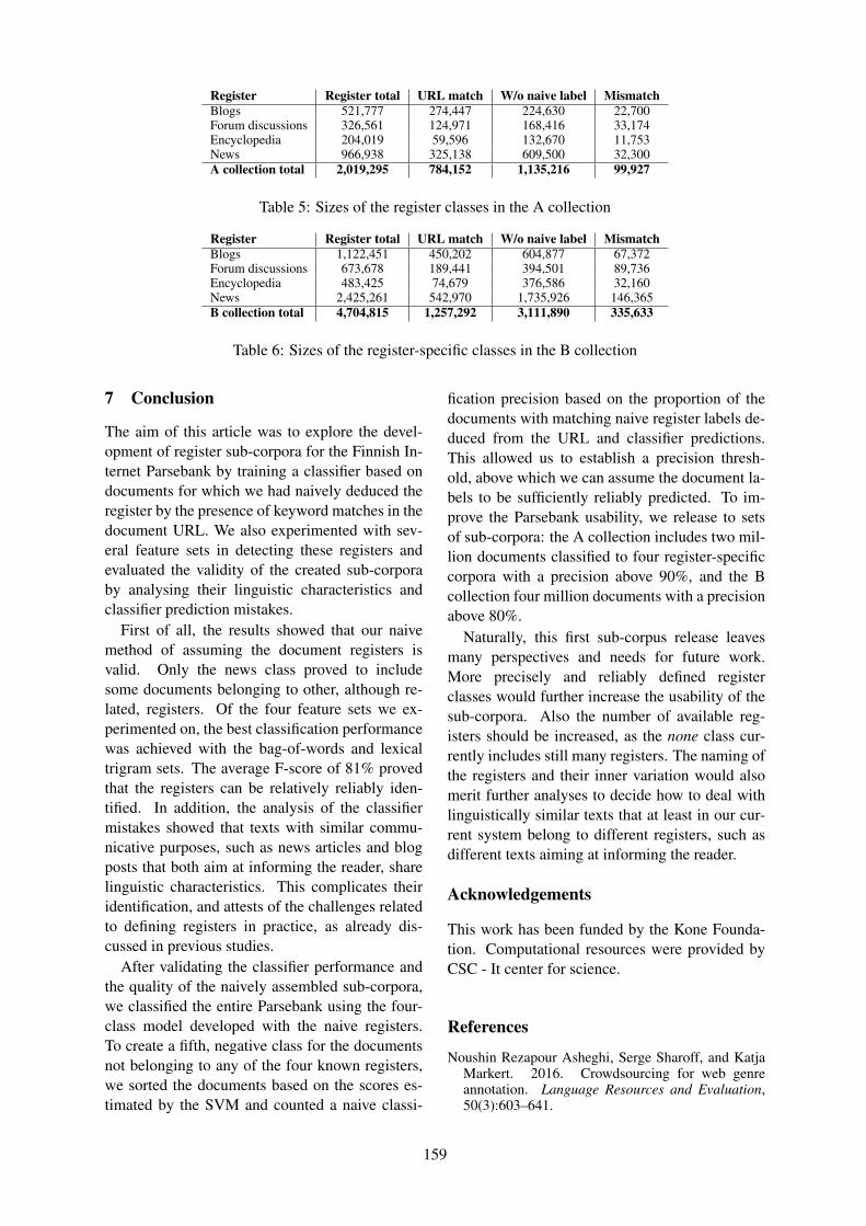
Register Register total URL match W/o naive label MismatchBlogs 521,777 274,447 224,630 22,700Forum discussions 326,561 124,971 168,416 33,174Encyclopedia 204,019 59,596 132,670 11,753News 966,938 325,138 609,500 32,300A collection total 2,019,295 784,152 1,135,216 99,927

Table 5: Sizes of the register classes in the A collection

Register Register total URL match W/o naive label MismatchBlogs 1,122,451 450,202 604,877 67,372Forum discussions 673,678 189,441 394,501 89,736Encyclopedia 483,425 74,679 376,586 32,160News 2,425,261 542,970 1,735,926 146,365B collection total 4,704,815 1,257,292 3,111,890 335,633

Table 6: Sizes of the register-specific classes in the B collection

7 Conclusion

The aim of this article was to explore the devel-opment of register sub-corpora for the Finnish In-ternet Parsebank by training a classifier based ondocuments for which we had naively deduced theregister by the presence of keyword matches in thedocument URL. We also experimented with sev-eral feature sets in detecting these registers andevaluated the validity of the created sub-corporaby analysing their linguistic characteristics andclassifier prediction mistakes.

First of all, the results showed that our naivemethod of assuming the document registers isvalid. Only the news class proved to includesome documents belonging to other, although re-lated, registers. Of the four feature sets we ex-perimented on, the best classification performancewas achieved with the bag-of-words and lexicaltrigram sets. The average F-score of 81% provedthat the registers can be relatively reliably iden-tified. In addition, the analysis of the classifiermistakes showed that texts with similar commu-nicative purposes, such as news articles and blogposts that both aim at informing the reader, sharelinguistic characteristics. This complicates theiridentification, and attests of the challenges relatedto defining registers in practice, as already dis-cussed in previous studies.

After validating the classifier performance andthe quality of the naively assembled sub-corpora,we classified the entire Parsebank using the four-class model developed with the naive registers.To create a fifth, negative class for the documentsnot belonging to any of the four known registers,we sorted the documents based on the scores es-timated by the SVM and counted a naive classi-

fication precision based on the proportion of thedocuments with matching naive register labels de-duced from the URL and classifier predictions.This allowed us to establish a precision thresh-old, above which we can assume the document la-bels to be sufficiently reliably predicted. To im-prove the Parsebank usability, we release to setsof sub-corpora: the A collection includes two mil-lion documents classified to four register-specificcorpora with a precision above 90%, and the Bcollection four million documents with a precisionabove 80%.

Naturally, this first sub-corpus release leavesmany perspectives and needs for future work.More precisely and reliably defined registerclasses would further increase the usability of thesub-corpora. Also the number of available reg-isters should be increased, as the none class cur-rently includes still many registers. The naming ofthe registers and their inner variation would alsomerit further analyses to decide how to deal withlinguistically similar texts that at least in our cur-rent system belong to different registers, such asdifferent texts aiming at informing the reader.

Acknowledgements

This work has been funded by the Kone Founda-tion. Computational resources were provided byCSC - It center for science.

References

Noushin Rezapour Asheghi, Serge Sharoff, and KatjaMarkert. 2016. Crowdsourcing for web genreannotation. Language Resources and Evaluation,50(3):603–641.

159

Douglas Biber and Jesse Egbert. 2015. Using gram-matical features for automatic regisgter identifica-tion in an unrestricted corpus of documents fromthe Open Web. Journal of Research Design andStatistics in Linguistics and Communication Sci-ence, 2(1).

Douglas Biber, S. Johansson, G. Leech, Susan Conrad,and E. Finegan. 1999. The Longman Grammar ofSpoken and Written English. Longman, London.

Douglas Biber, Jesse Egbert, and Mark Davies. 2015.Exloring the composition of the searchable web: acorpus-based taxonomy of web registers. Corpora,10(1):11–45.

Douglas Biber. 1989. Variation across speech andwriting. Cambridge University Press, Cambridge.

Douglas Biber. 1995. Dimensions of Register Vari-ation: A Cross-linguistic Comparison. CambridgeUniversity Press, Cambridge.

Bernd Bohnet. 2010. Very high accuracy and fast de-pendency parsing is not a contradiction. In Proceed-ings of the 23rd International Conference on Com-putational Linguistics, COLING ’10, pages 89–97,Stroudsburg, PA, USA. Association for Computa-tional Linguistics.

Pedro. Carpena, Pedro. Bernaola-Galvan, MichaelHackenberg, Ana. V. Coronado, and Jose L. Oliver.2009. Level statistics of words: Finding keywordsin literary texts and symbolic sequences. PhysicalReview E (Statistical, Nonlinear, and Soft MatterPhysics), 79(3):035102.

Kevin Crowston, Barbara Kwasnik, and JosephRubleske, 2011. Genres on the Web: ComputationalModels and Empirical Studies, chapter Problems inthe Use-Centered Development of a Taxonomy ofWeb Genres, pages 69–84. Springer Netherlands,Dordrecht.

Jesse Egbert, Douglas Biber, and Mark Davies. 2015.Developing a bottom-up, user-based method of webregister classification. Journal of the Association forInformation Science and Technology, 66(9):1817–1831.

S. Meyer Zu Essen and Barbara Stein. 2004. Genreclassification of web pages: User study and fea-sibility analysis. Proceedings of the 27th AnnualGerman Conference on Artificial Intelligence, pages256–259.

Eugenie Giesbrecht and Stefan Evert. 2009. Is part-of-speech tagging a solved task? an evaluation of postaggers for the german web as corpus. In Web asCorpus Workshop (WAC5), pages 27–36.

Stephan Gries, John Newman, and Cyrus Shaoul.2011. N-grams and the clustering of registers. Em-pirical Language Research.

Stephan Gries, 2012. Methodological and analyticfrontiers in lexical research, chapter Behavioral Pro-files: a fine-grained and quantitative approach incorpus-based lexical semantics. John Benjamins,Amsterdam and Philadelphia.

Isabelle M. Guyon and Andre Elisseeff. 2003. Anintroduction to variable and feature selection. Thejournal of machine learning research, 3:1157–1182.

Jenna Kanerva, Matti Luotolahti, Veronika Laippala,and Filip Ginter. 2014. Syntactic n-gram collec-tion from a large-scale corpus of Internet Finnish.In Proceedings of the Sixth International ConferenceBaltic HLT 2014, pages 184–191. IOS Press.

Adam Kilgariff and Gregory Grefenstette. 2003. In-troduction to the special issue on Web as Corpus.Computational Linguistics, 29(3).

Christoph Lindemann and Lars Littig, 2011. Gen-res on the Web: Computational Models and Em-pirical Studies, chapter Classification of Web Sitesat Super-genre Level, pages 211–235. SpringerNetherlands, Dordrecht.

Juhani Luotolahti, Jenna Kanerva, Veronika Laippala,Sampo Pyysalo, and Filip Ginter. 2015. Towardsuniversal web parsebanks. In Proceedings of the In-ternational Conference on Dependency Linguistics(Depling’15), pages 211–220. Uppsala University.

C.R. Miller. 1984. Genre as social action. Quaterlyjournal of speech, 70(2):151–167.

Marina Santini and Serge Sharoff. 2009. Web genrebenchmark under construction. JLCL, 24(1):129–145.

Roland Schafer and Felix Bildhauer, 2016. Proceed-ings of the 10th Web as Corpus Workshop, chapterAutomatic Classification by Topic Domain for MetaData Generation, Web Corpus Evaluation, and Cor-pus Comparison, pages 1–6. Association for Com-putational Linguistics.

Mike Scott and Chistopher Tribble. 2006. Textual Pat-terns: keyword and corpus analysis in language ed-ucation. Benjamins, Amsterdam.

Serge Sharoff, Zhili Wu, and Katja Markert. 2010. Theweb library of Babel: evaluating genre collections.

John Sinclair. 1996. Preliminary recommendations oncorpus typology.

John Swales. 1990. Genre analysis: English in aca-demic and research settings. Cambridge UniversityPress, Cambridge.

Vedrana Vidulin, Mitja Lustrek, and Matjax Gams.2007. Using genres to improve search engines. InWorkshop ”Towards genre-enabled Search Engines:The impact of NLP” at RANLP, pages 45–51.

160

Bonnie Webber. 2009. Genre distinctions for dis-course in the Penn treebank. In Proceedings of thejoint conference of the 47th annual meeting of theACL and the 4th international joint conference onnatural language processing of the AFNLP., pages674–682. Association for Computational Linguis-tics.

161


KILLE: a Framework for Situated Agents for LearningLanguage Through Interaction

Simon DobnikCLASP

University of Gothenburg, [email protected]

Erik Wouter de GraafUniversity of Gothenburg, Sweden

[email protected]

AbstractWe present KILLE, a framework for situ-ated agents for learning language throughinteraction with its environment (percep-tion) and with a human tutor (dialogue).We provide proof-of-concept evaluationsof the usability of the system in two do-mains: learning of object categories andlearning of spatial relations.

1 Introduction

Situated conversational robots have to be capableof both linguistic interaction with humans and in-teraction with their environment through percep-tion and action if we want them a part of our dailylives. Humans interact through language very ef-ficiently and naturally and since most of them arenot expert programmers, interaction with a robotin a natural language will be preferred. Secondly,by being part of the human environment contain-ing everyday objects such as tables and chairs,robots too have to have knowledge how humansstructure and organise their world which is againreflected in human language.

Connecting language with perception and ac-tion is commonly known as grounding (Harnad,1990; Roy, 2002). The main challenge in ground-ing is that we are connecting two representa-tion systems, (i) a perceptual which is commonlycaptured in physical sciences as continuous real-valued features and (ii) a symbolic conceptual sys-tem that makes up human language. There is noone-to-one correspondence between the two: lin-guistic descriptions such as “close to the table”and “red” correspond to some function predict-ing the degree of acceptability over physical orcolour space (Logan and Sadler, 1996; Roy, 2002;Roy, 2005; Skocaj et al., 2010; Matuszek et al.,2012; Kennington and Schlangen, 2015; McMa-han and Stone, 2015). The relations between con-cepts are not flat but are made increasingly more

abstract, structures are embedded and recursive(Fellbaum, 1998; Tenenbaum et al., 2011) and or-ganised at several representational layers (Kruijffet al., 2007). It follows that several descriptionsmay be equally applicable for the same situation:the chair can be “close to the table” or “to theleft of the table” which means vagueness is preva-lent in grounding. This however, can be resolvedthrough interaction by adopting appropriate inter-action strategies (Kelleher et al., 2005; Skantze etal., 2014; Dobnik et al., 2015).

The meaning of words is not grounded just inperception and action but also grounded in particu-lar linguistic interactions or conversations: partic-ipants continuously adapt and agree on the mean-ing of words as a part of their interaction (Clark,1996; Fernandez et al., 2011). This means thathaving a static model of grounded language whichis learned offline from a corpus with a situatedrobot is not enough but this must be continuouslyadapted as the interaction unfolds (Skocaj et al.,2011; Matuszek et al., 2012). The idea of dy-namic, continuously updated grounded languagemodels is parallel to dynamic, continuously up-dated maps of the environment that have beencommonly used in mobile robotics for a while(Dissanayake et al., 2001). Static models used inearly robotics (Winograd, 1976) were just not ableto deal with any changes in its environment andthe uncertainty that these bring. We want to takethe same view for language which is dynamicallyadjusted through interaction strategies.

In this paper we describe a framework for sit-uated agents that learn grounded language in-crementally and online called KILLE (Kinect IsLearning LanguagE) with the help of a human tu-tor in the fashion previously described. KILLE is anon-mobile table-top robot connecting Kinect sen-sors with image processing and classification anda spoken dialogue system. The system learns torecognise objects presented to it by a human tu-

162

tor from scratch. It can direct learning by askingfor more objects of a particular category if it is notable to classify them with sufficient reliability. Ifmore objects of a particular category are availablein the scene and the system is able to recognisethem, the system queries the user to describe spa-tial relations between them. Each of these kinds ofdescriptions focus on different perceptual featuresand represent two fundamental linguistic semanticcategories: entities and entity relations. Overall,KILLE combines both passive and active learningwhich is incremental at the level of both kinds oflinguistic categories.

The contributions of the KILLE framework aretwo-fold: (i) from the computational perspectiveit provides a platform for building models of sit-uated language learning and answering questionshow to integrate and test existing language tech-nology tools (primarily intended for processingcorpora) in an interactive tutoring framework; (ii)it also provides a platform for testing linguisticand psycho-linguistic theories, formalisms and ap-plications on grounding language in interaction(Larsson, 2013; Dobnik et al., 2013) and imple-menting them computationally. This paper fo-cuses on the construction of the Kille frameworkand its properties while it also provides a proof-of-concept evaluation of such learning of simpleobject and spatial relations representations. Thepaper is organised as follows. In Section 2 wedescribe the main components of the system. InSections 3 and 4 we describe the perceptual repre-sentations and dialogue strategies that have beenimplemented so far. Section 5 describes proof-concept learning of objects and Section 5.2 learn-ing of spatial descriptions that demonstrate the us-ability of the framework. We give conclusions anddiscussion of future work in Section 6.

2 The KILLE system

The system and the architecture that KILLE is us-ing are similar to two existing systems for incre-mental interaction (Schlangen and Skantze, 2011)IrisTK (Skantze and Al Moubayed, 2012) and In-proTK (Kennington et al., 2014). The difference isthat instead of starting from the perspective of in-cremental language processing and dialogue man-agement we focus on the mapping between lan-guage and robot’s sensors and actuators and howto learn such mappings through particular dia-logue and interactional strategies. Therefore, we

opt for a Robot Operating System (ROS) (Quigleyet al., 2009) as our middle-ware which providesa common framework for building modules thatcommunicate with each other (send and receive in-formation) and runs on a variety of popular robotichardware implementations which makes modulesportable between them. We work with a very sim-ple robotic hardware: a Microsoft Kinect sensorsupported by the libfreenect library integrated inROS.1 The Kinect provides us with three sensors:an RGB camera of resolution 640x480, a depthsensor, which a structured-light 3D scanner thatcan perceive in a distance between 70 and 300cm and gives a 3d representation of object, anda multi-array microphone (not used). The Kinectsensor is attached to a laptop computer runningROS and other software and together they repre-sent our interactive robot. This robot does not haveactuators which means it is not mobile and so itcannot turn gaze and focus on objects not in itsvision field. Objects have to be brought into its at-tention field. We use glass pedestals as object sup-port as to avoid the problem of object segmenta-tion (e.g. object and hand) as glass is not detectedby the depth sensor. Although simple, the platformsatisfies well our requirements for incremental sit-uated learning of perceptual language through di-alogue. Through ROS the system can be ported toother, more sophisticated robotic platforms withvery little modification.

FreenectKinect driver

Kille Coreperceptual classificationclustering and SVM

Roscore

ROSDialbridge to OpenDial

OpenDialASR (speech recognition)TTS (text to speech)process natural language

topictopic topic

speech inputRGB frames depth frames

frames acknowledgement or recognition resultrequ

est

system output

variables

Figure 1: Kille modules

Figure 1 shows the main software modules thatmake up Kille and how they communicate witheach other within the ROS framework. Each com-ponent (e.g. Kille, ROSDial, etc.) is a node whichmay have one or several topics. A node can pub-lish to a topic or subscribe to a topic from anothernode. Roscore is a special node which is responsi-ble for communication. As communication is per-

1See http://wiki.ros.org/freenect stack We use an olderversion of Kinect hardware 1414 which is better supportedby libfreenect.

163

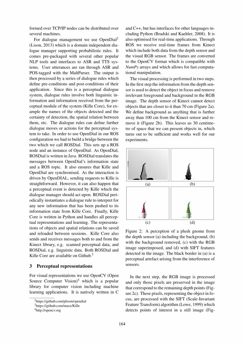
formed over TCP/IP nodes can be distributed overseveral machines.

For dialogue management we use OpenDial2

(Lison, 2013) which is a domain independent dia-logue manager supporting probabilistic rules. Itcomes pre-packaged with several other popularNLP tools and interfaces to ASR and TTS sys-tems. User utterances are ran through ASR andPOS-tagged with the MaltParser. The output isthen processed by a series of dialogue rules whichdefine pre-conditions and post-conditions of theirapplication. Since this is a perceptual dialoguesystem, dialogue rules involve both linguistic in-formation and information received from the per-ceptual module of the system (Kille Core), for ex-ample the names of the objects detected and thecertainty of detection, the spatial relation betweenthem, etc. The dialogue rules can define furtherdialogue moves or actions for the perceptual sys-tem to take. In order to use OpenDial in our ROSconfiguration we had to build a bridge between thetwo which we call ROSDial. This sets up a ROSnode and an instance of OpenDial. As OpenDial,ROSDial is written in Java. ROSDial translates themessages between OpenDial’s information stateand a ROS topic. It also ensures that Kille andOpenDial are synchronised. As the interaction isdriven by OpenDIAL, sending requests to Kille isstraightforward. However, it can also happen thata perceptual event is detected by Kille which thedialogue manager should act upon. ROSDial peri-odically instantiates a dialogue rule to interpret forany new information that has been pushed to itsinformation state from Kille Core. Finally, KilleCore is written in Python and handles all percep-tual representations and learning. The representa-tions of objects and spatial relations can be savedand reloaded between sessions. Kille Core alsosends and receives messages both to and from theKinect library, e.g. scanned perceptual data, andROSDial, e.g. linguistic data. Both ROSDial andKille Core are available on Github.3

3 Perceptual representations

For visual representations we use OpenCV (OpenSource Computer Vision)4 which is a popularlibrary for computer vision including machinelearning applications. It is natively written in C

2https://github.com/plison/opendial3https://github.com/masx/Kille4http://opencv.org

and C++, but has interfaces for other languages in-cluding Python (Bradski and Kaehler, 2008). It isalso optimised for real-time applications. ThroughROS we receive real-time frames from Kinectwhich include both data from the depth sensor andthe visual RGB sensor. The frames are convertedto the OpenCV format which is compatible withNumPy arrays and which allows for fast computa-tional manipulation.

The visual processing is performed in two steps.In the first step the information from the depth sen-sor is used to detect the object in focus and removeirrelevant foreground and background in the RGBimage. The depth sensor of Kinect cannot detectobjects that are closer to it than 70 cm (Figure 2a).We define background as anything that is furtheraway than 100 cm from the Kinect sensor and re-move it (Figure 2b). This leaves us 30 centime-tre of space that we can present objects in, whichturns out to be sufficient and works well for ourexperiments.

(a) (b)

(c) (d)

Figure 2: A perception of a plush gnome fromthe depth sensor (a) including the background, (b)with the background removed, (c) with the RGBimage superimposed, and (d) with SIFT featuresdetected in the image. The black border in (a) is aperceptual artefact arising from the interference ofsensors.

In the next step, the RGB image is processedand only those pixels are preserved in the imagethat correspond to the remaining depth points (Fig-ure 2c). These pixels, representing the object in fo-cus, are processed with the SIFT (Scale-InvariantFeature Transform) algorithm (Lowe, 1999) whichdetects points of interest in a still image (Fig-

164

ure 2c). Each point is represented as descriptor, ahigh dimensional vector which contains informa-tion about the visual properties surrounding eachkey-point, its orientation and location. SIFT is in-tended to be scale-invariant which means it is ro-bust against changes that are introduced by scal-ing, can handle rotation and small changes in il-lumination. Note that objects (including thosethat are very similar and belong to the same cate-gory) will have different numbers of SIFT descrip-tors detected depending on their visual properties:some objects have a lot of visual details while oth-ers are smoother. In our interactive scenario thiswill also be the case each time when the same ob-ject will be re-introduced to the system as the cap-tured frame will be slightly different from the pre-viously captured one because of slight changes inlocation, lighting and camera noise.

4 Dialogue games

In the dialogue manager we implemented dialoguerules that act upon both linguistic and perceptualknowledge and allow us to have the followingconversational games (Kowtko et al., 1992) withusers.

1. Direct instruction: objects

User: This is a cup.System: [Object is focused on and observed.]S: OK, I learned a cup.

2. Direct instruction: spatial relations

U: The book is to the right of the mug.S: [Objects are focused on and observed.]S: OK. This relation is called “to the right of”.S: [Objects are focused on and observed.]U: Where are the objects?S: The book is to the right of the mug.

3. Describing objects and relations with (un)certainty

U: What is this?S: [Object is focused on and observed.]U: The object is thought to be a book, but it might also

be a mug.

4. Reinforcement from feedback

U: What is this?S: [Object is focused on and observed.]S: This is a cup.U: That is correct.S: [Observation is added to the models.]

5. Self initiative: spatial relations

S: [Objects are focused on and observed.]S: One of the objects is book, the other one is box.

Please tell me where things are.

U: The book is to the left of the box.S: OK, this relation is called “to the left of”.

6. Unlearning immediately (e.g. after a mishearing)

U: This is a book.S: [Object is focused on and observed.]S: OK, this is a box.U: That is not what I said.S: OK, sorry. I will ignore it.

7. Unlearning later

U: Forget a book.S: OK. I forgot a book.

8. Renaming an object

U: This is a book.S: [Object is focused on and observed.]S: OK, this is a box.U: I said a book.S: OK, sorry. This is a book.

5 Interactive perceptional learning

In the following subsections we present a proof-of concept implementation and evaluation of per-ceptual learning through interaction which demon-strates the usability of the Kille framework.

5.1 Learning to recognise objectsAs described in Section 3 every scan, even of thesame scene, gives us a different set of SIFT de-scriptors which as data-structures are multidimen-sional vectors. One approach to use SIFT descrip-tors in classification is to pre-cluster them to bagsof visual words (BoVW) (see (Bruni et al., 2014)for discussion) and then apply their occurrencecounts as features in a classifier such as LinearSupport Vector Machine (SVM). However, in thecurrent implementation we chose a simple lazy-learning method based on SIFT clustering as itbetter fits with the incremental learning scenario.With the SVM method we would have to store andcluster instances and re-train the model on each in-stance update, thus doing far more computationalwork. Since the domain and the number of exam-ples are small, lazy-learning is justified.

The SIFT descriptors of each object instance arestored in a database and then at each classificationstep the current SIFT descriptions are comparedagainst objects stored in memory and the cate-gory of the best matching object is returned. Thematching of SIFT descriptors as k-nearest neigh-bours has been implemented in the FLANN library(Muja and Lowe, 2009). This takes the longest listof descriptors (either from the current instance or

165

a database instance) and matches each descriptorto k descriptors in the other list (in our case k = 2).The matched tuples (some of which will have zeroor no similarity) have to be filtered. For this theratio test of (Lowe, 2004) is used which calcu-lates the Euclidean distance between two descrip-tors and those pairs that fall below the empiricallydefined threshold of 0.75 are discarded. Sincedifferent object representations contain a differ-ent number of SIFT features and there is a biasthat representations with a small number of fea-tures match representations with a large numberof features, we take the harmonic mean of the ratio#Matched#Model and the ratio #Matched

#Perceived as the final match-ing score. In the evaluation 10 consecutive scansare taken and their recognition scores are averagedto a single score. This improves the performanceas it makes observations more stable to noise butdecreases the processing speed. The name of theitem in the database with the closest match is re-turned. If there are several top-ranking candidatesof the same category, their category is returnedwith their mean recognition score.

The location of the recognised object is es-timated by taking the locations of the twentymatched descriptors with the shortest distance.

To evaluate the system’s performance in an in-teractive tutoring scenario we chose typical house-hold objects that could be detected in the per-ception field of the Kinect sensor and which fallinto the following 10 categories: apple, banana,teddy bear, book, cap, car, cup, can of paint, shoeand shoe-box. A human tutor successively re-introduces the same 10 objects to the system in apre-defined order over four rounds trying to keepthe presentation identical as much as possible. Ineach round all objects are first learned and thenqueried. To avoid ASR errors both in learning andgeneration text input is used.

The average recognition scores over four roundsare shown in Table 1. We choose the name ofthe object with the highest recognition score. Thehighest values follow all but in one case the diago-nal which means that on overall objects are recog-nised correctly. The only problematic object is thecap which has been consistently confused with abanana. SIFT features do not contain colour in-formation according to which these two categoriesof objects could be distinguished. There were afew individual confusions which did not affect theoverall mean score (not shown in Table 1): the

shoe-box was confused with a car in rounds 1 and2, and with an apple in round 3. The apple wasrecognised as a banana in round 2. Otherwise, thesystem performed extremely accurately. The lastcolumn C-NI gives Correct-NextIncorrect score (adifference between the matching score of the tar-get object with the object of the correct categoryand the matching score of the target object withthe closest matching object not of the correct cate-gory) which shows on average how visually dis-tinct the object is. The models of most objectspreserve significant distinctiveness over presenta-tions and learning across the 4 rounds. If we rankobjects by this score, we get the following ranking(from more distinct to least distinct): book > car> shoe > cup > banana > bear > apple > paint> shoe-box > cap.

In the second experiment we evaluated re-recognition of objects at different degrees of rota-tion (45◦, 90◦, 135◦, 180◦, 225◦, 270◦ and 315◦ inthe clockwise direction) using the final model forobjects built after the completion of round 4 in theprevious experiment. Already at a rotation of 45◦

6 out of 10 objects are mis-recognised. Objects areaffected by rotation in different ways since theirsides are visually distinct. For example shoe-boxand to a large extent apple are correctly classi-fied at most rotational angles. We observe similarclassification scores at those angles at which sym-metric sides of objects are exposed: 45◦:315◦ and90◦:270◦, 135◦:225◦ and 0◦:180◦.

In the third experiment we tested the modelfrom the end of the round 4 in the first experimenton 3 new objects of each category. The modelsfor experiment one did not extend well to differ-ent objects for most categories. Only apples (2 outof 3 new objects) and shoe-boxes (all 3 new ob-jects) were recognised correctly. Shoe-box is alsothe most common mis-classification which meansit is similar to other objects.

Overall, the results and the discussion in thissection show that our system is able to learn torecognise objects incrementally through interac-tion with a human tutor from just a few obser-vations. The testing of our models in new con-texts from the context in which they were learned(rotation and classification of different objects ofthe same category) demonstrate how sensitive ourmodels are to the changes of contexts which arelikely to arise in the interactive scenario. Ofcourse, learning observations of objects in these

166

→ apple banana bear book cap car cup paint shoe shoe-box C-NIapple .343 .227 .076 .046 .099 .058 .126 .074 .053 .166 .116banana .201 .357 .058 .035 .085 .087 .148 .066 .046 .124 .155bear .080 .121 .260 .074 .089 .091 .120 .099 .074 .136 .123book .142 .233 .074 .496 .114 .197 .246 .130 .085 .220 .250cap .122 .208 .076 .049 .146 .096 .103 .083 .061 .114 -.062car .104 .183 .053 .067 .077 .414 .119 .076 .069 .149 .231cup .099 .145 .063 .066 .091 .052 .330 .094 .054 .120 .185paint .119 .140 .075 .076 .083 .147 .121 .221 .062 .111 .075shoe .078 .123 .070 .056 .079 .116 .124 .076 .319 .103 .196shoe-box .190 .332 .099 .188 .145 .305 .313 .166 .111 .376 .044

Table 1: Average recognition scores over four rounds. The object tested are represented in rows. Columnsindicate the categories that they were recognised as.

contexts specifically would increase the successof object recognition. Thus, the experiments alsopoint to the complexity of the object recognition.

5.2 Learning to recognise spatial relationsOnce the system learns to detect several objectsin the scene it starts querying the user to describespatial relations between them. The semantics ofspatial relations requires at least three componentsof meaning: (i) knowledge about the geometri-cal arrangement of objects in the scene; (ii) worldknowledge about the objects involved in particu-lar how they interact with each other or what isour take on the scene; (iii) dialogue interaction be-tween conversational partners, for example in co-ordinating and negotiation perspective or the ori-gin of the frame of reference (FoR) used. Wehope that Kille will provide us a platform for mod-elling and testing the interaction between all threecomponents, some of which, for example (ii), arelearned from a large corpus off-line. Here wemainly focus on interactive learning of the geo-metric component (i).

First, the system must recognise the target andthe landmark objects (“the gnome/TARGET is tothe left of the book/LANDMARK”) both in thelinguistic string and the perceptual scene. Twentyhighest ranking SIFT features are taken for eachobject and their x (width), y (height) and z (depth)coordinates are averaged, thus giving us the cen-troid of the 20 most salient features of an ob-ject.5 We chose the number 20 based on prac-tical experience. Higher numbers of features aremore demanding for processing in real time. Theorigin of the coordinate frame for spatial tem-plates must be at the centre of the landmark ob-

5This is a simplification as object shape is only partiallyexpressed in the y variable. This way we distinguish betweentall and short objects. Note also that the variables x and zdescribe object location while y describes object property.

ject which means that the coordinates of the tar-get must be expressed as relative to the landmark’slocation. A further transformation of the coordi-nate frame could be made depending on the orien-tation of the viewpoint that sets the perspective.However, in our scenario the geometric coordi-nate frame was always relative to the orientationof Kille. Of course, in conversations with Killehumans could describe locations from a differentperspective which means that this can lead (in anabsence of a model of FoR assignment) to a morecomplicated/noisy and ambiguous model of geo-metric spatial template learned. For example thesame region could be described as “to the left of”and “to the right of”. The relativised location ofthe target to the landmark are fed to a Linear Sup-port Vector Classifier (SVC) with descriptions astarget classes.

A human tutor taught the system by present-ing it the target object (a book) at 16 differentlocations in relation to the landmark (the car) asshown in Figure 3. The locations were arrangedso that there were 8 locations separated at 45◦ attwo different distances around and from the land-mark. These objects were chosen because theyhave achieved a good recognition accuracy in theprevious experiments. The book was shown to thesystem three times per location in a randomisedorder which gave us 48 presentations. The targetwas moved after each presentation. This ensuredthat there was no semantic influence on descrip-tions between the presentations.6 The spatial de-scriptions that the human instructor used were tothe left of, to the right of, in front of, behind of,near and close to (6). The first 4 descriptions areprojective descriptions and require grounding ofFoR, while the last two are topological descrip-

6In a different evaluation setting we might want to exploresuch bias.

167

tions and do not require grounding of the FoR,only distance. The relativised spatial coordinatesimplicitly encode both of these features.

1

23

4

5

67

8

9

10

11

12

13

14

15

16

car→

Kill

e↓

Hum

an↑

Figure 3: The locations of the target (“book”), thelandmark (“car”) and the conversational partners(Kille and the human). 1 and 9 have been slightlyrelaxed, as Kille would not be able to detect thecar behind the book otherwise.

Note that spatial descriptions are not mutuallyexclusive: location 4 in Figure 3 could be de-scribed as “near”, “close”, “to the right of” and“in front of” (taking the human FoR) and “near”,“close”, “to the left of” and “behind” (takingKille’s FoR) which makes learning a difficult task.In the evaluation we are interested if the systemwould agree strictly with human observers on themost relevant description for that context, if thisis not the case, would the system generate an al-ternative acceptable description. The agreementbetween annotators is highly informative as it tellsus about the difficulty of the task.

behind in front of close to near left of right of100

50

0

50

100

150

centi

mete

r

xyz

Figure 4: Average x, y and z values for spatial re-lations.

Figure 4 shows the average values of the x

(width), y (height) and z (depth) features with theorigin on the landmark object for the instances inour learning dataset. There is quite a clear opposi-tion between “behind” and “in front of” as well as“to the left of” and “to the right of” which meansthat the instructor was consistent in the usage ofthe FoR. What is interesting is that different FoR isused for the front-and-back and the lateral dimen-sions. “behind” and “in front of” are groundedin an FoR relative to Kille (away from and to-wards Kille respectively) while “left” and “right”are grounded in an FoR relative to the conversa-tional partner (e.g. “to the left of” corresponds topositive x values. Effectively, a split FoR is used.In this scenario, there is no effect of conversationalroles on the assignment of FoR (information giverand information receiver) which has been reportedby (Schober, 1995). The reason why the target isappears to be lower when it is described to be “be-hind” the landmark is due to the positioning of thesensor higher than the landmark at an angle look-ing down. This means that objects further awayappear shorter. Finally both “close” and “near”show short distances from the landmark in eachdimension as expected. However, there is, at leastin this model, no clear difference between thesetwo descriptions.

The performance of the system was indepen-dently evaluated by two human conversationalpartners, one of whom was also the tutor duringthe learning phase. As during learning, the targetobject was placed in one of the 16 locations andeach location was used twice, which gave eachhuman to evaluate a total of 32 situations whichwere presented in a random order. After each ob-ject placement, the evaluators first independentlywrote down the description they would use todescribe the scene. Then the system would bequeried to describe the location of the target. Thesystem’s response was recorded and also whetherthe evaluators agreed with the generated descrip-tion or not.

As mentioned earlier, several spatial descrip-tions may apply to the same location of the targetand the landmark. The observed strict agreementbetween the evaluators independently choosing adescription is 0.5313 (they independently choosethe same description in just over 1/2 of cases).However, when we correct this value by agree-ment by chance in the form of the Kappa coeffi-cient (κ), the estimated strict agreement between

168

the evaluators is κ = 0.4313. Choosing a spatialdescription is thus quite a subjective task.

Match Evaluator 1 Evaluator 2 Evaluator 1 + 2Independent 8 0.25 7 0.2188 15 0.2344Secondary 11 0.3438 13 0.4063 24 0.375Indep. + Second. 19 0.5938 20 0.6251 39 0.6094Incorrect 13 0.4063 12 0.375 25 0.3906Total 32 1 32 1 64 1

Table 2: Observed agreement between the evalua-tors and the system

The observed agreement between the evaluatorsand the system is shown in Table 2. The evaluatorsand the system independently chose the same de-scription in 23.44% of cases which is a decreasefrom 53.13% where only evaluators are comparedwith each other. However, even if the descriptionwas not the one that evaluators chose in this sit-uation, the evaluators thought that the generateddescription was nonetheless a good description infurther 37.5% of situations. Overall, evaluatorswere satisfied with 60.94% of generations, while39.06% were considered incorrect. Given the dif-ficulty of the task and that the system on averagehad a chance to learn each description only from 8trials (48/6 = 8), thus not observing each descrip-tion at all possible 16 locations, the results are en-couraging and are close to what has been reportedfor a similar task in the literature (Dobnik, 2009).

behind front left right close near Totalbehind 4 2 1 0 0 2 9

front 0 5 3 3 6 0 17left 0 6 1 0 0 0 7

right 4 1 3 3 0 1 12close 1 9 1 0 1 2 14near 1 1 1 0 1 1 5

Total 10 24 10 6 8 6 64

Table 3: Agreement between two human evalua-tors (rows) and the system (columns)

Table 3 shows a confusion matrix for all 64 tri-als. The Kappa coefficient, thus the strict observedagreement of 0.2344 (Table 2) discounted by theagreement by chance is κ = 0.0537. If we exam-ine Table 3 we can see, as also shown in Table 2,that non-agreements involve those descriptionsthat are appropriate alternatives. For example,we expect topological descriptions (e.g. “close”)to partially overlap with projective descriptions(e.g. “front”) or with other projective descriptions(e.g. “left” and “front”). The data also shows

that humans and evaluators have a slightly dif-ferent preference for assigning descriptions. Hu-mans assign descriptions with the following like-lihoods (from the highest to the lowest): “front”(0.2656) > “close” (0.2188) > “right” (0.1875)> “behind” (0.1406) > “left” (0.1094) > “near”(0.0781) while the system has the following pref-erence “front” (0.375) > “behind”/“left” (0.1563)> “close” (0.125) and > “right”/“near” (0.0938).The most important differences are thus in theusage of “close”/“right” vs “behind”/“left” anddemonstrate the subjective nature of the task andpossibly a usage of different FoRs.

6 Conclusion and future work

We presented Kille, a framework for situatedagents for learning language through interaction.This is based on a Robotic Operating System(ROS) which simplifies the development of newapplications and their communication, as well asallowing the system to be ported to a variety ofmore sophisticated popular robotic platforms. Wefocus on the linguistic interactional aspects with asituated agent in the context of learning throughinstruction and therefore our three main modulesare the robotic perceptual system provided by theKinect sensor, a dialogue system and a module forclassification of grounded lexical meanings. Wedemonstrate and evaluate the usability of the sys-tem on two proof-of-concept applications: learn-ing of object names and learning of spatial rela-tions.

As stated in the introduction we hope that theframework will allow us to explore computationaland linguistic questions related to situated learn-ing. In particular, we are interested in how (i) dif-ferent machine learning methods can be used withan interactive tutoring scenario including the ap-plication of image convolutions from deep learn-ing to replace SIFT features. (ii) Integration ofclassifiers learned offline from a large corpus withthe interactive learning and classification is also anopen question. On the language side we are inter-ested in (iii) what kind of interaction strategies ordialogue games are relevant in this scenario, (iv)how can these games be implemented in a situateddialogue system in terms of dialogue moves oper-ating on linguistic and perceptual representationsand linking to machine learning or classification,(v) and how effective individual dialogue gamesare in respect to the rate of learning.

169

ReferencesGary Bradski and Adrian Kaehler. 2008. Learning

OpenCV: Computer vision with the OpenCV library.” O’Reilly Media, Inc.”.

Elia Bruni, Nam-Khanh Tran, and Marco Baroni.2014. Multimodal distributional semantics. Journalof Artificial Intelligence Research (JAIR), 49(1-47).

Herbert H. Clark. 1996. Using language. CambridgeUniversity Press, Cambridge.

M. W. M. G Dissanayake, P. M. Newman, H. F.Durrant-Whyte, S. Clark, and M. Csorba. 2001. Asolution to the simultaneous localization and mapbuilding (SLAM) problem. IEEE Transactions onRobotic and Automation, 17(3):229–241.

Simon Dobnik, Robin Cooper, and Staffan Larsson.2013. Modelling language, action, and perceptionin Type Theory with Records. In Denys Duchierand Yannick Parmentier, editors, Constraint Solvingand Language Processing: 7th International Work-shop, CSLP 2012, Orleans, France, September 13–14, 2012, Revised Selected Papers, volume 8114 ofLecture Notes in Computer Science, pages 70–91.Springer Berlin Heidelberg.

Simon Dobnik, Christine Howes, and John D. Kelle-her. 2015. Changing perspective: Local align-ment of reference frames in dialogue. In ChristineHowes and Staffan Larsson, editors, Proceedings ofgoDIAL - Semdial 2015: The 19th Workshop on theSemantics and Pragmatics of Dialogue, pages 24–32, Gothenburg, Sweden, 24–26th August.

Simon Dobnik. 2009. Teaching mobile robots touse spatial words. Ph.D. thesis, University of Ox-ford: Faculty of Linguistics, Philology and Phonet-ics and The Queen’s College, Oxford, United King-dom, September 4.

Christiane Fellbaum. 1998. WordNet: an electroniclexical database. MIT Press, Cambridge, Mass.

Raquel Fernandez, Staffan Larsson, Robin Cooper,Jonathan Ginzburg, and David Schlangen. 2011.Reciprocal learning via dialogue interaction: Chal-lenges and prospects. In Proceedings of the IJCAI2011 Workshop on Agents Learning Interactivelyfrom Human Teachers (ALIHT), Barcelona, Catalo-nia, Spain.

Stevan Harnad. 1990. The symbol grounding problem.Physica D, 42(1–3):335–346, June.

J.D. Kelleher, F. Costello, and J. van Genabith. 2005.Dynamically structuring updating and interrelatingrepresentations of visual and linguistic discourse.Artificial Intelligence, 167:62–102.

Casey Kennington and David Schlangen. 2015. Sim-ple learning and compositional application of per-ceptually grounded word meanings for incremental

reference resolution. In Proceedings of the 53rd An-nual Meeting of the Association for ComputationalLinguistics and the 7th International Joint Confer-ence on Natural Language Processing (Volume 1:Long Papers), pages 292–301, Beijing, China, July.Association for Computational Linguistics.

Casey Kennington, Spyros Kousidis, and DavidSchlangen. 2014. Inprotks: A toolkit for incre-mental situated processing. Proceedings of SIGdial2014: Short Papers.

Jacqueline C Kowtko, Stephen D Isard, andGwyneth M Doherty. 1992. Conversationalgames within dialogue. HCRC research paperRP-31, University of Edinburgh.

Geert-Jan M. Kruijff, Hendrik Zender, Patric Jensfelt,and Henrik I. Christensen. 2007. Situated dialogueand spatial organization: what, where... and why?International Journal of Advanced Robotic Systems,4(1):125–138. Special issue on human and robot in-teractive communication.

Staffan Larsson. 2013. Formal semantics for percep-tual classification. Journal of Logic and Computa-tion, online:1–35, December 18.

Pierre Lison. 2013. Structured Probabilistic Mod-elling for Dialogue Management. Ph.D. thesis, De-partment of Informatics, Faculty of Mathematicsand Natural Sciences, University of Oslo, 30th Oc-tober.

Gordon D. Logan and Daniel D. Sadler. 1996. A com-putational analysis of the apprehension of spatial re-lations. In Paul Bloom, Mary A. Peterson, LynnNadel, and Merrill F. Garrett, editors, Language andSpace, pages 493–530. MIT Press, Cambridge, MA.

David G Lowe. 1999. Object recognition from localscale-invariant features. In Computer vision, 1999.The proceedings of the seventh IEEE internationalconference on, volume 2, pages 1150–1157. IEEE.

David G Lowe. 2004. Distinctive image features fromscale-invariant keypoints. International journal ofcomputer vision, 60(2):91–110.

Cynthia Matuszek, Nicholas FitzGerald, Luke Zettle-moyer, Liefeng Bo, and Dieter Fox. 2012. Ajoint model of language and perception for groundedattribute learning. In John Langford and JoellePineau, editors, Proceedings of the 29th Interna-tional Conference on Machine Learning (ICML2012), Edinburgh, Scotland, June 27th - July 3rd.

Brian McMahan and Matthew Stone. 2015. Abayesian model of grounded color semantics. Trans-actions of the Association for Computational Lin-guistics, 3:103–115.

Marius Muja and David G Lowe. 2009. Fast approx-imate nearest neighbors with automatic algorithmconfiguration. VISAPP (1), 2(331–340):2.

170

Morgan Quigley, Ken Conley, Brian Gerkey, JoshFaust, Tully Foote, Jeremy Leibs, Rob Wheeler,and Andrew Y Ng. 2009. ROS: an open-sourcerobot operating system. In ICRA workshop on opensource software, volume 3, page 5.

Deb K. Roy. 2002. Learning visually-grounded wordsand syntax for a scene description task. Computerspeech and language, 16(3):353–385.

Deb Roy. 2005. Semiotic schemas: a framework forgrounding language in action and perception. Artifi-cial Intelligence, 167(1-2):170–205, September.

David Schlangen and Gabriel Skantze. 2011. A gen-eral, abstract model of incremental dialogue pro-cessing. Dialogue and discourse, 2(1):83–111.

Michael F. Schober. 1995. Speakers, addressees,and frames of reference: Whose effort is minimizedin conversations about locations? Discourse Pro-cesses, 20(2):219–247.

Gabriel Skantze and Samer Al Moubayed. 2012.IrisTK: a statechart-based toolkit for multi-partyface-to-face interaction. In Proceedings of the 14thACM international conference on Multimodal inter-action, pages 69–76. ACM.

Gabriel Skantze, Anna Hjalmarsson, and CatharineOertel. 2014. Turn-taking, feedback and joint at-tention in situated human-robot interaction. SpeechCommunication, 65:50–66.

Danijel Skocaj, Miroslav Janicek, Matej Kristan,Geert-Jan M. Kruijff, Ales Leonardis, Pierre Lison,Alen Vrecko, and Michael Zillich. 2010. A basiccognitive system for interactive continuous learningof visual concepts. In ICRA 2010 workshop ICAIR- Interactive Communication for Autonomous Intel-ligent Robots, pages 30–36, Anchorage, AK, USA.

Danijel Skocaj, Matej Kristan, Alen Vrecko, MarkoMahnic, Miroslav Janıcek, Geert-Jan M. Krui-jff, Marc Hanheide, Nick Hawes, Thomas Keller,Michael Zillich, and Kai Zhou. 2011. A systemfor interactive learning in dialogue with a tutor. InIEEE/RSJ International Conference on IntelligentRobots and Systems IROS 2011, San Francisco, CA,USA, 25-30 September.

Joshua B. Tenenbaum, Charles Kemp, Thomas L. Grif-fiths, and Noah D. Goodman. 2011. How to grow amind: Statistics, structure, and abstraction. Science,331(6022):1279–1285.

Terry Winograd. 1976. Understanding Natural Lan-guage. Edinburgh University Press.

171


Data Collection from Persons with Mild Forms of Cognitive Impairment and Healthy Controls - Infrastructure for

Classification and Prediction of Dementia

Dimitrios Kokkinakis, Kristina Lundholm Fors, Eva Björkner

Department of Swedish University of Gothenburg

Sweden [email protected]

Arto Nordlund Department of Psychiatry and Neurochemistry

Sahlgrenska Academy, University of Gothenburg

Sweden [email protected]

Abstract

Cognitive and mental deterioration, such as difficulties with memory and language, are some of the typical phenotypes for most neurodegenerative diseases including Alzheimer's disease and other dementia forms. This paper describes the first phases of a project that aims at collecting various types of cognitive data, acquired from human subjects in order to study relationships among linguistic and extra-linguistic observations. The project’s aim is to identify, extract, process, correlate, evaluate, and disseminate various linguistic phenotypes and measurements and thus contribute with complementary knowledge in early diagnosis, monitor progression, or predict individuals at risk. In the near future, automatic analysis of these data will be used to extract various types of features for training, testing and evaluating automatic classifiers that could be used to differentiate individuals with mild symptoms of cognitive impairment from healthy, age-matched controls and identify possible indicators for the early detection of mild forms of cognitive impairment. Features will be extracted from audio recordings (speech signal), the transcription of the audio signals (text) and the raw eye-tracking data.

1 Introduction

Aiding the detection of very early cognitive impairment in Alzheimer's disease (AD) and assessing the disease progression are essential foundations for effective psychological assessment, diagnosis and planning; enabling patients to participate in new drug therapy research and design of new clinical trials; evaluating potential disease-modifying agents in suitable populations etc. Efficient tools for

routine dementia screening in primary health care, and particularly non-invasive and cost-effective methods in routine dementia screening for the identification of subjects who could be administered for further cognitive evaluation and dementia diagnostics, could provide specialist centres the opportunity to engage in more demanding, advanced investigations, care and treatment. New paths of research for acquiring knowledge about Alzheimer’s disease (AD) and its subtypes using Computational Linguistic/ Natural Language Processing (CL/NLP) techniques and tools based on the exploration of several complementary modalities, parameters and features, such as speech analysis and/or eye tracking could be integrated into established neuropsychological, memory and cognitive test batteries in order to explore potential (new) biomarkers for AD. This paper describes current efforts to acquire data from people with subjective (SCI) and mild cognitive impairment (MCI) and healthy, age-matched controls in order to analyse and evaluate potential useful linguistic and extra-linguistic features and build classifiers that could differentiate between benign and malignant forms of cognitive impairment. Non-invasive and cost-effective methods that could identify individuals at an early preclinical dementia stage remains a priority and a challenge for health care providers while language deficits have been reported early in the development of AD (Taler & Phillips, 2008). Moreover, NLP methods are applied more and more in various biomedical and clinical settings, while patient language samples and large datasets are used routinely in NLP research such as the Dementia Bank corpus (a part of the TalkBank project; MacWhinney et al., 2011) and the Cambridge Cookie-Theft Corpus (Williams et al., 2010). The SCI, the MCI, and the

172

Alzheimer's disease (AD) are on a spectrum of disease progression. Subjective cognitive impairment (SCI) is a common diagnosis in elderly people, sometimes suggested to be associated with e.g. depression, stress or anxiety, but also a risk factor for dementia (Jessen et al., 2010). On the other hand, mild cognitive impairment (MCI) is a prodromal state of dementia (Ritchie & Touchon, 2010), in which a human subject has minor problems with cognition (e.g., problems with memory or thinking) but these are not severe enough to warrant a diagnosis of dementia or interfere significantly with daily life, but still difficulties which are worse than would normally be expected for a healthy person of their age.

This paper describes some efforts underway to acquire, assess, analyze and evaluate linguistic and extra-linguistic data from people with subjective (SCI) and mild cognitive impairment (MCI) and healthy, age-matched controls, with focus on infrastructure (e.g., resource collection, envisaged analysis and feature acquisition and modeling).

2 Background

New findings aim to provide a comprehensive picture of cognitive status and some promising results have recently thrown more light on the importance of language and language (dis)abilities as an essential factor that can have a strong impact on specific measurable characteristics that can be extracted by automatic linguistic analysis of speech and text (Ferguson et al., 2013; Szatloczki et al., 2015). The work by Snowdon et al. (2000), “The Nun Study”, was one of the earliest studies which showed a strong correlation between low linguistic ability early in life and cognitive impairment in later life by analyzing autobiographies of American nuns. Snowdon et al. could predict who could develop Alzheimer's by studying the degradation of the idea density (that is, the average number of ideas expressed in 10 words; Chand et al., 2010) and syntactic complexity on the nuns’ autobiographical writings. Since then, the body of research and interest in CL/NLP in the area of processing data from subjects with mental, cognitive, neuropsychiatric, or neurode-generative impairments has grown rapidly. Automatic spoken language analysis and eye movement measurements are two of the newer complementary diagnostic tools with great potential for dementia diagnostics (Laske et al.,

2014). Furthermore, the identification of important linguistic and extra-linguistic features such as lexical and syntactic complexity, are becoming an established way to train and test supervised machine learning classifiers that can be used to differentiate between individuals with various forms of dementia and healthy controls or between individuals with different types of dementia (Lagun et al., 2011; Roark et al., 2011; Olubolu Orimaye et al., 2014; Rentoumi et al., 2014).

Although language is not the only diagnostic factor for cognitive impairment, several recent studies (Yancheva et al., 2015) have demonstrated that automatic linguistic analysis, primarily of connected speech samples, produced by people with mild or moderate cognitive impairment compared to healthy individuals can identify with good accuracy objective evidence and measurable (progressive) language disorders. Garrard & Elvevåg (2014) comment that computer-assisted analysis of large language datasets could contribute to the understanding of brain disorders. Although, none of the studies presented in the special issue of Cortex vol. 55 moved “beyond the representation of language as text” and therefore finding reliable ways of incorporating features, such as prosody and emotional connotation, into data representation remains a future challenge, the editors acknowledged that current research indicates that “the challenges of applying computational linguistics to the cognitive neuroscience field, as well as the power of these techniques to frame questions of theoretical interest and define clinical groups are of practical importance”. Nevertheless, studies have shown that a steady change in the linguistic nature of the symptoms and the degree in speech and writing are early and could be identified by using language technology analysis (Mortimer et al., 2005; Le et al., 2011). New findings also show a great potential to increase our understanding of dementia and its impact on linguistic degradation such as loss of vocabulary, syntactic simplification, poor speech content and semantic generalization. Analysis of eye movement is also a relevant research technology to apply, and text reading by people with and without mild cognitive impairment may give a clear ruling on how reading strategies differ between these groups, an area that has so far not been researched to any significant extent in this particular domain (Fernández et al., 2013, 2014;

173

Molitor et al., 2015). With the help of eye-tracking technology the eye movements of participants are recorded while suitable stimuli is presented (e.g., a short text).

3 Ethical Issues and Patient Recruitment

The ongoing Gothenburg mild cognitive impairment study (Nordlund et al., 2005; Wallin et al., 2016) is an attempt to conduct longitudinal in-depth phenotyping of patients with different forms and degrees of cognitive impairment using neuropsychological, neuroimaging, and neurochemical tools. The study is clinically based and aims at identifying neurodegenerative, vascular and stress related disorders prior to the development of dementia. All patients in the study undergo baseline investigations, such as neurological examination, psychiatric evaluation, cognitive screening (e.g., memory and visuospatial disturbance, poverty of language and apraxia), magnetic resonance imaging of the brain and cerebrospinal fluid collection. At biannual follow-ups, most of these investigations are repeated. The overall Gothenburg MCI-study is approved by the local ethical committee review board (reference number: L091–99, 1999; T479-11, 2011); while the currently described study by the local ethical committee decision 206-16, 2016). The project aims at gathering a rather homogeneous group of participants with respect to age and education level (50 with SCI/MCI and 50 controls). All subjects have participated into a comprehensive battery of e.g. memory, language and other tests which have been described in Wallin et al. (2016). Recruitment of patients in the project was consecutive and took place over the course of several months, from July 2016 to January 2017. All participants gave informed written consent and were advised that no notations were made that could be related to their identity, while the exclusion and inclusion criteria are specified according to the following protocol.

Inclusion criteria:

Age range 50-79 years

Swedish as a first language and not speaking languages other than Swedish before the age of 5

Comparable education length of the participants

No apparent organic cause of symptoms (such as e.g. stroke or brain tumor)

Research subjects have read information about the research project and approved voice recording and eye movement measurements

Participants have conducted recent neuropsychological tests – participants should not have deteriorated significantly since the last testing

Exclusion criteria:

Participants have comorbid conditions affecting reading (e.g. dyslexia or other reading difficulties)

Participants have deep depression

Participants have an ongoing abuse of any kind

Participants suffer from serious psychiatric or neurological diseases such as Parkinson's, Amyotrophic lateral sclerosis or have/had a brain tumor

Participants do not understand the question or the context in the selection process

Participants have poor vision (that cannot be corrected by glasses or lenses), cataract, nystagmus, or cannot see and read on the computer screen

Participants decline participation during telephone call or later at the recording site

Participants decline signing the paper of informed consent

Recordings or eye movement measurements are technically unusable.

4 Material and Experimental Design

4.1 Spoken signal/audio

For the acquisition of the audio signal we use the Cookie-theft picture 1 (see Figure 1) from the Boston Diagnostic Aphasia Examination (BDAE;

1 Cookie-theft is a picture that has been a source of knowledge for various clinical and experimental research worldwide which enables even future cross-linguistic comparisons.

174

Goodglass & Kaplan, 1983) which is often used to elicit speech from people with various mental and cognitive impairments. During the presentation of the Cookie-theft stimuli (which illustrates an event taking place in a kitchen) the subjects are asked to tell a story about the picture and describe everything that can be observed while the story is recorded. For the task the original label of the cookie jar is translated and substituted from the English "COOKIE JAR" to the Swedish label "KAKBURK". The samples are recorded in an isolated environment and the whole task is designed to evoke a monologue by the participant. The instruction given to the subject was: “Tell me everything you see going on in this picture, describe objects and events. You can go on as long as you prefer and you will be not interrupted until you indicate that you do not have more to say”.

Figure 1: The Cookie-theft picture.

We chose to use the Cookie Theft picture since it provides a standardized test that has been used in various studies in the past, and therefore comparisons can be made based on previous results, e.g. with research on the DementiaBank database or other collections (MacWhinney, 2007; Williams et al., 2010; Fraser & Hirst, 2016) and even Swedish studies (Tyche, 2001). The picture is considered an “ecologically valid approximation” to spontaneous discourse (Gilles et al., 1996). Moreover, in order to allow the construction of a comprehensive speech profile for each research participant, the speech task also includes reading aloud a short text from the International Reading Speed Texts collection (IReST; Trauzettel-Klosinski et al., 2012) presented on a computer screen. As a matter of fact, two texts are used from the IReST collection, in connection to the eye tracking experiment, but only one of those texts is read aloud and thus combined with eye-tracking recording; cf. Meilán et al., 2012 and 2014 for

similar “reading out” text passage experiments. IReST is a multilingual standardized text collection used to assess reading performance, for multiple equivalent texts for repeated measurements. Specifically in our project we use the Swedish IReST translations, namely texts “one” and “seven” (Öqvist Seimyr, 2010). For the audio capture of both we use a H2n Handy recorder while the audio files are saved and stored as uncompressed audio in .wav 44.1 kHz with 16-bit resolution. This recording is carried out in the same isolated environment in order to avoid noise.

4.2 Verbatim transcriptions

The textual part of the infrastructure consists of manually produced transcriptions of the two audio recordings previously described. The digitized speech waveform is semi-automatically aligned with the transcribed text. During speech transcription, special attention is also paid to non-speech acoustic events including speech dysfluencies consisting of filled pauses a.k.a. hesitation (“um”), false-starts, repetitions as well as other features, particularly non-verbal vocalizations such as laughing, sniffing and coughing. A basic transcription manual, with the various conventions to be used, is produced which helps the human transcribers accomplish a homogeneous transcription. For instance, all numerals should be written out as complete words, while symbols, such as square brackets, are used for the encoding of pauses or transcriber’s comments. Furthermore, for the transcription the PRAAT application (Boersma & Weenink, 2013) is utilized; using a 2-tier text grid configuration, one for orthographic transcription (standardized spelling) and one with maintained spoken language phenomena, such as partial words, see Figure 2.

Figure 2: Transcription of the collected data.

4.3 Eye-tracking

The investigation of eye movement functions in SCI/MCI, and any differences or changes in eye movements that could be potentially detected for those patients is of great importance to clinical

175

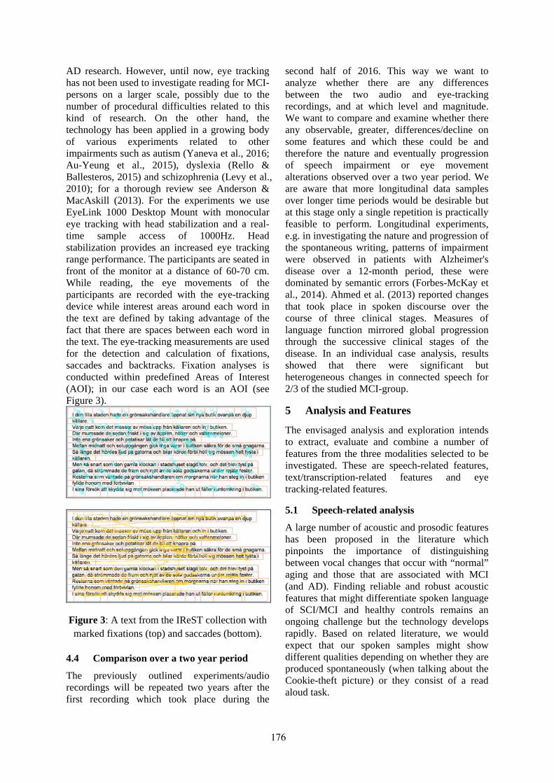
AD research. However, until now, eye tracking has not been used to investigate reading for MCI-persons on a larger scale, possibly due to the number of procedural difficulties related to this kind of research. On the other hand, the technology has been applied in a growing body of various experiments related to other impairments such as autism (Yaneva et al., 2016; Au-Yeung et al., 2015), dyslexia (Rello & Ballesteros, 2015) and schizophrenia (Levy et al., 2010); for a thorough review see Anderson & MacAskill (2013). For the experiments we use EyeLink 1000 Desktop Mount with monocular eye tracking with head stabilization and a real-time sample access of 1000Hz. Head stabilization provides an increased eye tracking range performance. The participants are seated in front of the monitor at a distance of 60-70 cm. While reading, the eye movements of the participants are recorded with the eye-tracking device while interest areas around each word in the text are defined by taking advantage of the fact that there are spaces between each word in the text. The eye-tracking measurements are used for the detection and calculation of fixations, saccades and backtracks. Fixation analyses is conducted within predefined Areas of Interest (AOI); in our case each word is an AOI (see Figure 3).

Figure 3: A text from the IReST collection with marked fixations (top) and saccades (bottom).

4.4 Comparison over a two year period

The previously outlined experiments/audio recordings will be repeated two years after the first recording which took place during the

second half of 2016. This way we want to analyze whether there are any differences between the two audio and eye-tracking recordings, and at which level and magnitude. We want to compare and examine whether there any observable, greater, differences/decline on some features and which these could be and therefore the nature and eventually progression of speech impairment or eye movement alterations observed over a two year period. We are aware that more longitudinal data samples over longer time periods would be desirable but at this stage only a single repetition is practically feasible to perform. Longitudinal experiments, e.g. in investigating the nature and progression of the spontaneous writing, patterns of impairment were observed in patients with Alzheimer's disease over a 12-month period, these were dominated by semantic errors (Forbes-McKay et al., 2014). Ahmed et al. (2013) reported changes that took place in spoken discourse over the course of three clinical stages. Measures of language function mirrored global progression through the successive clinical stages of the disease. In an individual case analysis, results showed that there were significant but heterogeneous changes in connected speech for 2/3 of the studied MCI-group.

5 Analysis and Features

The envisaged analysis and exploration intends to extract, evaluate and combine a number of features from the three modalities selected to be investigated. These are speech-related features, text/transcription-related features and eye tracking-related features.

5.1 Speech-related analysis

A large number of acoustic and prosodic features has been proposed in the literature which pinpoints the importance of distinguishing between vocal changes that occur with “normal” aging and those that are associated with MCI (and AD). Finding reliable and robust acoustic features that might differentiate spoken language of SCI/MCI and healthy controls remains an ongoing challenge but the technology develops rapidly. Based on related literature, we would expect that our spoken samples might show different qualities depending on whether they are produced spontaneously (when talking about the Cookie-theft picture) or they consist of a read aloud task.

176

Prosodic features have been found to be useful in distinguishing between subjects with cognitive impairment and healthy controls, and between groups with varying degrees of cognitive impairment. Pause frequency has been identified as a feature differentiating spontaneous speech in patients with AD from control groups (Gayraud et al., 2011), and may also be used to distinguish between mild, moderate and severe AD (Hoffman et al., 2010). Subjects with AD also tend to make more pauses and non-syntactic boundaries (Lee et al., 2011). Speech tempo, which is defined as phonemes per second (including hesitations) differs significantly between subjects with AD and controls. Speech tempo is also positively correlated with Mini Mental State Examination (MMSE) results (Hoffman et al., 2010), which suggests that people with less cognitive deficits will produce speech at a faster rate.

Speech-related features have been used successfully in machine learning experiments where the aim has been to identify subjects with AD. Roark et al. (2011) used 21 features in supervised machine learning experiments (using Support Vector Machines, SVM) from 37 MCI subjects and equally many controls (37/37). Features from both the audio and the transcripts included: pause frequency, filled pauses, total pause duration and linguistic variables such as Frazier and Yngve scores and idea density, while best accuracy with various feature configurations were 86.1% for the area under the ROC curve. Pause frequency has been identified as a feature differentiating spontaneous speech in patients with AD from control groups (Gayraud et al., 2011), and may also be used to distinguish between mild, moderate and severe AD (Hoffman et al., 2010). Meilán et al. (2014) used AD subjects and spoken data (read loud and clear sentences on a screen). They used acoustic measures such as pitch, volume and spectral noise measures. Their method was based on linear discriminant analysis and their results could characterize people with AD with an accuracy of 84.8%. Yancheva et al. (2015) used spoken and transcriptions features provided from the DementiaBank (Cookie-theft descriptions) using 393 speech samples (165/90). They extracted and investigated 477 different features both lexicosyntactic ones (such as syntactic complexity; word types, quality and frequency) and acoustic ones (such as Melfrequency cepstral coefficients – MFCC, including mean, variance, skewness, and kurtosis; pauses and fillers; pitch

and formants and aperiodicity measures) and semantic ones (such as concept mention) in order to predict MMSE scores with a mean absolute error of 3.83 while with individuals with more longitudinal samples the mean absolute error was improved to 2.91, which suggested that the longitudinal data collection plays an important role. König et al. (2015) looked also at MCI and AD subjects (23/26) and examined vocal features (silence, voice, periodic and aperiodic segment length; mean of durations) using Support Vector Machines. Their classification accuracy of automatic audio analysis was 79% between healthy controls and those with MCI; 87% between healthy controls and those with AD; and between those with MCI and those with AD, 80%. Tóth et al. (2015) used also SVM and achieved 85.3% F-score (32 MCI subjects and 19 controls) by starting with eight acoustic features extracted by applying automatic speech recognition (such as speech tempo i.e. phones per second) and extending them to 83. Finally, Fraser et al. (2016) also looked at the DementiaBank and using 240 samples from AD subjects and 233 from healthy controls, extracted 370 features, such as linguistic variables from transcripts (e.g., part-of-speech frequencies; syntactic complexity and grammatical constituents), psycholinguistic measures (e.g., vocabulary richness) and acoustic variables from the audio files (e.g., MFCC). Using logistic regression, Fraser et al. could obtain a classification accuracy of 81% in distinguishing individuals with AD from those without based on short samples of their language on the Cookie-theft picture description task.

In our analysis, we plan to extract prosodic features such as pitch variation, pause length and frequency, hesitation rate and speech rate, and use these both in stand-alone machine learning experiments, and combined with features extracted from voice analysis, eye-tracking and the transcriptions.

5.2 Voice acoustic-related analysis

Depression commonly occurs among patients diagnosed with MCI. Signs of depression are often expressed as an emotional feeling of sadness or “low mood”. Johnson et al (2013) found that MCI participants with depression experienced greater deficits in cognitive functioning than their non-depressed counterparts, and “low mood” were shown by Caracciolo et al. (2011) to be particularly prominent in the very early stages of cognitive

177

decline and strongly associated with amnestic mild cognitive impairment (aMCI), i.e. the pre-dementia stage of Alzheimer’s, than with global cognitive impairment. Different emotions are accompanied by various adaptive responses in the autonomic and somatic nervous systems (Johnstone & Scherer, 2000). These responses are known to lead to changes in the functioning parts of the speech production system, such as respiration, vocal fold vibration and articulation. The vibrating vocal folds produce the voiced sound (voice source) and the articulation determines the position of the formant frequencies (Hz), determining the vowel and the sound quality of the voice.

The most commonly used parameters in speech acoustic analysis are fundamental frequency (F0) and formant frequency analysis, perturbation measurement such as jitter and shimmer (cycle-to-cycle variations in frequency and amplitude, respectively), and harmonic-to-noise ratios (HNR/NHR). Studying the role of voice production in emotional speech, Patel et al (2011) found significant emotion main effects for 11 of 12 acoustic parameters for five emotions (joy, relief, hot anger, panic fear, sadness) where sadness was characterized by low energy and a hypo-functioning voice quality. Further, Meilán et al. (2014) found voice perturbation parameters to distinguish people with AD from healthy controls with an accuracy of 84.8%.

The aim of the acoustic analysis in the present study is to see if voice parameters can be used to distinguish also between healthy controls and SCI/MCI-patients. Several vowel /a/ and /i/-samples from the read aloud text and the spontaneously spoken Cookie-theft picture will be analyzed for each subject, using the Praat software (Boersma and Weenink). The acoustic data will be compared and correlated according to age, gender, length of education, depression score and other parameters gained from the neuropsychological assessment (Wallin et al., 2016).

5.3 Transcribed speech analysis

Many of the previous studies combine both acoustic features and features from the transcriptions; cf. the supplementary material in Fraser et al. (2016). Some of the most common features and measures from transcribed text follow the lexicon-syntax-semantics continuum. These measures include (i) lexical distribution measures (such as type-token ratio, mean word length, long word counts, hapax legomena,

hapax dislegomena, automated readability index and Coleman-Liau Index; also lexical and non-lexical fillers or disfluency markers, i.e. “um”, “uh”, “eh”) and out-of-vocabulary rate (Pakhomov et al., 2010). (ii) syntactic complexity markers (such as frequency of occurrence of the most frequent words and deictic markers; [context free] production rules, i.e. the number of times a production rule is used divided by the total number of productions; dependency distance, i.e. the length of a dependency link between a dependent token and its head, calculated as the difference between their positions in a sentence; parse tree height, i.e. is the mean number of nodes from the root to the most distant leaf; depth of a syntactic tree, i.e. the proportion of subordinate and coordinate phrases to the total number of phrases and ratio of subordinate to coordinate phrases; noun phrase average length and noun phrase density, i.e. the number of noun phrases per sentence or clause; words per clause); and (iii) semantic measures (such as the idea or propositional density, i.e. the operationalization of conciseness – the average number of ideas expressed per words used; the number of expressed propositions divided by the number of words; a measure of the extent to which the speaker is making assertions, or asking questions, rather than just referring to entities etc.). Since some of the features to be extracted (e.g. part-of-speech and syntactic labels from the speech transcriptions) are language-dependent it requires the use of a language-specific infrastructure (in our case Swedish), for that reason we plan to use available resources; cf. Ahlberg et al. (2013); therefore testing and modifications to the transcribed language are also envisaged. Two wide-coverage parser systems will be used for parsing the speech transcripts. The Malt parser for Swedish (Nivre et al., 2006), that outputs grammatical dependency relations, and a constituent parser for the same language (Kokkinakis, 2001) that utilises a semi-automatically developed grammar. Although the transcribed corpus is describing spoken language and contains various spoken language phenomena, such as filled pauses, we chose to keep the verbatim transcriptions intact. Such phenomena are usually deleted prior to parsing for better performance (Lease & Johnson 2006; Geertzen, 2009). Moreover, since we apply a 2-tier text grid configuration during the transcription, we can easily experiment with both

178

the orthographic transcription (standardized spelling) and the verbatim one.

5.4 Eye-tracking analysis

Eye tracking data has been used in machine learning methods in the near past. By taking advantage of biomarkers extracted from eye dynamics (Lagun et al; 2011) there is an indication that these could aid the automatic detection of cognitive impairment (i.e., distinguish healthy controls from MCI-patients). Several studies provide evidence and suggest that eye movements can be used to detect memory impairment and serve as a possible biomarker for MCI and, in turn, AD (Fernández et al., 2013). Basic features we intend to investigate in this study are fixations (that is the state the eye remains still over a period of time); saccades (that is the rapid motion of the eye from one fixation to another) and backtracks (that is the relationship between two subsequent saccades where the second goes in the opposite direction than the first); for a thorough description of possible eye-tracking related features cf. Holmqvist et al. (2015:262). Saccades are of particular interest because they are much related to attention and thus, they are likely to be disturbed by cognitive impairments associated with neurodegenerative disorders (Anderson & MacAskill, 2013). Note that there are many assumptions behind the use of eye tracking technology for experiments designed for people with MCI. For instance, the longer the eye gaze fixation is on a certain word, the more difficult the word could be for cognitive processing, therefore the durations of gaze fixations could be used as a proxy for measuring cognitive load (Just & Carpenter, 1980). Molitor et al. (2015) provide a recent review on the growing body of literature that investigates changes in eye movements as a result of AD and the alterations to oculomotor function and viewing behaviour.

5.5 Correlation analysis

We intend to further perform correlation analysis with the features previously outlined and the results of the various measures/scores on tasks from language-related tests performed in the Gothenburg MCI-study, applied for assessing possible dementia. Typically, clinicians use tests such as the MMSE, linguistic memory tests and language tests. Language tests include the token test, subtest V, which is a test of syntax comprehension; the Boston naming test, the

semantic similarity test; the letter/word fluency FAS test (the generation of words beginning by the letters F, A, and S) and the category or semantic fluency test (the generation of words that fall into a given semantic category, such as animals). This investigation intends to identify whether there are language-related features, acquired from the range of available tests, which could be (highly negative or highly positive) correlated with i.e. the MCI class, yet uncorrelated with each other i.e. the healthy controls or SCI. We want to further investigate which scores correlate with which variables derived from the picture description. It has been argued, Kavé & Goral (2016), that the picture naming task could be a better predictor of word retrieval in context than the semantic fluency task for several reasons, for instance the speech elicitation method most likely involves cognitive demands that are similar to the ones required for the picture naming task, e.g., specific labelling.


In this paper we have introduced work in progress towards the design and infrastructural development of reliable multi-modal data resources and a set of measures (features) to be used both for experimentation with feature engineering and evaluation of classification algorithms to be used for differentiating between SCI/MCI and healthy adults, and also as benchmark data for future research in the area. Evaluation practices are a crucial step towards the development of resources and useful for enhancing progress in the field, therefore we intend to evaluate both the relevance of features, compare standard algorithms such as Support Vector Machines and Bayesian classifiers and perform correlation analysis with the results of established neuropsychological, memory and cognitive tests. We also intend to repeat the experiments two years after (2018) the current acquisition of data in order to assess possible changes at each level of analysis. We believe that combining data from three modalities (a form of data fusion; Mitchel, 2007) could be useful, but at this point we do not provide any clinical evidence underlying these assumption since the analysis and experimentation studies are currently under way (year 2 of the project, 2017). Therefore, at this stage, the paper only provides a high-level review of the current stage of the work.

179

Acknowledgments

This work has received support from Riksbankens Jubileumsfond - The Swedish Foundation for Humanities and Social Sciences, through the grant agreement no: NHS 14-1761:1.

References

Malin Ahlberg et al. 2013. Korp and Karp – a bestiary of language resources: the research infrastructure of Språkbanken. 19th Nordic Conf of Computational Linguistics (NODALIDA). Linköping Electronic Conference Proceedings #85.

Samrah Ahmed, Anne-Marie Haigh, Celeste de Jager and Peter Garrard. 2013. Connected speech as a marker of disease progression in autopsy-proven Alzheimer's disease. Brain. 136(Pt 12):3727-37.

Tim J. Anderson and Michael R. MacAskill. 2013. Eye movements in patients with neurodegenerative disorders. Nat Rev Neurology 9: 74-85. doi:10.1038/nrneurol.2012.273.

Eiji Aramaki, Shuko Shikata, Mai Miyabe and Ayae Kinoshita. 2016. Vocabulary Size in Speech May Be an Early Indicator of Cognitive Impairment. PLoS One. 11(5):e0155195.

Sheena K. Au-Yeung, Johanna Kaakinen, Simon Liversedge and Valerie Benson. 2015. Processing of Written Irony in Autism Spectrum Disorder: An Eye-Movement Study. Autism Res. 8(6):749-60. doi: 10.1002/aur.1490.

Paul Boersma and David Weenink. 2013. Praat: doing phonetics by computer [Computer program]. Version 6.0.19, retrieved in Aug. 2016 from <http://www.praat.org/>.

Barbara Caracciolo et al. 2011. The symptom of low mood in the prodromal stage of mild cognitive impairment and dementia: a cohort study of a community dwelling elderly population. J Neurol Neurosurg Psychiatry. 82:788-793.

Vineeta Chand, Kathleen Baynes, Lisa M. Bonnici and Sarah Tomaszewski Farias. 2012. A Rubric for Extracting Idea Density from Oral Language Samples Analysis of Idea Density (AID): A Manual. Curr Protoc Neurosci. Ch. Unit10.5. doi:10.1002/0471142301.ns1005s58.

James W Dodd 2015. Lung disease as a determinant of cognitive decline and dementia. Alzh Res & Therapy, 7:32.

Alison Ferguson, Elizabeth Spencer, Hugh Craig and Kim Colyvas. 2014. Propositional Idea Density in women’s written language over the lifespan: Computerized analysis. Cortex 55. 107-121.

Gerardo Fernández et al. 2013. Eye Movement Alterations during Reading in Patients with Early

Alzheimer Disease. Investigative Ophthalmology & Visual Science. Vol.54, 8345-8352. doi:10.1167/iovs.13-12877.

Katrina Forbes-McKay, Mike Shanks and Annalena Venneria. 2014. Charting the decline in spontaneous writing in Alzheimer's disease: a longitudinal study. Acta Neuropsychiatrica. Vol. 26:04, pp 246-252.

Kathleen C. Fraser and Graeme Hirst. 2016. Detecting semantic changes in Alzheimer’s disease with vector space models. LREC Workshop: Resources and ProcessIng of linguistic and extra-linguistic Data from people with various forms of cognitive/psychiatric impairments (RaPID). Pp. 1-8. Portorož Slovenia.

Peter Garrard and Brita Elvevåg. 2014. Special issue: Lang., computers and cognitive neuroscience. Cortex 55; 1-4.

Frederique Gayraud, Hye-Ran Lee and Melissa Barkat-Defradas. 2011. Syntactic & lexical context of pauses and hesitations in the discourse of Alzheimer patients and healthy elderly subjects. Clin Ling&Phon. 25(3):198-209.

Jeroen Geertzen. 2009. Wide-coverage parsing of speech transcripts. 11th Pars. Tech (IWPT). Pp 218–221. France.

Elaine Gilles, Karalyn Patterson and John Hodges. 1996. Performance on the Boston Cookie Theft picture description task in patients with early dementia of the Alzheimer’s type: missing information. Aphasiology. 10:4:395-408.

Harald Goodglass and Edith Kaplan. 1983. The Assessment of Aphasia and Related Disorders. Lea&Febiger. USA.

Ildikó Hoffmann et al. 2010. Temporal parameters of spontaneous speech in Alzheimer’s disease. J of Speech-Language Pathology, 12(1), 29–34.

Kenneth Holmqvist, Richard Dewhurst, Marcus Nyström, Joost van de Weijer, Halszka Jarodzka and Richard Andersson. 2015. Eye Tracking - A comprehensive guide to methods & measures. OUP.

Frank Jessen et al. 2010. Prediction of dementia by subjective memory impairment: effects of severity and temporal association with cognitive impairment. Arch. Gen. Psychiatry, 67(4). Pp. 414–422.

Leigh A Johnson et al. 2013. Cognitive differences among depressed and non-depressed MCI participants. J Geriatr Psychiatry. 28(4):377-82.

Tom Johnstone and Klaus R. Scherer. 2000. Vocal communication of emotion. The Handbook of Emotion. Lewis & Haviland (eds). NY Guildford.

Marcel A. Just and Patricia A. Carpenter. 1980. A theory of reading: from eye fixations to

180

comprehension. Psychological review, 87(4):329-354.

Gitit Kavé & Mira Goral. 2016. Word retrieval in picture descriptions produced by individuals with Alzheimer's disease. J Clin Exp Neuropsychol. 38(9):958-66.

Dimitrios Kokkinakis. 2001. More than Surface-Based Parsing; Higher Level Evaluation of Cass-SWE. 13th Nordic Computational Linguistics Conference (NODALIDA). Uppsala, Sweden.

Alexandra König et al. 2015. Automatic speech analysis for the assessment of patients with predementia and Alzheimer’s disease. Alzheimer’s & Dementia: Diagnosis, Assessment & Disease Monitoring. 1:112–124. Elsevier.

Dmitry Lagun et al. 2011. Detecting cognitive impairment by eye movement analysis using automatic classification algorithms. J Neurosci Methods. 201(1): 196–203. doi:10.1016/j.jneumeth. 2011.06.027.

Christoph Laske et al. 2014. Innovative diagnostic tools early detection of Alzheimer’s disease. Alzheimer’s & Dementia. 1-18.

Xuan Le, Ian Lancashire, Graeme Hirst, and Regina Jokel. 2011. Longitudinal Detection of Dementia through Lexical and Syntactic Changes in Writing: A Case Study of Three British Novelists. JLLC 26 (4): 435-461.

Matthew Lease and Mark Johnson. 2006. Early deletion of fillers in processing conversational speech. Proceedings of the Human Language Technology Conference of the North American Chapter of the ACL, pages 73–76.

Hyeran Lee, Frederique Gayraud, Fabrice Hirsh and Melissa Barkat-Defradas. 2011. Speech dysfluencies in normal and pathological aging: A comparison between Alzheimer patients and healthy elderly subjects. ICPhS: proceedings of the 17th International Congress of Phonetic Sciences. Pp. 1174–1177. Hong Kong.

Deborah L. Levy, Anne B. Sereno, Diane C. Gooding,and Gilllian A. O’Driscoll. 2010. Eye Tracking Dysfunction in Schizophrenia: Characterization and Pathophysiology. Curr Top Behav Neurosci. 4: 311–347.

Juan JG. Meilán, Francisco Martínez-Sánchez, Juan Carro, José A. Sánchez and Enrique Pérez. 2012. Acoustic Markers Associated with Impairment in Language Processing in AD. Spanish J of Psych. Vol. 15:2, 487-494.

Juan JG. Meilán et al. 2014. Speech in Alzheimer’s Disease: Can Temporal and Acoustic Parameters Discriminate Dementia? Dement Geriatr Cogn Disord 2014;37:327–334. doi: 10.1159/000356726.

H. B. Mitchell. (2007). Multi-Sensor Data Fusion: An Introduction. Springer.

Robert J. Molitor, Philip C. Ko and Brandon A. Ally. 2015. Eye Movements in Alzheimer’s Disease. J of Alzheimer’s Disease 44, 1–12. IOS Press.

James A. Mortimer, Amy R. Borenstein, Karen M. Gosche and David A. Snowdon. 2005. Very Early Detection of Alzheimer Neuropathology and the Role of Brain Reserve in Modifying Its Clinical Expression. J Geriatr Psychiatry Neurol. 18(4): 218–223.

Joakim Nivre et al. 2007. MaltParser: A language-independent system for data-driven dependency parsing. Natural Language Engineering. 13(2):95-135.

Arto Nordlund, S. Rolstad, P. Hellström, M. Sjögren, S. Hansen and Anders Wallin. 2005. The Goteborg MCI study: mild cognitive impairment is a heterogeneous condition. J Neurol Neurosurg Psychiatry. 76(11):1485-90.

Sylvester Olubolu Orimaye, Jojo Sze-Meng Wong and Kren J. Golden. 2014. Learning Predictive Linguistic Features for Alzheimer’s Disease and related Dementias using Verbal Utterances. Workshop on Computational Ling. & Clinical Psychology: From Linguistic Signal to Clinical Reality. 78–87. Maryland, USA.

Serguei VS Pakhomov et al. 2010. A co-mputerized technique to assess language use patterns in patients with frontotemporal dementia. J Neuroling. 23(2):127–144.

Sona Patel, Klaus R. Scherer, Eva Björkner, Johan Sundberg. 2011. Mapping emotions into acoustic space: The role of voice production. Biological Psychology 87. 93–98.

Sajidkhan S. Pathan et al. 2011. Association of lung function with cognitive decline and dementia: the Atherosclerosis Risk in Communities (ARIC) Study. Eur J Neurol. 18(6):888-9.

Luz Rello and Miguel Ballesteros. 2015. Detecting Readers with Dyslexia Using Machine Learning with Eye Tracking Measures. Proceedings of the 12th Web for All Conference W4A. Florence, Italy.

Vassiliki Rentoumi, Ladan Raoufian, Samrah Ahmed and Peter Garrard. 2014. Features and Machine Learning Classification of Connected Speech Samples from Patients with Autopsy Proven Alzheimer's Disease with and without Additional Vascular Pathology. J of Alzheimer’s Disease 42. IOS Press. S3–S17.

Karen Ritchie and Jacques Touchon. 2010. Mild cognitive impairment: conceptual basis and current nosological status. The Lancet. Vol. 355:9199. Pp. 225–228. Doi:10.1016/S0140-6736(99)06155-3.

181

Brian Roark, Margaret Mitchell, John-Paul Hosom, Kristy Hollingshead, and Jeffrey Kaye. 2011. Spoken Language Derived Measures for Detecting Mild Cognitive Impairment. IEEE Trans Audio Speech Lang Processing. 19(7): 2081–2090.

David A. Snowdon, Lydia Greiner and William R. Markesbery. 2000. Linguistic ability in early life and the neuropathology of Alzheimer's disease and cerebrovascular disease. Findings from the Nun Study. Annals of the NY Academy of Sciences. 903:34-8.

Greta Szatloczki, Ildiko Hoffmann, Veronika Vincze, Janos Kalman and Magdolna Pakaski. 2015. Speaking in Alzheimer’s disease, is that an early sign? Importance of changes in language abilities in Alzheimer’s disease. Frontiers in Aging Neuroscience. Vol 7, article 195. doi: 10.3389/fnagi.2015.00195.

Vanessa Taler and Natalie Phillips. 2008. Language performance in Alzheimer's disease and mild cognitive impairment: A comparative review. J Clin Exp Neuropsychol. 30(5):501-56. doi: 10.1080/13803390701550128.

Susanne Trauzettel-Klosinski, Klaus Dietz & the IReST Study Group. 2012. Standardized Assessment of Reading Performance: The New International Reading Speed Texts IReST. Investigative Ophthalmol&Visual Sc. 53:9.

Laszló Tóth et al. 2015. Automatic Detection of MCI from Spontaneous Speech using ASR. Interspeech. Germany.

Anders Wallin et al. 2016. The Gothenburg MCI study: Design and distribution of Alzheimers disease and subcortical vascular disease diagnoses from baseline to 6-year follow-up. J Cer Blood Flow Metab. 36(1):114-31.

Olof Tyche. 2001. Subtila språkstörningar hos patienter med diagnosen MCI. Master's thesis. Karolinska institute, Sweden (In Swedish).

Brian MacWhinney, Davida Fromm, Margaret Forbes and Audrey Holland. 2011. AphasiaBank: Methods for studying discourse. Aphasiology. 25 (11), 1286-1307.

Caroline Williams et al. 2010. The Cambridge Cookie-Theft Corpus: A Corpus of Directed and Spontaneous Speech of Brain-Damaged Patients and Healthy Individuals. 7th Language Resources and Evaluation (LREC). Pp. 2824-2830. Malta.

Maria Yancheva, Kathleen Fraser and Frank Rudzicz. 2015. Using linguistic features longitudinally to predict clinical scores for Alzheimer’s disease and related dementias. 6th SLPAT. Pp. 134–139, Dresden, Germany.

Victoria Yaneva, Irina Temnikova and Ruslan Mitkov. 2016. Corpus of Text Data and Gaze Fixations from Autistic and Non-autistic Adults. 10th Language Resources and Evaluation (LREC). Pp. 480-487. Slovenia.

Gustaf Öqvist Seimyr. 2010. Swedish IReST translation. The Bernadotte Laboratory, Karolinska institute, Sweden.

182


Evaluation of language identification methods using 285 languages

Tommi JauhiainenUniversity of [email protected]

Krister LindenUniversity of [email protected]

Heidi JauhiainenUniversity of [email protected]

Abstract

Language identification is the task of giv-ing a language label to a text. It is an im-portant preprocessing step in many auto-matic systems operating with written text.In this paper, we present the evaluation ofseven language identification methods thatwas done in tests between 285 languageswith an out-of-domain test set. The evalu-ated methods are, furthermore, describedusing unified notation. We show that amethod performing well with a small num-ber of languages does not necessarily scaleto a large number of languages. The HeLImethod performs best on test lengths ofover 25 characters, obtaining an F1-scoreof 99.5 already at 60 characters.

1 Introduction

Automatic language identification of text has beenresearched since the 1960s. Language identifica-tion is an important preprocessing step in many au-tomatic systems operating with written text. Stateof the art language identifiers obtain high ratesin both recall and precision. However, even thebest language identifiers do not give perfect resultswhen dealing with a large number of languages,out-of-domain texts, or short texts. In this paperseven language identification methods are evalu-ated in tests incorporating all three of these hardcontexts. The evaluations were done as part of theFinno-Ugric Languages and The Internet project(Jauhiainen et al., 2015) funded by the Kone Foun-dation Language Programme (Kone Foundation,2012). One of the major goals of the project iscreating text corpora for the minority languageswithin the Uralic group.

In Section 2, we describe the methods chosenfor this evaluation. In Section 3, we present thecorpora used for training and testing the methods

and in Section 4 we discuss and present the resultsof the evaluations of the methods using these cor-pora.

2 Previous work

There are not many previously published arti-cles which provide language identification resultsfor more than 100 languages. Results for suchevaluations were provided by King and Dehdari(2008), Jauhiainen (2010), Vatanen et al. (2010),Rodrigues (2012), and Brown (2012). King andDehdari (2008) achieved 99% accuracy with 500bytes of input for over 300 languages. Vatanen etal. (2010) created a language identifier which in-cluded 281 languages and obtained an in-domainidentification accuracy of 62.8% for extremelyshort samples (5-9 characters). Rodrigues (2012)presents a boosting method using the method ofVatanen et al. (2010) for language identification.His method could possibly also be used with otherlanguage identification methods and we leave theevaluation of the boosting method to future work.The language identifier created by Brown (2012),”whatlang”, obtains 99.2% classification accuracywith smoothing for 65 character test strings whendistinguishing between 1,100 languages (Brown,2013; Brown, 2014).

The HeLI method described in Jauhiainen etal. (2016) was used successfully with 103 lan-guages by Jauhiainen (2010). Some of the moredetailed results concerning the Uralic languagesfor the evaluations presented in this paper werepreviously published by Jauhiainen et al. (2015).

In this section, we also include the originalmethod of Cavnar and Trenkle (1994), as it isthe most frequently used baseline in the languageidentification literature. As baselines, we havealso included the methods presented by Tromp andPechenizkiy (2011) and Vogel and Tresner-Kirsch(2012), which provided promising results whenused with 6 languages.

183

2.1 On notation (Jauhiainen et al., 2016)

A corpus C consists of individual tokens u whichmay be words or characters. A corpus C is a finitesequence of individual tokens, u1, ...,ul . The totalcount of all individual tokens u in the corpus C isdenoted by lC. A set of unique tokens in a corpusC is denoted by U(C). The number of unique to-kens is referred to as |U(C)|. A feature f is somecountable characteristic of the corpus C. When re-ferring to all features F in a corpus C, we use CF

and the count of all features is denoted by lCF . Thecount of a feature f in the corpus C is referred to asc(C, f ). An n-gram is a feature which consists of asequence of n individual tokens. An n-gram start-ing at position i in a corpus is denoted ui,...,i−1+n.If n = 1, u is an individual token. When referringto all n-grams of length n in a corpus C, we useCn and the count of all such n-grams is denotedby lCn . The count of an n-gram u in a corpus C isreferred to as c(C,u) and is defined by Equation 1.

c(C,u) =lC+1−n

∑i=1

{1 , if u = ui,...,i−1+n0 , otherwise (1)

The set of languages is G, and lG denotes thenumber of languages. A corpus C in language gis denoted by Cg. A language model O based onCg is denoted by O(Cg). The features given valuesby the model O(Cg) are the domain dom(O(Cg))of the model. In a language model, a value v forthe feature f is denoted by vCg( f ). A corpus in anunknown language is referred to as a mystery textM. For each potential language g of a corpus M, aresulting score R(g,M) is calculated.

2.2 N-Gram-Based Text Categorization

The method of Cavnar and Trenkle (1994) usesoverlapping character n-grams of varying size cal-culated from words. The language models are cre-ated by tokenizing the training texts for each lan-guage g into words and then padding each wordwith spaces, one before and four after. Eachpadded word is then divided into overlapping char-acter n-grams of sizes from 1 to 5 and the counts ofevery unique n-gram are calculated over the wholecorpus. The n-grams are ordered by frequency andk of the most frequent n-grams, u1, ...,uk, are usedas the domain of the language model O(Cg) forthe language g. The rank of an n-gram u in lan-guage g is determined by the n-gram frequency inthe training corpus Cg and denoted rankCg(u).

During language identification, the mystery textis treated in a similar way and a correspondingmodel O(M) of the k most frequent n-grams iscreated. Then a distance score is calculated be-tween the model of the mystery text and each ofthe language models. The value vCg(u) is calcu-lated as the difference in ranks between rankM(u)and rankCg(u) of the n-gram u in the domaindom(O(M)) of the model of the mystery text. If ann-gram is not found in a language model, a specialpenalty value p is added to the total score of thelanguage for each missing n-gram. The penaltyvalue should be higher than the maximum possi-ble distance between ranks. We use p = k+ 1, asthe penalty value.

vCg(u) ={|rankM(u)− rankCg(u)|, if u ∈ dom(O(Cg))p, if u /∈ dom(O(Cg))

(2)

The score Rsum(g,M) for each language g is thesum of values as in Equation 3.

Rsum(g,M) =lMF

∑i=1

vCg( fi) (3)

The language having the lowest scoreRsum(g,M) is selected as the identified lan-guage.

2.3 LIGA-algorithmThe graph-based n-gram approach called LIGAwas first described in (Tromp, 2011). The methodis here reproduced as explained in (Vogel andTresner-Kirsch, 2012). The language models con-sist of relative frequencies of character trigramsand the relative frequencies of two consecutiveoverlapping trigrams. The frequency of two con-secutive overlapping trigrams is exactly the sameas the 4-gram starting from the beginning of thefirst trigram. So the language models consist ofthe relative frequencies vCg(u) of 3- and 4-gramsas in Equation 4.

vCg(u) =c(Cg,u)

lCng

(4)

where c(Cg,u), is the number of 3- or 4-grams uand lCn

g, is the total number of 3- and 4-grams in

the training corpus.The mystery text M is scanned for the 3- and

4-grams u. For each 3- and 4-gram found in themodel of a language g, the relative frequencies areadded to the score Rsum(g,M) of the language g, asin Equation 3. The winner is the language with the

184

highest score as opposed to the lowest score withthe previous method.

In the logLIGA variation of the method, intro-duced by Vogel and Tresner-Kirsch (2012), thenatural logarithm of the frequencies is used whencalculating the relative frequencies, as in Equa-tion 5.

vCg(u) =ln(c(Cg,u))

ln(lCng)

(5)

Otherwise the method is identical to the originalLIGA algorithm.

2.4 The method of King and Dehdari (2008)King and Dehdari (2008) tested the use of the rela-tive frequencies of byte n-grams with Laplace andLidstone smoothings in distinguishing between312 languages. They separately tested overlap-ping 2-, 3-, and 4-grams with both smoothing tech-niques. They used the Universal Declaration ofHuman Rights corpus, which is accessible usingNLTK (Bird, 2006), separating the testing mate-rial before training. The values for each n-gramare calculated as in Equation 6,

vCg(u) =c(Cg,u)+λ

lCng+ |U(Cn

g)|λ(6)

where vCg(u) is the probability estimate of n-gramu in the model and c(Cg,u) its frequency in thetraining corpus. lCn

gis the total number of n-

grams of length n and |U(Cng)| the number of dis-

tinct n-grams in the training corpus. λ is the Lid-stone smoothing parameter. When using Laplacesmoothing, the λ is equal to 1 and with Lidstonesmoothing, the λ is usually set between 0 and1. King and Dehdari (2008) found that Laplacesmoothing with the bigram model turned out tobe the most accurate on two of their longer testsets and that Lidstone smoothing (with λ set to0.5) was better with the shortest test set. Kingand Dehdari (2008) used the entropy(model, text)function of NLTK, which evaluates the entropy be-tween text and model by summing up the log prob-abilities of words found in the text.1

2.5 ”Whatlang” program (Brown, 2013)The ”Whatlang” program uses variable length byten-grams from 3 to 12 bytes as its language model.K of the most frequent n-grams are extracted from

1Jon Dehdari recently uploaded the instruc-tions to: https://github.com/jonsafari/witch-language

training corpora for each language and their rel-ative frequencies are calculated. In the tests re-ported in (Brown, 2013), K varied from 200 to3,500 n-grams. After the initial models are gen-erated, n-grams, which are substrings of longer n-grams in the same model, are filtered out, if thefrequency of the longer n-gram is at least 62% ofthe shorter n-grams frequency. The value vCg(u)of an n-gram u in the model of the corpus Cg iscalculated as in Equation 7

vCg(u) =(c(Cg,u)

lCng

)0.27n0.09 (7)

where c(Cg,u) is the frequency of the n-gram uand lCn

gis the number of all n-grams of the length

n in the training corpus Cg. The weights in themodel are calculated so that the longer n-gramshave greater weights than short ones with thesame relative frequency. Baseline language mod-els Obase(Cg) are formed for each language g usingthe values vCg(u).

For each language model Obase(Cg), the cosinesimilarity between it and every other languagemodel is calculated. A union of n-grams is formedby taking all of the models for which the sim-ilarity is higher than an empirically determinedthreshold. The corpus Cg is scanned for occur-rences of the n-grams in the union. If some ofthe n-grams are not found at all, these n-gramsare then appended with negative weights to thebase model. The negative weight used for an n-gram u in the model O(Cg) is the maximum co-sine similarity between Obase(Cg) and the modelscontaining an n-gram u times the maximum vC(u)within those models. These negative weighted n-grams are called stop-grams. If the size of thetraining corpus for a certain model is less than 2million bytes, the weights of the stop-grams arediscounted as a function of the corpus size.

The score Rwhatlang(g,M) for the language g iscalculated as in Equation 8

Rwhatlang(g,M) =∑i vCg(ui)

lM1(8)

where ui are the n-grams found in the mystery textM. The score is also normalized by dividing itwith the length (in characters) of the mystery textlM1 . The language with the highest score is identi-fied as the language of the mystery text.

Brown (2013) tested ”Whatlang” with 1,100languages as well as a smaller subset of 184 lan-guages. The reported average of classification ac-

185

curacy with 1,100 languages for lines up to 65characters is 98.68%, which is extremely good.

2.6 VariKN toolkit (Vatanen et al., 2010)

The problem with short text samples was consid-ered by Vatanen et al. (2010). Several smooth-ing techniques with a naive Bayes classifier werecompared in tests of 281 languages. Absolute dis-counting (Ney et al., 1994) smoothing with a max-imum n-gram length of 5 turned out to be their bestmethod. When calculating the Markovian prob-abilities in absolute discounting, a constant D issubtracted from the counts c(C,un

i−n+1) of all ob-served n-grams un

i−n+1 and the left-out probabilitymass is distributed between the unseen n-grams inrelation to the probabilities of lower order n-gramsPg(ui|un−1

i−n+2), as in Equation 9.

Pg(ui|un−1i−n+1) =

c(C,uni−n+1)−D

c(C,un−1i−n+1)

+λun−1i−n+1

Pg(ui|un−1i−n+2)

(9)

The language identification is performed us-ing the ”perplexity” program provided with thetoolkit.2 Perplexity is calculated from the Marko-vian probability P(M|Cg) = ∏i Pg(ui|un−1

i−n+1) forthe mystery text M given the training data Cg asin Equations 10 and 11.

Hg(M) =− 1c(M,u) ∏

ilog2Pg(ui|un−1

i−n+1) (10)

Rperplexity(g,M) = 2Hg(M) (11)

2.7 The HeLI method

The HeLI3 method (Jauhiainen, 2010) is describedin Jauhiainen et al. (2016) using the same notationas in this article. In the method, each language isrepresented by several different language modelsonly one of which is used for every word found inthe mystery text. The language models for eachlanguage are: a model based on words and one ormore models based on character n-grams from oneto nmax. When a word not included in the modelbased on words is encountered in the mystery textM, the method backs off to using the n-grams ofthe size nmax. If it is not possible to apply the n-grams of the size nmax, the method backs off tolower order n-grams and continues backing off un-til character unigrams, if needed. A development

2https://github.com/vsiivola/variKN3https://github.com/tosaja/HeLI

set is used for finding the best values for the pa-rameters of the method. The three parameters arethe maximum length of the used character n-grams(nmax), the maximum number of features to be in-cluded in the language models (cut-off c), and thepenalty value for those languages where the fea-tures being used are absent (penalty p). Because ofthe large differences between the sizes of the train-ing corpora, we used a slightly modified imple-mentation of the method, where we used relativefrequencies as cut-offs c. The values in the mod-els are 10-based logarithms of the relative frequen-cies of the features u, calculated using only the fre-quencies of the retained features, as in Equation 12

vCg(u) =

{− log10

(c(Cg,u)

lCg

), if c(Cg,u)> 0

p , if c(Cg,u) = 0(12)

where c(Cg,u) is the number of features u and lCg

is the total number of all features in language g. Ifc(Cg,u) is zero, then vCg(u) gets the penalty valuep.

A score vg(t) is calculated for each word t inthe mystery text for each language g, as shown inEquation 13.

vg(t) ={

vCg(t) , if t ∈ dom(O(Cg))vg(t,min(nmax, lt +2)) , if t /∈ dom(O(Cg))

(13)

The whole mystery text M gets the scoreRHeLI(g,M) equal to the average of the scores ofthe words vg(t) for each language g, as in Equa-tion 14

RHeLI(g,M) =∑

lT (M)

i=1 vg(ti)lT (M)

(14)

where T (M) is the sequence of words and lT (M) isthe number of words in the mystery text M. Thelanguage having the lowest score is assigned to themystery text.

3 Test setting

In addition to the Uralic languages relevant to theproject (Jauhiainen et al., 2015), the languages forthe evaluation of the language identification meth-ods were chosen so that we were able to train andtest with texts from different sources, preferablyalso from different domains. We were able togather suitable corpora for a set of 285 languages.4

4The list of all the languages and most of the sourcescan be found at http://suki.ling.helsinki.fi/LILanguages.html.

186

In our project we are interested in gathering asmuch of the very rare Uralic texts as possible, sowe need a high recall. On the other hand, if ourprecision is bad, we end up with a high percent-age of incorrect language labels for the rare lan-guages. For these reasons we use the F1-scoreas the main performance measure when evalu-ating the language identifiers. We calculate thelanguage-level averages of recall, precision andthe F1-score. Language-level averages are referredto as macro-averages by Lui et al. (Lui et al.,2014). As the number of mystery texts for eachlanguage were identical, the macro-averaged re-call equals the commonly used classification accu-racy5. The Fβ -score is based on the effectivenessmeasure introduced by van Rijsbergen (1979) andis calculated from the precision p and recall r, asin Equation 15

Fβ = (1+β 2)

(pr

(β 2 p)+ r

)(15)

where β = 1 gives equal weight to precision andrecall.

3.1 Training Corpora

The biggest bulk of the training corpora is formedfrom various Wikipedias.6 The collection sizesrange from a few articles for the very small lan-guages to over a million articles in the English,German, French, Dutch and Italian collections.The sheer amount of linguistic material containedin the article collections makes using them astext corpora an appealing thought. The articlecollections had to be cleaned as they containedlots of non-lingual metadata and links as well astext in non-native languages. In addition to thetext from Wikipedia, there is material from bibletranslations7, other religious texts8, the LeipzigCorpora Collection (Quasthoff et al., 2006), theAKU project9, Sami giellatekno10, and genericweb pages. Even with these additions, the amount

5The evaluation results for all the languages and identi-fiers can be found at http://suki.ling.helsinki.fi/NodaEvalResults.xlsx.

6http://www.wikipedia.org7http://gospelgo.com/biblespage.html,

http://worldbibles.org, http://ibt.org.ru,http://gochristianhelps.com

8http://www.christusrex.org, https://www.lds.org

9http://www.ling.helsinki.fi/˜rueter/aku-index.shtml

10http://giellatekno.uit.no

of training material differs greatly between lan-guages.

Each language has one file including all thetraining texts for that language. Some of the textsare copyrighted, so they cannot be published assuch. The amount of training material differs dras-tically between languages: they span from 2,710words of Tahitian to 29 million words of En-glish. Some of the corpora were manually exam-ined to remove text obviously written in foreignlanguages. Even after all the cleaning, the trainingcorpora must be considered rather unclean.

3.2 Testing Corpora

The test corpora are mostly derived from thetranslations of the universal declaration of humanrights.11 However, the test set includes languagesfor which no translation of the declaration is avail-able and for these languages texts were collectedfrom some of the same sources as for the trainingcorpora, but also from Tatoeba.12 Most of the testtexts have been examined manually for purity, sothat obvious inclusions of foreign languages wereremoved.

The aim was to have the mystery texts from dif-ferent domains than the training texts. Wikipediarefers to the declaration of human rights in severallanguages and in many places. In order to dealwith possible inclusion of test material in train-ing corpora, every test corpus was divided into30 character chunks and any lines including thesechunks in the corresponding training corpus wereremoved. Also, if long sequences of numbers werenoticed, they were removed from both corpora.There are still numbers in the test set and for ex-ample some of the 5 character or even 10 charactersequences in the test set consist only or mostly ofnumbers.

The test set has been randomly generated fromthe test corpora. A test sample always begins at thebeginning of a word, but it might end anywhere,including in the middle of a word. An extra blankwas inserted in the beginning of each line whentesting those language identifiers, which did notautomatically expect the text to begin with a word.The test samples are of 19 different sizes rangingfrom 5 to 150 characters. Each language and sizepair has 1,000 random (some can be identical) testsamples. The full test set comprises of around 5.4

11http://www.unicode.org/udhr/12http://tatoeba.org/eng/

187

30

40

50

60

70

80

90

100

5 10 15 20 25 30 35 40 45 50 55 60 65 70

F-s

co

re

Test length in characters

LIGA LogLIGA Cavnar & Trenkle

Figure 1: Comparison between the F1-scores ofthe method of Cavnar and Trenkle (1994), LIGA,and logLIGA.

million samples to be identified.

4 The results and discussion

After training the aforementioned language identi-fiers with our own training corpora, we tested themagainst all the languages in our test suite.

4.1 The baselines

Cavnar and Trenkle (1994) included the 300 mostfrequent n-grams in the language models. In ourtests the best results were attained using 20,000n-grams with their method. From the LIGA vari-ations introduced by Vogel and Tresner-Kirsch(2012), we chose to test the logLIGA as it per-formed the best in their evaluations in additionto the original LIGA algorithm. For these threemethods, the averaged results of the evaluationsfor 285 languages can be seen in Figure 1.

The results of both the LIGA and logLIGA al-gorithms are clearly outperformed by the methodof Cavnar and Trenkle (1994). Especially thepoor results of logLIGA were surprising, as itwas clearly better than the original LIGA algo-rithm in the tests presented by Vogel and Tresner-Kirsch (2012). To verify the performance of ourimplementations, we tested them with the sameset of languages which were tested in (Vogel andTresner-Kirsch, 2012), where the baseline LIGAhad an average recall of 97.9% and logLIGA99.8% over 6 languages. The tweets in theirdataset average around 80 characters. The results

55

60

65

70

75

80

85

90

95

100

5 10 15 20 25 30 35 40 45 50 55 60 65 70

Recall

Test length in characters

LIGA LogLIGA

Figure 2: The recall of LIGA and logLIGA algo-rithms with 6 languages.

of our tests can be seen in Figure 2. The logLIGAclearly outperforms the LIGA algorithm and ob-tains 99.8% recall already at 50 characters evenfor our cross-domain test set. From these resultswe believe that especially the logLIGA algorithmdoes not scale to a situation with a large numberof languages.

4.2 The evaluations

For the evaluation of the method of King andDehdari (2008) we created Laplace and Lidstonesmoothed language models from our training cor-pora and programmed a language identifier, whichused the sum of log probabilities (we did not useNLTK) to measure the distance between the mod-els and the mystery text. We tested n-grams from1 to 6 with several different values of λ . King andDehdari (2008) used byte n-grams, but as our cor-pus is completely UTF-8 encoded, we use n-gramsof characters instead.

The best results (Figure 3) in our tests wereachieved with 5-grams and a λ of 0.00000001.These findings are not exactly in line with thoseof King and Dehdari (2008). The number of lan-guages used in both language identifiers is compa-rable, but the amount of training data in our cor-pus varies considerably between languages whencompared with the corpus used by King and De-hdari (2008), where each language had about thesame amount of material. The smallest test setthey used was 2%, which corresponds to around100 - 200 characters, which is comparable to the

188

Figure 3: The F1-scores of the six best evaluatedmethods.

longest test sequences used in this article. We be-lieve that these two dissimilarities in test settingcould be the reason for the differing results, butwe decided that investigating this further was notwithin the scope of this article.

In the evaluation of the method of Brown(2013), we used the ”mklangid” program providedwith the Brown’s package13 to create new lan-guage models for the 285 languages of our testsuite. The best results with the ”whatlang” wereobtained using up to 10-byte n-grams, 40,000 n-grams in the models, and 160 million bytes oftraining data as well as stop-grams. Stop-gramswere calculated for languages with a similarityscore of 0.4 or higher. The average recall obtainedfor 65 character samples was 98.9% with an F1-score of 99.0%. Brown’s method clearly outper-forms the results of the algorithm of Cavnar andTrenkle (1994), as can be seen in Figure 3. Onething to note is also the running time. Running thetests using the algorithm of Cavnar and Trenkle(1994) with 20,000 n-grams took over two days,as opposed to the less than an hour with Brown’s”Whatlang” program.

In order to evaluate the method used by Vatanenet al. (2010), we utilized the VariKN toolkit (Si-ivola et al., 2007) to create language models fromour training data with the same settings: absolutediscounting smoothing with a character n-gramlength of 5. When compared with the Browns

13https://sourceforge.net/projects/la-strings/

Figure 4: The F1-scores of the HeLI method com-pared with the methods of Brown (2012) and Vata-nen et al. (2010).

identifier the results are clearly in favor of theVariKN toolkit for short test lengths and almostequal at test lengths of 70 characters, after whichBrown’s language identifier performs better.

For the evaluation of the HeLI method we useda slightly modified Python based implementationof the method. In our implementation, we usedrelative frequencies as cut-offs c instead of justthe frequencies. In order to find the best possi-ble parameters using the training corpora, we ap-plied a simple form of the greedy algorithm us-ing the last 10% of the training corpus for eachlanguage as a development set. We started withthe same n-gram length nmax and the penalty valuep, which were found to provide the best resultsin (Jauhiainen, 2010). Then we proceeded usingthe greedy algorithm and found at least a local op-timum with the values nmax = 6, c = 0.0000005,and p = 7. The HeLI method obtains high recalland precision clearly sooner than the methods ofBrown (2013) or Vatanen et al. (2010). The F1-score of 99.5 is achieved at 60 characters, whileBrown’s method achieved it at 90 characters andthe method of Vatanen et al. (2010) at more than100 characters, which can be seen in Figure 4. Themethod of Vatanen et al. (2010) performs betterthan the HeLI method when the length of the mys-tery text is 20 characters or less.

The HeLI method was also tested without us-ing the language models composed of words. Itwas found that in addition to obtaining slightly

189

Lang. ISO HL LG LL VK WL CT KGN.-Aram. aii 5 5 5 5 5 10 80Amharic amh 5 5 20 5 10 5 -Tibetan bod 5 10 10 5 5 25 20Cherokee chr 5 10 15 5 5 20 -Greek ell 5 5 5 5 5 10 40Gujarati guj 5 5 5 5 5 10 15Armenian hye 5 5 5 5 5 10 65Inuktitut iku 5 10 15 5 5 10 -Kannada kan 5 5 5 10 5 10 30Korean kor 5 5 5 5 5 15 70Malayal. mal 5 5 5 5 5 15 15Thai tha 5 5 5 20 5 15 25

Table 1: Some of the easiest languages to iden-tify showing how many characters were needed for100.0% recall by each method.

Lang. ISO HL LG LL VK WL CT KGAchinese ace 120 - - - - - -Bislama bis 100 - - - - - -Chayah. cbt - 70 - - 80 90 90Danish dan 150 - - - - 100 -T. Enets enh 150 80 - 70 - - 45Evenki evn 150 - - - - - 150Erzya myv - - - - - - -Newari new - - - 90 - - -Tumbuka tum - - - 90 150 150 -Votic vot - - - 150 - 100 -

Table 2: Some of the most difficult languagesto identify showing how many characters wereneeded for 100.0% recall by each method.

lower F1-scores, the language identifier was alsomuch slower when the words were not used. Wealso tested using Lidstone smoothing instead ofthe penalty values. The best results were acquiredwith the Lidstone value of 0.0001, almost reach-ing the same F1-scores as the language identifierwith the penalty value p of 7. The largest differ-ences in F1-scores were at the lower mid-range oftest lengths, being 0.5 with 25-character samplesfrom the development set.

Some of the languages in the test set had suchunique writing systems that their average recallwas 100% already at 5 characters by many of themethods as can be seen in Table 1. Some of themost difficult languages can be seen in Table 2.In both of the Tables HL stands for HeLI, LG forLIGA, LL for LogLIGA, VK for VariKN, WL forWhatlang, CT for Cavnar and Trenkle, and KG forKing and Dehdari.


The purpose of the research was to test methodscapable of producing good identification resultsin a general domain with a large number of lan-guages. The methods of Vatanen et al. (2010)and Brown (2012) outperformed the other meth-ods, even though the original method of Cavnarand Trenkle (1994) also obtained very good re-

sults. The recently published HeLI method outper-forms previous methods and considerably reducesthe identification error rate for texts over 60 char-acters in length.

There still exists several interesting languageidentification methods and implementations thatwe have not evaluated using the test setting de-scribed in this article. These methods and imple-mentations include, for example, those of Lui andBaldwin (2012), Majli[Pleaseinsertintopreamble](2012), and Zampieri and Gebre (2014).

Acknowledgments

We would like to thank Kimmo Koskenniemi formany valuable discussions and comments. Thisresearch was made possible by funding from theKone Foundation Language Programme.

ReferencesSteven Bird. 2006. Nltk: the natural language

toolkit. In COLING-ACL ’06 Proceedings of theCOLING/ACL on Interactive presentation sessions,pages 69–72, Sydney.

Ralf D. Brown. 2012. Finding and identifying text in900+ languages. Digital Investigation, 9:S34–S43.

Ralf D. Brown. 2013. Selecting and weighting n-grams to identify 1100 languages. In Text, Speech,and Dialogue 16th International Conference, TSD2013 Pilsen, Czech Republic, September 2013 Pro-ceedings, pages 475–483, Pilsen.

Ralf D. Brown. 2014. Non-linear mapping forimproved identification of 1300+ languages. InProceedings of the 2014 Conference on EmpiricalMethods in Natural Language Processing (EMNLP2014), pages 627–632, Doha, Qatar.

William B. Cavnar and John M. Trenkle. 1994. N-gram-based text categorization. In Proceedings ofSDAIR-94, 3rd Annual Symposium on DocumentAnalysis and Information Retrieval, pages 161–175,Las Vegas.

Heidi Jauhiainen, Tommi Jauhiainen, and KristerLinden. 2015. The finno-ugric languages andthe internet project. Septentrio Conference Series,0(2):87–98.

Tommi Jauhiainen, Krister Linden, and Heidi Jauhi-ainen. 2016. Heli, a word-based backoff method forlanguage identification. In Proceedings of the 3rdWorkshop on Language Technology for Closely Re-lated Languages, Varieties and Dialects (VarDial),pages 153–162, Osaka, Japan.

Tommi Jauhiainen. 2010. Tekstin kielen automaatti-nen tunnistaminen. Master’s thesis, University ofHelsinki, Helsinki.

190

Josh King and Jon Dehdari. 2008. An n-gram basedlanguage identification system. The Ohio State Uni-versity.

Kone Foundation. 2012. The language programme2012-2016. http://www.koneensaatio.fi/en.

Marco Lui and Timothy Baldwin. 2012. langid.py:an off-the-shelf language identification tool. In Pro-ceedings of the 50th Annual Meeting of the Associ-ation for Computational Linguistics, pages 25–30,Jeju.

Marco Lui, Jey Han Lau, and Timothy Baldwin. 2014.Automatic detection and language identification ofmultilingual documents. Transactions of the Asso-ciation for Computational Linguistics, 2:27–40.

Martin Majlis. 2012. Yet another language identi-fier. In Proceedings of the Student Research Work-shop at the 13th Conference of the European Chap-ter of the Association for Computational Linguistics,pages 46–54, Avignon.

Hermann Ney, Ute Essen, and Reinhard Kneser. 1994.On structuring probabilistic dependences in stochas-tic language modelling. Computer Speech and Lan-guage, 8(1):1–38.

Uwe Quasthoff, Matthias Richter, and Christian Bie-mann. 2006. Corpus portal for search in monolin-gual corpora. In Proceedings of the fifth interna-tional conference on Language Resources and Eval-uation, LREC 2006, pages 1799–1802, Genoa.

Paul Rodrigues. 2012. Processing Highly Variant Lan-guage Using Incremental Model Selection. Ph.D.thesis, Indiana University.

Vesa Siivola, Teemu Hirsimaki, and Sami Virpi-oja. 2007. On growing and pruning kneser-ney smoothed n-gram models. IEEE Transac-tions on Audio, Speech and Language Processing,15(5):1617–1624.

Erik Tromp and Mykola Pechenizkiy. 2011. Graph-based n-gram language identification on short texts.In Benelearn 2011 - Proceedings of the TwentiethBelgian Dutch Conference on Machine Learning,pages 27–34, The Hague.

Erik Tromp. 2011. Multilingual sentiment analysis onsocial media. Master’s thesis, Eindhoven Universityof Technology, Eindhoven.

C. J. van Rijsbergen. 1979. Information Retrieval.Butterworths.

Tommi Vatanen, Jaakko J. Vayrynen, and Sami Virpi-oja. 2010. Language identification of short text seg-ments with n-gram models. In LREC 2010, SeventhInternational Conference on Language Resourcesand Evaluation, pages 3423–3430, Malta.

John Vogel and David Tresner-Kirsch. 2012. Ro-bust language identification in short, noisy texts:Improvements to liga. In The Third InternationalWorkshop on Mining Ubiquitous and Social Envi-ronments, pages 43–50, Bristol.

Marcos Zampieri and Binyam Gebrekidan Gebre.2014. Varclass: An open source language identifi-cation tool for language varieties. In Proceedings ofLanguage Resources and Evaluation (LREC.

191


Can We Create a Tool for General Domain Event Analysis?Siim Orasmaa

Institute of Computer Science,University of Tartu

[email protected]

Heiki-Jaan KaalepInstitute of Computer Science,

University of [email protected]

Abstract

This study outlines a question about thepossibility of creation of a tool for generaldomain event analysis. We provide rea-sons for assuming that a TimeML-basedevent modelling could be a suitable ba-sis for general domain event modelling.We revise and summarise Estonian ef-forts on TimeML analysis, both at auto-matic analysis and human analysis, andprovide an overview of the current chal-lenges/limitations of applying a TimeMLmodel in an extensive corpus annotation.We conclude with a discussion on reduc-ing complexity of the (TimeML-based)event model.

1 Introduction

It has been hypothesised in language comprehen-sion research that human understanding of natu-ral language involves a mental representation ofevents (situations) described in texts (Zwaan andRadvansky, 1998). As many texts can be inter-preted as stories/narratives that are decomposableinto events, the hypothesis gains further supportfrom research in communication (Fisher, 1984)and in computer science (Winston, 2011), whichemphasises the importance of the capability of un-derstanding stories/narratives in natural languageunderstanding. Following this, a creation of anautomatic tool that analyses texts for events andtheir characteristics (e.g. participants and circum-stances of events) can be seen as a prerequisite forapplications involving text understanding, such asautomatic question answering and summarisation.Furthermore, considering the vast amount of infor-mation created in online news media on daily ba-sis, one can argue for a clear need of such tool, as itwould help to provide a human intuitive overview(e.g. focusing on questions who did what, whenand where?) on what is reported in online media(Vossen et al., 2014).

Since the Message Understanding Conferences(MUC) and the initiation of information extrac-

tion (IE) research, numerous works have attackedthe problem from a domain-specific side, focus-ing on automatic analysis of specific “events ofinterest”. Following Cunningham (2005), this isdue to automatic analysis of complex information(such as events) requires restricting focus to a spe-cific domain (on specific events) to maintain an ac-ceptable performance level. However, a thread ofresearch, initiated by TimeML—a framework fortime-oriented event analysis—(Pustejovsky et al.,2003a), suggests a possibility that event analysis(the annotation of events in texts) could be con-sidered as an extensive automatic language anal-ysis task approachable in a general domain man-ner, “not restricted to a specific domain” (Saurıet al., 2005). The TimeML-driven fine-grained(word- and phrase-level) event analysis has gainedincreasing research interest ever since, with theanalysis being conducted for different languages(Bittar, 2010; Xue and Zhou, 2010; Caselli et al.,2011; Yaghoobzadeh et al., 2012), tested in severaltext domains (Pustejovsky et al., 2003b; Bethardet al., 2012; Galescu and Blaylock, 2012) andsub-domains (Bittar, 2010), and extended beyondtime-oriented analysis and towards generic eventanalysis (Bejan and Harabagiu, 2008; Moens etal., 2011; Cybulska and Vossen, 2013; Fokkenset al., 2013). However, the question whether thisthread of research should lead to a creation of atool for general-domain automatic event analy-sis—a tool allowing similar extensive automaticanalysis as grammatical level analysis tools (part-of-speech tagging, morphological analysis andsyntactic parsing) allow—has not been outlined.

The current work outlines this question, revisesand summarises the Estonian efforts on TimeML-based text annotation, both on automatic anno-tation (Orasmaa, 2012) and human annotation(Orasmaa, 2014a; Orasmaa, 2014b), and inter-prets the results in the context of creation ofa tool for general domain event analysis (Oras-maa, 2016). As the human performance (inter-annotator agreement) on text analysis can be seenas an upper limit for what automatic analysis can

192

achieve, this provides an overview of current chal-lenges/limitations of applying a TimeML model inan extensive corpus annotation. Observing theselimitations, we also discuss a simplified model thatcould be explored in the future: a model that ap-proximates event annotations to syntactic predi-cates, and focuses straightforwardly on the anno-tation of (temporal) relations, without the decom-position of the task.

This paper has the following structure. The nextsection gives a very general outline to the problemof event analysis, and also the motivation to pursuethe problem from the perspective of time-orientedanalysis. Section 3 introduces the TimeML model,and gives reasons why it could be considered asa suitable basis for general domain event model.Section 4 gives details on the basic assumptionsin TimeML markup, and also revises the Esto-nian experience in contrast to these assumptions.Subsections of Section 4 focus on event mention,temporal relation and temporal expression anno-tation. Finally, Section 5 provides a discussion onreducing the complexity of (TimeML-based) eventmodel, and a conclusion that attempts to put thetime-oriented event modelling to a broader per-spective.

2 The Problem of Event Analysis

Although not often emphasised, “the definitionof an “event” is ill-defined” in Natural LanguageProcessing (Bracewell, 2015), and the researchprogress on event analysis has been hindered by“linguistic and ontological complexity” of events(Nothman, 2013). The struggle with the defini-tion of “event” can also be encountered in otherfields, notably in philosophy, where “there is sig-nificant disagreement concerning the precise na-ture” of events (Casati and Varzi, 2014). In phi-losophy, important characteristics of events couldbe outlined, perhaps, only when contrasting eventsagainst “entities from other metaphysical cate-gories”, such as objects, facts, properties, andtimes (Casati and Varzi, 2014).

Despite the lack of common theoretical under-standing on the concept of event, ever-growingvolumes of digital and digitised natural languagetexts provide a motivation to pursue the researchon event analysis. As our understanding of naturallanguage texts can be seen as residing in under-standing the ”eventive” meanings encoded in texts(Zwaan and Radvansky, 1998), successes in au-

tomatic event analysis promise to open up morehuman-intuitive ways of automatically organisingand summarising large volumes of texts, e.g. pro-viding an overview about events described in on-line news media (Vossen et al., 2014).

While choosing a strong theoretical basis fora tool for automatic analysis of events is ratherdifficult, one could note that there seems to bean agreement among philosophers that events aregenerally related to time (“events /- - -/ have rela-tively vague spatial boundaries and crisp temporalboundaries”) (Casati and Varzi, 2014). Verbs—a linguistic category most commonly associatedwith events—often convey markers of temporalmeaning at the grammatical level, e.g. Estonianverb tenses provide a general distinction betweenpast and present. Furthermore, some influentialtheoretical works have generalised from lexicaland grammatical properties of verbs to models oftime: Reichenbach argued that tenses of verbs canbe abstracted to the level of temporal relations(Reichenbach, 1947), and Vendler proposed thatverbs can be classified by their temporal proper-ties (Vendler, 1957). This does suggest that it isreasonable to start out approaching general do-main event analysis focusing on modelling tem-poral characteristics of events in natural language,and this is also the approach used in the TimeMLframework (Pustejovsky et al., 2003a).

3 TimeML as a Base Model forGeneral-domain Event Analysis

TimeML (and also its revised version:ISO-TimeML (Pustejovsky et al., 2010)) proposesa fine-grained (word- and phrase-level) approachto event analysis: firstly, event-denoting words,such as verbs (e.g. meet), nouns (e.g. meeting)and adjectives (e.g. (be) successful), and temporalexpressions (such as on 1st of February or fromMonday morning) are annotated in text, and then,temporal relations holding between events, andalso between events and temporal expressionsare marked. For example, a TimeML annotationwould formalise that the sentence “After themeeting, they had a lunch at a local gourmetrestaurant” expresses temporal precedence: theevent of meeting happened before the event oflunch.

One can argue that TimeML’s approach is a par-ticularly suitable basis for a general-domain eventanalysis for the following reasons:

193

• TimeML’s event is ”simply something thatcan be related to another event or temporalexpression”, and, given this very generic def-inition, a TimeML-compliant event represen-tation could be used for ”different genres,styles, domains, and applications” (Puste-jovsky et al., 2010);

• In TimeML, only a word that best representsthe event is annotated in text (Xue and Zhou,2010), without the full mark up / analysisof event’s argument structure (except time-related arguments: temporal expressions).Following Cunningham (2005), there is atrade-off between an event model’s complex-ity and its general applicability: an accu-rate automatic analysis of an event’s com-plex argument structure requires focusing ona specific domain; however, TimeML’s light-weight commitment to modelling argumentstructure does suggest a possibility that anaccurate analysis could be extended beyondspecific domains;

• TimeML follows a principle that in case ofcomplex syntactic structures, only the head ofa construction is annotated as an event men-tion (Saurı et al., 2009). As Robaldo et al.(2011) argue, this makes it particularily fea-sible to build TimeML annotations upon (de-pendency) syntactic structures. In case ofa successful grounding of event annotationson syntactic structures, one could inherit thegeneral domain analysis capabilities from asyntactic analysis;

• The extensions and derivations of TimeMLevent model indicate its potential as a genericevent model. For instance, TimeML-basedevent models have been enriched with ad-ditional relations holding between events,such as subevent and causal relations (Be-jan and Harabagiu, 2008) and spatial rela-tions (Pustejovsky et al., 2011). A TimeML-derived model has been extended with othergeneric arguments, referring to participantsand locations of events, resulting in a fourcomponent event model (expressing seman-tics: who did what, when and where?)(Fokkens et al., 2013; Cybulska and Vossen,2013).

Considering the aforementioned reasons, we as-

sumed in this work that a TimeML model is a suit-able basis for developing a general domain eventanalysis tool.

4 Estonian Experience

In the next subsections, we will discuss the Es-tonian experience on adapting the TimeML anno-tation framework. Data and experimental resultswe use as a basis are from Estonian TimeML-annotated corpus (Orasmaa, 2014b; Orasmaa,2014a).1 The corpus has the following character-istics important to our study:

• The corpus is fully annotated by three inde-pendent annotators (2 annotators per text),thus it can be used for retrospective inter-annotator agreement studies. Human agree-ments on analysis indicate the possible upperlimits that automatic analysis could achieve;

• The corpus builds upon manually correctedmorphological and dependency syntactic an-notations of Estonian Dependency Treebank(Muischnek et al., 2014), thus it can be usedfor studying how well event annotations canbe grounded on (gold standard) grammaticalannotations;

• The corpus is compiled from news domaintexts and covers different sub-genres of news,including local and foreign news, sports, andeconomy news. Given the heterogeneity ofnews texts, we assume the corpus is variedenough for using it as a testbed for a generaldomain event modelling;

In the current work, the inter-annotator agreementexperiments on the corpus are revised, and the re-sults are interpreted in the context of creation of atool for general domain event analysis.

In addition, we also discuss Estonian experi-ence on automatic temporal expression tagging:we contrast the Estonian results (Orasmaa, 2012)with the state-of-the-art results in English, andopen up a discussion on the theoretical scope ofTimeML’s concept of temporal expression.

4.1 The Annotation of Event MentionsAssumptions. TimeML assumes that before onecan capture semantics of events in text, e.g. thetemporal ordering of events and the placement

1The corpus is available at: https://github.com/soras/EstTimeMLCorpus (Last accessed: 2017-01-13)

194

on a timeline, one needs to establish a consis-tent event mention annotation, upon which se-mantic relation annotation can be built. At the lin-guistic level, the range of potential event-denotingunits is assumed to be wide, covering “tensed oruntensed verbs, nominalizations, adjectives, pred-icative clauses, or prepositional phrases” (Puste-jovsky et al., 2003a).

When examining more closely, however, onecould note that TimeML’s modelling of events isleaning towards the verb category. Firstly, theguidelines (Saurı et al., 2009) instruct to mark upsurface-grammatical attributes for characterisingthe event, and most of these attributes describeverb-related (or verb phrase related) properties(e.g. tense, aspect2, polarity, or modality). For in-stance, the attribute modality indicates whether theevent mention is in the scope of a modal auxiliary,such as may, must, should. Secondly, if we makea rough generalisation from English TimeML an-notation guidelines (Saurı et al., 2006; Saurı et al.,2009) , with an admitted loss of some specific de-tails, it appears that: 1) most of the annotation ofnon-verb event mentions focuses on nouns, adjec-tives and pre-positions; 2) out of the three parts-of-speech, only noun annotations cover a wide rangeof syntactic positions, as event mention annota-tions on adjectives and prepositions are limited topredicative complement positions.

Considering this rough outline of the TimeMLevent model, it is interesting to ask, how well doesone extend the annotation of event mentions be-yond the category of verbs, which could be con-sidered as a “prototypical” category for event men-tions. The Estonian TimeML-annotated corpus al-lows us to examine this question more closely.

Estonian experience. The Estonian TimeMLannotation project aimed for a relatively extensiveevent mention annotation, attempting to maximisethe coverage on syntactic contexts interpretableas “eventive”. The corpus was created on top ofa gold standard grammatical annotations, and itcontains (independent) annotations of three differ-ent human annotators. Thus, the corpus allowsto take out grammatically constrained subsets ofevent mention annotations, and to study the inter-annotator agreements on these subsets.

Table 1 shows how the inter-annotator agree-

2Note that not all languages have the grammatical aspectas a property of the verb, and this is also the case with Esto-nian.

ment and the coverage on event mention annota-tions changes when the annotations are extendedbeyond prototypically “eventive” syntactic con-texts. The highest agreement, F1-score 0.982,was obtained in covering syntactic predicates withevent mention annotations. The syntactic predi-cate consists of the root node of the syntactic tree(mostly a finite verb), and, in some cases, also itsdependents: an auxiliary verb (in case of negation)or a finite verb (e.g. in case of modal verb con-structions, where an infinite verb dominates themodal finite verb). The agreement remained rel-atively high (F1-score 0.943) if all verbs, regard-less of their syntactic function, were allowed to beannotated as event mentions. However, includingpart-of-speech categories other than verbs in theevent model caused decrease in agreements, andthe largest decrease (F1-score falling to 0.832) wasnoted if nouns were included as event mentions.The high-agreement model (verbs as event men-tions) covered only ∼65% of all event mentionsannotated, and obtaining a high coverage (morethan 90% of all event annotations) required theinclusion of the problematic noun category in themodel.

4.2 Enriching Event Annotations: ProvidingTemporal Relation Annotations

Assumptions. Temporal semantics of events intext can be conveyed both by explicit and implicitmeans. Main explicit temporality indicators areverb tense, temporal relationship adverbials (e.g.before, after or until), and explicit time-referringexpressions (e.g. on Monday at 3 p.m.). The inter-pretation of implicit temporal information usuallyrequires world knowledge (e.g. knowledge abouttypical ordering of events), and/or applying tem-poral inference (inferring new relations based onexisting ones).

It is stated that the ultimate goal of TimeMLannotation is to capture/encode all temporal re-lations in text, “regardless of whether the rela-tion is explicitly signaled or not” (Verhagen et al.,2009). The TempEval-1 and TempEval-2 evalua-tion campaigns (Verhagen et al., 2009; Verhagenet al., 2010) have approached this goal by divid-ing the task into smaller subtasks, and by provid-ing systematic (relatively extensive in the cover-age) annotations for these subtasks. Notably in

3In cases of counting EVENT coverage, each token witha unique position in text was counted once, regardless of howmany different annotators had annotated it.

195

EVENT subset description EVENTcoverage3

IAA onEVENTextent

syntactic predicates 57.16% 0.982verbs 65.18% 0.943verbs and adjectives 70.18% 0.916verbs and nouns 93.69% 0.832verbs, adjectives and nouns 98.64% 0.815all syntactic contexts 100.0% 0.809

Table 1: How the annotation coverage and inter-annotator agreement (F1-score) changed when extendingEVENT annotations beyond (syntactic predicates and) verbs. Gold standard grammatical annotationswere used as a guide in selecting subsets of EVENT annotations provided by three independent humanannotators, and inter-annotator agreements and coverages (of all EVENT annotations provided by theannotators) were measured on these subsets. This is a revised version of the experiment firstly reportedby Orasmaa (2014b).

TempEval-2, the relation annotations were guidedby syntactic relations, e.g. one of the subtasks re-quired the identification of temporal relations be-tween two events in all contexts where one eventmention syntactically governed another.

Estonian experience. Following the TempEval-2 (Verhagen et al., 2010) example, the EstonianTimeML annotation project split the temporal re-lation annotation into syntactically guided sub-tasks, and attempted to provide a relatively ex-tensive/systematic annotation in these subtasks.However, the resulting inter-annotator agreementsshowed that approaching the task in this way isvery difficult: on deciding the type of temporal re-lation, the observed agreement was 0.474, and thechance-corrected agreement (Cohen’s kappa) waseven lower: 0.355.

Still, the systematic coverage of the tempo-ral annotations and the availability of gold stan-dard syntactic annotations enabled us to inves-tigate whether there existed grammatically con-strained subsets of annotations exhibiting higherthan average agreements. It was hypothesised thatthe human agreements were affected by explicittemporal cues: verb tenses encoded in morphol-ogy and temporal expressions syntactically gov-erned by verb event mentions4. Table 2 showshow the quality of temporal relation annotation,measured in terms of the proportion of VAGUE re-lations used by annotators and the inter-annotatoragreement, was affected by the presence of these

4Important explicit cues would also be temporal relation-ship adverbials, such as before or until, however, these tem-poral signals were not annotated in the Estonian corpus.

explicit temporal cues.

EVENTsubset de-scription

Proportionof VAGUErelations

AvgACC

Avg κ

EVENTs insimple pasttense

3.5% 0.574 0.333

EVENTs inpresent tense

28.5% 0.43 0.271

EVENTsgoverningTIMEX

4.04% 0.607 0.476

EVENTs notgoverning anyTIMEX

21.1% 0.447 0.291

Table 2: How presence of explicit temporal cuesaffected the quality of manual temporal relationannotation. The quality was measured in terms ofthe proportion of VAGUE relations used by anno-tators, and the average inter-annotator agreement(accuracy and Cohen’s kappa) on specifying tem-poral relation type. This is a revised version of theexperiment firstly reported by Orasmaa (2014a).

The results showed that the presence of tem-poral expressions contributed most to the inter-annotator agreements: the observed agreementrose to 0.607 (kappa to 0.476), and the usage ofVAGUE relations dropped to 4.04% (from 21.1%).The morphologically encoded verb tense, how-ever, provided to be an ambiguous indicator oftemporal semantics: simple past contributed to

196

making temporal relations more clearer for an-notators, while the present tense contributed toincreased temporal vagueness. This can be ex-plained by the Estonian simple past serving mostlya single function—expressing what happened inthe past—, while the present tense is convention-ally used to express temporal semantics of present,future, recurrence, and genericity.

4.3 Annotation of Temporal Expressions

Assumptions. Temporal expressions are usuallyseen as an important part of event’s structure, pro-viding answers to questions such as when did theevent happen (e.g. on 2nd of February or on Mon-day morning), how long did the event last (e.g. sixhours), or how often did the event happened (e.g.three times a week)?

The research on temporal expression (TIMEX)annotation has a long tradition, starting alongside with named entity recognition in the MUCcompetitions (Nadeau and Sekine, 2007), wherethe focus was mainly on mark-up of temporalexpression phrases, and leading to the annota-tion schemes TIMEX2 (Ferro et al., 2005) andTimeML’s TIMEX3 (Pustejovsky et al., 2003a),where, in addition to the mark-up, also expres-sions’ semantics are represented in a uniform for-mat. The representation of semantics (normal-isation) in TIMEX2 and TIMEX3 builds upona calendric time representation from the ISO8601:1997 standard. It allows to encode mean-ings of common date and time expressions (suchas on 20th of May, last Wednesday, or 12 minutesafter midday), as well as meanings of calendric ex-pressions with fuzzy temporal boundaries (e.g. inthe summer of 2014, or at the end of May), andgeneric references to past, present or future (e.g.recently or now). The TimeML scheme assumesa relatively clear separation between temporal ex-pressions and event mentions, with the encodingof semantics of temporal expressions being con-sidered as a straightforward task, while the encod-ing of semantics of event expressions being con-sidered a complex task of involving mark-up ofevents, temporal expressions, and temporal rela-tions connecting them.

From the practical point of view, the TimeMLTIMEX3 scheme has proven to be relatively suc-cessful if one considers performance levels of au-tomatic approaches. A recent evaluation of au-tomatic temporal expression tagging in news do-

main, TempEval-3 evaluation exercise (UzZamanet al., 2013), reports 90.32% as the highest F1-score on detecting temporal expressions in English(82.71% as the highest F1-score for detection withstrict phrase boundaries), and 77.61% as the high-est F1-score on the task involving both detectionand normalisation of expressions.

Estonian experience. A large-scale evaluationof an Estonian TimeML-based automatic tempo-ral expression tagger was reported by Orasmaa(2012). We took the results on the news portionof that evaluation (a corpus in size of approxi-mately 49,000 tokens and 1,300 temporal expres-sions), and recalculated precisions and recalls asTempEval-3 compatible F1-scores. The resultingscores are in the Table 3.

Subcorpus F1 F1(strict)

normal-isation(F1)

Local news 89.38 84.19 80.98Foreign news 91.83 88.44 85.68Opinions 87.77 80.19 75.13Sport 94.48 89.29 81.44Economics 86.16 79.92 77.99Culture 86.86 81.36 76.61Total(macro-average)

89.41 83.90 79.64

Table 3: The state-of-the-art performance of Es-tonian automatic temporal expression tagging ondifferent subgenres of news. The scores are basedon precisions and recalls reported by Orasmaa(2012), recalculated as TempEval-3 (UzZaman etal., 2013) compatible F1-scores.

The results indicate that the performance levelson automatic temporal expression tagging in En-glish (UzZaman et al., 2013) and Estonian com-pare rather well. Although the evaluation settingsare not fully comparable, the initial comparisonconfirms the potential of the TimeML’s TIMEX3scheme in enabling high accuracy general domainautomatic temporal expression tagging across dif-ferent languages. From the theoretical point ofview, however, we note that there is a roomfor a discussion on how well the information-extraction-oriented approach of TimeML schemecovers the language phenomenon.

The Grammar of Estonian (Erelt et al.,1993) describes a linguistic category similar toTimeML’s temporal expressions: temporal adver-bials. Temporal adverbials also express occur-rence times, durations and recurrences. While

197

Marsic (2012) states that temporal expressionsform “the largest subclass” of temporal adver-bials, we note that in addition to the large over-lap, the two categories also have notable differ-ences. Temporal adverbials in The Grammar ofEstonian are syntactically restricted to sentenceconstituents that modify the meaning of the mainverb or the sentence. Temporal expressions, onthe other hand, are not restricted to the syntacticrole of an adverbial, e.g. they can also modifythe meaning of a single constituent in the sentence,such as the expression today in the phrase today’smeeting. Semantically, the class of temporal ad-verbials in The Grammar of Estonian is open: italso includes time expressions with no explicit cal-endric information (such as in a stressful era) andevent-denoting time expressions (such as since thecongress). This contrasts to TimeML’s informa-tion extraction perspective that restricts the focusmainly on temporal expressions conveying calen-dric information.

5 Discussion

TimeML proposes a compositional approach toevent analysis: first event mentions should beidentified in text, and then, temporal semantics ofthe events should be encoded via markup of tem-poral relations.

It can be argued that temporal annotation inTimeML is inherently a very complex task, evenfor humans (Marsic, 2012), and that a high con-sistency in the process may not come from a sin-gle effort, but rather from an iterative annota-tion development process. An iteration in thisprocess involves modelling the phenomenon, an-notating texts manually according to the model,performing machine learning experiments on theannotations, and finally revising both the modeland the machine learning algorithms before start-ing a new iteration (Pustejovsky and Moszkowicz,2012; Pustejovsky and Stubbs, 2012). However,the aforementioned strategy may still not be suffi-cient to tackle the problem, as one could humblyremind that problems related to natural languageunderstanding “have not been studied in linguis-tics nor anywhere else in the systematic way that isrequired to develop reliable annotation schemas”(Zaenen, 2006).

Reversing the compositional approach ofTimeML, we can argue that a perceivable pres-ence of explicit temporal information is actually

one important indicator of “eventiveness”: thatone can interpret text units as “event mentions”with a high degree of certainty only in contextsthat allow to place events reliably on a time-line ortemporally order with respect to each other. How-ever, the Estonian experience on manual annota-tion indicates these contexts are not pervasive innews texts, like the grammatically analysable con-texts are. Rather, the evidence shows that higherthan average consistency can be obtained only incertain syntactic contexts characterised by explicittemporal cues, such as temporal expressions andpast-indicating verb tenses. This calls for a dis-cussion for an alternative modeling of events, withthe aim of reducing the complexity of the model.

Studies of narratology propose that the seman-tics of events have a lot to do with events’ rela-tions to other events. One could even go as faras to argue that events “become meaningful” only“in series”, and “it is pointless to consider whetheror not an isolated fact is an event” (Bal, 1997).This suggests that the perspective that considers asingle event as an atomic unit for analysis couldbe revised, and events could be analysed in se-ries from the beginning. A minimal unit to beannotated/detected would then be a pair of eventsconnected by a relation, e.g. by a temporal or acausal relation. Note that while the ultimate aimof TimeML is capturing temporal relations, be-cause of the decomposition of the task, someoneemploying the framework could easily get stuckwith the problems of event mention annotation(e.g. how to reliably ground the concept of event atthe grammatical level), and may be hindered fromreaching temporal relation annotation.

A simpler annotation model could focus di-rectly on annotation of relations between textunits, without the decomposition of annotationsinto events and relations. Before the creation ofTimeML, a similar idea was proposed by Katz andArosio (2001), who did not use event annotationand simply marked temporal relations on verbsin their annotation project. The Estonian annota-tion experience also showed a high inter-annotatoragreement on verbs as event mentions, and thehighest agreement on syntactic predicates (mainverbs). This suggests that syntactic predicatescould be a reasonable (although, admittedly, veryrough) approximation for event mentions, and thesimple model involving mark-up of relations onsyntactic predicates could be the first one to be de-

198

veloped and tested out in a general domain analy-sis, before developing more complex models, e.g.adding nouns as event mentions.

Lefeuvre-Halftermeyer et al. (2016) make asimilar proposal to ”characterize eventualities notat the text level, but on the syntactic structuresof a treebank”, i.e. to mark nodes in a syntactictree as event mentions. The benefit would be thatthe syntactic structure would already approximatethe event structure, and (to an extent) would pro-vide an access to event’s arguments without theneed for an explicit markup of event-argument re-lations. However, the authors do not discuss re-ducing the complexity of the event model, which,in our view, would also be worth experimentingwith. Focusing straightforwardly on the annota-tion of relations could enable more simple designsboth for human annotation and machine learningexperiments, which, in turn, could foster moreexperimentation and, hopefully, improvements onthe current results.

In the markup of temporal relations, the Esto-nian experience showed increased agreements andalso less vagueness in the contexts of temporal ex-pressions. As the results of automatic temporal ex-pression tagging in Estonian (reported in Table 3)were also rather encouraging, indicating that sat-isfactory practical performance levels (95% andabove) may not be very far from the reach, onecould argue for focusing future temporal relationannotation efforts on contexts with temporal ex-pressions, taking advantage of their high accuracypre-annotation.

However, contrasting TimeML-compatibletemporal expressions with temporal adverbialsdistinguished in Estonian grammatical traditionrevealed that the TIMEX (TIMEX2, TIMEX3)annotation standards have been, to a large extent,“optimised” for capturing “calendric” temporalexpressions, i.e. expressions whose semantics canbe modeled in the calendar system. A syntax-based view suggests that TimeML’s temporalexpressions do not cover non-calendric temporalreferences and also event mentions appearing inthe syntactic positions of temporal adverbials. In-stead, event mentions in TimeML are consideredas markables clearly separable from temporalexpressions.

If we are to step back, and attempt to put theproblem in a broader philosophical context, wemay note that historically, (calendric) temporal

expressions also originate from event mentions.They refer to “major cyclic events of the humannatural environment on earth”, such as “the alter-nation of light and dark, changes in the shape ofthe moon, and changes in the path of the sun acrossthe sky (accompanied by marked climatic differ-ences)” (Haspelmath, 1997). One could say that(driven by the need for expressing time) the natu-ral language has developed rather systematic andrelatively unambiguous ways for expressing “cal-endric events”.

This may also offer an explanation why thetask of generic event analysis is so difficult toestablish—compared to the task of analysing “cal-endric events” / temporal expressions. Tempo-ral expression tagging builds on the part of hu-man language usage that is already systematic, asit is based on a well-defined conventional systemof time-keeping. Yet, it is still an open questionwhether there is a similar convention of express-ing ”events in general” in natural language, uponwhich a systematic general-domain event analysercan be built. While tending towards answeringthis question, we believe that it is also worthwhileto revise the existing event models for their com-plexity, and to test out simpler models buildingstraightforwardly on the syntactic structure, andcentring them on the explicit temporal cues avail-able in texts.

Acknowledgments

This work was supported by Estonian Ministry ofEducation and Research (grant IUT 20-56 “Com-putational models for Estonian”).

ReferencesMieke Bal. 1997. Narratology: Introduc-

tion to the Theory of Narrative. Univer-sity of Toronto Press. https://archive.org/details/

BalNarratologyIntroductionToTheTheoryOfNarrative

(Date accessed: 2017-01-10).

Cosmin Adrian Bejan and Sanda M Harabagiu. 2008.A Linguistic Resource for Discovering Event Struc-tures and Resolving Event Coreference. In LREC.

Steven Bethard, Oleksandr Kolomiyets, and Marie-Francine Moens. 2012. Annotating Story Time-lines as Temporal Dependency Structures. In Pro-ceedings of the Eight International Conference onLanguage Resources and Evaluation (LREC’12), Is-tanbul, Turkey, may. European Language ResourcesAssociation (ELRA).

199

Andre Bittar. 2010. Building a TimeBank for French:a Reference Corpus Annotated According to theISO-TimeML Standard. Ph.D. thesis, UniversiteParis Diderot, Paris, France.

David B Bracewell. 2015. Long nights, rainy days, andmisspent youth: Automatically extracting and cate-gorizing occasions associated with consumer prod-ucts. SocialNLP 2015 @ NAACL, pages 29–38.

Roberto Casati and Achille Varzi. 2014. Events.In Edward N. Zalta, editor, The Stanford En-cyclopedia of Philosophy. Fall 2014 edition.http://plato.stanford.edu/archives/fall2014/entries/events/(Date accessed: 2017-01-20).

Tommaso Caselli, Valentina Bartalesi Lenzi, RacheleSprugnoli, Emanuele Pianta, and Irina Prodanof.2011. Annotating Events, Temporal Expressionsand Relations in Italian: the It-Timeml Experi-ence for the Ita-TimeBank. In Linguistic Annota-tion Workshop, pages 143–151. The Association forComputer Linguistics.

Hamish Cunningham. 2005. Information Extraction,Automatic. Encyclopedia of Language and Linguis-tics, 5:665–677.

Agata Cybulska and Piek Vossen. 2013. Semantic Re-lations between Events and their Time, Locationsand Participants for Event Coreference Resolution.In RANLP, pages 156–163.

Tiiu Erelt, Ulle Viks, Mati Erelt, Reet Kasik, HelleMetslang, Henno Rajandi, Kristiina Ross, HennSaari, Kaja Tael, and Silvi Vare. 1993. Eestikeele grammatika. 2., Suntaks (Grammar of Esto-nian: The syntax). Tallinn: Eesti TA Keele ja Kir-janduse Instituut.

Lisa Ferro, Laurie Gerber, Inderjeet Mani, BethSundheim, and George Wilson. 2005. TIDES2005 standard for the annotation of tempo-ral expressions. https://www.ldc.upenn.edu/sites/www.ldc.upenn.edu/files/english-timex2-guidelines-v0.1.pdf(Date accessed: 2017-01-15).

Walter R Fisher. 1984. Narration as a human commu-nication paradigm: The case of public moral argu-ment. Communications Monographs, 51(1):1–22.

Antske Fokkens, Marieke Van Erp, Piek Vossen, SaraTonelli, Willem Robert van Hage, Luciano Serafini,Rachele Sprugnoli, and Jesper Hoeksema. 2013.GAF: A grounded annotation framework for events.In NAACL HLT, volume 2013, pages 11–20. Cite-seer.

Lucian Galescu and Nate Blaylock. 2012. A corpus ofclinical narratives annotated with temporal informa-tion. In Proceedings of the 2nd ACM SIGHIT Inter-national Health Informatics Symposium, pages 715–720. ACM.

Martin Haspelmath. 1997. From space to time: Tem-poral adverbials in the world’s languages. LincomEuropa.

Graham Katz and Fabrizio Arosio. 2001. The anno-tation of temporal information in natural languagesentences. In Proceedings of the Workshop onTemporal and Spatial Information Processing, vol-ume 13, pages 15–22. Association for Computa-tional Linguistics.

Anaıs Lefeuvre-Halftermeyer, Jean-Yves Antoine,Alain Couillault, Emmanuel Schang, Lotfi Abouda,Agata Savary, Denis Maurel, Iris Eshkol-Taravella,and Delphine Battistelli. 2016. Covering variousNeeds in Temporal Annotation: a Proposal of Exten-sion of ISO-TimeML that Preserves Upward Com-patibility. In LREC 2016.

G. Marsic. 2012. Syntactically Motivated Task Def-inition for Temporal Relation Identification. Spe-cial Issue of the TAL (Traitement Automatique desLangues) Journal on Processing of Temporal andSpatial Information in Language - Traitement au-tomatique des informations temporelles et spatialesen langage naturel, vol. 53, no. 2:23–55.

Marie-Francine Moens, Oleksandr Kolomiyets,Emanuele Pianta, Sara Tonelli, and StevenBethard. 2011. D3. 1: State-of-the-art anddesign of novel annotation languages and tech-nologies: Updated version. Technical report,TERENCE project–ICT FP7 Programme–ICT-2010-25410. http://www.terenceproject.eu/c/document_library/get_file?p_l_id=16136&folderId=12950&name=DLFE-1910.pdf(Date accessed: 2017-01-15).

Kadri Muischnek, Kaili Muurisep, Tiina Puolakainen,Eleri Aedmaa, Riin Kirt, and Dage Sarg. 2014.Estonian Dependency Treebank and its annotationscheme. In Proceedings of 13th Workshop on Tree-banks and Linguistic Theories (TLT13), pages 285–291.

David Nadeau and Satoshi Sekine. 2007. A sur-vey of named entity recognition and classification.Lingvisticae Investigationes, 30(1):3–26.

Joel Nothman. 2013. Grounding event references innews. Ph.D. thesis, The University of Sydney.

Siim Orasmaa. 2012. Automaatne ajavaljendite tuvas-tamine eestikeelsetes tekstides (Automatic Recogni-tion and Normalization of Temporal Expressions inEstonian Language Texts). Eesti Rakenduslingvis-tika Uhingu aastaraamat, (8):153–169.

Siim Orasmaa. 2014a. How Availability of ExplicitTemporal Cues Affects Manual Temporal RelationAnnotation. In Human Language Technologies—The Baltic Perspective: Proceedings of the SixthInternational Conference Baltic HLT 2014, volume268, pages 215–218. IOS Press.

200

Siim Orasmaa. 2014b. Towards an Integration of Syn-tactic and Temporal Annotations in Estonian. InLREC, pages 1259–1266.

Siim Orasmaa. 2016. Explorations of the Problem ofBroad-coverage and General Domain Event Analy-sis: The Estonian Experience. Ph.D. thesis, Univer-sity of Tartu, Estonia.

James Pustejovsky and Jessica Moszkowicz. 2012.The Role of Model Testing in Standards Develop-ment: The Case of ISO-Space. In LREC, pages3060–3063.

James Pustejovsky and Amber Stubbs. 2012. Nat-ural Language Annotation for Machine Learning.O’Reilly Media, Inc.

James Pustejovsky, Jose Castano, Robert Ingria, RoserSaurı, Robert Gaizauskas, Andrea Setzer, and Gra-ham Katz. 2003a. TimeML: Robust specification ofevent and temporal expressions in text. In Fifth In-ternational Workshop on Computational Semantics(IWCS-5).

James Pustejovsky, Patrick Hanks, Roser Sauri, An-drew See, Robert Gaizauskas, Andrea Setzer,Dragomir Radev, Beth Sundheim, David Day, LisaFerro, et al. 2003b. The TimeBank corpus. In Cor-pus Linguistics, volume 2003, pages 647–656.

James Pustejovsky, Kiyong Lee, Harry Bunt, and Lau-rent Romary. 2010. ISO-TimeML: An InternationalStandard for Semantic Annotation. In LREC.

James Pustejovsky, Jessica L Moszkowicz, and MarcVerhagen. 2011. ISO-Space: The annotation of spa-tial information in language. In Proceedings of theSixth Joint ISO-ACL SIGSEM Workshop on Interop-erable Semantic Annotation, pages 1–9.

Hans Reichenbach. 1947. Elements of symbolic logic.Macmillan Co.

Livio Robaldo, Tommaso Caselli, Irene Russo, andMatteo Grella. 2011. From Italian text to TimeMLdocument via dependency parsing. In Computa-tional Linguistics and Intelligent Text Processing,pages 177–187. Springer.

Roser Saurı, Robert Knippen, Marc Verhagen, andJames Pustejovsky. 2005. Evita: a robust event rec-ognizer for QA systems. In Proceedings of the con-ference on Human Language Technology and Em-pirical Methods in Natural Language Processing,pages 700–707. Association for Computational Lin-guistics.

Roser Saurı, Jessica Littman, Robert Gaizauskas,Andrea Setzer, and James Pustejovsky. 2006.TimeML annotation guidelines, version 1.2.1.http://www.timeml.org/publications/timeMLdocs/annguide_1.2.1.pdf (Date ac-cessed: 2017-01-20).

Roser Saurı, Lotus Goldberg, Marc Verhagen, andJames Pustejovsky. 2009. Annotating Events inEnglish. TimeML Annotation Guidelines.http://www.timeml.org/tempeval2/tempeval2-trial/guidelines/EventGuidelines-050409.pdf (Date accessed:2017-01-15).

Naushad UzZaman, Hector Llorens, Leon Derczyn-ski, Marc Verhagen, James Allen, and James Puste-jovsky. 2013. SemEval-2013 Task 1: TEMPEVAL-3: Evaluating Time Expressions, Events, andTemporal Relations. http://derczynski.com/sheffield/papers/tempeval-3.pdf(Date accessed: 2017-01-15).

Zeno Vendler. 1957. Verbs and times. The philosophi-cal review, pages 143–160.

Marc Verhagen, Robert Gaizauskas, Frank Schilder,Mark Hepple, Jessica Moszkowicz, and JamesPustejovsky. 2009. The TempEval challenge: iden-tifying temporal relations in text. Language Re-sources and Evaluation, 43(2):161–179.

Marc Verhagen, Roser Sauri, Tommaso Caselli, andJames Pustejovsky. 2010. SemEval-2010 task 13:TempEval-2. In Proceedings of the 5th internationalworkshop on semantic evaluation, pages 57–62. As-sociation for Computational Linguistics.

Piek Vossen, German Rigau, Luciano Serafini, PimStouten, Francis Irving, and Willem Robert VanHage. 2014. Newsreader: recording history fromdaily news streams. In Proceedings of the 9thLanguage Resources and Evaluation Conference(LREC2014), Reykjavik, Iceland, May 26-31.

Patrick Henry Winston. 2011. The Strong Story Hy-pothesis and the Directed Perception Hypothesis. InPat Langley, editor, Technical Report FS-11-01, Pa-pers from the AAAI Fall Symposium, pages 345–352,Menlo Park, CA. AAAI Press.

Nianwen Xue and Yuping Zhou. 2010. Apply-ing Syntactic, Semantic and Discourse Constraintsin Chinese Temporal Annotation. In Proceedingsof the 23rd International Conference on Computa-tional Linguistics, COLING ’10, pages 1363–1372,Stroudsburg, PA, USA. Association for Computa-tional Linguistics.

Yadollah Yaghoobzadeh, Gholamreza Ghassem-Sani,Seyed Abolghasem Mirroshandel, and MahbanehEshaghzadeh. 2012. ISO-TimeML Event Extrac-tion in Persian Text. In COLING, pages 2931–2944.

Annie Zaenen. 2006. Mark-up barking up the wrongtree. Computational Linguistics, 32(4):577–580.

Rolf A Zwaan and Gabriel A Radvansky. 1998. Situ-ation models in language comprehension and mem-ory. Psychological Bulletin, 123(2):162.

201


From Treebank to Propbank:

A Semantic-Role and VerbNet Corpus for Danish

Eckhard BickInstitute of Language and Communication

University of Southern [email protected]

Abstract

This paper presents the first version of aDanish Propbank/VerbNet corpus,annotated at both the morphosyntactic,dependency and semantic levels. Bothverbal and nominal predications weretagged with frames consisting of aVerbNet class and semantic role-labeledarguments and satellites. As a secondsemantic annotation layer, the corpus wastagged with both a noun ontology andNER classes. Drawing on mixed news,magazine, blog and forum data fromDSL's Korpus2010, the 87,000 tokencorpus contains over 12,000 frames with32,000 semantic role instances. Wediscuss both technical and linguisticaspects of the annotation process,evaluate coverage and provide astatistical break-down of frames and rolesfor both the corpus as a whole and acrossdifferent text types.

1 Introduction

The syntactic potential and semantic structureof a language's lexicon can either be encodedexplicitly in a dictionary or ontology, orimplicitly through annotated data. Rule-basednatural-language processing (NLP) will typicallyrely on the former, machine-learning (ML)systems on the latter. For the semantic annotationof predicate-argument structures, two well-known English ressources each addressing one ofthese two approaches are FrameNet (Baker et al.1998, Johnson & Fillmore 2000, Ruppenhofer etal. 2010) and PropBank (Palmer et al. 2005),

respectively. While FrameNet categorizes verbsenses into frames with semantically restricted"slot-filler" arguments, PropBank departs fromsyntactically annotated corpus data to assign bothroles and argument structure to each verbconsecutively. The data-driven approach ofPropBank promises better coverage andstatistical balance1, and therefore betterautomatic ML tagging, but its semantic roleinventory and numbered arguments are highlypredicate-dependent, and do not supportsemantic generalization and interpretation aswell as FrameNet. A third approach, VerbNet(Kipper et al. 2006), opts for less granularity anda more limited set of roles and predicate classes.In recent years, corpora with such medium-granularity semantic-role annotation have beenpublished for various languages, e.g. German(Mújdricza-Maydt et al. 2009) and Dutch(Monachesi et al. 2007).

For Danish, a VerbNet-based FrameNet (Bick2011), with similar granularity (35 roles, 200predicate classes subdivided into 500), achievedreasonable coverage in automatic annotation, butso far no manually validated corpus has beenpublished. The SemDaX corpus (Pedersen et al.2016) does provide human-validated semanticannotation of a Danish corpus, but only for wordsenses, and (with the exception of 20 highlyambiguous nouns) only for WordNet super-senses (Fellbaum 1998), not for semantic rolesand predicate frames. In this paper, we present acorpus of similar size and composition, but with

1 Random or running text samples not only guarantees a real-life statistical representation of lexical items, but also forces annotators to confront - and resolve - unforeseen constructions and contexts.

202

the full structural Verbnet frame annotationproposed by (Bick 2011), and augmented withcorresponding frames for nominal predications.For verbs, this implies full sense disambiguation.For nouns, senses were added in the form ofsemantic-prototype tags, but only fullydisambiguated in the case of named entities.

2 The corpus

For our corpus, we use the term PropBank in ageneric sense, agreeing with Merlo & Van derPlas (2009) that VerbNet-style generalizationsare important in the face of new semantic roleinstances, and that they complement thestructural constraints that can be learned from aPropBank. Our data source is Korpus2010(Asmussen 2015), a sentence-randomized corpusof Danish around the year 2010, compiled anddistributed by the Danish Society of Languageand Literature (Det Danske Sprog- ogLitteraturselskab). The 44.1 million token corpushas a fairly broad coverage and includes bothprinted, electronically published and non-standard sources:

Danish PropBank section token percentageMagazines (text files) 44.99%Magazines (scanned) 12.97%National newspapers 14.58%Parliamentary speeches 10.51%Chat fora, young adults 2.48%Web sources (various) 5.9%blogs 8.51%

Table 1: Corpus composition

Our subcorpus of ca. 87,000 tokens (4,924sentences/utterances) was built using random id-based sentence extraction. Compared toKorpus2010 as a whole, the subcorpus has ahigher percentage of blog and chat data, lessnews and more magazines. A few excerpts werediscarded, mostly because the original automaticsentence separation was erroneously triggered byabbreviation dots resulting in incompletefragments.

3 Annotation levels

While our research focus is on the semanticannotation of verb-argument structures, and -widening this scope - the semantic annotation ofpredications and roles in general, this higher-level annotation is built upon a skeleton ofsyntactic tags and dependency links, and thecorpus can therefore also be used as an

"ordinary" treebank. As such, it complements thebigger, but older Danish Arboretum treebank,that contains data from Korpus90 andKorpus20002. Both resources are available in theELRA catalogue (http://catalog.elra.info/).

3.1 Tokenization and morpho-syntax

We use functional units as tokens, rather thanstrictly space-separated strings, in order tofacilitate assignment of higher-level syntacticand semantic tags. Thus, complex prepositionsand conjunctions (i=stedet=for [instead of],på=trods=af [despite], i=og=med [though],for=så=vidt [in so far as]) are used for syntacticperspicuity, and named entities are fused forsemantic reasons. Non-adjacent parts of lexemes(verb particles) are marked, but only linked at thesyntactic level.

Morphosyntactic annotation adopts ananalytical scheme, with separate tags for POS,syntactic function and each morphologicalfeature, rather than complex all-in-one tags. Dueto the underlying automatic pre-annotation,native annotation uses Constraint Grammar (CG)abbreviations, but the corpus is available in avariety of treebank output formats, such as thecross-language analytical VISL standard(visl.sdu.dk), MALT xml, TIGER xml andUniversal Dependencies in CoNLL format.

3.2 Valency and dependency relations

The corpus strives to make a connection betweena verb's valency potential, dependency relationsand semantic arguments. Thus, the latter can beviewed as fillers for valency slots projected bydependency links. We therefore mark both theinstantiated valency (e.g. <v:vt> formonotransitive), syntactic dependency links and(separate) semantic argument links. This way, wesupport a triple representation of tree structure:

(a) a shallow, verb-marked lexical valency tag,chosen according to which arguments areactually present in a given sentence

(b) a traditional syntactic dependency tree, withprepositions and auxiliaries as heads of PP'sand verb chains, respectively, and conjunctschained onto each other

(c) a semantic (tectogrammatical) tree with onlycontent words as nodes (i.e. main verbs and

2Like Arboretum, the new corpus will be distributed throughthe ELRA catalogue of Language Resources.

203

PP-nominals rather than auxiliaries andprepositions), and with conjuncts linked to thesame head in parallel

This multi-layered approach is similar to thesemantic role linking scheme used in the PragueDependency Treebank (Böhmová et al. 2003),and different from the Universal Dependenciesscheme (McDonald et al. 2003), which opts fora 1-layer approach by replacing syntactic linkswith semantic ones, while still maintaining"surface-near" non-semantic labels.

3.3 Semantic prototype annotation

Our annotation scheme maps a semanticontology onto nouns, with around 200 so-calledsemantic prototype categories3, organized in ashallow hierarchy. Thus, major categories like<H> (human), <V> (vehicle), <tool> etc. arefurther subdivided, e.g. <Hprof> (profession),<Vair> (planes), <tool-cut> etc. During treebankgeneration, these tags are used both forcontextual disambiguation and as slot fillers forthe identification of verb frames. Even in theface of polysemy, these tags are usuallysufficient to pinpoint a given verb sense andframe, because the choice is further constrainedby the syntactic function of a verb's arguments,as well as POS and morphological form.

Once frames and roles are established, thesecan be in turn used, to automatically discard non-appropriate noun senses, ideally leaving only oneor at least non-conflicting sense tags4. In thecurrent version of the Propbank, manualvalidation and disambiguation of sense tags hasnot yet been concluded. Once finished, anothertask will be to assign, where available, DanNetsenses (Pedersen et al. 2008) in a semiautomaticway by mapping one ontology onto another.

3.4 NER annotation

Named entity recognition and classification(NER) of proper nouns and numericalexpressions is needed to supplement semanticnoun classification, and important for verb frameidentification. In principle, the same ontologycould be used, but the underlying parser alreadyimplements a separate scheme with around 20

3 The category set adopted here is described at: http://visl.sdu.dk/semantic_prototypes_overview.pdf

4 A non-conflict is a combination of a subset tag with its superset tag, or underspecified <sem-r> (readable) and <sem-l> (listenable) for "værk" (work of art).

NER categories, which can be seen as anextension of - and in some cases synonyms of -the semantic noun tags. Following the MUCconference standard, there are six maincategories: person <hum>, organization <org>,place <top>, event <occ>, work of art <tit> andbrand <brand>. Because some names have across-category potential, <civ> (civitas) wasadded for places that can act (e.g. build or go towar), <inst> for site-bound organizations oractivities and <media> for names that canfunction as both titles and organizations (e.g.newspapers and certain websites). In these cases,the co-tagged semantic role label willfunctionally complete the NER categorization ofa given name, for instance §AG (agent) vs.§LOC (location) for towns or countries.Tokenization is an important issue in NER,because many names (almost half in our corpus)are multi-word units (MWU) and need to berecognized before they can be classified. To doso, the input parser relies on both patternmatching/reprocessing, a gazetteer lexicon andcontextual rules applied after the POS-taggingstage. In the published corpus, both NERtokenization and classification was manuallyrevised. 3.6% of all non-punctuation words in thecorpus are names, with a MWU proportion of42%, and an average MWU length of 2.4 parts.

3.5 Syntactic function and dependency

Dependency links are the necessary backbone ofa predicate-argument frame, and syntacticfunction tags (subject, different object types,subject and object complements, valency-boundadverbials etc.) are useful as argument slot-fillerconditions in the automatic assignment offrames. Annotation errors at the syntactic levelwill therefore often lead to frame and verb sense-errors. Because of this interdependency,inspection/revision of either annotation levelhelps identifying errors at the other one, too,effectively creating a traditional treebank and apropbank at the same time.

Structurally, however, syntactic trees andPropbank trees are not identical, because thelatter propagate ordinary dependency links tomeaning-carrying words. Thus, each argument inour corpus carries at least two head-id links, onefor the immediate syntactic head (e.g.preposition, first conjunct, auxiliary), and one forthe semantic relation (to a verbal or nominalpredicator). Furthermore, while traditionaldependency links only allow one head, semantic

204

relations may ask for multiple heads due to"transparent" arguments (e.g. relative pronouns) ,unexpressed arguments (subjects of infinitiveverbs) or coordination ellipsis. Thus, in Fig. 1,Majbrit, dependency-wise the subject of sige("speak"), is not only role-linked to the latter as§SP (speaker), but also - as §EXP (experiencer) -to the predicate in a depending relative clause,kan lide ("likes"), and finally - as §AG (agent) -to an infinitive clause, bo ... ("live ..."), threelevels further down in the dependency tree. Inthis case, ordinary treebank dependencies sufferfrom an argument overlap, impeding tasks likeinformation extraction. Propbank annotation, onthe other hand, clearly marks three differentpredications:

Majbrit§SP

siger (says)<fn:say>

...§SOA / §MES

Majbrit§EXP

kan lide (likes)<fn:like>

at bo ... (to live)§TH

Majbrit§AG

at bo (to live) <fn:lodge>

sammen med fire andre (with four others) §AG-COM

Table 2: Overlapping propositions

Fig.1: Multiple semantic heads(... says Majbrit, who likes the coziness in living

together with four others)

3.6 Verb frame annotation

Our annotation of proposition-argument

structures is based on the category set of theDanish FrameNet (Bick 2011), which uses ca.500 classes based on the original VerbNet senses,albeit with a modified naming system5 andadditional subclassification. Thus, thoughsyntactic alternations such as diathesis or wordorder are not considered frame-distinctors, theDanish FrameNet differs from both WordNet andVerbNet by introducing polarity antonyms likeincrease - decrease, like - dislike, and a self/otherdistinction (move_self, move_other). The schemealso avoids large underspecified classes,subdividing e.g. change_of_state into newclasses like heat - cool, activate - deactivate andopen - close.

A first-pass frame annotation was performedby running a frame-mapper program exploitingexisting morphosyntactic and semantic class tagsas well as argument-verb dependencies assignedby the DanGram parser. Action and event nounswith argument slots and a de-verbal morphology(in particular Danish -else/-ing verbs) wereannotated with the corresponding verb frames.All verbs and deverbal nouns were thenmanually inspected together with their

arguments, which ledto corrections in 15-20% of all frames.About a quarter ofthese were due tosyntactic annotationerrors or, sometimes,faulty POS-tagging6.Given the high lexemecoverage of the DanishFrameNet, very fewverbs were leftcompletely frameless,so most of the errorswere mistaggings dueto frame patterns notforeseen in the DanishFrameNet lexicon,often involving phrasalconstructions withincorporated adverbs

5 We wanted the class names to on the one hand be real verbs, on the other to reflect hypernym meanings wherever possible. Therefore, we avoided both example-based names (common in VerbNet) and - mostly - abstrac concept names (common in FrameNet) that are not verbs themselves.

6 The parser's error rate for POS is about 1%, and 5% for syntactic function.

205

and prepositions (e.g. slå ned på [hit down at] -"stop"-frame), or idiomatic expressions withnon-literal nominal arguments (e.g. bære frugt[carry fruit] - "succeed"-frame). In these cases,the frame tagger defaults to the first frame listedfor a given valency, or to a basic transitive orintransitive frame, if there is no valency match inthe lexicon either.

In order to speed up manual revision work,missing frames were added to the FrameNetlexicon, and missing valencies to the parserlexicon, and automatic annotation was thenrepeated for the remaining, not-yet-revised partof the Propbank in steps of about 20%.

3.7 Semantic role annotation

Our Propbank assigns semantic roles to bothpredicate arguments and free (adverbial)satellites not valency-bound by their head. Theformer are automatically mapped onto syntacticpredicate-argument "skeletons", together with thechosen verb sense, once a given frame is chosen.For a correct syntactic tree, errors in such roleswill always manifest as frame/sense errors, too.Satellite roles, on the other hand, depend less onthe verb, and have to be tagged from local cluesalone, e.g. the preposition and semantic nounclass of an adverbial PP. The annotation schemedistinguishes between 38 argument-capablesemantic roles and an additional 14 roles that canonly occur as satellites.

Fig. 2: Semantic-role token percentages

As can be seen from Fig. 2, the 5 main rolesaccount for over 60% of all cases. Compared tothe unrevised frame annotation of newspaper

data reported in (Bick 2011), place and timelocations (§LOC, §LOC-TMP) figure moreprominently and there are more incorporates(§INC). The most likely explanation for this isnot so much the difference in source genres, butrather the more complete coverage of satellite(free) adverbials and the exhaustive treatment ofall verb particles and incorporated nouns in thecorpus.

4 Annotation Procedure

The current annotation is a 1-annotator linguisticrevision of an automatic annotation, with parallelimprovements in the underlying DanGramparser7 and Danish FrameNet lexicon8 followedby intermittent re-annotation of not-yet-revisedportions, in 20%-steps. The lack of multi-annotator cross-checks, while not standardprocedure, has the advantage of reduced cost andmore data per time unit. As a side effect, there isa certain consistency advantage compared to atleast an incomplete multi-annotator setup wherenot all annotators revised all data, or whereannotators could not agree.

The revision was performed twice - first with afocus on main verbs and valency-boundarguments, then with a focus on non-verbalpredications and satellite roles. The first passalso resolved V/N part-of-speech errors, andconsequently major tree structure errors, togetherwith argument function errors. Unlike argumentsand verbs, which warrant 100% semantictagging, there is less linguistic consensus as towhich tokens should be marked semantically,with satellite roles. Apart from lexically pre-marked material (in particular space, directionand time adverbs), nouns and names are the mostlikely semantic role carriers. For the latter, acomplete, separate inspection pass was carriedout, for the former, a mini Constraint Grammarwas run on the already-annotated corpus to markmissing roles. The simplified marker rule belowlooks for nouns in the nominative without a §-marked role. Excluded are top-level nodes(ADVL [unattached adverbial] and NPHR[function-less NP]), plus transparent nouns(slags/art [kind of], quantifiers etc.). In order toensure that only the main noun in an NP isaddressed (e.g. amerikaneren professorPentland), there are NEGATE checks for

7 visl.sdu.dk/visl/da/parsing/automatic/parse.php

8 http://framenet.dk

THATRAG

LOCLOC-TMP

PATCOGINC

SOAACTBEN

TPDESSP

CAURES

0 5 10 15 20 25

206

immediate parent or child nodes withoutinterfering frame carriers (such as verbs).

MAP (§NOROLE) TARGET N + NOM - (/§.*/r) (NEGATE *p (/§.*/r) - (<fn:.*>r)

BARRIER (<fn:.*>r)) (NEGATE *c (/§.*/r @N<)

BARRIER (<fn:.*>r)) (NOT 0 @ADVL/NPHR OR <transparent>) ;

5 Evaluation and statistics

We evaluate our propbank statistically, in orderto assess corpus parameters such as lexicalspread, representativeness, frame and role typefrequencies. In addition, the relative distributionof these semantic categories across text types, aswell as their interdependence with other, lower-level linguistic categories is of interest, giventhat this is the first time a comprehensivelyannotated and revised Danish corpus is availablefor this level of annotation.

At the time of writing, the corpus contained10,708 instances of main verbs, covering 1275different lexemes, 100% of which wereannotated with frames. By comparison, only9.6% of the ca. 15,000 nouns were framecarriers, albeit with a much higher type/tokenration (741 lexemes/1722 tokens) than for verbs.Frames for other word classes were onlyassigned to about 190 adjectives (65 lexemetypes), a few direction adverbs and a singledeterminer:

bange for [afraid of] + §CAU

følsom over for [sensitive to] + §STI

syd for [south of] + §LOC

anden end [other than] + §COMP

In addition, 81 attributively used, prenominalparticiples (52 types), received "naked" verbframe senses, without arguments9, mostly9 This is a gray zone - a number of Danish deverbal adjectives could arguably also be read as -ende/-et participles [-ing/ed], but for now we simply followed the choices made in the parser lexicon, assigning frames to attributive participles only where they were productively derived from verbs. Another decision was not to tag the heads of such attributive participles with argument roles referring back to their own modifiers (e.g. voksende [growing] + §PAT. Postnominal participles, on the other hand, are all argument/satellite-carriers in Danish, and hence assigned roles.

corresponding to the default sense of theunderlying verb.

The corpus contains examples of 454 differentframes, covering 91.9% of all frame types in theDanish Framenet, and 598 (or 44.7%) of thepossible frame type combinations (e.g. "udgivesig for" - <fn: imitate && role_as>). Sinceframes are used to disambiguate the valencypotential of a given verb and to define its senses,it is also possible to quantify verb polysemy inthe corpus. All in all, we found different 2153verb senses10, amounting to an average of 1.69senses per verb lexeme, albeit with hugedifferences between lemmas (table 3).

verb sen-ses

3 most frequent frame senses(number of instances)

gå 54 run 30, leave 14, reach&&participate 13

være 47 be_copula 1522, exist 260, be_place 217

komme 41 reach 69, appear 24, occur 17tage 36 take 38, do 19, run 10holde 27 run_obj 8, persist 8, defend_cog,

endure, hold, keep, like, sustain 6have 26 have 346, own 18, cope 13stå 21 be_place 27, be_attribute 11,

spatial_conf 8sætte 21 put 12, start 6, decrease,

change_body_position 4lægge 20 put_spatial 14, suggest 5,

create_semantic 3slå 18 beat 6, confirm, deactivate,

integrate, succeed 2se 18 see 85, notice 22, be_attribute 16gøre 18 do 78, turn_into 43, cause 11få 18 get 165, cause 37, obtain 12

Table 3: Most polysemous verbs

In almost all cases, sense differences come withdifferences in argument structure or phrasalparticles etc., but the inverse is not true - theremay well be more than one syntactic realizationof a given verb sense. Thus, there are 24.6%more valency-sense combinations for the verbs

10 By comparison, the Danish FrameNet contains 11174 verbsenses for 7033 lexemes, i.e. 1.59 senses per verb. Hence, our corpus data is slightly more ambiguous, even on a type basis, than the lexicon, probably because the corpus only covers the 18.1% most frequent verbs, and 19.7% of all senses in the FrameNet lexicon, lacking many rare, but unambiguous verbs.

207

in the corpus than just verb senses11.Interestingly, senses have a much more evenfrequency distribution for some verbs (e.g."holde" [hold] and "slå" [hit]) than for others("være" [be], "have" [have]).

Semantic role statistics are complicated due tothe fact that one token may participate in severaldifferent frames across the sentence, andtherefore carry multiple role tags. All in all, therewere 20,437 semantic role tags for verbarguments, and 5252 role tags for verb satellites,corresponding to a 79.6% / 20.4% distribution.Arguments were more likely to share a tokenthan satellites (with an average of 1.1 roles pertoken for the former, and 1.026 for the latter).For the rarer non-verbal frame-heads (mostlynouns), the argument-satellite balance wasalmost the opposite (29.7% / 70.3%), with 1303argument roles and 3077 satellite roles, and a fewmulti-tag tokens (1.007 tag/token for argumentsand 1.008 for satellites).

For classifying semantic roles as arguments orsatellites, and to mark them for verbal or non-verbal head type, we used the same methoddescribed in ch. 4 for consistency checking,namely CG mark-up rules, exploiting syntacticfunction tags and frame relation links as context.

6 Linguistic text profiling

We also examined the distribution of both framesand semantic roles across different text types,hoping to identify text type- (or even genre-)specific traits in a semantically generalizedfashion, different from - and arguably morelinguistic and generalized than - standardtechniques such as bag of words.

Rolerank

News Maga-zines

Blog Forum Parlia-ment

Reci-pes

4909 14898 1026 740 1412 317

1 ORI MES DES STI FIN CIRC

2 BEN CAU LOC-TMP

COG TH-NIL

PAT

3 SP TH-NIL

COG EXP ACT EXT-TMP

4 ID TP INC ATR RES BEN

5 EV ID AG TH TP DES

11 This count includes difference between transitive and ditransitive use and between NP and clausal objects, but not the difference between active and passive

6 COMP SOA EXP COMP CAU LOC

7 EXP LOC ATR ID SOA TH

8 AG RES REC ORI ATR

9 SOA SP INC ACT

10 LOC REC BEN

Table 4: Relative role ranks across text types

The semantic role ranks in table 4 are computedby normalizing in-text relative frequenciesaccording to all-corpus relative frequencies. Onlyroles more frequent than the corpus average arelisted, and each role is bold-faced where it rankshighest in the table overall. By using normalizedfrequencies rather than absolute ranking, textdifferences are emphasized, and patterns becomemore salient.

Thus, the reporting style of news text rhymeswith top ranks for §SP (speaker), §ID (typical ofexplaining name appositions) and §EV (events).The high rank for §ORI (origin) is symptomaticof quote sourcing ("according to .." etc.).Furthermore, the news texts evaluate facts bycomparing them (§COMP) and by discussingwho was affected, profited or suffered (§BEN,benefactive). Magazines, though a similar texttype in other linguistic aspects, address morespecific audiences and topics (§TP), and are - bycomparison - more interested in bringing amessage across (§MES) and making claims(§SOA, state-of-affairs).

Blogs and discussion fora are the most personaltext types in our corpus, and are characterized byopinions and cognitiveness (§COG), relayingexperiences (§EXP, §STI) and describing orjudging things (§ATR, attribute). In addition,blogs, often written as a personal timeline ortravel report, rank high for time markers (§LOC-TMP) and destinations (§DES). Interestingly,blog writers have high scores for non-literallanguage, with a lot of verb incorporations(§INC). While in theory also 1-person text types,parliamentary speeches are very different fromblogs and fora, and more argumentative than therest of the corpus, scoring high onintention/planning (§FIN), results (§RES) anddiscussed actions (§ACT). Also, these speechesrank higher than even news texts for impersonalconstructions linked to formal subjects (§TH-NIL, "det er X der", "der + s-passive").

Finally, a small but "spicy" section of the corpusis dedicated to recipes, which are known to stand

208

out even in morphological ways (imperatives,uninflected nouns, unit numbers). In terms ofsemantic roles, recipe sentences are all aboutchanging (e.g. frying) things (food, §PATpatient) in certain circumstances (§CIRC) for acertain amount of time (§EXT-TMP).

For frames, a text-wise break-down isinformative, too, and provides a useful means ofabstraction compared to simple lemmafrequencies. Thus, frames help lump togetherboth morphological and POS variation (unhire =fyring, massefyring, fyre) and lexical variation(steal = snuppe, nappe, stjæle). For the weightedordering in table 5, relative in-text frequencieswere used, with a weighting exponent of 1.5 forthe numerator. Compound frames were split intoatomic frames.

Texttype

Weighted top-ranking frames (absolute numbers in parentheses)

News be_copula (221); unhire (7); behave (8); dispute (5); trade (5); have (54); reach (30); succeed (13); run_obj (19); tell (22);lower (4)

Maga-zines

be_copula (712); say (137); have (163); exist (130); assume (69); become (97); affect (43); get (88); cause (68); relate (56); be_part (41)

Blog long (5); serve_to (2); steal (3); be_copula (138); belong_to (3); send (10); know (25)

Forum like (7); appear (9); be_copula (62); hear (3); add (3); know (10); inquire (3)

Parlia-ment

compensate (7), exist (61); ensure (17); exempt (2); adjust (16); improve (15); unestablish (4); be_copula (160); agree (15); suggest (16); exaggerate (3)

Recipes prepare_food (23); supply (10); combine (7); cover_ize (4); add (5); pour (2); put_spatial (4); put_deposit (3)

Table 5: Frame ranking across text types

Frame analysis more or less supports the picturesuggested by semantic role distribution, but issomewhat more concrete, and provides moreinsight into topics. Thus, news text is about firingpeople (unhire), disputes, trade and how to runthings (run_obj). Parliamentary debates are aboutreform (ensure, improve, unestablish) anddiscussion (agree, suggest). The high rank for theexist-frame is a form-trait, and due to impersonalconstructions (der er). People in blogs and fora

are a bit more emotional (long, like), andinformation is essential (know, hear, inquire).The most concrete text type is recipes(prepare_food), where frames are aboutphysically manipulating things (combine, add,put, pour, cover_ize).

7 Conclusions and outlook

We have presented a first proposition bank forDanish, with extensive annotation of bothargument and satellite roles, for both verbal andnominal VerbNet frames. Offering both syntacticand semantic tree structures, and three levels ofnode annotation (syntactic function, semanticontology and semantic role), the corpus aims toserve multiple ML and linguistic purposes. Byway of example we have discussed frame- androle-based text profiling.

In terms of additional annotation, a useful nextstep would be to improve the semanticannotation of pronouns by adding anaphoricalrelations. The current, sentence-randomizedcorpus, however, will allow this only for in-sentence relations. The same is true for anothertype of relational annotation, discourse analysis,and a future version of the corpus shouldtherefore include a running text section from asource, where this is not a copyright problem.

Also, using randomized sentences from a multi-source corpus, while providing a good statisticalsample of a language, is not the best way to beatZipf's law. Therefore, in order to extend per-typecoverage for verb senses in the DanishFrameNet, future work should include a secondpropbank section, where sentences are extractedfrom an automatically pre-tagged Korpus2010not randomly, but based on which verb sensesthey contain.

References

Asmussen, Jørg. 2015. Corpus Resources &Documentation. Det Danske Sprog- ogLitteraturselskab, http://korpus.dsl.dk

Baker, Collin F.; J. Charles Fillmore; John B. Lowe.1998. The Berkeley FrameNet project. InProceedings of the COLING-ACL, Montreal,Canada

Bick, Eckhard. 2011. A FrameNet for Danish. In:Proceedings of NODALIDA 2011, May 11-13,

209

Riga, Latvia. NEALT Proceedings Series, Vol. 11,pp. 34-41. Tartu: Tartu University Library.

Böhmová, Alena ; Jan Hajič; Eva Hajji;Barbora Hladká. 2003. The Prague DependencyTreebank: A Three-Level Annotation Scenario. In:Anne Abeillé (ed.): Text, Speech and LanguageTechnology Series. Vol. 20. pp 103-127. Springer

Ryan McDonald, Joakim Nivre, Yvonne Quirmbach-Brundage, Yoav Goldberg, Dipanjan Das, KuzmanGanchev, Keith Hall, Slav Petrov, Hao Zhang,Oscar Täckström, Claudia Bedini, Núria BertomeuCastelló, and Jungmee Lee. 2013. Universaldependency annotation for multilingual parsing. InProceedings of ACL 2013

Fellbaum, Christiane (ed.). 1998. WordNet: AnElectronic Lexical Database. Language, Speechand Communications. MIT Press: Cambridge,Massachusetts.

Johnson, Christopher R. & Charles J. Fillmore. 2000.The FrameNet tagset for frame-semantic andsyntactic coding of predicate-argument structure.In: Proceedings of the 1st Meeting of the NorthAmerican Chapter of the Association forComputational Linguistics (ANLP-NAACL 2000),April 29-May 4, 2000, Seattle WA, pp. 56-62.

Kipper, Karin & Anna Korhonen, Neville Ryant, andMartha Palmer. 2006. Extensive Classifications ofEnglish verbs. Proceedings of the 12th EURALEXInternational Congress. Turin, Italy. September,2006.

Merlo, P. & Van Der Plas, L. (2009). Abstractionand generalisation in semantic role labels:Propbank, Verbnet or both? In: Proceedings ofthe Joint Conference of the 47th Annual Meeting ofthe ACL and the 4th International Joint Conference

on Natural Language Processing of the AFNLP:Volume 1-Volume 1, pp 288–296. ACL

Monachesi, P.; G. Stevens; J. Trapman. 2007.Adding semantic role annotation to a corpus ofwritten Dutch. In: Proceedings of the LinguisticAnnotation Workshop. pp 77–84. ACL

Mújdricza-Maydt; Éva & Silvana Hartmann; IrynaGurevych; Anette Frank. 2016. CombiningSemantic Annotation of Word Sense & SemanticRoles: A Novel Annotation Scheme for VerbNetRoles on German Language Data. In: Calzolari etal. (eds). Proceedings of LREC 2016.

Palmer, Martha; Dan Gildea; Paul Kingsbury. 2005.The Proposition Bank: An Annotated Corpus ofSemantic Roles. Computational Linguistics, 31:1.,pp. 71-105, March, 2005.

Pedersen, B.S.; S. Nimb; L. Trap-Jensen. 2008.DanNet: udvikling og anvendelse af det danskewordnet. In: Nordiske Studier i leksikografi Vol. 9,Skrifter published by Nordisk Forening forLeksikografi, pp. 353-370

Pedersen, Bolette Sandford; Braasch, Anna;Johannsen, Anders Trærup; Martinez Alonso,Hector; Nimb, Sanni; Olsen, Sussi; Søgaard,Anders; Sørensen, Nicolai. 2016. The SemDaXCorpus - sense annotations with scalable senseinventories. In: Proceedings of the 10th LREC(Slovenia, 2016).

Ruppenhofer, Josef; Michael Ellsworth; Miriam R. L.Petruck; Christopher R. Johnson; Jan Scheffczyk.2010. FrameNet II: Extended Theory and Practice.http://framenet.icsi.berkeley.edu/ index.php?option=com_wrapper&Itemid=126

210


Cross-lingual Learning of Semantic Textual Similaritywith Multilingual Word Representations

Johannes BjervaCenter for Language and Cognition Groningen

University of GroningenThe Netherlands

[email protected]

Robert OstlingDepartment of Linguistics

Stockholm UniversitySweden

[email protected]

Abstract

Assessing the semantic similarity betweensentences in different languages is chal-lenging. We approach this problemby leveraging multilingual distributionalword representations, where similar wordsin different languages are close to eachother. The availability of parallel data al-lows us to train such representations ona large amount of languages. This al-lows us to leverage semantic similaritydata for languages for which no such dataexists. We train and evaluate on five lan-guage pairs, including English, Spanish,and Arabic. We are able to train well-performing systems for several languagepairs, without any labelled data for thatlanguage pair.

1 Introduction

Semantic Textual Similarity (STS) is the task ofassessing the degree to which two sentences aresemantically similar. Within the SemEval STSshared tasks, this is measured on a scale rangingfrom 0 (no semantic similarity) to 5 (complete se-mantic similarity) (Agirre et al., 2016). Mono-lingual STS is an important task, for instance forevaluation of machine translation (MT) systems,where estimating the semantic similarity betweena system’s translation and the gold translation canaid both system evaluation and development. Thetask is already a challenging one in a monolin-gual setting, e.g., when estimating the similaritybetween two English sentences. In this paper, wetackle the more difficult case of cross-lingual STS,e.g., estimating the similarity between an Englishand an Arabic sentence.

Previous approaches to this problem have fo-cussed on two main approaches. On the one hand,MT approaches have been attempted (e.g. Lo et

al. (2016)), which allow for monolingual similar-ity assessment, but suffer from the fact that involv-ing a fully-fledged MT system severely increasessystem complexity. Applying bilingual word rep-resentations, on the other hand, bypasses this issuewithout inducing such complexity (e.g. Aldarmakiand Diab (2016)). However, bilingual approachesdo not allow for taking advantage of the increas-ing amount of STS data available for more thanone language pair.

Currently, there are several methods availablefor obtaining high quality multilingual word rep-resentations. It is therefore interesting to investi-gate whether language can be ignored entirely inan STS system after mapping words to their re-spective representations. We investigate the utilityof multilingual word representations in a cross-lingual STS setting. We approach this by com-bining multilingual word representations with adeep neural network, in which all parameters areshared, regardless of language combinations.

The contributions of this paper can be summedas follows: i) we show that multilingual inputrepresentations can be used to train an STS sys-tem without access to training data for a givenlanguage; ii) we show that access to data fromother languages improves system performance fora given language.

2 Semantic Textual Similarity

Given two sentences, s1 and s2, the task in STSis to assess how semantically similar these are toeach other. This is commonly measured using ascale ranging from 0–5, with 0 indicating no se-mantic overlap, and 5 indicating nearly identicalcontent. In the SemEval STS shared tasks, the fol-lowing descriptions are used:

0. The two sentences are completely dissimilar.

1. The two sentences are not equivalent, but are on thesame topic.

211

2. The two sentences are not equivalent, but share somedetails.

3. The two sentences are roughly equivalent, but some im-portant information differs/missing.

4. The two sentences are mostly equivalent, but someunimportant details differ.

5. The two sentences are completely equivalent, as theymean the same thing.

This manner of assessing semantic content oftwo sentences notably does not take important se-mantic features such as negation into account, andcan therefore be seen as complimentary to textualentailment. Furthermore, the task is highly relatedto paraphrasing, as replacing an n-gram with aparaphrase thereof ought to alter the semantic sim-ilarity of two sentences to a very low degree. Suc-cessful monolingual approaches in the past havetaken advantage of both of these facts (see, e.g.,Beltagy et al. (2016)). Approaches similar to thesecan be applied in cross-lingual STS, if the sen-tence pair is translated to a language for whichsuch resources exist. However, involving a fully-fledged MT system increases pipeline complexity,which increases the risk of errors in cases of, e.g.,mistranslations. Using bilingual word represen-tations, in order to create truly cross-lingual sys-tems, was explored by several systems in SemEval2016 (Agirre et al., 2016). However, such sys-tems are one step short of truly taking advantageof the large amounts of multilingual parallel data,and STS data, available. This work contributes toprevious work on STS by further exploring this as-pect, by leveraging multilingual word representa-tions.

3 Multilingual Word Representations

3.1 Multilingual Skip-gram

The skip-gram model has become one of the mostpopular manners of learning word representationsin NLP (Mikolov et al., 2013). This is in partowed to its speed and simplicity, as well as the per-formance gains observed when incorporating theresulting word embeddings into almost any NLPsystem. The model takes a word w as its input,and predicts the surrounding context c. Formally,the probability distribution of c given w is definedas

p(c|w;θ) =exp(~cT~w)

Σc∈V exp(~cT~w), (1)

where V is the vocabulary, and θ the parameters ofword emeddings (~w) and context embeddings (~c).

The parameters of this model can then be learnedby maximising the log-likelihood over (w,c) pairsin the dataset D,

J(θ) = ∑(w,c)∈D

log p(c|w;θ). (2)

Guo et al. (2016) provide a multilingual exten-sion for the skip-gram model, by requiring themodel to not only learn to predict English con-texts, but also multilingual ones. This can be seenas a simple adaptation of Firth (1957, p.11), i.e.,you shall judge a word by the multilingual com-pany it keeps. Hence, the vectors for, e.g., dogand perro ought to be close to each other in sucha model. This assumes access to multilingual par-allel data, as word alignments are used in orderto determine which words comprise the multilin-gual context of a word. Whereas Guo et al. (2016)only evaluate their approach on the relatively simi-lar languages English, French and Spanish, we ex-plore a more typological diverse case, as we ap-ply this method to English, Spanish and Arabic.We use the same parameter settings as Guo et al.(2016).

3.2 Learning embeddingsWe train multilingual embeddings on the Europarland UN corpora. Word alignment is performedusing the Efmaral word-alignment tool (Ostlingand Tiedemann, 2016). This allows us to extracta large amount of multilingual (w,c) pairs. Wethen learn multilingual embeddings by applyingthe word2vecf tool (Levy and Goldberg, 2014).

4 Method

4.1 System architectureWe use a relatively simple neural network ar-chitecture, consisting of an input layer with pre-trained word embeddings and a siamese networkof fully connected layers with shared weights. Inorder to prevent any shift from occurring in theembeddings, we do not update these during train-ing. The intuition here, is that we do not want therepresentation for, e.g., dog to be updated, whichmight push it further away from that of perro.We expect this to be especially important in caseswhere we train on a single language, and evaluateon another.

Given word representations for each word in oursentence, we take the simplistic approach of aver-aging the vectors across each sentence. The result-ing sentence-level representation is then passed

212

through a single fully connected layer, prior to theoutput layer. We apply dropout (p = 0.5) betweeneach layer (Srivastava et al., 2014). All weightsare initialised using the approach in Glorot andBengio (2010). We use the Adam optimisationalgorithm (Kingma and Ba, 2014), jointly moni-toring the categorical cross entropy of a one-hotrepresentation of the (rounded) sentence similar-ity score, as well as Pearson correlation using theactual scores. All systems are trained using a batchsize of 40 sentence pairs, over a maximum of 50epochs, using early stopping. Hyperparametersare kept constant in all conditions.

4.2 DataWe use all available data from all previous editionsof the SemEval shared tasks on (cross-lingual)STS. An overview of the available data is shownin Table 1.

Table 1: Available data for (cross-lingual) STSfrom the SemEval shared task series.

Language pair N sentences

English / English 3750English / Spanish 1000English / Arabic 2162Spanish / Spanish 1620Arabic / Arabic 1081

5 Experiments and Results

We aim to investigate whether using a multilin-gual input representation and shared weights al-low us to ignore languages in STS. We first trainand evaluate single-source trained systems (i.e. ona single language pair), and evaluate this both us-ing the same language pair as target, and on allother target language pairs.1 Secondly, we inves-tigate the effect of bundling training data together,investigating which language pairings are helpfulfor each other. We measure performance betweengold similarities and system output using the Pear-son correlation measure, as this is standard in theSemEval STS shared tasks.

5.1 Single-source trainingResults when training on a single source cor-pus are shown in Table 2. Training on the tar-get language pair generally yields the highest

1This setting can be seen as a sort of model transfer.

results, except for one case. When evaluatingon Arabic/Arabic sentence pairs, training on En-glish/Arabic texts yields comparable, or slightlybetter, performance than when training on Ara-bic/Arabic.

Table 2: Single-source training results (Pearsoncorrelations). Columns indicate training languagepairs, and rows indicate testing language pairs.Bold numbers indicate best results per row.HHHHHHTest

Train en/en en/es en/ar es/es ar/ar

en/en 0.69 0.07 -0.04 0.64 0.54en/es 0.19 0.27 0.00 0.18 -0.04en/ar -0.44 0.37 0.73 -0.10 0.62es/es 0.61 0.07 0.12 0.65 0.50ar/ar 0.59 0.52 0.73 0.59 0.71

5.2 Multi-source training

We combine training corpora in order to investi-gate how this affects evaluation performance onthe language pairs in question. In the first con-dition, we copy the single-source setup, exceptfor that we also add in the data belonging to thesource-pair at hand, e.g., training on both En-glish/Arabic and Arabic/Arabic when evaluatingon Arabic/Arabic (see Table 3).

Table 3: Training results with one source in ad-dition to in-language data (Pearson correlations).Columns indicate added training language pairs,and rows indicate testing language pairs. Boldnumbers indicate best results per row.HHHHHHTest

Train en/en en/es en/ar es/es ar/ar

en/en 0.69 0.68 0.67 0.69 0.71en/es 0.22 0.27 0.30 0.22 0.24en/ar 0.72 0.72 0.73 0.71 0.72es/es 0.63 0.60 0.63 0.65 0.66ar/ar 0.71 0.72 0.75 0.70 0.71

We observe that the monolingual language pair-ings (en/en, es/es, ar/ar) appear to be beneficial forone another. We therefore run an ablation exper-iment, in which we train on two out of three ofthese language pairs, and evaluate on all three. Notincluding any Spanish training data yields compa-rable performance to including it (Table 4).

213

Table 4: Ablation results (Pearson correlations).Columns indicate ablated language pairs, and rowsindicate testing language pairs. The none columnindicates no ablation, i.e., training on all threemonolingual pairs. Bold indicates results whennot training on the language pair evaluated on.PPPPPPPPPTest

Ablated en/en es/es ar/ar none

en/en 0.60 0.69 0.69 0.65es/es 0.64 0.64 0.67 0.60ar/ar 0.68 0.66 0.58 0.72

5.3 Comparison with MonolingualRepresentations

We compare multilingual embeddings with theperformance obtained using the pre-trained mono-lingual Polyglot embeddings (Al-Rfou et al.,2013). Training and evaluating on the same lan-guage pair yields comparable results regardlessof embeddings. However, when using monolin-gual embeddings, every multilingual language paircombination yields poor results.

6 Discussion

In all cases, training on the target language pair isbeneficial. We also observe that using multilingualembeddings is crucial for multilingual approaches,as monolingual embeddings naturally only yieldon-par results in monolingual settings. This is dueto the fact that using the shared language-agnosticinput representation allows us to take advantageof linguistic regularities across languages, whichwe obtain solely from observing distributions be-tween languages in parallel text. Using monolin-gual word representations, however, there is nosimilarity between, e.g., dog and perro to rely onto guide learning.

For the single-source training, we in one caseobserve somewhat better performance using othertraining sets than the in-language one: trainingon English/Arabic outperforms training on Ara-bic/Arabic, when evaluating on Arabic/Arabic.We expected this to be due to differing data setsizes (English/Arabic is about twice as big). Con-trolling for this does, indeed, bring the perfor-mance of training on English/Arabic to the samelevel as training on Arabic/Arabic. However, com-bining these datasets increases performance fur-ther (Table 3).

In single-source training, we also observe thatcertain source languages do not offer any gener-alisation over certain target languages. Interest-ingly, certain combinations of training/testing lan-guage pairs yield very poor results. For instance,training on English/English yields very poor re-sults when evaluating on English/Arabic, and viceversa. The same is observed for the combinationSpanish/Spanish and English/Arabic. This may beexplained by domain differences in training andevaluation data. A general trend appears to be thateither monolingual training pairs and evaluationpairs, or cross-lingual pairs with overlap (e.g. En-glish/Arabic and Arabic/Arabic) is beneficial.

The positive results on pairings without any lan-guage overlap are particularly promising. Train-ing on English/English yields results not toofar from training on the source language pairs,for Spanish/Spanish and Arabic/Arabic. Simi-lar results are observed when training on Span-ish/Spanish and evaluating on English/English andArabic/Arabic, as well as when training on Ara-bic/Arabic and evaluating on English/English andSpanish/Spanish. This indicates that we can esti-mate STS relatively reliably, even without assum-ing any existing STS data for a given language.


Multilingual word representations allow us toleverage more available data for multilinguallearning of semantic textual similarity. We haveshown that relatively high STS performance canbe achieved for languages without assuming exist-ing STS annotation, and relying solely on paral-lel texts. An interesting direction for future workis to investigate how multilingual character-levelrepresentations can be included, perhaps learn-ing morpheme-level representations and mappingsbetween these across languages. Leveraging ap-proaches to learning multilingual word represen-tations from smaller data sets would also be inter-esting. For instance, learning such representationsfrom only the new testament, would allow for STSestimation for more than 1,000 of the languages inthe world.

Acknowledgments

We would like to thank the Center for Informa-tion Technology of the University of Groningenfor providing access to the Peregrine high perfor-mance computing cluster.

214

ReferencesEneko Agirre, Carmen Banea, Daniel Cer, Mona Diab,

Aitor Gonzalez-Agirre, Rada Mihalcea, GermanRigau, and Janyce Wiebe. 2016. Semeval-2016task 1: Semantic textual similarity, monolingualand cross-lingual evaluation. In Proceedings of Se-mEval, pages 497–511.

Rami Al-Rfou, Bryan Perozzi, and Steven Skiena.2013. Polyglot: Distributed word representationsfor multilingual nlp. CoNLL-2013.

Hanan Aldarmaki and Mona Diab. 2016. GWU NLPat SemEval-2016 Shared Task 1: Matrix factoriza-tion for crosslingual STS. In Proceedings of Se-mEval 2016, pages 663–667.

Islam Beltagy, Stephen Roller, Pengxiang Cheng, Ka-trin Erk, and Raymond J Mooney. 2016. Repre-senting meaning with a combination of logical anddistributional models. Computational Linguistics.

John R Firth. 1957. A synopsis of linguistic theory,1930-1955. Blackwell.

Xavier Glorot and Yoshua Bengio. 2010. Understand-ing the difficulty of training deep feedforward neuralnetworks. In Aistats, volume 9, pages 249–256.

Jiang Guo, Wanxiang Che, David Yarowsky, HaifengWang, and Ting Liu. 2016. A representation learn-ing framework for multi-source transfer parsing. InProc. of AAAI.

Diederik Kingma and Jimmy Ba. 2014. Adam: Amethod for stochastic optimization. arXiv preprintarXiv:1412.6980.

Omer Levy and Yoav Goldberg. 2014. Dependency-based word embeddings. In ACL, pages 302–308.

Chi-kiu Lo, Cyril Goutte, and Michel Simard. 2016.Cnrc at semeval-2016 task 1: Experiments incrosslingual semantic textual similarity. Proceed-ings of SemEval, pages 668–673.

Tomas Mikolov, Kai Chen, Greg Corrado, and Jef-frey Dean. 2013. Efficient estimation of wordrepresentations in vector space. arXiv preprintarXiv:1301.3781.

Robert Ostling and Jorg Tiedemann. 2016. Efficientword alignment with markov chain monte carlo.The Prague Bulletin of Mathematical Linguistics,106(1):125–146.

Nitish Srivastava, Geoffrey E Hinton, Alex Krizhevsky,Ilya Sutskever, and Ruslan Salakhutdinov. 2014.Dropout: a simple way to prevent neural networksfrom overfitting. Journal of Machine Learning Re-search, 15(1):1929–1958.

215


Will my auxiliary tagging task help?Estimating Auxiliary Tasks Effectivity in Multi-Task Learning

Johannes BjervaUniversity of Groningen

The [email protected]

Abstract

Multitask learning often improves systemperformance for morphosyntactic and se-mantic tagging tasks. However, the ques-tion of when and why this is the case hasyet to be answered satisfactorily. Althoughprevious work has hypothesised that this islinked to the label distributions of the aux-iliary task, we argue that this is not suffi-cient. We show that information-theoreticmeasures which consider the joint labeldistributions of the main and auxiliarytasks offer far more explanatory value.Our findings are empirically supported byexperiments for morphosyntactic tasks on39 languages, and are in line with findingsin the literature for several semantic tasks.

1 Introduction

When attempting to solve a natural language pro-cessing (NLP) task, one can consider the fact thatmany such tasks are highly related to one another.A common way of taking advantage of this is toapply multitask learning (MTL, Caruana (1998)).MTL has been successfully applied to many lin-guistic sequence-prediction tasks, both syntacticand semantic in nature (Collobert and Weston,2008; Cheng et al., 2015; Søgaard and Goldberg,2016; Martınez Alonso and Plank, 2016; Bjerva etal., 2016; Ammar et al., 2016; Plank et al., 2016).It is, however, unclear when an auxiliary task isuseful, although previous work has provided someinsights (Caruana, 1998; Martınez Alonso andPlank, 2016).

Currently, considerable time and effort need tobe employed in order to experimentally investigatethe usefulness of any given main task / auxiliarytask combination. In this paper we wish to alle-viate this process by providing a means to investi-gating when an auxiliary task is helpful, thus also

shedding light on why this is the case. Concretely,we apply information-theoretic measures to a col-lection of data- and tag sets, investigate correla-tions between such measures and auxiliary taskeffectivity, and show that previous hypotheses donot sufficiently explain this interaction. We inves-tigate this both experimentally on a collection ofsyntactically oriented tasks on 39 languages, andverify our findings by investigating results foundin the literature on semantically oriented tasks.

2 Neural Multitask Learning

Recurrent Neural Networks (RNNs) are at the coreof many current approaches to sequence predic-tion in NLP (Elman, 1990). A bidirectional RNNis an extension which incorporates both preced-ing and proceeding contexts in the learning pro-cess (Graves and Schmidhuber, 2005). Recent ap-proaches frequently use either (bi-)LSTMs (LongShort-Term Memory) or (bi-)GRUs (Gated Recur-rent Unit), which have the advantage that they candeal with longer input sequences (Hochreiter andSchmidhuber, 1997; Chung et al., 2014).

The intuition behind MTL is to improve perfor-mance by taking advantage of the fact that relatedtasks will benefit from similar internal representa-tions (Caruana, 1998). MTL is commonly framedsuch that all hidden layers are shared, whereasthere is one output layer per task. An RNN canthus be trained to solve one main task (e.g. pars-ing), while also learning some other auxiliary task(e.g. POS tagging).

3 Information-theoretic Measures

We wish to give an information-theoretic perspec-tive on when an auxiliary task will be useful fora given main task. For this purpose, we intro-duce some common information-theoretic mea-sures which will be used throughout this work.1

1See Cover and Thomas (2012) for an in-depth overview.

216

The entropy of a probability distribution is ameasure of its unpredictability. That is to say, highentropy indicates a uniformly distributed tag set,while low entropy indicates a more skewed distri-bution. Formally, the entropy of a tag set can bedefined as

H(X) =−∑x∈X

p(x) log p(x), (1)

where x is a given tag in tag set X .It may be more informative to take the joint

probabilities of the main and auxiliary tag sets inquestion into account, for instance using condi-tional entropy. Formally, the conditional entropyof a distribution Y given the distribution X is de-fined as

H(Y |X) = ∑x∈X

∑y∈Y

p(x,y) logp(x)

p(x,y), (2)

where x and y are all variables in the given distri-butions, p(x,y) is the joint probability of variable xcooccurring with variable y, and p(x) is the prob-ability of variable x occurring at all. That is tosay, if the auxiliary tag of a word is known, this ishighly informative when deciding what the maintag should be.

The mutual information (MI) of two tag setsis a measure of the amount of information that isobtained of one tag set, given the other tag set. MIcan be defined as

I(X ;Y ) = ∑x∈X

∑y∈Y

p(x,y) logp(x,y)

p(x) p(y), (3)

where x and y are all variables in the given distri-butions, p(x,y) is the joint probability of variablex cooccurring with variable y, and p(x) is the prob-ability of variable x occurring at all. MI describeshow much information is shared between X andY , and can therefore be considered a measure of‘correlation’ between tag sets.

3.1 Information Theory and MTL

Entropy has in the literature been hypothesised tobe related to the usefulness of an auxiliary task(Martınez Alonso and Plank, 2016). We argue thatthis explanation is not entirely sufficient. Take,for instance, two tag sets X and X ′, applied to thesame corpus and containing the same tags. Con-sider the case where the annotations differ in thatthe labels in every sentence using X ′ have beenrandomly reordered. The tag distributions in Xand X ′ do not change as a result of this operation,hence their entropies will be the same. However,the tags in X ′ are now likely to have a very low

correspondence with any sort of natural languagesignal, hence X ′ is highly unlikely to be a usefulauxiliary task for X . Measures taking joint prob-abilities into account will capture this lack of cor-relation between X and X ′. In this work we showthat measures such as conditional entropy and MIare much more informative for the effectivity of anauxiliary task than entropy.

4 Data

For our syntactic experiments, we use the Univer-sal Dependencies (UD) treebanks on 39 out of the40 languages found in version 1.3 (Nivre et al.,2016).2 We experiment with POS tagging as amain task, and various dependency relation clas-sification tasks as auxiliary tasks. We also inves-tigate whether our hypothesis fits with recent re-sults in the literature, by applying our information-theoretic measures to the semantically orientedtasks in Martınez Alonso and Plank (2016), as wellas the semantic tagging task in Bjerva et al. (2016).

Although calculation of joint probabilities re-quires jointly labelled data, this issue can be by-passed without losing much accuracy. Assumingthat (at least) one of the tasks under considerationcan be completed automatically with high accu-racy, we find that the estimates of joint probabili-ties are very close to actual joint probabilities ongold standard data. In this work, we estimate jointprobabilities by tagging the auxiliary task data setswith a state-of-the-art POS tagger.

4.1 Morphosyntactic Tasks

Dependency Relation Classification is the task ofpredicting the dependency tag (and its direction)for a given token. This is a task that has not re-ceived much attention, although it has been shownto be a useful feature for parsing (Ouchi et al.,2014). We choose to look at several instantiationsof this task, as it allows for a controlled setup un-der a number of conditions for MTL, and sincedata is available for a large number of typologi-cally varied languages.

Previous work has suggested various possibleinstantiations of dependency relation classificationlabels (Ouchi et al., 2016). In this work, we use la-bels designed to range from highly complex andinformative, to very basic ones.3 The labellingschemes used are shown in Table 1.

2Japanese was excluded due to treebank unavailability.3Labels are automatically derived from UD.

217

Category Directionality Example H

Full Full nmod:poss/R L 3.77Full Simple nmod:poss/R 3.35Simple Full nmod/R L 3.00Simple None nmod 2.03None Full R L 1.54None Simple R 0.72

Table 1: Dependency relation labels used in thiswork, with entropy in bytes (H) measured on En-glish. The labels differ in the granularity and/orinclusion of the category and/or directionality.

The systems in the syntactic experiments aretrained on main task data (Dmain), and on auxiliarytask data (Daux). Generally, the amount of over-lap between such pairs of data sets differs, and canroughly be divided into three categories: i) iden-tity; ii) overlap; and iii) disjoint (no overlap be-tween data sets). To ensure that we cover severalpossible experimental situations, we experimentusing all three categories. We generate (Dmain,Daux) pairs by splitting each UD training set intothree portions. The first and second portions al-ways contain POS labels. In the identity condition,the second portion contains dependency relations.In the overlap condition, the second and final por-tions contain dependency relations. In the disjointcondition, the final portion contains dependencyrelations.

4.2 Semantic Tasks

Martınez Alonso and Plank (2016) experimentwith using, i.a., POS tagging as an auxiliary task,with main tasks based on several semantically ori-ented tasks: Frame detection/identification, NER,supersense annotation and MPQA. Bjerva et al.(2016) investigate using a semantic tagging taskas an auxiliary task for POS tagging. We donot train systems for these data sets. Rather, wedirectly investigate whether changes in accuracywith the main/auxiliary tasks used in these papersare correctly predicted by any of the information-theoretic measures under consideration here.

5 Method

5.1 Architecture and Hyperparameters

We apply a deep neural network with the exactsame settings in each syntactic experiment. Oursystem consists of a two layer deep bi-GRU (100dimensions per layer), taking an embedded wordrepresentation (64 dimensions) as input. We ap-

ply dropout (p = 0.4) between each layer in ournetwork (Srivastava et al., 2014). The output ofthe final bi-GRU layer, is connected to two out-put layers – one per task. Both tasks are alwaysweighted equally. Optimisation is done using theAdam algorithm (Kingma and Ba, 2014), with thecategorical cross-entropy loss function. We use abatch size of 100 sentences, training over a maxi-mum of 50 epochs, using early stopping and mon-itoring validation loss on the main task.

We do not use pre-trained embeddings. We alsodo not use any task-specific features, similarly toCollobert et al. (2011), and we do not optimiseany hyperparameters with regard to the task(s) athand. Although these choices are likely to affectthe overall accuracy of our systems negatively, thegoal of our experiments is to investigate the effectin change in accuracy when adding an auxiliarytask - not accuracy in itself.

5.2 Experimental OverviewIn the syntactic experiments, we train one systemper language, dependency label category, and splitcondition. For sentences where only one tag set isavailable, we do not update weights based on theloss for the absent task. Averaged results over alllanguages and dependency relation instantiations,per category, are shown in Table 2.

5.3 Replicability and ReproducibilityIn order to facilitate the replicability and repro-ducibility of our results, we take two methodologi-cal steps. To ensure replicability, we run all exper-iments 10 times, in order to mitigate the effect ofrandom processes on our results.4 To ensure repro-ducibility, we release a collection including: i) ADocker file containing all code and dependenciesrequired to obtain all data and run our experimentsused in this work; and ii) a notebook containing allcode for the statistical analyses performed in thiswork.5

6 Results and Analysis

6.1 Morphosyntactic TasksWe use Spearman’s ρ in order to calculate corre-lation between auxiliary task effectivity (as mea-sured using ∆acc) and the information-theoreticmeasures. Following the recommendations inSøgaard et al. (2014), we set our p cut-off value

4Approximately 10,000 runs using 400,000 CPU hours.5https://github.com/bjerva/mtl-cond-entropy

218

Auxiliary task ρ(∆acc,H(Y )) ρ(∆acc,H(Y |X)) ρ(∆acc, I(X ;Y ))

Dependency Relations (Identity) −0.06 (p=0.214) 0.12 (p=0.013) 0.08 (p=0.114)Dependency Relations (Overlap) 0.07 (p=0.127) 0.27 (p<0.001) 0.43 (p�0.001)Dependency Relations (Disjoint) 0.08 (p=0.101) 0.25 (p<0.001) 0.41 (p�0.001)

Table 2: Correlation scores and associated p-values, between change in accuracy (∆acc) and entropy(H(Y )), conditional entropy (H(Y |X)), and mutual information (I(X ;Y )), calculated with Spearman’s ρ ,across all languages and label instantiations. Bold indicates the strongest significant correlations.

to p < 0.0025. Table 2 shows that MI correlatessignificantly with auxiliary task effectivity in themost commonly used settings (overlap and dis-joint). As hypothesised, entropy has no significantcorrelation with auxiliary task effectivity, whereasconditional entropy offers some explanation. Wefurther observe that these results hold for almostall languages, although the correlation is weakerfor some languages, indicating that there are someother effects at play here. We also analyse whethersignificant differences can be found with respectto whether or not we have a positive ∆acc, using abootstrap sample test with 10,000 iterations. Weobserve a significant relationship (p < 0.001) forMI. We also observe a significant relationship forconditional entropy (p < 0.001), and again find nosignificant difference for entropy (p≥ 0.07).

Interestingly, no correlation is found in the iden-tity condition between ∆acc and any information-theoretic measure. This is not surprising, as themost effective auxiliary task is simply more datafor a task with the highest possible MI. Hence, inthe overlap/disjoint conditions, high MI is highlycorrelated with ∆acc, while in the identity condi-tion, there is no extra data. It is evident that tag setcorrelations in identical data is not helpful.

6.2 Semantic TasksAlthough we do not have access to sufficient datapoints to run statistical analyses on the results ob-tained by Martınez Alonso and Plank (2016), or byBjerva et al. (2016), we do observe that the meanMI for the conditions in which an auxiliary task ishelpful is higher than in the cases where an auxil-iary task is not helpful.

7 Conclusions

We have examined the relation between auxiliarytask effectivity and three information-theoreticmeasures. While previous research hypothesisesthat entropy plays a central role, we show exper-imentally that conditional entropy is a better pre-dictor, and MI an even better predictor. This claim

is corroborated when we correlate MI and changein accuracy with results found in the literature. It isespecially interesting that MI is a better predictorthan conditional entropy, since MI does not con-sider the order between main and auxiliary tasks.Our findings should prove helpful for researcherswhen considering which auxiliary tasks might behelpful for a given main task. Furthermore, itprovides an explanation for the fact that there isno universally effective auxiliary task, as a purelyentropy-based hypothesis would predict.

The fact that MI is informative when determin-ing the effectivity of an auxiliary task can be ex-plained by considering an auxiliary task to be sim-ilar to adding a feature. That is to say, useful fea-tures are likely to be useful auxiliary tasks. Inter-estingly, however, the gains of adding an auxiliarytask are visible at test time for the main task, whenno explicit auxiliary label information is available.

We tested our hypothesis on 39 languages, rep-resenting a wide typological range, as well as awide range of data sizes. Our experiments wererun on syntactically oriented tasks of various gran-ularities. We also corroborated our findings withresults from semantically oriented tasks in the lit-erature. Hence our results generalise both across arange of languages, data sizes, and NLP tasks.

Acknowledgments

This work was funded by the NWO-VICI grant”Lost in Translation – Found in Meaning” (288-89-003). We would like to thank Barbara Plank,Robert Ostling, Johan Sjons, and the anonymousreviewers for their comments on previous versionsof this manuscript. We would also like to thankthe Center for Information Technology of the Uni-versity of Groningen for their support and for pro-viding access to the Peregrine high performancecomputing cluster.

219

ReferencesWaleed Ammar, George Mulcaire, Miguel Ballesteros,

Chris Dyer, and Noah Smith. 2016. Many lan-guages, one parser. Transactions of the Associationfor Computational Linguistics, 4:431–444.

Johannes Bjerva, Barbara Plank, and Johan Bos. 2016.Semantic tagging with deep residual networks. InProceedings of COLING 2016, page 35313541, Os-aka, Japan.

Rich Caruana. 1998. Multitask learning. Ph.D. thesis,Carnegie Mellon University.

Hao Cheng, Hao Fang, and Mari Ostendorf. 2015.Open-domain name error detection using a multi-task rnn. In EMNLP.

Junyoung Chung, Caglar Gulcehre, KyungHyun Cho,and Yoshua Bengio. 2014. Empirical evaluation ofgated recurrent neural networks on sequence model-ing. arXiv preprint arXiv:1412.3555.

Ronan Collobert and Jason Weston. 2008. A unifiedarchitecture for natural language processing: Deepneural networks with multitask learning. In Pro-ceedings of the 25th international conference onMachine learning, pages 160–167. ACM.

Ronan Collobert, Jason Weston, Leon Bottou, MichaelKarlen, Koray Kavukcuoglu, and Pavel Kuksa.2011. Natural language processing (almost) fromscratch. Journal of Machine Learning Research,12(Aug):2493–2537.

Thomas M Cover and Joy A Thomas. 2012. Elementsof information theory. John Wiley & Sons.

Jeffrey L Elman. 1990. Finding structure in time.Cognitive science, 14(2):179–211.

Alex Graves and Jurgen Schmidhuber. 2005. Frame-wise phoneme classification with bidirectional lstmand other neural network architectures. Neural Net-works, 18(5):602–610.

Sepp Hochreiter and Jurgen Schmidhuber. 1997.Long short-term memory. Neural computation,9(8):1735–1780.

Diederik Kingma and Jimmy Ba. 2014. Adam: Amethod for stochastic optimization. arXiv preprintarXiv:1412.6980.

Hector Martınez Alonso and Barbara Plank. 2016.Multitask learning for semantic sequence predictionunder varying data conditions. In arXiv preprint, toappear at EACL 2017 (long paper).

Joakim Nivre, Marie-Catherine de Marneffe, Filip Gin-ter, Yoav Goldberg, Jan Hajic, Christopher D Man-ning, Ryan McDonald, Slav Petrov, Sampo Pyysalo,Natalia Silveira, et al. 2016. Universal dependen-cies v1: A multilingual treebank collection. In Pro-ceedings of the 10th International Conference onLanguage Resources and Evaluation (LREC 2016).

Hiroki Ouchi, Kevin Duh, and Yuji Matsumoto. 2014.Improving dependency parsers with supertags. InProceedings of the 14th Conference of the EuropeanChapter of the Association for Computational Lin-guistics, volume 2: Short Papers, pages 154–158.Association for Computational Linguistics.

Hiroki Ouchi, Kevin Duh, Hiroyuki Shindo, and YujiMatsumoto. 2016. Transition-Based DependencyParsing Exploiting Supertags. In IEEE/ACM Trans-actions on Audio, Speech and Language Processing,volume 24.

Barbara Plank, Anders Søgaard, and Yoav Goldberg.2016. Multilingual part-of-speech tagging withbidirectional long short-term memory models andauxiliary loss. In Proceedings of ACL 2016.

Anders Søgaard and Yoav Goldberg. 2016. Deepmulti-task learning with low level tasks supervisedat lower layers. In Proceedings of the 54th AnnualMeeting of the Association for Computational Lin-guistics, volume 2, pages 231–235. Association forComputational Linguistics.

Anders Søgaard, Anders Johannsen, Barbara Plank,Dirk Hovy, and Hector Martinez. 2014. Whats ina p-value in NLP? In CoNLL-2014.

Nitish Srivastava, Geoffrey E Hinton, Alex Krizhevsky,Ilya Sutskever, and Ruslan Salakhutdinov. 2014.Dropout: a simple way to prevent neural networksfrom overfitting. Journal of Machine Learning Re-search, 15(1):1929–1958.

220


Iconic Locations in Swedish Sign Language:Mapping Form to Meaning with Lexical Databases

Carl Borstell & Robert OstlingDepartment of Linguistics

Stockholm University{calle,robert}@ling.su.se

Abstract

In this paper, we describe a methodfor mapping the phonological featurelocation of Swedish Sign Language(SSL) signs to the meanings in theSwedish semantic dictionary SALDO. Bydoing so, we observe clear differencesin the distribution of meanings associatedwith different locations on the body. Theprominence of certain locations for spe-cific meanings clearly point to iconic map-pings between form and meaning in thelexicon of SSL, which pinpoints modality-specific properties of the visual modality.

1 Introduction

1.1 Language and iconicityThe word forms of a language have tradition-ally been regarded as arbitrary, that is, there isno motivation for why a certain meaning is en-coded by a specific form (de Saussure, 1916). Theiconicity found in the word forms of spoken lan-guage is normally restricted to a few categories—e.g. onomatopoeia and ideophones (Perniss etal., 2010)—but also visible in so-called phonaes-themes, grouping certain meanings together—e.g. tw- in twist and twirl (Kwon and Round,2015). Large-scale cross-linguistc comparisons ofform and meaning have shown that there are somepreferences for using and avoiding certain soundsfor certain meanings (Blasi et al., 2016). How-ever, since the extent of iconicity in spoken lan-guage is still quite limited, the general assumptionis still that arbitrary word forms are the norm forany given language in that modality.

1.2 Signed language and iconic locationsSigned language uses the other of the two natu-ral modalities of human language, being visual–gestural instead of auditive–oral. A key difference

Figure 1: The SSL sign THINK (Svenskt tecken-sprakslexikon, 2016).

between signed and spoken language is that theformer is widely regarded as more iconic (and con-sequently less arbitrary) than the latter, in terms ofboth lexically specified and morphologically mod-ified depiction (Klima and Bellugi, 1979). Thearticulation of any sign is located in the physicalspace on or around the body of the signer. The lo-cation of the sign (a.k.a. place of articulation) canbe iconic already in lexical signs (Taub, 2001), butsign locations may be altered to adhere to and syn-tax/discourse iconicity (Perniss, 2012; Meir et al.,2013).1 In this study, we only focus on lexicallyspecified locations of signs (see Section 2.1). Twoexamples of iconic locations in SSL signs are il-lustrated in Figure 1, in which the sign THINK islocated at the forehead (representing brain activ-ity), and Figure 2, in which the sign QUIET is lo-cated at the mouth (represented by a well-knowngesture, depicting an obstacle in front of the lips).

The iconic relationship between form andmeaning is well-attested for signed language, in-cluding location as one form feature. How-ever, few studies that have investigated this linkby quantitative means, and none for SSL.

1The co-speech gestures often accompanying spoken lan-guage may be similarly iconic, for instance with regard to thelocation of gesturing in the physical space (McNeill, 1992).

221

Figure 2: The SSL sign QUIET (Svenskt tecken-sprakslexikon, 2016).

2 Data and Methodology

2.1 The SSL online dictionary

The SSL dictionary (SSLD) (Svenskt tecken-sprakslexikon, 2016) is an online video dictionaryof SSL. It is an ongoing language resource anddocumentation project, creating a lexical databaseconstantly expanding in size (Mesch et al., 2012).The version used for this study included 15,874sign entries. Each sign entry has one or moreSwedish word translations, and also features aphonological transcription of the sign form, inwhich sign location is one value.

All sign data were exported from the SSLDdatabase, and from this raw data, Swedish key-words and sign locations were extracted using aPython script. For the purposes of this study, com-plex signs with more than one location (e.g. com-pounds) were excluded.

For single location signs, we also excluded a)signs using the so-called neutral space as the lo-cation, and b) signs for which the other, non-dominant, hand was used as the location (Cras-born, 2011). The former were excluded since wewere only interested in signs with body-specifiedlocations.2 The latter cases were excluded sincethe other hand is found to be iconic in terms ofits shape and interaction with the dominant hand,rather than as a location per se (Lepic et al., 2016).

The finalized SSLD data consist of a list of3,675 signs that met our criteria, their Swedishkeywords, and location. In this list, 29 locationswere present. These were collapsed into 20 lo-cations, conflating near identical locations (e.g.eyes and eye). Table 1 shows a list of all loca-tions and the number of signs per location.

2This does not necessarily entail body contact.

Location No. of signshead 81forehead 414upper face 159eyes 95face 153nose 214ears 103lower face 47cheeks 210mouth 398chin 325neck 196shoulders 77arm 36upper arm 47lower arm 110chest 860belly 101hip 42leg 7Total 3,675

Table 1: Distribution of signs across locations(anatomically descending).

2.2 SALDO

SALDO (Borin and Forsberg, 2009) is a semanticlexicon of Swedish, in which each word sense isarranged into a hierarchy through its (unique) pri-mary descriptor and its (one or more) secondarydescriptors. Unlike the more familiar WordNet(Miller, 1995) style lexica, the precise semanticrelationship indicated by SALDO’s descriptors isnot formally specified. While this makes some ofthe applications of WordNet difficult to reproducewith SALDO, generating a number of broad se-mantic categories is sufficient for our needs.

For the purposes of this work, we define thesemantic category defined by a word sense to bethe set of all primary or secondary descendants inSALDO. This implies that each sense in SALDOdefines a category, possibly overlapping, and thatthe choice of which categories to investigate isvery free. We selected categories that were largeenough to provide a sensible analysis, as well assemantically tied to the human body. BecauseSSLD does not contain any mapping to SALDO’sword senses, we approximate sense disambigua-tion by using the first SALDO sense of any SSLDentry. In practice, this amounts to looking up the

222

(a) ‘believe’ (b) ‘think’ (c) ‘see’ (d) ‘hear’ (e) ‘say’ (f) ‘feel’ (g) ‘eat’

Figure 3: Location distributions for seven semantic categories. Brightness represents the degree to whicha given body part is over-represented in the given semantic category, with respect to the distribution overlocations for all signs in the lexicon.

'think'(n=27)

'hear'(n=25)

'believe'(n=71)

'feel'(n=84)

'see'(n=94)

'say'(n=131)

'eat'(n=164)

Figure 4: The distribution of locations for signs within seven semantic categories (with number of signentries per semantic category in brackets).

Swedish translation available in each SSLD entryusing SALDO, and choosing the first sense in casethere are several. This is a surprisingly close ap-proximation, because the first sense is generallythe most common.3

To give a sense of how one of the semanticcategories we study looks, we sample ten ran-dom signs in the category ‘eat’: animal feed, ap-pendix (anatomy), kiwi, gravy, foodstuff, lunch,belly ache, anorexia, full, oatmeal. While manyactual types of food are included, we also seeterms such as appendix whose assocation to ‘eat’is more indirect.

3The exception to this among our concepts is ‘feel’,where we use the second SALDO sense of the correspond-ing Swedish word, ‘kanna’.

2.3 Visualization

We investigate the distribution of locations for agiven semantic category by first looking up itsmembers in SALDO as described above, thenlooking up the corresponding signs in SSLDthrough their Swedish translations. The locationsof the resulting set of signs is then visualized intwo ways:

• by varying the light level of body parts pro-portional to the (exponentiated) pointwisemutual information (PMI) of the given con-cept and that location (see Figure 3).

• by a jitter plot showing the number of signswithin a concept with a certain location (seeFigure 4).

223

Pointwise mutual information is defined as

PMI(l,c) = logp(l,c)

p(l)p(c)

where, as we use maximum-likelihood estimation,p(l) is the proportion of signs articulated at loca-tion l, p(c) is the proportion of signs that belongto category c, and p(l,c) the proportion that areboth of the above at the same time. Intuitively, thisis a measure of how overrepresented a location isamong the signs within a given concept, relativeto the overall distribution of locations in the SSLDlexicon. In our visualization, high PMI is repre-sented by brighter regions.

We have chosen to use two separate but simi-lar visualization techniques for reasons of clarity,since the first gives an intuitive picture of where onthe body a particular semantic category is focusedin SSL vocabulary, whereas the second makes iteasier to see the actual distribution of sign loca-tions within a concept without comparison to theoverall distribution.

3 Results

Figure 3 shows the location distributions for sevensemantic categories: ‘believe’, ‘think’, ‘see’,‘hear’, ‘say’, ‘feel’, and ‘eat’.

The amount of iconicity in SSL is clearly visi-ble in this figure, where signs in the categories ‘be-lieve’ and ‘think’ are over-represented around theforehead (with specific meanings such as suspectand ponder), ‘see’ around the eyes (e.g. stare),‘hear’ on the ears (e.g. listen), ‘say’ around themouth (e.g. speak, talk) or neck (e.g. voice), ‘feel’on several locations on the lower face related tosensory inputs (e.g. smell, sweet), and ‘eat’ aroundthe mouth (e.g. lunch) or belly (e.g. hungry).

This iconicity is by no means absolute, as in-dicated by Figure 4. This shows that even in themost extreme cases, such as ‘hear’ and ‘think’,the bias in location is not absolute. Other cat-egories, like ‘say’, are in fact distributed quitewidely throughout the body although the moutharea is clearly over-represented.4

4 Conclusions

In this paper, we have showed clear examplesof iconic patterning in the distribution of mean-ings across the lexically specified locations of SSL

4In Figure 4, the prominence of each location is shown bylevel of darkness in the plotted signs (i.e. darker means moreprominent).

signs. This is done by quantitative means, usinga novel method of matching Swedish word en-tries in the SSLD to the meanings in the seman-tic dictionary SALDO, followed by a visualiza-tion based on a prominence-ranking of locations tomeaning domains. The results illustrate that somebody locations are much more prominent than oth-ers within certain semantic domains. This is at-tributed to the iconic structure of signed language,with sign forms directly or metaphorically evok-ing salient properties of some referent. Since notall signs are necessarily iconic, and because iconicforms may choose from a range of features of itsreferent to depict, the distribution of meanings tolocations is not absolute. Instead, locations aremore or less prominent for certain meanings, andin many cases this is directly linked to iconicity.

Acknowledgments

We wish to thank the two anonymous reviewersfor comments and suggestions on this paper.

ReferencesDamian E. Blasi, Søren Wichmann, Harald Ham-

marstrom, Peter F. Stadler, and Morten H. Chris-tiansen. 2016. Sound–meaning association bi-ases evidenced across thousands of languages. Pro-ceedings of the National Academy of Sciences,113(39):10818–10823.

Lars Borin and Markus Forsberg. 2009. All in thefamily: A comparison of SALDO and WordNet.In NODALIDA 2009 Workshop on WordNets andother Lexical Semantic Resources – between LexicalSemantics, Lexicography, Terminology and FormalOntologies, pages 7–12, Odense, Denmark.

Onno Crasborn. 2011. The other hand in sign lan-guage phonology. In Marc van Oostendorp, Colin J.Ewen, Elizabeth Hume, and Keren Rice, editors, TheBlackwell companion to phonology, vol. 1, chap-ter 10, pages 223–240. Malden, MA & Oxford.

Ferdinand de Saussure. 1916. Cours de linguistiquegenerale. Payot, Paris.

Edward S. Klima and Ursula Bellugi. 1979. Iconicityin signs and signing. In Edward S. Klima and UrsulaBellugi, editors, The signs of language, pages 9–34.Harvard University Press, Cambridge, MA.

Nahyun Kwon and Erich R. Round. 2015. Phonaes-themes in morphological theory. Morphology,25(1):1–27.

Ryan Lepic, Carl Borstell, Gal Belsitzman, and WendySandler. 2016. Taking meaning in hand: Iconic mo-tivations for two-handed signs. Sign Language &Linguistics, 19(1):37–81.

224

David McNeill. 1992. Hand and Mind: What GesturesReveal about Thought. University of Chicago Press,Chicago, IL.

Irit Meir, Carol Padden, Mark Aronoff, and WendySandler. 2013. Competing iconicities in the struc-ture of languages. Cognitive Linguistics, 24(2):309–343.

Johanna Mesch, Lars Wallin, and Thomas Bjorkstrand.2012. Sign Language Resources in Sweden: Dic-tionary and Corpus. In Onno Crasborn, EleniEfthimiou, Evita Fotinea, Thomas Hanke, JetteKristoffersen, and Johanna Mesch, editors, Proceed-ings of the 5th Workshop on the Representation andProcessing of Sign Languages: Interactions betweenCorpus and Lexicon [LREC], pages 127–130, Paris.ELRA.

George A. Miller. 1995. WordNet: A lexicaldatabase for English. Communications of the ACM,38(11):39–41.

Pamela Perniss, Robin L. Thompson, and GabriellaVigliocco. 2010. Iconicity as a general propertyof language: evidence from spoken and signed lan-guages. Frontiers in Psychology, 1(227).

Pamela Perniss. 2012. Use of sign space. In RolandPfau, Markus Steinbach, and Bencie Woll, editors,Sign language: An international handbook, pages412–431. De Gruyter Mouton, Berlin/Boston, MA.

Svenskt teckensprakslexikon. 2016. Sign LanguageSection, Department of Linguistics, Stockholm Uni-versity. http://teckensprakslexikon.ling.su.se/.

Sarah F. Taub. 2001. Language from the body: Iconic-ity and metaphor in ASL. Cambridge UniversityPress, Cambridge.

225


Docforia: A Multilayer Document Model

Marcus KlangDepartment of computer science


Pierre NuguesDepartment of computer science


Abstract

In this paper, we describe Docforia, amultilayer document model and applica-tion programming interface (API) to storeformatting, lexical, syntactic, and seman-tic annotations on Wikipedia and otherkinds of text and visualize them. WhileWikipedia has become a major NLP re-source, its scale and heterogeneity makesit relatively difficult to do experimenta-tions on the whole corpus. These exper-imentations are rendered even more com-plex as, to the best of our knowledge, thereis no available tool to visualize easily theresults of a processing pipeline.

We designed Docforia so that it can storemillions of documents and billions of to-kens, annotated using different process-ing tools, that themselves use multiple for-mats, and compatible with cluster comput-ing frameworks such as Hadoop or Spark.The annotation output, either partial orcomplete, can then be shared more eas-ily. To validate Docforia, we processedsix language versions of Wikipedia: En-glish, French, German, Spanish, Russian,and Swedish, up to semantic role labeling,depending on the NLP tools available fora given language. We stored the results inour document model and we created a vi-sualization tool to inspect the annotationresults.

1 Introduction

Wikipedia is one of the largest freely available en-cyclopedic sources: It is comprehensive, multilin-gual, and continuously expanding. These uniqueproperties make it a popular resource now usedin scores of NLP projects such as translation(Smith et al., 2010), semantic networks (Navigli

and Ponzetto, 2010), named entity linking (Mihal-cea and Csomai, 2007), information extraction, orquestion answering (Ferrucci, 2012).

Nonetheless, the Wikipedia size, where manylanguage versions have now more that one millionof articles makes it more difficult to handle than“classic” and older corpora such as the Penn tree-bank (Marcus et al., 1993). Processing the com-plete collection of Wikipedia articles, or a part ofit, is a nontrivial task that requires dealing withmultiple markup variants across the language ver-sions, multiple tools and storage models. In addi-tion, the application of a NLP pipeline to carry outthe annotation (tokenization, POS tagging, depen-dency parsing, and so on) is a relatively costly op-eration that can take weeks on a single computer.

Docforia is a multilayer document model tostore formatting, lexical, syntactic, and semanticannotations on Wikipedia and other kinds of textand visualize them. To deliver results in a reason-able time, Docforia is compatible with cluster pro-gramming frameworks such as Spark or Hadoop.Using the Langforia language processing pipelines(Klang and Nugues, 2016a), we processed six lan-guage versions of Wikipedia: English, French,German, Spanish, Russian, and Swedish, up to se-mantic role labeling, depending on the NLP toolsavailable for a given language. We stored the re-sults in the document model. We designed an in-teractive visualization tool, part of Langforia, sothat a user can select languages, documents, andlinguistic layers and examine the annotation out-put.

2 The Document Model

We created the Docforia multilayer documentmodel library to store, query, and extract hyper-textual information common to many NLP taskssuch as part-of-speech tagging, coreference reso-lution, named entity recognition and linking, de-pendency parsing, semantic role labeling, etc., in

226

a standalone package.This model is intended for large and heteroge-

nous collection of text, including Wikipedia. Wedesigned it so that we could store the originalmarkup, as well as the the results of the subse-quent linguistic processing. The model consists ofmultiple layers, where each layer is dedicated toa specific type of annotation. It is nondestructiveand preserves the original white spaces.

The annotations are encoded in the form ofgraph nodes, where a node represents a piece ofdata: A token, a sentence, a named entity, etc., de-limited by ranges. These nodes are possibly con-nected by edges as in dependency graphs. Thedata structure used is similar to a property graphand Fig. 1 shows the conversion pipeline from theWikimedia dumps to the abstract syntactic trees(AST) and Docforia layers.

3 Previous Work

A few graph-based linguistic data models and se-rializations have structures that are similar to Doc-foria. They include HyGraphDB (Gleim et al.,2007), the Linguistic Framework Annotation (Ideand Suderman, 2014), Off-Road LAF (Lapponi etal., 2014), the D-SPIN Text Corpus Format (Heidet al., 2010), and the oft cited UIMA project (Fer-rucci and Lally, 2004). Some tools also extendUIMA such as DKPro Core (Eckart de Castilhoand Gurevych, 2014).

In contrast to the UIMA project (Ferrucci andLally, 2004), which also provides an infrastructureto represent unstructured documents, the Docfo-ria library by itself does not define an equivalentanalysis infrastructure or rich type system. Doc-foria’s main focus is data extraction and storage ofinformal heterogenous data, where the schema canchange many times during a project.

The primary motivation of Docforia was a fasteradaptability in research projects, where rigiditycan adversely affect productivity. Docforia issemi-structured, contains a simplified static-typesystem for common types of layers and has sup-port for a dynamic-type system. The static typesare defined by convention, can be overridden, andare by no means enforced.

4 Use-case: Wikipedia

We convert Wikipedia from HTML dumps intoDocforia records using an annotation pipeline.The first step converts the HTML documents into

DOM trees using jsoup1. The second step extractsthe original page structure, text styles, links, lists,and tables. We then resolve the links to uniqueWikidata identifiers. These steps are common toall the language editions we process.

Wikidata is central to the multilingual nature ofDocforia. Wikidata is an entity database, whichassigns unique identifiers across all the languageeditions of Wikipedia. The University of Gothen-burg, for instance, has the unique id: Q371522that enables to retrieve the article pages in English,French, Swedish, or Russian.

In addition to the common processing steps anddepending on the available tools, we can apply lin-guistic annotations that are language specific us-ing Langforia. These annotations can range froma simple tokenization to semantic-role labels orcoreference chains. We save all the results of theintermediate and final steps as files in the Parquetformat; each record being a Docforia document asbinary blob in addition to metadata such as Wiki-data Q-number, title, and page-type. We selectedthis format because of its portability, efficiency,and ease of use with the Apache Spark data pro-cessing engine.

5 Application Programming Interface

The Docforia API builds on the concepts of doc-ument storage and document engine. The docu-ment storage consists of properties, layers (nodeor edge layers) to store typed annotations, token,sentence, relationship, where the nodes can havea range, and finally sublayer variants: gold, pre-dicted, coreference chains. The document enginedefines query primitives such as covers, for in-stance the tokens in a anchor, transactions, andpartial lightweight documents called views.

The Docforia data structure is similar to a typedproperty graph. It consists of nodes (tokens, sen-tences, paragraphs, anchors, ...), edges (connec-tions between e.g tokens to form a dependencytree), and properties per node and edge (Token:pos, lemma, ...).

The piece of code below shows how to create to-kens from a string and assign a property to a rangeof tokens, here a named entity with the Locationlabel:

Document doc = new MemoryDocument(

"Greetings from Lund, Sweden!");

1http://jsoup.org/

227

Wiki markup

Wikimediadump

HTML

XOWA

HTML/ZIM

HTML/XOWA

DOM

jsoup

Sections

Text

Multilayer document model

Paragraphs

…

List itemsAnchorsTokensItalic characters

WDM parser

html

head

title

body

p

div

tableHTML/OnlineWikipediaOnline REST API

Wiki markup

Wikimediadump

HTML

XOWA

HTML/ZIM

HTML/XOWA

DOM

jsoup

SectionsText

Multilayer document model

Paragraphs

…

List itemsAnchorsTokensItalic characters

WDM parser

html

head

title

body

p

div

tableHTML/OnlineWikipediaOnline REST API

Figure 1: Conversion of Wikipedia dumps into abstract syntactic trees and the Docforia multilayer doc-ument model (Klang and Nugues, 2016b).

// 01234567890123456789012345678

Token Greetings =

new Token(doc).setRange(0, 9);

Token from =


Token Lund =


Token comma =


Token Sweden =


Token exclamation =


Sentence greetingsSentence =

new Sentence(doc).setRange(0, 28);

NamedEntity lundSwedenEntity =

new NamedEntity(doc)

.setRange(Lund.getStart(),

Sweden.getEnd())

.setLabel("Location");

The API provides SQL-like query capabilitiesand the code below shows how to find the namedentities in a document:

NodeTVar<Token> T = Token.var();

NodeTVar<NamedEntity> NE =

NamedEntity.var();

List<Token> lundLocation =

doc.select(T, NE)

.where(T).coveredBy(NE)

.stream()

.sorted(StreamUtils.orderBy(T))

.map(StreamUtils.toNode(T))

.collect(Collectors.toList());

6 Visualization

We built a front-end application, part of Langfo-ria, to enable the users to visualize the content ofDocforia-based corpora. This application has theform of a web server that embeds the Docforia li-brary and Lucene to index the documents. We cre-ated a Javascript component for the text visualiza-tion on the client. This client provides a user inter-face for searching and visualizing Docforia data inthe index. The layers are selectable from a drop-down menu and the supported visualizations arethe ranges and relationships between them.

Figure 2 shows the annotations of the parts ofspeech, named entities, and dependency relationsof the sentence:

Goteborgs universitet ar ett svensktstatligt universitet med atta fakul-teter, 37 000 studenter, varav 25 000helarsstudenter och 6000 anstallda.

‘The University of Gothenburg is aSwedish public university with eightfaculties, 37,000 students, (25,000full-time), and 6,000 staff members.’

The visualization tool is similar to the brat2 com-ponents (Stenetorp et al., 2012), but includes atooltip support and has a faster rendering. If wehover over the words, it shows the properties at-tached to a word in CoNLL-like format. In Fig. 3,the properties correspond to the word Vasaparken.

7 Conclusion and Future Work

We described Docforia, a multilayer documentmodel, structured in the form of a graph. It en-ables a user to represent the results of large-scalemultilingual annotations. Using it and the Lang-foria language processing pipelines, we annotated

2http://brat.nlplab.org/

228

Figure 2: Visualization of six layers including: Tokens, named entities, and dependency relations

Figure 3: Visualization of properties

Wikipedia dump (Klang and Nugues, 2016a).When applied to Wikipedia, MLDM links the dif-ferent versions through an extensive use of URIindices and Wikidata Q-numbers.

Together with Docforia, we used the Lucene li-brary to index the records. The resulting systemcan run on a single laptop, even with multiple ver-sions of Wikipedia.

Docforia is written in Java. In the future, weplan to develop a Python API, which will make itpossible to combine Python and Java tools. Thiswill enable the programmer to build prototypesmore quickly as well as experiment more easilywith machine learning algorithms.

Docforia is available from github at https://github.com/marcusklang/docforia.

Acknowledgements


ReferencesRichard Eckart de Castilho and Iryna Gurevych. 2014.

A broad-coverage collection of portable nlp compo-nents for building shareable analysis pipelines. InProceedings of the Workshop on Open Infrastruc-tures and Analysis Frameworks for HLT, pages 1–11, Dublin, Ireland, August. Association for Com-putational Linguistics and Dublin City University.

David Ferrucci and Adam Lally. 2004. UIMA: anarchitectural approach to unstructured informationprocessing in the corporate research environment.Natural Language Engineering, 10(3-4):327–348,September.

David Angelo Ferrucci. 2012. Introduction to “Thisis Watson”. IBM Journal of Research and Develop-ment, 56(3.4):1:1 –1:15, May-June.

Rudiger Gleim, Alexander Mehler, and Hans-JurgenEikmeyer. 2007. Representing and maintaininglarge corpora. In Proceedings of the Corpus Lin-guistics 2007 Conference, Birmingham (UK).

Ulrich Heid, Helmut Schmid, Kerstin Eckart, and Er-hard Hinrichs. 2010. A corpus representation for-mat for linguistic web services: The D-SPIN text

229

corpus format and its relationship with ISO stan-dards. In Proceedings of the Seventh InternationalConference on Language Resources and Evaluation(LREC’10), Valletta, Malta, may. European Lan-guage Resources Association (ELRA).

Nancy Ide and Keith Suderman. 2014. The Linguis-tic Annotation Framework: a standard for annota-tion interchange and merging. Language Resourcesand Evaluation, 48(3):395–418.

Marcus Klang and Pierre Nugues. 2016a. Langforia:Language pipelines for annotating large collectionsof documents. In Proceedings of COLING 2016,the 26th International Conference on ComputationalLinguistics: System Demonstrations, pages 74–78,Osaka, Japan, December. The COLING 2016 Orga-nizing Committee.

Marcus Klang and Pierre Nugues. 2016b.WIKIPARQ: A tabulated Wikipedia resourceusing the Parquet format. In Proceedings of theNinth International Conference on LanguageResources and Evaluation (LREC 2016), pages4141–4148, Portoroz, Slovenia, may.

Emanuele Lapponi, Erik Velldal, Stephan Oepen, andRune Lain Knudsen. 2014. Off-Road LAF: En-coding and processing annotations in NLP work-flows. In Proceedings of the Ninth InternationalConference on Language Resources and Evalua-tion (LREC’14), Reykjavik, Iceland, may. EuropeanLanguage Resources Association (ELRA).

Mitchell Marcus, Mary Ann Marcinkiewicz, and Beat-rice Santorini. 1993. Building a large annotated cor-pus of English: The Penn Treebank. ComputationalLinguistics, 19(2):313–330.

Rada Mihalcea and Andras Csomai. 2007. Wikify!:Linking documents to encyclopedic knowledge. InProceedings of the Sixteenth ACM Conference onCIKM, CIKM ’07, pages 233–242, Lisbon, Portu-gal.

Roberto Navigli and Simone Paolo Ponzetto. 2010.Babelnet: Building a very large multilingual seman-tic network. In Proceedings of the 48th annual meet-ing of the ACL, pages 216–225, Uppsala.

Jason R. Smith, Chris Quirk, and Kristina Toutanova.2010. Extracting parallel sentences from compa-rable corpora using document level alignment. InHuman Language Technologies: The 2010 AnnualConference of the North American Chapter of theACL, pages 403–411.

Pontus Stenetorp, Sampo Pyysalo, Goran Topic,Tomoko Ohta, Sophia Ananiadou, and Jun’ichi Tsu-jii. 2012. brat: a web-based tool for nlp-assistedtext annotation. In Proceedings of the Demonstra-tions at the 13th Conference of the European Chap-ter of the Association for Computational Linguistics,pages 102–107, Avignon, France, April. Associationfor Computational Linguistics.

230


Finnish resources for evaluating language model semantics

Viljami VenekoskiNational Defence University


Jouko VankkaNational Defence University


AbstractDistributional language models have con-sistently been demonstrated to capture se-mantic properties of words. However,research into the methods for evaluat-ing the accuracy of the modeled seman-tics has been limited, particularly forless-resourced languages. This researchpresents three resources for evaluating thesemantic quality of Finnish language dis-tributional models: (1) semantic similarityjudgment resource, as well as (2) a wordanalogy and (3) a word intrusion test set.The use of evaluation resources is demon-strated in practice by presenting them withdifferent language models built from variedcorpora.

1 Introduction

In the spirit of the distributional hypothesis stat-ing that semantically similar words appear in simi-lar contexts (Harris, 1954), distributional languagemodels of recent years have successfully been ableto capture semantics properties of words givenlarge corpora (e.g., Mikolov et al., 2013a; Pen-nington et al., 2014). However, there are only fewresources for evaluating the accuracy or validityof language models, particularly for less-spokenlanguages, due to language dependence of suchresources (Leviant and Reichart, 2015). Further,a single good resource may not be sufficient dueto the complexity of semantics; performance inan intrinsic evaluation task may not predict per-formance in extrinsic downstream language tech-nology applications (Chiu et al., 2016). Therefore,the evaluation of semantics should be based on avariety of tasks, estimating different semantic phe-nomena (Baroni et al., 2014).

With respect to language models, two distinctmeasures of semantic quality can be identified: va-lidity and completeness (Lindland et al., 1994).

The latter is dependent on the underlying corpusbecause a language model can only represent lin-guistic units which have been present in its trainingdata. While it is possible for some models to inferthe meaning of novel input, the inference can beconsidered an additional training step of the modeland thus an extension of the training corpus. Com-pleteness is also likely to affect the validity of amodel; given the distributional hypothesis (Harris,1954), more encompassing knowledge about thepossible contexts of words results in more accurateknowledge of their semantics. In this study, the lackof completeness is estimated only by presenting arate of out-of-vocabulary (OOV) words for eachseparate evaluation resource, but not investigatedfurther.

The aim of this research is to present scientistand practitioners working with Finnish tools toevaluate their language models with respect to se-mantics.1 While most research compares the per-formance of models to that of humans, we alsopresent effortlessly extensible tools requiring nohuman annotation. Finally, baseline results for theevaluation methods are reported, utilizing variedcorpora and language model architectures.

2 Materials and Methods

2.1 Language models

The distributional language models used in this re-search are constructed using word2vec (Mikolovet al., 2013a), GloVe (Pennington et al., 2014) andfastText (Bojanowski et al., 2016) software. Thesemodel architectures have been used to producevector representations of words, known as wordembeddings, efficiently from large corpora, withthe vectors yielding intuitively semantic proper-ties (Mikolov et al., 2013b; Baroni et al., 2014).The word embeddings have been used in a vari-

1The evaluation resources are available online atgithub.com/venekoski/FinSemEvl.

231

ety of semantics-incorporating downstream appli-cations such as sentiment analysis and text genera-tion (see e.g., Brigadir et al., 2015; Karpathy andFei-Fei, 2015; Bansal et al., 2014).

The models are constructed utilizing the defaulthyperparameters as set out by the authors of eachmodel, except for the minimum word frequencywhich is set to 5 for each model. Both Continu-ous Bag of Words (CBOW) and Skip-gram (SG)architectures of word2vec and fastText are used. Itshould be noted that these parameters may not beoptimal, particularly for Finnish (Venekoski et al.,2016), and tuning of the parameters would likelylead to better results.

2.2 Corpora and pre-processingThe language models are created based on four dif-ferent publicly available Finnish corpora. Theseinclude the Suomi24 (Aller Media Oy, 2014)and Ylilauta (Ylilauta, 2011) corpora of socialmedia discussions, as well as corpora derivedfrom a Wikipedia dump (Wikimedia Foundation,nd) and all Finnish language Project Gutenbergtexts (Project Gutenberg, nd). No pre-processingother than lowercasing of characters was conductedon the data. The descriptives of the corpora are re-ported in Table 1.

Corpus Tokens Unique tokens

Suomi24 2834M 31508KYlilauta 30M 524KWikipedia 79M 2747KGutenberg 72M 2034K

Table 1: Corpora and their sizes after tokenization.

2.3 Word similarity resourceArguably, the standard for evaluating semantic ac-curacy of language models is using word similar-ity resources. These typically comprise of a setof word pairs, each having a human-rated simi-larity score. The human ratings are then corre-lated with similarity scores produced by a computa-tional language model. Among the most utilized re-sources are WordSim-353 (Finkelstein et al., 2001),MEN (Bruni et al., 2012), and SimLex-999 (Hill etal., 2015). However, the resources differ in whatthey quantify; the instructions of WordSim-353lead its respondents to rate association betweenwords (Agirre et al., 2009), whereas the instruc-tions of SimLex-999 guided the subjects to evaluatesimilarity between words specifically (Hill et al.,

2015). Notably, performance in SimLex-999 pre-dicts the performance in downstream applications,unlike most intrinsic evaluation benchmarks (Chiuet al., 2016).

Similarity judgment resources cannot be usedcross-lingually by translating a resource to anotherlanguage and using the scores of the original re-source to evaluate cross-language models (Leviantand Reichart, 2015; but see Agirre et al., 2016).Thus, in order to evaluate Finnish language models,a new similarity resource based on SimLex-999(henceforth SL999) was constructed. Followingthe same instructions as in SL999, an online surveywas conducted in which respondents were asked torate the similarity of pairs of two words on a scaleof 0 to 10, where 0 meant no similarity betweenthe words while 10 meant that the words weresynonymous. The survey consisted of 300 wordpairs from SL999 which were translated to Finnish.The chosen words each had a single unambiguoussense in both Finnish and English, hence exclud-ing homographic words. This was to ensure thatthe Finnish participants would rate words denotingsenses most similar to their English counterparts,allowing cross-lingual comparisons. The transla-tions were agreed upon by two fluent bilingualresearchers. The inflectional form of the Finnishwords was singular nominative for nouns and ad-jectives and first infinitive for verbs. Finally, theset was randomly reduced to 300 pairs to reducesurvey fatigue of the respondents. The presentationorder of word pairs was randomized for each re-spondent. The survey was conducted online and therespondents recruited through social media. Onlynative Finnish speakers were instructed to fill outthe survey. To filter out outliers, the exclusion cri-terion of SL999 was followed: the respondentswhose answers’ average Spearman correlation withall other respondents’ answers deviated from themean of all such averages by more than one stan-dard deviation were excluded. As a result, 4 outof 59 total respondents were excluded from thesubsequent analyses. The resulting data set of simi-larity ratings for 300 Finnish word pairs as judgedby 55 respondents will henceforth be called theFinnSim-300 (or FS300) data set.

To obtain a human performance benchmark,inter-annotator agreement was calculated as theaverage pairwise Spearman correlation betweentwo human raters. The agreement was ρ = .53,and while lower than the agreement in SL999 (Hill

232

et al., 2015), ρ = .67, it can be considered suf-ficiently high as inter-annotator agreements canbe relatively low in similar ambiguous tasks (Ga-mon, 2004; Strapparava and Mihalcea, 2007). Thelower agreement in the Finnish resource and re-lated greater variance in individual responses canbe partially attributed to the fact that respondentsin SL999 rated word pairs on a smaller scale of1−7 (which the researches extrapolated to a 0−10scale). The standard deviations of respondent simi-larity ratings for individual items in SL999 rangedfrom .34 to 2.18 (Hill et al., 2015), scoring notablyhigher compared to a range of .13 to 3.35 in thecurrent Finnish survey.

More recently, it has been argued that the aver-age correlation of one human rater with the averageof all the other raters is a fairer measure for evaluat-ing computational models performance comparedto inter-rater agreement (Mrksic et al., 2016). Thisscore, gold standard agreement, was ρ = .72 inFS300, which is also more in line with the scorein SL999, ρ = .78.2 We consider this value as apoint of comparison for language model evalua-tion. Should the correlation between the similarityscores of a language model and the similarity judg-ment resource exceed this number, the model canbe considered to perform at a human level.

2.4 Analogies

Analogies have previously been used as a methodfor evaluating the semantic reliability of languagemodels (see e.g., Bojanowski et al., 2016; Sunet al., 2016). Alongside word2vec model, its au-thors released an English language analogy test set,consisting of approximately 20 000 syntactic andsemantic test units, each following the analogy Ais to B what C is to D (Mikolov et al., 2013a). Inthe test task, a well-performing model is expectedto estimate the correct word D given vectors ofwords A, B and C, by estimating the most similarword vector to that obtained from the linear op-eration wB +wC −wA. The test is correct if themost similar word is exactly that which has beendetermined by the test set. If there were no vectorrepresentation for one of the words in the analogy,the analogy determined incorrect. The overall per-centage of correct analogies indicates the extent inwhich a model is able to capture known semanticrelations.

2Reported by the authors at:http://www.cl.cam.ac.uk/%7Efh295/simlex.html.

The words the original English test set are notdirectly applicable to other language models, iftranslated, due to culture-specific terminology (e.g.US newspapers and sports teams). Thus, a smallFinnish analogy test was created, consisting of1037 analogies. The relation types in the anal-ogy set were in part taken from the Google anal-ogy set (capital-country, country-currency, female-male), but extended with other relation types aswell (antonymic adjectives, orthogonal directions,hockey team-city, cardinal-ordinal number).

The semantics of models are highly reliant on theconceptual knowledge that is exhibited in the data.The human authors of the underlying corpus mayhave distorted conceptual knowledge compared tothe curated analogy test sets. For instance, an in-dividual may think that the capital of Australia isSydney and consequently produce utterances corre-sponding to this proposition. Thus, even if a modelwould be able to perfectly capture the conceptualinformation of said individual, the model wouldfail at an analogy task utilizing capital-country re-lations. Therefore, the analogy task is not onlyan evaluatory tool for the semantic validity of alanguage model but also for the conceptual valid-ity of the corpus. If only the former evaluation isdesired, effort should be put onto making the anal-ogy test sets such that they contain unambiguous,uncontroversial, common knowledge factual rela-tionships, where the to-be-guessed word (notatedword D above) is the only correct alternative in thevocabulary.

2.5 Word intrusion

Word intrusion task (also known as odd-one-out oroddity task) is a traditional experimental paradigmin psycholinguistic research where the subject isinstructed to choose a word which is semanticallyincompatible with rest of the words in a list (seee.g., Albert et al., 1975; Campbell and Sais, 1995).More recently, the paradigm has been used in ma-chine learning literature to evaluate the semanticcoherence of topic models (Chang et al., 2009). Inthis setting, a list of n words (we call this an in-trusion set) is created, out of which n− 1 wordsare taken from one topic, constructed by the topicmodel, and one outlier word is taken from anothertopic. Human subjects are asked to point out theoutlier word, and if they agree with the topic modelpartition, the model is considered coherent.

The aim here is to utilize the intrusion task but

233

Task Corpus OOV GloVe word2vec fastTextCBOW SG CBOW SG

Similarity judgments Suomi24 0.00% .2381 .2431 .3070 .3724 .3788Ylilauta 1.00% .0823 .1689 .1876 .2605 .2379Wikipedia 0.67% .1385 .1460 .1855 .2780 .2121Gutenberg 10.67% .2312 .2583 .2953 .3430 .3323

Analogies Suomi24 0.00% .1861 .1302 .1948 .0366 .1986Ylilauta 23.14% .0897 .0984 .1485 .0492 .0916Wikipedia 0.00% .4330 .2507 .3655 .1543 .4098Gutenberg 40.12% .0540 .1138 .1340 .0569 .0887

Word intrusion Suomi24 52.09% .3983 .7227 .8297 .6081 .8288Ylilauta 81.89% .3449 .5846 .7016 .4805 .6944Wikipedia 51.17% .5484 .8116 .9207 .6805 .8825Gutenberg 85.75% .2938 .4272 .5329 .4620 .5901

Table 2: Performance of different language models in the three presented evaluation tasks. The scores ofthe best performing models for each corpus in each evaluation task are marked in bold.

turn attention away from evaluating coherence oftopics and towards evaluating the language modelitself. We conduct the same task but manuallyconstruct the intrusion sets from words which areknown, a priori, to belong to specified topics. Thetopics used in this research comprised of lists ofarticles from Finnish language Wikipedia. In total,16 lists were extracted, including lists of sports,illnesses, minerals, and professions, among others.The lists contained 4127 unique items in total. Inorder to evaluate the language model and not theunderlying corpus, only words which had a vectorrepresentation in the language model under evalua-tion were included in the intrusion sets.

Following (Chang et al., 2009), the size of theintrusion set was set to 6 words, where 5 words arerandomly sampled from word list A and one outlierword from list B. The intrusion task is conducted10 000 times with each ordered pair of the givenlists. This was done to increase the task’s reliabilityby reducing effects arising from random samplingof words from variable-length lists. A models scoreis the overall percentage of correctly determinedintruder words.

3 Results

To demonstrate the evaluation methods in effect,results on multiple distributional language modelsare presented in Table 2. Out of vocabulary ratesare reported for each task given a corpus.3 TheGutenberg corpus has the highest OOV rate in alltasks, suggesting that these evaluation sets functionbest with models built from contemporary corpora.

3OOV words were excluded from similarity and intrusiontasks but included and counted as errors in the analogy task.

While the performance of different models isvaried between different tasks and corpora, sometrends can be observed. The word2vec Skip-gramand fastText models appear to produce better re-sults compared to GloVe and word2vec-CBOWmodels. Conceptual relations as measured by theanalogy task are best captured from Wikipediacorpus, while the large social media corpus ofSuomi24 achieves the best correspondence withhuman similarity judgments.

4 Conclusions

In this study, Finnish language resources for evalu-ating semantic accuracy of language models werepresented. Such resources are necessary for opti-mizing language model construction and they giveresearchers quantifiable estimates for the extentin which models are able to capture meaning fromdata. The resources constructed include a similarityjudgment resource FinnSim-300, an analogy testset, and a word intrusion test set. Future researchis encouraged to expand and adapt the resourcesbecause corpus and domain-specific test sets arelikely to be more appropriate for most evaluations.While the presented methods serve as a startingpoint for evaluating semantic accuracy, a thoroughdiscussion on what aspects of semantics can be re-liably quantified is needed. Good performance inevaluation tasks provides basis for the claim thatcomputational models can indeed be valid and reli-able models of semantics.

234

ReferencesEneko Agirre, Enrique Alfonseca, Keith Hall, Jana

Kravalova, Marius Pasca, and Aitor Soroa. 2009.A study on similarity and relatedness using distribu-tional and wordnet-based approaches. In Proceed-ings of Human Language Technologies: The 2009Annual Conference of the North American Chap-ter of the Association for Computational Linguis-tics, pages 19–27. Association for ComputationalLinguistics.

Eneko Agirrea, Carmen Baneab, Daniel Cerd, MonaDiabe, Aitor Gonzalez-Agirrea, Rada Mihalceab,German Rigaua, Janyce Wiebef, and Basque Coun-try Donostia. 2016. Semeval-2016 task 1: Seman-tic textual similarity, monolingual and cross-lingualevaluation. Proceedings of SemEval, pages 497–511.

Martin L Albert, Avinoam Reches, and Ruth Silver-berg. 1975. Associative visual agnosia withoutalexia. Neurology, 25(4):322–326.

Aller Media Oy. 2014. The Suomi 24 Corpus. May14th 2015 version, retrieved October 27, 2016 fromhttp://urn.fi/urn:nbn:fi:lb-201412171.

Mohit Bansal, Kevin Gimpel, and Karen Livescu.2014. Tailoring continuous word representations fordependency parsing. In ACL (2), pages 809–815.

Marco Baroni, Georgiana Dinu, and GermanKruszewski. 2014. Don’t count, predict! Asystematic comparison of context-counting vs.context-predicting semantic vectors. In ACL (1),pages 238–247.

Piotr Bojanowski, Edouard Grave, Armand Joulin,and Tomas Mikolov. 2016. Enriching word vec-tors with subword information. arXiv preprintarXiv:1607.04606.

Igor Brigadir, Derek Greene, and Padraig Cunningham.2015. Analyzing discourse communities with dis-tributional semantic models. In Proceedings of theACM Web Science Conference, page 27. ACM.

Elia Bruni, Gemma Boleda, Marco Baroni, and Nam-Khanh Tran. 2012. Distributional semantics in tech-nicolor. In Proceedings of the 50th Annual Meet-ing of the Association for Computational Linguistics:Long Papers-Volume 1, pages 136–145. Associationfor Computational Linguistics.

Ruth Campbell and Efisia Sais. 1995. Acceleratedmetalinguistic (phonological) awareness in bilingualchildren. British Journal of Developmental Psychol-ogy, 13(1):61–68.

Jonathan Chang, Sean Gerrish, Chong Wang, Jordan LBoyd-Graber, and David M Blei. 2009. Readingtea leaves: How humans interpret topic models. InAdvances in Neural Information Processing Systems21 (NIPS), pages 288–296.

Billy Chiu, Anna Korhonen, and Sampo Pyysalo. 2016.Intrinsic evaluation of word vectors fails to predictextrinsic performance. In Proceedings of the 1stWorkshop on Evaluating Vector Space Representa-tions for NLP, pages 1–6. Association for Computa-tional Linguistics.

Lev Finkelstein, Evgeniy Gabrilovich, Yossi Matias,Ehud Rivlin, Zach Solan, Gadi Wolfman, and Ey-tan Ruppin. 2001. Placing search in context: Theconcept revisited. In Proceedings of the 10th inter-national conference on World Wide Web, pages 406–414. ACM.

Michael Gamon. 2004. Sentiment classification oncustomer feedback data: noisy data, large featurevectors, and the role of linguistic analysis. In Pro-ceedings of the 20th international conference onComputational Linguistics, page 841. Associationfor Computational Linguistics.

Zellig S Harris. 1954. Distributional structure. Word,10(2-3):146–162.

Felix Hill, Roi Reichart, and Anna Korhonen. 2015.SimLex-999: Evaluating semantic models with (gen-uine) similarity estimation. Computational Linguis-tics, 41(4):665–695.

Andrej Karpathy and Li Fei-Fei. 2015. Deep visual-semantic alignments for generating image descrip-tions. In Proceedings of the IEEE Conference onComputer Vision and Pattern Recognition, pages3128–3137.

Ira Leviant and Roi Reichart. 2015. Separated byan un-common language: Towards judgment lan-guage informed vector space modeling. CoRR,abs/1508.00106.

Odd Ivar Lindland, Guttorm Sindre, and Arne Solvberg.1994. Understanding quality in conceptual model-ing. IEEE software, 11(2):42–49.

Tomas Mikolov, Kai Chen, Greg Corrado, and Jef-frey Dean. 2013a. Efficient estimation of wordrepresentations in vector space. arXiv preprintarXiv:1301.3781.

Tomas Mikolov, Ilya Sutskever, Kai Chen, Greg Cor-rado, and Jeffrey Dean. 2013b. Distributed repre-sentations of words and phrases and their composi-tionality. In Advances in neural information process-ing systems, pages 3111–3119.

Nikola Mrksic, Diarmuid O Seaghdha, Blaise Thom-son, Milica Gasic, Lina Rojas-Barahona, Pei-HaoSu, David Vandyke, Tsung-Hsien Wen, and SteveYoung. 2016. Counter-fitting word vectors to lin-guistic constraints. In Proceedings of NAACL-HLT,pages 142–148. Association for Computational Lin-guistics.

Jeffrey Pennington, Richard Socher, and Christopher D.Manning. 2014. GloVe: Global vectors for wordrepresentation. In Empirical Methods in NaturalLanguage Processing (EMNLP), pages 1532–1543.

235

Project Gutenberg. n.d. Retrieved October 27, 2016from www.gutenberg.org.

Carlo Strapparava and Rada Mihalcea. 2007. Semeval-2007 task 14: Affective text. In Proceedings ofthe 4th International Workshop on Semantic Evalu-ations, pages 70–74. Association for ComputationalLinguistics.

Fei Sun, Jiafeng Guo, Yanyan Lan, Jun Xu, and XueqiCheng. 2016. Semantic regularities in documentrepresentations. arXiv preprint arXiv:1603.07603.

Viljami Venekoski, Samir Puuska, and Jouko Vankka.2016. Vector space representations of documentsin classifying finnish social media texts. In Pro-ceesings of the 22nd International Conference on In-formation and Software Technologies, ICIST 2016,pages 525–535. Springer.

Wikimedia Foundation. n.d. Wikipedia– the free encyclopedia. 2016-10-20dump, retrieved October 27, 2016 fromhttps://dumps.wikimedia.org/fiwiki/20161020/.

Ylilauta. 2011. Ylilauta Corpus. March 42015 version, retrieved October 27, 2016 fromhttp://urn.fi/urn:nbn:fi:lb-2015031802.

236


Málrómur: A Manually Verified Corpus of Recorded Icelandic Speech

Steinþór SteingrímssonThe Árni Magnússon

Institute forIcelandic [email protected]

Jón GuðnasonReykjavik University

[email protected]

Sigrún HelgadóttirThe Árni Magnússon

Institute forIcelandic [email protected]

Eiríkur RögnvaldssonDepartmentof Icelandic


AbstractThis paper describes the Málrómur cor-pus, an open, manually verified, Icelandicspeech corpus. The recordings were col-lected in 2011–2012 by Reykjavik Univer-sity and the Icelandic Center for LanguageTechnology in cooperation with Google.152 hours of speech were recorded from563 participants. The recordings weresubsequently manually inspected by eval-uators listening to all the segments, deter-mining whether any given segment con-tains the utterance the participant was sup-posed to read, and nothing else. Out of127,286 recorded segments 108,568 wereapproved and 18,718 deemed unsatisfac-tory.

1 Introduction

A common way to gather speech corpora for au-tomatic speech recognition is to build a large listof sentences that are then read and recorded by alarge number of people. Ideally, the sentence listprovides a good coverage of the language structureand the number of people is large enough to cap-ture the acoustic and phonetic variation present inthe spoken language. Each recording in the corpusis accompanied by its text transcription and possi-bly additional metadata, such as the speaker’s gen-der, age, or recording conditions. The recordingsare then commonly used in a supervised learningalgorithm to produce an acoustic model for auto-matic speech recognition systems.

The quality of the trained model depends bothon the quality of the recordings, and on the cor-rectness of their transcriptions. Errors in speechcorpora will lead to degraded acoustic models.Verifying the correctness of the data in a speechcorpus increases its quality.

Almannarómur, a free Icelandic speech cor-pus, was created in 2011–2012 (Guðnason et al.,

2012). The data were recorded in cooperation withGoogle, on Android G1 phones using Datahound(Hughes et al., 2010). The main aim of the projectwas to create a database of spoken sentences toaid development of automatic speech recognitionfor Icelandic. However, the database can be usedfor many other types of spoken language technolo-gies.

We created and executed a procedure to verifythe recordings in Almannarómur. It was evidentthat a proportion of the Almannarómur record-ings was flawed. The most prominent errors oc-cur when the participants read the prompts onlyin part, read them incorrectly or say somethingcompletely different. Recordings are also some-times incomplete, starting too late or stopping tooearly. The purpose of our verification process wasto create a subset of a raw speech corpus that is asclose to being 100% correct as possible. This wasdone by manually checking and verifying all therecordings. Manual verification of speech record-ings can be a tedious and time consuming task sowe designed a simple workflow, which could beused both for verification by an individual and bya group, and requires very little instruction.

All the recordings, along with the results of theverification process and other relevant metadata,are published with a CC BY 4.0 license1 on a web-site for Icelandic Language Technology (LT) re-sources2, Málföng (Helgadóttir and Rögnvaldsson,2013), under the name Málrómur.

2 Evaluating the Speech Corpus

The process starts by pre-processing the record-ings. The recordings then enter a two stage verifi-cation process and finally the accuracy of the ver-ification is evaluated.

1http://www.malfong.is2https://creativecommons.org/

237

2.1 Pre-Processing the Data

Before the verification process starts, we creatednew sound files by automatically trimming longperiods of silence at the beginning and end of therecordings. By this we achieve two objectives. 1)The manual verification process takes less time.The total duration of the untrimmed files is 151hours, 55 minutes and 26 seconds. The total du-ration of the trimmed files is 90 hours, 16 min-utes and 4 seconds. The duration of the trimmedfiles is thus only 59% of the original files’ dura-tion. 2) Recordings that are expected to contain nospeech can be identified as being completely trun-cated in this process and removed from the work-ing database for the verification.

To reduce bandwidth and loading times dur-ing data verification, the audio is transcoded intosmaller files using a lossy codec.

2.2 Data Verification

In the verification process, the recordings areplayed back to an evaluator who then classifiesthem according to given criteria. For a recordingto be verified as correct it has to be read correctlyand clearly and have no additional speech beforeor after it. Vocal segregates (e.g. uh, um, ah, eh)are an exception, they are allowed when they occurbefore the prompt is read, if there is a clear pausein between. Background noise is also allowed if itis clearly lower than the read segment.

To make the process as simple as possible forthe evaluators, a web-based system was imple-mented for these tasks, using PyBossa3, a crowd-sourcing environment. Due to the decentralizednature of the setup, evaluators are not bound toa physical workplace and, furthermore, collabo-ration of many hired evaluators and/or volunteersis easily achievable. No training is required, theguidelines for the evaluators can be explained inless than five minutes.

We set the evaluation up as a two stage process,designed so that we could build up a database ofverified recordings as fast as possible. In the firststage the trimmed recordings, as described in Sec-tion 2.1, are used. Most of the recordings are ex-pected to be correct so we only give the evaluatorstwo choices. If a recording meets the criteria de-scribed above it is to be accepted as correct. If notit should be rejected.

3http://pybossa.com

In the second stage, recordings that were re-jected in stage one are categorized into five cat-egories: 1) Unclear – unclear, inaudible and silentrecordings. 2) Incomplete – recording begins orends during the reading of the prompt. 3) Addi-tional Speech – read correctly, but there is addi-tional speech before or after. 4) Incorrectly Read– but clear and sensible. 5) Correct – truncated fileis flawed or the recording was incorrectly markedas flawed in stage one.

As the data pre-processing can generate errorsof type 2 – Incomplete, the non-trimmed audio isused for playback in the second stage.

The time spent on the verification was logged.The logs give insight into the workload of the pro-cess and make it possible to estimate the durationof future verifications.

The process allows for each recording to bechecked multiple times by different evaluators,which would likely reduce verification errors. Theprocess also makes it possible to crowdsource theevaluation process. Using the workload calcula-tions from this project the cost of doing more thanone pass of evaluation and the feasibility of tryingto crowdsource the work can be estimated.

Four evaluators worked on verifying the speechdata in stage one and two. Each recording wasonly checked once, by one evaluator. Four otherevaluators then estimated the accuracy of the eval-uation process by listening to a subset of 3000recordings and classifying them. All the accuracyevaluators listened to all the 3000 files, so each ofthe 3000 files was checked four times. The accu-racy evaluators listened to the original untrimmedrecordings and the results were compared to theclassification in stage one.

3 Results

Total files recorded were 127,286. Failed record-ings were 5,401, thus 121,885 were pre-processed.Out of these, 2,795 were identified as silent by thetruncating process. Therefore, 119,090 recordedsegments were to be verified.

In stage one, four evaluators listened to therecordings. 100,020 recordings were accepted ascorrect, and 19,070 were rejected and sent to stagetwo (see Table 1). Total duration af the segmentslabelled as correct was 136 hours.

There are three types of utterances in the cor-pus. Single word utterances, multiword utterancesand internet domain names. There were consid-

238

erably fewer errors for single word utterances anddomain names than for multiword utterances, asillustrated in Table 1.

Utterance Correct Total Correcttype (%)

Single Word 30,670 35,262 (86.98%)Multiword 58,053 71,092 (81.66%)Web Domain 11,297 12,736 (88.70%)Total 100,020 119,090 (83.99%)

Table 1: Stage one results for different utterancetypes.

The results obtained by each of the evaluatorsrange from 18.6% to 19.3% error rate. Taking intoaccount that the evaluators did not listen to thesame ratio of each of the three utterance categories(see Table 1), this range should not be surprising.

In stage two, two evaluators listened to the orig-inal untrimmed 19,070 recordings. The evaluatorsclassified each of the recordings into one of fiveclasses, as described in Section 2.2. In this round8,548 recordings, or 45% of the recordings pre-viously classified as incorrect, were classified ascorrect, giving a total of 10,522 incorrect record-ings, classified by four types of error:

Class Count (%)Unclear 1,381 (7.24%)Incomplete 5,526 (28.98%)Additional Speech 592 (3.10%)Incorrectly Read 3,023 (15.85%)Correct 8,548 (44.82%)Total 19,070 (100.00%)

Table 2: Stage two results.

Average time spent on each recorded segment instage one was 4.2 sec. In stage two, the two evalu-ators spent 7.1 sec on average verifying each seg-ment. By multiplying that duration with the totalnumber of recorded segments entering stage one,we can approximate the time saved by verifyingthe data in two stages to be in the vicinity of 58hours, compared to using the method in stage twofor all the recordings.

In order to evaluate the correctness of the ver-ification process four new evaluators listened to3000 recordings as described in section 2.2. Theirresults were compared to that of the verificationprocess in stage one. Out of the 3000 recordings

1509 had previously been classified as correct and1491 had been classified as incorrect. Accuracyevaluation is shown in table 3.

Stage One Stage OneEvaluation Correct IncorrectCorrect 1,499 726Incorrect 10 765Agreement 99.34% 51.31%

Table 3: Evaluating accuracy of stage one verifi-cation.

The recordings classified as correct in the ver-ification process were classified in the same wayin 99.34% of the cases in the correctness evalua-tion. Recordings classified as incorrect were clas-sified the same way 51.31% of the time by the cor-rectness evaluators. The ratio of segments previ-ously marked as incorrect, but which the correct-ness evaluators mark as correct is not far from theratio in stage two of the verification process, asevident by comparing tables 2 and 3. This is ex-pected as the same kind of data was being evalu-ated, in both cases the original, untrimmed record-ings. The trimmed versions of the same recordingswere rejected in stage one. This may indicate thatin the pre-processing trimming phase the thresholdfor cutting silent segments was set too low. Furthertweaking of the parameters might have resulted inbetter results.

4 Availability and Use

The final, verified corpus is published on the Ice-landic LT website Málföng under a permissive li-cense (CC BY 4.0) to promote research and de-velopment using this Icelandic language resource.The recordings are made available for downloadas recorded, in 16 kHz WAV-format, accompaniedby all relevant metadata: duration of recording infile, environment conditions, gender of speaker,age of speaker, prompt text and class determinedby the verification process described in this paperand listed in table 2.

5 Conclusion and Further Work

We have determined that out of the 121,885 speechsegments that were successfully recorded in theAlmannarómur project, 108,568 files, or 89%,were verified to be correct.

The accuracy evaluation shows that over 99% ofrecordings classified as correct in stage one were

239

verified to be correct. Having a corpus that hassuch a low ratio of incorrect data will be of greatbenefit for users of speech corpora.

About 51% of the recordings classified as in-correct were verified as incorrect by the accuracyevaluators (see Table 3). This is in line with theresults of stage two of the verification process,where about 55% of the recordings previouslyclassified as incorrect in stage one were verifiedas such (see Table 2). The reason for this is that instage one trimmed recordings were used for classi-fication but in the accuracy evaluation and in stagetwo untrimmed recordings were used. It was im-portant to use the untrimmed recordings for evalu-ating accuracy of stage one verification to see theaccuracy of the data classification rather than justthe accuracy of the four stage one evaluators.

We have shown that rather than verifying speechdata in one stage with no pre-processing, manualverification of a speech corpus can be done fasterby using a two stage verification process after pre-processing. The pre-processing includes trimmingthe files used for the first stage of verification andremoving recordings identified as silent.

Gathering information about different types oferrors is important, as analysis of errors in the in-correct data may allow to identify patterns the in-correct recordings exhibit. This can give feedbackto adjust the prompt selection or recording setupto improve the correctness of further recordings.

One error class in stage two, type 3 errors – Ad-ditional Speech, could be processed further in athird stage. These rejected recordings include cor-rect utterances but they are preceded and/or fol-lowed by unwanted speech. The recording couldbe cropped and the good part of the segment addedto the correct recordings. This has not been doneas a part of this project, but it would be worthwhileto estimate how much time is needed to crop therecordings in a third stage.

The Málrómur corpus is the largest of its kindfor Icelandic and is already being used for train-ing an Icelandic speech recognizer. It will also beused to develop tools helping corpus creators toautomatically evaluate the correctness of new Ice-landic speech data.

ReferencesJón Guðnason, Oddur Kjartansson, Jökull Jóhanns-

son, Elín Carstensdóttir, Hannes Högni Vilhjálms-son, Hrafn Loftsson, Sigrún Helgadóttir, Kristín M.

Jóhannsdóttir, and Eiríkur Rögnvaldsson. 2012. Al-mannarómur: An Open Icelandic Speech Corpus. InProceedings of SLTU ’12, 3rd Workshop on SpokenLanguages Technologies for Under-Resourced Lan-guages, Cape Town, South Africa.

Sigrún Helgadóttir and Eiríkur Rögnvaldsson. 2013.Language Resources for Icelandic. In K. De Smedt,L. Borin, K. Lindén, B. Maegaard, E. Rögnvalds-son, and K. Vider, editors, Proceedings of the Work-shop on Nordic Language Research Infrastructureat NODALIDA 2013, pages 60–76. NEALT Pro-ceedings Series 20. Linköping Electronic Confer-ence Proceedings, Linköping, Sweden.

Thad Hughes, Kaisuke Nakajima, Linne Ha, Atul Vasu,Pedro Moreno, and Mike LeBeau. 2010. BuildingTranscribed Speech Corpora Quickly and Cheaplyfor Many Languages. In Proceedings of the 11th An-nual Conference of the International Speech Com-munication Association (INTERSPEECH 2010),pages 1914–1917, Makuhari, Chiba, Japan.

240


The Effect of Translationese on Tuning for Statistical Machine Translation

Sara StymneDepartment of Linguistics and Philology


Abstract

We explore how the translation directionin the tuning set used for statistical ma-chine translation affects the translation re-sults. We explore this issue for three lan-guage pairs. While the results on differentmetrics are somewhat conflicting, usingtuning data translated in the same directionas the translation systems tends to givethe best length ratio and Meteor scores forall language pairs. This tendency is con-firmed in a small human evaluation.

1 Introduction

Translationese is a term that is used to describethe special characteristics of translated texts, asopposed to originally authored tests (Gellerstam,1986). Translations are different from originaltexts, which can be due both to influences from thesource language and as a result of the translationprocess itself. For instance, texts that are trans-lated tends to have shorter sentences and a lowertype/token ratio than original texts, and explicitateinformation, for instance by using more cohesivemarkers than in original texts (Lembersky, 2013).Several studies have shown that it is possible touse text classification techniques to distinguish be-tween original and translated texts with high ac-curacy (Baroni and Bernardini, 2006; Volansky etal., 2015), further supporting that there is a cleardifference between original and translated texts.However, the domain of the text interacts to ahigh degree with translationese identification (Ra-binovich and Wintner, 2015).

Translationese has been shown to have an ef-fect in relation to the training of statistical machinetranslation (SMT) systems, where the best resultsare seen when the texts used for training the SMTsystem have been translated in the same directionas that of the SMT system. This has been shown

both for the translation model (TM) (Kurokawa etal., 2009; Lembersky et al., 2012; Joelsson, 2016)and for the language model (LM) for which it isbetter to use translated than original texts (Lem-bersky et al., 2011). It works nearly as well to usepredicted translationese as known translationese,both for the LM and TM (Twitto et al., 2015).It has also been noted that the original languageof the test sentences influences the Bleu score oftranslations (Holmqvist et al., 2009).

Besides the data used for the LM and TM, an-other important text for SMT training is the dataused for tuning. The tuning set is used for tun-ing, or optimizing, the log-linear feature weightsof the models, such as TM, LM, and reorderingmodels. It is small compared to the other trainingdata, and usually contains a couple of thousandsof sentences, as opposed to millions of sentencesfor the LM and TM. It is supposed to be represen-tative of the test set. To the best of our knowledgethe effect of translationese has not previously beenstudied with respect to the tuning set.

We investigate the effect of the translation direc-tion in the tuning text. We explore this for trans-lation between English on one side, and German,French, and Czech on the other side, for the newsdomain. There is a tendency that tuning in thesame direction as the SMT system performs best,especially as measured by length ratio and Meteor.

2 Experimental setup

To facilitate presentation we will use the abbrevia-tions O for original texts and T for translated texts,and the term foreign to represent either of the lan-guages German, French, and Czech.

2.1 Data

We use data from the WMT shared tasks ofNews translation between 2008–2013 (Bojar et

241

al., 2013).1 This data includes the 5 languagesEnglish, German, Spanish, French, and Czech.The test and tuning sets contains roughly an equalamount of segments, normally a sentence, origi-nally written in each language. We collected alltest and tuning data from 2008–2013, a total of17093 segments, and split it based on the orig-inal language of each text. The lowest numberof segments for any source language is 2825. Tohave balanced sets we randomly selected 1412segments from each original language for the testand tuning sets, respectively. We also created amixed test set with segments from all five originalsource languages. The mixed and from-Englishsets are parallel across the language pairs, whereasthe from-foreign sets are different for each lan-guage.

For the test set we follow previous research, thathave either used a test set translated in the same di-rection as the SMT system, which mimics a real-istic translation scenario, where we normally havean original text we want to translate, or a mixedtest set, which is a common situation in MT eval-uation campaigns. For tuning we use tuning textsoriginally written in English and foreign. We alsotune systems for all 5 original languages, and cre-ate a custom system for the mixed test set, wherefor each sentence we use the tuning weights thatmatches the original language of that sentence.

Table 2.1 shows the length ratio of the numberof words between the foreign and English side ofthe tuning and test sets. For all languages there isa large ratio difference depending on the directionof translation. The foreign texts are always rel-atively longer when translated from English thancompared to being originally authored and trans-lated to English. The actual ratios are different be-tween the language pairs, though, where Frenchhas more words than English, Czech has fewerwords than English, and for German it depends onthe translation direction. The translationese in thisnews corpus, though, counted in words, is alwaysrelatively longer than originally authored texts,which is not a tendency that has been stressed inprevious research on translationese. The ratios forthe test and tuning corpus are similar in all casesexcept for Czech→English.

1Until 2013 the WMT test and tuning sets were parallelbetween all languages in the workshop, allowing us to use afive-way parallel corpus. From 2014 texts are parallel onlyper language pair, with no texts authored in a third language.In addition the language pairs used partly changed from 2014.

Data set Original German French Czech

Tuning Foreign 0.88 1.07 0.79English 1.03 1.16 0.92

TestForeign 0.90 1.09 0.85English 1.03 1.17 0.95Mixed 0.98 1.14 0.88

Table 1: Ratio of foreign to English words for setswith different original language.

2.2 SMT systemWe use Moses (Koehn et al., 2007) to trainstandard phrase-based SMT systems. ForGerman↔English we use word and POS-tag fac-tors (Koehn and Hoang, 2007) and have LMs forboth; for the other language pairs we only usewords. KenLM (Heafield, 2011) was used to traina 5-gram word LM and SRILM (Stolcke, 2002)was used to train a 7-gram POS LM. Taggingwas performed using Tree Tagger (Schmid, 1994).For training we used Europarl and News commen-tary, provided by WMT, with a total of over 2Msegments for German and French and .77M forCzech. For English→German we used additionaldata: bilingual Common Crawl (1.5M) and mono-lingual News (83M).

For tuning we used MERT (Och, 2003) as im-plemented in Moses, optimized towards the Bleumetric (Papineni et al., 2002). For each tuningcondition we ran tuning three times and show themean result, in order to account for optimizer in-stability (Clark et al., 2011). For the manual anal-ysis we use the system with the median Bleu score.

2.3 EvaluationIn much of the work on translationese, with theexception of Lembersky (2013), only Bleu (Pap-ineni et al., 2002) has been used for evaluation.Bleu has its limitations though, and to give a some-what more thorough evaluation we also show re-sults on Meteor (Denkowski and Lavie, 2010) andTER (Snover et al., 2006). These metrics cap-ture somewhat different aspects of MT quality.Bleu is mainly based on the precision of n-gramsup to length 4, and thus rewards local fluencyhighly. Meteor is based on a weighted F-scoreon unigrams, with a matching step that considerword forms, stems, synonyms (for English), andparaphrases with different weights for content andfunction words, and a fragmentation score. It isthus less sensitive than Bleu to allowable linguis-tic variation. Meteor is also tuned for different tar-get languages, to increase correlation with human

242

evaluation scores. TER is an extension of the Lev-enshtein distance, with the addition of a shift op-eration to account for movement. Like Bleu, TERonly considers exact word form matches. We alsogive the length ratio (LR), counted as the numberof words, of the translation hypothesis relative tothe reference text.

In addition we perform a small humanevaluation on a sample of segments forGerman→English translation. For each set-ting, we randomly picked 100 segments oflength 10–15 words. One annotator comparedthe output from two systems for overall quality.Using only short segments can introduce a bias,since they might not be representative for allsegments (Stymne and Ahrenberg, 2012), but ithas the trade-off of being much faster and moreconsistent.

3 Results

Table 2 shows the results on the O→T test set.The scores are obviously different for the differentlanguage pairs, which are due to both differencesbetween the languages, differences in the use oftraining data and factors in the SMT systems, andfor from-foreign, different test sets.

The differences between O→T and T→O areoften large, with up to 1.5 Bleu points differencefor English–German. This is quite notable sincethe actual models in the SMT systems are identi-cal; the only difference is in the weights balanc-ing the models and features of the SMT system.For all language pairs, except Czech–English, thelength ratio for O→T tuning is around 1, which isdesired, and much lower for T→O tuning. Thatthis is not the case for Czech–English is mostlikely due to the fact that the length ratios in theO→T tuning and test sets were different. On themetrics, however, the scores are somewhat con-flicting. In most cases Bleu and Meteor have thebest scores for O→T tuning, whereas the scoresfor TER are the worst. For Czech–English the twosystems have the same Bleu score, which proba-bly is due to the long length ratio with O→T tun-ing. For French–English O→T tuning gives a bet-ter TER score than T→O tuning. This is an excep-tion to the pattern, for which we do not yet have anexplanation.

Table 3 shows the results on the mixed test set.For all language pairs, the pattern is the same onthis test set as regards Meteor, which is higher for

O→T tuning, and TER which is lower for O→Ttuning. The length ratio is always low with T→Otuning. For O→T tuning, it is around 1 for from-English, but always high for from-foreign. Bleu isbetter on O→T than T→O tuning for four out ofthe six translation directions.

Table 3 also includes a custom system, wherethe tuning direction was chosen separately foreach sentence based on its original language. Wewould expect this system to give the best results onthis test set, since it is optimized for each languagedirection, but again the results are conflicting. Itoverall gives a good length ratio, though, and hasthe best or (near)-equal Bleu score to the O→Ttuning. The TER score is always between that ofT→O and O→T tuning. The Meteor score, how-ever, is always lower for the custom system thanfor O→T tuning, which might indicate that thereis some advantage with O→T tuning that showsup when using the flexible matching in Meteor.

To get some further insight we performed asmall, thus quite limited, human evaluation forGerman→English. A comparison on the O→Ttest set, between O→T and T→O tuning is shownin Table 4. The O→T system is preferred moreoften than the T→O system, even though the seg-ments were often of equal quality. The differenceis significant at the 0.01-level, using a two-sidedsign test. This gives at least some indication thatO→T is indeed the preferred system, as Bleu, Me-teor and the length ratio suggests in most cases.Table 5 shows a comparison between custom andO→T tuning on the mixed test set. In this casethe translations are similar to an even larger ex-tent, and we can find no difference between thesystems. This might indicate that Bleu punishesthe longer O→T system too harshly. In both casesthere is no agreement between TER and the humanevaluation.

Overall it seems that TER rewards very shorttranslations; the shortest translation for each set-ting always has the best TER score. According toour, very limited, human evaluation, short transla-tions should not be rewarded. On the other handthe longest system in each setting always has thebest Meteor score, which is in contrast to Bleu,which generally prefers translations with a lengthratio around 1. This is likely because Meteor takesrecall into account, as opposed to Bleu, whichis only based on precision and a brevity penalty.Long translations might be good, if they explici-

243

English–German English–French English–CzechTuning Bleu↑ Meteor↑ TER↓ LR Bleu↑ Meteor↑ TER↓ LR Bleu↑ Meteor↑ TER↓ LRO→T 21.0 42.0 61.4 1.00 22.3 51.3 57.6 0.99 13.6 20.8 70.0 0.97T→O 19.5 39.3 59.0 0.89 21.8 50.4 56.3 0.94 12.5 19.7 68.3 0.88

German–English French–English Czech–EnglishO→T 20.5 28.4 62.4 1.00 26.9 35.7 50.1 1.02 18.8 28.9 66.2 1.06T→O 19.8 27.8 59.2 0.90 25.8 33.9 51.0 0.95 18.8 28.1 62.1 0.95

Table 2: Metric scores and length ratio on the O→T test set.

English–German English–French English–CzechTuning Bleu↑ Meteor↑ TER↓ LR Bleu↑ Meteor↑ TER↓ LR Bleu↑ Meteor↑ TER↓ LRO→T 17.2 38.1 67.9 1.02 20.4 49.7 60.3 0.99 13.0 20.6 71.9 1.00T→O 16.5 36.1 64.3 0.91 20.0 48.9 59.1 0.95 12.4 19.9 69.5 0.92Custom 17.7 38.0 66.7 1.00 20.4 49.6 59.8 0.98 13.0 20.5 70.5 0.97

German–English French–English Czech–EnglishO→T 17.2 28.1 69.1 1.09 18.6 31.3 62.2 1.05 18.0 28.9 68.0 1.08T→O 18.4 27.7 63.3 0.97 18.0 30.0 60.9 0.98 18.2 28.1 63.9 0.96Custom 18.5 27.8 64.8 1.01 18.5 30.7 61.1 1.02 18.6 28.7 65.5 1.02

Table 3: Metric scores and length ratio on the mixed test set.

Equal Equal quality O→T better T→O better28 37 26 9

Table 4: Human comparison of O→T and T→Otuning for German-English O→T test set.

Equal Equal quality O→T better Custom better51 26 12 11

Table 5: Human comparison of O→T and customtuning for German-English mixed test set.

cate information in a good way. We doubt, how-ever, that this is what Meteor rewards, since it, likethe other metrics, is based on matching towardsone reference translation. We believe that a situa-tion like this, when the lengths of the two systemsto be compared are very different, is very difficultfor automatic metrics to handle in a fair way.

4 Conclusion

In this paper we have investigated the effect oftranslationese on SMT tuning for three languagepairs. We found that across language pairs, us-ing tuning texts translated in the same original di-rection as the SMT system tended to give a betterlength ratio, Meteor score, and often a better Bleuscore. However, the very short translations thatwere the result of tuning with a text translated inthe opposite direction were preferred by the TERmetric. We also explored a custom system, withtuning in the same direction as each test sentence,which overall performed on par with the systemwith tuning in the same direction. A small humanevaluation confirmed that tuning in the same direc-

tion was preferable to the opposite direction, butperformed on par with custom tuning.

As the study was relatively small we think thereis a need for extending it to more language pairs,other domains than news, and other tuning algo-rithms than MERT. We also think it would beimportant to do a more large-scale human eval-uation. Especially we want to find out if thereare other differences than length ratio, based ontuning direction, which we could not find in thissmall study. We would also like to extend thestudy of translationese to other types of MT thanSMT. Specifically, we want to focus on neural MT,which have given very good translation results re-cently, but for which no studies of the relation totranslationese have been attempted.

For most SMT research the translation direc-tion of neither test sets nor tuning sets have beentaken into account. The data from the WMT work-shops, for instance, contains data sets translatedfrom many different languages or in both direc-tions between a pair of languages. It is well-knownthat tuning sets should be representative of thetype of text the SMT system should be used for,but this has mostly been considered for content ordomain. This study shows that at least the lengthratio of the tuning set, and possibly also the trans-lation direction, is important. This study also indi-cates that automatic MT metrics may not be reli-able for situations where the hypotheses have verydifferent lengths and that different metrics favordifferent length ratios. However, this needs to befurther explored in future work. The interactionswith domain should also be further investigated.

244

Acknowledgments

This work was supported by the Swedish strategicresearch programme eSSENCE.

ReferencesMarco Baroni and Silvia Bernardini. 2006. A new

approach to the study of translationese: Machine-learning the difference between original and trans-lated text. Literary and Linguistic Computing,21(3):259–274.

Ondrej Bojar, Christian Buck, Chris Callison-Burch,Christian Federmann, Barry Haddow, PhilippKoehn, Christof Monz, Matt Post, Radu Soricut, andLucia Specia. 2013. Findings of the 2013 Work-shop on Statistical Machine Translation. In Pro-ceedings of the Eighth Workshop on Statistical Ma-chine Translation, pages 1–44, Sofia, Bulgaria.

Jonathan H. Clark, Chris Dyer, Alon Lavie, andNoah A. Smith. 2011. Better hypothesis testing forstatistical machine translation: Controlling for op-timizer instability. In Proceedings of the 49th An-nual Meeting of the ACL: Human Language Tech-nologies, pages 176–181, Portland, Oregon, USA.

Michael Denkowski and Alon Lavie. 2010.METEOR-NEXT and the METEOR paraphrase ta-bles: Improved evaluation support for five target lan-guages. In Proceedings of the Joint Fifth Work-shop on Statistical Machine Translation and Metric-sMATR, pages 339–342, Uppsala, Sweden.

Martin Gellerstam. 1986. Translationese in Swedishnovels translated from English. In Lars Wollinand Hans Lindquist, editors, Translation Studies inScandinavia: Proceedings from The ScandinavianSymposium on Translation Theory II, pages 88–95.CWK Gleerup, Lund, Sweden.

Kenneth Heafield. 2011. KenLM: Faster and smallerlanguage model queries. In Proceedings of the SixthWorkshop on Statistical Machine Translation, pages187–197, Edinburgh, Scotland.

Maria Holmqvist, Sara Stymne, Jody Foo, and LarsAhrenberg. 2009. Improving alignment for SMTby reordering and augmenting the training corpus.In Proceedings of the Fourth Workshop on Statis-tical Machine Translation, pages 120–124, Athens,Greece.

Jakob Joelsson. 2016. Translationese and Swedish-English statistical machine translation. Bachelorthesis, Uppsala University.

Philipp Koehn and Hieu Hoang. 2007. Factored trans-lation models. In Proceedings of the 2007 JointConference on Empirical Methods in Natural Lan-guage Processing and Computational Natural Lan-guage Learning, pages 868–876, Prague, Czech Re-public.

Philipp Koehn, Hieu Hoang, Alexandra Birch, ChrisCallison-Burch, Marcello Federico, Nicola Bertoldi,Brooke Cowan, Wade Shen, Christine Moran,Richard Zens, Chris Dyer, Ondrej Bojar, AlexandraConstantin, and Evan Herbst. 2007. Moses: Opensource toolkit for statistical machine translation. InProceedings of the 45th Annual Meeting of the ACL,Demo and Poster Sessions, pages 177–180, Prague,Czech Republic.

David Kurokawa, Cyril Goutte, and Pierre Isabelle.2009. Automatic detection of translated text and itsimpact on machine translation. In Proceedings ofMT Summit XII, pages 81–88, Ottawa, Canada.

Gennadi Lembersky, Noam Ordan, and Shuly Wintner.2011. Language models for machine translation:Original vs. translated texts. In Proceedings of the2011 Conference on Empirical Methods in NaturalLanguage Processing, pages 363–374, Edinburgh,Scotland.

Gennadi Lembersky, Noam Ordan, and Shuly Wintner.2012. Adapting translation models to translationeseimproves SMT. In Proceedings of the 13th Confer-ence of the EACL, pages 255–265, Avignon, France.

Gennadi Lembersky. 2013. The Effect of Transla-tionese on Statistical Machine Translation. Ph.D.thesis, University of Haifa, Israel.

Franz Josef Och. 2003. Minimum error rate trainingin statistical machine translation. In Proceedings ofthe 42nd Annual Meeting of the ACL, pages 160–167, Sapporo, Japan.

Kishore Papineni, Salim Roukos, Todd Ward, and Wei-Jing Zhu. 2002. BLEU: A method for automaticevaluation of machine translation. In Proceedingsof the 40th Annual Meeting of the ACL, pages 311–318, Philadelphia, Pennsylvania, USA.

Ella Rabinovich and Shuly Wintner. 2015. Unsuper-vised identification of translationese. Transactionsof the Association for Computational Linguistics,3:419–432.

Helmut Schmid. 1994. Probabilistic part-of-speechtagging using decision trees. In Proceedings of theInternational Conference on New Methods in Lan-guage Processing, pages 44–49, Manchester, UK.

Matthew Snover, Bonnie Dorr, Richard Schwartz, Lin-nea Micciulla, and John Makhoul. 2006. A studyof translation edit rate with targeted human notation.In Proceedings of the 7th Conference of the Associa-tion for Machine Translation in the Americas, pages223–231, Cambridge, Massachusetts, USA.

Andreas Stolcke. 2002. SRILM – an extensiblelanguage modeling toolkit. In Proceedings of theSeventh International Conference on Spoken Lan-guage Processing, pages 901–904, Denver, Col-orado, USA.

245

Sara Stymne and Lars Ahrenberg. 2012. On the prac-tice of error analysis for machine translation eval-uation. In Proceedings of the 8th InternationalConference on Language Resources and Evaluation(LREC’12), Istanbul, Turkey.

Naama Twitto, Noam Ordan, and Shuly Wintner. 2015.Statistical machine translation with automatic iden-tification of translationese. In Proceedings of theTenth Workshop on Statistical Machine Translation,pages 47–57, Lisbon, Portugal.

Vered Volansky, Noam Ordan, and Shuly Wintner.2015. On the features of translationese. DigitalScholarship in the Humanities, 30(1):98–118.

246


Multilingwis2 – Explore Your Parallel Corpus

Johannes Graën, Dominique Sandoz, Martin VolkInstitute of Computational Linguistics

University of Zurich{graen|volk}@cl.uzh.ch, [email protected]

Abstract

We present Multilingwis2, a web basedsearch engine for exploration of word-aligned parallel and multiparallel corpora.Our application extends the search facili-ties by Clematide et al. (2016) and is de-signed to be easily employable on any par-allel corpus comprising universal part-of-speech tags, lemmas and word alignments.

In addition to corpus exploration, it hasproven useful for the assessment of wordalignment quality. Loading the resultsof different alignment methods on thesame corpus as different corpora intoMultilingwis2 alleviates their comparison.

1 Introduction

In (ibid.), we introduced Multilingwis (Multilin-gual Word Information System), our approach forexploring translation variants of multi-word unitsin multiparallel corpora. It relies on a part-of-speech tagged and word-aligned parallel corpus assource material, a PostgreSQL database for effi-cient retrieval (see Graën, Clematide, et al. 2016)and a standard web server equipped with PHP forthe user interface. Our corpus data comes fromCoStEP (Graën, Batinic, et al. 2014), which isa cleaner version of the Europarl corpus (Koehn2005), and comprises 240 million tokens in En-glish, German, French, Italian, and Spanish.We, subsequently, received several requests re-

garding the portability of our retrieval engine andsearch interface to other corpora. Our decisionto decouple Multilingwis from the particular datastructure that our corpus had grown into and torelease a version that can easily be adopted toother corpora coincided with the introduction of

2This is the second version, not a footnote number.

a proximity search operator (see Bartunov andSigaev 2016, pp. 14–23) into PostgreSQL’s fulltext search engine (PostgreSQL Global Develop-ment Group 2017). This led to the redesign ofMul-tilingwis’ search engine to allow for more complexsearches by combining our queries with a full textsearch vector index.In this paper, we describe the preparatory steps

to produce the required corpus data, the function-ality of Multilingwis2 and the background of oursearch engine.

2 Corpus Preparation

We discriminate between content and functionwords and define content words to be either ad-jectives, adverbs, nouns or verbs, which we tellapart by means of universal part-of-speech tags(Petrov et al. 2012). Any corpus to be usedwith Multilingwis2 thus requires these tags. Theycan be obtained directly using a tagger that pro-duces universal tags or indirectly by mapping thelanguage-specific tagsets to the universal one.In addition to tagging, lemmatization is required

by Multilingwis to provide a lemma-based search.The new version of our search engine is also ca-pable to perform searches on word forms, but theresulting translation variants are always conflatedto lemma sequences.For our own corpus, we use the TreeTagger

(Schmid 1994) for both, tagging and lemmatiza-tion and apply a subsequent lemma disambiguationalgorithm similar to the one described in (Volk etal. 2016). This step reduces the amount of ambigu-ous lemmas, i.e. those for which the TreeTaggerhad seen more than one lemma during training, butsome lemmas remain ambiguous. While they willnot match any regular search query, they might ap-pear in the list of translation variants, though.Alongside those annotations, word alignments

(see Tiedemann 2011, ch. 5) are crucial for Mul-tilingwis. Any translation variant is derived from

247

the list of tokens aligned with a particular searchhit. Word alignment is usually preceded by sen-tence alignment as word alignment tools are typ-ically not capable of aligning whole documents.1For our corpus data, we used hunalign (Varga et al.2005) for sentence alignment, which can be pro-vided with a dictionary for a particular languagecombination, or learn the dictionary from the par-allel documents using a two-pass bootstrapping ap-proach.Word alignment tools such asGiza++ (Och and

Ney 2003) or fast_align (Dyer et al. 2013) produceunidirectional alignments which need to be sym-metrized to obtain symmetric alignments. This re-quirement does not apply to the Berkeley Aligner(Liang et al. 2006) whose models are trained toproduce symmetric alignments in the first place.Multilingwis expects word alignments to be sym-metric. Independent of whether they are symmet-ric or not, union symmetrization is performed dur-ing corpus initialization, which has no effect on al-ready symmetric alignments.Additional attributes used by Multilingwis for

visualization purposes are: white spaces that havebeen deleted during tokenization and any meta in-formation related to a particular document in formof attribute value pairs. All this information is op-tional and will merely be visualized if available.

3 Functionality

Multilingwis’ search strategy used to be simple:starting from a sequence of lemmas2, all occur-rences of those lemmas in the given order and withnothing in between them but (at most three) func-tion words were selected and the translation vari-ants calculated on this basis (see Clematide et al.2016, sec. 3). We now extend the search to allowfor any combination of search terms. The stan-dard search mode conforms with what most searchengines do: they find documents in which all ofthe given terms appear. In addition, a sequence ofsearch terms enclosed in brackets is expected to oc-cur consecutively without any intermediate token(phrasal search expressions).For all searches, the user can choose whether the

search is based on word forms or lemmas and if1Shorter sentences provide less opportunities for wrong

alignment. That is why we split sentences when we comeacross a colon or semicolon.

2The user was allowed to enter any sequence of wordforms, which was transformed into a sequence of lemmas bya finite-state conversion mechanism built on the corpus data.

function words should be ignored. Having cho-sen lemma search and to ignore function words,a search where all search terms are enclosed inbrackets will yield multi-word units.3 A combi-nation of phrasal and non-phrasal search expres-sions facilitates the search of multi-word expres-sions with flexible and fixed parts, e.g. Ger-man [in Frage] stellen ‘to question’ finds “Ichmöchte das in Frage stellen.” ‘I would like to ques-tion it.’ as well as “Keiner stellt das in Frage.”“Nobody questions it.” in our corpus, whereasin Frage stellen (without the phrasal restriction)will also yield sentences such as “Diese Frage stelltsich in der Tat.” “This question arises as a matterof fact.”.Placeholders in phrasal search expressions

provide means to express variable positionsin multi-word expressions such as “to keepone’s head above water”. The search query[keep * head above water] will match “They usedrug dealing, theft, and small-scale crime asmeansof keeping their heads above water.” and “Wehave been trying to keep our heads above waterfor years.”.In case meta information has been provided, the

attributes can serve as a filter. Europarl comprisesthe debates of the European Parliament, wherespeakers typically use their native language. Theinformation, which language has originally beenused is available in 82% of the speaker contribu-tions and is of great value for linguist, as we havelearned in various occasions where we presentedMultilingwis. By providing the original languageas meta information, we enable the user to limittheir search to a particular source language.The user interface allows to select the search

language. If none has been selected, Multiling-wis evaluates which languages comprise the searchterms as word forms or lemmas (depending on thesearch mode) and picks the one with the high-est frequency averaged over all results. In ourcorpus, the search con ‘with’ and calma ‘rest’(together ‘at rest’ in both languages) will preferSpanish over Italian since ‘con’ is much morefrequent in Spanish and ‘calma’ shows approxi-mately the same frequency in both languages. Thethird-ranked option is the combination of preposi-tion ‘con’ with adjective ‘calmo’, which comprises‘calma’ as word form. While search is performed

3That is the only search mode in the first version of Mul-tilingwis.

248

using the first-ranked option, the user can explic-itly select the search language, which will performa search based on the top-ranked option in that lan-guage.

4 Search Engine

Searches are performed by a PostgreSQL database,which not only provides fast retrieval but also per-forms the aggregation of individual search hits todistributions of translation variants in all languagesefficiently. The import of corpora into the databaseis done by means of a single tabular-separated in-put file (similar to the CoNLL format but extendedwith columns for all the information specified insection 2). Parting from that import data, Multil-ingwis reconstructs the hierarchical structure of thecorpus (documents, sentences, tokens), replacescolumns involved in search (word forms, lem-mas, meta information) by foreign key relation-ships with numerical identifiers, calculates full textsearch vectors on word forms and lemmas for bothsearch modes (all tokens or content words only),and extracts and symmetrizes word alignments.The last but most important step in preparation

of the database is to index all attributes that willbe used in retrieval. We create an inverted indexon each text search vector, so that the index canbe queried for the occurrence of all search terms(in a particular positional configuration if requiredby phrasal search expressions). All other attributesare indexed by standard B-tree indices. For theword alignment relation, we use a composite indexas described in (Graën, Clematide, et al. 2016).At search time, one of the inverted indices is

scanned according to the search configuration andthe matching tokens account for the search hits.With these hits as basis, the word alignment indexis used to retrieve the tokens aligned to each ofsource tokens. The sequence of lemmas of thosealigned tokens constitute the translation variantsthat are subsequently counted separately per lan-guage and build the statistics of translation vari-ants shown in the user interface. The order of thealigned tokens makes a difference, i.e. the same setof lemmas in different orders makes for differenttranslation variants. This is to distinguish expres-sion like “human rights violations” and “violationsof human rights”.After searching, the list of hits and aligned to-

kens can be inspected. The results are ordered bycommon shortness, i.e. shorter sentences in all lan-

guages come first.4 The user may filter the resultlist for individual sets of translation variants in alllanguages. If there is no corpus example agreeingwith the intersection of those filters, an empty listis shown.

5 Conclusions

We present Multilingwis2, an exploration tool forparallel corpora based on word-alignment. Unlikethe first version of Multilingwis, search is not lim-ited to lemmas, and function words are not ignoredper se.Our own search engine is equipped with three

different corpora: a seven-language corpus ex-tracted from CoStEP (Graën, Batinic, et al. 2014)covering English, German, Finnish, French, Ital-ian, Polish, and Spanish, the Text+Berg corpus(Göhring and Volk 2011) and the Bulletin corpus(Volk et al. 2016), and can be accessed at https://pub.cl.uzh.ch/purl/multilingwis2.We also provide the source code and an ex-

tended installation manual at the same place. Weoffer Multilingwis2 to anyone interested in using iton their own corpus.

Acknowledgments

This research was supported by the Swiss NationalScience Foundation under grant 105215_146781/1through the project “SPARCLING – Large-scaleAnnotation and Alignment of Parallel Corpora forthe Investigation of Linguistic Variation”.

4The more the sentences deviate in length, the more likelythey will have alignment errors.

249

References

Bartunov, Oleg and Teodor Sigaev (2016). “FTSis DEAD ? – Long live FTS !” https : / /www . slideshare . net / ArthurZakirov1 /better - full - text - search - in -postgresql. Accessed March 12th, 2017.

Clematide, Simon, Johannes Graën, and MartinVolk (2016). “Multilingwis – A MultilingualSearch Tool for Multi-Word Units in Multipar-allel Corpora”. In: Computerised and Corpus-based Approaches to Phraseology: Monolin-gual and Multilingual Perspectives – Fraseolo-gia computacional y basada en corpus: perspec-tivas monolingües y multilingües. Ed. by GloriaCorpas Pastor. Geneva: Tradulex, pp. 447–455.

Dyer, Chris, Victor Chahuneau, and Noah A.Smith (2013). “A Simple, Fast, and EffectiveReparameterization of IBM Model 2”. In: Pro-ceedings of the Conference of the North Amer-ican Chapter of the Association for Computa-tional Linguistics: Human Language Technolo-gies, pp. 644–649.

Göhring, Anne and Martin Volk (2011). “TheText+Berg Corpus An Alpine French-GermanParallel Resource”. In: Traitement Automatiquedes Langues Naturelles, p. 63.

Graën, Johannes, Dolores Batinic, andMartin Volk(2014). “Cleaning the Europarl Corpus for Lin-guistic Applications”. In: Proceedings of theConference on Natural Language Processing.(Hildesheim). Stiftung Universität Hildesheim,pp. 222–227.

Graën, Johannes, Simon Clematide, and MartinVolk (2016). “Efficient Exploration of Trans-lation Variants in Large Multiparallel CorporaUsing a Relational Database”. In: 4th Work-shop on Challenges in theManagement of LargeCorpora Workshop Programme. Ed. by PiotrBański, Marc Kupietz, Harald Lüngen, et al.,pp. 20–23.

Koehn, Philipp (2005). “Europarl: A parallel cor-pus for statistical machine translation”. In: Ma-chine Translation Summit. (Phuket). Vol. 5,pp. 79–86.

Liang, Percy, Ben Taskar, and Dan Klein (2006).“Alignment by Agreement”. In: Proceedingsof the main conference on Human LanguageTechnology Conference of the North AmericanChapter of the Association of ComputationalLinguistics, pp. 104–111.

Och, Franz Josef and Hermann Ney (2003). “ASystematic Comparison of Various StatisticalAlignment Models”. In: Computational linguis-tics 29.1, pp. 19–51.

Petrov, Slav, Dipanjan Das, and Ryan McDonald(2012). “A Universal Part-of-Speech Tagset”.In: Proceedings of the 8th International Con-ference on Language Resources and Evaluation.Ed. by Nicoletta Calzolari et al. Istanbul: Euro-pean Language Resources Association (ELRA).

PostgreSQL Global Development Group (2017).PostgreSQL 9.6 Documentation – Chapter 12.Full Text Search. https://www.postgresql.org/docs/9.6/static/textsearch.html.Accessed March 12th, 2017.

Schmid, Helmut (1994). “Probabilistic part-of-speech tagging using decision trees”. In: Pro-ceedings of International Conference on NewMethods in Natural Language Processing.(Manchester). Vol. 12, pp. 44–49.

Tiedemann, Jörg (2011). Bitext Alignment. Vol. 4.Synthesis Lectures on Human Language Tech-nologies 2. Morgan & Claypool.

Varga, Dániel, László Németh, Péter Halácsy, An-drás Kornai, Viktor Trón, and Viktor Nagy(2005). “Parallel corpora for medium den-sity languages”. In: Proceedings of the Re-cent Advances in Natural Language Processing.(Borovets), pp. 590–596.

Volk, Martin, Chantal Amrhein, Noëmi Aepli,Mathias Müller, and Phillip Ströbel (2016).“Building a Parallel Corpus on the World’s Old-est Banking Magazine”. In: Proceedings of theConference on Natural Language Processing.(Bochum).

250


A modernised version of the Glossa corpus search system

Anders Nøklestad1

[email protected]

Kristin Hagen1

[email protected]

Janne Bondi Johannessen1,2

[email protected]

Michał Kosek1

[email protected]

Joel Priestley1

[email protected]

1The Text Laboratory, ILN, University of Oslo, P.O. Box 1102 Blindern, N-0317 Oslo, Norway

2MultiLing, University of Oslo, P.O. Box 1102 Blindern, N-0317 Oslo, Norway

Abstract

This paper presents and describes a

modernised version of Glossa, a corpus

search and results visualisation system

with a user-friendly interface. The system

is open source and can be easily installed

on servers or even laptops for use with

suitably prepared corpora. It handles

parallel corpora as well as monolingual

written and spoken corpora. For spoken

corpora, the search results can be linked

to audio/video, and spectrographic

analysis and visualised geographical

distributions can be provided. We will

demonstrate the range of search options

and result visualisations that Glossa

provides.

1 Introduction

The paper presents and describes Glossa, a

corpus search and results visualisation system.

Glossa is a web application that allows a user to

search multilingual (parallel) corpora as well as

monolingual written and spoken corpora. It

provides the user with advanced search options,

but at the same time great care has been taken to

make the interface as user-friendly as possible.

The system supports login via eduGAIN as well

as local accounts. Figure 1 shows the search

interface of the Lexicographic Corpus of

Norwegian Bokmål.

Glossa is open source and can be freely

downloaded from GitHub. It can easily be

installed on servers or even laptops for use with

corpora that have been suitably prepared.

Figure 1: Leksikografisk bokmålskorpus

(Lexicographic Corpus of Norwegian Bokmål).

The metadata filtering options are located to the

left, the linguistic search box is in the middle.

The version of Glossa presented in this paper

is a modernised, reimplemented and improved

version of the search system described in

Johannessen et al. (2008). Glossa is part of the

CLARINO infrastructure at the Text Laboratory,

University of Oslo, and is financed by the

CLARINO project. In the following months, all

corpora in the Text Lab portfolio will be

searchable in this new version. Already,

important corpora like NoWaC, CANS,

NORINT, ELENOR, and the Nordic Dialect

Corpus are included.

Several alternative corpus interfaces are

available, see e.g. Bick (2004), Hoffmann and

Evert (2006), Meurer (2012) and Borin et. al

(2012). What makes Glossa special compared to

251

other systems is its combination of user

friendliness, especially with respect to

approachability for non-technical users, ease of

installation, and a unique set of search result

visualisations that includes audio and video clips,

spectrographic analysis and geographical map

views.

2 Technical details

The server code in Glossa is written in Clojure, a

modern dialect of Lisp that runs on the Java

Virtual Machine. Likewise, the client/browser

code is written in ClojureScript, a variant of

Clojure that is compiled to JavaScript in order to

run in the browser. Metadata pertaining to texts

or speakers in a corpus is recorded in a MySQL

database.

Running on the JVM enables Clojure to take

advantage of the huge number of libraries

available in the Java ecosystem. At the same

time, Clojure syntax is extremely concise

compared to that of Java, and its functional

rather than imperative nature typically helps

reduce bugs, especially when doing parallel

processing like we do in Glossa.

Glossa is agnostic with respect to search

engines, and different search engines may be

used for different corpora within the same Glossa

installation. Out of the box, Glossa comes with

built-in support for the IMS Open Corpus

Workbench (CWB, with the CQP search engine)

as well as the Federated Content Search

mechanism defined by the CLARIN

infrastructure.

Glossa is able to take advantage of multiple

CPU cores by automatically splitting a corpus

into a number of parts corresponding to the

number of cores on the machine. This leads to a

significant reduction in search time, especially

for heavy searches in large corpora. Search

speeds will keep increasing as the number of

cores grows, since Glossa automatically utilizes

all cores.

For instance, when searching for a first person

pronoun followed by a past tense verb in the 700

million words NoWaC corpus, a search directly

in CWB (on a single core) returns 1,190,403

occurrences in 38 seconds (measured on the

second run of the same query in order to allow

CWB to take advantage of any result caching).

The same search in Glossa, running on the same

machine but taking advantage of all of its 8 cores,

returns the same results in 12 seconds, i.e., about

one third of the time. Furthermore, the first 8775

results are displayed within a couple of seconds,

making the perceived search speed very high.

3 Querying with Glossa

A corpus user can query the corpus for linguistic

features or non-linguistic features, or a

combination. Glossa offers three different search

interfaces, ranging from a simple Google-like

search box for simple word or phrase queries, via

an extended view that allows complex,

grammatical queries, to a CQP query view that

allows the user to specify the CQP query

expression directly, potentially taking advantage

of all the sophisticated options that the CQP

search engine provides, see figure 1.

The most common linguistic queries involve

specifying a token by given attributes: word,

lemma, start or end of word, part of speech,

morphological features, and sentence position.

These queries can always be done in a user-

friendly way.

In (1) we exemplify what a search using a

search language of regular expressions would be

like, in order to search for a plural noun starting

with the letter sequence dag. In figure 2 we see

the same query in Extended Search in Glossa.

Noun plural is chosen from the box in figure 3.

(Example 1 is translated by Glossa into regular

expressions.)

(1) [word="dag.*" %c & ((pos="noun" & num="pl"))]

All searches are done using checkboxes, pull-

down menus, or writing simple letters to make

words or other strings. Lists of metadata

categories are conveniently located to the left of

the search results, allowing the results to be

gradually filtered through successive selections

of metadata values (see figure 4a).

Figure 2: Extended Search in Glossa.

252

Figure 3: Choosing parts of speech in Glossa.

4 Result visualisations in Glossa

The default result visualisation is in the form of a

concordance as in figure 5, but results can also

be shown as frequencies as in figure 4b or as

locations on a geographical map as in figure 6.

The results can also be downloaded as Excel or

CSV files.

Figure 4: a) Filtering metadata in the left menu.

b) Results shown as frequency list.

Figure 5: Results shown as concordance.

Figure 6: Geographical distribution of phonetic

forms.

With spoken corpora, search results can be

linked to audio and video files (figure 7), and

spectrographic analysis of the sound can be

displayed (figure 8).

Figure 7: Video of search result with

transcription.

Figure 8: Spectrogram view of search result.

5 Future work

In the future we plan to implement search in

syntactic annotations. We also plan to include

more result views such as collocations, syntactic

structures, and topic models.

253

References

Eckhard Bick. 2004. Corpuseye: Et Brugervenligt

Webinterface for Grammatisk Opmærkede

Korpora. Peter Widell and Mette Kunøe (eds).

Møde om Udforskningen af Dansk Sprog,

Proceedings. Denmark: Århus University. 46-57.

Lars Borin, Markus Forsberg and Johan Roxendal.

2012. Korp – the corpus infrastructure of

Språkbanken. Proceedings of LREC 2012. Istanbul:

ELRA, pages 474–478.

Sebastian Hoffmann and Evert, Stefan. 2006. Bncweb

(cqp-edition): The Marriage of two Corpus Tools.

S. Braun, K. Kohn, and J. Mukherjee (eds). Corpus

Technology and Language Pedagogy: New

Resources, New Tools, New Methods, volume 3 of

English Corpus Linguistics. Frankfurt am Main:

Peter Lang. 177 - 195.

Janne Bondi Johannessen, Lars Nygaard, Joel

Priestley, Anders Nøklestad. 2008. Glossa: a

Multilingual, Multimodal, Configurable User

Interface. Proceedings of the Sixth International

Language Resources and Evaluation (LREC'08).

Paris: European Language Resources Association

(ELRA).

Paul Meurer. 2012. Corpuscle – a new corpus

management platform for annotated corpora. In:

Gisle Andersen (ed.). Exploring Newspaper

Language: Using the Web to Create and

Investigate a large corpus of modern Norwegian,

Studies in Corpus Linguistics 49, John Benjamins,

2012.

Web sites

CANS (Corpus of Norwegian-American Speech):

http://tekstlab.uio.no/norskiamerika/english/

index.html

CLARIN federated content search:

https://www.clarin.eu/content/

federated-content-search-clarin-fcs

CLARINO: http://clarin.b.uib.no/

Clojure: https://clojure.org/

ELENOR:

http://www.hf.uio.no/ilos/studier/ressurser/elenor/

index.html

Glossa on GitHub: https://github.com/textlab/cglossa

IMS Open Corpus Workbench:

http://cwb.sourceforge.net/

Leksikografisk bokmålskorpus:https://tekstlab.uio.no/

glossa2/?corpus=bokmal

MySql: https://www.mysql.com/

Nordic Dialect Corpus: http://www.tekstlab.uio.no/

nota/scandiasyn/index.html

NORINT:

http://www.hf.uio.no/iln/english/about/organi

zation/text-laboratory/projects/norint/index.html

NoWaC (Norwegian Web as Corpus):

http://www.hf.uio.no/iln/om/organisasjon/tekstlab/

prosjekter/nowac/index.html

254


Dep search: Efficient Search Tool for Large Dependency Parsebanks

Juhani Luotolahti1,2, Jenna Kanerva1,2, and Filip Ginter1

1Turku NLP Group2University of Turku Graduate School (UTUGS)

University of Turku, [email protected], [email protected], [email protected]

Abstract

We present an updated and improved ver-sion of our syntactic analysis query toolkit,dep search, geared towards morphologi-cally rich languages and large parsebanks.The query language supports complexsearches on dependency graphs, includ-ing for example boolean logic and nestedqueries. Improvements we present here in-clude better data indexing, especially bet-ter database backend and document meta-data support, API access and improvedweb user interface. All contributions areavailable under open licences.

1 Introduction

Huge text collections crawled from the Internethave become a popular resource for natural lan-guage processing and linguistic studies. Recently,massive corpora with automatically analyzed fullsyntactic structure became available for 45 lan-guages (Ginter et al., 2017). To efficiently findand access specific types of sentences or syntac-tic structures from corpora with billions of tokens,powerful search systems are needed for both textand tree based queries, and combinations thereof.

The SETS dependency tree search tool (Lu-otolahti et al., 2015) is developed for efficientand scalable tree search in dependency treebanksand parsebanks, supporting complex searches onwords, lemmas, detailed morphological analysesand dependency graphs. It is implemented usingefficient data indexing and turning search expres-sions into compiled code.

In this paper we present the Turku dep searchtool, an improved version of SETS. In additionto changing the name, our main contributions are:1) major speed-up and reduction of stored indexsize by changing backend from SQLite to Solr1

1http://lucene.apache.org/solr/

and LMDB2; 2) API access and improved webuser interface; 3) supporting arbitrary sentence/-document metadata enabling for example sub-corpora and multilingual searches; 4) UniversalDependencies3 treebanks and automatically ana-lyzed UD parsebank data for 45 languages pub-licly available through dep search API and onlineinterface.

2 Query Language

The query language is in many ways inspired bylanguages used in existing tree query softwaresuch as TGrep (Rohde, 2004). The query lan-guage defines criteria for tokens and their rela-tions in dependency graphs to be queried. It allowsthe user to specify graph structures in the syntac-tic trees, tokens by their properties, linear orderof the tokens, and combinations thereof. Booleanlogic is supported and queries can be combinedand nested. The query itself is parsed into a treestructure, reflecting the nature of syntactic trees,and it is transformed into executable code withCython4. The query parser is able to differenti-ate between token word forms and tags present inthe queried corpora.

The query language is best presented by exam-ples. Arguably the most simple query is queryingfor all tokens. This is achieved by the query ,underscore representing any token. To restrict thetoken by a word form or a tag the query is the wordform itself, for example, to query the word cat theexpression is cat. The lemma cat can be queriedwith the expression L=cat. Similarly to find tags,a query to find nouns is NOUN. Token queries caneasily be combined using boolean operators. Forexample to search for a token with the lemma cator dog, that is not in genitive case, one can query:(L=cat | L=dog) & !Case=Gen.

2http://www.lmdb.tech/doc/3http://universaldependencies.org/4http://cython.org

255

We can add dependency restrictions to ourquery to search for syntactic structures in the de-pendency graphs. A simple query like this, lookslike cat > , which finds tokens with word formcat with a dependent token. In a similar vein, wecan search for a token with a typed dependent, forexample to find the token cat with an amod de-pendent, query is: cat >amod . The query forcat with two separate amod dependents query iscat >amod >amod and to look for chains ofamod dependencies from the token cat, one needsto use parenthesis in their query: cat >amod (

amod> ).

Boolean operators can be used with dependen-cies similarly as they can be used with the tokens.To negate a dependency relation, two options areoffered: The query cat !>amod looks for to-ken cat without an amod dependent, where as thequery cat >!amod searches for the token catwith a dependent not the type of amod. Since allparts of the query support boolean logic, subtreescan be negated, for example querying cat >amod!pretty would find token cat if it has an amoddependent which is anything but the word pretty.Besides using negation, one can use OR operatorto query dependency relations. For example, thequery cat >amod|>nmod finds cat with amodor nmod dependents.

The third class of query operators has to dowith the sentence; linear order of the tokens andset operations on subqueries. To query for tokensnext to each other in the sentence, query syntaxis: first . second, query to search for tokensin a window is cat <lin 2:3 NOUN, which findscat - tokens with a noun within two to three to-kens from it. The operation can be limited to aparticular direction by adding @R/@L - operator.The previous query limited to only tokens to theright is: cat <lin 2:3@R NOUN. The @R/@L-operator can also be applied to all dependencytypes. The universal quantifier operator (->) al-lows searching for sentences in which all tokensof certain type have a property. For examplequery: ( <nsubj ) -> (Person=3 <nsubj), finds sentences in which all subjects are in third

person. The plus operator allows us to find sen-tences with multiple properties, eg. to find sen-tences with both tokens cat and dog, where dog isa subject, query is: (dog <nsubj ) + cat. Inaddition to these, the size of the result can be setby adding {len set=limit} after the query. For

Operator Meaning<, > governed by, governs<@L, <@R governed by on the left, right>@L, >@R has dependent on the left, right. tokens are next to each other in linear order<lin s:e tokens are in s:e distance from each other!, &, | negation, and, or+ match if both sets not empty-> universal quantification

Table 1: Query language operators.

example: Clitic=Han {len set=2}.

3 Design

The search is executed in two main steps: 1)fetching candidate sentences from the indexeddata, so that in a returned candidate sentence,all restrictions must be individually met, and 2)evaluating these candidates to check whether theconfiguration of the sentence fully matches thequery. As the full configuration evaluation (part 2)stays mostly untouched compared to earlier ver-sion of the search tool, it is only briefly discussedhere, and more detailed information can be foundfrom Luotolahti et al. (2015).

For fast retrieval of candidate sentences, we usethe Solr search engine to return a list of sentenceids, where a sentence has to match all query re-strictions individually (for example, sentence hasa specific word, morphological tag, and/or relationtype), but no relations of these individual restric-tions are evaluated at this point. For fast retrievalof candidate sentences, an index is build individu-ally for all possible attributes (e.g. words, lemmas,morphological features and dependency relations).The actual sentence data is stored separately in afast memory-mapped database, LMDB, where foreach sentence the data is already stored in the bi-nary form used when the full sentence configura-tion is evaluated. The sentences can be fetchedfrom the LMDB using sentence ids given by thesearch engine.

Together with the different attribute indices, thesearch engine index can be used to store any neces-sary metadata related to sentences and documentsand further restrict the search also on metadatalevel. Metadata can be used for example to re-strict the search to a specific language, sub corporaor time span, naturally depending on the meta-data available for a corpus in use. This way wecan keep all data from different corpora and lan-guages in one database, giving us also the possibil-ity to search similar structures across languages.

256

Especially in the case of Universal Dependen-cies, cross-linguistically consistent treebank anno-tation, this gives a great opportunity to study sim-ilar structures across languages without compro-mising on speed or ability to limit the set of inter-esting languages.

After fetching the candidate sentences, their fullconfiguration is evaluated against the actual searchexpression. The search expression is turned into asequence of set operations, which can be compiledinto native binary code. This compilation is doneonly once in the beginning of the search, takingtypically less than a second. All sentences passingthis step are then returned to the user.

4 Benchmarks

Generally, by changing the database backend weare able to gain in terms of speed and disk space.We are also able to remove two major bottleneckqueries.

In the previous version of the search tool, onemajor bottleneck was queries involving rare lex-ical restrictions. When the SQLite backend wasused, the data index needed to be divided intomultiple small databases in order to keep retriev-ing fast. This however resulted slower querieswhen rare lexical items were queried because itwas needed to iterate through many of these smalldatabases with very few hits in each in order tofind enough hits for the user. The new Solr back-end is able to hold the whole data in one index,giving us a major speed-up when rare lexical itemsare searched.

Even bigger speed-up in the new version ofdep search is noticed when the query involves ORstatements. Solr handles alternative restrictionsmuch faster than SQLite is able to do, remov-ing the most computationally heavy part of thesequeries.

In addition to faster queries, dep search needsnow much less disk space for the data index. Inthe index of 20M trees the disk usage is ∼45G,which is about half of the size compared to whatthe old version was using.

5 Web User Interface and API

In addition to the search tool, we also provide agraphical web interface, which can be set to talk todep search API, and render results in browser us-ing Python Flask5 library, Ajax and BRAT annota-

5http://flask.pocoo.org/

tion tool (Stenetorp et al., 2012). Dep search APIis accessed through http, and receives the queryand the database name, and returns the matchingtrees as a response.

We maintain a public server for onlinesearches at http://bionlp-www.utu.fi/dep_search/, where we have indexed all 70 UniversalDependencies v2.0 treebanks (Nivre et al., 2017),as well as automatically analyzed parsebank datafor all the 45 languages present in UD parsebankcollection. For each of these 45 languages, 1Msentences are made available in the dep searchweb interface. Additionally, dep search is usedthrough its API to provide automatic content val-idation in the Universal Depedencies project,6 au-tomatically reindexed upon any update of a UDtreebank development repository. In the past 6weeks, the server processed over 11,000 requests— mostly related to the automated UD validation.

6 Conclusions

In this paper we presented the Turku dep searchdependency search tool with expressive querylanguage developed to support queries involv-ing rich morphological annotation and complexgraph structures. The search tool is made scal-able to parsebanks with billions of words us-ing efficient data indexing to retrieve candidatesentences and generating algorithmic implemen-tation of the actual search expression compiledinto native binary code. Dep search tool sup-ports indexing varying sentence and documentmetadata making it possible e.g. to focus thesearch to a specific time span or a set of lan-guages. Source code for the search backendand the web user interface is publicly avail-able at https://github.com/fginter/dep_

search and https://github.com/fginter/

dep_search_serve, respectively.Additionally, we provide a public, online search

interface, where we host all Universal Depen-dencies version 2.0 treebanks, together with UDparsebank data for 45 different languages.

Acknowledgements

This work was supported by the Kone Foundation.Computational resources were provided by CSC –IT Center for Science.

6http://universaldependencies.org/svalidation.html

257

ReferencesFilip Ginter, Jan Hajic, Juhani Luotolahti, Milan

Straka, and Daniel Zeman. 2017. CoNLL 2017shared task - automatically annotated raw texts andword embeddings. LINDAT/CLARIN digital li-brary at the Institute of Formal and Applied Linguis-tics, Charles University in Prague.

Juhani Luotolahti, Jenna Kanerva, Sampo Pyysalo, andFilip Ginter. 2015. Sets: Scalable and efficienttree search in dependency graphs. In Proceedings ofthe 2015 Conference of the North American Chap-ter of the Association for Computational Linguistics:Demonstrations, pages 51–55. Association for Com-putational Linguistics.

Joakim Nivre, Zeljko Agic, Lars Ahrenberg, Maria Je-sus Aranzabe, Masayuki Asahara, Aitziber Atutxa,Miguel Ballesteros, John Bauer, Kepa Ben-goetxea, Riyaz Ahmad Bhat, Eckhard Bick,Cristina Bosco, Gosse Bouma, Sam Bowman,Marie Candito, Gulsen Cebirolu Eryiit, GiuseppeG. A. Celano, Fabricio Chalub, Jinho Choi, CarColtekin, Miriam Connor, Elizabeth Davidson,Marie-Catherine de Marneffe, Valeria de Paiva,Arantza Diaz de Ilarraza, Kaja Dobrovoljc, Tim-othy Dozat, Kira Droganova, Puneet Dwivedi,Marhaba Eli, Tomaz Erjavec, Richard Farkas, Jen-nifer Foster, Claudia Freitas, Katarına Gajdosova,Daniel Galbraith, Marcos Garcia, Filip Ginter, IakesGoenaga, Koldo Gojenola, Memduh Gokrmak,Yoav Goldberg, Xavier Gomez Guinovart, BertaGonzales Saavedra, Matias Grioni, NormundsGruzitis, Bruno Guillaume, Nizar Habash, JanHajic, Linh Ha M, Dag Haug, Barbora Hladka,Petter Hohle, Radu Ion, Elena Irimia, Anders Jo-hannsen, Fredrik Jørgensen, Huner Kaskara, HiroshiKanayama, Jenna Kanerva, Natalia Kotsyba, SimonKrek, Veronika Laippala, Phng Le Hng, Alessan-dro Lenci, Nikola Ljubesic, Olga Lyashevskaya,Teresa Lynn, Aibek Makazhanov, Christopher Man-ning, Catalina Maranduc, David Marecek, HectorMartınez Alonso, Andre Martins, Jan Masek,Yuji Matsumoto, Ryan McDonald, Anna Mis-sila, Verginica Mititelu, Yusuke Miyao, Simon-etta Montemagni, Amir More, Shunsuke Mori, Bo-hdan Moskalevskyi, Kadri Muischnek, Nina Musta-fina, Kaili Muurisep, Lng Nguyn Th, Huyn NguynTh Minh, Vitaly Nikolaev, Hanna Nurmi, StinaOjala, Petya Osenova, Lilja Øvrelid, Elena Pascual,Marco Passarotti, Cenel-Augusto Perez, Guy Per-rier, Slav Petrov, Jussi Piitulainen, Barbara Plank,Martin Popel, Lauma Pretkalnia, Prokopis Proko-pidis, Tiina Puolakainen, Sampo Pyysalo, Alexan-dre Rademaker, Loganathan Ramasamy, Livy Real,Laura Rituma, Rudolf Rosa, Shadi Saleh, ManuelaSanguinetti, Baiba Saulite, Sebastian Schuster,Djame Seddah, Wolfgang Seeker, Mojgan Ser-aji, Lena Shakurova, Mo Shen, Dmitry Sichinava,Natalia Silveira, Maria Simi, Radu Simionescu,Katalin Simko, Maria Simkova, Kiril Simov, AaronSmith, Alane Suhr, Umut Sulubacak, Zsolt Szanto,Dima Taji, Takaaki Tanaka, Reut Tsarfaty, Fran-

cis Tyers, Sumire Uematsu, Larraitz Uria, Gert-jan van Noord, Viktor Varga, Veronika Vincze,Jonathan North Washington, Zdenek Zabokrtsky,Amir Zeldes, Daniel Zeman, and Hanzhi Zhu. 2017.Universal dependencies 2.0. LINDAT/CLARINdigital library at the Institute of Formal and AppliedLinguistics, Charles University in Prague.

Douglas L. T. Rohde, 2004. TGrep2 User Manual.Available at http://tedlab.mit.edu/˜dr/Tgrep2.

Pontus Stenetorp, Sampo Pyysalo, Goran Topic,Tomoko Ohta, Sophia Ananiadou, and Jun’ichi Tsu-jii. 2012. Brat: a web-based tool for nlp-assistedtext annotation. In Proceedings of the Demonstra-tions at the 13th Conference of the European Chap-ter of the Association for Computational Linguistics,pages 102–107. Association for Computational Lin-guistics.

258


Proto-Indo-European Lexicon: The Generative Etymological Dictionary of Indo-European Languages

Jouna Pyysalo Department of Modern Languages

University of Helsinki [email protected]

Abstract

Proto-Indo-European Lexicon (PIE Lexicon) is the generative etymological dictionary of Indo-European languages. The reconstruction of Proto-Indo-European (PIE) is obtained by applying the comparative method, the output of which equals the Indo-European (IE) data. Due to this the Indo-European sound laws leading from PIE to IE, revised in Pyysalo 2013, can be coded using Finite-State Transducers (FST). For this purpose the foma finite-state compiler by Mans Hulden (2009) has been chosen in PIE Lexicon. At this point PIE Lexicon generates data of some 120 Indo-European languages with an accuracy rate of over 99% and is therefore the first dictionary in the world capable of generating (predicting) its data entries by means of digitized sound laws.

1 Introduction: The IE language family, PIE and the generation of the data

The Indo-European language family, with some three billion native speakers, is the largest in the world. The family comprises some six hundred languages including one hundred and fifty archaic, partly extinct ones, the oldest of which were attested more than three thousand years ago. The IE language family is divided into a dozen subgroups (e.g. Germanic, Italic, and Anatolian), each of which was given a specific character by the common vocabulary of the subgroup and the set of common sound changes distinguishing it from the other subgroups.

The comparative method of reconstruction is the gold standard in the postulation of the proto-language, PIE. The method is based on comparison of originally identical IE morphemes. The postulation of the proto-

language is exclusively determined by the measurable features of the data. Consequently the reconstruction of a data segment is the equivalent of the data set it was inferred from. By coding the sound laws of each Indo-European language the words of the languages can be generated by sound law (foma) scripts detailing the changes applying to the languages.

In order to generate the data the most ancient Indo-European sound laws,1 critically chosen and revised in Pyysalo 2013, have been formulated in the foma finite-state compiler and arranged chronologically.2 By now also later sound laws have been added and the scripts have been implemented in PIE Lexicon at http://pielexicon.hum.helsinki.fi, generating the data in a manner explicated in this paper.

2 On the coding of sound laws and generation of data in PIE Lexicon

The digitization of the IE sound law system starts with the coding of the individual sound laws as the foma rules. These are then arranged in a chronological order into foma scripts of the languages.

2.1 Coding of the IE sound laws

The IE sound laws are of the implicational form PIE *x → IEz y (‘the PIE sound *x turns into sound y in the Indo-European language z’).

1 For the core of the traditional Indo-European sound law system, see Collinge 1985, 1995, and 1999.

2 For a state-of-the-art formulation of the finite-state technology, see Beesley & Karttunen 2003.

259

In foma the equivalents of the IE sound laws are expressed together with the environments in which they are operational. In practice the foma rules assume the format A -> B || C _ D (‘A changes into B in environment C_D’). Corresponding to the principle of regularity of sound changes in comparative Indo-European linguistics, the replacement of A with B is obligatory in foma, i.e. it always occurs in all instances of the environment C_D.

For example, the revised Brugmann’s law adds the glottal H to the environment: PIE *oHCV → PIIr. āCV (Pyysalo 2013: 121-125). This is written in foma as:

o -> ā || _ Glottal Consonant Vowel ;

Each foma rule coded is tested by the compiler and then placed in the foma (sound law) scripts.

2.2 Coding of the IE sound law foma scripts

After the digitization of the IE sound laws, each IE language is equipped with a foma script consisting of chronologically ordered foma rules. The data of PIE Lexicon has required all major archaic sound laws (i.e. ones applying to at least two subgroups) to be coded. The foma scripts of some 120 languages or dialects have already been implemented on the PIE Lexicon site, and are available in the control bar at the bottom of the site. E.g. the Hittite sound law script can be opened by first clicking Select rule set, then Hitt., and finally Show rules, opening the file: http://pielexicon.hum.helsinki.fi/?showrule=24.

Once the foma rules have been arranged into scripts, the consistency of the rules is tested both internally (with regard to the other rules of the script) and externally (with regard to the portion of the data the script is capable of generating).

2.3 On the generation of the IE data in PIE Lexicon

By March 2017 PIE Lexicon consists of some 120 foma scripts and generates some 35000 phonemes, some 175 of which are erroneous, i.e. the general accuracy rate is 99,5%.

Since the choice of the material is random, the digitized glottal fricative theory (GFT) of Pyysalo 2013, now tested and digitally published in PIE Lexicon, is valid, i.e. sound and complete.

The remaining errors – shown in red in PIE Lexicon – represent open research problems, for which foma rules cannot be specified, because the sound laws remain unknown. The errors can divided into two subsets:

(a) The PIE accent/tone problem, not treated in Pyysalo 2013, accounts for almost half of the errors, making it the fundamental problem of Indo-European linguistics at this point.

(b) A dozen minor sound law problems related to individual subgroups, languages and/or dialects are also open or only partially solved. In order to solve these problems the project has opened a journal, Proto-Indo-European Linguistics, at http://pielinguistics.org.

2.4 On the explicit foma proof chains

PIE Lexicon has added a special feature to the basic version of foma, which makes the proof chains of the generation of the data explicit for the PIE Lexicon users and editors. Consequently the entire generation of data can be immediately verified. Clicking the reconstruction on the left side of the individual IE data entries reveals the respective foma proof chain, and all foma chains can be opened simultaneously by clicking the Chains button at the bottom of the site.

A proof chain explicitly detailing all sound laws applied and their mutual order in the generation is thus attached to every IE form. This makes the proofs fully explicit and to a degree confirms the PIE reconstructions serving as the starting point of the generation of the data.

3 Concluding observations, remarks, and an outline of the project’s future development

The high success rate of PIE Lexicon in the automatic generation of the IE data shows that managing historical sound laws by applying finite-state transducers provides a rigorous formal calculus for mapping cognates from PIE to the daughter languages and automatically evaluating the consistency of such a system.

3.1 On the background of the successful generation of IE data

The success rate achieved in the generation of the Indo-European data is also explained by the following factors:

260

(a) In the comparative method the input (the PIE reconstruction) is not hypothetical, but a sum of the measurable features of the data and its comparison, hence the logical equivalent of the data. This in turn results in the respective success in its generation.

(b) The GFT comprises all correct sound law proposals, perfected if necessary, of two centuries of research in IE linguistics. Consequently, the sound law system stands on the shoulders of giants.

3.2 The coding of the IE language family tree

By the spring 2017 the coding of the ancient sound laws of the most archaic languages has been completed. Only late, unproblematic sound laws need be added when appearing in the new data to be published in PIE Lexicon.

Consequently the next, more abstract phase, the coding of the IE language family tree on the basis of the common sound laws, has already begun. For this purpose a foma rule bank, consisting of some 800 rules, has been coded. Instead of full sound law scripts the operating system uses the names of the rules which call the rules from the bank. This allows us to place the rules in an excel template in which identical rules are placed on the same row.

By means of this procedure the first IE language family tree based purely on the common sound laws is already being coded and will be published in PIE Lexicon once ready.

3.3 The coding of the decision method of Indo-European etymology

Once the main features of the IE language family tree have been coded, the preconditions for the digitization of the decision method of IE etymology have been created. This feature, originally outlined by August Schleicher (1852: iv-v) 3 has a counterpart in language technology. Once the sound law (foma) scripts are ready it is possible to run them in reverse direction, i.e. starting from the bottom (“apply up”). The technology already exists and once implemented it will generate all possible PIE prototypes of an

3 For a precise formulation of the decision method with a data example, see Pyysalo 2013: 475-476.

Indo-European word. The coding only requires the addition of tailored, language-family specific phonological constraints in order to eliminate potential infinite chains caused by historically lost phonemes.

Once the disjunctions of possible PIE prototypes of all IE words have been digitally generated it is not complicated to code an intersection function that seeks identical PIE prototypes between the disjunctions and proposes an etymology when there is an intersection of the disjunctions of two languages. If the identity is semantically feasible, the computer has found a PIE etymology.

After the coding of this feature it is in principle possible to test every etymology proposed during the history of Indo-European linguistics and to mechanically identify all potential etymologies, which in turn may reveal identities not noticed by the scholars, and thus revitalize the research.

3.4 Conclusion: Coding of the comparative method of reconstruction in Indo-European linguistics

Taken together the coding of the IE sound law system (§3.1), the IE language family tree (§3.2), and the decision method of IE etymology (§3.3) mean that the critical components of the comparative method of reconstruction itself have been digitized.

Once achieved, Operating System (OS) PIE Lexicon will be able to manage the comparative IE linguistics digitally for the first time in history. Thus in the 21st century, Indo-European linguistics will be in the frontline of digital humanities, equipped with a next-generation theory embedded in the methodic framework of natural sciences.

Credits

This paper summarizes a joint collaboration of Dr. Jouna Pyysalo (IE languages and their reconstruction), Prof. Mans Hulden (language technology and foma) and Mr. Fedu Kotiranta (web design and node.js), the coding of PIE Lexicon that started in the autumn 2014.

References Kenneth E. Beesley & Lauri Karttunen. 2003. Finite

State Morphology. Studies in computational

261

linguistics 3. Center for the Study of Language and Information, Stanford.

N. E. Collinge. 1985. The Laws of Indo-European. Benjamins, Amsterdam.

N. E. Collinge. 1995. Further Laws of Indo-European. In: On Languages and Language: The Presidental Adresses of the 1991 Meeting of the Societas Linguistica Europaea. ed, Werner Winter. BTrends in Linguistics. Studies and Monographs, 78. Mouton, Berlin: 27-52.

N. E. Collinge. 1999. The Laws of Indo-European: The State of Art. Journal of Indo-European Studies, 27:355-377.

Mans Hulden. 2009. Finite-State Machine Construction Methods and Algorithms for

Phonology and Morphology, PhD Thesis. University of Arizona.

Jouna Pyysalo. 2013. System PIE: The Primary Phoneme Inventory and Sound Law System for Proto-Indo-European. Publications of the Institute for Asian and African Studies 15. Unigrafia Oy, Helsinki.

August Schleicher. 1852. Die Formenlehre der kirchenslavischen Sprache, erklärend und vergleichend dargestellt. H. B. König, Bonn.

262


Tilde MODEL - Multilingual Open Data for EU Languages

Roberts Rozis

Tilde

[email protected]

Raivis Skadiņš

Tilde

[email protected]

Abstract

This paper describes a Multilingual Open

Data corpus for European languages that

was built in scope of the MODEL project.

We describe the approach chosen to select

data sources, which data sources were

used, how the source data was handled,

what tools were used and what data was

obtained in the result of the project.

Obtained data quality is presented, and a

summary of challenges and chosen

solutions are described, too.

This paper may serve as a guide and

reference in case someone might try to do

something similar, as well as a guide to the

new open data obtained.

1 Introduction

The European language technology community

relies on public corpora such as the DGT-TM

(Steinberger et al., 2012) and Europarl (Koehn,

2005) as a primary resource for developing

machine translation (MT) and many other

technologies for EU languages. DGT-TM is an

invaluable asset, making it the most-viewed

resource in the EU Open Data Portal. However, it

is also very limited, covering only the legislative

domain, therefore cannot lead to quality MT

systems in other domains.

The lack of language resources is one of the

biggest obstacles to the development of language

technology in Europe. In an effort to overcome

this obstacle, we have made a commitment to

create new multilingual corpora for European

languages – particularly the smaller languages

that need them most – and make them openly

available to researchers and developers.

As part of this initiative, we have identified and

collected multilingual open data sets in multiple

languages and several key domains. In addition,

1 http://www.meta-share.org/ 2 https://data.europa.eu/euodp/en/data/ 3 https://opendataincubator.eu/

collected resources has been cleaned, aligned, and

formatted using data-processing tools, thus

rendering the corpora useable for developing new

products and services.

At the end of the project (April, 2017), we plan

to submit over 10M segments of multilingual

open data for publication on the META-SHARE1

repository, maintained by the Multilingual Europe

Technology Alliance, and on the EU Open Data

Portal2. These open data sets will be available to

technology developers, researchers, localization

companies, and machine translation providers.

The corpora will provide a crucial resource for

boosting the quality of MT engines, including the

new breed of MT systems built with neural

networks.

The activities have been undertaken as part of

the ODINE Open Data Incubator for Europe 3 ,

which aims to support the next generation of

digital businesses and fast-track the development

of new products and services.

2 Data Sources

In ODINE Tilde undertook to collect 10 million

parallel segments of open parallel data from the

Web.

The extensive approach would mean crawling

hundreds of thousands of web sites in attempt to

identify parallel content and trying to build a

parallel corpus. The downside of this approach is

immense crawling and computing requirements as

well as our observation that only a small fraction

of multilingual content is really parallel, mostly

comparable or not really parallel at all. Going this way we would not fit in the time frame allocated

(6 month) and would require intensive human

work.

The intensive approach – first work on

identifying sources and selecting web sites of

public data containing large number of parallel

texts. We chose this approach and selected

domains, which have not been processed for at

263

least for last 5 years. We ended up with the

following data sources:

· RAPID – Press Releases database of

European Commission4 in all EU languages.

The content of the press releases is translated

precisely, which makes it interesting for being

used as a source for parallel corpus.

· EMA – European Medicines Agency 5

documents - Descriptions of medicines and

instructions of use of medicines as well as

various medical conditions.

· Documents portal of European Economic and

Social Committee6

· Web site of European Central Bank (ECB)7

· Web site of World Bank8 – content on World

Bank projects and activities in various regions of the world.

Corpora from EMA and ECB web sites have

been collected before (Tiedemann, 2009), but a lot

of new data have been published in these sites

since that. Besides processing the mentioned

major multilingual web sites, we also processed

many small web sites to collect data in culture and

travel domains; typical examples of such web

sites are airbaltic.com, fold.lv, riga2014.org,

umea2014.se, plzen2015.cz, wroclaw2016.pl,

dss2016.eu etc.

In great degree, the data processing workflow

is fixed and similar in top-level steps for any

resource processed. When a data source candidate

is selected, we crawl and download the data,

convert it to a normalized format – plain text, and

align the data resulting in data files usable for

training MT systems – Moses format (parallel

plain text files where file extension signifies the

language of the file) and TMX format files. Each

of these steps include many smaller steps and

processes carried out depending on each and

individual resource.

Crawling and downloading means exploring

the structure how the data is held in the server and

how we can reference each and individual page or

file. Often this is a multi-step process where table

of content pages must be crawled, or search by a

list of keywords must be queried. Doing so we get

a list of pages where the content can be found, or

a starting page to that, or a list of files metadata.

Only then we can get to the files or pages to

download them into a local storage. Downloading

4 http://europa.eu/rapid/ 5 http://www.ema.europa.eu/ema/ 6 https://dm.eesc.europa.eu/ 7 http://www.ecb.europa.eu/

hundreds of thousands of files/pages must be done

politely in order not to abuse the remote server.

Conversion to a normalized format means

extraction of plain text from whichever format be

it PDF or HTML, or DOC, DOCX, etc. It is

critical to retain the original text flow and

structure and sequence of paragraphs. Last step of

conversion is segmentation – the text is split in

segments, mostly sentences which are the smallest

granularity of data.

Alignment takes place by passing a large

number of data, mostly aligned files of plain text

segments to the alignment tool. The aligner builds

statistical model of matching data, and selects

matching segments, which are saved to the output.

3 Challenges & Solutions

Content downloading. We use custom-built and

tailored PERL/Python scripts for downloading

each of the selected resources. We do so to ensure

usage of all the metadata (file identification by

content and language) available from the source

to obtain aligned files by language in the input.

There are processing risks in other steps. The

smaller languages are not so well represented in

terms of parallel data, they tend to be more

complex and contain inflections leading to

potential alignment errors. We want to minimize

that risk in this step; it is part of the approach

chosen.

Content normalization. We used LibreOffice

on Linux to convert various office file formats to

plain text.

Dealing with PDF format files is still the hard nut.

In rare and specific cases like with files of EMA

(files originating from Microsoft Word) using

commercial tools (Adobe Acrobat) yield in a very

smooth process and high conversion quality.

However, when working with content originating

from QarkXPress or Adobe layout tools, use of a

mix of other tools (Skadiņš et al., 2014) is needed.

It remains a challenge to deal with

· Damaged files – files which might open for

view but would take forever to process

· Protected DOCs/PDFs – we just have to skip

those.

· Scanned PDFs – since multiple tools were

used, we did not learn how to identify and

skip those.

8 http://web.worldbank.org/

264

Segmentation. Until MODEL project we used

our in-house as well as third party tools for

segmentation of content before alignment. In this

project we adapted SRX segmentation rules and

integrated them with a Segment Program9.

To perform alignment of segments we use

Microsoft Bilingual Sentence Aligner 10 (Moore,

2002). We had to split the content in smaller

packages, otherwise the aligner would stop

working due to lack of memory.

Parallel computing. We did use the cloud

computing potential to speed up processing of

parallel data for multiple language pairs. With the

use of Amazon Web Services cloud, we could

achieve the result in 3 weeks for a resource that

would otherwise take a whole year in a serial

processing manner.

4 Results

We processed web sites described above and

obtained the following data (Table 1) in the output.

Corpus contains multilingual entries, English,

French and German segments aligned with

segments in all other represented languages. We

selected random subsets of data and manually

evaluated alignment quality, depending on

language pair only 2-8% of segments contained

alignment issues (Table 2).

Files Langu-

ages

Aligned

segments

RAPID 401K 24 4 M

EMA 81K 22 6 M

EESC portal 660K 36 6 M

ECB, World

Bank

103K 32 70 K

Culture and

travel domain

est. 5K 15 est. < 1M

Table 1: Amount of aligned data

de-en en-lv en-pl

RAPID 92 96 93

EMA 95 92 99

EESC portal 99 92 96

Table 2: Human QA results (% of correctly

aligned segments)

5 Conclusions

Scattered and isolated, without care about reuse in

MT from the side of data origin, there does exist

parallel content out there in the internet, which

can be found, collected, processed and used in

training MT systems. We are proud about being

able to share with MT community over 16M of

parallel segments of Tilde MODEL corpus

collected and processed during MODEL project.

At the end of the project (April, 2017), we

released the corpus as open data and published on

the META-SHARE 11 repository and on the EU

Open Data Portal.

Not all data crawled has been processed and

aligned, we had to discard huge amounts of PDF

files due to unsatisfactory text extraction tools

available. This leaves room for future work.

Acknowledgments

Work has been done in project “Multilingual

Open Data for EU Languages (MODEL)” under the project framework “Open Data INcubator for

Europe (ODINE ID: 644683)”.

References

Koehn, P. 2005. Europarl: A Parallel Corpus for

Statistical Machine Translation. In Conference

Proceedings: the tenth Machine Translation Summit.

Phuket, Thailand: AAMT, pp. 79-86

Moore, R.C. 2002. Fast and Accurate Sentence

Alignment of Bilingual Corpora. In Proceedings of

the 5th Conference of the Association for Machine

Translation in the Americas on Machine

Translation: From Research to Real Users. London,

UK: Springer-Verlag, pp. 135-144.

Skadiņš R., Tiedemann J., Rozis R., Deksne D. 2014.

Billions of Parallel Words for Free: Building and

Using the EU Bookshop Corpus. Proceedings of the

9th International Conference on Language

Resources and Evaluation (LREC’14), pp. 1850–

1855.

Steinberger, R., Eisele, A., Klocek, S., Pilos, S., &

Schlüter, P. 2012. DGT-TM: A freely Available

Translation Memory in 22 Languages. Proceedings

of the 8th international conference on Language

Resources and Evaluation (LREC'2012). Istanbul,

Turkey, pp. 454-459.

Tiedemann, J. 2009. News from OPUS - A Collection

of Multilingual Parallel Corpora with Tools and

Interfaces. In N. Nicolov and K. Bontcheva and G.

Angelova and R. Mitkov (eds.) Recent Advances in

Natural Language Processing (vol V), pp. 237-248,

John Benjamins, Amsterdam/Philadelphia

9 https://github.com/loomchild/segment 10 https://www.microsoft.com/en-

us/download/details.aspx?id=52608

11 http://metashare.tilde.com/repository/search/?q=Tilde+

MODEL

265


Mainstreaming August Strindberg with Text Normalization

Adam EkDepartment of Linguistics

Stockholm [email protected]

Sofia KnuutinenDepartment of Linguistics

Stockholm [email protected]

Abstract

This article explores the application oftext normalization methods based on Lev-enshtein distance and Statistical MachineTranslation to the literary genre, specif-ically on the collected works of AugustStrindberg. The goal is to normalize ar-chaic spellings to modern day spelling.The study finds evidence of success in textnormalization, and explores some prob-lems and improvements to the process ofanalysing mid-19th to early 20th centurySwedish texts. This article is part of anongoing project at Stockholm Universitywhich aims to create a corpus and web-friendly texts from Strindsberg’s collectedworks.

1 Introduction

The purpose of the current study is to asserthow well the Levenshtein and Statistical MachineTranslation (SMT) methods developed by Eva Pet-tersson work on the 19th century texts of AugustStrindberg. This is done to see preliminary resultson how well the normalization works on the textand in the future apply other Natural LanguageProcessing (NLP) tools to the normalized data.

Normalizing historical text is a fairly new areain NLP, but it has a growing interest among re-searchers. The main interest has been in normaliz-ing spelling and improving part of speech (POS)tagging. There is earlier research on normaliz-ing historical spelling to modern spelling and tofollow are a few examples on some. Rule-basedapproaches have been studied by Rayson et al.(2005), Baron and Rayson (2008) and Petterssonet al. (2012).

A rule-based study was done by Rayson et al.(2005) on 16th to 19th century English texts. Thisstudy resulted in a tool called VARD (VARiant

Detector). The VARD tool was compared to theresults of modern spellcheckers (MS-Word andAspell) that are not trained for historical data.The results showed that VARD was more accu-rate in normalizing historical text. This sametool was later developed even further by Baronand Rayson (2008). They implemented phoneticmatching against a modern dictionary and candi-date replacement rules for spelling variants withina text.

Pettersson et al. (2012) hand-crafted a small setof normalization rules based on 17th century courtrecords and church texts to improve tagging andparsing of historical text. Their results showed thata small set of rules can work well in normalizinghistorical text and that it works for spellings evenmore archaic than their training data.

Pettersson et al. (2013b) researched a Leven-shtein based approach which was tested on thesame data as Pettersson et al. (2012) used. TheLevenshtein approach uses a weighted distancemeasure for comparing the original word form toword forms listed in a modern corpus or dictio-nary. The accuracy baseline for the Levenshteinmethod turned out to become 77% and by addingan error handling cache, in the form of a manuallynormalized training corpus the results increasedeven more up to 86,9%.

Pettersson et al. (2013a) approached the nor-malization task as a form of translation. It re-sulted in a statistical machine translation (SMT)based approach. The translation was done basedon characters and not on words as whole. The re-sults showed that having even a small amount oftraining data works well and the SMT normaliza-tion showed an accuracy increase and reached alevel of 86,1%.

This paper deals with spelling normalizationof August Strindbergs books, which were writ-ten between 1869 and 1909. Strindbergs booksare mainly written during the era of Late Mod-

266

ern Swedish. This means that they are a bit moremodern than the data Pettersson et al. (2012)used when they began to research the differentapproaches to text normalization. There is evensome shifts in spelling in the books since Strind-bergs last books were written at the time whenContemporary Swedish was making its way for-ward. Strindberg is even considered as one of theauthors who had a big influence on the changes ofthe Swedish language.

The approaches used are Levenshtein-basednormalisation and SMT-based normalizationwhich is two out of four possible approachespresented by Pettersson (2016a). It will concen-trate on a qualitative analysis on both distinctivefeatures of archaic Swedish and how well theyare translated and on a few problematic areas innormalization picked from the data collected.

2 Method

2.1 Data

The data consists of August Strindbergs collectedworks,1 of which 59 books have been parsed toXML and then into raw text format. The collectedworks consists of novels, short stories, poems andplays. The data used for testing is the chaptersfrom each book excluding foreword, afterword,word clarifications, public reception. The data waspreprocessed by removing all non-alphabetic char-acters and tokenizing the text with one token perline.

It is noteworthy that Strindberg uses code-switching frequently in the text, which are wordsthat should not be considered as candidates fornormalization. Chapters containing only frenchtext has been removed manually and as many indi-vidual words as possible have been removed man-ually by identifying french spelling patterns.

The Swedish corpus, training and tuning datafor both methods was provided by Eva Pettersson(Pettersson 2016b).2 The corpus data (languagemodel data) consists of 1166539 tokens, the train-ing data consists of 28777 tokens and the tuningdata of 2650 tokens. The data is from a differentgenre, court records and church documents, whileStrindbergs works are mainly literary fiction. Thedata is also older (15th to 17th century) comparedto the texts of Strindberg which were written from

172 books in total provided by Litteraturbanken.2http://stp.lingfil.uu.se/˜evapet/histNorm/

1869 to 1909.3 This results in that the training datais not fully optimized for the current task.

The modern language dictionary used for bothmethods is the SALDO dictionary (version 2)(Baron et al., 2008). The corpus of originalspelling mapped to manually normalized wordforms is compiled from the Gender and Work cor-pus of court records and church texts from 15th to17th century. (Pettersson, 2016b)

2.2 Normalization

2.2.1 Levenshtein

The Levenshtein-based approach calculates theextended Levenshtein edit distance 4 between theoriginal word and any token present in a modernlanguage dictionary. It picks out the candidate(s)with the smallest distance and then proceeds tochoose the best candidate out of several (giventhere are more than one candidate for the word).Perl was used to perform the Levenshtein-basednormalization. The data used for this was a mod-ern language dictionary, a corpus of original wordsmapped to manually normalized spelling, a corpusof modern language to choose the most frequentcandidate in the case of more than one candidate, afile containing weights lower than 1 for commonlyoccurring edits observed in training data and a filecontaining the edit distance threshold value. Allthese, except for the input file, were provided inPettersson’s HistNorm package.

2.2.2 SMT

When using SMT, the task of text normalizationis seen as a translation, where the translation isbetween spelling conventions rather than betweendifferent languages. This is achieved by usingcharacter-based translations, where the individualcharacters rather than words are treated as the low-est level entity, words are treated as middle level,and sentences as the top level. The SMT-basednormalization was performed using Moses Statis-tical Machine Translation System,5 GIZA++6 andSRILM.7

3Strindberg wrote his later texts just as the Swedishspelling reform of 1906 took place. It is unclear if he decidedto follow their directions.

4Extended edit distance uses both single character editsand additional operations such as double deletion and single-to-double substitution (Pettersson,2016a)

5http://www.statmt.org/moses/6http://www.statmt.org/moses/giza/GIZA++.html7http://www.speech.sri.com/projects/srilm/

267

The input data was tokenized, then each char-acter in the word was separated with a whitespaceto indicate that each character should be regardedas the lowest level entity, and newlines to indicatethe end of a paragraph.

In a standard language model (LM) wherewords are considered words etc. a slightly lower n-gram order might be appropriate, but as the currentdata is based on characters rather than words then-gram order is increased to capture longer words,and their spellings. Work on this has been doneby Nakov and Tiedmann (2012), and their resultspointed towards an order of 10 for character-basedSMT.

Moses SMT was initialized with a languagemodel of order 10, with standard smoothing(Good-Turing Discounting) and (Linear) interpo-lation created with SRILM then trained and tunedwith the Minimum Error Rate Training (MERT)algorithm.

3 Results

The evaluation of Levenshtein and SMT is donewith a quantitative analysis (Table 1) and two qual-itative analyses (Table 2, Table 3).

The quantitative analysis of the normalizationis illustrated in Table 1, where the total number oftokens and types normalized in the text is shown.The normalizations in Table 1 shows all normal-izations that were made, regardless of their cor-rectness.

Method Data Total Norm. %LEV Types 162841 54505 33,4

Tokens 5941139 535956 9,2SMT Types 178292 40856 22,9

Tokens 5939067 380577 6,4

Table 1: Data normalization percentages for Lev-enshtein (LEV) and SMT. Norm = Normalized.

It can be seen that a significant yet not partic-ularly large amount of tokens were normalized,6,4% (SMT) and 9,2% (Levenshtein), however thenormalization rate for types is much higher forboth methods, 22,9% (SMT) and 22,9% (Leven-shtein).

The features examined in Table 2 is the follow-ing: hv (hvad, hvilken), qv (qvinna/kvinna, qvant-fysik/kvantfysik), dt (fasdt/fast, måladt/målat),fv (hufvud/huvud, ofver/over), archaic preteri-

tum conjucation of verbs ending with -o e.g.gingo/gick, fingo/fick, voro/var, these features werechosen based on their frequency and recognizabil-ity.

These words are only a subset of the totalityof words with archaic Swedish spelling, changessuch as e → a and less frequent archaic spellingconventions have been ignored.

Method Correct Incorrect AccuracyLEV 895 105 89,5%SMT 818 182 81,8%

Table 2: Normalizations of Swedish words witharchaic spelling. Correct = Archaic spelling nor-malized correctly, Incorrect = Archaic spellingnormalized incorrectly, Accuracy = Correct

Correct+Incorrect .

In Table 2, 1000 words with archaic spellingwas chosen randomly, the evaluations is then doneby manually checking if the words with archaicspelling is normalized to the correct modern ver-sion of the words.

True positives (TP), false positives (FP) andfalse negatives (FN) were identified manually.Among the 1000 candidates surnames such asLindqvist are normalized to Lindkvist, whichis correct, but in modern Swedish the archaicspelling is still being used, so these cases havebeen removed from the evaluation in Table 2.Many cases of French and English words appearand have been marked as FP (False Positive),also compound words such as sandtorrt have beenmarked as FP, the archaic Swedish spelling dt oc-curs in sandtorrt, but it is formed as the the twowords sand and torrt are concatenated, it is not anactual instance of archaic spelling.

At this stage the most interesting percentage isthe relationship between correct and incorrect nor-malizations, i.e. Correct

Correct+Incorrect , this shows howwell these methods perform on words with ar-chaic spelling, which is 89,5% for Levenshteinand 81,8% for SMT.

These numbers show how the methods performwhen only relevant data is selected by the meth-ods, however the score for the successful selec-tion rate among the selected elements (precision)is rather low for both methods, 8,2% for Leven-shtein and 7,3% for SMT. This means that out ofall the words selected by the methods, 8,2% and7,3% have archaic spelling. In contrast to this, theselection rate for the words with archaic spelling

268

(recall) is 95.3% for Levenshtein and 92.1% forSMT, which means that out of all the words witharchaic spelling, 95,3% and 92,1% of them arecaught. Table 3 shows the precision and recall ontypes in the dataset for both methods.

Method Precision RecallLEV 8,2% 95,3%SMT 7,3% 92,1%

Table 3: Precision TPTP+FP and recall TP

TP+FN for Lev-enshtein and SMT based on the normalization oftypes.

It can be observed that both methods generallyoutput similar result for correct and incorrect nor-malizations on archaic words, the same trend isseen in both precision and recall where the dif-ference is not huge, 3.2% for recall and 0.9% forprecision. An extensive and complete analysis ofthe errors in word selection has not been done atthis point, but the observed phenomenas will beaddressed below.

4 Discussion

From the normalization data it has been observedthat a large portion of the incorrectly normalizedwords is compound words, e.g. qvinnotårar →kvinnoårar (SMT), nordljuset → mordlust (Lev-enshtein). As shown in the first example (SMT),the first part of the compound is normalized cor-rectly, however the second compound part is in-correctly normalized with the removal of t, whichmakes this into an incorrect normalization.

The second example (Levenshtein) shows thatthe entire compound word may change form, boththe first and the second compound.

Levenshtein does word to word mappings andnormalizes compound words as two separatewords while searching for candidates. SMT onthe other hand regards each word as a collection ofcharacters and does not differentiate between com-pounds words and normal words.

SMT removed one letter in the first examplefrom the compound while Levenshtein regardedits compound as two separate entities which re-sulted in that the two words received normaliza-tions separately which changed the meaning ofboth parts instead of just one. For the Levenshtein-based approach there should be some tuningaround normalizing compound words. Compound

splitting can be a good thing but there could besome restrictions made to improve it.

The main issue for SMT is the different gen-res in the training data and the texts of AugustStrindberg. Common words with archaic Swedishspelling is caught, but also a few words that werenot archaic but had archaic spelling features byaccident were normalized, such as sandtorrt →stort (SMT). This phenomena is quite hard tosolve during the normalization process, the bestmethod would be a lexicon which consists of anupdated vocabulary with a larger scope than thecurrent one, this enables us to identify that sand-torrt is a compound word consisting of two mod-ern Swedish words and not an instance of archaicSwedish spelling.

As noted many instances of code-switching ap-pear in the text of Strindberg, and not all foreignwords are caught in the preprocessing as these of-ten appear randomly in the text. This lowers therepresentability of the test on total amount of typesand tokens normalized by the methods, the accu-racy is unaffected as the foreign words can be ruledout when manually checking the results.

The two problems, code-switching and com-pound words in conjunction is responsible for alarge portion of the normalised words in bothmethod, which as mentioned above distorts theactual number of relevant words that are normal-ized. Another issue is that the 5 features from Ta-ble 2 which were analyzed is not all of the wordsthat were normalized correctly, or have archaicSwedish spelling, which means that another por-tion of the normalized texts is correct. Many fea-tures of archaic Swedish has been overlooked atthe moment due to time limitations, as the data hasto be validated by hand.

What remains to do is to Part-Of-Speech tagthe text and evaluate the results of both the Lev-enshtein and SMT normalized versions, as well asthe original texts. The suspicion is that the normal-ized versions will perform better than the original,but the question remains, if and how much the textnormalization has done to improve the results.

Another use for POS-tagging is that the resultsof the POS-tagging may be an indicator of theoverall performance for both SMT and Leven-shtein. This can be seen from the fact that themeaning of an archaic spelled word should notbe different from the modern day spelling of theword. And thus, if the POS-tag has changed it can

269

be assumed that the word has been normalized in-correctly.8 Some changes in the POS-tagging iswanted, for words with archaic spelling, but allother changes in the POS-tags should be regardedas incorrect, thus in performing POS-tagging allthe false positive (FP) normalizations can be iden-tified.

5 Conclusions

The accuracy of both the methods showed suc-cess, however both methods in conjunction withthe training data results in a very low precisionrate. Some solutions to this has been suggested,such as foreign word recognition (FWR), further-more another data set for training that is moregenre specific and closer to 19th century Swedishas well as specific methods to handle compoundwords better, for both Levenshtein and SMT.

In conclusion, the current methods work ratherwell when the input is Swedish words with archaicspelling, but for texts which contains words withmodern Swedish spelling, a more complex systemwith additional components will be needed. Thisis seen clearly when comparing precision and re-call of the two methods. Both methods pick upmost of the instances of archaic spelling, but theyalso pick up a large amount of irrelevant data.

ReferencesA. Baron and P. Rayson. 2008. Vard2: A tool for deal-

ing with spelling variation in historical corpora, InPostgraduate Conference in Corpus Linguistics, As-ton University, Birmingham, UK.

E. Pettersson, B. Megyesi and J. Nivre. 2012 Rule-Based Normalisation of Historical Text a Di-achronic Study, Proceedings of KONVENS 2012(LThist 2012 workshop), Vienna, September 21,2012

E. Pettersson, B. Megyesi and J. Tiedemann. 2013 AnSMT Approach to Automatic Annotation of Histor-ical Text, Proceedings of the workshop on compu-tational historical linguistics at NODALIDA 2013.NEALT Proceedings Series 18 / Linkping ElectronicConference Proceedings 87: 5469.

E. Pettersson, B. Megyesi and J. Nivre. 2013Normalisation of Historical Text Using Context-Sensitive Weighted Levenshtein Distance and Com-pound Splitting , Proceedings of the 19th Nordic

8This method works with the assumption that the originalPOS-tag is correct. A change of tags could also mean that thenormalization is successful and an incorrectly tagged wordnow is tagged correctly.

Conference of Computational Linguistics (NODAL-IDA 2013); Linkping Electronic Conference Pro-ceedings 85: 163-179

E. Pettersson 2016 Spelling Normalisation and Lin-guistic Analysis of Historical Text for InformationExtraction, Studia Linguistica Upsaliensia 17. 147pp. Uppsala: Acta Universitatis Upsaliensis, Upp-sala, Sweden.

E. Pettersson 2016 User Manual for Normalisationof Noisy Input Data using HistNorm, Department ofLinguistics and Philology. Uppsala: Uppsala univer-sity, Uppsala, Sweden.

L. Borin, M. Forsberg and L. Lonngren. 2008 Saldo1.0 (svenskt associationslexikon version 2), Sprk-banken, Gothenburg: University of Gothenburg.Gothenburg, Sweden.

P. Rayson, D. Archer, and N. Smith. 2005. VARD ver-sus Word A comparison of the UCREL variant de-tector and modern spell checkers on English histor-ical corpora, In Proceedings from the Corpus Lin-guistics Conference Series online e-journal, volume1, Birmingham, UK.

P. Nakov, J. Tiedmann 2012. Combining word-leveland character-level models for machine translationbetween closely-related languages., In Proceedingsof the 50th Annual Meeting of the Association forComputational Linguistics (Volume 2: Short Papers)pages 301-305. Jeju Island, Korea. Association forComputational Linguistics.

270


Word vectors, reuse, and replicability:Towards a community repository of large-text resources

Murhaf Fares, Andrey Kutuzov, Stephan Oepen, Erik VelldalLanguage Technology Group

Department of Informatics, University of Oslo{murhaff |andreku |oe |erikve}@ifi.uio.no

AbstractThis paper describes an emerging sharedrepository of large-text resources for creat-ing word vectors, including pre-processedcorpora and pre-trained vectors for a rangeof frameworks and configurations. Thiswill facilitate reuse, rapid experimentation,and replicability of results.

1 Introduction

Word embeddings provide the starting point formuch current work in NLP, not least because theyoften act as the input representations for neuralnetwork models. In addition to be being time-consuming to train, it can be difficult to compareresults given the effects of different pre-processingchoices and non-determinism in the training algo-rithms. This paper describes an initiative to createa shared repository of large-text resources for wordvectors, including pre-processed corpora and pre-trained vector models for a range of frameworksand configurations.1 This will facilitate rapid ex-perimentation and replicability. The repository isavailable for public access at the following address:�

�http://vectors.nlpl.eu

To demonstrate the impact of different pre-processing choices and parameterizations, we pro-vide indicative empirical results for a first set ofembeddings made available in the repository (Sec-tion 3). Using an interactive web application, usersare also able to explore and compare different pre-trained models on-line (Section 4).

2 Motivation and background

Over the last few years, the field of NLP at large hasseen a huge revival of interest for distributional se-mantic representations in the form of word vectors

1Our repository in several respects complements and up-dates the collection of Wikipedia-derived corpora and pre-trained word embeddings published by Al-Rfou et al. (2013).

(Baroni et al., 2014). In particular, the use of densevectors embedded in low-dimensional spaces, so-called word embeddings, have proved popular. Asrecent studies have shown that beyond their tra-ditional use for encoding word-to-word semanticsimilarity, word vectors can also encode other re-lational or ‘analogical’ similarities that can be re-trieved by simple vector arithmetic, these modelshave found many new use cases. More importantly,however, the interest in word embeddings coincidesin several ways with the revived interest in neuralnetwork architectures: Word embeddings are nowstandardly used for providing the input layer forneural models in NLP, where their low dimension-ality is key. Some of the most popular frameworksfor training embeddings are also themselves basedon neural nets, like the neural language models un-derlying the word2vec-like algorithms (Mikolov,Sutskever, et al., 2013).

These models are sometimes referred to as‘prediction-based’, and contrasted with traditional‘count-based’ models based on representing co-occurrence counts, as the vector values of theseembeddings are optimized for predicting neighbor-ing words. In practice, this distinction is not clear-cut, and a more useful distinction can be madebetween explicit representations, where each di-mension of a high-dimensional and sparse vectordirectly corresponds to a contextual feature, andembeddings in the sense of dimensionality-reducedcontinuous representations. Of course, research onvectorial representations of distributional semanticsdates back several decades, including dimension-ality reduced variants like Latent Semantic Analy-sis (LSA) based on Singular Value Decomposition(Landauer & Dumais, 1997), Probabilistic LSAbased on a version of the EM algorithm (Hofmann,1999), Random Indexing based on random projec-tions (Kanerva et al., 2000; Karlgren & Sahlgren,2001; Widdows & Ferraro, 2009; Velldal, 2011),Locality Sensitive Hashing (LSH) (Ravichandran

271

et al., 2005; Durme & Lall, 2010), and others.

It it is important to note that although the practi-cal examples, experimental results and discussionin this paper will be concerned with embeddingsgenerated with neural skipgram models and GlobalVectors (GloVe) (Pennington et al., 2014), most ofthe issues will apply to word vectors more gener-ally. The repository itself is also intended to hostword vectors across all paradigms.

Deep learning and neural network architecturesare now increasingly replacing other modelingframeworks for a range of core different NLP tasks,ranging from tagging (Plank et al., 2016) and pars-ing (Dyer et al., 2015; Straka et al., 2015) to namedentity recognition (Lample et al., 2016) and sen-timent analysis (Socher et al., 2013; Kim, 2014).Word embeddings typically provide the standard in-put representations to these models, replacing tradi-tional feature engineering. Training is usually doneon large amounts of unlabeled text, and all stages in-volved in the data preparation can potentially affectthe resulting embeddings; content extraction frommark-up, sentence segmentation, tokenization, nor-malization, and so on. Just as important, the pro-cess for generating embeddings in with the afore-mentioned algorithms is non-deterministic: For thesame set of hyperparameters and the same inputdata, different embeddings can (and most probablywill) be produced. In sum these factors pose seriouschallenges for replicability for any work relying onword embeddings (Hellrich & Hahn, 2016).

The availability of pre-trained models is impor-tant in this respect. It can ensure that the sameembeddings are re-used across studies, so that ef-fects of other factors can be isolated and tested. Pre-trained models are currently available for a range ofdifferent algorithms: Continuous Skipgram, Con-tinuous Bag-of-Words, GloVe, fastText (Bojanowskiet al., 2016) and others. However, even when com-paring the results for different pre-trained embed-dings for a given data set, it can still be hard toknow whether an observed difference is due to theembedding algorithm or text pre-processing.

Moreover, the available choices for pre-trainedvectors are very limited in terms of data sets andpre-processing. Typically only embeddings trainedon full-forms are available. However, given theconvenience of using pre-trained vectors – train-ing your own can often take several days and becomputationally demanding – many studies use em-beddings not ideally suited for the particular task.

For many semantically oriented tasks for example,embeddings trained on PoS-disambiguated lemmaswould make more sense than using full-forms.

Given the considerations above, we find it im-portant to establish a shared repository where itis possible to share training data, pre-processingpipelines, and pre-trained embeddings. Wheneverpossible, the training texts should be made avail-able with various levels of pre-processing (e.g.,lemmatized and PoS-tagged). In cases where li-censing does not permit this, standardized pipelinesfor pre-processing should still be shared. In addi-tion, a selection of sets of pre-trained word vec-tors should be made available for a few differentparameterizations across different modeling frame-works, trained on data with varying degrees of pre-processing.

This will facilitate reuse and rapid experimen-tation. Should you still need to train you ownvectors, you can use a standardized pipeline forpre-processing the training data. Most importantly,such a repository will help to ensure the replicabil-ity of results.

3 On the effects of corpus preparation

Levy et al. (2015) show that careful optimizationof hyperparameters is often a more important fac-tor for performance than the choice of embeddingalgorithm itself. The explicit specification of thesehyperparameters is therefore essential to achievinga nuanced comparison between different word em-bedding approaches as well as replicability – inas-much as replicating word embeddings is possible.As discussed in Section 2, the space of parametersassociated with text pre-processing prior to train-ing is also an important factor. To the best of ourknowledge, however, there has been little researchon the effect of corpus preparation on the trainingand performance of word embeddings.

In addition to the choice of training corpus itself,e.g. Wikipedia or Gigaword (Parker et al., 2011),there are many pre-processing steps involved increating word embeddings. These steps include,but are not limited to, defining the basic tokenunit (full-form vs. lemma vs. PoS-disambiguatedlemma), stop-word removal, downcasing, numbernormalization, phrase identification, named entitiesrecognition and more. Other pre-processing stepsdepend on the nature of the training corpus; forexample in training embeddings on text extractedfrom Wikipedia, the actual training corpus depends

272

on the content-extraction tools used to interpretWiki markup. Moreover, in most cases the choiceof the particular tool to use for steps like tokeniza-tion and sentence splitting will also make a differ-ence. One of the important considerations we takein creating a shared repository of word embeddingsis to spell out such choices.

A pilot study To empirically demonstrate the im-pact of text pre-processing on word embeddings,we here present a pilot experiment, presenting in-trinsic evaluation of a suite of embeddings trainedfor different choices of training corpora and pre-processing.

We trained twelve word embedding models ontexts extracted from the English Wikipedia dumpfrom September 2016 (about 2 billion word tokens)and Gigaword Fifth Edition (about 4.8 billion wordtokens). We extracted the content from Wikipediausing WikiExtractor.2 Further, we sentence-split,tokenized, and lemmatized the text in Wikipediaand Gigaword using Stanford CoreNLP Toolkit3.6.0 (Manning et al., 2014). We also removedall stop-words using the stop list defined in NLTK(Bird et al., 2009). In terms of pre-processing, themodels differ in whether they were trained on full-forms or lemmas. Additionally, the models differ inthe training text: Wikipedia (words with frequencyless than 80 were ignored), Gigaword (frequencythreshold 100) and Wikipedia concatenated withGigaword (frequency threshold 200). All the cor-pora were shuffled prior to training.

The combination of the token choices and thetraining corpora leads to six different configura-tions. To eliminate the possibility of the effectof text pre-processing being approach-specific, wetrained embeddings using both GloVe (Penningtonet al., 2014) and Continuous Skipgram (Mikolov,Chen, et al., 2013) with negative sampling (SGNS).In terms of hyperparameters, we aligned GloVeand SGNS hyperparameters as much as possible:in both approaches we set the dimensionality to300 and the symmetric context window size to 5.The SGNS models were trained using the Gensimimplementation (Rehurek & Sojka, 2010), usingidentical seed for all models; the GloVe modelswere trained with the reference implementationpublished by the authors.

We then evaluated the resulting models on twostandard test datasets: SimLex-999 semantic sim-

2https://github.com/attardi/wikiextractor

ilarity dataset (Hill et al., 2015) and the GoogleAnalogies Dataset (Mikolov, Chen, et al., 2013).The former contains human judgments on whichword pairs are more or less semantically similarthan the others (for example ‘sea’ and ‘ocean’are more similar than ‘bread’ and ‘cheese’). Thetask for the model here is to generate similarityvalues most closely correlating with those in thedataset. We follow the standard approach of evalu-ating performance towards SimLex-999 by comput-ing Spearman rank-order correlation coefficients(Spearman, 1904), comparing the judgments onword pair similarities according to a given embed-ding model and the gold data.

The Google Analogies Dataset contains questionpairs with proportional analogies: a : a∗ :: b : b∗.For example, ‘Oslo’ is to ‘Norway’ as ‘Stockholm’is to ‘Sweden’. The task for the model is, given thevectors (a,a∗,b), to generate a vector, for whichthe closest vector in the model is b∗. As a rule,the models solve this using the 3CosAdd approach(Levy & Goldberg, 2014): b∗= a∗+b−a.

Results for the Google analogies test are stan-dardly reported for two distinct sets of analogies inthe data: 5 sections of ‘semantic’ relations (8,869 intotal) and 9 sections of ‘syntactic’ relations (10,675in total). The semantic relations are similar to theexample with the capitals, while the syntactic partfeatures analogies like ‘walk’ is to ‘walks’ as ‘run’is to ‘runs’. Measuring the effect of choices likeusing lemmas or full-forms only makes sense forthe semantic tests, so we will not focus on themorphological and derivational analogies in ourexperiments.3

Results and discussion Table 1 presents the re-sults of evaluating our trained models on the bench-mark datasets described above, showing how theresults depend both on linguistic pre-processingand on the embeddings algorithm used. In Table 1,‘wiki’, ‘giga’ and ‘comb’ denotes our 3 trainingcorpora. The GloVe embeddings were trained withthe default parameters except for the initial learn-ing rate (0.02), number of iterations (100) and thewindow and vector size (cf. Section 3), ‘SGNS’denotes Continuous Skipgram embeddings using

3It is worth noting that some of the sections standardlyregarded as ‘syntactic’ could well be argued to contain se-mantic relationships, like the ‘nationality–adjective’ section,but for comparability of results we here adhere to the stan-dard split, where the semantic part include the sections titled‘capital-common-countries’, ‘capital-world’, ‘currency’, ‘city-in-state’, and ‘family’.

273

Model SimLex Analogy

GloVe wiki lemmas 36.13 83.08GloVe wiki forms 31.27 81.80GloVe giga lemmas 37.74 73.37GloVe giga forms 32.36 72.20GloVe comb lemmas 39.96 78.90GloVe comb forms 34.81 77.46

SGNS wiki lemmas 40.19 78.86SGNS wiki forms 35.54 77.60SGNS giga lemmas 41.90 67.47SGNS giga forms 37.96 66.84SGNS comb lemmas 42.58 72.62SGNS comb forms 38.21 72.54

Table 1: Results for SimLex-999 and the semanticsections of the Google Analogies Dataset.

10 negative samples.Analysis of the evaluation results shows several

important issues. First, while our SGNS modelsperform slightly better for the semantic similaritytask, our GloVe models are more efficient in thesemantic analogy test. The latter observation isperhaps not so surprising given that analogical in-ference was one of the primary aims of its authors.

Second, we see that more data is not necessar-ily better. For the benchmarking against SimLex-999, we do see that more data consistently leadsto higher scores. For the semantic analogies task,however, the Gigaword corpus consistently resultsin models performing worse than Wikipedia, de-spite the fact that it is 2.5 times larger. CombiningGigaword and Wikipedia still yields lower scoresthan for Wikipedia alone. Moreover, with an ac-curacy of 83.08 for the semantic analogies, theGloVe model trained on the lemmatized version ofWikipedia outperforms the GloVe model trained on42 billion tokens of web data from the CommonCrawl reported in (Pennington et al., 2014), whichat an accuracy of 81.9 was the best result previouslyreported for this task.

Finally, for both the semantic analogy task andthe similarity task, we observe that the modelstrained on the lemmatized corpora are consistentlybetter than the full-form models. In the future weplan to also evaluate our models on more balancedanalogy datasets like that of Gladkova et al. (2016).

4 Infrastructure: Embeddings on-line

To achieve our goals of increased re-use and replica-bility, we are providing a public repository of texts,tools, and ready-to-use embeddings in the context

of the Nordic e-Infrastructure Collaboration4 andwith support from national supercomputing centers.A comprehensive collection of resources for En-glish and Norwegian5 is available for download aswell as for direct access by supercomputer users,combined with emerging documentation on thecomplete process of their creation, ‘getting started’guides for end users, as well as links to indicativeempirical results using these models. We invitefeedback by academic peers on the repository al-ready in this early stage of implementation and willwelcome contributions by others.

In ongoing work, we are extracting even largertext corpora from web-crawled data and collabo-rating with other Nordic research centers (notablythe University of Turku) to provide resources foradditional languages. As the underlying supercom-puting infrastructure is in principle open to all (non-commercial) researchers in the Nordic region, wehope that this repository will grow and develop intoa community-maintained resource that greatly re-duces the technological barrier to using very large-scale word vectors. The exact procedures for com-munity contributions have yet to be determined, butwe anticipate a very lightweight governing scheme.We intend to ‘snapshot’ versions of the repository atleast once a year and publish these releases throughthe Norwegian Data Archive, to ensure long-termaccessibility and citability.

The repository also provides the WebVectorsweb-service featuring pre-trained vectors for En-glish and Norwegian.6 Serving as an interactiveexplorer for the models, it allows users to retrievenearest semantic associates, calculate similarities,apply algebraic operations to word vectors and per-form analogical inference. It also features visualiza-tions for semantic relations between words in theunderlying models. This web service is thoroughlydescribed by Kutuzov & Kuzmenko (2017).

4https://neic.nordforsk.org/5While intended to continually grow, in mid-2017 the

repository already makes available the pre-trained Englishword embedding models produced by word2vec, fastText andGloVe. For these frameworks and for varying levels of textpre-processing, it contains models based on the GigawordCorpus, the British National Corpus and an English Wikipediadump from February 2017; we plan to regularly update theWikipedia-derived corpora and models, and also evaluate al-ternative text extraction frameworks for Wiki markup, e.g.Wikipedia Corpus Builder by Solberg (2012). Additionally,there are corresponding models trained on the NorwegianNews Corpus (Hofland, 2000).

6http://vectors.nlpl.eu/explore/embeddings/

274

Acknowledgments

This initiative is part of the Nordic Language Pro-cessing Laboratory (http://www.nlpl.eu),an emerging distributed research environment sup-ported by the Nordic e-Infrastructure Collaboration,the universities of Copenhagen, Helsinki, Oslo,Turku, and Uppsala, as well as the Finnish and Nor-wegian national e-infrastructure providers, CSCand Sigma2. We are grateful to all Nordic taxpay-ers.

References

Al-Rfou, R., Perozzi, B., & Skiena, S. (2013). Polyglot.Distributed word representations for multilingual NLP. InProceedings of the 17th Conference on Natural LanguageLearning (p. 183–192). Sofia, Bulgaria.

Baroni, M., Dinu, G., & Kruszewski, G. (2014). Don’t count,predict! A systematic comparison of context-counting vs.context-predicting semantic vectors. In Proceedings ofthe 52nd Annual Meeting of the Association for Computa-tional Linguistics (Volume 1: Long Papers) (p. 238–247).Baltimore, Maryland: Association for Computational Lin-guistics.

Bird, S., Klein, E., & Loper, E. (2009). Natural languageprocessing with Python. Beijing: O’Reilly.

Bojanowski, P., Grave, E., Joulin, A., & Mikolov, T. (2016).Enriching word vectors with subword information. arXivpreprint arXiv:1607.04606.

Durme, B. V., & Lall, A. (2010). Online generation of local-ity sensitive hash signatures. In Proceedings of the 48thMeeting of the Association for Computational Linguistics(p. 231–235). Uppsala, Sweden.

Dyer, C., Ballesteros, M., Ling, W., Matthews, A., & Smith,N. (2015). Transition-based dependency parsing withstack long short-term memory. In Proceedings of the 53rdMeeting of the Association for Computational Linguisticsand of the 7th International Joint Conference on NaturalLanguage Processing. Bejing, China.

Gladkova, A., Drozd, A., & Matsuoka, S. (2016). Analogy-based Detection of Morphological and Semantic Relationswith Word Embeddings: What Works and What Doesn’t.In Proceedings of the NAACL Student Research Workshop(p. 8–15). San Diego, California: Association for Compu-tational Linguistics.

Hellrich, J., & Hahn, U. (2016). Bad Com-pany—Neighborhoods in Neural Embedding Spaces Con-sidered Harmful. In Proceedings of COLING 2016, the26th International Conference on Computational Linguis-tics: Technical Papers (p. 2785–2796). Osaka, Japan: TheCOLING 2016 Organizing Committee.

Hill, F., Reichart, R., & Korhonen, A. (2015). SimLex-999:Evaluating Semantic Models With (Genuine) Similarity

Estimation. Computational Linguistics, 41(4), 665–695.

Hofland, K. (2000). A self-expanding corpus based on news-papers on the Web. In Proceedings of the Second Interna-tional Conference on Language Resources and Evaluation(LREC-2000).

Hofmann, T. (1999). Probabilistic latent semantic analysis. InProceedings of the fifteenth conference on uncertainty inartificial intelligence (p. 289–296). Stockholm, Sweden.

Kanerva, P., Kristoferson, J., & Holst, A. (2000). Randomindexing of text samples for latent semantic analysis. InProceedings of the 22nd annual conference of the cognitivescience society (p. 1036). PA, USA.

Karlgren, J., & Sahlgren, M. (2001). From words to under-standing. In Y. Uesaka, P. Kanerva, & H. Asoh (Eds.),Foundations of real-world intelligence (p. 294–308). Stan-ford, CA, USA: CSLI Publications.

Kim, Y. (2014). Convolutional neural networks for sen-tence classification. In Proceedings of the 2014 Conferenceon Empirical Methods in Natural Language Processing(p. 1746–1751). Doha, Qatar.

Kutuzov, A., & Kuzmenko, E. (2017). Building Web-Interfaces for Vector Semantic Models with the WebVectorsToolkit. In Proceedings of the Demonstrations at the 15thConference of the European Chapter of the Association forComputational Linguistics. Association for ComputationalLinguistics.

Lample, G., Ballesteros, M., Subramanian, S., Kawakami,K., & Dyer, C. (2016). Neural architectures for namedentity recognition. In Proceedings of the 2016 Meeting ofthe North American Chapter of the Association for Com-putational Linguistics and Human Language TechnologyConference (p. 260–270). San Diego, CA, USA.

Landauer, T. K., & Dumais, S. T. (1997). A solution toPlato’s problem: The Latent Semantic Analysis theory ofthe acquisition, induction, and representation of knowledge.Psychological Review(104), 211–240.

Levy, O., & Goldberg, Y. (2014). Linguistic Regularities inSparse and Explicit Word Representations. In Proceedingsof the Eighteenth Conference on Computational NaturalLanguage Learning (p. 171–180). Ann Arbor, Michigan:Association for Computational Linguistics.

Levy, O., Goldberg, Y., & Dagan, I. (2015). Improving Dis-tributional Similarity with Lessons Learned from WordEmbeddings. Transactions of the Association of Computa-tional Linguistics, 3, 211–225.

Manning, C. D., Surdeanu, M., Bauer, J., Finkel, J., Bethard,S. J., & McClosky, D. (2014). The Stanford CoreNLPNatural Language Processing Toolkit. In Association forComputational Linguistics (ACL) System Demonstrations(p. 55–60).

Mikolov, T., Chen, K., Corrado, G., & Dean, J. (2013). Effi-cient Estimation of Word Representations in Vector Space.

275

arXiv preprint arXiv:1301.3781.

Mikolov, T., Sutskever, I., Chen, K., Corrado, G. S., & Dean, J.(2013). Distributed Representations of Words and Phrasesand their Compositionality. Advances in Neural Informa-tion Processing Systems 26, 3111–3119.

Parker, R., Graff, D., Kong, J., Chen, K., & Maeda, K. (2011).English Gigaword Fifth Edition LDC2011T07 (Tech. Rep.).Technical Report. Linguistic Data Consortium, Philadel-phia.

Pennington, J., Socher, R., & Manning, C. (2014). GloVe:Global Vectors for Word Representation. In Proceedingsof the 2014 Conference on Empirical Methods in NaturalLanguage Processing (EMNLP) (p. 1532–1543). Doha,Qatar: Association for Computational Linguistics.

Plank, B., Søgaard, A., & Goldberg, Y. (2016). Multilingualpart-of-speech tagging with bidirectional long short-termmemory models and auxiliary loss. In Proceedings ofthe 54th Meeting of the Association for ComputationalLinguistics. Berlin, Germany.

Ravichandran, D., Pantel, P., & Hovy, E. (2005). Randomizedalgorithms and NLP: using locality sensitive hash functionfor high speed noun clustering. In Proceedings of the 43rdMeeting of the Association for Computational Linguistics(p. 622–629). Ann Arbor, MI, USA.

Rehurek, R., & Sojka, P. (2010). Software Framework forTopic Modelling with Large Corpora. In Proceedings ofthe LREC 2010 Workshop on New Challenges for NLPFrameworks (pp. 45–50). Valletta, Malta: ELRA.

Socher, R., Perelygin, A., Wu, J., Chuang, J., Manning, C.,Ng, A., & Potts, C. (2013). Recursive deep models forsemantic compositionality over a sentiment treebank. InProceedings of the 2013 Conference on Empirical Methodsin Natural Language Processing (p. 1631–1642). Seattle,WA, USA.

Solberg, L. J. (2012). A corpus builder for Wikipedia. Unpub-lished master’s thesis, University of Oslo, Norway.

Spearman, C. (1904). The Proof and Measurement of As-sociation between Two Things. The American Journal ofPsychology, 15(1), 72–101.

Straka, M., Hajic, J., Straková, J., & Hajic jr., J. (2015). Pars-ing universal dependency treebanks using neural networksand search-based oracle. In Proceedings of the 14th Inter-national Workshop on Treebanks and Linguistic Theories.Warsaw, Poland.

Velldal, E. (2011). Random indexing re-hashed. In Pro-ceedings of the 18th Nordic Conference of ComputationalLinguistics (p. 224–229). Riga, Latvia.

Widdows, D., & Ferraro, K. (2009). Semantic vectors: ascalable open source package and online technology man-agement application. In Proceedings of the 6th Interna-tional Conference on Language Resources and Evaluation.Marrakech, Morocco.

276


Improving Optical Character Recognition of Finnish HistoricalNewspapers with a Combination of Fraktur & Antiqua Models and Image

PreprocessingMika Koistinen

National Library of FinlandThe Centre for Preservation

and [email protected]

Kimmo KettunenNational Library of FinlandThe Centre for Preservation


Tuula PaakkonenNational Library of FinlandThe Centre for Preservation


Abstract

In this paper we describe a method for im-proving the optical character recognition(OCR) toolkit Tesseract for Finnish his-torical documents. First we create a modelfor Finnish Fraktur fonts. Second we testTesseract with the created Fraktur modeland Antiqua model on single images andcombinations of images with differentimage preprocessing methods. Againstcommercial ABBYY FineReader toolkitour method achieves 27.48% (FineReader7 or 8) and 9.16% (FineReader 11) im-provement on word level.

Keywords: Optical Character Recog-nition, OCR Quality, Digital ImageProcessing, Binarization, Noise Removal,Tesseract, Finnish, Historical Documents

1 Introduction

These days newspapers are published in digitalformat (born digital). However, historical docu-ments were born before the digital age and needto be scanned first and then extracted as text fromthe images by using optical character recognition(OCR). Currently the National Library of Fin-land (NLF) has over 10 million scanned histori-cal newspaper and journal pages and there is needto improve the OCR quality, because it affects theusability and information retrieval accuracy for in-dividual users, researchers and companies at theDigi newspaper collection.1

NLF’s current document collection is discussedmore in detail in Kettunen et al. (2016). UsuallyOCR quality of a historical document collection ismany times on the level of 70-80% word accuracy.Tanner et al. (2009) estimated that OCR qualityof the British 19th century newspaper collection

1digi.kansalliskirjasto.fi

has 78% word accuracy. According to Jarvelinet al. (2015) improved OCR quality would im-prove the usability and information retrieval re-sults for the Digi collection. Evershed and Fitch(2014) show that over 10% point OCR word ac-curacy improvement could improve the search re-call by over 9% point on OCRed historical Englishdocuments. According to Lopresti (2009) betterOCR quality would improve the possiblities to uti-lize other text analysis methods for example sen-tence boundary detection, tokenization, and part-of-speech tagging. Also other methods such asnamed entity recognition, topic modeling and ma-chine translation could benefit from better qualityinput data.

There are many existing commercial and opensource OCR tools available. Open source tools areattractive choices, because they are free and openfor improvement. For example Tesseract2 is anopen source OCR engine, that is combined withLeptonica image library processing. It has modelsfor over 100 languages. Some of the open sourceOCR tools e.g. Tesseract, Cuneiform, and OCRo-pus are discussed more in detail in (Smitha et al.,2016; Smith, 2007). From commercial tools AB-BYY FineReader is one of the most known ones.

In our work, we develop a Tesseract FinnishFraktur model using an existing German Frak-tur model3 as a starting point. We compare theresulting model with the commercial ABBYYFineReader toolkit. Previously, OCR quality ofTesseract and ABBYY FineReader has been com-pared by Helinski et al. (2012) on Polish historicaldocuments. In their experiments, Tesseract out-performed FineReader on good quality pages con-taining Fraktur fonts, while FineReader performedbetter on Antiqua fonts and bad quality pages.

In addition to developing a new Finnish Frakturmodel we study the effect of various preprocess-

2https://code.google.com/p/tesseract-ocr/3https://github.com/paalberti/tesseract-dan-fraktur

277

ing methods employed to improve the image qual-ity on final OCR accuracy. Previously these kindof methods have shown to yield improvements inthe image and/or OCR quality in several works(Smitha et al., 2016; Ganchimeg, 2015; El Harrajand Raissouni, 2015; Wolf et al., 2002; Sauvolaand Pietikainen, 1999).

The rest of the paper is organized as follows.In Section 2, we discuss challenges and methodsrelated to scanned newspaper image quality im-provement and Tesseract model teaching. The de-veloped method and its evaluation are then dis-cussed in Sections 3 and 4, respectively. Finally,we present conclusion on the work in section 5.

2 Challenges

OCRing of Finnish historical documents is diffi-cult mainly because of the varying quality newspa-per images and lack of model for Finnish Fraktur.Also the speed of the OCR algorithm is important,when there is need for OCRing a collection con-taining millions of documents. Scanned histori-cal document images have noise such as scratches,tears, ink spreading, low contrast, low brightness,and skewing etc. Smitha et al. (2016) present thatdocument image quality can be improved by bi-narization, noise removal, deskewing, and fore-ground detection. Image processing methods arebriefly explained next as a background for improv-ing the scanned image quality.

2.1 Improving the image quality by imageprocessing methods

Digital images can be processed either by sliding arectangular window through image to modify it’spixel values inside the window (local) or the wholeimage can be processed at once (global).

Binarization is image processing method thatturns grayscale image pixels into binary image.The pixels in image are transferred to eitherblack (0) or white (255) by a threshold value.Binarization methods according to Segzin andSankur (2004) are based on histogram shape-based methods, clustering-based methods such asOtsu (1979), entropy-based, object atribute-based,spatial methods and local methods such as Niblack(1986); Sauvola and Pietikainen (1999). Tesseracttoolkit uses Otsu’s algorithm for binarization as adefault, which is not always the best method fordegraded documents.

Wolf et al. (2002) developed image binarization

algorithm with much better recall and slightly bet-ter precision. The method is based on Niblack andSauvola algorithms. Niblack’s algorithm is usingrectangular window that is slided through the im-age. It’s center pixel threshold (T) is calculated byusing the mean (m) and variance (s) of the valuesinside the window.

T = m+ k ∗ s, (1)

where k is constant set to 0.2. This method unfor-tunately usually creates noise to areas where thereis no text. To avoid noise Sauvola’s method in-cluded hypothesis on gray values of text and back-ground pixels, thus modifying the formula into

T = m ∗ (1− k ∗ (1− s

R)), (2)

where R is the dynamics of standard deviation thatis set to 128. However this hypothesis does nothold in every image documents such as variablecontrast degraded documents. Therefore the for-mula was changed to normalize the contrast andmean gray level of the image.

T = m− k ∗ (1− s

R) ∗ (m−M)), (3)

where R is the maximum standard deviation fromall of the windows. M is the minimum graylevelof the image.

Smoothing or blurring is a method to attenu-ate the most frequent image pixels. It is typicallyused to reduce image noise. Gonzales and Woods(2002) (p. 119-125) presents smoothing windows(Figure 1),

Figure 1: Smoothing windows

where the former is the average of gray levels andlatter is the weighted average approach (windowis rough approximation of a Gaussian function).These windows can be slided through image andthe output is smoothed image. Ganchimeg (2015)presents history of document preprocessing meth-ods noise removal and binarization. These meth-ods can be based on thresholding, fuzzy methods,

278

histograms, morphology, genetic algorithms, andmarginal noise removal. The filtering techniquesGaussian, Sharpen, and Mean are compared, andit is noted that Gaussian blur is best for creat-ing clear and smooth images. Droettboom (2003)mentions problem with broken and touching char-acters in recognizing older documents, and pro-poses broken character connection algorithm us-ing k-nearest neighbours, which is able to findand join 91% of the broken characters. Original,blurred and some binarization methods for fourdifferent images can be seen below in Figure 2.

Figure 2: a) Grayscale(left) , b) Gaussian blur c)Niblack, d) Sauvola e) WolfJolion, f) Howe 367.

Image histogram presents image grayscale val-ues(x) between 0-255 and frequencies(y) for all ofthe image pixels, where value 0 is black and 255is white. It is a common way to visualize the im-age contents. According to Krutsch and Tenorio(2011) histogram equalization methods are His-togram expansion, Local area histogram equal-ization, Cumulative Histogram Equalization, ParSectioning and Odd Sectioning. These methodstry to improve the dynamic range of the image.High dynamic range means same as high contrast.Typically images with low contrast are visuallyvery dull, grayish.

Linear normalization is also called contraststretching or histogram expansion. Below inEquation 4, a linear transformation function isshown. This function is utilized to map the origi-nal images pixel values for broader range.

y = ymax ∗x− xmin

xmax − xmin(4)

Histogram equalization is another more ad-vanced method for enchancing image contrast. Itdiffers from linear transformation by using sta-tistical probability distributions instead of linearfunctions. Image pixel probability density func-tion (PDF) and cumulative density function (CDF)

are utilized to to calculate new image gray levels.However, global methods had problems with vary-ing intensities inside the image. Thus an AdaptiveHistogram Equalization (AHE) was developed. Itpartitions the image usually to 8 x 8 windows.For each of these image windows sub-histogram isused to equalize each window separately, but stillAHE created problematic artifacts inside regionsthat contained noise, but no text.

Pizer et al. (1990) developed Contrast LimitedAdaptive Histogram Equalization (CLAHE) thatwas limiting the error in the AHE. CLAHE usesthe slope of transform function. It clips the toppart of histogram (by predefined clip limit value)before calculating the CDF for each of the imagesin sliding window (see figure 3). The clipping re-duces the over-amplification AHE had. Result im-age depends from window size and clip limit, andare selected by the user.

Figure 3: CLAHE histogram clipping from Stan-hope (2016)

Below in Figure 4 results of contrast improve-ment methods are shown. CLAHE histogram hasclearly equalized more than the linear normalizedimage.

Figure 4: Original, Linear Normalized and Con-trast Limited Adaptive Histogram Equalized im-age and their histograms

279

Skewing can also be a problem and it can besolved by skew detection and deskewing. Accord-ing to Parashar and Sogi (2012) common meth-ods for skew detection are Hough transform, pro-jection profile and principal component analysis.Skew can be single or multiple. In multiple skewmultiple parts of the document are skewed in dif-ferent angle, and in single skew the image hasbeen skewed only to one angle. We are dealingwith multiple skew documents. More informationabout deskewing can be found from (Smith, 1995;Makkar and Singh, 2012). Our method does notuse deskewing so far, but it could be included topossibly improve the accuracy.

Multiple other image processing methods ex-ist, too. Image processing methods are widely re-searched for the use of historical document pro-cessing. For example annual International Con-ference on Document Analysis and RecognitionDIBCO competition offers new methods for his-torical document image processing (Pratikakis etal., 2013; Ntirogiannis et al., 2014; Howe, 2013).

3 Method

We created a model for Finnish Fraktur charac-ter recognition for Tesseract. After that we runTesseract OCR with different image preprocessingmethods and chose the best one, by comparing theaverage confidence measure documents have. Weused the hOCR-format8, which is an open standardfor presenting OCR results and it has confidencevalue for each word given by the used OCR tool.The average of Tesseract’s word confidences in adocument is used in this method.

Creation of Finnish Fraktur model was startedby using German Fraktur model as a baseline. TheFraktur model was iteratively improved. The char-acters that had most errors were improved in train-ing data boxes (letters and two letter combina-tions). Then Tesseract is run 1 to N times withthe developed Finnish Fraktur model and alreadyexisting Finnish Antiqua model9 in dual modelmode, where it selects best choice from Frakturand Antiqua results.

The images passed into Tesseract OCR on eachrun are either no processing, or processed by someimage processing methods. In case of 1 run thatrun is selected as a final document, and in caseof 2-N runs, the final resulting document is se-

8https://kba.github.io/hocr-spec/1.2/9https://github.com/tesseract-ocr/langdata/tree/master/fin

lected by the highest document confidence mea-sure value. Our proposed solution for preprocess-ing and OCRing using the obtained Finnish Frak-tur model can be seen below in Figure 5. Tesseracthas build in Otsu’s binarization so actually no pro-cessing means running the Otsu’s algorithm be-fore OCR. Otsu is also run inside Tesseract beforeOCR for all other methods.

Original document image

No processing Image Processing 1 Image Processing 2

Tesseract OCR

Keep the best document confidence result

Figure 5: Proposed OCR method

4 Experiments

4.1 DataFor training the Finnish Fraktur model we used72 images. The images contained 34 newspaperpage images from our newspaper collection, and38 synthetically created images with one columntexts with various Finnish Fraktur fonts. The doc-uments were manually boxed by using a box edi-tor10. Training data contained 184,852 charactersand two character combinations. Testing data wasa proofread set of 462 scanned newspaper pages.It contained 530,579 word tokens, 4,175,710 char-acters. 434 pages were Fraktur, and the rest partlyFraktur and/or Antiqua pages.

4.2 Accuracy measureAs accuracy measures we use word error rate(WER) and character accuracy rate (CER)11. Theyare defined below in Equations 5 and 6.

CER =i+ s+ d

n(5)

10https://github.com/zdenop/qt-box-editor11http://www.digitisation.eu/training/succeed-training-

materials/ocr-evaluation/ocrevaluation/measuring-ocr-quality/computing-error-rates/

280

where n is the total number of characters in ref-erence text, i is the minimal number of insertions,s is substitutions and d is deletions on characterlevel to obtain the reference text.

WER =iw + sw + dw

nw(6)

where nw is the total number of words in referencetext, iw is the minimal number of insertions, sw issubstitutions and dw is deletions on word level toobtain the reference text. Smaller WER and CERmeans better quality for words and characters. Forthe WER results Impact centre’s accuracy evalu-tion tool developed by Carrasco (2014) was uti-lized in this research. The Fraktur model CER re-sults were compared by utilizing the InformationScience Research Institute’s OCR accuracy tooldeveloped by Rice and Nartker (1996).

4.3 Results

WER results for the different runs of our methodcan be seen below in Table 1. Result of ABBYYFineReader 11 and 7 or 8 are shown as a base-line, our method with different image processingmethods and an Oracle are given as comparison.In our method, Tesseract was run with two mod-els (Fraktur and Antiqua), where Tesseract selectsthe better one as a result. Oracle is the best resultof the combined 2-4 images based on the resultingWER.

Method Result OracleABBYY FineReader 11 20.94 N/AABBYY FineReader 7 or 8 26.23 N/ATesseract (fi frak mk41+fin)

original (otsu) 23.32 N/Agaussian blur 24.24 N/Asauvola 39.49 N/Awolf 22.67 N/Aclahe 29.19 N/Al.norm 23.36 N/Aclahe+wolf 32.67 N/Al.norm+wolf 22.76 N/A

Combined 2

l.norm+wolf,clahe+wolf 20.30 19.42

clahe+wolf,orig 20.40 19.30

clahe+wolf,blur 20.58 19.44

clahe+wolf,wolf 19.98 19.19

Combined 3

clahe+wolf,wolf,blur 19.58 17.53l.norm+wolf, clahe+wolf,blur 19.68 17.57

l.norm+wolf, clahe,orig 19.69 17.99

l.norm, clahe+wolf,wolf 19.14 17.69

Combined 4

l.norm, clahe+wolf,orig,blur 19.11 17.61

l.norm, clahe+wolf,orig,wolf 19.32 16.94l.norm+wolf, clahe+wolf,orig,blur 19.41 16.94l.norm+wolf, clahe+wolf,orig,wolf 19.02 17.50

Table 1: WER results, the best of each 1-4 runs onbold (smaller is better)

CER results for the Fraktur model for originalimages can be seen below in Figure 3 and 4. Thefigures present the most frequent character errors,and their correctness percentage for the Frakturmodel, respectively.

Figure 6: Most frequent character errors

Figure 7: Correctness percentage

4.4 Execution times

Tesseract was run on IT Centre for Science(CSC)12 machines on 8 core Intel 2.6GHz CPU,2GB RAM, in Red Hat Enterprise Linux 7 (64-bit) virtual environment, in 8 document batchesby GNU parallel, developed by Tange (2011).ABBYY FineReader 11 was run on 1 core Intel2.6GHz CPU, 4GB RAM, in Windows Server (32-bit) virtual environment. Decoding speeds for theTesseract and ABBYY FineReader were 722,323tokens/hour and 30,626 tokens/hour, respectively.Re-OCRing millions of pages is feasible usingmultiple CSC machines in parallel.

12https://www.csc.fi

281

5 Conclusions

We have described a method for improving theTesseract OCR toolkit for Finnish historical doc-uments. In the tests Tesseract was run in dualmodel mode using created Finnish Fraktur modeland Finnish Antiqua model, and selecting the bestdocument by its confidence value with different 2-4 image combinations. This method has clearlyoutperformed the ABBYY FineReader results.

The best method was achieved by combiningfour methods (Linear Normalization + WolfJo-lion, Contrast Limited Adaptive Histogram Equal-ization+WolfJolion, original image and WolfJo-lion), which improves the word level quality ofOCR by 1.91 percentage points (which is 9.16%)against the best result on FineReader 11 and by7.21 percentage points (which is 27.48%) againstthe FineReader 7 and 8. It is great that FineReader11 results have clearly improved from an earlierFineReader results. However, our current wholecollection have been run only on FineReader 7 and8, and the FineReader 11 is not feasible to be runfor the whole collection due to the current licenc-ing policy. Therefore, our method would correctabout 84.6 million words (27.48%) more in thecurrent 1.06 million Finnish newpaper page col-lection (containing Finnish language). However, itcan still be improved. The method is 2.08 percent-age points from the optimal Oracle result (16.94).

The character accuracy results for Frakturmodel show that characters u, m and w have under80 percent correctness. These letters are overlap-ping with letters such as n and i. It seems, how-ever, that if accuracy for one of them is increasedaccuracy of others will decrease. Possibly alsoletter a could be improved, though is has similaroverlapping with letters a and a. From 20 mostfrequent errors only five are under 80% correct.Still, the Fraktur model could be developed more,possibly to recognize also bold letters.

Tesseract’s document confidence value can beused to find the weak quality documents for fur-ther processing. However, it is not a perfectmeasure when comparing and/or combining othermodel results together. The confidence measurecould possibly be improved by integrating it with amorphological tool, that checks words after OCR,and then weights the confidence measure for eachword. The image quality is one of the most impor-tant factors in the recognition accuracy, so furtherresearch with image processing algorithms should

continue. In addition to utilizing the confidencemeasure value, methods to determine noise levelin the image could possibly be utilized to chooseonly bad quality images for further preprocessing.

Acknowledgments

This research was supported by European Re-gional Development Fund (ERDF), University ofHelsinki, Mikkeli University Consortium and theCity of Mikkeli. (Project Digitalia)

ReferencesR. C. Carrasco. 2014. An open-source OCR evalua-

tion tool. In DATeCH ’14 Proceedings of the FirstInternational Conference on Digital Access to Tex-tual Cultural Heritage, pages 179–184.

M. Droettboom. 2003. Correcting broken charactersin the recognition of historical documents. In JCDL03 Proceedings of the 3rd ACM/IEEE-CS joint con-ference on Digital libraries, pages 364–366.

A. El Harraj and N. Raissouni. 2015. Ocr accuracy im-provement on document images through a novel pre-processing approach. In Signal & Image Processing: An International Journal (SIPIJ), volume 6, pages114–133.

J. Evershed and K. Fitch. 2014. Correcting NoisyOCR: Context beats Confusion (2014). In DATeCH’14 Proceedings of the First International Confer-ence on Digital Access to Textual Cultural Heritage,pages 45–51.

G. Ganchimeg. 2015. History document image back-ground noise and removal methods. In Interna-tional Journal of Knowledge Content Development& Technology, volume 5, pages 11–24.

R. C. Gonzales and R. E. Woods. 2002. Digital ImageProcessing. Prentice-Hall.

M. Helinski, M. Kmieciak, and T. Parkoła. 2012. Re-port on the comparison of Tesseract and ABBYYFineReader OCR engines. Technical report, PoznanSupercomputing and networking center, Poland.

N. Howe. 2013. Document Binarization with Auto-matic Parameter Tuning. In Journal InternationalJournal on Document Analysis and Recognition,volume 16, pages 247–258.

A. Jarvelin, H. Keskustalo, E. Sormunen, M. Saas-tamoinen, and K. Kettunen. 2015. Informationretrieval from historical newspaper collections inhighly inflectional languages: A query expansionapproach. In Journal of the Association for Infor-mation Science and Technology, volume 67.

282

K. Kettunen, T. Paakkonen, and M. Koistinen. 2016.Between diachrony and synchrony: evaluation oflexical quality of a digitized historical Finnish news-paper collection with morphological analyzers. InBaltic HLT 2016, volume 289, pages 122–129.

R. Krutsch and D. Tenorio. 2011. Histogram Equal-ization, Application Note. Technical report.

D. Lopresti. 2009. Optical character recognition er-rors and their effects on natural language processing.In International Journal on Document Analysis andRecognition, volume 12, pages 141–151.

N. Makkar and S Singh. 2012. A Brief tour to variousSkew Detection and Correction Techniques. In In-ternational Journal for Science and Emerging Tech-nologies with Latest Trend, volume 4, pages 54–58.

W. Niblack. 1986. An Introduction to Image Pro-cessing, volume SMC-9. Prentice-Hall, EaglewoodCliffs, NJ.

K. Ntirogiannis, B. Gatos, and I. Pratikakis. 2014.ICFHR2014 Competition on Handwritten Docu-ment Image Binarization (H-DIBCO 2014). In 201414th International Conference on Frontiers in Hand-writing Recognition, pages 809–813.

N. Otsu. 1979. A Threshold Selection Method fromGray-Level Histograms. In IEEE Transactions onSystems, Man and Cybernetics, volume SMC-9,pages 62–66.

S. Parashar and S. Sogi. 2012. Finding skewness anddeskewing scanned document. 3(4):1619–1924.

S. M. Pizer, R. E. Johnston, J. P. Ericksen, B. C.Yankaskas, and K. E. Muller. 1990. Contrast Lim-ited Histogram Equalization Speed and Effective-ness.

I. Pratikakis, B. Gatos, and K. Ntirogiannis. 2013. IC-DAR 2013 Document Image Binarization Contest(DIBCO 2013). In 2013 12th International Confer-ence on Document Analysis and Recognition, pages1471–1476.

S. V. Rice and T. A. Nartker. 1996. The ISRI AnalyticTools for OCR Evaluation Version 5.1. Technical re-port, Information Science Research Institute (ISRI).

J. Sauvola and M. Pietikainen. 1999. Adaptive Docu-ment Image Binarization. In The Journal of the Pat-tern recognition society, volume 33, pages 225–236.

M. Segzin and B. Sankur. 2004. Survey over im-age thresholding techniques and quantitative perfor-mance evaluation.

R. Smith. 1995. A Simple and Efficient Skew De-tection Algorithm via Text Row Algorithm. In Pro-ceedings 3rd ICDAR’95, IEEE (1995), pages 1145–1148.

R. Smith. 2007. An Overview of the Tesseract OCREngine. In Proc. Ninth Int. Conference on Doc-ument Analysis and Recognition (ICDAR), IEEE(1995), pages 629–633.

M. L. Smitha, P. J. Antony, and D. N. Sachin. 2016.Document Image Analysis Using Imagemagick andTesseract-ocr. In International Advanced ResearchJournal in Science, Engineering and Technology(IARJSET), volume 3, pages 108–112.

T. Stanhope. 2016. Applications of Low-Cost Com-puter Vision for Agricultural Implement Feedbackand Control.

O. Tange. 2011. GNU Parallel - The Command-LinePower Tool. In The USENIX Magazine, pages 42–47.

S. Tanner, T. Munoz, and P. Hemy Ros. 2009. Measur-ing Mass Text Digitization Quality and Usefulness.Lessons Learned from Assessing the OCR Accuracyof the British Library’s 19th Century Online News-paper Archive. 15(7/8).

C. Wolf, J. Jolion, and F. Chassaing. 2002. Text Lo-calization, Enhancement and Binarization in Multi-media Documents. In Proceedings of the Interna-tional Conference on Pattern Recognition (ICPR),volume 4, pages 1037–1040. Quebec City, Canada.

283


Redefining Context Windows for Word Embedding Models:An Experimental Study

Pierre LisonNorwegian Computing Center

Oslo, [email protected]

Andrei KutuzovLanguage Technology Group


Abstract

Distributional semantic models learn vec-tor representations of words through thecontexts they occur in. Although thechoice of context (which often takes theform of a sliding window) has a direct in-fluence on the resulting embeddings, theexact role of this model component is stillnot fully understood. This paper presentsa systematic analysis of context windowsbased on a set of four distinct hyper-parameters. We train continuous Skip-Gram models on two English-languagecorpora for various combinations of thesehyper-parameters, and evaluate them onboth lexical similarity and analogy tasks.Notable experimental results are the pos-itive impact of cross-sentential contextsand the surprisingly good performance ofright-context windows.

1 Introduction

Distributional semantic models represent wordsthrough real-valued vectors of fixed dimen-sions, based on the distributional properties ofthese words observed in large corpora. Re-cent approaches such as prediction-based models(Mikolov et al., 2013b) and GloVe (Pennington etal., 2014) have shown that it is possible to esti-mate dense, low-dimensional vectors (often calledembeddings) able to capture various functional ortopical relations between words. These embed-dings are used in a wide range of NLP tasks,including part-of-speech tagging, syntactic pars-ing, named entity recognition and semantic rolelabelling; see (Collobert et al., 2011; Lin et al.,2015; Zhou and Xu, 2015; Lample et al., 2016),among others.

As recently shown by (Levy et al., 2015), theempirical variations between embedding models

are largely due to differences in hyper-parameters(many of which are tied to the underlying defini-tion of context) rather than differences in the em-bedding algorithms themselves. In this paper, wefurther develop their findings with a comprehen-sive analysis of the role played by context windowparameters when learning word embeddings. Fourspecific aspects are investigated:

1. The maximum size of the context window;

2. The weighting scheme of context words ac-cording to their distance to the focus word;

3. The relative position of the context window(symmetric, left or right side);

4. The treatment of linguistic boundaries suchas end-of-sentence markers.

The next section 2 provides a brief overview onword embeddings and context windows. Section 3describes the experimental setup used to evaluatethe influence of these four aspects. Finally, Sec-tion 4 presents and discusses the results.

2 Background

The works of (Bengio et al., 2003) and (Mikolovet al., 2013b) introduced a paradigm-shift for dis-tributional semantic models with new prediction-based algorithms outperforming the existingcount-based approaches (Baroni et al., 2014). Theword2vec models from (Mikolov et al., 2013b),comprising the Continuous Skip-gram and theContinuous Bag-of-Words algorithms, are now astandard part of many NLP pipelines.

Despite their differences, all types of distribu-tional semantic models require the definition ofa context for each word observed in a given cor-pus. Given a set of (word, context) pairs extractedfrom the corpus, vector representations of wordscan be derived through various estimation meth-ods, such as predicting words given their contexts

284

(CBOW), predicting the contexts from the words(Skip-Gram), or factorizing the log of their co-occurrence matrix (GloVe). In all of these ap-proaches, the choice of context is a crucial factorthat directly affects the resulting vector representa-tions. The most common method for defining thiscontext is to rely on a window centered around theword to estimate (often called the focus word)1.The context window thus determines which con-textual neighbours are taken into account when es-timating the vector representations.

The most prominent hyper-parameter associ-ated to the context window is the maximum win-dow size (i.e. the maximum distance between thefocus word and its contextual neighbours). Thisparameter is the easiest one to adjust using exist-ing software, which is why it is comparatively wellstudied. Larger windows are known to induce em-beddings that are more ‘topical’ or ‘associative’,improving their performance on analogy test sets,while smaller windows induce more ‘functional’and ‘synonymic’ models, leading to better perfor-mance on similarity test sets (Goldberg, 2016).

However, the context window is also affectedby other, less obvious hyper-parameters. Insidea given window, words that are closer to the fo-cus word should be given more weights than moredistant ones. To this end, CBOW and Continu-ous Skip-gram rely on a dynamic window mech-anism where the actual size of the context win-dow is sampled uniformly from 1 to L, where Lis the maximum window size. This mechanism isequivalent to sampling each context word w j witha probability that decreases linearly with the dis-tance | j− i| to the focus word wi:

P(w j|wi) =L

∑window=1

P(w j|wi,window)P(window)

=1L(L−| j− i|+1)

where window is the actual window size (from 1to L) sampled by the algorithm. Similarly, the co-occurrence statistics used by GloVe rely on har-monic series where words at distance d from thefocus word are assigned a weight 1

d . For example,with the window size 3, the context word at theposition 2 will be sampled with the probability of2/3 in word2vec and the probability of 1/2 in GloVe.

1Other types of context have been proposed, such asdependency-based contexts (Levy and Goldberg, 2014) ormultilingual contexts (Upadhyay et al., 2016), but these areoutside the scope of the present paper.

Another implicit hyper-parameter is the sym-metric nature of the context window. Theword2vec and GloVe models pay equivalent atten-tion to the words to the left and to the right of thefocus word. However, the relative importance ofleft or right contexts may in principle depend onthe linguistic properties of the corpus language, inparticular its word ordering constraints.

Finally, although distributional semantic mod-els do not themselves enforce any theoretical limiton the boundaries of context windows, word em-beddings are in practice often estimated on a sen-tence by sentence basis, thus constraining the con-text windows to stop at sentence boundaries. How-ever, to the best of our knowledge, there is no sys-tematic evaluation of how this sentence-boundaryconstraint affects the resulting embeddings.

3 Experimental setup

To evaluate how context windows affect the em-beddings, we trained Continuous Skip-gram withNegative Sampling (SGNS) embeddings for var-ious configurations of hyper-parameters, whosevalues are detailed in Table 1. In particu-lar, the “weighting scheme” encodes how thecontext words should be weighted according totheir distance with the focus word. This hyper-parameter is given two possible values: a lin-ear weighting scheme corresponding to the defaultword2vec weights, or an alternative scheme usingthe squared root of the distance.

Hyper-parameter Possible values

Max. window size {1,2,5,10}Weighting scheme {L−d+1

L , L−√

d+1L }

Window position {left, right, symmetric}Cross-sentential {yes, no}Stop words removal {yes, no}

Table 1: Range of possible hyper-parameter valuesevaluated in the experiment.

The embeddings were trained on two English-language corpora: Gigaword v5 (Parker et al.,2011), a large newswire corpus of approx. 4 billionword tokens, and the English version of OpenSub-titles (Lison and Tiedemann, 2016), a large repos-itory of movie and TV subtitles, of approx. 700million word tokens. The two corpora correspondto distinct linguistic genres, Gigaword being a cor-pus of news documents (average sentence length

285

21.7 tokens) while OpenSubtitles is a conversa-tional corpus (average sentence length 7.3 tokens).OpenSubtitles notably contains a large numberof non-sentential utterances, which are utteranceslacking an overt predicate and depend on the sur-rounding dialogue context for their interpretation(Fernandez, 2006). The corpora were lemma-tized and POS-tagged with the Stanford CoreNLP(Manning et al., 2014) and each token was re-placed with its lemma and POS tag. Two versionsof the corpora were used for the evaluation: oneraw version with all tokens, and one filtered ver-sion after removal of stop words and punctuation.

The word embeddings were trained with 300-dimensional vectors, 10 negative samples perword and 5 iterations. Very rare words (lessthan 100 occurrences in Gigaword, less than 10in OpenSubtitles) were filtered out. The modelswere then evaluated using two standard test work-flows: Spearman correlation against SimLex-999semantic similarity dataset (Hill et al., 2015) andaccuracy on the semantic sections of the GoogleAnalogies Dataset (Mikolov et al., 2013a).

4 Results

All in all, we trained 96 models on Gigaword(GW) and 96 models on OpenSubtitles (OS)2. Fig-ure 1 illustrates the results for the SGNS embed-dings on lexical similarity and analogy tasks usingvarious types of context windows. The main find-ings from the experiments are as follows.

Window sizeAs expected for a lexical similarity task (Schutzeand Pedersen, 1993), narrow context windows per-form best with the SimLex999 dataset, which con-tains pairs of semantically similar words (not justrelated). For the analogy task, larger context win-dows are usually beneficial, but not always: theword embeddings trained on OpenSubtitles per-form best with the window size of 10, while thebest results on the analogy task for Gigaword areobtained with the window size of 2.

Window positionTable 2 shows how the position of the context win-dow influences the average model performance.Note that symmetric windows of, for instance, 10are in fact 2 times larger than the ‘left’ or ‘right’

2Encompassing different values of window size, weight-ing scheme, window position, cross-sentential boundariesand stop-words removal (4×2×3×2×2 = 96).

Window position SimLex999 Analogies

OS left 0.40 0.35OS right 0.43 0.35OS symmetric 0.43 0.45

GW left 0.43 0.64GW right 0.44 0.65GW symmetric 0.45 0.68

Table 2: Average performance across all modelsdepending on the window position.

windows of the same size, as they consider 10words both to the left and to the right of the focusword. This is most likely why symmetric windowsconsistently outperform ‘single-sided’ ones on theanalogy task, as they are able to include twice asmuch contextual input.

However, the average performance on the se-mantic similarity task (as indicated by the Spear-man correlation with the SimLex999 test set) doesnot exhibit the same trend. ‘Left’ windows are in-deed worse than symmetric ones, but ‘right’ win-dows are on par with the symmetric windows forOpenSubtitles and only one percent point behindthem for Gigaword. It means that in many cases(at least with English texts) taking into accountonly n context words to the right of the focus wordis sufficient to achieve the same performance withSimLex999 as by using a model which addition-ally considers n words to the left, and thus requiressignificantly more training time.

Cross-sentential contextsThe utility of cross-sentential contexts depends onseveral covariates, most importantly the type ofcorpus and the nature of the evaluation task. Forsimilarity tasks, cross-sentential contexts do notseem useful, and can even be detrimental for largewindow sizes. However, for analogy tasks, cross-sentential contexts lead to improved results thanksto the increased window it provides. This is espe-cially pronounced for corpora with short sentencessuch as OpenSubtitles (see Table 3).

Weighting schemeOur experimental results show that none of the twoevaluated weighting schemes (with weights thatdecrease respectively linearly or with the square-root of the distance) gives a consistent advantageaveraged across all models. However, the squaredweighting scheme is substantially slower (as it

286

1 2 5 100.30

0.35

0.40

0.45

0.50

Sim

Lex

(Spearm

an c

orr

.) corpus = Gigaword, unfiltered

1 2 5 10

corpus = Gigaword, filtered

1 2 5 10

corpus = OpenSubtitles, unfiltered

1 2 5 10

corpus = OpenSubtitles, filtered

window positionleft

right

symmetric

1 2 5 100.30

0.35

0.40

0.45

0.50

Sim

Lex

(Spearm

an c

orr

.)

1 2 5 10 1 2 5 10 1 2 5 10

distance measuresqrt

linear

1 2 5 10

window size

0.250.300.350.400.450.50

Sim

Lex

(Spearm

an c

orr

.)

1 2 5 10

window size1 2 5 10

window size1 2 5 10

window size

cross-sententialFalse

True

1 2 5 100.00.10.20.30.40.50.60.70.8

Google

Analo

gy corpus = Gigaword, unfiltered

1 2 5 10

corpus = Gigaword, filtered

1 2 5 10

corpus = OpenSubtitles, unfiltered

1 2 5 10

corpus = OpenSubtitles, filtered

window positionleft

right

symmetric

1 2 5 100.00.10.20.30.40.50.60.70.8

Google

Analo

gy

1 2 5 10 1 2 5 10 1 2 5 10

distance measuresqrt

linear

1 2 5 10

window size

0.00.10.20.30.40.50.60.70.8

Google

Analo

gy

1 2 5 10

window size1 2 5 10

window size1 2 5 10

window size

cross-sententialFalse

True

Figure 1: Results for the SGNS word embeddings trained with various types of context windows.

Cross-sentential SimLex999 Analogies

OS False 0.44 0.34OS True 0.40 0.43

GW False 0.44 0.66GW True 0.44 0.65

Table 3: Average performance across all modelswith and without cross-sentential contexts.

increases the number of context words to con-sider for each focus word), decreasing the train-ing speed about 25% with window size 5. Thus,the original linear weighting scheme proposed in(Mikolov et al., 2013b) should be preferred.

Stop words removalAs shown in Table 4, the removal of stop wordsdoes not really influence the average model perfor-mance for the semantic similarity task. The anal-ogy task, however, benefits substantially from thisfiltering, for both corpora. Although not shown inthe table, filtering stop words also significantly de-creases the size of the corpus, thereby reducing thetotal time needed to train the word embeddings.

Stop words removal SimLex999 Analogies

OS no removal 0.41 0.34OS with removal 0.42 0.43

GW no removal 0.44 0.64GW with removal 0.44 0.68

Table 4: Average performance across all modelsdepending on the removal of stop words.

5 Conclusion

Our experiments demonstrate the importance ofchoosing the right type of context window whenlearning word embedding models. The two mostprominent findings are (1) the positive role ofcross-sentential contexts and (2) the fact that, atleast for English corpora, right-side contexts seemto be more important than left-side contexts forsimilarity tasks, and achieve a performance com-parable to that of symmetric windows.

In the future, we wish to extend this study tothe CBOW algorithm, to other weighting schemes(such as the harmonic series employed by GloVe),and to non-English corpora.

287

ReferencesMarco Baroni, Georgiana Dinu, and German

Kruszewski. 2014. Don’t count, predict! asystematic comparison of context-counting vs.context-predicting semantic vectors. In Proceedingsof the 52nd Annual Meeting of the Associationfor Computational Linguistics (Volume 1: LongPapers), pages 238–247. Association for Computa-tional Linguistics.

Yoshua Bengio, Rejean Ducharme, and Pascal Vincent.2003. A neural probabilistic language model. Jour-nal of Machine Learning Research, 3:1137–1155.

Ronan Collobert, Jason Weston, Leon Bottou, MichaelKarlen, Koray Kavukcuoglu, and Pavel Kuksa.2011. Natural language processing (almost) fromscratch. Journal of Machine Learning Research,12(Aug):2493–2537.

Raquel Fernandez. 2006. Non-Sentential Utterancesin Dialogue: Classification, Resolution and Use.Ph.D. thesis, King’s College London.

Yoav Goldberg. 2016. A primer on neural networkmodels for natural language processing. Journal ofArtificial Intelligence Research, 57:345–420.

Felix Hill, Roi Reichart, and Anna Korhonen. 2015.Simlex-999: Evaluating semantic models with (gen-uine) similarity estimation. Computational Linguis-tics, 41(4):665–695.

Guillaume Lample, Miguel Ballesteros, Sandeep Sub-ramanian, Kazuya Kawakami, and Chris Dyer.2016. Neural architectures for named entity recog-nition. In Proceedings of the 2016 Conference ofthe North American Chapter of the Association forComputational Linguistics: Human Language Tech-nologies, pages 260–270, San Diego, California,June. Association for Computational Linguistics.

Omer Levy and Yoav Goldberg. 2014. Dependency-based word embeddings. In Proceedings of the 52ndAnnual Meeting of the Association for Computa-tional Linguistics, ACL 2014, pages 302–308.

Omer Levy, Yoav Goldberg, and Ido Dagan. 2015. Im-proving distributional similarity with lessons learnedfrom word embeddings. Transactions of the Associ-ation for Computational Linguistics, 3:211–225.

Chu-Cheng Lin, Waleed Ammar, Chris Dyer, and LoriLevin. 2015. Unsupervised pos induction with wordembeddings. In Proceedings of the 2015 Conferenceof the North American Chapter of the Associationfor Computational Linguistics: Human LanguageTechnologies, pages 1311–1316, Denver, Colorado,May–June. Association for Computational Linguis-tics.

P. Lison and J. Tiedemann. 2016. Opensubtitles2016:Extracting large parallel corpora from movie and TVsubtitles. In Proceedings of the 10th InternationalConference on Language Resources and Evaluation(LREC 2016), pages 923–929.

Christopher D. Manning, Mihai Surdeanu, John Bauer,Jenny Finkel, Steven J. Bethard, and David Mc-Closky. 2014. The Stanford CoreNLP natural lan-guage processing toolkit. In Association for Compu-tational Linguistics (ACL) System Demonstrations,pages 55–60.

Tomas Mikolov, Kai Chen, Greg Corrado, and Jef-frey Dean. 2013a. Efficient estimation of wordrepresentations in vector space. arXiv preprintarXiv:1301.3781.

Tomas Mikolov, Ilya Sutskever, Kai Chen, Greg S Cor-rado, and Jeff Dean. 2013b. Distributed represen-tations of words and phrases and their composition-ality. In C. J. C. Burges, L. Bottou, M. Welling,Z. Ghahramani, and K. Q. Weinberger, editors, Ad-vances in Neural Information Processing Systems26, pages 3111–3119. Curran Associates, Inc.

Robert Parker, David Graff, Junbo Kong, Ke Chen, andKazuaki Maeda. 2011. English gigaword fifth edi-tion, June. LDC2011T07.

Jeffrey Pennington, Richard Socher, and Christo-pher D. Manning. 2014. GloVe: Global vectors forword representation. In Empirical Methods in Nat-ural Language Processing (EMNLP), pages 1532–1543.

Hinrich Schutze and Jan Pedersen. 1993. A vectormodel for syntagmatic and paradigmatic relatedness.In Proceedings of the 9th Annual Conference of theUW Centre for the New OED and Text Research,pages 104–113.

Shyam Upadhyay, Manaal Faruqui, Chris Dyer, andDan Roth. 2016. Cross-lingual models of wordembeddings: An empirical comparison. In Proc. ofACL.

Jie Zhou and Wei Xu. 2015. End-to-end learning ofsemantic role labeling using recurrent neural net-works. In Proceedings of the 53rd Annual Meet-ing of the Association for Computational Linguisticsand the 7th International Joint Conference on Natu-ral Language Processing (Volume 1: Long Papers),pages 1127–1137, Beijing, China, July. Associationfor Computational Linguistics.

288


The Effect of Excluding Out of Domain Training Datafrom Supervised Named-Entity Recognition

Adam PerssonDepartment of Linguistics

Stockholm UniversitySE-106 91 [email protected]

Abstract

Supervised named-entity recognition(NER) systems perform better on textthat is similar to its training data. Despitethis, systems are often trained with asmuch data as possible, ignoring its rele-vance. This study explores if NER canbe improved by excluding out of domaintraining data. A maximum entropy modelis developed and evaluated twice witheach domain in Stockholm-Umea Corpus(SUC), once with all data and once withonly in-domain data. For some domains,excluding out of domain training dataimproves tagging, but over the entirecorpus it has a negative effect of less thantwo percentage points (both for strict andfuzzy matching).

1 Introduction

In named-entity recognition, the aim is to annotateall occurrences of explicit names, like John (per-son) and General Motors (organization) in a text,using some defined set of name tags. Machinelearning algorithms can be trained to perform thistask. However, names manifest themselves quitedifferently in different domains. It is challengingto create systems that perform well out of domain(Ciaramita & Altun, 2005).

In many cases, NER systems are trained with abalanced corpus to provide as much data as possi-ble. However, this generates a very general modelthat perhaps is not the best possible for any onedomain. This study aims to find out is such amodel could be outperformed by removing all outof domain training data. This is done using a ba-sic maximum entropy model (Berger et. al, 1996).There are of course other, more up to date meth-ods for NER, for example various types of neu-ral networks, such as the state of the art systems

presented by Lample et al. (2016). However,the maximum entropy model is sufficient for thisstudy as the subject of interest is the effect of ex-cluding out of domain data, not the machine learn-ing algorithm itself.

The results of this study have previously beenpresented in Persson (2016).

2 Data

Stockholm-Umea Corpus (Kallgren, 2006) isa balanced Swedish corpus, divided into ninetop-level domains: reportage, editorials, re-views, skills/trades/hobbies, popular lore, biogra-phies/essays, miscellaneous, learned/scientific,and imaginative prose. These domains differ sub-stantially in scope and size, ranging from 17 to127 documents per domain, each document con-sisting of approximately 2000 words. The distri-bution is inspired by The Brown Corpus (Francis& Kucera, 1964), but in SUC, imaginary prose isapparently considered a top-level domain, makingit the largest one. In The Brown Corpus, imagi-nary prose is a section consisting of six top-leveldomains.

In addition to SUC, the system created for thisstudy also takes advantage of two custom madegazetteers. One includes 1800 common Swedishperson names, equal parts boys’ names, girls’names, and surnames. The other one is made up oflocation names, including names of every Swedishtown, municipality, county, and province, as wellas all countries, capitals, continents, and US states.This was decided to be the very lowest level ofgazetteers that any Swedish NER-system shouldimplement.

3 System architecture

The system is implemented in Python 3.4.2 withSciKit-Learn (Pedregosa et al., 2011) 0.17.1’s lo-gistic regression (maximum entropy) model with

289

default settings, and the tagging was performedwith greedy search.

Following Salomonsson et al. (2012) andOstling (2013), the SUC name tags are remappedinto a more coarse-grained tag set of person, lo-cation, organization and other. On top of thesename tags, the system also implements BILOU-tags (Ratinov & Roth, 2009), giving one tag toeach token based on its position in a name. Multi-token names can consist of beginning (B), in-side (I) and last (L), while single-token names aretagged as unit-length (U). All non-name tokens aretagged as outside (O).

The label of each observed token is a concatena-tion of name tag and BILOU-tag, while its featuresconsists of the following:

• The label of the previous token.

• Word forms (3 features). 1: current token, 2:previous + current tokens, 3: current + fol-lowing tokens.

Word forms are used exactly as they appear inthe text. Lemmatization or case-insensitivityis not used.

• POS-tags (2 features). 1: current token, 2:previous + following tokens.

• Matching of gazetteers (2 features). 1: per-son names, 2: location names.

The gazetteer matching is done on the tokenlevel. To be able to match names in the gen-itive case, tokens that end with ”s” are com-pared twice, first with the ”s” included, andthen with it removed. The same token canbe matched with both gazetteers (for exampleSofia, capital of Bulgaria and the correspond-ing girls’ name).

• Pattern of capitalisation (2 features). 1: cur-rent token, 2: previous token.

The pattern of capitalisation have five pos-sible values: no capitalisation (xxx), fullcapitalisation (XXX), normal capitalisation(Xxx), sentence-initial capitalisation (. Xxx),capitalisation following dash (- Xxx), andother capitalisation (xXx, xXX, xxX).

As POS-tags are used as features, the trainedsystem cannot be applied to raw text. It must beused as a part of a pipeline, where the text is al-ready tokenised and POS-tagged.

These features were selected intuitively as theyare some of the most common features to be usedin NER-systems. Some basic testing was doneduring the constuction of the system, but there wasno real process of structured feature selection.

4 Experiment design

To measure the effect of excluding out of do-main training data, two balanced 10-fold cross-validations are carried out for each domain. The500 documents of SUC are sorted alphanumeri-cally with respect to their name (they are namedafter domain), and every tenth in-domain docu-ment is used for testing, beginning with the k’thdocument for each fold k. In the first cross-validation, all remaining documents in the corpusare used for training, while in the second cross-validation, only the remaining in-domain docu-ments are used.

When the system is comparing its tagging to thegold standard for evaluation, any given name canonly be part of one match, which can either be apartial match or a full match. The results of all tenfolds are summed and an F1-value is calculated forthe whole cross-validation.

Results are presented both for strict and fuzzymatching. Fuzzy matching accepts all names thathave at least one token correctly tagged, whilestrict matching demands the tagging of a name tobe identical to the gold standard.

In this study, the system uses SUC’s gold stan-dard POS-tagging instead of using a separate POS-tagger to prepare the test data.

5 Results

The overall result (summing all domains) showsthat the in-domain training data perform slightlyworse than the mixed training data. The de-crease in F1-score is 1.9 percentage points forstrict matching (see table 1) and 1.3 percentagepoints for fuzzy matching (see table 2).

There are some domains (editorial, miscel-laneous) and name classes (person, institution)which are, in total, improved by excluding out ofdomain training data in the total count, but noneof them show improvement in more than half ofits domain-class combinations.

Training, tagging, and evaluating the systemninety times (10-fold cross-validation for each ofthe nine domains) with a 2.4 GHz Intel XeonE5645 processor took 41 minutes using only in-

290

Person Place Institution Other TOTALReportage (44) 79.3 - 78.3 72.8 - 74.8 41.4 - 41.5 12.6 - 20.0 64.8 - 67.1Editorial (17) 71.4 - 70.4 64.3 - 70.0 66.1 - 57.6 0.0 - 25.6 65.3 - 64.3Reviews (27) 81.4 - 82.5 61.9 - 64.1 5.9 - 23.3 11.5 - 17.3 66.7 - 67.5Skills/trades/hobbies (58) 75.2 - 69.7 60.6 - 68.0 46.0 - 46.7 13.2 - 20.8 56.3 - 59.9Popular lore (48) 70.3 - 78.5 74.6 - 78.0 14.8 - 32.3 31.4 - 34.3 64.0 - 69.5Biographies/essays (26) 78.1 - 84.3 68.3 -69.8 0.0 - 34.3 8.0 - 25.0 67.9 - 72.4Miscellaneous (70) 75.2 - 52.3 78.6 - 81.4 41.9 - 38.2 37.9 - 40.3 63.2 - 60.8Learned/scientific (83) 61.5 - 67.4 67.3 - 69.6 10.1 - 27.0 17.0 - 23.7 52.6 - 57.8Imaginative prose (127) 68.1 - 86.6 74.4 - 74.7 0.0 - 16.5 54.0 - 52.9 80.3 - 80.9TOTAL (500) 78.5 - 78.3 71.3 - 73.9 39.4 - 39.0 23.7 - 29.4 65.7 - 67.6

Table 1: Strict matching results. F1-values are presented in pairs of in-domain training data (left) andmixed training data (right). Cases where in-domain training data gets the better result are highlighted.

Person Place Institution Other TOTALReportage (44) 84.4 - 83.3 74.3 - 76.8 49.3 - 48.5 18.5 - 26.9 69.5 - 71.6Editorial (17) 82.0 - 82.8 64.3 - 71.4 70.8 - 61.9 2.9 - 30.2 70.8 - 71.0Reviews (27) 86.4 - 89.1 63.1 - 66.0 7.8 - 30.8 25.2 - 27.5 72.1 - 73.8Skills/trades/hobbies (58) 81.9 - 74.3 66.5 - 70.1 49.9 - 50.9 19.2 - 27.3 61.9 - 63.9Popular lore (48) 75.5 - 82.9 77.9 - 81.4 16.8 - 40.2 36.3 - 41.9 68.1 - 74.0Biographies/essays (26) 84.5 - 86.5 69.0 - 72.8 0.0 - 38.7 9.6 - 28.9 72.8 - 75.1Miscellaneous (70) 85.6 - 56.1 80.3 - 83.0 55.3 - 48.2 37.9 - 44.0 69.7 - 65.1Learned/scientific (83) 68.7 - 72.0 67.7 - 70.3 12.6 - 35.7 23.5 - 29.8 57.4 - 62.0Imaginative prose (127) 91.1 - 91.9 76.2 - 76.6 0.0 - 19.9 55.8 - 57.7 84.5 - 84.8TOTAL (500) 84.3 - 83.1 73.4 - 75.8 46.2 - 45.8 29.3 - 35.7 70.7 - 72.0

Table 2: Fuzzy matching results. F1-values are presented in pairs of in-domain training data (left) andmixed training data (right). Cases where in-domain training data gets the better result are highlighted.

domain training data. Performing the same taskwith all available training data took 11 hours and16 minutes.

6 Summary and future work

This paper describes a maximum entropy systemwhich carries out a named-entity recognition taskwith different sets of training data. The purpose isto find out whether an NER-task can be improvedby removing all out of domain training data foreach fold in a cross-validation. Results are quitevaried. Some domains and name classes show im-provement, but most do not. The total count showsa worsening of less than two percentage points inboth strict and fuzzy matching.

As this is a relatively small (and inconsistent)loss in performance, but a very big saving in train-ing data size, the idea to focus more on relevancethan quantity in training data should not be dis-missed yet.

Future work should include normalisation oftraining data size, as the domains in SUC are ofdrastically different size. Many different trainingdata sizes should be tested to see if there are crit-ical points where in-domain data and mixed datastop getting better results with bigger data sets.Perhaps better results can be reached with a cer-tain ratio of in- and out of domain training data.

On the assumption that there is a way to achievebetter results by excluding (some of the) out of do-main training data, an NER-system might bene-fit from having different models trained for differ-ent domains, and using a text-classifier to choosethe appropriate model before tagging texts of un-known domain.

References

Berger, A. L., Pietra, V. J. D. & Pietra, S. A. D. 1996.A maximum entropy approach to natural languageprocessing. Computational linguistics, 22(1), 39-71.

291

Ciaramita, M. & Altun, Y. 2005. Named-entity recog-nition in novel domains with external lexical knowl-edge. In Proceedings of the NIPS Workshop on Ad-vances in Structured Learning for Text and SpeechProcessing.

Francis, W. N. & H. Kucera. 1964. Manual of Informa-tion to accompany A Standard Corpus of Present-Day Edited American English, for use with DigitalComputers. Providence, Rhode Island: Departmentof Linguistics, Brown University. Revised 1971. Re-vised and amplified 1979.

Kallgren, G. 2006. Documentation of the Stockholm-Umea Corpus. Manual of the Stockholm Umea Cor-pus version 2.0. Sofia Gustafson-Capkova and BrittHartmann (red). Stockholm University: Departmentof Linguistics.

Lample, G., Ballesteros, M., Subramanian, S.,Kawakami, K. & Dyer, C. 2016. Neural Architec-tures for Named Entity Recognition. In Proceedingsof NAACL-HLT, 260-270.

Pedregosa, F., Varoquaux, G., Gramfort, A., Michel, V.,Thirion, B., Grisel, O., Blondel, M., Prettenhofer, P.,Weiss, R., Dubourg, V., Vanderplas, J., Passos, A.,Cournapeau, D., Brucher, M. & Perrot, M. (2011).Scikit-learn: Machine learning in Python. The Jour-nal of Machine Learning Research, 12, 2825-2830.

Persson, A. 2016. Overvakad namntaggningmed domanspecifik traningsdata. (Bache-lor thesis, Stockholm University, Stockholm,Sweden) Retrieved from http://www.diva-portal.org/smash/get/diva2:934145/FULLTEXT01.pdf

Ratinov, L., & Roth, D. 2009. Design challenges andmisconceptions in named entity recognition. Pro-ceedings of the Thirteenth Conference on Computa-tional Natural Language Learning, 147-155. Associ-ation for Computational Linguistics.

Salomonsson, A., Marinov, S. & Nugues, P. 2012.Identification of entities in swedish. SLTC 2012, 63.

Sjobergh, J. 2003. Combining POS-taggers for im-proved accuracy on Swedish text. Proceedings ofNoDaLiDa, 2003.

Ostling, R. 2013. Stagger: An open-source part ofspeech tagger for Swedish. Northern European Jour-nal of Language Technology (NEJLT), 3, 1-18.

292


Quote Extraction and Attribution from Norwegian Newspapers

Andrew Salway, Paul Meurer, Knut Hofland and Øystein Reigem

Language and Language Technology Group

Uni Research, Bergen, Norway

[email protected]

Abstract

We present ongoing work that, for the first

time, seeks to extract and attribute

politicians’ quotations from Norwegian

Bokmål newspapers. Our method – using a

statistical dependency parser, a few regular

expressions and a look-up table – gives

modest recall (a best of .570) but very high

precision (.978) and attribution accuracy

(.987) for a restricted set of speaker names.

We suggest that this is already sufficient to

support some kinds of important social

science research, but also identify ways in

which performance could be improved.

1 Introduction

Social science researchers are increasingly

incorporating automatic text analysis techniques

into their research methods in order to exploit

large corpora, such as newspaper articles, social

media posts and political speeches. To date, it

has mostly been bag-of-words techniques, such

as topic modelling, that have been used and, as

such, the text is normally the basic unit of

analysis (Grimmer and Stewart, 2013).

For further progress, there is a need to be able

to recognize other units of analysis within texts,

such as quotations attributed to their speakers in

newspaper articles. The ways in which news

media select and present the reported speech of

politicians is important for the functioning of

democratic societies. Given a data set comprising

who is reported to have said what, and when,

social science researchers could study the

opinions of political leaders on key issues and

how they relate to those of the electorate

(representative democracy), and how different

newspapers present the views of different

politicians (media coverage and framing). This

data would also be relevant for citizens and

journalists to keep track of what a politician has

said about a certain issue and how this changes

over time. Our aim is to develop a method to

generate such data sets from Norwegian Bokmål

newspapers.

Quote extraction and attribution have been

well studied for English-language newspapers

(Krestel et al., 2008; O’Keefe et al., 2012; Pareti

et al., 2013). That research highlighted how the

ways in which quotes are presented, and hence

the challenges for extraction and attribution, vary

quite markedly between different varieties of

English and even different newspapers. Hence it

makes sense for us to look for a Norwegian-

specific solution. Also, in contrast to previous

work, our focus on generating data sets for social

science researchers leads us to prioritize very

high precision, at the cost of recall if necessary,

so long as there is no systematic bias in how

recall fails (Section 5 says more on this).

This paper presents ongoing work to extract

and attribute politicians’ quotes from Norwegian

Bokmål newspaper stories. Section 2 gives a

more precise task definition and describes the

creation of a testing set of newspaper stories in

which quotations are annotated. Section 3

describes the method for extraction and

attribution that we have implemented so far.

Section 4 presents an evaluation and discusses

remaining challenges, and Section 5 makes some

tentative conclusions.

2 Task Definition and Testing Set

Following O’Keefe et al. (2012), we define quote

extraction to be the task of identifying

continuous spans of direct speech – an instance

of a speaker's words being presented exactly as

they were spoken, and of indirect speech – an

instance of a speaker's words being reported, but

293

not as direct speech. The span of a quote may go

across sentence and paragraph boundaries. In

cases in which direct quotes are embedded

within indirect quotes, we take the whole span of

the indirect quote, with embedded direct quotes,

to be one quote. Quote attribution is then the task

of associating text spans with speakers.

Direct speech is marked with pairs of

quotations marks, and, in Bokmål newspapers at

least, more commonly with a preceding long

dash which leaves the end of the quote less

explicitly marked. For English-language

newspapers, O’Keefe et al. (2012) reported over

99% accuracy for extracting direct quotes by

searching for text between quotation marks. Such

a straightforward solution is not possible for

Bokmål newspapers, in part because of the

dashed quotes, and also because we observed the

frequent use of quotation marks around non-

speech text spans, especially to highlight words

and terms, and also for film and book titles.

Determining which text spans should be

considered as indirect reported speech is

somewhat problematic. Indirect speech implies

that the writer is, to some extent, filtering and/or

interpreting the spoken words. However, judging

how much filtering and interpreting can happen

before it is no longer reported speech can be

hard. On the one hand, it may be defined in

syntactic terms, e.g. a change from a first person

to a third person pronoun used to refer to the

speaker, and a change from absolute to relative

tense, but these criteria do not cover all cases. On

the other hand, although it may be harder, it also

may be more appropriate to define indirect

speech in semantic or pragmatic terms, e.g.

according to different categories of verbs, or the

attitude that the writer is perceived to express

towards the proposition. These criteria leave

fuzzy boundaries, for example between a clear

case of indirect reported speech such as ‘Person

X said that Proposition’ and something like

‘Person X thinks that Proposition’: in the latter,

it is hard to know how much the writer has

interpreted the spoken words. See Pareti et al.

(2013), and references therein, for a

comprehensive treatment of these issues.

To create annotated material for evaluation

purposes, two of the authors were responsible for

annotating quotes in a sample of Bokmål

newspaper texts. They first worked

independently on different parts of the material,

and then inspected, discussed and jointly edited

each other’s annotations. Although the aim was

to create a gold standard, at this stage in our

work we are not yet confident about a few cases

of indirect speech, for reasons mentioned above.

Quote attribution requires resolution of

pronouns and other nominal references. In our

work to date, with a focus on social science

applications, we have simplified this situation by

defining a closed set of speakers comprising 99

Norwegian politicians, subjectively selected for

their prominence from lists of governments over

the past 20 years. This made it feasible for our

method to include a manually compiled look-up

table with gender information and alternative

forms of full names (which may vary over time,

e.g. after marriage). We have not yet attempted

to resolve nominal references such as ‘the trade

minister’, which are time-sensitive, but these are

annotated in the test set and hence have a

negative impact on recall in evaluation (this

challenge is discussed in Section 4).

The sample of Bokmål texts was taken from a

Norwegian monitor corpus of newspaper texts –

Aviskorpus (Andersen and Hofland, 2012).

Having retrieved all texts which contained a

politician name, a speech verb and a nearby

quotation mark, we selected every 220th text for

the sample. For this, a list of 64 speech verbs was

compiled from a data-driven analysis of the co-

texts of politicians’ names in newspaper articles,

and extended with synonyms. It should be noted

that it appeared that a very few verbs account for

the vast majority of reported speech, i.e. ‘si’ (‘to

say’), ‘mene’ (‘to think’) and ‘kalle’ (‘to call’).

After manually removing articles in which the

mentioned politicians were not speakers this

gave 162 texts from 10 newspapers for 2001-

2016; most appeared to be regular news stories

of 600 words or less. A total of 1031 quotes were

annotated comprising 690 instances of direct

speech and 341 of indirect speech. This ratio is

different from the 50:50 estimated for English-

language newspapers (Pareti et al. 2013). We

also note that the majority of direct quotes – 630

out of 690 – appear with a preceding dash, rather

than in a pair of quotation marks.

3 Method

The main idea is to take the subject and the

complement of speech verbs as speaker and

reported speech respectively. Two extensions to

improve recall were conceived, in part from our

initial corpus-based investigations into how

quotations are expressed, and in part from

analysis of the annotated data (Section 2), which

was later used for evaluation. Thus, there may be

294

potential for a kind of “overfitting”, but the

extensions comprise a few simple heuristics

which we believe are generally applicable.

For each text that contains the full version of a

politician’s name, each sentence is analyzed by a

statistical dependency parser for Norwegian

Bokmål that was developed, in other ongoing

work, using the Stanford Neural Network parser

framework (Chen and Manning, 2014). It was

trained with a dependency treebank that was

derived from the INESS NorGramBank gold

standard treebank, i.e. the subset of manually

disambiguated and checked parses (Dyvik et al.,

2016). The word embeddings were trained on

1.58 billion tokens from news, parliamentary and

popular science texts.

If an inflected form of a speech verb is

detected, then its grammatical subject and

complement are extracted. Only speech verbs

that subcategorize for a sentence complement

were considered; a list was formed through a

search for verbs allowing a sentence complement

in the NorGram grammar lexicon. In practice,

this meant that the vast majority of detected

instances were for the verbs ‘si’ (‘to say’) and

‘mene’ (‘to think’). The subject is taken to be the

speaker and the complement is taken to be the

reported speech. We do not explicitly distinguish

direct and indirect speech, but note that

complements with a complementizer are mostly

indirect speech.

In the simplest case the subject is one of the

politicians’ full names. In the case that it is a

surname, or another variant of their name, then

the full name is looked up, and if the full name is

mentioned somewhere in the current story then

this is taken to be the speaker. If the subject is a

third person singular pronoun (‘han’, ‘hun’) then

the pronoun is resolved to the most recent

politician’s name if it has the correct gender.

The prevalence of dashed quotes requires an

extension to the core method. Sometimes these

are contained within a single sentence that starts

with a long dash, followed by direct speech,

followed by a speech verb and speaker.

However, there are also cases where the direct

speech continues over several sentences: only the

first sentence starts with a dash, and the verb and

speaker come only in the final sentence. Thus, in

those cases where the complement comes before

the speech verb, we use a simple regular

expression to check whether the current

sentence, or any preceding sentence in the

paragraph, starts with a dash. If so, then the text

span from the dash to the end of the complement

is taken to be the quote.

This extension to deal with dashed quotes was

refined to deal with dialogs such as when a

journalist is interviewing a politician. Here

dashed quotes typically follow each other with

alternate quotes coming from the politician but

the politician may only be mentioned with a

speech verb near the final quote. So, once a

dashed quote is found we look backwards for a

sequence of dashed quotes in which alternating

quotes end with a question mark, and then

attribute every other quote to the politician who

is attributed to the final quote.

A second extension was implemented to deal

with some of the cases in which the parser failed

to find either the subject or the complement of a

speech verb. Each sentence is tested for a simple

pattern comprising a comma followed by a

speech verb and a personal pronoun or a

politician’s name within three tokens to the right.

If this pattern matches, then the text span from

the start of the sentence to the comma is taken to

be a quote.

4 Evaluation

The quote extraction performance of the core

method, and of the two extensions, was

evaluated on the basis of the testing set (Section

2) with measures of recall and precision. Here

recall is the proportion of the quotes in the

testing set that were extracted by the method;

either wholly or at least partially. Precision is the

proportion of the extracted quotes that were

actually quotes according to the testing set; either

wholly, or at least partially.

The results for quote extraction are presented

in Table 1, with a best recall of .570 and a best

precision of .978. The need for the extension to

deal with dashed quotes that go over multiple

sentences is highlighted by the increase

from .246 to .409 for recall of whole quotes,

whilst there is little change in the value for recall

of at least partially extracted quotes (.503

to .509). Adding one pattern to capture quotes

that were missed by the parser gives a useful

increase in recall (.409 to .469, for whole quotes),

at the expense of some precision (.974 to .951).

The performance for quote attribution was

measured as attribution accuracy, i.e. the

proportion of the extracted actual quotes that

were attributed to the correct speaker. For ‘parse

+ dashed quotes’, 519 out of 526 quotes were

correctly attributed, giving an accuracy of 0.989.

295

It is not surprising that attribution accuracy is

very high because a quote will only be extracted

if one of the politician’s names is found as its

subject, or as the resolution of a pronoun.

Method Recall

whole (partial) Precision

whole (partial)

Parse only 254/1031 = .246

519/1031 = .503

518/531 = .976

519/531 = .977

Parse +

dashed quotes

422/1031 = .409

525/1031 = .509

523/537 = .974

525/537 = .978

P. + d.q. +

simple pattern

484/1031 = .469

588/1031 = .570

583/613 = .951

588/613 = .959

Table 1: Evaluation of quote extraction.

Consideration of the quotes that were not

recalled suggests several ways in which the

method could be extended. It seems the most

common problem is the occurrence of nominal

references such as ‘handelsministeren’ (‘the

trade minister’) in subject position. It would be

expensive to create a knowledge-base of which

politician held which role at which time. Our

next step will be to evaluate a simple look

around method, similar to how we resolve

pronouns and to the baseline method described

by O’Keefe et al. (2012). Beyond that, we may

look to connect nominal references and

politicians with evidence from the text, e.g.

introductions like ‘the trade minister, NAME …’.

Recall could also be improved by capturing

more ways in which quotes are signaled. Firstly,

we may extend the method to look for more

kinds of constructions such as: (i) extrapositions

in which a quote is split around the verb phrase,

e.g. ‘[Q part 1] sa Politician at [Q part 2]’ (‘[Q

part 1] said Politician [Q part 2]’); (ii) particle

verbs, e.g., ‘legge til’ (‘to add’); and, (iii) other

constructions that can take sentential

complements, e.g. ‘ifølge’ (‘according to’).

Of course, however many constructions are

added, the performance of the parser will still be

a limit on extraction and attribution results. For

example, we think that problems with the parsing

of co-ordination could be significant for

explaining the difference between partial recall

(.509) and whole recall (.409). The parser has a

labeled attachment score of about 89% which,

although it is quite close to the state-of-art,

means that 1 in 10 attachments will be incorrect.

More could be done to catch the cases where

parsing fails, i.e. by using more regular

expressions to match known patterns, although a

fall in precision would be expected. If recall was

to be prioritized over precision, or quotes for an

unrestricted set of speakers were needed, then the

use of machine learning with a large set of

diverse features should also be considered.

However, even then the best recall achieved in

the literature (for English) is 0.54 (P=0.66) for

whole quotes and 0.74 (P=0.79) for at least

partial quotes (Pareti et al., 2013).

5 Conclusions

This paper initiated work on quote extraction and

attribution from Norwegian Bokmål newspapers,

with the aim of creating data sets to support

social science research in areas such as

democratic representation, media coverage and

media framing. The creation of a testing set of

annotated quotations may be seen as a step

towards a gold standard to be used as the basis

for future work, but tricky issues remain around

the definition and annotation of indirect quotes.

Our method for extraction and attribution

addresses some of the characteristics of Bokmål

quotations (more direct speech and the common

use of dash quotes). We have identified ways to

improve on our method, particularly for recall,

but it can be argued that the levels of recall,

precision and attribution accuracy that were

achieved already may be sufficient for some

social science research.

Having high levels of precision and attribution

accuracy means that researchers can trust that

almost all of the extracted text spans are quotes

and that they are attributed to the correct

politician. It seems likely that very high precision

would be a prerequisite for using the data in

social science research, unless it was to be

checked manually; note, we estimate many

10,000’s quotes for 99 politicians in Aviskorpus.

Conversely, it seems to us that a modest recall

value (c. 0.5) would be acceptable if the set of

quotes is considered to be a good sample, i.e. if

there is no bias towards particular newspapers or

politicians when the method fails to extract

quotes. Whilst we cannot see any way in which

the method is biased towards certain politicians

(so long as the data in the look-up table is

accurate), it is possible that the idiosyncratic

style of some newspapers could have an impact,

and this must be investigated.

Acknowledgments

We thank the anonymous reviewers for their

insightful and constructive input.

296

References

Gisle Andersen and Knut Hofland. 2012. Building a

large corpus based on newspapers from the web. In:

Gisle Andersen (ed.), Exploring Newspaper

Language: Using the web to create and investigate

a large corpus of modern Norwegian: 1-30. John

Benjamins.

Danqi Chen and Christopher Manning. 2014. A Fast

and Accurate Dependency Parser Using Neural

Networks. Procs. 2014 Conference on Empirical

Methods in Natural Language Processing: 740-750.

Helge Dyvik, Paul Meurer, Victoria Rosén, Koenraad

De Smedt, Petter Haugereid, Gyri Smørdal

Losnegaard, Gunn Inger Lyse, and Martha Thunes.

2016. NorGramBank: A ‘Deep’ Treebank for

Norwegian. Procs. 10th International Conference

on Language Resources and Evaluation, LREC

2016: 3555-3562.

Justin Grimmer and Brandon M. Stewart. 2013. Text

as Data: The Promise and Pitfalls of Automatic

Content Analysis Methods for Political Texts.

Political Analysis, 21(3): 267-297.

Ralf Krestel, Sabine Bergler, and René Witte. 2008.

Minding the Source: Automatic Tagging of

Reported Speech in Newspaper Articles. Procs. 6th

International Language Resources and Evaluation

Conference, LREC 2008.

Tim O’Keefe, Silvia Pareti, James R. Curran, Irena

Koprinska, and Matthew Honnibal. 2012. A

Sequence Labelling Approach to Quote Attribution.

Procs. 2012 Joint Conference on Empirical

Methods in Natural Language Processing and

Computational Natural Language Learning: 790-

799.

Silvia Pareti, Tim O’Keefe, Ioannis Konstas, James R.

Curran, and Irena Koprinska. 2013. Automatically

Detecting and Attributing Indirect Quotations.

Procs. 2013 Conference on Empirical Methods in

Natural Language Processing: 989-999.

297


Wordnet extension via word embeddings:Experiments on the Norwegian Wordnet

Heidi Sand and Erik Velldal and Lilja ØvrelidUniversity of Oslo

Department of Informatics{heidispe,erikve,liljao}@ifi.uio.no

Abstract

This paper describes the process of auto-matically adding synsets and hypernymyrelations to an existing wordnet basedon word embeddings computed for POS-tagged lemmas in a large news corpus,achieving exact match attachment accu-racy of over 80%. The reported experi-ments are based on the Norwegian Word-net, but the method is language indepen-dent and also applicable to other wordnets.Moreover, this study also represents thefirst documented experiments of the Nor-wegian Wordnet.

1 Introduction

This paper documents experiments with an un-supervised method for extending a wordnet withnew words and automatically identifying the ap-propriate hypernymy relations. Using word em-beddings trained on a large corpus of news text(~330 million tokens), candidate hypernyms fora given target word are identified by computingnearest neighbors lists towards the wordnet and re-trieving the ancestors of the neighbors. The can-didate hypernyms are then scored according to acombination of distributional similarity and dis-tance in the wordnet graph. While the particularexperimental results reported here are for the Nor-wegian Wordnet (NWN), and using vectors esti-mated on POS tagged lemmas of the Norwegiannews corpus, the methodology is generally appli-cable and not specific to neither the language northe particular language resources used.

2 Background

Due to the coverage limitations of manually con-structed semantic resources, several approacheshave attempted to enrich various taxonomies withnew relations and concepts. The general approach

is to attempt to insert missing concepts into ataxonomy based on distributional evidence. Intheir probabilistic formulation, Snow et al. (2006)maximize the conditional probability of hyponym-hypernym relations based on observed lexico-syntactic patterns in a corpus. Jurgens and Pile-hvar (2015) extend the existing WordNet taxon-omy using an additional resource, Wiktionary, toextract sense data based on information (morphol-ogy/lexical overlap) in the term glosses.

The work which is most directly relevant to ourstudy is that of Yamada et al. (2009). They extendan automatically generated Wikipedia-taxonomyby inserting new terms based on various similar-ity measures calculated from additional web doc-uments. As the approach described in the currentpaper will abstractly adapt the approach of Ya-mada et al. (2009), we will devote some space toelaborate how the algorithm works, glossing overdetails that does not pertain to our setting. The in-sertion mechanism works as follows: For a giventarget word w we first find the k similar wordsthat are already present in the hierarchy, accord-ing to some distributional similarity measure simand with the constraint that the similarity is greaterthan some cutoff m. Secondly the hypernyms ofeach of these k similar words are assigned scores,based on a combination of the similarity measureand a depth penalty d. The latter is a function ofthe distance r in the hierarchy between the neigh-bor and the hypernym, as the hypernym candidatesalso include ancestor nodes beyond the immediateparents. Finally, the hypernym h↑ with the highestscore will be selected for attaching w.

The function used for scoring hypernym candi-dates is defined as follows (paraphrased here ac-cording to the notation of the current paper):

score(h↑) = ∑h↓∈desc(h↑)∩ksim(w)

dr(h↑,h↓)−1× sim(w,h↓) (1)

298

ksim(w) picks out the k nearest neighbors of thetarget word w according to the distributional sim-ilarity measure sim, with the constraint that thesimilarity is greater than a cutoff m. The functiondesc(h↑) picks out the descendants (hyponyms) ofthe candidate hypernym h↑. The term dr(h↑,h↓)−1 isthe depth penalty where the parameter d can havea value between 0 and 1, r(n↑,n↓) is the differencein hierarchy depth between h↑ and h↓.

For sim, two distributional similarity measuresare tested by Yamada et al. (2009), based on re-spectively 1) raw verb-noun dependencies and 2)clustering of verb-noun dependencies. Yamada etal. (2009) also apply a baseline approach, selectingthe hypernym of the most similar hyponym (base-line approach 1), which essentially is the same asspecifying k=1 when computing the nearest neigh-bors in the approach outlined above. Manuallyevaluating a random sample of 200 of the high-est scoring insertions, Yamada et al. (2009) reportan attachment accuracy of up to 91.0% among thetop 10,000, and 74.5% among the top 100,000,when using the clustering based similarity – a re-sult which substantially improves over the base-line (yielding scores of ~55%).

Although Yamada et al. (2009) work with a se-mantic taxonomy based on the Wikipedia struc-ture, the scoring function in Equation 1 whichforms the pivot of the approach is general enoughto be adopted for other settings as well. Notably,no assumptions are made about the particular sim-ilarity function instantiating sim(wi,w j). In thework reported in the current paper we experimentwith instead using a similarity function based onword embeddings computed from a large unanno-tated corpus, and apply this for extending NWN.

3 The Norwegian Wordnet

The Norwegian Wordnet (NWN) was created bytranslation from the Danish Wordnet (DanNet)(Pedersen et al., 2009). DanNet encodes bothrelations found in Princeton Wordnet (Fellbaum,1998) and EuroWordNet (Vossen, 1998), someof which are also employed in NWN. There areno prior publications documenting NWN, andthe current study provides the first reported ex-periments on this resource. Before commenc-ing our experiments it was therefore necessary topre-process NWN in order to (i) correct errorsin the format and/or the structure of NWN, and(ii) remove named entities and multiword expres-

POS Lemmas Synsets Senses Monos. Polys.

Noun 38,440 43,112 48,865 31,957 6,483Verb 2,816 4,967 5,580 1,612 1,204Adj 2,877 3,179 3,571 2,413 464

Total 44,133 51,258 58,016 35,982 8,151

Table 1: Number of lemmas, synsets, senses andmonosemous/polysemous words for nouns, verbsand adjectives in NWN.

sions. The resulting wordnet is summarized in Ta-ble 1, showing the number of lemmas, synsets andmonosemous/polysemous terms broken down bytheir part-of-speech (nouns, adjectives and verbs).The modified NWN, which forms the basis for ourexperiments, is made freely available.1

4 Word embeddings for tagged lemmas

This section describes how we generate the se-mantic context vectors representing both unseentarget words and the words already present inthe existing wordnet synsets. These vectors formthe basis of our distributional similarity measure,used both for computing nearest neighbors withinNWN for unclassified target words and for scor-ing candidate hypernyms according to Equation 1(where the similarity function will correspond tothe cosine of word vectors). Our semantic vectorsare given as word2vec-based word embeddings(Mikolov et al., 2013a; Mikolov et al., 2013b)estimated on the Norwegian Newspaper Corpus2.This is a corpus of Norwegian newspaper textsfrom the time period 1998–2014. We used approx-imately 25% of this corpus (due to some technicalissues), which amounts to 331,752,921 tokens and3,014,704 types.

Rather than estimating word embeddings fromraw text, we use POS-tagged lemmas in order tohave embeddings that more closely correspond tothe word representations found in NWN. In or-der to extract lemmas and their parts of speech,we pre-processed the data using the Oslo-BergenTagger3 (Johannessen et al., 2012), a rule-basedPOS-tagger for Norwegian which also performstokenization and lemmatization. The tagger wasaccessed through the Language Analysis Portal(LAP4) which provides a graphical web interface

1https://github.com/heisand/NWN2http://www.nb.no/sprakbanken/repositorium3http://www.tekstlab.uio.no/obt-ny4https://lap.hpc.uio.no

299

to a wide range of language technology tools (Lap-poni et al., 2013).

Word2vec implements two model types: con-tinuous bag-of-words (CBOW) and skip-gram.These differ in the prediction task they are trainedto solve: prediction of target words given contextwords (CBOW) or the inverse, prediction of con-text words given target words (skip-gram). Weused the word2vec implementation provided in thefree python library gensim (Rehurek and Sojka,2010), using the default parameters to train skip-gram models. The defaults are a minimum of 5occurrences in the corpus for the lemmas and anembedding dimension of size 100. Five iterationsover the corpus was made.

5 The attachment process

In this section we detail the steps involved in clas-sifying a new word w in the wordnet hierarchy.

5.1 Selecting nearest neighbors

The first step in the process is to compute the listof k nearest neighbors of w according to the distri-butional similarity sim(w,w′), a measure which inour case corresponds to the cosine of word embed-dings described in Section 4. Candidate neighborsare words that are (a) already defined in NWN,(b) have a hypernym in NWN, (c) have the samepart of speech as the target and (d) occur in thenews corpus with a sufficient frequency to have aword embedding in the model described in Sec-tion 4. In addition we discard any neighbors thathave a similarity less than some specified thresh-old m. As described in Section 6 we tune both kand m empirically.

5.2 Selecting candidate hypernyms

Hypernymy is a relation between synsets repre-senting word senses, which means that the processof selecting candidate hypernyms for scoring hasthe following steps: First we (a) identify the list ofk nearest neighbors for a given target word w, andthen (b) for each neighbor word retrieve all synsetsthat encode a sense for that word, before we finally(c) retrieve all hypernym synsets, including all an-cestor nodes, for those synsets.

Each candidate hypernym synset h↑ will in turnbe assigned a score according to Equation 1. Thesynset with the highest score is finally chosen asthe hypernym synset for the target word to be at-tached in NWN. Note that a given target word will

only be assigned a single hypernym.

5.3 EvaluationThere are several ways one could choose to evalu-ate the quality of the words that are automaticallyinserted into the hierarchy. For example, Yamadaet al. (2009) chose to manually evaluate a randomsample of 200 unseen words, while Jurgens andPilehvar (2015) treat the words already encodedin the hierarchy as gold data and then try to re-attach these. We here follow the latter approach.However, while Jurgens and Pilehvar (2015) re-strict their evaluation to monosemous words, wealso include polysemous words in order to makethe evaluation more realistic.

For evaluation and tuning we split the wordnetinto a development set and a test set, with 1388target words in each. Potential targets only com-prise words that have a hypernym encoded (which,in fact, are not that many, as NWN is relativelyflat) and occur in the news corpus sufficiently of-ten (≥ 5) to be represented by a word embedding.

We evaluate hypernym selection according toboth accuracy and attachment. While accuracyreflects the percentage of target words added thatwere correctly placed under the right hypernym,the attachment score is the percentage of targetwords that actually were inserted into NWN. Acandidate target word might end up not getting at-tached if it has no neighbors fulfilling the require-ments described in Section 5.1.

Computing accuracy based only on exactly cor-rect insertions is rather strict. Intuitively, a hyper-nymy relation can be right or wrong with varyingdegrees. We therefore also include a soft accu-racy measure that aims to take account of this bycounting how many hyponym or hypernym edgesthat separates a lemma from its correct position.Each edge will weight the count by a factor of 0.5,partly based on the accuracy measure of Jurgensand Pilehvar (2015), who, instead of weighting thescore, only measures accuracy as the number ofedges away that a lemma is placed from its orig-inal position. We defined the formula for soft ac-curacy as:

count(correct)+∑count(misplaced)0 1∗0.5edges

count(attached)(2)

6 Experiments and results

The parameters that need to be empirically tunedare: the depth penalty d, the number of k nearest

300

≥Freq. Dev. set #Words Att. Acc. Soft

5 1388 1337 96.33 55.80 63.25100 854 840 98.36 61.67 68.08500 461 448 97.18 62.50 68.89

1000 316 304 96.20 64.47 70.85

Table 2: Accuracy restricted to target words witha frequency higher than some given threshold.#Words shows the number of attached words.

neighbors to consider, and the minimum thresh-old m for the similarity of neighbors towards thetarget. After an initial round of experiments thatdetermined the approximate appropriate range ofvalues for these parameters, we performed an ex-haustive grid search for the best parameter combi-nation among the following values:

k ∈ [1,12] in increments of 1.

m ∈ [0.5,0.9] in increments of 0.05.

d ∈ [0.05,0.5] in increments of 0.05.

Optimizing for attachment accuracy, the best pa-rameter configuration after tuning on the develop-ment set was found to be k=6, m=0.5, and d=0.05,yielding an accuracy of 55.80% and a degree ofattachment of 96.33%.

As one might expect that the embeddings aremore reliable for high-frequent words than forlow-frequent words, we also computed the dev-setaccuracy relative to frequency of occurrence in thecorpus used for estimating the embeddings. Theresults are shown in Table 2. We indeed see thatthe accuracy goes up when enforcing a higher fre-quency cutoff, reaching 64.47% when setting thecutoff to 1000, though per definition this meanssacrificing coverage.

We also evaluated the effect of only insertingwords that had hypernyms with a score higher thana given cutoff, which again naturally leads to alower degree of attachment. Table 3 shows the ac-curacies over the development set when enforcingdifferent cutoffs, showing an increased accuracy.We see that the best performance is when the cut-off on the hypernym score is set to 4.6, with a cor-responding attachment accuracy of 83.26%.

Held-out results Applying the model configu-ration (without cutoffs) to the held-out test wordsof NWN yields an attachment of 95.97% and anaccuracy of 59.91% (soft acc. = 66.04%). Wesee that there is a slight increase in the accuracy

≥Hyp. score #Words Att. Acc. Soft

0.2 1337 96.33 55.80 63.251.0 1185 85.38 59.41 66.851.8 958 69.02 65.66 73.202.6 720 51.87 72.92 80.163.4 505 36.38 78.22 85.004.6 239 17.22 83.26 89.33

Table 3: Accuracy restricted to hypernyms witha score higher than some given threshold, com-puted over the 1388 words in the development set.#Words shows the number of attached words, e.g.1337 is 96.33% of 1388.

for the insertions performed with the word embed-dings when moving from the development data tothe held-out data. As a baseline approach we alsotried attaching each target word to the hypernymof its 1-nearest-neighbor. (When there are severalcandidate hypernyms available, we simply pickthe first candidate in the retrieved list.) Yieldingan accuracy of 47.61%, it is clear that we improvesubstantially over the baseline when instead per-forming insertion using the scoring function.

Applying the scoring function to the test setusing the cutoff with the highest accuracy fromTable 3, yields an accuracy of 84.96% (soft =90.38%), though at the cost of a lower attachmentrate (16.28%).

7 Summary and further work

This paper has demonstrated the feasibility of us-ing word embeddings for automatically extendinga wordnet with new words and assigning hyper-nym relations to them. When scoring candidatehypernyms we adopt the scoring function of Ya-mada et al. (2009) and show that this yields highaccuracy even-though we apply it with a differenttype of taxonomic hierarchy and different typesof distributional similarity measures. We com-pute distributional similarity based on word em-beddings estimated from the Norwegian news cor-pus, using this as our basis for automatically at-taching new words into hypernym relations in theNorwegian Wordnet, with exact-match accuraciesof over 80%. For immediate follow-up work weplan to let the parameter tuning be optimized to-wards a combination of attachment and accuracy,rather than just accuracy alone.

301

References

Christiane Fellbaum, editor. 1998. WordNet: An Elec-tronic Lexical Database. MIT Press, Cambridge,MA.

Janne Bondi Johannessen, Kristin Hagen, AndreLynum, and Anders Nøklestad. 2012. Obt+stat: Acombined rule-based and statistical tagger. In GisleAndersen, editor, Exploring Newspaper Language:Using the web to create and investigate a large cor-pus of modern Norwegian. John Benjamins, Amster-dam, The Netherlands.

David Jurgens and Mohammad Taher Pilehvar. 2015.Reserating the awesometastic: An automatic exten-sion of the wordnet taxonomy for novel terms. InProceedings of the 2015 Conference of the NorthAmerican Chapter of the Association for Compu-tational Linguistics Human Language Technologies(NAACL HLT 2015).

Emanuele Lapponi, Erik Velldal, Nikolay AleksandrovVazov, and Stephan Oepen. 2013. HPC-ready lan-guage analysis for human beings. In Proceedings ofthe 19th Nordic Conference of Computational Lin-guistics (NODALIDA 2013).

Tomas Mikolov, Kai Chen, Gregory S. Corrado, andJeffrey Dean. 2013a. Efficient estimation of wordrepresentations in vector space. In Proceedings ofthe International Conference on Learning Represen-tations (ICLR).

Tomas Mikolov, Ilya Sutskever, Kai Chen, Gregory S.Corrado, and Jeffrey Dean. 2013b. Distributed rep-resentations of words and phrases and their com-positionality. Advances in Neural Information Pro-cessing Systems.

Bolette Sandford Pedersen, Sanni Nimb, Jørg As-mussen, Nicolai Hartvig Srensen, Lars Trap-Jensen,and Henrik Lorentzen. 2009. DanNet: the chal-lenge of compiling a WordNet for Danish by reusinga monolingual dictionary. Language Resources andEvaluation, 43:269–299.

Radim Rehurek and Petr Sojka. 2010. SoftwareFramework for Topic Modelling with Large Cor-pora. In Proceedings of the LREC 2010 Workshopon New Challenges for NLP Frameworks.

Rion Snow, Daniel Jurafsky, and Andrew Y. Ng. 2006.Semantic taxonomy induction from heterogenousevidence. In Proceedings of the 21st InternationalConference on Computational Linguistics and the44th Annual Meeting of the Association for Compu-tational Linguistics.

Piek Vossen, editor. 1998. EuroWordNet: A Multi-lingual Database with Lexical Semantic Networks.Kluwer, Dordrecht, The Netherlands.

Ichiro Yamada, Kentaro Torisawa, Jun’ichi Kazama,Kow Kuroda, Masaki Murata, Stijn De Saeger, Fran-cis Bond, and Asuka Sumida. 2009. Hypernym dis-covery based on distributional similarity and hierar-chical structures. In Proceedings of the 2009 Con-ference on Empirical Methods in Natural LanguageProcessing.

302


Universal Dependencies for Swedish Sign Language

Robert Ostling, Carl Borstell, Moa Gardenfors, Mats WirenDepartment of Linguistics

Stockholm University{robert,calle,moa.gardenfors,mats.wiren}@ling.su.se

Abstract

We describe the first effort to annotatea signed language with syntactic depen-dency structure: the Swedish Sign Lan-guage portion of the Universal Depen-dencies treebanks. The visual modalitypresents some unique challenges in anal-ysis and annotation, such as the possi-bility of both hands articulating separatesigns simultaneously, which has implica-tions for the concept of projectivity in de-pendency grammars. Our data is sourcedfrom the Swedish Sign Language Corpus,and if used in conjunction these resourcescontain very richly annotated data: de-pendency structure and parts of speech,video recordings, signer metadata, andsince the whole material is also translatedinto Swedish the corpus is also a paralleltext.

1 Introduction

The Universal Dependencies (UD) project(Nivre et al., 2016b) has produced a language-independent but extensible standard for morpho-logical and syntactic annotation using a formalismbased on dependency grammar. This standard hasbeen used to create the Universal Dependenciestreebanks (Nivre et al., 2016a), which in itslatest release at the time of writing (version 1.4)contains 64 treebanks in 47 languages—one ofwhich is Swedish Sign Language (SSL, ISO639-3: SWL), the topic of this article.

There are very few sign languages for whichthere are corpora. Most of the available sign lan-guage corpora feature only simple sign segmenta-tion and annotations, often also with some type oftranslation into a spoken language (either as writ-ten translations or as spoken voice-overs). Signlanguage corpora with more extensive syntactic

annotation is limited to Australian Sign Language,which contains some basic syntactic segmentationand annotation (Johnston, 2014). Apart from this,smaller parts of the corpora of Finnish Sign Lan-guage (Jantunen et al., 2016) and Polish Sign Lan-guage (Rutkowski and Łozinska, 2016), have hadsome syntactic segmentation and analysis, and an-other such project is under way on British SignLanguage.1

To the best of our knowledge, we present thefirst dependency annotation and parsing experi-ments with sign language data. This brings us onestep closer to the goal of bridging the gap in avail-ability between written, spoken and sign languagenatural language processing tools.

2 Universal Dependencies

The Universal Dependencies project aims to pro-vide uniform morphological and syntactic (in theform of dependency trees) annotations across lan-guages (Nivre et al., 2016b).2 Built on a language-universal common core of 17 parts of speech and40 dependency relations, there are also language-specific guidelines which interpret and when nec-essary extend those in the context of a given lan-guage.

3 Swedish Sign Language

Swedish Sign Language (SSL) is the main signlanguage of the Swedish Deaf community.3 It isestimated to be used by at least 10,000 as oneof their primary languages, and is the only signlanguage to be recognized in Swedish law, giv-ing it a special status alongside the official minor-

1http://www.bslcorpusproject.org/projects/bsl-syntax-project/

2Note that our work predates version 2 of the UD guide-lines, and is based on the first version.

3Capital D “Deaf” is generally used to refer to the lan-guage community as a cultural and linguistic group, ratherthan ‘deaf’ as a medical label.

303

ity languages (Ahlgren and Bergman, 2006; Park-vall, 2015). The history of SSL goes back at least200 years, to the inauguration of the first Deafschool in Sweden, and has also influenced the twosign languages of Finland (i.e. Finnish Sign Lan-guage and Finland-Swedish Sign Language) withwhich SSL can be said to be related (Bergman andEngberg-Pedersen, 2010).

4 Data source

The SSL Corpus Project ran during the years2009–2011 with the intention to establish thefirst systematically designed and publicly avail-able corpus of SSL, resulting in the SSL Corpus(SSLC). Approximately 24 hours of video data ofpairs of signers conversing was recorded, compris-ing 42 signers of different age, gender, and ge-ographical background, spanning 300 individualvideo files (Mesch, 2012). The translation and an-notation work is still on-going, with new releasesbeing made available online as the work movesforward. The last official release of the SSLC in-cludes just under 7 hours of video data (Meschet al., 2012) along with annotation files contain-ing 53,625 sign tokens across 6,197 sign types(Mesch, 2016).

The corpus is annotated using the ELAN soft-ware (Wittenburg et al., 2006), and the annotationfiles are distributed in the corresponding XML-based .eaf format. Each annotation file containstiers on which annotations are aligned with thevideo file, both video and annotation tiers beingvisible in the ELAN interface (see Figure 1). TheSSLC annotation files currently include tiers forsign glosses, and others for Swedish translations.Sign glosses are written word labels that repre-sent signs with approximate meanings (e.g. PRO1for a first person pronoun). The sign gloss anno-tation tiers are thus segmented for lexical items(i.e. individual signs), and come in pairs for eachsigner—each tier representing one of the signer’shands (one tier for the so-called dominant hand,and another for the non-dominant hand) (Meschand Wallin, 2015).4 Sign glosses also contain apart-of-speech (PoS) tag which have been derivedfrom manually correcting the output of a semi-automatic method for cross-lingual PoS tagging(Ostling et al., 2015). The translation tier is seg-mented into longer chunks, representing stretches

4The dominant hand is defined as the hand preferred by asigner when signing a one-handed sign.

of discourse that can be represented by an id-iomatic Swedish translation. However, the transla-tion segmentations do not represent clausal bound-aries in either SSL or Swedish (Borstell et al.,2014). More recently, a portion of the SSLC wassegmented into clausal units and annotated for ba-sic syntactic roles (Borstell et al., 2016), which ledto the current UD annotation work. Figure 1 showsthe basic view of the SSLC videos and annotationsin the ELAN software, with tiers for sign glossesand translations on the video timeline.

5 Annotation procedure and principlesfor SSL

For practical purposes, annotation was performedby extending the ELAN files of our source mate-rial from the SSLC project (see Figure 2 for anexample). These annotations were automaticallyconverted to the CoNLL-U format used by Uni-versal Dependencies.

The annotation of UD based syntactic structurestarted by coming up with a procedure for anno-tating a signed language using ELAN. Signed lan-guage is more simultaneous than spoken language,particularly in the use of paired parallel articula-tors in form of the signer’s two hands (Vermeer-bergen et al., 2007). We handle this by allowingsigns from both hands into the same tree structure,which leads to well-formed trees consistent withthe dependency grammar formalism’s single-head,connectedness and acyclicity constraints. Thesetrees can however have some unusual propertiescompared to spoken languages. For the purpose ofconforming to the CoNLL-U data format, whichrequires an ordered sequence of tokens, we sortsigns by their chronological order. The chrono-logical order spans both sign tiers per signer, andis defined as the onset time of each sign anno-tation. In the case of two signs on each handtier (i.e. dominant vs. non-dominant hand) hav-ing identical onsets, favor is given to signs artic-ulated by the signer’s dominant hand. This work-ing definition is by no means the only reasonablelinearization, which means that the notion of pro-jectivity to some extent loses its meaning. A treecan be considered projective or non-projective de-pending on how the ordering of simultaneously ar-ticulated signs is defined—assuming one wants toimpose such an ordering in the first place.

Because the source material contains no seg-mentation above the sign level, we decided to use

304

Figure 1: Screenshot of an SSLC file in ELAN. This is the material we base our dependency annotationson, and the annotator can easily view the source video recording.

Figure 2: Screenshot zooming into the UD annotation tiers and sign–dependency linking for the utterancefrom Figure 1. This is the interface used by the annotator.

verb verb verb noun det verbSATTA-SIG ATA(Q) TITTA-PA SNOˆGUBBE PEK ATA(Q)SIT-DOWN EAT(Q) LOOK-AT SNOWˆOLD-MAN POINT EAT(Q)

root

conj

conj

dobj det

conj

‘He is sitting there eating looking out at the snowman.’

Figure 3: The example from Figure 1 and Figure 2 with dependency annotations visualized. The (Q)suffix on the ATA(Q) gloss indicates which of the multiple signs for ‘eat’ in SSL is used in this case.

305

0 5 10 15 20 25 30Number of sign tokens

0

5

10

15

20

25

Num

ber o

f tre

es

Figure 4: Distribution of tree sizes for the SwedishSign Language Universal Dependencies treebank.

a bottom-up annotation procedure where subtreeswere connected until we could find no more suit-able mergers. In other words, the segmentation isentirely based on syntactic structure. The result-ing fully connected trees were then used as “sen-tences” in the CoNLL-U format.

One peculiar feature of many sign languages isthe repetition of verbs, sometimes referred to asverb sandwiches, in which one verb occurs in themiddle of a sentence and also repeated at the end(Bergman and Dahl, 1994). Such a construction isfound in Figure 3, in which the verb EAT appearsin two places. Whereas verb chains (i.e. multi-ple verbs in one clause) were treated as coordi-nated elements linked to the root verb using thelabel conj, we decided to treat repeated verbs dif-ferently by labeling the repeated verb as a coor-dinated element linked to its first occurrence (seeFigure 3).

6 Treebank statistics

The SSL treebank released in version 1.4 of theUD treebanks contains 82 trees with a total of 672sign tokens (mean 8.2, median 7). The distribu-tion of tree sizes (in tokens) is shown in Figure 4,as described in Section 5 these were produced ina bottom-up fashion and reflect our judgment ofthe largest sensible syntactic segmentation of thematerial. As could be expected from a corpus ofspontaneous conversation, there is a large num-ber of small trees. For comparison, the only spo-ken language (Slovenian) treebank has mean 9.1and median 6, while the written Swedish treebankhas mean 14.3 and median 13 sentence length, notcounting punctuation.

7 Dependency parsing

Given that this is the first sign language UD tree-bank, we decided to perform some dependencyparsing experiments to establish baseline results.We use the parser of Straka et al. (2015), part ofthe UDpipe toolkit (Straka et al., 2016), for ourexperiments. The training (334 tokens), develop-ment (48 tokens) and test (290 tokens) split fromUD treebanks 1.4 was used. A hundred itera-tions of random hyperparameter search was per-formed for each of their parser models (projective,partially non-projective and fully non-projective),and the model with highest development set accu-racy was chosen. Unsurprisingly given the smallamount of training data, we found the most con-strained projective model performed best, in spiteof the data containing non-projective trees (seeFigure 3). Development set attachment score was60 and 56 (unlabeled and labeled, respectively)while the corresponding test set scores were 36and 28. The discrepancy can be partly attributedto the much shorter mean sentence length of thedevelopment set: 6.0 vs 10.4 for the test set. Suchlow scores are not yet useful for practical tasks, butwe emphasize that our primary goal in this workis to explore the possibility of UD annotation for asign language. Our annotation project is ongoing,and we intend to further expand the SSL part infuture UD treebanks releases.

8 Conclusions and future work

In releasing the Universal Dependencies treebankof Swedish Sign Language (SSL), the first suchresource for a signed language, we hope to en-able new computational research into sign lan-guage syntax. We have shown that even thoughsome theoretical and practical issues exist whenapplying UD principles to a sign language, it ispossible to come up with a reasonable annotationscheme. In the long run, we hope this will stim-ulate the development of Natural Language Pro-cessing (NLP) tools capable of processing signlanguages. Finally, because we have both paralleldata in Swedish and language-independent syntac-tic annotations, we also believe this resource couldprove particularly useful in cross-lingual NLP.

Acknowledgments

Part of this work has been supported by an infras-tructure grant from the Swedish Research Council(SWE-CLARIN, project 821-2013-2003).

306

ReferencesInger Ahlgren and Brita Bergman. 2006. Det svenska

teckenspraket. In Teckensprak och teckensprakiga:Kunskaps- och forskningsoversikt (SOU 2006:29),pages 11–70. Statens offentliga utredningar.

Brita Bergman and Osten Dahl. 1994. Ideophonesin sign language? The place of reduplication inthe tense-aspect system of Swedish Sign Language.In Carl Bache, Hans Basbøll, and Carl-Erik Lind-berg, editors, Tense, Aspect and Action. Empiricaland Theoretical Contributions to Language Typol-ogy, pages 397–422. Mouton de Gruyter.

Brita Bergman and Elisabeth Engberg-Pedersen. 2010.Transmission of sign languages in the Nordic coun-tries. In Diane Brentari, editor, Sign languages: ACambridge language survey, chapter 4, pages 74–94. Cambridge University Press, New York, NY.

Carl Borstell, Johanna Mesch, and Lars Wallin. 2014.Segmenting the Swedish Sign Language Corpus: Onthe possibilities of using visual cues as a basis forsyntactic segmentation. In Onno Crasborn, EleniEfthimiou, Evita Fotinea, Thomas Hanke, JetteKristoffersen, and Johanna Mesch, editors, Proceed-ings of the 6th Workshop on the Representation andProcessing of Sign Languages: Beyond the ManualChannel, pages 7–10, Paris. European Language Re-sources Association (ELRA).

Carl Borstell, Mats Wiren, Johanna Mesch, and MoaGardenfors. 2016. Towards an annotation of syn-tactic structure in Swedish Sign Language. In EleniEfthimiou, Stavroula-Evita Fotinea, Thomas Hanke,Julie Hochgesang, Jette Kristoffersen, and JohannaMesch, editors, Proceedings of the 7th Workshopon the Representation and Processing of Sign Lan-guages: Corpus Mining, pages 19–24, Paris. Euro-pean Language Resources Association (ELRA).

Tommi Jantunen, Outi Pippuri, Tuija Wainio, Anna Pu-upponen, and Jorma Laaksonen. 2016. Annotatedvideo corpus of FinSL with Kinect and computer-vision data. In Eleni Efthimiou, Stavroula-EvitaFotinea, Thomas Hanke, Julie Hochgesang, JetteKristoffersen, and Johanna Mesch, editors, Proceed-ings of the 7th Workshop on the Representationand Processing of Sign Languages: Corpus Mining,pages 93–100, Paris. European Language ResourcesAssociation (ELRA).

Trevor Johnston. 2014. The reluctant oracle: Addingvalue to, and extracting of value from, a signed lan-guage corpus through strategic annotations. Cor-pora, 9(2):155–189.

Johanna Mesch and Lars Wallin. 2015. Gloss annota-tions in the Swedish Sign Language Corpus. Inter-national Journal of Corpus Linguistics, 20(1):103–121.

Johanna Mesch, Lars Wallin, Anna-Lena Nilsson, andBrita Bergman. 2012. Dataset. Swedish Sign Lan-guage Corpus project 2009–2011 (version 1).

Johanna Mesch. 2012. Swedish Sign Language Cor-pus. Deaf Studies Digital Journal, 3.

Johanna Mesch. 2016. Annotated files for the SwedishSign Language Corpus. Version 4.

Joakim Nivre, Zeljko Agic, Lars Ahrenberg, Maria Je-sus Aranzabe, Masayuki Asahara, Aitziber Atutxa,Miguel Ballesteros, John Bauer, Kepa Ben-goetxea, Yevgeni Berzak, Riyaz Ahmad Bhat, Eck-hard Bick, Carl Borstell, Cristina Bosco, GosseBouma, Sam Bowman, Gulsen Cebirolu Eryiit,Giuseppe G. A. Celano, Fabricio Chalub, CarColtekin, Miriam Connor, Elizabeth Davidson,Marie-Catherine de Marneffe, Arantza Diaz deIlarraza, Kaja Dobrovoljc, Timothy Dozat, KiraDroganova, Puneet Dwivedi, Marhaba Eli, TomazErjavec, Richard Farkas, Jennifer Foster, ClaudiaFreitas, Katarına Gajdosova, Daniel Galbraith, Mar-cos Garcia, Moa Gardenfors, Sebastian Garza, FilipGinter, Iakes Goenaga, Koldo Gojenola, MemduhGokrmak, Yoav Goldberg, Xavier Gomez Guino-vart, Berta Gonzales Saavedra, Matias Grioni, Nor-munds Gruzitis, Bruno Guillaume, Jan Hajic, LinhHa M, Dag Haug, Barbora Hladka, Radu Ion,Elena Irimia, Anders Johannsen, Fredrik Jørgensen,Huner Kaskara, Hiroshi Kanayama, Jenna Kanerva,Boris Katz, Jessica Kenney, Natalia Kotsyba, Si-mon Krek, Veronika Laippala, Lucia Lam, PhngLe Hng, Alessandro Lenci, Nikola Ljubesic, OlgaLyashevskaya, Teresa Lynn, Aibek Makazhanov,Christopher Manning, Catalina Maranduc, DavidMarecek, Hector Martınez Alonso, Andre Martins,Jan Masek, Yuji Matsumoto, Ryan McDonald, AnnaMissila, Verginica Mititelu, Yusuke Miyao, Simon-etta Montemagni, Keiko Sophie Mori, ShunsukeMori, Bohdan Moskalevskyi, Kadri Muischnek,Nina Mustafina, Kaili Muurisep, Lng Nguyn Th,Huyn Nguyn Th Minh, Vitaly Nikolaev, HannaNurmi, Petya Osenova, Robert Ostling, Lilja Øvre-lid, Valeria Paiva, Elena Pascual, Marco Passarotti,Cenel-Augusto Perez, Slav Petrov, Jussi Piitulainen,Barbara Plank, Martin Popel, Lauma Pretkalnia,Prokopis Prokopidis, Tiina Puolakainen, SampoPyysalo, Alexandre Rademaker, Loganathan Ra-masamy, Livy Real, Laura Rituma, Rudolf Rosa,Shadi Saleh, Baiba Saulite, Sebastian Schuster,Wolfgang Seeker, Mojgan Seraji, Lena Shakurova,Mo Shen, Natalia Silveira, Maria Simi, RaduSimionescu, Katalin Simko, Maria Simkova, KirilSimov, Aaron Smith, Carolyn Spadine, Alane Suhr,Umut Sulubacak, Zsolt Szanto, Takaaki Tanaka,Reut Tsarfaty, Francis Tyers, Sumire Uematsu,Larraitz Uria, Gertjan van Noord, Viktor Varga,Veronika Vincze, Lars Wallin, Jing Xian Wang,Jonathan North Washington, Mats Wiren, ZdenekZabokrtsky, Amir Zeldes, Daniel Zeman, andHanzhi Zhu. 2016a. Universal dependencies 1.4.LINDAT/CLARIN digital library at the Institute ofFormal and Applied Linguistics, Charles Universityin Prague.

Joakim Nivre, Marie-Catherine de Marneffe, Filip Gin-ter, Yoav Goldberg, Jan Hajic, Christopher D. Man-

307

ning, Ryan McDonald, Slav Petrov, Sampo Pyysalo,Natalia Silveira, Reut Tsarfaty, and Daniel Zeman.2016b. Universal dependencies v1: A multilingualtreebank collection. In Nicoletta Calzolari (Con-ference Chair), Khalid Choukri, Thierry Declerck,Sara Goggi, Marko Grobelnik, Bente Maegaard,Joseph Mariani, Helene Mazo, Asuncion Moreno,Jan Odijk, and Stelios Piperidis, editors, Proceed-ings of the Tenth International Conference on Lan-guage Resources and Evaluation (LREC 2016),Paris, France, may. European Language ResourcesAssociation (ELRA).

Robert Ostling, Carl Borstell, and Lars Wallin. 2015.Enriching the Swedish Sign Language Corpus withpart of speech tags using joint Bayesian word align-ment and annotation transfer. In Beata Megyesi,editor, Proceedings of the 20th Nordic Conferenceon Computational Linguistics (NODALIDA 2015),NEALT Proceedings Series 23, pages 263–268, Vil-nius. ACL Anthology.

Mikael Parkvall. 2015. Sveriges sprak i siffror: vilkasprak talas och av hur manga? Sprakradet.

Paweł Rutkowski and Sylwia Łozinska. 2016. Argu-ment linearization in a three-dimensional grammar:A typological perspective on word order in PolishSign Language (PJM). Journal of Universal Lan-guage, 17(1):109–134.

Milan Straka, Jan Hajic, Jana Strakova, and JanHajic jr. 2015. Parsing universal dependency tree-banks using neural networks and search-based or-acle. In Proceedings of Fourteenth InternationalWorkshop on Treebanks and Linguistic Theories(TLT 14), December.

Milan Straka, Jan Hajic, and Strakova Jana. 2016. UD-Pipe: trainable pipeline for processing CoNLL-Ufiles performing tokenization, morphological anal-ysis, pos tagging and parsing. In Proceedings ofthe Tenth International Conference on Language Re-sources and Evaluation (LREC’16), Paris, France,May. European Language Resources Association(ELRA).

Myriam Vermeerbergen, Lorraine Leeson, and OnnoCrasborn, editors. 2007. Simultaneity in signed lan-guages: Form and function. John Benjamins, Ams-terdam/Philadelphia, PA.

Peter Wittenburg, Hennie Brugman, Albert Russel,Alex Klassmann, and Han Sloetjes. 2006. ELAN: Aprofessional framework for multimodality research.In Proceedings of the 5th International Confer-ence on Language Resources and Evaluation (LREC2006), pages 1556–1559.

308


Services for Text Simplification and Analysis

Johan Falkenjack, Evelina Rennes, Daniel Fahlborg, Vida Johansson, Arne JonssonLinkoping University and RISE SICS East AB

Linkoping, [email protected], [email protected], [email protected]

Abstract

We present a language technology servicefor web editors’ work on making textseasier to understand, including tools fortext complexity analysis, text simplifica-tion and text summarization. We alsopresent a text analysis service focusing onmeasures of text complexity.

1 Introduction

Our research on digital inclusion has resultedin a variety of tools for making texts easierto understand, including an automatic text sum-marizer (Smith and Jonsson, 2011a; Smith andJonsson, 2011b), syntactic (Rennes and Jonsson,2015) and lexical (Keskisarkka and Jonsson, 2013;Johansson and Rennes, 2016) simplification, anda number of measures of text complexity (Falken-jack et al., 2013; Falkenjack and Jonsson, 2014).In the project TECST1 (Text Complexity and Sim-plification Toolkit) we developed a web servicethat integrated all these tools and made them eas-ily available for producers of easy-to-read texts.The service can also be used by end users, i.e.anyone wanting to make a text easier to compre-hend. Similar systems exist for other languages,such as Spanish (Saggion et al., 2015), BrazilianPortuguese (Scarton et al., 2010) and English (Leeet al., 2016).

The set of text complexity measures providedby the TECST service is limited to a subset of fea-tures that is meant to be easily understandable bynon-linguists. The complete set of features has in-stead been made available in the separate serviceSCREAM2. All services presented in this papercan also be accessed through the SAPIS REST

1http://www.ida.liu.se/projects/scream/webapp/

2http://www.ida.liu.se/projects/scream/webapp/analysis/index.html

API (Fahlborg and Rennes, 2016). In what fol-lows we will first present the features included inSCREAM and continue with the tools included inTECST.

2 Text analysis

All tools in TECST use Stagger (Ostling, 2013)for tagging and MaltParser (Nivre et al., 2007) forparsing. We have also implemented support forthe OpenNLP part-of-speech tagger (Morton et al.,2005) and older versions of MaltParser.

3 SCREAM – Text complexity features

SCREAM currently comprises 117 features.

3.1 Shallow featuresShallow text features are features that can beextracted after tokenization by simply countingwords and characters. They include:

MWLC Mean word length calculated as the aver-age number of characters per word.

MWLS Mean word length calculated as the aver-age number of syllables per word. The num-ber of syllables is approximated by countingthe number of vowels.

MSL Mean sentence length calculated as the av-erage number of words per sentence.

3.2 Lexical featuresOur lexical features are based on categorical wordfrequencies extracted after lemmatization and cal-culated using the basic Swedish vocabulary Sw-eVoc (Heimann Muhlenbock, 2013). SweVoc issomewhat comparable to the list used in the classicDale-Chall formula for English (Dale and Chall,1949). Though developed for similar purposes,special sub-categories have been added (of whichthree are specifically considered). The followingfrequencies are calculated:

309

SweVocC SweVoc lemmas fundamental for com-munication (category C).

SweVocD SweVoc lemmas for everyday use (cat-egory D).

SweVocH SweVoc other highly frequent lemmas(category H).

SweVocT Unique, per lemma, SweVoc words (allcategories, including some not mentionedabove) per sentence.

3.3 Morpho-syntactic featuresThe morpho-syntactic features concern a morphol-ogy based analysis of text. The analysis relies onpreviously part-of-speech annotated text, which isinvestigated with regard to the following features:

UnigramPOS Unigram probabilities for 26 dif-ferent parts-of-speech tags in the document,i.e. the ratio of each part-of-speech, on aper token basis, as individual attributes. Sucha unigram language model based on part-of-speech, and similar metrics, has shown to bea relevant feature for readability assessmentfor English (Heilman et al., 2007; Petersen,2007; Dell’Orletta et al., 2011). The tag setused is collected from the Stockholm-UmeaCorpus (Ejerhed et al., 2006).

RatioContent The ratio of content words (nouns,verbs, adjectives and adverbs), on a per tokenbasis, in the text. Such a metric has been usedby for instance Alusio et al. (2010).

3.4 Syntactic featuresThese features are estimable after syntactic pars-ing of the text. The dependency based featuresconsist of:

ADDD The average dependency distance in thedocument on a per dependent basis. A longeraverage dependency distance could indicate amore complex text (Liu, 2008).

ADDS The average dependency distance in thedocument on a per sentence basis. Alonger average total dependency distanceper sentence could indicate a more complextext (Liu, 2008).

RD The ratio of right dependencies to total num-ber of dependencies in the document. A highratio of right dependencies could indicate amore complex text.

SD The average sentence depth. Sentences withdeeper dependency trees could be indicativeof a more complex text in the same way asphrase grammar trees have been shown tobe (Petersen and Ostendorf, 2009).

Dependency type tag ratio Unigram probabili-ties for the dependency type tags resultingfrom the dependency parsing, on a per to-ken basis, as individual parameters. Thisis viewed as a single feature but is repre-sented by 63 parameters. These parametersmake up a unigram language model and iscomparable to the phrase type rate based onphrase grammar parsing used in earlier re-search (Nenkova et al., 2010).

VR The ratio of sentences with a verbal root, thatis, the ratio of sentences where the root wordis a verb to the total number of sentences(Dell’Orletta et al., 2011).

AVA The average arity of verbs in the document,calculated as the average number of depen-dants per verb (Dell’Orletta et al., 2011).

UVA The ratio of verbs with an arity of 0-7 asdistinct features (Dell’Orletta et al., 2011).This is viewed as a single feature but is rep-resented by 8 parameters.

TPC The average number of tokens per clause inthe document. This is related to the shallowfeature average number of tokens per sen-tence.

PreM The average number of nominal pre-modifiers per sentence.

PostM The average number of nominal post-modifiers per sentence.

PC The average number of prepositional comple-ments per sentence in the document.

TokensPerClause The average number of tokensper clause in the document. This is related tothe shallow feature average number of tokensper sentence.

PreModifiers The average number of nominalpre-modifiers per sentence.

PostModifiers The average number of nominalpost-modifiers per sentence.

310

PrepComp The average number of prepositionalcomplements per sentence in the document.

3.5 Text quality metricsThe three most used traditional text quality metricsused to measure readability for Swedish are:

LIX Lasbarhetsindex, readability index. Ratio ofwords longer than 6 characters coupled withaverage sentence length.

OVIX Ordvariationsindex, word variation index,which is essentially a reformulation of type-token ratio less sensitive to text length.

NR Nominal ratio, the ratio of nominal word,used to measure formality of text rather thanreadability, however, this is traditionally as-sumed to correlate to readability.

4 TECST

TECST consists of a subset of the features fromSCREAM, the text simplifier STILLETT, and thetext summarizer FRIENDLYREADER.

4.1 STILLETT

STILLETT is a rule-based tool for automatic textsimplification in Swedish. StilLett was originallydeveloped as an extension of CogFlux (Rybing etal., 2010) that included a set of text rewriting oper-ations (Decker, 2003). The first version of STIL-LETT (Rennes and Jonsson, 2015) was extendedto support additional rules; rewriting from passiveto active tense, quotation inversion, rearrangementto straight word order, and sentence split. Dueto the inefficiency of phrase based parsers, a newversion of STILLETT was developed, now rely-ing on dependencies, providing faster simplifica-tion. We are currently working on methods for theautomatic extraction of simplification operationsbased on an aligned corpus of simplified and regu-lar texts (Rennes and Jonsson, 2016; Albertsson etal., 2016). The automatically harvested rules willeventually be included in addition to the existingrule sets.

4.2 FRIENDLYREADER

FRIENDLYREADER (Smith and Jonsson, 2011a;Smith and Jonsson, 2011b) is the automatic textsummarizer used in TECSTthat extracts the mostimportant sentences in a text based on distribu-tional semantics. It uses a word space model, inthis case Random Indexing (RI) (Hassel, 2007;

Hassel, 2011) with pre-trained word vectors. Fur-thermore, to handle long sentences with manywords, the mean document vector is subtractedfrom each of the sentence’s word vectors beforesummarizing the vectors (Higgins and Burstein,2007). FRIENDLYREADER does not directly usea vector distance metric to select sentences, in-stead it uses the Weighted PageRank algorithm torank the sentences (Chatterjee and Mohan, 2007).In this case each vertex depicts a unit of text andthe edges between the units represent a connec-tion between the corresponding text units, c.f. Tex-tRank (Mihalcea, 2004). Thus, the importance of avertex within a graph considers global informationfrom the entire graph, not only the local context ofthe vertices, as ranks are recursively computed sothat the rank of a vertex depends on all the ver-tices’ ranks.

5 SAPIS

SAPIS3 (StilLett SCREAM API Service) is aback-end solution providing the calculation of textcomplexity features (SCREAM) and the applica-tion of simplification operations (STILLETT) on aremote server. SAPIS is able to present simplifi-cation feedback on a sentence level by identifyingsentences where any of the rules in STILLETTisapplicable. A textual feedback is returned for eachsentence that matches any of the patterns given inthe simplification rule sets.

SAPIS also provides simple access to part-of-speech tagging and dependency parsing.

6 Conclusions

We have presented a service that integrates a vari-ety of tools aiming to make texts easier to under-stand. Current work focuses on corpus collectionfor STILLETT, and interaction design to improveusability and make the measures of text complex-ity easier to interpret.

Acknowledgments

This research is financed by Internetfonden, Vin-nova and SweClarin.

ReferencesSarah Albertsson, Evelina Rennes, and Arne Jonsson.

2016. Similarity-based alignment of monolingual

3http://www.ida.liu.se/projects/stillett/Publications/SAPIS_User_Manual.pdf

311

corpora for text simplification. In Coling 2016Workshop on Computational Linguistics for Linguis-tic Complexity (CL4LC), Osaka, Japan.

Sandra Alusio, Lucia Specia, Caroline Gasperin, andCarolina Scarton. 2010. Readability assessment fortext simplification. In Proceedings of the NAACLHLT 2010 Fifth Workshop on Innovative Use of NLPfor Building Educational Applications, pages 1–9.

Nilhadri Chatterjee and Shiwali Mohan. 2007.Extraction-Based Single-Document SummarizationUsing Random Indexing. In Proceedings of the 19thIEEE international Conference on Tools with Artifi-cial intelligence – (ICTAI 2007), pages 448–455.

Edgar Dale and Jeanne S. Chall. 1949. The concept ofreadability. Elementary English, 26(23).

Anna Decker. 2003. Towards automatic grammati-cal simplification of swedish text. Master’s thesis,Stockholm University.

Felice Dell’Orletta, Simonetta Montemagni, and Giu-lia Venturi. 2011. READ-IT: Assessing Readabil-ity of Italian Texts with a View to Text Simplifica-tion. In Proceedings of the 2nd Workshop on Speechand Language Processing for Assistive Technolo-gies, pages 73–83, July.

Eva Ejerhed, Gunnel Kallgren, and Benny Brodda.2006. Stockholm Umea Corpus version 2.0.

Daniel Fahlborg and Evelina Rennes. 2016. Intro-ducing SAPIS - an API service for text analysis andsimplification. In The second national Swe-Clarinworkshop: Research collaborations for the digitalage, Umea, Sweden.

Johan Falkenjack and Arne Jonsson. 2014. Classify-ing easy-to-read texts without parsing. In The 3rdWorkshop on Predicting and Improving Text Read-ability for Target Reader Populations (PITR 2014),Goteborg, Sweden.

Johan Falkenjack, Katarina Heimann Muhlenbock, andArne Jonsson. 2013. Features indicating read-ability in Swedish text. In Proceedings of the19th Nordic Conference of Computational Linguis-tics (NoDaLiDa-2013), Oslo, Norway, NEALT Pro-ceedings Series 16.

Martin Hassel. 2007. Resource Lean and PortableAutomatic Text Summarization. Ph.D. thesis, ISRN-KTH/CSC/A–07/09-SE, KTH, Sweden.

Martin Hassel. 2011. Java Random Indexingtoolkit, January 2011. http://www.csc.kth.se/~xmartin/java/.

Michael J. Heilman, Kevyn Collins-Thompson, JamieCallan, and Maxine Eskenazi. 2007. CombiningLexical and Grammatical Features to Improve Read-ability Measures for First and Second LanguageTexts. In Proceedings of NAACL HLT 2007, pages460–467.

Katarina Heimann Muhlenbock. 2013. I see whatyou mean. Assessing readability for specific tar-get groups. Dissertation, Sprakbanken, Dept ofSwedish, University of Gothenburg.

Derrick Higgins and Jill Burstein. 2007. Sentence sim-ilarity measures for essay coherence. In Proceed-ings of the 7th International Workshop on Computa-tional Semantics (IWCS), Tilburg, The Netherlands.

Vida Johansson and Evelina Rennes. 2016. Automaticextraction of synonyms from an easy-to-read corpus.In Proceedings of the Sixth Swedish Language Tech-nology Conference (SLTC-16), Umea, Sweden.

Robin Keskisarkka and Arne Jonsson. 2013. In-vestigations of Synonym Replacement for Swedish.Northern European Journal of Language Technol-ogy, 3(3):41–59.

John Lee, Wenlong Zhao, and Wenxiu Xie. 2016. Acustomizable editor for text simplification. In Pro-ceedings of COLING, Osaka, Japan.

Haitao Liu. 2008. Dependency distance as a metric oflanguage comprehension difficulty. Journal of Cog-nitive Science, 9(2):169–191.

Rada Mihalcea. 2004. Graph-based ranking al-gorithms for sentence extraction, applied to textsummarization. In Proceedings of the ACL 2004on Interactive poster and demonstration sessions,ACLdemo ’04, Morristown, NJ, USA. Associationfor Computational Linguistics.

Thomas Morton, Joern Kottmann, Jason Baldridge, andGann Bierner. 2005. Opennlp: A java-based nlptoolkit.

Ani Nenkova, Jieun Chae, Annie Louis, and EmilyPitler. 2010. Structural Features for Predicting theLinguistic Quality of Text Applications to MachineTranslation, Automatic Summarization and Human–Authored Text. In E. Krahmer and M. Theune, ed-itors, Empirical Methods in NLG, pages 222–241.Springer-Verlag.

Joakim Nivre, Johan Hall, Jens Nilsson, AtanasChanev, Gulsen Eryigit, Sandra Kubler, SvetoslavMarinov, and Erwin Marsi. 2007. MaltParser:A language-independent system for data-driven de-pendency parsing. Natural Language Engineering,13(2):95–135.

Robert Ostling. 2013. Stagger: an open-source part ofspeech tagger for swedish. Northen European Jour-nal of Language Technology, 3.

Sarah Petersen and Mari Ostendorf. 2009. A machinelearning approach toreading level assessment. Com-puter Speech and Language, 23:89–106.

Sarah Petersen. 2007. Natural language processingtools for reading level assessment and text simplifi-cation for bilingual education. Ph.D. thesis, Univer-sity of Washington, Seattle, WA.

312

Evelina Rennes and Arne Jonsson. 2015. A tool forautomatic simplification of swedish texts,. In Pro-ceedings of the 20th Nordic Conference of Com-putational Linguistics (NoDaLiDa-2015), Vilnius,Lithuania,.

Evelina Rennes and Arne Jonsson. 2016. Towards acorpus of easy to read authority web texts. In Pro-ceedings of the Sixth Swedish Language TechnologyConference (SLTC-16), Umea, Sweden.

Jonas Rybing, Christian Smith, and Annika Silvervarg.2010. Towards a Rule Based System for AutomaticSimplification of Texts. In Swedish Language Tech-nology Conference, SLTC, Linkoping, Sweden.

Horacio Saggion, Sanja Stajner, Stefan Bott, SimonMille, Luz Rello, and Biljana Drndarevic. 2015.Making it simplext: Implementation and evaluationof a text simplification system for spanish. ACMTransactions on Accessible Computing, 6(4).

Carolina Scarton, Matheus de Oliveira, Arnaldo Can-dido, Jr., Caroline Gasperin, and Sandra MariaAluısio. 2010. Simplifica: A tool for authoring sim-plified texts in brazilian portuguese guided by read-ability assessments. In Proceedings of the NAACLHLT 2010 Demonstration Session, HLT-DEMO ’10,pages 41–44, Stroudsburg, PA, USA. Associationfor Computational Linguistics.

Christian Smith and Arne Jonsson. 2011a. AutomaticSummarization As Means Of Simplifying Texts, AnEvaluation For Swedish. In Proceedings of the18th Nordic Conference of Computational Linguis-tics (NoDaLiDa-2010), Riga, Latvia.

Christian Smith and Arne Jonsson. 2011b. Enhancingextraction based summarization with outside wordspace. In Proceedings of the 5th International JointConference on Natural Language Processing, Chi-ang Mai, Thailand.

313


Exploring Properties of Intralingual and Interlingual AssociationMeasures Visually

Johannes Graën, Christof BlessInstitute of Computational Linguistics

University of [email protected], [email protected]

Abstract

We present an interactive interface to ex-plore the properties of intralingual andinterlingual association measures. Inconjunction, they can be employed forphraseme identification in word-alignedparallel corpora.

The customizable component we built tovisualize individual results is capable ofshowing part-of-speech tags, syntactic de-pendency relations and word alignmentsnext to the tokens of two correspondingsentences.

1 Introduction

In corpus linguistics, statistical association mea-sures are used to empirically identify words that at-tract each other, i.e. that appear together in a corpussignificantly more often than pure change wouldlet us expect. Several association measures havebeen proposed andmotivated in different ways (foran overview see Evert 2004, 2008). What theyhave in common is that they provide a scale thatallows for ordering: from high association to nomeasurable association to negative association.1Association measures can not only be applied to

monolingual corpora, where they help identifyingcollocations, but also to interlingual relations, inour case word alignments in parallel corpora. In(Graën 2017), we exploit the fact that while somewords in parallel texts are regular translations ofeach other, others are forced by idiomatic con-straints. To find these constraints and thus iden-tify phrasemes, we combine intralingual associa-tion measures on syntactical relations with inter-lingual association measures on word alignments.

1It is worth mentioning that some association measuresdo not differentiate between high positive and high negativeassociations. Our application only uses those that make thisdifference.

This paper describes the necessary steps to pre-pare our corpus, which association measures wedefined and how the results can visually be ex-plored through our graphical interface.

2 Corpus Preparation

We extracted parallel texts from the Corrected &Structured Europarl Corpus (CoStEP) (Graën etal. 2014), which is a cleaner version of the Eu-roparl corpus (Koehn 2005).For tagging and lemmatization, we used the

TreeTagger (Schmid 1994)with the languagemod-els available from the TreeTagger’s web page. Toincrease tagging accuracy for words unknown tothe language model, we extended the tagging lex-icons, especially the German one, with lemmasand part-of-speech tags for frequent words. In ad-dition, we used the word alignment informationbetween all the languages (see below) to disam-biguate lemmas for those tokens where the Tree-Tagger provided multiple lemmatization options.This approach is similar to the one described byVolk et al. (2016).On the sentence segments identified (about 1.7

million per language), we performed pairwise sen-tence alignment with hunalign (Varga et al. 2005)and based on that word alignment with the Berke-ley Aligner (Liang et al. 2006).2 To increase align-ment accuracy, we not only calculated the align-ments on the word form of all tokens, but also onthe lemmas of content words.3 For the latter, wemapped the tagsets of the individual languages tothe universal tagset defined by Petrov et al. (2012)

2The Berkeley Aligner employs a symmetrically trainedalignment model, whereas other word alignment tools such asGiza++ (Och and Ney 2003) or fastalign (Dyer et al. 2013)require an additional symmetrization step for obtaining sym-metrical alignments. Symmetric alignment in the first place isto be preferred over symmetrization of two asymmetric align-ments (cf. Tiedemann 2011).

3Here, we used the word form instead if no lemma wasprovided.

314

and defined content words to be those tokens thatare tagged as either nouns, verbs, adjectives or ad-verbs.We used the MaltParser (Nivre et al. 2006) to

derive syntactical dependency relations in Ger-man, English and Italian. As there was no pre-trained model available for Italian, we built onebased on the Italian Stanford Dependency Tree-bank (ISDT).4 Each parser model uses particularlanguage-specific dependency relations. Univer-sal dependency relations (McDonald et al. 2013)could facilitate the definition of syntactic relations.For our purpose however (see next section), it suf-fices to identify the direct object relationship ofverbs. Moreover, at the time we prepared the cor-pus, there were no ready-to-use universal depen-dency parsers available for the languages required.Mapping language-specific parser models to uni-versal dependency relations is not as straightfor-ward as mapping individual tagsets to universalpart-of-speech tags (cf. Marneffe et al. 2014).

3 Interlingual Association Measures

We aim at identifying phrasemes, i.e. highly id-iomatic multi-word units. In (Graën 2017), weemploy the example of support verb constructionsconsisting of a verb and its direct object, wherethe verb “supports” the semantics of the expres-sion leaving aside its own. A walk, for instance,cannot literally be taken or given (Spanish: dar unpaseo, literally ‘give a walk’). Supporting verbsoften show a “light” character, hence the alias lightverb construction.Following the example of support verb con-

structions, we regard all verbs with aligned di-rect objects in parallel sentences as candidates.There are four relations that can be evaluated: Be-sides the intralinguistic association measure on theverb and its direct object in each language, wecan also measure the association of both verbs andboth objects by using the same association mea-sures on the interlinguistic relation of word align-ment. While an intralinguistic associationmeasuremakes a statement about the relative frequency oftwo words appearing in a particular constellationin amonolingual corpus, an interlinguistic associa-tion measures makes a statement about the relativefrequency of two words being aligned in a parallelcorpus.5

4http://medialab.di.unipi.it/wiki/ISDT5When calculating association measures, we only take

In the – frequent – case that the supporting verbsare otherwise not common translations of eachother, i.e. they show little attraction apart from theconstellation we are looking at, the interlinguisticassociation measure of the aligned verbs yields acomparably low score. We exploit this fact andrank all candidates in such a way that for a highrank this verb alignment score is required to be lowwhile all other scores are required to be high.

4 Visual Exploration

Different properties of the well-known associationscores make them suited for different tasks and dif-ferent levels of cooccurrence (Evert 2008, cps. 3–5). It is less clear though, what the characteristicsof association on word alignment are. We, there-fore, implemented an interface (depicted in Fig. 1)to explore the results of different association mea-sures applied to particular patterns, which are de-scribed by syntactic relations and attributes.This pattern is searched in the corpus, results

are aggregated using the lemmas of all tokens andsorted by frequency of such lemma combinations.6The user can change the sort criterion to any of thefollowing association measures: t-score, z-score,mutual information (MI), observed/expected ratio(O/E) and O2/E. Both lemmas can be filtered usingregular expressions.When the user select a combination from the re-

sulting list, the distribution of aligned lemma com-binations of all available languages7 is shown. Thesame association measures can be employed forsorting.To explore the individual examples, we set up

a visualization that displays the sentence and itsaligned counterparts on top of each other. Theuser can navigate through all the sentences that in-clude the selected linguistic constellation (sourceand target lemma combinations).Two kinds of relations can be switched on

and off: syntactic dependency relations betweenthe words in both languages and the word align-ments. In addition, universal part-of-speech tagsare shown if requested. The tokens belonging toone of the lemma combinations are highlighted by

lemmas into account to reduce variation and get more reliablevalues.

6We do this for English, German and Italian as source lan-guages and store the precalculated association measures in adatabase.

7Our corpus comprises alignments between English,Finnish, French, German, Italian, Polish and Spanish.

315

Figure 1: The support verb construction “play a role” and its translation into four other languages. Resultsin the target languages are sorted using t-score as association measure.

default. The attributes of all other tokens can bemade visible interactively or switched on perma-nently. Integrating all this information on one pagefacilitates tracing differences in the usage of a par-ticular linguistic schema.8The graphical display is designed to be cus-

tomizable and reusable. Its output can not onlybe used interactively, it also serves for printing asthe graphics is rendered in Scalable Vector Graph-ics (SVG) format. Furthermore, the user can ad-just the spacing between individual tokens and thegap between both sentences, and reposition depen-dency labels to achieve the best visual appearance.

5 Conclusions

We built an interface for exploration of differenttypes of association measures. Intralingual asso-ciation measures are widely used to assess the at-traction of pairs of words in a corpus. Interlingualassociation measures do essentially the same buton word-alignments between corresponding sen-tences in two languages.Our interface is an approach to visually explore

the properties of different association measures.Results of a particular pattern applied to a sourcelanguage and the aligned patterns in different tar-get languages can be sorted according to a selec-tion of association measures. Unlike the approach

8It also helps to detect recurring tagging, parsing or align-ment errors.

described in (Graën 2017), we do not (yet) providethe option of a weighted combined score.The interface described here is available for

exploring at: http://pub.cl.uzh.ch/purl/visual_association_measures. We also pro-vide the source code of the visualization compo-nent there.

Acknowledgments

This research was supported by the Swiss NationalScience Foundation under grant 105215_146781/1through the project “SPARCLING – Large-scaleAnnotation and Alignment of Parallel Corpora forthe Investigation of Linguistic Variation”.

316

References

Dyer, Chris, Victor Chahuneau, and Noah A.Smith (2013). “A Simple, Fast, and EffectiveReparameterization of IBM Model 2”. In: Pro-ceedings of the Conference of the North Amer-ican Chapter of the Association for Computa-tional Linguistics: Human Language Technolo-gies, pp. 644–649.

Evert, Stefan (2004). “The Statistics of WordCooccurrences: Word Pairs and Collocations”.PhD thesis. Universität Stuttgart.

– (2008). “Corpora and collocations”. In: Corpuslinguistics: An international handbook 2. Ed. byA. Lüdeling and M. Kytö, pp. 1212–1248.

Graën, Johannes (2017). “Identifying Phrasemesvia Interlingual Association Measures”. In:Lexemkombinationen und typisierte Rede immehrsprachigen Kontext. Ed. by ChristineKonecny et al. Tübingen: Stauffenburg Linguis-tik.

Graën, Johannes, Dolores Batinic, andMartin Volk(2014). “Cleaning the Europarl Corpus for Lin-guistic Applications”. In: Proceedings of theConference on Natural Language Processing.(Hildesheim). Stiftung Universität Hildesheim,pp. 222–227.

Koehn, Philipp (2005). “Europarl: A parallel cor-pus for statistical machine translation”. In: Ma-chine Translation Summit. (Phuket). Vol. 5,pp. 79–86.

Liang, Percy, Ben Taskar, and Dan Klein (2006).“Alignment by Agreement”. In: Proceedingsof the main conference on Human LanguageTechnology Conference of the North AmericanChapter of the Association of ComputationalLinguistics, pp. 104–111.

Marneffe, Marie-Catherine de, Timothy Dozat,Natalia Silveira, Katri Haverinen, Filip Gin-ter, Joakim Nivre, and Christopher D. Man-ning (2014). “Universal Stanford Dependen-cies: A cross-linguistic typology”. In: Pro-ceedings of the Ninth International Conferenceon Language Resources and Evaluation. Ed.by Nicoletta Calzolari et al. Vol. 14. Euro-pean Language Resources Association (ELRA),pp. 4585–4592.

McDonald, Ryan T., Joakim Nivre, YvonneQuirmbach-Brundage, Yoav Goldberg, Dipan-jan Das, Kuzman Ganchev, Keith B. Hall, SlavPetrov, Hao Zhang, Oscar Täckström, ClaudiaBedini, Núria Bertomeu Castelló, and Jungmee

Lee (2013). “Universal Dependency Annotationfor Multilingual Parsing”. In: Proceedings ofthe 51st Annual Meeting of the Association forComputational Linguistics. 2, pp. 92–97.

Nivre, Joakim, Johan Hall, and Jens Nilsson(2006). “Maltparser: A data-driven parser-generator for dependency parsing”. In:Proceed-ings of the 5th International Conference onLanguage Resources and Evaluation. Vol. 6,pp. 2216–2219.

Och, Franz Josef and Hermann Ney (2003). “ASystematic Comparison of Various StatisticalAlignment Models”. In: Computational linguis-tics 29.1, pp. 19–51.

Petrov, Slav, Dipanjan Das, and Ryan McDonald(2012). “A Universal Part-of-Speech Tagset”.In: Proceedings of the 8th International Con-ference on Language Resources and Evaluation.Ed. by Nicoletta Calzolari et al. Istanbul: Euro-pean Language Resources Association (ELRA).

Schmid, Helmut (1994). “Probabilistic part-of-speech tagging using decision trees”. In: Pro-ceedings of International Conference on NewMethods in Natural Language Processing.(Manchester). Vol. 12, pp. 44–49.

Tiedemann, Jörg (2011). Bitext Alignment. Vol. 4.Synthesis Lectures on Human Language Tech-nologies 2. Morgan & Claypool.

Varga, Dániel, László Németh, Péter Halácsy, An-drás Kornai, Viktor Trón, and Viktor Nagy(2005). “Parallel corpora for medium den-sity languages”. In: Proceedings of the Re-cent Advances in Natural Language Processing.(Borovets), pp. 590–596.

Volk, Martin, Chantal Amrhein, Noëmi Aepli,Mathias Müller, and Phillip Ströbel (2016).“Building a Parallel Corpus on the World’s Old-est Banking Magazine”. In: Proceedings of theConference on Natural Language Processing.(Bochum).

317


TALERUM - learning Danish by doing Danish

Peter Juel HenrichsenDanish Center for Applied Speech Technology

[email protected]

Abstract

Talerum is an interactive L2 learning environment,here presented publicly for the first time. Talerum isdesigned for use in Danish language classesthroughout the vast and sparsely populated West-Nordic area. In a town-like setting (resemblingCopenhagen) the pupil navigates among shops (foods,clothes, tools), a cafe, a school and, importantly, ahome base where the game opens and the pupil iswelcomed as an exchange student. Through elaboratedialogues with the game characters, the pupildiscovers and pursues a secret mission. Talerum thususes elements of game-logic, informal dialogue, andrelatively deep semantic analysis to get and keep theattention of the language student of generation IT.

1 Background

Talerum is the last corner stone in the suite oflanguage training tools developed and user-testedby the working group FRASAR. The entire suiteis hosted by Iceland University at

https://taleboblen.hi.is

Established in 2012, the Frasar group (Nordiccomputational linguists and didacticians) reachesout to language teachers and pupils in the vastWest-Nordic area (Greenland, Iceland, theFaroese Islands) where Danish is taught as asecond/third language. The Frasar tools supportthe productive aspects of language learning,especially informal Danish as used in everydaysituations (smalltalk, friends' conversations,greetings, shopping, ...). The tools are browser-based and combine gaming elements, exampledialogues (with recordings by native Danes),spoken language exercises (acoustic analysis ofpupils' pronunciation), songs, jokes, puzzles andinteractivity to stimulate language awareness andprepare the pupil to meet the Danes. See Lihong(2013) and Chik (2014) for perspectives ongaming as a strategy for L2 teaching wrt.individual and social learning.

2 Talerum

At NODALIDA-17 we will demonstrateTalerum, perhaps the most ambitious Frasar tool.Talerum offers a free-style exploration of avirtual suburb with shops, a cafe, a school, and ahome base. Pupils enter the game with little or noformal preparation. The intended, but untold,plan is for the pupil to first explore the gameuniverse aimlessly, then uncover a hiddenmission, and finally work systematically onsolving her task to earn a reward of points andpraise. Each step requires (and rewards) conciseand relevant Danish-language productions innumerous dialogues with the game characters.While most of the Frasar tools aim at languagecorrectness, Talerum allows the pupil to dothings with language: present themselves to astranger, obtain information through dialogue,negotiate with a shop attendant, and evensmalltalk. Contrary to most CALL tools (Johnson2005, Godwin-Jones 2014, Chun 2016) Talerumcombines shallow syntax analysis (not penalizingsyntax errors) with fairly deep semanticevaluation. See Berns (2012) and Chik (2014) forrelevant discussion. Also we admit to beinginspired by the classical Larry Laffer game.

Figure 1. Talerum scenes and gates. All sessionsbegin and end at the family home (state"Home"). α-gates are always open, β-gatesdepend on the pupil's current game status.

IN

Home

School

Cafe

OUT

Store Malltables

yard

class

cashier cachier

clothes

shoes

haute

booth

dining

living

kitchensleep

food

candy

bottles

tools

α α

α

α

α

α α

β

β

α

α

α

α

β

α

α

β

α

α

β

ββ

β

αα

α

β

α

β

α

α

318

2.1 Interaction modalities

Pupil clicks a gate button. System responds bychanging the scene (e.g. "Prøverum" in fig.2).

Pupil initiates or continues a dialogue with oneof the Talerum characters, e.g. an opener "Dav,jeg hedder Thor", hello I'm Thor, or a specificquery "har du et par sorte cowboybukser ismall?", do you have pair of black jeans size S?System returns a Danish phrase in response.

Pupil clicks on a former phrase. Systemresponds by playing back the phrase in speechsynthesis (prosody of Danish vernacular: highspeech rate, falling contour, phonetic reductions).

Pupil clicks a help button. System responds bysupplying context-relevant information, eitherlanguage assistance (specific Danish terms orphrases, with translations in the pupil's L1) orgame-related advice (usually 'indirect', e.g. "IDanmark betaler næsten alle med dankort", MostDanes pay their bills with the dankort, a hint tothe user to search for and collect a paycard.

2.2 Environments, scenes and gates

Talerum has five main environments, viz. a homebase, a school, a café, a department store, and afood court (see fig. 1, Home, School, Cafe, Store,Mall, respectively). The environments serve ashubs, each connecting a sub-system of scenes(lowercased in the graph). Some scenes arestatic, others dynamic. Static scenes only allowentry and exit (they serve to widen the navigationspace and add a little suburb realism, liked byour child testers). Passage through static scenesdoes not contribute to the game mission and isneither rewarded nor punished wrt. performanceevaluation. Dynamic scenes, in contrast, involvedialogue potentially promoting the mission.

The most elaborate interaction takesplace in the home environment (living room,sleeping room, kitchen), the food market, and theclothing shop SuperChik (fig. 2). The latter is asecond-hand store for fashion items (becomingever more popular in Copenhagen), the pupiltaking the role as a customer enquiring aboutparticular items specifying her wishes andnegotiating quality and price. She may evenchange her mind or ask broader questions notrelating to clothing. The system's replies aregenerated by a range of strategies includingcanned lines ("Hvad skulle det være?"), phrase

templates ("Vi fører desværre ikke X"), andgenuinely compositional constructions(introduced below). On the user side, Talerum'sspelling control is strict, syntax control relaxed.

As illustrated in fig.2, the three mostrecent turns remain visible. The line "Dig før: enblå kjole" (You before: a blue dress) quotes thepupil (and also links to the TTS playback). Thenext line is the attendant's turn (here describing aparticular dress). The third line "Din tur: ja tak,den tager jeg" (Your turn: OK, I'll take it) has justbeen entered by the pupil, but not sent yet.Pressing "Sig det!" at this point will have theeffect of a classical speech act. The attendant willacknowledge the sale transferring the commodityto the pupil's basket, while the gate panel (rightside) will change accordingly replacing gate"Megazin" (building exit) by a new gate"Kassen" (Cashier, fig.3).

Figure 2. SuperChik, a second-hand clothingshop in the Department Store environment.

Figure 3. The cachier's desk. Access to this scenerequires an item in the pupil's shopping basket.Exit from this scene to the Department Store'smain hall requires a successful payment.

319

2.3 Talerum dialogue - an example

Pupil:- Dav, jeg vil gerne se på et par støvler. [hello, I'd like to see some boots]

Clerk:- Vi fører desværre ikke fodtøj. Var derandet, du kunne tænke dig? [I'm sorry, but we don't have footware; anything else?]

Pupil:- Så vil jeg gerne have nogle bukser. [then I'd like to look at some trousers]

Clerk:- Ja tak. Vi har mange forskellige slags, varder noget bestemt du kunne tænke dig? [we have several kinds, anything in particular you'd like?]

Pupil:- Gerne hvide, og helst af ren bomuld [white is best, and of pure cotton if possible]

Clerk:- Hvad med den her, en lækker hvid buks ibomuld til 149 kroner. Noget for dig? [what about this, a nice pair of white jeans size M, at 149]

Pupil:- kan jeg prøve den på? [can I try them on?]

Clerk:- ja, prøverummet er lige her ved siden af [certainly, the booth is right next to us]

Pupil:- [kommer tilbage] De er lidt for store [they're somewhat large]

Clerk:- Her er en skøn bomuldsbuks i small, nokmest til dagligbrug, til 89 kroner. Var det noget? [what about this lovely cotton, size S, at 89, you like it?]

Pupil:- ja tak, den tager jeg. [yes please, I'll take them]

Clerk:- mange tak. Du kan betale i Kassen. [thank you very much, please proceed to the cachier]

2.4 Semantic evaluation

Dialogues in the Home environment follow apredefined sequence of stages where eachproduction may or may not allow a step forward.

In contrast, dialogues in the shops areuser-driven, and responses are generated withinference-based methods. The derived discourse-information is accumulated (until the pupilleaves the scene) enabling the use of pronominalanaphor, stepwise clarification of wishes andoffers, re-negotiation, and even intermediate off-topic enquiries.

The response generator takes as input (i)the pupil's latest production (normalized byfiltering out function words etc.), (ii) a stack ofpropositions representing the preceding discourse(may contain contradicting information after re-negotiation, such as "size medium" and "largerthan medium", giving priority to the most-recent), (iii) the set of all entities (goods), (iv) ano-go list of entities already rejected or sold, (v)a focus entity (only defined if a particular entityis being negotiated). The resulting type-logical

expression is mapped to a Danish phrasereflecting its type: a yes/no-question (e.g. "Kandu lide denne her?", do you like this one?), amaterial question ("Hvad kunne du ellers tænkedig?", what else would you like?), a statement("Vi har ikke flere kjoler i den farve", we haveno more dresses in that color), or a simpleboolean (e.g. "Ja tak", yes please, or "Nej,desværre", no we don't).

The inference system is written inProlog, the language-specific and www-relatedparts in Perl, Python and Linux-shell. Client-sidecode is html5 (including css and JavaScript). Theoverall architecture is module-based, so mostfunctional modifications require local changesonly, such as commodity types and properties,scenes&gates, dialogues, characters, and more.Portation of the entire Talerum to a new languagelocale only requires rewriting a single module(the phrase database used by the responsegenerator) and replacing the lexicon file (wordforms cum PoS). More technological details areto be published soon. Do ask us at NODALIDA.

2.5 The challenge

We have tested Talerum with children during theconstruction phase. Most like shopping aroundrandomly and trying their hand with Danishdialogue for a while. However, after a while theyloose interest, so we added a secret challenge.Through dialogue with your roomy (called Emilfor boy users, Ida for girls, same age as thepupil) and family members you learn the detailsof your task, eventually sending you to town toobtain something (e.g. a present) makingsomeone relieved or surprised. Completing thetask will earn you a seasoned appreciation(depending on your time score and efficiency).

3 Concluding remarks

Talerum is currently being tested in folkeskolerand gymnasier in Kalaallit Nunaat, Ísland andFøroyar (pupils 11-14Y). The results (metadataand performance data) will be released in late2017 and might be interesting for comparativestudies. We already know from earlier work(Henrichsen 2015A&B, forthcom.) that Icelandicand Greenlandic pupil groups differ markedlywrt. proficiency, motivatedness, and linguisticchallenges faced with the Danish language.

Talerum (ver. 2.0) will be released soonfor classroom use. For practical info contactFRASAR's founder and chair Auður Hauksdóttir.

320

References

Anke Berns, A Gonzalez-Pardo. D. Camacho. 2012.Game-like Language Learning in Virtual 3DEnvironments. 2012. Journal of Computers andEducation. 60(1):210-220.

Alice Chik. 2014. Digital Gaming and LanguageLearning: Autonomy and Community. Journal ofLanguage Learning and Technology. 18(2): 85-100

Dorothy Chun, R. Kern, B. Smith. 2016. Technologyin Language Use, Language Teaching, andLanguage Learning. The Modern LanguageJournal. 100(S1):64-80.

Robert Godwin-Jones. 2014. Games in LanguageLearning: Opportunities and Challenges. Jorunalof Language Learning and Technology. 18(2): 9-19.

Peter Juel Henrichsen. 2015A. Talebob – anInteractive Speech Trainer for Danish.NODALIDA 2015.

Peter Juel Henrichsen. 2015B. Taking the DanishSpeech Trainer from CALL to ICALL. NLP4CALL(workshop at NODALIDA 2015).

W. Lewis Johnson, Hannes Vilhjalmsson, and StacyMarsella. 2005. Serious Games for LanguageLearning: How Much Game, How Much AI? C.-K.Looi et al. (Eds.) IOS Press.

Cao Lihong. 2013. Development and Prospect ofOnline Language Learning, Journal of XiangnanUniversity. 13(03)

321


Cross-Lingual Syntax:Relating Grammatical Framework with Universal Dependencies

Aarne RantaUniversity of [email protected]

Prasanth KolachinaUniversity of Gothenburg

[email protected]

Thomas HallgrenUniversity of [email protected]

Abstract

GF (Grammatical Framework) and UD(Universal Dependencies) are two differ-ent approaches using shared syntactic de-scriptions for multiple languages. GF isa categorial grammar approach using ab-stract syntax trees and hand-written gram-mars, which define both generation andparsing. UD is a dependency approachdriven by annotated treebanks and statisti-cal parsers. In closer study, the grammat-ical descriptions in these two approacheshave turned out to be very similar, so thatit is possible to map between them, tothe benefit of both. The demo presentsa recent addition to the GF web demo,which enables the construction and visu-alization of UD trees in 32 languages. Thedemo exploits another new functionality,also usable as a command-line tool, whichconverts dependency trees in the CoNLLformat to high-resolution LATEXand SVGgraphics.

1 Introduction

GF (Grammatical Framework, (Ranta, 2011) andUD (Universal Dependencies, (Nivre et al., 2016))are two attempts to use shared syntactic descrip-tions for multiple languages. In GF, this isachieved by using abstract syntax trees, similarto the internal representations used in compilersand to Curry’s tectogrammatical formulas (Curry,1961). The trees can be converted to strings indifferent languages by linearization functions,similar to pretty-printing rules in compilers andto Curry’s phenogrammatical rules. Linearizationrules are reversible to parsers (Ljunglof, 2004).

In UD, the shared descriptions are dependencylabels, part of speech tags and morphological fea-tures used in dependency trees. The words in the

leaves of UD trees are language-specific, and eachlanguage can extend the core descriptions to havea set of its own tags and labels. The relation be-tween trees and strings is not defined by grammarrules, but by constructing a set of example trees —a treebank. From a treebank, a parser is typicallybuilt using statistical methods (Nivre, 2006).

The abstract syntax trees of GF can be automati-cally converted to UD trees (Kolachina and Ranta,2016), by utilizing the shared abstract syntax ofGF to allow simultaneous generation of UD treesin many languages. The proposed demo showstools that use this conversion. An example isshown in Figure 3, whose contents are producedby these tools. The configurations used are de-fined for the GF Resource Grammar Library (GF-RGL) (Ranta, 2009), which currently contains 32languages. An inverse conversion from UD to GFis work in progress (Ranta and Kolachina, 2017)and can also be shown in the demo.All grammars, configurations, and software areavailable from the GF homepage. 1

2 Command-line functionalities

The richest set of functionalities is available in theGF shell (the program launched by the commandgf). Figure 1 shows a part of the help entry forthese functionalities.

The -conll2latex option can be indepen-dently interesting for dependency parser commu-nity. It is the only tool known to us that convertsCoNLL to standard LATEXcode (lines, ovals, etc)with no extra packages required. The same codebase also produces SVG graphics from CoNLL.

3 UD trees in the incremental parserinterface

This functionality is the easiest one to test, since itdoes not require any software to be installed, other

1www.grammaticalframework.org

322

options:

-v show extra information

-conll2latex convert conll to latex

flags:

-file configuration file for labels, format per line ’fun label*’

-output output format of graph source (dot, latex, conll)

-view program to open the resulting file

examples:

gr | vd -view=open -output=latex --generate tree, show on Mac

gr -number=1000 | vd -file=dep.labels -output=conll --generate random treebank

rf -file=ex.conll | vd -conll2latex | wf -file=ex.tex --convert conll file to latex

Figure 1: The usage of GF shell command vd = visualize dependency.

Figure 2: Dependency tree in the “minibar” incre-mental parser interface. Clicking the tree symbolfor each language shows the UD tree. A secondclick shows the phrase structure tree. (The choiceof words in this purely syntax-based generationcan be wrong: e.g. the verb “eat” when used foranimals should in German be fressen’.)

than a web browser. It builds on GF’s web-basedtool set (Ranta et al., 2010). It is accessible viathe GF Cloud2. The currently supported grammaroption is “ResourceDemo”; see Figure 2.

4 UD trees in the PGF web service

For grammars that have been equipped with a UDlabel configuration file, UD trees can be requested

2http://cloud.grammaticalframework.org/minibar/minibar.html

from the PGF web service. An example request:http://cloud.grammaticalframework.

org/grammars/ResourceDemo.pgf?command=

deptree&format=svg&to=ResourceDemoEng&

tree=...

The GF web demo Minibar allows users to se-lect a grammar, construct grammatical sentencesin one language and see translations to the otherlanguages supported by the grammar. UD treescan be displayed next to the translations by click-ing on a tree icon (Figure 2).

5 Annotating Configurations

The example in Figures 2 and 3 is produced by thefollowing abstract syntax configurations includedin an annotation file:

PredVP nsubj head

DetCN det head

ComplV2 head dobj

RConjNP cc head conj

ModCN head amod

A configuration consists of an abstract syntaxfunction together with a list of labels, one for eachargument of the function. An extended notionof these configurations is described in (Kolachinaand Ranta, 2016). The basic algorithm is a top-down tree-transducer that deterministically mapseach argument of a function in the abstract syntaxtree to its UD label, generating a connected depen-dency tree. We refer the reader to Kolachina andRanta (2016) for more details.

323

Figure 3: An abstract syntax tree and UD trees in 14 languages. The abstract syntax tree is shown inthe middle. The languages corresponding to the UD trees from top-left: Thai, Sindhi, Nepali, French,Icelandic, English, Italian, Bulgarian, Latvian, Japanese, Maltese, Finnish, Greek, Polish. The gf2udfunction uses language-independent configurations specified on the abstract syntax to simultaneouslygenerate UD trees for all the languages. Here, we use png dump of the high-resolution originals, due todifficulties in rendering all the fonts in LATEX.

324

ReferencesHaskell B. Curry. 1961. Some Logical Aspects of

Grammatical Structure. In Structure of Languageand its Mathematical Aspects: Proceedings of theTwelfth Symposium in Applied Mathematics, pages56–68. American Mathematical Society.

Prasanth Kolachina and Aarne Ranta. 2016. From Ab-stract Syntax to Universal Dependencies. LinguisticIssues in Language Technology, 13(2).

Peter Ljunglof. 2004. The Expressivity and Complex-ity of Grammatical Framework. Ph.D. thesis, De-partment of Computing Science, Chalmers Univer-sity of Technology and University of Gothenburg.

Joakim Nivre, Marie-Catherine de Marneffe, Filip Gin-ter, Yoav Goldberg, Jan Hajic, Christopher D. Man-ning, Ryan McDonald, Slav Petrov, Sampo Pyysalo,Natalia Silveira, Reut Tsarfaty, and Daniel Zeman.2016. Universal Dependencies v1: A MultilingualTreebank Collection. In Proceedings of the Tenth In-ternational Conference on Language Resources andEvaluation (LREC 2016), Paris, France, May. Euro-pean Language Resources Association (ELRA).

Joakim Nivre. 2006. Inductive Dependency Parsing.Springer.

Aarne Ranta and Prasanth Kolachina. 2017. FromUniversal Dependencies to Abstract Syntax. InNoDaLiDa Workshop on Universal Dependencies(UDW 2017) (to appear), Gothenburg, Sweden.

Aarne Ranta, Krasimir Angelov, and Thomas Hall-gren. 2010. Tools for Multilingual Grammar-BasedTranslation on the Web. In Proceedings of the ACL2010 System Demonstrations, pages 66–71, Upp-sala, Sweden, July. Association for ComputationalLinguistics.

Aarne Ranta. 2009. The GF Resource Grammar Li-brary. Linguistic Issues in Language Technology,2(2).

Aarne Ranta. 2011. Grammatical Framework: Pro-gramming with Multilingual Grammars. CSLI Pub-lications, Stanford.

325


Exploring Treebanks with INESS Search

Victoria RosénUniversity of [email protected]

Helge DyvikUniversity of [email protected]

Paul MeurerUni Research

[email protected]

Koenraad De SmedtUniversity of [email protected]

AbstractWe demonstrate the current state ofINESS, the Infrastructure for the Explo-ration of Syntax and Semantics. INESSis making treebanks more accessibleto the R&D community. Recent workincludes the hosting of more treebanks,now covering more than fifty languages.Special attention is paid to NorGramBank,a large treebank for Norwegian, and to theinclusion of the Universal Dependencytreebanks, all of which are interactivelysearchable with INESS Search.

1 Introduction

The richly structured information in treebanks re-quires powerful, user friendly tools for their ex-ploration. We demonstrate the current state ofINESS, the Infrastructure for the Exploration ofSyntax and Semantics (Rosén et al., 2012a; Meureret al., 2013). The project implementing and oper-ating this infrastructure is carried out by the Uni-versity of Bergen (Norway) and Uni Computing (adivision of Uni Research, also in Bergen), and isfunded by the Research Council of Norway and theUniversity of Bergen (2010–2017).INESS is aimed at providing access to treebanks

to the R&D community in language technologyand the language sciences. It is is developed andoperated in Norway, and has been integrated inCLARINO, the Norwegian part of CLARIN. Oneof the project’s main activities is the implementa-tion and operation of a comprehensive open tree-banking environment for building, hosting and ex-ploring treebanks. The other main activity is thedevelopment of a large parsebank for Norwegian.INESS offers comprehensive services for the

construction, management and exploration of tree-banks. A modern web browser is sufficient as aclient platform for accessing, searching and down-loading treebanks, and also for the annotation of

LFG-based parsebanks, including computer-aidedmanual disambiguation, text cleanup and handlingof unknown words (Rosén et al., 2009; Rosén etal., 2012b; Rosén et al., 2016). These functions aresupported by cataloguing, resource managementand visualization (Meurer et al., 2016).INESS has become a valuable service for re-

search groups who have developed or want to de-velop treebanks, but who cannot or do not want toinvest in their own suite of web services for tree-banking. Among the larger treebanks developedby others and made available through INESS arethe Icelandic Parsed Historical Corpus (IcePaHC,73,014 sentences) (Wallenberg et al., 2011), theGerman Tiger treebank (50,472 sentences withdependency annotation, 9,221 with LFG annota-tion) (Brants et al., 2002) and the dependency partof the Bulgarian BulTreeBank (11,900 sentences)(Simov and Osenova, 2004).The remainder of this paper provides search ex-

amples in recently added treebanks. In Section 2we present NorGramBank and illustrate search inLFG treebanks. Search in the UD treebanks is il-lustrated in Section 3.

2 NorGramBank

NorGramBank (Dyvik et al., 2016) is a largetreebank constructed by parsing Norwegian textwith a wide coverage grammar and lexicon (Nor-Gram) based on the Lexical-Functional Grammar(LFG) formalism (Bresnan, 2001). Approximately350,000 words of parsed text have been manu-ally disambiguated and checked using computer-generated discriminants. Through stochastic dis-ambiguation the corpus has been extended to about50 M word tokens. A grammar coverage test wasperformed on 500 random sentences, of which78.4% received gold analyses and 6.8% receivedanalyses with only a single local error (Dyvik etal., 2016).INESS Search is is a querying system for tree-

326

banks in a variety of formats (Meurer, 2012).It handles search in constituency, dependencyand HPSG treebanks as well as in LFG tree-banks. The core of INESS Search is a reim-plementation of TIGERSearch in Common Lispand contains numerous extensions and improve-ments. INESS Search supports almost full first-order predicate logic (existential and universalquantification; negation; quantifier scope can bespecified), with the exception of universal quan-tification over disjunctions (Meurer, 2012, for fur-ther details on the query language and the imple-mentation). Partial structures that match variablesin queries are highlighted in the interface.The query language contains some operators

that are specific for searching in LFG structures.Among them are the projection operator (to queryfor c- to f-structure projections), the path opera-tor (to search for f-structure paths satisfying a reg-ular expression over f-structure attributes), the c-command and the extended head operator.The rich information in NorGramBank allows

highly detailed queries. As an example, considerthe task — of interest to lexicographers, for exam-ple— to study the set of nouns modified by a givenadjective, with frequencies. The syntactic expres-sion of such modification may take several forms:attributive position (a successful result), simplepredicative (the result wasn’t very successful), ob-ject predicative (they considered the result highlysuccessful), predicative in a relative clause (it isdifficult to get a result which is completely success-ful), etc. Across all these varieties the noun andthe adjective always share the value of the featureGEND (gender) by reentrancy in the f-structurerepresentations. This can be exploited in a querylike (1), searching for nouns modified in varioussyntactic ways by vellykket ‘successful’.

(1) #x_ >PRED ’vellykket’ & #x_ >ATYPE &#x_ >GEND #g_ & #y_ >GEND #g_ & #y_>(NTYPE NSEM) & #y_ >PRED #p

The query says that there exists an f-structure#x_ which has ‘vellykket’ as the value of the at-tribute PRED (predicate), has a value for ATYPE (i.e.,it is an adjective), and has the value #g_ for GEND.Furthermore there exists an f-structure #y_ whichalso has #g_ as the value of GEND, has a value forthe path (NTYPE NSEM) (i.e., it is a noun), and hasthe value #p for PRED. The absence of an under-score in the variable name #p signals that its val-ues should be listed in the output, which makes it

possible to sort the hits by the predicate values ofthe modified nouns. This gives the output shownin Table 1, showing the top of the list of 355 nounsfound, with frequencies. Clicking on one of thelines in the table brings up a display of the sen-tences found for that word combination.

Table 1: Top of the list of nouns modified by vel-lykket ‘successful’

Figure 1 shows the analysis of a sentence fromthe search output with the values of the search vari-ables from the query expression highlighted in red:Ekspedisjonen ble ansett som vellykket ‘The expe-dition was considered (as) successful’. The exam-ple illustrates how the query expression, based ona shared GEND value, finds examples where themodification relation between adjective and nounis mediated by complex syntactic constructions in-volving object predicatives, passive, control, etc.

3 The UD treebanks

The Universal Dependencies (UD) project is de-veloping cross-linguistically consistent treebankannotation for many languages.1 The number ofUD treebanks has been increasing dramatically.We have imported and indexed all publicly avail-able UD treebanks (up to v2.0), in order to makethem searchable with INESS.Since all treebanks in this large collection follow

the same general annotation principles, they aregood targets for showing the capability of INESSSearch to search acrossmany treebanks at the sametime. For instance, an earlier pilot study (De Smedtet al., 2015) illustrated the use of INESS Search toget a quick indication of the correctness and con-sistency of annotation across all the UDversion 1.1treebanks.

1http://universaldependencies.org

327

Figure 1: The analysis of a retrieved sentence with the values of the search variables highlighted in red

According to the UD guidelines version 2 on theUD website, the fixed dependency relation is oneof the three relations for multiword expressions(MWEs). The fixed label is to be used for certainfixed grammaticized expressions without any in-ternal structure, but the guidelines do not make itentirely clear whether such expressions must con-sist of only adjacent words. If one is interested infinding out whether this relation is actually usedfor annotating non-adjacent words, query (2) canbe used to search for binary fixed relations that arenon-adjacent.

(2) #x >fixed #y & !(#y . #x) & !(#x .#y) & !(#x >fixed #z & #z != #y) ::lang

Query (2) says that there is a node #x whichdominates a node #y through a fixed relation. Fur-thermore, it is not the case (the exclamation pointis the negation operator) that #y immediately pre-cedes #x, and it is not the case that #x immediatelyprecedes #y. It is also not the case that #x has afixed relation to a node #z which is not equal to#y.The result in Table 2 shows the top search re-

sults obtained by (2) from the UD v1.3 treebanksfor German, Italian, Spanish and Swedish, and alsoillustrates that the global variable lang (for lan-guage) can add useful information from the meta-data. Figure 2 shows an example of a non-adjacentfixed relation in Swedish. The search variables are

added in red, making it easy to spot them when in-specting a large dependency structure.

Table 2: Top search results for nonadjacent fixedrelations obtained by query (2)

Figure 2: The analysis of a retrieved fixed relationwith the search variables in red

328

ReferencesSabine Brants, Stefanie Dipper, Silvia Hansen, Wolf-

gang Lezius, and George Smith. 2002. The TIGERtreebank. In Proceedings of the 1st Workshop onTreebanks and Linguistic Theories, pages 24–41.

Joan Bresnan. 2001. Lexical-Functional Syntax.Blackwell, Malden, MA.

Koenraad De Smedt, Victoria Rosén, and Paul Meurer.2015. Studying consistency in UD treebankswith INESS-Search. In Markus Dickinson, Er-hard Hinrichs, Agnieszka Patejuk, and AdamPrzepiórkowski, editors, Proceedings of the Four-teenth Workshop on Treebanks and Linguistic The-ories (TLT14), pages 258–267, Warsaw, Poland. In-stitute of Computer Science, Polish Academy of Sci-ences.

Helge Dyvik, Paul Meurer, Victoria Rosén, KoenraadDe Smedt, Petter Haugereid, Gyri Smørdal Losne-gaard, Gunn Inger Lyse, and Martha Thunes. 2016.NorGramBank: A ‘Deep’ Treebank for Norwegian.In Nicoletta Calzolari, Khalid Choukri, Thierry De-clerck, Marko Grobelnik, Bente Maegaard, JosephMariani, Asunción Moreno, Jan Odijk, and SteliosPiperidis, editors, Proceedings of the Tenth Inter-national Conference on Language Resources andEvaluation (LREC’16), pages 3555–3562, Portorož,Slovenia. ELRA.

Paul Meurer, Helge Dyvik, Victoria Rosén, KoenraadDe Smedt, Gunn Inger Lyse, Gyri Smørdal Losne-gaard, and Martha Thunes. 2013. The INESS tree-banking infrastructure. In Stephan Oepen, KristinHagen, and Janne Bondi Johannessen, editors, Pro-ceedings of the 19th Nordic Conference of Computa-tional Linguistics (NODALIDA 2013), May 22–24,2013, Oslo University, Norway. NEALT Proceed-ings Series 16, number 85 in Linköping ElectronicConference Proceedings, pages 453–458. LinköpingUniversity Electronic Press.

Paul Meurer, Victoria Rosén, and Koenraad De Smedt.2016. Interactive visualizations in the INESS tree-banking infrastructure. In Annette Hautli-Janisz andVerena Lyding, editors, Proceedings of the LREC’16workshop VisLR II: Visualization as Added Value inthe Development, Use and Evaluation of LanguageResources, pages 1–7. ELRA.

Paul Meurer. 2012. INESS-Search: A search sys-tem for LFG (and other) treebanks. In Miriam Buttand Tracy Holloway King, editors, Proceedings ofthe LFG ’12 Conference, LFG Online Proceedings,pages 404–421, Stanford, CA. CSLI Publications.

Victoria Rosén, Paul Meurer, and Koenraad De Smedt.2009. LFG Parsebanker: A toolkit for building andsearching a treebank as a parsed corpus. In FrankVan Eynde, Anette Frank, Gertjan van Noord, andKoenraad De Smedt, editors, Proceedings of the Sev-enth International Workshop on Treebanks and Lin-guistic Theories (TLT7), pages 127–133, Utrecht.LOT.

Victoria Rosén, Koenraad De Smedt, Paul Meurer,and Helge Dyvik. 2012a. An open infrastructurefor advanced treebanking. In Jan Hajič, Koen-raad De Smedt, Marko Tadić, and António Branco,editors, META-RESEARCH Workshop on AdvancedTreebanking at LREC2012, pages 22–29, Istanbul,Turkey.

Victoria Rosén, Paul Meurer, Gyri Smørdal Los-negaard, Gunn Inger Lyse, Koenraad De Smedt,Martha Thunes, and Helge Dyvik. 2012b. An inte-gratedweb-based treebank annotation system. In IrisHendrickx, Sandra Kübler, and Kiril Simov, editors,Proceedings of the Eleventh International Work-shop on Treebanks and Linguistic Theories (TLT11),pages 157–167, Lisbon, Portugal. Edições Colibri.

Victoria Rosén, Martha Thunes, Petter Haugereid,Gyri Smørdal Losnegaard, Helge Dyvik, PaulMeurer, Gunn Inger Lyse, and Koenraad De Smedt.2016. The enrichment of lexical resources throughincremental parsebanking. Language Resources andEvaluation, 50(2):291–319.

Kiril Simov and Petya Osenova. 2004. BulTree-Bank Stylebook. BulTreeBank Project TechnicalReport 5, Bulgarian Academy of Sciences.

Joel Wallenberg, Anton Karl Ingason, Einar Freyr Sig-urðsson, and Eiríkur Rögnvaldsson. 2011. IcelandicParsed Historical Corpus (IcePaHC) version 0.9.

329


A System for Identifying and Exploring Text Repetitionin Large Historical Document Corpora

Aleksi Vesanto,1 Asko Nivala,2,3 Tapio Salakoski,1 Hannu Salmi,2 and Filip Ginter1

1Turku NLP Group, Department of FT2Cultural History

3Turku Institute for Advanced StudiesUniversity of Turku, Finland

[email protected]

Abstract

We present a software for retrieving andexploring duplicated text passages in lowquality OCR historical text corpora. Thesystem combines NCBI BLAST, a soft-ware created for comparing and aligningbiological sequences, with the Solr searchand indexing engine, providing a web in-terface to easily query and browse theclusters of duplicated texts. We demon-strate the system on a corpus of scannedand OCR-recognized Finnish newspapersand journals from years 1771 to 1910.

1 Introduction

The task of finding repeated passages from oldnewspapers and magazines is relevant to the his-torians who study the spread of news in timeand space. The underlying corpora – in ourcase scanned and OCR-transcribed newspapersand journals, some over 200 years old – pose anumber of technical challenges. Firstly, the sizeof the corpora is large, in the millions of pagesrange. And, more importantly, the text producedusing OCR is often of poor quality – sometimesnearly unreadable as shown in Figures 1 and 2.This makes the corpora inaccessible to commonlyused fast methods such as Passim (Smith et al.,2014) which rely on identifying seed overlaps thatare several full words in length, a rare occurrencein our data whose error rate has been estimated to25-30% in terms of words, depending on period ofprint (Kettunen et al., 2016).

In this demo, we present a system for identi-fying text repetitions and forming their clustersusing BLAST (Altschul et al., 1990), a softwaredeveloped to compare and align biological se-quences. To browse and search these clusters, weindex them using Solr, an open-source search en-gine, and provide a web interface that is capable of

searching and visualizing these repeated text clus-ters and their associated metadata.

We demonstrate the software and its web in-terface on a corpus of OCR scanned old Finnishnewspapers and journals from years 1771 to 1910,around 3 million pages in total.

2 Software Architecture

2.1 Data Preprocessing and Indexing

NCBI BLAST is built for fuzzy-aligning proteinand nucleotide sequences and querying massivesequence databases. As such, it seems an idealtool for the task, but the assumption of workingwith biological data is ubiquitous throughout theBLAST codebase, and it cannot be easily used formatching arbitrary alphabets. Therefore, to applyBLAST in our setting, we need to first encode ourwhole corpus into protein sequences composed ofan alphabet of 23 amino acids. As we are limitedby the number of distinct amino acids, we can onlymap the 23 most common lowercase letters in ourcorpus to distinct amino acids. We then lowercaseour corpus and replace all characters using thismapping. Characters that do not have an equiv-alent in our mapping are discarded – and naturallyrestored later. This encoding also simultaneouslyworks as a preprocessing method, as the docu-ments have a lot of noise in them in the form of ar-bitrary characters and spaces. These characters arenot among the 23 most common letters, so they arediscarded in the encoding process. Interestingly,although space is the most used character in thecorpus, we found that discarding spaces neverthe-less makes the BLAST query process more thantwice as fast and the hits we find are also slightlylonger. Once encoded into protein sequences, thedocuments are indexed using BLAST for a subse-quent fast retrieval.

330

cru− i . _ , i , 1 i l and m a l f i l l y t o l i g i h t mndcr C ; , b a l n c r ; a s ; ! i i t ’ t f i n , t h e worHd , : , : i ( t 1 i ( t c \ ’ i ; ; i l a t i o c o n l t i i i i eCihr lC ’ t i i l i f ’ u l i f o l l i ’ t −’ a i n d f I r v a n t i i t c ( / . i i l i l c ’ s e n c l . An11e i l . T7 jeJZa / n l / t / h P / r i / ? / l J 9 ’ , iC J−e i n g now ,d e a r l y h b e l ed bhrc− i . i h r c i , t h a t t h i s ( Chi / i ! by Balp− ; 1 1 i r e . n e g n c i r a t e , ; l a n d g r a f t e d i n t o h i l e l : ; , dy o f C h r i t l t’ s C h i l l r e h , l e t i i S i x e t h a n k l s un to A l n i g h t y ( , o d l : o r t h c l e b e l l n e i t s

c r u c i f i e d , and m l a n f u l l y t o f i g h t u n d l e r h i ; banne ! aigm~ n i t f i n , t h e v o r l d J , and t h e d e v i l ; an−d t o c o n t i n u o e C h r i f t ’ s f a ~i t h f a l f o l d l i e r and f e r v i a n t un to h i s l i f e ’ s end . , Amlen . Theni j h ~ a l l t h e P r i e s 3 fay , S E EiIN~ G now . d e a r l y r b e l o v e d i

b r e i h r e n , t h t h i s h i i s by B a p t i f m r g n e a e a n r f t d i t t h e bod ly o f C h r i f i ~ s Chuirch , l e t us g i v e t h a ~ nks un to A l m l i g h l t y Godf a t t h e i i e b e n e f i t s

Figure 1: A hit pair from a run with ECCO dataset. (OCR-scanned books from 18th century)

Multa t \ ä@tä f y N l k Ã D s i i i k c h t a l o s t u , c t , Äb o u i l Äs i , 3 wic ! l ä t i c i u n ’ t > t , mi t ä ä>« , » v a a l i i l u i f t t i i l o i s t a M,m i ’ ö i e t t ä u i U f a t f p ä im −u h k a i s i l o u i i H v i a r a t , m i i n t o fu ^ t i a a n i ’ f a t i f e f i − f u f f o t a i » lÃDujaTHi r o i n i n , p u u t a r h a s s a j a , i p i c i ’ i l i t s i hwi ’ t t < i i ö i i fmmiamcrk ^ i U i j a anoo » » imi lyMla ,

Mutta t ä s t ä synk ä s t ä k o h t a l o s t a e i Äbbu l Äs i b » i e l ä t i e n n y t mi t ä än , vaan » i e t t i i l o i s t a e l ämä ä T s h i r a g a n i S s a . Sek ä s i s » S t ä « t tä u lk oa p ä i n u h k a s i v a t « a a r a t . mu t t a s u l t t a a n i k a t s e l i l u k k o t a i s t e l u j a T f h i i a a a n i n p u u t a r h a s s a j a p a l k i t s i v o i t t a j a nl u n n i c n n e r l e i l l ä j a a rÂ r v o n i m i t y k s i l l ä .

Figure 2: A hit pair from Finnish newspapers.

2.2 Clustering

Every document in the corpus, 3 million pagesin our case, is subsequently matched by BLASTagainst the entire indexed collection – i.e. all pair-wise comparisons are calculated. The matchingdocument pairs contain the starting and endingoffsets from each document, which we use to con-nect and combine pairs that share a text passagewith a sufficient overlap. Because the matchingis fuzzy and the texts are very noisy, if the sametext passage is reused in a number of documents,each of the identified document pairs will marka slightly different beginning and end of the pas-sage. For instance, if a passage from a documentA is reused in documents B and C, the offsets inA will be slightly different between the A-B andA-C pairs. To deal with the problem, we calcu-late consensus indexes that combine all passagesin one document from individual document pairsthat are close to each other – in our example thetwo passages in A from the A-B and A-C pairs.We do this by averaging the starting and endingindexes of passages that overlap by at least 80%,obtaining consensus passages.

After identifying all the distinct consensus pas-sages for each document, we create a graph withthe consensus passages in individual documents asnodes, and edges between corresponding passagepairs. Subsequently, we extract all connected com-ponents from the graph, providing us with an ini-tial estimate of clusters of documents that sharea passage. The identification of passage clus-ters through connected components in the graphcan be seen as a high recall method. A strayedge – not uncommon in the noisy data – may

connect two otherwise disjoint clusters together.To deal with this, we separate these clusters us-ing community detection. To this end, we applythe Louvain method (Blondel et al., 2008) whichidentifies communities within the connected com-ponents of the graph and we subdivide thoseconnected components that have several distinct,highly-connected communities (subcomponents).This removes the likely stray edges that were con-necting them. After this subdivision, we obtain thefinal clusters and the nodes within them are the re-peated text passages we seek.

2.3 Finnish newspapers

We applied our system to old OCR-scannedFinnish newspapers and journals from years 1771to 1910, around 3 million pages in total. Wefound nearly 8 million passage clusters containingaround 49 million repeating passages. We onlyconsidered hits that are 300 characters or longer,as the shorter hits would either be too fractionedto be useful or they are just boilerplate text. Themost computationally intensive part of the pro-cess is running the BLAST queries, which took150,000 CPU-core hours. Clearly, a dataset ofthis size requires an access to a cluster computer,which is not surprising given the complexity in-volved in fuzzy-matching 3 million pages of textagainst each other. This computationally intensivestep however only needs to be performed once andits results can be reused at a later point.

3 Web User Interface

For the user interface, we index our data with Solr.More specifically, we index the data as nested doc-

331

Figure 3: A screenshot showing the user interface.

uments, where the parent document is the clus-ter and child documents are the hits within thatcluster. Solr is capable of querying the data veryefficiently, easily allowing for a swift, real-timesearch. Solr has built-in support for Apache Ve-locity Template Engine and out of the box it pro-vides a simple browse page where one can browsethe query results. Using this template engine, weimplement an easy-to-use interface suitable to thenature of the data.

A screenshot of a result page is shown in Fig-ure 3. At the top, a search field allows a free textsearch. Below is a field for direct search by clus-ter number. This will result in all hits that belongto that cluster as well as other information aboutthe cluster, such as average length of hits, numberof hits and the year of its first occurrence. On theright, we see a small snippet of the results. For ev-ery matching hit we can see the name of the orig-inal file, date when that issue was published, thename of the newspaper or journal, URL for view-ing the original scanned document online, clusternumber and the text itself with the query hits high-lighted. Clicking the cluster number link showsall hits, i.e. occurrences of the same repeated textpassage, within the cluster. Finally on the left wehave a facet view, currently giving an overview ofhits from a specific magazine. The rich query lan-guage employed by Solr gives us the capability ofperforming fuzzy and proximity search, which isespecially useful in our case of low-quality OCR-recognized documents.

As one would expect from a mature search en-gine like Solr, querying this large collection of re-

peated text clusters is effortless and real-time. Forinstance, querying for kissa, the Finnish word fora cat, found over 23,000 results, returning the firstpage of 10 results in 38ms.

4 Conclusions

The ability to identify text repetition in large his-torical corpora is of great importance to histori-ans, and the problem of fuzzy match in large textcollections is of a broader interest in corpus re-search and NLP in general. We have presenteda fully implemented and currently deployed soft-ware and web interface to identify repeated textpassages in large corpora of poor OCR quality, andpresent them through a simple web interface. Wehave shown that the BLAST algorithm works effi-ciently in identifying regions of similarity in his-torical text corpora, even in cases where the qual-ity of OCR is extremely low, for instance wherethe original text has been printed with Gothic type-set (Fraktur), or with poor paper and ink quality.The development of new tools for text reuse detec-tion is essential for further enhancement of the useof scanned historical documents, and work withnoisy corpora in general.

Acknowledgments

The work was supported by the research consor-tium Computational History and the Transforma-tion of Public Discourse in Finland, 1640-1910,funded by the Academy of Finland. Computa-tional resources were provided by CSC — IT Cen-tre for Science, Espoo, Finland.

332

ReferencesStephen F. Altschul, Warren Gish, Webb Miller, Eu-

gene W. Myers, and David J. Lipman. 1990. Basiclocal alignment search tool. Journal of MolecularBiology, 215(3):403–410, Oct.

Vincent D Blondel, Jean-Loup Guillaume, RenaudLambiotte, and Etienne Lefebvre. 2008. Fast un-folding of communities in large networks. Journalof Statistical Mechanics: Theory and Experiment,2008(10):P10008.

Kimmo Kettunen, Tuula Pääkkönen, and Mika Koisti-nen. 2016. Between diachrony and synchrony:Evaluation of lexical quality of a digitized historicalfinnish newspaper and journal collection with mor-phological analyzers. In Baltic HLT.

David A. Smith, Ryan Cordell, Elizabeth MaddockDillon, Nick Stramp, and John Wilkerson. 2014.Detecting and modeling local text reuse. In Pro-ceedings of the 14th ACM/IEEE-CS Joint Confer-ence on Digital Libraries, JCDL ’14, pages 183–192, Piscataway, NJ, USA. IEEE Press.

333

Author Index

Antonsen, Lene, 123

Basirat, Ali, 20Bick, Eckhard, 202Biemann, Chris, 11, 105Bjerva, Johannes, 211, 216Björkner, Eva, 172Bless, Christof, 314Bondi Johannessen, Janne, 251Börstell, Carl, 221, 303

de Graaf, Erik, 162De Smedt, Koenraad, 326Dobnik, Simon, 162Drobac, Senka, 70Dubremetz, Marie, 37Dyvik, Helge, 326

Ek, Adam, 266

Fahlborg, Daniel, 309Falkenjack, Johan, 309Fares, Murhaf, 271

Gambäck, Björn, 77Gärdenfors, Moa, 303Gerstenberger, Ciprian, 123Ginter, Filip, 152, 255, 330Graën, Johannes, 247, 314Guðnason, Jón, 237

Hagen, Kristin, 251Hallgren, Thomas, 322Helgadóttir, Sigrún, 237Hofland, Knut, 293Hohle, Petter, 1, 142

Jauhiainen, Heidi, 183Jauhiainen, Tommi, 183Johansson, Vida, 309Johnson, Ryan, 115Jönsson, Arne, 309Juel Henrichsen, Peter, 318

Kaalep, Heiki-Jaan, 192Kanerva, Jenna, 255

Kappfjell, Maja, 123Kauppinen, Pekka, 70Kettunen, Kimmo, 29, 277Klang, Marcus, 226Knuutinen, Sofia, 266Koistinen, Mika, 277Kokkinakis, Dimitrios, 172Kolachina, Prasanth, 11, 322Kosek, Michał, 251Koskenniemi, Kimmo, 56Kurimo, Mikko, 65Kutuzov, Andrey, 271, 284Kyröläinen, Aki-Juhani, 152

Laippala, Veronika, 152Laur, Sven, 96Leino, Katri, 65Lindén, Krister, 70, 183Lison, Pierre, 284Löfberg, Laura, 29Lundholm Fors, Kristina, 172Luotolahti, Juhani, 152, 255

Massimiliano Cecchini, Flavio, 105Megyesi, Beáta, 132Meurer, Paul, 293, 326Muromägi, Avo, 96

Näsman, Jesper, 132Nivala, Asko, 330Nivre, Joakim, 20, 37Nøklestad, Anders, 251Nordlund, Arto, 172Nugues, Pierre, 46, 87, 226Nystø Ráhka, Sandra, 123

Oepen, Stephan, 271Olthuis, Marja-Liisa, 123Orasmaa, Siim, 192Östling, Robert, 211, 221, 303

Pääkkönen, Tuula, 277Palmér, Anne, 132Persson, Adam, 289Pirinen, Tommi, 115

335

Priestley, Joel, 251Puolakainen, Tiina, 115Pyysalo, Jouna, 259

Ranta, Aarne, 322Reigem, Øystein, 293Rennes, Evelina, 309Riedl, Martin, 11, 105Rögnvaldsson, Eiríkur, 237Rosén, Victoria, 326Rozis, Roberts, 263

Salakoski, Tapio, 152, 330Salmi, Hannu, 330Salway, Andrew, 293Sand, Heidi, 298Sandoz, Dominique, 247Sirts, Kairit, 96Skadinš, Raivis, 263Södergren, Anton, 87Steingrímsson, Steinþór, 237Steinskog, Asbjørn, 77Stymne, Sara, 241

Therkelsen, Jonas, 77Trosterud, Trond, 115, 123Tyers, Francis M., 115, 123

Unhammer, Kevin, 115

Vankka, Jouko, 231Velldal, Erik, 1, 142, 271, 298Venekoski, Viljami, 231Vesanto, Aleksi, 330Volk, Martin, 247Øvrelid, Lilja, 1, 142, 298

Wallin, Alexander, 46Wirén, Mats, 303

ecp17131.pdf - LiU Electronic Press

Documents

Transcript of ecp17131.pdf - LiU Electronic Press