Proceedings of OMAE 2006 25th International Conference on Offshore Mechanics and Arctic Engineering

Hamburg, Germany, June 4-9, 2006

OMAE2006-92019

WAVE-HEIGHT DISTRIBUTIONS AND NONLINEAR EFFECTS

M. Aziz Tayfun Civil Engineering Department

Kuwait University, Kuwait aziztayfun@usa.net

Francesco Fedele GEST & GMAO, NASA Goddard Space Flight Center

Greenbelt, MD, USA. fedele@gmao.gsfc.nasa.gov

Proceedings of OMAE2006 25th International Conference on Offshore Mechanics and Arctic Engineering

June 4-9, 2006, Hamburg, Germany

OMAE2006-92019

ABSTRACT Theoretical distributions for describing the crest-to-trough

heights of linear waves are reviewed briefly. To explore the effects of nonlinearities, these and two approximations that follow from the Tayfun [28] model are generalized to nonlinear waves via the second-order quasi-deterministic model of Fedele and Arena [7]. The potential utility of Gram-Charlier type approximations [17, 18, 29, 31] in representing the statistics of nonlinear wave heights is also explored. All models and a fifth-order Stokes-Rayleigh type model recently proposed by Dawson [5] are compared with linear and nonlinear waves simulated from the JONSWAP spectrum representative of long-crested extreme seas, and also with observational data gathered during two severe storms in the North Sea. The results indicate first that nonlinearities do not appear to affect the crest-to-trough wave heights significantly. Most models and their nonlinear extensions yield similar and reasonable predictions of the data trends observed. The present comparisons do not confirm the efficacy of Gram-Charlier type approximations in modeling the statistics of unusually large wave heights. INTRODUCTION Current interest in the mechanics and statistics of large waves necessitates a re-examination of various theoretical forms for describing the distribution of wave heights [6-8, 11-14, 17, 18, 20-24, 32, 33]. Over the years, a variety of numerical and analytic wave-height distributions have been proposed. This study will first consider an initial short list of just three analytical models due to Naess [19], Boccotti [1] and Tayfun [25, 28]. Of these, Naess’s model (N) has received wide popularity. This is justifiably so due to its simple normalized form despite the fact that previous comparisons [28] and those to be presented here indicate that N consistently underestimates the observed wave heights slightly. In contrast, Tayfun’s model

(T) for large wave heights appears more complicated. However, Boccotti’s model (B) is just about as simple as N, but has not received the attention that it probably deserves. Thus, one of the present objectives is to review these models briefly, including two obvious and simple approximations (T1 & T2) that follow from T. All are then compared with simulated waves and 9-h measurements gathered from the TERN platform in 167 m water depth in the northern North Sea during a severe storm in January, 1993 [10].

Since large waves are nonlinear, the linear models considered are subsequently modified to include the effects of second-order nonlinearities, using the extension of Boccotti's [1] linear quasi-deterministic theory to second-order waves by Fedele and Arena [7]. These and the fifth-order Stokes-Rayleigh model of Dawson [5] are then compared with simulated nonlinear waves and the TERN data.

Although most oceanic data analyzed in the past as well as the present TERN measurements clearly indicate that wave heights are not noticeably affected by nonlinearities, the analyses and comparisons in [12, 14, 17, 18, 20, 23] and several other recent studies suggest that the occurrence of extreme wave heights systematically larger than those typically predicted with the conventional probability laws can be explained in terms of third-order free-wave interactions and the attendant fourth-order normalized cumulants of the sea surface. Thus, to include the potential effects of such nonlinearities, two approximate Gram-Charlier (G-C) distributions are also considered, guided by the results in Tayfun and Lo [29] and Mori and Janssen [18]. The potential effects of high-order nonlinearities and issues related to the sampling properties of probability estimates are then examined to a limited extent by way of comparisons of the G-C type approximations to a second data set comprising five 20-min measurements gathered during severe weather conditions from

1 Copyright © 2006 by ASME

the Draupner platform in the central North Sea in 70 m water depth in January, 1995 [11]. LINEAR MODELS The exceedance distribution functions (EDF) of present interest and applicable to the crest-to-trough wave height, say H , scaled with the sea-surface rmsσ have the general form: )exp()(}/Pr{ 2

10 hchfchHE −=>= σ (1) The corresponding probability density function (PDF) easily follows from dhdE /− . The parameters 10 , cc and the

function f are summarized all in Table 1 for N, B, T, T1, T2 and the conventional Rayleigh (R) EDF. To elaborate these further, let jm , )(τρ and )(τρ ′′ represent, respectively, the ordinary spectral moments and the auto-correlation coefficient functions of the surface elevation and its temporal derivative. The upper (+) and lower (-) envelopes of )(τρ are

22 ˆ)( ρρτ +±=± r , where ρ̂ is the Hilbert transform of

ρ [28]. On this basis, rr = (0.5Tm), *)(τρ=a and

*)(τρ ′′=b , where Tm )/(2 10 mmπ= , and ≡*τ time lag at which the first minimum of ρ occurs [2, 19]. Obviously, all the preceding parameters can be estimated either from a time series of the surface or, somewhat more accurately and just as simply, from the associated frequency spectrum [2, 9, 28].

It is noticed that only N, T2 and R are properly normalized to unity at .0=h Others are not since they are derived using the asymptotic behavior of either the surface itself , as in B, or its envelope, as in T and T1 both. So, the non-normalized EDFs in the table are valid over the range of relatively large waves whereas the normalized ones are valid for 0≥h . Note further that T1 corresponds to the lower bound EDF in [28]. Thus, T2 represents a normalized approximation to that, as N to B. As the spectrum bandwidth approaches zero, then

,1→→−→ baρ and all EDFs assume the same limit form of R. In general, r is similar to, but always slightly larger than a− , leading to the result that T2 EDF≥ N EDF invariably. SECOND-ORDER WAVES Suppose that the surface elevation measured from the mean sea level at a fixed point and scaled with σ is of the usual second-order form 21 ηηη += , and that a wave crest occurs at

time 0tt = . Defining )( 011 tηξ ≡ as the linear component of

that crest, the conditional mean of )( 01 τη +t , given

1)( 101 >>= ξη t , is described by [2, 15, 16, 21]

Model 0c 1c )(hf

N 1 )1(4

1a−

1

B )1(2

1ab

b−

+

)1(41

a− 1

T rr

21+

)1(41

r+

2

2

411

hrr−

+

T1 rr

21+

)1(41

r+ 1

T2 1 )1(4

1r+

1

R 1 81

1

Table 1. Parameter definitions in different EDF models. )()(|)( 1110101 τρξξητη =⟩=+⟨ tt (2) where ⟩+⟨==⟩+⟨= )()()()( 0001011 tttt ητηρητηρ , correct to first-order in wave steepness and consistent the second-order theory. The extension of this result to second-order waves by Fedele and Arena [7] gives the conditional mean of η as

)(61)()(|)( 2

1100 τλξτρξξητη +=⟩=+⟨ tt

(3) where ≡ξ second-order nonlinear crest height at 0t ; and,

∫ ∫

′

−−++ ′+′=

⟩+⟨=

k k

kdkdKK

tt

r r

rr]coscos[

23

)()(3)(

3

0021

φφψψσ

τηητλ

(4) with ≡k

rwave-number vector, ≡ψ wave-number spectrum,

τωωφ )( ′±=± , ≡ω angular frequency related to ||kr

via

the usual dispersion relationship, and ≡±K second-order interaction kernels (see e.g. [10] ). It turns out that

≤)(τλ ≡⟩⟨== 33)0( ηλλ skewness coefficient of η [31,

32]. So, the nonlinear crest height at 0t follows from Eq. (3)

with 0=τ as

2 Copyright © 2006 by ASME

2131 6

1 ξλξξ += (5)

The wave trough, say, ζ immediately following the crest ξ

at 0t occurs at time *0 τ+= tt . From Eq. (3)

211 *)(

61*)( ξτλτρξζ += (6)

Thus, the crest-to-trough wave height ζξ −≡h can be written in the simple quadratic form

211 2

1 hhh β+= (7)

where ≡−= )1(11 ah ξ first-order linear wave height, *)(τρ=a as before, and

23

)1(*

31

a−−

=λλ

β (8)

with *)(* τλλ = for simplicity. For 2D deep-water waves,

gK /|| 22 ωω ′±±=± so that *λ as given by Eq. (4) reduces to a double integral of the frequency spectrum, thus simplifying β somewhat [7]. It can also be estimated from a time series of η in a more practical but somewhat approximate fashion.

Strictly, 1h has the form implied by N only. However, all the models in Table 1 can be used for the linear wave heights just as well, including all Ts if the parameters *λ and a are replaced by λ (0.5Tm) and r , respectively. Numerical computations with various JONSWAP-type spectra show that these modifications introduce negligible errors in the resultingβ , and that ≈β 0.003 ~ 0.022 typically. The larger values represent relatively wide-band spectra that decay ∝ 4−ω over high frequencies, and the smaller values imply relatively narrow-band spectra.

It is noticed from Eq. (7) that

11 2

11 hhh β+= (9)

With ≈β 0.003 ~ 0.004 representing a typical narrow-band

case, Eq. (9) gives 1.006 ~ 1.008 ≤≤ 1/ hh 1.036 ~ 1.048 for

4 ≤≤ 1h 12. This result suggests that the effect of second-order nonlinearities is simply rather small for narrow-band waves. The situation is somewhat different for waves with wide-band spectra, as will be shown later. Nonetheless, it is clear at this point that the preceding model coupled with R as a model

for 1h can not possibly explain unusually large waves attributed to nonlinear interactions of second and higher order.

The EDF of h would follow from Eq. (1) simply as )exp()()()( 2

11101 hchfchEhE −== (10)

where ββ /)211(1 hh ++−= . The corresponding PDF

is then given by )/()/( 11 dhdhdhdE− . DAWSON MODEL The EDF of scaled nonlinear wave heights in Dawson’s fifth-order model (D) [5] is given in the present notation by

]3072107

1631[)2exp()( 442222 hhhhE DDD µµα −−−=

(11) where sD H/σα ≡ ; ≡= gD /2ωσµ steepness parameter;

><= T/2πω ; and , sH and >< T represent, respectively, the significant wave height and mean zero-up-crossing period derived from actual measurements. These definitions suggest that D can not be used before the latter two statistics are actually estimated from the data itself. So, D is not a predictive model in the same sense as the other models considered here. COMPARISONS The simulation of 2D linear deep-water waves uses a modified JONSWAP spectrum of the form

)()4

5exp()( )(4

40 uqu

um

S ug

p

γω

ω −= − (12)

where ≡pω spectral-peak frequency, ≡γ peak enhancement

factor, 10/2.0 ≤=≤ pu ωω , ≡)(ug standard exponent

function of γ , and 1)( =uq for ,4≤u and 4)4/()( −= uuq for 4>u . The ‘filter’ function )(uq helps

simulate second-order waves whose spectrum attenuates as 4−ω approximately. This is consistent with the behavior of oceanic spectra and the second-order results in [30].

In the present simulations, ≅0m 10 m2, =pω 0.467 s-1

≅pT( 13.44 s) and =γ 3.3. An ensemble of 40 linear and nonlinear time series sampled at 5 Hz was simulated, following an efficient approach elaborated in [27], but with linear random spectral amplitudes whose rms values mimic the spectral shape in Eq. (12). These yield altogether about 450,000 linear waves first and subsequently 470,000 nonlinear waves. The linear and nonlinear target spectra are compared with the spectra of linear and nonlinear series simulated in Fig. 1.

3 Copyright © 2006 by ASME

0 1 2 3 4 5 6 7 8 9 10 11 12 13 1410

-6

10-5

10-4

10-3

10-2

10-1

100

101

ω / ωp

ωp S

/ m

0

σ1 = 3.189 mσ2 = 3.275 mTp = 13.445 s λ3 = 0.260

ω - 8

~ω - 4

- - - linear target___ linear simulated- - - nonlinear target___ nonlinear simulated

Fig. 1. Targeted and simulated spectra.

Prior to comparisons, consider the order statistics of a set of n independent observations of h with the theoretical PDF and EDF given by p and E , respectively. Rank-order these into the

order statistics nhhh >>> K21 . The PDF of jh is given by (see e.g. [3] )

)()1(!)(!)1(

!)( 1 xpEEjnj

nxp jnjj

−− −−−

=

(13) Regard E now as a random variable, as it would be in estimating it from the order statistics. Since dxxpdE )(−= by definition, the PDF of E follows from the identity

|||| dxpdEp jE = as

jnjE EE

jnjnEp −− −

−−= )1(

!)(!)1(!)( 1 (14)

where 10 ≤≤ E by definition The corresponding mean and standard deviation are easily evaluated after some algebra as

1+

=⟩⟨n

jE (15)

2

)1(1

1+

+−+

=n

jnjnEσ (16)

Thus, the coefficient of variation ⟩⟨= EEE /σδ is given by

)2(1

++−

=nj

jnEδ (17)

Notice that jE /1≈δ for large n , given nj << . Thus, for

the largest few wave heights, the stability of the estimate E is

relatively poor. In particular, Eδ of the largest wave height is

100% since Eσ is as large as E itself. And, it does not get much better for the next few largest waves either. Clearly, the larger the sample population n, the more stable are the estimates of E , but the stability characteristics of the largest group of wave heights, say, the largest five or so remain persistently poor. This result should be of some concern in interpreting the frequency of occurrence associated with just a few exceptionally large waves in oceanic measurements. A comparison of the theoretical models with the simulated wave heights in the linear case is given in Fig. 2 in a semi-logarithmic form. This figure shows only R, B, T and T1 predictions as it is rather difficult to contrast with clarity all the models in this type of conventional plots. Differences between various models are more easily seen in a form popularized by Forristall [9] and shown in Fig. 3, where the ratio rh / is plotted

as a function of E , with )ln(8 Er −= representing the wave height that would be predicted by the Rayleigh law at the same E level. Notice that Fig. 2 includes the comparisons for 453,416 wave heights derived from 40 independent simulations pooled together and also 11,385 wave heights from the series containing the largest wave height to demonstrate the effect of the sample size n on both the estimates of E and their stability. The latter are indicated in the figure as bands of EE σ± in the same colors as the simulated data. The high variability in the estimates of E for the largest waves is obvious. This aside, the simulated data trends follow the B, T and T1 predictions quite well, as more clearly seen in Fig. 3. Among all models, B appears to describe the relatively large wave heights most accurately, except toward the very extreme tail where T and T1

0 1 2 3 4 5 6 7 8 9 10 1110

-6

10-5

10-4

10-3

10-2

10-1

100 JONSWAP: linear waves vs. theoretical models.

h

E

453,416 waves

11,385 waves

_ _ R ___ B ~T~ T1

E + σE

E - σE

Fig. 2. Linear wave heights, theoretical predictions, and stability of E versus sample size .n

4 Copyright © 2006 by ASME

10-6

10-5

10-4

10-3

10-2

10-1

100

0.90

0.91

0.92

0.93

0.94

0.95

0.96

0.97

0.98

0.99

1.00

E

JONSWAP: linear waves vs. theoretical models.

B (1989)

T (1990)

T1

T2

N (1985)

σ = 3.189 mν = 0.434 a = - 0.732 b = 0.459 r = 0.752

R 453,416 waves

h /

r

Fig. 3. Linear wave heights vs. theoretical models. coalesce and represent the data somewhat better. R over predicts the simulated wave heights by 7-8%, as is often noted. In contrast, N under predicts the larger waves by about 2%. So does T2 also but with errors less than 1%. In general, all the models except R appear to describe the simulated data well over the high wave range with maximum errors of about 2% or less.

Linear and nonlinear wave heights are compared in Fig. 4 with the predictions from Eq. (10) appropriate to the second-order quasi-deterministic (Q-D) extensions of B, T, T1, T2 and N. The latter are designated as B Q-D, T Q-D, etc. to differentiate them from their linear limits. The same figure also includes D of Eq. (11) with =Dα 0.263 and =Dµ 0.167 estimated from the simulated nonlinear data. Evidently, second-order nonlinearities tend to increase the relative frequency of larger waves, and also amplify their heights somewhat. This

10-6

10-5

10-4

10-3

10-2

10-1

100

0.90

0.92

0.94

0.96

0.98

1.00

1.02

1.04 JONSWAP: linnear & non-linear waves vs. non-linear models.

E

h / r

B Q-D

T Q-D

T1 Q-D

471,309 non-linear waves 453,416 linear waves

T2 Q-D N Q-D

R

D

Fig. 4. Linear and nonlinear wave heights vs. theoretical models.

tendency is predicted by all models except D. In this case, N Q-D seems to best mimic the data trend over high waves.

TERN as a whole contains 3,173 waves. Analyzing these in ½ h segments reduces the count of wave heights scaled with the segmentalσ to 3,157. These and the corresponding linear model predictions are shown in Fig. 5. It is seen that in contrast with the previous simulations, nonlinearities do not appear to have any significant effect on the observed heights. The data trend is described extremely well by B in general, and by T and T1 over high waves. Most oceanic data should fit this pattern, consistent with past comparisons [9]. None of the nonlinear Q-D type models provide any predictions consistent with TERN. So, they are not included in these comparisons, except for D with the observed average values =Dα 0.257and =Dµ 0.119.

10-4

10-3

10-2

10-1

100

0.90

0.92

0.94

0.96

0.98

1.00

1.02

1.04TERN data: wave heights vs. theoretical models.

E

h / r

B (1989)

T (1990)

T1

T2

N (1985)

R

3,157 waves σ = 3.024 m Hs = 11.754 m λ 3 = 0.174

D

Fig. 5. TERN: observed wave heights vs. linear models.

0 1 2 3 4 5 6 7 8 9 1010

-5

10-4

10-3

10-2

10-1

100 TERN: wave heights vs. theoretical models.

h

E

n = 3,157 waves

a = - 0.726 b = 0.331 r = 0.752

n = 347 waves

R

B~T

D

α D = 0.257µ D = 0.119

Fig. 6. TERN: effect of sample size n on EDF

5 Copyright © 2006 by ASME

. To illustrate the effect of the sample size n on the EDF, 3,157 wave heights from TERN are shown again in Fig. 6 in a comparison with 347 wave heights extracted from the third hour of TERN containing the largest wave. Clearly, the shorter hourly data overshoots B, T as well as R over the high wave range where the variability of the EDF estimates is simply too high. And, the apparent trend depicted by the larger wave heights can lead to false conclusions about their relative frequencies of occurrence. GRAM-CHARLIER APPROXIMATIONS The joint statistics of the nonlinear wave envelope and phase were considered in [29, 31]. In the present notation, the nonlinear surface elevation and its Hilbert transform are defined by θξη cos= and θξη sinˆ = , with ≡ξ wave envelope

scaled with σ ; and, ≡θ wave phase. Formally, η̂ is the principal value of

τττη

πη dt

∫∞

∞−

−=

)(1ˆ (18)

And, a key point in the formulation is that if η is statistically homogeneous, then

0)()(1ˆ =⟩−⟨

=⟩⟨ ∫∞

∞−

ττ

τηηπ

ηη dtt (19)

since the integrand is odd. This allows the joint PDF of η and

η̂ to be expanded in Hermite polynomials more simply as (cf. Eq. 11 in [29])

⎥⎦

⎤⎢⎣

⎡++= ∑∑

=−−

=

+− 4

0,4,3

3

0

)ˆ(21

121)ˆ,(

22

nnnnn

nGFep

ηη

πηη

(20) where nnF ,3− and nnG ,4− comprise Hermite polynomials of

various orders and the normalized joint cumulants of η and η̂ to third and fourth order, respectively. The joint PDF ofξ and θ follows from a routine change of variables, and integrating out θ yields the marginal PDF and EDF of ξ as

])88(1[)( 2421 2

+−Λ+=−

ξξξξξ

ep (21)

])4(1[)( 2221 2

−Λ+=−

ξξξξ

eE (22) where

)2(641

042240 λλλ ++=Λ (23)

and 34

40 −⟩⟨= ηλ (24a) 1ˆ 22

22 −⟩⟨= ηηλ (24b)

3ˆ 404 −⟩⟨= ηλ (24c)

are the fourth-order normalized cumulants that remain. All of nnF ,3− containing the third-order cumulants nmλ for which

3=+ mn , and the terms that contain the fourth-order 31λ

and 31λ in nnG ,4− integrate out.

If the definition of wave heights is changed to ξ2=h as suggested previously in [23], the corresponding PDF and EDF are given, respectively, by

])12832[16

1[4

)( 2481 2

+−Λ

+=−

hhehhph

(25)

])16(16

1[)( 2281 2

−Λ

+=−

hhehEh

(26)

In theory, these results are quite general in the sense that they are not conditioned on any restrictive assumptions except for statistical homogeneity. But, the wave-height definition can differ significantly from the crest-to-trough definition as it ignores the variation of the wave envelope in the time interval between a wave crest and the following wave trough. Formally, the difference between the two definitions is of first-order in spectral bandwidth, and that can be significant indeed for relatively wide-band waves typically observed under oceanic conditions.

For second-order narrow-band waves, the joint cumulants will admit various approximations. For example, Tayfun and Lo [29] express all three cumulants in Eq. (23) to second-order in wave steepness and to first-order in spectral bandwidth. The wave envelope is also scaled with 2σ . If allowance is made for these, it can be verified that the final result given in Eq. (48) of [29] is in fact the same as Eq. (21).

If the spectral bandwidth approaches zero, then 4004 λλ =

and 40223 λλ = correct to second-order in wave steepness

[29]. Under these conditions, ξ2=h approximates the crest-to-trough wave height, and Eq. (26) becomes

6 Copyright © 2006 by ASME

])16(38411[)( 22

4081 2

−+=−

hhehEh

λ (27)

Apparently, Mori and Yasuda [17] also draw on the Tayfun and Lo [26] formulation. In what corresponds to Eq. (20) here, some of their conclusions on the nature of the third and fourth-order cumulants disagree with the results in [29]. However, these turn out to be inconsequential as they all integrate out. And, the more recent Eq. (46) derived in Mori and Janssen [18] is identical to the preceding expression, referred to as a modified Edgeworth-Rayleigh (MER) distribution. MER compares quite favorably with the distribution of a relatively small population of about 350-450 waves generated in a 2D flume (see e.g. Fig. 1 in [18]). To explore the Gram-Charlier type approximations, the distribution of crest-to-trough wave heights gathered from the Draupner platform in the central North Sea is compared in Fig. 7 with MER, R and also with Eq. (26), tagged as G-C. The same data is also plotted in the Forristall style in Fig. 8, which also includes the second-order Q-D forms of T1, T2, N, and also D. Clearly, the observed population size is rather small, comprising just 499 wave heights. These were scaled with the 20-min segmental rms values. The latter differ by less than 5% from the overall average ≅σ 2.922 m, suggesting that the sea state was reasonably steady during these measurements. The G-C prediction from Eq. (26) uses ≅Λ 0.005 based on the overall average values of the 20-min segmental fourth-order cumulants. Not surprisingly, these cumulants do not relate to one another in the manner they are expected to do in narrow-band seas. The Draupner data is not narrow-band. One of the five 20-min time series contains the much-celebrated New-Year-Wave, the largest h value plotted in the figure. The MER distribution from Eq. (27) was plotted using the overall average value =40λ 0.272 of all five 20-min data segments. Evidently, Fig. 8 shows that the larger wave heights follow a trend between MER as an upper bound and N Q-D as an approximate lower bound. The sampling properties of EDFs indicate that definitive conclusions about the nature and significance of the observed deviations from the conventional models would require much larger sample populations, and more systematic and pronounced discrepancies than those displayed by the Draupner data. And, such discrepancies should occur at higher probability levels, viz. for 4≥h , for establishing the relative validity of the G-C type distributions, as in Fig. 1 of Mori and Janssen [18] and in numerous results of Onorato et al. [20]. Nonetheless, the results in Figs. 7 and 8 possibly warrant including MER and G-C type distributions in future analyses and comparisons of oceanic data. EXPECTED SHAPE OF LARGE WAVES

The expected shape of large linear waves has previously been explored by Lindgren [15, 16], Boccotti [2], and Phillips et al. [21]. The extensions to second-order waves are more recent and include among others the closed-form formulations of Fedele and Arena (F-A) [7] and Jensen [13, 14]. The F-A model is exact for second-order waves, and Jensen’s model relies on

0 2 4 6 8 1010

-4

10-3

10-2

10-1

100 Draupner: wave heights vs. G-C approximations.

h

E

Λ = 0.005 avg λ 40 = 0.272 avg λ 22 = 0.063 avg λ 04 = 0.113

E + σE

E - σE

G-C R

n = 499 waves u

MER

D

α D = 0.255µ D = 0.083

Fig. 7. Draupner data vs. MER, G-C and R models.

10-3

10-2

10-1

1000.85

0.90

0.95

1.00

1.05

1.10

1.15

1.20

1.25 Draupner data: wave heights vs. nonlinear models.

E

h / r R

MER G-C

N Q-D T2 Q-D

avg σ = 2.922 m avg a = -0.654 avg r = 0.693 β = 0.020 (N) β = 0.017 (T1 & T2)

T1 Q-D

D

Fig. 8. Draupner data vs. various nonlinear models.

Gram-Charlier type expansions. In F-A, the conditional mean of second-order )( 0 τη +t , given that 1)( 0 >>= ξη t and coincident with a wave crest, is described by Eq. (3). Some applications of this result are in [7] and OMAE2006-92012.

One of Jensen’s [13] G-C type representations for the mean shape of large waves has the form

)()1(21)(|)( 300201

200 λρλξρξξητη −−+=⟩=+⟨ tt

(29)

7 Copyright © 2006 by ASME

where ⟩+⟨= )()( 002

201 τηηλ tt and 3300 λλ = . Jensen [13] indicates that the difference between the preceding approximation and his more extensive expression involving additional third-order moments diminishes for largeξ . As in the

F-A model of Eq. (3), the statistics ρ , 3λ and 201λ of the model above, say J for brevity, can be derived directly from the surface time series or from the associated spectrum. The latter approach yields more accurate results, but it is also rather impractical as it requires evaluating multiple integrals involving the surface spectrum, as in F-A.

As a simpler alternative, consider the second-order narrow-band (N-B) model [27, 32], viz.

)ˆ(21 2

1211 ηηµηη −+= (30)

where 3/3λµ = and ≡1η̂ Hilbert transform of 1η . It

requires some algebra coupled with the joint statistics of 1η and

1η̂ to verify that the conditional mean of )( 0 τη +t , given that

ξη =)( 0t and coincident with a wave crest, is given by

)ˆ()1(

21

)(|)(

2221

100

ρρξµ

ξρξητη

−−+

=⟩=+⟨ tt

(31) where ⟩+⟨≡ )()(ˆ)(ˆ 00 tt ητητρ and corresponds to the Hilbert transform of ρ . In the actual results, both ρ and

ρ̂ are defined in terms of 1η . But, they are equally well defined in terms of η , correct to )(µO , and this is entirely consistent

with the second-order theory. Again, both ρ and ρ̂ can be derived from the surface time series directly or from the cosine and sine transforms of the associated spectral estimates. In this case, the latter approach not only yields more accurate estimates, but it is also considerably easier than it can be implemented in the F-A and J models. Note that setting 0=τ in Eq. (31) will give

)1(21 2

11 −+= ξµξξ (32)

Consequently,

)211(1 21 µξµ

µξ +++−= (33)

on the right-hand side of Eq. (31).

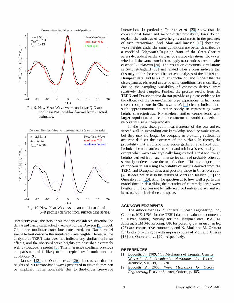
For the New-Year-Wave, == maxηξ 6.204, =µ 0.137,

and =1ξ 4.733 from Eq. (33). The actual profile scaled with the corresponding segmental =σ 2.981 m is plotted in Fig. 9. The same figure also displays the mean N-B shape from Eq. (31) using the spectral estimates of ρ and ρ̂ , and the corresponding linear Q-D form [2, 15, 16, 21] )()(|)( 00 τρξξητη =⟩=+⟨ tt (34) It is seen that because the preceding expression ignores the nonlinear nature of the actual profile, it does not depict the magnitude and shape of the New-Year-Wave as well as the nonlinear N-B model does. The N-B model approximates the actual profile surprisingly well indeed. This is despite the fact that the New-Year-Wave is a random realization from 3D directional seas whereas the N-B profile is a statistical expectation appropriate to 2D waves. There is a slight horizontal distortion in the actual profile in that the front of the wave is steeper than its rear, quite possibly because of surface stresses. The low sampling rate (~2.13 Hz) of the Draupner data as a fixed-point time series suggests that the actual wave is possibly larger than the New-Year-Wave. All aside, Fig. 9 suggests that the New-Year-Wave is likely to be a relatively “rare realization of a typical population” as opposed to being “a typical realization of a rare population ” [11]. As an additional comparison, Fig. 10 shows the New-Year-Wave together with J from Eq. (29) and N-B from Eq. (31), using in this case 3λ , 201λ , ρ and ρ̂ estimated from the 20-min time series. Contrasting Figs. 9 and 10, it is seen that the N-B profile in the latter figure does not compare with the observed wave as favorably as the spectrum-based prediction in Fig. 9. The J prediction does quite well, particularly around the large wave crest, but it becomes more oscillatory than the observed profile away from the wave crest. A more comprehensive comparison of J given in [14] uses Jensen’s full formulation and spectral expressions, and thus compares with the New-Year-Wave noticeably better than the present J prediction does. CONCLUDING REMARKS The 2D linear simulations carried out here suggest that the models of Boccotti [1] and Tayfun [25] yield similar predictions. Both models, in particular, Boccotti’s describe the data trends over relatively large waves quite accurately. The widely popular Naess [16] model under predicts the linear wave heights somewhat, as in previous comparisons [28]. Both approximations (T1 & T2) of the Tayfun model are just as simple as the Naess model, and they also describe the linear wave heights slightly and consistently better than the Naess model.

The 2D nonlinear simulations for narrow-band long-crested seas lead to a re-distribution of wave heights biased slightly toward the higher waves. For this extreme and possibly rather

8 Copyright © 2006 by ASME

-20 -15 -10 -5 0 5 10 15 20

-4

-2

0

2

4

6

Draupner New-Year-Wave vs. model predictions.

τ (s)

< η

(t o + τ

) | η

( t o )

= η m

ax >

σ = 2.981 m ηmax= 6.204 λ3 = 0.412

New-Year-Wave nonlinear N-B linear Q-D

Fig. 9. New-Year-Wave vs. mean linear Q-D and nonlinear N-B profiles derived from spectral estimates.

-20 -15 -10 -5 0 5 10 15 20-3

-2

-1

0

1

2

3

4

5

6

Draupner: New-Year-Wave vs. theoretical models based on time series.

τ (s)

< η

(t o + τ

) | η

( t o )

= η m

ax >

λ3 = 0.412 ηmax = 6.204

σ = 2.981 m New-Year-Wave nonlinear N-B nonlinear Jensen

Fig. 10. New-Year-Wave vs. mean nonlinear J and N-B profiles derived from surface time series. unrealistic case, the non-linear models considered describe the data trend fairly satisfactorily, except for the Dawson [5] model. Of all the nonlinear extensions considered, the Naess model seems to best describe the simulated wave heights. However, the analysis of TERN data does not indicate any similar nonlinear effects, and the observed wave heights are described extremely well by Boccotti’s model [1]. This in essence confirms previous comparisons and is likely to be a typical result under oceanic conditions [9].

Janssen [12] and Onorato et al. [20] demonstrate that the heights of 2D narrow-band waves generated in wave flumes can be amplified rather noticeably due to third-order free-wave

interactions. In particular, Onorato et al. [20] show that the conventional linear and second-order probability laws do not explain the statistics of wave heights and crests in the presence of such interactions. And, Mori and Janssen [18] show that wave heights under the same conditions are better described by a modified Edgeworth-Rayleigh form of the Gram-Charlier series dependent on the kurtosis of surface elevations. However, whether if the same conclusions apply to oceanic waves remains essentially unknown [20]. The results on directional simulations in Socquet-Juglard [23] and related other studies indicate that this may not be the case. The present analyses of the TERN and Draupner data lead to a similar conclusion, and suggest that the discrepancies observed under oceanic conditions are most likely due to the sampling variability of estimates derived from relatively short samples. Further, the present results from the TERN and Draupner data do not provide any clear evidence for the efficacy of the Gram-Charlier type expansions. In fact, some recent comparisons in Cherneva et al. [4] clearly indicate that such approximations do rather poorly in representing wave height characteristics. Nonetheless, further comparisons with larger populations of oceanic measurements would be needed to resolve this issue unequivocally.

In the past, fixed-point measurements of the sea surface served well in expanding our knowledge about oceanic waves, but they may no longer be adequate in providing sufficiently accurate data on the extremes of the surface. In theory, the probability that a surface time series gathered at a fixed point includes the true surface maxima and minima is essentially nil, except when waves are atypically long-crested. Crest and trough heights derived from such time series can and probably often do seriously underestimate the actual values. This is a major point of concern in assessing the validity of results derived from the TERN and Draupner data, and possibly those in Cherneva et al. [4]. It does not arise in the results of Mori and Janssen [18] and Onorato et al. [20]. And, the question as to how well a particular model does in describing the statistics of extremely large wave heights or crests can not be fully resolved unless the sea surface is measured in both time and space. ACKNOWLEDGMENTS The authors thank G..Z. Forristall, Ocean Engineering, Inc., Camden, ME, USA, for the TERN data and valuable comments, S. Haver, Statoil, Norway for the Draupner data, P.A.E.M. Janssen, ECMWF, Reading, UK for pointing out an error in Eq. (23) and constructive comments, and N. Mori and M. Onorato for kindly providing us with in-press copies of Mori and Janssen [18] and Onorato et al. [20], respectively. REFERENCES [1] Boccotti, P., 1989, “On Mechanics of Irregular Gravity

Waves,” Atti Accademia Nazionale dei Lincei, Memorie, VIII, 19, 111-70.

[2] Boccotti P., 2000, Wave Mechanics for Ocean Engineering, Elsevier Science, Oxford, p. 405.

9 Copyright © 2006 by ASME

[3] Borgman, L.E., and Resio, D.T., 1982, “ Extremal Statistics in Wave Climatology,” Proc.,Topics in Ocean Physics, Italian Physical Society, Bologna, Italy, 439-471.

[4] Cherneva, Z., Petrova, P., Andreeva, N., and Soares, C. G., 2005, “Probability Distributions of Peaks, Troughs and Heights of Wind Waves Measured in the Black Sea Coastal Zone,” Coastal Eng., Elsevier Science, 52, 599-615

[5] Dawson, T.H., 2004, “Stokes Correction for Nonlinearity of Wave Crests in Heavy Seas.” J. of Waterw., Port, Coastal and Ocean Eng., ASCE, 130(1), 39-44.

[6] Fedele, F. and Arena, F., 2003, “On the Statistics of High Nonlinear Random Waves,” Proc.,13th Inter. Offshore and Polar Eng. Conf., ISOPE, Honolulu, Hawaii, USA, May 25-30, 17-22.

[7] Fedele, F. and Arena, F., 2005, “Weakly Nonlinear Statistics of High Random Waves.” Phys. of Fluids, APS, 17(1), paper no. 026601.

[8] Fedele, F., 2006, “Extreme Events in Nonlinear Random Seas,” J. of Offshore Mechanics and Arctic Eng., ASME, 128, 11-16.

[9] Forristall, G.Z., 1984, “The Distribution of Measured and Simulated Wave Heights as a Function of Spectral Shape,” J. Geophys. Res., AGU, 89(C6), 547-552.

[10] Forristall, G.Z., 2000, “Wave Crest Distributions: Observations and Second-Order Theory,” J. Phys. Oceanogr., AMS, 38(8), 1931-1943.

[11] Haver, S. and Andersen, O.A., 2000, “Freak Waves: Rare Realizations of a Typical Population or Typical Realizations of a Rare Population?” Proc., 10th Inter. Offshore and Polar Eng. Conf., ISOPE, Seattle, USA, May 28–June 2, 123-130.

[12] Janssen, P. A. E. M., 2003, “Nonlinear Four-Wave Interactions and Freak Waves,” J. Phys. Oceanogr., AMS, 33(4), 863-884.

[13] Jensen, J.J., 1996, "Second-Order Wave Kinematics Conditional on a Given Wave Crest," Appl. Ocean Res., Elsevier Science, 18(2), 119-128.

[14] Jensen, J.J., 2005, "Conditional Second-Order Short-Crested Water Waves Applied to Extreme Wave Episodes,”J. Fluid Mech., 545, 29-40.

[15] Lindgren, G., 1970, “Some Properties of a Normal Process Near a Local Maximum,” Ann. Math. Statist., 4(6), 1870-1883.

[16] Lindgren, G., 1972, “Local Maxima of Gaussian Fields,” Arkiv förMatematik, 10, 195-218..

[17] Mori, N. and Yasuda, T., 2002, “A weakly Non-Gaussian Model of Wave Height Distribution for Random Wave Train,” Ocean Eng., Elsevier Science, 29, 1219-1231.

[18] Mori, N. and Janssen, P. A. E. M., 2006, “On Kurtosis and Occurrence Probability of Freak Waves,” J. Phys. Oceanogr., AMS, in press.

[19] Naess, A., 1985, “On the Distribution of Crest to Trough Wave Heights.” Ocean Eng., Elsevier Science, 12(3), 221-234.

[20] Onorato, M., Osborne, A.R., Serio, M., Cavaleri, L., Brandini, C. and Stansberg, C.T., 2006, “Extreme Waves, Modulational Instability and Second-Order Theory: Wave Flume Experiments on Irregular Waves.” European J. Mech B/Fluids, in press.

[21] Phillips, O.M., Daifang, G., and Donelan, M., 1993, “On the Expected Structure of Extreme Waves in a Gaussian Sea: Part I: Theory and SWADE Buoy Measurements,” J. Phys. Oceanogr., AMS, 23, 992-1000.

[22] Soares, C.G. and Pascoal, R., 2005, “On the Profile of Large Ocean Waves,” J. of Offshore Mechanics and Arctic Eng., ASME, 127, 306-314.

[23] Socquet-Juglard, H., 2005, Spectral Evolution and Probability Distributions of Surface Ocean Gravity Waves and Extreme Events. DSc. Thesis, Dept. of Math., Univ. of Bergen, Norway.

[24] Stansell, P., 2004, “Distributions of Freak Wave Heights Measured in the North Sea,” Appl. Ocean Res., Elsevier Science, 26, 35-48.

[25] Tayfun, M.A., 1981, “Distribution of Crest-to-Trough Wave Heights.” J. of Waterw., Port, Coastal and Ocean Eng., ASCE, 107(WW3), 149-158.

[26] Tayfun,M.A., 1983, “Frequency Analysis of Wave Heights Based on Wave Envelope,” J. Geophys. Res., AGU, 88(C12), 7573-7587.

[27] Tayfun, M.A., 1986, “On Narrow-Band Representation of Ocean Waves: 1. Theory & Part 2. Simulations,” J. Gephys. Res., AGU, 91(C6), 7743-7759.

[28] Tayfun, M.A., 1990, “Distribution of Large Wave Heights.” J. of Waterw., Port, Coastal and Ocean Eng., ASCE, 116(6), 686-707.

[29] Tayfun, M.A. and Lo, J-M., 1990 “Non-linear Effects on Wave Envelope and Phase,” J. of Waterw., Port, Coastal and Ocean Eng., ASCE, 116(1), 79-100.

[30] Tayfun, M.A., 1990, “High-Wave-Number/Frequency Attenuation of Wind-Wave Spectra,” J. of Waterw., port, Coastal and Ocean Eng., ASCE, 116(3), 381-398.

[31] Tayfun, M.A., 1994, “Distributions of Wave Envelope and Phase in Weakly Nonlinear Random Waves,” J. Eng. Mech., ASCE, 120(5), 1009-1025.

[32] Tayfun, M. A., 2006, “Statistics of Nonlinear Wave Crests and Groups,” Ocean Eng., Elsevier Science, in press.

[33] Walker, D.A.G., Taylor, P.H. and Taylor, R.E., 2004, “The Shape of Large Surface Waves on the Open Sea and the Draupner New Year wave,” Appl. Ocean Res., Elsevier Science, 26, 73-83.

10 Copyright © 2006 by ASME