NBER WORKING PAPER SERIES

WAGE STRUCTURE AND LABOR MOBILITY IN NORWAY 1980�1997

Arngrim HunnesJarle Møen

Kjell G. Salvanes

Working Paper 12974http://www.nber.org/papers/w12974

NATIONAL BUREAU OF ECONOMIC RESEARCH1050 Massachusetts Avenue

Cambridge, MA 02138March 2007

This is a country study for Norway forthcoming in "Wage Structure, Raises and Mobility: InternationalComparisons of the Structure of Wages Within and Across Firms," edited by Edward Lazear and KathrynShaw. The views expressed herein are those of the author(s) and do not necessarily reflect the viewsof the National Bureau of Economic Research.

© 2007 by Arngrim Hunnes, Jarle Møen, and Kjell G. Salvanes. All rights reserved. Short sectionsof text, not to exceed two paragraphs, may be quoted without explicit permission provided that fullcredit, including © notice, is given to the source.

Wage Structure and Labor Mobility in Norway 1980�1997Arngrim Hunnes, Jarle Møen, and Kjell G. SalvanesNBER Working Paper No. 12974March 2007JEL No. J31,J50,J62,J63,M52

ABSTRACT

To what extent do different firms follow different wage policies? How do such policies affect workermobility between firms, and what are the effects of different wage bargaining regimes? The empiricalbranch of personnel economics has long been hampered by a lack of representative data sets. Norwayis one of a handful of countries that has produced rich linked employer/employee data suitable forsuch analysis. This paper has three parts. First, we describe the wage setting and employment protectioninstitutions in Norway. Next, we describe the Norwegian datasets. Finally, we document a large numberof stylized facts regarding wage structure and labor mobility within and between Norwegian firms.Our main dataset covers white-collar workers in the manufacturing and private sectors for the period1980-1997. We also have blue-collar data for the 1986-1997 period covering the core of the manufacturingsector. Information about occupations, monthly wages, hours worked and bonuses is available, as wellas various worker and firm characteristics.

Arngrim HunnesDepartment of EconomicsNorwegian School of Economicsand Business AdministrationHelleveien 30N-5045 BergenNorwayArngrim.Hunnes@nhh.no

Jarle MøenNorwegian School of Economics & BusinessDepartment of Finance & ManagementHelleveien 30, N-5045Bergen, NORWAYjarle.moen@nhh.no

Kjell G. SalvanesDepartment of EconomicsNorwegian School of Economics & BusinessHellev. 30, N-5035 Bergen, NORWAYkjell.salvanes@nhh.no

1 Introduction

In the 1980s and 1990s, most Western European countries broke the trend of increasing the size

of the welfare state and the use of solidaristic wage policies that were developed in the 1950s

and continued through the 1970s. Increased and persistent unemployment and budget deficits

led many countries to question the size of the welfare state and egalitarian wage policies. Also,

Scandinavian countries—most notably Sweden—were forced to reassess their welfare policies,

and centralized wage negotiations were abandoned. Norway went in a different direction and

resisted the trend observed in other developed countries in this period. In the early 1980s,

wages were negotiated at the industry level, but in 1986/87, bargaining was further centralized

to the national level. In the early 1990s, the so-called “solidarity alternative” wage policy

was introduced. This strengthened the guarantied negotiated minimum wage for the lowest

paid (Wallerstein et al., 1997; Kahn, 1998; Freeman, 1997). It is notable that the earnings

distribution did not increase as in most other countries but stayed compressed until the mid

1990s (Aaberge et al., 2000).1

Because of high wage compression and strong labor market institutions, the Norwegian

economy differs from most other Western economies. However, we do not know much about

the precise workings of the labor market in Norway. To what extent do different firms follow

different wage policies? Do such differences relate to how workers move between firms? What

are the effects of different wage bargaining regimes? The empirical branch of personnel

economics has long been hampered by a lack of representative data sets. Norway is one of a

handful of countries that has produced rich linked employer–employee data suitable for such

analysis.2 A special feature of our data is detailed information on occupational hierarchies

and very detailed information on wage compensation for normal hours and overtime, as well

as bonuses. There is also very good information on hours worked. We match these data to

the main register-based employer–employee data set, containing detailed information on firm

and worker characteristics.3

Our paper is very descriptive in nature, and it should be read as a detailed country study

together with the other country studies in this volume. The paper has three parts. First,

we describe the wage setting and employment protection institutions in Norway. Next, we

describe the Norwegian data sets. Finally, we document a large number of stylized facts

regarding wage structure and labor mobility within and between Norwegian firms. We cover

the period 1980–1997. One topic analyzed is within and between firm wage dispersion, and

1See Kahn (1998) and Hægeland et al. (1999) for explanations for the increased wage compression.2Some work on both the job and worker turnover and wage structure has been undertaken before, but

very little has been conducted on wage mobility within and between firms. See Salvanes (1997), Salvanes andFørre (2003) and Margolis and Salvanes (2001).

3See Møen et al. (2004) for a description of the main employer–employee data set used in several previousstudies.

2

whether wage dispersion has been stable over time. Although overall wage dispersion has

been stable, there might still have been changes in the individual components of the variance

both across firms and across worker groups. There might also have been increased sorting of

workers across firms. We document these types of patterns and also those of worker mobility

for different groups of firms and workers. A unique feature of our data is that we can compare

mobility across occupations within firms for white-collar workers as opposed to the more

standard mobility patterns across firms. Another feature is the ability to compare wage and

worker mobility for white- and blue-collar workers separately. The wage setting institutions

are very different for white- and blue-collar workers. There is no centrally bargained wage for

white-collar workers, whereas blue-collar workers have a two-tier system with both national (or

industry) and firm-level negotiations. In this way, we have an extra institutional “experiment”

within the country. Furthermore, the period we analyze was volatile in terms of business

cycle movements. Hence our data are well suited for studying the cyclical pattern of wage

and worker mobility.

The remainder of the paper is organized as follows. In Section 2, we describe the macroe-

conomic conditions in the period we are analyzing. Section 3 presents the institutional setting

in Norway, and Section 4 presents the data we are using. In Section 5, we look at the wage

structure and labor mobility in detail. Section 6 summarizes our empirical findings.

2 Macroeconomic conditions

Table 1 and Figure 1 show unemployment and growth rates for Norway for each of the years

from 1972 to 2002. We see that the macroeconomic conditions have not been stable in the

period covered by our analysis, 1980–1997. There was a mild downturn in the early 1980s,

with a peak in the business cycle around 1985–87. The unemployment rate was then about 2%

of the labor force. From 1988 onwards, Norway experienced its worst economic recession in

the postwar period, when the unemployment rate was about 6%. After 1993, growth picked

up, and 1997 was a peak year in the relatively stable period after the mid 1990s. Given

these business cycle fluctuations, we have picked 1981 and 1993 as two low-growth years and

1986/87 and 1997 as two high-growth years in our empirical analysis.

The Norwegian Government plays an important part in coordinating wage settlements,

and this had important implications for wage determination in the period analyzed. For

instance, wage negotiations in 1988 were undertaken with considerable concern about the

future of the Norwegian economy. Partly because of the oil price fall in 1986, the Norwegian

krone had been devalued by 10% in May 1986. The largest employer association, NAF, the

predecessor of NHO (the Confederation of Norwegian Business and Industry), called a lock-out

that failed, largely because of disagreement among the employers. This lead to reductions in

work time and high increases in wages in 1986. After the subsequent downturn in the economy,

3

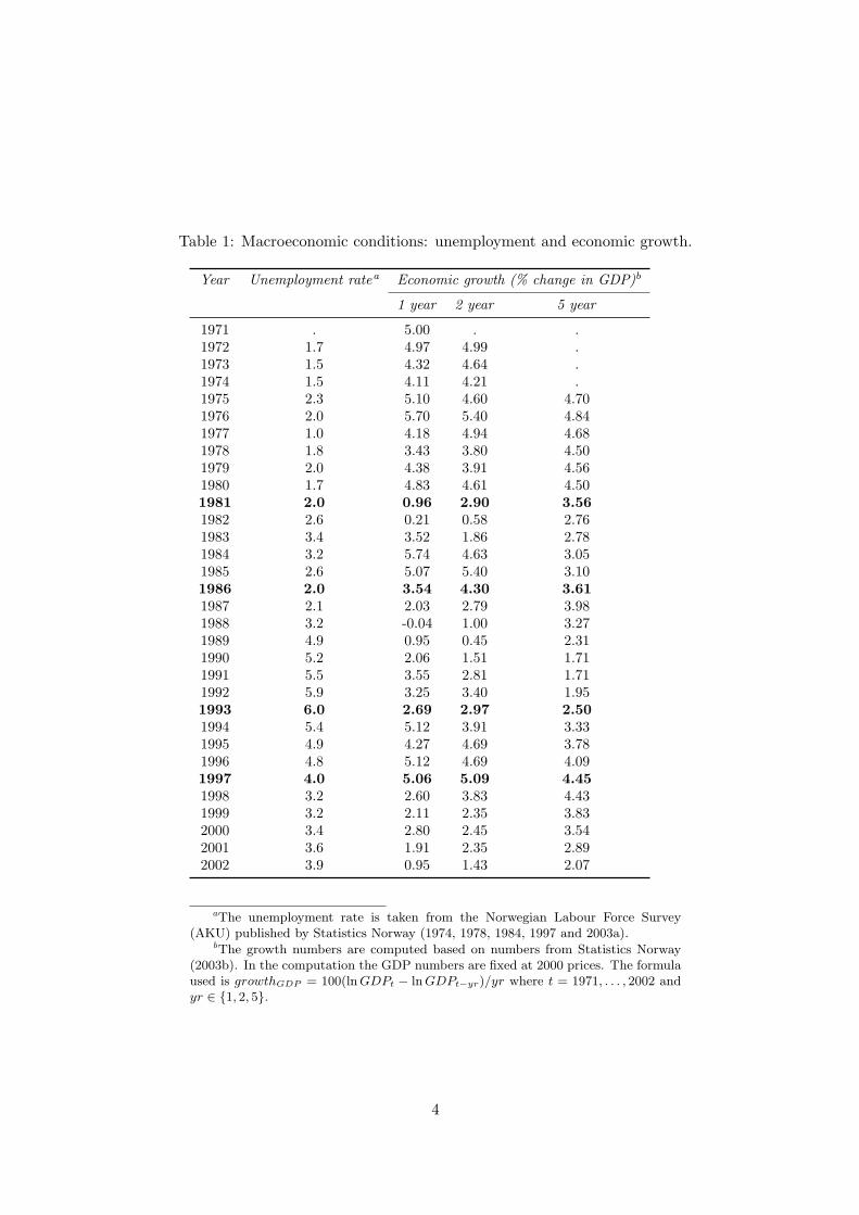
Table 1: Macroeconomic conditions: unemployment and economic growth.

Year Unemployment ratea Economic growth (% change in GDP)b

1 year 2 year 5 year

1971 . 5.00 . .1972 1.7 4.97 4.99 .1973 1.5 4.32 4.64 .1974 1.5 4.11 4.21 .1975 2.3 5.10 4.60 4.701976 2.0 5.70 5.40 4.841977 1.0 4.18 4.94 4.681978 1.8 3.43 3.80 4.501979 2.0 4.38 3.91 4.561980 1.7 4.83 4.61 4.501981 2.0 0.96 2.90 3.561982 2.6 0.21 0.58 2.761983 3.4 3.52 1.86 2.781984 3.2 5.74 4.63 3.051985 2.6 5.07 5.40 3.101986 2.0 3.54 4.30 3.611987 2.1 2.03 2.79 3.981988 3.2 -0.04 1.00 3.271989 4.9 0.95 0.45 2.311990 5.2 2.06 1.51 1.711991 5.5 3.55 2.81 1.711992 5.9 3.25 3.40 1.951993 6.0 2.69 2.97 2.501994 5.4 5.12 3.91 3.331995 4.9 4.27 4.69 3.781996 4.8 5.12 4.69 4.091997 4.0 5.06 5.09 4.451998 3.2 2.60 3.83 4.431999 3.2 2.11 2.35 3.832000 3.4 2.80 2.45 3.542001 3.6 1.91 2.35 2.892002 3.9 0.95 1.43 2.07

aThe unemployment rate is taken from the Norwegian Labour Force Survey(AKU) published by Statistics Norway (1974, 1978, 1984, 1997 and 2003a).

bThe growth numbers are computed based on numbers from Statistics Norway(2003b). In the computation the GDP numbers are fixed at 2000 prices. The formulaused is growthGDP = 100(ln GDPt − ln GDPt−yr)/yr where t = 1971, . . . , 2002 andyr ∈ {1, 2, 5}.

4

Figure 1: Unemployment rate and 1-year growth rate GDP.

02

46

%

1972 1977 1982 1987 1992 1997 2002Year

Unemployment rate 1−year growth rate GDP

the main labor union, LO (the Norwegian Confederation of Trade Unions) and NAF/NHO

agreed to a moderate wage increase in 1988. To ensure that all groups followed suit, the

Storting (the Norwegian national assembly) passed a law that wages could not increase by

more than 5%, in line with the outcome of the wage settlements between LO and NHO. A

similar law was passed in 1989. Therefore, a wage freeze policy at 5% nominal increase was

in place in these two years.

In 1990, the income regulation laws expired, yet the LO and NHO agreed that wage

increases should still be moderate, because of high unemployment and the weak competitive

position of the trading sector. In 1992, the agreement among the labor market organizations

on wage restraint was formalized in the Solidarity Alternative. In 1994, a major revision

was undertaken by industry, yet wage growth was moderate, following the lead from the

metal industry. In 1996 and 1998, however, proposed agreements in line with the Solidarity

Alternative were rejected in ballots. This led to strikes and subsequent agreements on higher

wage growth.

3 Institutional setting

This section describes wage setting institutions in Norway for different worker groups and

institutions for employment protection.

5

3.1 Wage setting

In the private sector in Norway, about half of the labor force is covered by collective agreements

(Stokke et al., 2003).4 Union density, i.e., the share of employees who are members of a union,

is somewhat lower: 43% in the private sector (Stokke et al., 2003). These figures were very

stable in the period we analyze (Wallerstein et al., 1997). Bargaining coverage is higher than

union density because firms covered by a collective agreement follow the agreement for all

employees. However, in contrast to many other European countries, extension mechanisms

imposing regulations from collective agreements onto the non-unionized sectors, are not used

in Norway.

The largest employees’ association is LO, to which about half of all union members belong.

The traditional stronghold of LO is among blue-collar workers in the manufacturing indus-

try, but LO is also prominent in some private service sectors, and for non-professionals and

unskilled employees in the public sector. LO is organized as union branches, to a large degree

covering different industry sectors. Other employees’ associations are YS (The Confederation

of Vocational Unions), covering many of the same workers as LO; UHO (The Confederation

of Higher Education Unions), covering teachers, nurses, the police, etc; and Akademikerne

(The Federation of Norwegian Professional Associations), covering employees with higher ed-

ucation. On the employers’ side, NHO is the dominant association in the private sector,

being the main counterpart of the LO. NHO has about 16,000 member companies, employing

about 490,000 employees in Norway (Stokke et al., 2003), i.e., about one quarter of the total

workforce of 2.3 million.

For employees covered by collective agreements, wage setting takes place at two levels

national (or industry) and at the firm level (wage drift). Central negotiations concern col-

lective agreements, wage regulations, working hours, working conditions, pensions, medical

benefits, etc. Firm-level negotiations determine possible local adjustments and additions to

the collective agreements. These negotiations are generally conducted under a peace clause,

preventing strikes and lock-outs within the contract period of the collective (i.e., central)

agreements (Holden, 1998). Collective agreements usually last for two years. Since 1964, the

main revisions to the collective agreements have been undertaken every second year, in even

years (most recently in 2004). The draft agreement in a main revision is subject to a ballot

among union members. Occasionally, draft agreements are rejected by the members, leading

to a strike and subsequent negotiations during or after the strike. There are also central

negotiations in intermediate years, but the scope for these negotiations is usually limited to

wages only. Furthermore, negotiations in intermediate years are undertaken at the national

level, without any ballot requirements, which usually ensures a more moderate wage outcome.

Broadly, we can distinguish three types of collective agreements:

4See Holden and Salvanes (2005) on more details on the wage setting process.

6

• minimum wage agreements,

• normal wage agreements, and

• agreements without wage rates.

Most workers are covered by minimum wage agreements, which specify minimum wage

rates, as well as other working conditions. For these workers, there are local negotiations about

additions to the central agreements. Importantly, as the local agreements specify additions to

the central agreements, an increase in the centrally specified minimum wage rates raises the

wage of all workers, even if they are paid more than the minimum rates. Workers covered by

normal wage agreements are not supposed to have local wage negotiations, so their wages and

working conditions are fully specified by the central agreements. At the opposite end, there

are also agreements without wage rates, specifying only procedures for the local wage setting.

These agreements are only used for white-collar workers. Hence, an important feature of the

Norwegian wage setting is that white-collar wages are mainly set at the firm level and thus

reflect conditions at the firm level. It should also be noted that there is no national, statutory

minimum wage for all workers in Norway. Minimum wages only apply to workers covered by

collective agreements.

Although blue-collar wages are negotiated centrally, there is considerable variation be-

tween sectors with regard to the number of firms with local bargaining, and the importance

of the wage drift—the change in wages due to local negotiations. Figure 2 shows the total

wage change in the period 1970–1996 for blue-collar workers. As can be seen from the figure,

quite a large proportion of total wage gains is realized at the local level; see also Holden and

Rødseth (1990). This means that the sector minimum wage will not be binding for several

firms, since they have locally contracted higher wages. In our data, a relatively small pro-

portion of the workforce is paid at or near the minimum wage, and local bargaining could be

one reason why this is so.

3.2 Employment protection5

Rules regarding individual and collective dismissals, as well as those about the flexibility

of industrial plants with respect to temporary hiring and the use of subcontractors, are

important aspects of employment protection and thus the costs of adjustment for firms. The

different types of constraints regulating the hiring and firing of workers are not completely

transparent, since, in addition to national laws, collective agreements between employers

and workers’ organizations are also very important in regulating the adjustment of the labor

5A new law of employment protection and the use of time-limited labor contracts has been proposed by thegovernment and is to be decided upon in 2005. The main proposals are to allow more flexible use of fixed-termcontracts and more flexible use of overtime work.

7

Figure 2: Total wage change in Norway decomposed by national (or industry) and locallybargained wage in the private sector in Norway. Source: “Det tekniske beregningsutvalgetfor inntekts-oppgjørene.”

05

1015

20P

erce

nt c

hang

e

1971 1976 1981 1986 1991 1996Year

Total Local negotiationsNational (or industry) bargained wage

factor. These agreements may differ across industries and workers, depending upon workers’

age, tenure, etc.

Two main laws govern the labor relations in Norway: The law on employment (“Sysselset-

tingsloven”) and the law on labor relations (“Arbeidsmiljøloven”). The law on employment

mainly regulates changes in labor during a period of restructuring and mass lay-offs by the

firm. The latter was enacted in 1982, and it includes standards for general working conditions,

overtime regulations and legal regulation for employment protection. According to the law on

labor relations, dismissals for individual reasons are limited to cases of disloyalty, persistent

absenteeism, etc. In general, it is possible, but very difficult, to replace an individual worker

in a given job with another worker. Hence, there is strong employment protection in Norway.

The law on employment states that the general rule for laying off a worker for economic reasons

is that it can occur only when the job is “redundant” and the worker cannot be retained in

another capacity. This regulation covers all workers regardless of how long they have been

employed. Requirements for collective dismissals in Norway basically follow the common

minimum standards for EU-countries. It is important to note that a firm can dismiss workers

not only when it is making a loss but also when it is performing poorly. There is no actual

rule on the selection of workers to be dismissed. However, the legal practice narrows down

which workers can be dismissed. Conversations with lawyers in the employees’ organizations

8

indicate that many, if not most, dismissal cases are taken to court. This is costly for firms.

When it comes to other costs of dismissal, the employment law states that employment

is terminable with one month’s notice for workers with tenure of less than or equal to five

years. This one-month notice period is at the lower end of the spectrum compared to many

countries. However, most workers have a three-months’-notice requirement for both parties to

the contract. Although there is no generalized legal requirement for severance pay in Norway,

agreements in the private sector require lump-sum payments to workers aged between 50 and

55. As an example, in the contract between LO and NHO, a worker who is 50 and has been

working for 10 consecutive years in the firm, or 20 years in total, is eligible for one to two

months’ pay. Similar agreements exist for the other unions. Some EU-countries have even

stronger job protection rules, including, for instance, general compensation, a social plan for

re-training or transfer to another plant within a firm. Although not mandatory, some of these

other requirements are also commonplace in Norway. Note finally that while some costs of

reducing the workforce (such as redundancy payments) are related to the size of the reduction,

others (such as advance notice requirements, legal and other administrative costs) may have

significant fixed components.

The workforce flexibility of an economy can be enhanced by allowing fixed-term contracts

in addition to standard contracts, and by the use of temporary work agencies. In many OECD

countries, there has been a strong trend towards liberalizing the use of these two schemes.

In Norway, the use of fixed-term contracts is allowed only for limited situations, such as

specific projects, seasonal work or the replacement of workers who are absent temporarily.

However, it is not as restrictive as it appears, since defining a specific project for a firm is

partly open to discretion. Repeated temporary contracts are possible with some limitations,

and there is no rule limiting the accumulated duration of successive contracts. In general, the

use of temporary work agencies is prohibited, but substantial latitude exists for service sector

occupations. Restrictions for the number of renewals exist, and two years is the maximum

for accumulated contracts. Compared to other OECD countries, Norway is ranked a little bit

above average for the strictness of the use of temporary employment (OECD, 1999). Very

few comparative studies of the overall degree of employment protection exist. A much-cited

study by Emerson (1987) ranks Italy as having the strongest employment protection rules,

while the UK, and on some criteria, Denmark are at the other end of the spectrum. Norway is

ranked together with Sweden, France and to a lesser extent Germany (when all regulations are

taken together) as an intermediate country with a fairly high degree of protection. Obviously,

intercountry comparisons are difficult. The most recent comparison was made by the OECD

in 1999, where Norway was ranked at number 12 out of 19 OECD countries in the late 1980s,

and as number 19 out of 26 OECD countries in the late 1990s in the degree of restrictiveness

(OECD, 1999). Evidence on the flexibility of the Norwegian economy from job and worker

flows data suggests that it is about average for OECD countries, although worker flows are a

9

bit below average (Salvanes, 1997 and Salvanes and Førre, 2003). The overall impression is

that legislation, contracts, and common practice impose important additional costs in Norway

when adjusting the labor force downward, and possibly upward as well. See Nilsen, Salvanes

and Sciantarelli (2003) for an analysis of the effect of labor adjustment costs in Norway.

4 Data

Like other Scandinavian countries, Norway has rich and high-quality linked employer–employee

data sets. The sources and structure are basically the same as the data sets used in Denmark,

Sweden and France. The basis of the Norwegian data is administrative files from Statistics

Norway and plant-level information from the annual census for manufacturing plus a similar

data set for private and public service sectors. Information on R&D and trade statistics has

been added as well. See Møen et al. (2004) and Salvanes and Førre (2003) for a general

description of the Norwegian linked employer–employee data sets.

In this paper, we take advantage of two new data sets, one for white-collar workers and

one for blue-collar workers. We can match these to the linked employer–employee data as

they both use the same series of person identifiers. Both these data sets are from NHO,

the main employers’ association in Norway. The white-collar data set is the main data set

used in this paper. Its main advantage over data that has been available so far is that it

contains information on hourly wages, overtime hours, pay, and bonus pay as well as detailed

information on occupations. The main employer–employee data set contains only information

on annual earnings and education, but none about occupations.

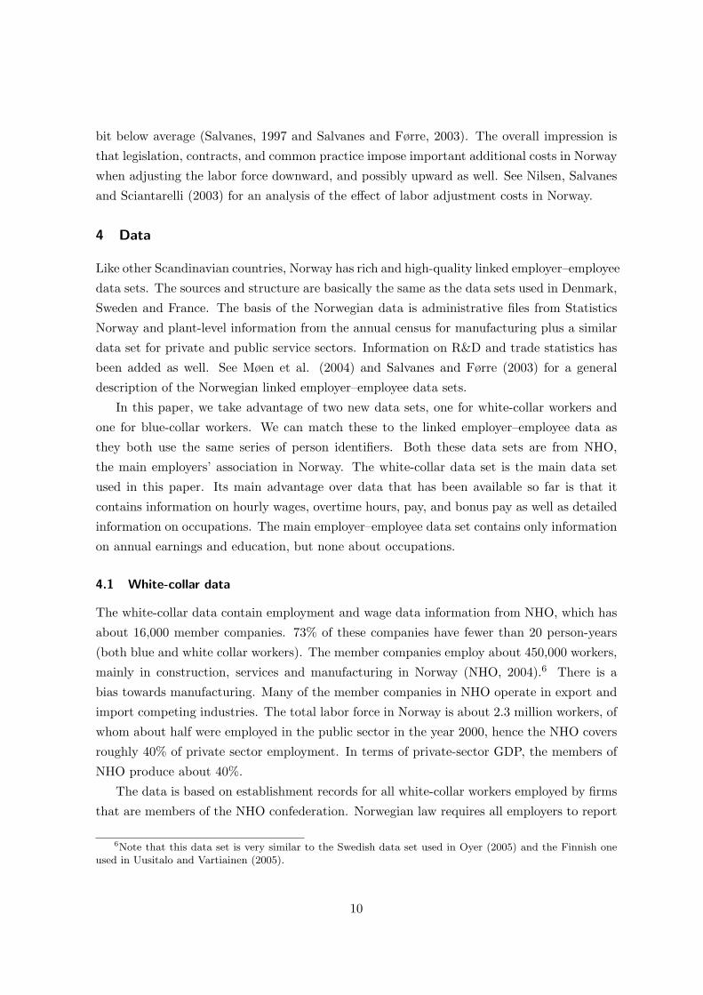
4.1 White-collar data

The white-collar data contain employment and wage data information from NHO, which has

about 16,000 member companies. 73% of these companies have fewer than 20 person-years

(both blue and white collar workers). The member companies employ about 450,000 workers,

mainly in construction, services and manufacturing in Norway (NHO, 2004).6 There is a

bias towards manufacturing. Many of the member companies in NHO operate in export and

import competing industries. The total labor force in Norway is about 2.3 million workers, of

whom about half were employed in the public sector in the year 2000, hence the NHO covers

roughly 40% of private sector employment. In terms of private-sector GDP, the members of

NHO produce about 40%.

The data is based on establishment records for all white-collar workers employed by firms

that are members of the NHO confederation. Norwegian law requires all employers to report

6Note that this data set is very similar to the Swedish data set used in Oyer (2005) and the Finnish oneused in Uusitalo and Vartiainen (2005).

10

data on wages and employment annually to Statistics Norway. Until 1997, NHO collected

data for their member plants under this law, and Statistics Norway collected data for the rest

of the economy. From 1997, Statistics Norway collected data from all sectors. The data set is

considered to be very precise, since the wage data were a major source of information for the

collective bargaining process in Norway between the NHO and the unions. See Holden and

Salvanes (2005) for an assessment of the wage data from this source as compared to other

sources of earnings data from Norwegian registers.

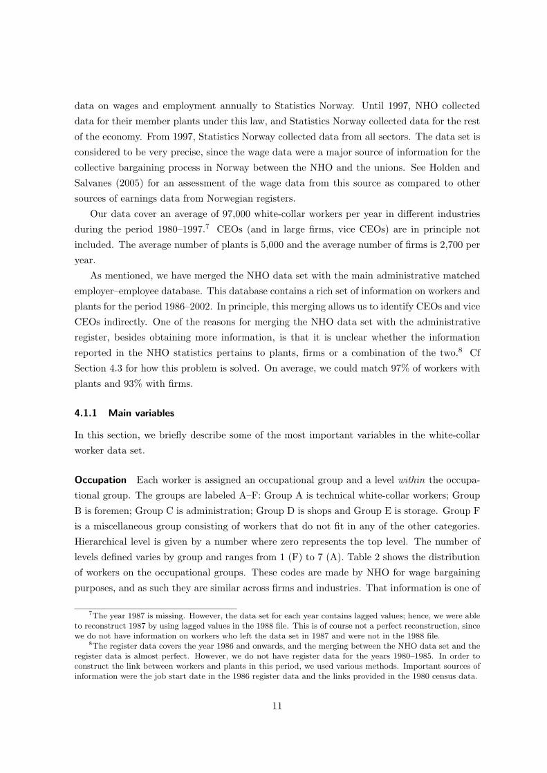
Our data cover an average of 97,000 white-collar workers per year in different industries

during the period 1980–1997.7 CEOs (and in large firms, vice CEOs) are in principle not

included. The average number of plants is 5,000 and the average number of firms is 2,700 per

year.

As mentioned, we have merged the NHO data set with the main administrative matched

employer–employee database. This database contains a rich set of information on workers and

plants for the period 1986–2002. In principle, this merging allows us to identify CEOs and vice

CEOs indirectly. One of the reasons for merging the NHO data set with the administrative

register, besides obtaining more information, is that it is unclear whether the information

reported in the NHO statistics pertains to plants, firms or a combination of the two.8 Cf

Section 4.3 for how this problem is solved. On average, we could match 97% of workers with

plants and 93% with firms.

4.1.1 Main variables

In this section, we briefly describe some of the most important variables in the white-collar

worker data set.

Occupation Each worker is assigned an occupational group and a level within the occupa-

tional group. The groups are labeled A–F: Group A is technical white-collar workers; Group

B is foremen; Group C is administration; Group D is shops and Group E is storage. Group F

is a miscellaneous group consisting of workers that do not fit in any of the other categories.

Hierarchical level is given by a number where zero represents the top level. The number of

levels defined varies by group and ranges from 1 (F) to 7 (A). Table 2 shows the distribution

of workers on the occupational groups. These codes are made by NHO for wage bargaining

purposes, and as such they are similar across firms and industries. That information is one of

7The year 1987 is missing. However, the data set for each year contains lagged values; hence, we were ableto reconstruct 1987 by using lagged values in the 1988 file. This is of course not a perfect reconstruction, sincewe do not have information on workers who left the data set in 1987 and were not in the 1988 file.

8The register data covers the year 1986 and onwards, and the merging between the NHO data set and theregister data is almost perfect. However, we do not have register data for the years 1980–1985. In order toconstruct the link between workers and plants in this period, we used various methods. Important sources ofinformation were the job start date in the 1986 register data and the links provided in the 1980 census data.

11

the unique features of this data set, and it gives us a picture of how the hierarchical structure

looks within each firm. For example, we are able to study mobility within a firm and questions

related to promotion.

Table 2: Distribution of the workers on the occupational groups.

Year

Occupational group 1981 1986 1993 1997

A0 0.40 0.50 0.51 0.55A1 2.18 2.58 3.69 4.13A2 4.80 6.50 6.91 6.89A31 4.44 5.22 4.34 4.64A32 5.66 6.64 8.76 8.34A41 1.45 1.63 1.36 1.19A42 7.30 7.34 7.34 8.43A5 4.83 4.80 4.08 4.61A6 1.79 1.68 1.61 1.33B1 0.59 0.54 0.68 0.76B2 2.24 1.93 1.95 1.92B3 11.96 9.16 7.27 6.35C0 0.91 1.02 1.07 1.11C1 5.54 5.51 6.59 6.41C2 8.82 9.80 10.33 10.61C3 13.34 14.09 14.60 13.89C4 9.88 7.92 6.28 5.80D1 0.33 0.24 0.36 0.29D2 0.96 0.68 0.92 0.86E1 1.44 1.20 0.93 0.79E2 3.04 2.91 1.81 1.91F 8.09 8.10 8.63 9.20Total 100.00 100.00 100.00 100.00

We define an occupation as a combination of group and level. That gives us 22 occupa-

tions.9 To create a single hierarchy within a firm, we aggregate the 22 different occupations

into seven different levels. This gives a maximum of seven levels in a single firm.10 To help

in the aggregation, we have carefully utilized the NHO’s descriptions of the different occu-

pational groups. Still, such a harmonization across occupational groups is difficult. One

problem lies in the fact that some levels are overlapping with respect to responsibility in the

organization. For example, even though we aggregate occupational Groups A31 and A32 into

the same level (see Table 3), we know that they differ in responsibility, since A31 involves

management of other workers while A32 does not (however, they are both ranked above the

A4 level). Furthermore, the levels defined within each group do not necessarily align; e.g.,

9In the data set we also have a much richer set of four-digit job codes. These are less consistently usedacross firms and perhaps also within firms across time. We have therefore not yet utilized this information.

10Note that not all firms will have workers on each of the seven levels.

12

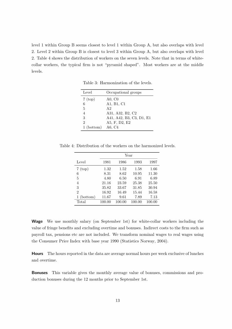
level 1 within Group B seems closest to level 1 within Group A, but also overlaps with level

2. Level 2 within Group B is closest to level 3 within Group A, but also overlaps with level

2. Table 4 shows the distribution of workers on the seven levels. Note that in terms of white-

collar workers, the typical firm is not “pyramid shaped”. Most workers are at the middle

levels.

Table 3: Harmonization of the levels.

Level Occupational groups

7 (top) A0, C06 A1, B1, C15 A24 A31, A32, B2, C23 A41, A42, B3, C3, D1, E12 A5, F, D2, E21 (bottom) A6, C4

Table 4: Distribution of the workers on the harmonized levels.

Year

Level 1981 1986 1993 1997

7 (top) 1.32 1.52 1.58 1.666 8.31 8.62 10.95 11.305 4.80 6.50 6.91 6.894 21.16 23.59 25.38 25.503 35.82 33.67 31.85 30.942 16.92 16.49 15.44 16.581 (bottom) 11.67 9.61 7.89 7.13Total 100.00 100.00 100.00 100.00

Wage We use monthly salary (on September 1st) for white-collar workers including the

value of fringe benefits and excluding overtime and bonuses. Indirect costs to the firm such as

payroll tax, pensions etc are not included. We transform nominal wages to real wages using

the Consumer Price Index with base year 1990 (Statistics Norway, 2004).

Hours The hours reported in the data are average normal hours per week exclusive of lunches

and overtime.

Bonuses This variable gives the monthly average value of bonuses, commissions and pro-

duction bonuses during the 12 months prior to September 1st.

13

Tenure To create the tenure variable, we used the job start variable that is present in the

administrative register data.

4.1.2 Restrictions on the sample

We put the following restrictions on the sample:

1. To remove outliers in the data, we imposed the restriction that the monthly wage should

be at least 2,000 NOK measured in 1980 kroner.

2. The number of hours worked per week is 30 or above, i.e., we look at full-time workers.

3. The number of full-time workers in each firm is at least 25 in year t.

4. The number of full-time workers in each firm is at least 25 in year t− 1.11

Since our data set only contains white-collar workers, this means that we are looking at

large firms by Norwegian standards. In 1993, a firm with 25 full-time white-collar workers

had on average 60 blue-collar workers. Table 5 shows the effect of our restrictions on the

number of workers and firms.

Table 5: The effect (i.e. the difference between each row in the table) of the restrictions onthe number of white collar workers (top panel) and firms in the sample.

1981 1986 1993 1997

No restrictions 74,075 91,911 100,087 111,336Outliers 74,074 91,896 99,648 110,516Hours per week ≥ 30 73,776 91,695 94,404 104,899Firmsize ≥ 25 in year t 60,657 78,587 80,831 87,533Firmsize ≥ 25 in year t− 1 56,838 73,600 76,449 79,259

1981 1986 1993 1997

No restrictions 2,348 2,622 2,682 3,838Outliers 2,348 2,622 2,638 3,715Hours per week ≥ 30 2,327 2,614 2,509 3,518Firmsize ≥ 25 in year t 532 591 586 679Firmsize ≥ 25 in year t− 1 467 506 521 565

4.2 Blue-collar data12

11This restriction, agreed on by all project members present at an NBER-meeting in Boston in April 2004,introduces a selection bias in the entry and exit rates related to firms crossing the 25 worker threshold.

12Since these data are used only in a small part of our analysis, this description will be somewhat brieferthan our description of the white-collar data.

14

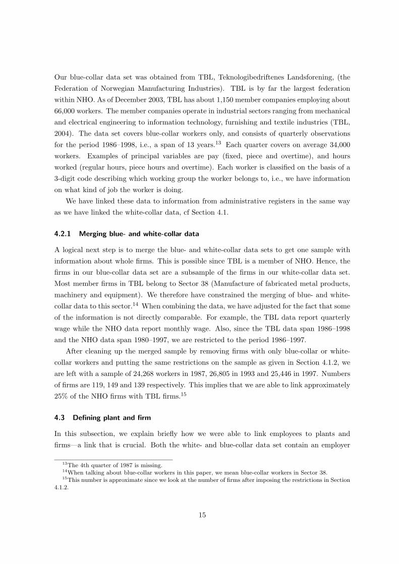
Our blue-collar data set was obtained from TBL, Teknologibedriftenes Landsforening, (the

Federation of Norwegian Manufacturing Industries). TBL is by far the largest federation

within NHO. As of December 2003, TBL has about 1,150 member companies employing about

66,000 workers. The member companies operate in industrial sectors ranging from mechanical

and electrical engineering to information technology, furnishing and textile industries (TBL,

2004). The data set covers blue-collar workers only, and consists of quarterly observations

for the period 1986–1998, i.e., a span of 13 years.13 Each quarter covers on average 34,000

workers. Examples of principal variables are pay (fixed, piece and overtime), and hours

worked (regular hours, piece hours and overtime). Each worker is classified on the basis of a

3-digit code describing which working group the worker belongs to, i.e., we have information

on what kind of job the worker is doing.

We have linked these data to information from administrative registers in the same way

as we have linked the white-collar data, cf Section 4.1.

4.2.1 Merging blue- and white-collar data

A logical next step is to merge the blue- and white-collar data sets to get one sample with

information about whole firms. This is possible since TBL is a member of NHO. Hence, the

firms in our blue-collar data set are a subsample of the firms in our white-collar data set.

Most member firms in TBL belong to Sector 38 (Manufacture of fabricated metal products,

machinery and equipment). We therefore have constrained the merging of blue- and white-

collar data to this sector.14 When combining the data, we have adjusted for the fact that some

of the information is not directly comparable. For example, the TBL data report quarterly

wage while the NHO data report monthly wage. Also, since the TBL data span 1986–1998

and the NHO data span 1980–1997, we are restricted to the period 1986–1997.

After cleaning up the merged sample by removing firms with only blue-collar or white-

collar workers and putting the same restrictions on the sample as given in Section 4.1.2, we

are left with a sample of 24,268 workers in 1987, 26,805 in 1993 and 25,446 in 1997. Numbers

of firms are 119, 149 and 139 respectively. This implies that we are able to link approximately

25% of the NHO firms with TBL firms.15

4.3 Defining plant and firm

In this subsection, we explain briefly how we were able to link employees to plants and

firms—a link that is crucial. Both the white- and blue-collar data set contain an employer

13The 4th quarter of 1987 is missing.14When talking about blue-collar workers in this paper, we mean blue-collar workers in Sector 38.15This number is approximate since we look at the number of firms after imposing the restrictions in Section

4.1.2.

15

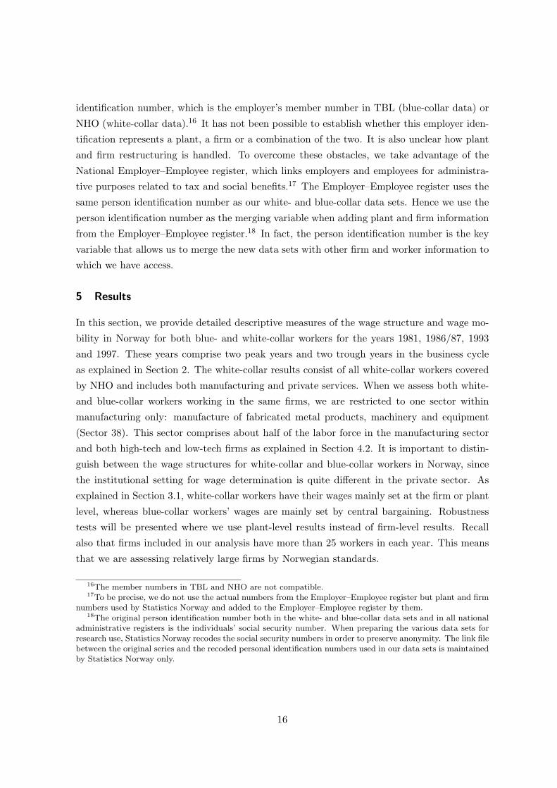
identification number, which is the employer’s member number in TBL (blue-collar data) or

NHO (white-collar data).16 It has not been possible to establish whether this employer iden-

tification represents a plant, a firm or a combination of the two. It is also unclear how plant

and firm restructuring is handled. To overcome these obstacles, we take advantage of the

National Employer–Employee register, which links employers and employees for administra-

tive purposes related to tax and social benefits.17 The Employer–Employee register uses the

same person identification number as our white- and blue-collar data sets. Hence we use the

person identification number as the merging variable when adding plant and firm information

from the Employer–Employee register.18 In fact, the person identification number is the key

variable that allows us to merge the new data sets with other firm and worker information to

which we have access.

5 Results

In this section, we provide detailed descriptive measures of the wage structure and wage mo-

bility in Norway for both blue- and white-collar workers for the years 1981, 1986/87, 1993

and 1997. These years comprise two peak years and two trough years in the business cycle

as explained in Section 2. The white-collar results consist of all white-collar workers covered

by NHO and includes both manufacturing and private services. When we assess both white-

and blue-collar workers working in the same firms, we are restricted to one sector within

manufacturing only: manufacture of fabricated metal products, machinery and equipment

(Sector 38). This sector comprises about half of the labor force in the manufacturing sector

and both high-tech and low-tech firms as explained in Section 4.2. It is important to distin-

guish between the wage structures for white-collar and blue-collar workers in Norway, since

the institutional setting for wage determination is quite different in the private sector. As

explained in Section 3.1, white-collar workers have their wages mainly set at the firm or plant

level, whereas blue-collar workers’ wages are mainly set by central bargaining. Robustness

tests will be presented where we use plant-level results instead of firm-level results. Recall

also that firms included in our analysis have more than 25 workers in each year. This means

that we are assessing relatively large firms by Norwegian standards.

16The member numbers in TBL and NHO are not compatible.17To be precise, we do not use the actual numbers from the Employer–Employee register but plant and firm

numbers used by Statistics Norway and added to the Employer–Employee register by them.18The original person identification number both in the white- and blue-collar data sets and in all national

administrative registers is the individuals’ social security number. When preparing the various data sets forresearch use, Statistics Norway recodes the social security numbers in order to preserve anonymity. The link filebetween the original series and the recoded personal identification numbers used in our data sets is maintainedby Statistics Norway only.

16

5.1 Wage structure in Norway

5.1.1 Wage dispersion for workers 1980–1997

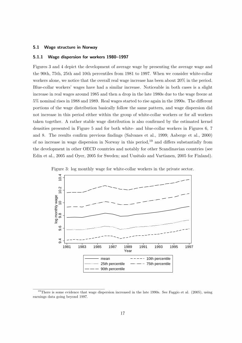
Figures 3 and 4 depict the development of average wage by presenting the average wage and

the 90th, 75th, 25th and 10th percentiles from 1981 to 1997. When we consider white-collar

workers alone, we notice that the overall real wage increase has been about 20% in the period.

Blue-collar workers’ wages have had a similar increase. Noticeable in both cases is a slight

increase in real wages around 1985 and then a drop in the late 1980s due to the wage freeze at

5% nominal rises in 1988 and 1989. Real wages started to rise again in the 1990s. The different

portions of the wage distribution basically follow the same pattern, and wage dispersion did

not increase in this period either within the group of white-collar workers or for all workers

taken together. A rather stable wage distribution is also confirmed by the estimated kernel

densities presented in Figure 5 and for both white- and blue-collar workers in Figures 6, 7

and 8. The results confirm previous findings (Salvanes et al., 1999; Aaberge et al., 2000)

of no increase in wage dispersion in Norway in this period,19 and differs substantially from

the development in other OECD countries and notably for other Scandinavian countries (see

Edin et al., 2005 and Oyer, 2005 for Sweden; and Uusitalo and Vartianen, 2005 for Finland).

Figure 3: log monthly wage for white-collar workers in the private sector.

9.4

9.6

9.8

1010

.210

.4lo

g m

onth

ly w

age

1981 1983 1985 1987 1989 1991 1993 1995 1997Year

mean 10th percentile25th percentile 75th percentile90th percentile

19There is some evidence that wage dispersion increased in the late 1990s. See Faggio et al. (2005), usingearnings data going beyond 1997.

17

Figure 4: log monthly wage for workers in the machinery and equipment industry (Sector38).

9.5

1010

.59.

510

10.5

1987 1989 1991 1993 1995 1997

1987 1989 1991 1993 1995 1997

All workers Blue collar workers

White collar workers

mean 10th percentile25th percentile 75th percentile90th percentile

year

Graphs by All workers/Blue collar workers/White collar workers

Figure 5: Kernel densities for white-collar workers in the private sector.

0.5

11.

5K

erne

l den

sity

8 9 10 11 12log monthly wage

1981 19861993 1997

18

Figure 6: Kernel densities for both blue- and white-collar workers in the machinery andequipment industry (Sector 38).

01

23

Ker

nel d

ensi

ty

8.5 9 9.5 10 10.5 11log monthly wage

1987 19931997

Figure 7: Kernel densities for workers in the machinery and equipment industry (Sector 38).

01

23

4

8 9 10 11 8 9 10 11

Blue collar White collar

1987 19931997

Ker

nel d

ensi

ty

log monthly wage

Graphs by group

19

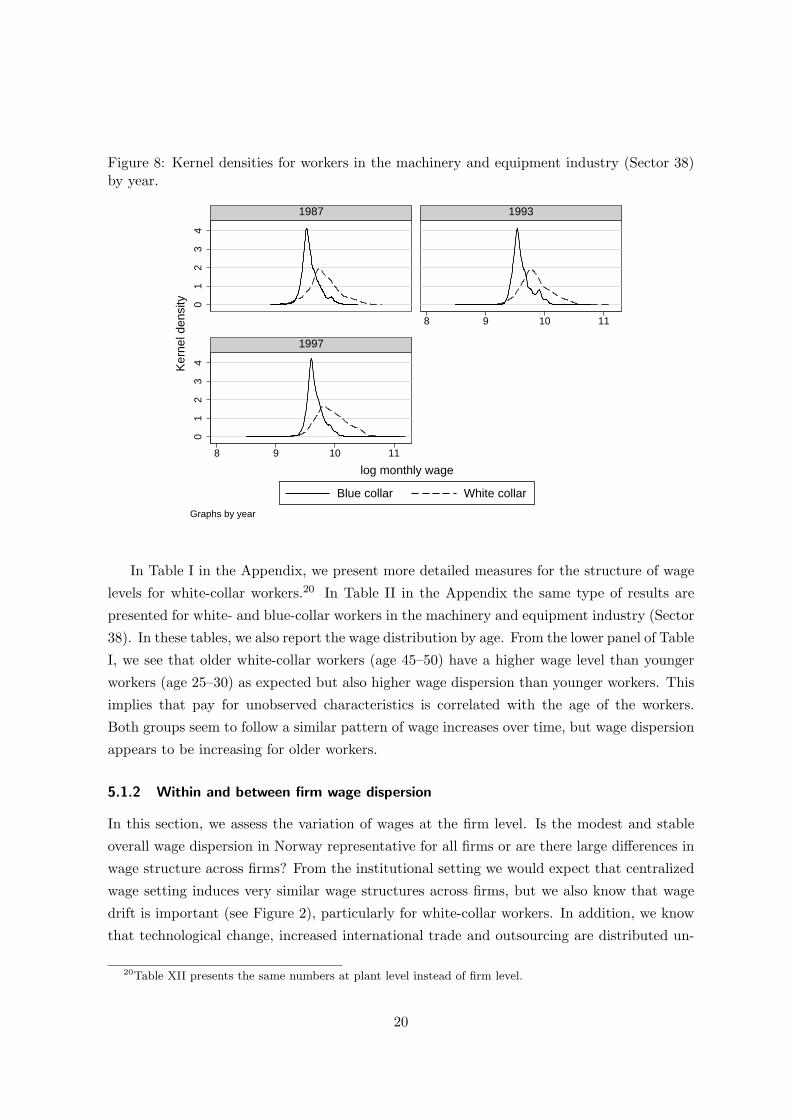
Figure 8: Kernel densities for workers in the machinery and equipment industry (Sector 38)by year.

01

23

40

12

34

8 9 10 11

8 9 10 11

1987 1993

1997

Blue collar White collar

Ker

nel d

ensi

ty

log monthly wage

Graphs by year

In Table I in the Appendix, we present more detailed measures for the structure of wage

levels for white-collar workers.20 In Table II in the Appendix the same type of results are

presented for white- and blue-collar workers in the machinery and equipment industry (Sector

38). In these tables, we also report the wage distribution by age. From the lower panel of Table

I, we see that older white-collar workers (age 45–50) have a higher wage level than younger

workers (age 25–30) as expected but also higher wage dispersion than younger workers. This

implies that pay for unobserved characteristics is correlated with the age of the workers.

Both groups seem to follow a similar pattern of wage increases over time, but wage dispersion

appears to be increasing for older workers.

5.1.2 Within and between firm wage dispersion

In this section, we assess the variation of wages at the firm level. Is the modest and stable

overall wage dispersion in Norway representative for all firms or are there large differences in

wage structure across firms? From the institutional setting we would expect that centralized

wage setting induces very similar wage structures across firms, but we also know that wage

drift is important (see Figure 2), particularly for white-collar workers. In addition, we know

that technological change, increased international trade and outsourcing are distributed un-

20Table XII presents the same numbers at plant level instead of firm level.

20

equally across firms. These forces have been as important in Norway as in most other countries

and may lead to differences in wage dispersion across firms (Salvanes and Førre, 2003). Such

possible differences may of course reflect different factors such as productivity differences,

differences in wage policy or differences in the composition of the workforce.

Recall that the average wage increase is about 20% for white-collar workers in the period

we are analyzing. In Figure 9, we present the real wage increase at the firm level for both

the mean wage level and different parts of the distribution. We see that the wage increase

has been very similar for different parts of the wage distribution of firms. This implies that

there has not been any increased wage dispersion across firms over time in Norway. More

detailed results, and results for blue- and white-collar workers together in the machinery and

equipment industry can be found in Tables III and IV in the Appendix.

Figure 9: Mean of firm mean log monthly white-collar wage in the private sector.

9.4

9.6

9.8

1010

.2m

ean

of fi

rm m

ean

log

mon

thly

wag

e

1981 1983 1985 1987 1989 1991 1993 1995 1997Year

mean 10th percentile25th percentile 75th percentile90th percentile

In order to further assess the wage structures within and between firms, we decompose

the wage structure. These results are presented in Figure 10 for white-collar workers only

and in Figure 11 for blue- and white-collar workers in the machinery and equipment industry

(Sector 38). Corresponding numbers are given in Tables IX and X in the Appendix.21 As

expected, only 15–20% of the wage variation for white-collar workers are between firms. Thus,

must of the wage dispersion in Norway is within firms. It is important to note, however, that

there was a slight increase in the magnitude of firm wage differences at the end of the period

21Table XIII gives the numbers for white-collar workers where we use plants instead of firms.

21

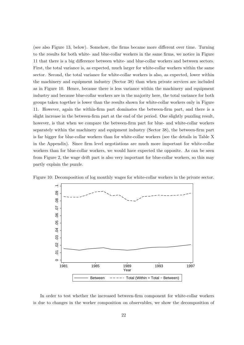
(see also Figure 13, below). Somehow, the firms became more different over time. Turning

to the results for both white- and blue-collar workers in the same firms, we notice in Figure

11 that there is a big difference between white- and blue-collar workers and between sectors.

First, the total variance is, as expected, much larger for white-collar workers within the same

sector. Second, the total variance for white-collar workers is also, as expected, lower within

the machinery and equipment industry (Sector 38) than when private services are included

as in Figure 10. Hence, because there is less variance within the machinery and equipment

industry and because blue-collar workers are in the majority here, the total variance for both

groups taken together is lower than the results shown for white-collar workers only in Figure

11. However, again the within-firm part dominates the between-firm part, and there is a

slight increase in the between-firm part at the end of the period. One slightly puzzling result,

however, is that when we compare the between-firm part for blue- and white-collar workers

separately within the machinery and equipment industry (Sector 38), the between-firm part

is far bigger for blue-collar workers than for white-collar workers (see the details in Table X

in the Appendix). Since firm level negotiations are much more important for white-collar

workers than for blue-collar workers, we would have expected the opposite. As can be seen

from Figure 2, the wage drift part is also very important for blue-collar workers, so this may

partly explain the puzzle.

Figure 10: Decomposition of log monthly wages for white-collar workers in the private sector.

0.0

1.0

2.0

3.0

4.0

5.0

6.0

7.0

8.0

9.1

1981 1985 1989 1993 1997Year

Between Total (Within = Total − Between)

In order to test whether the increased between-firm component for white-collar workers

is due to changes in the worker composition on observables, we show the decomposition of

22

Figure 11: Decomposition of log monthly wage for workers in the machinery and equipmentindustry (Sector 38).

0.0

2.0

4.0

6.0

80

.02

.04

.06

.08

1987 1989 1991 1993 1995 1997

1987 1989 1991 1993 1995 1997

All workers Blue collar workers

White collar workers

Between Total (Within = Total − Between)

Year

Graphs by All workers/Blue collar workers/White collar workers

the residual wage distribution in Figure 12 after controlling for type of education, gender and

age in a Mincer wage equation estimated annually (corresponding numbers are given in Table

XI in the Appendix). Two important findings are evident. We basically get the same result

in the first part of the period. Between-firm wage dispersion accounts for about 17% of the

total dispersion. However, controlling for compositional changes, the increase in the wage

dispersion across firms at the end of the period completely disappears. This is made even

clearer in Figure 13, where we report the ratio of the between-firm and total variation. The

large increase in differences in wages due to changes in the workforce composition started

in the beginning of the large downturn of the Norwegian economy in the late 1980s. The

finding of relatively strong compositional changes in Norwegian firms in this period is also

supported by other studies that assess reallocation of jobs and workers (Salvanes and Førre,

2003). Salvanes and Førre find that the bulk of reallocation of jobs is between firms within

5-digit sectors, indicating that structural change at this level has been important in explaining

the change in the composition of workers in the firms. The change has been connected to

increased technological change and increased international trade.

It is interesting to compare our results with other Scandinavian countries that have dif-

ferent wage setting institutions. Sweden started out with centralized wage bargaining like

Norway’s, but in the early 1980s, it basically decentralized wage bargaining to the industry

level and, unlike Norway, did not recentralize. Finland has had partly decentralized wage bar-

23

Figure 12: Decomposition of residuals from Mincer-equations for white-collar workers in theprivate sector.

0.0

1.0

2.0

3.0

4.0

5

1981 1985 1989 1993 1997Year

Between Total (Within = Total − Between)

Figure 13: Fraction of total variance for white-collar workers in the private sector explainedby between-firm effects.

.14

.16

.18

.2.2

2

1981 1985 1989 1993 1997Year

log monthly wage Residuals

24

gaining at the industry level since the early 1980s, and, as in Norway, plant-level bargaining

has been important over the whole period. When we compare total wage dispersion and the

importance of the firm level in determining wages, Norway is very similar to Sweden in the

1980s, when the wage bargaining institutions were similar. According to Edin et al. (2005),

the firm-level part constituted about 20% until about 1990, and then it increased to about

30% of wage dispersion in Sweden around year 2000. For Norway, it increased less, at least

until 1997. A similar pattern is found when controlling for sorting to explain the increased

importance of firms in determining wages. Sorting is important both in Sweden and in Nor-

way, but in Sweden, real firm effects also exist. Finland is very different from Norway and

Sweden in that the total wage dispersion is much smaller and constant throughout the period.

Furthermore, Finland is vastly different when it comes to the importance of firm effects: the

firm effect was negligible in the beginning and explains the entire wage dispersion from the

late 1990s (Uusitalo and Vartiainen, 2005).

5.2 Firm size

Davis and Haltiwanger (1996) has shown firm size to be important in explaining wage differ-

ences. Figure 14 shows the average of log monthly wage for white-collar workers distributed

by firm size. Here we use a sample where the firm size restriction is at least 2 white-collar

workers instead of 25 white-collar workers. In line with the previous literature, we find that

wages increase with firm size. Note that the wage differences between different firm size

classes are roughly unchanged over time.

To picture the wage dispersion, we use the coefficient of variation between and within

firms.22 Figure 15 shows that wage dispersion within firms tends to increase with firm size,

while wage dispersion between firms tends to decrease with firm size.23

5.3 Wage dynamics

Figure 16 presents the average log wage changes for private-sector white-collar workers. We

notice that wage growth differs strongly over the business cycle for this group of workers.

Wage growth is much higher for the two peak periods of 1985–1986 and 1996–1997 than at

the two low-point years. From 1980 to 1981, there is even a decline in real average wages. This

pro-cyclical pattern is strong and characterizes all segments of the wage change distribution.

When comparing the group of workers moving between firms to all workers (presented

in Figure 16), the results indicate that most moves are voluntary, since movers have a much

22We have no controls, i.e., we look at the raw wage data.23Davis and Haltiwanger (1996) writes: “The negative relationship of establishment size to wage dispersion

[...] entirely reflects the behavior of the between-plant component of wage dispersion. [...] In contrast, thewithin-plant coefficient of wage variation tends to rise with establishment size.”

25

Figure 14: Mean of firm mean log monthly wage by firm size. White-collar workers in theprivate sector.

9.6

9.7

9.8

9.9

9.6

9.7

9.8

9.9

2−9 10−24 25−49 50−99 100−149 150−2−9 10−24 25−49 50−99 100−149 150−

1981 1986

1993 1997

Mea

n of

firm

mea

n lo

g m

onth

ly w

age

Firm sizeGraphs by Year

Figure 15: Coefficient of Variation within and between firms. White-collar workers in theprivate sector.

.01

.015

.02

.025

.03

.01

.015

.02

.025

.03

2−9 10−24 25−49 50−99 100−149 150−2−9 10−24 25−49 50−99 100−149 150−

1981 1986

1993 1997

Coefficient of Variation between Coefficient of Variation within

Firm size

Graphs by Year

26

higher wage increase than the overall average for almost the whole period. Table III in the

Appendix reports the wage changes for different parts of the distribution, and we see that

the same pattern is especially strong for the 75th percentile. Again the cyclical patterns are

strong, pointing to voluntary moves.

Figure 16: Average change in log monthly wage for all white-collar workers and for white-collar workers who switch firms in the private sector.

−.0

20

.02

.04

.06

.08

Ave

rage

cha

nge

log

mon

thly

wag

e

1981 1983 1985 1987 1989 1991 1993 1995 1997Year

All workers Workers who switch firms

Figure 17 presents the wage increases for short- and long-tenured workers. As we would

expect, workers with short tenure have much higher wage increases than workers who have

stayed with the firm for a while. Again the cyclical pattern is strong.

Turning to the sample of both blue- and white-collar workers presented in Table IV in the

Appendix, a pro-cyclical pattern is present but much less pronounced. This indicates that

white-collar workers are under a more flexible regime in terms of wage setting, whether it has

to do with firm-level negotiations or other factors. Results for movers and differences between

short- and long-tenured workers hold also for this group of workers.

5.4 Worker mobility within and across firms

In this section, we present patterns of worker mobility across firms, i.e., firings and separations,

as well the worker mobility rates within firms, e.g., promotions. We want to assess the

distribution of worker exit and entry rates both across groups of workers and firms and over

the business cycle. A novel feature is that we can calculate internal turnover rates and entry

rates for different occupations within the firms. We will focus on the results for white-collar

27

Figure 17: Average change in log monthly wage for all white-collar workers in the privatesector, by tenure.

−.0

20

.02

.04

.06

Ave

rage

cha

nge

log

mon

thly

wag

e

1981 1983 1985 1987 1989 1991 1993 1995 1997Year

Tenure less than 3 years Tenure 3 years or more

workers in the manufacturing sector and private services.

5.4.1 Worker exit and entry rates

We start by presenting in Figure 18 the development and size distribution for all firms defined

as 25+ workers both in t and t − 1 in the white-collar data set as well as for large firms

defined as 100+ workers, to make the results comparable across countries. Note that none of

these groups will be representative for the Norwegian economy, since firms with 25+ white-

collar workers are relatively large in Norway. However, from Figure 19, we see that the size

distribution for all firms is very stable. For “all firms”, i.e., 25+, average firm size increased

from 121 employees in 1981 to 139 in 1997. For “100+ firms” size increased from 287 to 345

employees.

In order to illustrate the patterns of worker mobility, we present in Figures 20, 21 and

22 exit and entry rates by year, firm size, and for lower and upper segments of the wage

distribution. Tables V, VI and VII in the Appendix provide more detailed information.24

The exit rate or worker separation rate for all white-collar workers taken together is about

15% annually for all firms in our sample, and about 10% for large firms. Salvanes and Førre

24Table VIII in the Appendix provides numbers for both white- and blue-collar workers in the machineryand equipment industry (Sector 38). Table XIV provides numbers for white-collar workers by plant instead offirm.

28

Figure 18: Number of white-collar workers and employment growth for firms in the privatesector, by firm size. Large firms defined as at least 100 white collar workers.

100

150

200

250

300

350

Em

ploy

ees

0.0

5.1

.15

.2E

mpl

oym

ent g

row

th

1981 1985 1989 1993 1997Year

All firms

100

150

200

250

300

350

Em

ploy

ees

0.0

5.1

.15

.2E

mpl

oym

ent g

row

th

1981 1985 1989 1993 1997Year

Employment growth Employees

Large firms

29

Figure 19: Kernel density log firm size. White-collar data.

0.2

.4.6

Ker

nel d

ensi

ty

2 4 6 8log firmsize

1981 19861993 1997

(2003) using a data set without a lower limit on firm size find an exit rate around 25%. This

is only slightly below results for the US economy. The entry or hiring rate is between 14%

and 19% for all firms and between 9% and 12% for large firms. One observation, therefore, is

that the turnover rates are high for white-collar workers and that they decrease with firm size

as expected. These findings are in line with previous work using other data sets and different

parts of the firm size distribution (Salvanes and Førre, 2003). Looking at different segments

of the workforce, see Figures 21 and 22, we notice that white-collar workers in low paid jobs

have much higher exit and entry rates than workers in high paid jobs.25 Thus, low paid jobs

are more volatile than high paid jobs. Figure 23 shows the kernel densities for exit and entry

rates at the firm level. The cyclical pattern is quite interesting for worker flows. The exit

rate is quite stable over the cycle, whereas the job destruction rate that comprise one part

of the exit rate is for many countries found to be counter-cyclical (for the US see, Davis and

Haltiwanger, 1992; for Norway see Salvanes, 1997). This pattern appears to be true for all

segments of the firms. It is the entry rate that varies over the cycle in a pro-cyclical fashion.

Looking at job creation rate only, a part of the entry rate, the standard result is that they are

stable over the cycle. This pattern also appears to be true for all segments of the workforce,

25Low and high pay is here defined as being in the bottom or top quartile of the within firm wage distribution,respectively. Very similar results can be found in Tables VI and VII in the Appendix, looking at high andlow level jobs rather than high and low paid workers. High and low level jobs are defined as follows: First wecalculate median wages for all jobs, then we rank all jobs by their median wage. High level jobs are those jobswhose median wage is in the top 20% of the wage distribution and low level jobs are those in the bottom 20%.

30

but it seems to be more pronounced for the lower-level jobs.

In Table V in the Appendix, we see that entry rates are positively correlated with wage

growth, suggesting that growing firms raise wages to attract new workers. Somewhat surpris-

ingly, the relationship between wage growth and the worker exit rates is much weaker. One

would expect wage growth to be negatively correlated with the exit rate, and to some extent

this is so for low level jobs. For workers in high level jobs, however, Table VI show that there

is significant, positive correlation between wage growth and exit rates. One explanation could

be that managers in successful firms get attractive outside offers. Within firm wage dispersion

does not seem related to exit rates, nor to entry rates with one exception. For high level jobs,

there is significant positive correlation between wage dispersion and entry.

Figure 20: Firm level exit and entry rates. White-collar workers in the private sector. Largefirms defined as at least 100 white collar workers.

.1.1

5.2

1981 1985 1989 1993 19971981 1985 1989 1993 1997Note: exit rates for 1987 and 1988 are omitted. Note: exit rates for 1987 and 1988 are omitted.

All Large

Entry rate Exit rate

Year

Graphs by All/Large firms

5.4.2 Internal worker dynamics

Since we have information on the internal structure of the firms’ labor market, we can assess

the internal worker turnover rates. Two measures will be presented: internal turnover rates

across occupations and the share hired from within the firm.26 We look at 22 different

occupations, cf Section 4.1.1. The number of occupations represented in each firm has been

stable over the period. The average is 13 for all firms and 16 for large firms. The number

26See Hunnes et al. (2003) for more details on this.

31

Figure 21: Firm level exit rates. White-collar workers in the private sector. Split bytop/bottom quartile of the within firm wage distribution. Large firms defined as at least100 white collar workers.

.1.1

5.2

.25

1981 1985 1989 1993 19971981 1985 1989 1993 1997Note: exit rates for 1987 and 1988 are omitted. Note: exit rates for 1987 and 1988 are omitted.

All firms Large firms

Exit rate bottom quartile Exit rateExit rate top quartile

Year

Graphs by All/Large firms

Figure 22: Firm level entry rates. White-collar workers in the private sector. Split bytop/bottom quartile of the within firm wage distribution. Large firms defined as at least 100white collar workers.

.1.1

5.2

.25

.3

1981 1985 1989 1993 19971981 1985 1989 1993 1997

All firms Large firms

Entry rate bottom quartile Entry rateEntry rate top quartile

Year

Graphs by All/Large firms

32

Figure 23: Kernel densities for firm level exit and entry rates. White-collar workers in theprivate sector.

02

46

8K

erne

l den

sity

0 .2 .4 .6 .8 11981

Whole firm

02

46

8K

erne

l den

sity

0 .2 .4 .6 .8 11981

Top quartile of firm wages

02

46

8K

erne

l den

sity

0 .2 .4 .6 .8 11981

Bottom quartile of firm wages

02

46

8K

erne

l den

sity

0 .2 .4 .6 .8 11986

02

46

8K

erne

l den

sity

0 .2 .4 .6 .8 11986

02

46

8K

erne

l den

sity

0 .2 .4 .6 .8 11986

02

46

8K

erne

l den

sity

0 .2 .4 .6 .8 11993

02

46

8K

erne

l den

sity

0 .2 .4 .6 .8 11993

02

46

8K

erne

l den

sity

0 .2 .4 .6 .8 11993

02

46

8K

erne

l den

sity

0 .2 .4 .6 .8 11997

Exit Entry

02

46

8K

erne

l den

sity

0 .2 .4 .6 .8 11997

Exit Entry

02

46

8K

erne

l den

sity

0 .2 .4 .6 .8 11997

Exit Entry

33

of hierarchical levels has also been stable over time. The average is 6 for all firms and 6.8

for the 100+ firms. The number of levels appears to be larger for Norwegian firms than the

figure Oyer (2005) reports for Swedish firms.

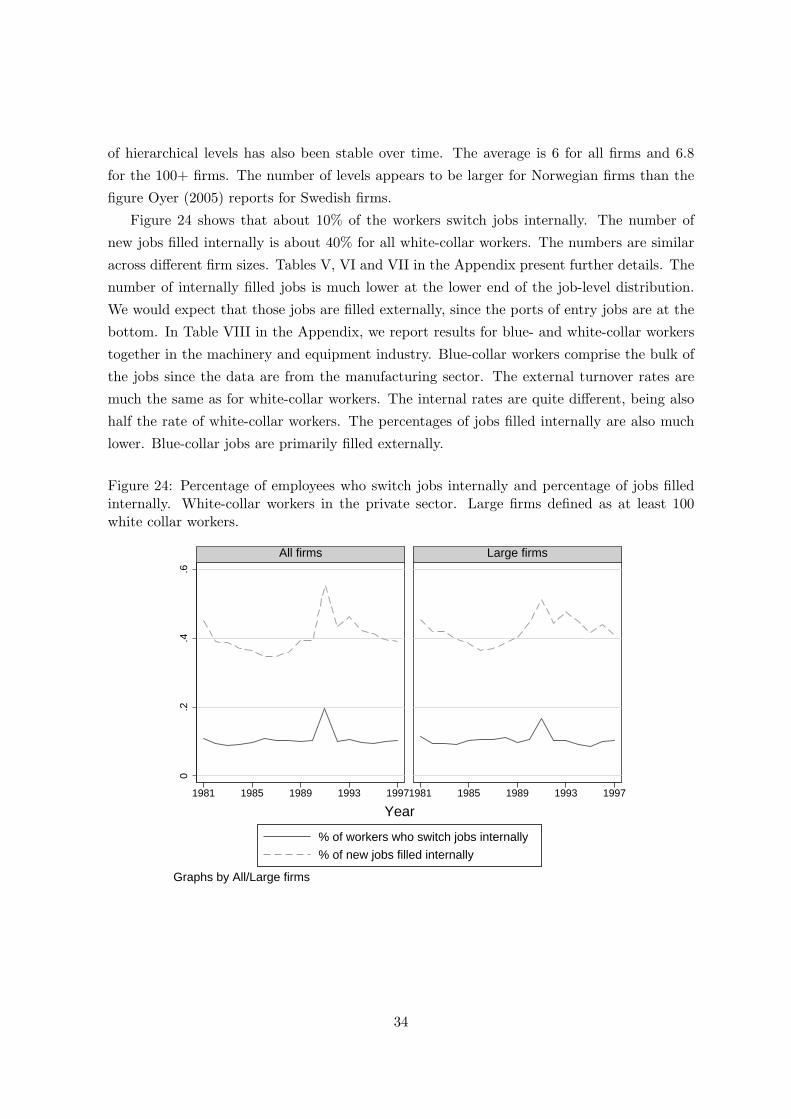
Figure 24 shows that about 10% of the workers switch jobs internally. The number of

new jobs filled internally is about 40% for all white-collar workers. The numbers are similar

across different firm sizes. Tables V, VI and VII in the Appendix present further details. The

number of internally filled jobs is much lower at the lower end of the job-level distribution.

We would expect that those jobs are filled externally, since the ports of entry jobs are at the

bottom. In Table VIII in the Appendix, we report results for blue- and white-collar workers

together in the machinery and equipment industry. Blue-collar workers comprise the bulk of

the jobs since the data are from the manufacturing sector. The external turnover rates are

much the same as for white-collar workers. The internal rates are quite different, being also

half the rate of white-collar workers. The percentages of jobs filled internally are also much

lower. Blue-collar jobs are primarily filled externally.

Figure 24: Percentage of employees who switch jobs internally and percentage of jobs filledinternally. White-collar workers in the private sector. Large firms defined as at least 100white collar workers.

0.2

.4.6

1981 1985 1989 1993 19971981 1985 1989 1993 1997

All firms Large firms

% of workers who switch jobs internally

% of new jobs filled internally

Year

Graphs by All/Large firms

34

6 Concluding remarks

To what extent do different firms follow different wage policies? Do such differences relate to

how workers move between firms? What are the effects of different wage bargaining regimes?

The aim of this paper has been threefold. First, to describe the Norwegian wage setting

and employment protection institutions. Next, to describe data sets available for empirical

analysis, and finally to document stylized facts about the wage structure and the worker

mobility patterns in Norway. We analyze within and between firm wage differences and

worker entry and exit rates in the period 1980–1997. Norway is an interesting case to study

for several reasons. The Norwegian economy is very open, but wage dispersion in Norway

has remained low while most OECD countries have experienced a strong increase. Also,

certain labor market institutions are different from other European countries. Most notably,

centralized wage bargaining is quite important. Differences in wage bargaining institutions

between white- and blue-collar workers within Norway, provide an additional dimension for

comparison.

Norway is a high wage country. Average monthly white-collar wage in the early 1990s was

about NOK 20,000, the equivalent of 2,500 EURO. Average monthly wage across both blue-

and white-collar workers in the machinery and equipment industry was about NOK 17,000.

Real white-collar wages grew 18% over the 16 year period 1981-1997. Wage dispersion was

low and stable with a coefficient of variation for white-collar workers of 31.8% in 1981 and

32.4% in 1997, i.e. the standard deviation of white-collar wages was less than a third of

the wage level. Country studies from Finland, Germany, Italy, Sweden and Denmark find

coefficients of variation in wages in the interval 33–41%. We find that wage dispersion among

blue-collar workers is much smaller than wage dispersion among white-collar workers. This

is to be expected, as blue-collar workers is a much more homogeneous group.

An important question we have analyzed is to what extent firms differ in their wage

setting. Numerous economic models portraits all firms as similar, using the “representative

firm” metaphor. How far from the truth is this simplification? We find that most of the wage

variation in Norway is within firms. The average standard deviation of wages within firms

is 79% of the overall standard deviation. Still, firms vary considerably in their average wage

level. The standard deviation of average firm wages is about 13% of the overall average wage,

and between firm wage variation represents 17–23% of the overall wage variation. The between

share has increased over time, suggesting that firms are becoming somewhat more dissimilar.

This development is related to changes in the workforce composition and disappears when

observable worker characteristics are controlled for.

The correlation between the firm’s average wage and the standard deviation of wages

within the firm, is positive and significant, both when we look at the wage level and the log

of wages. Hence, high wage firms have larger within firm wage dispersion than low wage

35

firms. Whether this is because high wage firms are more heterogeneous with respect to the

composition of the work force or because high wage firms follow a different wage policy, is an

interesting and important question that we will pursue in future work.

Firms may differ not only with respect to average wage and wage dispersion, but also

with respect to average wage growth. Looking into this, we find some heterogeneity. The

interquartile range in average wage growth across firms is 3–4 percentage points in the 1980s,

and about 2 percentage points in the 1990s. These numbers are for white-collar workers.

Wage growth is strongly procyclical. When looking at the sample of both blue- and white-

collar workers in the machinery and equipment industry, however, the procyclical pattern is

less pronounced. This might be related to centralized wage bargaining being more important

for blue-collar workers. Workers who change firms have above average wages growth in all

years. This finding suggests that there are more voluntary moves than layoffs, even during

economic downturns.

In our sample, dominated by relatively large firms, about 15% of the workers leave their

employer each year. This is a fairly low number compared to other countries. A previous

study for Norway, using the entire universe of firms, have found the exit rate to be about 25%.

We find that the exit rate is very stable over the business cycle. This may seem surprising,

but it is in line with previous studies suggesting that higher job destruction rates in bad years

are counter-acted by less voluntary job changes. The entry rate, on the other hand, is highly

procyclical, and varies between 14–19%. Previous studies suggest that this is driven by more

voluntary job changes is good years while the job creation rates are fairly stable over the

cycle. Entry and exit rates are much higher for workers in low level jobs than for workers in

high level jobs. Hence, low level jobs have on average a shorter duration.

There is substantial heterogeneity in entry and exit rates across firms. Some of this

heterogeneity is explained by firm characteristics. First, we find that entry and exit rates

are smaller in large firms than in small firms. Obviously, large internal labor markets offer

better career opportunities within firms. Second, entry rates are positively correlated with

wage growth, suggesting that growing firms raise wages to attract new workers. Somewhat

surprisingly, the relationship between wage growth and the worker exit rates is much weaker.

One would expect wage growth to be negatively correlated with the exit rate, and to some

extent this is so for low level jobs. For workers in high level jobs, however, there is significant,

positive correlation between wage growth and the exit rate. One explanation could be that

managers in successful firms get attractive outside offers.

Having information about the internal structure of firms’ labor markets, we are not re-

stricted to analyzing worker mobility across firms. Looking at within firm job mobility, we

find that about 10% of white-collar workers change occupation each year. Occupations are

broadly defined in our data, hence, these workers should experience a significant shift in their

job content. The share of workers changing occupation internally is similar for small and large

36

firms, and the number is also stable over the business cycle. The share of new white-collar

jobs filled internally varies between 35 and 46%. There is more external hiring in good years.

Consistent with the hypothesis that low level jobs are “ports of entry” into the firms, we find

that the share of jobs filled internally is much lower for low level jobs than for high level jobs.

The difference is particularly large in large firms. Among blue-collar workers, the share of

workers who change occupation within firms is much lower than for white-collar workers. The

share of new jobs filled internally is also much lower.

Future work on the Norwegian data should go deeper into the importance of sorting, and

clarify further to what extent different wage structures reflect differences in the workforce

composition and to what extent it reflect managerial choices. How has sorting of workers

developed over time and what are possible driving forces? How do different managerial

choices with respect to wage policy affect firm productivity? A related issue is the effect of

technological change and innovativeness on the wage structure. Finally, there is more work

to be done on the effect of different wage bargaining regimes, exploiting differences between

blue- and white-collar workers, different sectors and different time periods.

References

Aaberge, R., A. Bjørklund, M. Jannti, P. Pedersen, N. Smith, and T. Wennemo(2000): “Unemployment Shocks and Income Distribution: How did the Nordic CountriesFare During Their Crisis?,” Scandinavian Journal of Economics, 102, 77–100.

Davis, S., and J. Haltiwanger (1992): “Gross Job Creation, Gross Job Destruction, andEmployment Reallocation,” Quarterly Journal of Economics, 107(3), 819–863.

Davis, S. J., and J. Haltiwanger (1996): “Employer Size and the Wage Structure in U.S.Manufacturing,” Annales d’Economie Et De Statistique, (41-42), 323–367.

Edin, P.-A., B. Holmlund, and O. N. Skans (2005): “Wage Structure in Sweden 1985-2000,” This Volume.

Emerson, M. (1987): “Labour Market Flexibility and Jobs: A Survey of Evidence fromOECD Countries with Special Reference to Europe: Comments,” in The Fight againstUnemployment: Macroeconomic Papers from the Centre for European Policy Studies, ed.by R. Lyard, and L. Calmfors, pp. 77–84. MIT Press.

Faggio, G., K. G. Salvanes, and J. V. Reenen (2005): “Understanding Wage andProductivity Dispersion in the United Kingdom and Norway,” Memo, LSE.

Freeman, R. B. (1997): “Are Norway’s Solidaristic and Welfare State Policies Viable in theModern Global Economy?,” in Making Solidarity Work?: The Norwegian Labour Marketin Transition, ed. by J. E. Dølvik, and A. H. Steen, chap. 2. Scandinavian University Press.

37

Hægeland, T., T. J. Klette, and K. G. Salvanes (1999): “Declining Returns to Edu-cation in Norway? Comparing Estimates across Cohorts, Sectors and Time,” ScandinavianJournal of Economics, 101(4), 555–576.

Holden, S. (1998): “Wage Drift and the Relevance of Centralised Wage Setting,” Scandi-navian Journal of Economics, 100(4), 711–731.

Holden, S., and A. Rødseth (1990): “Wage Formation in Norway,” in Wage Formationand Macroeconomic Policy in the Nordic Countries, ed. by L. Calmfors, pp. 237–280. SNSand Oxford University Press.

Holden, S., and K. G. Salvanes (2005): “Downward Nominal Wage Rigidity in Norway,”Memo, Norwegian School of Economics and Business Administration.

Hunnes, A., J. Møen, and K. G. Salvanes (2003): “Ports of Entry: The NorwegianCase,” Memo, Norwegian School of Economics and Business Administration.

Kahn, L. (1998): “Against the Wind: Bargaining Recentralisation and Wage Inequality inNorway 1987-91,” The Economic Journal, 108(448), 603–645.

Margolis, D. N., and K. G. Salvanes (2001): “Do Firms Really Share Rents with TheirWorkers?,” IZA Discussion Paper No. 330. Institute for the Study of Labor.

Møen, J., K. G. Salvanes, and E. Ø. Sørensen (2004): “Documentation of the LinkedEmployer-Employee Data Base at the Norwegian School of Economics and Business Ad-ministration,” Memo. Norwegian School of Economics and Business Administration.

NHO (2004): http://www.nho.no/.

Nilsen, Ø. A., K. G. Salvanes, and F. Schiantarelli (2003): “Employment Changes,the Structure of Adjustment Costs, and Plant Size,” IZA Discussion Paper No. 920. Insti-tute for the Study of Labor.

Oecd (1999): Employment Outlook. OECD, Paris.

Oyer, P. (2005): “Wage Structure and Labor Mobility in Sweden 1970-1990,” This Volume.

Salvanes, K. G. (1997): “Market Rigidities and Labour Market Flexibility: An InternationalComparison.,” Scandinavian Journal of Economics, 99, 315–333.

Salvanes, K. G., S. Burgess, and J. Lane (1999): “Sources of Earnings Dispersion ina Linked Employer-Employee Data Set: Evidence from Norway,” in The Creation andAnalysis of Employer-Employee Matched Data, ed. by J. C. Haltiwanger, J. I. Lane, J. R.Spletzer, J. J. M. Theeuwes, and K. R. Troske. North-Holland.

Salvanes, K. G., and S. E. Førre (2003): “Effects on Employment of Trade and TechnicalChange: Evidence from Norway,” Economica, 70, 293–329.

Statistics Norway (1974): “Arbeidsmarkedsstatistikk 1974,” Statistisk Sentralbyra.

(1978): “Arbeidsmarkedsstatistikk 1978,” Statistisk Sentralbyra.

(1984): “Arbeidsmarkedsstatistikk 1984,” Statistisk Sentralbyra.

38

(1997): “Arbeidsmarkedsstatistikk 1997,” Statistisk Sentralbyra.

(2003a): “Arbeidsmarkedsstatistikk 2003,” Statistisk Sentralbyra.

(2003b): “Statistisk Arbok 2003,” Statistisk Sentralbyra.

(2004): “Konsumprisindeksen fra 1865 (1998=100),” Statistisk Sentralbyra.http://www.ssb.no/kpi/1-7t.html.

Stokke, T. A., S. Evju, and H. O. Frøland (2003): Det kollektive arbeidslivet: Organ-isasjoner, tariffavtaler, lønnsoppgjør og inntektspolitikk. Universitetsforlaget.

TBL (2004): http://www.tbl.no/.

Uusitalo, R., and J. Vartiainen (2005): “Finland: Firm Factors in Wages and WageChanges,” This Volume.

Wallerstein, M., M. Golden, and P. Lange (1997): “Unions, Employers’ Associations,and Wage-Setting Institutions in Northern and Central Europe, 1950-1992,” Industrial andLabor Relations Review, 50(3), 379–401.

A Tables

39

Table I: Structure of wages within and between firms. White-collar workers in the privatesector.

Monthly wage log monthly wage

1981 1986 1993 1997 1981 1986 1993 1997

Average wage 18,259 19,694 20,001 21,855 9.768 9.840 9.858 9.945sd 5,810 6,560 6,455 7,072 0.293 0.305 0.296 0.30090%-ile 25,872 28,934 29,175 31,959 10.161 10.273 10.281 10.37210%-ile 12,231 13,090 13,447 14,625 9.412 9.480 9.507 9.590N-workers 56,838 73,600 76,449 79,259 56,838 73,600 76,449 79,259Average of firm average wage 17,226 18,201 18,677 20,395 9.713 9.766 9.791 9.879sd 2,350 2,404 2,656 2,977 0.135 0.130 0.135 0.14190%-ile 20,114 21,231 22,023 24,360 9.875 9.926 9.962 10.06110%-ile 14,042 15,114 15,601 16,686 9.525 9.596 9.622 9.697N-firms 467 506 521 565 467 506 521 565Average of sd of wage 4,568 5,006 5,121 5,566 0.249 0.255 0.253 0.252sd 1,206 1,381 1,653 1,641 0.048 0.053 0.051 0.04890%-ile 6,125 6,713 6,852 7,421 0.302 0.312 0.310 0.30810%-ile 2,999 3,356 3,537 3,744 0.194 0.200 0.197 0.198N-firms 467 506 521 565 467 506 521 565Average Coefficient ofvariation of wage 0.263 0.273 0.271 0.270 0.026 0.026 0.026 0.026sd 0.050 0.055 0.061 0.057 0.005 0.005 0.005 0.00590%-ile 0.323 0.341 0.339 0.334 0.031 0.031 0.032 0.03110%-ile 0.197 0.208 0.204 0.204 0.020 0.021 0.020 0.020N-firms 467 506 521 565 467 506 521 565Corr(average wage, sd wage) 0.738 0.732 0.727 0.726 0.203 0.155 0.364 0.333Significance level 0.000 0.000 0.000 0.000 0.000 0.001 0.000 0.000Average wage for workersbetween 25 and 30 15,486 16,984 16,304 17,630 9.627 9.716 9.679 9.757sd 3,179 3,795 3,282 3,547 0.201 0.216 0.200 0.20190%-ile 19,725 22,120 20,564 22,202 9.890 10.004 9.931 10.00810%-ile 11,774 12,626 12,483 13,386 9.374 9.444 9.432 9.502N-workers 7,378 11,628 10,833 9,123 7,378 11,628 10,833 9,123Average wage for workersbetween 45 and 50 19,970 21,352 21,368 23,262 9.858 9.920 9.919 10.003sd 6,291 7,182 7,327 7,845 0.290 0.305 0.312 0.31690%-ile 28,747 32,092 31,592 34,461 10.266 10.376 10.361 10.44810%-ile 13,576 14,309 14,094 15,250 9.516 9.569 9.554 9.632N-workers 7,231 9,031 14,641 13,962 7,231 9,031 14,641 13,962The numbers are real wages, transformed from nominal wages using the Consumer Price Index

from Statistics Norway with base year 1990.

40

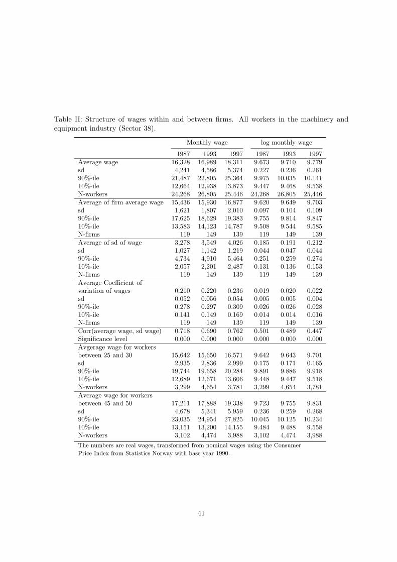
Table II: Structure of wages within and between firms. All workers in the machinery andequipment industry (Sector 38).

Monthly wage log monthly wage

1987 1993 1997 1987 1993 1997Average wage 16,328 16,989 18,311 9.673 9.710 9.779sd 4,241 4,586 5,374 0.227 0.236 0.26190%-ile 21,487 22,805 25,364 9.975 10.035 10.14110%-ile 12,664 12,938 13,873 9.447 9.468 9.538N-workers 24,268 26,805 25,446 24,268 26,805 25,446Average of firm average wage 15,436 15,930 16,877 9.620 9.649 9.703sd 1,621 1,807 2,010 0.097 0.104 0.10990%-ile 17,625 18,629 19,383 9.755 9.814 9.84710%-ile 13,583 14,123 14,787 9.508 9.544 9.585N-firms 119 149 139 119 149 139Average of sd of wage 3,278 3,549 4,026 0.185 0.191 0.212sd 1,027 1,142 1,219 0.044 0.047 0.04490%-ile 4,734 4,910 5,464 0.251 0.259 0.27410%-ile 2,057 2,201 2,487 0.131 0.136 0.153N-firms 119 149 139 119 149 139Average Coefficient ofvariation of wages 0.210 0.220 0.236 0.019 0.020 0.022sd 0.052 0.056 0.054 0.005 0.005 0.00490%-ile 0.278 0.297 0.309 0.026 0.026 0.02810%-ile 0.141 0.149 0.169 0.014 0.014 0.016N-firms 119 149 139 119 149 139Corr(average wage, sd wage) 0.718 0.690 0.762 0.501 0.489 0.447Significance level 0.000 0.000 0.000 0.000 0.000 0.000Avgerage wage for workersbetween 25 and 30 15,642 15,650 16,571 9.642 9.643 9.701sd 2,935 2,836 2,999 0.175 0.171 0.16590%-ile 19,744 19,658 20,284 9.891 9.886 9.91810%-ile 12,689 12,671 13,606 9.448 9.447 9.518N-workers 3,299 4,654 3,781 3,299 4,654 3,781Average wage for workersbetween 45 and 50 17,211 17,888 19,338 9.723 9.755 9.831sd 4,678 5,341 5,959 0.236 0.259 0.26890%-ile 23,035 24,954 27,825 10.045 10.125 10.23410%-ile 13,151 13,200 14,155 9.484 9.488 9.558N-workers 3,102 4,474 3,988 3,102 4,474 3,988The numbers are real wages, transformed from nominal wages using the Consumer

Price Index from Statistics Norway with base year 1990.

41

Table III: Wage dynamics for white-collar workers in the private sector.

∆ monthly wage ∆ log monthly wage

1981 1986 1993 1997 1981 1986 1993 1997

Average change in wage -93 903 329 709 -0.004 0.047 0.016 0.032sd 1,228 1,263 1,430 1,488 0.065 0.061 0.054 0.06890%-ile 1,276 2,274 1,241 2,057 0.074 0.116 0.064 0.09310%-ile -1,226 -79 -308 -131 -0.066 -0.005 -0.018 -0.007N-workers 49,975 60,499 68,162 69,210 49,975 60,499 68,162 69,210Average of firm averagechange in wage -171 820 246 623 -0.008 0.046 0.013 0.030sd 627 471 369 494 0.036 0.027 0.019 0.02390%-ile 514 1,396 666 1,186 0.031 0.075 0.034 0.05710%-ile -849 267 -176 120 -0.050 0.016 -0.010 0.006N-firms 467 506 521 565 467 506 521 565Average of sd ofchange in wage 955 1,001 892 1,198 0.052 0.053 0.047 0.059sd 399 464 823 777 0.024 0.028 0.028 0.03790%-ile 1,381 1,499 1,434 2,019 0.076 0.077 0.078 0.09510%-ile 552 562 373 503 0.029 0.031 0.021 0.026N-firms 467 506 521 565 467 506 521 565Average change in wage forworkers who change firms 242 1,644 533 1,091 0.015 0.081 0.025 0.050sd 1,838 2,403 1,708 2,141 0.098 0.117 0.075 0.09990%-ile 2,405 4,414 2,128 3,424 0.132 0.220 0.100 0.15710%-ile -1,512 -465 -443 -215 -0.068 -0.026 -0.021 -0.011N-workers 1,265 814 2,688 2,842 1,265 814 2,688 2,842Average change in wage forworkers with tenure < 3 205 1,215 549 1,000 0.014 0.067 0.028 0.048sd 1,342 1,434 1,260 1,712 0.075 0.075 0.064 0.08590%-ile 1,750 2,788 1,726 2,808 0.105 0.151 0.091 0.13510%-ile -1,109 -32 -300 -137 -0.062 -0.002 -0.016 -0.007N-workers 4,766 13,314 10,626 10,829 4,766 13,314 10,626 10,829Average change in wage forworkers with tenure ≥ 3 -170 815 289 655 -0.009 0.041 0.014 0.029sd 1,156 1,196 1,454 1,436 0.059 0.055 0.051 0.06390%-ile 1,116 2,085 1,128 1,873 0.060 0.103 0.058 0.08410%-ile -1,236 -84 -310 -131 -0.068 -0.005 -0.019 -0.007N-workers 25,065 46,834 57,469 58,295 25,065 46,834 57,469 58,295Wage change is wage in year t minus wage in year t− 1.

The numbers are real wages, transformed from nominal wages using the Consumer Price Index from

Statistics Norway with base year 1990.

42

Table IV: Wage dynamics for all workers in the machinery and equipment industry (Sector38).

∆ monthly wage ∆ log monthly wage

1987 1993 1997 1987 1993 1997Average change in wage 341 308 473 0.027 0.017 0.024sd 1,423 1,269 1,513 0.084 0.072 0.08090%-ile 1,686 1,402 1,822 0.112 0.083 0.09710%-ile -1,180 -489 -506 -0.060 -0.027 -0.027N-workers 20,401 22,957 19,489 20,401 22,957 19,489Average of firm averagechange in wage 444 175 396 0.034 0.011 0.022sd 488 364 473 0.031 0.023 0.02690%-ile 1,054 579 884 0.077 0.035 0.04910%-ile -121 -178 -98 -0.004 -0.013 -0.010N-firms 119 149 139 119 149 139Average of sd ofchange in wage 1,127 820 1,146 0.072 0.049 0.065sd 696 656 610 0.034 0.033 0.03190%-ile 1,678 1,417 1,956 0.102 0.078 0.09710%-ile 598 260 473 0.040 0.016 0.031N-firms 119 149 139 119 149 139Average change in wage forworkers who change firms 297 346 597 0.025 0.016 0.023sd 1,684 2,222 2,406 0.103 0.114 0.14090%-ile 2,205 2,679 3,362 0.142 0.157 0.15910%-ile -1,355 -1,169 -1,998 -0.084 -0.070 -0.119N-workers 609 319 697 609 319 697Average change in wage forworkers with tenure < 3 617 612 736 0.050 0.039 0.041sd 1,558 1,573 1,955 0.106 0.095 0.10690%-ile 2,398 2,234 2,403 0.181 0.141 0.14110%-ile -1,073 -505 -545 -0.059 -0.025 -0.031N-workers 4,488 3,272 3,289 4,488 3,272 3,289Average change in wage forworkers with tenure ≥ 3 264 257 420 0.021 0.014 0.020sd 1,373 1,203 1,401 0.075 0.067 0.07390%-ile 1,492 1,221 1,665 0.099 0.072 0.08510%-ile -1,220 -487 -492 -0.060 -0.027 -0.025N-workers 15,913 19,685 16,200 15,913 19,685 16,200Wage change is wage in year t minus wage in year t− 1.

The numbers are real wages, transformed from nominal wages using the Consumer

Price Index from Statistics Norway with base year 1990.

43

Table V: Mobility white-collar workers in the private sector. All jobs.

All firms Firms with 100+ employees

1981 1986 1993 1997 1981 1986 1993 1997

N-firms 467 506 521 565 144 170 174 173Employees 122 145 147 140 287 332 341 345sd 199 294 293 304 297 453 448 491Number of occupations 13 13 13 12 16 16 16 15sd 4 4 4 4 3 3 3 3Number of levels 6 6 6 6 7 7 7 7sd 1 1 1 1 0 0 1 1Employment growth 0.00 0.06 0.03 0.04 0.03 0.09 0.13 0.08sd 0.23 0.20 0.46 0.27 0.32 0.21 0.74 0.38Exit rate (all) 0.16 0.14 0.14 0.16 0.11 0.09 0.08 0.10Exit rate 0.16 0.15 0.14 0.17 0.16 0.13 0.12 0.14sd 0.10 0.10 0.13 0.12 0.11 0.08 0.08 0.07Exit rate, top quartile 0.12 0.13 0.13 0.15 0.12 0.12 0.11 0.12sd 0.12 0.12 0.14 0.14 0.11 0.10 0.10 0.08Exit rate, bottom quartile 0.23 0.19 0.17 0.19 0.22 0.17 0.15 0.16sd 0.15 0.15 0.16 0.16 0.13 0.11 0.11 0.10Entry rate 0.14 0.19 0.14 0.18 0.15 0.18 0.14 0.17sd 0.11 0.10 0.13 0.13 0.12 0.10 0.14 0.13Entry rate, top quartile 0.08 0.12 0.11 0.13 0.09 0.12 0.13 0.11sd 0.12 0.12 0.15 0.13 0.12 0.11 0.17 0.12Entry rate, bottom quartile 0.22 0.32 0.18 0.25 0.24 0.30 0.19 0.24sd 0.17 0.17 0.17 0.20 0.16 0.15 0.16 0.18% of employees who switchjobs internally 0.11 0.11 0.10 0.10 0.11 0.11 0.10 0.10sd 0.10 0.09 0.08 0.09 0.10 0.07 0.07 0.09% of new jobs filled internally 0.45 0.35 0.46 0.39 0.45 0.36 0.48 0.41sd 0.29 0.21 0.26 0.25 0.26 0.18 0.20 0.22% of workers who havebeen at firm 5+ years 0.07 0.56 0.67 0.62 0.08 0.56 0.69 0.67sd 0.15 0.24 0.23 0.24 0.15 0.24 0.20 0.23Corr(exit rate, average wage) -0.158 -0.126 -0.061 0.008 -0.118 -0.143 0.017 0.134Significance level 0.001 0.005 0.166 0.841 0.159 0.063 0.820 0.079Corr(exit rate, avg wage change) 0.002 0.054 -0.010 0.132 0.006 -0.065 -0.050 0.223Significance level 0.963 0.224 0.825 0.002 0.942 0.400 0.512 0.003Corr(exit rate, sd wage) -0.080 -0.033 0.029 0.127 -0.061 -0.098 0.122 0.261Significance level 0.085 0.453 0.511 0.003 0.467 0.205 0.107 0.001Corr(entry rate, average wage) -0.099 -0.151 0.018 -0.186 0.007 -0.028 0.052 -0.136Significance level 0.032 0.001 0.674 0.000 0.930 0.716 0.494 0.074Corr(entry rate, avg wage change) 0.062 0.233 0.114 0.111 0.132 0.254 0.029 0.091Significance level 0.182 0.000 0.009 0.008 0.115 0.001 0.704 0.233Corr(entry rate, sd wage) 0.033 0.058 0.063 -0.056 0.098 0.204 0.000 -0.010Significance level 0.476 0.192 0.152 0.181 0.243 0.008 0.998 0.891Top and bottom quartiles are quartiles in the within firm wage distribution.

44

Table VI: Mobility white-collar workers in the private sector. High level jobs.∗

All firms Firms with 100+ employees

1981 1986 1993 1997 1981 1986 1993 1997

N-firms 465 503 515 546 144 170 174 173Employees 18 24 29 29 40 56 69 75sd 29 81 107 141 43 133 177 245Number of occupations 3 3 3 3 4 4 4 4sd 1 1 1 1 1 1 1 1Number of levels 2 2 2 2 3 3 3 3sd 1 1 1 1 0 0 1 1Employment growth 0.05 0.13 0.06 0.06 0.10 0.11 0.19 0.05sd 0.47 0.55 0.65 0.50 0.55 0.33 0.99 0.29Exit rate (all) 0.14 0.12 0.13 0.15 0.10 0.08 0.09 0.10Exit rate 0.13 0.14 0.14 0.15 0.12 0.12 0.11 0.13sd 0.16 0.16 0.17 0.17 0.12 0.11 0.11 0.10Exit rate, top quartile 0.13 0.15 0.16 0.19 0.13 0.15 0.12 0.15sd 0.23 0.24 0.26 0.27 0.17 0.17 0.16 0.15Exit rate, bottom quartile 0.14 0.14 0.14 0.13 0.14 0.10 0.11 0.13sd 0.24 0.24 0.25 0.23 0.18 0.14 0.16 0.15Entry rate 0.07 0.11 0.11 0.12 0.08 0.11 0.13 0.11sd 0.12 0.13 0.17 0.17 0.12 0.12 0.17 0.13Entry rate, top quartile 0.07 0.12 0.14 0.15 0.07 0.12 0.15 0.14sd 0.17 0.22 0.25 0.25 0.15 0.17 0.22 0.19Entry rate, bottom quartile 0.07 0.12 0.10 0.11 0.09 0.13 0.11 0.10sd 0.16 0.21 0.21 0.23 0.15 0.16 0.19 0.16% of employees who switchjobs internally 0.15 0.15 0.11 0.11 0.16 0.15 0.11 0.12sd 0.19 0.17 0.15 0.15 0.15 0.13 0.12 0.13% of new jobs filled internally 0.48 0.46 0.39 0.37 0.64 0.56 0.51 0.52sd 0.44 0.39 0.40 0.40 0.37 0.32 0.35 0.35% of workers who havebeen at firm 5+ years 0.07 0.63 0.67 0.67 0.08 0.62 0.71 0.72sd 0.19 0.29 0.27 0.29 0.18 0.27 0.21 0.24Corr(exit rate, average wage) -0.132 -0.098 0.015 0.159 -0.062 -0.140 0.044 0.175Significance level 0.004 0.029 0.728 0.000 0.462 0.068 0.565 0.021Corr(exit rate, avg wage change) 0.108 0.101 0.139 0.079 -0.012 -0.089 0.094 0.149Significance level 0.020 0.024 0.002 0.065 0.890 0.247 0.217 0.051Corr(exit rate, sd wage) -0.012 0.004 0.109 0.072 -0.036 -0.030 0.063 0.170Significance level 0.801 0.933 0.014 0.101 0.669 0.699 0.405 0.026Corr(entry rate, average wage) -0.018 -0.014 0.151 0.120 0.045 0.050 0.018 0.032Significance level 0.707 0.750 0.001 0.005 0.595 0.520 0.809 0.677Corr(entry rate, avg wage change) 0.067 0.136 0.034 0.033 0.100 0.144 -0.048 -0.022Significance level 0.149 0.002 0.438 0.437 0.235 0.061 0.529 0.776Corr(entry rate, sd wage) 0.115 0.101 0.171 0.096 0.086 0.175 0.010 0.164Significance level 0.014 0.024 0.000 0.027 0.306 0.022 0.892 0.031∗ See footnote 25 for definition of high level jobs.

Top and bottom quartiles are quartiles in the within firm wage distribution.

45

Table VII: Mobility white-collar workers in the private sector. Low level jobs.∗

All firms Firms with 100+ employees

1981 1986 1993 1997 1981 1986 1993 1997

N-firms 455 493 496 528 144 170 172 167Employees 20 20 16 15 43 39 33 32sd 29 29 32 31 42 42 50 50Number of occupations 2 2 2 2 3 2 2 2sd 1 1 1 1 1 1 1 1Number of levels 2 2 1 1 2 2 2 2sd 0 0 1 0 0 0 0 0Employment growth -0.04 0.20 0.09 0.12 0.03 0.13 0.11 0.13sd 0.56 0.85 0.65 0.63 0.71 0.48 0.69 0.65Exit rate (all) 0.22 0.17 0.17 0.20 0.14 0.11 0.11 0.12Exit rate 0.24 0.20 0.16 0.18 0.22 0.17 0.15 0.17sd 0.19 0.19 0.20 0.21 0.13 0.13 0.15 0.17Exit rate, top quartile 0.16 0.16 0.13 0.16 0.12 0.14 0.11 0.12sd 0.25 0.25 0.24 0.27 0.16 0.18 0.19 0.19Exit rate, bottom quartile 0.31 0.24 0.21 0.22 0.30 0.21 0.20 0.23sd 0.29 0.29 0.31 0.31 0.21 0.19 0.25 0.26Entry rate 0.20 0.29 0.17 0.23 0.22 0.29 0.19 0.21sd 0.21 0.21 0.20 0.24 0.19 0.17 0.18 0.20Entry rate, top quartile 0.12 0.18 0.13 0.17 0.13 0.19 0.13 0.16sd 0.23 0.27 0.26 0.28 0.20 0.22 0.22 0.24Entry rate, bottom quartile 0.32 0.47 0.22 0.31 0.34 0.46 0.26 0.29sd 0.33 0.35 0.30 0.36 0.28 0.27 0.28 0.29% of employees who switchjobs internally 0.05 0.06 0.07 0.06 0.05 0.05 0.07 0.06sd 0.11 0.12 0.13 0.13 0.09 0.08 0.11 0.09% of new jobs filled internally 0.15 0.13 0.23 0.16 0.19 0.13 0.26 0.20sd 0.28 0.23 0.34 0.28 0.26 0.20 0.30 0.27% of workers who havebeen at firm 5+ years 0.05 0.44 0.64 0.60 0.06 0.45 0.67 0.67sd 0.13 0.29 0.31 0.33 0.13 0.26 0.27 0.28Corr(exit rate, average wage) -0.199 -0.131 0.011 -0.081 -0.245 -0.287 0.080 -0.155Significance level 0.000 0.004 0.815 0.062 0.003 0.000 0.296 0.045Corr(exit rate, avg wage change) 0.036 0.019 -0.100 -0.087 0.019 -0.047 -0.141 -0.059Significance level 0.445 0.675 0.026 0.050 0.825 0.542 0.065 0.451Corr(exit rate, sd wage) -0.047 0.004 -0.045 -0.043 -0.123 -0.059 -0.182 -0.020Significance level 0.327 0.927 0.330 0.350 0.145 0.442 0.017 0.800Corr(entry rate, average wage) -0.179 -0.286 -0.122 -0.241 -0.155 -0.317 -0.221 -0.248Significance level 0.000 0.000 0.007 0.000 0.064 0.000 0.004 0.001Corr(entry rate, avg wage change) 0.126 0.170 0.048 0.098 0.097 0.196 0.016 0.111Significance level 0.008 0.000 0.287 0.026 0.248 0.011 0.834 0.154Corr(entry rate, sd wage) 0.075 0.154 0.047 -0.054 0.016 0.173 0.046 0.048Significance level 0.117 0.001 0.311 0.238 0.845 0.024 0.554 0.540∗ See footnote 25 for definition of low level jobs.

Top and bottom quartiles are quartiles in the within firm wage distribution.

46

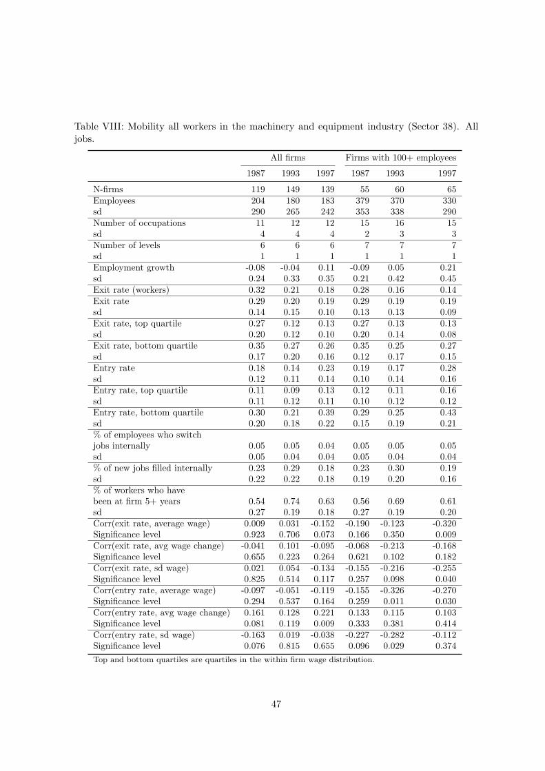
Table VIII: Mobility all workers in the machinery and equipment industry (Sector 38). Alljobs.

All firms Firms with 100+ employees

1987 1993 1997 1987 1993 1997

N-firms 119 149 139 55 60 65Employees 204 180 183 379 370 330sd 290 265 242 353 338 290Number of occupations 11 12 12 15 16 15sd 4 4 4 2 3 3Number of levels 6 6 6 7 7 7sd 1 1 1 1 1 1Employment growth -0.08 -0.04 0.11 -0.09 0.05 0.21sd 0.24 0.33 0.35 0.21 0.42 0.45Exit rate (workers) 0.32 0.21 0.18 0.28 0.16 0.14Exit rate 0.29 0.20 0.19 0.29 0.19 0.19sd 0.14 0.15 0.10 0.13 0.13 0.09Exit rate, top quartile 0.27 0.12 0.13 0.27 0.13 0.13sd 0.20 0.12 0.10 0.20 0.14 0.08Exit rate, bottom quartile 0.35 0.27 0.26 0.35 0.25 0.27sd 0.17 0.20 0.16 0.12 0.17 0.15Entry rate 0.18 0.14 0.23 0.19 0.17 0.28sd 0.12 0.11 0.14 0.10 0.14 0.16Entry rate, top quartile 0.11 0.09 0.13 0.12 0.11 0.16sd 0.11 0.12 0.11 0.10 0.12 0.12Entry rate, bottom quartile 0.30 0.21 0.39 0.29 0.25 0.43sd 0.20 0.18 0.22 0.15 0.19 0.21% of employees who switchjobs internally 0.05 0.05 0.04 0.05 0.05 0.05sd 0.05 0.04 0.04 0.05 0.04 0.04% of new jobs filled internally 0.23 0.29 0.18 0.23 0.30 0.19sd 0.22 0.22 0.18 0.19 0.20 0.16% of workers who havebeen at firm 5+ years 0.54 0.74 0.63 0.56 0.69 0.61sd 0.27 0.19 0.18 0.27 0.19 0.20Corr(exit rate, average wage) 0.009 0.031 -0.152 -0.190 -0.123 -0.320Significance level 0.923 0.706 0.073 0.166 0.350 0.009Corr(exit rate, avg wage change) -0.041 0.101 -0.095 -0.068 -0.213 -0.168Significance level 0.655 0.223 0.264 0.621 0.102 0.182Corr(exit rate, sd wage) 0.021 0.054 -0.134 -0.155 -0.216 -0.255Significance level 0.825 0.514 0.117 0.257 0.098 0.040Corr(entry rate, average wage) -0.097 -0.051 -0.119 -0.155 -0.326 -0.270Significance level 0.294 0.537 0.164 0.259 0.011 0.030Corr(entry rate, avg wage change) 0.161 0.128 0.221 0.133 0.115 0.103Significance level 0.081 0.119 0.009 0.333 0.381 0.414Corr(entry rate, sd wage) -0.163 0.019 -0.038 -0.227 -0.282 -0.112Significance level 0.076 0.815 0.655 0.096 0.029 0.374Top and bottom quartiles are quartiles in the within firm wage distribution.

47

Table IX: Decomposition of log monthly wage. White-collar workers in the private sector.

Year Total Between

1981 0.0857 0.01521982 0.0849 0.01451983 0.0850 0.01351984 0.0884 0.01501985 0.0921 0.01581986 0.0929 0.01651987 0.0869 0.01471988 0.0879 0.01401989 0.0809 0.01331990 0.0797 0.01411991 0.0857 0.01571992 0.0865 0.01691993 0.0877 0.01771994 0.0869 0.01731995 0.0874 0.01821996 0.0879 0.01961997 0.0903 0.0207

Table X: Decomposition of log monthly wage. All workers in the machinery and equipmentindustry (Sector 38).

All workers White collar Blue collar

Year Total Between Total Between Total Between

1987 0.0517 0.0089 0.0657 0.0049 0.0238 0.01151988 0.0541 0.0078 0.0689 0.0049 0.0179 0.00921989 0.0500 0.0084 0.0630 0.0040 0.0190 0.00991990 0.0451 0.0078 0.0625 0.0043 0.0166 0.00871991 0.0528 0.0094 0.0660 0.0043 0.0191 0.01111992 0.0525 0.0097 0.0664 0.0048 0.0195 0.01131993 0.0558 0.0120 0.0648 0.0062 0.0247 0.01601994 0.0549 0.0114 0.0654 0.0060 0.0187 0.01131995 0.0582 0.0124 0.0679 0.0063 0.0207 0.01151996 0.0582 0.0137 0.0668 0.0059 0.0225 0.01151997 0.0680 0.0158 0.0693 0.0065 0.0291 0.0114

48

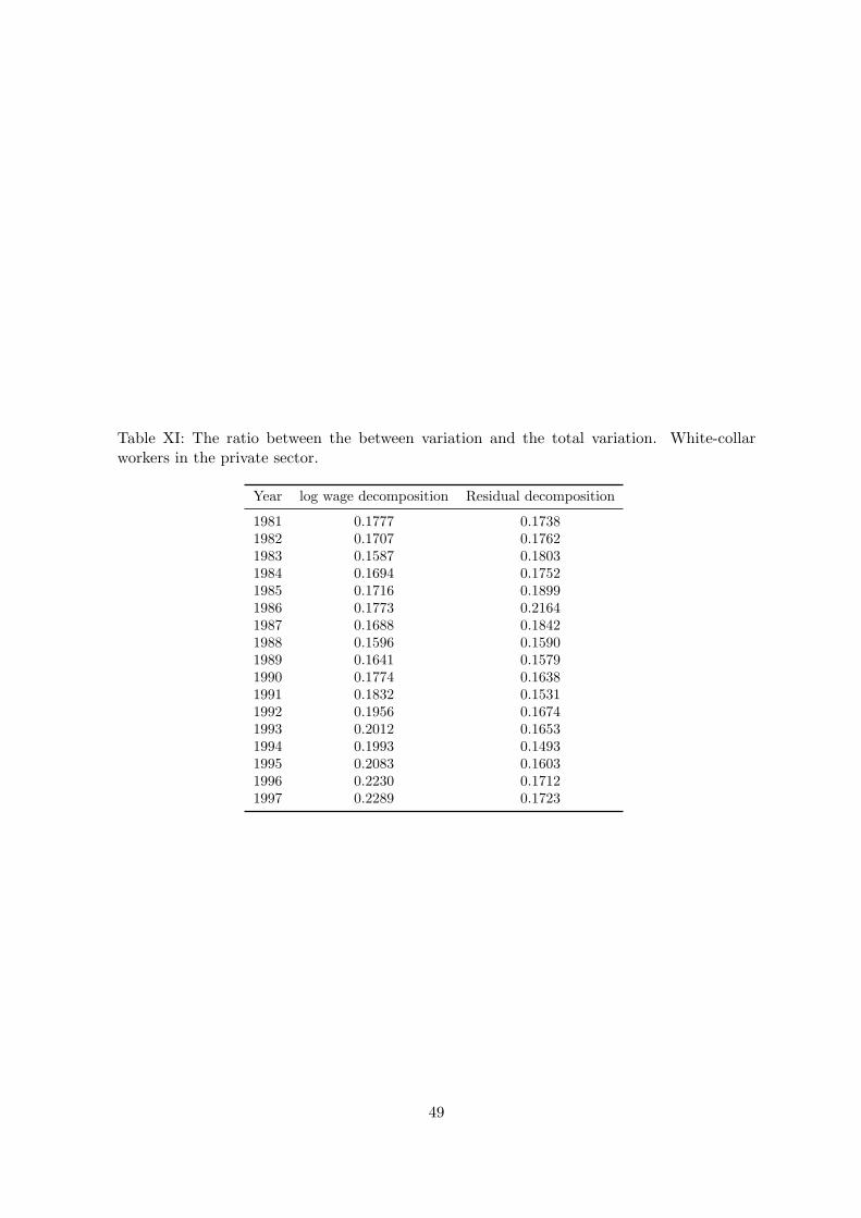
Table XI: The ratio between the between variation and the total variation. White-collarworkers in the private sector.

Year log wage decomposition Residual decomposition

1981 0.1777 0.17381982 0.1707 0.17621983 0.1587 0.18031984 0.1694 0.17521985 0.1716 0.18991986 0.1773 0.21641987 0.1688 0.18421988 0.1596 0.15901989 0.1641 0.15791990 0.1774 0.16381991 0.1832 0.15311992 0.1956 0.16741993 0.2012 0.16531994 0.1993 0.14931995 0.2083 0.16031996 0.2230 0.17121997 0.2289 0.1723

49

Table XII: Structure of wages within and between plants. White-collar workers in the privatesector.

Monthly wage log monthly wage

1981 1986 1993 1997 1981 1986 1993 1997

Average wage 18,606 19,972 20,378 22,242 9.787 9.854 9.876 9.964sd 5,901 6,580 6,576 7,130 0.293 0.303 0.297 0.29990%-ile 26,376 29,280 29,652 32,344 10.180 10.285 10.297 10.38410%-ile 12,415 13,258 13,632 14,874 9.427 9.492 9.520 9.607N-workers 48,226 65,825 65,839 68,900 48,226 65,825 65,839 68,900Average of firm average wage 17,770 18,658 19,068 20,776 9.743 9.790 9.812 9.898sd 2,404 2,553 2,723 3,027 0.132 0.134 0.135 0.14090%-ile 20,618 21,813 22,496 24,696 9.893 9.947 9.985 10.07710%-ile 14,654 15,344 15,881 17,264 9.566 9.608 9.649 9.731N-firms 535 613 614 688 535 613 614 688Average of sd of wage 4,807 5,182 5,222 5,629 0.252 0.256 0.252 0.250sd 1,303 1,452 1,774 1,727 0.047 0.053 0.055 0.05190%-ile 6,420 6,944 7,036 7,468 0.309 0.315 0.313 0.30610%-ile 3,150 3,410 3,406 3,657 0.193 0.196 0.192 0.189N-firms 535 613 614 688 535 613 614 688Average Coefficient ofvariation of wages 0.268 0.276 0.271 0.268 0.026 0.026 0.026 0.025sd 0.053 0.059 0.067 0.061 0.005 0.005 0.005 0.00590%-ile 0.334 0.346 0.343 0.333 0.032 0.032 0.032 0.03110%-ile 0.200 0.206 0.201 0.200 0.020 0.020 0.020 0.019N-firms 535 613 614 688 535 613 614 688Corr(average wage, sd wage) 0.718 0.701 0.693 0.692 0.261 0.198 0.369 0.337Significance level 0.000 0.000 0.000 0.000 0.000 0.000 0.000 0.000Average wage for workersbetween 25 and 30 15,720 17,185 16,457 17,821 9.643 9.729 9.689 9.770sd 3,180 3,784 3,269 3,460 0.199 0.214 0.197 0.19490%-ile 19,890 22,298 20,703 22,260 9.898 10.012 9.938 10.01110%-ile 11,927 12,784 12,647 13,606 9.387 9.456 9.445 9.518N-workers 6,232 10,752 9,660 8,050 6,232 10,752 9,660 8,050Average wage for workersbetween 45 and 50 20,385 21,725 21,902 23,818 9.879 9.938 9.943 10.027sd 6,409 7,235 7,496 7,947 0.288 0.304 0.313 0.31590%-ile 29,510 32,617 32,255 34,960 10.292 10.393 10.381 10.46210%-ile 13,945 14,614 14,372 15,539 9.543 9.590 9.573 9.651N-workers 6,161 7,939 12,419 12,009 6,161 7,939 12,419 12,009The numbers are real wages, transformed from nominal wages using the Consumer Price Index from

Statistics Norway with base year 1990.

50

Table XIII: Wage dynamics for white-collar workers in the private sector. Plants.

∆ monthly wage ∆ log monthly wage

1981 1986 1993 1997 1981 1986 1993 1997

Average change in wage -80 917 349 725 -0.003 0.046 0.017 0.032sd 1,243 1,271 1,489 1,495 0.064 0.060 0.054 0.06690%-ile 1,316 2,307 1,271 2,085 0.075 0.115 0.066 0.09410%-ile -1,237 -80 -306 -112 -0.065 -0.005 -0.017 -0.006N-workers 42,734 54,712 59,319 60,755 42,734 54,712 59,319 60,755Average of firm averagechange in wage -150 819 257 620 -0.007 0.045 0.013 0.029sd 645 483 378 486 0.037 0.026 0.019 0.02390%-ile 539 1,428 686 1,163 0.032 0.076 0.034 0.05510%-ile -849 268 -173 118 -0.047 0.016 -0.009 0.006N-firms 535 613 614 688 535 613 614 688Average of sd ofchange in wage 950 989 868 1,132 0.050 0.051 0.045 0.054sd 405 479 994 729 0.022 0.024 0.029 0.03390%-ile 1,380 1,498 1,456 1,870 0.073 0.074 0.076 0.08510%-ile 516 532 353 482 0.027 0.029 0.019 0.024N-firms 535 613 614 687 535 613 614 687Average change in wage forpeople who change firms 168 1,633 645 1,107 0.012 0.081 0.031 0.049sd 1,713 2,314 1,810 2,072 0.090 0.110 0.081 0.09390%-ile 2,149 4,317 2,345 3,303 0.123 0.211 0.112 0.14510%-ile -1,440 -343 -390 -106 -0.066 -0.016 -0.021 - 0.006N-workers 1,690 811 2,312 3,261 1,690 811 2,312 3,261Average change in wage forworkers with tenure < 3 257 1,251 577 1,023 0.017 0.068 0.030 0.049sd 1,364 1,417 1,269 1,691 0.075 0.072 0.062 0.08290%-ile 1,862 2,812 1,742 2,802 0.111 0.152 0.092 0.13410%-ile -1,091 -5 -277 -89 -0.060 0.000 -0.014 -0.005N-workers 3,769 12,133 9,363 9,494 3,769 12,133 9,363 9,494Average change in wage forworkers with tenure ≥ 3 -163 822 306 670 -0.008 0.040 0.015 0.029sd 1,156 1,210 1,522 1,449 0.058 0.055 0.052 0.06290%-ile 1,135 2,116 1,162 1,907 0.060 0.102 0.059 0.08410%-ile -1,242 -93 -310 -114 -0.067 -0.005 -0.018 -0.006N-workers 21,769 42,255 49,898 51,202 21,769 42,255 49,898 51,202Wage change is wage in year t minus wage in year t− 1.

The numbers are real wages, transformed from nominal wages using the Consumer Price Index from

Statistics Norway with base year 1990.

51

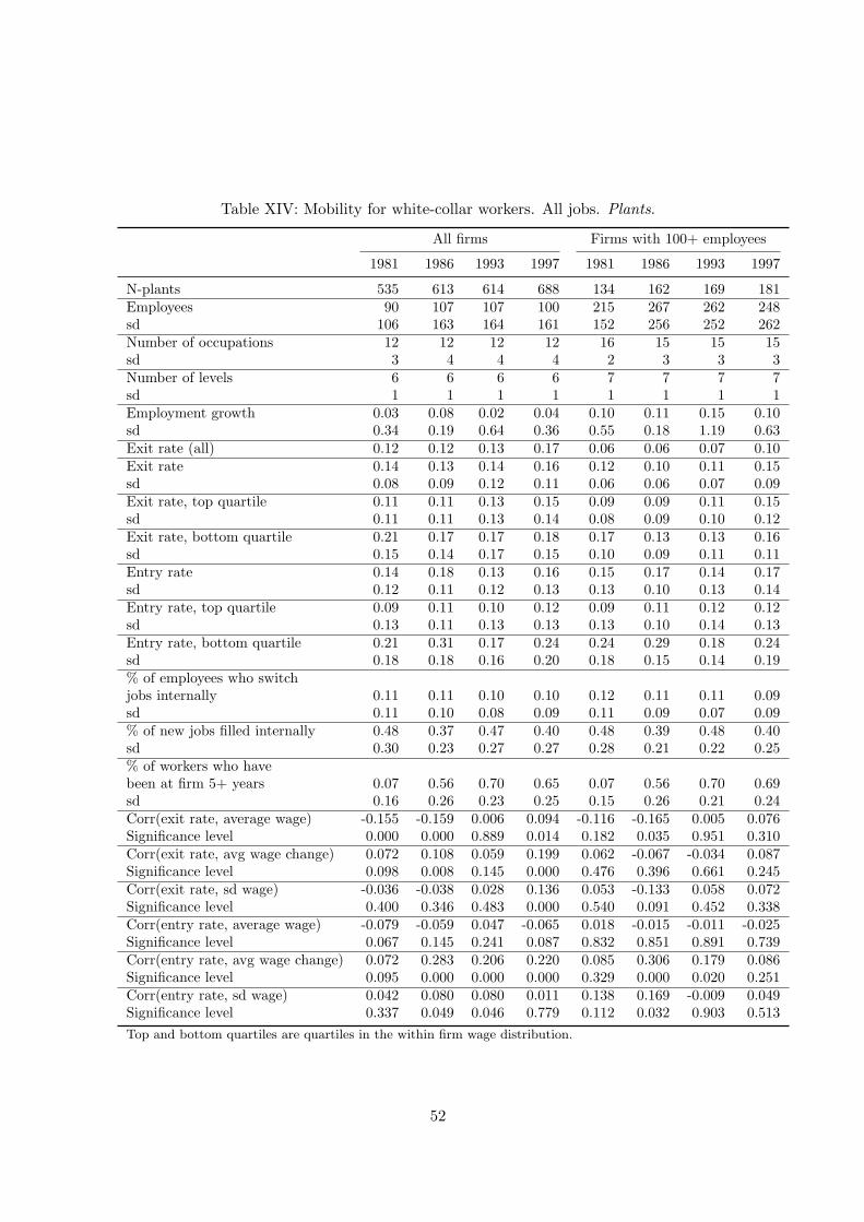
Table XIV: Mobility for white-collar workers. All jobs. Plants.

All firms Firms with 100+ employees

1981 1986 1993 1997 1981 1986 1993 1997

N-plants 535 613 614 688 134 162 169 181Employees 90 107 107 100 215 267 262 248sd 106 163 164 161 152 256 252 262Number of occupations 12 12 12 12 16 15 15 15sd 3 4 4 4 2 3 3 3Number of levels 6 6 6 6 7 7 7 7sd 1 1 1 1 1 1 1 1Employment growth 0.03 0.08 0.02 0.04 0.10 0.11 0.15 0.10sd 0.34 0.19 0.64 0.36 0.55 0.18 1.19 0.63Exit rate (all) 0.12 0.12 0.13 0.17 0.06 0.06 0.07 0.10Exit rate 0.14 0.13 0.14 0.16 0.12 0.10 0.11 0.15sd 0.08 0.09 0.12 0.11 0.06 0.06 0.07 0.09Exit rate, top quartile 0.11 0.11 0.13 0.15 0.09 0.09 0.11 0.15sd 0.11 0.11 0.13 0.14 0.08 0.09 0.10 0.12Exit rate, bottom quartile 0.21 0.17 0.17 0.18 0.17 0.13 0.13 0.16sd 0.15 0.14 0.17 0.15 0.10 0.09 0.11 0.11Entry rate 0.14 0.18 0.13 0.16 0.15 0.17 0.14 0.17sd 0.12 0.11 0.12 0.13 0.13 0.10 0.13 0.14Entry rate, top quartile 0.09 0.11 0.10 0.12 0.09 0.11 0.12 0.12sd 0.13 0.11 0.13 0.13 0.13 0.10 0.14 0.13Entry rate, bottom quartile 0.21 0.31 0.17 0.24 0.24 0.29 0.18 0.24sd 0.18 0.18 0.16 0.20 0.18 0.15 0.14 0.19% of employees who switchjobs internally 0.11 0.11 0.10 0.10 0.12 0.11 0.11 0.09sd 0.11 0.10 0.08 0.09 0.11 0.09 0.07 0.09% of new jobs filled internally 0.48 0.37 0.47 0.40 0.48 0.39 0.48 0.40sd 0.30 0.23 0.27 0.27 0.28 0.21 0.22 0.25% of workers who havebeen at firm 5+ years 0.07 0.56 0.70 0.65 0.07 0.56 0.70 0.69sd 0.16 0.26 0.23 0.25 0.15 0.26 0.21 0.24Corr(exit rate, average wage) -0.155 -0.159 0.006 0.094 -0.116 -0.165 0.005 0.076Significance level 0.000 0.000 0.889 0.014 0.182 0.035 0.951 0.310Corr(exit rate, avg wage change) 0.072 0.108 0.059 0.199 0.062 -0.067 -0.034 0.087Significance level 0.098 0.008 0.145 0.000 0.476 0.396 0.661 0.245Corr(exit rate, sd wage) -0.036 -0.038 0.028 0.136 0.053 -0.133 0.058 0.072Significance level 0.400 0.346 0.483 0.000 0.540 0.091 0.452 0.338Corr(entry rate, average wage) -0.079 -0.059 0.047 -0.065 0.018 -0.015 -0.011 -0.025Significance level 0.067 0.145 0.241 0.087 0.832 0.851 0.891 0.739Corr(entry rate, avg wage change) 0.072 0.283 0.206 0.220 0.085 0.306 0.179 0.086Significance level 0.095 0.000 0.000 0.000 0.329 0.000 0.020 0.251Corr(entry rate, sd wage) 0.042 0.080 0.080 0.011 0.138 0.169 -0.009 0.049Significance level 0.337 0.049 0.046 0.779 0.112 0.032 0.903 0.513Top and bottom quartiles are quartiles in the within firm wage distribution.

52