Wage Setting, Taxes, and Demand for Labor in Greece: A Multivariate Analysis of Cointegrating...

Wage Setting, Taxes, and Demand for Laborin Greece: A Multivariate Analysis ofCointegrating Relationships

Georgios P. Kouretas, Department of Economics,University of Crete

Leonidas P. Zarangas, Ministry of Labour, and Centre ofPlanning and Economic Research

This paper considers a nine-dimensional vector that is defined in accordance with amodel of wage setting and demand for labor specified in a bargaining framework. TheFIML multivariate cointegration technique is applied. Recent developments associatedwith this procedure are considered. First, a formal test developed by Paruolo (1996) for thepresence of I(2) components in a multivariate context is applied along with the estimation ofthe roots of the companion matrix (Juselius, 1995). Second, structural restrictions identi-fying the long-run relations of interest are specified as proposed by Johansen and Juselius(1994) and Johansen (1995b), because more than one cointegrating vector is found. Restric-tions that characterize wage-setting and labor-demand schedules are imposed and tested,first separately and then jointly. Finally, stability tests proposed by Hansen and Johansen(1993) are applied, and it is shown that the dimension of the cointegration space issample independent and the estimated coefficients do not exhibit instability in recursiveestimations. 2000 Society for Policy Modeling. Published by Elsevier Science Inc.

Key Words: Cointegration; I(2) Analysis; Companion matrix; Identification; Stability;Wage determination; Labor demand.

Address correspondence to Dr. Georgios P. Kouretas, 40 Argonafton Street, GR-15125,Maroussi, Greece. email: [email protected]

An earlier version of this paper was presented at the 1996 Annual Conference of theEuropean Association of Labour Economists, held in Chania, Greece, 19–22 September1996. Thanks are due to conference participants for many valuable comments. We also thankGeorge Alogoskoufis, Vassilis Droukopoulos, Dimitris Georgoutsos, Dimitris Moschos, Yan-nis Stournaras, and Timo Tyrvainen for many helpful comments and discussions. We alsothank an anonymous referee for his constructive comments. The usual disclaimer applies.

Received September 1996; final draft accepted February 1997.

Journal of Policy Modeling 22(2):171–195 (2000) 2000 Society for Policy Modeling 0161-8938/00/$–see front matterPublished by Elsevier Science Inc. PII S0161-8938(98)00034-9

172 G. P. Kouretas and L. P. Zarangas

1. INTRODUCTION

During the last decade econometrics of nonstationary variableshas undergone a great deal of development, having as a startingpoint the seminal paper of Engle and Granger (1987), which intro-duced the concept of cointegration and its relevance in investigat-ing the existence of long-run relationships that are suggested byeconomic theory. Within the subject of labor economics, the issuesof wage determination and labor demand are often candidatesfor testing such kinds of long-run relations, and the relevant litera-ture is therefore substantial.

In the present paper, wage setting and demand for labor inGreece are investigated, applying the Johansen FIML multivariatecointegration methodology. In addition, we apply several recentdevelopments that are associated with this approach. First, a for-mal test developed by Paruolo (1996) is used to test for the pres-ence of I(2) components in the multivariate framework. This testis coupled with the roots of the companion matrix as suggestedby Juselius (1995), and we are thus able to identify the order ofthe system and the dimension of the cointegration space in a moreprecise way. Second, we pay particular attention to issues related toidentification of the system by imposing linear and homogeneousrestrictions as suggested by Johansen and Juselius (1994) andJohansen (1995b). Finally, three tests of parameter stability inVAR models proposed by Hansen and Johansen (1993) are ap-plied to examine whether the rank of the cointegration space issample independent, and if the estimated coefficients are stablein recursive estimations. Therefore, we are interested in: (1) formalidentification, which is related to the statistical model; (2) empiricalidentification, which is related to the actual estimated parameters;and (3) economic identification, which is related to the economicinterpretability of the estimated coefficients of a formally andempirically identified model.

The rest of the paper is organized as follows. Section 2 intro-duces the economic model. Section 3 discusses the Johansen for-mulation in the presence of I(1) and I(2) components, the identifi-cation of the long-run structure and the stability analysis. InSection 4, an unrestricted VAR model derived from the theoreticalconsiderations is specified, and the estimation of the model ispresented. In Section 5 we report the structural identification ofthe long-run relationships as well as further empirical results.Section 6 provides our concluding remarks.

WAGE SETTING, TAXES, AND LABOR IN GREECE 173

2. THE ECONOMIC MODEL

There are n identical firms, which have a production functionQ 5 F(N,m,K,t) with three inputs: labor (N); raw materials (m);and capital (K), which is treated as predetermined. Technicalprogress (steady) is embodied in t. Imperfect competition is as-sumed to prevail in the product market. The first maximizes profits,which are defined as the difference between sales revenues andproduction costs (Eq. 1):

p 5 P[ZF(N,m,K)]F(N,m,K) 2 W(1 1 s)N 2 Pmm (1)

where Qd 5 p21 (P)Z21 ; D(P)Z is a downward sloping demandcurve of the separable form introduced by Nickell (1978). Here,Z 5 Z21 is a parameter describing the position of the demandcurve faced by the firm and P is the producer price of the firmthat is considered endogenous, P 5 competitors’ producer price,W 5 nominal consumer wage, s 5 payroll tax, Pm 5 price of rawmaterials (including energy). The output of the firm, Q, is treatedas endogenous. According to the marginal product condition, opti-mal use of an input is determined by the relative price. If the firmuses raw materials optimally, the demand for labor schedule hasthe following standard form (Eq. 2):

Nd 5 Nd1W(1 1 s)P

,Z,Pm

P,K,t2 (2)

In an organized labor market the firm bargains with a union.The welfare of the union depends on the after-tax real wageof its employed members and the (real) unemployment benefitreceived by the unemployed members, U 5 U(W(1 2 t)/Pc,N,B),where Pc is the consumer prices, t is the income taxes, and B isthe replacement ratio (unemployment benefit in real terms). Thepartial derivatives of this general preference function are:

U91,U92,U93 . 0 and U″1,U″2,U″3 , 0.

The union model that is used in this paper is a “right-to-manage”model that assumes that wages are bargained over and the profit-maximizing firm sets employment unilaterally. The game is speci-fied as a standard Nash solution of a cooperative game followingBinmore and colleagues (1986) (Eq. 3):

maxw

(U 2 U0)u(p 2 p0)12us.t.N(.) 5 argN

maxp (3)


where u refers to the bargaining power of unions, 0 , u , 1. U0

is the fall-back utility of the union in the event that an agreementis not reached. In Greece, the relevant alternative to an agreementis a strike. Thus, we assume that the U0 depends on strike allow-ances, U0 5 U0(A). p0 is the fall-back profit that reflects fixed costsduring a production stoppage. When p0 is deducted from the“undercontract” profits, fixed costs cancel out. For simplicity fixedcosts were already omitted from Equation 1.

The model for the equilibrium (real) wage consists of variablesinfluencing profits, on the one hand, and the utility of the union,on the other hand. In addition, a role is played by determinantsof the fall-back utilities of the parties. Finally, relative bargainingpower is important. The general form of the wage-setting scheduleis (Eq. 4):

W* 5 W(P,s,t,Pc

P,u,Pm,Z,B,A,K,t) (4)

Indirect tax, y exerts an influence as part of the price wedge, Pc /P.

3. ECONOMETRIC METHODOLOGY

A visual examination of the data reveals that the observationsare strongly time dependent, pointing to the need for modelsbased on adjustment to steady states. Given the definitions ofthe Zit series in Section 4 below, it would be hard to accept theassumption that any of them could be nonstochastic. Therefore,a probability formulation of the whole data is needed.

A formal framework was suggested by Hendry and Richard(1983), where the joint probability function for the data was givenin the form of sequential probabilities conditional on past valuesof the process. By allowing for a set of conditioning variables Dt 5[d1t, . . . , dqt] to control for institutional factors, and assumingmultivariate normality, the vector autoregressive model is ob-tained as a tentative statistical model for the data-generating pro-cess. In the error correction term it is given by (Eq. 5):

Dzt 5 G1Dzt21 1 . . . 1 Gk21Dzt2k11 1 Pzt2k 1 gDt 1 m 1 et (5)

where et | Niidp(0,S). The parameters (G1, . . . , Gk21,g) define theshort-run adjustment to the changes of the process, whereas P 5ab9 defines the short-run adjustment, a, to the cointegrating rela-tionships, b. If the short-run effects are basically different from thelong-run effects, due, for instance, to costly arbitrage or imperfectinformation, the explicit specification of the short-run effects is


probably crucial for a successful estimation of the steady-staterelations of interest.

Model (5) will be treated as the benchmark model, within whichall the subsequent hypotheses are tested. Because the parameterset u 5 (G, . . . , Gk21,P,g,m,S) varies unrestrictedly, it followsthat the I(1) and the I(2) models are submodels of (5). In theunrestricted form, therefore, model (5) corresponds to the I(0)model. Hence, in the statistical sense the I(0) model is the mostgeneral, because the higher order models are nested in this model.For simplicity we assume k 5 2 in all subsequent discussions ofmodel (5), i.e. (Eq. 6),

Dzt 5 G1Dzt21 1 ab9zt22 1 gDt 1 m 1 et (6)

3A. The I(1) Model

Johansen (1991) shows that if Zi | I(1), the following restrictionson model (6) have to be satisfied (Eq. 7):

P 5 ab9, (7)

where P has reduced rank, r, a, and b are (p 3 r) matrices, and(Eq. 8)

C 5 a⊥(2I 1 G1)b⊥ 5 wh9, (8)

where C is a (p-r) 3 (p-r) matrix of full rank, w and h are (p-r) 3(p-r) matrices, and a⊥ and b⊥ are p 3 (p-r) matrices orthogonalto a and b, respectively. The parameterization in (7) and (8)facilitates the investigation of, on the one hand, the r linearlyindependent stationary relations between the levels of the vari-ables and, on the other hand, the p 2 r linearly independentnonstationary relations. This duality between the stationary rela-tions and the nonstationary common trends is very useful for afull understanding of the generating mechanisms behind the cho-sen data. Although the autoregressive (AR) representation of themodel is useful for the analysis of the long-run relations in thedata, the moving average (MA) representation is useful for theanalysis of the common stochastic and deterministic trends thathave generated the data.

3B. The I(2) Model

If condition (8) for the I(1) model is violated, the process Zt isintegrated of second order or higher. When the process is I(2), itis useful to rewrite model (6) in second differences (Eq. 9):

D2zt21 5 GDt21 1 ab9zt22 1 gDt 1 m 1 et (9)


where G 5 2 I 1 G1 and ab9 has reduced rank r. If Zt | I(2), thefollowing restriction on the parameters of model (9) has to besatisfied (Eq. 10):

C 5 a9⊥Gb⊥ 5 wh, (10)

where w and h are (p-r) 3 s1 matrices and s1 , (p 2 r).Johansen (1997) shows that the space spanned by the vector Zt

can be decomposed into r stationary directions, b, and p 2 rnonstationary directions, b⊥, and the latter into the directions(b1

⊥,b2⊥), where b1

⊥ 5 b⊥h is of dimension p 3 s1 and b2⊥ 5

b⊥(b9⊥b⊥)21h⊥ is of dimesnion p 3 s2 and s1 1 s2 5 p-r. Theproperties of the process are described by

I(2):hb2⊥j,

I(1):hb9ztj,hb19⊥j,

I(0):hb19⊥Dztj,hb29⊥D2ztj,hb9zt 1 v9Dztj

where v is a p 3 r matrix of weights, designed to pick out theI(2) components of Zt (Johansen, 1995a).

Johansen (1991) shows how the model can be written in movingaverage form, while Johansen (1997) derives the FIML solution tothe estimation problem for the I(2) model. Furthermore, Johansen(1995a) provides an asymptotically equivalent two-step procedurethat is computationally simpler. It applies the standard eigenvalueprocedure derived for the I(1) model twice: first to estimate thereduced rank of the P matrix, and then, for given estimates of aand b, to estimate the reduced rank of a9⊥Gb⊥ (Juselius 1994, 1995,1996, provides a complete statistical analysis).

3C. The Identification Problem

In a multivariate framework like the one provided by the wagemodel under consideration, a vector error correction model maycontain multiple cointegrating vectors. In such a case the individualcointegrating vectors are underidentified in the absence of suffi-cient linear restrictions on each vector. Recently, Johansen andJuselius (1994) and Johansen (1995b) have addressed the issue ofidentification in cointegrated systems.

The necessary and sufficient conditions for identification in acointegrated system in terms of linear restrictions on the columnsof the accepted eigenvectors, b, are analogous to the classicalidentification problem. Thus, the order condition for identification


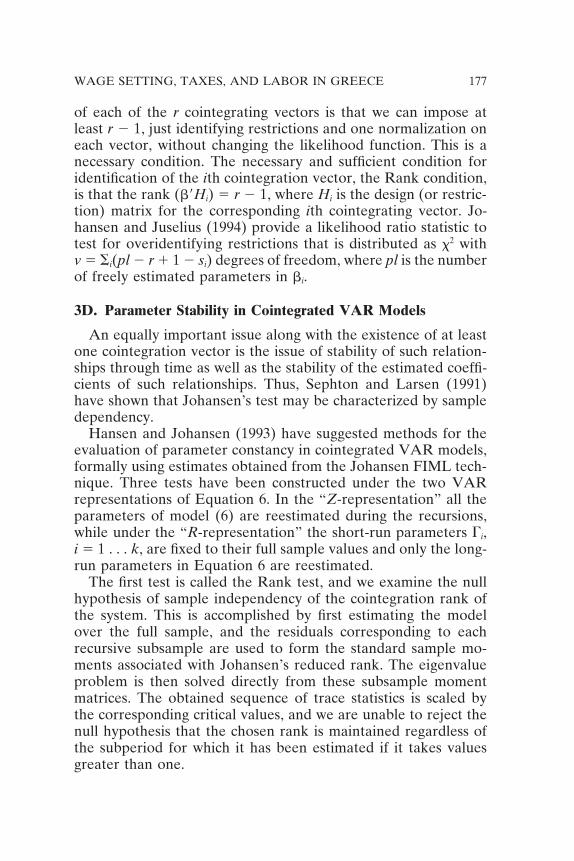
of each of the r cointegrating vectors is that we can impose atleast r 2 1, just identifying restrictions and one normalization oneach vector, without changing the likelihood function. This is anecessary condition. The necessary and sufficient condition foridentification of the ith cointegration vector, the Rank condition,is that the rank (b9Hi) 5 r 2 1, where Hi is the design (or restric-tion) matrix for the corresponding ith cointegrating vector. Jo-hansen and Juselius (1994) provide a likelihood ratio statistic totest for overidentifying restrictions that is distributed as x2 withv 5 Si(pl 2 r 1 1 2 si) degrees of freedom, where pl is the numberof freely estimated parameters in bi.

3D. Parameter Stability in Cointegrated VAR Models

An equally important issue along with the existence of at leastone cointegration vector is the issue of stability of such relation-ships through time as well as the stability of the estimated coeffi-cients of such relationships. Thus, Sephton and Larsen (1991)have shown that Johansen’s test may be characterized by sampledependency.

Hansen and Johansen (1993) have suggested methods for theevaluation of parameter constancy in cointegrated VAR models,formally using estimates obtained from the Johansen FIML tech-nique. Three tests have been constructed under the two VARrepresentations of Equation 6. In the “Z-representation” all theparameters of model (6) are reestimated during the recursions,while under the “R-representation” the short-run parameters Gi,i 5 1 . . . k, are fixed to their full sample values and only the long-run parameters in Equation 6 are reestimated.

The first test is called the Rank test, and we examine the nullhypothesis of sample independency of the cointegration rank ofthe system. This is accomplished by first estimating the modelover the full sample, and the residuals corresponding to eachrecursive subsample are used to form the standard sample mo-ments associated with Johansen’s reduced rank. The eigenvalueproblem is then solved directly from these subsample momentmatrices. The obtained sequence of trace statistics is scaled bythe corresponding critical values, and we are unable to reject thenull hypothesis that the chosen rank is maintained regardless ofthe subperiod for which it has been estimated if it takes valuesgreater than one.


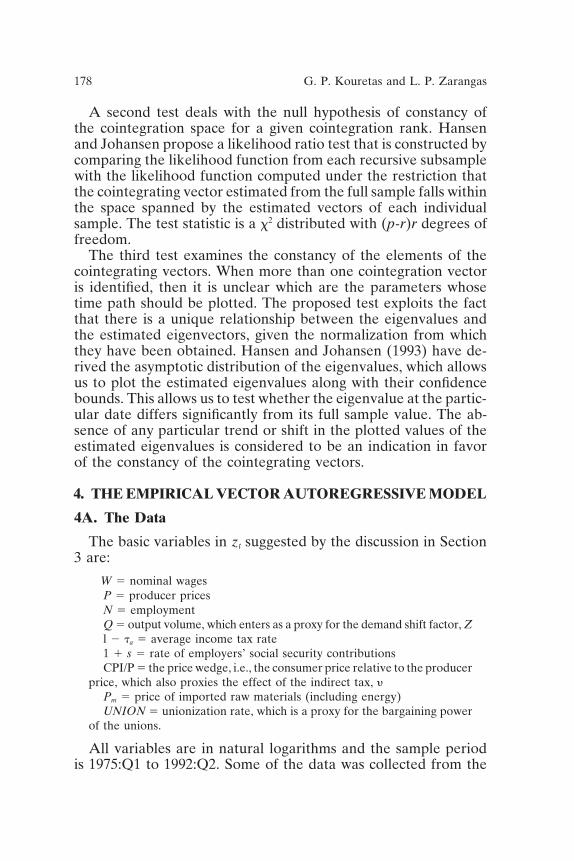
A second test deals with the null hypothesis of constancy ofthe cointegration space for a given cointegration rank. Hansenand Johansen propose a likelihood ratio test that is constructed bycomparing the likelihood function from each recursive subsamplewith the likelihood function computed under the restriction thatthe cointegrating vector estimated from the full sample falls withinthe space spanned by the estimated vectors of each individualsample. The test statistic is a x2 distributed with (p-r)r degrees offreedom.

The third test examines the constancy of the elements of thecointegrating vectors. When more than one cointegration vectoris identified, then it is unclear which are the parameters whosetime path should be plotted. The proposed test exploits the factthat there is a unique relationship between the eigenvalues andthe estimated eigenvectors, given the normalization from whichthey have been obtained. Hansen and Johansen (1993) have de-rived the asymptotic distribution of the eigenvalues, which allowsus to plot the estimated eigenvalues along with their confidencebounds. This allows us to test whether the eigenvalue at the partic-ular date differs significantly from its full sample value. The ab-sence of any particular trend or shift in the plotted values of theestimated eigenvalues is considered to be an indication in favorof the constancy of the cointegrating vectors.

4. THE EMPIRICAL VECTOR AUTOREGRESSIVE MODEL

4A. The Data

The basic variables in zt suggested by the discussion in Section3 are:

W 5 nominal wagesP 5 producer pricesN 5 employmentQ 5 output volume, which enters as a proxy for the demand shift factor, Zl 2 ta 5 average income tax rate1 1 s 5 rate of employers’ social security contributionsCPI/P 5 the price wedge, i.e., the consumer price relative to the producer

price, which also proxies the effect of the indirect tax, yPm 5 price of imported raw materials (including energy)UNION 5 unionization rate, which is a proxy for the bargaining power

of the unions.

All variables are in natural logarithms and the sample periodis 1975:Q1 to 1992:Q2. Some of the data was collected from the


Monthly Bulletin of the Bank of Greece and some from the Minis-try of Labour data bank. Furthermore, it has been shown thatthere is a major difference between the behavior of the wageand employment series for the public sector and the rest of theeconomy. We, therefore, exclude the public sector and focus onthe analysis of the private sector. Moreover, because our maininterest is the study of real wage resistance, i.e., the impact oftaxes on wage setting and demand for labor, we omit variablesof great interest such as the capital stock and the related user costas well as unemployment benefits and strike allowances (Tyr-vainen, 1992, 1995; Lockwood and Manning, 1993). This is neces-sary to make our system manageable. Finally, we use a vector ofdummies Dt that includes three centered seasonal dummies thataccount for the short-run effects that will otherwise violate theGaussian assumption about the residuals, and we use two interven-tion dummies as well. The first one captures the change in politicalregime, and takes the value zero for the period 1974–81, whenthe conservative party was in power, and 1 for the period 1981to 1989 when the socialist party was in power. The second policydummy variable reflects the effects of political cycles and takesthe value of 1 during election years and zero otherwise.

4B. Testing the General Specification of the Model

All empirical models are inherently approximations of the ac-tual data generating process, and the question is whether thebenchmark model (6) is a satisfactorily close approximation. Twodifferent aspects of the model will be investigated: (1) the stochas-tic specification regarding residual correlation, heteroscedasticity,and normality; and (2) the relevance of the conditioning variablesin Dt. These two aspects of the model are clearly related in thesense that residual misspecification often arises as a consequenceof omitting important variables in Dt.

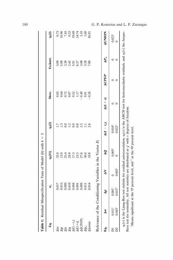
According to the residual tests reported in Table 1, the bench-mark model for k 5 3 and zt and Dt as specified above, seems toprovide a reasonably good approximation of the data-generatingprocess. The estimated residual standard deviations are generallyvery small, indicating that most of the variation of the vectorprocess can be accounted for by the chosen information set.

The estimates of the short-run effects of the conditioning vari-ables are also presented in Table 1. To facilitate readability, coef-ficients with a t-value less than 1.0 have been set to zero. As


Tab

le1:

Res

idua

lM

issp

ecif

icat

ion

Tes

tsof

Mod

el(6

)w

ithk

53

Eq.

se

h1(

21)

h2(

2)Sk

ew.

Ex.

kurt

.h

3(2)

Dlw

0.01

735

.01.

70.

053.

090.

73D

lp0.

013

13.9

1.3

0.64

5.08

10.9

6D

ln0.

009

25.4

0.9

0.72

3.30

7.43

Dlq

0.01

929

.91.

20.

072.

420.

53D

l(12

t a)

0.00

417

.30.

00.

525.

9119

.69

Dl(

11s)

0.00

123

.50.

81.

176.

5714

.74

Dl(

CP

I/P

)0.

009

27.6

2.5

20.

493.

083.

10D

lpm

0.01

130

.01.

10.

013.

281.

60D

luni

on0.

014

19.8

2.6

20.

267.

8045

.01

Rel

evan

ceof

the

Con

diti

onin

gV

aria

bles

inth

eV

ecto

rD

t

Eq.

Dw

Dp

DN

DQ

D(1

2t a

)D

(11

s)D

CP

I/P

DP

mD

UN

ION

D1

0.01

110.

0011

00.

0051

0.01

820

00

0.02

31

D2

0.04

310.

0152

0.00

310

0.02

220

00

0

h1(

v)is

the

Lju

ng-B

oxte

stst

atis

tic

for

resi

dual

auto

corr

elat

ion,

h2(

v)is

the

AR

CH

test

for

hete

rosc

edas

tic

resi

dual

s,an

dh

3(v)

the

Jarq

ue-

Ber

ate

stfo

rno

rmal

ity.

All

test

stat

isti

csar

edi

stri

bute

das

x2

wit

hv

degr

ees

offr

eedo

m.

1M

eans

sign

ific

ant

atth

e95

perc

ent

leve

l,an

d2

atth

e99

perc

ent

leve

l.


Table 2: Testing the Rank in the l(2) and the l(1) Model

Testing the joint hypothesis H(s1>r)p-r r Q(s1>r)H0

9 0 625.9 497.4 435.6 389.4 355.5 324.6 298.3 276.8 246.9502.9 454.8 411.2 372.1 332.9 299.5 269.8 243.9 221.9

8 1 456.9 404.3 365.6 304.5 287.8 249.1 234.2 199.2405.1 363.4 324.1 287.4 256.1 227.4 203.3 183.2

7 2 344.3 303.4 267.9 240.9 201.3 188.2 175.6317.5 280.2 245.5 215.5 188.4 166.1 147.5

6 3 277.2 235.8 195.0 166.8 143.2 125.9240.3 206.8 179.0 154.1 132.8 115.4

5 4 226.6 189.7 155.4 122.7 114.3171.9 145.6 122.0 102.7 86.9

4 5 154.3 124.5 99.5 84.3116.3 94.7 76.8 63.1

3 6 100.6 87.5 67.870.8 54.5 42.9

2 7 68.5 29.236.1 26.0

1 8 19.212.9

s2 9 8 7 6 5 4 3 2 1

The numbers in italics are the critical values (Paruolo, 1996; Table 5).

expected, both intervention dummies that refer to change in politi-cal regimes and to political cycles have their significant effectmainly on the wage rate, the price level, and the tax rate, and alesser effect on employment and output.

4C. Determining the Cointegration Rank and the Orderof Integration

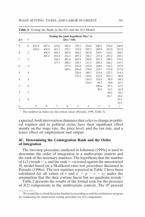
The two-step procedure analyzed in Johansen (1995a) is used todetermine the order of integration in a multivariate context andthe rank of the necessary matrices. The hypothesis that the numberof L(1) trends 5 s1 and the rank 5 r is tested against the unrestrictedH0 model based on a likelihood ratio test procedure discussed inParuolo (1996a). The test statistics reported in Table 2 have beencalculated for all values of r and s91 5 p 2 r 2 s2, under theassumption that the data contain linear but no quadratic trends.1

Table 2 presents the results of the formal tests for the presenceof I(2) components in the multivariate context. The 95 percent

1 We would like to thank Katarina Juselius for providing us with her preliminary programfor conducting the multivariate testing procedure for I(2) components.


quantiles of the asymptotic test distributions are taken from Table 5Paruolo (1996), and reproduced underneath the calculated test val-ues. Starting from the most restricted hypothesis {r 5 0, s1 5 0, ands2 5 9} and testing successively less and less restricted hypothesesaccording to the Pantula (1989) principle shows that essentially allI(2) hypotheses can be rejected on the 5 percent level.

In addition to the formal tests, Juselius (1995) offers furtherinsight into the I(2) and I(1) analysis and the determination ofthe correct cointegration rank. She argues that the results of thetrace and maximum eigenvalue test statistics of the I(1) analysisshould be interpreted with some caution: First, the conditioningon intervention dummies and weakly exogenous variables is likelyto change the asymptotic distributions to some (unknown) extent.Second, the asymptotic critical values may not be very close ap-proximations in small samples. Juselius (1995) suggests the use ofthe companion matrix as an additional tool for determining thecorrect cointegration rank.

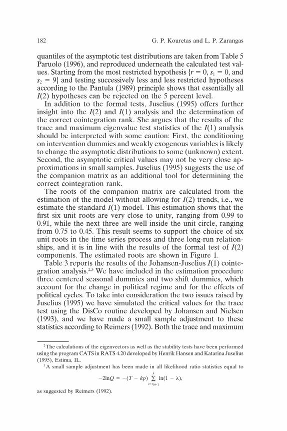
The roots of the companion matrix are calculated from theestimation of the model without allowing for I(2) trends, i.e., weestimate the standard I(1) model. This estimation shows that thefirst six unit roots are very close to unity, ranging from 0.99 to0.91, while the next three are well inside the unit circle, rangingfrom 0.75 to 0.45. This result seems to support the choice of sixunit roots in the time series process and three long-run relation-ships, and it is in line with the results of the formal test of I(2)components. The estimated roots are shown in Figure 1.

Table 3 reports the results of the Johansen-Juselius I(1) cointe-gration analysis.2,3 We have included in the estimation procedurethree centered seasonal dummies and two shift dummies, whichaccount for the change in political regime and for the effects ofpolitical cycles. To take into consideration the two issues raised byJuselius (1995) we have simulated the critical values for the tracetest using the DisCo routine developed by Johansen and Nielsen(1993), and we have made a small sample adjustment to thesestatistics according to Reimers (1992). Both the trace and maximum

2 The calculations of the eigenvectors as well as the stability tests have been performedusing the program CATS in RATS 4.20 developed by Henrik Hansen and Katarina Juselius(1995), Estima, IL.

3 A small sample adjustment has been made in all likelihood ratio statistics equal to

22lnQ 5 2(T 2 kp) ok

i5r011

ln(1 2 l),

as suggested by Reimers (1992).


Figure 1. The eigenvalues of the companion matrix.

eigenvalue statistics reject the existence of zero cointegrating vectorsor nine common trends. The two statistics suggest that we can acceptthree significant cointegrating vectors. These results reconfirm thedecision made based on the roots of the companion matrix.

Table 3 also reports the results of several significant tests. Ac-cording to the first test, none of the variables of the system isnonrelevant and, hence, could be excluded from the cointegratingvector (the exclusion test). The second test shows that all seriesare in a nonstationary conditional upon three cointegration vectors(the multivariate stationarity test). Finally, weak exogeneity istested with the last test, and it is rejected for all variables ofour system. In addition, Table 3 reports the multivariate residualstatistics, because the Gaussian assumption is violated in the pres-ence of nonnormality, serial correlation, and conditional hetero-skedasticity in the residuals of the VAR. No evidence of seriousmisspecification was detected.4

4 Gonzalo (1994) shows that the performance of the maximum likelihood estimator ofthe cointegrating vectors is little affected by nonnormal errors. Lee and Tse (1996) haveshown similar results when conditional heteroskedasticity is present.


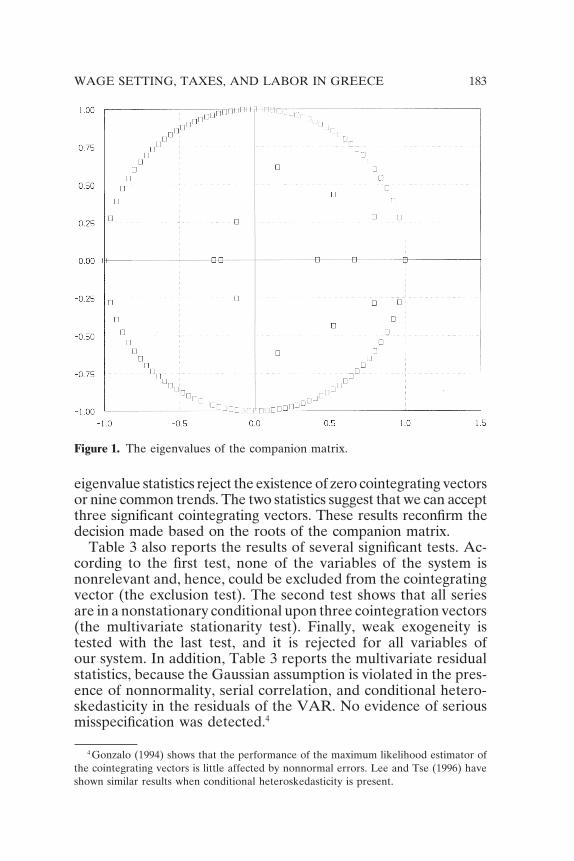
Table 3: Johansen-Juselius cointegration tests

95 Percent critical valuesr Trace lmax Trace lmax

r 5 0 312.411 78.031 223.35 66.89r < 1 234.391 64.341 168.98 60.34r < 2 170.051 50.141 135.78 49.12r < 3 99.87 38.59 100.60 42.33r < 4 81.31 29.75 84.98 37.45r < 5 51.57 22.26 60.09 33.88r < 6 29.31 18.01 33.43 31.56r < 7 11.30 9.75 14.67 12.56r < 8 1.55 1.55 3.45 3.45

Exclusion Stationary WeakVariable restrictions test exogeneity

lw 9.811 26.401 9.731

lp 25.211 25.961 10.081

ln 8.441 29.081 9.721

lq 21.931 20.981 8.221

l(1 2 ta) 9.651 28.221 9.051

l(1 1 s) 8.201 32.901 10.021

l(CPI/P) 10.341 30.551 8.931

lpm 32.011 25.531 14.381

lunion 17.011 26.081 14.901

Multivariate residual statistics

LB(17) 5 1461.63(0.06) x2(18) 5 68.98(0.02)

Notes: r denotes the number of eigenvectors. Trace and lmax denote, respectively,the trace and maximum eigenvalue likelihood ratio statistics. The 95-percent critical valueshave been simulated using the Johansen-Nielsen (1993) DisCo program for a model withtwo intervention dummies. In performing the Johansen-Juselius tests, a structure of threelags was chosen according to a likelihood ratio test, corrected for the degrees of freedomand the Ljung-Box Q statistic for detecting serial correlation in the residuals of theequations of the VAR. A model with an unrestricted constant in the VAR equation isestimated according to the Johansen (1992) testing methodology.

1 Indicates statistical significance at the 5 percent critical level.

Notes: For the test of exclusion restrictions figures are x2 statistics with three degreesof freedom, for the stationarity test figures are x2 with five degrees of freedom, and forthe weak exogeneity test figures are x2 with three degrees of freedom.

Notes: LB 5 Ljung-Box statistic for serial correlation with 17 degrees of freedom. x2

is the Bera-Jarque test for normality distributed with 18 degrees of freedom.


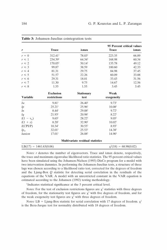
Figure 2. The Trace tests.

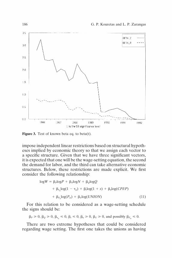
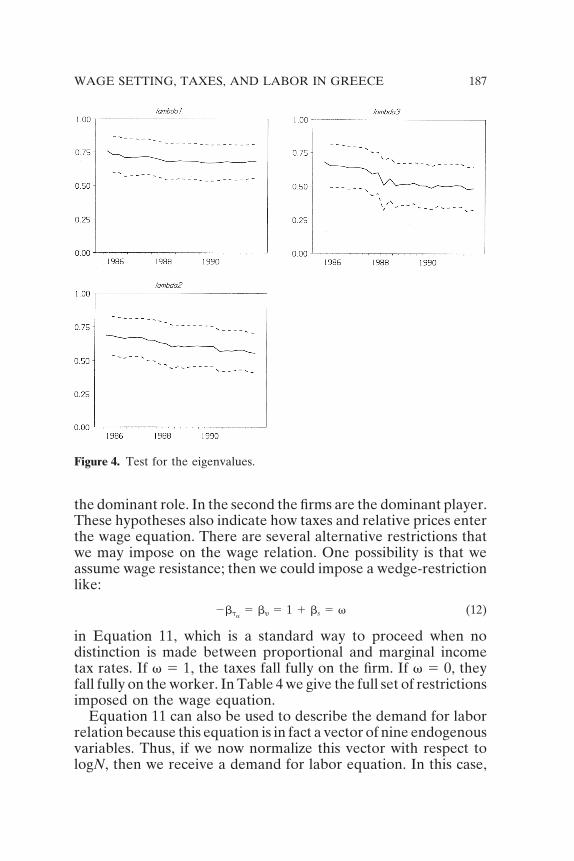
Figures 2–4 report the results of applying the recursive tests forparameter stability of Johansen’s results. Figure 2 shows that therank of the cointegration space does not depend on the samplesize from which it has been estimated, because we are unable toreject the null hypothesis of a constant rank—in our case threeaccepted eigenvectors. Furthermore, Figure 3 shows that we al-ways accept the null hypothesis of the constancy of the cointegra-tion space for a given cointegration rank. Finally, Figure 4 showsthat the estimated coefficients do not exhibit instability in recursiveestimation, because each corresponding eigenvalue has no signifi-cant trend or shift during the period under investigation.

4D. Structural Identification

The model in Section 2 was designed for analysis of wage settingand the demand for labor. As we explained in Section 3, whenmore than one significant vector has been found, then we must


Figure 3. Test of known beta eq. to beta(t).

impose independent linear restrictions based on structural hypoth-eses implied by economic theory so that we assign each vector toa specific structure. Given that we have three significant vectors,it is expected that one will be the wage-setting equation, the secondthe demand for labor, and the third can take alternative economicstructures. Below, these restrictions are made explicit. We firstconsider the following relationship:

logW 5 bPlogP 1 bNlogN 1 bQlogQ

1 btalog(1 2 ta) 1 bslog(1 1 s) 1 bylog(CPI/P)

1 bPmlog(Pm) 1 bUlog(UNION) (11)

For this relation to be considered as a wage-setting schedulethe signs should be:

bP > 0, bQ > 0, bta< 0, bs < 0, by > 0, bU > 0, and possibly bPm

< 0.

There are two extreme hypotheses that could be consideredregarding wage setting. The first one takes the unions as having


Figure 4. Test for the eigenvalues.

the dominant role. In the second the firms are the dominant player.These hypotheses also indicate how taxes and relative prices enterthe wage equation. There are several alternative restrictions thatwe may impose on the wage relation. One possibility is that weassume wage resistance; then we could impose a wedge-restrictionlike:

2bta5 by 5 1 1 bs 5 v (12)

in Equation 11, which is a standard way to proceed when nodistinction is made between proportional and marginal incometax rates. If v 5 1, the taxes fall fully on the firm. If v 5 0, theyfall fully on the worker. In Table 4 we give the full set of restrictionsimposed on the wage equation.

Equation 11 can also be used to describe the demand for laborrelation because this equation is in fact a vector of nine endogenousvariables. Thus, if we now normalize this vector with respect tologN, then we receive a demand for labor equation. In this case,


Tab

le4:

FIM

LE

stim

ated

Coe

ffic

ient

san

dId

enti

fica

tion

Wag

ese

ttin

gL

abor

dem

and

Out

put

Coe

ff.

Var

iabl

esb

ia

ib

ia

ib

ia

i

bw

W1.

000

0.00

32

0.16

32

0.10

01.

260

20.

008

bP

P2

1.61

60.

022

0.52

32

0.01

42

1.91

22

0.00

2b

NN

1.04

50.

015

1.00

02

0.01

22

0.41

40.

018

bQ

Q2

1.95

50.

041

21.

142

0.12

51.

000

0.00

9b

ta1

2t a

2.28

32

0.00

72

0.03

22

0.00

42

2.85

40.

005

bs

11

s2.

840

20.

001

25.

401

0.00

91.

640

0.00

1b

yC

PI/

P2

2.70

42

0.01

12

0.33

80.

045

2.30

02

0.00

9b

Pm

Pm

2.00

72

0.03

62

0.50

60.

033

1.15

32

0.00

1b

UU

NIO

N2

0.11

62

0.06

40.

063

21.

267

0.01

12

0.25

9

Hyp

othe

sis

test

ing

Wag

ese

ttin

gL

abor

dem

and

Out

put

(1)

(2)

(3)

(4)

(5)

bw

52

bP

5b

w5

2b

Pb

w5

2b

Pb

w5

2b

P5

bw

52

bP

5

2b

Pm

5b

t a,

2b

Pm

5b

N5

2b

Pm

5b

s,b

s,b

t a5

2b

y,b

N5

2b

Q,

2b

Q5

2b

t a,

bt a

5b

y e5

bt a

5b

y5

bN

52

bQ,

bt a

51

2b

s5

bt a

51

2b

s5

bU

50

bP

m5

bU

50

bs

5b

Pm

5

2b

y2

by

bU

50

x2

51.

03x

25

5.03

x2

57.

33x

25

3.99

x2

55.

78Q

(16)

511

.59

Q(1

6)5

10.4

5

(Con

tinue

d)


Tab

le4:

Con

tinue

d

Est

imat

esof

the

impa

ctof

cum

ulat

edin

nova

tion

sin

vari

able

j,on

vari

able

k

k/j

wP

NQ

12

t a1

1s

CP

I/P

Pm

UN

ION

w2

0.08

22

0.61

00.

171

0.12

92

0.95

84.

049

0.30

02

0.2

0.01

8P

0.02

10.

477

0.17

60.

142

0.03

50.

604

0.20

20.

40.

008

N2

0.00

90.

230

0.43

12

0.13

50.

405

20.

379

0.80

32

0.1

0.00

1Q

20.

011

20.

041

20.

006

0.17

70.

236

0.70

70.

176

0.04

0.00

91

2t a

0.01

22

0.10

00.

073

0.07

92

0.17

12

0.35

20.

002

0.1

0.00

21

1s

0.01

10.

006

0.01

42

0.00

50.

017

0.11

30.

038

20.

00.

000

CP

I/P

0.03

52

0.11

10.

381

0.16

22

0.25

42

1.33

50.

331

0.2

0.00

6P

m2

0.01

50.

592

0.08

90.

289

0.15

22

1.10

12

0.07

30.

70.

009

UN

ION

0.58

42

5.29

12

3.97

57.

262

23.

659

17.7

102

5.97

24.

20.

243

Not

es:

All

test

sar

ex

2di

stri

bute

dw

ith

5,6,

6,an

d8

degr

ees

offr

eedo

mre

spec

tive

ly.

Q(.

)is

the

Joha

nsen

and

Juse

lius

(199

4)te

stfo

rov

erid

enti

fyin

gre

stri

ctio

nsan

dis

ax

2di

stri

bute

dw

ith

16de

gree

sof

free

dom

.

Not

es:

The

t-va

lues

for

the

impa

ct-m

atri

xfo

rth

eM

Are

pres

enta

tion

can

befo

und

inP

aruo

lo(1

997)

.


the expected signs of the coefficients should be bw < 0, bP > 0,bQ > 0, bta 5 0, bs < 0, by 5 0, and possibly bPm < 0. The impactsof both the income tax and the indirect tax derive from their wageeffect. If the union has a direct influence on employment (for agiven wage), then by ? 0. The restriction bw 5 2bP 5 2bQ 5 bs . 0implies that it is the real labor cost for a produced unit that isimportant. Again, if it is the relative raw material price that isimportant, we write bw 5 2 bP 2 bPm 2 bQ 5 bs.

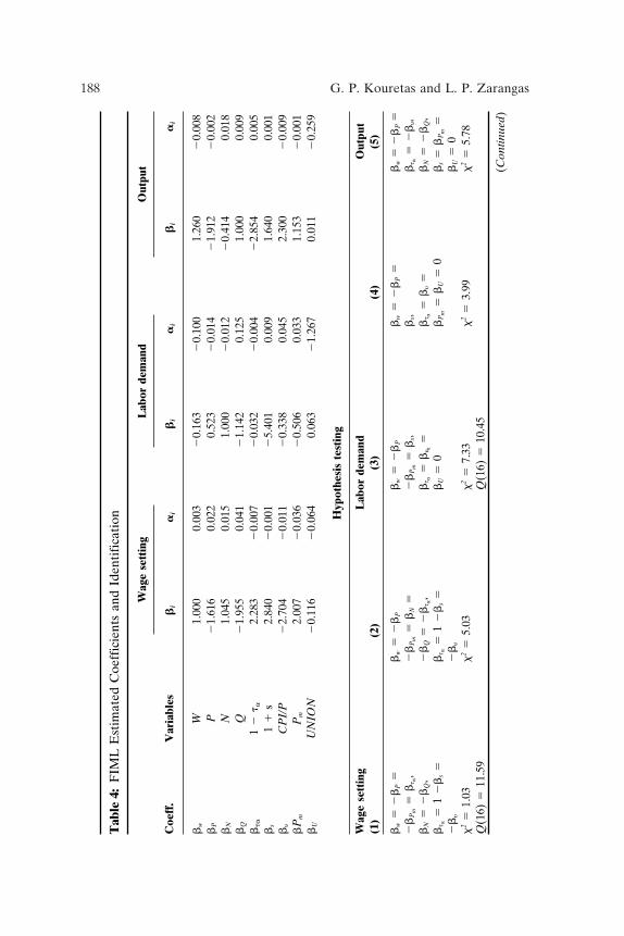
We concluded above that there are probably three cointegratingvectors in our data space. Two of them are well specified, i.e., awage-setting schedule and demand-for-labor condition. The thirdeigenvector could describe either the demand side or the supplyside of the variables concerned. Thus, we expect the following tobe possible candidates: (1) the supply of output, (2) the demandfor output, (3) the constant mark-up pricing rule, and (4) pricesetting conducted by the product-market demand conditions. How-ever, the resulting “semirelations” may also be mixtures of twoor more competing but misspecified relations. Hence, one shouldnot put too much emphasis on the interpretation of the remainingvectors. Table 4 introduces the three nonrestricted eigenvectors.

The strategy applied below is as follows. First, we do partialidentification for each of the three vectors based on the wage setting,demand for labor and the other “semirelations.” This sort ofidentification is done through the imposition of linear and homoge-neous restrictions on each vector (Johansen and Juselius, 1990,1992). Second, following Johansen and Juselius (1994) and Jo-hansen (1995a) and the discussion in Section 3C, we provide formalidentification of the joint hypotheses of the complete model.

5. TESTING STRUCTURAL HYPOTHESES

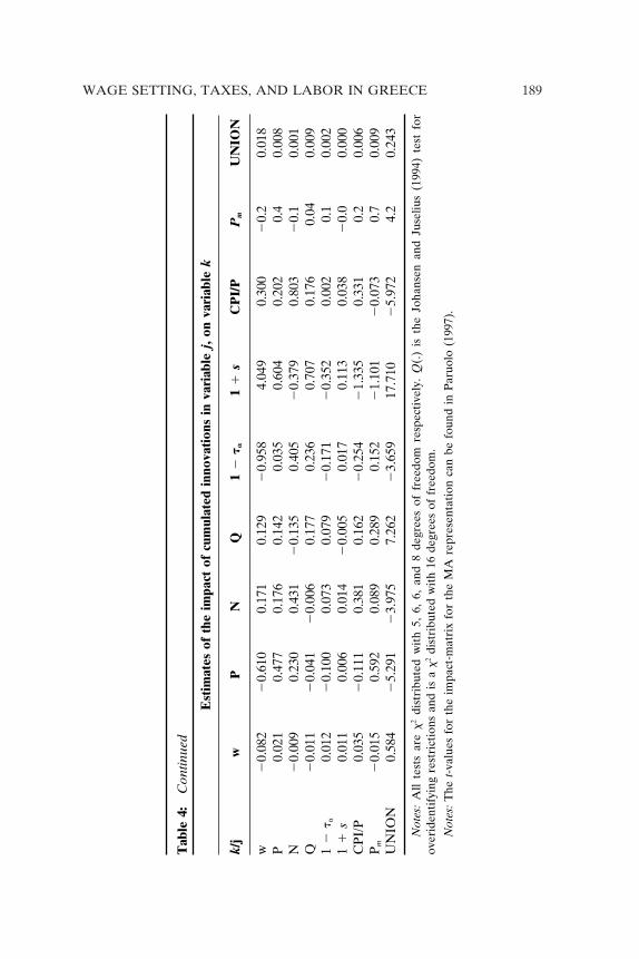
Table 4 introduces the estimates of the three nonrestricted coin-tegrating vectors obtained from the Johansen FIML technique.The bi coefficients indicate the long-run relationships embodiedin the eigenvectors. All coefficients are correctly signed, they havereasonable magnitudes, and they are statistically significant. Aninteresting issue concerns how rapidly the long-run equilibriumin the labor market is attained. This question is answered by theestimate of the matrix “error correction” terms a, which can beconsidered as the speed of adjustment of each variable with respectto a disturbance in the long-run equilibrium. Table 4 also reportsthe estimates of the cumulated innovations derived from the MA


representation of the model. As is shown the innovations fromthe price level, the level of employment and the output have thelargest effect on the wage rate, while the effect of the degree ofunionization is low.

We proceed by imposing restrictions describing long-run prop-erties that the vectors of interest are expected to fulfill. Short-term adjustment (to changes in the process and in the long-runsteady states) is determined freely. However, insofar as relevantcointegrating relations with behavioral interpretation will be de-tected, we expect the error-correcting property to reveal themeven more clearly.

5A. Wage-Setting Schedule

First, we evaluate the two extreme hypotheses concerning thedominance of the bargaining parties and the tax incidence aug-mented with the restriction (bN 5 2bQ), which makes productivitythe driving force of real wages. We are unable to reject bothcontradictory hypotheses. The hypothesis of union dominance(with taxes fully borne by firms) generates a x2 statistic equal to1.03, whereas the opposite hypothesis has a x2 value of 5.09. Giventhis outcome, we proceed to test whether the absolute values ofthe coefficients of (l 2 ta), (l 1 s), (CPI/P) are equal in absolutevalue. This restriction was also accepted. Furthermore, column 2indicates that the long-run homogeneity hypothesis between thereal wage and productivity is rejected, and this result may beattributed to the presence of a linear trend in the model. Finally,we impose the restriction for testing the degree of wage indexationthat is given in Equation 12. In column 1 it is shown that thisrestriction for the case of real wage resistance v 5 1 is acceptedand, therefore, it can be argued that the Greek labor marketexhibits a considerable degree of real-wage resistance.

5B. Demand for Labor

The definition of the demand-for-labor schedule was givenabove. As is clear from Equation 2, the payroll tax is the only taxfactor included. Therefore, we should expect that bta 5 by 5 0.First, we test whether the hypothesis that in the long-run firmsoperate on the labor demand curve holds if determinants of reallabor cost are such that bw 5 2bP 5 bs. The above restrictionsand the omission of union effects on employment are easily ac-cepted, as shown in column 3. Thus, we argue that the demand


for labor is guided by real labor cost and the level of activity.However, the absolute values of elasticities with respect to boththese factors are significantly below unity, which would be ex-pected under simple Cobb-Douglas technology.

Given these findings, it appears that there is some evidenceagainst the efficient bargaining model. In the right-to-managemodel (3) that we consider here, employment is determined bythe profit-maximizing condition (2), which only includes variablesentering the profit function. In the efficient bargaining modelthe profit maximization condition is relaxed and employment isdefined in the bargaining solution. In this case, all variables enter-ing the game play a role in the determination of employment.Thus, the determinants of profit enter the employment functionsignificantly while other variables do not. This indicates that theequilibrium level of employment is on the labor demand curve.

Column 4 indicates that the effect of real raw material pricesdoes not differ significantly from zero. This finding leads to thesame conclusion that holds in several countries, as Hamermesh(1991) has shown. He argues that labor and energy are pricesubstitutes, with a very small crossprice elasticity, and thus it isnot surprising that we were unable to distinguish an impact forraw material prices on the demand for labor function. Finally, weimpose the restriction that the output elasticity is equal to thelabor cost effect, and it is easily rejected.

5C. Output “Semischedule”

The cointegration results have shown that there is a third statisti-cally significant eigenvector. As we have explained, this vectorcan capture elements of both the demand side and the supply sideof the labor market. In column 5 we consider one possibility,namely that the third vector resembles a demand-for-output sched-ule, and it is clear that we are unable to reject the required restric-tions. However, given that the hypothesis for the Cobb-Douglastechnology, (bN 5 2bQ) is also accepted, this could also capturesupply-side elements.

5D. Joint Hypotheses

The final step of our analysis is to provide tests of joint hypothe-ses for the complete system as was discussed in Section 3C. Wenow test whether the restrictions imposed on each vector indepen-dently will be accepted simultaneously. This test is described in


Johansen and Juselius (1994), and the results are given in Table4. Because there is a large number of combinations that we couldmake, we present here only the analysis of the full set of restric-tions. Thus, the first case is that we consider columns 1, 3, and 5,and the second one refers to columns 2, 4, and 5. In both casesit is shown that we pass the test for overidentifying restrictions,because the value of the likelihood ratio statistic Q with 16 degreesof freedom is equal to 11.59 and 10.45 in the first and secondcases, respectively, and therefore, we argue that the system of thethree statistically significant vectors resembles the three long-runrelationships that we have considered, namely, the wage-settingschedule, the demand-for-labor schedule, and the output schedule.

6. CONCLUSIONS

This paper considers a well-specified model that relates wagesetting, demand for labor and the impact of taxes in a bargainingframework. Our analysis is done with the use of recent develop-ments in cointegration theory. First, we apply a newly developedtesting procedure suggested by Paruolo (1996), which allows usto test in the multivariate context the existence of I(2) and I(1)components. Second, this formal test was also coupled with thestudy of the estimated roots of the companion matrix. Thus, wewere able to correctly specify the cointegration rank of our systembased on the characteristics of the data-generating process in thecomplete system and relying on the standard univariate unit roottests. Third, we apply the Johansen multivariate cointegrationtechnique for the case of I(1) specification from which we wereable to estimate three statistically significant eigenvectors. Follow-ing Johansen and Juselius (1994) and Johansen (1995b), structuralrestrictions identifying the long-run relations of interest were spec-ified and tested first in partial and then in joint analysis. Thus, wehave identified one vector with the wage-setting schedule, a secondone with the demand for labor, and finally the third was shownto mimic the output schedule. This concerns the economic identi-fication. However, testing empirical identification is still notstraightforward, although the application of a series of likelihoodratio tests indicates that the preferred relations also satisfy thiscondition. All these considerations play a role in ensuring thatthe structure applied does not suffer from the potential lack ofidentification of wage-setting relations addressed by Bean (1992)and Manning (1992). Finally, we have also shown by means of


the testing methodology suggested by Hansen and Johansen(1993) that the identified long-run relationships are sample inde-pendent, and that the estimated coefficients do not exhibit instabil-ities in recursive estimations.

The major findings of this paper lead to the conclusion that in theprivate sector in Greece, neither of the bargaining parties—employ-ers or employees—has gained full dominance in the wage-settingprocess. In addition parameter estimates indicate a considerabledegree of real-wage resistance. Finally, equilibrium employmentappears to be on the labor demand curve in the aggregate privatesector in Greece, and this contradicts the efficient bargaining hy-pothesis (Layard, Nickell, and Jackman, 1991).

REFERENCESBean, C. (1992) European Unemployment: A Survey, London School of Economics.

Centre for Economic Performance. Discussion Paper No 71.Binmore, K., Rubinstein, A., and Wolinsky, A. (1986) The Nash Bargaining Solution in

Economic Modelling. Rand Journal of Economics 17:176–188.Engle, R.F., and Granger, C.W.J. (1987) Co-Integration and Error Correction: Representa-

tion, Estimation, and Testing. Econometrica 55:251–276.Gonzalo, J. (1994) Comparison of Five Alternative Methods of Estimating Long-Run

Equilibrium Relationships. Journal of Econometrics 60:203–233.Harmermesh, D.S. (1991) Labor Demand: What Do We Know? What Don’t We Know?

NBER Working Paper 3890.Hansen, H., and Johansen, S. (1993) Recursive Estimation in Cointegrated VAR Models,

Reprint 1. Copenhagen: Institute of Mathematical Statistics, University of Copen-hagen.

Hansen, H., and Juselius, K. (1995) CATS in RATS Manual to Cointegration Analysis ofTime Series. Evanston, IL: Estima, Inc.

Hendry, D.F., and Richard, J.-F. (1983) The Econometric Analysis of Economic TimeSeries (with discussion). International Statistical Review 51:111–163.

Johansen, S. (1991) Estimation and Hypothesis Testing of Cointegration Vectors inGaussian Vector Autoregressive Models. Econometrica 59:1551–1581.

Johansen, S. (1992) Determination of Cointegration Rank in the Presence of a LinearTrends. Oxford Bulletin of Economics and Statistics 54:383–397.

Johansen, S. (1995a) A Statistical Analysis of Cointegration for I(2) Variables. EconometricTheory 11:25–29.

Johansen, S. (1995b) Identifying Restrictions of Linear Equations. Journal of Econometrics69:111–132.

Johansen, S. (1997) A Likelihood Analysis of the I(2) Model. Scandinavian Journal ofStatistics 24:433–462.

Johansen, S., and Juselius, K. (1990) Maximum Likelihood Estimation and Inference onCointegration: With Applications to the Demand for Money. Oxford Bulletin ofEconomics and Statistics 52:169–210.


Johansen, S., and Juselius, K. (1992) Testing Structural Hypotheses in a MultivariateCointegration Analysis of the PPP and UIP for UK. Journal of Econometrics53:211–244.

Johansen, S., and Juselius, K. (1994) Identification of the Long-Run and the Short-RunStructure: An Application to the ISLM Model. Journal of Econometrics 63:7–36.

Johansen, S., and Nielsen, B. (1993) Asymptotics for Cointegration Rank Test in thePresence of Intervention Dummies: Manual for the simulation program DisCo,Reprint. University of Copenhagen.

Juselius, K. (1994) On the Duality Between Long-Run Relations and Common Trends inthe I(1) and the I(2) case: An Application to the Aggregate Money Holdings.Econometric Reviews 13:151–178.

Juselius, K. (1995) Do Purchasing Power Parity and Uncovered Interest Rate Parity Holdin the Long Run? An Example of Likelihood Inference in a Multivariate Time-Series Model. Journal of Econometrics 69:211–240.

Juselius, K. (1996) A Structured VAR Under Changing Monetary Policy. Discussion Paper,Department of Economics, University of Copenhagen.

Layard, R., Nickell, S., and Jackman, R. (1991) Unemployment. Oxford: Oxford UniversityPress.

Lee, T.-H., and Tse, Y. (1996) Cointegration Test With Conditional Heteroskedasticity.Journal of Econometrics 73:401–410.

Lockwood, B., and Manning, A. (1993) Wage Setting and the Tax System: Theory andEvidence for the UK. London School of Economics, Centre for Economic Perfor-mance, Discussion Paper 115.

Manning, A. (1992) Wage Bargaining and the Phillips Curve: The Identification andSpecification of Aggregate Wage Equations. London School of Economics, Centrefor Economic Performance, Discussion paper 62.

Nickell, S.J. (1978) The Investment Decisions of Firms. Cambridge: Cambridge UniversityPress.

Pantula, S.G. (1989) Testing for Unit Roots in Time Series Data. Econometric Theory5:256–271.

Paruolo, P. (1996) On the determination of integration indices in I(2) systems. Journal ofEconometrics 72:313–356.

Paruolo, P. (1997) Asymptotic Inference on the Moving Average Impact Matrix in Cointe-grated I(1) VAR Systems. Econometric Theory 13:79–118.

Reimers, H.E. (1992) Comparison of Tests for Multivariate Co-integration. StatisticalPapers 33:335–339.

Sephton, P.S., and Larsen, K.H. (1991) Tests of Exchange Market Efficiency: FragileEvidence From Cointegration Tests. Journal of International Money and Finance10:561–570.

Tyrvainen, T. (1992) Unions, Wages and Employment: Evidence from Finland. AppliedEconomics 24:1275–1286.

Tyrvainen, T. (1995) Wage Setting, Taxes and Demand for Labour: Multivariate Analysisof Cointegrating Relationships. Empirical Economics 20:271–297.

Wage Setting, Taxes, and Demand for Labor in Greece: A Multivariate Analysis of Cointegrating...

Documents

Transcript of Wage Setting, Taxes, and Demand for Labor in Greece: A Multivariate Analysis of Cointegrating...