NBER WORKING PAPER SERIES

AN EMPIRICAL ASSESSMENT OF ALTERNATIVE MODELS OF RISKY DECISION MAKING

Pamela K. Lattimore

Ann D. Witte

Joanna R. Raker

Working Paper No. 2717

NATIONAL BUREAU OF ECONOMIC RESEARCH 1050 Massachusetts Avenue

Cambridge, MA 02138

September 1988

We would like to thank the young adults who agreed to participate in our

study and the North Carolina Department of Correction and the Institute for Research in Social Science for allowing us to use subjects in ongoing projects. Jerry Green, Bronwyn Hall, Bob Lee, John Payne and Helen Tauchen

provided valuable comments and suggestions that allowed us to sharpen our

thinking and improve our work. Ann Witte's work on this project was

supported by a grant from the National Science Foundation (NSF). Points of views expressed do not represent the position of the U.S. Department of

Justice, the NSF, or the National Bureau of Economic Research.

NBER Working Paper #2717

September 1988

AN EMPIRICAL ASSESSMENT OF ALTERNATIVE MODELS OF RISKY DECISION MAKING

ABSTRACT

In thia paper, we aaaess the degree to which four of the most commonly

used models of risky decision making can explain the choices individuals

make when faced with risky prospects. To make this assessment, we use

experimental evidence for two random samples of young adults. Using a

robust, nonlinear least squares procedure, we estimate a model that is

general enough to approximate Kahnenman and Tversky's prospect theory and

that for certain parametric values will yield the expected utility model, a

subjective expected utility model and a probability-transform model.

We find that the four models considered explain the decision-making

behavior of the majority of our subjects. Surprisingly, we find that the

choice behavior of the largest number of subjects is consistent with a

probability-transform model. Such models have only been developed recently

and have not been used in applied settings. We find least support for the

expected utility model - - the most widely used model of risky decision

making.

Pamela K. Lattimore Ann D. Witte

National Institute of Justice Department of Economics 633 Indiana Avenue, NW. Wellesley College Washington, DC 20531 Wellesley, MA 02181

Joanna R. Baker

Department of Management Science

Virginia Polytechnic Institute and State University

Blacksburg, VA 24061

I. Introduction

Depending upon one's viewpoint, the modelling of risky decision making

is either in a state of chaos or fecundity)' Most applications of this

type of decision modeling continue to use the expected utility approach.

However, as a result of persistent evidence from laboratory experiments

that people do not make decisions in the manner suggested by the expected

utility model, theorists have developed a number of alternative

representations. When developing these new approaches, researchers have

aought models that are generally consistent with the major findings of

laboratory studies of choice behavior in risky situations.

Psychologists have generally developed their theories inductively

(e.g., Edwards, 1955, Kahnennian and Tveraky, 1979) while economists have

pursued deductive approaches (e.g., Handa. 1977; Machina, 1982, Yaari,

1987). Thia work providea a variety of suggested parametric forms for the

preference functional.

To date, as far as we are aware, there have been no attempts to

eatimate and compare the relative explanatory power of a number of

alternative models. In this paper, we begin this task. Specifically, we

assess the relative explanatory power of four of the major models of

decision making under uncertainty that have been proposed. To do this, we

uae a functional form that is general enough to approximate Kahnenman and

Tversky'a prospect theory model and that for certain parametric values will

yield the expected utility model, a subjective expected utility model

(Savage, 1954; Edwards, 1955), and a model that transforms probabilities

but not outcomes (Handa, 1977; Yaari, 1987).

To summarize briefly our moat interesting results, we find that the

four models explain the decision-making behavior of the majority of our

2

subjects. Surprisingly, we find the decision-making behavior of the

largest number of subjects to be consistent with a model in which

probabilities but not outcomes are transformed. Such models have been

developed quite recently and have not been used in applied settings. We

find least support for the expected utility model - - the moat widely used

model of risky decision making.

Our results suggest that the decision-making model appropriate for

situations involving potential gains is different from the model

appropriate for situations with potential losses. This is, of course, a

major contention of Kahneman and Tversky (1979) who suggest that the

outcome transform will be different in the two settings. Contrary to

Kahneman and Tveraky's suggestion, we find that it is differences in the

way in which probabilities are transformed, not differences in the way

outcomes are transformed, that usually distinguishes the model for gains

from the model for losses.

The paper is organized as follows. In the next section, we briefly

describe the models of risky decision making we consider. Section III

presents our empirical model and Sections IV and V describe the data and

methods we use to estimate the model. In Section VI, we discuss our

results and the final section contains a summary and our conclusions.

II. The Models Considered

Consider a simple prospect Y which yields x1 with probability p and x2 with probability (l-p). Under an expected utility model, the decision

maker is assumed to maximize expected utility which is defined as

pu(x1) +

(l-p)u(x2).

3

Note that the decision maker uses objective probabilities to weight the

utility, u(x.), of outcomes. Attitudes toward risk are reflected in the

shape of the utility function.

Since the 1950s some researchers have been uncomfortable with this

model because they feel that decision makers do not use objective

probabilities, but rather develop subjective probabilities, s(p), that are

used to weight outcomes. These subjective probabilities are asawned to

follow standard probability rules, but they need not be equal to objecttve

probabilities. For example, Savage (1954) suggests that the individual

seeks to maximize subjective expected utility which is defined as

a(p)u(x1) + s(l-p)u(x2).

Like the expected utility model this subjective expected utility model

assumes that attitudes toward risk are reflected in the utility function.

Edwards (1955) develops a similar model but suggests that attitudes toward

risk are embedded in the probability transform not in the utility or value

function.

More recently a n.unber of economists have developed axiomatic decision

models which embed risk attitudes in the probability transform and assume

no transformation of outcomes. We refer to such models as probability-

transform models. As far as we are aware, Handa (1977) developed the first

such axiomatic model. Under his model the individual is assumed to

maximize

x1h(p) + x2h(l-p).

4

The function h transforms objective into subjective probabilities and risk

attitudes are reflected in the shape of the probability transform. For

prospects with more than two outcomes, Fishburn (1978) has shown that

Hands's model implies maximization of expected returns if violations of

stochastic dominance are to be avoided.

Quite recently Ysari (1987) has developed a theory dual to the

expected utility model that transforms probabilities but not outcomes,

embeds risk attitudes in the probability transform and avoids diffirulties

with previous models of this type (e.g., Hands, 1977; Quiggina, 1982)L

Yaari sees the transform on probabilities as indicating how "perceived risk

is processed into choice" (p.108). Note that Yaari's transform of

probabilities is quite different than the transform proposed in subjertive

expected utility models or Hands's model.

Kshnemsn and Tversky (1979) propose an inductively developed theory.

"prospect theory," under which both probabilities and outcomes are

transformed. Under their model the decision maker is see as maximizing

ir(p)v(x1) ir(l-p)v(x2)

where v is a value function which converts outcomes to value and ir is a

decision weighting function over probabilities. The value function is

defined on deviations from a reference point. Kahneman and Tveraky suggest

that the value function is concave above and convex below the reference

point and that the function is steeper for losses than for gains. The

decision weights are not required to obey the mathematical rules of

probability. They measure "the impact of events on the desirability of the

prospects and not merely the perceived likelihood of these events"

S

(Kahneman and Tversky, 1979, p.285). Conceptually these decision weights

are more like Yaari's probability trsnsform than the probability transforms

of the other models we have considered. The decision weights are assumed

to have the following properties:

1. subadditivity, ir(rp) > rm(p) for O<r<l,

2. subcertainty, Thr(p.) C 1 and

3. subproportionality, ir(pr)/r(p) C ir(pqr)/ir(pq) for O<p,q,r<l which implies that the ratio of the weights of small

probabilities is closer to 1 than those of large probabilities.

In Kahnemsn and Tversky's model, attitudes toward risk are embedded in both

the value transform and the decision weighting function.

III. The Empirical Model

Consider the following model for a two outcome prospect:

V(Y) = f(p)v(x1) + f(l-p)v(x2)

where V(Y) is a preference function over the risky prospect, and v and f,

respectively, convert outcomes and probabilities into choice relevant

variables. As ia traditional, we value the risky prospect by its certainty

equivalent, CE, and assume that the function that transforms outcomes into

values also transforms the certainty equivalent of a prospect into a

decision relevant value, That is, we assume

V(Y) v(CE).

Assuming that v is monotonic end continuous, we obtain

(1) CE — v[f(p)v(x1) + f(l-p)v(x2)].

To further spetify the model, we must select a functional form for f

and v that will allow us to approximate Kahneman and Tversky's model and

that will for certain parameter values yield: (1) an expected utility

model, (2) a subjective expect!d utility model, and (3) a model in which

probabilities but not outcomes are transformed.

We assume that v can be approximated by a power function, e.g.,

(2) v(x) = xl.

The function will be concave, linear or convex as y <=> 1. This fora hoe

been used extensively in the literature and has been found to provide s

good fit to laboratory data (Fishburn and Kochenberger, 1979).

The four models we consider imply different interpretations and values

for T The implications are summarized in Table 1. Under an expected

utility model (EU) or a subjective expected utility model (SEU) of the type

developed by Savage (1954), one would expect either y < 1, implying risk

aversion, or 1 > 1 implying risk-seeking behavior. Under these models a

value of 1 — 1 would imply risk neutrality and thst the decision maker

maximizes expected value not expected utility. Under a probability-

transform model such as that proposed by Handa (1977) or Yaari (1987), one

would expect -y — 1. Under a prospect theory model, one would expect that

C 1 for gains and -y > 1 for losses. To allow for this possibility, we

estimate separate models for gains and losses.3

For the function that transforms probabilities, we select a form that

allows a continuous approximation to Kahneman and Tversky's decision

weighting function:

7

(3) f(p) ap + (1-p)

The properties of f depend upon the values of a and , particularly upon

whether these parameters are less than, equal to or greater than 1. If

a < 1 and $ < 1, the function is aubadditive, subcertain and

subproportional as posited by Kahneman and Tversky for their decision

weights. The form implied by these parametric values is depicted in panel

a of Figure 1.

Neither Handa (1977) not Yaari (1987) present a specific form for

their probability transform. However, Handa does provide us with a picture

(1977, Figure 1, p. 113) which suggests that a form like that in panel a

would be appropriate.

Subjective expected utility models imply that f is symmetric around

0.5 and that people generally overweight probabilities below .5 and

underweight probabilities above that value. Further, subjective expected

utility models are certain not subcertain. Our function will have the

characteristics assumed by subjective expected utility models if a =1 and

C 1 as shown in panel b of Figure

Finally, the expected utility model assumes no transformation of

probabilities. This implies that a = $ = 1. See panel c of Figure 1.

To obtain our empirical model, we substitute equations (2) and (3)

into equation (1) and add a stochastic error term to reflect such things as

measurement and judgement error. This yields:

CE — ap a(l-p) x1 + c + (l-p) + a(l-p

8

which we estimate separstely for gains and losses.

If we find that a < 1 and $ < I for both gains and losses and that -y C

1 for gsins and -y > 1 for losses, our work will support a prospect theory

model. If, instead, we find the above parameter values for a and $, but

that -y — 1 for both gains and losses than a probability-transform model

would seem more appropriate. Our results will support a subjective

expected utility model if a 1, $ < I and — 1 and s expected utility

model if a — $ = 1 and 1.

IV. The Data

Our data were obtained from two groups of young adult North

Carolinians. The first group of 47 was selected at random from the

undergraduate student body at the University of North Carolina at Chapel

Hill. These students were part of a computer administered panel study and,

thus, were familiar with the type of interattive computer program that we

use to sdminister the decision-making scenarios. Students are the most

commonly used subjects for laboratory experiments.

To broaden the socioeconomic representstion of participants, we

selected a second group of 23 subjects at random from a set of

incarcerated, young (18-22) male property offenders. These offenders had

been randomly assigned to participate in an innovative job training/

reintegration program.

Each group was presented with two types of risky decisions. The first

was a set of standard money gambles (over gains and losses) of the kind

generally used in this type of laboratory experiment. The second involved

a criminal choice (gain) scenario and a plea bargain (loss) scenario.

Responses to the latter type of decisions appeared to be subject to fewer

9

attention lapses and judgement errors, perhaps because the scenarios

appeared more concrete. We present results only for the second type of

risky decisions although our general conclusion would be similar if we used

data for the standard money gambles.

Because the amount of time with students was limited, we developed an

interactive computer program that contained instructions and presented the

decision-making scenarios. Students were paid for their participation in

the study.

We provided the offenders in our study with verbal instructions and

a set of "practice" risky decisions on the computer because of their lqver

level of education and lack of experience with interactive computer

programs. Their responses to the practice decisions were observed.

Misunderstandings were cleared up and questions answered. The offenders

were then presented with scenarios by the same interactive computer progrsis

ss used with the students.

To obtain certsinty equivalents (CEs) for gains we presented subjects

with scenarios like the following:

Suppose that you had decided to break into one of two markets -- Jack's or Harry's. Further, suppose that you knew that it would take the same skill to break into either market and that the risk of capture waa the same. Further, suppose that you know that Jack has $900 in his register half of the time and $100 the other half, while Harry always has some cash in his register.

The options available to the subject were then presented in tabular form

and the subject was asked "what is the smallest number of dollars there

would have to be in Harry's register before you would choose to break into

Harry's rather than Jack's?". This is the certainty equivalent value we

use when estimating our model.5

10

The possible cash amounts in Jack's register (x1 and in our model)

ranged from $0 to $1000. The values of p considered were from 0.01 to

0.99.

The loss scenarios were presented in a similar fashion. Subjects were

asked to choose between a certain sentence agreed to in a plea bargain and

the risky prospect of going to trial. Possible trial outcomes (x1

and x,)

C were sentences ranging from 0 to 36 months. Values for probabilities were

the same as for the illegal-gains scenario, Subjects were asked to

indicate the longest sentence length they would accept in a plea bargain in

order to forego a trial (the risky prospect).

To prevent the order of presentation of prospects from affecting

response7, scenario selection was random for both the gain and loss

settings. Further, subjects were equally likely to be presented with the

gain or loss scenarios first. To prevent some meaningless responses, the

subjects were instructed to choose a certainty equivalent value between the

two values for the risky prospect (a value between and x2)

. If a subject choose a vslue outside this range, they were again instructed to

choose s value within the range. This iterstive procedure continued until

the subject chose s value between and x2.

Inmates provided certainty equivalents for 34 gain and 34 loss

scenarios. Due to the limitation on student time noted above, students

provided responses to only 29 gain and 29 loss scenarios. Thus, student

models are estimated with 29 data points and inmate models with 34.

V. Method of Estimation

We use an iteratively reweighted nonlinesr least squares technique to

estimate our model. This procedure is robust to outliers because it gives

11

less weight to such observations than would a standard least squares

procedure. The method of reweighting observations is due to Beaton and

Tukey (1974) . We feel it is desirable to downweight outlying observations

because for the type of data we are using such observations generally occur

due to fatigue and attention lapses. Nonlinear least squares parameter

estimates were obtained by a numerical procedure due to Ralston and

Jennrich (1978)

VI. Results

We estimated our decision-making models (gain and loss models) for 57

of the 70 students selected for the study. We were unable to use the data

for 13 of our 70 subjects because of unreasonable responses (e.g. , same

response to all scenarios) or a failure of the parameter estimates to

8 converge.

In general our model fit the decision data for our subjects quite

well. The R2s for the model ranged from 0.21 to 0.99 for the gain

scenarios with R2s above 0.50 for eighty-two percent of the subjects. For

the loss scenarios, the R2s were from 0.13 to 0.98 with R2s above 0.5 for

eighty-eight percent of the subjects.

A. The Outcome and Probability Transforms for Gains

Consider first the results for the function that transforms outcomes,

v x1. For the majority of subjects, over sixty percent (34 of the 57)

we cannot reject9 the null hypothesis that -y—l. These results would be

consistent with either an expected value or probability-transform model.

For the bulk of the remaining subjects, thirty percent, our results

indicate that y is significantly less than 1. This implies that for these

12

subjects the gains function is concave which would be consistent with so

expected utility, subjective expected utility or prospect theory model.

For the remaining nine percent of the subjects, our results indicste that y

is significantly greater than one. This is not generally expected for any

of the models considered, but under sn expected utility or subjective

expected utility model, this result could be interpreted as indicating risk

seeking behavior for this minority group of subjects.

Turning next to the function that trsnsforms probabilities, our

results indicate that almost half (46 percent) of the subjects transform

probabilities in the manner suggested by the subjective expected utility

model. Specifically, for these subjects, we cannot reject the null

hypothesis that a = 1 and find support for the alternative hypothesis that

a C 1. See penel b of Figure 1. For nineteen percent of the subjects (11

subjects) test statistics support the contention thst a C 1 end fi C 1.

These psrsmeter values indicate that probabilities are transformed as

indicsted by prospect theory. See panel s of Figure 1. For sixteen

percent of the subjects (9 subjects), results indicate thst there is no

trsnsformstion of probabilities (i.e., a = 1). These results sre

consistent with either an expected utility or an expected value model.

For the remaining nineteen percent of our subjects (11 subjects) , the

shape of the probability transform implied by our results were not

consistent with any of the models considered. For four of these subjects

the test statistics support the contention that a < 1 and fi — 1. The shape

of the probability transform implied by these parametric values is depicted

in panel a of Figure 2. As can be clearly seen, these subjects underweight

all probabilities. Under Handa's model these subjects would be seen as

13

globally riak averse and under Yaari's as behaving Ilpessimistically.TT For

another six of these nonconforming subjects, results indicate that o > 1

and c 1. See panel b of Figure 2. Theae subjects overweight all but

high probabilities. The probability transform is supracertain (i.e., f(p)

> 1) which is not suggeated by any of the models we consider. Finally, for

one subject, a probability transform like that in panel c of Figure 2 is

suggested. Comparing thia ahape with the shape implied by the subjective

expected utility model (panel b of Figure 1) , the reader will note that

this is the mirror isage of the form suggested by that model. This subject

underweighta probabilities below 0.5 and overweights probabilities above

0.5.

3. The Outcome and Probability Transforms for Losses

For losses, we find that sixty-nine percent of our subjects do not

tranaforma outcomes, i.e., we cannot reject the null hypothesis that i

For both the gains and loss scenarios, our results for the Outcome

transform are most in accord with a probability-transform or expected value

model. For sixteen of the remaining eighteen subjects, our results

indicate risk-seeking behavior. This outcome is predicted by prospect

theory. For the two remaining subject test statistics indicated risk

aversion over losses.

Turning to results for the function that transforms probabilities, we

find that for losses the probability transform is as suggested by prospect

theory for 42 percent (24 subjects) of our subjects. For these subjects,

the probability transform is subadditive for small probabilities,

subcertain and subproportional and subjects overweight low probabilities

and underweight high ones. See panel a of Figure 1. A probability

14

transform of the type suggested by subjective expected utility is supported

for 26 percent of our subjects. See panel b of Figure 1. For sixteen

percent of our subjects, results suggest no transform of probabilities as

posited by expected utility and expected value models.

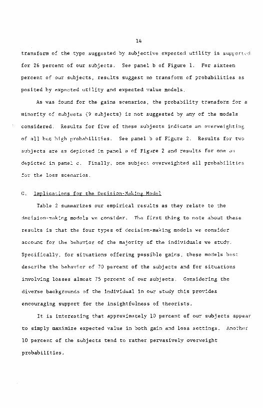
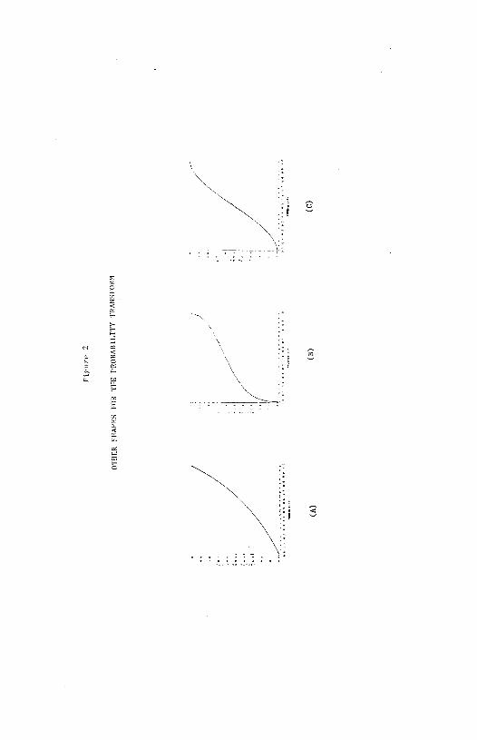
As was found for the gains scenarios, the probability transform for a

minority of subjects (9 subjects) is not suggested by any of the models

considered. Results for five of these subjects indicate an overweighting

of all but high probabilities. See panel b of Figure 2. Results for two

subjects are as depicted in panel a of Figure 2 and results for one as

depicted in panel c. Finally, one subject overweighted all probabilities

for the loss scenarios.

C. Implications for the Decision-Makina Model

Table 2 summarizes our empirical results as they relate to the

decision-making models we consider. The first thing to note about these

results is that the four types of decision-making models we consider

account for the behavior of the majority of the individuals we study.

Specifically, for situations offering possible gains, these models beat

describe the behavior of 70 percent of the subjects and for situations

involving losses almost 75 percent of our subjects. Considering the

diverse backgrounds of the individual in our study this provides

encouraging support for the inaightfulness of theorists.

It is interesting that approximately 10 percent of our subjects appear

to simply maximize expected value in both gain and loss settings. Another

10 percent of the subjects tend to rather pervasively overweight

probabilities.

15

Comparing the relative performance of the four models we find that a

probability-transform model, a model that transforms probabilities but not

outcomes, describes the decision-making behavior of the largest number of

subjects. This model well represents the behavior of 42 percent of all

subjects when facing gains and 51 percent of all subjects when facing

losses. For gains scenarios, the subjective expected utility model is

appropriate for the next largest number of subjects (16 percent) and for

loss scenarios, a prospect theory model (14 percent). It is interesting

that the expected utility model appear to describe the behavior of only 5

percent of our subjects.

VII. Conclusions

We believe that our work makes both a methodological and substantive

contribution. From a methodological perspective, we have developed and

implemented a procedure that allows researchers to more systematically use

laboratory evidence to evaluate alternative models of risky decision

making. To date, both economists and psychologists have generally

marshalled laboratory evidence, on samples of convenience, to assess or

develop a single model of risky decision making. To be more specific,

laboratory data are generally obtained from readily available subjects such

as college undergraduate volunteers or students in particular classes. The

patterns observed in these data are then used either to infer a model

(e.g. , Kahnenman and Tversky, 1979) or to corroborate a deductively

developed model (e.g., Handa, 1977; Yaari, 1987). Corroboration is not

generally obtained through the use of standard statistical procedures or

standard statistical tests. The relative explanatory power of alternative

models is not generally considered.

16

We obtain our laboratory data from random samples of subjects, uae a

mathematical form that encompasses a number of the most commonly used

models of risky decision making and assess the relative merits of the

alternative models using scandard statistical tests. More specifically,

our dats are for a group that is representative of the undergraduate

population of a large state university and a group representative of the

young, male property offenders. While these samples are certainly not

ideal, they are representative of identifiable populations and come from a

broader range of socioeconomic backgrounds than has usually been the case.

The mathematical form we use will, under various parametric restrictions,

yield a prospect theory, a subjective expected utility, a probability

transform and an expected utility model. We estimate the parameters of

this model using a robust, nonlinear least squares procedure and use

standard statistical tests to distinguish among the alternative models.

Substantively, we provide rather surprising evidence regarding the

relative explanatory power of the four models considered. Comfortingly, ac

find that the four models considered explain the decision-making behavior

of the majority (seventy to seventy five percent) of our subjects.

Surprisingly, our results provide most support for a probability-transform

model. Under this type of model, risk attitudes are reflected in the

function that transforms probabilities and outcomes are not transformed.

Such models have been developed quite recently (e.g., Handa, 1977; Yaeri,

1987) and have not, as far as we are aware, been used in applied settings.

However, Yasri ties such models to more widely used models by showing that

there is a probability transform model dual to the expected utility model.

It is interesting that of the four models we consider, we find least

17

support for the expected utility model - - the most widely used model of

risky decision making.

Turning to insights for future modelling efforts, our results indicate

that the decision-making model appropriate for situations involving

potential gains is different from the model appropriate for settings

involving potential losses. This is, of course, a major contention of

Kshneman and Tversky (1979) who suggest that the outcome transform will be

different in the two settings. However, we do not find that it is the

outcome transform that is different in the two settings. Recall that the

majority of our aubjecta do not appear to transform outcomes. Our results

suggest that the major difference in decision making for gain and loss

settings results from differences in the way in which probabilities are

transformed. Hands (1977) discusses this possibility. For gains, the most

common form for the probability transform is that suggested by the

subjective expected utility model. This transform indicates that people

overweight probabilities below .5 and underweight probabilities below .5.

See panel a of Figure 1. In loss setting, the most common transform is

that suggeated by prospect theory. With such a transform, people

overweight a narrower range of low probabilities and underweight a wider

range of high probabilities. See panel b of Figure 1.

18

Notes

1. For surveys of the litersture, see Schoemaker (1982), Sugden (1986) or

Machins (1987).

2. In both Quiggins' (1982) snd Yasri's model the transform is not over

the simple probability of an outcome but rather over all (Quiggins) or part

of the distribution (Yaari, 1987).

3. Work by Kahnenman and Tversky (1979) and Fishburn and Kochenberger

(1979) suggests that the reference point is near the current asset level

and, thus, separate assessments over gains and losses should capture this

aspect of Kshneninan and Tversky's model for the young adult subjects we

use. We treat losses as positive numbers as we must if we are to use this

outcome transform. This, of course, means that under an expected utility

or subjective expected utility model, risk aversion is implied by convexity

and risk-seeking behavior by concavity when the model is estimated for

losses.

4. Additionally, it should be noted that equation (3) with = 1 is

identical to the decision weighting function suggested by Karmarksr (1978)

for his subjectively weighted utility model. Ksrmsrkar suggested that

k\7(xk) m

v(CE) — , where wk

p . For prospects involving more k p +(l—p)

thsn two oucomes,

our decision weighting function would be

—

apk jlj 5. The careful reader will note thst this is only a very close

approximation to s true certainty equivslent. However, this method of

presentation greatly simplified the subjects' task and increased their

understanding of the decision making problem. Given rounding this

"threshold equivalent" should be virtually identical to the certainty

equivalent.

19

6. These sentence lengths are reasonable under North Carolina statutes.

See Clarke and Rubinsky (1981).

7. See Tversky and Kahneman (1982) for a discussion.

8. For gain scenarios seven subjects provided unreasonable responses and

parameter estimates for six subjects failed to converge. For loss

scenarios, eleven subjects provided unreasonable responses and parameter

estimates for two subjects failed to converge.

9. Unless otherwise noted all two-tailed tests of significance are at the

a .05 level and all one-tailed tests at the a — .025 level.

20

REFERENCES

Beaton, A.E. and J.W. Tukey (1974). "The fitting of power seriea, meaning polynomials, illustrated on band-spectroscopic data." Technometrics 16: pp. 147-185.

Clarke, S.H. and E.W. Rubinsky (1981). "North Carolina'e Fair Sentencing Act: Explanation, Text, and Felony Classification Table." Chapel Hill, NC: Institute of Government, University of North Carolina.

Fishburn, P. and GA. Kochenberger (1979). "Two-piece von Neumann-Morgenstern utility functions." Decision Sciences 10: pp. 503-518.

Edwards, W. (1955). "The prediction of decisions among bets." Journal o Expecimental Psychology 50: pp. 201-214.

Hands, J. (1977). "Risk, probability, and a new theory of cardinal utility." Journal of Political Economy 85: pp. 97-122.

Kadneman, 0. and A. Tversky (1979). "Prospect theory: an analysis of decision under risk." Econometrics 47: pp. 263-291.

Karmarkar, U.S. (1978). "Subjectively weighted utility: a descriptive extension of the expected utility model." Organizational Behavior and Human Performance 24: pp. 67-72.

Hachina, H. (1982). "'Expected utility' analysis without the independence sxiom. " Econometrics 50: pp. 277-323.

Machins, M. (1987). "Choice under uncertainty: problems solved and unsolved." Journal of Economic Perspectives 1: pp. 121-154.

Quiggin, J. (1982). "A theory of anticipated utility." jaW.rnai of Economic Behavior and Orgsnizstion 3: pp. 323-343.

Ralston, M.L. and RI. Jennrich (1978). "Dud, a derivative-free algorithm for nonlinear least squares." Technometrics 20: pp. 7-14.

Savage, L.J. (1954). The Foundations of Ststistics. New York: Wiley.

Schoemaker, P.J.H. (1982). "The expected utility model: Its variants, purposes, evidence, and limitations". Journal of Economic Literature 20: pp. 529-563.

Sugden, R. (1986) . "New developments in the theory of choice under uncertainty." Bulletin of Economic Research 38: pp. 1-24.

Tversky, A. and 0. Kahneman (1982) "Judgement under Uncertainty: Heuristics and Biases" in 0. Kahneman, P. Slovic and A. Tverksy, eds. Judgement under Uncertainty: Heuristics and Biases. Cambridge: Cambridge Univ. Press, pp. 3-20.

Yaari, N.E. (1987). "The dusl theory of choice under risk." Econometrics 55: pp. 95-115.

F' ure

1

RE

LA

TIO

NSH

IP O

F' PR

OB

AIIT

liii

0110 O

NE

IT

T

ON

W

E

I 01110

11)11 'Fl

Ill M

OI)FiI,S

CO

NS

I D

F,RE

I)

7)

(II)

/

/ /

(C)

(A)

Fig

ure

2

OIlI

ER

ShA

PE

S F

OR

TilE

PR

OB

AB

ILT

'FY

IRA

NS

PO

RM

/1//

—

H

/

I(A

)(B

)(C

)

Table 1

Shape and Interpretation of the Outcome Transform

Interpretation -

Shape of the Expected Utility! Outcome Subjective Expected Probability Prospect

Value of -y Transform Utility (Savage) model Transform Theory

y < 1 Concave Risk Aversion Assumed Ovet Gains

= 1 Linear Risk (Expecte

Neutrality d Value Mcdel)

Assumed Linear

-y > 1 Convex Risk Seeking Assumed

Over Losses

Table 2

Implications for the Decision-Making Models

Percent of Subjects, Percent of Subjects, Model Gains Losses

Ebplicitlv considered

Expected Value 10.5 10.5

Expected Utility 5.3 0.0 (risk avereion)

Expected Utility 0.0 5.3 (risk seeking)

Subjective Expected Utility 10.5 0.0 (risk aversion)

Subjective Expected Utility 5.3 3.5

(risk seeking)

Probability Transform 29.8 22.8 (S EU-type)

Probability Transform 12.3 28.1 (PT-cype)

Prospect Theory (PT) 7.0 1.8 (concave value function)

Prospect Theory 0.0 123m (convex value function)

"Aberrent"

Supracertain 10.5 10.5

Always Underweight 7.0 3.5 Probabilities

Mirror Subjective Expected 1.8 1.8 Utility

aSince we treated losses as positive numbers for purposes of estimation, an estimated concave function (p<l) equates to a convex function in the loss domain (negative quadrant) and am estimated convex function to a concave one. For the purposes of this table, we have classified results as they would be if the function were estimated in the loss domain.