NBER WORKING PAPER SERIES

THE ECONOMICS OF TIME-LIMITED DEVELOPMENT OPTIONS:THE CASE OF OIL AND GAS LEASES

Evan M. HerrnstadtRyan Kellogg

Eric Lewis

Working Paper 27165http://www.nber.org/papers/w27165

NATIONAL BUREAU OF ECONOMIC RESEARCH1050 Massachusetts Avenue

Cambridge, MA 02138May 2020

We thank William Patterson, Pengyu Ren, Grant Strickler, and especially Nadia Lucas for outstanding research assistance. We are grateful for the many thoughtful suggestions from conference and seminar participants at Aalto, AEA, AERE, Arizona, BYU, CBO, CEPR, Chicago, Columbia, DOJ, Energy Institute at Haas Energy Camp, FDIC, Federal Reserve Board, GAO, Harvard, Heinz-Tepper IO Conference, Indiana, Mannheim, Michigan, Naval Academy, Northwestern, NYU, Penn, Penn State, Rice Workshop on Economic and Environmental Effects of Oil and Gas, SITE, Texas, Texas A&M, Southern Economic Association, Toulouse, University of Utah, Utah Winter Business Economics Conference, Washington University, and the Winter Marketing-Economics Summit. The analysis and conclusions expressed herein are solely those of the authors and do not represent the views of the U.S. Congressional Budget Office. The views expressed herein are those of the authors and do not necessarily reflect the views of the National Bureau of Economic Research.

NBER working papers are circulated for discussion and comment purposes. They have not been peer-reviewed or been subject to the review by the NBER Board of Directors that accompanies official NBER publications.

© 2020 by Evan M. Herrnstadt, Ryan Kellogg, and Eric Lewis. All rights reserved. Short sections of text, not to exceed two paragraphs, may be quoted without explicit permission provided that full credit, including © notice, is given to the source.

The Economics of Time-Limited Development Options: The Case of Oil and Gas LeasesEvan M. Herrnstadt, Ryan Kellogg, and Eric LewisNBER Working Paper No. 27165May 2020JEL No. D82,D86,L24,L71,Q35

ABSTRACT

Oil and gas leases between mineral owners and extraction firms ubiquitously include royalty and primary term clauses. The royalty denotes the share of revenue that is paid to the mineral owner, and the primary term specifies the date by which the firm must complete a well, lest it lose the lease. Using data from the Louisiana shale boom, we first show that wells' drilling timing is substantially bunched just before lease expiration, raising the question of why leases include development deadlines that distort drilling decisions. We then develop a contracting model in which mineral owners face firms with private information and have the ability to contract on both realized revenue and drilling timing. We show that primary terms can increase both the owner's expected revenue and total surplus because they counteract the delay incentives imposed by the royalty.

Evan M. HerrnstadtFord House Office Building2nd and D St. SWUnited StatesWashington, DC 20515Evan.Herrnstadt@cbo.gov

Ryan KelloggUniversity of ChicagoHarris School of Public Policy1307 East 60th StreetChicago, IL 60637and NBERkelloggr@uchicago.edu

Eric LewisTexas A&M Universityericlewis@tamu.edu

HBP/tree/fc7e27bacd5b38c8fc54b6850a1b687dba8add62A Code repository (with link to data), versioned for this NBER WP is available at https://github.com/kelloggrk/Public_HBP/tree/fc7e27bacd5b38c8fc54b6850a1b687dba8add62A Code repository (with link to data), most recent version of paper is available at https://github.com/kelloggrk/Public_HBP

1 Introduction

Because the owners of subterranean oil and gas often lack the expertise or financial capital

necessary to extract their resources, they typically write contracts with specialized extraction

firms to act as their agents. In the United States, as well as several other countries, these

contracts take the form of mineral leases that ubiquitously contain royalty and “primary

term” clauses, the latter of which are use-it-or-lose-it requirements for the firm. This paper

is aimed at understanding the effects of these clauses on firms’ activities and on the expected

revenue obtained by firms and mineral owners, with an emphasis on the recent boom in U.S.

oil and gas production from shale resources.

An oil and gas lease grants a firm an option, but not an obligation, to develop the mineral

owner’s property by drilling wells and extracting the hydrocarbons. Upon signing a lease,

the firm pays the owner a flat fee, known as a “bonus”. The primary term specifies a period

of time (typically 3 to 10 years) that the firm has to drill at least one well and commence

production. If it does so, the lease is then “held by production” and enters a secondary

term that lasts until the firm ceases production. During the secondary term, the firm may

also drill additional wells on the parcel to increase its overall production rate. On the other

hand, if the firm does not commence production by the end of the primary term, the lease

terminates, and the mineral owner is then free to sign a new contract with another firm or

re-contract with the original firm.

The royalty specified in the lease dictates the percentage of the lease’s oil and gas revenue

that the firm must pay to the mineral owner. These royalties are often significant, as the

royalty rate typically lies between 12.5% and 25%. Brown et al. (2016) estimates that royalty

payments associated with the six largest U.S. shale plays totaled $39 billion in 2014.

The royalty and primary term clauses distort firms’ incentives regarding when to drill

wells and how much effort to invest in fracking and well completion. The incentive to drill at

least one well before primary term expiration has received considerable attention within the

industry, with numerous reports of firms drilling unprofitable wells for the sake of holding

their lease acreage. For instance, the San Antonio Express News reported in 2012 that “many

companies . . . are drilling quickly simply to meet the terms of their contract and keep

their leases—not because they want to drill gas wells now” (Hiller 2012). Although royalties

are less prominent in the news, they also distort firm decisions because they are a tax on

1

revenue only, thereby driving a wedge between the firm’s profit and total surplus.

We begin our analysis by studying data from the Haynesville Shale in Louisiana, where

the institutional structure and data availability are conducive for studying lease terms. We

discuss relevant institutional features of the Haynesville in section 2, discuss our data sources

in section 3, and then show in section 4 that there is substantial bunching of drilling in the

months just prior to lease expiration.1 We further show that many leases—especially those in

less productive areas of the Haynesville—are characterized by having only a single well that

was drilled just before lease expiration, suggesting that drilling in these areas was primarily

motivated by holding acreage for future wells rather than by immediate profits.

Because the bunching of drilling that we observe suggests that primary terms distort

firms’ drilling decisions, we next explore theoretically why mineral owners might include

these contractual terms in their leases. Section 5 presents an analytic model of lease design

that builds off of insights from Laffont and Tirole (1986) and Board (2007). In our model the

firm has a hidden signal of the productivity of the lease, which leads to information rents.

The firm, if it signs a lease, chooses when to drill and can also exert hidden costly effort that

determines how much oil and gas is produced. Effort and cost are not contractible, so the

contract can only be contingent on production, revenues, and the date of drilling.

We show that the mineral owner can maximize its expected payoff by offering the firm

a menu of contracts that include two types of contingent payments: a royalty and a drilling

subsidy. The royalty, per intuition from Riley (1988), Hendricks et al. (1993), Bhattacharya

et al. (2018), and Ordin (2019), reduces the firm’s information rent but also delays drilling

and reduces the firm’s hidden effort. Our contribution is to show that the owner can partially

mitigate the royalty-induced delay by also including in the contract a drilling subsidy that

is paid to the firm once it drills a well.

In practice, however, oil and gas leases almost always include primary terms rather than

drilling subsidies. A primary term, like the drilling subsidy, counteracts the royalty by

bringing drilling forward in time, but it does so in a coarser way that leads to the bunching

that we observe in the data. We discuss a variety of reasons why primary terms rather

than drilling subsidies may be used in practice, including owner liquidity constraints and

preferences for simpler contracts.

1To be concise in the introduction, we ignore here the pooling of leases into pooling units. We are clearabout the distinction between leases and units in the body of the paper below.

2

We next consider whether primary terms are a viable second-best tool for mineral owners

to increase their expected revenues, relative to a royalty-only infinite horizon lease. We

address this question using a computable model that we present in section 6. The mineral

owner makes a take-it-or-leave-it offer to the firm that includes a bonus payment, royalty,

and possibly a primary term. As with the analytic model, the firm has private information

on expected gas production and solves a drilling timing problem once the lease is signed.

Our modeling of this problem builds off of prior work on the determinants of drilling timing,

including Kellogg (2014), Bhattacharya et al. (2018), Ordin (2019), and Agerton (2020).

Two new features of our model are: (1) the inclusion of completion (fracking) effort choice,

following Covert’s (2015) fracking production function; and (2) the incorporation of the

possibility that the firm and mineral owner may agree to extend the lease upon expiration

of the primary term, subject to payment of a second bonus.

In section 7, we discuss how we calibrate our computational model to the median lease in

our Haynesville data. Then, in section 8, we use the model to explore the economic effects of

different lease terms, beginning with a simple case in which the lease can only accommodate

a single well. We find that the optimal contract includes not just a royalty but also a finite

primary term, and that including the primary term improves the mineral owner’s expected

revenues by 2.4% ($104,000) relative to a royalty-only contract. In addition, we find that

the optimal primary term improves not just the owner’s value but also total (owner + firm)

surplus. These improvements occur despite the discontinuous drop in drilling probability

that the contract induces at the primary term’s expiration date.

We also show that if the owner is able to offer a drilling subsidy, it can shift drilling forward

without creating a bunching distortion. In line with our analytic model, a contract with an

optimally-set drilling subsidy modestly improves the owner’s expected revenue relative to

the contract with an optimal primary term.

Finally, we enrich the model to examine the effects of primary terms when a single well

can hold a lease (or collection of leases) upon which additional future wells may be drilled.

We show that primary terms in this situation no longer convey a substantial revenue benefit

to the mineral owner because they do not create an incentive to accelerate drilling for any

well other than the first one, and because the incentive to accelerate the drilling of the first

well is too large. This result may help explain why mineral owners in Louisiana have litigated

over Louisiana’s unitization policies and why mineral owners in other states are adopting

3

lease clauses that prevent firms from holding large amounts of acreage with a single well.

Our paper is predated by an extensive literature examining oil and gas auctions and es-

tablishing a theoretical foundation for understanding asset sales with contingent payments.

Porter (1995) and Haile et al. (2010) summarize studies of federal offshore oil and gas auc-

tions. These papers have focused on how the informational environment affects bonus bidding

and drilling programs, largely taking the royalty and primary term as given. The literature

on auctions with contingent payments was recently surveyed in Skrzypacz (2013). Of this

large literature, our work is most closely related to papers that study the tradeoff between

limiting buyers’ information rents and minimizing ex-post moral hazard. This tradeoff was

examined in static contexts in Laffont and Tirole (1986) and McAfee and McMillan (1987),

and was extended to the study of sales of options in Board (2007) and Cong (forthcoming),

both of which use oil and gas auctions as motivation. Bhattacharya et al. (2018) and Ordin

(2019) are then perhaps closest to our work, as they quantify optimal oil and gas royalties

in auctions of state-owned parcels in New Mexico, accounting for how royalties reduce firms’

information rents but delay drilling by winning bidders.

Our paper is distinct in that it is the first, to the best of our knowledge, to study how

primary terms impact economic outcomes in these settings. We show that primary terms

can serve as a complement to royalty clauses by mitigating the moral hazard in drilling

timing that would otherwise be induced. The upshot is that optimally-set primary terms can

increase not only the owner’s expected revenue but also the total expected surplus, despite

creating what appears to be inefficient bunching of drilling ex-post. We relate primary terms

to other possible contract designs, such as subsidization of drilling, and we also examine how

lease terms affect well completion (fracking) decisions conditional on drilling, rather than

just drilling timing alone.

The U.S. shale oil and gas industry is a prominent and data-rich environment in which

to study sales of time-limited development options, but the underlying economics we study

are likely to be relevant in other settings. For instance, master franchise contracts in retail

settings typically specify royalty payments to the franchisor and impose a finite period of

time for the franchisee to develop a minimum number of units (Kalnins 2005). Licenses

for adaptations of creative works (such as adaptations of novels for screenplays) often allow

producers only a finite period to commence or complete production, lest the property rights

revert to the original author (Litwak 2012). And U.S. Federal Communication Commission

4

spectrum auctions impose buildout requirements upon winning firms (Cramton 1997; GAO

2014). Our hope is that this paper can serve as a springboard for studying the economics of

contract term length in these and other settings.

2 Institutional background

2.1 The Haynesville Shale

Our study focuses on the Haynesville Shale, a shale gas formation in northwest Louisiana and

east Texas. The development of new techniques combining horizontal drilling with hydraulic

fracturing made it profitable to extract from the Haynesville, and speculation and drilling

in the Haynesville surged in early 2008. The same technology led to drilling booms in other

shale formations throughout the United States.

We focus on the Haynesville Shale—and specifically the Louisiana portion of the Haynesville—

for two reasons. First, the Haynesville produces almost exclusively dry natural gas. The

near-absence of liquids production allows us to focus our analysis on a single output. Sec-

ond, the economic and legal institutions in Louisiana that shape leasing and the pooling

of leases into units facilitate our empirical work, which requires us to match wells to their

pooling units and associated leases. We summarize these institutions below.

2.2 Background on leases and pooling units

When a firm is interested in drilling on privately-owned land, it must negotiate a lease with

the mineral owner.2 Since at least the early 20th century, U.S. oil and gas leases have

regularly included a cash bonus paid at signing, a royalty, and a primary term (Smith 1965).

The royalty rate denotes the fraction of oil and gas revenue that must be paid to the mineral

owner, and the primary term sets the amount of time that the firm has an option to drill and

commence production before it loses the lease. If the firm drills a productive well before the

lease expires, the lease is “held by production”, which means that the firm continues to hold

the lease as long as it maintains commercial oil and gas production. A lease may also include

2The lease structure we describe here also applies nearly ubiquitously to publicly-owned oil and gas inthe U.S. The primary difference between private and public leasing—as highlighted in Covert and Sweeney(2019)—is that public leases are usually allocated by organized bonus bid auctions (rather than unstructurednegotiations), in which the royalty and primary term are fixed in advance.

5

an extension clause, which gives the firm an option to extend the lease for a pre-specified

amount of time in exchange for an additional, pre-specified payment to the mineral owner.

In practice, leases typically have a continuous operations clause that allows the firm

to hold a lease beyond expiration, even if it is not producing, so long as it is actively in

the process of drilling or “completing” a well (“completing” means fracking the well and

installing production equipment).3 Our analysis will therefore focus on “spudding” a well—

i.e., commencing drilling—as the necessary step to hold a lease beyond its primary term.

One problem for firms and regulators is that leases are often small relative to the area

that is drained by a well, which in the shale era may have a horizontal length of 5,000 feet

or more. Therefore, state regulators have established rules for combining leases into pooling

units. In Louisiana, the default pooling unit for the Haynesville Shale formation is the

square-mile section from the Public Land Survey System (PLSS). These units are created

when leaseholding firms apply for and then receive a unitization order from the Louisiana

Department of Natural Resources (DNR). Typically, multiple firms will hold leases within a

given pooling unit, and drilling operations then effectively function as a joint venture. One

lead firm, typically the one with the highest acreage share of leases, becomes the operating

firm and decision maker. Costs and revenues are distributed to all leaseholding firms on an

acreage-weighted basis. Each firm then has the obligation to distribute royalties on revenues

to its mineral owners on an acreage-weighted basis.

Drilling a Haynesville well within a Haynesville pooling unit holds all current leases

within the unit, not just those overlying the well itself. In addition, because horizontal wells

in shale formations primarily recover only gas that is located in rock close to the well bore,

square-mile units have space for multiple horizontal wells that run parallel to one another.

Thus, drilling a single well in a unit grants the operating firm the indefinite right to drill

additional wells within the same unit.

Owners of minerals that are unleased at the time of drilling—either because their parcels

were never leased or because their leases expired prior to drilling—effectively become par-

ticipants in the joint venture with acreage-weighted shares in the profits. Thus, firms lose

the ability to earn profits from acreage that is unleased.4 It is therefore the threat that

3The level of activity sufficient to qualify as “continuous operation” can either be defined explicitly inthe lease or be defined as common law good faith effort.

4Because mineral owners typically do not have the financial liquidity to pay their share of the drillingand completion costs, Louisiana statute (LA R.S. 30:10) provides them the option not to pay. In that case,they do not receive their share of revenues until the well’s overall revenues cover its costs (i.e., the well “pays

6

acreage in a unit will convert from leased to unleased that gives firms an incentive to drill

prior to the expiration of primary terms. A unit will typically consist of many leases, not all

of which expire at the same time. The drilling incentive provided by a given lease’s pending

expiration then depends on the acreage of that particular lease as well as the schedule of

expiration dates for remaining leases.5

3 Data sample and summary statistics

To examine how primary terms affect drilling timing, we use data on natural gas prices, rig

dayrates, wells, leases, and units. This section summarizes these data and how we gather,

clean, and merge them. Additional detail is provided in appendix A.

3.1 Price and rig dayrate data

We obtain our measure of the price of natural gas from 12-month natural gas futures prices

for delivery at Henry Hub, Louisiana.6 For the 2009 to 2013 period (during which most of the

Haynesville drilling happens), the average natural gas price is $5.07 per mmBtu (mmBtu =

million British thermal units), with a minimum of $3.39 and a maximum of $7.75 (all prices

are deflated to December 2014 dollars).7

We also obtain—from Enverus (formerly DrillingInfo), a private industry intelligence

firm—data on rig dayrates, which are the cost of renting a drilling rig for one day. The

average dayrate from 2009–2013 was $16,841 (December 2014 dollars), with a minimum of

$12,470 and a maximum of $18,721.

out”). As a consequence, firms cannot earn strictly positive profits from unleased acreage, except to theextent that they can “pad” costs in their cost reports to the state and to unleased mineral interests.

5For instance, if the schedule of lease expirations is such that only one small lease expires today, withall other acreage expiring two years from now, the expiration of the small lease today provides only a smallincentive to drill immediately.

6We use prices for delivery at a 12-month horizon because wells produce gas gradually rather thaninstantaneously and because 12 months is the longest horizon at which futures are consistently liquidlytraded.

7We deflate all gas price, rig dayrate, and drilling cost data using the Bureau of Labor Statistics’ Con-sumer Price Index for all goods less energy, all urban consumers, and not seasonally adjusted. The CPIseries ID is CUUR0000SA0LE.

7

Table 1: Summary statistics for wells

Variable Obs Mean Std. Dev. P10 P50 P90Well spud year 2685 2010.5 1.5 2009 2010 2013Well completion year 2685 2011 1.6 2009 2011 2013Accounting well cost (millions, Dec 2014$) 2495 10.4 2.4 7.8 10.1 13.3Water volume (millions of gallons) 2401 6 2.8 3.5 5.5 8.9PV total production (millions mmBtu) 2484 3.6 1.5 1.8 3.5 5.4

Note: Table includes all Haynesville wells, as defined in section 3.2 and appendix A.2. The number of

observations varies across rows due to missing values.

3.2 Well data

We obtain data on well drilling and completions from the Louisiana Department of Natural

Resources (DNR). These data include permit dates, spud dates, completion dates, the volume

of water used in hydraulic fracturing, whether the well targets the Haynesville formation, and

drilling and completion costs.8 We obtain well-level monthly production data from Enverus.

We focus our analysis on wells that targeted the Haynesville formation. Summary statis-

tics for these wells are given in table 1. Most Haynesville wells were spudded and completed

between 2009 and 2013. Water used in hydraulic fracturing ranged from less than 3.5 mil-

lion gallons to more than 8.9 million gallons (these data are generally only available for wells

drilled from 2010 onward). Reported drilling and completion costs (adjusted to December

2014 dollars) range from less than $7.8 million to more than $13.3 million.

To estimate the cumulative lifetime production from each well, we fit a decline curve to

Enverus’s monthly well-level production data.9 Our decline model is based on Patzek et al.

(2013), which derives a production decline functional form for shale gas wells.10 We use the

estimated parameters to predict well-level production over time (extrapolating beyond our

observed data) and then to predict the present value of each well’s total lifetime cumulative

production.11 Production summary statistics are shown in the last row of table 1. We find

that the median present value of cumulative production is 3.5 million mmBtu, with 10th

and 90th percentiles of 1.8 million mmBtu and 5.4 million mmBtu, respectively.

8These drilling and completion costs come from drilling and completion cost reports that unit operatorsfile with the Louisiana DNR for the purpose of determining severance taxes. These costs are tax deductible.

9Following Anderson et al. (2018), and consistent with Newell et al. (2019), we assume that wells’production decline rate is unaffected by natural gas price shocks.

10Appendix A.2 discusses the details of our production decline model.11We use an annual discount factor of 0.909, consistent with Kellogg (2014).

8

Table 2: Summary statistics for leases

Variable Obs Mean Std. Dev. P5 P50 P95Year lease starts 35331 2008.5 1.7 2005 2008 2011Year lease ends 35331 2011.6 1.8 2008 2012 2014Primary term length (months) 35331 37.2 6.4 36 36 60Royalty rate 27754 23.1 3.4 18.8 25 25Indicator: Has extension clause 35252 .8 .4 0 1 1Extension length (months) 27405 24.1 2.9 24 24 24Area in acres 35134 42 154.5 .2 4.7 163.3

Note: Table includes leases in our analysis sample of Haynesville units, as defined in section 3.4.

Number of observations varies across rows due to missing values.

3.3 Lease data

From Enverus, we compile data on the universe of oil and gas leases in Louisiana that started

between 2002 and 2015. These data include the start date of the lease, the primary term,

any extension options, the royalty rate, the lease’s PLSS section, and the acreage of the

lease. The initial signing bonus is not recorded.

We focus on leases that are within our sample of Haynesville pooling units, as described in

section 3.4 below. Table 2 presents descriptive statistics for the 35,331 leases in this sample.

Leases typically started between 2005 and 2011. Most leases have 36 month primary terms,

and royalties are typically between 19% and 25%, with 25% the most common royalty rate.

About 78% of leases have extension clauses, with the vast majority of extensions lasting 2

years. Exercising the extension option requires the payment of an additional bonus, but

these bonuses are not usually recorded in the lease documents. Finally, leases range from

less than 0.19 acres to more than 160 acres, with a mean of about 42 acres.

3.4 Pooling unit data

We obtain shapefiles for designated Haynesville units from the Louisiana DNR. These units

are typically PLSS square-mile (640 acre) sections, though some units have slight irregulari-

ties.12 In addition to these DNR-designated Haynesville units, we also include in our sample

PLSS sections that that lie within the convex hull of the DNR-designated units.

Since we are interested in how the incentive to hold acreage affects the drilling of Hay-

12We drop a small number of units that have fewer than 580 acres or more than 680 acres.

9

Figure 1: Map of Louisiana Haynesville units

(a) Units in analysis sample

In sample

Not in sample

(b) Wells drilled per unit

0 wells

1 well

2 wells

3+ wells

Note: Panel (a) is a map of Haynesville units (each square is a unit), where units that are in the analysis

sample are colored dark. The red rectangle is the outline of the map in figure 2. Panel (b) is a map of

Haynesville units, with units colored by how many Haynesville wells were drilled as of March 2017.

nesville wells, we remove from our sample units that may be held by drilling or production

from other oil and gas formations.13 We do so by dropping units that have leases executed

prior to 2004, non-zero oil or gas production in 2006, or non-Haynesville wells drilled after

2000. Our remaining sample, which we refer to as our analysis sample because we use it for

the analysis in section 4 below, includes 1,226 units, which we map in panel (a) of figure 1.

We match leases to units using the reported section in each lease document.14 In some

cases, the reported total acreage of all leases in a unit exceeds the actual unit acreage due to

likely duplicates in the data. We use a clustering procedure—described in detail in appendix

A.3—to identify and downscale acreage for these likely duplicates.15

13We are especially concerned that wells drilled into the Cotton Valley formation, which sits above theHaynesville, may hold Haynesville acreage. Individual leases may or may not contain “vertical Pugh clauses”that restrict the ability of a lessee to hold acreage in one formation by drilling into another formation at adifferent depth. Because we do not observe information on Pugh clauses in our data, we conservatively dropall units that might potentially be held by drilling or production in other formations.

14In cases where a lease spans multiple sections and acreage within each section is not reported, we assumeacreage is divided equally between the spanned sections.

15Duplicates typically arise in cases of undivided mineral interests, which occur when a parcel is jointlyowned by the descendants of an initial owner and a separate lease is filed for each descendant.

10

Figure 2: An example of drilling patterns in the Haynesville Shale.

●●

●●

●●●

●

●●

●

●

●

●

●

●

●

●

●

●●

●

● ●

●

●●

●

●

●

●

●

●

●●

●

●

●

●●

●

●

●

●

●

●

●

●

●●

●

●

●

●

● ●

●

●

● ●

●

●

●

●

●

●

●

●

●

●

●

●

●

●●

●

●

●

●

●

●

●

●

●

●

●●

●

●●

●

●

●

●

●●

●

●

●

●

●●

●

●

●

●

●

●

●

●

●

● ●

●

●

●

●

●

●

●

●

●

●

●

●

● ●

●

●

● ●

●

●

●

●

●

●

●

●

●

●

●

●

●

●●

●

●

●

●

●

●

●

●

●

●

●

●

●

●

●

●

●

●

●

●

●●

●

●

●

●

● ●

●

●

●

●

●

● ●

●

●

●

●●

●

●

●

●

●

●

●

●

●

●

●

●

●

●

●

●

●

●

●

●

●

●

●

●

●

●

●

●

●

●●

●

●

●

●

●

●

●

●●

●

●

● ●

● ●

●

●

●

●

●

●

●

●

●

●

●

●●●●

●

●

●

●

●

●

●

●●

●●

●●●

●

●●

●

●

●

●

●

●

●

●

●

●●

●

● ●

●

●●

●

●

●

●

●

●

●●

●

●

●

●●

●

●

●

●

●

●

●

●

●●

●

●

●

●

● ●

●

●

● ●

●

●

●

●

●

●

●

●

●

●

●

●

●

●●

●

●

●

●

●

●

●

●

●

●

●●

●

●●

●

●

●

●

●●

●

●

●

●

●●

●

●

●

●

●

●

●

●

●

● ●

●

●

●

●

●

●

●

●

●

●

●

●

● ●

●

●

● ●

●

●

●

●

●

●

●

●

●

●

●

●

●

●●

●

●

●

●

●

●

●

●

●

●

●

●

●

●

●

●

●

●

●

●

●●

●

●

●

●

● ●

●

●

●

●

●

● ●

●

●

●

●●

●

●

●

●

●

●

●

●

●

●

●

●

●

●

●

●

●

●

●

●

●

●

●

●

●

●

●

●

●

●●

●

●

●

●

●

●

●

●●

●

●

● ●

● ●

●

●

●

●

●

●

●

●

●

●

●

●●●●

●

●

●

●

●

●

●

Note: Map produced using data from the Louisiana DNR’s SONRIS. Each square is a unit,

white dots are wellheads, and black lines are the approximate horizontal well path. Units

are colored by unit operator. Data are as of March 2017 and include all Haynesville units,

not just those in the analysis sample. The red rectangle in panel (a) of figure 1 plots where

in the Haynesville unit map this example is located.

To match wells to units, we use GIS techniques to identify which unit the majority

of a well’s horizontal leg passes through. Further details are in appendix A.4. Figure 2

shows a March 2017 snapshot of well laterals and pooling units for a selected portion of the

Haynesville, illustrating the mapping of wells to units.

Table 3 shows summary statistics for our analysis sample of units. Units tend to have

their first lease expire between 2008 and 2011, with a median of 2009. A total of 712 units

(58%) have Haynesville wells drilled, with the first spud typically between 2008 and 2011.

Of the units with drilling, 74% have only one well drilled, 15% have 2 wells drilled, 5% have

3 wells drilled, and 7% have 4 or more wells drilled. The most wells we observe in a single

unit is 18. Panel (b) of figure 1 maps the number of wells drilled per unit.

Finally, figure 3 presents time series aggregates, within our analysis sample of Haynesville

units, for three major variables: the natural gas price, leasing, and drilling. This figure shows

that the gas price and Haynesville leasing peaked in early 2008, but drilling did not peak

until about two years later, shortly before many leases were to expire. This pattern suggests

that primary terms may have had a significant effect on aggregate drilling activity in the

Haynesville, a possibility we examine more directly in our bunching analysis below.

11

Table 3: Unit-level summary statistics

Variable Obs Mean Std. Dev. P5 P50 P95Section acres 1226 641.7 13.7 620.2 642.7 662.3Year first lease starts 1226 2006.5 1.4 2005 2006 2008Year first lease expires 1226 2009.5 1.5 2008 2009 2011Number of Hay. wells 712 1.6 1.6 1 1 4Year of first Hay. spud 712 2009.8 1 2008 2010 2011

Note: Table includes units in our analysis sample of Haynesville units, as defined in

section 3.4. Rows 4 and 5 only include units with non-zero drilling.

Figure 3: Time series of the Henry Hub, Louisiana natural gas 12-month futures price,Haynesville leases signed, and the number of Haynesville wells spudded

0

5

10

15

HH

futu

res

pric

e (2

014

$)

0

500

1000

1500

2000

2500

Leas

es s

igne

d pe

r m

onth

0

10

20

30

40

50

Jan 2006 Jan 2007 Jan 2008 Jan 2009 Jan 2010 Jan 2011 Jan 2012 Jan 2013 Jan 2014 Jan 2015Date

Wel

ls s

pudd

ed p

er m

onth

Note: Panels showing leasing and well spudding only include activity in units in our analysis

sample of Haynesville units, as defined in section 3.4.

12

4 Evidence on primary terms and bunching of drilling

To study the role of lease expirations in motivating drilling in the Haynesville, we compare

the date that the first Haynesville well is spudded in each unit in our analysis sample to the

first date that a lease within the unit reaches the end of its primary term. Figure 4, panel

(a) presents a kernel-smoothed distribution of spud timing relative to that expiration date,

along with a 95% confidence interval. Panel (b) of figure 4 presents a histogram of the same

data. The substantial spike in the density prior to the expiration of the first lease suggests

that lease expiration is frequently a binding constraint. In appendix B.1, we use a formal

bunching test to confirm that this spike is both large and statistically significant. Appendix

B.2 further shows that wells drilled just before expiration are fully-completed, producing

wells: they do not exhibit remarkably low production, water inputs, or drilling costs.

Some leases in the Haynesville have a built-in extension clause that allows the firm to pay

an additional bonus to extend the primary term by two years. Accordingly, both panels of

figure 4 show a secondary spike in drilling two years after the primary term expires. Figure 5

splits out our sample into units in which the first lease to expire had an extension clause

versus those that did not. The figure shows that units with extensions had a less pronounced

drilling spike prior to the expiration of the original primary term and a larger drilling spike

prior to the expiration of the extension term two years later.

Figures 4 and 5 indicate that drilling sometimes occurs after the first lease in the unit

expires. It may be rational for operators to drill after the first lease expires if that lease does

not account for a large share of the overall leased acreage and the remaining leases do not

expire for some time. We examine this possibility in appendix B.3 and find that, in line with

firms’ incentives, bunching of drilling at the first lease expiration is more pronounced when

little time remains before most of the remaining leased acreage expires.

If the primary term is pushing firms to drill a well to hold leased acreage when they

otherwise would not drill, we would expect that many units would have only a single well

for an extended period of time. Indeed, of the units in our sample that have drilling, 74% of

them have only one well. Figure 1, panel (b) and figure 2 similarly show that a large fraction

of drilled units only had one well, even as late as March, 2017. These facts suggest that

drilling of these wells was primarily motivated by the possibility of drilling additional future

wells, rather than the prospect of immediate profits. We further examine this hypothesis in

13

Figure 4: Date of first drilling relative to first expiration date

(a) Kernel density

0

.01

.02

.03

.04

Mon

thly

pro

babi

lity

of d

rillin

g

-40 -20 0 20 40 60Months since first lease expiration

95% CIAll sections

(b) Histogram

0

.01

.02

.03

.04

.05

Dril

ling

activ

ity

-40 -20 0 20 40Months since first lease expiration

Note: Panel (a) is a kernel-smoothed estimate of the probability of drilling the first Haynesville well in a

unit on a given date, relative to the expiration date of the first lease within the unit to expire. Panel (b) is

a histogram showing the same data, in which each bar represents two months. Vertical lines are drawn at

the date of first lease expiration and two years after first lease expiration.

Figure 5: Comparison of units where the first expiring lease had a built-in two-year exten-sion clause versus units where the first expiring lease did not have any extension clause

0

.01

.02

.03

.04

Mon

thly

pro

babi

lity

of d

rillin

g

-40 -20 0 20 40 60Months since first lease expiration

Sections with extensionSections with no extension

95% CI95% CI

Note: Figure shows kernel-smoothed estimates of the probability of drilling the first Hay-

nesville well in a unit on a given date, relative to the expiration date of the first lease within

the unit to expire. Vertical lines are drawn at the date of first lease expiration and two years

after first lease expiration.

14

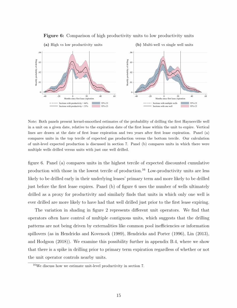
Figure 6: Comparison of high productivity units to low productivity units

(a) High vs low productivity units

0

.01

.02

.03

.04

Mon

thly

pro

babi

lity

of d

rillin

g

-40 -20 0 20 40 60Months since first lease expiration

Sections with productivity > 66%Sections with productivity < 33%

95% CI95% CI

(b) Multi-well vs single well units

0

.01

.02

.03

.04

Mon

thly

pro

babi

lity

of d

rillin

g

-40 -20 0 20 40 60Months since first lease expiration

Sections with multiple wellsSections with one well

95% CI95% CI

Note: Both panels present kernel-smoothed estimates of the probability of drilling the first Haynesville well

in a unit on a given date, relative to the expiration date of the first lease within the unit to expire. Vertical

lines are drawn at the date of first lease expiration and two years after first lease expiration. Panel (a)

compares units in the top tercile of expected gas production versus the bottom tercile. Our calculation

of unit-level expected production is discussed in section 7. Panel (b) compares units in which there were

multiple wells drilled versus units with just one well drilled.

figure 6. Panel (a) compares units in the highest tercile of expected discounted cumulative

production with those in the lowest tercile of production.16 Low-productivity units are less

likely to be drilled early in their underlying leases’ primary term and more likely to be drilled

just before the first lease expires. Panel (b) of figure 6 uses the number of wells ultimately

drilled as a proxy for productivity and similarly finds that units in which only one well is

ever drilled are more likely to have had that well drilled just prior to the first lease expiring.

The variation in shading in figure 2 represents different unit operators. We find that

operators often have control of multiple contiguous units, which suggests that the drilling

patterns are not being driven by externalities like common pool inefficiencies or information

spillovers (as in Hendricks and Kovenock (1989), Hendricks and Porter (1996), Lin (2013),

and Hodgson (2018)). We examine this possibility further in appendix B.4, where we show

that there is a spike in drilling prior to primary term expiration regardless of whether or not

the unit operator controls nearby units.

16We discuss how we estimate unit-level productivity in section 7.

15

5 An analytic model of oil and gas lease design

Section 4 presented evidence that primary terms in oil and gas leases distort firms’ decisions,

leading to bunching of drilling at lease expiration. This section presents a model that at-

tempts to shed light on why mineral owners might write leases that include a primary term,

in spite of the ex-post distortion that it may generate.

Our model is rooted in a principal-agent framework—with the mineral owner as the

principal and the firm as the agent—in which the firm possesses private information about

the expected productivity from drilling a well. This private information might reflect the

firm’s superior geologic knowledge of the subterranean formation itself, or information about

the productivity of its own drilling and completion techniques.17 The central tension in the

model lies between the owner’s desire to minimize the firm’s information rent and the desire

to not overly distort the firm’s incentives to efficiently extract the gas.

To simplify exposition and more easily distill intuition, we assume that the owner proposes

contracts to a single firm rather than to a set of competing firms. This assumption is

consistent with evidence that most owners only talk to a single firm during the leasing

process.18 Relaxing this assumption (short of going all the way to a perfectly competitive

model) would not qualitatively change our conclusions regarding the structure of the optimal

contract.19

How should the owner write the contract, assuming that it has the power to set the

contractual terms?20,21 We assume that the contract can be contingent on two ex-post out-

17Covert (2015), for instance, finds that different well completion decisions can lead to substantiallydifferent levels of production.

18A 2010 survey of mineral lessors in the Marcellus Shale in Pennsylvania found that only 21% of themspoke with more than one company before signing a lease (Ward and Kelsey 2011).

19Laffont and Tirole (1987) and McAfee and McMillan (1987) extend the single-agent Laffont and Tirole(1986) model to include competition, showing that the contract structure is unchanged (though the contractselected by the winning firm becomes “flatter” in expectation as competition increases). Similar results holdwith increased competition in Board (2007).

20Throughout the paper, we refer to an individual owner as “it”, acknowledging the fact that mineralowners can sometimes be firms or holding companies.

21As DeMarzo et al. (2005) explains, this assumption is not innocuous. If the owner holds all of thebargaining power, its optimal contract will be a contingent contract of the type discussed in this section. Ifinstead the firm holds all of the bargaining power, the equilibrium contract will involve a flat cash transferto the owner with no contingent payments. The fact that private oil and gas leases are not characterized bysimple flat payments suggests that owners have some bargaining power (e.g., via the bilateral negotiationprocess in which they can make counter offers). Mineral owners also have bargaining power because theiroutside option (in Louisiana) is to be a working interest owner in their unit, which entitles them to acontingent payment that takes the form of a call option.

16

comes that are driven by the firm’s choices: (1) the date at which the well is drilled; and

(2) the quantity of gas extracted. In practice, both outcomes are observable and verifiable

because drilling creates an obvious surface disturbance (and requires government permits)

and because gas production is metered and reported to regulatory authorities. In contrast,

we assume that the other dimensions of the firm’s “effort”—such as the quantity and quality

of its fracking inputs—and the overall drilling and completion cost are non-contractible.

Given these contractibility assumptions, our model combines features of Laffont and

Tirole (1986) and Board (2007). Laffont and Tirole (1986) presents a static model of pro-

curement contracts that are contingent on ex-post cost reports. Board (2007) models a

setting in which a principal sells a development option to an agent, where the execution date

is contractible but ex-post profits and revenue are not. Our approach combines the ex-post

cost contractibility (in our case, ex-post revenue contractibility) of Laffont and Tirole (1986)

with the dynamic option execution model in Board (2007).

5.1 Analytic model setup

The key objects in our model are as follows:

• Time is discrete and denoted by t ∈ {0, ..., T}, where T is possibly infinite. The lease

contract is set at t = 0, and then starting at t = 1 the firm can decide whether to

execute the option to drill and complete a well. The owner observes the period in

which both drilling and completion occur. Only one well may be drilled on the lease.

• e ∈ R+ denotes non-contractible completion “effort”. For instance, e may represent

the volume of fracking fluid used or engineering expenditures on well design.

• The cost of drilling and completing the well is given by c0 + c1e, where c0 and c1 are

strictly positive scalars that are common knowledge.

• θ denotes the productivity of the natural gas resource should the firm drill and complete

a well. θ is known by the firm but not by the owner.22 F (θ) denotes the owner’s rational

belief about the distribution of θ. F (θ) has support on [0, θ].

22Allowing the firm to have incomplete information about the true value of the underground reserve willnot affect the paper’s results, so long as the firm remains better-informed than the owner.

17

• y = g(e)θ(1 + ε) denotes the volume of natural gas extracted if the firm drills and

completes a well with effort e. y is contractible, and for simplicity we assume that y is

completely realized in the same period that the well is drilled and completed.23 The pro-

duction function g(e) is common knowledge and maps completion effort onto a recovery

ratio, with the properties that g : R+ → [0, 1), g(0) = 0, g′ > 0, lime→0+ g′(e) → ∞,

and g′′ < 0. Finally, ε is a mean-zero disturbance that is unknown prior to drilling by

both the owner and firm. ε is orthogonal to e and θ, and its distribution function Λ(ε)

is common knowledge.

• The gas price at time t is denoted Pt and is common knowledge. The gas price evolves

stochastically via a process that is common knowledge and has the property that Pt is

bounded above. P t denotes the entire history of prices from time 0 through t.

Both the owner and firm are risk neutral, share a common per-period discount factor δ,

and seek to maximize the expected present value of their respective cash flows. At t = 0,

the owner can offer a menu of contracts to the firm; the firm must then choose one such

contract or decline entirely (yielding a payoff of 0). The contracts can specify transfers that

are contingent on observed extraction y, the drilling and completion date t, and the history

of prices P t. After the firm selects its contract, it then faces an optimal stopping problem

regarding when to drill, and when it drills it must choose its completion effort e.

5.2 The revenue-optimal mineral lease

This section discusses the optimal contract implied by our model. We relegate its derivation—

which draws heavily from Laffont and Tirole (1986) and Board (2007)—to appendix C.

The mineral owner maximizes the expected present value of its cash flows by offering the

firm a menu of contracts that include an up-front payment due at signing and a contingent

payment that is affine in gas revenue. Specifically, the optimal contingent payment z that is

paid from the firm to the owner at well completion time τ takes the form

z(θ, Pτy) = −z0(θ) + z1(θ)Pτy, (1)

23y can be thought of as the present discounted volume of production over the life of the well, andaccordingly Pt can be thought of as the weighted average natural gas price that is expected to prevail overthe life of a well that is completed at t. We assume that a well’s production is not affected by gas priceinnovations subsequent to completion, consistent with Anderson et al. (2018) and Newell et al. (2019).

18

where z0(θ) and z1(θ) are both positively-valued, decreasing functions of θ (see equation (25)

in appendix C). Both z0(θ) and z1(θ) are zero for θ, reflecting the standard intuition that

incentives for the highest type are not distorted.

The intuition for the royalty z1(θ) on production revenue in equation (1) flows from

the linkage principle (Milgrom and Weber 1982; Riley 1988; DeMarzo et al. 2005) and has

been discussed in prior work on oil leasing (Hendricks et al. 1993; Bhattacharya et al. 2018;

Ordin 2019): Because revenue is correlated with the firm’s private information θ, the royalty

reduces the firm’s information rent by compressing the distribution of payoffs across types.

A 100% royalty is not desirable, however, because such a confiscatory royalty would result

in the drilling option never being exercised. The optimal royalty therefore strikes a balance

between reducing the firm’s information rent and minimizing distortions to the firm’s effort.

In standard mechanism design problems of this type, such as Laffont and Tirole (1986),

“effort” is one-dimensional and unobservable. In oil and gas drilling, however, it is useful

to (loosely) think of “effort” as having two dimensions: the decision of when to drill and

the decision of how much labor, capital, and material to invest in the well. The former is

straightforward for the mineral owner to observe and contract on, while the latter is not.

The essence of our result in equation (1) is that, given that the mineral owner wants to tax

natural gas revenue, it can mitigate the resulting distortions to contractible dimensions of

the firm’s effort by subsidizing them. Specifically, the owner can mitigate royalty-induced

delays in drilling by paying a subsidy z0(θ) to the firm when it drills. In the extreme, if all

dimensions of effort were contractible, the optimal mechanism would call for the owner to

pay the full cost of the well and then receive 100% of the production revenue.

5.3 Primary terms versus drilling subsidies

Oil and gas leases in practice employ a primary term in conjunction with the royalty, rather

than the subsidy and royalty combination derived above. Per intuition from Board (2007),

the royalty and subsidy in the optimal mechanism act as a Pigouvian tax and subsidy, in that

they align the firm’s profit-maximization problem with the owner’s objectives. A primary

term is qualitatively similar to a drilling subsidy, in the sense that both provide the firm

with an incentive to drill sooner than it otherwise would, given the royalty. If the future

path of natural gas prices were certain at t = 0, the two policies would be able to achieve

the same outcome. But gas prices in reality are stochastic, and per the intuition given by

19

Weitzman (1974) and Kaplow and Shavell (2002), a “quantity policy” such as a primary

term will result in an expected utility loss relative to a “price policy” that is an optimal

Pigouvian subsidy. In particular, the primary term may result in drilling occurring too soon

if realized gas prices are lower than expected, and it may result in drilling occurring too late

if realized gas prices are higher than expected.

So why use a primary term rather than the subsidy? Mineral owners’ liquidity constraints

are likely to be one practical obstacle to the subsidy. Indeed, one reason why mineral owners

contract with oil and gas firms in the first place is to address their inability to finance resource

extraction themselves.24 Even after receiving the bonus payment, it may not be possible for

the owner to guarantee the payment of a significant subsidy to the firm at a time of the

firm’s choosing.25 Alternatively, a contract involving delayed royalty payments could closely

mimic the optimal royalty and subsidy combination without requiring cash outlays by the

owner. Alberta, Canada, has recently implemented such a system, though we are not aware

of such contracts in U.S. private oil and gas leasing.26

The widespread use of primary terms may also be related to the fact that they are

“notched” policies—in the spirit of Kleven (2016)—in that they impose a discontinuous

change in the return to drilling a well just before versus just after the expiration date. As

Kleven (2016) notes, notched policies are widely used in public regulation and private con-

tracts, despite their suboptimality in standard economic models.27 Kleven (2016) speculates

that one reason behind the ubiquity of notches may be that individuals “find discrete cat-

egories simpler and more intuitive than a continuum” (p. 461). In this spirit, one might

imagine how a mineral owner might more easily process the effect of a discrete deadline on

drilling behavior than the subtler continuous and probabilistic effect of a subsidy.

Whatever factors drive the observed use of primary terms in lieu of drilling subsidies,

24Liquidity constraints would seem to be less of a concern in the case of federal oil and gas leases, butin that case there may be political and budgetary constraints to having the government fund oil and gasdrilling, particularly when the decision-making is under the control of the firm.

25This problem could be remedied by holding the part of the bonus that would be used for the subsidyin escrow until drilling occurs. But doing so would impose costs by tying up capital in a low-return accountfor potentially many years.

26In Alberta’s “modernized royalty framework”, the government computes a well-level cost al-lowance based on industry average costs and basic well characteristics. It then receives a lower roy-alty rate from each well drilled until that allowance is paid down. See https://www.alberta.ca/

albertas-royalty-framework.aspx for details.27For instance, health insurance policies typically impose open enrollment deadlines every calendar year

rather than a continuously varying penalty for delayed elections.

20

it remains to assess whether primary terms can increase mineral owners’ expected payoff

relative to a royalty-only lease. Because modeling the returns from a lease with a primary

term is not analytically tractable, we turn next to a computational model of drilling decisions,

firms’ profits, and mineral owners’ revenues. This model will let us compare how these

economic outcomes are affected by alternative lease designs, including the use of primary

terms, drilling subsidies, or neither. It will also allow us to incorporate into our analysis the

ability of firms in the Haynesville to hold an entire unit—and therefore the option to drill

multiple future wells—by completing a single well. Section 6 presents the structure of our

computational model, section 7 discusses how we calibrate it, and then section 8 presents

simulated economic outcomes from counterfactual lease designs.

6 Computational model

The goal of our computational model is to assess how different lease terms affect drilling ac-

tivity and the value that accrues to the firm and the mineral owner. This section summarizes

the structure of the model. Additional detail is provided in appendix D.28

We begin by considering a simple case, aligned with our analytic model, in which a single

mineral owner offers a lease contract to a single firm, and the lease can accommodate at

most one well. We abstract away from the problem of pooling leases into a unit by assuming

that the owner’s acreage alone is sufficient for the well. As with the analytic model, the

extraction firm has a type θ drawn from a distribution F (θ). While the firm knows θ, the

mineral owner only knows F (θ).

At the beginning of the game (t = 0), the owner makes a take-it-or-leave-it lease offer

to the firm. The contract includes a primary term T ∈ {N,∞} that specifies the period in

which the lease expires, a royalty rate k1 ∈ [0, 1] that specifies the fraction of revenues to be

paid to the owner, and a bonus R1 ∈ R+ that is paid to the owner when the firm signs the

lease. The contract may also include a subsidy for drilling S1 ∈ R+. We denote the vector

of lease characteristics χ1 = {T , k1, R1, S1}. If the firm accepts the lease offer, it pays the

bonus R1 in period t = 0 and the game continues.

In each period t = 1 to t = T , the firm chooses to drill one well or not. The payoff

28To simplify the exposition, this section ignores severance taxes, income taxes, and operating costs. Wediscuss these taxes and costs in section 7 and appendices D and E.

21

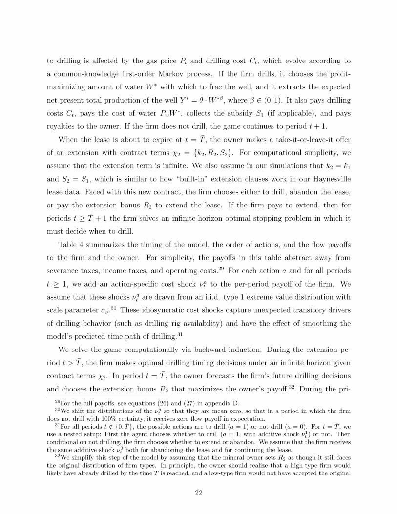
to drilling is affected by the gas price Pt and drilling cost Ct, which evolve according to

a common-knowledge first-order Markov process. If the firm drills, it chooses the profit-

maximizing amount of water W ∗ with which to frac the well, and it extracts the expected

net present total production of the well Y ∗ = θ ·W ∗β, where β ∈ (0, 1). It also pays drilling

costs Ct, pays the cost of water PwW∗, collects the subsidy S1 (if applicable), and pays

royalties to the owner. If the firm does not drill, the game continues to period t+ 1.

When the lease is about to expire at t = T , the owner makes a take-it-or-leave-it offer

of an extension with contract terms χ2 = {k2, R2, S2}. For computational simplicity, we

assume that the extension term is infinite. We also assume in our simulations that k2 = k1

and S2 = S1, which is similar to how “built-in” extension clauses work in our Haynesville

lease data. Faced with this new contract, the firm chooses either to drill, abandon the lease,

or pay the extension bonus R2 to extend the lease. If the firm pays to extend, then for

periods t ≥ T + 1 the firm solves an infinite-horizon optimal stopping problem in which it

must decide when to drill.

Table 4 summarizes the timing of the model, the order of actions, and the flow payoffs

to the firm and the owner. For simplicity, the payoffs in this table abstract away from

severance taxes, income taxes, and operating costs.29 For each action a and for all periods

t ≥ 1, we add an action-specific cost shock νat to the per-period payoff of the firm. We

assume that these shocks νat are drawn from an i.i.d. type 1 extreme value distribution with

scale parameter σν .30 These idiosyncratic cost shocks capture unexpected transitory drivers

of drilling behavior (such as drilling rig availability) and have the effect of smoothing the

model’s predicted time path of drilling.31

We solve the game computationally via backward induction. During the extension pe-

riod t > T , the firm makes optimal drilling timing decisions under an infinite horizon given

contract terms χ2. In period t = T , the owner forecasts the firm’s future drilling decisions

and chooses the extension bonus R2 that maximizes the owner’s payoff.32 During the pri-

29For the full payoffs, see equations (26) and (27) in appendix D.30We shift the distributions of the νat so that they are mean zero, so that in a period in which the firm

does not drill with 100% certainty, it receives zero flow payoff in expectation.31For all periods t /∈ {0, T}, the possible actions are to drill (a = 1) or not drill (a = 0). For t = T , we

use a nested setup: First the agent chooses whether to drill (a = 1, with additive shock ν1t ) or not. Thenconditional on not drilling, the firm chooses whether to extend or abandon. We assume that the firm receivesthe same additive shock ν0t both for abandoning the lease and for continuing the lease.

32We simplify this step of the model by assuming that the mineral owner sets R2 as though it still facesthe original distribution of firm types. In principle, the owner should realize that a high-type firm wouldlikely have already drilled by the time T is reached, and a low-type firm would not have accepted the original

22

Table 4: Game structure: Timing, actions, and flow payoffs

Lease stage: ` = 0 Time period: t = 0(1) Nature draws prices and costs(2) Owner chooses initial lease terms χ1, including T(3) Firm chooses to accept contract χ1 or not

Accepts contract:Firm payoff: −R1

Owner payoff: R1

Rejects contract:Firm payoff: 0Owner payoff: 0

Lease stage: ` = 1 Time periods: 1 ≤ t ≤ T − 1(1) Nature draws prices and costs(2) Firm chooses to drill or wait

Drills:Firm payoff: (1− k1)PtθW

∗β − Ct − PwW ∗ + S1 + ν1t

Owner payoff: k1PtθW∗β − S1

Waits:Firm payoff: ν0

t

Owner payoff: 0

Lease stage: ` = 1 Time period: t = T(1) Nature draws prices and costs(2) Owner chooses extension lease terms χ2

(3) Firm chooses to drill, pay bonus to continue, or abandonDrills:

Firm payoff: (1− k1)PtθW∗β − Ct − PwW ∗ + S1 + ν1

t

Owner payoff: k1PtθW∗β − S1

Continues:Firm payoff: −R2 + ν0

t

Owner payoff: R2

Abandons:Firm payoff: ν0

t

Owner payoff: 0

Lease stage: ` = 2 Time periods: t ≥ T + 1(1) Nature draws prices and costs(2) Firm chooses to drill or wait

Drills:Firm payoff: (1− k2)θW ∗β − Ct − PwW ∗ + S2 + ν1

t

Owner payoff: k2θY∗(θ)− S2

Waits:Firm payoff: ν0

t

Owner payoff: 0

Note: Payoffs shown here ignore taxes and operating costs, and assume there are no unleased mineral

interests. For the full payoffs, see equations (26) and (27) in appendix D.23

mary term periods t < T , the firm forecasts the extension contract terms χ2 (including the

extension bonus R2) that the owner will offer in t = T and incorporates those terms into

the expected payoff of waiting. In the initial time period t = 0 the owner anticipates future

drilling decisions and sets contract terms χ1, including the bonus R1, that maximize its

profits. Because we assume no random shocks in the initial period, there will be a threshold

type θ∗ such that all types with θ ≥ θ∗ accept the initial contract.

In appendix D.3, we discuss how we extend the model to the case of multiple wells per

unit, where a total of M wells can be drilled in the unit. In this extension, we allow the firm

to drill an additional M − 1 wells in either the same period the first well is drilled or any

period thereafter, since the initial well holds the lease by production.

7 Calibration of the computational model

This section discusses how we calibrate the computational model, including stochastic price

processes, drilling costs, the production function, and the distribution of productivity F (θ).

Our goal is to calibrate the model to a representative pooling unit in the Haynesville shale in

the first quarter of 2010, when data on wells’ production and water input become regularly

available. A summary of calibrated parameters is near the end of this section in table 5, and

appendix E provides additional detail on our calibration procedures.

Natural gas prices and rig dayrates: We calibrate the stochastic process for natural gas

prices Pt using our natural gas price data series, aggregated to the quarterly level. Following

Kellogg (2014), we assume that Pt follows a Markov process given by equation (2):

lnPt+1 = lnPt + κP0 + κP1 Pt + σPηPt+1, (2)

where the drift parameters κP0 and κP1 allow for mean reversion. We assume that price

volatility σP is constant. We estimate κP0 and κP1 by regressing lnPt+1 − lnPt on Pt, using

data from 1993 (when futures prices are first reliably liquid) through 2009. The parame-

ter estimates are shown in table 5 and imply that the long-run mean natural gas price is

$4.99/mmBtu.

contract χ1. However, allowing the mineral owner to update its beliefs in this manner would result in anintractably complicated state space and a much larger computational burden, since the type distribution atT is a function of the complete realized price and drilling cost path during the primary term.

24

Similar to the stochastic process for gas prices, we assume that rig dayrates Dt follow

the Markov process given by equation (3):

lnDt+1 = lnDt + κD0 + κD1 Dt + σDηDt+1. (3)

We assume that κD0 = κP0 and κD1 = κP1 Dt/Pt, so that dayrate mean reversion is pro-

portional to that of natural gas prices.33 These parameters imply that the long-run mean

dayrate is $9597 per day. We assume that the shocks ηDt+1 and ηPt+1 are each drawn from

an i.i.d. bivariate standard normal distribution, with a covariance matrix that we estimate

using the residuals of equations (2) and (3).

Taxes and operating costs: Louisiana imposes a 4% severance tax on Haynesville shale

wells that becomes payable after either the well has been producing for two years or the well’s

drilling costs have been paid, whichever comes first (Kaiser 2012). Following Gulen et al.

(2015), we simplify this rule by assuming a tax of 4% on production revenue and allowing

the firm to deduct drilling costs (subject to revenue exceeding costs). The severance tax

applies to both the firm’s production and the mineral owner’s royalty share.

Following Gulen et al. (2015), we use a combined state and federal marginal corporate

tax rate in Louisiana of 40.2%. We treat 50% of drilling and completion expenditures as

immediately expensable, while the remainder must be capitalized and depreciated over time

using the double declining balance method (Metcalf 2010).34 We assume that the marginal

tax rate of 40.2% also applies to the mineral owner’s royalty income. By equating the

mineral owner’s and the firm’s tax rate on revenues, we avoid building into the model any tax

advantages for shifting income from the firm to the mineral owner (or vice-versa). Moreover,

all bonus payments and drilling subsidies in our simulations can then be interpreted as

post-tax payments.35

Finally, we follow Gulen et al. (2015) by assuming that operating and gathering costs are

$0.60/mmBtu throughout the life of the well.36 We also assume that operating and gathering

33Pt and Dt denote the average price and dayrate, respectively, over 1993–2009.34The effective marginal tax rate on drilling and completion costs is then 36.8%.35In reality, the marginal tax rate faced by mineral owners is likely to be heterogeneous given underlying

heterogeneity in income from other sources. We also do not model the fact that royalties are tax-advantagedrelative to bonus payments, since the firm must capitalize bonuses but can expense royalties.

36Gulen et al. (2015) calculates operating and gathering costs of $0.55–$0.60/mmBtu for Haynesvillewells in the early years of operation, increasing thereafter as fixed operating costs are spread over declining

25

costs are fully expensable for income taxes but not severance taxes.

Production function: The production function for the cumulative lifetime gas output Yi

from well i drilled at location {loni, lati} using Wi gallons of water is:

Y (θloni,lati ,Wi) = θloni,latiWβi εi (4)

Using our well-level lifetime cumulative production estimates, discussed in section 3.2, we

estimate the coefficient β and a spatially smoothed distribution of unit-level productivities

θ by applying the difference estimator described in Robinson (1988) to the log of equation

(4). This procedure, described in detail in appendix E, yields an estimate of β of 0.19

and a set of unit-level expected log productivity values that are optimized for out-of-sample

prediction using leave-one-out cross-validation. Figure 7 displays the inputs and outputs of

this procedure. Panel (a) shows cumulative well production, averaged within each unit.37

Panel (b) shows predicted unit-level production after spatial smoothing, evaluated at the

sample mean level of water use.

Following Covert (2015), our identification assumption is that log(εi) is orthogonal to

log(Wi), conditional on θloni,lati .38 If instead there are factors affecting the marginal produc-

tivity of water that are observed by the firm but not by us, our estimate of β will be biased

upward. We therefore examine the sensitivity of our main simulation results in section 8 to

the use of a lower value for β.39

Mineral owner’s belief about the productivity distribution F (θ): We assume that

the mineral owner believes that θ is distributed lognormally with mean and standard devia-

tion parameters (on log(θ)) µθ and σθ, and we estimate these parameters from the distribution

of unit-level productivities estimated above. We estimate µθ =11.79 and σθ =0.43.40

The estimate of σθ is large in the sense that it implies that the mineral owner’s 95%

production.37See section 3.2 and appendix A.2 for a discussion of cumulative well production.38Our estimate of β of 0.19 is similar to the summed estimates of the coefficients on water and sand in

columns (3) and (4) of table 5 in Covert (2015): 0.2544 and 0.2791, respectively.39We find that the owner’s optimal royalty increases when β is smaller, in line with the intuition that when

there is less opportunity for moral hazard in water input choice, the royalty can be increased. Decreasing βhas little impact on the optimal primary term. See table 7 in appendix E.

40The estimate of µθ implies that at the calibration sample average water use of 6.0 million gallons, awell drilled in the median unit can be expected to produce 2.7 million mmBtu of gas (in present value).

26

Figure 7: Haynesville unit-level productivity

(a) Actual average production per well

Actual ln(Production)

(9.73,13.8]

(13.8,14]

(14,14.2]

(14.2,14.5]

(14.5,14.8]

(14.8,15]

(15,15.2]

(15.2,16.1]

NA

(b) Smoothed predictions of production per well

Predicted ln(Production)

(9.73,13.8]

(13.8,14]

(14,14.2]

(14.2,14.5]

(14.5,14.8]

(14.8,15]

(15,15.2]

(15.2,16.1]

NA

Note: Panel (a) is a map of Haynesville units showing the calculated present value of aggregate well pro-

duction, averaged within each unit, using decline estimation procedures discussed in section 3 and appendix

A.2. Panel (b) plots the spatially smoothed distribution of unit-level production, evaluated at the sample

mean level of water use, as discussed in section 7.

confidence interval for log(θ) encompasses an interval of ±0.84 log points around µθ. In

essence, our calculation assumes that the mineral owner knows the distribution of predicted

unit-level productivity across the entire Haynesville play but does not know where the pro-

ductivity of its own parcel falls within this distribution. This approach will over-estimate

mineral owners’ uncertainty over θ to the extent that they have at least a rough knowledge of

whether their parcel lies on a relatively productive or unproductive part of the Haynesville.

We therefore examine and discuss in section 8 how the use of smaller values for σθ affects

the optimal royalties and primary terms from our simulations.

Water price, drilling costs, and idiosyncratic cost shocks: The remaining parame-

ters to calibrate are the water price Pw, the level of drilling costs Cit and their sensitivity to

the rig dayrate Dt, and the scale parameter σν that governs the variance of the idiosyncratic

cost shocks νat . We calibrate these parameters by fitting unit-level simulations of the firm’s

drilling problem to data on actual drilling timing, water use, and costs. This procedure

uses only the components of our model needed to simulate drilling conditional on the unit’s

27

productivity, the contractual terms of the leases in the units, and the timing with which

leases expire. It does not use the model components that track the owner’s value or solve

for the owner’s optimal lease.

To calibrate these parameters, we start with our analysis sample, defined in section 3.4,

that excludes units that are held by drilling or production from non-Haynesville formations.

Within this sample, the set of units that are suitable for calibration is limited by the facts

that we do not regularly observe water use until 1Q 2010, and that data for some variables

are missing or measured with error. We therefore restrict our sample to the 891 units that

were actively leased by 1Q 2010 but in which drilling had not yet occurred by 1Q 2010, and

we then further drop units for which royalty rates, leased acreage data, or our productivity

estimates are either missing or likely to be imprecise (see appendix E for details). Our final

calibration sample then contains 160 units.41

We assume that the price of water Pw is time-invariant and estimate it using the com-

ponent of the model that computes the firm’s static drilling profits and optimal water use,

conditional on drilling. The estimated Pw is that which minimizes the mean squared distance

between profits (conditional on drilling) under optimal water use and observed water use,

across all wells in the calibration sample. Our static profit function, discussed in greater

detail in appendices D and E, accounts for each unit’s royalties and taxes, productivity, and

share of acreage that is leased, along with the gas price and rig dayrate prevailing at the

time of drilling. There are 96 drilled wells in the calibration sample, including wells beyond

the first well drilled in each unit. We estimate Pw = $0.39/gallon. This value should be

thought of as the marginal cost of not just the water itself but also the associated labor and

capital (e.g. pumping equipment) necessary to conduct the fracturing job.

To estimate the sensitivity of drilling costs to the rig dayrate, we project each well’s

reported cost Cit, less its cost of water PwWi, onto the rig dayrate Dt per equation (5):42

Cit − PwWi = α0 + α1Dt. (5)

41Units in the calibration sample may be less productive, on average, than a typical Haynesville unit dueto our selection procedure. We therefore examine the robustness of our main simulation results to increasingall units’ productivity by 33% (by increasing µθ). Table 7 in appendix E shows that our optimal royalty andprimary term are qualitatively unaffected by this change, or by decreasing productivity by 33%.

42Because our calibration sample is concentrated in just a few quarters of 2010 and 2011 (see panel (a)of figure 8) we estimate α1 using the full sample of Haynesville wells for which we have reported cost andwater input data.

28

We estimate α1 = 57 days. This value is inflated relative to actual drilling and completion

times because the rig dayrate is one of several service costs that vary over time. Our projec-

tion in equation (5) essentially treats variation in rig dayrates as an index for variation in

overall drilling and completion service costs.

Our cost data may systematically over or under-report true drilling and completion costs

(firms have an incentive to over-report, but might also be unable to credibly report some

costs such as engineering effort), so while we view these data as useful for estimating the

slope term α1, we are wary of relying on them and the projection in equation (5) for our

estimate of the drilling cost intercept α0.

Instead, we use maximum likelihood to jointly estimate the drilling cost intercept α0 and

the scale parameter σν of the cost shocks νat . For a given pair of parameters, the model

predicts the probability that the first well in each unit would be drilled in a given quarter

(or not at all). The estimator fits these probabilities to the drilling decisions observed in

our calibration sample (in which 71 of 160 units are drilled). The cost intercept α0 governs

the overall level of drilling (with higher costs reducing drilling), while the scale parameter

σν governs how drilling within and across units responds to gas price shocks, differences in

unit-level productivity, and anticipated expiration of leased acreage (with higher values of

σν reducing the sensitivity of drilling to these factors). We provide additional detail on our

log-likelihood calculation in appendix E.

We find that large cost shocks are necessary to rationalize observed drilling: our estimate

of σν is $7.0 million.43 This value reflects the fact that our model abstracts away from factors

such as rig availability, learning, and financial frictions that also affect firms’ drilling deci-

sions (Covert 2015; Agerton 2020; Fetter et al. 2018; Hodgson 2018; Steck 2018; Gilje et al.

forthcoming). Prior work that models firms’ dynamic drilling problem has also estimated

large shocks in order to fit the data (Kellogg 2014; Agerton 2020).

The large estimate of σν then drives a large estimate of the drilling cost intercept α0:

$26.0 million. Because drilling in our model is often associated with the realization of a

large negative cost shock, a large mean drilling cost intercept α0 is necessary to generate a

reasonable mean drilling cost (excluding water costs) conditional on drilling: $7.3 million.44

43The value of σν of $7.0 million is pre-tax. When we compute the model, we scale down σν for incometaxes, severance taxes, and unleased acreage, just as we do for the other components of drilling costs inequation (26) in appendix D.

44In the calibration sample, the average quarterly drilling hazard is 3.0%. The expected value of α0 plus

29

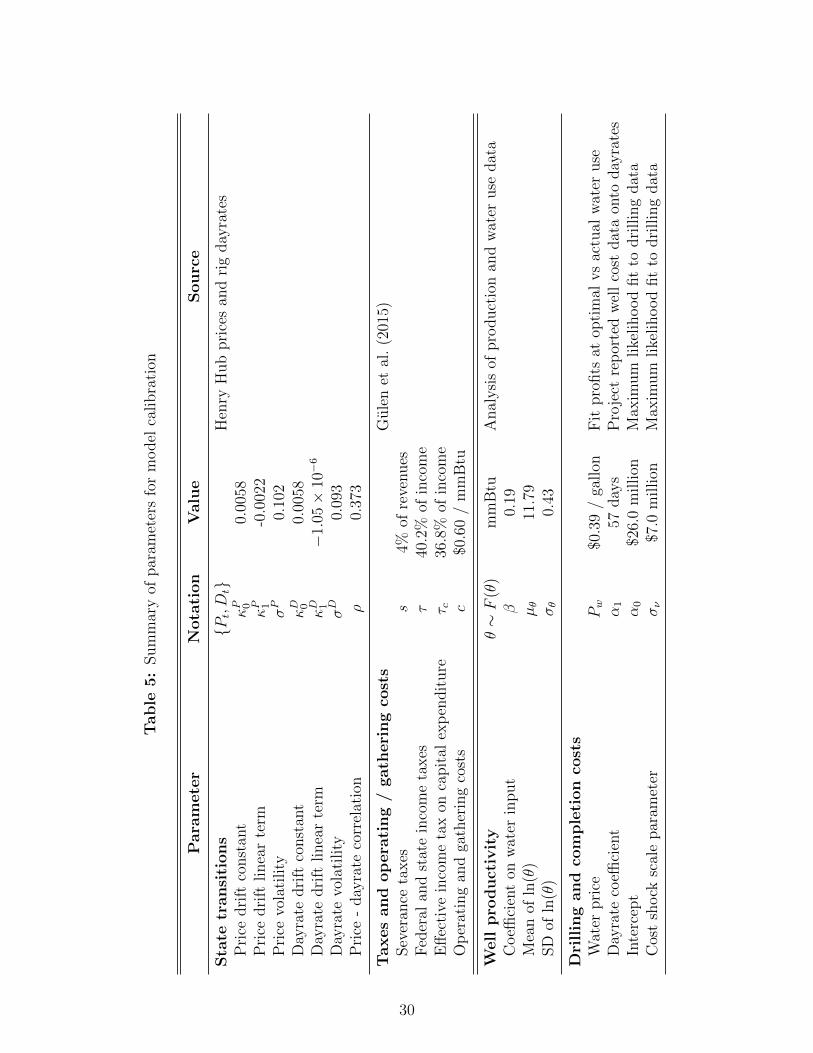
Table

5:

Sum

mar

yof

par

amet

ers

for

model

calibra

tion

Para

mete

rN

ota

tion

Valu

eS

ou

rce

Sta

tetr

ansi

tions

{Pt,Dt}

Hen

ryH

ub

pri

ces

and

rig

day

rate

sP

rice

dri

ftco

nst

ant

κP 0

0.00

58P

rice

dri

ftlinea

rte

rmκP 1

-0.0

022

Pri

cevo

lati

lity

σP

0.10

2D

ayra

tedri

ftco

nst

ant

κD 0

0.00

58D

ayra

tedri

ftlinea

rte

rmκD 1

−1.

05×

10−

6

Day

rate

vola

tility

σD

0.09

3P

rice

-day

rate

corr

elat

ion

ρ0.

373

Taxes

and

op

era

ting

/gath

eri

ng

cost

sG

ule

net

al.

(201

5)Sev

eran

ceta

xes

s4%

ofre

venues

Fed

eral

and

stat

ein

com

eta

xes

τ40

.2%

ofin

com

eE

ffec

tive

inco

me

tax

onca

pit

alex

pen

dit

ure

τ c36

.8%

ofin

com

eO

per

atin

gan

dga

ther

ing

cost

sc

$0.6

0/

mm

Btu

Well

pro

duct

ivit

yθ∼F

(θ)

mm

Btu

Anal

ysi

sof

pro

duct

ion

and

wat

eruse

dat

aC

oeffi

cien

ton

wat

erin

put

β0.

19M

ean

ofln

(θ)

µθ

11.7

9SD

ofln

(θ)

σθ

0.43

Dri

llin

gand

com

ple

tion

cost

sW

ater

pri

cePw

$0.3

9/

gallon

Fit

pro

fits

atop

tim

alvs

actu

alw

ater

use

Day

rate

coeffi

cien

tα

157

day

sP

roje

ctre

por

ted

wel

lco

stdat

aon

today

rate

sIn

terc

ept

α0

$26.

0m

illion

Max

imum

like

lihood

fit

todri

llin

gdat

aC

ost

shock

scal

epar

amet

erσν

$7.0

million

Max

imum

like

lihood

fit

todri

llin

gdat

a

30

Figure 8: Fit of calibrated model to the drilling data

(a) Time series of units drilled per quarter

2010 2011 2012 2013 2014Date

0

5

10

15

20

25

30

Wel

ls d

rille

d pe

r qu

arte

r

Simulated drilling Actual drilling

(b) Cross section of drilling vs productivity

0 0.05 0.1 0.15 0.2 0.25

Productivity coefficient (106 mmBtu)

0

0.2

0.4

0.6

0.8

1

Dri

lling

pro

babi

lity

Actual drilling Lowess fit to actual drilling Simulated drilling probability Lowess fit to simulated drilling prob

Note: Panel (a) plots the number of times each quarter in which a unit is drilled for the first time, in both the

actual data (circles) and calibrated simulation (solid line). Panel (b) plots the following unit-level variables

against the unit’s productivity coefficient θ: whether the unit was ever actually drilled (circles plotted as 0

or 1), a lowess fit to actual drilling (solid line), the simulated probability the unit is ever drilled (x’s), and a

lowess fit to the simulated probability (dashed line). Plotted data include all units in the calibration sample.

Figure 8 shows that the drilling simulated by the calibrated model fits the data reasonably

well in both the time series and cross-section, though overall simulated drilling is slightly

higher than actual drilling (77 units simulated versus 71 units actually drilled). Table 7

in appendix E assesses the sensitivity of our simulation results to smaller values of σν and

α0, finding that the model’s computed optimal royalty and primary term are qualitatively

unaffected by decreases in these parameters.

8 Results from simulation of alternative lease terms

The computational model presented in section 6 and calibrated per section 7 provides us

with a tool to evaluate how drilling outcomes, the firm’s profits, and the mineral owner’s

profits vary as a function of the lease’s contractual terms. This section focuses on how

the royalty and primary term shape drilling activity and the two parties’ payoffs, with an

emphasis on whether a finite primary term can improve both the mineral owner’s surplus and

the cost shock νat for a well with a 3.0% chance of being drilled is $7.3 million, which is similar to theintercept of $7.2 million estimated directly from projecting the cost data on dayrates per equation (5).

31

total surplus. We also study an alternative lease design—in which the owner pays a drilling

subsidy to the firm—that is more closely aligned with our analytical results in section 5.

8.1 Optimal contracts for simple units with one well

We begin by studying the mineral owner’s optimal contract for a simple lease, calibrated per

table 5, on which only a single well can be drilled. For each set of lease terms we examine,

we assume that the owner offers the firm a take-it-or-leave-it bonus payment that maximizes

the owner’s expected revenue conditional on the lease terms and the state variables (the gas

price and rig dayrate) at the time of lease signing.45 We use a lease signing date of 1Q 2010,

aligned with our calibration, at which time the gas price was $6.70/mmBtu, and the rig

dayrate was $13064 per day.

We find that the mineral owner’s expected discounted revenue is maximized with a lease

that has a 53% royalty and a 4.75 year primary term.46 This contract improves the owner’s

expected revenue by $104,000 (2.4%) relative to a lease with a 53% royalty and an infinite

primary term (which generates $4.32 million in expected value for the owner).47 Figure 9,

panel (a) shows how the owner’s expected value varies with the primary term, holding the

royalty fixed at 53%. The figure shows expected values not just for our central case in which

the gas price at lease signing is $6.70/mmBtu, but also cases in which the gas price is 33%

higher or lower. We normalize the owner’s value in each case by presenting it as a share

of the total surplus that would be delivered by the socially optimal drilling program (i.e., a

program in which drilling is not distorted by lease terms). In each case, the owner’s value is

maximized with a finite primary term, and the optimal primary term is a decreasing function

of the initial gas price.

The owner’s optimal royalty of 53% is substantially higher than the 20–25% royalty rates

typically observed in the Haynesville Shale. We believe that there are at least four factors

45Recall that the owner knows only that the productivity of the lease is distributed F (θ), so the owner’srevenues are an expectation taken over that distribution and over the future evolution of gas prices and rigdayrates.

46We find the optimal royalty and primary term via a nested search. Given a royalty, we find the discrete(and possibly infinite) primary term length that maximizes the owner’s payoff. We then search for theoptimal (continuous) royalty, optimizing the primary term at each iteration.

47The majority of the owner’s value comes from the royalty rather than the bonus. The expected bonusrevenue is $1.96 million with no primary term and $1.03 million with the optimal 4.75 year primary term.On a per-acre basis (assuming a well drains one-third of a standard 640-acre unit), these bonuses are on parwith anecdotally reported Haynesville bonus amounts of thousands or tens of thousands of dollars per acre(Bogan 2009).

32

Figure 9: Expected value to the mineral owner as a function of lease terms

(a) Owner’s value vs. primary term

0 3 6 9 12 15Primary term (years)

64

66

68

70

72

74

76

78

Val

ue to

ow

ner

(as

% o

f so

cial

ly o

ptim

al s

urpl

us)

$4.47/mmBtu$6.70/mmBtu$8.93/mmBtu

Initial gas price

(b) Owner’s value vs. drilling subsidy

0 2 4 6 8Drilling cost paid by owner ($million)

64

66

68

70

72

74

76

78

Val

ue to

ow

ner

(as

% o

f so

cial

ly o

ptim

al s

urpl

us)

$4.47/mmBtu$6.70/mmBtu$8.93/mmBtu

Initial gas price

Note: In both panels, the royalty is held fixed at 53%. In panel (a) the drilling subsidy is $0, and in panel

(b) the primary term is infinite. All expected values are shown as a percentage of the expected total surplus

from the socially optimal drilling program. See text for details.

driving our optimal royalty rate higher. First, the optimal royalty rate is closely related to

the mineral owner’s uncertainty about productivity, which is governed by the parameter σθ.

As discussed in section 7, our value of σθ is drawn from the dispersion of predicted production

across the entire Haynesville Shale. If mineral owners have at least a rough idea of whether

they are in a relatively productive or unproductive part of the shale, actual information

asymmetry is less than what we are modeling, which will lead to a lower optimal royalty.

We quantify this effect in sensitivity analyses, shown in table 7 of appendix E. When we

reduce σθ by 50% or by 75%, we find that the optimal royalty falls from 53% to 46% or 38%,

respectively. We also find that with the lower optimal royalty, the optimal primary term is

lengthened (to 5.50 or 6.25 years, respectively).

The second factor that may lead our model to predict higher-than-actual royalties is our

assumption that owners can make a take-it-or-leave-it offer to firms. Leases in the Haynesville

are instead typically negotiated, and if the firm has bargaining power the resulting royalty

is likely to be less than what we find here (and the royalty should be zero if the firm has

the ability to make a take-it-or-leave-it offer (DeMarzo et al. 2005)). Third, mineral owners

may be risk averse relative to firms, which will lead them to prefer larger bonuses over larger

royalties. Fourth, our optimal bonus calculations assume that there is only one firm to whom

33

Figure 10: Sum of the owner’s and firm’s expected values as a function of lease terms

(a) Firm + owner value vs. primary term

0 3 6 9 12 15Primary term (years)

78

80

82

84

86

88

90

92

Firm

+ o

wne

r va

lue

(as

% o

f so

cial

opt

imum

)

$4.47/mmBtu$6.70/mmBtu$8.93/mmBtu

Initial gas price

(b) Firm + owner value vs. drilling subsidy

0 2 4 6 8Drilling cost paid by owner ($million)

78

80

82

84

86

88

90

92

Firm

+ o

wne

r va

lue

(as

% o

f so

cial

opt

imum

)

$4.47/mmBtu$6.70/mmBtu$8.93/mmBtu

Initial gas price

Note: In both panels, the royalty is held fixed at 53%. In panel (a) the drilling subsidy is $0, and in panel

(b) the primary term is infinite. All expected values are shown as a percentage of the expected total surplus

from the socially optimal drilling program. See text for details.

to offer a lease. In the presence of competition in the leasing market, bonus auctions become

more effective at reducing firms’ information rents, so that the optimal royalty is reduced.

The analytic model presented in section 5 indicates that a drilling subsidy, rather than

a primary term, should be combined with the royalty to maximize the owner’s expected

payoff. Panel (b) of figure 9 shows that an optimally-set drilling subsidy, combined with

the 53% royalty, indeed outperforms the optimal primary term. At an initial gas price of

$6.70/mmBtu, a lease with an optimally-set drilling subsidy of $3.00 million improves the

owner’s payoff by $141,000 relative to a lease with a royalty only; whereas a primary term

improves the owner’s payoff by $104,000 relative to a lease with a royalty only.48

Figure 10 illustrates how the total (owner + firm) expected surplus from the lease is

affected by the primary term (panel (a)) and drilling subsidy (panel (b)), holding the royalty

fixed at 53%. These results show that primary terms and drilling subsidies can increase not

just the owner’s value but also the total surplus from a lease. In fact, the primary term

that maximizes total surplus at each initial price is nearly identical to the primary term that

maximizes the owner’s value in figure 9. Thus, even though the bunching of drilling induced

48The $3.00 million drilling subsidy is optimal at the 53% royalty associated with the optimal primaryterm. The optimal royalty and drilling subsidy combination is a 60% royalty with a $3.80 million subsidy.This combination increases the owner’s value by $165,000 relative to the 53% royalty-only lease.

34

Figure 11: Owner’s value and total surplus as a function of royalty

(a) Owner’s value vs. royalty

10 20 30 40 50 60 70 80 90Royalty rate (%)

30

40

50

60

70

80

90

100

Val

ue to

ow

ner

(as

% o

f so

cial

ly o

ptim

al s

urpl

us)

$4.47/mmBtu$6.70/mmBtu$8.93/mmBtu

Initial gas price

(b) Total surplus vs. royalty

10 20 30 40 50 60 70 80 90Royalty rate (%)

30

40

50

60

70

80

90

100

Firm

+ o

wne

r va

lue

(as

% o

f so

cial

opt

imum

)

$4.47/mmBtu$6.70/mmBtu$8.93/mmBtu

Initial gas price

Note: In both panels, the primary term is held fixed at 4.75 years, and the drilling subsidy is $0. All expected

values are shown as a percentage of the expected total surplus from the socially optimal drilling program.

See text for details.

by primary terms appears highly distortionary ex-post, these results indicate that a primary

term can increase both expected revenue and total surplus ex-ante, since it can partially

mitigate the distortions induced by the royalty.

We also consider how expected values vary with the royalty. Panels (a) and (b) of figure 11

display the owner’s value and total surplus, respectively, as a function of the royalty, holding

the primary term fixed at 4.75 years. We see that both outcomes are highly sensitive to

the royalty, and that total surplus is maximized at a royalty substantially lower than that

which maximizes the owner’s take.49 In particular, royalties that are too high cause excessive

distortions to drilling (and to production conditional on drilling), and royalties that are too

low leave the firm with large information rents.

Figure 12, panel (a) presents the per-period drilling probabilities associated with the

social optimum, the royalty-only lease, and the lease with the optimal primary term. The

royalty-only contract induces a significant delay to drilling. The contract with the primary

term partially counteracts this delay but imposes a notch in the drilling profile upon ex-

piration. The time path of drilling induced by the drilling subsidy, shown in panel (b),

49The total-surplus-maximizing royalty is not zero because at zero royalty, the large optimal bonus causesmany firm types to not accept the lease contract.

35

Figure 12: Drilling probabilities as a function of lease terms

(a) Optimal primary term

0 3 6 9 12 15Years since lease signed

0

0.005

0.01

0.015

0.02

0.025

0.03

0.035

0.04

Exp

ecte

d dr

illin

g pr

obab

ility

(qu

arte

rly)

Social optimum53% royalty, no primary term53% royalty, 4.75 year primary term

(b) Optimal drilling cost subsidy

0 3 6 9 12 15Years since lease signed

0

0.005

0.01

0.015

0.02

0.025

0.03

0.035

0.04

Exp

ecte

d dr

illin

g pr

obab

ility

(qu

arte

rly)

Social optimum53% royalty, no owner drilling payment53% royalty, $3.00m drilling payment

Note: Drilling probabilities are evaluated at the time of lease signing, with a gas price at signing of

$6.70/mmBtu. See text for details.

also partially counteracts the delay induced by the royalty and does so smoothly, without

imposing a notch in the drilling profile.

Finally, our model accounts for not only how lease terms affect drilling timing, but also

for how they affect drilling inputs and production, conditional on drilling. In the absence

of lease-induced distortions, the expected water input to a drilled well in our model is 12.5

million gallons. But under the optimal royalty and primary term combination, expected

water use conditional on drilling falls by 68% to 4.0 million gallons. This reduction in input

use causes cumulative discounted lifetime production (conditional on drilling) to decrease by

19%, from 3.54 to 2.86 million mmBtu.

8.2 Multiple wells per lease

Finally, we turn to the extended model in which each lease can accommodate multiple wells.

Figure 13, panel (a) plots the mineral owner’s expected value against the primary term

length when leases accommodate 3 wells, holding the royalty fixed at 53%. Relative to the

single-well lease case, shown in panel (a) of figure 9, the optimal primary term is longer at

all three initial prices and yields a smaller improvement in the owner’s expected value. At

the initial gas price of $6.70/mmBtu, the optimal primary term is 12.50 years and increases

36

Figure 13: Owner’s value and total surplus as a function of the primary term, with multiple-well leases

(a) Owner’s value vs. primary term

0 3 6 9 12 15Primary term (years)

64

66

68

70

72

74

76

Val

ue to

ow

ner

(as

% o

f so

cial

ly o

ptim

al s

urpl

us)

$4.47/mmBtu$6.70/mmBtu$8.93/mmBtu

Initial gas price

(b) Total surplus vs. primary term

0 3 6 9 12 15Primary term (years)

80

82

84

86

88

90

Firm

+ o

wne

r va

lue

(as

% o

f so

cial

opt

imum

)

$4.47/mmBtu$6.70/mmBtu$8.93/mmBtu

Initial gas price

Note: In both panels, leases can accommodate up to 3 wells, the royalty is held fixed at 53%, and the drilling

subsidy is $0. Drilling only the first well is necessary to satisfy the primary term requirement and hold

the lease indefinitely. All expected values are shown as a percentage of the expected total surplus from the

socially optimal drilling program. See text for details.

the owner’s value, relative to an infinite primary term, by just 0.3%. Figure 13, panel (b)

shows that primary terms are also less effective at increasing total surplus than they were in

the single-well case presented in figure 10.

There are two reasons why primary terms perform poorly for the mineral owner when

leases accommodate multiple wells. First, the primary term has no effect on the firm’s

decision to drill any well other than the first one. These later wells therefore remain delayed

in expectation due to the royalty. Second, the net cost of drilling a well at the deadline

can be much lower than the bonus payment required to extend the lease, since the bonus is

optimized to capture the value from drilling all of the potential wells, not just one of them.

Thus, the primary term will substantially increase the probability of drilling the first well—

potentially above and beyond the drilling probability at the social optimum—as shown in

the simulated drilling probabilities and hazards in figure 14.

These results perhaps help explain some mineral owners’ frustration at firms’ ability to

hold large amounts of acreage with a single well. In 2010, a group of mineral owners filed suit

against the state of Louisiana, arguing that the DNR’s 640-acre spacing rule—while perhaps

37

Figure 14: First-well drilling probabilities and hazards as a function of lease terms,when the lease accommodates multiple wells

(a) Drilling probabilities

0 3 6 9 12 15Years since lease signed

0

0.005

0.01

0.015

0.02

0.025

0.03

0.035

0.04

Exp

ecte

d dr

illin

g pr

obab

ility

(qu

arte

rly)

Social optimum53% royalty, no primary term53% royalty, 4.75 year primary term

(b) Drilling hazards

0 3 6 9 12 15Years since lease signed

0.01

0.02

0.03

0.04

0.05

0.06

0.07

Exp

ecte

d dr

illin

g ha

zard

(qu

arte

rly)

Social optimum53% royalty, no primary term53% royalty, 4.75 year primary term

Note: Drilling hazard each period is conditioned on not having drilled or let the lease expire prior

to that period, as well as on accepting the initial lease terms (i.e., paying the bonus) in the first

place. In all cases, leases can accommodate up to 3 wells, and the drilling subsidy paid by the

mineral owner is $0. See text for details.

appropriate for conventional, high-permeability formations in which a single gas well could

drain such a large area—was excessive for the Haynesville shale, where multiple wells were

required.50 In other states, where pooling unitization practices tend to be governed more by

common law than civil law, large mineral owners have moved to include aggressive “retained

acreage” clauses in their leases that strictly limit the acreage that any one well can hold,

though the precise specification of these clauses has also been the subject of litigation.51

50The plaintiffs did not prevail in court. Gatti et al. vs State of Louisiana, decided January 15, 2014.51The increased use of retained acreage clauses was discussed by industry participants at the March, 2020

Rice University Workshop on Economic and Environmental Effects of Oil and Gas. These clauses are usuallyused in combination with a “continuous development” clause that allows the firm to retain all acreage in thelease so long as it is actively drilling and completing wells. See https://www.oilandgaslawyerblog.com/

more-on-retained-acreage-clauses/ for sample language that is recommended to mineral owners. Forexamples of recent litigation, see Durrett (2017) and especially the discussion therein of Endeavor EnergyResources, L.P. v. Discovery Operating, Inc., decided by Texas’s Eastland Court of Appeals in 2014 and bythe Texas Supreme Court on April 13, 2018.

38

9 Conclusion

This paper begins by presenting evidence that primary terms embedded into mineral leases

in the Haynesville Shale in Louisiana have led to a substantial bunching distortion in firms’

drilling activity. This result raises the question of why mineral owners and firms would

include these apparently surplus-decreasing terms in their leases. The model we develop

in this paper suggests an answer: primary terms can actually improve the owner’s ex-ante

expected value by providing a complement to the royalty. The royalty reduces firms’ infor-

mation rents, and the primary term then partially mitigates the delay distortion induced by

the royalty.

Using a computational model that we calibrate to the Haynesville, we show that an

optimally-set primary term can increase both the mineral owner’s expected value and the

total (owner + firm) expected surplus from the lease. These improvements occur despite the

discontinuous drop in drilling probability that the contract induces at the primary term’s

expiration date. In line with our analytic results, we show that alternative contract designs

that use a drilling subsidy rather than a primary term can achieve additional, albeit modest,

improvements in the owner’s expected take.

We also show that conventional primary term clauses are less effective at delivering value

to resource owners when either state regulation or lease language allows a single well to hold

acreage sufficient to drill multiple follow-up wells in the future. This last result is consistent

with recent litigation initiated by Louisiana mineral owners, and with owners’ moves in other

states to adopt stricter retained acreage clauses.

This paper’s model and results could be enriched or extended in several ways in future

work. Our model abstracts away from factors such as learning and economies of scale that

impact firms’ drilling and completion productivity (Covert 2015; Agerton 2020; Fetter et al.

2018; Hodgson 2018; Steck 2018). Integrating these productivity dynamics into our model

would be computationally challenging but could reveal implications for oil and gas lease de-

sign. Our model also concentrates all bargaining power into the hands of the mineral owner.

This assumption is useful for revealing the contractual form that is most advantageous for

the owner but in practice is violated in private mineral leasing, where terms are often bilat-

erally negotiated. Theoretical advances in modeling bargaining problems with asymmetric

information that go beyond cases in which either the seller or the buyer (as in DeMarzo et al.

39

(2005)) can make take-it-or-leave-it offers would be valuable in improving our understand-

ing of private oil and gas leasing outcomes. Finally, our approach could be combined with

the modeling in Cong (forthcoming) to evaluate the economics of leases with primary terms

when the timing with which leases are initially signed is endogenous.

Extending our modeling framework to other settings is also likely to be worthwhile.

Within the oil and gas sector, expanding the geographic scope to include the other major

U.S. shale plays would permit an assessment of how royalties and primary terms have affected

aggregate U.S. oil and gas supply. Such work could examine the role of mineral leases in

driving misallocation of shale drilling across time and space in the U.S., relating to Asker

et al.’s (2019) recent work on aggregate wedges between optimal and observed global oil

extraction, and to Gilje et al.’s (forthcoming) documentation of how debt renegotiations have

distorted U.S. shale drilling. Our framework could also be used to evaluate the economics

of carbon policies in a second-best environment in which oil and gas production is already

distorted by mineral lease terms. Finally, the ideas in this paper could be extended to other

settings—such as retail franchising or intellectual property licensing—in which principals sell

time-limited development options to agents.

References

Agerton, M. (2020): “Learning Where to Drill: Drilling Decisions and Geological Quality

in the Haynesville Shale,” Working paper.

Anderson, S. T., R. Kellogg, and S. W. Salant (2018): “Hotelling Under Pressure,”

Journal of Political Economy, 126, 984–1026.

Asker, J., A. Collard-Wexler, and J. D. Loecker (2019): “(Mis)Allocation, Market

Power, and Global Oil Extraction,” American Economic Review, 109, 1568–1615.

Bhattacharya, V., A. Ordin, and J. W. Roberts (2018): “Bidding and Drilling

Under Uncertainty: An Empirical Analysis of Contingent Payment Auctions,” Working

paper.

Board, S. (2007): “Selling Options,” Journal of Economic Theory, 136, 324–340.

Bogan, J. (2009): “Boom Times at the Haynesville Shale,” Forbes.

40

Brown, J., T. Fitzgerald, and J. G. Weber (2016): “Capturing Rents from Natu-

ral Resource Abundance: Private Royalties from U.S. Onshore Oil & Gas Production,”

Resource and Energy Economics, 46, 23–38.

Chetty, R., J. N. Friedman, T. Olsen, and L. Pistaferri (2011): “Adjustment

Costs, Firm Responses, and Micro vs. Macro Labor Supply Elasticities: Evidence from

Danish Tax Records,” Quarterly Journal of Economics, 126, 749–804.

Cong, L. W. (forthcoming): “Timing of Auctions of Real Options,” Management Science.

Covert, T. R. (2015): “Experiential and Social Learning in Firms: the Case of Hydraulic

Fracturing in the Bakken Shale,” Working paper.

Covert, T. R. and R. L. Sweeney (2019): “Relinquishing Riches: Auctions vs Informal

Negotiations in Texas Oil and Gas Leasing,” Working paper.

Cramton, P. (1997): “The FCC Spectrum Auctions: An Early Assessment,” Journal of

Economics and Management Strategy, 6, 431–495.

DeMarzo, P. M., I. Kremer, and A. Skrzypacz (2005): “Bidding with Securities:

Auctions and Security Design,” American Economic Review, 95, 936–959.

Durrett, B. (2017): “Fun New Ways for Density and Proration Rules to Bust Your Lease:

Retained Acreage Clauses and “Governmental Authority” Language in the Wake of Three

Recent Texas Cases,” Paper presented at the 43rd Annual Ernest E. Smith Oil, Gas, &

Mineral Law Institute.

Fetter, T. R., A. L. Steck, C. Timmins, and D. Wrenn (2018): “Learning by

Viewing? Social Learning, Regulatory Disclosure, and Firm Productivity in Shale Gas,”

NBER working paper No. 25401.

GAO (2014): “Spectrum Management: FCC’s Use and Enforcement of Buildout Require-

ments,” GAO-14-236.

Gilje, E. P., E. Loutskina, and D. Murphy (forthcoming): “Drilling and Debt,”

Journal of Finance.

41

Gulen, G., S. Ikonnikova, J. Browning, K. Smye, and S. W. Tinker (2015):

“Production Scenarios for the Haynesville Shale Play,” SPE Economics & Management,

7.

Haile, P., K. Hendricks, and R. Porter (2010): “Recent U.S. Offshore Oil and Gas

Lease Bidding: A Progress Report,” International Journal of Industrial Organization, 28,

390–396.

Hendricks, K. and D. Kovenock (1989): “Asymmetric Information, Information Ex-

ternalities, and Efficiency: the Case of Oil Exploration,” RAND Journal of Economics,

20, 164–182.

Hendricks, K. and R. H. Porter (1996): “The Timing and Incidence of Exploratory

Drilling on Offshore Wildcat Tracts,” American Economic Review, 86, 388–407.

Hendricks, K., R. H. Porter, and G. Tan (1993): “Optimal Selling Strategies for

Oil and Gas Leases with an Informed Buyer,” American Economic Review Papers and

Proceedings, 83, 234–239.

Hiller, J. (2012): “Eagle Ford Lease Deadlines Driving Drilling,” San Antonio Express-

News.

Hodgson, C. (2018): “Information Externalities, Free Riding, and Optimal Exploration in

the UK Oil Industry,” Working paper.

Kaiser, M. J. (2012): “Profitability Assessment of Haynesville Shale Gas Wells,” Energy,

38, 315–330.

Kalnins, A. (2005): “Overestimation and Venture Survival: an Empirical Analysis of

Development Commitments in International Master Franchising Ventures,” Journal of

Economics and Management Strategy, 14, 933–953.

Kaplow, L. and S. Shavell (2002): “On the Superiority of Corrective Taxes to Quantity

Regulation,” American Law and Economics Review, 4, 1698–1734.

Kellogg, R. (2014): “The Effect of Uncertainty on Investment: Evidence from Texas Oil

Drilling,” American Economic Review, 104, 1698–1734.

42

Kleven, H. J. (2016): “Bunching,” Annual Review of Economics, 8, 435–464.

Laffont, J.-J. and J. Tirole (1986): “Using Cost Observation to Regulate Firms,”

Journal of Political Economy, 94, 614–641.

——— (1987): “Auctioning Incentive Contracts,” Journal of Political Economy, 95, 921–937.

Lin, C. C.-Y. (2013): “Strategic Decision-Making with Information and Extraction Ex-

ternalities: a Structural Model of the Multistage Investment Timing Game in Offshore

Petroleum Production,” Review of Economics and Statistics, 95, 1601–1621.

Litwak, M. (2012): Contracts for the Film & Television Industry, 3rd Edition, Silman-

James Press.

Male, F., A. W. Islam, T. W. Patzek, S. Ikonnikova, J. Browning, and M. P.

Marder (2015): “Analysis of Gas Production from Hydraulically Fractured Wells in

the Haynesville Shale Using Scaling Methods,” Journal of Unconventional Oil and Gas

Resources, 10, 11–17.

McAfee, R. P. and J. McMillan (1987): “Competition for Agency Contracts,” RAND

Journal of Economics, 18, 296–307.

Metcalf, G. E. (2010): “Investment in Energy Infrastructure and the Tax Code,” in Tax

Policy and the Economy, Volume 24, ed. by J. R. Brown, University of Chicago Press.

Milgrom, P. R. and I. Segal (2002): “Envelope Theorems for Arbitrary Choice Sets,”

Econometrica, 70, 583–601.

Milgrom, P. R. and R. J. Weber (1982): “A Theory of Auctions and Competitive

Bidding,” Econometrica, 50, 1089–1122.

Newell, R. G., B. C. Prest, and A. Vissing (2019): “Trophy Hunting vs. Manu-

facturing Energy: The Price-Responsiveness of Shale Gas,” Journal of the Association of

Environmental and Resource Economists, 6, 177–217.

Ordin, A. (2019): “Investment and Taxation: the Case of Oil and Gas in the Permian

Basin,” Working paper.

43

Patzek, T. W., F. Male, and M. Marder (2013): “Gas Production in the Barnett

Shale Obeys a Simple Scaling Theory,” PNAS, 110, 19731–19736.

Porter, R. H. (1995): “The Role of Information in U.S. Offshore Oil and Gas Lease

Auctions,” Econometrica, 63, 1–27.

Riley, J. G. (1988): “Ex Post Information in Auctions,” Review of Economic Studies, 55,

409–429.

Robinson, P. M. (1988): “Root-n-consistent Semiparametric Regression,” Econometrica,

56, 931–954.

Skrzypacz, A. (2013): “Auctions with Contingent Payments—an Overview,” International

Journal of Industrial Organization, 31, 666–675.

Smith, J. C. (1965): “Oil and Gas Leases,” Ohio State Law Journal, 26, 370–403.

Steck, A. L. (2018): “Industry Dynamics with Social Learning: Evidence from Hydraulic

Fracturing,” Working paper.

Ward, M. M. and T. W. Kelsey (2011): “Natural Gas Lessors’ Experiences in Bradford

and Tioga Counties, 2010,” Marcellus Education Fact Sheet, PennState Extension.

Weitzman, M. L. (1974): “Prices vs. Quantities,” Review of Economic Studies, 41, 477–

491.

44

Online Appendix for “The Economics of Time-Limited

Development Options: The Case of Oil and Gas Leases”

A Detail on data sources, cleaning, and merging

In this data appendix, we discuss: (1) our data sources; (2) how we estimate well declineand the present value of well cumulative production; (3) how we clean lease data and matchleases to units; and (4) how we match wells to Haynesville units.

A.1 Data sources

We gather data from the following sources:

• Publicly-available Louisiana DNR Strategic Online Natural Resources Information Sys-tem (SONRIS) data on well drilling and completions. The well-level data include spuddate, completion date, well name, formation targeted, top hole location, bottom holelocation, and lateral location shapefiles. DNR SONRIS includes a data file that listsHaynesville wells. DNR SONRIS also includes a shapefile for Haynesville units.

– Drilling cost and fracking input data. We obtain drilling cost information fromreports (“Applications for Well Status Determination”) that unit operators filewith the Louisiana DNR for the purpose of determining severance taxes. Weobtain data on fracking inputs (water use and the number of frac stages used)from well completion reports that are available from the DNR. We used manualdouble-entry to digitize this information from the raw pdf files.

• Enverus production data. Enverus takes unit-level reported monthly production datafrom the Louisiana DNR and then imputes well-level monthly production using thestart date of each well’s production.

• Enverus lease data. Enverus collects data on leases signed in Louisiana. Further detailsare below.

• Henry Hub natural gas futures prices. We obtained daily futures price data, at allavailable delivery dates, from Bloomberg.

• Enverus dayrate data. We use dayrates that correspond to the “ArkLaTx” region,for rigs with depth ratings between 10,000 and 12,999 feet (which corresponds to thedepth of the Haynesville).

A.2 Well data and production decline estimation

We identify Haynesville wells using three sources. First, for each well we see if the wellis included in an auxiliary DNR file that is limited to Haynesville wells. Second, we usethe name of the well: wells targeting the Haynesville typically have names that begin with“HA” or “HAY”. Third, we check whether the listed formation that the well targets is the

A-1

Haynesville. We denote a well as a Haynesville well if it satisfies at least one of these threecriteria. We also impose a restriction that Haynesville wells must have been spudded on orafter September 2006.

To estimate wells’ production decline, we follow Patzek et al. (2013), which derives declinecurves for shale gas formations. This paper shows that production initially declines inverselyproportional to the square root of time, and then begins to decline more quickly, at anexponential rate, once the well’s fractures interfere with one another. More precisely, weassume that cumulative production of natural gas for well i at month t takes the followingfunctional form:

mi(t) =

Mi

√t/τ if 0 ≤ t ≤ τ

Mi +Mi

2τd[1− exp(−d(t− τ))] if t > τ

(6)

where τ is the time at which the decline function changes to exponential, d is the ex-ponential decline rate, and Mi is a well-specific production multiplier corresponding to theexpected cumulative production at t = τ .52

Before estimating these parameters, we make a number of adjustments to the data. First,because a well’s production is substantially affected by the length of the lateral well leg, wenormalize the measure of cumulative production by a scalar si which is equal to 1485 metersdivided by the length of the lateral portion of the well. We drop any well with missinglateral length information or a well lateral of less than 150 meters to eliminate potentiallymisclassified vertical wells.53

We find that about 7% of wells had recompletions. As recompletions are designed torapidly increase production, we exclude from the data observations that come during orafter months in which well recompletions were performed. (When we later use our estimatesto predict total production, we assume no recompletions.)

Following Patzek et al. (2013), we limit the sample to observations that are the fourthmonth or later (t ≥ 4) because early months of production tend to be noisy. This noise isdue in part to the fact that hydrofracturing water is still being back-produced in the earlymonths of production. Similarly, for any given date with no production but in which there isproduction both before and after the date, we assume that the production process is pausedon that date and resumes when production resumes.

Rather than estimating τ directly, we use estimates from Male et al. (2015) for theHaynesville, which finds that τ is 14.16 months. We then use non-linear least squares to findthe values of Mi and d that minimize the sum of the squared differences between true andpredicted log cumulative production, as shown in equation (7).∑

i

∑t|t≥4

(logmi(t)si − log mi(t|Mi, τ, d))2 (7)

The estimated decline parameter d is equal to 0.037. The 25th, 50th, and 75th percentiles

52This functional form incorporates the structure of Patzek et al. (2013) but also imposes the requirementthat cumulative production be differentiable at t = τ .

53150 meters is a reasonable breakpoint: there are no wells with laterals between 150 and 400 meters inour data.

A-2

of the estimated Mi are 1.51 million, 2.02 million, and 2.53 million mmBtu, respectively.We then use our estimates of d and Mi to predict total discounted well production

(equation (8)). Following Gulen et al. (2015), we assume that wells have a total productionlifetime of 20 years. We use an annual discount factor of 0.909, following Kellogg (2014).Figure 7, panel (a) shows a map of our measures of the present value of total well production.Where there are multiple wells, we take an average over all wells within the unit. Units withno drilling have no shading and are labeled NA.

Yi =240∑t=1

[mi(t|Mi, τ, d)− mi(t− 1|Mi, τ, d)]δt−1 (8)

A.3 Lease data and clustering of duplicate leases within units

We downloaded, in February, 2016, raw data of oil and gas leases in Louisiana from Enverus.We keep only leases in Bienville, Bossier, Caddo, De Soto, Natchitoches, Red River, Sabine,and Webster parishes—the parishes that cover the Louisiana portion of the Haynesvilleformation. Because we ultimately map leases to units, we keep only those observations thatreport Public Land Survey System township, range and section.

We keep observations that are listed as being leases, memo of leases, lease options, leaseextensions, and lease amendments. We drop observations that are mineral rights assign-ments, lease ratifications, mineral deeds, royalty deeds, and other documents. Leases includeinformation on the grantor of the lease (typically the original mineral owner) and the grantee(the oil and gas firm that leases the land). In some cases we find that oil and gas firms arelisted as grantors, with other oil and gas firms listed as grantees. As these observations arelikely cases where the land was re-leased or subleased, we drop these observations from oursample.

We drop leases with zero or missing acreage. We also drop excess lease observations thatare perfect duplicates, leases that have lengths of fewer than 10 days, and leases in whichthe reported township, range, and section are not within the stated reported parish.

We find that in some cases, a single firm grantee has leased from multiple grantors, andthe reported acreage appears to be the total over all grantors. We identify these leases byidentifying duplicates that share the same grantee name and the same acreage, and wherethe acreage reported is unusual—i.e., is either large and/or is not equal to a multiple ofcommon lot sizes (e.g., 10 acres, 40 acres). In these cases we impute a new acreage measureby dividing the reported acreage by the number of apparent duplicates.

After taking the above steps, we find that the total leased acreage in a unit still sometimesadds up to more than the total acreage of the unit (usually 640 acres), and sometimessignificantly so. Many of these cases appear to be driven by undivided mineral interests:cases where there are multiple grantors on the same plot (e.g., husband and wife, multiplesiblings or cousins, etc), and separate observations for each grantor. In other cases it appearsthat data were entered multiple times and inconsistencies were not reconciled, so that theexcess observations were not dropped when we removed duplicates.

To identify these likely duplicates, we use an agglomerative, hierarchical clustering methoddescribed by https://stat.ethz.ch/R-manual/R-devel/library/stats/html/hclust.html.In particular, we use the hclust function within the cluster package, version 2.0.7-1, for R.

A-3

The hclust function uses information on how similar multiple observations are to each otherto determine whether they are likely duplicates. The algorithm puts observations that arelikely duplicates into the same “cluster”; from there we use proportional downweightingof all observations within the same cluster to obtain updated acreage. This method relieson constructing some kind of measure of similarity between any two observations i and j.Depending on the threshold level of similarity that the researcher imposes, the number ofclusters can range from the total number of observations (no clustering) to 1 (all observationsare placed within the same cluster).

This similarity measure we use is a Euclidean-like distance measure in which the distancebetween observation i and observation j takes the form:

dij =

√∑k

wkmk(xki , xkj ) (9)

Here k indexes characteristics of the observation—e.g., grantor name, the start date ofthe lease, the acreage, the reported royalty rate, etc. The function mk is a function thatdetermines how similar two observations are, and is equal to 0 if identical, and positiveotherwise. Depending on the characteristic, we use different types of mk functions:

• mk(xki , x

kj ) = (xki − xkj )2 for some numerical characteristics like the start date of the

lease. Prior to inputting variables xk into this function, we standardize them so thatthey have a mean of zero and standard deviation of one.

• mk(xki , x

kj ) = 1(xki 6= xkj ) for other numerical and binary characteristics like reported

royalty rate, acreage, and whether there is an extension option.

• mk(xki , x

kj ) is a fuzzy match score for string characteristics like grantee name and

grantor name. We use the partial ratio function from the fuzzywuzzy Python package,version 0.16.0. The partial ratio function uses Levenshtein distance augmented withpartial string matching. It allows us to identify cases where some subsets of wordswithin strings match or nearly match, even if the length of the two strings is verydifferent. This technique is useful for catching cases with identical last names butdiffering or missing first names. We scale this measure so that it ranges from 0 to 1.

For cases where information is missing, we set a value of mk = 0.4 if both observationsare missing and mk = 0.7 if only one observation is missing.

wk are positive weights. We set wk = 1 for all characteristics other than acreage, forwhich we set wk = 100.54 This weighting ensures that leases that vary in acreage will not bepresumed to be duplicates.

How many observations are clustered together depends on the threshold level of similarityimposed by the researcher. To determine our threshold, we choose a calibration date of

54In an alternative specification, we set wk = 1/2 for grantor name and wk = 2 for grantee name. Thisspecification is motivated by the facts that grantor names can potentially differ substantially for siblings ifthey change their names through marriage, and that there is little variation in grantee name within units.Results using this approach are similar to what we obtain from our baseline specification with equal weightson grantor and grantee names.

A-4

January 1, 2010, examining only the leases that were active on that date.55 We first examineevery possible threshold that could be used to cluster the leases in each unit. For eachpossible threshold, we find the resulting clusters, downweight each lease’s acreage by thetotal number of observations in its cluster, and then compute what total leased acreagewould be within the unit. Then, for each unit, we find the threshold would be that wouldset total acreage leased to be equal to or just less than the total unit area. We refer to thisthreshold as the unit-level threshold height. We then set our preferred overall threshold tobe equal to the 90th percentile of all the unit-level thresholds.56 The threshold height thatresults from this computation is 2.004.

We then apply the clustering procedure, using this threshold, to each unit and eachquarterly date of our sample, ranging from January 1, 2005 to January 1, 2016. Thisprocedure gives us lease by date-specific downweights. We find that in some cases leasedownweights vary depending on the date. For example, a lease may be in a cluster of fiveon April 1, 2010 but a cluster of six July 1, 2010—resulting in a downweight of 1/5 for April1, 2010 and a downweight of 1/6 for July 1, 2010. In these situations, we take the inverse ofthe arithmetic average of the inverse downweight over all quarterly dates to obtain a masterdownweight for each lease (yielding, in this example, a weight of 1/5.5).

In some outlier unit-quarters we find that even with this downweighting, total leasedacreage still exceeds section acreage. In these cases we then proportionally reduce the areaof all leases in the unit so that total leased acreage is equal to total unit acreage in the mostheavily leased quarter.

A.4 Matching of wells to units

To match wells to units, we use information on the reported laterals, reported bottom holes,and reported top hole locations. If, for a given well, the data only report top hole location,we use the location of the top hole to identify which unit the well is in. If the data reportbottom hole but not lateral information, we use the location of the bottom hole to identifywhich unit the well is in. If the data report lateral information, we use the unit that thelateral runs through to identify the well’s unit.

In a few instances, the well lateral intersects multiple units. There are two possiblereasons for these occurrences. One is that the well’s top hole is located in a different unitthan the unit the well extracts from, for the purpose of sharing a well pad with other wellsor to give sufficient space to accommodate the curvature of transitioning from the verticalto the horizontal while still extracting from a maximum area within the targeted unit. Asecond reason is that the well actually targets multiple units. In cases where a well borepasses through multiple units, we only match a well to a unit if at least 300 meters of thehorizontal well bore pass through the unit.

55We find that using other calibration dates gives similar results. We use January 1, 2010, as it was ata period of peak leasing, and therefore a period in which it is most likely that most of a section had beenleased. Leases whose primary terms would have expired but may have been extended are not included inthis group.

56We find similar results if we use a threshold height of 85%. We find that using the 100th percentileis not feasible as some outlier units have leases with large acreage such that total leased acreage is alwaysgreater than unit acreage unless leases of different acreage are combined into the same cluster.

A-5

B Additional empirical analysis

This appendix presents additional empirical results relating to the bunching analysis pre-sented in section 4.

B.1 Bunching analysis

To test the statistical significance of the drilling bunching shown in figure 4, we use a bunchingestimator similar to that of Chetty et al. (2011). We take time of spud relative to first leaseexpiration date, discretize it to the quarterly level, and compute total wells spudded (acrossall units in our analysis sample) for each quarter (34 quarters in total). We create someindicator variables for whether the spud date is two quarters before lease expiration (pre 2),one quarter before lease expiration (pre 1), one quarter after lease expiration (post 1), andtwo quarters after lease expiration (post 2). We also add similar variables for spud timingrelative to the extension expiration date (pre ext2, pre ext1, post ext1, and post ext2).

We then estimate a regression of the form:

ct = f(t) + β1 · pre 2 + β2 · pre 1 + β3 · post 1 + β4 · post 2

+ β5 · pre ext2 + β6 · pre ext1 + β7 · post ext1 + β8 · post ext2 + εt(10)

where ct is total well count, t is quarter, and f(t) is a polynomial of degree 9. Our mainregression estimates are in column (1) of table 6. The estimates of β1, β2, β5, and β6 areall statistically significant with p-values less than 0.05, indicating that there is significantlymore drilling in the two quarters prior to the primary term expiration and the two quartersprior to any extension term expiration. Column (2) of table 6 uses the same empiricalspecification as column (1) except that the dependent variable is the log of the count ratherthan the count, and results are similar. For a sense of magnitude, the estimate of β2 (thecoefficient on “pre 1”) in column (2) means that the actual number of wells drilled is 1.1 logpoints larger than the polynomial fit in the quarter prior to expiration. In figure 15, we plotour data and the number of wells predicted by our polynomial fit, which graphically displaysthe size of the bunching effect.

We also explore the possibility that these high spikes in drilling are being driven byother factors that might affect drilling in particular time periods. For instance, one mightworry that periods with substantial lease expirations might coincide with periods in whichgas prices or industry-wide productivity is high. To address this possibility, we construct ameasure of total spud counts at the calendar quarter by quarter of lease level. For example,one observation in this count data will be the total number of spuds in 2010 quarter 3when the spud happened between 3 and 6 months before the first primary term is set toexpire. Columns (3) and (4) of table 6 use the same empirical specification as columns (1)and (2), only with this more disaggregated data. Columns (5) and (6) then use the samedisaggregation as columns (3) and (4), but also add in calendar-time quarter fixed effects.Across columns (3) and (5), the coefficient on pre 1 is large, statistically significant, andsimilar in magnitude, implying that the high drilling before the expiration date is not beingdriven by high drilling at particular calendar dates. The same holds in logs for columns (4)and (6).

A-6

Table 6: Bunching estimates

count log(count) count log(count) count log(count)pre 2 12.72 0.40 1.06 0.19 1.02 0.21

(5.25) (0.21) (0.88) (0.30) (0.82) (0.30)pre 1 60.94 1.10 3.91 0.78 3.99 0.88

(5.71) (0.21) (1.36) (0.29) (1.29) (0.29)post 1 6.03 0.31 0.31 -0.07 0.44 0.04

(5.74) (0.21) (0.77) (0.28) (0.70) (0.27)post 2 -8.92 -0.09 -0.50 -0.21 -0.53 -0.17

(5.32) (0.19) (0.61) (0.25) (0.58) (0.25)pre ext2 13.70 0.26 1.24 0.52 1.39 0.53

(4.75) (0.19) (1.11) (0.34) (1.05) (0.34)pre ext1 21.73 0.52 1.79 1.19 1.93 1.15

(5.23) (0.22) (1.26) (0.31) (1.16) (0.31)post ext1 -4.99 -0.24 -0.32 -0.05 -0.23 0.04

(5.19) (0.21) (0.72) (0.32) (0.72) (0.32)post ext2 -3.70 -0.11 -0.26 0.28 -0.15 0.41

(4.61) (0.17) (0.64) (0.30) (0.67) (0.37)Quarter of lease X XQuarter by quarter of lease X X X XFixed effects X XR Squared 0.97 0.93 0.24 0.3 0.42 0.44Observations 35 30 363 235 363 235

Note: Table presents estimates of equation (10). Newey-West standard errors, computed with two quarterly

lags, are in parentheses. Estimates in columns (1) and (2) use data that are aggregated to the lease-level

quarter, which is defined as the time between first primary term expiration and spudding, measured at

quarterly intervals. Estimates in columns (3) through (6) use data that is aggregated to the lease-level

quarter by calendar-level quarter. That is, these columns aggregate wells drilled that share both a common

lease-level quarter and a common calendar quarter-of-sample. Estimates in columns (5) and (6) include

calendar quarter fixed effects.

B.2 Drilling inputs and outputs as a function of drilling time

This appendix examines how wells’ natural gas production, water inputs, and reporteddrilling costs vary depending on whether drilling is done early, just prior to the first pri-mary term expiring, or after the first primary term expires. Figure 16, panel (a) plots thelogged first 12 months of each unit’s first well’s gas production against the date of drillingrelative to the date that the first primary term expires. Panels (b) and (c) present similarinformation, but with water use and reported drilling costs as the outcome variables, respec-tively. Over all three plots, the data are noisy, and there is no strong relationship betweenthe outcome variables and drilling timing, apart from a slight downward trend over time. Inparticular, wells drilled just before first lease expiration are not especially unproductive anddo not use especially low levels of inputs.

A-7

Figure 15: Estimates from bunching analysis

0

20

40

60

80

100

Num

ber o

f wel

ls sp

udde

d

-12 -4 4 12 20Time in quarters since first lease expiration

Wells spuddedBunching fixed effects quartersPolynomial fit excluding bunching fixed effects

Note: Figure presents data and estimates corresponding to the bunching analysis in

column (1) of table 6. Plotted data include counts of wells spudded, the quarters to

which we add bunching fixed effects, and the polynomial predicted probabilities given

the bunching estimator fixed effects. Timing is relative to the expiration date of the

first lease within the unit to expire. Vertical lines are drawn at the date of first lease

expiration and two years after first lease expiration.

B.3 Distribution of the expiration dates of leases

The vast majority of units have multiple leases on them. Typically, leases are signed atdifferent dates, and therefore the primary terms tend to end on different dates. In thissubsection, we show that the distribution of the expiration dates affects the extent to whichdrilling responds to the expiration of the first lease in a unit.

For each unit, we calculate the amount of time from when the first lease expires to thetime at which 50% of all acreage would expire. We refer to this duration as time-to-50%-expiration. We then compare drilling for units with above-median time-to-50%-expirationto units with below-median time-to-50%-expiration. Figure 17 shows that units with above-median time-to-50%-expiration have a less-pronounced spike in drilling in the few monthsprior to the first lease expiring. This result is consistent with the theory that if most of theleases in a unit do not expire for some time after the first lease expires, there is a reducedincentive for the firm to drill prior to the first expiration.

B.4 Information externalities and common pools

One alternative explanation for the drilling patterns we observe is a cross-unit informationor common pool externality. Common pool externalities might lead to a race to drill. In-formation externalities might lead to a reluctance to drill, as firms wait to learn from other

A-8

Figure 16: Wells’ production, water use, and cost vs. time relative to first lease expiration

(a) First 12 months of gas production (log mmBtu)

12

13

14

15

16

log

first

12

mon

ths g

as p

rodu

ctio

n

-1000 -500 0 500 1000first spud - first lease expiration in days

(b) Water use (log gallons)

14.5

15

15.5

16

16.5

log

tota

l wat

er

-1000 -500 0 500 1000first spud - first lease expiration in days

(c) Reported drilling and completion cost (log $2014)

15.8

16

16.2

16.4

16.6

log

wel

l cos

t

-1000 -500 0 500 1000first spud - first lease expiration in days

Note: Data are for the first well drilled in each unit. The horizontal axis is measured in days

relative to the first lease expiration that the well was spudded. The line is the predicted value

from a local polynomial regression.

firms’ drilling outcomes. To examine whether such externalities might be driving our results,we compare units in which most of the unit’s neighbors are operated by the same operatorwith units in which most of the neighbors are operated by a different operator. The formershould be less susceptible to externalities than the latter. We define neighboring units asthose for which the centroids of the two units are within 1.2 miles (results are similar whenusing a threshold of 1.7 miles, which will include the diagonal units).

In figure 18, panel (a) we compare drilling probabilities for these two types of units,using our analysis sample described in subsection 3.4. For both types of units, we observesubstantial bunching of drilling just before the first lease in the unit expires, leading us toconclude that cross-unit externalities are not a substantial driver of our results. Because theanalysis sample has few units in which ≥ 50% of neighboring operators are the same, panel(b) uses the full set of Haynesville units that had drilling. It finds similar results.

A-9

Figure 17: Comparison of units with more vs less time before most acreage expires

0

.01

.02

.03

.04

Mon

thly

pro

babi

lity

of d

rillin

g

-40 -20 0 20 40 60Months since first lease expiration

Longer time to 50% of leases expiringShorter time to 50% of leases expiring

95% CI95% CI

Note: Figure shows kernel-smoothed estimates of the probability of drilling the first Haynesville

well in a unit on a given date, relative to the expiration date of the first lease within the unit to

expire. Vertical lines are drawn at the date of first lease expiration and two years after first lease

expiration. “Longer (shorter) time to 50% of leases expiring” corresponds to units with an above

(below)-median time between when the first lease expires and 50% of all acreage expires.

Figure 18: Comparison of units with identical vs different neighboring operators

(a) Units in analysis sample

0

.01

.02

.03

.04

.05

Mon

thly

pro

babi

lity

of d

rillin

g

-40 -20 0 20 40 60Months since first lease expiration

≥ 50% of neighbors are same operator< 50% of neighbors are same operator

95% CI95% CI

(b) All Haynesville units

0

.01

.02

.03

.04

Mon

thly

pro

babi

lity

of d

rillin

g

-40 -20 0 20 40 60Months since first lease expiration

≥ 50% of neighbors are same operator< 50% of neighbors are same operator

95% CI95% CI

Note: Figure shows kernel-smoothed estimates of the probability of drilling the first Haynesville

well in a unit on a given date, relative to the expiration date of the first lease within the unit to

expire. Vertical lines are drawn at the date of first lease expiration and two years after first lease

expiration. Figure compares units in which most of the nearby units have the same operator vs.

units where most of the nearby units have a different operator. Neighboring units are defined as

those with centroids within 1.2 miles of the centroid of the given unit. Panel (a) limits the units

to our analysis sample, as described in subsection 3.4. Panel (b) uses all Haynesville units.

A-10

C Derivation of the optimal contingent contract for

the mineral owner

This appendix derives the optimal contract for the principal (mineral owner), given themodel setup from section 5.1. The exposition below closely follows parts of Laffont andTirole (1986) and Board (2007). To facilitate the derivation of the optimal contract, wefollow the standard approach of considering a direct revelation mechanism in which the firmreports a type θ and is then assigned an up-front “bonus” transfer of R(θ) at t = 0 and acontingent payment zt(θ, y, P

t) to be paid when the option is executed. For now, we allowthis payment to be contingent on the reported type, ex-post production, and the price historyup to execution, though in practice conditioning only on the first two arguments and theprice at execution will be necessary for optimality.

C.1 Firm’s problem

The firm must make three decisions, in sequence:

1. Report a type θ to the owner at t = 0 (or opt-out)

2. Choose a time τ ∈ {1, ...T} at which to exercise the option to drill, where τ = ∞signifies not drilling.

3. Conditional on drilling, select an effort level e ∈ R+

Let τ ∗(θ, z) denote a decision rule that dictates whether the well should be drilled in eachperiod t given the gas price Pt (we suppress the dependence of z on θ, y, and P t). The firm’sproblem, conditional on participation, is then given by

maxθ,τ∗(θ,z),e

Π(θ, τ ∗(θ, z), e, θ) = EP [(Pτg(e)θ − (c0 + c1e)

− zτ (θ, g(e)θ(1 + ε), P t))δτ ]−R(θ), (11)

where EP is the expectation at the start of period 0, taken over all prices. Note thattotal surplus is maximized by the solution to (11) when the transfers z and R are set to zero.

From the definition of g(e) in section 5.1, it is clear that the effort selection problem hasa unique, interior solution. In addition, the decision rule τ ∗(θ, z) will be given by an optimalstopping rule.57

We restrict attention to truth-telling mechanisms that induce the agent to report θ = θ.Let τ(θ) and e(θ) denote the timing rule and effort function that correspond to the optimaltruthful mechanism. Because drilling is observable, τ(θ) can be imposed by the owner.For truth-telling to be incentive compatible, it must be the case that e(θ) (which is notcontractible and therefore cannot be imposed) is the optimal effort level for the firm, subjectto the mechanism.

57Board (2007) proves the existence of such a rule for the case in which effort e is fixed. Existence inour model follows the same proof, with the assumptions that Pt and g(e) are bounded above replacing theBoard (2007) assumption that costs are bounded below.

A-11

To characterize the firm’s ability to deviate from e(θ) and thereby reap informationrent, we follow Laffont and Tirole (1986) by first restricting our attention to deviations in aconcealment set in which, for any report θ, the chosen effort e is such that g(e)θ = g(e(θ))θ.Thus, absent uncertainty generated by ε, any deviation outside the concealment set can bedetected by the owner.58

Within the concealment set, the firm’s choice of report θ determines the firm’s effort levele. Define an inverse production function H(E) by g(H(E)) = E. The derivatives of g andH are related by H ′(g(e)) = 1/g′(e). The firm’s problem may then be written:

maxθ

Π(θ, θ) = EP [(Pτ(θ)g(e(θ))θ − (c0 + c1H(g(e(θ))θ

θ))

− zτ(θ)(θ, g(e(θ))θ(1 + ε), P τ(θ)))δτ(θ)]−R(θ). (12)

To obtain the marginal information rent for a firm of type θ, we need the derivative ofΠ(θ, θ) with respect to θ. Using the envelope theorem, this marginal rent is given by thepartial derivative:59

∂Π(θ, θ)

∂θ

∣∣∣∣θ=θ

= EP

[c1g(e(θ))δτ(θ)

g′(e(θ))θ

](13)

Equation (13) is the first-order incentive compatibility condition. The second ordermonotonicity condition is given by

∂Π(θ, θ)

∂θ∂θ≥ 0. (14)

From equation (13), it is apparent that the mechanism will satisfy this condition if theoptimal stopping time is decreasing in θ and ∂e(θ)/∂θ ≥ 0.

To see that satisfaction of equation (14) is sufficient for incentive compatibility, considera type θ firm that deviates to report type θ 6= θ. We have:

Π(θ, θ) = Π(θ, θ) +

∫ θ

θ

∂Π(θ, s)

∂θds

≤ Π(θ, θ) +

∫ θ

θ

∂Π(s, s)

∂θds

= Π(θ, θ), (15)

where the second line follows from the monotonicity condition.Given incentive compatibility, integration of equation (13) yields the firm’s information

58In the presence of a non-degenerate distribution Λ(ε), the sufficiency condition for implementing themechanism will be stricter than the conditions given below that the optimal stopping time is decreasing inθ and that ∂e(θ)/∂θ ≥ 0 (also see footnote 61).

59Following Board (2007), we use generalised envelope theorem of Milgrom and Segal (2002) because thespace of stopping times is more complicated than R+.

A-12

rent:

Π(θ, θ) = EP

[∫ θ

θ

c1g(e(s))δτ(s)

g′(e(s))sds

], (16)

where θ denotes the lowest type that participates, so that Π(θ, θ) = 0.

C.2 Revenue-maximizing contract for the owner

Continuing to follow Laffont and Tirole (1986) and Board (2007), we treat the owner’sproblem as an optimal control problem in which the objective is to find τ(θ) and e(θ) suchthat the expectation of total surplus minus information rent is maximized. We thereforewrite the owner’s problem as

maxτ(θ),e(θ,P ),θ

∫ θ

θ

[EP (Pτg(e(θ))θ − c0 − c1e(θ)) δ

τ(θ) −∫ θ

θ

c1g(e(s))δτ(s)

g′(e(s))sds

]f(θ)dθ, (17)

where the owner also chooses the type θ for which the individual rationality constraint bindswith equality.

To eliminate the double integral, we can use Fubini’s theorem. Letting h(θ) ≡ f(θ)/(1−F (θ)) denote the hazard function, we re-write the owner’s problem as:

maxτ(θ),e(θ,P ),θ

∫ θ

θ

EP

[(Pτg(e(θ))θ − c0 − c1e(θ)−

c1

θh(θ)

g(e(θ))

g′(e(θ))

)δτ(θ)

]f(θ)dθ. (18)

At this point, it is useful to recall the firm’s problem, equation (11). Following the logicin Board (2007), the owner can induce the firm to follow the stopping rule implied by (18) bysetting the contingent payment z equal to the information rent term in (18), since doing somakes the firm’s problem equivalent to the owner’s problem. Thus, the revenue-maximizingcontingent payment is given by:60

zτ (θ, y, Pt) =

c1

θh(θ)

g(e(θ))

g′(e(θ)). (19)

The optimal contingent payment z from the firm to the owner is positive, which will leadto delayed drilling relative to the social optimum. Note that the optimal payment is zerofor the highest type θ firm because 1/h(θ) = 0, reflecting the standard “no distortion atthe top” rule. The optimal up-front payment R(θ) is set to equate the firm’s utility to theinformation rent expressed in equation (16), where the utility of the endogenously chosentype θ firm is set to zero.

60The owner’s optimal timing and effort functions as defined by equations (18) and (20) will satisfy thefirm’s second order conditions (the optimal stopping time is decreasing in θ and e′(θ) ≥ 0) if the hazard rateis monotonically increasing (h′(θ) ≥ 0) and if g′′′ ≤ 0. To see this sufficiency, observe that the total derivativeof the term in parentheses in (18) is strictly increasing in θ, via application of the envelope theorem to thefirm’s problem. Thus, per Lemma 1 in Board (2007), the optimal stopping time is decreasing in θ. Second,take the derivative of (20) with respect to θ and collect terms involving e′(θ). It then becomes apparent thath′(θ) ≥ 0 and g′′′ ≤ 0 are sufficient for e′(θ) > 0.

A-13

The presence of a contingent payment upon execution of the option echoes Board’s (2007)result. What differs here is that the optimal payment is contingent not just on drilling butalso on effort. Because effort is not observable to the owner, this optimal mechanism mustbe implemented using a payment that is contingent on production y rather than effort itself.Paralleling Laffont and Tirole (1986), we now examine an implementation that involves anaffine contingent payment: a lump sum transfer combined with a linear tax on production.The appeal of an affine payment is that its optimality is robust to the distribution of thedisturbance ε. The downside is that the sufficient conditions for incentive compatibility willbe stronger than those discussed in section C.1 above, since the affine payment structureconstrains punishments for deviations outside of the concealment set.61

To derive the optimal linear production tax, we first take the pointwise derivative of (18)with respect to e(θ) to obtain the FOC that defines the owner’s optimal effort function,conditional on drilling at τ . Suppressing the dependence of g(e(θ)) and its derivatives on θ,this FOC is given by:

FOCe(θ) : Pτg′θ − c1 −

c1

θh(θ)

g′2 − gg′′

g′2= 0 (20)

In FOC (20), the last term will be positive due to the assumption that g′′ < 0, and thefirst two terms together will equal zero at the socially optimal effort level. Thus, for equation(20) to hold, e(θ) must be strictly less than socially optimal effort except for type θ, wherethe fact that 1/h(θ) = 0 implies that the highest type firm will exert optimal effort. Again,this is the standard “no distortion at the top” result.

To obtain the optimal production tax, we return to the firm’s problem, taking the deriva-tive of equation (11) with respect to e to derive the firm’s FOC for its optimal effort, condi-tional on drilling at τ :

FOCe : Pτg′θ − c1 −

∂zτ (θ, y, Pt)

∂yg′θ = 0 (21)

Combining equations (20) and (21) yields the linear tax on production that aligns thefirm’s incentives with the effort function that the owner wishes to induce:

∂zτ (θ, y, Pt)

∂y=

c1

θ2h(θ)g′g′2 − gg′′

g′2

=c1

θ2h(θ)g′

(1− gg′′

g′2

)(22)

We can now solve for the optimal affine contingent payment using equations (19) and(22):

zτ (θ, y, Pt) =

c1

θh(θ)

g

g′+

c1

θ2h(θ)g′

(1− gg′′

g′2

)(y − gθ) (23)

61The sufficient conditions for incentive compatibility of the affine contingent payment (equation (25))are difficult to characterize in terms of primitives. In the event that they are not satisfied, the owner willneed to “iron” over regions in the type space where incentive compatibility does not hold.

A-14

Rearranging, we obtain:

zτ (θ, Pt, y) =

c1g

θh(θ)g′gg′′

g′2+c1(1− gg′′

g′2)

θ2h(θ)g′y (24)

Finally, we may use equation (21) to eliminate c1 in equation (24) and obtain:

zτ (θ, Pt, y) =

gg′′Pτgθ

θh(θ)g′2 + g′2 − gg′′+

(g′2 − gg′′)Pτyθh(θ)g′2 + g′2 − gg′′

(25)

Equation (25) corresponds to equation (1) in section 5.2 of the main text. The secondterm in (25) is a positive tax on revenue Pτy; i.e., a royalty. The first term is negative(because g′′ < 0) and represents a payment from the owner to the firm at the time of drillingthat is not dependent on output. The affine implementation of the optimal mechanismtherefore taxes natural gas production and subsidizes drilling, where the tax and subsidyrates are type-dependent. The up-front bonus payment R(θ) is used to capture the remainderof the available surplus, net of information rents.

D Computational model details

This appendix describes the model from section 6 in greater detail.The model has five state variables. The first is the firm’s type, θ, which is known to

the firm but not to the mineral owner. The second is the stage ` the lease is in and theassociated contract characteristics χ`. The third is the period, t, which directly affects thefirm’s continuation payoffs during the primary term. The fourth is the time-specific naturalgas price Pt, and the fifth is the expected drilling and completion cost Ct, both of whichevolve stochastically. We use the subscript triplet {`, t, θ} to denote the three deterministicstates, and we explicitly list the stochastically-evolving states. That is, V a

`,t,θ(Pt, Ct) denotesthe expected value to the firm of taking action a given lease regime χ`, time t, firm type θ,and the current gas price and drilling cost {Pt, Ct}.

D.1 Well payout and the static profit function

The static drilling profits accruing to the firm differ depending on whether its profits beforetaxes, royalties, and operating costs are positive (i.e., whether the well “pays out”). Asdiscussed in section 2, unleased mineral interests are not liable for well costs if the well failsto pay out. In addition, severance taxes are waived. These rules create a kink in the profitfunction at the payout point. This kink also affects the optimal amount of water use, sincethe firm’s first-order condition that determines optimal water use will depend on whetherthe firm expects the well to pay out or not.

If a well drilled at time t “pays out”, its profits are given by equation (26):

πt(W ) = (1− τ)(γ(1− s)(1− k)Pt− c)θW β − γ(1− s+ sk)((1− τ)PwW + (1− τc)Ct) (26)

where γ denotes the share of acreage leased, s denotes the severance tax, k denotes the

A-15

unit’s royalty,62 c denotes operating expenses, Ct denotes drilling and completion costs otherthan water use, τ is the income tax rate, and τc is the effective income tax rate on capitalexpenditure.

If the well does not pay out, the firm does not pay severance taxes or make payments tounleased mineral interests, so that profits are instead given by equation (27):

πt(W ) = (1− τ)((1− γk)Pt − c)θW β − ((1− τ)PwW + (1− τc)Ct) (27)

Given the parameter inputs to the static profit function, we determine the optimal wateruse W ∗ by first finding the values W+ and W− that maximize equations (26) and (27),respectively. If W+ results in positive payout, we set W ∗ = W+. Alternatively, if W− resultsin negative payout, we set W ∗ = W−. Finally, it is possible that W− results in positive payoutwhile W+ results in negative payout. In that case we interpolate the value of W ∗ ∈ (W+,W−)that results in zero payout.

Given W ∗, we then compute the firm’s static drilling profits using either equation (26)or equation (27), depending on the payout condition.

D.2 Solving the dynamic model

The model is solved with backward induction. We therefore discuss the solution in reverseorder.

D.2.1 Extension phase (t ≥ T + 1, ` = 2): the firm’s problem

In the extension phase (` = 2), the firm can drill (a = 1) or not drill (a = 0). Conditionalon the price and cost states, the value function is stationary with respect to t. Hence, we donot index the extension period’s value function by t.

The expected payoff from drilling in period t and in lease regime ` = 2, with firm type θ,is determined by contract terms k2 and S2, the share of land leased γt, the firm’s expectedpresent value of production θ, the natural gas price Pt, and the drilling and extraction costCt is:

V 1`=2,θ(Pt, Ct) = π∗`=2,θ(Pt, Ct) + S2 (28)

If the firm does not drill (a = 0), it continues in the game and receives the continuationvalue:

V 0`=2,θ(Pt, Ct) = δE[V`=2,θ(Pt+1, Ct+1)|Pt, Ct] (29)

The continuation value E[V`=2,θ(Pt+1, Ct+1)|Pt, Ct] is the expected value of next periodconditional on this period’s observable states, and the expectation is taken over all possibledraws of shocks and the transition of output price and costs.

The cost shocks each period are denoted νat for each action a, and they additively affectthe payoff of each action. The firm’s total payoff for choosing action a in period t is then

62Within each unit we assume there is a single, time-invariant unit royalty equal to the acreage-weightedaverage royalty across the unit’s leases.

A-16

V a`=2,θ(Pt, Ct) + νat . The expected value to the firm at the “start” of a given period t, before

the νat shocks are realized and the action is chosen, is then:

E[V`=2,θ(Pt, Ct)] = E[max{V 1`=2,θ(Pt, Ct) + ν1

t , V0`=2,θ(Pt, Ct) + ν0

t }] (30)

We assume that ν1t and ν0

t are i.i.d. draws from a type 1 extreme value distribution withmean zero and scale parameter σν . With these distributional assumptions on the shocks νat ,the probability of drilling in period t conditional on not having drilled before is:

pd`=2,θ(Pt, Ct) =

exp

(V 1`=2,θ(Pt, Ct)

σν

)exp

(V 1`=2,θ(Pt, Ct)

σν

)+ exp

(V 0`=2,θ(Pt, Ct)

σν

) (31)

We solve for the value functions and drilling probabilities using value function iteration.

D.2.2 End of Primary Term (t = T , ` = 1): the mineral owner’s problem:

When deciding which contract terms to offer for the extension, the mineral owner predictshow the firm will respond to its choice of contract terms χ2. For every possible price path,for each period t ≥ T + 1, and for each type θ, the mineral owner forecasts the probabilityof each of the firm’s actions a and the effect of each action on the mineral owner’s payoff.Specifically, if firm type θ drills (a = 1) in period t in lease regime ` = 2, the mineral ownerreceives a royalty payment and pays the drilling subsidy per the contract terms χ2. If thefirm continues in the lease, the mineral owner receives zero in that period. Using the drillingprobabilities from equation (31) and the state transition matrix for Pt and Ct, the owner cancalculate its expected present value payment for each firm type θ, given contract terms χ2.

As discussed in the main text, we assume that the royalty k2 and subsidy S2 are the sameas those from the primary term, consistent with practice in the Haynesville. The owner’sproblem is then simply to choose the optimal extension bonus R2. Because the owner cancalculate both its own expected value from the continuation period as well as the expectedvalues V 0

`=1,T ,θfor each type θ, this problem is equivalent to an optimal reserve price problem.

As noted in the main text, we make the tractability assumption that the distribution of typesthat the owner believes it faces at T is the same as the initial distribution at t = 0.

D.2.3 End of primary term (t = T , ` = 1): the firm’s problem

In t = T , the firm’s problem is similar to the case of t ≥ T + 1, with three exceptions. First,the lease is in the last phase of the primary term in which ` = 1, meaning that if the firmdrills, its payoffs depend on χ1 rather than χ2. Second, the value function is non-stationaryduring the primary term. That is, because the firm can extend or abandon the lease at timeT , the value function is a function of t itself. Third, rather than choosing between drillingand waiting, the firm instead chooses between drilling, abandoning the lease, and signingthe extension. We assume that the random shock for abandoning is the same as the randomshock for extending and is equal to ν0

`=1,T. Therefore we can treat the firm’s problem as a

nested problem in which the firm first chooses whether to drill or not drill. Then conditional

A-17

on not drilling, the firm must decide whether to abandon or to extend. As above, the actionto not drill is denoted as a = 0, and the value of not drilling is:

V 0`=1,T ,θ(PT , CT ) = max{−R2 + δE[V`=2,θ(PT+1, CT+1)|PT , CT ], 0} (32)

The firm’s expected value at the “start” of period t = T , before the νaT

shocks are realizedand the action is chosen, is then given by the expected value of the maximum over the choicesto drill and not drill:

E[V`=1,T ,θ(PT , CT )] = E[max{V 1`=1,T ,θ(PT , CT ) + ν1

T , V0`=1,T ,θ(PT , CT ) + ν0

T}] (33)

With our distributional assumptions on the shocks νat , the probability of drilling in periodt = T conditional on not having drilled before is:

pd`=1,T ,θ(PT , CT ) =

exp

(V 1`=1,T ,θ

(PT , CT )

σν

)

exp

(V 1`=1,T ,θ

(PT , CT )

σν

)+ exp

(V 0`=1,T ,θ

(PT , CT )

σν

) (34)

Similarly, the probability of extending, given that the firm has not drilled previously, canbe written as below, where the indicator term indicates whether the firm would prefer toextend rather than abandon:

pe`=1,T ,θ(PT , CT ) =

exp

(V 0`=1,T ,θ

(PT , CT )

σν

)

exp

(V 1`=1,T ,θ

(PT , CT )

σν

)+ exp

(V 0`=1,T ,θ

(PT , CT )

σν

) ·1[V 0`=1,T ,θ(PT , CT ) ≥ 0

]

(35)

D.2.4 Primary term 1 ≤ t ≤ T − 1: firm’s problem:

During the periods in which 1 ≤ t ≤ T − 1, the firm can choose between drilling (a = 1)and waiting (a = 0). We can write the same value functions and choice probabilities as insection D.2.1, but with two differences. First, the lease regime is ` = 1 rather than ` = 2,meaning the payoffs from drilling depend on contract terms χ1. Second, as mentioned insection D.2.3, the finite primary term means that the value function is a function of t. Thepayoff from waiting and therefore the overall payoff each period also depend on the firm’sexpectations of how the mineral owner will choose χ2 (and in particular R2).

We solve for the firm’s drilling probabilities and value function in each period of theprimary term by iterating backwards from the values calculated in section D.2.3.

A-18

D.2.5 Initial time period t = 0: firm’s problem

Given the initial contract terms χ1 that the mineral owner offers the firm, the firm will chooseto accept and pay the initial bonus R1 if the expected profits exceed the bonus payment.Therefore the firm accepts if:

δE[V`=1,1,θ(P1, C1)|P0, C0] ≥ R1 (36)

We assume that there are no shocks here, which implies that there will be a thresholdvalue θ∗(χ1) such that δE[V`=1,1,θ∗(χ1)(P1, C1)|P0, C0] = R1, and all firm types θ ≥ θ∗(χ1)will accept the lease.

D.2.6 Initial time period t = 0: mineral owner’s problem

In the initial period, the mineral owner observes the current market price and cost conditions,and chooses contract terms χ1, including the primary term T , to maximize the expected sumof payoffs during the primary term, from any extension payments, and payoffs during theextension. In our counterfactuals, we sometimes fix the royalty, drilling subsidy, or primaryterm components of χ1, but we always model the owner as choosing the initial bonus R1 tomaximize its payoff (given the other components in χ1).

D.3 Additional wells

In some analyses we augment the model so that the lease can accommodate multiple wells.Consistent with practice in the Haynesville, we assume the firm needs to only drill one wellto hold the lease. Once one well is drilled, the lease is held by production, and additionaldrilling can happen at any later time period. We assume that the total number of wells thatcan be drilled on the lease is M .

To simplify the analysis, we make some assumptions on the functional form of payoffs.We assume that there is an additive shock ν1

t that applies to each well that the firm drills inperiod t and another additive shock ν0

t that applies to each (remaining) possible well that thefirm could drill but does not drill in period t. We also assume no economies of scale in drillingcosts and that any cost subsidy S` is paid for each well. Therefore the total one-time payofffor drilling N wells out of a total of M possible wells is is N [π∗`,θ(Pt, Ct)+S`+ν

1t ]+(M−N)ν0

t .These additivity assumptions allow us to significantly decrease the number of choices

we need to consider. Flow profits increase linearly in the number of wells drilled. Thus, ifthe lease has no expiration date, whether because it is held by production or due to a leaseextension, the firm will always drill either zero wells or all possible wells.

However, if the lease is in its primary term and is not held by production, we must alsoconsider the possibility that the firm would prefer to drill a single well. Drilling a single wellextends the lease indefinitely; such an extension would otherwise require an additional bonuspayment. Thus, the incremental payoff from the first well is larger than that of subsequentwells, and total payoff is no longer linear in the number of wells drilled. However, beyondthat first well, the incremental payoffs are again constant, so the firm would never choose todrill strictly between one and M wells.

A-19

In this extension of the model, we need to define some additional notation. We use thetilde to denote the firm’s per-well continuation value, equal to the total continuation valuedivided by the number of total remaining wells that can be drilled on the lease.

• Let E[V`,t+1,θ|Pt, Ct]) denote the firm’s per-value continuation value at t if the leasehas not been held by production at period t.

• Let E[W`,t+1,θ|Pt, Ct]) denote the firm’s per-well continuation value if the lease hasbeen held by production by date t (i.e., if there has been drilling at t or before).63

Because the constraint of a primary term decreases the expected continuation value of thelease, E[V`,t+1,θ|Pt, Ct] < E[W`,t+1,θ|Pt, Ct].

We focus here on the primary term: periods t ∈ [1, T − 1] for which no drilling has yetoccurred. Once the lease is extended indefinitely by drilling or making an extension payment,the problem becomes nearly identical to the single well case, so we omit these cases fromthe exposition. As discussed above, the firm has three choices. First, the firm may chooseto drill all M wells (a = M), thus ending the optimal stopping problem. The firm receivesM times the per-well profits.

V M`,t,θ(Pt, Ct) = M [π∗`,t,θ + S`] (37)

Second, the firm may choose to drill only one well (a = 1), thus holding the lease. Asin the single-well case, the firm receives the profits from that decision. In addition, the firmreceives the continuation payoff associated with the option to drill M − 1 future wells:

V 1`,t,θ(Pt, Ct) = π∗`,t,θ + S` + δ(M − 1)E[W`,t+1,θ|Pt, Ct] (38)

Finally, the firm can retain the lease without drilling (a = 0). It gets the continuationvalue associated with an undrilled lease capable of holding M wells.

V 0`,t,θ(Pt, Ct) = δME[V`,t+1,θ(Pt+1, Ct+1)|Pt, Ct] (39)

And, as discussed above, we also assume additive shocks to the firm’s payoff: for eachwell that the firm drills, it gets the shock ν1

t . For each potential well that it does not drill,it gets ν0

t . Thus the full payoffs from each of the three choices are:

Drill all M wells: V M`,t,θ(Pt, Ct) +Mν1

t

Drill 1 well: V 1`,t,θ(Pt, Ct) + ν1

t + (M − 1)ν0t

Drill zero wells (continue): V 0`,t,θ(Pt, Ct) +Mν0

t

(40)

This structure leads to a tractable set of choice probabilities. Let u1`,t,θ = π∗`,t,θ+S` denote

the deterministic payoff from drilling a single well. Combining equation (40) with equations(37)–(39), we can characterize the firm’s choice probabilities. The firm prefers drilling all M

63Once the well is held by production, the problem becomes stationary: W and π∗ only vary over timethrough the arguments Pt and Ct. However, in this subsection, we use the t subscript for V , W , and π∗,suppressing the arguments Pt and Ct to save space.

A-20

wells to a single well if:

ν1t − ν0

t > δE[W`,t+1,θ|Pt, Ct]− u1`,t,θ. (41)

In addition, the firm prefers drilling M wells to not drilling any wells if:

ν1t − ν0

t > δE[V`,t+1,θ|Pt, Ct]− u1`,t,θ. (42)

Since E[W`,t+1,θ|Pt, Ct] > E[V`,t+1,θ|Pt, Ct], it is clear that if the firm prefers drilling M wellsto drilling one well, it also prefers drilling M wells to drilling zero wells.

Finally, the firm prefers drilling one well to drilling no wells if:

ν1t − ν0

t > MδE[V`,t+1,θ|Pt, Ct]− (M − 1)δE[W`,t+1,θ|Pt, Ct]− u1`,t,θ (43)

This system of preferences is then an ordered logit. There are three distinct intervalson the support of ν1

t − ν0t , each associated with a single optimal action: drill all M wells,

drill 1 well, or drill no wells. This result produces some intuitive firm behavior. Supposethat the lease is early in the primary term. Then E[W`,t+1,θ|Pt, Ct] and E[V`,t+1,θ|Pt, Ct] arereasonably close to one another because the value of moving into the indefinite secondaryterm immediately is low (if they were indeed equal, the interval on which a = 1 is chosenwould be zero). Thus, conditional on wanting to drill at least one well early on in the lease,the firm is likely to drill all of them. On the other hand, suppose E[W`,t+1,θ|Pt, Ct] is muchlarger than E[V`,t+1,θ|Pt, Ct] because the lease is late in the primary term. Then the payofffrom moving into the secondary term is large, and the firm will be more likely to drill justone well conditional on drilling any at all.

The expression is somewhat more complicated when we move to the case where theprimary term is about to expire (t = T ). Now the firm’s choice to drill zero wells nowincludes two possible sub-actions: pay to extend, or abandon. Now we write the value ofdrilling zero wells as:

V 0`,T ,θ(PT , CT ) = max{−R2 + δME[V`,T+1,θ|PT , CT ], 0} (44)

Again, the firm’s decision probabilities can be solved as an ordered logit, in which thefirm chooses between drilling all M wells, drilling one well, or drilling zero wells. Then,conditional on drilling zero wells, the firm continues only if V 0

`,T ,θ(PT , CT ) ≥ 0.

E Additional details on model calibration

This appendix provides the details of our model calibration procedures, summarized in sec-tion 7 in the main text.

E.1 Production function estimation

Our production function depends on a geographically varying productivity parameter θ(loni, lati)and the coefficient on water use, β. We use a partially linear model to smoothly predict pro-ductivity at the centroid of each potential unit. We do this for two reasons. First, some

A-21

units did not have drilling, and this method allows us to predict unobserved productivityon those units. The second is that our measure of expected production Yi is noisy, and oursmoothing approach gives a more reasonable measure of a firm’s expected productivity.

We implement the difference estimator suggested in Robinson (1988). We model produc-tion as:

ln(Yi) = Θ(loni, lati) + βwi + ui (45)

where wi = ln(Wi) is the log of the amount of water used in fracking well i, and Θ(·) is anonparametric function of well coordinates {loni, lati}.

First, we estimate a nonparametric regression of ln(Yi) on the location of each well toobtain predicted values (my

i ) and residuals (eyi ).64 Second, we estimate a nonparametric

regression of wi on the location of each well to obtain predictions (mwi ) and residuals (ewi ).

Third, we regress eyi on ewi . This last regression returns an estimate of the production

function coefficient β that accounts for the fact that different amounts of water were used indifferent areas on average. Fourth, we subtract the effect of water from each well’s smoothedpredicted productivity:

mi = myi − βmw

i (47)

We nonparametrically smooth these values to predict the productivity of a well drilled atthe centroid of unit u.

ln(θlonu,latu) = Θ(latu, lonu) =

∑i′ /∈u φ(d(u, i′), σ2

φ,u) · mi∑i′ /∈u φ(d(u, i′), σ2

φ,u)(48)

Here u indexes units and d(i′, u) is a measure of distance between a well i and the centroidof a unit u.

E.2 Restrictions imposed in the calibration sample

As noted in section 7, we impose restrictions on the sample of units used to calibrate the waterprice Pw, the level of drilling costs and their sensitivity to the rig dayrate Dt, and the scaleparameter σν governing the variance of the idiosyncratic cost shocks νat . These restrictionsare designed to reduce the influence of measurement error in unit-level productivity, royalties,and leased acreage.

64In each nonparametric regression that follows, we use a Gaussian kernel of functional form φ(0, σ2φ,x),

where φ is the normal pdf with a mean of 0 and a standard deviation of σφ,x. For each variable of interestx, we compute a separate optimal bandwidth using a leave-one-out estimator. We use a weighted average ofall wells i′ that are not in i’s unit to predict the value of x for well i. The optimal bandwidth is the valuethat minimizes the sum of the squares of the differences between the actual and predicted values of xi:

σφ,x = arg minσ>0

∑i

(xi −

∑i′ /∈u(i) φ(d(i, i′), σ2) · xi′∑i′ /∈u(i) φ(d(i, i′), σ2)

)2

(46)

In the final regressions (but not during cross-validation), we also apply a caliper that assigns zero weight toany observations greater than four bandwidths away from the observation of interest.

A-22

Figure 19: Locations of units in the calibration sample

Not in final calibration sample

In final calibration sample

Starting with the sample of 891 units that were actively leased by 1Q 2010 but in whichdrilling had not yet occurred by 1Q 2010, we first filter out units for which there are fewerthan two nearby wells in the productivity estimation caliper and units with no royalty data.These restrictions affect 91 and 48 units, respectively.

We then drop units in which reported leased acreage ever increases after 1Q 2010, affecting518 out of the original 891 units. This restriction is necessary because the process of addingacreage (and bargaining with multiple landowners) is outside the scope of our model. Wethen mitigate problems with measurement error in reported acreage by dropping units neverhaving more than 160 acres leased in our data (affecting 258 out of the original 891 units)and then re-scaling each unit’s leased acreage in each quarter so that the maximum acreageleased in each unit during the sample period is 640 acres (the standard unit size). Thatis, we multiply the leased acreage in each unit i in quarter t by 640 and divide by themaximum reported acreage for i during the sample. This re-scaling is motivated by ourbelief that reported changes in relative acreage leased within a unit over time, particularlywhen changes are driven by lease expiration, are less error-prone that reported levels ofacreage.

Finally, we drop units in which a well is drilled when leased acreage is zero in our data.This last restriction removes 4 units, following the imposition of the other restrictions. It isnecessary because our model can never rationalize drilling when acreage is zero (since thefirm makes no profits), but we sometimes see zero acreage in the data due to missing andmis-reported data in the lease records. The final calibration sample then contains 160 units.Figure 19 maps the distribution of these units within the Haynesville Shale.

A-23

E.3 Static profit function

The static profit function that we use throughout our calibration and counterfactual simula-tions accounts for unit-level royalties and taxes, leased acreage, and productivity, along withthe gas price and rig dayrate prevailing at the time of drilling. If the well “pays out” (wherethe pay out condition is based on profits before any taxes, royalties, or operating costs),65

profits are given by equation (26) in appendix D, which we reproduce here:

πt(W ) = (1− τ)(γ(1− s)(1− k)Pt− c)θW β − γ(1− s+ sk)((1− τ)PwW + (1− τc)Ct) (49)

where γ denotes the share of acreage leased, s denotes the severance tax, k denotes the unit’sroyalty,66 c denotes operating expenses, Ct denotes drilling and completion costs other thanwater use, τ is the income tax rate, and τc is the effective tax rate on capital expenditure.

If the well does not pay out, the firm does not pay severance taxes or make paymentsto unleased mineral interests, so that profits are instead given by equation (27), which wereproduce here:

π(W ) = (1− τ)((1− γk)Pt − c)θW β − ((1− τ)PwW + (1− τc)Ct) (50)

E.4 Log-likelihood computation for estimating α0 and σν

To compute the probability prit that a given unit i is drilled in a particular quarter t (ornot drilled at all), we use our model to run unit-specific simulations that incorporate ourunit-specific productivities and royalties, the actual time path of gas prices and dayrates(which are common across units), and the time path by which each unit’s leased acreage isexpected to expire. For each lease, we model the expiration date as lease’s explicit primaryterm plus any built-in extension period. We assume the extension payment (which is notobserved in our data) is zero to simplify the computation and because we do not observebunching of drilling prior to the start of the extension period in our data (recall figure 5).Reductions in leased acreage reduce the firm’s profits from drilling, per equation (26), whichgenerates an incentive in our model for firms to drill prior to expiration in order to retainacreage for subsequent drilling. To maintain the tractability of these simulations, in whichleased acreage can vary continuously between 0 and 640, we shut down the possibility of alease extension offer upon expiration of acreage. Thus, we force acreage to expire if it is notdrilled in time. This assumption substantially increases tractability (we avoid modeling therich state space of all combinations of extended vs. expired acreage) but may exaggerate theincentive to drill prior to lease expiration.

We assume that firms anticipate being able to drill up to 3 wells per unit, equal to theaverage number of wells in each unit of our sample in which at least 2 wells were drilled.In our simulations, once a firm drills the first well in its unit, its leased acreage at that

65When testing the payout condition, we compute non-water drilling costs Ct using the rig dayrateapplicable to each well and estimates of α0 and α1 obtained from estimating the projection in equation (5),given Pw.

66Within each unit we assume there is a single, time-invariant unit royalty equal to the acreage-weightedaverage royalty across the unit’s leases.

A-24

time is maintained indefinitely, and this acreage is used to simulate the value of drilling theadditional wells in future periods.

The log-likelihood objective function is given by equation (51), where dit is a 0/1 flag forwhether unit i was drilled in quarter t, and pri0 is the simulated probability that the unit isnever drilled.

LL(α0, σν ; data) =∑i

(∑t

(ln(prit(α0, σν ; data)) · dit) + ln(pri0) · (1−∑t

dit)

)(51)

E.5 Sensitivity of model output to alternative input parameters

Table 7 shows how the mineral owner’s optimal royalty and primary term vary with param-eter inputs to the model. Row 1 reproduces the main results from our baseline calibration.In rows 2 and 3, we reduce the owner’s uncertainty over the firm’s type by reducing thestandard deviation of log productivity σθ by 50% and 75%, respectively. Row 4 reducesthe production coefficient β on water input by 50%. Rows 5 and 6 increase and decrease,respectively, the expected productivity of each unit by 33%. Row 7 reduces the scale σνof the logit shocks by 50%. And row 8 reduces the drilling cost intercept α0 to the valueobtained from projecting reported costs, less water costs, onto the rig dayrate per equation(5).

Table 7: Sensitivity of optimal royalty and primary term to input parameters

Increase inOptimal Optimal owner’s value vs.

Row Parameters royalty pri term royalty-only lease

1 Baseline calibration from table 5 53% 4.75 years 2.4%2 Reduce productivity std dev σθ by 50%1 46% 5.50 years 2.4%3 Reduce productivity std dev σθ by 75%1 38% 6.25 years 1.9%4 Reduce water coefficient β by 50%2 60% 5.00 years 3.4%5 Increase expected productivity by 33%3 52% 4.00 years 2.7%6 Reduce expected productivity by 33%3 57% 6.25 years 1.9%7 Reduce scale σν of iid shocks by 50%4 42% 3.25 years 1.6%8 Use projection (5) to estimate α0

5 52% 2.25 years 3.0%

Notes:1When we reduce σθ, we also increase µθ so that expected productivity E[θ] in levels is held constant.2When we reduce β, we increase µθ to hold production at the average water use constant, and we re-estimate

the water price Pw.3We shift µθ so that average productivity increases or decreases by 33%.4When we reduce σν , we re-estimate α0 using maximum likelihood.5When we fix α0 using the drilling cost projection (5), yielding an estimate of α0 of $7.2 million, we re-

estimate σν using maximum likelihood.

A-25