VOLUME III ISSUE II

HTTP : / /DERGIPARK .GOV .TR /CPOST

CONFERENCE

PROCEEDINGS OF

SCIENCE AND

TECHNOLOGY

VOLUME III ISSUE II

IECMSA 2020

ISSN 2651-544X

Conference Proceeding of 9th International Eurasian Conference on Mathematical Sciences andApplications (IECMSA-2020) Skopje - North Macedonia

CONFERENCE PROCEEDINGS

OF SCIENCE

AND TECHNOLOGY

ISSN: 2651-544X

Preface

It is my great pleasure and honour to welcome you at the 9th International Eurasian Conference on MathematicalSciences and Applications (IECMSA-2020) which has been organized in cooperation with Sakarya University andInternational Balkan University.

Unfortunately, in 2020 humanity has faced an unusual, dangerous challenge connected with the new COVID-19 andone impact of this virus has placed constraints on the ability of researchers to join a face-to-face meeting. As thehealth and safety of everyone is our priority, IECMSA will proceed with our annual gathering this year through avirtual conference, instead of an in-person event. The decision to hold IECMSA-2020 as a virtual conference onthe original dates has appeared preferable to a postponed meeting face to face in Skopje, especially during thisuncertain time. Thus, the virtual conference format will allow us to present our studies whilst still providing manyof the benefits of a face to face meeting. Besides, virtual presentations will be more widely available, yielding agreater exposure to our studies.

Established since 2012, the series of IECMSA features the latest developments in the field of mathematics and appli-cations. The previous conferences were held as follows: IECMSA-2012, Prishtine, Kosovo, IECMSA-2013, Sarajevo,Bosnia and Herzegovina, IECMSA-2014, Vienna, Austria, IECMSA-2015, Athens, Greece, IECMSA-2016, Belgrade,Serbia, IECMSA-2017, Budapest, Hungary, IECMSA-2018, Kyiv, Ukraine, and IECMSA-2019, Baku, Azerbaijan.These conferences gathered a large number of international world-renowned participants.

Now in IECMSA-2020, the scientific committee members and the external reviewers invested significant time inanalyzing and assessing multiple papers, consequently, they hold and maintain a high ii standard of quality forthis conference. The scientific committee accepted 116 virtual presentations. Despite the effects of coronavirus,136 participants are attending the conference from 23 different countries. The scientific program of the conferencefeatures keynote talks, followed by contributed presentations in two parallel sessions.

The conference program represents the efforts of many people. I would like to express my gratitude to all membersof the scientific committee, external reviewers, sponsors and, honorary committee for their continued support tothe IECMSA. I also thank the invited speakers for presenting their talks on current researches. Also, the successof IECMSA depends on the effort and talent of researchers in mathematics and its applications that have writtenand submitted papers on a variety of topics. So, I would like to sincerely thank all participants of IECMSA-2020for contributing to this great meeting in many different ways. I believe and hope that each of you will get themaximum benefit from the conference.

Wish you all health and safety during this difficult timeProf. Dr. Murat TOSUNChairmanOn behalf of the Organizing Committee

i

Editor in Chief

Murat TosunDepartment of Mathematics, Faculty of Science and Arts, Sakarya University, Sakarya-TURKIYE

[email protected]

Managing Editors

Emrah Evren KaraDepartment of Mathematics,Faculty of Science and Arts, Duzce University,[email protected]

Mahmut AkyigitDepartment of Mathematics,

Faculty of Science and Arts, Sakarya University,Sakarya-TURKIYE

[email protected]

Merve Ilkhan KaraDepartment of Mathematics,Faculty of Science and Arts, Duzce University,[email protected]

Fuat UstaDepartment of Mathematics,

Faculty of Science and Arts, Duzce University,Duzce-TURKIYE

[email protected]

Editorial Board of Conference Proceedings of Science and Technology

H. Hilmi HacısalihogluBilecik Seyh Edebali University,TURKEY

Kazım IlarslanKırıkkale University,

TURKEY

Cihan OzgurBalıkesir University,TURKEY

Hatice Gul Ince IlarslanGazi University,

TURKEY

Flaut CristinaOvidius University,ROMANIA

F. Nejat EkmekciAnkara University,

TURKEY

Nihal OzgurBalıkesir University,TURKEY

Murat KirisciIstanbul University,

TURKEY

Mehmet Ali GungorSakarya University,TURKEY

Hidayet Huda KosalSakarya University,

TURKEY

ii

Editorial Secretariat

Pınar Zengin AlpDepartment of Mathematics,Faculty of Science and Arts, Duzce University,Duzce-TURKEY

Editorial Secretariat

Bahar Dogan YazıcıDepartment of Mathematics,

Faculty of Science and Arts, Bilecik Seyh EdebaliUniversity, Sakarya-TURKEY

iii

Contents

1 On Integral Transforms of Some Special Functions

Serpil Halıcı, Sule Curuk 215-221

2 Global Existence and General Decay of Solutions for Quasilinear System with Degenerate

Damping Terms

Erhan Piskin, Fatma Ekinci 222-226

3 Generalized Spherical Fuzzy Einstein Aggregation Operators: Application to Multi-Criteria

Group Decision-Making Problems

Elif Guner, Halis Aygun 227-235

4 Risk Assessment of Cognitive Development of Early Childhood Children in Quarantine Days:

A New AHP Approach

Murat Kirisci, Nihat Topac, Musa Bardak 236-241

5 On a Different Method For Determining the Primary Numbers

Serpil Halici, Nazli Koca 242-246

6 On Excellent Safe Primary Numbers and Encryption

Nazlı Koca, Serpil Halıcı 247-251

iv

Conference Proceeding Science and Technology, 3(2), 2020, 215–221

Conference Proceeding of 9th International Eurasian Conference on Mathematical Sciencesand Applications (IECMSA-2020).

On Integral Transforms of Some SpecialFunctions

ISSN: 2651-544X

http://dergipark.gov.tr/cpost

Serpil HALICI1,∗ Sule ÇÜRÜK2

1Pamukkale Uni., Depart. of Math. Denizli,Turkey, ORCID: 0000-0002-8071-04372Pamukkale Uni., Depart. of Math. Denizli,Turkey, ORCID: 0000-0002-4514-6156* Corresponding Author E-mail: [email protected], [email protected]

Abstract: In this study, known integral transforms such as Fourier and Hartley are studied and these integral transforms are stud-

ied in detail for bicomplex numbers. In addition, the properties of the bicomplex Hartley transform have been investigated. Also,

the relation between Hartley and Fourier transform for bicomplex numbers is given.

Keywords: Bicomplex functions, Fourier transformations, Integral transformations.

1 Introduction

The concept of bicomplex number was first defined by Corrada Segre (1863− 1924) in 1892 . This number system has been considered as

a generalization of complex numbers and is defined as BC = z1 + z2j|z1, z2 ∈ C, j2 = −1 where j plays a role as an imaginary unit[10]. Any bicomplex number Z can be written as a linear combination of bases e1 and e2: Z = (z1 − z2i)e1 + (z1 + z2i)e2, where therelationships between bases e1 and e2 are e1 + e2 = 1, e1e2 = e2e1 = 0. The idempotent coefficients are z1 − iz2 and z1 + iz2.The aim of this study is to first recall the Fourier and Hartley transformations and then examine these transformations in a set of bicomplexnumbers. As well known that the Fourier transform plays an important role in solving differential equations and integral equations. Especiallyin mathematical statistics, statistical mechanics problems, problems related to free vibration, diffusion, in geophysical engineering; measuringthe resistance and strength of fault lines, the two-dimensional wave equation or Cauchy problems, solution of unknown f(x) functions inintegral equations, Fourier transforms are used effectively.The Fourier transform of a function f(x) with k ∈ R is represented by the symbol Ff(x), and it is defined as

Ff(x) =1√2π

∫∞−∞

eikx

f(x)dx. (1)

This integral is called complex Fourier transform or exponential Fourier transform. The only condition for obtaining the Fourier transform of afunction f(x) is its absolute integration.

The inverse Fourier transform is represented by the symbol F−1F (k) = f(x) and is given as

F−1F (k) = f(x) =

1√2π

∫∞−∞

eikx

F (k)dk (2)

where, F−1 is called the inverse Fourier transform operator. Let a and b be any real constants. If the Fourier transforms of functions f(x)and g(x) are denoted by Ff(x) = F (k) and Fg(x) = G(k), respectively, the properties of the Fourier transform associated with thesefunctions can be given in the following table.

Faf(x) + bg(x) = aFf(x)+ bFg(x) = aF (k) + bG(k) Linearity property

Feiaxf(x) = F (k − a) Translation Property

Ff(x− a) = e−ikaF (k) Shifting Property

Ff(ax) = 1|a|

F (ka ) Scaling property

Fxnf(x) = (i)n dn

dxnF (k) The property of multiplication by xn

If it′s fn(x) → 0 for |x| → ∞, then Ffn(x) = (ik)nF (k) Fourier Transform of Derivative

Table 1 Properties of the Fourier transform

Example. If f(x) = e−a|x| with a ∈ R and w = u+ iv ∈ C, then we find the Fourier transform of the function f(x).

© CPOST 2020 215

f(w) =

∫∞−∞

eiwx

f(x)dx =

∫∞−∞

eiwx

e−a|x|

dx

f(w) =

∫0−∞

eiwx

eax

dx+

∫∞0

eiwx

e−ax

dx

f(w) =

∫0−∞

e(iw+a)x

dx+

∫∞0

e(iw−a)x

dx.

If we write u+ iv instead of w, we get the following equality.

f(w) =

∫0−∞

e(iu−v+a)x

dx+

∫∞0

e(iu−v−a)x

dx.

When the necessary operations are done, we get the following equality:

f(w) =2v

a2 + u2 − v2 + 2iuv. (3)

Now, let us mention from bicomplex Fourier transform. In this section, our aim is to extend the Fourier transform F : D ⊂ R → BC in bicomlexvariables from its complex version and examine its fundamental properties.

2 Bicomplex Fourier Transform

There are some studies on bicomplex Fourier transform in the literature. One of them belongs to Banerjee. In this section, we will first discussand remind you of these transformations. Let f(t) be a real valued continuous function for the values t, −∞ < t < ∞. Accordingly,

|f(t)| ≤ c1e−αt

, t ≥ 0, α > 0 (4)

|f(t)| ≤ c2eβt, t ≤ 0, β > 0. (5)

The above equations show that f is absolutely integrable in the whole real plane [1].

The complex Fourier transform of f(t) satisfying the condition |f1(w1)| < ∞ where w1 is a complex frequency, is defined as

f1(w1) = Ff(t) =

∫∞−∞

eiw1tf(t)dt, w1 = x+ iy.

Then,

|f1(w1)| = |∫∞−∞

eiw1tf(t)dt| ≤

∫∞−∞

|e−ytf(t)|dt =

∫0−∞

e−yt|f(t)|dt+

∫∞0

e−yt|f(t)|dt.

Thus, we write

|f1(w1)| ≤ c2

∫0−∞

e(β−y)t

dt+ c1

∫∞0

e−(α+y)t

dt =c2

β − y+

c1

α+ y.

Note that in order to be |f1(w1)| < ∞ it must be ˘α < y < β.

That is, |f1(w1)| is holomorphic in the Ω1 region below:

Ω1 = w1 ∈ C : −∞ < Re(w1) < ∞, −α < Im(w1) < β. (6)

Similarly, the complex Fourier transform of f(t) associated with the other complex frequency w2 is as follows:

f2(w2) = Ff(t) =

∫∞−∞

eiw2tf(t)dt, w2 ∈ C.

f2(w2) is holomorphic in the Ω2 region below:

Ω2 = w2 ∈ C : −∞ < Re(w2) < ∞, −α < Im(w2) < β. (7)

The complex functions f1(w1) and f2(w2) can be written as follows with the help of idempotent bases e1 and e2:

f1(w1)e1 + f2(w2)e2 =

∫∞−∞

eiw1tf(t)dte1 +

∫∞−∞

eiw2tf(t)dte2

f1(w1)e1 + f2(w2)e2 =

∫∞−∞

ei(w1e1+w2e2)tf(t)dt =

∫∞−∞

eiwt

f(t)dt = f(w).

Since f1(w1) and f2(w2) are complex holomorphic functions in Ω1 and Ω2, respectively, then the bicomplex function f(w) will beholomorphic in the region Ω:

Ω = w ∈ BC : w = w1e1 + w2e2, w1 ∈ Ω1 and w2 ∈ Ω2. (8)

The complex-valued holomorphic functions f1(w1) and f2(w2) are absolutely convergent in the regions Ω1 and Ω2, respectively. Then the

region of absolute convergence of f(w) is region Ω.

216 © CPOST 2020

Let w1 = x1 + ix2, w2 = y1 + iy2, x1, x2, y1, y2 ∈ R be with w1, w2 ∈ C. For w1 ∈ Ω1 and w2 ∈ Ω2

−∞ < x1, y1 < ∞, −α < x2 < β, −α < y2 < β.

Using the last inequalities and the idempotent elements e1, e2, w transforms to 4− component form as follows:

w =x1 + y1

2+ i

x2 + y2

2+ j

y2 − x2

2+ ij

x1 − y1

2= a0 + ia1 + ja2 + ija3

where a0, a1, a2, a3 ∈ R. For the elements x2, y2 we have three possible states with respect to these. That is

1) If x2 = y2, then

−α < a1 < β, a2 = 0.

2) If x2 > y2, then

−α− a2 < a1 < β + a2, −α+ β

2< a2 < 0.

3) If x2 < y2, then

−α+ a2 < a1 < β − a2, 0 < a2 <α+ β

2.

In the above all three cases we have −∞ < a0, a3 < ∞. Thus, considering these inequalities we get the following results:

−∞ < a0, a3 < ∞

−α+ |a2| < a1 < β − |a2| 0 ≤ |a2| <α+ β

2.

And so, the convergence region Ω of f(w) is as follows:

Ω = w ∈ BC : −∞ < a0, a3 < ∞, α+ |a2| < a1 < β − |a2|, 0 ≤ |a2| <α+ β

2. (9)

Now, let us investigate the existence of the bicomplex Fourier transform f(w):

If w = a0 + ia1 + ja2 + ija3 ∈ Ω, then we have

−∞ < a0, a3 < ∞, α+ |a2| < a1 < β − |a2| 0 ≤ |a2| <α+ β

2.

If we can write the number w using idempotent bases, that is

w = (a0 + a3) + i(a1 − a2)e1 + (a0 − a3) + i(a1 + a2)e2 = w1e1 + w2e2,

then we get the following inequalities:

1) If a2 = 0,−α < a1 < β, then

−α < a1 − a2 < β, −α < a1 + a2 < β.

2) If a2 < 0, using by the first side of inequality −α− a2 < a1 < β + a2, we get

−α < a1 + a2, a1 − a2 < β.

Since a2 < 0, if we combine these two results, we get

−α < a1 + a2 < a1 − a2 < β.

From here, this state can be interpreted as

−α < a1 + a2 < a1 − a2, a1 + a2 < a1 − a2 < β.

3) If a2 > 0, from the first side of inequality we get

−α+ a2 < a1 < β − a2, −α < a1 − a2.

And a1 + a2 < β is obtained from the end side. Since a2 > 0, if we combine the two result, the we have

−α < a1 − a2 < a1 + a2 < β.

So, we can write as

−α < a1 − a2 < a1 + a2, a1 − a2 < a1 + a2 < β.

Let f(t) be a real valued continuous function in the interval (−∞,∞) that satisfies (4) and (5). Then the Fourier transform of f(t) is asfollows:

f(w) = Ff(t) =

∫∞−∞

eiwt

f(t)dt, w ∈ BC. (10)

We know that the Fourier transform f(w) exists and holomorphic for all w ∈ Ω, where Ω is the convergence region of f(w) [1].

That is if the function f(t) satisfies (4) and (5) is a continuous and real-valued function for −∞ < t < ∞, then the Fourier transform f(w)

© CPOST 2020 217

exist in the region (9). Let’s give this theorem.

Theorem 1. [1] Let the Fourier transforms of f(t) and g(t) functions be f(w) and g(w), respectively. If f(w) = g(w), then

f(t) = g(t). (11)

Now, let’s give some of basic Properties of the Fourier transform.

1. Linearity Property. Let the Fourier transforms of f(t) and g(t) be f(w) and g(w), respectively. Then linearity property can be givenas follows:

Faf(t) + bg(t) = af(w) + bg(w)

where a and b are constants in the region Ω [1].

2. Shifting Property. Let f(w) be the Fourier transform of the continuous function f(t). Then, Ff(t− a) = eiwaf(w) with t− a ∈ Ω [1].

3. Scaling Property. Let f(w) be the Fourier transform of the continuous function f(t). Then, with a 6= 0,

Ff(at) =1

|a| f(w

a).

Before giving the convolution theorem for the Fourier transform, let us give the convolution property.4. Convolution Property. If f(t) and g(t) functions are piecewise continuous in the interval [0,∞), then convolution of f and g is as followsand denoted by f ∗ g:

f(t) ∗ g(t) =∫ t0f(x)g(t− x)dx.

Theorem 2. (Convolution Theorem) [1] If the Fourier transforms of f(t) and g(t) functions be f(w) and g(w) respectively, then

Ff(t) ∗ g(t) = F∫∞−∞

f(u)g(t− a)du = f(w)g(w).

Theorem 3. [1] If f(t) and trf(t) functions are integrable in the interval −∞ < t < ∞ with r = 1, 2, . . . ., n, then

Ftnf(t) = in dn

dwnf(w). (12)

Where, f(w) is the Fourier transform of the function f(t).

Proof: For n = 1, let’s examine the right side of the equation.

d

dwf(w) =

∂

w1f1(w1)e1 +

∂

w2f2(w2)e2

=∂

w1

∫∞−∞

eiw1tf(t)dte1 +

∂

w2

∫∞−∞

eiw2tf(t)dte2

When the necessary operations are done, we obtain the following equality:

d

dwf(w) = iFtf(t).

Thus, Ftf(t) = −i ddw

f(w). Similarly, let’s see for n = 2.

d2

dw2f(w) =

d

dw[d

dwf(w)] = i

d

dw[

∫∞−∞

eiwt

f(t)dt]

= i∂

w1

∫∞−∞

eiw1ttf(t)dte1 + i

∂

w2

∫∞−∞

eiw2ttf(t)dte2

When the necessary operations are done, we obtain the following equality:

d2

dw2f(w) = −Ft

2f(t).

Thus, Ft2f(t) = (−i)2 d2

dw2 . If this is continued, the following result will be obtained:

Ftnf(t) = in dn

dwnf(w).

218 © CPOST 2020

Theorem 4. [1] If f(t) and f (r)(t), r = 1, 2, ...., n, are piecewise smooth and tend to 0 as |t| → ∞ and f with its derivatives of order up ton are integrable in −∞ < t < ∞, then

Ffn(t) = (−iw)nf(w), (13)

where f(w) is the Fourier transform of the function f(t) and fr(t) = dr

dtr f(t).

Example. If f(t) =

e−2t, t > 0

0, x ≤ 0, where α = 2, β any positive number,

then we get f(w) = 12−iw . Actually,

f(w) =

∫∞0

e−2t

eiwt

dt =

∫∞0

e−t(2−iw)

dt = [e−t(2−iw)

2− iw]∞0 =

1

2− iw.

Its the convergent region is

Ω = w = a0 + ia1 + ja2 + ija3 ∈ BC : 0 ≤ |a2| <2 + β

2, a1 > −2

where β ∈ Z+.

Example. If f(x) = e−a|x| with a ∈ R and w = w1 + jw2 ∈ BC, then we find the Fourier transform of the function f(x). Where w1 isFn + iFn+1, w2 is Fn+2 + iFn+3 and Fn is nth Fibonacci number.

The Fourier transform of f(w) could be written as follows with the help of idempotent bases:

f(w) = f1(w1)e1 + f2(w2)e2.

Let’s first find the f1(w1) Fourier transform.

f1(w1) =

∫∞−∞

eiw1xe

−a|x|dx

=

∫0−∞

eiw1xe

axdx+

∫∞0

eiw1xe

−axdx

=

∫0−∞

e(iw1+a)x

dx+

∫∞0

e(iw1−a)x

dx.

If we write Fn + iFn+1 instead of w1, we get the following equality:

f1(w1) =

∫0−∞

e(iFn−Fn+1+a)x

dx+

∫∞0

e(iFn−Fn+1−a)x

dx.


f1(w1) =2a

a2 + F 2n − F 2

n+1 + 2iFnFn+1.

Now, let’s find the f2(w2) Fourier transform.

f2(w2) =

∫∞−∞

eiw2xe

−a|x|dx

=

∫0−∞

eiw2xe

axdx+

∫∞0

eiw2xe

−axdx

=

∫0−∞

e(iw2+a)x

dx+

∫∞0

e(iw2−a)x

dx.

If we write Fn+2 + iFn+3 instead of w2, we get the following equality:

f2(w2) =

∫0−∞

e(iFn+2−Fn+3+a)x

dx+

∫∞0

e(iFn+2−Fn+3−a)x

dx.


f2(w2) =2a

a2 + F 2n+2 − F 2

n+3 + 2iFn+2Fn+3.

Thus,

f(w) = 2a(1

a2 + F 2n − F 2

n+1 + 2iFnFn+1e1 +

1

a2 + F 2n+2 − F 2

n+3 + 2iFn+2Fn+3e2).

© CPOST 2020 219

3 Bicomplex Hartley Transform

Let us briefly mention about the Hartley transformation. The Hartley transform is an integral transformation that maps to a real valued frequencyfunction through the kernel casvx = cosvx+ sinvx. This new version of the Fourier transform was discovered by Ralph Vinton Lyon Hartleyin 1942. Sinusoids are waves that acting between certain frequencies and certain amplitudes that repeat. The Fourier transform involves thecomplex sum of real and imaginary numbers and sinusoidal functions. The Hartley transform includes the real sum of real numbers andsinusoidal functions. Both transformations were effective in solving fluctuating events.Hartley transform is a transform obtained by taking thefunction cas instead of the exponential kernel in the Fourier transform. The Hartley transformation is as

H(f) =

∫∞−∞

caswtV (t)dt =

∫∞−∞

cas2πftV (t)dt. (14)

Where t is time, V (t) is a absolute integrable function in the (−∞,∞) depends on t, f is frequency, w is angular frequency and cast =cost+ sint. This integral transform is called the Hartley transform of the V (t) function. Additionally, w = 2πf . V (t) function is found as

V (t) =

∫∞−∞

caswtH(f)dt =

∫∞−∞

cas2πftH(f)dt. (15)

Now, let’s mention about the bicomplex Hartley transformation. So, let us first give the complex Hartley transform.Let’s define the complex Hartley transform H : D ⊂ R → C. We can define the complex Hartley transformation of V (t) satisfying the condition|H1(w1)| < ∞, where w1 is a complex frequency as

H1(w1) =

∫∞−∞

cas2πw1tV (t)dt.

The transform H1(w1) is holomorphic in the region

Ω1 = w1 ∈ C : −∞ < Re(w1) < ∞.

Similarly, the complex Hartley transform of V (t) associated with the other complex frequency w2 is as follows:

H2(w2) =

∫∞−∞

cas2πw2tV (t)dt.

The transform H2(w2) is holomorphic in the region

Ω2 = w2 ∈ C : −∞ < Re(w2) < ∞.

The complex functions H1(w1) and H2(w2) are written with the help of idempotent bases e1 and e2 as follows:

H1(w1)e1 +H2(w2)e2 =

∫∞−∞

cas2πw1tV (t)dte1 +

∫∞−∞

cas2πw2tV (t)dte2

=

∫∞−∞

(cos2πw1t+ sin2πw1t)V (t)e1 +

∫∞−∞

(cos2πw2t+ sin2πw2t)V (t)e2

=

∫∞−∞

cas2πwtV (t)dt = H(w).

Since H1(w1) and H2(w2) are complex holomorphic functions in the regions Ω1 and Ω2, respectively, the H(w) bicomplex function isholomorphic in the region

Ω = w ∈ BC : w = w1e1 + w2e2, w1 ∈ Ω1 and w2 ∈ Ω2. (16)

The complex valued H1(w1) and H2(w2) holomorphic functions are convergent in the regions Ω1 and Ω2, respectively. Then, the convergenceregion of H(w) is region Ω.Let w1 = x1 + ix2, w2 = y1 + iy2, x1, x2, y1, y2 ∈ R be with w1, w2 ∈ C.

Where, −∞ < x1, y1 < ∞ for w1 ∈ Ω1 and w2 ∈ Ω2. Using the e1 = 1+ij2 and e2 = 1−ij

2 equations, w is transformed into a 4-componentform.

w =x1 + y1

2+ i

x2 + y2

2+ j

y2 − x2

2+ ij

x1 − y1

2= a0 + ia1 + ja2 + ija3.

Where, a0, a1, a2, a3 ∈ R. There are three possible cases:

1. If x1 = y1, then

a3 = 0.

2. If x1 > y1, thenx1 − y1

2> 0.

That is, a3 > 0.3. If x1 < y1,then

x1 − y1

2< 0.

That is, a3 < 0.

220 © CPOST 2020

Thus, from these three cases we get the following inequalities:

−∞ < a0 < ∞, −∞ < a3 < ∞. (17)

So, the region of convergence of H(w) is as follows:

Ω = w ∈ BC : −∞ < a0 < ∞,−∞ < a3 < ∞. (18)

Let V (t) be a real valued continuous function in the (−∞,∞). The Hartley transformation of V (t) is as follows:

H(w) =

∫∞−∞

cas2πwtV (t)dt, w ∈ BC. (19)

The Hartley transform H(w) exists and holomorphic for all w ∈ Ω, where Ω is the convergence region of H(w). We give the followingtheorems without proof.

Theorem 5. If the function V (t) is a continuous and real-valued function for −∞ < t < ∞, Then the Hartley transform H(w) exists in theregion (18).

Theorem 6. Let Hartley transformations of V1(t) and V2(t) functions be H1(w) and H2(w), respectively. If H1(w) = H2(w), then V1(t) =V2(t).

4 Conclusion

In future studies, different properties of these special integral transforms, which we have defined and examined here, can be examined.

5 References

1 A. Banerjee, S. K. Datta, M. A. Hoque, Fourier transform for functions of bicomplex variables, arXiv preprint arXiv: 1404.4236, (2014).

2 M. Futagawa, On the theory of functions of a quaternary variable, Tohoku Mathematical Journal, First Series, 29 (1928), 175-222.

3 M. Futagawa, On the theory of functions of a quaternary variable (Part II), Tohoku Mathematical Journal, First Series, 35, (1932), 69-120.

4 K. Koklu, Integral Dönüsüm ve Uygulamaları, Papatya Yayıncılık, Istanbul, 2018.

5 M. E. Luna-Elizarraras, M. Shapiro, D. C. Struppa, A. Vajiac, Bicomplex numbers and their elementary functions. Cubo (Temuco), 14(2) (2012), 61-80.

6 G. B. Price, An introduction to multicomplex spaces and functions., M. Dekker, New York, 1991.

7 J. D. Riley, Contributions to the theory of functions of a bicomplex variable. Tohoku Mathematical Journal, Second Series, 5(2) (1953), 132-165.

8 D. Rochon, M. Shapiro, On algebraic properties of bicomplex and hyperbolic numbers, Anal. Univ. Oradea, fasc. math, 11(71), (2004), 110.

9 S. Rönn, Bicomplex algebra and function theory, (2001). arXiv preprint math/0101200.

10 C. Segre, Le rappresentazioni reali delle forme complesse e gli enti peralgebrici. Mathematische Annalen, 40(3), (1892), 413-467.

11 P. Usta Puhl, Hartley dönüsümleri ve uygulamaları, MsC Thesis, Yildiz Technical Uni, 2016.

© CPOST 2020 221



Global Existence and General Decay ofSolutions for Quasilinear System withDegenerate Damping Terms

ISSN: 2651-544X


Erhan Piskin1 Fatma Ekinci2,∗

1Dicle University, Department of Mathematics, Diyarbakır, Turkey, ORCID: 0000-0001-6587-44792Dicle University, Department of Mathematics, Diyarbakır, Turkey, ORCID: 0000-0002-9409-3054

* Corresponding Author E-mail: [email protected], [email protected]

Abstract: In this work, we investigate a quasilinear system of two viscoelastic equations with degenarete damping, dispersion

and source terms under Dirichlet boundary conditions. Under suitable conditions on the relaxation function hi (i = 1, 2) and initial

data, we establish global existence and general decay results. This work generalizes and improves earlier results in the literature.

Keywords: General decay, Viscoelastic equations, Degenerate damping, Quasilinear equations.

1 Introduction

In this work, we considere the following quasilinear system of two viscoelastic equations with degenerate damping, dispersion and sourceterms:

|ut|η utt −∆u+

∫t0 h1(t− s)∆u(s)ds−∆utt +

(

|u|k + |v|l)

|ut|j−1 ut = f1 (u, v) , (x, t) ∈ Ω× (0, T ) ,

|vt|η vtt −∆v +

∫t0 h2(t− s)∆v(s)ds−∆vtt +

(

|v|θ + |u|)

|vt|s−1 vt = f2 (u, v) , (x, t) ∈ Ω× (0, T ) ,

u (x, t) = v (x, t) = 0, (x, t) ∈ ∂Ω× (0, T ) ,u (x, 0) = u0 (x) , ut (x, 0) = u1 (x) , x ∈ Ω,v (x, 0) = v0 (x) , vt (x, 0) = v1 (x) , x ∈ Ω,

(1)

where Ω is a bounded domain with a sufficiently smooth boundary in Rn (n ≥ 1) , j, s ≥ 1, η > 0, k, l, θ, ≥ 0; hi(.) : R+ → R+ (i =

1, 2) are positive relaxation functions which will be specified later.(

|(.)|a + |(.)|b)

∣

∣(.)t∣

∣

τ−1(.)t and −∆(.)tt are the degenerate damping

term and the dispersion term, respectively.By taking

f1 (u, v) = a |u+ v|2(κ+1) (u+ v) + b |u|κ u |v|κ+2 ,

f2 (u, v) = a |u+ v|2(κ+1) (u+ v) + b |v|κ v |u|κ+2 ,

in which a > 0, b > 0, and

1 < κ < +∞ if n = 1, 2 and 1 < κ ≤3− n

n− 2if n ≥ 3. (2)

It is easy to show that

uf1 (u, v) + vf2 (u, v) = 2 (κ+ 2)F (u, v) , ∀ (u, v) ∈ R2, (3)

where

F (u, v) =1

2 (κ+ 2)

[

a |u+ v|2(κ+2) + 2b |uv|κ+2]

. (4)

To motivate our problem (1) can trace back to the initial boundary value problem for the single viscoelastic equation of the form

|ut|η utt −∆u+

∫ t0h(t− s)∆u(s)ds−∆utt + |ut|

j−2 ut = |u|p−2 u (5)

which was studied by Wu [1]. The author established a general uniform decay result under some appropriate assumptions on the relaxationfunction h and the initial data. Then in [2], the author investigated same problem and obtained general decay result for j = 2.

222 © CPOST 2020

For a coupled system, He [3] looked into the following problem

|ut|η utt −∆u+

∫t0 h1(t− s)∆u(s)ds−∆utt + |ut|

j−2 ut = f1 (u, v) ,

|vt|η vtt −∆v +

∫t0 h2(t− s)∆v(s)ds−∆vtt + |vt|

s−2 vt = f2 (u, v) ,(6)

where η > 0, j, s ≥ 2. The author studied general decay results and a blow-up result. Then, in [4], the author investigated same problemwithout damping term and established a general decay result of solutions.

The rest paper is arranged as follows: In Section 2, as preliminaries, we give necessary assumptions and lemmas that will be used later. Insection 3, we prove the global existence of solution. In last section, we studied the general decay of solutions.

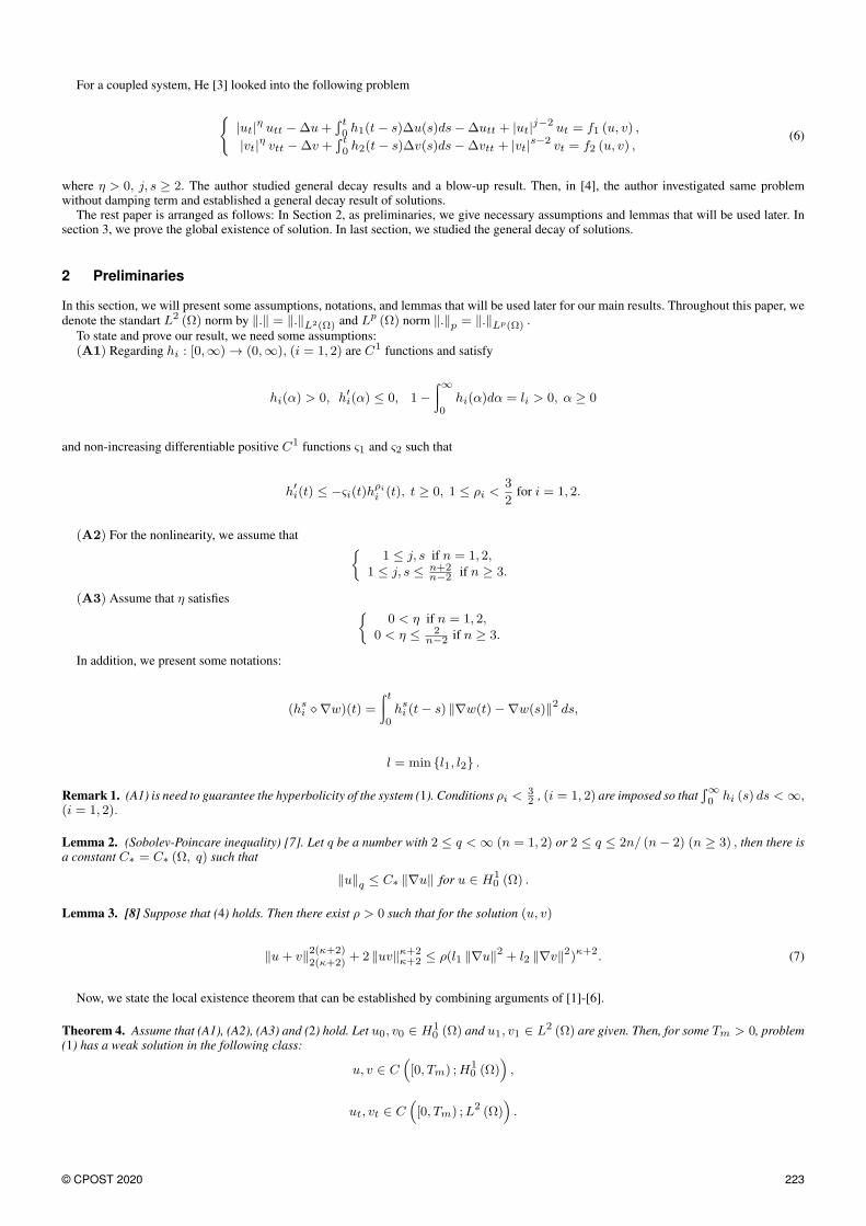
2 Preliminaries

In this section, we will present some assumptions, notations, and lemmas that will be used later for our main results. Throughout this paper, we

denote the standart L2 (Ω) norm by ‖.‖ = ‖.‖L2(Ω) and Lp (Ω) norm ‖.‖p = ‖.‖Lp(Ω) .To state and prove our result, we need some assumptions:

(A1) Regarding hi : [0,∞) → (0,∞), (i = 1, 2) are C1 functions and satisfy

hi(α) > 0, h′i(α) ≤ 0, 1−

∫∞

0hi(α)dα = li > 0, α ≥ 0

and non-increasing differentiable positive C1 functions ς1 and ς2 such that

h′i(t) ≤ −ςi(t)hρi

i (t), t ≥ 0, 1 ≤ ρi <3

2for i = 1, 2.

(A2) For the nonlinearity, we assume that

1 ≤ j, s if n = 1, 2,1 ≤ j, s ≤ n+2

n−2 if n ≥ 3.

(A3) Assume that η satisfies

0 < η if n = 1, 2,0 < η ≤ 2

n−2 if n ≥ 3.

In addition, we present some notations:

(hsi ⋄ ∇w)(t) =

∫ t0hsi (t− s) ‖∇w(t)−∇w(s)‖2 ds,

l = min l1, l2 .

Remark 1. (A1) is need to guarantee the hyperbolicity of the system (1). Conditions ρi <32 , (i = 1, 2) are imposed so that

∫∞

0 hi (s) ds < ∞,(i = 1, 2).

Lemma 2. (Sobolev-Poincare inequality) [7]. Let q be a number with 2 ≤ q < ∞ (n = 1, 2) or 2 ≤ q ≤ 2n/ (n− 2) (n ≥ 3) , then there isa constant C∗ = C∗ (Ω, q) such that

‖u‖q ≤ C∗ ‖∇u‖ for u ∈ H10 (Ω) .

Lemma 3. [8] Suppose that (4) holds. Then there exist ρ > 0 such that for the solution (u, v)

‖u+ v‖2(κ+2)2(κ+2)

+ 2 ‖uv‖κ+2κ+2 ≤ ρ(l1 ‖∇u‖2 + l2 ‖∇v‖2)κ+2. (7)

Now, we state the local existence theorem that can be established by combining arguments of [1]-[6].

Theorem 4. Assume that (A1), (A2), (A3) and (2) hold. Let u0, v0 ∈ H10 (Ω) and u1, v1 ∈ L2 (Ω) are given. Then, for some Tm > 0, problem

(1) has a weak solution in the following class:

u, v ∈ C(

[0, Tm) ;H10 (Ω)

)

,

ut, vt ∈ C(

[0, Tm) ;L2 (Ω))

.

© CPOST 2020 223

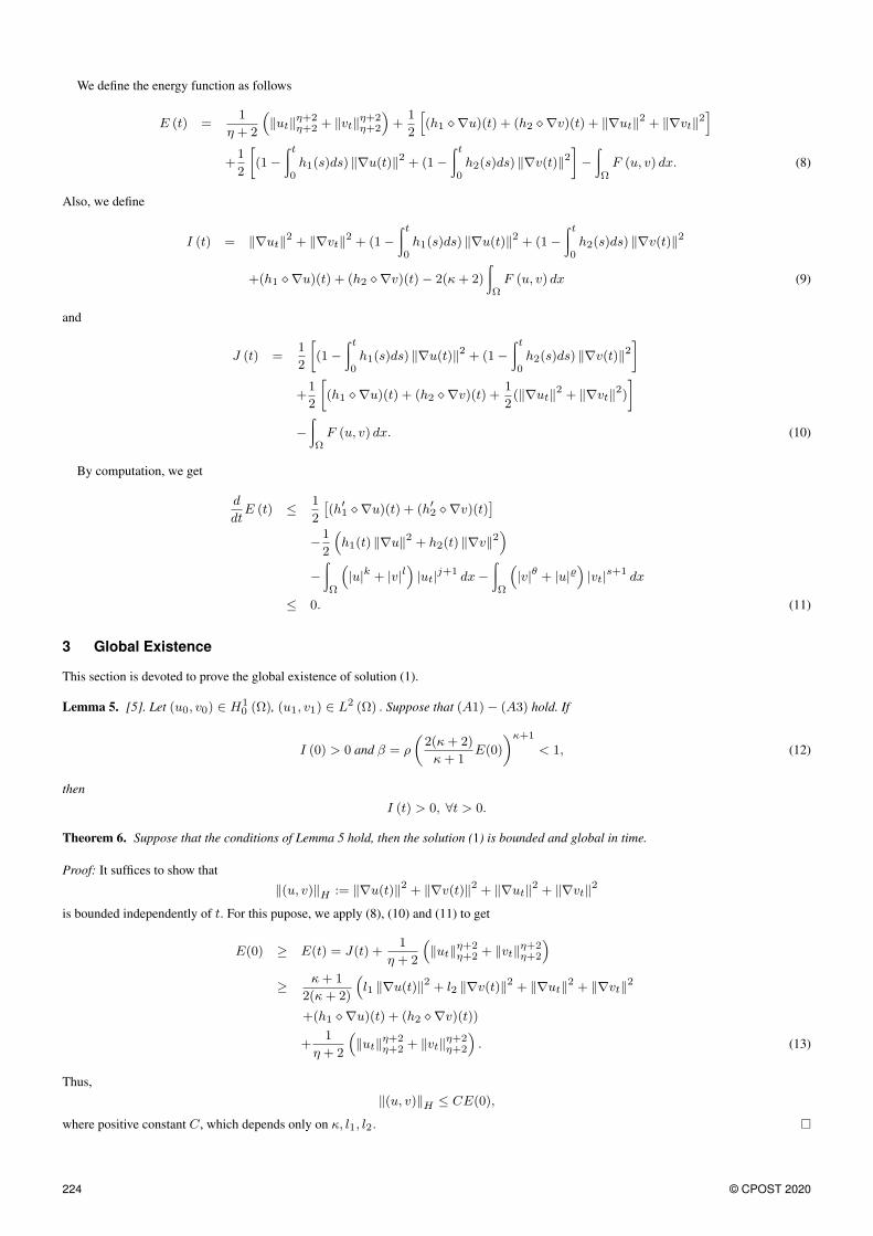
We define the energy function as follows

E (t) =1

η + 2

(

‖ut‖η+2η+2 + ‖vt‖

η+2η+2

)

+1

2

[

(h1 ⋄ ∇u)(t) + (h2 ⋄ ∇v)(t) + ‖∇ut‖2 + ‖∇vt‖

2]

+1

2

[

(1−

∫ t0h1(s)ds) ‖∇u(t)‖2 + (1−

∫ t0h2(s)ds) ‖∇v(t)‖2

]

−

∫ΩF (u, v) dx. (8)

Also, we define

I (t) = ‖∇ut‖2 + ‖∇vt‖

2 + (1−

∫ t0h1(s)ds) ‖∇u(t)‖2 + (1−

∫ t0h2(s)ds) ‖∇v(t)‖2

+(h1 ⋄ ∇u)(t) + (h2 ⋄ ∇v)(t)− 2(κ+ 2)

∫ΩF (u, v) dx (9)

and

J (t) =1

2

[

(1−

∫ t0h1(s)ds) ‖∇u(t)‖2 + (1−

∫ t0h2(s)ds) ‖∇v(t)‖2

]

+1

2

[

(h1 ⋄ ∇u)(t) + (h2 ⋄ ∇v)(t) +1

2(‖∇ut‖

2 + ‖∇vt‖2)

]

−

∫ΩF (u, v) dx. (10)

By computation, we get

d

dtE (t) ≤

1

2

[

(h′1 ⋄ ∇u)(t) + (h′2 ⋄ ∇v)(t)]

−1

2

(

h1(t) ‖∇u‖2 + h2(t) ‖∇v‖2)

−

∫Ω

(

|u|k + |v|l)

|ut|j+1 dx−

∫Ω

(

|v|θ + |u|)

|vt|s+1 dx

≤ 0. (11)

3 Global Existence

This section is devoted to prove the global existence of solution (1).

Lemma 5. [5]. Let (u0, v0) ∈ H10 (Ω), (u1, v1) ∈ L2 (Ω) . Suppose that (A1)− (A3) hold. If

I (0) > 0 and β = ρ

(

2(κ+ 2)

κ+ 1E(0)

)κ+1

< 1, (12)

then

I (t) > 0, ∀t > 0.

Theorem 6. Suppose that the conditions of Lemma 5 hold, then the solution (1) is bounded and global in time.

Proof: It suffices to show that

‖(u, v)‖H := ‖∇u(t)‖2 + ‖∇v(t)‖2 + ‖∇ut‖2 + ‖∇vt‖

2

is bounded independently of t. For this pupose, we apply (8), (10) and (11) to get

E(0) ≥ E(t) = J(t) +1

η + 2

(

‖ut‖η+2η+2 + ‖vt‖

η+2η+2

)

≥κ+ 1

2(κ+ 2)

(

l1 ‖∇u(t)‖2 + l2 ‖∇v(t)‖2 + ‖∇ut‖2 + ‖∇vt‖

2

+(h1 ⋄ ∇u)(t) + (h2 ⋄ ∇v)(t))

+1

η + 2

(

‖ut‖η+2η+2 + ‖vt‖

η+2η+2

)

. (13)

Thus,

‖(u, v)‖H ≤ CE(0),

where positive constant C, which depends only on κ, l1, l2.

224 © CPOST 2020

4 General Decay of Solutions

This section is devoted to prove the decay of solution (1). Set

Γ(t) := ME(t) + εΦ(t) +(t), (14)

where M and ε are some positive constants to be specified later and

Φ(t) = δ1 (t)

[

1

η + 1

∫Ω|ut|

η utudx+

∫Ω∇ut∇udx

]

+δ2 (t)

[

1

η + 1

∫Ω|vt|

η vtvdx+

∫Ω∇vt∇vdx

]

, (15)

(t) = δ1 (t)

[∫Ω

(

∆ut −|ut|

η utη + 1

) ∫ t0h1(t− s)(u(t)− u(s))dsdx

]

+δ2 (t)

[∫Ω

(

∆vt −|vt|

η vtη + 1

) ∫ t0h2(t− s)(v(t)− v(s))dsdx

]

. (16)

Lemma 7. For ε small enough while M large enough, the relation

α1Γ(t) ≤ E(t) ≤ α2Γ(t), ∀t ≥ 0. (17)

holds for two positive constants α1 and α2.

Proof: As references [9]-[5], it is easy to see that Γ(t) and E(t) are equivalent in the sense that α1 and α2 are positive constants, depending onε and M.

Lemma 8. [1] Assume that (12) holds. Let (u, v) be the solution of problem (1). Then, for σ ≥ 0, we get

∫Ω

(∫t0 h1(t− s)(u(t)− u(s))ds

)σ+2dx ≤ (1− l1)

σ+1cσ+2∗

(

2(κ+2)E(0)l1(κ+1)

)σ2

(h1 ⋄ ∇u)(t)

∫Ω

(∫t0 h2(t− s)(v(t)− v(s))ds

)σ+2dx ≤ (1− l2)

σ+1cσ+2∗

(

2(κ+2)E(0)l2(κ+1)

)σ2

(h2 ⋄ ∇v)(t). (18)

Lemma 9. Let u0, v0 ∈ H10 (Ω), u1, v1 ∈ L2(Ω) be given and satisfying (12). Assume that (A1)− (A3) hold. Then, for any t0, the functional

Γ(t) verifies, along solution of (1),

Γ′(t) ≤ −ξ1E(t) + ξ2 [(h1 ⋄ ∇u)(t) + (h2 ⋄ ∇v)(t)] (19)

for some ξi > 0, (i = 1, 2).

Proof: As references [9]-[5]-[1], it is easy to obtain desired result. We omit it.

Now, we are ready to state our stability result.

Theorem 10. Assume that (4), (A1)− (A3) hold and that (u0, u1) ∈ H10 (Ω)× L2(Ω) and (v0, v1) ∈ H1

0 (Ω)× L2(Ω) and satisfy E (0) <E1 and

(

l1 ‖∇u0‖2 + l2 ‖∇v0‖

2)

1

2

< α∗. (20)

Then for each , there exist two positive constants K and k such that the energy of (1) satisfies

E(t) ≤ Ke−k

∫t

t0δ(s)ds

, t ≥ t0 (21)

where δ(t) := min δ1(t), δ2(t) .

© CPOST 2020 225

Proof: Multiplying (19) by δ(t), we have

δ(t)Γ′(t) ≤ −ξ1δ(t)E(t) + ξ2δ(t) [(h1 ⋄ ∇u)(t) + (h2 ⋄ ∇v)(t)] .

Since (A2) and δ(t) := min δ1(t), δ2(t) and using the fact that −[

(h′1 ⋄ ∇u)(t) + (h′2 ⋄ ∇v)(t)]

≤ −2E′(t) by (11), we get

δ(t)Γ′(t) ≤ −ξ1δ(t)E(t)− ξ2δ(t)[

(h′1 ⋄ ∇u)(t) + (h′2 ⋄ ∇v)(t)]

≤ −ξ1δ(t)E(t)− 2ξ2E′(t), ∀t ≥ t0. (22)

That is

G′(t) ≤ −c∗δ(t)E(t) ≤ −kδ(t)G(t), ∀t ≥ t0, (23)

where G(t) = δ(t)Γ(t) + CE(t) is equivalent to E(t) due to (17) and k is a positive constant. A simple integration of (23) leads to

G(t) ≤ G(t0)e−k

∫t

t0δ(s)ds

, ∀t ≥ t0 (24)

This completes the proof.

5 Conclusion

As far as we know, there is not any global existence and general decay results in the literature known for quasilinear viscoelastic equations withdegenerate damping terms. Our work extends the works for some quasilinear viscoelastic equations treated in the literature to the quasilinearviscoelastic equation with degenerate damping terms.

6 References

1 ST. Wu, General decay of solutions for a viscoelastic equation with nonlinear damping and source terms, Acta Math Sci., (318), (2011), 1436-1448.

2 ST. Wu, General decay of energy for a viscoelastic equation with damping and source terms, Taiwan J Math., 16 (1), (2012), 113-128.

3 L. He, On decay and blow-up of solutions for a system of equations, Appl Anal., (2019), 1-30. Doi: 10.1080/00036811.2019.1689562

4 L. He, On decay of solutions for a system of coupled viscoelastic equations, Acta Appl Math. (167), (2020), 171-198.

5 E. Piskin, F. Ekinci, General decay and blow-up of solutions for coupled viscoelastic equation of Kirchhoff type with degenerate damping terms, Math Meth Appl Sci., 42 (16),

(2019), 5468-5488.

6 ST. Wu, General decay of solutions for a nonlinear system of viscoelastic wave equations with degenerate damping and source terms, J Math Anal Appl., (406), (2013), 34-48.

7 Adams RA, Fournier JJF. Sobolev Spaces. Academic Press, New York, 2003.

8 B. Said-Houari, SA. Messaoudi, A. Guesmia, General decay of solutions of a nonlinear system of viscoelastic wave equations, NoDEA Nonlinear Differential Equations Appl.,

(2011), (18), 659-684.

9 W. Liu, General decay and blow-up of solution for a quasilinear viscoelastic problem with nonlinear source, Nonlinear Anal. (73), (2010), 1890-1904.

226 © CPOST 2020



Generalized Spherical Fuzzy EinsteinAggregation Operators: Application toMulti-Criteria Group Decision-MakingProblems

ISSN: 2651-544X


Elif Güner1,∗ Halis Aygün2

1Department of Mathematics, Faculty of Science and Arts, Kocaeli University, Kocaeli, Turkey, ORCID: 0000-0002-6969-400X

* Corresponding Author E-mail: [email protected] of Mathematics, Faculty of Science and Arts, Kocaeli University, Kocaeli, Turkey, ORCID: 0000-0003-3263-3884

Abstract: The aim of this paper is to present the extension of a concept related to aggregation operators from spherical fuzzy

sets to generalized spherical fuzzy sets. We first introduce Einstein sum, product and scalar multiplication for generalized spher-

ical fuzzy sets based on Einstein triangular norm and triangular conorm. Then we give the generalized spherical fuzzy Einstein

weighted averaging and generalized spherical fuzzy Einstein weighted geometric operators, namely generalized spherical fuzzy

Einstein aggregation operators, constructed on these operations. After investigating some fundamental properties of these oper-

ators, we develop a model for generalized spherical fuzzy Einstein aggregation operators to solve the multiple attribute group

decision-making problems. Finally, we give a numerical example to demonstrate that the developed method is suitable and effec-

tive for the decision process.

Keywords: Generalized spherical fuzzy number, Einstein aggregation operators, Multi-criteria group decision making.

1 Introduction

In 1965, Zadeh [32] introduced the theory of fuzzy set (FS) in which is discussed the degree of membership (positive-membership) of an elementto a set. FS theory has a wide range of applications in numerous fields such as artificial intelligence, engineering, economics, computer scienceand etc. [7]-[32]-[33]-[34]. Also, the study of multi-criteria decision-making was started in fuzzy environment by Bellman and Zadeh [7] in1970. While the studies and developments in the field of FS theory were continued, Atanassov [6] observed that there are some deficienciesin this theory and defined the concept of intuitionistic fuzzy set (IFS) as a generalization of FS. Since each element is expressed by a positive-membership degree and a negative-membership degree in the IFS theory, this theory is a more powerful tool to deal with vagueness than the FStheory. Then basing on the well-known weighted averaging (WA) operator [16] and the ordered weighted averaging (OWA) operator [30], Xu[29] investigated some aggregation operators in the intuitionistic fuzzy environment and studied their applications to the multi-criteria decision-making process. Another idea which is an extension of the FS theory is the soft set (SS) theory introduced by Molodtsov [22] to deal with thevagueness and uncertainties of many problems that arise in engineering, social science, medical science, economics and etc. A first practicalapplication of soft sets to the decision-making problems was given by Maji et al. [20]-[21]. They have also initiated the concept of a fuzzy softset (FSS) which is a combination of FS and SS and obtained some of its properties. In literature, there are many significant applications of theSS and FSS theories. (see [5]-[9]-[24]-[25]).

After, Yager [31] extended the IFS theory to Pythagorean fuzzy set (PyFS) theory by considering the condition that the sum of the squares ofits positive-membership and negative-membership degrees is less than or equal to 1. IFS theory and PyFS theory have been successfully usedin many distinct areas, but it is not enough to use these theories when we face human opinions involving more answers of types such as yes,no, abstain, refusal. Voting in a democratic election is a good example of such a case since the voters may be divided into four groups of thosewho: vote for, vote against, abstain, refusal of the voting. So, Cuong [8] proposed the notion of picture fuzzy set (PFS) which is an extensionof IFS. PFS gives the positive-membership degree, the neutral-membership degree and the negative-membership degree of an element to a set.The PFS theory resolved the voting problem successfully and was applied to decision-making problems by many authors in different ways[27]-[28]-[3]-[4]-[10]. But there are some situations that PFS theory may not be handled in some uncertain and unstable data. For example, ifa person said their opinions about the situation in terms of yes is 0.7, abstained is 0.3, and no is 0.5, then we obtain that 0.7 + 0.5 + 0.3 1.So PFS theory is not able to handle under such types of cases. To use in these types of situations, Mahmood et al. [19] initiated the conceptof spherical fuzzy set (SFS) and T-spherical fuzzy set (T-SFS) as an extension of FS, IFS and PFS. While in SFS theory the sum of the squareof the three membership degrees is less than or equal to 1, in T-SFS theory the nth power of the three membership degrees is less than orequal to 1. Also, Mahmood et al. [19] defined some fundamental operations of SFSs and T-SFSs along with spherical fuzzy relations andpresented medical diagnostics and decision-making problems in the SFSs and T-SFSs environments as practical applications. Then, Ashraf andAbdullah [1] extended different strict Archimedean triangular norms and triangular conorms to aggregate the spherical fuzzy information andalso defined some spherical aggregation operators and applied these operators to multi-criteria group decisionâARmaking problems. Differenttypes of aggregation operators for SFSs can be found in [2]-[19]-[23]. Later, Jin et al. [17] proposed a new method to solve the spherical

© CPOST 2020 227

fuzzy multi-criteria group decision-making problems by investigating logarithmic operations of spherical fuzzy sets. Also, GÃijndogdu andKahraman [12]-[13]-[14] extended the TOPSIS, VIKOR and WASPAS methods to the spherical fuzzy environment. Recently, Haque et al.[15] presented the notion of generalized spherical fuzzy set (GSFS) as an expansion of the SFS in which the sum of the square of the threemembership degrees is less than or equal to 3. They established a new exponential operational law for GSFS and investigated its variousalgebraic properties. They also developed a multi-criteria group decision-making method in the generalized spherical fuzzy environment byusing the established exponential operational law. Peng et al. [26] introduced the Pythagorean fuzzy soft set (PyFSS) along with various binaryoperations and also proposed an algorithm for decision making. Then, Cuong[8] proposed the notion of picture fuzzy soft set (PFSS) as acombination of PFS and SS and also discussed various properties and operations in the theory of PFSS. Guleria and Bajaj [11] extend theconcept of PFSS by proposing the T-spherical fuzzy soft set (T-SFSS) along with various aggregation operators and applications.

The main purpose of this paper is to establish the generalized spherical fuzzy Einstein aggregation operators and develop a model forgeneralized spherical fuzzy Einstein aggregation operators to solve the multiple attribute group decision-making problems. This paper iscontained in the following sections: In Section 2, we recollect some basic notions and relevant concepts that are used in the main section. InSection 3, we introduce Einstein sum, product and scalar multiplication for GSFSs based on Einstein triangular norm and triangular conorm.Then, we give the generalized spherical fuzzy Einstein weighted averaging (GSEWA) and generalized spherical fuzzy Einstein weightedgeometric (GSEWG) operators, namely generalized spherical fuzzy Einstein aggregation operators, constructed on the Einstein sum, productand scalar multiplication for GSFSs. Also, we investigate some fundamental properties of these operators. In section 4, we develop a model tosolve the multiple attribute group decision-making problems in generalized spherical fuzzy environment. Then, we give a medical treatmentselection problem as an example which demonstrates that the developed method is effective and suitable for the decision-making process.Finally, we give a brief summary in Section 5.

2 Preliminaries

In this section, we recall some fundamental definitions which will be used in the main sections. Throughout this paper U will denote the set ofthe universe.

Definition 1. [6]-[31] Let µ : U → [0, 1] and ν : U → [0, 1] be two mappings. A set I = < x, µ(x), ν(x) > |x ∈ U is called(i) Intuitionistic fuzzy set (IFS) if the condition 0 ≤ µ(x) + ν(x) ≤ 1 hold for all x ∈ U .

(ii) Pythagorean fuzzy set (PyFS) if the condition 0 ≤ µ2(x) + ν2(x) ≤ 1 hold for all x ∈ U .The values µ(x), ν(x) ∈ [0, 1] denote the degree of positive-membership and negative-membership of x to I , respectively.

The pair I =< µ, ν > where µ, ν ∈ [0, 1] and µ+ ν ≤ 1 (or µ2 + ν2 ≤ 1), is called a intuitionistic fuzzy number (IFN) (or Pythagoreanfuzzy number (PyFN)).

Remark 1. [31] The set of intuitionistic fuzzy numbers is the subset of the set of Pythagorean fuzzy numbers.

Definition 2. [1]-[8]-[15] Let µ : U → [0, 1], ι : U → [0, 1] and ν : U → [0, 1] be three mappings. A set G = < x, µ(x), ι(x), ν(x) > |x ∈U is called

(i) Picture fuzzy set (PFS) if the condition 0 ≤ µ(x) + ι(x) + ν(x) ≤ 1 hold for all x ∈ U .

(ii) Spherical fuzzy set (SFS) if the condition 0 ≤ µ2(x) + ι2(x) + ν2(x) ≤ 1 hold for all x ∈ U .

(ii) Generalized spherical fuzzy set (GSFS) if the condition 0 ≤ µ2(x) + ι2(x) + ν2(x) ≤ 3 hold for all x ∈ U .The values µ(x), ι(x), ν(x) ∈ [0, 1] denote the degree of positive-membership, neutral-memberhip and negative-membership of x to G,

respectively.

The triplet G =< µ, ι, ν > where µ, ι, ν ∈ [0, 1] and µ2 + ι2 + ν2 ≤ 3 (or µ+ ι+ ν ≤ 1 and µ2 + ι2 + ν2 ≤ 1, resp.), is called ageneralized spherical fuzzy number (GSFN) (or Picture fuzzy number (PFN) and Spherical fuzzy number (SFN), resp.).

Remark 2. [15] (1) The set of spherical fuzzy numbers is the subset of the set of generalized spherical fuzzy numbers and the set of picturefuzzy numbers is the subset of the set of spherical fuzzy numbers.

(2) In PFN, since the sum of the three membership functions (positive, neutral and negative) is less than or equal to 1, the sum is taken aslinearly and it represents a plane in space. But in the case of SFN and GSFN, it is considered the non-linear form of membership functionswhich represents a sphere in space.

Definition 3. [15] Let G =< µ, ι, ν >,G1 =< µ1, ι1, ν1 >, G2 =< µ2, ι2, ν2 > be three GSFNs and a ≥ 0. Then the operations betweengeneralized spherical fuzzy numbers are defined as follows:

(i) Gc =< ν, ι, µ >,(ii) G1 ≤ G2 iff µ1 ≤ µ2, ι1 ≥ ι2 and ν1 ≥ ν2,(iii) G1 = G2 iff G1 ≤ G2 and G2 ≤ G1,

(iv) G1 +G2 =<

√

µ21 + µ2

2 − µ21µ

22, ι1ι2, ν1ν2 >,

(v) aG =<√

1− (1− µ2)a, ιa, νa >,

(vi) Ga =< µa, ιa,√

1− (1− ν2)a >.

Lemma 1. [15] Let G1 =< µ1, ι1, ν1 >, G2 =< µ2, ι2, ν2 > be two GSFNs and a, a1, a2 ≥ 0. Then the following properties hold:(i) G1 +G2 = G2 +G1,(ii) a(G1 +G2) = aG1 + aG2,(iii) (a1 + a2)G1 = a1G1 + a2G2,(vi) (Ga1

1 )a2 = Ga1a2

1 .

Definition 4. [15] Let G be the collection of all GSFNs and G ∈ G where G =< µ, ι, ν >.

(i) A score function SF : G → [−1, 1] is defined as SF (G) = 3µ2−2ι2−ν2

3 .

(ii) An accuracy function AF : G → [0, 1] is defined as AF (G) = 1+3µ2−ν2

4 .

228 © CPOST 2020

Definition 5. [15] Let G1 =< µ1, ι1, ν1 > and G2 =< µ2, ι2, ν2 > be two GSFNs. Then the ranking method (comparison technique) asfollows:

(i) If SF (G1) < SF (G2), then G1 < G2,(ii) If SF (G1) > SF (G2), then G1 > G2,(iii) SF (G1) = SF (G2), then

(a) AF (G1) < AF (G2), then G1 < G2,(b) AF (G1) > AF (G2), then G1 > G2,(c) AF (G1) = AF (G2), then G1 = G2.

3 Generalized Spherical Fuzzy Einstein Aggregation Operators

In this section, we introduce the Einstein sum, product and scalar multiplication for generalized spherical fuzzy sets based on Einstein triangularnorm and triangular conorm. Then we define the generalized spherical fuzzy Einstein weighted averaging and generalized spherical fuzzyEinstein weighted geometric operators based on these operations. Also, we investigate some fundamental properties of these operators.

Definition 6. Let G =< µ, ι, ν >,G1 =< µ1, ι1, ν1 > and G2 =< µ2, ι2, ν2 > be three GSFNs and a ≥ 0. Then the Einstein operationsare defined over the GSFNs as follow:

(i) G1 ⊕E G2 =

⟨

√

µ21+µ2

2

1+µ21.µ2

2

,

√

ι21.ι2

2

1+(1−ι21)(1−ι2

2),

√

ν21.ν2

2

1+(1−ν21)(1−ν2

2)

⟩

,

(ii) G1 ⊙E G2 =

⟨

√

µ21.µ2

2

1+(1−µ21)(1−µ2

2),

√

ι21.ι2

2

1+(1−ι21)(1−ι2

2),

√

ν21+ν2

2

1+ν21.ν2

2

⟩

,

(iii) a·EG =

⟨

√

(1+µ2)a−(1−µ2)a

(1+µ2)a+(1−µ2)a,√

2ι2a

(2−ι2)a+ι2a,√

2ν2a

(2−ν2)a+ν2a

⟩

,

(iv) G∧Ea =

⟨

√

2µ2a

(2−µ2)a+µ2a ,√

2ι2a

(2−ι2)a+ι2a,√

(1+ν2)a−(1−ν2)a

(1+ν2)a+(1−ν2)a

⟩

.

Lemma 2. Let G1 =< µ1, η1, ν1 >, G2 =< µ2, η2, ν2 > be two GSFNs and a, a1, a2 ≥ 0. Then the following properties hold:(i) G1 ⊕E G2 = G2 ⊕E G1,(ii) a·E(G1 ⊕E G2) = a·EG1 ⊕E a·EG2,(iii) (a1 + a2)·EG1 = a1·EG1 ⊕E a2·EG2,(iv) G1 ⊙E G2 = G2 ⊙E G1,(v) (G1 ⊙E G2)

∧Ea = G∧Ea1 ⊙E G∧Ea

2 ,

(vi) G∧Ea1 ⊙E G∧Ea2 = G∧Ea1+a2 ,(vii) (G∧Ea1

1 )∧Ea2 = G∧Ea1a2

1 .

Proof: Proofs of (i) and (iv) are trivial.

(ii) We can write the equation G1 ⊕E G2 =

⟨

√

µ21+µ2

2

1+µ21.µ2

2

,

√

ι21.ι2

2

1+(1−ι21)(1−ι2

2),

√

ν21.ν2

2

1+(1−ν21)(1−ν2

2)

⟩

in the following way:

G1 ⊕E G2 =

⟨

√

(1+µ21)(1+µ2

2)−(1−µ2

1)(1−µ2

2)

(1+µ21)(1+µ2

2)+(1−µ2

1)(1−µ2

2),

√

2.ι21.ι2

2

(2−ι21)(2−ι2

2)+ι2

1.ι2

2

,

√

2.ν21.ν2

2

(2−ν21)(2−ν2

2)+ν2

1.ν2

2

⟩

.

If we take s = (1 + µ21)(1 + µ2

2), t = (1− µ21)(1− µ2

2), u = ι21.ι22, x = (2− ι21)(2− ι22), y = ν21 .ν

22 and z = (2− ν21 )(2− ν22 ), by the

Einstein operational law (ii), we have that

a·E(G1 ⊕E G2) = a·E

⟨

√

s− t

s+ t,

√

2u

x+ u,

√

2y

z + y

⟩

=

⟨

√

√

√

√

(1 + s−ts+t )

a − (1− s−ts+t )

a

(1 + s−ts+t )

a + (1− s−ts+t )

a,

√

√

√

√

2( 2ux+u )

a

(2− 2ux+u )

a + ( 2ux+u )

a,

√

√

√

√

2( 2yz+y )

a

(2− 2yz+y )

a + ( 2yz+y )

a

⟩

=

⟨

√

sa − ta

sa + ta,

√

2ua

xa + ua,

√

2ya

za + ya

⟩

=

⟨√

(1 + µ21)

a(1 + µ22)

a − (1− µ21)

a(1− µ22)

a

(1 + µ21)

a(1 + µ22)

a + (1− µ21)

a(1− µ22)

a,

√

2ι2a1 .ι2a2(2− ι21)

a(2− ι22)a + ι2a1 .ι2a2

,

√

2ν2a1 .ν2a2(2− ν21 )

a(2− ν22 )a + ν2a1 ν2a2

⟩

.

Also, if we take s1 = (1 + µ21)

a, t1 = (1− µ21)

a, u1 = ι2a1 , x1 = (2− ι21)a, y1 = ν2a1 , z1 = (2− ν21 )

a, s2 = (1 + µ22)

a, t2 = (1− µ22)

a,u2 = ι2a2 , x2 = (2− ι22)

a, y2 = ν2a2 and z2 = (2− ν22 )a, then we have that

a·EG1 =

⟨

√

s1−t1s1+t1

,√

2u1

x1+u1,√

2y1

z1+u1

⟩

and a·EG2 =

⟨

√

s2−t2s2+t2

,√

2u2

x2+u2,√

2y2

z2+u2

⟩

.

© CPOST 2020 229

By the Einstein operational law (i), we get that

a·EG1 ⊕E a·EG2 =

⟨

√

√

√

√

( s1−t1s1+t1

) + ( s2−t2s2+t2

)

1 + ( s1−t1s1+t1

)( s2−t2s2+t2

),

√

√

√

√

( 2u1

x1+u1)( 2u2

x2+u2)

1 + (1− 2u1

x1+u1)(1− 2u2

x2+u2),

√

√

√

√

( 2y1

z1+y1)( 2y2

z2+y2)

1 + (1− 2y1

z1+y1)(1− 2y2

z2+y2)

⟩

=

⟨

√

s1s2 − t1t2

s1s2 + t1t2,

√

2u1u2x1x2 + u1u2

,

√

2y1y2z1z2 + y1y2

⟩

=

⟨√

(1 + µ21)

a(1 + µ22)

a − (1− µ21)

a(1− µ22)

a

(1 + µ21)

a(1 + µ22)

a + (1− µ21)

a(1− µ22)

a,

√

2ι2a1 ι2a2(2− ι21)

a(2− ι22)a + ι2a1 ι2a2

,

√

2ν2a1 ν2a2(2− ν21 )

a(2− ν22 )a + ν2a1 ν2a2

⟩

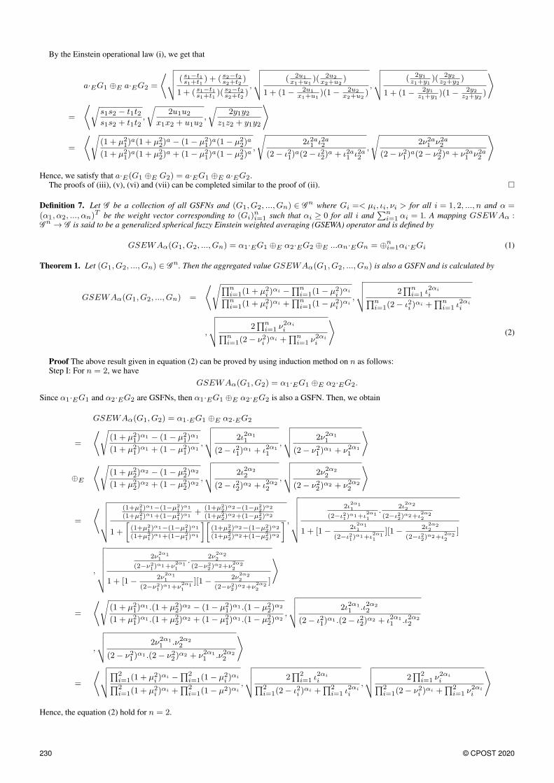
Hence, we satisfy that a·E(G1 ⊕E G2) = a·EG1 ⊕E a·EG2.The proofs of (iii), (v), (vi) and (vii) can be completed similar to the proof of (ii).

Definition 7. Let G be a collection of all GSFNs and (G1, G2, ..., Gn) ∈ Gn where Gi =< µi, ιi, νi > for all i = 1, 2, ..., n and α =

(α1, α2, ..., αn)T be the weight vector corresponding to (Gi)

ni=1 such that αi ≥ 0 for all i and

∑ni=1 αi = 1. A mapping GSEWAα :

Gn → G is said to be a generalized spherical fuzzy Einstein weighted averaging (GSEWA) operator and is defined by

GSEWAα(G1, G2, ..., Gn) = α1·EG1 ⊕E α2·EG2 ⊕E ...αn·EGn = ⊕ni=1αi·EGi (1)

Theorem 1. Let (G1, G2, ..., Gn) ∈ Gn. Then the aggregated value GSEWAα(G1, G2, ..., Gn) is also a GSFN and is calculated by

GSEWAα(G1, G2, ..., Gn) =

⟨√

∏ni=1(1 + µ2

i )αi −

∏ni=1(1− µ2

i )αi

∏ni=1(1 + µ2

i )αi +

∏ni=1(1− µ2

i )αi

,

√

√

√

√

2∏n

i=1 ι2αi

i∏n

i=1(2− ι2i )αi +

∏ni=1 ι

2αi

i

,

√

√

√

√

2∏n

i=1 ν2αi

i∏n

i=1(2− ν2i )αi +

∏ni=1 ν

2αi

i

⟩

(2)

Proof The above result given in equation (2) can be proved by using induction method on n as follows:Step I: For n = 2, we have

GSEWAα(G1, G2) = α1·EG1 ⊕E α2·EG2.

Since α1·EG1 and α2·EG2 are GSFNs, then α1·EG1 ⊕E α2·EG2 is also a GSFN. Then, we obtain

GSEWAα(G1, G2) = α1.EG1 ⊕E α2.EG2

=

⟨√

(1 + µ21)

α1 − (1− µ21)

α1

(1 + µ21)

α1 + (1− µ21)

α1,

√

√

√

√

2ι2α1

1

(2− ι21)α1 + ι2α1

1

,

√

√

√

√

2ν2α1

1

(2− ν21 )α1 + ν2α1

1

⟩

⊕E

⟨√

(1 + µ22)

α2 − (1− µ22)

α2

(1 + µ22)

α2 + (1− µ22)

α2,

√

√

√

√

2ι2α2

2

(2− ι22)α2 + ι2α2

2

,

√

√

√

√

2ν2α2

2

(2− ν22 )α2 + ν2α2

2

⟩

=

⟨

√

√

√

√

√

√

(1+µ21)α1−(1−µ2

1)α1

(1+µ21)α1+(1−µ2

1)α1

+(1+µ2

2)α2−(1−µ2

2)α2

(1+µ22)α2+(1−µ2

2)α2

1 +

[

(1+µ21)α1−(1−µ2

1)α1

(1+µ21)α1+(1−µ2

1)α1

][

(1+µ22)α2−(1−µ2

2)α2

(1+µ22)α2+(1−µ2

2)α2

] ,

√

√

√

√

√

√

√

2ι2α11

(2−ι21)α1+ι

2α11

.2ι

2α22

(2−ι22)α2+ι

2α22

1 + [1−2ι

2α11

(2−ι21)α1+ι

2α11

][1−2ι

2α22

(2−ι22)α2+ι

2α22

]

,

√

√

√

√

√

√

√

2ν2α11

(2−ν21)α1+ν

2α11

.2ν

2α22

(2−ν22)α2+ν

2α22

1 + [1−2ν

2α11

(2−ν21)α1+ν

2α11

][1−2ν

2α22

(2−ν22)α2+ν

2α22

]

⟩

=

⟨√

(1 + µ21)

α1 .(1 + µ22)

α2 − (1− µ21)

α1 .(1− µ22)

α2

(1 + µ21)

α1 .(1 + µ22)

α2 + (1− µ21)

α1 .(1− µ22)

α2,

√

√

√

√

2ι2α1

1 .ι2α2

2

(2− ι21)α1 .(2− ι22)

α2 + ι2α1

1 .ι2α2

2

,

√

√

√

√

2ν2α1

1 .ν2α2

2

(2− ν21 )α1 .(2− ν22 )

α2 + ν2α1

1 .ν2α2

2

⟩

=

⟨

√

√

√

√

∏2i=1(1 + µ2

i )αi −

∏2i=1(1− µ2

i )αi

∏2i=1(1 + µ2

i )αi +

∏2i=1(1− µ2)αi

,

√

√

√

√

2∏2

i=1 ι2αi

i∏2

i=1(2− ι2i )αi +

∏2i=1 ι

2αi

i

,

√

√

√

√

2∏2

i=1 ν2αi

i∏2

i=1(2− ν2i )αi +

∏2i=1 ν

2αi

i

⟩

Hence, the equation (2) hold for n = 2.

230 © CPOST 2020

Step II: Now, we suppose that the equation (2) hold for n = k, that is

GSEWAα(G1, G2, ..., Gk) = α1·EG1 ⊕E α2·EG2 ⊕E ...⊕E αk·EGk

=

⟨

√

√

√

√

∏ki=1(1 + µ2

i )αi −

∏ki=1(1− µ2

i )αi

∏ki=1(1 + µ2

i )αi +

∏ki=1(1− µ2)αi

,

√

√

√

√

2∏k

i=1 ι2αi

i∏k

i=1(2− ι2i )αi +

∏ki=1 ι

2αi

i

,

√

√

√

√

2∏k

i=1 ν2αi

i∏k

i=1(2− ν2i )αi +

∏ki=1 ν

2αi

i

⟩

Similarly, we show that the equation (2) hold for n = k + 1. Then, we have

GSEWAα(G1, G2, ..., Gk, Gk+1) = GSEWAα(G1, G2, ..., Gk)⊕E αk+1Gk+1

=

⟨

√

√

√

√

∏ki=1(1 + µ2

i )αi −

∏ki=1(1− µ2

i )αi

∏ki=1(1 + µ2

i )αi +

∏ki=1(1− µ2)αi

,

√

√

√

√

2∏k

i=1 ι2αi

i∏k

i=1(2− ι2i )αi +

∏ki=1 ι

2αi

i

,

√

√

√

√

2∏k

i=1 ν2αi

i∏k

i=1(2− ν2i )αi +

∏ki=1 ν

2αi

i

⟩

⊕E

⟨

√

√

√

√

(1 + µ2k+1)

αk+1 − (1− µ2k+1)

αk+1

(1 + µ2k+1)

αk+1 + (1− µ2k+1)

αk+1,

√

√

√

√

2ι2αk+1

k+1

(2− ι2k+1)

αk+1 + ι2αk+1

k+1

,

√

√

√

√

2ν2α1

k+1

(2− ν2k+1)

αk+1 + ν2αk+1

k+1

⟩

=

⟨

√

√

√

√

√

√

√

√

∏k

i=1(1+µ2

i)αi−

∏k

i=1(1−µ2

i)αi

∏k

i=1(1+µ2

i)αi+

∏k

i=1(1−µ2)αi

+(1+µ2

k+1)αk+1−(1−µ2

k+1)αk+1

(1+µ2k+1

)αk+1+(1−µ2k+1

)αk+1

1 +

(

∏k

i=1(1+µ2

i)αi−

∏k

i=1(1−µ2

i)αi

∏k

i=1(1+µ2

i)αi+

∏k

i=1(1−µ2)αi

)(

(1+µ2k+1

)αk+1−(1−µ2k+1

)αk+1

(1+µ2k+1

)αk+1+(1−µ2k+1

)αk+1

)

,

√

√

√

√

√

√

√

√

√

(

2∏

k

i=1ι2αi

i∏k

i=1(2−ι2

i)αi+

∏k

i=1ι2αi

i

)(

2ι2αk+1

k+1

(2−ι2k+1

)αk+1+ι2αk+1

k+1

)

1 +

(

1−2∏

k

i=1ι2αi

i∏k

i=1(2−ι2

i)αi+

∏k

i=1ι2αi

i

)(

1−2ι

2αk+1

k+1

(2−ι2k+1

)αk+1+ι2αk+1

k+1

)

,

√

√

√

√

√

√

√

√

√

(

2∏

k

i=1ν2αi

i∏k

i=1(2−ν2

i)αi+

∏k

i=1ν2αi

i

)

(

2ν2αk+1

k+1

(2−ν2k+1

)αk+1+ν2αk+1

k+1

)

1 +

(

1−2∏

k

i=1ν2αi

i∏k

i=1(2−ν2

i)αi+

∏k

i=1ν2αi

i

)(

1−2ν

2αk+1

k+1

(2−ν2k+1

)αk+1+ν2αk+1

k+1

)

⟩

(3)

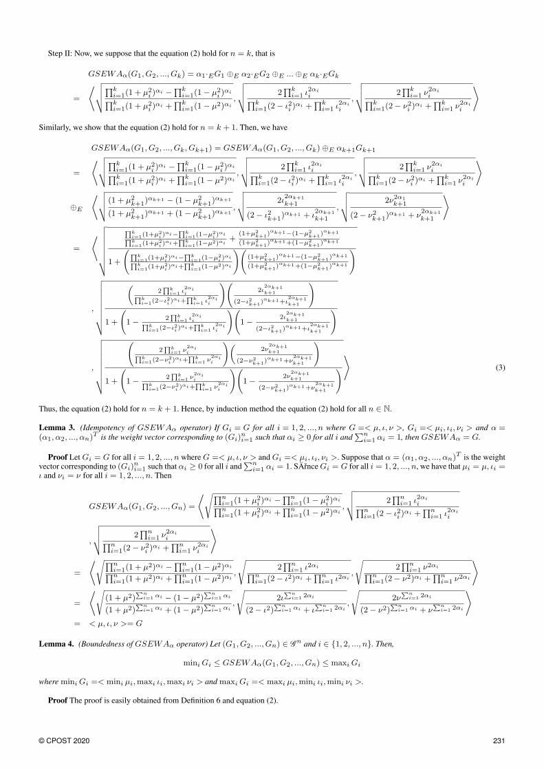
Thus, the equation (2) hold for n = k + 1. Hence, by induction method the equation (2) hold for all n ∈ N.

Lemma 3. (Idempotency of GSEWAα operator) If Gi = G for all i = 1, 2, ..., n where G =< µ, ι, ν >, Gi =< µi, ιi, νi > and α =(α1, α2, ..., αn)

T is the weight vector corresponding to (Gi)ni=1 such that αi ≥ 0 for all i and

∑ni=1 αi = 1, then GSEWAα = G.

Proof Let Gi = G for all i = 1, 2, ..., n where G =< µ, ι, ν > and Gi =< µi, ιi, νi >. Suppose that α = (α1, α2, ..., αn)T is the weight

vector corresponding to (Gi)ni=1 such that αi ≥ 0 for all i and

∑ni=1 αi = 1. SÄrnce Gi = G for all i = 1, 2, ..., n, we have that µi = µ, ιi =

ι and νi = ν for all i = 1, 2, ..., n. Then

GSEWAα(G1, G2, ..., Gn) =

⟨√

∏ni=1(1 + µ2

i )αi −

∏ni=1(1− µ2

i )αi

∏ni=1(1 + µ2

i )αi +

∏ni=1(1− µ2)αi

,

√

√

√

√

2∏n

i=1 ι2αi

i∏n

i=1(2− ι2i )αi +

∏ni=1 ι

2αi

i

,

√

√

√

√

2∏n

i=1 ν2αi

i∏n

i=1(2− ν2i )αi +

∏ni=1 ν

2αi

i

⟩

=

⟨√

∏ni=1(1 + µ2)αi −

∏ni=1(1− µ2)αi

∏ni=1(1 + µ2)αi +

∏ni=1(1− µ2)αi

,

√

2∏n

i=1 ι2αi

∏ni=1(2− ι2)αi +

∏ni=1 ι

2αi

,

√

2∏n

i=1 ν2αi

∏ni=1(2− ν2)αi +

∏ni=1 ν

2αi

⟩

=

⟨√

(1 + µ2)∑

n

i=1αi − (1− µ2)

∑n

i=1αi

(1 + µ2)∑

n

i=1αi + (1− µ2)

∑n

i=1αi

,

√

2ι∑

n

i=12αi

(2− ι2)∑

n

i=1αi + ι

∑n

i=12αi

,

√

2ν∑

n

i=12αi

(2− ν2)∑

n

i=1αi + ν

∑n

i=12αi

⟩

= < µ, ι, ν >= G

Lemma 4. (Boundedness of GSEWAα operator) Let (G1, G2, ..., Gn) ∈ Gn and i ∈ 1, 2, ..., n. Then,

mini Gi ≤ GSEWAα(G1, G2, ..., Gn) ≤ maxi Gi

where mini Gi =< mini µi,maxi ιi,maxi νi > and maxi Gi =< maxi µi,mini ιi,mini νi >.

Proof The proof is easily obtained from Definition 6 and equation (2).

© CPOST 2020 231

Lemma 5. (Monotonicity of GSEWAα operator) Let (G1, G2, ..., Gn), (G′

1, G′

2, ..., G′n) ∈ G

n. If Gi ≤ G′

i for all i = 1, 2, .., n, then

GSEWAα(G1, G2, ..., Gn) ≤ GSEWAα(G′

1, G′

2, ..., G′n).


Definition 8. Let G be a collection of all GSFNs and (G1, G2, ..., Gn) ∈ Gn where Gi =< µi, ιi, νi > for all i = 1, 2, ..., n and α =

(α1, α2, ..., αn)T be the weight vector corresponding to (Gi)

ni=1 such that αi ≥ 0 for all i and

∑ni=1 αi = 1. A mapping GSEWGα :

Gn → G is said to be a generalized spherical fuzzy Einstein weighted geometric (GSEWG) operator and is defined by

GSEWGα(G1, G2, ..., Gn) = G∧Eα1

1 ⊙E G∧Eα2

2 ⊙E ...⊙E G∧Eαn

n = ⊙ni=1G

∧Eαi

i (4)

Theorem 2. Let (G1, G2, ..., Gn) ∈ Gn. Then the aggregated value GSEWGα(G1, G2, ..., Gn) is also a GSFN and is calculated by

GSEWGα(G1, G2, ..., Gn) =

⟨

√

√

√

√

2∏n

i=1 µ2αi

i∏n

i=1(2− µ2i )

αi +∏n

i=1 µ2αi

i

,

√

√

√

√

2∏n

i=1 ι2αi

i∏n

i=1(2− ι2i )αi +

∏ni=1 ι

2αi

i

,

√

∏ni=1(1 + ν2i )

αi −∏n

i=1(1− ν2i )αi

∏ni=1(1 + ν2i )

αi +∏n

i=1(1− ν2)αi

⟩

(5)

Proof The proof is obtained similar to the proof of Theorem 1.

Lemma 6. (Idempotency of GSEWGα operator) If Gi = G for all i = 1, 2, ..., n where G =< µ, ι, ν >, Gi =< µi, ιi, νi > and α =(α1, α2, ..., αn)

T is the weight vector corresponding to (Gi)ni=1 such that αi ≥ 0 for all i and

∑ni=1 αi = 1, then GSEWGα = G.

Proof The proof is easily obtained from equation (5).

Lemma 7. (Boundedness of GSEWGα operator) Let (G1, G2, ..., Gn) ∈ Gn and i ∈ 1, 2, ..., n. Then,

mini Gi ≤ GSEWGα(G1, G2, ..., Gn) ≤ maxi Gi

where mini Gi =< mini µi,maxi ιi,maxi νi > and maxi Gi =< maxi µi,mini ιi,mini νi >.


Lemma 8. (Monotonicity of GSEWGα operator) Let (G1, G2, ..., Gn), (G′

1, G′

2, ..., G′n) ∈ G

n. If Gi ≤ G′

i for all i = 1, 2, .., n, then

GSEWGα(G1, G2, ..., Gn) ≤ GSEWGα(G′

1, G′

2, ..., G′n).


4 An Application of Generalized Spherical Fuzzy Einstein Aggregation Operators to Multi-Criteria GroupDecision-Making Problems

In this section, we develop a method for multi-criteria group decision-making problems under the generalized spherical fuzzy environmentusing the defined GSEWA and GSEWG operators and then we give a numerical example to explain this method.

4.1 Methodology

Let A = A1, A2, ..., Am be the set of m different options and E = E1, E2, ..., En be the set of n different attributes. Assume that α =(α1, α2, ..., αn) is the weight vector of the attribute Ei (i = 1, 2, ..., n) where αi ≥ 0 for all i = 1, 2, ..., n and

∑ni=1 αi = 1. Also suppose

that D = D1, D2, ..., Dk is the set of n distinct decision-makers with the options whose weight vector is expressed as δ = (δ1, δ2, ..., δk)

where δi ≥ 0 for all i = 1, 2, ..., k and∑k

i=1 δi = 1. This vector (δ) has been handled according to the age, experience, education, thinkingability, and knowledge power of the decision-maker. Actually, as a first step decision matrices associated with options to attribute values arebuilt on considering the preference of the decision-makers. But here, we consider the entity of the decision matrices as GSFNs and are givenby Br

ij =< µrij , ι

rij , ν

rij > (i = 1, 2, ...,m), (j = 1, 2, ..., n), (r = 1, 2, ..., k) and the associated decision matrix is given as follows:

Dr =

Br11 Br

12 . . . Br1n

Br21 Br

22 . . . Br2n

...... . . .

...Brm1 Br

m2 . . . Brmn

.

Now, we develop the multi-criteria group decision-making procesure under the generalized spherical fuzzy environment as the followingsteps:

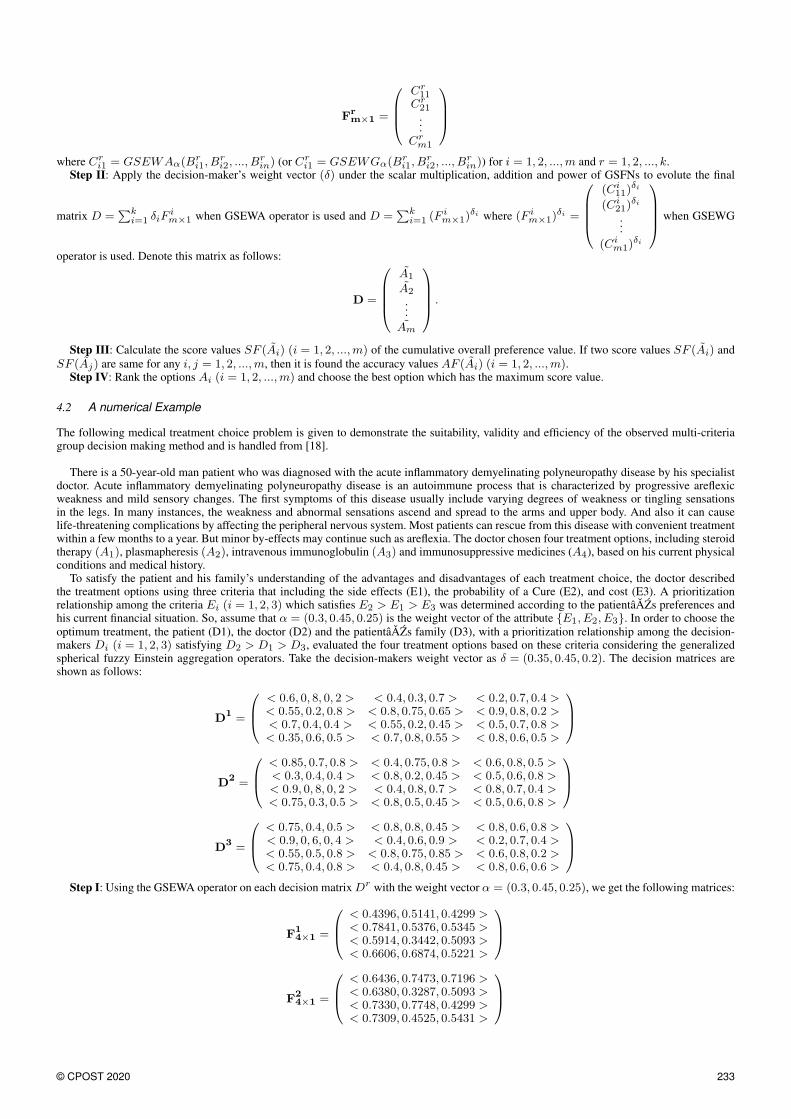
Step I: Use the either GSEWA or GSEWG operator on each decision matrix Dr to get the following matrix:

232 © CPOST 2020

Fr

m×1 =

Cr11

Cr21...

Crm1

where Cri1 = GSEWAα(B

ri1, B

ri2, ..., B

rin) (or Cr

i1 = GSEWGα(Bri1, B

ri2, ..., B

rin)) for i = 1, 2, ...,m and r = 1, 2, ..., k.

Step II: Apply the decision-maker’s weight vector (δ) under the scalar multiplication, addition and power of GSFNs to evolute the final

matrix D =∑k

i=1 δiFim×1 when GSEWA operator is used and D =

∑ki=1 (F

im×1)

δi where (F im×1)

δi =

(Ci11)

δi

(Ci21)

δi

...(Ci

m1)δi

when GSEWG

operator is used. Denote this matrix as follows:

D =

A1

A2...

Am

.

Step III: Calculate the score values SF (Ai) (i = 1, 2, ...,m) of the cumulative overall preference value. If two score values SF (Ai) andSF (Aj) are same for any i, j = 1, 2, ...,m, then it is found the accuracy values AF (Ai) (i = 1, 2, ...,m).

Step IV: Rank the options Ai (i = 1, 2, ...,m) and choose the best option which has the maximum score value.

4.2 A numerical Example

The following medical treatment choice problem is given to demonstrate the suitability, validity and efficiency of the observed multi-criteriagroup decision making method and is handled from [18].

There is a 50-year-old man patient who was diagnosed with the acute inflammatory demyelinating polyneuropathy disease by his specialistdoctor. Acute inflammatory demyelinating polyneuropathy disease is an autoimmune process that is characterized by progressive areflexicweakness and mild sensory changes. The first symptoms of this disease usually include varying degrees of weakness or tingling sensationsin the legs. In many instances, the weakness and abnormal sensations ascend and spread to the arms and upper body. And also it can causelife-threatening complications by affecting the peripheral nervous system. Most patients can rescue from this disease with convenient treatmentwithin a few months to a year. But minor by-effects may continue such as areflexia. The doctor chosen four treatment options, including steroidtherapy (A1), plasmapheresis (A2), intravenous immunoglobulin (A3) and immunosuppressive medicines (A4), based on his current physicalconditions and medical history.

To satisfy the patient and his family’s understanding of the advantages and disadvantages of each treatment choice, the doctor describedthe treatment options using three criteria that including the side effects (E1), the probability of a Cure (E2), and cost (E3). A prioritizationrelationship among the criteria Ei (i = 1, 2, 3) which satisfies E2 > E1 > E3 was determined according to the patientâAZs preferences andhis current financial situation. So, assume that α = (0.3, 0.45, 0.25) is the weight vector of the attribute E1, E2, E3. In order to choose theoptimum treatment, the patient (D1), the doctor (D2) and the patientâAZs family (D3), with a prioritization relationship among the decision-makers Di (i = 1, 2, 3) satisfying D2 > D1 > D3, evaluated the four treatment options based on these criteria considering the generalizedspherical fuzzy Einstein aggregation operators. Take the decision-makers weight vector as δ = (0.35, 0.45, 0.2). The decision matrices areshown as follows:

D1 =

< 0.6, 0, 8, 0, 2 > < 0.4, 0.3, 0.7 > < 0.2, 0.7, 0.4 >< 0.55, 0.2, 0.8 > < 0.8, 0.75, 0.65 > < 0.9, 0.8, 0.2 >< 0.7, 0.4, 0.4 > < 0.55, 0.2, 0.45 > < 0.5, 0.7, 0.8 >< 0.35, 0.6, 0.5 > < 0.7, 0.8, 0.55 > < 0.8, 0.6, 0.5 >

D2 =

< 0.85, 0.7, 0.8 > < 0.4, 0.75, 0.8 > < 0.6, 0.8, 0.5 >< 0.3, 0.4, 0.4 > < 0.8, 0.2, 0.45 > < 0.5, 0.6, 0.8 >< 0.9, 0, 8, 0, 2 > < 0.4, 0.8, 0.7 > < 0.8, 0.7, 0.4 >< 0.75, 0.3, 0.5 > < 0.8, 0.5, 0.45 > < 0.5, 0.6, 0.8 >

D3 =

< 0.75, 0.4, 0.5 > < 0.8, 0.8, 0.45 > < 0.8, 0.6, 0.8 >< 0.9, 0, 6, 0, 4 > < 0.4, 0.6, 0.9 > < 0.2, 0.7, 0.4 >< 0.55, 0.5, 0.8 > < 0.8, 0.75, 0.85 > < 0.6, 0.8, 0.2 >< 0.75, 0.4, 0.8 > < 0.4, 0.8, 0.45 > < 0.8, 0.6, 0.6 >

Step I: Using the GSEWA operator on each decision matrix Dr with the weight vector α = (0.3, 0.45, 0.25), we get the following matrices:

F1

4×1 =

< 0.4396, 0.5141, 0.4299 >< 0.7841, 0.5376, 0.5345 >< 0.5914, 0.3442, 0.5093 >< 0.6606, 0.6874, 0.5221 >

F2

4×1 =

< 0.6436, 0.7473, 0.7196 >< 0.6380, 0.3287, 0.5093 >< 0.7330, 0.7748, 0.4299 >< 0.7309, 0.4525, 0.5431 >

© CPOST 2020 233

F3

4×1 =

< 0.7861, 0.6162, 0.5431 >< 0.6305, 0.6243, 0.6 >

< 0.6962, 0.6819, 0.6151 >< 0.6515, 0.6162, 0.5826 >

Step II: Applying the decision-maker’s weight vector δ = (0.35, 0.45, 0.2), we get the following matrix:

D =

< 0.6312, 0.6308, 0.5680 >< 0.6989, 0.4439, 0.5352 >< 0.6837, 0.5685, 0.49 >

< 0.6932, 0.5572, 0.5432 >

Step III: Now, we calculate the score values SF (Ai) (i = 1, 2, 3, 4). Here, we have that SF (A1) = 0.03, SF (A2) = 0.26, SF (A3) =0.1719 and SF (A4) = 0.1752.

Step IV: The ranking order of score values is that SF (A2) > SF (A4) > SF (A3) > SF (A1). Hence, according to the Definition 5, theranking order of the options is that A2 > A4 > A3 > A1. Therefore, the best option is A2.

4.3 Sensitivity analysis of the numerical example

The aim of sensitivity analysis is to observe the weights of the decision-makers keeping the rest of the other terms are fixed in the problem.So, the sensitivity analysis is given to understand how decision-makers’ weight affects the final matrix and its ranking. The sensitivity analysisresult for the problem given in the above section is shown respect to the GSEWA and GSEWG operators in Table 1 and Table 2, respectively.

Weights of the decision-makers Final decision matrix Ranking order

< 0.35, 0.45, 0.2 >

< 0.6312, 0.6308, 0.5680 >< 0.6989, 0.4439, 0.5352 >< 0.6837, 0.5685, 0.49 >

< 0.6932, 0.5572, 0.5432 >

A2 > A4 > A3 > A1

< 0.35, 0.4, 0.25 >

< 0.6412, 0.62471, 0.5600 >< 0.6987, 0.4584, 0.5396 >< 0.6816, 0.5649, 0.4989 >< 0.6892, 0.5658, 0.5451 >

A2 > A3 > A4 > A1

< 0.35, 0.36, 0.29 >

< 0.6490, 0.6199, 0.5538 >< 0.6984, 0.4703, 0.5432 >< 0.6799, 0.5620, 0.5061 >< 0.6860, 0.5729, 0.5466 >

A2 > A4 > A3 > A1

< 0.3, 0.5, 0.2 >

< 0.6388, 0.6427, 0.5828 >< 0.6909, 0.4331, 0.5339 >< 0.6902, 0.5920, 0.4859 >< 0.6967, 0.5456, 0.5443 >

A2 > A4 > A3 > A1

< 0.3, 0.55, 0.15 >

< 0.6287, 0.6489, 0.5910 >< 0.6912, 0.4194, 0.5296 >< 0.6922, 0.5958, 0.4773 >< 0.7006, 0.5372, 0.5424 >

A2 > A4 > A3 > A1

Table 1 Sensitivity analysis under GSEWA operator

234 © CPOST 2020

Weights of the decision-makers Final decision matrix Ranking order

< 0.35, 0.45, 0.2 >

< 0.9910, 0.6308, 0.05263 >< 0.9893, 0.4439, 0.06192 >< 0.9920, 0.5685, 0.05885 >< 0.9922, 0.5572, 0.03185 >

A2 > A4 > A3 > A1

< 0.35, 0.4, 0.25 >

< 0.9898, 0.6247, 0.0557 >< 0.9882, 0.4584, 0.0650 >< 0.9910, 0.5649, 0.0584 >< 0.9914, 0.5658, 0.0373 >

A2 > A4 > A3 > A1

< 0.35, 0.36, 0.29 >

< 0.9893, 0.6199, 0.0571 >< 0.9878, 0.4703, 0.0661 >< 0.9906, 0.5620, 0.0565 >< 0.9911, 0.5729, 0.0409 >

A2 > A3 > A4 > A1

< 0.3, 0.5, 0.2 >

< 0.9913, 0.6427, 0.0511 >< 0.9899, 0.4331, 0.0605 >< 0.9923, 0.5920, 0.0648 >< 0.9925, 0.5456, 0.0334 >

A2 > A4 > A3 > A1

< 0.3, 0.55, 0.15 >

< 0.9929, 0.6489, 0.0462 >< 0.9916, 0.4194, 0.0552 >< 0.9937, 0.5958, 0.0618 >< 0.9938, 0.5373, 0.0264 >

A2 > A4 > A3 > A1

Table 2 Sensitivity analysis under GSEWG operator

5 Conclusion and Future Work

In this paper, we give the generalized spherical fuzzy Einstein weighted averaging and generalized spherical fuzzy Einstein weighted geometricoperators constructed on Einstein sum, product and scalar multiplication for generalized spherical fuzzy sets which are based on Einstein tri-angular norm and triangular conorm. We also investigate some fundamental properties of these operators and develop a model for generalizedspherical fuzzy Einstein aggregation operators to solve the multi-criteria group decision-making problems. Further, we give a numerical exam-ple related to the medical treatment choosing to demonstrate that the developed method is suitable and effective for the decision process. Forfuture work, we propose to develop the methods by considering different types of operators to solve the multi-criteria group decision-makingproblems under the generalized spherical fuzzy environment and also we aim to compare all obtained operators in terms of their results.

6 References

1 S. Ashraf, S. Abdullah, Spherical aggregation operators and their application in multiattribute group decision-making, International Journal of Intelligent Systems, 34(3) (2019),493-523.

2 S. Ashraf, S. Abdullah, T. Mahmood, Spherical fuzzy Dombi aggregation operators and their application in group decision making problems, Journal of Ambient Intelligence andHumanized Computing, 11, (2020), 2731-2749.

3 S. Ashraf, T. Mahmood, S. Abdullah, Q. Khan, Different approaches to multi-criteria group decision making problems for picture fuzzy environment, Bull Braz Math Soc., 50 (2),(2018), 373-397.

4 S. Ashraf, T. Mahmood, S. Abdullah, Q, Khan, Picture fuzzy linguistic sets and their applications for multi-attribute group, Nucleus, 55 (2), (2018), 66-73.5 A. Aygünoglu, H. Aygün, Some notes on soft topological spaces, Neural computing and Applications, 21 (1), (2012), 113-119.6 K. T. Atanassov, Intuitionistic fuzzy sets, Fuzzy Sets and Systems, 20,(1), (1986), 87-96.7 R. Bellman, L. A. Zadeh, Decision-making in a fuzzy environment, Manage Sci. 17, (1970), 141-154.8 B. Cuong, Picture fuzzy sets-first results, Seminar on neuroâASfuzzy systems with applications Institute of Mathematics, Hanoi, (2013).9 V. Çetkin, A. Aygünoglu, H. Aygün, A new approach in handling soft decision making problems, J. Nonlinear Sci. Appl 9 (2016), 231-239.

10 H. Garg, Some picture fuzzy aggregation operators and their applications to multicriteria decision-making, Arabian Journal for Science and Engineering, 42 (12), (2017),5275-5290.

11 A. Guleria, R. K. Bajaj, T-spherical Fuzzy Soft Sets and its Aggregation Operators with Application in Decision Making, Scientia Iranica , (2019).12 F. Kutlu GÃijndoÄ§du, C. Kahraman, A novel VIKOR method using spherical fuzzy sets and its application to warehouse site selection, Journal of Intelligent and Fuzzy Systems,

37(1), (2019), 1197-1211.13 F. Kutlu Gundogdu, C. Kahraman, Extension of WASPAS with spherical fuzzy sets, Informatica, 30 (2, (2019), 269-292.14 F. Kutlu Gündogdu, C. Kahraman, Spherical fuzzy sets and spherical fuzzy TOPSIS method, Journal of Intelligent and Fuzzy Systems, 36 (1), (2019), 337-352.15 T. S. Haque, A. Chakraborty, S. P. Mondal, S. Alam, Approach to solve multi-criteria group decision-making problems by exponential operational law in generalized spherical

fuzzy environment, CAAI Transactions on Intelligence Technology, 5 (2), (2020), 106-114.16 J. C. Harsanyi, Cardinal welfare, individualistic ethics, and interpersonal comparisons of utility, J. Political Econ. (63), (1955), 309âAS321.17 Y. Jin, S. Ashraf, S. Abdullah, Spherical fuzzy logarithmic aggregation operators based on entropy and their application in decision support systems, Entropy, 21(7), (2019), 628.18 Y. X. Ma, J. Q. Wang, J. Wang, X. H. Wu, An interval neutrosophic linguistic multi-criteria group decision-making method and its application in selecting medical treatment

options, Neural Computing and Applications, 28 (9), (2017), 2745-2765.19 T. Mahmood, U. Kifayat, Q. Khan, N. Jan, An approach toward decision making and medical diagnosis problems using the concept of spherical fuzzy sets, Neural Computing and

Applications, 31, (2018), 7041-7053.20 P. K. Maji, A. R. Roy, An application of soft set in decision making problem, Comput. Math. Appl., 44, (2002), 1077-1083.21 P. K. Maji, R. Biswas, A. R. Roy, Soft set theory, Comput. Math. Appl., 45 (2003), 555-562.22 D. Molodtsov, Soft set theory-first results, Computers Mathematics with Appl., 37, (1999), 19-31.23 M. Munir, H. Kalsoom, K. Ullah, T. Mahmood, Y. M. Chu, T-spherical fuzzy Einstein hybrid aggregation operators and their applications in multi-attribute decision making

problems, Symmetry, 12 (3), (2020), 365-389.24 B. Pazar Varol, H. Aygün, Fuzzy soft topology, Hacettepe Journal of Mathematics and Statistics, 41 (3), (2012), 407-419.25 B. Pazar Varol, A. Sostak, H. Aygün, A new approach to soft topology, Hacettepe Journal of Mathematics and Statistics, 41 (5), (2012), 731-741.26 X. Peng, Y. Yang, J. Song, Y. Jiang, Pythagorean Fuzzy Soft Set and Its Application, Computer Engineering, 41, (2015), 224âAS229.27 G. Wei, Picture fuzzy aggregation operators and their application to multiple attribute decision making, Journal of Intelligent and Fuzzy Systems, 33(2), (2017), 713-724.28 G. Wei, Picture fuzzy Hamacher aggregation operators and their application to multiple attribute decision making, Fundamenta Informaticae, 157 (3), (2018), 271-320.29 Z. Xu, Intuitionistic fuzzy aggregation operators, IEEE Trans. Fuzzy Syst. 15, (2007), 1179-1187.30 R. R. Yager, On ordered weighted averaging aggregation operators in multi-criteria decision making, IEEE Trans. Syst., Man, Cybern., 18, (1988), 183âAS190.31 R. R. Yager, Pythagorean fuzzy subsets, In Proceedings of Joint IFSA World Congress and NAFIPS Annual Meeting, Edmonton, Canada, (2013), 57-61.32 L. A. Zadeh, Fuzzy sets, Information and Control 8, (1965), 338-353.33 L. A. Zadeh, Similarity relations and fuzzy orderings, Inf. Sci., 3 (1971), 177-206.

© CPOST 2020 235

34 L. A. Zadeh, A fuzzy-alogorithmic approach to the definition of complex or imprecise concepts, Int. J. Man. Mach. Stud. 8, (1976), 249-291.

236 © CPOST 2020



Risk Assessment of Cognitive Developmentof Early Childhood Children in QuarantineDays: A New AHP Approach

ISSN: 2651-544X


Murat Kirisci1,∗ Nihat Topaç2 Musa Bardak3

1Department of Biostatistics and Medical Informatics, Istanbul University-Cerrahpasa, Istanbul, Turkey, ORCID: 0000-0003-4938-5207

* Corresponding Author E-mail: [email protected] Istanbul University-Cerrahpasa, HAYEF, Department of Early Childhood Education, Istanbul, Turkey, ORCID: 0000-0001-9364-40723 Istanbul Sabahattin Zaim University, Department of Early Childhood Education, Istanbul, Turkey, ORCID: 0000-0001-5585-8002

Abstract: The world is faced with disasters caused by natural or human effects from time to time. The various political, economic,

health, and social consequences of these disasters affect people for different periods of time. In natural disasters and especially

in epidemic diseases, some measures are taken to protect people from the negative effects of the situation. One of the measures

that can be taken is quarantine. The target audience of this study is children aged 5-6 in the early childhood. Children of this age

group are in the process of gaining skills in expressing their feelings during this period. In addition, the emotional responses of

these children can be noticed by a careful observer or even an expert. The purpose of this study is to evaluate the risks of the

effects of quarantine status related to COVID-19 pandemic on cognition and behavior of children staying at home. A new AHP

technique was used to assess the risks of the quarantine process in early childhood children.

Keywords: COVID-19, early childhood, risk assessment, Pythagorean fuzzy set, analytic hierarchy process, cognitive develop-

ment, behavioural development.

1 Introduction

Risk is always related to what can happen in the future. In today’s world, risk can be accurately defined, analyzed and managed in a rationalway. People knows that the probability of harmful events is a natural part of life. Such events can be caused by natural forces, such as flooding,lightning, natural disasters, or earthquake. Some harmful events can be foreseen and readily addressed, while other come unexpectedly becausethey appear foreseeable or have only a very remote likelihood of occurrence. Risk analysis is used to identify the causes of harmful events, todetermine the possible consequences of harmful events, to identify and prioritize barriers, and to form a basis for deciding whether or not therisk related to a system is tolerable.

The aim of this study is to investigate the effects of quarantine status due to the COVID-19 pandemic on the cognitions and behaviours ofchildren who stay at home. In this study, we first identified what possible cognitive an behavioral hazardous of COVID-19 quarantine could bein early childhood children. Secondly, we determined the answers to the probability of cognitive and behavioral changes in children and thepossible consequences of their harms with qualitative statements. Finally, we assigned the cognitive and behavioral harmful states of childrenof the COVID-19 quarantine.

2 Preliminaries

Throughout the paper, the initial universe, parameters sets will denote U , P , respectively.

The FS has emerged as a generalization of the classical set concept. If we choose a non-empty set U , then a function mA : U → [0, 1] iscalled FS on U and represented by

A = (xi,mA(xi)) : mA(xi) ∈ [0, 1]; ∀xi ∈ U .

FS A on U can be expressed by set of ordered pair as follows:

A = (x,mA(x)) : x ∈ U .

The set

B = (x,mB(x), nB(x)) : x ∈ U

236 © CPOST 2020

is called an intuitionistic fuzzy set(IFS) B on U , where, mB : U → [0, 1] and nB : U → [0, 1] such that 0 ≤ mB(x) + nB(x) ≤ 1 for anyx ∈ U [1].

The degree of indeterminacy pB = 1−mB(x)− nB(x).

An Pythagorean fuzzy set(PFS) C in U is given by

C = (x,mC(x), nC(x)) : x ∈ U,

where mC : U → [0, 1] denotes the degree of membership and nC : U → [0, 1] denotes the degree of non-membership of the element x ∈ Uto the set C, respectively, with the condition that 0 ≤ [mC(x)]

2 + [nC(x)]2 ≤ 1 [7–9].

The degree of indeterminacy pC =√

1− [mC(x)]2 − [nC(x)]2.

An interval valued PFS defined by Peng and Yang [5] as follows:

D = (x,mD(x), nD(x)) : x ∈ U

where mD(x) =[

mID(x),mJ

D(x)]

⊂ [0, 1] and nD(x) =[

nID(x), nJ

D(x)]

⊂ [0, 1].

Cosine similarity is an angle-based measure of similarity between two vectors of n dimensions using the cosine of the angle between them.It measures the similarity between two vectors based only on the direction [2]. The cosine value of the angle between the two vectors expressesthe similarity between the two vectors. Cosine similarity measures the angle between two vectors and calculates by dividing the inner productof those vectors by multiplication of their length [4]. In cosine similarity, the similarity between two users is between 0 and 1. The cosinesimilarity between two vectors di and dj is formulated as follows:

simcos(di, dj) =

−→di .

−→dj

‖−→di‖.‖

−→dj‖

. (1)

3 Method

Weighted scales for PFAHP method are given in Table 1 [3, 6], where Linguistic terms Certainly Low Importance, Very Low Importance, LowImportance, Below Average Importance, Average Importance, Above Average Importance, High Importance, Very High Importance, CertainlyHigh Importance, Exactly Equal are shown as α, β, γ, δ, ε, η, θ, λ, µ, ϕ, respectively.

The steps of Pythagorean fuzzy AHP are presented as follows:

Step 1. Construct the pairwise comparison matrix E = (eik)m×m as given in according to experts’ evaluations based on Table 1.Step 2. Obtain the differences matrix F = (fik)m×m with respect to lower and upper values of the membership and non-membershipfunctions using Equations 2 and 3.Step 3. Obtain the interval multiplicative matrix G = (gik)m×m by using Equations 4 and 5.Step 4. Compute the determinacy value H = (hik)m×m of the eik by employing Equation 6.Step 5. Multiply the determinacy values with G = (gik)m×m matrix to obtain the weights matrix before normalization, T = (tik)m×m, byusing Equation 7.Step 6. Calculate the normalized priority weights ωi by adopting Equation 8.

The new PFAHP method [6] is as follows:

Step 1. Identify work activities to determine the potential hazards and the interval valuation scale.Step 2. Classify those hazards to form a hierarchy by consulting the partners and transform the problem into a hierarchy of goals and criteria.Step 3. Generate binary comparison matrices for the criteria using range-valued sets based Table 1.Step 4. Calculate the normalized criteria weights using the recommended interval valuation scale.Step 4.1. The values in each column of the matrix are collected.Step 4.2. After selecting the highest values for each parameter, each parameter is divided by the highest value selected.Step 4.3. Calculate the average of each sequence to calculate the priority vectors.Step 4.4. The steps above are repeated for each criterion and weight vectors are obtained for all. These procedures were repeated to obtain thepriority weights of these criteria.Step 5. Apply the cosine similarity measure between each alternative pair using the obtained priority weights.Step 6. Using the linear regression function, the corresponding AHP score is assigned.Step 7. Alternative weights were obtained based on the classic AHP steps.Step 8. To be able to use the L matrix method, the probability and severity criteria of alternatives are rated according to alternative weights.Step 9. Apply the L matrix method using the obtained grades.

© CPOST 2020 237

Table 1 Weighted scales for the PFAHP

Linguistic termsPFN equivalentsIVPF numbers

mI mJ nI nJ

α 0 0 0.9 1β 0.1 0.2 0.8 0.9γ 0.2 0.35 0.65 0.8δ 0.35 0.45 0.55 0.65ε 0.45 0.55 0.45 0.55η 0.55 0.65 0.35 0.45θ 0.65 0.8 0.2 0.35λ 0.8 0.9 0.1 0.2µ 0.9 1 0 0ϕ 0.195 0.195 0.195 0.195

fikI = m2

ikI − n2

ikI (2)

fikU = m2

ikJ − n2

ikJ (3)

gikI =√

1000fikI (4)

gikJ =√

1000fikJ (5)

hik = 1−(

m2

ikJ −m2

ikI

)

−(

n2

ikJ − n2

ikI

)

(6)

tik =gikI + gikJ

2

hik (7)

ωi =

∑mk=1

tik∑m

i=1

∑mk=1

tik(8)

4 COVID-19 Quarantine Application

In order to determine the criteria to be measured, the cognitive and behavioral status of children should be taken into account when performingrisk analysis in accordance with their attitudes in quarantine practice. For the weighting procedure, an aggregate of expert opinions consistingof evaluations of Early Childhood experts will be taken. After this stage, the sub-criteria and their weights will be used as inputs for both AHPmethods to prioritize the goals and take the final decision. The experts in this study are people working on Early Childhood. Experts comparethe criteria determined according to the cognitive and behavioral attitudes of these age children and express their evaluations.

The linguistic terms and their numeric labels are: For Questions to be asked to the child: Yes (1), maybe/some (2), no (3). For Questions tobe asked to parents: too much (1), much (2), some (3), too little (4), none (5). The survey was prepared to be answered on the internet. Surveyquestions were asked to children aged 5-6 and their families. The survey included the following questions:

Questions to be asked to the child:

E1 Do you know Corona-virus?E2 Does Corona-virus harm people?E3 Does Corona-virus harm animals?E4 Can Corona-virus be prevented?E5 Are you afraid of Corona-virus?E6 Do you think it’s nice not to go to school?E7 Are you upset that you can’t go to school?E8 Is the obligation to stay home boring?E9 Can we be protected from Corona-virus by staying at home?E10 Do you think you can go to school from now on?

Questions to be asked to parents:

P1 Does your child pay more attention to cleaning after Corona-virus?P2 Has your child’s sleep pattern been impaired after Corona-virus?P3 Have there been changes in your child’s nutritional habits after Corona-virus?P4 Does your child behave anxiously after Corona-virus?P5 Is your child afraid when a conversation about Corona-virus has passed?P6 Does your child ask about Corona-virus?P7 Did your child develop undesirable behaviour after Corona-virus?P8 Is your child happy because she/he can’t go to school?P9 Has the time your child spent on the Internet after Corona-virus increased?P10 Has the time your child spent in front of the TV increased after Corona-virus?

238 © CPOST 2020

Table 2 Classifications of hazards about children’s cognition

Current status information(CSI)

Children’s COVID-19 knowledge E1The idea of COVID-19 harming people E2The idea of COVID-19 harming animals E3

Knowledge of to prevent COVID-19 E4

Affecting children’s emotions(ACE)

Children’s fear of COVID-19 E5Nice not to go to school E6

It’s sad to not go to school E7The boringness of staying in the compulsory home E8

Affecting children’s thoughts(ACT)Being protected from COVID-19 by staying at home E9

To think that schools can be reopened E10

Table 3 Classifications of hazards about children’s behaviour

Change of basic habits of children(CBHC)Change in cleaning habits after COVID-19 P1Disruption in sleep pattern after COVID-19 P2

in the quarantine period Change in nutritional habits after COVID-19 P3

Change in behavioural after COVID-19(CB)

Anxiety increase after COVID-19 P4The emergence of fear when COVID-19 is spoken P5

Asking questions about COVID-19 P6Development of undesirable behavior after COVID-19 P7

The idea that it is good not to go to school P8

Change in behavior relatedincrease in time spent on the internet P9Increase in time spent in front of TV P10

to Information Technologies(CBIT)

The cognitive and behavioral distributions of questions are as follows:

For children’s cognition;

C1 Do children know about the current situation? (4 questions)C2 Does the current situation affect children’s emotions? (4 questions)C3 Does the current situation affect children’s thoughts? (2 questions)

For children’s behavioral;

B1 Has Corona-virus changed the basic habits of children? (3 questions)B2 Did behavior change occur in children after quarantine? (5 questions)B3 Did children’s behavior regarding information technologies increase after quarantine? (2 questions)

In this study, from Turkey, 201 children ages 5-6 units and 201 parents were the participants. Opinions of each child and each parent aboutthe questions asked were got. The effect of quarantine on their own cognition in line with the answers given by the children and the effect ofthe behaviour of their children in line with the observations of the parents have been revealed.

Fig. 1: Risk analysis a) for children’s cognition, b) for children’s behavioural

Risk factors were identified as a result of interviews and evaluations with Early Childhood experts. Basic problem and sub-problems relatedto this problem were created and data were obtained. The evaluations of early childhood experts were obtained for the weights with the acquireddata. The risk analysis structure of children’s and parents’ evaluations is given in Figure 1. Cognitive and behavioral risks that can be classified

© CPOST 2020 239

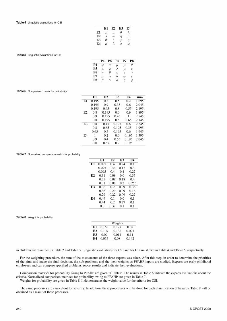
Table 4 Linguistic evaluations for CSI

E1 E2 E3 E4

E1 ϕ µ θ λE2 λ ϕ η µE3 θ δ ϕ γE4 µ λ ε ϕ

Table 5 Linguistic evaluations for CB

P4 P5 P6 P7 P8

P4 ϕ ε µ µ θP5 µ ϕ λ µ εP6 η θ ϕ ε γP7 µ λ θ ϕ εP8 β γ α γ ϕ

Table 6 Comparison matrix for probability

E1 E2 E3 E4 sum

E1 0.195 0.8 0.5 0.2 1.6950.195 0.9 0.35 0.6 2.0450.195 0.65 0.8 0.55 2.195

E2 0.8 0.195 0.0 0.9 1.8950.9 0.195 0.45 1 2.5450.8 0.195 0.5 0.65 2.145

E3 0.8 0.45 0.195 0.8 2.2450.8 0.65 0.195 0.35 1.9950.65 0.5 0.195 0.6 1.945

E4 1 0.2 0.0 0.195 1.3950.9 0.4 0.55 0.195 2.0450.0 0.65 0.2 0.195

Table 7 Normalized comparison matrix for probability

E1 E2 E3 E4

E1 0.095 0.4 0.24 0.10.095 0.44 0.17 0.30.095 0.4 0.4 0.27

E2 0.31 0.08 0.0 0.350.35 0.08 0.18 0.40.31 0.08 0.2 0.255

E3 0.36 0.2 0.09 0.360.36 0.29 0.09 0.160.29 0.22 0.09 0.27

E4 0.49 0.1 0.0 0.10.44 0.2 0.27 0.10.0 0.32 0.1 0.1

Table 8 Weight for probability

Weights

E1 0.165 0.178 0.08E2 0.107 0.136 0.093E3 0.09 0.014 0.11E4 0.055 0.08 0.142

in children are classified in Table 2 and Table 3. Linguistic evaluations for CSI and for CB are shown in Table 4 and Table 5, respectively.

For the weighting procedure, the sum of the assessments of the three experts was taken. After this step, in order to determine the prioritiesof the aims and make the final decision, the sub-problems and the their weights as PFAHP inputs are studied. Experts are early childhoodemployees and can compare specified problems, report results and indicate their evaluations.

Comparison matrices for probability owing to PFAHP are given in Table 6. The results in Table 6 indicate the experts evaluations about thecriteria. Normalized comparison matrices for probability owing to PFAHP are given in Table 7.

Weights for probability are given in Table 8. It demonstrates the weight value for the criteria for CSI.

The same processes are carried out for severity. In addition, these procedures will be done for each classification of hazards. Table 9 will beobtained as a result of these processes.

240 © CPOST 2020

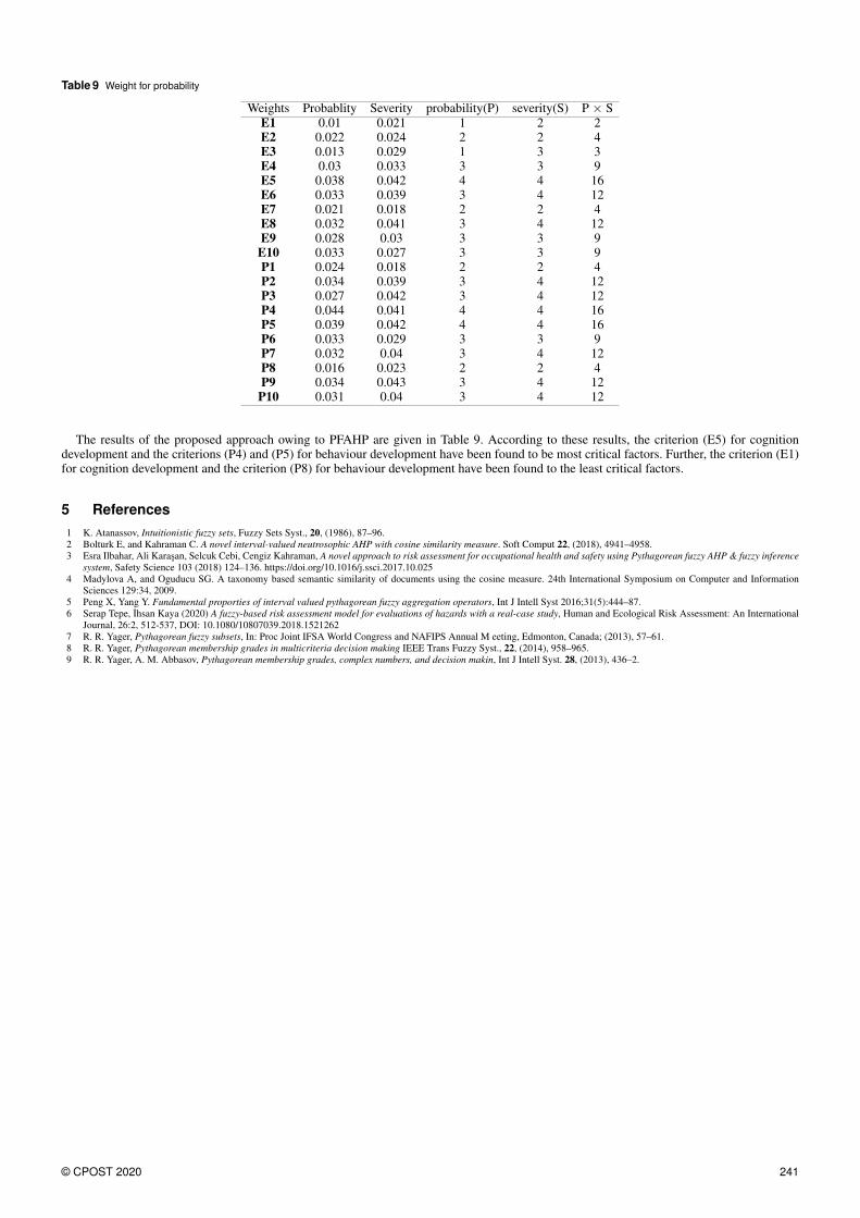
Table 9 Weight for probability

Weights Probablity Severity probability(P) severity(S) P × S

E1 0.01 0.021 1 2 2E2 0.022 0.024 2 2 4E3 0.013 0.029 1 3 3E4 0.03 0.033 3 3 9E5 0.038 0.042 4 4 16E6 0.033 0.039 3 4 12E7 0.021 0.018 2 2 4E8 0.032 0.041 3 4 12E9 0.028 0.03 3 3 9

E10 0.033 0.027 3 3 9P1 0.024 0.018 2 2 4P2 0.034 0.039 3 4 12P3 0.027 0.042 3 4 12P4 0.044 0.041 4 4 16P5 0.039 0.042 4 4 16P6 0.033 0.029 3 3 9P7 0.032 0.04 3 4 12P8 0.016 0.023 2 2 4P9 0.034 0.043 3 4 12

P10 0.031 0.04 3 4 12

The results of the proposed approach owing to PFAHP are given in Table 9. According to these results, the criterion (E5) for cognitiondevelopment and the criterions (P4) and (P5) for behaviour development have been found to be most critical factors. Further, the criterion (E1)for cognition development and the criterion (P8) for behaviour development have been found to the least critical factors.

5 References

1 K. Atanassov, Intuitionistic fuzzy sets, Fuzzy Sets Syst., 20, (1986), 87–96.

2 Bolturk E, and Kahraman C. A novel interval-valued neutrosophic AHP with cosine similarity measure. Soft Comput 22, (2018), 4941–4958.

3 Esra Ilbahar, Ali Karasan, Selcuk Cebi, Cengiz Kahraman, A novel approach to risk assessment for occupational health and safety using Pythagorean fuzzy AHP & fuzzy inference

system, Safety Science 103 (2018) 124–136. https://doi.org/10.1016/j.ssci.2017.10.025

4 Madylova A, and Oguducu SG. A taxonomy based semantic similarity of documents using the cosine measure. 24th International Symposium on Computer and Information

Sciences 129:34, 2009.

5 Peng X, Yang Y. Fundamental proporties of interval valued pythagorean fuzzy aggregation operators, Int J Intell Syst 2016;31(5):444–87.

6 Serap Tepe, Ihsan Kaya (2020) A fuzzy-based risk assessment model for evaluations of hazards with a real-case study, Human and Ecological Risk Assessment: An International

Journal, 26:2, 512-537, DOI: 10.1080/10807039.2018.1521262

7 R. R. Yager, Pythagorean fuzzy subsets, In: Proc Joint IFSA World Congress and NAFIPS Annual M eeting, Edmonton, Canada; (2013), 57–61.

8 R. R. Yager, Pythagorean membership grades in multicriteria decision making IEEE Trans Fuzzy Syst., 22, (2014), 958–965.

9 R. R. Yager, A. M. Abbasov, Pythagorean membership grades, complex numbers, and decision makin, Int J Intell Syst. 28, (2013), 436–2.

© CPOST 2020 241



On a Different Method For Determining thePrimary Numbers

ISSN: 2651-544X


Serpil Halici1,∗ Hamit Cacur2 Nazli Koca3

1Pamukkale Universitesi, Department of Mathematics, Denizli, Turkey, ORCID: 0000-0002-8071-04372Pamukkale Universitesi, Department of Mathematics, Denizli, Turkey,3Pamukkale Universitesi, Department of Mathematics, Denizli, Turkey, ORCID: 0000-0002-4663-6253

* Corresponding Author E-mail: [email protected], [email protected]

Abstract: In this study, firstly, ordinal numbers of the odd integers were defined to reach prime numbers, and a new prime number

sieve was obtained with the help of these numbers. A general formula was given to examine this sieve. Then, by representing the

ordinal numbers with the help of matrices, some properties of these numbers were also examined.

Keywords: Prime Numbers, Prime Number Sieves, Applications of Sieves Methods.

1 Introduction and Preliminaries

While identifying prime numbers is simple, finding a new and large prime number is difficult. To date, the distribution of prime numbers, thenext major prime number, prime number calculation algorithms, etc. Mathematicians have developed many theories on topics. The study of themost common and known prime numbers is the study of Euclid in about 300 BC and this also constitutes the basic principles of arithmetic [1].The Eratosthenes sieve, handled by the Greek mathematicians, is not sufficient in calculating large numbers in terms of cost and time . Then, inthe 17th century, Fermat and Euler worked on the properties of prime numbers and to make them more understandable. Today, efforts are beingmade to find the largest prime number within the scope of the Great Internet Mersenne Prime Search (GIMPS) project [2]. As is known, Euclidproved that the prime numbers are infinite. However, no exact formula has yet been found to find these prime numbers. Therefore, studies arestill ongoing on prime numbers. Since it is not easy to find prime numbers or to distinguish them from composite numbers, prime numbers aregrouped according to some properties [1].To date, a formula found and proven to generate prime numbers is not yet available in the literature [3]. Through trial-and-error, the search forprime numbers using mathematical calculations and algorithms continues. In this study, we gave a screening algorithm different from previousstudies. We supported this method first with the help of tables.Since we will work on set of the odd integers in our study, and every element of this set is likely to be prime, we named this set of numbers as apossible set of prime numbers and denoted this set with the letter Ms. To further narrow the single set of integers than the probability of beingprime, we examined the finale digits of potentially prime numbers. It should be noted that the numbers in the last digit should end with one ofthe numbers 1, 3, 7 and 9, but the numbers that end in each of the last digits with one of these numbers are not prime. In this method, unlikeother prime number tests, we have defined and used the numbers of possible prime numbers. Let’s give some definitions that we use and whichare not available in the literature.

Definition 1. The numbers obtained by subtracting 1 from Ms numbers and dividing by 2 are called the number of rows of possible primenumbers and are indicated Mss. For example,Mss(3) = 1,Mss(5) = 2,Mss(7) = 3, · · ·

It is not possible to find prime numbers directly in Ms array. Therefore, it will be found that the non-prime numbers are found and theremaining numbers are prime numbers. These operations will be done using the row numbers of possible numbers. For b ∈ Zodd and s, a ∈ Zthe number s shows the number of rows of the number b. Let’s define the following numbers with the help of this number b:

a = (s, s+ 1, s+ 2, s+ 3, · · · ) = (s+ n); n ∈ N.

Using these numbers, let’s call the numbers described below as the number of rows of non-prime numbers.

M′

ss = s (1, 1, 1, . . .) + b (s, s+ 1, s+ 2, · · · ) .

242 © CPOST 2020

Number of rows with multiples of 3

M′

ss 4 7 10 13 16 19 22 25 28 31s 1 1 1 1 1 1 1 1 1 1a 1 2 3 4 5 6 7 8 9 10


M′

ss 12 17 22 27 32 37 42 47 52 57s 2 2 2 2 2 2 2 2 2 2a 2 3 4 5 6 7 8 9 10 11


M′

ss 24 31 38 45 52 59 66 73 80 87s 3 3 3 3 3 3 3 3 3 3a 3 4 5 6 7 8 9 10 11 12


M′

ss 40 49 58 67 76 85 94 103 112 121s 4 4 4 4 4 4 4 4 4 4a 4 5 6 7 8 9 10 11 12 13


M′

ss 60 71 82 93 104 115 126 137 148 159s 5 5 5 5 5 5 5 5 5 5a 5 6 7 8 9 10 11 12 13 14


M′

ss 84 97 110 123 136 149 162 175 188 201s 6 6 6 6 6 6 6 6 6 6a 6 7 8 9 10 11 12 13 14 15


M′

ss 112 127 142 157 172 187 202 217 232 247s 7 7 7 7 7 7 7 7 7 7a 7 8 9 10 11 12 13 14 15 16


M′

ss 144 161 178 195 212 229 246 263 280 297s 8 8 8 8 8 8 8 8 8 8a 8 9 10 11 12 13 14 15 16 17

For example,for s ∈ Z+ , b = 3, 5, 7, 9 a sequence of numbers as follows is obtained using the formula above, respectively.

(1, 1, 1, · · · ) + 3(1, 2, 3, · · · ) = (4, 7, 10, · · · ),

(2, 2, 2, · · · ) + 5(2, 3, 4, · · · ) = (12, 17, 22, · · · ),

(3, 3, 3, · · · ) + 7(3, 4, 5, · · · ) = (24, 31, 38, · · · ),

(4, 4, 4, · · · ) + 9(4, 5, 6, · · · ) = (40, 49, 58, · · · ).

The first sequence (4, 7, 10, · · · ) here is the sequence numbers of the odd multiples of the number 3, respectively (12, 17, 22, · · · ), respectively.The sequence numbers of the odd multiples floors of the number 5, (24, 31, 38, · · · ), respectively, gives the number of rows of odd multiples

of 7, respectively. Tables for M′

ss numbers can also be edited:According to the table above, the following theorem can be given.

Theorem 1. The following formula is true for the ordinal numbers of non-prime numbers.

a× b+ s = M′

ss

By looking at the M′

ss numbers in the table above, we can give information about whether a given number is a prime number: If the givennumber is included in this table, it is not a prime number. For example, let’s examine whether the number 299 is prime or not with the abovetable. First, let’s write the number of rows of 299 using.

Definition 2. M′

ss=149. Since the number 149 is included in above table, this number cannot be a prime number. Non-prime numbers can

also be obtained on the matrix by using M′

ss numbers, that is, the ordinal numbers of non-prime numbers. If the sequence numbers, M′

ss ofnon-prime numbers for the integer s ≤ 8 are placed on the matrix, then the following equation can be written using the above theorem.

© CPOST 2020 243

1 0 0 0 0 0 0 02 2 0 0 0 0 0 03 3 3 0 0 0 0 04 4 4 4 0 0 0 05 5 5 5 5 0 0 06 6 6 6 6 6 0 07 7 7 7 7 7 7 08 8 8 8 8 8 8 8

×

3 0 0 0 0 0 0 00 5 0 0 0 0 0 00 0 7 0 0 0 0 00 0 0 9 0 0 0 00 0 0 0 11 0 0 00 0 0 0 0 13 0 00 0 0 0 0 0 15 00 0 0 0 0 0 0 17

+

1 0 0 0 0 0 0 01 2 0 0 0 0 0 01 2 3 0 0 0 0 01 2 3 4 0 0 0 01 2 3 4 5 0 0 01 2 3 4 5 6 0 01 2 3 4 5 6 7 01 2 3 4 5 6 7 8

M′

ss =

4 0 0 0 0 0 0 07 12 0 0 0 0 0 010 17 24 0 0 0 0 013 22 31 40 0 0 0 016 27 38 49 60 0 0 019 32 45 58 71 84 0 022 37 52 67 82 97 112 025 42 59 76 93 110 127 144

The diagonal matrix b in this last formula consists of odd integers. Matrix a is obtained from the row numbers of the numbers in matrix b.This M

′

ss matrix gives us the ordinal numbers of non-prime numbers. Also, the formed M′

ss matrix is a sub-triangular matrix, and the numberson the prime diagonal of the M

′

ss matrix give the sequence numbers of the exact squares of the odd non-prime numbers. For example, the maindiagonal of the matrix M

′

ss ; 12, 24, 40, 60, 84, 112, 144 non-prime rank numbers correspond to 9, 25, 49, 81, 121, 169, 225, 289 respectively.Here, the M

′

ss matrix can be further generalized if desired. With the help of a matrix with an infinite number of rows and columns, formulas ofthe number of rows of non-prime numbers will also be given in the following theorem.

Theorem 2. k, n ∈ Z+, k is the number of lines, we have

M′row

ss = 2n(n+ 1) + (k − 1)(2n+ 1), k ≥ 1.

We will call this formula the matrix row formula for non-prime numbers. Let’s examine this formula on an example below. Line 1 formulais as follows, so for k = 1 we have M

′row

ss = 2n2 + 2n. For k = 2,

M′row

ss = 2n2 + 2n+ 1 + 1.(2n+ 1) = 2n2 + 4n+ 1.

Continuing in this way, the desired equations for lines k = 3, 4, 5, . . . can be written similarly. These operations can also be written in matrixform as follows:

n=1 n=2 n=3 · · ·

2n2 + 2n

2n2 + 4n+ 1

2n2 + 6n+ 2...

4 12 24 · · ·7 17 31 . . .10 22 38 . . ....

......

. . .

The formula given here is the generalized form of the formula a× b+ s=M′

ss. The first column in this matrix returns the number of rows of oddmultiples of the number 3. The second column gives the number of rows of odd multiples of number 5. The third column gives the number ofrows of odd multiples of number 7, and so on. Now, let’s give the column formula below for the expanded M

′

ss matrix. The sequence numbers ofnon-prime numbers from the matrix row formula can be written in the matrix form, or the same operations can be arranged as a column formula:

Theorem 3. For a, b ∈ Z+, b ≥ 1, we have

M′column

ss = (3a+ 1) + (b− 1)(2a+ 1).

Where b is the number of columns.

Let’s examine this formula for some values: According to the formula, when the 1st column formula, b = 1, the following equation isobtained.

M′column

ss = (3a+ 1).

For b = 2, we get

M′column

ss = (3a+ 1) + 1(2a+ 1) = (5a+ 2).

Continuing with the same idea, similar equations can be written for b=3 ,4, 5 . . . lines. These equations can be written again in matrix form asfollows:

244 © CPOST 2020

a=1 a=2 a=3 · · ·

3a+15a+27a+3

...

4 7 10 · · ·7 12 17 . . .10 17 24 . . ....

......

. . .

Note that this matrix has a diagonal and symmetrical matrix feature. Lower and upper triangular matrices can also be created with the help ofsymmetrical matrix.

4 0 0 07 12 0 010 17 24 013 22 31 40

or

4 7 10 130 12 17 220 0 24 310 0 0 40

The formula given in the theorem can be considered as the formula that gives the number of rows in the column. Therefore, we will call thisformula the matrix column formula for non-prime numbers. Similarly, we will create a matrix of row numbers of prime numbers, and we willshow the matrix of row numbers of these prime numbers as Mss. First, some prime numbers are given below.

3, 5, 7, 11, 13, 17, 23, 29, 31, 37, 41, 43, 47, 53, 59, 61, 67, . . . .

The line numbers of these prime numbers are as follows.

Mss = 1, 2, 3, 5, 6, 8, 9, 11, 14, 15, 18, 20, 21, 23, 26, 28, 30, 33, . . . .

Here, the elements of the following x and y matrices are integers, and the columns of the z matrix are the following formula, consisting of theordinal numbers of the prime numbers:

Mss = xy + z

M′

ss =

0 0 0 0 00 1 0 0 00 1 1 0 00 1 1 1 00 1 1 1 18 8 8 8 8

×

0 0 0 0 01 4 3 10 241 2 3 5 62 6 6 10 121 4 6 5 6

+

1 2 3 4 5 61 2 3 4 5 61 2 3 4 5 61 2 3 4 5 61 2 3 4 5 6

M′

ss =

1 2 3 5 62 6 6 15 303 8 9 20 365 14 15 30 486 18 21 35 54

M′

ss and Mss matrices are applications on the matrices, except for the table representation of non-prime numbers and the sequence numbersof prime numbers, respectively.

Definition 3. The formula giving the M′

ss numbers on the prime diagonal can be given as follows. Kss=Mss (1 +Ms). Here Kss is thesequence number of the square of non-prime numbers. For example,

Ms = 7, Mss = 3, Kss = 3(1 + 7) = 24, M′

ss(24) = 49 = 72

Ms = 11, Mss = 5, Kss = 5(1 + 11) = 60, M′

ss(60) = 121 = 112

Definition 4. Let Ms = x. Then, we write

Mss =(x− 1)

2and Kss = (

x− 1

2)(1 + x) =

(x2 − 1)

2.

Here, the following definition can be given if the formula obtained to find non-prime numbers in the row and column in the graph of the formulas

Kss and M(′column)ss is developed.

Theorem 4. For b ∈ Zodd and b > 2, we have

(b2 − 1)

2,

(b2 + 2b− 1)

2,

(b2 + 4b− 1)

2,

(b2 + 6b− 1)

2, . . . (1)

© CPOST 2020 245

For b = 3, the ordinal numbers of the multiples of 3 are obtained. So, 4, 7, 10, 13, 16, 19, 22, 25, ... Accordingly, since the number of rowsis 13, the number itself is 39, this number is not prime. For b = 5, that is, the number of rows of multiples of 5.

12, 17, 22, 27, 32, 37, 42, . . .

The same operations are repeated for other odd numbers.

b b2−12

b2+2b−1

2b2+4b−1

2b2+6b−1

2b2+8b−1

2b2+10b−1

22 1,5 3,5 5,5 7,5 9,5 11,53 4 7 10 13 16 194 7,5 11,5 15,5 19,5 23,5 27,55 12 17 22 27 32 376 17,5 23,5 29,5 35,5 41,5 47,57 24 31 38 45 52 598 31,5 39,5 47,5 55,5 63,5 71,59 40 49 58 67 76 85

10 49,5 59,5 69,5 79,5 89,5 99,511 60 71 82 93 104 11512 71,5 83,5 95,5 107,5 119,5 131,513 84 97 110 123 136 149

Observation results

1) The number of rows of no prime numbers is found in the table above.2) When an even number is given instead of b, it is seen that even numbers correspond to the number of rows.3) When odd number values are given instead of b, it is seen that the result is odd non-prime numbers.4) When odd numbers are given instead of b, single multiples of the given number are obtained, respectively.

2 References

1 J.J O’Connor, J.J., Robertson, E.F., Prime Numbers, (2019), http://www-history.mcs.st-andrews.ac.uk/HistTopics/Primenumbers.html.2 https://www.mersenne.org/. Access date: 13.07.2020.3 C. Özgü, A Study on Prime Number Patterns and Goldbach Conjecture, Master Thesis, Ege University Institute of Science, International Computer Program, (2002).4 T. Yerlikaya, T., Kara, O., Prime Number Testing Algorithms Used in Cryptology, Trakya Uni.J.Eng.Sci., 18(1), (2017).

246 © CPOST 2020



On Excellent Safe Primary Numbers andEncryption

ISSN: 2651-544X


Nazlı Koca1,∗ Serpil Halıcı2

1Pamukkale Uni., Depart. of Math. Denizli,Turkey, ORCID: 0000-0002-4663-62532Pamukkale Uni., Depart. of Math. Denizli,Turkey, ORCID: 0000-0002-8071-0437

* Corresponding Author E-mail: [email protected]

Abstract: In this study, we firstly included the definition of perfectly safe prime numbers that we created. We then examined the

RSA and Rabin cryptosystem, which are the techniques of implementing prime numbers in encrypting any message. Finally, we

used these perfectly safe prime numbers, which were first defined, in RSA and Rabin’s encryption methodsssss.

Keywords: Prime Numbers, Distribution of Primes, Applications of Prime Numbers.

1 Introduction and Preliminaries

Prime numbers are also used to send encrypted messages in the field Cryptography in the past and today. In cryptography, each user has twodifferent keys, one open and one secret for encryption and decryption. The public key is public and anyone can see it. The secret key is keptconfidential and should not be known to anyone other than its owner. Encryption is done with a public key, while the decryption is done witha private key. These encryption keys are used in binary and the other key decodes the information that one encrypts. The most known andused encryption method today is the RSA encryption method, the public key encryption method. The name of this system carries the surnamesof scientists named Ron Rivest, Adi Shamir and Leonard Adlemen in 1978, namely the method was named after factoring the integers [1].Another public key encryption method is Rabin’s encryption technique. The Rabin’s encryption method is a crypto system found in 1979 byMichael Rabin. This cryptosystem is based on the asymmetric encryption technique. Rabin’s cryptosystem, which is a different type of RSAmethod, takes advantage of the difficulty of factoring the compound numbers as in RSA [2].In this study, we will start with the definition ofperfectly safe prime numbers that we will use in encryption with prime numbers. Then we will use the perfect numbers that we have created inRSA and Rabin encryptions.

Definition 1. When applying the formula(k−1)

2 for k > 0 and k ∈ Z+ the lower row number of k is obtained.

For example, the lower row number of 17 is 8.

Definition 2. When applying the formula(k+1)

2 for k > 0 and k ∈ Z+ the upper row number of k is obtained.

For example, the upper row number of 21 is 11.

Definition 3. Let p be the prime number. So that if p’s lower row number and upper row number is prime number, p number is called perfectsafe prime number.

For example, p = 5 prime number is six row number 2 and top row number is 7. So, p = 5 is the perfect safe prime number, since the lowerrow number and the upper row number are prime. Some perfectly safe prime numbers are: 5, 11, 23, 83, 179, 359, 719, · · · .In the table 1.2 below, consecutive odd numbers are given in the white region. The upper row numbers are written on the odd numbers in thiswhite section. To the next higher row, the upper row number of the number written below will be written. Also, the lower row number of thesenumbers is written in the lower part of the numbers in the white part. If the result is an even number when writing down the lower row number,it is not continued. Because we will do our operations on odd numbers. Numbers indicated in red are prime numbers. The prime number in themiddle of 3 consecutive prime numbers constitutes perfectly safe prime numbers. We highlighted the perfectly safe prime number in green.

© CPOST 2020 247

255 383 511 639 767 895 1023 1151 1279 1407 1535 1663 1791

127 191 255 319 383 447 511 575 639 703 767 831 895

63 95 127 159 191 223 255 287 319 351 383 415 447

31 47 63 79 95 111 127 143 159 175 191 207 223

15 23 31 39 47 55 63 71 79 87 95 103 111

7 11 15 19 23 27 31 35 39 43 47 51 55

3 5 7 9 11 13 15 17 19 21 23 25 27

1 2 3 4 5 6 7 8 9 10 11 12 13

1 2 3 4 5 6

1 2

Table 1.1 Perfect safe prime numbers

1919 2047 2175 2303 2431 2559 2687 2815 2943 3071 3199 3327 3479

959 1023 1087 1151 1215 1279 1343 1407 1471 1535 1599 1663 1739

479 511 543 575 607 639 671 703 735 767 799 831 869

239 255 271 287 303 319 335 351 367 383 399 415 431

119 127 135 143 151 159 167 175 183 191 199 207 215

59 63 67 71 75 79 83 87 91 95 99 103 107

29 31 33 35 37 39 41 43 45 47 49 51 53

14 15 16 17 18 19 20 21 22 23 24 25 26

7 8 9 10 11 12

3 4 5

1 2

Table 1.2 Perfect safe prime numbers

Let’s give the above table with the following theorem.

Theorem 1. Perfect numbers are increasing rapidly as prime numbers progress irregularly.

From here we can say that it is not easy to reach Perfect prime numbers.In the following sections, we will use this feature of perfect numbers to use to encrypt messages. Modular mathematics is used in the RSAalgorithm. Below we n ,coutline the RSA algorithm.

2 Encryption with Primary Numbers

Public Key Generation Algorithm. Each person A creates their public key as follows:Selects two prime numbers, p and q, which are different, random and have the same number of digits. Calculates n = pq and ϕ =(p− 1)× (q − 1).Selects a random c number such that 1 < c < ϕ and (c, ϕ(n)) = 1. Using the Euclidean algorithm, it calculates the number d satisfying thecondition.1 < d < ϕ(n) and cd ≡ 1(modϕ(n))Person A has a public key (n, c) and his secret key becomes d.So, encryption can generally be given as follows: The pair (n, c)the public key, is known to the person sending the information.The explicit text is converted to an integer such that M ∈ [0, n− 1] .The encrypted text is calculated as C ≡Mc (modn).The person sending the information sends the C encrypted text to the person receivingthe information [3].

PLAIN TEXT ⇒ ENCRYPTION ⇒ ENCRYPED TEXT ⇒ DECODING ⇒ PLAIN TEXT

Algorithm 2.1 Encryption and decryption algorithm

The flow chart for the RSA algorithm is given in the figure below.

248 © CPOST 2020

SENDER

⇓

OPEN TEXT (M)⇓

NUMBER BLOCKS (M1,M2, ...)⇓

ENCRYPED TEXTC1 ≡Me

1modn C2 ≡Me2modn

⇓

DECODED TEXTM1≡ Ce

1 mod n M2≡ Ce2 mod n

⇓

RECEIVER

⇓

RANDOM NUMBER (e)HIDDEN KEY← → OPEN KEY

Algorithm 2.2 Flow Chart of RSA Algorithm

Encryption Algorithm. If person B wants to send an m message to A, person B does the following to encrypt the message m:

• First, he learns the public key (n, e) of person A.• Writes the message m in the range [0, n− 1].• Then it calculatesC ≡Mc (modn).• Sends the formed C password to person A.To find clear text from encrypted C text, person A does the following:• By using the secret key d and executing m ≡ cd(modn), m reaches the open text [4].

For example, choose prime numbers p = 11, q = 17.

Then, n = 11× 17 = 187 and ϕ(n) = (11− 1)(17− 1) = 160 For 1 < c < ϕ(n), choose c = 3. And let d = 107 satisfy dc ≡1(modϕ(n)). According to this, dc ≡ 321 ≡ 1(modϕ(n)).

Definition 4. Let p be the prime number. So that if p is the number of the previous row and the number of next row is the prime number, pnumber is called the perfect safe prime number.

For example, p is the perfectly safe prime number since p = 5 is the prime number, and the next 7 is the prime number. Some perfectly safeprime numbers are 5, 11, 23, 83, 179, 359, 719,...

3 RSA Method and Perfect Prime Numbers

Now, in this section, an application of the RSA security algorithm for perfectly safe prime numbers will be given. Let p and q be two consecu-

tive perfectly safe prime numbers: p = 11, q = 23 then we write n = (2q + 1)(2q + 1) = 23.47 = 1081 ϕ(n)=(p−1)

2 ×(q−1)

2 = 5× 11=55.Let’s choose a random number e. And e = 19 with 1 < e < n and (e, ϕ(n)) = 1. d = 29 can be taken as a number that satisfies de ≡1(modϕ(n)). Since, de ≡ 551 ≡ 1(modϕ(n)) the public key becomes (n, e) = (1081, 19). Thus, the closed key is (n, d) = (1081, 29).

As a example let us choose p = 5, q = 11 consecutive perfectly safe prime numbers. n = (2p+ 1)× (2q + 1) = 253 ϕ(n) =(p−1)

2 .(q−1)

2 = 10.Let’s choose a random number e. Let this number be prime between 1 < e < n and (e, ϕ(n)) = 1. If we take e = 3, then we havede ≡ 1(modϕ(n)), d = 7 and de = 21 ≡ 1(modϕ(n)). The public key is(n, e) = (253, 3) and the closed key is (n, e) = (253, 7).Now, let the text you want to send be "SIFRE". If the letters are numbered respectively,S = 1, I = 2, F = 3, R = 4, E = 5. The person towhom the message will be sent and anyone who reads the message is given the numbers n calculated above and randomly selected e. Calcula-tion is made according toe = 3 and (mod10) for SIFRE = 12345.

13 ≡ 1 (mod10)23 ≡ 8 (mod10)33 ≡ 7 (mod10)43 ≡ 4 (mod10)53 ≡ 5 (mod10).

So the password to be sent will be 18745. Deciphering is completed by converting this number into "SIFRE" text using our codes. Forexample, letters are matched to numbers between integer values in [0, ϕ(n− 1)].

A I K M N O R S U Y0 1 2 3 4 5 6 7 8 9

© CPOST 2020 249

Table 3.1 Encryption table of some letters.

To be able to send a message using the letters we have numbered above, let’s encrypt our message first. We find the values required for encryp-tion as ϕ(n) = 10 and e = 3.

Message M I R A Y K O N U S U Y O R

Number V alue 3 1 6 0 9 2 5 4 8 7 8 9 5 6

Power of e 33

13

63

03

93

23

53

43

83

73

83

93

53

63

V alue 27 1 216 0 729 8 125 64 512 343 512 729 125 216

Remaining 7 1 6 0 9 8 5 4 2 3 2 9 5 6

Password message S I R A Y U O N K M K Y O R

Table 3.2 message encryption table.

The person who receives our encrypted message will do the following to turn this message into understandable text.

Password message S I R A Y U O N K M K Y O R

Power of d 77

17

67

07

97

87

57

47

27

37

27

97

57

67

V alue 27 1 216 0 729 8 125 64 512 343 512 729 125 216

Remaining 3 1 6 0 9 2 5 4 8 7 8 9 5 6

Message M I R A Y K O N U S U Y O R

Table 3.3 encryption message decoding.

It should be noted that for open the encrypted message we need to know the secret key d = 7.

In the section below, we have examined a different encryption method using the special prime numbers we have defined.

Rabin’s Encryption Algorithm. This method is a cryptosystem method given by Michael Rabin in 1979. This cryptosystem is an asymmetric encryp-

tion technique. The Rabin’s cryptosystem is a version of RSA. But there are some differences between them. Some of these are given below.

It is a great advantage over RSA that it is not easy for any text in the Rabin’s cryptosystem to be able to obtain the encrypted text by someone who can factor

only the n public key. The decoding of the Rabin cryptosystem proved to be equivalent to the factor of dividing integers. Therefore, the Rabin method is safer

than the RSA method. When e = 3 is taken, there is a modular multiplication and a modular squared operation in the RSA method. However, since there is

only one modular squaring process in the Rabin method, the processes are faster than the RSA method [2]. The disadvantage of the Rabin’s cryptosystem

is difficult to find out which of the four different keys is correct. This is a disadvantage compared to the RSA method, although it is attempted to select the

correct output with the addition method [3].

The key generation in the Rabin cryptosystem is done as follows:

Approximately the same size, large and random p, q prime numbers are selected. n = p× q is calculated. Therefore, the number n is the public key and the

(p, q) ordered pair is the secret key. When encrypting in the Rabin’s cryptosystem method, someone who wants to encrypt the m message is created with

the number m not less than n. The sender’s public key is reached. And the equivalence of c ≡ m2(modn) is calculated. The sender sends the encrypted c

message to the person he wants.

Password decoding with the Rabin’s cryptosystem method is done as follows:

The person receiving the encrypted message calculates the m value using his private key.

Accordingly, there are two solutions of mp and mq . Using the extended Euclidean algorithm, yp × p+ yq × q = 1 is calculated. Then the roots of m1,

m2, m3, m4 are calculated as follows.

m1 = (yp × p×mq +mq × q ×mp)(modn), m2 = n−m1, m3 = (yp.p.mq −mq .q.mp)(modn), m4 = n−m3

Here, one of the roots m1, m2, m3, m4 is the key for us to open the sent text. For example, for person A key generation; p = 277and q = 331

by choosing the prime numbers, he finds n = 91687. The public key of person A is n = 91687 and the secret key is p = 277, q = 331 . For the encryption

process, the message of person A to be encrypted is m = 40569. Then, c ≡ 405692(mod91687) = 62111 is obtained. This found c message is sent to

person B.

Decryption. Person B calculates c encrypted text with n = 91687 public key, four square roots of c according to (modn) The following four roots

are available from different roots:

m1 = 69654, m2 = 22033, m3 = 40569, m4 = 51118.

Here m3 opens the message c, which is the encrypted text, and reaches the original, real message. Let’s examine the Rabin’s method using the perfect prime

numbers in the example below:

Our message to be encrypted: get MRY.

250 © CPOST 2020

M 1

I 0

R 5

A 7

y 8

Table 3.4 Coding table of some letters.

We matched the letters with the numbers we chose arbitrarily. Now let’s choose perfectly safe primes p = 11 and q = 23. From here, n = p.q = 253. Our

public key is n = 253, and our private key is (p, q) = (11, 23).

Let’s choose the number m as m = 158 so that m < n. So, c ≡ 1582(mod253) = 170.

Our secret message we send is MAI. The recipient of our secret message with MAI, using his public key, n = 253 m11 ≡ 170(11+1)

4 (mod11) = 4 and

m23 ≡ 170(23+1)

4 (mod23) = 3 finds their numbers. Using the extended Euclidean algorithm, yp × p+ yq × q = 1. There are unknown things from

equality:

yp = −2, yq = 1 . The roots are follows:

m1 = (−2× 11× 3 + 1× 23× 4)(mod253) = 26,

m2 = 253− 26 = 227,

m3 = (−2× 11× 3− 1× 23× 4)(mod253) = 95,

m4 = 253− 95 = 158.

The root that opens the real message here is the number m4. So, our encrypted MAI secret message is calculated by the public key, n = 253, the actual

message m4 = 158 found; MRY opens.

4 Conclusions

As a result, we have created perfectly safe prime numbers by taking advantage of the irregular progression of the prime numbers. Thus, we used the perfectlysecure prime numbers we obtained in RSA and RABIN cryptosystems and thus made encryption more secure.

5 References

1 Akbar, A. A., Asal Sayıların Sifreleme Teorisindeki Uygulamalari, Yüksek Lisans Tezi, Atatürk Uni. Fen Bil. Enst., Erzurum, (2015).

2 http://bilgisayarkavramlari.sadievrenseker.com, 2009, 6(4), /rabin-sifreleme. 1.06.2020.

3 Beskirli, A., Ozdemir, D., Beskirli, M., Sifreleme Yontemleri ve RSA Algoritması Uzerine Bir Inceleme, Avrupa Bilim ve Teknoloji Derg., Ozel sayi, 2019, 284-291.

4 Zuckerman, H.S., Niven, I. And Monygomery H.L., An Introduction To The Theory Of Numbers, New York: John Wiley Sons, 1991, 25-26.

© CPOST 2020 251

VOLUME III ISSUE II

Documents

Transcript of VOLUME III ISSUE II