This article was downloaded by: 10.3.98.104On: 27 Mar 2022Access details: subscription numberPublisher: CRC PressInforma Ltd Registered in England and Wales Registered Number: 1072954 Registered office: 5 Howick Place, London SW1P 1WG, UK

Volume I Measurement and SafetyInstrument and Automation Engineers’ HandbookBéLa G. Lipták, Kriszta Venczel

Calibration

Publication detailshttps://www.routledgehandbooks.com/doi/10.1201/9781315370330-4

H. M. Hashemian, B. G. LiptákPublished online on: 06 Oct 2016

How to cite :- H. M. Hashemian, B. G. Lipták. 06 Oct 2016, Calibration from: Volume IMeasurement and Safety, Instrument and Automation Engineers’ Handbook CRC PressAccessed on: 27 Mar 2022https://www.routledgehandbooks.com/doi/10.1201/9781315370330-4

PLEASE SCROLL DOWN FOR DOCUMENT

Full terms and conditions of use: https://www.routledgehandbooks.com/legal-notices/terms

This Document PDF may be used for research, teaching and private study purposes. Any substantial or systematic reproductions,re-distribution, re-selling, loan or sub-licensing, systematic supply or distribution in any form to anyone is expressly forbidden.

The publisher does not give any warranty express or implied or make any representation that the contents will be complete oraccurate or up to date. The publisher shall not be liable for an loss, actions, claims, proceedings, demand or costs or damageswhatsoever or howsoever caused arising directly or indirectly in connection with or arising out of the use of this material.

Dow

nloa

ded

By:

10.

3.98

.104

At:

07:4

0 27

Mar

202

2; F

or: 9

7813

1537

0330

, cha

pter

1_3,

10.

1201

/978

1315

3703

30-4

27

1.3

CALIBrAtIonserVICes

Conductivity, DO, pH: http://www.thomasnet.com/ products/conductivity-analyzers-1649300-1.html

Control Valve: http://www.thomasnet.com/products/ calibration- services-10021202-1.html

Flowmeter: http://www.thomasnet.com/products/ calibrating-services-flowmeter-10021244-1.html

Gas Services: http://www.thomasnet.com/products/ calibrating-services-gas-detector-96117320-1.html

I/P Transducers: http://www.thomasnet.com/products/transducers-currenttopressure-i-p-voltagetopressure-e-p-96004957-1.html

Pressure, Level, Temperature, Load, Torque, etc.: http://www.thomasnet.com/products/instrument- calibrating-services-40379000-1.html

Temperature Sensor: http://www.thomasnet.com/products/temperature-calibrating-services-84151471-1.html

IntroDuCtIon

Calibration refers to the act of reducing the error in measure-ment equipment over the full range of the sensor being cali-brated. Accuracy is the degree of closeness of measurements

to its true value (see Figures 1.1a and 1.1b). Total error is the sum of random error (precision) and systematic error (bias). Calibration aims at reducing this total error. For that purpose, a “reference standard” is used, which itself has some error, but is much more accurate, than the detector being calibrated. Usually an order of magnitude better accu-racy is expected from the reference than the detector, which is being calibrated.

The value of a process instrument such as a flow, tempera-ture, or pressure sensor normally depends on its accuracy and response time. Accuracy is a qualitative term that describes how correctly the instrument may measure the process param-eter (see Chapter 1.1 for an in-depth discussion), and response time is the time it takes for an instrument, in response to a change in its input, to move its output to the corresponding output value. Accuracy and response time are largely indepen-dent and are therefore identified through separate procedures.

The accuracy of a process instrument is established through its calibration, and the response time is the time it takes for an instrument, in response to a change in its input, to move its output to the corresponding output value. Calibration is done by comparing the measurement of the sensor with the “reference value” detected by a superior sensor and eliminating the difference. The different types of

Calibration

H.M.HAsHeMIAn(2003) B.G.LIPtáK(2017)

1

Dow

nloa

ded

By:

10.

3.98

.104

At:

07:4

0 27

Mar

202

2; F

or: 9

7813

1537

0330

, cha

pter

1_3,

10.

1201

/978

1315

3703

30-4

28 General Considerations

errors have been discussed in connection with Figures 1.1a and 1.1b and are summarized here in Figure 1.3a.

typesoferrors

The goal of calibration is to minimize the zero and span errors. In Figure 1.3b, the calibration of a linear transmitter is approxi-mated by a straight line, representing the equation y = mx + b, where y is the output, x is the input, m is the slope of the line, and b is the intercept. The calibration of an instrument may change due to a change in zero, a change in span, or a change in both zero and span.

A change in zero is also referred to as a bias  error,  systematic error, or zero shift. A zero shift results in a change in instrument reading (either positive or negative) at all points along its range (Figure 1.3c). A zero shift can result from sev-eral causes, such as a change in ambient temperature affect-ing the calibration. For example, if an instrument is calibrated at room temperature and used at a different temperature, its output may include a bias error (or zero shift) due to the tem-perature difference.

The change in span is also referred to as a gain error or span shift. A span shift means an increase or a decrease in the slope of the instrument output line for the same input

1

Span shift

Zero shift100

0

b

% ou

tput

y

0 100% input x

m

Actual

calibrat

ion cu

rve

Specifie

d chara

cteris

tic cu

rve

Span

Fig. 1.3bIllustration of  zero and span. b = zero elevation; m = gain of a linear transmitter; span = the change in input (x) as it travels from 0% to 100%; range = the change  in output  (y) corresponding  to 0%–100% span; output @ input = 0 is called lower range value; output @ input = 100% is called upper range value.

Desired value

% ou

tput

% input% input

% inputLinear sensor’s span error Linear sensor’s zero error

Nonlinearity caused errorLinear sensor’s combined span and zero error

% input

Actual value

Actual value

Actual value

Combined zero andspan errors

Span errors

Zero errors

100%

100%

100% 100%

100%00

100%

0

% ou

tput

% ou

tput

% ou

tput

Errors causedby nonlinearity

100%0

100%

Fig. 1.3aThere can be at least four types of errors in the % output (measurement) of a sensor as it detects the value of a process variable (% input).

Dow

nloa

ded

By:

10.

3.98

.104

At:

07:4

0 27

Mar

202

2; F

or: 9

7813

1537

0330

, cha

pter

1_3,

10.

1201

/978

1315

3703

30-4

1.3  Calibration    29

(see Figure 1.3d). Typically, calibration errors involving span shift alone are less common than calibration errors due to both zero and span shifts. In Figure 1.3d, both cases are shown: span shift without zero shift and span shift with zero shift. In pressure transmitters, about 40% of the calibration changes are caused by zero shift, about 30% by

span shift, and only about 20% by span shift alone.* As for the remaining 10%, the calibration changes are due to other effects, such as nonlinearity.

reFerenCestAnDArD

The key requirement for obtaining high-precision calibration is to have a high-quality reference standard against which the sensor can be calibrated. For the calibration of most vari-ables, it is easy to provide such reference standards (pressure, differential pressure, level, most analyzers, etc.) while for others, it is difficult. For example, the calibration (or reca-libration) of large flowmeters for either liquid or gas service can be expensive and difficult. This is because the number of such large calibration facilities is limited and shipping the flow detector to it requires the availability and installation of a backup unit.

Due to this cost and inconvenience, it is often the case that large flowmeters remain in service for many years with-out recalibration.

Some users take intermediate steps to alleviate this situation. One such approach is to install “clamp-on” flow-meters onto the pipe. This cannot be called calibration, because an ultrasonic clamp-on flowmeter does not qualify for a reference standard, as its accuracy is much worse than the in-line flowmeter, let it be a magnetic, turbine, Coriolis, or just about any other part. So, while this cannot be called calibration, it is a way to determine if flowmeter mainte-nance or replacement is needed.

Another half way step toward recalibration is to test part of the system. For example, in case of a magnetic flowmeter, some users just test the electronics of the loop, but not the flow element. They do that by switching from the millivolt output of the magnetic flowmeter to an accurately generated millivolt signal from a simulator and checking if the receiver is correctly displaying the simulated signal or if there is an error, such as a zero shift, in which case the receiver is reca-librated. This too is a step in the right direction, but is by no means a substitute for recalibration, because it disregards the sensor itself, which usually is the cause of measurement errors (electrode coating, liner failure, grounding, etc.).

PressureorD/Psensors

Calibration of pressure sensors (including both absolute and differential-pressure sensors) can be done by the use of a constant pressure source such as a deadweight

* EPRI Topical Report, On-line monitoring of instrument channel performance, TR-104965-R1 NRC SER, Electric Power Research Institute, Final Report, Palo Alto, CA, September 2000.

1

Input

Span shift+ zero shift

Span shift withoutzero shift

Out

put

Input

Out

put

Fig. 1.3dIllustration of span shifts.

Input

+Zeroshift

–Zeroshift

Out

put

Fig. 1.3cIllustration of a zero shift in an instrument calibration.

Dow

nloa

ded

By:

10.

3.98

.104

At:

07:4

0 27

Mar

202

2; F

or: 9

7813

1537

0330

, cha

pter

1_3,

10.

1201

/978

1315

3703

30-4

30 General Considerations

tester  (see  Figure  1.3e). With a deadweight tester, con-stant pressure is produced for the sensor, while the sensor output is monitored and adjusted to make the electrical output proportional to the applied pressure. For example, a pressure sensor may be calibrated to produce an elec-tronic analog output in the range of 4–20 mA (or a digital one) for pressure inputs covering the whole span of the sensor (0%–100%). For most analog electronic pressure sensors, with no pressure applied, the transmitter output is adjusted to produce a 4 mA signal. Next, a pressure that corresponds to 100% of the span is applied by the dead-weight tester, and the sensor output is adjusted to 20 mA. These adjustments to the output are made by setting two potentiometers provided in the pressure sensor. These adjustment devices are referred to as the zero and span potentiometers. The next step in the calibration of a pres-sure transmitter is to apply known pressures between 0% and 100% of span to verify the linearity of the transmitter and to make any necessary adjustments to obtain accurate mA outputs for all inputs.

The zero and span adjustments of a pressure sensor interact, meaning that changing one will cause a change in the other to change, and vice versa. Thus, in calibrating a pressure sensor, the zero and span are often both adjusted to produce the most accurate output that can be achieved for each input pressure. Because of the nonlinearities in some pressure sensors, the input/output relationships can-not be exactly matched, no matter how well the span and zero adjustments are tuned together. For that reason, in most pressure sensors, a linearity adjustment is also pro-vided (in addition to the zero and span potentiometers) to help achieve the best agreement between the input pressure and the output current.

In lieu of a deadweight tester, one can also use a sta-ble pressure source and a precision pressure gauge as the input. Precision pressure gauges are available in a variety of ranges from a number of manufacturers (see Chapter 7.2). Highly accurate digital pressure indicators can also be used for calibration. As will be seen later, automated

pressure sensor calibration equipment is also available that uses digital technology to offer both accuracy and convenience.

As-FounDAnDAs-LeFtDAtA

The calibration of an instrument can change with time. Therefore, instruments are recalibrated periodically. The periodic calibration procedure typically involves two steps: (1) determine if calibration is needed, and (2) calibrate if needed. In the first step, known input signals (e.g., 0%, 25%, 50%, 75%, and 100% of span) are applied to the instru-ment, and its output is recorded on a data sheet. The data thus generated is referred to as the as-found calibration data (see Table  1.3a). If  the as-found data show that the instru-ment’s calibration is still acceptable, no calibration is needed. Otherwise, the instrument is calibrated by systematically applying a series of input signals and making zero and span adjustments as necessary to bring the sensor within accep-tance limits or criteria. The input/output data after this cali-bration is referred to as the as-left data, and the difference between the as-found and as-left data is often termed the calibration drift or calibration shift.

The acceptance criterion for calibration is normally established by the user, based on the accuracy requirements for the instrument and/or on the manufacturer’s specifica-tion. Typically, manufacturers state the inaccuracy (the error or uncertainty) of an instrument in terms of a percentage of span throughout the range of the instrument. For example, pressure sensor errors can be as low as about 0.05% of span in extremely high-precision sensors or 1% of span in sensors for general applications.

The high-precision performance can only be obtained if the sensor is properly calibrated, because overall accu-racy depends as much on the quality of the calibration process as it does on the ability of the sensor to provide a particular accuracy. Reliable calibration requires the availability of trained personnel, written procedures, and accurate calibration equipment. Obviously, the accuracy

1

Table 1.3aExample of an Instrument Calibration Data

Input Signal (% of Span) 

Desired Output (mA)

As-Found Data (mA)

As-Left Data (mA)

0 4.00 3.93 3.99

25 8.00 8.03 8.01

50 12.00 11.92 12.04

75 16.00 16.09 15.96

100 20.00 20.12 19.97

Weights

Pressure gauge

50 607080

90100

102030

40

0

Plunger

Oil

Piston

Fig. 1.3eSchematic of a typical deadweight tester.

Dow

nloa

ded

By:

10.

3.98

.104

At:

07:4

0 27

Mar

202

2; F

or: 9

7813

1537

0330

, cha

pter

1_3,

10.

1201

/978

1315

3703

30-4

1.3  Calibration    31

of the calibration equipment must be much better than the equipment being calibrated, and the calibration personnel must understand the calibration process and exercise care in performing the calibration task, reading the calibration data, and documenting the results. If an instrument is not properly calibrated, it will not produce accurate and reli-able measurements, even if the quality of the instrument itself is high.

HysteresIs

Hysteresis is a phenomenon that causes an instrument’s output to vary, depending on the direction of the applied input signals, that is, whether it is increasing or decreas-ing (Figure 1.3f). To account for hysteresis, instruments are sometimes calibrated using both increasing and decreasing input signals, and the results are averaged. For example, a pressure sensor may be calibrated using input signals in this sequence: 0%, 25%, 50%, 75%, 100%, 75%, 50%, 25%, and 0% of span.

Normally, a manufacturer’s specification of an instru-ment’s accuracy is arrived at considering hysteresis, linearity, repeatability, and other factors that can affect the instrument’s input/output relationship (see Chapter 2.3 for the definitions of these terms).

CALIBrAtIontrACeABILIty

To be valid and acceptable, all calibrations should be traceable to a national standard or to a known physical phenomenon. In the United States, equipment calibrations are expected to be traceable to the National Institute of Standards and Technology (NIST), in Gaithersburg, MD. Each country has its own stan-dard calibration laboratory for a variety of parameters such as

pressure, temperature, voltage, resistance, weight, time, and so on. The national standards laboratories are normally charged with calibration of primary standards. A primary standard is an instrument that is calibrated at the national standard laboratory like the NIST and used to calibrate other equipment. For exam-ple, the primary standard for calibration of resistance tempera-ture detectors (RTDs) is a precision RTD that is referred to as a standard platinum resistance thermometer or SPRT. Each RTD calibration laboratory has one or more SPRTs that are sent to NIST periodically to be calibrated.

To be calibrated by a national standard laboratory such as NIST, a primary standard must be in good working con-dition and meet certain requirements. Otherwise, NIST may not calibrate it. National standards laboratories are charged with helping to maintain primary standards and therefore do not calibrate common-purpose equipment, nor do they repair equipment that is not in good working order.

To protect the primary standard equipment, a secondary standard (also called transfer standard) may be used. In this case, the primary standard is used to calibrate the secondary standard, which is then used for calibration of other instru-ments. The advantage of this approach is that it preserves the integrity as well as the accuracy of the primary standard by minimizing its handling and use. The disadvantage is that, every time an instrument is calibrated, the accuracy that can be claimed is below the accuracy of the standard that is used in its calibration. Therefore, in going from a primary standard to a secondary standard, a loss of accuracy results.

A common rule is that an instrument shall be calibrated using a standard that is at least four times more accurate than the instrument being calibrated. This requirement is sometimes difficult to meet, as instruments have become so accurate in recent years that one may not find a standard that can be four times more accurate.

LIneArItyAnDDAMPInG

As was mentioned before, in addition to zero and span, some instruments also have a linearity adjustment that is used to produce the most linear input/output relationship throughout the span. A damping adjustment is also available in some instruments. This adjustment does not affect the calibration of an instrument, but it affects its response time. The purpose of the damping adjustment is to reduce the noise in the output signal of the instrument when the process is very noisy. This is accomplished by increasing the damping, which slows the dynamic response of the instrument so that it is not sensitive to high-frequency or noisy inputs.

AutoMAteDCALIBrAtIonequIPMent

Recent advancements in electronics and computer tech-nologies have resulted in the development of a variety of automated test equipment and computer-aided calibrations.

1

Input

Out

put

Fig. 1.3fIllustration of hysteresis.

Dow

nloa

ded

By:

10.

3.98

.104

At:

07:4

0 27

Mar

202

2; F

or: 9

7813

1537

0330

, cha

pter

1_3,

10.

1201

/978

1315

3703

30-4

32 General Considerations

For example, Figure 1.3g illustrates the components of an automated pressure sensor calibration system. It consists of a programmable pressure source that is controlled by a com-puter and produces known pressure inputs that are applied to the sensor being calibrated. The output of the sensor is recorded by the same computer and produces the record of the as-found data.

The sensor is calibrated using both increasing and decreasing input signals as shown in Figure 1.3h, and a hys-teresis curve is also produced. Next, the software compares the as-found data against the acceptance criteria and auto-matically determines if the sensor needs to be recalibrated.

If so, the system provides the necessary input signals to the sensor under calibration and holds the input value constant until zero and span adjustments are made manually. After the calibration, the software produces a report and stores the calibration data for trending, incipient failure detection, and other purposes.

CALIBrAtIonoFteMPerAturesensors

Temperature sensors such as RTDs and thermocouples can be calibrated using a constant-temperature bath and a standard thermometer. The type of calibration bath used depends on the temperature range, the accuracy require-ments, and the application of the sensor. For example, for the calibration of primary and secondary temperature stan-dards, melting- or freezing-point cells are used. These cells are made of materials such as tin, zinc, silver, and gold whose melting or freezing temperatures are set by nature and are accurately known. These cells are referred to as intrinsic standards. These fixed-point cells are expensive, difficult to maintain, and normally are used only in stan-dard laboratories.

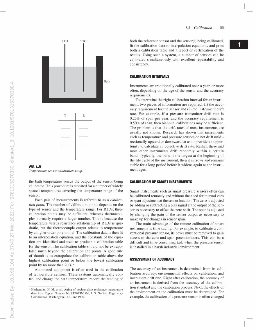
For the calibration of average temperature sensors, the fixed-point cells are seldom used. The more likely choice for a reference cell is an ice bath, an oil bath, or an electric furnace-controlled bath. As shown in Figure 1.3i, the sensor to be calibrated is installed in a temperature bath along with a standard reference sensor. The reference sensor is used to measure the bath temperature. A data table is then made of

1Hydraulic or pneumatic line

Pressuresensor

Programmablepressure source

Computer

Fig. 1.3gPrinciple of an automated pressure sensor calibration system.

Fig. 1.3hCalibration results from automated calibration.

Dow

nloa

ded

By:

10.

3.98

.104

At:

07:4

0 27

Mar

202

2; F

or: 9

7813

1537

0330

, cha

pter

1_3,

10.

1201

/978

1315

3703

30-4

1.3  Calibration    33

the bath temperature versus the output of the sensor being calibrated. This procedure is repeated for a number of widely spaced temperatures covering the temperature range of the sensor.

Each pair of measurements is referred to as a calibra-tion point. The number of calibration points depends on the type of sensor and the temperature range. For RTDs, three calibration points may be sufficient, whereas thermocou-ples normally require a larger number. This is because the temperature versus resistance relationship of RTDs is qua-dratic, but the thermocouple output relates to temperature by a higher order polynomial. The calibration data is then fit to an interpolation equation, and the constants of the equa-tion are identified and used to produce a calibration table for the sensor. The calibration table should not be extrapo-lated much beyond the calibration end points. A good rule of thumb is to extrapolate the calibration table above the highest calibration point or below the lowest calibration point by no more than 20%.*

Automated equipment is often used in the calibration of temperature sensors. These systems automatically con-trol and change the bath temperature, record the reading of

* Hashemian, H. M. et al., Aging of nuclear plant resistance temperature detectors, Report Number NUREG/CR-5560, U.S. Nuclear Regulatory Commission, Washington, DC, June 1990.

both the reference sensor and the sensor(s) being calibrated, fit the calibration data to interpolation equations, and print both a calibration table and a report or certification of the results. Using such a system, a number of sensors can be calibrated simultaneously with excellent repeatability and consistency.

CALIBrAtIonInterVALs

Instruments are traditionally calibrated once a year, or more often, depending on the age of the sensor and the accuracy requirements.

To determine the right calibration interval for an instru-ment, two pieces of information are required: (1) the accu-racy requirement for the sensor and (2) the instrument drift rate. For example, if a pressure transmitter drift rate is 0.25% of span per year, and the accuracy requirement is 0.50% of span, then biannual calibrations may be sufficient. The problem is that the drift rates of most instruments are usually not known. Research has shown that instruments such as temperature and pressure sensors do not drift unidi-rectionally upward or downward so as to provide an oppor-tunity to calculate an objective drift rate. Rather, these and most other instruments drift randomly within a certain band. Typically, the band is the largest at the beginning of the life cycle of the instrument, then it narrows and remains stable for a long period before it widens again as the instru-ment ages.

CALIBrAtIonoFsMArtInstruMents

Smart instruments such as smart pressure sensors often can be calibrated remotely and without the need for manual zero or span adjustment at the sensor location. The zero is adjusted by adding or subtracting a bias signal at the output of the sen-sor as necessary to offset the zero shift. The span is adjusted by changing the gain of the sensor output as necessary to make up for changes in sensor span.

The main advantage of the remote calibration of smart instruments is time saving. For example, to calibrate a con-ventional pressure sensor, its cover must be removed to gain access to the zero and span potentiometers. This can be a difficult and time-consuming task when the pressure sensor is installed in a harsh industrial environment.

AssessMentoFACCurACy

The accuracy of an instrument is determined from its cali-bration accuracy, environmental effects on calibration, and instrument drift rate. Right after calibration, the accuracy of an instrument is derived from the accuracy of the calibra-tion standard and the calibration process. Next, the effects of the environment on the calibration must be determined. For example, the calibration of a pressure sensor is often changed

1RTD SPRT

Bath

T R

Fig. 1.3iTemperature sensor calibration setup.

Dow

nloa

ded

By:

10.

3.98

.104

At:

07:4

0 27

Mar

202

2; F

or: 9

7813

1537

0330

, cha

pter

1_3,

10.

1201

/978

1315

3703

30-4

34 General Considerations

by variations in the ambient temperature. In the case of dif-ferential-pressure sensors, changes in the static pressure of the process can also change the calibration. The manufacturer can usually provide data on temperature and static pressure effects on accuracy. For a detailed discussion of the effect of operating and test pressure and temperature differences, see Chapter 1.1. The errors caused by these effects must be com-bined with the calibration errors to arrive at the total error of the installed sensor.

Next, the instrument drift must be accounted for in determining the total error. Usually, the drift error is added to the sum of calibration error and the errors due to the environmental effects so as to calculate the total error. The inaccuracy of the sensor is then stated based on this total error. A common formula for determining the total error is

Total error = Root sum squared (RSS) of random errors + Sum of bias errors  1.3(1)

Typically, the total error may be a number like 0.35% of span, of range, or of the actual indicated value, depending on the type of sensor used. This number, although an indication of the total error, is referred to as the inaccuracy or uncertainty of the instrument.

CALIBrAtIonAnDrAnGesettInG

Calibration and range setting are the same in case of analog transmitters. As for intelligent devices, calibration and range setting are different. For example, for smart (HART) trans-mitters, calibration is called trim to distinguish it from range. For fieldbus devices, ranging is called scale to distinguish it from calibration. Ranging is accomplished by selecting input values at which the outputs are 4 and 20 mA, while calibra-tion is performed to correct the sensor reading when it is inaccurate.

For example, if a differential-pressure sensor has a lower range limit (LRL) of −200 in. of water and an upper range limit (URL) of +200 in. of water, and if one wants to use it to measure a differential pressure in the range of 0–100 in. of water, then both the LRV and the URV settings must be changed. This adjustment would “range” (increase) the lower range value (LRV) to equal 0 and lower the upper range value (URV) to be 100 in. of water. Note that this is ranging and not calibration. Calibration is when at zero differential pressure,

the transmitter reading is found to be 1 in. of water and it is corrected to read 0 in. of water.

Abbreviations

HART Highway addressable remote transducerLRL Lower range limitLRV Lower range valueRSS Root sum squaredSPRT Standard platinum resistance thermometerURL Upper range limitURV Upper range value

organization

NIST National Institute of Standards and Technology

Bibliography

Bucher, J. L., Quality  Calibration  Handbook, 2007, https://www.isa.org/store/quality-calibration-handbook-developing-and-managing-a-calibration-program/116457.

Cable, M., Calibration: A Technician’s Guide, 2005, https://www.isa.org/store/calibration-a-technicians-guide/116177.

NIST, Calibrations, 2010, http://www.nist.gov/calibrations/flow_measurements.cfm.

Persson, P., Calibration of measuring equipment, December 2014, http://www.qualitymag.com/articles/92306-calibration- o f-measuring-equipment.

Reithmayer, K., Calibrating standard electrochemical parameters in water analysis – pH value, dissolved oxygen (DO) and conduc-tivity, 2011, http://www.globalw.com/support/calibration.html.

Skoog, D. A., James Holler, F., and Crouch, S. R., Principles  of Instrumental  Analysis. Pacific Grove, CA: Brooks Cole, 2007, ISBN 0-495-01201-7, http://www.worldcat.org/title/principles-of-instrumental-analysis/oclc/456101774.

UNIDO, Role of measurement and calibration, 2006, https://www.unido.org/fileadmin/user_media/Publications/Pub_free/Role_of_measurement_and_calibration.pdf.

US Dept. of Interior, Calibrating pressure gauges, November 2014, http://www.usbr.gov/pmts/geotech/rock/EMpart_2/USBR1040.pdf.

Wright, J. D., The long term calibration stability of critical flow nozzles and laminar flowmeter, 1998  NCSL  Workshop  and Symposium, NCSL, Albuquerque, NM, 1998, http://www.nist.gov/calibrations/upload/ncsl_4e03.pdf.

Yeh, T. T., Hydrocarbon liquid flow calibration service, 2005, http://www.nist.gov/calibrations/upload/sp250_1039-2.pdf.

1