Volume 89 (1 & 2), 2014 - The Indian Geographical Society
152
-
Upload
khangminh22 -
Category
Documents
-
view
1 -
download
0
Transcript of Volume 89 (1 & 2), 2014 - The Indian Geographical Society
Governing Council of the Indian Geographical Society
President: Dr. K. Devarajan
Vice Presidents: Dr. P. Ilangovan
Dr. B. HemaMalini
Dr. H.N. Misra
Dr. R.B. Singh
Dr. R. Vaidyanadhan
General Secretary: Dr. R. Jaganathan
Joint Secretaries: Dr. R. Bhavani
Dr. R. Shyamala
Dr. J. Uma
Dr. R. Jegankumar
Treasurer: Dr. V. Madha Suresh
Council Members:
Ms. R. Valli
Dr. S.R. Nagarathinam
Dr. S. Balaselvakumar
Dr. P.H. Anand
Mr. G. Jagadeesan
Dr. N. Subramanian
Mr. C. Subramaniam
Member Nominated to the Executive Committee from the Council:
Dr. S.R. Nagarathinam
Editor: Prof. K. Kumaraswamy
Authors, who wish to submit their papers for publication in the Indian
Geographical Journal, are most welcome to send their papers to the Editor only through e-mail: [email protected]
Authors of the research articles in the journal are responsible for the
views expressed in their articles and for obtaining permission for copyright materials.
For details and downloads visit: www.igschennai.org
Information to Authors
The Indian Geographical Journal is published half-yearly in June and December by The Indian Geographical Society, Chennai. It invites manuscripts of original research on any geographical subject providing information of importance to geography and related disciplines with an analytical approach. The article should be submitted only through the Editor’s e-mail: [email protected]
The manuscript should be strictly ordered as follows: Title page, author (s) name, designation, e-mail ID, and telephone number, abstract, keywords, text (Introduction, Study Area, Methodology, Results and Discussion, Conclusion), Acknowledgements, References, Tables and Figures. You may refer IGS website (www.igschennai.org) for reference.
The title should be brief, specific and amenable to indexing. Not more than five keywords should be indicated separately; these should be chosen carefully and must not be phrases of several words. Abstract and summary should be limited to 100 words and convey the main points of the paper, outline the results and conclusions and explain the significance of the results.
Maps and charts should be submitted in the final or near-final form. The authors should however agree to revise the maps and charts for reproduction after the article is accepted for publication. Each figure should have a concise caption describing accurately what the figure depicts.
If you include figures that have already been published elsewhere, you must obtain permission from the copyright owner(s) for both the print and online format. Please be aware that some publishers do not grant electronic rights for free and that IGS will not be able to refund any costs that may have occurred to receive these permissions.
Acknowledgements of people, grants, funds etc. should be placed in a separate section before the reference list. The names of funding organisations should be written in full.
References should be listed in alphabetical order, serially numbered at the end of the paper as per MLA format. The list of references should only include works that are cited in the text and that have been published or accepted for publication.
The manuscripts should be accompanied with a letter stating that the article has not been published or sent for publication to any other journal and that it will not be submitted elsewhere for publication. Further, the authors could also send name and address with e-mail ids and phone number of four referees to review the article.
For details and downloads visit: www.igschennai.org
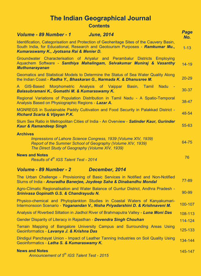
The Indian Geographical Journal Contents
Volume - 89 Number - 1 June, 2014 Page No.
Identification, Categorisation and Protection of Geoheritage Sites of the Cauvery Basin, South India, for Educational, Research and Geotourism Purposes - Ramkumar Mu., Kumaraswamy K., Jyotsana Rai & Menier D.
1-13
Groundwater Characterisation of Ariyalur and Perambalur Districts Employing Aquachem Software - Santhiya Mahalingam, Selvakumar Muniraj & Vasanthy Muthunarayanan
14-19
Geomatics and Statistical Models to Determine the Status of Sea Water Quality Along the Indian Coast - Radha Y., Bhaskaran G., Narmada K. & Dhanusree M.
20-29
A GIS-Based Morphometric Analysis of Vaippar Basin, Tamil Nadu - Balasubramani K., Gomathi M. & Kumaraswamy K.
30-37
Regional Variations of Population Distribution in Tamil Nadu - A Spatio-Temporal Analysis Based on Physiographic Regions - Lazar A.
38-47
MGNREGS in Sustainable Paddy Cultivation and Food Security in Palakkad District - Richard Scaria & Vijayan P.K.
48-54
Slum Sex Ratio in Metropolitan Cities of India - An Overview - Satinder Kaur, Gurinder Kaur & Ramandeep Singh
55-63
Archives Impressions of Lahore Science Congress, 1939 (Volume XIV, 1939) Report of the Summer School of Geography (Volume XIV, 1939) The Direct Study of Geography (Volume XIV, 1939)
64-75
News and Notes Results of 4
th IGS Talent Test - 2014
76
Volume - 89 Number - 2
December, 2014
The Urban Challenge - Provisioning of Basic Services in Notified and Non-Notified Slums of India - Anuradha Banerjee, Joydeep Saha & Dinabandhu Mondal
77-89
Agro-Climatic Regionalisation and Water Balance of Guntur District, Andhra Pradesh - Srinivasa Gopinath G.S. & Chandrayudu N.
90-99
Physico-chemical and Phytoplankton Studies in Coastal Waters of Kanyakumari-Intermonsoon Scenario - Yoganandan V., Nisha Priyadarshini D. & Krishnaveni M.
100-107
Analysis of Riverbed Siltation in Jiadhol River of Brahmaputra Valley - Luna Moni Das
108-113
Gender Disparity of Literacy in Rajasthan - Devendra Singh Chouhan
114-124
Terrain Mapping of Bangalore University Campus and Surrounding Areas Using Geoinformatics - Lavanya J. & Krishna Das
125-133
Dindigul Panchayat Union - Impact of Leather Tanning Industries on Soil Quality Using Geoinformatics - Latha S. & Kumaraswamy K.
134-144
News and Notes Announcement of 5
th IGS Talent Test - 2015
145-147
The Indian Geographical Journal
Volume 89 (1) June - 2014, pp 1-13 ISSN 0019-4824
1
IDENTIFICATION, CATEGORISATION AND PROTECTION OF
GEOHERITAGE SITES OF THE CAUVERY BASIN, SOUTH
INDIA, FOR EDUCATIONAL, RESEARCH AND GEOTOURISM
PURPOSES
Ramkumar Mu.1, Kumaraswamy K.
2, Jyotsana Rai
3 and Menier D.
4
1Department of Geology, Periyar University, Salem - 636 011
2Department of Geography, Bharathidasan University, Tiruchirappalli - 620 024
3 Birbal Sahni Institute of Paleosciences, 53 University Road, Lucknow - 226 007 4GMGL UMR CNRS 6538, Université de Bretagne Sud, Vannes Cedex 56017
E-mail: [email protected]
Abstract
Geoheritage sites are those sites identified and protected for their value in geoscience and
aesthetics. Worldover, serious efforts are being made to identify, categorise and to protect
such sites. A more or less complete stratigraphic record of Barremian-Danian along with
diverse fossil, sedimentary structural and other features occur in the region bound between
Vellar and Coleroon in South India. With the pace of rapid urbanisation developments and
the mining activities in the vicinity, it is of public knowledge that the geologically important,
unique archives of the past are being unscrupulously plundered and unless systematic
documentation and sincere efforts of protection are initiated, these geological treasure
troves will be lost forever. Given cognizance to all these, propose identification, protection
and establishment of field museum sites under six categories, namely, sites of fossil
locations, sites of natural exposures, sites of stratigraphic importance, sites of unique facies
types, sites of excellent traverses and sites of newly excavated mine and other sections.
We also propose to establish an online catalogue of important locales according to these
six categories, creation of Web-GIS enabled interactive and informative kiosk containing
basic information on these sites and making this resource an open-source model. Finally,
this study suggests that the proposed field-museum encompassing the six-category sites
may be named after Dr. M.S. Krishnan, the illustrious geologist of Geological Survey of
India.
Keywords: Geoheritage, Geo-hotspots, Geotourism, Cauvery basin, Conservation, India
Introduction
Geoheritage sites are being identified worldover, in order to preserve geologically
important sites and naturally or antropogenically well-exposed sections for the purposes of
posterity, education, research and also for aesthetic values. While the importance of
preserving and protecting these sites are being realised and efforts are made by
governmental and non-governmental agencies all over the world, India lags behind and this
2
Ramkumar Mu., Kumaraswamy K. et al. The Indian Geographical Journal, 89 (1) June – 2014
poses serious threat to the valuable information and the utility value of these sections and
sites contain within them. The earliest presence of mankind and tools used from
Palaeolithic age in the Northern India are found in literary sources (Koushic, 1963). With the
bludgeoning population, liberalisation of economy and free-licensing policies, the
urbanisation and industrialisation exert additional pressures on these very geological
treasures that contain archives of past environment-climate and biological events, which in
turn may be lost forever, due to unplanned excavation-construction activities, indiscriminate
mining of mineral deposits. These activities also invariably deprive the geologically
important information that may be unearthed by researchers in future (Krishnan, 1943). In
this paper, an attempt is made to impress upon the reader the importance of identification,
categorisation and protection of geoheritage sites in and around Ariyalur, Cauvery Basin,
South India.
Exposures in and Around Ariyalur - The Treasure Trove of Geological Information
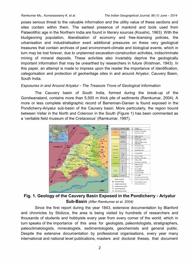
The Cauvery basin of South India, formed during the break-up of the
Gondwanaland, contains more than 5,500 m thick pile of sediments (Ramkumar, 2004). A
more or less complete stratigraphic record of Barremian-Danian is found exposed in the
Pondicherry-Ariyalur sub-basin of the Cauvery basin. More particularly, the region bound
between Vellar in the North and Coleroon in the South (Figure 1) has been commented as
a ‘veritable field museum of the Cretaceous’ (Ramkumar, 1997).
Fig. 1. Geology of the Cauvery Basin Exposed in the Pondicherry - Ariyalur
Sub-Basin (After Ramkumar et al. 2004)
Since the first report during the year 1843, extensive documentation by Blanford
and chronicles by Stolizca, the area is being visited by hundreds of researchers and
thousands of students and hobbyists every year from every corner of the world, which in
turn speaks of the importance of this area for geologists, paleontologists, stratigraphers,
paleoclimatologists, mineralogists, sedimentologists, geochemists and general public.
Despite the extensive documentation by professional organisations, every year many
international and national level publications, masters and doctoral theses, that document
3
Ramkumar Mu., Kumaraswamy K. et al. The Indian Geographical Journal, 89 (1) June – 2014
newer fossils, geological information, depositional and diagenetic phenomena, sedimentary
mechanisms, paleo-environmental and climatic events, sea level oscillations, etc., the area
has not received the required attention with special emphasis on its conservation and
protection for future studies.
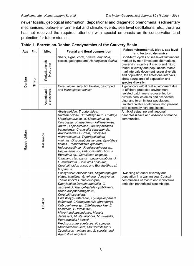
Table 1. Barremian-Danian Geodynamics of the Cauvery Basin
Age Fm. Mbr. Faunal and floral composition Paleoenvironmental, biotic, sea level
and tectonic dynamics
Dan
ian
Nin
iyur
Periyakurichchi
bio
str
om
al
Shark, algae, coral, bivalve, amphibia, pisces, gastropod and Hercoglossa danica
Short-term cycles of sea level fluctuations marked by marl-limestone alternations, preserving significant macro and micro faunal diversity and populations. While marl intervals document lesser diversity and population, the limestone intervals show abundance of population and species diversity.
Anandavadi
are
naceous
Coral, algae, serpulid, bivalve, gastropod and Hercoglossa danica
Typical coral-algal reef environment due to offshore protected environment. Isolated patch reefs represented by diverse coral colonies and associated algal and foraminiferal populations. Isolated bivalve shell banks also present with extremely rich populations.
Ma
astr
ich
tian
Kalla
me
du
Abelisauridae, Troodontidae, Sudamericidae, Bruhatkayosaurus matleyi, Megalosaurus sp. cf. Simosuchus sp., Crocodylia , Kurmademys kallamedensis, Anura , Lepisosteidae , Aquilapollenites bengalensis, Cranwellia cauveriensis, Araucariacites australis, Tricolpites microreticulatus, Triporopollenites minimus, Discorhabdus ignotus, Eprolithus floralis , Pseudomicula quadrata, Holococcolith sp., Prediscosphaera sp., Uniplanarius sp., Petrobrasiella? bownii, Eprolithus sp., Corollithion exiguum, Ottavianus terrazetus, Lucianorhabdus cf. L. maleformis, Calculites obscurus, Ceratolithoides pricei, and Biantholithus cf. B.sparsus
A mix of estuarine and lagoonal nannofossil taxa and absence of marine communities.
Ott
akoil
Pachydiscus otacodensis, Stigmatophygus elatus, Nautilus, Gryphaea, Alectryonia, Thalassinoides, Ophiomorpha, Dactyloidites Durania mutabilis, G. gansseri, Arkhangel-skiella cymbiformis, Braarudosphaerabigelowii, Ceratolithusaculeus, Chiastozyguslitterarius, Cyclagelosphaera deflandrei, Cribrosphaerella ehrengergii, Cribrosphaera sp., Eiffelithusgorkae, E. parallelus, E. turriseiffeli, Microrhabdulusundosus, Macula decussata, M. staurophora, M. swastika, Petrobrasiella? bownii, Prediscosphaeracretacea, P. spinosa, Stradneriacrenulata, Staurolithitescrux, Zygodiscus minimus and Z. spiralis, and Agerostrea ungulata
Dwindling of faunal diversity and population in a waning sea. Coastal communities of macro and ichnofauna amid rich nannofossil assemblage.
4
Ramkumar Mu., Kumaraswamy K. et al. The Indian Geographical Journal, 89 (1) June – 2014
Ka
llankurichchi
Sri
niv
asa
pu
ram
gry
ph
ean
L.S
t.
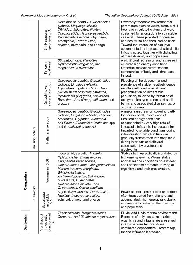
Gavelinopsis bembix, Gyroidinoides globosa, Lingulogavelinella, Cibicides, Siderolites, Pecten, Onychocellida, Hauriceras rembda, Perustrombus indicus, Gryphaea, Alectryonia, Terebratulida, bryozoa, ostracoda, and sponge
Extremely favorable environmental parameters such as warm, clear, turbid free, and circulated waters that were sustained for a long duration by stable sealevel. These provided for diverse and rich fauna and floral composition. Toward top, reduction of sea level accompanied by increase of siliciclastic influx is noted, together with dwindling of fossil diversity and population
Ta
nce
m
bio
str
om
al Stigmatophygus, Planolites,
Ophiomorpha irregularia, and Megaloolithus cylindricus
A significant regression and increase in episodic high energy conditions. Opportunistic colonizers, coastal communities of body and ichno taxa thrived.
Ka
ttu
pirin
giy
am
inoce
ram
us L
.St.
Gavelinopsis bembix, Gyroidinoides globosa, Lingulogavelinella, Agerostrea ungulata, Ceratostreon pliciferum Planospirites ostracina, Pycnodonte (Phygraea) vesicularis, Rastellum (Arcostrea) pectinatum, and bryozoa
Flooding of the depocenter and prevalence of stable, relatively deeper middle shelf conditions allowed predomination of inoceramus population, followed by formation of exogyra, alectryonia dominant shell banks and associated diverse macro and microfauna
Ka
llar
are
naceo
us
Gavelinopsis bembix, Gyroidinoides globosa, Lingulogavelinella, Cibicides, Siderolites, Gryphaea, Alectronia, and Pecten Eubaculites Orbitoides spp. and Goupillaudina daguini
A major transgression covering partly the former shelf. Prevalence of turbulent energy conditions accompanied by very high rate of lithoclastic influx into the depocenter thwarted hospitable conditions during initial duration, which in turn was gradually transformed into hospitable during later part and allowed colonization by gryphea and alectryonia
Ca
mp
an
ian
Sill
akkud
i
Va
rana
va
si S
.St.
Inoceramid, serpulid, Turritella, Ophiomorpha, Thalassinoides, Karapadites karapadense, Globotruncana arca, Globigerinelloides, Marginotruncana marginata, Whiteinella baltica, Archaeoglobigerina, Bolivinoides culverensis, B. decorates, Globotruncana elevata , and G. ventricosa, Ostrea zitteliana
Stable shelf, episodically inundated by high-energy events. Warm, stable, normal marine conditions on a widest shelf conditions promoted thriving of organisms and their preservation.
Sa
du
rbag
a
m p
ebb
ly
S.S
t.
Algae, Rhynchonella, Terebratulid, Nautilus, Inoceramus balitus, echinoid, crinoid, and bivalve
Fewer coastal communities and others often transported from offshore and accumulated. High energy siliciclastic environments restricted the diversity and population.
Sa
nto
nia
n
Va
raku
pp
ai
lithocla
stic
con
glo
me
rat
e
Thalassinoides, Marginotruncana Coronate, and Dicarinella asymmetrica
Fluvial and fluvio-marine environments. Remains of only coastal/estuarine organisms and infauna are preserved in an otherwise tectonic-fluvial dominated depocenters. Toward top, marine influence increases.
5
Ramkumar Mu., Kumaraswamy K. et al. The Indian Geographical Journal, 89 (1) June – 2014
Co
nia
cia
n
Garu
dam
angala
m
Anaip
adi S
.St.
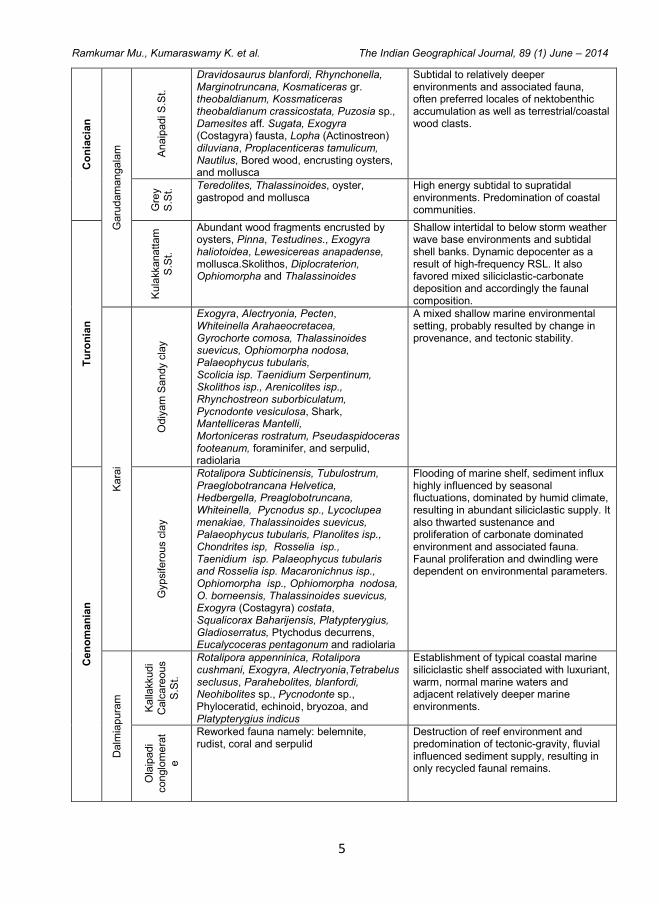
Dravidosaurus blanfordi, Rhynchonella, Marginotruncana, Kosmaticeras gr. theobaldianum, Kossmaticeras theobaldianum crassicostata, Puzosia sp., Damesites aff. Sugata, Exogyra (Costagyra) fausta, Lopha (Actinostreon) diluviana, Proplacenticeras tamulicum, Nautilus, Bored wood, encrusting oysters, and mollusca
Subtidal to relatively deeper environments and associated fauna, often preferred locales of nektobenthic accumulation as well as terrestrial/coastal wood clasts.
Gre
y
S.S
t. Teredolites, Thalassinoides, oyster,
gastropod and mollusca High energy subtidal to supratidal environments. Predomination of coastal communities.
Tu
ron
ian
Kula
kkanattam
S.S
t.
Abundant wood fragments encrusted by oysters, Pinna, Testudines., Exogyra haliotoidea, Lewesicereas anapadense, mollusca.Skolithos, Diplocraterion, Ophiomorpha and Thalassinoides
Shallow intertidal to below storm weather wave base environments and subtidal shell banks. Dynamic depocenter as a result of high-frequency RSL. It also favored mixed siliciclastic-carbonate deposition and accordingly the faunal composition.
Kara
i
Odiy
am
Sandy c
lay
Exogyra, Alectryonia, Pecten, Whiteinella Arahaeocretacea, Gyrochorte comosa, Thalassinoides suevicus, Ophiomorpha nodosa, Palaeophycus tubularis, Scolicia isp. Taenidium Serpentinum, Skolithos isp., Arenicolites isp., Rhynchostreon suborbiculatum, Pycnodonte vesiculosa, Shark, Mantelliceras Mantelli, Mortoniceras rostratum, Pseudaspidoceras footeanum, foraminifer, and serpulid, radiolaria
A mixed shallow marine environmental setting, probably resulted by change in provenance, and tectonic stability.
Cen
om
an
ian
Gypsifero
us c
lay
Rotalipora Subticinensis, Tubulostrum, Praeglobotrancana Helvetica, Hedbergella, Preaglobotruncana, Whiteinella, Pycnodus sp., Lycoclupea menakiae, Thalassinoides suevicus, Palaeophycus tubularis, Planolites isp., Chondrites isp, Rosselia isp., Taenidium isp. Palaeophycus tubularis and Rosselia isp. Macaronichnus isp., Ophiomorpha isp., Ophiomorpha nodosa, O. borneensis, Thalassinoides suevicus, Exogyra (Costagyra) costata, Squalicorax Baharijensis, Platypterygius, Gladioserratus, Ptychodus decurrens, Eucalycoceras pentagonum and radiolaria
Flooding of marine shelf, sediment influx highly influenced by seasonal fluctuations, dominated by humid climate, resulting in abundant siliciclastic supply. It also thwarted sustenance and proliferation of carbonate dominated environment and associated fauna. Faunal proliferation and dwindling were dependent on environmental parameters.
Dalm
iapura
m
Kalla
kkudi
Calc
are
ous
S.S
t.
Rotalipora appenninica, Rotalipora cushmani, Exogyra, Alectryonia,Tetrabelus seclusus, Parahebolites, blanfordi, Neohibolites sp., Pycnodonte sp., Phyloceratid, echinoid, bryozoa, and Platypterygius indicus
Establishment of typical coastal marine siliciclastic shelf associated with luxuriant, warm, normal marine waters and adjacent relatively deeper marine environments.
Ola
ipadi
conglo
me
rat
e
Reworked fauna namely: belemnite, rudist, coral and serpulid
Destruction of reef environment and predomination of tectonic-gravity, fluvial influenced sediment supply, resulting in only recycled faunal remains.
6
Ramkumar Mu., Kumaraswamy K. et al. The Indian Geographical Journal, 89 (1) June – 2014
Alb
ian
Dalm
iya b
ioherm
al
L.S
t.
Red algae, coral, bryozoa, gastropod, bivalve, echinoid, ostracoda, foraminifera, sponge, Anomalinoides, Gavelinella plummerae, Gyroidinoidesglobosa, Lenticulina, Melobesioideae, Melobesioideae, Lithophyllum alternicellum, Pseudoamphiroa propria Quadrimorphina, Rastellum (Arcostrea) carinata, and Ostrea sp.
Typical reef forming organisms and associated fauna and algae.
Vara
gupadi bio
str
om
al L.S
t. Bivalve, rudist, coral, algae, foraminifera,
ostracoda, bryozoa, echinoid, Melobesioideae, Melobesioideae, Lithophyllum alternicellum and Pseudoamphiroa propria Turrilites costatus, Acanthoceras sp., Mammites conciliatus, Nautilus, huxleyanus, Parachaetetesas vapattii, Sporolithon sp., Lithothamnion sp., Lithophyllum sp., Pseudoamphiroapropria, Neomeriscretaceae, Salpingoporella verticelata and Agardioliopsis cretaceae
Establishment of shallow, relatively stable, normal marine depocenters and development of reef-reef associated environments. Reef forming organisms and reef dwellers thrived.
Gre
y s
hale
Palynoflora, H. planispira, Parachaetetes asvapattii, Sporolithon sp., Lithothamnion sp., Lithophyllum sp., Pseudoamphiroa propria, Neomeris cretaceae, Salpingoporella verticelata, Agardioliopsis cretaceae, Ostracoda, bryozoa, and gastropoda
Marine flooding and resultant creation of deeper oxygen poor environments located adjacent to highly productive regions. Very-high frequency oscillations of oxygen poor-normal conditions as a result of RSL fluctuations. The durations of normal conditions increase toward top. Very high abundance of planktic and recycled benthic fauna.
Ap
tian
Siv
aganga
Te
rani cla
y Ptilophyllum, Gymnoplites, Pascoeites,
Microcachyidites, Cooksonites, Aequitriradites and inoceramid
Coastal freshwater lakes, inundated as a result of marine incursion. Freshwater environment supported only microfauna, while the marine incursion resulted in accumulation of recycled bioclastic components.
Kovandan-
kurichchi
S.S
t.
Early Cretaceous palynoflora Creation of subaqueous fan deltaic environments dominated by siliciclastic deposition and turbid conditions, as a result of which, only drifted and or extra-basinal palynofloral remains are preserved.
Barr
em
ian
Basal
Conglo
me
rate
Globigerina boteriveca Initiation of basin and coastal marine deposition under very high energy conditions; only deeper regions contain certain microfauna.
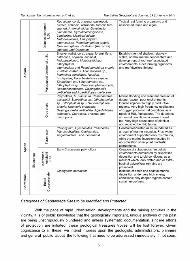
Categories of Geoheritage Sites to be Identified and Protected
With the pace of rapid urbanisation, developments and the mining activities in the
vicinity, it is of public knowledge that the geologically important, unique archives of the past
are being unscrupulously plundered and unless systematic documentation, sincere efforts
of protection are initiated, these geological treasures troves will be lost forever. Given
cognizance to all these, we intend impress upon the geologists, administrators, planners
and general public about the following that need to be addressed immediately, if not soon.
7
Ramkumar Mu., Kumaraswamy K. et al. The Indian Geographical Journal, 89 (1) June – 2014
We propose identification, protection and establishment of field museum sites under six
categories.
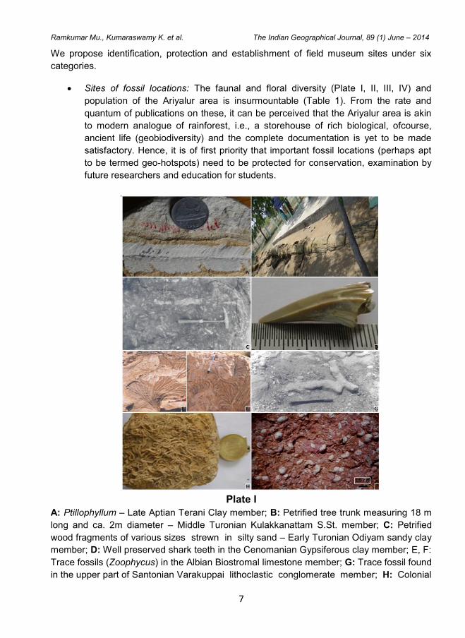
Sites of fossil locations: The faunal and floral diversity (Plate I, II, III, IV) and
population of the Ariyalur area is insurmountable (Table 1). From the rate and
quantum of publications on these, it can be perceived that the Ariyalur area is akin
to modern analogue of rainforest, i.e., a storehouse of rich biological, ofcourse,
ancient life (geobiodiversity) and the complete documentation is yet to be made
satisfactory. Hence, it is of first priority that important fossil locations (perhaps apt
to be termed geo-hotspots) need to be protected for conservation, examination by
future researchers and education for students.
Plate I
A: Ptillophyllum – Late Aptian Terani Clay member; B: Petrified tree trunk measuring 18 m
long and ca. 2m diameter – Middle Turonian Kulakkanattam S.St. member; C: Petrified
wood fragments of various sizes strewn in silty sand – Early Turonian Odiyam sandy clay
member; D: Well preserved shark teeth in the Cenomanian Gypsiferous clay member; E, F:
Trace fossils (Zoophycus) in the Albian Biostromal limestone member; G: Trace fossil found
in the upper part of Santonian Varakuppai lithoclastic conglomerate member; H: Colonial
8
Ramkumar Mu., Kumaraswamy K. et al. The Indian Geographical Journal, 89 (1) June – 2014
serpulids in the Middle-Late Campanian Varanavasi sandstone member; I: Thick population
of Gryphea in the Early Maastrichtian Srinivasapuram gryphean limestone member.
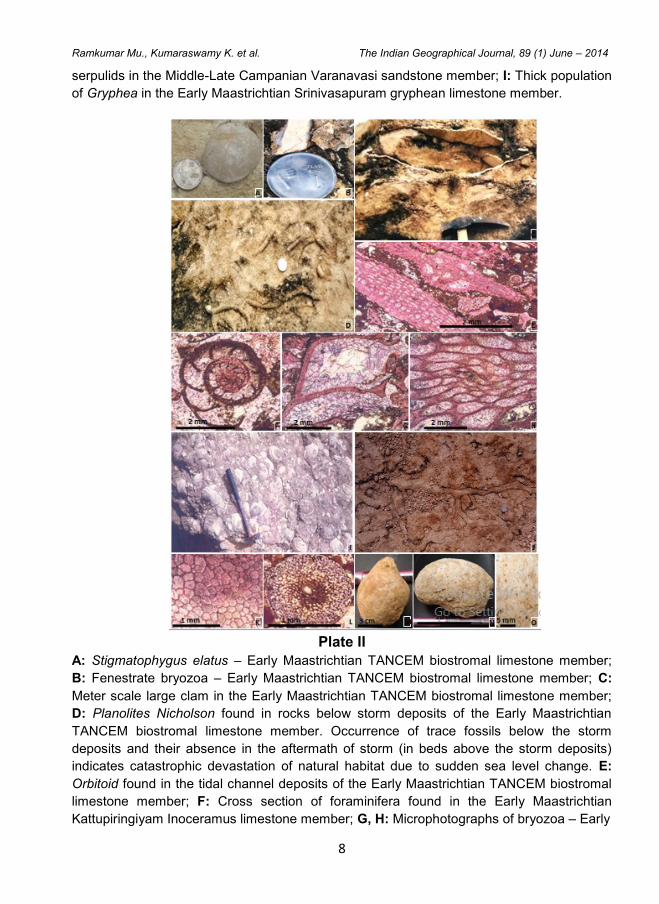
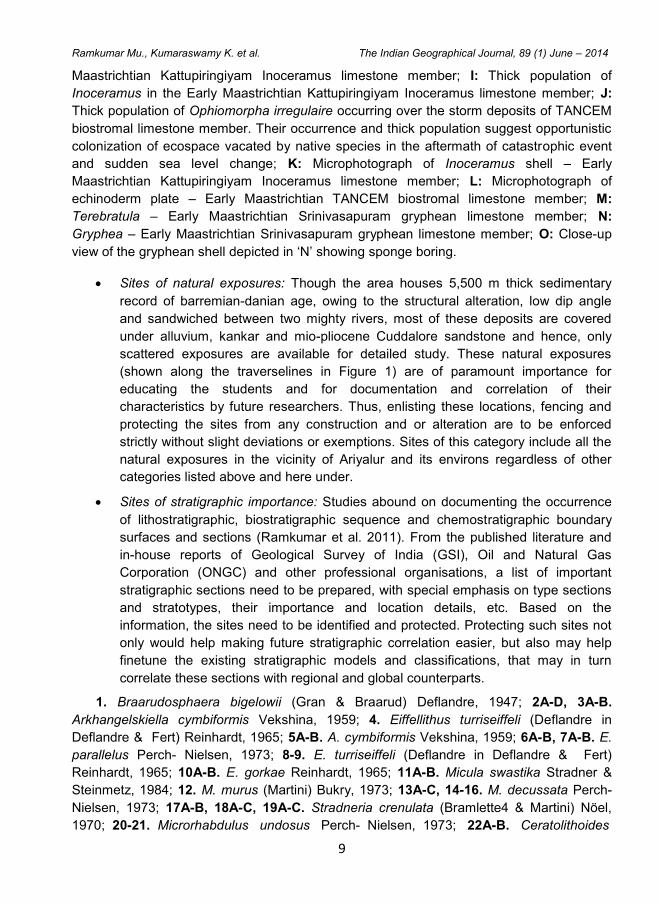
Plate II
A: Stigmatophygus elatus – Early Maastrichtian TANCEM biostromal limestone member;
B: Fenestrate bryozoa – Early Maastrichtian TANCEM biostromal limestone member; C:
Meter scale large clam in the Early Maastrichtian TANCEM biostromal limestone member;
D: Planolites Nicholson found in rocks below storm deposits of the Early Maastrichtian
TANCEM biostromal limestone member. Occurrence of trace fossils below the storm
deposits and their absence in the aftermath of storm (in beds above the storm deposits)
indicates catastrophic devastation of natural habitat due to sudden sea level change. E:
Orbitoid found in the tidal channel deposits of the Early Maastrichtian TANCEM biostromal
limestone member; F: Cross section of foraminifera found in the Early Maastrichtian
Kattupiringiyam Inoceramus limestone member; G, H: Microphotographs of bryozoa – Early
9
Ramkumar Mu., Kumaraswamy K. et al. The Indian Geographical Journal, 89 (1) June – 2014
Maastrichtian Kattupiringiyam Inoceramus limestone member; I: Thick population of
Inoceramus in the Early Maastrichtian Kattupiringiyam Inoceramus limestone member; J:
Thick population of Ophiomorpha irregulaire occurring over the storm deposits of TANCEM
biostromal limestone member. Their occurrence and thick population suggest opportunistic
colonization of ecospace vacated by native species in the aftermath of catastrophic event
and sudden sea level change; K: Microphotograph of Inoceramus shell – Early
Maastrichtian Kattupiringiyam Inoceramus limestone member; L: Microphotograph of
echinoderm plate – Early Maastrichtian TANCEM biostromal limestone member; M:
Terebratula – Early Maastrichtian Srinivasapuram gryphean limestone member; N:
Gryphea – Early Maastrichtian Srinivasapuram gryphean limestone member; O: Close-up
view of the gryphean shell depicted in ‘N’ showing sponge boring.
Sites of natural exposures: Though the area houses 5,500 m thick sedimentary
record of barremian-danian age, owing to the structural alteration, low dip angle
and sandwiched between two mighty rivers, most of these deposits are covered
under alluvium, kankar and mio-pliocene Cuddalore sandstone and hence, only
scattered exposures are available for detailed study. These natural exposures
(shown along the traverselines in Figure 1) are of paramount importance for
educating the students and for documentation and correlation of their
characteristics by future researchers. Thus, enlisting these locations, fencing and
protecting the sites from any construction and or alteration are to be enforced
strictly without slight deviations or exemptions. Sites of this category include all the
natural exposures in the vicinity of Ariyalur and its environs regardless of other
categories listed above and here under.
Sites of stratigraphic importance: Studies abound on documenting the occurrence
of lithostratigraphic, biostratigraphic sequence and chemostratigraphic boundary
surfaces and sections (Ramkumar et al. 2011). From the published literature and
in-house reports of Geological Survey of India (GSI), Oil and Natural Gas
Corporation (ONGC) and other professional organisations, a list of important
stratigraphic sections need to be prepared, with special emphasis on type sections
and stratotypes, their importance and location details, etc. Based on the
information, the sites need to be identified and protected. Protecting such sites not
only would help making future stratigraphic correlation easier, but also may help
finetune the existing stratigraphic models and classifications, that may in turn
correlate these sections with regional and global counterparts.
1. Braarudosphaera bigelowii (Gran & Braarud) Deflandre, 1947; 2A-D, 3A-B.
Arkhangelskiella cymbiformis Vekshina, 1959; 4. Eiffellithus turriseiffeli (Deflandre in
Deflandre & Fert) Reinhardt, 1965; 5A-B. A. cymbiformis Vekshina, 1959; 6A-B, 7A-B. E.
parallelus Perch- Nielsen, 1973; 8-9. E. turriseiffeli (Deflandre in Deflandre & Fert)
Reinhardt, 1965; 10A-B. E. gorkae Reinhardt, 1965; 11A-B. Micula swastika Stradner &
Steinmetz, 1984; 12. M. murus (Martini) Bukry, 1973; 13A-C, 14-16. M. decussata Perch-
Nielsen, 1973; 17A-B, 18A-C, 19A-C. Stradneria crenulata (Bramlette4 & Martini) Nöel,
1970; 20-21. Microrhabdulus undosus Perch- Nielsen, 1973; 22A-B. Ceratolithoides
10
Ramkumar Mu., Kumaraswamy K. et al. The Indian Geographical Journal, 89 (1) June – 2014
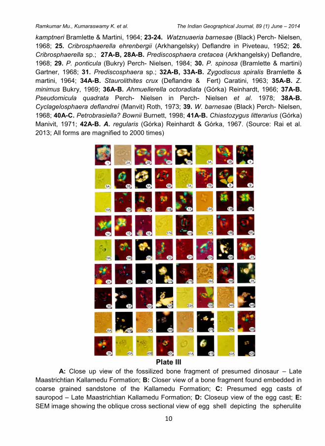
kamptneri Bramlette & Martini, 1964; 23-24. Watznuaeria barnesae (Black) Perch- Nielsen,
1968; 25. Cribrosphaerella ehrenbergii (Arkhangelsky) Deflandre in Piveteau, 1952; 26.
Cribrosphaerella sp.; 27A-B, 28A-B. Prediscosphaera cretacea (Arkhangelsky) Deflandre,
1968; 29. P. ponticula (Bukry) Perch- Nielsen, 1984; 30. P. spinosa (Bramlette & martini)
Gartner, 1968; 31. Prediscosphaera sp.; 32A-B, 33A-B. Zygodiscus spiralis Bramlette &
martini, 1964; 34A-B. Staurolithites crux (Deflandre & Fert) Caratini, 1963; 35A-B. Z.
minimus Bukry, 1969; 36A-B. Ahmuellerella octoradiata (Górka) Reinhardt, 1966; 37A-B.
Pseudomicula quadrata Perch- Nielsen in Perch- Nielsen et al. 1978; 38A-B.
Cyclagelosphaera deflandrei (Manvit) Roth, 1973; 39. W. barnesae (Black) Perch- Nielsen,
1968; 40A-C. Petrobrasiella? Bownii Burnett, 1998; 41A-B. Chiastozygus litterarius (Górka)
Manivit, 1971; 42A-B. A. regularis (Górka) Reinhardt & Górka, 1967. (Source: Rai et al.
2013; All forms are magnified to 2000 times)
Plate III
A: Close up view of the fossilized bone fragment of presumed dinosaur – Late
Maastrichtian Kallamedu Formation; B: Closer view of a bone fragment found embedded in
coarse grained sandstone of the Kallamedu Formation; C: Presumed egg casts of
sauropod – Late Maastrichtian Kallamedu Formation; D: Closeup view of the egg cast; E:
SEM image showing the oblique cross sectional view of egg shell depicting the spherulite
11
Ramkumar Mu., Kumaraswamy K. et al. The Indian Geographical Journal, 89 (1) June – 2014
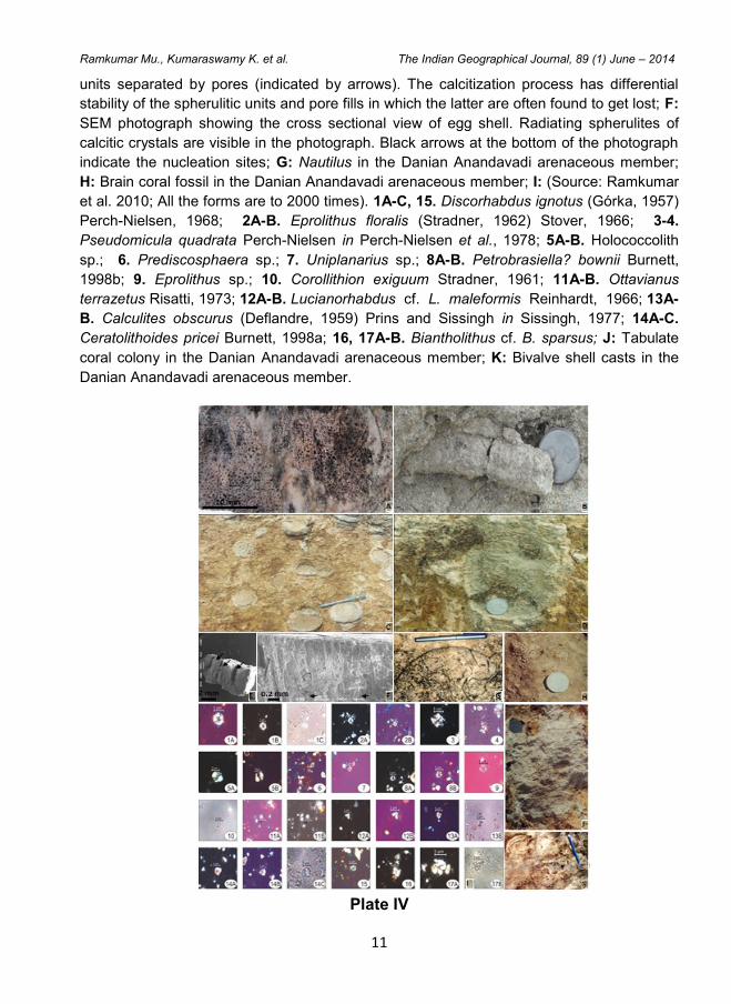
units separated by pores (indicated by arrows). The calcitization process has differential
stability of the spherulitic units and pore fills in which the latter are often found to get lost; F:
SEM photograph showing the cross sectional view of egg shell. Radiating spherulites of
calcitic crystals are visible in the photograph. Black arrows at the bottom of the photograph
indicate the nucleation sites; G: Nautilus in the Danian Anandavadi arenaceous member;
H: Brain coral fossil in the Danian Anandavadi arenaceous member; I: (Source: Ramkumar
et al. 2010; All the forms are to 2000 times). 1A-C, 15. Discorhabdus ignotus (Górka, 1957)
Perch-Nielsen, 1968; 2A-B. Eprolithus floralis (Stradner, 1962) Stover, 1966; 3-4.
Pseudomicula quadrata Perch-Nielsen in Perch-Nielsen et al., 1978; 5A-B. Holococcolith
sp.; 6. Prediscosphaera sp.; 7. Uniplanarius sp.; 8A-B. Petrobrasiella? bownii Burnett,
1998b; 9. Eprolithus sp.; 10. Corollithion exiguum Stradner, 1961; 11A-B. Ottavianus
terrazetus Risatti, 1973; 12A-B. Lucianorhabdus cf. L. maleformis Reinhardt, 1966; 13A-
B. Calculites obscurus (Deflandre, 1959) Prins and Sissingh in Sissingh, 1977; 14A-C.
Ceratolithoides pricei Burnett, 1998a; 16, 17A-B. Biantholithus cf. B. sparsus; J: Tabulate
coral colony in the Danian Anandavadi arenaceous member; K: Bivalve shell casts in the
Danian Anandavadi arenaceous member.
Plate IV
12
Ramkumar Mu., Kumaraswamy K. et al. The Indian Geographical Journal, 89 (1) June – 2014
Sites of unique facies types: The sedimentary deposits of Ariyalur area house many
unique facies types. For example, the turbiditic deposits near Tirupattur
(Ramkumar, 2008), boulder-rich ripple imbricate structures and contact between
middle-shelf deposits and continental fluvial deposits near Kallagam (Ramkumar et
al. 2005), hummocky-cross stratified paleo-tsunami deposits near Kallankurichchi
(Ramkumar 2006), paleo-gas hydrate/hydrocarbon venting site near Reddipalaiyam
(Ramkumar, 2007), cretaceous-paleogene contact (Ramkumar et al. 2010), black
shales near Dalmiapuram (Ramkumar et al. 2004), etc. are unique to this region
and need to be protected for future studies and education. In addition,
documentation of lithofacies and associated characteristics of these sites may help
to understand paleoclimatic and other important geological events more precisely.
Hence, identification of similar sites and protecting them is essential.
Sites of excellent traverses: Ariyalaur area is known for many traverses exposing
rock records of important time-slices and fossil occurrences. For example, Karai-
Kulakkanattam, Kunnam-Mungilpadi, Kallagam-Sadurbagam, Kilpalur-Sillakkudi
can be sited as most visited, yet not protected traverses from pilferage and
plundering by unscrupulous elements. Though visited by thousands of researchers
and students every year, each time, new and newer information are being
documented and hence, such traverses have unique educational and research
purposes and need to be protected.
Sites of newly excavated mines and other sections: With the accelerated
infrastructure development and mining activities, newer exposures of road-cutting
sections, mine sections and abandoned mine floor exposures are becoming
available during recent times. These not only provide access to hitherto unknown
and or little-known rock records of important time-slices, but also provide important
clues and evidences to sedimentary structural, stratigraphic relationship, facies
types, fossil occurrences and their biotic interactions. Selected sections of these
newer exposures have to be documented and protected for future studies and
education.
Establishment of Field Museum and Honouring Dr. M.S. Krishnan
Through this paper, we propose to establish an online catalogue of important
locales according to the categories listed above, creation of Web-GIS enabled interactive
and informative kiosk containing basic information on these sites and making this resource
an open-source model, so that whoever has additional information, can contribute to enrich
the online database for the benefit of all those who are interested. Such an effort would not
only help protect the natural geological resource, but would also promote geotourism. It is
to be noted that the State government of Tamil Nadu has already started taken few
initiatives in the identification of geologically important locations and protecting them and
commenced infrastructure development such as construction of approach road, provision of
basic amenities, fencing, etc., near to such sites. However, systematic documentation of
13
Ramkumar Mu., Kumaraswamy K. et al. The Indian Geographical Journal, 89 (1) June – 2014
sites according to the six categories as listed in this paper, making similar infrastructure and
other amenities to all of these sites are essential.
Considering the importance of geoscientific contribution to the Ariyalur and other
areas of India by Dr. M.S. Krishnan, the illustrious geologist of GSI, we suggest that the
proposed field-museum encompassing the six-category sites discussed in this paper, may
be named after him. This will be a fitting tribute to him both for his vast research
contribution to Ariyalur region and also as the Former President of the Indian Geographical
Society, in 1947, when he was the Superintending Geologist, GSI, Madras Circle,
Bheemasena Gardens, Mylapore, Madras and contributed enormously for the development
of the Society.
References
1. Kaushic, S.D. (1963). Dating the Paleolithic Age in India, The Indian Geographical Journal, 38(2), pp. 49-52.
2. Krishnan, M.S. (1943). The Structure of India, The Indian Geographical Journal, 18(4),
pp. 137-155.
3. Rai, J., Ramkumar, M. and Sugantha, T., (2013). Calcareous nannofossils from the Ottakoil Formation of the Cauvery Basin, South India: Implications on Age and Late Cretaceous environmental conditions. In: Ramkumar, M., (Ed.), On a Sustainable Future of the Earth’s Natural Resources. Springer-Verlag., Heidelberg. pp. 109-122.
4. Ramkumar, M., (1997). Plea for National Geological Field Museum. Ind. Assc. Sediment. Newsletters. 1, pp. 2-3.
5. Ramkumar, M., (2006). A Storm event during the Maastrichtian in the Cauvery Basin, South India. Ann. Geol. Penins. Balk. 67, pp. 35-40.
6. Ramkumar, M., (2007). Dolomitic limestone in the Kallankurichchi Formation (Lower Maastrichtian) Ariyalur Group, South India. Jour. Earth Sci. 1(1), pp. 7-21.
7. Ramkumar, M., (2008). Cyclic fine-grained deposits with polymict boulders in Olaipadi member of the Dalmiapuram Formation, Cauvery Basin, south India: Plausible causes and sedimentation model. ICFAI Jour.Earth. Sci. 2, pp. 7-27.
8. Ramkumar, M., Anbarasu, K., Sugantha, T., Jyotsana Rai., Sathish, G. and Suresh, R., (2010). Occurrences of KTB exposures and dinosaur nesting site near Sendurai, India: An initial report. Inter. Jour. Phy. Sci. 22, pp. 573-584.
9. Ramkumar, M., Subramanian, V. and Stüben, D., (2005). Deltaic sedimentation during Cretaceous Period in the Northern Cauvery Basin, South India: Facies architecture, depositional history and sequence stratigraphy. Jour. Geol. Soc. Ind. 66, pp. 81-94.
10. Ramkumar, M., Harting, M. and Stüben, D. (2005). Barium anomaly preceding K/T boundary: Plausible causes and implications on end Cretaceous events of K/T sections in Cauvery Basin (India), Israel, NE-Mexico and Guatemala. Inter.Jour.Earth.Sci. 94, pp. 475-489.
11. Ramkumar, M., Stüben, D. and Berner, Z., (2004). Lithostratigraphy, depositional history and sea level changes of the Cauvery Basin, South India. Ann. Geol. Penins. Balk. 65, pp. 1-27.
12. Ramkumar, M., Stüben, D. and Berner, Z., (2011). Barremian-Danian chemostratigraphic sequences of the Cauvery Basin, South India: Implications on scales of stratigraphic correlation. Gondwana Res. 19, pp. 291-309.
The Indian Geographical Journal
Volume 89 (1) June - 2014, pp 14-19 ISSN 0019-4824
14
GROUNDWATER CHARACTERISATION OF ARIYALUR AND
PERAMBALUR DISTRICTS EMPLOYING AQUACHEM
SOFTWARE
Santhiya Mahalingam, Selvakumar Muniraj and Vasanthy Muthunarayanan
Department of Environmental Biotechnology, Bharathidasan University,
Tiruchirappalli - 620 024
E-mail: [email protected], [email protected]
Abstracts
The objectives of this study are to analyse the undergroundwater quality of Ariyalur and
Perambalur region by water quality index. Physico-chemical parameters such as pH,
Electrical conductivity, Total Solids, Total Dissolved Solids, Total Suspended Solids, Total
Alkalinity, Total Acidity, Total Hardness, Calcium, Magnesium, Chloride, Dissolved Oxygen,
Biological Oxygen Demand, Chemical Oxygen Demand, Phosphate, Sulphate, Silicate,
Nitrate, Sodium and Potassium collected from 48 different locations since a period of 2012-
2013 were analysed. The type of water that predominates in the study area is Ca-HCO3
type during year, based on hydro-chemical facies. In this study, 80 percent water samples
were found of good quality and only 20 percent water samples fall under moderately poor
category. Therefore, there is a need of some treatment before usage and also it is
necessary to protect that area from contamination.
Keywords: Hardness, Piper diagram, Groundwater, Chemical characters, BOD
Introduction
Water is one of the nature’s most important gifts to mankind. Pure water is an
odourless, tasteless, clear liquid. Water is one of the most essential elements needed for
good health and it is also necessary for livelihood of people. Water is also reported to be a
precious asset. Water is needed for domestic purposes and energy production. Above all,
water is the most critical limiting factor for many aspects of life such as economic growth,
environmental stability, biodiversity conservation, food security and health care. Health
officials emphasize the importance of drinking water by suggesting to drink at least eight
glasses of clean water each and every day to maintain good health (Venkatesharaju et al.,
2010). The existence of a wide range of contaminants in drinking water makes it essential
to limit their concentration levels in order to safeguard human health. The primary pathways
for exposure to chemical substances are ingestion, inhalation and dermal sorption. The
relative impact of each of the exposure pathways depends upon the physical and the
chemical nature of the contaminant.
Potable water can be defined as “Water free from disease-causing organisms, and
free from minerals and organic substances that may produce adverse physiological effects
and aesthetically pleasing with respect to turbidity, color, taste and odor” (AWWA, 1990).
Although, biological contaminants have traditionally received more attention from a public
15
Santhiya Mahalingam et. al. The Indian Geographical Journal, 89 (1) June – 2014
health standpoint, in recent years, there has been growing concern for chemical
contaminants present in drinking water that might be hazardous to human health. Exposure
to contaminants in water is thought to lead to human health problems ranging from minor
effects such as fatigue to more serious effects such as cancer (Wilkes et al., 1992).
Most public water supplies depend on a chlorine disinfection process, which may
produce water containing chloroform and other tri halo methane (Lindstrom and Pleil,
1996). In addition, a wide variety of volatile and synthetic organic chemicals, pesticides,
inorganic chemicals and radio nuclides have been detected in water supplies (AWWA,
1990). Groundwater represents the largest available source of fresh water as more than 97
percent of the total freshwater on the earth is undergroundwater (Rai and Sharma, 1991).
Groundwater is naturally replenished by surface water from precipitation, streams and
rivers when this recharge reaches the water table. Groundwater recharge is the process by
which water percolates down the soil and reaches the water table. The recharge from
rainfall is significant where rainfall coincide with increased humidity; otherwise the recharge
is reduced partially or totally by evaporation and transpiration. In India rainfall is the most
important source of groundwater recharge (Mall et al., 2006; Mohd Saleem et al, 2016).
Groundwater is a readily available source of water for irrigation, domestic and
industrial uses. However, with increase in water demand due to population pressure this
resource is over exploited in many parts of the world resulting in permanent depletion of the
aquifer system and associated environmental consequences such as water quality
deterioration. With the change in land use and increase in quantities and type of
agricultural, domestic and industrial effluents entering the hydrological cycle a gradual
decline in water quality due to surface and subsurface pollution also takes place (Sharma et
al., 2004; Karanth, 1989). The objective of the present work is to discuss the major ion
chemistry of groundwater of Ariyalur and Perambalur Districts. This was done in terms of
piper trilinear diagram.
Study Area
Ariyalur District has a geographical area of 1,949 sq. km. It lies between the latitude
10o 54' and 11.30' of north longitude 780 40' and 10o 30' of East. The district has an
average rainfall of 951.1 mm. The maximum temperature is 38°C and the minimum
temperature is 24°C. Land of Limestone Ferruginous red loam occurs in Ariyalur district.
The soils are of medium depth with good drainage, free from accumulation of salt and
calcium carbonate, pH ranges from 6.5 to 8.0 and contain low amounts of organic matter,
nitrogen and phosphorus but with generally adequate amounts of potash and lime.
Perambalur District is centrally located in Tamil Nadu and is 267kms away in
southern direction from Chennai. The Perambalur district is located between the East
longitudes 79o 15’ to 79o 30’E and North latitudes 11o 22’ to 11o 30’N. Total Area is
reported to be 691 sq.km. The district has an average Rainfall of 951.1 mm (Annual). The
district for administrative purpose has been divided into three taluks namely,
Perambalur, Kunnam, Veppanthattai which is further sub-divided into four blocks such as
16
Santhiya Mahalingam et. al. The Indian Geographical Journal, 89 (1) June – 2014
Perambalur, Veppanthattai, Veppur, Alathur. The district is fairly rich in mineral deposits.
Celeste, Lime Stone, Shale, Sand Stone, Canker and Phosphate nodules occur at various
places in the district. A good deal of building stone is quarried in Perambalur, Kunnam, and
Veppanthattai taluks. It is an inland district without any coastal line. The District has Vellar
River in the North and Kollidam River in the South and it has no well-marked natural
divisions. The Pachamalai hill situated on the North of Perambalur is the most important hill
in the district.
Database and Methodology
The collected samples were analyzed for different physicochemical parameters
such as pH, Electrical conductivity, Total Solids, Total Dissolved Solids, Total Suspended
Solids, Total Alkalinity, Total Acidity, Total Hardness, Calcium, Magnesium, Chloride,
Dissolved Oxygen, Biological Oxygen Demand, Chemical Oxygen Demand, Phosphate,
Sulphate, Silicate, Nitrate, Sodium and Potassium (APHA, 2005). The analytical data can
be used for the classification of water for utilitarian purposes and for ascertaining various
factors on which the chemical characteristics of water depend.
Results and Discussion
The drinking water sampled from different stations of Ariyalur and Perambalur
districts has been characterized in terms of pH, Electrical conductivity, Total Solids, Total
Dissolved Solids, Total Suspended Solids, Total Alkalinity, Total Acidity, Total Hardness,
Calcium, Magnesium, Chloride, Dissolved Oxygen, Biological Oxygen Demand, Chemical
Oxygen Demand, Phosphate, Sulphate, Silicate, Nitrate, Sodium and Potassium. Maximum
and minimum concentration of major ions present in the groundwater from the study areas
is presented in Table 1 and 2. The values were plotted using piper tri-linear diagram. (Aqua
chem software version- 5.1) and were represented in Figure 1. The Piper-Hill diagram is
used to infer hydro-geochemical facies. These plots include two triangles, one for plotting
cations and the other for plotting anions. The cations and anions fields are combined to
show a single point in a diamond-shaped field, from which inference is drawn on the basis
of hydro-geochemical facies concept (Sadashivaiah et al, 2008). These tri-linear diagrams
are useful in bringing out chemical relationships among groundwater samples in more
definite terms rather than with other possible plotting methods.
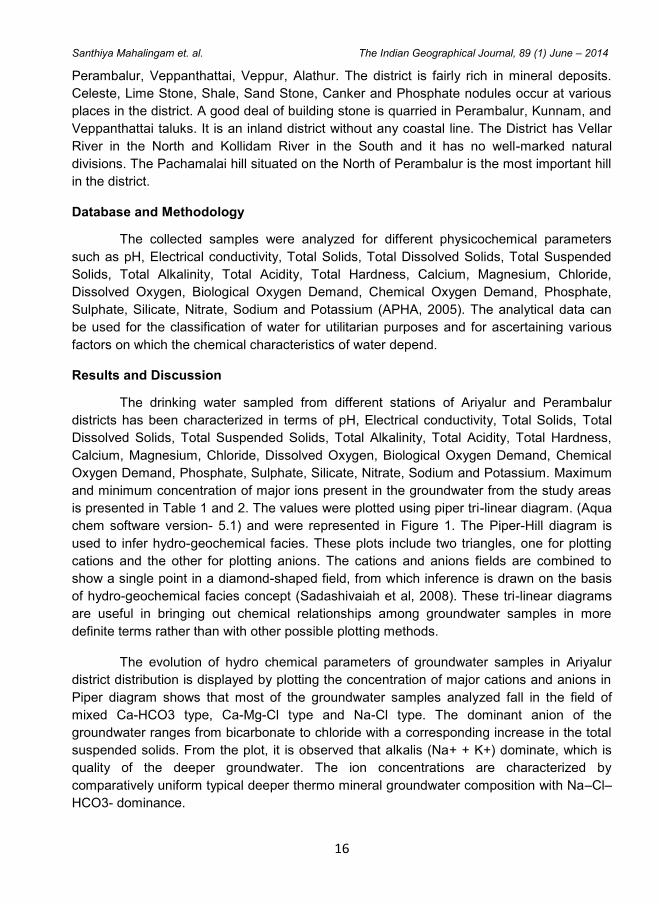
The evolution of hydro chemical parameters of groundwater samples in Ariyalur
district distribution is displayed by plotting the concentration of major cations and anions in
Piper diagram shows that most of the groundwater samples analyzed fall in the field of
mixed Ca-HCO3 type, Ca-Mg-Cl type and Na-Cl type. The dominant anion of the
groundwater ranges from bicarbonate to chloride with a corresponding increase in the total
suspended solids. From the plot, it is observed that alkalis (Na+ + K+) dominate, which is
quality of the deeper groundwater. The ion concentrations are characterized by
comparatively uniform typical deeper thermo mineral groundwater composition with Na–Cl–
HCO3- dominance.
17
Santhiya Mahalingam et. al. The Indian Geographical Journal, 89 (1) June – 2014
Fig. 1. Groundwater Samples from Ariyalur (on left) and Perambalur (on right)
Districts Plotted Piper-Trilinear Diagram
The groundwater characteristics of Perambalur district plotted in Piper diagram
represented that the Ca and Na+K were dominant among the cations, HCO3- and Cl- were
present among the anions, resulting in three types of groundwater such as Ca-HCO3 type,
Ca- Mg-Cl type and Na-Cl type respectively. Romani, (1981) reported that the Uruli-
Devachi area is conspicuous by the presence of (Na+K) type of water and such water has
temporary hardness and residual sodium carbonate. The excess alkali ions present in the
water is compensated by these anions. The majority of the samples are concentrated with
Ca-HCO3 present in the fields (Perambalur and Kunnam taluk) representing the dominance
of fresh water recharge into the aquifer.
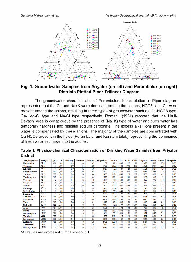
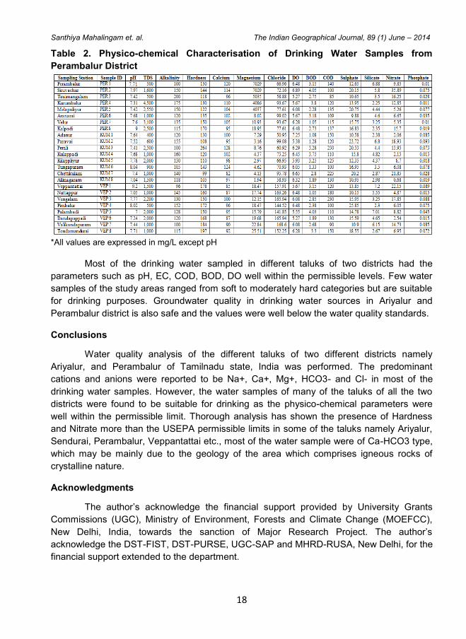
Table 1. Physico-chemical Characterisation of Drinking Water Samples from Ariyalur
District
*All values are expressed in mg/L except pH
18
Santhiya Mahalingam et. al. The Indian Geographical Journal, 89 (1) June – 2014
Table 2. Physico-chemical Characterisation of Drinking Water Samples from
Perambalur District
*All values are expressed in mg/L except pH
Most of the drinking water sampled in different taluks of two districts had the
parameters such as pH, EC, COD, BOD, DO well within the permissible levels. Few water
samples of the study areas ranged from soft to moderately hard categories but are suitable
for drinking purposes. Groundwater quality in drinking water sources in Ariyalur and
Perambalur district is also safe and the values were well below the water quality standards.
Conclusions
Water quality analysis of the different taluks of two different districts namely
Ariyalur, and Perambalur of Tamilnadu state, India was performed. The predominant
cations and anions were reported to be Na+, Ca+, Mg+, HCO3- and Cl- in most of the
drinking water samples. However, the water samples of many of the taluks of all the two
districts were found to be suitable for drinking as the physico-chemical parameters were
well within the permissible limit. Thorough analysis has shown the presence of Hardness
and Nitrate more than the USEPA permissible limits in some of the taluks namely Ariyalur,
Sendurai, Perambalur, Veppantattai etc., most of the water sample were of Ca-HCO3 type,
which may be mainly due to the geology of the area which comprises igneous rocks of
crystalline nature.
Acknowledgments
The author’s acknowledge the financial support provided by University Grants
Commissions (UGC), Ministry of Environment, Forests and Climate Change (MOEFCC),
New Delhi, India, towards the sanction of Major Research Project. The author’s
acknowledge the DST-FIST, DST-PURSE, UGC-SAP and MHRD-RUSA, New Delhi, for the
financial support extended to the department.

19
Santhiya Mahalingam et. al. The Indian Geographical Journal, 89 (1) June – 2014
Reference
1. APHA, (American Public Health Association), (2005). Standard methods for the examination of water and waste water, 21
st ed., Washington, D.C.
2. AWWA, (American Water Works Association), (1990). Water Quality and Treatment: A Handbook of Community Water Supplies, 4rth ed., McGraw Hill Inc.
3. Karanth, K. R., (1989). Hydrogeology. New Delhi: Tata McGraw-Hill. 4. Lindstrom, A. B., Pleil, J.D., (1996). A methodological approach for exposure
assessment studies in residences using volatile organic compound – contaminated water. Journal of the Air and Waste Management Association, (46), pp.1058-1066.
5. Mall, R. K., Gupta, A., Singh, R., Singh, R.S., Rathore, L.S., (2006). Water resources and climate change. An Indian perspective, Curr. Sci, 90(12), pp.1610–1626.
6. Mohd Saleem., Athar Hussain., Gauhar Mahmood., (2016). Analysis of groundwater quality using water quality index: A case study of greater Noida (Region), Uttar Pradesh (U.P), India. Cogent Engineering, 3, 1237927, pp.1-11.
7. Rai, D.N., Sharma, U.P., (1991). Phyto-coenological structure and classification of wetlands in North- BiharIn, Aquatic Sciences in India. Indian Association for Limnology and Oceanography, New Delhi, pp.111-116.
8. Romani, S., (1981). A new diagram for classification of natural waters and interpretation of chemical analysis data. Studies in Environmental Science, (17), pp. 743-748.
9. Sadashivaiah, C., Ramakrishnaiah, C.R., Ranganna, G., (2008). Hydrochemical Analysis and Evaluation of Groundwater Quality in Tumkur Taluk, Karnataka State, India. Int. J. Environ. Res. Public Health 2008, 5(3), pp.158-164.
10. Sharma Surendra Kumar., Vijendra Singh., Singh Chandel, C.P., (2004). Groundwater pollution problem and evaluation of Physico-Chemical properties of Groundwater. Environment and Ecology, (22), pp.319-324.
11. Venkatesharaju, K., Ravikumar, P., Somashekar, R.K., Prakash, K.L., (2010). Physico- chemical and Bacteriological Investigation on the river Cauvery of Kollegal Stretch in Karnataka. Journal of science Engineering and technology, (1), pp.50-59.
12. Wilkes, C. R., Small, M. J., Andelman, J. B., Giardino, N. J., Marshall, J., (1992). Inhalation exposure model for volatile chemicals from indoor uses of water. Atmospheric Environment, (26), pp. 2227-2236.
The Indian Geographical Journal
Volume 89 (1) June - 2014, pp 20-29 ISSN 0019-4824
20
GEOMATICS AND STATISTICAL MODELS TO DETERMINE
THE STATUS OF SEA WATER QUALITY ALONG THE
INDIAN COAST
Radha Y., Bhaskaran G., Narmada K. and Dhanusree M.
Department of Geography, University of Madras, Chennai - 600 005
E-mail: [email protected], [email protected]
Abstract
Marine water quality has become a matter of serious concern because of its effects on
human health and aquatic ecosystems, including a rich array of marine life, with the growth
of population and commercial industries, marine water has received large amounts of
pollution from municipal and industrial sources, as also from surface runoff. In this research,
an attempt was made to present the complex datasets in a more comprehensive approach,
in a single indicator of Coastal Water Quality Index (CWQI). For the study mainly eight
water quality parameters (DO, pH, Water Temperature, BOD, Nitrate, Phosphate,
Suspended Sediments), were chosen for four seasons (Summer, Pre-monsoon, Monsoon,
Post monsoon) from 1990 to 2010 and coastal water quality index was calculated along the
Indian coast for 15 COMAPS locations. The GIS techniques add simplification and
visualisation to the dataset by integrating multiple layers like discharge points, sampling
stations and water quality variables that help in easy understanding. From this study it has
been proved that geoinformatics is a vital tool for decision makers to identify the sources
and polluted areas. It was found out that Kochi was the only location having bad WQI -
average value (47.82) and Ennore, Kakinada, Hazira, Mumbai, Pondicherry location are at
the verge of getting into bad WQI but they are in medium water quality range according to
NSFWQI.
Keywords: Water Quality Index, Geomatics, Coastal Areas, GIS
Introduction
Good quality coastal water is an important part of keeping our coasts healthy for
the future. Natural marine systems, including plant, animal and fish life need clean coastal
water to survive. The coastal regions are believed to hold better biodiversity than open
ocean regions. However, it has been altered over time due to the consequences of human
activities. Decline in water quality is mainly due to the increased concentration of various
pollutants such as oils, heavy metals, nutrient and organic compounds causing turbidity and
a significant drop in dissolved oxygen levels (Chang-An Yan, 2015). Coastal water quality
variables such as pH, dissolved oxygen, biochemical oxygen demand, total suspended
solids, ammonia, nitrate, total phosphorous, chlorophyll-a and fecal coliform are the health
indicators of coastal environment. Thus, this is an attempt to present the complex datasets
21
Radha Y., Bhaskaran G. et al. The Indian Geographical Journal, 89 (1) June – 2014
in a more comprehensive approach, a single indicator of Coastal Water Quality Index
(CWQI). The CWQI is a dimensionless number that combines multiple water quality
variables into a single number by normalising values to subjective rating curves.
The CWQI takes complex scientific information of measured parameters and
synthesises into a single number (0 to 100 scale) based on the recommended level to
derive significant information that are easily understandable by the coastal policy managers
and administrator. Coastal regions played a significant role in the history of human
settlement as it provides natural resources as well as route for the trade. The human
dependence on the bays and channels for livelihood has given rise to urbanisation that led
to decline of water quality. The concern on coastal water quality is being raised in the past
two decades due to excessive settlements near the coastal areas and over exploitation.
The Integrated Coastal Marine Area Management Centre of Earth System Science
Organisation (ESSOICMAM) has been implementing a program called ‘Coastal Ocean
Monitoring and Prediction System (COMAPS)’ with the objectives to monitor water quality
parameters periodically in selected locations in the coastal waters of India and to develop
possible prediction of sea water quality.
Study Area
Coastal India spans from the south west Indian coastline along the Arabian sea
from the coastline of the Gulf of Kutch in its western most corner and stretches across the
Gulf of Khambhat and through the Salsette Island of Mumbai along the Konkan and
southwards across the Raigad region and through Kanara and further down through
Mangalapuram or Mangalore and along the Malabar through Cape Comorin in the
southernmost region of South India with coastline along the Indian Ocean and through the
Coromandal Coast or Cholamandalam Coastline on the South Eastern Coastline of the
Indian Subcontinent along the Bay of Bengal through the Utkala Kalinga region until the
easternmost corner of shoreline near the Sunderbans in Coastal East India.
Database and Methodology
The coastal water quality measurements, erstwhile in operation under the name
COMAPS for the last two decades have been reviewed annually and the data generated by
different participating institutions are deposited with INCOIS of MoES. The data generated
are made available through web site of the Ministry for Public dissemination as well as
through user agencies such as Pollution Control Boards, Department of Fisheries, and
Department of Environment (Coastal Water Quality Measurements Protocol for COMAPS
Programme, 2012).
Eight water quality parameters (DO, PH, Water Temperature, BOD, Nitrate,
Phosphate and Suspended Sediments), were chosen for four seasons (summer,
premonsoon, monsoon, post monsoon) from 1990-2010 and coastal water quality index
was calculated along the Indian coast for 15 COMAPS locations Vadinar, Hazira, Thane

22
Radha Y., Bhaskaran G. et al. The Indian Geographical Journal, 89 (1) June – 2014
Mumbai, Ratnagiri, Mandovi, Kochi, Kavaratti, Sandheads, Hooghly, Paradip, Kakinada,
Ennore (Chennai), Pondicherry, Port Blair for 1 km from shore.
Fig. 1. Study Area
Arc GIS 10.3, was used for interpolation of different water quality index parameters
and for deriving thematic maps. Finally, it was used as a decision support system to easily
interpret the calculated results. Origin Pro 3.4, as statistics software was used for plotting
the trend line graphs of all water quality parameters for all seasons. It was also used for
analysing the relationship between different parameters by giving double-y coordinate
graphs.
After the data collection, managing the data and creation of database is important.
In this study both the spatial dataset (i.e. latitude, longitude) for each COMAPS location and
accurate attribute data for physic-chemical parameters is of significance. In order to study
the variations of the different parameters the interpolation (Krigging) method was done.
Finally, the water quality index was calculated.
This study proposes an innovative approach by combing CWQI and Geographical
Information System (GIS) in a comprehensive manner to visually demarcate the healthy
and polluted areas for sustainable coastal resources management.
Results and Discussions
Water Quality Index
Monitoring programs of aquatic systems play a significant role in water quality
management. However, the water quality is difficult to be evaluated from a large number of
samples, each containing concentrations of many water quality variables. A Water Quality
Index (WQI) summarises large amounts of water quality data into simple terms (e.g.,
excellent, good and poor.). The WQI can be used as a tool in comparing the water quality of
different sources and it gives the public a general idea of the possible problems with water
in a particular region (Srinivasan, 2013). The indices are among the most effective ways to
23
Radha Y., Bhaskaran G. et al. The Indian Geographical Journal, 89 (1) June – 2014
communicate the information on water quality trends for the water quality management.
Available water quality indices have some limitations such as incorporating a limited
number of water quality variables and providing deterministic outputs.
Water quality index is a performance measurement that aggregates information into
a usable form, which reflects the composite influence of significant physical, chemical and
biological parameters of water quality conditions. The use of a WQI allows ‘good’ and ‘poor
water quality to be quantified by reducing a large quantity of data on a range of physico-
chemical and biological variables to be a single number in a simple, objective and
reproducible manner. The use of a numerical index as a management tool in water quality
assessment is a rather recent innovation. An index is a number, usually dimensionless,
which expresses the relative magnitude of some complex phenomenon or condition.Water
quality index is a 100 point scale that summarises results from a total of eight different
measurements such as temperature, pH, Dissolved Oxygen, Turbidity, Nitrates, Total
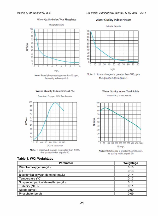
Phosphates, Total Suspended Solids and Biochemical Oxygen.
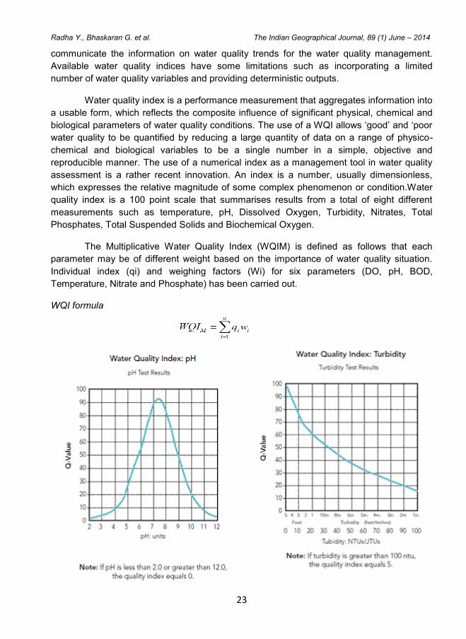
The Multiplicative Water Quality Index (WQIM) is defined as follows that each
parameter may be of different weight based on the importance of water quality situation.
Individual index (qi) and weighing factors (Wi) for six parameters (DO, pH, BOD,
Temperature, Nitrate and Phosphate) has been carried out.
WQI formula
24
Radha Y., Bhaskaran G. et al. The Indian Geographical Journal, 89 (1) June – 2014
Table 1. WQI Weightage
Parameter Weightage
Dissolved oxygen (mg/L) 0.18
pH 0.16
Biochemical oxygen demand (mg/L) 0.14
Temperature (°C) 0.13
Suspended particulate matter (mg/L) 0.11
Turbidity (NTU) 0.11
Nitrate (μmol) 0.09
Phosphate (μmol) 0.09

25
Radha Y., Bhaskaran G. et al. The Indian Geographical Journal, 89 (1) June – 2014
Finally, the numbers shown in the total column were added to determine the overall
Water Quality Index (WQI) for the sample point.
Table 2. NSFWQI Standards for WQI
National Sanitation Foundation Water Quality Index (NSFWQI)
WQI Value Rating of Water Quality
91-100 Excellent water quality
71-90 Good water quality
51-70 Medium water quality
26-50 Poor water quality
0-25 Very poor water quality
The Water Quality Index uses a scale from 0 to 100 to rate the quality of the water,
with 100 being the highest possible score. Once the overall WQI score is known, it can be
compared against the following scale to determine how healthy the water is.
Water supplies with ratings falling in the good or excellent range would able to
support a high diversity of aquatic life. In addition, the water would also be suitable for all
forms of recreation, including those involving direct contact with the water. Water supplies
achieving only an average rating generally have less diversity of aquatic organisms and
frequently have increased algae growth.
Water supplies falling into the fair range are only able to support a low diversity of
aquatic life and are probably experiencing problems with pollution. Water supplies that fall
into the poor category may only be able to support a limited number of aquatic life forms,
and it is expected that these waters have abundant quality problems. A water supply with a
poor quality rating would not normally be considered acceptable for activities involving
direct contact with the water, such as swimming.
Water Quality Index Calculation
Table 3. WQI for Mandovi - Summer
Parameter Actual Value Q Value Weightage WQI
Water temperature (⁰C) 29.64 89 0.11 09.8
PH 07.98 90 0.12 10.8
DO(mg/l) 06.02 43 0.18 07.7
BOD(mg/l) 02.26 80 0.12 09.6
NO3(μmol/l) 15.63 43 0.10 04.3
Phosphate(μmol/l) 04.96 12 0.11 01.3
Total 0.74 43.5
WQI = 43.55/0.74 = 58.85 (51-70 Medium WQI - from table NSFWQI)
Likewise the water quality index is calculated for all the COMAPS locations for all
the four seasons from 1990-2010. The coastal water quality index is calculated for summer
season from 1990-2010, where Ennore (50.02), Kakinada (48.93), Kochi (48.14) Mumbai
(48.93) are having poor water quality in the summer season (26-50 poor WQI - from table
NSFWQI). Other locations have medium WQI based on National Sanitation Foundation
Water Quality Index (NSFWQI).
26
Radha Y., Bhaskaran G. et al. The Indian Geographical Journal, 89 (1) June – 2014
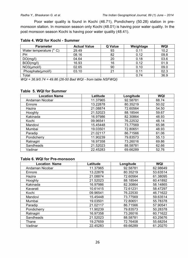
Poor water quality is found in Kochi (46.71), Pondicherry (50.28) station in pre-
monsoon station. In monsoon season only Kochi (48.01) is having poor water quality. In the
post monsoon season Kochi is having poor water quality (48.41).
Table 4. WQI for Kochi - Summer
WQI = 36.9/0.74 = 49.86 (26-50 Bad WQI - from table NSFWQI)
Table 5. WQI for Summer
Location Name Latitude Longitude WQI
Andaman Nicobar 11.37965 92.58781 68.74
Ennore 13.22878 80.35219 50.02
Hazira 21.08874 72.60564 54.50
Hooghly 21.52023 88.18544 59.67
Kakinada 16.97986 82.30864 48.93
Kochi 09.96541 76.22532 48.14
Mandovi 15.45448 73.77569 65.98
Mumbai 19.03501 72.80651 48.93
Paradip 21.02117 86.71566 61.06
Pondicherry 11.90239 79.83573 55.13
Ratnagiri 16.97358 73.26016 69.86
Sandheads 21.52023 88.58781 62.66
Vadinar 22.45283 69.66289 52.76
Table 6. WQI for Pre-monsoon
Location Name Latitude Longitude WQI
Andaman Nicobar 11.37965 92.58781 62.98649
Ennore 13.22878 80.35219 53.63514
Hazira 21.08874 72.60564 61.38095
Hooghly 21.52023 88.18544 60.41892
Kakinada 16.97986 82.30864 58.14865
Kavarati 10.61415 72.61231 58.47297
Kochi 09.96541 76.22530 46.71622
Mandovi 15.45448 73.77569 59.63514
Mumbai 19.03501 72.80651 55.78378
Paradip 21.02117 86.71566 57.90541
Pondicherry 11.90239 79.83573 50.28378
Ratnagiri 16.97358 73.26016 60.71622
Sandheads 21.52023 88.58781 63.25676
Thane 19.27659 72.76408 55.68254
Vadinar 22.45283 69.66289 61.20270
Parameter Actual Value Q Value Weightage WQI
Water temperature (⁰ C) 29.49 93 0.11 10.2
PH 08.16 82 0.12 09.8
DO(mg/l) 04.64 20 0.18 03.6
BOD(mg/l) 16.93 16 0.12 01.9
NO3(μmol/l) 02.65 90 0.10 09.0
Phosphate(μmol/l) 03.10 21 0.11 02.3
Total 0.74 36.9
27
Radha Y., Bhaskaran G. et al. The Indian Geographical Journal, 89 (1) June – 2014
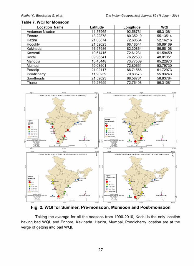
Table 7. WQI for Monsoon
Location Name Latitude Longitude WQI
Andaman Nicobar 11.37965 92.58781 65.31081
Ennore 13.22878 80.35219 55.13514
Hazira 21.08874 72.60564 52.16216
Hooghly 21.52023 88.18544 59.89189
Kakinada 16.97986 82.30864 56.58108
Kavarati 10.61415 72.61231 61.59459
Kochi 09.96541 76.22530 48.01351
Mandovi 15.45448 73.77569 65.22973
Mumbai 19.03501 72.80651 53.79730
Paradip 21.02117 86.71566 61.72973
Pondicherry 11.90239 79.83573 55.93243
Sandheads 21.52023 88.58781 58.83784
Thane 19.27659 72.76408 56.31081
Fig. 2. WQI for Summer, Pre-monsoon, Monsoon and Post-monsoon
Taking the average for all the seasons from 1990-2010, Kochi is the only location
having bad WQI, and Ennore, Kakinada, Hazira, Mumbai, Pondicherry location are at the
verge of getting into bad WQI.

28
Radha Y., Bhaskaran G. et al. The Indian Geographical Journal, 89 (1) June – 2014
Table 8. WQI for Post-monsoon
Fig. 6. Average WQI
Table 9. Average WQI
29
Radha Y., Bhaskaran G. et al. The Indian Geographical Journal, 89 (1) June – 2014
Conclusions
Assembling multiple parameters into single unit leads to easy classification and
interpretation of index, thus providing an important tool for environmental management
purposes. However, it is vital to provide precise information and evidence of specific
ecosystem to allow policy makers to decide and implement plans on particular problems.
This also helps the policy makers to understand the problem clearly and take necessary
mitigation measures for the specific area. On the other hand, GIS techniques add
simplification and visualisation to the dataset by integrating multiple layers like discharge
points, sampling stations and water quality variables that helps in easy understanding. It
has also proved to be a vital tool for decision makers to identify the sources and polluted
areas. The data accuracy was checked using trend line graphs and the relationship
between various parameters were studied which showed that pH and water temperature
are directly proportion, BOD and DO are directly proportional and the Nitrate and DO are
inversely proportional. Then the CWQI was calculated. From the calculated data, Kochi was
the only location having bad WQI - average value (47.82) and Ennore, Kakinada, Hazira,
Mumbai, Pondicherry location are at the verge of getting into poor WQI, but it falls in
medium water quality range according to NSFWQI.
Acknowledgements
The Author acknowledges Dr. Tune Usha, Scientist-F and ICMAM Project Team of
NIOT, Chennai for their constant support throughout the project.
References
1. Chang-An Yan, Wanchang Zhang, Zhijie Zhang, Yuanmin Liu, Cai Deng, Ning Nie, (2015). Assessment of Water Quality and Identification of Polluted Risky Regions Based on Field Observations and GIS in the Honghe River Watershed, China, National Natural Science Foundation of China. 4, pp. 31-36.
2. Coastal Water Quality Measurements Protocol for COMAPS Programme (2012), Technical Note (TN), 15th November, 2012, ICMAM Project Directorate
3. Srinivasan V., Usha Natesan and Parthasarathy A. (2013). Seasonal Variability of Coastal Water Quality in Bay of Bengal and Palk Strait, Tamil Nadu, Southeast Coast of India, An international Journal Brazilian Archives of Biology and Technology 56, pp. 875-884.
The Indian Geographical Journal
Volume 89 (1) June - 2014, pp 30-37 ISSN 0019-4824
30
A GIS-BASED MORPHOMETRIC ANALYSIS OF VAIPPAR
BASIN, TAMIL NADU
Balasubramani K., Gomathi M. and Kumaraswamy K.
Department of Geography, Bharathidasan University, Tiruchirappalli - 620 024
E-mail: [email protected]
Abstract
Geographic Information Systems (GIS) opens up new horizons in spatial planning and
simplify the complex mapping as well as planning processes. In this paper, GIS has been
used in order to determine the spatial variations in the drainage characteristics of the
Vaippar River basin and its sub-basins. The evaluation of morphometric characteristics of
the basin helps us to understand the terrain characteristics and hydrological related
parameters in a quantitative manner. This paper presents a simplified methodology to
generate stream network, delineate sub-basins and extract basin parameters from Digital
Elevation Model (DEM) using the Spatial Analyst extension tool in ArcGIS. The
conventional quantities such as stream order, stream length, bifurcation ratio, drainage
density, drainage texture, stream frequency and circulatory ratio were extracted from the
DEM based stream network for each delineated sub-basin. The extracted values were used
to characterise the drainage basin systems. The study finds that Charnokite dominated
Arjuna Nadi sub-basin has higher values of stream order, stream number, stream length,
stream frequency, drainage texture and drainage density; lower values of circulatory ratio
indicates that there is a strong geologic control in the landscape development of this basin
and susceptible to higher risks of soil erosion and peak flood discharge.
Keywords: GIS, Drainage basin, DEM, Morphometric parameters, Vaippar basin
Introduction
Generally, drainage channels are the arteries on the earth surface. The spatial
arrangement of a number of streams gives the formation of the drainage basin and studying
its typical arrangement provides insight into the interdependency of geology, climate and
fluvial processes. Morphometry is a classic technique which is based on the measurement
and mathematical analysis of the geometry of streams, relief features and dimensions of
drainage basins. It provides a quantitative description of the basin geometry so as to
understand inequalities in the rock hardness, structural controls, recent diastrophism and
geomorphic processes of the drainage basin (Strahler, 1964). Morphometric analysis of a
basin is an essential first step, toward a basic understanding of landscape dynamics
(Thomas et al., 2010). Basin morphometry is a kind of specific morphometric technique
which is capable of bringing out size, shape, form and functional variations and their inter-
relationships between basins / sub-basins (Kumaraswamy, 1994). Horton (1932, 1945) is
the pioneer in basin morphometric analysis and he has established the practical value of
31
Balasubramani K., Gomathi M. and Kumaraswamy K. The Indian Geographical Journal, 89 (1) June – 2014
this analysis. Later, Miller (1953), Smith (1950), Suchumn (1956), Strahler (1964), Chorley
(1969) and several scientists have developed many quantitative techniques for
morphometric analysis and applied for different drainage basins throughout the world.
The GIS is a convenient system for morphometric analysis as it provides a various
set of tools for delineation of basins, extraction of basin parameters and visualisation of
results (Tripathi et al., 2013). It simplifies the extraction of drainage network and provides
accurate details for morphometric calculations (Ahmed et al., 2010). It also provides very
powerful tools to automatic extraction of stream network and basin parameters from DEM.
Unlike the traditional methods, the DEM based automatic extraction of basin parameters
are standardised throughout the basin. Further, GIS offers very powerful tools for
visualisation of basin landscape using DEM. The present study demonstrates the
application of GIS in the morphometric analysis by taking a case study area. The study also
tries to find out and visualise the intra-basin variations in the morphometric parameters at
the sub-basin level.
Study Area
Vaippar basin in South Tamil Nadu, India has been chosen for the present
investigation. The basin is bound between 8o 57’ 13” N to 90 46‘33” N latitudes and 77o 14’
34” East to 780 14’ 34” East longitudes with an area of about 5,200 sq.km (Figure 1).
Vaippar is a non-perennial river, collects water from the eastern sides of Western Ghats
and drains into the Bay of Bengal. The river Vaippar is 147 km long and has two major
branches viz., upper Vaippar in the south and Arjuna Nadi in the north. The basin covers
Tirunelveli, Thoothukudi, Virudhunagar, Madurai and Ramanathapuram Districts and
shared a boundary with Vaigai basin (West and North West), Gundar basin (North,
Northeast), Pampa and Achankovil basins (Southwest) and Thamaraparani basin (South
and Southeast). The topography of upper part of Vaippar basin is rugged and marked by
ridges eastwest in the south and northeast-southwest in the north. The important hills
located in the western part of the basin are Sangumalai, Kurangumalai, Ambarimedumalai,
Kottamalai (2016 m - the highest point in the study area) Toppimalai, Ambarimedumalai,
Sivavigirimalai and Kodalapparimottai. After a certain distance of eastward travel from
these hills, the topography suddenly drops down and gives birth to a number of tanks. All
the tanks are rainfed and remain dry except Thenmalaikulam and Puttur tanks. Most of the
streams running parallel to each other from the retreating scarp face join the next higher
order segments at a height of 120-150 metres above Mean Sea Level (MSL). About 70
percent of the drainage basin, especially the central and eastern parts, is underlined by
Genesis and 25 percent by Charnokite (western part). An alluvial track prevails in the lower
reaches of the basin (Figure 2). The basin falls under semi-arid tropical monsoon type of
climate with the mean temperature of 35o C and an annual average of rainfall of 812 mm.
Database and Methodology
To study the morphometric characteristics of Vaippar basin, DEM of the study area
was collected from ASTER (Advanced Spaceborne Thermal Emission and Radiometer)

32
Balasubramani K., Gomathi M. and Kumaraswamy K. The Indian Geographical Journal, 89 (1) June – 2014
data (30 m pixel resolution). The gaps and spikes in the DEM were corrected with the help
of sink and fill tools in ArcGIS (Figure 3). The direction of surface flow from DEM was
identified with the help of flow direction tool and accumulation of water flow was estimated.
The flow direction layer was used to delineate the basin boundary and the flow
accumulation layer was used to generate a stream network by determining the cell value of
more than 100 in the raster calculator. The generated stream network later converted into a
vector in order to extract parameters for morphometric analysis. The workflow of automatic
stream generation is presented graphically in Figure 4.
Based on topography configuration and major tributaries of the main river, the basin
was divided into six major sub-basins viz. Upper Vaippar, Arjuna Nadi, Mannarkkottai,
Melkaranai Odai, Uppar and Lower Vaippar by fixing the pour points at appropriate
locations. The generated stream network of all sub-basins were cross verified with Survey
of India toposheets (1:50,000) and altered wherever blunder appears. The amount of
blunders usually high in the lower parts of the basin and almost negligible in the upper
reaches. The measurements of shape and length of stream networks were derived from
rectified stream networks to calculate conventional morphometric parameters’ (stream
length, relief ratio, drainage density, stream frequency, elongation ratio and circulatory ratio)
adopting methods are presented in Table 1. All the parameters were tabulated (Table 2)
and maps were prepared (Figure 5) to bring out the intra-basin variations.
Fig. 3. Asters Derived Digital Elevation Model
Fig. 2. Geology of the Basin with Major
Streams and Contours
Fig.1. Location of Vaippar
Basin
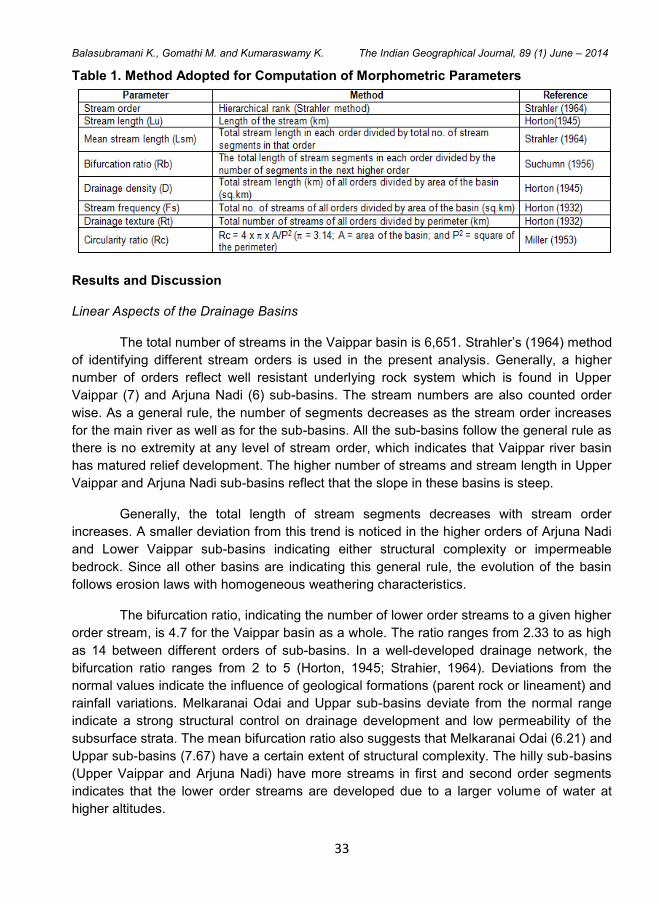
33
Balasubramani K., Gomathi M. and Kumaraswamy K. The Indian Geographical Journal, 89 (1) June – 2014
Table 1. Method Adopted for Computation of Morphometric Parameters
Results and Discussion
Linear Aspects of the Drainage Basins
The total number of streams in the Vaippar basin is 6,651. Strahler’s (1964) method
of identifying different stream orders is used in the present analysis. Generally, a higher
number of orders reflect well resistant underlying rock system which is found in Upper
Vaippar (7) and Arjuna Nadi (6) sub-basins. The stream numbers are also counted order
wise. As a general rule, the number of segments decreases as the stream order increases
for the main river as well as for the sub-basins. All the sub-basins follow the general rule as
there is no extremity at any level of stream order, which indicates that Vaippar river basin
has matured relief development. The higher number of streams and stream length in Upper
Vaippar and Arjuna Nadi sub-basins reflect that the slope in these basins is steep.
Generally, the total length of stream segments decreases with stream order
increases. A smaller deviation from this trend is noticed in the higher orders of Arjuna Nadi
and Lower Vaippar sub-basins indicating either structural complexity or impermeable
bedrock. Since all other basins are indicating this general rule, the evolution of the basin
follows erosion laws with homogeneous weathering characteristics.
The bifurcation ratio, indicating the number of lower order streams to a given higher
order stream, is 4.7 for the Vaippar basin as a whole. The ratio ranges from 2.33 to as high
as 14 between different orders of sub-basins. In a well-developed drainage network, the
bifurcation ratio ranges from 2 to 5 (Horton, 1945; Strahier, 1964). Deviations from the
normal values indicate the influence of geological formations (parent rock or lineament) and
rainfall variations. Melkaranai Odai and Uppar sub-basins deviate from the normal range
indicate a strong structural control on drainage development and low permeability of the
subsurface strata. The mean bifurcation ratio also suggests that Melkaranai Odai (6.21) and
Uppar sub-basins (7.67) have a certain extent of structural complexity. The hilly sub-basins
(Upper Vaippar and Arjuna Nadi) have more streams in first and second order segments
indicates that the lower order streams are developed due to a larger volume of water at
higher altitudes.
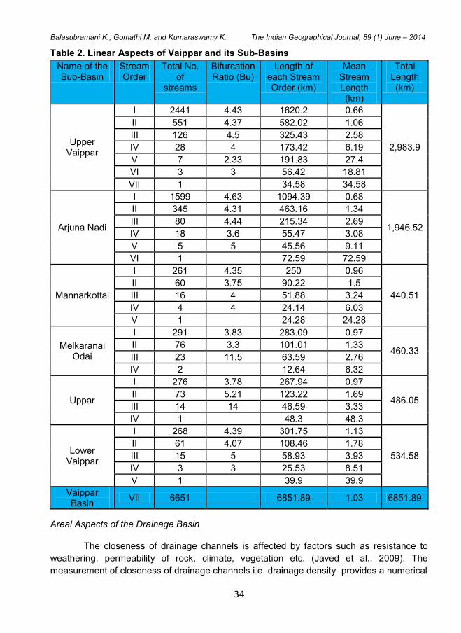
34
Balasubramani K., Gomathi M. and Kumaraswamy K. The Indian Geographical Journal, 89 (1) June – 2014
Table 2. Linear Aspects of Vaippar and its Sub-Basins
Name of the Sub-Basin
Stream Order
Total No. of
streams
Bifurcation Ratio (Bu)
Length of each Stream Order (km)
Mean Stream Length (km)
Total Length (km)
Upper Vaippar
I 2441 4.43 1620.2 0.66
2,983.9
II 551 4.37 582.02 1.06
III 126 4.5 325.43 2.58
IV 28 4 173.42 6.19
V 7 2.33 191.83 27.4
VI 3 3 56.42 18.81
VII 1 34.58 34.58
Arjuna Nadi
I 1599 4.63 1094.39 0.68
1,946.52
II 345 4.31 463.16 1.34
III 80 4.44 215.34 2.69
IV 18 3.6 55.47 3.08
V 5 5 45.56 9.11
VI 1 72.59 72.59
Mannarkottai
I 261 4.35 250 0.96
440.51
II 60 3.75 90.22 1.5
III 16 4 51.88 3.24
IV 4 4 24.14 6.03
V 1 24.28 24.28
Melkaranai Odai
I 291 3.83 283.09 0.97
460.33 II 76 3.3 101.01 1.33
III 23 11.5 63.59 2.76
IV 2 12.64 6.32
Uppar
I 276 3.78 267.94 0.97
486.05 II 73 5.21 123.22 1.69
III 14 14 46.59 3.33
IV 1 48.3 48.3
Lower Vaippar
I 268 4.39 301.75 1.13
534.58
II 61 4.07 108.46 1.78
III 15 5 58.93 3.93
IV 3 3 25.53 8.51
V 1 39.9 39.9
Vaippar Basin
VII 6651 6851.89 1.03 6851.89
Areal Aspects of the Drainage Basin
The closeness of drainage channels is affected by factors such as resistance to
weathering, permeability of rock, climate, vegetation etc. (Javed et al., 2009). The
measurement of closeness of drainage channels i.e. drainage density provides a numerical
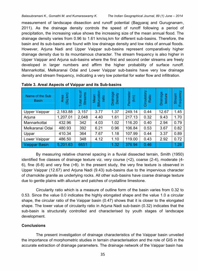
35
Balasubramani K., Gomathi M. and Kumaraswamy K. The Indian Geographical Journal, 89 (1) June – 2014
measurement of landscape dissection and runoff potential (Bagyaraj and Gurugnanam,
2011). As the drainage density controls the speed of runoff following a period of
precipitation, the increasing value shows the increasing size of the mean annual flood. The
drainage density varies from 0.96 to 1.61 km/sq.km for different sub-basins. Therefore, the
basin and its sub-basins are found with low drainage density and low risks of annual floods.
However, Arjuna Nadi and Upper Vaippar sub-basins represent comparatively higher
drainage density due to its mountainous character. The stream frequency is also higher in
Upper Vaippar and Arjuna sub-basins where the first and second order streams are freely
developed in larger numbers and affirm the higher probability of surface runoff.
Mannarkottai, Melkaranai Odai and Lower Vaippar sub-basins have very low drainage
density and stream frequency, indicating a very low potential for water flow and infiltration.
Table 3. Areal Aspects of Vaippar and its Sub-basins
Name of the Sub
Basin Are
a
(Sq
.km
)
To
tal no
.of
Str
ea
ms
Me
an
Bifu
rca
tio
n
ratio
Dra
inage
De
nsity
Pe
rim
ete
r
(km
)
Cir
cu
lato
ry
Ra
tio
Dra
inage
textu
re
Str
ea
m
Fre
que
ncy
Upper Vaippar 2,183.88 3,157 3.77 1.37 249.14 0.44 12.67 1.45
Arjuna 1,207.01 2,048 4.40 1.61 217.13 0.32 9.43 1.70
Mannarkottai 432.96 342 4.03 1.02 116.20 0.40 2.94 0.79
Melkaranai Odai 480.93 392 6.21 0.96 106.84 0.53 3.67 0.82
Uppar 410.34 364 7.67 1.18 107.99 0.44 3.37 0.89
Lower Vaippar 486.50 348 4.12 1.10 119.00 0.43 2.92 0.72
Vaippar Basin 5,201.63 6651 1.32 376.94 0.46 1.28
By measuring relative channel spacing in a fluvial dissected terrain, Smith (1950)
identified five classes of drainage texture viz. very course (<2), coarse (2-4), moderate (4-
6), fine (6-8) and very fine (>8). In the present study, the very fine texture is observed in
Upper Vaippar (12.67) and Arjuna Nadi (9.43) sub-basins due to the impervious character
of charnokite granite as underlying rocks. All other sub-basins have coarse drainage texture
due to gentle plains with alluvium and patches of crystalline limestone.
Circularity ratio which is a measure of outline form of the basin varies from 0.32 to
0.53. Since the value 0.0 indicates the highly elongated shape and the value 1.0 a circular
shape, the circular ratio of the Vaippar basin (0.47) shows that it is closer to the elongated
shape. The lower value of circularity ratio in Arjuna Nadi sub-basin (0.32) indicates that the
sub-basin is structurally controlled and characterised by youth stages of landscape
development.
Conclusions
The present investigation of drainage characteristics of the Vaippar basin unveiled
the importance of morphometric studies in terrain characterisation and the role of GIS in the
accurate extraction of drainage parameters. The drainage network of the Vaippar basin has
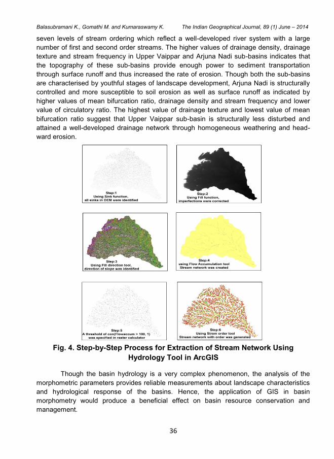
36
Balasubramani K., Gomathi M. and Kumaraswamy K. The Indian Geographical Journal, 89 (1) June – 2014
seven levels of stream ordering which reflect a well-developed river system with a large
number of first and second order streams. The higher values of drainage density, drainage
texture and stream frequency in Upper Vaippar and Arjuna Nadi sub-basins indicates that
the topography of these sub-basins provide enough power to sediment transportation
through surface runoff and thus increased the rate of erosion. Though both the sub-basins
are characterised by youthful stages of landscape development, Arjuna Nadi is structurally
controlled and more susceptible to soil erosion as well as surface runoff as indicated by
higher values of mean bifurcation ratio, drainage density and stream frequency and lower
value of circulatory ratio. The highest value of drainage texture and lowest value of mean
bifurcation ratio suggest that Upper Vaippar sub-basin is structurally less disturbed and
attained a well-developed drainage network through homogeneous weathering and head-
ward erosion.
Fig. 4. Step-by-Step Process for Extraction of Stream Network Using
Hydrology Tool in ArcGIS
Though the basin hydrology is a very complex phenomenon, the analysis of the
morphometric parameters provides reliable measurements about landscape characteristics
and hydrological response of the basins. Hence, the application of GIS in basin
morphometry would produce a beneficial effect on basin resource conservation and
management.
37
Balasubramani K., Gomathi M. and Kumaraswamy K. The Indian Geographical Journal, 89 (1) June – 2014
Acknowledgements
The authors' extend sincere thanks to Mr. C. Satheesh and Mr. M. Sathish Kumar
for their assistance in cross verification of DEM generated stream network with SOI
toposheets. MG and KK are grateful to UGC, New Delhi for the financial support to execute
the present study.
References
1. Ahmed, S.A., Chandrashekarappa, K.N., Raj, S.K. Nischitha, V. and Kavitha, G. (2010). Evaluation of Morphometric Parameters Derived from ASTER and SRTM DEM – A study on Bandihole Sub-watershed Basin in Karnataka. Journal of Indian Society for Remote Sensing, 38, pp. 227–238.
2. Bagyaraj, M. and Gurugnanam, B. (2011). Significance of Morphometry Studies, Soil Characteristics, Erosion Phenomena and Landform Processes Using Remote Sensing and GIS for Kodaikanal Hills, A Global Biodiversity Hotpot in Western Ghats, Dindigul District, Tamil Nadu, South India. Research Journal of Environmental and Earth Sciences, 3(3), pp. 221-233.
3. Chorley, R.J. (1969). Introduction to fluvial processes: Methuen and Co. Ltd., London, pp. 30-53.
4. Horton, R. E. (1932). Drainage basin characteristics. Transactions of American Geophysical Union, 13, pp. 350–361.
5. Horton, R. E. (1945). Erosional development of streams and their drainage basins; hydrophysical approach to quantitative morphology. Geological Society of America Bulletin, 56, pp. 275–370.
6. Javed, A., Khanday, M.Y. and Ahmed, R. (2009). Prioritization of Sub-watersheds based on Morphometric and Land Use Analysis using Remote Sensing and GIS Techniques. Journal of Indian Society for Remote Sensing, 37, pp. 261–274.
7. Kumaraswamy, K., Jayakumar, R. and Kamaraj, M. (1994). Morphostatistical Analysis of Vaippar Basin, Tamil Nadu, National Geographer, 21(2), pp. 107-113.
8. Miller, V.C. (1953). A quantitative geomorphic study of drainage basin characteristics in the Clinch mountain area, Virginia and Tennessee. In Project NR 389-402, Technical Report 3. New York: Columbia University.
9. Schumm, S. A. (1956). Evolution of drainage systems and slopes in Badlands at Perth Amboy, New Jersey. Geological Society of America Bulletin, 67, pp. 597–646.
10. Smith KG (1950). Standards for grading textures of erosional topography. American Journal of Science, 248, pp. 655–668.
11. Strahler, A. N. (1964). Handbook of applied hydrology. In V. T. Chow (Ed.), Quantitative geomorphology of drainage basins and channel networks. New York: Mc-Graw Hill Book Company, 39–76.
12. Thomas, J., Joseph, S. and Thrivikramaji, K.P. (2010). Morphometric aspects of a small tropical mountain river system, the southern Western Ghats, India. International Journal of Digital Earth, 3(2), pp. 135-156.
13. Tripathi, S., Soni, S. K., and Maurya, A. K. (2013). Morphometric characterization and prioritization of sub watersheds of Seoni river Madhya Pradesh, through remote sensing and GIS technique. International Journal of Remote Sensing Geoscience, 2, pp. 46–54.
The Indian Geographical Journal
Volume 89 (1) June - 2014, pp 38-47 ISSN 0019-4824
38
REGIONAL VARIATIONS OF POPULATION DISTRIBUTION IN
TAMIL NADU - A SPATIO-TEMPORAL ANALYSIS BASED ON
PHYSIOGRAPHIC REGIONS
Lazar A.
Directorate of Census Operations, Chennai - 600 090
E-mail: [email protected]
Abstract
The ability to adapt to the prevailing environment of human beings is influenced by the
physiographic settings. However, the adaptability to the physiographic settings is not
uniform in the global distribution of population. It is essential to compile the demographic,
socio-economic variables at physiographic regional level to ascertain the distribution
pattern, dependencies and to help in regional planning and disaster responses. In this
study, the regional variations of population distribution in the physiographic region of Tamil
Nadu are discussed. The study compiles and infers Census data published during 1981,
1991, 2001 and 2011 on the basis of physiographic regions which was devised during 1981
Census and revised in 1991, but which were consequently discontinued. Computation and
analysis of the variations in population distribution at sub-micro regional level and measure
the distribution inequality across the regions using appropriate statistical methods are
carried out in this study. The sub-micro regional level cumulative proportion of area (Xi) and
cumulative proportion of population (Yi) have been used to compute the Spatial Gini’s
coefficient. The Census data at physiographic regional level have been compiled using GIS
application by utilising the spatial data of physiographic regional boundaries and locations
of villages / towns. The results shows that the State of Tamil Nadu have 0.38 Spatial Gini’s
coefficient which is fairly distributed across the two meso regions within the State but at
micro regional level we could see inequality of population distribution. Thus, the study helps
to understand the influences on population distributions in a physiographic region.
Keywords: Physiography, Population Distribution, Spatial-GINI’s Coefficient
Introduction
The global distribution of population has been influenced by many factors and
primarily by the interaction of humans with physiographical settings and their ability to
sustain in the prevailing environment. It is observed that the characteristics of continental
physiography such as elevation, proximity to nearest coastline or river presumably influence
habitation (Small and Cohen, 2004). But over time these dependencies are getting reduced
depending upon the level of development attained by the occupied population. But this
adaptability to the physiographic settings is not uniform across the globe and depends on
various socio-economic variables.
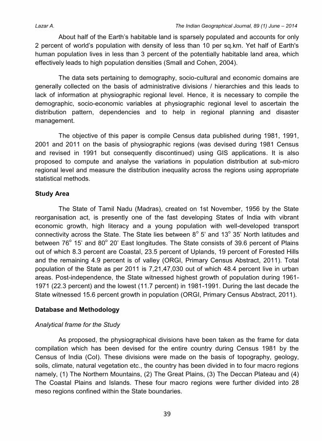
39
Lazar A. The Indian Geographical Journal, 89 (1) June – 2014
About half of the Earth’s habitable land is sparsely populated and accounts for only
2 percent of world’s population with density of less than 10 per sq.km. Yet half of Earth's
human population lives in less than 3 percent of the potentially habitable land area, which
effectively leads to high population densities (Small and Cohen, 2004).
The data sets pertaining to demography, socio-cultural and economic domains are
generally collected on the basis of administrative divisions / hierarchies and this leads to
lack of information at physiographic regional level. Hence, it is necessary to compile the
demographic, socio-economic variables at physiographic regional level to ascertain the
distribution pattern, dependencies and to help in regional planning and disaster
management.
The objective of this paper is compile Census data published during 1981, 1991,
2001 and 2011 on the basis of physiographic regions (was devised during 1981 Census
and revised in 1991 but consequently discontinued) using GIS applications. It is also
proposed to compute and analyse the variations in population distribution at sub-micro
regional level and measure the distribution inequality across the regions using appropriate
statistical methods.
Study Area
The State of Tamil Nadu (Madras), created on 1st November, 1956 by the State
reorganisation act, is presently one of the fast developing States of India with vibrant
economic growth, high literacy and a young population with well-developed transport
connectivity across the State. The State lies between 8o 5’ and 13
o 35’ North latitudes and
between 76o 15’ and 80
o 20’ East longitudes. The State consists of 39.6 percent of Plains
out of which 8.3 percent are Coastal, 23.5 percent of Uplands, 19 percent of Forested Hills
and the remaining 4.9 percent is of valley (ORGI, Primary Census Abstract, 2011). Total
population of the State as per 2011 is 7,21,47,030 out of which 48.4 percent live in urban
areas. Post-independence, the State witnessed highest growth of population during 1961-
1971 (22.3 percent) and the lowest (11.7 percent) in 1981-1991. During the last decade the
State witnessed 15.6 percent growth in population (ORGI, Primary Census Abstract, 2011).
Database and Methodology
Analytical frame for the Study
As proposed, the physiographical divisions have been taken as the frame for data
compilation which has been devised for the entire country during Census 1981 by the
Census of India (CoI). These divisions were made on the basis of topography, geology,
soils, climate, natural vegetation etc., the country has been divided in to four macro regions
namely, (1) The Northern Mountains, (2) The Great Plains, (3) The Deccan Plateau and (4)
The Coastal Plains and Islands. These four macro regions were further divided into 28
meso regions confined within the State boundaries.
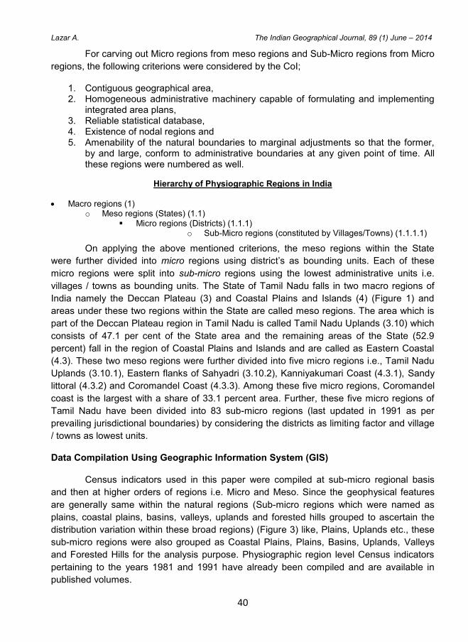
40
Lazar A. The Indian Geographical Journal, 89 (1) June – 2014
For carving out Micro regions from meso regions and Sub-Micro regions from Micro
regions, the following criterions were considered by the CoI;
1. Contiguous geographical area, 2. Homogeneous administrative machinery capable of formulating and implementing
integrated area plans, 3. Reliable statistical database, 4. Existence of nodal regions and 5. Amenability of the natural boundaries to marginal adjustments so that the former,
by and large, conform to administrative boundaries at any given point of time. All these regions were numbered as well.
Hierarchy of Physiographic Regions in India
Macro regions (1) o Meso regions (States) (1.1)
Micro regions (Districts) (1.1.1) o Sub-Micro regions (constituted by Villages/Towns) (1.1.1.1)
On applying the above mentioned criterions, the meso regions within the State
were further divided into micro regions using district’s as bounding units. Each of these
micro regions were split into sub-micro regions using the lowest administrative units i.e.
villages / towns as bounding units. The State of Tamil Nadu falls in two macro regions of
India namely the Deccan Plateau (3) and Coastal Plains and Islands (4) (Figure 1) and
areas under these two regions within the State are called meso regions. The area which is
part of the Deccan Plateau region in Tamil Nadu is called Tamil Nadu Uplands (3.10) which
consists of 47.1 per cent of the State area and the remaining areas of the State (52.9
percent) fall in the region of Coastal Plains and Islands and are called as Eastern Coastal
(4.3). These two meso regions were further divided into five micro regions i.e., Tamil Nadu
Uplands (3.10.1), Eastern flanks of Sahyadri (3.10.2), Kanniyakumari Coast (4.3.1), Sandy
littoral (4.3.2) and Coromandel Coast (4.3.3). Among these five micro regions, Coromandel
coast is the largest with a share of 33.1 percent area. Further, these five micro regions of
Tamil Nadu have been divided into 83 sub-micro regions (last updated in 1991 as per
prevailing jurisdictional boundaries) by considering the districts as limiting factor and village
/ towns as lowest units.
Data Compilation Using Geographic Information System (GIS)
Census indicators used in this paper were compiled at sub-micro regional basis
and then at higher orders of regions i.e. Micro and Meso. Since the geophysical features
are generally same within the natural regions (Sub-micro regions which were named as
plains, coastal plains, basins, valleys, uplands and forested hills grouped to ascertain the
distribution variation within these broad regions) (Figure 3) like, Plains, Uplands etc., these
sub-micro regions were also grouped as Coastal Plains, Plains, Basins, Uplands, Valleys
and Forested Hills for the analysis purpose. Physiographic region level Census indicators
pertaining to the years 1981 and 1991 have already been compiled and are available in
published volumes.
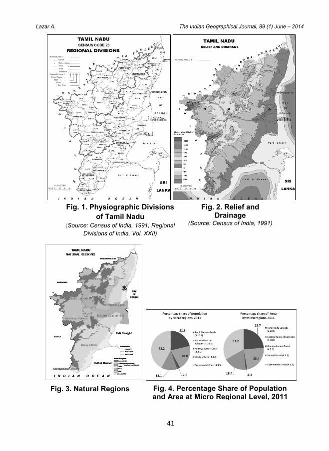
41
Lazar A. The Indian Geographical Journal, 89 (1) June – 2014
Fig. 4. Percentage Share of Population and Area at Micro Regional Level, 2011
Fig. 3. Natural Regions
Fig. 2. Relief and Drainage
(Source: Census of India, 1991)
Fig. 1. Physiographic Divisions
of Tamil Nadu (Source: Census of India, 1991, Regional
Divisions of India, Vol. XXII)
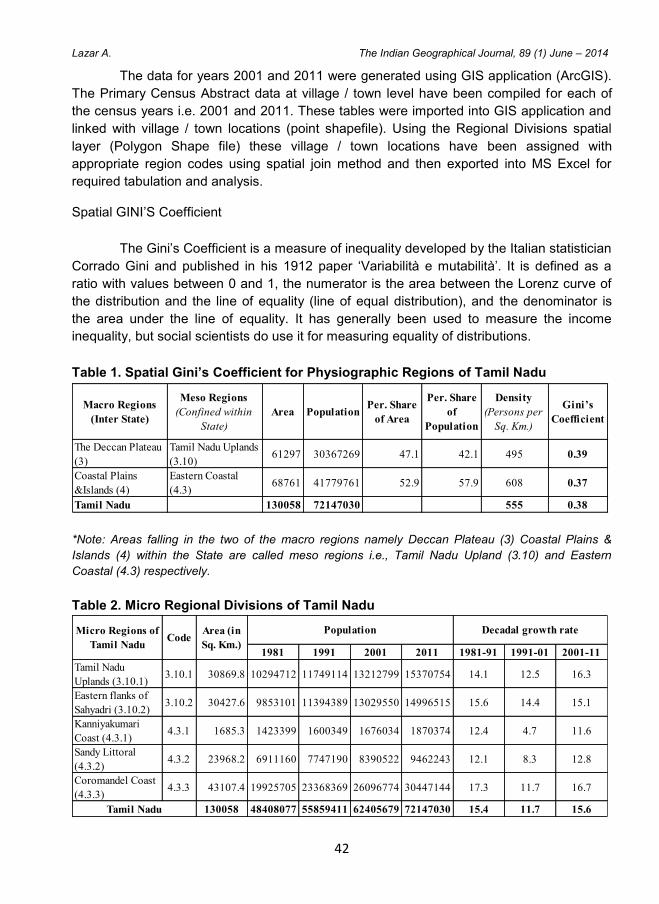
42
Lazar A. The Indian Geographical Journal, 89 (1) June – 2014
The data for years 2001 and 2011 were generated using GIS application (ArcGIS).
The Primary Census Abstract data at village / town level have been compiled for each of
the census years i.e. 2001 and 2011. These tables were imported into GIS application and
linked with village / town locations (point shapefile). Using the Regional Divisions spatial
layer (Polygon Shape file) these village / town locations have been assigned with
appropriate region codes using spatial join method and then exported into MS Excel for
required tabulation and analysis.
Spatial GINI’S Coefficient
The Gini’s Coefficient is a measure of inequality developed by the Italian statistician
Corrado Gini and published in his 1912 paper ‘Variabilità e mutabilità’. It is defined as a
ratio with values between 0 and 1, the numerator is the area between the Lorenz curve of
the distribution and the line of equality (line of equal distribution), and the denominator is
the area under the line of equality. It has generally been used to measure the income
inequality, but social scientists do use it for measuring equality of distributions.
Table 1. Spatial Gini’s Coefficient for Physiographic Regions of Tamil Nadu
*Note: Areas falling in the two of the macro regions namely Deccan Plateau (3) Coastal Plains &
Islands (4) within the State are called meso regions i.e., Tamil Nadu Upland (3.10) and Eastern
Coastal (4.3) respectively.
Table 2. Micro Regional Divisions of Tamil Nadu
Macro Regions
(Inter State)
Meso Regions
(Confined within
State)
Area PopulationPer. Share
of Area
Per. Share
of
Population
Density
(Persons per
Sq. Km.)
Gini’s
Coefficient
The Deccan Plateau
(3)
Tamil Nadu Uplands
(3.10)61297 30367269 47.1 42.1 495 0.39
Coastal Plains
&Islands (4)
Eastern Coastal
(4.3)68761 41779761 52.9 57.9 608 0.37
Tamil Nadu 130058 72147030 555 0.38
Table No:1 Spatial Gini’s Coefficient for Physiographic Regions of Tamil Nadu
1981 1991 2001 2011 1981-91 1991-01 2001-11
Tamil Nadu
Uplands (3.10.1)3.10.1 30869.8 10294712 11749114 13212799 15370754 14.1 12.5 16.3
Eastern flanks of
Sahyadri (3.10.2)3.10.2 30427.6 9853101 11394389 13029550 14996515 15.6 14.4 15.1
Kanniyakumari
Coast (4.3.1)4.3.1 1685.3 1423399 1600349 1676034 1870374 12.4 4.7 11.6
Sandy Littoral
(4.3.2)4.3.2 23968.2 6911160 7747190 8390522 9462243 12.1 8.3 12.8
Coromandel Coast
(4.3.3)4.3.3 43107.4 19925705 23368369 26096774 30447144 17.3 11.7 16.7
130058 48408077 55859411 62405679 72147030 15.4 11.7 15.6
Table No. 2 : Micro Regional Divisions of Tamil Nadu
Tamil Nadu
Population Decadal growth rateMicro Regions of
Tamil NaduCode
Area (in
Sq. Km.)
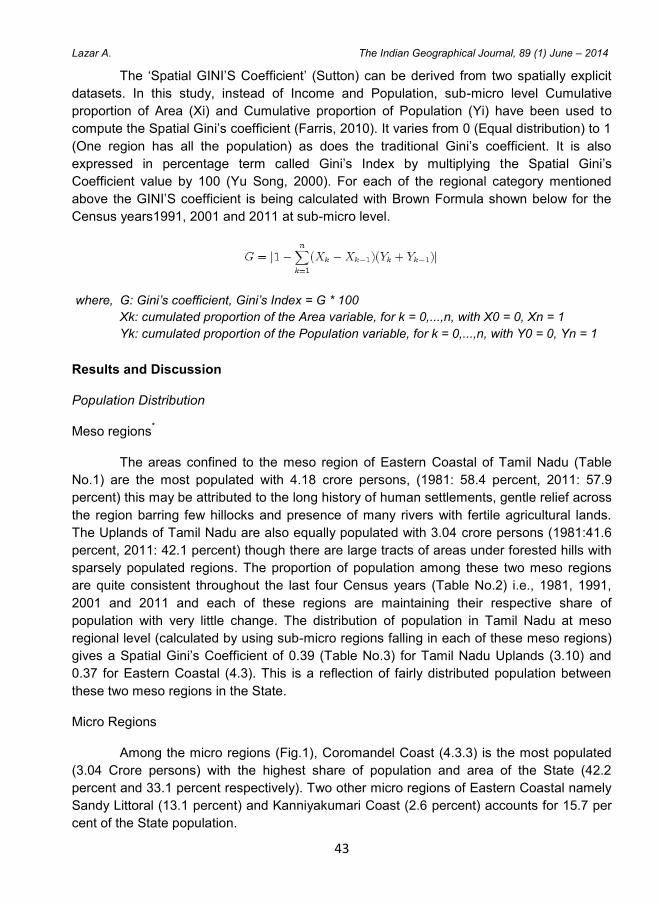
43
Lazar A. The Indian Geographical Journal, 89 (1) June – 2014
The ‘Spatial GINI’S Coefficient’ (Sutton) can be derived from two spatially explicit
datasets. In this study, instead of Income and Population, sub-micro level Cumulative
proportion of Area (Xi) and Cumulative proportion of Population (Yi) have been used to
compute the Spatial Gini’s coefficient (Farris, 2010). It varies from 0 (Equal distribution) to 1
(One region has all the population) as does the traditional Gini’s coefficient. It is also
expressed in percentage term called Gini’s Index by multiplying the Spatial Gini’s
Coefficient value by 100 (Yu Song, 2000). For each of the regional category mentioned
above the GINI’S coefficient is being calculated with Brown Formula shown below for the
Census years1991, 2001 and 2011 at sub-micro level.
where, G: Gini’s coefficient, Gini’s Index = G * 100
Xk: cumulated proportion of the Area variable, for k = 0,...,n, with X0 = 0, Xn = 1
Yk: cumulated proportion of the Population variable, for k = 0,...,n, with Y0 = 0, Yn = 1
Results and Discussion
Population Distribution
Meso regions*
The areas confined to the meso region of Eastern Coastal of Tamil Nadu (Table
No.1) are the most populated with 4.18 crore persons, (1981: 58.4 percent, 2011: 57.9
percent) this may be attributed to the long history of human settlements, gentle relief across
the region barring few hillocks and presence of many rivers with fertile agricultural lands.
The Uplands of Tamil Nadu are also equally populated with 3.04 crore persons (1981:41.6
percent, 2011: 42.1 percent) though there are large tracts of areas under forested hills with
sparsely populated regions. The proportion of population among these two meso regions
are quite consistent throughout the last four Census years (Table No.2) i.e., 1981, 1991,
2001 and 2011 and each of these regions are maintaining their respective share of
population with very little change. The distribution of population in Tamil Nadu at meso
regional level (calculated by using sub-micro regions falling in each of these meso regions)
gives a Spatial Gini’s Coefficient of 0.39 (Table No.3) for Tamil Nadu Uplands (3.10) and
0.37 for Eastern Coastal (4.3). This is a reflection of fairly distributed population between
these two meso regions in the State.
Micro Regions
Among the micro regions (Fig.1), Coromandel Coast (4.3.3) is the most populated
(3.04 Crore persons) with the highest share of population and area of the State (42.2
percent and 33.1 percent respectively). Two other micro regions of Eastern Coastal namely
Sandy Littoral (13.1 percent) and Kanniyakumari Coast (2.6 percent) accounts for 15.7 per
cent of the State population.
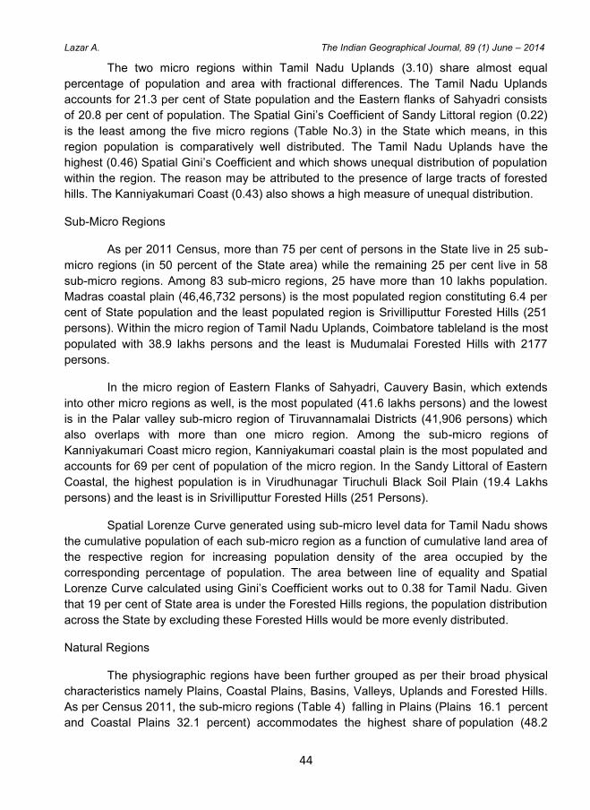
44
Lazar A. The Indian Geographical Journal, 89 (1) June – 2014
The two micro regions within Tamil Nadu Uplands (3.10) share almost equal
percentage of population and area with fractional differences. The Tamil Nadu Uplands
accounts for 21.3 per cent of State population and the Eastern flanks of Sahyadri consists
of 20.8 per cent of population. The Spatial Gini’s Coefficient of Sandy Littoral region (0.22)
is the least among the five micro regions (Table No.3) in the State which means, in this
region population is comparatively well distributed. The Tamil Nadu Uplands have the
highest (0.46) Spatial Gini’s Coefficient and which shows unequal distribution of population
within the region. The reason may be attributed to the presence of large tracts of forested
hills. The Kanniyakumari Coast (0.43) also shows a high measure of unequal distribution.
Sub-Micro Regions
As per 2011 Census, more than 75 per cent of persons in the State live in 25 sub-
micro regions (in 50 percent of the State area) while the remaining 25 per cent live in 58
sub-micro regions. Among 83 sub-micro regions, 25 have more than 10 lakhs population.
Madras coastal plain (46,46,732 persons) is the most populated region constituting 6.4 per
cent of State population and the least populated region is Srivilliputtur Forested Hills (251
persons). Within the micro region of Tamil Nadu Uplands, Coimbatore tableland is the most
populated with 38.9 lakhs persons and the least is Mudumalai Forested Hills with 2177
persons.
In the micro region of Eastern Flanks of Sahyadri, Cauvery Basin, which extends
into other micro regions as well, is the most populated (41.6 lakhs persons) and the lowest
is in the Palar valley sub-micro region of Tiruvannamalai Districts (41,906 persons) which
also overlaps with more than one micro region. Among the sub-micro regions of
Kanniyakumari Coast micro region, Kanniyakumari coastal plain is the most populated and
accounts for 69 per cent of population of the micro region. In the Sandy Littoral of Eastern
Coastal, the highest population is in Virudhunagar Tiruchuli Black Soil Plain (19.4 Lakhs
persons) and the least is in Srivilliputtur Forested Hills (251 Persons).
Spatial Lorenze Curve generated using sub-micro level data for Tamil Nadu shows
the cumulative population of each sub-micro region as a function of cumulative land area of
the respective region for increasing population density of the area occupied by the
corresponding percentage of population. The area between line of equality and Spatial
Lorenze Curve calculated using Gini’s Coefficient works out to 0.38 for Tamil Nadu. Given
that 19 per cent of State area is under the Forested Hills regions, the population distribution
across the State by excluding these Forested Hills would be more evenly distributed.
Natural Regions
The physiographic regions have been further grouped as per their broad physical
characteristics namely Plains, Coastal Plains, Basins, Valleys, Uplands and Forested Hills.
As per Census 2011, the sub-micro regions (Table 4) falling in Plains (Plains 16.1 percent
and Coastal Plains 32.1 percent) accommodates the highest share of population (48.2
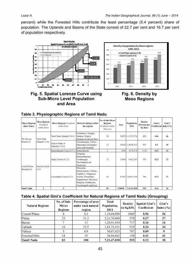
45
Lazar A. The Indian Geographical Journal, 89 (1) June – 2014
percent) while the Forested Hills contribute the least percentage (5.4 percent) share of
population. The Uplands and Basins of the State consist of 22.7 per cent and 16.7 per cent
of population respectively.
Table 3. Physiographic Regions of Tamil Nadu
Table 4. Spatial Gini’s Coefficient for Natural Regions of Tamil Nadu (Grouping)
Macro Regions
(Inter State)
Meso Regions
(Confined
within State)
Micro Regions (Confined
within State
Districts falling within
the regions
No. of Sub-Micro
Regions
(Confined within
Districts)
AreaPopulation,
2011
Density
(Persons per
Sq. Km.)
Gini’s
Coefficient
Gini’s
Index (%)
Tamil Nadu Uplands(3.10.1)
Coimbatore, Tiruppur,
Madurai, Nilgiris,
Dindigul, Erode and Theni
24 30870 1,53,70,754 498 0.46 46
Eastern flanks of
Sahyadri(3.10.2)
Tiruvannamalai, Vellore,
Dharmapuri, Krishnagiri,
Salem and Namakkal
15 30428 1,49,96,515 493 0.3 30
Kanniyakumari Coast (4.3.1) Kanniyakumari 3 1685 18,70,374 1110 0.43 43
Sandy Littoral (4.3.2)
Sivaganga,
Ramanathapuram,
Virudhunagar,
Thoothukkudi and
Tirunelveli
15 23968 94,62,243 395 0.22 22
Coromandel Coast (4.3.3)
Thiruvallur,
Kancheepuram, Chennai,
Cuddalore, Viluppuram,
Ariyalur, Perambalur,
Nagapattinam, Thiruvarur,
Thanjavur, Pudukkottai,
Tiruchirappalli and Karur.
26 43107 3,04,47,144 706 0.37 37
Tamil Nadu 2 5 83 130058 7,21,47,030 555 0.36 36
Table No: 3 Physiographic Regions of Tamil Nadu
The Deccan
Plateau (3)
Tamil Nadu
Uplands (3.10)
Coastal Plains
&Islands (4)
Eastern Coastal
(4.3)
Natural Regions
No. of Sub-
Micro
Regions
Percentage of area
under each natural
region
Total
Population,
2011
Density
in Sq.KM.
Spatial Gini’s
Coefficient
Gini’s
Index (%)
Coastal Plains 8 8.3 1,16,04,098 1069 0.56 56
Plains 23 31.3 2,31,76,060 570 0.27 27
Basins 7 13 1,20,91,954 717 0.16 16
Uplands 16 23.5 1,63,72,431 535 0.24 24
Valleys 5 4.9 50,07,625 787 0.09 9
Forested Hills 24 19 38,94,862 158 0.41 41
Tamil Nadu 83 100 7,21,47,030 555 0.22 38
Table No:4 Spatial Gini’s Coefficient for Natural Regions of Tamil Nadu (Grouping)
Fig. 6. Density by
Meso Regions Fig. 5. Spatial Lorenze Curve using
Sub-Micro Level Population
and Area
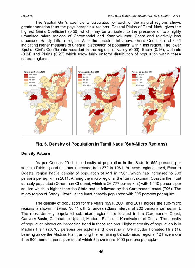
46
Lazar A. The Indian Geographical Journal, 89 (1) June – 2014
The Spatial Gini’s coefficients calculated for each of the natural regions shows greater variation than the physiographical regions. Coastal Plains of Tamil Nadu gives the highest Gini’s Coefficient (0.56) which may be attributed to the presence of two highly urbanised micro regions of Coromandel and Kanniyakumari Coast and relatively less urbanised Sandy Littoral region. Also the forested hills have Gini’s Coefficient of 0.41 indicating higher measure of unequal distribution of population within this region. The lower Spatial Gini’s Coefficients recorded in the regions of valley (0.09), Basin (0.16), Uplands (0.24) and Plains (0.27) which show fairly uniform distribution of population within these natural regions.
Fig. 6. Density of Population in Tamil Nadu (Sub-Micro Regions)
Density Pattern
As per Census 2011, the density of population in the State is 555 persons per
sq.km. (Table 1) and this has increased from 372 in 1981. At meso regional level, Eastern
Coastal region had a density of population of 411 in 1981, which has increased to 608
persons per sq. km in 2011. Among the micro regions, the Kanniyakumari Coast is the most
densely populated (Other than Chennai, which is 26,777 per sq.km.) with 1,110 persons per
sq. km which is higher than the State and is followed by the Coromandel coast (706). The
micro region of Sandy Littoral is the least densely populated with 395 persons per sq.km.
The density of population for the years 1991, 2001 and 2011 across the sub-micro
regions is shown in (Map. No.4) with 5 ranges (Class Interval of 200 persons per sq.km.).
The most densely populated sub-micro regions are located in the Coromandel Coast,
Cauvery Basin, Coimbatore Upland, Madurai Plain and Kanniyakumari Coast. The density
of population shows an increasing trend in these regions. Highest density of population is in
Madras Plain (26,705 persons per sq.km) and lowest is in Srivilliputtur Forested Hills (1).
Leaving aside the Madras Plain, among the remaining 82 sub-micro regions, 12 have more
than 800 persons per sq.km out of which 5 have more 1000 persons per sq.km.
Persons per Sq. Km, 1991
801 & Above
601 - 800
401 - 600
201 - 400
200 & Below
Persons per Sq. Km, 2001
801 & Above
601 - 800
401 - 600
201 - 400
200 & Below
Persons per Sq. Km, 2011
801 & Above
601 - 800
401 - 600
201 - 400
200 & Below
47
Lazar A. The Indian Geographical Journal, 89 (1) June – 2014
Conclusions
As proposed, the Census data at physiographic regional level have been compiled
using GIS application by utilising the spatial data of Physiographic regional boundaries and
locations of Villages / Towns. The compiled census data for each of the regions at different
levels have been analysed for exploring the distribution pattern and inequality.
It is found that the State of Tamil Nadu have 0.38 Spatial Gini’s Coefficient which is
fairly distributed across the two meso regions within the State but at micro regional level we
could see inequality of population distribution. The Eastern flanks of Sahyadri have the
highest Spatial Gini’s Coefficient value of 0.46. The derived Spatial Gini’s Coefficient of the
six Natural regions gives higher regional variations in population distribution. The most
unequal distribution of population could be seen in the coastal Plains (0.56) and the least
unequal distribution in valleys (0.09).
For better understanding of the relationships between population distribution and
physiographic regions discussed in this paper, a detailed analysis using more number of
demographic, socio-cultural and economic variables is needed. Some of the Sub-micro
regions along the coast and important transport corridor may offer economic and strategic
advantages which could be the driving force for the unequal distribution of population. By
extending this type of quantitative analysis to more socio-economic variables we may be
able to have a better understanding of the influences on population distributions.
References
1. Census of India (1981, 1991). Regional divisions of India - A cartographic analysis,
Office of the Registrar General & Census Commissioner India, New Delhi.
2. Census of India (2001, 2011). Primary Census Abstracts, Office of the Registrar
General and Census Commissioner India, New Delhi.
3. Small C. and Cohen J. E. (2004). Continental physiography, climate and the global
distribution of human population, Current Anthropology, 45(2).
4. Farris F.A. (2010). The Gini’s index and measures of inequality, The Mathematical
Association of America, p. 117.
5. Yu Song (2010). The application of Spatial Lorenz Curve (SLC) and Gini’s coefficient in
measuring land use structure change, International conference on geoinformatics,
2010, Xiamen.
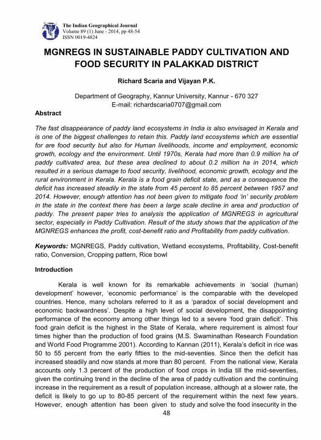
The Indian Geographical Journal
Volume 89 (1) June - 2014, pp 48-54 ISSN 0019-4824
48
MGNREGS IN SUSTAINABLE PADDY CULTIVATION AND
FOOD SECURITY IN PALAKKAD DISTRICT
Richard Scaria and Vijayan P.K.
Department of Geography, Kannur University, Kannur - 670 327
E-mail: [email protected]
Abstract
The fast disappearance of paddy land ecosystems in India is also envisaged in Kerala and
is one of the biggest challenges to retain this. Paddy land ecosystems which are essential
for are food security but also for Human livelihoods, income and employment, economic
growth, ecology and the environment. Until 1970s, Kerala had more than 0.9 million ha of
paddy cultivated area, but these area declined to about 0.2 million ha in 2014, which
resulted in a serious damage to food security, livelihood, economic growth, ecology and the
rural environment in Kerala. Kerala is a food grain deficit state, and as a consequence the
deficit has increased steadily in the state from 45 percent to 85 percent between 1957 and
2014. However, enough attention has not been given to mitigate food ‘in’ security problem
in the state in the context there has been a large scale decline in area and production of
paddy. The present paper tries to analysis the application of MGNREGS in agricultural
sector, especially in Paddy Cultivation. Result of the study shows that the application of the
MGNREGS enhances the profit, cost-benefit ratio and Profitability from paddy cultivation.
Keywords: MGNREGS, Paddy cultivation, Wetland ecosystems, Profitability, Cost-benefit
ratio, Conversion, Cropping pattern, Rice bowl
Introduction
Kerala is well known for its remarkable achievements in ‘social (human)
development’ however, ‘economic performance’ is the comparable with the developed
countries. Hence, many scholars referred to it as a ‘paradox of social development and
economic backwardness’. Despite a high level of social development, the disappointing
performance of the economy among other things led to a severe ‘food grain deficit’. This
food grain deficit is the highest in the State of Kerala, where requirement is almost four
times higher than the production of food grains (M.S. Swaminathan Research Foundation
and World Food Programme 2001). According to Kannan (2011), Kerala’s deficit in rice was
50 to 55 percent from the early fifties to the mid-seventies. Since then the deficit has
increased steadily and now stands at more than 80 percent. From the national view, Kerala
accounts only 1.3 percent of the production of food crops in India till the mid-seventies,
given the continuing trend in the decline of the area of paddy cultivation and the continuing
increase in the requirement as a result of population increase, although at a slower rate, the
deficit is likely to go up to 80-85 percent of the requirement within the next few years.
However, enough attention has been given to study and solve the food insecurity in the

49
Richard Scaria and Vijayan P.K. The Indian Geographical Journal, 89 (1) June – 2014
state. The researcher has suggested the MGNREGS expand intervention in paddy
cultivation for reducing the labour costs of production, as labour cost is the main component
in the production of paddy and gaining profits from paddy cultivation to synthesis, the
present study attempts link to MGNREGS in paddy cultivation the application expand and
its impact in the food crop sector for transforming a country into a state of food surplus.
Study Area
Palakkad District has a total geographical area of 4,480 sq. km, which represents
11.55 percent of the state total geographical area. It extends between 100
24’ North to 11
0
14’ North latitudes and 76
0 20
’ East to 76
0 54
’ East longitudes and it is surrounded by
Malappuram District on the North and Northwest, Thrissur on the South and Coimbatore
District on the East. It is situated almost at the centre of the State, spreading over the
midland plains and mountainous highlands. Palakkad is one of the four districts that do not
have a coast line (Figure 1).
Palakkad, one of the interior districts of Kerala, is unique in many respects. The
majestic Western Ghats, which stretches over 1,000 km, break the continuity of the
Palakkad Gap with a width of 40 km. On either side of the gap are the giant Nilgiri Hills and
Anamalai Hills. The Palakkad Gap acts as a corridor between Kerala and Tamil Nadu which
plays a stellar role in trade contacts between the East and West coasts of the Peninsular
India. Palakkad District has extensive paddy fields and is suitably known as the granary of
Kerala and is a vast expanse of luxuriant plains interrupted with hills, rivers, mountains,
streams and forests (Figure 2). The key objective of the study is to develop a model of
MGNREGS intervention for paddy land sustainability.
Fig. 2. Landuse Fig. 1. Location of Palakkad
District
50
Richard Scaria and Vijayan P.K. The Indian Geographical Journal, 89 (1) June – 2014
Results and Discussion
Kerala has a long history of being a food grain deficit state. Coastal Travancore has
passed through a food famine due to unemployment and high prices in 1941 and 1942 and
the food shortage gave high prices in the whole State in 1943 and the first quarter of 1944.
During these years the quantity of rice consumption was at the rate of 350 grams to 450
grams per day of rice per capita per annum for an adult population of 55 lakhs (treating one
fourth of the population as non-adults) which was 6 lakh tonnes. The annual production of
rice was estimated to 2.4 lakh tonnes. The net deficit in rice was thus 3.6 lakh tonnes in
Travancore. For Cochin, it was 90,000 tonnes during the period 1944-1945 (Sivaswamy et
al., 1945). Since then deficit in rice has increased steadily from 45 percent to 85 percent
between 1957 and 2007 in Kerala. In 1956 the state of Kerala was an acute food deficit
region with 7.59 lakh hectares of land under food crops. However, per capita availability of
rice was only 182 grams against the minimum requirement of 330 gms. In fact, the area
under food crops increased to 10.8 lakh hectares and per capita rice availability increased
to 213 grams between 1956-57 and 1980-81. The production has increased from 8.83 to
12.9 lakh tonnes and productivity increased from 1,164 to 1,638 kgs per ha during this
period. Since then, rice production has declined significantly in Kerala (Chib, 1988).
During the past two decades, Kerala has witnessed a decline in food grains
production at an annual rate of 1.09 percent. Area under food grains fell from 960,000
hectares in 1970 –1971 to 560,000 hectares in 1990-91. The share of cultivators to total
work force declined from 17.8 to 12.24 between 1970-71 and 1990-91. In the country as a
whole the area under food grains has declined marginally during the nineties but the output
increased by around 15 percent. Kerala experienced a different trend, area under food
grains declined 37 percent and the output by 33 percent (GOK, 1990).
Rice deficit in Kerala has increased significantly between 1991-1992 and 2013-
2014. Kerala’s rice deficit of around 70 percent in 1991-1992 and then it increased
significantly upto 85 percent in 2013-2014. This shows that, Kerala has produced just one
third of its requirements in 1991-1992 and less than one-fifth in 2013-2014. The availability
of rice in Kerala is 10.6 lakh MT in 1991-1992 and then it decreased very sharply up to 3.28
lakh MT in 2013-2014. It gives an insight that the availability of rice in Kerala declined more
than 50 percent during this period (GOK, 2013). There is a huge gap between the
availability and requirements of rice in Kerala. More importantly, the gap between the
availability and requirements of rice has increased for the last five decades in the state of
Kerala especially, since 1991. Paradoxically, Kerala has also been experiencing an
unprecedented consumption boom, especially in food items and increasing standards of
living of the Keralites as a result of the remittances from the gulf countries. Despite its
remarkable and somewhat unique development experience, Kerala is said to be passing
through a severe food grain crisis, especially in rice. In fact, there are number of reasons
behind it. The most important among them are as follows: i) shift in the cropping system
from food crops to non-food crops; ii) labour cost in the paddy cultivation is very high in
Kerala, as compared to other states in India- among other things led to a severe crisis in
the production of food crops in the state.
51
Richard Scaria and Vijayan P.K. The Indian Geographical Journal, 89 (1) June – 2014
MGNREGS Intervention for Sustainable Paddy Cultivation
In reviewing the voluminous and controversial literature on the problem of food and
hunger, six dominant lines of thought can be identified namely, neo-malthusianism,
technological determinism, monetarism, structuralism, over consumption and poverty. A
review of the arguments introduced by each of these theses reveals the many interrelated
facets that this complex crisis assumes as well as the ideological underpinnings of
alternative interpretations. However, all these theories are trying to identify reason of the
food crisis. None of these theories are trying to solve the present crisis. In view of this, the
research feeds the need to develop a new theoretical model to solve the food crisis in the
state. In order to achieve this researcher is the opinion that to apply the MGNREGA in the
Paddy cultivation in Palakkad District where food crisis is too severe, as compared other
places in India. Hence, the present theoretical attempts is to show the application of the
MGNREGA in the food-crop sector and its impact on demand for labour, production of food
crops and profitability of farmers in the state of Kerala State as well as Palakkad District.
As the main problem faced by rice cultivators is the availability of labour and the
labour cost, which cannot be reduced and the working hours cannot be increased as, paddy
cultivation is labour intensive. As mechanisation are not always possible in Kerala because
of its undulated topography. A sincere and low cost approach should be made applicable.
The survey conducted at the sample locations for the study has revealed that there is need
for about 100 to 110 days of labour for paddy cultivation. As there is a labour, the
MGNREGS can be wisely turned to the work of the paddy fields based on their knowledge
and experience. In this way, the Government interventions can tackle this serious problem
judiciously in the following way (Figure 3).
Competitiveness is highly correlated with cost of production. Thus, the
competitiveness of farmers will increase, if the total cost of production declines. While
analysing the competitiveness of farmers in Kerala, it was observed that their
competitiveness was very low due to high cost of production, especially because of the
reason that the labour cost was high. This is because of the reason that the wage of the
skilled and unskilled agricultural reported for male and female labourers are very high in the
state. Hence, labour cost of production accounts to 60 percent to 78 percent of the total
cost of paddy cultivation in Kerala. This would have an adverse impact on the production
cost. In order to avoid the high labour cost of production in paddy, there is a need for an
intervention, which can be accomplished through MGNREGS towards paddy cultivation in
the case of marginal and small paddy cultivators in Kerala. Thus, the labour cost of paddy
production among rice farmers could be reduced relatively, to a large extent. As a result,
the competitiveness can be increased among the paddy farmers. The net return from the
marginal and small paddy farmers can be increased, resulting in increased paddy
cultivation, net income, biodiversity, employment, and decrease in rural poverty and
backwardness.
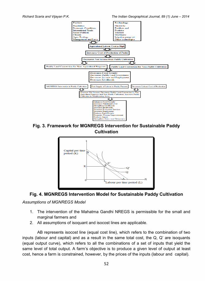
52
Richard Scaria and Vijayan P.K. The Indian Geographical Journal, 89 (1) June – 2014
Fig. 3. Framework for MGNREGS Intervention for Sustainable Paddy
Cultivation
Fig. 4. MGNREGS Intervention Model for Sustainable Paddy Cultivation
Assumptions of MGNREGS Model
1. The intervention of the Mahatma Gandhi NREGS is permissible for the small and
marginal farmers and
2. All assumptions of isoquant and isocost lines are applicable.
AB represents isocost line (equal cost line), which refers to the combination of two
inputs (labour and capital) and as a result in the same total cost, the Q, Q’ are isoquants
(equal output curve), which refers to all the combinations of a set of inputs that yield the
same level of total output. A farm’s objective is to produce a given level of output at least
cost, hence a farm is constrained, however, by the prices of the inputs (labour and capital).
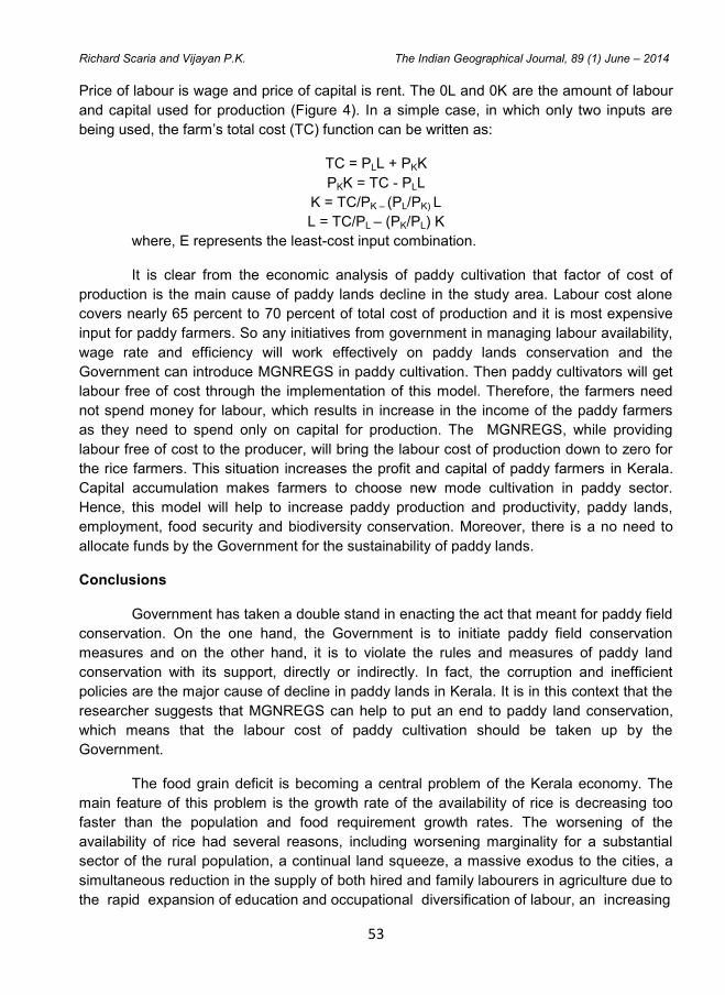
53
Richard Scaria and Vijayan P.K. The Indian Geographical Journal, 89 (1) June – 2014
Price of labour is wage and price of capital is rent. The 0L and 0K are the amount of labour
and capital used for production (Figure 4). In a simple case, in which only two inputs are
being used, the farm’s total cost (TC) function can be written as:
TC = PLL + PKK
PKK = TC - PLL
K = TC/PK – (PL/PK) L
L = TC/PL – (PK/PL) K
where, E represents the least-cost input combination.
It is clear from the economic analysis of paddy cultivation that factor of cost of
production is the main cause of paddy lands decline in the study area. Labour cost alone
covers nearly 65 percent to 70 percent of total cost of production and it is most expensive
input for paddy farmers. So any initiatives from government in managing labour availability,
wage rate and efficiency will work effectively on paddy lands conservation and the
Government can introduce MGNREGS in paddy cultivation. Then paddy cultivators will get
labour free of cost through the implementation of this model. Therefore, the farmers need
not spend money for labour, which results in increase in the income of the paddy farmers
as they need to spend only on capital for production. The MGNREGS, while providing
labour free of cost to the producer, will bring the labour cost of production down to zero for
the rice farmers. This situation increases the profit and capital of paddy farmers in Kerala.
Capital accumulation makes farmers to choose new mode cultivation in paddy sector.
Hence, this model will help to increase paddy production and productivity, paddy lands,
employment, food security and biodiversity conservation. Moreover, there is a no need to
allocate funds by the Government for the sustainability of paddy lands.
Conclusions
Government has taken a double stand in enacting the act that meant for paddy field
conservation. On the one hand, the Government is to initiate paddy field conservation
measures and on the other hand, it is to violate the rules and measures of paddy land
conservation with its support, directly or indirectly. In fact, the corruption and inefficient
policies are the major cause of decline in paddy lands in Kerala. It is in this context that the
researcher suggests that MGNREGS can help to put an end to paddy land conservation,
which means that the labour cost of paddy cultivation should be taken up by the
Government.
The food grain deficit is becoming a central problem of the Kerala economy. The
main feature of this problem is the growth rate of the availability of rice is decreasing too
faster than the population and food requirement growth rates. The worsening of the
availability of rice had several reasons, including worsening marginality for a substantial
sector of the rural population, a continual land squeeze, a massive exodus to the cities, a
simultaneous reduction in the supply of both hired and family labourers in agriculture due to
the rapid expansion of education and occupational diversification of labour, an increasing
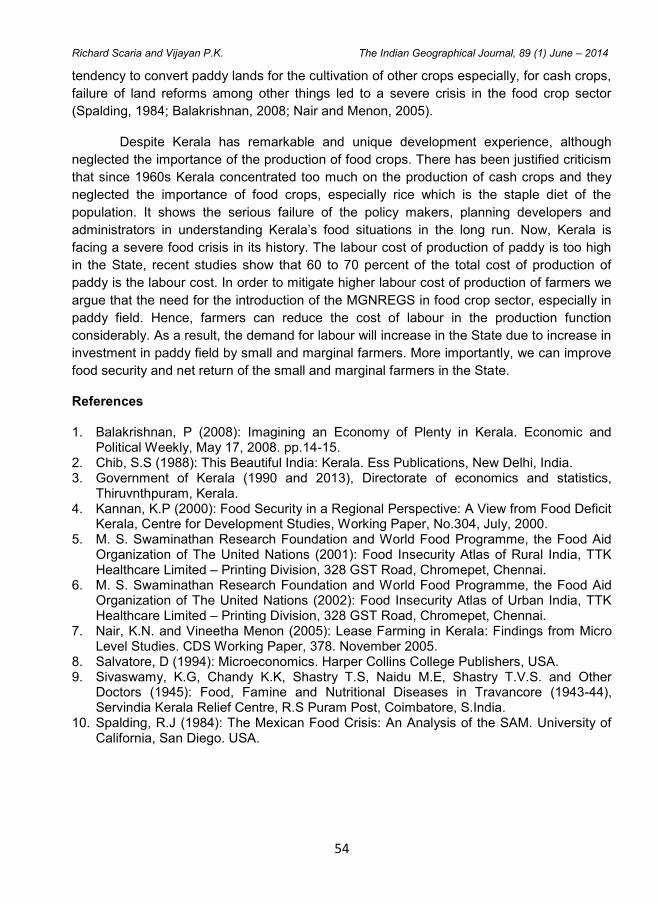
54
Richard Scaria and Vijayan P.K. The Indian Geographical Journal, 89 (1) June – 2014
tendency to convert paddy lands for the cultivation of other crops especially, for cash crops,
failure of land reforms among other things led to a severe crisis in the food crop sector
(Spalding, 1984; Balakrishnan, 2008; Nair and Menon, 2005).
Despite Kerala has remarkable and unique development experience, although
neglected the importance of the production of food crops. There has been justified criticism
that since 1960s Kerala concentrated too much on the production of cash crops and they
neglected the importance of food crops, especially rice which is the staple diet of the
population. It shows the serious failure of the policy makers, planning developers and
administrators in understanding Kerala’s food situations in the long run. Now, Kerala is
facing a severe food crisis in its history. The labour cost of production of paddy is too high
in the State, recent studies show that 60 to 70 percent of the total cost of production of
paddy is the labour cost. In order to mitigate higher labour cost of production of farmers we
argue that the need for the introduction of the MGNREGS in food crop sector, especially in
paddy field. Hence, farmers can reduce the cost of labour in the production function
considerably. As a result, the demand for labour will increase in the State due to increase in
investment in paddy field by small and marginal farmers. More importantly, we can improve
food security and net return of the small and marginal farmers in the State.
References
1. Balakrishnan, P (2008): Imagining an Economy of Plenty in Kerala. Economic and Political Weekly, May 17, 2008. pp.14-15.
2. Chib, S.S (1988): This Beautiful India: Kerala. Ess Publications, New Delhi, India. 3. Government of Kerala (1990 and 2013), Directorate of economics and statistics,
Thiruvnthpuram, Kerala. 4. Kannan, K.P (2000): Food Security in a Regional Perspective: A View from Food Deficit
Kerala, Centre for Development Studies, Working Paper, No.304, July, 2000. 5. M. S. Swaminathan Research Foundation and World Food Programme, the Food Aid
Organization of The United Nations (2001): Food Insecurity Atlas of Rural India, TTK Healthcare Limited – Printing Division, 328 GST Road, Chromepet, Chennai.
6. M. S. Swaminathan Research Foundation and World Food Programme, the Food Aid Organization of The United Nations (2002): Food Insecurity Atlas of Urban India, TTK Healthcare Limited – Printing Division, 328 GST Road, Chromepet, Chennai.
7. Nair, K.N. and Vineetha Menon (2005): Lease Farming in Kerala: Findings from Micro Level Studies. CDS Working Paper, 378. November 2005.
8. Salvatore, D (1994): Microeconomics. Harper Collins College Publishers, USA. 9. Sivaswamy, K.G, Chandy K.K, Shastry T.S, Naidu M.E, Shastry T.V.S. and Other
Doctors (1945): Food, Famine and Nutritional Diseases in Travancore (1943-44), Servindia Kerala Relief Centre, R.S Puram Post, Coimbatore, S.India.
10. Spalding, R.J (1984): The Mexican Food Crisis: An Analysis of the SAM. University of California, San Diego. USA.
The Indian Geographical Journal
Volume 89 (1) June - 2014, pp 55-63 ISSN 0019-4824
55
SLUM SEX RATIO IN METROPOLITAN CITIES OF INDIA - AN OVERVIEW
Satinder Kaur1, Gurinder Kaur
2 and Ramandeep Singh
1
1Department of Geography, S.R. Govt. College for Women, Amritsar - 143 001
2Department of Geography, Punjabi University, Patiala - 147 002 E-mail: [email protected]; [email protected]
Abstract
Sex ratio is an important demographic parameter, which defines as number of females per 1,000 males. It is also an important index of socio-economic conditions of an area and also a composite indicator of women’s status in the society. The objective of the present paper is to study the spatial patterns of slum sex ratio and to find out the reasons behind spatial variation in metropolitan cities of India. It is also an endeavor to compare slum sex ratio with that of urban sex ratio and to study the trends in slum sex ratio during 2001 and 2011. Results reveal that slums and urban areas have identical sex ratio at national level and with little variations at city level. It depicts that the male child ‘obsession’ is prevalent in both cases.
Keywords: Sex ratio, Sex composition, Slum, Metropolitan city, Female foeticide
Introduction
The sex ratio is one of the important demographic parameters, which indicates the
balance between females and males in the society. It is an important index of the socio-
economic conditions of an area and also a composite indicator of women’s status in the
society (Kaur, 2011). The study of proportion of the two sexes is fundamental to the
geographic analysis of an area as it manipulates the other demographic elements and
provides an additional means for analysing the regional landscape. Sex ratio is used as a
tool for cross sectional analysis to measure gender balance. The Census of India defines
the sex ratio as number of females per 1,000 males in the population, whereas sex ratio in
many western countries such as United States of America is defined as number of males
per 100 females (Chandna, 2012). Comparing India’s sex ratio with other developing and
developed countries of the world, it’s observed that India is one of the few countries in the
world where there are more males than females as per Census of India 2011. The
neighboring countries of Nepal (1,014 females), Pakistan (943 females), Sri Lanka (1,034
females) and Myanmar (1,048 females) are having higher sex ratio than India (Kaur, 2011).
One study found that sex-selective abortion is less available and acceptable in Pakistan
and Bangladesh (Hesketh and Xing, 2006).
India supports a heterogeneous society consisting of numerous stratifications
based on religion, caste and class; however, unfortunately gender discrimination is
practiced in all classes and castes. All religious groups in the country preach equality of
males and females yet preference for sons is high amongst all religious groups and social

56
Satinder Kaur et al. The Indian Geographical Journal, 89 (1) June – 2014
classes (Aggarwal, 2005). Historical evidences show that the gender bias, deep-rooted
prejudice and discrimination against girl child have been prevailing in the Indian society
from the centuries. But the concern for same has grown recently as now even the fetus of a
girl child has started facing the peril of pre-birth elimination i.e. female foeticide. As per
World Bank estimation, over the last two decades, each year, around 2.5 lakh girls were
killed in India (Pal, 2014). In the beginning of 20th century, the average sex ratio in the
country was 972 and decreased to 940 in 2011. Female selective abortions in the country
rose from 0 to 2.0 million in the 1980s to 1.2 to 4.1 million in the 1990s and further 3.1 to
6.0 in the 2000s (Jha et.al, 2011). Son preference is the foremost reason for female deficit
which seems to be a part of Indian culture. The objective of the present paper is to study
the spatial patterns of slum sex ratio in metropolitan cities of India.
Study Area
Republic of India is the seventh-largest country of the world by area (32, 87,613 sq.
km, 2.4 percent of the total area of the world) and the second-most populous country of the
world next to China with over 1.2 billion people. Metropolitan cities of the country act as
focal points on the cultural landscape of India. Presently, there are 46 metropolitan cities in
the country as per Census of India 2011. Varanasi and Patna in the North and Madurai in
the South are the oldest existing cities in India which originated around 500 BC, are
symbolic of India’s long urban heritage originated during the medieval period (Kumar,
2014). Kolkata Mumbai and Chennai had emerged as major port cities and became
metropolitan cities in 1901, 1911 and 1951 respectively. Delhi also emerged as an
administrative centre and got metropolitan status in 1951. In the British period, introduction
of the railways and modern industry led to the creation of new Industrial township such as
Kanpur, Dhanbad, Asansol and Jamshedpur. The post-Independence period saw the influx
of refugees in settlements like Faridabad, Amritsar and Ludhiana and consequently
population increased in these cities and they emerged as important metropolitan cities of
north. The origin of metropolitan cities viz. Dhanbad, Jabalpur, Jamshedpur, Raipur, Durg-
Bhilainagar was the outcome of industrialisation.
Database and Methodology
An attempt has also made to compare slum sex ratio with that of urban sex ratio
and to study the trends in slum sex ratio during 2001 and 2011. For the present study,
secondary data is collected from Census of India, Primary Census Abstract for slums for
2001 and 2011.
Results and Discussion
Indian Status of Slum Sex Ratio
In 2011, average slum sex ratio and urban sex ratio is recorded as 928 and 929
respectively in India. However, it varies from one state / union territory to another. Like
general sex ratio, South Indian States are marked with a relatively favorable slum sex ratio

57
Satinder Kaur et al. The Indian Geographical Journal, 89 (1) June – 2014
in comparison to north and Northwestern States. Kerala in south India has recorded the
highest slum sex ratio while union territory of Chandigarh recorded the lowest slum sex
ratio among both cases. Average sex ratio of slums and urban India is recorded almost
equal at national level (Census of India, 2011).
Slum Sex Ratio in Major Metropolitan Cities of India
Unlike western countries, there is paucity of females in urban India (Krishan and
Chandna, 1973). The Table 1 shows that an average slum sex ratio in the country is
recorded as 928. However, it varies from one metropolitan city to another. Among
metropolitan cities, Chennai and Coimbatore recorded the highest slum sex ratio (1,003)
while Surat city recorded the lowest slum sex ratio (698). It further shows that number of
females exceeded the number of males in four metropolitan cities namely Chennai,
Coimbatore, Madurai and Vijayawada. Out of 46 metropolitan cities, 15 cities are having
slum sex ratio above national average and rest of the cities recorded slum sex ratio below
national average (928).
Furthermore, Table 1 and Chart 1 represents comparison between urban sex ratio
and slum sex ratio. Average urban sex ratio is (929) marginally higher than slum sex ratio
(928). The highest urban sex ratio (999) is recorded in Madurai metropolitan in Tamil Nadu
State while the highest slum sex ratio (1,003) is shared by 2 metropolitan cities i.e. Chennai
and Coimbatore also located in Tamil Nadu. The lowest slum sex ratio (698) is recorded in
the city of Surat (Gujarat) which is 56 points lesser than it’s urban sex ratio (754).
Hyderabad and Ahmadabad have identical sex ratio of 955 and 898 respectively in both
cases. In Bhopal and Dhanbad, urban sex ratio is recorded only one point higher than their
slum sex ratio.
There are four metropolitan cities i.e. Coimbatore, Chennai, Madurai and
Vijayawada where slum sex ratio is in favour of females i.e. more than 1,000. On the other
hand, urban sex ratio is found low in all the metropolitan cities of the country. In 21 cities,
slum sex ratio is found adverse i.e. less than 900 while in urban areas, there are 20 such
cities with adverse sex ratio. Among 46 metropolitan cities, 23 cities recoded relatively
higher slum sex ratio in comparison to urban sex ratio while 21 metropolitan cities recorded
higher urban sex ratio than that of slum sex ratio. Thus, there is not found huge difference
between slum sex ratio and urban sex ratio.
Spatial pattern of Slum Sex Ratio in Metropolitan Cities of the Country
The Figure 1 shows the spatial pattern of slum sex ratio in metropolitan cities of the
country. Three categories are represented on the map:
(a) Metropolitan cities with relatively high slum sex ratio (950 and above)
(b) Metropolitan cities with moderate slum sex ratio (900 to 949)
(c) Metropolitan cities with Relatively Low Slum Sex Ratio (900 and below)

58
Satinder Kaur et al. The Indian Geographical Journal, 89 (1) June – 2014
Chart 1. Urban and Slum Sex Ratio in Metropolitan Cities of India, 2011
(a) Metropolitan Cities with Relatively High Slum Sex Ratio (950 and above)
The Figure 1 and Table 2 shows that among 46 metropolitan cities of the country,
12 cities are recorded relatively high slum sex ratio. All the metropolitan cities with relatively
high slum sex ratio are found in South India with the exception of Srinagar, Ranchi and
Raipur. All the metropolises falling in the States of Andhra Pradesh and Tamil Nadu viz.
Vijayawada, Vishakhapatnam, Hyderabad, Coimbatore, Chennai and Madurai are recorded
relatively high slum sex ratio. Other metropolitan cities with high slum sex ratio include
Bengaluru in Karnataka, Nagpur, Pune in Maharashtra, Raipur in Chhattisgarh, Srinagar in
Jammu and Kashmir and Ranchi in Jharkhand.
Figure 1. Slum Sex Ratio in Metropolitan Cities (2011) (Source: Primary Census Abstract for Slums, Census of India, 2011)
59
Satinder Kaur et al. The Indian Geographical Journal, 89 (1) June – 2014
High slum sex ratio in all of these cities is positively associated to their high female
work participation rate (except Srinagar and Vishakhapatnam), high female literacy rate
(Census of India, 2011) and sizable proportion of scheduled caste and schedule tribe
population (as in the case of Ranchi, Raipur and Vishakhapatnam) (Kumar, 2014).
Furthermore, family migration to cities also positively impact sex ratio. Woodruff (1960)
observed that postwar industrial boom in Bangalore has attracted in-migration from different
States of the country in search of employment. Migration stream arrived in the form of
family-migration instead of male-selective migration (Krishna, 2013). Thus, high status of
women in the society and high female education in slum areas of Coimbatore and Chennai
can be attributed to high slum sex ratio as an educated woman is likely to be less
dependent on their sons as a source of social status and old-age security and this reduces
preference of boy and resists male pressure to discriminate in favour of boys (Murthi et.al.,
1995).
(b) Metropolitan Cities with Moderate Slum Sex Ratio (901-949)
Out of 46 metropolitan cities, 13 cities of the country namely Aurangabad, Jabalpur,
Nasik, Jodhpur, Indore, Lucknow, Bhopal, Pimpri-Chinchwad, Vadodara, Jaipur, Patna,
Kolkata, Kota are recorded moderate slum sex ratio (Table 2). The major reasons of
moderate slum sex ratio in these cities are preference for son over daughter, neglect of girl
child and dowry demand, raising crime rate against girls, male-selective migration
(Srivastava et.al. 2005 and Datta, 2011).
(c) Metropolitan Cities with Relatively Low Sex Ratio (900 and below)
Rest of 23 metropolitan cities of the country recorded relatively low slum sex ratio.
Most of the metropolitan cities with low slum sex ratio are located in North and
Northwestern parts of the country and forms the part of Gangetic plains and are hubs of
economic and industrial activities in their respective states and predominance of male
selective migration therein which adversely impact the slum sex ratio (Das and Murmu,
2010). In-migration is the main components of the growth of urban population of Delhi
(Singh, 2009). The lower sex ratio in NCT Delhi may be attributed to large scale male
selective in-migration. Delhi received 1.7 million migrants in 2001, mainly from Uttar
Pradesh, Bihar and Haryana.
Slums are the most convenient places for their settlement. Sex ratio of net migrants
in Delhi was only 673 in 2001 (Census of India, 2001). Similarly, large scale male selective
migration resulted in skewed sex ratio in favour of males in metropolitan cities which
traditionally attract migrant as workers such as Mumbai, Thane and Pune (Barakade,
2012). The volume of male and female migrants is highest for Mumbai urban agglomeration
in comparison to other mega cities. But the percent of female migrants for Mumbai urban
agglomeration decreased in 2001 that may result in lowering of slum sex ratio in the city
(Census of India, 2001 and Das and Murmu, 2010).
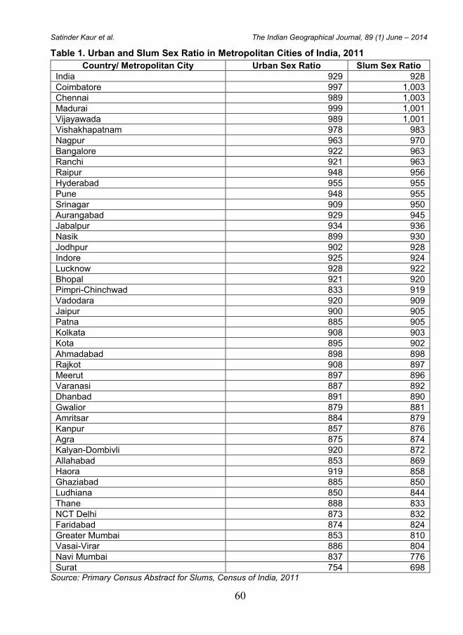
60
Satinder Kaur et al. The Indian Geographical Journal, 89 (1) June – 2014
Table 1. Urban and Slum Sex Ratio in Metropolitan Cities of India, 2011
Country/ Metropolitan City Urban Sex Ratio Slum Sex Ratio
India 929 928
Coimbatore 997 1,003
Chennai 989 1,003
Madurai 999 1,001
Vijayawada 989 1,001
Vishakhapatnam 978 983
Nagpur 963 970
Bangalore 922 963
Ranchi 921 963
Raipur 948 956
Hyderabad 955 955
Pune 948 955
Srinagar 909 950
Aurangabad 929 945
Jabalpur 934 936
Nasik 899 930
Jodhpur 902 928
Indore 925 924
Lucknow 928 922
Bhopal 921 920
Pimpri-Chinchwad 833 919
Vadodara 920 909
Jaipur 900 905
Patna 885 905
Kolkata 908 903
Kota 895 902
Ahmadabad 898 898
Rajkot 908 897
Meerut 897 896
Varanasi 887 892
Dhanbad 891 890
Gwalior 879 881
Amritsar 884 879
Kanpur 857 876
Agra 875 874
Kalyan-Dombivli 920 872
Allahabad 853 869
Haora 919 858
Ghaziabad 885 850
Ludhiana 850 844
Thane 888 833
NCT Delhi 873 832
Faridabad 874 824
Greater Mumbai 853 810
Vasai-Virar 886 804
Navi Mumbai 837 776
Surat 754 698 Source: Primary Census Abstract for Slums, Census of India, 2011
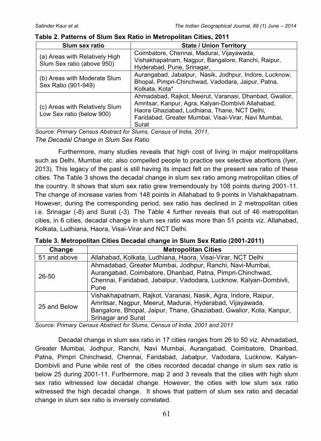
61
Satinder Kaur et al. The Indian Geographical Journal, 89 (1) June – 2014
Table 2. Patterns of Slum Sex Ratio in Metropolitan Cities, 2011
Slum sex ratio State / Union Territory
(a) Areas with Relatively High Slum Sex ratio (above 950)
Coimbatore, Chennai, Madurai, Vijayawada, Vishakhapatnam, Nagpur, Bangalore, Ranchi, Raipur, Hyderabad, Pune, Srinagar,
(b) Areas with Moderate Slum Sex Ratio (901-949)
Aurangabad, Jabalpur, Nasik, Jodhpur, Indore, Lucknow, Bhopal, Pimpri-Chinchwad, Vadodara, Jaipur, Patna, Kolkata, Kota*
(c) Areas with Relatively Slum Low Sex ratio (below 900)
Ahmadabad, Rajkot, Meerut, Varanasi, Dhanbad, Gwalior, Amritsar, Kanpur, Agra, Kalyan-Dombivli Allahabad, Haora Ghaziabad, Ludhiana, Thane, NCT Delhi, Faridabad, Greater Mumbai, Visai-Virar, Navi Mumbai, Surat
Source: Primary Census Abstract for Slums, Census of India, 2011,
The Decadal Change in Slum Sex Ratio
Furthermore, many studies reveals that high cost of living in major metropolitans
such as Delhi, Mumbai etc. also compelled people to practice sex selective abortions (Iyer,
2013). This legacy of the past is still having its impact felt on the present sex ratio of these
cities. The Table 3 shows the decadal change in slum sex ratio among metropolitan cities of
the country. It shows that slum sex ratio grew tremendously by 108 points during 2001-11.
The change of increase varies from 148 points in Allahabad to 9 points in Vishakhapatnam.
However, during the corresponding period, sex ratio has declined in 2 metropolitan cities
i.e. Srinagar (-8) and Surat (-3). The Table 4 further reveals that out of 46 metropolitan
cities, in 6 cities, decadal change in slum sex ratio was more than 51 points viz. Allahabad,
Kolkata, Ludhiana, Haora, Visai-Virar and NCT Delhi.
Table 3. Metropolitan Cities Decadal change in Slum Sex Ratio (2001-2011)
Change Metropolitan Cities
51 and above Allahabad, Kolkata, Ludhiana, Haora, Visai-Virar, NCT Delhi
26-50
Ahmadabad, Greater Mumbai, Jodhpur, Ranchi, Navi-Mumbai, Aurangabad, Coimbatore, Dhanbad, Patna, Pimpri-Chinchwad, Chennai, Faridabad, Jabalpur, Vadodara, Lucknow, Kalyan-Dombivli, Pune
25 and Below
Vishakhapatnam, Rajkot, Varanasi, Nasik, Agra, Indore, Raipur, Amritsar, Nagpur, Meerut, Madurai, Hyderabad, Vijayawada, Bangalore, Bhopal, Jaipur, Thane, Ghaziabad, Gwalior, Kota, Kanpur, Srinagar and Surat
Source: Primary Census Abstract for Slums, Census of India, 2001 and 2011
Decadal change in slum sex ratio in 17 cities ranges from 26 to 50 viz. Ahmadabad,
Greater Mumbai, Jodhpur, Ranchi, Navi Mumbai, Aurangabad, Coimbatore, Dhanbad,
Patna, Pimpri Chinchwad, Chennai, Faridabad, Jabalpur, Vadodara, Lucknow, Kalyan-
Dombivli and Pune while rest of the cities recorded decadal change in slum sex ratio is
below 25 during 2001-11. Furthermore, map 2 and 3 reveals that the cities with high slum
sex ratio witnessed low decadal change. However, the cities with low slum sex ratio
witnessed the high decadal change. It shows that pattern of slum sex ratio and decadal
change in slum sex ratio is inversely correlated.
62
Satinder Kaur et al. The Indian Geographical Journal, 89 (1) June – 2014
Conclusions
Sex ratio is an important social indicator to measure the extent of prevailing equity
between males and females in a society. The cultural differences also manifest themselves
in the form of lower or higher sex ratios in different cities. Women are valued more in South
and Northeastern parts of the country where they enjoy greater autonomy and higher social
status. In contrast, women are undervalued in Northern and Western regions of the country
that is evident in the sex ratio of their respective populations in different metropolitan cities
of the country. Economically better off north Indian metropolitan cities in the states of
Punjab, Haryana, Chandigarh, Delhi and Gujarat are declared the worst offenders. Despite
economic prosperity and the advances made in education, literacy, health care and income
in northern region, gender inequality still prevails and attitude towards women is alarmingly
‘biased’. A comparative picture of sex ratio in slums and urban areas reveals that slums and
urban areas have identical sex ratio at national level and with little variations at city level. It
depicts that the male child ‘obsession’ is similar in both cases.
Better economic status of North Indian metropolitan cites has adversely affected
sex ratio in this region while high literacy rate and better status of women has positively
affected sex ratio in the metropolitan cities located in southern part of the country.
Furthermore, the cities with high slum sex ratio witnessed low decadal change and vice
versa. Recently, government has taken several measures and is also making endeavors to
elevate the status of women in the society by promoting equality of men and women. To
reduce excessive son preference, North India needs to accept bilateral kinship systems.
More recently different schemes (such as cradle Scheme, Ladli and Balika Samridhi Yojna,
Apni Beti Apna Dhan, Shagan scheme and the newly proposed national scheme scheme
Beti Bachao Beti Padhao) are launched in the country to spread awareness among people
regarding female foeticide, women education and empowerment. The negative impact of
son preference has already started showing its impact in form of high proportions of
unmarried men in most affected areas. The lawmakers of the country, law enforcement
agencies, educators and administrators can play an important role to alter the old crumbling
value system through awareness campaigns and laws.
References
1. Agarwal, S. (2005). Discrimination against Girl Child in Rural Haryana, India: From Conception through Childhood. Paper for the Poster Presentation in the IUSSP 25 International Population Conference Tours, France, July 18-23.
2. Barakade, A.J. (2012). Declining Sex Ratio: An Analysis with Special Reference to Maharashtra State. Geo sciences Research, 3(1), 92-95.
3. Census of India (2001). Migration Tables, Data Highlights. Office of the Registrar General and Census Commissioner, India.
4. Census of India (2011). Primary Census Abstract for Slums, Office of the Registrar General and Census Commissioner, India
5. Chandna, R.C. (2012). Geography of Population, Concepts, Determinants, and Patterns. (pp. 284,314, 320). Kalyani Publisher.
6. Das, K. and Murmu, A. (2010). Female Migration to Mega Cities of India. Journal of history and Social Sciences, 1 (1), 9.
63
Satinder Kaur et al. The Indian Geographical Journal, 89 (1) June – 2014
7. Datta, R. (2011). Kolkata Sees Dip in Population, Suburbs Register an Increase. Livemint, April 5.
8. Hesketh, H. and Xing Z. W. (2006). Abnormal Sex Ratio in Human Population: Causes and Consequences. PNAS (Proceeding of the National Academy of Sciences of the United States of America), 103 (36), pp. 13273.
9. Iyer, M. (2013). Eight Wards Shame City with Skewed Sex Ratio at Birth. Forun Against Sex Selection (FASS) February 20.
10. Jha, P.; Kesler, M. A.; Kumar, R.; Ram, F.; Ram, U.; Aleksandrowicz, L.; Bassani, D. G.; Chandra, S. and Banthia, J. K. (2011). Trends in Selective Abortion of Female Foetuses in India: Analysis of Nationally Representative Birth Histories from 1990–2005 and Census Data from 1991–2011. The Lancet, 377 (9781), 1921-1928.
11. Kaur, G. (2011). Declining Child Sex Ratio in India and Its Implications. Population Geography, 33 (1 and 2), 1-13.
12. Krishan, G. and Chandna, R. C. (1973). Sex Composition in Haryana’s Districts. Geographical Review of India, 35 (2), 113.
13. Krishna, A. (2013). Stuck in Place: Investigating Social Mobility in 14 Bangalore Slums. The Journal of Development Studies. 49 (7), 1014.
14. Kumar, A. (2014). Urban Sex Ratio: A Study on Regional wise towns in erstwhile Andhra Pradesh, India. Global Journal for Research Analysis. July, 3 (7), 137.
15. Murthi, M.; Drèze, J. and Guio, A. C. (1995). Mortality, Fertility and Gender Bias in India: A District Level Analysis. Research Gate. DOI: 10.2307/2137773.
16. Pal, S. (2014). The Statistics of Gender Bias. The Hindu, March 25. 17. Singh, P. (2009). Sheltering Delhi’s Slums. Working Paper 230, Delhi Development
Report, 93-110. 18. Srivastava, A.; Dasgupta, P. and Rai, S. (2005). Attitude towards Girl Child and
Declining Sex Ratio in Bhopal, Bhopal Centre for Women’s Studies, 42. 19. Woodruff, G. (1960): Family Migration into Bangalore. The Economic Weekly, 12 (4-5-
6), 163.
The Indian Geographical Journal
Volume 89 (1) June - 2014, pp 64-75 ISSN 0019-4824
64
Archives - 1
IMPRESSIONS OF LAHORE SCIENCE CONGRESS, 1939
Formerly Known as The Journal of The Madras Geographical Association (Volume XIV, 1939, pp. 59-64)
By
N. SUBRAHMANYAM Editor, The Journal of The Madras Geographical Association
On January 2, 1939, the Science Week of the Indian Science Congress Association
was inaugurated at the University Buildings of Lahore by H. E. Sir Henry Craik, the
Governor of the Punjab. Dr. J. C. Ghosh of Dacca, the President of the year, delivered the
General Address, reviewing Science Progress in India. From the following day, the eleven
sectional presidents gave their addresses to their several sections.
Geography has been made into a separate section permanently from this year; and
Mr. N. Subrahmanyam, M.A., L.T., F.R .G .S., of Madras, this year's president, delivered his
address to a throng of delegates from all sections and from various Provinces. The subject
chosen was, “The Geographical Personality of India." The address met with warm
approbation all round, for matter, form, and style. „It is a comprehensive survey of India,'
said some, „It makes a new synthetic approach‟; „it is eloquent, brimming all over with
sympathy,‟ said some high authorities. „I never thought Geography can be so full of life and
interest,' said many a delegate, upon hearing it read.
This new section of Geography was able to attract as many as twenty papers on
various topics. Dr. Chatterjee of Calcutta led off with his Lecture on Ranchi, giving it, he
said, in the true French manner as a series of slides with explanations in between. His next
paper on Puri was similarly done. Mr. A. C. Bannerjee, also of Calcutta, read a paper on
„some of the markets of Calcutta.‟
Mr. B. M. Tirunaranan of Madras presented two papers; one was on certain
methods of anticipating Tank Breaches; the other, on the Boundaries of Tamil Nadu. He
made helpful contributions to the discussions, accompanying them often with drawings on
the blackboard drawn with remarkable ease and accuracy. He has a working belief in the
maxim, „no Maps, no Geography.‟ It may be stated, by the way, that from his study of
Lahore Map, he made himself, on the very first day, as familiar with the streets and lanes
and buildings as a long-time resident. And he has done so for other towns he visited on his
way to Lahore up and down.
The summaries of several papers of absentee-members were read; and others
were taken as read. These are a few titles of such papers: - The Sources of the
Brahmaputra; Sugar-cane cultivation in India; The growth of a modern city (Coimbatore);
65
The Fisheries of Cochin; Cole Cultivation in Cochin; Results of irrigational changes in
Tanjore; Potential Spas of Sind; Greater Karachi; Tanning in South India; the Cheyyar
Basin; etc.
Besides the papers of the Section, there were joint discussions with other Sections.
Dr. Arthur Geddes of Edinburgh, who had been on a Geographical Tour in India
stayed on expressly to attend the Geography Section at Lahore before sailing home. He
read his suggestive paper on “Some Problems of Geographical Reconnaissance in India”,
which is valuable equally for the methods indicated and for the new angles of approach in
geographical studies. In his quiet but illuminating way, he made valuable contributions to
the several discussions. With ever-ready pencil, note-book and camera, he sets an
example to field-geographers in India, taking notes and sketches, observing keenly, and
vivifying and verifying facts, wherever he can.
Prof. Pithawalla of Karachi made a plea for a Regional Division of India, so as to
make such division the basis of scientific records. Admittedly, the present Political Divisions
of India are not helpful from a scientific stand-point, being more divisions of administrative
convenience or bare results of historical accidents. A division by natural regions is a want
generally felt but there is no consensus as to the criteria or their practical application.
The particular map drawn by Prof. Pithawalla turns largely on geological data; but,
observed Mr. Tirunaranan, it did not adequately provide for climatic differences: the same
relief sets up two different regimes of life, one on the front and the other on the lee side.
Prof. Agharkar of Calcutta presented the Botanist's objection. The Botanist is not impressed
by geological limits, he said, and would have his divisions follow ecology; every science
should make such divisions as suit it best; and the time for finding elements common to all
is not yet.
The Discussion on the Dynamic Role of the Modern Geographer was opened by
Mr. N. Subrahmanyam in a lucid and convincing speech summing up the arguments from
all points of view. Followed by Mr. Bannerjee, Dr. Chatterjee reverted to the teaching side;
and incidentally threw it out that he intended making a soil survey of Bengal, by sampling,
with his band of 150 scholars, in the Long Vacation. Dr. Geddes pointed out how
inadequate it must be and he and others thought that Government alone could do it well,
and suggested better utilisation of Government records and machinery.
The next discussion was also opened by the President and it was on The
Agricultural Cycle in relation to the Rhythm of Life in India. Dr. Ramakrishna Ayyar of
Coimbatore, the Entomologist, dwelt on the necessity of co-ordinating efforts and putting
the valuable results obtained into a calendar provided with maps and charts. He pointed out
also the attendant difficulties. Mr. Ramdas of Poona gave the Meteorologist's view. For this
very purpose, he said, phenological studies of 3,000 plants have been taken up in England;
not one plant has been so observed in India; it will be a long, long time before any success
can be attained. All were agreed, however, that each department should make its own start,
66
even now, making fullest use of Geographical Methods of Distribution, Correlation and
Expression.
Mr. Mackenzie Taylor of The Irrigation Research Department opened the
discussion on Erosion, touching on all its Indian aspects. The piece de resistance was the
contribution by Mr. Gorrie, who, with well-planned slides, convinced all present of the havoc
wrought in the Punjab by the unrestricted grazing by goat (to which should be added the
camel). Such places were contrasted with the careful husbandry in Hissar; the Punjab sides
with the U. P. sides of the same mountains. His remarks explain the denuded landscape
that greets the traveller in the Punjab; the denudations are so extensive that he, too, that
runs by rail or bus, cannot help reading them.
It was acknowledged on all hands that in the discharge of his several duties as
President, Mr. N. Subrahmanyam was admirably tactful and business-like.
The last, but by no means the least of his work, lay in his infecting with his own
enthusiasm the Geographers of Lahore so as to bring them together into a common
association, reconciling certain conflicts of view that showed themselves. There has been a
Punjab Geographical Association under the guidance of Rai Bahadur Sohan Lal who has
done yeoman's service for Geography in schools. As a result of the appeal, it has since
opened a Research Section. There are keen Geographers in the Punjab. To mention but a
few names, there are Messrs. Dean of the Forman Christian College and Syed Gauhar Ali
of Gujrat; the Misses C. L. H. Geary of Women's College and Grace W.Mason of Kinnaird
College. The University has Degree Courses already. One may therefore confidently hope
that Punjab will stride into its rightful place in Geographical Research before long.
Mr. Dean as Local Secretary made the arrangements, excellent; Prof. Bhatnagar
was all attention; the Local Secretary, Diwan Anand was very obliging. The General
Secretary, Mr.J.N.Mukherji, has brought scientific method to bear on the working of the
Science Week and has raised it to a Fine Art. The working, accordingly, went off efficiently;
smoothly and grandly.
The foregoing description is a brief account of the transactions at one section only,
the Geography section, the youngest section and a small segment of the whole. At the
Physics section, discussion on one paper alone went on from day to day; the number of
papers in Chemistry Section fairly beat the time and would last beyond Sunday but for
closure.
There were side-dishes also: every evening there was a general lecture and one
morning, Sir Shah Sulaiman, the Federal Judge threw on the screen his formulae
combining Newton and Einstein, the verification of which he expects in the Solar Eclipse of
1940.
At the Science Week, the output of intellectual work is great; and much of it is
available, too, later on, in cold print. But greater than that by far is the coming together into
close contact of kindred spirits from far and near. To meet, discuss and „change views is a
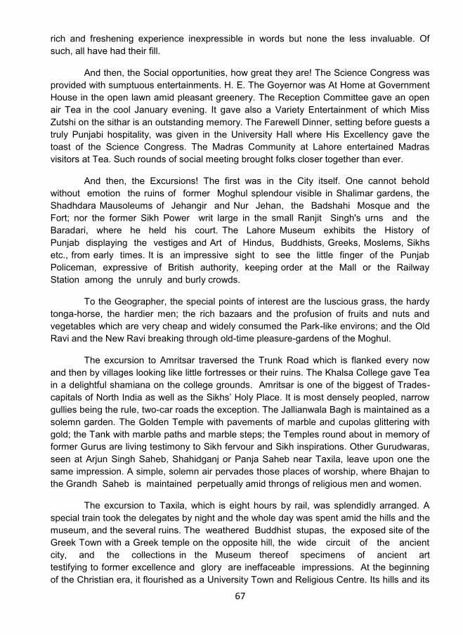
67
rich and freshening experience inexpressible in words but none the less invaluable. Of
such, all have had their fill.
And then, the Social opportunities, how great they are! The Science Congress was
provided with sumptuous entertainments. H. E. The Goyernor was At Home at Government
House in the open lawn amid pleasant greenery. The Reception Committee gave an open
air Tea in the cool January evening. It gave also a Variety Entertainment of which Miss
Zutshi on the sithar is an outstanding memory. The Farewell Dinner, setting before guests a
truly Punjabi hospitality, was given in the University Hall where His Excellency gave the
toast of the Science Congress. The Madras Community at Lahore entertained Madras
visitors at Tea. Such rounds of social meeting brought folks closer together than ever.
And then, the Excursions! The first was in the City itself. One cannot behold
without emotion the ruins of former Moghul splendour visible in Shalimar gardens, the
Shadhdara Mausoleums of Jehangir and Nur Jehan, the Badshahi Mosque and the
Fort; nor the former Sikh Power writ large in the small Ranjit Singh's urns and the
Baradari, where he held his court. The Lahore Museum exhibits the History of
Punjab displaying the vestiges and Art of Hindus, Buddhists, Greeks, Moslems, Sikhs
etc., from early times. It is an impressive sight to see the little finger of the Punjab
Policeman, expressive of British authority, keeping order at the Mall or the Railway
Station among the unruly and burly crowds.
To the Geographer, the special points of interest are the luscious grass, the hardy
tonga-horse, the hardier men; the rich bazaars and the profusion of fruits and nuts and
vegetables which are very cheap and widely consumed the Park-like environs; and the Old
Ravi and the New Ravi breaking through old-time pleasure-gardens of the Moghul.
The excursion to Amritsar traversed the Trunk Road which is flanked every now
and then by villages looking like little fortresses or their ruins. The Khalsa College gave Tea
in a delightful shamiana on the college grounds. Amritsar is one of the biggest of Trades-
capitals of North India as well as the Sikhs‟ Holy Place. It is most densely peopled, narrow
gullies being the rule, two-car roads the exception. The Jallianwala Bagh is maintained as a
solemn garden. The Golden Temple with pavements of marble and cupolas glittering with
gold; the Tank with marble paths and marble steps; the Temples round about in memory of
former Gurus are living testimony to Sikh fervour and Sikh inspirations. Other Gurudwaras,
seen at Arjun Singh Saheb, Shahidganj or Panja Saheb near Taxila, leave upon one the
same impression. A simple, solemn air pervades those places of worship, where Bhajan to
the Grandh Saheb is maintained perpetually amid throngs of religious men and women.
The excursion to Taxila, which is eight hours by rail, was splendidly arranged. A
special train took the delegates by night and the whole day was spent amid the hills and the
museum, and the several ruins. The weathered Buddhist stupas, the exposed site of the
Greek Town with a Greek temple on the opposite hill, the wide circuit of the ancient
city, and the collections in the Museum thereof specimens of ancient art
testifying to former excellence and glory are ineffaceable impressions. At the beginning
of the Christian era, it flourished as a University Town and Religious Centre. Its hills and its
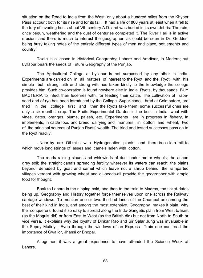
68
situation on the Road to India from the West, only about a hundred miles from the Khyber
Pass account both for its rise and for its fall. It had a life of 800 years at least when it fell to
the fury of invading hosts about Vth century A.D. and was buried in its own debris. The ruin,
once begun, weathering and the dust of centuries completed it. The River Hari is in active
erosion; and there is much to interest the geographer, as could be seen in Dr. Geddes‟
being busy taking notes of the entirely different types of men and place, settlements and
country.
Taxila is a lesson in Historical Geography; Lahore and Amritsar, in Modern; but
Lyllapur bears the seeds of Future Geography of the Punjab.
The Agricultural College at Lyllapur is not surpassed by any other in India.
Experiments are carried on in all matters of interest to the Ryot; and the Ryot, with his
simple but strong faith and strong will, has taken kindly to the knowledge the college
provides him. Such co-operation is found nowhere else in India. Ryots, by thousands, BUY
BACTERIA to infect their lucernes with, for feeding their cattle. The cultivation of rape
seed and of rye has been introduced by the College. Sugar-canes, bred at Coimbatore, are
tried in the college first and then the Ryots take them: some successful ones are
only a six-months' crop. The Fruits Experimental Garden is the best in India, what with
vines, dates, oranges, plums, palash, etc. Experiments are in progress in fishery, in
implements, in cattle food and breed, dairying and manures; in cotton and wheat, two
of the principal sources of Punjab Ryots' wealth. The tried and tested successes pass on to
the Ryot readily.
. Near-by are Oil-mills with Hydrogenation plants; and there is a cloth-mill to
which move long strings of asses and camels laden with cotton.
The roads raising clouds and whirlwinds of dust under motor wheels; the ashen
grey soil; the straight canals spreading fertility wherever its waters can reach; the plains
beyond, denuded by goat and camel which leave not a shrub behind; the ramparted
villages verdant with growing wheat and oil-seeds-all provide the geographer with ample
food for thought.
Back to Lahore in the nipping cold, and then to the train to Madras, the ticket-dates
being up. Geography and History together force themselves upon one across the Railway
carriage windows. To mention one or two: the bad lands of the Chambal are among the
best of their kind in India, and among the most extensive. Geography makes it plain why
the conquerors found it so easy to spread along the Indo-Gangetic plain from West to East
(as the Moguls did) or from East to West (as the British did) but not from North to South or
vice versa. It explains why the loyalty of Dinkar Rao and Sir Salar Jung was invaluable in
the Sepoy Mutiny . Even through the windows of an Express Train one can read the
importance of Gwalior, Jhansi or Bhopal.
Altogether, it was a great experience to have attended the Science Week at
Lahore.
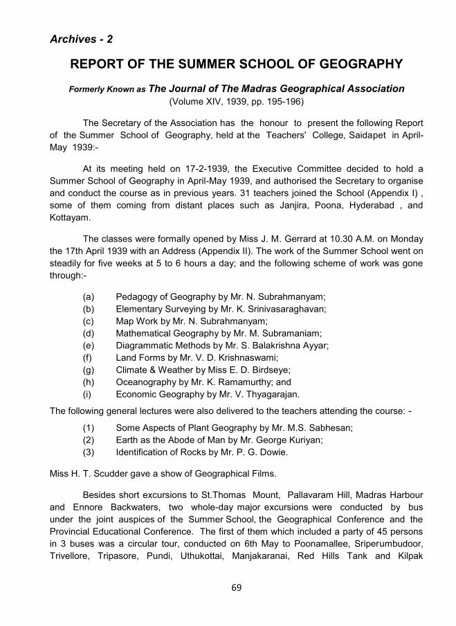
69
Archives - 2
REPORT OF THE SUMMER SCHOOL OF GEOGRAPHY
Formerly Known as The Journal of The Madras Geographical Association (Volume XIV, 1939, pp. 195-196)
The Secretary of the Association has the honour to present the following Report
of the Summer School of Geography, held at the Teachers' College, Saidapet in April-
May 1939:-
At its meeting held on 17-2-1939, the Executive Committee decided to hold a
Summer School of Geography in April-May 1939, and authorised the Secretary to organise
and conduct the course as in previous years. 31 teachers joined the School (Appendix I) ,
some of them coming from distant places such as Janjira, Poona, Hyderabad , and
Kottayam.
The classes were formally opened by Miss J. M. Gerrard at 10.30 A.M. on Monday
the 17th April 1939 with an Address (Appendix II). The work of the Summer School went on
steadily for five weeks at 5 to 6 hours a day; and the following scheme of work was gone
through:-
(a) Pedagogy of Geography by Mr. N. Subrahmanyam;
(b) Elementary Surveying by Mr. K. Srinivasaraghavan;
(c) Map Work by Mr. N. Subrahmanyam;
(d) Mathematical Geography by Mr. M. Subramaniam;
(e) Diagrammatic Methods by Mr. S. Balakrishna Ayyar;
(f) Land Forms by Mr. V. D. Krishnaswami;
(g) Climate & Weather by Miss E. D. Birdseye;
(h) Oceanography by Mr. K. Ramamurthy; and
(i) Economic Geography by Mr. V. Thyagarajan.
The following general lectures were also delivered to the teachers attending the course: -
(1) Some Aspects of Plant Geography by Mr. M.S. Sabhesan;
(2) Earth as the Abode of Man by Mr. George Kuriyan;
(3) Identification of Rocks by Mr. P. G. Dowie.
Miss H. T. Scudder gave a show of Geographical Films.
Besides short excursions to St.Thomas Mount, Pallavaram Hill, Madras Harbour
and Ennore Backwaters, two whole-day major excursions were conducted by bus
under the joint auspices of the Summer School, the Geographical Conference and the
Provincial Educational Conference. The first of them which included a party of 45 persons
in 3 buses was a circular tour, conducted on 6th May to Poonamallee, Sriperumbudoor,
Trivellore, Tripasore, Pundi, Uthukottai, Manjakaranai, Red Hills Tank and Kilpak
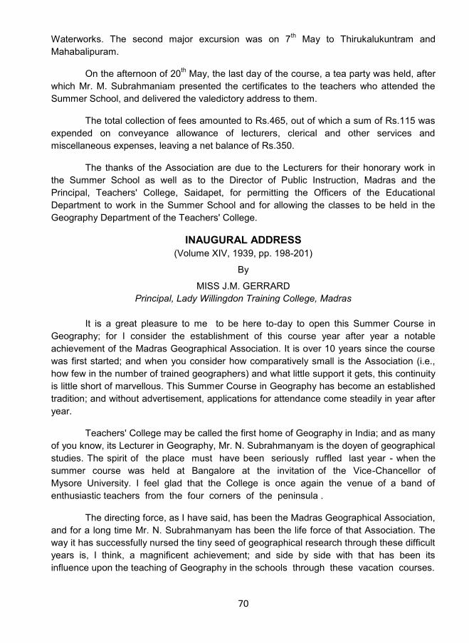
70
Waterworks. The second major excursion was on 7th May to Thirukalukuntram and
Mahabalipuram.
On the afternoon of 20th May, the last day of the course, a tea party was held, after
which Mr. M. Subrahmaniam presented the certificates to the teachers who attended the
Summer School, and delivered the valedictory address to them.
The total collection of fees amounted to Rs.465, out of which a sum of Rs.115 was
expended on conveyance allowance of lecturers, clerical and other services and
miscellaneous expenses, leaving a net balance of Rs.350.
The thanks of the Association are due to the Lecturers for their honorary work in
the Summer School as well as to the Director of Public Instruction, Madras and the
Principal, Teachers' College, Saidapet, for permitting the Officers of the Educational
Department to work in the Summer School and for allowing the classes to be held in the
Geography Department of the Teachers' College.
INAUGURAL ADDRESS
(Volume XIV, 1939, pp. 198-201)
By
MISS J.M. GERRARD
Principal, Lady Willingdon Training College, Madras
It is a great pleasure to me to be here to-day to open this Summer Course in
Geography; for I consider the establishment of this course year after year a notable
achievement of the Madras Geographical Association. It is over 10 years since the course
was first started; and when you consider how comparatively small is the Association (i.e.,
how few in the number of trained geographers) and what little support it gets, this continuity
is little short of marvellous. This Summer Course in Geography has become an established
tradition; and without advertisement, applications for attendance come steadily in year after
year.
Teachers' College may be called the first home of Geography in India; and as many
of you know, its Lecturer in Geography, Mr. N. Subrahmanyam is the doyen of geographical
studies. The spirit of the place must have been seriously ruffled last year - when the
summer course was held at Bangalore at the invitation of the Vice-Chancellor of
Mysore University. I feel glad that the College is once again the venue of a band of
enthusiastic teachers from the four corners of the peninsula .
The directing force, as I have said, has been the Madras Geographical Association,
and for a long time Mr. N. Subrahmanyam has been the life force of that Association. The
way it has successfully nursed the tiny seed of geographical research through these difficult
years is, I think, a magnificent achievement; and side by side with that has been its
influence upon the teaching of Geography in the schools through these vacation courses.
71
To-day we have a situation in which the schools and the teachers are crying out for
training in Geography. From Hyderabad from Bombay, from Travancore they are here to-
day, besides from all the districts of our own Presidency! But the Colleges stand aloof,
refusing to give the instruction for which there is so great a demand. Thus the future
Geography teacher is penalised by having to put in a fifth year, if he wants to be fair to his
pupils, and he takes the Diploma Course of the Madras University. That there are some
who do take this extra year says a great deal both for them and for the interest the subject
gives. Such men and women are the fortunate few who can afford it, and they are limited to
a large extent to those who live in the metropolis. But for the greater number of Geography
teachers- in the schools of this Presidency alone-no opportunity for geographical study is
provided.
This is where the Madras Geographical Association steps in with its introductory
course.
Geography is one of the most difficult subjects to teach. Partly it is due to the fact
that the subject as a science is developing so rapidly. To look back 25 years as I can, is to
realize what, strides have been made, and how the emphasis has changed. For the school
teacher there is first the problem of selection - what regions to teach and how much detail
to be demanded at each stage. Local geography, the homeland, the world-all three have to
be kept going simultaneously.There is no subject in the school curriculum, which needs so
much adjustment to the conditions of the local environment; and every Geography teacher
must be capable of re-arranging his teaching syllabus accordingly. Then there is the need
for training in geographic method and in the tools of learning. You cannot take a course in
map-reading and finish it off in any one year-this involves a progression of training to be
accomplished in the whole school scheme. (And what are we going to do about teaching
the one-inch map when the medium of instruction is Tamil or Kannada etc.?).
The teaching syllabus has to plan for this progression. The teaching of climate
similarly has to provide for training in the recording of local observations, in the reading of
maps showing the distribution of temperature, pressure and rainfall, and the study of
climatic regions-each with its regime of temperature and pressure through the year, where
both a spatial and a time factor have to be taken into account. In each year of the school
scheme something of this has to be provided for, each stage a little more difficult than the
last. Thus all the three aspects have to be provided for, simultaneously in teaching
Geography in school-acquisition of skills in the use of geographic tools, the development of
geographic ideas, and the acquisition of geographical facts. Such is the nature of the
subject, which is to be taught, apparently, without any previous training-by the light of
nature alone.
Now this course has been admirably planned to help the teacher. This year it has
been extended to a period of five weeks, giving 180 hours of work; thus it is more intensive
than the training given to the Geography teacher in the L. T. course. The emphasis is to be
placed on practical work; and this is most wise, for not only is practical work becoming of
increasing importance in the school curriculum, but it is just that part of Geography which is
most difficult for the learner to acquire without a guidance and help. The middle school

72
course should be two-thirds practical. We have tried out this experiment in our school for
the last two years; and the good results most noticeable are-the children get a grasp of the
fundamentals of Geographic method, the use of maps of all kinds, the value and use of
statistics, training in direct observation and some elementary training in deduction and
induction, which helps them to understand the work in the upper forms. Unless time is given
to this kind of training in the middle school, the later work can be nothing but unintelligible
cram.
This course has been planned to give something of that practical foundation.
Surveying, you will find, will give you a fresh outlook altogether and a new sense of power
over your environment, besides a deeper understanding of maps. Every school should have
a map of its building and lay-out of its grounds, and it is the business of the Geography
teacher to produce this. I believe the middle school Mathematics and Geography teaching
would benefit by the introduction of a little map-making. This was tried out last year in Form
I of the Wesley School, and I believe the interest and enthusiasm shown by the boys was
astonishing. The course on map-reading will also be particularly valuable to you, and
especially that on the one-inch map, since there is no treatise published to guide you in the
intricacies of the geographical interpretation of Indian maps.
In fact, the whole course has been admirably planned to help you; it is being taught
by a body of experts; and your teaching of the subject will be enormously enriched by this
introduction to it. Not only that, but it will also open a vista to an entrancing subject; and
some of you I hope will want to follow it up the whole way. You can do that by taking the
Geography Diploma to be followed up later by an Honours course at some Indian
University, if you are lucky enough to get a windfall in cash!
Fellow-teacher -let me congratulate you on your enterprise and your sense of duty
to your profession, evidence of which is your attendance here; let me prophesy for you five
weeks of intense activity-considerable exercise of brain and limb-and at the end a feeling
of satisfaction at a piece of work well done!
NEWS AND NOTES
(Volume XIV, 1939, p. 208)
The 27th session of the Indian Science Congress will be held at Madras from
January 2 to 8, 1940. Dr. S.P. Chatterjee of Calcutta University has been elected President,
Mr. George Kuriyan the Recorder, and Mr. B.M. Thirunaranan the Local Secretary of the
Geography and Geodesy section for this session. It is hoped that several good papers will
be contributed to this section, which was confirmed as a separate one only last year.
73
Archives - 3
THE DIRECT STUDY OF GEOGRAPHY Hints and Suggestions with Special Reference to Saidapet
Formerly Known as The Journal of The Madras Geographical Association (Volume XIV, 1939, pp. 435-438)
By
N. SUBRAHMANYAM,
Editor, The Journal of The Madras Geographical Association
Under the above caption goes an important section of the new L.T. Syllabus in
Geography, which reads as follows: “The .observation and expression of the facts of Local
Geography: the possibilities and uses of different environments. (This should be done
through a practical study either of the student's home region or of the home region of the
Training College)." As the home regions of the students under training will necessarily be
different, it is proposed to offer some hints and comments regarding some of the main
topics relating to Saidapet in a suggestive rather than a comprehensive way. It is expected
that the students will be able to apply and follow them up for their own respective places
also, when they return to them. Probably it is unnecessary to state that it is not a full
regional survey that is intended, as that term is applied for what is a good deal more than
Geography. But in so far as the geographical part of it (which is its core) is concerned, its
aims and methods may be adopted especially by way of personal investigation, recording
the data, mapping the distributions and expressing the data diagrammatically.
The start may be made by getting a bird's-eye view of the whole locality from what
may be called, an “outlook tower” - an eminence in the neighbourhood such as the top of
St. Thomas Mount, and fixing the features and landmarks with the help of the one-inch
topographical map of the Survey of India. With the same map or better still with one on a
bigger scale, preliminary rambles may be made to different parts of the town, noting facts
and features not to be found in the map owing to changes having taken place since the
map was prepared at first, either by removal or by addition and growth. For example, on the
latest one-inch map the present Teachers' College is still shown as Agricultural College, in
spite of the fact that it is over 30 years since the latter was removed to Coimbatore.
Conversely, Todhunternagar, Y. M. C. A. College of Physical Education, the Golf Links,
the Richards Park, Panagal Buildings, Water storage tank, etc., do not find a place in it. It is
a good exercise for groups of students to go round the different parts of the locality and
note such changes in an outline map. Surveying the college compound, contouring levels
near the Adyar bank or Little Mount, and sketching the different areas visited and noting the
features observed and the routes are other important items of practical work, connected
with map-making. The times and exact directions of sunrise and sunset and midday
altitudes of the sun should be noted periodically in the course of the year, expressed
diagrammatically and correlated with the seasons. The method of finding and drawing the
74
meridian line should be learnt and applied. Simple methods of finding the midday altitude of
the sun will be learnt incidentally.
The surface levels and features and the courses of the Adyar and the Cooum,
especially the curves and the bed of the latter, should be observed and noted in
rambles and visits, gathering evidences of erosion and deposition. Specimens of rocks
and soils in the neighbourhood should be collected, examined and classified. Peeps at
bed-rock may be obtained in railway cuttings and in diggings made for underground
drainage, wells or foundations for buildings. The changing water-table in the wells of
the different parts of the locality should be noted in the different seasons. Visits to the
countryside and to the rivers in flood are particularly useful in illuminating much that is
otherwise purely theoretical in the study of physical geography. Weather recording
offers a specially rich field for observational work. Wind direction, maximum and minimum
temperature and rainfall are some of the chief items to be observed, recorded and
expressed in appropriate diagrams such as the wind-rose and the climograph. The results
of observational work may be compared with published normals and actual figures available
in the meteorological reports.
Preparation of land utilisation maps affords scope for another valuable kind of direct
study of environment. Important public buildings, groups of residential areas, cultivable
lands, open spaces, parks, etc., may be noted in special outline maps and studied side by
side with the topographical map as already suggested. The straggling nature of the
municipality of Saidapet, extending from Chengamedu on the right bank of the Cooum
through Puliyur, Kodambakkam, Saligramam, West Mambalam, Mettupalaiyam, and
Saidapet proper to Guindy and Little Mount beyond the Adyar river, with large stretches of
cultivated and barren land and brick pits intervening, the water-works, the bazaar, the
temples, mosques and churches, and the groupings of the people in communities,
occupational or otherwise should all find their places in the map. The difficulties of natural
drainage (said to be due to the bunding up of the Adyar bank for the construction of the
Marmalong bridge) , the methods of disposal of sullage water and their relation to public
health are worthy of note.
On the economic side, there are important items to observe and collect data about.
In the adjoining cultivable lands, agriculture is precarious owing to poor fertility of the soil
and want of irrigation facilities; but, market gardening, especially of vegetables and flowers,
is more important, owing to the proximity of the town. The brick industry is a flourishing one;
the location of the kilns, the soil and other conditions, transport and market are to be
studied. The weaving industry of Thopet is another local industry to be investigated. The
locality, the community engaged in it, the kinds of stuff woven, the market and the present
condition of the industry should be inquired into. Dhobying is another well-known
occupation in Saidapet, the bed of the Adyar being a dhobykhana of Madras. The easy
transport and the fresh water in the river above the tidal limit as well as the presence of the
washer class in connection with the bleaching work of the weaving industry should be noted
as favouring causes. Jutka-making and jutka-repairing were well-known in Saidapet; but
this industry seems to have fallen on evil days with the growth of the motor transport and
75
the running of the electric train. Regarding the population: besides noting its distribution in
the several wards, it will be interesting to find out the extent to which Saidapet is suburban
in character, that is, what proportion of its inhabitants are working for their livelihood in
Madras and not at Saidapet. The relative popularity of the train and the bus is an interesting
piece of investigation to make. Taking the road transport: the southern trunk road-or the
Mount Road as it is called here, as leading to St. Thomas Mount-with its width, tarring, etc.,
and the colleges, and open spaces on either side of it-is what gives the best impression of
Saidapet to the casual passer-by. But the other roads, especially those linking Saidapet
with West Mambalam, Saligramam and Chengamedu should be visited, and the causes for
their bad condition should be investigated: e.g., the effect of brick carts, bad finances of the
municipality or the unremunerative nature of some of these roads, having to link up distant
residential areas. The traffic in the trunk road should be observed and noted at different
times in the day and in the different seasons, as to the kinds of goods taken and as to how
far it is local and how far „through‟. Some of the commonest in evidence are brick, straw,
hay, grain, curds and vegetables in head loads, fish in Ford cars from Sadras, hides and
skins, tanning materials. Note the extra hard cementing of the sides of the road for heavy
laden carts to pass. Note also the diversion of the slow traffic on race days through Alandur
road, when the congested motor traffic has to pass through the bottle-neck of the
Marmalong bridge. The seasonal fruits, flowers and vegetables in the market and in the
field should also receive attention.
One of the most interesting topics is the study of the formation and growth of the
different types of settlements in the locality itself: for example, Guindy and Fanepet as
roadside settlements; Little Mount as a Christian settlement round the place of martyrdom
of a Saint; the weaving ward of Thopet with its broad open streets for pitching the looms;
the old type of settlement round a temple as in Perumal Koil St., Karaneeswarar Koil St.,
and southern part of West Mambalam; the bungalow type near the Guindy Railway
Overbridge. The location of particular trades and occupations in particular places is to be
noted; as the dhoby near the river, the potter just on the outskirts, the jutka-repairer near
the main road and the binder near the college.
Further, as Saidapet is a suburb of Madras, lying on the trunk road and the electric
railway (four stations on which serve the municipality) possibilities of planning new
extensions on the lines of Theagarayanagar may be examined and explored, taking into
account the lie and structure of the land and facilities of water supply, drainage, open
space, etc. Geography has as much to do with man's play and leisure as with his work: and
sports competitions and physical demonstrations in the colleges, the races at Guindy, the
festivities in the Little Mount and of the Karaneeswara temple that draw large crowds from
the city and its environs are noteworthy-the times and seasons when they take place, the
incidental increase of trade and transport in particular directions at the time of the festivities,
and how far they disturb the normal even life of the residents and their other reactions.
Possibilities of improvement are not outside the scope of local study. It is unnecessary to
repeat that personal observation, collection of data, mapping and diagrammatic expression,
and interpretation should all go hand in hand in such a study, Most of this can be co-
operative work.
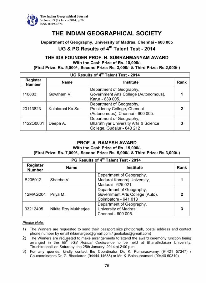
The Indian Geographical Journal
Volume 89 (1) June - 2014, p 76 ISSN 0019-4824
76
THE INDIAN GEOGRAPHICAL SOCIETY
Department of Geography, University of Madras, Chennai - 600 005
UG & PG Results of 4th Talent Test - 2014
THE IGS FOUNDER PROF. N. SUBRAHMANYAM AWARD With the Cash Prize of Rs. 10,000/‐
(First Prize: Rs. 5,000/‐, Second Prize: Rs. 3,000/‐ & Third Prize: Rs.2,000/-)
UG Results of 4th
Talent Test - 2014 Register Number
Name Institute Rank
110803 Gowtham V. Department of Geography, Government Arts College (Autonomous), Karur - 639 005.
1
20113823 Kalaiarasi Ka.Sa. Department of Geography, Presidency College, Chennai (Autonomous), Chennai - 600 005.
2
1122Q0031 Deepa A. Department of Geography, Bharathiyar University Arts & Science College, Gudalur - 643 212
3
PROF. A. RAMESH AWARD With the Cash Prize of Rs. 15,000/‐
(First Prize: Rs. 7,000/‐, Second Prize: Rs. 5,000/‐ & Third Prize: Rs.3,000/-)
PG Results of 4th
Talent Test - 2014
Register Number
Name Institute Rank
B205012 Sheeba V. Department of Geography, Madurai Kamaraj University, Madurai - 625 021.
1
12MAG204 Priya M. Department of Geography, Government Arts College (Auto), Coimbatore - 641 018
2
33212405 Nikita Roy Mukherjee Department of Geography, University of Madras, Chennai - 600 005.
3
Please Note:
1) The Winners are requested to send their passport size photograph, postal address and contact phone number by email ([email protected] / [email protected])
2) The Winners are requested to make arrangements to attend the award ceremony function being arranged in the 89
th IGS Annual Conference to be held at Bharathidasan University,
Tiruchirappalli on Saturday, the 25th January, 2014 at 2:00 p.m. 3) For any queries, kindly contact the Coordinator Dr. K. Kumaraswamy (94421 57347) /
Co-coordinators Dr. G. Bhaskaran (94444 14688) or Mr. K. Balasubramani (99440 60319).
The Indian Geographical Journal
Volume 89 (2) December - 2014, pp 77-89 ISSN 0019-4824
77
THE URBAN CHALLENGE - PROVISIONING OF BASIC
SERVICES IN NOTIFIED AND NON-NOTIFIED SLUMS OF
INDIA
Anuradha Banerjee1, Joydeep Saha
2 and Dinabandhu Mondal
1
1 School of Social Sciences, Jawaharlal Nehru University, New Delhi - 110 067 2Department of Geography, Bijoy Krishna Girls‟ College, Howrah - 711 101
E-mail: [email protected], [email protected]
Abstract
This paper attempts to explore whether the gap between ‘notified’ and ‘non-notified’ slums
have reduced or not, across nine selected states over a decade of decentralised
governance regime and also to relate the issue of provisioning water and sanitation
services within the slum development planning and policy domain. Using the secondary
data provided by NSSO from 2002 to 2012, across three different rounds, this paper
focuses on the condition of basic amenities, its temporal changes and the role played by
various stakeholders in the improvement of slums. It finds that while ‘notified’ slums
continue to receive services and remain in more or less better conditions, whereas ‘non-
notified’ slums still have a long way to go.
Keywords: Slum, Services, ULB, Sanitation, Planning
Introduction
In an academic sense, the notion of „slums‟ in India is complex and added to that
the „definition‟ followed by Census of India and National Sample Survey Organisation
(NSSO) and a substantial number of legal documents, create a taxonomy of „notified‟ and
„non-notified‟ slums. National Sample Survey Organisation (NSSO), since 2002 to 2012,
has been categorising „notified‟ and „non-notified‟ slums and then „defines‟ the respective
categories of slums as the “areas notified as slums by the concerned municipalities,
corporations, local bodies or development authorities were termed notified slums‟, and „any
compact settlement with a collection of poorly built tenements, mostly of temporary nature,
crowded together, usually with inadequate sanitary and drinking water facilities in
unhygienic conditions, was considered a slum by the survey, provided at least 20
households lived there. Such a settlement, if not a notified slum, was called a non-notified
slum”. Census of India also agrees largely with this „definition‟, as it denotes own one as: “A
slum, for the purpose of Census, has been defined as a residential area where dwellings
are unfit for human habitation by reasons of dilapidation, overcrowding, faulty arrangements
and design of such buildings, narrowness or faulty arrangement of street, lack of ventilation,
light or sanitation facilities or any combination of these factors which are detrimental to the
safety and health”. Census of India, in 2011, categorises slums into three categories -
‘notified’, ‘recognised’ and ‘identified’. The first category is ‘notified’ by state / local
administration through legal acts; second one is also ‘recognised but not formally notified’
78
Anuradha Banerjee et al. The Indian Geographical Journal, 89 (2) December – 2014
by these bodies; and the last category is defined as “A compact area of at least 300
population or about 60-70 households of poorly built congested tenements, in unhygienic
environment usually with inadequate infrastructure and lacking in proper sanitary and
drinking water facilities”. Two things appear very clearly from these definitions – one,
recognition and notification of slums are done by Urban Local Bodies / Parastatal Agencies
and second, non-notified slums are hardly availing basic amenities like drinking water and
sanitation system. The only visible difference in these two definitions is the minimum cut-off
in the number of households and it has been argued that with increasing events of slum
eviction cycles and breakdown of large slums into smaller clusters in Indian cities today,
present Census definition lacks inclusive nature (Bhan and Jana, 2013).
The paucity of basic services in residential areas lived by poor people, according to
Mitlin (2005), is one of the basic reasons behind chronic urban poverty. It is also generally
portrayed in the literature that urban poor mainly lives in slums. While the notified slums
usually receive some basic services provided by Urban Local Bodies or Parastatal
Agencies, non-notified slums remain less served in India. Even if policy-makers often
suggest amelioration of the living condition of those places where urban poor live, in
practice, demolition and dislocation of large-sized slums is not uncommon. In addition to
that, continuous inflow of new migrants into large cities lead to the formation of small-sized
slum clusters over a period of time. As the entire process of „recognition‟ and „notification‟ of
slums takes time, these clusters mushroom haphazardly and that too without basic
provisions of water and sanitations. Against such a backdrop, this paper attempts to explore
whether the gap between „notified‟ and „non-notified‟ slums have reduced or not. This paper
also attempts to focus on the condition of basic amenities, its temporal changes and the
role played by various stakeholders in the improvement of slums while relating the issues of
basic service provisioning within India's slum development planning and policy domain.
Database and Methodology
After looking at the variables of slum database in both Census of India and NSSO
files, few issues need to be discussed before moving onto the main paper. Firstly, in both
the datasets, the availability of amenities like drinking water and latrines is captured, not
adequacy. Secondly, Census captures household level information on availability and
accessibility of such amenities, whereas NSSO takes into account slum level information,
gathered from knowledgeable persons living in the slum. Thirdly, „It is for the first time in
Census that datasets on Housing stock, Amenities, and Assets based on the Houselisting
and Housing Census are being released. In Census 2001, information on Slums was
released only on demographic characteristics based on the Population Enumeration. For
this purpose, Slum Blocks were identified in Statutory Towns having a population of 20,000
by the local authorities at the time of Population Enumeration phase. In Census 2011, Slum
Blocks have been delineated in all statutory towns irrespective of population size‟ (Census
of India website). Fourthly, NSSO provides an additional information, i.e. change in the
„conditions‟ of these amenities and „sources of improvement‟. Fifthly, as already mentioned,
NSSO data is more inclusive in nature as compared to Census dataset. Given all such
79
Anuradha Banerjee et al. The Indian Geographical Journal, 89 (2) December – 2014
advantages and disadvantages of both datasets at the outset, it would be more judicious to
use NSSO dataset on slums, across three different Rounds, i.e. 58th Round- „Condition of
Urban Slums‟ (2002), 65th Round- „Some Characteristics of Urban Slums‟ (2008-09) and
69th Round- „Key Indicators of Urban Slums in India‟ (2012).
For all three Rounds, nine common states, for which data is available, have been
taken into account: Andhra Pradesh, Gujarat, Karnataka, Madhya Pradesh, Maharashtra,
Odisha, Tamil Nadu, Uttar Pradesh and West Bengal. This paper largely focuses on the
qualitative aspects of the living environment in slums. In terms of living environment, some
of the basic urban amenities related to water and sanitation have been taken into
consideration. These are: drinking water, latrine, drainage, sewerage, and garbage
disposal. Another point is that these indicators have direct linkages with health, hygiene,
and well-being of slum dwellers (WHO). Conspicuously, a majority of existing research
works on slum environment are based on the primary survey in particular cities/towns.
These papers are helpful to assess the ground situation of slums. But, macro-level
discussion of slums' living environment, where a composite and analytical picture is
depicted, could draw the attention of policymakers for prioritizing issues and directing slum
improvement schemes. Undoubtedly, Census 2011 provides important information on
slums for each statutory towns, but the decadal data is not sufficient. In case of NSSO data,
unequal and inadequate distribution of sample slums in different geographical regions, to a
considerable extent, limits the scope of a detailed analysis in this paper.
Results and Discussion
Changing Number of Slums
In absolute figures, the number of slums has consistently declined over three
Rounds. This is truer in case of „notified‟ slums, whereas „non-notified‟ slums, in between
58th and 65
th Round, do not show much change. If one looks at the percentage figures, the
proportion of „notified' slums have declined, whereas the proportion of „non-notified slums'
has increased. This reestablishes concerns of "exclusionary urbanisation" raised by urban
experts (for example, see Kundu and Roy Saraswati, 2012), which assert that cities have
become so hostile these days, that poor migrants are unable to find a space to live and
work. The figures in Table 1, absolute and percentage, also show the proliferation of non-
notified slums as compared to notified slums, thereby leading one to presume that poor
migrants, if able to settle in cities for livelihood, stay in very small clusters, and might need
strong political roots and temporal stability to get „recognition‟ and „notification‟ from
concerned ULBs / Parastatal Agencies. This decline is sharper in Maharashtra, and less in
Andhra Pradesh. States like Uttar Pradesh, West Bengal, and Gujarat shows a substantial
increase in the number of „notified slums‟ in between 58th and 65
th Round, and then again a
certain drop in the 69th Round. Karnataka, in the last two Rounds, does not show much
change. Maharashtra and Andhra Pradesh exhibit consistent increase in the proportion of
„non-notified' slums over three Round. Odisha‟s scenario is beyond any possible
explanation, and one of the plausible reasons is the very small number of sample slums in
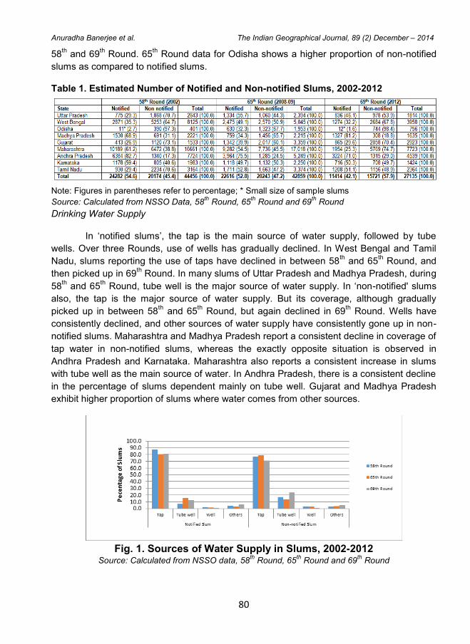
80
Anuradha Banerjee et al. The Indian Geographical Journal, 89 (2) December – 2014
58th and 69
th Round. 65
th Round data for Odisha shows a higher proportion of non-notified
slums as compared to notified slums.
Table 1. Estimated Number of Notified and Non-notified Slums, 2002-2012
Note: Figures in parentheses refer to percentage; * Small size of sample slums
Source: Calculated from NSSO Data, 58th Round, 65
th Round and 69
th Round
Drinking Water Supply
In „notified slums‟, the tap is the main source of water supply, followed by tube
wells. Over three Rounds, use of wells has gradually declined. In West Bengal and Tamil
Nadu, slums reporting the use of taps have declined in between 58th and 65
th Round, and
then picked up in 69th Round. In many slums of Uttar Pradesh and Madhya Pradesh, during
58th and 65
th Round, tube well is the major source of water supply. In „non-notified' slums
also, the tap is the major source of water supply. But its coverage, although gradually
picked up in between 58th and 65
th Round, but again declined in 69
th Round. Wells have
consistently declined, and other sources of water supply have consistently gone up in non-
notified slums. Maharashtra and Madhya Pradesh report a consistent decline in coverage of
tap water in non-notified slums, whereas the exactly opposite situation is observed in
Andhra Pradesh and Karnataka. Maharashtra also reports a consistent increase in slums
with tube well as the main source of water. In Andhra Pradesh, there is a consistent decline
in the percentage of slums dependent mainly on tube well. Gujarat and Madhya Pradesh
exhibit higher proportion of slums where water comes from other sources.
Fig. 1. Sources of Water Supply in Slums, 2002-2012 Source: Calculated from NSSO data, 58
th Round, 65
th Round and 69
th Round
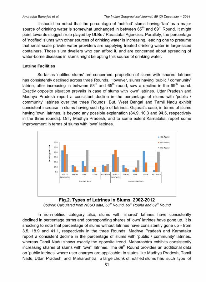
81
Anuradha Banerjee et al. The Indian Geographical Journal, 89 (2) December – 2014
It should be noted that the percentage of „notified‟ slums having „tap‟ as a major
source of drinking water is somewhat unchanged in between 65th and 69
th Round. It might
point towards sluggish role played by ULBs / Parastatal Agencies. Parallely, the percentage
of „notified' slums with other sources of drinking water is increasing, leading one to presume
that small-scale private water providers are supplying treated drinking water in large-sized
containers. Those slum dwellers who can afford it, and are concerned about spreading of
water-borne diseases in slums might be opting this source of drinking water.
Latrine Facilities
So far as „notified slums‟ are concerned, proportion of slums with „shared‟ latrines
has consistently declined across three Rounds. However, slums having „public / community‟
latrine, after increasing in between 58th and 65
th round, saw a decline in the 69
th round.
Exactly opposite situation prevails in case of slums with „own' latrines. Uttar Pradesh and
Madhya Pradesh report a consistent decline in the percentage of slums with „public /
community' latrines over the three Rounds. But, West Bengal and Tamil Nadu exhibit
consistent increase in slums having such type of latrines. Gujarat's case, in terms of slums
having „own‟ latrines, is beyond any possible explanation (84.9, 10.3 and 94.5, respectively
in the three rounds). Only Madhya Pradesh, and to some extent Karnataka, report some
improvement in terms of slums with „own‟ latrines.
Fig.2. Types of Latrines in Slums, 2002-2012 Source: Calculated from NSSO data, 58
th Round, 65
th Round and 69
th Round
In non-notified category also, slums with „shared‟ latrines have consistently
declined in percentage terms and corresponding shares of „own‟ latrines have gone up. It is
shocking to note that percentage of slums without latrines have consistently gone up - from
3.5, 18.9 and 41.1, respectively in the three Rounds. Madhya Pradesh and Karnataka
report a consistent decline in the percentage of slums with „public / community' latrines,
whereas Tamil Nadu shows exactly the opposite trend. Maharashtra exhibits consistently
increasing shares of slums with „own‟ latrines. The 69th Round provides an additional data
on „public latrines' where user charges are applicable. In states like Madhya Pradesh, Tamil
Nadu, Uttar Pradesh and Maharashtra, a large chunk of notified slums has such type of
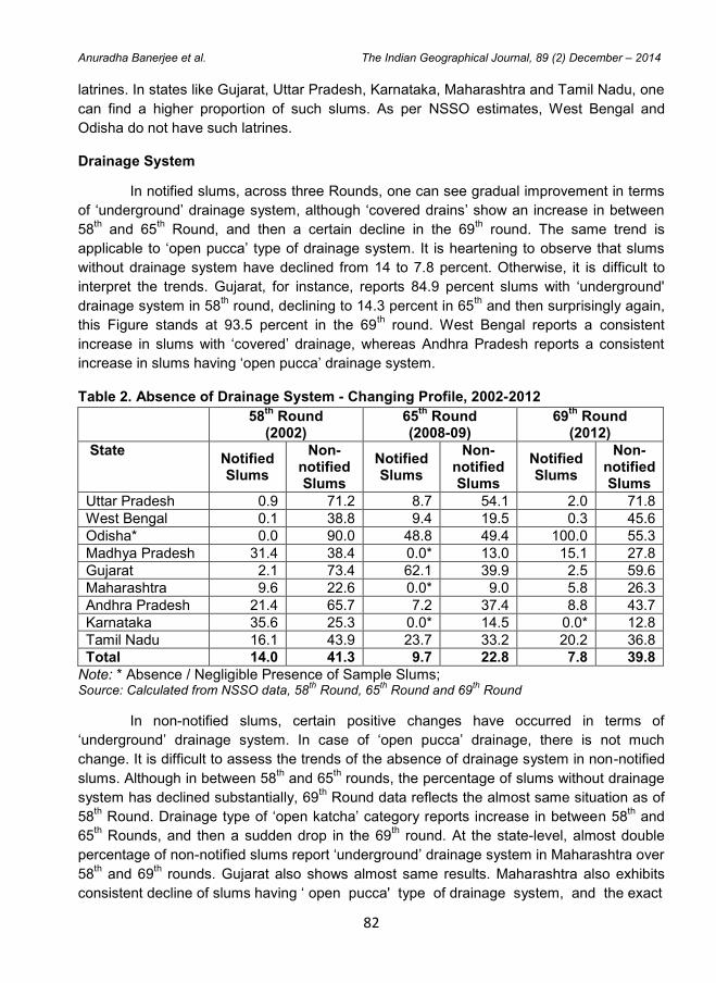
82
Anuradha Banerjee et al. The Indian Geographical Journal, 89 (2) December – 2014
latrines. In states like Gujarat, Uttar Pradesh, Karnataka, Maharashtra and Tamil Nadu, one
can find a higher proportion of such slums. As per NSSO estimates, West Bengal and
Odisha do not have such latrines.
Drainage System
In notified slums, across three Rounds, one can see gradual improvement in terms
of „underground‟ drainage system, although „covered drains‟ show an increase in between
58th and 65
th Round, and then a certain decline in the 69
th round. The same trend is
applicable to „open pucca‟ type of drainage system. It is heartening to observe that slums
without drainage system have declined from 14 to 7.8 percent. Otherwise, it is difficult to
interpret the trends. Gujarat, for instance, reports 84.9 percent slums with „underground'
drainage system in 58th round, declining to 14.3 percent in 65
th and then surprisingly again,
this Figure stands at 93.5 percent in the 69th round. West Bengal reports a consistent
increase in slums with „covered‟ drainage, whereas Andhra Pradesh reports a consistent
increase in slums having „open pucca‟ drainage system.
Table 2. Absence of Drainage System - Changing Profile, 2002-2012
58th
Round (2002)
65th
Round (2008-09)
69th
Round (2012)
State Notified Slums
Non-notified Slums
Notified Slums
Non-notified Slums
Notified Slums
Non-notified Slums
Uttar Pradesh 0.9 71.2 8.7 54.1 2.0 71.8
West Bengal 0.1 38.8 9.4 19.5 0.3 45.6
Odisha* 0.0 90.0 48.8 49.4 100.0 55.3
Madhya Pradesh 31.4 38.4 0.0* 13.0 15.1 27.8
Gujarat 2.1 73.4 62.1 39.9 2.5 59.6
Maharashtra 9.6 22.6 0.0* 9.0 5.8 26.3
Andhra Pradesh 21.4 65.7 7.2 37.4 8.8 43.7
Karnataka 35.6 25.3 0.0* 14.5 0.0* 12.8
Tamil Nadu 16.1 43.9 23.7 33.2 20.2 36.8
Total 14.0 41.3 9.7 22.8 7.8 39.8
Note: * Absence / Negligible Presence of Sample Slums; Source: Calculated from NSSO data, 58
th Round, 65
th Round and 69
th Round
In non-notified slums, certain positive changes have occurred in terms of
„underground‟ drainage system. In case of „open pucca‟ drainage, there is not much
change. It is difficult to assess the trends of the absence of drainage system in non-notified
slums. Although in between 58th and 65
th rounds, the percentage of slums without drainage
system has declined substantially, 69th Round data reflects the almost same situation as of
58th Round. Drainage type of „open katcha‟ category reports increase in between 58
th and
65th Rounds, and then a sudden drop in the 69
th round. At the state-level, almost double
percentage of non-notified slums report „underground‟ drainage system in Maharashtra over
58th and 69
th rounds. Gujarat also shows almost same results. Maharashtra also exhibits
consistent decline of slums having „ open pucca' type of drainage system, and the exact
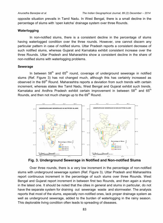
83
Anuradha Banerjee et al. The Indian Geographical Journal, 89 (2) December – 2014
opposite situation prevails in Tamil Nadu. In West Bengal, there is a small decline in the
percentage of slums with „open katcha‟ drainage system over three Rounds.
Waterlogging
In non-notified slums, there is a consistent decline in the percentage of slums
having waterlogged condition over the three rounds. However, one cannot discern any
particular pattern in case of notified slums. Uttar Pradesh reports a consistent decrease of
such notified slums, whereas Gujarat and Karnataka exhibit consistent increase over the
three Rounds. Uttar Pradesh and Maharashtra show a consistent decline in the share of
non-notified slums with waterlogging problems.
Sewerage
In between 58th and 65
th round, coverage of underground sewerage in notified
slums (Ref. Figure 3) has not changed much, although this has certainly increased as
observed in the 69th Round. Maharashtra reports a deviation from such trends with certain
increment, whereas states like Tamil Nadu, West Bengal and Gujarat exhibit such trends.
Karnataka and Andhra Pradesh exhibit certain improvement in between 58th and 65
th
Rounds, and then not much change up to the 69th Round.
Fig. 3. Underground Sewerage in Notified and Non-notified Slums
Over three rounds, there is a very low increment in the percentage of non-notified
slums with underground sewerage system (Ref. Figure 3). Uttar Pradesh and Maharashtra
report continuous increment in the percentage of such slums over three Rounds. West
Bengal and Gujarat report increment in between first two Rounds, and then again a slump
in the latest one. It should be noted that the cities in general and slums in particular, do not
have the separate system for draining out sewerage waste and stormwater. The analysis
reports that most of the slums, especially non-notified ones, lack proper drainage system as
well as underground sewerage, added to the burden of waterlogging in the rainy season.
This deplorable living condition often leads to spreading of diseases.

84
Anuradha Banerjee et al. The Indian Geographical Journal, 89 (2) December – 2014
Garbage Disposal
In more than 75 percent of the notified slums, the arrangement of garbage disposal
is borne by Urban Local Bodies (ULBs) like Municipality or Municipal Corporation. This is
very much prominent in highly urbanized states like Maharashtra and Tamil Nadu.
However, for non-notified slums, residents and other agencies also have some contribution.
Over three Rounds, ULB service coverage for non-notified slums has gradually improved,
from 47.3 to 59.5 percent.
On the other hand, the absence of garbage disposal arrangement is more
prominent in non-notified slums as compared to notified slums. In such non-notified slums,
over three Rounds, the role of residents has not changed much. However, the role of other
agencies has sharply declined to zero in between 65th and 69
th Rounds.
Table 3. No Arrangement for Garbage Disposal - Changing Profile, 2002-2012
58th
Round (2002)
65th
Round (2008-09)
69th
Round (2012)
Notified Slums
Non-notified Slums
Notified Slums
Non-notified Slums
Notified Slums
Non-notified Slums
Uttar Pradesh 1.7 81.5 16.0 54.3 12.0 46.4
West Bengal 4.1 43.2 11.3 22.3 6.0 39.2
Odisha* 100.0* 81.2 32.8 48.1 0.0* 68.5
Madhya Pradesh 41.4 59.1 48.3 23.7 18.0 30.1
Gujarat 4.2 30.1 62.3 32.7 3.0 61.2
Maharashtra 10.5 17.0 2.6 6.3 13.8 18.3
Andhra Pradesh 16.2 62.1 2.6 39.8 7.7 23.4
Karnataka 49.9 55.3 0.2 14.9 3.8 12.6
Tamil Nadu 0.9 46.5 11.5 39.0 26.4 27.0
Total 14.4 41.0 10.8 22.7 11.5 32.7 Note: * Absence/Negligible Presence of Sample Slums
Source: Calculated from NSSO data, 58th
Round, 65th Round and 69
th Round
Given the fact of gradual pace of ULB service coverage in these slums, the
corresponding percentage of slums without any garbage disposal arrangement has
suddenly gone up from 22.7 to 32.7 percent. In few states like Uttar Pradesh and Andhra
Pradesh, the percentage of such type of slums without such arrangement has consistently
declined.
With the introduction of Urban Local Bodies and NGOs' growing contribution in
slum amelioration schemes, residents' role sometimes gets minimised to a certain extent,
and sometimes it again revives. Perhaps due to the slowdown of NGO‟s role in one hand
and residents‟ increasing awareness level lead to such revival. Sengupta (1999) has
argued that at the end of the day, slum residents experience the real situation of their living
environment. Therefore, environmental management at the community level is seriously
required. His studies on slums of Howrah in West Bengal show how such community can
play a role in amelioration of living environment.
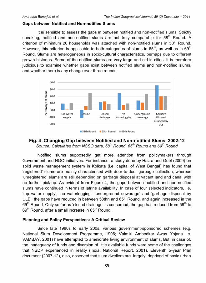
85
Anuradha Banerjee et al. The Indian Geographical Journal, 89 (2) December – 2014
Gaps between Notified and Non-notified Slums
It is sensible to assess the gaps in between notified and non-notified slums. Strictly
speaking, notified and non-notified slums are not truly comparable for 58th Round. A
criterion of minimum 20 households was attached with non-notified slums in 58th Round.
However, this criterion is applicable to both categories of slums in 65th, as well as in 69
th
Round. Slums are heterogeneous in socio-cultural characteristics, perhaps due to different
growth histories. Some of the notified slums are very large and old in cities. It is therefore
judicious to examine whether gaps exist between notified slums and non-notified slums,
and whether there is any change over three rounds.
Fig. 4 .Changing Gap between Notified and Non-notified Slums, 2002-12 Source: Calculated from NSSO data, 58
th Round, 65
th Round and 69
th Round
Notified slums supposedly get more attention from policymakers through
Government and NGO initiatives. For instance, a study done by Hazra and Goel (2009) on
solid waste management system in Kolkata (i.e. capital of West Bengal) has found that
„registered‟ slums are mainly characterised with door-to-door garbage collection, whereas
„unregistered‟ slums are still depending on garbage disposal at vacant land and canal with
no further pick-up. As evident from Figure 4, the gaps between notified and non-notified
slums have continued in terms of latrine availability. In case of four selected indicators, i.e.
„tap water supply‟, „no waterlogging‟, „underground sewerage‟ and „garbage disposal by
ULB‟, the gaps have reduced in between 58thn and 65th Round, and again increased in the
69th Round. Only so far as „closed drainage‟ is concerned, the gap has reduced from 58
th to
69th Round, after a small increase in 65
th Round.
Planning and Policy Perspectives: A Critical Review
Since late 1980s to early 200s, various government-sponsored schemes (e.g.
National Slum Development Programme, 1996; Valmiki Ambedkar Awas Yojana i.e.
VAMBAY, 2001) have attempted to ameliorate living environment of slums. But, in case of,
the inadequacy of funds and diversion of little available funds were some of the challenges
that NSDP experienced in reality (India: National Report, 2001). Eleventh 5-year Plan
document (2007-12), also, observed that slum dwellers are largely deprived of basic urban
-20.0
-10.0
0.0
10.0
20.0
30.0
40.0
Tap watersupply
Latrine Closeddrainage
NoWaterlogging
Undergroundsewerage
GarbageDisposal
arranged byULB
Pe
rcen
tage
of
Slu
ms
58th Round 65th Round 69th Round

86
Anuradha Banerjee et al. The Indian Geographical Journal, 89 (2) December – 2014
facilities like water supply and sanitation. Existing schemes of VAMBAY and discontinued
scheme of NSDP were subsumed into Integrated Housing and Slum Development
Programme (IHSDP). It also aimed at ameliorating living conditions of slum dwellers as well
as holistic slum development in terms of shelter and other physical amenities. An Approach
to the Twelfth 5-year Plan (2011) noted that urban poor still „lack access to basic amenities
such as water supply, sanitation, healthcare, education, social security and decent housing‟
and are going through „multiple deprivations and vulnerabilities'. A major finding that
emerges is that in spite of various Government initiatives, a larger chunk of urban poor is
living in the squalor of slums and squatter settlements. One should note that there have
only been mere changes in names and funding patterns for all these schemes, but the
focus (i.e. amelioration of living environment in slums) and components (physical
infrastructure like water supply and drainage system and social infrastructure like health
centres and schools) have remained more or less same. Apart from this, the norms and
guidelines attached to many of these schemes are itself problematic. For instance, the
“basic norms” of Environmental Improvement of Urban Slums, as per Delhi Urban Shelter
Improvement Board – the nodal agency maintaining jhuggi-jhopdi clusters in Delhi,
mandates „1 Tap/hydrant for 50 persons‟ / „1 WC Seat for 25 persons‟. Although it appears
sensible to Government, one-hour water supply in summer thereby allows only 3 minutes
for a 5-member household in general and long waiting time in the line for toilet use and
consequent chaos might lead slum dwellers to defecate openly, especially in the morning.
Another thing appears clearly: Government is gradually moving towards slum-free cities to
facilitate cities' beauty and economic growth or say to promote urban management.
Scholars have argued that urban rich and poor live in a symbiotic socio-economic sphere
and share common public space (Patel, 2011). However, urban poor have little to say in
political decision making. As evident in Delhi, preparation of Commonwealth Games (2010)
as part of „world-class city' has led to the demolition of several slums. Delhi's slum policy,
being biased against poor residents, tends to create mushrooming of squatter settlements
(Dupont, 2008).
Although Jawaharlal Nehru Urban Renewal Mission (JNNURM), the major urban
programme launched in 2005, had two attached schemes for Non-Mission Small & Medium
Towns: (1) Urban Infrastructure Development Scheme for Small And Medium Towns
(UIDSSMT) - binding together the existing programmes of Integrated Development Scheme
for Small and Medium Towns (IDSMT) and Accelerated Urban Water Supply Programme
(AUWSP) and (2) Integrated Housing and Slum Development Programme (IHSDP) –
subsuming the existing programmes of Valmiki Ambedkar Awas Yojana (VAMBAY) and
discontinued National Slum Development Programme (NSDP). Most of the projects
undertaken in JNNURM were concentrated in relatively more developed states like
Maharashtra, West Bengal, Tamil Nadu, Uttar Pradesh, Andhra Pradesh and Gujarat. Out
of total funding of JNNURM (Approximately Rs.18,462 crore), Basic Service for the Urban
Poor (BSUP) component received only 22.7 percent and Urban Infrastructure and
Governance (UIG) received 77.3 percent. There was a systematic decline in the percentage
of population covered by JNNURM with size-class of urban centres (Kundu and Samanta,
2011). Scholars have critically argued that through advocating neo-liberal urban agenda,
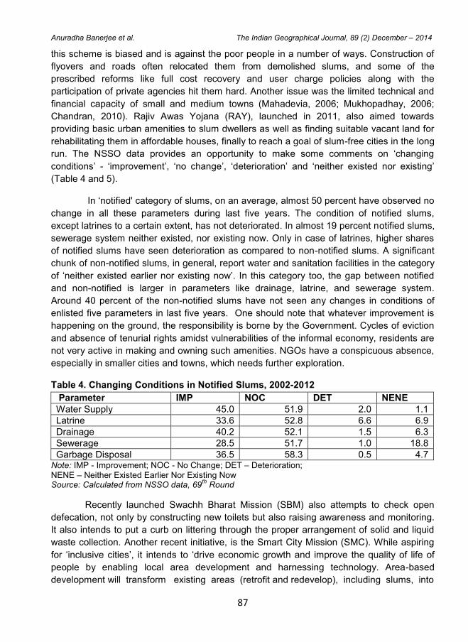
87
Anuradha Banerjee et al. The Indian Geographical Journal, 89 (2) December – 2014
this scheme is biased and is against the poor people in a number of ways. Construction of
flyovers and roads often relocated them from demolished slums, and some of the
prescribed reforms like full cost recovery and user charge policies along with the
participation of private agencies hit them hard. Another issue was the limited technical and
financial capacity of small and medium towns (Mahadevia, 2006; Mukhopadhay, 2006;
Chandran, 2010). Rajiv Awas Yojana (RAY), launched in 2011, also aimed towards
providing basic urban amenities to slum dwellers as well as finding suitable vacant land for
rehabilitating them in affordable houses, finally to reach a goal of slum-free cities in the long
run. The NSSO data provides an opportunity to make some comments on „changing
conditions‟ - „improvement‟, „no change‟, „deterioration‟ and „neither existed nor existing‟
(Table 4 and 5).
In „notified' category of slums, on an average, almost 50 percent have observed no
change in all these parameters during last five years. The condition of notified slums,
except latrines to a certain extent, has not deteriorated. In almost 19 percent notified slums,
sewerage system neither existed, nor existing now. Only in case of latrines, higher shares
of notified slums have seen deterioration as compared to non-notified slums. A significant
chunk of non-notified slums, in general, report water and sanitation facilities in the category
of „neither existed earlier nor existing now‟. In this category too, the gap between notified
and non-notified is larger in parameters like drainage, latrine, and sewerage system.
Around 40 percent of the non-notified slums have not seen any changes in conditions of
enlisted five parameters in last five years. One should note that whatever improvement is
happening on the ground, the responsibility is borne by the Government. Cycles of eviction
and absence of tenurial rights amidst vulnerabilities of the informal economy, residents are
not very active in making and owning such amenities. NGOs have a conspicuous absence,
especially in smaller cities and towns, which needs further exploration.
Table 4. Changing Conditions in Notified Slums, 2002-2012
Parameter IMP NOC DET NENE
Water Supply 45.0 51.9 2.0 1.1
Latrine 33.6 52.8 6.6 6.9
Drainage 40.2 52.1 1.5 6.3
Sewerage 28.5 51.7 1.0 18.8
Garbage Disposal 36.5 58.3 0.5 4.7 Note: IMP - Improvement; NOC - No Change; DET – Deterioration; NENE – Neither Existed Earlier Nor Existing Now Source: Calculated from NSSO data, 69
th Round
Recently launched Swachh Bharat Mission (SBM) also attempts to check open
defecation, not only by constructing new toilets but also raising awareness and monitoring.
It also intends to put a curb on littering through the proper arrangement of solid and liquid
waste collection. Another recent initiative, is the Smart City Mission (SMC). While aspiring
for „inclusive cities‟, it intends to „drive economic growth and improve the quality of life of
people by enabling local area development and harnessing technology. Area-based
development will transform existing areas (retrofit and redevelop), including slums, into
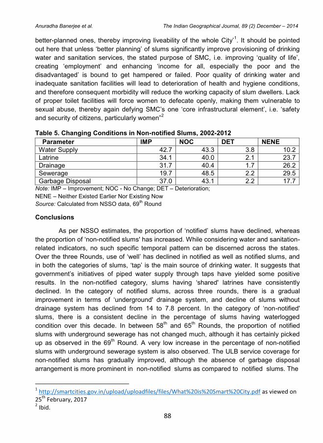
88
Anuradha Banerjee et al. The Indian Geographical Journal, 89 (2) December – 2014
better-planned ones, thereby improving liveability of the whole City‟1. It should be pointed
out here that unless „better planning‟ of slums significantly improve provisioning of drinking
water and sanitation services, the stated purpose of SMC, i.e. improving „quality of life‟,
creating „employment‟ and enhancing „income for all, especially the poor and the
disadvantaged‟ is bound to get hampered or failed. Poor quality of drinking water and
inadequate sanitation facilities will lead to deterioration of health and hygiene conditions,
and therefore consequent morbidity will reduce the working capacity of slum dwellers. Lack
of proper toilet facilities will force women to defecate openly, making them vulnerable to
sexual abuse, thereby again defying SMC‟s one „core infrastructural element‟, i.e. „safety
and security of citizens, particularly women”2
Table 5. Changing Conditions in Non-notified Slums, 2002-2012
Parameter IMP NOC DET NENE
Water Supply 42.7 43.3 3.8 10.2
Latrine 34.1 40.0 2.1 23.7
Drainage 31.7 40.4 1.7 26.2
Sewerage 19.7 48.5 2.2 29.5
Garbage Disposal 37.0 43.1 2.2 17.7 Note: IMP – Improvement; NOC - No Change; DET – Deterioration;
NENE – Neither Existed Earlier Nor Existing Now
Source: Calculated from NSSO data, 69th
Round
Conclusions
As per NSSO estimates, the proportion of „notified‟ slums have declined, whereas
the proportion of „non-notified slums' has increased. While considering water and sanitation-
related indicators, no such specific temporal pattern can be discerned across the states.
Over the three Rounds, use of „well‟ has declined in notified as well as notified slums, and
in both the categories of slums, „tap‟ is the main source of drinking water. It suggests that
government‟s initiatives of piped water supply through taps have yielded some positive
results. In the non-notified category, slums having „shared' latrines have consistently
declined. In the category of notified slums, across three rounds, there is a gradual
improvement in terms of „underground' drainage system, and decline of slums without
drainage system has declined from 14 to 7.8 percent. In the category of „non-notified'
slums, there is a consistent decline in the percentage of slums having waterlogged
condition over this decade. In between 58th and 65
th Rounds, the proportion of notified
slums with underground sewerage has not changed much, although it has certainly picked
up as observed in the 69th Round. A very low increase in the percentage of non-notified
slums with underground sewerage system is also observed. The ULB service coverage for
non-notified slums has gradually improved, although the absence of garbage disposal
arrangement is more prominent in non-notified slums as compared to notified slums. The
1 http://smartcities.gov.in/upload/uploadfiles/files/What%20is%20Smart%20City.pdf as viewed on
25th
February, 2017 2 Ibid.
89
Anuradha Banerjee et al. The Indian Geographical Journal, 89 (2) December – 2014
gaps between notified and non-notified slums have continued to increase in terms of latrine
availability. Four indicators, however, show inconsistent results (i.e. decline of gaps in
between 58th and 65
th Round, and increase in 69
th Round). The evaluation of plans,
policies, and schemes coupled with latest Round observations on changing conditions of
water and sanitation related parameters suggest that slums still need better availability of
amenities. Non-notified slums are in comparatively poorer condition, because a lion's share
of these clusters have not seen the presence of any services earlier and even now in last
five years, these services are conspicuously absent. Given the fact of very low shares of
expenditure allotted under BSUP in JNNURM, discontinuation of RAY and only limited
expansion of Swachh Bharat Mission programme, it is understandable that slums will take
much time to even get such basic amenities, and the gap between notified and non-notified
slums may continue to remain at large. This also raises broader issues of how to achieve
inclusive urban growth and make out cities resilient and smart.
Acknowledgements
We are thankful to our peer Research Scholars in CSRD, namely, Sharmistha
Singh for providing NSSO raw dataset and, Asha Bauri and Biswajit Kar for helping in data
extraction methods. CSRD deserves special mention for making raw NSSO dataset
available.
References
1. Bhan, G., and Jana, A. (2013). of slums or poverty: Notes of Caution from Census 2011. Economic and Political Weekly, 48(18), pp. 13-16.
2. Chandran, D. (2010). An appraisal of Jawaharlal Nehru National Urban Renewal Mission (JNNURM): Case Studies of Thiruvananthapuram and Kochi, MPhil Dissertation, Jawaharlal Nehru University, New Delhi, India.
3. Dupont, V. (2008). Slum Demolitions in Delhi since the 1990s: An Appraisal. Economic and Political Weekly, 43(28), pp. 79-87.
4. Hazra, T., and Goel, S. (2009). Solid waste management in Kolkata, India: Practices and Challenges. Waste Management, 29, pp. 470-478.
5. Kundu, A., and Saraswati, L. R. (2012). Migration and Exclusionary Urbanisation in India. Economic and Political Weekly, 47 (26-27), pp. 219-227.
6. Kundu, D., and Samanta, D. (2011). Redefining the Inclusive Urban Agenda in India. Economic and Political Weekly, 46(5), pp. 55-63.
7. Mahadevia, D. (2006). NURM and the Poor in Globalising Mega Cities. Economic and Political Weekly. 41(31), pp. 3399-3403.
8. Ministry of Urban Development and Poverty Alleviation (2001). India: National Report - Progress of Implementation of the Habitat Agenda (1996-2000), Istanbul +5 UNCHS (Habitat) Conference, 2001.
9. Mitlin, D. (2005). Understanding chronic poverty in urban areas. International Planning Studies. 10:1, pp. 3-19.
10. Mukhopadhay, P. (2006). Whither Urban Renewal?. Economic and Political Weekly, 41(10), pp. 879-884.
11. Patel, S. B. (2011). Inclusionary Housing. Economic and Political Weekly, 46(43), pp. 13-14.
12. Sengupta, C. (1999). Dynamics of Community Environmental Management in Howrah
Slums. Economic and Political Weekly, 34(21), pp. 1292-1296. World Health
Organisation.
The Indian Geographical Journal
Volume 89 (2) December - 2014, pp 90-99 ISSN 0019-4824
90
AGRO-CLIMATIC REGIONALISATION AND WATER BALANCE OF GUNTUR DISTRICT, ANDHRA PRADESH
Srinivasa Gopinath G.S.1 and Chandrayudu N.
2
1VLITS, Department of BS & H, Vadlamudi - 522 213
2Department of Geography, S.V. University, Tirupati - 517 502
E-mail: [email protected], [email protected] Abstract
An ‘Agro-climatic zone’ is a land unit in terms of major climates, suitable for a certain range
of crops. Agro-climatic conditions mainly refer to soil types, rainfall, temperature and water
availability (Water balance) which influences the type of vegetations. The study area is one
of the few ‘Crop intensive districts’ in A. P. In Guntur district different Agricultural&
Horticultural crops are being raised. By using ‘water balance technique’ Agro-climatic
Regionalisation can be studied. The water balance study has also become important in the
field of eco climatology. It also strives to gauge and estimate the water balance of the study
area by adopting the method of Thornthwaite and Mather. The water-balance framework
thus extracted guides in the understanding the agricultural appropriateness of the region,
establishment of drought years by their magnitude and portrayal of drought-prone areas.
The study indicated that crop cultivation without dependability on irrigation is not possible in
the district especially during Rabi season. Agro-climatic regionalisation revealed the fact
that paddy cultivation is not possible without irrigation in most parts of the district. With
irrigation, paddy cultivation will be prosperous in coastal regions. However, with little
irrigation facilities, millet crops will give good yields. The present study is an attempt on an
area which has typical physical and climatic variations, in turn, leads for agro-climatic
regionalisation.
Keywords: Indian Economy, Seasonal soil moisture, Agro-climatic region, Coefficient of
rainfall variability, Crop suitability.
Introduction
Agricultural development of any region is mainly controlled by climatic and edaphic
factors of a region. In addition, proper planning of land use/land cover conditions is quite
indispensable for achieving the desired target. Agriculture is the key input for India‟s
economy. About forty-five percent of India‟s geographical area is availed for agriculture and
two-thirds of country‟s population engaged in agriculture, the success of which almost
wholly depends on a sufficient and well-distributed rainfall apart from other climatic and
edaphic conditions. Higher crop production can be achieved by proper management of
water and soil resources in the light of temperature and rainfall conditions though irrigation
projects have coming up in a big way during the last few decades, yet the area under
irrigation remains to be less than adequate. Hence, suitable crops should be selected
according to the available resources instead of going for the crop which is not suitable for
91
Srinivasa Gopinath G.S. and Chandrayudu N. The Indian Geographical Journal, 89 (2) December – 2014
existing climatic conditions. The guiding principle in the selection of crops and cropping
systems should be that their growth period should coincide with the duration of moisture
availability. The following are the objectives for the present study 1. To find out that
temperature is not a constraint factor for the growth of crops in tropical environments like
India in general and Andhra Pradesh / Guntur in particular. 2. To assess the variability of
rainfall and water balance. 3. To assess the agro -climatic regions (agro climatic
regionalisation).
The study proposes following hypotheses namely, 1. An „Agro-climatic zone‟ is a
land unit in terms of major climates, suitable for a certain range of crops. Agro-climatic
conditions mainly refer to soil types, rainfall, temperature and water availability (Water
balance) which influences the type of vegetations. 2. The study area is one of the few „Crop
intensive districts‟ in A. P. 3. In Guntur district different Agricultural& Horticultural crops are
being raised. By using „water balance technique‟ Agro-climatic Regionalisation can be
studied.
Database and Methodology
For the present study two atmospheric elements viz., mean monthly air
temperature and mean monthly rainfall are needed to do water balance. Thus, the data of
twenty representative Mandals of the Guntur district were collected/gathered from the
records of India Meteorological Department for a period of 30 years that is from 1983-2013.
Agricultural improvement of any region can be accomplished by an appropriate outlying of
land use/land cover, taking into the climatic and soil factors of the region into consideration.
The two environmental parameters that are associated with crop production are rainfall and
temperature. Temperature is now not a constraint aspect for the increase of crops in the
tropical environments like India in typical and Andhra Pradesh / Guntur in particular, while,
rainfall which is a principle ecological parameter is accountable for various agricultural
patterns in the world. High or low attention of farming is completely established on rainfall
intensity. The low and erratic nature of rainfall is responsible for the low seasonal soil
moisture availability at the root zone. Thus, the study of the variability of rainfall in specific
vicinity is essential. The book-keeping method of Thornthwaite and Mather, which has a
multivariate utility in scientific research additionally acts as a device to delineate agro-
climatic regions is used for this study. Each of the agro-climatic areas indicates its suitability
to specific crops based totally on the soil moisture prominence of that region. In addition,
water balance process helps in measuring soil moisture storage which is the principal
element to be understood for agricultural planning. GIS technique is also employed for the
representation of the results.
Study Area
Guntur district is in Andhra Pradesh, India, on the east coast of Bay of Bengal. It
has a coastline of about 100 kilometres. The district is located between 15018
' - 16
050
' N
latitude and 79019‟-80
055
' East longitude. The total area of the district is about 11,400
sq.km with a population of 48.9 lakh (2011, Census). The district‟s population density is 430
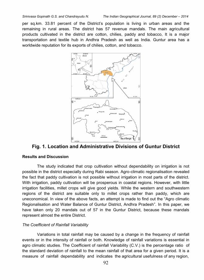
92
Srinivasa Gopinath G.S. and Chandrayudu N. The Indian Geographical Journal, 89 (2) December – 2014
per sq.km. 33.81 percent of the District‟s population is living in urban areas and the
remaining in rural areas. The district has 57 revenue mandals. The main agricultural
products cultivated in the district are cotton, chilies, paddy and tobacco, It is a major
transportation and textile hub in Andhra Pradesh as well as India. Guntur area has a
worldwide reputation for its exports of chilies, cotton, and tobacco.
Fig. 1. Location and Administrative Divisions of Guntur District
Results and Discussion
The study indicated that crop cultivation without dependability on irrigation is not
possible in the district especially during Rabi season. Agro-climatic regionalisation revealed
the fact that paddy cultivation is not possible without irrigation in most parts of the district.
With irrigation, paddy cultivation will be prosperous in coastal regions. However, with little
irrigation facilities, millet crops will give good yields. While the western and southwestern
regions of the district are suitable only to millet crops rather than paddy, which are
uneconomical. In view of the above facts, an attempt is made to find out the “Agro climatic
Regionalisation and Water Balance of Guntur District, Andhra Pradesh”. In this paper, we
have taken only 20 mandals out of 57 in the Guntur District, because these mandals
represent almost the entire District.
The Coefficient of Rainfall Variability
Variations in total rainfall may be caused by a change in the frequency of rainfall
events or in the intensity of rainfall or both. Knowledge of rainfall variations is essential in
agro climatic studies. The Coefficient of rainfall Variability (C.V.) is the percentage ratio of
the standard deviation of rainfall to the mean rainfall of that area for a given period. It is a
measure of rainfall dependability and indicates the agricultural usefulness of any region,
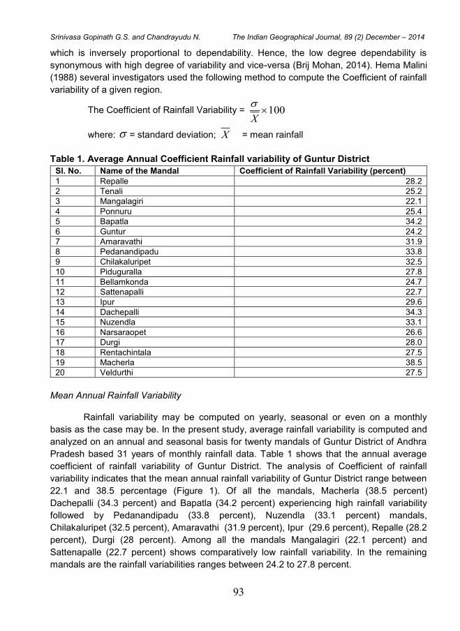
93
Srinivasa Gopinath G.S. and Chandrayudu N. The Indian Geographical Journal, 89 (2) December – 2014
which is inversely proportional to dependability. Hence, the low degree dependability is
synonymous with high degree of variability and vice-versa (Brij Mohan, 2014). Hema Malini
(1988) several investigators used the following method to compute the Coefficient of rainfall
variability of a given region.
The Coefficient of Rainfall Variability = 100X
where: = standard deviation; X = mean rainfall
Table 1. Average Annual Coefficient Rainfall variability of Guntur District
Sl. No. Name of the Mandal Coefficient of Rainfall Variability (percent)
1 Repalle 28.2
2 Tenali 25.2
3 Mangalagiri 22.1
4 Ponnuru 25.4
5 Bapatla 34.2
6 Guntur 24.2
7 Amaravathi 31.9
8 Pedanandipadu 33.8
9 Chilakaluripet 32.5
10 Piduguralla 27.8
11 Bellamkonda 24.7
12 Sattenapalli 22.7
13 Ipur 29.6
14 Dachepalli 34.3
15 Nuzendla 33.1
16 Narsaraopet 26.6
17 Durgi 28.0
18 Rentachintala 27.5
19 Macherla 38.5
20 Veldurthi 27.5
Mean Annual Rainfall Variability
Rainfall variability may be computed on yearly, seasonal or even on a monthly
basis as the case may be. In the present study, average rainfall variability is computed and
analyzed on an annual and seasonal basis for twenty mandals of Guntur District of Andhra
Pradesh based 31 years of monthly rainfall data. Table 1 shows that the annual average
coefficient of rainfall variability of Guntur District. The analysis of Coefficient of rainfall
variability indicates that the mean annual rainfall variability of Guntur District range between
22.1 and 38.5 percentage (Figure 1). Of all the mandals, Macherla (38.5 percent)
Dachepalli (34.3 percent) and Bapatla (34.2 percent) experiencing high rainfall variability
followed by Pedanandipadu (33.8 percent), Nuzendla (33.1 percent) mandals,
Chilakaluripet (32.5 percent), Amaravathi (31.9 percent), Ipur (29.6 percent), Repalle (28.2
percent), Durgi (28 percent). Among all the mandals Mangalagiri (22.1 percent) and
Sattenapalle (22.7 percent) shows comparatively low rainfall variability. In the remaining
mandals are the rainfall variabilities ranges between 24.2 to 27.8 percent.

94
Srinivasa Gopinath G.S. and Chandrayudu N. The Indian Geographical Journal, 89 (2) December – 2014
The inference is the high rainfall variability indicates a low degree of dependability
on rainfall and that exists in Macharla and Dachepalle mandals. The dependability on
rainfall is comparatively high in Mangalagiri and Sattenapalle, which shows low rainfall
variabilities. In the remaining districts, the dependability on rainfall is in between. The
analysis indicates that in the higher rainfall variability regions, there is a need for systematic
irrigation scheduling and preparation of crop weather calendar to adjust the phenology
growth of the crop.
Seasonal Rainfall Variability
Further, knowledge of seasonal variability of rainfall provides better information as it
is significant in agriculture point of view. Hence, for better understanding, seasonal rainfall
variability of the study area during cropping seasons was worked out. In India, cropping
season is from July to June and it is mainly recognized as two seasons namely the Kharif
and Rabi. „Kharif‟ means autumn in Arabic. Kharif crops are sown with the beginning of first
rains in July, during the monsoon season and harvest in autumn (October-November).
Kharif crops are totally dependent on the quantity of rainfall as well as on its timing. The
main crops grown during kharif season include paddy, jowar, bajra, maize, ragi, pulses,
sesamum, castor, sunflower, soya bean, cotton and sugarcane and the crops grown from
October to March are known as Rabi crops.
The kharif season starts with the onset of southwest monsoon while the rabi
season kicks off after the summer monsoon and continues through the following spring
associated with northeast winter monsoon (October-December). The major rabi crops are
barley, potato, wheat, grams, mustard, onion. Etc. The precipitation during the term of
summer monsoon season contributes soil moisture to rabi crops, at the same time kharif
crops are precisely influenced by day-to-day fluctuations in summer monsoon precipitation.
Hence, the precipitation in summer monsoon season is significant for both the kharif and
rabi crops (Gadgil, 1996; Swami, 2001 and Chaudhary, 2010).
Southwest monsoon season which is associated with kharif cropping performs a
crucial role in agriculture, economy, quality of life and living status of the population. More
than 75 percent of rainfall received by India is during this season. Therefore, the prosperity
of Kharif crops completely based on the quantity of rainfall received during this season. An
upturn in precipitation generally associated with a boost in the yields of food grain. And the
decrease of rainfall reflects in the decrease in the yields and sometimes completes failure
of crops. Fluctuations in the monsoon‟s precipitation dominate the Indian economy
drastically as it is mostly based on agriculture (Jameson, 1932).
Studies indicated that Year to year variations strongly related to kharif grain food
production, even 10 percent decrease of the long-term average precipitation leads to
serious shrinkage in paddy yields (Palmer, 1995; Gadgil, 1996 and Brij Mohan, 2014).
According to Gadgil (1996), the deficit of monsoon precipitation during kharif season has a
larger negative impact than the positive impact of good rainfall on crops. Drought due to
lack of rainfall during this season reduces the yields of the crops and excess rainfall
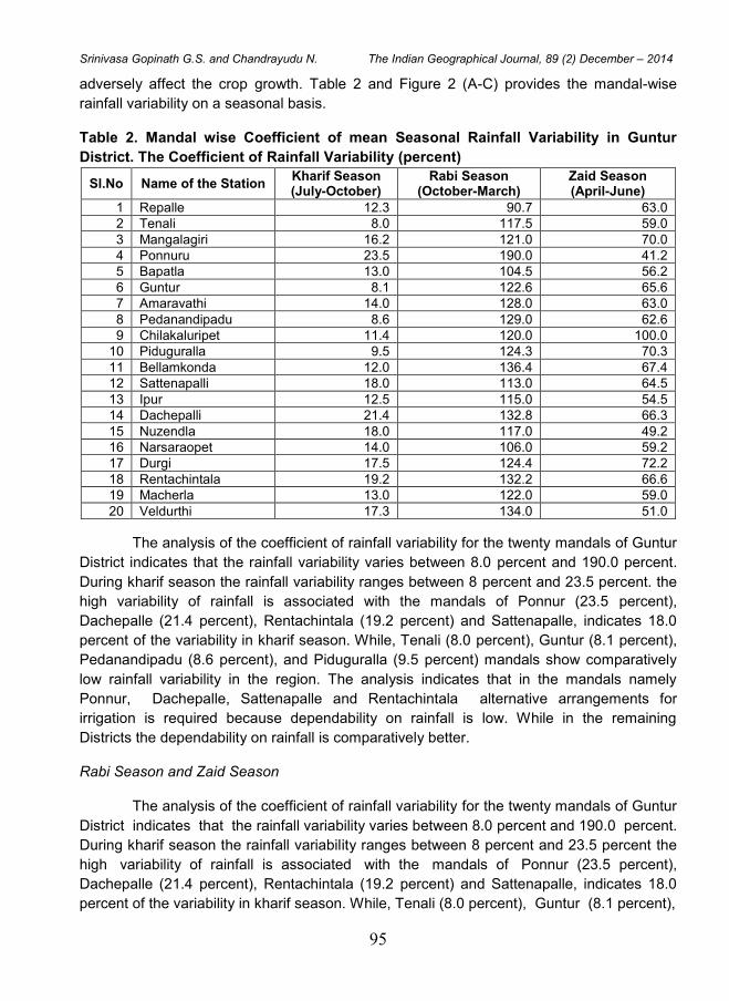
95
Srinivasa Gopinath G.S. and Chandrayudu N. The Indian Geographical Journal, 89 (2) December – 2014
adversely affect the crop growth. Table 2 and Figure 2 (A-C) provides the mandal-wise
rainfall variability on a seasonal basis.
Table 2. Mandal wise Coefficient of mean Seasonal Rainfall Variability in Guntur
District. The Coefficient of Rainfall Variability (percent)
Sl.No Name of the Station Kharif Season (July-October)
Rabi Season (October-March)
Zaid Season (April-June)
1 Repalle 12.3 90.7 63.0
2 Tenali 8.0 117.5 59.0
3 Mangalagiri 16.2 121.0 70.0
4 Ponnuru 23.5 190.0 41.2
5 Bapatla 13.0 104.5 56.2
6 Guntur 8.1 122.6 65.6
7 Amaravathi 14.0 128.0 63.0
8 Pedanandipadu 8.6 129.0 62.6
9 Chilakaluripet 11.4 120.0 100.0
10 Piduguralla 9.5 124.3 70.3
11 Bellamkonda 12.0 136.4 67.4
12 Sattenapalli 18.0 113.0 64.5
13 Ipur 12.5 115.0 54.5
14 Dachepalli 21.4 132.8 66.3
15 Nuzendla 18.0 117.0 49.2
16 Narsaraopet 14.0 106.0 59.2
17 Durgi 17.5 124.4 72.2
18 Rentachintala 19.2 132.2 66.6
19 Macherla 13.0 122.0 59.0
20 Veldurthi 17.3 134.0 51.0
The analysis of the coefficient of rainfall variability for the twenty mandals of Guntur
District indicates that the rainfall variability varies between 8.0 percent and 190.0 percent.
During kharif season the rainfall variability ranges between 8 percent and 23.5 percent. the
high variability of rainfall is associated with the mandals of Ponnur (23.5 percent),
Dachepalle (21.4 percent), Rentachintala (19.2 percent) and Sattenapalle, indicates 18.0
percent of the variability in kharif season. While, Tenali (8.0 percent), Guntur (8.1 percent),
Pedanandipadu (8.6 percent), and Piduguralla (9.5 percent) mandals show comparatively
low rainfall variability in the region. The analysis indicates that in the mandals namely
Ponnur, Dachepalle, Sattenapalle and Rentachintala alternative arrangements for
irrigation is required because dependability on rainfall is low. While in the remaining
Districts the dependability on rainfall is comparatively better.
Rabi Season and Zaid Season
The analysis of the coefficient of rainfall variability for the twenty mandals of Guntur
District indicates that the rainfall variability varies between 8.0 percent and 190.0 percent.
During kharif season the rainfall variability ranges between 8 percent and 23.5 percent the
high variability of rainfall is associated with the mandals of Ponnur (23.5 percent),
Dachepalle (21.4 percent), Rentachintala (19.2 percent) and Sattenapalle, indicates 18.0
percent of the variability in kharif season. While, Tenali (8.0 percent), Guntur (8.1 percent),
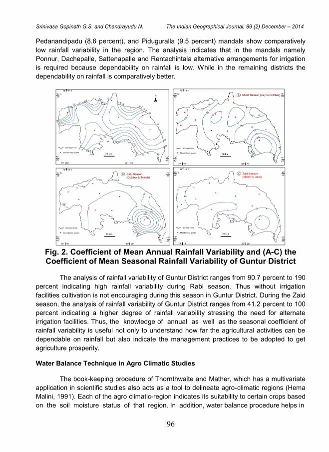
96
Srinivasa Gopinath G.S. and Chandrayudu N. The Indian Geographical Journal, 89 (2) December – 2014
Pedanandipadu (8.6 percent), and Piduguralla (9.5 percent) mandals show comparatively
low rainfall variability in the region. The analysis indicates that in the mandals namely
Ponnur, Dachepalle, Sattenapalle and Rentachintala alternative arrangements for irrigation
is required because dependability on rainfall is low. While in the remaining districts the
dependability on rainfall is comparatively better.
Fig. 2. Coefficient of Mean Annual Rainfall Variability and (A-C) the Coefficient of Mean Seasonal Rainfall Variability of Guntur District
The analysis of rainfall variability of Guntur District ranges from 90.7 percent to 190
percent indicating high rainfall variability during Rabi season. Thus without irrigation
facilities cultivation is not encouraging during this season in Guntur District. During the Zaid
season, the analysis of rainfall variability of Guntur District ranges from 41.2 percent to 100
percent indicating a higher degree of rainfall variability stressing the need for alternate
irrigation facilities. Thus, the knowledge of annual as well as the seasonal coefficient of
rainfall variability is useful not only to understand how far the agricultural activities can be
dependable on rainfall but also indicate the management practices to be adopted to get
agriculture prosperity.
Water Balance Technique in Agro Climatic Studies
The book-keeping procedure of Thornthwaite and Mather, which has a multivariate
application in scientific studies also acts as a tool to delineate agro-climatic regions (Hema
Malini, 1991). Each of the agro climatic-region indicates its suitability to certain crops based
on the soil moisture status of that region. In addition, water balance procedure helps in
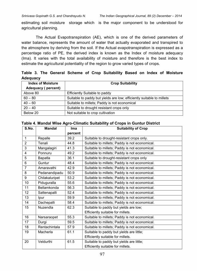
97
Srinivasa Gopinath G.S. and Chandrayudu N. The Indian Geographical Journal, 89 (2) December – 2014
estimating soil moisture storage which is the major component to be understood for
agricultural planning.
The Actual Evapotranspiration (AE), which is one of the derived parameters of
water balance, represents the amount of water that actually evaporated and transpired to
the atmosphere by deriving from the soil. If the Actual evapotranspiration is expressed as a
percentage ratio of PE, the derived index is known as the Index of moisture adequacy
(Ima). It varies with the total availability of moisture and therefore is the best index to
estimate the agricultural potentiality of the region to grow varied types of crops.
Table 3. The General Scheme of Crop Suitability Based on Index of Moisture
Adequacy
Index of Moisture
Adequacy ( percent)
Crop Suitability
Above 80 Efficiently Suitable to paddy
60 – 80 Suitable to paddy but yields are low; efficiently suitable to millets
40 – 60 Suitable to millets; Paddy is not economical
20 – 40 Suitable to drought resistant crops only
Below 20 Not suitable to crop cultivation
Table 4. Mandal Wise Agro-Climatic Suitability of Crops in Guntur District
S.No. Mandal Ima
percent
Suitability of Crop
1 Repalle 39.2 Suitable to drought-resistant crops only.
2 Tenali 44.8 Suitable to millets; Paddy is not economical.
3 Mangalagiri 41.3 Suitable to millets; Paddy is not economical.
4 Ponnuru 49.2 Suitable to millets; Paddy is not economical.
5 Bapatla 36.1 Suitable to drought-resistant crops only
6 Guntur 48.4 Suitable to millets; Paddy is not economical.
7 Amaravathi 42.9 Suitable to millets; Paddy is not economical.
8 Pedanandipadu 50.9 Suitable to millets; Paddy is not economical.
9 Chilakaluripet 53.2 Suitable to millets; Paddy is not economical.
10 Piduguralla 55.6 Suitable to millets; Paddy is not economical.
11 Bellamkonda 56.3 Suitable to millets; Paddy is not economical.
12 Sattenapalli 52.4 Suitable to millets; Paddy is not economical.
13 Ipur 59.9 Suitable to millets; Paddy is not economical.
14 Dachepalli 58.4 Suitable to millets; Paddy is not economical.
15 Nuzendla 62.3 Suitable to paddy but yields are low;
Efficiently suitable for millets.
16 Narsaraopet 55.3 Suitable to millets; Paddy is not economical.
17 Durgi 59.5 Suitable to millets; Paddy is not economical.
18 Rentachintala 57.9 Suitable to millets; Paddy is not economical.
19 Macherla 61.1 Suitable to paddy but yields are little;
Efficiently suitable for millets.
20 Veldurthi 61.5 Suitable to paddy but yields are little;
Efficiently suitable for millets.
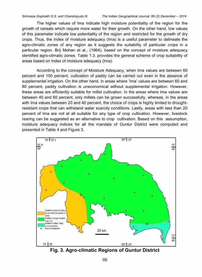
98
Srinivasa Gopinath G.S. and Chandrayudu N. The Indian Geographical Journal, 89 (2) December – 2014
The higher values of Ima indicate high moisture potentiality of the region for the
growth of cereals which require more water for their growth. On the other hand, low values
of this parameter indicate low potentiality of the region and restricted for the growth of dry
crops. Thus, the Index of moisture adequacy (Ima) is a useful parameter to delineate the
agro-climatic zones of any region as it suggests the suitability of particular crops in a
particular region. Brij Mohan et al., (1964), based on the concept of moisture adequacy
identified agro-climatic zones. Table 1.3. provides the general scheme of crop suitability of
areas based on Index of moisture adequacy (Ima).
According to the concept of Moisture Adequacy, when Ima values are between 60
percent and 100 percent, cultivation of paddy can be carried out even in the absence of
supplemental irrigation. On the other hand, in areas where „Ima‟ values are between 60 and
80 percent, paddy cultivation is uneconomical without supplemental irrigation. However,
these areas are efficiently suitable for millet cultivation. In the areas where Ima values are
between 40 and 60 percent, only millets can be grown successfully, whereas, in the areas
with Ima values between 20 and 40 percent, the choice of crops is highly limited to drought-
resistant crops that can withstand water scarcity conditions. Lastly, areas with less than 20
percent of Ima are not at all suitable for any type of crop cultivation. However, livestock
rearing can be suggested as an alternative to crop cultivation. Based on this assumption,
moisture adequacy indices for all the mandals of Guntur District were computed and
presented in Table 4 and Figure 3.
Fig. 3. Agro-climatic Regions of Guntur District
99
Srinivasa Gopinath G.S. and Chandrayudu N. The Indian Geographical Journal, 89 (2) December – 2014
Conclusions
The moisture adequacies of Guntur District as a whole ranging between 36.1
percent and 62.3 percent. The maximum crop potentiality lies along with the coastal areas
and it decreases towards western and south-western interior parts. However, the entire
district can be recognized into three distinct agro-climatic zones namely; (1) suitable to
paddy but efficiently suitable to millets, and (2) suitable to millets, Paddy is not economical,
(3) Reasonable to drought-resistant crops only. (Figure 3). Based on moisture status it was
found that the mandals of the district namely Nuzandla, Veldurthy and Macherla are
suitable to paddy but efficiently suitable to millets. However, with efficient irrigation, Paddy
may be prosperous in these mandals. The remaining mandals of the coastal region are
suitable to millets only. Though paddy is grown in these regions with the help of irrigation
facilities, those efforts will be uneconomical because of low yields of paddy. Instead, if the
same irrigation facilities extended to millet crops in these mandals, the yield will be high and
economical.
References
1. Brij Mohan S.R., Ridhima S., Vivek S., Laxman S R., Tilok S.R., Subrahmanyam G.V.,
Murari Mohan Roy, (2014). Drought Conditions and Management Strategies in India,
Country Report prepared for the Regional Workshop for Asia- Pacific as part of the UN-
Water Initiative on “Capacity Development to support national Drought Management
Policies, pp. 1-7.
2. Census (2001), Census of India, http://censusindia.gov.in (Accessed on 18.06.2013)
3. Chaudhary K.B., (2010). Climate Change and Indian Agriculture, National Magazine of
farmer‟s voice, Agric. Easterling, pp. 50-57.
4. Gadgil S., (1996). Climate change and agriculture – an Indian perspective; In Climate
Variability and Agriculture (eds) Abrol YR, Gadgil S and Pant G B (New Delhi, India:
Narosa) pp. 1–18.
5. Jameson, H., (1932). The Liability to drought at Colombo. .R.met.Soc, 58, pp.50-65
John Wiley & Sons, Chister, pp. 9 -194.
6. Hema Malini B., (1991). Agro-climatic regionalisation and crop suitability: a case study
of Visakhapatnam district, in Agriculture: Planning and Development (Ed.), IBH Publ.,
pp. 163-172.
7. Hema Malini, B., (1988). Ecoclimatological aspects of the drought-prone area of Andhra
Pradesh - Anantapur. Report submitted to University Grants Commission, New Delhi.
8. Palmer, Waye. C., (1965). Meteorological droughts, weather bureau research paper
No.5, U.S, Department of Commerce, and Washington D.C. Sapozhniskova, S.A.,
91958): Agro-climatic indices in agrometeorological problems, (Eds. P.F. Davitaya and
M.S. Kulik, Met. Transl. No.7. Dept. of Transport (Met. branch), Toronto, pp.71-74.
9. Swami, S. K., (2001). Management of drought in India. UNDP Sub-regional Seminar on
Drought Mitigation, Iran.
The Indian Geographical Journal
Volume 89 (2) December - 2014, pp 100-107
ISSN 0019-4824
100
PHYSICO-CHEMICAL AND PHYTOPLANKTON STUDIES IN
COASTAL WATERS OF KANYAKUMARI-INTERMONSOON
SCENARIO
Yoganandan V.1, Nisha Priyadarshini D.
2, and Krishnaveni M.
2
1Department of Marine Science, Bharathidasan University, Tiruchirappalli - 620 024
2Department of Marine Science, M.S. University, Rajakkamangalam - 629 502
E-mail: [email protected]
Abstract
As we know about 60 per cent of the world population live near the coastal area and they
depend on the ocean for their survival and it is well-known fact that 80 per cent of the world
fish catch comes from the continental shelf region. Hence, monitoring coastal water is
essential to maintain the healthy coastal ecosystem. In the present study physico-chemical
parameters and phytoplankton studies carried out in the inshore coastal waters of
Kanyakumari during the intermonsoon period to know the environmental condition of the
marine environment, nutrient level and the link between the oceanographic conditions. The
study revealed that distribution and diversity of the phyto and zooplankton community
influence the nutrient level of the coastal waters and regional climatic conditions that plays
a significant role in the nutrient level of the coastal water, which is proved through this
study.
Keywords: Inter-monsoon, Southeastern Arabian Sea, Phytoplankton, Physico-chemical,
Coastal waters
Introduction
Oceans cover nearly 70 per cent of the Earth's surface, which not only gives a
pleasant blue colour to our planet earth but also drives and regulates the earths’ climate
system through its physical, chemical and biological processes, which makes existence of
life forms. It is also proved that the climate change has control on specie’s diversity in the
earth. Biological productivity in the Arabian Sea is strongly linked to the intensity of the
monsoon, although the lowest biological productivity was noticed during the inter-monsoon
period in the Arabian Sea. These strong seasonal contrasts during summer, winter and
inter-monsoon periods reflects in water column productivity of the Arabian Sea and
therefore, considered as an excellent natural laboratory to study the productivity changes.
The complex dynamism in physico-chemical characteristics of coastal waters is related to
riverine flows, upwellings, atmospheric depositions, vertical mixing and other anthropogenic
sources. Hence, the present study was carried out to know the nutrient status of the coastal
waters, off Kanyakumari, especially during the pre-monsoon season of 2011 with an aim to
avoid dilution effect by the copious southwest monsoon.
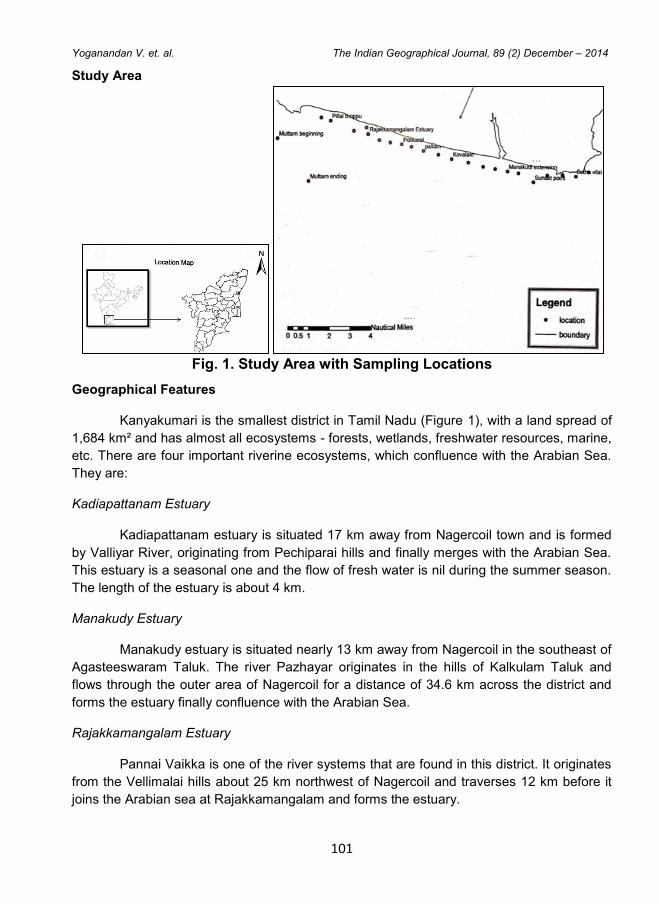
101
Yoganandan V. et. al. The Indian Geographical Journal, 89 (2) December – 2014
Study Area
Fig. 1. Study Area with Sampling Locations
Geographical Features
Kanyakumari is the smallest district in Tamil Nadu (Figure 1), with a land spread of
1,684 km² and has almost all ecosystems - forests, wetlands, freshwater resources, marine,
etc. There are four important riverine ecosystems, which confluence with the Arabian Sea.
They are:
Kadiapattanam Estuary
Kadiapattanam estuary is situated 17 km away from Nagercoil town and is formed
by Valliyar River, originating from Pechiparai hills and finally merges with the Arabian Sea.
This estuary is a seasonal one and the flow of fresh water is nil during the summer season.
The length of the estuary is about 4 km.
Manakudy Estuary
Manakudy estuary is situated nearly 13 km away from Nagercoil in the southeast of
Agasteeswaram Taluk. The river Pazhayar originates in the hills of Kalkulam Taluk and
flows through the outer area of Nagercoil for a distance of 34.6 km across the district and
forms the estuary finally confluence with the Arabian Sea.
Rajakkamangalam Estuary
Pannai Vaikka is one of the river systems that are found in this district. It originates
from the Vellimalai hills about 25 km northwest of Nagercoil and traverses 12 km before it
joins the Arabian sea at Rajakkamangalam and forms the estuary.
102
Yoganandan V. et. al. The Indian Geographical Journal, 89 (2) December – 2014
Thengapattinam Estuary
Thengapattinam estuary, formed by the confluence of river Thamirabarani in
between Thengapattinam and Erayumanthurai.
Database and Methodology
Physico Chemical Parameters Analysis
The temperature was measured on board by high resolution (0.1) thermometer.
Salinity was measured by using salinity refractometer. The pH is a negative logarithm of
hydrogen ion concentration it was measured by digital pH meter.
Inorganic phosphate
The 40 ml water sample taken in the conical flask and mixed reagent is added then
the sample was diluted with distilled water and OD was taken at 882 nm.
Reactive Silicate
Water sample is mixed with 1 ml of HCl, 2 ml of ammonium molybdate after 10
minutes the oxalic acid solution was added and OD was taken at 410 nm.
Nitrate
The NaCl, H2S04 was added in the water sample and mixed well then 0.1ml brucine
sulfanilic acid was added and then placed in a hot water bath for 20 minutes then cooled
and OD was taken at 410 nm. Nitrite: Water sample was mixed with 0.2ml of sulfanilamide
solution and waited for 2 minutes then 0.2ml naphthyl ethylenediamine solution was added
and OD was taken at 543 nm.
Phytoplankton Analysis
For phytoplankton analysis, 500 ml of water sample was preserved in Lugol's iodine
and for the analysis, to identify plankton species we used an inverted microscope at 100x –
400x magnification following the standard literature (Subrahmanyan, 1959, 1971).
Results and Discussion
The physicochemical parameters were analysed from the coastal water of
Kanyakumari and the data is presented here in Table.1.
Temperature
In the present study surface water temperature recorded a minimum of 29.5°C and
a maximum of 30.5° C. Normally tropical water temperature is almost constantly above
25o C.
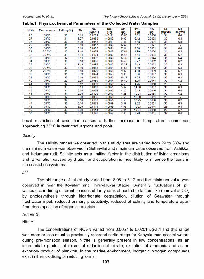
103
Yoganandan V. et. al. The Indian Geographical Journal, 89 (2) December – 2014
Table.1. Physicochemical Parameters of the Collected Water Samples
Local restriction of circulation causes a further increase in temperature, sometimes
approaching 35o C in restricted lagoons and pools.
Salinity
The salinity ranges we observed in this study area are varied from 29 to 33‰ and
the minimum value was observed in Sothavilai and maximum value observed from Azhikkal
and Kelamanakudi. Salinity acts as a limiting factor in the distribution of living organisms
and its variation caused by dilution and evaporation is most likely to influence the fauna in
the coastal ecosystems.
pH
The pH ranges of this study varied from 8.08 to 8.12 and the minimum value was
observed in near the Kovalam and Thiruvalluvar Statue. Generally, fluctuations of pH
values occur during different seasons of the year is attributed to factors like removal of CO2
by photosynthesis through bicarbonate degradation, dilution of Seawater through
freshwater input, reduced primary productivity, reduced of salinity and temperature apart
from decomposition of organic materials.
Nutrients
Nitrite
The concentrations of NO2-N varied from 0.0057 to 0.0201 μg-at/l and this range
was more or less equal to previously recorded nitrite range for Kanyakumari coastal waters
during pre-monsoon season. Nitrite is generally present in low concentrations, as an
intermediate product of microbial reduction of nitrate, oxidation of ammonia and as an
excretory product of plankton. In the marine environment, inorganic nitrogen compounds
exist in their oxidising or reducing forms.
104
Yoganandan V. et. al. The Indian Geographical Journal, 89 (2) December – 2014
Nitrate
The concentrations of NO3-N varied from 0.0040 to 0.0161 μg-at/l and this range
was more or less equal to previously recorded nitrite range for Kanyakumari coastal waters
during pre-monsoon season. Nitrogen supplied through rivers mainly exists as dissolved
nitrate, which is derived from rock weathering and drainage from agricultural lands. Nitrate
is considered as the stable oxidation level of nitrogen in seawater.
Reactive Silicate
The present study shows a minimum of 3.97 and maximum of 17.30 μg Si-at/l. The
source of silica to the marine environment is mainly through river discharges (Livingstone,
1963), with submarine hydrothermal emanations and glacial weathering (Warnke, 1970;
Wolery and Sleep, 1997) also contributing substantially. Silicon is biologically essential for
the growth and the formation of their skeletal materials in marine organisms like diatoms,
radiolarians, and sponges.
Phosphate
Present study shows concentrations of phosphate varied from 3.57 to 16.94 μg-at/l
and this range was more or less equal to the previously recorded range for Kanyakumari
coastal waters. Ecological interest in phosphorus stems from its major role in biological
metabolism in spite of its relatively subdued presence in the hydrosphere. Weathering of
earth's crust and surface water transport deliver phosphorus to coastal waters through
rivers.
Phytoplankton Analysis
We analysed phytoplankton soup under the microscope with the magnification of
100x. Through this analysis, we recorded 20 species and observation also shows
phytoplankton abundant species which is given in Table 2. Marine phytoplankton can be
described as ‘The Jewel of the Ocean’. It contains a unique combination of life-sustaining
nutrients and antioxidants including essential fatty acids, amino acids, protein, vitamins,
chlorophyll, minerals, trace elements, and phytonutrients. Zooplankton is the primary
consumers of the oceans and grazes on the phytoplankton. They themselves are an
important food source for large animals. Basking sharks, whales, fish and some species of
rays rely on zooplankton for their food supply.
Results and Discussion
Temperature and Salinity
Analytical data of the present study are shown in Table 1. The surface water
temperature recorded a minimum of 29.5° C and a maximum of 30.5° C. This range is
considered slightly high when compared to other seasons from earlier studies.
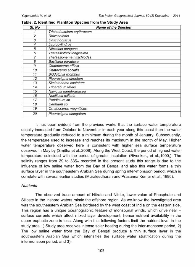
105
Yoganandan V. et. al. The Indian Geographical Journal, 89 (2) December – 2014
Table. 2. Identified Plankton Species from the Study Area
Sl. No Name of the Species
1 Trichodesmium erythraeum
2 Rhizosolenia
3 Coscinodiscus
4 Leptocylindrus
5 Nitszchia pungens
6 Thalassiothrix longissima
7 Thalassionema nitschiodes
8 Bacillaria paradoxa
9 Chaetoceros affinis
10 Chatoceros socialis
11 Biddulphia rhombus
12 Pleurosigma directum
13 Skeletonema costatum
14 Triceratium favus
15 Navicula membranacea
16 Noctiluca miliaris
17 Peridinium sp.
18 Ceratium sp.
19 Ornithocerus magnificus
20 Pleurosigma elongatum
It has been evident from the previous works that the surface water temperature
usually increased from October to November in each year along this coast then the water
temperature gradually reduced to a minimum during the month of January. Subsequently,
the temperature used to increase and reaches its maximum in the month of May. Higher
water temperature observed here is consistent with higher sea surface temperature
observed in May by (Smitha et al.,2008). Along the West Coast, the period of highest water
temperature coincided with the period of greater insolation (Rivonker., et al.,1990,). The
salinity ranges from 29 to 33‰ recorded in the present study this range is due to the
influence of low saline water from the Bay of Bengal and also this water forms a thin
surface layer in the southeastern Arabian Sea during spring inter-monsoon period, which is
correlate with several earlier studies (Muraleedharan and Prasanna Kumar et al., 1996).
Nutrients
The observed trace amount of Nitrate and Nitrite, lower value of Phosphate and
Silicate in the inshore waters mimic the offshore region. As we know the investigated area
was the southeastern Arabian Sea bordered by the west coast of India on the eastern side.
This region has a unique oceanographic feature of monsoonal winds, which drive near –
surface currents which affect mixed layer development, hence nutrient availability in the
upper euphotic zone is less. Along with this following factors limit the nutrient level in the
study area 1) Study area receives intense solar heating during the inter-monsoon period, 2)
The low saline water from the Bay of Bengal produce a thin surface layer in the
southeastern Arabian Sea which intensifies the surface water stratification during the
intermonsoon period, and 3).
106
Yoganandan V. et. al. The Indian Geographical Journal, 89 (2) December – 2014
The very scanty rainfall during this season which drastically reduces the nutrient
influx to the study area (Muraleedharan and Prasannakumar, 1996; Qasim, 2003).All the
above mentioned earlier studies gave the excellent reason for the low nutrient level at
offshore region during the intermonsoon period. If we see the present data set, which
mimics the offshore region, which proved that present study area around 30 metre water
depth also has the similar oceanographic condition, in addition to this phytoplankton
analysis of present study also giving supporting evidence to present argument (which is
discussed below).
Response of Phytoplankton
Through phytoplankton analysis, we identified twenty sp, which is distributed in the
study area during the intermonsoon period; an interesting observation is we could see the
dominance of the following species Trichodesmium erythraeum, Rhizosolenia,
Coscinodiscus, and Leptocylindrus.
The earlier studies from this region suggest that chlorophyll-a concentration is high
in the offshore region, which is contributed mostly by the dominant sp Trichodesmium
erythraeum, the reason for the dominance of this sp is prevailed environmental condition in
this region, which is discussed in-detail in the previous paragraph while discussing nutrient
limiting factors. This interpretation is supported by following previous studies (Nair et
al.,1992; Carpenter, 1993; Capone et al., 1997; Jyothibabu et al., 2003). The present study
area also shows a lower value of major nutrients especially traces amount of nitrogen. This
condition facilitates the dominance of the above-motioned species.
Conclusions
Physico-chemical parameter and phytoplankton studies carried out in the inshore
coastal waters of Kanyakumari during the inter-monsoon period to know the environmental
condition, nutrient level and to know the link between the oceanographic condition and
physicochemical parameter. A summary of the work carried out and the salient findings of
this study are described below. Present study shows that inter-monsoon period has second
highest values of temperature and thin low saline surface water in this region and also the
field observation shows that sea was calm and low wind speed. Influence of upwelling was
not observed during the early stage of the inter-monsoon season. The lower values of all
major nutrients in the surface water suggest that the river input contribution play a major
role in coastal waters. From the present phytoplankton analysis twenty phytoplankton sp
was recorded among this few species were found abundant and they are Trichodesmium
erythraeum, rhizosolenia, coscinodiscus, and leptocylindrus. Distribution and diversity of the
phyto and zoo-plankton community influence the nutrient level of the coastal waters and
regional climatic condition plays a significant role in the nutrient level of the coastal water
which is proved by this study.
107
Yoganandan V. et. al. The Indian Geographical Journal, 89 (2) December – 2014
References
1. Capone, D. G., Zehr, J. P., Paerl, H. W., Bergman, B., and Carpenter, E. J. (1997). Trichodesmium, a globally significant marine cyanobacterium. Science, 276(5316), pp. 1221-1229.
2. Carpenter, E. J., O'Neil, J. M., Dawson, R., Capone, D. G., Siddiqui, P. J., Roenneberg, T., and Bergman, B. (1993). The tropical diazotrophic phytoplankter Trichodesmium: biological characteristics of two common species. Marine Ecology Progress Series, pp. 295-304.
3. Jyothibabu, R., Madhu, N. V., Murukesh, N., Haridas, P. C., Nair, K. K. C., and Venugopal, P. (2003). Intense blooms of Trichodesmium erythraeum (Cyanophyta) in the open waters along east coast of India. Indian Journal of Marine Sciences, 32, pp. 165-167.
4. Livingstone, D. A. (1963). Chemical composition of rivers and lakes. US Government Printing Office. Proc.Pap. u.s.Geol.Surv. 440 G. p. 64.
5. Muraleedharan, P. M., and Prasannakumar, S. (1996). Arabian Sea upwelling-A comparison between coastal and open ocean regions.Current Science 71, pp. 842-846.
6. Nair, S. S., Devassy, V. P., and Madhupratap, M. (1992). Blooms of phytoplankton along the west coast of India associated with nutrient enrichment and the response of zooplankton.Science of the total environment, Supplement, Elsevier Science Publishers B.V., Amsterdam, pp. 819-828.
7. Qasim, S. Z. (2003). Indian estuaries (Allied publication Pvt. Ltd. Heriedia Marg, Ballard estate, Mumbai). pp. 259.
8. Rivonker, C. U., Verlencar, X. N., and Reddy, M. P. M. (1990). Physicochemical Characteristics of Fishing Grounds off Mangalore, West-Coast Of India. Indian J Mar Sci, 19, pp. 201-205.
9. Smitha, B. R., Sanjeevan, V. N., Vimalkumar, K. G., & Revichandran, C. (2008). On the upwelling off the southern tip and along the west coast of India. Journal of Coastal Research, 24(sp3), pp. 95-102.
10. Subrahmanyan, R. (1959). Studies on the phytoplankton of the west coast of India. In Proceedings of the Indian Academy of Sciences-Section B (Vol. 50, No. 4, pp. 189-252).
11. Subrahmanyan, R, (1971). The Dinophycea of the Indian Seas, Memoir II, Part 2, Family Peridineacea, Marine Biological Asociation of India, Cochin, India.
12. Warnke, D. A. (1970). Glacial erosion, ice rafting, and glacial-marine sediments; Antarctica and the Southern Ocean. American Journal of Science, 269(3), pp. 276-294.
13. Wolery, T. J., and Sleep, N. H. (1976). Hydrothermal circulation and geochemical flux at mid-ocean ridges. The Journal of Geology, 84(3), pp. 249-275.
The Indian Geographical Journal
Volume 89 (2) December - 2014, pp 108-113
ISSN 0019-4824
108
ANALYSIS OF RIVERBED SILTATION IN JIADHOL RIVER OF
BRAHMAPUTRA VALLEY
Luna Moni Das
Department of Geography, North Eastern Hill University, Shillong - 793 022
E-mail - [email protected]
Abstract
Most of the North bank tributaries of the Brahmaputra River brings heavy loads of
sediments to the plains and makes siltation a major problem in the region. Jiadhol River is
one among those rivers; it is a small yet very dynamic North bank tributary of the
Brahmaputra River. The upper catchment of this river is within West Siang District of
Arunachal Pradesh and the river flows through Dhemaji and Lakhimpur District of Assam.
This paper is an attempt to understand the pattern and rate of riverbed siltation in the
Jiadhol River basin. The channel cross-section has been observed over a period of two
years to understand the pattern of siltation in different sections of the river. The study of the
change in channel cross-section confirms that the heavy river bed siltation has occurred in
the river from the foothills and in the centre of the basin but the lower reaches has
experienced riverbed erosion during the period of 2013 and 2014. During the period of
2007 to 2014, 2.32 m thick layer of silt deposited under the Jiadhol RCC bridge located in
the centre of the basin. A sediment rating curve has also been derived for the river Jiadhol
through this paper to establish an empirical relationship between discharge and sediment
load of the river.
Keywords: Siltation, Sediment rating curve, Jiadhol River, Width-depth ratio.
Introduction
Riverbed siltation is a process of settling down of the load transported by a river on
its own bed due to the loss of transporting capacity. This is a very important and common
process in all the fluvial systems. The high rate of siltation has been considered as a major
problem in many of the literature (Dendy, 1968; Mahmood, 1987; Walling,1997; Ali, 2007).
The problem of siltation becomes more severe when it occurs out of the river channels in
the areas of human settlement and cultivation. High sedimentation or siltation is obviously
related to high erosional rate in the upper catchment (Robinson, 1977; Mahmood, 1987;
Walling, 1997). It has been mentioned that the increase in the sediment flux is due to
catchment disturbance by human activities (Meade, 1982). Asselman (2000) in his paper
has provided a method of curve fitting and interpretation of sediment rating curve for a
better understanding of the relationship between sedimentation and discharge. Field survey
is considered as one of the best methods for analysing the pattern and trend of siltation in
river (Yin Hongfu, et al., 2004). The Jiadhol or Jiya Dhol River is one of the most notorious
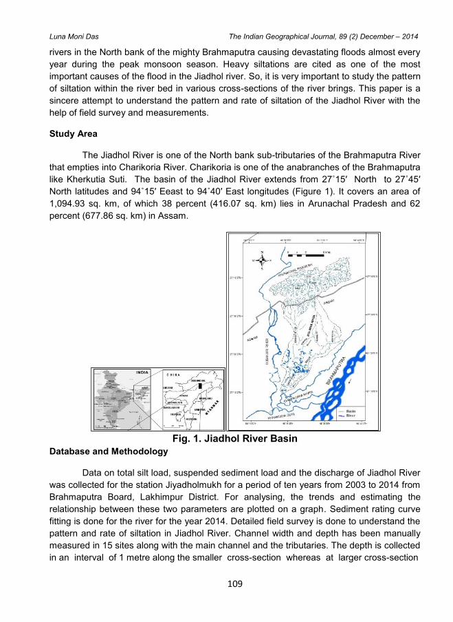
109
Luna Moni Das The Indian Geographical Journal, 89 (2) December – 2014
rivers in the North bank of the mighty Brahmaputra causing devastating floods almost every
year during the peak monsoon season. Heavy siltations are cited as one of the most
important causes of the flood in the Jiadhol river. So, it is very important to study the pattern
of siltation within the river bed in various cross-sections of the river brings. This paper is a
sincere attempt to understand the pattern and rate of siltation of the Jiadhol River with the
help of field survey and measurements.
Study Area
The Jiadhol River is one of the North bank sub-tributaries of the Brahmaputra River
that empties into Charikoria River. Charikoria is one of the anabranches of the Brahmaputra
like Kherkutia Suti. The basin of the Jiadhol River extends from 27˚15′ North to 27˚45′
North latitudes and 94˚15′ Eeast to 94˚40′ East longitudes (Figure 1). It covers an area of
1,094.93 sq. km, of which 38 percent (416.07 sq. km) lies in Arunachal Pradesh and 62
percent (677.86 sq. km) in Assam.
Fig. 1. Jiadhol River Basin
Database and Methodology
Data on total silt load, suspended sediment load and the discharge of Jiadhol River
was collected for the station Jiyadholmukh for a period of ten years from 2003 to 2014 from
Brahmaputra Board, Lakhimpur District. For analysing, the trends and estimating the
relationship between these two parameters are plotted on a graph. Sediment rating curve
fitting is done for the river for the year 2014. Detailed field survey is done to understand the
pattern and rate of siltation in Jiadhol River. Channel width and depth has been manually
measured in 15 sites along with the main channel and the tributaries. The depth is collected
in an interval of 1 metre along the smaller cross-section whereas at larger cross-section
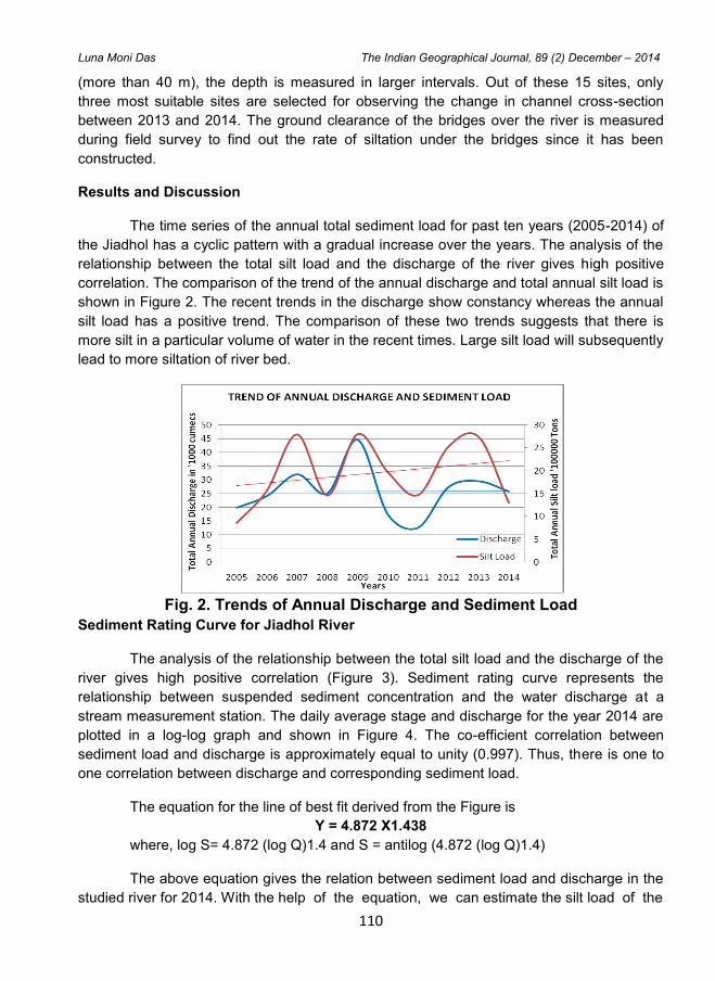
110
Luna Moni Das The Indian Geographical Journal, 89 (2) December – 2014
(more than 40 m), the depth is measured in larger intervals. Out of these 15 sites, only
three most suitable sites are selected for observing the change in channel cross-section
between 2013 and 2014. The ground clearance of the bridges over the river is measured
during field survey to find out the rate of siltation under the bridges since it has been
constructed.
Results and Discussion
The time series of the annual total sediment load for past ten years (2005-2014) of
the Jiadhol has a cyclic pattern with a gradual increase over the years. The analysis of the
relationship between the total silt load and the discharge of the river gives high positive
correlation. The comparison of the trend of the annual discharge and total annual silt load is
shown in Figure 2. The recent trends in the discharge show constancy whereas the annual
silt load has a positive trend. The comparison of these two trends suggests that there is
more silt in a particular volume of water in the recent times. Large silt load will subsequently
lead to more siltation of river bed.
Fig. 2. Trends of Annual Discharge and Sediment Load
Sediment Rating Curve for Jiadhol River
The analysis of the relationship between the total silt load and the discharge of the
river gives high positive correlation (Figure 3). Sediment rating curve represents the
relationship between suspended sediment concentration and the water discharge at a
stream measurement station. The daily average stage and discharge for the year 2014 are
plotted in a log-log graph and shown in Figure 4. The co-efficient correlation between
sediment load and discharge is approximately equal to unity (0.997). Thus, there is one to
one correlation between discharge and corresponding sediment load.
The equation for the line of best fit derived from the Figure is
Y = 4.872 X1.438
where, log S= 4.872 (log Q)1.4 and S = antilog (4.872 (log Q)1.4)
The above equation gives the relation between sediment load and discharge in the
studied river for 2014. With the help of the equation, we can estimate the silt load of the
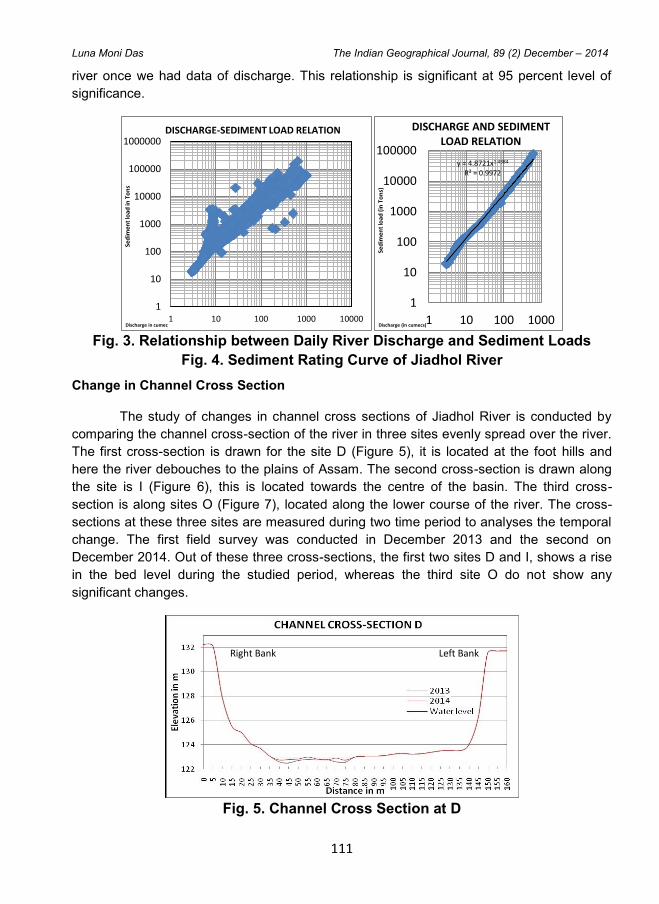
111
Luna Moni Das The Indian Geographical Journal, 89 (2) December – 2014
river once we had data of discharge. This relationship is significant at 95 percent level of
significance.
Fig. 3. Relationship between Daily River Discharge and Sediment Loads
Fig. 4. Sediment Rating Curve of Jiadhol River
Change in Channel Cross Section
The study of changes in channel cross sections of Jiadhol River is conducted by
comparing the channel cross-section of the river in three sites evenly spread over the river.
The first cross-section is drawn for the site D (Figure 5), it is located at the foot hills and
here the river debouches to the plains of Assam. The second cross-section is drawn along
the site is I (Figure 6), this is located towards the centre of the basin. The third cross-
section is along sites O (Figure 7), located along the lower course of the river. The cross-
sections at these three sites are measured during two time period to analyses the temporal
change. The first field survey was conducted in December 2013 and the second on
December 2014. Out of these three cross-sections, the first two sites D and I, shows a rise
in the bed level during the studied period, whereas the third site O do not show any
significant changes.
Fig. 5. Channel Cross Section at D
1
10
100
1000
10000
100000
1000000
1 10 100 1000 10000
Sed
ime
nt
load
in T
on
s
Discharge in cumec
DISCHARGE-SEDIMENT LOAD RELATION
y = 4.8721x1.4384 R² = 0.9972
1
10
100
1000
10000
100000
1 10 100 1000
Sed
ime
nt
load
(in
To
ns)
Discharge (in cumecs)
DISCHARGE AND SEDIMENT LOAD RELATION
Left Bank Right Bank
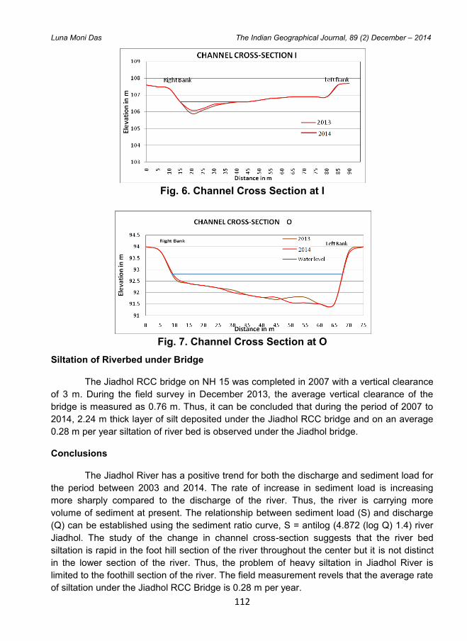
112
Luna Moni Das The Indian Geographical Journal, 89 (2) December – 2014
Fig. 6. Channel Cross Section at I
Fig. 7. Channel Cross Section at O
Siltation of Riverbed under Bridge
The Jiadhol RCC bridge on NH 15 was completed in 2007 with a vertical clearance
of 3 m. During the field survey in December 2013, the average vertical clearance of the
bridge is measured as 0.76 m. Thus, it can be concluded that during the period of 2007 to
2014, 2.24 m thick layer of silt deposited under the Jiadhol RCC bridge and on an average
0.28 m per year siltation of river bed is observed under the Jiadhol bridge.
Conclusions
The Jiadhol River has a positive trend for both the discharge and sediment load for
the period between 2003 and 2014. The rate of increase in sediment load is increasing
more sharply compared to the discharge of the river. Thus, the river is carrying more
volume of sediment at present. The relationship between sediment load (S) and discharge
(Q) can be established using the sediment ratio curve, S = antilog (4.872 (log Q) 1.4) river
Jiadhol. The study of the change in channel cross-section suggests that the river bed
siltation is rapid in the foot hill section of the river throughout the center but it is not distinct
in the lower section of the river. Thus, the problem of heavy siltation in Jiadhol River is
limited to the foothill section of the river. The field measurement revels that the average rate
of siltation under the Jiadhol RCC Bridge is 0.28 m per year.
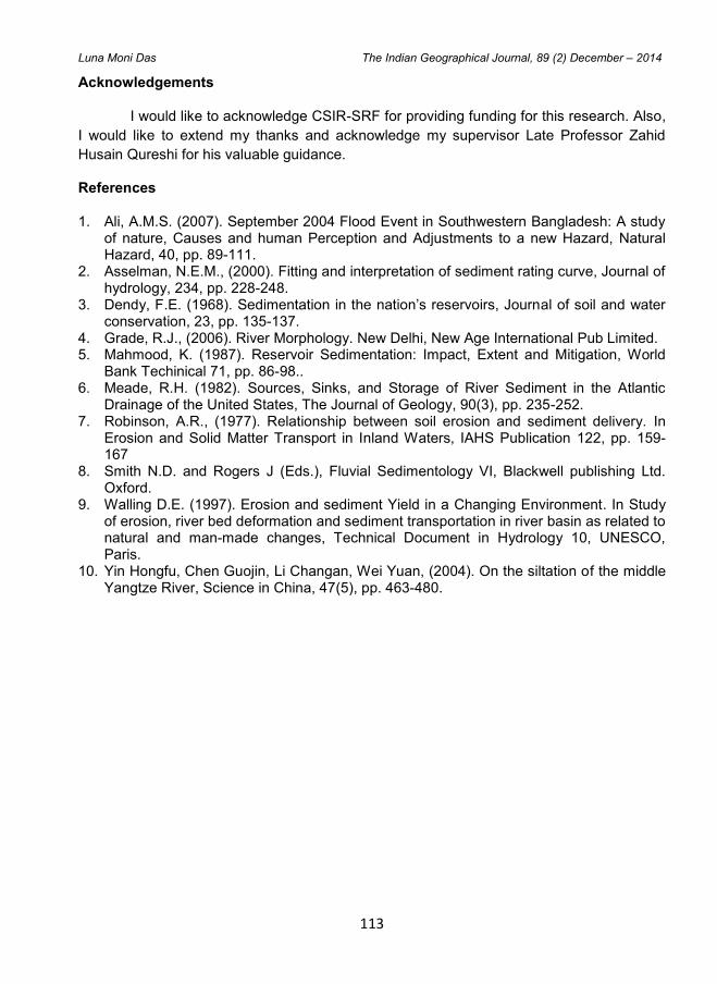
113
Luna Moni Das The Indian Geographical Journal, 89 (2) December – 2014
Acknowledgements
I would like to acknowledge CSIR-SRF for providing funding for this research. Also,
I would like to extend my thanks and acknowledge my supervisor Late Professor Zahid
Husain Qureshi for his valuable guidance.
References
1. Ali, A.M.S. (2007). September 2004 Flood Event in Southwestern Bangladesh: A study of nature, Causes and human Perception and Adjustments to a new Hazard, Natural Hazard, 40, pp. 89-111.
2. Asselman, N.E.M., (2000). Fitting and interpretation of sediment rating curve, Journal of hydrology, 234, pp. 228-248.
3. Dendy, F.E. (1968). Sedimentation in the nation’s reservoirs, Journal of soil and water conservation, 23, pp. 135-137.
4. Grade, R.J., (2006). River Morphology. New Delhi, New Age International Pub Limited. 5. Mahmood, K. (1987). Reservoir Sedimentation: Impact, Extent and Mitigation, World
Bank Techinical 71, pp. 86-98.. 6. Meade, R.H. (1982). Sources, Sinks, and Storage of River Sediment in the Atlantic
Drainage of the United States, The Journal of Geology, 90(3), pp. 235-252. 7. Robinson, A.R., (1977). Relationship between soil erosion and sediment delivery. In
Erosion and Solid Matter Transport in Inland Waters, IAHS Publication 122, pp. 159-167
8. Smith N.D. and Rogers J (Eds.), Fluvial Sedimentology VI, Blackwell publishing Ltd. Oxford.
9. Walling D.E. (1997). Erosion and sediment Yield in a Changing Environment. In Study of erosion, river bed deformation and sediment transportation in river basin as related to natural and man-made changes, Technical Document in Hydrology 10, UNESCO, Paris.
10. Yin Hongfu, Chen Guojin, Li Changan, Wei Yuan, (2004). On the siltation of the middle Yangtze River, Science in China, 47(5), pp. 463-480.
The Indian Geographical Journal
Volume 89 (2) December - 2014, pp 114-124
ISSN 0019-4824
114
GENDER DISPARITY OF LITERACY IN RAJASTHAN
Devendra Singh Chouhan
Department of Geography, M. L. Sukhadia University, Udaipur - 313 001
E-mail: [email protected]
Abstract
Gender issues mean the discussion on both men and woman, though woman who suffer
from gender inequality. From all gender issues, gender inequality is the most prevalent in
Rajasthan. According to the 2011 Census of Rajasthan, the overall rate of literacy is only
66.10 percent. But breaking up the state average reveals that while the rate of literacy for
male is 79.20 percent and for females, it is 52.12 percent. This means that more than one-
fourth the state's population is still illiterate. Within that figure, nearly one-fifth of male are
illiterate compared with more than one-third of the females there. It shows there is a slow
rate of improvement in female literacy as compared with male literacy, is a matter of grave
concern. Despite the number of efforts made at state and national level, there exist a
significant number of illiterate woman in society, a disturbing factor for all development
efforts. Literacy plays a significant role in reducing gender inequality. The purpose of the
research is to map and analyse gender disparity in literacy across the districts.
Keywords: Census, Education, Female literacy, Male literacy, Gender disparity
Introduction
Human capital is the most important ingredient in the overall development of a
society (Dubey, 1981). Education is a key element as it has the potential to increase human
capital; it removes inequality from society, impacts the growth of employment and improves
a country's Gross National Product (GNP). Literacy is the basic building block and a crucial
element in the development of education in society. In the context of Indian society, which
is essentially patria renal, it is the women and girls suffer especially due to low accessibility
to education (Chattoraj, 2015). In other words, gender becomes an important factor in
determining the education level of an individual. Woman constitutes approximately half,
which is 48.14 percent of the population in Rajasthan. However, a large gap exists between
the male and female population in the levels of literacy. According to the 2011 Census of
Rajasthan, there is difference of about 27.85 percent between the two reference groups.
The problem of illiteracy, especially among women, is a huge concern not only in Rajasthan
but also across India which directly affects the development efforts. This research attempts
to analyse levels of literacy across the various districts of Rajasthan. It has been divided
into three major sections. The first section analyses literacy trends in Rajasthan with special
reference to the period 1951 to 2011. The second section examines patterns of literacy in
Rajasthan. The last section provides details of gender disparity (Jhaniya, 2014) with respect
to males and females across Rajasthan.

115
Devendra Singh Chouhan The Indian Geographical Journal, 89 (2) December – 2014
Database and Methodology
The major objectives of the study are to analysis the spatial pattern of gender
disparity and identify the factors that are responsible for gender disparity and to provide
suggestions to reduce gender disparity. The present study primarily based on the
secondary data extracted from the Census of Rajasthan, 2011. Besides, some other reports
and government publications have also been used to supplement in the analysis.
Three major statistical tools are used for showing the regional patterns of literacy
rate and examining the gender gap between males and females. First, a simple literacy rate
was computed for trend analysis and spatial analysis of the study. Second, it has been
applied for analysing the regional pattern of gender disparity across Rajasthan. Finally,
Geographic Information System (GIS) mapping was followed using choropleth mapping for
showing regional disparity in the State.
Study Area
Rajasthan is situated in North-western parts of the India. It lies between 23˚3' to
30˚12' North latitudes and 69˚30' to 78˚17' East longitudes. Rajasthan is bounded by
Pakistan in the West and North and by Haryana in the North-east. In East it is surrounded
by Uttar Pradesh, by Madhya Pradesh in the South-east and Gujarat in the South-west. It is
the largest State in terms of area in India has an area (3,42,239 square kilometres). From
East to West it is about 869 km and from North to South it is about 826 km long, the State
can be divided into two major divisions along the Aravalli Range which divides the State
into East and West Rajasthan. The most notable feature of the State is the Aravalli Range
of hills. It is one of the oldest mountain systems in Western sandy plains and the area lying
to the East of it is called as Central highlands. On the basis of relief features, the State can
be divided into the following physiographic divisions: 1. Western Sandy Plain, 2. Aravalli
Range and Hilly Region, 3. Eastern Plain and 4. Hadoti Plateau or South-eastern Rajasthan
Plateau.
Gender Disparity
There are disparity index to measure the disparities. According to this method, if X1
and X2 represent the respective percentage values of the variable groups 1 and 2, than the
disparity index (D) can be calculated by the following formula:
D = Log (X2/X1) + Log [(Q-X1) / (Q-X2)]
where, X2 > or = X1 and Q = 100
In this method, group 2 is taken for the variable having a comparatively higher
value and group 1 is taken for the variable with a relatively lower value. In case there is no
disparity (perfect equality), the value of D will be 0. This method reveals that the higher the
value of D, the higher the extent of disparity and the lower the value of D, the lower the
extent of disparity.
116
Devendra Singh Chouhan The Indian Geographical Journal, 89 (2) December – 2014
Fig. 1. Study Area - Rajasthan
Results and Discussion
Table 1 reveals that the literacy rate for people, both males and females, have
been increasing continuously. The literacy rate has increased 9 times during 1951-2011
(Sawant, 2002). The literacy rate of males has increased 5.59 times during 1951-2011. The
literacy rate of females has increased 17.53 times during 1951 and 2011.
These figures also reveals that gender disparity in literacy has increased
continuously from 1951-1991 and it became 3.03 times during 1951-1991. During the last
40 years, it got decreased by 2.75 percent points for the first time in 2001. Thereafter, it had
been decreasing continuously until 2011. If there is a comparison of gender disparity across
different years, it can be observed that gender disparity was the lowest (11.4 percent) in
1951, while it was the highest (34.6 percent) in 1991.
Overall, gender disparity in literacy has increased 3.03 times during 1951-2011
from 11.4 percent to 27.85 percent. The Figure 1 shows that total literacy is continuously
increasing during the reference period (1951-2011) and it got increased during 1991 to
2011.
Literacy among males and females has the same rate of pace in the same periods.
Gender gap in literacy between males and females was increasing between 1951 and 1981
with few exceptions (Chattoraj, 2015). Afterwards, this gap started declining at relatively
faster rate and reached below 20 percent. Thus, the Figure reveals that the literacy is
increasing and literacy gap between male and females are declining the reference period.
The Table 2 reveals that more than one-fifth of the population is still illiterate in the
State. The gender disparity in literacy is 27.86 percent. In rural areas, it is 31.24 percent,
while in urban areas it is 17.63 percent. There is a difference of 13.61 percent in gender
disparity in literacy between rural and urban areas.
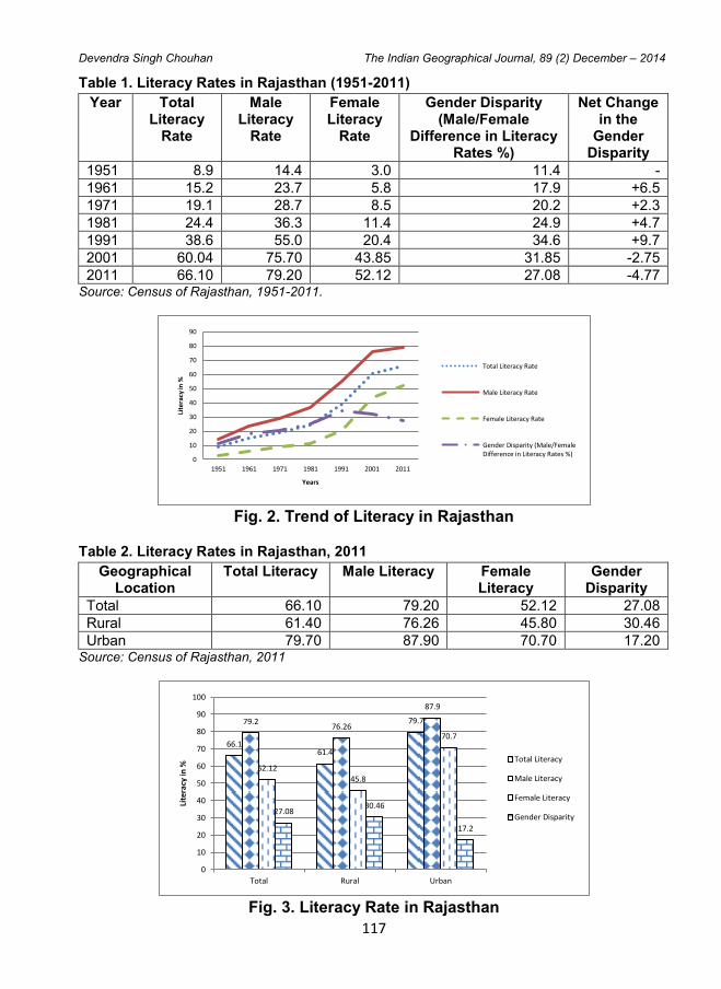
117
Devendra Singh Chouhan The Indian Geographical Journal, 89 (2) December – 2014
Table 1. Literacy Rates in Rajasthan (1951-2011)
Year Total Literacy
Rate
Male Literacy
Rate
Female Literacy
Rate
Gender Disparity (Male/Female
Difference in Literacy Rates %)
Net Change in the
Gender Disparity
1951 8.9 14.4 3.0 11.4 -
1961 15.2 23.7 5.8 17.9 +6.5
1971 19.1 28.7 8.5 20.2 +2.3
1981 24.4 36.3 11.4 24.9 +4.7
1991 38.6 55.0 20.4 34.6 +9.7
2001 60.04 75.70 43.85 31.85 -2.75
2011 66.10 79.20 52.12 27.08 -4.77 Source: Census of Rajasthan, 1951-2011.
Fig. 2. Trend of Literacy in Rajasthan
Table 2. Literacy Rates in Rajasthan, 2011
Geographical Location
Total Literacy Male Literacy Female Literacy
Gender Disparity
Total 66.10 79.20 52.12 27.08
Rural 61.40 76.26 45.80 30.46
Urban 79.70 87.90 70.70 17.20 Source: Census of Rajasthan, 2011
Fig. 3. Literacy Rate in Rajasthan
0
10
20
30
40
50
60
70
80
90
1951 1961 1971 1981 1991 2001 2011
Lite
racy
in %
Years
Total Literacy Rate
Male Literacy Rate
Female Literacy Rate
Gender Disparity (Male/FemaleDifference in Literacy Rates %)
66.1 61.4
79.7 79.2 76.26
87.9
52.12 45.8
70.7
27.08 30.46
17.2
0
10
20
30
40
50
60
70
80
90
100
Total Rural Urban
Lite
racy
in %
Total Literacy
Male Literacy
Female Literacy
Gender Disparity
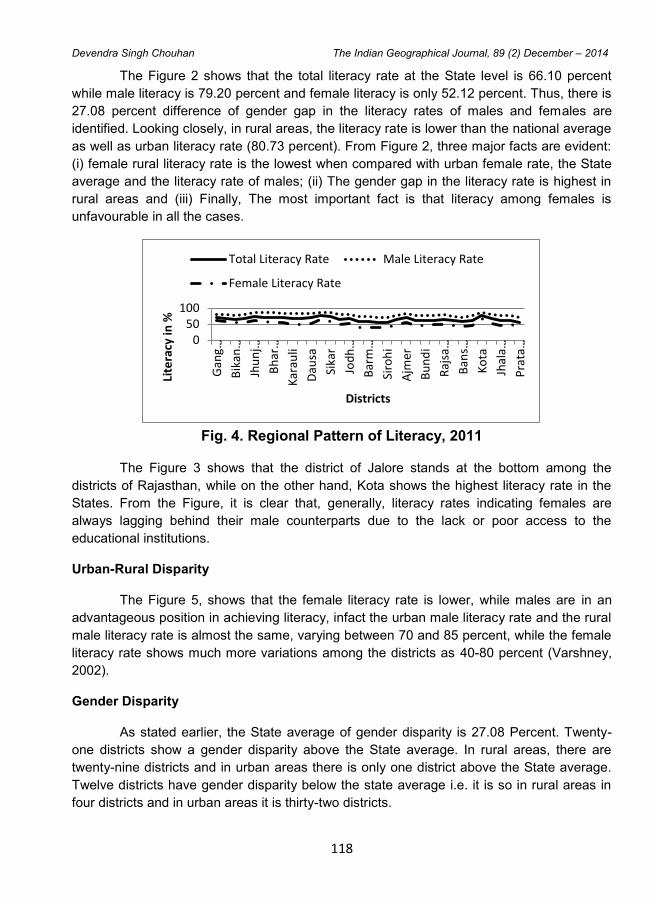
118
Devendra Singh Chouhan The Indian Geographical Journal, 89 (2) December – 2014
The Figure 2 shows that the total literacy rate at the State level is 66.10 percent
while male literacy is 79.20 percent and female literacy is only 52.12 percent. Thus, there is
27.08 percent difference of gender gap in the literacy rates of males and females are
identified. Looking closely, in rural areas, the literacy rate is lower than the national average
as well as urban literacy rate (80.73 percent). From Figure 2, three major facts are evident:
(i) female rural literacy rate is the lowest when compared with urban female rate, the State
average and the literacy rate of males; (ii) The gender gap in the literacy rate is highest in
rural areas and (iii) Finally, The most important fact is that literacy among females is
unfavourable in all the cases.
Fig. 4. Regional Pattern of Literacy, 2011
The Figure 3 shows that the district of Jalore stands at the bottom among the
districts of Rajasthan, while on the other hand, Kota shows the highest literacy rate in the
States. From the Figure, it is clear that, generally, literacy rates indicating females are
always lagging behind their male counterparts due to the lack or poor access to the
educational institutions.
Urban-Rural Disparity
The Figure 5, shows that the female literacy rate is lower, while males are in an
advantageous position in achieving literacy, infact the urban male literacy rate and the rural
male literacy rate is almost the same, varying between 70 and 85 percent, while the female
literacy rate shows much more variations among the districts as 40-80 percent (Varshney,
2002).
Gender Disparity
As stated earlier, the State average of gender disparity is 27.08 Percent. Twenty-
one districts show a gender disparity above the State average. In rural areas, there are
twenty-nine districts and in urban areas there is only one district above the State average.
Twelve districts have gender disparity below the state average i.e. it is so in rural areas in
four districts and in urban areas it is thirty-two districts.
050
100
Gan
g…
Bikan
…
Jhunj…
Bhar…
Kar
auli
Dau
sa
Sika
r
Jodh…
Barm…
Siro
hi
Ajm
er
Bu
nd
i
Rajsa…
Ban
s…
Ko
ta
Jhala…
Prata…
Lite
racy
in %
Districts
Total Literacy Rate Male Literacy Rate
Female Literacy Rate

119
Devendra Singh Chouhan The Indian Geographical Journal, 89 (2) December – 2014
Fig. 5. Regional Pattern of Rural and Urban Literacy in Rajasthan, 2011
Table 4. Disparity Index of Different Years
Year Disparity Index
1951 5.93
1961 5.31
1971 4.66
1981 4.57
1991 4.46
2001 4.04
2011 3.94
The data on disparity presented in Table 4 reveals that the gender disparity in
literacy levels had been continuously decreasing from 1951 to 2011. The rank correlation
measurement of Table 5 reveals the in urban areas there exists a high positive correlation
between the total literacy rate and the male literacy rate, the total literacy rate. It means that
if literacy increases, male and female literacy will also increases. If the male literacy rate
increases, the female literacy will also increase. But there is a negative correlation between
gender disparity and the total literacy rate, the male literacy rate and the female literacy
rate. It means that if the literacy rate increases the gender disparity decrease.
Fig. 6 . Male and Female Disparity in Literacy, 2011
0
50
100
Gan
ga…
Bik
aner
Jhunjh…
Bhara…
Kar
auli
Dau
sa
Sika
r
Jod
hp
ur
Bar
mer
Siro
hi
Ajm
er
Bu
nd
i
Rajsa…
Ban
sw…
Ko
ta
Jhala…
Pratap…
Lite
racy
in %
Districts
Rural Male Literacy Rate Rural Female Literacy Rate
Urban Male Literacy Rate Urban Female Literacy Rate
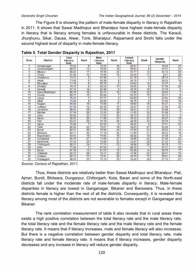
120
Devendra Singh Chouhan The Indian Geographical Journal, 89 (2) December – 2014
The Figure 6 is showing the pattern of male-female disparity in literacy in Rajasthan
in 2011. It shows that Sawai Madhopur and Bharatpur have highest male-female disparity
in literacy that is literacy among females is unfavourable in these districts. The Karauli,
Jhunjhunu, Sikar, Dausa, Alwar, Tonk, Bharatpur, Rajsamand and Sirohi falls under the
second highest level of disparity in male-female literacy.
Table 5. Total Gender Disparity in Rajasthan, 2011
Source: Census of Rajasthan, 2011.
Thus, these districts are relatively better than Sawai Madhopur and Bharatpur. Pali,
Ajmer, Bundi, Bhilwara, Dungarpur, Chittorgarh, Kota, Baran and some of the North-east
districts fall under the moderate rate of male-female disparity in literacy. Male-female
disparities in literacy are lowest in Ganganagar, Bikaner and Banswara. Thus, in these
districts female is higher than the rest of all the districts. Consequently, it is revealed that
literacy among most of the districts are not severable to females except in Ganganagar and
Bikaner.
The rank correlation measurement of table 6 also reveals that in rural areas there
exists a high positive correlation between the total literacy rate and the male literacy rate,
the total literacy rate and the female literacy rate and the male literacy rate and the female
literacy rate. It means that if literacy increases, male and female literacy will also increases.
But there is a negative correlation between gender disparity and total literacy rate, male
literacy rate and female literacy rate. It means that if literacy increases, gender disparity
decreases and any increase in literacy will reduce gender disparity.
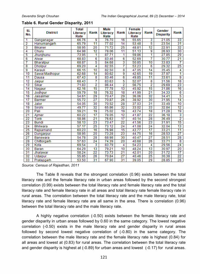
121
Devendra Singh Chouhan The Indian Geographical Journal, 89 (2) December – 2014
Table 6. Rural Gender Disparity, 2011
Source: Census of Rajasthan, 2011
The Table 8 reveals that the strongest correlation (0.96) exists between the total
literacy rate and the female literacy rate in urban areas followed by the second strongest
correlation (0.99) exists between the total literacy rate and female literacy rate and the total
literacy rate and female literacy rate in all areas and total literacy rate female literacy rate in
rural areas. The correlation between the total literacy rate and the male literacy rate, total
literacy rate and female literacy rate are all same in the area. There is correlation (0.96)
between the total literacy rate and the male literacy rate.
A highly negative correlation (-0.50) exists between the female literacy rate and
gender disparity in urban areas followed by 0.60 in the same category. The lowest negative
correlation (-0.50) exists in the male literacy rate and gender disparity in rural areas
followed by second lowest negative correlation of (-0.80) in the same category. The
correlation between the male literacy rate and the female literacy rate is highest (0.84) for
all areas and lowest at (0.83) for rural areas. The correlation between the total literacy rate
and gender disparity is highest at (-0.89) for urban areas and lowest (-0.17) for rural areas.
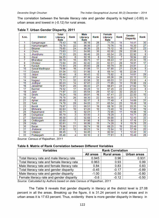
122
Devendra Singh Chouhan The Indian Geographical Journal, 89 (2) December – 2014
The correlation between the female literacy rate and gender disparity is highest (-0.60) in
urban areas and lowest in (-0.12) for rural areas.
Table 7. Urban Gender Disparity, 2011
Source: Census of Rajasthan, 2011
Table 8. Matrix of Rank Correlation between Different Variables
Variables Rank Correlation
All areas Rural areas Urban areas
Total literacy rate and male literacy rate 0.945 0.96 0.931
Total literacy rate and female literacy rate 0.963 0.93 0.99
Male literacy rate and female literacy rate 0.84 0.83 0.83
Total literacy rate and gender disparity -0.45 -0.17 -0.89
Male literacy rate and gender disparity -1.00 -0.50 -0.80
Female literacy rate and gender disparity -0.6 -0.12 -0.50 Source: Calculated by Authors based on data Census of Rajasthan, 2011
The Table 9 reveals that gender disparity in literacy at the district level is 27.08
percent in all the areas. Breaking up the figure, it is 31.24 percent in rural areas and in
urban areas it is 17.63 percent. Thus, evidently there is more gender disparity in literacy in
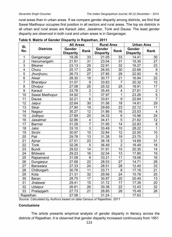
123
Devendra Singh Chouhan The Indian Geographical Journal, 89 (2) December – 2014
rural areas than in urban areas. If we compare gender disparity among districts, we find that
Sawai Madhopur occupies first position in all sectors and rural areas. The top six districts in
all urban and rural areas are Karauli Jalor, Jaisalmer, Tonk and Dausa. The least gender
disparity are observed in both rural and urban areas is in Ganganagar.
Table 9. Matrix of Gender Disparity in Rajasthan, 2011
Sl. No.
Districts
All Areas Rural Area Urban Area
Gender Disparity
Rank Gender
Disparity Rank
Gender Disparity
Rank
1 Ganganagar 19.26 33 21.05 33 14.41 30
2 Hanumangarh 21.91 31 23.54 31 15.30 27
3 Bikaner 23.13 29 22.91 32 16.27 23
4 Churu 25.17 28 26.93 30 22.66 9
5 Jhunjhunu 26.73 27 27.85 29 22.92 6
6 Alwar 28.30 18 30.77 21 16.94 22
7 Bharatpur 31.07 9 33.83 7 20.32 15
8 Dholpur 27.08 25 29.32 25 18.91 17
9 Karauli 33.78 2 35.45 4 27.81 2
10 Sawai Madhopur 34.92 1 37.97 1 23.26 5
11 Dausa 32.21 6 33.61 9 22.84 7
12 Jaipur 22.64 30 31.56 18 14.61 29
13 Sikar 27.90 19 29.69 23 22.12 11
14 Nagaur 30.27 12 31.86 16 23.53 4
15 Jodhpur 27.89 20 34.33 6 15.96 24
16 Jaisalmer 32.86 4 34.41 5 21.62 12
17 Barmer 31.29 7 31.95 14 22.83 8
18 Jalor 33.10 3 33.49 10 28.22 1
19 Sirohi 30.97 10 32.84 12 22.50 10
20 Pali 29.78 13 31.28 19 23.75 3
21 Ajmer 27.51 23 36.18 3 14.69 31
22 Tonk 32.26 5 36.49 2 18.49 18
23 Bundi 29.52 14 31.91 15 20.35 14
24 Bhilwara 29.23 16 32.04 13 17.80 19
25 Rajsamand 31.08 8 33.21 11 19.06 16
26 Dungarpur 27.68 22 28.53 27 14.71 28
27 Banswara 27.33 24 28.51 28 12.40 33
28 Chittorgarh 30.76 11 33.71 8 17.16 21
29 Kota 21.31 32 29.56 24 15.78 25
30 Baran 28.75 17 30.97 20 20.49 13
31 Jhalawar 29.41 15 31.72 17 17.39 20
32 Udaipur 26.81 26 30.38 22 12.43 32
33 Pratapgarh 27.73 21 28.85 26 15.49 26
Rajasthan 27.08 31.24 17.63 Source: Calculated by Authors based on data Census of Rajasthan, 2011
Conclusions
The article presents empirical analysis of gender disparity in literacy across the
districts of Rajasthan. It is observed that gender disparity increased continuously from 1951
124
Devendra Singh Chouhan The Indian Geographical Journal, 89 (2) December – 2014
to 1991 and for the first time gender disparity decreased by 2.75 percent in 2001. Since
then, it has been continuously decreasing based on this study; we found that the district of
Sawai Madhopur has the maximum gender disparity in both rural and urban areas.
Meanwhile, the district of Ganganagar has the minimum gender disparity in rural areas and
Banswara has the lowest disparity in urban areas. The article concludes that there is an
inverse relationship between literacy and gender disparity; it reveals that there identifies
higher gender disparity in rural areas than in urban areas (Ali, 2009). Major reasons for
gender disparity in literacy in Rajasthan are traditional value system and social customs,
anti-female attitude or biased mentality, distance from schools / colleges, lack of transport
facilities, high dropout ratio among females, crime against females, more household
responsibilities and so on. Some other reasons are poverty, family discouragement, lack of
self-confidence, lack of awareness, low mobility, non-availability of proper guidance,
unemployment, child marriage etc.
There is no district in the state which has better rate of female literacy than that of
males. Hence, there is an urgent need to focus on female literacy in all areas, particularly
rural areas to address the issue of gender disparity. It should be (Govt., common people
and other organizations) demoralised the anti-female attitude and biased mentality among
the people for better gender equality.
References
1. Ali, A. (2009), "Literacy in Uttar Pradesh: Spatial Dimension", National Geographical Journal of India, 55, (I), pp. 99-110.
2. Census of India, (1951-2011), New Delhi, India. 3. Chattoraj, K.K. and Chand, S. (2015), "Literacy Trend of West Bengal and its
Differentials: A District Level Analysis", IOSR Journal of Humanities and Social Science (JOSR-JHSS), 20, 9, pp. 1-19.
4. Dubey, R.S. and Mishra, R.P. (1981), "Level of Education: A Versatile Indicator of Regional Development", Geographical Review of India, 43, No.3, pp. 278-285.
5. Jhaniya, G.P. and Jain, C.K. (2014), "Pattern and Differential of Literacy in Madhya Pradesh", IOSR Journal of Humanities and Social Science (JOSR-JHSS), Vol.19, Issue 9, pp. 77-84.
6. Majumdar, P. (1999), "Spatial Pattern of Literacy in West Bengal: District Wise Analysis of 1991 Census", Geographical Review of India, Vol. 61, pp. 12-21.
7. Sawant, M.N. and Lewis, C. (2002), "Literacy in Goa: A Spatial-Temporal Review", The Goa Geographers, 2(2), pp. 32-41.
8. Som, K.S. and Mishra, R.P. (2014), "Literacy and Their Differential in West Bengal", International Journal of Science and Research (IJSR), 3 (6), pp. 1537-1545.
9. Varshney, H.K. (2002), "Inter State Gender Disparity in Literacy Rates: A Look at Census Data (1991 and 2001)", Journal of Educational Planning and Administration,
14(4), pp. 537-549.
The Indian Geographical Journal
Volume 89 (2) December - 2014, pp 125-133
ISSN 0019-4824
125
TERRAIN MAPPING OF BANGALORE UNIVERSITY CAMPUS
AND SURROUNDING AREAS USING GEOINFORMATICS
Lavanya J.1 and Krishna Das
2
1Department of Geography, Osmania University, Hyderabad - 500 007 2Department of Geography, Guwahati University, Guwahati - 781 014
E-mail: [email protected], [email protected]
Abstract
This study is attempted to map and also to study the surface terrain condition of Bangalore
University campus with its surrounding areas using geoinformatics. Terrain is used as a
general term in physical geography, referring to the lay of the land. This is usually
expressed in terms of the elevation, slope and orientation of terrain features. The SRTM 30
metre resolution DEM data is used to extract useful terrain parameters like relief, slope,
aspect, TRI and viewshed. The TIN model of the study area has visualised the terrain in
three-dimensions. The study has found 790 metre as the base height that ranges to 885
metre as the maximum point. The study has also generated a GIS-based model for check
dam site suitability and observed around 15 percent areas are suitable for the check dam.
The entire study has focussed the applications of geospatial technology in mapping and
analysing surface terrain characteristics of the study area. Terrain mapping and analyses
results of this study will provide the base and also help the decision makers to make
various infrastructural development planning choices in and around the study area with a
scientific framework.
Keywords: Terrain, Development, DEM, TIN, TRI, GIS
Introduction
This study attempts to map and also to study the surface terrain conditions of
Bangalore University campus with its surrounding areas using geoinformatics. The study
area is located in the southwestern part of Bengaluru city in Karnataka State of India.
Terrain analysis employs elevation data, usually in conjunction with other geospatial
information, to describe the landscape, for basic visualisation, modelling or to support
decision making. This is done under GIS environments using satellite-derived DEM, various
terrain parameters like relief, slope, aspect, ruggedness, viewshed etc. The objectives of
this study is to extract contours, triangulated irregular network, surface elevation profile of
the study area using satellite derived digital elevation model (DEM) data; to map the terrain
elements of the study area like relief, slope, aspect, terrain ruggedness index (TRI),
viewshed using DEM data and to prepare a check dam site suitability model of the study
area using parameters like slope, TRI and normalised difference vegetation index (NDVI).

126
Lavanya J and Krishna Das The Indian Geographical Journal, 89 (2) December – 2014
Study Area
The study is confined to Bangalore University campus and surrounding areas that
come within 500 metres within the University campus. The geographical extension of the
study area is from 12.921°N to 12.965° N latitudes and 77.490° E to 77.525° E longitudes.
The study area covers 12.32 sq. km with a volume of 45, 977,2131.06 cubic metres from
790 metre plane height. The study area includes whole of Gnana Bharathi University
campus and some parts of surrounding areas like Nagarbhavi, Suvarna Badavane,
Kenchenhalli, Jnana Ganga Nagar (Figure 1). Bangalore University has around 131
buildings in the campus comprising the roof top area of about 97,850 sq. mts. The
landscape area of Bangalore University comprises of built-up land, road networks, green
vegetation, plantations, waterbodies etc. There are check dams (waterbodies) in campus
for water harvesting. Borewells and septic tanks also add up to the landuse of Bangalore
University. The vegetation cover of 300 acre bio-park which is a lung space is also present
in the campus.
Database and Methodology
Shuttle Radar Topography Mission (SRTM) DEM data is the prime data source of
this study. The SRTM data is a satellite derived DEM data with one arc-second, i.e. 30
metre resolution. The SRTM is an international research effort. The elevation models are
arranged into tiles, each covering one degree of latitude and one degree of longitude,
named according to their south-western corners. It follows that ‘n45e006’ stretches from 450
N and 60 East to 46
0 N and 7
0 East and ‘s45w006’ from 45
0 S ad 6
0 West to 44
0 South and
50 West. The resolution of the cells of the source data is one arc second. The IRS LISS III
data with 23.5 metre resolution is also used in this study. The LISS III data have been
collected from the Bhuvan geo-portal of ISRO. These satellite datasets have been projected
on WGS84UTM 43 North projection system for further analysis in GIS environments.
Fig. 2. Satellite Datasets used in the Study
Fig. 1. Study Area
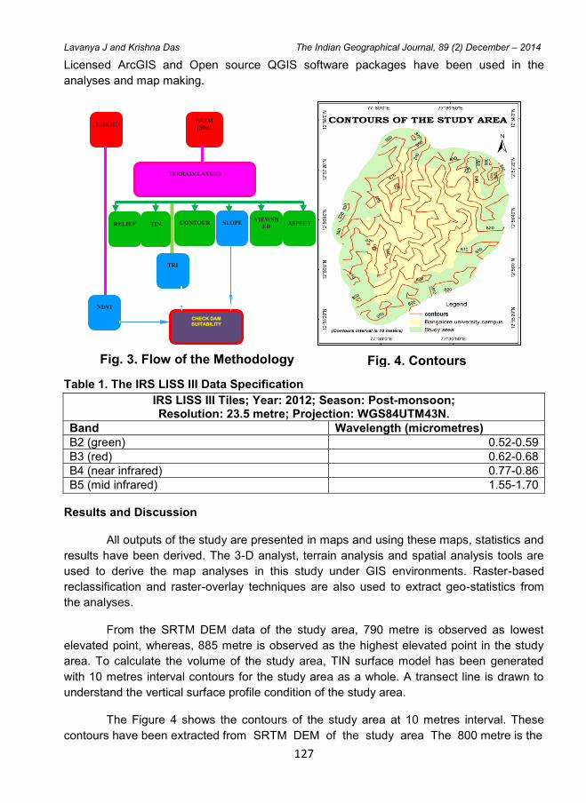
127
Lavanya J and Krishna Das The Indian Geographical Journal, 89 (2) December – 2014
Licensed ArcGIS and Open source QGIS software packages have been used in the
analyses and map making.
Table 1. The IRS LISS III Data Specification
IRS LISS III Tiles; Year: 2012; Season: Post-monsoon; Resolution: 23.5 metre; Projection: WGS84UTM43N.
Band Wavelength (micrometres)
B2 (green) 0.52-0.59
B3 (red) 0.62-0.68
B4 (near infrared) 0.77-0.86
B5 (mid infrared) 1.55-1.70
Results and Discussion
All outputs of the study are presented in maps and using these maps, statistics and
results have been derived. The 3-D analyst, terrain analysis and spatial analysis tools are
used to derive the map analyses in this study under GIS environments. Raster-based
reclassification and raster-overlay techniques are also used to extract geo-statistics from
the analyses.
From the SRTM DEM data of the study area, 790 metre is observed as lowest
elevated point, whereas, 885 metre is observed as the highest elevated point in the study
area. To calculate the volume of the study area, TIN surface model has been generated
with 10 metres interval contours for the study area as a whole. A transect line is drawn to
understand the vertical surface profile condition of the study area.
The Figure 4 shows the contours of the study area at 10 metres interval. These
contours have been extracted from SRTM DEM of the study area The 800 metre is the
Fig. 4. Contours Fig. 3. Flow of the Methodology
RELIEF TIN
SRTM
(30m) LISS III
TERRAIN LAYERS
CONTOUR VIEWSH
ED ASPECT
NDVI
TRI
CHECK DAM
SUITABILITY
SLOPE
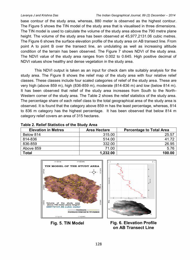
128
Lavanya J and Krishna Das The Indian Geographical Journal, 89 (2) December – 2014
base contour of the study area, whereas, 880 meter is observed as the highest contour.
The Figure 5 shows the TIN model of the study area that is visualised in three dimensions.
The TIN model is used to calculate the volume of the study area above the 790 metre plane
height. The volume of the study area has been observed at 45,977,2131.06 cubic metres.
The Figure 6 shows the surface elevation profile of the study area on AB transect line. From
point A to point B over the transect line, an undulating as well as increasing altitude
condition of the terrain has been observed. The Figure 7 shows NDVI of the study area.
The NDVI value of the study area ranges from 0.002 to 0.645. High positive decimal of
NDVI values show healthy and dense vegetation in the study area.
This NDVI output is taken as an input for check dam site suitably analysis for the
study area. The Figure 8 shows the relief map of the study area with four relative relief
classes. These classes include four scaled categories of relief of the study area. These are
very high (above 859 m), high (836-859 m), moderate (814-836 m) and low (below 814 m).
It has been observed that relief of the study area increases from South to the North-
Western corner of the study area. The Table 2 shows the relief statistics of the study area.
The percentage share of each relief class to the total geographical area of the study area is
observed. It is found that the category above 859 m has the least percentage, whereas, 814
to 836 m category has the highest percentage. It has been observed that below 814 m
category relief covers an area of 315 hectares.
Table 2. Relief Statistics of the Study Area
Elevation in Metres Area Hectare Percentage to Total Area
Below 814 315.00 25.57
814-836 514.00 41.72
836-859 332.00 26.95
Above 859 71.00 5.76
Total 1,232.00 100.00
Fig. 6. Elevation Profile on AB Transect Line
Fig. 5. TIN Model
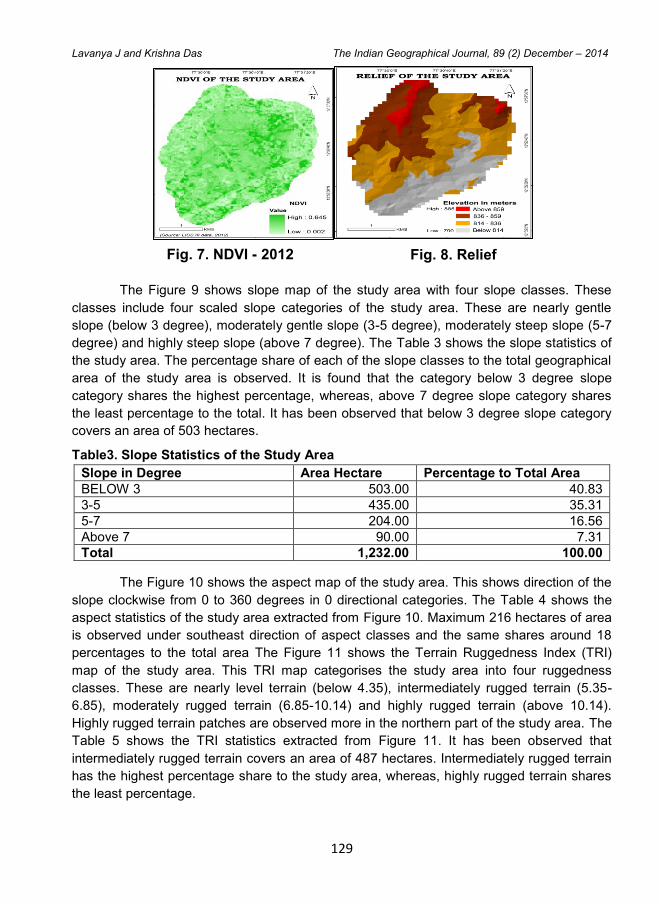
129
Lavanya J and Krishna Das The Indian Geographical Journal, 89 (2) December – 2014
The Figure 9 shows slope map of the study area with four slope classes. These
classes include four scaled slope categories of the study area. These are nearly gentle
slope (below 3 degree), moderately gentle slope (3-5 degree), moderately steep slope (5-7
degree) and highly steep slope (above 7 degree). The Table 3 shows the slope statistics of
the study area. The percentage share of each of the slope classes to the total geographical
area of the study area is observed. It is found that the category below 3 degree slope
category shares the highest percentage, whereas, above 7 degree slope category shares
the least percentage to the total. It has been observed that below 3 degree slope category
covers an area of 503 hectares.
Table3. Slope Statistics of the Study Area
Slope in Degree Area Hectare Percentage to Total Area
BELOW 3 503.00 40.83
3-5 435.00 35.31
5-7 204.00 16.56
Above 7 90.00 7.31
Total 1,232.00 100.00
The Figure 10 shows the aspect map of the study area. This shows direction of the
slope clockwise from 0 to 360 degrees in 0 directional categories. The Table 4 shows the
aspect statistics of the study area extracted from Figure 10. Maximum 216 hectares of area
is observed under southeast direction of aspect classes and the same shares around 18
percentages to the total area The Figure 11 shows the Terrain Ruggedness Index (TRI)
map of the study area. This TRI map categorises the study area into four ruggedness
classes. These are nearly level terrain (below 4.35), intermediately rugged terrain (5.35-
6.85), moderately rugged terrain (6.85-10.14) and highly rugged terrain (above 10.14).
Highly rugged terrain patches are observed more in the northern part of the study area. The
Table 5 shows the TRI statistics extracted from Figure 11. It has been observed that
intermediately rugged terrain covers an area of 487 hectares. Intermediately rugged terrain
has the highest percentage share to the study area, whereas, highly rugged terrain shares
the least percentage.
Fig. 8. Relief Fig. 7. NDVI - 2012

130
Lavanya J and Krishna Das The Indian Geographical Journal, 89 (2) December – 2014
Table 4. Aspect Statistics of the Study Area
Aspect Direction Area Hectare Percentage To Total Area
Flat 1.00 0.08
North 55.00 4.46
Northeast 135.00 10.96
East 186.00 15.10
Southeast 216.00 17.53
Southeast 160.00 12.99
Southwest 152.00 12.34
West 168.00 13.64
Northwest 123.00 9.98
North 36.00 2.92
Total 1,232.00 100.00
Table 5. The TRI Statistics of the Study Area
The Figure 12 shows the viewshed condition map of the study area observed from
eight random locations. A, B, C, D, E, F, G, and H are the observed random locations from
where terrain visibility condition has been observed. From these eight observed locations,
the visibility conditione is observed and mapped under two major categories. These two
categories are visible and not visible classes. The Table 6 shows the statistics of viewshed
analysis. Visible class covers an area of 662 hectares, whereas, non-visible class covers an
area of 570 hectares. From the eight observed locations around, 54 percent area is visible
to the total study area. The Table 7 shows the co-ordinate’s details of the observed random
locations in terms of latitude, longitude and altitude from point A to point H.
Table 6. Viewshed Statistics of the Study Area
Viewshed Area in Hectares Percentage to Total Area
Not Visible 570.00 46.27
Visible 662.00 53.73
Total 1,232.00 100.00
Table 7. Location Details of the Random Observed Points for Viewshed Analysis
ID Code Longitude (X) Latitude (Y) Altitude in Metres
1 A 773462.60618100000 1433710.05303999000 857
2 B 772360.56220100000 1433867.48789000000 824
3 C 772035.85281499900 1431997.94900000000 842
4 D 771150.28176000000 1429803.70072000000 794
5 E 770727.17558899900 1432922.87877000000 837
6 F 770559.90105600000 1431240.29376000000 825
7 G 772439.27962799900 1430640.07338000000 814
8 H 773620.04103500000 1432558.81067000000 825
TRI Area in Hectares Percentage to Total Area
Below 4.35 375.00 30.44
4.35-6.85 487.00 39.53
6.85-10.14 286.00 23.21
Above 10.14 84.00 6.82
Total 1,232.00 100.00
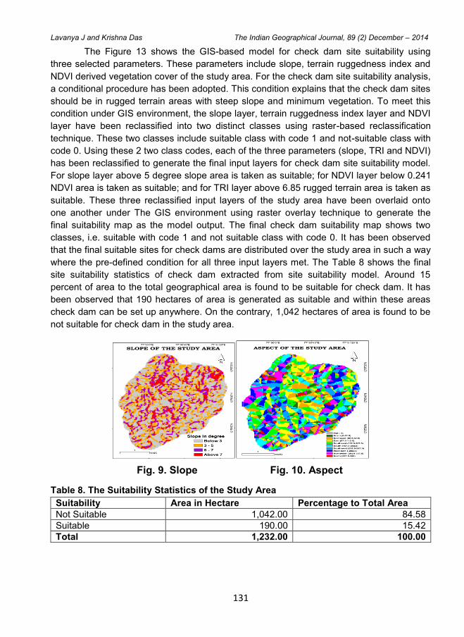
131
Lavanya J and Krishna Das The Indian Geographical Journal, 89 (2) December – 2014
The Figure 13 shows the GIS-based model for check dam site suitability using
three selected parameters. These parameters include slope, terrain ruggedness index and
NDVI derived vegetation cover of the study area. For the check dam site suitability analysis,
a conditional procedure has been adopted. This condition explains that the check dam sites
should be in rugged terrain areas with steep slope and minimum vegetation. To meet this
condition under GIS environment, the slope layer, terrain ruggedness index layer and NDVI
layer have been reclassified into two distinct classes using raster-based reclassification
technique. These two classes include suitable class with code 1 and not-suitable class with
code 0. Using these 2 two class codes, each of the three parameters (slope, TRI and NDVI)
has been reclassified to generate the final input layers for check dam site suitability model.
For slope layer above 5 degree slope area is taken as suitable; for NDVI layer below 0.241
NDVI area is taken as suitable; and for TRI layer above 6.85 rugged terrain area is taken as
suitable. These three reclassified input layers of the study area have been overlaid onto
one another under The GIS environment using raster overlay technique to generate the
final suitability map as the model output. The final check dam suitability map shows two
classes, i.e. suitable with code 1 and not suitable class with code 0. It has been observed
that the final suitable sites for check dams are distributed over the study area in such a way
where the pre-defined condition for all three input layers met. The Table 8 shows the final
site suitability statistics of check dam extracted from site suitability model. Around 15
percent of area to the total geographical area is found to be suitable for check dam. It has
been observed that 190 hectares of area is generated as suitable and within these areas
check dam can be set up anywhere. On the contrary, 1,042 hectares of area is found to be
not suitable for check dam in the study area.
Table 8. The Suitability Statistics of the Study Area
Suitability Area in Hectare Percentage to Total Area
Not Suitable 1,042.00 84.58
Suitable 190.00 15.42
Total 1,232.00 100.00
Fig. 10. Aspect Fig. 9. Slope

132
Lavanya J and Krishna Das The Indian Geographical Journal, 89 (2) December – 2014
Fig. 13. Site Suitability for Check Dam in the Study Area
Conclusions
The study has observed terrain condition of Bangalore University campus and
surrounding areas through the analyses of satellite derived DEM data using geoinformatics.
SRTM 30 meter resolution DEM data is used to extract useful terrain parameters like relief,
slope, aspect, TRI and viewshed. TIN model of the study area has visualized the terrain in
three-dimensions. The study has found 790 meter as the base height that ranges to 885
meter maximum point. The study has also generated a GIS-based model for check dam
site suitability and observed around 15 percent areas are suitable for the check dam. The
entire study has focussed on the applications of geospatial technology in mapping and
analysing surface terrain characteristics of the study area. This study will certainly provide
Fig. 12. Viewshed Fig. 11. TRI
133
Lavanya J and Krishna Das The Indian Geographical Journal, 89 (2) December – 2014
useful knowledge and information to the researcher community for effective application of
geoinformatics in various natural resources observational studies. Terrain mapping and
analyses results of this study will provide the base and also help the decision makers to
plan various infrastructural developments in and around the study area with a scientific
framework.
References
1. Ashok Hanjagi (2006). Mapping Bangalore university campus for information: using GPS, The National Association of Geographers India,. 14(1), pp. 43-47.
2. Amir Neupane (2015). Comparative study on cadastral surveying using Total station and high resolution satellite image, Coordinates, 11(12), pp.35-36.
3. Bhunumurthy (2015). NDRF inks pact with NRSC to get satellite data, Coordinates, 11(12), pp.58.
4. Gopal and Srila (2013). Study of water supply &sanitation practices in India using GIS: some design and other considerations in a village setting, Arc India News, 7(2), pp.19-20.
5. Koteswara Rao, A. (2014). GPS will help RTC to run buses on schedule and maintain punctuality of services, Geospatial Today, 12(12), pp. 7.
6. Manoj Kumar Agarwal (2013). West Bengal to map highway network, Geospatial Today, 12(10), pp. 46.
7. Meehan and Bill (2014). Utilities can now better respond to outages and serve customers more effectively, Geospatial Today, 12(11), pp. 7.
8. Oommen and Voommen (2014). Color coded maps mark ecologically sensitive areas in Kerala, Geospatial Today, 13(2), pp. 11.
9. Rajesh Aggarwal (2014). Maharashtra government to clean up electoral data, Geospatial Today, 13(4), pp. 9.
10. Rajiv and Jalota (2014). Brihan Mumbai municipal corporation to levy heavy penalties on those damaging underground utilities, Geospatial Today, 13(4), pp.12.
11. Reddy (2014). CBI to use satellite imagery in investigating mining scandals, Geospatial Today, 12(12), pp. 7.
12. Rakesh and Verma (2014). Map my India locate app to secure cab passengers in NCR, Geospatial Today, 13(3), pp. 13.
13. Sandhya Kiran, G. (2014). MS university to assess biodiversity in central Gujarat, Geospatial Today, 12(12), pp. 2.
14. Samadrita and Mukherjee (2015). Accuracy of cartosat-1 DEM and its derived attribute at multiple scale representation, Earth system science, 124, (3), pp. 487-495.
The Indian Geographical Journal
Volume 89 (2) December - 2014, pp 134-144
ISSN 0019-4824
134
DINDIGUL PANCHAYAT UNION - IMPACT OF LEATHER
TANNING INDUSTRIES ON SOIL QUALITY USING
GEOINFORMATICS
Latha S. and Kumaraswamy K.
Department of Geography, Bharathidasan University, Tiruchirappalli - 620 024
E-mail: [email protected], [email protected]
Abstract
Our standard of living, that predominantly depends on agriculture, is often determined by a
combination of the physical, chemical and biological characteristics of the soils and the
crops raised on them. Soil is defined as a natural medium, which serves as a reservoir of
nutrients and water for crops and provides mechanical anchorage and favourable tilth for
crops. Soil quality degradation is a serious problem affecting the agricultural productivity.
The industrial waste dumped in the soil, deteriorates the quality of the soil and leads to
degradation. The toxic effluents of the 38 leather tanning industries have highly degraded
the soil quality of the study area, Dindigul Panchayat Union. The surface soil samples were
collected and subjected to chemical analysis for various parameters. The results prove that
the soil quality of the study area has lost its importance and it is slowly stepping towards
degradation. Hence in the present study, an attempt is made to assess the the impact of
leather tanning industries on soil quality in relation to plant growth in Dindigul panchayat
union using Geographic information System. The present study will contribute to the
methodology of scientific analysis on the one hand and will also help to preserve the quality
of the soil on the other hand.
Keywords: Soil quality, Leather tanning industries, Chemical analysis
Introduction
Soil is defined as a natural medium, which serves as a reservoir of nutrients and
water for crops and provides mechanical anchorage and favourable tilth for crops. The
knowledge of soil is very essential for any kind of planning for development and
management of land for agriculture, better land use and cropping pattern and water
management practices for better production of crops. Our standard of living that
predominantly depends on agriculture is often determined by a combination of the physical,
chemical and biological characteristics of the soils and the crops raised on them. Soils
provide essential material on which agriculture is based, and therefore, any comprehensive
survey of the geography of agriculture should undertake a fairly thorough treatment of soil.
Soil exhaustion results very rapidly from excessive population pressure,
unenlightened farming practices and the excessively liberal and therefore, dangerous
135
Latha S. and Kumaraswamy K. The Indian Geographical Journal, 89 (2) December – 2014
doctrine of production at the lowest investment of soil-capital. The toxic effluents of the
leather tanning industries, located in the study area, have highly degraded the soil quality of
the study area. Hence in the present study, an attempt is made to assess the soil quality in
relation to plant growth in Dindigul panchayat union.
Bhavani (1995) has assessed the soil quality in North Arcot District, Tamil Nadu,
India. In the study, the soil quality is measured through standardized soil testing methods
and the alkalinity, acidity and salinity levels were analysed. Carlos et al., (2002), made an
analysis on the adverse effects of chromium among the tannery workers. Chandhuri (1984)
has attempted to study the soil fertility of Bolpur District of West Bengal. The results of the
study proves that the different chemical constituents i.e., nutritive elements like nitrogen,
phosphorus and potassium, have an integrated effect on crop yield. Chapman (1963)
observed that tannery wastes has altered the entire physical and chemical characteristics of
the soil. His results proved that the tannery waste water that was taken in by the plants had
influenced their metabolic processes.
During the dry and rainy season, to assess the effect of farming along river banks
on the quality of water, where a significant seasonal change is studied by Chimwanza et.al.,
(2006). Gerald (2001) in his study on arsenic contamination by a tannery site near Compton
town house in Wilmington has reported that the arsenic concentration in the soil was higher
than the acceptable level. This arsenic concentration has made the soil barren.
Vijayakumari (2003), made a study on the impact of textile dyeing effluent on growth of
soybean. Vidal et.al., (2004), analysed the combined oxidative and biological treatment of
separated streams of tannery wastewater. Krishna et.al., (2007) undertook a study on soil
contamination in Surat, Gujarat, to determine the extent and distribution of heavy metals
and have delineated the geogenic and anthropogenic sources and correlation of metals in
soils.
Study Area
Dindigul panchayat union is situated in Dindigul District, Tamil Nadu (Figure 1). It
lies between 10°14’45” and 10°31’00” North latitudes and 77°45’ and 78°4’30” East
longitudes covering the Survey of India (SOI) topographic map 58 F/14, F/15, F/16 and 58
J/3 extending over an area of 378.71 sq.km. The area consists of 18 administrative units
i.e., village panchayats namely Adiyanuthu, Agaram, Alakkuvarpatti, Ammakulathupatti,
Anaipatti, Balakrishnapuram, Chettinaickanpatti, Kovilur, Kurumbapatti, Mullipadi, Pallapatti,
Periyakottai, Silapadi, Sirumalai, Thadikombu, Thamaraipadi, Thottanuthu and Vellodu.
Among these, Sirumalai village panchayat is a hilly area located in the southern part of the
study area (Figure 2).
Out of the 61 leather tanning industries located in Dindigul District, 38 leather
tannery units (62.3 percent of the district’s units) are located in Dindigul panchayat union.
The 38 leather tannery units that are located in Dindigul panchayat union were captured
using GPS (Global Positioning System) survey and mapped. These 38 leather tanning
industries are distributed in Pallapatti (19), Adiyanuthu (12) village panchayat, Dindigul
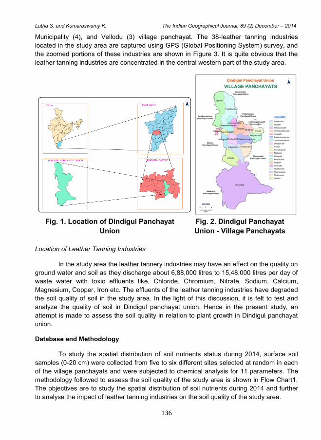
136
Latha S. and Kumaraswamy K. The Indian Geographical Journal, 89 (2) December – 2014
Municipality (4), and Vellodu (3) village panchayat. The 38-leather tanning industries
located in the study area are captured using GPS (Global Positioning System) survey, and
the zoomed portions of these industries are shown in Figure 3. It is quite obvious that the
leather tanning industries are concentrated in the central western part of the study area.
Location of Leather Tanning Industries
In the study area the leather tannery industries may have an effect on the quality on
ground water and soil as they discharge about 6,88,000 litres to 15,48,000 litres per day of
waste water with toxic effluents like, Chloride, Chromium, Nitrate, Sodium, Calcium,
Magnesium, Copper, Iron etc. The effluents of the leather tanning industries have degraded
the soil quality of soil in the study area. In the light of this discussion, it is felt to test and
analyze the quality of soil in Dindigul panchayat union. Hence in the present study, an
attempt is made to assess the soil quality in relation to plant growth in Dindigul panchayat
union.
Database and Methodology
To study the spatial distribution of soil nutrients status during 2014, surface soil
samples (0-20 cm) were collected from five to six different sites selected at random in each
of the village panchayats and were subjected to chemical analysis for 11 parameters. The
methodology followed to assess the soil quality of the study area is shown in Flow Chart1.
The objectives are to study the spatial distribution of soil nutrients during 2014 and further
to analyse the impact of leather tanning industries on the soil quality of the study area.
Fig. 2. Dindigul Panchayat
Union - Village Panchayats
Fig. 1. Location of Dindigul Panchayat
Union
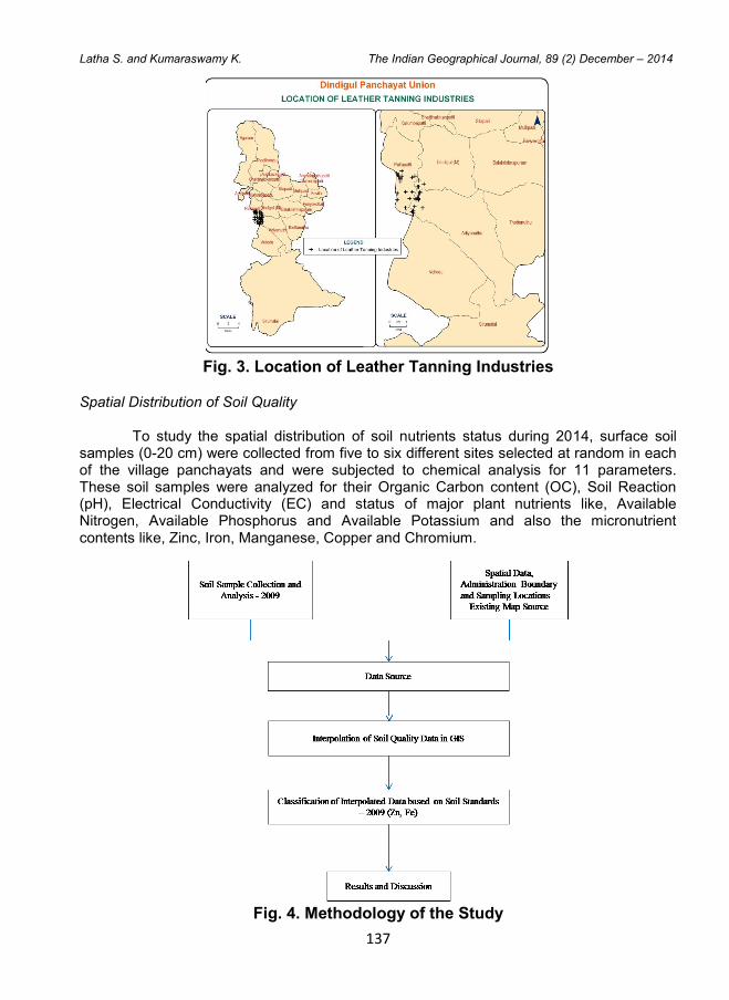
137
Latha S. and Kumaraswamy K. The Indian Geographical Journal, 89 (2) December – 2014
Fig. 3. Location of Leather Tanning Industries
Spatial Distribution of Soil Quality
To study the spatial distribution of soil nutrients status during 2014, surface soil samples (0-20 cm) were collected from five to six different sites selected at random in each of the village panchayats and were subjected to chemical analysis for 11 parameters. These soil samples were analyzed for their Organic Carbon content (OC), Soil Reaction (pH), Electrical Conductivity (EC) and status of major plant nutrients like, Available Nitrogen, Available Phosphorus and Available Potassium and also the micronutrient contents like, Zinc, Iron, Manganese, Copper and Chromium.
Fig. 4. Methodology of the Study
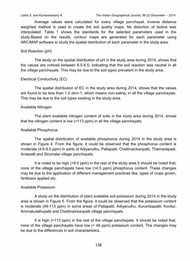
138
Latha S. and Kumaraswamy K. The Indian Geographical Journal, 89 (2) December – 2014
Average values were calculated for every village panchayat. Inverse distance
weighted method is used to create the soil quality maps. No distortion of isoline was
interpolated. Table 1 shows the standards for the selected parameters used in the
study.Based on the results, contour maps are generated for each parameter using
ARC/MAP software to study the spatial distribution of each parameter in the study area.
Soil Reaction (pH)
The study on the spatial distribution of pH in the study area during 2014, shows that
the values are noticed between 6.5-8.5, indicating that the soil reaction was neutral in all
the village panchayats. This may be due to the soil types prevalent in the study area.
Electrical Conductivity (EC)
The spatial distribution of EC in the study area during 2014, shows that the values
are found to be less than 1.0 dsm-1, which means non-saline, in all the village panchayats.
This may be due to the soil types existing in the study area.
Available Nitrogen
The plant available nitrogen content of soils in the study area during 2014, shows
that the nitrogen content is low (<113 ppm) in all the village panchayats.
Available Phosphorus
The spatial distribution of available phosphorus during 2014 in the study area is
shown in Figure 4. From the figure, it could be observed that the phosphorus content is
moderate (4.6-9.0 ppm) in parts of Adiyanuthu, Pallapatti, Chettinaickanpatti, Thamaraipadi,
Anaipatti and Sirumalai village panchayats.
It is noted to be high (>9.0 ppm) in the rest of the study area.It should be noted that,
none of the village panchayats have low (<4.5 ppm) phosphorus content. These changes
may be due to the application of different management practices like, types of crops grown,
fertilizers applied etc.
Available Potassium
A study on the distribution of plant available soil potassium during 2014 in the study
area is shown in Figure 5. From the figure, it could be observed that the potassium content
is moderate (49-113 ppm) in some areas of Pallapatti, Adiyanuthu, Kurumbapatti, Kovilur,
Ammakulathupatti and Chettinaickanpatti village panchayats.
It is high (>113 ppm) in the rest of the village panchayats. It should be noted that,
none of the village panchayats have low (< 48 ppm) potassium content. The changes may
be due to the differences in soil characteristics.

139
Latha S. and Kumaraswamy K. The Indian Geographical Journal, 89 (2) December – 2014
Manganese
The spatial distribution of concentration of manganese during 2014, in the study
area is shown in Figure 6. From the Figure, it could be observed that the manganese
content is deficient for plant growth (<2.0 ppm) in Silapadi and small parts in Periyakottai,
Kovilur, Mullipadi, Agaram, Chettinaickanpatti and Thadikombu village panchayats totally
covering an area of 12.84 sq.km.
In the remaining areas, the manganese content is sufficient for plant growth (>2.0
ppm) totally covering an area of 396.86 sq.km. The spatial distribution of concentration of
manganese, shows that the manganese content is deficient for plant growth in 3.13 percent
and it is sufficient for plant growth in about 96.87 percent of the study area.
Zinc
The study on the concentration of zinc during 2014, in the study area is shown in
Figure 7. From the figure, it could be observed that the zinc content is deficient for plant
growth (<1.2 ppm) in Agaram, Thadikombu, Anaipatti, Chettinaickanpatti, Alakkuvarpatti,
Silapadi, Thamaraipadi, Ammakulathupatti, Vellodu and parts of Adiyanuthu and Kovilur
village panchayats covering an area of 155.94 sq.km. In the remaining areas, the content of
zinc is sufficient for plant growth (>1.2 ppm), occupying an area of 253.76 sq.km. The
spatial distribution of concentration of zinc shows that it is deficient for plant growth in about
38.06 percent and is sufficient for plant growth in about 61.94 percent of the study area.
Iron
The spatial distribution of concentration of iron during 2014, in the study area is
shown in Figure 8. From the figure, it could be observed that the iron content is deficient for
plant growth (<3.5 ppm) in minor areas of Thamaraipadi and Agaram village panchayats
covering an area of only 0.99 sq.km. In the rest of the areas, the iron content is sufficient for
plant growth (>3.5 ppm) occupying an area of 408.71 sq.km. The spatial distribution of
concentration of iron, shows that it is deficient for plant growth in about 0.24 percent and it
is sufficient for plant growth in about 99.76 percent of the study area.
Copper
In the study area, the spatial distribution of concentration of copper during 2014, is
shown in Figure 9. From the figure, it could be observed that the copper content is deficient
for plant growth (<1.2 ppm) only for 0.02 sq.km in Alaguvarpatti village panchayat.
In the remaining areas, the copper content is sufficient for plant growth (>1.2 ppm)
covering an area of 409.68 sq.km. The spatial distribution of concentration of copper,
shows that it is deficient for plant growth in about 0.01 percent and it is sufficient for plant
growth in about 99.99 percent of the study area.
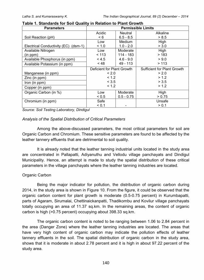
140
Latha S. and Kumaraswamy K. The Indian Geographical Journal, 89 (2) December – 2014
Table 1. Standards for Soil Quality in Relation to Plant Growth Parameters Permissible Limits
Soil Reaction (pH)
Acidic < 6
Neutral 6.5 - 8.5
Alkaline > 8.5
Electrical Conductivity (EC) (dsm-1)
Low < 1.0
Medium 1.0 - 2.0
High > 3.0
Available Nitrogen (in ppm)
Low < 113
Moderate 114 - 183
High > 183
Available Phosphorus (in ppm) < 4.5 < 48
4.6 - 9.0 49 - 113
> 9.0 > 113 Available Potassium (in ppm)
Manganese (in ppm)
Deficient for Plant Growth < 2.0 < 1.2 < 3.5 < 1.2
Sufficient for Plant Growth > 2.0 > 1.2 > 3.5 > 1.2
Zinc (in ppm)
Iron (in ppm)
Copper (in ppm)
Organic Carbon (in %) Low < 0.5
Moderate 0.5 - 0.75
High > 0.75
Chromium (in ppm) Safe < 0.1
-
Unsafe > 0.1
Source: Soil Testing Laboratory, Dindigul
Analysis of the Spatial Distribution of Critical Parameters
Among the above-discussed parameters, the most critical parameters for soil are
Organic Carbon and Chromium. These sensitive parameters are found to be affected by the
leather tannery effluents that are detrimental to soil quality.
It is already noted that the leather tanning industrial units located in the study area
are concentrated in Pallapatti, Adiyanuthu and Vellodu village panchayats and Dindigul
Municipality. Hence, an attempt is made to study the spatial distribution of these critical
parameters in the village panchayats where the leather tanning industries are located.
Organic Carbon
Being the major indicator for pollution, the distribution of organic carbon during
2014, in the study area is shown in Figure 10. From the figure, it could be observed that the
organic carbon content for plant growth is moderate (0.5-0.75 percent) in Kurumbapatti,
parts of Agaram, Sirumalai, Chettinaickanpatti, Thadikombu and Kovilur village panchayats
totally occupying an area of 11.37 sq.km. In the remaining areas, the content of organic
carbon is high (>0.75 percent) occupying about 398.33 sq.km.
The organic carbon content is noted to be ranging between 1.06 to 2.84 percent in
the area (Danger Zone) where the leather tanning industries are located. The areas that
have very high content of organic carbon may indicate the pollution effects of leather
tannery effluents in the soil. The spatial distribution of organic carbon in the study area,
shows that it is moderate in about 2.78 percent and it is high in about 97.22 percent of the
study area.
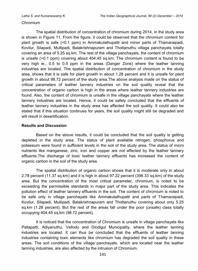
141
Latha S. and Kumaraswamy K. The Indian Geographical Journal, 89 (2) December – 2014
Chromium
The spatial distribution of concentration of chromium during 2014, in the study area
is shown in Figure 11. From the figure, it could be observed that the chromium content for
plant growth is safe (<0.1 ppm) in Ammakulathupatti and minor parts of Thamaraipadi,
Kovilur, Silapadi, Mullipadi, Balakrishnapuram and Thottanuthu village panchayats totally
covering an area of 5.25 sq.km. The rest of the village panchayats, the content of chromium
is unsafe (>0.1 ppm) covering about 404.45 sq.km. The chromium content is found to be
very high ie., 0.5 to 0.9 ppm in the areas (Danger Zone) where the leather tanning
industries are located. The spatial distribution of concentration of chromium in the study
area, shows that it is safe for plant growth in about 1.28 percent and it is unsafe for plant
growth in about 98.72 percent of the study area.The above analysis made on the status of
critical parameters of leather tannery industries on the soil quality reveal that the
concentration of organic carbon is high in the areas where leather tannery industries are
found. Also, the content of chromium is unsafe in the village panchayats where the leather
tannery industries are located. Hence, it could be safely concluded that the effluents of
leather tannery industries in the study area has affected the soil quality. It could also be
stated that if this situation continues for years, the soil quality might still be degraded and
will result in desertification.
Results and Discussion
Based on the above results, it could be concluded that the soil quality is getting
depleted in the study area. The status of plant available nitrogen, phosphorus and
potassium were found in sufficient levels in the soil of the study area. The status of micro
nutrients like manganese, zinc, iron and copper are not affected by the leather tannery
effluents.The discharge of toxic leather tannery effluents has increased the content of
organic carbon in the soil of the study area.
The spatial distribution of organic carbon shows that it is moderate only in about
2.78 percent (11.37 sq.km) and it is high in about 97.22 percent (398.33 sq.km) of the study
area. But the concentration of the most critical parameter, chromium, is noted to be
exceeding the permissible standards in major part of the study area. This indicates the
pollution effect of leather tannery effluents in the soil. The content of chromium is noted to
be safe only in village panchayats like Ammakulathupatti and parts of Thamaraipadi,
Kovilur, Silapadi, Mullipadi, Balakrishnapuram and Thottanuthu covering about only 5.25
sq.km (1.28 percent). But the rest of the areas fall under the poor (unsafe) class totally
occupying 404.45 sq.km (98.72 percent).
It is noticed that the concentration of Chromium is unsafe in village panchayats like
Pallapatti, Adiyanuthu, Vellodu and Dindigul Municipality, where the leather tanning
industries are located. It can thus be concluded that the effluents of leather tanning
industries containing toxic elements like chromium has degraded the soil quality in these
areas. The soil conditions of the village panchayats, which are located near the leather
tanning industries, are also affected by the intrusion of Chromium.
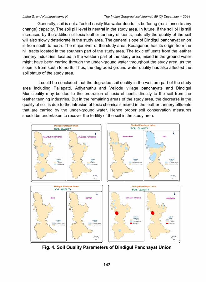
142
Latha S. and Kumaraswamy K. The Indian Geographical Journal, 89 (2) December – 2014
Generally, soil is not affected easily like water due to its buffering (resistance to any
change) capacity. The soil pH level is neutral in the study area. In future, if the soil pH is still
increased by the addition of toxic leather tannery effluents, naturally the quality of the soil
will also slowly deteriorate in the study area. The general slope of Dindigul panchayat union
is from south to north. The major river of the study area, Kodaganar, has its origin from the
hill tracts located in the southern part of the study area. The toxic effluents from the leather
tannery industries, located in the western part of the study area, mixed in the ground water
might have been carried through the under-ground water throughout the study area, as the
slope is from south to north. Thus, the degraded ground water quality has also affected the
soil status of the study area.
It could be concluded that the degraded soil quality in the western part of the study
area including Pallapatti, Adiyanuthu and Vellodu village panchayats and Dindigul
Municipality may be due to the protrusion of toxic effluents directly to the soil from the
leather tanning industries. But in the remaining areas of the study area, the decrease in the
quality of soil is due to the intrusion of toxic chemicals mixed in the leather tannery effluents
that are carried by the under-ground water. Hence proper soil conservation measures
should be undertaken to recover the fertility of the soil in the study area.
Fig. 4. Soil Quality Parameters of Dindigul Panchayat Union

143
Latha S. and Kumaraswamy K. The Indian Geographical Journal, 89 (2) December – 2014
This study on soil quality of Dindigul panchayat union has proved that the status of
soil has been degraded due to the intrusion of the toxic effluents from the leather tannery
industries located in the study area. Hence, the following recommendations are suggested
for improving the soil quality in the study area.
1. Fertilizer consumption determines the growth of a crop. But recently it is observed that
the use of chemical fertilizers may damage the quality of soil. Hence increased use of
green manure consumption will enhance the soil quality of a region. Bio fertilizer and
compost may stabilize the fertility of the soil.
2. Pesticide consumption at the proper time also helps to increase the productivity of soil.
Chemical fertilizers use has to be avoided so as to improve productivity of soil from
further degradation. Natural farming using herbal pesticides will protect the
microorganisms in soil. Pest attack recommendations suggested by the agricultural
department should be followed.
3. Periodical soil testing has to be done. Based on this the crops suitable for cultivation
can be selected. Soil testing also help in further plant protection measures. Proper soil
management is the dire need for increasing the productivity of soil. Soil enrichment can
be made by following effective irrigation systems that includes drip and sprinkler
irrigation. Dry farming technologies such as soil conservation measures are also
suggested.
4. Policies should be framed in adopting suitable restriction on the use of vulnerable
lands. This can be better achieved through national spirit and co-operation with
technical experts, planners, administrators and active participation of farmers. Cultural
practices like removal of weeds should be done in summer season. Based upon the
tests, market requirement and season, the crops which suits the soil quality should be
selected for cultivation. Native trees, which need less water, may also be planted on all
fallow and waste lands. Neem is the best native tree that can be grown in any type of
soil.
Conclusions
By adopting these measures in the right time, the area under low quality soil can
also be used successfully to obtain a high produce. By following the necessary
recommendations suggested in the study, the further deterioration of the soil quality can be
minimised to a certain level in Dindigul panchayat union. The present study on soil quality
would help in knowing the real causes for the agricultural backwardness and will provide a
sound base for the rural economic progress making agriculture more viable and
sustainable. Hence, delineating and improving the quality of the soil is a pre-requisite for
future planning and development of agricultural activities in the study area.
References
1. Bhavani, R. (1995). Soil quality assessment in North Arcot district, Tamil Nadu, India,
Transactions, Institute of Indian Geographers, 9(1), pp. 44.
144
Latha S. and Kumaraswamy K. The Indian Geographical Journal, 89 (2) December – 2014
2. Carlos, K, Katarzyna, W, Kazimierg, W, Juan, M.M, Laura, E, Nava, L, Gomez, R.G
(2002). Possible adverse effects of chromium in occupational exposure of tannery
workers, Industrial Health, 40, pp. 207-213.
3. Chandhuri, K. (1984). A study of soil fertility of Bolpur district of West Bengal, Paper
presented in V Annual Conference of the Institute of Indian Geographer, Department of
Geography, Gujarat University, Ahmedabad, pp.44.
4. Chapman, H. (1963). A report on diagnostic criteria for plants and soils, A report,
University of California, pp.793-800
5. Chimwanza, B, Mumba, P.P, Moyo, Kadewa, W. (2006). The impact of farming on river
banks on water quality of the rivers, International Journal of Environmental Science and
Technology, 2(4), pp. 353-358.
6. Gerald, L. (2001). Soil testing for arsenic contamination associate with historic tannery
site near Compton townhouse apartment in Wilmington, The Deleware Department of
National Resource and Environmental Control (DNREC News), 31(78), p.88.
7. Krishna, A.K. & Govil, P.K (2007). Soil contamination due to heavy metals from an
industrial area of Surat, Gujarat, Western India, Environmental Monitoring and
Assessment, 124(1-3), pp 263–275.
8. The Ground Water Division (1999). Ground Water Prospective - A profile of Dindigul
district, Tamil Nadu, WRO Ground Water Wing, PWD, Government of Tamil Nadu,
Chennai, p. 63.
9. Vidal, G, Nieto, J, Mansilla, H.D. and Bornhardt (2004). Combined oxidative and
biological treatment of separated streams of tannery wastewater. Water Science and
Technology, 49(4), pp. 287-92.
10. Vijayakumari, B. (2003). Impact of textile dyeing effluent on growth of soybean. Journal
of Ecotoxicology Environmental Monitoring, 13, pp. 59-64.
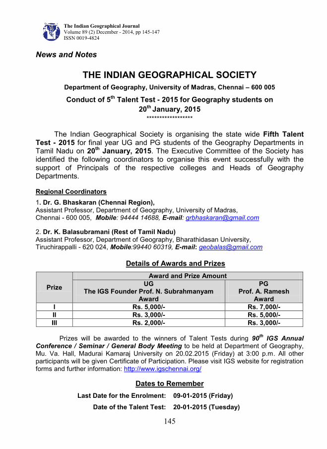
The Indian Geographical Journal
Volume 89 (2) December - 2014, pp 145-147 ISSN 0019-4824
145
News and Notes
THE INDIAN GEOGRAPHICAL SOCIETY
Department of Geography, University of Madras, Chennai – 600 005
Conduct of 5th Talent Test - 2015 for Geography students on
20th January, 2015
******************
The Indian Geographical Society is organising the state wide Fifth Talent Test - 2015 for final year UG and PG students of the Geography Departments in Tamil Nadu on 20th January, 2015. The Executive Committee of the Society has identified the following coordinators to organise this event successfully with the support of Principals of the respective colleges and Heads of Geography Departments. Regional Coordinators
1. Dr. G. Bhaskaran (Chennai Region), Assistant Professor, Department of Geography, University of Madras, Chennai - 600 005, Mobile: 94444 14688, E-mail: [email protected]
2. Dr. K. Balasubramani (Rest of Tamil Nadu) Assistant Professor, Department of Geography, Bharathidasan University, Tiruchirappalli - 620 024, Mobile:99440 60319, E-mail: [email protected]
Details of Awards and Prizes
Prize
Award and Prize Amount
UG The IGS Founder Prof. N. Subrahmanyam
Award
PG Prof. A. Ramesh
Award
I Rs. 5,000/- Rs. 7,000/-
II Rs. 3,000/- Rs. 5,000/-
III Rs. 2,000/- Rs. 3,000/-
Prizes will be awarded to the winners of Talent Tests during 90
th IGS Annual
Conference / Seminar / General Body Meeting to be held at Department of Geography, Mu. Va. Hall, Madurai Kamaraj University on 20.02.2015 (Friday) at 3:00 p.m. All other participants will be given Certificate of Participation. Please visit IGS website for registration forms and further information: http://www.igschennai.org/
Dates to Remember
Last Date for the Enrolment: 09-01-2015 (Friday)
Date of the Talent Test: 20-01-2015 (Tuesday)
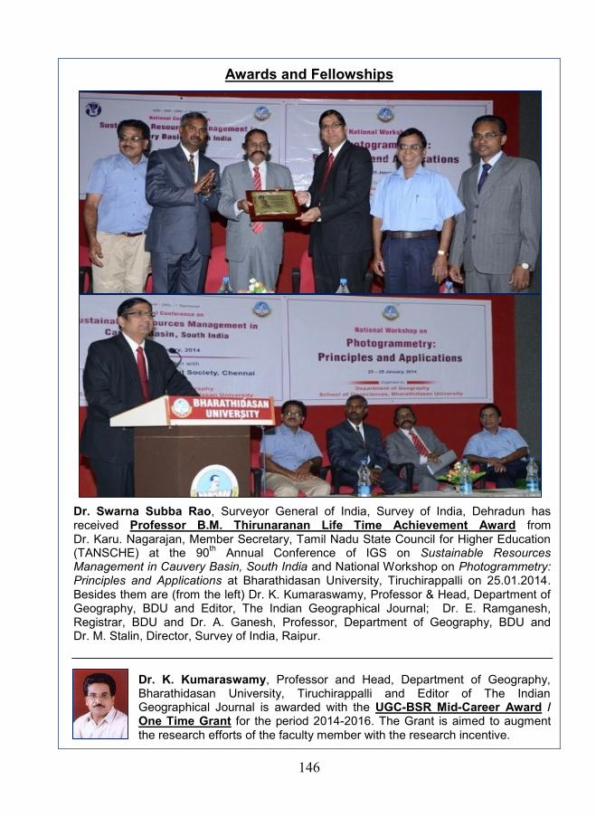
146
Awards and Fellowships
Dr. Swarna Subba Rao, Surveyor General of India, Survey of India, Dehradun has received Professor B.M. Thirunaranan Life Time Achievement Award from Dr. Karu. Nagarajan, Member Secretary, Tamil Nadu State Council for Higher Education (TANSCHE) at the 90
th Annual Conference of IGS on Sustainable Resources
Management in Cauvery Basin, South India and National Workshop on Photogrammetry: Principles and Applications at Bharathidasan University, Tiruchirappalli on 25.01.2014. Besides them are (from the left) Dr. K. Kumaraswamy, Professor & Head, Department of Geography, BDU and Editor, The Indian Geographical Journal; Dr. E. Ramganesh, Registrar, BDU and Dr. A. Ganesh, Professor, Department of Geography, BDU and Dr. M. Stalin, Director, Survey of India, Raipur.
Dr. K. Kumaraswamy, Professor and Head, Department of Geography, Bharathidasan University, Tiruchirappalli and Editor of The Indian Geographical Journal is awarded with the UGC-BSR Mid-Career Award / One Time Grant for the period 2014-2016. The Grant is aimed to augment the research efforts of the faculty member with the research incentive.
147
Statement about ownership and other particulars about
THE INDIAN GEOGRAPHICAL JOURNAL Department of Geography, University of Madras, Chennai - 600 005
Form IV
1. Place of Publication University of Madras, Chennai
2. Periodicity of its Publication Bi-annual
3. Printer’s Name Nationality Address
A. Paghyaselvam Indian J.J. Printers, 4/726, P.S.K., Nager Hussain Colony Pallapatti - P.O., Sivakasi - 626 189
4. Publisher’s Name Nationality Address
Dr. K. Kumaraswamy Indian Professor and Head Department of Geography Bharathidasan University Tiruchirappalli - 620 024
5. Editor’s Name Nationality Address
Dr. K. Kumaraswamy Indian Professor and Head Department of Geography Bharathidasan University Tiruchirappalli - 620 024
6. Names and Address of Individuals who own the journal and society
The Indian Geographical Society Department of Geography University of Madras Chennai - 600 005
I, K. Kumaraswamy, hereby declare that the particulars given above are true to the best of my knowledge and belief.
Dr. K. Kumaraswamy Editor, The Indian Geographical Journal

![Intersite Assemblage Variation from the US 89 Project Area. [US Highway 89 near Sunset Crater, AZ]](https://static.fdokumen.com/doc/165x107/6317d4eeb6c3e3926d0e0fa5/intersite-assemblage-variation-from-the-us-89-project-area-us-highway-89-near.jpg)


![James Stirling’s ‘Real Function’ [from OASE 89]](https://static.fdokumen.com/doc/165x107/632397ff5f71497ea90467ae/james-stirlings-real-function-from-oase-89.jpg)