EDITOR IN CHIEF

Prof. Dr. Murat YAKAR

Mersin University Engineering Faculty Turkey

CO-EDITORS

Asst Prof. Dr. Osman ORHAN

Mersin University Engineering Faculty Turkey

Prof. Dr. Ekrem TUŞAT

Konya Technical University Faculty of Engineering and Natural Sciences

Turkey

Prof. Dr. Songnian Li,

Ryerson University Faculty of Engineering and Architectural Science,

Canada

Asst. Prof. Dr. Ali ULVI

Mersin University Engineering Faculty Turkey

ADVISORY BOARD

Prof. Dr. Orhan ALTAN

Honorary Member of ISPRS, ICSU EB Member Turkey

Prof.Dr. Naser El SHAMY

The University of Calgary Department of Geomatics Engineering, Canada

Prof. Dr. Armin GRUEN

ETH Zurih University Switzerland

Prof.Dr. Ferruh YILDIZ Selcuk University Engineering Faculty

Turkey

Prof. Dr. Artu ELLMANN

Tallinn University of Technology Faculty of Civil Engineering

Estonia

EDITORIAL BOARD

Prof.Dr.Alper YILMAZ

Environmental and Geodetic Engineering, The Ohio State University, USA

Prof.Dr. Chryssy Potsiou

National Technical University of Athens-Rural and Surveying Engineering, Greece

Prof.Dr. Cengiz ALYILMAZ

AtaturkUniversity Kazim Karabekir Faculty of Education Turkey

Prof.Dr. Dieter FRITSCH

Universityof Stuttgart Institute for Photogrammetry Germany

Prof.Dr. Edward H. WAITHAKA

Jomo Kenyatta University of Agriculture & Technology Kenya

Prof.Dr. Halil SEZEN Environmental and Geodetic Engineering, The Ohio State University

USA

Prof.Dr. Huiming TANG

China University of Geoscience..,Faculty ofEngineering, China

Prof.Dr. Laramie Vance POTTS

New Jersey Institute of Technology,Department of Engineering Technology USA

Prof.Dr. Lia MATCHAVARIANI

Iv.Javakhishvili Tbilisi State University Faculty of Geography Georgia

Prof.Dr. Məqsəd Huseyn QOCAMANOV

Baku State University Faculty of Geography Azerbaijan

Prof.Dr. Muzaffer KAHVECI

Selcuk University Faculty of Engineering Turkey

Prof.Dr. Nikolai PATYKA

National University of Life and Environmental Sciences of Ukraine Ukraine

Prof.Dr. Petros PATIAS

The AristotleUniversity of Thessaloniki, Faculty of Rural & Surveying Engineering Greece

Prof.Dr. Pierre GRUSSENMEYER

National Institute of Applied Science, Department of civilengineering and surveying France

Prof.Dr. Rey-Jer You

National Cheng Kung University, Tainan · Department of Geomatics

China

Prof.Dr. Xiaoli DING The Hong Kong Polytechnic University,Faculty of Construction and Environment

Hong Kong

Assoc.Prof.Dr. Elena SUKHACHEVA Saint Petersburg State University Institute of Earth Sciences

Russia

Assoc.Prof.Dr. Semra ALYILMAZ Ataturk University Kazim Karabekir Faculty of Education

Turkey

Assoc.Prof.Dr. Fariz MIKAILSOY Igdir University Faculty of Agriculture

Turkey

Assoc.Prof.Dr. Lena HALOUNOVA Czech Technical University Faculty of Civil Engineering

Czech Republic

Assoc.Prof.Dr. Medzida MULIC University of Sarajevo Faculty of Civil Engineering

Bosnia and Herzegovina

Assoc.Prof.Dr. Michael Ajide OYINLOYE Federal University of Technology, Akure (FUTA)

Nigeria

Assoc.Prof.Dr. Mohd Zulkifli bin MOHD YUNUS Universiti TeknologiMalaysia, Faculty of Civil Engineering

Malaysia

Assoc.Prof.Dr. Syed Amer MAHMOOD University of the Punjab, Department of Space Science

Pakistan

Assist. Prof. Dr. Yelda TURKAN

Oregon State University, USA

Dr. G. Sanka N. PERERA

Sabaragamuwa University Faculty of Geomatics Sri Lanka

Dr. Hsiu-Wen CHANG

National Cheng Kung University, Department of Geomatics Taiwan

The International Journal of Engineering and Geosciences (IJEG)

The International Journal of Engineering and Geosciences (IJEG) is a tri-annually published journal. The journal includes a wide scope of information on scientific and technical advances in the geomatics sciences. The International Journal of Engineering and Geosciences aims to publish pure and applied research in geomatics engineering and technologies. IJEG is a double peer-reviewed (blind) OPEN ACCESS JOURNAL that publishes professional level research articles and subject reviews exclusively in English. It allows authors to submit articles online and track his or her progress via its web interface. All manuscripts will undergo a refereeing process; acceptance for publication is based on at least two positive reviews. The journal publishes research and review papers, professional communication, and technical notes. IJEG does not charge for any article submissions or for processing.

CORRESPONDENCE ADDRESS Journal Contact: engineeringandgeoscience@gmail.com

CONTENTS Volume 6 - Issue 2

ARTICLES

** Multi criteria decision analysis to determine the suitability of agricultural crops for land consolidation areas Fatih Sarı, Fatma Koyuncu Sarı 64

** Accuracy comparison of interior orientation parameters from different photogrammetric software and direct linear transformation method Zaide Duran, Muhammed Enes Atik 74

** Accuracy assessment of digital surface models from unmanned aerial vehicles’ imagery on archaeological sites Emre Şenkal, Gordana Kaplan, Uğur Avdan 81

** Analysis of literature on 3D cadastre Fatih Döner 90

** Determining highway slope ratio using a method based on slope angle calculation Osman Salih Yılmaz, Gülgün Özkan, Fatih Gülgen 98

** Determining the habitat fragmentation thru geoscience capabilities in Turkey: A case study of wildlife refuges

Arif Oguz Altunel , Sadık Caglar, Tayyibe Altunel 104

* Corresponding Author Cite this article

*(fatihsari@selcuk.edu.tr) ORCID ID 0000 – 0001 – 8674 – 9028 (fdmnkync90@gmail.com) ORCID ID 0000 – 0001 – 5829 – 0061 Research Article / DOI: 10.26833/ijeg.683754

Sarı F & Sarı F K (2021). Multi criteria decision analysis to determine the suitability of agricultural crops for land consolidation areas. International Journal of Engineering and Geosciences, 6(2), 64-73

Received: 03/02/2020; Accepted: 21/05/2020

International Journal of Engineering and Geosciences– 2021; 6(2); 64-73

International Journal of Engineering and Geosciences

https://dergipark.org.tr/en/pub/ijeg

e-ISSN 2548-0960

Multi criteria decision analysis to determine the suitability of agricultural crops for land consolidation areas

Fatih Sarı*1 , Fatma Koyuncu Sarı 2

1Selcuk University, Cumra Applied Sciences, Department of Geomatics Information Systems, Konya, Turkey 2Selcuk University, Faculty of Agriculture, Department of Landscape Architecture, Konya, Turkey

Keywords ABSTRACT Multi-Criteria decision analysis Analytical hierarchy process TOPSIS Geographical information systems Sustainable land management

Crop selection for sustainable and effective agricultural land management has to take into accounts several issues such as chemical, physical, environmental, economic and social conditions. Especially after land consolidation projects, sustainable agricultural crop management should be investigated for each crop which are suitable for the project area to benefit from the land consolidation contributions such as irrigation, roads, modified parcel boundaries and surfaces. Thus, Geographical Information Systems (GIS) aided suitability analysis techniques are required to determine the suitable crops for the consolidated areas. In this study, Analytic Hierarchy Process (AHP) and Technique for Order Preference by Similarity to Ideal Solution (TOPSIS) multi-criteria decision techniques are integrated with GIS to determine most suitable crops for parcels. The suitability maps of wheat, clover, sugar beet and corn crops are generated for the projected area using 63 Land Mapping Units (LMU) with considering pH, lime, texture, salinity, organic matter, electrical conductivity, permeability, slope, aspect and the distance to settlements and roads within chemical, physical, topological and socio-economic criteria.

1. INTRODUCTION

The agricultural activities have an importance that can accelerate the development of a country with its economic proceeds. There is a very close relation between the agricultural lands of a city and its economic-social status. Thus, the planning of agricultural activities and establishing Sustainable Agriculture Management (SAM) systems in developing cities are very important in the field of economic, social and environmental criteria (Rigby et al. 2001; Cauwenbergh et al. 2007; Radulescu et al. 2011; Akar and Gökalp 2018).

Crop suitability analysis, sustainable agricultural yield, pest control and irrigation are involved in SAM environment. Especially in land consolidation projects, site suitability analysis for crop selection is getting more essential to benefit from the advantages of land consolidation projects.

The Food and Agricultural Organisation (FAO) suggested an approach for crop suitability via a ranking from suitable to not suitable including soil properties, climatic conditions and land facilities (FAO 1976). Addition to this, crop suitability requires considering chemistry and physics of soil, topographic, climatic and environmental data when deciding (Wang et al. 1990; Joerin et al. 2001; Ceballos-Silva and Lopez-Blanco 2003a; Eliasson et al. 2010; Yu et al. 2011; Confalonieri et al. 2013; Elsheikh et al. 2013).

The existence of a wide range data in crop suitability and the complexity of criteria are the scope of Multi Criteria Decision Analysis (MCDA) (Zolekar and Bhagat 2015). MCDA is a general term that refers to determine the best alternative from all of the existing alternatives in the presence of multiple criteria (Zeleny 1982; Radulescu et al. 2010; Ramírez-García et al. 2015).

International Journal of Engineering and Geosciences– 2021; 6(2); 64-73

65

In this concept, Analytical Hierarchy Process (AHP) is one of the most applied methods in MCDA, which aims to calculate weights for each criterion among the parameters that involved in crop suitability (Saaty 1977, Saaty 1994, Saaty 2001; Saaty and Vargas 1991). AHP involves the calculations to determine most suitable solutions to the desired problem within multiple criteria by calculating weights with a pairwise comparison matrix (Arentze and Timmermans 2000; Chen et al. 2010). Calculated weights represent the affect rate of each criterion to the total suitability. On the other hand, TOPSIS is another method based on determining the distances, which has the shortest distance to positive ideal solution and longest distance from negative ideal solution (Hwang and Yoon 1981; Sarı et al. 2020).

In literature, there are considerable amounts of researches, which initialize the suitability of crops. The common alternative cropping systems via MCDA, cover crop species and cultivars selection were studied by (Hayashi 2000; Prakash 2003; Sadok et al. 2008; Thapa and Murayama 2008; Chen et al. 2010; Ramírez-García et al. 2015). The other studies were based on a special crop such as; strawberry and rubber tree (Roudeillac et al. 1997; Diaby et al. 2010), walnut cultivars (Srdjevic et al. 2004); lilium species and clones (Li et al. 2011); maize and potato (Ceballos-Silva and Lopez-Blanco, 2003b); tobacco (Chavez et al. 2012); faba bean (Kazemi et al. 2016); oat crop (Ceballos-Silva and Lopez-Blanco 2003a); olive crop (Elaalem 2013), the fruit crops (Chuong 2007), biomass crop (Cobuloglu and Buyuktahtakın 2015), paddy crops, vegetable and flower, annual crops, mulberry, coffee and tea (Dinh and Duc 2012). Although one crop type is examined in recent studies, most common agricultural crop types were studied in this paper and addition to AHP, TOPSIS method was used for crop suitability. The study area and parcel counts are one of the largest of recent studies and land consolidation area was used in this study.

In this study, AHP and TOPSIS methods are integrated to determine the suitability of corn, clover, wheat and sugar beet, which are the main crops of the study area, for consolidated lands in Seydişehir, Konya. There are 63 Land Map Units (LMU) units and their chemical, physical, topographical and socio-economic features are considered which are obtained from soil survey analysis of the project area. LMU’s are the soil survey points, which are established before land consolidation projects to define the soil properties by taking soil samples. The suitability maps for crops are generated with MCDA and Geographical Information Systems (GIS) integration. The results of the study can guide to the crop management and irrigation planning by determining suitable parcels for crops to increase the sustainable agricultural activities and economic income. The results can also guide to land consolidation projects considering the crop cover.

2. MATERIALS and METHODS

2.1. Study Area

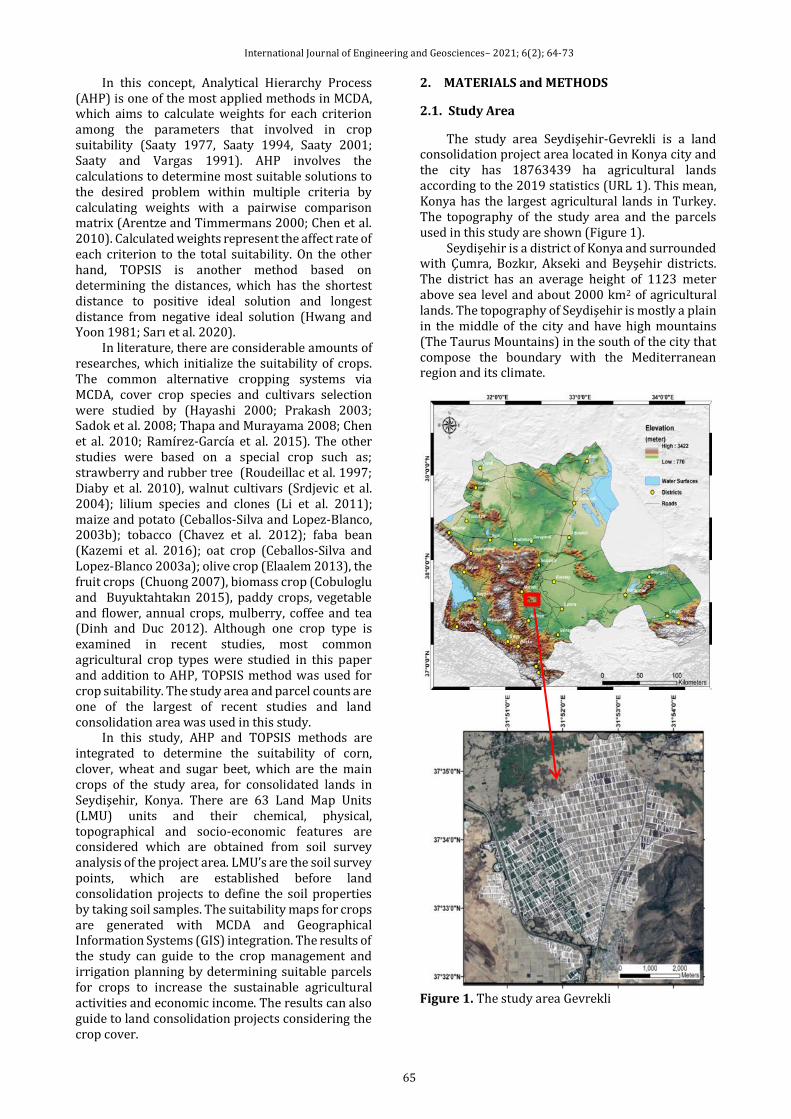
The study area Seydişehir-Gevrekli is a land consolidation project area located in Konya city and the city has 18763439 ha agricultural lands according to the 2019 statistics (URL 1). This mean, Konya has the largest agricultural lands in Turkey. The topography of the study area and the parcels used in this study are shown (Figure 1).

Seydişehir is a district of Konya and surrounded with Çumra, Bozkır, Akseki and Beyşehir districts. The district has an average height of 1123 meter above sea level and about 2000 km2 of agricultural lands. The topography of Seydişehir is mostly a plain in the middle of the city and have high mountains (The Taurus Mountains) in the south of the city that compose the boundary with the Mediterranean region and its climate.

Figure 1. The study area Gevrekli

International Journal of Engineering and Geosciences– 2021; 6(2); 64-73

66

The pH of the soil is varied from slightly acid to strongly alkaline that suitable for a large amount of agricultural crops. The salinity values are appropriate for most of the crops and there are quite a few areas, which have slightly, and moderately salinity. The lime rate of the soils can rise to 46%.

The common texture of the area is loamy and clay-loamy which can be accepted as appropriate for most of the agricultural crops. The common area has poor organic matter rate; thus, fertilizer usage should be considered for agricultural crops. The area has an average 2% slope commonly except the east of the study area.

2.2. Methodology

The application model consists of a combination of AHP and TOPSIS. GIS functions will contribute the visualization and generating suitability maps.

2.2.1 Criteria selection

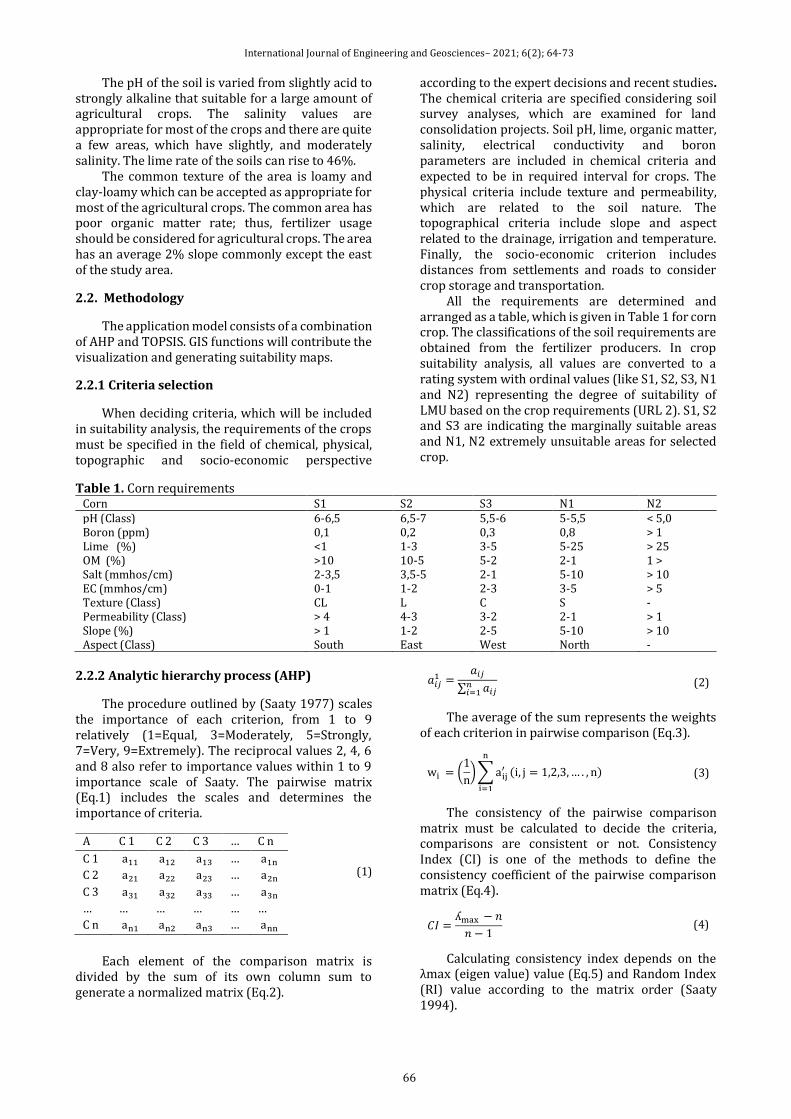
When deciding criteria, which will be included in suitability analysis, the requirements of the crops must be specified in the field of chemical, physical, topographic and socio-economic perspective

according to the expert decisions and recent studies. The chemical criteria are specified considering soil survey analyses, which are examined for land consolidation projects. Soil pH, lime, organic matter, salinity, electrical conductivity and boron parameters are included in chemical criteria and expected to be in required interval for crops. The physical criteria include texture and permeability, which are related to the soil nature. The topographical criteria include slope and aspect related to the drainage, irrigation and temperature. Finally, the socio-economic criterion includes distances from settlements and roads to consider crop storage and transportation.

All the requirements are determined and arranged as a table, which is given in Table 1 for corn crop. The classifications of the soil requirements are obtained from the fertilizer producers. In crop suitability analysis, all values are converted to a rating system with ordinal values (like S1, S2, S3, N1 and N2) representing the degree of suitability of LMU based on the crop requirements (URL 2). S1, S2 and S3 are indicating the marginally suitable areas and N1, N2 extremely unsuitable areas for selected crop.

Table 1. Corn requirements Corn S1 S2 S3 N1 N2 pH (Class) 6-6,5 6,5-7 5,5-6 5-5,5 < 5,0 Boron (ppm) 0,1 0,2 0,3 0,8 > 1 Lime (%) <1 1-3 3-5 5-25 > 25 OM (%) >10 10-5 5-2 2-1 1 > Salt (mmhos/cm) 2-3,5 3,5-5 2-1 5-10 > 10 EC (mmhos/cm) 0-1 1-2 2-3 3-5 > 5 Texture (Class) CL L C S - Permeability (Class) > 4 4-3 3-2 2-1 > 1 Slope (%) > 1 1-2 2-5 5-10 > 10 Aspect (Class) South East West North -

2.2.2 Analytic hierarchy process (AHP)

The procedure outlined by (Saaty 1977) scales the importance of each criterion, from 1 to 9 relatively (1=Equal, 3=Moderately, 5=Strongly, 7=Very, 9=Extremely). The reciprocal values 2, 4, 6 and 8 also refer to importance values within 1 to 9 importance scale of Saaty. The pairwise matrix (Eq.1) includes the scales and determines the importance of criteria.

(1)

Each element of the comparison matrix is divided by the sum of its own column sum to generate a normalized matrix (Eq.2).

𝑎𝑖𝑗1 =

𝑎𝑖𝑗

∑ 𝑎𝑖𝑗𝑛𝑖=1

(2)

The average of the sum represents the weights of each criterion in pairwise comparison (Eq.3).

wi = (1

n) ∑ aij

′

n

i=1

(i, j = 1,2,3, … . , n) (3)

The consistency of the pairwise comparison matrix must be calculated to decide the criteria, comparisons are consistent or not. Consistency Index (CI) is one of the methods to define the consistency coefficient of the pairwise comparison matrix (Eq.4).

𝐶𝐼 =ʎmax − 𝑛

𝑛 − 1 (4)

Calculating consistency index depends on the λmax (eigen value) value (Eq.5) and Random Index (RI) value according to the matrix order (Saaty 1994).

A C 1 C 2 C 3 … C n

C 1 a11 a12 a13 … a1n

C 2 a21 a22 a23 … a2n

C 3 a31 a32 a33 … a3n

… … … … … …

C n an1 an2 an3 … ann

International Journal of Engineering and Geosciences– 2021; 6(2); 64-73

67

ʎ 𝐦𝐚𝐱=

𝟏

𝐧∑ [

∑ 𝐚𝐢𝐣 𝐰𝐣𝐧𝐣=𝟏

𝐰𝐢]

𝐧

𝐢=𝟏

(5)

If CR (Eq.6) exceeds 0.1, based on expert knowledge and experience (Saaty and Vargas 1991), recommends a revision of the pairwise comparison matrix with different values.

𝐶𝑅 =𝐶𝐼

𝑅𝐼 (6)

2.2.3. Topsis

In evaluation matrix Ai, A = (1,2, … , n) represents the alternatives and Ci, C = (1,2, … , m) a set of criteria; where Xi (X11 to Xnm) defines the ratings (Eq.7).

(7)

Calculate the weighted normalized decision matrices R and V via Eq.8 (Hwang and Yoon 1981).

𝒓𝒊𝒋(𝒙) =𝒙𝒊𝒋

√∑ 𝒙𝒊𝒋𝟐𝒏

𝒊=𝟏

, 𝒊 = 𝟏, … . 𝒏 , 𝒋 = 𝟏, … . 𝒎

(8) 𝒗𝒊𝒋(𝒙) = 𝒘𝒊 𝑿 𝒓𝒊𝒋(𝒙) 𝒊 = 𝟏, … . 𝒏 , 𝒋 = 𝟏, … . 𝒎

While positive ideal solution consists of the largest element of weighted normalized decision matrix V, negative ideal solution consists of the smallest element. The J1 and J2 are the benefit (maximization) and the cost (minimization) criteria (Eq.9).

Calculate the separation of the alternatives from the positive and negative ideal solutions via Euclidean distance calculation. The number of Di* and Di- (Eq.10) will be equal to the number of alternatives (Triantaphyllou 2000; Peters and Zelewski 2007).

𝐀+ = {𝐕𝟏+(𝐱), 𝐕𝟐

+(𝐱), . , 𝐕𝐦+(𝐱)} = {(𝐦𝐚𝐱

𝒊𝒗𝒊𝒋 (𝒙) | 𝒋 ∈ 𝒋𝟏) 𝐦𝐢𝐧

𝒊𝒗𝒊𝒋 (𝒙) | 𝒋 ∈ 𝒋𝟐|𝒊 = 𝟏, 𝒏} (9)

𝐀− = {𝐕𝟏−(𝐱), 𝐕𝟐

−(𝐱), . , 𝐕𝐦−(𝐱)} = {(𝐦𝐢𝐧

𝒊𝒗𝒊𝒋 (𝒙) | 𝒋 ∈ 𝒋𝟏) 𝐦𝐚𝐱

𝒊𝒗𝒊𝒋 (𝒙) | 𝒋 ∈ 𝒋𝟐|𝒊 = 𝟏, 𝒏} (9)

𝐃𝐢∗ = √∑⌊𝐕𝐢𝐣(𝐗) − 𝐕𝐣

+(𝐗)⌋𝟐

,

𝐦

𝐣=𝟏

(10)

𝐃𝐢− = √∑⌊𝐕𝐢𝐣(𝐗) − 𝐕𝐣

−(𝐗)⌋𝟐

,

𝐦

𝐣=𝟏

𝐢 = 𝟏, . . , 𝐧 (10)

Calculate the relative closeness to the ideal

solution Ci* with Di* and Di-, where 1 > Ci* > 0. The Ci* values close to 1 will be the better solution relatively (Eq.11).

𝑪𝒊∗ =

𝑫𝒌−

𝑫𝒌∗ + 𝑫𝒌

− (11)

2.2.4. Weight Calculation

Each criterion is reclassified and mapped via ArcGIS 10.1 software, which are visualized in Figure 2 using Inverse Distance Weighted (IDW) spatial analysis. Criteria maps are illustrated from green to red, which represent suitability from high to low.

The first step of generating suitability maps is weight calculation of physical, chemical, topographical and socio-economic criteria with a pairwise comparison matrix (Table 2). Because

chemical parameters and components have vital importance on crop growth, chemical criteria are weighted 60 %. Other criteria weights are calculated 20 % for physical and 10 % for topographic and socio-economic criteria because topographic and socio-economic criteria have indirect effect on crop suitability. The weights of the criteria were specified considering recent studies. Table 2. Crop suitability pairwise matrix

A1 C1 C2 C3 C4 W C1 1 4.7 5 5.1 0.60036 C2 1/4.7 1 2 2.3 0.20114 C3 1/5 1/2 1 1 0.10274 C4 1/5.1 1/2.3 1/1 1 0.09575

A1= Crop Suitability, C1= Chemical, C2=Physical, C3= Topographical, C4=Socio-Economic, CR=0,038, W=Weights

In the second stage, criteria weights are calculated separately according to the criteria (W1) and main criteria (W2). The CR values of all comparisons are lower than 0.10 indicate that the use of the weights are suitable. W3 weights represent the total weight of each main criterion when generating suitability. All the AHP weights are given in Table 3.

C1 C2 C3 … Cm

A1 𝐗𝟏𝟏 𝐗𝟏𝟐 𝐗𝟏𝟑 … 𝐗𝟏𝐦 A2 𝐗𝟐𝟏 𝐗𝟐𝟐 𝐗𝟐𝟑 … 𝐗𝟐𝐦 A3 𝐗𝟑𝟏 𝐗𝟑𝟐 𝐗𝟑𝟑 … 𝐗𝟑𝐦 … … … … … … An 𝐗𝐧𝟏 𝐗𝐧𝟐 𝐗𝐧𝟑 … 𝐗𝐧𝐦

International Journal of Engineering and Geosciences– 2021; 6(2); 64-73

68

Figure 2. Criteria Maps Distance to roads (DR), Distance to settlements (DS), Ph, Salinity (S), Texture (T), Boron (B), Lime (L), Permeability (P), Electrical Conductivity (EC), Organic Matter (OM), Slope (S), Aspect (A)

Table 3. AHP weights of each criterion

Criteria W1 Main-Criteria W2 W3= W1X W2

Chemical 0,6

PH 0.33 0.20

EC 0.12 0.07

B 0.12 0.07

L 0.12 0.07

OM 0.09 0.05

S 0.19 0.11

Physical 0,2 T 0.75 0.15

P 0.25 0.05

Topographic 0,1 S 0.75 0.07

A 0.25 0.02

Social-Economic 0,1 DR 0.60 0.06

DS 0.40 0.04

International Journal of Engineering and Geosciences– 2021; 6(2); 64-73

69

After weight calculation with AHP, TOPSIS technique is applied to be able to determine crop suitability. The TOPSIS technique aims to determine the distances from selected alternative to negative and positive ideal solutions. The selected alternative should have the shortest distance from the positive ideal solution and the longest from the negative ideal solution. The respective distances to positive and negative ideal solutions are defined as a similarity index (Hwang and Yoon 1981). In crop suitability analysis, S1 is considered to be ideal point and the N2 is the negative ideal point for each crop.

The TOPSIS evaluation matrix includes 63 LMU and related rankings in 0-30, 30-60, 60-120 cm depth for 12 criteria which are included in 4 main criteria. The ranking values for each criterion are defined between 1-9 considering the LMU values and crop requirements (Table 1). The ranking values are used to calculate R and V matrices via W3 weights that calculated with AHP (Table 2). The positive ideal solution A+ and the negative ideal solution A-, which are the maximum and minimum values of the V matrix, are calculated.

Based on the A+ and A- values, distance to positive ideal solutions Di* and distance to negative ideal solution Di- values are calculated for each LMU. Finally, relative closeness to ideal solution Ci* values are calculated (Table 4) to determine the land suitability ranking definition. The Ci* values are classified as follows;

Ci* > 0.8: Highly Suitable (S1), 0.8 > Ci* > 0.65: Moderately Suitable (S2), 0.65 > Ci* > 0.50: Slightly Suitable (S3), 0.50 > Ci* > 0.40: Moderately not Suitable (N1), Ci* <0.40: None Suitable (N2).

Table 4. Distances from positive and negative ideal solutions

LMU Di* Di- Ci* Classification 1(0-30) 0.007 0.033 0.82571 S2 1 (30-60) 0.019 0.022 0.53753 S3 1 (60-120) 0.023 0.021 0.48719 N1 2(0-30) 0.013 0.031 0.70879 S2 2 (30-60) 0.018 0.018 0.50375 S3 2 (60-120) 0.010 0.032 0.76626 S2 … … … … … 63 (0-30) 0.008 0.030 0.79496 S2 63 (30-60) 0.038 0.016 0.29240 N2 63 (60-120) 0.040 0.007 0.14884 N2

3. RESULTS and DISCUSSION

The suitability index maps are produced according to the 0-30, 30-60 and 60-120 cm depths of LMU’s respectively. The suitability index maps are generated by using Ci* values which are calculated by TOPSIS method.

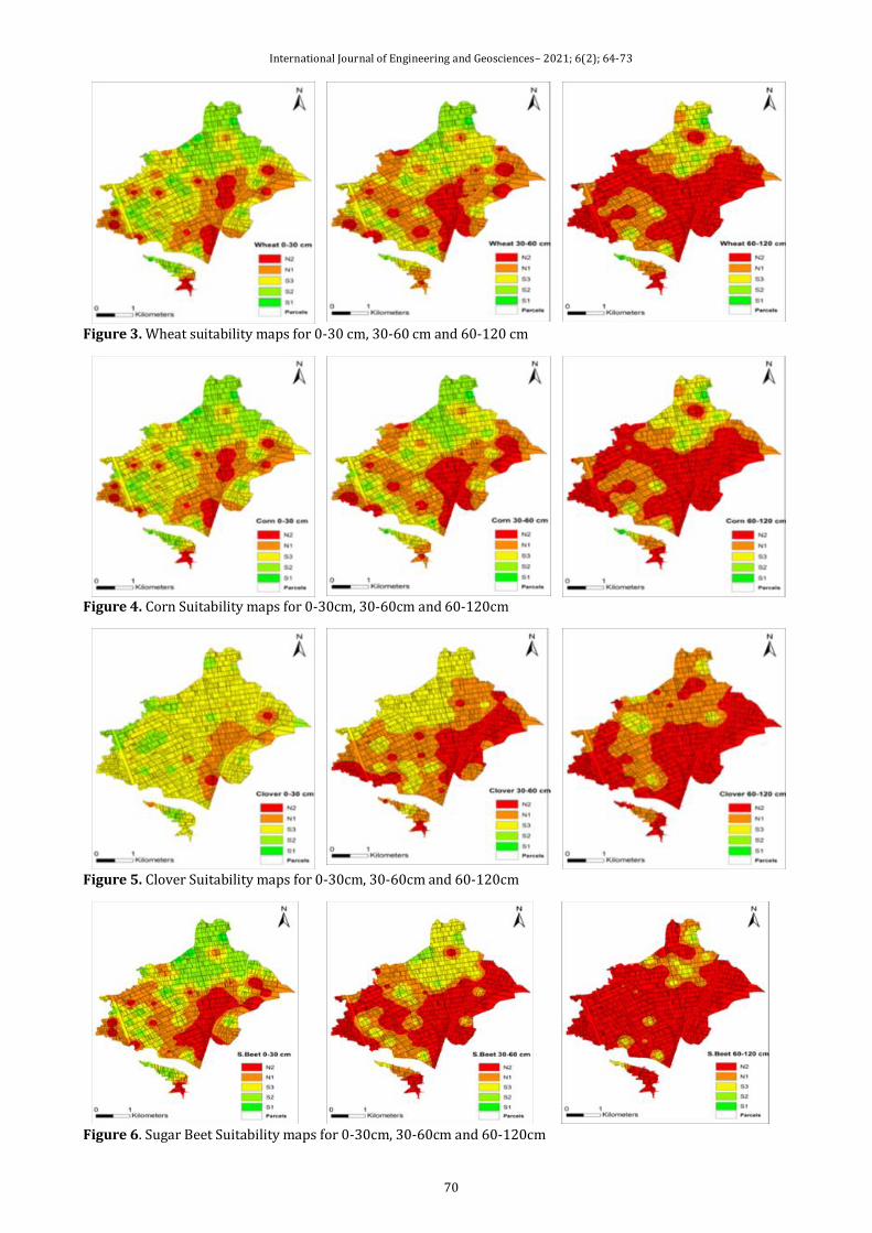
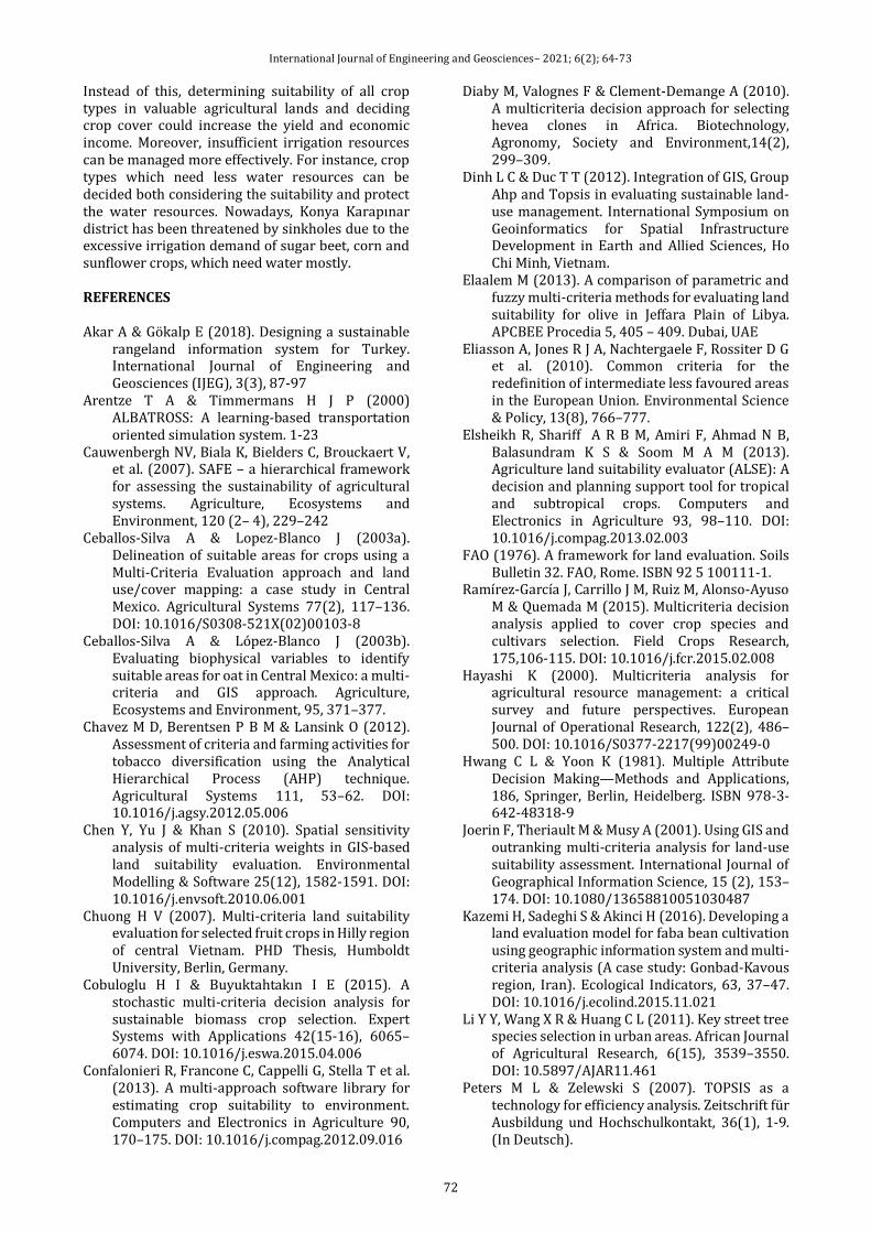
Because corn and wheat requirements are quite similar to each other, suitability maps can be investigated together. Wheat and corn are the most widely grown crops in the study area. Addition to this, there are a considerable amount of parcel which has high suitability for wheat and corn. Especially the north of the study area has very high suitability with 0.838 for corn and 0.860 for wheat. The parcels that have very low suitability are quite a few due to the slightly alkaline soils, high salinity and very low permeability values. The lowest suitability index values for corn is 0.14 and for wheat 0.18. The general suitability of the area is calculated 59 % for corn and 46 % for wheat including S1, S2 and S3.

The clover and sugar beet crop needs high values of boron. However, the boron values of the area are not sufficient for these crops. Addition to this, clover needs moderately alkaline soils, thus, slightly alkaline soils affect the growth respectively. The S1 is not included in the study area for clover and the 5 % of the study area have very low suitability. The sugar beet suitability index is varied from 0.85 to 0.16 and clover 0.73 to 0.29. The suitability index maps for clover, wheat, sugar beet and clover are given in Figure 3, 4, 5 and 6.

The suitability ranking (S1, S2, S3, N1 and N2) rates are compared according to the 63 LMU of the study area. The S1, S2 and S3 are assigned as suitable areas and N1, N2 as unsuitable. According to this, 59 % of the study area have suitability for corn, 43 % for sugar beet, 76 % for clover and 46 % for wheat for 0-30 cm depth. The comparisons of the suitability rankings are given in Table 5 and 6.

The suitability ranking rates are compared according to the 2382 parcels. The highest value of the S1 is 22 for sugar beet. Considering the S1, S2 and S3 are suitable rankings, 1481 parcels for corn, 1457 parcels for wheat, 2027 parcels for clover and 1127 parcels for sugar beet are suitable. In other words, 1000,22 ha for corn, 985,5 ha for wheat, 1285,71 ha for clover and 764,16 ha of the total 1524,47 ha study area for sugar beet are suitable. The comparisons of the parcel counts are given in Table 6.

Validating suitability maps can only be possible with crop statistics of the study area. Thus, 2016 parcel based crop records are retrieved from Republic Of Turkey Ministry Of Food, Agriculture and Livestock Seydişehir Directorates with using farmer registration system database. As shown in Figure 7, wheat is the most widely grown crop in study area with 80.5% rate of total crop. However, habits, agricultural incentives and continuously changing prices are more decisive factors than suitability. Due to this, crop records may not reflect agricultural lands suitability.

International Journal of Engineering and Geosciences– 2021; 6(2); 64-73

70

Figure 3. Wheat suitability maps for 0-30 cm, 30-60 cm and 60-120 cm

Figure 4. Corn Suitability maps for 0-30cm, 30-60cm and 60-120cm

Figure 5. Clover Suitability maps for 0-30cm, 30-60cm and 60-120cm

Figure 6. Sugar Beet Suitability maps for 0-30cm, 30-60cm and 60-120cm

International Journal of Engineering and Geosciences– 2021; 6(2); 64-73

71

Table 5. Comparisons of the 63 LMU

Class Corn

30 cm Corn

60 cm Corn

120 cm S.Beet 30 cm

S.Beet 60 cm

S.Beet 120 cm

Clover 30 cm

Clover 60 cm

Clover 120 cm

Wheat 30 cm

Wheat 60 cm

Wheat 120 cm

S1 7 5 5 4 0 0 0 0 0 6 3 3 S2 30 16 16 21 7 1 15 2 2 9 13 13 S3 0 10 10 2 13 10 33 21 4 14 12 12 N1 12 12 12 12 7 4 12 18 15 15 13 13 N2 14 20 20 24 36 48 3 22 42 19 22 22

Table 6. Parcel count comparisons of suitability classes

Class Corn 30cm

Corn 60cm

Corn 120cm

S.Beet 30 cm

S.Beet 60 cm

S.Beet 120 cm

Clover 30 cm

Clover 60 cm

Clover 120 cm

Wheat 30

Wheat 60 cm

Wheat 120 cm

S1 19 8 9 21 0 0 0 0 0 22 7 9 S2 585 348 56 533 55 2 270 1 4 580 255 56 S3 877 743 374 573 490 98 1757 736 124 855 775 367 N1 659 776 619 770 598 295 317 985 874 664 888 545 N2 238 503 1320 481 1235 1983 34 656 1376 257 453 1401

Figure 7. Crop Map of the Gevrekli

4. CONCLUSION

Although determining the crop suitability is a very complex study from planning to the establishing stage, the integration of AHP, TOPSIS and GIS functions provide an effective platform to determine the suitability. In this context, the most important factors are the criteria selection and data preparation for the study area. Firstly, the decision makers must decide the priorities of crops. Then, the weights of the criteria can be easily modified with the AHP according to the priorities. Although 12 criteria are used in this study, several criteria can be added such as; meteorological and irrigation. Because the parcels are included in a completed land consolidation project area, all the parcels have an irrigation canal. Meteorological parameters should be observed such as; humidity, soil temperature, wind, wind direction and the minimum and maximum temperature. However, there aren’t any distinctive topographical features that meteorological observations can change. Addition to

this, these parameters should be included in AHP and TOPSIS. Thus, more realistic crop suitability can be determined by enlarging the scope of the land facilities. Another important issue in this scope is the data collection and accuracy. Because there are 63 LMU in the study area, the accuracy of the suitability decreased relatively. While 63 LMU are enough to decide, higher LMU will be better to determine the suitability accurately.

The comparison of the determined suitable crops and grown crops should be evaluated each year. The suitability results can easily integrate with farmer registration systems or sustainable agricultural management systems. Thus, the consistency of the study and comparisons can be investigated together with irrigation, fertilization and pest control to improve the crop yields.

Although recent studies based on AHP method (Hayashi 2000; Prakash 2003; Sadok et al. 2008; Thapa and Murayama 2008; Chen et al. 2010; Ramírez-García et al. 2015), this study introduced TOPSIS method via AHP weight calculation for crop suitability analysis. Moreover, wheat, corn, clover and sugar beet crops were examined in this study which are the main crop cover of the study area. However, (Roudeillac et al. 1997; Diaby et al. 2010; Ceballos-Silva A & Lopez-Blanco 2003a; Ceballos-Silva and Lopez-Blanco, 2003b; Chuong 2007; Li et al. 2011; Chavez et al. 2012; Dinh and Duc 2012; Elaalem 2013; Srdjevic et al. 2014; Cobuloglu and Buyuktahtakın 2015; Kazemi et al. 2016) studied on a special crop type. Thus, this study and method can be applied to a large amount of agricultural lands which crop cover is similar to the study area. This can lead more comprehensive approach for crop management and planning by examining all crops in a study area.

This study also guide to the local authorities as like province agricultural directorates for planning and deciding agricultural incentives. In recent status, directorates are giving incentives to farmers to increase the yield and decrease the expenditures of agricultural activities. However, the suitability of crops are not examining in this stage. Additionally, for rural development, farmers are encouraged for different crop types to provide new economic field.

International Journal of Engineering and Geosciences– 2021; 6(2); 64-73

72

Instead of this, determining suitability of all crop types in valuable agricultural lands and deciding crop cover could increase the yield and economic income. Moreover, insufficient irrigation resources can be managed more effectively. For instance, crop types which need less water resources can be decided both considering the suitability and protect the water resources. Nowadays, Konya Karapınar district has been threatened by sinkholes due to the excessive irrigation demand of sugar beet, corn and sunflower crops, which need water mostly. REFERENCES Akar A & Gökalp E (2018). Designing a sustainable

rangeland information system for Turkey. International Journal of Engineering and Geosciences (IJEG), 3(3), 87-97

Arentze T A & Timmermans H J P (2000) ALBATROSS: A learning-based transportation oriented simulation system. 1-23

Cauwenbergh NV, Biala K, Bielders C, Brouckaert V, et al. (2007). SAFE – a hierarchical framework for assessing the sustainability of agricultural systems. Agriculture, Ecosystems and Environment, 120 (2– 4), 229–242

Ceballos-Silva A & Lopez-Blanco J (2003a). Delineation of suitable areas for crops using a Multi-Criteria Evaluation approach and land use/cover mapping: a case study in Central Mexico. Agricultural Systems 77(2), 117–136. DOI: 10.1016/S0308-521X(02)00103-8

Ceballos-Silva A & López-Blanco J (2003b). Evaluating biophysical variables to identify suitable areas for oat in Central Mexico: a multi-criteria and GIS approach. Agriculture, Ecosystems and Environment, 95, 371–377.

Chavez M D, Berentsen P B M & Lansink O (2012). Assessment of criteria and farming activities for tobacco diversification using the Analytical Hierarchical Process (AHP) technique. Agricultural Systems 111, 53–62. DOI: 10.1016/j.agsy.2012.05.006

Chen Y, Yu J & Khan S (2010). Spatial sensitivity analysis of multi-criteria weights in GIS-based land suitability evaluation. Environmental Modelling & Software 25(12), 1582-1591. DOI: 10.1016/j.envsoft.2010.06.001

Chuong H V (2007). Multi-criteria land suitability evaluation for selected fruit crops in Hilly region of central Vietnam. PHD Thesis, Humboldt University, Berlin, Germany.

Cobuloglu H I & Buyuktahtakın I E (2015). A stochastic multi-criteria decision analysis for sustainable biomass crop selection. Expert Systems with Applications 42(15-16), 6065–6074. DOI: 10.1016/j.eswa.2015.04.006

Confalonieri R, Francone C, Cappelli G, Stella T et al. (2013). A multi-approach software library for estimating crop suitability to environment. Computers and Electronics in Agriculture 90, 170–175. DOI: 10.1016/j.compag.2012.09.016

Diaby M, Valognes F & Clement-Demange A (2010). A multicriteria decision approach for selecting hevea clones in Africa. Biotechnology, Agronomy, Society and Environment,14(2), 299–309.

Dinh L C & Duc T T (2012). Integration of GIS, Group Ahp and Topsis in evaluating sustainable land-use management. International Symposium on Geoinformatics for Spatial Infrastructure Development in Earth and Allied Sciences, Ho Chi Minh, Vietnam.

Elaalem M (2013). A comparison of parametric and fuzzy multi-criteria methods for evaluating land suitability for olive in Jeffara Plain of Libya. APCBEE Procedia 5, 405 – 409. Dubai, UAE

Eliasson A, Jones R J A, Nachtergaele F, Rossiter D G et al. (2010). Common criteria for the redefinition of intermediate less favoured areas in the European Union. Environmental Science & Policy, 13(8), 766–777.

Elsheikh R, Shariff A R B M, Amiri F, Ahmad N B, Balasundram K S & Soom M A M (2013). Agriculture land suitability evaluator (ALSE): A decision and planning support tool for tropical and subtropical crops. Computers and Electronics in Agriculture 93, 98–110. DOI: 10.1016/j.compag.2013.02.003

FAO (1976). A framework for land evaluation. Soils Bulletin 32. FAO, Rome. ISBN 92 5 100111-1.

Ramírez-García J, Carrillo J M, Ruiz M, Alonso-Ayuso M & Quemada M (2015). Multicriteria decision analysis applied to cover crop species and cultivars selection. Field Crops Research, 175,106-115. DOI: 10.1016/j.fcr.2015.02.008

Hayashi K (2000). Multicriteria analysis for agricultural resource management: a critical survey and future perspectives. European Journal of Operational Research, 122(2), 486–500. DOI: 10.1016/S0377-2217(99)00249-0

Hwang C L & Yoon K (1981). Multiple Attribute Decision Making—Methods and Applications, 186, Springer, Berlin, Heidelberg. ISBN 978-3-642-48318-9

Joerin F, Theriault M & Musy A (2001). Using GIS and outranking multi-criteria analysis for land-use suitability assessment. International Journal of Geographical Information Science, 15 (2), 153–174. DOI: 10.1080/13658810051030487

Kazemi H, Sadeghi S & Akinci H (2016). Developing a land evaluation model for faba bean cultivation using geographic information system and multi-criteria analysis (A case study: Gonbad-Kavous region, Iran). Ecological Indicators, 63, 37–47. DOI: 10.1016/j.ecolind.2015.11.021

Li Y Y, Wang X R & Huang C L (2011). Key street tree species selection in urban areas. African Journal of Agricultural Research, 6(15), 3539–3550. DOI: 10.5897/AJAR11.461

Peters M L & Zelewski S (2007). TOPSIS as a technology for efficiency analysis. Zeitschrift für Ausbildung und Hochschulkontakt, 36(1), 1-9. (In Deutsch).

International Journal of Engineering and Geosciences– 2021; 6(2); 64-73

73

Prakash T N (2003). Land Suitability Analysis for Agricultural Crops: A Fuzzy Multicriteria Decision Making Approach. MS Thesis, International Institute for Geo-information Science and Earth Observation. Netherlands.

Radulescu C Z, Radulescu M, Rahoveanu A T, Rahoveanu MT & Beciu S (2011). A multi-criteria approach for assessment of agricultural systems in context of sustainable agriculture. Recent Researches in Applied Informatics, 167-171.

Radulescu C Z, Rahoveanu A T & Radulescu M (2010). A hybrid multi-criteria method for performance evaluation of romanian South Muntenia Region in context of sustainable agriculture. Proceedings of the International Conference on Applied Computer Science (ACS), 1, 303-308.

Rigby D, Woodhouse P, Young T & Burton M (2001). Constructing a farm level indicator of sustainable practice. Ecological Economics 39(3), 463– 478.

Roudeillac P, Faedi W & Lavialle O (1997). A multicriteria decision aid to determine the genetic performance of strawberry through a varietal observatory network in Western Europe. Acta Horticulturae, 439, 307–317.

Saaty T L (1977). A scaling method for priorities in hierarchical structures. Journal of Mathematical Psychology, 15(3), 234–281.

Saaty T L (1994). Fundamentals of decision making and priority theory with the analytical hierarchy process. RWS Publucations, Pittsburg, 69-84. ISBN: 9780962031762

Saaty T L (2001) Decision Making with Dependence and Feedback: The Analytic Network Process, 2nd edition, PRWS Publications, Pittsburgh PA. ISBN: 9780962031793

Saaty T L & Vargas L G (1991). Prediction, Projection and Forecasting. Springer Netherlands. ISBN 978-94-015-7954-4

Sadok W, Angevin F, Bergez J, Bockstaller C et al. (2008). Ex ante assessment of the sustainability of alternative cropping systems: implications for using multi-criteria decision-aid methods. A review. Agronamy and Sustainable

Development, 28, 163–174. DOI: 10.1051/agro:2007043

Sarı F, Ceylan D A, Özcan M M & Özcan M M (2020). A comparison of multicriteria decision analysis techniques for determining beekeeping suitability. Apidologie. DOI: 10.1007/s13592-020-00736-7.

Srdjevic B, Srdjevic Z, Kolarov V (2004). Group evaluation of walnut cultivars as a multi criterion decision-making process. CIGR International Conference, Beijing, China.

Wang F, Hall G B, Subaryono (1990). Fuzzy information representation and processing in conventional GIS software: data base design and application. International Journal of Geographical Information System, 4(3), 261–283. DOI: 10.1080/02693799008941546

Thapa R B, Murayama Y (2008). Land evaluation for peri-urban agriculture using analytical hierarchical process and geographic information system techniques: A case study of Hanoi. Land use policy, 25(2), 225-239. DOI: 10.1016/j.landusepol.2007.06.004

Triantaphyllou E (2000). Multi-criteria decision making methods: A comparative study, 44, Springer, Boston, MA. ISBN: 978-1-4757-3157-6

Yu J, Chen Y, Wu J, Khan S (2011). Cellular automata-based spatial multi-criteria land suitability simulation for irrigated agriculture. International Journal of Geographical Information Science, 25 (1), 131–148.

Zeleny M (1982). Multiple Criteria Decision-making. McGraw-Hill, New York, NY, 563 pages. ISBN: 9780070727953

URL 1. Turkish Statistical Institute Official web site. https://biruni.tuik.gov.tr/medas/?kn=92&locale=tr (Accessed date: 18.05.2020)

URL 2. FAO Official web site. Available at “http://www.fao.org/3/x5648e/x5648e0j.htm (Last visited 18.05.2020).

Zolekar R B & Bhagat V S (2015). Multi-criteria land suitability analysis for agriculture in hilly zone: Remote sensing and GIS approach. Computers and Electronics in Agriculture, 118, 300–321.

© Author(s) 2021. This work is distributed under https://creativecommons.org/licenses/by-sa/4.0/

* Corresponding Author Cite this article

(duranza@itu.edu.tr) ORCID ID 0000 – 0002 – 1608 – 0119 *(atikm@itu.edu.tr) ORCID ID 0000 – 0003 – 2273 – 7751 Research Article / DOI: 10.26833/ijeg.691696

Duran Z & Atik M E (2021). Accuracy comparison of interior orientation parameters from different photogrammetric software and direct linear transformation method. International Journal of Engineering and Geosciences, 6(2), 74-80.

Received: 20/02/2020; Accepted: 01/05/2020

International Journal of Engineering and Geosciences– 2021; 6(2); 74-80

International Journal of Engineering and Geosciences

https://dergipark.org.tr/en/pub/ijeg

e-ISSN 2548-0960

Accuracy comparison of interior orientation parameters from different photogrammetric software and direct linear transformation method

Zaide Duran1 , Muhammed Enes Atik*1

1Istanbul Technical University, Civil Engineering Faculty, Geomatics Engineering Department, İstanbul, Turkey

Keywords ABSTRACT Camera calibration Accuracy assessment Three-Dimensional model Photogrammetry Interior orientation

The integration of computer vision algorithms and photogrammetric methods leads to procedures that increasingly automate the image-based 3D modeling process. The main objective of photogrammetry is to obtain a three-dimensional model using terrestrial or aerial images. Calibration of the camera and detection of the orientation parameters are important for obtaining accurate and reliable 3D models. For this purpose, many methods have been developed in the literature. However, since each method has different mathematical background, calibration results may be different. In this study, the effect of camera interior orientation parameters obtained from different methods on the accuracy of three-dimensional model will be examined. In this context, a test area consisting of 21 points was used. The test network was coordinated in a local coordinate system using geodetic methods. Some points of the test area were selected as the check point and accuracy analysis was performed. Direct Linear Transformation (DLT) method, MATLAB, Agisoft Lens, Photomodeler, 3D Flow Zephyr software were analysed. The lowest error value of 7.7 cm was achieved by modelling with Agisoft Lens.

1. INTRODUCTION

Photogrammetry involves scientific methods that calculate three-dimensional coordinates of an object by measuring the corresponding points in overlapping images. The mathematical relationship between an image point and an object point is derived by equinox linear equations based on central projection (Akcay et al. 2017). Photogrammetry is the most reliable and useful method for 3D modelling of the real world. Recording of historical artefacts (Duran and Aydar 2012; Ulvi and Toprak 2016), 3D modelling of the surface (Nex and Remondino 2014; Yemenicioglu et al. 2016), medical studies (Reis 2018) and in different situations where measurement must be made without contact with objects (Linder 2009), photogrammetry is widely used. Camera calibration is the determination of internal orientation parameters of the camera by the 3D coordinates of a point in space and the corresponding image coordinates (Song et al. 2013). There are many studies about camera calibration

that is used for enhancing 3D modelling. Zhao et al. (2015) were developed faster calibration method. They used a matching method based on heterodyne multi-frequency phase-shifting. Root mean square error (RMSE) was obtained as 2.5 cm. In another study, self-calibration of range cameras was realised using bundle adjustment (Lichti et al. 2010). 3-D coordinate errors were reduced by up to 74%. In addition to these studies, there are also comprehensive studies that examine calibration methods in general. In the study conducted by Hemayed (2003), self-calibration methods for determining interior parameters were examined. In another large-scale study, calibration methods were examined as traditional camera calibration method, camera self-calibration method, and camera calibration method based on active vision (Song et al. 2013).

Among the existing methods, Structure from Motion (SFM) is a popular algorithm. This algorithm creates 3D models using photographs taken from different angles of an object. The positional accuracy

International Journal of Engineering and Geosciences– 2021; 6(2); 74-80

75

of the created models is affected by camera calibration. Therefore, accurate calibration of the camera is important in terms of 3D modelling. In this study, the effect of camera calibration values obtained from different popular software on 3D model accuracy was investigated. MATLAB, Agisoft Lens, Photomodeler, 3D Flow Zephyr and Direct Linear Transformation (DLT) methods have been selected. A three dimensional test area was created to evaluate the calibration results.

2. MATERIAL and METHODS

2.1. Material

Application was carried out with a Nikon D800 camera (Figure 1). The camera with a variable lens is set to a focal length of 24 mm.

Figure 1. Nikon D800 Digital SLR Camera

Within the scope of the study, a test network was established. The test area contains 21 points (Figure 2). The local coordinates of the points were determined by geodetic measurements using Total Station. It has 3 mm + 2 ppm distance accuracy and 3” (0.9 mgon) angle accuracy. Points with different height values have been established for an accurate assessment. The height varies between the lowest and the highest point by 10 cm. Photos of the test area were taken at a distance of approximately 50 cm.

Figure 2. Test area

2.2. Camera Calibration

The camera calibration is one of the classic problems of the field of photogrammetry. Calibration of a camera can be regarded as the inverse of photogrammetric process. In the photogrammetric process, orientation parameters are known and coordinates of the object points are searched, but in camera calibration, the coordinates of the object points are known and the elements of the internal orientation are searched (Kraus 1993). Camera parameters can vary with temperature, humidity, atmospheric pressure, and the camera must be calibrated from time to time for the detection of parameters. (Song et al. 2013). Since the study was carried out in a laboratory environment and its atmospheric conditions were standard laboratory conditions (25 °C at 100 kPa).

Camera calibration is performed to obtain the interior orientation parameters of the camera. With these parameters obtained as a result of the calibration, the spatial beam is fixed to the projection centre (Ozdemir and Duran 2017). Interior orientation parameters are calibrated focal length c, coordinates of principal point coordinates (x0, y0) and distortion parameters. When the camera focuses on a point, the focal length is represented by c. The focal length should be precisely determined because it affects the coordinates due to the mathematical model of photogrammetry. Most of the cameras used in photogrammetry produce photographs which can also be considered central projections of sufficiently accurate spatial bodies. The central point of the central projection is called the projection centre. The projection centre’s projection point on the image is called the principal point.

Radial distortion is the image displacement that occurs when the rays coming from different angles to the lens focus on or behind the projection plane due to angular magnification caused by the lens. Radial distortion affects the position of the point on the image radially. Radial distortion should be modelled with high accuracy because of its positional effect on coordinates. The tangential distortion occurs if the lens elements and the centres of the image sensor are not coincident and their planes are not parallel (Ozdemir and Duran 2017). The image coordinates with radial and tangential distortion (x', y') formulas are shown in equation (1) and (2).

In equation (1) and equation (2), �̅�=x-x0, �̅�=y-y0, 22 '' yxr

Tangential distortion parameters are k, radial distortion parameters are p (Drap and Lefèvre 2016). These are calculated in calibration process.

x'=x+�̅�(𝑘 ⥂1 𝑟2 + 𝑘2𝑟

4 + 𝑘3𝑟6 +⋯) + [𝑝1(𝑟

2 + 2𝑥′2) + 2𝑝2𝑥

′𝑦 ′](1 + 𝑝3𝑟2 +⋯) (1)

y'=y+�̅�(𝑘 ⥂1 𝑟2 + 𝑘2𝑟

4 + 𝑘3𝑟6 +⋯) + [𝑝2(𝑟

2 + 2𝑦′2) + 2𝑝1𝑥′𝑦′](1 + 𝑝3𝑟

2+. . . ) (2)

International Journal of Engineering and Geosciences– 2021; 6(2); 74-80

76

3. APPLICATION

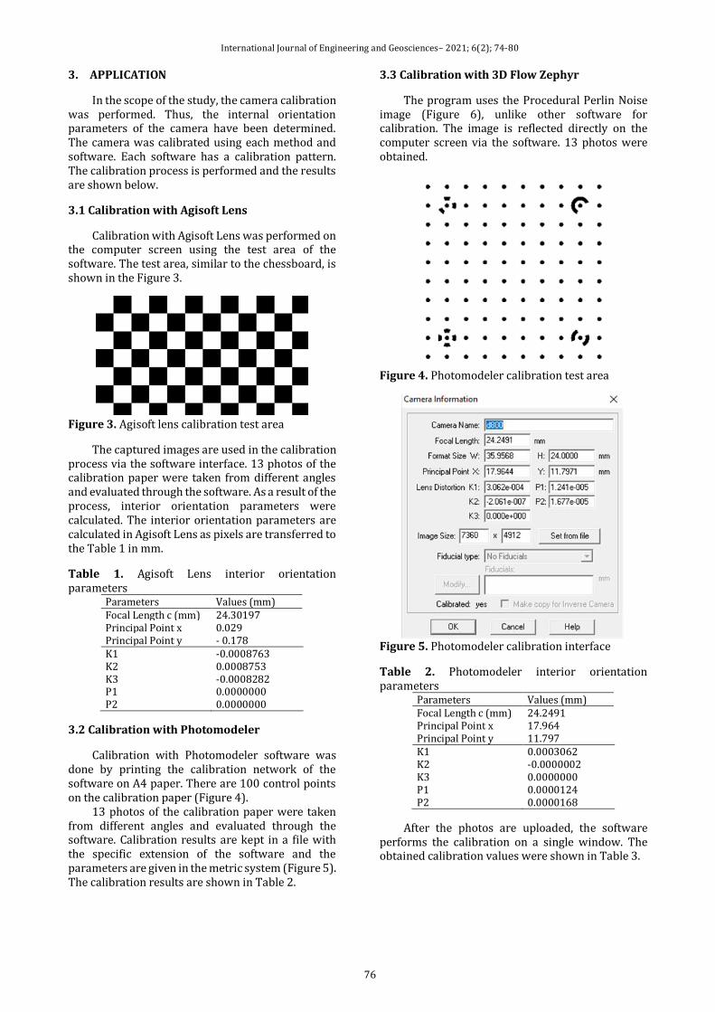
In the scope of the study, the camera calibration was performed. Thus, the internal orientation parameters of the camera have been determined. The camera was calibrated using each method and software. Each software has a calibration pattern. The calibration process is performed and the results are shown below.

3.1 Calibration with Agisoft Lens

Calibration with Agisoft Lens was performed on the computer screen using the test area of the software. The test area, similar to the chessboard, is shown in the Figure 3.

Figure 3. Agisoft lens calibration test area

The captured images are used in the calibration process via the software interface. 13 photos of the calibration paper were taken from different angles and evaluated through the software. As a result of the process, interior orientation parameters were calculated. The interior orientation parameters are calculated in Agisoft Lens as pixels are transferred to the Table 1 in mm.

Table 1. Agisoft Lens interior orientation parameters

Parameters Values (mm) Focal Length c (mm) 24.30197 Principal Point x 0.029 Principal Point y - 0.178 K1 K2 K3 P1 P2

-0.0008763 0.0008753 -0.0008282 0.0000000 0.0000000

3.2 Calibration with Photomodeler

Calibration with Photomodeler software was done by printing the calibration network of the software on A4 paper. There are 100 control points on the calibration paper (Figure 4).

13 photos of the calibration paper were taken from different angles and evaluated through the software. Calibration results are kept in a file with the specific extension of the software and the parameters are given in the metric system (Figure 5). The calibration results are shown in Table 2.

3.3 Calibration with 3D Flow Zephyr

The program uses the Procedural Perlin Noise image (Figure 6), unlike other software for calibration. The image is reflected directly on the computer screen via the software. 13 photos were obtained.

Figure 4. Photomodeler calibration test area

Figure 5. Photomodeler calibration interface

Table 2. Photomodeler interior orientation parameters

Parameters Values (mm) Focal Length c (mm) 24.2491 Principal Point x 17.964 Principal Point y 11.797 K1 K2 K3 P1 P2

0.0003062 -0.0000002 0.0000000 0.0000124 0.0000168

After the photos are uploaded, the software performs the calibration on a single window. The obtained calibration values were shown in Table 3.

International Journal of Engineering and Geosciences– 2021; 6(2); 74-80

77

Figure 6. Procedural Perlin Noise image

Table 3. 3D Flow Zephyr interior orientation parameters

Parameters Values (mm) Focal Length c (mm) 24.1469 Principal Point x 17.982 Principal Point y 11.745 K1 K2 K3 P1 P2

-0.0008726 0.0000713 0.0001438 0.0000000 0.0000000

3.4 Calibration with MATLAB

Camera Calibrator is used in the computer vision toolbox for calibration via MATLAB. MATLAB Camera Calibrator estimates camera interior orientation, exterior orientation, and lens distortion parameters. The program benefits from previous studies for necessary calculations (Zhang 2000).

The test area used by the program is in the form of a chessboard. A checkerboard image can be created within the software in different sizes and dots. The left half of the checkerboard image is in black and white and the right half is in black and grey to define the coordinate system (Figure 7).

Figure 7. MATLAB calibration test area

When the software completes the calibration process, it sends the results and errors to the MATLAB workspace as a variable. The interior orientation parameters produced with MATLAB are shown in Table 4.

Table 4. MATLAB interior orientation parameters Parameters Values (mm) Focal Length c (mm) 24.3622 Principal Point x 17.993 Principal Point y 11.822 K1 K2 K3 P1 P2

-0.0007385 -0.0003338 0.0040482 0.0000062 -0.0000012

3.5 Calibration with Direct Linear Transformation (DLT)

Direct Linear Transformation (DLT) method is a linear calibration method. It was developed in 1971 by Abdel-Aziz and Karara (2015). The major advantage of this method is that the solution is linear and does not have an approximate value problem. With DLT equations, it is possible to reach the space coordinates directly from the image coordinates (Tasdemir et al. 2009). In addition to the parameters added to the 11 parameters, DLT equations are given in the following equations. There are 16 parameters in direct linear transformation method. 11 are used for conversion.

Basic equations of DLT are obtained by rearranging the mathematical model of photogrammetry. This equation (3) and (4) shows the relationship between the image coordinates and the object coordinates.

𝑢 − 𝛥𝑢 =𝐿1𝑥 + 𝐿2𝑦 + 𝐿3𝑧 + 𝐿4

𝐿9𝑥 + 𝐿10𝑦 + 𝐿11𝑧 + 1 (3)

𝑣 − 𝛥𝑣 =𝐿5𝑥 + 𝐿6𝑦 + 𝐿7𝑧 + 𝐿8

𝐿9𝑥 + 𝐿10𝑦 + 𝐿11𝑧 + 1 (4)

where x,y,z = object coordinates of point, u, v=image coordinates, 𝛥𝑢, 𝛥𝑣=distortion values.

The parameters from L1 to L11 are the camera calibration parameters. L12, L13, L14 related to radial distortion, L15, L16 are the parameters related to tangential distortion. The parameters were calculated using MATLAB (Table 5). The calculated parameters are as follows. Calibration with DLT was performed on the prepared 3D test area. In the equations (3) and (4), the unknown object coordinates are x, y, z. At least three equations are required to solve a system with three unknowns. It is not possible to solve the system, since two equations for a point can be obtained from one image. However, four equations can be obtained for one point from two images and x, y, z unknowns can be calculated. For 3D coordinate calculation, DLT parameters must be calculated on at least two images. Below are the points of the two images (Figure 8).

The interior orientation parameters obtained by using the DLT parameters are as follows (Table 6).

International Journal of Engineering and Geosciences– 2021; 6(2); 74-80

78

3.6 Comparison of Calibration Parameters

The obtained calibration parameters were compared and visualized using graphs. For focal length, the methods gave similar results except DLT. The focal length that was computed by DLT, had higher value. The closest value to the prior focal length value (24 mm) was the computed focal length by 3D Flow Zephyr software. The proximity to the prior value is not meaningful for photogrammetry. The method that can best detect the change in focal length gives more accurate results.

Figure 8. Images used for DLT calibration

Table 5. DLT parameters for Image 1 and Image 2 Parameters Image 1 Image 2

L1 -0,322373374 0,140190398 L2 -23,01061838 0,95382684 L3 3,576539156 2,485046498 L4 19,75360416 -3,584883124-- L5 -23,40591264 0,06446149 L6 0,005902536 1,051023064- L7 -2,545372994 4,307002585 L8 25,94926373 -5,303660721 L9 0,056994319 -0,028437462

L10 -0,158729043 -0,17646057 L11 -0,896653801 -0,79326842 L12 -0,000125723 0,02108416 L13 -9,75E-07 -0,000139306 L14 4,95E-09 2,62E-07 L15 0,000672215 0,033999895 L16 0,000295521 0,001409398

Table 6. DLT interior orientation parameters Parameters Values (mm) Focal Length c (mm) 25.5206 Principal Point x 0.513 Principal Point y 1.138 K1 K2 K3 P1 P2

0.0104792 -0.0000701 0.0000001 0.0173360 0.0073831

Figure 9. Focal length values

In radial distortion graph, there were three distortion values. Photomodeller software calculated distortion values K1, K2 and K3 near to 0.

Figure 10. Radial distortion values

Significant results were obtained at the tangential distortion. While the methods outside the DLT were calculated to be almost 0, DLT calculated high value tangential distortion. It is note that the interior orientation parameters have been calculated with different values for each method. The effects of the changes on the accuracy of the 3D model to be produced was examined.

Figure 11. Tangential distortion values

4. RESULTS and DISCUSSION

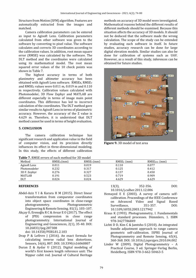
A test area of 21 points was used in the study. 11 points of the test area were identified as control points and 10 points as check points. A 3D model was created in Agisoft Photscan by using 15 images taken with Nikon D800 camera (Figure 9). The model is coordinated and scaled in the local coordinate system. Agisoft Photscan is a software that uses

International Journal of Engineering and Geosciences– 2021; 6(2); 74-80

79

Structure from Motion (SFM) algorithm. Features are automatically extracted from the images and matched.

Camera calibration parameters can be entered as input to Agisoft Lens. Calibration parameters calculated from other software was given to the software by converting to pixel value. The software calculates and corrects 3D coordinates according to the calibration values. In addition, root mean square error (RMSE) was calculated by the software. The DLT method and the coordinates were calculated using its mathematical model. The root mean squared error values of the 10 check points was shown in Table 7.

The highest accuracy in terms of both planimetry and altimeter accuracy has been obtained with Agisoft Lens software. RMSEx, RMSEY and RMSEZ values were 0.011 m, 0.019 m and 0.110 m respectively. Calibration values calculated with Photomodeler, 3D Flow Zephyr and MATLAB are different especially in terms of image main point coordinates. This difference has led to incorrect calculation of the coordinates. The DLT method gave similar results to Agisoft Lens in terms of planimetric accuracy. However, the accuracy of the Z value is 4.629 m. Therefore, it is understood that DLT method cannot be used in terms of height evaluation.

5. CONCLUSION

The camera calibration technique has significant research and application value in the field of computer vision, and its precision directly influences its effect in three-dimensional modeling. In this study, the effects of different calibration

methods on accuracy of 3D model were investigated. Mathematical reasons behind the different results of different methods should be examined. Because this situation affects the accuracy of 3D models. It should not be deduced that the software made the wrong calculation. The scope of the study can be extended by evaluating each software in itself. In future studies, accuracy research can be done for large digital elevation models. Similar studies can also be done for calibration of systems such as UAV. However, as a result of this study, inferences can be obtained for future studies.

Figure 9. 3D model of test area

Table 7. RMSE errors of each method for 3D model Method RMSEX (mm) RMSEY (mm) RMSEZ (mm) RMSEXYZ (mm)

Agisoft Lens 0.011 0.019 0.110 0.077 Photomodeler 0.232 0.317 0.125 0.412 3D F. Zephyr 0.276 0.327 0.137 0.450 MATLAB 0.191 0.523 0.719 0.909 DLT 0.024 0.024 4.629 4.629

REFERENCES

Abdel-Aziz Y I & Karara H M (2015). Direct linear transformation from comparator coordinates into object space coordinates in close-range photogrammetry. Photogrammetric Engineering & Remote Sensing. 81(1), 103–107.

Akçay O, Erenoğlu R C & Avsar E O (2017). The effect of JPEG compression in close range photogrammetry. International Journal of Engineering and Geosciences, 2(1), 35-40. DOI: 10.26833/ijeg.287308 doi: 10.14358/PERS.81.2.103

Drap P & Lefèvre J (2016). An exact formula for calculating inverse radial lens distortions. Sensors, 16(6), 807. DOI: 10.3390/s16060807

Duran Z & Aydar U (2012). Digital modeling of world's first known length reference unit: The Nippur cubit rod. Journal of Cultural Heritage

13(3), 352-356. DOI: 10.1016/j.culher.2011.12.006

Hemayed E E (2003). A survey of camera self-calibration. Proceedings of the IEEE Conference on Advanced Video and Signal Based Surveillance, 351-357. DOI: 10.1109/AVSS.2003.1217942

Kraus K (1993). Photogrammetry, I. Fundamentals and standard processes. Dümmlers, 1. ISBN 978-3427786849

Lichti D D, Kim C & Jamtsho S (2010). An integrated bundle adjustment approach to range camera geometric self-calibration. ISPRS Journal of Photogrammetry and Remote Sensing, 65(4), 360-368. DOI: 10.1016/j.isprsjprs.2010.04.002

Linder W (2009). Digital Photogrammetry – A Practical Course, 3 ed. Springer-Verlag Berlin, Heidelberg. ISBN 978-3-662-50463-5

International Journal of Engineering and Geosciences– 2021; 6(2); 74-80

80

Nex F & Remondino F (2014). UAV for 3D mapping applications: a review. Applied Geomatics, 6, 1-15.

Ozdemir E & Duran Z (2017). Comparison of commonly used camera calibration software. Afyon Kocatepe University Journal of Science and Engineering, 17(4), 1-11. (in Turkish)

Reis H Ç (2018). Bone anomaly of the foot detection using medical photogrammetry. International Journal of Engineering and Geosciences, 3(1), 1-5. DOI: 10.26833/ijeg.333686

Song L, Wu W, Guo J & Li X (2013). Survey on camera calibration technique. 2013 5th International Conference on Intelligent Human-Machine Systems and Cybernetics, 2, 389-392. DOI: 10.1109/IHMSC.2013.240

Tasdemir S, Urkmez A, Yakar M & Inal S (2009). Determination of camera calibration parameters at digital image analysis. 5th International Advanced Technologies Symposium (IATS’09). (in Turkish)

Ulvi A & Toprak A S (2016). Investigation of three-dimensional modelling availability taken photograph of the unmanned aerial vehicle; sample of Kanlidivane Church. International Journal of Engineering and Geosciences, 1(1), 1-7. DOI: 10.26833/ijeg.285216

Yemenicioglu C, Kaya S & Seker D Z (2016). Accuracy of 3D (Three-dimensional) terrain models in simulations. International Journal of Engineering and Geosciences, 1(1), 30-33. DOI: 10.26833/ijeg.285223

Zhang Z (2000). A flexible new technique for camera calibration. IEEE Transactions on Pattern Analysis and Machine Intelligence, 22. (11), 1330–1334. DOI: 10.1109/34.888718

Zhao H, Wang Z, Jiang H, Xu Y & Dong C (2015). Calibration for stereo vision system based on phase matching and bundle adjustment algorithm. Optics and Lasers in Engineering, 68, 203-213. DOI:10.1016/j.optlaseng.2014.12.001

© Author(s) 2021. This work is distributed under https://creativecommons.org/licenses/by-sa/4.0/

* Corresponding Author Cite this article

*(emresnkl@gmail.com) ORCID ID 0000 – 0003 – 3366 – 3786 (gkaplan@eskisehir.edu.tr) ORCID ID 0000 – 0001 – 7522 – 9924 (uavdan@eskisehir.edu.tr) ORCID ID 0000 – 0001 – 7873 – 9874 Research Article / DOI: 10.26833/ijeg.696001

Senkal E, Kaplan G & Avdan U (2021). Accuracy assessment of digital surface models from unmanned aerial vehicles’ imagery on archaeological sites. International Journal of Engineering and Geosciences, 6(2), 81-89

Received: 28/02/2020; Accepted: 06/05/2020

International Journal of Engineering and Geosciences– 2021; 6(2); 81-89

International Journal of Engineering and Geosciences

https://dergipark.org.tr/en/pub/ijeg

e-ISSN 2548-0960

Accuracy assessment of digital surface models from unmanned aerial vehicles’ imagery on archaeological sites

Emre Şenkal *1 , Gordana Kaplan 2 , Uğur Avdan 3

1Eskisehir Technical University, Remote Sensing and Geographical Information Systems Department, Eskisehir, Turkey 2Eskisehir Technical University, Earth and Space Sciences Institute, Eskisehir, Turkey

Keywords ABSTRACT Unmanned aerial vehicle Digital surface model Accuracy analysis GIS Remote sensing

With the developing technologies, the use of unmanned aerial vehicles’s (UAV) is increasing in all areas. Compared with the conventional photogrammetry and remote sensing sensors, UAVs are more convenient to collect data for small areas. In this study, the accuracy of UAV products was investigated in the archeological area of Eskişehir Şarhöyük. In order to produce reference data for the orthophoto and DTM accuracy analysis, a digital map from the test area was produced using in-situ measurements. Also, for the comparison of the point cloud, a small test area was determined and reference point cloud data was collected with terrestrial laser scanner. The comparison of the results showed significant difference between the UAV images and images collected by conventional methods. Thus, while there was 1 m difference between the data without the use of control points, and the use of control points significantly improved the results.

1. INTRODUCTION

With the rapid development of remote sensing technologies, Unmanned Aerial Vehicles (UAVs) have been widely used in many different research areas producing high-resolution data, including Digital Surface Models (DSMs) and orthorectified images (orthophotos) (Gindraux et al. 2017). The wide range of application include but are not limited to; agriculture (Costa et al. 2012), ecological studies (Anderson and Gaston 2013), water resource management (DeBell et al. 2016), glacier monitoring (Fugazza et al. 2015), soil erosion (d'Oleire-Oltmanns et al. 2012), landslide mapping (Comert et al. 2019), photogrammetric remote sensing and geo-information (Colomina and Molina 2014), building extraction (Comert and Kaplan 2018, Comert et al. 2018) etc.

UAV data has also been used for mapping and monitoring archeological areas (Tscharf et al. 2015, Holness et al. 2016, Themistocleous 2017). Thus, here we give brief literature review of the

archeological studies conducted with UAV data. (Eisenbeiss and Zhang 2006) compared DSM from UAV and terrestrial laser scanner in the Pinchango Alto archaeological field. The results showed that the height modes were substantially consistent with each other. In their study, (Sauerbier and Eisenbeiss 2010) used two different UAVs for documenting and monitoring excavations in three archaeological sites. The results of the study showed that the data obtained with UAV can be successfully used for documenting archaeological and cultural heritage. (Lin et al. 2011) used satellite imagery, UAV, and ground radar for detection of archaeological anomalies in three different archaeological sites in north Mongolia. The results showed that satellite imagery from Geo-Eye 1 can be used for objects long 1 – 10 m, while for smaller objects, UAV data should be used. Ground radar data can be used in order to obtain additional data about the archaeological remaining underground. Aiming to test UAV use in archeological areas, (Chiabrando et al. 2011) used a small remote controlled helicopter and a small

International Journal of Engineering and Geosciences– 2021; 6(2); 81-89

82

aircraft over the Reggia di Venaria Reale and Augusta Bagiennorum sites in Italy. The experiments carried out from 100 and 60 meter heights from the small aircraft, and the 50 and 15 meters’ heights flights were used to produce 1/200 and 1/100 scale orthophoto and digital maps, respectfully. As a result of the study, it was revealed that UAVs are useful for producing large scale maps needed in archaeological documentation. In addition, the low cost and speed of data collection has been shown to be suitable for archaeological survey studies. Using a camera placed on a helium balloon, collected data and obtained DTM and 3 Dimensional model of the archeological area of Cerrillo Blanco in Spain. As a result of the study, it was concluded that the balloon system used in the scope of the study is suitable for mapping small and medium sized archaeological sites in areas where the wind effect can be controlled.

In more recent studies, researchers have used UAV technology with conjunction with geo-information systems (GIS) and ground positioning systems (GPS) for protection and management of cultural heritage and archeological sites (Tache et al. 2018). Similar studies have been conducted for several other sites in Turkey (Ilci et al. 2019), Patara, Jordan (Hasting 2019) etc. Combination of UAV and Ground Penetrating Radar (GPR) has been used in order to detect non-invasive detection of buried objects (Garcia-Fernandez et al. 2018).

However, not many studies can be found evaluating the accuracy of the produced UAV maps. (Rusli et al. 2019) compared accuracy of DEM obtained from UAV and TanDEM-X satellite sensor. The results indicated difference of 3 to 4 in the DEMs. Perez et al. (Pérez et al. 2019) did an investigation concerning the positional accuracy and maximum allowable scale of UAV products for archaeological site documentation.

The main aim of this study is to investigate the accuracy of UAV products (ortophoto image, DSM, point cloud) produced from processed photographs obtained from UAV. The investigation was made over the Şarhoyük archeological site in Eskisehir, Turkey. Thus, data acquisition from different heights and different overlays were performed. The aim of image acquisition at different heights and different overlays is to investigate the effect of height and overlay on the resulting image.

In order to investigate the accuracy of the produced data, ground control points (GCP) were placed in the pre-flight area and the coordinates of these points were determined precisely by the geodetic GNSS receiver. Some of the control points were used to coordinate the produced orthophoto and DSM, while other control points were used in the comparison process for the accuracy analysis of the orthophoto images. In addition, for the accuracy analysis of the DSM obtained from the UAV, the DSM of the study area was produced by topographic method. The numerical surface model created by

geodetic method and surface models created by unmanned aerial vehicle were compared.

The main purpose of this study is to investigate the accuracy of the final products produced from images obtained by UAV. For this purpose, the accuracy of the orthophoto, point cloud and DSM to be produced from UAV were compared with data collected with conventional methods.

2. METHODOLOGY

2.1. Study Area

The ancient city of Dorylaeum or Dorylaion, or Şarhoyük in Turkish, is the oldest settlement in the northeast of Eskişehir. With 17 meters’ heights, it is one of the largest mounds in Central Anatolia. About 1 km west of the lower city, there is a necropolis which was founded around the mound. The excavations yielded finds from the Early Bronze Age, Hittite, Phrygian, Hellenistic, Roman, Byzantine and Ottoman periods. According to William Mitchell Ramsay, after Dorylaion was abandoned, a new settlement was established in the south of the city and the region where Dorylaion was located was called Eskişehir (Old Town). The reason for the selection of Sharhoyuk as a study area in this paper, are the different heights of the land, the number of excavation and filling areas on the land, and the fact that this is a protected archeological site where the human effects are lower than other areas.

2.2. Data and Methods

In order to provide the relationship between images obtained from the UAV and the ground, white cross with red dot GCPs were deployed and fixed on the archeological site. The GCP center were fixed prior to the UAV flights with a Javad TRIUMPH geodetic Global Navigation Satellite System (GNSS) receiver. The GCPs were measured before the flight. The GCPs measurement was executed in real-time kinematic (RTK) mode using virtual reference stations from the permanent GNSS station network of Turkey (TUSAGA-Active Turkish National Permanent GPS Active Stations Network). From repeated measurements of fixed locations, it was estimated that the mean accuracy of the measurements is 1-2 cm. In flat areas of the study area, the GCPs measurements were made at approximately 10 meters and less than 10 meters in non-flat areas. Each point was measured in five epochs. As a results, 5965 GCPs were deployed in the study area (Figure 2). excavation and filling areas on the land, and the fact that this is a protected archeological site where the human effects are lower than other areas. The study area is presented in Figure 1.

International Journal of Engineering and Geosciences– 2021; 6(2); 81-89

83

Figure 1. Study area; Şarhoyük archeological site, Eskisehir, Turkey

Figure 2. GCPs over the study area

For the image acquisition, SenseFly eBee UAV was used. The flight was automatically carried out and arranged according to the prepared flight plan. Technical specifications of the used UAV are given in Table 1. Two Canon cameras were used during the data acquisition, Canon IXUS 125 HS and Canon PowerShot ELPH 110 HS. The main difference between the two cameras is the spectral range. While the first camera operates in the Red, Green, Blue (RGB) part, the second camera operated in the Near Infrared, Green, Blue (NIRGB) part of electromagnetic spectrum. During the image acquisition, an on-board GPS and an inertial measurement unit provide information about the

approximate 3D position, roll, pitch and yaw of the UAV.

Table 1. Technical specification of the UAV used in this study

Wing Span 96 cm Weights 700 g Active time ~45 min Flight speed 36 – 57 km/h Radio range 3 km Covering area 1.5 – 10 km2 Spatial resolution 3 – 30 cm

Flights were planned with the software eMotion 2.4 provided by SenseFly. A minimum of 60% lateral and 70% longitudinal ground overlap was ensured between adjacent images. The first step in the flight planning was to determine the height of the flight. The UAV used in this study has a capability of flying between 50 and 1000 meters, with a spatial resolution of the images between 2 and 40 cm. After determining the flight height, the flight operation should be prepared taking into consideration the overlap ratios of the image frames, depending on the area covered in the field. The flight preparation was made as recommended in (Eisenbeiß 2009, Karakış 2012).

In order to obtain photogrammetric images of the study area, three different flights were prepared with the e-Motion2 software. Details about each flight are given in Table 2.

International Journal of Engineering and Geosciences– 2021; 6(2); 81-89

84

The images obtained from the field were processed with PostFlight Terra 3D software. The data processing process consists of three steps:

i) Initial Processing ii) ii) Point Cloud Densification iii) iii) Digital Surface Model and

Orthomosaic Production.

In order to investigate the accuracy of the data obtained from the UAV, the data were processed in four different ways. First, the data were processed

without a GCPs, then the study area was divided into three levels: low level, medium level and high level depending on the terrain height (Figure 3). The purpose of this process is to observe the effects of GCPs over the results within a certain height range. Using the GCPs located at these three levels, three different data manipulations were performed for the results of each flight. Afterwards, data were processed by using low, medium and high level GCPs from the existing control points (Figure 3).

Table 2. Flight details Parameter 1. Flight 2. Flight 3. Flight

Camera RGB NIRGB RGB

Terrain mode Easy Easy Difficult

Flight height 130 m 130 m 196 m

Ground Sample Range 4 cm 4 cm 6 cm

Lateral Overlap 60 % 60 % 85 %

Longitudinal Overlap 70 % 70 % 70 %

Image Number 105 101 137

Flight time 13 min 12 min 22 min

Figure 3. GCPs on different levels on the study area

3. RESULTS and DISCUSSION

The coordinates obtained from the field measurements with the GNSS receiver were compared with the coordinates of the digitized GCPs over the orthophoto image obtained from the UAV. First, the coordinates of the GCPs over the product produced without GCPs were compared with the coordinates measured at site. The differences from the 34 GCPs, from both easy and difficult flight mode, used on the three different levels (Figure 3), are shown in Table 3.

The same analyses were conducted for all six projects between the measured GCPs and the coordinated from the product obtained with the use of GCPs. The differences between the coordinates of the measured GCPs and the GCPs from the three different levels (low, medium, high) were compared with the results from both easy and difficult flight results. For this purpose, the GCPs from specific level

were excluded and the GCPs from the two other levels were used for the evaluation of the results. The results are presented in Table 4 and Table 5.

From the comparison of the results, it has been seen that the GCPs in the middle and high levels have more difference in comparison with the GCPs in the low level of the study area. In comparison of the two different terrain models, there was no significant difference noticed between the results.

3.2 Field Data Comparison

Four of the eleven excavation sites in the study area were selected for the comparison of the field data (Figure 4 – a). In order to minimize the error, each edge of the selected excavation was measured using the same points on the raster. As a result of the measurements, no significant difference was found between the terrain data and the data obtained from the UAV and the produced raster images. The use of

International Journal of Engineering and Geosciences– 2021; 6(2); 81-89

85

GCPs or flight height difference did not have a significant effect on length in the selected area. In the point-to-point comparison process, approximately 1 meter offset was detected between the raster data produced with and without GCPs (Figure 4 – b). This offset does not affect the length as it acts in the same direction on the edges of the excavation area. In order to compare the DSM results and to determine the product with least error, different GCPs have been compared. In addition, in order to investigate the effect of the flight height in the DSM production, comparison of the results obtained from flights with different height has been made. The results show the height differences for pixel based DSM. By examining in the areas of the height differences overlap, it is possible to determine the

accuracy of the numerical surface model. In order to compare the produced products with field measurements, a DSM was produced from the 5965 points field measured with GNSS receiver. The results are presented in Figure 5. As stated before, the DSM from the UAV data collection was compared with the field measurements. The two different DSM models were compared in order to investigate the effect of the obtained results. The result of the comparison indicates that there is high overlap in the areas obtained with GCPs. High differences are being notices over the areas where there is low overlap between the images, especially on the edges of the study area. The difference between the DSM created with all GCPs with easy and difficult terrain mode are presented in Figure 6.

Table 3. Difference between the GCPs

No Easy terrain mode Difficult flight mode

∆Y ∆X ∆Z ∆Y ∆X ∆Z

GCP1 -0.308 -0.703 0.860 0.795 0.125 0.498 GCP2 -0.127 -0.742 0.751 1.172 -0.182 0.539 GCP3 -0.084 -0.766 0.789 1.333 -0.258 0.549 GCP4 0.020 -0.833 0.806 1.567 -0.416 0.662 GCP5 0.048 -0.752 0.701 1.736 -0.216 0.800 GCP6 0.002 -0.617 0.622 1.749 0.078 0.880 GCP7 -0.123 -0.547 0.558 1.667 0.350 0.878 GCP8 -0.231 -0.500 0.486 1.635 0.624 0.844 GCP9 -0.145 -0.476 0.443 1.879 0.612 0.912

GCP10 0.050 -0.607 0.541 2.050 0.135 0.945 GCP11 0.151 -0.804 0.784 1.972 -0.412 0.849 GCP12 0.101 -0.937 0.856 1.636 -0.701 0.530 GCP13 -0.016 -0.982 0.956 1.243 -0.799 0.471 GCP14 -0.169 -0.976 0.907 0.846 -0.797 0.248 GCP15 -0.347 -0.936 0.973 0.456 -0.577 0.186 GCP16 -0.376 -0.988 1.071 0.257 -0.797 0.306 GCP17 -0.550 -0.946 1.230 -0.185 -0.580 0.355 GCP18 -0.639 -0.770 1.262 -0.078 0.062 0.272 GCP19 -0.597 -0.701 1.079 0.220 0.229 0.172 GCP20 -0.563 -0.634 1.019 0.439 0.380 0.274 GCP21 -0.632 -0.592 1.099 0.371 0.627 0.380 GCP22 -0.479 -0.748 0.948 0.503 0.136 0.302 GCP23 -0.184 -0.626 0.678 1.185 0.151 0.620 GCP24 -0.054 -0.649 0.664 1.496 0.015 0.821 GCP25 -0.142 -0.603 0.595 1.447 0.262 0.825 GCP26 -0.267 -0.522 0.695 1.152 0.475 0.708 GCP27 -0.433 -0.562 0.766 0.931 0.574 0.629 GCP28 -0.586 -0.412 0.834 0.870 1.095 0.710 GCP29 -0.332 -0.516 0.641 1.255 0.706 0.729 GCP30 -0.127 -0.477 0.542 1.595 0.626 0.828 GCP31 0.082 -0.745 0.661 1.899 -0.202 0.839 GCP32 0.024 -0.888 0.886 1.366 -0.640 0.568 GCP33 -0.158 -0.891 0.830 0.959 -0.484 0.309 GCP34 -0.258 -0.824 0.854 0.761 -0.268 0.383

Square Mean Error

0.318 0.733 0.830 1.272 0.503 0.630

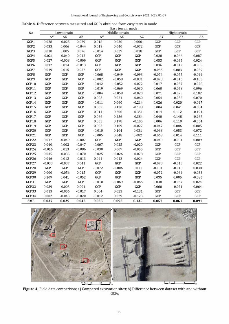
International Journal of Engineering and Geosciences– 2021; 6(2); 81-89

86

Table 4. Difference between measured and GCPs obtained from easy terrain mode

No

Easy terrain mode Low terrain Middle terrain High terrain

∆Y ∆X ∆Z ∆Y ∆X ∆Z ∆Y ∆X ∆Z

GCP1 0.028 -0.025 0.029 0.018 0.030 0.000 GCP GCP GCP

GCP2 0.033 0.006 -0.044 0.019 0.040 -0.072 GCP GCP GCP

GCP3 0.010 0.005 0.076 -0.014 0.029 0.018 GCP GCP GCP

GCP4 -0.021 -0.040 0.042 GCP GCP GCP 0.028 -0.066 0.087

GCP5 0.027 -0.008 -0.009 GCP GCP GCP 0.053 -0.046 0.024

GCP6 0.032 0.014 -0.013 GCP GCP GCP 0.036 -0.012 -0.005

GCP7 0.019 0.015 0.057 GCP GCP GCP -0.035 0.003 -0.029

GCP8 GCP GCP GCP -0.068 -0.049 -0.093 -0.074 -0.055 -0.099

GCP9 GCP GCP GCP -0.082 -0.058 -0.091 -0.078 -0.046 -0.105

GCP10 GCP GCP GCP -0.042 -0.052 -0.072 0.017 -0.037 -0.028

GCP11 GCP GCP GCP -0.019 -0.069 -0.030 0.060 -0.068 0.096

GCP12 GCP GCP GCP -0.004 -0.058 -0.020 0.071 -0.075 0.102

GCP13 GCP GCP GCP 0.003 0.021 -0.060 0.054 -0.035 0.070

GCP14 GCP GCP GCP -0.011 0.090 -0.214 0.026 0.020 -0.047

GCP15 GCP GCP GCP 0.003 0.120 -0.198 0.004 0.041 -0.084

GCP16 GCP GCP GCP 0.014 0.200 -0.351 0.014 0.112 -0.194

GCP17 GCP GCP GCP 0.066 0.256 -0.384 0.040 0.148 -0.267

GCP18 GCP GCP GCP 0.053 0.178 -0.105 0.006 0.110 -0.054

GCP19 GCP GCP GCP 0.003 0.109 -0.027 -0.047 0.086 0.005

GCP20 GCP GCP GCP -0.010 0.104 0.031 -0.068 0.053 0.072

GCP21 GCP GCP GCP -0.005 0.048 0.082 -0.068 0.014 0.111

GCP22 0.017 -0.049 -0.007 GCP GCP GCP -0.040 -0.004 0.009

GCP23 0.040 0.002 -0.047 -0.007 0.025 -0.020 GCP GCP GCP

GCP24 -0.016 0.013 -0.086 -0.030 0.009 -0.055 GCP GCP GCP

GCP25 0.035 -0.035 -0.070 -0.025 -0.026 -0.078 GCP GCP GCP

GCP26 0.046 0.012 -0.013 0.044 0.043 -0.024 GCP GCP GCP

GCP27 -0.033 -0.037 0.041 GCP GCP GCP -0.078 -0.018 0.022

GCP28 GCP GCP GCP -0.072 -0.006 0.011 -0.131 -0.018 0.038

GCP29 0.000 -0.056 0.015 GCP GCP GCP -0.072 -0.064 -0.033

GCP30 0.109 0.041 -0.052 GCP GCP GCP 0.035 0.005 -0.086

GCP31 GCP GCP GCP -0.010 -0.069 -0.066 0.038 -0.067 0.024

GCP32 0.039 -0.003 0.001 GCP GCP GCP 0.060 -0.021 0.064

GCP33 0.013 -0.056 -0.017 0.004 0.023 -0.131 GCP GCP GCP

GCP34 0.002 -0.043 -0.020 -0.012 0.029 -0.123 GCP GCP GCP

SME 0.037 0.029 0.043 0.035 0.093 0.135 0.057 0.061 0.091

Figure 4. Field data comparison; a) Compared excavation sites; b) Difference between dataset with and without

GCPs

International Journal of Engineering and Geosciences– 2021; 6(2); 81-89

87

Figure 5. Difference between DSM and field measurements; a) Difficult terrain mode; b) Easy terrain mode

Figure 6. Difference between DSMs created with all GCPs using easy and difficult terrain mode.

The overall results showed that the lowest error of the UAV products is obtained with the use of the low level GCPs. The main reason is that low level GCP are better spread over the study area. The control points at the middle and high levels appear to be clustered. When the square mean error of the products produced without the GCPs is examined, it can be seen that the least error rate is obtained with the flight in difficult terrain mode. The main reason for this is that, in difficult terrain mode, the volume of data is higher and more data is obtained from the field.

From the DSM comparison it can be concluded that the UAV results are in agreement with the field measurements. Thus, there is no significant difference (higher than 10 cm) between the results. High differences can be noticed in areas without measurements. In order to avoid damaging the

excavation areas, no data was collected from these parts.

4. CONCLUSION

UAVs have been widely used in many different research areas producing high-resolution data, including DSMs and orthorectified images. The evaluation of the accuracy of the UAV maps hasn’t been addressed in many studies. Thus, the main objective in this study was the investigation of the accuracy of UAV products. For that purpose, UAV data from different heights and different overlays were collected over an archeological site in Eskisehir, Turkey. In order to investigate the accuracy of the produced data, 5965 GCP were placed in the study area.

The finding of the study indicates that the difference between the UAV data and the field measurements is different with and without GCPs. Thus, while there was approximately 1 m difference between the coordinates obtained by terrestrial method and UAV, with the use of GCPs this difference has been lowered to 5 cm. One of the most important features of UAVs is the quick, precise and in a low cost of data collection without damaging the archaeological area.

As a result of length and area comparisons, UAVs were found to be as reliable as terrestrial measurements. In fact, they provide great advantages to the users by avoiding the human error factor that may occur during terrestrial measurement. The comparison of the DSMs, showed that the differences between terrestrial measurements and UAV measurements are generally ± 10 cm in the Z axis. It was determined that the height of the GCPs used in the comparison of DSM did not have much effect on the final product. Contrary to the height, the number of GCPs and the

International Journal of Engineering and Geosciences– 2021; 6(2); 81-89

88

distribution pattern were found to be more important.

ACKNOWLEDMENT

This research was funded by Anadolu University Scientific Research Projects Commission under the grant no: 1502E084 and it is a part of Emre Senkal’s master thesis.

REFERENCES

Anderson K & Gaston K J (2013). Lightweight unmanned aerial vehicles will revolutionize spatial ecology. Frontiers in Ecology and the Environment, 11(3), 138-146. DOI:10.1890/120150

Chiabrando F, Nex F, Piatti D & Rinaudo F (2011). UAV and RPV systems for photogrammetric surveys in archaelogical areas: two tests in the Piedmont region (Italy). Journal of Archaeological Science, 38(3), 697-710. DOI: 10.1016/j.jas.2010.10.022

Colomina I & Molina P (2014). Unmanned aerial systems for photogrammetry and remote sensing: A review. ISPRS Journal of Photogrammetry and Remote Sensing, 92, 79-97. DOI: 10.1016/j.isprsjprs.2014.02.013

Comert R, Avdan U, Gorum T & Nefeslioglu H A (2019). Mapping of shallow landslides with object-based image analysis from unmanned aerial vehicle data. Engineering Geology 260: 105264. DOI:10.1016/j.enggeo.2019.105264

Comert R & Kaplan O (2018). "Object based building extraction and building period estimation from unmanned aerial vehicle data. ISPRS Annals of the Photogrammetry, Remote Sensing and Spatial Information Sciences 4(3).

Comert R, Matcı D K & Avdan U (2018). Detection of collapsed building from unmanned aerial vehicle data with object based image classification. Eskişehir Teknik Üniversitesi Bilim ve Teknoloji Dergisi-B Teorik Bilimler 6, 109-116.

Costa F G, Ueyama J, Braun T, Pessin G, Osório F S & Vargas P A (2012). The use of unmanned aerial vehicles and wireless sensor network in agricultural applications. IEEE International Geoscience and Remote Sensing Symposium, 5045-5048.

d'Oleire-Oltmanns S, Marzolff I, Peter K D & Ries J B (2012). Unmanned aerial vehicle (UAV) for monitoring soil erosion in Morocco. Remote Sensing 4(11): 3390-3416. DOI:10.3390/rs4113390

DeBell L, Anderson K, Brazier R E, King N & Jones L (2016). Water resource management at catchment scales using lightweight UAVs: Current capabilities and future perspectives. Journal of Unmanned Vehicle Systems 4(1): 7-30. DOI:10.1139/juvs-2015-0026

Eisenbeiß H (2009). UAV photogrammetry. PHD Thesis, ETH Zurich.

Eisenbeiss H & Zhang L (2006). Comparison of DSMs generated from mini UAV imagery and terrestrial laser scanner in a cultural heritage application. International Archives of Photogrammetry, Remote Sensing and Spatial Information Sciences 36(5): 90-96.

Fugazza D, Senese A, Azzoni R S, Smiraglia C, Cernuschi M, Severi D & Diolaiuti G A (2015). High-resolution mapping of glacier surface features. The UAV survey of the Forni Glacier (Stelvio National Park, Italy). Geografia Fisica e Dinamica Quaternaria, 38, 25-33. DOI 10.4461/GFDQ.2015.38.03

Garcia-Fernandez M, Alvarez-Lopez Y, Gonzalez-Valdes B, Rodriguez-Vaqueiro Y, Arboleya-Arboleya A, Heras F L & Pino A (2018). GPR system onboard a UAV for non-invasive detection of buried objects. IEEE International Symposium on Antennas and Propagation & USNC/URSI National Radio Science Meeting, 1967-1968.

Gindraux S, Boesch R & Farinotti D (2017). Accuracy assessment of digital surface models from unmanned aerial vehicles’ imagery on glaciers. Remote Sensing, 9(2): 186. 10.3390/rs9020186

Hasting L (2019). "Using Unmanned Aerial Vehicle (UAV) Technology for Archaeology: A Case Study of Petra, Jordan." Scholars Week, 30.

Holness C, Matthews T, Satchell K & Swindell E C (2016). Remote sensing archeological sites through unmanned aerial vehicle (UAV) imaging. IEEE International Geoscience and Remote Sensing Symposium (IGARSS), 6695-6698. DOI: 10.1109/IGARSS.2016.7730748

Ilci V, Ozulu I M, Bilgi S & Alkan R M (2019). The usage of unmanned aerial vehicles (UAVs) for 3D mapping of archaeological sites. FEB-Fresenius Environmental Bulletin, 28(2), 968-974.

Karakış S (2012). Searching The Posibilities of Large Scale Photogrammetric Map Production via Model Aircraft. Harita Dergisi, 147, 13-20. (in Turkish)

Lin A Y-M, Novo A, Har-Noy S, Ricklin N D & Stamatiou K (2011). Combining GeoEye-1 satellite remote sensing, UAV aerial imaging, and geophysical surveys in anomaly detection applied to archaeology. IEEE Journal of selected topics in applied earth observations and remote sensing, 4(4), 870-876.

Pérez J A, Gonçalves G R & Charro M C (2019). On the positional accuracy and maximum allowable scale of UAV-derived photogrammetric products for archaeological site documentation. Geocarto International, 34(6): 575-585. DOI: 10.1080/10106049.2017.1421714

Rusli N, Majid M R, Razali N F A A & Yaacob N F F (2019). Accuracy assessment of DEM from UAV and TanDEM-X imagery. IEEE 15th International Colloquium on Signal Processing

International Journal of Engineering and Geosciences– 2021; 6(2); 81-89

89

& Its Applications (CSPA), 127-131, Penang, Malaysia.

Sauerbier M & Eisenbeiss H (2010). UAVs for the documentation of archaeological excavations. International Archives of Photogrammetry, Remote Sensing and Spatial Information Sciences, 38(5), 526-531.

Tache A V, Sandu I C A, POPESCU O-C & PETRIŞOR A-I (2018). UAV solutions for the protection and management of cultural heritage. Case study: Halmyris Archaeological site. International Journal of Conservation Science, 9(4), 795-804.

Themistocleous K (2017). The use of UAVs to monitor archeological sites: the case study of

Choirokoitia within the PROTHEGO project. Fifth International Conference on Remote Sensing and Geoinformation of the Environment (RSCy2017), International Society for Optics and Photonics. DOI: 10.1117/12.2292351

Tscharf A, Rumpler M, Fraundorfer F, Mayer G & Bischof H (2015). On the use of UAVs in mining and archaeology-geo-accurate 3D reconstructions using various platforms and terrestrial views. ISPRS Annals of Photogrammetry, Remote Sensing & Spatial Information Sciences, 2, 15-22.

© Author(s) 2021. This work is distributed under https://creativecommons.org/licenses/by-sa/4.0/

* Corresponding Author Cite this article

*(fatihdoner@gumushane.edu.tr) ORCID ID 0000 – 0002 – 3620 – 5687 Research Article / DOI: 10.26833/ijeg.703244

Doner F (2021). Analysis of literature on 3D cadastre. International Journal of Engineering and Geosciences, 6(2), 90-97

Received: 13/03/2020; Accepted: 26/06/2020

International Journal of Engineering and Geosciences– 2021; 6(2); 90-97

International Journal of Engineering and Geosciences

https://dergipark.org.tr/en/pub/ijeg

e-ISSN 2548-0960

Analysis of literature on 3D cadastre

Fatih Döner*1

1Gumushane University, Faculty of Engineering and Natural Sciences, Department of Geomatics Engineering, Gumushane, Turkey

Keywords ABSTRACT Cadastre 3D Cadastre LADM Literature survey

In this study, it is aimed to analyse the three-dimensional (3D) cadastre literature in terms of legal, institutional, and technical aspects. For this purpose, 441 publications published between 2001 and 2019 were examined. In the literature, which includes publications from 59 different countries the studies mostly focused on technical issues. An international consensus on legal, institutional, and technical aspects of a 3D cadastre solution seems difficult. Since rights, restrictions, and responsibilities with a 3D component are somehow registered administratively, stakeholders from the legal domain are reluctant to 3D cadastre. From a technical point of view, the technology required to use 3D digital data for registration has matured sufficiently in the past twenty years. However, further research on a real 3D cadastre solution, creating a workflow that considers both current legal and technical framework beyond pilot studies, is needed.

1. INTRODUCTION

The substantial increase in the world population in the past two centuries has led to intensification of land use, especially in urban areas. This increasing trend in the population has gradually altered the relationship between the land and the people, increasing the importance of land ownership (Ting and Williamson 1999). Accordingly, a system was required to record the ownership of the property in a clear and undisputable way. Although various names (land information system, land recording, land administration, etc.) are used to describe this system, it is now called cadastre (FIG 1995; Dale and Mclaughlin 1999; Steudler et al. 2004). From a conceptual point of view, one of the foundations of the cadastre is that there can be no gaps or overlaps in the parcelation on which the rights are based, that is, a planar partition of the surface. The same foundation (a partition of space with no overlaps or gaps) is also the basis of the conceptual thinking with respect to 3D cadastre (Stoter 2004; Döner et al. 2008). In other words, 3D cadastre is a cadastre that registers and represents the space where rights (also the restrictions and

responsibilities) applied (Döner 2010). Reflection of this conceptual definition can be seen in logo of International Federation of Surveyors (FIG) Working Group on 3D Cadastres in Figure 1.

Figure 1. Logo of FIG working group on 3D cadastres

Numerous studies have been conducted to compare and classify the researches focused on cadastre and land administration. Çağdaş and Stubkjær (2009) analysed selected PhD theses written in English about cadastre in terms of methodology, concepts, and methods. Paulsson and Paasch (2015) conducted a literature review for the LADM (Land Administration Domain Model, ISO 19152), which was accepted as an ISO standard in 2012. Oosterom (2013) evaluated the activities of the FIG Working Group on 3D Cadastres. Paulsson and Paasch (2013) discussed the publications

International Journal of Engineering and Geosciences– 2021; 6(2); 90-97

91

written in English between 2001 and 2011 on the concept of 3D property in terms of their legal aspects.

The first international discussion about the 3D cadastre subject took place in 2001 at the workshop entitled 3D Cadastres, under the seventh commission of the FIG. At the 24th FIG congress held in Sydney in April 2010, it was decided to re-establish a working group called '3D Cadastre' in order to make further progress on 3D cadastre research. The main purpose of the working group is to create a functioning structure for 3D cadastre. For this structure, two main goals were determined. The first is to follow a common concept and terminology. For this purpose, the use of ISO 19152 LADM has been adopted. Secondly, common levels for 3D cadastre applications were determined as legal, organisational and technical. Thus, it will be possible to compare different ideas and applications more easily (Döner et al. 2011; van Oosterom et al. 2014). In the past twenty years, many scientific meetings, academic studies, and pilot projects (Cemellini et al. 2020; Larsson et al. 2020; Vandysheva et al. 2011; Ying et al. 2012; Guo et al. 2011) have been performed on 3D cadastre. Nevertheless, during that period, there have been significant changes in the visualization of 3D data, data collection techniques, the usability of BIM (Building Information Modelling) data (Ying et al. 2017; Thompson et al. 2017; Atazadeh et al. 2017), as well as in policies and institutional structures. The effects of the changes on 3D cadastre research have not been extensively studied so far. Therefore, in this study, the 3D cadastre literature was analysed, and the trends and challenges in research and applications were investigated in terms of legal, institutional, and technical aspects. For this analysis, the approach of analysing the publications published in English between 2001 and 2019 under the FIG Working Group on 3D Cadastres was adopted. In the second section, the publications used for analysis and the approach in the classification of these publications are introduced. Findings of the analysed 3D cadastre publications are presented in the third section. Then, challenges and trends in 3D cadastre research are evaluated in three groups under the fourth section. Finally, the study ends with conclusions in section 5.

2. MATERIALS and METHODS

Quantitative analysis of certain characteristics of scientific documents is defined as bibliometric analysis (Schloegl and Gorraiz 2006). This analysis aims to determine the priority areas and development direction by examining the publications in a specific journal or publications related to a specific subject (Motoyama and Eisler 2011; Alcantara and Martens 2019). While the analysis is performed, answers are sought to

1www.gdmc.nl/3dcadastres/literature/ (accessed

December 19th, 2019).

questions such as what types the publications are, what the most frequently used keywords are, how the number of publications is distributed by years, the number of authors of the publications, and at which institutions the authors work (Biljecki 2016; De Bakker et al. 2005; Garnett et al. 2013).

The methodological basis of this study is the analysis of 3D cadastre publications. For this purpose, 3D cadastre publications will first be classified into categories; then the trends in each class will be determined. Since it is not possible to capture all 3D cadastre literature that exists, selection of most relevant publications is an important part of the methodology. Therefore, the publications to be examined in the study were determined to be those published in the FIG Working Group on 3D Cadastres web page1 between 2001 and 2019. The reason why year 2001 was chosen as the beginning is that it was the first time that 3D cadastre was discussed at an international meeting. The publications on the FIG website are intended for international audiences and therefore are published in English. That prevents the classification of studies related to specific countries and written in languages other than English. Publications in languages other than English are excluded from the scope of this article.

In this study, three classes were identified in the classification of publications in 3D cadastre literature. These are legal, institutional and technical classes. This classification approach for 3D cadastre was actually adopted in the first 3D Cadastre Workshop in 2001. In the second 3D Cadastre Workshop held in 2011, four classes were proposed to classify and compare 3D cadastre studies. Those are registration of 3D parcels, 3D data management, 3D visualization, and sharing of 3D parcels. When the two approaches are considered together for classification, it is understood that the registration of 3D parcels in the second approach coincides with the legal class in the first approach, that the 3D visualization class in the second approach corresponds to the technical class in the first approach, and that the sharing of 3D parcels in the first approach can be described with the institutional class in the first approach. Therefore, in this article, 3D cadastre literature has been classified and analysed in the three classes of legal, institutional, and technical due to the simpler structure.

When 3D cadastre publications are analysed, it is seen that some publications can fit into two of the classes identified in this study (legal and institutional, legal and technical, or institutional and technical) or into all three classes at the same time. In such cases, the approach of usage of primary and secondary classes as applied in Paulsson and Paasch (2015) was adopted to determine the class of the publication. The primary and secondary classes describe the dominant class and the less dominant

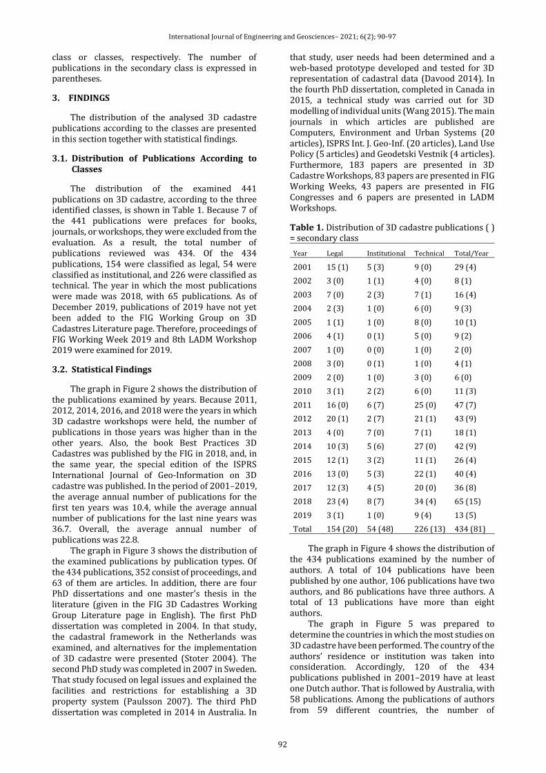
International Journal of Engineering and Geosciences– 2021; 6(2); 90-97

92

class or classes, respectively. The number of publications in the secondary class is expressed in parentheses.

3. FINDINGS

The distribution of the analysed 3D cadastre publications according to the classes are presented in this section together with statistical findings.

3.1. Distribution of Publications According to Classes

The distribution of the examined 441 publications on 3D cadastre, according to the three identified classes, is shown in Table 1. Because 7 of the 441 publications were prefaces for books, journals, or workshops, they were excluded from the evaluation. As a result, the total number of publications reviewed was 434. Of the 434 publications, 154 were classified as legal, 54 were classified as institutional, and 226 were classified as technical. The year in which the most publications were made was 2018, with 65 publications. As of December 2019, publications of 2019 have not yet been added to the FIG Working Group on 3D Cadastres Literature page. Therefore, proceedings of FIG Working Week 2019 and 8th LADM Workshop 2019 were examined for 2019.

3.2. Statistical Findings

The graph in Figure 2 shows the distribution of the publications examined by years. Because 2011, 2012, 2014, 2016, and 2018 were the years in which 3D cadastre workshops were held, the number of publications in those years was higher than in the other years. Also, the book Best Practices 3D Cadastres was published by the FIG in 2018, and, in the same year, the special edition of the ISPRS International Journal of Geo-Information on 3D cadastre was published. In the period of 2001–2019, the average annual number of publications for the first ten years was 10.4, while the average annual number of publications for the last nine years was 36.7. Overall, the average annual number of publications was 22.8.

The graph in Figure 3 shows the distribution of the examined publications by publication types. Of the 434 publications, 352 consist of proceedings, and 63 of them are articles. In addition, there are four PhD dissertations and one master's thesis in the literature (given in the FIG 3D Cadastres Working Group Literature page in English). The first PhD dissertation was completed in 2004. In that study, the cadastral framework in the Netherlands was examined, and alternatives for the implementation of 3D cadastre were presented (Stoter 2004). The second PhD study was completed in 2007 in Sweden. That study focused on legal issues and explained the facilities and restrictions for establishing a 3D property system (Paulsson 2007). The third PhD dissertation was completed in 2014 in Australia. In

that study, user needs had been determined and a web-based prototype developed and tested for 3D representation of cadastral data (Davood 2014). In the fourth PhD dissertation, completed in Canada in 2015, a technical study was carried out for 3D modelling of individual units (Wang 2015). The main journals in which articles are published are Computers, Environment and Urban Systems (20 articles), ISPRS Int. J. Geo-Inf. (20 articles), Land Use Policy (5 articles) and Geodetski Vestnik (4 articles). Furthermore, 183 papers are presented in 3D Cadastre Workshops, 83 papers are presented in FIG Working Weeks, 43 papers are presented in FIG Congresses and 6 papers are presented in LADM Workshops.

Table 1. Distribution of 3D cadastre publications ( ) = secondary class

Year Legal Institutional Technical Total/Year

2001 15 (1) 5 (3) 9 (0) 29 (4)

2002 3 (0) 1 (1) 4 (0) 8 (1)

2003 7 (0) 2 (3) 7 (1) 16 (4)

2004 2 (3) 1 (0) 6 (0) 9 (3)

2005 1 (1) 1 (0) 8 (0) 10 (1)

2006 4 (1) 0 (1) 5 (0) 9 (2)

2007 1 (0) 0 (0) 1 (0) 2 (0)

2008 3 (0) 0 (1) 1 (0) 4 (1)

2009 2 (0) 1 (0) 3 (0) 6 (0)

2010 3 (1) 2 (2) 6 (0) 11 (3)

2011 16 (0) 6 (7) 25 (0) 47 (7)

2012 20 (1) 2 (7) 21 (1) 43 (9)

2013 4 (0) 7 (0) 7 (1) 18 (1)

2014 10 (3) 5 (6) 27 (0) 42 (9)

2015 12 (1) 3 (2) 11 (1) 26 (4)

2016 13 (0) 5 (3) 22 (1) 40 (4)

2017 12 (3) 4 (5) 20 (0) 36 (8)

2018 23 (4) 8 (7) 34 (4) 65 (15)

2019 3 (1) 1 (0) 9 (4) 13 (5)

Total 154 (20) 54 (48) 226 (13) 434 (81)

The graph in Figure 4 shows the distribution of the 434 publications examined by the number of authors. A total of 104 publications have been published by one author, 106 publications have two authors, and 86 publications have three authors. A total of 13 publications have more than eight authors.

The graph in Figure 5 was prepared to determine the countries in which the most studies on 3D cadastre have been performed. The country of the authors’ residence or institution was taken into consideration. Accordingly, 120 of the 434 publications published in 2001–2019 have at least one Dutch author. That is followed by Australia, with 58 publications. Among the publications of authors from 59 different countries, the number of

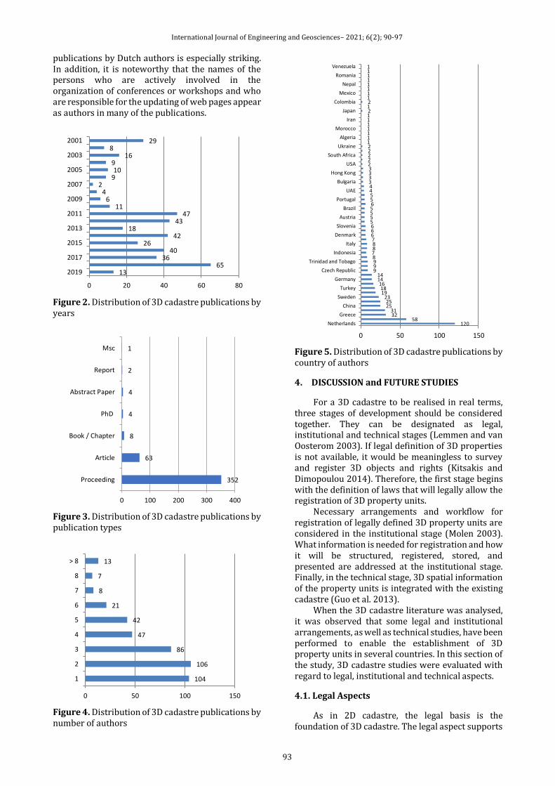
International Journal of Engineering and Geosciences– 2021; 6(2); 90-97

93

publications by Dutch authors is especially striking. In addition, it is noteworthy that the names of the persons who are actively involved in the organization of conferences or workshops and who are responsible for the updating of web pages appear as authors in many of the publications.

Figure 2. Distribution of 3D cadastre publications by years

Figure 3. Distribution of 3D cadastre publications by publication types

Figure 4. Distribution of 3D cadastre publications by number of authors

Figure 5. Distribution of 3D cadastre publications by country of authors

4. DISCUSSION and FUTURE STUDIES

For a 3D cadastre to be realised in real terms, three stages of development should be considered together. They can be designated as legal, institutional and technical stages (Lemmen and van Oosterom 2003). If legal definition of 3D properties is not available, it would be meaningless to survey and register 3D objects and rights (Kitsakis and Dimopoulou 2014). Therefore, the first stage begins with the definition of laws that will legally allow the registration of 3D property units.

Necessary arrangements and workflow for registration of legally defined 3D property units are considered in the institutional stage (Molen 2003). What information is needed for registration and how it will be structured, registered, stored, and presented are addressed at the institutional stage. Finally, in the technical stage, 3D spatial information of the property units is integrated with the existing cadastre (Guo et al. 2013).

When the 3D cadastre literature was analysed, it was observed that some legal and institutional arrangements, as well as technical studies, have been performed to enable the establishment of 3D property units in several countries. In this section of the study, 3D cadastre studies were evaluated with regard to legal, institutional and technical aspects.

4.1. Legal Aspects

As in 2D cadastre, the legal basis is the foundation of 3D cadastre. The legal aspect supports

1365

3640

2642

1843

4711

64

2910

916

829

0 20 40 60 80

2019

2017

2015

2013

2011

2009

2007

2005

2003

2001

352

63

8

4

4

2

1

0 100 200 300 400

Proceeding

Article

Book / Chapter

PhD

Abstract Paper

Report

Msc

104

106

86

47

42

21

8

7

13

0 50 100 150

1

2

3

4

5

6

7

8

> 8

12058

3231

2525

231918

161414

99987887666555565544333322222111111121211111111

0 50 100 150

Netherlands

Greece

China

Sweden

Turkey

Germany

Czech Republic

Trinidad and Tobago

Indonesia

Italy

Denmark

Slovenia

Austria

Brazil

Portugal

UAE

Bulgaria

Hong Kong

USA

South Africa

Ukraine

Algeria

Morocco

Iran

Japan

Colombia

Mexico

Nepal

Romania

Venezuela

International Journal of Engineering and Geosciences– 2021; 6(2); 90-97

94

the registration of 3D property in 3D cadastre. It was observed that the number of publications evaluated in the legal class after 2010 more than doubled when compared to the period before 2010. Despite that increase, publications in the legal class consisted of only one third of the total publications, and the number of publications dealing with purely legal aspects of 3D cadastre was quite small. In the publications considered to be of legal class, the existing legal framework in the country is explained mostly in terms of defining boundaries of property rights on land, establishing individual units and limited real rights. After the introductory explanations, the researchers present technical solutions for a 3D cadastre in their publications. However, they do not mention about availability of the legal regulations required for the implementation of these solutions.

On the other hand, legal regulations in some countries are noteworthy in the publications reviewed. For instance, legal arrangements have been made to improve the registration of individual units in Scandinavian countries (Larsson et al. 2018; Shnaidman et al. 2019) and, in the Netherlands, legal arrangements have been made to include 3D digital information on utilities and complex buildings in the title deed (Stoter et al. 2017). In addition, it is legally possible to establish vertically bounded property units in some states of Australia (Shojaei et al. 2017) and Canada (Pouliot et al. 2016). Those 3D property units are called volumetric parcels in Australia, while they are called air-space parcels in Canada. In Turkey, an amendment to the Expropriation Act has been ratified so that the property of space required for utilities over or under the parcel in question can be separated from the parcel property without expropriating it when required conditions are satisfied (OG, 2014).

4.2. Institutional Aspects

Cadastral systems only make sense if they exist within an institutional framework. The institutional aspect of the 3D cadastre therefore includes the duties and responsibilities of the public registration and mapping institutions for 3D registration (van Oosterom 2013). At this stage of the study, it is preferred to use the word institutional together with the word organisational. This is because, in some publications, the word organisational, which is more comprehensive, was used instead of institutional.

The institutional/organisational aspect of the 3D cadastre includes the authority and responsibilities in production, management, updating, and distribution of the 3D data as well as the workflow required to realize the 3D cadastre. The number of publications in the institutional/ organisational class is approximately 1/8 of the total publications, and it is the class with the least number of publications of all classes.

The fact that the number of publications in the institutional/organisational class is less than that of

the publications in the technical class can be explained by a few reasons. Firstly, the cost of establishing a 3D cadastre is more prominent than its benefits. In terms of the institutional aspect, it is difficult to identify the economic benefits of better registration and representation of legal situation. As a result, it is hard to study the efficiency (cost, time, and compliance ratios) and the measurement of impact (cost-benefit analysis) in the institutional/organisational aspect.

Secondly, in many publications proposing solutions to the technical issues of 3D cadastre, researchers assume that the legal and institutional framework required for implementing the proposed solution is already present. However, cadastral institutions have structures with absolute procedures based on robust legal foundations. The legal task of the cadastre and land registry is to register the boundaries of real estate and to provide information on the legal status on the real estate. When performing that task, institutions prefer themselves keep away from 3D cadastre due to uncertainties such as defining 3D property boundaries even though 3D modelling and representation possibilities improved. In many countries especially where registration is under state guarantee, there is a view that complexities caused by changes on legal and institutional framework for 3D cadastre would exceed the benefit of 3D cadastre. As a result, for employees of institutions responsible for the legal affairs of the land registration, such as lawyers and notaries, remaining at a familiar area is more appealing.

4.3. Technical Aspects

As expected, in the 3D cadastre publications analysed, the largest number of publications falls into the technical class. About half of all publications are in the technical class. In the past two decades, technologies for collecting, storing, presenting, and visualizing 3D data have developed sufficiently. Furthermore, the relationship between the 3D models of the physical world and legal entities has become more visible, thanks to new 3D data collection techniques and BIM models.

The main research topics of the technical class publications are spatial data infrastructures, data modelling, database management, geographic information systems, visualization and geometric representation, cadastral surveying, topology, data exchange formats, and LADM.

In the decade after 2001, which was accepted as the starting point for 3D cadastre research, technical studies were mainly about modelling 3D cadastral data in Database Management System (DBMS), accessing and querying 3D cadastral data by using Computer Aided Design (CAD) and Geographic Information Systems (GIS) tools (Döner and Biyik 2011; Baz and Geymen, 2006), and preparing the selected data for the cases of 3D situations.

International Journal of Engineering and Geosciences– 2021; 6(2); 90-97

95

After the adoption of LADM as an ISO standard (ISO 19152) in 2012, it was observed that, in many countries, the conceptual scheme of LADM was used for 3D cadastre designs and country profiles were prepared (Lee et al. 2015; Janečka and Souček 2017; Felus et al. 2014; Radulović et al. 2017). In the last five-year-period, on the other hand, studies for modelling 3D information of individual units by using GML-based (CityGML, IndoorGML) and IFC-based (BIM) spatial data models are more dominant. In addition, it was observed that some 3D cadastre research and applications are supported in projects under the subheadings of Smart Cities and Digital Twins within the scope of European Union Horizon 2020 grant program. These studies aim to create an infrastructure for sustainable city design, management, and planning by integrating digital 3D property information with data such as noise, energy, air pollution, mobility, and temperature (Stoter et al. 2019).

From legal point of view, although there are laws pertaining to the use of the vertical dimension of property in each country, there is no internationally recognized definition of a 3D property. In some publications, 3D property refers to a volumetrically restricted property, while in others, the word space is used to refer to a larger unit that includes several real estate or utilities. When the legal-class publications were examined, it was understood that there are problems in translating legal terms into English. Sometimes different authors from the same country would use different expressions to translate the same terms into English. Therefore, a common terminology should be used to provide further progress in legal aspect.

From organisational point of view, the benefits of 3D cadastre to the organisation and users, whether those benefits are outweighed by the costs in the short or long term, should be investigated when implementation of 3D cadastre is considered. Comparative studies with a greater number of participants from different countries are needed to recognize different legal and institutional framework and to learn their strengths in the implementation of 3D cadastre.

From technical point of view, developments in 3D geo-information sciences can now be regarded as evidence that the demand for the use of 3D information has increased to the extent that it cannot be confined to legal purposes alone. Therefore, 3D cadastre will need to be evaluated from a wider perspective in the future. Further technical issues to be addressed in the future can be listed as revision of LADM, integration of 3D physical and legal objects, four-dimensional 4D cadastre, and more advanced visualization (augmented reality and virtual reality).

5. CONCLUSION

The inadequacy of the existing cadastral systems in registering and representing of some situations that emerge in the modern world has led

to an increase in interest and research in 3D cadastre along with the effect of developing technology in the last twenty years. In this article, 441 publications from 59 different countries published between 2001 and 2019 were classified and analysed to point out legal, institutional, and technical trends and challenges in 3D cadastre research. According to the results of the analysis, it is seen that there have been significant changes in the twenty-year period since the start of 3D cadastre research and that these changes have partly changed the scope of the 3D cadastre. Nowadays, the 3D cadastre should be considered from a wider perspective by accepting that 3D property information is only one of the information type needs to create the infrastructure for management of cities. The interest of legal and institutional stakeholders to 3D cadastre tends to decrease due to uncertainties in defining property boundaries in 3D and lack of legal regulation. Therefore, further research on a real 3D cadastre solution, creating a workflow that considers both current legal and technical framework beyond pilot studies, is needed. Potential future research areas for researchers to consider in a 3D cadastre research are the revision of LADM, the use of digital data models in cadastre, institutional arrangements for dissemination of 3D cadastral data via spatial data infrastructures and integration of legal and physical 3D objects in cadastre. REFERENCES Alcantara D P & Martens (2019). Technology road

mapping (TRM): a systematic review of the literature focusing on models. Technological Forecasting and Social Change, 138, 127-138. DOI: 10.1016/j.techfore.2018.08.014

Atazadeh B, Kalantari M, Rajabifard A & Ho S (2017). Modelling building ownership boundaries within BIM environment: A case study in Victoria, Australia. Computers, Environment and Urban Systems, 61, 24–38. DOI: 10.1016/j.compenvurbsys.2016.09.001

Baz İ & Geymen A (2006). Automatic document preparation by interacting GIS software packages using office programs. Advances in Engineering Software, 37(11), 763-769. DOI: 10.1016/j.advengsoft.2006.04.004

Biljecki F (2016). A scientometric analysis of selected GIScience journals. International Journal of Geographical Information Science, 30(7), 1302-1335. DOI: 10.1080/13658816.2015.1130831

Çağdaş V & Stubkjær E (2009). Doctoral research on cadastral development. Land Use Policy, 26(4), 869-889.DOI: 10.1016/j.landusepol.2008.10.012

Cemellini B, van Oosterom P, Thompson R & deVries M (2020). Design, development and usability testing of an LADM compliant 3D Cadastral prototype system. Land Use Policy DOI: 10.1016/j.landusepol.2019.104418

International Journal of Engineering and Geosciences– 2021; 6(2); 90-97

96

Dale P & Mclaughlin J (1999). Land Administration. New York: Oxford University Press. ISBN 0198233906

Davood S (2014). 3D cadastral visualisation: understanding users’ requirements. PhD Thesis, University of Melbourne, Australia.

De Bakker F G A, Groenewegen P & Den Hond F. (2005). A bibliometric analysis of 30 years of research and theory on corporate social responsibility and corporate social performance. Business & Society, 44 (3), 283–317. DOI: 10.1177/0007650305278086

Döner F & Biyik C (2011). Modelling and mapping third dimension in a spatial database. International Journal of Digital Earth, 4(6), 505-520. DOI: 10.1080/17538947.2011.571723

Döner F (2010). A 3D Approach for Turkish Cadastral System, PhD Thesis, Karadeniz Technical University, Turkey. (in Turkish)

Döner F, Bıyık C & Demir O (2011). Three Dimensional Cadastre Applications in the World. Hkm - Jeodezi, Jeoinformasyon ve Arazi Yönetimi Dergisi, 2011(2), 53-59. (in Turkish).

Döner F, Thompson R, Stoter J, Lemmen C, Ploeger H & van Oosterom P (2008). 4D land administration solutions in the context of the spatial information infrastructure. FIG Working Week 2008, Stockholm, Sweden.

Felus Y, Barzani S, Caine A, Blumkine N & van Oosterom P (2014). Steps towards 3D Cadastre and ISO 19152 (LADM) in Israel. 4th International Workshop on 3D Cadastres, Dubai, United Arab Emirates.

FIG (1995). The FIG Statement on the Cadastre, FIG Publication No: 11.

Garnett A, Lee G & Illes J (2013). Publication trends in neuroimaging of minimally conscious states. Peer J, 1(4).

Guo R, Li L, He B, Luo P, Ying S, Zhao Z & Jiang R (2011). 3D cadastre in China: A case study in Shenzhen city, 2nd International Workshop on 3D Cadastres, Delft, the Netherlands, 291-307.

Guo R, Li L, Ying S, Luo P, He B & Jiang R (2013). Developing a 3D cadastre for the administration of urban land use: A case study of Shenzhen, China. Computers, Environment and Urban Systems. 40, 46-55. DOI: 10.1016/j.compenvurbsys.2012.07.006

Janečka K & Souček P (2017). A country profile of the Czech Republic based on an LADM for the Development of a 3D Cadastre. ISPRS International Journal of Geo-Information, 6(5). DOI: 10.3390/ijgi6050143

Kitsakis D & Dimopoulou E (2014). 3D cadastres: legal approaches and necessary reforms. Survey Review, 46, 322-332. DOI: 10.1179/1752270614Y.0000000119

Larsson K, Paasch J M & Paulsson J (2020). Representation of 3D cadastral boundaries—from analogue to digital. Land Use Policy doi:10.1016/j.landusepol.2019.104178.

Larsson K, Paasch J M, Paulsson J (2018). Conversion of 2D analogue cadastral boundary plans into 3D digital information - problems and challenges illustrated by a Swedish case. Proceedings of 6th International FIG 3D Cadastre Workshop, Delft, the Netherlands, 75-92.

Lee B-M, Kim T-J, Kwak B-Y, Lee, Y-H & Choi J (2015). Improvement of the Korean LADM country profile to build a 3D cadastre model. Land Use Policy 49, 660-667. DOI: 10.1016/j.landusepol.2015.10.012

Lemmen C & van Oosterom P (2003). 3D Cadastres. Computers, Environment and Urban Systems (CEUS), 27, 337-343.

Molen P (2003). Institutional aspects of 3D cadastres. Computers, Environment and Urban Systems, 27(4), 383–394.

Motoyama Y & Eisler M N (2011). Bibliometry and nanotechnology: A meta-analysis. Technological Forecasting and Social Change, 78(7), 1174-1182. DOI: 10.1016/j.techfore.2011.03.013

OG (Official Gazette) (2014). Law on re-structure of some law and legislative decisions and rebuilding of the receivables, (in Turkish), Available at: https://www.resmigazete.gov.tr/eskiler/2014/09/20140911M1-1.htm (Accessed Date: December 29th, 2019).

Paulsson J & Paasch J M (2013). 3D property research from a legal perspective. Computers, Environment and Urban Systems, 40, 7-13. DOI: 10.1016/j.compenvurbsys.2012.11.004

Paulsson J & Paasch J M (2015). The land administration domain model – A literature survey. Land Use Policy, 49, 546-551. DOI: 10.1016/j.landusepol.2015.08.008

Paulsson J (2007). 3D Property Rights- An analysis of key factors based on international experience. PhD Thesis, Royal Institute of Technology, Sweden.

Pouliot J, Hubert F, Wang C, Ellul C, Rajabifard A (2016). 3D Cadastre visualization: Recent progress and future directions. Proceedings of the 5th International FIG 3D Cadastre Workshop, 337-357.

Radulović A, Sladić D & Govedarica M (2017). Towards 3D Cadastre in Serbia: Development of Serbian Cadastral Domain Model, ISPRS International Journal of Geo-Information, 6(10).

Schloegl C & Gorraiz J (2006). Document delivery as a source for bibliometric analyses: The case of Subito. Journal of Information Science, 32(3), 223-237. DOI: 10.1177/0165551506064410

Shnaidman A, van Oosterom P, Lemmen C, Ploeger H, Karki S & Rahman A A (2019). Analysis of the Third FIG 3D Cadastres Questionnaire: Status in 2018 and Expectations for 2022. Proceedings of FIG Working Week 2019, Hanoi, Vietnam.

Shojaei D, Olfat H, Briffa M & Rajabifard A (2017). 3D Digital Cadastre Journey in Victoria, Australia. ISPRS Annals of the Photogrammetry, Remote

International Journal of Engineering and Geosciences– 2021; 6(2); 90-97

97

Sensing and Spatial Information Sciences, IV-4/W5, 117-123.

Steudler D, Rajabifard A & Williamson I P (2004). Evaluation of land administration systems. Land Use Policy, 21(4), 371–380. DOI: 10.1016/j.landusepol.2003.05.001

Stoter J (2004). 3D Cadastre, PhD Thesis, Delft University of Technology, the Netherlands.

Stoter J, Ho S & Biljecki F (2019). Considerations for a contemporary 3D Cadastre for our times. International Archives of the Photogrammetry, Remote Sensing and Spatial Information Sciences, XLII-4/W15, 81-88.

Stoter J, Ploeger H, Roes R, van der Riet E, Biljecki F, Ledoux H, Kok D & Kim S (2017). Registration of multi-level property rights in 3D in the Netherlands: Two cases and next steps in further implementation. ISPRS International Journal of Geo-Information, 6(6), 158. DOI: 10.3390/ijgi6060158

Thompson R J, van Oosterom P & Soon K H (2017). LandXML encoding of mixed 2D and 3D survey plans with multi-level topology. ISPRS International Journal of Geo-Information, 6(6), 171. DOI: 10.3390/ijgi6060171

Ting L & Williamson I P (1999). Cadastral Trends: A Synthesis. Australian Surveyor, 44(1), 46–54. DOI: 10.1080/00050351.1999.10558772

van Oosterom P (2013). Research and development in 3D cadastres. Computers, Environment and Urban Systems, 40, 1-6. DOI: 10.1016/j.compenvurbsys.2013.01.002

van Oosterom P, Stoter J, Ploeger H, Lemmen C, Thompson R & Karki S (2014). Initial analysis of the second FIG 3D cadastres questionnaire: status in 2014 and expectations for 2018. 4th International Workshop on 3D Cadastres, Dubai, United Arab Emirates.

Vandysheva N, Tikhonov V, van Oosterom P, Stoter J, Ploeger H, Wouters R & Penkov V (2011). 3D cadastre modelling in Russia. FIG Working Week, Marrakech, Morocco.

Wang C (2015). 3D Visualization of Cadastre: Assessing the Suitability of Visual Variables and Enhancement Techniques in the 3D Model of Condominium Property Units. PHD Thesis, Universite Laval, Québec, Canada.

Ying S, Guo R, Li L & He B (2012). Application of 3D GIS to 3D cadastre in urban environment. 3rd International Workshop on 3D Cadastres: Developments and Practices, Shenzhen, China.

Ying S, Guo R, Yang J, He B, Zhao Z & Jin F (2017). 3D space shift from CityGML LoD3-based multiple building elements to a 3D volumetric object. ISPRS International Journal of Geo-Information, 6(1), 17. DOI: 10.3390/ijgi6010017

© Author(s) 2021. This work is distributed under https://creativecommons.org/licenses/by-sa/4.0/

* Corresponding Author Cite this article

*(osmansalih.yilmaz @cbu.edu.tr) ORCID ID 0000 – 0003 – 4632 – 9349 (gozkan@ktun.edu.tr) ORCID ID 0000 – 0002 – 0815 – 2899 (fgulgen@yildiz.edu.tr) ORCID ID 0000 – 0002 – 8754 – 9017 Research Article / DOI: 10.26833/ijeg.704317

Yılmaz O S, Özkan G & Gülgen F (2021). Determining highway slope ratio using a method based on slope angle calculation. International Journal of Engineering and Geosciences, 6(2), 98-103

Received: 16/03/2020; Accepted: 30/04/2020

International Journal of Engineering and Geosciences– 2021; 6(2); 98-103

International Journal of Engineering and Geosciences

https://dergipark.org.tr/en/pub/ijeg

e-ISSN 2548-0960

Determining highway slope ratio using a method based on slope angle calculation

Osman Salih Yılmaz*1 , Gülgün Özkan2 , Fatih Gülgen3

1Manisa Celal Bayar University, Demirci Vocational School, Department of Architecture and Urban Planning, Manisa, Turkey 2Konya Technical University, Faculty of Engineering and Natural Sciences, Department of Geomatics Engineering, Konya, Turkey

3Yıldız Technical University, Faculty of Civil Engineering, Department of Geomatics Engineering, İstanbul, Turkey

Keywords ABSTRACT Geographic information systems (GIS) Highway construction Stability analysis Slope ratio Slope angle

Geographic Information System (GIS) is a vital tool used in numerous areas related to natural science and engineering studies. Managing complex data and obtaining accurate results from the analysis are essential functions of GIS. It is also efficiently used in highway designing both in project and application phases. This study proposes a new calculation method of slope angles to determine the suitable slope modal of a road by using topographic and geological datasets in a GIS environment. Using this method in the preparation phase of the project enables a more accurate calculation of earthwork volume. The proposed method was applied to a highway to prove this idea. The selected road is a significant tertiary of which project was completed by the Turkish General Directorate of Highways. In this study, the calculated values of the project were considered as references. Comparing both results obtained from the proposed method and application project, the accuracy of the slope modal of the proposed method is 71%, and the accuracy of its earthwork volume is 99%. The proposed approach will enable project managers and designers to determine more reliable earthwork volume during project feasibility studies without any application in the field.

1. INTRODUCTION

With the development of technology, the need for producing, storing, and managing information has increased. For many sectors and professional disciplines, Geographic Information Systems (GIS) is one of the fundamental tools used for answering questions about geographical affairs (Chang 2016). A wide range of applications from the management of the distributed assets of utility companies to emergency response uses GIS (Clarke 1986; Goodchild 2009). GIS technologies, it has been widely employed to support the planning and designing of different types of linear infrastructures, ranging from roads to pipelines (Effat and Hassan 2013).

In the traditional approach, highways designers determine the optimal route by considering the alternative ones. Numerous factors affect the route design, such as engineering structures, topography, ecology, geology, soil types, land use patterns, environment, and even community concerns (Sadek

et al. 2000; Kim et al. 2005). Determining the most suitable route is hard, complicated, and time-consuming without using GIS and mathematical models (Jong et al. 2000; Luettinger and Clark 2005; Ramírez-Rosado et al. 2005).

Using optimization techniques is the most suitable approach in the determination of the best route. The goal of optimization is to find the safest and least-cost planning route between two given points (Jong and Schonfeld, 2003). In literature, there are various academic studies on highway route optimization. Dijkstra (1959) algorithm, developed to determine the shortest route, is the most well-known and commonly used one. It is also adapted to raster representation as in the gateway-shortest-path algorithm Lombard and Church (1993) and the least-cost-paths algorithm (Collischonn and Pilar 2000). Also, Eastman (1989) push broom, Tomlin (1990) spread, and Berry (2000) splash algorithms are some of the different raster representation-oriented corridor siting algorithms (Aissi et al. 2012). The genetic algorithms developed by Jong

International Journal of Engineering and Geosciences– 2021; 6(2); 98-103

99

(1998), and Jong and Schonfeld (2003), relied on manual inputs and worked only with artificial maps. These are integrated with GIS and used in highway optimization by many researchers (Jong et al. 2000; Jha and Schonfeld, 2000a; Jha and Schonfeld 2000b; Jha, 2001a; Jha et al. 2001b; Kim et al. 2004; Jha and Schonfeld 2004; Kim et al. 2005; Jha and Kim 2006; Kang et al. 2009; Kang et al. 2012).

According to Chew et al. (1989), the factors drainage, earthwork, pavement, bridges, miscellaneous items, and land are taken into consideration in determining the route. They affect the cost of the highway directly. Their average effects are; drainage 10%, earthwork 25%, pavement 30%, bridges 20%, miscellaneous items 10%, land 5-10%, according to Organisation for Economic Co-operation and Development (OECD 1973). Among them, earthwork (25%) is the most important part of the cost. Earthwork differs due to the length of the route, landscape, and standards of a highway and highly related to the cut incline of slope (Jha and Schonfeld 2003; Jha and Kim 2006). The cutting slope is determined with the calculations of slope angle and slope stability. In most applications, the primary purpose of slope stability analysis is to contribute to the safe and economical design of excavation, embankments, earth dams, landfills, and spoil heaps (Abramson et al. 2001). Cut slope differs due to the type of rocks. The difference in cut slope also changes the cross-section area and earthwork volume.

In most of the highway applications until now, studies have focused on route optimization. Informs of minimum cost, maximum benefit (Jha and Schonfeld, 2000a) calculating cut and fill cost 25% accurately will increase the reliability. This study aims to determine the earthwork of cut and fill in the preliminary project, minimizing the land works in-ground stability, developing the cutting slope method based on GIS.

Determining the safe slope is a critical process at the designing stage of road construction. Slope stability analysis is implemented to assess the robust design of human-made slopes and the equilibrium conditions. Stability analysis and design methods for rock slopes fall into two groups; limit equilibrium analysis and numerical analysis (Wyllie and Mah 2005). Limit equilibrium analysis provides stability by using a general process that involves comparing the available shear strength along the sliding surface with the energy required to maintain the slope in equilibrium. Due to its simplicity and applicability, it has beneficial procedures that are valid on various terrain surfaces. It can be applied to different failures such as plane, wedge, circular, and toppling. The other processes, such as kinematic and empirical methods, which are known as popular ones, are also used instability analysis. The numerical study examines the stresses and strains developed in the slope to compensate for the stability. It includes continuum modeling, discontinuous modeling, and hybrid modeling (Raghuvanshi 2019).

The common fractured rocks that cover the fills in the testing area tend to behave as soil and fail in a circular mode when the slope dimensions are substantially more significant than the sizes of the rock fragments. When the material is fragile, as in a soil slope, or the rock mass is very heavily jointed or broken, as in waste rock dump, the failure is defined by a sing discontinuity surface but tends to follow a circular path (Wyllie and Mah 2005). It is one of the most probable instabilities on slopes with severely crushed rock or soil slopes (Mohtarami et al. 2014).

The proposed method used in this study enables the project managers to calculate the project cost, depending on the cut and fill amount, reliably using GIS tools. It also minimizes the groundwork and drilling that affect the value negatively concerning time and finance.

2. STUDY AREA and DATASET

This study was elaborated on a highway connecting Melikli, Davutlu, and Yedisehirli villages of Akdagmadeni in Yozgat province of Turkey (Figure 1). The testing route between Melikli and Yedişehirli villages indicated in a solid black line in Figure 1 is almost a total of 9.82 km length.

The topographic and geological maps of the region are the primary datasets used in this study. The topographic map at the scale 1:1 000 obtained from the terrestrial surveys was produced by the surveying teams of the 6th Regional Directorate of the Turkish General Directorate of Highways (TGDH). The map clearly shows the rough terrain surface in the region. While the elevations on the studied route changes between 1100 m and 1250 m, the average height is about 1170 m.

Figure 1. Highway route close to Akdağmadeni district used for experimental testing

The geological data used in this study was obtained from the geological map at the scale of 1:25 000 produced by the Turkish General Directorate of Mineral Research and Exploration. The ground of the highway route is covered by dry rocks that are broken, shattered, and without tension cracks. The geological structure is composed of Late Eocene-basaltic andesite, basaltic trachyte andesite, trachyte

International Journal of Engineering and Geosciences– 2021; 6(2); 98-103

100

andesite, andesite, dacite, and rhyolite and formed by minerals of plagioclase, alkali feldspar, quartz, hornblende, augite, and biotite.

The soil classification and slope angle values of the relevant highway's application project were also used to be comparing the values obtained by the calculation method of the slope angle proposed in this study. According to the application project, ground classification of the first 7 km differs from the last 3 km. These classifications are the values obtained by geotechnical experiments and ground drilling of TGHD (Table 1).

Table 1. Slope angles associated with the ground classes

Part (m) Soil classes Slope

0-6960 20% Hard rock 80% Soft rock

2/3

6960-9820 50% Soft rock 50% Crowbar

1/1

3. METHOD

One of the favorable environments for the integration and configuration of data collected from different sources is GIS. In route optimization studies, administers usually need a GIS environment to be able to manage data from a central point. An accurate and valid slope designing study is based on input data obtained from topographic and geological maps. In this context, the authors propose first to configure all map data in a geodatabase to derive the information needed in this study.

The average slope height along the route is determined from the topographic data. Alternatively, If there is a project team in the field, they can determine the average slope height by also performing reconnaissance.

The soil stability is depended on the safe slope angles. The stabilization analysis needs the cohesion c and friction angle Φ values. They are usually derived from the geological data of a geodatabase. Hoek (1970) has developed design graphs to simplify the calculations of failures by avoiding some of the tedious formulas (Sjöberg 1999). The design graphs generated for the circular failure provide a preliminary evaluation for stability analysis on slopes where landslips can be expected. In one of the Hoek (1970) design graphs describing the relationship between the slope angle and the slope height, the horizontal axis shows the X function depending on the slope angles. The vertical axis indicates the Y function correlated to the slope heights (Figure 2).

X and Y functions modifying the axis are explained in sample two dimensional cross-sections (Figure 3). These function formulas are related to the slope angle and slope height. According to the geological formation of the study area, the terrain formation is close to dry, and tension cracks free slopes. In this case, Eq. (1) and Eq. (2) are used to calculate functions of slope height, and slope angle in this study.

𝑿 = 𝑰 − 𝟏.𝟐 ×𝚽 (1)

𝐘 =(𝛄 × 𝐇)

𝐜 (2)

Figure 2. Circular failure design graph (Hoek 1970)

Figure 3. Slope geometry sections (Hoek 1970)

In Eq. (1) the symbol I indicates the slope angle and Φ symbolizes friction angle. The fixed value of 1.2 expresses the factor of safety for the circular failure used in this study. The safety coefficient is evaluated as the ratio of the resisting force (the shear strength force acting upwards along the plane that resists sliding) to the driving force (the force acting downwards along the sliding plane) along the failure plane (Park et al. 2016). For balancing the slopes, f>1 is a must. In practice, 1,2 and 1,5 are chosen frequently. In this study, the value 1,2 is used. γ indicates weight per unit, H shows slope height, and c symbolizes cohesion value in Eq. (2).

Ground and rock parameters of c, Φ and γ are determined realistically by doing drilling and lab. Tests of uniaxial compressive strength, triaxial

International Journal of Engineering and Geosciences– 2021; 6(2); 98-103

101

compressive strength. On the contrary, drilling activities and lab. Tests are time-consuming and costly. Thus, kinds of rocks and formerly calculated parameters are mostly used in engineering studies searching for ground (Wyllie and Mah 2005).

The cohesion values, friction angle, and rock types of each layer, constituted by Hoek and Bray (1974), are added to the related fields of each feature class table. Due to the study region formed by dry and tension crack free slopes, the slope angle is explained using the circular failure design graph. Lastly, the tight slope angle I obtained from Eq. (1).

The most suitable slope design is applied by considering the calculated secure angle. Figure 4 indicates the standard gradients of the cut slope used in highway studies.

Figure 4. Slope ratios

4. RESULTS

In this study, the slope height was selected 10 m by considering the contours of the topographic map and the geological formations of the study area. The cohesion and the unit volume weight are 300 kN/m2 and 220 kg/m3, respectively, using a script developed in the GIS environment. The slope height value of 73.33 is calculated from Eq. (2), and its associated slope angle value extracted from the graphic in Figure 2 was -3. Due to the selected safety factor 1.2, the slope angle is calculated as 50º by using Eq. (1). According to the calculated slope angle, the slope ratio of 2/3 is chosen as the best cut slope (Figure 4b).

Figure 5. Five types of slope ratios used in the TGHD’s specification

5. DISCUSSION For checking the validity of the proposed

method, the chosen ratio is compared with the data of the reference project performed by TGDH. The assessments on the robustness of the proposed method are discussed in two stages. First, the accuracy of the recommended slope ratio is scrutinized. Then, the excavation quantities of the

other slope ratios are presented for comparison (Table 2).

Table 2. Data comparison between the proposed method and the application project

Alternatives Slope Part Vol. (m3)

Total (m3)

1(Proposed) 2/3 0-9820 64 998 64 998 2 1/1 0-9820 85 765 85 765 3 1/2 0-9820 39 241 39 241 4 3/2 0-9820 23 073 230 730 5 2/1 0-9820 60 909 609 090

Application Project

2/3 0-6960 64 771 65 030

1/1 6960-9820 259

5.1 Discussion of Slope Ratios

According to TGHD’s application project, the 2/3 slope ratio was applied to the first 6960 m (Figure 4c). This ratio is compatible with the rate designed depending on the calculation of the slope angle proposed in our methodology. The consistent part is about 71% of the total length of the route. On the other hand, the 1/1 slope ratio was employed for the remaining 2860 m apart in the reference data (Figure 4c). The rates in the result of this study and application project differ for this part of the route.

5.2 Discussion of Earthwork Volume

One of the vital issues that should be finding solutions in highway projects is to calculate earthwork volume that affects the project cost in the preparation phase. The project managers make this calculation by using a digital terrain model (DTM). There are three sources of DEM data: terrestrial survey techniques, topographic maps, and image data acquired from remote sensing (Nelson et al. 2009). In this study, the DTM is produced from irregularly distributed elevation points collected from the ground survey by the sixth regional directorate of TGDH using the TopotoRaster interpolation algorithm (Hutchinson 1989). The algorithm uses the typography and hydrography data combining with the irregularly distributed elevation points to produce a hydrologically corrected DTM (Gülgen and Gökgöz 2010).

From the DTM, the cross-sections of 20 m intervals along the test path were extracted (Figure 5). The highway designers can apply one of the slope ratios from the five types used in the TGHS's highway specification. Table 2 indicates the calculated excavation volumes for each slope ratio.

According to the application project, the total earthwork volume calculated from both ratios is 65 030 m3. The earthwork volume obtained from 2/3 type cross-section, which is also proposed in this study, is 64 998 m3. Thus, the difference between the two obtained results is 23 m3. The success of the proposed method is 99.95% regarding earthwork volume. If the 1/1 ratio were used along the entire route, the success rate would be 75.8%. Likewise, the success rate would be 60.3%, 28.2%, and 10.7% for the 1/2, 2/3, and 2/1 slope ratios, respectively.

International Journal of Engineering and Geosciences– 2021; 6(2); 98-103

102

These results indicate that earthwork volume increases while the incline of the slope decreases. The increase in volume points out the importance of using a proper slope ratio in engineering applications.

6. CONCLUSION

One of the essential processes in designing a highway is to find the optimum one from the alternative routes. Engineering structures, topography, ecology, geology, soil types, land use patterns, environment, and even community concerns are some of the factors that affect the selection of the optimum route. All of these are closely related to the cost of highway design. After the choice of optimum path, the engineers calculate the cost values of the construction of highway structures at the second stage of the highway design. In this study, we focus on the evaluation of earthwork volume, which is an essential factor affecting the cost. When the proposed method that contributes to calculating proper slope angles considering the geological structure of the land is used, the engineers precisely determines the amount of earthwork volume. Thus, the cost can be calculated. Although it suggests using an average slope angle along the entire route, the earthwork volume is quite close to a reference value used in the application project.

Highway engineers can utilize the geospatial analysis capabilities of GIS in the highway designing project. Commonly, the GIS enables (1) to integrate geological and topographical data obtained from different sources, (2) to reach the attribute data stored in a geospatial database, (3) to create the DTM used in each calculation step of the project. In this study, the calculations necessary for stability analyzes were made in the GIS environment. The required equations were taken from Hoek (1970), and GIS integration was provided with a script.

Apart from highway projects, the proposed method may be used in a different project that uses land stability such as speed train, dam, pond, and pipeline applications to calculate the cost at the preparation stage. On the other hand, the most significant deficiency of the proposed ratio is the suggestion of an average slope ratio based on the calculated angles along the route. However, different slope ratios may need to be applied for a road, as seen in the application project carried out in this study. In the future, we are going to plan to add a decision-making system to the proposed method to consider the needs of slope changes along the route.The decision-making system integrated with GIS will provide a more accurate calculation of slope angles.

REFERENCES

Abramson L W, Lee T S, Sharma S & Boyce G M (2001). Slope stability and stabilization

methods. John Wiley & Sons. ISBN: 978-0471384939

Aissi H, Chakhar S & Mousseau V (2012). GIS-based multicriteria evaluation approach for corridor siting. Environment and Planning B: Planning and Design, 39(2), 287–307. DOI: 10.1068/b37085

Berry J K (2000). Analyzing accumulation surfaces. Map Analysis: Procedures and Applications in GIS Modelling Technical Report. Berry and Associates//Spatial Informations Systems Inc.

Chang K T (2016). Introduction to geographical information systems. 8th edition. McGraw Hill. New York, USA.

Chew E P, Goh C J & Fwa T F (1989). Simultaneous optimization of horizontal and vertical alignments for highways. Transportation Research Part B: Methodological, 23(5), 315–329. DOI: 10.1016/0191-2615(89)90008-8

Clarke K C (1986). Advances in Geographic information systems. Computers, Environment and Urban Systems, 10, 175-184. DOI: 10.1016/0198-9715(86)90006-2

Collischonn W & Pilar J V (2000). A direction dependent least-cost-path algorithm for roads and canals. International Journal of Geographical Information Science, 14(4), 397–406. DOI: 10.1080/13658810050024304

Dijkstra E W (1959). A note on two problems in connexion with graphs. Numerische Mathematik, 1(1), 269–271.

Eastman J R (1989). Pushbroom algorithms for calculating distances in raster grids. In Proceedings Autocarto, 9, 288–297.

Effat H A & Hassan O A (2013). Designing and evaluation of three alternatives highway routes using the Analytical Hierarchy Process and the least-cost path analysis, application in Sinai Peninsula, Egypt. The Egyptian Journal of Remote Sensing and Space Sciences, 16(2), 141–151. DOI: 10.1016/j.ejrs.2013.08.001

Goodchild M F (2009). Geographic Information System. Encyclopedia of Database Systems. Springer, Boston, MA: Springer US.

Gülgen F & Gökgöz T (2010). A new algorithm for extraction of continuous channel networks without problematic parallels from hydrologically corrected DEMs. Boletim de Ciências Geodésicas, 16(1), 20–38.

Hoek E (1970). Estimating the stability of excavated slopes in opencast mines. Institution of Mining and Metallurgy A, 105, A132.

Hutchinson M F (1989). A new procedure for gridding elevation and stream line data with automatic removal of spurious pits. Journal of Hydrology, 106(3–4), 211–232. DOI: 10.1016/0022-1694(89)90073-5

Jha M K & Kim E (2006). Highway route optimization based on accessibility, proximity, and land-use changes. Journal of Transportation Engineering-Asce, 132(5), 435–439.

International Journal of Engineering and Geosciences– 2021; 6(2); 98-103

103

Jha M K & Schonfeld P (2000a). Geographic Information System-Based Analysis of Right-of-Way Cost for Highway Optimization. Transportation Research Record, 1719(1), 241–249. DOI: 10.3141/1719-32

Jha M K & Schonfeld P (2000b). Integrating genetic algorithms and geographic information system to optimize highway alignments. Transportation Research Record, 1719(1), 233–240. DOI: 10.3141/1719-31

Jha M K & Schonfeld P (2003). Trade-offs Between Initial and Maintenance Costs of Highways in Cross-Slopes. Journal of Infrastructure Systems, 9(1), 16–25.

Jha M K & Schonfeld P (2004). A highway alignment optimization model using geographic information systems. Transportation Research Part A: Policy and Practice, 38(6), 455–481. DOI: 10.1016/j.tra.2004.04.001

Jha M K (2001a). Using a geographic information system for automated decision making in highway cost analysis. Transportation Research Record, 1768(1), 260–267. DOI: 10.3141/1768-30

Jha M K, McCall C & Schonfeld P (2001b). Using GIS, genetic algorithms, and visualization in highway development. Computer-Aided Civil and Infrastructure Engineering, 16(6), 399–414.

Jong J C & Schonfeld P (2003). An evolutionary model for simultaneously optimizing three-dimensional highway alignments. Transportation Research Part B: Methodological, 37(2), 107–128. DOI: 10.1016/S0191-2615(01)00047-9

Jong J C (1998). Optimizing highway alignments with genetic algorithms. PhD Thesis. University of Maryland, College Park.

Jong J C, Jha M K & Schonfeld P (2000). Preliminary highway design with genetic algorithms and geographic information systems. Computer-Aided Civil and Infrastructure Engineering, 15(4), 261-271.

Kang M W, Jha M K & Schonfeld P (2012). Applicability of highway alignment optimization models. Transportation Research Part C: Emerging Technologies, 21(1), 257–286. DOI: 10.1016/j.trc.2011.09.006

Kang M W, Schonfeld P & Yang N (2009). Prescreening and repairing in a genetic algorithm for highway alignment optimization. Computer-Aided Civil and Infrastructure Engineering, 24(2), 109–119.

Kim E, Jha M K & Son B (2005). Improving the computational efficiency of highway alignment optimization models through a stepwise genetic algorithms approach. Transportation Research

Part B: Methodological, 39(4), 339–360. DOI: 10.1016/j.trb.2004.06.001

Kim E, Jha M K, Lovell D J & Schonfeld P (2004). Intersection modeling for highway alignment optimization. Computer-Aided Civil and Infrastructure Engineering, 19(2), 119–129.

Lombard K & Church R L (1993). The gateway shortest path problem: generating alternative routes for a corridor location problem. Geographical Systems, 1, 25–45.

Luettinger J & Clark T (2005). Geographic information system-based pipeline route selection process. Journal of Water Resources Planning and Management, 131(3), 193–200.

Mohtarami E, Jafari A & Amini M (2014). Stability analysis of slopes against combined circular-toppling failure. International Journal of Rock Mechanics and Mining Sciences, 67, 43–56. DOI: 10.1016/j.ijrmms.2013.12.020

Nelson A, Reuter H I & Gessler P (2009). DEM production methods and sources. Developments in Soil Science, 33, 65–85. DOI: 10.1016/S0166-2481(08)00003-2

OECD (1973). Optimisation of Road Alignment by the Use of Computers. Organisation for Economic Co-operation and Development. ISBN: 978-9264111066

Park H J, Lee J H, Kim K M & Um J G (2016). Assessment of rock slope stability using GIS-based probabilistic kinematic analysis. Engineering Geology, 203, 56–69. DOI: 10.1016/j.enggeo.2015.08.021

Raghuvanshi T K (2019). Plane failure in rock slopes - A review on stability analysis techniques. Journal of King Saud University - Science, 31(1), 101–109. DOI: 10.1016/j.jksus.2017.06.004

Ramírez-Rosado I J, Fernández-Jiménez L A, García-Garrido E, Zorzano-Santamaria P, Zorzano-Alba E, Miranda V & Monteiro C (2005). Advanced model for expansion of natural gas distribution networks based on geographic information systems. Analysis (Cell Size), 468(067), 280.

Sadek S, Kaysi I & Bedran M (2000). Geotechnical and environmental considerations in highway layouts: An integrated GIS assessment approach. International Journal of Applied Earth Observation and Geoinformation, 2(3–4), 190–198. DOI: 10.1016/S0303-2434(00)85013-8

Sjöberg J (1999). Analysis of large scale rock slopes. PHD Thesis, Luleå tekniska universitet, Sweden.

Tomlin C D (1990). Geographic information systems and cartographic modeling. Prentice Hal, New Jersey, US. ISBN 0-13-350927-3

Wyllie D C & Mah C W (2005) Rock Slope Engineering. 5th edition. Taylor&Francis, New York, USA. ISBN: 0-203-57083-9

© Author(s) 2021. This work is distributed under https://creativecommons.org/licenses/by-sa/4.0/

* Corresponding Author Cite this article

*(aoaltunel@kastamonu.edu.tr) ORCID ID 0000 – 0003 – 2597 – 5587 (scaglar@kastamonu.edu.tr) ORCID ID 0000 – 0002 – 0437 – 4718 (taltunel@kastamonu.edu.tr) ORCID ID 0000 – 0002 – 2169 – 975X Research Article / DOI: 10.26833/ijeg.712549

Altunel A O. Caglar S & Altunel T (2021). Determining the habitat fragmentation thru geoscience capabilities in Turkey: A case study of wildlife refuges. International Journal of Engineering and Geosciences, 6(2), 104-116.

Received: 01/04/2020; Accepted: 04/06/2020

International Journal of Engineering and Geosciences– 2021; 6(2); 104-116

International Journal of Engineering and Geosciences

https://dergipark.org.tr/en/pub/ijeg

e-ISSN 2548-0960

Determining the habitat fragmentation thru geoscience capabilities in Turkey: A case study of wildlife refuges

Arif Oguz Altunel *1 , Sadık Caglar1 , Tayyibe Altunel 1

1Kastamonu University, Faculty of Forestry, Department of Forest Engineering, Kastamonu, Turkey

Keywords ABSTRACT Fragmentation Roading Suburban expansion Geographic information systems Landsat

Technical forest management started 180 years ago in Turkey, during which time there have been various approaches and policy changes. The primary objective of forestry has been considered as timber production, so the intangible benefits have never been given the proper attention they deserve. The majority of Turkey’s wildlife has prospered within the forest ecosystems. This situation has gradually led to a change of status, so some forests and land areas have been reassigned with the conservation agendas as the primary purpose; however timber production has never slowed down. Thus, operational forestry practices, such as roading, logging, etc., have kept on exploiting these lands to their full extent despite their conservation statuses. In Turkey and anywhere else, since forestry has always evolved around extracting the timber out of the forest lands, the accessibility has long been provided, building roads to take related services to forested ecosystems. The remnants of these roads, along with the more standardized new ones can be found everywhere, regardless of the land status. Such expansion has resulted in habitat fragmentation emerging as a major threat for the protected areas. In this study, the expansion of all-weather and dry-weather accessible roads and suburban spread was examined in two adjacent, Ilgaz and Gavurdagi, wildlife refuges for the years of 1960, 1993, 2010 and 2019, relying heavily on the mapping, geographic information systems (GIS) and remote sensing. It was found that 275.5 km dry-weather roads in 1960 rose to 700 km in 2017, which meant 254% increase. Additionally, when the core along with the surrounding 3000 m buffer area was considered, 51 km all-weather roads in 1960 increased almost four and a half times by 2019. Suburban expansion was relatively stable inside the core area but had almost quadrupled within the surrounding areas, exposing the refuges to more people. These findings indicated that the wildlife habitats of Turkey are fragmented and under heavy human pressure.

1. INTRODUCTION

The geographic location of Turkey has allowed it to host a diverse flora and fauna, with the country being home to more than 10.000 species of plants, 32% of which are endemic, and around 1500 terrestrial and marine vertebrate species (URL-1, 2018).

Large-scale infrastructure works, such as highways and roads, crisscross the country at an ever-increasing rate, linking places and people, and facilitating commerce. Thus, these and many other measures that have been hastily imposed on Turkey in the name of development have caused habitat destruction and environmental degradation (Eken et

al. 2016; Sekercioglu et al. 2011). The environment has long been conceptualized as dispensable in Turkey, so protective measures have had little effect on people’s perception about the environmental conservation (Boluk and Mert 2015). Consequently, Turkey ranks 172nd out of 180 listed countries in the Environmental Performance Indexing (URL-2, 2018). The first national park was established for nature conservation in 1958. Since then, the number of national parks has increased to 46 as of 2019. There are also 81 “wildlife refuges” (WRs), or “wildlife development areas” as they are locally known.

There are a number of climatic zones in Turkey due to its unique positioning and varying

International Journal of Engineering and Geosciences– 2021; 6(2); 104-116

105

topography, so the land covers also vary dramatically (Kaya and Raynal 2001), forming an ideal setting for vegetation growth and high levels of biodiversity. This is particularly true in the Western Black Sea Region (Yildiz et al. 2007), where the majority of the country’s timber is produced. A number of objectives are associated with the management of forests and forest services but the primary goals are to sustainably manage the forest resources and generate tangible and intangible revenues via timber and non-timber sales, soil protection, water preservation, climate control, and recreation (Lundmark et al. 2014; Bekiroglu et al. 2015; Bussotti et al. 2015; Milodowski et al. 2015; Jones et al. 2018; Towerton et al. 2016; Suleiman et al. 2017; Won et al. 2017). The region provides perfect habitats for a range of wildlife, from big game animals such as elk (Cervus elaphus), roe deer (Capreolus capreolus), brown bear (Ursus arctos), wolf (Canis lupus), Eurasian lynx (Lynx lynx) and wildcat (Felis silvestris) through to smaller predators, rodents, and insect-eating mammals (Soyumert 2010; Erturk 2017). Consequently, eight WRs have been established in this region.

Both forestry and nature conservancy are managed within the same piece of land in the country. Forest Service (FS) is responsible for the administration, establishment, and upkeep of any type of forested land and primarily deals with the sustainable management of timber resources because 98% of all forests, covering 27% of the entire land area, are owned and managed for production by the state. Other governmental agencies are only allowed to function within the forests if the land(s) are reassigned with a function other than timber production. The General Directorate of Nature Conservation and National Parks (GDNCN), at this point, looks after the biodiversity and wildlife resources without altering the ecosystem dynamics within the land under their authority vested by the national constitution. The Department of Wildlife (DW) within GDNCN oversees all aspects, such as administration, decision-making, and on-site practices of the conservation areas in Turkey. This two-headed administration situation, FS vs. GDNCN, has created a dilemma in such wildlife conservation designated areas, in mind, because the notion of which value, forest management or wildlife conservation, should prevail, is still rather vague. Therefore, timber production continues unimpededly, and runs exclusively on forest roads because mechanization has not been effectively integrated into forest management in the country (Di Gironimo et al. 2015).

The road standards, i.e. type, slope, drainage requirements, etc., vary according to the designated purpose(s) of the land (production, afforestation, conservation, nature conservancy) (Demir and Hasdemir 2005), so their direct and indirect effects also vary considerably (Lugo and Gucinski 2000; Caliskan 2013). The planning, design, and

implementation of roads for forest management are drafted in forest management plans (Akay et al. 2012; OGM 2008). However, haphazard applications of the same procedures to all forest lands could further worsen erosion and sedimentation, sub-surface water dispersals on slopes and edge phenomenon (Araujo et al. 2014; Al-Chokhachy et al. 2016; Edwards et al. 2016) and create unforeseeable new ones in the longer term (Fahrig 2002; Laurance and Balmford 2013). One of the most understood and studied side effects of roads is habitat fragmentation (Ortega and Capen 1999; Heilman Jr. et al. 2002; Liu et al. 2014; Amin and Fazal 2017), which involves the partitioning of an uninterrupted piece of land, a continuous habitat, into smaller pieces through either natural or anthropogenic processes (Skole and Tucker 1993; Forman et al. 2002). Habitat fragmentation naturally occurs because of climatic conditions, large water bodies, and mountain chains (Geffen at al. 2004; Bartakova et al. 2015; Machado et al. 2018). However, human induced development and management strategies can further exacerbate this to highly detrimental results (Crooks et al. 2017).

Two of these refuges, Ilgaz (OSIB 2012) and Gavurdagi (OSIB 2015), were the subjects of this particular study. Since both WRs have long been considered as prime regions for wildlife to live and prosper (Soyumert et al. 2019; Soyumert 2020), it is logical to think that habitat fragmentation would not be an issue if human interference has been kept to a minimum. These WRs were selected because the region was one of a couple heavily timber production oriented regions around the country, in which the first steps of wildlife oriented conservation efforts were introduced approximately 40 years ago (OSIB 2012). It was conceptualized that there was no better way than geoscience capabilities to backtrack how forest management has shaped these recently-status-changed-areas. Both were constitutionalized in 7 September 2005, (OSIB 2012; OSIB 2015). Turkey has come a long way since the 1960s. Infrastructure investments are vast, however what has been overlooked while doing all these, is wide open for researchers to delve into. Therefore, the aim of this study was to assess the level of habitat fragmentation caused by all-weather accessible roads (highways, hard-surface roads with two or more lanes and suburb / village access roads) and dry-weather accessible roads (including forest roads) linking the suburbs (forest villages) and these forests to major arteries, as well as the level of suburban expansion in and around these adjacent WRs.

2. MATERIAL and METHODS

2.1. Study Area

This study was conducted in Ilgaz and Gavurdagi WRs, which are located in Kastamonu, Turkey. These WRs lie adjacent to one another inside

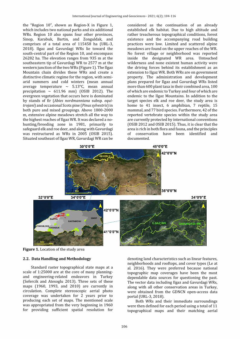
International Journal of Engineering and Geosciences– 2021; 6(2); 104-116

106

the “Region 10”, shown as Region-X in Figure 1, which includes two national parks and six additional WRs. Region 10 also spans four other provinces, Sinop, Karabuk, Bartin, and Zonguldak, and comprises of a total area of 115458 ha (URL-3, 2018). Ilgaz and Gavurdagi WRs lie toward the south-central part of the Region 10, and encompass 26282 ha. The elevation ranges from 935 m at the southeastern tip of Gavurdagi WR to 2577 m at the western junction of the two WRs (Figure 1). The Ilgaz Mountain chain divides these WRs and create a distinctive climatic regime for the region, with semi-arid summers and cold winters (mean annual average temperature ~ 5.13°C, mean annual precipitation ~ 611.96 mm) (OSIB 2012). The evergreen vegetation that occurs here is dominated by stands of fir (Abies nordmanniana subsp. equi-trojani) and occasional Scots pine (Pinus sylvestris) in both pure and mixed groupings. Above 1800-2000 m, extensive alpine meadows stretch all the way to the highest reaches of Ilgaz WR. It was declared a no-hunting/breeding zone in 1981, primarily to safeguard elk and roe deer, and along with Gavurdagi was restructured as WRs in 2005 (OSIB 2015). Situated southeast of Ilgaz WR, Gavurdagi WR can be

considered as the continuation of an already established elk habitat. Due to high altitude and rather treacherous topographical conditions, forest existence and the accompanying road building practices were low. Limited and scattered alpine meadows are found on the upper reaches of the WR. No forest village or neighborhood was reported inside the designated WR area. Untouched wilderness and none existent human activity were the driving forces behind its establishment as an extension to Ilgaz WR. Both WRs are on government property. The administration and development plans prepared for Ilgaz and Gavurdagi WRs listed more than 600 plant taxa in their combined area, 100 of which are endemic to Turkey and four of which are endemic to the Ilgaz Mountains. In addition to the target species elk and roe deer, the study area is home to 41 insect, 6 amphibian, 7 reptile, 15 mammal, and 77 bird species. Furthermore, 42 of the reported vertebrate species within the study area are currently protected by international conventions (OSIB 2012 and OSIB 2015). Thus, it is clear that the area is rich in both flora and fauna, and the principles of conservation have been identified and documented.

Figure 1. Location of the study area 2.2. Data Handling and Methodology

Standard raster topographical state maps at a scale of 1:25000 are at the core of many planning- and engineering-related endeavors in Turkey (Sefercik and Atesoglu 2013). Three sets of these maps (1960, 1993, and 2010) are currently in circulation. Complete stereoscopic aerial photo coverage was undertaken for 2 years prior to producing each set of maps. The mentioned scale was appropriated from the very beginning in 1960 for providing sufficient spatial resolution for

denoting land characteristics such as linear features, neighborhoods and rooftops, and cover types (Le at al. 2016). They were preferred because national topographic map coverages have been the most dependable data sources for questioning the past. The vector data including Ilgaz and Gavurdagi WRs, along with all other conservation areas in Turkey, were obtained from the GDNCN open-access data portal (URL-3, 2018).

Both WRs and their immediate surroundings were then defined for each period using a total of 11 topographical maps and their matching aerial

International Journal of Engineering and Geosciences– 2021; 6(2); 104-116

107

photographs, which included 10 black and white aerial photographs scaled to 1:50000 from 1955, 12 black and white aerial photographs scaled to 1:40000 from 1990, and 16 four-band-color infrared aerial photographs scaled to 1:5000 from 2008

(Figure 2). Since Ilgaz and Gavurdagi WRs are adjacent to each other, these analyses were made over their combined area, named as “the core area” hereafter for computational convenience.

Figure 2. Aerial photograph dated 1955 and the corresponding topographical map dated 1960 (not to be scaled)

In the first part of data handling, the topographical maps were geo-referenced according to the abovementioned intervals to generate three separate coverages. The corresponding aerial photographs were then co-registered onto the registered maps and placed in their respective regions. Next, all-weather, dry-weather accessible roads and linear fashioned man-made marks, and house rooftops occurring within the neighborhoods were meticulously digitized through the coverages, while simultaneously cross-checking their validities through aerial photographs in AcrGIS-10.6 (Figure 2). This enabled us to draw every linearly fashioned man-made object within the core area and aggregate them as one coverage result measured in length through UTM projection. The majority of forest roads in the study area had a 3 to 4 m platform width which was bordered by a 0.5 to 1 m wide side ditch, and lacked surface material. However, as oppose to the procedure applied in this study, not all road-designated linear features on maps or in aerial photographs were considered in road density calculations in Turkey. Other government agencies like rural affairs, provincial governorships, state provinces bank, etc., also provide access to the regions and communities, which can be used all-year round. However, these additions do not count towards the calculation of road density in forest management by regulation (OGM 2008), even though they link to forest road networks and continue to fragment the area even further. Dry-weather roads were digitized within the core + 1000 m buffer area to establish continuity for further calculations. All-weather roads, on the other hand, were digitized, starting from behind 3000 m buffer

area with the same intension and to see the bigger perspective (Figure 3). Road covered area percentage was calculated by multiplying the respected road lengths with 4 m in dry-weather, and with 6 m in all weather, and dividing them with the corresponding acreages, in three scenarios (Table 1 and Table 2). As the roads have been built, the intact habitat continuity has kept on dwindling. Thus, we wanted to see the number of such forest patches completely surrounded by roads in the forms of closed polygons both within the core + 1000 m buffer area, and within the core +3000 m buffer area. While digitizing both road types, all connections defined by point, end, edge and vertex snapping algorithm within and across the road type(s) were carefully placed to form and measure these closing polygons frequently named as patches (Hawbaker and Radeloff 2004). In the beginning, only the dry-weather roads were forming patches, enclosed area of which got smaller in every coverage period. However, as the time progressed, higher standard all-weather roads, too, started forming patches around the core area. Finally, decommissioned roads were removed and newly constructed roads were added along with any suburban expansion to create a fourth coverage for 2019 through the Google Earth Pro. This process was quick and efficient because the majority of roads from the 2010 coverage were usually identical and easily visible on the high-spatial-resolution imagery, thanks to the matching projection. As for the suburban expansion figures, each settlement was assigned with a location number to allow us to keep track of it over the coverage periods, along with the number of houses in the vicinity and the type of usage i.e., permanent

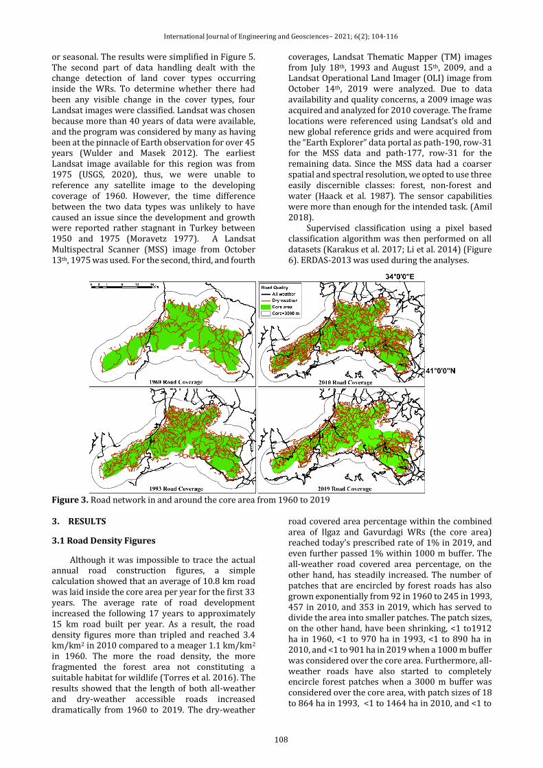
International Journal of Engineering and Geosciences– 2021; 6(2); 104-116

108

or seasonal. The results were simplified in Figure 5. The second part of data handling dealt with the change detection of land cover types occurring inside the WRs. To determine whether there had been any visible change in the cover types, four Landsat images were classified. Landsat was chosen because more than 40 years of data were available, and the program was considered by many as having been at the pinnacle of Earth observation for over 45 years (Wulder and Masek 2012). The earliest Landsat image available for this region was from 1975 (USGS, 2020), thus, we were unable to reference any satellite image to the developing coverage of 1960. However, the time difference between the two data types was unlikely to have caused an issue since the development and growth were reported rather stagnant in Turkey between 1950 and 1975 (Moravetz 1977). A Landsat Multispectral Scanner (MSS) image from October 13th, 1975 was used. For the second, third, and fourth

coverages, Landsat Thematic Mapper (TM) images from July 18th, 1993 and August 15th, 2009, and a Landsat Operational Land Imager (OLI) image from October 14th, 2019 were analyzed. Due to data availability and quality concerns, a 2009 image was acquired and analyzed for 2010 coverage. The frame locations were referenced using Landsat’s old and new global reference grids and were acquired from the “Earth Explorer” data portal as path-190, row-31 for the MSS data and path-177, row-31 for the remaining data. Since the MSS data had a coarser spatial and spectral resolution, we opted to use three easily discernible classes: forest, non-forest and water (Haack et al. 1987). The sensor capabilities were more than enough for the intended task. (Amil 2018).

Supervised classification using a pixel based classification algorithm was then performed on all datasets (Karakus et al. 2017; Li et al. 2014) (Figure 6). ERDAS-2013 was used during the analyses.

Figure 3. Road network in and around the core area from 1960 to 2019 3. RESULTS

3.1 Road Density Figures

Although it was impossible to trace the actual annual road construction figures, a simple calculation showed that an average of 10.8 km road was laid inside the core area per year for the first 33 years. The average rate of road development increased the following 17 years to approximately 15 km road built per year. As a result, the road density figures more than tripled and reached 3.4 km/km2 in 2010 compared to a meager 1.1 km/km2 in 1960. The more the road density, the more fragmented the forest area not constituting a suitable habitat for wildlife (Torres et al. 2016). The results showed that the length of both all-weather and dry-weather accessible roads increased dramatically from 1960 to 2019. The dry-weather

road covered area percentage within the combined area of Ilgaz and Gavurdagi WRs (the core area) reached today’s prescribed rate of 1% in 2019, and even further passed 1% within 1000 m buffer. The all-weather road covered area percentage, on the other hand, has steadily increased. The number of patches that are encircled by forest roads has also grown exponentially from 92 in 1960 to 245 in 1993, 457 in 2010, and 353 in 2019, which has served to divide the area into smaller patches. The patch sizes, on the other hand, have been shrinking, <1 to1912 ha in 1960, <1 to 970 ha in 1993, <1 to 890 ha in 2010, and <1 to 901 ha in 2019 when a 1000 m buffer was considered over the core area. Furthermore, all-weather roads have also started to completely encircle forest patches when a 3000 m buffer was considered over the core area, with patch sizes of 18 to 864 ha in 1993, <1 to 1464 ha in 2010, and <1 to

International Journal of Engineering and Geosciences– 2021; 6(2); 104-116

109

1463 ha in 2019. Consequently, the average patch size first decreased, then increased in both road types (Table 1 and Table 2). The study results yielded rather striking figures across the coverage periods showing that there was a dramatic increase in the road density of both all-weather and dry-weather roads. The decreasing numbers between 2010 and 2019 were due to decommissioning of the roads which had been laid before the establishments of both WRs. They were constructed everywhere regardless of the land cover or logging needs, thus when WRs were constıtutionalized after 2010, some of such roads did not surface in 2019.

3.2 Suburban Expansion Figures

Our study showed that both the combined area of Ilgaz and Gavurdagi WRs and their immediate surroundings have been subject to human settlement, a perfect example of which is seen in the bustling industrial sub-province of Tosya, which is still growing in the southeastern tip of the core area, today (Figure 4).

Although the town is outside the core area on municipal property and terms, its neighborhoods

simply border the core area. Two types of settlement were present within and around the core area: permanent and seasonal. In 1960, there were two permanent villages with 55 houses inside the core area. In 1993, there was no additional permanent habitation within the core area, with the house count decreasing to 46. However, the number of houses increased to 65 in 2010 and to 74 in 2019. By contrast, seasonal habitation fluctuated during the study period because such settlements lacked legitimacy, thus were subjected to unexpected crackdowns by the authorities. Evaluation of a 1000 m buffer showed that there was an incredible increase in the number of permanent habitation around the villages and in the sub-province Tosya, which squeezed Gavurdagi WR from the southeastern tip of the core area. In this study, it was evident that there were more seasonal locations than permanent villages inside the core area (Figure 5 (a), whereas the opposite was true in the surrounding 1000 m buffer area (Figure 5 (b). WRs have systematically been squeezed from within and outside.

Table 1. Road statistics for the study area from 1960 to 1993 Coverage period 1960 1993 Quality (all-weather (1) vs. dry-weather (2)) 1 2 Total 1 2 Total Road tally within core area* (km) 6.6 275.5 282.1 11.9 627.6 639.5 Road covered area % within core area (262.8 km2) 0.02 0.42 0.03 0.96 Road tally within 1000 m buffer area (km) 16.7 199.7 216.4 40.3 302.1 342.5 Road covered area % within buffer area (128.8 km2) 0.08 0.62 0.19 0.94 Road tally within 3000 m buffer area (km) 51 - 51 124.5 - 124.5 Road covered area % within buffer area (373.2 km2) 0.08 0.2 Road density within the core area (km/km2) 0.02 1.05 1.07 0.04 2.4 2.4

within 1000 m buffer (km/km2) 0.13 1.55 1.68 0.3 2.4 2.7 within 3000 m buffer (km/km2) 0.14 - 0.14 0.3 - 0.3

Number of patches within the core area+1000 m - 92 92 - 245 245 range of patch sizes (ha) - <1 to 912 - - <1 to 970 -

average patch size (ha) 112 88 Number of patches within the core area+3000 m - - - 3 - -

range of patch sizes (ha) - - - 18 to 864 - - average patch size (ha) 584

Table 2. Road statistics for the study area from 2010 to 2019

Coverage period 2010 2019 Quality (all-weather (1) vs. dry-weather (2)) 1 2 Total 1 2 Total Road tally within core area* (km) 72.9 828.8 901.7 72 700 772 Road covered area % within core area (262.8 km2) 0.17 1.26 0.16 1.07 Road tally within 1000 m buffer area (km) 60.8 409.6 470.4 62.4 370 432.4 Road covered area % within buffer area (128.8 km2)

0.28 1.27

0.29 1.15

Road tally within 3000 m buffer area (km) 216 - 216 222 - 222 Road covered area % within buffer area (373.2 km2)

0.35

0.36

Road density within the core area (km/km2) 0.3 3.2 3.4 0.3 2.7 2.9 within 1000 m buffer (km/km2) 0.5 3.2 3.6 0.5 2.9 3.4 within 3000 m buffer (km/km2) 0.6 - 0.6 0.6 - 0.6

Number of patches within the core area+1000 m - 457 457 - 353 353 range of patch sizes (ha) - <1 to 890 - - <1 to 910 -

average patch size (ha) 56 74 Number of patches within the core area+3000 m 21 - - 19 - -

range of patch sizes (ha) <1 to 1464 -

- <1 to 1463 - -

average patch size (ha) 287 338

International Journal of Engineering and Geosciences– 2021; 6(2); 104-116

110

Figure 4. Settlement locations in and around the core area from 1960 to 2019 (*Permanent,** Seasonal)

Figure 5. Settlement figures in and around the core area from 1960 to 2019

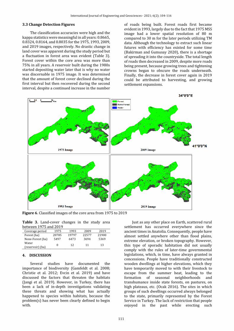
International Journal of Engineering and Geosciences– 2021; 6(2); 104-116

111

3.3 Change Detection Figures

The classification accuracies were high and the kappa statistics were meaningful in all years: 0.8665, 0.8324, 0.8164, and 0.8035 for the 1975, 1993, 2009, and 2019 images, respectively. No drastic change in land cover was apparent during the study period but a fluctuation in forest area was evident (Table 3). Forest cover within the core area was more than 75% in all years. A reservoir built during the 1980s started depositing water later that is why no water was discernable in 1975 image. It was determined that the amount of forest cover declined during the first interval but then recovered during the second interval, despite a continued increase in the number

of roads being built. Forest roads first became evident in 1993, largely due to the fact that 1975 MSS image had a lower spatial resolution of 80 m compared to 30 m for the later periods utilizing TM data. Although the technology to extract such linear futures with efficiency has existed for some time (Bakirman and Gumusay 2020), there is a shortage of spreading it into the countryside. The total length of roads then decreased in 2009, despite more roads being present, because growing trees and tightening crowns began to obscure the roads underneath. Finally, the decrease in forest cover again in 2019 could be attributed to harvesting, and growing settlement expansions.

Figure 6. Classified images of the core area from 1975 to 2019 Table 3. Land-cover changes in the study area between 1975 and 2019

Coverage period 1975 1993 2009 2019

Forest (ha) 20785 19797 22577 21900

None-Forest (ha) 5497 6473 3694 5369

Water

(reservoir) (ha) 0 12 11 13

4. DISCUSSION

Several studies have documented the importance of biodiversity (Gamfeldt et al. 2008; Christie et al. 2012; Evcin et al. 2019) and have discussed the factors that threaten the habitats (Jangi et al. 2019). However, in Turkey, there has been a lack of in-depth investigations validating these threats and showing what has actually happened to species within habitats, because the problem(s) has never been clearly defined to begin with.

Just as any other place on Earth, scattered rural settlement has occurred everywhere since the ancient times in Anatolia. Consequently, people have almost settled anywhere other than flood plains, extreme elevation, or broken topography. However, this type of sporadic habitation did not usually comply with the rules of later-time governmental legislations, which, in time, have always granted in concessions. People have traditionally constructed wooden dwellings at higher elevations, which they have temporarily moved to with their livestock to escape from the summer heat, leading to the formation of seasonal neighborhoods and transhumance inside state forests, on pastures, on high plateaus, etc. (Ocak 2016). The sites in which groups of such dwellings occurred always belonged to the state, primarily represented by the Forest Service in Turkey. The lack of restriction that people enjoyed in the past while erecting such

International Journal of Engineering and Geosciences– 2021; 6(2); 104-116

112

neighborhoods has gradually vanished. The agencies governing the area(s)-region(s) have started monitoring and restricting the movement of people, particularly in conservation areas (Hanacek and Rodriguez-Labajos 2018).

Accessibility has always been of paramount importance for forest management in Turkey, with roads having been considered as the only option for managing the resource and transporting all related services to and from it. New roads have been added to the forest road network each year (Turk and Gumus 2017). The current forest road building notification has stated that no more than 1% of the total forest area could be used for road building, which is the accepted norm within the Turkish forest management practice, today. However, the same notification has also stated that the above mentioned rate should be applied even less in other types of functionality assigned forests (OGM 2008).

When the land is reassigned with a new agenda, one could anticipate that the footprints of past forest management practices would be somewhat remedied. As obvious from the results of this study, the situation did not materialize like this inside the core area because timber harvesting has continued. The conservation status has not changed the wrong-doing. Consequently, poaching is rampant, as the fines and sentencing do not act as deterrents, and policing is undermanned and ineffective.

It has previously been reported that small mammals avoid crossing forest roads, mainly due to various types of predation risks, so the presence of roads causes their home ranges to shrink, their existing habitat usage patterns to change, and population isolation to occur (Ascensao et al. 2017). Although roads and the resulting forest fragmentation do not have as great an effect on larger game animals as they do on smaller ones, they still have direct impacts in the form of vehicle collisions when there are high volumes of traffic (Litvaitis et al. 2015), increased mobility for human access (Bischof et al. 2017), and from the changing nature of the ecosystem services (Coffin 2007). Collisions involving bears, roe deer, wild boars, and occasional elk occur on the Kastamonu-Ankara intercity road that crosses Ilgaz WR in a north-northeast to south-southwest direction, especially in early winter and late spring months were reported (OSIB 2012) as higher.

It has been shown that underground or aboveground wildlife passages effectively mitigate these impacts and are frequently used by all sorts of animals, even insects (Martinig and Belangar-Smith 2016; Wang et al. 2018). However, no such passage exists inside the core area. A recent global study showed that habitat fragmentation is responsible for 13%-75% biodiversity loss and prevents ecosystem functions from occurring efficiently (Haddad et al. 2015). The study area has long been considered as a prime habitat for wildlife. Although the quality of a habitat can be considered as a primary indicator of species abundance, it is a rather weak indicator of

the distribution and similarity of species (Dambros et al. 2015). There is not any published study looking into the effects of forest fragmentation on the quality and abundance of any species in Turkey.

Turkish legislation prohibits big game hunting for the general public, but according to inventories carried out by DW, issues licenses annually for harvesting a number elk, roe deer and wild boar. These licenses are rather expensive for rural people, so it is generally the international hunters applying for them. If no one applies, the tags are left. There is no “must be fulfilled” policy meaning that the animals are not required to be harvested. However, although these regulations seem appropriate and by the code, poaching continues, and is increasing. The Kastamonu sub-branch of DW has been recording the number of poaching cases in Region 10 since the beginning of 2000s. In the first 10 years, there were very few records of poaching, despite Kastamonu being a sizable province and 67% of its land area being covered by forests. However, there has been an increase in the number of poaching-related crimes annually since 2010, with cumulative figures of 15, 33, 52, 85, 69, 77, 119, 99, and 86 each year from 2010 to December 2019. However, these were only the documented cases of a much bigger problem.

Therefore, this many people residing in or around such habitats that are covered with such a large amount of road, on which they can both track the animals and flee from rangers, could be considered detrimental for the resources (Boston 2016).

The core area has long been considered as a pristine habitat for a large number of animals, ranging from big game animals to small mammals, birds, reptiles, and insects. However, no studies have investigated fragmentation and its effects on resident species in Turkey, so the current health, distribution, and stress level of these species are unknown. The results showing the road-building trend in Turkish forest habitats and the final assessment for 2019 are important as they show the current state of forest habitats in two, Ilgaz and Gavurdagi, of Turkey’s WRs, and to emphasize the problem on these issues and provide a baseline for future research.

The data used in this study, are easily achievable for anywhere within Turkey, thus similar studies for other regions are sincerely encouraged to display the situation in sensitive areas.

5. CONCLUSION

Turkey lies between three bio-geographical regions (Euro-Siberia, Iran-Turania, and the Mediterranean) and forms a bridge between Europe and Asia, resulting in many things changing within short distances. The country is blessed with a rich biodiversity in terms of both its flora and fauna. However, this wealth is not receiving the attention it deserves because Turkey is trying to take its place among the developed countries of the world. This is

International Journal of Engineering and Geosciences– 2021; 6(2); 104-116

113

a difficult ambition, and the sacrifices are being made, the functionalities of many things across the country are misleading and policing is insufficient. WRs in Turkey are under heavy human pressure, so it is unclear whether all of the documented species are in good standing. Thanks to the invaluable potential of mapping, remote sensing and GIS, this study has showed how fragmented the forest habitats are in Turkey, even in areas where least expected. This assertion must be taken seriously either to nullify the situation or to go deeper to investigate the health of the habitats in all dimensions. This study can be criticized as being a straight-forward mapping exercise, lacking novelty both in the approach and the analysis, however it is still an important work to show that nothing could be kept hidden when geo-science capabilities are utilized for the sake of environmental issues. If the forests would continue to be used for a number of causes, not only for timber production, it is important that the impacts of humans are kept to a bare minimum or eliminated to protect the biodiversity.

ACKNOWLEDMENT

We thank our colleagues, Alper Bulut, PhD; Ferhat Kara, PhD and Oytun E. Sakici, PhD for the inspiration and insight.

REFERENCES

Akay A E, Wing M G, Sivrikaya F & Sakar D (2012). A GIS-based decision support system for determining the shortest and safest route to forest fires: a case study in Mediterranean Region of Turkey. Environmental Monitoring and Assessment, 184: 1391-1407. DOI 10.1007/s10661-011-2049-z

Al-Chokhachy R, Black T A, Thomas C, Luce C H, Rieman B, Cissel R, Carlson A, Hendricson S, Archer E K & Kerhner J L (2016). Linkages between unpaved forest roads and streambed sediment: why context matters in directing road restoration. Restoration Ecology, 24(5): 589-598.

Amil T A (2018). Determining of different inundated land use in Salyan plain during 2010 the Kura river flood through GIS and remote sensing tools. International Journal of Engineering and Geosciences, 3(3), 80-86. DOI: 10.26833/ijeg.412348

Amin A & Fazal S (2017). Assessment of forest fragmentation in district of Shopian using multitemporal land cover (A GIS Approach). Journal of Geosciences and Geomatics, 5(1), 12-23. DOI:10.12691/jgg-5-1-2

Araujo H A, Page A, Cooper A B, Venditti J, MacIsaac E, Hassan M A & Knowler D (2014). Modelling changes in suspended sediment from forest road surface in a coastal watershed of British

Columbia. Hydrological Processes, 28, 4914-4927. DOI: 10.1002/hyp.9989

Ascensao F, Lucas P S, Costa A & Bager A (2017). The effects of roads on edge permeability and movement patterns for small mammals: A case study with Montane Akodont. Landscape Ecology, 32, 781-790. DOI 10.1007/s10980-017-0485-z

Bakirman T & Gumusay M U (2020). Integration of custom street view and low cost motion sensor. International Journal of Engineering and Geosciences, 5(2), 66-72. DOI: 10.26833/ijeg.589489

Bartakova V, Reichard M, Blazek R, Polacik M & Bryja J (2015). Terrestrial fishes: rivers are barriers to gene flow in annual fishes from the African savanna. Journal of Biogeography 42: 1832-1844. DOI:10.1111/jbi.12567

Bekiroglu S, Destan S, Can M, Turkoglu T & Tolunay A (2015). Econometric analysis of a forest recreation area: An Example from Istanbul, Turkey. Fresenius Environmental Bulletin, 24(9a), 2937-2945.

Bischof R B, Steyaert S M J G & Kindberg J (2017). Caught in the mesh: roads and their networkscale impediment to animal movement. Ecography, 40, 1369-1380. DOI: 10.1111/ecog.02801

Boluk G & Mert M (2015). The renewable energy, growth and environmental Kuznets curve in Turkey: An ARDL approach. Renewable and Sustainable Energy Reviews, 52, 587-595. DOI: 10.1016/j.rser.2015.07.138

Boston K (2016). The potential effects of forest roads on the environment and mitigating their impacts. Current Forestry Reports, 2, 215-222. DOI: 10.1007/s40725-016-0044-x

Bussotti F, Pollastrini M, Holland V & Brüggemann W (2015). Functional traits and adaptive capacity of European forests to climate change. Ennvironmental and Experimental Botany, 111, 91-113. DOI: 10.1016/j.envexpbot.2014.11.006

Caliskan E (2013). Environmental impacts of forest road construction on mountainous terrain. Iranian Journal of Environmental Health Science and Engineering, 10, 23, DOI: 10.1186/1735-274610-23.

Christie M, Fazey I, Cooper R, Hyde T & Kenter J O (2012). An evaluation of monetary and non-monetary techniques for assessing the importance of biodiversity and ecosystem services to people in countries with developing economies. Ecological Economics, 83, 67-78. DOI: 10.1016/j.ecolecon.2012.08.012

Coffin A W (2007). From roadkill to road ecology: A review of the ecological effects of roads. Journal of Transport Geography, 15, 396-406. DOI: 10.1016/j.jtrangeo.2006.11.006

Crooks K R, Burdett C L, Theobald D M, King S R B, Di Marco M Rondinini C & Boitani L (2017). Quantification of habitat fragmentation reveals extinction risk in terrestrial mammals.

International Journal of Engineering and Geosciences– 2021; 6(2); 104-116

114

Proceedings of the National Academy of Sciences of the United States of America, 114(29): 7635-7640. DOI: 10.1073/pnas.1705769114

Dambros C S, Caceres N C, Magnus L & Gotelli N J (2015). Effects of neutrality, geometric constraints, climate and habitat quality on species richness and composition of Atlantic Forest small mammals. Global Ecology and Biogeography, 24, 1084-1093. DOI: 10.1111/geb.12330

Demir M & Hasdemir M (2005). Functional Planning Criterion of Forest Network Systems According to Recent Forestry Development and Suggestions in Turkey. American Journal of Environmental Sciences, 1(1), 22-28.

Di Gironimo G, Balsamo A, Esposito G, Lanzotti A, Melemez K & Spinelli R (2015). Simulation of forest harvesting alternative processes and concept design of an innovative skidding winch focused on productivity improvement. Turkish Journal of Agriculture and Forestry, 39, 350-359. DOI: 10.3906/tar-1408-64

Edwards P J, Wood F & Quinlivan R L (2016). Effectiveness of Best Management Practices that Have Application to Forest Roads: A Literature Synthesis. United States Department of Agriculture, General Technical Report NRS-163, Forest Service Northern Research Station.

Eken G, Isfendiyaroglu S, Yeniyurt C, Erkol I L, Karatas A & Ataol M (2016). Identifying key biodiversity areas in Turkey: a multi-taxon approach. Internatioal Journal of Biodiversity Science, Ecosystem Services & Management, 12(3): 181-190. DOI: 10.1080/21513732.2016.1182949

Erturk A (2017). Research on the Spatial Ecology and Population Structure of Anatolian Canis lupus L. 1758 (gray wolf). PhD dissertation, Hacettepe University, in Turkish.

Evcin O, Kucuk O & Akturk E (2019). Habitat suitability model with maximum entropy approach for European roe deer (Capreolus capreolus) in the Black Sea Region. Environmental Monitoring and Assessment 191: 669. DOI: 10.1007/s10661-019-7853-x

Fahrig L (2002). Effect of habitat fragmentation on the extinction threshold: A Synthesis. Ecological Applications, 12(2), 346-353.

Forman R T T, Sperling D, Bissonette J A, Clevenger A P, Cutshall C D, Dale V H, Fahrig L, France R, Goldman C R, Heanue K, Jones J A, Swanson F J, Turrentine T & Winter T C (2002). Road Ecology, Science and Solutions, Island Press. ISBN: 978-1559639330

Gamfeldt L, Hillebrand H & Jonsson P R (2008). Multiple functions increase the importance of biodiversity for overall ecosystem functioning. Ecology, 89(5), 1223-1231. DOI: 10.1890/06-2091.1

Geffen E, Anderson M J & Wayne R K (2004). Climate and habitat barriers to dispersal in the highly

mobile grey wolf. Molecular Ecology, 13, 2481-2490. DOI: 10.1111/j.1365-294X.2004.02244.x

Haack B, Bryant N & Adams S (1987). An assessment of Landsat MSS and TM Data for urban and near-urban land-cover digital classification. Remote Sensing of Environment, 21(2), 201-213. DOI: 10.1016/0034-4257(87)90053-8

Haddad N M, Brudvig L A, Clobert J, Davies K F et al. (2015). Habitat fragmentation and its lasting impact on Earth’s ecosystems. Applied Ecology 1(2), e1500052.

Hanacek K & Rodriguez-Labajos B (2018). Impacts of land-use and management changes on cultural agroecosystem services and environmental conflicts—A global review. Global Environmental Change, 50, 41-59.

Hawbaker T J & Radeloff V C (2004). Roads and landscape pattern in Northern Wisconsin based on a comparison of four road data sources. Conservation Biology, 18(5): 1233-1244. DOI: 10.1111/j.1523-1739.2004.00231.x

Heilman Jr. G E, Strittholt J R, Slosser N C & Dellesala D A (2002). Forest fragmentation of the conterminous Unites States: Assessing forest intactness through road density and spatial characteristics, BioScience, 52(5): 411-422.

Jangi M N, Noori G, Karami M & Jangi A N (2019). Threatening and destructing factors associated with the habitat of francolin in Sistan region (Case study: Jazinak corridor). International Journal of Environmental Science and Technology,16: 1967-1972. DOI 10.1007/s13762-017-1614-6

Jones J Smith R, Jost G, Winkler R et al. (2018). Summary of the Forests and Water Workshop. Journal of Watershed Management, 2(1), 1-22. DOI: 10.22230/jwsm.2018v2n1a1

Karakus P, Karabork H & Kaya S (2017). A comparison of the classification accuracies in determining the land cover of Kadirli region of Turkey by using the pixel based and object based classification algorithms. International Journal of Engineering and Geosciences, 2(02), 52-60. DOI: 10.26833/ijeg.298951

Kaya Z & Raynal D J (2001). Biodiversity and conservation of Turkish forests. Biological Conservation, 97, 131-141.

Laurance W F & Balmford A (2013). A global map for road building. Nature, 495, 308-309.

Le H L, Miyagi T, Shinro A & Hamasaki E (2016). Landslide typology using a morphological approach and establishment of an inventory map based on aerial photo interpretation in Central Vietnam. Geomorphology and Society, Advances in Geographical and Environmental Sciences. Springer, Tokyo. 149-163.

Li C, Wang J, Wang L, Hu L & Gong P (2014). Comparison of classification algorithms and training sample sizes in urban land classification with Landsat Thematic Mapper Imagery. Remote Sensing, 6, 964-983. DOI: 10.3390/rs6020964

International Journal of Engineering and Geosciences– 2021; 6(2); 104-116

115

Litvaitis J A, Reed G C, Carroll R P, Litvaitis M K, Tash J, Mahard T, Broman D J A, Callahan C & Ellingwood M (2015). Bobcats (Lynx rufus) as a Model Organism to Investigate the effects of Roads on Wide-Ranging Carnivores. Environmental Management, 55(6): 1366-1376. DOI 10.1007/s00267-015-0468-2

Liu S, Dong Y, Deng L, Liu Q, Zhao H & Dong S (2014). Forest fragmentation and landscape connectivity change associated with road network extension and city expansion: A case study in the Lancang River Valley. Ecological Indicators, 36, 160-168. DOI: 10.1016/j.ecolind.2013.07.018

Lugo A E & Gucinski H (2000). Function, effects and management of forest roads. Forest Ecology and Management, 133(3), 249-262. DOI: 10.1016/S0378-1127(99)00237-6

Lundmark T, Bergh J, Hofer P, Lundström A, Nordin A, Poudel B C, Sathre R, Taverna R & Werner F (2014). Potential Roles of Swedish Forestry in the Context of Climate Change Mitigation. Forests, 5(4), 557-578. DOI: 10.3390/f5040557

Machado A P, Clement L, Uva V, Goudet J & Roulin A (2018). The Rocky Mountains as a dispersal barrier between barn owl (Tyto alba) populations in North America. Journal of Biogeography, 45, 1288-1300. DOI: 10.1111/jbi.13219

Martinig A R & Belanger-Smith K (2016). Factor influencing the discovery and use of wildlife passages for small fauna. Journal of Applied Ecology, 53, 825-836. DOI: 10.1111/1365-2664.12616

Milodowski D T, Mudd S M & Mitchard E T A (2015). Erosion rates as a potential bottom-up control of forest structural characteristics in the Sierra Nevada Mountains. Ecology, 96(1), 31-38. DOI: 10.1890/14-0649.1

Moravetz D (1977). Twenty-five Years of Economic Development 1950-1975. The World Bank, Report #10098, 125 p.

Ocak S (2016). Transhumance in Central Anatolia: A resilient interdepence between biological and cultural diversity. Journal of Agricultural and Environmental Ethics, 29, 439-453. DOI 10.1007/s10806-016-9613-z

OGM (2008). Notification on the drafting, construction and maintenance of forest road, Notification # 292. Environment and Forestry Ministery, Forest Service (OGM): Ankara, Turkey, in Turkish, 338 p.

Ortega Y K & Capen D E (1999). Effects of Forest Roads on Habitat Quality for Ovenbirds in a Forested Landscape. The Auk, 116(4), 937-946.

OSIB (2012). Ilgaz Wildlife Refuge Administration and Development Plan, Kastamonu Sub-branch, Region 10 Directorate, the Ministry of Agriculture and Forestry, Kastamonu, Turkey, (in Turkish), 151 p.

OSIB (2015). Kastamonu Tosya Gavurdagi Wildlife Refuge Administration and Development Plan,

Kastamonu Sub-branch, Region 10 Directorate, the Ministry of Agriculture and Forestry, Kastamonu, Turkey, (in Turkish), 133 p.

Sefercik U G & Atesoglu A (2013). Uydu Verileri Kullanarak Meşcere Boyu Belirlenmesine Yönelik Yeni Bir Yaklaşım, TUFUAB 6thTechnical Symposium, Trabzon, Turkey (in Turkish)

Sekercioglu C H, Anderson S, Akcay E, Bilgin R, Can O E et al. (2011). Turkey’s globally important biodiversity in crisis. Biological Conservation, 144(12), 2752-2769. DOI: 10.1016/j.biocon.2011.06.025

Skole D & Tucker C (1993). Tropical Deforestation and Habitat Fragmentation in the Amazon: Satellite Data from 1978 to 1988. Science, 260(5116), 1905-1910. DOI: 10.1126/science.260.5116.1905

Soyumert A (2010). Determining large mammal species and their ecology via the camera trap methods in Northwestern Anatolian Forests. PhD dissertation, Hacettepe University. (in Turkish).

Soyumert A (2020). Camera-trapping two felid species: Monitoring Eurasian lynx (Lynx lynx) and wildcat (Felis silvestris) populations in mixed temperate forest ecosystems. Mammal Study, 45(1), 41-48. DOI: 10.3106/ms2019-0046

Soyumert A, Erturk A & Tavsanoglu C (2019). The importance of lagomorphs for the Eurasian lynx in Western Asia: Results from a large scale camera-trapping survey in Turkey. Mammalian Biology, 95: 18-25. DOI: 10.1016/j.mambio.2019.01.003

Suleiman M S, Wasonga O V, Mbau J S & Elhadi Y A (2017). Spatial and temporal analysis of forest cover change in Falgore Game Reserve in Kano, Nigeria. Ecological Processes, 6(11): DOI: 10.1186/s13717-017-0078-4

Torres A, Jaeger J A G & Alonso J C (2016). Assessing large-scale wildlife responses to human infrastructure development. Proceedings of the National Academy of Sciences of the United States of America, 113(30): 8472-8477.

Towerton A L, Kavanagh R P, Penman T D & Dickman C R (2016). Ranging behavior and movements of the red fox in remnant forest habitats. Wildlife Research, 43, 492-506. DOI: 10.1071/WR15203

Turk Y & Gumus S (2017). Evaluation of the tender results of forest road constructions: A case study in Bolu Regional Directorate. Journal of the Faculty of Forestry, Istanbul University 67(2), 194-202.

URL-1. (2018). “Noah’s Ark” National Biodiversity Database, Ministry of Agriculture and Forestry, Geographical Information Systems, Available online at: http://www.nuhungemisi.gov.tr/Giris/indexen.aspx, Accessed date: 27.05.2020.

URL-2. (2020). Environmental Performance Index, Biodiversity & Habitat, Yale Center for Environmental Law & Policy, Available online

International Journal of Engineering and Geosciences– 2021; 6(2); 104-116

116

at: https://sedac.ciesin.columbia.edu/data/collection/epi/sets/browse, Accessed date: 06.06.2020.

URL-3. (2020). Conservation Areas of Turkey”, Available online at: http://www.kursatozcan.com/korunan_alanlar/, Accessed date: 30.05.2020

USGS. (2020). Earth Explorer data portal, USGS, Available online at: https://earthexplorer.usgs.gov/, Accessed date: 07.04.2020.

Wang Y, Guan L, Chen J & Kong Y (2018). Influences on mammals frequency of use of small bridges and culverts along the Qinghai-Tibet railway, China. Ecological Research, 33, 879-887. DOI: 10.1007/s11284-018-1578-0

Won H K, Jeon H S, Han H, Lee S J & Jung B H (2017). Combining Timber Production and Wood Processing for Increasing Forestry Income: A Case Study of 6th Industrialization in Korean Forestry. Journal of Forest and Environmental Science, 33(4): 355-360. DOI: 10.7747/JFES.2017.33.4.355

Wulder M A & Masek J G (2012). Landsat Legacy Special Issue: Continuing the Landsat Legacy. Remote Sensing of Environment, 122, 1.

Yildiz O, Sarginci M, Esen D & Cromack Jr K (2007). Effects of vegetation control on nutrient removal and Fagus orientalis, Lipsky regeneration in the western Black Sea Regin of Turkey. Forest Ecology and Management, 240, 186-194. DOI: 10.1016/j.foreco.2007.01.018

© Author(s) 2021. This work is distributed under https://creativecommons.org/licenses/by-sa/4.0/

IJEG Volume 6 - Issue 2

ARTICLES

** Multi criteria decision analysis to determine the suitability of agricultural crops for land

consolidation areas

Fatih Sarı, Fatma Koyuncu Sarı 64

** Accuracy comparison of interior orientation parameters from different photogrammetric

software and direct linear transformation method

Zaide Duran, Muhammed Enes Atik 74

** Accuracy assessment of digital surface models from unmanned aerial vehicles’ imagery on

archaeological sites

Emre Şenkal, Gordana Kaplan, Uğur Avdan 81

** Analysis of literature on 3D cadastre

Fatih Döner 90

** Determining highway slope ratio using a method based on slope angle calculation

Osman Salih Yılmaz, Gülgün Özkan, Fatih Gülgen 98

** Determining the habitat fragmentation thru geoscience capabilities in Turkey: A

case study of wildlife refuges

Arif Oguz Altunel , Sadık Caglar, Tayyibe Altunel 104