Volume 2, Issue 1, 2008

An Efficient Algorithm for the Computation of Response-time Bounds forCAN Messages

Imad Alzeer, Assis. Prof., Al-Quds University, im_alzeer@eng.alquds.eduNaji Qatanani, Assoc. Prof., Al-Quds University, nqatanani@science.alquds.edu

AbstractThis paper presents an efficient computational exhaustive method that permits to calculate both up-per and lower response-time bounds for CAN messages. Response-time analysis for CAN messages isrelatively limited for computations of the worst case situation. It is computed assuming a maximum trans-mission time and critical instant releasing of messages in the CAN system. This pessimism implies themaximum interference between messages circulated on the bus. It may be correct from a hard real-timeperspective when synchronous releasing, but it doesn’t give good outlook when non-common messagesreleasing. Hence to obtain an analysis close to the reality, the investigated temporal constraints musttake into account both effects of time phasing and bit-stuffing. By using a suitable data structure, ourwork introduces an elegant algorithm that is able to deal with the previous effects. The obtained resultsfor best and worst cases response-times are different from previous results obtained when assuming anoptimist and a pessimist bit-stuffing length.

Keywords: CAN messages, bit-stuffing, scheduling, response-time, computational algorithm.

1. Introduction

A lot of work has been done and many algorithms have been developed to compute the worst caseresponse-time for CAN messages [4, 7]. The majority of the present studies deal with the circum-stances where messages are queued at the critical instants. Because the schedulability analysis isquite pessimistic, it assumes that a missed deadline in the worst case is equivalent to always missingthe deadline for all instant messages [13]. So in messages scheduling, the reliability is regarded as anobjective issue and the performance of any scheduling algorithm is measured generally by two factors:

1. Its ability to generate a feasible schedule for the set of messages covering all possible combina-tions of transmitted messages.

2. Determining whether these messages will meet their deadlines or not.

Bit-stuffing is performed by CAN to maintain the phase-locked bit timing. When the transmitter logicdetects five consecutive bits of the same level, it inserts a sixth complementary bit into the originalstream [5]. According to the content of original message, an extra number of bits (stuff bits) is insertedand merged with the original frame.

Since the scheduling on CAN is non-preemptive, and despite of a fixed number of data bytes that may beconveyed in each message, the number of inserted stuff bits resulting from stuffing rule may vary fromany transmission period to the next (when the transmitted data is variable). Therefore certain disorderingin the transmission sequence will occur.

This paper extends a scheduling analysis to allow computations of the worst and the best case response-time taking into account the variation in stuff bits length when error-free message transmission.

2. CAN Messages

According to the terminology of CAN, two types of messages in CAN system may be used:

• Standard CAN frame with 11 bits identifier;

• Extended CAN frame with 29 bit identifier.

Value of the identifier is assigned statically before starting the communication process. As shown in Fig.1, an extended CAN message format contains 67 bits of protocol control information, including 29 bitsidentifier associated with each message assigning its priority, 4 bits for a message length field, 15 bitsfor CRC field, 7 bits for the end-of-frame signal, and 3 bits for the intermission between frames.

1

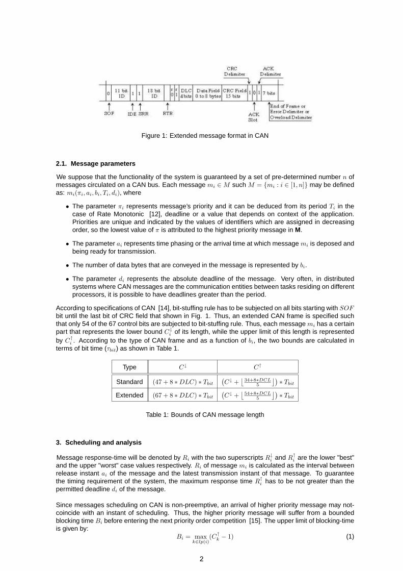
Figure 1: Extended message format in CAN

2.1. Message parameters

We suppose that the functionality of the system is guaranteed by a set of pre-determined number n ofmessages circulated on a CAN bus. Each message mi ∈ M such M = {mi : i ∈ [1, n]} may be definedas: mi(πi, ai, bi, Ti, di), where

• The parameter πi represents message’s priority and it can be deduced from its period Ti in thecase of Rate Monotonic [12], deadline or a value that depends on context of the application.Priorities are unique and indicated by the values of identifiers which are assigned in decreasingorder, so the lowest value of π is attributed to the highest priority message in M.

• The parameter ai represents time phasing or the arrival time at which message mi is deposed andbeing ready for transmission.

• The number of data bytes that are conveyed in the message is represented by bi.

• The parameter di represents the absolute deadline of the message. Very often, in distributedsystems where CAN messages are the communication entities between tasks residing on differentprocessors, it is possible to have deadlines greater than the period.

According to specifications of CAN [14], bit-stuffing rule has to be subjected on all bits starting with SOFbit until the last bit of CRC field that shown in Fig. 1. Thus, an extended CAN frame is specified suchthat only 54 of the 67 control bits are subjected to bit-stuffing rule. Thus, each message mi has a certainpart that represents the lower bound C↓

i of its length, while the upper limit of this length is representedby C↑

i . According to the type of CAN frame and as a function of bi, the two bounds are calculated interms of bit time (τbit) as shown in Table 1.

Type C↓ C↑

Standard (47 + 8 ∗ DLC) ∗ Tbit

(C↓ +

⌊34+8∗DCL

5

⌋) ∗ Tbit

Extended (67 + 8 ∗ DLC) ∗ Tbit

(C↓ +

⌊54+8∗DCL

5

⌋) ∗ Tbit

Table 1: Bounds of CAN message length

3. Scheduling and analysis

Message response-time will be denoted by Ri with the two superscripts R↓i and R↑

i are the lower "best"and the upper "worst" case values respectively. Ri of message mi is calculated as the interval betweenrelease instant ai of the message and the latest transmission instant of that message. To guaranteethe timing requirement of the system, the maximum response time R↑

i has to be not greater than thepermitted deadline di of the message.

Since messages scheduling on CAN is non-preemptive, an arrival of higher priority message may not-coincide with an instant of scheduling. Thus, the higher priority message will suffer from a boundedblocking time Bi before entering the next priority order competition [15]. The upper limit of blocking-timeis given by:

Bi = maxk∈lp(i)

(C↑k − 1) (1)

2

where lp represents the subset of messages that are lower priority than the message mi.

To focus on the effect of incertitude in the length and the time phasing on response-time computations,the releasing jitter delay of the message is integrated in the time phasing parameter ai and will not beappeared or discussed here.

3.1. Scheduling Period

The proposed CAN model that we will study allows messages to be released asynchronously with arbi-trary periods. Hence according to [11], when the messages are released synchronously, the sched-ule period SP is calculated as the least common multiple (LCM) of their periods, otherwise SP =maxi={1..n}(ai) + 2 ∗ LCM . Many studies are done to reduce the SP in the asynchronous releasecase [9]. To keep the scheduling duration small, whenever this is possible, the approach is to makemessage periods multiples of one another.

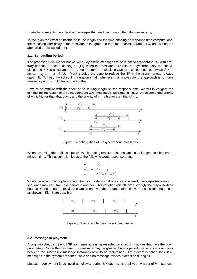
Now, to be familiar with the effect of bit-stuffing length on the response-time, we will investigate thescheduling interaction of the 3 independent CAN messages illustrated in Fig. 2. We assume that priorityof m1 is higher than that of m2, and the priority of m2 is higher than that of m3.

Figure 2: Configuration of 3 asynchronous messages

When assuming the traditional pessimist bit-stuffing result, each message has a longest possible trans-mission time. This assumption leads to the following worst response-times:

R↑1 = C↑

1

R↑2 = C↑

1 + C↑2

R↑3 = C↑

1 + C↑2 + C↑

3

When the effect of time phasing and the incertitude in stuff bits are considered, messages transmissionsequence may vary from one period to another. This variation will influence strongly the response-timebounds. Concerning the previous example and with the progress of time, two transmission sequencesas shown in Fig. 3 are possible.

Figure 3: Two possible transmission sequences

3.2. Message deployment

Along the scheduling period SP, each message is represented by a set of instances that have their ownparameters. Since the deadline of a message may be greater than its period, precedence constraintsbetween the successive message instances have to be maintained. The system is schedulable if allmessages in the system are schedulable and no message misses a deadline during SP.

Message deployment is achieved as follows: during SP, each mi is deployed by a set of ki instances,

3

where ki =⌊

SPTi

⌋. Thus, the extended set X contains K =

∑ni=1 ki of deployed instances that have the

same period SP. Parameters of the jth instance of the message mi are calculated as:

• since the message has a fixed priority, all instances of the message have the same priority: πji =

πi;

• activation instants are shifted by the period and related with time phasing of the first instance:aj

i = ai + (j − 1) ∗ Ti;

• two bounds are the same of the original message: Cm↓i = C↓

i and Cm↑i = C↑

i ;

• absolute deadline of the instance is related with the period and the deadline of the first instance:Dj

i = Di + (j − 1) ∗ Ti.

The deployment mechanism is explained by taking the 3-messages shown in 2. Without loss of thegenerality and for simplicity, we assume that T3 = 2 ∗ T1 = 2 ∗ T2 = 30 and other parameters are:m1 = (π1, a1, C

↓1 , C↑

1 ) = (1, 0, 3, 4),m2 = (2, 4, 3, 5) and m3 = (3, 3, 3, 4). Since all instances of messagesstart during the LCM and terminates before the time instant 30, SP can be considered as LCM . So, theextended list X contains 5 elements as shown in Fig. 4.

Figure 4: Deployed instances of 3 messages

3.2.1. Activation array

Since each deployed instance has its own activation date, elements of the extended list X are arrangedaccording to their activation instants. When many instances are activated at the same instant, thenthey are mutually referenced. This mechanism prevents us from doing any non-necessary manipulationduring the calculation. Concerning our example of five instances, this array is shown in Table 2.

# instant Instance1 0 m1

1

2 3 m13

3 4 m12

4 15 m21

5 19 m22

Table 2: Array of activation dates

3.3. Transmission Sequences

The large number of combinations that results from the application of bit-stuffing do not lead mostly to thesame number of the transmission sequences. The number of combinations resulted from N instances is

N∏i=1

(C↑i − C↓

i + 1).

Concerning our previous example, the incertitude in the length of 5 instances leads to 72 combinationsas shown in Fig. 5. For simplicity we show partially the upper part of the combinational tree. The

4

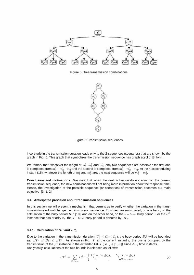
Figure 5: Tree transmission combinations

Figure 6: Transmission sequences

incertitude in the transmission duration leads only to the 2-sequences (scenarios) that are shown by thegraph in Fig. 6. This graph that symbolizes the transmission sequence has graph acyclic [8] form.

We remark that: whatever the length of m11, m1

3 and m12, only two sequences are possible : the first one

is composed from m11−m1

3−m12 and the second is composed from m1

1−m12−m1

3. At the next schedulinginstant (15), whatever the length of m2

1 and m22 are, the next sequence will be m2

1 − m22.

Conclusion and motivations: We note that when the next activation do not effect on the currenttransmission sequence, the new combinations will not bring more information about the response time.Hence, the investigation of the possible sequence (or scenarios) of transmission becomes our mainobjective [3, 1, 2].

3.4. Anticipated prevision about transmission sequences

In this section we will present a mechanism that permits us to verify whether the variation in the trans-mission time will not change the transmission sequence. This mechanism is based, on one hand, on thecalculation of the busy period BP [10], and on the other hand, on the k − level busy period. For the kth

instance that has priority πk, the k − level busy period is denoted by BPk.

3.4.1. Calculation of BP and BPk

Due to the variation in the transmission duration (C↓i ≤ Ci ≤ C↑

i ), the busy period BP will be boundedas: BP ↓ ≤ BP ≤ BP ↑. As shown in Fig. 7, at the current instant tc the bus is occupied by thetransmission of the jth instance in the extended list X (i.e. j ∈ [1,K]) since durj time instants.Analytically, calculations of the two bounds is released as follows:

BP ↓ =∑

i∈Imin

C↓i +

{C↓

j − durj(tc), C↓j > durj(tc)

0 , otherwise(2)

5

Figure 7: Busy period bounds

BP ↑ =∑

i∈Imax

C↑i + C↑

j − durj(tc) (3)

The subsets Imin and Imax are related to BP ↓ and BP ↑ respectively. They result from:

1. Ready instances at the current instant tc.

2. Those instances will be ready during the concerned busy period (BP ↓ or BP ↑)

However, the lower bound of k − level busy period BP ↓ is calculated as:

BP ↓k =

∑i∈(Imin∩(hp(k)∪k))

C↓i +

{C↓

j − durj(tc), C↓j > durj(tc)

0 , otherwise(4)

The subset (Imin ∩ (hp(k)∪ k)) consists of all instances having a priority level equal or greater than thatof the kth instance providing that these instances are activated during the continuous period BA↓

k. Sinceall instances are included in the activation array, process of calculation and verification is effectuatediteratively.

We explain the previous method by an example of 3 configurations as shown in Fig. 8. At the time in-stant tc, the 3 configurations lead to the same bounds: BP ↓ = 14 and BP ↑ = 19, but their transmissionsequences may be different. Thus, according to the category of activation, we can judge if the trans-

Figure 8: Different release configurations

mission sequence is certainly unique (unique transmission scenario) or not. Generally, three activationcategories may be distinguished:

1. Synchronous activations: when all instances belong to the busy period are activated at the sameinstance (Fig. 8-a). In this case, whatever their durations, the transmission sequence will beunique.

2. Pseudo synchronous activations: assuming that π1 < π2 < π3 < π4, as shown in Fig. 8-b,the activation of an instance occurs certainly before the transmission of any other lower priorityinstance. This implies that the transmission of all instances belong to the busy period occurredaccording to their priority order.

6

3. Asynchronous activations: the transmission of the instances can not be guaranteed to agree withtheir priorities as shown in Fig. 8-c.

Due to the incertitude in the duration of m1 and m2, at t = 10, there is no guarantee that m4 (whichis less priority than m3) has not yet started its transmission. Hence, to make sure that the instance jhaving a priority πj is not preceded by the transmission of another less priority instance, the condition:∀tc, ai ≥ tc, aj ∈ [tc, BP ↓

j ] must holds.

4. Verification model

The investigated verification method is based basically on the calculation of response time boundaries.Because of the incertitude in the transmission duration, exhaustive calculations imply the prevision of allpossible transmission scenarios (sequences), thereby calculate response times for instances compos-ing each possible scenario. A performant prevision policy must be capable to predict and to verify allprobable combinations of transmission patterns during the hyper-period. The system is schedulable ifall instances in the system are schedulable and no one misses a deadline during the schedule period.

4.1. Computational method

The fundamental idea in our computational method is based on the investigation of all possible schedul-ing sequences of deployed instances in the list X. Since the deadlines (in our model) are not related toperiods, a FIFO policy is used to schedule the successive instances of the same message.

During the scheduling process along the hyper-period, an instance can be in one of the following threestates:

• Waiting to be released;

• Ready to run but not running;

• Running.

A released instance will be denoted as an activity. Each activity represented by a compact data structurecalled activity node (AN) that shown in Fig. 9-a. Each AN is symbolized by data structure that is capableto link the scheduled activities in a way giving low size scheduling map. Thus, the AN has the followingdata fields:

- Ind as the index of the activity in X.

- Dur to indicate the assumed duration of the CA that produces the current scenario.

- Pre to link the activity node with another node in the same scheduling scenario.

- EOE (End Of Execution) to indicate the completion instant of the CA.

At each instant along the schedule period, the scheduling process on a resource is symbolized by aresource node (RN) data structure as shown in Fig. 9-b.

Figure 9: Used data structures

The RN data structure has the following data fields:

- CA to indicate the current activity that is in execution. If no activity is running CA = −1.

- EC as an execution counter for the activity executed on a resource. If no activity is in executionEC = 0.

7

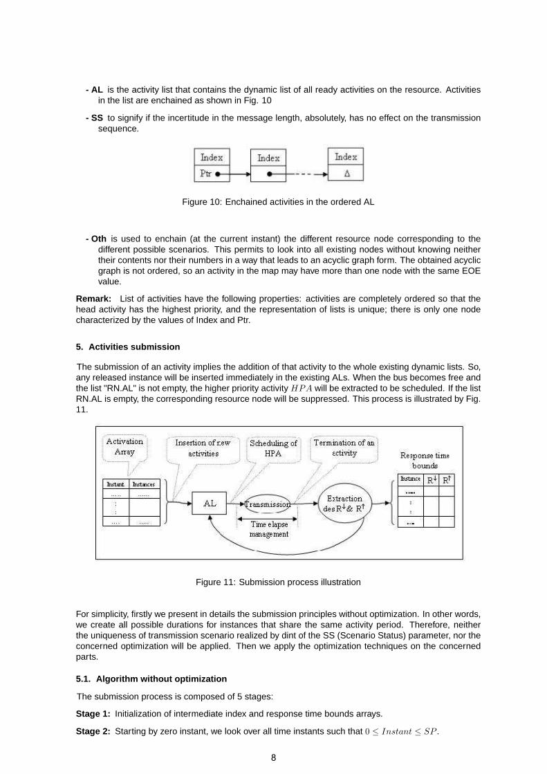
- AL is the activity list that contains the dynamic list of all ready activities on the resource. Activitiesin the list are enchained as shown in Fig. 10

- SS to signify if the incertitude in the message length, absolutely, has no effect on the transmissionsequence.

Figure 10: Enchained activities in the ordered AL

- Oth is used to enchain (at the current instant) the different resource node corresponding to thedifferent possible scenarios. This permits to look into all existing nodes without knowing neithertheir contents nor their numbers in a way that leads to an acyclic graph form. The obtained acyclicgraph is not ordered, so an activity in the map may have more than one node with the same EOEvalue.

Remark: List of activities have the following properties: activities are completely ordered so that thehead activity has the highest priority, and the representation of lists is unique; there is only one nodecharacterized by the values of Index and Ptr.

5. Activities submission

The submission of an activity implies the addition of that activity to the whole existing dynamic lists. So,any released instance will be inserted immediately in the existing ALs. When the bus becomes free andthe list "RN.AL" is not empty, the higher priority activity HPA will be extracted to be scheduled. If the listRN.AL is empty, the corresponding resource node will be suppressed. This process is illustrated by Fig.11.

Figure 11: Submission process illustration

For simplicity, firstly we present in details the submission principles without optimization. In other words,we create all possible durations for instances that share the same activity period. Therefore, neitherthe uniqueness of transmission scenario realized by dint of the SS (Scenario Status) parameter, nor theconcerned optimization will be applied. Then we apply the optimization techniques on the concernedparts.

5.1. Algorithm without optimization

The submission process is composed of 5 stages:

Stage 1: Initialization of intermediate index and response time bounds arrays.

Stage 2: Starting by zero instant, we look over all time instants such that 0 ≤ Instant ≤ SP .

8

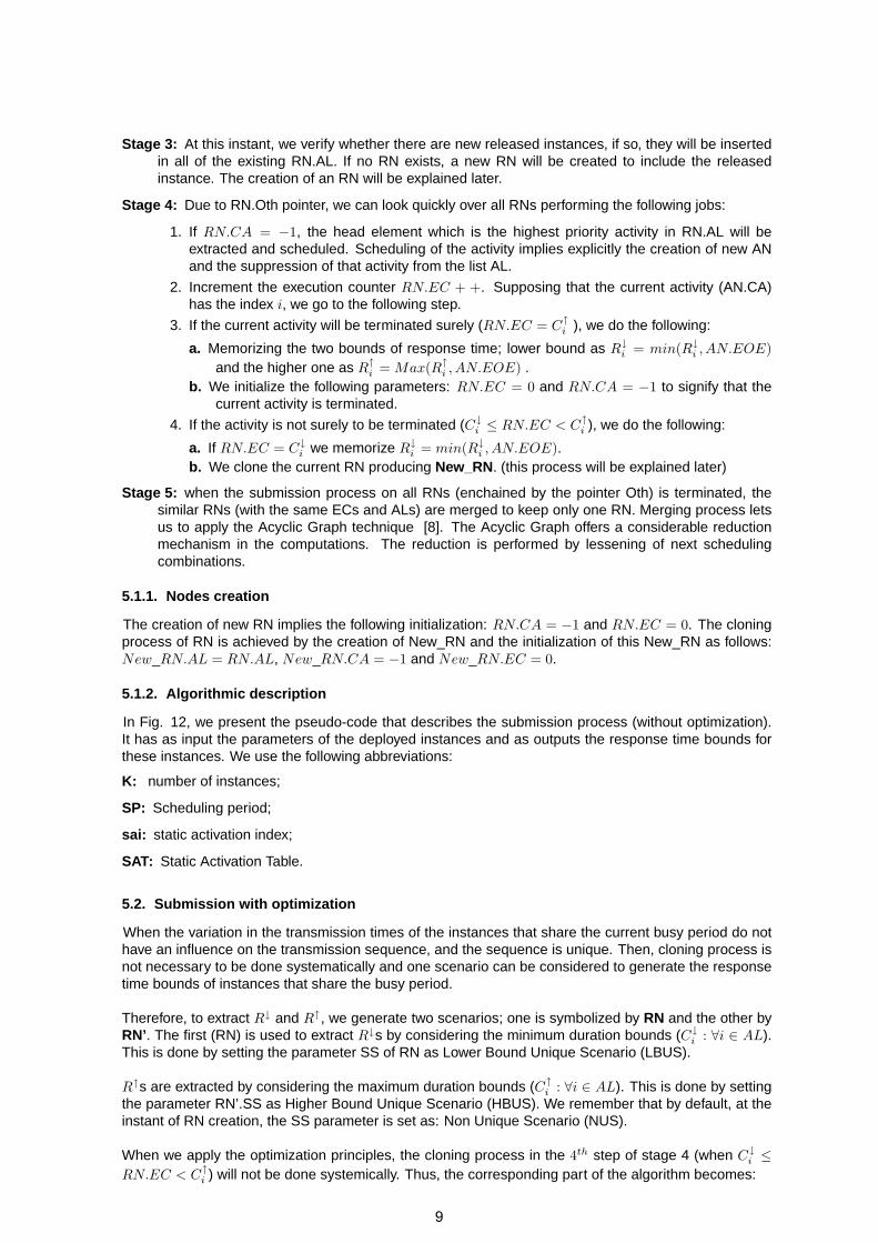
Stage 3: At this instant, we verify whether there are new released instances, if so, they will be insertedin all of the existing RN.AL. If no RN exists, a new RN will be created to include the releasedinstance. The creation of an RN will be explained later.

Stage 4: Due to RN.Oth pointer, we can look quickly over all RNs performing the following jobs:

1. If RN.CA = −1, the head element which is the highest priority activity in RN.AL will beextracted and scheduled. Scheduling of the activity implies explicitly the creation of new ANand the suppression of that activity from the list AL.

2. Increment the execution counter RN.EC + +. Supposing that the current activity (AN.CA)has the index i, we go to the following step.

3. If the current activity will be terminated surely (RN.EC = C↑i ), we do the following:

a. Memorizing the two bounds of response time; lower bound as R↓i = min(R↓

i , AN.EOE)and the higher one as R↑

i = Max(R↑i , AN.EOE) .

b. We initialize the following parameters: RN.EC = 0 and RN.CA = −1 to signify that thecurrent activity is terminated.

4. If the activity is not surely to be terminated (C↓i ≤ RN.EC < C↑

i ), we do the following:

a. If RN.EC = C↓i we memorize R↓

i = min(R↓i , AN.EOE).

b. We clone the current RN producing New_RN. (this process will be explained later)

Stage 5: when the submission process on all RNs (enchained by the pointer Oth) is terminated, thesimilar RNs (with the same ECs and ALs) are merged to keep only one RN. Merging process letsus to apply the Acyclic Graph technique [8]. The Acyclic Graph offers a considerable reductionmechanism in the computations. The reduction is performed by lessening of next schedulingcombinations.

5.1.1. Nodes creation

The creation of new RN implies the following initialization: RN.CA = −1 and RN.EC = 0. The cloningprocess of RN is achieved by the creation of New_RN and the initialization of this New_RN as follows:New_RN.AL = RN.AL, New_RN.CA = −1 and New_RN.EC = 0.

5.1.2. Algorithmic description

In Fig. 12, we present the pseudo-code that describes the submission process (without optimization).It has as input the parameters of the deployed instances and as outputs the response time bounds forthese instances. We use the following abbreviations:

K: number of instances;

SP: Scheduling period;

sai: static activation index;

SAT: Static Activation Table.

5.2. Submission with optimization

When the variation in the transmission times of the instances that share the current busy period do nothave an influence on the transmission sequence, and the sequence is unique. Then, cloning process isnot necessary to be done systematically and one scenario can be considered to generate the responsetime bounds of instances that share the busy period.

Therefore, to extract R↓ and R↑, we generate two scenarios; one is symbolized by RN and the other byRN’. The first (RN) is used to extract R↓s by considering the minimum duration bounds (C↓

i : ∀i ∈ AL).This is done by setting the parameter SS of RN as Lower Bound Unique Scenario (LBUS).

R↑s are extracted by considering the maximum duration bounds (C↑i : ∀i ∈ AL). This is done by setting

the parameter RN’.SS as Higher Bound Unique Scenario (HBUS). We remember that by default, at theinstant of RN creation, the SS parameter is set as: Non Unique Scenario (NUS).

When we apply the optimization principles, the cloning process in the 4th step of stage 4 (when C↓i ≤

RN.EC < C↑i ) will not be done systemically. Thus, the corresponding part of the algorithm becomes:

9

Figure 12: Pseudo code describing the submission process (without optimization)

Stage 4: ... 4) When C↓i ≤ RN.EC < C↑

i , we perform the following:

A. If RN.EC = C↓i , we memorize the lower bound of response time as R↓

i = min(R↓i , AN.EOE),

B. If RN.SS = NUS (non unique scenario) and the current AL is not empty, we calculate the busyperiod Eq. 3, then we do one of the following operations:

- If the new activations (if any) during the current PA↑ do not change certainly the transmis-sion sequence, we clone the current RN setting its SS as HBUS while New_RN.SS asLBUS.

- Otherwise, or in other words, if the new activations can change the context or it is notpossible to determine if the new activations can change current sequence, we clone thecurrent RN without changing any SS parameter.

C. If RN.SS = LBUS, this signifies that the transmission scenario is unique and the current re-source node is used to generate strictly the lower bounds of response times. Therefore weterminate the current activity immediately (this means at RN.EC = C↓

i ). The termination isachieved by setting RN.EC = 0 and RN.CA = −1.

D. Otherwise, when RN.SS = HBUS or (SS = NUS while AL is empty), we go to stage 5.

These modifications in the previous procedure are illustrated by the pseudo code illustrated in Fig. 13.The function No_context_change realizes the anticipated prevision mechanism (§3.4). It is implemented

10

in a recursive manner. It takes the following parameters as input: current time instant and the upperbound of the busy period. It returns a Boolean value; yes when no change in the context and no in thecontrary case.

Figure 13: Stage 4 of the pseudo code after optimization

5.3. Response time extraction

Our method permits to extract dynamically response time bounds without the memorization of resultsrelated to the created RNs. Extraction of absolute bounds (R↓

i and R↑i ) of the message mi from the

bounds of instances related to the message the achieved as:

{R↓

i = min{Rm↓i − (m − 1) ∗ Ti}

R↑i = max{Rm↑

i − (m − 1) ∗ Ti} , for m = 1...ki. (5)

where ki =⌊

SPTi

⌋.

6. Case studies

To be familiar with our developed computational algorithm, we consider two examples. As a first examplewe show a simple computation model in details, whereas for the second example we show only resultswithout schedule map.

6.1. Example 1

We study a simple system composed of the three messages which have the deployed instances shownin Fig. 4. As shown in Tab. 2, the deploying leads to five instants. At the first activation instant (instant0), the resource node RN1 will be created. The evolution in the bus state is illustrated by the parametersof RN1, · · ·, RN4 as shown in Tab. 3.

The shadowed cells represent instants at which new activity nods are created. The single star notation

11

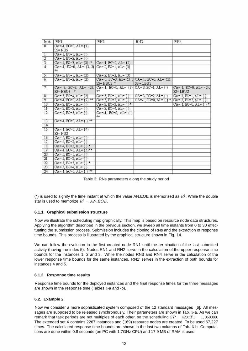
Table 3: RNs parameters along the study period

(*) is used to signify the time instant at which the value AN.EOE is memorized as R↓, While the doublestar is used to memorize R↑ = AN.EOE.

6.1.1. Graphical submission structure

Now we illustrate the scheduling map graphically. This map is based on resource node data structures.Applying the algorithm described in the previous section, we sweep all time instants from 0 to 30 effec-tuating the submission process. Submission includes the cloning of RNs and the extraction of responsetime bounds. This process is illustrated by the graphical structure shown in Fig. 14.

We can follow the evolution in the first created node RN1 until the termination of the last submittedactivity (having the index 5). Nodes RN1 and RN2 serve in the calculation of the upper response timebounds for the instances 1, 2 and 3. While the nodes RN3 and RN4 serve in the calculation of thelower response time bounds for the same instances. RN1’ serves in the extraction of both bounds forinstances 4 and 5.

6.1.2. Response time results

Response time bounds for the deployed instances and the final response times for the three messagesare shown in the response time (Tables 4-a and -b).

6.2. Example 2

Now we consider a more sophisticated system composed of the 12 standard messages [6]. All mes-sages are supposed to be released synchronously. Their parameters are shown in Tab. 5-a. As we canremark that task periods are not multiples of each other, so the scheduling SP = 420xT1 = 1, 050000.The extended set X contains 2267 instances and (169) resource nodes are created. To be used 67,227times. The calculated response time bounds are shown in the last two columns of Tab. 5-b. Computa-tions are done within 0.8 seconds (on PC with 1.7GHz CPU) and 17.9 MB of RAM is used.

12

# Instance R↓ R↑

1 m11 3 4

2 m13 6 13

3 m12 7 12

4 m21 18 19

5 m22 22 24

mi R↓ R↑

m1 3 4m2 7 12m3 6 13

a) instances b) messages

Table 4: Response times

The column lg_lp contains the length of the longest lower priority message. This length is calculatedas: lg_lpi = Max{∀k ∈ lp(i)}. Applying the analytical method used by Tindell, we obtain the worstcase response times results shown in the last column of the Tab. 5-b. The difference between eachupper response time bound calculated by our method (R↑

i ) and that (WCET) calculated by Tindell equalalways the blocking time minus one unity (lg_lpi − 1). This means that no blockage by a lower prioritymessage will be produced along the scheduling period and no priority inversion will happen.

mi πi bi C↓i C↑

i Ti

m1 1 8 111 135 2500m2 2 3 71 85 3500m3 5 3 71 85 5000m4 3 2 63 75 3750m5 6 5 87 105 5000m6 8 5 87 105 10000m7 4 4 79 95 3750m8 9 5 87 105 12500m9 7 4 79 95 5000m10 11 7 103 125 25000m11 10 5 87 105 12500m12 12 1 55 65 25000

mi R↓i R↑

i lg_lpi WCRTm1 111 135 125 259m2 71 220 125 344m3 182 475 125 599m4 63 295 125 419m5 269 580 125 704m6 435 780 125 904m7 142 390 125 514m8 198 885 125 1009m9 348 675 125 799m10 625 1115 65 1179m11 285 990 125 1114m12 680 1180 0 1180

a) parameters b) response times

Table 5: 12 CAN messages

7. Conclusions

The reliability of a CAN model depends on its ability to provide a good conception about absolute limits ofschedulability behavior during the hyper duration that symbolizes the eternal life of the system. Focusingon the impact of the incertitude in stuff bits, we have introduced a general computational method ableto generate and compute response-times for all possible transmission combinations of CAN messages.To reduce the computational resources when aiming to calculate absolute response-time bounds, weapplied the acyclic graph technique. Then we investigated the direct impact of stuffing result on thesebounds. By this, we have shown that the worst and the best case scenarios that have been discussedare different from the case of non-common messages releasing.

13

Figure 14: Scheduling structure illustrating evolution in resource nodes

References

[1] I. Alzeer. Analyse exhaustive du comportement temporel de tâches et messages temps réel. Thèsede doctorat, Université de Nantes, France, Décembre 2004.

[2] I. Alzeer, P. Molinaro, and Y. Trinquet. Calcul exhaustif du temps de réponse de tâches et messagesdans un système temps réel réparti. Proc. of 12th Real-Time Systems Conference, RTS’05, Paris,April 2005, pp. 304-322.

[3] I. Alzeer, P. Molinaro, and Y. Trinquet. Response time calculations for non-preemptive tasks withvariable execution time. ETFA’2003, 19th IEEE Conference On Emerging Technologies And FactoryAutomation, Lisbon, Portugal, Sept. 2003, pp. 131-136.

14

[4] N. Audsley, A. Burns, M. Richardson, K. Tindell, and A. Wellings. Applying new scheduling theory tostatic priority pre-emptive scheduling. Software Engineering Journal, 8(5), Sept. 1993, pp. 284-292.

[5] R. Bosch. CAN specifications Version 2.0, http://www.can.bosch.com/. BOSCH, Stuttgart, 1991.

[6] P. Castelpietra, Y. Song, F. Simonot, and O. Cayrol. Performance evaluation of a multiple networkedin-vehicle embedded architecture. Proc. of IEEE International Workshop on Factory Communica-tion Systems, Sep. 2000, pp. 187-194.

[7] M. Colnaric, D. Verber, R. Gumzej, and W. Halang. Implementation of hard real-time embeddedcontrol systems. Real-Time Systems, 14, May 1998, pp. 293-310.

[8] R. Diestel. Graph Theory. Book: Electronic ed. 2000. ftp://ftp.math.uni-hamburg.de/pub/unihh/math/books/diestel/GraphTheoryII.pdf.

[9] E. Grolleau, A. Choquet-Geniet, and F. Cottet. Cyclicité des séquences d’ordonnancement au plustôt des systèmes de tâches temps réel à contraintes strictes. Rapport de Recherche, LISI-ENSMA,1997.

[10] J. Lehoczky. Fixed priority scheduling of periodic task sets with arbitrary deadlines. Proc. 11thIEEE Real-Time Systems Symposium, Lake Buena Vista, FL, USA, Dec. 1990, pp. 201-209.

[11] J. Leung and M. Merrill. A note on preemptive scheduling of periodic real-time tasks. Informationprocessing letter, 11(3), 1980, pp. 115-118.

[12] C. Liu and J. Layland. Scheduling algorithms for multiprogramming in a hard-real-time environment.Journal of the ACM, 20(1), 1973, pp. 46-61.

[13] T. Nolte, H. Hansson, C. Norstrom, and S. Punnekkat. Using Bit-Stuffing distribution in CAN Anal-ysis. IEEE Real-Time Embedded Systems Workshop, Dec, 2001.

[14] R. Siegl and J. R. Howell. http://www.can-cia.de, CAN in Automation. CAN specifications 2.0.Part-A and Part-B.

[15] K. Tindell, A. Burns, and A. Wellings. An extendible approach for analyzing fixed priority hard realtime tasks. Real-Time Systems, 6, 1994, pp. 133-151.

15