Electronic copy available at: http://ssrn.com/abstract=1410616

Volatility Forecasting Using Threshold Heteroskedastic Models

of the Intra-day Range

∗Cathy W. S. Chen(1), Richard Gerlach(2), and Edward M.H. Lin(1)

(1)Graduate Institute of Applied Statistics, Feng Chia University, Taiwan.

(2)Econometrics and Business Statistics, University of Sydney, Australia.

Abstract

An effective approach for forecasting return volatility via threshold nonlinear het-eroskedastic models of the daily asset price range is provided. The return is definedas the difference between the highest and lowest log intra-day asset price. A generalmodel specification is proposed, allowing the intra-day high-low price range to de-pend nonlinearly on past information, or an exogenous variable such as US marketinformation. The model captures aspects such as sign or size asymmetry and het-eroskedasticity, which are commonly observed in financial markets. The focus is onparameter estimation, inference and volatility forecasting in a Bayesian framework. AnMCMC sampling scheme is employed for estimation and shown to work well in simu-lation experiments. Finally, competing range-based and return-based heteroskedasticmodels are compared via out-of-sample forecast performance. Applied to six inter-national financial market indices, the range-based threshold heteroskedastic modelsare well supported by the data in terms of finding significant threshold nonlinear-ity, diagnostic checking and volatility forecast performance under various volatilityproxies.

Key words: size and sign asymmetry; volatility model; conditional autoregressive range (CARR) model;threshold variable; Bayes inference; MCMC methods.

∗Corresponding author is Cathy W. S. Chen, Graduate Institute of Applied Statistics, FengChia University, Taiwan. Email: chenws@fcu.edu.tw; Ph: +886 4 24517250 ext. 4412; Fax: +8864 24517092.

1

Electronic copy available at: http://ssrn.com/abstract=1410616

1 Introduction

When modelling financial markets, it is important to describe asset return volatility dynamics and subse-quently forecast volatility. Such forecasts form quite an important input into risk management processes(e.g. Value at Risk, expected shortfall), option pricing, hedging and many other financial methods andproducts. It is well known that asset return volatility is time-varying and somewhat predictable in sample,however has proven difficult to forecast accurately. One reason is that volatility is not directly observable,hence parameters and forecasts in a volatility model can be subject to much uncertainty. Setting up amore accurate asset return volatility model will be highly useful for investors and market analysts interms of dynamic hedging, portfolio selection and controlling financial risk effectively.

The family of autoregressive conditional heteroskedastic (ARCH) models by Engle (1982) and generalizedARCH (GARCH) by Bollerslev (1986), has become the widely accepted volatility model. These usuallyemploy (squared) close to close asset returns to model return volatility. However many papers haveshown the intra-day range to be a far more efficient measure of return volatility, e.g. see Parkinson(1980), Garman and Klass (1980) and recently Anderson and Bollerslev (1998) and Alizadeh et al. (2002).Mandelbrot (1971) applied the range to examine the existence of long-term dependence in asset prices,while Beckers (1983) extended the range estimator to incorporate historical information on differentvariance measures.

As such, there are several advantages in directly using the intra-day high-low price range for volatilitymeasurement and forecasting, relative to the use of absolute or squared return data, or even realizedvariance from intra-day returns. For daily or lower frequency returns, Garman and Klass (1980) pointout that “· · · intuition tells us that high and low prices contain more information regarding to volatilitythan do the opening and closing prices.”. Corrado and Truong (2004) mentioned that by only lookingat opening and/or closing prices we may wrongly conclude that volatility on a given day is small, ifthe closing price is near the previous opening or closing price, despite large intra-day price fluctuations.Logically, the range is more efficient. Further, high-low price range data is widely available in financialdatabases, often when high-frequency intra-day returns are not. Also, even when high-frequency intra-dayreturns are available, Andersen and Bollerslev (1998) report that market microstructure issues such asnon-synchronous trading effects, discrete price observations and bid-ask spreads may limit the effectivenessof intra-day return variances, or realized intra-day volatility, as volatility forecasts or proxies. As such,intra-day high and low values may bring more integrity into volatility estimation.

Recently, the range has been used in volatility models: Gallant et al. (1999) and Alizadeh et al. (2002)incorporated the range with the stochastic volatility model. Brandt and Jones (2006) proposed a range-based EGARCH model, using observed range data and a link between the range and volatility, showingthat the their model had better out-of-sample forecast performance than standard volatility models. Chou(2005a), using range as a direct measure of volatility, further proposed the conditional autoregressive rangemodel (CARR) to capture range dynamics. The CARR model is simply a GARCH-type model employingdata on the range instead of squared returns. This model is also closely related to the autoregressiveconditional duration (ACD) model of Engle and Russell (1998).

Black (1976) discovered the now well-known phenomenon of volatility asymmetry: higher volatility iscorrelated with negative shocks in asset returns. GARCH-type models devised to capture this trait includethe exponential (Nelson, 1991), the quadratic (Sentana, 1995), the GJR-GARCH (Glosten et al. 1993)

1

and the unobserved component Q-STARCH (Broto and Ruiz 2006). Poon and Granger (2003) pointed outthat asymmetric volatility models outperformed symmetric models in forecasting asset return volatility;while Bali (2000) showed nonlinear models are useful for interest rate volatility. In this paper we proposeregime-switching for modeling size and/or sign asymmetries, presenting a general nonlinear volatilitymodel for the range. We call this the range-based threshold conditional autoregressive model, denoted byTARR. The model predicts and allows forecasts of the intra-day range and captures the most importantstylized features of stock return volatility: time clustering and size or sign asymmetry. One objective ofthis paper is to demonstrate the usefulness of the range in leading to more precise range-based estimatesand forecasts of volatility.

What does this new model offer in comparison to the multitude of volatility models in the literature?Firstly, the TARR model will be one of the few that directly model the intra-day range dynamically.Thus it may provide more efficient volatility estimates and forecasts than models that employ squared orabsolute returns only. Secondly, the TARR model will capture asymmetry through a nonlinear specifica-tion, allowing threshold information to determine where the change of regime occurs. We focus on sizeasymmetry: as has been discussed by Leeves (2007) among others, employing range data as a thresholdvariable; and also sign asymmetry, employing a return based threshold variable. The relevant thresholdvariable could come from the local market or from an exogenous factor such as the US market. Exogenousthresholds have been shown to be important in volatility modeling, see e.g Chen et al. (2003), Chen et al.(2006) and Gerlach et al. (2006). Third, the TARR model will allow the usual trait of volatility clusteringor persistence. A trait that no existing asymmetric volatility model, including ours, will capture is Markovswitching in regimes, as e.g. in the MS-GARCH models of Gray (1996) and Klaassen (2002); while DeLuca and Zuccolotto (2006) proposed a related regime switching ACD model. We leave such models forfuture research.

We take a Bayesian approach to estimation, allowing simultaneous inference for model parameters, in-cluding the threshold value and the time delay lag. Also, valid inference under positivity and stationarityconstraints for parameters is straightforward in this approach. Numerical methods such as Markov chainMonte Carlo (MCMC) are utilised; shown to be very effective in threshold models by e.g. Chen and Lee(1995) and Chen et al. (2003).

This paper is organized as follows. Section 2 describes the range-based TARR model. Sections 3 and 4present Bayesian methods for estimation and for forecasting volatility. Section 5 presents a simulationstudy showing the estimation performance of the methods in Section 3. Empirical results from six majorfinancial markets are reported in Section 6, where we compare the out-of-sample volatility forecastingability between two TARR and two GARCH models. Section 7 offers conclusions.

2 Range-based threshold heteroskedastic model

Let Pt be the logarithm of the price of an asset observed at time t, where t = 1, 2, . . . , n and Rt =(Max{Pit}−Min{Pit})× 100; Rt is the (percentage log) range at time t and the index i is for the intra-period measurements Pit. If we consider daily stock prices, Max{Pit} and Min{Pit} are the highest andlowest log prices observed during the day; Rt is the intra-day log price range for day t, or the maximum

2

achievable intra-day return. We propose the following nonlinear TARR(p, q) model:

Rt = λtεt, εt ∼ f (·) ,

λt = α(j)0 +

pj∑

i=1

α(j)i Rt−i +

qj∑

i=1

β(j)i λt−i, rj−1 ≤ zt−d ≤ rj , (1)

where j = 1, . . . , g, the delay lag d is a positive integer, and f (·) is a distribution with support (0,∞) andunit mean. εt is assumed to follow a Weibull distribution, with parameters (c, s, η) which are the location,scale and shape parameters, respectively. The Weibull distribution is a special case of the GeneralizedExtreme Value distribution and has been extensively used as a model of time to failure. Recently, itsapplications have expanded to include finance and climatology.

We set the Weibull location parameter c = 0 to ensure range positivity i.e. Rt = λtεt ≥ 0. Moreover, thescale parameter s is set to [Γ(1 + 1

η )]−1 to ensure that E(εt) = 1, so that E(Rt|It−1) = λt, independentlyof εt. The threshold values rj satisfy 0 < r0 < r1 < · · · < rg = ∞, so that [rj−1, rj), j = 1, . . . , g, forma partition of the space of the threshold variable zt. zt could be local market information (e.g. laggedvalues of the series Rt), or an exogenous factor such as international market movements, a financialindex or interest rate, etc. If zt is exogenous, we call the model TARRX. The special case g = 1 givesthe symmetric, linear CARR model of Chou (2005a). Later Chou (2005b) extended this model to theACARR model, claiming this model to capture asymmetry in volatility. However, the ACARR is simplytwo separate, dynamic, linear structures for the positive and negative side intra-period ranges of assetprices. It is not an asymmetric or nonlinear model in the spirit of regime-switching behavior. Thus, thereis a clear gap in the literature for a nonlinear type asymmetric CARR model to be developed. One goalof this paper is to fill that gap.

Similar to results for GARCH-type models, when g = 2 regimes, the unconditional mean range in eachregime for the TARR model is

E(Rt) =α

(1)0

1−p1∑

i=1

α(1)i −

q1∑i=1

β(1)i

, zt−d ≤ r1,

E(Rt) =α

(2)0

1−p1∑

i=1

α(2)i −

q1∑i=1

β(2)i

, zt−d > r1,

while the persistence in volatility is given byp1∑

i=1

α(1)i +

q1∑

i=1

β(1)i , zt−d ≤ r1

p1∑

i=1

α(2)i +

q1∑

i=1

β(2)i , zt−d > r1.

So, (α(1)0 , α

(1)1 , β

(1)1 ) will characterize the dynamic range behaviour in response to small lagged values of

zt and (α(2)0 , α

(2)1 , β

(2)1 ) in response to larger values. The TARR model thus allows both average volatility

(as measured by range) and volatility persistence to differ between regimes, in response to a thresholdvariable. It will thus allow size asymmetry (for a range threshold) and sign asymmetry (for a returnthreshold) in the range via a piecewise linear relationship. To ensure positivity and stationarity of therange, we enforce the standard GARCH-type restrictions:

α(j)0 > 0; α

(j)i ≥ 0, β

(j)i ≥ 0 and

pj∑

i=1

α(j)i +

qj∑

i=1

β(j)i < 1. (2)

3

The essential distinction between the ACARR and the TARR model is that the ACARR uses two inde-pendently estimated linear CARR models and compares results to describe the asymmetric volatility. TheTARR model proposed here is a truly nonlinear model and allows more traditional asymmetric volatilityresponses.

Gray (1996) and Klaassen (2002) discussed Markov switching (MS) GARCH models and applied thesemodels to interest rate and exchange rate data. An important difference between threshold models andMS models is that, given the threshold limits r, the regime indicators are fixed, known and non-stochasticin a threshold model; while in an MS model regime indicators are not observed and are still stochasticeven if all other model parameters are known. Further the threshold variable in our nonlinear model,which determines the regime at each time point, is observed and is not assumed to generate regimes thatpersist over time, as is the case for MS models.

3 Bayesian inference

Bayesian methods allow simultaneous inference on parameters in finite samples. Stationarity and posi-tivity constraints can also be incorporated directly into the prior distribution. Silvapulle and Sen (2004)have illustrated problems in large sample theory inference under positivity and stationarity constraints,problems not shared by the Bayesian approach. Chen et al. (1995, 2003, 2005) provide a rigorous treat-ment of Bayesian inference via MCMC methods for nonlinear threshold GARCH models. We adapt theirapproach.

Let θ represent the vector of all unknown parameters. Define αj = (α(j)0 , . . . , α

(j)pj , β

(j)1 , . . ., β

(j)qj )′, and

r = (r1, . . . , rg−1)′ as the mean and threshold parameter vectors respectively; d0 as the maximum delayand s = max(p1, . . . , pg, d0). Assuming a Weibull distribution with shape parameter η, the conditionallikelihood function for the TARR model is:

L(Rs+1,T |θ) =T∏

t=s+1

g∑

j=1

η

Rt

Γ

(1 + 1/η

)Rt

λt

η

exp

−

Γ

(1 + 1/η

)Rt

λt

η

Ijt

, (3)

where Ijt is the indicator variable I(rj−1 ≤ zt−d ≤ rj) and Γ is the Gamma function.

We choose a mostly uninformative prior, flat over the parameter constraint region in (2), so that the like-lihood dominates inference. We also generate parameters in blocks, where practical, to speed convergenceof the Markov chain; see Carter and Kohn (1994).

The delay has been set as d = 1 in most previous studies of threshold models, see e.g. Li and Li (1996),Brooks (2001), etc; we thus choose the prior of d with large probability for more recent lags, so thatPr(d = i) = 4−i

6 , i = 1, 2, 3, where d0 is 3. To ensure the required constraints on αj , we adopt a uniformprior p(αj) over the region (2). Further, we choose the prior of r as p(r) ∝ I(B), where B ensureseach regime contains at least h percent of zt−d. For the Weibull distribution, the shape parameter η isre-parameterized via τ = log(η); ensuring that η > 0 as required. The prior on τ is a N(0, 1), allowing alarge range of possible values for η = exp(τ) on the positive real line, but with most weight on smaller

4

values, as found in Chou (2005a). These are assumed a priori independent, so that:

p(θ) =

g∏

j=1

p(αj)p(τ)

p(d)p(r). (4)

The posterior distribution is proportional to the multiplication of the likelihood in (3) and the prior in(4). Let γ be, in turn, one of αj , d, r and τ and let θ−γ be the parameter vector θ excluding the elementγ. MCMC methods require conditional posterior distributions for each choice of γ. In each case, the targetposterior is:

p(γ|Rs+1,T , θ−γ) ∝ L(Rs+1,T |θ)p(γ). (5)

The posterior distributions in (5), for each choice of γ, are of non-standard form, except the delayparameter d, which is sampled from the multinomial distribution:

p(d = j|Rs+1,T ,θ−d) =L(Rs+1,T |d = j, θ−d)p(d = j)

d0∑i=1

L(Rs+1,T |d = i, θ−d)p(d = i), j = 1, . . . , d0. (6)

The Metropolis-Hastings (MH) algorithm (Metropolis et al., 1953; Hastings, 1970) is applied to drawfrom (5) for all other parameters. We combine two versions of MH methods: the random walk Metopolisalgorithm and the independent kernel MH algorithm, to achieve the desired parameter samples in anadaptive MCMC sampling scheme. See Chen et al. (2005) for details of this method and its application.

We use an MCMC sample of N iterations, deleting the first M as a burn-in, and keeping the last N −M

iterations for analysis. Tierney (1994) showed that the MCMC sample for each parameter tends towardsit’s marginal distribution p(γ|R) when the Monte Carlo sample size is large enough; in practice we confirmconvergence via traceplots and correlograms of sample iterates.

4 Forecasting volatility with TARR models

We now discuss forecasting with TARR models. A rolling sample method is used with n + k − 1 datapoints used for estimation successively for k = 1, 2, . . . , T . We provide one and two-step ahead forecasts: Rn+k−1+l|R1,n+k−1, where T is the forecast horizon, n + k − 1 is the forecast origin and l = 1, 2.

Firstly, the conditional mean E(Rt|It−1) = λt is a known function of θ and R1,t−1 that we label asgt(R1,t−1,θ). Under the TARR model:

gt(R1,t−1, θ) =g∑

j=1

[α

(j)0 +

pj∑

i=1

α(j)i Rt−i +

qj∑

i=1

β(j)i λt−i

]I(rj−1 ≤ zt−d ≤ rj).

which is a one-step-ahead forecast of Rt when the parameter values are known. The threshold variable zt−d

is known at time t−1 since d ≥ 1. Note that parameter uncertainty is accounted for in our forecasts, sincee.g. λ

[i]n+1 = gn+1(R1,n, θ[i]), i = 1, . . . , N −M form a posterior MCMC sample from p(λn+1|R1,n) where

θ[i] is an MCMC sample from p(θ[i]|R1,n), obtained as in section 3. A Bayesian forecast of Rn+1|R1,n isthen the posterior mean: ∑N−M

i=1λ

[i]n+1

/(N −M).

5

The required forecast sample λ[i]n+1 can be formed simultaneously with the MCMC sample of parameters.

For l ≥ 2 step ahead forecasting, we need to sample λ[i]n+1, . . . , λ

[i]n+l conditionally on R1,n. This can be

done by the method of composition and MCMC integration with the decomposition:

p(λn+1, . . . , λn+l|R1,n) =l∏

j=1

p(λn+j |λ1,n+j−1,R1,n)

=l∏

j=1

∫p(λn+j , Rn+j−1,θ|λ1,n+j−1,R1,n)dRn+j−1dθ.

We can do this integration numerically inside the MCMC parameter sampling scheme as follows:

1. Calculate λ[i]n+1 = gn+1(R1,n, θ[i]) using the relevant TARR model;

2. Simulate ε[i]n+1 ∼ Weibull(0, sn+1, η

[i]) where sn+1 = 1/Γ(1 + 1η[i] );

3. Calculate R[i]n+1 = λ

[i]n+1ε

[i]n+1, which comes from the distribution of Rn+1|R1,n.

4. Calculate λ[i]n+2 = gn+2(R1,n, R

[i]n+1, λ

[i]n+1,θ

[i]). This comes from the distribution of E(Rn+2|R1,n, Rn+1)as required.

5. Simulate ε[i]n+2 ∼ Weibull(0, sn+1, η

[i])...

The process is continued up to the calculation of λ[i]n+l = gn+l(R1,n, R

[i]n+l−1, λ

[i]n+l−1, θ

[i]) which comesfrom the distribution of E(Rn+l|R1,n, Rn+l−1). The final forecasts of Rn+l|R1,n are the posterior means:

∑N−M

i=1λ

[i]n+k

/(N −M),

for k = 1, . . . , l, which estimates E(Rn+l|R1,n). Note that the numerical simulation of the range Rn+l−1 isnecessary for l ≥ 2, since the threshold variables needed in forecasting, zn+k−d, are unobserved for k > d

at forecast origin n. In the TARRX model, the exogenous threshold zn+k−d must also be forecasted, froma model specified by the user, as part of the algorithm above.

Two criteria are commonly used to evaluate the forecast accuracy of competing models: mean squarederror (MSE) and mean absolute deviation (MAD). We employ both these measures. MSE provides aquadratic loss function which disproportionately weights large forecast errors more heavily relative toMAD. We also formally compare different forecast models using the Diebold-Mariano (DM) test forequal forecast accuracy, see Diebold and Mariano (1995) for details.

In practice, volatility is unobserved and so the accuracy of any volatility forecasting model is hard tojudge. The squared close to close return is often used as a volatility proxy when calculating forecastaccuracy measures; see e.g. Tsay (2005), Chou (2005a). Parkinson (1980), Garman and Klass (1980) andAlizadeh et al. (2002) propose and discuss range-based volatility proxies and show that squared returns,while being unbiased, are far more noisy and inefficient proxies of volatility than their proposals. Weconsider four volatility proxies:

σ21,t = y2

t ,

σ22,t =

R2t

4 log(2)≈ 0.3607R2

t ,

σ23,t = R2

t ,

σ24,t = exp[2× (log(Rt)− 0.43 + 0.292)].

6

The first proxy is simply the squared close to close log-return. The second proxy was derived by Parkinson(1980); it makes some sense in that the intra-day range is the maximum achievable return during eachday, thus this may need to be down-weighted to better reflect volatility. The third proxy was suggestedby Chou (2005a). The fourth proxy is derived from work by Alizadeh et al. (2002), who found an accurateprobability link between quadratic variation and range data for Martingale processes. The link is:

log(σt) ∼ N(log(Rt)− 0.43, 0.292).

The proxy is then deduced by the properties of the log-normal distribution: it is equivalent to E(σ2t )

under the log-normal distribution for σt.

Many recent papers have explored the use of intra-day realized volatility as a proxy, which requires theavailability of intra-period prices. However we consider only daily data in this paper. We also note thatrealized volatility is highly influenced by the choice of intra-day frequency, which is the subject of muchon-going research.

5 Simulation study

We now illustrate the proposed Bayesian methods for simulated data from various parameter settings.We used 100 replications with three different sample sizes, n = 1000, 2000 and n = 4000, from threemodels specified below. For each data set, N = 20000 MCMC iterations were used; with a burn-in ofM = 8000 iterations. We selected all initial MCMC iterates randomly from their prior distribution. Thetrue models are specified as:

Model 1: The true model is TARRX (1,1):

Rt = λtεt,

λt =

{0.20 + 0.18Rt−1 + 0.69λt−1, zt−1 ≤ 1.500.38 + 0.21Rt−1 + 0.61λt−1, zt−1 > 1.50,

while zt ∼ CARR(1, 1)

CARR(1, 1) : λz,t = 0.04 + 0.18zt−1 + 0.79λz,t−1,

where εt is a Weibull with unit mean and shape η = 1.2; the threshold has ηz = 1.2.

We set the parameters in Model 1 to reflect empirical observations from threshold GARCH models andour real data examples that the unconditional volatility (range) is larger in regime two than in regimeone. The remaining models also follow this criterion.

Model 2: Model 2 is the same as Model 1 except the parameter values:

Rt = λtεt,

λt =

{0.10 + 0.20Rt−1 + 0.70λt−1, zt−1 ≤ 1.500.45 + 0.20Rt−1 + 0.65λt−1, zt−1 > 1.50,

while zt ∼ CARR(1, 1)

CARR(1, 1) : λz,t = 0.04 + 0.18zt−1 + 0.79λz,t−1.

7

Model 3: The true model is TARR (1,1):

Rt = λtεt,

λt =

{0.04 + 0.13Rt−1 + 0.80λt−1, Rt−1 ≤ 0.870.11 + 0.19Rt−1 + 0.71λt−1, Rt−1 > 0.87,

where εt follows a Weibull with unit mean and shape η = 1.2.

We set the parameter values in these Models to reflect our empirical observations both from thresholdGARCH models and from the TARR model applied to our real data examples in the next section. Theseare:

1 The unconditional mean of the range (volatility) is greater in regime 2 than regime 1;2 The volatility persistence α1 + β1 is higher in regime 1 than regime 2,

when using a range threshold variable. The actual values chosen in Models 1-3 are very similar to theestimates obtained in the real examples, except for η. We chose η to be more extreme and close to 1 toensure an error distribution that was quite heavily skewed in the positive direction. This was to ensurewe properly tested our estimation method on a reasonably non-normal error distribution.

We selected the prior for r as U(Q1, Q3), where Q1 and Q3 are the first and third sample quartilesseparately, which is a common choice, and the maximum lag for the delay term, d, is chosen to be 3,which is higher than what is usually found or assumed in practice. When simulating data from thesemodels, MCMC convergence appeared almost immediate from trace plots of the iterates.

Table 1 displays the true values plus the means, standard deviations and the 2.5th and 97.5th percentiles ofthe 100 posterior mean estimates for the model parameters for Models 1−3, for sample sizes n = 1000, 2000and n = 4000. Posterior modes (not shown) were all chosen as d = 1. Also displayed are true values andaverage posterior estimates for the unconditional mean range (volatility) in each regime. There appearsto be a lot of sampling variation at n = 1000 so that bias is difficult to judge, however all true valuesare contained inside the 2.5th and 97.5th percentiles for the posterior means, except for β1 for Model2, at this sample size. At higher sample sizes, all parameter estimates seem unbiased and are all notsignificantly different from their true values. The precision and accuracy of the estimators thus increaseswith sample size. Also, the lag d = 1 is correctly identified from all 100 replications in each model and ateach sample size the unconditional means in each regime appear close to their true values. In summary,parameter estimation appears to work well for the proposed asymmetric TARR models using the methodsin section 3. Favorable results are also achieved across two choices of threshold variable: past ranges oran exogenous range factor.

6 Empirical study

In this section, we analyze the intra-day high-low prices from six stock markets, obtained from thewebsite “finance.yahoo.com”. The data is collected from January 1, 1998, through December 31, 2004, andincludes the Asia-Pacific financial markets: namely Nikkei 225 Index (Japan), KOSPI Composite Index

8

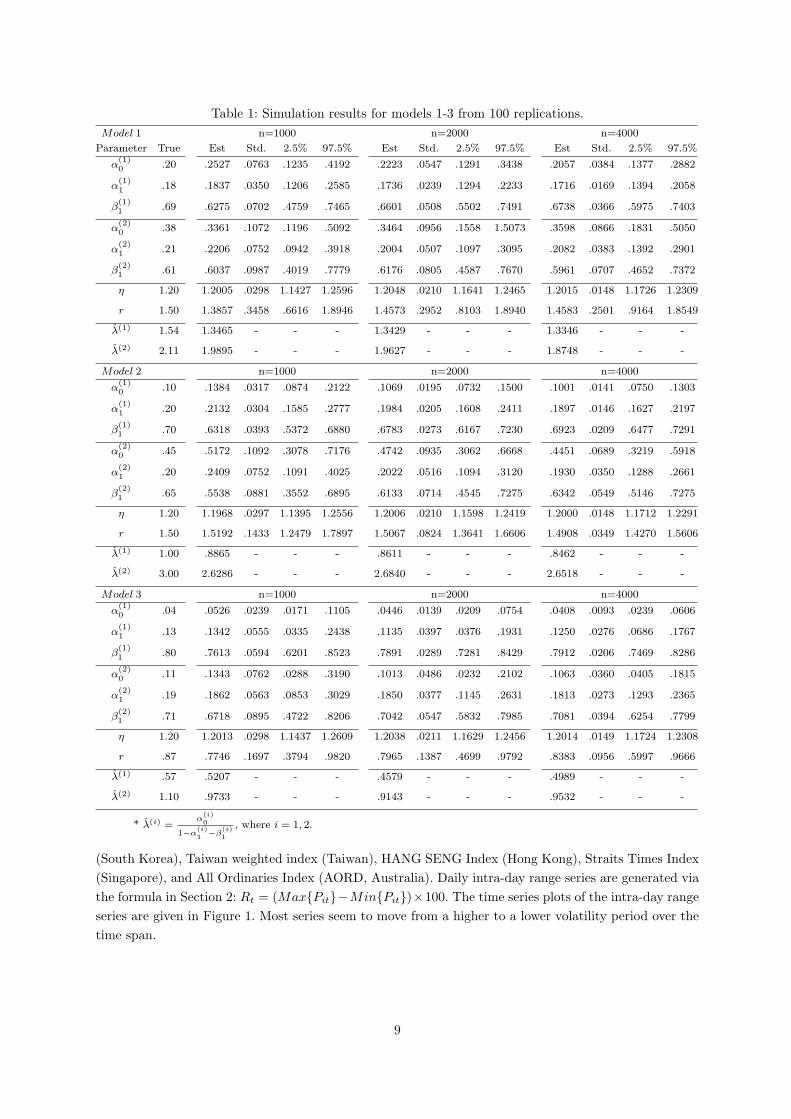
Table 1: Simulation results for models 1-3 from 100 replications.Model 1 n=1000 n=2000 n=4000

Parameter True Est Std. 2.5% 97.5% Est Std. 2.5% 97.5% Est Std. 2.5% 97.5%

α(1)0 .20 .2527 .0763 .1235 .4192 .2223 .0547 .1291 .3438 .2057 .0384 .1377 .2882

α(1)1 .18 .1837 .0350 .1206 .2585 .1736 .0239 .1294 .2233 .1716 .0169 .1394 .2058

β(1)1 .69 .6275 .0702 .4759 .7465 .6601 .0508 .5502 .7491 .6738 .0366 .5975 .7403

α(2)0 .38 .3361 .1072 .1196 .5092 .3464 .0956 .1558 1.5073 .3598 .0866 .1831 .5050

α(2)1 .21 .2206 .0752 .0942 .3918 .2004 .0507 .1097 .3095 .2082 .0383 .1392 .2901

β(2)1 .61 .6037 .0987 .4019 .7779 .6176 .0805 .4587 .7670 .5961 .0707 .4652 .7372

η 1.20 1.2005 .0298 1.1427 1.2596 1.2048 .0210 1.1641 1.2465 1.2015 .0148 1.1726 1.2309

r 1.50 1.3857 .3458 .6616 1.8946 1.4573 .2952 .8103 1.8940 1.4583 .2501 .9164 1.8549

λ(1) 1.54 1.3465 - - - 1.3429 - - - 1.3346 - - -

λ(2) 2.11 1.9895 - - - 1.9627 - - - 1.8748 - - -

Model 2 n=1000 n=2000 n=4000

α(1)0 .10 .1384 .0317 .0874 .2122 .1069 .0195 .0732 .1500 .1001 .0141 .0750 .1303

α(1)1 .20 .2132 .0304 .1585 .2777 .1984 .0205 .1608 .2411 .1897 .0146 .1627 .2197

β(1)1 .70 .6318 .0393 .5372 .6880 .6783 .0273 .6167 .7230 .6923 .0209 .6477 .7291

α(2)0 .45 .5172 .1092 .3078 .7176 .4742 .0935 .3062 .6668 .4451 .0689 .3219 .5918

α(2)1 .20 .2409 .0752 .1091 .4025 .2022 .0516 .1094 .3120 .1930 .0350 .1288 .2661

β(2)1 .65 .5538 .0881 .3552 .6895 .6133 .0714 .4545 .7275 .6342 .0549 .5146 .7275

η 1.20 1.1968 .0297 1.1395 1.2556 1.2006 .0210 1.1598 1.2419 1.2000 .0148 1.1712 1.2291

r 1.50 1.5192 .1433 1.2479 1.7897 1.5067 .0824 1.3641 1.6606 1.4908 .0349 1.4270 1.5606

λ(1) 1.00 .8865 - - - .8611 - - - .8462 - - -

λ(2) 3.00 2.6286 - - - 2.6840 - - - 2.6518 - - -

Model 3 n=1000 n=2000 n=4000

α(1)0 .04 .0526 .0239 .0171 .1105 .0446 .0139 .0209 .0754 .0408 .0093 .0239 .0606

α(1)1 .13 .1342 .0555 .0335 .2438 .1135 .0397 .0376 .1931 .1250 .0276 .0686 .1767

β(1)1 .80 .7613 .0594 .6201 .8523 .7891 .0289 .7281 .8429 .7912 .0206 .7469 .8286

α(2)0 .11 .1343 .0762 .0288 .3190 .1013 .0486 .0232 .2102 .1063 .0360 .0405 .1815

α(2)1 .19 .1862 .0563 .0853 .3029 .1850 .0377 .1145 .2631 .1813 .0273 .1293 .2365

β(2)1 .71 .6718 .0895 .4722 .8206 .7042 .0547 .5832 .7985 .7081 .0394 .6254 .7799

η 1.20 1.2013 .0298 1.1437 1.2609 1.2038 .0211 1.1629 1.2456 1.2014 .0149 1.1724 1.2308

r .87 .7746 .1697 .3794 .9820 .7965 .1387 .4699 .9792 .8383 .0956 .5997 .9666

λ(1) .57 .5207 - - - .4579 - - - .4989 - - -

λ(2) 1.10 .9733 - - - .9143 - - - .9532 - - -

* λ(i) =α

(i)0

1−α(i)1 −β

(i)1

, where i = 1, 2.

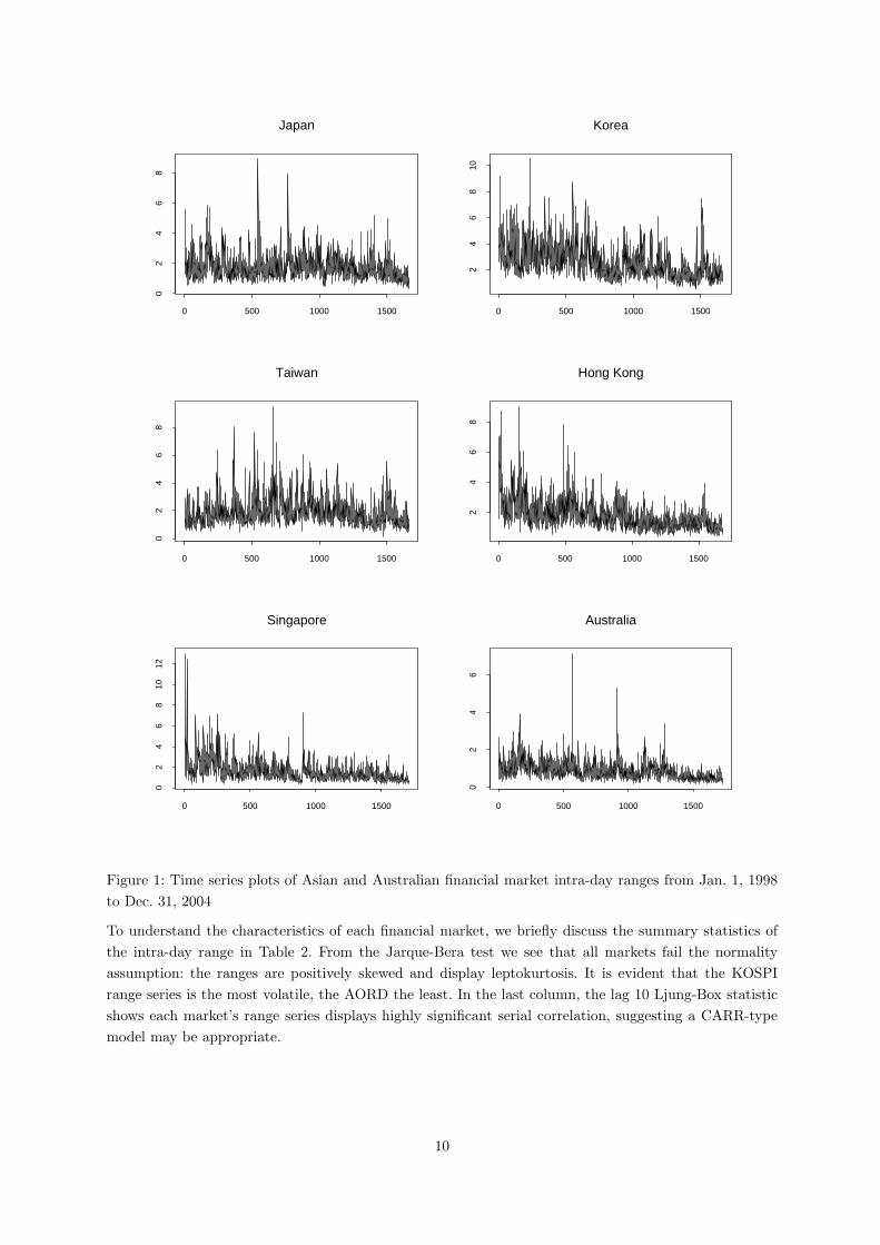
(South Korea), Taiwan weighted index (Taiwan), HANG SENG Index (Hong Kong), Straits Times Index(Singapore), and All Ordinaries Index (AORD, Australia). Daily intra-day range series are generated viathe formula in Section 2: Rt = (Max{Pit}−Min{Pit})×100. The time series plots of the intra-day rangeseries are given in Figure 1. Most series seem to move from a higher to a lower volatility period over thetime span.

9

Japan

0 500 1000 1500

02

46

8

Korea

0 500 1000 1500

24

68

10

Taiwan

0 500 1000 1500

02

46

8

Hong Kong

0 500 1000 1500

24

68

Singapore

0 500 1000 1500

02

46

810

12

Australia

0 500 1000 1500

02

46

Figure 1: Time series plots of Asian and Australian financial market intra-day ranges from Jan. 1, 1998to Dec. 31, 2004

To understand the characteristics of each financial market, we briefly discuss the summary statistics ofthe intra-day range in Table 2. From the Jarque-Bera test we see that all markets fail the normalityassumption: the ranges are positively skewed and display leptokurtosis. It is evident that the KOSPIrange series is the most volatile, the AORD the least. In the last column, the lag 10 Ljung-Box statisticshows each market’s range series displays highly significant serial correlation, suggesting a CARR-typemodel may be appropriate.

10

Table 2: Summary statistics: The data consist of daily intra-day ranges for six stock marketsfrom January 1,1998, through December 31, 2004.

Obs. Mean Min. Max. Std. Skewness Excess Jarque-Bera Q(10)

Dev. Kurtosis Test

Japan 1662 1.7269 .2993 8.9294 .8111 1.8804 4.9330 5337.5198 1071.9561

(< .001) (< .001)

Korea 1663 2.5522 .5130 10.5060 1.2715 1.2976 -.7182 827.4361 2581.0053

(< .001) (< .001)

Taiwan 1664 1.8769 .1461 9.5013 .9761 1.8174 2.9865 340.7276 1362.0289

(< .001) (< .001)

Hong Kong 1680 1.7905 .4138 9.0348 .9831 2.0659 4.8555 5514.5995 3109.7643

(< .001) (< .001)

Singapore 1706 1.5988 .3896 12.9511 1.0393 3.3189 18.4183 3574.8925 2464.5437

(< .001) (< .001)

Australia 1727 .8862 .1814 7.1280 .5026 2.7184 16.4923 29467.5496 1932.4600

(< .001) (< .001)

For application to each market, we firstly consider four range-based models: the symmetric linear CARRmodel, the TARR with local domestic market (endogenous) range threshold, the TARRX model with(exogenous) US Standard & Poor 500 Index market range threshold and finally a model which has theUS market return as the threshold variable, denoted TARRX-R. Details of these models were given insection 2.

The TARR and TARRX models capture size asymmetry only, while the TARRX-R allows sign asymmetry.The choice of US market range as the exogenous variable is based on the global economic scale andinfluence of the US market and on the findings of strong US influence in nonlinear GARCH models byChen et al. (2003), Gerlach et al. (2006) and Chen and So (2006).

Parameter estimates are given in Tables 3−4. These illustrate clear asymmetric behavior in volatility inall markets. For size asymmetry the usual response would be to have higher volatility following largepositive movements in the range variable; while for sign asymmetry, large negative returns are followedby higher volatility: both these responses are clearly evident in our results.

For the TARR (’Local’) and TARRX (’US’) models, α(2)0 is greater than α

(1)0 in most markets, and sub-

sequently the unconditional mean range (volatility) in the second regime is also larger than that in thefirst regime, excepting the TARR model in Hong Kong and Singapore. For the TARRX-R model, the re-verse occurs with average volatility higher in regime one, following negative returns (below approximately-0.5% or 0.5% in each market), than regime two. This asymmetry is further shown in Figure 2, whichdisplays the estimated mean range in each regime for the TARRX and TARRX-R models. We measurethe significance of this finding by calculating the percentage of MCMC iterates where the unconditionalmean of regime 1 (low volatility regime) is less than that of regime 2 (high volatility regime) for all TARRmodels; also presented in Tables 3−4 and denoted Percentage. 10 out of 12 estimated models (with rangethreshold) have this percentage above 85%, while 6 models are above 95%, showing clear evidence of asignificant difference in average range in each regime, and clear size asymmetric behavior in volatility inall markets, in response to previous range observations. For the TARRX-R model this percentage is lessthan 3% in all markets, showing that regime one volatility is significantly higher than in regime two andshowing clear sign asymmetry.

11

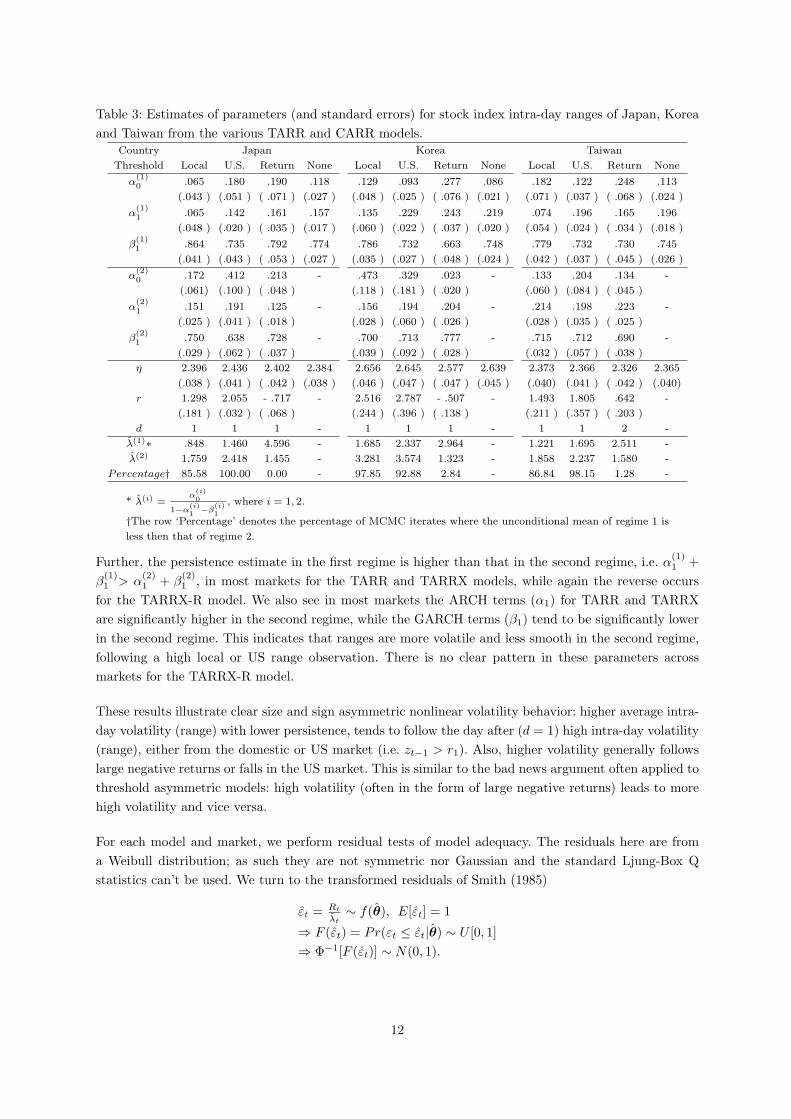
Table 3: Estimates of parameters (and standard errors) for stock index intra-day ranges of Japan, Koreaand Taiwan from the various TARR and CARR models.

Country Japan Korea Taiwan

Threshold Local U.S. Return None Local U.S. Return None Local U.S. Return None

α(1)0 .065 .180 .190 .118 .129 .093 .277 .086 .182 .122 .248 .113

(.043 ) (.051 ) ( .071 ) (.027 ) (.048 ) (.025 ) ( .076 ) (.021 ) (.071 ) (.037 ) ( .068 ) (.024 )

α(1)1 .065 .142 .161 .157 .135 .229 .243 .219 .074 .196 .165 .196

(.048 ) (.020 ) ( .035 ) (.017 ) (.060 ) (.022 ) ( .037 ) (.020 ) (.054 ) (.024 ) ( .034 ) (.018 )

β(1)1 .864 .735 .792 .774 .786 .732 .663 .748 .779 .732 .730 .745

(.041 ) (.043 ) ( .053 ) (.027 ) (.035 ) (.027 ) ( .048 ) (.024 ) (.042 ) (.037 ) ( .045 ) (.026 )

α(2)0 .172 .412 .213 - .473 .329 .023 - .133 .204 .134 -

(.061) (.100 ) ( .048 ) (.118 ) (.181 ) ( .020 ) (.060 ) (.084 ) ( .045 )

α(2)1 .151 .191 .125 - .156 .194 .204 - .214 .198 .223 -

(.025 ) (.041 ) ( .018 ) (.028 ) (.060 ) ( .026 ) (.028 ) (.035 ) ( .025 )

β(2)1 .750 .638 .728 - .700 .713 .777 - .715 .712 .690 -

(.029 ) (.062 ) ( .037 ) (.039 ) (.092 ) ( .028 ) (.032 ) (.057 ) ( .038 )

η 2.396 2.436 2.402 2.384 2.656 2.645 2.577 2.639 2.373 2.366 2.326 2.365

(.038 ) (.041 ) ( .042 ) (.038 ) (.046 ) (.047 ) ( .047 ) (.045 ) (.040) (.041 ) ( .042 ) (.040)

r 1.298 2.055 - .717 - 2.516 2.787 - .507 - 1.493 1.805 .642 -

(.181 ) (.032 ) ( .068 ) (.244 ) (.396 ) ( .138 ) (.211 ) (.357 ) ( .203 )

d 1 1 1 - 1 1 1 - 1 1 2 -

λ(1)∗ .848 1.460 4.596 - 1.685 2.337 2.964 - 1.221 1.695 2.511 -

λ(2) 1.759 2.418 1.455 - 3.281 3.574 1.323 - 1.858 2.237 1.580 -

Percentage† 85.58 100.00 0.00 - 97.85 92.88 2.84 - 86.84 98.15 1.28 -

* λ(i) =α

(i)0

1−α(i)1 −β

(i)1

, where i = 1, 2.

†The row ‘Percentage’ denotes the percentage of MCMC iterates where the unconditional mean of regime 1 is

less then that of regime 2.

Further, the persistence estimate in the first regime is higher than that in the second regime, i.e. α(1)1 +

β(1)1 > α

(2)1 + β

(2)1 , in most markets for the TARR and TARRX models, while again the reverse occurs

for the TARRX-R model. We also see in most markets the ARCH terms (α1) for TARR and TARRXare significantly higher in the second regime, while the GARCH terms (β1) tend to be significantly lowerin the second regime. This indicates that ranges are more volatile and less smooth in the second regime,following a high local or US range observation. There is no clear pattern in these parameters acrossmarkets for the TARRX-R model.

These results illustrate clear size and sign asymmetric nonlinear volatility behavior: higher average intra-day volatility (range) with lower persistence, tends to follow the day after (d = 1) high intra-day volatility(range), either from the domestic or US market (i.e. zt−1 > r1). Also, higher volatility generally followslarge negative returns or falls in the US market. This is similar to the bad news argument often applied tothreshold asymmetric models: high volatility (often in the form of large negative returns) leads to morehigh volatility and vice versa.

For each model and market, we perform residual tests of model adequacy. The residuals here are froma Weibull distribution; as such they are not symmetric nor Gaussian and the standard Ljung-Box Qstatistics can’t be used. We turn to the transformed residuals of Smith (1985)

εt = Rt

λt∼ f(θ), E[εt] = 1

⇒ F (εt) = Pr(εt ≤ εt|θ) ∼ U [0, 1]⇒ Φ−1[F (εt)] ∼ N(0, 1).

12

Table 4: Estimates of parameters (and standard errors) for stock index intra-day ranges of Hong Kong,Singapore and Australia from the various TARR and CARR models.

Country Hong Kong Singapore Australia

Threshold Local U.S. Return None Local U.S. Return None Local U.S. Return None

α(1)0 .048 .023 .033 .022 .032 .016 .080 .033 .046 .020 .102 .017

(.015 ) (.012 ) ( .011) (.009 ) (.018 ) (.011 ) ( .026 ) (.011 ) (.012 ) (.013 ) ( .020 ) (.006 )

α(1)1 .058 .158 .167 .163 .115 .200 .307 .212 .085 .140 .244 .185

(.020 ) (.025 ) ( .015) (.013 ) (.035 ) (.016 ) ( .034 ) (.015 ) (.029 ) (.032 ) ( .014 ) (.017 )

β(1)1 .897 .826 .828 .825 .851 .783 .679 .768 .824 .791 .739 .796

(.014 ) (.025 ) ( .016) (.015 ) (.024 ) (.018 ) ( .037 ) (.016 ) (.023 ) (.040 ) ( .025 ) (.020 )

α(2)0 .032 .048 .032 - .023 .235 .063 - .151 .078 .022 -

(.029 ) (.030 ) ( .024) (.017 ) (.065 ) ( .019 ) (.036 ) (.017 ) ( .009 )

α(2)1 .230 .175 .090 - .276 .254 .141 - .147 .216 .138 -

(.022 ) (.040 ) ( .028) (.024 ) (.035 ) ( .017 ) (.029 ) (.022 ) ( .018 )

β(2)1 .729 .804 .857 - .684 .623 .803 - .729 .717 .806 -

(.026 ) (.046 ) ( .032) (.029 ) (.060 ) ( .021 ) (.035 ) (.030 ) ( .024 )

η 2.593 2.558 2.523 2.556 2.257 2.264 2.218 2.244 2.298 2.309 2.308 2.271

(.045 ) (.044 ) ( .045) (.043 ) (.037 ) (.038 ) ( .038 ) (.036 ) (.038 ) (.038 ) ( .040 ) (.036 )

r 2.030 1.738 .579 - 1.445 1.806 - .712 - .887 1.053 .716 -

(.091 ) (.335 ) ( .160) (.081 ) (.042 ) ( .038 ) (.012 ) (.024) ( .016 ) -

d 1 1 1 - 1 1 1 - 1 1 1 -

λ(1)∗ 1.061 1.411 7.328 - .932 .915 7.260 - .496 .270 5.390 -

λ(2) .639 2.305 .639 - .485 1.902 1.128 - 1.207 1.146 .389 -

Percentage† 23.76 87.70 0.00 - 14.06 97.28 0.00 - 100.00 100.00 0.00 -

* λ(i) =α

(i)0

1−α(i)1 −β

(i)1

, where i = 1, 2.

†The row ‘Percentage’ denotes the percentage of MCMC iterates where the unconditional mean of regime 1 is

less then that of regime 2.

This method allows residuals from any distribution to be transformed to achieve standard normality, ifthe correct model has been fit to the data: now the Ljung-Box Q statistics apply. We display the resultsfor each stock market, in Table 5, up to the 20th lag. The models seem to fit the data well in all marketsexcept Japan and Singapore. The models in Japan are marginally acceptable, especially accounting formultiple testing effects. However, all models are strongly rejected in Singapore. Perhaps the Weibulldistribution is not appropriate for the range in Singapore or perhaps a higher lag structure is neededin the TARR models. Clearly, in four or five markets we have quite acceptable models for the dynamicintra-day range; however, the diagnostics do not distinguish between the different TARR models or theCARR model in any of these markets.

6.1 Out-of-Sample Forecasting

To evaluate the performance between the competing range-based models, we consider forecasting therange in each market. Let Rt+l|It denote the l-step-ahead forecast for the conditional range, from forecastorigin time t, where t = 1, . . . , (N − T + l − 1); N is the total sample size and T is the forecast horizon.

We use T = 120 days horizon and rolling samples to generate 120 one and two-step-ahead range forecasts.As we forecast together with our MCMC parameter sampling method, there are 12000 MCMC iteratesof λ

[i]n+k+l simulated from the predictive distribution p(λn+k+l|R1,n+k), for k = 0, . . . , (120− l).

We firstly compare the range-based models for their ability to forecast the intra-day range. Table 6

13

Figure 2: The estimated mean range in each regime for each model.

compares the forecast ranks (higher rank has lower forecast error under each measure) for l = 1, 2 stepahead forecasts from these four models, over the 120 day period in each market. Combining across MSEand MAD measures, in each market the TARRX, with exogenous US range-based threshold variable,seems the favoured forecasting model; except in Australia, where the TARR model with local rangethreshold seems preferred and Japan, where the TARRX-R model is consistently preferred. Here weagain see the strong influence the US market has over volatility in international markets. Over all marketscombined, the TARRX is clearly the preferred and best forecasting model, with competition from the

14

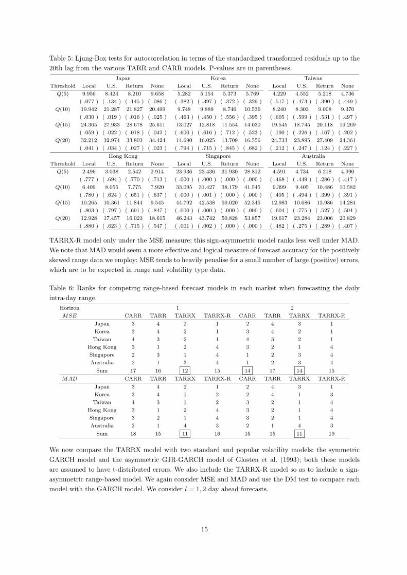
Table 5: Ljung-Box tests for autocorrelation in terms of the standardized transformed residuals up to the20th lag from the various TARR and CARR models. P-values are in parentheses.

Japan Korea Taiwan

Threshold Local U.S. Return None Local U.S. Return None Local U.S. Return None

Q(5) 9.956 8.424 8.210 9.658 5.282 5.154 5.373 5.769 4.229 4.552 5.218 4.736

( .077 ) ( .134 ) ( .145 ) ( .086 ) ( .382 ) ( .397 ) ( .372 ) ( .329 ) ( .517 ) ( .473 ) ( .390 ) ( .449 )

Q(10) 19.942 21.287 21.827 20.499 9.748 9.889 8.746 10.536 8.240 8.303 9.008 9.370

( .030 ) ( .019 ) ( .016 ) ( .025 ) ( .463 ) ( .450 ) ( .556 ) ( .395 ) ( .605 ) ( .599 ) ( .531 ) ( .497 )

Q(15) 24.365 27.933 28.678 25.611 13.027 12.818 11.554 14.030 19.545 18.745 20.118 19.269

( .059 ) ( .022 ) ( .018 ) ( .042 ) ( .600 ) ( .616 ) ( .712 ) ( .523 ) ( .190 ) ( .226 ) ( .167 ) ( .202 )

Q(20) 32.212 32.974 33.803 34.424 14.690 16.025 13.709 16.556 24.733 23.895 27.409 24.361

( .041 ) ( .034 ) ( .027 ) ( .023 ) ( .794 ) ( .715 ) ( .845 ) ( .682 ) ( .212 ) ( .247 ) ( .124 ) ( .227 )

Hong Kong Singapore Australia

Threshold Local U.S. Return None Local U.S. Return None Local U.S. Return None

Q(5) 2.496 3.038 2.542 2.914 23.936 23.436 31.930 28.812 4.591 4.734 6.218 4.990

( .777 ) ( .694 ) ( .770 ) ( .713 ) ( .000 ) ( .000 ) ( .000 ) ( .000 ) ( .468 ) ( .449 ) ( .286 ) ( .417 )

Q(10) 6.409 8.055 7.775 7.920 33.095 31.427 38.179 41.545 9.399 9.405 10.486 10.582

( .780 ) ( .624 ) ( .651 ) ( .637 ) ( .000 ) ( .001 ) ( .000 ) ( .000 ) ( .495 ) ( .494 ) ( .399 ) ( .391 )

Q(15) 10.265 10.361 11.844 9.545 44.792 42.538 50.020 52.345 12.983 10.686 13.986 14.284

( .803 ) ( .797 ) ( .691 ) ( .847 ) ( .000 ) ( .000 ) ( .000 ) ( .000 ) ( .604 ) ( .775 ) ( .527 ) ( .504 )

Q(20) 12.928 17.457 16.023 18.615 46.243 43.742 50.828 53.857 19.617 23.284 23.006 20.829

( .880 ) ( .623 ) ( .715 ) ( .547 ) ( .001 ) ( .002 ) ( .000 ) ( .000 ) ( .482 ) ( .275 ) ( .289 ) ( .407 )

TARRX-R model only under the MSE measure; this sign-asymmetric model ranks less well under MAD.We note that MAD would seem a more effective and logical measure of forecast accuracy for the positivelyskewed range data we employ; MSE tends to heavily penalise for a small number of large (positive) errors,which are to be expected in range and volatility type data.

Table 6: Ranks for competing range-based forecast models in each market when forecasting the dailyintra-day range.

Horizon 1 2

MSE CARR TARR TARRX TARRX-R CARR TARR TARRX TARRX-R

Japan 3 4 2 1 2 4 3 1

Korea 3 4 2 1 3 4 2 1

Taiwan 4 3 2 1 4 3 2 1

Hong Kong 3 1 2 4 3 2 1 4

Singapore 2 3 1 4 1 2 3 4

Australia 2 1 3 4 1 2 3 4

Sum 17 16 12 15 14 17 14 15

MAD CARR TARR TARRX TARRX-R CARR TARR TARRX TARRX-R

Japan 3 4 2 1 2 4 3 1

Korea 3 4 1 2 2 4 1 3

Taiwan 4 3 1 2 3 2 1 4

Hong Kong 3 1 2 4 3 2 1 4

Singapore 3 2 1 4 3 2 1 4

Australia 2 1 4 3 2 1 4 3

Sum 18 15 11 16 15 15 11 19

We now compare the TARRX model with two standard and popular volatility models: the symmetricGARCH model and the asymmetric GJR-GARCH model of Glosten et al. (1993); both these modelsare assumed to have t-distributed errors. We also include the TARRX-R model so as to include a sign-asymmetric range-based model. We again consider MSE and MAD and use the DM test to compare eachmodel with the GARCH model. We consider l = 1, 2 day ahead forecasts.

15

Table 7: Estimates of parameters (and standard errors) for daily stock index returns from GARCH-t andGJR-GARCH-t models.

Country Japan Korea Taiwan

model GARCH GJR GARCH GJR GARCH GJR

α0 .1636 .1720 .1127 .0608 .1308 .1773

( .0429 ) ( .0400 ) ( .0373 ) ( .0326 ) ( .0421 ) ( .0505 )

α1 .0692 .0335 .0826 .0491 .0883 .0223

( .0172 ) ( .0165 ) ( .0149 ) ( .0132 ) ( .0181 ) ( .0171 )

β1 .8637 .8544 .9052 .9232 .8750 .8567

( .0279 ) ( .0257 ) ( .0163 ) ( .0160 ) ( .0260 ) ( .0312 )

w - .0866 - .0475 - .1440

- ( .0303 ) - ( .0214 ) - ( .0316 )

ν 10.2843 9.6230 6.3175 6.6092 7.9236 8.0390

( 2.2080 ) ( 1.9343 ) ( .9125 ) ( 1.0009 ) ( 1.5948 ) ( 1.5057 )

Country Hong Kong Singapore Australia

model GARCH GJR GARCH GJR GARCH GJR

α0 .0467 .0295 .1009 .0880 .0112 .0146

( .0190 ) ( .0116 ) ( .0291 ) ( .0279 ) ( .0046 ) ( .0045 )

α1 .0713 .0011 .1408 .0687 .0873 .0059

( .0123 ) ( .0082 ) ( .0225 ) ( .0200 ) ( .0146 ) ( .0164 )

β1 .9176 .9453 .8215 .8432 .8963 .9079

( .0151 ) ( .0112 ) ( .0258 ) ( .0271 ) ( .0180 ) ( .0179 )

w - .0928 - .1069 - .1288

- ( .0164 ) - ( .0306 ) - ( .0249 )

ν 6.3211 7.2096 6.7347 7.1092 9.2979 8.1956

( .8075 ) ( 1.2234 ) ( 1.0138 ) ( 1.1482 ) ( 1.3838 ) ( 1.2697 )

†GARCH-t model: yt = at; at =√

htεt; ht = α0 + α1a2t−1 + β1ht−1; εt ∼ tν .

†GJR-GARCH-t model: yt = at; at =√

htεt; ht = α0 + α1a2t−1 + β1ht−1 + wa2

t−1I(at−1 < 0); εt ∼ tν .

Parameter estimates for the GARCH models are shown in Table 7. These show the well-known behav-iuours of high volatility persistence α1 + β1 ≈ 1 and significantly higher volatility (asymmetry) afternegative returns ω > 0. We note that the estimates of persistence for these models are higher than thosefor the TARR models, possibly due to the more noisy squared return data which can cause GARCHmodels to over-react to large returns.

The GARCH models forecast the close to close return volatility, while the TARRX model forecasts theintra-day range. To align these models, we consider separately the four volatility proxies in section 4, toadjust the intra-day range forecasts into volatility forecasts. Firstly, in Tables 8 and 9, we consider thesquared return proxy and measure how well the GARCH models forecast this proxy. A priori, we expectthat the GARCH models would forecast σ2

1,t better than the TARRX model, since they use actual returndata in estimation. However, since σ2

1,t is such a noisy volatility proxy, this is not necessarily a goodforecast measure by itself. Further, we also employ the three range-based volatility proxy formulas totransform the intra-day range forecasts from the TARRX models into volatility forecasts (shown under(A), (B) and (C) in Tables 8 and 9) and compare these to the squared return proxy. Finally, we thenalternately use the three range based volatility proxies: σ2

2,t, σ23,t, and σ2

4,t to compare all the competingforecast models in Tables 10-12. We expect the TARR models to forecast the purely range-based proxiesσ2

2,t, σ23,t and σ2

4,t better than the GARCH models. These a priori expectations were not always satisfiedin our results.

Results shown in Tables 8-12 are for the GARCH, GJR-GARCH (GJR), TARRX and TARRX-R models.The p-values from the DM test for equal forecast accuracy, comparing each model with the GARCH model,are also shown. In each row the minimum MSE or MAD is boxed, while all results significantly better

16

Table 8: MSE, MAD measures and Diebold-Mariano DM test for equal l-step-ahead forecast accuracy ofdaily stock stock market volatility Japan, Korea, and Taiwan proxied by σ2

1,t. P-values are in parentheses.

Japan (A) (B) (C) (A) (B) (C)

Horizon GARCH GJR TARRX TARRX TARRX TARRX-R TARRX-R TARRX-R

MSE 1 2.117 2.145 2.140 1.540 1.641 2.181 1.598 1.690

( .847 ) ( .625 ) (.000 ) ( .014 ) ( .815 ) ( .001 ) ( .030 )

MSE 2 2.138 2.056 2.282 1.571 1.656 2.132 1.559 1.660

( .001 ) ( .978 ) (.000 ) ( .016 ) ( .468 ) ( .000 ) ( .019 )

MAD 1 1.251 1.256 1.271 .873 .814 1.266 .887 .825

( .678 ) ( .807 ) (.000 ) ( .000 ) ( .722 ) ( .000 ) ( .000 )

MAD 2 1.259 1.225 1.317 .890 .826 1.256 .874 .814

( .000 ) ( .997 ) (.000 ) ( .000 ) ( .457 ) ( .000 ) ( .000 )

Korea (A) (B) (C) (A) (B) (C)

Horizon GARCH GJR TARRX TARRX TARRX TARRX-R TARRX-R TARRX-R

MSE 1 6.868 6.615 6.210 5.331 5.669 7.909 5.398 5.559

(.023 ) (.006 ) (.001 ) (.033 ) ( .996 ) (.000 ) (.014 )

MSE 2 6.828 6.373 6.362 5.466 5.782 7.716 5.310 5.502

(.001 ) (.017 ) (.007 ) (.067 ) ( .972 ) (.000 ) (.012 )

MAD 1 2.084 1.972 1.992 1.400 1.331 2.342 1.493 1.384

(.000 ) (.028 ) (.000 ) (.000 ) ( 1.000 ) (.000 ) (.000 )

MAD 2 2.077 1.918 1.996 1.438 1.371 2.322 1.506 1.402

(.000 ) (.046 ) (.000 ) (.000 ) ( 1.000 ) (.000 ) (.000 )

Taiwan (A) (B) (C) (A) (B) (C)

Horizon GARCH GJR TARRX TARRX TARRX TARRX-R TARRX-R TARRX-R

MSE 1 4.326 4.467 4.218 3.581 3.708 4.801 3.658 3.720

( .916 ) ( .256 ) ( .008 ) ( .062 ) ( .995 ) ( .014 ) ( .063 )

MSE 2 4.326 4.279 4.305 3.629 3.744 4.859 3.615 3.675

( .331 ) ( .425 ) ( .019 ) ( .083 ) ( .997 ) ( .007 ) ( .046 )

MAD 1 1.653 1.708 1.629 1.148 1.065 1.783 1.189 1.083

( .975 ) ( .244 ) ( .000 ) ( .000 ) ( .999 ) ( .000 ) ( .000 )

MAD 2 1.679 1.651 1.646 1.157 1.068 1.824 1.202 1.089

( .142 ) ( .148 ) ( .000 ) ( .000 ) ( 1.000 ) ( .000 ) ( .000 )

1. For the real (proxied) volatility of each market, σ21,t is the squared return.

2. For model TARRX and TARRX-R, estimated hts are denoted by (A) for R2t , (B) for exp[2×(log(Rt)−0.43+0.292)]

and (C) for R2t /4ln(2).

than the GARCH model, at a 10% level, are bolded. Firstly, Tables 8 and 9 show results when forecastingthe squared returns proxy σ2

1,t and these are surprisingly all in favour of the TARRX models under MSEand MAD. Both the TARRX and TARRX-R models, under either proxy 2 or 4, are significantly betterthan the GARCH models in all markets under both MSE and MAD and l = 1, 2. The squared rangeproxy 3 of Chou (2005a) is much closer to the GARCH models in each market. In each market the bestTARRX and TARRX-R models are not significantly different to each other (p-values not shown) underproxies 2 and 4. These models performed similarly in each market: out of 24 contests under MAD andMSE combined, TARRX ranked best 16 times, compared to 8 for TARRX-R. In summary then, theTARRX and/or TARRX-R models were statistically better than both GARCH models in all marketswhen forecasting squared returns σ2

1,t. This is a surprising and very positive result for the TARR typemodels, in that they could possibly forecast squared returns better than GARCH and GJR-GARCH,since returns were not used to estimate the TARR model parameters.

Results when forecasting two of the three range-based proxies, (σ22,t and σ2

4,t), are clearly in favour of theTARRX models for all markets under both MSE and MAD. For σ2

2,t all markets clearly and statisticallyfavour one of the TARRX models under MSE and MAD and l = 1, 2. The TARRX and TARRX-R are

17

Table 9: MSE, MAD measures and Diebold-Mariano DM test for equal l-step-ahead forecast accuracy ofdaily stock market volatility for Hong Kong, Singapore, and Australia proxied by σ2

1,t. P-values are inparentheses.

HongKong (A) (B) (C) (A) (B) (C)

Horizon GARCH GJR TARRX TARRX TARRX TARRX-R TARRX-R TARRX-R

MSE 1 1.225 1.097 1.199 .942 .987 1.417 .940 .963

(.000 ) ( .266 ) (.005 ) (.041 ) ( .996 ) (.001 ) (.018 )

MSE 2 1.214 1.039 1.123 .920 .975 1.341 .904 .938

(.000 ) (.018 ) (.005 ) (.047 ) ( .971 ) (.001 ) (.016 )

MAD 1 0.966 .892 .940 .672 .624 1.045 .710 .640

(.000 ) ( .111 ) (.000 ) (.000 ) ( .999 ) (.000 ) (.000 )

MAD 2 0.968 .864 .914 .661 .620 1.022 .695 .628

(.000 ) (.006 ) (.000 ) (.000 ) ( .985 ) (.000 ) (.000 )

Singapore (A) (B) (C) (A) (B) (C)

Horizon GARCH GJR TARRX TARRX TARRX TARRX-R TARRX-R TARRX-R

MSE 1 .450 .416 .404 .262 .279 .525 .283 .286

(.000 ) (.045 ) (.000 ) (.000 ) ( .987 ) (.000 ) (.000 )

MSE 2 .486 .417 .433 .285 .297 .547 .290 .290

(.000 ) (.035 ) (.000 ) (.001 ) ( .969 ) (.000 ) (.000 )

MAD 1 .585 .557 .538 .344 .329 .624 .373 .343

(.000 ) (.004 ) (.000 ) (.000 ) ( .980 ) (.000 ) (.000 )

MAD 2 .618 .561 .553 .360 .337 .646 .382 .347

(.000 ) (.000 ) (.000 ) (.000 ) ( .944 ) (.000 ) (.000 )

Australia (A) (B) (C) (A) (B) (C)

Horizon GARCH GJR TARRX TARRX TARRX TARRX-R TARRX-R TARRX-R

MSE 1 .072 .068 .106 .063 .064 .087 .068 .071

(.063 ) ( .999 ) (.011 ) (.079 ) ( 1.000 ) ( .251 ) ( .473 )

MSE 2 .073 .069 .115 .070 .071 .082 .067 .071

(.018 ) ( 1.000 ) ( .306 ) ( .345 ) ( .998 ) ( .124 ) ( .362 )

MAD 1 .223 .215 .285 .177 .161 .260 .174 .159

(.017 ) ( 1.000 ) (.000 ) (.000 ) ( 1.000 ) (.000 ) (.000 )

MAD 2 .228 .214 .286 .184 .166 .251 .173 .157

(.000 ) ( 1.000 ) (.000 ) (.000 ) ( 1.000 ) (.000 ) (.000 )

1. For the real (proxied) volatility of each market, σ21,t is the squared return.

2. For models TARRX and TARRX-R, estimated hts are denoted (A) for R2t , (B) for exp[2× (log(Rt)−0.43+0.292)]

and (C) for R2t /4ln(2).

not statistically different to each other in all markets, but over the 24 comparisons of MSE and MAD, theTARRX was lower in 15, compared to 9 for the TARRX-R model. When forecasting σ2

4,t again all marketsstrongly and statistically favour the TARRX models. For these two proxies again the TARRX model had15 counts of lowest MSE or MAD to TARRX-R’s count of 9. This is a strong result: even though wesuspected the TARRX model would perform better on the range based proxies, since it employs rangedata directly, the level of out-performance compared to the GARCH and GJR-GARCH models is highlyand strongly significant. We remind readers of the strong and stable link between volatility and rangefound by Alizadeh et al. (2002), and successfully employed by Brandt and Jones (2006), that leads to the4th volatility proxy σ2

4,t. This is a proven highly efficient volatility measure and for a model to forecast itbetter than standard and popular GARCH models is a result worth emphasizing. Finally, results for thesquared-range proxy 3 are surprisingly in favour of the GARCH models, though often not statistically. Weknow that squared returns are very noisy and thus squared range data will also be a very noisy volatilityproxy. Here we see the value of Parkinson’s simple adapted squared range proxy 2.

In summary, the TARR models are surprisingly the most accurate at forecasting squared returns compared

18

Table 10: MSE, MAD measures and Diebold-Mariano DM test for equal l-step-ahead forecast accuracyof daily stock market volatility proxied by σ2

2,t. P-values are in parentheses.Japan Korea

Horizon GARCH GJR TARRX TARRX-R GARCH GJR TARRX TARRX-R

MSE 1 1.548 1.589 .170 .165 3.104 2.717 .650 .647

( .945 ) (.000 ) (.000 ) (.000 ) (.000 ) (.000 )

MSE 2 1.649 1.535 .175 .169 3.356 2.716 .575 .584

( .000 ) (.000 ) (.000 ) (.000 ) (.000 ) (.000 )

MAD 1 1.194 1.207 .342 .339 1.621 1.482 .557 .592

( .911 ) (.000 ) (.000 ) (.000 ) (.000 ) (.000 )

MAD 2 1.239 1.188 .359 .347 1.704 1.493 .541 .579

( .000 ) (.000 ) (.000 ) (.000 ) (.000 ) (.000 )

Taiwan Hong Kong

Horizon GARCH GJR TARRX TARRX-R GARCH GJR TARRX TARRX-R

MSE 1 1.896 2.022 .470 .499 .681 .541 .101 .102

( .911 ) ( .000 ) ( .000 ) (.000 ) (.000 ) (.000 )

MSE 2 2.029 1.865 .477 .504 .721 .503 .094 .100

( .017 ) ( .000 ) ( .000 ) (.000 ) (.000 ) (.000 )

MAD 1 1.291 1.318 .448 .487 .763 .655 .237 .253

( .824 ) ( .000 ) ( .000 ) (.000 ) (.000 ) (.000 )

MAD 2 1.332 1.264 .464 .514 .790 .632 .232 .254

( .004 ) ( .000 ) ( .000 ) (.000 ) (.000 ) (.000 )

Singapore Australia

Horizon GARCH GJR TARRX TARRX-R GARCH GJR TARRX TARRX-R

MSE 1 .343 .301 .058 .063 .029 .028 .010 .009

(.000 ) (.000 ) (.000 ) ( .219 ) (.000) (.000)

MSE 2 .405 .311 .061 .066 .031 .026 .011 .009

(.000 ) (.000 ) (.000 ) (.000 ) (.000) (.000)

MAD 1 .553 .518 .157 .177 .157 .149 .076 .072

(.000 ) (.000 ) (.000 ) (.028 ) (.000) (.000)

MAD 2 .602 .526 .160 .181 .161 .144 .079 .071

(.000 ) (.000 ) (.000 ) (.000 ) (.000) (.000)

For the real (proxied) volatility of each market, σ22,t = .3607R2

t .

19

Table 11: MSE, MAD measures and Diebold-Mariano DM test for equal l-step-ahead forecast accuracyof daily stock market volatility proxied by σ2

3,t. P-values are in parentheses.Japan Korea

Horizon GARCH GJR TARRX TARRX-R GARCH GJR TARRX TARRX-R

MSE 1 1.206 1.230 1.304 1.267 4.819 4.914 4.992 4.973

( .860 ) ( .971 ) ( .823 ) ( .804 ) ( .750 ) ( .648 )

MSE 2 1.221 1.202 1.343 1.301 4.101 4.255 4.417 4.488

( .211 ) ( .992 ) ( .895 ) ( .904 ) ( .979 ) ( .871 )

MAD 1 0.903 .912 .950 .939 1.545 1.526 1.545 1.642

( .836 ) ( .981 ) ( .929 ) ( .210 ) ( .502 ) ( .918 )

MAD 2 0.926 .902 .994 .961 1.455 1.438 1.499 1.606

(.005) ( 1.000 ) ( .942 ) ( .279 ) ( .842 ) ( .990 )

Taiwan Hong Kong

Horizon GARCH GJR TARRX TARRX-R GARCH GJR TARRX TARRX-R

MSE 1 3.553 3.426 3.616 3.839 .732 .736 .773 .781

( .113 ) ( .736 ) ( .967 ) ( .559 ) ( .892 ) ( .815 )

MSE 2 3.537 3.393 3.666 3.873 .709 .726 .720 .771

( .039 ) ( .867 ) ( .977 ) ( .727 ) ( .639 ) ( .928 )

MAD 1 1.265 1.270 1.242 1.350 .637 .613 .657 .702

( .573 ) ( .220 ) ( .981 ) (.061 ) ( .845 ) ( .995 )

MAD 2 1.297 1.243 1.287 1.426 .642 .609 .643 .703

( .018 ) ( .376 ) ( .999 ) (.035 ) ( .509 ) ( .994 )

Singapore Australia

Horizon GARCH GJR TARRX TARRX-R GARCH GJR TARRX TARRX-R

MSE 1 .418 .413 .447 .484 .066 .065 .074 .070

( .221 ) ( .870 ) ( .998 ) ( .282 ) ( .772 ) ( .871 )

MSE 2 .431 .418 .470 .505 .066 .067 .086 .070

( .140 ) ( .894 ) ( .998 ) ( .680 ) ( .994 ) ( .929 )

MAD 1 .443 .425 .434 .490 .174 .172 .210 .201

(.001 ) ( .314 ) ( .996 ) ( .314 ) ( .992 ) ( 1.000 )

MAD 2 .469 .434 .444 .502 .177 .173 .220 .198

(.000 ) (.097 ) ( .979 ) ( .125 ) ( .999 ) ( 1.000 )

For the real (proxied) volatility of each market, σ23,t = R2

t .

20

Table 12: MSE, MAD measures and Diebold-Mariano DM test for equal l-step-ahead forecast accuracyof daily stock market volatility proxied by σ2

4,t. P-values are in parentheses.Japan Korea

Horizon GARCH GJR TARRX TARRX-R GARCH GJR TARRX TARRX-R

MSE 1 1.290 1.328 .327 .317 2.553 2.271 1.251 1.246

( .942 ) ( .000 ) ( .000 ) (.000 ) (.000 ) (.000 )

MSE 2 1.373 1.279 .337 .326 2.678 2.212 1.107 1.125

(.000 ) ( .000 ) ( .000 ) (.000 ) (.000 ) (.000 )

MAD 1 1.054 1.066 .475 .470 1.421 1.300 .774 .822

( .899 ) ( .000 ) ( .000 ) (.000 ) (.000 ) (.000 )

MAD 2 1.092 1.043 .498 .481 1.472 1.284 .750 .804

(.000 ) ( .000 ) ( .000 ) (.000 ) (.000 ) (.000 )

Taiwan Hong Kong

Horizon GARCH GJR TARRX TARRX-R GARCH GJR TARRX TARRX-R

MSE 1 1.776 1.846 .906 .962 .552 .444 .194 .196

( .791 ) ( .000 ) ( .000 ) (.000 ) (.000 ) (.000 )

MSE 2 1.880 1.720 .919 .971 .581 .414 .181 .193

( .012 ) ( .000 ) ( .000 ) (.000 ) (.000 ) (.000 )

MAD 1 1.202 1.231 .622 .676 .664 .569 .329 .352

( .851 ) ( .000 ) ( .000 ) (.000 ) (.000 ) (.000 )

MAD 2 1.240 1.179 .645 .714 .686 .550 .322 .352

( .006 ) ( .000 ) ( .000 ) (.000 ) (.000 ) (.000 )

Singapore Australia

Horizon GARCH GJR TARRX TARRX-R GARCH GJR TARRX TARRX-R

MSE 1 .293 .259 .112 .121 .026 .025 .018 .017

(.000 ) (.000 ) (.000 ) ( .203 ) (.000 ) (.000 )

MSE 2 .344 .269 .118 .126 .028 .024 .022 .018

(.000 ) (.000 ) (.000 ) (.002 ) (.013 ) (.000 )

MAD 1 .496 .463 .217 .246 .148 .142 .105 .101

(.000 ) (.000 ) (.000 ) (.073 ) (.000 ) (.000 )

MAD 2 .544 .476 .222 .251 .151 .139 .110 .099

(.000 ) (.000 ) (.000 ) (.000 ) (.000 ) (.000 )

For the real (proxied) volatility of each market, σ24,t = exp[2× (log(Rt)− 0.43 + 0.292)].

21

to GARCH models, and were always significantly better under the MSE and MAD measures. For variousrange-based proxies of volatility, the TARRX models are clearly far superior, both in terms of rank andstatistical significance, at forecasting these more efficient and less noisy proxies, in the markets considered.Overall, the proposed TARR models seem the superior volatility forecasting tool, compared to the popularGARCH and GJR-GARCH models. Compared to the linear CARR model, the asymmetric TARR modelsalso performed better in forecasting, with the TARRX and TARRX-R seemingly indistinguishable involatility forecasting over the markets considered.

7 Conclusion

A family of range-based threshold heteroskedastic models is proposed to model dynamic volatility andcapture asymmetry in financial markets. The structure of this model allows stock market range (volatility)data to react asymmetrically to past information or an exogenous variable, around a threshold value.Simultaneous estimation of the threshold values, the time delay, and other parameters is feasible viaMCMC sampling methods. A simulation study showed that reliable estimation for this model is providedby a Bayesian approach. An empirical application to six financial market indices suggested that theconditional mean range exhibits significant threshold nonlinearity, via sign and size asymmetry, at a lagd = 1 day, both in response to past local market and the US market range and return data. The proposedTARR models, with local or US market range or US market return as the threshold variable (i.e. sizeasymmetry), were preferred as a forecasting tool over the linear CARR model in five of the six markets,except Japan. A comparison with GARCH and GJR-GARCH models revealed clear forecasting dominancefor both TARRX models of squared returns and of two range-based volatility proxies. The proposedTARR models seem the superior volatility forecasting tools, compared to popular GARCH models. Bothsign and size asymmetry were found to be important with neither dominating the other in forecastingvolatility. Further research could involve different threshold variables, such as a weighted average ofauxiliary variables, to further gauge the efficiency gain of the TARR over its rivals. Additional rivalscould include Markov switching GARCH models or the proposal of a Markov switching autoregressiverange-based model similar to the ACD models of De Luca and Zuccolotto (2006).

Acknowledgement We wish to thank the Guest Editor, Professor Herman van Dijk, and two referees fortheir comments which helped to improve the paper. Cathy W.S. Chen is supported by National ScienceCouncil (NSC) of Taiwan grants NSC95-2118-M-035-001.

References

Alizadeh, S., Brandt, M.W., Diebold, F.X., 2002. Range-based estimation of stochastic volatility modelsor exchange rate dynamics are more interesting than you think. J. Finance 57, 1047-1092.

Andersen, T., Bollerslev, T., 1998. Answering the skeptics: yes, standard volatility models do provideaccurate forecasts. International Economic Review 39, 885-905.

Bali, T.G., 2000. Testing the empirical performance of stochastic volatility models of the short-terminterest rate. Journal of Financial and Quantitative Analysis 35, 191-215.

22

Beckers, S., 1983. Variance of security price return based on high, low and closing prices. Journal ofBusiness 56, 97-112.

Black, F., 1976. Studies in stock price volatility changes. Proceedings of the 1976 Business Section.American Statistical Association, 177-181.

Bollerslev, T., 1986. Generalized autoregressive conditional heteroskedasticity. J. Econometrics 31, 307-327.

Brandt, M.W., Jones, C.S., 2006. Volatility forecasting with range-based EGARCH models. J. BusinessEconom. Statist. 24, 470-486.

Brooks, C., 2001. A double-threshold GARCH model for the French Franc/Deutschmark exchange rate.J. Forecasting 20, 135-143.

Broto, C., Ruiz, E., 2006. Unobserved component models with asymmetric conditional variances. Com-putational Statistics and Data Analysis 50, 2146-2166.

Carter, C.K., Kohn, R., 1994. On Gibbs sampling for state space models. Biometrika 81, 541-553.Chen, C.W.S., Lee, J.C., 1995. Bayesian inference of threshold autoregressive models. Journal of Time

Series Analysis 16, 483-492.Chen, C.W.S., Chiang, T.C., So, M.K.P., 2003. Asymmetrical reaction to US stock-return news: evidence

from major stock markets based on a double-threshold model. J. Econom. Business 55, 487-502.Chen, C.W.S., Gerlach, R., So, M.K.P., 2006. Comparison of non-nested asymmetric heteroskedastic

models. Computational Statistics and Data Analysis 51, 2164-2178.Chen, C.W.S., So, M.K.P., Gerlach, R., 2005. Assessing and testing for threshold nonlinearity in stock

returns. Austral. NZ J. Statist. 47, 473-488.Chen, C.W.S., So, M.K.P., 2006. On a threshold heteroscedastic model. International Journal of Fore-

casting 22, 73-89.Chou, R., 2005a. Forecasting Financial Volatilities With Extreme Values: The Conditional Autoregres-

sive Range (CARR) Model. Journal of Money Credit and Banking 37, 561-582.Chou, R., 2005b. Modeling the Asymmetry of Stock Movements Using Price Ranges, Advances in Econo-

metrics 20, 212-231.De Luca, G., Zuccolotto, P., 2006. Regime-switching Pareto distributions for ACD models. Computa-

tional Statistics and Data Analysis 51, 2179-2191.Engle, R.F., 1982. Autoregressive conditional heteroscedasticity with estimates of the variance of United

Kingdom inflation. Econometrica 50, 987-1008.Engle, R.F., Russell, J.R., 1998. Autoregressive conditional duration: A new model for irregular spaced

transaction data. Econometrica 66, 1127-1162.Gallant, A., Hsu C., Tauchen G., 1999. Calculating volatility diffusions and extracting integrated volatil-

ity. Review of Economics and Statistics 81, 617-631.Garman, M.B., Klass, M.J., 1980. On the estimation of price volatility from historical data. Journal of

Business 53, 67-78.Gerlach, R., Chen, C.W.S, Lin, D.S.Y., Huang, M.H., 2006. Asymmetric reaction to trading volume:

Evidence from major stock markets based on a double-threshold model. Physica A -StatisticalMechanics And Its Applications 360, 422-444.

Glosten, L.R., Jagannathan, R., Runkle, D.E., 1993. On the relation between the expected value andthe volatility of the nominal excess return on stocks. J. Finance 487, 1779-1801.

Gray, S.F., 1996. Modeling the Conditional Distribution of Interest Rates as a Regime-Switching Process.Journal of Financial Economics 42, 27-62.

Hastings, W.K., 1970. Monte-Carlo sampling methods using Markov chains and their applications.Biometrika 57, 97-109.

23

Klaassen, F., 2002. Improving GARCH Volatility Forecasts with Regime-Switching GARCH. EmpiricalEconomics 27, 363-394.

Leeves, G., 2007. Asymmetric volatility of stock returns during the Asian crisis: evidence from Indonesia.International Review of Economics & Finance 16 272-286.

Li, C.W., Li, W.K., 1996. On a double-threshold autoregressive heteroscedastic time series model. J.Appl. Econometrics 11, 253-274.

Mandelbrot, B., 1971. When can price be arbitraged efficiently? A limit to the validity of the randomwalk and martingale models. Review of Economics and Statistics 53, 225-236.

Metropolis, N., Rosenbluth, A.W., Rosenbluth, M.N., Teller, E., 1953. Equations of state calculationsby fast computing machines. J. Chem. Phys. 21, 1087-1091.

Nelson, D.B., 1991. Conditional heteroscedasticity in asset pricing: a new approach. Econometrica 59,347-370.

Parkinson, M., 1980. The extreme value method for estimating the variance of the rate of return. Journalof Business 53, 61-65.

Poon, S.H., Granger, C.W.J., 2003. Forecasting volatility in financial markets: a review. J. Econom.Literature 41, 478-539.

Sentana, E., 1995. Quadratic ARCH Models. Review of Economic Studies 62, 639-661.Silvapulle, M.J., Sen, P.K., 2004. Constrained Statistical Inference: Inequality, Order, and Shape Re-

strictions. Wiley-Interscience, Portland.Smith, J.Q., 1985. Diagnostic checks of non-standard time series models. J. Forecasting 4, 283-291.Tierney, L., 1994. Markov chains for exploring posterior distribution, with discussion. Ann. Stat. 22,

1701-1762.Tsay, R.S., 2005. Analysis of Financial Time Series. secend ed., Wiley, Hoboken.

24