arX

iv:1

002.

0014

v1 [

astr

o-ph

.CO

] 2

9 Ja

n 20

10

Voids as a Precision Probe of Dark Energy

Rahul Biswas1, Esfandiar Alizadeh1, and Benjamin D. Wandelt1,2,31 Department of Physics,

University of Illinois at Urbana-Champaign,1110 W. Green Street, Urbana,

IL 61801, USA2 Department of Astronomy,

University of Illinois at Urbana-Champaign,1002 W.Green Street, Urbana,

IL 61801, USA and3 Institut d’Astrophysique de Paris, 98 bis bd Arago,

France, CNRS/Universite Pierre et Marie Curie

A signature of the dark energy equation of state may be observed in the shape of voids. Weestimate the constraints on cosmological parameters that would be determined from the ellipticitydistribution of voids from future spectroscopic surveys already planned for the study of large scalestructure.

The constraints stem from the sensitivity of the distribution of ellipticity to the cosmologicalparameters through the variance of fluctuations of the density field smoothed at some length scale.This length scale can be chosen to be of the order of the comoving radii of voids at very earlytimes when the fluctuations are Gaussian distributed. We use Fisher estimates to show that theconstraints from void ellipticities are promising. Combining these constraints with other traditionalmethods results in the improvement of the Dark Energy Task Force Figure of Merit on the darkenergy parameters by an order of hundred for future experiments. The estimates of these futureconstraints depend on a number of systematic issues which require further study using simulations.We outline these issues and study the impact of certain observational and theoretical systematicson the forecasted constraints on dark energy parameters.

I. INTRODUCTION

A number of observations have established that the expansion of the universe is accelerating at latetimes [1–9]. The cause of acceleration is usually attributed to an otherwise unobserved component calleddark energy, but models of dark energy are generically plagued by fine-tuning issues [10–14]. One can alsointerpret these observations as a consequence of the gravitational dynamics being different from the evolutionof a standard FRW universe under general relativity. Such differences could arise due to the symmetries ofthe FRW universe being broken in the real universe, and the assumptions of smallness of the perturbationsbeing invalid [15–18], or because General Relativity is not a correct description of gravity [19–21]. Withsuch fundamental questions at stake, a prime objective of physical cosmology is to understand the sourceand nature of this acceleration. All available current data [9, 22–29] is consistent with an FRW universehaving dark energy in the form of a cosmological constant, yet various models of different classes are stillallowed by the data. Therefore an important objective of current and future observational efforts is to studythe acceleration of the universe in different ways and detect departures in the behavior from that expectedin a standard ΛCDM model.In order to compute parameter constraints from observational data, one usually parametrizes our ignorance

about dark energy with a time dependent equation of state (EoS) of dark energy as a specific function ofredshift and theoretically computes the observational signatures. A very widely used choice, following therecommendations of the Dark Energy Task Force [30], is the CPL parametrization of the Equation of state[31, 32]. This results in joint constraints on different parameters of the cosmological model, including theparameters of the EoS of dark energy. It is important to use different sets of observational data. Differentkinds of data sets probe different physical imprints of dark energy leading to distinct shapes of constraintson parameters. Consequently, the simultaneous use of many ‘complementary’ probes leads to the tightestconstraints on cosmological parameters [33–36].Moreover, as indicated above, we can hardly be certain that the specific parametrization of the EoS

chosen, or even the choice of the physical model causing the acceleration is correct. In that light, probingthe observable effects of dark energy in terms of different physical aspects is even more important. A tension

2

between constraints computed from different subsets of available data may be indicative of an incorrectparametrization [37], or even an untenable choice of a physical model. Traditionally, the main observationsused to constrain cosmological parameters have pertained to the apparent magnitudes of Type IA supernovae,the power spectrum of anisotropies of the Cosmic Microwave Background (CMB), and the power spectrumof inhomogeneities in the matter distribution (matter power spectrum). The constraints from the supernovaerelate to effects on the geometry of the universe due to dark energy through the changes in the backgroundexpansion. The CMB and matter power spectrum constraints stem mostly from a measurement of thegeometry through the angular location of peaks of the anisotropy power spectrum and the peak positionsof the Baryon Acoustic Oscillations (BAO), but also its effects on the growth of perturbations through themagnitude of the power spectrum. Current status of the parameter constraints on the basis of recent CMB,LSS, SNE observations can be found in [38–40]. Further, the use of observations of clusters of galaxies andweak lensing can be used to measure the growth of perturbations. It is therefore important to use probesof different aspects of cosmic evolution for constraining the cosmological parameters and models. From theviewpoint of both these perspectives, new probes for studying dark energy parameters are invaluable.In the above mentioned probes of the growth of cosmic structures, one studies the dependence of the

dynamical growth of fluctuations on the cosmological parameters through the dependence of the growth ofthe amplitude (ie. size) of the fluctuations on the cosmology. However, in standard cosmology, while thefluctuations are stochastically isotropic, the individual fluctuations are not isotropic. Thus, a measure of theanisotropy and the time evolution of such measures can depend on cosmology in a distinct way. Consequently,this may be used to further constrain cosmological parameters. One expects that the signatures of anisotropicmeasures in observations would be related to the shapes of observed structures. Studying the evolution ofshapes of high density regions (observable as galaxies or galaxy clusters at late times) and comparing withtheory (eg. [41]) is difficult because this requires high resolution numerical simulations capturing the non-linear evolution of these systems. This difficulty can be avoided to a large extent by studying voids usingsemi-analytic methods. Therefore, the shapes of voids can be used to probe cosmology through the evolutionof the anisotropy of fluctuations during cosmic growth.Park and Lee [42, 43] identified the probability distribution of a quantity which they called ellipticity

[80] related to the eigenvalues of the tidal tensor. They showed that the distribution was sensitive to thedark energy equation of state. Besides, they stated that the ellipticity could be derived from a catalogof galaxies, identifying voids of different sizes and measuring their shapes, and the distribution was verifiedusing results from N-body simulations. This ellipticity is an example of a measure of anisotropy of individualfluctuations. The comparison of the probability distribution can provide complementary constraints on darkenergy parameters if its cosmology dependence is different from other probes. We will not require newprobes to study constraints from voids, rather one can study them using probes designed to study large scalestructure in conventional ways, thereby allowing for better leveraging of data. Voids may be detected by theuse of different void identification algorithms [44–48], which find voids using different characteristics, andmay be considered to be different definitions of voids. Properties of voids have been explored in 2dF [49] inSDSS [50, 51]. The shapes and sizes of voids in the SDSS DR5 have been explored in Foster and Nelson[52].The main objective of this paper is twofold: (a) we want to quantify the potential of using void ellipticities

to probe the nature of dark energy in terms of constraints on dark energy parameters, (b) and to clarify themodel assumptions that are important for this procedure, which should be verified, or modified according toresults from simulations. This paper is organized as follows: In Sec. II we review the idea that the shapesof voids can be quantified in terms of asymmetry parameters that can be related to the tidal tensor. Wediscuss the initial distribution of eigenvalues of the tidal tensor, and their evolution to study the evolution ofthe asymmetry parameters of voids and their dependence on the underlying cosmology. There are differenttheoretical choices of models to approximate the non-linear evolution of the initial potential field to observablevoid ellipticities. We discuss two different choices in the appendix and show that our results are insensitiveto these choices. In Sec. III, we discuss the parameters from the surveys considered and our method ofestimating the number of voids identified from these surveys. In Sec. IV, we write down a likelihood andexplicit formulae for the Fisher matrix and use them to forecast constraints from these surveys. We alsostudy how the constraints are degraded by systematic issues. We summarize the paper and discuss ouroutlook in Sec. V.

3

II. THEORY

In this section, we outline the basic idea of using asymmetry parameters describing the shapes of voidsin estimating cosmological parameters. The anisotropy of fluctuations may be captured by studying theeigenvectors and eigenvalues of the tidal tensor, which may be visualized as an ellipsoid with its principalaxes along the eigenvectors of the tidal tensor, and sizes of the principal axes equal to the eigenvalues of thetidal tensor. At early times, the distribution of these eigenvalues at any point in space is known, and theirevolution can be studied by semi-analytic methods. Therefore, the distribution of these quantities may becomputed theoretically and it is desirable to find observational signatures of this distribution. Voids formaround the minima in the density field of matter. The void geometry may be approximated by an ellipsoidalshape, which we shall refer to as the void ellipsoid. The central idea of Park and Lee [42] is that the shape ofthe void ellipsoid as quantified by relative sizes of its principal axes is set by the geometry (functions of theeigenvalues) of the tidal ellipsoid and these should be strongly correlated. This implies that the ellipticitymeasured from the geometry of voids can be used as an observable for specific functions of the eigenvaluesof the tidal tensor. Observations of void shapes at different redshifts can then be used to trace the evolutionof the stochastic distribution of these eigenvalues of the tidal ellipsoid at different redshifts. This containsdynamical information that may be used to constrain cosmological parameters.We briefly describe measures of ellipticity of the void ellipsoid and their connection to the eigenvalues of

the tidal ellipsoid in subsection IIA: this specifies the functions of the tidal eigenvalues that are constrainedby the void shapes. We then describe the distribution of eigenvalues of the initial tidal tensor appropriateto an observed void in subsection II B. Then, in appendices B and C, we study the time evolution of theinitial eigenvalues using two different approximations, and find them to be consistent.

A. Relating the Asymmetry Parameters to the tidal tensor

To describe the dynamics, we choose the comoving coordinates of particles (or galaxies) as the Euleriancoordinates ~x, while the Lagrangian coordinates are taken to be ~q, which are approximately the ‘initial’Eulerian coordinates at some chosen large redshift. The two coordinates are always related through the

displacement field ~Ψ(~q, τ).

~x = ~q + ~Ψ(~q, τ) (1)

While the solution Ψ(~q, τ) describes the dynamics completely, partial aspects of the dynamics may be de-scribed by other measures. The asymmetry of the fluctuation can be understood in terms of the eigenvectors

and eigenvalues of the tidal tensor Ti,j =∂Ψi(~q)∂qj

. This can be visualized as an ellipsoid, which we shall refer

to as the tidal ellipsoid, with principal axes along the eigenvectors of the tidal tensor with sizes equal to theeigenvalues. For a spherically symmetric fluctuation, these eigenvalues are equal, while the departure fromspherical symmetry may be characterized by different choices of functions of ordered eigenvalues of the tidaltensor. (See Appendix A for some other popular choices in the literature.) This was recognized and used incorrecting for ellipsoidal collapse of halos rather than spherical collapse in Press-Schechter like estimates ofthe mass function of dark matter halos [53–55]. From a theoretical side, we can describe the evolution ofthe distribution of these eigenvalues. Therefore, it is these dynamical quantities that we are interested in,even though they are not directly observable.We will next proceed to describe observable quantities which relate to the shape of the voids, and then

show how functions of those observables trace functions of these dynamical quantities. Since voids formaround minima of the density fields where the gradient of field vanishes, one can approximate the densityprofiles around the minima by truncating the Taylor expansion at second order. This gives density profilesthat are ellipsoidal in shape. One may expect voids to inherit this shape, and therefore be approximatelyellipsoidal. In fact, voids have often been modeled as spherical (eg. [56]), while others have argued that theshapes of larger voids fit ellipsoids well only for smaller voids [57]. For irregularly shaped voids (obtained bysuitable void identification algorithms), one can define a void ellipsoid by fitting a moment of inertia tensorto the positions of observed void galaxies ~x in Eulerian coordinates relative to the void center ~xv

Sij =

∑

k(xki − xv

i )(xkj − xv

j )

N ,

4

where the index k runs over the observed galaxies in the void region, and N is the number of galaxies fitted.The void ellipsoid can be defined as the ellipsoid with principal axes along the eigenvectors of this masstensor, and lengths proportional to the square root of the eigenvalues J1, J2, J3. Here, we shall ignore thediscrepancy between the actual shape and this void ellipsoid. Following Park and Lee [42] (see Appendix. Cof Lavaux and Wandelt [58] for a calculation to first order), one can relate the eigenvalues of the tidal tensorλ1, λ2, λ3 to the functions of the ratio of eigenvalues of the void ellipsoid which were called ellipticity.Accordingly, the ellipticities ǫ, ω of the void ellipsoid are to first order

ǫ = 1−(

J1J3

)1/4

≈ 1−(

1− λ1

1− λ3

)1/2

, ω = 1−(

J2J3

)1/4

≈ 1−(

1− λ2

1− λ3

)1/2

. (2)

Clearly, this relation will be affected, at least to some extent, by more detailed dynamics. This would leadto ǫ measured from data sets on voids being correlated with the functions of λi with some scatter. Incomputing parameter constraints, we shall account for this in terms of a variance in the quantity ǫ whichalso contains contributions from observational errors. We shall assess the impact of this assumption of thevoid shapes being perfect tracers of the eigenvalues by studying the degradation of constraints on increasingthe variance in our study of systematics in Section. IVC.

B. Distribution of Initial Eigenvalues of the Tidal Tensor

An observed void evolves from a fluctuation of low underdensity at early times when the distribution offluctuations was Gaussian. Given a void of a given density contrast, at a particular redshift, we wish tocalculate the distribution of eigenvalues of the tidal tensor of the initial fluctuation.At early times, the fluctuations are small enough, their growth can be described by linear perturbation

theory, and the distribution remains Gaussian. One can use the statistical properties of filtered isotropicand homogeneous Gaussian fields to derive a probability distribution of the ordered eigenvalues of the tidaltensor given by the Doroshkevich formula.

P (λ1, λ2, λ3|σR) =3375

8√5σ6

R

exp

(

−−3K21

2σ2R

+15K2

2σ2R

)

K3 (3)

where K1 = λ1 + λ2 + λ3, K2 = λ1λ2 + λ2λ3 + λ3λ1, while K3 = −(λ1 − λ2)(λ2 − λ3)(λ3 − λ1), and σ2R is

the variance of the smoothed overdensity field at the filtering scale R at that time. Note, that this gives thedistribution of the size of the eigenvalues over all spatial points. This distribution is extremely similar butslightly different if restricted to the maxima of the Gaussian field [59], or the minima of the Gaussian field[58] which should evolve to voids. For the small fluctuations, one can use the Jacobian of the transformationfrom Eulerian to Lagrangian coordinates to show that the sum of the eigenvalues K1 can be identified withthe density contrast.

It should be noted that this distribution depends on the filtering scale RSmooth as a parameter while thesize of voids is not important. This is appropriate for comparison with a dataset of voids obtained fromredshift surveys by means of an algorithm which uses a filtering scale as a parameter, rather than the voidsize. This is true for a class of algorithms that define voids as regions of space where the smoothed matterdensity is a minimum (eg.[58, 60]) with the smoothing scale RSmooth being a parameter, with the actual sizeof voids not being crucial to the definition. On the other hand there are Void Finding algorithms whichdefine voids as the largest contiguous underdense regions, obtained by some form of clustering algorithms.A corresponding parameter here is the size R of the voids related to the void volume by R3 ≡ 3V

4π , whilethe smoothing scale is not crucial. While each algorithm might yield slightly different properties of voids,it would be expected that they are not too different. In Appendix B, we show that a calculation based onthe generalized excursion set formalism can be used to calculate the distribution of eigenvalues of an initialfluctuation that evolves to form a void of size R. The result of this calculation supports the above result.

5

C. Evolution of the Tidal Eigenvalues

At low redshifts, gravitational collapse introduces non-linearities into the evolution leading to non-Gaussian distributions of the density field. Thus, the distribution of the tidal eigenvalues of the previoussubsection which assumed Gaussianity are not directly applicable. We study the evolution of theseeigenvalues with time in two different methods, one based on the Zeldovich approximation and one basedon Bond and Myers [61].

It is well known that non-linearity is manifested much less in the displacement field or the gravitational (andthe related displacement) potential than in the density field. Therefore before shell-crossing, the evolution ofstructures from initial condition may be described by the Zeldovich approximation, where the displacement

field is assumed to be separable into a time dependent and time independent part. Ψ(q, τ) = D(τ)D(τ0

Ψ(q, τ0),

where D(τ) is the linear growth function. Hence, at a particular spatial point, its eigenvalues λi(τ) at timeτ evolve linearly from the eigenvalues λi(τ0) at some initial time τ0 as λi(τ) = D(τ)λi(τ0)/D(τ0). Rewritingthe early time eigenvalues in the Doroshkevich formula (Eqn. 3) in terms of the eigenvalues at time τ, onecan then find a distribution of eigenvalues at any time to be given by the Doroshkevich formula where theσR is replaced by D(τ)σR/D(τ0), the linearly extrapolated variance over the Lagrangian smoothing scale R.The formula is exactly the same as Eqn. 3 with the variance σ2

R being replaced by the linearly extrapolatedvariance σ2(R, z), and λi replaced by the eigenvalues at the redshift of the void. Further, since the sum ofthe eigenvalues K1 at early times was equal to the density contrast at that time, the term K1 is equal to thelinearized density contrast of the time of the void

δlin(τ) =D(τ)

D(τ0)δ(τ0) =

D(τ)

D(τ0)(λ1(τ0) + λ2(τ0) + λ3(τ0)) = (λ1(τ) + λ2(τ) + λ3(τ)) (4)

In regions of high density peaks where structure forms, it has been found that modeling the density growthas a collapse of a homogeneous ellipsoid leads to a better approximation to N body simulations. It is unclearwhether this should also be true for low density regions like voids. In Appendix C, we study the evolutionof the eigenvalues of the tidal tensor based on ellipsoidal collapse [61] and find the differences with theevolution computed using Zeldovich approximation to be small.

D. Cosmology Dependence of the Distribution of Ellipticity

Therefore, using the Zeldovich approximation, one can write down the probability distribution of theeigenvalues of the tidal tensor at any time. Further, using the relations of the ellipticities of the void (Eqn.2) and the relation of the linearly extrapolated density contrast to the eigenvalues λ1, λ2, λ3, one can recastthis as the joint distribution of the ellipticities ǫ, ω given the smoothing scale and the linearly extrapolateddensity contrast. Following Park and Lee, we define µ, ν and write the probability distribution for the largerellipticity ǫ

µ = (J2/J3)1/4

, ν = (J1/J3)1/4

P (µ, ν|σlin(R, z), δlin(z)) =34/4

Γ(5/2)

(

5

2 σ2lin(R, z)

)5/2

exp

(

− 5δ2lin(z)

2 σ2lin(R, z)

+15Kδ

2

2 σ2lin(R, z)

)

Kδ3J

P (ǫ|σlin(R, z), δlin(z)) =

∫ 1

1−ǫ

dµP (µ, 1− ǫ|σlin(R, z), δlin(z)) (5)

where Kδ2 ,K

δ3 are the values of K2,K3 in Eqn. 3 in terms of µ, ν when the constraint of Eqn. 4 holds, and

J is the Jacobian in the transformation from the coordinates λ1, λ2, δlin to µ, ν, δlin. This last equationgives the probability distribution of the larger ellipticity ǫ marginalized over the smaller ellipticity ω. Itdepends on the cosmology only through the linearly extrapolated variance σ2

lin(R, z) of density fluctuationsδ(x, z) smoothed at a certain filtering scale R by a window function WR(x, x

′).

σ2lin(R, z) ≡ 〈δ⋆R(x, z)δR(x, z)〉 = D2(τ)σ2

R δR(x, z) =

∫

d3x′δ(x, z)WR(x, x′) (6)

6

where D(τ) is the growth function and σR is evaluated at early times. For qualitative understanding, it isuseful to think of the variance depending on cosmology through σR which depends on the primordial powerspectrum and the wave mode dependent transfer function, and the subsequent scale independent growthdescribed by the growth function D(τ). While the transfer function depends on most of the cosmologicalparameters, in most models dark energy does not become significant at early times. Therefore most of theeffects of dark energy are embedded in the growth function. Closed analytic forms for the growth functionare not known for non-flat cosmologies, with time varying equations of state dark energies, but Percival [62]improves upon a fit to the growth function by Basilakos [63], so that the fit works for non-flat cosmologieshaving dark energy with time varying equation of state as long as they are close to flat LCDM models, evenwhen the equation of state is less than -1. If we consider the CPL parametrization

w(z) = w0 + waz

z + 1, (7)

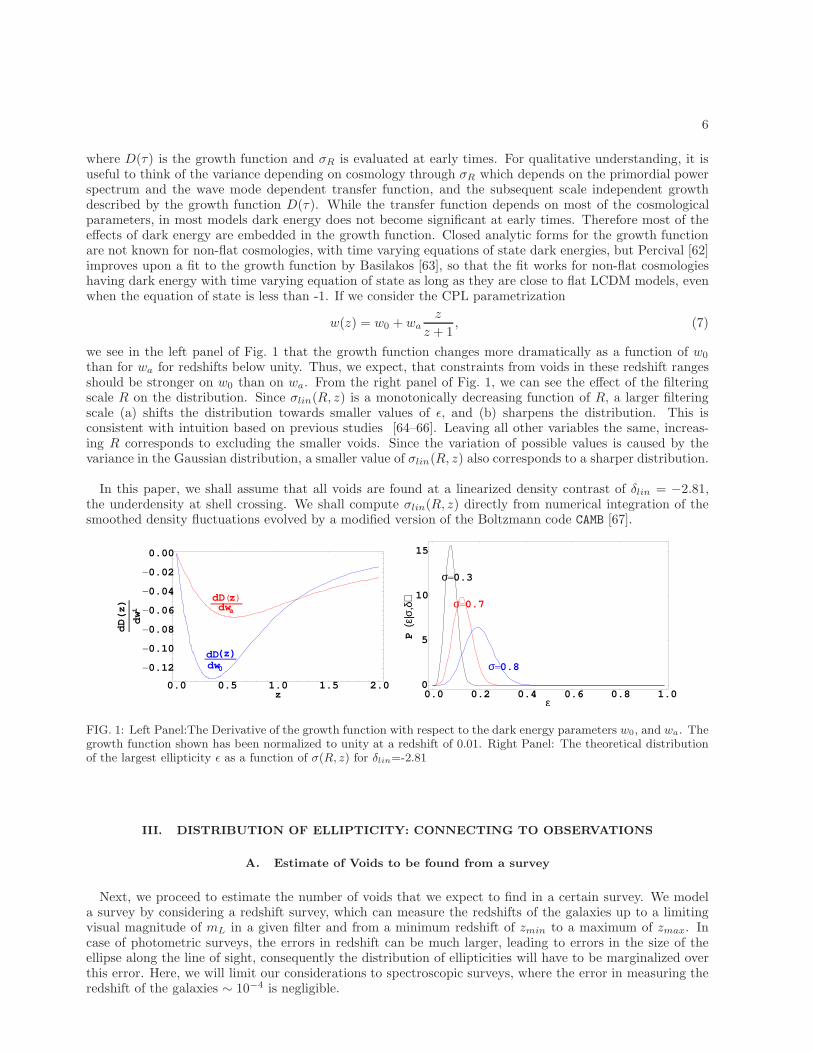
we see in the left panel of Fig. 1 that the growth function changes more dramatically as a function of w0

than for wa for redshifts below unity. Thus, we expect, that constraints from voids in these redshift rangesshould be stronger on w0 than on wa. From the right panel of Fig. 1, we can see the effect of the filteringscale R on the distribution. Since σlin(R, z) is a monotonically decreasing function of R, a larger filteringscale (a) shifts the distribution towards smaller values of ǫ, and (b) sharpens the distribution. This isconsistent with intuition based on previous studies [64–66]. Leaving all other variables the same, increas-ing R corresponds to excluding the smaller voids. Since the variation of possible values is caused by thevariance in the Gaussian distribution, a smaller value of σlin(R, z) also corresponds to a sharper distribution.

In this paper, we shall assume that all voids are found at a linearized density contrast of δlin = −2.81,the underdensity at shell crossing. We shall compute σlin(R, z) directly from numerical integration of thesmoothed density fluctuations evolved by a modified version of the Boltzmann code CAMB [67].

0.0 0.5 1.0 1.5 2.0

−0.12

−0.10

−0.08

−0.06

−0.04

−0.02

0.00

z

dD(z)

dwi

dD(z)dw0

dD(z)dwa

0.0 0.2 0.4 0.6 0.8 1.00

5

10

15

ε

P(ε

|σ,δ

)

σ=0.3

σ=0.8

σ=0.7

FIG. 1: Left Panel:The Derivative of the growth function with respect to the dark energy parameters w0, and wa. Thegrowth function shown has been normalized to unity at a redshift of 0.01. Right Panel: The theoretical distributionof the largest ellipticity ǫ as a function of σ(R, z) for δlin=-2.81

III. DISTRIBUTION OF ELLIPTICITY: CONNECTING TO OBSERVATIONS

A. Estimate of Voids to be found from a survey

Next, we proceed to estimate the number of voids that we expect to find in a certain survey. We modela survey by considering a redshift survey, which can measure the redshifts of the galaxies up to a limitingvisual magnitude of mL in a given filter and from a minimum redshift of zmin to a maximum of zmax. Incase of photometric surveys, the errors in redshift can be much larger, leading to errors in the size of theellipse along the line of sight, consequently the distribution of ellipticities will have to be marginalized overthis error. Here, we will limit our considerations to spectroscopic surveys, where the error in measuring theredshift of the galaxies ∼ 10−4 is negligible.

7

In order to estimate the number of voids of a particular size at a particular redshift, we use the Press-Schechter formalism to determine the number density of voids in a redshift bin centered at z, with Euleriancomoving radius between RE and RE +dRE . Simulations indicate that the number density of voids peaks ata density contrast of δ ≈ −0.85 [42], we shall consider all the voids to have a density contrast of 0.8, whichcan be seen to correspond to a linearly extrapolated density contrast of -2.81 using the fitting function in Moand White [68]. While the usual Press-Schechter formalism matches simulations well at redshift ranges below≈ 2, it fails to predict the number of voids correctly at small scales due to the ‘void in cloud problem’ , whichcan be avoided if at each redshift, we restrict ourselves to scales larger than the non-linearity length scale(Lagrangian)RV inC

min (z) where σ(RV inCmin (z), z) = 1 [69]. Then, the Press-Schechter formalism reliably predicts

the number of voids with the replacement δc = 1.69 → δv = −2.81 in the standard Press-Schechter formalism[70]. The number of voids of a particular size can then be found by integrating over the cosmological volumein the redshift bin, and over the range of radii allowed.

nv(RE , z)dRE =3

2πR3E

P

(

−|δv(z)|σRE

) ∣

∣

∣

∣

d

dRE

−|δv(z)|σRE

∣

∣

∣

∣

dRE (8)

Nvoid =

∫ z+∆z

z

dΩdz

∫ RE+∆RE

RE

dREdV

dzdΩnv(RE)

where P (y) =√

12exp(−y2/2). The number density of voids thus depends exponentially on σR and therefore

the number of voids is extremely sensitive to the minimum radius used. Since voids are detected byobserving galaxies rather than the matter density, the number of voids detected with small radii will bestrongly affected by shot noise (discussed in subsection IVC). We therefore only consider voids with radii

greater than a critical radius R ≥ Rshotmin (z,Survey). For our purposes then, the minimum of the range of

radii of voids at a redshift z considered must be set to the maximum of RV incmin (z) and Rshot

min (z, Survey).

We now explain our method for computing Rshotmin (z, Survey), from the parameters for a survey. The

minimum radius of voids that we will consider should be related to the average separation of galaxiesobserved lsep(z) at the redshift z by the survey in question. We choose this relationship to be linear

Rshotmin (z,Survey) = Alsep(z), and relate the average separation to the average number density of observed

galaxies nbggal(z) at that redshift for the survey. A choice of A = 2 implies that the probability that a detected

void is just due to shot noise is less than 0.5 percent while such a scenario for A = 1 is of the order of 50percent, though void identification algorithms can do better, since they can exploit the contrast betweenvoids and their higher density environments. In any case, the interesting regime is in between these numbersand we shall later explore the sensitivity of constraints to this range.

This background number density of observed galaxies nbggal(z) can be related to the survey parameters.

The mean number density of galaxies in the background universe can be calculated from the luminosityfunction [71] of galaxies at the filter band used in the survey by,

nbggal(z) =

∫ ML

−∞

dMΦX(M, z) (9)

where ΦX is the luminosity function for the filter X and ML is the limiting absolute magnitude of objectsat redshift z which are observed by the survey. It can be calculated from the limiting apparent magnitudeof the survey mL by using the formula,

ML = mL − 5 log10 DL(z) + 5−A(z)−K(z) (10)

Here DL(z) is the luminosity distance to the redshift z in units of pc, A(z) is the correction due to extinctionand K(z) is the K correction arising from the difference in the observed luminosity of and the rest frameluminosity of an object in a particular frequency band due to redshifting of photons.We note that RV inC

min depends on the cosmology, but is independent of the survey, while Rshotmin(z, survey)

also depends on the survey through the filter band, and the limiting magnitude. A plot of Rnoisemin and

RV inCmin for surveys considered in this paper is shown in Fig. 2. Thus, our estimate of the number of voids

identified by each survey depends on the cosmology, the value of the proportionality constant A and thesurvey parameters.

8

0.00 0.05 0.10 0.15 0.20 0.25 0.300

10

20

30

40

z

R(h

Mpc

)−

1

0.0 0.5 1.0 1.5 2.00

10

20

30

40

z

R(h −

1 Mpc

)

FIG. 2: Setting the minimum size of voids: the dashed red curve shows the RV inCmin , while the solid thin (thick) curves

show the (twice) the average separation of observed galaxies for a SDSS DR7 like survey (left) and a EUCLID likesurvey (right). At a particular redshift, we only consider voids with sizes larger than both these scales.

TABLE I: Surveys and parameters used for estimating the number of voids that can be found by the survey. Wechose a survey like SDSS DR7 as an example of a current survey, and EUCLID as an example of a futuristic survey.For reference, we show the number of galaxies that these surveys are expected to observe.

Survey fsky Freq Band Limiting Magnitude Number of Voids Number of Galaxies

A = 2,A = 1

SDSS DR7a 0.24 r 18 1292,3104 1.7 106

EUCLID b 0.48 K 22 1.4 105, 2.3 106 5.2 108

ahttp://www.sdss.org/dr7/coverage/index.htmlbhttp://hetdex.org/other_projects/euclid.php

IV. RESULTS

A. Likelihood function and Fisher matrix

In order to study the potential constraints on cosmological parameters, we need to write down a simplemodel for the data. We assume that by applying appropriate simulation algorithms, we can identify a setof voids at each redshift bin corresponding to a particular smoothing scale. We expect to measure theellipticities of each of these voids with some error. We model the error as an additive Gaussian noise n onthe ellipticity ǫs:

ǫd(R, z) = ǫs(R, z) + n, n ∼ G(0, σǫ) (11)

ǫs itself is a random variable following the distribution of the ellipticities at the relevant redshift. Then wecan write down the likelihood function, which is the probability for finding a void with a measured largestellipticity ǫd given the cosmological parameters

L(ǫd|Θ) =

∫

dǫsP (ǫd|ǫs)P (ǫs|σǫ,Θ) (12)

One expects that the error in measuring the ellipticities will be set by the errors in measuring the principalaxes of the void ellipsoid. For a spectroscopic survey, the positions of galaxies are well measured. Ignoringeffects of redshift distortion/finger of god effects the precision level of the measurement of the principal axeswould be set by the errors in the void finding algorithm. Of course, this will be limited by the relative sizesof the void wall thickness to the void radius ∆. For ∆ ∼ 0.1−0.4, ǫ ≈ 0.2 around the maximum for standardcosmological parameters, the error in ǫ is of the order of 0.1. The errors in the measurement of each void isstatistically independent. Thus the likelihood function for an entire data set consisting of voids at different

9

redshifts can be computed as the product of Eqn. 12 for each void. Consequently, the log of the likelihoodfunction L(ǫd|Θ) is additive for each void.Given the likelihood function for a single void, one can compute the Fisher matrix F defined as an

expectation over all possible sets of data,

Fij =

⟨

∂L(ǫd|Θ, σǫ)

∂Θi

∂L(ǫd|Θ, σǫ)

∂Θj

⟩

=

∫ 1

0

dǫdL(ǫd|Θ, σǫ)∂L(ǫd|Θ, σǫ)

∂Θi

∂L(ǫd|Θ, σǫ)

∂Θj(13)

where all the derivatives are taken at a fiducial choice of the cosmological parameters Θp. Since, in ourmodel the error in measuring the ellipticity is independent of the cosmological parameters, and the ellipticitydepends on the cosmological parameters through the variance of the fluctuations σ2

R only, we can factorizethis into a matrix of mixed partial derivatives of σR with respect to the cosmological parameters, and thederivatives of the log likelihood with respect to σR. We evaluate both of these derivatives numerically. Themain contribution to the derivatives comes from the regions where the probability is smallest. However, thesecontributions are suppressed in the expectation values, since these regions have low probabilities. Finally, wemust sum this contribution for the Fisher matrix over all the voids in the data set. The result thus dependscritically on the number of voids in the data set.

B. Forecasts of constraints on the CPL parameters

We consider Fisher forecasts for a cosmology with the non-baryonic matter assumed to be cold, neglecteffects of neutrino masses and parametrize the evolution of the dark energy equation of state with a CPLparametrization. The primordial perturbations are assumed to be Gaussian distributed, and characterizedby a spectrum which is a power law with an initial amplitude As, and a scale independent tilt ns. Thedistribution of ellipticities depends on both the amplitude of primordial perturbations, and the spectralindex through the dependence of the variance on the scale of smoothing. As is well known, these quantitiesAs, ns are not exactly known, and have a degeneracy with τ, the optical depth of reionization. Further,the constraints on the equation of state parameters can depend strongly on the knowledge of the curva-ture parameter [40]. We therefore consider forecasts for constraints on the CPL parameters w0, wa aftermarginalizing over all other cosmological parameters from a maximal set shown in Table. IVB, along withthe fiducial values used for computing the Fisher forecasts.All of these parameters are not well constrained by a single experiment. Consequently, we shall consider

Fisher forecasts using ellipticity distribution of voids from two spectroscopic surveys: the recent SDSS DR7and the futuristic EUCLID with the survey parameters assumed summarized in Table. III A. We will assumeA = 1, σǫ = 0.1. Following the work in [58], we will identify the smoothing scale as being a quarter of theradius of the void. For CMB constraints, we will consider Fisher forecasts computed from PLANCK [81] Theexpressions for the Fisher matrix for CMB data are given in Tegmark et al. [34]. The survey parameters forPLANCK are taken from the Table. 1.1 of the PLANCK Bluebook [72], and are summarized in Table. III. Weconsider Fisher forecasts of Supernovae from two surveys: for a survey like Dark Energy Survey the numberof supernovae expected is of the order of 1300, and the maximum redshift is around 0.7. We model thiswith a redshift distribution taken from [73] designed to be cut off at z=0.7, and assume perfect measurementof redshift, due to plans of spectroscopic follow-up. The errors in the magnitude are assumed to be ofthe order of the intrinsic dispersion from light curve fitting techniques today (0.15). We also consider afuturistic photometric Supernova IA survey LSST [74], where about 500,000 SNe IA suitable for constrainingdark energy parameters could be observed. We model the errors by assuming magnitude errors of theorder of 0.12 from intrinsic dispersion, and photometric errors in redshift determination of the order of∆z = 0.01(1+ z), and assuming that this adds an error dm

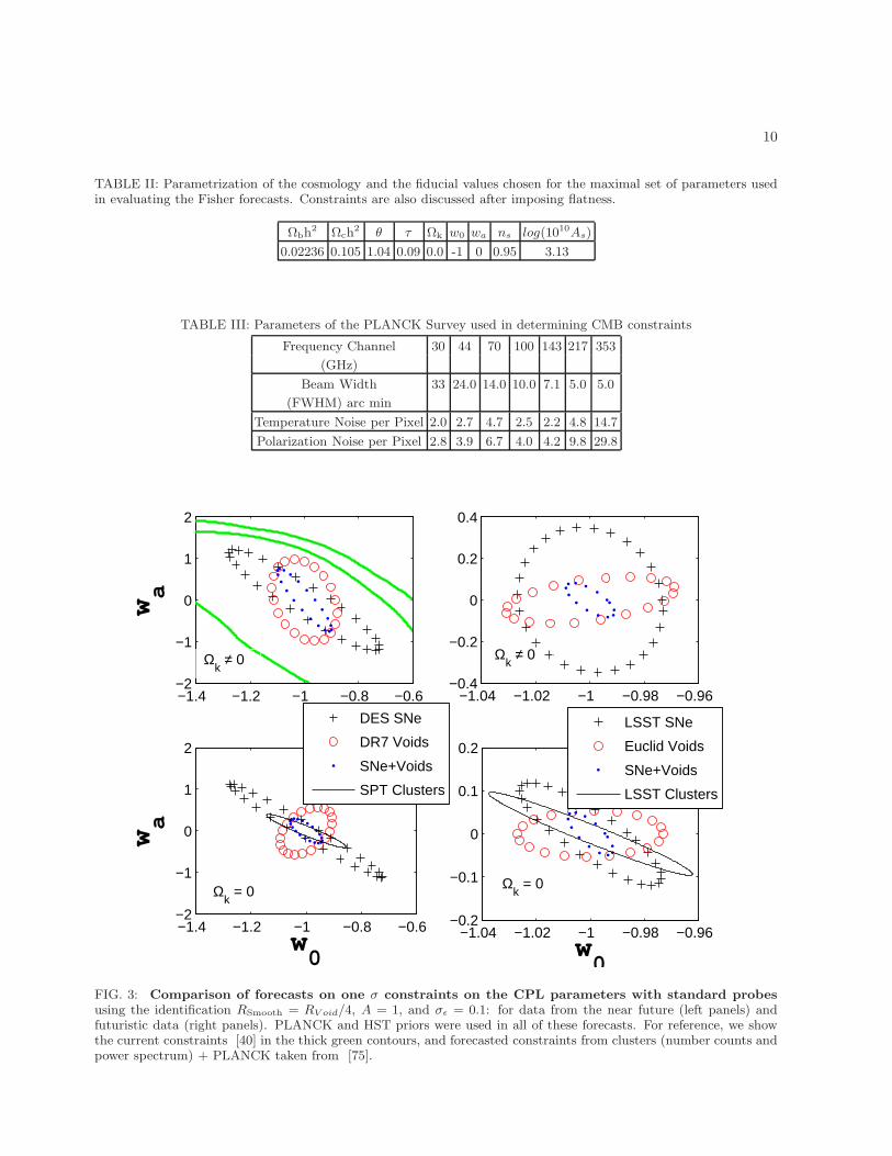
dz ∆z in quadrature to the intrinsic dispersion. Weuse the redshift distribution in Table 1.2 of the [74] to model the redshift distribution of the LSST survey.In Fig. 3, we present the constraints on the equation of state parameters w0, wa by combining constraints

for two sets of data (a) data representative of current or near future (left panels), and (b) data representativeof more futuristic data (right panels). The forecasts for one sigma constraints using void ellipticities + CMB+ HST are shown in open circles, assuming A = 1. The error in measuring the ellipticities σǫ is taken as 0.1.The ellipses made of black ”+” show the constraints for SNe + HST +CMB (PLANCK). The solid, thick,blue ellipses show the constraints when these constraint are combined (CMB (PLANCK) +SNE +HST +

10

TABLE II: Parametrization of the cosmology and the fiducial values chosen for the maximal set of parameters usedin evaluating the Fisher forecasts. Constraints are also discussed after imposing flatness.

Ωbh2 Ωch

2 θ τ Ωk w0 wa ns log(1010As)

0.02236 0.105 1.04 0.09 0.0 -1 0 0.95 3.13

TABLE III: Parameters of the PLANCK Survey used in determining CMB constraints

Frequency Channel 30 44 70 100 143 217 353

(GHz)

Beam Width 33 24.0 14.0 10.0 7.1 5.0 5.0

(FWHM) arc min

Temperature Noise per Pixel 2.0 2.7 4.7 2.5 2.2 4.8 14.7

Polarization Noise per Pixel 2.8 3.9 6.7 4.0 4.2 9.8 29.8

−1.4 −1.2 −1 −0.8 −0.6−2

−1

0

1

2

wa

−1.4 −1.2 −1 −0.8 −0.6−2

−1

0

1

2

w0

wa

DES SNe

DR7 Voids

SNe+Voids

SPT Clusters

−1.04 −1.02 −1 −0.98 −0.96−0.4

−0.2

0

0.2

0.4

−1.04 −1.02 −1 −0.98 −0.96−0.2

−0.1

0

0.1

0.2

w0

LSST SNe

Euclid Voids

SNe+Voids

LSST Clusters

Ωk ≠ 0

Ωk = 0

Ωk ≠ 0

Ωk = 0

FIG. 3: Comparison of forecasts on one σ constraints on the CPL parameters with standard probes

using the identification RSmooth = RV oid/4, A = 1, and σǫ = 0.1: for data from the near future (left panels) andfuturistic data (right panels). PLANCK and HST priors were used in all of these forecasts. For reference, we showthe current constraints [40] in the thick green contours, and forecasted constraints from clusters (number counts andpower spectrum) + PLANCK taken from [75].

11

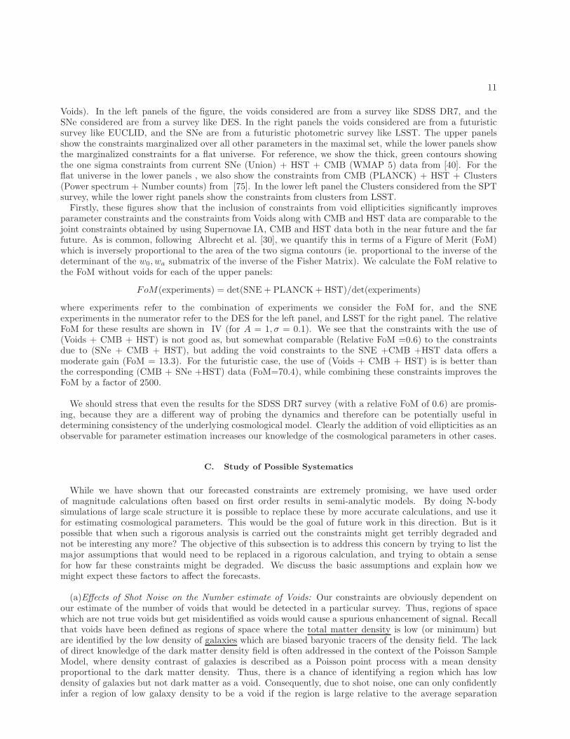
Voids). In the left panels of the figure, the voids considered are from a survey like SDSS DR7, and theSNe considered are from a survey like DES. In the right panels the voids considered are from a futuristicsurvey like EUCLID, and the SNe are from a futuristic photometric survey like LSST. The upper panelsshow the constraints marginalized over all other parameters in the maximal set, while the lower panels showthe marginalized constraints for a flat universe. For reference, we show the thick, green contours showingthe one sigma constraints from current SNe (Union) + HST + CMB (WMAP 5) data from [40]. For theflat universe in the lower panels , we also show the constraints from CMB (PLANCK) + HST + Clusters(Power spectrum + Number counts) from [75]. In the lower left panel the Clusters considered from the SPTsurvey, while the lower right panels show the constraints from clusters from LSST.Firstly, these figures show that the inclusion of constraints from void ellipticities significantly improves

parameter constraints and the constraints from Voids along with CMB and HST data are comparable to thejoint constraints obtained by using Supernovae IA, CMB and HST data both in the near future and the farfuture. As is common, following Albrecht et al. [30], we quantify this in terms of a Figure of Merit (FoM)which is inversely proportional to the area of the two sigma contours (ie. proportional to the inverse of thedeterminant of the w0, wa submatrix of the inverse of the Fisher Matrix). We calculate the FoM relative tothe FoM without voids for each of the upper panels:

FoM(experiments) = det(SNE + PLANCK+HST)/det(experiments)

where experiments refer to the combination of experiments we consider the FoM for, and the SNEexperiments in the numerator refer to the DES for the left panel, and LSST for the right panel. The relativeFoM for these results are shown in IV (for A = 1, σ = 0.1). We see that the constraints with the use of(Voids + CMB + HST) is not good as, but somewhat comparable (Relative FoM =0.6) to the constraintsdue to (SNe + CMB + HST), but adding the void constraints to the SNE +CMB +HST data offers amoderate gain (FoM = 13.3). For the futuristic case, the use of (Voids + CMB + HST) is is better thanthe corresponding (CMB + SNe +HST) data (FoM=70.4), while combining these constraints improves theFoM by a factor of 2500.

We should stress that even the results for the SDSS DR7 survey (with a relative FoM of 0.6) are promis-ing, because they are a different way of probing the dynamics and therefore can be potentially useful indetermining consistency of the underlying cosmological model. Clearly the addition of void ellipticities as anobservable for parameter estimation increases our knowledge of the cosmological parameters in other cases.

C. Study of Possible Systematics

While we have shown that our forecasted constraints are extremely promising, we have used orderof magnitude calculations often based on first order results in semi-analytic models. By doing N-bodysimulations of large scale structure it is possible to replace these by more accurate calculations, and use itfor estimating cosmological parameters. This would be the goal of future work in this direction. But is itpossible that when such a rigorous analysis is carried out the constraints might get terribly degraded andnot be interesting any more? The objective of this subsection is to address this concern by trying to list themajor assumptions that would need to be replaced in a rigorous calculation, and trying to obtain a sensefor how far these constraints might be degraded. We discuss the basic assumptions and explain how wemight expect these factors to affect the forecasts.

(a)Effects of Shot Noise on the Number estimate of Voids: Our constraints are obviously dependent onour estimate of the number of voids that would be detected in a particular survey. Thus, regions of spacewhich are not true voids but get misidentified as voids would cause a spurious enhancement of signal. Recallthat voids have been defined as regions of space where the total matter density is low (or minimum) butare identified by the low density of galaxies which are biased baryonic tracers of the density field. The lackof direct knowledge of the dark matter density field is often addressed in the context of the Poisson SampleModel, where density contrast of galaxies is described as a Poisson point process with a mean densityproportional to the dark matter density. Thus, there is a chance of identifying a region which has lowdensity of galaxies but not dark matter as a void. Consequently, due to shot noise, one can only confidentlyinfer a region of low galaxy density to be a void if the region is large relative to the average separation

12

−1.4 −1.2 −1 −0.8 −0.6−2

−1

0

1

2

w0

wa

DES SNe

DR7 Voids

Voids (deg)

SNe+Voids

SNe +Voids (deg)

−1.1 −1.05 −1 −0.95 −0.9−0.4

−0.2

0

0.2

0.4

w0

LSST SNe

EUCLID Voids

Voids (deg)

SNe+Voids

SNe +Voids (deg)

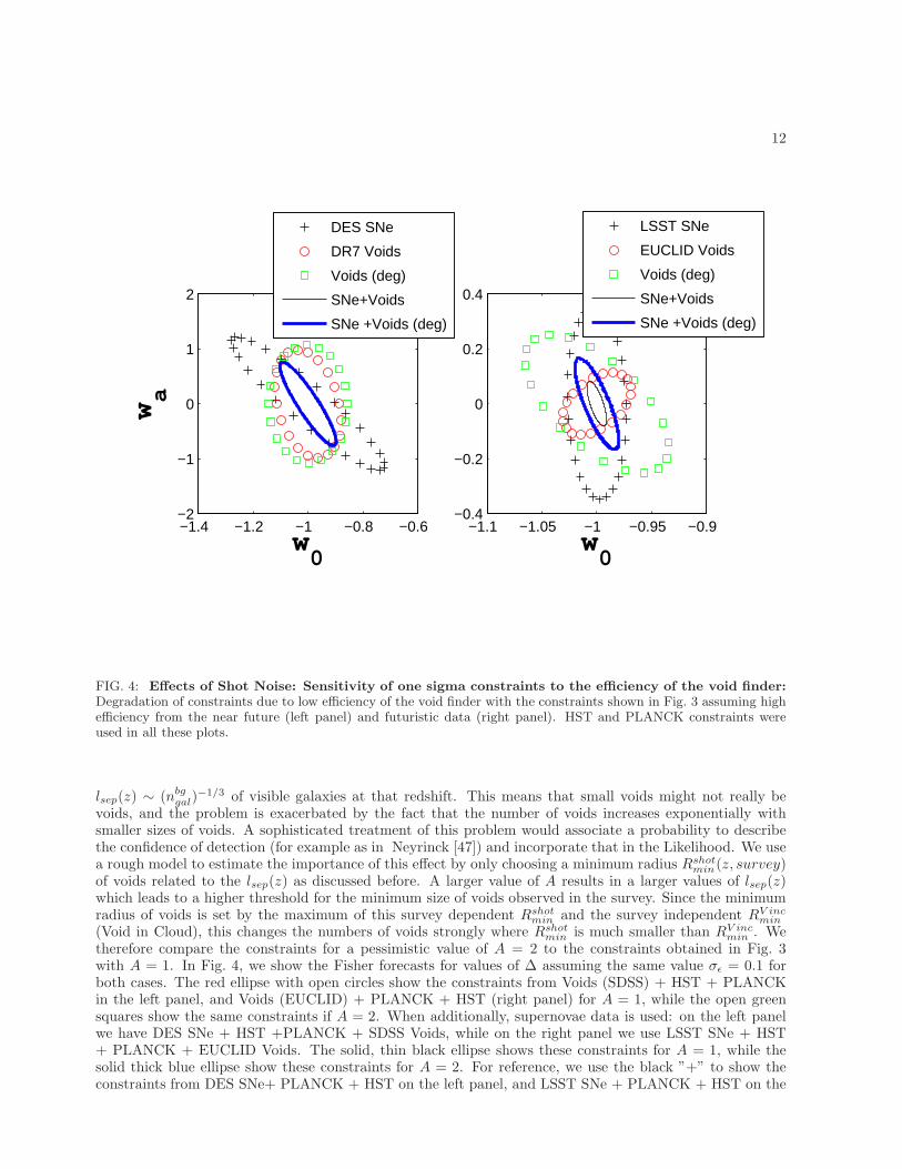
FIG. 4: Effects of Shot Noise: Sensitivity of one sigma constraints to the efficiency of the void finder:

Degradation of constraints due to low efficiency of the void finder with the constraints shown in Fig. 3 assuming highefficiency from the near future (left panel) and futuristic data (right panel). HST and PLANCK constraints wereused in all these plots.

lsep(z) ∼ (nbggal)

−1/3 of visible galaxies at that redshift. This means that small voids might not really bevoids, and the problem is exacerbated by the fact that the number of voids increases exponentially withsmaller sizes of voids. A sophisticated treatment of this problem would associate a probability to describethe confidence of detection (for example as in Neyrinck [47]) and incorporate that in the Likelihood. We usea rough model to estimate the importance of this effect by only choosing a minimum radius Rshot

min(z, survey)of voids related to the lsep(z) as discussed before. A larger value of A results in a larger values of lsep(z)which leads to a higher threshold for the minimum size of voids observed in the survey. Since the minimumradius of voids is set by the maximum of this survey dependent Rshot

min and the survey independent RV incmin

(Void in Cloud), this changes the numbers of voids strongly where Rshotmin is much smaller than RV inc

min . Wetherefore compare the constraints for a pessimistic value of A = 2 to the constraints obtained in Fig. 3with A = 1. In Fig. 4, we show the Fisher forecasts for values of ∆ assuming the same value σǫ = 0.1 forboth cases. The red ellipse with open circles show the constraints from Voids (SDSS) + HST + PLANCKin the left panel, and Voids (EUCLID) + PLANCK + HST (right panel) for A = 1, while the open greensquares show the same constraints if A = 2. When additionally, supernovae data is used: on the left panelwe have DES SNe + HST +PLANCK + SDSS Voids, while on the right panel we use LSST SNe + HST+ PLANCK + EUCLID Voids. The solid, thin black ellipse shows these constraints for A = 1, while thesolid thick blue ellipse show these constraints for A = 2. For reference, we use the black ”+” to show theconstraints from DES SNe+ PLANCK + HST on the left panel, and LSST SNe + PLANCK + HST on the

13

−1.4 −1.2 −1 −0.8 −0.6−2

−1

0

1

2

w0

wa

DES SNe

DR7 Voids

Voids (deg)

SNe+Voids

SNe +Voids (deg)

−1.2 −1.1 −1 −0.9 −0.8−0.4

−0.2

0

0.2

0.4

w0

LSST SNe

EUCLID Voids

Voids (deg)

SNe+Voids

SNe+Voids (deg)

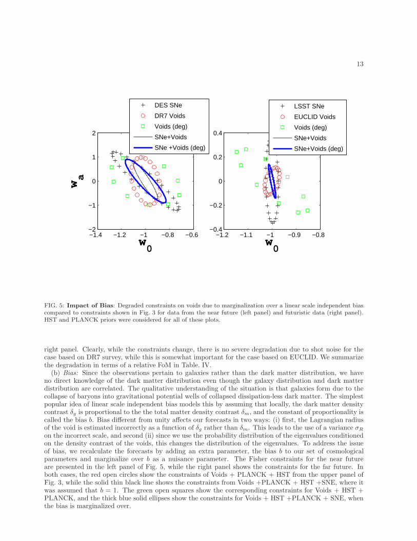
FIG. 5: Impact of Bias: Degraded constraints on voids due to marginalization over a linear scale independent biascompared to constraints shown in Fig. 3 for data from the near future (left panel) and futuristic data (right panel).HST and PLANCK priors were considered for all of these plots.

right panel. Clearly, while the constraints change, there is no severe degradation due to shot noise for thecase based on DR7 survey, while this is somewhat important for the case based on EUCLID. We summarizethe degradation in terms of a relative FoM in Table. IV.(b) Bias: Since the observations pertain to galaxies rather than the dark matter distribution, we have

no direct knowledge of the dark matter distribution even though the galaxy distribution and dark matterdistribution are correlated. The qualitative understanding of the situation is that galaxies form due to thecollapse of baryons into gravitational potential wells of collapsed dissipation-less dark matter. The simplestpopular idea of linear scale independent bias models this by assuming that locally, the dark matter densitycontrast δg is proportional to the the total matter density contrast δm, and the constant of proportionality iscalled the bias b. Bias different from unity affects our forecasts in two ways: (i) first, the Lagrangian radiusof the void is estimated incorrectly as a function of δg rather than δm. This leads to the use of a variance σR

on the incorrect scale, and second (ii) since we use the probability distribution of the eigenvalues conditionedon the density contrast of the voids, this changes the distribution of the eigenvalues. To address the issueof bias, we recalculate the forecasts by adding an extra parameter, the bias b to our set of cosmologicalparameters and marginalize over b as a nuisance parameter. The Fisher constraints for the near futureare presented in the left panel of Fig. 5, while the right panel shows the constraints for the far future. Inboth cases, the red open circles show the constraints of Voids + PLANCK + HST from the upper panel ofFig. 3, while the solid thin black line shows the constraints from Voids +PLANCK + HST +SNE, where itwas assumed that b = 1. The green open squares show the corresponding constraints for Voids + HST +PLANCK, and the thick blue solid ellipses show the constraints for Voids + HST +PLANCK + SNE, whenthe bias is marginalized over.

14

−1.4 −1.2 −1 −0.8 −0.6−2

−1

0

1

2

w0

wa

DES SNeDR7 R=4R

sm

R>Rsm

R=Rsm

−1.04 −1.02 −1 −0.98 −0.96−0.4

−0.2

0

0.2

0.4

w0

LSST SNeEUCLID R=4R

sm

R>Rsm

R=Rsm

FIG. 6: Sensitivity of Fisher Constraints with respect to the prescription of Void Selection: Comparisonof the constraints (red open circles) from voids shown in Fig. 3 with other prescriptions. PLANCK and HST priorswere used in all these plots. The other prescriptions lead to better constraints

(c) Void Selection Prescription While the eigenvalues of the void ellipsoid are expected to trace the eigen-values of the tidal ellipsoid, the eigenvalues themselves are stochastic quantities and the connection to theorycomes from studying the distribution of these eigenvalues. Hence it is important to select a set of voids fromthe data that will accurately reflect the theoretical distribution computed. As discussed in Colberg et al.[48], the void finders available use different methods to identify voids, and these result in different definitionsof voids. A number of these void finders are based on demarcating contiguous regions of space of differentshapes through some variant of a clustering algorithm, while other void finders like Lavaux and Wandelt[58] identify voids from a density field smoothed at a particular length scale. On the theoretical side, wecan compute the probability distribution of the eigenvalues of the tidal tensor analytically through theDoroshkevich formula Eqn. 3, which we use in the computations here, which is the distribution valid at allpoints in space rather than at voids in particular. One may also compute the distribution of the eigenvalues(i) for a void of size R identified with the size of the fluctuation at shell crossing as shown in subsectionsII B and IIC, or (ii) at the minima of the density field when smoothed at a particular length scale (eg. seeAppendix B of Lavaux and Wandelt [58]). Both of these are not analytic estimates, but they can used toconstruct samples of the eigenvalue distributions using Monte Carlo methods and lend themselves naturallyto use with the two classes of void finders respectively. The use of computationally intensive Monte Carlois beyond the scope of this paper based on Fisher estimates. Instead we use the analytic Doroshkevichformula which was shown to be close to both of these distributions, but this requires us to identify the set

15

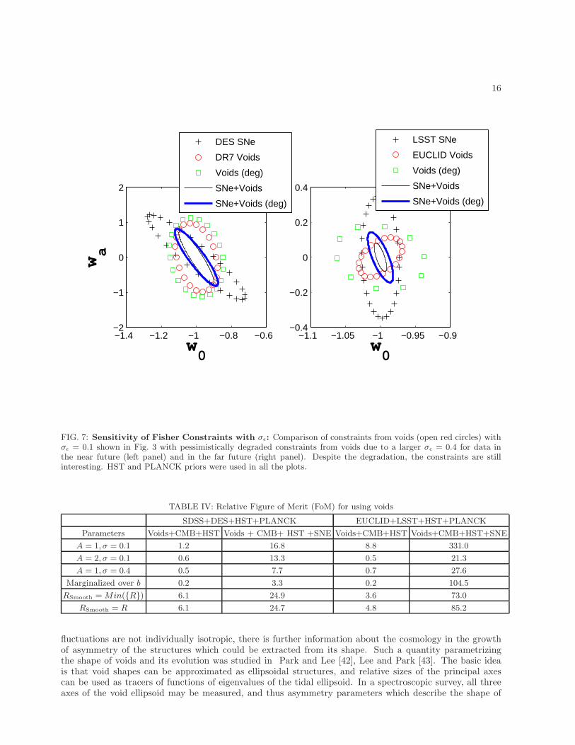
of voids that correspond to the voids obtained by smoothing the density field at a particular Lagrangianscale RSmooth. If we find a set of voids at a particular redshift of a set of different sizes, how can we identifywhat smoothing scale these voids correspond to? Given a set of point particles in space, we understand theaction of smoothing: it tends to homogenize the field at scales below the smoothing scale. Thus, one mayexpect that on smoothing by a scale RSmooth, one will be left with voids with distribution such that thereare few voids of size below ≈ RSmooth, while the smoothing operation may slightly modify the shapes andsizes voids of larger size. At a particular redshift, the probability of forming large voids is much smaller thanforming smaller voids. Consequently, the distribution of sizes of voids when the density field is smoothed toa scale RSmooth, should be peaked at ∼ RSmooth. From simulations used in Lavaux and Wandelt [58], itappears that the distribution of the number of voids with radius R in a density field smoothed by a filterof size RSmooth, is peaked at R ≈ 4RSmooth and falls off rapidly above that. While this inspired our choicefor identification of voids, it is important to keep in mind that the distribution depends on the cosmologicalparameters through σlin(R, z). Consequently using an inaccurate selection criterion for voids can introducebiases in parameter estimation, and the correct prescription may also change the errors and constraints.In order to get a sense for how severely the constraints might be degraded when this is done, we computethe constraints for three different prescriptions of identification the set of voids and compare how far theconstraints are degraded in different cases that suggest themselves. From the right panel of Fig. 1, wesee that the distribution gets broader for larger values of σR. Since this corresponds to lower theoreticalpredictability, we should expect the parameter constraints to get degraded as the filtering scale R becomessmaller. On the other hand, this will lead to a larger number of voids since there are many more smaller voids.

One may expect that when the density field is smoothed at RSmooth, a non-negligible fraction of thevoids have radii between RSmooth and 4RSmooth. We can therefore use a different limit R = RSmooth

in accordance with our calculations using the generalized excursion set formalism in subsection. II B.Finally, if we assume that all voids larger than a particular smoothing scale would be found, we can takeRSmooth = Min(R) found in that redshift bin. This is similar to the method adopted by Lee and Park[43]. The corresponding constraints are shown in Fig. 6. The red open circles show the constraints shownin Fig. 3 for the prescription where RSmooth = R/4, while the blue asterisks show the constraints obtainedfor the case where RSmooth = R, and the open green squares show the constraints for the case whereRSmooth = Min(R).

(d)Sensitivity to Error Levels

As discussed before, in our method of forecasting for Fig. 3, we have used a Gaussian Likelihood withan error σǫ = 0.1 assuming that its order was set by the uncertainty of measuring the void size which waslimited by the size of the void shell (if ∆ ≈ 0.4). Indeed, this seems larger than the values of the error levelscomputed in section 5.3.2 of Lavaux and Wandelt [58]. Further, in our analysis, we have assumed that theellipticities of the mass tensor of voids are perfect tracers of ellipticity of the tidal tensor. More realistically,there would be some scatter around the correlation as shown in section 5.2 of Lavaux and Wandelt [58]. Itis quite possible that scatter of this kind, or the assumptions that we have made might increase the level oferror bars on ǫ quantitatively. Therefore, we investigate the sensitivity of the constraints to the value of σǫ,the error to which the ellipticity was assumed to be measured.We show these constraints in Fig. 7, where the contours with red open circles show the constraints usingVoids + PLANCK + HST shown in the upper panels of Fig. 3 with A = 1 and σǫ = 0.1, while the open greensquares are the constraints where σepsilon has been increased to 0.4. The solid lines show the constraintswhere the constraints are estimated with simultaneous use of the SNe data, ie. DES SNE for the left paneland LSST SNe for the right panel. The thin black solid line is for σǫ = 0.1, while the thick blue solid lineis for σǫ = 0.4. The contours in black ”+” symbols show the constraints from SNe + PLANCK + HST forreference.

V. SUMMARY AND DISCUSSIONS

The growth of cosmic structures with time depends on the background cosmology. Consequently, thegrowth of structures have been used to constrain the parameters of the background cosmology. Traditionally,the measures of growth used have characterized the growth of the volume of fluctuations. However, since the

16

−1.4 −1.2 −1 −0.8 −0.6−2

−1

0

1

2

w0

wa

DES SNe

DR7 Voids

Voids (deg)

SNe+Voids

SNe+Voids (deg)

−1.1 −1.05 −1 −0.95 −0.9−0.4

−0.2

0

0.2

0.4

w0

LSST SNe

EUCLID Voids

Voids (deg)

SNe+Voids

SNe+Voids (deg)

FIG. 7: Sensitivity of Fisher Constraints with σǫ: Comparison of constraints from voids (open red circles) withσǫ = 0.1 shown in Fig. 3 with pessimistically degraded constraints from voids due to a larger σǫ = 0.4 for data inthe near future (left panel) and in the far future (right panel). Despite the degradation, the constraints are stillinteresting. HST and PLANCK priors were used in all the plots.

TABLE IV: Relative Figure of Merit (FoM) for using voids

SDSS+DES+HST+PLANCK EUCLID+LSST+HST+PLANCK

Parameters Voids+CMB+HST Voids + CMB+ HST +SNE Voids+CMB+HST Voids+CMB+HST+SNE

A = 1, σ = 0.1 1.2 16.8 8.8 331.0

A = 2, σ = 0.1 0.6 13.3 0.5 21.3

A = 1, σ = 0.4 0.5 7.7 0.7 27.6

Marginalized over b 0.2 3.3 0.2 104.5

RSmooth = Min(R) 6.1 24.9 3.6 73.0

RSmooth = R 6.1 24.7 4.8 85.2

fluctuations are not individually isotropic, there is further information about the cosmology in the growthof asymmetry of the structures which could be extracted from its shape. Such a quantity parametrizingthe shape of voids and its evolution was studied in Park and Lee [42], Lee and Park [43]. The basic ideais that void shapes can be approximated as ellipsoidal structures, and relative sizes of the principal axescan be used as tracers of functions of eigenvalues of the tidal ellipsoid. In a spectroscopic survey, all threeaxes of the void ellipsoid may be measured, and thus asymmetry parameters which describe the shape of

17

the ellipsoid are related to the quantities involving the eigenvalues of the tidal tensor, which depend onthe background cosmology through the linearly extrapolated variance in fluctuations. Such spectroscopicsurveys have been planned for studying large scale structure using traditional methods; thus the use of shapesdoes not necessarily require new surveys, but allows one to leverage data in an additional way. Lavaux andWandelt [58] show that recovering the the tidal ellipticity of voids to high precision is indeed feasible. To doso, they identify voids and characterize the void tidal ellipticity using the simulated galaxy positions derivedfrom a numerical simulation. These derived ellipticities are then compared to the tidal ellipticity of thecomplete displacement field given by the simulation.In this paper, we study the constraints on dark energy parameters from future surveys in terms of Fisher

forecasts. The likelihood is a strong function of the linearly extrapolated variance of fluctuations at theredshift of the void at the scale of the Lagrangian size of the void. Since voids expand in comoving coordinates,their Lagrangian size is smaller than their observed (comoving) size, and this corresponds to a larger variance.variance at a smaller scale than the observed void size. We assume an error model with Gaussian noise onthe measured ellipticity of the voids, and an arbitrarily assumed error on the ellipticity. We provide explicitformulae for Fisher matrices, and an estimate of the number of voids expected to be found from plannedfuture surveys using semi-analytic methods. By comparing these Fisher constraints using void shapes fromthese surveys to the traditional constraints from other measures, we find this method to be promising: theconstraints are quite competitive with traditional probes in the near future and combining the constraintswith supernovae data improves the DETF Figure of Merit for the supernovae data by a factor of about ten.For futuristic data, we find that the constraints are close to ten times better than supernovae data, andcombining with supernovae data, we can improve the FoM by a factor of a few hundred.We have used the Doroshkevich formula for the ellipticity throughout, but it has been shown [58] that the

distribution of ellipticity for a minima in the density field is slightly different. In actual parameter estimation,we will have to account for this. We shall also have to use the scatter in the correlation of the ellipticityof the void ellipsoid with the real shape of the tidal tensor as obtained from specific void identificationalgorithms. An issue we have not addressed here is the ellipticity of voids that can be generated due toredshift distortions [76, 77] which would have to be modeled to obtain unbiased parameter constraints fromvoids.The Fisher constraints are computed using simple models of dynamics and a likelihood. For estimation of

parameters, each of these would need to be computed precisely. In the subsection IVC, we discuss some ofthe main sources of errors and ambiguities in our forecasts. We indicate how more rigorous, though computa-tionally intensive calculations may be devised. We attempt to estimate how the parameter constraints mightbe affected by these more rigorous methods. While the constraints are often weakened, they still remainat least competitive with other constraints in the near future and the far future. In the case of futuristicsurveys, addition of the void ellipticity to other constraints result in an improvement of the FoM by a factorof at least a hundred, in spite of degradation due to additional systematics. We therefore feel that our studymakes a strong case for pursuing this idea in greater detail.

VI. ACKNOWLEDGMENTS

We would like to thank G. Lavaux for many useful discussions and sharing insights from his results thatmotivated some choices in this paper. RB would like to thank W.M. Wood-Vasey for discussions aboutLSST supernovae. The authors would like to thank the California Institute of Technology for hospitalityduring which part of this work was done. The authors acknowledge financial support from NSF grantAST07-08849.

[1] S. Perlmutter, G. Aldering, G. Goldhaber, R. A. Knop, P. Nugent, P. G. Castro, S. Deustua, S. Fabbro, A. Goo-bar, D. E. Groom, et al., Astrophys. J. 517, 565 (1999), arXiv:astro-ph/9812133.

[2] A. G. Riess, A. V. Filippenko, P. Challis, A. Clocchiatti, A. Diercks, P. M. Garnavich, R. L. Gilliland, C. J.Hogan, S. Jha, R. P. Kirshner, et al., Astron. J. 116, 1009 (1998), arXiv:astro-ph/9805201.

18

[3] P. M. Garnavich, S. Jha, P. Challis, A. Clocchiatti, A. Diercks, A. V. Filippenko, R. L. Gilliland, C. J. Hogan,R. P. Kirshner, B. Leibundgut, et al., Astrophys. J. 509, 74 (1998), arXiv:astro-ph/9806396.

[4] R. A. Knop, G. Aldering, R. Amanullah, P. Astier, G. Blanc, M. S. Burns, A. Conley, S. E. Deustua, M. Doi,R. Ellis, et al., Astrophys. J. 598, 102 (2003), arXiv:astro-ph/0309368.

[5] J. L. Tonry, B. P. Schmidt, B. Barris, P. Candia, P. Challis, A. Clocchiatti, A. L. Coil, A. V. Filippenko,P. Garnavich, C. Hogan, et al., Astrophys. J. 594, 1 (2003), arXiv:astro-ph/0305008.

[6] A. G. Riess, L.-G. Strolger, J. Tonry, S. Casertano, H. C. Ferguson, B. Mobasher, P. Challis, A. V. Filippenko,S. Jha, W. Li, et al., Astrophys. J. 607, 665 (2004), arXiv:astro-ph/0402512.

[7] P. Astier, J. Guy, N. Regnault, R. Pain, E. Aubourg, D. Balam, S. Basa, R. G. Carlberg, S. Fabbro, D. Fouchez,et al., Astron. Astrophys. 447, 31 (2006), arXiv:astro-ph/0510447.

[8] W. M. Wood-Vasey, G. Miknaitis, C. W. Stubbs, S. Jha, A. G. Riess, P. M. Garnavich, R. P. Kirshner, C. Aguil-era, A. C. Becker, J. W. Blackman, et al., Astrophys. J. 666, 694 (2007), arXiv:astro-ph/0701041.

[9] M. Hicken, W. M. Wood-Vasey, S. Blondin, P. Challis, S. Jha, P. L. Kelly, A. Rest, and R. P. Kirshner, ArXive-prints (2009), 0901.4804.

[10] S. Weinberg, Reviews of Modern Physics 61, 1 (1989).[11] S. M. Carroll, W. H. Press, and E. L. Turner, Ann. Rev. Astron. Astrophys. 30, 499 (1992).[12] S. Weinberg, ArXiv Astrophysics e-prints (2000), arXiv:astro-ph/0005265.[13] S. M. Carroll, Living Reviews in Relativity 4, 1 (2001), arXiv:astro-ph/0004075.[14] S. M. Carroll, pp. 235–+ (2004).[15] T. Buchert, M. Kerscher, and C. Sicka, Phys. Rev. D 62, 043525 (2000), arXiv:astro-ph/9912347.[16] E. W. Kolb, S. Matarrese, A. Notari, and A. Riotto, Phys. Rev. D 71, 023524 (2005), arXiv:hep-ph/0409038.[17] G. F. R. Ellis and T. Buchert, Physics Letters A 347, 38 (2005), arXiv:gr-qc/0506106.[18] E. W. Kolb, S. Matarrese, and A. Riotto, New Journal of Physics 8, 322 (2006), arXiv:astro-ph/0506534.[19] G. Dvali, G. Gabadadze, and M. Porrati, Physics Letters B 485, 208 (2000), arXiv:hep-th/0005016.[20] S. M. Carroll, A. de Felice, V. Duvvuri, D. A. Easson, M. Trodden, and M. S. Turner, Phys. Rev. D 71, 063513

(2005), arXiv:astro-ph/0410031.[21] B. Jain and P. Zhang, Phys. Rev. D 78, 063503 (2008), 0709.2375.[22] W. L. Freedman, B. F. Madore, B. K. Gibson, L. Ferrarese, D. D. Kelson, S. Sakai, J. R. Mould, R. C. Kennicutt,

Jr., H. C. Ford, J. A. Graham, et al., Astrophys. J. 553, 47 (2001), arXiv:astro-ph/0012376.[23] S. Cole, W. J. Percival, J. A. Peacock, P. Norberg, C. M. Baugh, C. S. Frenk, I. Baldry, J. Bland-Hawthorn,

T. Bridges, R. Cannon, et al., Mon. Not. Roy. Astron. Soc. 362, 505 (2005), arXiv:astro-ph/0501174.[24] M. Tegmark, D. J. Eisenstein, M. A. Strauss, D. H. Weinberg, M. R. Blanton, J. A. Frieman, M. Fukugita, J. E.

Gunn, A. J. S. Hamilton, G. R. Knapp, et al., Phys. Rev. D 74, 123507 (2006), arXiv:astro-ph/0608632.[25] W. J. Percival, S. Cole, D. J. Eisenstein, R. C. Nichol, J. A. Peacock, A. C. Pope, and A. S. Szalay, Mon. Not.

Roy. Astron. Soc. 381, 1053 (2007), 0705.3323.[26] E. Komatsu, J. Dunkley, M. R. Nolta, C. L. Bennett, B. Gold, G. Hinshaw, N. Jarosik, D. Larson, M. Limon,

L. Page, et al., ArXiv e-prints (2008), 0803.0547.[27] J. Dunkley et al. (WMAP) (2008), 0803.0586.[28] M. Oguri, N. Inada, M. A. Strauss, C. S. Kochanek, G. T. Richards, D. P. Schneider, R. H. Becker, M. Fukugita,

M. D. Gregg, P. B. Hall, et al., Astron. J. 135, 512 (2008), 0708.0825.[29] M. Kowalski, D. Rubin, G. Aldering, R. J. Agostinho, A. Amadon, R. Amanullah, C. Balland, K. Barbary,

G. Blanc, P. J. Challis, et al., Astrophys. J. 686, 749 (2008), 0804.4142.[30] A. Albrecht, G. Bernstein, R. Cahn, W. L. Freedman, J. Hewitt, W. Hu, J. Huth, M. Kamionkowski, E. W.

Kolb, L. Knox, et al., ArXiv Astrophysics e-prints (2006), arXiv:astro-ph/0609591.[31] M. Chevallier and D. Polarski, International Journal of Modern Physics D 10, 213 (2001), arXiv:gr-qc/0009008.[32] E. V. Linder, Physical Review Letters 90, 091301 (2003), arXiv:astro-ph/0208512.[33] M. Tegmark, D. J. Eisenstein, W. Hu, and R. Kron, ArXiv Astrophysics e-prints (1998), arXiv:astro-ph/9805117.[34] M. Tegmark, D. J. Eisenstein, and W. Hu, ArXiv Astrophysics e-prints (1998), arXiv:astro-ph/9804168.[35] D. J. Eisenstein, W. Hu, and M. Tegmark, Astrophys. J. 518, 2 (1999), arXiv:astro-ph/9807130.[36] J. A. Frieman, D. Huterer, E. V. Linder, and M. S. Turner, Phys. Rev. D 67, 083505 (2003), arXiv:astro-

ph/0208100.[37] S. Cole, A. G. Sanchez, and S. Wilkins, ArXiv Astrophysics e-prints (2006), arXiv:astro-ph/0611178.[38] Y. Wang, Phys. Rev. D 77, 123525 (2008), 0803.4295.[39] J.-Q. Xia, H. Li, G.-B. Zhao, and X. Zhang, Phys. Rev. D 78, 083524 (2008), 0807.3878.[40] R. Biswas and B. D. Wandelt, ArXiv e-prints (2009), 0903.2532.[41] S. Ho, N. Bahcall, and P. Bode, Astrophys. J. 647, 8 (2006), arXiv:astro-ph/0511776.[42] D. Park and J. Lee, Physical Review Letters 98, 081301 (2007).[43] J. Lee and D. Park, ArXiv e-prints (2007), 0704.0881.[44] H. El-Ad and T. Piran, Astrophys. J. 491, 421 (1997), arXiv:astro-ph/9702135.[45] F. Hoyle and M. S. Vogeley, ArXiv Astrophysics e-prints (2001), arXiv:astro-ph/0110449.

19

[46] F. Hoyle and M. S. Vogeley, Astrophys. J. 566, 641 (2002), arXiv:astro-ph/0109357.[47] M. C. Neyrinck, Mon. Not. Roy. Astron. Soc. 386, 2101 (2008), 0712.3049.[48] J. M. Colberg, F. Pearce, C. Foster, E. Platen, R. Brunino, M. Neyrinck, S. Basilakos, A. Fairall, H. Feldman,

S. Gottlober, et al., Mon. Not. Roy. Astron. Soc. 387, 933 (2008), 0803.0918.[49] F. Hoyle and M. S. Vogeley, Astrophys. J. 607, 751 (2004), arXiv:astro-ph/0312533.[50] D. M. Goldberg, T. D. Jones, F. Hoyle, R. R. Rojas, M. S. Vogeley, and M. R. Blanton, Astrophys. J. 621, 643

(2005), arXiv:astro-ph/0406527.[51] A. V. Tikhonov, Astronomy Letters 33, 499 (2007), 0707.4283.[52] C. Foster and L. A. Nelson, ArXiv e-prints (2009), 0904.4721.[53] R. K. Sheth, H. J. Mo, and G. Tormen, Mon. Not. Roy. Astron. Soc. 323, 1 (2001), arXiv:astro-ph/9907024.[54] R. K. Sheth and G. Tormen, Mon. Not. Roy. Astron. Soc. 329, 61 (2002), arXiv:astro-ph/0105113.[55] T. Chiueh and J. Lee, Astrophys. J. 555, 83 (2001), arXiv:astro-ph/0010286.[56] R. van deWeygaert, R. Sheth, and E. Platen, in IAU Colloq. 195: Outskirts of Galaxy Clusters: Intense Life in the Suburbs,

edited by A. Diaferio (2004), pp. 58–63.[57] S. Shandarin, H. A. Feldman, K. Heitmann, and S. Habib, Mon. Not. Roy. Astron. Soc. 367, 1629 (2006),

arXiv:astro-ph/0509858.[58] G. Lavaux and B. D. Wandelt, ArXiv e-prints (2009), 0906.4101.[59] J. M. Bardeen, J. R. Bond, N. Kaiser, and A. S. Szalay, Astrophys. J. 304, 15 (1986).[60] O. Hahn, C. Porciani, C. M. Carollo, and A. Dekel, Mon. Not. Roy. Astron. Soc. 375, 489 (2007), arXiv:astro-

ph/0610280.[61] J. R. Bond and S. T. Myers, Astrophys. J. Suppl. Ser. 103, 1 (1996).[62] W. J. Percival, Astron. Astrophys. 443, 819 (2005), arXiv:astro-ph/0508156.[63] S. Basilakos, Astrophys. J. 590, 636 (2003), arXiv:astro-ph/0303112.[64] S. D. M. White and J. Silk, Astrophys. J. 231, 1 (1979).[65] V. Icke, Mon. Not. Roy. Astron. Soc. 206, 1P (1984).[66] R. van de Weygaert and E. Bertschinger, Mon. Not. Roy. Astron. Soc. 281, 84 (1996), arXiv:astro-ph/9507024.[67] A. Lewis, A. Challinor, and A. Lasenby, Astrophys. J. 538, 473 (2000), arXiv:astro-ph/9911177.[68] H. J. Mo and S. D. M. White, Mon. Not. Roy. Astron. Soc. 282, 347 (1996), arXiv:astro-ph/9512127.[69] R. K. Sheth and R. van de Weygaert, Mon. Not. Roy. Astron. Soc. 350, 517 (2004), arXiv:astro-ph/0311260.[70] W. H. Press and P. Schechter, Astrophys. J. 187, 425 (1974).[71] M. R. Blanton, J. Dalcanton, D. Eisenstein, J. Loveday, M. A. Strauss, M. SubbaRao, D. H. Weinberg, J. E.

Anderson, Jr., J. Annis, N. A. Bahcall, et al., Astron. J. 121, 2358 (2001).[72] The Planck Collaboration, ArXiv Astrophysics e-prints (2006), arXiv:astro-ph/0604069.[73] H. Zhan, L. Wang, P. Pinto, and J. A. Tyson, Astrophys. J. Lett. 675, L1 (2008), 0801.3659.[74] LSST Science Collaborations and LSST Project., ArXiv e-prints (2009), 0912.0201.[75] S. Wang, J. Khoury, Z. Haiman, and M. May, Phys. Rev. D 70, 123008 (2004), arXiv:astro-ph/0406331.[76] B. S. Ryden, Astrophys. J. 452, 25 (1995), arXiv:astro-ph/9506028.[77] B. S. Ryden and A. L. Melott, Astrophys. J. 470, 160 (1996), arXiv:astro-ph/9510108.[78] G. R. Blumenthal, L. N. da Costa, D. S. Goldwirth, M. Lecar, and T. Piran, Astrophys. J. 388, 234 (1992).[79] D. J. Eisenstein and A. Loeb, Astrophys. J. 439, 520 (1995), arXiv:astro-ph/9405012.[80] We note that this is not the conventional definition of ellipticity. Nevertheless, this is a convenient measure of

the departure from spherical symmetry. Following Park and Lee [42], we shall refer to it as the ellipticity in therest of the paper

[81] http://www.rssd.esa.int/index.php?project=Planck

Appendix A: Other Parametrizations of Asphericity of fluctuations

A popular choice [59] for density profiles, or [53, 54] expresses this in terms of ”ellipticity” and ”prolate-ness” for the tidal ellipsoid:

e =(λ1 − λ3)

2(λ1 + λ2 + λ3)p =

(λ1 + λ3 − 2λ2)

2(λ1 + λ2 + λ3)(A1)

Since this is a function of the eigenvalues λ, there is a one to one correspondence with the asphericityparameters describing the void ellipsoid in Eqn. 2.

20

Appendix B: Generalized Excursion Set Formalism

It should also be noted that the Doroshkevich formula is based on conditioning on the variance within asmoothing scale R at initial times (or equivalently Lagrangian smoothing scale R), rather than the size ofthe structures themselves at later times. This seems suitable for void finders such as DIVA [58], which usethe variance σR as a parameter, but may be unsuitable for use with other void finders which find voids ofparticular radii at redshifts.In order to confront data obtained from the class of void finding algorithm based on clustering of

underdense regions which uses the sizes of voids as parameters, one needs to theoretically study adistribution of shapes of voids for different sizes. This in turn requires a theoretical definition of the voidboundary. A void expands faster than the background universe, and this results in shell crossing formingthe denser void wall. Accordingly, Blumenthal et al. [78] argued that the formation of a void correspondsto this shell crossing and is thus directly analogous to the collapse of a halo into a point in the sphericalcollapse model . In a spherical expansion model, they found that the linearly extrapolated density fieldat the time of shell crossing, is δv = −2.81. Following them, we assume a void forms when the linearlyextrapolated underdensity inside it reaches this critical value which is analogous to the critical overdensityof the Press-Schechter method. Since, we are interested in the asphericity of the voids, we use a generalizedexcursion set method to construct a distribution of the ellipticity of the tidal tensor of points at early times,given that they evolve to form the voids of Lagrangian size R. Each point mass belongs to a void of acertain radius at some redshift, and had an initial Tidal tensor. The goal of this method is to assign toeach point mass in Lagrangian space (a) the radius of the void to which this point will belong at any givenredshift, and (b) the eigenvalues λ1, λ2, λ3 of the initial tidal tensor at that point. We provide a briefsummary of the method and the results here.

We start with a large Lagrangian radius R, so the smoothed variance of density fluctuations σ(R) is 0 andthe tidal tensor T is taken to be zero. We perform a random walk where we decrease the radius R by stepsof ∆R (thereby increasing σ(R) at each step), and execute six dimensional random walk in the independentelements of the Tidal Tensor, with the probability of each element P (∆Ti,j , R) at radius R depending onσ(R) and equal to the probability implied by the statistics of Gaussian fields. The random walk is stoppedat the largest value of R when the linearized density field given by the sum of the eigenvalues of the tidaltensor Ti,j(R) =

∑

>R ∆Ti,j crosses the critical value of −2.81, and the values of the eigenvalues λ1, λ2, λ3and R at the point of termination are taken to be a sample of the tidal tensor eigenvalues and void sizeat that initial redshift. The mass function of voids thus obtained is identical to the mass function thatwould be obtained by a spherical collapse model (without accounting for the Void in Cloud problem), butit gives us a distribution of the asphericity parameters. Repeating the process, one can construct samplesof the multivariate distribution n(R, λ), from which one can obtain samples for any particular asphericityparameter for voids of size R by restricting the samples to a bin around R and marginalizing over other theasphericity parameter.In Fig. 8, we show the histograms of the “ellipticity” e and “prolateness” p parameters of Eqn. A1 of proto-voids that form voids of radius R obtained from the generalized excursion set formalism for different values ofν = δ

σ overplotted with the distribution implied by the Doroshkevich formula in terms of the same parameterswhen smoothed over a radius R. The figure shows good agreement between the two. As discussed, in Lavauxand Wandelt [58], it was shown that the samples of the eigenvalues of the tidal tensor of fields smoothed ata particular smoothing scale RSmooth are similar to the Doroshkevich Formula. Together, this implies thatboth methods while giving slightly different results are fairly consistent, increasing our confidence in thesemethods.

Appendix C: Eulerian Evolution of Triaxial Systems

It is well known that the Zeldovich approximation fails to describe structure formation at small scales inthe vicinity of density peaks. This is because in high density regions, caustics form making the Lagrangianmapping non-invertible. The onset of this problem is characterized by shell crossing. Thus, at the minima ofthe density field well inside a void, which is our region of interest, the Zeldovich approximation should workwell. Here, we compare with another approximation which works reasonably well in the vicinity of peaks.

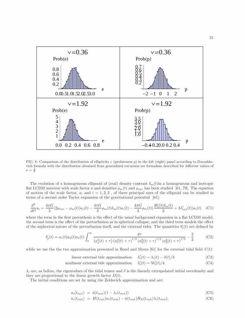
21

0.00.51.01.52.02.53.0e

0.20.40.60.8

ProbHeLî=0.36

-2 -1 0 1 2p

0.20.30.40.50.60.7

ProbHpLî=0.36

0.0 0.2 0.4 0.6 0.8e

12345

ProbHeLî=1.92

-0.4-0.20.0 0.2 0.4p

1.01.52.02.53.03.5

ProbHpLî=1.92

FIG. 8: Comparison of the distribution of ellipticity e (prolateness p) in the left (right) panel according to Doroshke-vich formula with the distribution obtained from generalized excursion set formalism described for different values ofν = δ

σ

The evolution of a homogeneous ellipsoid of (real) density contrast δm(t)in a homogeneous and isotropicflat LCDM universe with scale factor a and densities ρm(t) and ρvac has been studied [61, 79]. The equationof motion of the scale factor, ai and i = 1, 2, 3 , of three principal axes of the ellipsoid can be studied interms of a second order Taylor expansion of the gravitational potential [61]:

d2

dt2ai =

4πG

3(2ρvac − ρm(t))ai(t)−

4πG

3ρm(t)δm(t)ai(t)−

4πG

3ρm(t)(

3b′i(t)δm(t)

2+ 3λ′

ext(t))ai(t) (C1)

where the term in the first parenthesis is the effect of the usual background expansion in a flat LCDM model,the second term is the effect of the perturbation as in spherical collapse, and the third term models the effectof the aspherical nature of the perturbation itself, and the external tides. The quantities b′i(t) are defined by

b′j(t) = a1(t)a2(t)a3(t)

∫

∞

0

dτ(

a2j(t) + τ)

(a21(t) + τ)1/2

(a22(t) + τ)1/2

(a23(t) + τ)1/2

− 2

3(C2)

while we use the the two approximation presented in Bond and Myers [61] for the external tidal field λ′(t):

linear external tide approximation: λ′

i(t) = λi(t)− δ(t)/3 (C3)

nonlinear external tide approximation: λ′

i(t) = 5b′i(t)/4 (C4)

λi are, as before, the eigenvalues of the tidal tensor and δ is the linearly extrapolated initial overdensity andthey are proportional to the linear growth factor D(t).The initial conditions are set by using the Zeldovich approximation and are:

ai(tinit) = a(tinit)(1 − λi(tinit)) (C5)

ai(tinit) = H(tinit)ai(tinit)− a(tinit)HD(tinit)λi(tinit), (C6)

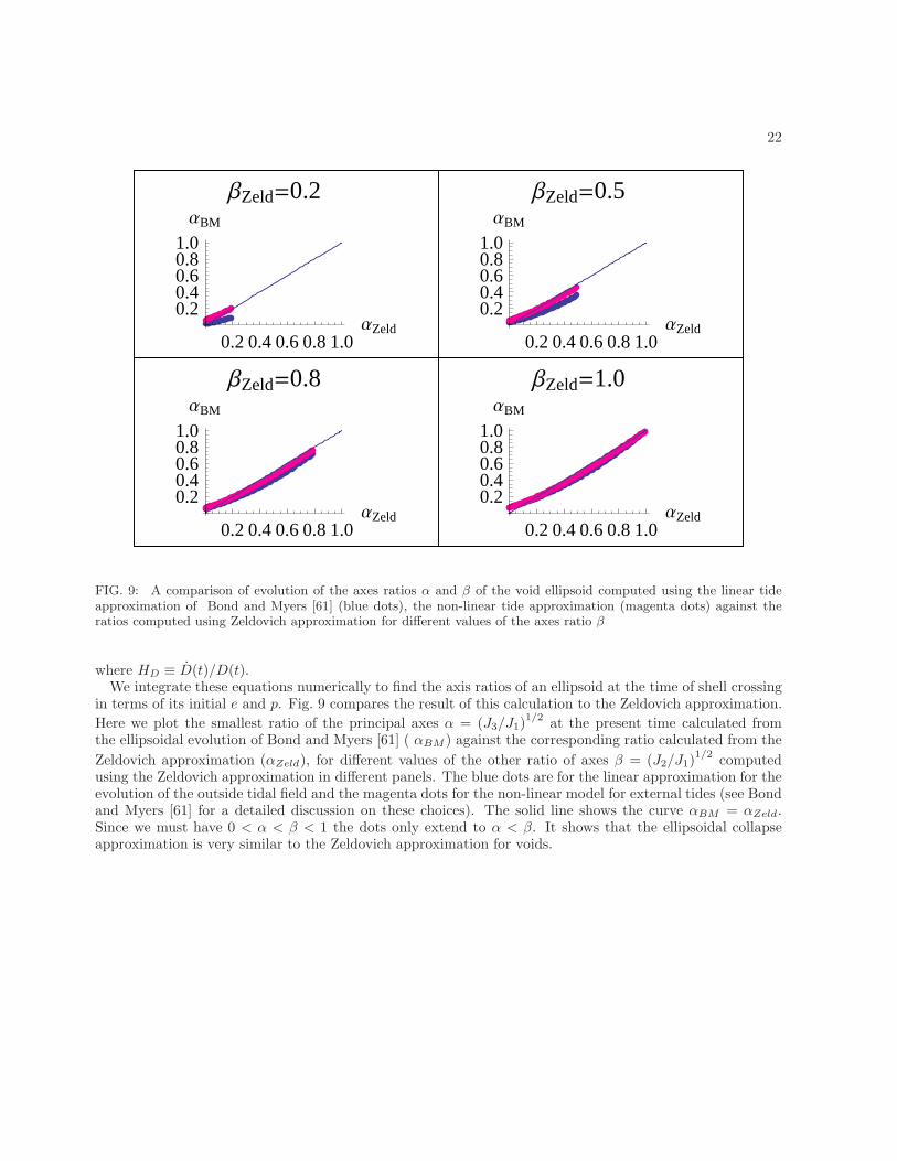
22

0.2 0.4 0.6 0.8 1.0ΑZeld

0.20.40.60.81.0ΑBM

ΒZeld=0.2

0.2 0.4 0.6 0.8 1.0ΑZeld

0.20.40.60.81.0ΑBM

ΒZeld=0.5

0.2 0.4 0.6 0.8 1.0ΑZeld

0.20.40.60.81.0ΑBM

ΒZeld=0.8

0.2 0.4 0.6 0.8 1.0ΑZeld

0.20.40.60.81.0ΑBM

ΒZeld=1.0

FIG. 9: A comparison of evolution of the axes ratios α and β of the void ellipsoid computed using the linear tideapproximation of Bond and Myers [61] (blue dots), the non-linear tide approximation (magenta dots) against theratios computed using Zeldovich approximation for different values of the axes ratio β

where HD ≡ D(t)/D(t).We integrate these equations numerically to find the axis ratios of an ellipsoid at the time of shell crossing

in terms of its initial e and p. Fig. 9 compares the result of this calculation to the Zeldovich approximation.

Here we plot the smallest ratio of the principal axes α = (J3/J1)1/2

at the present time calculated fromthe ellipsoidal evolution of Bond and Myers [61] ( αBM ) against the corresponding ratio calculated from the

Zeldovich approximation (αZeld), for different values of the other ratio of axes β = (J2/J1)1/2

computedusing the Zeldovich approximation in different panels. The blue dots are for the linear approximation for theevolution of the outside tidal field and the magenta dots for the non-linear model for external tides (see Bondand Myers [61] for a detailed discussion on these choices). The solid line shows the curve αBM = αZeld.Since we must have 0 < α < β < 1 the dots only extend to α < β. It shows that the ellipsoidal collapseapproximation is very similar to the Zeldovich approximation for voids.