Visualizing Bezier´s curves: some applications of Dynamic System Geogebra

The whole paper must be written with Times New Roman 12, with the

exception of the title

Visualizing Bezier´s curves: some applications of Dynamic System Geogebra

Francisco Regis Vieira Alves, Instituto Federal de Educação, Ciência e

Tecnologia do Estado do Ceará – IFCE. Brazil, [email protected]

ABSTRACT: In this paper we discuss some properties and

visual characteristics of the emblematic Bézier´s curves.

Indeed, we find in the standard literature in Algebraic

Geometry some briefly indications about it. Moreover, we can

obtain particular algebraic examples of applications (the

Bernstein polynomials , ( )n iB t ). On the other hand, with the

Dynamic System Geogebra - DSG, we can visualize certain

situations and qualitative characteristic that are impossible to

perceive and understanding without the actual technology.

KEYWORDS: Visualization, Bezier´s curves, Geogebra.

1 Introduction

In a general context, we find several methods related to seek a desired curve

that passes through specified points. Related with this goal, we can observe

that “a Bézier curve is confined to the convex hull of the control polygon

that defines it” (BARSKY, 1985, p. 2). So, among these methods, the Bezier

curve can promote a “visual adjust correspondently the points distribution”.

This author indicates still some graphics and a close relationship with the

Bernstein’s polynomials (for the cases 5n = and 6n = ) (see fig. 1).

Vainsencher (2009, p. 116) explains that “the Bezier´s curves can be

used with certain computational and aesthetic advantages. Are provided that

now, we are content with a rational curve that ‘visually adjust’ the graphic

distribution of points”. Precisely, when we considering

1 1 1 2 2 2 3 3 3( , ), ( , ), ( , ), , ( , )d d dP x y P x y P x y P x y= = = =… we seek a rational

curve which passes through of these points. Moreover, we need that the

tangents at these points containing the segments 1 2 2 3 3 4 1, , , , d dP P P P P P P P−… .



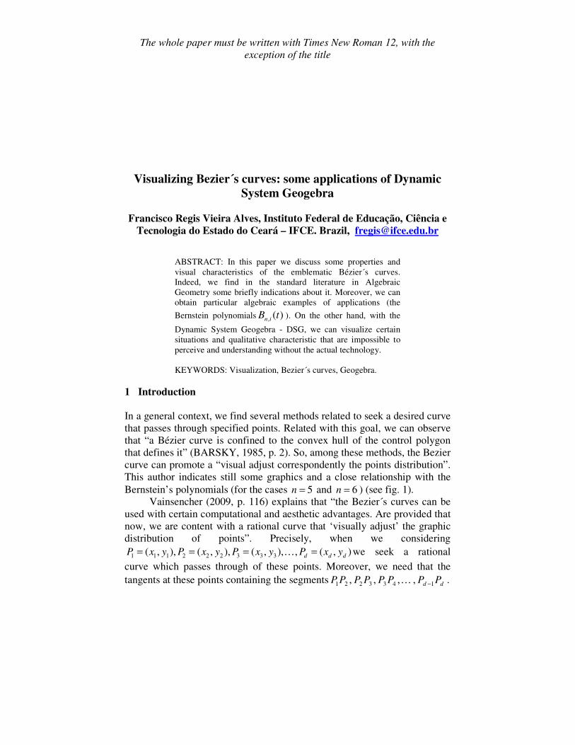
In the next section we will show some examples related to these

consideration. On the other hand, en virtue to understanding this basic

construction, we need to talk some information about the Bernstein’s

polynomials (see fig. 1). Indeed, we know the Bernstein’s polynomials

defined by ,

!( ) (1 ) (1 )

!( )!

i n i i n i

i n

n nB t t t t t

i i n i

− − = − = −

− , with 0 i n≤ ≤ . (*)

Figure 1. Visualization of a twisted curve inside a rectangular parallelepiped in three-

space and the Bernstein’s polynomials (BARSKY, 1985, p. 3-6)

In a general way, we define a Bézier curve as a spline curve that uses

the Berstein polynomials as a basis. A Bézier curve ( )r t of degree n is

represented by ,

0

( ) ( )n

i i n

i

r t b B t=

=∑ under condition 0 1t≤ ≤ . One way to

computing a point of a Bezier curve, is first to evaluate the Berstein

polynomials. Another, and more direct method, is the Casteljau’s algorithm

(see figure 3).

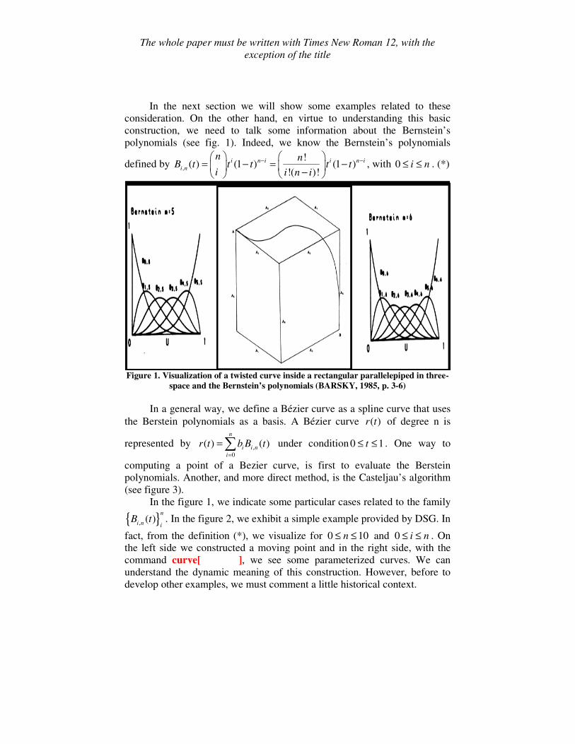
In the figure 1, we indicate some particular cases related to the family

{ },( )

n

i n iB t . In the figure 2, we exhibit a simple example provided by DSG. In

fact, from the definition (*), we visualize for 0 10n≤ ≤ and 0 i n≤ ≤ . On

the left side we constructed a moving point and in the right side, with the

command curve[ ], we see some parameterized curves. We can

understand the dynamic meaning of this construction. However, before to

develop other examples, we must comment a little historical context.



Figure 2. Visualization of Bernstein’s polynomials with the DSG´s help

2 The Bezier´s curves and some properties

In the historic context, we know that Bezier´s theory curves were developed

independently by P. Casteljau in 1959 and by P. Bezier in 1962. Both

approaches are based on the Bernstein’s polynomials. This polynomials

class is known in approximation theory. Vainsencher (2009, p. 115-116)

shows an application (and a little figure), although we identify the author's

intention on a heuristic idea of a curve related to a transmission through

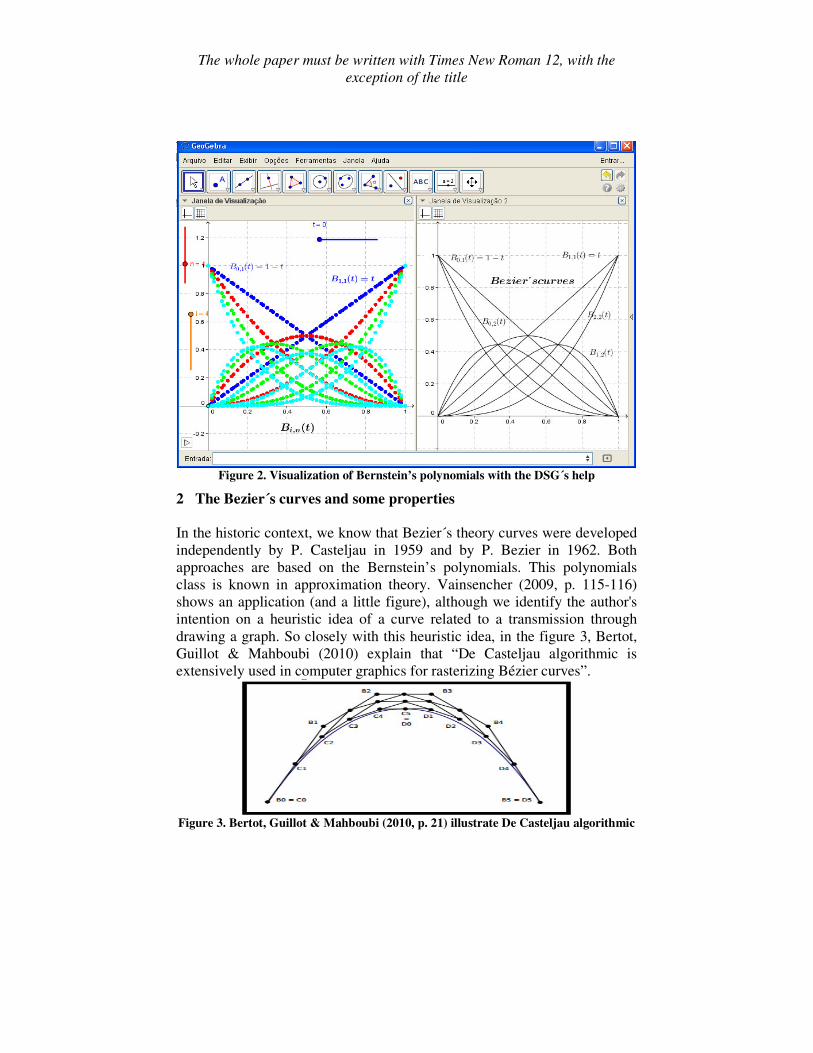
drawing a graph. So closely with this heuristic idea, in the figure 3, Bertot,

Guillot & Mahboubi (2010) explain that “De Casteljau algorithmic is

extensively used in computer graphics for rasterizing Bézier curves”.

Figure 3. Bertot, Guillot & Mahboubi (2010, p. 21) illustrate De Casteljau algorithmic



A parameterization is obtained from a recursive way

(VAINSENCHER, 2009, p. 116). Indeed, we can start with the polygonal

determined by the 1d − segments. We write

1

1 1 2

1

2 2 3

1

1 1

( ) (1 )

( ) (1 )

( ) (1 )d d d

t t P tP

t t P tP

t t P tP

σ

σ

σ − −

= − +

= − + = − +

�

.

In the next step we must substitute each consecutives pairs of polygonal by

an interpolation. In our case, we take a parabola in the following way: 2 1 1

1 1 2

2 1 1

2 2 3

2 1 1

2 2 1

( ) (1 ) ( ) ( )

( ) (1 ) ( ) ( )

( ) (1 ) ( ) ( )d d d

t t t t t

t t t t t

t t t t t

σ σ σ

σ σ σ

σ σ σ− − −

= − +

= − + = − +

�

. Lets consider the set of the points:

1 2 3 4( 1,1), (0, 0), ( 1.2, 1.2), (2, 1.5)P P P P= − = = − − = − . Easily, we find:

1

1 1 2

1

2 2 3

1

3 3 4

( ) (1 ) (1 ) ( 1,1) (0,0) ( 1,1 )

( ) (1 ) (1 )(0,0) ( 1.2, 1.2) ( 1.2 , 1.2 )

( ) (1 ) (1 )( 1.2, 1.2) (2, 1.5) (3.2 1.2, 0.3 1.2)

t t P tP t t t t

t t P tP t t t t

t t P tP t t t t

σ

σ

σ

= − + = − ⋅ − + ⋅ = − −

= − + = − + − − = − −

= − + = − − − + − = − − −

.

In the next step, we compute: 2 2 2

1

2 2 2

2

( ) (1 )( 1,1 ) ( 1.2 , 1.2 ) ( 2.2 2 1, 0.2 2 1)

( ) (1 )( 1.2 , 1.2 ) (3.2 1.2, 0.3 1.2) (4.4 2.4 ,0.9 2.4 )

t t t t t t t t t t t

t t t t t t t t t t t

σ

σ

= − − − + − − = − + − − − +

= − − − + − − − = − −.

Finally, we find the following parameterized cubic curve 3 2 2 3 2 3 2

1 1 1( ) (1 ) ( ) ( ) (6.6 6.6 3 1,1.1 0.6 3 1)t t t t t t t t t t tσ σ σ= − + = − + − − − + .

We still take the set of points:

1 2 3 4( 1,0), (0,0), (1,2), (2,0)Q Q Q Q= − = = = . Following a similar procedure,

we establish that:

1

1

1

2

1

3

( ) (1 )( 1,0) (0,0) ( 1,0)

( ) (1 )(0,0) (1,2) ( ,2 )

( ) (1 )(1,2) (2,0) (1 ,2 2 )

t t t t

t t t t t

t t t t t

σ

σ

σ

= − − + = −

= − + =

= − + = + −

. We continue by the

calculations

2 2

1

2 2

2

( ) (1 )( 1,0) ( ,2 ) ( ,2 )

( ) (1 )( ,2 ) (1 ,2 2 ) (2 ,4 4 )

t t t t t t t t

t t t t t t t t t t

σ

σ

= − − + =

= − + + − = − and, finally, we

obtain a Bezier cubic 3 2 2 2 2 3

1 ( ) (1 )( ,2 ) (2 , 4 4 ) ( ,6 6 )t t t t t t t t t t t tσ = − + − = + − .

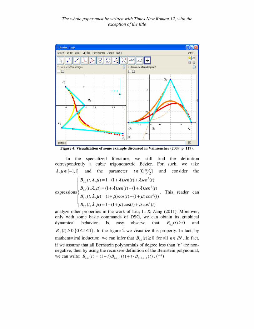
In the figure 4, we show the dynamic construction associated to which of

these recursive parameterization for four control points.



Figure 4. Visualization of some example discussed in Vainsencher (2009, p. 117).

In the specialized literature, we still find the definition

correspondently a cubic trigonometric Bézier. For such, we take

, [ 1,1]λ µ ∈ − and the parameter [0, ]2

t π∈ and consider the

expressions

2

0,3

2

1,3

2

2,3

2

3,3

( , , ) 1 (1 ) ( ) ( )

( , , ) (1 ) ( ) (1 ) ( )

( , , ) (1 ) cos( ) (1 )cos ( )

( , , ) 1 (1 )cos( ) cos ( )

B t sen t sen t

B t sen t sen t

B t t t

B t t t

λ µ λ λ

λ µ λ λ

λ µ µ µ

λ µ µ µ

= − + +

= + − +

= + − +

= − + +

. This reader can

analyze other properties in the work of Liu; Li & Zang (2011). Moreover,

only with some basic commands of DSG, we can obtain its graphical

dynamical behavior. Is easy observe that 0,1( ) 0B t ≥ and

1,1( ) 0B t ≥ ( )0 1t≤ ≤ . In the figure 2 we visualize this property. In fact, by

mathematical induction, we can infer that , ( ) 0i nB t ≥ for all n IN∈ . In fact,

if we assume that all Bernstein polynomials of degree less than ‘n’ are non-

negative, then by using the recursive definition of the Bernstein polynomial,

we can write: , , 1 1, 1( ) (1 ) ( ) ( )i n i n i nB t t B t t B t− − −= − + ⋅ . (**)



3 Visualization provided by DSG and the Bernstein polynomials

In this section we will discuss some conceptual properties related to the

Bernstein polynomials. En virtue its definition in (*), we can get easily that: 2 2 3

0,1 1,1 0,2 1,2 2,2 0,3( ) 1 , ( ) , ( ) (1 ) , ( ) 2 (1 ), ( ) , ( ) (1 )B t t B t t B t t B t t t B t t B t t= − = = − = − = = − ,

2 2 3

1,3 2,3 3,3( ) 3 (1 ) , ( ) 3 (1 ), ( )B t t t B t t t B t t= − = − = , etc. In the specialized

literature, we find several properties related to this notion.

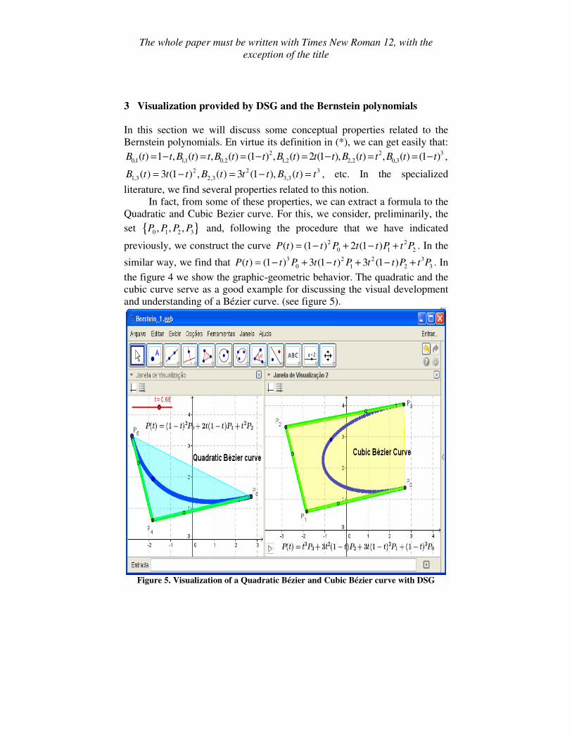
In fact, from some of these properties, we can extract a formula to the

Quadratic and Cubic Bezier curve. For this, we consider, preliminarily, the

set { }0 1 2 3, , ,P P P P and, following the procedure that we have indicated

previously, we construct the curve 2 2

0 1 2( ) (1 ) 2 (1 )P t t P t t P t P= − + − + . In the

similar way, we find that 3 2 2 3

0 1 2 3( ) (1 ) 3 (1 ) 3 (1 )P t t P t t P t t P t P= − + − + − + . In

the figure 4 we show the graphic-geometric behavior. The quadratic and the

cubic curve serve as a good example for discussing the visual development

and understanding of a Bézier curve. (see figure 5).

Figure 5. Visualization of a Quadratic Bézier and Cubic Bézier curve with DSG



First, is easy observe from (*), the following property:

,

0 0

( ) (1 ) ( 1) ( 1) k k

n k n ki n i i k k k i i k

i n

k k

n n n i n n iB t t t t t t

i i i

− −− − +

= =

− − = − = − = − =

∑ ∑

0

( 1) ( 1)

n k nk i k k i k

k i k

n n i n kt t

i n i k i

−− −

= =

− = − ⋅ = − ⋅

− ∑ ∑ . Similarly, we can

show that each of these power basis elements can be written as a linear

combination of Bernstein Polynomials. In fact, if we have a basis 2 31, , ,t t t

so, the Bernstein basis associated is described 3 2 2 3(1 ) ,3 (1 ) ,3 (1 ),t t t t t t − − − . Moreover, we can still verify the propriety

previously indicated in (**), by the following algebraic procedure:

1 1 1 ( 1)

, 1 1, 1

1 1(1 ) ( ) ( ) (1 ) (1 ) (1 )

k 1

1 1 1 1(1 ) (1 ) (1 )

k 1 k 1

(1 )

k n k k n k

i n i n

k n k k n k k n k

k

n nt B t t B t t t t t t t

k

n n n nt t t t t t

k k

nt t

k

− − − − − −

− − −

− − −

− − − + ⋅ = − − + − =

−

− − − − = − + − = + ⋅ ⋅ − =

− −

= ⋅ ⋅ −

, ( )n k

n kB t− =

From a geometric point of view, when we consider the figure 2, we

can infer too that all member of the family of polynomials are linearly

independent. We did not demonstrate this formal property, despite being

true. On the other hand, regarding the properties earlier commented, we note

that its description does not provide an easy description en geometric way,

even with the aid of a mathematical software.

We consider the quadratic curve described in the follow

manner 2 2

0 1 2( ) (1 ) 2 (1 )P t t P t t P t P= − + − + . When we lead with four

points in the plane, we reach the cubic of Bezier 3 2 2 3

0 1 2 3( ) (1 ) 3 (1 ) 3 (1 )Q t t P t t P t t P t P= − + − + − + . Well, is easy

to verify that 2 2 2 2 2(1 ) 2 (1 ) 1 2 2 2 1t t t t t t t t t− + − + = − + + − + = . And with a

similar analytical argumentation, we can get too

( )33 2 2 3(1 ) 3 (1 ) 3 (1 ) 1 (1 ) 1t t t t t t t t− + − + − + = = − + = . This last

equality is obtained by 1 1 (1 ) 1 ((1 ) ) 1 1n nt t t t= ↔ − + = ↔ − + = = , { }2,3n∈ .

In the context of research in engineering, we can think a curve in

terms of its center of mass. For example, we take five control points

0 1 2 3, , ,P P P P like in the figure below. We still admit that each mass varies as



a function of some parameter t in the following manner: 3 2 2 3

0 1 2 3(1 ) , 3 (1 ) , 3 (1 ),m t m t t m t t m t= − = − = − = and, easily we compute

that 0 1 2 3 1m m m m+ + + = . Well, we know the expression corresponding to

the mass center of four points

0 0 1 1 2 2 3 3 0 0 1 1 2 2 3 3

0 1 2 3

( ) ( ) ( ) ( ) ( ) ( ) ( ) ( )( )

1

m P t m P t m P t m P t m P t m P t m P t m P tP t

m m m m

+ + + + + += =

+ + +.

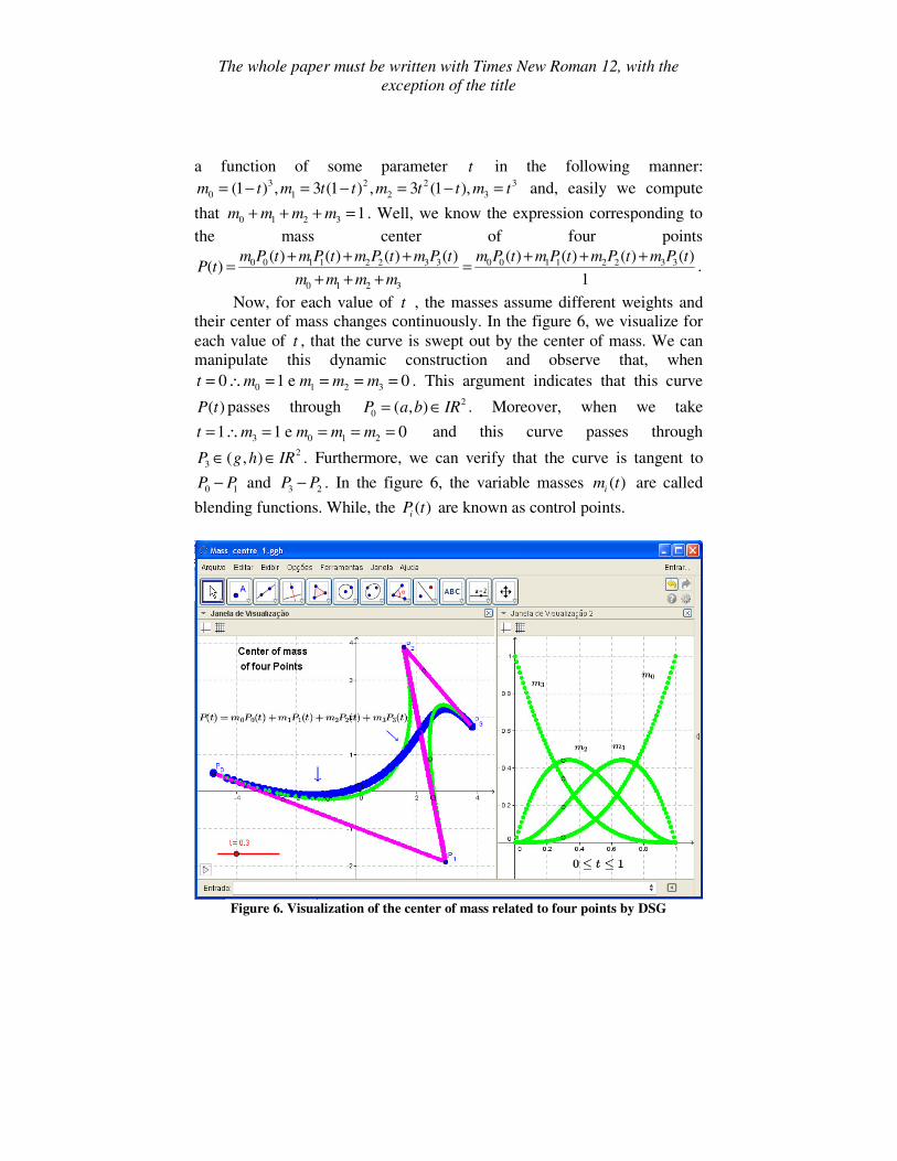
Now, for each value of t , the masses assume different weights and

their center of mass changes continuously. In the figure 6, we visualize for

each value of t , that the curve is swept out by the center of mass. We can

manipulate this dynamic construction and observe that, when

0 1 2 30 1 e 0t m m m m= ∴ = = = = . This argument indicates that this curve

( )P t passes through 2

0 ( , )P a b IR= ∈ . Moreover, when we take

3 0 1 21 1 e 0t m m m m= ∴ = = = = and this curve passes through 2

3 ( , )P g h IR∈ ∈ . Furthermore, we can verify that the curve is tangent to

0 1P P− and 3 2P P− . In the figure 6, the variable masses ( )im t are called

blending functions. While, the ( )iP t are known as control points.

Figure 6. Visualization of the center of mass related to four points by DSG



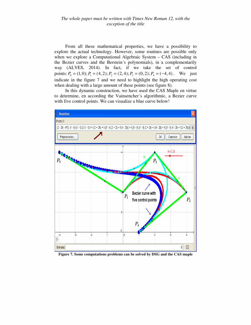
From all these mathematical properties, we have a possibility to

explore the actual technology. However, some routines are possible only

when we explore a Computational Algebraic System – CAS (including in

the Bezier curves and the Berstein´s polynomials), in a complementarily

way (ALVES, 2014). In fact, if we take the set of control

points: 0 1 2 3 4(1, 0); (4, 2); (2, 4); (0, 2); ( 4, 4)P P P P P= = = = = − . We just

indicate in the figure 7 and we need to highlight the high operating cost

when dealing with a large amount of these points (see figure 8).

In this dynamic construction, we have used the CAS Maple en virtue

to determine, en according the Vainsencher´s algorithmic, a Bezier curve

with five control points. We can visualize a blue curve below!

Figure 7. Some computations problems can be solved by DSG and the CAS maple



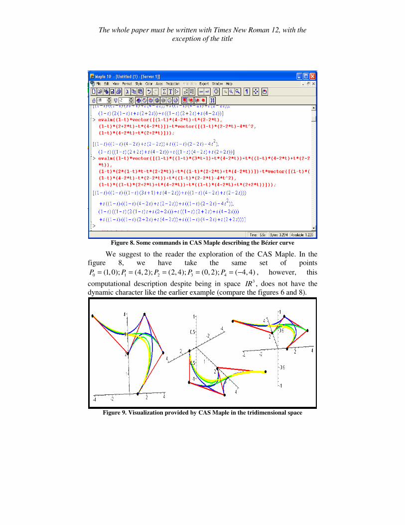
Figure 8. Some commands in CAS Maple describing the Bézier curve

We suggest to the reader the exploration of the CAS Maple. In the

figure 8, we have take the same set of points

0 1 2 3 4(1,0); (4, 2); (2, 4); (0, 2); ( 4, 4)P P P P P= = = = = − , however, this

computational description despite being in space 3IR , does not have the

dynamic character like the earlier example (compare the figures 6 and 8).

Figure 9. Visualization provided by CAS Maple in the tridimensional space



Final remarks In several computational methods we identify the multiple uses of Bézier

curves (like in Robotics and Computer Aided Geometric Design). In this

work, we have emphasized some application en virtue to describe some

basic graphical behavior of this concept and the Berstein´s polynomials too.

From historical point of view, the Bézier curve was formulated by

Pierre Bézier, in 1962 and, approximately of this period, Paul De Casteljau

developed the same curve. “The conic sections, the brachistochrone curve,

cycloids, hypocycloids, epicycloids are all examples of very interesting

curves that can be easily described and analyzed parametrically”

(NEUERBURG, 2003, p. 1). On the other hand, the difficulties with these

traditional examples of parameterization are the lack of applications

associated with them in several Calculus Books (ALVES, 2014)

Moreover, several computational problems indicate a strong

relationship between the Bernstein’s polynomials and the Bézier curves. In

fact, Bertot, Guillot & Mahboubi (2010) explain various situations. So, en

virtue a didactic preoccupation, similarly the Vainsencher´s intention, we

observe that some aspects that we have discussed here have a relevant

pedagogical value, particularly with regard to intuitive and geometric

understanding of a method briefly discussed in the context of Algebraic

Geometry (VAINSENCHER, 2009, p. 117). Indeed, we can visually

compare in the fig 9, an old and static description related to a Bezier curve.

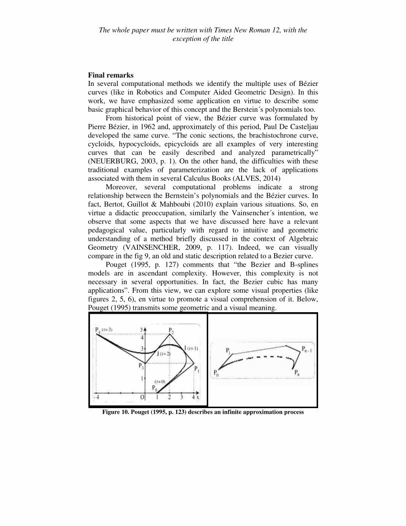
Pouget (1995, p. 127) comments that “the Bezier and B-splines

models are in ascendant complexity. However, this complexity is not

necessary in several opportunities. In fact, the Bezier cubic has many

applications”. From this view, we can explore some visual properties (like

figures 2, 5, 6), en virtue to promote a visual comprehension of it. Below,

Pouget (1995) transmits some geometric and a visual meaning.

Figure 10. Pouget (1995, p. 123) describes an infinite approximation process



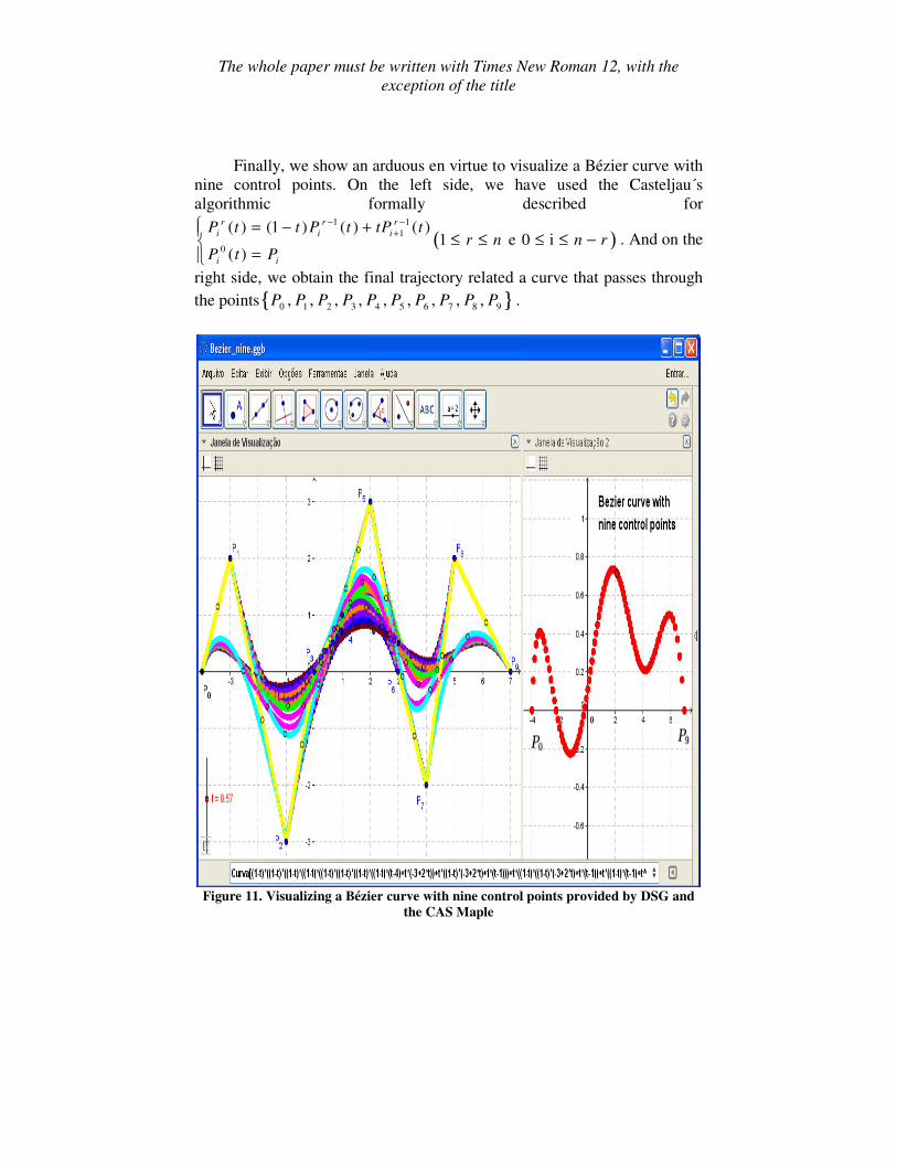
Finally, we show an arduous en virtue to visualize a Bézier curve with

nine control points. On the left side, we have used the Casteljau´s

algorithmic formally described for

( )1 1

1

0

( ) (1 ) ( ) ( )1 e 0 i

( )

r r r

i i i

i i

P t t P t tP tr n n r

P t P

− −+

= − +≤ ≤ ≤ ≤ −

=. And on the

right side, we obtain the final trajectory related a curve that passes through

the points{ }0 1 2 3 4 5 6 7 8 9, , , , , , , , ,P P P P P P P P P P .

Figure 11. Visualizing a Bézier curve with nine control points provided by DSG and

the CAS Maple



References

[Bed10] Y, Bertot; F. Guillot & A. Mahboubi – A formal study of

Berstein coefficients and polynomials, Orsay: Université

D´Orsay, University of Sussex, 2010. Available in:

http://hal.archives-ouvertes.fr/docs/00/52/01/44/PDF/RR-

7391.pdf

[FR14] F. R. V. Alves – Semiotic Register and the Internal Transition

to Calculus: Elements for a Didactic Engineer, Lima: Catholic

University of Peru, Conference, 2014.

[VI09] I. Vainsencher– Introdução às Curvas Algébricas, Rio de

Janeiro: IMPA, 2009.

[VI85] B. A. Barsky – Arbitrary subdivision of a Bézier Curves,

Califórnia: University of California, 1985.

[KMN03] K. M. Neuerburg – Bézier Curves, Lousinanna: Proceedings of

Mathematical Society of America - MMA, 2003. Avaliable in:

http://www.mc.edu/campus/users/travis/maa/proceedings/spring

2003/index.html

[GU08] T. Guillod – Interpolations, courbes de Bézier et B-Splines,

Buletin de la Societé des Enseignants Neuchâtelois de Sciences,

nº 34, 2008. Avaliable in: http://www.sens-

neuchatel.ch/bulletin/no34/art3-34.pdf

[VI09] J. P. Pouget – Modèle de Bézier et modèle de B-splines,

REPERE, IREM, nº 15, 119-134, 1995. Avaliable in:

http://www.univ-irem.fr/reperes/articles/15_article_105.pdf

[LLZ11] H Liu; L. Li & D. Zang – Study on a Class of TC-B´ezier

Curve with Shape Parameters, Journal of Information &

Computational Science, v. 8, nº 7, 2011, 1217-1223. Avaliable

in:

http://www.joics.com/publishedpapers/2011_8_7_1217_1223.pd

f

Visualizing Bezier´s curves: some applications of Dynamic System Geogebra

Documents

Transcript of Visualizing Bezier´s curves: some applications of Dynamic System Geogebra