Visualization of the High Level Structure of the Internet with HERMES

Journal of Graph Algorithms and Applicationshttp://jgaa.info/

vol. 6, no. 3, pp. 281–311 (2002)

Visualization of the High Level Structure of the

Internet with Hermes

Andrea Carmignani1 Giuseppe Di Battista1 Walter Didimo2

Francesco Matera1 Maurizio Pizzonia1

1Dipartimento di Informatica e Automazione,Universita di Roma Tre, via della Vasca Navale 79,

00146 Roma, Italy.{carmigna,gdb,matera,pizzonia}@dia.uniroma3.it

http://www.dia.uniroma3.it/2Dipartimento di Ingegneria Elettronica e dell’Informazione,

Universita di Perugia, Via G. Duranti 93, 06125 Perugia, [email protected]

http://www.diei.unipg.it/

Abstract

Hermes is a system for exploring and visualizing the Internet struc-ture at the level of the Autonomous Systems and their interconnections.It relies on a three-tier architecture, on a large repository of routing infor-mation coming from heterogeneous sources, and on sophisticated graphdrawing engine. Such an engine exploits static and dynamic graph draw-ing techniques, specifically devised for the visualization of large graphswith high density.

Communicated by Michael Kaufmann: submitted February 2001;revised December 2001 and May 2002.

Research supported in part by the European Commission – Fet Open project COSIN

IST-2001-33555.

Carmignani et al., Hermes, JGAA, 6(3) 281–311 (2002) 282

1 Introduction and Overview

Computer networks are an endless source of problems and motivations for theGraph Drawing and for the Information Visualization communities. Several sys-tems aim at giving a graphical representation of computer networks at differentabstraction levels and for different types of users. To give only some examples(an interesting survey can be found in [17]):

1. Application level: Visualization of Web sites structures, Web maps [18,16], and Web caches [10].

2. Network level: Visualization of multicast backbones [23], Internet traf-fic [24], routes, and interconnection of routers.

3. Data Link level: Interconnection of switches and repeaters in a local areanetwork [2].

We deal with the problem of exploring and visualizing the interconnectionsbetween Autonomous Systems. An Autonomous System (in the following AS) isa group of networks under the same administrative authority. Roughly speaking,an AS can be seen as a portion of the Internet, and Internet can be seen asthe totality of its ASes. To maintain the reachability of any portion of theInternet each AS exchanges routing information with a group of other ASesmainly selected on the basis of economic and social considerations. Severaltools have been developed for analyzing and visualizing the Internet topologyat the ASes level [9, 12, 24, 30]. However, in our opinion, such tools are stillnot completely satisfactory both in the interaction with the user and in theeffectiveness of the drawings. Some of them have the goal of showing largeportions of Internet, but the maps they produce can be difficult to read (seee.g. [9]). Other tools point the attention on a specific AS, only showing that ASand its direct connections (see e.g. [24]).

In this work we describe a new system, called Hermes, that provides a pub-licly accessible service over the Web1. It has a three-tier architecture whichallows the user to visually explore the Internet topology by means of automat-ically computed maps. Such maps are computed by a graph drawing modulebased on the GDToolkit library [21] whose main features are the following:

• Its basic drawing convention is the podevsnef [20] model for orthogonaldrawings having vertices of degree greater than four. However, since thehandled graphs have often many vertices (ASes) of degree one connectedwith the same vertex, the podevsnef model is enriched with new featuresfor representing such vertices.

• It is equipped with two different graph drawing algorithms. In fact, ateach exploration step the map is enriched and hence it has to be redrawn.Depending on the situation, the system (or the user) might want to use a

1http://www.dia.uniroma3.it/∼hermes


static or a dynamic algorithm. Of course, the dynamic and the static al-gorithms have advantages and drawbacks. The dynamic algorithm allowsthe user to preserve its mental map [19, 27] but can lead, after a certainnumber of exploration steps, to drawings that are less readable than thoseconstructed with a static algorithm.

• The static algorithm is based on the topology-shape-metrics approach [14]and exploits recent compaction techniques that can draw vertices with anyprescribed size [13]. The topology-shape-metrics approach has been shownto be very effective and reasonably efficient in practical applications [15].

• The dynamic algorithm is a new dynamic graph drawing algorithm thathas been devised according to three main constraints. (1) It had to becompletely integrated within the topology-shape-metrics approach in sucha way to be possible to alternate its usage with the usage of the static al-gorithm. (2) It had to be consistent with the variation of the podevsnefmodel used by Hermes. (3) It had to allow vertices of arbitrary size.Several algorithms have been recently proposed in the literature on dy-namic graph drawing algorithms. A linear time algorithm for orthogonaldrawings is presented in [5]. In this algorithm the position of the verticescannot be changed after the initial placement. Four different scenarios forinteractive orthogonal graph drawings are studied in [29]. Each scenariodefines the changes allowed in the common part of two consecutive draw-ings. An interactive version of Giotto [33] is described in [8]; it allowsthe user to incrementally add vertices and edges to an orthogonal draw-ing in such a way that the shape of the common part of two consecutivedrawings is preserved and the number of bends is minimized under thisconstraint. A dynamic algorithm for orthogonal drawings that allows usto specify the relative importance of the number of bends vs. the numberof changes between two consecutive drawings is given in [6]. Other algo-rithms for constructing drawings of graphs incrementally, while preservingthe mental map of the user, are for example [26, 11, 28]. Also, a study ondifferent metrics that can be used to evaluate the changes between draw-ings in an interactive scenario is presented in [7]. However, as far as weknow, none of the cited dynamic algorithms enforces all the constraints(1), (2), and (3).

The paper is organized as follows. In Section 2 we give basic definitionsabout graph drawing and AS level networking which are needed to understandthe rest of the work. The reader that is not interested in networking may skipSection 2.1. In Section 3 we explain how the user interacts with Hermes andprovide a high level description of the functionalities of the system. In Section 4we give some details about the three-tier architecture of Hermes. Section 5shows the results of a study on the ASes interconnection graph. Such a studyhas been performed in order to design the drawing convention and the drawingalgorithms of Hermes. In particular, we analyze the density of the graph andits distribution, and we give measures on the average degree of the vertices.


In Section 6 we describe in detail the drawing convention and the algorithmsused by system. The techniques we adopt are not limited to the application do-main described in this paper, but they are suitable for exploring and visualizinggeneral large graphs with high density. In Section 7 some statistics about theeffectiveness of Hermes as a Web service are provided. Conclusions and openproblems are given in Section 8.

2 Background

2.1 Networking

Each AS groups a set of networks. An AS is identified over the Internet byan integer number while each network is identified by its IP address. A routeis a (directed) path on the Internet that can be used to reach a specific setof (usually contiguous) IP addresses, representing a set of networks. A routeis completely described by its destination IP addresses, its cost, and by theordered set of ASes that it traverses (usually called AS-path). Routes can beseen as advertisements, from an AS to its adjacent ASes, meaning “through meyou can reach a certain set of networks, with a certain cost and traversing acertain set of other ASes”.

In order to exchange information about the routes, the ASes adopt a routingprotocol called BGP (Border Gateway Protocol) [31]. Such a protocol is basedon a distributed architecture where border routers that belong to distinct ASesexchange information about the routes they know. Two border routers thatdirectly exchange information are said to perform a peering session, and theASes they belong to are said to be adjacent. We define the ASes interconnectiongraph as the graph having a vertex for each AS and one edge between each pair ofadjacent ASes. Note that, according to our definition, the ASes interconnectiongraph is not a multigraph.

Each route is incrementally built. A route is originated by an AS and initiallyit contains only such AS, then it is propagated to adjacent ASes which appendtheir identifiers to the AS-path of the route and propagate it again. Hence, inthe AS-path of a route two consecutive ASes are always adjacent.

2.2 Graph Drawing

We assume familiarity with elementary graph theory and graph connectiv-ity [22].

A plane drawing Γ of a graph G maps each vertex of G to a point of theplane, and each edge of G to a Jordan curve between the two points associatedwith the end-vertices of the edge. A drawing Γ of G is planar if any two edgesnever intersect except at common end-vertices. A graph is planar if it admitsa planar drawing. A planar drawing Γ of G induces for each vertex v of G acircular clockwise ordering of the edges incident on v. Also, Γ subdivides theplane into topologically connected regions, called faces. Exactly one of these


faces is unbounded; it is called external face. The other faces are said to beinternal. Two planar drawings of G are said to be equivalent if (i) for eachvertex v of G they induce the same ordering of the edges around v, and (ii) theyhave the same external face. Note that two equivalent drawings of G have thesame set of faces. An embedding φ of G is a class of equivalent planar drawings ofG. In other words, we can regard an embedding of G as the choice of a clockwiseordering of the edges around every vertex plus the choice of the external face.An embedded graph Gφ is a planar graph G with a given embedding φ.

An orthogonal drawing of G is a drawing of G such that all edges are rep-resented as polygonal lines of horizontal and vertical segments. Clearly, anorthogonal drawing of G exists if and only if G is 4-planar, that is, each vertexof G has at most four incident edges. An orthogonal representation (or shape) ofG is an equivalence class of planar orthogonal drawings such that the followinghold:

1. For each edge (u, v) of G, all the drawings of the class have the samesequence of left and right turns (bends) along (u, v), while moving from uto v.

2. For each vertex v of G, and for each pair {e1, e2} of clockwise consecutiveedges incident on v, all the drawings of the class determine the same anglebetween e1 and e2.

Roughly speaking, an orthogonal representation defines a class of orthogonaldrawings that may differ only for the length of the segments of the edges.

In order to orthogonally draw graphs of arbitrary vertex degree, differentdrawing conventions have been introduced in the literature. Here we recall thepodevsnef (planar orthogonal drawing with equal vertex size and not emptyfaces) drawing convention, defined by Foßmeier and Kaufmann [20]. In a pode-vsnef drawing (see Figure 1 (a)):

1. Vertices are points of an integer coordinate grid (but it is easier to thinkof them in terms of squares of half unit sides centered at grid points).

2. Two segments that are incident on the same vertex may overlap. Observethat the angle between such segments has zero degree.

3. All the polygons representing the faces have area strictly greater thanzero.

4. If two segments overlap they are presented to the user as two very nearsegments.

An algorithm that computes a podevsnef drawing of an embedded planargraph with the minimum number of bends is presented in [20] . Further, theauthors conjecture that the drawing problem becomes NP-hard when Condi-tion 3 is omitted. The podevsnef drawings generalize the concept of orthogonal


1

2

3

4 5

6 7

(a)

4

6 7

5

3

vertex width height

1 1 12 2 03 0 04 0 0

6 0 07 0 0

5 0 1

1

2

(b)

Figure 1: (a) A podevsnef drawing; (b) A podavsnef drawing with the sameshape as the drawing in (a); the sizes of the vertices are specified in the table.

representation, allowing angles between two edges incident to the same vertex tohave a zero degree value. The consequence of the assumption that the polygonsrepresenting the faces have area strictly greater than zero is that the angleshave specific constraints. Namely, because of Conditions 2 and 3, each zerodegree angle is in correspondence with exactly one bend [20]. An orthogonalrepresentation corresponding to the above definition is a podevsnef orthogonalrepresentation.

A drawing convention that allows the user to draw graphs in which each sin-gle vertex has a prescribed size (width and height) has been introduced in [13].Such a drawing convention is referred to as podavsnef (planar orthogonal draw-ing with assigned vertex size and non-empty faces). A podavsnef drawing hasthe following properties (see also Figure 1 (b)):

1. Each vertex is a box with specific width and height (assigned to eachsingle vertex by the user).


2. Two segments that are incident on the same vertex may overlap. Again,the angle between such segments has zero degree.

3. Consider any side of length l ≥ 0 of a vertex v and consider the set I ofarcs that are incident on such side.

(a) If l + 1 > |I| then the edges of I cannot overlap.

(b) If l+1 ≤ |I| then the edges of I are partitioned into l+1 non-emptysubsets such that all the edges of the same subset overlap.

4. The orthogonal representation constructed from a podavsnef drawing bycontracting each vertex into a single point is a podevsnef orthogonal rep-resentation.

A polynomial time algorithm for computing podavsnef drawings of an em-bedded planar graph with the minimum number of bends over a wide class ofpodavsnef drawings is also described in [13].

3 Using Hermes

The user interacts with Hermes through a map (subgraph) of the ASes inter-connection graph. A map is initially constructed using two possible startingprimitives.

AS selection An AS is chosen. The obtained map consists of such an AS plusall the ASes that are connected to it. See Fig. 2(a).

Routes selection A set of routes is selected. The user has three possibilities:(1) selection of all the routes traversing a specific AS (see Fig. 3(a)); (2)selection of the routes starting from a specific AS (see Figs. 3(b)); (3)selection of all the routes traversing a specific pair of ASes. The obtainedmap consists of all the ASes and connections traversed by the selectedroutes.

The user can explore and enrich the map by using the following primitive:

AS exploration an AS u among those displayed in the current map is selected.The current map is augmented with all the ASes that are connected tou. Further, for each AS v connected to u an edge (u, v) is added. Ob-serve that, according to this definition, a map is a subgraph of the ASesinterconnection graph but in general it is not an induced subgraph.

Fig. 2 shows a sequence of exploration primitives applied to the map of Fig. 2(a).ASes 5583, 5484, and 6715 are explored in Fig’s. 2(b), 2(c), and 2(d), respec-tively. Fig. 2 highlights several features of Hermes. Hermes can constructnew drawings either using a static or a dynamic graph drawing algorithm. Thedrawing of Fig. 2(b) has been constructed with a dynamic algorithm starting


(a) Selection of AS 12300. (b) Exploration of AS 5583.

(c) Exploration of AS 5484. (d) Exploration of AS 6715.

Figure 2: Exploration steps in the ASes graph. The selected AS is always drawnred.


(a) Map containing all the routes traversingAS 137.

(b) Map containing only routes starting fromAS 137.

Figure 3: Selection of the routes traversing AS 137.


Figure 4: A map obtained with several exploration steps.

from the drawing of Fig. 2(a), and the drawing of Fig. 2(d) has been constructedwith the same algorithm starting from the drawing of Fig. 2(c). Conversely, thedrawing of Fig. 2(c) is obtained with a static algorithm. The choice of the al-gorithm to be applied can be done by the system (see Section 6) or forced bythe user. Since the ASes degree can be large (see Section 5), in the project ofthe drawing algorithms of Hermes, special attention has been devoted to therepresentation of vertices of high degree. Fig. 2 shows how the vertices of degreeone are placed around their adjacent vertices. A more complex map obtainedwith Hermes is depicted in Fig. 4. It contains more than 150 ASes.

Working on a map, independently on the way it has been obtained, the usercan get several information on any AS:

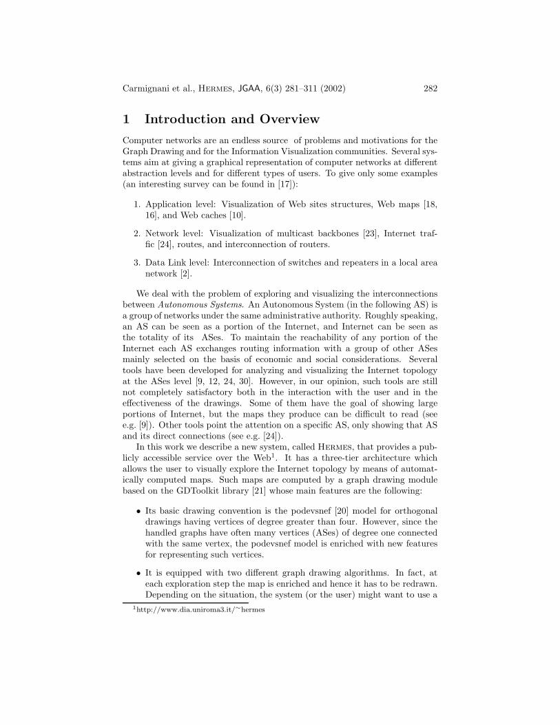
General Info name, maintainers, and description of the AS. See Fig. 5.

Routing Policies For each connected AS, an expression describing the policyand its cost. See Fig. 5. This is possible both for in and for out policies.The default AS is also displayed.

Internal Routers List of the known border routers with the IP-numbers ofthe interfaces. Peering sessions with other routers are displayed.


Figure 5: General Info and routing policies for AS 5484.

Routes List of the routes originated by the AS (see Fig. 6). It is also possibleto visualize the propagation of a given route in the ASes composing themap.

AS Macros List of the macros [3] including the AS.

4 A Three-Tier Architecture

Hermes has a three-tier client/server architecture. The user interacts with atop-tier client which is in charge of collecting user requests and showing results.The requests are forwarded by the client to a middle-tier server which is incharge to process the raw data extracted from a repository (bottom-tier).

The client is a multi-document GUI-based application. It allows the user tocarry-on multiple explorations of the ASes interconnection graph at the sametime. The Java technology has been used to ensure good portability. Snapshotsof the GUI have been shown in Section 3.

In Hermes the middle-tier server maintains the state of the session, that isthe current map, for each connected user. The client communicates with the


Figure 6: Routes through AS 5583.


server opening a permanent TCP connection for each user. This permits toamortize the inefficiency of the connection set up over all the requests of ses-sion. The protocol transported by such connections is specifically tailored forour application. In particular, the server sends its reply in the form of serial-ized software objects describing ASes, links, and related geometric information.The Java run-time environment transparently encodes objects into bytes on themiddle-tier server and consistently decodes them on the client side.

The repository is updated off-line from a plurality of sources. At the momentwe access the following databases adopting, for representing data, the RPSL lan-guage [1]: ANS, APNIC, ARIN, BELL, CABLE&WIRELESS, CANET, MCI,RADB, RIPE, VERIO. Further, we access the routing BGP data provided bythe Route views project of the Oregon University [25]. However, the repositoryis easily extensible to other data sources.

Data are filtered so that only the information used by Hermes are storedin the database, but no consistency check or ambiguity removal is performedin this stage. The overall size of the repository is about 50 MB. The adoptedDBMS technology is currently mysql.

The crucial part of the system is mainly located in the middle-tier. Thetop-tier requests two types of service to the middle-tier.

General info services the top-tier queries about ASes, routes, and path prop-erties.

Topology services the top-tier queries for a new exploration and gets back anew map.

Info services requests are independent of each other and hence are independentlyhandled by the middle-tier. On the contrary, topology services requests arealways part of a drawing session. Each client may open one or more drawingsessions. Each drawing session is associated with a map that can be enrichedby means of exploration requests.

Info services requests are directly dispatched to a mediator. The mediatormodule is in charge to retrieve the data from the repository and to removeambiguities on-the-fly.

Topology services requests are handled by the kernel of the middle-tier. Itgets information from the mediator and inserts new edges and vertices into themap. The drawing is computed by the drawing engine module (see Section 6).The drawing engine is based on the GDToolkit [21] library.

5 AS Interconnection Data from a Graph Draw-

ing Perspective

In order to devise effective graph drawing facilities for Hermes, we have ana-lyzed the ASes interconnection graph G. The data at our disposal2 show thefollowing structure for G.

2Observation of May 2000.


1

10

100

1000

50 100 150 200 250 300 350 400 450

Num

ber

of A

Ses

Degree

Figure 7: AS degree distribution (log. scale)

1

10

100

1000

10000

0 5 10 15 20 25 30

Num

ber

of A

Ses

Local density

Figure 8: AS local density distribution (log. scale)


0

20

40

60

80

100

0 5 10 15 20 25 30

perc

enta

ge o

f AS

es

density

Figure 9: Percentage of ASes adjacent to an AS whose local graph has at leasta given value of density

The number of vertices of G is 6, 849 and the number of edges is 27, 686.Fig. 7 illustrates the distribution of the degree of the vertices. The figure showsthat while there are many vertices (about 75%) with degree less than or equal to4, there are also several vertices whose degree is more than 100. For improvingthe readability of the chart, we have omitted two vertices with degree 862 and1, 044, respectively. Further, consider that G contains 473 isolated vertices.

The density of G is 4.04. However, the “local” density can be much greater.In order to estimate such a local density, we have computed, for each vertexv, the density of the subgraph induced by the vertices adjacent to v. We callsuch graphs local graphs. Fig. 8 illustrates the distribution of the densities ofthe local graphs. From the figure it is possible to observe that about 5% of thelocal graphs have density greater than 10.

We have also tried to estimate the probability, for a user that explores G, toencounter a portion of G that is locally dense. Fig. 9 shows, for each value d ofdensity, what is the percentage of vertices that are adjacent to a vertex whoselocal graph has density at least d. Note that more than 30% of the vertices areadjacent to a vertex whose local graph has density at least 10.

Concerning connectivity, the graph has 480 connected components, includingthe above mentioned 473 isolated vertices. One of them has 6, 360 vertices; eachof the remaining 6 components has less than 6 vertices.


6 Drawing Conventions and Algorithms

We recall that the user interacts with the maps of the ASes interconnectiongraph G by means of the AS exploration primitive, described in Section 3.Namely, each time such a primitive is applied on a vertex u of the current mapM , such a map is enriched with the vertices and the edges that are directlyconnected to u in G and that were not present in M . Then a drawing of thenew current map is computed and displayed.

The choice of our exploration primitive for G is mainly motivated by theanalysis performed on the structure of G (see Section 5). In particular, sinceG has many vertices that are adjacent to a vertex whose local graph has highdensity, we decided to discard a classical exploration approach based on inducedsubgraphs, because it is often lead to extremely dense maps.

In Section 6.1 we describe the drawing convention we adopt for visualizingthe maps of G throughout a sequence of exploration steps performed by theuser. In Section 6.2 we provide two different strategies for computing drawingsof the maps within the defined drawing convention.

6.1 Drawing Convention

When the AS exploration primitive is applied on the current map M of G,the vertices of G−M added to M will have degree one in the new current map.Also, these vertices of degree one are often numerous, due to the structure ofG. Hence, for drawing a map we use a specific drawing convention that allowsus to optimize the space occupied by the vertices of degree one.

Such a drawing convention is based on a variation of the podevsnef model fororthogonal drawings with high degree vertices (see Section 2.2). We modify thepodevsnef model as follows. Each vertex of degree one adjacent to a vertex v isappropriately positioned on an integer coordinate grid around v and connectedto v with a straight-line edge. Namely, as shown in Figure 10, vertex v isassociated with a box partitioned into nine rectangles arranged into three rowsand three columns. Denote these rectangles as Bij , (i, j ∈ {1, 2, 3}). RectangleB22 is used for drawing v centered on a grid point. Rectangles B11, B13, B31,and B33 are used for drawing the degree-one vertices adjacent to v. Theirincident edges are represented with straight-line segments, possibly overlappingother degree-one vertices. Actually, they are drawn on the back of the vertices.Rectangles B12, B21, B32, and B23 are used for hosting the connections of v tothe other vertices.

The height hc of the center row is equal to one grid unit as well as the widthwc of the center column. Rectangles B11, B13, B31, and B33 have all the samewidth w and height h. The values of h and w are expressed in terms of gridunits and must guarantee enough room for placing all the degree-one vertices.How w and h are computed will be detailed in Section 6.3.


wc

h c

B11 B13

B21 B23

B31 B33

B12

B22

B32

h

h

w w

(a) (b)

Figure 10: Using a box to make room around a vertex. (a) The nine rectanglesthat partition the box. (b) Using the nine rectangles to place the degree-onevertices. Each vertex in the box is centered on an integer grid point.

6.2 Algorithms Overview

In this section we describe two different strategies for computing drawings of themaps within the defined drawing convention, during a sequence of explorationsteps. Namely, at each exploration step Hermes computes a new drawing ofthe current map, by applying one of the two following algorithms:

Static algorithm The current map is completely redrawn, after the new ver-tices and edges have been added.

Dynamic algorithm The new vertices and edges are added to the currentdrawing in such a way that the shape of the existing edges and the positionof the existing vertices and bends are preserved “as much as possible”.

Both the dynamic and the static algorithms have advantages and drawbacks.The dynamic algorithm allows the user to preserve its mental map but can lead,after a certain number of exploration steps, to drawings that are less readablethan those constructed by the static algorithm. In fact, the dynamic algorithmmakes use of local optimization strategies. The optimization strategies of thestatic algorithm are global and more effective. However, with the static algo-rithm, the new drawing can be quite different from the previous one and theuser’s mental map can be lost.

Because of the above motivations, Hermes automatically chooses betweenthe static algorithm and the dynamic algorithm, according to the following cri-teria. Suppose v is the vertex that the user wants to explore. Hermes computes


a dynamic exploration cost associated with v. Such a cost represents an esti-mate of the efficiency and effectiveness of the dynamic algorithm with respectto the new exploration. In the current implementation of Hermes it simplydepends on the kind and the number of drawing primitives (see Section 6.5)that would be needed for constructing the drawing of the new map with thedynamic algorithm and on how many consecutive times the dynamic algorithmhas been invoked before the exploration of v. Once the exploration cost hasbeen computed, Hermes compares it with a threshold value that can be set-upin a configuration menu of the system. If the exploration cost is lower thanthe threshold value, Hermes applies the dynamic algorithm, else it applies thestatic algorithm.

In the next two subsections we give details on how the static and the dynamicalgorithms work in practice.

6.3 The Static Algorithm

Let G be the ASes interconnection graph and let M be the current map. Werecall that M is a subgraph of G. Let v be the vertex of M explored by theuser at the generic step. Map M is enriched with the vertices and the edgesof G that are not present in M and are directly connected to v in G. Thenew map, which we still call M for simplicity, is fully redrawn according to thestatic algorithm, which consists of the following steps.

1. (Degree-one Vertex Removal) Vertices of degree one are temporarily re-moved from M . We call M ′ the new map. Each vertex u of M ′ is labeledby the number δ(u) of vertices of degree one that were attached to it.

2. (Planarization) A standard planarization [14] technique is applied to M ′.In this phase a planar embedding ofM ′ is computed and crossings amongedges are represented by dummy vertices that will be removed later. Wecall such vertices cross vertices.

3. (Orthogonalization) A podevsnef representation ofM ′ is constructed withinthe computed embedding.

4. (Compaction) A drawing for M ′ is computed from its orthogonal repre-sentation by assigning coordinates to vertices and bends. Since for eachvertex u, our drawing convention requires that δ(u) vertices of degree oneare placed around u, we must guarantee enough room for them (see Sec-tion 6.1). To do that we compute a podavsnef drawing by applying thealgorithm described in [13]. Each vertex u is drawn as a box whose heighth and width w depend on δ(u). We set w = √δ(u)/2. The height his set equal to = w − 1 if this ensures enough room for all the vertices tobe placed; else we set h = w. If δ(u) = 0 then we set h = w = 0. Werecall that w and h are expressed in terms of grid units. For example,referring to Figure 10, we have that δ(u) = 32 (u is the vertex on thecenter of the box and has 32 vertices of degree one connected to it) and


then w = 3. Also, h = 2 is not sufficient for hosting all the 32 verticesinto the four rectangles B11, B13, B31, B33 (in fact, if h = 2 we can placeat most w × h × 4 = 3 × 2 × 4 = 24 vertices inside the box). Hence his set equal to 3 (in this way we can place up to 36 vertices inside thebox; we use 32 positions for placing vertices and 4 positions will be notused). We also have to guarantee that the edges that connect u to nondegree-one vertices are always incident on the middle points of the sidesof the box. The basic version of the algorithm described in [13] allows theedges to freely shift along the side they are incident on. However, it ispossible to easily adapt such an algorithm so that each edge is incident ona pre-assigned point. Finally, cross vertices are removed.

5. (Degree-one Vertex Re-insertion) The drawing is completed by replacingthe box of each vertex u such that δ(u) > 0 with a half unit square (edgesthat are incident on u are stretched). Also, the vertices of degree one thatare incident on u are distributed in the rectangles B11, B13, B31, and B33

and connected to u, according to the adopted drawing convention (seeFigure 10(b)).

6.4 The Dynamic Algorithm

As in the case of the static algorithm, we denote by G the ASes interconnectiongraph and by M the current map. Also, denote by D the current drawing ofM . Let v be the vertex of M explored by the user at the generic step.

The dynamic algorithm enrichesM and D incrementally, by adding the ver-tices and the edges of G that are not present inM and are directly connected tov in G, in such a way that the user mental map is preserved as much as possible.Before describing how the dynamic algorithm works, we need to introduce somefurther notation.

Denote by ∆Ev and by ∆Vv the set of the edges and the set of the verticesto be inserted for exploring v. We recall that all the edges in ∆Ev are incidenton v and that the vertices in ∆Vv will be degree-one vertices attached to v in thefinal drawing. For simplicity, we always use the notationM and D to denote theintermediate maps and drawings during the execution of the dynamic algorithm.In other words, we are assuming thatM and D change dynamically throughoutthe algorithm execution. However, at the generic step of the dynamic algorithm,some of the vertices of M might be not explicitly represented in D. Namely,each vertex u of D might absorb all the degree-one vertices adjacent to it andimplicitly represent the number of these vertices by a label δ(u), as in the caseof the static algorithm. We call V1 the set of degree-one vertices of M thatare not explicitly represented in D, and V2 all the vertices of M that are alsoexplicitly represented in D. Note that, V1 and V2 partition the set of vertices ofM , and that at the beginning of the dynamic algorithm V1 is empty. Sets ∆Vv,V1, and V2 are modified during the algorithm execution.

A high level description of the dynamic algorithm is as follows (refer toFigure 11):


u2

u1

u2 u2

u2

u1

u2

u1

u2

u1

2

6

3

v

2

6

3

v v

v

7

2

4

2

6

4

v

(a) (b) (c)

(d) (e) (f)

Figure 11: An example of the dynamic algorithm. (a) The initial drawing of amap; the user chooses to explore vertex v; suppose that v is directly connected tou1 and u2 in the ASes interconnection graph. (b) In the first step of the dynamicalgorithm all the degree-one vertices of the drawing are temporarily removed;the remaining vertices are labeled with the number of vertices of degree one thatwere connected to them. (c) Vertex v is reinserted by using the Attach-Vertexprimitive. (d) Vertex u1 is reinserted by using the Attach-Vertex primitive andthen edge (v, u1) is inserted by using the New-Edge primitive. (e) Edge (v, u2)is inserted by using the New-Edge primitive. (f) The compaction step is appliedand the removed degree-one vertices are completely reinserted.

Step 1 We temporarily remove from D all the degree-one vertices. Each vertexu of D is labeled with the number δ(u) of vertices of degree one that wereattached to it (see Figure 11 (b)). The deleted vertices are moved fromV2 to V1. Note that, D is now a podevsnef drawing in the standard sense,where edge crossings are still replaced by cross vertices.

Step 2 We incrementally add to M the edges of ∆Ev and the vertices of ∆Vv.At the same time, specific subsets of edges and vertices ofM are added toD, by applying on D a sequence of two primitives that modify the drawingwithin the podevsnef standard. The two primitives are as follows:

New-Edge(u,z) A new edge is added to the drawing between the twovertices u and z; vertices u and z must be already explicitly repre-sented in D.


Attach-Vertex(u) A new vertex z is added toD and connected to u witha new edge (u, z); vertex u must be already explicitly representedin D.

How such primitives work in practice will be detailed in Section 6.5. Theinsertion of vertices and edges in M and D is performed according to thefollowing ordered set of rules:

• If the explored vertex v belongs to V1 (that is, if v is a one-degreevertex in M), we call w the vertex of V2 that is connected to v inM . We reinsert v in D (that is, we explicitly represent v in D) byperforming primitive Attach-Vertex(w) (see Figure 11 (c)). Consis-tently, we decrease δ(w) by a unit, set δ(v) = 0, and move v from V1

to V2.

• For each edge e = (v, u) of ∆Ev we insert in M vertex u, if it is notalready present in M , and edge e. After that, drawing D is modifiedaccording to the following three cases:

1. If u is in V1, we reinsert (explicitly represent) u in D by per-forming primitive Attach-Vertex(z), where z is the vertex of V2

connected to u in M ; then we add e to D, by applying primitiveNew-Edge(v,u) (see Figure 11 (d)). Consistently, we decreaseδ(z) by a unit, set δ(u) = 0 and move u from V1 to V2 .

2. If u is in V2, we add edge e to D by performing primitive New-Edge(v,u)(see Figure 11 (e)).

3. If u is in ∆Vv we just increase δ(v) by a unit, and move u from∆Vv to V1 (u will be implicitly represented in D).

Once all edges in ∆Ev have been considered ∆Vv is empty, M iscompletely updated with the vertices and edges selected for insertionby the exploration of v, and the only vertices that remain to be addedto D (those in V1) are all the vertices (different from v) that havedegree one in M .

Step 3 We perform onD the Compaction step and the Degree-one Vertex Rein-sertion step described for the static algorithm. The degree-one verticesreinserted are those in V1 (see Figure 11 (f)).

6.5 Primitives of the Dynamic Algorithm

In this section we conclude the description of the dynamic algorithm by explain-ing how primitive New-Edge and Attach-Vertex work.

We recall that these primitives modify a podevsnef drawing D preservingthis drawing standard. Both the primitives compute the position of the newvertices and edges trying to optimize, at the same time, the following measures:number of crossings, number of bends, and edge length. Each of these measureshas a prescribed cost that can be passed as a parameter to the primitives.


1246

Figure 12: Collapsing the edges incident on the same side of a vertex. The labelsrepresent the thickness of the edges. The small circles are the chain vertices.

In this way it is possible to decide the priority of each measure in the wholeoptimization. Once any of the primitives has been applied, the new drawing isguaranteed to have the same shape as the previous one, for the common parts.

The two primitives use two auxiliary data structures to perform their work.These data structures are a simplified orthogonal representation of the currentdrawing and a directed network associated with this orthogonal representation.We now describe these two data structures. After that, we shall describe howthey are used by the primitives.

Let H be the orthogonal representation of D. The first data structure is anorthogonal representation H ′ obtained from H in the following way:

• H is simplified so that all vertices have degree less than or equal tofour. This is done with a standard technique adopted in the podevsnefmodel [4], where all the edges incident on the same vertex from the sameside are collapsed into a chain of edges (see Fig. 12). Each edge of thechain replaces a certain number of edges (possibly only one). We associatewith each edge a thickness representing the number of edges replaced byit. We call the new vertices inserted by this operation chain vertices.

• Each face of H (including the external one) is decomposed into rectanglesby adding a suitable number of dummy edges and vertices, with the lineartime algorithm described in [32]. We call dashed the dummy edges andsolid the edges of the original orthogonal representation.

The second data structure is a directed network N associated with H ′. Wecall such a network the incidence network ofH ′. N is used to implicitly describeall the orthogonal paths that a new edge can follows inH ′. Further, N is definedso that each path has an associated cost that reflects the cost of the new edgein terms of bends, edge crossings, and edge length. We denote by χ, β, and λthe costs of one crossing, one bend, and one edge length unit, respectively. Asalready mentioned at the beginning of this section, these costs can be set-up bythe user in order to determine the priority level of the three different measuresduring the optimization.

Network N is defined as follows (see Fig. 13(a)):


• N has a node v associated with each edge e (solid or dashed) of H ′. Also,v has an associated cost that represents the cost of crossing e. Namely:

– If e is a solid edge then the cost of v is set-up equal to the thicknessof e multiplied by χ (see Fig. 13(a)). This reflects the fact that apath of N traversing v corresponds to a new edge of H ′ traversingedge e, and hence to a new edge of H that crosses a number of edgesequal to the thickness of e.

– If e is a dashed edge then the cost of v is set-up equal to zero. Thisis because dashed edges of H ′ are dummy and will be removed in thefinal drawing. Hence, they do not really originate edge crossings.

• N has an arc between every pair of nodes associated with two edges e1and e2 in the same face f of H ′. Such an arc represents an orthogonalpath inside f , which can be used to reach e2 from e1 (or vice-versa) in H ′.We distinguish three different kinds of arcs of N with respect to a face fof H ′ (refer to Fig. 13):

– An arc a between nodes associated with two horizontal (vertical)edges that lie on different sides of f (see, for example, arc a1 inFig. 13(a)). In this case, we associate with a a straight-line path p (apath with no bends) inside f , because it suffices to move from a sideof f to its opposite in the orthogonal representation (see Fig. 13(b)).Hence, denoted by d1, d2 (d3, d4) the lengths (in terms of number ofedges) of the vertical (horizontal) sides of f , we assign cost dλ to arca, where d = max{d1, d2} (d = max{d3, d4}). Such a cost is a lowerbound on the length of p.

– An arc a between a node associated with a horizontal edge eh and anode associated with a vertical edge ev of f (see, for example, arc a3in Fig. 13(a)). In this case, we associate with a an orthogonal path pwith exactly one bend, as depicted in Fig. 13(c). Denoted by sv theside of f on which ev lies, let dv be the number of edges of sv thatare necessarily spanned (completely or partially) by the projection ofp on sv. Analogously, denoted by sh the side of f on which eh lies,let dh be the number of edges of sh that are necessarily spanned bythe projection of p on sh. Hence, the cost we assign to a is equalto β + (dv + dh)λ. In particular, (dv + dh)λ still represents a lowerbound on the length of p, while β is the cost for one bend.

– An arc a between the nodes associated with two edges e1 and e2 thatlie on the same side of f (see, for example, arc a2 in Fig. 13(a)). Inthis case, we associate with a an orthogonal path p with two bends,as shown in Fig. 13(d). Denoted by s the side of f in which lie thetwo edges, let d be the number of edges of s that are necessarilyspanned (completely or partially) by p. Hence, the cost we assign toa is equal to 2β+(d+2)λ. The two extra units for the length are due


3χ 2χ χ

χ

χ

χ

2λ1aβ2 + 4λ

2a

3aβ+3λ

(a) Nodes (little squares) and three arcsof the incidence network for a face of asimplified orthogonal representation.

d1=2 d =2 1

d =4 2

d =3 3

p

(b) The orthogonal path p associatedwith arc a1.

1d =h

2d =v

p

(c) The orthogonal path p associatedwith arc a3.

2=d

p

(d) The orthogonal path p associatedwith arc a2.

Figure 13: Example of construction of an incidence network and related orthog-onal paths.


p

u v

(a)

pu

v

(b)

p

u

v

(c)

p

v

u

(d)

pu

v

(e)

p

u v

(f)

Figure 14: Possible cases of orthogonal paths between two vertices of the sameface of an orthogonal representation.

to the fact that p consists also of two (unit-length) segments havinga direction (vertical or horizontal) orthogonal to the direction of s.

We now explain how primitives New-Edge and Attach-Vertex perform onthe current drawing D.

• Primitive New-Edge(u,v) computes from D the simplified orthogonal rep-resentation H ′ and the associated network N ′ above described. Clearly,from the point of view of the primitive interface, H ′ and N are transpar-ent. It just needs to know u, v and D. After that, two different cases arepossible:

Case 1 Nodes u and v belong to two different faces of H ′. In this case,the primitive completes network N by adding two extra nodes rep-resenting u and v. For simplicity we still refer to these extra nodesas u and v. Also, for each edge e of H ′ incident on u (resp. v) theprimitive adds to N an arc between u (resp. v) and the node of Nassociated with e. All these extra arcs of N have zero cost. At thispoint, the primitive computes on N a shortest path between u andv. Such a path determines the route and the shape of the new edge(u, v) in H ′, according to the rules illustrated in the construction ofN . Namely, the new edge is added to H ′ following the arcs of theshortest path. Note that, the route and the shape of the new edge inH ′ uniquely induces the route and the shape of the same edge in H .Hence, the primitive adds edge (u, v) to H and computes the new


drawing D by compacting H with a standard compaction algorithmfor podevsnef orthogonal representations [20, 4].

Case 2 Nodes u and v belong to the same face. In this case the shapeof edge (u, v) is simply chosen according to the set of cases shown inFigure 14.

• Primitive Attach-Vertex(u) works much simpler then New-Edge. It mustadd a new edge e that connects a new node to u. The primitive looks inH ′ for a side s of u such that either no edge is incident on s or a dashededge is incident on s. If such a side s exists, the primitive add to H ′, andtherefore to H , edge e as a straight edge incident on s. Otherwise, theprimitive chooses an arbitrary side of u to insert edge e, and in this caseedge e will have one bend in H . Finally, the new drawing D is computedby compacting H with a standard compaction algorithm for podevsneforthogonal representations.

Note that, if a sequence of consecutive dynamic primitives have to be appliedbeforeD is displayed (as it often happens in a singleHermes’s exploration step),the computation of D can be delayed until the end of the sequence. In thiscase, H ′ and N can be kept up to date after each primitive is executed insteadof reconstructing them each time.

7 Statistics on the Hermes Service

We implemented Hermes as a service publicly available on the Web3. In thissection we intend to show the effectiveness of the service. To this aim we pro-vide several statistics obtained from data collected from September 2000 toNovember 2001. The total number of connections to the service during the con-sidered period has been 4, 063. The number of distinct users (that is, distinctIP addresses) that accessed the service has been 860.

Figure 15(a) shows how many connections (y-axis) have been performed bya certain number of users (x-axis). Such a chart provides hints about the loyaltyof the users to the Hermes service. About 70 users have accessed the servicemore than 10 times. For several of them we observed usage peaks of one or twodays at distance of months.

Figure 15(b) shows the percentage of connections (y-axis) in which the userperformed a certain number of exploration steps (x-axis). This chart providesinformation about the overall usability of the service which may be affectedby drawing performances, reply speed, significance of the data, etc. A highnumber of exploration steps suggests that the quality of the drawing engineand its performance meet the user needs. However, consider that, due to thehigh local density of the ASes interconnection graph, after a certain number ofexploration steps (usually 4 or 5) the visualized map often becomes quite large

3http://www.dia.uniroma3.it/∼hermes/


(more than 200 vertices) and the information difficult to read. In these cases,the user usually prefers to interrupt the exploration of the current map andrestarts the whole exploration from another AS. The chart shows that for about20% of the connections, the number of exploration steps has been greater thanor equal to 3. In some cases the number of steps has been greater than 10.

Figure 15(c) shows the distribution of the users within the Internet top leveldomains4. About half of the users belongs to domains .net and .com and aremainly Internet service providers and companies with interests in networking.About 20% of domains .it is due to system development and testing.

8 Conclusions

In this work we presented Hermes, a system for exploring and visualizing theinterconnections between Autonomous Systems. In particular, we discussed thearchitecture of Hermes and we described efficient algorithms used by the systemto compute pleasing drawings of ASes interconnection subgraphs. We explainedhow the adopted drawing convention and algorithms have been motivated bythe structure of the ASes interconnection graph.

In the near future we plan to enrich Hermes with new functionalities forvisualizing the internal structure of an AS, and with tools for evidencing incon-sistency in the data sources.

From the point of view of the drawing algorithms, there are several openproblems that can be considered. A limited list of such problems follows:

• Often, after many exploration steps the drawing tends to become verylarge, so increasing both the computational complexity of successive ex-ploration steps and the difficulty for the user to understand and to interactwith the map. Hence, it would be interesting to devise strategies for delet-ing “old vertices” in the maps throughout the exploration.

• To increase the effectiveness of the visualization, it could be useful toassign to the vertices different sizes, depending on the different “impor-tance” of the corresponding ASes. To this aim, an extension of the usedconvention and algorithms to drawings with vertices of prescribed size isneeded.

• It would be interesting to extend the applicability of our drawing algo-rithms to other domains, such as state diagrams, class diagrams, etc?

Acknowledgements

We are grateful to Sandra Follaro and Antonio Leonforte for their fundamentalcontribution in the implementation of the dynamic algorithm. We are alsograteful to Andrea Cecchetti for useful discussion on the repository.

4The data are obtained from 60% of all users. The remaining part of the users is notassociated to any domain.


(a)

(b)

(c)

Figure 15: (a) Number of connections (y-axis) performed by a certain numberof users (x-axis). (b) Percentage of connections (y-axis) in which the user per-formed a certain number of exploration steps (x-axis). (c) Distribution of theusers within the Internet top level domains.


References

[1] C. Alaettinoglu, C. Villamizar, E. Gerich, D. Kessens, D. Meyer, T. Bates,D. Karrenberg, and M. Terpstra. Routing policy specification language(rpsl). On line, 1999. rfc 2622.

[2] Aprisma. Spectrum. On line. http://www.aprisma.com.

[3] T. Bates, E. Gerich, L. Joncheray, J. M. Jouanigot, D. Karrenberg,M. Terpstra, and J. Yu. Representation of ip routing policies in a rout-ing registry. On line, 1994. ripe-181, http://www.ripe.net, rfc 1786.

[4] P. Bertolazzi, G. Di Battista, and W. Didimo. Computing orthogonal draw-ings with the minimum numbr of bends. IEEE Transactions on Computers,49(8), 2000.

[5] T. C. Biedl and M. Kaufmann. Area-efficient static and incrementalgraph darwings. In R. Burkard and G. Woeginger, editors, Algorithms(Proc. ESA ’97), volume 1284 of Lecture Notes Comput. Sci., pages 37–52.Springer-Verlag, 1997.

[6] U. Brandes and D. Wagner. Dynamic grid embedding with few bends andchanges. In K.-Y. Chwa and O. H. Ibarra, editors, ISAAC’98, volume 1533of Lecture Notes Comput. Sci., pages 89–98. Springer-Verlag, 1998.

[7] S. Bridgeman and R. Tamassia. Difference metrics for interactive orthogo-nal graph drawing algorithms. In S. H. Withesides, editor, Graph Drawing(Proc. GD ’98), volume 1547 of Lecture Notes Comput. Sci., pages 57–71.Springer-Verlag, 1998.

[8] S. S. Bridgeman, J. Fanto, A. Garg, R. Tamassia, and L. Vismara. In-teractiveGiotto: An algorithm for interactive orthogonal graph drawing.In G. Di Battista, editor, Graph Drawing (Proc. GD ’97), volume 1353 ofLecture Notes Comput. Sci., pages 303–308. Springer-Verlag, 1998.

[9] CAIDA. Otter: Tool for topology display. On line. http://www.caida.org.

[10] CAIDA. Plankton: Visualizing nlanr’s web cache hierarchy. On line.http://www.caida.org.

[11] R. F. Cohen, G. Di Battista, R. Tamassia, and I. G. Tollis. Dynamic graphdrawings: Trees, series-parallel digraphs, and planar ST -digraphs. SIAMJ. Comput., 24(5):970–1001, 1995.

[12] Cornell University. Argus. On line.http://www.cs.cornell.edu/cnrg/topology aware/discovery/argus.html.

[13] G. Di Battista, W. Didimo, M. Patrignani, and M. Pizzonia. Orthogonaland quasi-upward drawings with vertices of prescribed sizes. In J. Kra-tochvil, editor, Graph Drawing (Proc. GD ’99), volume 1731 of LectureNotes Comput. Sci., pages 297–310. Springer-Verlag, 1999.


[14] G. Di Battista, P. Eades, R. Tamassia, and I. G. Tollis. Graph Drawing.Prentice Hall, Upper Saddle River, NJ, 1999.

[15] G. Di Battista, A. Garg, G. Liotta, R. Tamassia, E. Tassinari, andF. Vargiu. An experimental comparison of four graph drawing algorithms.Comput. Geom. Theory Appl., 7:303–325, 1997.

[16] G. Di Battista, R. Lillo, and F. Vernacotola. Ptolomaeus: The web cartog-rapher. In S. H. Withesides, editor, Graph Drawing (Proc. GD ’98), volume1547 of Lecture Notes Comput. Sci., pages 444–445. Springer-Verlag, 1998.

[17] M. Dodge. An atlas of cyberspaces. On line.http://www.cybergeography.com/atlas/atlas.html.

[18] P. Eades, R. F. Cohen, and M. L. Huang. Online animated graph drawingfor web navigation. In G. Di Battista, editor, Graph Drawing (Proc. GD’97), volume 1353 of Lecture Notes Comput. Sci., pages 330–335. Springer-Verlag, 1997.

[19] P. Eades, W. Lai, K. Misue, and K. Sugiyama. Preserving the mental mapof a diagram. In Proceedings of Compugraphics 91, pages 24–33, 1991.

[20] U. Foßmeier and M. Kaufmann. Drawing high degree graphs with lowbend numbers. In F. J. Brandenburg, editor, Graph Drawing (Proc. GD’95), volume 1027 of Lecture Notes Comput. Sci., pages 254–266. Springer-Verlag, 1996.

[21] GDToolkit:. Graph drawing toolkit. On line. http://www.gdtoolkit.com.

[22] F. Harary. Graph Theory. Addison-Wesley, Reading, MA, 1972.

[23] B. Huffaker. Tools to visualize the internet multicast backbone. On line.http://www.caida.org.

[24] IPMA. Internet performance measurement and analysis project. On line.http://www.merit.edu/ipma.

[25] D. Meyer. University of oregon route views project. On line.http://www.antc.uoregon.edu/route-views.

[26] K. Miriyala, S. W. Hornick, and R. Tamassia. An incremental approach toaesthetic graph layout. In Proc. Internat. Workshop on Computer-AidedSoftware Engineering, 1993.

[27] K. Misue, P. Eades, W. Lai, and K. Sugiyama. Layout adjustment and themental map. J. Visual Lang. Comput., 6(2):183–210, 1995.

[28] S. North. Incremental layout in DynaDAG. In F. J. Brandenburg, editor,Graph Drawing (Proc. GD ’95), volume 1027 of Lecture Notes Comput.Sci., pages 409–418. Springer-Verlag, 1996.


[29] A. Papakostas and I. G. Tollis. Interactive orthogonal graph drawing. IEEETransactions on Computers, 47(11):1297–1309, 1998.

[30] C. Rachit. Octopus: Backbone topology discovery. On line.http://www.cs.cornell.edu/cnrg/topology aware/topology/Default.html.

[31] Y. Rekhter. A border gateway protocol 4 (bgp-4). IETF, rfc 1771.

[32] R. Tamassia. On embedding a graph in the grid with the minimum numberof bends. SIAM J. Comput., 16(3):421–444, 1987.

[33] R. Tamassia, G. Di Battista, and C. Batini. Automatic graph drawing andreadability of diagrams. IEEE Trans. Syst. Man Cybern., SMC-18(1):61–79, 1988.

Visualization of the High Level Structure of the Internet with HERMES

Documents

Transcript of Visualization of the High Level Structure of the Internet with HERMES