Visualization of Effective Connectivity of the Brain

Vision, Modeling, and Visualization (2010)

Visualization of Effective Connectivity of the Brain

Sebastian Eichelbaum1, Alexander Wiebel2, Mario Hlawitschka3, Alfred Anwander2, Thomas Knösche2 and Gerik Scheuermann1

1Institut für Informatik, Universität Leipzig, Germany2Max Planck Institute for Human Cognitive and Brain Sciences, Leipzig, Germany

3Department of Computer Science, University of California, Davis, CA, USA

Abstract

Diffusion tensor images and higher-order diffusion images are the foundation for neuroscience researchers who

are trying to gain insight into the connectome, the wiring scheme of the brain. Although modern imaging devices

allow even more detailed anatomical measurements, these pure anatomical connections are not sufficient for

understanding how the brain processes external stimuli. Anatomical connections constraint the causal influences

between several areas of the brain, as they mediate causal influence between them. Therefore, neuroscientists

developed models to represent the causal coherence between several pre-defined areas of the brain, which has

been measured using fMRI, MEG, or EEG. The dynamic causal modeling (DCM) technique is one of these models

and has been improved to use anatomical connection as informed priors to build the effective connectivity model.

In this paper, we present a visualization method allowing neuroscientists to perceive both, the effective connec-

tivity and the underlying anatomical connectivity in an intuitive way at the same time. The metaphor of moving

information packages is used to show the relative intensity of information transfer inside the brain using a GPU

based animation technique. We provide an interactive way to selectively view one or multiple effective connec-

tions while conceiving their anatomical connectivity. Additional anatomical context is supplied to give further

orientation cues.

Categories and Subject Descriptors (according to ACM CCS): Computer Graphics [I.3.3]: Display algorithms—Computer Graphics [I.3.7]: Animation—

1. Introduction

Diffusion-weighted magnetic resonance imaging (DW-MRI)has become a window to the anatomical structures of the hu-man brain and allows in-vivo reconstruction of fiber tractsthat form neural networks. Although the size of single nervefibers is far below the resolution capabilities of today’s imag-ing devices, neuroscientists use tracked fiber clusters inten-sively to understand the human brain’s structure, in particu-lar its connectome, i.e., the wiring scheme of the brain. Onthe other hand-side, Electroencephalography (EEG), mag-netoencephalography (MEG) and functional MRI (fMRI)allow scientists to measure functional coherences betweenthe activation in different brain areas in response to externalstimuli.

A major goal in biology, medicine, and, in particular,neuroscience is the understanding of structure-function re-lationships. To combine both, the anatomical knowledgeand the experimental results and to model the influences

of structural connections in an experimental context, manyapproaches have been developed. One of these modelsis Dynamic Causal Modeling (DCM) [FHP03] which canbe seen as a generalization of structural equation mod-elling [MGL94]. The basic idea is to find a reasonable modelthat represents interacting cortical regions. DCM aims atmaking estimations about the causal architecture of cou-pled brain regions and, even more interesting, how this cou-pling is influenced by experimentally induced stimuli. In2009, Stephan et. al. [STK∗09] introduced an approach to in-clude tractography-based anatomical knowledge into DCMand has provided the first formal evidence that anatomicalknowledge can improve DCM.

As a result, effective connectivity can be calculated be-tween the cortical regions used in the setup, denoting theactual information transfer between these regions. It is ameasure for causal relation between two regions. For eachpair of regions A and B connected anatomically, two effec-

c© The Eurographics Association 2010.

S. Eichelbaum & A. Wiebel & M. Hlawitschka & A. Anwander & T. Knösche & G. Scheuermann / Eff. Conn. Vis.

tive connectivity values can be computed, one in each direc-tion along the same anatomical path, i.e. a directed effectiveconnectivity describing the information transfer from A toB and one from B to A. These models are usually repre-sented visually as a graph, where each node represents a cer-tain area of the brain and is connected to other nodes withdirected, weighted edges, denoting the effective connectiv-ity. Two-dimensional graph layouts do not allow the inclu-sion of anatomically guided geometric relationships and are,therefore, not able to show the structure–function relation-ship properly. Additionally, the visualization of two valuesin opposing directions on the same anatomical connection isa serious problem for common visualization methods.

In this paper, we present a method to circumvent the aboveproblems. We combine anatomical and effective connectiv-ity to embed the DCM model into its underlying anatomicalcontext. The anatomical pathways, transporting the informa-tion between each pair of connected regions, get extractedand used to project the effective connectivity using an ani-mation technique for relative visualization of up to two ef-fective connectivity values at the same time.

2. Related Work

Visualization of medical data is a wide-spread field andmany approaches have been developed to visualize almostall imaging and measurement modalities separately or inconjunction with each other.

In the context of our work, methods regarding severalkinds of connectivity are of special interest. Fiber tractogra-phy has been introduced to provide a global view on locallyacquired data [BPP∗00]. To interactively explore the whitematter pathways, it has proven advantageous to pre-calculatea large number of fiber tracts in advance and selectively filterthem by using regularly shaped regions of interest [ASM∗04,BBP∗05]. Another approach is to create large-scale struc-tural brain networks describing anatomical connection be-tween several cortical regions of the brain [HCG∗08]. Thesenetworks can be visualized by graphs and even by embed-ding them into the three-dimensional context of the brain,where they can be explored interactively [GCTH10].

Functional connectivity is another challenge. The vastamount of data requires statistical methods to find signifi-cant relations, which can be understood best by providing anunderlying anatomical context and interactive tools to selec-tively view the information provided [MWZ∗00,WMZ∗01].

For visualization of volumetric data, the marchingcubes algorithm [LC87] and direct volume rendering (e.g.,[EHK∗06]) are common methods of choice. Surface-basedapproaches, which are able to ray-trace an isosurface in real-time [KWH09], are of special interest for our approach be-cause we use surfaces to show effective connectivity on itand for providing anatomical context.

Figure 1: Example effective connectivity graph. Shown are

the involved regions, fusiform gyrus (FG) left and right as

well as lingual gyrus (LG) left and right. The regions are

connected anatomically (red) and, as modelled in the DCM

model, by effective connections. The connection modulation

(gray dotted lines) has been modeled by task and stimulus

properties. Several stimuli have been applied as individual

events to the lingual gyrus in the left visual field (LVF), right

visual field (RVF) and both visual fields (BVF). For more

details, see [SMP∗07].

3. Motivation

To understand the need for a new kind of visualization, oneneeds to understand the difference between effective connec-tivity and, for example, anatomical connectivity.

As anatomical connections can be seen as an undirectedgraph, fiber tracts or three-dimensionally embedded graphsare the visualization methods of choice. In contrast, thegraph representing effective connectivity is a weighted graph(cf. Figure 1), where effective connectivity is the weight oneach edge. Along one anatomical connection, two contrarilydirected effective connectivity values may need to be visual-ized. This requirement rules out several standard techniquesto quantitatively visualise directed information as they arenot able to properly show two quantities in contrary direc-tions. Besides nearly trivial methods like color-coding offiber tracts or visualization by arrows, this also accountsfor particle animation [KKKW05] , line integral convolu-tion (LIC) [CL93] or GPU based advection [LJH03,TvW03]methods. In any case, Holten and van Wijk [HvW09] ana-lyzed several possibilities to show directed information andfound that standard arrow representation should be avoidedand color-/intensity-/transparency-gradient-based visualiza-tion is not free of ambiguities. It also states the potential ofanimation for representation of direction.

Our neuroscientist collaboration partners required an in-tuitive and, at the same time, appealing visualisation with amore illustrative and metaphoric character than a precise vi-sualization of quantity values. The metaphor of moving “in-formation packages” on their underlying anatomical connec-



tion meets this requirements best and embodies the meaningof effective connectivity perfectly.

Although we present a visualization for effective connec-tivity, one should always keep in mind that visualization rep-resents only a model of reality. The exact modalities of phys-iological information transfer inside the brain are not knownby now.

4. Method

Now, as the terms of effective and anatomical connectivityhas been described, including some specialties and their cal-culation, we will continue with how we extract the fiber tractcluster, building the foundation for our anatomically basedvisualization. Following next is the volumization of the pre-viously selected fiber tract cluster and the post-processingof the volume data, which is then used for animating effec-tive connectivity on an isosurface in the volumized fiber tractdata.

In the following sections, the effective connectivity graphis handled as a weighted directed graph: (V,A,e). Each noder ∈ V is anatomically represented by a region of the brainand each arc c ∈ A correlates with a cluster of fiber tracts,corresponding to the anatomical connection. The weight-ing function e(i, j) provides the directed effective connec-tivity value for each connected pair of regions ri and r j.Another convention we will use in the following sectionsis to treat each fiber tract as an ordered sequence of points:f = {x|x ∈ R

3} in the set of all fiber tracts f ∈ F . In a real-world dataset, this ordering is defined by the set of line seg-ments f segments = {(a,b)|a,b ∈ f}. This set also defines twodesignated elements:

fx0 ∈ f with ¬∃w ∈ f : (w, fx0) ∈ f segments and (1)

fx| f |−1 ∈ f with ¬∃y ∈ f : ( fx| f |−1 ,y) ∈ f segments, (2)

denoting the first and the last vertex of the fiber tract if theorder in f is assumed to be the order of appearance of eachvertex along the tract ( f segments).

4.1. Fiber Tract Selection

As the graph in Figure 1 implies, the anatomical connectionis always defined between two distinct areas of the brain.These regions need to be known beforehand and can be ex-tracted in several ways. In our example, the fusiform gyrus

and lingual gyrus have been segmented manually. An alter-native to manually segmenting the required regions is the useof atlas-based methods (e.g., [RBM∗05]).

With the help of the segmented regions, the selection ofall fiber tracts, belonging to the anatomical connections inA, can be done by checking whether a fiber f ∈ F connectsthe regions ri and r j with ri,r j ∈ V and, therefore, by clas-sifying them to belong to a cluster C(ri,r j). To actually per-form this selection, Blaas et. al. [BBP∗05] presented a fast

(a) (b)

(c) (d)

Figure 2: The selected part of the forceps occipitalis (a) se-lected by LG left and LG right volumized (b) and filtered

using one iteration of the Gaussian filter (c). Applying the

Gaussian filter once yields a smooth surface, maintaining

the anatomical structure. The parameterization (d) is used

to characterize the main direction of the fiber tract cluster at

each point in the volume.

selection method for regular masks, boxes in their case. Asour classification needs to be done with irregular masks andneeds to be computed only once, such optimization strate-gies are not worth the additional computational effort. Eachfiber tract can be classified very fast by simply testing eachfiber tract’s vertices x ∈ f ∈ F against both regions ri andr j while loading the pre-integrated fiber tract data set. Addi-tionally, vertices get discarded if they are not inside one ofthe regions or between them to cut away parts not needed torepresent the anatomical connection between both areas. Asthis fiber selection is straight forward, besides some issuesregarding the sampling theorem, we omit the details here.

Figure 2(a) shows a part of the forceps occipitalis selectedby the left and right lingual gyrus, supplemented with thecorresponding masks.

4.2. Fiber Tract Volumetric Representation

Depending on the location of the selection regions r ∈ V inthe brain, the amount and density of the fibers may vary.This again becomes problematic for surface based anima-tion. The animation might not even be perceptible if the fibertract cluster is too thin or too sparse. To avoid this prob-lem, we create a volume out of the cluster. The volume canthen be post-processed to close holes or for thickening the



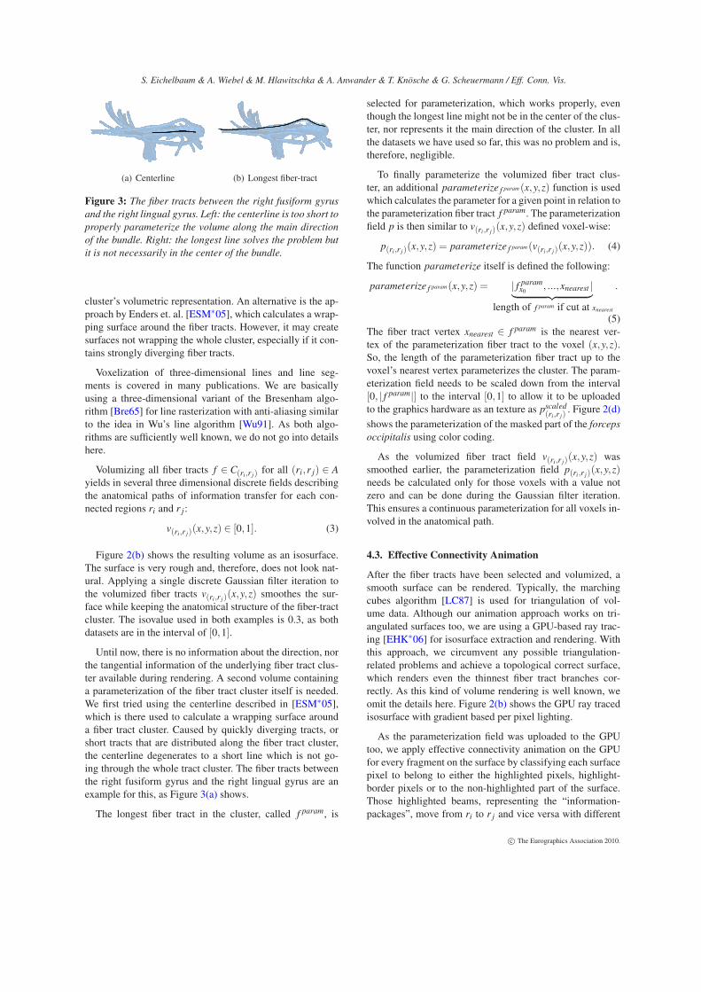
(a) Centerline (b) Longest fiber-tract

Figure 3: The fiber tracts between the right fusiform gyrus

and the right lingual gyrus. Left: the centerline is too short to

properly parameterize the volume along the main direction

of the bundle. Right: the longest line solves the problem but

it is not necessarily in the center of the bundle.

cluster’s volumetric representation. An alternative is the ap-proach by Enders et. al. [ESM∗05], which calculates a wrap-ping surface around the fiber tracts. However, it may createsurfaces not wrapping the whole cluster, especially if it con-tains strongly diverging fiber tracts.

Voxelization of three-dimensional lines and line seg-ments is covered in many publications. We are basicallyusing a three-dimensional variant of the Bresenham algo-rithm [Bre65] for line rasterization with anti-aliasing similarto the idea in Wu’s line algorithm [Wu91]. As both algo-rithms are sufficiently well known, we do not go into detailshere.

Volumizing all fiber tracts f ∈ C(ri,r j) for all (ri,r j) ∈ A

yields in several three dimensional discrete fields describingthe anatomical paths of information transfer for each con-nected regions ri and r j:

v(ri,r j)(x,y,z) ∈ [0,1]. (3)

Figure 2(b) shows the resulting volume as an isosurface.The surface is very rough and, therefore, does not look nat-ural. Applying a single discrete Gaussian filter iteration tothe volumized fiber tracts v(ri,r j)(x,y,z) smoothes the sur-face while keeping the anatomical structure of the fiber-tractcluster. The isovalue used in both examples is 0.3, as bothdatasets are in the interval of [0,1].

Until now, there is no information about the direction, northe tangential information of the underlying fiber tract clus-ter available during rendering. A second volume containinga parameterization of the fiber tract cluster itself is needed.We first tried using the centerline described in [ESM∗05],which is there used to calculate a wrapping surface arounda fiber tract cluster. Caused by quickly diverging tracts, orshort tracts that are distributed along the fiber tract cluster,the centerline degenerates to a short line which is not go-ing through the whole tract cluster. The fiber tracts betweenthe right fusiform gyrus and the right lingual gyrus are anexample for this, as Figure 3(a) shows.

The longest fiber tract in the cluster, called f param, is

selected for parameterization, which works properly, eventhough the longest line might not be in the center of the clus-ter, nor represents it the main direction of the cluster. In allthe datasets we have used so far, this was no problem and is,therefore, negligible.

To finally parameterize the volumized fiber tract clus-ter, an additional parameterize f param(x,y,z) function is usedwhich calculates the parameter for a given point in relation tothe parameterization fiber tract f param. The parameterizationfield p is then similar to v(ri,r j)(x,y,z) defined voxel-wise:

p(ri,r j)(x,y,z) = parameterize f param(v(ri,r j)(x,y,z)). (4)

The function parameterize itself is defined the following:

parameterize f param(x,y,z) = | f paramx0, ...,xnearest |

︸︷︷︸

length of f param if cut at xnearest

.

(5)The fiber tract vertex xnearest ∈ f param is the nearest ver-tex of the parameterization fiber tract to the voxel (x,y,z).So, the length of the parameterization fiber tract up to thevoxel’s nearest vertex parameterizes the cluster. The param-eterization field needs to be scaled down from the interval[0, | f param|] to the interval [0,1] to allow it to be uploadedto the graphics hardware as an texture as pscaled(ri,r j)

. Figure 2(d)

shows the parameterization of the masked part of the forcepsoccipitalis using color coding.

As the volumized fiber tract field v(ri,r j)(x,y,z) wassmoothed earlier, the parameterization field p(ri,r j)(x,y,z)needs be calculated only for those voxels with a value notzero and can be done during the Gaussian filter iteration.This ensures a continuous parameterization for all voxels in-volved in the anatomical path.

4.3. Effective Connectivity Animation

After the fiber tracts have been selected and volumized, asmooth surface can be rendered. Typically, the marchingcubes algorithm [LC87] is used for triangulation of vol-ume data. Although our animation approach works on tri-angulated surfaces too, we are using a GPU-based ray trac-ing [EHK∗06] for isosurface extraction and rendering. Withthis approach, we circumvent any possible triangulation-related problems and achieve a topological correct surface,which renders even the thinnest fiber tract branches cor-rectly. As this kind of volume rendering is well known, weomit the details here. Figure 2(b) shows the GPU ray tracedisosurface with gradient based per pixel lighting.

As the parameterization field was uploaded to the GPUtoo, we apply effective connectivity animation on the GPUfor every fragment on the surface by classifying each surfacepixel to belong to either the highlighted pixels, highlight-border pixels or to the non-highlighted part of the surface.Those highlighted beams, representing the “information-packages”, move from ri to r j and vice versa with different



(a) With overlapping (b) No overlapping

Figure 4: The final rendering of the fiber tract cluster from

left to right lingual gyrus with both effective connectivity

beams. For a video showing the animation, take a look at

the supplemental material accompanying this paper. Left:

This image was made at a time-step where the beams of LG

left→LG right and LG left←LG right do overlap to show

how we combine both beams. Right: without overlapping at

another time-step.

size to represent the effective connectivity. Please take a lookin the supplemented material accompanying this paper to seethe animation.

To ease the following description up, we will describeonly one moving package in the direction ri to r j along thecorresponding anatomical connection in v(ri,r j)(x,y,z). In thenext paragraphs, we call those “packages” only “beams” asthey look similar to moving beams on the surface. Due tothe graphics hardware architecture, only one fragment canbe processed at a time. Neighboring pixels are not accessi-ble for write or for read. This is why we need to calculatethe current midpoint of the “information-package” for eachfragment:

m= ((t+o)∗ v) mod (k+k

3)−

k

6(6)

The Equation 6 is very simple and uses two parameters. Thecurrent time t with an offset o in milliseconds and the ve-locity v. It is the well known physical relationship betweendistance, time and velocity. The offset parameter is used toavoid that the beam ri → r j starts at the same moment asthe beam ri← r j starts. This creates a better impression as itdoes not look as artificial as if they would have been startedat the same time, meeting both exactly in the middle of thecluster. The modulo operation ensures that there is a peri-odic beam-movement from ri to r j along the current voxel’sgradient in parameterization space in k units along the fibertract cluster. In our implementation we are using k = 100,which creates a smooth movement. To ensure that the beamdoes not abruptly end when the middle of the beam reachesthe end of the cluster and to ensure that the beam does notpop up on the other side with the beam’s middle at the be-ginning of the cluster, the interval is stretched. The value ofm then also covers the invisible part of the parameter space,large enough to contain half of a beam’s maximum size, in

this case k6 on each end of the parameter space. For more

details on the size of the beams, see section 4.3.1. The valueof m then represents the current position of the beam as aline perpendicular to the main direction (the current gradi-ent) on the surface. This line moves, depending on time andspeed, along the surface and is then used for classifying thecurrent fragments parameter in p(ri,r j)(x,y,z) (recall that theparameterization field in Equation 7 is scaled to the interval[0,1] to be uploaded as pscaled

(ri,r j)(x,y,z) in a texture), whether

it belongs to the current beam, or “information package”:

b(ri,r j)(x,y,z) = |m− k ∗ s(ri,r j)pscaled(ri,r j)

(x,y,z)|−l(ri,r j)

2. (7)

Equation 7 describes an environment of size l(ri,r j) (thelength of the beam from ri to r j) around the current beam-center m and describes a predicate for each fragment at thecurrent coordinate whether it is inside the beam (b<−ε), onthe border of the beam (b ∈ [−ε,0]) or outside of it (b > ε),where ε denotes the border width. Ignoring the additionalparameter s, this simply tests whether the actual fragmentalong the main direction of the fiber tract cluster is nearthe current position m. The parameter s is used to ensureequal speeds and the correct size-relation between the beamsfor all beams on all fiber tract clusters and is the relationbetween the fiber used for parameterization of the cluster(ri,r j) and one of the parameterization fibers of all the clus-ters in A:

s(ri,r j) =| f

param

(ri,r j)|

| fparamre f |

,(ri,r j) ∈ A, ref ∈ A. (8)

The final pixel color can finally be determined using anarbitrary color map. In our implementation, we use the fol-lowing mapping:

c f ragment =

c(ri,r j) if b(ri,r j) <−ε

c(r j ,ri) if b(r j ,ri) <−ε

c(ri,r j) if b(ri,r j) <−ε∧

b(r j ,ri) <−ε∧

l(ri,r j) ≤ l(r j ,ri)c(r j ,ri) if b(ri,r j) <−ε∧

b(r j ,ri) <−ε∧

l(ri,r j) > l(r j ,ri)white if b(r j ,ri) ∈ [−ε,0]

csur f ace else

(9)

The surface itself has a user defined color csur f ace, whichis set if the fragment does not belong to either one of thebeams and is shaded by a previously calculated per-pixelPhong shading. Equation 9 also covers the case where thebeams overlap. If this is the case, the color of the smallerbeam is used. Blending both colors would irritate the usertoo much. The white border around each beam ensures thatthe beam is visible even if the contrast between the beam’scolor c(ri,r j) or c(r j ,ri) and the surface color is very low. Fig-ure 4 shows two time-steps of the animation, one with over-lapping beams.



4.3.1. Determining the length of the beams

The effective connectivity represented by the specific beamis used to define its length. To have the length and, espe-cially, their relation between each other consistent, we mapthe interval [0,1], representing the smallest and largest beamto the interval of the involved effective connectivities (theconnectivity graph’s weighting function e):

[min{e(i, j)|(ri,r j) ∈ A},max{e(i, j)|(ri,r j) ∈ A}] (10)

The mapping function has to map between [0,1] and the in-terval of the smallest to the largest connectivity value. Thismapping can be adapted to the possible cases. In our ex-amples, the effective connectivities do not spread wide in R

and, therefore we use a linear mapping. If the effective con-nectivities vary very strongly, a logarithmic scale can helpto avoid many very small beams of not distinguishable sizeand very few large beams. It is worth mentioning, that thebeam length interval [0,1] itself needs to be mapped to theactual beam sizes. This mapping is strongly dependent to theparameter k of the above equations 6 and 7. A good choice isto set the beam sizes to [ k

100 ,k3 ] which creates beams not too

small and avoids extremely large beams covering the wholesurface.

4.4. Labeling

Due to the scaling and the movement of the beams on thesurface, it is difficult to read the actual effective connec-tivity value. Only relationships can be seen. Therefore, ourapproach is supplemented with some labeling features, al-lowing the user the see the real effective connectivity valueand the names of the involved regions. To avoid, that thelabels overlap the actual surface and animation, we haveimplemented a boundary based labeling, similar to the onein [BKSW04]. We arrange labels with the name of the re-gions on the boundary of the bounding box enclosing thewhole scene.

Figure 5 and 6 shows the example fiber tract cluster withthe corresponding labels. The video accompanying the papershows the dynamics of label placement.

5. Results

In this section, we demonstrate our method for two differenttypes of datasets: a real data set (cf. Figure 5 and 6) obtainedby DCMwith tractography-based priors and an artificial dataset (cf. Figure 7). We use artificial data to show the method inmore complex environments. The data taken from [STK∗09]and [SMP∗07] examined only the connection of a region inone hemisphere and the connectivity to their relatively closecounterpart in the other hemisphere (see Figure 1).

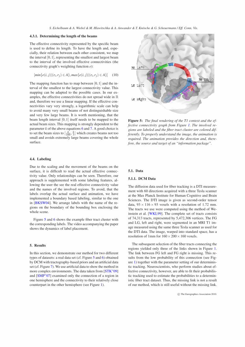
Figure 5: The final rendering of the T1 context and the ef-

fective connectivity graph from Figure 1. The involved re-

gions are labeled and the fiber tract cluster are colored dif-

ferently. To properly understand the image, the animation is

required. The animation provides the direction and, there-

fore, the source and target of an “information package”.

5.1. Data

5.1.1. DCM Data

The diffusion data used for fiber tracking is a DTI measure-ment with 60 directions acquired with a three Tesla scannerat the Max Planck Institute for Human Cognitive and BrainSciences. The DTI image is given as second-order tensordata, 93× 116× 93 voxels with a resolution of 1.72 mm.The tracts we use were computed using the method of We-instein et al. [WKL99]. The complete set of tracts consistsof 74,313 tracts, represented by 5,472,306 vertices. The FGand LG, left and right, were segmented in an MRI T1 im-age measured using the same three Tesla scanner as used forthe DTI data. The image, warped into standard space, has aresolution of 1mm for 160×200×160 voxels.

The subsequent selection of the fiber tracts connecting theregions yielded only three of the links shown in Figure 1.The link between FG left and FG right is missing. This re-sults from the low probability of this connection (see Fig-ure 1) together with the parameter setting of our determinis-tic tracking. Neuroscientists, who perform studies about ef-fective connectivity, however, are able to fit their probabilis-tic tracking used to estimate the probabilities to a determin-istic fiber tract dataset. Thus, the missing link is not a resultof our method, which is still useful without the missing link.



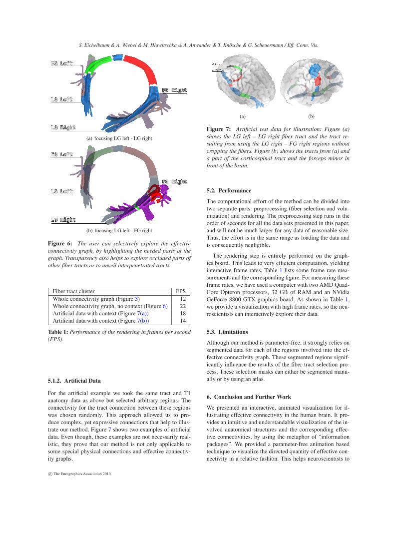
(a) focusing LG left - LG right

(b) focusing LG left - FG right

Figure 6: The user can selectively explore the effective

connectivity graph, by highlighting the needed parts of the

graph. Transparency also helps to explore occluded parts of

other fiber tracts or to unveil interpenetrated tracts.

Fiber tract cluster FPSWhole connectivity graph (Figure 5) 12Whole connectivity graph, no context (Figure 6) 22Artificial data with context (Figure 7(a)) 18Artificial data with context (Figure 7(b)) 14

Table 1: Performance of the rendering in frames per second

(FPS).

5.1.2. Artificial Data

For the artificial example we took the same tract and T1anatomy data as above but selected arbitrary regions. Theconnectivity for the tract connection between these regionswas chosen randomly. This approach allowed us to pro-duce complex, yet expressive connections that help to illus-trate our method. Figure 7 shows two examples of artificialdata. Even though, these examples are not necessarily real-istic, they prove that our method is not only applicable tosome special physical connections and effective connectiv-ity graphs.

(a) (b)

Figure 7: Artificial test data for illustration: Figure (a)

shows the LG left – LG right fiber tract and the tract re-

sulting from using the LG right – FG right regions without

cropping the fibers. Figure (b) shows the tracts from (a) and

a part of the corticospinal tract and the forceps minor in

front of the brain.

5.2. Performance

The computational effort of the method can be divided intotwo separate parts: preprocessing (fiber selection and volu-mization) and rendering. The preprocessing step runs in theorder of seconds for all the data sets presented in this paper,and will not be much larger for any data of reasonable size.Thus, the effort is in the same range as loading the data andis consequently negligible.

The rendering step is entirely performed on the graph-ics board. This leads to very efficient computation, yieldinginteractive frame rates. Table 1 lists some frame rate mea-surements and the corresponding figure. For measuring theseframe rates, we have used a computer with two AMD Quad-Core Opteron processors, 32 GB of RAM and an NVidiaGeForce 8800 GTX graphics board. As shown in Table 1,we provide a visualization with high frame rates, so the neu-roscientists can interactively explore their data.

5.3. Limitations

Although our method is parameter-free, it strongly relies onsegmented data for each of the regions involved into the ef-fective connectivity graph. These segmented regions signif-icantly influence the results of the fiber tract selection pro-cess. These selection masks can either be segmented manu-ally or by using an atlas.

6. Conclusion and Further Work

We presented an interactive, animated visualization for il-lustrating effective connectivity in the human brain. It pro-vides an intuitive and understandable visualization of the in-volved anatomical structures and the corresponding effec-tive connectivities, by using the metaphor of “informationpackages”. We provided a parameter-free animation basedtechnique to visualize the directed quantity of effective con-nectivity in a relative fashion. This helps neuroscientists to



see and understand the information transfer between the in-volved regions in the context of their underlying anatomi-cal context. In complex DCM graphs and networks, the an-imation can get confusing as many anatomical paths showinformation-transfer and, therefore, create visual clutter. Weavoid visual clutter by allowing the user to selectively viewparts of the graph and fading out animation on others thusretaining the other anatomical structures. The incorporationof focus and context principles and interactive selection ofparts of the data makes it even more useful for daily use andexploration of data.

An interesting avenue of future research can be the directincorporation of probabilistic tractography data as used forthe studies yielding the effective connectivity values. Thiscan serve as basis for a connection representation instead ofthe volumized deterministic tracking lines. This would alsosolve the problem of anatomical connections, not found bythe current preprocessing step. We will furthermore evaluatedifferent kinds of animation with our neuroscientist users topossibly find other, even better representations of effectiveconnectivity in its anatomical context.

References

[ASM∗04] AKERS D., SHERBONDY A., MACKENZIE R.,DOUGHERTY R., WANDELL B.: Exploration of the brain’s whitematter pathways with dynamic queries. In IEEE VIS ’04 (2004),pp. 377–384. 2

[BBP∗05] BLAAS J., BOTHA C. P., PETERS B., VOS F. M.,POST F. H.: Fast and reproducible fiber bundle selection in dtivisualization. IEEE VIS ’05 0 (2005), 59–64. 2, 3

[BKSW04] BEKOS M. A., KAUFMANN M., SYMVONIS A.,WOLFF E.: Boundary labeling: Models and efficient algorithmsfor rectangular maps. In Symposium on Graph Drawing (GD’04),

LNCS 3383 (2004), pp. 49–59. 6

[BPP∗00] BASSER P. J., PAJEVIC S., PIERPAOLI C., DUDA J.,ALDROUBI A.: In vivo fiber tractography using dt-mri data.Magnetic resonance in medicine 44, 4 (October 2000), 625–632.2

[Bre65] BRESENHAM J. E.: Algorithm for computer control of adigital plotter. IBM System Journal 4, 1 (1965), 25–30. 4

[CL93] CABRAL B., LEEDOM L. C.: Imaging vector fields usingline integral convolution. In SIGGRAPH ’93 (1993), pp. 263–270. 2

[EHK∗06] ENGEL K., HADWIGER M., KNISS J., REZK-SALAMA C., WEISKOPF D.: Real-time Volume Graphics. AK Peters, 2006. 2, 4

[ESM∗05] ENDERS F., SAUBER N., MERHOF D., HASTREITER

P., NIMSKY C., STAMMINGER M.: Visualization of white mat-ter tracts with wrapped streamlines. In IEEE VIS ’05 (2005),pp. 51–58. 4

[FHP03] FRISTON K., HARRISON L., PENNY W.: Dynamiccausal modelling. NeuroImage 19, 4 (2003), 1273 – 1302. 1

[GCTH10] GERHARD S., CAMMOUN L., THIRAN J.-P., HAG-MANN P.: ConnectomeViewer.org, 2010. Ecole PolytechniqueFédérale de Lausanne and University Hospital Center and Uni-versity of Lausanne. 2

[HCG∗08] HAGMANN P., CAMMOUN L., GIGANDET X.,MEULI R., HONEY C. J., WEDEEN V. J., SPORNS O.: Map-ping the structural core of human cerebral cortex. PLoS Biol 6, 7(07 2008), e159. 2

[HvW09] HOLTEN D., VAN WIJK J. J.: A user study on visualiz-ing directed edges in graphs. In CHI ’09 (2009), pp. 2299–2308.2

[KKKW05] KRÜGER J., KIPFER P., KONDRATIEVA P., WEST-ERMANN R.: A particle system for interactive visualization of3D flows. IEEE TVCG 11, 6 (11 2005), 744–756. 2

[KWH09] KNOLL A. M., WALD I., HANSEN C. D.: Coherentmultiresolution isosurface ray tracing. Vis. Comput. 25, 3 (2009),209–225. 2

[LC87] LORENSEN W. E., CLINE H. E.: Marching cubes: A highresolution 3d surface construction algorithm. In SIGGRAPH ’87

(1987), pp. 163–169. 2, 4

[LJH03] LARAMEE R. S., JOBARD B., HAUSER H.: Imagespace based visualization of unsteady flow on surfaces. In IEEE

VIS ’03 (2003), p. 18. 2

[MGL94] MCINTOSH A. R., GONZALEZ-LIMA F.: Structuralequation modeling and its application to network analysis infunctional brain imaging. Human Brain Mapping 2, 1-2 (1994),2–22. 1

[MWZ∗00] MUELLER K., WELSH T., ZHU W., MEADE J.,VOLKOW N.: Brainminer: A visualization tool for roi-based dis-covery of functional relationships in the human brain. In NPIVM’00 (2000), pp. 481–485. 2

[RBM∗05] ROHLFING T., BRANDT R., MENZEL R., RUS-SAKOFF D. B., MAURER JR. C. R.: Handbook of Biomedical

Image Analysis: Registration Models. Springer–Verlag BerlinHeidelberg, 2005, ch. Quo Vadis, Atlas-Based Segmentation?,pp. 435–486. 3

[SMP∗07] STEPHAN K. E., MARSHALL J. C., PENNY W. D.,FRISTON K. J., FINK G. R.: Interhemispheric Integration of Vi-sual Processing during Task-Driven Lateralization. J. Neurosci.

27, 13 (2007), 3512–3522. 2, 6

[STK∗09] STEPHAN K. E., TITTGEMEYER M., KNÖSCHE

T. R., MORAN R. J., FRISTON K. J.: Tractography-based pri-ors for dynamic causal models. NeuroImage 47, 4 (2009), 1628– 1638. 1, 6

[TvW03] TELEA A., VAN WIJK J. J.: 3D IBFV: Hardware-accelerated 3d flow visualization. In IEEE VIS ’03 (2003), p. 31.2

[WKL99] WEINSTEIN D., KINDLMANN G., LUNDBERG E.:Tensorlines: advection-diffusion based propagation through dif-fusion tensor fields. In VIS ’99 (1999), pp. 249–253. 6

[WMZ∗01] WELSH T., MUELLER K., ZHU W., VOLKOW N.,MEADE J.: Graphical strategies to convey functional relation-ships in the human brain: a case study. In VIS ’01 (Washington,DC, USA, 2001), pp. 481–484. 2

[Wu91] WU X.: An efficient antialiasing technique. SIGGRAPH’91 25, 4 (1991), 143–152. 4


Visualization of Effective Connectivity of the Brain

Documents

Transcript of Visualization of Effective Connectivity of the Brain