ANALYTICAL MODELLING OF HYDROGEN TRANSPORTIN REACTOR CONTAINMENTS

byVincent P. Manno and Michael W. Golay

Energy Laboratory Report No. MIT-EL-83-009

October 1983

j_morris

Typewritten Text

Author miss numbered pages. Pages 231 through 239 do not exist.

ANALYTICAL MODELLING OF HYDROGEN TRANSPORT

IN REACTOR CONTAINMENTS

by

Vincent P. Manno

and

Michael W. Golay

Energy Laboratory and

Department of Nuclear Eng-ineering

Massachusetts Institute of Technology

Cambridge, MA 02139

MIT-EL-83-009

October 1983

Sponsored by:

Boston Edison Co.Duke Power Co.Northeast Utilities Service Corp.Public Service Elpctric and Gas Co. of New Jersey

-2-

ABSTRACT

ANALYTICAL MODELLING OF HYDROGEN TRANSPORT

IN REACTOR CONTAINMENTS

by

Vincent P. Manno and Michael W. Golay

A versatile computational model of hydrogen transportin nuclear plant containment buildings is developed. Thebackground and significance of hydrogen-related nuclearsafety issues are discussed. A computer program is con-structed that embodies the analytical models. The thermo-fluid dynamic formulation spans a wide applicability rangefrom rapid two-phase blowdown transients to slow incompres-sible hydrogen injection. Detailed ancillary models ofmolecular and turbulent diffusion, mixture transport pro-perties, multi-phase multicomponent thermodynamics and heatsink modelling are addressed. The nume'rical solution ofthe continuum equations emphasizes both accuracy and effic-iency in the employment of relatively coarse discretizationand long time steps. Reducing undesirable numerical diffu-sion is addressed. Problem geometry options include lumpedparameter zones, one dimensional meshes, two dimensionalCartesian or axisymmetric coordinate systems and threedimensional Cartesian or cylindrical regions. An efficientlumped nodal model is included for simulation of events inwhich spatial resolution is not significant.

Several validation calculations are reported. Demon-stration problems include the successful reproduction ofanalytical or known solutions, simulation of large scaleexperiments and analyses of "thought experiments" whichtest the physical reasonableness of the predictions. Inparticular, simulation of hydrogen transport tests per-formed at the Battelle Frankfurt Institute and HanfordEngineering Development Laboratory show good agreement withmeasured hydrogen concentration, temperature and flowfields. The results also indicate that potential areas ofimprovement are enhanced computational efficiency, furtherreduction of numerical diffusion and development of con-tainment spray models. Overall, a useful tool applicableto many nuclear safety problems is described.

-3-

ACKNOWLEDGEMENTS

This research was conducted under the sponsorship of

Boston Edison Co., Duke Power Co., Northeast Utilities

Service Corp. and Public Service Electric and Gas Co. of

New Jersey. The authors gratefully acknowledge this

support. The first author also received partial support

from the U.S. Department of Energy. The authors thank all

those who assisted them during this research especially

Dr. Kang Y. Huh, Dr. Lothar Wolf, Mr. B.K. Riggs, Ms. Cindy

Sheeks, Ms. Rachel Morton and Prof. Andrei Schor. The work

was expertly typed by Mr. Ted Brand and-Ms. Eva Hakala.

-4-

TABLE OF CONTENTSPage

ABSTRACT 2

ACKNOWLEDGEMENTS 3

TABLE OF CONTENTS 4

LIST OF FIGURES 7

LIST OF TABLES 10

NOMENCLATURE 11

1.0 Introduction 141.1 Problem Description 141.2 Historical Background 161.3 Scope of Work 21

2.0 Literature Review 232.1 Hydrogen Related Problems in Nuclear

Plants 232.2 Relevant Computational Methods 312.3 Containment Analysis Tools 36

3.0 Analytical Modelling 413.1 Overview 413.2 Modification of the BEACON Program 44

3.2.1 Continuum Regions 443.2.2 Lumped Parameter Zones 51

3.2.2.1 Inclusion of H 2 inExisting Formulation 51

3.2.2.2 Model Improvement 523.2.3 Ancillary Model Development 59

3.2.3.1 Thermodynamic andTransport Properties 59

3.2.3.2 Condensate Films andHeat Transfer 60

3.2.4 Inherent Limitations of theModified Code 63

3.3 Longer Term Transient Modelling--MITHYD 643.3.1 Basic Equation Formulation 663.3.2 Turbulence Effects 733.3.3 Mass Diffusion 783.3.4 Solution Scheme 81

3.3.4.1 Treatment of Convectionand Numerical Diffusion 84

3.3.4.2 Flow and Pressure Fields 873.3.4.3 Transport Equations 983.3.4.4 Information Update and

State Determination 1083.3.4.5 Initial and Boundary

Conditions 116

-5-

Page

3.3.4.6 Incompressibility Check 1183.3.5 Physical and Computational Inter- 119

facing of MITHYD and Overall Code

4.0 Results and Discussion 1224.1 Validation Methodology 1224.2 Results Using the Modified BEACON 124

Equation Set4.2.1 Air and Water Blowdown 1254.2.2 Hydrogen and Water Blowdown 1294.2.3 Analysis of Slower Transients 1334.2.4 Transition to Slower Mixing Model 138

4.3 Longer Mixing Transients 1394.3.1 Battelle Frankfurt Tests 143

4.3.1.1 Facility and Testing 143Program Review

4.3.1.2 Simulations Based on 158Selected Tests

4.3.2 Hanford Engineering Development 209Laboratory Tests4.3.2.1 Facility and Testing 209

Progran Review4.3.2.2 Simulations Based on 214

Selected Tests4.4 Lumped Parameter Model Results 2484.5 Discussion of Results 2524.6 Model Capabilities vs Other Approaches 2554.7 Computational Effort Analysis 258

5.0 Conclusions and Recommendations 2615.1 Conclusions 2615.2 Recommendations for Future Work 264

6.0 References 267

APPENDIX A: COMPUTER APPLICATION TOPICS 275A.1 General Principles 2754.2 Acquisition, Installation and Modification 276A.3 Brief Review of Modifications 2814.4 Segmented Loading 283A.5 Production Mode Execution 289A.6 Application on a Non-CDC System 290

APPENDIX B: INPUT DECKS FOR REPORTED SIMULATIONS 292

APPENDIX C: ANALYTICAL ASPECTS OF POSSIBLE EXTENSION 304TO CHEMICALLY REACTIVE FLOWS

C.1 Introduction 304C.2 Important Phenomena 304

C.2.1 Ignition Phenomena 305

-6-

Page

C.2.2 Deflagration Regime 306C.2.3 Detonations 309

C.3 Flow Modelling 312C.3.1 Flows Near a Stationary Flame 312C.3.2 Reactive Flows 314

C.4 Outline of a Composite Model 319C.5 Conclusions 322C.6 References 324

APPENDIX D: IMPORTANT CONSIDERATIONS FOR 326ASSESSING AN IMPLICIT SLOW MIXINGSOLUTION SCHEME

APPENDIX E: ADDITIONAL REMARKS ON THE SOLUTION OF 335THE SLOW MIXING MODEL ENERGY EQUATION

-7-

LIST OF FIGURES

Figure Title Page

1.1 PWR Ice Condenser Containment 171.2 Hydrogen Concentration vs Metal Water 19

Reaction

2.1 Flammability and Combustion Limits of 27Air-Water-Hydrogen Mixtures

2.2 Effect of Steam on Hydrogen Combustion 30

3.1 Basic BEACON Time Advancement Logic 493.2 Coordinate System Definition 503.3 Molecular Mass Diffusivities 803.4 MITHYD Solution Logic 823.5 Thermodynamic Property Functional Fits 115

4.1 Blowdown Problem Geometry 1264.2 Gas Phase Flow Field at 0.1 Second 1274.3 Void Fraction Transients at Selected 128

Locations4.4 Gaseous Flow Field and Hydrogen Distri- 130

bution Map at 0.10 Second4.5 Gaseous Flow Field and Hydrogen Distri- 131

bution Map at 0.20 Second4.6 Hydrogen Volume Percent vs Time 1324.7 Problem Geometry Used In BEACON Analysis 136

of BF2-Type Transients4.8 Computational Switching Problem Specifi- 140

cation and Convergence Behavior4.9 Evolution of Hydrogen and Velocity Fields 1414.10 Flow Field and Hydrogen Concentration at 142

1 and 10 Seconds4.11 Schematic Diagram of Battelle Frankfurt 145

Facility4.12 Perspective View of BF Facility 1464.13 Possible Compartmental Connections and 147

Dimensions4.14 Typical BF Instrumentation Locations and 149

Source Injection Schematic4.15 Hydrogen Sensor Electrical Schematic 1504.16 32 Node Coarse Mesh Model of BF2 and BF6 1614.17-4.19 Hydrogen Volume Fraction and Velocity 163-

Profiles at 20, 100 and 200 Seconds of 165BF2 Simulation

4.20 Development of Velocity Field in BF2 167Simulation

4.21 Hydrogen Concentr.tion Transients at 168Five Selected Locations During BF2Simulation

-8-

Page

4.22 Hydrogen Volume Fraction and Velocity 170Profile at 100 Seconds of Open-BF2Simulation

4.23 Development of the Velocity Field in 171Open-BF2 Simulation

4.24 Hydrogen Concentration Transients at Five 173Selected Locations During Open-BF2 Simulation

4.25 Time Dependent Behavior of Turbulence 175Parameters

4.26 Hydrogen Volume Fraction and Velocity 176Profile at 100 Seconds of Closed-BF2Simulation

4.27- 178-

4.29 Hydrogen Volume Fraction and Velocity 180Profiles at 20, 100 and 200 Seconds of BF6Simulation

4.30 Hydrogen Concentration Transients During 182First 200 Seconds of BF6 Simulation

4.31 Development of the Velocity Field During 183

First 200 Seconds of BF6 Simulation4.32 Mixture Density Time Response During 184

First 200 Seconds of 8F6 Simulation4.33-4.34 Hydrogen VolumeFraction and Velocity 186-

Profiles at 2000 and 4000 Seconds of BF6 187Simulation

4.35 Comparison of Predicted and Measured 188Hydrogen Concentrations for BF6

4.36 Local Temperature Behavior During BF6 189Simulation

4.37 Mixture Density Behavior During BF6 190Simulation

4.38 Vertical Orifice Velocities vs Time 192

4.39 Estimated Numerical Diffusion Coefficients 194at 1000 Seconds of BF6 Simulation

4.40 50 Node Model for BF6 Simulation 196

4.41 Velocity Profile and Time History During 19750 Node BF6 Simulation

4.42-4.44 Hydrogen Volume Fraction Profile During 199-

50 Node BF6 Simulation at 1000, 3000 201and 5000 Seconds

4.45-4.47 Temperature Profile During 50 Node BF6 202-

Simulation at 1000, 3000 and 5000 Seconds 204

4.48 Comparison of Measured and Predicted 205Hydrogen Concentrations During 50 NodeBF6 Simulation

4.49 Development History of Velocity Field 207

During 50 Node BF6 Simulation

-9-

Page

4.50 Comparison of Orifice Region Froude Numbers 208

of the Two BF6 Simulations

4.51- 210-4.52 HEDL Facility Schematics 211

4.53 HEDL Lumped Parameter Analysis 2184.54 Discrete Model of HEDL Facility 2194.55- 221-4.58 Flow and Temperature Fields at 50 and 300 225

Seconds into HEDL B Simulation4.59 Hydrogen Concentrations During HEDL B 226

Simulation vs Data4.60 Normalized Velocity Component Behavior 228

During HEDL 8 Simulation4.61 96 Node Model of HEDL Facility 2404.62-4.65 Flow and Temperature Fields in Jet and Non- 241-

Jet Regions at 50 and 350 Seconds into 24496 Node HEDL B Simulation

4.66 Hydrogen Volume Fraction Predictions vs 246Data During 96 Node HEDL B Simulation

4.67 Behavior of Normalized Velocity Components 247During 96 Node HEDL B Simulation

4.68 Six Room Lumped Problem 2494.69 H2 Transient of Six Room Problem 251

A.1 Basic Computer Application Plan of Operation 279A.2 Slow Mixing Code Solution Structure Logic 285A.3 Segmented Loading Directives 288

-10-

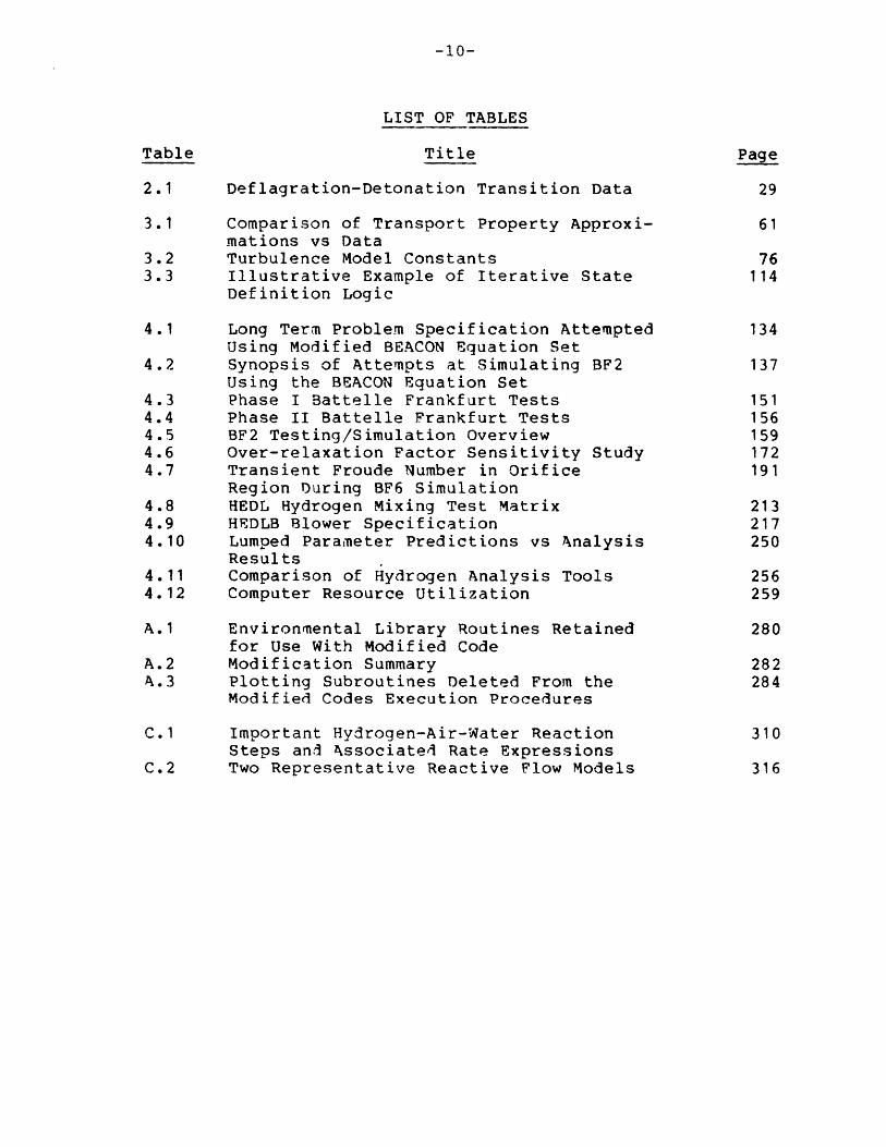
LIST OF TABLES

Table Title Page

2.1 Deflagration-Detonation Transition Data 29

3.1 Comparison of Transport Property Approxi- 61mations vs Data

3.2 Turbulence Model Constants 763.3 Illustrative Example of Iterative State 114

Definition Logic

4.1 Long Term Problem Specification Attempted 134Using Modified BEACON Equation Set

4.2 Synopsis of Attempts at Simulating BF2 137Using the BEACON Equation Set

4.3 Phase I Battelle Frankfurt Tests 1514.4 Phase II Battelle Frankfurt Tests 1564.5 BF2 Testing/Simulation Overview 1594.6 Over-relaxation Factor Sensitivity Study 1724.7 Transient Froude Number in Orifice 191

Region During BF6 Simulation4.8 HEDL Hydrogen Mixing Test Matrix 2134.9 HEDLB Blower Specification 2174.10 Lumped Parameter Predictions vs Analysis 250

Results4.11 Comparison of Hydrogen Analysis Tools 2564.12 Computer Resource Utilization 259

A.1 Environmental Library Routines Retained 280for Use With Modified Code

A.2 Modification Summary 282A.3 Plotting Subroutines Deleted From the 284

Modified Codes Execution Procedures

C.1 Important Hydrogen-Air-Water Reaction 310Steps and Nssociated Rate Expressions

C.2 Two Representative Reactive Flow Models 316

-11-

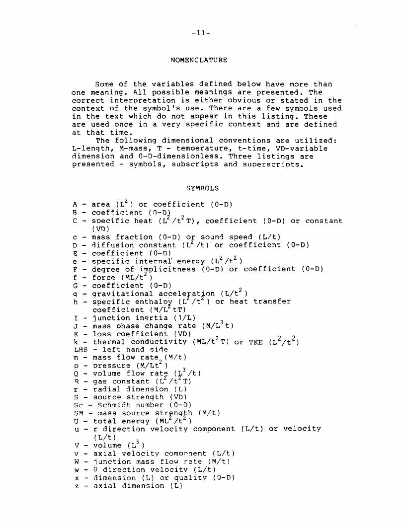
NOMENCLATURE

Some of the variables defined below have more thanone meaning. All possible meanings are presented. Thecorrect interpretation is either obvious or stated in thecontext of the symbol's use. There are a few symbols usedin the text which do not appear in this listing. Theseare used once in a very specific context and are definedat that time.

The following dimensional conventions are utilized:L-lenqth, M-mass, T - temoerature, t-time, VD-variabledimension and 0-D-dimensionless. Three listings arepresented - symbols, subscripts and superscripts.

SYMBOLS

A - area (L 2 ) or coefficient (0-D)8 - coefficient (0-0~C - specific heat (L /t2T), coefficient (0-D) or constant

(VI)c - mass fraction (0-D) or sound speed (L/t)D - diffusion constant (L2/t) or coefficient (0-D)E - coefficient (0-0)e - specific internal' energy (L2 /t2 )F - degree of implicitness (0-D) or coefficient (0-D)f - force (ML/t 2 )

G - coefficient (0-D)q - gravitational acceleyat on (L/t 2 )h - specific enthaloy (L /t ) or heat transfer

coefficient (M/L tT)I - junction inertia (1/L)J - mass ohase change rate (M/L t)K - loss coefficient (VD)k - thermal conductivity (ML/t T) or TKE (L2 /t 2 )

LHS - left hand sidem - mass flow rate (M/t)p- pressure (M/Lt )Q - volume flow rate ( /t)R - gas constant (L /t T)r - radial dimension (L)S - source strength (VD)Sc - Schmidt number (0-D)SM - mass source strnq 2th (M/t)U - total energy (ML /t )u - r direction velocity component (L/t) or velocity

(L/t)V - volume (L )v - axial velocity comoonent (L/t)W - junction mass flow rate (M/t)w - 6 direction velocity (L/t)x - dimension (L) or quality (0-D)z - axial dimension (L)

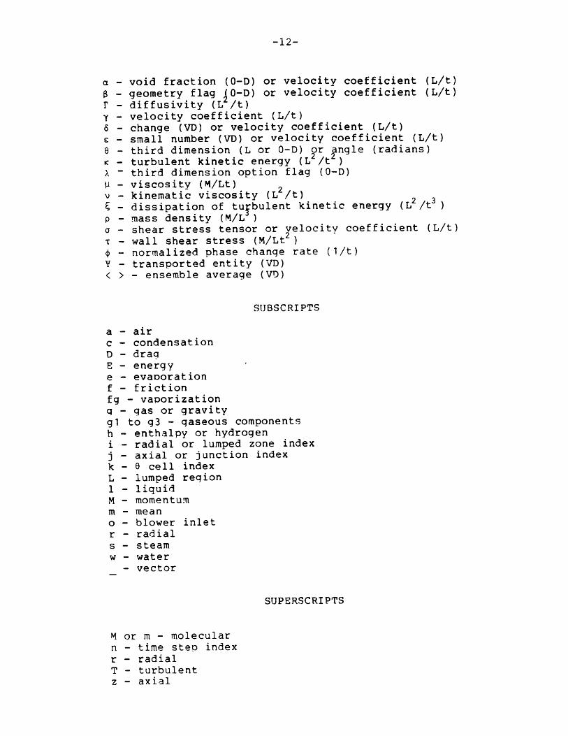
-12-

a - void fraction (0-D) or velocity coefficient (L/t)8 - geometry flag 0O-D) or velocity coefficient (L/t)r - diffusivity (L /t)y - velocity coefficient (L/t)6 - change (VD) or velocity coefficient (L/t)E - small number (VD) or velocity coefficient (L/t)6 - third dimension (L or O-D) or angle (radians)K - turbulent kinetic energy (L /t )X - third dimension option flag (0-D)

- viscosity (M/Lt) 2v - kinematic viscosity (L /t)- dissipation of turbulent kinetic energy (L2 /t3 )

p - mass density (M/L )a - shear stress tensor or velocity coefficient (L/t)T - wall shear stress (M/Lt2 )

- normalized phase change rate (1/t)Y - transported entity (VD)< > - ensemble average (VD)

SUBSCRIPTS

a - airc - condensationD - draqE - energye - evanorationf - frictionfg - vaporizationq - gas or gravitygl to g3 - qaseous componentsh - enthalpy or hydrogeni - radial or lumped zone indexj - axial or junction indexk - 6 cell indexL - lumped reqion1 - liquidM - momentumm - meano - blower inletr - radials - steamw - water

- vector

SUPERSCRIPTS

M or m - molecularn - time step indexr - radialT - turbulentz - axial

-13-

6 - third direction- turbulent and molecular- fluctuation or perturbation- aooroximate value

o - old value- time rate of change

-14-

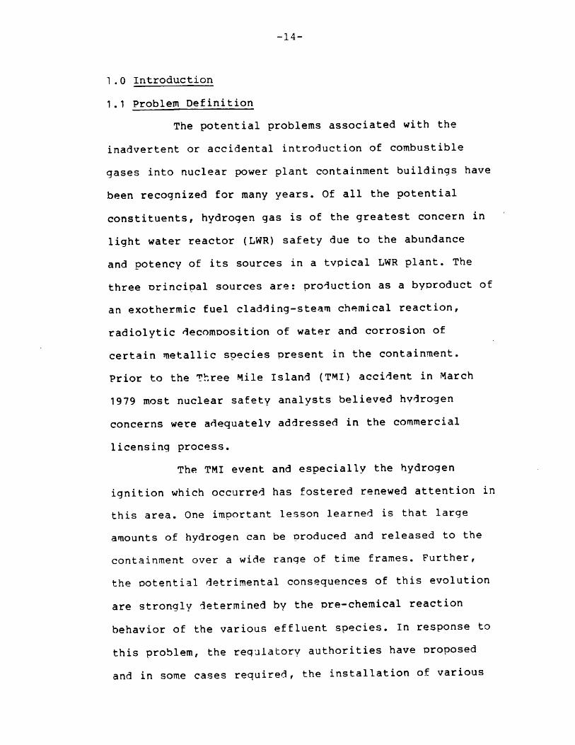
1.0 Introduction

1.1 Problem Definition

The potential problems associated with the

inadvertent or accidental introduction of combustible

gases into nuclear power plant containment buildings have

been recognized for many years. Of all the potential

constituents, hydrogen gas is of the greatest concern in

light water reactor (LWR) safety due to the abundance

and potency of its sources in a typical LWR plant. The

three orincipal sources are: production as a byoroduct of

an exothermic fuel cladding-steam chemical reaction,

radiolytic decomposition of water and corrosion of

certain metallic species present in the containment.

Prior to the Three Mile Island (TMI) accident in March

1979 most nuclear safety analysts believed hydrogen

concerns were adequately addressed in the commercial

licensing process.

The TMI event and especially the hydrogen

ignition which occurred has fostered renewed attention in

this area. One important lesson learned is that large

amounts of hydrogen can be produced and released to the

containment over a wide range of time frames. Further,

the potential detrimental consequences of this evolution

are strongly determined by the pre-chemical reaction

behavior of the various effluent species. In response to

this problem, the requlatory authorities have proposed

and in some cases required, the installation of various

-15-

prevention and/or mitigation schemes including deliberate

ignition and ignition prevention systems. In many

instances remedies are formulated without the benefit of

sufficient analytical support to aid in the assessment of

efficacy or desirability.

When one considers the progression of hydrogen

behavior in nuclear containments, five general phenomena

are identified. The first is hydrogen source definition

since its characteristics define both the relevant time

frames and bounding compositional end states. The second

phenomenological regime involves the pre-chemical

reaction flow transient which determines the combustion

potential through the specification of local fluid-

thermodynamic conditions. As hydrogen concentrations

increase, ignition criteria and proqression become

important. Dependina uoon the local conditions and

strength of the ignition source, either a subsonic

deflaqration wave (flame) or a detonation wave (shock)

will result.

The purpose of this work is to develop

analytical methods to treat the pre-chemical reaction

thermo-fluid dynamic transient. The analytical

methodology is applicable to rapid or slow transients. As

models are described their assumptions and limitations

are specified. Further, this work unifies these models

into a single tool (comouter program) for the convenient

analysis of a wide range of problems.

-16-

Prior to proceeding to the body of this work, a

general introductory remark is in order. The overall

thrust of this endeavor is to develop a realistic

approach to an actual nuclear safety problem. The general

lesson that should be ascertained from the TMI experience

is that nuclear safety analysis must become more

concerned with events that will probably occur over the

course of a plant's operating life and less fixated on

scenarios of events which have only the smallest

possibility of occurrence. Also, the analytical approach

must be based on the goal of producing best estimate

results with well understood uncertainty bounds. This is

indeed in line with the good engineering practice of

applying conservatisms after a realistic analysis is

performed. In the consideration of complex systems with

strong interactions, the orescriptive definition of

"conservative" analyses as embodied in the current

nuclear requlatory apparatus is intrinsically flawed and

worthy of change.

1.2 Historical Background

The inadvertent combustion of volatile elements

is a common safety concern in many industrial

facilities. In nuclear plant applications these concerns

arise during normal operation and unexoected events. The

unexpected occurrences are of the greatest significance.

Figure 1.1 deoicts a particular containment design and is

-17-

FIGURE 1.1: PWR ICE CONDENSER CONTAINMENT

-18-

provided as a physical reference for the problem. The

hydrogen damage ootential increases precisely when the

proper operation of critical safety systems needs to be

assured. Equipment damaqe can result from the impact of

detonation waves originating at explosions or from

exposure to elevated temperatures or flames.

The most significant hydrogen source is its

production as a chemical byproduct of the exothermic

zircaloy fuel cladding - high temperature steam reaction

which can occur during undercooling events. The reaction

has an approximate threshold temperature of 1600°K. The

potency of this source is graphically depicted in Figure

1.2. The imoortance of this figure is noted when one

realizes that the nominal flammability limit of hydrogen

in air is 4% by volume. In order to "control" this

source, the regulatory requirements state that peak

cladding temperatures cannot exceed 1480°K and total

zircaloy metal reacted cannot exceed 1% of the core

inventory during a credible accident. The conformance to

this standard is demonstrated throuqh the use of

conservative licensing analysis in conjunction with

prescribed assumptions as to the performance of man and

machines during the postulated events. By using this

approach this source is "eliminated".

Radiolytic decomposition of water occurs in

both the reactor coolait system (RCS) and containment

sump after a postulated loss of coolant. This source

-19-

BWR - MARK & II

70

60

50

40

30

20

10

0 20 40 60 80 100

% METAL WATER REACTION

FIGURE 1.2:CONTAINMENT HYDROGEN CONCENTRATION VS

METAL WATER REACTION

BWR - MARK III

-20-

dominated pre-TMI licensing considerations since it could

not be eliminated physically or analytically. While the

total amount of hydrogen potentially produced by this

source is large, its production rate is relatively low

(order of many hours). Hence concentration control can be

accomplished through the use of various removal devices

such as catalytic recombiners. Hydrogen production due to

the corrosion of metallic elements is accelerated in the

warm and humid post-accident environment. Two elements of

greatest concern are aluminum and zinc (which appears

principally in paints and protective coatings). Control

of this source is accomplished by strict material

accountinq procedures.

The TMI accident demonstrated the shortcomings

of this overall approach in that the significance of the

metal-water reaction hydrogen potential has been

underestimated. While hydrogen produced in the reactor

and trapped in the coolant svstem (eg. the infamous

"hydroqen bubble" of the TMI accident) has little

reaction potential due to the depressed oxygen level in

the system, once it is vented from the RCS the

containment can easily support an ignition. This indeed

occurred at TMI as evidenced by a pressure spike in the

containment pressure measurements, depressed containment

oxygen content and subsequent visual evidence of

equipment damage.

-21-

The regulatory reaction to these concerns has

focused on the installation of new prevention/mitigation

systems. Included amonq these are inerting strategies

(which decrease oxygen concentration but also causes

operational concerns when human access is required) and

controlled ignition devices which deliberately burn

hvdroqen at lean, non-detonable, concentrations. In

addition, the use of flame suooressants (eq. HALON gas),

controlled containment venting (which aggravates

radiological releases), water-foqginq systems and

catalytic absorption systems have been proposed. The

basic concern which motivates the present research is

that implementation is leading analytical support which

calls into question the efficacy or even the desirability

of any one or combination of these aforementioned

alternatives.

1.3 Scope of Work

There are many ohenomena related to this work

worthy of study. The scope of this work encompasses the

develooment and testing of analytical methods which

accurately predict pre-chemical reaction flow. The

hydrogen source strength and introduction mode are

assumed to be defined a priori to these analyses. The

division of pre- and oost-reaction reqimes is a logical

one since the important physical phenomena as well as the

porcess time scales of each regime are qualitatively

distinct. (Appendix C addresses the modelling of

-22-

chemical reactions.)

The dynamic domain of interest spans rapid

two-phase blowdown transients which are descriptive of

jet or relief valve releases to slower near-homogeneous

flows which are exemplary of slowly degrading cores or

radiolytic sources. The treatment of longer term

scenarios are more central to this work since they

encompass most of the potential occurrences addressed by

the proposed regulatory remedies. The major physical

asoects of the problem are: two-ohase effects, buoyancy,

turbulence, diffusion, heat transfer and condensate

behavior. The computational schemes must be both

physically and economically appropriate to the problem.

An example of physical appropriateness is the proper

treatment of diffusion which can be a dominant transport

mechanism in a low flow regime. Economical

appropriateness relates the computational exoense of

solving a problem versus the quantity and quality of the

information accrued from such an analysis.

Given the stated work scooe and acknowledging

this to be the initial product of a larqer research

effort, the particular qoal of this work is to develop a

basic tool which identifies and treats basic phenomena in

a reasonable fashion. Recommendation as to possible areas

of improvement are also addressed. Nevertheless, the

methodology described herein represents a valid and

useful technique.

-23-

2.0 Literature Review

Given the large scope of this work, the

literature review has the dual purpose of highlighting

particularly important work and guiding the reader to

more extensive information sources. The survey is divided

into three categories - hydrogen related problems in

nuclear power plants, relevant computational methods and

containment analysis tools.

2.1 Hydrogen Related Problems in Nuclear Power Plants

During normal operation of a nuclear plant

combustible gases accumulate in various treatment systems

and require careful monitoring. The greatest concerns

arise during accident conditions when the available

hydrogen sources are orders of magnitude stronger.

Hydrogen control was recognized as an important design

constraint earlier in the development of large LWR

plants. The article of Bergstrom and Chittenden [1] is

illuminating in that it documents hydroqen design

constraints in containment construction as early as

1959. Keilholtz [2] has assembled an extensive annotated

bibliography of hydrogen safety literature through 1977

and is noteworthy as a general reference. The literature

in this area can usually be divided into three

overlapping categories - generation, behavior and

control.

The three principal hydrogen generation

mechanisms are metal-water reactions, water radiolysis

-24-

and corrosion. All three are enhanced under accident

conditions. The reaction of zirconium fuel cladding and

steam during core undercooling events is the largest

source in terms of both strength and duration. The

analytical and empirical study of this reaction is

reported in the seminal work of Baker and Just [3]. Their

semi-empirical formulation of a finite rate process

controlled by steam availability and temperature,

characterized by an activation energy, is an important

analysis tool. The ootential accident dynamics of the

reaction in a power reactor core are described by Baker

and Ivins [4] and Genco and Raines [5]. In the radiolytic

decomposition of water ambient radiation (especially

neutron and gamma fluxes) split the water molecules into

their elemental parts thus yielding hydrogen.

Experimental investigations of radiolysis are reported by

Bell et.al. [6] and Zittel [7]. Fletcher et.al.[8] not

only investigated radiolysis but also combined the

resultant generation rates with assumed metal-water

reaction and corrosion to estimate overall containment

hydrogen concentrations. In their analysis flammability

limits are not reached since only very limited core

damage is assumed. The measured radiolysis generation

rates are 0.33 H2 molecules/100 eV absorbed radiation and

0.44 H2 molecules/100 eV for the sump and core water

chemistries, respectively. The difference arises from the

higher dissolved H2 content in the reactor. The chief

-25-

corrosion sources are metals either in the structural or

protective coating material. For example, Lopata [9]

analyzes the generation rate due to zinc paint primers.

In core meltdown analyses more exotic sources such as

core-concrete interactions and aluminum corrosion become

important.

The topic of hydrogen behavior includes

pre-chemical reaction mixing, ignition, deflagration and

detonation. (The latter three areas are mentioned here

but are treated in greater detail in Appendix C.) The TMI

2 accident orovides an undesired yet significant

empirical demonstration of many aspects of this behavior.

A thorough analysis of the TMI hydrogen burn is provided

by Henrie and Postma [10]. They calculated an average

pre-burn H2 wet (including steam) volume fraction of

7.9%. The burn was apparently initiated at a lower

elevation but propagated through the entire containment

height in roughly 10 seconds. Though very high local

temperatures occurred (>750°C), equipment thermal

excursions were probably limited to 1 or 2 °C. Areas near

steam vents showed significantly less fire damage. All

these findinqs are consistent with smaller scale

observations.

Two recent large scale hydrogen mixing tests

are significant because they are directly apolicable to

reactor containment analysis and are well instrumented to

provide useful data for analytical model validation.

-26-

One program was carried out at the Battelle Frankfurt

Institute in West Germany. This testing program is

described in Chapter 4. Useful resources are the reports

of Langer [11] and various data reports issued by the

German Federal Ministry for Research and Technology

[12]. The second program was performed at the Hanford

Engineering Development Laboratory (HEDL) and is also

described in Chapter 4. A detailed review of the facility

design, operation and results is given by Bloom et.al.

[13] and Bloom and Claybrook [14]. Zinnari and Nahum [15]

also report a small scale test simulation for BWR

containments.

The combustion literature contains innumerable

studies of various hydrogen reactions. Sherman et.al.[ 16]

provide a general review of important implications in

nuclear safety. Figure 2.1 is abstracted from that work

and depicts the parametric dependencies of constituent

concentrations and thermodynamic state. Hertzberg and

Cashdollar [17] present a review of current theoretical

understanding of the size and shape of the flammability

limit surface in containment volumes. J. C. Cummings

et.al. [18] report work performed at Sandia National

Laboratories in which qeometrical effects are studied.

Jaunq et.al. [19] analyze the containment atmosphere

system to better understand the transition from

deflagration (subsonic orooagation -i.e. flame) to

detonation (sonic wave prooaqation). Table 2.1 is

-27-

100 % AIR

100% REAC'

100% REACTION(410K)

DETONATION--.....

LIMIT

10% REACTION (375K)

A . FLAMMABILITY

80 60 40 20 100% STEAM

FIGURE 2.1:FLAMMABILITY AND DETONATION LIMITS OF

HYROGEN - AIR - STEAM MIXTURES

100% H2

8020

-28-

taken from that work. Finally Kumar et.al.[20]

empirically investigated parametric effects at high

concentrations including sensitivity to steam

concentration and obstacles. Figure 2.2 illustrates on of

their more important results. Steam is shown to restrain

both the magnitude and extent of the hydrogen reaction.

The issue of post-accident hydrogen control is

directly related to the underlying scenario assumptions.

If a small core oxidation source is assumed as was

required by the regulatory authorities prior to the TMI 2

accident [21], control involved demonstrating conformance

analytically through safety analysis and through physical

installation of relatively small recombining devices to

handle the weaker radiolysis source. The regulatory

perspective has distinctly changed after the accident as

is evidenced in the presentation of Butler et.al.[22].

The control measures described in this work are

classified as either preventive and mitigative.

Preventive measures most frequently involve enhanced

emergency core cooling systems. This enhancement is

sometimes guided by probabalistic risk assessment (PRA)

(see Boyd et.al.[23]). Potential mitigative measures

include pre-accident inerting, Dost-accident inerting,

deliberate ignition, filtered-vented structures,

water-fogging and catalytic absorption. Demonstrating the

necessity and efficacy of any of these ootions is the

underlying motivation for this and many other studies

-29-

Table 2.1 : Detonation / Deflagration Transition

Regime

I-near stoi-

chiometric

(detonation oossible)

[I-transitionallv

reactive

III-weakly reactive

Ignition Source

Glow plugs

Deflagration

Blast wave

Local explosion

Glow plugs

Deflagration

Blast wave

Local explosion

From tube

Result

Defla

Deton

Defla

Defla

g

g/Deton

g/Deton

Deflag

Deflag/local

No reaction

No reaction

Deflag or

Deton

Glow plugs

Deflaqration

Blast wave

Local explosion

Deflag

No reaction

No reaction

No reaction

i

I

-30-

300

10% H2

250 97 kPaDRY

373 K

200

20% STEAM

S30% STEAMo 150

H

UM 100g 40% STEAM

0

50

0 1 2 3 4 5

TIME AFTER IGNITION (SEC)

FIGURE 2.2: EFFECT OF STEAM ON H2 COMBUSTION

-31-

(see Thompson [24].)

2.2 Relevant Computational Methods

Prior to the citation of works of narrower

scope, a few qeneral references are noted which are used

throuqhout the analytical development. First, the

pioneering text of Richtmeyer and Morton [26] addresses

the general topic of numerical solution of initial-valued

problems. Of particular note are the review of finite

difference approximations and their associated accuracy

and stability characteristics (see Chapter 8 of that

reference). Roache [27] has provided an encyclopedic

review of most schemes utilized in the area of

computational fluid dynamics. The stability analyses of

each scheme orovides an excellent overview to Aid in the

selection of appropriate techniques. The stability

analysis of finite difference equations desctibed by

Roache is based to a larqe extent on the work oE Hirt

[28]. More recently Patankar [29] focuses on a single but

quite qeneral flow solution methodolqy (ie. Semi-Implicit

Method for Pressure-Linked Equations or SIMPLE) and also

provides a basic understanding of the application of

finite difference techniques to the solution of fluid and

heat transfer problems. Ransom and Traoo [30] have

presented a short but thorough review of the use of

various computational methods in nuclear thermal

hydraulic analysis. Finally, while there are many

techniques, most are based on aoolying the procedures

-32-

of numerical analysis, especially of linear systems. In

this regard, the text of Isaacson and Keller [31] is

useful for the specification of desirable numerical

methods such as the inversion of banded matrices.

The solution method used for the solution of

the rapid blowdown problems is the Implicit Continuum

Eulerian (ICE) technique developed by Harlow and Amsden

[32]. The technique allows a stable solution limited by

the material Courant time step (ie. 6t<6x/u) rather than

the full Courant limit (6t<6x/u+c) tyoical of other

compressible flow techniques. Rivard and Torrey [33]

applied this technique coupled with a two-phase flow

formulation due to Ishii [34] to develop the K-FIX code

which was the fluid solution subprogram of the BEACON

code. A very efficient method applicable to

incompressible oroblems is the Simplified Marker and Cell

or SMAC procedure developed by Amsden and Harlow [35]. It

is closely related to the ICE method in both its

semi-imDlicit iterative procedure as well as its

discretization logic.

The Courant limitation is rather restrictive in

longer duration simulations in which the flow

characteristics change slowly in time. In order to

eliminate this restriction the use of implicit techniques

deserves consideration. The application of completely

implicit techniques to pure diffusional problems of the

form

-33-

af = V * F V T (2.1)at

is straightforward. An especially efficient technique is

the alternating direction implicit (ADI) method.

Important theoretical considerations of this class of

methods are provided by Douglas and Gunn [36]. The

application of analogous methods to mixed convection/

diffusion problems characterized by

aT + V * uV' = V * r VY (2.2)at

is more complex and not generally amenable to closed form

stability and accuracy analysis. Briley and McDonald

([37] and [38]) have analyzed these nroblems under the

general heading of linearized block imolicit schemes.

They point out that the consistent splitting of the

directional sweeps is crucial to a method's success.

Nevertheless, the application of the methods described

by Briley and McDonald are limited to fully compressible

problems since a necessary validity condition is the

presence of each dependent variable in a time derivative

in at least one equation. In an incompressible problem

density does not conform to this constraint.

Stability is not the only computational

consideration. Accuracy is of equal importance. This is

particularly true in cases when physically diffusive

mechanisms are encountered in convective problems. The

discretized treatment of convective terms usually gives

rise to a computed solution which exhibits an enhanced

-34-

diffusional nature. This so-called numerical diffusion

must be carefully assessed in order to ensure that the

numerical solution technique does not produce an

unrealistic physical solution. The work of Huh [39]

addresses this problem as it relates to hydrogen

transport analysis and it should be consulted for a more

thorough treatment of the topic.

Some early higher order techniques are

discussed by Roberts and Weiss [40]. The greatest

limitation of these early techniques are the prohibitive

storage and computinq effort associated with correcting

convective term inaccuracies. Similar methods are

discussed in a review paper by Fromm [41]. More recently,

workers have studied Lagrangian-based techniques. Typical

among these is the work of Raithby ([42] and [43]) who

surveys various upstream differencing techniques and

develops an original skewed differencing which he claims

can significantly decrease false diffusion in some

oroblems. Chang [44] studied a number of these methods in

terms of a method-of-characteristics (MOC) solution. (See

Weisman and Tentner [45] for a general review of MOC

application to nuclear engineering problems.) Chang

emphasizes that the interpolation method used to estimate

the upstream path value of the convected entity

significantly affects accuracy and physical

reasonableness. A related approach termed the tensor

viscosity (TV) method has been reported by Dukowicz and

-35-

Ramshaw [46].

The numerical solution of turbulent flow

problems usually involves simplifying assumptions in

order to render the problem tractable. Invariably, higher

order correlation functions arising from the expansion of

the primitive flow variables into constant and

fluctuating components are grouped together to define a

reasonable physical characteristic of the average flow.

The algebraic eddy viscosity approach is the simplest

approximation since no additional conservation equations

require solution. Unfortunately, algebraic and first

order approaches (such as mixing length hypothesis) are

inadequate for recirculating flow analyses. A general

introduction to these considerations is provided by

Launder and Spalding [47] in a series of published

lectures at the Imperial College in England. Second order

methods in which additional conservation equations for

two turbulence parameters such as turbulent kinetic

energy and dissipation are generally accented as the best

current alternative. The review article of Lumley [48] is

useful for ascertaining a physical interpretation of second

order methods. Rodi [491 presents a number of second order

methods applicable to atmospheric transport problems.

These models are also useful in the present application

since buoyant turbulent production is a significant

driving force in both physical regimes.

Most of the computational methods cited above

-36-

relate to the solution of continuum problems. Lumped

parameter or nodal methods are also very useful

analytical tools. The pioneering work of Porsching et al.

[50] addresses the stable numerical integration of

conservation equations for hydraulic networks. The

technique is semi-implicit which is a highly

desirable characteristic since an explicit time step

stability constraint is quite prohibitive in most

oroblems of this type.

2.3 Containment Analysis Tools

Analytical models of nuclear containment

response to accidents have evolved from simple lumped

parameter analysis to continuum modelling. The chief

application of these tools are the assessment of

containment integrity and providing boundary conditions

for nuclear steam supply system analysis. The lumped

parameter analysis codes are exemplified by the CONTEMPT

series of programs (see D. W. Harqroves et.al.[51] for

examole). As the requirements for accuracy and improved

spatial resolution increased, multi-comoartment analysis

tools were developed. The CONTEMPT4 program described by

L. J. Metcalfe et al. [52] addresses the behavior of a

wide range of containment designs including dry

containments, suppression pool designs, ice condensers

and others.

As hydrogen related issues gained imoortance,

basic lumped parameter models were extended to handle

-37-

the transport of additional non-condensibles. The fRALOC

code developed by Jahn ([53] and [54]) is an examble of

this approach. Some distinguishing characteiistics of the

RALOC code are its explicit modelling of hydrogen

generation rates, treatment of component diffusion and

mixed implicit/explicit integratiOn methods. An

assessment of this program is reported by Buxton et.al.

([55] and [56]). They conclude that the codi produces

good qualitative results and fairly stable numerics.

Areas worthy of improvement are expansion of base set of

components, multiple source injection logic, improved

heat slab modelling, removal of the saturation constraint

and allowance of user-controlled loss resistances. The

last point is particularly salient to the distusion of

all lumped parameter tools. These modeli are very

well suited to scoping or global analysis. ihe

application of these methods to the ptediction dt

detailed spatial distributions is hindered by the

inability of the basic conservation model to hahdie local

effects. One of the major restrictions is the rather

arbitrary specification of junction characteristics such

as resistance or inertia when modelling an essentially

open space. Fujimoto et.al. [57] report the development

of a code named MAPHY (Mixing Analysis Program of

Hydrogen) which seems nearly identical to RALOC except

for a completely implicit integration logic. Fischer

et.al. [58] report the development of the WAVCO program

-38-

for the analysis of general non-condensible transport in

containments including hydrogen and CO2 (from

core/concrete interactions during meltdown events). The

model includes a treatment of sump water dynamics.

The analysis of hydrogen behavior in

containments is more complex when chemical reactions are

considered. Lumped parameter tools are reasonable in this

regard if the analyst is interested in bounding

temperatures and pressures. The HECTR code developed by

Camp et.al. [59] at Sandia Labs is a recent example of

such a program. In addition to the usual nodal flow

models, HECTR includes a hydrogen burn and radiative heat

transfer models. The burn model is conceptually simple

since actual chemical kinetics cannot be modelled in a

lumped code due to the dependence of reaction kinetics on

local conditions. Deflaqration is assumed to be initiated

after a user-defined global concentration level is

achieved and flame speed is computed using an empirical

correlation of the form

flame speed = A xh + B, (2-3)

where: A,B = empirical constants,and

x = mole fraction.

The burn completeness can either be user specified or an

additional internal emoirical correlation is employed.

If spatial definition is important as is the

case in assessing many hydrogen safety questions, a

continuum problem must be solved. A one dimensional

-39-

formulation is an intermediate step between lumped

parameter models and multi-dimensidnal analyses. It is

most appropriate for problems where variations in a

preferred direction dominate dynamic effects. Willcutt

and Gido [60] and Wilcutt et.al. [61] have discussed

application of this approach to hydrogen transport. The

flow formulation depends heavily upon boundary layer

approximations to define the field. The method is applied

to the analysis of radiolytic hydrogen source in a single

room. Molecular, turbulent and buoyant effects are

treated separately and together in order to assess

individual contributions. The aPolication of this method

to single region Problems with well-defined boundary

conditions can accrue the benefits of a more

sophisticated multidimensional analysis with considerably

reduced computational effort.

Pinallv, multi-dimensional models are

available. The BEACON code described by Broadus et.al.

[62] is of central importance to this work. Its basic

formulation allows the treatment of fluid regions in

terms of zero (lumped), one or two dimensional zones.

Two-phase continuum equations describe the

multi-dimensional regions from an Eulerian viewpoint.

The program includes explicit models for transient heat

conduction in solids and condensate film dyhamics. This

code is more fully described in the next chapter. Other

continuum programs are beinq apolied to the hydrogen

-40-

problem. Trent [63] and Trent and Eyler [64] have

modified the single region TEMPEST code to track

hydrogen. This program allows three (or two) dimensional

modelling of a single region includinq heat conductinq

solids. Turbulence is modelled through the use of a two

equation closure model. The HMS (Hydrogen Migration

Studies) program developed by Travis ([65] and [66]) is

based on a compressible flow solution using the ICE

method. Three dimensional single room modelling is

employed. Mixing enhancement due to turbulence is handled

by an input eddy viscosity. Component diffusion is not

taken into account in the soecies transport equations.

Thurgood [67] has applied the two-phase code COBRA-NC to

these problems A couoled two-field (gas and liquid)

solution is accomplished in continuum reqions while a

lumped ootion also exists.

-41-

3.0 Analytical Modelling

3.1 Overall Approach

In the interest of efficiency and to minimize the

duplication of effort, the starting point of this analytical

development is an existing containment code. As noted in

Section 2.3, the BEACON code possesses a number of features

necessary for the valid simulation of hydrogen transport

transients and this program provides the superstructure upon

which the overall tool is built. The justification for using

BEACON rather than another code or developing a completely

new code is first presented in this section. Following this,

the two-stage development/modification is described. These

discussions demonstrate that the final product is substantially

different from the original code.

There are six major characteristics favoring the choice

of BEACON. First, it was developed with modelling options

such as compartment geometries, input specification and

material property data representative of containment problems.

Second, the internal code structure is distinctly modular.

This feature allows modification of one submodel without

serious impact on unrelated models. The computer application

discussion of Appendix A further demonstrates this 'top down'

programming approach. Third, BEACON's treatment of fluid

regions is substantially more versatile than most containment

codes in that a region can be modelled as zero-dimensional

(lumped parameter), one-dimensional or two-dimensional

Eulerian zone. Further, more than one of these options can

-42-

be invoked in a single problem such that multi-compartment

problems with user specified spatial resolution are possible.

The pre-chemical reaction flow transient as well as the

chemical kinetics of hydrogen reactions are strongly influenced

by the presence of water. Therefore, the inclusion of

condensate film formation and behavior in the original code

is a desirable characteristic. Local containment thermal

conditions are determined in part by the interaction with

structural heat sinks such as walls, gratings and equipment.

These structures themselves experience thermal transients

over the course of an event. The BEACON code contains a

one-dimensional heat conduction model to handle these effects.

Finally, the code is available at relatively little expense

on a timely basis from the National Energy Software Center.

The requirements of hydrogen analysis in conjunction

with the basic deficiencies of the BEACON code specify the

required development effort. The basic continuum formulation

of the program involves a complex two-phase multi-equation

dynamic model with the provision of non-equilibrium inter-

phasic mass, momentum and energy transport in a fully

compressible format. The original components are water in

gaseous or liquid phase and air. Air and water are also the

only allowed components of the lumped parameter, condensate

film, heat transfer and transport property calculations.

These limitations define the first modification step such

that hydrogen is consistently included in all the basic

models. The resultant product of this first step is a tool

-43-

with the ability to handle hydrogen transport during rapid

blowdown transients dominated by compressibility and two-

phase flow effects.

The inherent limitations of the BEACON program

necessitates the development of a completely new slow mixing

model. In a slower transient, non-equilibrium thermo-

dynamics, multiphase transport effects and total fluid

compressibility are not as important as buoyancy, molecular

and turbulent diffusion and compositional changes. The

development of an appropriate formulation and solution

methodology is detailed in the discussions of section 3.3.

The new models are independent of the original BEACON

equation set. Particular aspects of the new subcode are:

basic model formulation, turbulence modelling, consistent

definition of thermodynamic state and detailed consideration

of the accuracy and efficiency of the computational scheme.

The validity bounds of the new model are also specified.

A substantial amount of time and attention are involved

in the acquisition, installation, modification and validation

of any large computer program. The work reported here is no

exception to this general rule. A number of computer

application topics are addressed in Appendix A. This appendix

interfaces with the analytical discussions of sections 3.2

and 3.3. More information is contained in the new code's

(LIMIT) users manual.

-44-

3.2 Modification of the BEACON Code for Rapid Transients

The modification of the BEACON equation set for the

analysis of rapid blowdown events is divided into four sub-

topics. First, the inclusion of hydrogen in the continuum

equations and solution logic is described. Second, the

treatment of hydrogen in lumped parameter formulations is

specified. Following this a number of smaller ancillary

model developments are detailed including basic thermo-

dynamics, hydrogen and mixture transport properties, the

effect of hydrogen on condensate film dynamics and heat

transfer aspects. Finally, the inherent limitations of the

modified BEACON equations are set forth. In many instances,

the original program documentation is a useful accompanying

reference for this section.

3.2.1 Continuum Equations and Their Solution

The original BEACON continuum formulation is best

suited for the analysis of rapid transients. The formula-

tion is actually based on the K-FIX code. The model

derivation includes non-equilibrium interphasic exchanges.

The revised equations are presented below in an abbreviated

manner since the exact form of the various exchange functions

is not central to this discussion. A thorough treatment of

the multifield model equations is provided by Ishii [34].

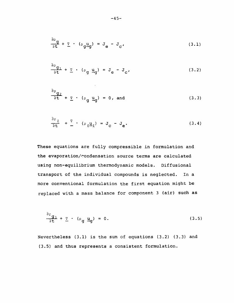
The major alteration is the addition of a fourth mass

balance to represent hydrogen transport. The following mass

conservation equations are solved:

-45-

v + (pu ) = J - Jc (3.1)t g-g e c

S+ (p u) = - Jc, (3.2)- g -c

at + V * (p u ) = 0, and (3.3)g -g

+ V (u ) = J - Je (3.4)at - = c e

These equations are fully compressible in formulation and

the evaporation/condensation source terms are calculated

using non-equilibrium thermodynamic models. Diffusional

transport of the individual compounds is neglected. In a

more conventional formulation the first equation might be

replaced with a mass balance for component 3 (air) such as

93 + V (p u ) = 0. (3.5)at - -g

Nevertheless (3.1) is the sum of equations (3.2) (3.3) and

(3.5) and thus represents a consistent formulation.

-46-

Each phase is described by

energy conservation equations.

modified and are presented here

can be seen and compared to the

time momentum balances are:

its own pair of momentum and

These equations were not

so that their general structure

new slower mixing model. The

ap u9 + V ( u u ) =

at g-g-g

- aVP + V a +p f+ f (U l J - ) (3.6)-g g- -M -g e

and

+t + U ( u) =

(a-l)VP + V*(l-a) + P f - f (U g t Je Jc ) "

(3.7)

The f function represents non-equilibrium interphasic-M1

momentum exchange due to velocity slip and phase change. The

shear stress tensor embodies only molecular effects including

bulk viscosity using Stoke'shypothesis. The neglect of

turbulent-enhanced viscosity is a reasonable simplification

in blowdown calculations. f represents body forces such as

gravity.

-47-

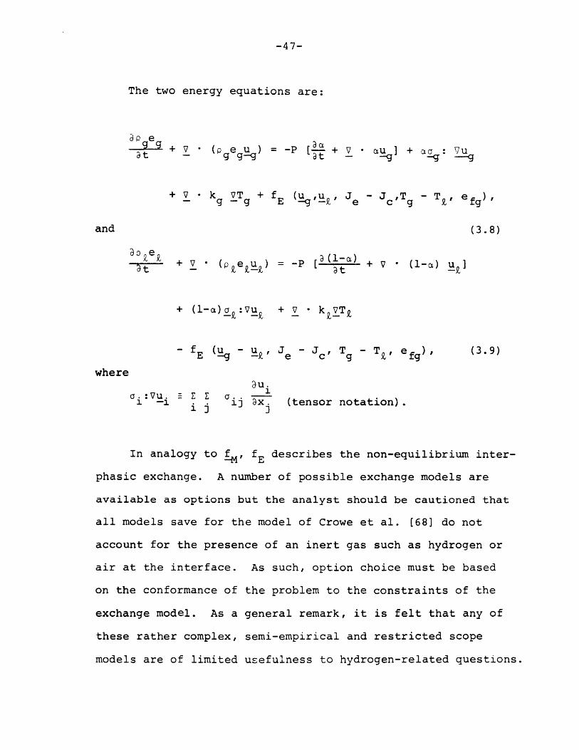
The two energy equations are:

pg e+ (p e ) = -P [-. + V ctu I + ao : Vuat 9 g-g at- -g -- g

+ V kg VTg + fE (U ,u , J - Jc,Tg - T, efg),

(3.8)

-t + V " (pze u)

+ (l-a)c :Vu

- fE (u - u ,

where

a. :Vu. E a..1 -1 13 ax

= P [ (t + V (l-u) u ]

+ V k VTk

Je - Jc, Tg - T, efg),

(tensor notation).

In analogy to f , fE describes the non-equilibrium inter-

phasic exchange. A number of possible exchange models are

available as options but the analyst should be cautioned that

all models save for the model of Crowe et al. [68] do not

account for the presence of an inert gas such as hydrogen or

air at the interface. As such, option choice must be based

on the conformance of the problem to the constraints of the

exchange model. As a general remark, it is felt that any of

these rather complex, semi-empirical and restricted scope

models are of limited usefulness to hydrogen-related questions.

and

(3.9)

-48-

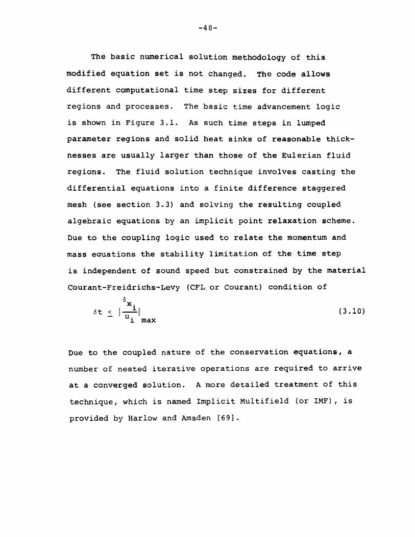
The basic numerical solution methodology of this

modified equation set is not changed. The code allows

different computational time step sizes for different

regions and processes. The basic time advancement logic

is shown in Figure 3.1. As such time steps in lumped

parameter regions and solid heat sinks of reasonable thick-

nesses are usually larger than those of the Eulerian fluid

regions. The fluid solution technique involves casting the

differential equations into a finite difference staggered

mesh (see section 3.3) and solving the resulting coupled

algebraic equations by an implicit point relaxation scheme.

Due to the coupling logic used to relate the momentum and

mass equations the stability limitation of the time step

is independent of sound speed but constrained by the material

Courant-Freidrichs-Levy (CFL.or Courant) condition of

X.6t < _ (3.10)

i max

Due to the coupled nature of the conservation equations, a

number of nested iterative operations are required to arrive

at a converged solution. A more detailed treatment of this

technique, which is named Implicit Multifield (or IMF), is

provided by Harlow and Amsden [69].

-49-

FIGURE 3.1: BASIC TIME ADVANCEMENT LOGIC

CONTROL TIMES

CALCULATED

-50-

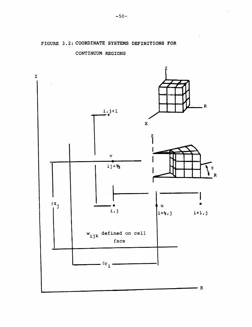
FIGURE 3.2: COORDINATE SYSTEMS DEFINITIONS FOR

CONTINUUM REGIONS

i,j+1.....- *

ij + 04

ijilj

wijk defined on cell

face

Ii+1,j

R

-51-

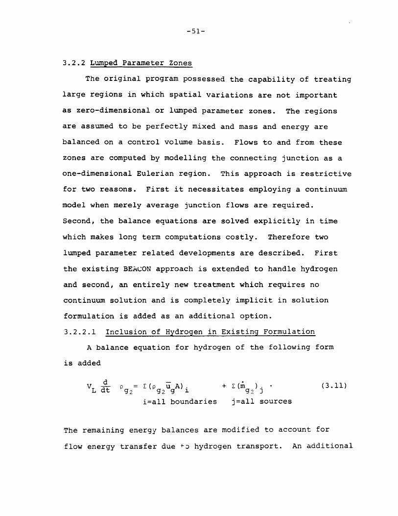
3.2.2 Lumped Parameter Zones

The original program possessed the capability of treating

large regions in which spatial variations are not important

as zero-dimensional or lumped parameter zones. The regions

are assumed to be perfectly mixed and mass and energy are

balanced on a control volume basis. Flows to and from these

zones are computed by modelling the connecting junction as a

one-dimensional Eulerian region. This approach is restrictive

for two reasons. First it necessitates employing a continuum

model when merely average junction flows are required.

Second, the balance equations are solved explicitly in time

which makes long term computations costly. Therefore two

lumped parameter related developments are described. First

the existing BEACON approach is extended to handle hydrogen

and second, an entirely new treatment which requires no

continuum solution and is completely implicit in solution

formulation is added as an additional option.

3.2.2.1 Inclusion of Hydrogen in Existing Formulation

A balance equation for hydrogen of the following form

is added

V p = Z (p u A) + Z(m ) • (3.11)L d- g 2 92 9 g 2

i=all boundaries j=all sources

The remaining energy balances are modified to account for

flow energy transfer due +D hydrogen transport. An additional

-52-

limitation of the original formulation is that the nodal

balances are specified as to be compatible with the two-

phase non-equilibrium model and as such the lumped parameter

state solution exhibits the same limitations as the continuum

solution.

3.2.2.2 Model Improvement

In light of the limitations elucidated above, a new

lumped parameter model is developed.. The formulation

presented is based on thewell-established nodal solution

methodology used in the RELAP and FLASH programs and as such

only the essential points are presented. Three nodal

mass balances are used.

Mik = W. - W. +SMik,ik j j P

(3.12)j=to junctions j=from junctions

where: k = air, hydrogen and water and

i = node.

The nodal energy conservation equation is

d U = h. W. - Eh. W.dt i 3 3 1 3

j=to junctions j=from junctions

+ ESMik hsk, (3.13)

k=1,3

where: h = 1[U+pV] and

hsk = source enthalpy.sk

-53-

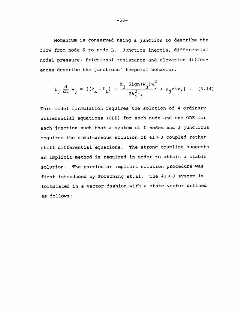
Momentum is conserved using a junction to describe the

flow from node K to node L. Junction inertia, differential

nodal pressure, frictional resistance and elevation differ-

ences describe the junctions' temporal behavior.

K. Sign(W.)W2Ij d W (P L) - 3 2 + P j g6 zj ] . (3.14)

3 dt W K L 2A 22Ajpj

This model formulation requires the solution of 4 ordinary

differential equations (ODE) for each node and one ODE for

each junction such that a system of I nodes and J junctions

requires the simultaneous solution of 41 + J coupled rather

stiff differential equations. The strong coupling suggests

an implicit method is required in order to attain a stable

solution. The particular implicit solution procedure was

first introduced by Porsching et.al. The 41 +J system is

formulated in a vector fashion with a state vector defined

as follows:

-54-

W

wJ

M al

aIMhl

S = : . (3.15)

MhI

Mwl

wI

Ul

and the system is described by:

dv- = f(Z,t) . (3.16)

A Taylor series expansion of the vector function, f, in-

cluding only first order terms and assuming a forward time

difference for the left hand side is

n+l nnt = f( tn) + n+- n) . (3.17)

6t Y a n n Y_

The terms of the Jacobian matrix are evaluated assuming the

state variables are independent of each other. Under this

constraint, the junction mass flow difference equation is

-55-

6t 2A 2 (I -W

I KP n+l n P n+1 n

U MK K K L L

+ ()(n+~1)-UnL (Un+1

+ 1 n_ pn J3 +h nK L 2 n I.

J -2A 3 p 3

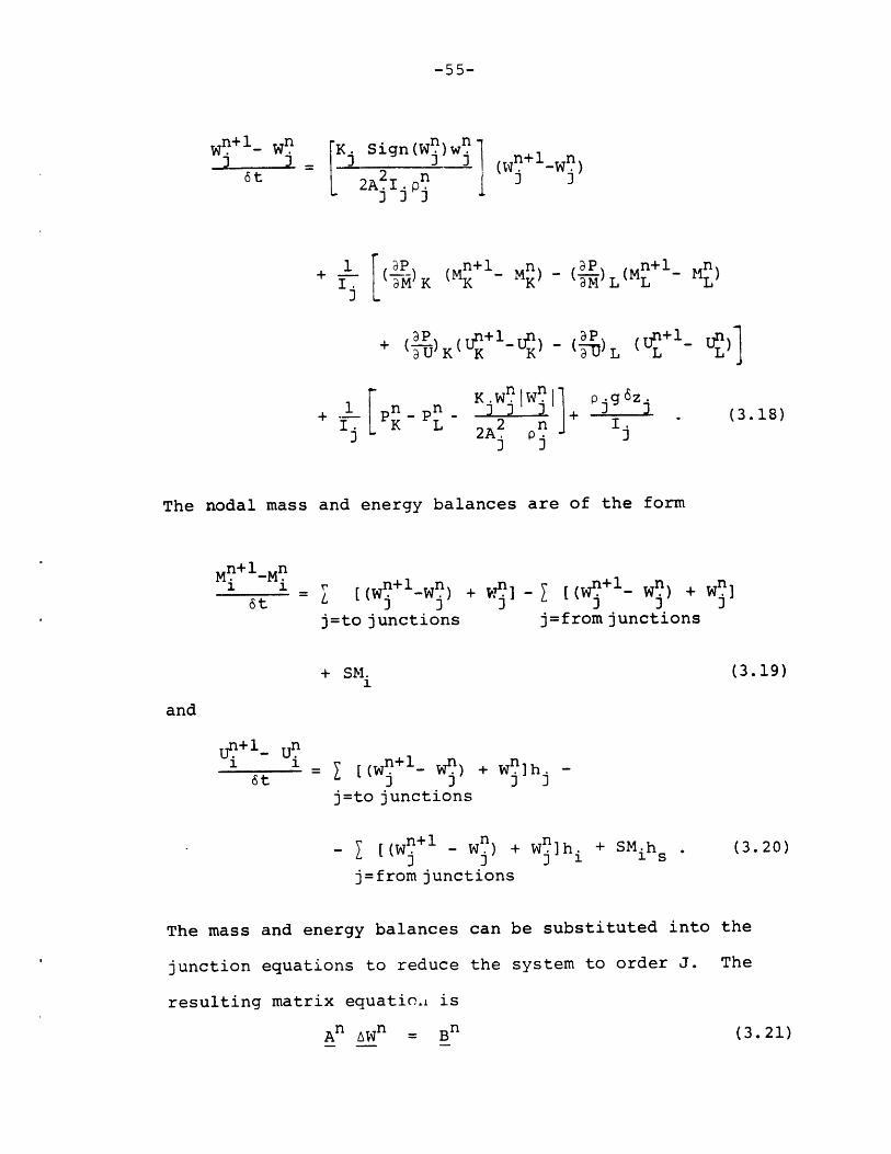
The nodal mass and energy balances are of the form

1 16t

n+l_ n n - ((wn+l_ n + wnJ J I ) J J

j=to junctions

+ SM.1

j=from junctions

(3.19)

u + 1_ Un1 1 [(n+l Wn ) + Wn]h

6t j -3 W

j=to junctions

- [(w n + 1 _ Wn) + Wn] + SM.h . (3

j=from junctions

The mass and energy balances can be substituted into the

junction equations to reduce the system to order J. The

resulting matrix equatio.i is

An AWn = Bn (3

(3.18)

and

.20)

.21)

-56-

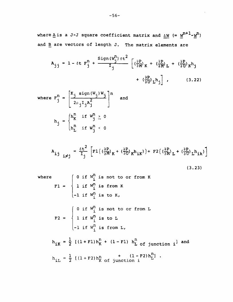
where Ais a JxJ square coefficient matrix and AW (= Wn+l-W n)

and B are vectors of length J. The matrix elements are

Sign(Wa1 ) 2

A. = 1- t F + () + () + () hS"a I. (M)K aM) L aU Kj

+ () Lhj , (3.22)

where Fnj 2p IjA2

K" n inWjj2 W

n ifn > 0

hn if Wn < 0L j

A13 isj

2 F1(( I p )K+ ( ) KhiK))+ F( ( )L + ( ) Lhik)Ij T K + K P LP

0 if Wni

F1 = 1 if Wn1

-1 if wn

t0 if Wn

F2 = 1 if Wn

1-1 if W. nI

(3.23)

is not to or from K

is from K

is to K,

is not to or from L

is to L

is from L,

1 n nh [(1+ Fl)h + (1-Fl) h of junction i and

iK 2K L of junction i

1 + (1-F2)h]iL 2 K of junction i

and

where

-57-

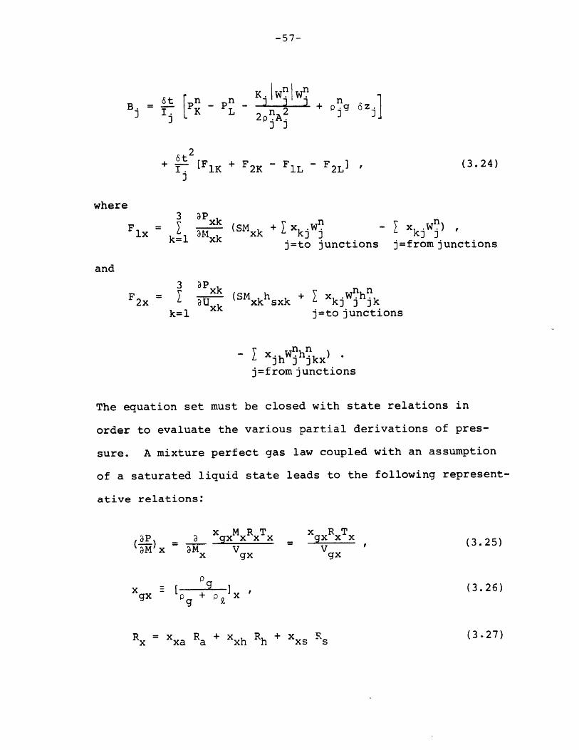
6t n n K- n4B - 3 3 + p g 6z jj I K L 2p A2 j3 L

6t1K 2K 1L 2L+ 5. [FIK + F2K- FIL- F 2L (3.24)3

where3 aP

F I xk (SMx + xk W - x .Wn)

ix = k= axk xk kjj kj 'j=to junctions j=fromjunctions

and

3 apF3 aP k (SM h + I x .Wnhn

2x I U x (Sxk sxk kjj jkk=1 xk j=to junctions

- I X Wnhnkx)3 3 3j=from junctions

The equation set must be closed with state relations in

order to evaluate the various partial derivations of pres-

sure. A mixture perfect gas law coupled with an assumption

of a saturated liquid state leads to the following represent-

ative relations:

x MRT x RTaP a gx x x x gx x x(325)

x gx gx

x - [ ] , (3.26)gx Pg P

0

(3.27)R Xxa Ra x x R + Xxsx xa a xh h xs s

-58-

V = V = V [ - , (3.28)gx x fx Pfx

x MRTP a x xxx (3.29)()x U V ox Vgx

but we know

Ux = Mx[xxgeg + (1- xxg)ez ]

= Mx[Xg (XaCaT + xhChT + sCsT) + (1 - Xg)(efo + C T)]x)

(3.30)

orU

Tx = [- (- Xg)efox[g(xaCa + XhCh + XsCs - C)

-1+ C ] (3.31)+ x .

Hence the partial derivatives of P in relation U may be

evaluated as

aP xg xx Vgx [x (XaCa + XhCh + xsC s - C ) + C(3x .32)

The coefficient matrix assumes a general structure that

need not be diagonally dominant and is therefore not amenable

to iterative solution. In the case of a chain of nodes where

one volume is connected to only its up and downstream neigh-

bor the matrix takes on a block-like structure but in gen-

eral containment problems the solution must rely on direct

inversion using Gaussian elimination. The outcome of this

calculation are the respective AW. for each junction whichJ

-59-

can be back-substituted into the nodal mass and energy

balances to arrive at the updated nodal densities and tem-

peratures. The definition of the actual nodal state given

the possible presence of steam and water deserves additional

comment but this discussion is delayed until the slower

mixing transient model derivation.

3.2.3 Ancillary Model Development

Numerous additional models are required to fully define

the problem solution. One is the ability to model hydrogen

as a possible source material. This addition is dependent

upon defining the thermodynamic characteristics of hydrogen.

Once hydrogen is introduced, its effect on the mixture

transport parameters such as thermal conductivity and visco-

sity must be considered. Development and definition of

these properties are presented below. Following this discus-

sion the effect of hydrogen on condensate film behavior as

well as reasonable heat transfer modelling of this flow

regime is addressed.

3.2.3.1 Thermodynamic and Transport Properties

Given that the state relations are based on a

mixture of perfect gases, the required hydrogen thermodyna-

mic values are molecular weight and relation between the

specific heat and the gas constant. The molecular weight

of hydrogen used is 2.0158 AMU which leads to a gas constant

-60-

of

R 2 2H = 4124.58 m /sec OK . (3.33)

MH2

The ratio Cp/RH for hydrogen varies from 3.451 to 3.519

over a temperature range of 280 to 500 0K according to

Reference 70 and hence a value of 3.47 is utilized. Specific

heat at constant volume is taken as 2.47 R (i.e. Cp - R = C ).

In accordance with the law of partial pressures, the overall

state definition (assuming uniform temperatures) is

P = ([ piRi)T where i = gaseous components (3.34)i

The two transport parameters are molecular viscosity

and thermal conductivity. The two properties are expressed

as linear functions of temperature. The two curve fits

based on a linear regression of experimental data are:

M -4 (3.35)kH = 0.03437 + 4.892 x 10 T (W/m0 K), and (3.35)

H = 2.942 x 10 6 + 2.002 x 108 T (kg/m sec). (3.36)

A comparison of these functional approximations and the

actual data is provided in Table 3.1. As is seen the

agreement is quite acceptable especially in the expected

containment temperature range below 400 0K (2600 F).

3.2.3.2 Condensate Film and Heat Transfer

Very detailed condensate film modelling is available

-61-

TABLE 3.1: Comparison of Property Approximations vs. Data [70]

MkH

T

(OK)

280

300

350

500

AVERAGE ERROR

AVERAGE ERROR

w/o 500 K DATA

(W/m

EQUATION

0.171

0.181

0.206

0.279

OK)

DATA

0.171

0.181

0.205

0.272

±1.3%

±0.2%

M 6H xl0

(kg/m sec)

EQUATION DATA

8.548 8.554

8.948 8.958

9.949 9.942

12.952 12.242

±1.2%

±0.1%

-62-

in BEACON such that the time dependent flow behavior of a

film travelling along a solid surface can be predicted.

The transfer of mass and energy at the film/bulk fluid

interface is strongly determined by the local component

profiles. As such the original film model is modified to

account for the presence of hydrogen in this interfacial

region. If the film model is employed, the heat transfer

at the film/fluid boundary is computed on the basis of a

mass/heat transfer analogy and the heat transfer at the

boundary is computed using a film Nusselt number correla-

tion. If a film is not modelled explicitly, the original

code allows the use of three options -- input constant co-

efficients, coefficients based on vapor content or tempera-

ture or using a Stanton number correlation for a flat plate

of the form:

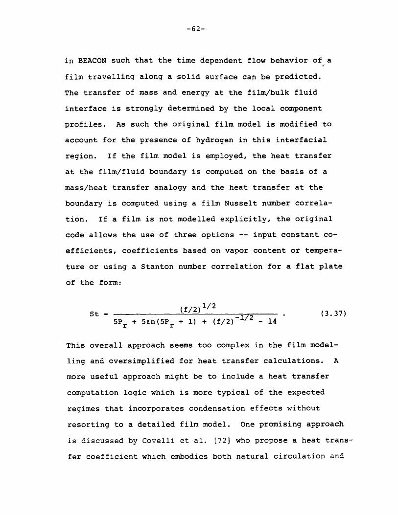
St = (f/2) 1/2St= . (3.37)5Pr + 5 tn( 5Pr + 1) + (f/2)/2 - 14

This overall approach seems too complex in the film model-

ling and oversimplified for heat transfer calculations. A

more useful approach might be to include a heat transfer

computation logic which is more typical of the expected

regimes that incorporates condensation effects without

resorting to a detailed film model. One promising approach

is discussed by Covelli et al. [72] who propose a heat trans-

fer coefficient which embodies both natural circulation and

-63-

condensation. The general form of this expression is

h = hNC + C hc (3.38)

where C = function of condensation rate. Corradini [71]

also reports a condensation model for both forced and

natural convection based on extending the Reynolds-Colburn

analogy to mass and momentum transfer.

3.2.4 Inherent Limitations of the Modified Code

A comparison of the desired capabilities of a hydrogen

transport code with the characteristics of the program after

this first series of modifications demonstrates that sub-

stantially more development is required. The so-called

modified BEACON equation set can handle hydrogen as a third

gaseous component but still subject to the overall assump-

tions and limitations of the original code. The use of

these analytical models is restricted to rapid two-phase

transients. The use of non-equilibrium thermodynamics is

unwarranted in slower mixing transients and leads to inordi-

nate amounts of computational effort. Clearly, the nested

iteration aspects of a compressible flow solution should

only be used when the problem demands it. Nevertheless,

the model at this stage of development addresses important

parts of the hydrogen scenario spectrum in its appropriate

application to two-phase jet-like releases such as might

occur from a pressure relief valve or the study of large

interconnected rooms using a lumped-parameter approach.

-64-

The limitations of the modified code define the re-

quirements for the slow mixing model described in the next

section. Also addressed in the following discussions is

the boundary of applicability between the two analytical

models of continuum regions.

3.3 Longer Term Transient Modelling - MITHYD

While blowdown transients are dominated by two-phase

compressibility effects, longer term transients, which

involve the gradual build-up of hydrogen over an extended

period (e.g. degrading core or radiolytic decomposition),

are characterized by a nearly incompressible multi-component

homogeneous flow field. The model formulation described in

this section is based on this physical regime. Important

effects include molecular and turbulent-driven transport

as well as buoyancy-driven convection.

The basic theoretical formulation is first derived and

specialized to the problems of interest. The model is based

on a primitive variable formulation augmented by turbulence

transport equations. The turbulence modelling is based on

a 2 equation k-E formulation employing seven empirically-

derived closure constraints. The problem is complicated by

the presence of a condensible species-water. Consistent

thermodynamic state determination must be carefully con-

sidered. An assumption of interphasic equilibrium is made

to formulate this approach.

-65-

The definition of the overall equation set is the first

step in creating a model. The coupled set of non-linear

partial differential equations is clearly not amenable to

analytic closed form solution and hence a numerical tech-

nique is required. The solution scheme is based on a finite

difference discretization of the continuum equations using

a staggered computational grid. Given that physically

diffusive phenomena are important, the numerical scheme

should not introduce false diffusion. This usually arises

from the treatment of convective terms in the conservation

equations and hence a proper limited diffusion technique

is needed.

The nearly incompressible assumption allows the solu-

tion of the momentum/continuity equations independently of

the energy equation save for the feedback of buoyancy

effects. At first glance one would assume that this allows

the straightforward application of an established technique

such as the SMAC method. However in buoyancy-dominated flow

closer attention to the coupling is necessary. Once the

flow field is computed, the remaining mass transport energy

and turbulence equations must be solved. The solution of

these equations involve accurate models of mass diffusion

and nodal phase changes as well as reference state definition.

A complete problem definition involves not only the prescrip-

tion of the controlling rquations but also a complete and

consistent specification of initial and boundary conditions.

-66-

This is especially so in a discretized solution regime.

Finally the underlying assumptions, especially that of in-

compressibility, need to be monitored in order to assure

the solution remains within the appropriate physical bounds.

The following subsections elaborate in detail upon the

points made above. The model has been implemented in a

subcode named MITHYD. The MITHYD subcode is modular in

structure as is further described in Appendix A. The com-

putational coupling to the overall code is analogous to the

role played by the K-FIX two phase flow subcode. In effect

insofar as the slower mixing computations are concerned,

the MITHYD subprogram uses the remaining portions of the

code for data processing, ancillary effects calculations

and input/output processing.

3.3.1 Basic Equation Formulation

The basic thermo-fluid dynamic equation set which con-

stitutes the theoretical foundation of the slow mixing model

is presented. Detailed equation derivations are omitted

but may be found in standard transport phenomena texts

such as Bird et al. [73]. The equations are presented first

in vector notation so that individual terms can be addressed

from a physical standpoint. They are then specialized to

a 3-D cylindrical/Cartesian coordinate system. The equa-

tions are formulated such that a 2-D system can be solved.

A 2-D formulation is compatible with the rapid transient

-67-

model and is expected to be used in the majority of applica-

tions. The three dimensional option is provided for prob-

lems in which such modelling complexity and computational

effort is required.

The general fully compressible mass conservation or

continuity equation without source effects is

+ V. (pu) = 0 . (3.39)

If the incompressibility assumption is made, (3.39) may be

simplified to

0 0

S+ pVu + p = 0 or V*u = 0 . (3.40)

The momentum equation is

auPr [ - + (uu)] = - VP + v.& + pf + fD (3.41)

M Twhere = + c

The reference state density formulation is typical of the

Boussinesq approximation. Physically the lefthand side (LHS)

are the time rate of change of momentum and the convective

momentum transport, respectively. The first right hand

side (RHS) term is the pressure field gradient. The second

term is the shear stress which embodies both molecular and

turbulent mixing effects. The third term represents body

forces which in this application are limited to gravity

while the final term involves frictional and form losses

-68-

due to objects within the flow field. This term is included

to account for gratings, small obstacles, structural mem-

bers, etc.

The fully compressible mixture internal energy conser-

vation equation is

ape + V*pue = V*kVT - pV*u + 0e , (3.42)at

where k = kM + kT , and

wD = viscous dissipation.

The incompressible formulation of the momentum equation

leads to the neglection of the flow work term. The viscous

dissipation term is assumed negligible in problems of in-

terest. Omitting the flow work contribution is a reason-

able approximation for situations in which convection is

dominant and forces on the fluid are dominated by mass trans-

port induced buoyancy (e.g. introduction of a light gas)

or momentum sources (jet effects). Both conditions are

satisfied in the slow mixing analysis. Therefore, the

actual mixture energy equation utilized in the model is

_pe + V*pue = V*kVT . (3.43)

The substantive derivative is kept in a conservative

form to more accurately track the convective transport. In

comparison with the BEACON energy equations, compressive

work, viscous dissipation and non-equilibrium interphasic

-69-

transport are neglected. It may also be noted that if

separate gaseous and liquid phase energy equations were

used in the slow mixing model, an additional source term

due to phase change energy absorption or liberation would

have been required.

The single continuity equation is inadequate for track-

ing the transport of the individual species. Hence four

additional mass transport equations are introduced. The

general equation form equates the species substantive deri-

vative to diffusion, source and phase change effects and

has the form

ac.+ V.(uc.) = V*D.Vc + i , (3.44)

-t - -1 1

where i = air, hydrogen, steam and liquid,

M TD. = D + D , and

i i

i = phase change rate (for steam and water only).

The appropriatenessof this equation for the three gaseous

components is well-established. The phase change rate is

calculated on the basis of a thermodynamic equilibrium

assumption. The proper treatment of multi-component molecu-

lar diffusion is addressed below. Nevertheless the appli-

cation of an equation of this form to liquid transport

which would actually involve a spectrum of droplet sizes

and speeds is not truly aDpropriate. It is used here as a

first approximation and in anticipation of the development

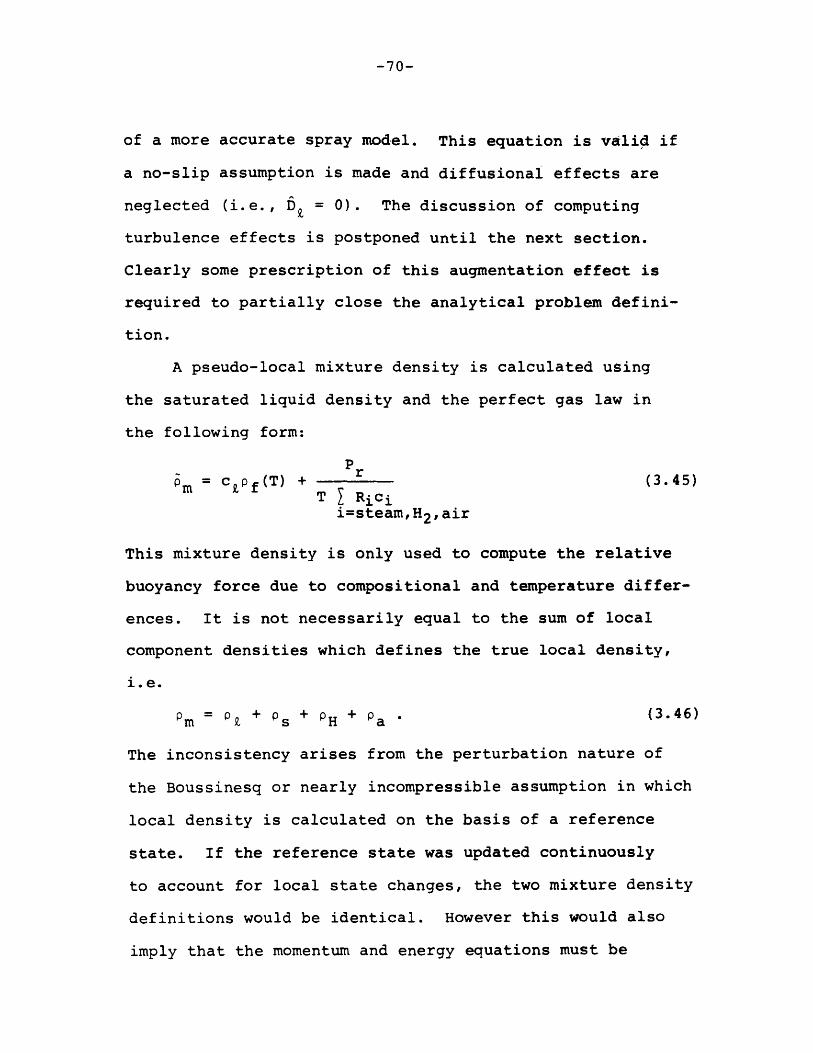
-70-

of a more accurate spray model. This equation is valid if

a no-slip assumption is made and diffusional effects are

neglected (i.e., DE = 0). The discussion of computing

turbulence effects is postponed until the next section.

Clearly some prescription of this augmentation effect is

required to partially close the analytical problem defini-

tion.

A pseudo-local mixture density is calculated using

the saturated liquid density and the perfect gas law in

the following form:

Pm = c pf(T) + r (3.45)T 1 Ric i

i=steam,H2 ,air

This mixture density is only used to compute the relative

buoyancy force due to compositional and temperature differ-

ences. It is not necessarily equal to the sum of local

component densities which defines the true local density,

i.e.

m = P + Ps + PH + Pa . (3.46)

The inconsistency arises from the perturbation nature of

the Boussinesq or nearly incompressible assumption in which

local density is calculated on the basis of a reference

state. If the reference state was updated continuously

to account for local state changes, the two mixture density

definitions would be identical. However this would also

imply that the momentum and energy equations must be

-71-

solved simultaneously completing the path back to a fully

compressible formulation. The advantage of allowing this

degree of inaccuracy is the ability to solve the two

equations (and the individual component equations) indepen-

dently. The error in the buoyancy term increases as the

actual state departs from the assumed reference

state. Periodic redefinition of the reference state can

limit the magnitude of this error and is discussed in

greater detail in the solution scheme subsection.

The fluid dynamic equations are now presented in a

generalized 3-D formulation. The parameter a allows the

equations to be descriptive of either cylindrical or

Cartesian coordinates while the parameter X is used to

specialize the equations to either a 2 or 3 dimensional

form. The logic of this specification is

0 1

0 2-D 2-DCartesian axisymmetric

1 3-D 3-DCartesian cylindrical

The coordinate system is shown in Figure 3.2.

The continuity equation is

1 a ra + w 0r ru + -v + -0

r r(3.47)

-72-

The vector momentum equation is decomposed into three scalar

relations representing force balances along the principal

axes of the appropriate coordinate system. The radial

momentum equation is

au 2 a Bu x a 8wP [ + _-Lu + uv + 2 + u w ]r at ar az 8 s ae rr r r

+ + 1 a -. au a+ -u a au3r r Dr r -r 5z az + r arr

az ar 28r

+1 [ u 1 a( aw 8w+ [ a +r2 8 ae r are ar

28f aw

r2B ae

The formulation also accounts for spatial variation in visco-

sity. The axial or z-momentum balance is

P av a V + + uv X avwr at ar az aer r

1 a B- 8av av a au+ f + a r - + v + u +Dz a r . r vz az + r az

r2 e -6 r+ ae az "

aP +az z

ai avaz az

(3.49)

Finally the optional third dimensional equation is

(3.48)

-73-

aw a 1 a 2 a 2 Buwr at ar sae oz 6r r

1 aP 1 a 6 aw 1 a - awr a Do r6 ar +r 2 ae ae

aw B au 1 a+ -- - + -- (2 -w) + ( a - w)az a r28 -e a 3

1 a aw i a av+r 2 a 31w+ 2Bu) +B a. a " (3.50)2ae ae r6 z ae

The e-momentum equation does not contain a gravitational

term since normal orientations are expected to be typical

of containment problems. The energy and other transport

equation can all be described by the following generalized

form

[ + a r u + vt + w ] =at r Br a B aer r

r 2 -+ + + S (3.51)rB ar r az az r2 ae ae

3.3.2 Turbulence Effects

Turbulent transport processes are a significant physi-

cal effect that must be addressed in slower mixing tran-

sients. The selection of a turbulence model is not a

trivial task especially in this application. The multi-

component flow field is affected by buoyancy induced

-74-

convection arising from both local temperature and concen-

tration perturbations. Also, the flow fields typical of

enclosed region problems exhibit recirculating flow and

local relaminarization or transitional flows. The general

approach taken in this work is to utilize a so-called 'two-

equation' turbulence model. These additional closure

equations arise from the resolution of the Navier-Stokes

equations into constant and time-varying components. The

resultant new terms arise from the non-zero ensemble

averaging of correlation functions. The reader is referred

to a turbulence text such as Hinze [74] for more detailed

derivations.

The form of the turbulence model used in this model

is already suggested by the diffusion terms in the various

conservation equations in which the molecular transport

coefficient is augmented by an effective turbulent diffu-

sivity. The implicit assumption is that turbulent trans-

port can be related to the gradient of the transported

property as is the case for molecular effects. Early at-

tempts at computing the value of this turbulent or eddy

diffusivity employed either constants based on the pioneer-

ing arguments of Boussinesq or a single equation model

such as Prandtl's mixing length. Though simplicity and

reduced reliance on empiricism are attractive features of

a mixing length argument, the actual definition of a single

length scale descriptive of transport through a recircu-

-75-

lating flow is physically unrealizable. Most current

models utilize two-equation closure models as an accept-

able compromise between accuracy and effort. There are

much more complex models which basically involve transport

equations for higher order correlation functions. Unfortu-

nately utilization of such models requires even more em-

pirically derived closure constants which in turn render

the model less general. Further the computational effort

increases unboundedly. To quote Launder and Spalding:

'the proponents of the most detailed turbulence models have

themselves been armchair explorers.'

Numerous two-equation models have been proposed. Most

involve the behavior of the turbulent kinetic energy and

turbulent viscosity (k-a models) or turbulent kinetic

energy and its dissipation (k-c models). Launder and

Spalding argue from a physical standpoint that the k-c

models are more appropriate but both classes of models seem

to be useful. As alluded to above, turbulent kinetic

energy and its dissipation are analytical constructs of

correlation terms originating from the Navier-Stokes

equations. In terms of the primitive variables the two

turbulence parameters are

k < u'u'>, and (3.52)

pM u iuM < >. (3.53)P xkaxk

Lum-ley [48] comments that the name, dissipation, is

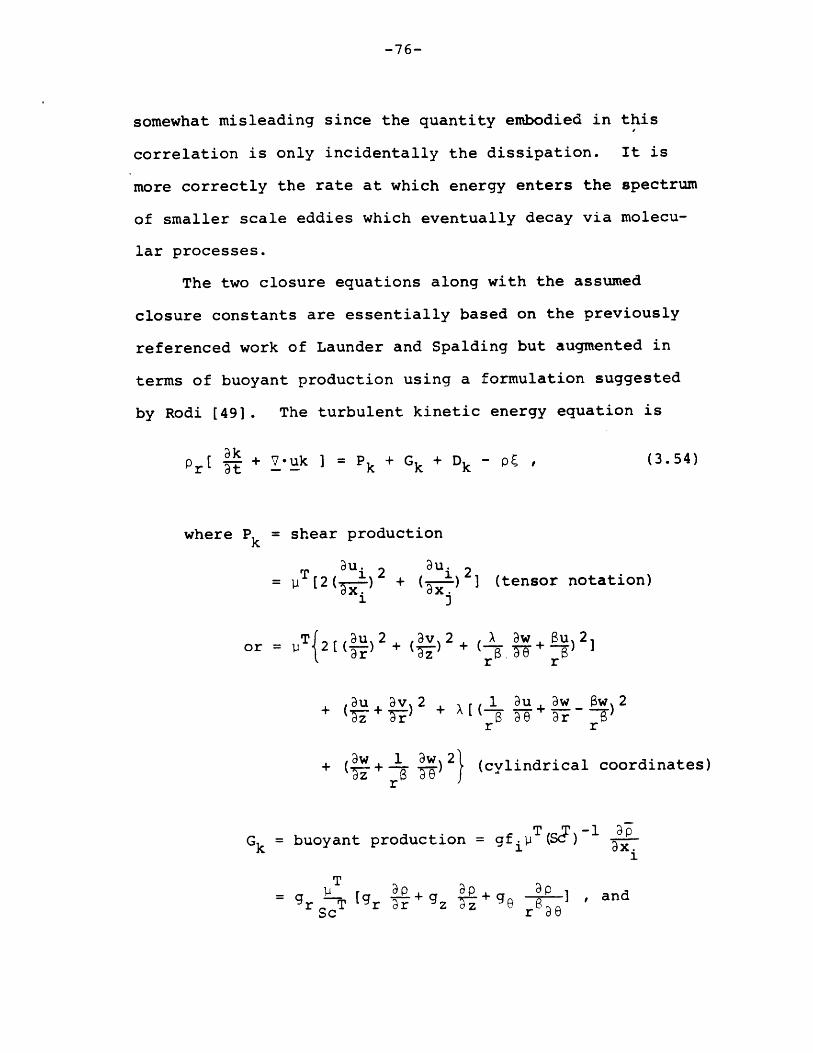
-76-

somewhat misleading since the quantity embodied in this

correlation is only incidentally the dissipation. It is

more correctly the rate at which energy enters the spectrum

of smaller scale eddies which eventually decay via molecu-

lar processes.

The two closure equations along with the assumed

closure constants are essentially based on the previously

referenced work of Launder and Spalding but augmented in

terms of buoyant production using a formulation suggested

by Rodi [49]. The turbulent kinetic energy equation is

pr[ -k + V*uk = Pk + Gk + Dk - (354)

where Pk = shear production

T ui2 ui2= [2( + (- ) I (tensor notation)

1 3

or = T 2[ (u) 2 + (v) 2 + aw Bu+ )2]3r r r

+ u v 2 1 3u aw aw)2+ (V£+%-£) + X[( + --r r

+ ( .aw+- aw)2} (cylindrical coordinates)

Gk = buoyant production = gf i T (SJ)l x.

= g T ar + g ] , andSc r

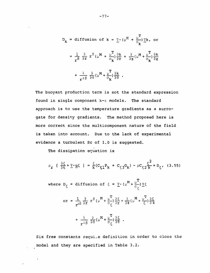
-77-

D = diffusion of k = V*(m + )Vk, ork V( + )k, ork

T T1 a 8 M 1 k a M 9) kS -r (M + ) 9k + ( + )r akr k r ok 3z

SX (M ,T 9k

r 2 90 ak ae

The buoyant production term is not the standard expression

found in single component k-c models. The standard

approach is to use the temperature gradients as a surro-

gate for density gradients. The method proposed here is

more correct since the multicomponent nature of the field

is taken into account. Due to the lack of experimental

evidence a turbulent Sc of 1.0 is suggested.

The dissipation equation is

E 2

S [ +Vu] (C + C 3 Gk) pC +D, (3.55)r t k (1 k + 3 k E2k (

Twhere D = diffusion of E = V* ( + P_)VE

T T1 orrB M Tr aM M Tor - r( + + -( +r2 ar a 9r 5z E az

X 9 M ) T+ ( -l E

Six free constants requi-e definition in order to close the

model and they are specified in Table 3.2.

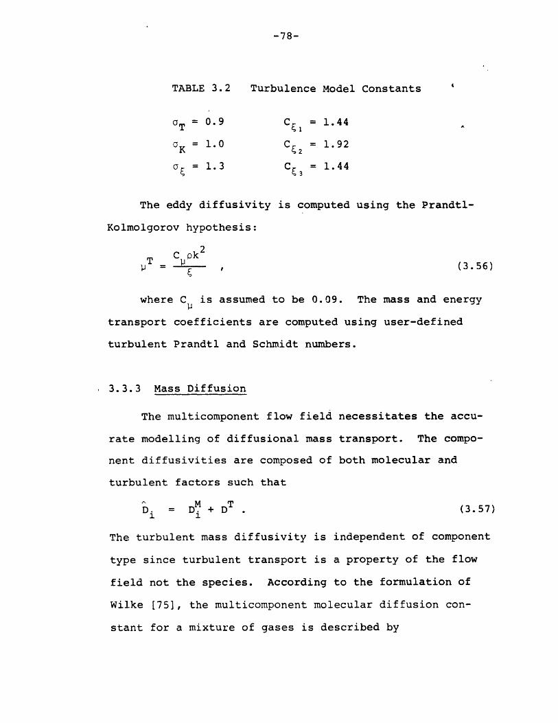
-78-

TABLE 3.2 Turbulence Model Constants

S= 0.9 C 1.44

aK = 1.0 C = 1.92

a = 1.3 CE3 = 1.44

The eddy diffusivity is computed using the Prandtl-

Kolmolgorov hypothesis:

C kPT = , (3.56)

where C is assumed to be 0.09. The mass and energy

transport coefficients are computed using user-defined

turbulent Prandtl and Schmidt numbers.

3.3.3 Mass Diffusion

The multicomponent flow field necessitates the accu-

rate modelling of diffusional mass transport. The compo-

nent diffusivities are composed of both molecular and

turbulent factors such that

M TD. = D. + D (3.57)

1 1

The turbulent mass diffusivity is independent of component

type since turbulent transport is a property of the flow

field not the species. According to the formulation of

Wilke [75], the multicomponent molecular diffusion con-

stant for a mixture of gases is described by

-79-

1 - C.M =_D = (3.58)

i C j/DMjiji M

Bird et al. provide the following prescription for the

binary diffusion constants.

1.8583 x 10- /T 3 (- +-)M M. M.Di 2 (3.59)

Pji 5Dji

M 2where D. = m /sec,ji

M = molecular weight,

p = pressure (atm),

T = temperature (OK), and

Q = empirical constant, function of tempera-

ture and binary components

Using the applicable factors for the three possible binary

combinations (air-hydrogen, steam-hydrogen and steam-air)

the binary coefficients were fit to curves of the following

functional form:

D = 4.9492 x 10 T 6947 (3.60)ah

Dhs = 2.8916 x 10 - 5 T 1. 8 1 4 4 , and (3.61)

-6 1 9035D = 4.681 x 10 T. (3.62)as

These approximate curves are compared with the analytical

values in Figure 3.3. The agreement is quite good over

the expected temperature range. In problems in which

-80-

1.5 - CURVE FIT

1.2 - D-

I I Dah

o 0.6

as

0.3-

0.0280 300 320 340 360 380

TEMPERATURE (K)

FIGURE 3.3: MOLECULAR BINARY DIFFUSIVITIES AT

ATMOSPHERIC PRESSURE

-81-

molecular effects are unimportant a constant component-

specific diffusion constant may be employed.

As stated in the turbulence modelling discussion,

turbulent mass diffusivity is computed on the basis of

the turbulent viscosity and a user-supplied reciprocal

turbulent Schmidt number. (1.0 is the suggested value

for most simulations.) This leads to

pC kT T -1 T 1 p

pSc

or

C k 2

D = T (3.63)Sc~

3.3.4 Solution Scheme

The set of non-linear partial differential equations

and constituent relations which define the slower mixing

analytical model are not amenable to closed form solution

without substantial simplification. Therefore a numeri-

cal solution technique is formulated. An overview of the

solution scheme is provided in Figure 3.4. The continuum

is discretized into a computational mesh exemplified by

Figure 3.2. This staggered mesh arrangement of variable

definition in which all cell parameters except momentum

are cell-centered while che cell momenta fluxes are

defined at cell boundaries is typical of Marker and Cell

(MAC) type algorithms.

-82-

NO

NO

FIGURE 3.4: BASIC SLOW MIXING SOLUTION LOGIC

-83-

Given that the pertinent transients are such that phy-

sically diffusive mechanisms are important, the numerical

scheme should not introduce false diffusion due to its

discretization. The convective terms are most susceptible

to this limitation and must be formulated accordingly. Ir-

regardless of the convective treatment, the incompressible

assumption allows the nearly decoupled solution of the

conservation equations. The continuity/momentum solution

is accomplished using a 3-D form of the modified Simplified

Marker and Cell (SMAC) method. Once the updated velocity

and local pressure fields are computed, the remaining con-

servation equations can be solved. These equations are

solved with either an explicit or implicit technique de-

pending upon particular stability constraints. The liquid

and steam transport equations must be solved neglecting

the condensation/evaporation contribution since the value

of this term is determined by the local state which itself

depends upon the local mass fractions. The knowledge of

the local mixture energy and total mass density coupled

with a thermodynamic state constraint is used to define the

local temperature and phase change rate.

The solution of any set of partial differential equations

requires the complete and consistent definition of initial

and boundary conditions. With the addition of new flow

variables such as turbulent parameters, proper initial con-

dition definition must be addressed. New boundary conditions

-84-

for the turbulence parameters and the optional three dimen-

sional flow field need definition. Finally, given the

underlying incompressibility assumption, the solution

methodology should have internal validity checks to assure

the physical appropriateness of the technique. These

various facets of the scheme are now described in more

detail.

3.3.4.1 Treatment of Convection and Numerical Diffusion

The discretization of the continuum equations gives

rise to inaccuracies in the computed solution when compared

to exact analytical results. One important source of

error is false or numerical diffusion. This false diffu-

sion arises from the treatment of advection terms and

manifests itself by producing distributions in which the

entity is transported further in the normal direction (to

the flow) than can be accounted for by physical processes.

The donor cell treatment of convection exhibits signifi-

cant numerical diffusion. The donor cell logic is de-

scribed by

aui = U+P- (3.64)ax 6x

where u+,u_ = velocities defined at cell boundaries,

S of the cell if u+ > 0i of the right cell if u+ < 0, and

-85-

i of the left cell if u_ > 0

of the cell if u_ < 0.

Huh [39] has described the errors associated with this

approach in terms of truncation and cross-flow errors.

Crossflow diffusion is especially important in recircula-

tion problems when velocity vectors problems where. velocity

vectors substantially deviate from the orthogonal mesh

coordinate system. Huh has quantified the equivalent dif-

fusion constant due to the donor cell treatment as follows:

Dr = u 6r (1- Pr) , (3.65)

Dz = v 6z (1- Pz) , (3.66)

De = w r866 ( -Pe ) , (3.67)

where

Di = directional diffusivity,

P. = directional cell Peclet number

ui/6x i

3Sui/6xi1 ii=l

The donor cell treatment is seen to increase in accuracy

as cell spacing is decreased.

The good stability characteristics and the conservative

nature of the donor cell treatment makes it the primary

treatment of convection. Nevertheless, applications may

arise in which coarser nodalizations are desirable. For

such situations, two possible corrective schemes are

-86-

proposed. The first and most appropriate for transient

problems is to subtract the local numerical diffusion con-

stant from the local physical diffusivity. The reader is

referred to the original work for a detailed consideration

of the stability constraints of this approach. In brief,

not all the numerical diffusion can be corrected and the

approximate correction made is

Dtotal = Dphysical - SF DND (3.68)

where

SF = safety factor.

A second alternative is provided but its application

to transient problems is not recommended. The technique

treats the convection terms in a Lagrangian manner while

the remaining diffusive and source terms are treated in

a Eulerian orientation. This work is related to that of

Raithby [43] and Stukley et al. [76]. In effect each

conservation equation is solved in a two step fashion as

depicted by the following generalized formulation.

S+ V-u = verfV4 + S (3.69)3t -

is replaced by

n

- + V~ = 0 and (3.70)6t

n+1 _= V*Vr + S . (3.71)

6t -

The first equation which is purely convective

-87-

is solved using the new scheme while the solution of the

second class of equations is accomplished using the ex-

plicit/implicit method described below.

The Lagrangian scheme intuitively involves a coordi-

nate transformation to the trajectory of the con-

vected entity over the time step. This trajectory will

nearly always intersect a location for which the entity

is not defined and therefore some sort of spatial inter-

polation to arrive at a useable value. Of course in

situations in which the intersecting location lies out-

side the physical domain, the donor cell scheme is used.

This is not a major weakness since in this boundary

region flows more closely follow grid directions. The

most significant weakness of this type of Lagrangian

approach is its non-conservative nature. A complete

understanding of the inaccuracies arising from utilizing

such an approach are not fully appreciated at this time.

3.3.4.2 Flow and Pressure Fields

The Simplified Marker and Cell (SMAC) method intro-

duced by Harlow and Amsden is used to solve the momentum/

continuity equation set. The exact form of the solution

scheme is described in some detail herein because the

complete formulation of the technique applicable to a

general non-uniform three dimensional cylindrical mesh

is derived. Most available references on the SMAC method

-88-

are usually limited to uniform 2-D meshes.

The first step in the method is computation of an

estimated or 'tilde' velocity field based on a completely

explicit advancement of the component momentum equations.

The form of the drag term is assumed to be

fDX = -Kx IUx n u n +x (3.72)

Using this form the three tilde velocities are specified.

In order to streamline the notation the following sub-

scripting logic is employed:

if no subscript u ii+!jk

v v+ k ,

w w. ijk+, and

ijk

Only deviations from this are shown

e.g. ui- = ui_ jk

The r-direction tilde velocity is

1 un t aP 1 agru 3 aua B T-,,[- r r + -

6tKrJUl n ~ r r

1+Pr

Y 2 2+ar ar + t zr r2B r2B ae + (e r r

28GA aw PrBu Xpr w n2 w Pru + r n 2 a+ 28 u rB r ] -6t [- u + uv

+B uw]n , (3.73)r

where

aP 2-- - +(P-P )ar - Tr i+ '

~Pi+l+P-2PrPgr - 2 g

1 r Br r

u 2 ai+1rik (u -u) pr (u-ui )

6r+ (r+--) ri+

(3.76)

Su 1 i+l + + a +1-u)z u z z 6 z i)(u-u-15z ]

(3.77)

(3.78)Bu ~ i+l- ui+ -u u-ui

[ + 1 2r r 6r+ 6ri+ 6r+ i+1

B v ~ 1 1[ (v -v+v -v.)az ar 46z 6r+ i+1 i+lj- -j- )

(j+li+lj+l- i-lj i+lj-1 ) ]

-6u -ui+12r 7dr 2 2r (r+ -)

(3.79)

(3.80)

A 9 ^u ~ 2A i(Uk+l-uk) k-1(u-k-l)v - 6 r 2 kk1)

r (r+ -) 66 + 6 -

(3.81)

-89-

(3.74)

(3.75)

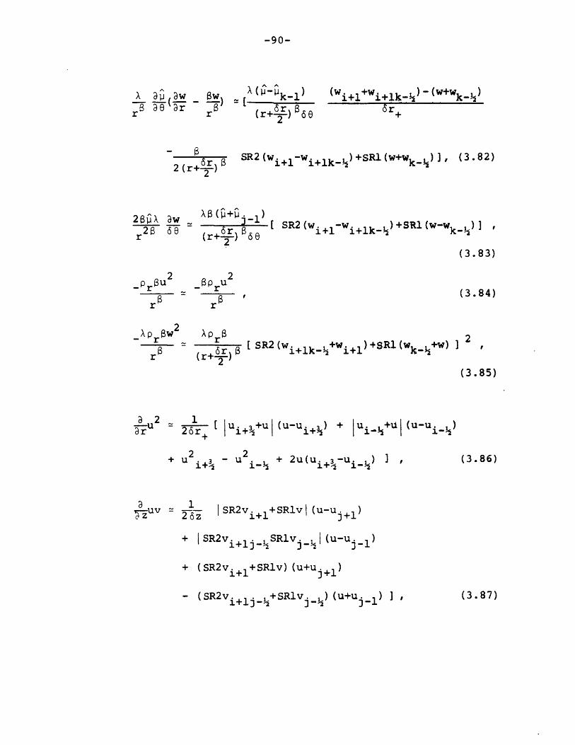
-90-

;e 3r (r+'r) '6e

(w )+w ww

S2w i+l1Wi+1kJT%)LSR1w~wk J]1 (3.82)2 (r+6r)

SR(w+l-wi+lk )+ lw k )

(3.83)

(3.84)-

I

Xp [R2w ilk 1 +w. 1~)+SR1(w +W)(rlk-r)1

(3.85)

-ru 26r~ +: (ji+ (Uuj+ ) + Hui. +ul (u-ui )

+ u + - ,2 *- + 2u(u .~3-ui-h)If

7-zu 2 63- SR2v i 1 +SRlv (u-u jl

+ I SR2v i+ 1 i --2SRlv -I (u-u j-

+ (SR2v i++SRlv) (u+u +1

- ( R~ i lj +S~v --12 j + u -

2ap~X aw

r 2a6

(3.86)

(3.87)

-91-

x u W rx [ ISR2wi+I+SRw (u-uk+ )r T (r+--) kl

+ sR2wi+lk-+SRwk-1 (1 (u-uk-1)

+ (SR2wi+ +SRlw) (u+uk+l)

- (SR2wi +SRlwk) (u+uk ). i+lk-= + k-1 k-1

6x = 6x + 6x.+/-+1/i-

SR1 = 6ri+1/6r+

and

SR2 = 6r/6r+

The z-direction tilde velocity estimate is

1 fVn +

1+r 6 tkvPr

+ u + v +ar az Bz az

6t -P6 [a- +r

r 2

a 3 2 x6 t [-- uV + -- v+ -- vwrar at ,

where

1 a + avpg + - r p-- +z 6ar ar

r Buv

rrr

(3.92)n

P 2z 6z+ j+

f gz [Pj+l+P-2r] 2

2(r+6r)a av 2-r 6r

(v i+l-V) - (v-v

6r+ 6r

(3.88)

(3.89)

(3.90)

(3.91)

a ^avaz az

n

]

(3.93)

1

r

(3.94)

(3.95)

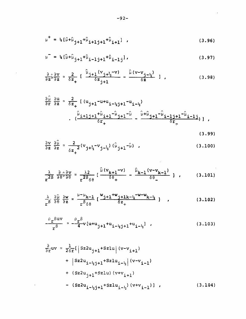
-92-

S= bl' +l+p i+lj+l+i+l] ,

14-= i+i +^ +

^v ~ 2 [j+ ) (v-vzz 6z + 6z 6z+ j+1

(3.96)

(3.97)

(3.98)

26z+ j+l i-j+l-Ui-

A A A

- 1J+~I.A ^r

i+l+l + i+ l + 16r.

(3.99)

(3.100)3v 311 2az a z j+ -j j+l-

X ^av

r

S2 (Vk+l-V) k- (V-Vk-

r 6e + 66

S w -k-1 Wj+l+W j+lk--1W-k-r8 36 az r86e 6z+

Prau v Pr8

r6 4 v[u+uj +l+uij +ul+ ]

9 1uv - [ Sz2uj+Szlu (v-vi+l)

+ ISz2ui_.j+l+Szlui._ (v-v i 1 )

+ (Sz2u j++Szlu) (v+vi+1 )j+1 ~

- (Sz2u i 1 +Szlu. ) (v+vi )) Ii-2 1 12

(3.101)

(3.102)

(3.103)

(3.104)

3p 3uar az

-93-

S2 1 j 2v- - V2 6 z j+ +V2 j- j+

2-V j + 2v(v. 3-. )]

j+-2 3J-(3.105)

rr 8D-v

2 [ I sz2wj+l+szwl (Y-vkl)2r 66 (+1vk+1

+ ISz2wj +lk +Szlw.jl (v-vk-1)

+ (Sz2w j++Szlw) (v+vk+l)

- (Sz 2wj+lk+Szlwj_) (V+Vk ) ] ,

Szl = 6zj+1/6z ,

and

Sz2 = 6z./6z .I +

(3.106)

(3.107)

(3.108)

Finally, the optional third dimension tilde velocity is

wn + 6st 1 P 1 a w 1 ^Dw

w S 3u + 1 -(u +1 3(3w 2'

+ - -+ (2 -- w) + 1 LI-r Bw) + + 2Bu)2 z aze r2 9r a8 2 e 9er r r

n1 ^ av 2prUW n 1 2 3 n

3 6z ] - 6t [uw + - - + vw] 'r r r

(3.109)

(3.110)where 1 p 2 [P P

rB 6 rk+e1+

-94-

r r 8^ew 2r

r8 -r r- 6r

(r+r) 8(w -w)6r+

6r

1 3 w 2 k+l (Wk+3 ) (W-Wk-r- ea8 2 l 6 ]r r 6, k+1

3 3Dw 2 (w +-) -1 (w -1z z [ -P- i-+-

B(2u alli-128 we r 28r r

(uk+ 1 +ui_-k+1-u-u i_)

6eW ](3.114)-

1 ( u i-i) k+l+Ui- k+l--Ui- - w (3.115)

ra ar ae ra6r +

2(_ )w S -S1 aw p 2 +l S62Wk+ - S1W k- Sek+l-S k2(-#- + 2 8 u ) ( (6 ' 68 k6 6 w)r r 66+ k+l k+l k

+ B(S8 2 (uk+l+ui. k+l) + Sel(u+u i+))

1 rj av 1- j-1 Vk+l+vj- k+1 -V-V i

r a z ae -rz 6e

2p ruw wp rr r8 [S82(uk+l+ui- k+l) + S61(u+Ui)] ,

(3.116)

(3.117)

(3.118)

(3.111)

(3.112)

(3.113)

-95-

1u w = 2-I Se2 Uk+l+SsluI (w-wi+l)

+ ISe2u i-k+l+Selui 1 (w-w i_)

+ (S82uk+1+S61u)(w+wi+l)

-(S 2ui- k+l+SSlu ) (w+w ) ] , (3.119)

1 3 2 1(-kr e r [Iwk+3+wI (w-wk+2) + IWk+W- - W-Wk /

r 2r 68 k

+ W2 k+3 - W2k + 2 w(wk+3-wk ) ], (3.120)

- 26z [ S82vk++S61v (w-wj+l

+ jS62v. jk+l+Selv._ (w-wj_)

+ (Se2vk+l+Slv) (w+wj+ I )

- (SO2vj k+l+seIvj_- )(w+wj ) ] , (3.121)

sl1 = 6 8k+l/ 6 + , and (3.122)

s82 = 68/6 + . (3.123)

These difference equations are for an internal mesh point.

A discussion of the treatment of boundary cells is post-

poned until section 3.3.4.5.

The resultant tilde velocity field will not usually

satisfy the continuity constraint, i.e.,

-96-

r 6 6r +(r+-W) -(r-6r) u i V-V.D - V-u = 2+

r6r 6r

+ k- 0 . (3.124)r 60

The velocity field is modified by adjusting the local

pressure to produce a zero divergence (actually a small

non-zero value) field. This pressure correction is for-

mulated in the following manner. First if the gradient

of the vector momentum equation is taken and viscous and

higher order velocity derivatives are neglected, the

resulting equation is

Vu _ 1 V2p-at p

or

SV.u 1 2p

or

D 1 2p . (3.125)t p

Rewriting (3.125) in a finite difference formulation

yields

n+l (P ) r (P-PilDn-D n + _ 2 r i+ (P i + l r (P-i

P t r 6r 6r+ 6r

-P P-P. 2X Pk+l -P P-Pk-l+ j+l - ] + -[ ]

6z+ Sz- r + -

(3.126)

-97-

(Here n represents iteration number.)

An iterative correction scheme is established by assuming

that only a pressure correction for the (i,j,k) cell is

computed and setting Dn+ l equal to zero; this yields

6P 6t = -pBD n , (3.127)

where

r r6r. + rB 6r 6z +6z1 i+6- i- + 1 - +

B = 2- +6r rBr 6r 6z 6z + 6z-

68 + 68 -11 ++ 1 (3.128)

286 68 68r 66 - +

The iteration can usually be made more quickly con-

vergent by utilizing a selective over-relaxation proce-

dure such that B is multiplied by a factor ranging from

1 to 2. The velocity components are iteratively corrected

using the pressure field corrections using the following

algorithm:

2 6P6tu = u 6t (3.129)p6r+ 1+6tKr ju

v = v 2 6t , and (3.130)p6z+ 1+6tKZlvi

w=q 2 66t (3.131)

r p6e+ 1+6tK6 wI

The iteration is continued until the condition

-98-

max Dijk I < (3.132)

is satisfied where E is a user specified small number.

3.3.4.3 Transport Equations

Once the velocity field at the new time is ascer-

tained, the remaining transport equations are solved.

The accurate and efficient solution of these equations

is particularly important because of their coupling to

the momentum equation through the body force term.

Before proceeding to the exact form of the solution pro-

cedure, an important but subtle aspect of the equation

coupling is addressed.

A simplified form of the incompressible conservation

equation describing the transport of a passive entity is

[ + V-u] = (LHS) , (3.133)

which upon expansion yields

Pr [ + u ] = (LHS) - p (Vu) (3.134)

In a completely divergence free velocity field the final

term would be exactly zero. Unfortunately, the SMAC

procedure yields a flow field that exhibits small cell

divergences such that an error of order pr e results.

In most applications this is not significant but in prob-

lems involving a slowly changing density field must be

-99-

considered. Consider that an E of 10-4 causes a buoyancy

error equivalent to a velocity of 10-3 m/sec in an air

environment. This can easily be of the same order of

magnitude as a slowly injected hydrogen source.

The solution of course is to reduce the error until

it becomes insignificant. One option is to'set a tight

convergence criterion (i.e., small Jci) in the SMAC

solution. However, there are physical situations in

which this is not possible. For example, in a problem

involving a net volumetric inflow, the absolute value of

the total field divergence is equal to the net inflow

as the following development demonstrates.

IVD dV =r (V.u)dV = ISAudA = NET INFLOW , (3.135)

or in discrete terms, the SMAC iteration has a lower

bound such that

S Dcell V cell> NET INFLOW . (3.136)all cells

Further the computational effort of attaining very small

divergences may be substantial. These considerations

motivate the development of an alternative.

First, consider the fully compressible transport

equation

+ V-p u = (LHS) . (3.137)

Assume p and p can be described by a perturbation analysis

which is reasonable in these nearly incompressible

-100-

flows, i.e.,

P = Pr + p' , and (3.138)

' = 4) + 4' (3.139)

Substitution yields

at Prr + atP r ' + -P'r + at'' +

(pr r + p'4) r + p r' + p'4')V.u +

u(Vpr, + Vp') + Vp r' + Vp'4') = (LHS) . (3.140)r r p- r r _

Ignoring the products of perturbations, taking into account

the spatial independence of reference conditions and

simplifying results in the expression:

P ap' + V*u' = (LHS) (p +p') - 'tr at at r r at

- 4 r[(Pr+p')V-u + uV p'] . (3.141)

This equation can be further simplified by using a per-

turbation analysis of the fully compressible continuity

equation.

3P + V*pu = 0 , (3.142)at

which after simplification yields:

1 aPr ap'V*u = + ' + t + uVp' . (3.143)

Using this relation and the identity 4' = 4-r in (3.141)

-101-

results in

D r aprp [ + Vu] = (LHS) + p rr V*u - p r - rr at - -at at

(3.144)

The form of this equation suggests a correction may be

added to the original incompressible equation to counter-

act the non-zero divergence. In most problems only the

first correction is required and hence the actual equa-

tions to be solved are of the form

r [ + V*u ] = (LHS) + pr r (V - u) , (3.145)

where the final term is treated as a source term in the

solution procedure since the divergence is already known

at the time of the conservation equation solution. There

are problems in which this first order correction is not

sufficient but these problems are truly compressible in

nature and should be solved accordingly.

The solution procedure is described for a general

equation form which can be easily specialized to the

entity of interest:1

ap a Bu

1 ar + Z + e +Sar az a^z + a~ae + . (3.146)

r r

This equation is cast i:ito a discrete form utilizing the

following information. First, if the Lagrangian treatment

1Appendix E addresses the energy equation solution.

-102-

of convection is utilized prior to this step in the

procedure, the advective terms are dropped and the

previous value of a parameter is described by

oold value E = (l-C)p' + Cp , (3.147)

where C = 0 if donor cell logic is employed, and

= value of p calculated in Lagrangian step.

Second, the donor cell logic implies the following defi-

nitions:

_i u uS 26r u i+ul

Lu. (1+_u + (1-u ) j (3.148)

-V - uiv [ ( I + - ) i + (1- )

. _I I_,Iv v

v. V.

- vj + ( J- ) 1 + (1- ] , (3.149)-vj j-Ivj_

and

_w _ I l(l+ ) + (1r 2r IWI IWI' k+

- Wk [ ( 1 + Wk-- + ( Wk- .

wk- (k1 wk-.1

(3.150)

Third, the diffusional terms are represented by

-103-

1 3 4 r 1r a r Ir ra6r

(r+--) (F +r) (i_)2 i+ i+r+

(r-) 8 82 i-1 i-1

6r , (3.151)

z r 6z(f +1) (Jpj+l ~ 3 -1 j-1]

and

A a ^ ~ X k+l+ k) ( k+1 -

26 e e r 6 +r r 60 +

(+kl) (- l)k-1k-1 .

(3.153)

Finally, each value of $ is treated in a variable

explicit manner such that

n+l 0S= F + (1-F) ,

implicit/

(3.154)

where F = degree of implicitness (0<F<1).

Using these prescriptions, the generalized conser-

vation equation's discrete form is

[n+l n+ n n+

r 6t + (1-C) [-l[a+Fn+l + (1-F) + -F 1Fi+1

n+l n- ax. -y_(l-F) i-ii-1 i-1

- 8_Fn+l + 8(-F) n ]

1 n+l n n+l n6z [y+F l + y+(l-F) + 6 Fj+I + 6+(1-F)j+l

- 6_Fn+l - 6 (1-F)n] +

(3.152)

n+ (1-F) i+l

Sn+l- yF j-1

n- y_ (1-F) n_

j-1

-104-

1 + n+l n+l n+ 1 [E F+ + E (1-F) l + a Fk+l + (1-F)k+1

r6 + + + k+l + k+l

Fn+l n- F 1 - E_( 1 -F) k-k-1 k-1

- oF n + l

- a F$ r - a (1-F) n]

[ n+l _ n+l+ r [F(a +_) n+1+ (1-F) (a +8 )n + FB +12r

n+ (1-F) 1 Faj 1 + (1-F) 1 ]*i+l + i-i

SrF +l 1F)r+ i+l i+l

- (1-F)9]

n+l 0 n+1[F- n + + (1-F)4 - F n +

1 - (1-F)4 ]r- i-I i-i

+n+l F+ A Z+[Fj+I + (1-F) j+l

n+1 0 n+1- A [F n + (1-F)4 - F jn 1z- j-1

S[Fn+l + (+ xAr+[Flk+ + (-F)k+l

- (1-F)1

o

- (1-F)4 'j]

- (1-F)]

- xArF[F n+l + (1-F) - F n+l - (l-F)k-l]e- k-1 F) ' k-11

where+1

C = u 12 (1+ u ')1 i u

ui±B = ui+ (1 u±

V.

6 = v ± (l- )V v.

+ n (3.155)

(3.156)

(3.157)

(3.158)

(3.159)

Sn + l- FJ

SF n+ l

SF n+ l

-105-

SWk- , (3.160)

+ = Wk± lWk1

(r+-r)+2 i+1Ar = 2 + (3.162)r+ 6r r'6r r

(r- ) 8(+ i l)2 i-iA = r (3.163)r- 6r rB

AFz+/r = (+ I)/6z , and (3.164)

A+/ = (F+F )/66r (3.165)6+/- k±l

The next steps in this development cast the dif-

ference equations into a format which allows solution

using either a fully explicit or implicit approach. The

implicit solution is accomplished using the alternating

direction implicit (ADI) method originated by Douglas

and Gunn [36]. The particular form used herein where

the problem solution yields relative changes rather than

absolute magnitudes was suggested by Trent [63] in his

formulation of the TEMPEST program. First, using the

definition

.A - @n+l _ (l-C) n - C (3.166)

in the complete discrete equations allows it to be written

-106-

in the following concise form

A= F (AAi+ + BAj+ + HAk+ + (cr+Ce+Cz)A

+ GAk-l + DAj 1 + EAil] +AE , (3.167)

wherer+ 1

A 6t[ r (1-C) +(Tr + )] (3.168)rr 2r

z+ +B = St[ (-C) 1, (3.169)

Pr 6z

r1 ++a-C= 6t [ (A +A ) - (1-C)( + )I,

p r+ r- 6r 2r

(3.170)

C 6t 1[ (A +A ) - (1-C)( )J , (3.171)r 8r 6

C = 6t [- (ArF++rz_) - (1-C)( z ) ] (3.172)

r

z--D =6t [ + (1-C)-], (3.173)pr 6z

LrEr- + (1-C) ( + )] (3.174)

P 6r Yr 2r

AFe6--

G = 16t [ + (1-C) ] , (3.175)r r 68

H = 16t[ + (1-C) I , and (3.176)r r 68

-107-

E = A~i+l + B j+l + H k+l + (Cr+Ce+c)

0 n 6t+ G k-l + D j- 1 + Ei- S 6t . (3.177)

The APE is noted as completely explicit in time and

represents the fully explicit solution since all other

terms are dropped if F is set to zero. The choice of

which solution procedure to utilize can be made on the

basis of a stability argument. The overall problem time

step is limited by the SMAC procedure to the material

Courant limit, i.e.,

6r 6z r686tSMAC < min (i I, I ,) (3.178)all ijk

In most cases this inequality is satisfied with additional

margin through the use of an arbitrary multiplier. The

explicit stability constraint of these transport equa-

tions is suggested by Roache [27] and is of the form

6t < min [(C(l-1 + - + w I)6 m(6rl 6z r66all cells

+ 1 1 A -1+ 2(-- + ) ] (3.179)6r 6z r 68

If the stability test is not satisfied, the ADI

method is employed. The scheme involves a three pass

implicit solution of tle following equation set.

1 1 r1 1 EA = F[AAi+1 + C rA + EA i1l ] + A4 , (3.180)i+l i-l

-108-

2 2 z 2 2 1A = F[BA j+1 + C + DAj_] + A , (3.181)

and

A = F[HA4k+ + C + G + A62 (3.182)

The solution of each directional pass can be accomplished

using an efficient elimination quadrature given the

simple banded structure of the coefficient matrices.

All conservation equations are solved using this

versatile explicit/implicit technique. The turbulence

equations contain LHS source terms which involve the

primitive variables. These source terms are evaluated

completely explicitly since their variation over a single

computational time step should not be significant. Once

the solutions are computed, the absolute magnitude of the

variable of interest is evaluated using

n+l 0= + A. (3.183)

3.3.4.4 Information Update and State Determination

The solution of the conservation euqations does not

complete the computational cycle. Three additional

tasks require completion. One is the complete specifi-

cation of the local thermodynamic state. The component

and energy conservation equations specify the cell total

mass density and mixture energy but temperature and liquid

content have yet to be computed. Second, various useful

-109-

data such as hydrogen mass and volume fractions, void

fraction and density change rate must be calculated.

Finally, the redefinition of the reference state can be

accomplished in the interest of improving the physical

accuracy of the incompressible assumption.

The basic goal of the state definition is finding

the component densities and temperatures once the total

density and mixture energy are known. The analysis begins

with this simple total cell energy calculation

n+l n+l n+l n+lp e = p. e. . (3.184)

i=all components

This can be expanded if the assumptions of thermodynamic

equilibrium (all temperatures are equal), saturated liquid

and perfect gas description of non-condensibles are made.

Hence,

n+l n+l n+l1 Tn+l n+l Tn+l n+l n+lp e = pa CT + p ChT + p e . (3.185)a a h h w w

In cases where no water is present, this equation can be

solved directly to yield

n+l n+l n+l n+l n+la a Ph Ch) (3.186)

and

steam mass 0 (3.187)Xw liquid mass

The total water .ensity is known but the liquid and

vapor fractions are not. If saturated conditions exist,

-110-

the water specific internal energy is described by

e w = ef + Xwefg . (3.188)

Both ef and efg can be approximated in the temperature

range of interest by

ef = ef0 + C T = -1143624.4 + 4186.8 T (J/kg), (3.189)

and

e fg efg0 - BT = 3177400 - 2920.5 T (J/kg) . (3.190)

Given these definitions equation (3.185) is rewritten

such that

n+l n+l n+l n+l n+l n+l n+ln+e n+ = (a C + p Ch + p C )T + e

+ pn+l (e -BTn+) . (3.191)

The updated steam density remains as the sole undefined

variable (besides local temperature). The saturated

steam density is well represented by

P (T)P s (3.192)

g TR (T)

where

P (T) ATae /T 6.0573 x 1026T-5.3512e-6 8 90.81/T

(N/m 2 ),

and

-111-

Rs(T) Rs0 - YT = 485.27-.07966T N-m/kgOK

or

n+1 A(Tn+ ae /Tn+1/ n+1(R s -YT ) . (3.193)g

Thus, there are two equations (3.191 and 3.193) and two

unknowns (p g,T). Since the vapor density equation is

transcendental, a closed form algebraic solution is impos-

sible. However a rapidly convergent iterative solution

can be accomplished by substituting the density expres-

sion into the energy constraint and solving for the

temperature in the exponential which is

ew (pe-Pwef f-TpiC i ) (R-YT)Tn e w = 8/in[ ] . (3.194)

(e -BT)ATl (3.194)fgO

The new temperature estimate may yield a vapor density

greater than the total water density. If this occurs,

a superheated steam condition is possible. If this is

the case, the temperature can be computed directly using

pe-P w (e f+e fg +Ts (C1 -Cs-B)T/= zpC + p C (3.195)superheated 1 w ssteam

where

T = saturation temperature,

Cs = steam specific heat, and

'PiC i = PaCa + hC.

If this temperature also yields a larger saturated vapor

density than the total density, the solution is complete.

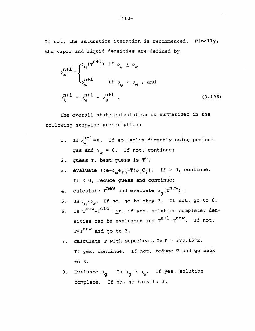
-112-

If not, the saturation iteration is recommenced. Finally,

the vapor and liquid densities are defined by

n+lpnl (T ) if pg < Pw

n+ n+l

Pw if p > Pw andw g w

n+l n+l n+lP = Pw (3.196)

The overall state calculation is summarized in the

following stepwise prescription:

n+l1. Is pn 1 =0. If so, solve directly using perfect

gas and X = 0. If not, continue;

2. guess T, best guess is Tn.

3. evaluate (pe-Pwef 0-TPiCi). If > 0, continue.

If < 0, reduce guess and continue;

4. calculate Tnew and evaluate Pg (Tnew);

5. Isp >pw . If so, go to step 7. If not, go to 6.

6. IslTnew-Told <E, if yes, solution complete, den-

n+l newsities can be evaluated and T =T+1 . If not,

T=Tnew and go to 3.

7. calculate T with superheat. Isr > 273.150 K.

If yes, continue. If not, reduce T and go back

to 3.

8. Evaluate p Is p > P w If yes, solution

complete. If no, go back to 3.

-113-

The iteration usually converges to an error of

0.001K in roughly 5 iterations. The most difficult

convergence is encountered near saturation as the itera-

tion in Table 3.3 illustrates. Finally, the curve fits

of the thermodynamic properties previously specified

are plotted in Figure 3.5. Good agreement is observed.

Many additional useful data are calculated once the

state and quality are defined. Three which merit addi-

tional comment are hydrogen volume fraction, void frac-

tion and change of density with temperature. Hydrogen

volume fraction is usually the most important datum in

this application and is computed assuming:the cell volume

occupied by liquid is negligible and the perfect gas law

is applicable. As such

xH (3.197)fH (mw)h (mw)(3.197)

h hxh +-- -- +- - xh+(mw)a a (mw) s

where x i = mass fraction,

(mw) /(mw) . = ratio of molecular weights.

The void fraction is computed assuming the liquid density

is that of saturated water.

n+lP Pf

a = void fraction = n (3.198)n+1 n+1

P -P z -Pi

The final task in he computational cycle is an

optional reference state update. The frequency of this

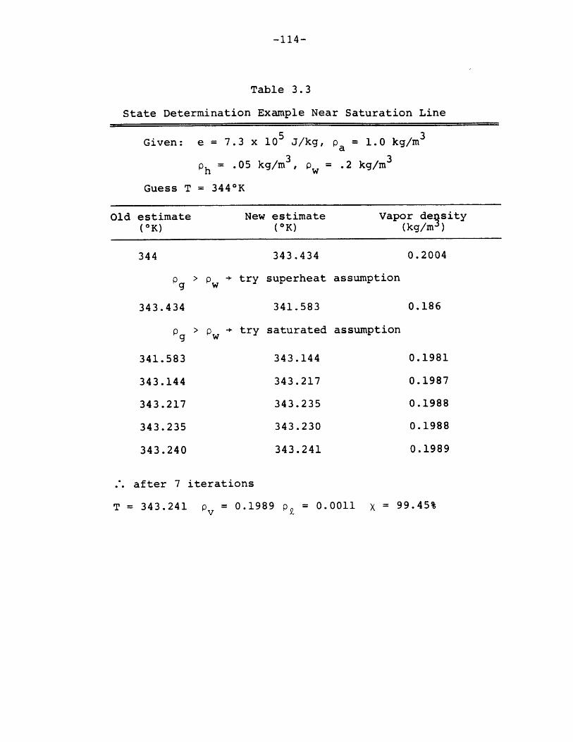
-114-

Table 3.3

State Determination Example Near Saturation Line

Given: e = 7.3 x 105 J/kg, p = 1.0 kg/m 3

Ph = .05 kg/m 3, P = .2 kg/m 3

Guess T = 344 0 K

Old estimate New estimate Vapor desity(OK) (OK) (kg/m )

344 343.434 0.2004

Pg > Pw - try superheat assumption

343.434

Pg

341.583

343.144

343.217

343.235

343.240

341.583

> Pw + try saturated assumption

343.144

343.217

343.235

343.230

343.241

.'. after 7 iterations

T = 343.241 pv = 0.1989 p = 0.0011 X = 99.45%

0.186

0.1981

0.1987

0.1988

0.1988

0.1989

-115-

SATURATED VAPOR

H 000 1.00

10z

980 2400 00 320 340 360 380

960 300 0.100

z z

w 940 2200

efg

900

280 300 320 340 360 380

TEMPERATURE (K)

SATURATION PROPERTIES OF WATERFIGURE 3.5:

-116-

update is user-defined with the greater frequency yielding

increased accuracy at the cost of additional computation.

The procedure consists of adding all the mass in a region,

evaluating the new reference density, gas density, average

temperature and gas constant, and redefining a new refer-

ence pressure.

3.3.4.5 Boundary and Initial Conditions

The boundary and initial condition options of the

original code remain unaltered by the new model additions.

Two restrictions in utilizing three dimensional modelling

are that it is only valid for the slower mixing option

and connected continuum regions cannot be defined.

The new model formulations have introduced the need to

specify additional conditions for a complete problem

definition.

Boundary conditions for the two theta-direction

bounding surfaces must be specified in all 3-D problems

except those involving a complete cylinder in which

case there are no intervening solid surfaces. The no-

slip boundary option for solid surfaces has additional

ramifications when the turbulence model is employed.

This boundary condition should only be employed in

problems where the near-wall mesh spacing is on the same

scale as the boundary layer thickness such that purely

molecular effects are significant. If such is the case

-117-

a modified "law of the wall" is utilized (see Launder

and Spalding).

The logarithmic law of the wall approximation is

illustrated for a boundary on the right-most fluid cell.

icr1 2n P [Cpck][C k ] = In[E m ] C, (3.199)(/P)w K 2

where K = von Karman's constant = 0.42, and

E = 9.793

Near the wall

(T/p) = [Ck] (3.200)

and we call approximate v by

v + v. _v = 2 (3.201)

Substitution yields

2 kIn k + 28k 2 0 , (3.202)

k -k

E6rpC 1

where 6 In[ i , andk 2 i m

a k -K(v+vj_ )/2C.

The defining transcendental equation can be solved using

Newton's method. Once the boundary cell turbulent

kinetic energy is calcr-iated, the dissipation level is

computed using the following prescription:

-118-

C kg 6r (3.203)

K--f-

The turbulence model also necessitates the speci-

fication of initial turbulence levels. Recall the eddy

viscosity is

pC k 2T PCk 2

(3.204)

Since turbulent velocity components usually experience

fluctuations less than the absolute magnitude of the

mean velocity, a reasonable initial k is the square of

the maximum expected velocity. The authors of the VARR-II

code suggest an initial dissipation level of

C u_ 5 max (3.205)initial 6x (3.205)

Finally, the reference density definition should

be computed as follows,

P0p - + P (3.206)

3.3.4.6 Incompressibility Check

The underlying assumption of the slow mixing model

is incompressibility. Local densities are computed on

the basis of a reference pressure and are assumed to be

-119-

close enough to the reference density to be considered

perturbations. In order to conform to this requirement

local changes should not be large during a computational

cycle. This limit is implemented by checking local den-

sity changes such that

n+l nmax < small number . (3.207)

all cells p

The limiting criterion is user-specified and 1% seems to

be a conservative value. If this test is not satisfied,

the computational time step is halved and the calculation

is redone until the incompressibility check is satisfied.

This procedure coupled with judicious reference state

updating can substantially broaden the range of applica-

bility for this basically incompressible formulation.

3.3.5 Physical and Computational Interfacing BetweenMITHYD and the Overall Code

Given that the MITHYD subcode introduces a new

fluid dynamic model, the question of interfacing with

existing models in the code arises. These interface

considerations can be grouped into two categories--physical

and computational. The physical aspects relate to deciding

what is the correct phenomenological model for the problem

of interest. This may be apparent to the analyst a priori

and hence the user is Allowed to specify which model to

use. However, a problem could involve flows which at

-120-

various times or places require both models. One example

is a situation in which hydrogen is introduced as part

of a steam jet which is of significant size when compared

to the flow domain. This problem is best treated using

the two-phase modified BEACON equation set. If the jet

ceases after some time as could be the case if a relief

valve reseated, the flow problem is then best described

by the slower mixing equation set.

The exemplary scenario described is treated by an

internal checking logic in the code. The most basic

distinction between the two fluid models is the treatment

of compressibility effects. Therefore a compressibility

check is performed and the code can automatically switch

to the slower mixing model from the BEACON model. Only

this switching mode (not the reverse from MITHYD to BEACON)

is allowed. Further, this switching is limited to one

occurrence in each flow mesh. The rationale for these

restrictions arises from the desire to minimize computa-

tional complexity. The next logical step in computational

interfacing could be based on combining the two models into

a single scheme. This seems to be a preferable alternative

to devising a more complex switching logic. Nevertheless,

the simplicity of the present formulation provides the

analyst with significant latitude.

Computational aspects address the computer programming

interface problem. These are addressed in detail in

-121-

Appendix A. In brief, the new models are formulated to be

completely compatible with the variables utilized in the

original formulations. The MITHYD subcode utilizes

existing software for data management, input/output pro-

cessing and ancillary calculations. Structurally, it is

attached to the larger code in a highly modular fashion

which allows for easy modification and understanding.

-122-

4.0 Results and Discussion

The development of analytical models as exemplified by

the previous chapter is only part of the process. The suc-

cessful implementation of these models can only be demon-

strated by performing computer computations. The underlying

framework of demonstrating a code's validity relies on com-

paring predictions to measured data (or at least other reli-

able calculations). This chapter details a number of

validation calculations which demonstrate the capabilities

and limitations of this tool. After results are presented,

an analysis of their implications is undertaken. The results

must be considered not only for their accuracy but also the

computational effort involved in achieving them. Therefore,

the final sections of this chapter compare the capabilities

of this methodology versus other approaches.

4.1 Validation Methodology

The program possesses three major computational

options. The first is the modified BEACON equation set

which is most appropriate for detailed simulations of flows

driven by compressible two phase effects. The basic code

capability in this area is already demonstrated by the

developers and subsequent users and hence is not a necessary

part of this validation effort. The ability to handle

-123-

hydrogen transport during such transients however is a

required task. The approach taken is to revise existing

sample problems with known results and comparing code pre-

dictions with them. Attempts at using the modified BEACON

equation set for longer transients are also reported in

order to demonstrate its inadequacies of treating such

events.

The bulk of the validation effort is focused upon the

simulation of longer mixing transients using the MITHYD sub-

code. Two large scale experimental programs are the source

of validation case studies. The first and largest simulation

effort utilizes data from a series of single phase experi-

ments performed at the Battelle-Frankfurt (BF) Institute in

the Federal Republic of Germany. These tests are chosen

because of their extensive documentation, simple structure,

range of testing and direct applicability. The second source

of empirical information originates from a series of multi-

component and two phase tests performed at the Handford

Engineering Development Laboratory (HEDL). These tests

involve complex geometries and flow regimes, and are con-

sidered to be the most challenging from a simulation stand-

point. These simulations demonstrate the limitations of the

MITHYD methodology.

Finally, lumped parameter model validation is reported.

The new junction and node model described in Chapter 3 is

used to simulate a number of problems including some of the

-124-

more complex multiroom BF tests. The simulations not only

demonstrate the enhanced capability afforded by this addition

but also illustrate the importance of input data such as time

step size and junction characteristics. The input data decks

for all simulations reported in this chapter are included in

Appendix B.

4.2 Results Using the Modified BEACON Equation Set

Four simulations are reported in this section. The

first problem which involves the rapid injection of an air/

water flow into an initially stagnant region is identical

to a reported BEACON sample problem. The results demon-

strate that original code's capabilities have not been com-

promised during the development process.

The second problem is similar to the first except

hydrogen is substituted for air in the incoming flow. This

simulation addresses the issue of tracking hydrogen and is

easily compared to the first problem. The ability (or

inability) of the code to handle slower single phase transi-

ents was not known a priori. The third result discussion

involves various attempts at simulating one of the more

simple BF tests. A successful simulation is never achieved.

Finally, the computational transition from the BEACON equa-

tions to the slower mixing model is tested in the final

subsection.

-125-

4.2.1 Air and Water Blowdown

The geometry for this problem is shown in Figure 4.1

which depicts a single compartment in a Cartesian geometry

with internal flow obstacles. Initially, the room consists

of a uniform distribution of 90% air and 10% water (liquid)

by volume which is stagnant and at atmospheric pressure and

333 0K. The incoming flow is a 333 0 K mixture of 50% air/50%

water by volume entering the left bottom boundary 3.05 m/sec.

Gravity is not considered. Non-equilibrium interphasic

momentum and energy exchanges are modelled but solid heat

transfer and detailed condensate film formation are not

considered. All solid surfaces are considered to be no-slip

boundaries.

Figure 4.2 depicts the gas phase (air) flow field at

0.10 seconds into the transient. These results are identical

to those presented in the original BEACON documentation. A

physically reasonable velocity field is predicted with the

solid walls producing the expected flow diversion. Figure

4.3 is a plot of the void fraction transient at five dif-

ferent locations. The location indexing is provided in

Figure 4.1. This plot illustrates the progression of the

lower void fraction inlet flow as it penetrates the field.

Though it is not easily seen in this plot the data of

points 3 and 4 are interesting in that the difference between

the two actually reaches . maximum at about 0.08 seconds and

if one extrapolates the results the void fraction at 3 will

-126-

KINITIALLY STAGNANT

INFLOW 2ITHER 50% AIR / 50% LIQUID

OR

50% H2 / 50% LIQUID

FIGURE 4.1: BEACON SAMPLE PROBLEM GEOMETRY

-127-

t

tt

f/ttt!

.4od -- t

FIGURE 4 .2 :GAS VELOCITY FIELD AT 0.1 SECOND

. .4 .. x

r ti

/ t

t t

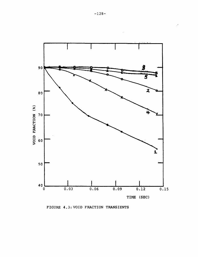
-128-

90 -

80

z 70

o 60

50

4o I I I I0 0.03 0.06 0.09 0.12 0.15

TIME (SEC)

FIGURE 4.3: VOID FRACTION TRANSIENTS

-129-

in fact become lower than that of 5 at some later time.

This is consistent with the hydrogen transport results

reported in the next subsection. In all, a satisfactory

result is accomplished for this case and the original

capability remains intact.

4.2.2 Hydrogen and Water Blowdown

This problem is similar to the previous simulation

save for the fact that hydrogen is now the inflow gaseous

component. The resultant velocity profile of the gaseous

phase was nearly the same as the previous problem. The only

significant difference was the velocity profile developed

a bit faster in this simulation. As a quantitative illustra-

tion, the velocity vectors at point 3 in the field at 0.1

seconds were 5.31 m/sec (-50 from vertical) and 5.62 m/sec

(-50 from vertical), respectively for the two transients.

Figure 4.4 illustrates both the gas velocity and con-

centration field at 0.1 seconds into the transient. The

velocity profile has not yet fully developed as can be seen

by comparing this figure to Figure 4.5 which shows these

fields at 0.20 seconds. The effect of the sharp corner of

the central obstacle is to retard the flow and hence inhibit

the convective transport of the hydrogen in this area.

The time history of the H2 volume fraction at the 5 calcula-

tional points discussed p-eviously are shown in Figure 4.6.

The 4% line is drawn on this figure since it represents a

-130-

4 -0 -0 .0

-Jv -0 -W .9

I

KI0 -0 4

.0 -9 -ow -0 -

A ~ -~ ~ -~ A o p

tol

2'** - __O -"amm '"ftm --

5 O-- -

- - -tttt i

FIGURE 4.4: VELOCITY AND HYDROGEN CONCENTRATION

FIELDS AT 0.1 SECOND

I /

0.dP

ZOHO

0 0

x

100

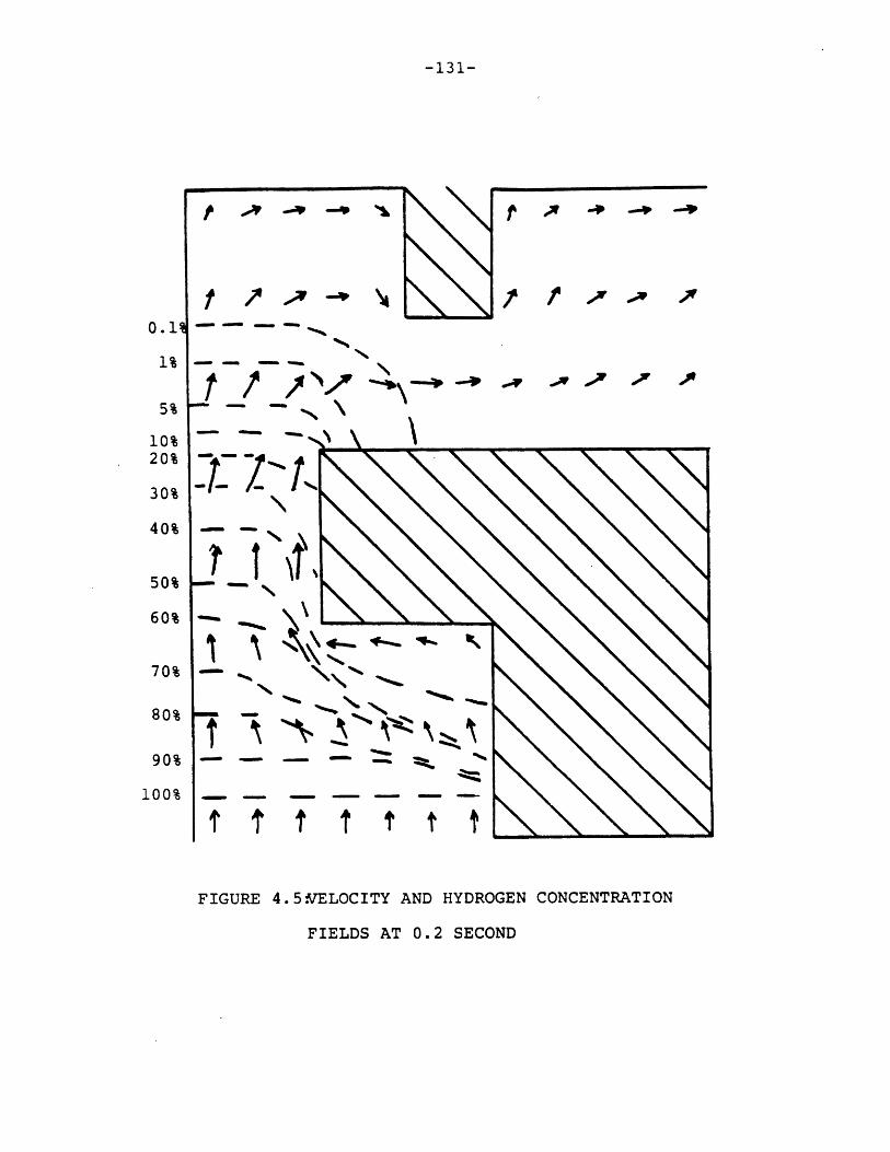
-131-

t0 -.* -. 7

7fv -t~

0.14

1%

5%

10%20% -

30%

40% -

50%

60% ***

70% -

80% l -

90% . -100%- - - -100%

FIGURE 4.5.VELOCITY AND HYDROGEN CONCENTRATION

FIELDS AT 0.2 SECOND

A

-132-

100.

1

0

S0.1-

z .01o 3

.001

0 0.04 0.08 0.12 0.16

TIME (SEC)

FIGURE 4.6: HYDROGEN CONCENTRATION TRANSIENTS

0.20

-133-

nominal ignition lower bound. An additional point to be

observed in this figure is the intersection of the curves

for points 3 and 5. This is analogous to the void fraction

behavior reported in the previous subsection.

Taken together with the air/water blowdown transient,

these results demonstrate the capability of the modified

equations set to handle rapid transients. The time step size

during these calculations were on the order of 0.001 seconds.

The number of iterations required to converge the continuity-5constraint to 10-5 (0. being completely divergent free) was on

the order of 10.

4.2.3 Analysis of Slower Transients

Simulation of a longer term transient is attempted

in order to test the limitations of this analytical model.

Test No. 2 of the Battelle Frankfurt series (see 4.3.1) is

used as the test case. This experiment involves the intro-

duction of a hydrogen/nitrogen mixture into a closed air-

filled vessel with internal flow orificing. The experiment

is characterised by a very slow injection rate. An abbre-

viated specification of this experiment is provided in Table

4.1. Figure 4.7 illustrates the basic geometry and the

coarse nodalization used in the baseline simulation.

Numerous attempts of performing this calculation failed

and a successful simulation beyond a few seconds is never

achieved. The reasons for this lack of success are now

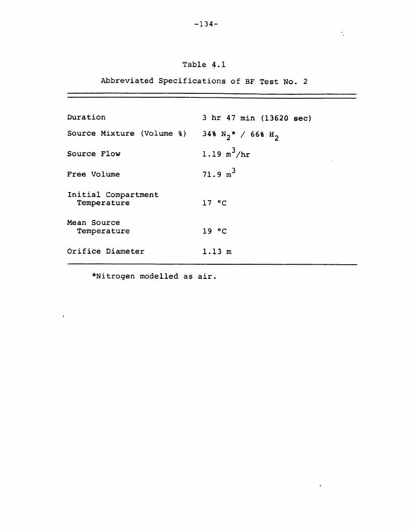
-134-

Table 4.1

Abbreviated Specifications of BF Test No. 2

3 hr 47 min (13620 sec)

Source Mixture (Volume %)

Source Flow

Free Volume

Initial CompartmentTemperature

Mean SourceTemperature

Orifice Diameter

34% N2* / 66% H2

1.19 m 3/hr

71.9 m3

17 OC

19 OC

1.13 m

*Nitrogen modelled as air.

Duration

-135-

addressed. There are several significant differences between

this problem and the previous two. Time scale is the most

important of these distinctions. The blowdown events

involved total problem times of less than a second with

Courant time step sizes on the order of 10- 3 to 10-2 seconds.

This BF-based simulation involves an event which lasted over

13600 seconds and the expected Courant limit time steps are

1-10 seconds. Second, liquid phase water is not involved in

the Battelle test. Given the absence of the liquid phase,

interphasic effects are inappropriate and should not be

included.

In lieu of providing a very detailed account of the

problems encountered, Table 4.2 is presented as a summary

of events. A close investigation of these attempts leads

to the conclusion that the overall solution methodology is

ill-suited for problems involving long time steps and no

liquid phase at all. The non-equilibrium interphasic

exchange formulation is particularly destabilizing in low

convection flows when the usually small non-equilibrium

exchanges become significant. One disturbing aspect of the

existing BEACON computational logic is that interphasic

exchanges cannot be neglected since the input specification

of null coefficients causes the code to completely bypass

the energy equations' solution. This is noted in the table

under the entry labelled Attempt 4. Secondly, the code is

unable to handle zero or unity void fraction flows. This

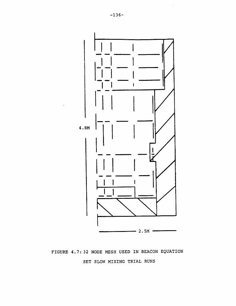
-136-

I II i I-l -

I t

2. 5M

FIGURE 4.7: 32 NODE MESH USED IN BEACON EQUATION

SET SLOW MIXING TRIAL RUNS

Table 4.2

Synopsis of Attempts at Simulating BF2 Using the BEACON Equation Set

Attempt

Base case, no liquid,best estimate inter-phasic exchange, 16nodes, initial At=lsecond.

32 nodes, negligibleuser-defined inter-phasic parameters.

16 nodes, even smallerinterphasic constants.

16 nodes, interphasicconstants set to 0.

16 nodes, small inter-phasic exchange andsome liquid in initial

No convergence, erraticenergy conservationleading to non-physicalstate.

No convergence, similarto Attempt 1.

Simulation to 5300seconds, erratic con-vergence and non-physical results.

Simulation to 3 seconds,no convergence.

Better convergencebehavior.

Demonstrates under-lying difficulties.

Nodalization did notaffect solution.Erratic energy con-servation seems toarise from non-conser-vative velocity fieldand interphasic exchangecalculations.

Convergence achievedtemporarily but lostas At increased.

At's < 0.1 seconds.Energy equations notsolved.

Demonstrates solution,requires some liquidand small At's.

-138-

limitation is also reported by Gido et al. [77]. Finally,

the stability limit seems to be quite a bit below the

expected Courant constraint (less than 10% of the CFL limit).

In short, the modified BEACON equation set is shown to be

ill-suited for longer simulations. An approximate calcula-

tion would probably be successful if a fictitious liquid

field is assumed and a very limiting time step constraint is

utilized. However, the computational cost of performing such

a calculation is unreasonable. For example, a simulation of

a 10000 second (real time) event using 0.010 second time

steps with perhaps 20 iterations per calculation cycle would

involve over 300 million calculational passes and many tens

of hours of computer time. Further, the resultant solution

would not address turbulence or multicomponent diffusion.

Clearly, another methodology is required for such analysis.

4.2.4 Transition to the Slower Mixing Model

The analytical aspects of the interfacing between the two

continuum models is discussed in 3.3.5. A simple simulation

is reported which demonstrates the code's ability to perform

such a switch. The problem geometry is a simple 6 m3 2-D

Cartesian region divided into 6 mesh cells. Hydrogen is

introduced into the lower left cell at a rate of 10-4 kg/sec

(equivalent to 4 m3/hr) for a period of 10 seconds (total

injection = .011 m3). The BEACON equation set is initially

solved using a time step of 0.5 seconds. After 2

-139-

computational cycles, the code switched to the slower mixing

model. Figure 4.8 depicts both the problem geometry and

the convergence behavior of the simulation. The switching

point is clearly evident at the end of 1 second of simula-

tion. The poor convergence behavior of the BEACON model is

not surprising given the similarity of this problem to the

attempts described in 4.2.3. The slower mixing model handles

this transient very well with an average 6 iterations per

time step.

Figure 4.9 contains time history plots of the developing

velocity and hydrogen fields. Physically reasonable results

are observed and the traces show no sign of instability or

discontinuity. Finally, Figure 4.10 provides schematic

representations of the flow and concentration fields at both

1 and 10 seconds. The profiles at one second indicate that

the BEACON models predict reasonable fields even though com-

plete convergence is not achieved. In summary, the code is

shown to successfully execute the desired computational

transition.

4.3 Longer Mixing Transients Using MITHYD

The results reported in the previous section demonstrate

the need for the longer term mixing model detailed in Chapter

3 and embodied in the MITHYD subcode. The extensive develop-

ment effort which involves transforming the equations and

assumptions of Chapter 3 into a working and (nearly)

-140-

U> 60-

zO

H

240

0"-

0 2 4 6 8 10

TIME (SEC)

FIGURE 4.8: SWITCHING PROBLEM GEOMETRY AND

CONVERGENCE BEHAVIOR

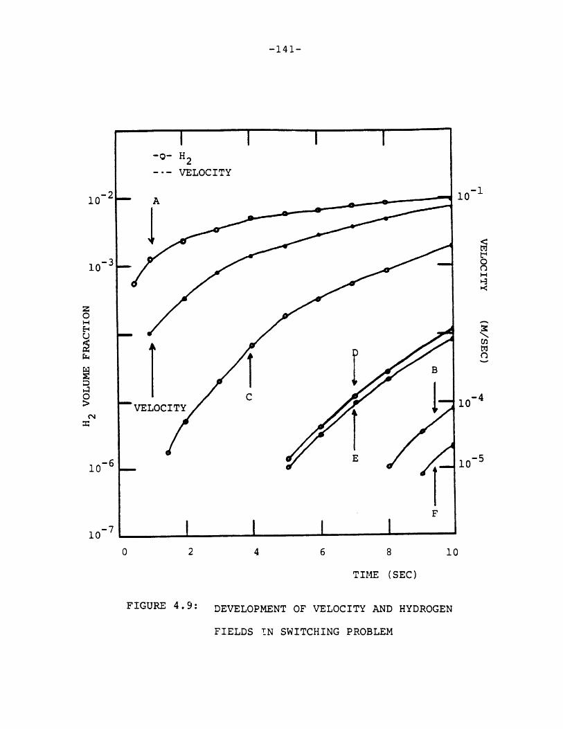
-141-

2 4 6 8

TIME (SEC)

FIGURE 4.9: DEVELOPMENT OF VELOCITY AND HYDROGEN

FIELDS IN SWITCHING PROBLEM

1-2

-3

10

zO0

uuH

lo-0

1-1

0H

ic

Ntm

10 - 5

-142-

TIME= 1 SECONDFLOW

TIME= 10 SECONDS

FIGURE 4.10: FLOW AND HYDROGEN FIELDS AT 1 AND 10

SECONDS

I I\

//

/'I

\

8.34-5 2.36-6

1.84-3 1.10-4

9.57-3 7.46-6

H2 FRACTION

1.17-10 5.1-15

7.47-7 1.66-10

1.17-3 1.58-7

-143-

error-free computer program is not documented here. The

effort consists of careful planning, thorough review of

coding, numerous debugging runs and extensive comparison of

calculated results with hand calculations and known analyti-

cal solutions. The end product of this process is a useable

but unvalidated tool. Validation is demonstrated by compari-

son of computed predictions with experimental data. The two

chief sources of empirical data are large scale experiments

performed at the Battelle Frankfurt Institute and the Hand-

ford Engineering Development Laboratory. Prior to the

result presentations for each simulation group, a brief

overview of the testing programs and facilities are provided.

4.3.1 Battelle Frankfurt Tests

This subsection is divided into two parts. First the

facility and relevant tests are reviewed. Following this

a number of simulations and comparisons based on particular

BF tests are reported. These tests are particularly useful

in code validation because many emphasized a separate-effects

approach which allows for straightforward interpretation.

4.3.1.1 Facility and Testing Program Review

The hydrogen mixing tests performed at the Battelle Frank-

furt (BF) test facility provide many of the principal test

cases for the model valied tion. Given the central role of

these tests, this subsection is included in order to provide

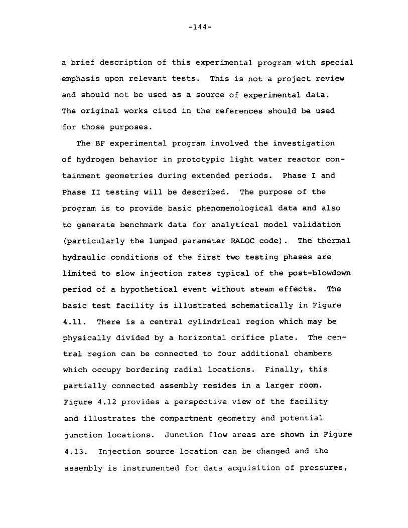
-144-

a brief description of this experimental program with special

emphasis upon relevant tests. This is not a project review

and should not be used as a source of experimental data.

The original works cited in the references should be used

for those purposes.

The BF experimental program involved the investigation

of hydrogen behavior in prototypic light water reactor con-

tainment geometries during extended periods. Phase I and

Phase II testing will be described. The purpose of the

program is to provide basic phenomenological data and also

to generate benchmark data for analytical model validation

(particularly the lumped parameter RALOC code). The thermal

hydraulic conditions of the first two testing phases are

limited to slow injection rates typical of the post-blowdown

period of a hypothetical event without steam effects. The

basic test facility is illustrated schematically in Figure

4.11. There is a central cylindrical region which may be

physically divided by a horizontal orifice plate. The cen-

tral region can be connected to four additional chambers

which occupy bordering radial locations. Finally, this

partially connected assembly resides in a larger room.

Figure 4.12 provides a perspective view of the facility

and illustrates the compartment geometry and potential

junction locations. Junction flow areas are shown in Figure

4.13. Injection source location can be changed and the

assembly is instrumented for data acquisition of pressures,

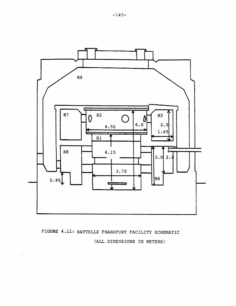
-145-

FIGURE 4.11: BATTELLE FRANKFURT FACILITY SCHEMATIC

(ALL DIMENSIONS IN METERS)

-146-

FIGURE 4.12:THREE DIMENSIONAL VIEW OF BATTELLE

FRANKFURT FACILITY

C = CIRCULAR OPENING

R = RECTANGULAR OPENINGC, 1. M2

22C, 0.16M

R, 0.9M

2C,0.06M 22R, 0.324 2

2R,0.324M2

FIGURE 4.13: ROOM CONNECTION ARRANGEMENT AND SIZES FOR BATTELLE FRANKFURT

FACILITY

-148-

temperatures, hydrogen concentrations, flow rates, etc. as is

illustrated in Figure 4.14. The source itself is a pad

covered with a porous cloth through which premixed gas mix-

tures are passed. This is also shown in Figure 4.14. The

hydrogen measurement probe and its associated circuitry are

depicted in Figure 4.15. Basically, the probe is a catalytic

device in which a gas sample is nearly completely burned li-

berating heat which in turn changes the electrical resistivity of

the coil. The change in resistivity is proportional to the

original gas sample hydrogen concentration. The reference

coil serves to compensate for ambient temperature changes in

the local probe vicinity. The data sampling rates were on

the order of every 40 seconds. Use of these probes in a

steam environment has not been tested.

The Phase I series consisted of 9 tests and involved only

the central cylindrical region of the facility which has a

net free volume of approximately 80 m3 and two of the smaller

horizontally connected compartments. Phase I tested the

measurement and data acquisition equipment and provided

useful information into hydrogen behavior in large compart-

ments. A synopsis of this test series is provided in Table

4.3. Tests 1 through 6 involve the central cylindrical geo-

metry. The flow rates in test 1 and 6 were corrected some-

time into each test as indicated. Tests 7 through 9 were

performed in the smaller horizontally connected compartments.

This table also details the overall objectives of each test.

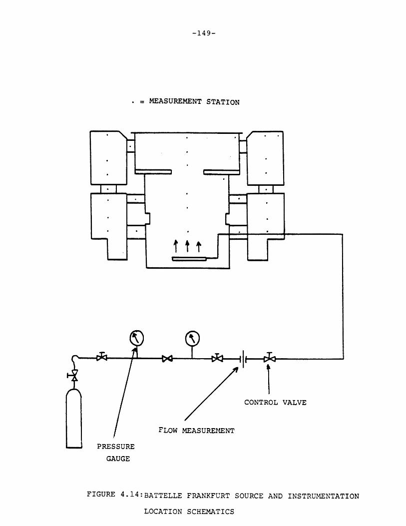
-149-

* = MEASUREMENT STATION

ttt

CONTROL VALVE

FLOW MEASUREMENT

GAUGE

FIGURE 4 .1 4 :BATTELLE FRANKFURT SOURCE AND INSTRUMENTATION

LOCATION SCHEMATICS

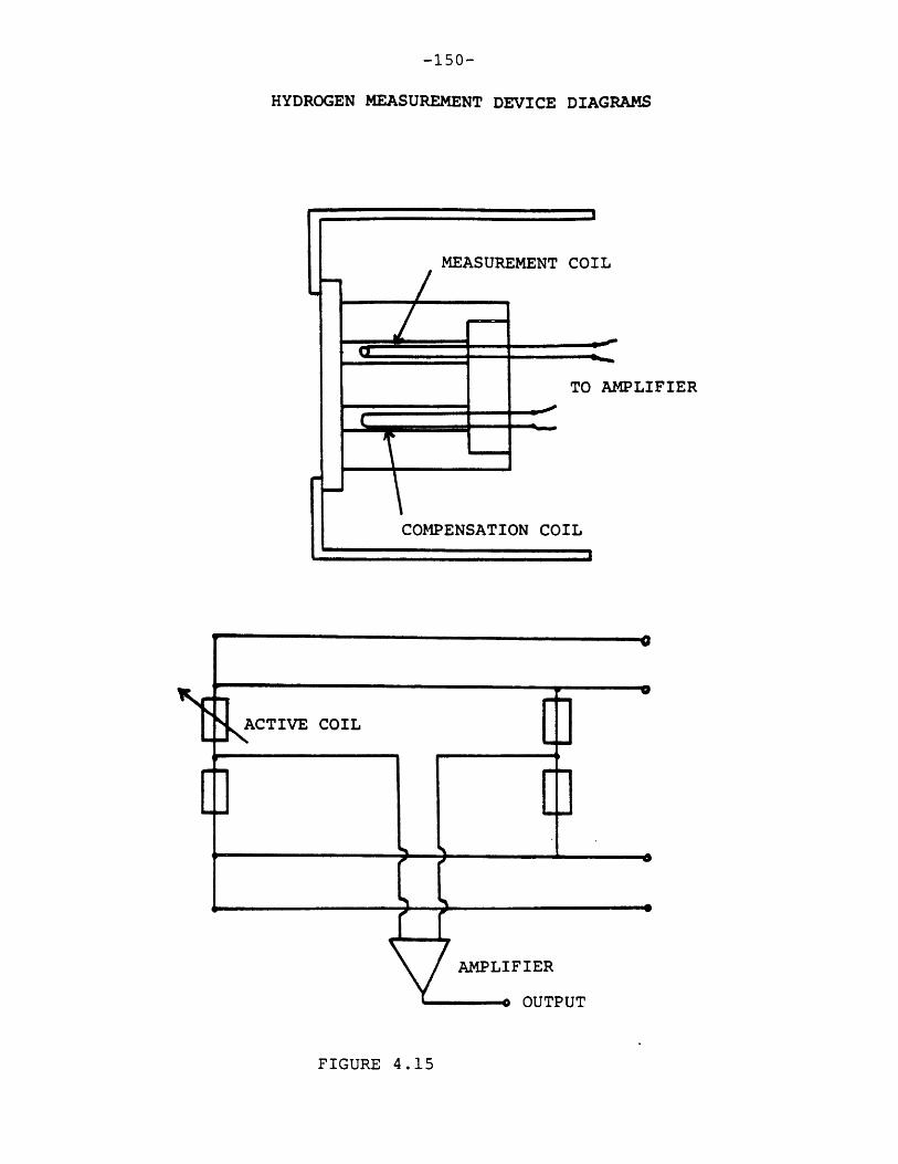
-150-

HYDROGEN MEASUREMENT DEVICE DIAGRAMS

MEASUREMENT COIL

TO AMPLIFIER

FIGURE 4.15

= I

io-

COMPENSATION COIL

I 1

I

I I

I I~

m

Table 4.3

Phase I Battelle Frankfurt Tests

Test No. 1

Duration of release (sec) 1380 + 11220

Gas mixture N2/H2 68/32(volume %)

Release rate (m /sec) 1.66E-3/7.55E-4

Total released volume (m3) 2.3/2.272

Initial air volume (m3) 70.8

Initial room temperature (OC) 18

Injection gas temperature (OC) 16/19

Orifice diameter (m)/area (m2 )

Height of source above 0.6ground (in)

Test objective Basic testdensityconvection

Test No. 2

13620

34/66

3.306E-4

4.51

71.9

17

19

1.13/1.0

0.6

Test No. 3

10320

34/66

3.389E-4

3.49

71.4

17

18.5

0.62/0.3

0.6

Test No. 4

7800

34/66

3.444E-4

2.67

71.9

22

25

3.4

Test No. 5

31200

34/66

1.417E-4

4.44

71.8

19

21

0.6

Density con- Density con- Diffusion by Replicationvection with vection with change of of Test No.large ori- small ori- source 1 with con-fice fice location stant Ai

Table

4.3

Phase I Battelle Frankfurt Tests

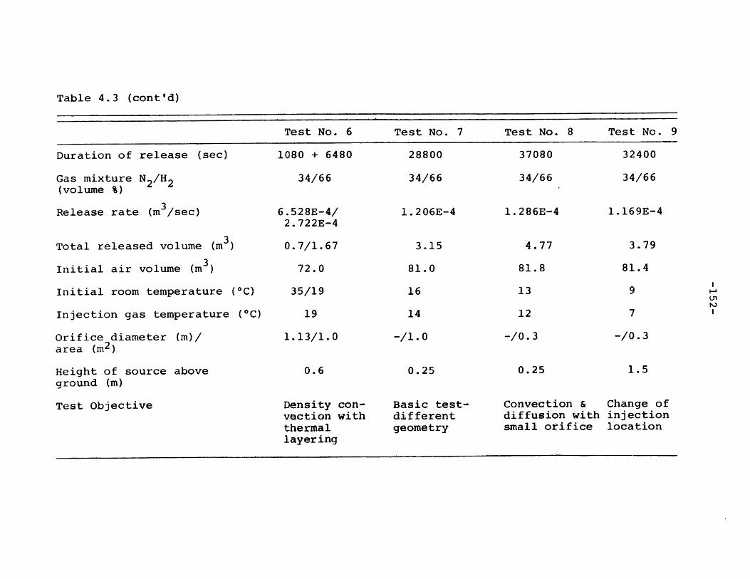
Table 4.3 (cont'd)

Duration of release (sec)

Gas mixture N2/H 2(volume %)

Release rate (m3/sec)

Total released volume (m3 )

Initial air volume (m3)

Initial room temperature (OC)

Injection gas temperature (OC)

Orifice diameter (m)/area (m 2 )

Height of source aboveground (m)

Test Objective

Test No. 6

1080 + 6480

34/66

6.528E-4/2.722E-4

0.7/1.67

72.0

35/19

19

1.13/1.0

0.6

Density con-vection withthermallayering

Test No. 7

28800

34/66

1.206E-4

3.15

81.0

16

14

-/1.0

0.25

Basic test-differentgeometry

Test No. 8

37080

34/66

1.286E-4

4.77

81.8

13

12

-/0.3

0.25

Test No. 9

32400

34/66

1.169E-4

3.79

81.4

9

7

-/0.3

1.5

Convection & Change ofdiffusion with injectionsmall orifice location

~ ' ''

"

-153-

The chief parametric investigations of this series involve

injection rate, source location, orifice-size and placement,

initial compartment temperature distribution, compartment

geometry and orientation. The observations drawn from these

tests are as follows.

The injection rate affected mixing in that rates below

-4 36 x 10 m /sec resulted in very homogeneous mixtures while

heterogeneities developed at faster rates. The concentration

profile of Test No. 4 in which the source was located at the

geometry mid-height exhibited a distinct difference between

the upper and lower portions. The upper portion contained a

nearly homogeneous mixture while a gradient existed below.

In fact, the lower region behavior was compared to a pure

one-dimensional diffusional problem. From this analysis

the BF personnel estimated a binary H2/air diffusion coeffi-

cient ranging from 6 x 10- 5 to 6.3 x 10- 5 m 2/sec which com-

pares very well with literature value around 6.1 x 10-5

m /sec. Similar results were obtained in the horizontally-

connected geometry. These findings indicate that a source

located in an unfavorable location can induce substantial

non-uniform concentrations if convective effects are

supressed.

Two different orifice sizes were used in both geometries.

The cylindrical geometry data indicates that a phenomena

which might be called a "critical orifice size" exists such

that larger openings have little effect on intercompartmental

mixing while small openings cause stratification and

-154-

retardation of mixing. The effect of orifice size is less

noticeable in the horizontal geometry where concentration

differences between compartments is nearly proportional to

orifice area. (In quantitative terms, at 15000 seconds

into each experiment, a difference of 0.4% was observed in

the 1.0 m2 case (No. 7) while a difference of 1.2% was seen

in the 0.3 m2 case (No. 2).)

In test No. 6 an initial compartment temperature inver-

sion is introduced in order to test the effects of the

stratification on hydrogen transport. A dramatic difference

in hydrogen concentration is observed between the two com-

partments. For example at 5000 seconds, the average con-

centrations of the upper and lower portions of the vessel are

1% vs 3.5%, respectively. The measurement station at the

orifice also exhibited interesting behavior. Periodically,

a rapid inflow to the upper compartment would occur indi-

cating times when the buoyancy force of the lighter mixture

overcame the blockage effect of the physical contraction and

the thermal inversion. Nevertheless, these periodic inflows

are not sufficient to substantially homogenize the vessel

concentrations. Finally, the main finding in the area of

compartment geometry and orientation is that the vertically

connected compartments (cylindrical region) benefit from the

buoyancy-induced convection to a significantly greater degree

than the horizontally-joined geometry where small local

conveotive and diffusion driven transport drive the flow.

-155-

The Phase II tests utilize multi-compartment geometries

with longer term tests and more complex objectives. Phase

II tests are also useful in the testing of lumped parameter

models (see 4.4). Table 4.4 provides an overview of this

testing program. These are four main parametric tests

related to Phase II. They are assessments of the effect of

a horizontally and vertically connected multi-room geome-

tries, effect of various compartmental temperature distri-

butions, reduction of injection rate with concurrent exten-

tion of testing period and finally, the use of helium as an

alternative for hydrogen in order to allow higher concentra-

tions in later tests.

The major empirical findings are the following. First,

homogeneous concentrations within compartments result when

the initial compartmental temperature distribution is uniform

(AT < 20C) but thermal inversions do cause local concentra-

tion heterogeneities. However, the multi-compartment geo-

metry aids in breaking down inversions due to the greater

potential for destabilizing natural convective paths to

develop. Local humidity has a distinct effect such that

high humidity seems to favor local hydrogen accumulation.

Third, the initial convection pattern has an important effect

on the course of the transient. Fourth, air blowers or

recirculation fans seem to provide effective mixing and

finally, helium seems to be a reasonable substitute for

hydrogen but the measurement system requires upgrading.

Table 4.4

List of Tests - Phase II

Para- Temperature Injec. mH2 Injec. m He Individual Objectivemeter Temp. Gra- Loc. 2 Loc.Test No. dient H2 m3/h He m3/h2 m3/h i/

CT

CT

CT

constant

constant

constant

constant

constant

variable

constant

variable

variable

R1 1.5 Diffusion through convectionwithout thermal effect

R1,bottom

R1 0.3

1.5

R1 1.5

R1 0.3

R1 1.5

R6 1.5

R1 1.5

R1 1.5

R1 0.3

1.0* Same as 10, suitability ofhelium as test gas

-- Same as 10, effect of injectionrate

- - Same as 10, with hinderingthrough thermal inversion, however

- - Same as 13, except for 6additional sampling probes

- - Same as 12, effect of injectionrate

- - Same as 14, noticeable eventualbreakthrough, however

- - Effect of the injection location

- - Effect of the location of theheater coil

R1bottom

2.0 Same as 13, except for break-through forced by the injection

- - Observation of Temp. Equalization

Same as 20, except withoutH2 injection

10

15

17

18

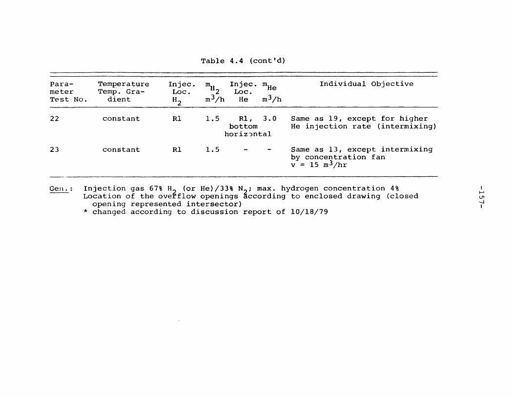
Table 4.4 (cont'd)

Para- Temperature Injec. mH2 Injec. mHe Individual Objectivemeter Temp. Gra- Loc. 2 Loc.Test No. dient H2 m 3/h He m 3/h

constant 1.5 R1, 3.0bottomhorizDntal

Same as 19, except for higherHe injection rate (intermixing)

constant 1.5 Same as 13, except intermixingby concentration fanv = 15 m 3/hr

Gen.: Injection gas 67% H (or He)/33% N ; max. hydrogen concentration 4%Location of the oveiflow openings according to enclosed drawing (closedopening represented intersector)

* changed according to discussion report of 10/18/79

23

-158-

Table 4.5 is provided as an overall summary of the Phase

I and II testing programs. Also included in this table is

a compilation of tests which have been calculated using

other analytical models and the model developed in this

work.

4.3.1.2 Simulations Based On Selected Experiments

A number of simulation runs are reported in this section

to demonstrate the slow mixing model's predictive capa-

bility of single phase mixing experiments. Two Phase I

Battelle Frankfurt tests are emphasized. Both were con-

ducted in the central cylindrical region of the facility with

an orifice plate in place between the upper and lower

regions. The first simulation set is based on BF Test 2

(designated hereafter as BF2) during which a hydrogen/

nitrogen mixture was introduced near the floor of the lower

region and the initial atmosphere is isothermal. A number

of short term simulations of this test and some "thought

experiment" variations on it are reported. First, a simula-

tion of the first 200 seconds of the test is reported.

Second, the same problem but without an orifice plate is

studied. This open geometry case is also used for study of

numerical procedure optimization and turbulence model behav-

ior. Third, a complete closed orifice simulation is

described to act as a point of comparison with the previous

two results.

Table 4.5

BF Testing/Simulation Overview

Test Numbers

1 2 3 4 5 6 7 8 9 10 11 12 13 14 15 16 17 18 19 20 21 22 23

Convection / / / / / / / / / / / / / / / / /

Diffusion / / / / / / / / / / / / / / / / /

Orifice Size / / /

Thermal Stratification / / / / / / / / / / /

Injection Rate / / / / /

Source Location / / / /

He vs H 2 / /

Heater Coil /

Calculated by 1 12 2 2 12 1 13 34 3 4 4 45 57 5 5 5 76 76 6

Notes

Test 5 - Same as 1, except xh corrected.Test 13 - Thermal inversion.Test 14 - Same as 13, but additional sampling

points.Test 16 - Inversion varied to cause breakthrough.Test 21 - H 2 not used.Test 23 - Same as 13, except fan used.

Calculated by:

1 - Jahn (GRS) - RALOC2 - Trent et.al. (BNWL) - Tempest3 - Travis et.al. (LANL) - HMS4 - Buxton et.al. (Sandia) - RALOC5 - KWU model6 - Thurgood (BNWL) - COBRANC7 - LIMIT (MIT)

-160-

BF Test 6 (BF6) is the second experiment emphasized in

these single-phase slow mixing validation runs. This test

is similar to BF2 except the injection rate is higher (by

approximately a factor of two) and a stable thermal strati-

fication existed prior to injection. A number of both

short- and long-term test simulations are reported. The

first set of results are based on a coarse mesh model.

The coarse mesh limits the spatial definition of the inver-

sion behavior. It also amplifies numerical diffusion

effects in areas of significant intermesh crossflow as is

typical of inversion interfaces. The second simulation

demonstrates the predictive accuracy gained by optimizing

the mesh definition, modelling solid heat sinks and reducing

numerical dispersion.

The coarse mesh model of the BF facility used in all

simulations save for the final BF6 series of calculations

is depicted in Figure 4.16. A 32 node, two-region problem

zone is defined assuming two-dimensional axisymmetry along

the centerline. In all cases the lower three left-hand

cells are source cells. Five particular cells are desig-

nated with letters (A through E) which denote areas which are

referenced in the resultant figures. Finally, a selected

group of hydrogen and temperature sensor locations are

designated by numbers. These are also used in subsequent

figures to allow easier simulation/empirical data comparison.

-161-

I 2.5M

I-

88

- m m m -

87

B C81 JD6...

83 110

i I I Dm m - - m

82

AI 181

109

E

89

IS S Si

111

81-89: H2 DATA

106-111: TEMP DATA

4.8M

A - E: SELECTED MESH

POINTS

S: SOURCE CELLS

- 2. OM

FIGURE 4.16:BASIC 32 NODE MODEL OF BATTELLE FRANKFURT

INNER VESSEL USED IN MOST SIMULATIONS

-162-

4.3.1.2.1 Scenario Based On BF2

This simulation describes the first 200 seconds of the

BF2 test. A minor difference between the simulation and

experiment is that while the source introduction was spati-

ally uniform (radially) in the test, the simulation assumed

a slightly skewed (bias away from centerline) definition.

The assymmetry was small (10% or so) and should not inhibit

useful comparison. An initially uniform air atmosphere at

a temperature of 170C is assumed to exist, into which a

190C 66%/34% (by volume) H2/air flow is introduced at a

rate of 1.19 m3/hr. A laminar isothermal flow field is

assumed. Figures 4.17, 4.18 and 4.19 depict the predicted

velocity and hydrogen concentration fields at 20, 100 and 200

seconds, respectively. At 20 seconds the circulation induced

by the lighter hydrogen is developing in the lower region,

while the upper region is as yet unaffected save for a small

net inflow due to the expansion present in the lower region.

The H2 profile reflects this scenario. The flow fields at

100 and 200 seconds are very similar. The developed velocity

field involves a strong central jet of hydrogen-rich flow

which continues through the orifice region into the upper

region. The central flow causes shear driven (due to walls

and orifice plate) recirculations in both regions. A number

of other interesting observations are noted. The mixture

becomes stably stratified away from the central region in

both the upper and lower regions. The shear driven

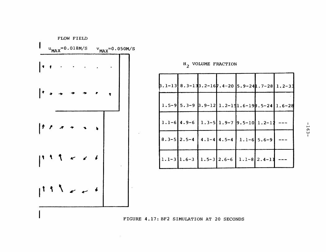
FLOW FIELD

uMAX=0.018M/S VMAX=0.050M/S

It o, - -4 P

I I I

H2 VOLUME FRACTION2

FIGURE 4.17: BF2 SIMULATION AT 20 SECONDS

3.1-13 8.3-1 3.2-167.4-20 5.9-24 .7-28 1.2-3

1.5-9 5.3-9 3.9-12 1.2-1 1.6-19 .5-24 1.6-2

1.1-6 4.9-6 1.3-5 1.9-7 9.5-10 1.2-1

8.3-5 2.5-4 4.1-4 4.5-4 1.1-6 5.6-9

1.1-3 1.6-3 1.5-3 2.6-6 1.1-8 2.4-11

.t

I \ ,

FLOW FIELD

u MAX=0.042M/S MAX=0. 2 4M/S

It, * -

I4u t- i

I1tf ~ -

*.. '

H2 VOLUME FRACTION X 1000

2.0 1.0 0.85 0.49 0.10 5.8-3 7.9-5

2.0 0.06 0.02 0.03 3.7-5 8.7-5 5.9-7

2.0 0.88 0.84 0.81 0.86 0.88

2.1 1.5 0.70 0.44 0.63 0.77

2.3 1.7 1.1 0.18 0.26 0.41-.-.-.- - -

FIGURE 4.18:BF2 SIMULATION AT 100 SECONDS

FLOW FIELD

UMAX=0.054M/SMAX vMAX=0.26M/S

H2 VOLUME FRACTION X

FIGURE 4.19:BF2 SIMULATION AT 200 SECONDS

1000

2.6 1.5 1.2 1.0 0.94 0.87 0.73

2.6 0.27 0.31 0.36 0.43 0.53 0.59

2.7 1.3 1.3 1.2 1.2 1.1

2.8 2.1 1.3 0.94 1.0 1.0 ---

2.9 2.3 1.7 0.76 0.80 0.86

-166-

recirculation produces a hydrogen gradient along the prin-

cipal flowpaths.

The development history of the velocity field is shown

in Figure 4.20. Also plotted is the Courant time step size.

The velocity profile requires roughly 50 seconds to develop

and thereafter remains relatively unchanged. The hydrogen

volume fraction transients at five selected locations are

plotted in Figure 4.21. The concentration gradient peak at

the centerline is also evident in this figure. The behavior

of point D is noteworthy in that it is not monotonic. The

physical explanation of the behavior is as follows. The

lower region major recirculation loops develop faster than

that of the upper region. Secondly, the buoyant central

plume takes some time to penetrate the orifice and reach

the facility ceiling where it will turn and cause clockwise

flow in the upper region. Prior to the development of the

upper region flow field, relatively hydrogen rich flow is

directed at D. After the upper circulation commences,

hydrogen-free atmosphere is pumped down into the lower

region through the right half of the orifice. This dilutant

stream is entrained in the lower recirculation and is con-

vected to D. This depression is transitory since eventually

the dilutant effect diminishes as the upper region gains

hydrogen.

The actual experiment ran for a few hours. However,

the short-term predictions can be compared to early data

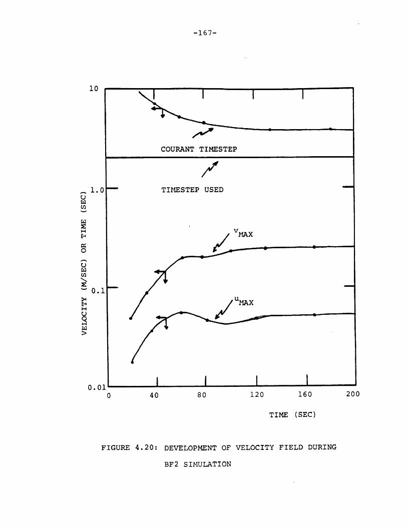
-167-

1.0

0.1

0.01 '0 40 80 120 160

TIME (SEC)

FIGURE 4.20: DEVELOPMENT OF VELOCITY FIELD DURING

BF2 SIMULATION

200

-168-

10 I I I

82

B- 3 **- - - 89

o /

O

zo-4

C

10-510 40 80 120 160 200

TIME (SEC)

APPROXIMATE READING AT MEASUREMENT POINT 82

**APPROXIMATE READING AT MEASUREMENT POINT 89

FIGURE 4.21: HYDROGEN CONCENTRATION TRANSIENTS

-169-

measurements. The measured hydrogen concentrations at sensor

locations 82 and 89 are indicated in Figure 4.21. Good

agreement is seen. Further extrapolation of the short-term

predictions indicate good physical agreement with the general

findings of BF2.

4.3.1.2.2 Completely Open Compartment

This simulation is identical to the previous one except

the orifice plate is completely removed. This case is

similar to the BF Test 1 except that different source flow

rates are used. This problem is discussed to illustrate

the effect of the orifice upon the physical phenomena and

the computational effort involved. The flow field and H2

concentration profile at 100 seconds is depicted in Figure

4.22. When this figure is compared to Figure 4.18 it is

seen that the open geometry leads to more uniform hydrogen

concentrations with small axial and radial gradients. An

extreme example of this difference is the upper left node

of the domain where the hydrogen concentrations are 7.6-4

and 7.9-8, respectively, in the two cases. The velocity

field develops at nearly the same rate as in the previous

case and the terminal velocity magnitudes were similar in

both cases. The development of the flow field is illustrated

in Figure 4.23. Nevertheless, significant differences

between the fully open arl orificed geometry are evident.

The velocity magnitudes are nearly 20% higher in the open

geometry demonstrating the flow resistance afforded by the

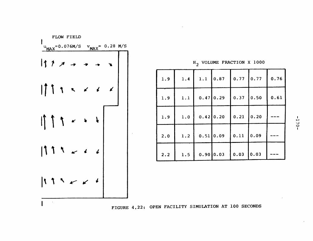
FLOW FIELD

uMAX=0.076M/S VMAX = 0.28 M/S

H. VOLUME FRACTION X 1000

FIGURE 4.22: OPEN FACILITY SIMULATION AT 100 SECONDS

1.9 1.4 1.1 0.87 0.77 0.77 0.76

1.9 1.1 0.47 0.29 0.37 0.50 0.61

1.9 1.0 0.42 0.20 0.21 0.20 ---

2.0 1.2 0.51 0.09 0.11 0.09

2.2 1.5 0.90 0.03 0.03 0.03..-.. .- - -i i

-171-

0 20 40 60 80 100

TIME (SEC)

FIGURE 4.23: DEVELOPMENT OF VELOCITY FIELD DURING

OP2N FACILITY SIMULATION

10.0

1.0

u

0

r0.1>

0.01

-172-

orifice. The stable stratification of the non-source regions

spans the entire height of the facility. The "shelf-region"

of the upper volume causes a slight upward velocity trajec-

tory which inhibits the formation of a large single recir-

culation region but instead two distinct upper and lower

circulations develop.

The hydrogen concentration transients of five selected

locations are presented in Figure 4.24. It is interesting

to note that point D displays similar qualitative behavior

as seen before. The physical scenario however, is a bit

different in that this transitory depression of hydrogen

abundance is caused by the location of D in the border region

to two low flow recirculation foci. The orifice effect is

also clear in that all centerline locations lead other

regions regardless of elevation.

As described in Chapter 3, successive over-relaxation

is employed in the SMAC solution procedure. The degree of

over-relaxation is a free parameter selected by the analyst.

The results of a sensitivity study of this value for BF-type

transients was performed using this scenario as the bench-

mark. The results of the study are summarized in Table 4.6.

Table 4.6

Over-relaxation Factor Average Iterations Per Cycle

1.5 41

1.7 31

1.8 27

1.9 33

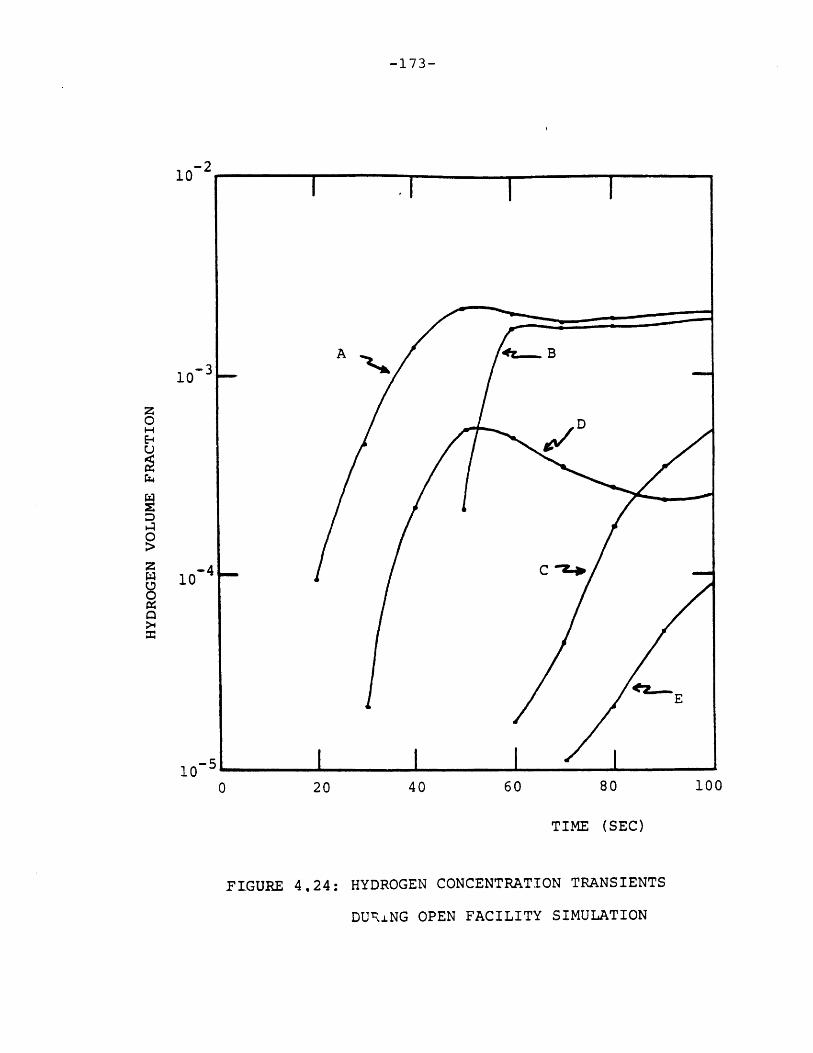
-173-

0 20 40 60 80

TIME (SEC)

FIGURE 4.24: HYDROGEN CONCENTRATION TRANSIENTS

DURiNG OPEN FACILITY SIMULATION

10-2l0

10-3

100

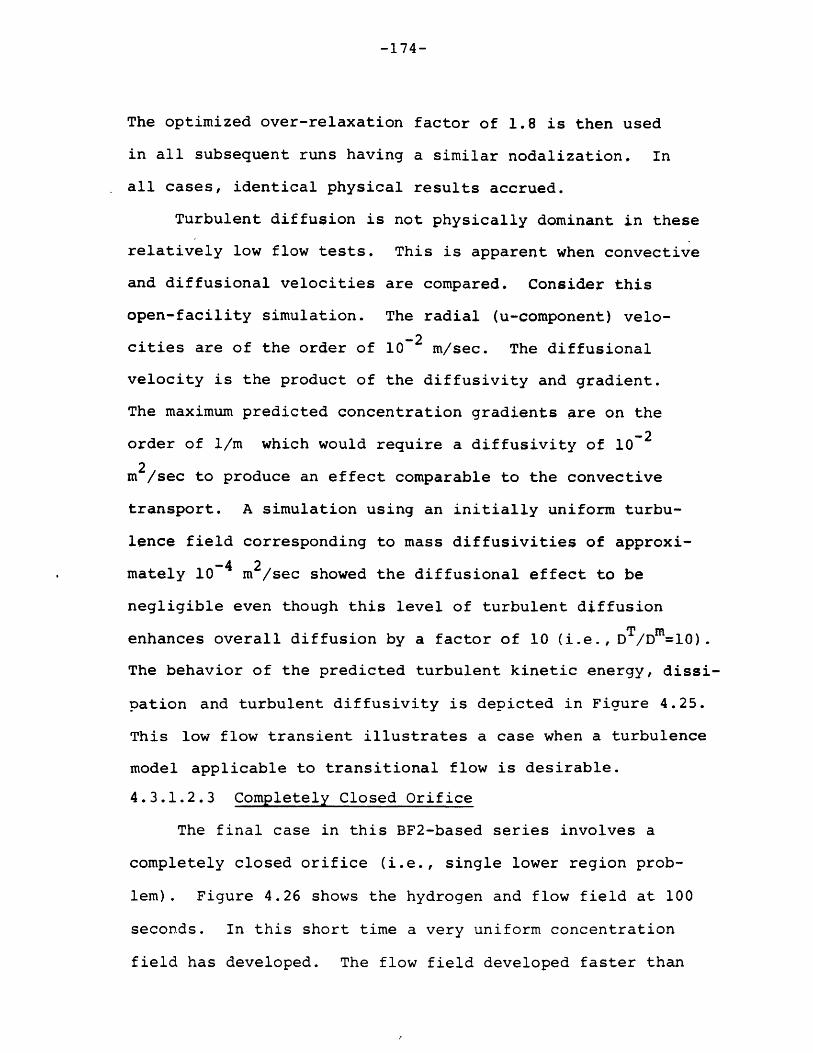
-174-

The optimized over-relaxation factor of 1.8 is then used

in all subsequent runs having a similar nodalization. In

all cases, identical physical results accrued.

Turbulent diffusion is not physically dominant in these

relatively low flow tests. This is apparent when convective

and diffusional velocities are compared. Consider this

open-facility simulation. The radial (u-component) velo-

-2cities are of the order of 10-2 m/sec. The diffusional

velocity is the product of the diffusivity and gradient.

The maximum predicted concentration gradients are on the

order of 1/m which would require a diffusivity of 10-2

m /sec to produce an effect comparable to the convective

transport. A simulation using an initially uniform turbu-

lence field corresponding to mass diffusivities of approxi-

mately 10-4 m2/sec showed the diffusional effect to be

negligible even though this level of turbulent diffusion

enhances overall diffusion by a factor of 10 (i.e.,D T/Dm=10).

The behavior of the predicted turbulent kinetic energy, dissi-

pation and turbulent diffusivity is depicted in Figure 4.25.

This low flow transient illustrates a case when a turbulence

model applicable to transitional flow is desirable.

4.3.1.2.3 Completely Closed Orifice

The final case in this BF2-based series involves a

completely closed orifice (i.e., single lower region prob-

lem). Figure 4.26 shows the hydrogen and flow field at 100

seconds. In this short time a very uniform concentration

field has developed. The flow field developed faster than

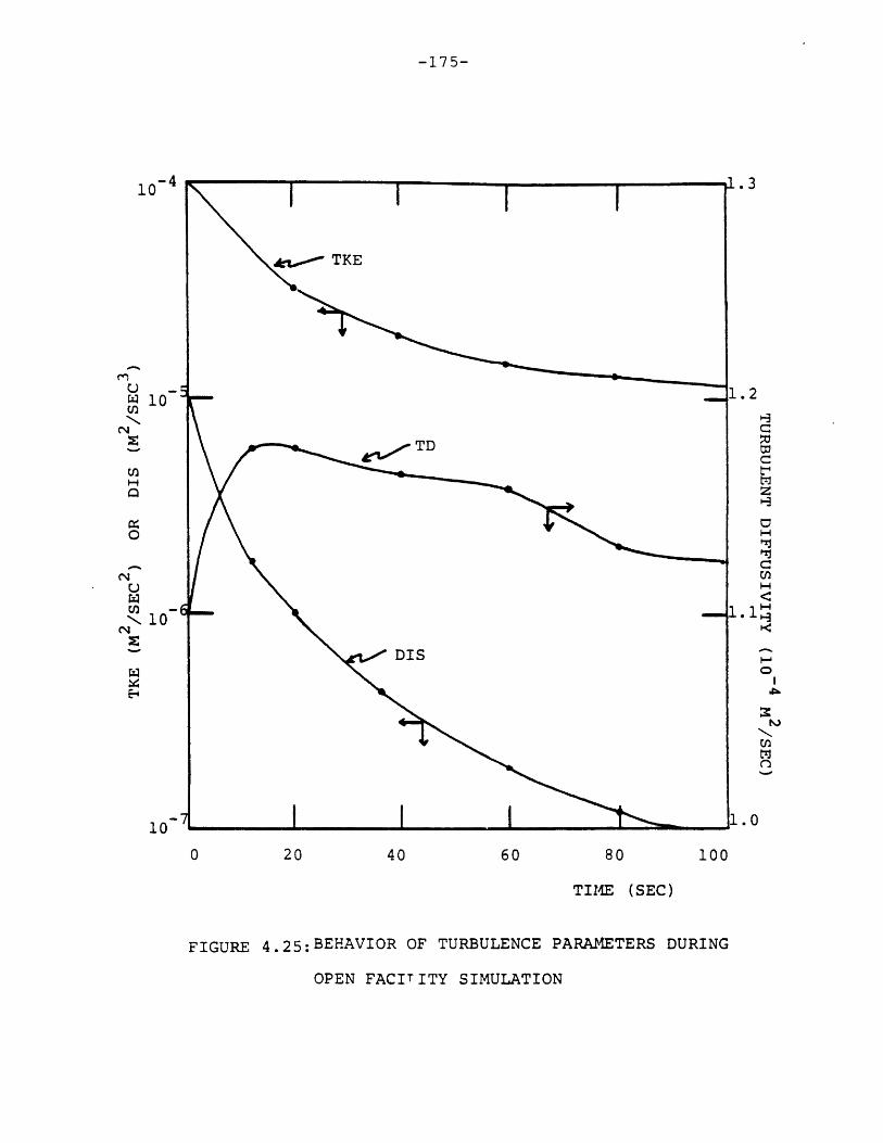
-175-

40 60

.2

z-3H

c<H0

N

UI

r

o

100

TIME (SEC)

FIGURE 4.25:BEHAVIOR OF TURBULENCE PARAMETERS DURING

OPEN FACITITY SIMULATION

N

N

vu

NuuUrnj

Cl

NN~

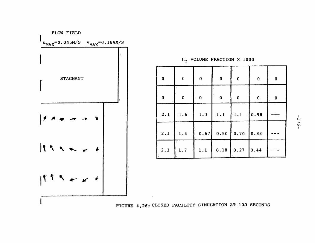
FLOW FIELD

UMAX =0. 045M/S vMAX=0. 189M/S, 0.045,/S VMA

STAGNANT

I-

H2 VOLUME FRACTION X 1000

0 0 0 0 0 0 0

0 0 0 0 0 0 0

2.1 1.6 1.3 1.1 1.1 0.98

2.1 1.4 0.67 0.50 0.70 0.83

2.3 1.7 1.1 0.18 0.27 0.44

FIGURE 4.26: CLOSED FACILITY SIMULATION AT 100 SECONDS

I *" -.

&*

- ~~- ' - ' ' ---- ~

-177-

in the previous two cases (elapsed time of about 30 seconds),

but the magnitude of the axial velocity components are less

than the previous simulations due to the retarding effects

of the enclosing walls.

4.3.1.2.4 BF Test No. 6 Simulation I - Coarse Mesh

This test was performed in the same geometry as the

BF2 test. However, a stable thermal atmospheric inversion

was introduced prior to hydrogen injection. The upper

region was heated to approximately 350C while the lower

region's temperature was 190 C. These are approximate tem-

perature values as the exact temperature distribution was

not measured. A 66/34 H2/N2 mixture was introduced in the

lower region at an initial rate of approximately 2.3 m3/hr.

At 1080 seconds this rate was reduced to 0.9 m3/hr which was

maintained until 7460 seconds at which time all injection was

terminated. The simulation reported here uses laminar flow

modelling (turbulence model not employed), no heat sinks are

modelled, and the coarse 32 node mesh discretization. The

limitations of these assumptions are illustrated in the

reported results.

The flow and hydrogen fields at 20,100 and 200 seconds

are depicted in Figures 4.27, 4.28, 4.29, respectively. A

comparison with the calculated fields for the BF2 and com-

pletely closed orifice predictions at 100 seconds is enlight-

ening. The BF6 result is distinctly different from the BF2

FLOW FIELD

I UMAX=0.034M/S v MAX=0.087M/S

I .

I 4

I i* J i

I I

H2 VOLUME FRACTION

.5-12 1.3-121.5-13 2.2-1 2.3-20 7-25 4.4-3

7.6-8 6.4-8 ..6-10 7.7-132.7-16 2-20 4.5-21-. .. . ... -. . -. .. . . . . . -..- -

8.8-5 9.1-5 6.1-5 2.6-6 3.2-8 8.6-1 ---

1.2-3 1.2-3 9.1-4 1.7-4 8.2-6 7.5-8 ---

3.5-3 3.2-3 2.0-3 1.0-5 1.6-7 7.2-11

.. . . . -. . .-.. .. .... .-.

I FIGURE 4.27:BF6 SIMULATION AT 20 SECONDS

FLOW FIELD

u =MAX0.054M/S v =0.257M/SMAX MAX

I .- ~ .. H2 VOLUME FRACTION X 1000

0.0037 .0046 .0058 .0075 0.010 0.014 0.013

0.39 0.19 0.12 0.088 0.072 0.064 0.034

4.4 3.2 2.5 2.3 2.1 1.9

4.5 2.6 1.4 1.4 1.6 1.6

5.0 3.5 2.3 0.71 0.72 0.95

FIGURE 4.28:BF6 SIMULATION AT 100 SECONDS

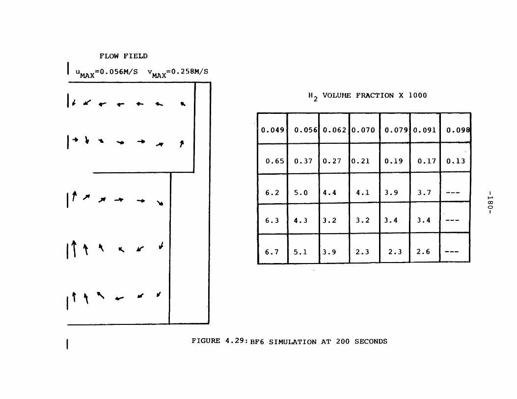
FLOW FIELD

uMAX=0.056M/SMAX vMAX= 0.258M/S

*1 * * *

I % b 4

H2 VOLUME FRACTION X

FIGURE 4 .2 9 :BF6 SIMULATION AT 200 SECONDS

I

I -

1000

0.049 0.056 0.062 0.070 0.079 0.091 0.09

0.65 0.37 0.27 0.21 0.19 0.17 0.13

6.2 5.0 4.4 4.1 3.9 3.7

6.3 4.3 3.2 3.2 3.4 3.4

6.7 5.1 3.9 2.3 2.3 2.6A of

of l

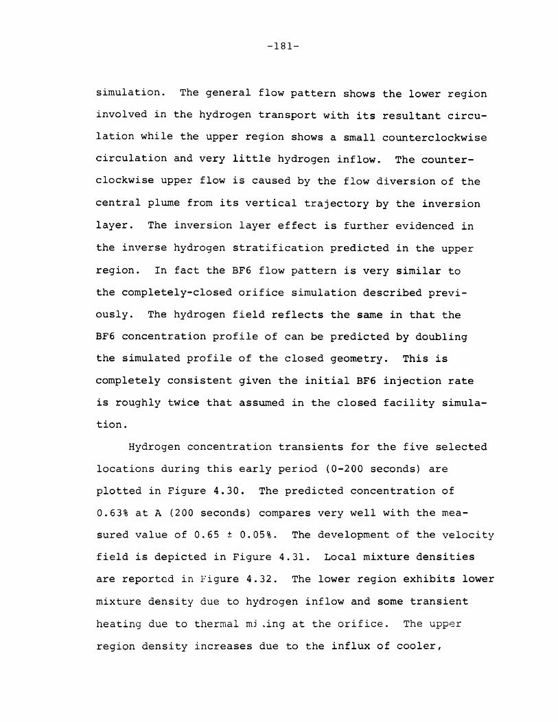
-181-

simulation. The general flow pattern shows the lower region

involved in the hydrogen transport with its resultant circu-

lation while the upper region shows a small counterclockwise

circulation and very little hydrogen inflow. The counter-

clockwise upper flow is caused by the flow diversion of the

central plume from its vertical trajectory by the inversion

layer. The inversion layer effect is further evidenced in

the inverse hydrogen stratification predicted in the upper

region. In fact the BF6 flow pattern is very similar to

the completely-closed orifice simulation described previ-

ously. The hydrogen field reflects the same in that the

BF6 concentration profile of can be predicted by doubling

the simulated profile of the closed geometry. This is

completely consistent given the initial BF6 injection rate

is roughly twice that assumed in the closed facility simula-

tion.

Hydrogen concentration transients for the five selected

locations during this early period (0-200 seconds) are

plotted in Figure 4.30. The predicted concentration of

0.63% at A (200 seconds) compares very well with the mea-

sured value of 0.65 ± 0.05%. The development of the velocity

field is depicted in Figure 4.31. Local mixture densities

are reported in Figure 4.32. The lower region exhibits lower

mixture density due to hydrogen inflow and some transient

heating due to thermal mi .ing at the orifice. The upper

region density increases due to the influx of cooler,

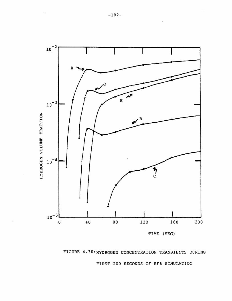
-182-

0 40 80 120 160 200

TIME (SEC)

FIGURE 4.30:HYDROGEN CONCENTRATION TRANSIENTS DURING

FIRST 200 SECONDS OF BF6 SIMULATION

-183-

40 80 120 160 200

TIME (SEC)

FIGURE 4 .3 1 :VELOCITY FIELD DEVELOPMIENT DURING FIRST

200 SECONDS OF BF6 SIMULATION

10.0

1.0

u

>4

ol0 "

0.0

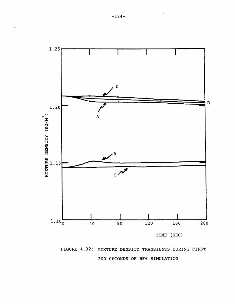
-184-

1.25

1.20

>4

z

1.15

xH

1.10o

C /S,

I II80 120 160 200

TIME (SEC)

FIGURE 4.32: MIXTURE DENSITY TRANSIENTS DURING FIRST

200 SECONDS OF BF6 SIMULATION

--

E

A

*B

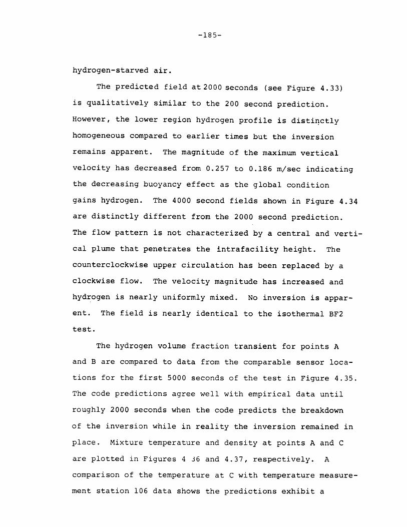
-185-

hydrogen-starved air.

The predicted field at 2000 seconds (see Figure 4.33)

is qualitatively similar to the 200 second prediction.

However, the lower region hydrogen profile is distinctly

homogeneous compared to earlier times but the inversion

remains apparent. The magnitude of the maximum vertical

velocity has decreased from 0.257 to 0.186 m/sec indicating

the decreasing buoyancy effect as the global condition

gains hydrogen. The 4000 second fields shown in Figure 4.34

are distinctly different from the 2000 second prediction.

The flow pattern is not characterized by a central and verti-

cal plume that penetrates the intrafacility height. The

counterclockwise upper circulation has been replaced by a

clockwise flow. The velocity magnitude has increased and

hydrogen is nearly uniformly mixed. No inversion is appar-

ent. The field is nearly identical to the isothermal BF2

test.

The hydrogen volume fraction transient for points A

and B are compared to data from the comparable sensor loca-

tions for the first 5000 seconds of the test in Figure 4.35.

The code predictions agree well with empirical data until

roughly 2000 seconds when the code predicts the breakdown

of the inversion while in reality the inversion remained in

place. Mixture temperature and density at points A and C

are plotted in Figures 4 36 and 4.37, respectively. A

comparison of the temperature at C with temperature measure-

ment station 106 data shows the predictions exhibit a

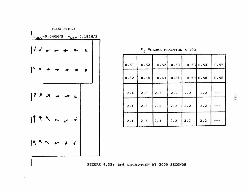
FLOW FIELD

.040M/S vu, ,,=0 . 186M/S

v- F

4"...

it A f

It

1

H VOLUME FRACTION X 100

0.51 0.52 0.52 0.53 0.53 0.54 0.55

0.82 0.68 0.63 0.61 0.59 0.58 0.56

2.4 2.3 2.3 2.2 2.2 2.2

2.4 2.3 2.2 2.2 2.2 2.2

2.4 2.3 2.3 2.2 2.2 2.2

FIGURE 4.33: BF6 SIMULATION AT 2000 SECONDS

FLOW FIELD

uMAX = 0.048M/SMAXv MAX=0.226M/SMAX

-q --v --

'TU-

-

H2 VOLUME2 FRACTION X 100

2.6 2.5 2.5 2.5 2.5 2.5 2.5

-- - -

2.6 2.4 2.4 2.4 2.4 2.4 2.4

2.6 2.5 2.5 2.5 2.5 2.5

2.6 2.6 2.5 2.5 2.5 2.5

2.7 2.6 2.5 2.4 2.4 2.4- --i

FIGURE 4.34:BF6 SIMULATION AT 4000 SECONDS

IT

-188-

1000 2000 3000 4000 500

TIME (SEC)

FIGURE 4.35;:COMPARISON OF MEASURED VS PREDICTED H2

CONCENTRATIONS DU7ING 32 NODE BF6

0

SIMULATION

1

0- -

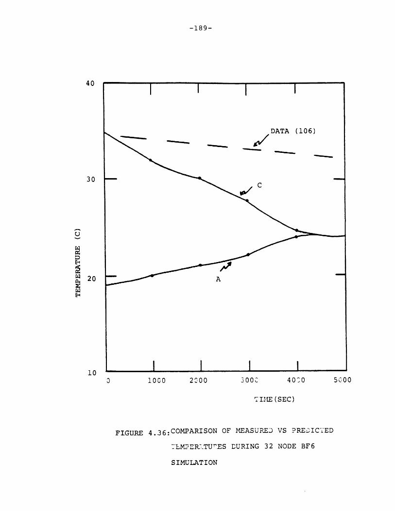
-189-

0 1000 2000 300c 40^0 5000

TIME (SEC)

FIGURE 4 .3 6 :COMPARISON OF MEASURED VS PREDICTED

[LM~ER.TU ES DURING 32 NODE BF6

SIMULATION

40

30

u

S20

10

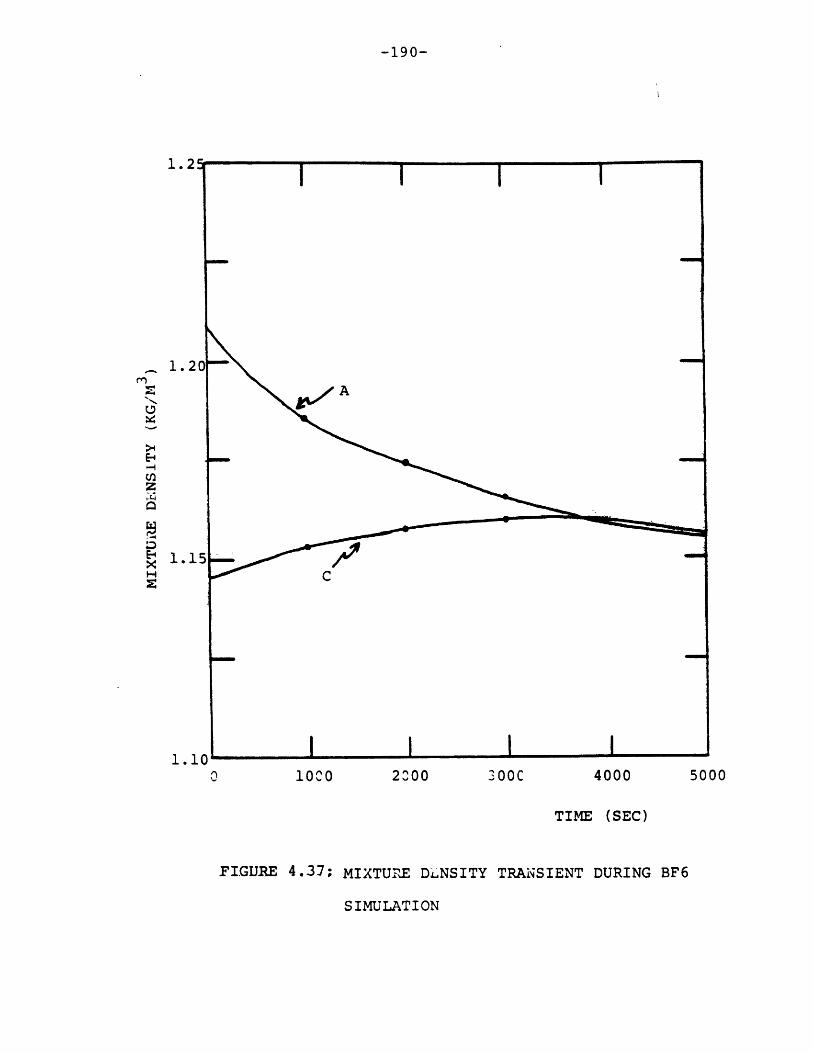
-190-

1000 2000 300C 4000 5000

TIME (SEC)

FIGURE 4.37; MIXTURE DLNSITY TRANSIENT DURING BF6

SIMULATION

1.2

1.2-,

>4

E-4

z

xI-4H3z

1.10

-191-

substantially faster thermal mixing transient. The mixture

density plots mirror this effect. Clearly, the inversion

breakdown allows the plume penetration into the orifice

region. The plot of orifice region vertical velocities

in Figure 4.38 clearly illustrates this bimodal behavior.

The orifice region Froude number based on the following

similitude

Fr - (4.1)

is reported in Table 4.7. This further demonstrates the

diminishing inverse buoyancy effect.

Table 4.7

Orifice Froude Number

Time(s) Fr

0 0

200 .035

400 .040

600 .048

800 .055

1000 .063

1200 .049

2000 .078

3000 .20

4000 3.0

-192-

0.2

uCENTER NODE .*

>40.1

-NODE

0.

U-0.1H NEIGHBORING

0 1000 2000 3000 4000 5000

TIME (SEC)

FIGURE 4 .3 8 :BEHAVIOR OF ORIFICE RZGICN VERTICAL

FLOW DURING BF6 SIMULATION

-193-

A number of effects can be identified to explain the

discrepancies between predictions and measurements. First,

the lack of heat sink modelling neglects the thermal storage

capacity of the concrete walls which in turn would retard

the thermal transient. Second, the laminar flow assumption

causes the central hydrogen-rich plume to be narrower in the

initial period of the test. This higher hydrogen concentra-

tion causes enhanced buoyancy in the central core and thus

earlier flow penetration in the orifice region. Third, the

buoyancy effect embodied in the body force term of the

momentum equation is based on a reference state. The

reference state for this simulation was not updated to

reflect the rising hydrogen concentration. This effect can

mispredict buoyant velocities by as much as 25%.

Fourth, and most significant, the use of a very coarse

mesh leads to an inaccurate prediction of the velocity

field near the inversion layer (orifice region) and also

causes high numerical diffusion. Figure 4.39 is a map of

the estimated numerical diffusion coefficients at 1000

seconds. These constants are much higher than physical dif-

fusive effects and are highest in the distinctly crossflow

region near the orifice. As a confirmatory study of this

conclusion the thermal inversion decay transient was inter-

preted as a transient slab conduction problem. The resultant

thermal diffusivity compuied is roughly 19 x 10- m2 /sec

which is in excellent agreement with the computed numerical

-194-

NUMERICAL DIFFUSIVITY MAP AT 1000 SECONDS

(M2/SEC)

MOLECULAR DIFFUSIVITY - 0.10-3 M 2/SEC

TURBULENT DIFFUSIVITY - 1.00-3 M 2/SEC

FIGURE 4.39: COMPARISON OF MOLECULAR, TURBULENT AND NUMERICAL

DIFFUSIVITIES AT 1000 SECONDS INTO BF6 SIMULATION

-195-

diffusivities (average 21 x 10- 3 m2 /sec). The im-

proved prediction of the test using techniques to diminish

the limitations reported in this simulations is shown in

the next section.

4.3.1.2.5 BF Test No. 6 Simulation II - Model

Improvements

A second simulation of BF6 is reported which is form-

ulated to address the shortcomings of the first calcula-

tion. The major model improvements are: a finer mesh,

partial correction of numerical diffusion, better defini-

tion of initial thermal stratification, use of turbulence

model and modelling of heat sinks. The problem nodaliza-

tion is presented in Figure 4.40. A 50 node discretiza-

tion with two vertical heat sinks (concrete) is used. The

closer mesh spacing of the orifice region allows for more

accurate velocity field definition. Periodic reference

state update is employed to more accurately evaluate buoy-

ancy effects. The partial numerical diffusion correction

scheme discussed in Chapter 3 is also invoked.

The first 5000 seconds of the test are simulated.

Figure 4.41 depicts the flow field during this period.

The qualitative characteristics of the field did not

change over this interval and nothing in the velocity

transient indicated that the flow was making a transition

to the non-inversion pattern. The flow is characterized

by a strong central plume causing a clockwise recirculation

-196-

87

81

IS SI I

1 ' S I

CONCRETE/DR' S

0 .28250.2825-0.57400.86100.4500

DZ'S0.4290.4290.4290.4290.4290.4290.4290.4000.4550.4550.4550.434

CONCRETE

81,87: H2 MEASUREMENT

POINTS

S=SOURCE CELL

FIGURE 4.40: 50 NODE MODEL FOR BF6 SIMULATION

-197-

*l *

*I.

~t I\l'sH

£

A I

CONCRETE

VELOCITY HISTORY

t(s)

1000

2000

3000

4000

5000

Umax(m/s)

Vmax(m/s)

0.0870 0.2419

0.0649 0.1798

0.0645 0.1790

0.0642 0.1783

0.0639 0.1776

CONCRETE

FIGURE 4.41: VELOCITY PrOFILE AND TIME HISTORY DURING 50

NODE BF6 SIMULATION

0

c-

*--

-198-

in the lower region. The upper region admits very little

hydrogen and experiences a small counterclockwise recircu-

lation predominantly in the lower elevations of the upper

compartment. The quantitative data describing the velo-

city field are also summarized in Figure 4.41. The de-

crease in the steady state vertical components around 1000

seconds is due to a reduction in the source flow at that

time.

Figures 4.42 through 4.44 illustrate the predicted

hydrogen concentration profiles at 1000, 3000 and 5000

seconds, respectively. The inversion blocks the hydrogen

build-up in the upper region throughout the simulation.

Also, the convective and diffusive (including turbulence)

transport homogenizes the lower region distribution. The

temperature profiles depicted in Figures 4.45 through 4.47

reflect the same physical circumstances. An additional

effect helping to stabilize the inverse thermal stratifi-

cation is the interaction of the concrete heat slabs.

Figure 4.48 presents a comparison of the code predic-

tions of the hydrogen transients at two representative

locations in the lower and upper regions with the measured

data. Much better agreement is noted in contrast to the

previous coarse mesh laminar simulation. The upper region

predictions remain in good agreement throughout the calcu-

lation. The predicted lower region concentrations fall

below the measurements by as much as 1 volume percent.

This lack of quantitative agreement is also noted by

199-

H2 VOLUME FRACTIONS X 1000

0.03 0.04 0.03 0.03 0.04

0.10 0.10 0.11 0.12 0.12

0.50 0.50 0.51 0.54 0.59

1.58 1.08 0.83 0.74 0.67

12.34 11.76

12.41 11.64 11.15 11.00

12.43 11.41 10.71 10.84

12.46 11.38 10..62 10.69

12.55 11.48 10.74 10.55

12.72 11.64 10.84 10.42

13.01 11.94 11.03 10.26

13.65 12.75 11.80 10.05

FIGURE 4.42: HYDROGEN VOLUME FRACTION PROFILE AT 1000

SECONDS INTO 50 NODE BF6 STMULATION

-200-

H 2 VOLUME FRACTION X 100

FIGURE 4.43: HYDROGEN VOLUME FRACTION PROFILE AT 3000

SECONDS INTO 50 NODE BF6 SIMULATION

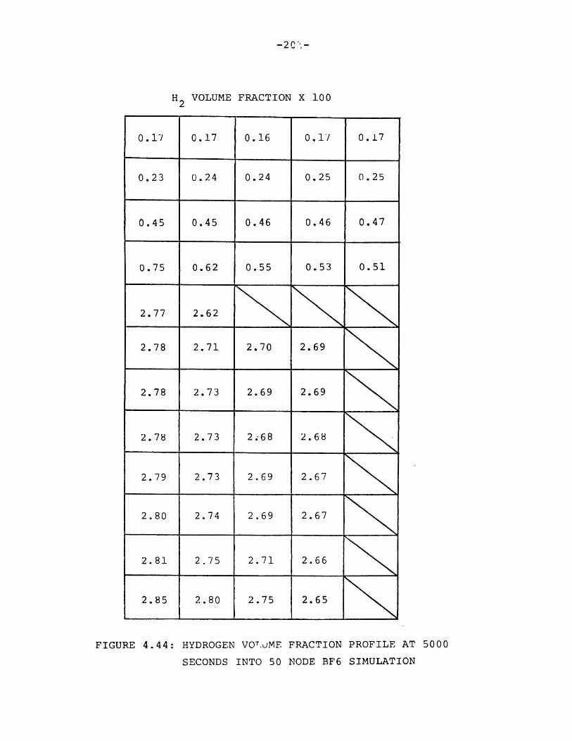
H2 VOLUME FRACTION X 100

FIGURE 4.44: HYDROGEN VOTLME FRACTION PROFILE AT 5000

SECONDS INTO 50 NODE BF6 SIMULATION

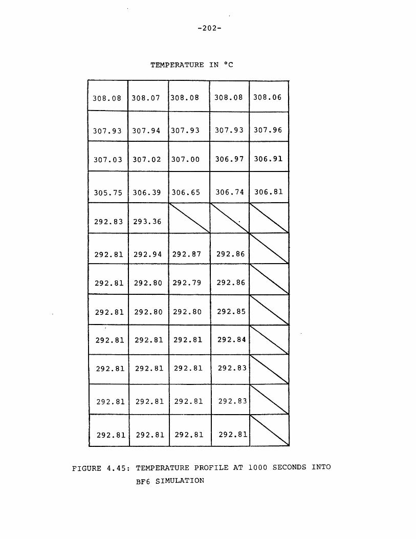
-202-

TEMPERATURE IN OC

FIGURE 4.45: TEMPERATURE PROFILE AT 1000 SECONDS INTO

BF6 SIMULATION

-203-

TEMPERATURE IN

307.75 307.75 307.75 307.74 307.71

307.37 307.37 307.35 307.36 307.36

305.83 305.82 305.81 305.78 305.72

304.86 305.30 305.49 305.57 305.62

293.34 293.74

293.31 293.41 293.36 293.35

293.31 293.30 293.30 293.35

293.31 293.31 293.30 293.34

293.31 293.31 293.31 293.33

293.31 292.31 293.31 293.33

293.31 293.31 293.31 293.33

293.31 293.31 293.31 293.31

FIGURE 4.46: TEMPERATURE PROFILE AT 3000 SECONDS INTO

BF6 SIMULATION

-204-

TEMPERATURE IN OC

307.11 307.10 307.11 307.10 307.07

306.53 306.51 306.50 306.50 306.50

304.55 304.55 304.53 304.49 304.42

303.17 303.81 304.08 304.18 304.27

294.00 294.62

293.97 294.12 294.04 294.04

293.97 293.96 293.96 294.04

293.97 293.97 293.96 294.02

293.9 293.97 293.97 294.00

293.9\ 293.97 293.98 294.00

293.97 293.97 293.98 293.99

293.91 293.97 293.97 293.98,- - ] -- I -L

FIGURE 4.47: TEMPERATURE PROFILE AT 5000 SECONDS INTO

BF6 SIMULATION

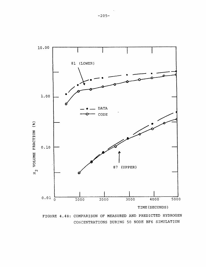
-205-

10.00 I I

81 (LOWER)

1.00

_ • DATA

0- CODE

dP

z

0.10

O

> 87 (UPPER)

0.01 0 1000 2000 3000 4000 5000

TIME (SECONDS)

FIGURE 4.48: COMPARISON OF MEASURED AND PREDICTED HYDROGEN

CONCENTRATIONS DURING 50 NODE BF6 SIMULATION

-206-

Thurgood [67] and Trent [64] which suggests a possible

error in the measurement of source flow during the

experiment.

The maximum vertical and horizontal velocity compo-

nents are plotted vs. time in Figure 4.49. The two most

important characteristics observed are the development

period of approximately 100 seconds and the transition to

a new lower vertical component which is caused by the

reduction in the hydrogen injection rate. Finally, Figure

4.50 is a comparison of the orifice region Froude numbers

of this result and the previous simulation. The substan-

tially different behaviors verify the physical character-

istics of the two calculations. In summary, the second

finer mesh simulation utilizing turbulence modelling,

accounting for solid heat sinks/sources, periodic refer-

ence state update and partial numerical diffusion correc-

tion is a much more accurate model of the BF6 test.

-207-

0.3

0.2

0.1uMAX

0.0 I I0 1000 2000 3000 4000 5000

TIME (SECONDS)

FIGURE 4.49: DEVELOPMENT HISTORY OF VELOCITY FIELD DURING

50 NODE BF6 SIMULATION

-208-

10.00

1.00

0.10

0.010 1000 2000 3000 4000 5000

TIME (SECONDS)

FIGURE 4.50: COMPARISON OF ORIFICE REGION FROUDE NUMBERS

OF THE TWO BF6 SIMULATIONS

-209-

4.3.2 Hanford Engineering Development Laboratory Tests

The hydrogen mixing tests performed at the Hanford

Engineering Development Laboratory (HEDL) are representative

of events in which hydrogen is injected at higher rates than

typical of a degrading core events. One example is a release

from a pipe break in the reactor coolant system early in the

postulated event. The facility and tests are conducted to

be representative of actual containment conditions including

the presence of steam, complex geometrical arrangements and

containment air recirculation systems. The tests are per-

formed in the HEDL Containment Systems Test Facility (CSTF).

Given the complexity of the tests, their simulation is more

difficult and costly. The physical regimes encountered

test the validity bounds of the slower mixing model.

4.3.2.1 Facility and Testing Program Review

The facility and associated features are depicted in

Figures 4.51 and 4.52. The underlying modelling criteria

are based on scale modelling of a Pressurized Water Reactor

(PWR) ice condenser containment. The large vessel is 20.4 m

3high, 7.6 m in diameter with a free volume of 850 m

Detailed design and testing data are provided by Bloom et al.

and Bloom and Claybrook. The vessel is compartmentalized so

that the lower region can simulate the lower compartment of

an ice condenser contain .ent. This lower test volume is

approximately 150 m 3 in volume and occupies 30 0 0 of the

-210-

CSTF

VESSEL

HORIZONTAL

JET

14.1M

4.7M

4 IM

VERTICAL JET

FIGURE 4. 51: HEDL FACILITY SCHEMATIC

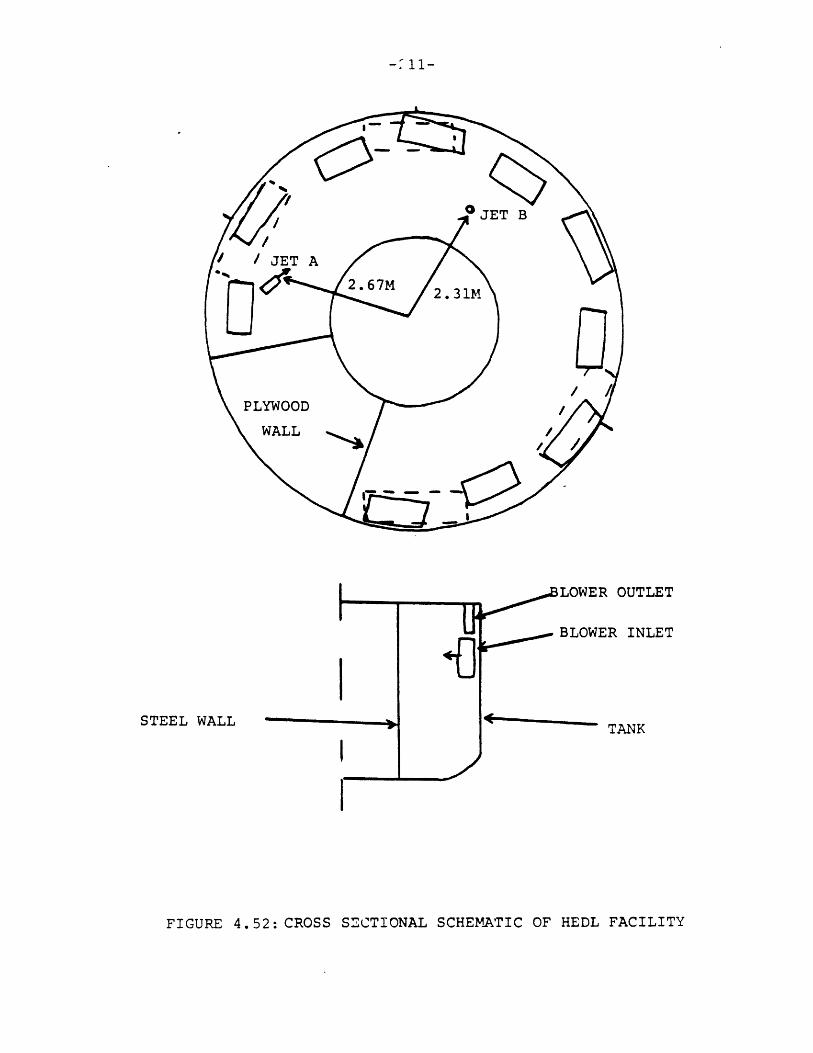
- 11-

STEEL WALL

ILOWER OUTLET

BLOWER INLET

TANK

FIGURE 4.52: CROSS SECTIONAL SCHEMATIC OF HEDL FACILITY

B

-212-

annular region. The central core of the lower region

represents the reactor cavity.

Air blowers which circulate the atmosphere from the

upper to the lower region are included in the facility as

shown in Figure 4.51. The four air blower openings operate

at a total flowrate of 1.8 m3/sec. Twenty-four return flow

paths from the lower to the upper compartment are situated

in the manner depicted in Figure 4.52. These represent

partially open ice condenser bays. The test compartment

does not contain any obstacles representative of vessels,

piping and other structure. The facility is extensively

instrumented with temperature, velocity and hydrogen sensors

(i.e., thermocouples, film anemometers and gas analyzers).

Three sets of tests define the experiment matrix as

shown in Table 4.8. The first series of tests (HM-Pl

through P4) were performed to test the effect of the air

recirculation system and initial thermal conditions. The

second series involved the introduction of either hydrogen

or helium in the form of a high velocity gas-steam horizontal

jet. The jet size was scaled to represent a 2 inch break in

a real system. The jet location which is labelled "Jet A"

in Figure 4.51 is centered in the annulus at 275 (azimuthal)

at a height of 1.5 m. The final two tests involved the

injection of a vertical gas-steam jet at location "Jet B"

which is located at 1800 at a height of 1.2 m. The vertical

jet tests are scaled to represent a release from the rupture

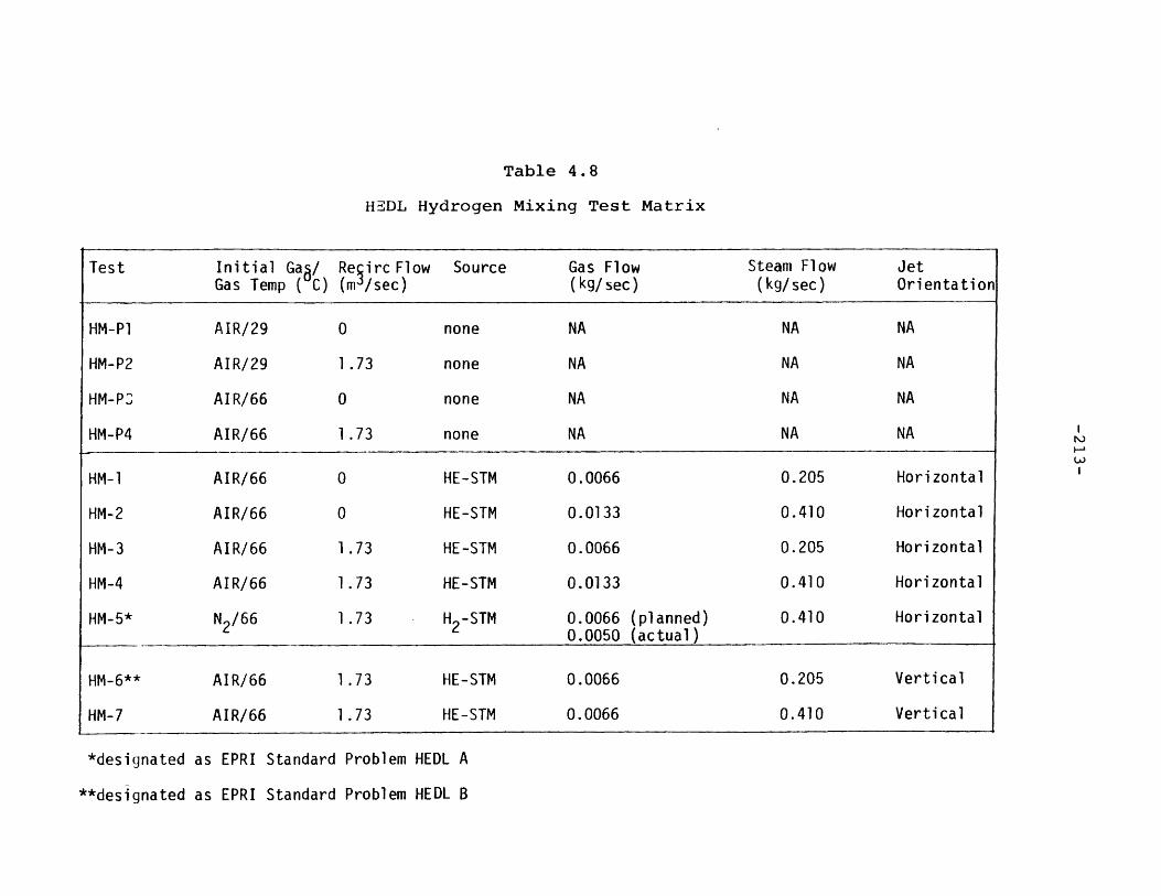
Table 4.8

HEDL Hydrogen Mixing Test Matrix

Test Initial GaA/ Resirc Flow Source Gas Flow Steam Flow JetGas Temp ( C) (m /sec) (kg/sec) (kg/sec) Orientation

HM-Pl AIR/29 0 none NA NA NA

HM-P2 AIR/29 1 .73 none NA NA NA

HM-PC AIR/66 0 none NA NA NA

HM-P4 AIR/66 1.73 none NA NA NA

HM-1 AIR/66 0 HE-STM 0.0066 0.205 Horizontal

HM-2 AIR/66 0 HE-STM 0.0133 0.410 Horizontal

HM-3 AIR/66 1.73 HE-STM 0.0066 0.205 Horizontal

HM-4 AIR/66 1.73 HE-STM 0.0133 0.410 Horizontal

HM-5* N2/66 1.73 H2-STM 0.0066 (planned) 0.410 Horizontal0.0050 (actual)

HM-6** AIR/66 1.73 HE-STM 0.0066 0.205 Vertical

HM-7 AIR/66 1.73 HE-STM 0.0066 0.410 Vertical

*designated as EPRI Standard Problem HEDL A

**designated as EPRI Standard Problem HEDL B

-214-

disk of the pressurizer relief tank. Tests HM-5 and HM-6

are designated Standard Problems HEDL A and HEDL B by the

EPRI/HEDL hydrogen assessment research program.

The qualitative empirical observations are now sum-

marized. In the absence of a jet source (i.e., preliminary

tests) measured natural circulation velocities are on the

order of .1 m/sec to .3 m/sec depending upon initial thermal

conditions, while velocities with recirculation fans oper-

ating range from 0.15 to 0.45 m/sec over the same thermal

condition spectrum. The enhanced mixing characteristic of

higher thermal gradients are expected to be more typical of

the actual containment post accident environment. The gas

release simulations produced the largest concentration

gradients for horizontal gas releases coupled with no forced

recirculation. The jet momentum influenced flow far from

the injection location especially in the case of vertical

jets. Finally, helium is shown to be a valid simulant for

hydrogen. In summary, these more complex tests reinforce

lessons learned from the Battelle Frankfurt tests and also

demonstrate the important mixing effects of the source con-

figuration, ventilation system operation and initial thermal

conditions.

4.3.2.2 Simulations Based On Selected Tests

Of the two HEDL tests designated as standard problems,

the vertical jet case (Case B - HM6) is utilized for a

-215-

validation calculation. This test is chosen since it pro-

duced the more significant spatial variations in gas concen-

trations. In addition, helium was used in HEDL B and this

analysis demonstrates the code's ability to model hydrogen

simulant gases. Helium flow is modelled as a hydrogen flow

of half the mass flow rate so that the similitude of the

buoyancy introduced is maintained. The one-half factor

arises from the ratio of the two gases' molecular weights.

An implicit assumption in this approach is that the helium

jet is a small contributor to the source flow's momentum

source contribution since halving the gas mass flow reduces

the momentum flux. The validity of this assumption is demon-

strated in the following calculation.

Momentum of steam jet = .24 k g- x 80 m 19.2 kg-m/sec2sec sec

Momentum of actual helium jet = .0068- k g x 80 msec sec

= 0.5 kg-m/sec 2

Momentum of assumed hydrogen jet= 0.5 x 0.5 = 0.25 kg-m/sec2

Total momentum of actual jet = 19.7 kg-m/sec2

2Momentum of simulated jet = 19.45 kg-m/sec2

As is seen this model introduces an error of 1.2% in the

momentum source. An additional assumption is that hydrogen

transport properties are similar to those of hydrogen.

The HEDL facility cc .tains recirculation blowers which

enhance mixing between the upper and lower volumes. An

ancillary model is developed to represent this blower effect

-216-

by user-defined blower-cells which exhibit source/sink

characteristics. Hydrogen, air and the resultant energy

mixing effects are expressed through the following model

equations:

Pa_ Q_- - p -p 1 , (4.1)t V ao a

h QPh [ -Ph ] , and (4.2)t V ho h

3pe - V[(pe) + ( p e ) - ( p e ) a - (pe)h] . (4.3)Bt V ao ho a h

These equations are solved implicitly after the overall

mass and energy transport equations are solved. The model

input specification assumes knowledge of the time dependent

behavior of inlet blower flowrate, temperature, hydrogen and

air densities. These have been ascertained from the experi-

mental data reports. The blower characteristics of HEDL B

are summarized in Table 4.9. This modelling approach can

possibly be used when more complex fan cooler component

simulations are undertaken.

Before performing a detailed continuum analysis of

HEDL B, a simple hand calculation based on a well-mixed

single region lumped parameter model is reported. This

exercise serves two purposes; first, it validates the data

utilized in the blower model and second, it tests the

validity of the helium/hydrogen modelling approach. Both

-217-

Table

HEDL B Blower

HydrogenDensity(kg/m3)

0.0

0.0

0.00078

0.00104

0.00234

0.00260

0.00270

*flow of one blower (total = 4 x

4.9

Specification

Temperature(OK)

308.0

315.0

316.0

319.5

325.0

325.5

322.5

0.433 = 1.733)

HEDL A and B are simulated in this manner and the calculated

results are compared to the experimental gas concentration

data in Figure 4.53. As is evident, excellent agreement

is noted especially in the horizontal jet case (HEDL A).

Of course, the axial stratification and azimuthal asymmetry

of the vertical jet case cannot be predicted by a lumped

model. Nevertheless, these results validate the blower and

mass source data and also demonstrate the usefulness of

simplified analysis to parameterize more complex calcula-

tions.

The problem mesh nodalization is depicted in Figure

4.54. The 80 node mesh is used as a compromise between the

desire for accuracy and the need to perform an economical

Time(sec)

0

90

270

330

630

690

870

AirDensity(kg/m 3 )

1.1303

1.1052

1.1017

1.0896

1.0712

1.0695

1.0795

Flow*(m3/sec)

0.433

0.433

0.433

0.433

0.433

0.433

0.433

HEDL A (HM5)

600

.>4

dP

i-0

1200 600

TIME (SEC) TIME (SC)

FIGURE 4. 53: COMPARISON OF LUMPED PARAMETER ANALYSIS RESULTS TO

DATA FOR TESTS HEDL A AND HEDL B

10

8

LqD

-40

1200

HEDL B (HM6)

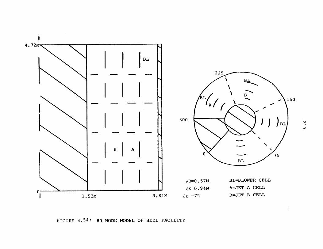
4.72

3.81M

300

0

6R=0. 57M

6Z=0.94M

66 =75

BL=BLOWER CELL

A=JET A CELL

B=JET B CELL

FIGURE 4.54: 80 NODE MODEL OF HEDL FACILITY

150

1.52M

-220-

computation. All four upper right hand cells are designated

as blower cells. The initial volume is assumed to be filled

with air at 338.150 K. The jet flow temperature varies from

373K to 388 0 K over the course of the injection. A jet

velocity of 80 m/sec is assumed and the jet effect is treated

as a momentum source in the source cell. This approach

while incapable of providing spatial resolution of the

near jet flow field allows for an economical way to represent

a jet in a coarse spatial mesh. The turbulence model is

used as well as the enhanced containment heat transfer

package. The heat sink model is the steel tank outer sur-

face. The inner cylinder boundary as well as the 600 wood

block are modelled as insulated surfaces.

Though the jet injection continued for over 600

seconds (H2 injection actually began at 45 seconds after

jet was initiated), only the first 300 seconds of the test

are simulated. The two main reasons for the abbreviated

simulation are calculational cost and the fact that the

characteristics of the predictions are apparent by the 300

second point. Figures 4.55 and 4.56 depict the flow and

thermal fields at 50 seconds in the jet and a non-jet

azimuthal regions, respectively. The flow field depicted

in these figures represent the two-dimensional resolution

(in the r-z plane) of the velocity vectors. Azimuthal

velocity components at the cell back and front faces are

noted in the diagram. The non-jet region exhibits a

FLOW FIELD*

TEMPERATURE FIELD

* Flow vectors correspond to r-z velocity.Values qiven at cell top and bottcn arefront and back face azimuthal velocitycaponents, respectively.

I max= .24 m/s v max= .52 m/smax wmax= .19 m/smax

FIGURE 4.55: FLOW AND TEMPERATURE FIELDS IN NON-JET (K=3) REGION AT 50

SECONDS INTO HEDL B SIMULATION

320.2 319.7 318.7 312.9

310.8 311.9 311.8 312.7

309.3 308.7 312.7 312.3

308.6 309.2 310.0 311.7

308.9 309.5 310.0 310.8

FLOW FIELD*

TEMPERATURE FIELD

* Flow field followsprevious figure.

convention of

= 1.21 m/s w = .19 m/smax

FIGURE 4.56:FLOW AND TEMPERATURE FIELDS IN JET (K=4) REGION AT 50

SECONDS INTO HEDL B SIMULATION

342.2 342.6 341.7 336.9

336.8 342.2 340.0 337.3

332.6 342.3 337.1 337.4

326.0 342.6 334.2 337.1

314.6 320.8 329.3 333.3

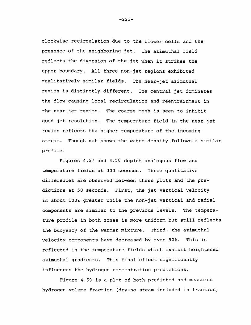
-223-

clockwise recirculation due to the blower cells and the

presence of the neighboring jet. The azimuthal field

reflects the diversion of the jet when it strikes the

upper boundary. All three non-jet regions exhibited

qualitatively similar fields. The near-jet azimuthal

region is distinctly different. The central jet dominates

the flow causing local recirculation and reentrainment in

the near jet region. The coarse mesh is seen to inhibit

good jet resolution. The temperature field in the near-jet

region reflects the higher temperature of the incoming

stream. Though not shown the water density follows a similar

profile.

Figures 4.57 and 4.58 depict analogous flow and

temperature fields at 300 seconds. Three qualitative

differences are observed between these plots and the pre-

dictions at 50 seconds. First, the jet vertical velocity

is about 100% greater while the non-jet vertical and radial

components are similar to the previous levels. The tempera-

ture profile in both zones is more uniform but still reflects

the buoyancy of the warmer mixture. Third, the azimuthal

velocity components have decreased by over 50%. This is

reflected in the temperature fields which exhibit heightened

azimuthal gradients. This final effect significantly

influences the hydrogen concentration predictions.

Figure 4.59 is a pl-t of both predicted and measured

hydrogen volume fraction (dry-no steam included in fraction)

FLOW FIELD*

TEMPERATURE FIELD

335.8 335.3 335.1 331.0

331.5 331.4 331.5 331.2

331.3 331.4 331.3 331.2

331.2 331.3 331.3 331.3

331.2 331.3 331.4 331.4

-_ - -

* Flow field follows convention ofprevious figure.

v = .58 m/s w = .06 m/smax max

FIGURE 4.57: FLOW AND TEMPERATURE FIELD IN NON-JET REGION (K=3) AT 300

SECONDS INTO HEDL B SIMUIATION

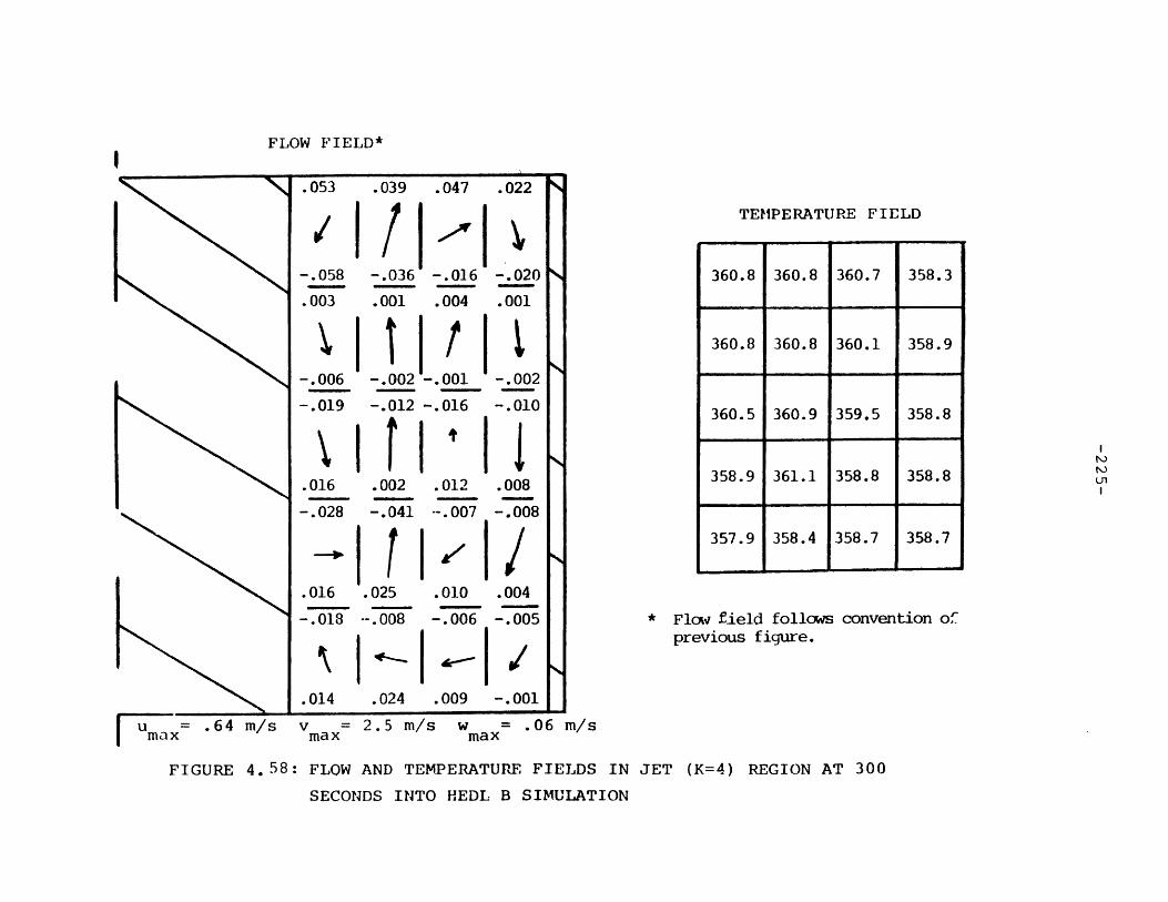
FLOW FIELD*

TEMPERATURE FIELD

-.018 --.008 -.006 -.0051 * Flow field follows convention of

previous figure.

.014 .024 .009 -.001

= .64 m/s v = 2.5 m/s w = .06 m/sIx max max

FIGURE 4.58: FLOW AND TEMPERATURE FIELDS IN JET (K=4) REGION AT 300

SECONDS INTO HEDL B SIMULATION

360.8 360.8 360.7 358.3

360.8 360.8 360.1 358.9

360.5 360.9 359.5 358.8

358.9 361.1 358.8 358.8

357.9 358.4 358.7 358.7

-226-

9.0

7.5 - 1 above jet

2 upper region average

3 lower region average

dP 6.00

z

o / 2

0.0> 3.0 __>4

0 60 120 180 210 30jet on

TIME (SECONDS)

FIGURE 4. 59: HYDROGEN VOLUME FRACTION PREDICTIONS VS

DATA DURING HEDL B EXPERIMENT

-227-

during the first 300 seconds of the injection. Three pairs

of curves are included. Type 1 curves are the volume frac-

tions at the upper elevation in the jet region. Curves 2

and 3 are azimuthally-averaged concentrations at the upper

and lower axial elevations. The agreement of the averaged

data is good. The code predicts a larger degree of homogeni-

zation but the axial stratification is still apparent.

The near-jet data are in the least agreement. At 300

seconds, the code results are nearly twice as large as the

measurements. In general, the hydrogen concentrations in

the near-jet region are 2-3 times larger than in other

azimuthal zones. Probable causes of this disagreement

in azimuthal homogenization are addressed below. The plots

of normalized maximum velocity components versus time

provided in Figure 4.60 is helpful in understanding this

simulation. The axial and radial velocities exhibit similar

behavior in that they reach a peak and then slowly decrease.

The azimuthal component reaches a peak and then decays,with

some oscillation, to more depressed levels. The azimuthal

convective mixing is decreasing in time.

After detailed data analysis of this simulation, three

effects are identified as contributors to the underprediction

of azimuthal mixing. These effects are not independent

and indeed may act synergistically. The coarse mesh,

especially in the azimu'hal direction, leads to inaccurate

specification of parameter profiles. This is especially

-228-

60 120 180 240 300

TIME (SECONDS)

FIGURE 4.60: BEHAVIOR OF NORMALIZED VELOCITY COMPONENTS

DURING HEDL B SIMULATION

1.2

1.0

0.8

0.6

b 0.4

0.2

0.0

-229-

important in the evaluation of second derivatives which

describe diffusional processes. Given the dimensions of

the problem, the radial second differences and the

azimuthal second differences can be estimated as follows.

radial second difference ~ 12 16 , and.25

azimuthal second difference ~ ~1 0.15(2 x 1.3)

Thus, the very coarse azimuthal resolution can depress the

importance of diffusional effects. The effect causes

inaccuracies in the diffusion of both hydrogen and momentum.

The momentum diffusion, driven by molecular and turbulent

viscosity, is an important mechanism for promoting the

development and sustenance of the azimuthal field. With

decreasing viscosity, the jet will become increasingly two-

dimensional. The second related cause is an inaccurate

specification of turbulence levels. The input levels cor-

-4 2 2responded to TKE levels of 10 m /s which is small com-

-2 -3pared to the estimated jet region levels of 10 - 10

m /s . This effect will also inhibit diffusional transport.

Finally, the blower model utilized while accurate in an

integral sense does not accurately describe the mixing and

momentum source of the recirculation flow. A more accurate

description of these typos of devices would enhance the

quality of their predicted local effect.

-230-

Despite these limitations, the overall simulation is

a success especially given the model and the discretiza-

tion used. The local thermodynamic state algorithm

behaved quite well showing excellent convergence even in

cells with over 50% water (by mass). The average hydrogen

concentration predictions showed general agreement with

the data and sources of inaccuracy are reasonably well

categorized.

A second simulation is reported which addresses a few

of the limitations noted above. A 96 node three dimen-

sional model is utilized as depicted in Figure 4.61. The

azimuthal nodalization is increased by 50% while the axial

mesh spacing is increased slightly. The input data are

similar to the first simulation except for refinement of

the source and blower conditions based on more detailed

experimental measurement data. This input refinement led

to a somewhat different timing sequence such that the

basic transient events are: blowers on (0 s), steam on

(15 s) and hydrogen on (100 s). Therefore the results of

this run cannot be compared with the preceding data in

regards to time. Figures 4.62 and 4.63 depict the velo-

city and temperature fields at 50 seconds in the non-jet

and jet regions, respectively. These fields are very

similar to the 80 node simulation in this time frame. The

higher temperature steam jet is seen to dominate the dyna-

mics in both the near-jet flow and thermal fields.

Figures 4.64 and 4.65 depict analogous predictions in the

4.72M

1. 52M

200

300

6R = 0.57M6Z = 1. 18M

60 = 500

BL = Blower Cell

B = JET B

FIGURE 4.61: 96 NODE MODEL OF HEDL FACILITY

3.48M

FLOW FIELD*

TEMPERATURE FIELD

Flow field follows convention of previous

HEDL figures.

FIGURE 4.62: FLOW AND TEMPERATURE FIELDS IN NON-JET REGION AT 50 SECONDS INTO 96 NODE

HEDL B SIMULATION

328.1 327.2 329.0 310.5

322.7 321.9 322.4 313.1

321.2 319.4 318.0 314.1

319.8 318.2 318.0 315.5

FLOW FIELD*

TEMPERATURE FIELD

Flow field follows

HEDL figures.

convention of previous

FIGURE 4.63: FLOW AND TEMPERATURE FIELDS IN JET REGION AT 50 SECONDS INTO 96 NODE

HEDL B SIMULATION

336.4 335.6 332.0 322.6

329.1 334.6 326.6 321.0

316.8 336.3 316.2 319.4.

317.7 313.9 313.1 315.8

FLOW FIELD*

TEMPERATURE FIELD

354.1 350.0 349.5 345.4

341.6 342.3 342.1 345.1

341.8 342.7 343.1 344.7

341.9 342.9 343.0 344.0

Flow field follows convention of previous

HEDL figures.

FIGURE 4.64: FLOW AND TEMPERATURE FIELDS IN NON-JET REGION AT 350 SECONDS INTO 96 NODE

HEDLB SIMULATION

Umax max max

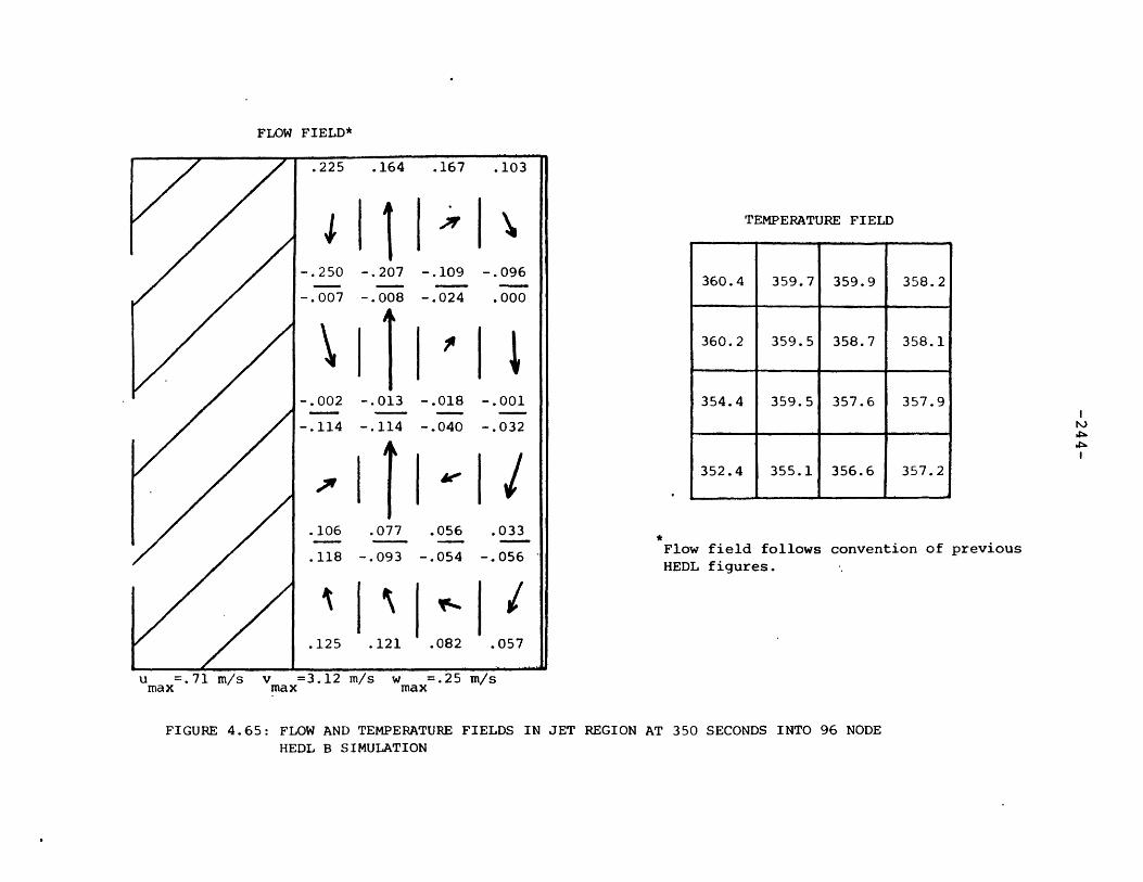
FLOW FIELD*

TEMPERATURE FIELD

Flow field follows convention of previous

HEDL figures.

FIGURE 4.65: FLOW AND TEMPERATURE FIELDS IN JET REGION AT 350 SECONDS INTO 96 NODE

HEDL B SIMULATION

360.4 359.7 359.9 358.2

360.2 359.5 358.7 358.1

354.4 359.5 357.6 357.9

352.4 355.1 356.6 357.2

max max

-245-

same regions at 350 seconds (end of simulation). In the

non-jet region, the shear caused by the jet leads to a

peaked axial velocity component away from the left side

boundary. This influence of the jet in planes away from

the source region is not observed in the coarser azimuthal

nodalization calculation. The jet region fields are qual-

itatively similar to previous results but show better jet

resolution and increased entrainment.

Figure 4.66 depicts the predicted and measured hydro-

gen volume fractions during the first 350 seconds of the

experiment. As compared to the 80 node simulation, this

result shows improved agreement with data especially in

the region average data. The code still underpredicts

azimuthal mixing but the disagreement has decreased by

roughly 50%. The two reasons identified for this improve-

ment are the decreased azimuthal node spacing and better

source definition. Nevertheless the remaining disagree-

ment reinforces the need for further increased nodaliza-

tion and an improved blower model. The transient behavior

of the three normalized velocity components shown in

Figure 4.67 indicates that the azimuthal component is

starting to behave more congruently with the axial and

radial velocities.

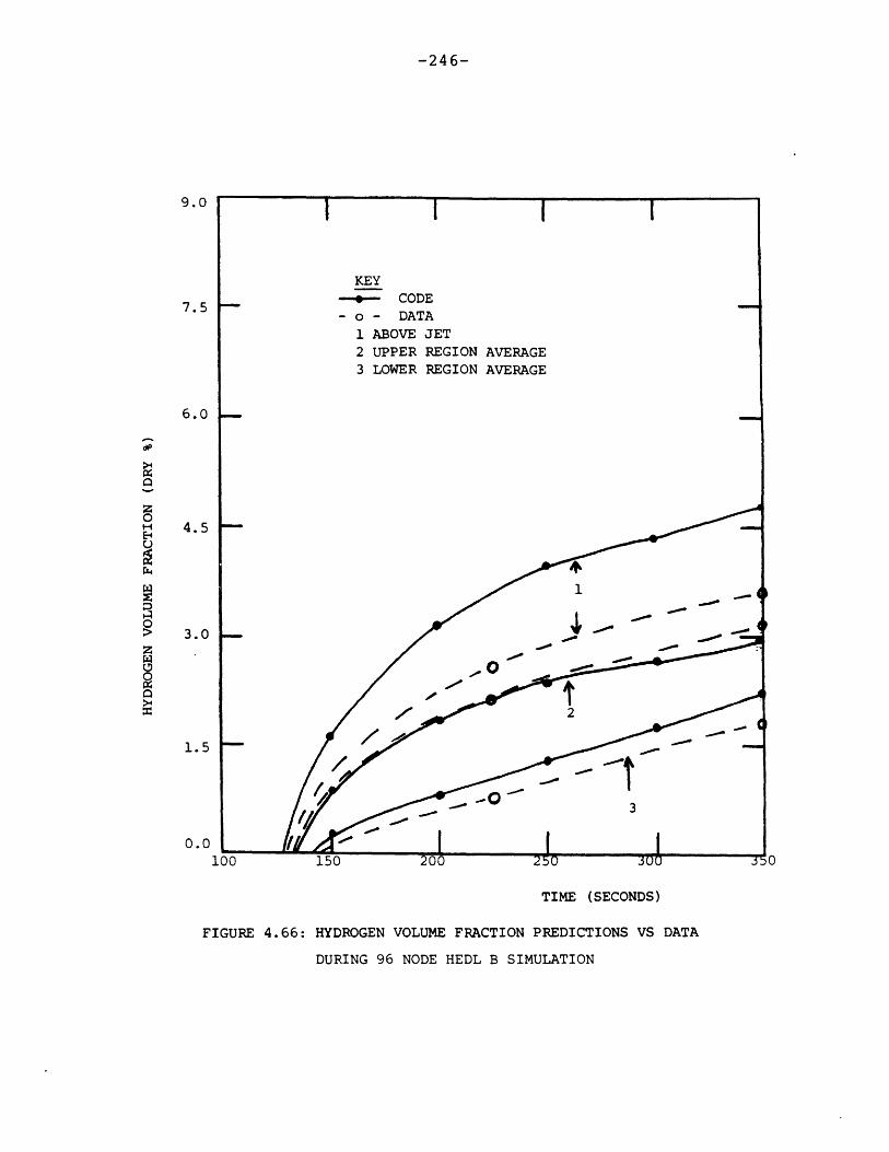
-246-

9.0

KEY

-*- CODE7.5 - o - DATA

1 ABOVE JET

2 UPPER REGION AVERAGE

3 LOWER REGION AVERAGE

6.0

dP

H 4.5

3.0 -z

S2

1.5 /

0.0 0100 150 20 0

TIME (SECONDS)

FIGURE 4.66: HYDROGEN VOLUME FRACTION PREDICTIONS VS DATA

DURING 96 NODE HEDL B SIMULATION

-247-

1.2

1.0 -

w0.8

H

0.2

0 70 140 210 280 350

TIME (SECONDS)

FIGURE 4.67: BEHAVIOR OF NORMALIZED VELOCITY COMPONENTS

DURING 96 NODE HEDL B SIMULATION

-248-

4.4 Lumped Parameter Model Results

The development of the lumped parameter capability is

not a central part of this work and is based on well-known

methods. As such, the model is used in a few sample calcu-

lations to demonstrate that it has been implemented cor-

rectly. The results reported here are ascertained using the

full nodal model. Experience with the original BEACON

lumped/continuum calculations has shown that such coupled

simulations are susceptible to time step instabilities if

the bounding lumped regions' global state changes quickly.

Also, using the continuum options to model internodal flow

paths as is required by the original formulation is compu-

tationally inefficient and sometimes physically inappro-

priate.

The first simulation is a simple three region problem

in which air is injected into one compartment. Each volume

is 1 m , connected in tandem fashion (1i-2-+3) and at an

initial state of 289.150K and atmospheric pressure. Air of

the same temperature is injected into room 1 at a rate ofi-3

103 kg/sec. The code's predictions for the average compart-

mental state is compared to the exact solution in Table 4.10.

Excellent agreement is noted.

The second problem is a six region multiconnected

geometry as defined in Figure 4.68. The room sizes and

flowpath characteristics resemble the BF facility. Hydrogen

and air are introduced in the lower central compartment at

FIGURE 4.68 : PROBLEM GEOMETRY AND CONNECTION LOGIC FOR

SIX ROOM LUMPED PARAMETER PROBLEM

ROOM 5

40.4 M3

ROOM 2

30.2 M3

ROOM 3

41.1 M3

ROOM 6

38.3 M

ROOM 1

40.5 M

ROOM 4

38.9 M3

-250-

Table 4.10

Comparison of Code Predictions to Exact Results for Three

Region Air Injection Problem at 20 Seconds

Parameter Exact Code

Pressure (N/m2) 102128 102128

Temperature (OK) 289.788 289,787

Density (kg/m3 ) 1.22787 1.22788

rates of 5.0 x 10 - 6 and 3.7 10 - 5 kg/sec, respectively.

A 10000 second simulation is reported which utilized a con-

stant time step of 5 seconds. The computed hydrogen volume

fraction transients are depicted in Figure 4.69.

This multiroom simulation is similar to the BFl2

test except for the disconnection of regions 1 and 2.

The BFl2 data indicated more homogeneous hydrogen profiles.

This is due to the connection between rooms 1 and 2.

Attempts at simulating this configuration with its potential

for recirculating flow paths produced results very sensitive

to junction characteristic input. This highlights the

inherent weakness of nodal methods in that the inexact speci-

fication of junction loss coefficients and inertias signi-

ficantly affect predictions. Automatic time step control

is also required if flow rates become large enough to cause

instabilities. Second, the vertical streaming of a more

buoyant gas such as hydrogen through a relatively stagnant

-251-

100

10-2 ROOMS 4 & 6

z010-4

U

rROOMS 3 & 5

S-6

o 10

zw

00

10-8 ROOM 2

10-10

0 2000 4000 6000 8000 10000

TIME (SECONDS)

FIGURE 4.69: ROOM HYDROGEN CONCENTRATION TRANSIENTS

FOP LUMPED PARAMETER PROBLEM

-252-

region without good mixing into an upper vertically con-

nected region cannot be predicted by nodal methods such

as that utilized here. The inaccuracy arises from the

well-mixed assumption implicit in the nodal formulation.

Overall, the reported results demonstrate the useful-

ness of this added capability. Its present limitations

include the inability to treat vertical streaming, the need

for a versatile time step control logic and better defini-

tion criteria for junction characteristics.

4.5 Discussion of Results

The results reported are a representative sample of

calculations which demonstrate the capabilities and limita-

tions of the analytical models described herein as they are

embodied in a computer code named LIMIT. In general, a

versatile computational tool with a wide range of applica-

bility is demonstrated. Before addressing the performance

of the three major modelling options, a general observation

is made. Over the course of this developmental effort, no

clearly advantageous choice between implementing a fully

general model applicable to lumped and continuum analyses of

varying time scales or using the phenomenon-specific approach

presented here became apparent. The former approach is

designed to accommodate all significant phenomena no matter

which dominate in a particular situation. This minimizes

the chances of neglecting important effects. However this

route pays the price of greater complexity, less computational

-253-

efficiency and certain inaccuracies due to the unavoidable

extension of ancillary models. The approach used in this

work is more efficient, less complex and has the potential

for greater problem specific accuracy. Nevertheless, the

analyst is required to have a good a prior understanding of

the problem to make a proper choice. Further, certain

physical situations are not clearly placed within the

validity bounds of any one modelling option. The HEDL

problem is a good example of such a situation.

The modified BEACON equation set or rapid blowdown

transient model is shown to be applicable to physical situa-

tions dominated by two-phase effects. Predictions of

transients of this nature are both reasonable and well-

behaved. The current version of this model has inherited

the original BEACON code sensitivity to very high or low

(nearly single phase) flows. The coupled phasial equations

and especially the interphasial exchange models are most

suspect. The model also consumes large amounts of compu-

tational resources (see 4.7).

The continuum slow mixing model is the most useful for

many pertinent analyses. The Battelle Frankfurt based

simulations demonstrate that it is most accurate in situa-

tions where local states are true perturbations of a

reference state and compressibility effects are small.

Some unique features of +he model formulation which help

relax the usual incompressible assumption constraints are a

-254-

conservative formulation of certain transport equations,

a thermodynamic model which can treat a condensible component

and periodic reference state update. The two major limita-

tions of the model are the Courant time step and numerical

diffusion. Both constraints require the use of a fine

mesh and a commensurate amount of computation time. The

simulation of the BF6 test demonstrates the importance of

these considerations. Nevertheless, the model can be con-

fidently utilized in this type of simulation if the computing

resources are expended. The HEDL based problems test the

validity bounds of the slow mixing model and invoke most of

the new ancillary models. Given the coarse mesh and basic

incompressible formulation, the results compare well with

data at least qualitatively. Most significant is the demon-

strated ability of the thermodynamic model to treat problems

in which water occupies a significant mass fraction (~50%).

The HEDL simulation also demonstrates the full 3-D cylindri-

cal spatial definition of the model. Numerical diffusion

remains a source of inaccuracy in these simulations as is

evidenced by the predicted hydrogen concentration axial

gradients being less sever than the measured data.

The lumped parameter model, especially in its com-

pletely nodal (no continuum regions) formulation, allows

numerous economical scoping calculations. The results of

such sensitivity or global state computations are useful to

either define the scenarios worthy of more detailed continuum

-255-

analysis or provide a means of testing modelling hypotheses.

The problems reported show that the LIMIT lumped model is

properly formulated and produces physically reasonable

results. Of course, the well-mixed nodal assumption does

limit the applicability range of the model. For example,

such phenomena as vertical streaming of buoyant hydrogen

through a compartment without radial mixing cannot be

predicted.

4.6 Model Capabilities vs Other Approaches

Of the analytical tools currently being applied to

hydrogen transport analysis, six methods in addition to this

work are worthy of additional comment. Specifically these

are: KWU lumped parameter analysis, the RALOC program as

utilized by German researchers [54] and at Sandia National

Laboratory [56], the MAPHY code [57] developed in Japan,

TEMPEST [63] utilized at Battelle Northwest Laboratory

(BNWL), HMS [65] developed at Los Alamos National Laboratory,

COBRA-NC [67] employed at BNWL and the LIMIT code. The major

analytical features of these methods are summarized in Table

4.11.

On the basis of a limited survey, the following com-

parative critique is presented. The KWU method is a manual

calculation informally reported in a BF experimental progress

report. As is expected, it is of limited use but does pro-

vide quick order of magnitude assessment. The RALOC and

Table 4.11

Representative Hydrogen Transport Models

Model

Feature KWU RALOC MAPHY TEMPEST HMS COBRA-NC LIMIT(Hand (GRS or (Japan) (BNWL) (LANL) (BNWL) (MIT)

Calculated) Sandia)

Continuum X X X X

Lumped Parameter X X X X X X

Two-Phase Effects X X X X X

Blowdown X X X

Turbulence Model 2 Equat. Eddy 2 Equat.k-E Viscosity k-E

Multi-Compartments X X X X

Fan Coolers/Sprays X X X X

Chemical Reactions No ? ? No ? ? ?

-257-

MAPHY codes are quite similar. Both are based on nodal

lumped parameter formulations and offer limited spatial

definition capability. They are both good nodal tools but

have difficulty handling problems involving many regions due

to the stiff coupling of the governing differential equa-

tions. TEMPEST is a single region (but multi-material)

continuum code based on a strict incompressible flow

formulation. Its predictive ability of slow single phase

problems is noteworthy but a rather fine mesh discretization

is required. The lack of a multicompartment capability

as well as the omission of a condensible field limits its

usefulness in analyzing more complex transients involving

realizstic geometries and steam injection.

HMS, COBRA-NC and the MIT method are the most versatile

and appropriate tools. The HMS program has been successfully

applied to the solution of benchmark problems. The lack of

a lumped parameter option, detailed turbulence model and

multicompartment option are significant limitations but

overall the HMS code embodies a worthwhile approach.

COBRA-NC is more versatile and has been used to accurately

reproduce selected empirical results. The continuum model

based on a two-fluid two phase model is very accurate but

seems inappropriately complex for the economical analysis

of longer quasi-homogeneous transients. However, the single

model formulation avoids che model choice inherent in the

MIT code. The COBRA turbulence model may not be adequate

-258-

for analyzing transients dominated by turbulent diffusive

transport.

The capabilities of the current work's method in the

areas of problem versatility, computational efficiency,

reduction of numerical diffusion and proper heat/mass

transfer modelling are unique. Two negative aspects of

this work are the need to enhance the transition between

applicable continuum models and greater validation. Never-

theless, the current version of the MIT program compares

quite favorably with other alternatives. Finally, while the

analysis of post-chemical reaction flow is not of central

interest to this work (see Appendix C for preliminary discus-

sion), the direct extension of any of these methods to this

more complex regime is questionable.

4.7 Computational Effort Analysis

An important goal of this research is to produce an

analysis tool which is relatively economical to employ.

A major disadvantage of most other tools used in hydrogen

transport modelling is that utilization in a production mode

operation in which budgetary and computing facility limita-

tions are present is not achievable if useful predictions are

required. The LIMIT code is a good first step in achieving

cost efficient yet accurate simulation. Table 4.12 illu-

strates the computational effort required for the simulations

reported earlier. The cost and running time figures

Table 4.12

Representative Computational Costs

Type Problem Number CPU Time CPU Time/ ApproximateDuration of Cells (s) Duration-Cell Cost2

(s) ($)

FAST 0.2 100 651 32.55 60.

SLOW-BF 8000.0 32 5033 0.020 360.

SLOW-HEDL 200.0 80 3332 0.208 225.

LUMPED 10000.0 6 56 0.00093 11

Notes: 1. Fluid Cells

2. Based on 0.7 SBU/CPUs, weekend priority, includes printing andtapes costs on a CDC CYBER-176.

-260-

presented are approximate values utilizing a CYBER-176

computer on a commercial basis. The rapid transient model

is clearly the most resource consuming as is expected.

The cost efficiency of the slower mixing model is noted.

The HEDL jet type analysis is seen to be an order of mag-

nitude greater than BF type transients and the economy of

the lumped model is clearly demonstrated.

More detailed analysis of the slower mixing model

behavior indicates the following qualitative observations.

If Courant numbers are limited to 0.5, the number of pres-

sure iterations required to attain a divergence free flow

field is 10-20. Approximately 15 pressure iterations require

the same amount of computation as the remaining non-iterative

calculations. That is, if a computational cycle involved

30 iterations and used 9 seconds of computing time, 3

seconds are spent solving the passive transport equations

and the tilde phase of the momentum equation solution while

6 seconds are used in the flow field selective over-relaxa-

tion iteration. Finally, the total transient computing time

using the slower mixing model is proportional to the number

of fluid cells raised to the approximately 1.25 power.

For example, if an 80 node HEDL computation requires 1000

seconds, a 100 node simulation of the same problem would

utilize roughly 1300 seconds of CPU time.

-261-

5.0 Conclusions and Recommendations

5.1 Conclusions

The analytical models and the computer program which

embodies them described in this work are shown to fulfill

the need to accurately model hydrogen gas transport in

nuclear reactor containment buildings. Though hydrogen

safety is the central focus of the research, the tool

itself is potentially applicable to a much broader range

of analyses. The validation and demonstration calculations

presented in Chapter 4 illustrate the code's capabilities

and limitations.

The general conclusion drawn from this work is that

a versatile basic tool has been produced. Some more specific

concluding observations are now presented and suggestions

for future work are contained in the following section.

The use of two different continuum models depending

upon the dominant physical phenomena is shown to be an

effective way to achieve economical yet useful results.

This flexibility allows the analyst to match the tool to

the problem's requirements. Two weaknesses of this approach

must be remembered. First, the analyst must make a choice

based on engineering judgment. Second, certain applications

may straddle the boundary of the two models' applicability.

The modified two-fluid BFXCON equation set is not recommended

for longer transients or physical situations which are

single-phase in nature.

-262-

The lumped parameter modelling capability (especially

the pure nodal model) provides a very useful option. The

principal applications of this model are situations where

spatial resolution is less important than global state

changes. The demonstration problems show not only its

efficiency but also its limitations. Modelling flow junction

characteristics (loss coefficients, inertias, etc.) always

involves approximation. Also, the well-mixed volume assump-

tion cannot account for preferential component transport

such as hydrogen or steam streaming induced by local

buoyancy or jet effects.

The slow mixing model is shown to be an adequate

physical representation of most problems of interest. The

incompressible flow field assumption allows for economical

numerical solution due to the decoupling of the conservation

equations. A certain degree of compressibility is introduced

however in the formulation of the buoyancy forces and the

energy conservation equations. Nevertheless, experience has

shown that application of this method to truly compressible

problems leads to significant mispredictions.

Numerical diffusion especially due to the donor cell

treatment of convective terms has been shown to be a very

important consideration. The use of coarse mesh spacing

in the interest of economy aggravates the false diffusion

problem. The failure to properly predict the breakdown

of atmospheric inversions is a problem caused by this effect.

-263-

A partial improvement in this regard is the use of a

numerical diffusivity correction and the utilization of

optimized problem meshes. However, a complete solution

to this problem save for the brute force approach of very

fine mesh spacing and small time steps is not achieved.

The local thermodynamic state determination model

and calculational logic has proved to be quite successful.

The specific successive substitution algorithm is stable

and converges to a desirable accuracy quickly. Its applica-

tion to other situations of similar characteristics such as

moist plumes is strongly suggested.

The validation and demonstration simulations reported

provide a good degree of confidence in the code's ability

to predict real physical situations. The Battelle Frankfurt

simulations tested the physical regime of single-phase,

pure plume behavior. The simulation of tests in which a

neutrally stratified pre-test atmosphere existed is accu-

rate even when coarse mesh spacing is utilized. The mixing

in thermally stratified fields is not accurately predicted

(first simulation of BF6) if coarse mesh spacing is used and

numerical diffusion is not corrected.

The application of the slow mixing model to the HEDL

experiments tests the validity boundary of the model.

Modelling a high velocity steam/gas jet as a distributed

momentum source is a useful approximation. Its major

limitation is that a detailed knowledge of the near-jet

flow field is compromised. A recirculation blower model is

-264-

described which adequately represented the test facility

ventilation system. Nevertheless, a more versatile fan

cooler is desirable. The thermodynamic state model performed

reasonably well except for some predictions near the steam

jet. Finally, the overall prediction of hydrogen concentra-

tions is seen to be acceptable considering the relatively

coarse discretization. However, application of the method

in its present form to problems exhibiting stronger com-

pressibility and phase change effects should be done with

proper caution.

The overall code characteristics and its computational

efficiency compare quite well with other methods. Simula-

tions of significant problems can be accomplished at

reasonable cost. The major limitation of both the rapid and

slow mixing models is the Courant time step stability

restriction. This is especially so in longer slowly varying

transients.

5.2 Recommendations For Future Work

This work represents the first major step in an ongoing

research project and as expected further effort is desirable.

The areas of proper diffusion modelling is being addressed

in a related effort and some of the benefits of that work

are incorporated into the current program. The area of

ancillary effects modelling such as heat transfer, surface

mass transfer, containment sprays and fan cooler models are

-265-

also under development. Four additional topics are recom-

mended for future consideration.

First, model improvement in a number of specific

instances is recommended. The need and possible methods

of extending the so-called slow mixing model to problems

exhibiting more significant compressibility is advisable.

If the need is demonstrated the main options are either

modification of the existing solution method or implementa-

tion of a new scheme. The former choice is the more

straightforward while the latter has greater potential for

achieving significant improvement. The relaxation of the

time step limitations as well as the potential for fully

correcting false diffusion both suggest the investigation of

implicit methods. Appendix D is provided as a starting

point for such an investigation. The general area of code

streamlining and optimization are worthy of additional effort.

A potential running time reduction of roughly 20% could

probably be accrued from a careful reprogramming program.

The second area of suggested future work is additional

model validation. The current effort is limited to a few

selected simulations. Comparison predictions with the more

complex (and expensive to run) BF and HEDL experiments would

afford greater confidence in the method and also illuminate

problem areas requiring improvement. An important aspect of

this work is to accompli-h it in a more economical situation

than the commercial computer time rates imposed on the pres-

ent development.

-266-

The application of the model to actual containment

design and licensing problems is the third recommended

topic. The purpose of the code is for it to be employed

in real world applications and a systematic performance of

such analyses is of definite benefit.

Finally, the methods developed and implemented can

be extended to other analysis areas. A few suggested areas

are containment fission product transport, general post-

accident containment response and analysis of non-nuclear

combustible gas problems. The general area of modelling

reacting flows is addressed in Appendix C. The potential

for extension to these areas is conceptual at this time and

can only be accurately assessed by a systematic study.

-267-

6.0 References

-268-

1. R.W. Bergstrom and W.A. Chittenden, "Reactor-Contain-ment Engineering: Our Experience To Date," Nucleonics17, pp. 86-93, April 1959.

2. G.W. Keilholtz, "Annotated Bibliography of HydrogenConsiderations in Light-Water Power Reactors," ORNL-NSIC-120, February 1976.

3. L. Baker, Jr. and L.C. Just, "Studies of Metal-WaterReactions at High Temperatures III-Experimental andTheoretical Studies of the Zirconium-Water Reaction,"ANL-6548, December 1964.

4. L. Baker, Jr. and R.D. Ivins, "Analyzing the Effectsof a Zirconium-Water Reaction," Nucleonics 23, pp.70-74, July 1965.

5. J.M. Genco and G.E. Raines, "Metal Water ReactionsDuring a Loss-of-Coulant-Accident--The Zirconium-SteamReaction," ANS Transactions 9, pp. 555-556, October1966.

6. M.J. Bell et al., "Post-LOCA Hydrogen Generation inPWR Containments," ANS Transactions 13, pp. 203-204,June 1970.

7. H.E. Zittel, "Radiolytic Hydrogen Generation AfterLoss-of-Coolant Accidents in Water Cooled Power Reac-tors," Nuclear Safety 13, pp. 459-467, November 1972.

8. W.D. Fletcher et al., "Post-LOCA Hydrogen Generationin PWR Containments," Nuclear Technology 10, pp.420-427, April 1971.

9. J.R. Lopata, "Control of Containment H2 Levels Evolvedfrom Zinc Primers during a LOCA," Power Engineering 78,pp. 48-51, November 1974.

10. J.O. Henrie and A.K. Postma, "Analysis of the ThreeMile Island (TMI-2) Hydrogen Burn," Proceedings ofthe Second International Meeting on Nuclear ThermalHydraulics, pp. 1157-1170, January 1983.

11. G. Langer et al., "Experimental Investigation of Hydro-gen Distribution in a Containment of a Light Water Reac-tor Following a Coolant Loss Accident," BF-63.363-3,Battelle Institute e.V. Frankfurt, translated October1980.

-269-

12. "Experimental Investigation of the Hydrogen Distribu-tion in a Model Containment (Preliminary ExperimentsPhase II)," BF-R-64.036-1, Federal Ministry forResearch and Technology, Bonn, July 1980.

13. G.R. Bloom et al., "Hydrogen Distribution In a Con-tainment With a High-Velocity Hydrogen-Steam Source,"HEDL-SA-2682, October 1982.

14. G.R. Bloom and S.W. Claybrook, "Standard Problems OnHydrogen Mixing and Distribution," Westinghouse HanfordCompany, March 1982.

15. R. Zinnari and C. Nahum, "Research Activities on theHydrogen Behavior Inside BWR Containment after LOCADeveloped Under the CNEM-AMN Agreement," SandiaHydrogen Workshop, January 1981.

16. M.P. Sherman et al., "The Behavior of Hydrogen DuringAccidents in Light Water Reactors," NUREG/CR-1561,SAND 80-1495, 1980.

17. M. Hertzberg and K.L. Cashdollar, "FlammabilityBehavior and Pressure Development of Hydrogen Mix-tures in Containment Volumes," Proceedings of theSecond International Meeting on Nuclear Thermal-hydraulics, pp. 29-37, January 1983.

18. J.C. Cummings et al., "Hydrogen Combustion ResultsFrom the Sandia Intermediate Scale (VGES) Tank andthe Sandia Critical-Tube-Diameter Test Facility,"Proceedings of the Second International Meeting onNuclear Thermalhydraulics, pp. 1212-1218, January1983.

19. R. Jaung et al., "Detonability of Containment BuildingAtmospheres During Core-Meltdown Accidents," Proceedingsof the Second International Meeting on Nuclear Thermal-hydraulics, pp. 1171-1177, January 1983.

20. R.K. Kumar et al., "Combustion of Hydrogen at HighConcentrations Including the Effect of Obstacles,"Proceedings of the Second International Meeting onNuclear Thermalhydraulics, pp. 1203-1211, January1983.

21. Code of Federal Regulations, Title 10, Part 50.

22. W.R. Butler et al., "Regulatory Perspective On HydrogenControl For LWR Plants," Sandia Hydrogen Workshop,January 1981.

-270-

23. C.J. Boyd et al, "A Probabilistic Risk AssessmentPerspective of the Impact of Hydrogen on PWR Safety,"Sandia Hydrogen Workshop, January 1981.

25. L. Thompson, "Hydrogen Combustion and Control," EPRIJournal, pp. 56-58, May 1982.

26. R.D. Richtmeyer and K.W. Morton, Difference Methodsfor Initial Value Problems, Second Edition, Wiley,New York, 1967.

27. P.J. Roache, Computational Fluid Dynamics, Hermosa,Albuquerque, 1976.

28. C.W. Hirt, "Heuristic Stability Theory for Finite-Difference Equations," J. Comp. Physics, 2, 1968.

29. S.V. Patankar, Numerical Heat Transfer and Fluid Flow,Hemisphere, New York, 1980.

30. V.H. Ransom and J.A. Trapp, "Applied MathematicalModels in Nuclear Thermal Hydraulics," Proceedingsof the Second International Meeting on Nuclear Thermal-hydraulics, pp. 99-110, January 1983.

31. E. Isaacson and H.B. Keller, Analysis of NumericalMethods, Wiley, New York, 1966.

32. F.H. Harlow and A.A. Amsden, "Multifluid Flow Calcula-tions at All Mach Numbers," J. Comp. Physics 16,pp. 1-19, 1974.

33. W.C. Rivard and M.D. Torrey, "K-FIX: A Computer Pro-gram for Transient Two-Dimensional, Two-Fluid Flow,"LA-NUREG-6623, April 1977.

34. M. Ishii, Thermo-Fluid Dynamic Theory of Two-Phase Flow,Collection de la Direction des Etudes et Recherchesd'Electricite de France, 1975.

35. A.A. Amsden and F.H. Harlow, "The SMAC Method: ANumerical Technique for Calculating IncompressibleFluid Flows," LA-4370, May 1970.

36. J. Douglas and J.E. Gunn, "A General Formulation ofAlternating Direction Methods," Num. Math 6, pp. 428-453, 1964.

37. W.R. Briley and H. McDonald, "Solution of the Multi-dimensional Compressible Navier Stokes Equations by aGeneralized Implicit Method," J. Comp. Physics 24,372-397, 1977.

-271-

38. W.R. Briley and H. McDonald, "On the Structure and Useof Linearized Block Implicit Schemes," J. Comp. Physics34, pp. 54-73, 1980.

39. K.Y. Huh, Treatment of Physical and Numerical Diffusionin Fluid Dynamic Simulations, Ph.D. Thesis, Departmentof Nuclear Engineering, MIT, August, 1983.

40. K.V. Roberts and N.O. Weiss, "Convective DifferenceSchemes," Math of Comp. 20, No. 94, pp. 271-99, 1966.

41. J.E. Fromm, "Practical Investigation of ConvectiveDifference Approximations of Reduced Dispersion,"High Speed Computing in Fluid Dynamics, The Physicsof Fluids, Supplement 2, ed. F.N. Frenkiel andK. Stewartson, 1969.

42. G.D. Raithby, "A Critical Evaluation of UpstreamDifferencing Applied to Problems Involving FluidFlow," Comp. Methods in Appl. Mech. and Eng. 9,pp. 75-103, 1976.

43. G.D. Raithby, "Skew Upstream Differencing Scheme forProblems Involving Fluid Flow," Comp. Methods inAppl. Mech. and Eng. 9, pp. 153-164, 1976.

44. S.H. Chang, Comparative Analysis of Numerical Methodsfor the Solution of Navier-Stokes Equations, Ph.D.thesis, M.I.T. Department of Nuclear Engineering,May 1981.

45. J. Weisman and A. Tentner, "Application of the Methodof Characteristics to Solution of Nuclear EngineeringProblems," Nucl. Science and Eng. 78, pp. 1-29, 1981.

46. J.K. Dukowicz and J.D. Ramshaw, "Tensor ViscosityMethod for Convection in Numerical Fluid Dynamics,"J. Comp. Physics 32, pp. 71-79, 1979.

47. B.E. Launder and D.B. Spalding, Mathematical Models ofTurbulence, Academic Press, London, 1972.

48. J.L. Lumley, "Second Order Modelling of TurbulentFlows," from Prediction Methods for Turbulent Flows,W. Kollman, ed., Hemisphere, New York, 1980.

49. W. Rodi, "Turbulence Models for Environmental Problems,"from Prediction Methods for Turbulent Flows, W. Kollman,ed., Hemisphere, New York, 1980.

-272-

50. T.A. Porsching et al., "Stable Numerical Integration ofConservation Equations for Hydraulic-Networks," Nuck.Science and Eng. 43, pp. 218-225, 1971.

51. D.W. Hargroves et al., CONTEMPT-LT/028--A ComputerProgram for Predicting Containment Pressure-TemperatureResponse to a Loss-of-Coolant Accident, NUREG/CR-0252, TREE-1279, August 1978.

52. L.J. Metcalfe et al., CONTEMPT4/MOD4--A MulticompartmentContainment System Analysis Program, TREE-NUREG-1202,February 1978.

53. H.L. Jahn, "RALOC--A New Model for the Calculation ofLocal Hydrogen Concentrations in Subdivided Contain-ments Under LOCA Aspects," Thermal Reactor SafetyTopical Meeting, Idaho 1977.

54. H.L. Jahn, "Hydrogen Distribution in SubcompartedContainments: Analysis and Experiments," Water ReactorSafety International Meeting, 1980.

55. L.D. Buxton et al., "Transport of Gases in LWR Contain-ments," presented November 1981 at Sandia NationalLaboratories.

56. L.D. Buxton, "Assessment of RALOC-Mod 1 With 1980Updates," SAND 82-2005C, October 1982.

57. T. Fujimoto et al., "Development of Mixing AnalysisComputer Code on Behavior of Hydrogen in Subcompart-mented Containment Vessel After LOCA," Sandia HydrogenWorkshop, October 1982.

58. M. Fischer et al., "The Multi-Compartment-Code WAVCO,Developed to Analyze the Behavior of Non-CondensablesDuring Hypothetical Accidents," Proceedings of theSecond International Meeting on Nuclear Thermal-hydraulics, pp. 1058-1063, January 1983.

59. A.L. Camp et al., "HECTR: A Computer Program forModelling the Response to Hydrogen Burns in Contain-ments," SAND 82-1964C, 1982.

60. G.J.E. Willcutt, Jr. and R.G. Gido, "Mixing of Radio-lytic Hydrogen Generated Within a Compartment Followinga LOCA," NUREG/CR-0304, LA-7421-MS, August 1978.

61. G.J.E. Willcutt, Jr. et al., "Hydrogen Mixing in aClosed Containment Compartment Based on a One-Dimen-sional Model with Convective Effects," NUREG/CR-1575,LA-8429MS, September 1980.

-273-

62. C.R. Broadus et al., BEACON/Mod 3: A Computer Programfor Thermal Hydraulic Analysis of Nuclear ReactorContainments--Users Manual, NUREG/CR-1148, April 1980.

63. D.S. Trent, "Computation of Hydrogen DistributionUsing the Tempest Code," BNWL Report at EPRI H2Workshop, October 1981.

64. D.S. Trent and L.L. Eyler, "Application of the TEMPESTComputer Code for Simulating Hydrogen Distribution inModel Containment Structures," Sandia Hydrogen Work-shop, October 1982.

65. J.R. Travis et al., "Modelling of H Migration InLWR Containments," LA-UR-81-3171, O tober 1981.

66. J.R. Travis, "HMS: A Model for Hydrogen MigrationStudies In LWR Containments," LA-UR-82-2702, October1982.

67. M.J. Thurgood, "Application of COBRA-NC to HydrogenTransport," Sandia Hydrogen Workshop, October 1982.

68. C.T. Crowe et al., "The Particle-Source-In Cell (PSI-Cell) Model for Gas Droplet Flows," Journal of FluidsEngineering, ASME Transactions 99, pp. 325-332, June,1977.

69. F.H. Harlow and A.A. Amsden, "Numerical Calculation ofMultiphase Fluid Flow," J. Comp. Physics 17, 1974.

70. Handbook of Tables for Applied Engineering Science,R.E. Bolz and G.L. Tuve, ed., Chemical Rubber Company,1970.

71. M. Corradini, "Turbulent Condensation On A Cold WallIn The Presence Of A Noncondensible Gas," Proceedingsof the Second International Meeting on Nuclear Thermal-hydraulics, pp. 1102-1110, January 1983.

72. B. Covelli et al., "Simulation of Containment CoolingWith Outside Spray After a Core Meltdown," NuclearEng. and Design 69, pp. 127-137, 1982.

73. R.B. Bird et al., Transport Phenomena, Wiley, NewYork, 1960.

74. 0. Hinze, Turbulence, Second Edition, McGraw-Hill,New York, 1980.

-274-

75. C.R. Wilke, "Diffusional Properties of MulticomponentGases," Chemical Eng. Progress 46(2), pp. 95-106,February 1950.

76. G.D. Stubley et al., "Simulation of Convection andDiffusion Processes by Standard Finite DifferenceSchemes and by Influence Schemes," Comp. Math. Appl.Mech. and Engr. 35, pp. 153-168, 1982.

77. R.G. Gido et al., "COMPARE and BEACON vs. Battelle-Frankfurt Tests," LA-MS-9461, 1982.

-275-

APPEJNDIX A

COMPUTER APPLICATION TOPICS

A.1 General Principles

The development of analytical models is only

part of the process of creating useful computational

tools. The correct and efficient implementation of

these models in computer programs is as important.

The purpose of this appendix is to review the methods

utilized in this work in order to document the

process and also provide guidance to future workers.

This discussion is not meant to present a compendium

of detailed coding changes. Acquisition,

installation and modification involve substantial

time and effort especially if the work involves the

use of software not directly compatible with the

available computer systems. Some insight into this

process is provided in the next section.

The inclusion of the model changes derived in

the main body of this work necessitated extensive

modification of the code. A review of the

modifications from a programming standpoint is

presented in A.3. A unique feature of executing

larger programs on CDC equipment is the concept of

segmented loading. Basically, this feature allows

efficient computer co-e memory utilization through

the active storage of only those software modules

-276-

which are required for execution at a particular

time. The specific loading logic for the revised

program is specified in A.4. After a code is

developed, most of its use is in a production

execution mode. Therefore various production mode

options are addressed in section A.5.

Finally, future work may require the application

of the code on a non-CDC system. The overall

experience accrued in this work leads to a cautionary

note that such a change involves a significant amount

of time, effort and detailed knowledge of both CDC

and the new host system both from a hardware and

software viewpoint. Nevertheless the final section

of this appendix points out some of the more

important areas in this regard.

A.2 Acquisition, Installation and Modification

The BEACON code was chosen as the foundation for

this work for the technical reasons presented in the

main body of this work. Another positive aspect is

that it was available at relatively little expense on

a timely basis from the National Energy Software

Center (NESC). From a computer applications

standpoint, the code's most negative feature is its

incompatibility with non-Control Date Corporation

-27 '-

(CDC) systems. The code was developed at the Idaho

National Engineering Laboratory (INEL) using a

CDC-7600 computer with software specification

compatible with either SCOPE 2.1 or NOS/BE operating

systems. Specifically, the code takes advantage of

the overlay segmented loading particular to CDC,

utilizes the CDC UPDATE utility in its source file

management, and employs variable large and small core

memory (LCM and SCM) allocation. Finally many

input/output (I/O) and data management tasks are

accomplished using the CDC-version of the INEL

Environmental Subroutine Library.

MIT has no formal access to CDC machines and

hence alternative computational plans are necessary.

The two major options are to transform the code to an

IBM (MIT)-compatible version or use CDC machines on a

commercial basis. The former option is very costly

in terms of time, effort and money and the latter

alternative is pursued in this work. The available

commercial CDC equipment is a CYBER-176 machine with

a NOS operating system. A review of tne CDC

commercial charge schedule reveals that while most

costs are comparable, disk storage space is much more

expensive for the CDC system. Therefore after the

code was received at vIT, many changes were made

using IBM systems. Of course the code could only be

-278-

modified but not tested. Subsequent compilation,

debugging, modification and execution is done on the

CDC system. Figure A.1 provides an overview of this

process.

The direct installation of the code onto the

CYBER-176 is also not a straightforward procedure.

The NOS system is not completely equivalent to the

SCOPE 2.1 or NOS/BE systems. Hence a substantial

amount of machine-specific software study and

modification is required. As part of this effort the

job control language, program compilation, program

loading and execution software is revised. One major

set of changes relate to the environmental library.

Many of these routines are not called by BEACON 4nd

some are written in a non-compatible form.

Therefore, this library is edited such that only

those routines called by the code are saved. It is

also necessary to delete certain output data plotting

options. The environmental library routines compiled

and used by the code are listed in Table A.1.

Finally, all use of quotation marks (") must be

eliminated from routine CVI since it is not

compatible with NOS-based COMPASS (CDC assembly

language).

The FTN/176 Extended Fortran 4 compiler is needed

to compile and execute the program. Other compilers

such as FTN are not applicable. Further the compiler

IBM PRINTER

MIT

I - OUTPUT

IBM - 370

MIT

4-

CDC PRINTER

WALTHAM, MA

EDITING,DATA & TAPE

IIANACEMENT a

NSC

ARGONNE, IL

S14 MIT

CDC

CYBER-176

NOS

/ COMPILATION,DEBUG,

4 - EXECUTION AND

MODIFICATION

4--- CDC, ROCKVILLE,MD

FIGURE A.1: BASIC COMPUTER APPLICATION MODES OF OPERATION

I

10 1

-280-

Table A.1

Environmental Library Routines Retained

For Use With Modified Code

CVI* IDFIND SHIFT

CVIERC INITIAL ZEROUT

DELETE INP FTBMXJ

DMPLST INPPCK CPL

DSCRIB INPUPK CPV

ERROR INP2 DROLHP

FABEND INP5 DROLPH

FTBEXP INP6 HEADERX

FTBFTB INP8 LCNTGS

FTBMEM LINK LCONTG

FTBOUT LOCATE REMTM

FTBMV2 MODE THCV

FTBRDC MOVE TL

FTBRSV SHFTLK VISCL

*COMPASS programming modified

-281-

must operate in a STATIC mode. Finally the user must

explicitly expand LCM and SCM prior to loading the

object code since the default memory specifications

of the FTN/176 compiler are not sufficient to properly

store the code and its data.

Utilization of the CDC UPDATE utility and

subroutine library object code storage may seem more

cumbersome than direct source file editing and

compilation but their use allows more economical code

development and testing. In order for the procedures

to be used, the program must be stored in the

following form. First a file containing the entire

code in an UPDATE Program Library format is

required. Second, a compiled object code file of a

subroutine library is needed. Third, a compiled

object code version of the main program, BEACON, is

needed as well as the environmental subroutines. The

detailed mechanics of performing changes are

addressed in the LIMIT user's manual [A-1].

A.3 Brief Review of Modifications

Both the original and modified codes are very

large Fortran programs consisting of hundreds of

subroutnes and tens of common blocks. Any

subroutine-specific acounting of all modifications

is not appropriate here. Table A.2 summarizes the

modification effort. The majority of the modified

Table A.2

Modification Summary

Original Code Changed Deleted Added New Total

Common Blocks 25 15 0 5 30

Routines 213 66 14 31 230

-283-

routines and common blocks are altered to either accommodate

hydrogen as a constituent or handle new calculations arising

from the optional 3-D or lumped parameter models. All the

14 deleted subroutines involve plotting options that are not

executable on a CYBER-176 system. Actually these lines are

merely "commented-out" and can easily be retrieved by future

workers if it is so desired. A list of the deleted routines

is provided in Table A.3. The logic structure of the slower

mixing computation is shown schematically in Figure A.2.

The modular "top down" structure allows for easy under-

standing and modification.

A.4 Segmented Loading

Due to the size of the code it is loaded into the core

of the CDC machine in a segmented manner in order to effi-

ciently utilize storage. The segmented loading utility

allows only those parts of a software package which are

required by each other for proper execution to reside in

core concurrently. The segmented loading directions in this

work is shown in Figure A.3. The changes noted describe

the differences between this loading directive and that

of the original code (Figure 70 of BEACON manual).

Also shown is the "load tree" which results when

these directives are utilized. The tree diagram

indicates that the main program is always in core

(the trunk of the "tree") but the four main branches

(BCNINP, PRINT, KFIXT, and HTCNTL) never reside in

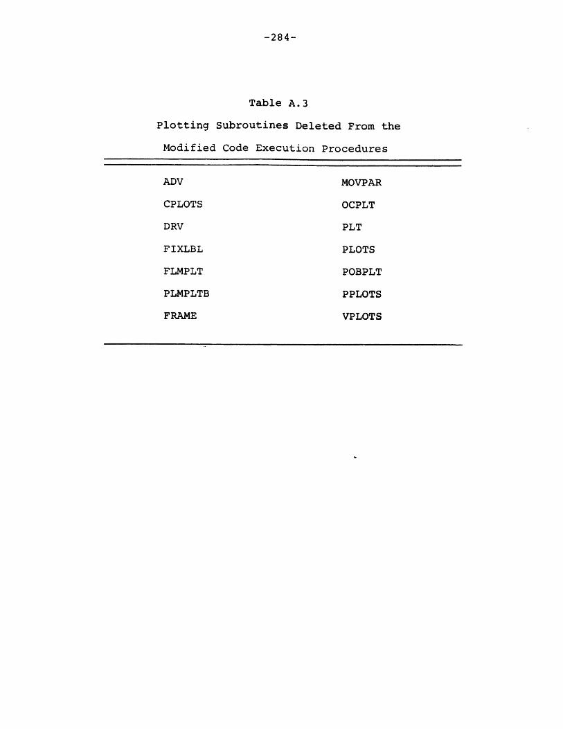
-284-

Table A.3

Plotting Subroutines Deleted From the

Modified Code Execution Procedures

ADV MOVPAR

CPLOTS OCPLT

DRV PLT

FIXLBL PLOTS

FLMPLT POBPLT

PLMPLTB PPLOTS

FRAME VPLOTS

-285-

FIGURE A.2: SLOW MIXING SUBCODE CODING STRUCTURE

MITHYD

SAVCQ

- - - SORE

SSAVCQQ

- m - MOCSLV

I A

TILDEM

A

B

S-C

PITER

.. DRAG

-- A

ENADI

I - - - ADISLV

A

I

(continue)

HYDROCS

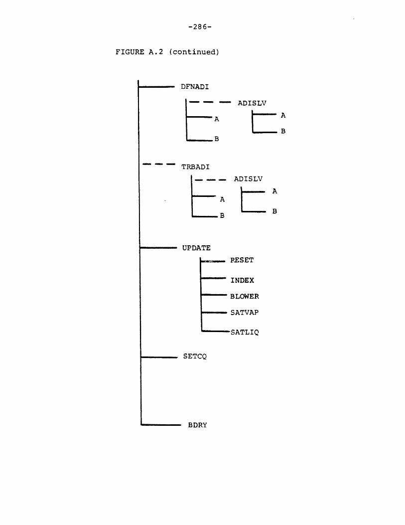
-286-

FIGURE A.2 (continued)

DFNADI

ADISLV

i A B

TRBADI

---- ADISLV

UP DATE

RE SET

INDEX

BLOWER

SATVAP

SATLIQ

SETCQ

BDRY

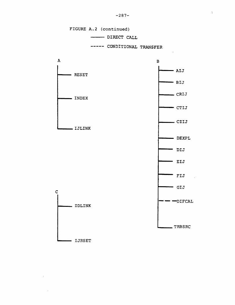
-287-

FIGURE A.2 (continued)

DIRECT CALL

----- CONDITIONAL TRANSFER

B

RESET

INDEX

IJLINK

AIJ

BIJ

CRIJ

CTIJ

CZIJ

DEXPL

DIJ

EIJ

FIJ

GIJ

- - -DIFCAL

....TRBSRC

ZDLINK

IJRSET

BCNPGM TREE,KFIXT,HTCNTL)BEACON INCLUDEINP INCLUDEMESINP INCLUDELNKINP INCLUDEHTINP INCLUDEPRINT INCLUDEKFIXT INCLUDE,WALTRN, FLMSURFHTCNTL INCLUDE

GLOBALGLOBALGLOBALGLOBALGLOBALGLOBALLEVELTREE

DUMMY GLOBALEND

TREE DIAGRAM*BEACON

?? BCNINP???? KCHINP?????? INP?????? MESINP?????? LNKINP???? HITINP

? PRINT

? KFIXT

BEACON HYDROGEN - MIT SEGLOAD DIRECTIVES CHANGE

BEACON-(BCNINP-(KCHINP-(INP,MESINP,LNKINP),HTINP),PRINT, 1

HYDROCS,IJLINK,RESET,INITAL FLMTHK,STANTN,IPHMT 2

PGMINP,SOLINP, SETC,KRASET1CELINP,OCINP,BDYINP,VELINP,RPINP,PLMINP,ZDINPSCINP,CELCHK,CELMAP,IJMAP,OPINP,FPLINPHTCOM,HT1INPPRINT,ZDPRNT,FBPRNT,FLMDBP,HTOUT 1

TILDE,BETAS,ITER,ICONV,ZEROD,SORE,ZDSORE,FLMDRV,FLMSAV, 3

,MITHYD 4

HTBCDN,HT1SST,HT1TDPSTP.END,FCL.C,Q8.IO.KSC,PLTCOM,PPCOM,MMCOM,ZDCOM,MANDE,SCCOM,CNTLCOMGLOBAL, IJCOM,TABCOM,EOSCOM,SCALAR,INPCOMTRBCOM,MOMCOM,DFNCOM 5

HTNCOM,BLOCOM 5

FTB, FLMCOM, PHCOM, FLCOM,FAST I

DUMMY 00

DUMCOMBEACON

(continued)

? HTCNTL

EXPLANATION OF CHANGES

1 - deletion of plotting routines

2 - deletion of PACKZZ (EL)

3 - deletion of PLMDBP (plotting)

4 - inclusion of MITHYD in KFIXT branch

5 - new global common blocks

FIGURE A.3: SEGMENTATION LOADING DIRECTIVES AND

RESULTING LOAD TREE

-289-

core concurrently. Further information is available

in CDC documentation of the LOADER utility

(particularly LDSET and LOAD commands).

A.5 Production Mode Execution

The successful execution of the code in a

production (i.e. no modifications) mode requires at

least three pieces of software. The first is

compiled object code of the main program, subroutines

and environmental library. These may reside in one

to three files. Splitting them into three has an

advantage if modifications are required (see below).

The second item is the segmentation loading directive

file (see A.4). Finally, input data defining the

desired simulation must be specified.

The utilization of three separate files for

storage of the main program, subroutines and

environmental library, respectively, allows the user

to employ the procedures described in section 3 of

the code's users manual to accomplish code changes.

Briefly this storage mode coupled with storage of the

code in an UPDATE program library format allows

piecewise code modification and recompilation thereby

minimizing costs.

-290-

A.6 Application on a Non-CDC System

The conversion of the program to a form

compatible with a non-CDC system is a formidable

task. This is especially true if the new host system

is IBM. The problems can be grouped into two major

categories. First and foremost are system software

and hardware differences. The system level problem

areas are segmented loading, dynamic memory

allocation and the environmental subroutine library.

The latter two are closely related. Second, the

Fortran coding itself requires straightforward but

extremely tedious editing given the code's size

(=40000 lines). The switch to non-segmented loading

basically requires 4 much larger core allocation.

This is also true of non-dynamic memory allocation.

The memory allocation problems are complicated by the

extensive use of environmental library routines to

read, manipulate, reconfigure and retrieve data.

In general, CDC Fortran is more flexible than

IBM Fortran. Some specific differences are now

enunciated.

1. All equivalenced arrays must be explicitly

dimensioned.

2. Maximum number of characters defining a

variable must be reduced from 7 to 6. This

is a major problem.

-291-

3. Data storage overlaying such as the "Level

2" specification of all CELCOM variables is

not allowed and host-system specific

overlaying must be formulated.

4. Plotting routines are not transferable.

This is also true of the IGS post-processing

plot package.

5. Multiple equal signs are unacceptable.

6. Hollerith variable size is limited to 4

characters on IBM while CDC allows larger

specification. This disturbs not only

naming but also logic functions.

[A-l] V.P. Manno and M.W. Golay, Users Manual for the

LIMIT Code - Hydrogen Analysis in Reactor Contain-

ments, MIT Energy Laboratory, MIT-EL-83-010,

September, 1983.

-292-

Appendix B: Input Decks For Reported Simulations

The input data decks reported in this appendix

correspond to a number of simulations reported in Chapter

4. Some problems were run with earlier versions of the

code and as such slight differences in format may exist.

If one wishes to use these specifications, the user should

consult the users manual to verify the validity of each

entry. The files included are listed below.

DATA DECK

DATA1

DATA2

DATA 3

DATEST

DATA3A

DATBF6

DNBF6

HEDLB

ROOM6

DESCRIPTION (REFERENCE)

air/water blowdown (4.2.1)

H2 /water blowdown (4.2.2)

BF2 using BEACON (4.2.3)

switching test (4.2.4)

basic BF2 model (4,3.1)

32 node BF6 model (4.3.1)

49 node BF6 model (4.3.1)

80 node HEDL B model (4.3.2)

6 room lumped problem (4.4)

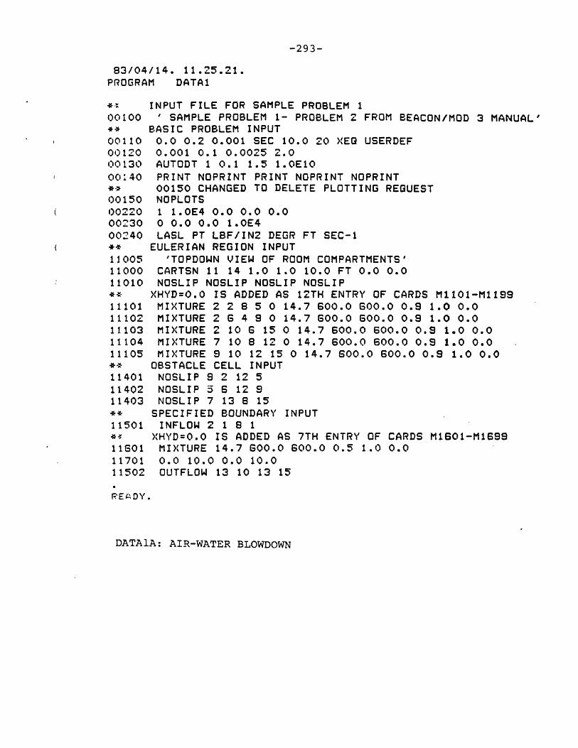
-293-

83/04/14. 11.25.21.PROGRAM DATA1

*V INPUT FILE FOR SAMPLE PROBLEM 100100 ' SAMPLE PROBLEM 1- PROBLEM 2 FROM BEACON/MOD 3 MANUAL'* BASIC PROBLEM INPUT00110 0.0 0.2 0.001 SEC 10.0 20 XEG USERDEF00120 0.001 0.1 0.0025 2.000130 AUTODT 1 0.1 1.5 1.0E10

00:40 PRINT NOPRINT PRINT NOPRINT NOPRINT** 00150 CHANGED TO DELETE PLOTTING REGUEST00150 NOPLOTSS00220 1 1.0E4 0.0 0.0 0.000230 0 0.0 0.0 1.0E400240 LASL PT LBF/IN2 DEGR FT SEC-1*+ EULERIAN REGION INPUT11005 'TOPDOWN VIEW OF ROOM COMPARTMENTS'11000 CARTSN 11 14 1.0 1.0 10.0 FT 0.0 0.011010 NOSLIP NOSLIP NOSLIP NOSLIP** XHYD=0.0 IS ADDED AS 12TH ENTRY OF CARDS M1101-M119911101 MIXTURE 2 2 8 5 0 14.7 600.0 600.0 0.9 1.0 0.011102 MIXTURE 2 6 4 9 0 14.7 600.0 600.0 0.9 1.0 0.011103 MIXTURE 2 10 6 15 0 14.7 600.0 600.0 0.S 1.0 0.011104 MIXTURE 7 10 8 12 0 14.7 600.0 600.0 0.9 1.0 0.011105 MIXTURE 9 10 12 15 0 14.7 600.0 600.0 0.9 1.0 0.0*k OBSTACLE CELL INPUT11401 NOSLIP 9 2 12 5

11402 NOSLIP 5 6 12 911403 NOSLIP 7 13 8 154* SPECIFIED BOUNDARY INPUT11501 INFLOW 2 1 8 1*I XHYD=0.0 IS ADDED AS 7TH ENTRY OF CARDS Mi601-M169911601 MIXTURE 14.7 600.0 600.0 0.5 1.0 0.011701 0.0 10.0 0.0 10.011502 OUTFLOW 13 10 13 15

RE4DY.

DATAlA: AIR-WATER BLOWDOWN

-294-

83/02/10. 13.58.23.PROGRAM DATA2

,4 INPUT FILE FOR SAMPLE PROBLEM 200100 ' SAMPLE PROBLEM 2- MODIFIED BEACON SP2 WITH H2 INFLOW'* BASIC PROBLEM INPUT00110 0.0 0.2 0.001 SEC 10.0 20 XEG USERDEF00120 0.001 0.1 0.0025 2.000130 AUTODT 1 0.1 1.5 1.0E1000140 PRINT NOPRINT PRINT NOPRINT NOPRINT4+ 00150 CHANGED TO DELETE PLOTTING REGUEST00150 NOPLOTS00220 1 1.0E4 0.0 0.0 0.000230 0 0.0 0.0 1.0E400240 LASL PT LBF/IN2 DEGR FT SEC-1** EULERIAN REGION INPUT11005 'TOPDOWN VIEW OF ROOM COMPARTMENTS'11000 CARTSN 11 14 1.0 1.0 10.0 FT 0.0 0.011010 NOSLIP NOSLIP NOSLIP NOSLIP

* XHYD=0.0 IS ADDED AS 12TH ENTRY OF CARDS M1101-M119911101 MIXTURE 2 2 8 5 0 14.7 600.0 600.0 0.9 1.0 0.011102 MIXTURE 2 6 4 9 0 14.7 600.0 600.0 0.9 1.0 0,011103 MIXTURE 2 10 S 15 0 14.7 600.0 600.0 0.9 1.0 0.011104 MIXTURE 7 10 8 12 0 14.7 600.0 600.0 0.9 1.0 0.011105 MIXTURE 9 10 12 15 0 14.7 600.0 600.0 0.9 1.0 0.0+* OBSTACLE CELL INPUT11401 NOSLIP 9 2 12 511402 NOSLIP 5 6 12 911403 NOSLIP 7 13 8 15** SPECIFIED BOUNDARY INPUT11501 INFLOW 2 1 8 1*2 XHYD=1.0 IS ADDED AS 7TH ENTRY OF CARDS M1601-M16994* NOTE INFLOW IS NOW ALL HYDROGEN11601 MIXTURE 14.7 600.0 600.0 0.5 0.0 1.011701 0.0 10.0 0.0 10.011502 OUTFLOW 13 10 13 15

READY.olddabF12READY.

DATA2: H 2/WATER BLOWDOWN2

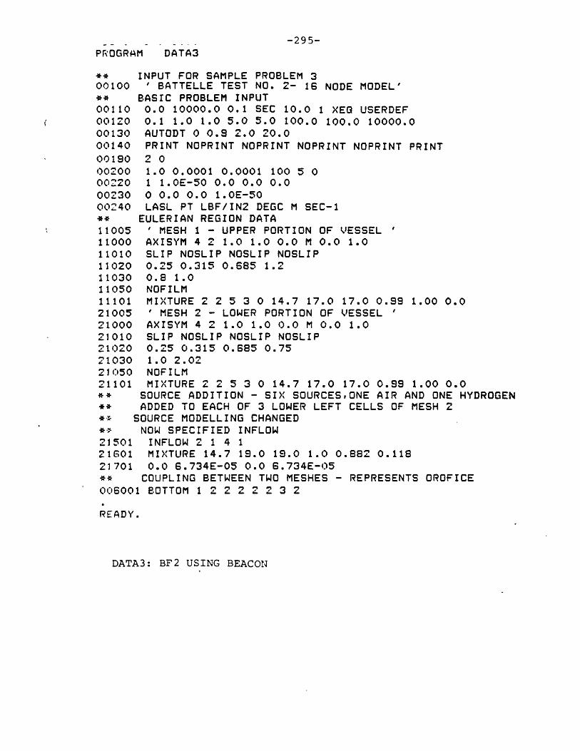
-295-

PROGRAM DATA3

* INPUT FOR SAMPLE PROBLEM 300100 ' BATTELLE TEST NO. 2- 1s NODE MODEL'4* BASIC PROBLEM INPUT00110 0.0 10000.0 0.1 SEC 10.0 1 XEG USERDEF00120 0.1 1.0 1.0 5.0 5.0 100.0 100.0 10000.000130 AUTODT 0 0.9 2.0 20.000140 PRINT NOPRINT NOPRINT NOPRINT NOPRINT PRINT00190 2 0

00200 1.0 0.0001 0.0001 100 5 000220 1 1.OE-50 0.0 0.0 0.0

00230 0 0.0 0.0 1.OE-5000240 LASL PT LBF/IN2 DEGC M SEC-1+4 EULERIAN REGION DATA11005 ' MESH 1 - UPPER PORTION OF VESSEL11000 AXISYM 4 2 1.0 1.0 0.0 M 0.0 1.0

11010 SLIP NOSLIP NOSLIP NOSLIP11020 0.25 0.315 0.685 1.211030 0.8 1.011050 NOFILM11101 MIXTURE 2 2 5 3 0 14.7 17.0 17.0 0.99 1.00 0.021005 ' MESH 2 - LOWER PORTION OF VESSEL21000 AXISYM 4 2 1.0 1.0 0.0 M 0.0 1.021010 SLIP NOSLIP NOSLIP NOSLIP21020 0.25 0.315 0.685 0.7521030 1.0 2.0221050 NOFILM21101 MIXTURE 2 2 5 3 0 14.7 17.0 17.0 0.99 1.00 0.0* SOURCE ADDITION - SIX SOURCES 1ONE AIR AND ONE HYDROGEN

+* ADDED TO EACH OF 3 LOWER LEFT CELLS OF MESH 2** SOURCE MODELLING CHANGED

NOW SPECIFIED INFLOW21501 INFLOW 2 1 4 121501 MIXTURE 14.7 19.0 19.0 1.0 0.882 0.118

21701 0.0 6.734E-05 0.0 6.734E-05+* COUPLING BETWEEN TWO MESHES - REPRESENTS OROFICE

006001 BOTTOM 1 2 2 2 2 2 3 2

READY.

DATA3: BF2 USING BEACON

-296-

11i t

83/04/14. 11.42.29.PROGRAM DATEST

** TEST DATA FOR SWITCHING CHECK00100 ' SWITCHING TEST CASE '

00110 0.0 10.0 0.5 SEC 10.0 1 XEG USERDEF 0 1.OE+10

00120 0.5 2.0 1.0 10.000130 CONST 20 0.5 1.25 10.000140 PRINT NOPRINT PRINT NOPRINT NOPRINT NOPRINT00190 1 0 10.000200 1.0 0.00010 0.00010 100 20 000220 1 1.0OE+04 0.0 0.0 0.000230 0 0.0 0.0 1.OE+0400240 LASL PT LBF/IN2 DEGC M SEC-100400 0 1.0 1.8 1.OE-20 1.OE-20 1.0OE-20 1.0E-2000410 0.000 1.44 1.92 1.44 200.0 1.0 1.300420 0 0.0 0.0 0.0 0.011005 ' TEST MESH '11000 CARTSN 2 3 1.0 1.0 1.0 M 0.0 1.0 0 1.22120611010 SLIP SLIP SLIP SLIP11050 NOFILM11101 AIR 2 2 3 4 0 14.7 16.03010 HYD 1 2 2 003011 0.0 DEGREES 1.0 1.0 1.0 0.03011 SEC KG/SEC J/KG M SEC-130i2 0.0 1.OE-04 4.124E+06 0.03013 10.0 1.OE-04 4.124E+06 0.0

READY.

DATEST:SWITCHING TEST

-297-

PROGRAM DATA3A

** INPUT FOR SAMPLE PROBLEM 3A00100 ' BF2 OPEN - RELAX=1.8 TURB - 32 NODES** BASIC PROBLEM INPUT00110 0.0 100.0 2.0 SEC 10.0 1 XEG USERDEF 1 1.0E+0600120 2.0 20.0 10.0 100.0 20.0 200.0 200.0 10000.000130 AUTODT 75 0.5 1.25 50.000140 PRINT NOPRINT PRINT NOPRINT NOPRINT PRINT00190 2 000200 1.0 .000025 .000025 100 1000 000220 1 1.0OE-50 0.0 0.0 0.0

00230 0 0.0 0.0 1.OE-50

00240 LASL PT LBF/IN2 DEGC M SEC-1** NEW INPUT CARDS00400 0 1.0 1.80 1.0 1.0 1.0 1.000410 0.090 1.44 1.92 1.44 200.0 1.0 1.3** EULERIAN REGION DATA11005 ' MESH 1 - LOWER REGION11000 AXISYM 6 3 1.0 1.0 0.0 M 0.0 1.0 1 1.21699711010 SLIP SLIP SLIP SLIP11020 0.2825 0.2825 0.3092 0.3401 0.3741 0.4115

11030 1.0 1.0 1.011050 NOFILM11101 AIR 2 2 7 4 0 14.7 17.011201 2 2 7 4 0. 0. 0. 0. 1.OE-04 1.OE-0521005 ' MESH 2 - UPPER REGION '21000 AXISYM 7 2 1.0 1.0 0.0 M 0.0 1.0 1 1.21699721010 SLIP SLIP SLIP SLIP21020 0.2825 0.2825 0.3092 0.3401 0.3741 0.4115 0.450121030 1.0 0.813821050 NOFILM21101 AIR 2 2 8 3 0 14.7 17.021201 2 2 8 3 0. O. 0. 0. 1.OE-04 1.0OE-05** SOURCE ADDITION - SIX SOURCESONE AIR AND ONE HYDROGEN+* ADDED TO EACH OF 3 LOWER LEFT CELLS OF MESH 13010 AIR 1 2 2 003011 0.0 DEGREES 0.0657 1.0 1.0 0.03060 AIR 1 3 2 003011 0.0 DEGREES 0.2701 1.0 1.0 0.03110 AIR 1 4 2 003011 0.0 DEGREES 0.6642 1.0 1.0 0.03011 SEC KG/SEC J/KG M SEC-13012 0.0 1.367E-04 2.934E+05 0.03013 10000.0 1.367E-04 2.934E+05 0.03160 HYD 1 2 2 003061 0.0 DEGREES 0.0657 1.0 1.0 0.0

3210 HYD 1 3 2 003061 0.0 DEGREES 0.2701 1.0 1.0 0.03260 HYD 1 4 2 003061 0.0 DEGREES 0.6642 1.0 1.0 0.03061 SEC KG/SEC J/KG M SEC-13062 0.0 1.828E-05 4.181E+06 0.0

3063 10000.0 1.828E-05 4.181E+06 0.0++ COUPLING

006001 TOP 1 2 4 6 2 2 2 6

READY.0

DATA3A: BASIC BF2 MODEL

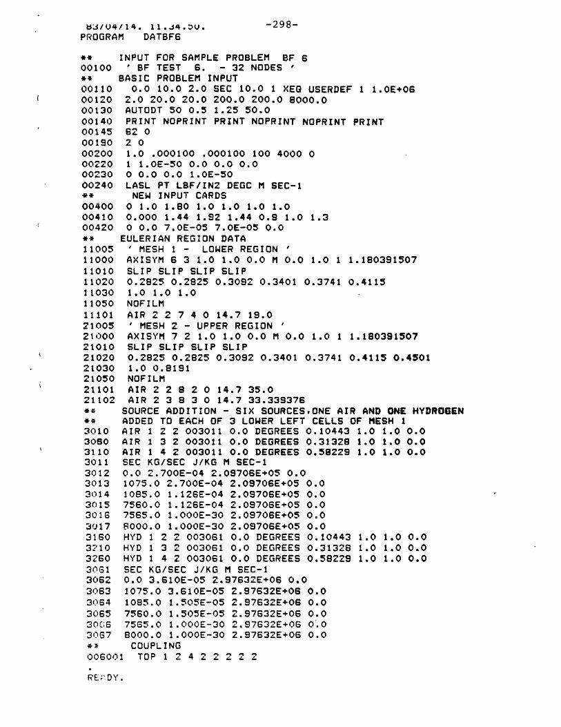
L3/04/14. 1.J4.DU. -298-

PROGRAM DATBF6

** INPUT FOR SAMPLE PROBLEM BF 600100 ' BF TEST 6. - 32 NODES** BASIC PROBLEM INPUT00110 0.0 10.0 2.0 SEC 10.0 1 XEG USERDEF 1 1.0E+0600120 2.0 20.0 20.0 200.0 200.0 8000.000130 AUTODT 50 0.5 1.25 50.000140 PRINT NOPRINT PRINT NOPRINT NOPRINT PRINT00145 62 000190 2 000200 1.0 .000100 .000100 100 4000 000220 1 1.OE-50 0.0 0.0 0.000230 0 0.0 0.0 1.OE-5000240 LASL PT LBF/IN2 DEGC M SEC-1** NEW INPUT CARDS00400 0 1.0 1.80 1.0 1.0 1.0 1.000410 0.000 1.44 1.92 1.44 0.9 1.0 1.300420 0 0.0 7.0E-05 7.OE-05 0.0** EULERIAN REGION DATA11005 ' MESH 1 - LOWER REGION '11000 AXISYM 6 3 1.0 1.0 0.0 M 0.0 1.0 1 1.18039150711010 SLIP SLIP SLIP SLIP11020 0.2825 0.2825 0.3092 0.3401 0.3741 0.411511030 1.0 1.0 1.011050 NOFILM11101 AIR 2 2 7 4 0 14.7 19.021005 ' MESH 2 - UPPER REGION21000 AXISYM 7 2 1.0 1.0 0.0 M 0.0 1.0 1 1.18039150721010 SLIP SLIP SLIP SLIP21020 0.2825 0.2825 0.3092 0.3401 0.3741 0.4115 0.450121030 1.0 0.819121050 NOFILM21101 AIR 2 2 8 2 0 14.7 35.021102 AIR 2 3 8 3 0 14.7 33.339376** SOURCE ADDITION - SIX SOURCES,ONE AIR AND ONE HYDROGEN+* ADDED TO EACH OF 3 LOWER LEFT CELLS OF MESH I3010 AIR 1 2 2 003011 0.0 DEGREES 0.10443 1.0 1.0 0.03060 AIR 1 3 2 003011 0.0 DEGREES 0.31328 1.0 1.0 0.03110 AIR 1 4 2 003011 0.0 DEGREES 0.58229 1.0 1.0 0.03011 SEC KG/SEC J/KG M SEC-13012 0.0 2.700E-04 2.09706E+05 0.03013 1075.0 2.700E-04 2.09706E+05 0.03014 1085.0 1.126E-04 2.09706E+05 0.03015 7560.0 1.126E-04 2.09706E+05 0.03016 7565.0 1.000E-30 2.09706E+05 0.03017 P000.0 1.000E-30 2.09706E+05 0.03160 HYD 1 2 2 003061 0.0 DEGREES 0.10443 1.0 1.0 0.03210 HYD 1 3 2 003061 0.0 DEGREES 0.31328 1.0 1.0 0.03260 HYD 1 4 2 003061 0.0 DEGREES 0.58229 1.0 1.0 0.030G1 SEC KG/SEC J/KG M SEC-13062 0.0 3.610E-05 2.97632E+06 0.03063 1075.0 3.610E-05 2.97632E+06 0.03064 1085.0 1.505E-05 2.97632E+06 0.03065 7560.0 1.505E-05 2.97632E+06 0.030C;6 7565.0 1.000E-30 2.97632E+06 0.03067 8000.0 1.000E-30 2.97632E+06 0.09, COUPLING006001 TOP 1 2 4 2 2 2 2 2

RE DY.

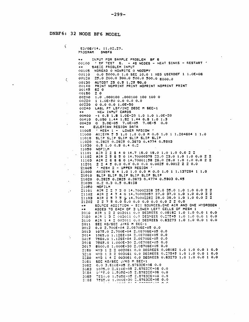
-299-

DNBF6: 32 NODE BF6 MODEL

2/0o6/14. 11.02.27.ROGRAM DNBFG

*4 INPUT FOR SAMPLE PROBLEM SF 600100 ' ?F TEST G. - 49 NODES - HEAT SINKS - RESTART44 SASIC PROBLEM INPUT00105 NOREAD 0 NOWRITE 0 NOCIOPY00110 0.0 5000.0 1.0 SEC 10.0 1 XEG USERDEF 1 1.0E+06001:0 25.0 200.0 300.0 500.0 500.0 0O00.000130 AUTODT 25 0.5 1.25 40.0

00!40 PRINT NOPRINT PRINT NOPRINT NOPRINT PRINT00145 s2 0'0190 2 000200 1.0 .000100 .000100 100 100 00 0220 1 1.0E-50 0.0 0.0 0.000230 0 0.0 0.0 1.OE-5000240 LASL PT LSF/IN2 DEGC M SEC-1** NEW INPUT CARDS00400 -1 0.5 1.8 1.0E-20 1.0 1.0 1.0E-2000410 0.090 1.44 1.92 1.44 0.9 1.0 1.300420 0 3.0E-05 7.0E-05 7.OE-5 0.0** EULERIAN REGION DATA11005 ' MESH 1 - LOWER RFGION1:000 AI7SYM 5 5 1.0 1.0 0.0 M 0.0 1.0 1 1.204604 1 1.011010 SL:P SLIP SLIP SLIP SLIP SLIP:1020 0.2825 0.2e25 0.3673 0.4774 0.590311030 0.5 1.0 0.9 0.4 0.211050 NOFILM11101 AIR 2 2 S 4 0 14.7 1i.0 19.0 1.0 1.0 0.0 2 211102 AIR 2 5 6 5 0 14.70000379 23.0 :3.0 1.0 1.0 0.0 2 211103 AIR 2 S S S 0 14.70001:58 26.0 26.0 1.0 1.0 0.0 2 211201 2 2 4 5 0.0 0.0 0.0 0.0 0.0025 0.0012 2 2 0.021005 ' MESH 2 - UPPER REGION21000 AXISYM 6 4 1.0 1.0 0.0 M 0.0 1.0 1 1.137294 1 1.0

21010 SLIP SLIP SLIP SLIP SLIP SLIP21020 0.2925 0.2825 0.3673 0.4774 0.5903 0.45

2:030 0.2 0.3 0.5 0.8138Z1050 NOFILM21101 AIR 2 2 7 3 0 14.70002328 35.0 35.0 1.0 1.0 0.0 2 2

O1102 AIR 2 4 7 4 0 14.70002057 37.0 37.0 1.0 1.0 0.0 2 2'1103 AIR 2 5 7 5 14.700022E2 39.0 39.0 1.0 1.0 0.0 2 221202 2 2 7 5 0.0 ).0 0.0 0.0 0.0 0.0 2 2 0.0** SOUCE ADDITION - SI, SOURCES,GNE AIR AND ONE HYDROGEN** ADDED TO EACH OF 3 LOWER LEFT CELLS OF MESH 120:0 AIR 1 2 2 003011 0.0 DER-EES 0.09182 1.0 1.0 0.0 1 0.020f0 AIR : 3 2 C'O:0: 1 0.? "E'EES 0.7?A5 1.0 1.0 0.0 1 0.03110 AIR 1 4 2 00011. 0.0 DEGREES 0.63273 1.0 1.0 0.0 1 0.03011 SEC KG/SEC J/KG M SEC-13012 0.0 2.700E-04 2.0570GE'05 0.03013 1075.0 2.700E-04 2.0S70 6+05 0.03014 1065.0 1. I2E-0 - 2.0S70GE+05 0.030:5 7560.0 1.126E-04 2.070oE-05 0.00!6 7565.0 1.000E-30 2. 0S706E+05 0.0

3017 8000.0 1.000E-30 2.S0970GE+05 0.02150 HYD I 2 2 002061 0.0 DEGREES 0.09182 1.0 1.0 0.0 1 0.032:*0 HYD 1 3 2 003061 0.0 DEGREES 0.27545 1.0 1.0 0.0 1 0.0

ZSO0 HYD 1 4 2 003061 0.0 DEGREES 0.63273 1.0 1.0 0.0 1 0.02061 SEC KG/SEC J/KG M SEC-1"062 0.0 3.610E-05 2.97S32E+"S.5 0.02063 1075.0 2.E10E-05 2.972S2505 0.02E:4 1*i'-.0 I.505E-05 2.97632E+)0 0.03lj5 550.0 1.1505E-05 Z.9763ZE+06 0.0-:--S 7%5.0 1.000E-30 ".976332EOE 0.0

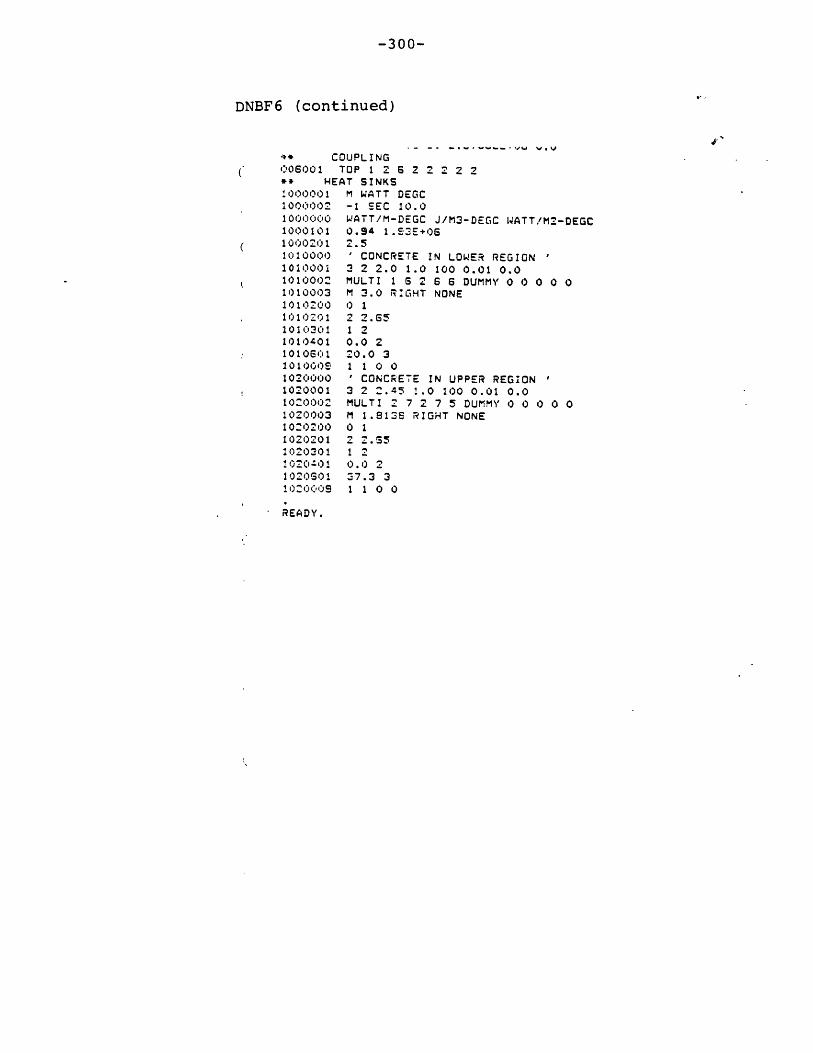
-300-

DNBF6 (continued)

COUPLING.006001 TOP 1 2 6 2 2 2 2 2•** HEAT SINKS

:000001 M WATT DEGC1000002 -1 SEC 10.01000000 WATT/M-DEGC J/M3-DEGC WATT/M2-DEGC1000101 0.94 I.53E+061000201 2.51010000 ' CONCRETE IN LOWER REGION1010001 3 2 2.0 1.0 100 0.01 0.01010002 MULTI 1 G 2 6 6 DUMMY 0 0 0 0 01010003 M 3.0 RIGHT NONE1010200 0 11010201 2 2.651010301 1 21010401 0.0 21010601 20.0 31010006 1 1 0 0102c3000 ' CONCRETE IN UPPER REGION1020001 3 2 2.45 1.0 100 0.01 0.01020002 MULTI 2 7 2 7 5 DUMMY 0 0 0 0 01020003 M 1.8136 RIGHT NONE1020200 0 11020201 2 2.551020301 1 2!020401 0.0 21020601 37.3 3102000o 1 1 0 0

READY.

-301-

POGRCAM HEDLB

00100 ' HEDL S SIMULATION 100 NODE 3D MODEL** RESTART SPECS0010, NOREAD 0 WRITE 2 NOCOPY-,* SASIC INPUT DATA

C 00110 0.0 700.0 0.1 SEC 10. 1 XEG USERDEF 3 1.0E+1000120 50.0 100.0 100.0 900.000130 AUTGDT 10 0.5 1.25 10.000140 PRINT NOPRINT PRINT NOPRINT NOPRINT PRINT001iS 1 0 10.000200 1.0 0.00010 0.00010 100 50 0** DUMMY INTERPHASIC PARAMETERS00220 1 0.0 0.0 0.0 0.000230 0 0.0 0.0 0.000240 LASL PT LBF/IN2 DEGC M SEC-1** NEW INPUT CARDS00400 0 1.0 1.8 1.0 1.0 1.0 1.OE-2000410 0.090 1.44 1.92 1.44 0.9 1.0 1.300'20 0 3.3E-05 6.0E-04 3.3E-05 0.0** BLOWER MODEL00500 400510 5 6 2 700511 0.0 1.1303 0.0 308.0 0.4333300512 90.0 1.!052 0.0 315.0 0.4333300513 270.0 1.1017 0.00078 316.0 0.4333300514 330.0 1.0896 0.00104 319.5 0.4333300515 530.0 1.07!2 0.00234 325.0 0.4333300516 690.0 1.0695 0.00260 325.5 0.4333300517 870.0 1.0795 0.00270 322.5 0.4333300520 5 6 3 7

( 0u521 0.0 1.1303 0.0 306.0 0.4333300522 90.0 1.1052 0.0 315.0 0.4333300523 270.0 1.1017 0.00078 316.0 0.4333300524 330.0 1.0996 0.00104 319.5 0.4333300525 630.0 1.0712 0.00234 325.0 0.4333300526 60.0 1.095 0.00260 325.5 0.4333300527 870.0 1.07S5 0.00270 322.5 0.4333300530 5 6 4 700531 0.0 1.1303 0.0 308.00 0.4333300532 SO.0 1.1052f 0.0 31g,0 0.4333300533 270.0 1.1017 0.00078 316.0 0.4333300534 330.0 1.0896 0.00104 319.5 0.43333300535 630.0 1.0712 0.00234 325.0 0.4333300536 690.0 1.0695 0.00260 225.5 0.4333300537 e70.0 1.0795 0.00270 322.5 0.4333300540 5 6 5 700541 0.0 1.1303 0.0 306.0 0.4333300542 90.0 1.1052 0.0 315.0 0.4333300543 270.0 1.1017 0.00078 316.0 0.4333300544 330.0 1.0896 0.00104 319.5 0.4333300545 630.0 1.0712 0.00234 325.0 0.433330546 6G0.0 1.0695 0.00260 325 .5 0.4333300547 870.0 1.0795 0.00270 322.5 0.43333** CONTINUUM REGION INPUT11005 ' HEDL e FACILITY - 80 NODES'11000 AXISYM 4 5 1.0 1.0 1.52 M 0.0 1.0 1 1.04425 4 1.011010 SLIP SLIP SLIP SLIP SLIP SLIP:1020 0.5725 0.5725 0.5725 0.572511030( 0.944 0.944 0.94 0.9 4 0.94411C40 0.20623 0.20833 0.20633 0.208331:050 NOFILt:1101 AIR ; 2 5 6 0 14.7 65.0 65.0 1.0 1.0 0.0 2 51:201 2 2 5 6 0.0 0.0 0.0 0.0 1.OE-04 1.OE-06 2 5 0.0

HEDLB: 80 NODE HEDLB MODEL

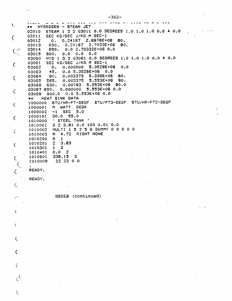
-302-

** HYDROGEN - STEAM JET

03010030110301203013S 00140-015030600306103062030630306403065030660306703068

STEAM 1 3 3 03011 0.0 DEGREES 1.0 1.0 1.0 0.0 4 0.0

SEC KG/SEC J/KG M SEC-10. 0.24167 2.6678E+06 80.

630. 0.24Z67 2.7033E+06 80.690. 0.0 2.70332E+06 0.0

900. 0.0 0.0 0.0HYD 1 3 3 03061 0.0 DEGREES 1.0 1.0 1.0 0.0 4 0.0

SEC KG/SEC J/KG M SEC-10. 0.000000 5.3528E+06 0.0

45. 0.0 5.3528E+06S 0.090. 0.003375 5.339E+06 80.

585. 0.003375 5.553E+06 80.630. 0.00783 5.553E+06 80.0690. 0.000000 5.553E+06 0.0900.0 0.0 5.553E+06 0.0

** HEAT SINK DATA1000000 BTU/HR-FT-DEGF BTU/FT3-DEGF BTU/HR-FT2-DEGF

1000001 M WATT DEGK1000002 -1 SEC 5.0

C 1000101 30.0 55.01010000 ' STEEL TANK1010001 3 2 3.81 0.0 100 0.01 0.0

1010002 MULTI 1 5 2 5 6 DUMMY 0 0 0 0 0

1010003 M 4.72 RIGHT NONE

1010200 0 11010201 2 3.831010301 1 21010401 0.0 21010601 338.15 31010009 22 22 0 0

READY.

READY.

HEDLB (continued)

4 1

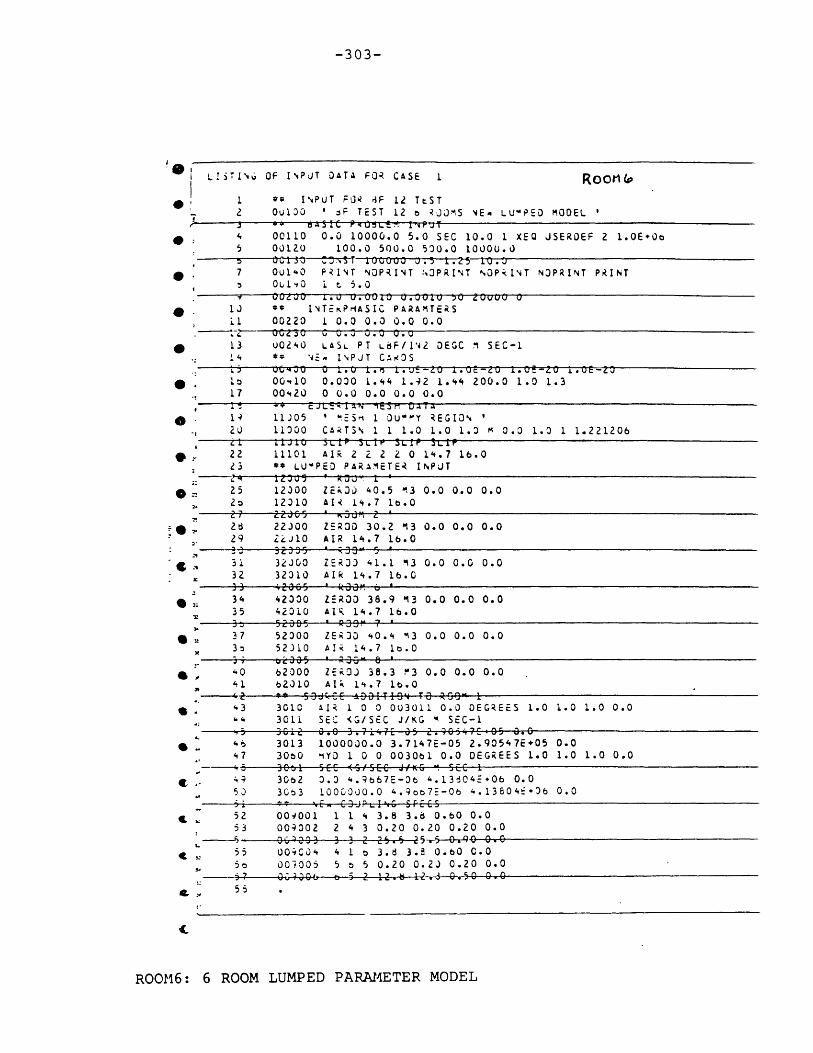
-303-

L

0'I

STING OF INPOT OATA FOR CASE 1 RooM 4I * INPUT FO iF 12 TtST2 Ou310 ' F TEST 12 b RJ MS vE. LUPED MODEL '

4 00110 0.0 10000.0 5.0 SEC 10.0 1 XEQ JSEROEF 2 1.OE'Oo5 00120 100.0 500.0 500.0 10000.0

o 0130 1uT 1000U0 J.3 1.25 10.07 u0010 PRINT NOPRINT N3PRINT NOP INT NOPRINT PRINT

Ou lO Lt 5.0, . 0.00o O .J4 0.JUL000 20UU0 0

13 ** INTEKPrASIC PARAMTERSii 00220 1 0.0 0.0 0.0 0.0

. 0O0?30 G 0.3 0.0 0.013 u0240 LASL PT LBF/I142 EGC m SEC-1

44 * 4 " ,, INPJT CADSS 00 40 0 U !.0 £. t.E-OL .IUe- L. .oe-Lo i.oE-LJ

lt 00410 0.000 1.44 1.42 1.44 200.0 1.0 1.317 00..20 0.0 0.0 0.0 0.0

19 11J05 ' "ES5 1 OU40 Y REGION21 11300 CARTS 1 I 1.0 1.0 1.3 M 0.0 1.0 1 1.221206tt J1iO 3LIP STPl ' SLIP SLIP22 11101 AIR Z 2 2 2 0 14.7 16.023 ** LU'PED PARAMETER INPJT24 i2005 k kij* L25 12300 ZER3 40.5 ,3 0.0 0.0 0.0

20 12310 AIR 14.7 lb.027 22d3 ' m5M 2 '26 22300 ZERDD 30.2 13 0.0 0.0 0.029 2iJ10 AIR 14.7 16.0-4i 32a55 R99- 5

31 32J00 ZER)3 41.1 3 0.0 0.0 0.032 32010 AIR 14.7 16.033 4E035 k aO . '34 42030 ZEROD 38.9 "13 0.0 0.0 0.035 42010 AIR 14.7 16.0

37 52000 ZERD 40.4 %3 0.0 0.0 0.03n 52310 AI 14.7 lb.0

40 62000 ZEROJ 38.3 !3 0.0 0.0 0.041 b2310 AIk 14.7 1b.0

1 2 t dlC;EC ADITI9n TO R00 1'43 3010 AIR 1 0 0 003011 0.0 DEGREES 1.0 1.0 1.0 0.0'' 3011 SEC <G/SEC J/KG 4 SEC-1

301. 0.0 3.71'7 E ,S 2. 047 -05 0.C46 3013 1000000.0 3.7147E-05 2.90547E+05 0.047 3060 YD 1 0 0 003061 0.0 DEGREES 1.0 1.0 1.0 0.0-- 3 EE 5.. (/.CC J/G " S C-!,9 3062 0.3 4. 667E-36 4.13604E+06 0.0

53 3C03 1000000.0 4.9o07E-06 4.138041+36 0.0-N G.cn CJJPulG SfC5S52 004001 1 1 4 3.8 3.8 0.60 0.053 009002 2 4 3 0.20 0.20 0.20 0.0

0------ 3 3 2 25.5 25 ---. q 0.055 004034 4 1 t 3.8 3. 0.bO C.O0

50 003005 5 t 5 0.20 0.23 0.20 0.07---5-_ --- 5 2i-2 -- , a CQ,_.0 .0

ROOM LUMPED PARAMETER MODELROOM6: 6

-304-

APPENDIX C

ANALYTICAL ASPECTS OF POSSIBLE EXTENTION TO

CHEMICALLY REACTIVE FLOWS

C.1 Introduction

When one considers the progression of hydrogen

related accidents in nuclear containments, five general

phenomena are identified. The first is the hydrogen

source behavior since its characteristics will define

both the relevant time frames and bounding compositional

end states. Once hydrogen appears the pre-chemical

reaction flow transient will determine local fluid and

thermodynamic conditions. The accurate prediction of this

pre-chemical reaction phase is the focus of the main body

of this work. Nevertheless, as hydrogen concentrations

increase, ignition criteria and progression become impor-

tant. Depending upon the local conditions and the strength

of the ignition source, either a subsonic deflagration or

a detonation will result. The purpose of this appendix is

to briefly review the new physical and computational

aspects of introducing chemical reactions to analytical

models of hydrogen transport.

C.2 Important Phenomena

The three imporcant physical processes are ignition

phenomena, deflagration (subsonic combustion wave

-305-

propagation) and detonations. A brief discussion of each

of these is presented.

C.2.1 Ignition Phenomena

At the relatively low pressures (a few atmospheres

at most) and temperatures (less than 400*K) typical of

the post-accident environment, a chemical reaction must be

instigated by a significant ignition source. The contain-

ment however does contain equipment which can act as an

inadvertent trigger (e.g., sparks from electric motors

associated with pumps and valve operators). Due to the

presence of these items, analysis studies which are not

concerned with ignition, per se, may proceed under the

assumption that an adequate ignition source is present.

One possible calculational approach would be to artifici-

ally hold the temperature in a particular region at a high

value typical of a postulated ignition source and use

equations descriptive of the chemical reactions of inter-

est.

For analyses in which ignition is of central impor-

tance such as studying deliberate igniter locations,

greater modelling effort is required. Toong [C-l] points

out that ignition criteria may be categorized by two

independent quantities: critical power density and criti-

cal energy-deposition duration. A detailed chemical

reaction analysis of the H2-reaction mechanism is provided

-306-

by Lewis and von Elbe [C-2] who use fourteen separate

reactions. As discussed earlier and theoretically

explained by Lewis and von Elbe, the water vapor content

of the mixture is of great importance since even a small

amount significantly inhibits the reaction.

Good analytical treatment of ignition depends upon

accurate quantitative rate descriptions. In this regard

the works of Sawyer and Glassman [C-3] and Jensen and Jones

[C-4] are noteworthy. The former provides the results of

a detailed experimental investigation of the reaction of

hydrogen with nitrogen dioxide, pure oxygen and mixtures

of oxygen and nitric oxide. The latter work provides an

extensive tabulation of rate constants especially appli-

cable to flame propagation calculations. Local hydraulics

including turbulence level must be included in such

simulations. Ballal and Lefebvre [C-5] provide a discus-

sion of the influence of flow parameters on both ignition

and quenching phenomena. Nevertheless, due to the prob-

lem's complexity, detailed investigation of ignition

phenomena must chiefly rely on experimental programs.

C.2.2 Deflagration Regime

The physical picture of this regime involves the

burning of a combustible mixture such that subsonic propa-

gation waves (flames) dominate the dynamics. The appro-

priate level of analytical sophistication depends upon the

-307-

spatial and temporal accuracy required. The range of

desired detail may be qualitatively grouped into three

categories. The crudest sort of analysis would involve

a lumped parameter or large control volume approach with

the addition of mass and energy source terms in the balance

equations. The information provided from such an analysis

should give a good qualitative picture of the change in

the global thermodynamic state of a rather large region.

For example, the overall pressure and temperature rise in

a particular containment room may be estimated by this

method. (The previously referenced HECTR code is an

example of this approach.)

The lumped parameter approach gives little insight

into spatial details. In regions with non-uniform geo-

metries, flow patterns and ignition source locations, more

accurate procedures must be invoked. Such approaches are

based on the solution of continuum equations augmented by

chemical kinetic models. It is clear that the greater

information content of the analysis is achieved at the

expense of greater phenomenological modelling and computa-

tional effort. This is especially true in turbulent flow

fields in which the coupling of the fluid dynamics and

chemistry is important.

The third category of deflagration analysis addresses

the detailed structure of the flame and its propagation

behavior. This level of detail is not as of much interest

-308-

in the nuclear safety area as the reacting flow analysis.

Toong provides a theoretical discussion of premixed flame

behavior which describes the physics in terms of an

eigenproblem, with propagation speed being the eigenvalue.

While laminar flames are well understood and predicted by

current methods, turbulent flame propagation remains an

area of extensive research.

In the laminar regime, analytical solutions based on

a boundary layer approach are useful. Of particular note

is the effect of chemical reaction on the temperature

profile in the boundary layer. Reitz [C-6] has reported

a numerical solution based on an explicit computational

technique using a one-dimensional Lagrangian mesh. His

equation set is based on Lewis number equal to one and

neglecting radiation, body force and bulk-viscosity

effects. The two-step (time level splitting) technique is

shown to be more efficient yet as accurate as more complex

methods.

The turbulent flame literature is vast and only a few

particular works are referenced here. The work of Spalding

[C-7] is significant because of its survey nature and the

knowledge of the-author in the area of computational tur-

bulence. Kennedy and Plumb [C-8] have presented a turbu-

lence boundary layer analysis to describe buoyancy con-

trolled wall flames. They employ a rather sophisticated

three parameter turbulence closure model: k (turbulent

-309-

kinetic energy), c (dissipation of K), and G (root mean

square fluctuation of mixture density). The authors

include the third transport equation for G in order to

account for the contribution of compositionally-induced

buoyancy in the turbulent processes. This additional

equation adds an additional algebraic closure relation

of the form,

<u'T'> = C(Gok) , (C.1)

where C is an empirical constant (- 0.5).

Pergament and Fishburne [C-9] performed an empirical

and analytical investigation of hydrogen/air diffusion

flames in a pilot ignition cylindrical burner geometry.

Using a stream function-vorticity approach, they modelled

turbulence effects using a zero equation or algebraic

model. This model produces qualitatively correct results

but mispredicts the flame's structural characteristics and

they recommend a more complex model. They also report some

improved values for rate expressions which are reproduced

in Table C.l.

C.2.3 Detonations

Detonations of any type are to be strictly avoided in

nuclear containments. If hydrogen concentration is kept

below 20% by volume, detonations should not be a problem.

If they should occur however, the central concern is the

strength of the supersonic detonation wave and potential

-310-

Table C. 1

Important Hydrogen-Air-Water Reaction Steps and

Associated Rate Expressions (from [C-9])

Reaction

- OH + M (--H 2 0 + M

- H + M +--OH + M

O + M--O2 + M

H + M--H2 + M

+ 0 -- H + 02

+ H-- H 2 + 0

+ H22 + H2 0 + H

+ OH- HH20 + 0

Rate Coefficients (molecule-cm-sec)

1.0 X 10 - 2 8 T- 2

3.0 X 1032

5.0 X 10- 30 T- 1 exp (-340/RT)

5.0 X 10- 30 T-1

4.0 X 1011

1.4 X 104 T exp (-7000/RT)

1.0 X 10-17 T2 exp (-2900/RT)

1.0 X 1011 exp (-1100/RT)

H

O

O

H

OH

OH

OH

OH

-311-

structural damage. Toong provides physical insight into

the processes with the underlying findings that while

propagation may seem steady macroscopically, the dynamics

of the fluid-chemical coupling is through unsteady, three

dimensional wave interactions. The three major concepts

to be considered in detonation studies are structure,

sustenance and stability. Many workers have reported

calculational tools of varying complexity and two are

mentioned as representative (Cohen et al. [C-10] and Oran

et al. [C-ll,C-12]). Both are based on a one dimensional

compressible flow solution coupled to chemical kinetics

models using a Lagrangian approach. Oran reports good

spatial definition of the shock front due to the minimal

numerical diffusion and no use of artificial viscosities in

the hydrodynamic solution scheme. The intrinsic difficulty

arising from simulating processes of significantly differ-

ent time scales (chemistry and flow) is addressed through

the use of fractional step techniques. In contrast to the

relatively small numbers of non-equilibrium reaction steps

(order of 10) used in deflagration analysis, Oran et al.

used over 40 reaction steps to simulate H2 detonation

shocks in a shock tube geometry. The need for such exten-

sive chemical kinetic modelling is due to the shorter time

scales associated with sonic flow problems.

-312-

C.3 Flow Modelling

As discussed in C.2, if spatial resolution and

quantitative accuracy are important, the analyst is forced

to solve the continuum problem. In this subsection some

approaches proposed by workers in the field will be high-

lighted. Following this, a proposed analytical modelling

approach is presented. This regime can itself be quali-

tatively divided into two flow-types: flows which are

essentially non-reactive but are strongly influenced in a

passive way (e.g., thermally-induced buoyancy) due to

proximity to a stationary flame, and truly reactive flows

involving flame propagation.

C.3.1 Flows Near a Stationary Flame

The presence of a flame affects the local flow field

in a number of ways. The principal effect is strong

buoyancy especially if the flame is in lower regions.

Second, the products of combustion are introduced into the

field thus changing its physical characteristics such as

thermal diffusivity and viscosity. A good overview of

various aspects of fire in enclosed spaces is provided by

Emmons [C-13] who divides the phenomena into four spatial

zones: the fire, the plume, hot layer and junctions to

other regions. The physically reasonable constituitive

equations are somewh-t different in each region. Of

course, one may formulate general equations which are

-313-

universally applicable but this is not always the most

fruitful approach since limiting the range of applica-

bility (if appropriate to the problem) may enhance accuracy

through the use of refined modelling and simplify computa-

tion.

The regime far from the fire may be considered a

weakly buoyant flow. The underlying physical assumptions

of weakly buoyant flows is the local density variations are

small compared to a reference state. Analysis of these

flows may be performed using techniques such as that

developed in this work. As local state changes become

larger, the underlying perturbation assumption becomes

invalid and a fully compressible problem must be solved.

In the modelling of strongly buoyant flows charac-

terized by substantial density variations, the inclusion

of a physically accurate turbulence model is of importance.

One approach is to include a production term in the tur-

bulent kinetic energy (k) equation due to buoyancy and also

include a similar effect in the dissipation (E) equation.

While this is less complex than the addition of a third

turbulence equation (as suggested by Kennedy and Plumb),

it may be equally accurate since the use of empirically

derived ( and therefore applicability limited) closure

constants is lessened. Morton [C-14] describes the region

directly above the fire in terms of a strongly buoyant

plume. In this region he states that two important

-314-

physical ramifications are the inclusion of radiation as a

significant heat transfer mechanism and proper modelling

of turbulent entrainment. Two major conclusions drawn by

Morton are: entrainment into very hot plumes is depressed

when compared to cooler plumes which implies a weakly

buoyant model would underestimate flame height; and the

strongly buoyant plume spreads less than a weakly buoyant

one due to the large upward accelerations of the central

core of the plume.

C.3.2 Reactive Flows

A number of computational tools for the solution of

reactive flow problems have been proposed. Two representa-

tive approaches will be described in this subsection. The

reader is referred to the original works for detailed

information. Given the complex geometries typical of a

nuclear containment, a Eulerian formulation is more appro-

priate when setting up problems. Both these tools are

Eulerian in nature. Both methods also use a similar

spatial discretization such that mass density, energy and

other parameters are defined at the cell center while

velocity and momentum flux are defined at the cell boun-

daries. This is consistent with this work's approach.

The first method was developed at the Los Alamos

National Laboratory uring a modified ICE method. Butler

and O'Rourke [C-15] described the initial formulation which

is used in a program called RICE. The chemical kinetic

-315-

modelling including turbulence is based on the work of

Rivard et al. [C-16]. The RICE code was modified by

Westbrook [C-17] who changed the computational scheme to be

more physically consistent with reactive flow problems.

The second model is based on an extension of the SIMPLE

algorithm to reactive flow and is described by Hjertager

[C-181. This methodology is utilized in the FLAKS code.

The basic model specifications are summarized in

Table C.2. Both methods solve the compressible equations.

The momentum equations are nearly the same and it is noted

that bulk viscosity effects are included in the molecular

shear stress tensor. The RICE code conserves internal

energy and includes viscous dissipation while the FLAKS

program conserves enthalpy but neglects dissipation.

The treatment of turbulence is distinctly different.

The RICE approach uses an eddy diffusivity turbulence model

(0-equation) while the FLAKS code uses a k-e model. This

k-E model does not include any turbulence production due to

buoyancy and effective similarity moduli (Pr and Sc num-

bers) are employed. The FLAKS component equations are

based on the assumption of a single step irreversible reac-

tion of fuel (fu) to products of combustion. The two

quantities actually calculated are fuel mass fraction and

mixture fraction. The RICE chemical kinetics are more

general in that the user describes the relevant processes

in terms of a number of finite rate processes using a rate

Table C.2

Two Representative Models

Model RICE Code FLAKS Code

Mixture + = V'DTVp p+ VTpumassat + Vpu =.0mass at

___ m T

Mixture + V-puu = -VP + V + V+ puu = - + m+Tat + V puu -VP + V*(a +0)

momentum .tam includes bulk viscosity 0m includes bulk viscosity

ape + Vpeu = -P(V-u) + a Vu aph DP TMixt re t + V-puh- + V Vh + qc-t Dt - a cenergy P h

SV(kmVT+phD V) + qS T -p c h = effective PR number

+ eV*D Vp

R = reaction component

Componenttransport

ap PkPt + V-Pku = V-pDmkV + Sat -- k p

+ VDT Vpkk

mfu m T

t Pfu - fu -Vmfu + Sfu

afp m T+ V.puf = V Vf

at - - ff

a = effective SC number

Turbulence constant eddy diffusivity 2 equation k-E model

--no buoyancy effects

--

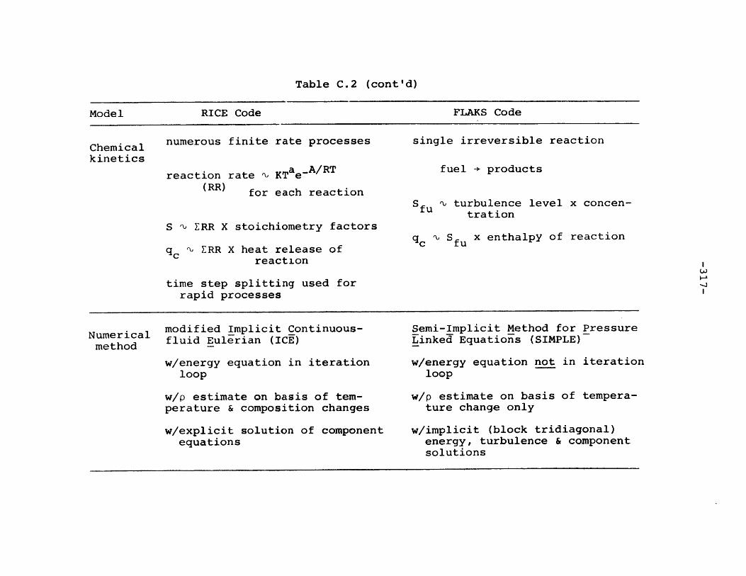
Table C.2 (cont'd)

RICE Code FLAKS Code

numerous finite rate processes

reaction rate % KTae - A/RT

(RR) for each reaction

S E CRR X stoichiometry factors

q % ERR X heat release ofreaction

time step splitting used forrapid processes

modified Implicit Continuous-fluid Eulerian (ICE)

w/energy equation in iterationloop

w/p estimate on basis of tem-perature & composition changes

w/explicit solution of componentequations

single irreversible reaction

fuel - products

S fu turbulence level x concen-tration

qc % Sfu x enthalpy of reaction

Semi-Implicit Method for PressureLinked Equations (SIMPLE)

w/energy equation not in iterationloop

w/p estimate on basis of tempera-ture change only

w/implicit (block tridiagonal)energy, turbulence & componentsolutions

Model

Chemicalkinetics

Numericalmethod

-318-

law as shown. The sum of the products of reaction rate and

heat release constitute the energy source term. The FLAKS

chemistry is significantly simpler in that mass source

strength is computed on the basis of empirical constants

and turbulence level.

The numerical techniques have some notable departures.

The basic SIMPLE routine is kept intact in FLAKS such that

the energy equation (as well as component and turbulent

equations) solution is done outside of the major iterative

loop. The iterative loop involves converging to a con-

sistent velocity, pressure and density field with the esti-

mated pressure correction due to state changes accomplished

through an explicitly derived sound speed. This is similar

to the original RICE version described by Butler and

O'Rourke. However, Westbrook states that not including the

energy equation in the iterative loop can cause inaccura-

cies due to the intimate coupling of energy and momentum

transfer in reactive flows. He also suggests that the

updated pressure estimate should be based not only on den-

sity effects (explicit sound speed approach) but also com-

positional changes.

Finally, the RICE authors also report an artificial

deflagration wave thickening technique which alleviates the

need for very fine calculational meshes. The FLAKS authors

have reported physica'ly reasonable simulations of shock

tube problems and also furnace type environments. The RICE

-319-

authors have published simulations of combustion chambers

and general obstacle flow geometries. For problems in

which experimental data was available, most discrepancies

were less than 20%.

The proper treatment of turbulence is of central

importance in these problems. Neither model seems superior

to the other in the cases reported. The limitations of an

eddy diffusivity approach are well known. However, the use

of a more complex model does not guarantee a commensurate

accuracy gain since the closure constants were probably

derived from incompressible pipe or duct flow which is

phenomenologically distinct from reactive flows. On the

basis of physical intuition, however, if one should go to

a higher order model as has been done in FLAKS, buoyancy

effects should be included since they are a dominant

physical mechanism in flows of such heightened thermicity.

C.4 Outline of a Composite Model

The information presented in the previous sections can

be used to outline a composite analytical model of reacting

flows in a post-accident nuclear containment environment.

The limitations of the model are the following. First, the

hydrogen source strength and location are known a priori.

Second, the model will not be used in detailed studies of

deliberate ignition device placement and operation. As

stated in C.2.1, such efforts should rely heavily on

-320-

experimental studies. Third, flame structure and small

scale combustion-turbulence interaction are not modelled

in greater detail than is required to produce reasonable

macroscopic predictions. Finally, detonation wave propa-

gation is not of central concern.

The desirable characteristics of a model falling

within this scope are grouped into four categories - basic

conservation equations, turbulence, chemistry and numerical

method. The most important requirement of the conservation

equations is their compressible formulation. Though this

is a more difficult approach than a Boussinesq-type

analysis, it is crucial for the correct prediction of the

local state and its effect on chemical kinetics. Second,

turbulence effects (augmentation of transport processes)

should be included in the mass, momentum and energy

balances since the strong buoyancy induced by exothermic

reactions as well as the complex problem geometry make

turbulent flow unavoidable. The inclusion of viscous

dissipation should be carefully considered. It may be

valid to neglect this term as done by Hjertager but an

order of magnitude analysis would be helpful in justifying

this approach. Since the problem involves at least four

components (hydrogen, air, steam and liquid), the indi-

vidual transport equations of the RICE code are favored.

This is especially trve when the rate effect of steam con-

centration is recalled. As such, evaporation and

-321-

condensation need be included in the model.

The question of proper turbulence modelling can not

be fully answered given the present state of the art. The

complex flow field itself does suggest the use of a more

sophisticated model and buoyancy effects should be

included. The basic problem physics calls for the inclu-

sion of buoyancy since the time averaged equations contain

terms involving the correlation of density and velocity

(and density and temperature) fluctuations. While these

terms are not usually important in thermal hydraulic prob-

lems, they are significant in turbulent reactive flows.

The chemistry modelling should also properly reflect the

dependence of the reaction rate on local steam concentra-

tion. Therefore, modelling the chemical kinetics through

the use of rate equations as in the RICE formulation is

desirable. An analysis of the relevant reaction steps in

light of the expected global conditions may lead to sig-

nificant simplicification in this area such as reducing

the required number of kinetic equations.

Numerical method selection remains part art and part

science. Two general points do emerge from the material

presented. The first involves the computational coupling

of the energy equation to the momentum and continuity

equations. Westbrook argues that since this coupling is

physically strong, the numerics (embodied in the simul-

taneous nested iterative solution of the three) should

-322-

reflect the same. This is seen to be a valid constraint.

Second, both the RICE and FLAKS programs were formulated

so that the calculational time step was not limited by the

sound speed. This is highly desirable for economical com-

putation of subsonic flows and therefore should be

employed. Again, Westbrook points out the pressure

updating algorithm to accomplish this goal should include

not only sound speed corrections but also compositional

effects. The uncoupled solution of the remaining equations

seems reasonable given the smaller degree of physical

coupling involved.

The modelling framework described itbove should have an

applicability range from pre-chemical reaction flow through

strong deflagration propagation. Given this broad scope,

the model developer should fine tune the appraoch if one

physical regime is dominant. For example, the energy/

momentum-continuity coupling may be relaxed to the ICE or

SIMPLE method in pre-chemical reactive flow. Chemical

kinetics can also be simplified and viscous dissipation

neglected in certain situations. Such refinement would

improve the computational efficiency of the analysis with-

out much loss of accuracy.

C.5 Conclusions

A logical extens'on of the research effort reported

in the main body of this work is to include chemical

-323-

reactions in the analytical models. A review of the state

of the art leads to the conclusion that a physically rea-

sonable modelling approach is difficult but achievable and

some consideration of desirable model characteristics are

addressed. Chief among these are - the momentum/energy

transfer coupling should be tight; turbulence modelling

must reflect the physical picture of a reacting flow

especially through buoyancy; steam transport must be

addressed in both the conservation and chemical kinetic

formulations; the global state constraints may simplify

the chemistry modelling; numerical technique should con-

sistently reflect the physics; and ancillary modelling of

particular effects such as phase change needs to be

included.

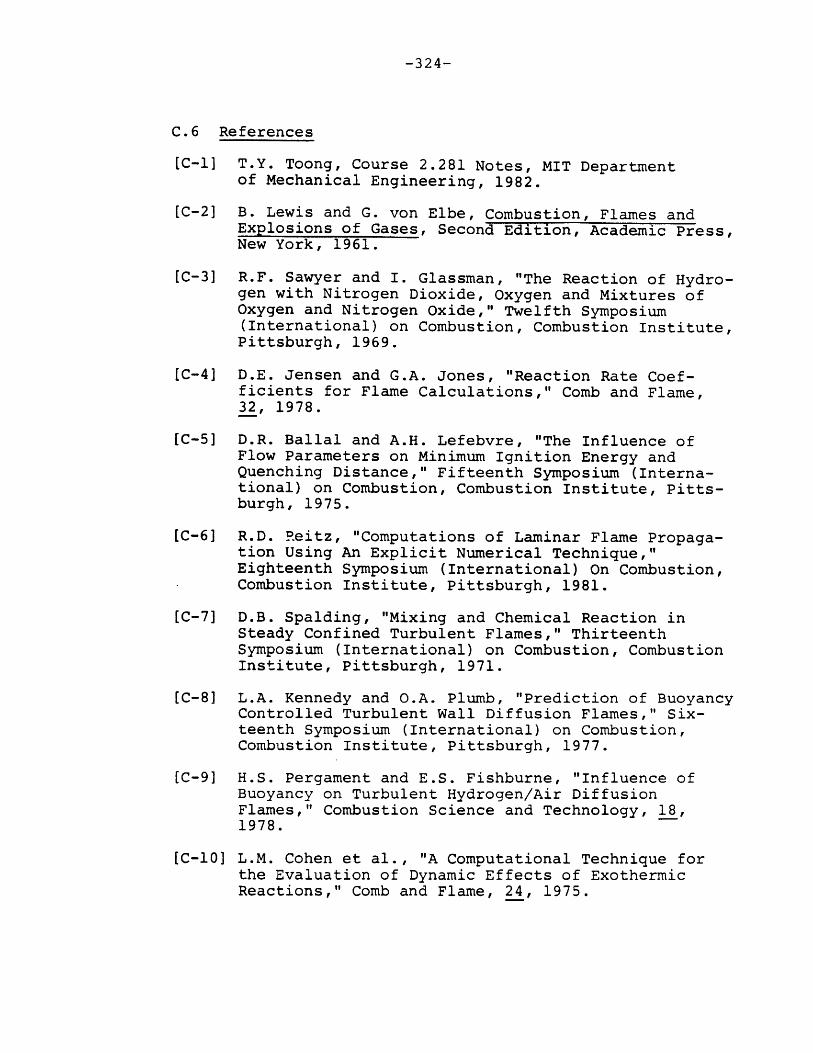
-324-

C.6 References

[C-l] T.Y. Toong, Course 2.281 Notes, MIT Departmentof Mechanical Engineering, 1982.

[C-2] B. Lewis and G. von Elbe, Combustion, Flames andExplosions of Gases, Second Edition, Academic Press,New York, 1961.

[C-3] R.F. Sawyer and I. Glassman, "The Reaction of Hydro-gen with Nitrogen Dioxide, Oxygen and Mixtures ofOxygen and Nitrogen Oxide," Twelfth Symposium(International) on Combustion, Combustion Institute,Pittsburgh, 1969.

[C-4] D.E. Jensen and G.A. Jones, "Reaction Rate Coef-ficients for Flame Calculations," Comb and Flame,32, 1978.

[C-5] D.R. Ballal and A.H. Lefebvre, "The Influence ofFlow Parameters on Minimum Ignition Energy andQuenching Distance," Fifteenth Symposium (Interna-tional) on Combustion, Combustion Institute, Pitts-burgh, 1975.

[C-6] R.D. Reitz, "Computations of Laminar Flame Propaga-tion Using An Explicit Numerical Technique,"Eighteenth Symposium (International) On Combustion,Combustion Institute, Pittsburgh, 1981.

[C-7] D.B. Spalding, "Mixing and Chemical Reaction inSteady Confined Turbulent Flames," ThirteenthSymposium (International) on Combustion, CombustionInstitute, Pittsburgh, 1971.

[C-8] L.A. Kennedy and O.A. Plumb, "Prediction of BuoyancyControlled Turbulent Wall Diffusion Flames," Six-teenth Symposium (International) on Combustion,Combustion Institute, Pittsburgh, 1977.

[C-9] H.S. Pergament and E.S. Fishburne, "Influence ofBuoyancy on Turbulent Hydrogen/Air DiffusionFlames," Combustion Science and Technology, 18,1978.

[C-10] L.M. Cohen et al., "A Computational Technique forthe Evaluation of Dynamic Effects of ExothermicReactions," Comb and Flame, 24, 1975.

-325-

[C-ll] E.S. Oran et al., "Application of Time DependentNumerical Methods to the Description of ReactionShocks," Seventeenth Symposium (International) onCombustion, Combustion Institute, Pittsburgh, 1979.

[C-12] E.S. Oran et al., "Numerical Simulation of Detona-tions in Hydrogen-Air and Methane-Air Mixtures,"Eighteenth Symposium (International) on Combustion,Combustion Institute, Pittsburgh, 1981.

(C-13] H.W. Emmons, "Fire," Sixth International Meeting ofApplied Mechanics Proceedings, 1977.

[C-14] B.R. Morton, "Modeling Fire Plumes," Tenth Sympo-sium (International) on Combustion, CombustionInstitute, Pittsburgh, 1965.

[C-15] T.D. Butler and P.J. O'Rourke, "A Numerical Methodfor Two Dimensional Reacting Flows," SixteenthSymposium (International) on Combustion, CombustionInstitute, Pittsburgh, 1977.

[C-16] W.C. Rivard et al., "The Transient Dynamics ofChemically Reactive Gaseous Mixtures With Turbu-lence," Lecture Notes in Physics, 35, 1975.

[C-171 C.K. Westbrook, "A Generalized ICE Method forChemically Reactive Flows In Combustion Systems,"J. Comp. Physics, 29, 1978.

[C-18] B.H. Hjertager, "Simulation of Transient Compres-sible Turbulent Reactive Flows," Comb. Science andTechnology, 27, 1982.

-326-

APPENDIX D

IMPORTANT CONSIDERATIONS FOR ASSESSING AN

IMPLICIT SLOW MIXING SOLUTION SCHEME

The main body of this work has demonstrated the

capabilities of the explicit slow mixing solution methodol-

ogy. The explicit method does incur two important limita-

tions--Courant time-step stability limit and incomplete

numerical diffusion correction. An implicit formulation

has the potential to address both these constraints. The

relaxation of the Courant limit would allow more economical

simulation while Huh [D-l] suggests that an implicit scheme

could completely compensate for numerical diffusion with

unconditional stability. The potential negative aspects

of the implicit approach are increased computational

effort, unknown stability limits when linearizations are

required, increased programming complexity and potential

unphysical (but stable) solution modes. The purpose of

this appendix is to summarize the important points in this

regard, describe one possible momentum equation treatment

and provide guidance for future more detailed studies.

An implicit solution scheme requires substantially

more computational work per time step than an explicit

scheme due to the simultaneous nature of the implicit

equations. The momercum equation is particularly limiting

in this regard due to its vectorial nature and the non-

-327-

linearity of the convective terms. A fully implicit

numerical formulation of the momentum equation leads to

a very large non-linear set of coupled algebraic equations.

The solution of such a set by either direct or iterative

means is impractical for typical problem discretizations.

A more fruitful approach is linearization of the convec-

tive terms and application of a fractional step method

such as the Alternating Direction Implicit(ADI) scheme.

A typical convective linearization is

n+l n+lau un(Ui+l-U

u - un ( . (D.1)ax 5x

While this linearization renders the problem tractable,

it introduces a degree of explicitness which in turn

compromises the unconditional stability of the method.

A few investigators including Huh have found stability

limits in the range of Courant numbers of 2 or 3. The

passive transport equations (energy, components, turbu-

lence) do not require any linearization approximation.

The central question to be considered is to quantify the

amount of effort required to carry out a single implicit

cycle compared to 2 or 3 explicit cycles. One must keep

in mind that an implicit treatment of the slow mixing model

involves 30 directional sweeps (i.e., matrix inversions)

per cycle.

A multipass ADI treatment of the transport equations

has been presented in Chapter 3. The following formulation

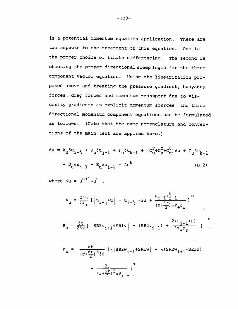
-328-

is a potential momentum equation application. There are

two aspects to the treatment of this equation. One is

the proper choice of finite differencing. The second is

choosing the proper directional sweep logic for the three

component vector equation. Using the linearization pro-

posed above and treating the pressure gradient, buoyancy

forces, drag forces and momentum transport due to vis-

cosity gradients as explicit momentum sources, the three

directional momentum component equations can be formulated

as follows. (Note that the same nomenclature and conven-

tions of the main text are applied here.)

6u = A u. i+ B 6Uj+ + Fu6k+ + (Cr+Cz+C )6u + G 6u + u +1 u k+l u u u u G k-l

+ D 6u + E 5u + AuE (D.2)u j-1 u i-

n+l nwhere 6u = u -u ,

A 6r [ ui+.+uj - ui+. -2u + ]Au=U + - +- 6r+ (r+ 6) Sr p

2 ( +1

Bu [ SR2vi +SRlv -(SR2v i ) +u 26z +1 i+ 6z +Pr

F = [ SR2w i++SRlwj - (SR2w i+l+SRlw)(r+T) 66

2 2

+ -+ I(r+ ) 6e p2 + r

-329-

r 26t - _U+ui_u 6r 1-

1 i+1ri+1 pr Hr il6 + l

pr(r+) i+1

C z [-j SR2vi+1+SRlv - SR2vi+1 +SRV.

- (SR2v i++SRIv) + (SR2vi+lj-+SlRvj_ )

2 (IJ+i +p 6z+ 6zr + I ,

C= [-SR2w. +SR1wI - ISR2w. +SRlw1 I2(r+--) 66

- (SR2wi+1+SRIw) + (SR2wi+k..

k - n+ SRlwk_) r lk-H

p-(r+ ) -+ +

G = 6t [ISR2w i+lk-+SR1wk I + (Syswi+lk-

2(r+--) 68

+ SRlw ) + 4 n(r+ ) p 68.

2 r -

D = 6t [SR2vi +SRv + (SR2v +SRlv )u 26z [- +- + S-+ j2

2(1+1iS j+ IPr _

-330-

E 6 [ l u + u l + u i - + 2 u + ( r ]

26 u+ i -+U. 2 (r+--) 6rp

Au = [-6t M + Aui+ + Buuj+ + Fuk+ + (Cr+CZ+C )up u +1 u k+ u u

+ GUk + DUj + Eui_ ] andu k-1 u j-1 1-2 I

Pr 2 2 aP ap au ay avM = [ (w -u D + pg + f + +u ar r Dr r r az r

S1u 1 ap aw w) 2 p aw- -- + ( ) 2

r r r r 6

6v = A 6v +B 6vj3 + E 6v + (C r+C+C )6vv i+l + v +2 v k+l v v v

+ G 6v + D 6v + EV 6v + Av , (D.3)v k-1 v - v i-i

n+1 nwhere 6v = v -v ,

A = 6t [ Sz2uj+. +Szlul - (Sz2uj+ +Szlu)

4(r+,) n

r pr 6r+ +

6t 4 j+l nB - [ vj++vj - vj+3 -2v +V 6z + + 2+ r6z j+1

F - 2r6 [ Sz2wj+l+Szlwl - (Sz2wj+,+Szlw)2r 66 I

+] ]nr 6+ ,

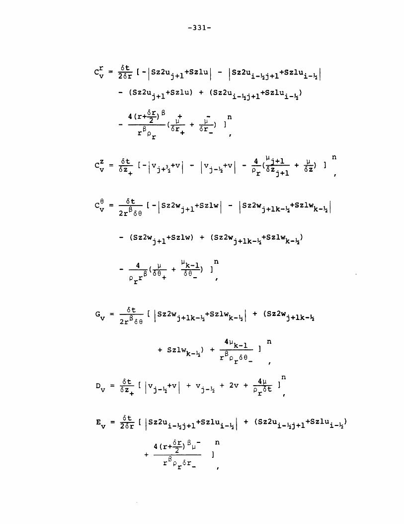
-331-

Cr 6t - Szu+Slu - S2u -j+. 1u +Szlu

- (Sz2u +Szlu) + (Sz2u . +Szlu.i )j+1+

6r4 (r+--) + - n

r + ]

Cz = 6t 4++v +v Tz - vj +v j- 6z+ 1r j 6

C 6t Sz2w +Sz2wszw +SzlwkIv 2r866 [Szwj + j+lk- k-

- (Sz2w j+l+Szlw) + (Sz2w j+lk_+Szlwk_ )

4 p Pk- n(T8 + 6e_) I

G - r6t[ ISz2w j+lk_+Szlw k1I + (Sz2wj+ik_v 2r 66 I i+1k k j+1k-

4p n+ Szlw ) + 4 Pk-1

6 k 8 _

D = [ Iv. +vl + vj. + 2v + -4v z - 3- pr t

6tE = 6t [ Sz2ui_ +Szlu. + (Sz2u i_ +Szlu_)

v 2To i-j+ i-i +

6r - n4(r+-) n

+ a rrBp 6rr -

-332-

AvE =[M + A v + B vj+v + +(C+C +C)vpv v i+1 vvk+ v v v

+ Gvvk- + Dv. + EVk- ]v k-1 V 3 v k-1 and

M = [- + + f + u +v I 3z z Dz Dr az az az

1 e aw+ i 7 - ]nr

6w = A 6w. + B w + F 6w + (Cr+C+C )6ww = i+1 w j+l w k+ w w w

+ Gw6w k + D 6w. + AwE- w j-1 (D.4)

n+l6w = wn- w

A 6t [ S62uk+l+Slu -

w 26r k+1t

w 26t vk+1+slvl

(se2uk+ +Selu)

(S62v k+l+Slv)k+1

4(r+-r) v+ 2

ra6r+Pr

+ 4pr 6 z

t [ wk+w - wk+w r 66 k+k++

4 k+1-2w + ir 6 k+l

Cr _6t IS82Sl - 2u-. 6kw 26r S2uk++S Iu - 2u i-k+l+S i-

- (Se 2uk+l+Selu) + (S 6 2 ui- k+l+S61ui_)

6rp (r+6-) p (r f-)

5r + 6rrp_ +

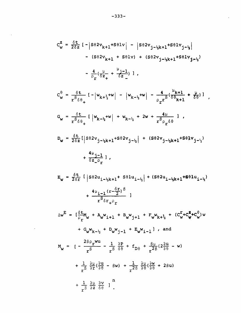
-333-

Cz 6t [ISe2v +Blvi ISo2v. 1 +Selv._1w 26z -k+ -k+ j4

(S2v k+1 + SOlv) + (S82vj- k+l+selv.1)

4 1

r + -

_ 0 6t w k+rw 66 + Pr k+1

G 6t [ +w + Wk + 2w + 4w r8 + rk Pr 6

+ rE = SAt + A w. + B w + F w + (Cr+CZ+ )w6z_6 r

S 6t [ S62v S0v + (S2ui_k++S1ui_)

w r w ik+1 l j k+ + w w

+Gwk +Dw +Ew i ,and

z 6ai6r+ rE t W + 1. + c cr+ ,Cw)

23WU 1 2P + +- ( 3uSwE fDB r-- W 2 w)

1 w u + w +1 aU(3w+ Gw 2+ Dw + 2u)r r r

1 u v n

r + 6 w.

-334-

The equations presented above define the basic matrix

problem. However, the proper directional sweeping logic

must be determined. A total of nine directional passes must

be performed and a proper sequencing chosen. It is expected

that the choice of sweep logic will affect not only accuracy

but also stability.

Implementation of this solution logic into the LIMIT

code is not a trivial exercise. An initial assessment of

this aspect leads to the suggestion that two rather large

subroutines are required. One would control the sweeping

logic and perform the matrix inversion while the other cal-

culates the direction and component dependent matrix coeffi-

cients and source terms. A final suggestion in this area is

to allow the ADI solution to be optional.

The last major area requiring study is the overall

question of unphysical solution behavior. The method pro-

posed hasn't been used in any major applications and the

potential for unphysical results has been identified by some

workers [D-l]. The unknown subtleties must be better under-

stood before this method can be applied to complex problems

such as hydrogen mixing analysis.

[D-l] K.Y. Huh, Treatment of Physical and Numerical Diffusionin Fluid Dynamic Simulations, Ph.D. Thesis, MIT Depart-ment of Nuclear Engineering, August 1983.

-335-

Appendix E: Additional Remarks On the Solution of

the Slow Mixing Model Energy Equation

Section 3.3.4.3 addresses the solution of the passive

entity transport equations in the slow mixing continuum

model. The general methodology described in that section

can be specialized to the energy equation (i.e., Eq. 3.43)

using the formulation presented here. In abbreviated

form, the energy conservation equation is:

ape + C = D (E.1)at

where C = convective terms and

D = diffusive (conduction) terms.

Expanding the temporal derivative and rearranging Eq. E.1

yields

ae app a - -C + D -e - - . (E.2)at at

For the other scalar transport equations which were

formulated in an incompressible manner, the last RHS term

of Eq. E.2 is approximated using the derivation presented

in the discussion preceding Eq. 3.145, i.e.,

ap- p V.u . (E..3)at

However since the energy equation is cast in a

conservative form, a more correct approach is to utilize

the compressible continuity equation for the value of the

temporal density derivation. Thus,

-336-

P -V-pu . (E.4)at

Using the established nomenclature, the finite difference

approximation for this term is

a 8r.i+(pa+i+ 8+) - r. i(p i

a +p)eV*pu = e[ i+1 -

rB Sr

(py +p j 6 ) - (P 1 Y+p6_)+ ++1 + j-1

6z

X(pe +p a -p E -po )+ P+Pk++-k---P-)] . (E.5)

rt60