VILNIUS GEDIMINAS TECHNICAL UNIVERSITY

VILNIUS GEDIMINAS TECHNICAL UNIVERSITY

FACULTY OF ENVIRONMENTAL ENGINEERING

DEPARTMENT OF GEODESY AND CADASTRE

Eugenijus Streikus

3D MIESTO MODELIAVIMAS NAUDOJANT LiDAR DUOMENIS IR GIS

TECHNOLOGIJŲ ANALIZĘ

3D CITY MODELLING USING LIDAR DATA AND GIS TECHNOLOGIES

FEATURES ANALYSIS

Master‘s degree Thesis

Innovative Solutions in Geomatics, joint study programme, state code 6281EX001

Measurement engineering study field

Vilnius, 2019




APPROVED BY

Head of Department ______________________

(Signature) Jūratė Sužiedelytė-Visockienė

(Name, Surname) ______________________

(Date)

Eugenijus Streikus

3D CITY MODELLING USING LIDAR DATA AND GIS TECHNOLOGIES

FEATURES ANALYSIS

Master‘s degree Thesis



Supervisor prof. dr. Eimuntas Kazimieras Paršeliūnas _________ ________ (Title, Name, Surname) (Signature) (Date)

Vilnius, 2019




APPROVED BY

Head of department

_________________________ (Signature)

Jūratė Sužiedelytė-Visockienė (Name, Surname)

_______________________ (Date)

OBJECTIVES FOR MASTER THESIS

.......………...No. ................

Vilnius

For student Eugenijus Streikus (Name, Surname)

Master Thesis title: 3D city modelling using LIDAR data and GIS technologies features analysis.

Approved on 29 November, 2018 by Dean‘s decree No. 192ap (day, Month) (year)

The Final work has to be completed by ................................................., 201..... (Day, Month) (Year)

THE OBJECTIVES:

Perform analysis of literary sources on the topic of Master's thesis. Examine the peculiarities and principles

of airborne laser scanning. Review what affects data accuracy. Find out what LiDAR data formats are used

in GIS software and compare scan data of 2007 and 2018. Perform and describe in detail the 3D city

modelling process using existing LiDAR data and GIS technologies. Create scripts, models and CGA rules

for 3D city modelling and adapt them using ArcGIS Pro and CityEngine environment……………………….

..................................................................................................................................................................……....

.............................................................................................................................................................…….........

...................................................................................................................................................................……...

...............................................................................................................................................................…….......

...................................................................................................................................................................……...

...................................................................................................................................................................……....

Consultants of the Master Thesis: ………………………………………………………………….……………

................................................................................................................................................................……....... (Title, Name, Surname)

Academic Supervisor ................................ prof. dr. Eimuntas Kazimieras Paršeliūnas (Signature) (Title, Name, Surname)

Objectives accepted as a guidance for my Master Thesis

………………………………….. (Student‘s signature)

Eugenijus Streikus (Student‘s Name, Surname)

……………………………..….... .

(Date)



Baigiamojo darbo anotacija lietuviu

Baigiamojo darbo anotacija anglu

Saziningumo deklaracija

7

CONTENTS

1. PRINCIPLES OF LIDAR REMOTE SENSING ....................................................................... 14

1.1. Basics of airborne laser scanning ........................................................................................ 14

1.2. Principle of airborne laser scanning .................................................................................... 14

1.3. Lidar accuracy ..................................................................................................................... 15

1.4. Lidar data formats ................................................................................................................ 16

1.5. Overview of LiDAR data in Lithuania ................................................................................ 19

2. 3D CITY MODELLING ............................................................................................................. 21

2.1. Building extraction .............................................................................................................. 22

2.1.1. Creating a LAS dataset ................................................................................................. 22

2.1.2. DTM raster generation ................................................................................................. 24

2.1.3. DSM raster generation ................................................................................................. 26

2.1.4. nDSM raster generation ............................................................................................... 27

2.1.5. Building footprints extraction ...................................................................................... 28

2.1.6. Calculation of building geometry parameters .............................................................. 30

2.1.7. Segmentation of building roof parts ............................................................................. 34

2.1.8. CGA rule creation for buildings ................................................................................... 36

2.1.9. Confidence measurement ............................................................................................. 41

2.1.10. Manual Editing ............................................................................................................. 43

2.2. Road extraction .................................................................................................................... 46

2.3. Vegetation extraction ........................................................................................................... 51

2.4. Sharing ................................................................................................................................. 57

CONCLUSION .................................................................................................................................. 58

REFERENCES ................................................................................................................................... 60

APPENDIXES ................................................................................................................................... 65

8

LIST OF FIGURES

Figure 1. Principle scheme of airborne laser scanning (Petrie 2011) ................................................. 15

Figure 2. Example of LiDAR data in ASCII data files. The numbers in each row are: (a) x, y, z; (b)

GPS time, x, y, z, intensity. ................................................................................................................ 16

Figure 3. LiDAR points rendered by elevation (top) and RGB (bottom) spectral values .................. 18

Figure 4. Case study area ................................................................................................................... 22

Figure 5. Flowchart of 3D building extraction ................................................................................... 22

Figure 6. Generated LAS dataset statistics of study area ................................................................... 23

Figure 7. 2D and 3D view of LiDAR data (displayed by elevation and intensity) ............................ 24

Figure 8. Comparing input LAS dataset (displayed by coding values) and output DTM raster

(displayed by elevation values) .......................................................................................................... 26

Figure 9. Comparing input LAS dataset (displayed by coding values) and output DSM raster

(displayed by elevation values) .......................................................................................................... 27

Figure 10. DSM, DTM, and nDSM (Mirosław-Świątek et al 2016) ................................................. 27

Figure 11. Generated nDSM raster (displayed by elevation) ............................................................. 28

Figure 12. Rasters representing building footprints. Elevation raster (left), single value raster (right)

............................................................................................................................................................ 29

Figure 13. Extracted building polygon features ................................................................................. 29

Figure 14. Comparison of extracted building footprints (orange – from nDSM, green – from

classified LiDAR) .............................................................................................................................. 30

Figure 15. nDSM with elevation threshold ........................................................................................ 30

Figure 16. Slope raster of building areas ............................................................................................ 31

Figure 17. Aspect rasters (at left - general aspect raster, at right – reclassified aspect raster) .......... 31

Figure 18. Building base elevation calculation (DTM in background, green – building footprints,

blue circles – building centers) ........................................................................................................... 32

Figure 19. Eave height calculation (in background clipped building DSM raster, green – sloped roof

planes, purple – largest roof slope plane, red circles – largest roof plane points) ............................. 33

Figure 20. Flat (red colour) and not flat (blue colour) building areas ................................................ 34

Figure 21. Input building footprint polygons and intermediate segmentation results ....................... 35

Figure 22. Input building footprints (left) and segmented building footprints (right) ....................... 35

Figure 23. Supported CityEngine data formats (Ribeiro et al 2014) ................................................. 37

Figure 24. CityEngine scene creation wizard ..................................................................................... 37

Figure 25. CityEngine main window ................................................................................................. 38

Figure 26. Defining attributes ............................................................................................................ 38

Figure 27. Extrusion rule example ..................................................................................................... 39

Figure 28. Building splitting into parts .............................................................................................. 39

Figure 29. Describing facades ............................................................................................................ 39

Figure 30. Defining roof form ............................................................................................................ 39

Figure 31. Modelling rule for roof types ............................................................................................ 40

Figure 32. Inspection view and applied rule in CityEngine ............................................................... 41

Figure 33. Individual model inspection .............................................................................................. 41

Figure 34. Active 3D building layer and attribute connections in ArcGIS Pro ................................. 42

Figure 35. Building footprints visualisation by RMSE (from low to high (green to red)) ................ 43

Figure 36. Building geometry errors caused by vegetation ............................................................... 43

Figure 37. Misaligned building, editing footprint vertices, modified footprint ................................. 44

Figure 38. Multiple roof parts segmentation errors and modified segments ..................................... 44

Figure 39. Segmented building with single height value and original LiDAR data .......................... 45

9

Figure 40. LiDAR point pop-up window ........................................................................................... 45

Figure 41. Building segment attributes and modified building .......................................................... 46

Figure 42. Flowchart of roads extraction ........................................................................................... 47

Figure 43. Intensity raster ................................................................................................................... 47

Figure 44. Binary image of ground points with NoData values (white) ............................................ 48

Figure 45. Intensity raster of ground points ....................................................................................... 49

Figure 46. Segmented image by SVM classifier ................................................................................ 50

Figure 47. Road network with calculated mean values of segmented raster ..................................... 50

Figure 48. Final result of extracted road areas (and some other ground features) ............................. 51

Figure 49. Multiple return explanation (A Complete Guide to LiDAR 2018) .................................. 52

Figure 50. Different individual tree detection methods based on LiDAR-derived raster surface

(Moradi et al 2016) ............................................................................................................................. 52

Figure 51. ArcGIS pro model for individual tree extraction .............................................................. 53

Figure 52. CHM explanation (Wasser 2018) ..................................................................................... 53

Figure 53. Generated DTM, DSM and CHM rasters ......................................................................... 54

Figure 54. Part of CHM raster before (left) and after (right) applying local maxima ....................... 54

Figure 55. Curvature raster points and aggregated polygons ............................................................. 55

Figure 56. Flow direction raster, flow direction raster overlaid with sink raster (orange), filtered

treetop points ...................................................................................................................................... 55

Figure 57. Thiessen (red) polygons separating tree (green) crowns (blue) ........................................ 56

Figure 58. Principle of tree crown diameter information extraction .................................................. 56

Figure 59. Extracted 3D trees ............................................................................................................. 57

10

LIST OF TABLES

Table 1.4.1. LAS 1.4 format definition .............................................................................................. 17

Table 1.4.2. An example of point data record format ........................................................................ 17

Table 1.4.3. ASPRS Standard LiDAR Classes (Point data record formats 6-10) .............................. 18

Table 1.5.1. Comparison of LiDAR data technical characteristics .................................................... 20

11

LIST OF ABBREVIATIONS

LIDAR Light Detection and Ranging

GPS Global Positioning System

DGPS Differential Global Positioning System

IMU Inertial Measurement Unit

RMSE Root Mean Square Error

ASCII American Standard Code for Information Interchange

ASPRS American Society for Photogrammetry and Remote Sensing

VLR Variable Length Record

EVLR Extended Variable Length Record

GIS Geographic Information System

12

INTRODUCTION

Relevance of the work. Within a time of only two decades airborne laser scanning have well

established surveying techniques for the acquisition of (geo) spatial information. A wide variety of

instruments is commercially available, and a large of companies operationally use airborne scanners,

by many dedicated data acquisition, processing and visualisation software packages. The high quality

3D point clouds produced by laser scanners are nowadays routinely used for a diverse array of

purposes including the production of digital terrain models and 3D City models, forestry sector,

corridor mapping, etc. However the publicly accessible knowledge on laser scanning is distributed

over a very large number of scientific publications, web pages and tutorials. With sensor resolution,

point clouds acquired by airborne laser scanners nowadays dense enough to also retrieve detailed on

detection and extraction 3D of buildings and other urban-specific features.

Every day, planners use geographic information system (GIS) technology to research, develop,

implement, and monitor the progress of their plans. GIS provides planners, surveyors, and engineers

with the tools they need to design and map their neighbourhoods and cities. Planners have the

technical expertise, political savvy, and fiscal understanding to transform a vision of tomorrow into

a strategic action plan for today, and they use GIS to facilitate the decision-making process.

Planners have always been involved in developing communities. Originally, this meant designing

and maintaining cities and counties through land use regulation and infrastructure support. Agencies

have had to balance the needs of residential neighbourhoods, agricultural areas, and business

concerns. Now, in addition to that complex challenge, local governments must factor into these

decisions the requirements of a growing list of regional, state, and federal agencies as well as special

interest groups.

Rapidly changing economic conditions have further complicated the process by threatening the

funding needed to carry out these functions. To date, local governments have been rightsized and

downsized and have had budgets drastically cut while trying to maintain service levels. Information

technology, especially GIS, has proven crucial in helping local governments cope in this environment.

ESRI software solutions help planning, building and safety, public works, and engineering

professionals meet or exceed these demands. ESRI ArcGIS Pro and CityEngine software is one of the

local governments’ options for mapping and analysis. Using this software, planning agencies have

already discovered how traditional tasks can be performed more efficiently and tasks - previously

impractical or impossible - can be easily accomplished.

The objective of this work is to give a comprehensive overview of the principles how airborne

laser scanning technology and 3D point clouds acquired by laser scanners can be served for 3D city

modelling and urban features reconstruction using GIS technology.

13

Work objective. Perform an analysis of the features of 3D city modelling in GIS environment.

Work tasks:

1. Examine the peculiarities and principles of airborne laser scanning. Review what affects data

accuracy. Find out what LiDAR data formats are used and compare scan data of 2007 and

2018.

2. Perform and describe in detail the 3D city modelling process using existing LiDAR data and

GIS technologies.

3. Create scripts, models and CGA rules for 3D city modelling and adapt them using ArcGIS

Pro and CityEngine environment.

Object of research. 1 km x 1 km area of Vilnius city center.

Research methodology. Practical application and processing of LiDAR data, and features

extraction data using GIS technologies.

Scientific novelty. In Lithuania, 3D city GIS models are not used, offered technique and

methodology how this can be done in practice.

Practical importance of scientific work, its applicability. Analyse and describe the 3D city

modelling using existing LiDAR data and GIS technologies. Provide practical application of the

obtained results.

Publications and reports on conferences were published on the topic of the final work. 21st

conference for Junior Researchers “Science – Future of Lithuania”, civil engineering and geodesy,

on March 23, 2018, an article was published, entitled “3D building modelling by LiDAR data and

GIS technologies”. The article is included in the appendixes.

Scope and structure of the work. The Final Thesis consists of four parts: introduction, two

chapters, conclusions, bibliographic resources.

Scope of Thesis: 58 pages of text without appendixes, 59 figures, 4 tables, 42 bibliographic

resources.

Appendixes included.

14

1. PRINCIPLES OF LIDAR REMOTE SENSING

LiDAR is a remote sensing technology that detects the distances (or ranges), based on the time

from laser signal transmission and reception. In practice, pulsed or continuous wave lasers are used:

pulsed lasers transmit energy for a very short time and determine ranges based on amplitudes of

received signals; on the contrary, continuous wave lasers detect ranges according to phase differences

between transmitted and received signals (Baltsavis 1999b).

1.1.Basics of airborne laser scanning

Over the past decades, topographic laser profiling and scanning systems have evolved rapidly

and have undoubtedly become an important technology for collecting geographic data. Equipped with

both on-air and on-board platforms, these systems can collect clear 3D data in large quantities without

any precedent. The complexity of the measured laser data processing is not high, which has led to a

rapid spread of this technology to various applications. Although the invention of the laser begins in

the early 1960s (Nelson 2014), the lack of a variety of supportive technologies has prevented the use

of this device from mapping for decades.

At the end of the nineties, already having GPS, a method was developed to accurately determine

the situation and orientation in large areas. By introducing a differential GPS (DGPS), the scanner's

position has become known in horizontal and vertical coordinates in the subdecimeter range (Krabill

1989, Friess 1989). Improvements to DGPS technology, combined with Kalman filtering and IMU

use, have been precise enough since the early 1980s (Lindenberger 1989, Schwarz et al 1994,

Ackermann 1994). Standard height data accuracy increased by +10 cm and +50 cm. By the end of

the 1980s, measurements were made by means of laser profilers (Ackermann 1988, Lindenberger

1993), providing laser pulses but without a scanning mechanism. Since early 1990s, profilers were

replaced with scanning devices that generated from 5000 to 10,000 laser pulses per second.

Nowadays, laser pulse rates can reach 300 kHz frequency.

1.2.Principle of airborne laser scanning

Airborne laser scanning is performed from a fixed wing aircraft or helicopter. This technique is

based on two main components: 1. A laser scanner system that measures the distance to a location on

the ground. 2. The GPS/IMU combination that accurately measures the position and orientation of

the system. Laser scanning systems are relatively independent of the sun and can be performed during

daytime or at night. This characteristic is a great advantage comparing to other ways of measuring

landscapes.

15

The aircraft's laser scanner is completed by a GPS ground station. The ground station acts as a

reference station for separate differential GPS (DGPS) calculations. DGPS is very important in

compensating for atmospheric effects, preventing accurate positioning and achieving decimetre

accuracy In order to cope with different atmospheric conditions and obtain better results, the distance

between the aircraft and the GPS ground station must not exceed 30 km (although sometimes the

correct accuracy is achieved over long distances).

Airborne laser scanners can be complemented by a digital camera system. Image data received

along with range data makes it easier to interpret data in cases where it is difficult to recognize objects

only from range data. Image data generally provides better spatial resolution and provides the basis

for an integrated 3D point cloud and image processing. The optimal location for the camera is on the

scanner assembly’s ground plate, because then the existing IMU registrations can be shared for

georeferencing images.

Figure 1. Principle scheme of airborne laser scanning (Petrie 2011)

1.3.Lidar accuracy

In practice, LIDAR accuracy is checked by comparing known points (measured) with laser scan

data and defined as the standard deviation (σ2) and root mean square error (RMSE) (Csanyi & Toth

2007).

According to Csanyi & Toth, modern LiDAR technology can reach several centimetres accuracy

in ideal conditions, and this precision is sufficient for most engineering topographical works.

16

However, the desired accuracy is limited due to a navigation-based sensor platforms, as well as the

LiDAR system consisting of a variety of multisensory and components, even after both the system

and individual sensor calibration work can be identified certain errors which degrades the final

accuracy of LiDAR data. The most common errors are navigation-based, these errors cannot be

avoided without data control, so for LiDAR-specific ground control points is recommended to use to

get the best results.

1.4.Lidar data formats

In the very first days when LiDAR data was collected and stored, many companies used a generic

American Standard Code interchange system (ASCII). However, using this format has encountered

some problems: (1) the reading and interpretation of ASCII data can be very slow and the file size

can be very high even for small amounts of data, all of which greatly affects performance. (2) Loss

of useful information is related to LiDAR data. (3) Format is not standard (Fig. 2).

Figure 2. Example of LiDAR data in ASCII data files. The numbers in each row are: (a) x, y, z; (b) GPS

time, x, y, z, intensity.

In order to better exchange LiDAR point cloud data, the American Society for Photogrammetry

and Remote Sensing (ASPRS) introduced the LAS file format. This is binary file format that

maintains information specific to the LiDAR nature of the data while being not very complex. The

ASPRS LAS 1.0 Format Standard was released on May 9, 2003; LAS 1.1 on May 7, 2005; LAS 1.2

on September 2, 2008; LAS 1.3 on October 24, 2010; and LAS 1.4 On November 14, 2011. Since

update (July 26 2013) of LAS 1.4 format the LiDAR mapping community has ability customize the

LAS file format to meet their needs. The mechanism that makes this available is the LAS Domain

Profile which is derivative of the base LAS 1.4 version specification that adds (but not removes alters)

point classes and attributes. The point cloud files used in the project are all in LAS format. The up-

to-date specifications of all LAS versions can be accessed on the website of ASPRS.

The structure of the LAS data file is described in detail in the LAS specification document

(ASPRS 2011). Each LAS file consists of a public header block. Any number of Variable Length

Records (VLRS), point data records, and any number of Extended Variable Length Records

17

(EVLRS). Tile public header block stores basic summary information such as boundary and the total

number of the points. VLR consists of information about map projection and other metadata. EVLR

is mainly used to store waveform data. EVLR started only from version 1.3 of the LAS. Public header

block and point data records are required, but VLR and EVLR are optional. Therefore, LAS files do

not necessarily include information such as the LiDAR data map projection. In this case, the user

must get information from metadata files, reports, or by data provider.

Table 1.4.1. LAS 1.4 format definition

LAS file section Note

Public header block Required

Variable length records (VLRs) Optional

Point data records Required

Extended Variable Length Records (EVLRs) Optional

Each point data record stores specific information such as the points x, y, z, intensity, return

number, number of returns (given pulse), scan direction, edge of flight line, classification, GPS time,

point source, etc. (Table 1.4.2). If the images were taken during the flight, the spectral values (e.g.

red, green, blue) can be also stored at the point data record. Spectral values useful for realistic

visualisation of the scanned landscapes (Figure 3).

Table 1.4.2. An example of point data record format

Item

X

Y

Z

Intensity

Return Number

Number of returns

Scan Direction Flag

Edge of Flight line

Classification

Scan Angle Rank (+90 to -90) -Left

side

User Data

Point Source ID

Red

Green

Blue

18

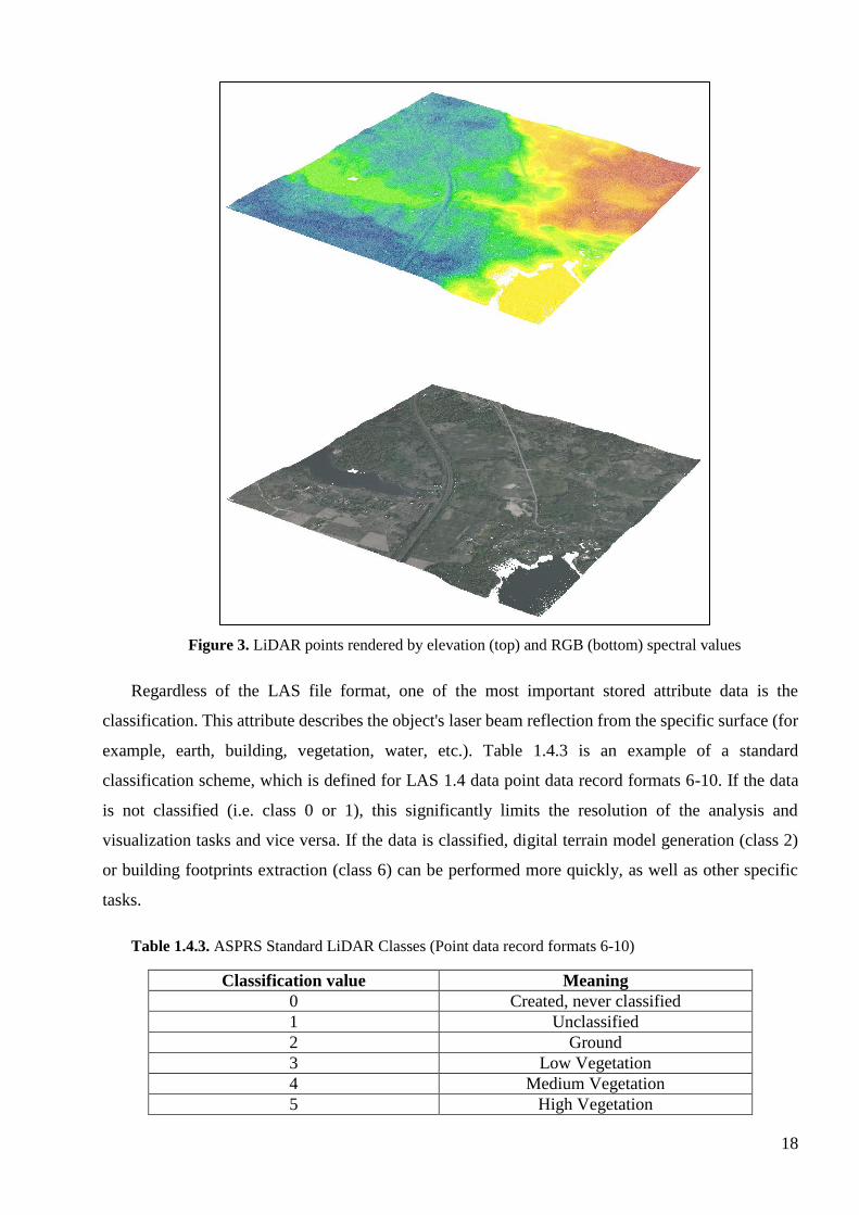
Figure 3. LiDAR points rendered by elevation (top) and RGB (bottom) spectral values

Regardless of the LAS file format, one of the most important stored attribute data is the

classification. This attribute describes the object's laser beam reflection from the specific surface (for

example, earth, building, vegetation, water, etc.). Table 1.4.3 is an example of a standard

classification scheme, which is defined for LAS 1.4 data point data record formats 6-10. If the data

is not classified (i.e. class 0 or 1), this significantly limits the resolution of the analysis and

visualization tasks and vice versa. If the data is classified, digital terrain model generation (class 2)

or building footprints extraction (class 6) can be performed more quickly, as well as other specific

tasks.

Table 1.4.3. ASPRS Standard LiDAR Classes (Point data record formats 6-10)

Classification value Meaning

0 Created, never classified

1 Unclassified

2 Ground

3 Low Vegetation

4 Medium Vegetation

5 High Vegetation

19

6 Building

7 Low Point (noise)

8 Reserved

9 Water

10 Rail

11 Road Surface

12 Reserved

13 Wire – Guard (Shield)

14 Wire – Conductor (Phase)

15 Transmission Tower

16 Wire-structure Connector (e.g. Insulator)

17 Bridge Deck

18 High Noise

19-63 Reserved

64-255 User definable

1.5.Overview of LiDAR data in Lithuania

In spring of 2007, at the order of the National Land Service under the Ministry of Agriculture,

for the first time in Lithuania were made 10 largest cities - county centers: Vilnius, Kaunas,

Marijampolė, Alytus, Klaipėda, Tauragė, Telšiai, Šiauliai, Panevėžys and Utena - a total of 2,475

km2 area (Žalnierukas et al 2009).

At the same time, a digital aerial photograph of large-scale urban areas was also made and

orthophotographic maps produced. The aim of the work is the creation of 3D urban models using

hybrid laser scanning and digital aerial photography technology. Airborne scans and

orthophotographs were produced by the French FIT Conseil - Géométres Experts. Ground

measurements were carried out by UAB InfoERA in Lithuania, and the quality control of production

was carried out by the Institute of Aerogeodesis.

Urban areas are scanned by the Optech ALTM 3100 scanner from Antonov-2. For ground

measurements, use the Z-Max GPS receivers (FIT Conseil 2007). The position is determined by the

Trimble 750 GPS Navigation System - Applanix POS/AV IMU.

When compiling the 2007 LiDAR data, the technical requirements foresee that there should be 4

fixed points per square meter, the average distance between the points is 0.50 m. The height

measurement accuracy shall not be less than 15 cm and the accuracy of the planimetric shall be 30

cm. The LiDAR laser radius measures from 1 to 3 cm to a hard surface (Kalantaitė et al 2010). Other

data for the flight: speed - 205 km / h; distance between lanes - 300 m; side overlay - 30%; laser dot

density 3-4 points per 1m2 (Žalnierukas et al 2009).

More than ten years later, the National Land Service under the Ministry of Agriculture carried

out LiDAR scanning work with orthophoto images for the same 10 largest county centers.

20

In accordance with the technical requirements (National Land Service under Ministry of

Agriculture, 2017), the number of points per square meter must be not less than 1.2, the average

square error of the horizontal position of the point is not more than 30 cm, the average square error

of the vertical position of the point is not more than 10 cm, scan angle - no more than +/- 25 degrees,

side overlay is not less than 30 percent. The comparison between the 2007 and 2018 LiDAR data is

shown in Table 1.5.1.

Table 1.5.1. Comparison of LiDAR data technical characteristics

Year of LiDAR data

Characteristics

2007 2018

File format *.xyz (ASCII) *.LAS (v1.2)

Classification Separate files (4 classes) 10 classes

Number of points (1m2) 4 12

Colorization - +

Horizontal mean square

error

No more 30 cm No more 30 cm

Vertical mean square error No more 15 cm No more 10 cm

Scanning bands

overlapping

30 % 30 %

Aerial mapping date 2009 2018 (not yet produced)

21

2. 3D CITY MODELLING

The digital three-dimensional city model generally describes the geometry of the city's

environment. Most commonly understood, the 3D city model combines information collections with

certain objects that can be used in urban environments, expressed in three dimensional geometry (e.g.,

urban projects, surfaces, vegetation, and 3D construction models). These patterns are usually created

through 3D reconstruction and data integration, for example, combining photogrammetry or laser

scan data with Geographic Information System (GIS) data such as building tracks, unique ID

numbers, or addresses.

3D city models can be used in many areas for tasks related to planning, environmental analysis,

transportation, service of communication companies, risk management, or simply visualization of

planned objects and decision-making. In addition, 3D city patterns can be seen as a factor in a smart

city connecting the user to a city environment system or service platform. Together with advanced

3D data acquisition systems and applications, 3D city patterns have become routine resources for city

geospatial data.

3D models are used in professional GIS tools or virtual globes. GIS platforms are typically

designed for professional users, such as city planners, architects, etc. The virtual world has 3D spatial

viewers, where the user can move freely and change the viewing angle or zooming (e.g., Google

Earth, ArcGIS Online). Without the need for special software, browser-based virtual globes are most

commonly used to target public audiences.

This 3D city modelling project was made using the 2018 LiDAR data. The analysis focuses on

the central area of the city, due to the variety of building types and their high elevation, relief changes,

and other specific features of the urban environment. The analysis of the territory of Vilnius city

consists of four LAS data files measuring 0.5 km x 0.5 km (Fig. 4). The main topics analysed are

digital terrain model generation, acquisition of 3D geometry of buildings, recognition of road

infrastructure, extraction of individual trees, and publication of results on the internet.

The products used by ESRI are ArcGIS Pro and CityEngine. ArcGIS Pro is a professional 2D and

3D mapping tool with intuitive user interface for visualization, analysis, image and data processing

as well as integration. CityEngine is an advanced 3D simulation software designed to create a vast,

interactive and visual urban environment. With this software, mass modelling is done much faster

than traditional methods.

22

Figure 4. Case study area

2.1. Building extraction

Manual modelling of buildings is not timely and financially effective, so automated and semi-

automatic processes are used to obtain results. Following the sequence of actions (Fig. 5), get 3D

buildings using ArcGIS platform.

Figure 5. Flowchart of 3D building extraction

2.1.1. Creating a LAS dataset

A LAS dataset (.lasd) is a stand-alone file that stores reference to one or more LAS files on disk

(What is LAS dataset? n.d.). A LAS dataset can also store reference to feature classes containing

surface constraints which could be breaklines, water polygons, area boundaries, or any other type of

surface feature enforced in the LAS dataset. There may be two additional files associated with an

LAS database: LAS auxiliary file (.lasx), and projection file (.prj) (Create LAS Dataset n.d.). A .lasx

file is created when statistics are calculated for any LAS file in an LAS dataset. The .lasx file provides

a spatial index structure that helps improve the performance of an LAS dataset. If LAS files do not

have a spatial reference or have an incorrect spatial reference defined in the header of the LAS file, a

projection file (.prj) can be created for each LAS file. In that case, the new coordinate system

LIDAR DATA

LAS DATASET

DTM DSM nDSMBUILDING

FOOTPRINTS

BUILDING GEOMETRY

PARAMETERS CALCULATION

SEGMENTATIONCGA RULE CREATION

CONFIDENCE MEASUREMENT

MANUAL EDITING

23

information in the .prj file will take precedence over the spatial reference in the header section of the

LAS file. Currently spatial reference system is defined already in the header of the LAS file, a

projection file (.prj) is not needed, and additionally LAS dataset statistics were calculated.

Figure 6. Generated LAS dataset statistics of study area

24

Figure 7. 2D and 3D view of LiDAR data (displayed by elevation and intensity)

2.1.2. DTM raster generation

A DTM is a 3D representation of a terrain’s surface in digital form (Karan et al 2014). According

GIS literature, the term DTM refers to the bare ground elevation points without any non-ground points

(e.g., buildings and vegetation). Generating a DTM from LiDAR points initial step is to separate the

points into ground and non-ground points. One of the most commonly used methods is to convert the

LiDAR point data into a digital image by gridding the data points. The LiDAR points in each grid

cell can have different elevations (z-values), for instance, the ground point elevation is lower than its

25

neighbour object points. In the case of hitting the ground surface, the minimum z-value of the LiDAR

points in a grid cell reflects the elevation of the bare ground.

Because a LiDAR point cloud is irregularly distributed, the smaller grid size results in more void

areas (i.e., cells with no data point) within the model. Karan et al pays attention that to have a desired

output, point density and number of LiDAR points should also be taken into account.

Interpolation is the procedure of predicting the value of attributes at unsampled site from

measurements made at point locations within the same area or region (Zouaouid et al 2016).

As reported IDW interpolation method creates DEM with less overall error compared to other

methods and the accuracy of DEM varies with the changes in terrain and land cover type. There are

many opinions regarding on which interpolation method produces the highest accuracy LiDAR DEM.

It can be seen that IDW and Kriging are the main competitors when it comes to producing DEM when

comparing RMSEs.

For the generation of DTM in the ArcGIS Pro environment, a LAS Dataset To Raster

geoprocessing tool was used. Main features described below:

Classification codes used: 2 (Ground), 9 (Water), 11 (Road surface);

Return values: 1;

Value field: Elevation;

Interpolation type: Binning (determines each output cell using the points that fall within

its extent);

Cell assignment: IDW (Inverse Distance Weighted interpolation);

Void fill method: Natural Neighbor (finds the closest subset of input samples to a query

point and applies weights to them based on proportionate areas to interpolate a value

(Sibson 1981));

Output data type: Floating point (32-bit floating point output raster);

Sampling type: Cell size (Defines the cell size of the output raster);

Sampling value: 0,2m (Resolution of output raster);

26

Figure 8. Comparing input LAS dataset (displayed by coding values) and output DTM raster (displayed

by elevation values)

2.1.3. DSM raster generation

The DSM includes all objects on the earth’s surface (Karan et al 2014). A terrain can be digitally

modelled either by a series of regular grid points (altitude matrices) or as a triangulated irregular

network (TIN). The former is a raster-based model consisting of a matrix of grids in which each grid

contains a value representing surface elevation. A TIN is a vector-based model of the surface that is

defined using a finite number of points in discrete formats in which each point is placed on the corner

of triangles or rectangles by its coordinates (i.e., three-dimensional coordinates (x; y; z) or two-

dimensional horizontal coordinates (x; y) and height (h)) (Wilson and Gallant 2000). Also, the data

source (e.g., field surveying, aerial imagery, or satellite images) greatly affects the distribution of the

reference points on the terrain.

For the generation of DSM with ArcGIS Pro, the same geoprocessing tool (LAS Dataset To

Raster) was used. Main features described below:

Classification codes used: 2 (Ground), 6 (Building), 9 (Water), 11 (Road surface);

Return values: 1;



its extent);


Void fill method: Natural Neighbor (finds the closest subset of input samples to a query

point and applies weights to them based on proportionate areas to interpolate a value

(Sibson 1981));




27

Figure 9. Comparing input LAS dataset (displayed by coding values) and output DSM raster (displayed

by elevation values)

2.1.4. nDSM raster generation

Subtraction a DTM from a DSM of the same area produces nDSM (normalised digital surface

model) (Mirosław-Świątek et al 2016) representing the heights of features from the surface. All

features placed on zero-elevation surface.

Figure 10. DSM, DTM, and nDSM (Mirosław-Świątek et al 2016)

Theoretically these features in nDSM should be zero or positive. However, it is very common to

have negative values due to accuracy issues in DTM and DSM, interpolation process or other

artefacts. In this case Minus geoprocessing tool was used for subtraction a DTM from a DSM.

Generated nDSM negative values reaches up to -10 meters. To fix this issue Raster Calculator

(mathematical computations tool) was used. Conditional calculation applied – if raster value < 0

applied value – 0, other values remains same. Newly generated nDSM raster elevation values varies

from 0 to 149 meters.

28

Figure 11. Generated nDSM raster (displayed by elevation)

2.1.5. Building footprints extraction

There are few approaches for building footprints extraction: 1. Using classified LiDAR data or

2. Using generated nDSM.

For generating building footprints from LiDAR data used Las Dataset To Raster geoprocessing

tool. Main parameters described below:

Classification codes used: 6 (Building)

Return values: 1;



its extent);


Void fill method: Simple (Averages the values from data cells immediately surrounding

a NoData cell to eliminate small voids);




As a result we got floating point elevation raster which represents buildings. At the next step

floating point raster values converted to single value with condition: if raster value < 1, set NoData

values, else values transformed into a value of 1.

29

Figure 12. Rasters representing building footprints. Elevation raster (left), single value raster (right)

To convert raster dataset to polygon features – Raster to Polygon geoprocessing tool used,

optionally polygons were simplified.

Figure 13. Extracted building polygon features

Second method which was used for results comparison is building footprint extraction of nDSM.

To get results used Raster Calculator function. For input used nDSM and applied conditional rule: if

raster values < 2 (buildings of which height is less than 2 meters to remove small buildings and other

artefacts which may contain errors) set NoData, other remaining values set to 1. For final result used

Raster To Polygon function to convert raster to polygon features. Results showed that some polygons

are missing which was extracted from nDSM, at some cases building footprint geometry spatially

30

inaccurate (Fig 14). For the further development of the project, building footprints used from

extraction of classified LiDAR data.

Figure 14. Comparison of extracted building footprints (orange – from nDSM, green – from classified

LiDAR)

2.1.6. Calculation of building geometry parameters

The roof form extraction process uses LiDAR derived raster data and polygon building footprints

to find both flat and sloped planar areas within an area of a building. The tool then estimates a standard

architectural form for the roof based on the attributes collected from these planar surfaces. These

attributes will then be used to procedurally create these features in 3D. The stand-alone script was

created to combine number of calculations and tools into one.

Script input requires previously generated DTM, DSM, nDSM rasters, building polygon features,

minimum of sloped and flat roof areas, and minimum building height.

First script step uses raster calculator which uses nDSM raster and removes values of which are

lower than minimum building height value. In this case used value of 3 meters and nDSM values

which are lower than 3 meters were set to null values.

Figure 15. nDSM with elevation threshold

31

Next used Slope geoprocessing tool. This tool identifies the slope (gradient or steepness) from

each cell of a raster. As an input used generated nDSM with building height threshold. Conditional

rule was also applied to eliminate minimum and maximum values of sloped roof. Roof areas which

slope angles were outside determined limits (less than 10 and more than 60 degrees of slope angle)

were set as 0 (flat roof area).

Figure 16. Slope raster of building areas

Aspect geoprocessing tool was used to identify the compass direction that the downhill slope

faces for each location. Generated aspect sloped roof areas were reclassified – created simplified

aspect raster which contains 9 classes (aspect values from 110 to 155 set to class 3, from 155 to 200

set to 4 and etc.). Reclassified aspect raster converted to polygon feature class with Raster To Polygon

geoprocessing tool. Finally Intersect tool was used to calculate the geometric intersection of building

footprints feature class and roof aspect polygon feature class. Attribute values from the input feature

classes were copied to the output feature class. Select function was used to select sloped roof polygons

by minimum area values which was determined at the beginning of the script.

Figure 17. Aspect rasters (at left - general aspect raster, at right – reclassified aspect raster)

32

For calculation of building base elevation values Zonal Statistics was used. This tool calculates

statistics on values of a raster within the zones of another dataset. As an input used building footprint

polygon features and DTM raster. Statistics type was set to minimum, and as result get masked

elevation raster which contains single elevation value for each building footprint. Feature To Point

used to get building footprints as center points and Add Surface Information used to calculate

elevation values for each point which represents center of building polygon.

Figure 18. Building base elevation calculation (DTM in background, green – building footprints, blue

circles – building centers)

Calculation of eave height values for sloped roofs are partly similar as in previous step. Select

function was used for extraction of largest plane of the same building by area parameter, Feature To

Point for converting largest building slope plane to point feature. All features except largest sloped

plane areas were masked out of the DSM and Zonal Statistics generated raster with minimum value

of DSM at largest sloped roof plane area. Add Surface Information used to calculate Z value.

33

Figure 19. Eave height calculation (in background clipped building DSM raster, green – sloped roof

planes, purple – largest roof slope plane, red circles – largest roof plane points)

In the calculation of flat roof parameters, the slope raster was mainly used. Roof slope raster

converted to raster of 2 values using condition in Raster Calculator. If slope value less than threshold

(10 degrees) convert values into 1, other values (not flat roof areas) remains as 0. Zero values

converted to null values using SetNull function in raster calculator. Flat roof areas converted to

polygon features using Raster To Polygon geoprocessing tool. Intersect tool removed artefacts

outside building polygons and joined building attributes. Select tool used for remove small flat roof

areas which are lower than given threshold, at this case used 250m2 of minimum flat roof area.

34

Figure 20. Flat (red colour) and not flat (blue colour) building areas

For final corrections all planes were merged together (aggregated) using Dissolve function. Zonal

statistics clipped DSM raster by merged roof planes as maximum value within an area. Feature To

Point converted planes into points and Add Surface Information calculated maximum values

representing building heigh. Mathematical computations with polygon vertices and edges used to

calculate additional parameters which describes roof orientation along building footprint.

2.1.7. Segmentation of building roof parts

Some buildings may have different roof types and roof parts. To represent these buildings more

accurately, used a script which contains of few geoprocessing tools inside and helps automatically

split building footprints into multiple roof segments.

At first Select tool copies building footprint areas where the roof type of the building attribute

table described as flat. Using raster functions, raster values of DSM which are outside the building

footprint polygon set to null.

Segment mean shift used to group DSM adjacent pixels that have similar spectral characteristics

into segments. Segmentation described by three input parameters: Spectral detail, spatial detail, and

minimum segment size in pixels. Spectral detail sets the level of importance to the spectral differences

of features in imagery. Valid values range from 1 to 20 (in this case used value of 20). A higher value

is appropriate for features to classify separately but have somewhat similar spectral characteristics.

Smaller values create spectrally smoother outputs. Spatial detail sets the level of importance to the

proximity between features in imagery. Valid values ranges also from 1 to 20 (used value of 20). A

higher value is appropriate for features of interest are small and clustered together. Smaller values

35

creates spatially smoother outputs. Minimum segment size in pixels merges segments which are

smaller than input size with their best fitting neighbour segment. At this case used value of 500.

Raster To Polygon used to convert segmented raster into polygon features.

Figure 21. Input building footprint polygons and intermediate segmentation results

Segmented polygons which area was less than threshold (500 pixels) were removed. Regularize

Adjacent Building Footprint geoprocessing tool used (method – right angles and diagonals and

precision of 0.25) for regularization of building footprints that have common boundaries. As a result

get segmented roof polygons for later processing.

Figure 22. Input building footprints (left) and segmented building footprints (right)

36

2.1.8. CGA rule creation for buildings

CityEngine is a standalone computing application for designing, planning and modelling urban

environments in 3D (Župan et al 2018). It was designed to help professional users in GIS, CAD and

other 3D systems to:

Quickly generate 3D cities from the existing 2D GIS data;

Realize conceptual design in 3D based on the GIS data and procedural rules;

Model virtual 3D urban environments for simulation and entertainment.

The concept of CityEngine is the "procedural" approach to modelling. The computer is a code

that represents a number of commands - geometric modelling. Instead of "classical" user intervention,

i.e. manual interaction with the model and 3D geometry modelling, the task is described as "abstract"

in the "rule" file. Commands available in the CGA shape grammar format of CityEngine such as

"extrude", "split" or "texture" are widely-known commands in most 3D applications so that each user

can easily adopt and create complex architectural shapes in a relatively short period of time (ESRI

CityEngine 2018).

One "rule" file can be used to generate many 3D models. For example, the rule may use

information about attributes stored in the GIS data such as the number of building height, roof type,

wall material type, etc. - to generate a range of alternative 3D models that accurately represent the

properties of each feature. The more attributes are, the more accurate the model can be. The 3D model

is nothing more than a 3D object that is the result of an extruded 2D form according to the rules

defined in the CGA "rule" file. The origin of these 2D forms is variable:

It can be imported from Esri Shapefiles or File Geodatabase;

It can be manually build in CityEngine;

It can be generated through CGA rules

Three-dimensional objects represented in CityEngine do not have to be all generated within

CityEngine. CityEngine supports the variety of data formats for import and export (Fig. 23).

CityEngine supports geographic data, 2D data, 3D data (polygonal networks) and Python scripting as

input data types and offers a wide variety of formats for exporting 3D data.

37

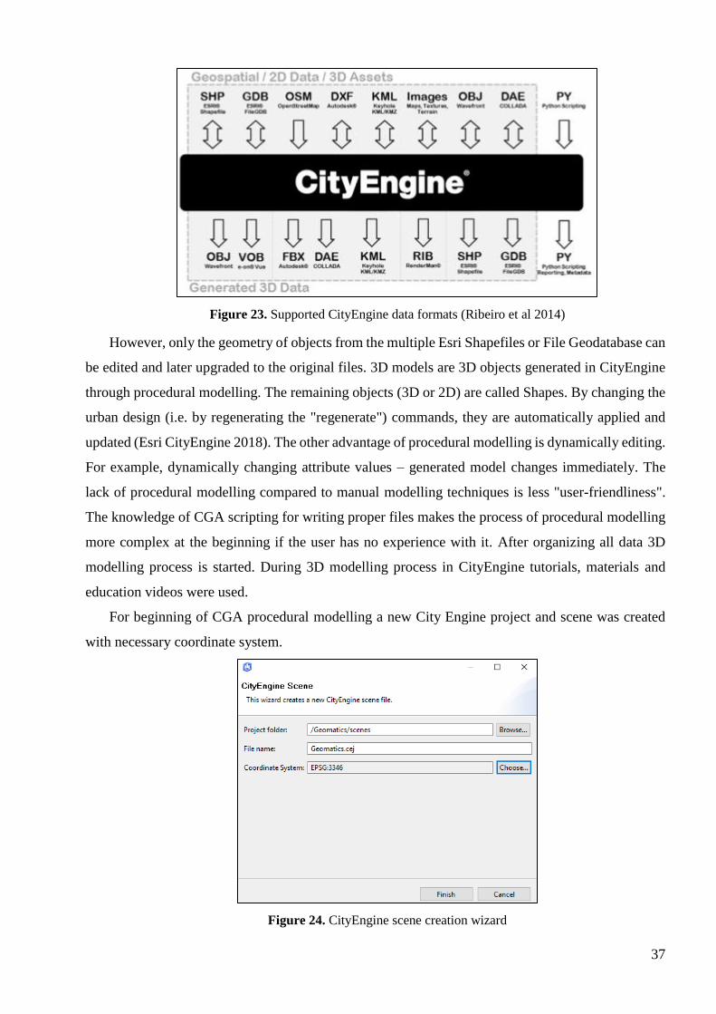
Figure 23. Supported CityEngine data formats (Ribeiro et al 2014)

However, only the geometry of objects from the multiple Esri Shapefiles or File Geodatabase can

be edited and later upgraded to the original files. 3D models are 3D objects generated in CityEngine

through procedural modelling. The remaining objects (3D or 2D) are called Shapes. By changing the

urban design (i.e. by regenerating the "regenerate") commands, they are automatically applied and

updated (Esri CityEngine 2018). The other advantage of procedural modelling is dynamically editing.

For example, dynamically changing attribute values – generated model changes immediately. The

lack of procedural modelling compared to manual modelling techniques is less "user-friendliness".

The knowledge of CGA scripting for writing proper files makes the process of procedural modelling

more complex at the beginning if the user has no experience with it. After organizing all data 3D

modelling process is started. During 3D modelling process in CityEngine tutorials, materials and

education videos were used.

For beginning of CGA procedural modelling a new City Engine project and scene was created

with necessary coordinate system.

Figure 24. CityEngine scene creation wizard

38

As soon as scene created, previously generated shapefiles with their building and roof parameters

were imported.

Figure 25. CityEngine main window

At next step new CGA shape grammar rule file created (New-CityEngine-CGA Rule File) and

editor is opened. In the CGA editor, grammar authoring can now be started by defining the building

parameters: building height, eave height, base elevation and etc.

Figure 26. Defining attributes

After attributes were defined the creation of the building starts. The first rule is called Lot. The

mass model is created with the extrude operation as follows:

39

Figure 27. Extrusion rule example

A mass model was divided into its facades by applying the component split. This rule splits the

shape named Building, the mass model, into its faces by applying a component split. This results in

a front shape, several side shapes as facades, and a roof shape.

Figure 28. Building splitting into parts

After building was splitter into components, facades were set as solid components without any

additional geometry.

Figure 29. Describing facades

For the start of roof modelling at first conditional rule was applied according roof type

parameters.

Figure 30. Defining roof form

40

For each roof type different rules were set. Some roof types (Flat, Shed, Gabled, Hip, Pyramid)

are already supported by CityEngine without having use in-depth cga rules, however, for some types

mansard, dome, vault, were created with more calculations and parameters.

Figure 31. Modelling rule for roof types

Created rule was applied for building footprint shapes to check if there are no mistakes in the

same rule. Inspector window shows that attributes in rule and shapes connected and generation was

applied.

41

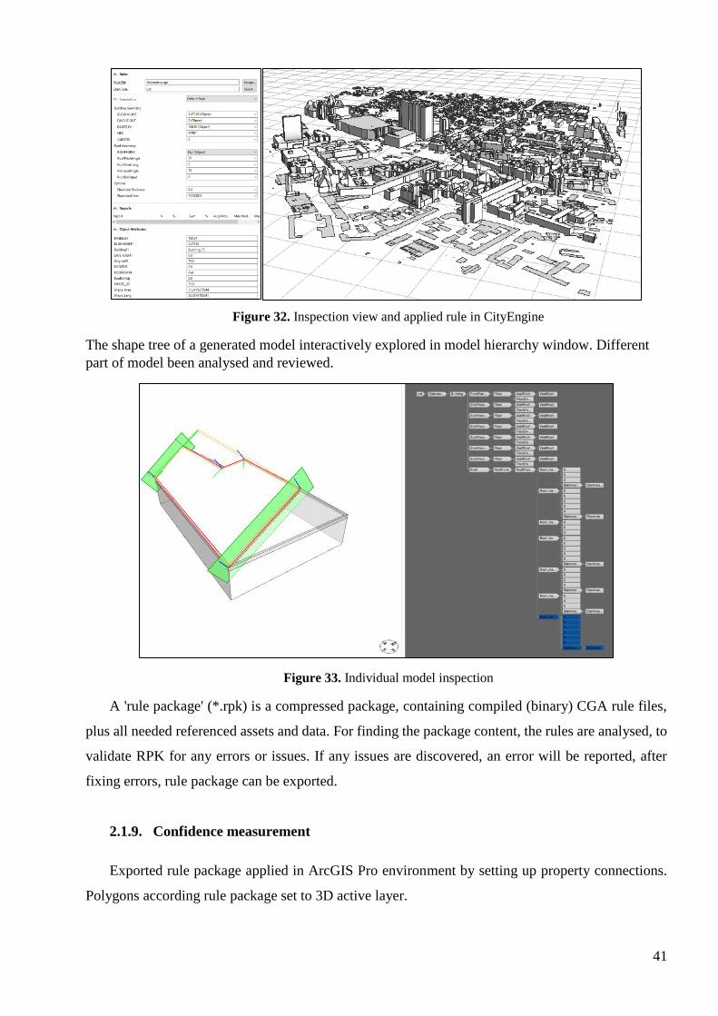
Figure 32. Inspection view and applied rule in CityEngine

The shape tree of a generated model interactively explored in model hierarchy window. Different

part of model been analysed and reviewed.

Figure 33. Individual model inspection

A 'rule package' (*.rpk) is a compressed package, containing compiled (binary) CGA rule files,

plus all needed referenced assets and data. For finding the package content, the rules are analysed, to

validate RPK for any errors or issues. If any issues are discovered, an error will be reported, after

fixing errors, rule package can be exported.

2.1.9. Confidence measurement

Exported rule package applied in ArcGIS Pro environment by setting up property connections.

Polygons according rule package set to 3D active layer.

42

Figure 34. Active 3D building layer and attribute connections in ArcGIS Pro

Script of confidence measurement applied to perform a visual inspection of data. Script rasterizes

building shells by Multipatch to Raster geoprocessing tool. This tool burn 3D building features (as

multipatches) into a DTM. Zonal statistics applied to calculate mean values between original DSM

and DTM raster with burned building footprints. Raster of RMSE converted into points and joined

by unique building id with existing buildings. New attribute field created with RMSE values.

Symbology of graduated colours applied to visually inspect extrusion quality.

RMSE field shows the root-mean-square-error of the generated building multipatch to the

underlying surface model. The higher this number, the more likely that the roof-form extraction

process encountered an error in classification. In general, a value of 1 meter or less is desirable,

though this depends on the required application of the output features, and the resolution of the input

data.

43

Figure 35. Building footprints visualisation by RMSE (from low to high (green to red))

2.1.10. Manual Editing

Visual comparison reveals that most of the buildings with high RMSE seem to have multiple

parts with different heights or geometry errors caused by vegetation-covered roofs. The RMSE may

have been caused by the building footprint not reflecting the actual extent of the building.

Additionally, the footprint appears to be misaligned with the imagery.

Figure 36. Building geometry errors caused by vegetation

44

One of the problems with the building was that the building footprint was misaligned with the

imagery and elevation data. Before we made any other changes, vertices has been modified for better

alignment. Turning on nDSM as background and standard editing tools used. Vertices were dragged

to align them better with the building's location on the nDSM basemap.

Figure 37. Misaligned building, editing footprint vertices, modified footprint

Second problem appears when comparing the building footprint to nDSM and the LAS point

cloud, we see that the building footprint had one uniform height evenly spread across its area, the

actual building had two parts with vastly different heights: the main tower of the building and part

around it. To fix this problem, we split the building footprint into two features with standard editing

tools, one to represent each part of the footprint.

Figure 38. Multiple roof parts segmentation errors and modified segments

Features were splitted into multiple parts, but now all new features have the same attribute

information as the original feature. The one building feature has the correct building height, but the

feature that represents other building parts has the wrong height. In order to fix it we need to change

attribute values of each part.

45

Figure 39. Segmented building with single height value and original LiDAR data

To identify segment height click on LiDAR point to open pop-up.

Figure 40. LiDAR point pop-up window

Depending on clicked location, the pop-up window shows that approximate building part

elevation is about 127m. However, the LAS points have the true elevation of the point, the building

height attribute in the roof form features has the maximum height of the building (which excludes the

ground elevation). So we need to subtract the base elevation of the building from the elevation of the

clicked point to get the elevation for the building height attribute.

46

Figure 41. Building segment attributes and modified building

The data is currently only a 2D feature class symbolized to look 3D (active 3D layer). After

finished editing we need to convert these features to multipath for later use and sharing. Using Layer

3D to feature class converted existing features into multipath features and according unique building

id to keep certain attributes like address, real estate number and etc. belonging to whole building.

2.2. Road extraction

Road information has an important role in many modern applications, including navigation,

transportation and enables existing GIS databases to be uploaded efficiently (Matkan et al 2014). In

GIS field, road extraction from digital images has received considerable attention in the past decades.

Increasingly, LiDAR data has been used for road extraction (e.g., Boyko and Funkhouser 2011, Zuo

& Quakenbush 2010, Matkan et al 2014). Fully automated road extraction in urban areas can be

difficult due to the complexity of urban features, while manual digitizing of roads from images can

be time consuming. In many cases, a semi-automated approach to road extraction can be implemented

to improve the efficiency, accuracy, and cost-effectiveness of data development activities.

Ground features such as water bodies and asphalt pavement usually have very low intensity

values, while some buildings roofs may also have similar intensity values. The approach of

integration of LiDAR intensity data, DTM and DSM used for road extraction (Fig. 42).

47

Figure 42. Flowchart of roads extraction

At first step LiDAR intensity image was created using LAS Dataset To Raster. Used first return

values, Binning Inverse Distance Weighted interpolation method, raster cell size set to 0.2. Generated

intensity image converted from 16-bit into 8-bit raster image for later processing.

Figure 43. Intensity raster

LIDAR DATA

•INTENSITY RASTER

•DSM RASTER

•DTM RASTER

DSM-DTM

•nDSM

nDSM

•nDSM (GROUND FILTERED)

nDSM (GROUND FILTERED)

•nDSM (BINARY RASTER)

INTENSITY RASTER

•CLIPPED INTENSITY RASTER (NON-GROUD FEATURES REMOVED USING nDSM)

CLIPPED INTENSITY RASTER

•TRAINING SAMPLES CREATION

•SVM CLASSIFICATION

SVM CLASSIFIED RASTER

•SELECTED ROAD FEATURES

SELECTED ROAD FEATURES

•MORPHOLOGICAL FILTERING

•RASTER TO POLYGON CONVERSION

48

Then a DSM and DTM rasters were created from LiDAR points by LAS Dataset To Raster.

Elevation values was used for raster generation, interpolation type set to binning, cell size set to 0.2,

Inverse Distance Weighted point values assigned and voids were eliminated using linear void fill

method. Using minus function created nDSM raster. Using threshold (from -1 to 1) new binary raster

was generated out of nDSM. Value of 0 represents ground features and value of 1 other features like

buildings, trees and etc. Values that represents other non-ground features were set to NoData using

raster calculator.

Figure 44. Binary image of ground points with NoData values (white)

Using raster calculator intensity raster values that overlaps nDSM raster were extracted. As result

new intensity image was generated without buildings, trees and etc.

49

Figure 45. Intensity raster of ground points

At next step used image classification training samples manager. With this tool selected

representative sites for each land cover class in the image. These sites are called training samples. A

training sample has location information (point or polygon) and associated land cover class. The

image classification algorithm uses the training samples to identify the land cover classes in the entire

image. Training samples are saved as a feature class locally. Total five classes were used as training

samples: asphalt, concrete, grassland, gravel, water.

Support Vector Machine (SVM) classification performed which mapped input data vectors into

a higher dimensional feature space and optimally separated the data into the different classes. Support

vector machines can handle very large images, and is less susceptible to noise, correlated bands, or

an unbalanced number or size of training sites within each class. As result segmented image was

generated.

50

Figure 46. Segmented image by SVM classifier

Segmented image reclassified with raster calculator to keep only values that represent roads.

Focal statistics applied to calculate for each input cell location a mean statistics of the values within

a circular (radius = 5 cells) neighbourhood around it.

Figure 47. Road network with calculated mean values of segmented raster

For final result raster calculator applied to remove values which are higher than threshold (0.45).

Generated raster converted to polygonal features and morphological filters used to eliminate rough

inconsistencies.

51

Figure 48. Final result of extracted road areas (and some other ground features)

Final road network can be corrected through interactive editing and converted into line features

(centerlines). Attribute information can be filled for both lines and polygon features to better represent

information related to roads and road network.

2.3. Vegetation extraction

Urban forests are relatively large financial investment for cities. Despite efforts and resources

used for tree care, many cities often lack detailed information about their condition. LiDAR remote

sensing technology, already used in commercial forest management and shows great potential as a

forest monitoring tool. LiDAR data provides three-dimensional information directly and receives

multiple return signals from vegetation (Fig. 49).

52

Figure 49. Multiple return explanation (A Complete Guide to LiDAR 2018)

The single tree detection using airborne LiDAR data was primarily proposed by Brandtberg

(1999), Hyyppä and Inkinen (1999) and Samberg and Hyyppä, (1999), which later became an

accepted topic for researchers (Hyyppä et al. 2008). Most published algorithms detect individual trees

from an interpolated raster surface from LiDAR points that hit on the tree canopy surface (Moradi et

al 2016) (Fig. 50)

Figure 50. Different individual tree detection methods based on LiDAR-derived raster surface (Moradi

et al 2016)

On the basis of studies and analyses carried out by Plowright (2015), Moradi et al (2016),

Argamosa et al (2016), Quinto et al (2017) and Liu (2013) the algorithm (Fig. 51) was created to

delineate individual tree crowns and information (tree height, canopy width) using ArcGIS tools.

53

Figure 51. ArcGIS pro model for individual tree extraction

Canopy height model (CHM) is the difference between the DSM (with tops of the trees) and the

DTM. The CHM represents the actual height of trees with the influence of ground elevation removed.

CHM raster was created from DSM by subtracting DTM raster values (Fig. 53).

Figure 52. CHM explanation (Wasser 2018)

54

Figure 53. Generated DTM, DSM and CHM rasters

The minimum height of the tree (2 meters) was determined for CHM raster using raster calculator.

Taking the CHM as an input, pixels with elevation values greater than or equal to 2 meters were

extracted, other values set to null. The maximum value of a 1 m radius in a cell was obtained from

this raster using Focal Statistics tool.

Figure 54. Part of CHM raster before (left) and after (right) applying local maxima

Next part takes the CHM as an input to compute for the slope (Slope tool) and setting output

measurement units as degrees and planar method. Generated slope raster used to compute for

curvature using Curvature geoprocessing tool. The profile curvature was computed by getting the

curve parallel to the maximum slope and values less than 0 were set to null. Generated curvature

raster converted to points (Raster To Point) and later to polygons (Aggregate). Polygons were created

around clusters of three or more points within the aggregation distance of 1 meter.

55

Figure 55. Curvature raster points and aggregated polygons

CHM with previously calculated elevation threshold and local maxima used to find treetops.

Using Negate function changed cell values from positive to negative on a cell-by-cell basis. Using

negative CHM raster as an input created a raster of flow direction from each cell to its downslope

neighbours cells using D8 method. Using Sink function all sinks or areas of internal drainage were

recognized. Filter function performed for edge-enhancing (High pass) and conditional rule (value is

equal to 0) applied for extraction of lowest areas from adjacent values. Filtered values converted to

points (Feature to point) with unique ids.

Figure 56. Flow direction raster, flow direction raster overlaid with sink raster (orange), filtered treetop

points

Using the previously generated treetop representing points Thiessen polygons were created.

Create Thiessen polygons tool was used to divide the area covered by the input point features into

Thiessen or proximal zones. These zones represent full areas where any location within the zone is

closer to its associated input point than to any other input point. Thiessen polygons used as a boundary

of each tree crown.

56

Figure 57. Thiessen (red) polygons separating tree (green) crowns (blue)

The parts of the tree crown that were not spatially connected to the tree to points were removed.

Circles were created with Minimal Boundary Geometry to obtain information on the diameter of the

tree crown. Add Surface Information tool was used to gather information of tree height. Each feature

class layer with information was joined by unique attribute (id) and using multiple attribute

calculators’ information was stored into specific feature class fields.

Figure 58. Principle of tree crown diameter information extraction

As a final result point feature class was generated with an attribute information of ground

elevation, height, and crown diameter. Preset Layers integrated in ArcGIS Pro is another way to

57

display and share data in three-dimensional environment. Realistic Trees preset layers used to show

trees in real-world form and textures. At this case the tree type connected to the attribute fields which

contains the height and crown width information. Generated 3D trees used for visualisation and can

be shared across platform.

Figure 59. Extracted 3D trees

2.4. Sharing

There are few solutions for sharing data across ArcGIS platform like ArcGIS Online or Portal.

ArcGIS Online is a cloud-based mapping and analysis solution. Through Map Viewer and 3D

Scene Viewer, information of basemaps, styles templates and widgets can be accessed.

Portal for ArcGIS is a component of ArcGIS Enterprise that allows to share maps, scenes, apps,

and other geographic information with other people in organization.

58

CONCLUSION AND DISCUSSION

In order to use LiDAR data, we need to know the basic principles of LiDAR remote sensing.

Airborne laser scanning is performed from a fixed wing aircraft or helicopter. Technique is based on

two main components: a laser scanner system that measures the distance to a location on the ground

and the GPS/IMU combination that measures the position and orientation of the system. LiDAR

accuracy is checked by comparing measured points with laser scan data and defined as the standard

deviation (σ2) and root mean square error (RMSE). The most common errors are navigation-based,

these errors cannot be avoided without data control, so for LiDAR-specific ground control points is

recommended to improve final accuracy. Received LIDAR data may be provided in a variety of data

formats depending on the software platform being used. ESRI’s company ArcGIS software uses the

*.las data format, so knowing the structure (version and type) of this format, we know what

information the data contains (number of classification classes and other attributes).

In Lithuania, LiDAR scanning were performed twice (in 2007 and 2018). Recent data is presented

in a more compatible data format (LAS) than before (XYZ). Although the accuracy of the data

obtained has slightly improved, however, the increased density of points and the number of classes

make it possible to use the data more widely and efficiently.

3D city model combines information collections of certain objects and expressed in three

dimensional geometry. Two ESRI products (ArcGIS Pro and CityEngine) used for main topics

features analysis. Features of 3D building generation, recognition of road infrastructure and extraction

of individual trees are analysed and described. 1 km x 1 km of central area of the city was analysed,

due to the variety and height of the buildings, relief changes, and other specific features of the urban

environment.

3D buildings were extracted in semi-automatic way. Created Las dataset for use of point clouds

on ArcGIS platform, as well as visualization and statistical calculations. DTM and DSM rasters were

used as a basis for extraction of 3D buildings. Building geometry parameters for extracted footprints

calculated using ArcGIS tools and mathematical computations. Segmentation (optional) process used

for complex rooftops extraction. CityEngine platform used for CGA rule creation and visualization

of buildings by attribute data. Buildings with the highest RMSE value were edited manually.

To build road representing polygons used intensity, DTM and DSM rasters. Non-ground features

were removed from intensity image. SVM classification technique used for segmentation and feature

extraction.

For individual tree extraction a model was created in ArcGIS Pro environment. DTM and DSM

used as a basis. As a result point feature class generated with attribute values of base elevation, tree

height and crown diameter. Results displayed in 3D using Preset layers in ArcGIS Pro.

59

The workflow traditionally used to reconstruct 3D buildings from airborne LiDAR is relatively

straight-forward: the LiDAR point-cloud is transformed into a DTM and DSM rasters, then inspected

by human editors for buildings present. If a building is found, one or more polygon describing the

roof form of the building is manually digitized, e.g. if it is a large hip roof with two gable outlets,

there will be three polygons (one hip and two gables on top) drawn by the editor or recognized in the

segmentation process. Once all the roofs are described that way, a set of ArcGIS Procedural rules is

applied to extrude the building models using the roof segments, with heights and ridge directions

computed from the DSM.

Artificial Intelligence (AI), Machine Learning (ML), and Deep Learning (DL) have been quite

popular in the recent years. Success stories from self-driving cars to medical imaging are filling the

media. GIS is not falling behind: having efficient and intelligent tools will significantly cut costs of

creating and maintaining GIS content and bring its quality to higher standards.

Artificial Intelligence is a broad family of computer algorithms and methodologies which

encompasses fields like Machine Learning (based on statistical methods), and, as we will be diving

into here, Deep Learning (based on deep artificial neural networks). The unique and valuable feature

of these approaches is the ability to learn and self-improve over time. Now, with deep convolutional

neural networks (CNN), that is no longer needed; the network will learn these coefficients by itself

during training, which is done by providing it with enough examples. There are experiments and

examples presented by Esri to explore ways to streamline the creation of 3D content using Artificial

Intelligence.

60

REFERENCES

1. Baltsavias, E., 1999. ‘Airborne laser scanning: basic relations and formulas’, ISPRS Journal

of Photogrammetry and Remote Sensing, vol. 54, no. 2-3, pp. 199-214, doi: 10.1016/S0924-

2716(99)00015-5

2. American Society for Photogrammetry and Remote Sensing (ASPRS) n.d., Laser (Las) File

Format Exchange Activities, viewed 6 May 2018, https://www.asprs.org/divisions-

committees/LiDAR-division/laser-las-file-format-exchange-activities

3. American Society for Photogrammetry and Remote Sensing (ASPRS) 2011, LAS

specification, version 1.4 - R13, viewed 10 May 2018, https://www.asprs.org/wp-

content/uploads/2010/12/LAS_1_4_r13.pdf.

4. Csanyi, N & Toth, CK 2007, ‘Improvement of LiDAR Data Accuracy Using LiDAR-Specific

Ground Targets’, Photogrammetric Engineering & Remote Sensing, vol. 73, no. 4, pp. 385-

396, doi: 10.14358/PERS.73.4.385

5. Žalnierukas, A, Ruzgienė, B, Kalantaitė, A & Valaitienė, R 2009, ‘Miestų skenavimo LiDAR

metodu tikslumo analizė‘, Geodesy and Cartography, vol. 35, no. 2, pp. 55-60, doi:

10.3846/1392-1541.2009.35.55-60

6. Kalantaitė, A, Putrimas, R & Šlikas, D 2010, ‘Erdvinių skenavimo duomenų taikymas

vietovės trimačiams modeliams generuoti‘, Geodesy and Cartography, vol. 36, no. 4, pp.

151-155. doi: 10.3846/gc.2010.24

7. FIT Conseil (Géométres Experts), UAB InfoERA, 2007, ‘Lietuvos Respublikos detalaus

erdvinio modelio sudarymas, iš LIDAR skrydžių ir duomenų kaupimo kokybės kontrolės

ataskaita‘, 13 p.

8. National Land Service under Ministry of Agriculture, 2017, ‘Lietuvos Respublikos apskričių

centrų lazerinio skenavimo taškų erdvinių duomenų rinkinio sudarymo kokybės kontrolės

paslaugų techninė specifikacija’, viewed 20 September 2018,

http://www.cvpp.lt/index.php?option=com_vpt&theme=new&task=view&tender_id=34061

3.

9. Nelson, R 2014, ‘How did we get here? An early history of forestry lidar 1’, Canadian

Journal of Remote Sensing, vol. 39, no. S1, pp. 6-17, doi: 10.5589/m13-011

10. Krabill, WB 1989, ‘GPS applications to laser profiling and laser scanning for digital terrain

models’, In Photogrammetric Week 1989, Wichmann Verlag, Heidelberg, Germany.

11. Friess, P 1989, ‘Empirical accuracy of positions computed from airborne GPS data’, In High

Precision Navigation, Linkwitz, K, & Hangleiter, U (Eds.), Springer Verlag, Berlin and

Heidelberg, Germany, pp. 163 - 175.

https://www.asprs.org/divisions-committees/lidar-division/laser-las-file-format-exchange-activities

https://www.asprs.org/divisions-committees/lidar-division/laser-las-file-format-exchange-activities

61

12. Lindenberger, J 1989, ‘Test results of laser profiling for topographic terrain survey’,

Proceedings 42nd Photogrammetric Week, Stuttgart, Germany, Wichmann Verlag,

Heidelberg, Germany, pp. 25 - 39.

13. Schwarz, KP, Chapman, M, Cannon, M, Gong, P & Cosandier, D 1994, ‘A precise

positioning/attitude system in support of airborne remote sensing’, Proceedings of the

GIS/ISPRS Conference, 6 - 10 June, Ottawa, Canada.

14. Ackermann, E 1994, ‘On the status and accuracy performance of GPS photogrammetry’,

Proceedings Of Mapping and Remote Sensing Tools for the 21st Century, 26 - 29 August,

Washington, DC, pp. 80 - 90.

15. Ackermann, E 1988, ‘Digital terrain models of forest areas by airborne profiling’, In High

precision Navigation, Linknvitz, K, & Hangleiter, U (Eds.), pp. 239—250, Springer-Verlag,

New York, NY, USA.

16. Lindenberger, J 1993, ‘Laser-Profilmessung zur topographischen Geländeaufnahme’, PhD

dissertation, Deutsche Geodätische Kommission bei der Bayerischen Akademie der

Wissenschaften.

17. Petrie, G 2011, ‘Airborne Topographic Laser Scanners: Current Developments in the

Technology’, GEO Informatics, vol. 14, pp. 34 – 44, viewed 10 July,

https://www.researchgate.net/publication/281309092_Airborne_Topographic_Laser_Scann

ers_Current_Developments_in_the_Technology.

18. ArcGIS Pro help n.d., What is a LAS dataset?, viewed 11 November 2018,

http://pro.arcgis.com/en/pro-app/help/data/las-dataset/what-is-a-las-dataset-.htm.

19. ArcGIS Pro help n.d., Create LAS Dataset, viewed 11 November 2018

http://pro.arcgis.com/en/pro-app/tool-reference/data-management/create-las-dataset.htm.

20. Karan, PE, Sivakumar, R, Irizarry, J & Guhathakurta, S 2014, ‘Digital Modeling of

Construction Site Terrain Using Remotely Sensed Data and Geographic Information Systems

Analyses’, Journal of Construction Engineering and Management, vol. 140, no. 3, doi:

10.1061/(ASCE)CO.1943-7862.0000822

21. Zouaouid, I, Khanan, A, Faisal, M, Omar, Z, Abdul Rahman FZ, Salleh, M & Radhie, M,

2016, ‘Evaluating Error of LiDar Derived DEM Interpolation for Vegetation Area’,

International archives of the photogrammetry, remote sensing and spatial information

sciences - ISPRS archives, XLII-4/W1, pp. 141 – 150, doi: 10.5194/isprs-archives-XLII-4-

W1-141-2016

22. Sibson, R 1981, ‘A Brief Description of Natural Neighbor Interpolation’, chapter 2 in

Interpolating Multivariate Data, New York: John Wiley & Sons, 1981, pp. 21 - 36.

62

23. Wilson, JP & Gallant, JC 2000, ‘Terrain analysis: Principles and applications’, Wiley, New

York.

24. Guo, T & Yasuoka, Y 2002, ‘Snake-based approach for building extraction from high-

resolution satellite images and height data in urban areas’, Proceedings of the 23rd Asian

Conference on Remote Sensing.

25. Mirosław-Świątek, D, Szporak-Wasilewska, S, Michałowski, R, Kardel, I & Grygoruk, M

2016, ‘Developing an algorithm for enhancement of a digital terrain model for a densely

vegetated floodplain wetland’, Journal of applied remote sensing, vol. 10, issue 3, doi:

10.1117/1.JRS.10.036013.

26. Župan, R, Župan, K, Frangeš, S & Vinković, A 2018, ‘Automatic procedural 3d modelling of

buildings’, Technical Journal, vol. 12, no. 3, doi: 10.31803/tg-20180713143638

27. ESRI CityEngine 2018, Advanced 3D city design software, viewed 10 December 2018,

https://www.esri.com/en-us/arcgis/products/esri-cityengine/overview

28. Ribeiro, A, Duarte De Almeida, JP & Ellul, C 2014, ‘Exploring CityEngine as a Visualisation

Tool for 3D Cadastre’, 4th International FIG 3D Cadastre Workshop, 9-11 November 2014,

Dubai, United Arab Emirates, viewed 2 December 2018,

http://www.gdmc.nl/3dcadastre/literature/3Dcad_2014_25.pdf.

29. Matkan, A, Hajeb, M & Sadeghian, S 2014, ‘Road Extraction from Lidar Data Using Support

Vector Machine Classification’, Photogrammetric Engineering & Remote Sensing, vol. 80,

pp. 409 – 422, doi: 10.14358/PERS.80.5.409

30. Boyko, A & Funkhouser, T 2011, ‘Extracting roads from dense point clouds in large scale

urban environment’, ISPRS Journal of Photogrammetry and Remote Sensing, vol. 66:S2-S12,

doi: 10.1016/j.isprsjprs.2011.09.009

31. Zuo, Y & Quackenbush, L 2010, ‘Road extraction form lidar data in residential and

commercial areas of Oneida County, New York’, ASPRS 2010 Annual Conference, San

Diego, California, April 26 - 30, 2010, viewed 5 November 2018,

https://pdfs.semanticscholar.org/74eb/172c7857aad4fe5ba4e13718d9f37afba717.pdf

32. GIS Geography, 2018, A Complete Guide to LiDAR: Light Detection and Ranging, GIS

Geography, viewed 3 December 2018, https://gisgeography.com/lidar-light-detection-and-

ranging/

33. Hyyppä, J, Hyyppä, H, Leckie, D, Gougeon, F, Yu, X & Maltamo, M 2008, ‘Review of

methods of small‐footprint airborne laser scanning for extracting forest inventory data in

boreal forests’, International Journal of Remote Sensing, vol. 29, pp. 1339-1366, doi:

10.1080/01431160701736489

63

34. Brandtberg, T 1999, ‘Automatic Individual Tree-based Analysis of High Spatial Resolution

Remotely Sensed Data’ Ph.D. dissertation, Acta Universitatis, Agriculutae Sueciae, Silvestria

118, Swedish University of Agricultural Sciences, Uppsala, Sweden, viewed 13 September

2018, https://www.researchgate.net/publication/35985290_Automatic_individual_tree-

based_analysis_of_high_spatial_resolution_remotely_sensed_data

35. Hyyppa, J, & Inkinen, M 1999, ‘Detecting and estimating attributes for single trees using

laser scanner’, Photogrammetric Engineering & Remote Sensing, vol. 68, no. 9, September

2002, pp. 925-932, viewed on 22 November 2018,

https://pdfs.semanticscholar.org/f4c8/638742e1ae48f13eb4e6f98688cc45394721.pdf

36. Samberg, A, Hyyppä, J, Ruppert, G, Hyyppä, H, Ziegler, M, Schardt, M & Soininen, A 1999,

‘Evaluation of the laser scanner data in the forest area’, Laser Radar Technology and

Applications IV, Proceedings vol. 3707, pp. 570-581, https://doi.org/10.1117/12.351385

37. Moradi, A, Satari, M & Momeni, M 2016, ‘Individual tree of urban forest extraction from

very high density lidar data’, The International Archives of the Photogrammetry, Remote

Sensing and Spatial Information Sciences, vol. XLI-B3, 2016 XXIII ISPRS Congress, 12 -

19 July 2016, Prague, Czech Republic, doi: 10.5194/isprsarchives-XLI-B3-337-2016

38. Plowright, A 2015, Extracting trees in an urban environment using airborne LiDAR Report,

9 March 2015, viewed 26 September 2018,

https://open.library.ubc.ca/cIRcle/collections/graduateresearch/42591/items/1.0075836

39. Argamosa, R, Paringit, E, Quinton, KR, AM Tandoc, F, Faelga, RA, A.G. Ibañez, C, A.V.

Posilero, M & Zaragosa, G 2016, ‘Fully automated gis-based individual tree crown

delineation based on curvature values from a lidar derived canopy height model in a

coniferous plantation’, ISPRS - International Archives of the Photogrammetry, Remote

Sensing and Spatial Information Sciences, vol. XLI-B8, pp. 563-569, doi: 10.5194/isprs-

archives-XLI-B8-563-2016

40. Quinto, M, Beronilla, R, Damian, G, Camaso, E & Alberto, R, 2017, 'Extraction of Forest

Plantation Resources in Selected Forest of San Manuel, Pangasinan, Philippines Using

LiDAR Data for Forest Status Assessment', World Academy of Science, Engineering and

Technology, International Science Index 127, International Journal of Biological,

Biomolecular, Agricultural, Food and Biotechnological Engineering, vol. 11(7), pp. 530 –

534, doi: doi.org/10.5281/zenodo.1131786

41. Liu, H 2013, ‘Automated Treetop Detection and Tree Crown Identification Using Discrete-

return Lidar Data’, thesis, Denton, Texas, viewed 13 October 2018,

https://digital.library.unt.edu/ark:/67531/metadc271858/

64

42. Wasser, L 2018, ‘Lesson 4. Create a Canopy Height Model With Lidar Data’, image, viewed

15 December 2018, https://www.earthdatascience.org/courses/earth-analytics/lidar-raster-

data-r/lidar-chm-dem-dsm/

65

APPENDIXES

VILNIUS GEDIMINAS TECHNICAL UNIVERSITY

Documents

Transcript of VILNIUS GEDIMINAS TECHNICAL UNIVERSITY