Vignettes and health systems responsiveness in cross-country comparative analyses

HEDG Working Paper 09/29

Vignettes and health systems

responsiveness in cross-country comparative analyses

Nigel Rice

Silvana Robone

Peter C Smith

August 2009

ISSN 1751-1976

york.ac.uk/res/herc/hedgwp

1

Vignettes and health systems responsiveness in cross-

country comparative analyses

Nigel Rice, Silvana Robone, Peter C. Smith

Centre for Health Economics, University of York

August 2009

Abstract

This paper explores the use of anchoring vignettes as a means to adjust survey reports of health system performance for differential reporting behaviour using data contained within the World Health Survey (WHS). Survey respondents are asked to rate their experiences of health systems across a number of domains on a five-point categorical scale. Using data provided through a set of vignettes we investigate variations in reporting of interactions with health services across both socio-demographic groups and countries. We show how the method of anchoring vignettes can be used to enhance cross-country comparability of performance. Our results show large differences in the rankings of country performance once adjustment for systematic country-level reporting behaviour has been undertaken compared to a ranking based on raw unadjusted data.

Keywords: Anchoring vignettes, Cross-country comparison, Health care responsiveness, Health system performance Contact Author: Nigel Rice, Centre for Health Economics, Alcuin Block A, University of York, Heslington, York, YO10 5DD, United Kingdom. Email: [email protected] Acknowledgements: This research was funded by the Economic and Social Research Council under the Public Services Programme, grant number RES-166-25-0038. We would like to thank the World Health Organization for providing access to the World Health Survey and, in particular, Somnath Chatterji, Amit Prasad, Nicole Valentine and Emese Verdes. We are also grateful to the Health, Econometrics and Data Group Seminar Series at the University of York for helpful comments on an earlier draft.

2

1. Introduction

Increasingly patients’ views and opinions are being recognized as an essential means for

assessing the provision of health services, to stimulate quality improvements and more

recently, in measuring health systems performance (Coulter and Magee, 2003). While

traditionally, patients’ views have been sought on the quality of care provided and

satisfaction with health services, in the context of performance assessment, the WHO has

proposed the concept of responsiveness as a more desirable measure by which health

systems can be judged (Valentine et al, 2003a). Responsiveness relates to a system’s ability

to respond to the legitimate expectations of potential users about non-health enhancing

aspects of care and together with health and fairness of financial contribution has been

suggested as an intrinsic goal of health system performance (Murray and Frenk, 2000). In

broad terms, health system responsiveness has been defined as the way in which individuals

are treated and the environment in which they are treated and importantly, encompasses

the notion of an individual’s experience of contact with the health system (Valentine et al,

2003a).

A central purpose for measuring outcomes, such as health system responsiveness, is to

enable institutions to compare and contrast their performance to that of others, including

at a macro level, to performance obtained in other countries. By establishing relevant

benchmarks, cross-national comparison offers opportunities for countries to assess their

place in relation to others; to learn from experience elsewhere; and to identify and explore

trends in performance (O’Mahony and Stevens, 2004; Gonzalez Block, 1997). To this end,

international comparison has become one of the most influential levers for change in the

provision of public services. This is perhaps best evidenced by the extensive resources

invested by national and international organizations in the collection, publication and

analyses of cross-national data. The Commonwealth Fund is a useful example of an

organisation that has a track record in conducting cross-country comparative surveys of the

public and health professionals. Recent surveys include patients’ experiences of interactions

with primary care services across five countries (Schoen et al., 2004); patients’ use and

views of health care (Schoen et al., 2007); a comparison of health care spending in OECD

countries (Anderson et al., 2007); and the comparison of international rates of amenable

mortality across industrialized countries (Nolte and McKee, 2008). Such analyses aim to

measure key attributes of health systems to assess comparative performance, to identify

underperformance and to inform potential policy developments.

3

Perhaps the most ambitious attempt to date to compare health system performance was

The world health report 2000 (World Health Organization, 2000). The report aimed to

assess the performance and relative ranking of the world’s health systems across five

dimensions of performance including health and responsiveness (in both levels and

distribution) and fairness in financial contributions. The report generated an enormous

interest but also attracted criticism on the basis of its scientific merits and associated

country-level league tables (Williams, 2001; Gravelle, et al., 2002; Richardson, et al., 2003).

Nevertheless, the report helped to promote comparative analyses and represents a

landmark in the evaluation of health systems. A recent European Ministerial Conference on

Health Systems, Tallin 2009, attested to the continued interest in comparative analysis of

health system performance.

The challenge of how appropriately to compare across countries with different institutional

settings and populations is a central feature of comparative work across all public services.

Traditionally, many of the data that international comparisons have relied upon have been

reported at broad aggregate country level. A reliance on aggregate data, however, often

makes it difficult to successfully disentangle the many possible reasons for observed

variation between countries and accordingly the results of such analyses are often highly

contested and inconclusive. More recently, the measurement and comparison of

performance has shifted towards the use of data measured at an individual level, often

derived from administrative records or cross-country surveys of respondents’ experiences.

A fundamental problem with a reliance on survey data, recognized by Blendon et al. (2003),

is that studies aimed at comparative inference have rarely taken into consideration possible

variations in cultural expectations that might influence the reporting behaviour of surveyed

respondents. Attempts to enhance cross-country comparison has tended to focus on

defining objective measures of desired outcomes and developing survey instruments that

are relevant and understandable across cultural settings (e.g. Lynn et al., 2005; Okazaki and

Sue, 1995; Brislin, 1986; Murray et al, 2003). In itself this is, however, unlikely to ensure

response comparability if individuals, when faced with survey questions about the

functioning of health systems, systematically interpret the meaning of the available

response categories, such as `poor’ or `good’ performance, differently across population or

population sub-groups (Sadana et al., 2002). For example, it is natural to believe that poor

system performance means different things to different people, and as a result, individuals

4

may attach very different interpretations to survey response categories. Where this is the

case then a fixed level of underlying performance is unlikely to be rated equally across

populations of interest (see Tandon et al., 2003) and correspondingly cross-population

comparison may produce misleading assessments of relative performance. This differential

mapping from the underlying latent construct of interest (objective performance) to the

available survey response categories is a source of reporting heterogeneity and has been

variously described as state-dependent bias (Kerkhofs and Lindeboom, 1995), scale of

reference bias (de Groot, 2000), response category cut-point shift (Sadana, 2002) and

differential item functioning (Kapteyn et al., 2007).

The degree to which self-reported survey data are comparable across individuals, socio-

economic groups or populations has been debated extensively, usually with regard to

measures of health status (for example, Jürges, 2007, Bago d’Uva et al., 2008; Lindeboom

and van Doorslaer, 2004; Iburg et al., 2002; Manderbacka, 1998; Kempen et al., 1996;

Kerkhofs and Lindeboom, 1995; Idler and Kasl, 1995) and health-related disability

(Kapteyn et al., 2007). Similar concerns extend to self-reported survey data on health

system performance, for example the responsiveness of the system, where the

characteristics of survey respondents and cultural norms regarding the use and experiences

of public services are likely to be influential in shaping an individual’s responses.

Recently, the method of anchoring vignettes has been promoted as a means for controlling

for systematic differences in preferences and norms when responding to survey questions

(for example, see Salomon et al., 2004). Vignettes represent hypothetical descriptions of

fixed levels of a latent construct, such as responsiveness. If we consider a categorical

reporting scale varying from `very bad’ to `very good’, then reporting behaviour results

from individuals applying different response thresholds, that map underlying performance

on a latent scale to the ordinal response categories. Since the vignettes are fixed and pre-

determined, any systematic variation across individuals in the rating of the vignettes can be

attributed to differences in reporting behaviour. Accordingly, the responses to the vignette

questions allow the response thresholds, or cut-points, to be modelled as a function of the

socio-demographic characteristics of respondents. Since individuals are asked to evaluate

the vignettes in the same way as they evaluate their own experiences, this information can

then be used subsequently to adjust the self-reported data of a respondent’s own contact

with health services. For within-country analyses applying the thresholds observed for a

5

typical respondent (the average) as a benchmark, responses of other individuals can be re-

scaled, or anchored to the benchmark to provide adjusted comparable data. Similarly for

cross-country comparative analysis, responses can be re-scaled to a chosen benchmark

country. This allows comparison of responsiveness to be made with respect to the

predicted proportion of respondents rating the system as say `poor’ or alternatively as `very

good’ where these predictions are purged of reporting behaviour.

A number of studies have applied the vignette approach and made use of what has been

termed the hierarchical ordered probit (HOPIT) model to adjust self-reported data for

systematic differences in respondents’ use of threshold values. The method has

predominantly been applied to self-reported data on health status (for example see, Iburg

et al., 2002; Tandon et al., 2003; Murray et al., 2003; King et al., 2004; Bago d’Uva et al.,

2008). More recently, there have been attempts to extend the methodology to health

systems performance, for example Valentine et al. (2003b) have considered the role of sex,

age, years of education and reported health status on reporting behaviour applied to the

World Health Organisation Multi-Country Survey (WHO-MCSS) responsiveness module

while Puentes Rosas et al. (2006) consider age, sex, education and type of health care

provider using a survey of user satisfaction in Mexico.

This paper explores the utility of using information from vignettes to adjust self-reported

data on health system responsiveness to enhance both within and across country

comparability of health system performance. We illustrate the use of the method by

exploring information from the World Health Survey (WHS) across several countries. First,

we describe the existence of reporting behaviour across socio-demographic groups within

each of nine illustrative countries. Secondly, we apply the HOPIT model within countries

to model and adjust for systematic reporting and thirdly, we extend the method to consider

cross-country comparison of health system responsiveness. To aid analysis, we stratify the

countries into three groups according the United Nations Human Development Index

(HDI)(United Nations Development Programme, 2006). Finally, by benchmarking

reporting behaviour to that of a selected country within each of the three HDI groups, we

evaluate whether differential reporting behaviour affects cross-country rankings of health

system responsiveness.

6

2. Health system responsiveness

The concept of responsiveness as a measure of health systems performance was developed

and promoted by the World Health Organisation (WHO). The concept covers a set of

non-clinical and non-financial dimensions of quality of care that reflect respect for human

dignity and interpersonal aspects of the care process (Valentine et al., 2009). Human rights

include concepts such as respecting patient autonomy and dignity, while interpersonal

aspects of care, or client orientation, focus on aspects that are commonly expressed as

hotel facilities, for example, the quality of basic amenities. These are measured across eight

domains chosen to reflect the goals for health care processes and systems valued highly by

individuals in their contact with health systems. The domains are: autonomy, choice, clarity of

communication, confidentiality of personal information, dignity, prompt attention, quality of basic amenities

and access to family and community support. Definitions of these domains together with

examples of the questions asked to survey respondents are provided in Figure 1.

Increasingly patients’ views and opinions are being recognised as the appropriate source of

information on non-technical aspects of the health care process and accordingly the

measurement of health system responsiveness is based on surveys of user views. In

principle, the concept covers both interactions with health services together with broader

experiences and interactions with health systems, including, for example, health promotion

campaigns, and public health interventions (Valentine et al., 2009). Respondents are asked

to rate their most recent (in the previous year) experience of contact with the health system

within each of the eight domains. The response categories available are `very good’, `good’,

`moderate’, `bad’ and `very bad’. As such responsiveness is viewed as a multidimensional

concept, with each domain measured as a categorical variable for which there is an

assumed underlying latent scale.

3. Empirical approach

The reporting of responsiveness is via an ordered categorical variable that is assumed to be

a discrete representation of some underlying latent scale. If it is assumed that individuals

map the latent scale to the response categories in a consistent way, irrespective of their

characteristics or circumstances, then we observe homogeneous reporting behaviour. In

these circumstances the standard ordered probit estimator that assumes a set of constant

7

thresholds in the mapping of the latent scale to the response categories, would provide an

appropriate method to model the data. In contrast, reporting heterogeneity, or differential

reporting behaviour, arises when individuals differ in the positioning of thresholds when

mapping the latent construct to the available response categories. Systematic variation in

reporting behaviour can be examined in relation to measured attributes of individuals such

as their socio-economic status. For example, income has been shown to be a determinant

of differential reporting behaviour in self-reported general health status such that more

wealthy individuals have higher expectations of health and hence report lower levels of

objectively identical health status compared to less wealthy counterparts (Bago d’Uva et al.,

2008).

Differential reporting behaviour can be shown diagrammatically with the example in Figure

2. Assume individuals in country A and country B are asked to rate the responsiveness of

their health systems according to the scale ranging from `very bad’ to `very good’ and

assume for ease of exposition that individuals within a country have the same reporting

behaviour. The thresholds ( )µ represent the points that divide the available response

categories. Reporting heterogeneity results in respondents in country A applying a different

set of thresholds to the underlying latent construct compared to respondents in country B.

A casual inspection of the ratings in the two countries would suggest that individuals in

country A face poorer health system responsiveness compared to individuals in country B

(for example, the proportion of individuals reporting `very good’ responsiveness is less in

country A than in country B). However, both groups face the same underlying level of

responsiveness as depicted by the solid vertical line. Anchoring the location of the

thresholds to a common scale is fundamental to comparative analysis across the two

countries. The challenge is to model the positioning of the thresholds as functions of

observed characteristics of the relevant populations and to use this information to

benchmark a comparison to a chosen threshold scale.

3.1. The Hierarchical Ordered Probit Model (HOPIT)

The ordered probit model makes use of a set of constant thresholds applicable to all

individuals to map responses on a latent scale to observed outcomes. Where this

assumption does not hold, estimates of the impact of explanatory variables on outcomes

(responsiveness) of interest will be biased. The hierarchical ordered probit model (HOPIT)

8

developed by Tandon et al. (2003) (also see Terza, 1985) is an extension of the ordered

probit model that allows the thresholds to vary across individuals. The method draws on

the use of the anchoring vignettes to provide a source of external information that

facilitates the identification of the thresholds as functions of covariates. The model can be

specified in two parts. The first part draws on the use of vignettes to identify the thresholds

as a function of relevant characteristics (reporting behaviour equation). The second part maps

individual socio-economic and other characteristics to underlying health system

responsiveness while controlling for differences in reporting behaviour obtained through

the first step (responsiveness equation). The two parts are outlined more formally below.

Reporting behaviour equation

To identify the thresholds as a function of respondent covariates, let ∗vikR represent

underlying health system responsiveness for vignette k , rated by individual i . Given that

each vignette is fixed and unrelated to a respondent’s characteristics, it is assumed that the

expected value of the underlying latent scale depends solely on the corresponding vignette,

such that:

( )1,0~|, NKKR ivik

vikkik

vik εεη +=∗ (1)

where ikK is the vector of vignettes, kη is a conformably dimensioned vector of parameters

and vikε is an idiosyncratic error term. ∗v

ikR is unobservable to the researcher and instead we

observe the vignette rating, vikr on a five point scale ranging from `very bad’ to `very good’.

We assume the observed category of vikr is related to ∗v

ikR through the following

mechanism:

j

ivik

ji

vik Rifjr µµ <≤= ∗−1 (2)

for 5,,1;,,, 50 K=∀∞=−∞= jkiii µµ

Should the thresholds represent fixed constants, common to all individuals, then the above

mapping defines the ordered probit model. For the HOPIT model the thresholds are

assumed to be functions of covariates, X such that:

9

j

ij

i X γµ = (3)

where 5,1, K=jjγ are parameters to be estimated along with kη . Further, we assume an

ordering of the thresholds such that .521iii µµµ <<< K 1 If we impose the restriction that the

covariates affect all thresholds by the same magnitude then we have parallel cut-point shift.

However, if the degree of reporting heterogeneity varies across thresholds such that it is

greater at some levels of responsiveness than others, we refer to this as non-parallel shift

(Jones et al. 2007).

Responsiveness equation

Underlying health system responsiveness faced by individual i can be expressed as:

( )2,0~|, σεεβ NZZR isi

sii

si +=∗ (4)

where iZ represents a set of regressors predictive of responsiveness. As with the vignettes, ∗s

iR represents an unobserved latent variable and we assume that the observed categorical

response, sir , relates to ∗s

iR in the following way:

j

isi

ji

si Rifjr µµ <≤= ∗−1 (5)

for 5,,1;,, 50 K=∀∞=−∞= jiii µµ

where jiµ are defined by (3) with jγ fixed and it is assumed that ∗v

ikR and ∗siR are

independent for all Ni ,,1 K= and .,,1 Vk K= Note that 2σ̂ in (4) is identified due to the

thresholds being fixed through the reporting behaviour equation.

1 The linearity of the regression specification in the threshold equation may specify a model that is internally inconsistent for some data vectors and “cannot ensure that the probabilities are always positive” (Green and Hensher 2009, p. 81). Terza (1985) and Pudney and Shields (2000) overcome this potential problem by modelling the thresholds as an exponential rather than a linear function of the covariates. We have run a robustness check using an exponential function for a model using data for Mexico. The coefficients of the model estimated specifying the thresholds as an exponential function of the covariates are extremely similar to those of the model using thresholds as a linear function of the covariates (results are available on request). For ease of computation and interpretation we retain a linear specification in all that follows.

10

It follows that the probabilities associated with each of the five response categories are

given by:

( ) ( ) ( ) 5,,1,Pr 1 K=−Φ−−Φ== − jZZjr ij

iij

ii βµβµ (6)

where ( ).Φ is the cumulative standard normal distribution.

The use of vignettes to identify reporting heterogeneity relies on the following two

assumptions:

Response consistency: it is assumed that individuals classify the vignettes in a way that is

consistent with the rating of their own experiences of health system responsiveness. This

implies that the mapping used from the latent level of responsiveness shown by the

vignettes to the response categories is the same as the mapping used to translate latent

responsiveness of own experiences to the response categories.

Vignette equivalence: it is assumed that “the level of the variable represented by any one

vignette is perceived by all respondents in the same way and on the same unidimensional

scale” (King et al., 2004; p.194). This assumption implies that, conditional on the socio-

economic characteristics that determine reporting behaviour, for each vignette there is an

actual (unobserved) level of reponsiveness that all individuals agree to, irrespectively of

their country of residence, their sociodemographic characteristics or the level of

responsiveness they face. This assumption might not be tenable in cross-country analyses

where, for example, differences in institutional settings might lead to different perceived

levels of underlying responsiveness. Comparing across reasonably homogeneous groups of

countries and conditioning on country-level characteristics will alleviate some of these

concerns (Kristensen and Johanson, 2008).

4. Data – The World Health Survey (WHS)

11

The most ambitious attempt to date to measure and compare health systems

responsiveness is the World Health Survey (WHS). The WHS is an initiative launched by

the WHO in 2001 aimed at strengthening national capacity to monitor critical health

outputs and outcomes through the fielding of a valid, reliable and comparable household

survey instrument (see Üstün et al., 2003). Seventy countries participated in the WHS 2002-

2003, consisting of a combination of 90-minute in-household interviews (53 countries), 30-

minute face-to-face interviews (13 countries) and computer assisted telephone interviews (4

countries). All surveys were drawn from nationally representative frames with known

probability resulting in sample sizes of between 600 and 10,000 respondents across the

countries surveyed. Samples have undergone extensive quality assurance procedures,

including the testing of the psychometric properties of the responsiveness instrument (for

example, see Valentine et al., 2009).

Of particular interest to our study is the information contained in the WHS on health

system responsiveness. The WHS responsiveness module has been developed from an

extensive consultation process aimed at gathering information on the aspects of the

delivery of health care that individuals value most. The resulting instrument was fielded in

the WHO Multi-Country Survey Study on Health and Responsiveness (2000-2001) (MCSS

- see Üstün et al., 2003) and a refined version of the MCSS module was incorporated in the

WHS. The WHS responsiveness module gathers basic information on health care

utilisation for both inpatient and outpatient services. Here we focus exclusively on inpatient

services.

The data contains information on the importance respondents place on each of the eight

domains present in the responsiveness section of the WHS. In the interests of brevity and

to conserve space we present analyses for the following four domains: Dignity,

Confidentiality, Quality of Facilities and Clarity of Communication. These domains are considered

most important by the respondents across the countries used to illustrate reporting

behaviour. In general, for the set of illustrative countries, those categorised within the high

HDI group place greater importance on the domains Confidentiality and Clarity of

Communication, while for the medium and low HDI countries Dignity and Quality of facilities

have greater relevance. Two question items are rated by respondents for each of the

domains.

12

The first part of our analysis illustrates the level and determinants of reporting behaviour

and the application of the HOPIT model using the following nine countries: Mexico,

Spain, Malaysia, India, Philippines, Sri Lanka, Burkina, Malawi and Ethiopia. These

countries have been selected on the basis of the following criteria. First, the long version

(90-minute in-household) questionnaire was used in these countries. The long version

questionnaire is more informative than the short version in containing two items questions

for each domain (the short version questionnaire contains only one item per domain).

Secondly, the countries satisfy well the set of psychometric properties of feasibility,

reliability and validity for the responsiveness module in the WHS and hence have desirable

survey properties (see Valentine et al., 2009). Accordingly, these countries have acceptable

response rates, strong test-retest properties and the responsiveness items satisfy properties

of homogeneity and the uni-dimensionality (see Ustun et al., 2003). Thirdly, the countries

represent geographical areas characterized by different levels of development, defined by

the Human Development Index (HDI). We use this index to stratify countries into high,

medium and low HDI groups. The HDI is a composite index of human development

which combines indicators of life expectancy, educational attainment and income (United

Nations Development Programme, 2006). Mexico, Spain and Malaysia belong to the high

HDI group; India, Philippines and Sri Lanka to the medium HDI group; and Burkina,

Malawi and Ethiopia to the low HDI group. Finally, the countries selected have a high

sample size in comparison to other countries belonging to the same HDI group.2

4.1. Explanatory variables

Variables available in the WHS on individual characteristics include age, gender, level of

education and income. Level of education is measured as both a categorical variable

containing seven categories representing, for example, ‘primary school completed’,

‘secondary school completed’ to ‘post graduate degree completed’ and a continuous

variable measuring the number of years in education. Gender is a dummy variable coded 1

for women and 0 for men. Income is derived from a measure of permanent income based

on information on the physical assets owned by households. The approach to its

measurement (which relies on a variant of the HOPIT model to improve cross-country

2 We note that the sample size for Mexico (38,455) is far greater than that for other countries, increasing the scope and precision of analysis for this country.

13

comparability) is described by Ferguson et al. (2003).3 In our analysis we construct dummy

variables to indicate the tertiles of the within-country distribution of household permanent

income to which individuals belong.4 To assess comparability of the country-specific

income distributions we compute the coefficient of variation as a summary measure of

dispersion. The distribution of income is broadly similar across the nine countries and with

the exception of Spain and Malaysia all have a coefficient of variation less than unity.5 For

the analysis presented here, the first income tertile is considered as the base category.

Descriptive statistics for the set of explanatory variables for each of the nine countries are

presented in Table 1.6 These variables have been extensively used in the studies

investigating reporting bias in self-reported measure of health (Bago d`Uva et al., 2008;

Iburg et al., 2002; Murray et al., 2003; Valentine et al., 2003b) and health-related disability

(Kapteyn et al., 2007).

4.2. Vignettes

The WHS contains a number of vignettes describing the experiences of hypothetical

individuals within each of the eight domains of responsiveness. The vignettes have been

divided into four sets (Set A-D) with each set containing five vignettes for each item

present across two domains. For example, Set A contains five vignettes for each of the two

items in the domain of Dignity (items representing respect and privacy) and five vignettes

for each of the two items in the domain Prompt Attention (items representing travelling time

and waiting time). Due to constraints of interview length, each respondent in the survey

rated the vignettes present in only one of the sets. Therefore, each vignette has been rated

by approximately 25% of survey respondents. The response scale available to respondents

answering the vignettes is the same as the scale available when responding to their own

experiences of health system responsiveness. Examples of the vignettes are provided in

Figure 3.

3 As a check of the robustness of the approach we computed an alternative measure of permanent income based on the ownership of assets computed through the use of principal components analysis (see O`Donnell et al., 2007; p. 45). For all the nine countries considered in the first part of the analysis there is an acceptable level of correlation between the two measures of income (the correlation index varies between 0.62 (Malawi) and 0.92 (Malaysia)). 4 Models are specified using tertiles of the distribution of income. For the descriptive analysis we use income quintiles 5 The coefficient of variation, in absolute value, varies between 0.25 and 0.82, with the exception of Spain and Malaysia where the coefficient is greater than 1.0. 6 We exclude from our analysis a few outlying observations reporting more than 25 years of education

14

5. Empirical strategy

Our empirical approach is as follows. First, for each of the nine illustrative countries we

establish prima-facie evidence of differential reporting behaviour and investigate whether

this systematically varies by demographic and/or socio-economic characteristics of

respondents. We then make use of the HOPIT model to estimate the relationship between

the model thresholds that determine the mapping from the latent level of responsiveness to

the observed reporting categories and the set of individual characteristics (3). Conditional

on this relationship, we then estimate the responsiveness equation, again, as a function of

respondent characteristics (4). The coefficients estimated by the HOPIT model are

compared to the corresponding estimates derived from a more standard ordered probit

model assuming fixed thresholds across all individuals.

The model is then extended to assess differential reporting behaviour across countries. In

so doing, we consider a larger set of countries available in the WHS and restrict

comparison to countries within each of three HDI groups.7 Analysis within HDI groups

imposes a degree of homogeneity across countries in terms of their stage of development

which aids in maintaining the assumption of vignette equivalence. In addition to the

demographic and socio-economic characteristics outlined above, the models contain

dummy variables to represent attributes of the included countries. These might reflect, for

example, economic and cultural differences across countries within a given HDI group.

The specification of the HOPIT model further includes interaction terms between the

country dummies and the socio-economic characteristics in the responsiveness equation

(4), and interaction terms between the country dummies and income tertiles in the

reporting behaviour equation (3).

Finally, we evaluate whether the ranking of countries in each HDI group according to the

responsiveness of their health system is affected by the presence of differential reporting

behaviour. This is achieved by comparing observed unadjusted raw frequencies of

responsiveness to predictions obtained from the HOPIT model. For ease of presentation

7 We do not consider data collected through computer assisted telephone interviews as these are likely to be of lower quality. This excludes Australia, Luxemburg and Norway from our analysis.

15

we compare rankings of the proportion of respondents reporting `very good’

responsiveness.8

6. Results

6.1. Differential reporting behaviour

Figure 4 presents histograms of the proportion of respondents reporting each of the five

categories of responsiveness for the set of vignettes (vig1 to vig5) available for the first

item of each of the four domains considered. Respondents’ valuations of their own

experience of contact with health services are also shown (own). To conserve space we

present descriptive results for Mexico only.9 Heterogeneity in respondent reports is also

observed across other item and domain combinations and within other countries.

Figure 4 clearly shows heterogeneity across response categories in reporting of the

vignettes. For example, the third vignette (vig3) for Clarity of communication attracts similar

ratings (approximately between 25-35%) across three of the five response categories. Given

the fixed and exogenous nature of the vignettes, such variation in respondents’ ratings

provides prime-facie evidence of differential reporting behaviour. A comparison of ratings

of own experiences of contact with health services versus vignette ratings clearly indicates

that individuals exhibit less dispersion in the reporting of own experiences compared to the

hypothetical cases provided through the vignettes. For example, the distribution of

responses across the available categories for own responsiveness is similar across the four

domains with approximately 70% of respondents rating their experience as `good’. In

contrast, the vignette ratings are far more dispersed and are infrequently observed to be

above 50% for any particular response category. Own ratings of responsiveness, however,

conflate actual experiences of health services with differential reporting behaviour while, in

contrast differences in the ratings of the vignettes are assumed to be due solely to reporting

behaviour.

Figure 5 investigates reporting behaviour by socio-demographic position of respondents.

These are illustrated using the second vignette in the domain Clarity of communication for

8 This is illustrative and different rankings are likely to result by considering other categories in the response scale. 9 The larger sample size afforded to Mexico ensures that the frequencies are estimated with greater precision than for the other countries.

16

Mexico.10 Results are provided stratified by educational attainment, income quintiles,

gender and age respectively. A gradient across the levels of a variable for any of the specific

response categories (for example, `very good’) provides evidence of systematic reporting

behaviour. For example, we observe a clear gradient across educational achievement: in

general, better educated respondents are more likely to rate this particular vignette as `very

good’ compared to less educated respondents.11 A gradient is also apparent across income

quintiles where individuals further along the income distribution are more likely to report

`very good’ and less likely to report `moderate’ responsiveness compared to individuals at

the lower end of the distribution. While there is some evidence of variation across age

groups, in general reporting behaviour does not appear to be influenced greatly by gender

or age.

6.2. Within country analyses

Homogeneity in reporting behaviour

Table 2 presents results of separate tests for homogeneity in reporting behaviour and

parallel cut-point shift (a shift that is a function of covariates but, importantly, is an equal

shift across all thresholds). For the test for homogeneity, p-values from a Wald test of the

joint significance of the estimated coefficients across the four thresholds of the model are

reported in the first six columns of the table. These are reported for each of the socio-

demographic characteristics considered. Rejection of the null indicates the thresholds are

functions of the respective socio-demographic characteristic. Results are shown by age,

gender, educational attainment (in years) and two dummy variables representing the second

and third income tertiles. In addition to separate tests for each variable, the first column

reports a joint test across all socio-demographic characteristics. For the majority of country

and domain combinations, the null hypothesis of homogenous reporting can be rejected

for at least one of the socio-demographic variables. There is however, variation in the

extent of systematic reporting behaviour across countries and domains. In general, and

consistent with the descriptive analysis, the results indicate greater reporting heterogeneity

by income and education, compared to age and gender.

10 Clarity of communication is rated as being most relevant by Mexican respondents. 11 Some caution is required when interpreting these results as the education category ‘Post Graduate’ is sparsely populated and hence the response ratings are not estimated with same level of precision as for other education groups.

17

The final six columns of Table 2 report results investigating the existence of parallel cut-

point shift. Again, tests are presented separately by income, education, age and gender and

jointly across all characteristics. The table shows p-values from a Wald test of equality of

respective coefficients across the four thresholds. If we consider the joint tests across all

characteristics, then parallel cut-point shift is rejected for the vast majority of country and

domain combinations. For individual socio-demographic variables, a similar pattern

emerges for the tests for parallel cut-point shift as for tests for homogeneity. Accordingly,

where thresholds appear to be related to the socio-demographic characteristics of

respondents, in general, this results in non-parallel cut-point shift.

Determinants of reporting behaviour

We investigate further the determinants of reporting behaviour as a function of respondent

characteristics by focusing on education. Table 3 (a) presents estimated coefficients of years

of education across the four thresholds together with their associated standard errors.

These are derived from modelling the vignette data (equations (1) to (3)). For a particular

domain and item combination, positive coefficients across the thresholds indicate higher

expectations of health services and an associated lower probability of reporting high levels

of responsiveness as years in education increase. This scenario is observed for both items

of the domain Dignity for India. Accordingly, more educated individuals appear to rate a

fixed level of responsiveness in this domain less favourably than their less educated

counterparts.

In general, the results for Malaysia, Mexico, Philippines, and Sri Lanka provide evidence

that the better educated rate responsiveness more extremely than their less educated

counterparts. This can be seen by the positive coefficient estimated on the first threshold

and the negative estimated coefficient on the fourth threshold. Results for Malawi reflect

those for India. For the remaining countries, it is difficult to draw generalisations. Across

all results many of the coefficients fail to attain statistical significance implying that within a

specific country and domain, education influences a limited number of thresholds.

Similar conclusions can be drawn from a comparison of the effect of income (results

shown in Table 3 (b)). While for certain countries a pattern emerges, suggesting reporting

18

behaviour is systematically related to income, for other countries it is difficult to draw

generalisations.

Adjusting for reporting heterogeneity

The impact of adjusting for differential reporting behaviour can be investigated using data

on the self-reports of respondents’ own experiences of health service contact. This can be

assessed by comparing the estimated coefficients, β̂ , in the responsiveness equation (4)

with and without adjustment for reporting behaviour using the ordered probit (unadjusted)

and the HOPIT model (adjusted). Note that for an ordered probit model it is customary to

fix the constant and variance to 0 and 1 respectively (for example, see Greene, 2003).

However, to obtain comparability of the coefficients we fixed the constant and variance

parameters of the ordered probit model to those of the HOPIT model.

To conserve space we report the impact of adjusting for differential reporting behaviour

within countries by comparing the estimated coefficient for the dummy variable

representing the third tertile of income. Results are reported in Table 4. If we focus on

countries within the medium HDI group, then for the majority of the domains and items,

coefficients from the ordered probit model indicate a positive and significant income

effect, implying higher responsiveness is enjoyed by wealthier individuals compared to their

less wealthy counterparts. The coefficients from the HOPIT model, however, differ from

those obtained using the ordered probit model. For India, adjusting for reporting

behaviour depresses the income effect, whilst for the Philippines the income effect

generally increases for the HOPIT model compared to the ordered probit results. The

results for Sri Lanka are more ambiguous with some domain and item combinations

increasing and others decreasing. Within countries, a comparison of the estimated

coefficients and associated standard errors obtained from the ordered probit model to

those from the HOPIT model suggests that for a number of domain and item

combinations the differences are large enough to attain statistical significance.

As a further indication of the effects of adjusting for within-country reporting

heterogeneity, Table 5 presents the ex-ante and ex-post frequencies of reporting each of

the five response categories for both items of the four domains considered. To conserve

space, results are shown for the three example countries belonging to the high HDI

19

groups. Ex-ante results report the frequencies observed in the raw data for each domain

and item. The ex-post results are based on predictions obtained from either the ordered

probit model or the HOPIT model adjusting for within-country differential reporting

behaviour. For all countries, predictions from the ordered probit model are remarkably

similar to the ex-ante frequencies observed in the raw data. Although not large, the

difference between the ex-ante frequencies and the ex-post frequencies are more notable

when considering predictions from the HOPIT model, particularly for Mexico.12 Overall,

the results suggest that within-country predictions of responsiveness with or without

adjustment for differential reporting behaviour vary little from the raw frequencies

observed in the data.

6.3. Cross-country analyses

We now consider the impact of adjusting for reporting behaviour across countries. This is

achieved by extending the model presented in the previous section by specifying the

thresholds (3) as a function of the set of individual socio-demographic characteristics,

country-specific dummy variables and interactions between the country-specific dummy

variables and income tertiles.13 The responsiveness equation (4) is specified as a function of

the set of individual socio-demographic characteristics, country-specific dummy variables

and interactions between the country-specific variables and the socio-demographic

characteristics. To enhance comparability of results models are estimated across countries

within each of the three HDI groups.

Table 6 reports the coefficients and standard errors for the set of country dummies by

HDI group for the item Respect (in the domain Dignity). To conserve space results for High

and Low HDI country groups only are shown.14 The set of coefficients are contrasted

against the baseline countries of Mexico and Malawi respectively. The variation in country

coefficients illustrates the existence of differential reporting behaviour across countries.

With the exception of France and Ethiopia, the estimated coefficients attain statistical

12 Applying a RESET test (a test of no neglected non-linearities in the functional form of the model, Ramsey, 1969) suggests that both the ordered probit and the HOPIT model are well specified for the majority of item and domain combinations and across the various countries. 13 Models where the specification of the thresholds included interaction terms between country dummies and other socio-demographic characteristics failed to achieve convergence. 14 Results for the set of medium HDI countries are available on request.

20

significance for at least one of the four thresholds for each country.15 For countries within

the High HDI group, the coefficients for the first threshold are generally positive while

those for the fourth threshold are generally negative. These results imply that compared to

Mexico, countries are likely to make greater use of the extremes of the available reporting

categories when rating performance. A similar result is observed across the countries within

the low HDI group although, in general, there appears to be less variation in estimated

coefficients and fewer coefficients attain statistical significance.

The results of Table 6 establish the existence of differential reporting behaviour across

countries. We next investigate the impact of adjusting for country-specific reporting

behaviour by comparing predictions of reporting `very good’ responsiveness from both the

ordered probit and the HOPIT model. Results are presented in Table 7 for the item Respect.

Results are presented separately for the three HDI groups. The first column of the table

reports the raw frequencies from respondent ratings observed in the data. These vary

substantially and have been ranked in order of reporting `very good’ responsiveness. For

example, in the High HDI group 61.9% of respondents in Austria compared to 16.3% of

respondents in Mexico report `very good’ responsiveness. This variation in ratings will

reflect differences in true underlying health system responsiveness faced by individuals, but

will also, in part, reflect systematic reporting behaviour that differs across countries. The

challenge for comparative analysis is to isolate the impact of the former, abstracting from

the impact of the latter.

The second column reports predicted frequencies from an ordered probit model. This

model includes the socio-demographic variables together with a set of country dummy

variables and interaction terms between country dummies and the socio-demographic

variables as predictors in the responsiveness model but assumes a set of fixed thresholds

common to all countries. Estimation is undertaken on data pooled across all countries

within each HDI group. If we consider the ranking of the countries, overall there is little

change between the observed frequencies derived from the raw data and the predictions

from the ordered probit model. For high HDI countries Austria, Demark, Sweden and the

United Kindom are ranked highly; countries such as The Netherlands, Estonia and Bosnia

tend to be placed in the middle of the rankings; and Mauritius, Malaysia and Mexico tend

to be towards the bottom of the rankings. A test of the independence of the rankings

15 It should be noted that statistical significance is, in part, due to the chosen baseline country.

21

rejects the null in favour of dependence (p<0.01), indicating an association between the

rankings from the predictions of the ordered probit model and the observed raw

frequencies.16

Columns (3) and (4) present predicted frequencies obtained from the HOPIT model. The

model contains the same set of explanatory variables in the responsiveness equation (4) as

specified in the ordered probit model. In addition, the thresholds are modelled as functions

of the socio-demographic variables and the set of country dummy variables (and

interactions with income tertiles). The modelling of the thresholds allows us to control for

differential reporting behaviour across individuals within countries (via socio-demographic

characteristics) and across countries (via country dummy variables). We use the results in

two ways. First, the results presented in column (3) represent the predictions obtained from

the model calculated separately for each country, and adjusting for within country reporting

behaviour. Crucially the model does not adjust for differences in reporting across countries.

Predictions are obtained by anchoring the relevant parameters in the thresholds to the

characteristics of the `average’ respondent in each of the countries considered. We refer to

this model as the `country-specific’ HOPIT model. Due to the use of within country

thresholds, the predicted frequencies should resemble more closely the frequencies

observed in the raw data than the corresponding predictions from the ordered probit

model (which assumes a set of thresholds common to all countries). This is supported by

our results and is most evident in the medium and low HDI countries. For each HDI

group, Kendal’s correlation coefficient is larger when comparing the ranking of column (3)

with column (1) than the corresponding correlations derived from the rankings of the

ordered probit model. The increases are, however, marginal.17 Again, a test of the

independence of the rankings is firmly rejected.

Secondly, to provide rankings comparable across countries we benchmark reporting

behaviour to that observed in the baseline countries. We then predict the reporting of `very 16 Kendall’s tau rank correlation (Kendall, 1938) is used as a measure of the degree of correspondence between the rankings. Perfect agreement leads to a coefficient of 1, perfect disagreement -1, and independence 0. The test is performed under the null hypothesis of independence. 17 Note that in general the greater the number of countries used in the comparison, the larger the difference between the correlation coefficients from comparing the ranking from the ordered probit predictions and the raw frequencies and the rankings from the `country-specific’ HOPIT model and the raw frequencies. This is shown in Table 8. For the eight items, the table compares the correlation coefficients of the rankings obtained from the ordered probit model (1) with the corresponding coefficient from the `country-specific’ HOPIT model (2). The comparison is given across models increasing in the number of countries considered. In general, the greater the number of countries, the closer the rankings from the `country-specific’ HOPIT predictions are to the raw frequencies compared to the ordered probit predictions.

22

good’ responsiveness, irrespective of country of residence, as if all respondents had the

reporting behaviour of the baseline country. That is, for each country within an HDI group

the predicted probability of reporting `very good’ responsiveness is computed using the

thresholds estimated for the baseline country. By adopting the reporting characteristics for

a specific country we define a comparable basis on which to rank countries. The resulting

rankings are provided in column (4). Inspection of these results reveals a different ranking

to that observed for the raw frequencies. This is most evident for countries within the

medium and low HDI groups.18 For example, for the high HDI group of countries, Austria

falls 11 places and Bosnia falls eight places in the rankings once benchmarked for reporting

behaviour. In contrast The Netherlands moves up 10 places and Finland seven places in

the rankings post benchmarking. For the countries in the medium HDI group, Bangladesh

and Tunisia fall 10 places in the rankings whilst Philippines rises 20 places and Dominican

Republic rises seven places. Among the countries in the low HDI group, Mali drops from

the top of the rankings to the middle, and Chad from near the bottom of the distribution

to near the top.19

A test of independence of the rankings between the HOPIT model benchmarked to the

chosen baseline country and the frequencies observed in the raw data fails to reject the null

hypothesis for the low HDI group of countries (p = 0.580) and fails to reject at the 1%

level for the medium HDI countries. This implies a different orderings of the countries

before and after adjusting for reporting behaviour. While the same test rejects the null of

independence for the high HDI countries, a visual inspection of the rankings reveals large

differences as outlined above. Further we observe a large decrease in the correlation

coefficient, decreasing from 0.992 when comparing the `country-specific’ HOPIT model

rankings to those obtained in the raw frequencies to 0.671 for the benchmarked HOPIT

model rankings.

Predictions from the benchmarked HOPIT model allow us to consider the importance of

adjusting for differential reporting in explaining cross-country differences in reported rates

of responsiveness. For example, if we consider the group of high HDI countries, the

difference in reporting `very good’ responsiveness between the country ranked first

18 The correlation coefficient assumes the value 0.671, 0.517 and 0.247 in the High, Medium and Low HDI group, respectively. 19 Note that while the relative ranking of countries is independent of the choice of country to anchor against, the absolute level of country predictions is partly determined by the choice of benchmark country.

23

(Austria) and the baseline country (Mexico) is 45.6 percent (61.9 – 16.3). If we anchor

reporting behaviour in Austria to the response scales used by Mexican respondents, the

difference is reduced to 10.7 percent (28.4 – 17.7). Accordingly, between the highest and

lowest ranked countries approximately three-quarters of the observed difference in the

frequencies of reporting `very good’ responsiveness appears to be due to reporting

behaviour. For medium and low HDI countries similar comparisons suggest that

approximately 39 percent and 83 percent respectively of the observed difference between

the highest ranked and benchmarked country is due to differences in cross-country

reporting behaviour. While these results will vary by the choice of countries compared, the

results provide an indication of the potential impact of reporting behaviour on

comparisons of performance.

7. Conclusions and discussion

A clear purpose for outcome measurement is to enable institutions to compare and

contrast their performance to that of others, including at the macro level the performance

secured in other countries. To this end international comparison has become one of the

most influential levers for change in public services. Increasingly patients’ views and

opinions obtained through surveys are being recognised as a legitimate and important

means for assessing the performance of health systems. A reliance on individual-level

survey data based on respondent self-reports of system performance presents challenges

for international comparison. In particular, self-reported data is likely to suffer from the

existence of systematic variations in reporting behaviour. This might be evident both across

individuals, stratified by socio-demographic characteristics, within countries and across

countries. Systematic reporting behaviour, or reporting heterogeneity, results from survey

respondents applying different thresholds when reporting (using a categorical scale) an

underlying latent construct such as health system responsiveness. Accordingly, a given

fixed level of performance might be rated differently across survey respondents. In order to

identify true underlying differences in performance, measures of performance need to be

purged of systematic variations in reporting behaviour. Using the method of anchoring

vignettes this paper has illustrated how reporting of health system responsiveness might

vary both within and across countries. Our results indicate the presence of systematic

reporting behaviour variation that is linked to the socio-demographic characteristics of

24

survey respondents within countries. Whilst the degree to which these characteristics

influence reporting varies across country our results indicate that adjusting for differential

reporting behaviour within countries has little effect on the overall reporting of health

system responsiveness at country level. Within countries the predicted frequencies of

reporting `very poor’ to `very good’ responsiveness obtained from an application of the

HOPIT model do not vary greatly from the corresponding frequencies observed in the raw

data. 20

Differential reporting behaviour, however, appears more prevalent across countries where

differences in norms and cultural expectations are likely to be more marked than within

countries. This is evident in the WHS data where country-level rankings of responsiveness

obtained from the observed raw data vary from the rankings obtained through the HOPIT

model where reporting behaviour is anchored to a common scale. While some caution is

merited when interpreting the rankings as definitive indications of comparative system

performance, the results suggest that cross-country analyses that rely on survey

respondents’ reports of interactions with public services need to consider the extent of

systematic differences in reporting behaviour. To this end, the method of anchoring

vignettes offers a potentially powerful tool to adjust survey results and to place cross-

country comparative analysis on a more consistent footing than that obtained from a

simple comparison of observed raw data frequencies.

The use of anchoring vignettes in conjunction with the HOPIT model promises to be an

important tool to aid cross country comparison of health system performance. The use of

the approach, however, has limitations. First, the set of socio-demographic variables

extracted from the WHS used in this work are arguably better predictors of variation in

reporting behaviour (used to model the thresholds, (3)) than predictors of underlying

health system responsiveness (used in the responsiveness equation, (4)). Future research

might focus on the appropriate determinants of health system responsiveness to further aid

cross-country comparison. Secondly, the method relies on the assumption of response

consistency and vignette equivalence and the validity of these assumptions remains the 20 Where interest lies in comparing responsiveness across socio-demographic groups within a country and not across countries, then benchmarking reporting behaviour is likely to affect ratings of performance. For example, if we are interested in the responsiveness of a system across education groups, then we might want to benchmark to a single educational category (e.g. degree of higher degree). We might then observe changes in ratings of responsiveness before and after adjusting for reporting behaviour. However, for broad country-level comparison adjusting for socio-demographic reporting behaviour has little impact on ratings when compared to the raw frequencies observed in the data. .

25

object of current research (Kapteyn et al., 2007; Kirstensen and Johanson, 2008). Finally,

the inclusion within surveys of vignettes necessarily entails a cost on survey implementation

and it is important to consider the design of included vignettes to ensure they elicit relevant

information efficiently, and the principles underlying the efficient design of vignettes is a

further area of ongoing research activity (King and Wand, 2007).

26

References Anderson, G.F., Frogner, B.K. and Reinhardt, U.E. (2007) Health spending in OECD

countries in 2004: an update. Health Affair., 26, 1481-89. Bago d'Uva, T., van Doorlsaer, E., Lindeboom, M. and O'Donnell, O., (2008), Does

reporting heterogeneity bias the measurement of health disparities? Health Econ. 17 (3), 351-375.

Blendon, R. J., Schoen, C., DesRoches, C., Osborn, R. and Zapert, K. (2003), Common Concerns Amid Diverse Systems: Health Care Experiences In Five Countries. Health Affair., 22(3), 106-121.

Brislin, R.W. (1986) The wording and translation of research instruments. Field methods in cross-cultural research. In Field methods in cross-cultural research (eds W.J. Lonner and J.W. Berry), pp 137-164. Beverly Hills, CA: Sage.

Coulter, A. and Magee, H. (2003), The European patient of the future (state of health). Maidenhead: Open University Press.

Gonzalez Block, M. A. (1997) Comparative research and analysis methods for shared learning from health system reforms. Health Policy, 42, 187-209.

de Groot, W. (2000) Adaptation and scale of reference bias in self-assessments of quality of life. J Health Econ., 19, 403-420.

Gravelle, H., Jacobs, R., Jones, A.M. and Street, A. (2002) Comparing the efficiency of national health systems: econometric analysis should be handled with care. Mimeo: University of York.

Green, W.H. (2003) Econometric Analysis. Upper Saddle River, New Jersey: Pearson International Edition.

Green, W.H. and Hensher, D.A. (2009) Modeling Ordered Choices: A primer and Recent Developments. New York: Cambridge University Press.

Ferguson, B.D., Tandon, A., Gakidou, E. and Murray, C.J.L. (2003) Estimating Permanent Income using Indicator Variables. In Health systems performance assessment: debates, methods and empiricism (eds C.J.L. Murray and D.B. Evans), pp 748-760. Geneva: World Health Organisation.

Iburg, K. M., Salomon, J., Tandon, A. and Murray, C. J. L. (2002) Cross-country comparability of physician-assessed and self-reported measures of health. In: Summary measures of population health: concepts, ethics, measurement and applications (eds C. J. Murray, J.A. Salomon, C.D. Mathers and A.D. Lopez), pp 433-448. Geneva: The World Health Organization.

Idler, E. L. and Kasl, S. V. (1995) Self-ratings of health: do they also predict change in functional ability?. J Gerontol Soc Sci., 50B, 344-353.

Jones, A.M., Rice, N., Bago d'Uva, T. and Balia, S. (2007) Applied Health Economics, New York: Routledge.

Jürges, H. (2007) True health versus response styles: exploring cross-country differences in self-reported health. Health Econ., 16(2), 163-178.

Kapteyn, A., Smith, J. and van Soest, A. (2007) Vignettes and self-reports of work disability in the US and the Netherlands. Am Econ Rev., 97(1), 461-473.

Kempen, G.I., Steverink, N., Ormel, J. and Deeg, D.J. (1996) The assessment of ADL among frail elderly in an interview survey: self-report versus performance-based tests and determinants of discrepancies. J Gerontol Soc Sci., 51B, 254-260.

Kendal, M. (1938) A new measure of rank correlation. Biometrika, 30, 81-89. Kerkhofs, M. J. M. and Lindeboom, M. (1995) Subjective health measures and state

dependent reporting errors. Health Econ., 4, 221-235. King, G. and Wand, J. (2007) Comparing Incomparable Survey Responses: New Tools for

Anchoring Vignettes. Polit Anal., 15, 46-66.

27

King, G., Murray, C. J. L., Salomon, J. and Tandon, A. (2004) Enhancing the validity and cross-cultural comparability of measurement in survey research. Am Polit Sci Rev., 98(1), 184-91.

Kristensen, N. and Johansson, E. (2008) New evidence on cross-country differences in job satisfaction using anchoring vignettes. Labour Econ., 15, 96-117.

Lindeboom, M. and van Doorslaer, E. (2004) Cut-point shift and index shift in self-reported health. J Health Econ., 23(6), 1083-1099.

Lynn, P., Japec, L., Lyberg, L. (2006) What’s so special about cross-national surveys?. ISER Working Paper 2005-16, Colchester.

Manderbacka, K. (1998) Examining what self-rated health question is understood to mean by respondents. Scand J Soc Med., 26(2), 145-153.

Murray, CJL. and Frenk, J. (2000) A framework for assessing the performance of health systems. B World Health Org., 78, 717-731.

Murray, C. J. L., Ozaltin, E., Tandon, A., Salomon, J., Sadana, R. and Chatterji, S. (2003) Empirical evaluation of the anchoring vignettes approach in health surveys. In Health systems performance assessment: debates, methods and empiricism (eds C.J.L. Murray and D.B. Evans), pp 369-399. Geneva: World Health Organisation.

Nolte, E. and McKee, C.M. (2008) Measuring the health of nations: updating an earlier analysis. Health Affair., 27, 58-71.

O'Donnell, O., van Doorslaer, E., Wagstaff, A. and Lindelow, M. (2007) Quantitative Techniques for Health Equity Analysis. New York: World Bank Publications.

O` Mahony, M., and Stevens, P.A. (2004) International comparisons of performance in the provision of public services: outcome based measures for education. London: National Institute of Economic and Social Research.

Okazaki, S. and Sue, S. (1995) Methodological issues in assessment research with ethnic minorities. Psychol Assessment, 7, 367-375.

Pudney, S. and Shields, M. (2000) Gender, Race, Pay and Promotion in the British Nursing Profession: Estimation of a Generalized Ordered Probit Model. J Appl Econom., 15 (4), 367-399.

Puentes Rosas, E., Gómez Dantés, O. and Garrido Latorre, F. (2006) Trato a los usuarios en los servicios públicos de salud en México. Rev Panam Salud Publica., 9(6), 394–402.

Ramsey, J.B. (1969) Tests for specification errors in classical linear least squares regression analysis, J Roy Stat Soc B Met., 31, 350-371.

Richardson, J., Wildman, J. and Robertson, I.K. (2003) A critique of the World Health Organisation's evaluation of health system performance. Health Econ., 12, 355-366.

Sadana, R., Mathers, C.D., Lopez, A.D., Murray, C.J.L. and Iburg, K.M. (2002) Comparative analyses of more than 50 household surveys on health status. In: Summary measures of population health: concepts, ethics, measurement and applications (eds C. J. Murray, J.A. Salomon, C.D. Mathers and A.D. Lopez), pp 369-386. Geneva: The World Health Organization.

Salomon, J., Tandon, A., Murray, C. J. L. and World Health Survey Pilot Study Collaborating Group (2004) Comparability of self-rated health: Cross sectional mutli-country survey using anchoring vignettes. Brit Med J,, 328, 258.

Schoen, C., Osborn, R., Doty, M.M., Bishop, M., Peugh, J. and Murukutla, N. (2007) Towards higher-performance health systems: adults' health care experiences in seven countries, 2007. Health Affair., 26, w717-w734.

Schoen, C., Osborn, R., Huynh, P.T., Doty, M., Davis, K., Zapert, K. and Peugh, J. (2004) Primary care and health system performance: adults' experiences in five countries. Health Affair., Suppl Web Exclusives, w4-487 - w4-503.

Tandon, A., Murray, C. J. L., Salomon, J. A. and King G., (2003) Statistical models for enhancing cross-population comparability. In Health systems performance assessment: debates,

28

methods and empiricism (eds C.J.L. Murray and D.B. Evans), pp 727-746. Geneva: World Health Organisation.

Terza, J. V. (1985) Ordinal probit: a generalization. Commun Stat., 14(1), 1-11. United Nation Development Programme (2006) Human Development Report. New York:

UNDP. Üstün, T. B., Chatterji, S., Mechbal, A., Murray C., et al. (2003) The World Health Surveys.

In Health systems performance assessment: debates, methods and empiricism (eds C.J.L. Murray and D.B. Evans), pp 762-796. Geneva: World Health Organisation.

Valentine, N.B., De Silva, A., Kawabata, K., Darby, C., Murray, C.J.L. and Evans, D. (2003a) Health system responsiveness: concepts, domains and operationalization. In Health systems performance assessment: debates, methods and empiricism (eds C.J.L. Murray and D.B. Evans), pp 573-596. Geneva: World Health Organisation.

Valentine, N.B., Ortiz, J.P., Tandon, A., Kawabata, K., Evans, D.B. and Murray, C.J.L. (2003b) Patient Experiences with Health Services: Population Surveys from 16 OECD Counties. In Health systems performance assessment: debates, methods and empiricism (eds C.J.L. Murray and D.B. Evans), pp 643 – 652. Geneva: World Health Organisation.

Valentine, N.B., Prasad, A., Rice, N., Robone, S. and Chatterji S. (2009) Health systems responsiveness - a measure of the acceptability of health care processes and systems In: Performance measurement for health system improvement: experiences, challenges and prospects (eds P. Smith,E. Mossialos, S. Leatherman). London: WHO European Regional Office.

Williams, A. (2001) Science or marketing at WHO? Rejoinder from Alan Williams. Health Econ., 10, 283-285.

World Health Organization (2000) World Health Report 2000: Health sytems; improving performance. Geneva: World Health Organization.

29

Figure 1: Domains of responsiveness

The eight domains of responsiveness defined by the WHO are as follows (see Valentine et al., 2003a for a full exposition of these domains):

Autonomy: respect of patients’ views of what is appropriate and allowing the patient to make informed choices;

Choice: An individual’s right or opportunity to choose a health care institution and health provider and to secure a second opinion and access specialist services when required;

Clarity of communication: Clear explaination to patients and family the nature of the illness, details of treatment and available options;

Confidentiality of Personal Information: privacy in the environment in which consultations are conducted and the concept of privileged communication and confidentiality of medical records;

Dignity: the ability of patients to receiving care in a respectful, caring, and non-discriminatory setting;

Prompt attention: the ability to access care rapidly in the case of emergencies, or readily with short waiting times for non-emergencies;

Quality of basic amenities: the physical environment and services often referred to as “hotel facilities”, including clean surroundings, regular maintenance, adequate furniture, sufficient ventilation, enough space in waiting rooms etc;

Access to family and community support: the extent to which patients have access to their family and friends when receiving care and the maintenance of regular activities (e.g. opportunity to carry out religious and cultural practices).

Example questions used in the WHS to measure responsiveness include: Autonomy: How would you rate your experience of being involved in making decisions about your health care of treatment?

Choice: How would you rate the freedom you had to choose the health care providers that attended to you?

Communication: How would you rate your experience of how clearly health care providers explained things to you?

Confidentiality: How would you rate the way your personal information was kept confidential? Dignity: How would you rate the way your privacy was respected during physical examinations and treatments?

Quality of basic amenities: How would you rate the cleanliness of the rooms inside the facility, including toilets?

Prompt attention: How would you rate the amount of time you waited before being attended to? Access to family and friends: How would you rate the ease of having family and friends visit you?

The above provide examples only and not an exhaustive list of questions for each domain. The

response categories available to respondents were “very good”, “good”, “moderate”, “bad” and “very bad”.

30

Figure 3: Examples of vignette questions used in the WHS Respectful Treatment [Anya] took her baby for a vaccination. The nurse said hello but did not ask for [Anya’s] or the baby’s name. The nurse also examined [Anya] and made her remove her shirt in the waiting room. Q1: How would you rate her experience of being greeted and talked to respectfully? Q2; How would you rate the way her privacy was respected during physical examinations and treatments? Communication [Rose] cannot write or read. She went to the doctor because she was feeling dizzy. The doctor didn’t have time to answer her questions or to explain anything. He sent her away with a piece of paper without telling her what it said. Q1: How would you rate her experience of how clearly health care providers explained things to her? Q2: How would you rate her experience of getting enough time to ask questions about her health problem of treatment? Confidentiality [Simon] was speaking to his doctor about an embarrassing problem. There was a friend and a neighbour of his in the crowded waiting room and because of the noise the doctor had to shout when telling [Simon] the treatment he needed. Q1: How would you rate the way the health services ensured [Simon] could talk privately to health care providers? Q2: How would you rate the way [Simon’s] personal information was kept confidential? Quality of Basic Amenities [Wing] had his own room in the hospital and shared a bathroom with two others. The room and bathroom were cleaned frequently and had fresh air. Q1: How would you rate the cleanliness of the rooms inside the facility, including toilets? Q2: How would you rate the amount of space [Wing] had?

Note that the above provide examples only and not an exhaustive list of possible vignettes for each domain. The response categories available to respondents were “very good”, “good”, “moderate”, “bad” and “very bad”.

31

Table 1: Descriptive statistics for variables at individual level

Country

n mean sd mea sd mean sd mean sd mean sdMalaysia 5,889 0.56 0.50 41 15 18 98 3.86 1.58 1 7 8.36 4.53 0 25 2.00 0.82 Mexico 38,738 0.58 0.49 41 17 18 106 4.10 0.63 3 7 7.20 4.96 0 25 2.00 0.82 Spain 6,229 0.59 0.49 53 18 18 101 3.94 1.39 1 7 8.92 5.21 0 25 2.01 0.82 Philippines 10,056 0.54 0.50 39 15 18 99 3.57 1.23 1 7 8.52 3.70 0 24 2.00 0.82 India 8,373 0.50 0.50 39 15 15 101 2.91 1.80 1 7 5.17 5.09 0 25 2.03 0.82 Sri Lanka 5,971 0.53 0.50 41 15 18 100 3.70 1.08 1 7 8.39 3.99 0 25 2.00 0.81 Malawi 4,850 0.57 0.50 35 16 18 91 2.24 0.87 1 7 6.17 4.33 0 21 2.04 0.82 Ethiopia 2,172 0.40 0.49 31 11 16 95 3.31 0.98 1 7 6.90 3.69 0 20 2.40 0.73 Burkina 3,832 0.52 0.50 36 15 18 110 1.61 1.18 1 7 2.25 4.46 0 25 2.03 0.82

range range range

Income tertileWomen Age Education level Education - years

Note: For “educational level” Mexico only has levels 3 to 7

32

Figure 4: Summary frequencies for the reporting of own contacts with health services and vignettes: Mexico. a) Dignity (item respect) b) Confidentiality (item talk privately)

c) Quality of Facilities (item cleanliness) d) Clarity of communication (item clarity)

Figure 5: Vignette ratings for Clarity of Communication (Vignette 2, 1st item: How clear health care providers explained things): Mexico (a) Education (b) Income quintiles

(c) Gender (d) Age

0 .1 .2 .3 .4 .5 .6

%

own vig1 vig2 vig3 vig4 vig5

verygood good moderate bad verybad

0

.1

.2

.3

.4

.5

.6

%



0 .1 .2 .3 .4 .5 .6

%



0

.1

.2

.3

.4

.5

.6

%



33

Figure 2: Illustration of reporting heterogeneity Country A

Country B

NOTE:

Yi* = latent (and unobservable) possible levels of responsiveness µ = cut points that divide two different response categories Red vertical line = (unobservable) level of responsiveness experienced by individual in every country

*iY

Very Bad Bad ModerateGood Very Good

1µ ′ 2µ ′

3µ′ 4µ′

*iY

Very Bad Bad Moderate

GoodVery Good

1µ 2µ 3µ 4µ

34

Table 2: Tests of homogenous reporting and parallel cut-point shift, by individual countries

All D.Inc2 D.Inc3 Women Age Educ. All D.Inc2 D.Inc3 Women Age Educ.respect 0.00 0.35 0.00 0.79 0.43 0.00 0.00 0.23 0.00 0.66 0.35 0.00privacy 0.00 0.66 0.00 0.87 0.30 0.00 0.00 0.56 0.00 0.87 0.20 0.00clear comm. 0.00 0.01 0.01 0.87 0.14 0.00 0.00 0.01 0.08 0.78 0.41 0.00time quest. 0.00 0.02 0.07 0.88 0.00 0.00 0.00 0.01 0.44 0.78 0.04 0.00talk privately 0.00 0.55 0.02 0.03 0.19 0.00 0.00 0.90 0.90 0.01 0.12 0.00conf. info 0.00 0.35 0.00 0.31 0.29 0.00 0.00 0.59 0.10 0.19 0.21 0.00clean 0.00 0.17 0.06 0.36 0.12 0.00 0.00 0.20 0.04 0.45 0.35 0.00space 0.00 0.21 0.00 0.04 0.22 0.00 0.00 0.18 0.00 0.17 0.59 0.00

All D.Inc2 D.Inc3 Women Age Educ. All D.Inc2 D.Inc3 Women Age Educ.

respect 0.00 0.00 0.00 0.00 1.00 0.00 0.00 0.00 0.00 0.00 0.99 0.00privacy 0.00 0.00 0.00 0.00 0.78 0.00 0.00 0.01 0.00 0.00 0.63 0.00clear comm. 0.00 0.03 0.00 0.23 0.01 0.00 0.00 0.02 0.00 0.13 0.00 0.00time quest. 0.00 0.00 0.00 0.01 0.10 0.00 0.00 0.00 0.00 0.01 0.06 0.00talk privately 0.00 0.17 0.00 0.00 0.00 0.00 0.00 0.51 0.00 0.01 0.19 0.00conf. info 0.00 0.02 0.00 0.00 0.00 0.00 0.00 0.64 0.00 0.00 0.05 0.00clean 0.00 0.00 0.00 0.53 0.12 0.00 0.00 0.00 0.00 0.37 0.06 0.00space 0.00 0.00 0.00 0.01 0.55 0.00 0.00 0.00 0.00 0.00 0.39 0.00







MalaysiaHomogeneity Parallel cut-point shift

MexicoHomogeneity Parallel cut-point shift

SpainHomogeneity Parallel cut-point shift

Philippines

Homogeneity Parallel cut-point shiftIndia

Homogeneity Parallel cut-point shift

Clarity of Communication

Quality of Facilities

Dignity

Confidentiality

Dignity


Confidentiality


Dignity


Confidentiality


Dignity


Confidentiality


Dignity


Confidentiality


Note: Figures represent p-values derived for either tests of homogeneity in reporting or parallel cut-point shift. Figures in bold indicate significance at 5% level D.Inc2 represents a dummy variable for the 2nd income tertile. Similarly, D.Inc3 represents a dummy variable for the 3rd tertile.

35

Table 2: Continued






Dignity


Confidentiality


Dignity


Confidentiality


Dignity


Confidentiality



Dignity

Confidentiality


SriLankaHomogeneity Parallel cut-point shift

BurkinaHomogeneity Parallel cut-point shift

EthiopiaHomogeneity Parallel cut-point shift

MalawiHomogeneity Parallel cut-point shift

Note: Figures represent p-values derived for either tests of homogeneity in reporting or parallel cut-point shift. Figures in bold indicate significance at 5% level D.Inc2 represents a dummy variable for the 2nd income tertile. Similarly, D.Inc3 represents a dummy variable for the 3rd tertile.

36

Table 3 (a): Estimated coefficients and standard errors of education of the thresholds by individual countries High HDI Countries

µ1 µ2 µ3 µ4 µ1 µ2 µ3 µ4 µ1 µ2 µ3 µ4

Dignityrespect coeff 0.030 -0.016 -0.002 -0.036 0.007 0.001 -0.002 -0.008 -0.007 -0.005 -0.001 -0.008

st. err 0.009 0.007 0.007 0.007 0.002 0.002 0.002 0.002 0.006 0.005 0.005 0.005privacy coeff 0.025 0.001 -0.004 -0.032 0.007 0.002 0.000 -0.010 0.000 0.002 0.000 -0.010

st. err 0.008 0.007 0.007 0.007 0.002 0.002 0.002 0.002 0.006 0.005 0.005 0.005Clarity of Communicationclear comm. coeff 0.024 -0.006 0.003 -0.013 0.010 0.003 0.001 -0.013 0.012 0.015 0.013 0.001

st. err 0.008 0.007 0.007 0.007 0.002 0.002 0.002 0.002 0.006 0.005 0.005 0.006time quest. coeff 0.034 -0.001 -0.002 -0.012 0.012 0.003 -0.001 -0.011 0.010 0.013 0.011 0.000

st. err 0.008 0.007 0.007 0.007 0.002 0.002 0.002 0.002 0.006 0.005 0.005 0.006Confidentialitytalk privately coeff 0.016 -0.001 -0.012 -0.024 0.016 0.007 0.003 -0.008 0.000 0.009 0.005 -0.004

st. err 0.007 0.006 0.006 0.007 0.002 0.002 0.002 0.002 0.004 0.004 0.005 0.005conf. info coeff 0.020 -0.011 -0.017 -0.031 0.014 0.006 0.003 -0.008 0.006 0.007 0.002 -0.005

st. err 0.007 0.006 0.006 0.007 0.002 0.002 0.002 0.002 0.004 0.005 0.005 0.006Quality of Facilitiesclean coeff 0.041 0.013 0.009 -0.025 0.014 0.006 0.000 -0.008 0.010 0.006 0.005 0.001

st. err 0.007 0.008 0.008 0.008 0.002 0.002 0.002 0.002 0.005 0.006 0.006 0.006space coeff 0.038 0.012 0.015 -0.020 0.012 0.007 0.002 -0.008 0.010 0.000 -0.003 -0.008

st. err 0.008 0.007 0.008 0.008 0.002 0.002 0.002 0.002 0.005 0.006 0.006 0.006Medium HDI Countries

µ1 µ2 µ3 µ4 µ1 µ2 µ3 µ4 µ1 µ2 µ3 µ4

Dignityrespect coeff 0.011 0.011 0.009 0.010 0.008 0.003 -0.002 -0.003 0.004 0.006 0.009 -0.002

st. err 0.005 0.004 0.004 0.004 0.006 0.004 0.004 0.006 0.007 0.005 0.005 0.005privacy coeff 0.016 0.013 0.013 0.009 0.008 0.004 -0.007 -0.003 0.016 0.007 0.006 -0.012

st. err 0.005 0.004 0.004 0.004 0.006 0.004 0.004 0.006 0.006 0.005 0.005 0.005Clarity of Communicationclear comm. coeff 0.019 0.006 -0.003 0.003 0.012 0.012 -0.008 -0.009 0.010 0.008 -0.004 -0.022

st. err 0.006 0.004 0.004 0.004 0.007 0.005 0.004 0.005 0.007 0.005 0.005 0.006time quest. coeff 0.008 -0.004 -0.006 -0.001 0.006 0.014 -0.008 -0.007 0.013 0.005 -0.003 -0.026

st. err 0.006 0.004 0.004 0.004 0.007 0.005 0.004 0.005 0.007 0.005 0.005 0.006Confidentialitytalk privately coeff 0.007 0.000 -0.003 0.002 -0.001 0.007 -0.013 -0.014 -0.004 0.003 -0.004 -0.012

st. err 0.005 0.004 0.004 0.004 0.006 0.004 0.004 0.006 0.006 0.005 0.005 0.005conf. info coeff -0.004 -0.004 -0.001 0.001 0.010 0.006 -0.014 -0.021 0.011 0.013 0.007 -0.002

st. err 0.004 0.004 0.004 0.005 0.006 0.004 0.004 0.006 0.006 0.005 0.005 0.005Quality of Facilitiesclean coeff -0.002 -0.005 -0.003 0.006 0.016 0.012 -0.001 -0.012 0.015 0.009 0.004 -0.013

st. err 0.005 0.004 0.004 0.005 0.005 0.005 0.005 0.005 0.006 0.005 0.005 0.006space coeff 0.002 -0.004 -0.007 -0.007 0.009 0.006 -0.004 -0.013 0.012 0.003 0.002 -0.011

st. err 0.005 0.004 0.004 0.005 0.005 0.005 0.005 0.006 0.006 0.005 0.005 0.006Low HDI Countries

µ1 µ2 µ3 µ4 µ1 µ2 µ3 µ4 µ1 µ2 µ3 µ4

Dignityrespect coeff 0.014 0.010 0.009 -0.006 0.009 0.002 0.013 0.001 0.020 -0.011 0.002 0.004

st. err 0.008 0.007 0.007 0.008 0.011 0.009 0.009 0.009 0.007 0.006 0.006 0.006privacy coeff 0.017 0.003 0.006 0.004 0.000 0.004 0.003 -0.002 0.023 -0.003 0.004 -0.001

st. err 0.008 0.007 0.007 0.007 0.012 0.010 0.009 0.009 0.007 0.006 0.006 0.006Clarity of Communicationclear comm. coeff -0.001 0.009 0.009 -0.003 -0.002 -0.009 -0.023 -0.025 0.014 0.002 0.002 0.017

st. err 0.010 0.008 0.008 0.008 0.012 0.009 0.009 0.009 0.007 0.006 0.006 0.006time quest. coeff -0.006 0.003 0.011 -0.014 -0.001 0.000 -0.003 -0.011 0.011 0.001 0.000 0.020

st. err 0.009 0.008 0.008 0.008 0.012 0.009 0.009 0.010 0.007 0.006 0.006 0.006Confidentialitytalk privately coeff 0.007 0.009 0.014 0.001 -0.015 -0.007 -0.013 -0.026 0.028 -0.011 -0.005 0.017

st. err 0.008 0.007 0.007 0.009 0.010 0.009 0.009 0.011 0.006 0.006 0.006 0.008conf. info coeff 0.007 0.002 0.006 -0.002 -0.022 -0.004 -0.015 -0.012 0.014 -0.010 -0.004 0.014

st. err 0.008 0.007 0.008 0.009 0.010 0.009 0.010 0.011 0.006 0.006 0.007 0.008Quality of Facilitiesclean coeff -0.004 -0.002 -0.002 -0.015 0.019 -0.003 -0.002 -0.002 0.006 -0.003 0.003 0.021

st. err 0.009 0.008 0.009 0.009 0.011 0.010 0.011 0.011 0.007 0.006 0.007 0.007space coeff -0.015 0.006 0.004 0.002 0.009 -0.011 0.001 -0.008 0.002 -0.004 0.004 0.007

st. err 0.009 0.008 0.008 0.009 0.011 0.010 0.011 0.011 0.006 0.006 0.006 0.007

Malawi

Malaysia

Burkina

India

Ethiopia

Mexico Spain

Philippines SriLanka

Note: Figures in bold indicate significance at 5% level

1µ to 4µ refer to thresholds 1 to 4.

37

Table 3 (b): Estimated coefficients and standard errors of permanent income (third tertile) of the thresholds by individual countries High HDI Countries

µ1 µ2 µ3 µ4 µ1 µ2 µ3 µ4 µ1 µ2 µ3 µ4

Dignityrespect coeff -0.113 0.116 0.081 0.256 0.066 0.044 -0.006 -0.101 0.144 0.115 0.055 -0.092

st. err 0.084 0.069 0.066 0.076 0.024 0.019 0.018 0.025 0.076 0.067 0.061 0.070privacy coeff 0.034 0.034 0.113 0.321 0.063 0.043 -0.005 -0.055 0.139 0.024 -0.066 -0.076

st. err 0.081 0.067 0.065 0.073 0.023 0.019 0.018 0.024 0.073 0.067 0.061 0.065Clarity of Communicationclear comm. coeff 0.142 0.146 0.001 0.138 0.115 0.044 0.021 -0.068 0.195 -0.044 0.045 0.073

st. err 0.080 0.066 0.066 0.074 0.023 0.018 0.018 0.027 0.069 0.063 0.063 0.073time quest. coeff 0.155 0.099 0.046 0.145 0.099 0.054 0.027 -0.024 0.198 0.048 0.002 0.054

st. err 0.081 0.064 0.064 0.074 0.023 0.018 0.018 0.027 0.066 0.063 0.064 0.073Confidentialitytalk privately coeff 0.147 0.146 0.143 0.186 0.078 0.066 0.054 -0.020 0.096 0.017 -0.051 -0.055

st. err 0.072 0.056 0.060 0.066 0.021 0.017 0.018 0.024 0.056 0.055 0.059 0.065conf. info coeff 0.093 0.179 0.242 0.315 0.121 0.079 0.047 0.005 0.073 0.032 -0.002 -0.017

st. err 0.074 0.056 0.059 0.064 0.020 0.017 0.018 0.025 0.056 0.059 0.065 0.068Quality of Facilitiesclean coeff 0.148 -0.024 -0.135 -0.001 0.229 0.105 0.079 -0.061 0.183 -0.072 0.023 -0.043

st. err 0.070 0.079 0.082 0.080 0.021 0.019 0.019 0.025 0.065 0.077 0.075 0.077space coeff 0.168 0.083 -0.185 -0.029 0.243 0.083 0.054 -0.096 0.233 0.008 0.051 -0.014

st. err 0.072 0.070 0.075 0.077 0.021 0.019 0.019 0.026 0.063 0.070 0.071 0.079Medium HDI Countries

µ1 µ2 µ3 µ4 µ1 µ2 µ3 µ4 µ1 µ2 µ3 µ4

Dignityrespect coeff -0.036 -0.074 -0.099 -0.165 -0.084 -0.026 -0.061 -0.052 0.036 0.020 -0.081 -0.002

st. err 0.060 0.045 0.042 0.058 0.049 0.036 0.037 0.053 0.064 0.049 0.044 0.049privacy coeff 0.068 -0.023 -0.117 -0.158 -0.027 0.008 -0.037 -0.111 -0.141 -0.012 -0.085 -0.007

st. err 0.058 0.046 0.042 0.057 0.047 0.036 0.037 0.051 0.058 0.048 0.046 0.048Clarity of Communicationclear comm. coeff -0.154 -0.013 -0.059 -0.158 -0.092 -0.004 0.068 0.137 0.105 0.125 0.131 0.142

st. err 0.073 0.047 0.044 0.061 0.059 0.040 0.038 0.057 0.063 0.049 0.048 0.049time quest. coeff 0.008 0.052 0.035 -0.114 -0.043 -0.007 0.076 0.096 0.053 0.092 0.072 0.073

st. err 0.067 0.047 0.044 0.062 0.056 0.039 0.038 0.056 0.060 0.048 0.047 0.050Confidentialitytalk privately coeff 0.080 0.012 -0.063 -0.050 -0.104 -0.036 0.033 0.021 -0.046 -0.086 -0.119 -0.138

st. err 0.061 0.042 0.043 0.058 0.055 0.034 0.036 0.048 0.056 0.043 0.044 0.047conf. info coeff 0.053 0.086 0.012 -0.077 -0.093 0.069 0.059 0.044 -0.021 0.011 0.051 -0.030

st. err 0.054 0.042 0.045 0.059 0.051 0.034 0.036 0.047 0.052 0.044 0.045 0.044Quality of Facilitiesclean coeff 0.097 0.090 -0.043 -0.012 0.019 0.054 0.029 0.103 -0.074 -0.169 -0.102 0.011

st. err 0.052 0.046 0.048 0.067 0.043 0.041 0.043 0.055 0.055 0.048 0.048 0.055space coeff 0.067 0.061 -0.043 -0.009 0.058 0.046 -0.002 0.098 -0.168 -0.112 -0.067 -0.044

st. err 0.053 0.046 0.048 0.065 0.043 0.039 0.042 0.056 0.054 0.047 0.048 0.054Low HDI Countries

µ1 µ2 µ3 µ4 µ1 µ2 µ3 µ4 µ1 µ2 µ3 µ4

Dignityrespect coeff 0.067 0.253 0.136 0.242 0.154 0.158 -0.131 -0.133 -0.025 -0.044 0.025 0.044

st. err 0.109 0.090 0.089 0.126 0.121 0.099 0.091 0.447 0.074 0.062 0.060 0.086privacy coeff -0.051 0.123 -0.024 -0.120 0.284 0.253 0.018 -0.123 0.013 -0.043 0.073 0.110

st. err 0.110 0.091 0.091 0.114 0.124 0.102 0.093 0.424 0.074 0.063 0.061 0.076Clarity of Communicationclear comm. coeff 0.149 0.175 0.193 0.005 0.299 0.193 0.024 -0.169 0.047 -0.096 -0.051 -0.141

st. err 0.115 0.093 0.091 0.127 0.145 0.106 0.099 0.496 0.070 0.061 0.060 0.090time quest. coeff 0.215 0.271 0.160 -0.086 0.288 0.288 -0.120 -0.193 0.037 -0.114 -0.065 -0.128

st. err 0.111 0.093 0.092 0.126 0.142 0.105 0.101 0.498 0.067 0.062 0.060 0.096Confidentialitytalk privately coeff -0.075 -0.037 -0.146 0.039 0.506 0.252 0.090 -0.030 -0.064 -0.111 0.029 0.040

st. err 0.099 0.079 0.084 0.115 0.109 0.087 0.092 0.405 0.057 0.056 0.061 0.087conf. info coeff -0.076 -0.084 -0.106 0.170 0.499 0.284 0.140 -0.030 -0.025 -0.071 0.040 0.056

st. err 0.095 0.081 0.087 0.112 0.107 0.087 0.094 0.384 0.056 0.058 0.064 0.089Quality of Facilitiesclean coeff 0.434 0.258 0.176 0.125 0.179 0.083 0.046 -0.266 0.087 -0.033 -0.067 -0.227

st. err 0.110 0.098 0.103 0.133 0.121 0.112 0.125 0.625 0.062 0.062 0.065 0.085space coeff 0.284 0.183 0.186 0.057 0.200 0.209 0.047 -0.176 0.123 0.001 -0.006 -0.098

st. err 0.106 0.096 0.101 0.138 0.120 0.109 0.118 0.566 0.061 0.061 0.064 0.085

Mexico Spain


Ethiopia Malawi

Malaysia

Burkina

India


1µ to 4µ refer to thresholds 1 to 4.

38

Table 4: Coefficients of permanent income (third tertile) in the OPROBIT and HOPIT model, by individual countries High HDI Countries

OPROBIT HOPIT OPROBIT HOPIT OPROBIT HOPITDignityrespect coeff 0.017 0.195 0.077 0.020 0.087 0.040

st. err 0.081 0.085 0.037 0.029 0.080 0.079privacy coeff 0.007 0.246 0.093 0.057 0.032 -0.040

st. err 0.083 0.083 0.038 0.027 0.081 0.074Clarity of Communicationclear comm. coeff -0.066 0.025 0.082 0.048 0.148 0.201

st. err 0.083 0.084 0.037 0.031 0.077 0.084time quest. coeff 0.048 0.145 0.066 0.060 0.089 0.123

st. err 0.082 0.084 0.037 0.031 0.076 0.084Confidentialitytalk privately coeff 0.037 0.204 0.010 0.021 0.092 0.040

st. err 0.082 0.073 0.036 0.028 0.078 0.073conf. info coeff -0.032 0.258 0.049 0.064 0.063 0.046

st. err 0.084 0.072 0.037 0.029 0.080 0.076Quality of Facilitiesclean coeff -0.017 -0.069 -0.022 -0.019 -0.101 -0.127

st. err 0.082 0.090 0.036 0.029 0.078 0.088space coeff 0.093 -0.002 -0.029 -0.048 -0.039 -0.021

st. err 0.081 0.086 0.036 0.029 0.075 0.090Medium HDI Countries

OPROBIT HOPIT OPROBIT HOPIT OPROBIT HOPITDignityrespect coeff 0.370 0.243 0.098 0.037 0.236 0.188

st. err 0.072 0.064 0.070 0.059 0.076 0.055privacy coeff 0.381 0.256 0.087 0.032 0.202 0.151

st. err 0.072 0.062 0.070 0.057 0.076 0.054Clarity of Communicationclear comm. coeff 0.374 0.271 0.162 0.233 0.194 0.324

st. err 0.071 0.068 0.070 0.063 0.074 0.057time quest. coeff 0.432 0.407 0.128 0.194 0.161 0.234

st. err 0.071 0.069 0.070 0.062 0.072 0.059Confidentialitytalk privately coeff 0.429 0.372 0.096 0.116 0.123 -0.005

st. err 0.071 0.065 0.070 0.053 0.073 0.054conf. info coeff 0.439 0.423 0.081 0.139 0.100 0.124

st. err 0.071 0.066 0.071 0.053 0.075 0.051Quality of Facilitiesclean coeff 0.506 0.495 0.206 0.250 0.160 0.070

st. err 0.070 0.075 0.069 0.061 0.071 0.065space coeff 0.462 0.447 0.220 0.240 0.124 0.037

st. err 0.070 0.072 0.069 0.062 0.071 0.063Low HDI Countries

OPROBIT HOPIT OPROBIT HOPIT OPROBIT HOPITDignityrespect coeff -0.073 0.123 -0.040 -0.099 0.007 0.031

st. err 0.133 0.127 0.496 0.443 0.085 0.093privacy coeff -0.068 -0.128 0.331 0.357 0.144 0.224

st. err 0.138 0.113 0.501 0.420 0.086 0.083Clarity of Communicationclear comm. coeff 0.131 0.260 0.019 -0.006 0.121 0.024

st. err 0.131 0.128 0.501 0.492 0.084 0.096time quest. coeff 0.158 0.297 -0.310 -0.376 0.128 0.060

st. err 0.130 0.128 0.502 0.493 0.082 0.103Confidentialitytalk privately coeff 0.106 0.031 0.400 0.557 0.147 0.158

st. err 0.131 0.115 0.501 0.401 0.083 0.092conf. info coeff 0.120 0.097 -0.066 0.037 0.129 0.157

st. err 0.138 0.114 0.514 0.380 0.086 0.096Quality of Facilitiesclean coeff -0.223 -0.055 -0.424 -0.504 -0.029 -0.155

st. err 0.132 0.135 0.497 0.618 0.083 0.090space coeff -0.366 -0.204 -0.045 -0.010 0.013 -0.027

st. err 0.133 0.139 0.491 0.561 0.083 0.091

Mexico Spain


Ethiopia Malawi

Malaysia

Burkina

India


39

Table 5: ex-ante frequencies, ex-post frequencies computed through the OPROBIT and through the HOPIT model, for Malaysia, Mexico and Spain.

ex ante prob

ex post prob

PROBIT

ex post prob

HOPITex ante

prob ex post prob

PROBIT

ex post prob

HOPITex ante

prob ex post prob

PROBIT

ex post prob

HOPIT

RESPECT very bad 0.3% 0.3% 0.0% 0.7% 0.7% 0.0% 0.7% 0.7% 0.0%bad 2.4% 2.5% 2.6% 3.0% 3.0% 2.9% 0.8% 0.9% 1.7%moderate 10.6% 10.7% 12.1% 8.7% 8.7% 12.3% 6.1% 6.2% 7.6%good 68.5% 67.7% 65.5% 71.2% 71.2% 67.0% 61.4% 61.4% 59.0%very good 18.2% 18.8% 19.8% 16.3% 16.3% 17.6% 30.9% 30.7% 31.6%

PRIVACY very bad 0.4% 0.4% 0.0% 0.4% 0.4% 0.0% 0.2% 0.2% 0.0%bad 2.1% 2.2% 2.4% 2.2% 2.3% 1.9% 1.9% 1.9% 1.4%moderate 8.2% 8.3% 10.1% 7.4% 7.4% 10.4% 5.2% 5.3% 7.4%good 69.5% 69.1% 66.5% 73.5% 73.5% 70.2% 65.9% 65.8% 63.5%very good 19.7% 20.0% 21.0% 16.5% 16.4% 17.5% 26.8% 26.7% 27.6%

CLEAR COMM. very bad 0.2% 0.2% 0.0% 0.7% 0.7% 0.0% 0.7% 0.8% 0.1%bad 2.5% 2.5% 1.5% 3.2% 3.2% 2.5% 2.6% 2.7% 3.4%moderate 8.2% 8.3% 11.6% 7.9% 7.9% 13.3% 11.0% 11.2% 13.0%good 70.0% 70.0% 67.0% 71.8% 71.8% 66.2% 60.3% 60.1% 57.2%very good 19.1% 19.0% 19.9% 16.3% 16.3% 18.1% 25.4% 25.3% 26.3%

TIME QUEST. very bad 0.2% 0.2% 0.0% 0.7% 0.7% 0.0% 0.9% 0.9% 0.2%bad 3.6% 3.5% 2.7% 3.6% 3.7% 2.8% 4.5% 4.7% 5.6%moderate 11.9% 11.5% 14.6% 8.5% 8.5% 14.0% 13.6% 13.7% 15.1%good 68.3% 68.6% 65.6% 71.0% 71.0% 65.3% 59.9% 59.7% 57.3%very good 15.9% 16.2% 17.1% 16.1% 16.1% 17.9% 21.2% 21.0% 21.8%

TALK PRIVATELY very bad 0.3% 0.3% 0.0% 0.6% 0.6% 0.0% 1.0% 1.1% 0.0%bad 2.6% 2.4% 2.4% 4.2% 4.2% 3.9% 3.7% 3.8% 5.3%moderate 11.9% 11.6% 13.9% 10.6% 10.6% 15.8% 10.4% 10.7% 13.6%good 69.3% 69.3% 65.9% 70.6% 70.6% 64.1% 62.4% 62.2% 56.9%very good 15.9% 16.4% 17.8% 14.0% 14.0% 16.2% 22.5% 22.2% 24.2%

CONF. INFO very bad 0.1% 0.1% 0.0% 1.2% 1.2% 0.0% 0.8% 0.8% 0.0%bad 1.0% 1.1% 0.7% 2.7% 2.7% 4.0% 1.8% 1.8% 2.6%moderate 8.4% 8.7% 10.4% 10.0% 10.0% 15.1% 7.6% 7.7% 11.2%good 69.9% 70.2% 68.1% 71.9% 71.9% 63.8% 67.7% 67.7% 61.9%very good 20.6% 19.9% 20.7% 14.3% 14.2% 17.1% 22.1% 22.0% 24.3%

CLEAN very bad 0.2% 0.2% 0.0% 0.7% 0.7% 0.0% 0.5% 0.5% 0.1%bad 1.3% 1.4% 1.3% 3.3% 3.2% 3.1% 1.3% 1.3% 2.9%moderate 7.6% 7.8% 8.8% 10.0% 9.9% 13.9% 10.4% 10.6% 9.0%good 67.1% 67.1% 66.0% 70.1% 70.1% 65.4% 60.3% 60.2% 60.7%very good 23.7% 23.5% 23.9% 15.9% 16.1% 17.7% 27.5% 27.4% 27.3%

SPACE very bad 0.1% 0.1% 0.0% 0.8% 0.8% 0.0% 1.9% 2.0% 0.7%bad 1.6% 1.5% 1.4% 4.7% 4.7% 4.4% 6.6% 6.7% 8.7%moderate 14.1% 14.4% 14.9% 11.8% 11.7% 16.8% 16.0% 16.2% 17.2%good 67.5% 67.4% 67.0% 68.1% 68.0% 62.1% 54.5% 54.3% 51.8%very good 16.6% 16.5% 16.7% 14.6% 14.7% 16.6% 21.0% 20.8% 21.6%

Confidentiality


ItemDomain

Dignity


MALAYSIA MEXICO SPAIN

40

Table 6: Respect: coefficients and standard errors (for the agents in the first income tertile) of cut-points as a function of country dummy variables in the model

coeff. st.er. coeff. st.er. coeff. st.er. coeff. st.er.U. Arab Emirates 0.079 0.083 -0.002 0.068 0.032 0.064 -0.496 0.068

Austria -0.012 0.143 -0.221 0.113 -0.246 0.101 -0.594 0.101Belgium 0.547 0.127 0.402 0.113 0.385 0.111 -0.069 0.117Bosnia 0.275 0.085 -0.006 0.074 -0.025 0.070 -0.390 0.073

Czech Rep. 0.054 0.111 -0.054 0.095 0.100 0.086 -0.429 0.088Germany 0.260 0.099 -0.010 0.085 0.007 0.079 -0.343 0.081Denmark 0.697 0.112 0.497 0.100 0.553 0.099 -0.134 0.107

Spain 0.193 0.045 0.053 0.038 -0.055 0.036 -0.169 0.038Estonia -0.063 0.104 0.022 0.086 0.104 0.081 -0.277 0.083Finland 0.390 0.092 0.249 0.078 0.568 0.075 0.080 0.084France 0.262 0.152 0.125 0.125 0.209 0.118 -0.164 0.125

UK 0.551 0.093 0.252 0.084 0.276 0.080 -0.288 0.083Greece 0.410 0.091 0.076 0.081 0.123 0.077 -0.488 0.080Croatia 0.217 0.103 0.312 0.087 0.594 0.083 -0.263 0.086

Hungary 0.127 0.079 -0.072 0.066 0.018 0.061 -0.593 0.063Ireland 0.820 0.106 0.328 0.098 0.241 0.096 -0.438 0.101

Italy 0.242 0.207 -0.314 0.179 -0.206 0.157 -0.586 0.157Latvia 0.587 0.104 0.156 0.094 0.171 0.089 -0.294 0.093

Mauritius 0.326 0.049 0.432 0.042 0.303 0.041 -0.065 0.044Malaysia -0.138 0.053 0.002 0.042 -0.032 0.039 -0.200 0.042

Netherlands 0.087 0.125 0.250 0.101 0.314 0.096 0.137 0.109Portugal -0.050 0.113 0.051 0.092 0.229 0.084 0.206 0.099Slovakia 0.049 0.075 -0.076 0.063 -0.059 0.060 -0.521 0.061Slovenia 0.485 0.117 0.226 0.104 0.059 0.102 -0.272 0.109Sweden 0.601 0.097 0.532 0.085 0.557 0.083 0.136 0.092Uruguay 0.237 0.063 0.121 0.053 0.084 0.050 0.027 0.055

LOW HDI COUNTRIES

Burkina 0.583 0.273 0.428 0.197 0.176 0.176 -0.103 0.199Coted`Ivoire 0.409 0.271 0.491 0.195 0.414 0.174 0.196 0.198

Ethiopia 0.339 0.267 0.345 0.191 0.235 0.169 -0.348 0.191Kenya 0.588 0.264 0.476 0.189 0.210 0.167 -0.313 0.189

Mauritania 0.117 0.292 0.427 0.204 0.572 0.182 0.170 0.210Mali 0.572 0.264 0.491 0.189 0.083 0.167 -0.505 0.188

Senegal 0.394 0.272 0.382 0.195 0.199 0.173 -0.464 0.195Chad 0.227 0.277 0.514 0.196 0.582 0.175 0.437 0.204

Zambia 0.481 0.263 0.407 0.188 0.305 0.166 -0.181 0.188Zimbabwe 0.450 0.265 0.457 0.189 0.217 0.167 0.049 0.189

µ2 µ3 µ4µ1HIGH HDI COUNTRIES

Note: Mexico and Malawi are the baseline for the High and Low HDI countries, respectively. Figures in bold indicate significance at 5% level. 1µ to 4µ refer to thresholds 1 to 4.

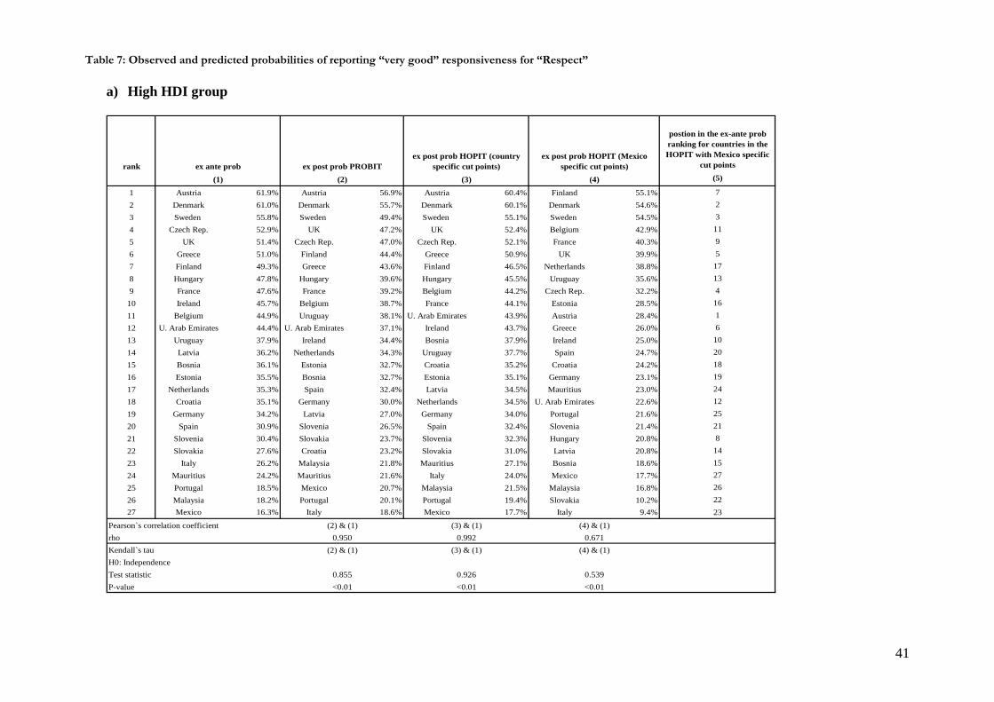
41

Table 7: Observed and predicted probabilities of reporting “very good” responsiveness for “Respect”

a) High HDI group

rank

postion in the ex-ante prob ranking for countries in the HOPIT with Mexico specific

cut points (5)

1 Austria 61.9% Austria 56.9% Austria 60.4% Finland 55.1% 72 Denmark 61.0% Denmark 55.7% Denmark 60.1% Denmark 54.6% 23 Sweden 55.8% Sweden 49.4% Sweden 55.1% Sweden 54.5% 34 Czech Rep. 52.9% UK 47.2% UK 52.4% Belgium 42.9% 115 UK 51.4% Czech Rep. 47.0% Czech Rep. 52.1% France 40.3% 96 Greece 51.0% Finland 44.4% Greece 50.9% UK 39.9% 57 Finland 49.3% Greece 43.6% Finland 46.5% Netherlands 38.8% 178 Hungary 47.8% Hungary 39.6% Hungary 45.5% Uruguay 35.6% 139 France 47.6% France 39.2% Belgium 44.2% Czech Rep. 32.2% 4

10 Ireland 45.7% Belgium 38.7% France 44.1% Estonia 28.5% 1611 Belgium 44.9% Uruguay 38.1% U. Arab Emirates 43.9% Austria 28.4% 112 U. Arab Emirates 44.4% U. Arab Emirates 37.1% Ireland 43.7% Greece 26.0% 613 Uruguay 37.9% Ireland 34.4% Bosnia 37.9% Ireland 25.0% 1014 Latvia 36.2% Netherlands 34.3% Uruguay 37.7% Spain 24.7% 2015 Bosnia 36.1% Estonia 32.7% Croatia 35.2% Croatia 24.2% 1816 Estonia 35.5% Bosnia 32.7% Estonia 35.1% Germany 23.1% 1917 Netherlands 35.3% Spain 32.4% Latvia 34.5% Mauritius 23.0% 2418 Croatia 35.1% Germany 30.0% Netherlands 34.5% U. Arab Emirates 22.6% 1219 Germany 34.2% Latvia 27.0% Germany 34.0% Portugal 21.6% 2520 Spain 30.9% Slovenia 26.5% Spain 32.4% Slovenia 21.4% 2121 Slovenia 30.4% Slovakia 23.7% Slovenia 32.3% Hungary 20.8% 822 Slovakia 27.6% Croatia 23.2% Slovakia 31.0% Latvia 20.8% 1423 Italy 26.2% Malaysia 21.8% Mauritius 27.1% Bosnia 18.6% 1524 Mauritius 24.2% Mauritius 21.6% Italy 24.0% Mexico 17.7% 2725 Portugal 18.5% Mexico 20.7% Malaysia 21.5% Malaysia 16.8% 2626 Malaysia 18.2% Portugal 20.1% Portugal 19.4% Slovakia 10.2% 2227 Mexico 16.3% Italy 18.6% Mexico 17.7% Italy 9.4% 23

ex ante prob ex post prob PROBIT ex post prob HOPIT (country

specific cut points)ex post prob HOPIT (Mexico

specific cut points)(1) (2) (3) (4)

Pearson`s correlation coefficient (2) & (1) (3) & (1) (4) & (1)rho 0.950 0.992 0.671

H0: IndependenceKendall`s tau (2) & (1) (3) & (1) (4) & (1)

P-value <0.01 <0.01 <0.01Test statistic 0.5390.855 0.926

42

b) Medium HDI group

rank

postion in the ex-ante prob ranking for

countries in the HOPIT with India specific cut

points (5)

1 Paraguay 53.6% Paraguay 47.4% Paraguay 50.4% Paraguay 39.4% 12 Brazil 38.7% Brazil 36.2% Brazil 38.9% Georgia 36.4% 33 Georgia 31.4% Georgia 32.7% Georgia 34.3% Brazil 33.4% 24 Ecuador 31.0% Ecuador 28.2% Ecuador 30.1% Myanmar 32.8% 215 South-Africa 27.7% Domin. Rep. 22.4% South-Africa 27.6% Domin. Rep. 30.6% 126 Ghana 27.1% Ghana 21.8% Ghana 27.0% Philippines 30.3% 267 Namibia 25.2% India 20.3% Namibia 25.2% China 28.7% 178 Morocco 25.1% Myanmar 19.4% Morocco 23.8% Guatemala 27.3% 169 Bangladesh 24.6% Guatemala 18.9% Swaziland 21.1% Ecuador 25.3% 4

10 India 20.5% South-Africa 18.8% Congo 19.8% South-Africa 23.3% 511 Swaziland 17.6% Namibia 18.5% India 19.1% Namibia 22.8% 712 Domin. Rep. 17.1% Lao 18.1% Bangladesh 18.4% Congo 21.9% 1313 Congo 16.6% Bangladesh 16.7% Domin. Rep. 17.4% Comoros 21.9% 1914 Tunisia 16.2% Kazakhstan 16.5% Kazakhstan 17.0% India 19.1% 1015 Lao 15.8% China 16.1% Lao 17.0% Ghana 18.8% 616 Guatemala 15.0% Sri-Lanka 14.3% Russia 16.3% Kazakhstan 18.0% 2017 China 14.6% Swaziland 13.8% China 16.3% Lao 17.6% 1518 Russia 13.1% Tunisia 13.3% Tunisia 15.7% Russia 15.8% 1819 Comoros 12.8% Russia 13.0% Sri-Lanka 15.2% Bangladesh 15.8% 920 Kazakhstan 12.7% Vietnam 12.4% Comoros 13.6% Pakistan 15.4% 2321 Myanmar 11.6% Nepal 11.5% Myanmar 12.8% Ukraine 15.4% 2222 Ukraine 9.9% Morocco 11.0% Ukraine 11.6% Swaziland 14.7% 1123 Pakistan 9.8% Philippines 10.9% Vietnam 11.4% Vietnam 12.9% 2724 Sri-Lanka 9.4% Congo 10.1% Pakistan 9.4% Tunisia 12.4% 1425 Nepal 9.2% Comoros 10.0% Philippines 8.9% Nepal 12.1% 2526 Philippines 7.6% Ukraine 9.3% Guatemala 8.0% Sri-Lanka 9.8% 2427 Vietnam 7.4% Pakistan 8.8% Nepal 6.4% Morocco 7.6% 8

ex ante prob ex post prob PROBIT ex post prob HOPIT

(country specific cut points)ex post prob HOPIT (India


Pearson`s correlation coefficient (2) & (1) (3) & (1) (4) & (1)

(3) & (1) (4) & (1)rho 0.876 0.961 0.517

H0: IndependenceTest statistic

Kendall`s tau (2) & (1)

0.547P-value < 0.01 < 0.01 0.013

0.809 0.342

c) Low HDI group

rank

postion in the ex-ante prob ranking for

countries in the HOPIT with Malawi specific cut

points (5)

1 Mali 42.4% Mali 34.5% Mali 39.9% Kenya 21.3% 52 Zambia 28.6% Kenya 28.1% Zambia 28.3% Chad 18.0% 93 Zimbabwe 24.5% Zimbabwe 28.0% Ethiopia 27.5% Zimbabwe 17.9% 34 Ethiopia 24.3% Zambia 25.7% Zimbabwe 25.4% Burkina 16.5% 75 Kenya 24.3% Ethiopia 22.8% Mauritania 24.8% Zambia 16.1% 26 Cote dÌvoire 21.9% Burkina 22.6% Kenya 21.4% Mali 15.2% 17 Burkina 15.1% Mauritania 18.9% Cote dÌvoire 20.8% Senegal 12.8% 118 Mauritania 14.5% Chad 18.6% Burkina 19.8% Ethiopia 11.9% 49 Chad 13.2% Cote dÌvoire 17.9% Chad 16.8% Malawi 10.1% 1010 Malawi 12.2% Senegal 13.3% Malawi 10.7% Mauritania 9.7% 811 Senegal 5.4% Malawi 12.5% Senegal 8.5% Cote dÌvoire 7.5% 6

ex ante prob ex post prob PROBIT

ex post prob HOPIT (country specific cut

points)ex post prob HOPIT (India


Pearson`s correlation coefficient (2) & (1) (3) & (1) (4) & (1)rho 0.890 0.923 0.247Kendall`s tau (2) & (1) (3) & (1) (4) & (1)H0: IndependenceTest statistic 0.709 0.818P-value < 0.01 < 0.01

0.1460.580

43

Table 8: Pearson correlation coefficients between the raw data frequencies and the ordered probit predictions (1), and between the raw data frequencies and HOPIT country-specific predictions (2)

Number of countries

Respect Privacy Clear comm. Time quest. Talk privately Conf. info Clean Space

(1) (2) (1) (2) (1) (2) (1) (2) (1) (2) (1) (2) (1) (2) (1) (2) 2 3 4 5 20 27

1.000 .979 .909 .987 .889 .887

1.000 .869 .866 .984 .964 .966

1.000 .942 .934 .990 .926 .923

1.000 .805 .856 .979 .964 .964

1.000 1.000 .974 .989 .862 .865

1.000 .794 .843 .967 .958 .957

1.000 .993 .968 .936 .785 .803

1.000 .885 .896 .959 .943 .947

1.000 .998 .983 .983 .916 .910

1.000 .873 .888 .962 .920 .922

1.000 .970 .937 .974 .886 .893

1.000 .751 .787 .950 .917 .903

1.000 .931 .887 .980 .864 .871

1.000 .999 .917 .982 .946 .942

1.000 .982 .949 .984 .882 .871

1.000 .993 .962 .986 .937 .929

Note: (1) Pearson correlation coefficient between the raw frequencies and predictions obtained from the ordered probit model (2) Pearson correlation coefficient between the raw frequencies and predictions obtained from the “country-specific” HOPIT model Number of countries: 2: India and Philippines; 3: 2 + Sri Lanka; 4: 3 + Pakistan; 5: 4 + Brazil; 20: 5 + Bangladesh, Congo, Dominican Republic, Ecuador, Ghana, Guatemala, Kazakhstan, Leo, Morocco, Myanmar, Namibia, Nepal, Paraguay, Swaziland, Tunisia; 27: 20 + Vietnam, China, Comoros, Georgia, Russia, South Africa, Ukraine

Vignettes and health systems responsiveness in cross-country comparative analyses

Documents

Transcript of Vignettes and health systems responsiveness in cross-country comparative analyses