Vibration Control in Cricket Bats using Piezoelectric ... - CORE
302
Vibration Control in Cricket Bats using Piezoelectric-based Smart Materials A thesis submitted in fulfilment of the requirements for the degree of Doctor of Philosophy. Jia Long Cao. MEng (RMIT University) School of Aerospace, Mechanical and Manufacture Engineering RMIT University Melbourne, Australia. August 2006
-
Upload
khangminh22 -
Category
Documents
-
view
1 -
download
0
Transcript of Vibration Control in Cricket Bats using Piezoelectric ... - CORE
Vibration Control in Cricket Bats using
Piezoelectric-based Smart Materials
A thesis submitted in fulfilment of the requirements for the degree of
Doctor of Philosophy.
Jia Long Cao.
MEng (RMIT University)
School of Aerospace, Mechanical and Manufacture Engineering RMIT University
Melbourne, Australia. August 2006

Declaration i
Declaration
I hereby declare that
a. The work presented in this thesis is that of my own except where acknowledged to
others, and has not been submitted previously, in whole or in part, in respect of any
academic award.
b. The work of this research program has been carried out since the official
commencement date of the program approved.

Acknowledgements ii
Acknowledgements I would like to thank my senior supervisor, Associate Professor Sabu John, for his guidance
and tremendous support during my PhD study. His generous help, substantial information and
regular encouragement always kept me on track and was the key to my completion. I felt
fortunate to have the opportunity to work under his supervision.
I would also like to thank my second supervisor, Dr. Tom Molyneaux, for his excellent
technical advice, invaluable knowledge and great help.
Thirdly, I would like to thank our industry partners, Kevin Davidson from Davidson
Measurement and Peter Thompson from Kookaburra Sport, for their financial contribution
and great interest in the project, their precious time spent on our regular meetings and
materials contributed to the project.
In addition, I would like to thank our lab and workshop technicians, Peter Tkatchyk and Terry
Rosewarne, for their generous and friendly help with my experiments and products
prototyping, otherwise, I would have had a lot of troubles.
Finally, I would like to thank the Australia Research Council (ARC) for the funding of the
project and the scholarship which supported my graduate study.

iii
Table of Contents
Declaration …...……………………………….………...…………...…...……….…...…... i
Acknowledgements .……………………………………………………………..…...……. ii
Table of Contents ...………………………………….…………………...……….…..…… iii
Abstract …………...………………………………………………………………...…..…. xiv
List of Symbols …………...……………………………………………………………….. xv
Chapter 1 Introduction.…………..……….………..……..……..…………….….…... 1
1.1 Motivation ...…...….………...……………………………………….....…...…. 1
1.2 Vibration control with Smart materials ……...……………..……....………….. 2
1.3 The objectives of this study ...………………....……………………..…..….…. 3
1.4 The organization of the thesis ………..……...………………………….....…... 4
1.5 Publications originated from this research ...………………………….....…….. 6
Chapter 2 Literature Review: Mechanical Vibration Control ...….…..…..…… 7
2.1 Background of the Cricket bat ……………..…………….…....….…...………. 8
2.2 Traditional mechanical vibration control techniques .….....….…....…………... 11
2.2.1 Vibration isolation …...………………………………...……….……….. 11
2.2.2 Vibration absorption …...………………………………...…….……….. 12
2.2.3 Vibration damping …...…………………………………....…….……… 13
2.2.3.1 Viscoelastic damping …...…………………….…………...……. 13
2.2.3.2 Structural damping …...……………………..….…………...…... 16
2.3 Non-conventional vibration control with Smart material components..…...…... 16
2.3.1 Smart material and structure ..……………...……………...…….……… 16
2.3.2 Piezoelectric materials ..…………………....……………...…….……… 18
2.3.2.1 Orientation and notation …...………….…………………...…… 22
2.3.2.2 Piezoelectric constitute equations ………………………………. 23
2.3.2.3 Modelling of piezoelectric transducer ………………………….. 26
2.3.3 Passive piezoelectric vibration shunt control …………...…………….… 26

iv
2.3.4 Active piezoelectric vibration control ……..…………...……….………. 36
2.3.5 Power system for active piezoelectric vibration control ……...………… 40
2.3.6 Advantages and disadvantages of passive and active piezoelectric controls ………………………………………………………………….. 42
2.4 Chapter summary………….……...……………………………………...…….. 43
Chapter 3 Analytical Modelling of Passive Piezoelectric Vibration Shunt on Beams …..…...……………………………………..……...…………...… 45
3.1 Motion equation derivation of composite beam using energy method ………... 46
3.1.1 Euler-Bernoulli beam model …………………………...…………...…... 46
3.1.2 Displacement, strain, stress and velocity relations ……………………… 47
3.1.3 Potential energy ……………………………………………….………… 49
3.1.4 Kinetic energy ………………………...……………………….………... 51
3.1.5 Hamilton’s principle ……………………………………………….……. 52
3.2 Convert partial differential equations (PDE) to ordinary differential equations (ODE) using Galerkin’s method ……….…………………………… 55
3.3 Vibration control with the piezoelectric shunt circuit …………..……….....…. 57
3.3.1 Series R-L shunt ………………………..…………………………...…... 57
3.3.2 Parallel R-L shunt ………………………………….…………….…..… 62
3.4 Numerical examples …………………….………………………...……..…..… 66
3.4.1 Vibration shunt control simulation 1 (PZT placed at L/2).……………… 67
3.4.2 Vibration shunt control simulation 2 (PZT placed at L/4)…….…..…..… 70
3.4.3 Sensitivity test of control frequency mismatch………………………..… 71
3.5 Chapter summary ……………..…….…………………………………..….….. 76
Chapter 4 Composite Beam Analysis and Design ……………………………..…. 77
4.1 Stress and strain in composite beam ...…………………….……………......…. 77
4.2 Parameters of the two-layer piezoelectric composite beam …………………… 80
4.2.1 Neutral surface location ………………………….……………………... 80
4.2.2 Area moment of inertia ……………….………….……………………... 85
4.2.3 Average normal strain and stress ………….….……….………………... 90
4.3 Discussion of composite beam design for maximizing strain in the PZT ……... 94
v
4.3.1 The relation between electrical field and mechanical strain in the PZT ... 94
4.3.2 Analytical precursor to the strain analysis in the PZT Patch …….…….. 99
4.3.3 Comparison of FEA simulation results of piezoelectric vibration shunt control for beams with different materials ……………….………….…. 104
4.3.4 Application of the PZT-composite beam technology and analysis of the handle of the Cricket bat - Introduction of carbon-fibre composite material ………………………………………………………………….. 113
4.3.5 Proposed design of Cricket bat handle ………………………………….. 115
4.3.6 Other benefits of using carbon-fibre material in Cricket bat …………… 117
4.4 Chapter summary …….…………………..………………………………….… 119
Chapter 5 Numerical Modelling of Passive Piezoelectric Vibration Control
using FEA Software ANSYS®…………….……………………...……. 121
5.1 Introduction of ANSYS® ………………….……………….…...……………... 122
5.1.1 General steps of a finite element analysis with ANSYS®….……..…..…. 122
5.1.2 Some elements used for implementation ……………..………..…..…… 123
5.1.3 Couple field analysis ……………..………………………….……...…... 127
5.2 A simple example of the finite element formulation ………………….…….…. 127
5.3 Modelling of passive piezoelectric shunt circuit with PSpice®………….….…. 133
5.3.1 Single mode resistor-inductor (R-L) shunt..…………………………….. 133
5.3.2 Multimode parallel resistor-inductor shunt...………….….…………..…. 136
5.4 Modelling of passive piezoelectric shunt circuit with ANSYS®……....…...….. 139
5.4.1 Single mode resistor-inductor shunt..………………...………….………. 139
5.4.2 Multi-mode resistor-inductor shun.….……………………...……..…….. 141
5.4.3 Shunt effectiveness related to the placement of the PZT patch ………… 142
5.5 Modelling and analysis of the Cricket bat…………………………………...…. 147
5.5.1 Cricket bat with wooden handle …………………………...…………..... 147
5.5.2 Cricket bat with composite hollow tube handle ………..……..………… 148
5.5.3 Cricket bat with sandwiched handle …………………....……..………… 150
5.6 Chapter summary ………………………………………..…………………..… 154
Chapter 6 Experiment and Implementation ….……….………………………..…. 156
6.1 Shunt circuit design .………………………………………………………..….. 157
vi
6.2 Vibration shunt control for beams ….………...……………………………..…. 160
6.3 Modal test of Cricket bats with laser vibrometer …...…………………………. 163
6.3.1 Wooden handle Cricket bat …………………….…………...…………... 164
6.3.2 Carbon-fibre composite tube handle Cricket bat …………………….….. 165
6.3.3 Carbon-fibre composite sandwich handle Cricket bat ………………….. 168
6.3.4 Vibration shunt control for the Cricket bat ……………….…………….. 172
6.4 Field testing of the Smart bat ………………………………………………….. 183
6.5 Chapter summary …...…………………………………………………………. 184
Chapter 7 Frequency Estimation and Tracking ………………………………..…. 185
7.1 Introduction of filters.……………………………………………………..…… 185
7.2 Generic notch filter………………….………...……………………………..… 188
7.3 Adaptive notch filter …...………………………………...……………………. 191
7.3.1 Simplified adaptive notch filter …………………….…………...……..... 191
7.3.2 Notch filter coefficient estimation ……………..……………….……….. 193
7.3.3 Examples of adaptive using cascaded 2nd order notch ANFs……………. 195
7.4 Chapter summary …...…………………………………………………………. 203
Chapter 8 Conclusions and future work ……....………………………………..….. 204
8.1 Conclusions .………………………………………………………………..….. 205
8.1.1 Analytical work on the PZT-based vibration shunt circuit ………….….. 205
8.1.2 Field-Coupled Simulations ………….…………………………………... 205
8.1.3 Cricket bat Innovations ………….………………………………….…... 205
8.1.4 Frequency Tracking Analysis ………….……………………………….. 206
8.1.5 Power amplifier proposal ………….……………………………………. 206
8.1.6 Cricket bat prototyping and field testing ………………………………... 206
8.2 Future work ….………...………………………………………..…………...… 207

vii
Appendix 1 Modelling of Vibration Isolation and Absorption of the SDOF Structure………….………….….….……………………………………... 208
Appendix 2 Estimation of System Damping ……………………………………… 215
Appendix 3 Positive Position Feedback (PPF) Control ………………………… 220
Appendix 4 Proposed Power Amplifier using Amplitude Modulation and Piezoelectric Transformer for Active Vibration Control …………. 226
Appendix 5 Beam Modelling and Modal Analysis ………………………………. 232
Appendix 6 Derivation of the Equations in Chapter 3 ..………………………... 247
Appendix 7 Partial List of ANSYS® and MATLAB® Simulation Codes ….. 255
References ……....………………………………..………………………………………. 273
List of Tables
Table 2-1 Types of fundamental piezoelectric relation ……...….….…………………. 23
Table 6-1 Natural frequency comparison among various Cricket bats ……...….….…. 172
Table A5-1 Common boundary conditions for lateral vibration of uniform beam ….….. 241
List of Figures
Figure 2-1 Geometric parameters of Cricket bat ………………….…………………… 9
Figure 2-2 Mechanical structures interconnected by isolation system .………………... 12
Figure 2-3 Visco-elastic material (VEM) models ……...…………………………….… 14
Figure 2-4 Viscoelastic damping treatments……………………………………………. 15
Figure 2-5 Crystal structure of a traditional ceramic..………………………………….. 19
Figure 2-6 Polarizing of a piezoelectric ceramic.………………………..………….….. 20
Figure 2-7 Coordinator axes for piezoceramic …….…………………………...……… 22
Figure 2-8 Piezoceramic under stress ……..………………………………………..….. 25
Figure 2-9 Simplified equivalent circuit for a piezoelectric transducer ……………….. 26
Figure 2-10 Basic classification of passive piezoelectric vibration shunt.…………...….. 27
Figure 2-11 Passive piezoelectric vibration damping.………………………...……...….. 28
Figure 2-12 Inductive piezoelectric shunt …………………………………………...…... 29
viii
Figure 2-13 Model comparison of resonant shunted piezoelectric of a SDOF system….. 30
Figure 2-14 Model comparison of proof mass damper of a SDOF system.………….….. 30
Figure 2-15 Multi-mode vibration shunt using multiple R-L-C shunt branches …..…….. 31
Figure 2-16 Equivalent model for a piezoelectric material with a load resistor ………… 32
Figure 2-17 Inductor-resistor (R-L) parallel shunt.…………...………………………….. 33
Figure 2-18 Multi-mode vibration shunt using series blocking circuits ………………… 34
Figure 2-19 Multi-mode vibration shunt using parallel blocking circuits ………………. 34
Figure 2-20 Block diagram of a basic active control system.…………...……………….. 37
Figure 2-21 Voltage vs. force generation vs. displacement of a piezo actuator ………… 41
Figure 3-1 Composite beam made of a cantilever beam with PZT attached ……….….. 46
Figure 3-2 Beam deformation on x-z plane due to bending ……………………………. 47
Figure 3-3 Equivalent circuit of series piezoelectric R-L shunt ……………………….. 58
Figure 3-4 Equivalent circuit of parallel piezoelectric R-L shunt …………….……….. 63
Figure 3-5 Impulse response of beam (PZT placed at L/2) …......………………….….. 68
Figure 3-6 Frequency response of beam (PZT placed at L/2) ……..…………………... 69
Figure 3-7 Impulse response of beam (PZT placed at L/4) ……..………………….….. 70
Figure 3-8 Frequency response of beam (PZT placed at L/4) ……..…………………... 71
Figure 3-9 Sensitivity test (1st mode) ………………………………………………....... 72
Figure 3-10 Sensitivity test (2nd mode) ……………………………………………….…. 74
Figure 3-11 Sensitivity test (3rd mode) ………………………………………………….. 75
Figure 4-1 A two-layer composite beam made of the PZT and uniform beam .……….. 78
Figure 4-2 Cross sectional area of a multi-layer composite beam ……………………... 81
Figure 4-3 Neutral surface location of composite beam …..………………..………….. 83
Figure 4-4 Distance between neutral surface and centeroid of the PZT …….…………. 84
Figure 4-5 Area moment of inertia of the PZT layer about the neutral surface …....…... 88
Figure 4-6 Area moment of inertia of the beam layer about the neutral surface ………. 89
Figure 4-7 Total area moment of inertia of the composite beam about the neutral surface …………...…………………………………………………………. 90
Figure 4-8 Average strain of the PZT layer ……...…………………………………….. 91
Figure 4-9 Average strain of the beam layer …………………………………...……… 92
Figure 4-10 Average stress of the PZT layer …………………..………………...……… 93
Figure 4-11 Average stress of the beam layer …………………………………...……… 94
Figure 4-12 Average strain in the PZT layer (the zoomed plot of Figure 4-8) ………….. 96
Figure 4-13 Average strain in the PZT layer (the zoomed plot of Figure 4-8) ………….. 97
Figure 4-14 Average strain in the PZT layer against the thickness ratio ……………….. 98
ix
Figure 4-15 Strain energy of the PZT ( pU ) …………………………..……………..….. 101
Figure 4-16 Strain energy of the beam ( bU ) …………………………………….……… 101
Figure 4-17 Total strain energy of the composite beam ( pb UU + ) …………………….. 102
Figure 4-18 Ratio of strain energy of the PZT over strain energy of the beam ( bp UU / ) ……....………………………………………………………..….. 102
Figure 4-19 Ratio of strain energy of the PZT over total strain energy of the composite beam ( UU p / ) ………………………………………………….. 103
Figure 4-20 Harmonic analysis of the aluminium beam vibration ……………………… 106
Figure 4-21 Harmonic analysis of the wooden beam vibration …………………………. 109
Figure 4-22 Composite beam with a PZT patch attached ……………………………….. 109
Figure 4-23 Modal analysis of the carbon-fibre beam …………………………….…….. 110
Figure 4-24 Harmonic analysis of the carbon-fibre beam vibration …………………….. 112
Figure 4-25 The Young’s modulus of materials against density ………………….…….. 113
Figure 4-26 Structure of a multi-pile carbon-fibre material …………….………………. 114
Figure 4-27 The variable stiffness lay-up combination for a 12-pile carbon-fibre strip 115
Figure 4-28 Cross sectional of the carbon-fibre and the wood sandwich beam ………… 116
Figure 4-29 Cross sectional area of the sandwich beam with the PZT attached …….….. 116
Figure 4-30 Impulse signal and its corresponding power spectrum …………………….. 119
Figure 5-1 SOLID45 3-D 8-Node structural solid ………….………………………….. 124
Figure 5-2 SOLID95 3-D 20-Node structural solid ………….………………………… 124
Figure 5-3 SOLID5 3-D coupled-field solid ………….……………..…………………. 125
Figure 5-4 CIRCU94 piezoelectric circuit element …..………..……………..…….….. 126
Figure 5-5 Two-node beam element ……………….……………………………….….. 128
Figure 5-6 Hermitian shape functions …….……………………………………………. 129
Figure 5-7 Two-element beam ………….………………………………………..…….. 132
Figure 5-8 PSpice® model of single mode series resistor-inductor piezoelectric shunt …………………………………………………………………….….. 133
Figure 5-9 Transfer function of the single mode resistor-inductor shunt …………..….. 135
Figure 5-10 Multiple parallel single mode shunt circuits in series with “blocking” switch ………………………………………………………………….…… 136
Figure 5-11 Multiple parallel single mode shunt circuits in series with “blocking” circuit ………………………………………………………………….…… 137
Figure 5-12 Equivalent circuit of multi-mode parallel shunt ..………………..………… 138
Figure 5-13 Transfer function of a multi mode parallel R-L shunt …..…………………. 138
Figure 5-14 ANSYS® modelling of the parallel R-L piezoelectric shunt for beam …….. 139

x
Figure 5-15 First four bending modes of the structure (with PZT attached) ……………. 140
Figure 5-16 ANSYS® modelling of the multi-mode piezoelectric shunt for beam ……... 141
Figure 5-17 Harmonic analysis of beam vibration with multi-mode piezoelectric shunt .. 142
Figure 5-18 Beam with PZT patch attached in the middle of the beam (free-free BC) 143
Figure 5-19 First four bending modes of the beam in Figure 5-15 ……………………… 143
Figure 5-20 Harmonic analysis of the beam in Figure 5-17 …………………………….. 144
Figure 5-21 Beam with PZT attached away from the middle of the beam ………….…... 145
Figure 5-22 First four bending modes of the beam in Figure 5-20 ……………………… 145
Figure 5-23 Harmonic analysis of the beam in Figure 5-20………...…………………… 146
Figure 5-24 Cricket bat model built with Solidworks®…………………….……………. 147
Figure 5-25 Bending modes of the Cricket bat with wooden handle (less stiff handle) 148
Figure 5-26 Bending modes of the Cricket bat with hollow composite handle (stiffer handle) ……………………………………………………………… 149
Figure 5-27 Cricket bat mounted with PZT patch ………………………………………. 150
Figure 5-28 Bending modes of hollow composite handle Cricket bat mounted with PZT patch ……………………………………………………………….….. 151
Figure 5-29 Fork like composite beam ………………………………………………….. 151
Figure 5-30 Cricket bat with sandwich handle ………………………………………….. 152
Figure 5-31 Bending modes of Cricket bat with sandwich handle ……………………… 153
Figure 5-32 Preferred model of Cricket bat handle embedded with composite beam and PZT …………..…………………………………………………….…... 153
Figure 5-33 Bending mode of the Cricket bat in Figure 5-31 …………………………… 154
Figure 6-1 Block diagram of cantilever beam shunted with parallel R-L shunt ……….. 156
Figure 6-2 Generalized impedance converter (GIC) ….……………..…………………. 157
Figure 6-3 Parallel R-L piezoelectric shunt circuit with a gyrator-based inductor …….. 158
Figure 6-4 Transfer function of parallel R-L shunt with gyrator-based inductor ……… 159
Figure 6-5 Double adjustable gyrator-based inductors ………………………………… 160
Figure 6-6 Vibration shunt for aluminium beam (test 1) ………………………………. 161
Figure 6-7 Vibration shunt for aluminium beam (test 2) ………………………………. 161
Figure 6-8 Vibration shunt for wooden beam (test 1) ………………………………….. 161
Figure 6-9 Vibration shunt for wooden beam (test 2) ………………………………….. 162
Figure 6-10 Vibration shunt for carbon-fibre composite beam (test 1) …………………. 162
Figure 6-11 Vibration shunt for carbon-fibre composite beam (test 2) …………………. 162
Figure 6-12 Set-up of Cricket bat testing with laser vibrometer ……...………………… 163
Figure 6-13 Wooden handle Cricket bat ………………………………………………… 164
xi
Figure 6-14 Bending modes of the wooden handle Cricket bat ………………………… 165
Figure 6-15 Carbon-fibre composite tube handle Cricket bats #1……………….………. 165
Figure 6-16 Carbon-fibre composite tube handle Cricket bats #2……………….………. 166
Figure 6-17 First three bending modes of the bat in Figure 6-15 .………………………. 166
Figure 6-18 First three bending modes of the bat in Figure 6-16 .………………………. 167
Figure 6-19 Carbon-fibre composite sandwich handle Cricket bat #1 ……………….…. 168
Figure 6-20 Bending modes of the carbon-fibre composite sandwich handle Cricket bat #1 …………..……………………………………………………….…... 169
Figure 6-21 Carbon-fibre composite sandwich handle Cricket bat #2 ……………….…. 169
Figure 6-22 Accelerate spectrum of the #2 sandwich handle Cricket bat …………....…. 170
Figure 6-23 Bending modes of the carbon-fibre composite sandwich handle Cricket bat #2 …………..……………………………………………………….…... 171
Figure 6-24 Blade and pre-made sandwich handle for sandwich handle Cricket bat #3… 171
Figure 6-25 The location of the PZT patches on the handle ……....…………………….. 173
Figure 6-26 Vibration of the sandwich handle Cricket bat #1 (1st mode) .……………… 174
Figure 6-27 Vibration of the sandwich handle Cricket bat #1 (2nd mode) ………………. 174
Figure 6-28 Vibration of the sandwich handle Cricket bat #1 (3rd mode) ……………… 174
Figure 6-29 Vibration of the sandwich handle Cricket bat #1 (4th mode) ……………… 175
Figure 6-30 Vibration of the sandwich handle Cricket bat #1 (1st mode, random excitation ………………………………………………………………….... 175
Figure 6-31 Vibration of the sandwich handle Cricket bat #1 (2nd mode, random excitation ………………………………………………………………….... 175
Figure 6-32 The first prototype of new Cricket bat integrated with vibration shunt circuit ……………………………………………………………………….. 176
Figure 6-33 Exploded view of the handle of the first prototype of new Cricket bat ……. 177
Figure 6-34 Vibration of the first new Cricket bat prototype (1st mode) ...……………… 177
Figure 6-35 Vibration of the first new Cricket bat prototype (2nd mode) ……………….. 178
Figure 6-36 Vibration of the first new Cricket bat prototype (3rd mode) ……………….. 178
Figure 6-37 Vibration of the first new Cricket bat prototype (4th mode) ……………….. 178
Figure 6-38 The influence of power supply to the effectiveness of shunt control ……… 181
Figure 6-39 The second prototype of new Cricket bat integrated with vibration shunt circuit ……………………………………………………………………….. 182
Figure 6-40 Vibration of the second new Cricket bat prototype (1st mode, random excitation) …………………………………………………………………... 183
Figure 7-1 Direct realization of an Nth order non-recursive FIR digital filter …………. 186
Figure 7-2 Direct realization of an Nth order recursive IIR digital filter ………..….….. 187
Figure 7-3 Block diagram of the general adaptive digital filter ……………………….. 187
xii
Figure 7-4 Block diagram of the generic notch filter …………………………….……. 188
Figure 7-5 Frequency response of notch filter ………………….……………………… 190
Figure 7-6 Pole-zero diagram of the 2nd order notch filter ……………….……………. 190
Figure 7-7 Adaptive notch filter by cascading multiple 2nd order ANF sections ……… 191
Figure 7-8 Direct realization of the constrained 2nd order IIR notch filter …………….. 196
Figure 7-9 Input signal and the output signals of each 2nd order ANF (SNR = 0 dB) 197
Figure 7-10 Adaptation history of the ANF (SNR = 0 dB) ……………………………… 198
Figure 7-11 Transfer functions of the ideal and estimated notch filters (SNR = 0 dB) …. 198
Figure 7-12 Spectra of the input signal and the output signals of each 2nd order ANF (SNR = 0 dB) …..……………………………………………………….…... 199
Figure 7-13 Input signal and the output signals of each 2nd order ANF (SNR = -10 dB) …..…………………………………………………………. 199
Figure 7-14 Adaptation history of the ANF (SNR = –10 dB) …………………………… 200
Figure 7-15 Transfer functions of the ideal and estimated notch filter (SNR = -10 dB) … 200
Figure 7-16 Spectra of the input signal and the output signals of each 2nd order ANF (SNR = –10 dB) ..………………………………………………………..….. 201
Figure 7-17 Input and output signals of each 2nd order ANF (decayed sinusoid, SNR = 0 dB) ..………………………………………………………..……………….. 201
Figure 7-18 Adaptation history of the ANF (decayed sinusoid, SNR = 0 dB) …………... 202
Figure 7-19 Transfer functions of the ideal and estimated notch filter (decayed sinusoid, SNR = 0 dB) ..………………………………………………………..……... 202
Figure 7-20 Spectra of the input signal and the output signals of each 2nd order ANF (decayed sinusoid, SNR = 0 dB) ……………………………………………. 203
Figure A1-1 Single-degree-of-freedom vibration isolator ……………………………….. 208
Figure A1-2 Models of vibration absorber ………..….………………………………….. 211
Figure A1-3 Spectrum of structure displacement with damped absorber ……………….. 214
Figure A2-1 Single-degree-of-freedom (SDOF) system ……………………….………... 215
Figure A2-2 Frequency response of a SDOF system ……………………………………. 218
Figure A2-3 Impulse response of a SDOF system ….…………………………………… 219
Figure A3-1 Block diagram of SDOF structure with PPF control ………………………. 220
Figure A3-2 SIMULINK model of SDOF structure with positive position feedback …… 222
Figure A3-3 Impulse/frequency response of SDOF structure with/without PPF control ... 223
Figure A3-4 SIMULINK model of 4-DOF structure with positive position feedback ….. 224
Figure A3-5 Impulse/frequency response of 4-DOF structure with/without PPF control .. 225
Figure A4-1 Rosen type piezoelectric transformer ………………………………………. 226
Figure A4-2 Transoner® piezoelectric transformer ………..….…………………………. 227
xiii
Figure A4-3 Block diagram of an AM power amplifier …………………………………. 228
Figure A4-4 PSpice® functional model of an AM amplifier ……………………….……. 228
Figure A4-5 Simulation result of the modulated signal before being amplified ………… 229
Figure A4-6 Actuation signal before (in red) and after (in green) being amplified ….….. 229
Figure A4-7 Spectrum of actuation signal before (in red) and after (in green) being amplified ..………………..……………………………………………..….. 230
Figure A4-8 History of piezoelectric transformers in terms of power capability ……….. 231
Figure A5-1 Vibration of beam element with rotary inertia and shear deformation …….. 233
Figure A5-2 Bending mode shapes of a clamped-free Euler-Bernoulli beam …..….……. 243
Figure A5-3 Illustration of obtaining mode shapes of a structure from the imaginary part of the FRFs ……..……………………………………………..……….. 244
Figure A5-4 Experimental mode shapes of a clamped-free beam before curve fitting ….. 245
Figure A5-5 Experimental mode shapes of a clamped-free beam after curve fitting ……. 245
Figure A5-6 Comparison between theoretical and experimental mode shapes …….……. 246

Abstract xiv
Abstract The vibrations of a Cricket bat are traditionally passively damped by the inherent damping
properties of wood and flat rubber panels located in the handle of the bat. This sort of passive
damping is effective for the high frequency vibrations only and is not effective for the low
frequency vibrations. Recently, the use of Smart materials for vibration control has become an
alternative to the traditional vibration control techniques which are usually heavy and bulky,
especially at low frequencies. In contrast, the vibration controls with Smart materials can
target any particular frequency of vibration. This has advantages such as it results in smaller
size, lighter weight, portability, and flexibility in the structure. This makes it particularly
suitable for traditional techniques which cannot be applied due to weight and size restrictions.
This research is about the study of vibration control with Smart materials with the ultimate
goal to reduce the vibration of the Cricket bat upon contact with a Cricket ball. The study
focused on the passive piezoelectric vibration shunt control technique. The scope of the study
is to understand the nature of piezoelectric materials for converting mechanical energy to
electrical energy and vice versa. Physical properties of piezoelectric materials for vibration
sensing, actuation and dissipation were evaluated. An analytical study of the resistor-inductor
(R-L) passive piezoelectric vibration shunt control of a cantilever beam was undertaken. The
modal and strain analyses were performed by varying the material properties and geometric
configurations of the piezoelectric transducer in relation to the structure in order to maximize
the mechanical strain produced in the piezoelectric transducer. Numerical modelling of
structures was performed and field-coupled with the passive piezoelectric vibration shunt
control circuitry. The Finite Element Analysis (FEA) was used in order for the analysis,
optimal design and for determining the location of piezoelectric transducers. Experiments
with the passive piezoelectric vibration shunt control of beam and Cricket bats were carried
out to verify the analytical results and numerical simulations. The study demonstrated that the
effectiveness of the passive piezoelectric vibration shunt control is largely influenced by the
material properties of the structures to be controlled. Based on the results from simple beam
evaluations, vibration reduction of up to 42% was obtained with the designed Smart Cricket
bat. Finally, for the control circuit to automatically track the frequency shift of structures
required in real applications, an adaptive filter protocol was developed for estimating multiple
frequency components inherent in noisy systems. This has immediate application prospects in
Cricket bats.
List of Symbols xv
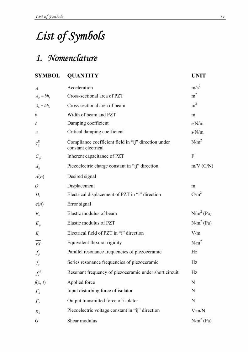
List of Symbols 1. Nomenclature
SYMBOL QUANTITY UNIT
A Acceleration m/s2
pp bhA = Cross-sectional area of PZT m2
bb bhA = Cross-sectional area of beam m2
b Width of beam and PZT m
c Damping coefficient s⋅N/m
cc Critical damping coefficient s⋅N/m
Eijc Compliance coefficient field in “ij” direction under
constant electrical N/m2
pC Inherent capacitance of PZT F
ijd Piezoelectric charge constant in “ij” direction m/V (C/N)
)(nd Desired signal
D Displacement m
iD Electrical displacement of PZT in “i” direction C/m2
)(ne Error signal
bE Elastic modulus of beam N/m2 (Pa)
pE Elastic modulus of PZT N/m2 (Pa)
iE Electrical field of PZT in “i” direction V/m
EI Equivalent flexural rigidity N⋅m2
pf Parallel resonance frequencies of piezoceramic Hz
sf Series resonance frequencies of piezoceramic Hz
Erf Resonant frequency of piezoceramic under short circuit Hz
f(x, t) Applied force N
SF Input disturbing force of isolator N
TF Output transmitted force of isolator N
ijg Piezoelectric voltage constant in “ij” direction V⋅m/N
G Shear modulus N/m2 (Pa)

List of Symbols xvi
bh Thickness of beam m
ph Thickness of PZT m
ijh Electrical displacement-stress coefficient of PZT in “ij” direction
N/C
)(nh Finite length impulse response sequence
)(xH Heaviside function
bI Area moment of inertia of beam about the neutral axis m4
pI1 Area moment of inertia of PZT about the neutral axis m4
pI2 Current source of PZT A
tI Total area moment of inertia
bJ Mass moment of inertia kg⋅m
k Stiffness N/m
nk Wavenumber m-1
ijK Electromechanical coupling coefficient in “ij” direction
L Length of beam m
eqL Equivalent inductor value of gyrator-based inductor
m Mass kg
M Bending moment N⋅m
n Young’s modulus ratio of PZT over beam
)(tqr Time function
Q1 Electrical charge of PZT C
Q2 Shear force N
r Ratio of the disturbing force frequency to the natural frequency of isolation system
Eijs Elasticity constant in “ij” direction under constant
electrical field m2/N
Dijs Elasticity constant in “ij” direction under constant
dielectric displacement m2/N
)( 12 xxbSp −= Surface area of PZT m2
bT Kinetic energy of beam J (N⋅m)
pT Kinetic energy of PZT J (N⋅m)
),( txu ),( tyv
Axial displacements m
List of Symbols xvii
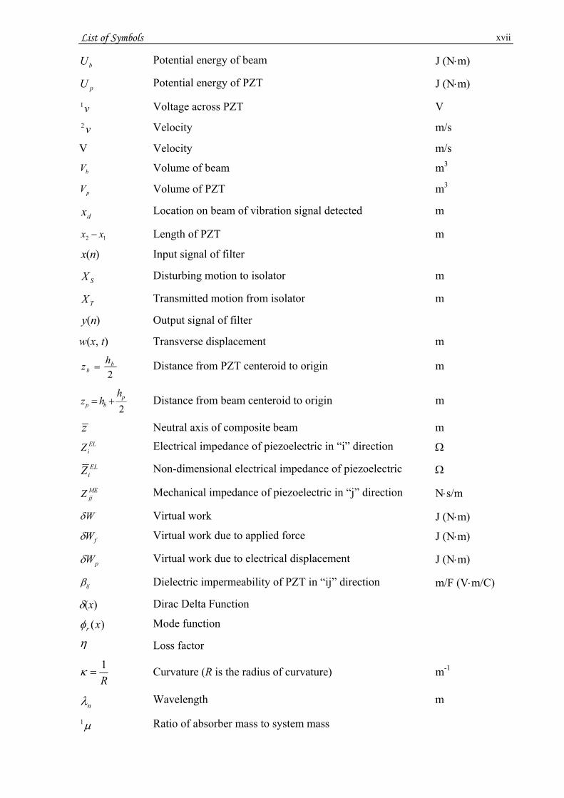
bU Potential energy of beam J (N⋅m)
pU Potential energy of PZT J (N⋅m)
v1 Voltage across PZT V
v2 Velocity m/s
V Velocity m/s
bV Volume of beam m3
pV Volume of PZT m3
dx Location on beam of vibration signal detected m
12 xx − Length of PZT m
)(nx Input signal of filter
SX Disturbing motion to isolator m
TX Transmitted motion from isolator m
)(ny Output signal of filter
w(x, t) Transverse displacement m
2b
bhz = Distance from PZT centeroid to origin m
2p
bp
hhz += Distance from beam centeroid to origin m
z Neutral axis of composite beam m ELiZ Electrical impedance of piezoelectric in “i” direction Ω EL
iZ Non-dimensional electrical impedance of piezoelectric Ω
MEjjZ Mechanical impedance of piezoelectric in “j” direction N⋅s/m
Wδ Virtual work J (N⋅m)
fWδ Virtual work due to applied force J (N⋅m)
pWδ Virtual work due to electrical displacement J (N⋅m)
ijβ Dielectric impermeability of PZT in “ij” direction m/F (V⋅m/C)
δ(x) Dirac Delta Function
)(xrφ Mode function
η Loss factor
R1
=κ Curvature (R is the radius of curvature) m-1
nλ Wavelength m
μ1 Ratio of absorber mass to system mass
List of Symbols xviii
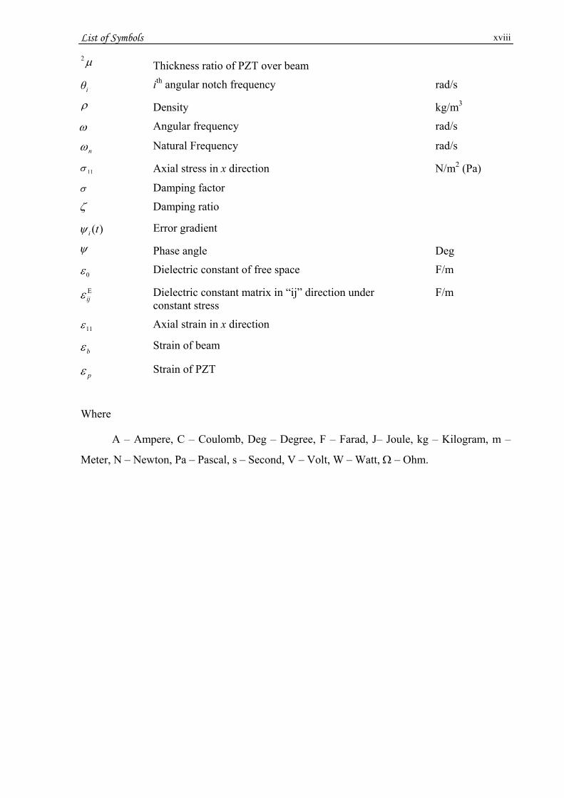
μ2 Thickness ratio of PZT over beam
iθ ith angular notch frequency rad/s
ρ Density kg/m3
ω Angular frequency rad/s
nω Natural Frequency rad/s
11σ Axial stress in x direction N/m2 (Pa)
σ Damping factor
ζ Damping ratio
)(tiψ Error gradient
ψ Phase angle Deg
0ε Dielectric constant of free space F/m
Eijε Dielectric constant matrix in “ij” direction under
constant stress F/m
11ε Axial strain in x direction
bε Strain of beam
pε Strain of PZT
Where
A – Ampere, C – Coulomb, Deg – Degree, F – Farad, J– Joule, kg – Kilogram, m –
Meter, N – Newton, Pa – Pascal, s – Second, V – Volt, W – Watt, Ω – Ohm.

List of Symbols xix
2. Subscripts
i Thickness direction of the piezoelectric material
j Loading direction
k Direction transverse to loading direction
ij Loading in j direction and shunt across i direction. The first subscript gives the direction of electrical parameters - the voltage applied or the charge produced. The second subscript gives the direction of mechanical parameters - stress or strain
D Measured under constant electrical displacement
E Measured under constant electrical field (short circuit)
S Measured under constant strain
T Measured under constant stress
3. Superscripts
D Measured under constant electrical displacement (open circuit)
E Measured under constant electrical field (short circuit)
EL Electrical
ME Mechanical
PMD Proof Mass Damper
RSP Resonant Shunted Piezoelectric
S Measured under constant strain
SU Shunt
T Measured under constant stress

List of Symbols xx
4. Acronyms and Abbreviations
AFC Active Fibre Composite
AM Amplitude Modulation
ANF Adaptive Notch Filter
AVC Active Vibration Control
CFRP Carbon Fiber Reinforced Plastic
COP Centre Of Percussion
COT Coefficient Of Restitution
DOF Degree-Of-Freedom
DSP Digital Signal Processing
EMI Electro-Magnetic Interference
ER Electro-Rheological
FEA Finite Element Analysis
FIR Finite Impulse Response
FRF Frequency Response Function
GIC Generalized Impedance Converter
IIR Infinite Impulse Response
LQG Linear Quadratic Gaussian
MDOF Multi-Degree-Of-Freedom
MFC Macro-Fibre Composites
MR Magneto-Rheological
PDE Partial Differential Equation
PMD Proof Mass Damper
PPF Positive Position Feedback
PT Piezoelectric Transformer
PVC Passive Vibration Control
PVDF PolyVinylidine DiFluoride (CH2CF2)
PZT Lead-Zirconium-Titanium (PbZrTiO3)
RLS Recursive Least Squares
RMS Root Mean Square
RSP Resonant Shunted Piezoelectric
SDOF Single-Degree-Of-Freedom
SMA Shape Memory Alloy

List of Symbols xxi
SNR Signal-to-Noise Ratio
TMD Tuned Mass Damper
TVA Tuned Vibration Absorber
TVD Tuned Viscoelastic Damper
VEM Visco-Elastic Materials
HR Handle radius
POS Apex position
POSF Ridge length
SCD Scoop height
SCF Scoop length
STC Centre spring
TH Apex height
TOE Toe thickness
W Edge thickness

Chapter 1 Introduction 1
Chapter 1
Introduction
1.1 Motivation
Cricket has been around for more than a Century but until now, improvements in the
performance of the Cricket bat have been somewhat limited (Bailey, T., 1997, Pratomo, D.,
2001). It’s partly due to game regulation restrictions and partly because the application of
appropriate high technology to the bat has been virtually non-existent. As anyone who has
played the game of Cricket knows, the effect of hitting a ball away from the Sweet Spot can be
very uncomfortable due to the transmitted structure-borne torsional and lateral vibration on a
player’s hands. There is also a chance for batsman to be injured as a result of the transient
vibration. These transient vibrations have up until now, been passively and mechanically
damped by the inherent damping properties of wood and flat rubber panels in the handle
(Penrose, et al, 1998, Knowles et al, 1996). The understanding is that this sort of passive
damping is effective for the high frequency vibrations only while the low frequency vibrations
remain uninterrupted.
The high technology has played a significant role in sports competition today. The high
technology equipment can give players a more competitive edge as well as greater comfort.
As for Cricket, the high technology could potentially result in a simple yet better design of a
Cricket bat leading to a marginal advantage over other designs, by offering superior quality
and enhanced performance. It can reduce the risk of a Cricket player being physically injured
due to the serious vibrations.
The rules of Cricket, although strict, have left open an opportunity to alter the handle design
where there is no limitation to the innovative possibilities, either in the form of improved
structure, material composition or additional instrument incorporation in the handle. It is
possible to incorporate novel state-of-the-art Smart technologies to provide enhanced
performance. The use of high stiffness to weight ratio advanced fibre composites and the
Chapter 1 Introduction 2
opportunity for innovative design and manufacture using textile composites, present the
possibility of significantly altering the dynamic characteristics of the bat by tailoring the
design of the handle.
The motivation of this study is to try to bring advanced vibration control technology into the
sporting goods industry, seeking and establishing novel applications using modern Digital
Signal Processing (DSP) techniques for future sporting goods. Scientifically, the research
project gives a theoretical and systematic understanding of the piezoelectric vibration control
for Cricket bat and initially links the modern electronics and digital signal processing
technology to the traditional Cricket bat. It will have ramifications in the development of even
more sophisticated Cricket bats.
1.2 Vibration control with Smart materials
Traditionally, unwanted vibrations are removed or attenuated with a variety of passive
treatments including rubber mounts, foam, viscoelastic layers, frication and tuned mass
damper (TMD). However, the outcome of these solutions somehow is limited for many
applications. In addition, temperature variation and geometric constraints sometimes make
them impractical. In the past decade, many researchers have turned their attention to so-called
Smart materials technology in conjunction with modern electronic technology as an
alternative to traditional mechanical vibration control techniques. The traditional mechanical
vibration control techniques are usually vibration isolation which reduces vibration energy
transmission from one body to another, by using low stiffness materials such as rubber;
vibration absorption which converts some of the vibration energy into another form of energy
with viscoelastic materials, usually heat; spring-mass damping which dissipates vibration
energy into heat with motion and time by adding mass. The drawbacks of these techniques
include: bulkiness and extra weight when being used for low frequency applications. Other
drawbacks of traditional vibration suppression methods include: inflexibility in applications
due to changing operating field conditions, lack of adaptability and ineffectiveness for high
frequency vibration reduction. The Smart materials such as piezoelectric materials integrated
with digital signal processing techniques may overcome these drawbacks.
Piezoelectric materials such as lead-zirconate-titanate ceramics (PZT), piezoelectric polymers
and Macro-Fiber Composites (MFC) are typical Smart materials suitable for vibration control.
They have the ability to convert mechanical energy into electronic energy and vice versa. The
piezoelectric materials have a broadband frequency response which can be used to tackle a
wide range of vibration frequencies. Compared to the traditional mechanical vibration control

Chapter 1 Introduction 3
techniques, the vibration control with Smart materials can result in a smaller size, lighter
weight, lower cost, and is more effective in on-going vibration suppression due to changing
operating conditions of the structure. They are especially suitable where the traditional
techniques cannot be applied due to weight and size restrictions (such as for spaceships,
satellites and aircrafts).
The scope of this study is to understand the nature of piezoelectric materials for energy
transduction. Physical properties of piezoelectric materials for vibration sensing, actuating
and dissipating will be evaluated. The analytical study of vibration energy coupling between
beams made of different materials and piezoelectric materials will be undertaken. The
numerical study will be carried out using the Finite Element Analysis (FEA) software package
ANSYS®; in modeling and designing of a Cricket bat with a composite handle. It will also
include modeling piezoelectric vibration shunt control for optimal design and placement of
the piezoelectric patches on the Cricket bat. The experimental study of the vibration control
will be conducted on beams as well as on Cricket bats to verify the results of analytical and
numerical studies. Different types of passive vibration shunt networks (Lesieutre, 1998) will
be simulated and tested. An adaptive notch filter algorithms for adaptive vibration control
with piezoelectric materials will also be studied and simulations implemented.
1.3 The objectives of this study
The objectives of this study are to:
(a) Bring innovation to vibration attenuation in the Cricket bats, especially 1st ~ 3rd modes.
(b) Reduce the unwanted vibration energy irrespective of the excited frequency.
(c) Achieve a reasonable vibration reduction in a short transient time period for improving
the dynamic performance of Cricket bats by using piezoelectric vibration control
technique in order to reduce the levels of shock and vibration impact on the batsman.
(d) Ease the risk of being injured by reducing the discomfort of the players due to the
vibrations, caused by the Cricket bat-ball impact.
(e) To ensure that the design and implementation should be in line with the international
manufacturing standards of Cricket bats and it should conform to the rules of the sport
(Oslear, 2000).
Initially, the design may use an external power source such as a battery as a power supply for
this study but self-powering will be the ultimate goal in the future. The delivered product is

Chapter 1 Introduction 4
expected to have such innovative features that will be perceived as being commercially
attractive as long as the rules of the Cricket game are complied with.
The task includes:
(1) Model the piezoelectric vibration shunt control for Cricket bats.
(2) Design, model and prototype new Cricket bat.
(3) Design and implement piezoelectric vibration control shunt technology in Cricket bats.
(4) Design the algorithm for adaptive vibration control to account for the inherent variations
in a Cricket bat’s natural frequencies due to the natural variability of the structure of
wood.
1.4 The organization of the thesis
This thesis contains seven further chapters:
In chapter 2, a brief overview of Cricket bat history and the research being carried out on
Cricket bats is presented. The literature review of traditional vibration control techniques,
Smart materials, particularly focusing on piezoelectric materials, passive and active
piezoelectric vibration control methods and their issues are presented.
In chapter 3, the analytical study of the passive piezoelectric vibration shunt control of
cantilever beam is undertaken. This is undertaken to test the feasibility on the shunt
technology on a simple structure such as a uniform-sectioned beam, before applying the
technique on the Cricket bat. The equation of motion of a composite beam which consists of
a cantilever beam bonded with a PZT patch using Hamilton’s principle and Galerkin’s method
was derived.
In chapter 4 the strain, stress analyses and design of composite beams were performed. The
influences of geometry sizes and material properties of the composite structure on strain and
stress distribution have been discussed. The design of the Smart Cricket bat is proposed.
Piezoelectric shunt circuit modeling in CAD software PSpice®, numerical modeling of the
passive piezoelectric vibration shunt control of beams with FEA software ANSYS® are
carried out in chapter 5. Different types of Cricket bat handles are designed and modeled with
the help of the CAD software - Solidworks®.
In chapter 6 the design and implementation of the shunt circuit using a gyrator-based inductor
is presented. Also included, are the modal analyses of Cricket bats using a laser vibrometer,

Chapter 1 Introduction 5
the experimental results of the passive piezoelectric vibration shunt control of the beams and
Cricket bats.
In chapter 7, the design of an adaptive notch filter using the Recursive Least-Squares (RLS)
algorithm for the estimation of frequencies is introduced. This design is verified by a
MATLAB® - based simulation. As explained above, this was undertaken to account for the
inherent variations in a Cricket bat’s natural frequencies due to the natural variability of the
structure of wood.
Conclusions and future work are highlighted in chapter 8.

Chapter 1 Introduction 6
1.5 Publications that originated from this research
[1] Cao, J. L. John, S. and Molyneaux, T., “Finite Element Analysis Modeling of
Piezoelectric Shunting for Passive Vibration Control”, International Conference on
Computational Intelligence for Modeling Control and Automation – CIMCA'2004, 12-
14 July 2004, Gold Coast, Australia.
[2] Cao, J. L. John, S. and Molyneaux, T., “Piezoelectric-based Vibration Control
Optimization Using Impedance Matching Technique”, 2nd Australasian Workshop on
Structural Health Monitoring, 16-17December 2004, Melbourne, Australia.
[3] Cao, J. L. John, S. and Molyneaux, T., “Piezoelectric-based Vibration Control
Optimization in Nonlinear Composite Structures”, 12th SPIE Annual International
Symposium on Smart Structures and Materials, 6-10 March 2005, San Diego, California
USA. (SPIE Code Number: 5764-46)
[4] Cao, J. L. John, S. and Molyneaux, T., “Computer Modeling and Simulation of Passive
Piezoelectric Vibration Shunt Control”, The 2005 International Multi-Conference in
Computer Science & Computer Engineering, June 27-30, 2005, Las Vegas, Nevada,
USA.
[5] Cao, J. L. John, S. and Molyneaux, T., “The Effectiveness of Piezoelectric Vibration
Shunt Control Based on Energy Transmission considerations”. Accepted for
presentation at EMAC 2005 and paper submitted to the Australian and New Zealand
Industrial & Applied Mathematics Division of the Australian Mathematical (ANZIAM)
Society Journal. (Under review)
[6] Cao, J. L. John, S. and Molyneaux, T., “Optimisation of Passive Piezoelectric Vibration
Shunt Control Based on Strain Energy Transfer and Online Frequency Detection”, 13th
SPIE Annual International Symposium on Smart Structures and Materials, 26 February-
2 March 2006, San Diego, California USA. (SPIE Code Number: 6167-66)
[7] Cao, J. L. John, S. and Molyneaux, T., “Strain Effect Modelling of Piezoelectric-based
Vibration Control in Composite Material Structures”, submitted to IOP Journals, Smart
Materials and Structures. (Under review)
[8] Cao, J. L. John, S. and Molyneaux, T., “Piezoelectric-based Vibration Control in
Composite Structures”, The 2006 World Congress in Computer Science, Computer
Engineering and Applied Computing, June 26-29, 2006, Las Vegas, Nevada, USA.

Chapter 2 Literature Review: Mechanical Vibration Control 7
Chapter 2
Literature Review:
Mechanical Vibration Control
Noise and vibration control has long been a subject of engineering research. One can
encounter noise and vibration everywhere in daily life, at home and work, during a trip, in
sports and recreation etc. In most cases, noise and vibration are undesirable and hazardous.
They can harm, damage, and even threaten human health. On the other hand, noises and
vibrations are difficult to control, especially with traditional techniques, which are mainly
isolation, absorption, and viscoelastic material damping, particularly at low frequencies due to
long wavelengths. These methods often result in bulky size, heavy weight and high costs. In
addition, temperature variation, geometry constraints and weight limitations sometimes make
them impractical for some applications. Noise and vibration in general stem from particle
movements in the media which can be represented by wave propagation. Often noises are
generated by vibrations. The former are undesired wave disturbances in air and the latter are
undesirable wave disturbances in mechanical structures. So the noise control and the vibration
control have their similarities. However, this study only focuses on the vibration control and
its application on Cricket bats. In this chapter, firstly, an overview of the background of
Cricket bat, including the rules restricting the design of Cricket bats and the possibilities of
improving Cricket bat performance by using advanced material and electronic technologies
within the boundaries of Cricket bat governing rules. Secondly, a review of traditional
mechanical vibration control techniques which are the foundation of modern vibration control
techniques. This is followed by introduction of Smart materials and structures, focusing on
piezoelectric materials and the literature review of piezoelectric vibration control methods
which basically fall into two categories: passive piezoelectric vibration control and active

Chapter 2 Literature Review: Mechanical Vibration Control 8
piezoelectric vibration control. Finally, discussion of their advantages/disadvantages and their
suitability for Cricket bat applications will be presented.
2.1 Background of the Cricket bat
As in many industries, the sporting goods industry faces fierce competition today. In order to
win the competition and prevent being phased out, it is important for manufacturers to
innovate products and give their goods added functionalities at an acceptable price. These are
not only to meet some players’ personal taste, but also to have benefits from a marketing point
of view. In sports competition, unwanted vibrations affect the performance, and comfort of
players, as well as shorten the life span of products. In recent years, optimising bat/ball impact
for ball-hitting games, shock and vibration control on sporting goods, which will suffer severe
shock and vibration impact, has come to the fore. The examples are such as aluminium
baseball bats (Russell, [I 10]) golf clubs (Bianchini et al, 1999), tennis rackets (Head_a, [I 5]),
mountain bike Smart shock system (Perkins, 1997), skis (Head_b, [I 6]), and Intelligence
snowboards (Head_c, [I 7]) which use advanced material technology with/without electronic
technology to either enhance performance for the games or reduce the risk of game players
being injured, bringing comfort to the game players. These innovative designs have made the
sports more attractive, enjoyable and entertaining.
Cricket is a sport with a long history and rich tradition. It is a global sport that uses a Cricket
bat to hit a bounce-delivered ball. The Cricket bat consists of basic structures of blade and
handle. The former is traditionally made of willow and the latter is made of cane. Due to deep
conservatism in the modern rules of the games, formulated in 1774 (Bailey, 1979), restrict the
games equipment from using new sport enhancement technologies that have proven to benefit
other games of sport. Only a little enhancement has been made to improve the performance of
Cricket bat since its inception. The laws of Cricket are a set of rules framed by the
Marylebone Cricket Club (MCC) which serve to standardise the format of Cricket matches
across the world to ensure uniformity and fairness. The laws of Cricket Law 6 –– The Bat,
limits the bat overall shall not be more than 38 inches/96.5cm in length; the blade of the bat
shall be made solely of wood and shall not exceed 41⁄4 in/10.8cm at the widest part; the blade
may be covered with material for protection, strengthening or repair, such material shall not
exceed 1⁄16 in/1.56mm in thickness, and shall not be likely to cause unacceptable damage to
the ball (MCC, [I 8]). Within the boundaries of the game rules, several improved bat designs
have proceeded to commercial production. These include the introduction of cane and rubber
laminates (parallel with the bat length) as handle material aimed to ultimately reduce the
Chapter 2 Literature Review: Mechanical Vibration Control 9
transmission of vibration from the blade to the handle on impact and the introduction of
improved perimeter weighting in 1960’s on the blade. However, these changes were still far
from optimum. The rules of the Cricket game prohibit radical improvement to the blade in
which no alteration to the material composition of the blade is permitted, English Willow or
its equivalent is mainly used in this regard, which restricts the blade design. The rules do not
strictly restrict the handle design, where there is no limitation to the innovative possibilities
either in the form of improved structure, material composition, or additional instrument
incorporation in the handle. This has left a door open for the possibility to design innovative
Cricket bats. These changes are however under the control of the MCC.
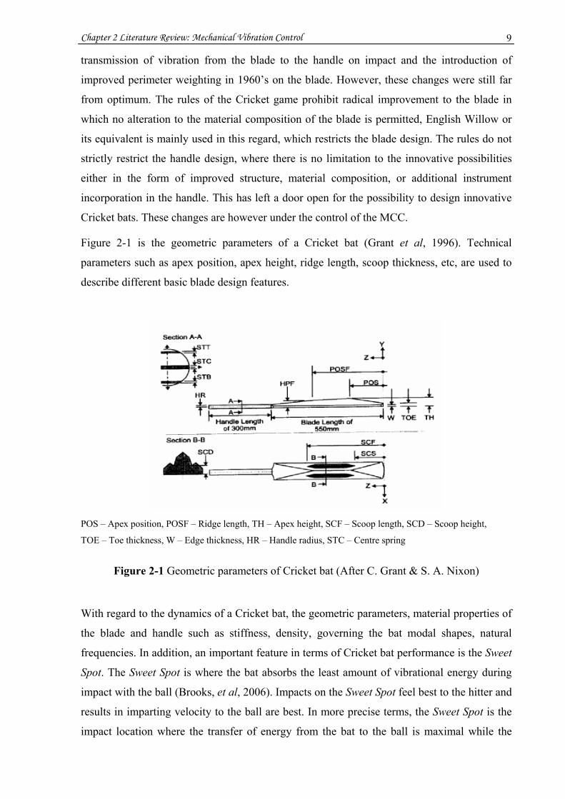
Figure 2-1 is the geometric parameters of a Cricket bat (Grant et al, 1996). Technical
parameters such as apex position, apex height, ridge length, scoop thickness, etc, are used to
describe different basic blade design features.
POS – Apex position, POSF – Ridge length, TH – Apex height, SCF – Scoop length, SCD – Scoop height,
TOE – Toe thickness, W – Edge thickness, HR – Handle radius, STC – Centre spring
Figure 2-1 Geometric parameters of Cricket bat (After C. Grant & S. A. Nixon)
With regard to the dynamics of a Cricket bat, the geometric parameters, material properties of
the blade and handle such as stiffness, density, governing the bat modal shapes, natural
frequencies. In addition, an important feature in terms of Cricket bat performance is the Sweet
Spot. The Sweet Spot is where the bat absorbs the least amount of vibrational energy during
impact with the ball (Brooks, et al, 2006). Impacts on the Sweet Spot feel best to the hitter and
results in imparting velocity to the ball are best. In more precise terms, the Sweet Spot is the
impact location where the transfer of energy from the bat to the ball is maximal while the

Chapter 2 Literature Review: Mechanical Vibration Control 10
transfer of energy to the hands is minimal (Noble, [I 9]). It is probably due to at this location
where the rotation forces of the bat are completely balanced out when hitting a ball in this
area. The Sweet Sport is often believed to be the same as Centre of Percussion (COP).
The Centre of Percussion is a point at a distance r below the centre of a object, for example a
rod, does not move at the instant the rod is struck (Sears, 1958). The Centre of Percussion
may or may not be the Sweet Spot depending on the pivot point chosen. The Centre of
Percussion of a cricket bat is the point on a bat, where a perpendicular impact will produce
translational and rotational forces which perfectly cancel each other out at some given pivot
point while the Sweet Spot of a bat exists partly because bat vibrations are not excited
significantly at that spot where the contact between bat and ball and partly because the spot is
close to the COP.
The Sweet Spot is essentially an area of a sporting instrument that inflicts maximum velocity
of the ball and minimum response to the holder of the instrument (Naruo et al, 1998). On the
other hand, when Cricket ball hits outside the Sweet Spot area, less kinetic energy will return
back to the ball and the lost energy will remain in the Cricket bat and become vibration wave
travelling back and forth. The holy grail of good Cricket bat design is that it should have a
Sweet Spot area that is as large as possible.
From the literature of Cricket bat research, researchers mainly focus on improving the
dynamic performance of Cricket bats. C. Grant and S. A. Nixon (Grant et al, 1996) used
Finite Element Analysis (FEA) to optimise the blade geometric parameters and C. Grant
(Grant, 1998) suggested that handle stiffness be strengthened with composite material in order
to raise the 3rd flexural vibration mode out of the excitation spectrum, that is, the 3rd mode is
not excited during ball/bat impact, results in the 3rd vibration mode being removed
completely, leaving only the 1st and 2nd modes to have significant impact on the batsman. R.
Brooks and S. Knowles, et al (Knowles et al, 1996) compared impact characteristics and
vibrational response between traditional wooden Cricket bats and full composite Cricket bats
through impact tests as well as computational analysis. Their findings implied that the
composite bat could have higher Coefficient Of Restitution (COR = ball output speed/ball
input speed) which means the ball can be bounced back at faster speed. In addition, they
implied that the contact time of bat/ball might be optimally tuned with the composite bat, to
match the time it takes for the bat to deflect and return to its original position (Brooks et al,
1997). The energy of vibration in the bat can then be returned to the ball giving it a high exit
velocity. This contact time matches one of the vibration frequencies of the bat. In similar
studies with FEA, J. M. T. Penrose, et al (Penrose et al, 1998), S. John and Z. B. Li (John et

Chapter 2 Literature Review: Mechanical Vibration Control 11
al, 2002) had similar conclusions that the bat/ball contact time (or dwell time) appears
approximately constant and dictated by the local Hertzian parameters. The ball exit velocity
might be increased by optimal tuning of the frequencies of the 2nd or 3rd modes to give a time
period of half a cycle approximately equal to the time of contact. They also believed that the
1st flexure mode dominates the impact. These researchers have given an insight and valuable
contribution to designing better Cricket bats in future. However, there is little information
regarding to the attenuation or reduction of the vibration excited in the Cricket bat. The study
of removing or controlling the post-impact vibration in Cricket bats is still in its infancy. The
goal of this study is to explore the post-impact vibration control of the Cricket bats. In the
next few sections, traditional vibration control methods as well as the emerging new vibration
control with Smart material components will be discussed.
2.2 Traditional mechanical vibration control techniques
The collision of two objects will generate vibration in the objects. The impact of the collision
excites the vibrations of the natural frequencies of the objects. The natural frequencies, which
are decided by the geometry size and material properties of the object, are one of the most
important characteristics of the object. Each excited natural frequency results in a single
frequency vibration. The vibration of the object is the combination of every single natural
frequency vibration of the object. Theoretically, the excited vibration will exist forever if
there is no energy dissipation in the object, such as internal damping. Therefore, the
mechanical vibration control is to control vibration energy transmission and dissipation. The
basic traditional mechanical vibration control techniques are vibration isolation, vibration
absorption and vibration damping. They are discussed in following sections respectively.
2.2.1 Vibration isolation
Vibration isolation is achieved by using isolators to reduce the transmission of vibratory force
or motion from one mechanical structure to another. The isolator interconnects the source
system in which the vibration is generated and the receive system in which the vibration is to
be prevented.
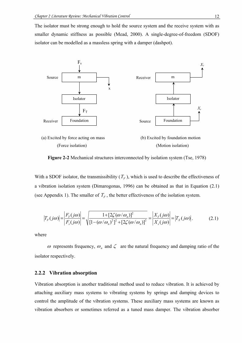
The Figure 2-2 shows the block diagram of two mechanical structures interconnected by an
isolator where the foundation is considered as rigid and the mass is not considered
(Dimarogonas, 1996). In the figure, m represents mass, ‘ SF ’ and ‘ TF ’ are the input disturbing
force and output transmitted force of the isolator respectively; ‘ SX ’ and ‘ TX ’ are the input
disturbing motion and output transmitted motion of the isolator respectively.
Chapter 2 Literature Review: Mechanical Vibration Control 12
The isolator must be strong enough to hold the source system and the receive system with as
smaller dynamic stiffness as possible (Mead, 2000). A single-degree-of-freedom (SDOF)
isolator can be modelled as a massless spring with a damper (dashpot).
(a) Excited by force acting on mass (b) Excited by foundation motion
(Force isolation) (Motion isolation)
Figure 2-2 Mechanical structures interconnected by isolation system (Tse, 1978)
With a SDOF isolator, the transmissibility ( FT ), which is used to describe the effectiveness of
a vibration isolation system (Dimarogonas, 1996) can be obtained as that in Equation (2.1)
(see Appendix 1). The smaller of FT , the better effectiveness of the isolation system.
)()()(
)]/(2[])/(1[)]/(2[1
)()()( 222
2
ωωω
ωωζωωωωζ
ωωω jT
jXjX
jFjFjT X
s
T
nn
n
s
TF ==
+−+
== . (2.1)
where
ω represents frequency, nω and ζ are the natural frequency and damping ratio of the
isolator respectively.
2.2.2 Vibration absorption
Vibration absorption is another traditional method used to reduce vibration. It is achieved by
attaching auxiliary mass systems to vibrating systems by springs and damping devices to
control the amplitude of the vibration systems. These auxiliary mass systems are known as
vibration absorbers or sometimes referred as a tuned mass damper. The vibration absorber
FT
Fs
x
m
Foundation
Isolator
Source
Receiver
XT
Xs
Foundation
m
Isolator
Source
Receiver

Chapter 2 Literature Review: Mechanical Vibration Control 13
absorbs vibration energy by transferring the energy from base structure to absorber.
Depending on applications, vibration absorbers fall into two categories. If an absorber has a
little damping factor, it is called a dynamic vibration absorber or undamped vibration
absorber. Due to the lack of damping, the undamped dynamic vibration absorber has a very
high level of vibration itself and is easy to cause fatigue failures. Therefore, it is often
necessary to add damping to the absorber (Dimarogonas, 1996). The absorber with damping
factor is called a damped vibration absorber or auxiliary mass damper (Harris et al, 2002).
Absorbers are most effective when placed in positions of high displacement or anti-nodes of
structures. The absorbers reduce vibrations by absorbing the vibration energy through its mass
deflection. The absorber spring must be stiff enough to withstand large forces and deflections.
Since absorbers are designed to meet sa ωω = or 2/ saa km ω= , high stiffness ak leads to large
am , especially for low natural frequencies. This will make the absorber system heavier. Also,
the mass-spring structure is not suitable for some applications which have space and location
constraints. Details of analytical modelling of vibration absorbers for the SDOF structure can
be found in Appendix 1.
2.2.3 Vibration damping
The third traditional passive vibration control technique is vibration damping. Vibration
damping refers to a mechanism to dissipate mechanical energy extracted from a vibrating
system into another form, usually heat. The vibration damping can be classified in two types:
material damping or viscous damping and structural damping or system damping (Ruzicka,
1959). Material damping is the damping inherent in the material to dissipate kinetic and strain
energy into heat. Structural (system) damping is the damping caused by discontinuity of
mechanical structures, such as at joint, interface, etc.
2.2.3.1 Viscouselastic damping
There are three major types of material used for material damping: (1) viscoelastic materials
(VEM), (2) structural metals and non-metals, (3) surface coatings (Harris et al, 2002).
A viscoelastic material such as rubber, plastics and polymers, exhibit characteristics of both
viscous fluid and elastic solid. Like elastic materials, viscoelastic materials return to their
original shape after being stressed but at lower speed due to viscous damping force. The stress
response of viscoelastic materials obeys the superposition principle. The deformation of
viscoelastic materials at any instant is a summation of the deformation produced by history
stress and the deformation produced by current stress. Viscoelastic materials are sometimes
Chapter 2 Literature Review: Mechanical Vibration Control 14
called ‘materials with memory’. Usually, viscoelastic materials can dissipate much more
energy per cycle of deformation than steel and aluminium. For conventional structural
materials, the energy dissipation per unit-volume per cycle is very small compared to
viscoelastic materials.
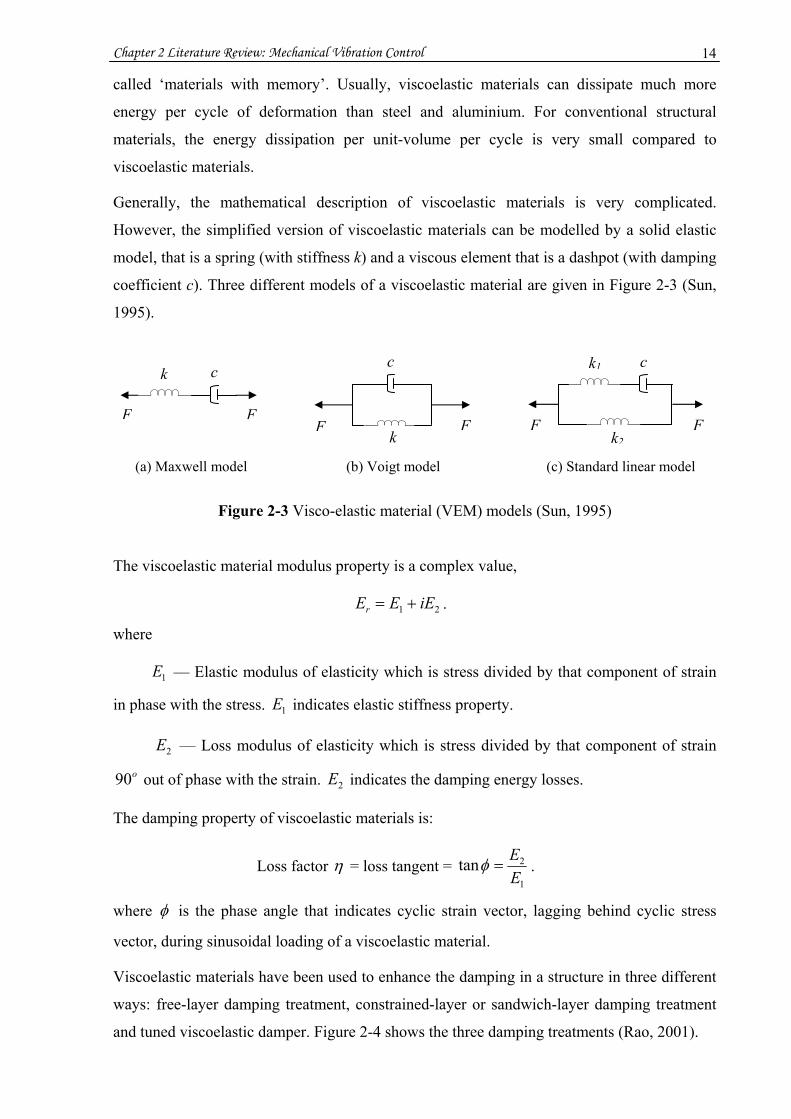
Generally, the mathematical description of viscoelastic materials is very complicated.
However, the simplified version of viscoelastic materials can be modelled by a solid elastic
model, that is a spring (with stiffness k) and a viscous element that is a dashpot (with damping
coefficient c). Three different models of a viscoelastic material are given in Figure 2-3 (Sun,
1995).
(a) Maxwell model (b) Voigt model (c) Standard linear model
Figure 2-3 Visco-elastic material (VEM) models (Sun, 1995)
The viscoelastic material modulus property is a complex value,
21 iEEEr += .
where
1E –– Elastic modulus of elasticity which is stress divided by that component of strain
in phase with the stress. 1E indicates elastic stiffness property.
2E –– Loss modulus of elasticity which is stress divided by that component of strain
o90 out of phase with the strain. 2E indicates the damping energy losses.
The damping property of viscoelastic materials is:
Loss factor η = loss tangent = 1
2tanEE
=φ .
where φ is the phase angle that indicates cyclic strain vector, lagging behind cyclic stress
vector, during sinusoidal loading of a viscoelastic material.
Viscoelastic materials have been used to enhance the damping in a structure in three different
ways: free-layer damping treatment, constrained-layer or sandwich-layer damping treatment
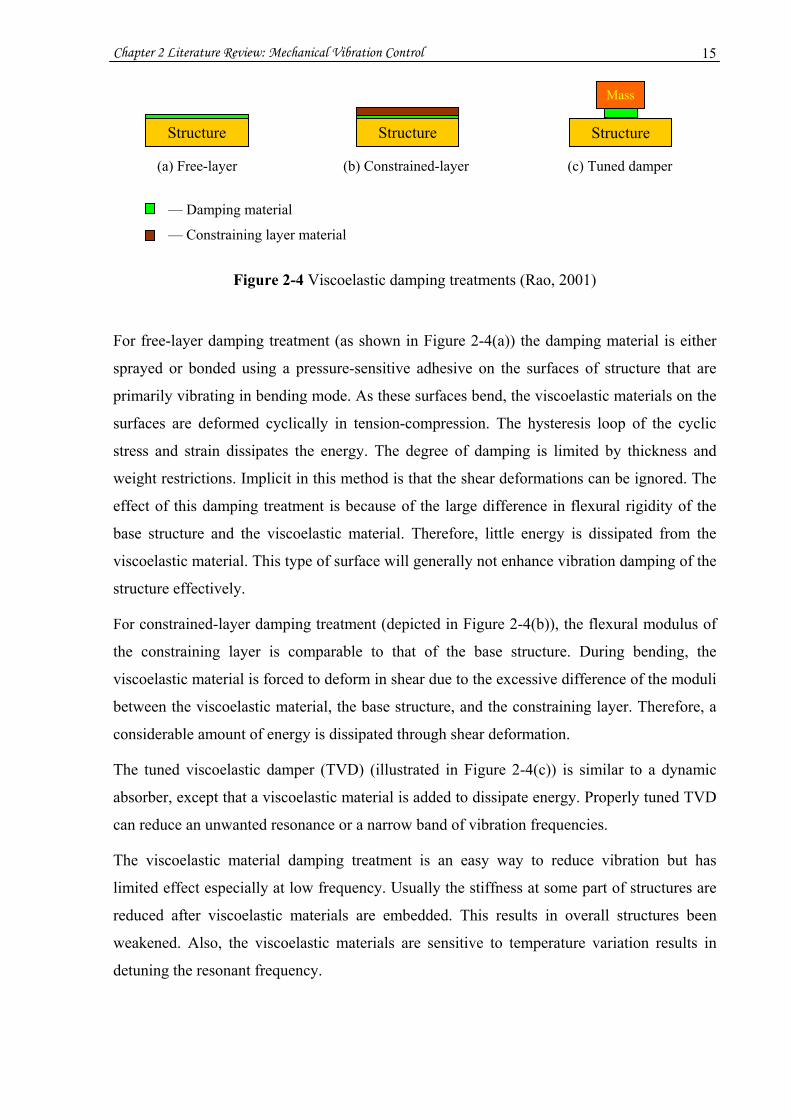
and tuned viscoelastic damper. Figure 2-4 shows the three damping treatments (Rao, 2001).
k c
F Fk
c
F Fk2
c k1
F F
Chapter 2 Literature Review: Mechanical Vibration Control 15
(a) Free-layer (b) Constrained-layer (c) Tuned damper
–– Damping material
–– Constraining layer material
Figure 2-4 Viscoelastic damping treatments (Rao, 2001)
For free-layer damping treatment (as shown in Figure 2-4(a)) the damping material is either
sprayed or bonded using a pressure-sensitive adhesive on the surfaces of structure that are
primarily vibrating in bending mode. As these surfaces bend, the viscoelastic materials on the
surfaces are deformed cyclically in tension-compression. The hysteresis loop of the cyclic
stress and strain dissipates the energy. The degree of damping is limited by thickness and
weight restrictions. Implicit in this method is that the shear deformations can be ignored. The
effect of this damping treatment is because of the large difference in flexural rigidity of the
base structure and the viscoelastic material. Therefore, little energy is dissipated from the
viscoelastic material. This type of surface will generally not enhance vibration damping of the
structure effectively.
For constrained-layer damping treatment (depicted in Figure 2-4(b)), the flexural modulus of
the constraining layer is comparable to that of the base structure. During bending, the
viscoelastic material is forced to deform in shear due to the excessive difference of the moduli
between the viscoelastic material, the base structure, and the constraining layer. Therefore, a
considerable amount of energy is dissipated through shear deformation.
The tuned viscoelastic damper (TVD) (illustrated in Figure 2-4(c)) is similar to a dynamic
absorber, except that a viscoelastic material is added to dissipate energy. Properly tuned TVD
can reduce an unwanted resonance or a narrow band of vibration frequencies.
The viscoelastic material damping treatment is an easy way to reduce vibration but has
limited effect especially at low frequency. Usually the stiffness at some part of structures are
reduced after viscoelastic materials are embedded. This results in overall structures been
weakened. Also, the viscoelastic materials are sensitive to temperature variation results in
detuning the resonant frequency.
Structure Structure Structure
Mass
Chapter 2 Literature Review: Mechanical Vibration Control 16
2.2.3.2 Structural damping
In complex structures, there is energy dissipation during vibration due to Coulomb friction in
contact surfaces, riveted joints, and so on. It is not possible to generally predict the damping
of a built-up structure. It is extremely difficult to estimate the energy transmitting and
exchanging at joints or interfaces of a complex structure because of the uncertainty about their
contacts. Testing is the only practical way for determining the damping of most large complex
structures. The methods of estimating damping ratio of a SDOF system in frequency domain
and time domain can be found in Appendix 2. The methods also can be extended to a multi-
degree-of-freedom (MDOF) system.
2.3 Non-conventional vibration control with Smart material components
Vibration control with Smart material is to incorporate Smart material as sensors and/or
actuators and electronic system to a structure in a proper way that turns the structure into a
Smart structure.
2.3.1 Smart material and structure
Smart systems trace their origin to a field of research that envisioned devices and materials
that could mimic human muscular and nervous systems. The essential idea is to produce non-
biological systems that will achieve the optimum functionality observed in biological systems
through emulation of their adaptive capabilities and integrated design (Akhras, [I 2]).
A Smart structure can be defined as a system which has embedded sensors, actuators and
control system, is capable of sensing a stimulus, responding to it, and reverting to its original
state after the stimulus is removed (is not damaged). The Smart structure can be used to
changing the shape of the structure in a controlled manner, or alternatively, changing the
mass, stiffness, or energy dissipation characteristics of the structure in a controlled manner to
alter the dynamic response characteristics, such as natural frequencies, mode shapes, settling
time of the structure.
Smart materials are the materials that, firstly, have the capability to respond to stimuli and
environmental changes, and secondly, to activate their functions according to these changes.
The common Smart materials are piezoelectric ceramics, shape memory alloys (SMAs),
electro-rheological fluids (ER fluids), magneto-rheological fluids (MR fluids), magneto-
restrictives, etc. Following are brief descriptions of the common Smart materials and their
applications.

Chapter 2 Literature Review: Mechanical Vibration Control 17
Piezoelectric materials –– Piezoelectric materials are widely used Smart materials which can
be classified into three types: piezoelectric ceramics, piezoelectric polymers and piezoelectric
composites. The piezoelectric ceramics are solid materials which generate charges in response
to a mechanical deformation, or alternatively they develop mechanical deformation when
subjected to an electrical field. These can be employed either as actuators or sensors in the
development of Smart structures. The shape of piezoelectric ceramic materials can be in disc,
washer, tube, block, stack, etc. The piezoelectric polymers are thin and soft polymer sheets
which usually are used as sensors. The piezoelectric composites are something between
ceramic and polymer which can be either used as actuators or sensors.
The piezoelectric materials have a broadband frequency response that can be used in high
frequency applications, and they are able to generate large actuation force. For example, stack
ceramic actuators with displacements of 100 μm can generate blocked forces equal to several
tonnes (Suleman, 2001). Details about piezoelectric materials will be discussed in the next
section.
Shape memory alloys (SMA) –– A Shape Memory Alloy (SMA) is an alloy which, when
deformed (in the martensitic phase) with the external stresses removed and then heated, will
regain its original "memory" shape (in the austenitic phase). Shape memory alloys can thus
transform thermal energy directly to mechanical work (Vessonen, 2002). The materials have
ability to remember their original shape that have given name of shape memory alloy. Shape
memory alloy materials can have shape in washer, tube, strip, wire, etc. In the process, they
generate an actuating force. The most popular one is a nickel-titanium alloy known as Nitinol,
which has a corrosion resistance similar to stainless steel. However, shape-memory alloys can
respond only as quickly as the temperature can shift, which only can be used for very low
frequency applications (few Hz).
Electro-rheological fluids (ER fluids) –– ER fluids are suspensions of micron-sized
hydrophilic particles suspended in suitable hydrophobic carrier liquids, that undergo
significant instanteous reversible changes in their mechanical properties, such as their mass
distribution, and energy-dissipation characteristics, when subjected to electric fields (Gandhi
et al, 1992). In the neutral state the particles are uniformly distributed throughout the fluid.
When the electric field is applied, the relatively high dielectric constant of the particles
captures this electric field, redistributes the charge densities within the particles, and cause
them to stick together in fibrils. The presence of these fibrils considerably modifies the
viscous properties of the fluid (by several orders of magnitude).
Chapter 2 Literature Review: Mechanical Vibration Control 18
Magneto-rheological fluids (MR fluids) –– MR fluid is a functional material consisting of
carrier liquid, ferro-magnetic particles, plus some additives, which are included to work
against article-liquid separation and wear of sealings, for example (Vessonen, 2002). When
subjected to a magnetic field, the fluid greatly increases its viscosity, to the point of becoming
a viscolelastic solid. The fluid can reversibly and instantaneously change from a free-flowing
liquid to a semi-solid with controllable yield strength when exposed to a magnetic field.
ER and MR fluids have applications in areas such as tuneable dampers, vibration isolation
systems, and in exercise equipment as clutches, brakes, and resistance controls.
Magnetostrictive materials –– Magnetostriction is observed in a substance when it strains
upon application of a magnetic field. Conversely a field is generated when the material is
stressed; this field is, however, proportional to the material’s rate of strain (Vessonen, 2002).
All magnetic materials exhibit varying degrees of magnetostriction, however only some
materials exhibit sufficient magnetostriction for practical use. Early magnetostrictive devices
were used Nickel as the magnetostrictive material and this principle found use in sonar
applications. Materials such as Terfenol-D are similar to piezoelectric but these respond to
magnetic rather than electric fields. Magnetostrictive materials are used to build actuators and
sensors. They are typically used in low frequency, high power sonar transducers motors and
hydraulic actuators.
2.3.2 Piezoelectric materials
“Piezoelectric effect” was first discovered by Pierre Curie and his brother Jacques in 1880.
When a crystal, such as Quartz and Rochelle salt, is under pressure (piezo means pressure in
Greek) an electrical potential appears across some of its faces (direct effect). When an
electrical field is applied, mechanical deformation of the crystal occurs (converse effect). The
essence of “piezoelectric effect” is the relation between electric polarization and mechanical
strain in crystals. “Direct effect” indicates that the electric polarization is produced by a
mechanical strain in crystals which is proportional to the strain. “Converse effect” indicates
that the crystals become strained when electrically polarized and the strain produced is
proportional to the polarizing field. The strains produced are about 0.1% at a field of about
10kV/cm. The strain (or displacement) vs. electrical field is nearly linear in the operating
region, but the strain saturates at very high fields (Suleman, 2001).
The “Piezoelectric effect” happens to materials with a crystalline structure but with no centre
of symmetry. These materials are called non-centrosymmetric materials. A single crystal with
a non-centrosymmetric structure has anisotropic characteristics, that is, the properties of the

Chapter 2 Literature Review: Mechanical Vibration Control 19
material differ according to the direction of measurement. In material having piezoelectric
properties, ions can be moved more easily along some crystal axes than others. Pressure in
certain directions results in a displacement of ions. When pressure is released, the ions return
to original positions. If a piece of piezoelectric material is heated above a certain temperature,
it will lose its piezoelectric properties. This temperature is known as Curie temperature. After
cooling below the Curie temperature, the piezoelectric material will not regain its
piezoelectric properties.
Figure 2-5 shows a crystal structure of a traditional ceramic (APC, [I 4]). In the Figure 2-5(a),
the crystal is under the condition that the temperature is above Curie temperature, the crystal
has a centrosymmetric structure and has no piezoelectric characteristics, exhibits a cubic
lattice, symmetric arrangement of positive and negative charges with no dipole moment. In
the Figure 2-5(b), the crystal is under the condition that the temperature is below Curie
temperature, the crystal has a non-centrosymmetric structure and exhibits tetragonal lattice
with a net electric dipole moment.
(a) Cubic lattice (b) Tetragonal lattice
Figure 2-5 Crystal structure of a traditional ceramic (APC, [I 4])
The ceramic material is composed of many randomly oriented crystals or grains, each having
one or a few domains, the regions where dipoles are aligned in the same direction. With the
dipoles randomly oriented, the ceramic material is isotropic and does not exhibit the
“Piezoelectric effect”. By applying electrodes and a strong DC electric field to the ceramic
material, a process known as poling, the dipoles will tend to align themselves parallel to the
field, so that the ceramic material will have a permanent polarization. Once the ceramic
material is polarized, it becomes piezoelectric ceramic with anisotropic. The direction of the
–– Pb2+/Ba2+, large divalent metal ion –– O2-, oxygen –– Ti4+/Zr4+, smaller trivalent metal ion
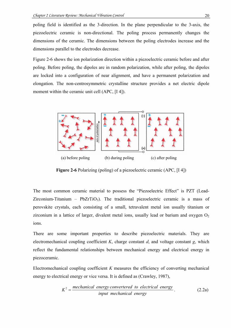
Chapter 2 Literature Review: Mechanical Vibration Control 20
poling field is identified as the 3-direction. In the plane perpendicular to the 3-axis, the
piezoelectric ceramic is non-directional. The poling process permanently changes the
dimensions of the ceramic. The dimensions between the poling electrodes increase and the
dimensions parallel to the electrodes decrease.
Figure 2-6 shows the ion polarization direction within a piezoelectric ceramic before and after
poling. Before poling, the dipoles are in random polarization, while after poling, the dipoles
are locked into a configuration of near alignment, and have a permanent polarization and
elongation. The non-centrosymmetric crystalline structure provides a net electric dipole
moment within the ceramic unit cell (APC, [I 4]).
(a) before poling (b) during poling (c) after poling
Figure 2-6 Polarizing (poling) of a piezoelectric ceramic (APC, [I 4])
The most common ceramic material to possess the “Piezoelectric Effect” is PZT (Lead-
Zirconium-Titanium – PbZrTiO3). The traditional piezoelectric ceramic is a mass of
perovskite crystals, each consisting of a small, tetravalent metal ion usually titanium or
zirconium in a lattice of larger, divalent metal ions, usually lead or barium and oxygen O2
ions.
There are some important properties to describe piezoelectric materials. They are
electromechanical coupling coefficient K, charge constant d, and voltage constant g, which
reflect the fundamental relationships between mechanical energy and electrical energy in
piezoceramic.
Electromechanical coupling coefficient K measures the efficiency of converting mechanical
energy to electrical energy or vice versa. It is defined as (Crawley, 1987),
energymechanicalinputenergyelectricaltodconvertereenergymechanicalK
=2 . (2.2a)

Chapter 2 Literature Review: Mechanical Vibration Control 21
energyelectricalinputenergymechanicaltodconvertereenergyelectricalK
=2 . (2.2b)
Electromechanical coupling coefficient K value is mode dependent. For vibration mode ‘33’,
coupling coefficient is 33K , which is much larger than that for other directions. For PZT, 33K
is about 0.5 ~ 0.7 while 31K and 32K are about 1/3 of the 33K .
⎟⎟⎠
⎞⎜⎜⎝
⎛ Δ⋅⋅⋅+
⎟⎟⎠
⎞⎜⎜⎝
⎛ Δ⋅⋅⋅
==
ss
p
ss
p
ff
ff
ff
ff
KK
2tan
21
2tan
23231 ππ
ππ
. (2.3)
⎟⎟⎠
⎞⎜⎜⎝
⎛ Δ⋅⋅⋅=
pp
s
ff
ffK
2tan
233ππ . (2.4)
where pf and sf are parallel and series resonance frequencies of piezoceramic respectively,
sp fff −=Δ .
d constant measures the efficiency of generating strain for a given electrical field that
indicates a material’s suitability for actuator applications. It is defined as:
⎟⎟⎠
⎞⎜⎜⎝
⎛==
stress applieddensity chargecircuit short
field applieddevelopedstrain d . (2.5)
g constant measures the efficiency of generating electrical charge for a given stress that
indicates a material’s suitability for sensor applications. It is defined as:
⎟⎟⎠
⎞⎜⎜⎝
⎛==
density charge applieddevelopedstrain
stress appliedfieldcircuit open g . (2.6)
High d is desirable for piezoceramic to develop motion or vibration. High g is desirable for
piezoceramic to generate voltage in response to a mechanical stress. In piezoceramic, there
are many K, d, and g donated as, and, which one been taken, depends on the directions of
applied electrical field, displacement, stress and strain.
2.3.2.1 Orientation and notation
Because a piezoelectric ceramic is anisotropic, physical constants relate to both the direction
of the applied mechanical or electric force and the directions perpendicular to the applied
force. Consequently, each constant generally has two subscripts that indicate the directions of
the two related quantities, such as stress (force on the ceramic element/surface area of the
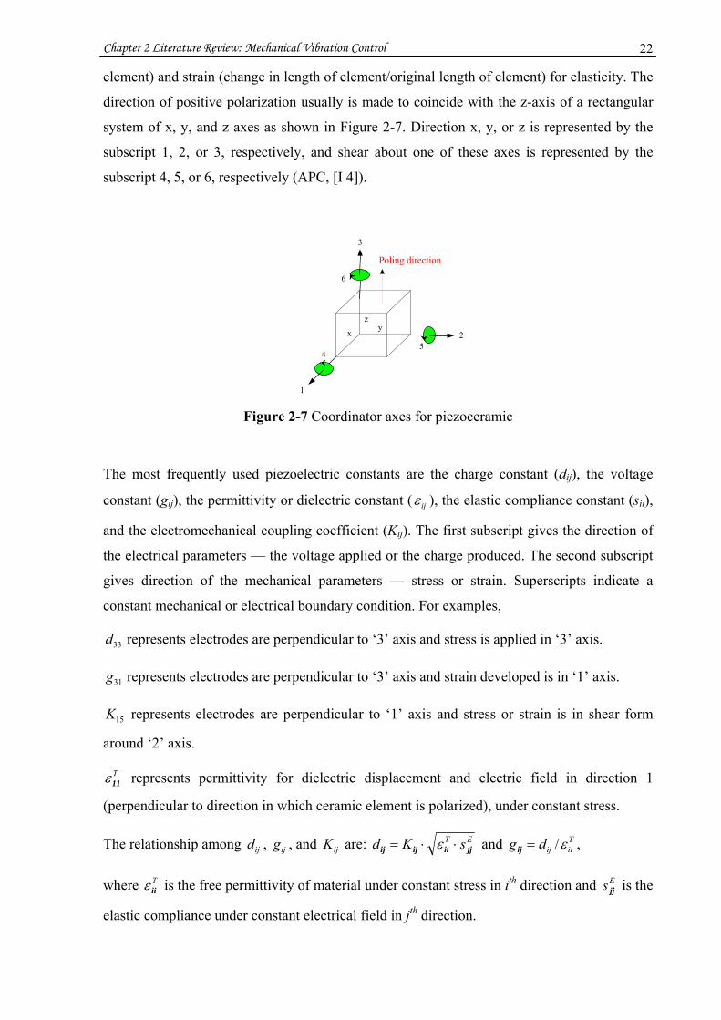
Chapter 2 Literature Review: Mechanical Vibration Control 22
3
1
y z
x
6
4
2
Poling direction
5
element) and strain (change in length of element/original length of element) for elasticity. The
direction of positive polarization usually is made to coincide with the z-axis of a rectangular
system of x, y, and z axes as shown in Figure 2-7. Direction x, y, or z is represented by the
subscript 1, 2, or 3, respectively, and shear about one of these axes is represented by the
subscript 4, 5, or 6, respectively (APC, [I 4]).
Figure 2-7 Coordinator axes for piezoceramic
The most frequently used piezoelectric constants are the charge constant (dij), the voltage
constant (gij), the permittivity or dielectric constant ( ijε ), the elastic compliance constant (sii),
and the electromechanical coupling coefficient (Kij). The first subscript gives the direction of
the electrical parameters — the voltage applied or the charge produced. The second subscript
gives direction of the mechanical parameters — stress or strain. Superscripts indicate a
constant mechanical or electrical boundary condition. For examples,
33d represents electrodes are perpendicular to ‘3’ axis and stress is applied in ‘3’ axis.
31g represents electrodes are perpendicular to ‘3’ axis and strain developed is in ‘1’ axis.
15K represents electrodes are perpendicular to ‘1’ axis and stress or strain is in shear form
around ‘2’ axis.
T11ε represents permittivity for dielectric displacement and electric field in direction 1
(perpendicular to direction in which ceramic element is polarized), under constant stress.
The relationship among ijd , ijg , and ijK are: ET sKd jjiiijij ⋅⋅= ε and Tiiijdg ε/=ij ,
where Tiiε is the free permittivity of material under constant stress in ith direction and Es jj is the
elastic compliance under constant electrical field in jth direction.

Chapter 2 Literature Review: Mechanical Vibration Control 23
2.3.2.2 Piezoelectric Constitutive Equations
The piezoelectric material has the linear constitutive relation (IEEE 1987). There are four
types of fundamental piezoelectric relations which are: h-form, d-form, g-form, and e-form
listed in the Table 2-1.
Table 2-1 Types of fundamental piezoelectric relation (Ikeda, 1996)
Independent Variable Type Piezoelectric relation Form
S, D Extensive DhS
hDScET
S
D
β+−−
==
⎩⎨⎧
h-form
T, E Intensive EdT
dETsDS
T
E
ε++
==
⎩⎨⎧
d-form
T, D Mixed DgT
gDTsES
T
D
β+−+
==
⎩⎨⎧
g-form
S, E Mixed EeS
eEScDT
S
E
ε+−
==
⎩⎨⎧
e-form
In the table, variables S and D are named as extensive variable while T and E are named as
intensive variable. When the variables used in the relations are solely extensive or intensive,
the type is called as extensive or intensive type respectively; otherwise the type is called as
mixed type.
The matrix representation of d-form is
⎥⎦
⎤⎢⎣
⎡⋅⎥⎦
⎤⎢⎣
⎡=⎥
⎦
⎤⎢⎣
⎡ET
dds
DS
Tt
E
ε. (2.7)
where
D is an electrical displacement vector (charge/area), E is an electrical field vector in a
material (volts/meter), S is a material engineering strains vector, T is a material stresses

Chapter 2 Literature Review: Mechanical Vibration Control 24
vector (force/area), d is piezoelectric charge-constant matrix, εT is dielectric constant matrix
under constant stress, and sE is piezoelectric compliance matrix under constant electrical field.
⎥⎥⎥
⎦
⎤
⎢⎢⎢
⎣
⎡=
3
1
DDD
2D , ⎥⎥⎥
⎦
⎤
⎢⎢⎢
⎣
⎡=
3
1
EEE
2E , ⎥⎥⎥
⎦
⎤
⎢⎢⎢
⎣
⎡=
0000000000000
333131
15
15
dddd
dd ,
⎥⎥⎥
⎦
⎤
⎢⎢⎢
⎣
⎡
=T
T
T
3
2
1
000000
εε
εTε ,
⎥⎥⎥⎥⎥⎥⎥⎥
⎦
⎤
⎢⎢⎢⎢⎢⎢⎢⎢
⎣
⎡
=
6
5
4
3
2
1
SSSSSS
S ,
⎥⎥⎥⎥⎥⎥⎥⎥
⎦
⎤
⎢⎢⎢⎢⎢⎢⎢⎢
⎣
⎡
=
6
5
4
3
2
1
TTTTTT
T and
⎥⎥⎥⎥⎥⎥⎥⎥
⎦
⎤
⎢⎢⎢⎢⎢⎢⎢⎢
⎣
⎡
=
E
E
E
EEE
EEE
EEE
ss
ssssssssss
66
55
55
331313
131112
131211
000000000000000000000000
Es .
where
Subscript, ( )t donates the conventional matrix transpose. Superscript ( )T and ( )E on
material properties denote that the values are measured under constant stress and constant
electrical field (e.g., short circuit) respectively. The “3” direction is associated with the
direction of poling and the material is approximately isotropic in other two directions. Note
that due to the structure symmetry of the piezoelectric materials, the material properties are
identical in the “1” and “2” directions, i.e. 3231 dd = and 2415 dd = (shear) (Hagood et al,
1991).
The “Piezoelectric Effect” indicates that there is energy conversion from one form to another,
happening during the course, which is the fundamental of piezoelectric vibration control.
Piezoelectric material can be used either as sensor or actuator. It should be pointed out that
usually the mechanical effect of the piezoelectric on structure dynamics is ignored when it is
used as a sensor, likewise, the electrical dynamics of the piezoelectric are ignored when it is
used as an actuator. Figure 2-8 shows that charges are generated in a piezoceramic and
accumulated on the surfaces of electrodes when it is under different kinds of stresses.
Extension stress Shear stress
Poling direction
Compression stress
Electrodes
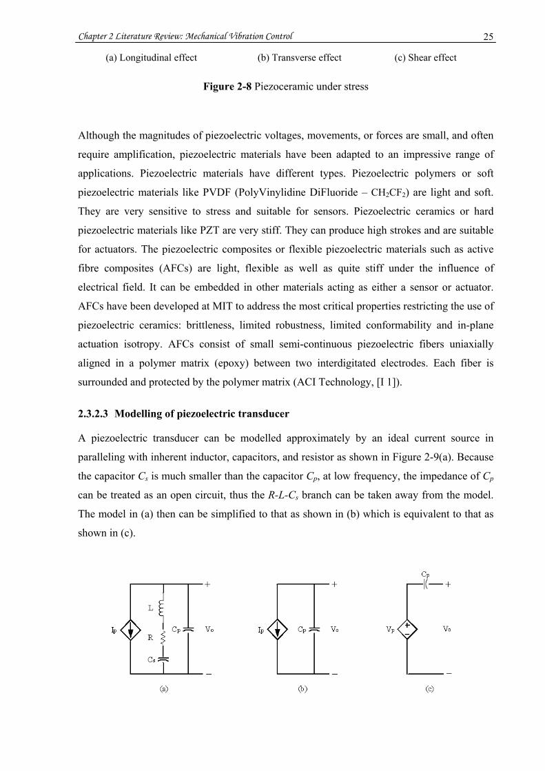
Chapter 2 Literature Review: Mechanical Vibration Control 25
(a) Longitudinal effect (b) Transverse effect (c) Shear effect
Figure 2-8 Piezoceramic under stress
Although the magnitudes of piezoelectric voltages, movements, or forces are small, and often
require amplification, piezoelectric materials have been adapted to an impressive range of
applications. Piezoelectric materials have different types. Piezoelectric polymers or soft
piezoelectric materials like PVDF (PolyVinylidine DiFluoride – CH2CF2) are light and soft.
They are very sensitive to stress and suitable for sensors. Piezoelectric ceramics or hard
piezoelectric materials like PZT are very stiff. They can produce high strokes and are suitable
for actuators. The piezoelectric composites or flexible piezoelectric materials such as active
fibre composites (AFCs) are light, flexible as well as quite stiff under the influence of
electrical field. It can be embedded in other materials acting as either a sensor or actuator.
AFCs have been developed at MIT to address the most critical properties restricting the use of
piezoelectric ceramics: brittleness, limited robustness, limited conformability and in-plane
actuation isotropy. AFCs consist of small semi-continuous piezoelectric fibers uniaxially
aligned in a polymer matrix (epoxy) between two interdigitated electrodes. Each fiber is
surrounded and protected by the polymer matrix (ACI Technology, [I 1]).
2.3.2.3 Modelling of piezoelectric transducer
A piezoelectric transducer can be modelled approximately by an ideal current source in
paralleling with inherent inductor, capacitors, and resistor as shown in Figure 2-9(a). Because
the capacitor Cs is much smaller than the capacitor Cp, at low frequency, the impedance of Cp
can be treated as an open circuit, thus the R-L-Cs branch can be taken away from the model.
The model in (a) then can be simplified to that as shown in (b) which is equivalent to that as
shown in (c).

Chapter 2 Literature Review: Mechanical Vibration Control 26
Figure 2-9 Simplified equivalent circuit for a piezoelectric transducer
In the Figure 2-9, Ip is an ideal current source and Vp is an ideal voltage source generated due
to an external stress, A is the surface area of the piezoelectric transducer where the electrodes
are attached. They are expressed as,
dATddADIA jijA ip ∫∫ == . (2.8)
dtdATddtIC
V jA ijpp
p ∫∫∫ −=−=1 . (2.9)
The Equation (2.9) shows that the voltage generated is proportional to the product of the d-
constant and the external stress.
2.3.3 Passive piezoelectric vibration shunt control
Passive piezoelectric shunt control on a vibration structure is achieved by connecting an
electrical shunt circuit in parallel with a piezoceramic (PZT) that is firmly bonded onto the
surface of the vibration structure where there is induced vibration strain presented. The
mechanical strain energy is then converted into electrical energy and absorbed/damped by the
piezoelectric shunt circuit. The shunt circuits as shown in Figure 2-10 are the classification of
most common piezoelectric vibration shunt circuits (Lesieutre, 1998).
(a) Resistive (b) Inductive (c) Capacitive (d) Switching
Figure 2-10 Basic classification of passive piezoelectric vibration shunt (Lesieutre, 1998)
Figure 2-10(a) is a resistive shunt circuit that dissipates vibration energy through Joule heat. It
is analogous to viscoelastic damping but the materials are much stiffer and less prone to
temperature variation. It is a wideband control but is not very effective.
Figure 2-10(b) is an inductive shunt circuit that can be tuned to a specific vibration frequency,
usually the natural frequency of the structure. The value of inductor is determined by equation
RpC
pV
PZT
R
pC
pV
LPZT
CpC
pV
PZT
pC
pV
SW
Zs
PZT

Chapter 2 Literature Review: Mechanical Vibration Control 27
)/(1 2pn CL ω= , where nω is the vibration frequency to be controlled. The purpose of the
inductor is to cancel the impedance of the inherent capacitor Cp, minimizing the output
impedance of the PZT thus maximizing the output of vibration energy from it. It is analogous
to a mechanical TMD or Tuned Vibration Absorber (TVA). When the shunt circuit is tuned
accurately to the vibration frequency, it can shunt the vibration energy much more efficiently
compared to the resistive shunt, however, it is narrowband control and will lose performance
dramatically when the targeted frequency is shifted away from the frequency of the shunt
circuit.
Figure 2-10(c) is a capacitive shunt circuit. It changes the effective stiffness of the
piezoceramic. It is analogous to a TVA.
Figure 2-10(d) is a switching shunt circuit. Zs represents the shunt circuit which can be one of
the shunt circuits in (a) ~ (c). The switch is to control the rate of energy transmission.
It was Forward (1979) who first suggested the possibility of using piezoelectric elements with
passive electrical shunt for vibration damping and control. He demonstrated vibration
damping on optical structures with a passive parallel R-L-C resonant shunt circuit
experimentally, which showed that substantial vibration amplitude was reduced.
Severely years later, Uchino et al (1988) experimentally demonstrated resistive piezoelectric
shunt and noted a significant vibration damping when the external resistance was changed
(Uchino et al, 1988).
At the same time, Hagood and von Flotow (1991) presented a detailed analysis of passive
piezoelectric shunt control. They also demonstrated vibration reduction on cantilever beams
with resistive and inductive shunt networks experimentally. Their general model is depicted in
Figure 2-11(a), where )(sZ SUi denotes the impedance of the shunt network. Figure 2-11(b) is
its equivalent circuit, where )(sZ MEjj is the mechanical impedance of the piezoelectric for
uniaxial loading in jth direction and )(sZ ELi is the electrical impedance of the piezoelectric
with shunt circuit.
)()]/(1[)()]/(1[
)(sZsCsZsC
sZ SUip
SUipEL
i +⋅
= . (2.10)
The non-dimensional electrical impedance of the piezoelectric with shunt circuit is,
)/(1)(
)()/(1)()(
pSUi
SUi
p
ELi
C
ELiEL
i sCsZsZ
sCsZ
ZZsZ
p+
=== . (2.11)

Chapter 2 Literature Review: Mechanical Vibration Control 28
The non-dimensional mechanical impedance of the piezoelectric is,
2
2
2
2
2
1)(1)(
1)()1()(1
1)(1
1)(
ij
ELiEL
i
ELiij
ELi
ijEL
iij
ijMEjj
ksZsZsZksZ
ksZk
ksZ
−−
−=
−+−
−=
−
−= . (2.12)
(a) Piezoelectric shunted by electrical impedance
(b) Equivalent circuit of piezoelectric shunt of (a)
Figure 2-11 Passive piezoelectric vibration damping (Hagood et al, 1991)
Figure 2-12 illustrates a simple series inductive piezoelectric shunt configuration.
Figure 2-12 Inductive piezoelectric shunt (Hagood et al, 1991)
where
RLssZ SUi +=)( ,
leads to
1:n
)(sZMEjj )(sZSU
ipC )(sZ ELi
+
−
iV
iIF+
−
Vel
ocity
(v)
iV
iI+
−R
L
)(sZ SUiiT
iTiS
iV
iI+
−
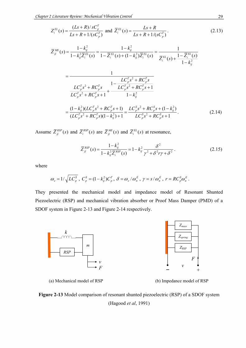
Chapter 2 Literature Review: Mechanical Vibration Control 29
)/(1/)(
)( Tp
TpEL
i sCRLssCRLs
sZ++
+= and
)/(1)( T
p
ELi sCRLs
RLssZ+++
= . (2.13)
2
2
2
2
2
1)(1)(
1)()1()(1
1)(1
1)(
ij
ELiEL
i
ELiij
ELi
ijEL
iij
ijMEjj
ksZsZsZksZ
ksZk
ksZ
−−
+=
−+−−
=−
−=
2
2
2
2
2
11
1
1
1
ij
Tp
Tp
Tp
Tp
Tp
Tp
Tp
Tp
ksRCsLC
sRCsLC
sRCsLCsRCsLC
−++
+−
+++
+
=
1
)1(1)1)(()1)(1(
2
22
22
22
++−++
=+−+++−
=sRCsLC
ksRCsLCksRCsLC
sRCsLCkSp
Sp
ijSp
Sp
ijTp
Tp
Tp
Tpij . (2.14)
Assume )(sZ RSPjj and )(sZ RSP
i are )(sZ MEjj and )(sZ EL
i at resonance,
222
22
2
2
1)(1
1)(
δγδγδ
++−=
−
−=
rk
sZkk
sZ ijRSPiij
ijRSPjj . (2.15)
where
Spe LC/1=ω , T
pijSp CkC )1( 2−= , E
ne ωωδ /= , Ens ωγ /= , E
nSpRCr ω= .
They presented the mechanical model and impedance model of Resonant Shunted
Piezoelectric (RSP) and mechanical vibration absorber or Proof Mass Damper (PMD) of a
SDOF system in Figure 2-13 and Figure 2-14 respectively.
(a) Mechanical model of RSP (b) Impedance model of RSP
Figure 2-13 Model comparison of resonant shunted piezoelectric (RSP) of a SDOF system
(Hagood et al, 1991)
m
RSP
k
vF
Zmass
vF
Zspring
ZRSP
− +

Chapter 2 Literature Review: Mechanical Vibration Control 30
(a) Mechanical model of PMD (b) Impedance model of PMD
Figure 2-14 Model comparison of proof mass damper (PMD) of a SDOF system
(Hagood et al, 1991)
In the impedance model, the mass, spring and RSP (PMD) impedances are connected in
parallel, where mssZmass =)( and sksZspring /)( = .
The overall mechanical impedances for the RSP and PMD of the SDOF systems can be
expressed as, respectively,
)(/)()()( sZskms
svsFsZ RSP
jj++== . (2.16)
)(/)()()( sZskms
svsFsZ PMD
jj++== . (2.17)
where
F(s) and v(s) are force and velocity respectively.
The modelling and derivation of mathematic equations by Hagood et al made a very
important contribution to the passive piezoelectric vibration control which has been the
foundation of much research work in this field since.
Edberg et al (1992) employed passive vibration shunt to large space truss structures. They
developed simulated (synthetic) inductor (known as gyrator) that is an electronic circuit made
of operational amplifiers, passive capacitors and resistors to have the characteristics of the
passive inductor. The gyrator-based inductor has solved the problem of the large inductor
value required for low frequency vibration shunt which is far beyond the range that a passive
inductor can normally reach.
Hollkamp (1993) proposed multimode vibration suppression using a single PZT by
paralleling several series R-L-C branches, except the very first one being a series R-L circuit.
Zmass
vF
Zspring
ZPMD
− +
m k
vF
PMD

Chapter 2 Literature Review: Mechanical Vibration Control 31
Each R-L-C branch introduces a resonant frequency which targets a particular mode to be
suppressed. Additional R-L-C branches can be added to the shunt circuit to increase the
amount of electrical resonance. The shunt design for the case of n electrical resonance is
shown in Figure 2-15.
Figure 2-15 Multi-mode vibration shunt using multiple R-L-C shunt branches
(Hollkamp, 1993)
The non-dimensional electrical impedance can be calculated as,
∑=
= N
k k
TpEL
i
sZ
sCsZ
0 )(1
)( . (2.18)
where
)/(1)(0TpsCsZ = ,
111 )( RsLsZ += ,
)/(1)( 2222 sCRsLsZ ++= , …, and
)/(1)( NNNN sCRsLsZ ++= .
However, it is difficult to tune the circuit since each individual branch of the shunt cannot be
considered as an individual single mode shunt. Tuning one electrical resonance to suppress a
particular mode will detune the rest of the circuit. He also developed a self-tuning
piezoelectric vibration absorber using a motorized potentiometer with a RMS searching
algorithm.
C. L. Davis and G. A. Lesieutre (Davis et al, 1995) used the strain energy approach to predict
the structural damping added by the use of a resistive piezoelectric shunt. By choosing various

Chapter 2 Literature Review: Mechanical Vibration Control 32
materials and structural parameters, a designer may add damping to structural vibration
modes.
Wang et al (1996) developed energy-based parametric control using semi-active piezoelectric
networks for structural vibration suppression. By analysing the base structure, the parameters
of shunt networks are on-line controlled to minimize the energy flowing into the main
structure.
Law et al (1996) described the resistive piezoelectric shunt as equivalent to a spring-dashpot
model as shown in Figure 2-16.
(a) Resistive piezoelectric shunt (b) Equivalent sprint-dashpot model
Figure 2-16 Equivalent model for a piezoelectric material with a load resistor
(Law et al, 1996)
In Figure 2-16(b), k and eqζ are the stiffness and equivalent damping ratio of a piezoelectric
ceramic respectively.
LA
sLEAk
ij
1== . (2.19)
2
20
0
2
20
02
)(11
)(1)(
41
ij
p
p
ij
p
p
pE
req
KRC
RCK
RCRC
Cf
ω
ωωω
πζ
+−
+⋅= . (2.20)
Where E is the Young’s modulus, ijs is the compliance, A is the surface area, L is the length,
Erf is the resonant frequency when the piezoelectric ceramic is short circuited, and ijK is the
electromechanical coupling coefficient of the piezoelectric ceramic respectively.
eqζ k0RpC
pV
PZT
I

Chapter 2 Literature Review: Mechanical Vibration Control 33
When the optimal value of the load resistor matches that of the internal impedance of the
piezoelectric ceramic, that is, pCR ω/10 = , maximum damping occurs. The maximum
damping ratio is,
2
2
0
max
)2/1(141
ij
ijE
req
K
KRf −
=π
ζ . (2.21)
Wu (Wu, 1996, 1998) proposed piezoelectric shunt with parallel R-L circuit as shown in
Figure 2-17 for structural damping on cantilever beam. He also employed a “blocking” circuit
in series with each parallel R-L shunt circuit for multiple-mode shunt damping of structural
vibration, using single PZT which is depicted in Figure 2-18, where Cp denotes the
capacitance of the PZT, Ci, and Li, R’i (i = 1, …, n) are denote external capacitor, inductor and
resistor.
Figure 2-17 Inductor-resistor (R-L) parallel shunt
The circuit in Figure 2-18 has n branches and shunts n natural frequencies simultaneously.
The circuit is designed so that each branch accepts only one particular natural frequency and
the rest of the natural frequencies (n-1) are blocked. The blocking circuit is in open circuit
when a natural frequency is equal to its resonant frequency, otherwise it is approximately
treated as a short circuit. The ith resonant frequency of a blocking circuit is determined by
iii CL/1=ω .
iV
iI+
−LR
pC
2L
3L
nL
'1L
2C
3C
nC
'1R
1−nL
1L
2−nL
'nL
1−nC
1C
2−nC
'nR
−
+
iV
2ω
3ω
nω
3ω
4ω
1ω
1−nω
1ω
2−nω
3L
4L
1L
'2L
3C
4C
1C
'2R
(n-1) blocking circuits in series
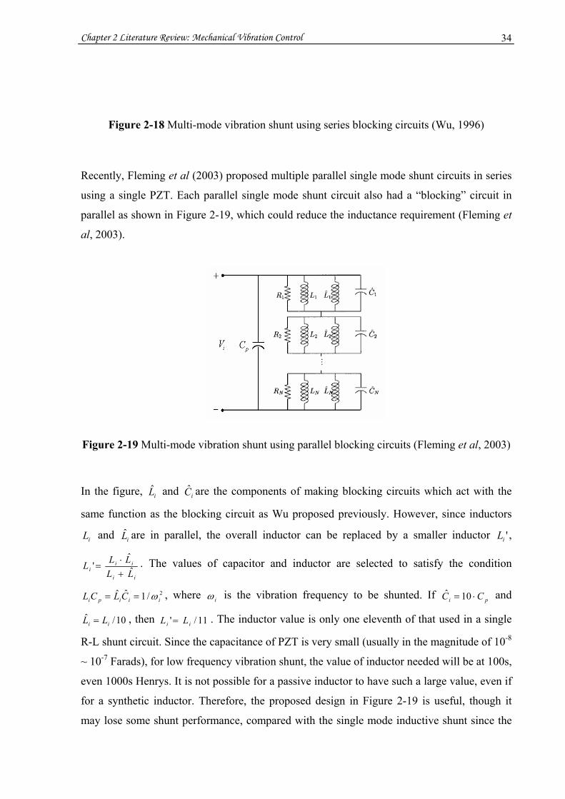
Chapter 2 Literature Review: Mechanical Vibration Control 34
Figure 2-18 Multi-mode vibration shunt using series blocking circuits (Wu, 1996)
Recently, Fleming et al (2003) proposed multiple parallel single mode shunt circuits in series
using a single PZT. Each parallel single mode shunt circuit also had a “blocking” circuit in
parallel as shown in Figure 2-19, which could reduce the inductance requirement (Fleming et
al, 2003).
Figure 2-19 Multi-mode vibration shunt using parallel blocking circuits (Fleming et al, 2003)
In the figure, iL and iC are the components of making blocking circuits which act with the
same function as the blocking circuit as Wu proposed previously. However, since inductors
iL and iL are in parallel, the overall inductor can be replaced by a smaller inductor 'iL ,
ii
iii LL
LLL ˆˆ
'+⋅
= . The values of capacitor and inductor are selected to satisfy the condition
2/1ˆˆiiipi CLCL ω== , where iω is the vibration frequency to be shunted. If pi CC ⋅= 10ˆ and
10/ˆii LL = , then 11/' ii LL = . The inductor value is only one eleventh of that used in a single
R-L shunt circuit. Since the capacitance of PZT is very small (usually in the magnitude of 10-8
~ 10-7 Farads), for low frequency vibration shunt, the value of inductor needed will be at 100s,
even 1000s Henrys. It is not possible for a passive inductor to have such a large value, even if
for a synthetic inductor. Therefore, the proposed design in Figure 2-19 is useful, though it
may lose some shunt performance, compared with the single mode inductive shunt since the
Chapter 2 Literature Review: Mechanical Vibration Control 35
blocking circuits cannot be in open/short circuit ideally. However compared with Wu’s
proposal, the circuit is much simpler and requires much less electrical components.
In addition to using piezoceramic materials for vibration shunt control mentioned in the
previous literature review, another type of piezoelectric materials, active fibre composites
(AFCs) are very promising for vibration control. As mentioned before, AFCs originated from
the work started at MIT by Bent and Hagood in 1992. AFCs are constructed using piezofibres
embedded in an epoxy resin matrix and coated with Kapton skin. Unlike piezoceramic,
piezofibres are flexible and soft. However, after the piezofibres being embedded in epoxy
resin matrix to form the AFCs, the stiffness of the AFCs increase significantly. AFCs
overcome the weakness of monolithic piezoceramic being brittle, they are tough yet flexible,
conformable, and have great potential towards integration in complex structures. AFCs
operate in the longitudinal mode and thus have significantly higher d and g constants (namely
33d and 33g ).
Belloli et al (2004) for the first time successfully implemented AFCs in an inductive shunt
circuit. They claimed a 17 dB vibration reduction on an aluminium plate during the
experiment they carried out. The result is close to that with piezoceramic, however the
inductor of the shunt circuit required was a lot higher than that required with piezoceramic
due to much smaller inherent capacitance of the AFCs.
Head Sport has employed active fibre composite to produce Smart tennis rackets (Head_a, [I
5]) and Smart skis (Head_b, [I 6]) with energy harvesting actuators made from PZT fibre. In
the case of the tennis racquet, piezoelectric composites embedded in the throat of the racquet
convert mechanical vibrations caused by the ball impact into electrical energy. The electrical
energy is then processed by an electronic circuit located in the racquet’s handle, and within
milliseconds the electronic circuit sends the electrical energy back to the piezoelectric
composites to reduce the racquet’s vibration. The piezoelectric composites increase power
and control authority by reducing the racquet’s vibration. The Smart ski uses similar
technology. Piezoelectric fibre composite technology that recycles non-usable, waste energy
to perform a function, free of outside control or source of power or batteries. As the ski
vibrates during a turn, or on ice, the processed electrical energy of that chatter is harnessed by
the piezoelectric fibre composites in the structure of the ski, which then rolls the edge of the
ski back into the snow. These self-powered Smart products actively damp the vibration
created during a ball strike or edge chatter from a ski turn and use the energy to create
electrical force to control the shape of the racket or ski, using PZT fibre’s electrical and
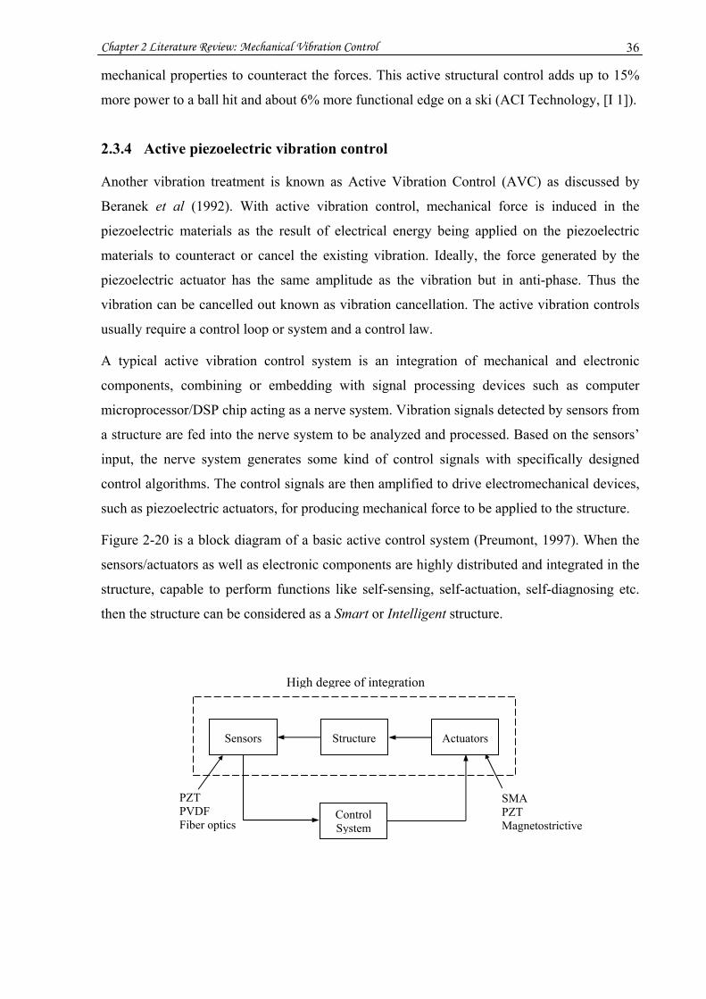
Chapter 2 Literature Review: Mechanical Vibration Control 36
mechanical properties to counteract the forces. This active structural control adds up to 15%
more power to a ball hit and about 6% more functional edge on a ski (ACI Technology, [I 1]).
2.3.4 Active piezoelectric vibration control
Another vibration treatment is known as Active Vibration Control (AVC) as discussed by
Beranek et al (1992). With active vibration control, mechanical force is induced in the
piezoelectric materials as the result of electrical energy being applied on the piezoelectric
materials to counteract or cancel the existing vibration. Ideally, the force generated by the
piezoelectric actuator has the same amplitude as the vibration but in anti-phase. Thus the
vibration can be cancelled out known as vibration cancellation. The active vibration controls
usually require a control loop or system and a control law.
A typical active vibration control system is an integration of mechanical and electronic
components, combining or embedding with signal processing devices such as computer
microprocessor/DSP chip acting as a nerve system. Vibration signals detected by sensors from
a structure are fed into the nerve system to be analyzed and processed. Based on the sensors’
input, the nerve system generates some kind of control signals with specifically designed
control algorithms. The control signals are then amplified to drive electromechanical devices,
such as piezoelectric actuators, for producing mechanical force to be applied to the structure.
Figure 2-20 is a block diagram of a basic active control system (Preumont, 1997). When the
sensors/actuators as well as electronic components are highly distributed and integrated in the
structure, capable to perform functions like self-sensing, self-actuation, self-diagnosing etc.
then the structure can be considered as a Smart or Intelligent structure.
PZT PVDF Fiber optics
Sensors Structure Actuators
Control System
SMA PZT Magnetostrictive
High degree of integration
Chapter 2 Literature Review: Mechanical Vibration Control 37
Figure 2-20 Block diagram of a basic active control system (Smart structure)
(Preumont, 1997)
In the wake of rapid advances in material technology, high speed electronic devices and
sophisticated digital signal processing techniques have made many previously “unthinkable”
become possible, and triggered vast interest in active vibration control among researchers and
engineers. In the past few decades, various methods of active vibration control have been
developed. The common control strategies of the active controls can be classified under two
major categories: feedback control such as active damping, and feedforward control such as
adaptive filtering. In terms of signal type, the control can also be classified into two types:
analogue control and digital control. Analogue control deals with continuous time domain
signal while digital control deals with desecrate signal data, usually the samples of analogue
signal.
Balas (1978) developed a feedback controller using a position sensor, force actuator and state
variable technique for active control of an n modes flexible structure. The flexible structure
was a simple supported beam with dynamics modelled on the Euler-Bernoulli partial
differential equation. One actuator and one sensor (at different locations) were used to control
three modes of the beam effectively. Spillover, due to residual (uncontrolled) modes, was
eliminated by prefiltering the sensor outputs to avoid feedback to the controller resulting in
instability in close loop.
Bailey et al (1985) designed an active vibration damper for a cantilever beam using a
distributed parameter actuator that was a piezoelectric polymer (PVDF) and distributed
parameter control theory of Lyapunov’s second method. With the method, if the angular
velocity of the tip of the beam is known, all modes of the beam can be controlled
simultaneously. This avoids any structural problems with uncontrolled modes. Test results
showed that using a constant-gain controller, more than a factor of two was increased in the
modal damping with a feedback voltage limit of 200 Vrms. With the same voltage limit, the
constant-amplitude controller achieved the same damping as the constant-gain controller for
large vibrations, but increased the modal loss factor by more than an order of magnitude to at
least 0.04 for small vibration levels.
Crawley (1986) presented the analytical and experimental development of piezoelectric
actuators as an element of Intelligent structures that are with highly distributed actuators,
Chapter 2 Literature Review: Mechanical Vibration Control 38
sensors, and processing networks. The segmented piezoelectric actuators are either bonded to
an elastic substructure or embedded in a laminated composite, which can excite the structure
independently. The distributed actuators are used for dynamic vibration and modal shape
controlling, predicting the behaviour of flexible structures.
McKinnell (1989) applied active forces to a vibrating beam structure to cancel propagating
and evanescent vibration waves by superposition of flexural waves (rather than the
superposition of an infinite set of natural modes of vibration) to prevent those waves from
carrying the effects of an external disturbance. A system was designed to detect bending
waves as they pass a sensor at one point and then inject vibration waves by an active force at
another point further downstream, resulting in the effect of the bending waves being cancelled
by the injected vibration waves. However, the dispersive nature of the waves made
implementation difficult. The difficulties were overcome by including the effects of waves
generated by the active forces, and detected at the controller input, in the control system
synthesis.
Hagood et al (1990) derived an analytical model of dynamic coupling between a structure and
an electrical network through a piezoelectric actuator, using Hamilton’s principle with a
Rayleigh-Ritz formulation. Several state space models of driving piezoelectric actuators have
been developed, which include direct driven using voltage driven electrodes, charge driven
electrodes, mixed voltage-charge driven electrodes, and indirect driven through a passive
electrical shunt network.
Tzou et al (1990) used a finite element analysis approach to evaluate the dynamic
performance of a structure with self-sensing and control capability. Performance of a thin
plate model coupled with the distributed piezoelectric sensor/actuator was studied and
evaluated in a free vibration analysis by the FEA method. Two control algorithms, constant-
gain negative velocity feedback and constant-amplitude negative velocity feedback, were
tested. Both feedback control algorithms showed that in generally damping ratio increases
when the feedback voltage/gain increases.
Bai et al (1996) proposed for suppressing the small amplitude random vibrations in flexible
beams by using PVDF as sensor, PZT as actuator and Linear Quadratic Gaussian (LQG) as
the controller algorithm. The controller is implemented on the basis of a floating-point digital
signal processor. The experimental results obtained by using the active vibration control
system showed significant attenuation of white noise disturbance in the frequency range of
approximately 100 – 800 Hz.

Chapter 2 Literature Review: Mechanical Vibration Control 39
Lay et al (1998) designed and implemented a controller by using modal feedback law with
collocated arrangement of sensor/actuator pairs for damping vibration in cantilever beams.
The benefits of a collocated sensor/actuator first can avoid spillover, which could destabilize
the system, and second is possible to implement feedback control system without a reference
signal. The controller’s characteristics are determined with the help of pole-zero placement.
Dosch et al (1992) developed an active vibration control technique which allows a single
piece of piezoelectric material to concurrently sense and actuate in a closed loop system. Such
a self-sensing actuator is truly collocated and suitable for Smart /Intelligent structures. The
experimental results showed that active damping vibration in a cantilever beam using a rate
feedback control with a single piezoceramic, the settling time of first and second vibration
modes were reduced by more than an order of magnitude.
Lee (1990) proposed distributed modal sensors/actuators using PVDF lamina in contrast to
conventional point sensors/actuators for active vibration control. Unlike most piezoelectric
materials that are fully covered with electrodes, the surfaces of the PVDF laminated modal
sensors/actuators were only partially covered with electrodes. The shapes of electrodes were
designed to match the specific mode shapes of a structure, thus can measure/excite these
modes by those modal sensors/actuators. The concept behind the modal sensors/actuators was
to use the charge collecting phenomenon of the surface electrode of piezoelectric materials to
perform the modal filtering in the spatial domain rather in the time domain. The surface
electrodes and the polarization profile of the distributed sensor/actuator can be used to
integrate sensor/actuator signals in the spatial domain. Therefore less intensive signal
processing is required. Because of the parallel processing nature presented in these modal
sensors/actuators, no phase-lag was generated in a control loop adopting these devices. The
sensor signal is proportional to the time derivative of the modal coordinate which is easily
used for velocity feedback control. The spillover phenomenon was not presented in such
integrated modal sensor/actuator pair. It was shown that critical damping could be achieved
using such PVDF sensor/actuator combination.
One of major problems associated with active vibration control is spillover. Flexible
structures are modelled as distributed parameter systems and have very large number
(theoretically an infinite number) of vibration modes. Some of them are beyond the
bandwidth of controllers since sensors/actuators, as well as electronic circuits, have limited
bandwidth. These uncontrolled high order modes may destabilize control systems. This is the
well-known phenomenon of spillover (Balas 1978). Goh and Caughey (1985) introduced
Positive Position Feedback (PPF) control. Since the frequency responses of PPF controllers

Chapter 2 Literature Review: Mechanical Vibration Control 40
have sharp roll-off, making closed loop control systems robust and insensitive to spillover,
these therefore guarantee the stability of the control systems. The PPF methodology is to
couple a highly damped electronic filter to a lightly damped structure through electro-
mechanical coupling to suppress the vibration of the structure. With PPF, the structure
position information is passed to the electronic filter first then the output of the filter,
multiplied by a gain factor, and is positively fed back to the structure (physically, the output
signal of the filter after being amplified drives actuators attached on the structure). PPF
behaves much like an electronic vibration absorber for structures. The analysis of the PPF
control can be found in Appendix 3.
2.3.5 Power system for active piezoelectric vibration control
The piezoelectric actuators have been demonstrated which they can produce high actuation
force, have broad frequency bandwidth and fast transient response to stimuli. They are very
attractive for many applications. However, some applications such as satellites use DC battery
power or self-powered systems and have limitations in power supply due to size and weight
constraints. On the other hand, the piezoelectric actuators are required to be driven by high
AC voltage (not necessary high current) in order to generate large force and/or displacement.
Figure 2-21 shows the force generation vs. displacement of a piezo actuator (displacement 30
µm, stiffness 200 N/µm) at various operating voltages (PI Ceramic, [I 9]). For example, a 333
V voltage can generate 2000 N maximum force with zero displacement or 10 μm maximum
displacement with zero force. 333 V is very high voltage though 10 µm displacement is not
considerable large. Therefore it is very important to design efficient power suppliers and
power amplifiers for driving piezoelectric actuators. Preferably they can be powered by the
energy harvested from mechanical energy by piezoelectric materials which become self-
powered actuation systems.

Chapter 2 Literature Review: Mechanical Vibration Control 41
Figure 2-21 Voltage vs. force generation vs. displacement of a piezo actuator
(PI Ceramic, [I 9])
According to Equation (2.7), strain produced by a piezoelectric actuator is TsEdS Et += .
When external stress T is zero, the strain S is the product of the charge constant td
(Meter/Volt) and electrical field E (Volt/Meter). Since td is a relatively small constant, at a
magnitude of 1010 − , thus it requires a very high voltage to produce a noticeable geometric
increment in certain direction, say 1 micrometer, by the piezoelectric actuator. The signals
from sensors and controllers are weak signals, and therefore, require amplification before
driving the actuator. The amplifiers for driving piezoelectric actuators should not only have a
high voltage gain, but also have a large dynamic voltage range and be able to withstand high
voltage. The amplifier supplying power to the active vibration control system decides the
efficiency and capability of the system. High power amplifiers are usually bulky and consume
a lot of power itself. Design of high efficiency, small size power amplifiers is part of ongoing
research by many researchers.
Luan et al (1998) developed a DC-DC high frequency switching amplifier for driving Smart
material actuators. They used average current mode control techniques to increase the current

Chapter 2 Literature Review: Mechanical Vibration Control 42
loop gain at low frequency, which is low due to the reactive (capacitive) load of Smart
material actuators.
Janocha et al (1998) presented a switching amplifier for piezoelectric actuators which could
transfer the portion of energy exactly necessary to achieve desired output value at the load in
every switching cycle. This approach could avoid unnecessary switching cycles which merely
heat the transducer and semiconductor components.
Carazo et al (2001) designed a DC-AC piezoelectric-based power supply for driving
piezoelectric actuators. The novelty of this approach is using a smaller, lighter, and EMI-free
piezoelectric transformer (PT) Transoner® instead of a larger, heavier and EMI-noisy
electromagnetic transformer, to convert the low DC voltage of a conventional battery to a
high AC voltage for driving piezoelectric actuators. They implemented a circuit that is
capable of converting a 24 V DC battery voltage for driving a multiplayer piezoelectric
actuator at 100 Vpp within the range of 10 Hz to 500 Hz.
2.3.6 Advantages and disadvantages of passive and active piezoelectric vibration
controls
The passive and active piezoelectric vibration controls have their own advantages and
disadvantages. The advantages of Passive Vibration Control (PVC) are that the control system
is relatively simple, little or no external power is required and is guaranteed to be stable.
Therefore, the control system can be made in a compact, portable size and is easier to be
embedded in a structure where electronic energy is expensive. However, this method has
limited effectiveness particularly when the volume of a structure to be controlled or the
magnitude of vibration in the structure is large. The percentage of vibration attenuation in the
structure is in inverse proportion to the volume of the structure or the level of vibration in the
structure. The effectiveness of the passive vibration control for low frequency vibration is also
less than that for high frequency vibration probably due to less energy conversion in unit time.
The passive vibration control usually targets at a particular frequency in a narrow band. The
control effectiveness is quite sensitive to frequency shifts caused by structure or environment
variations, boundary condition change etc. In addition, the large inductor value required for
the low frequency passive vibration control also tends to be a problem.
The advantages of the active vibration control are that the control system is robust and
flexible, it has broadband effectiveness, capable of suppressing a large level of vibration, has
high control authority, and the control effectiveness is less prone to condition variation.
Besides, the active vibration control system can be implemented in high-speed DSP chips

Chapter 2 Literature Review: Mechanical Vibration Control 43
using digital signal processing techniques with hardware and software, which makes modern
advanced control strategies such as adaptive control and Intelligent control to be implemented
in the control system possible, as well as allows the control system to be re-programmable
resulting in time-saving and lowered costs during design and implementation. Nevertheless,
the control system is much more complex, possibly unstable, requires sophisticated control
algorithms, and especially requires a large external power source to drive the actuator. The
last point is the major stumbling block to applying active vibration control in many
applications, since the higher power required for driving actuators means more power
consumption, and needs a larger, more complex power system. Many applications, like
portable or remote applications which only use battery power are not suitable for applying
active vibration control strategies unless some kind of techniques, such as self-powering, can
be used to solve the energy problem.
Based on the assumption that the piezoelectric transformer can be used as a voltage step-up
device as being suggested by Carazo et al (2001), a novel power amplifier designed by using
amplitude modulation technique with piezoelectric transformer for driving the piezoelectric
actuator has been proposed by author. The details of the power amplifier can be found in
Appendix 4. Functional simulation with PSpice® software suggests that the design works
correctly.
2.4 Chapter summary
In this chapter, first, a brief overview has been given of the history of the Cricket bat and the
research being carried out on Cricket bats. An interesting idea suggested by C. Grant (Grant,
1998) is to raise the 3rd flexure mode of the Cricket bat out of the excitation spectrum of
ball/bat impact by making the Cricket bat handle with composite materials to completely
remove the 3rd mode vibration. Then the traditional vibration techniques including vibration
isolation, vibration absorption and vibration damping have been discussed. Smart materials
particularly piezoelectric materials, their function, properties, mechanical/electrical models,
and constitutive equations have been presented. The “Piezoelectric effect” of the materials is
the foundation of modern advanced piezoelectric vibration control. The literature review of
piezoelectric vibration control has been carried out. It is generally classified as passive
vibration control and active vibration control. The passive vibration control including
resistive, inductive, capacitive, and switching vibration shunt has been discussed. Among
these, the inductive vibration shunt has been found most effective. The passive control system
is relatively simple, compact, low cost, creates less demand on electrical power and is
Chapter 2 Literature Review: Mechanical Vibration Control 44
guaranteed to be stable, but it has limited effectiveness especially for large objects or high
levels of vibration. The active vibration control, on the other hand, is more sophisticated,
robust, effective and flexible but is complex and possibly unstable. The major concern is its
high demand on electrical power which has limited its use on many portable and remote
applications. In the chapter, the work by other researchers on electrical power systems for
active piezoelectric vibration control has also been briefly mentioned. The piezoelectric
transformer has been considered as a promising alternative to electromagnetic transformer for
active piezoelectric vibration control by many researchers. Finally, the advantages and
disadvantages of the passive and active piezoelectric vibration control methods have been
summarised.
Some of the derivations related to the concepts introduced in this chapter are further
elucidated in the Appendices. The analytical analyses of vibration isolation, vibration
absorption and damping measurement of the SDOF structure are presented in Appendices 1 &
2. A PPF control example is given in Appendix 3. In Appendix 4, a novel power amplifier is
proposed.

Chapter 3 Analytical Modeling of Passive Piezoelectric Vibration Shunt on Beams 45
Chapter 3
Analytical Modeling of Passive
Piezoelectric Vibration Shunt on Beams
In chapter 2, piezoelectric vibration control techniques have been reviewed. There are mainly
two categories, one is the active control technique and the other is the passive control
technique. For the active piezoelectric vibration control method, it normally requires hundreds
of volts to drive the piezoelectric actuators. Although it is more effective than the passive
piezoelectric vibration control method, there is a bottleneck problem for practical
applications. It is difficult to produce such high voltage with a small electronic circuit at low
cost, especially when battery power is used as the power supply.
Due to the deep conservatism in the rules of the Cricket games, there are many restrictions
imposed on designing new Cricket bats. The rule only allows the designer to utilize and
modify the handle of Cricket bats. Considering the factors of space and weight limitation,
power supply issues, portability and cost concerns etc., the active control method seems
unfeasible for the vibration control of the Cricket bat, at least for the time being. Therefore,
the passive piezoelectric control method, namely using piezoelectric transducers in
conjunction with an electrical network to damp the structural vibration becomes an option.
The passive piezoelectric vibration control technique requires much less power consumption
compared to that of the active piezoelectric vibration control technique. There are several
types of passive piezoelectric vibration control configurations that have been briefly described
in chapter 2. Among them, the most effective configuration is the resistor-inductor (R-L)
shunt control. In terms of connection type between the electrical network and the piezoelectric
transducer, it can be further classified as series R-L shunt control, where the R-L shunt circuit
is connected in series to the piezoelectric transducer (Figure 2-15) and parallel R-L shunt
control which the R-L shunt circuit is connected in parallel to the piezoelectric transducer
(Figure 2-20).
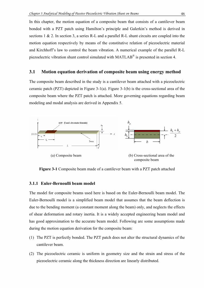
Chapter 3 Analytical Modeling of Passive Piezoelectric Vibration Shunt on Beams 46
In this chapter, the motion equation of a composite beam that consists of a cantilever beam
bonded with a PZT patch using Hamilton’s principle and Galerkin’s method is derived in
sections 1 & 2. In section 3, a series R-L and a parallel R-L shunt circuits are coupled into the
motion equation respectively by means of the constitutive relation of piezoelectric material
and Kirchhoff’s law to control the beam vibration. A numerical example of the parallel R-L
piezoelectric vibration shunt control simulated with MATLAB® is presented in section 4.
3.1 Motion equation derivation of composite beam using energy method
The composite beam described in the study is a cantilever beam attached with a piezoelectric
ceramic patch (PZT) depicted in Figure 3-1(a). Figure 3-1(b) is the cross-sectional area of the
composite beam where the PZT patch is attached. More governing equations regarding beam
modeling and modal analysis are derived in Appendix 5.
(a) Composite beam (b) Cross-sectional area of the composite beam
Figure 3-1 Composite beam made of a cantilever beam with a PZT patch attached
3.1.1 Euler-Bernoulli beam model
The model for composite beams used here is based on the Euler-Bernoulli beam model. The
Euler-Bernoulli model is a simplified beam model that assumes that the beam deflection is
due to the bending moment (a constant moment along the beam) only, and neglects the effects
of shear deformation and rotary inertia. It is a widely accepted engineering beam model and
has good approximation to the accurate beam model. Following are some assumptions made
during the motion equation derivation for the composite beam:
(1) The PZT is perfectly bonded. The PZT patch does not alter the structural dynamics of the
cantilever beam.
(2) The piezoelectric ceramic is uniform in geometry size and the strain and stress of the
piezoelectric ceramic along the thickness direction are linearly distributed.
ph
2pb hh +
b
bh
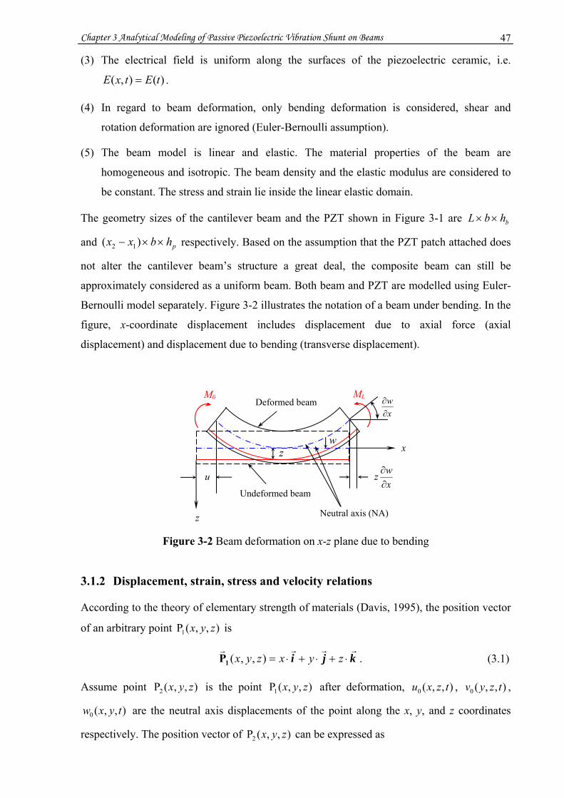
Chapter 3 Analytical Modeling of Passive Piezoelectric Vibration Shunt on Beams 47
(3) The electrical field is uniform along the surfaces of the piezoelectric ceramic, i.e.
)(),( tEtxE = .
(4) In regard to beam deformation, only bending deformation is considered, shear and
rotation deformation are ignored (Euler-Bernoulli assumption).
(5) The beam model is linear and elastic. The material properties of the beam are
homogeneous and isotropic. The beam density and the elastic modulus are considered to
be constant. The stress and strain lie inside the linear elastic domain.
The geometry sizes of the cantilever beam and the PZT shown in Figure 3-1 are bhbL ××
and phbxx ××− )( 12 respectively. Based on the assumption that the PZT patch attached does
not alter the cantilever beam’s structure a great deal, the composite beam can still be
approximately considered as a uniform beam. Both beam and PZT are modelled using Euler-
Bernoulli model separately. Figure 3-2 illustrates the notation of a beam under bending. In the
figure, x-coordinate displacement includes displacement due to axial force (axial
displacement) and displacement due to bending (transverse displacement).
Figure 3-2 Beam deformation on x-z plane due to bending
3.1.2 Displacement, strain, stress and velocity relations
According to the theory of elementary strength of materials (Davis, 1995), the position vector
of an arbitrary point ),,(P1 zyx is
kji ⋅⋅⋅ ++= zyxzyx ),,(1P . (3.1)
Assume point ),,(P2 zyx is the point ),,(P1 zyx after deformation, ),,(0 tzxu , ),,(0 tzyv ,
),,(0 tyxw are the neutral axis displacements of the point along the x, y, and z coordinates
respectively. The position vector of ),,(P2 zyx can be expressed as
x
z Neutral axis (NA)
xwz∂∂
xw∂∂
MLM0 Deformed beam
Undeformed beam
wz
u
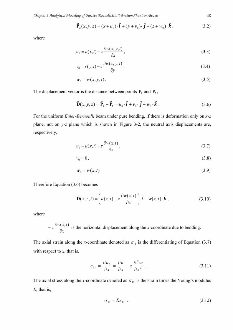
Chapter 3 Analytical Modeling of Passive Piezoelectric Vibration Shunt on Beams 48
kji ⋅⋅⋅ +++++= )()()(),,( 000 wzvyuxzyx2P . (3.2)
where
xtyxwztxuu
∂∂
−=),,(),(0 , (3.3)
ytyxwztyvv
∂∂
−=),,(),(0 , (3.4)
),,(0 tyxww = . (3.5)
The displacement vector is the distance between points 1P and 2P ,
kji ⋅⋅⋅ ++=−= 000),,( wvuzyx 12 PPD . (3.6)
For the uniform Euler-Bernoulli beam under pure bending, if there is deformation only on x-z
plane, not on y-z plane which is shown in Figure 3-2, the neutral axis displacements are,
respectively,
xtxwztxuu
∂∂
−=),(),(0 , (3.7)
00 =v , (3.8)
),(0 txww = . (3.9)
Therefore Equation (3.6) becomes
ki ⋅⋅ +⎟⎠⎞
⎜⎝⎛
∂∂
−= ),(),(),(),,( txwx
txwztxutzxD . (3.10)
where
xtxwz
∂∂
−),( is the horizontal displacement along the x-coordinate due to bending.
The axial strain along the x-coordinate denoted as 11ε is the differentiating of Equation (3.7)
with respect to x, that is,
2
20
11 xwz
xu
xu
∂∂
−∂∂
=∂∂
=ε . (3.11)
The axial stress along the x-coordinate denoted as 11σ is the strain times the Young’s modulus
E, that is,
1111 εσ E= . (3.12)

Chapter 3 Analytical Modeling of Passive Piezoelectric Vibration Shunt on Beams 49
In addition, the velocity of the particle is the differentiating of its displacement with respect to
time t. The velocity of the beam element on the x-z plane is the differentiating of Equation
(3.10)
ki ⋅⋅∂
∂+⎟⎟
⎠
⎞⎜⎜⎝
⎛∂∂
∂−
∂∂
=∂
∂=
ttxw
txtxwz
ttxu
ttzxtzx ),(),(),(),,(),,(
2DVc ,
The non-dimensional velocity is
222 ),(),(),(⎟⎠⎞
⎜⎝⎛
∂∂
+⎟⎟⎠
⎞⎜⎜⎝
⎛∂∂
∂−
∂∂
=t
txwtx
txwzt
txucV . (3.13)
3.1.3 Potential energy
The potential energy of the beam due to x-coordinate strain is
∫∫∫∫∫∫∫∫∫ ⎟⎟⎠
⎞⎜⎜⎝
⎛∂∂
−∂∂
===bbb V bbV bbV bb dV
xwz
xuEdVEdVU
2
2
22
111111 21
21
21 εεσ
∫∫∫⎪⎭
⎪⎬⎫
⎪⎩
⎪⎨⎧
⎟⎟⎠
⎞⎜⎜⎝
⎛∂∂
+∂∂
∂∂
−⎟⎠⎞
⎜⎝⎛∂∂
=bV bb dV
xwz
xw
xuz
xuE
2
2
22
2
22
221
dxdAxwz
xw
xuz
xuE
L
A bbb
∫ ∫∫⎪⎭
⎪⎬⎫
⎪⎩
⎪⎨⎧
⎥⎥⎦
⎤
⎢⎢⎣
⎡⎟⎟⎠
⎞⎜⎜⎝
⎛∂∂
+∂∂
∂∂
−⎟⎠⎞
⎜⎝⎛∂∂
=
0
2
2
22
2
22
221
dxxwdAz
xw
xuzdzb
xuAE
L
A b
h
bbb
b
∫ ∫∫∫ ⎟⎟
⎠
⎞
⎜⎜
⎝
⎛⎟⎟⎠
⎞⎜⎜⎝
⎛∂∂
⎟⎠⎞⎜
⎝⎛+
∂∂
∂∂
⎟⎠⎞⎜
⎝⎛−⎟
⎠⎞
⎜⎝⎛∂∂
=0
2
2
22
2
2
0
2
221
dxxwIE
xw
xuAhE
xuAE
L
bbbbbbb∫⎪⎭
⎪⎬⎫
⎪⎩
⎪⎨⎧
⎟⎟⎠
⎞⎜⎜⎝
⎛∂∂
+∂∂
∂∂
−⎟⎠⎞
⎜⎝⎛∂∂
=
0
2
2
2
2
22
21
. (3.14)
where
∫∫=bAb dzzI
2 is the area moment of inertia about the neutral axis, ),( txu and ),( txw are
the axial displacement and the transverse displacement of beam respectively, z is the distance
from neutral axis, bb bhA = is the cross sectional area of beam, bE is the Young’s modulus of
beam, and bdzdxdxdAdV bb == .
The potential energy of the PZT due to the x-coordinate strain is:

Chapter 3 Analytical Modeling of Passive Piezoelectric Vibration Shunt on Beams 50
[ ]∫∫∫∫∫∫ +−+=+=
pp V ppV pp dVDhDEdVEDU
)(21)(
21
33311313211331111 βεεεσ
pV p dVDxwz
xuhD
xwz
xuE
p∫∫∫
⎪⎭
⎪⎬⎫
⎪⎩
⎪⎨⎧
⎥⎦
⎤⎢⎣
⎡+⎟⎟
⎠
⎞⎜⎜⎝
⎛∂∂
−∂∂
−+⎟⎟⎠
⎞⎜⎜⎝
⎛∂∂
−∂∂
= 3332
2
313
2
2
2
21 β
2
2
22
2
222
1
221
⎟⎟⎠
⎞⎜⎜⎝
⎛∂∂
⎟⎠⎞⎜
⎝⎛+
∂∂
∂∂
⎟⎠⎞⎜
⎝⎛−
⎪⎩
⎪⎨⎧
⎟⎠⎞
⎜⎝⎛∂∂
= ∫∫∫ ∫+
xwdAzE
xw
xuzdzbE
xuAE pA
x
x p
hh
hpppp
pb
b
dxDAxwzdzbDh
xuDAh p
hh
hppb
b ⎭⎬⎫
+∂∂
⎟⎠⎞⎜
⎝⎛+
∂∂
− ∫+ 2
3332
2
331331 β
∫⎪⎩
⎪⎨⎧
⎟⎟⎠
⎞⎜⎜⎝
⎛∂∂
+∂∂
∂∂
+−⎟⎠⎞
⎜⎝⎛∂∂
= 2
1
2
2
2
2
22
)2(21 x
x pppbpppp xwIE
xw
xuhhbhE
xuAE
dxDAxwh
hbhDhxuDAh p
pbpp
⎭⎬⎫
+∂∂
++∂∂
− 23332
2
331331 )2
( β
∫⎪⎩
⎪⎨⎧
∂∂
∂∂
+−⎟⎟⎠
⎞⎜⎜⎝
⎛∂∂
+⎟⎠⎞
⎜⎝⎛∂∂
= 2
12
22
2
22
)2(21 x
x pbpppppp xw
xuhhAE
xwIE
xuAE
dxDAxwD
hhAh
xuDAh p
pbpp
⎭⎬⎫
+∂∂
++∂∂
− 23332
2
331331 )2
( β . (3.15)
where,
dzzIpAp ∫∫=
2 is the area moment of inertia about the neutral axis, pp bhA = is the cross
sectional area of PZT, 33311313 DhE βε +−= (using the h-form piezoelectric relation), and
bdzdxdxdAdV pp == .
The total potential energy of the composite beam is pb UUU += . If, for simplicity, only
strain caused by bending is considered, the strain caused by axial force xu∂∂ is not considered,
that is 0=∂∂
xu , then total strain can be simplified as:
dxxwIEUUU
L
bbpb ∫ ⎟⎟⎠
⎞⎜⎜⎝
⎛∂∂
=+=
0
2
2
2
21
dxxxHxxHDAxwD
hhAh
xwIE
L
pp
bppp )]()([)2
(21
0 2123332
2
331
2
2
2
∫ −−−⎪⎭
⎪⎬⎫
⎪⎩
⎪⎨⎧
+∂∂
++⎟⎟⎠
⎞⎜⎜⎝
⎛∂∂
+
β . (3.16)
where,

Chapter 3 Analytical Modeling of Passive Piezoelectric Vibration Shunt on Beams 51
)(xH is the Heaviside function, ⎩⎨⎧
≥<
=−0
00 1
0)(
xfor xxfor x
xxH .
3.1.4 Kinetic energy
The kinetic energy of the beam is the integration of the product of the mass and velocity of
beam elements within the beam volume. From Equation (3.13), the kinetic energy of beam
can be calculated as
∫∫∫∫∫∫⎪⎭
⎪⎬⎫
⎪⎩
⎪⎨⎧
⎟⎠⎞
⎜⎝⎛
∂∂
+⎟⎟⎠
⎞⎜⎜⎝
⎛∂∂
∂−
∂∂
==bb V bbV bb dV
ttxw
txtxwz
ttxudT
cV2222 ),(),(),(
21
21 ρρ
∫∫∫⎪⎭
⎪⎬⎫
⎪⎩
⎪⎨⎧
⎟⎠⎞
⎜⎝⎛∂∂
+⎟⎟⎠
⎞⎜⎜⎝
⎛∂∂
∂+
∂∂∂
∂∂
−⎟⎠⎞
⎜⎝⎛∂∂
=bV bb dV
tw
txwz
txw
tuz
tu
2222
22
221 ρ
∫ ∫∫∫⎪⎭
⎪⎬⎫
⎪⎩
⎪⎨⎧
⎟⎠⎞
⎜⎝⎛∂∂
+⎟⎟⎠
⎞⎜⎜⎝
⎛∂∂
∂+⎟⎟
⎠
⎞⎜⎜⎝
⎛∂∂
∂∂∂
−⎟⎠⎞
⎜⎝⎛∂∂
=L
bA
h
bb dxtwA
txwdAz
txw
tuzdzb
tuA
b
b
0
2222
0
22
221 ρ
dxtwA
txwI
txw
tuAh
tuA bbbbb
L
b⎥⎥⎦
⎤
⎢⎢⎣
⎡⎟⎠⎞
⎜⎝⎛∂∂
+⎟⎟⎠
⎞⎜⎜⎝
⎛∂∂
∂+
∂∂∂
∂∂
−⎟⎠⎞
⎜⎝⎛∂∂
= ∫22222
021
ρ . (3.17)
where
bρ is the density of beam, tu∂∂ and
tw∂∂ are the axial velocities,
txw∂∂
∂2
is the angular
velocity which is caused by the rotation of beam element. Let bbb IJ ρ= denotes the mass
moment of inertia about neutral axis per unit length of the beam.
Similarly, the kinetic energy of PZT is:
∫∫∫∫∫∫⎪⎭
⎪⎬⎫
⎪⎩
⎪⎨⎧
⎟⎠⎞
⎜⎝⎛
∂∂
+⎟⎟⎠
⎞⎜⎜⎝
⎛∂∂
∂−
∂∂
==pp V ppV pp dV
ttxw
txtxwz
ttxudT
cV2222 ),(),(),(
21
21 ρρ
∫∫∫⎪⎭
⎪⎬⎫
⎪⎩
⎪⎨⎧
⎟⎠⎞
⎜⎝⎛∂∂
+⎟⎟⎠
⎞⎜⎜⎝
⎛∂∂
∂+
∂∂∂
∂∂
−⎟⎠⎞
⎜⎝⎛∂∂
=pV pp dV
tw
txwz
txw
tuz
tu
2222
22
221 ρ
∫ ∫∫∫⎪⎭
⎪⎬⎫
⎪⎩
⎪⎨⎧
⎟⎠⎞
⎜⎝⎛∂∂
+⎟⎟⎠
⎞⎜⎜⎝
⎛∂∂
∂+⎟⎟
⎠
⎞⎜⎜⎝
⎛∂∂
∂∂∂
−⎟⎠⎞
⎜⎝⎛∂∂
=+2
1
2222
22
221 x
x pA
hh
hpp dxtwA
txwdAz
txw
tuzdzb
tuA
p
pb
b
ρ
dxxxHxxHtwA
txwI
txw
tuAhh
tuA ppppbp
x
x p )]()([)2(21
21
222222
1
−−−⎥⎥⎦
⎤
⎢⎢⎣
⎡⎟⎠⎞
⎜⎝⎛∂∂
+⎟⎟⎠
⎞⎜⎜⎝
⎛∂∂
∂+
∂∂∂
∂∂
+−⎟⎠⎞
⎜⎝⎛∂∂
= ∫
ρ .
(3.18)

Chapter 3 Analytical Modeling of Passive Piezoelectric Vibration Shunt on Beams 52
If axial force and beam rotation are ignored, that is axial velocity tu∂∂ and the angular velocity
txw∂∂
∂2
are disregarded, the total kinetic energy of the composite beam can be simplified as:
[ ] dxxxHxxH
twAdx
twATTT
L
pp
L
bbpb ∫∫ −−−⎟⎠⎞
⎜⎝⎛∂∂
+⎟⎠⎞
⎜⎝⎛∂∂
=+=
0 21
2
0
2
)()(21
21 ρρ . (3.19)
3.1.5 Hamilton’s principle
According to the Hamilton’s principle (Fung et al, 2001),
0)()( 2
1
2
1
∫∫ =++−=+−t
t fp
t
tdtWWUTdtWUT δδδδδ . (3.20)
where Wδ represents virtual work, pWδ is the virtual work due to electrical displacement,
fWδ is the virtual work due to applied force.
The virtual work due to electrical displacement generated across the electrodes of PZT is:
dxDEdzbdVDEW
x
x
hh
hV pppb
bp∫ ∫∫ ⎟
⎠⎞⎜
⎝⎛==
+2
13333
δδδ
dxDxxHxxHDAL
p 3210 333 )]()([ δβ −−−= ∫
. (3.21)
Since Equation (3.21) deals with the electrical field only, it does not take into account
electromechanical effect, therefore, 3333 DE β= .
The virtual work due to external force is:
dxtxwtxfW
L
f ),(),(0
δδ ∫=
. (3.22)
where ),( txf is the applied force.
Substituting Equations (3.14, 3.19, 3.21, 3.22) into Equation (3.20) obtains:
[ ]∫ ∫∫⎪⎩
⎪⎨⎧
−−−⎟⎠⎞
⎜⎝⎛∂∂
+⎟⎠⎞
⎜⎝⎛∂∂2
1 0 21
2
0
2
)()(21t
t
L
pp
L
bb dxxxHxxHtwAdx
twA
ρδρδ
[ ]∫∫ −−−⎟⎟⎠
⎞⎜⎜⎝
⎛∂∂
−⎟⎟⎠
⎞⎜⎜⎝
⎛∂∂
−L
pp
L
bb dxxxHxxHxwIEdx
xwIE
0 21
2
2
22
2
2
0)()(δδ
∫ −−−⎟⎟⎠
⎞⎜⎜⎝
⎛+
∂∂
+−L p
bp dxxxHxxHDxwD
hhhA
0 2123332
2
331 )]()([)2
( βδ

Chapter 3 Analytical Modeling of Passive Piezoelectric Vibration Shunt on Beams 53
0),()]()([0 0321333 =+−−−+ ∫ ∫ dtwdxtxfdxDxxHxxHDAL L
p
δδβ . (3.23)
The terms in Equation (3.23) can be derived respectively as below (see Appendix 6)
(A)
dtdxwtwAdtdx
twA
t
t
L
bb
t
t
L
bb
∫ ∫∫ ∫ ∂∂
−=⎟⎠⎞
⎜⎝⎛∂∂ 2
1
2
1 0 2
22
021 δρρδ . (3.24)
(B)
[ ] dtdxxxHxxHtwA
t
t
L
pp
∫ ∫ −−−⎟⎠⎞
⎜⎝⎛∂∂2
1 0 21
2
)()(21 ρδ
[ ] dtdxwxxHxxHtwA
t
t
L
pp∫ ∫ −−−∂∂
−= 2
1 0 212
2
)()(
δρ . (3.25)
(C)
dtdxxwIE
t
t
L
bb∫ ∫ ⎟⎟⎠
⎞⎜⎜⎝
⎛∂∂
− 2
1
2
2
2
021
δ
dtdxwxww
xw
xw
xwIE
t
t
LLL
bb
∫ ∫ ⎟⎟⎟
⎠
⎞
⎜⎜⎜
⎝
⎛
∂∂
+∂∂
−⎟⎠⎞
⎜⎝⎛∂∂
∂∂
−= 2
1 0 4
4
0
3
3
02
2
δδδ . (3.26)
(D)
[ ] dtdxxxHxxHxwIE
t
t
L
pp
)()(
21
21
2
2
2
0
2
1
−−−⎟⎟⎠
⎞⎜⎜⎝
⎛∂∂
− ∫ ∫δ
∫∫⎩⎨⎧
−−−∂∂
+−−−∂∂
−=Lt
t pp xxxxxwxxHxxH
xwIE
0 213
3
214
4
)]()([2)]()([2
1
δδ
wdxdtxxxx
xw δδδ
⎭⎬⎫
−−−∂∂
+ )](')('[ 212
2
. (3.27)
where
)(xδ is the Dirac-delta function, 0)( =xδ , for 0<x and 0>x ,
∫+
−=−
Δ
Δδ0
0
),()()( 00
x
xxfdxxxxf
0>Δ is a small number.
∫+
−−=−
Δ
Δδ0
0
)(')(')( 00
x
xxfdxxxxf
.

Chapter 3 Analytical Modeling of Passive Piezoelectric Vibration Shunt on Beams 54
(E)
∫ ∫ −−−⎟⎟⎠
⎞⎜⎜⎝
⎛+
∂∂
+− 2
1 0 2123332
2
331 )]()([)2
(t
t
L pbp dxxxHxxHD
xwD
hhhA
βδ
∫ ∫⎩⎨⎧
−−−⋅+−=2
1 0 21331 )](')('[)2
(21 t
t
L pbp wdxxxxxD
hhAh
δδδ
dtdxDxxHxxHDAL
p⎭⎬⎫
−−−− ∫
0 321333 )]()([ δβ . (3.28)
Substituting Equations (3.24 ~ 3.28) into Equation (3.23) obtains
[ ]∫ ∫⎩⎨⎧
−−−⋅⎟⎟⎠
⎞⎜⎜⎝
⎛∂∂
+∂∂
+∂∂
+∂∂2
1 0 212
2
4
4
2
2
4
4
)()(t
t
L
ppppbbbb xxHxxHtwA
xwIE
twA
xwIE
ρρ
)](')('[)2
()]()([2 213312
2
213
3
xxxxDh
hAhxwIExxxx
xwIE p
bppppp −−−⎟⎟⎠
⎞⎜⎜⎝
⎛+−
∂∂
+−−−∂∂
+ δδδδ
wdxdttxfDxxHxxHDADxxHxxHDA pp δδβδβ⎪⎭
⎪⎬⎫
−−−−−−−−+ ),()]()([)]()([ 321333321333
02
1
0
3
3
02
2
=⎟⎟⎟
⎠
⎞
⎜⎜⎜
⎝
⎛
∂∂
−⎟⎠⎞
⎜⎝⎛∂∂
∂∂
+ ∫ dtwxw
xw
xwIE
t
t
LL
bb
δδ ,
Or
[ ]∫ ∫⎩⎨⎧
−−−⋅⎟⎟⎠
⎞⎜⎜⎝
⎛∂∂
+∂∂
+∂∂
+∂∂2
1 0 212
2
4
4
2
2
4
4
)()(t
t
L
ppppbbbb xxHxxHtwA
xwIE
twA
xwIE
ρρ
⎟⎟⎠
⎞⎜⎜⎝
⎛+−
∂∂
+−−−∂∂
+ 3312
2
213
3
)2
()]()([2 Dh
hAhxwIExxxx
xwIE p
bppppp δδ
0),()](')('[ 2
1
0
3
3
02
2
21 =⎟⎟⎟
⎠
⎞
⎜⎜⎜
⎝
⎛
∂∂
−⎟⎠⎞
⎜⎝⎛∂∂
∂∂
+⎪⎭
⎪⎬⎫
−−−− ∫ dtwxw
xw
xwIEwdxdttxfxxxx
t
t
LL
bb δδδδδ . (3.29)
From Equation (3.29), for an arbitrary wδ in 0 < x < L, the motion Equation of the composite
beam with PZT attached can be obtained as:
[ ] )]()([2)()( 213
3
214
4
4
4
xxxxxwIExxHxxH
xwIE
xwIE ppppbb −−−
∂∂
+−−−∂∂
+∂∂ δδ
[ ])()()](')('[ 212
2
2
2
212
2
xxHxxHtwA
twAxxxx
xwIE ppbbpp −−−
∂∂
+∂∂
+−−−∂∂
+ ρρδδ

Chapter 3 Analytical Modeling of Passive Piezoelectric Vibration Shunt on Beams 55
),()](')('[)2
( 21331 txfxxxxDh
hAh pbp =−−−+− δδ . (3.30)
with the boundary condition:
⎪⎪
⎩
⎪⎪
⎨
⎧
==∂∂
⇒=∂∂
=⎟⎠⎞
⎜⎝⎛∂∂
=∂∂
⇒=⎟⎠⎞
⎜⎝⎛∂∂
∂∂
000
000
3
3
03
3
2
2
02
2
wor xww
xwIE
xwor
xw
xw
xwIE
L
bb
L
bb
δδ
δδ . (3.31)
3.2 Conversion of Partial Differential Equations (PDE) to Ordinary
Differential Equations (ODE) using Galerkin’s method
Equation (3.30) is a 4th order, two variables partial different equation (PDE) which describes
the distributed parameter model of the composite beam. It has to be solved nonlinearly. In
order to solve it linearly, one needs to separate the variables and convert it to an ordinary
different equation (ODE). With the mode separation method, the principle modes of the
transverse displacement can be expressed as (Fung et al, 2001)
)()()()(),(11
tqxtqxtxw r
N
rrr
rr ∑∑
=
∞
=
≈= φφ . (3.32)
where )(xrφ is the mode function that satisfies all the boundary conditions, )(tqr is a time
function.
Substituting Equation (3.32) into Equation (3.30) and using Galerkin’s method, the partial
differential Equation (3.30) can be discretized into an ordinary differential equation as shown
below
)]()([)()()( 211
)4(
1
)4( xxHxxHtqIEtqxIEN
rrrpp
N
rrrbb −−−+ ∑∑
==
φφ
)](')(')[()('')]()([)(2 211
211
)3( xxxxtqxIExxxxtqIEN
rrrpp
N
rrrpp −−−+−−−+ ∑∑
==
δδφδδφ
)()()]()([)()(1
211
tqxxxHxxHAtqxA r
N
rrppr
N
rrbb ∑∑
==
−−−++ φρφρ
),(),()](')('[)2
( 21331 txtxfxxxxDh
hAh pbp εδδ =−−−−+− . (3.33)
Minimizing ε by 0, =>< sφε (Fung et al, 2001)
0)(),(0
=∫ dxxtxL
s φε , (s = 1, 2, …, N). (3.34)
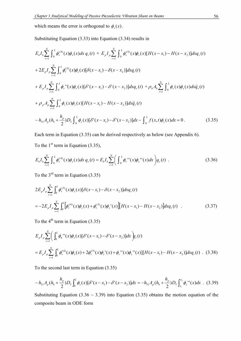
Chapter 3 Analytical Modeling of Passive Piezoelectric Vibration Shunt on Beams 56
which means the error is orthogonal to )(xsφ .
Substituting Equation (3.33) into Equation (3.34) results in
)()()(1
0
)4( tqdxxxIE rs
N
r
L
rbb φφ∑∫=
+ )()]()()[()( 211
0
)4( tdxqxxHxxHxxIE rs
N
r
L
rpp −−−∑∫=
φφ
)()]()()[()(2 211
0
)3( tdxqxxxxxxIE rs
N
r
L
rpp −−−+ ∑∫=
δδφφ
)()](')(')[()('' 211
0tdxqxxxxxxIE rs
N
r
L
rpp −−−+ ∑∫=
δδφφ + )()()(1
0tqdxxxA rs
N
r
L
rbb φφρ ∑∫=
)()]()()[()( 211
0tqdxxxHxxHxxA rs
N
r
L
rpp −−−+ ∑∫=
φφρ
0)(),()](')(')[()2
(00 21331 =−−−−+− ∫∫ dxxtxfdxxxxxxD
hhAh
L
s
L
sp
bp φδδφ . (3.35)
Each term in Equation (3.35) can be derived respectively as below (see Appendix 6).
To the 1st term in Equation (3.35),
)()()(1
0
)4( tqdxxxIE rs
N
r
L
rbb φφ∑∫=
)()('')(''1
0tqdxxxIE r
N
r
L
srbb ∑ ∫=
⎟⎠⎞⎜
⎝⎛= φφ . (3.36)
To the 3rd term in Equation (3.35)
)()]()()[()(2 211
0
)3( tdxqxxxxxxIE rs
N
r
L
rpp −−−∑∫=
δδφφ
[ ][ ]
∑∫=
−−−+−=N
r
L
rsrsrpp tdxqxxHxxHxxxxIE1
0 21)3()4( )()()()(')()()(2 φφφφ . (3.37)
To the 4th term in Equation (3.35)
)()](')(')[()(''1
210tqdxxxxxxxIE r
N
rs
L
pp ∑ ∫=
⎟⎠⎞⎜
⎝⎛ −−− δδφφ
r
∑∫=
−−−++=N
rrsrsrs
L
rpp tdxqxxHxxHxxxxxxIE1
21)3(
0
)4( )()]()()][('')('')(')(2)()( φφφφφφ
. (3.38)
To the second last term in Equation (3.35)
∫ −−−+−L
sp
bp dxxxxxxDh
hAh
0 21331 )](')(')[()2
( δδφ ∫+−= 2
1
)('')2
( 331
x
x sp
bp dxxDh
hAh
φ . (3.39)
Substituting Equation (3.36 ~ 3.39) into Equation (3.35) obtains the motion equation of the
composite beam in ODE form
Chapter 3 Analytical Modeling of Passive Piezoelectric Vibration Shunt on Beams 57
[ ] )()()()]()([1
0 21 tqdxxxxxHxxHAA r
N
r
L
srppbb
∑ ∫=
⎟⎠⎞⎜
⎝⎛ −−−+ φφρρ
[ ] )()('')('')]()([1
0 21 tqdxxxxxHxxHIEIE r
N
r
L
srppbb
∑ ∫=
⎟⎠⎞⎜
⎝⎛ −−−++ φφ
∫∫ =+−L
s
x
x sp
bp dxxtxfdxxDh
hAh
0331 )(),()('')2
( 2
1
φφ . (3.40)
where:
( ) ⎟⎟⎠
⎞⎜⎜⎝
⎛+=+= 1131
3311313
333
)(11 εβ
εβ
hhtvhEDp
. (3.41)
3.3 Vibration control with the piezoelectric shunt circuit
3.3.1 Series R-L shunt
The electrical current stemmed from electrical charge of PZT is
dtdDS
dtdQti p
3)( −=−= . (3.42)
where
)(ti is the output electrical current of PZT which is also the input current of the shunt
circuit, 3DSQ p= is the electrical charge of PZT, and )( 12 xxbS p −= is the surface area of
the PZT plate.
Substituting Equation (3.41) into Equation (3.42) as well as using 2
2
11 xwz
∂∂
−=ε obtains
⎟⎟⎠
⎞⎜⎜⎝
⎛
∂∂∂
−−=⎟⎟⎠
⎞⎜⎜⎝
⎛+−=
txwzh
dttdv
hS
hh
tvdtdS
tip
p
p
p2
3
3133
113133
)(1)()(β
εβ
or
txwzhhti
Sh
dttdv
pp
p
∂∂∂
+−= 2
3
3133 )()( β
. (3.43)
By using Kirchhoff’s voltage law, the voltage across the electrodes of the PZT is
)()()( 00 tiRdt
tdiLtv += . (3.44)
Substituting Equation (3.44) into Equation (3.43) obtains,

Chapter 3 Analytical Modeling of Passive Piezoelectric Vibration Shunt on Beams 58
txwzhhti
CdttdiR
dttidL p
P ∂∂∂
=++ 2
3
3102
2
0 )(1)()( , (3.45)
or
dttdV
xwzhh
dtddtti
CtiR
dttdiL
dtd s
pp
)()(1)()(2
2
31020 =⎟⎟⎠
⎞⎜⎜⎝
⎛∂∂
=⎟⎟⎠
⎞⎜⎜⎝
⎛++ ∫ . (3.46)
where
p
p
pp h
Sh
xxbC3333
12 )(ββ
=−
= –– The capacitance of PZT.
2
2
31)(xwzhhtV ps ∂
∂= –– The equivalent voltage source stemmed from mechanical
strain.
From Equation (3.46), one can have,
100 )()(1)()( DCsp
VtVdttiC
tiRtiL +=++ ∫ . (3.47)
where 1DCV is a constant representing DC voltage.
If DCV is neglected, Equation (3.47) becomes
)()(1)()( 00 tVdttiC
tiRtiL sp
=++ ∫ . (3.48)
The equivalent circuit model of Equation (3.48) is depicted in Figure 3-3 that represents the
series R-L shunt circuit connected to the piezoelectric transducer.
Figure 3-3 Equivalent circuit of series piezoelectric R-L shunt
Chapter 3 Analytical Modeling of Passive Piezoelectric Vibration Shunt on Beams 59
Integrate both sides of Equation (3.48) with 2
2
31)(xwzhhtV ps ∂
∂= from bh to pb hh + to
eliminate variable z,
∫∫ ∫++
∂∂∂
=⎟⎟⎠
⎞⎜⎜⎝
⎛++ pb
b
pb
b
hh
h p
hh
hp
dztx
wzhhdzdttiC
tiRtiL
2
3
3100 )(1)()(
one can have
22
231
00 2)2(
)(1)()(DC
pbp
p
Vxwhhhh
dttiC
tiRdt
tdiL +∂∂+
=++ ∫ . (3.49)
If 2DCV is disregarded, Equation (3.49) can be expressed as
02
)2()(1)()(
2
231
00 =∂∂+
−++ ∫ xwhhhh
dttiC
tiRdt
tdiL pbp
p
. (3.50)
Considering the relation
)()(''1)()(''1121
2
22
1
tqdxxxx
tqxxw
r
N
r
x
x rr
N
rr ⎟
⎠
⎞⎜⎝
⎛−
==∂∂ ∑ ∫∑
==
φφ
and to substitute it into Equation (3.50) obtains
0)('')(2
)2()(1)()(
112
3100
2
1
=⎟⎠
⎞⎜⎝
⎛−
+−++ ∑ ∫∫
=r
N
r
x
x rpbp
p
qdxxxx
hhhhdtti
CtiR
dttdiL φ . (3.51)
Equation (3.51) can be simplified as
0)()(1)()(
00
0 =+++ ∫ tqdttiCL
tiLR
dttdi
rrp
ψ . (3.52)
where,
∫−
+−= 2
1
)('')(2
)2(
012
31 x
x rpbp dxx
Lxxhhhh
r φψ (r = 1, …, N) . (3.53)
Since,
∫∫ −∂∂
=−= dttiCx
wzhhdttiC
tVtvp
pp
s )(1)(1)()( 2
2
31 ,
then,
⎟⎟⎠
⎞⎜⎜⎝
⎛
∂∂
−−∂∂
=⎟⎟⎠
⎞⎜⎜⎝
⎛+= ∫ 2
2
312
2
3133
113133
3 )(11)(1xwzhdtti
Chxwzhh
htvD
ppp βε
β
Chapter 3 Analytical Modeling of Passive Piezoelectric Vibration Shunt on Beams 60
∫∫ −=−= dttiS
dttiCh ppp
)(1)(1
33β. (3.54)
One can notice that Equation (3.54) is the integration of 3D in Equation (3.42). Substituting
Equation (3.54) into Equations (3.40) along with Equation (3.53) obtains
[ ] )()()()]()([1
0 21 tqdxxxxxHxxHAA r
N
r
L
srppbb
∑ ∫=
⎟⎠⎞⎜
⎝⎛ −−−+ φφρρ
[ ] )()('')('')]()([1
0 21 tqdxxxxxHxxHIEIE r
N
r
L
srppbb
∑ ∫=
⎟⎠⎞⎜
⎝⎛ −−−++ φφ
∫∫ =−L
sr dxxtxfdttiL
00 )(),()( φψ . (3.55)
The matrix form of Equation (3.55) is:
dfiBKqqM =++~
. (3.56)
When structure damping is considered, Equation (3.56) can be extended as:
dfiBKqqCqM =+++~
. (3.57)
where
[ ]T q 121 ... ×= NNqqq , [ ]T
i 121 ... ×= NNiii ,
dtdqq = , 2
2
dtd qq = , ∫= dtii~ ,
KMC γα += –– The Rayleigh damping (or proportional damping) coefficient, α
and γ are constants.
⎥⎥⎥
⎦
⎤
⎢⎢⎢
⎣
⎡=
NNN
N
mm
mm
1
111
M , ⎥⎥⎥
⎦
⎤
⎢⎢⎢
⎣
⎡=
NNN
N
kk
kk
1
111
K , ⎥⎥⎥
⎦
⎤
⎢⎢⎢
⎣
⎡=
NNN
N
cc
cc
1
111
C ,
1×⎥⎥⎥
⎦
⎤
⎢⎢⎢
⎣
⎡=
NdN
d1
f
f
df , .
[ ]∫ −−−+=L
srppbbsr dxxxxxHxxHAAm0 21 )()( )]()([ φφρρ ,
[ ]∫ −−−+=L
srppbbsr dxxxxxHxxHIEIEk0 21 )('')('' )]()([ φφ ,
⎥⎥⎥
⎦
⎤
⎢⎢⎢
⎣
⎡=
NB
B1
B0
0

Chapter 3 Analytical Modeling of Passive Piezoelectric Vibration Shunt on Beams 61
srsrsr kmc γα += ,
dxxxxtFdxxtxff sd
L
d
L
sds )()()()(),(00
φδφ −== ∫∫
(Point force applied at dx , s = 1, …, N),
∫−
+= 2
1
)('')(2
)2(
12
31 x
x rpbp dxx
xxhhhh
Br φ (r = 1, …, N).
Equation (3.52) represents piezoelectric vibration control with a single series R-L shunt
circuit. In general, vibration control with multiple series R-L shunt branches can be
represented as a matrix form (assume shunt branches are mutually non-interfering),
0ΨqiΩiΓi =+++~
. (3.58)
where
, , .
rR , rL are the resistor and inductor of the parallel R-L shunt circuit respectively, and rψ is
calculated by Equation (3.53).
Now convert the matrix Equations (3.57 & 3.58) into a state space form. Let
qx1 = ,
21 xqx
==dt
d,
d3-
2-
1-2 fMBxM-CxMKxMqx 1111 −+−−==
dtd
,
ix3~
= ,
43 xix
==dt
d ,
3214 xΓxΩΨxix
−−−==dt
d,
111 xCqC ==y .
⎥⎥⎥⎥⎥
⎦
⎤
⎢⎢⎢⎢⎢
⎣
⎡
=
N
N
LR
LR
1
1
Γ0
0 ⎥⎥⎥⎥⎥
⎦
⎤
⎢⎢⎢⎢⎢
⎣
⎡
=
Np
p
LC
LC
1
1
1
Ω0
0 ⎥⎥⎥
⎦
⎤
⎢⎢⎢
⎣
⎡=
Nψ
ψ1
Ψ0
0

Chapter 3 Analytical Modeling of Passive Piezoelectric Vibration Shunt on Beams 62
where,
N
mm
LxN
Lx
×⎥⎦⎤
⎢⎣⎡=
1
sinsin
1 C ππ , mx is the position where response measured.
Then the state space form of Equations (3.57 & 3.58) is
uDxCyuBxAx
SS
SS
+=+=
. (3.59)
where,
T14]
~[[ ×== NLLT
4321 i i q q]x x x xx , [ ] 1×= Ndfu
NN 44 ×
−−−
⎥⎥⎥⎥
⎦
⎤
⎢⎢⎢⎢
⎣
⎡
−−
−−−=
0ΓΩ-Ψ I000 0BMCMKM 00I0
A111
S ,
NN×
⎥⎥⎥⎥
⎦
⎤
⎢⎢⎢⎢
⎣
⎡
=
400
M0
B-1
S ,
[ ] N41×= 1S 0 0 0 CC , [ ] N S 0 D ×= 1 , N
mm
LxN
Lx
×⎥⎦⎤
⎢⎣⎡=
1
sinsin
1 C ππ and I is the
unit matrix.
3.3.2 Parallel R-L shunt
From Equations (3.41, 3.42), the electrical current of parallel piezoelectric R-L shunt can be
expressed as
RLpppp
pp iidt
dChhdtdvCh
htv
dtdS
dtdDSti +=−−=
⎪⎭
⎪⎬⎫
⎪⎩
⎪⎨⎧
⎟⎟⎠
⎞⎜⎜⎝
⎛+−=−= 11
31113133
3 )(1)( εεβ
. (3.60)
According to the Kirchhoff’s current law,
SRLC Iiii =++ . (3.61)
where
dtdvCi pC = is the electrical current of pC , Li and Ri are electrical currents of the
inductor and resistor of the shunt circuit respectively, dt
dChhI ppS11
31ε
−= is the equivalent
electrical current source generated due to mechanical stress, )(tv is the voltage across the
electrodes of PZT.

Chapter 3 Analytical Modeling of Passive Piezoelectric Vibration Shunt on Beams 63
The equivalent circuit model of Equation (3.61) is depicted in Figure 3-4 that represents the
parallel piezoelectric R-L shunt. As seen in the Figure, the voltage )(tv can be calculated as
below (DC current is disregarded similar to the DC voltage consideration in the series shunt)
( )∫ ∫∫ ⎟⎠⎞
⎜⎝⎛ ++−=−−== dtii
dtdChh
CdtiiI
Cdti
Ctv LRpp
pLRS
pC
p
1131
111)( ε
∫∫ −−−=⎟⎟⎠
⎞⎜⎜⎝
⎛++−= dti
Ci
CRLhhdti
dtdi
RL
dtdChh
C Lp
Lp
pLL
ppp
11
0
01131
0
01131 εε . (3.62)
Figure 3-4 Equivalent circuit of parallel piezoelectric R-L shunt
Substituting Equation (3.62) into Equation (3.41) obtains 3D for the parallel R-L shunt circuit
⎟⎟⎠
⎞⎜⎜⎝
⎛+−= ∫ dti
Ci
CRL
hD L
pL
pp
11
0
0
333 β
, (3.63)
Then Equation (3.40) becomes:
[ ] )()()()]()([1
0 21 tqdxxxxxHxxHAA r
N
r
L
srppbb ∑ ∫=
⎟⎠⎞⎜
⎝⎛ −−−+ φφρρ
[ ] )()('')('')]()([1
0 21 tqdxxxxxHxxHIEIE r
N
r
L
srppbb ∑ ∫=
⎟⎠⎞⎜
⎝⎛ −−−++ φφ
∫∫ =++L
sLRLL dxxtxfdtiBiB0
)(),( φ . (3.64)
where
∫−
+= 2
1
)('')(2
)2(
0
0
12
31 x
x spbp
L dxsRL
xxhhhh
B φ , (3.65)
∫−+
= 2
1
)('')(2
)2(
12
31 x
x spbp
R dxsxx
hhhhB φ . (3.66)

Chapter 3 Analytical Modeling of Passive Piezoelectric Vibration Shunt on Beams 64
On the other hand, the voltage of the inductor is dtdiLtv L
0)( = which is equal to the voltage of
resistor and capacitor in Figure 3-4. Combining with Equation (3.62), one can have
∫−−−= dtiC
iCR
LhhdtdiL L
pL
pp
L 1
0
011310 ε ,
Or
2
2
310
00
1xwzhhdti
Ci
CRL
dtdiL pL
pL
p
L
∂∂
=++ ∫ . (3.67)
where axial strain 11ε has been replaced by 2
2
xwz
∂∂
− .
Integrating both sides of Equation (3.67) to eliminate variable z and considering equation
)()(''1
2
2
tqxxw
r
N
rr ⎟
⎠
⎞⎜⎝
⎛=
∂∂ ∑
=
φ ,
∫∫ ∫++
∂∂
=⎟⎟⎠
⎞⎜⎜⎝
⎛++ pb
b
pb
b
hh
hp
hh
h Lp
Lp
L dzxwzhhdzdti
Ci
CRL
dtdiL
2
2
310
00
1
one can have:
0)('')(2
)2(111012
31
00
2
1
=⎟⎠
⎞⎜⎝
⎛−
+−++ ∑∫∫
=r
N
r
x
x rpbp
Lp
Lp
L qdxxLxxhhhh
dtiCL
iCRdt
di
φ . (3.68)
The Equation (3.64) can be written in concise form as:
)(211
tfdtiBiBqkqm dRLL
N
rrsr
N
rrsr =+++ ∫∑∑
==
. (3.69)
Equation (3.68) can be written as:
011100
=+++ ∑∫=
N
rrrL
pL
p
L qdtiCL
iCRdt
di ψ . (3.70)
Equation (3.70) represents piezoelectric vibration control with a single parallel R-L shunt
circuit. In general, multiple parallel R-L shunt control can be represented in matrix form
(assume each control circuit is mutual non-interference),
0ΨqiΩiΓi L LL =+++~
. (3.71)
where

Chapter 3 Analytical Modeling of Passive Piezoelectric Vibration Shunt on Beams 65
[ ]T Li 11 ×= NLNL ii , ∫= dtLL ii~ ,
dtd L
Lii = ,
, , .
rR , rL are the resistor and inductor of the parallel R-L shunt circuit respectively, Li is the
current of inductor, and rψ is calculated by Equation (3.53).
Equation (3.71) for parallel shunt has the same form as Equation (3.58) for series shunt but
with a different coefficient. In parallel shunt, the current of inductor Li is used as the control
variable instead of i in series shunt. Also similar to Equation (3.57), the matrix form of the
extended Equation (3.64) for parallel is
dL RLL fiBiBKqqCqM =++++~
. (3.72)
where
, .
∫−+
= 2
1
)('')(2
)2(
12
31 x
x ss
spbpLs dxx
RL
xxhhhh
B φ (s = 1, …, N),
∫−+
= 2
1
)('')(2
)2(
12
31 x
x spbpR
s dxxxx
hhhhB φ (s = 1, …, N),
M, C , K, and df are the same as those in series shunt.
To convert Equations (3.71 & 3.72) to state space form, let
qx1 = ,
21 xqx
==dt
d,
⎥⎥⎥⎥
⎦
⎤
⎢⎢⎢⎢
⎣
⎡
=L
N
L
B
B1
BL
0 0 ⎥
⎥⎥⎥
⎦
⎤
⎢⎢⎢⎢
⎣
⎡
=R
N
R
B
B1
BR
00
⎥⎥⎥⎥⎥
⎦
⎤
⎢⎢⎢⎢⎢
⎣
⎡
=
Np
p
RC
RC
1
1
1
Γ0
0 ⎥⎥⎥⎥⎥
⎦
⎤
⎢⎢⎢⎢⎢
⎣
⎡
=
Np
p
LC
LC
1
1
1
Ω0
0 ⎥⎥⎥
⎦
⎤
⎢⎢⎢
⎣
⎡=
Nψ
ψ1
Ψ0
0
Chapter 3 Analytical Modeling of Passive Piezoelectric Vibration Shunt on Beams 66
d4L-
3R-
2-
1-2 fMxBMxBM-CxMKxMqx 11111 −+−−−==
dtd ,
L 3 ix ~= ,
4L3 xix
==dt
d,
431L4 ΩxΓxΨxix
−−−==dt
d ,
111 xCqC ==y .
The state space form of Equations (3.71 & 3.72) is the same as Equation (3.59).
where:
T LL
T 4321 i i q q]x x x xx 1414 ]~[[ ×× == NN , [ ] 1×= N dfu ,
NN 44
L 1
R 111
S
ΩΓ0ΨI000
BMBMCMKM00I0
A
×
−−−−
⎥⎥⎥⎥
⎦
⎤
⎢⎢⎢⎢
⎣
⎡
−−−
−−−−= ,
NN×
⎥⎥⎥⎥
⎦
⎤
⎢⎢⎢⎢
⎣
⎡
=
400
M0
B-1
S ,
[ ] N41×= 1S 0 0 0 CC , [ ] N S 0D ×= 1 , N
mm
LxN
Lx
×⎥⎦⎤
⎢⎣⎡=
1
sinsin
1 C ππ .
So far, we have derived the motion equation of a cantilever beam connected to a piezoelectric
shunt network. Solving Equation (3.59) with either series shunt coefficients or parallel shunt
coefficients, one can obtain the time domain vibration signal of the composite beam. A
numerical example of parallel shunt control is given in the next section.
3.4 Numerical examples
Choose
)/sin()( Lxrxr πφ = , (r = 1, …, N)
which satisfies all boundary conditions (Hinged-Hinged), obtains
⎥⎦
⎤⎢⎣
⎡⎟⎠⎞
⎜⎝⎛−⎟
⎠⎞
⎜⎝⎛
−+
=Lxr
Lxr
Lxxrhhhh pbp
r21
012
31 coscos)(2
)2( πππψ , (r = 1, …, N)
⎥⎦
⎤⎢⎣
⎡⎟⎠⎞
⎜⎝⎛−⎟
⎠⎞
⎜⎝⎛
−+
=Lxs
Lxs
LRxxLshhhh
BLs
spbps
21
12
31 coscos)(2
)2( πππ , (s = 1, …, N)

Chapter 3 Analytical Modeling of Passive Piezoelectric Vibration Shunt on Beams 67
⎥⎦
⎤⎢⎣
⎡⎟⎠⎞
⎜⎝⎛−⎟
⎠⎞
⎜⎝⎛
−+
=Lxs
Lxs
Lxxshhhh
BR pbps
21
12
31 coscos)(2
)2( πππ , (s = 1, …, N)
For rs = ,
⎥⎦
⎤⎢⎣
⎡⎟⎠⎞
⎜⎝⎛−⎟
⎠⎞
⎜⎝⎛+
−+=
Lrx
Lrx
rLAxxALA
m ppppbbrr
2112 2sin2sin22
)( πππ
ρρρ ,
⎭⎬⎫
⎩⎨⎧
⎥⎦
⎤⎢⎣
⎡⎟⎠⎞
⎜⎝⎛−⎟
⎠⎞
⎜⎝⎛+
−+⎟⎠⎞
⎜⎝⎛=
Lrx
Lrx
rLIExxIELIE
Lrk ppppbb
rr2112
4 2sin2sin22
)( πππ
π .
For rs ≠ ,
⎟⎠⎞+−⎜
⎝⎛ −
−=
Lxs
Lxrs
Lxr
Lxsr
Lxs
Lxrs
Lxr
Lxsr
srLA
m ppsr
2222111122 cossincossincossincossin)(
πππππππππρ
,
.cossincossincossincossin)(
22221111
2
2
2
22 ⎟⎠⎞+−⎜
⎝⎛ −⎟⎟
⎠
⎞⎜⎜⎝
⎛−
=Lxs
Lxrs
Lxr
Lxsr
Lxs
Lxrs
Lxr
Lxsr
Lrs
srLIE
k ppsr
ππππππππππ
3.4.1 Vibration shunt control simulation 1 (PZT placed at L/2)
Given an aluminum beam and a PZT, the parameters are
Aluminum beam:
)m(5.0 =L , )m(025.0 =b , )m(003.0 =bh , )kg/m(2700 3 =bρ , )GPa(70 =bE .
PZT:
)m(000250 .hp = , )m(22.01 =x , )m(28.02 =x , )kg/m(7600 3 =pρ , )GPa(70 =pE ,
(V/m)1065.7 831 ×=h , )m/F(1033.7 7
33 ×=β (Wang et al, 1996), )nF(82 =pC .
Solving the state space Equation (3.59) with MATLAB® obtains the impulse responses of the
composite beam with a force vector [ ]T d f 11110 2−= (which is equivalent to have equal
point force being applied at the anti-node of each mode) and vibration measured at 4/Lxm =
from origin resulting in, )4/sin()/sin()(1 ππ rLxrrC m == , r = 1, 2, 3, as shown in Figure 3-5.
There are only three frequency components being considered in the vibration (N = 3) with
Rayleigh damping coefficient, 20.=α and 710−=γ . One can get the natural frequencies of
the composite beam from its eigenvalue λ since 2ωλ = (where ω is the circular natural

Chapter 3 Analytical Modeling of Passive Piezoelectric Vibration Shunt on Beams 68
frequency). The eigenvalue can be obtained by solving the characteristic equation
0=− MK λ . For this example, the eigenvalue is
⎥⎥⎥
⎦
⎤
⎢⎢⎢
⎣
⎡
251650000049500000030900
.
Thus the natural frequencies of the composite beam corresponding to the eigenvalue are
approximately 28, 112, and 252 Hz respectively.
The optimal value of inductor of the shunt circuit to target the ith mode can be calculated by
)3,2,1()2(
12 == iCF
Lpi
i π
where iF is the ith natural frequency and pC is the capacitance of the PZT patch.
0 0.1 0.2 0.3 0.4 0.5 0.6 0.7 0.8 0.9 1
-1
-0.8
-0.6
-0.4
-0.2
0
0.2
0.4
0.6
0.8
1 x 10⁻³ Impulse response of beam transverse displacement at xm=L/4
Time (sec)
Dis
plac
emen
t (m
)
Without PZT shuntWith PZT shunt
(a) without shunt control (dashed line),
(b) with shunt control (solid line) ( Hz281 ≈F , Hz1122 ≈F , Hz2523 ≈F , nF82 =pC ,
H4001 =L , H64.242 =L , H846.43 =L , shunt circuit targets at three modes)
Figure 3-5 Impulse response of transverse displacement of beam measured at xm = L/4 with
PZT patch attached in the middle of beam
Shunt circuit ON
Shunt circuit OFF

Chapter 3 Analytical Modeling of Passive Piezoelectric Vibration Shunt on Beams 69
Thus the inductor values to target three natural frequencies can be obtained as L1 = 395 H, L2
= 24.64 H and L3 = 4.846 H respectively. Figure 3-5 shows the impulse response of the
transverse displacement of the composite beam with the parallel R-L piezoelectric vibration
shunt circuit ON/OFF. However, the best shunt outcome of the 1st mode seems at H4001 =L
while other two are at their theoretical values.
Figure 3-6 shows the frequency response of the beam vibration in Figure 3-5. One can see that
the vibration amplitudes of the 1st mode and the 3rd mode have been reduced about 21 and 31
dB respectively when the shunt circuit is turned ON. However, the shunt circuit has no affect
to the 2nd mode since the PZT patch is placed at the middle of the beam i.e.
)m(25.02/2/)( 12 ==+ Lxx where is the node location of the 2nd mode (with hinged-hinged
boundary condition). Therefore, there is no difference in amplitude of the 2nd mode with or
without the shunt circuit being turned ON. However, if the PZT patch is placed away from its
node location, it can control the 2nd mode vibration when the shunt circuit is turned on. It can
be seen in the next example.
0 100 200 300 400 500 600 700 800 900 1000-80
-60
-40
-20
0
20
40Frequency response of beam transverse displacement at xm=L/4
Frequency (Hz)
Mag
nitu
de (d
B)
Without PZT shuntWith PZT shunt
Figure 3-6 Frequency response of transverse displacement of beam measured at xm = L/4
with PZT patch attached in the middle of beam

Chapter 3 Analytical Modeling of Passive Piezoelectric Vibration Shunt on Beams 70
3.4.2 Vibration shunt control simulation 2 (PZT placed at L/4)
The difference of this one from previous one is that the PZT patch is placed at different
location which is m095.01 =x , m155.02 =x , )m(125.04/2/)( 12 ==+ Lxx . The point where
vibration measured is still at L/4 from origin. Figure 3-7 shows the impulse response of the
beam with and without piezoelectric shunt control. With the PZT patch placed at this location,
it can control not only the 1st and 3rd modes, but also the 2nd mode since the PZT patch is not
at the node location of any mode. The vibration amplitude approaches to zero after a short
period of time. Figure 3-8 shows the frequency response of the beam vibration. The vibration
amplitudes of the 1st, 2nd and 3rd mode have been reduced about 15 dB, 24 dB and 28 dB
respectively but the control efficiency of the 1st and 3rd modes are 6 and 3 dB worse off
comparing with the results in previous example because the PZT patch is not attached at anti-
node of the 1st and 3rd modes as it was previously. This tells us that the location where the
PZT patch placed is very important to control a particular vibration mode. One can notice that
the efficiency of vibration control seems better for higher mode frequency though it depends
on the location of the PZT.
0 0.1 0.2 0.3 0.4 0.5 0.6 0.7 0.8 0.9 1-1
-0.8
-0.6
-0.4
-0.2
0
0.2
0.4
0.6
0.8
1 x 10⁻³ Impulse response of beam transverse displacement (xm=L/4)
Time (sec)
Dis
plac
emen
t (m
)
Without PZT shuntWith PZT shunt
(c) without shunt control (dashed line),
(d) with shunt control (solid line) ( Hz281 ≈F , Hz1122 ≈F , Hz2523 ≈F , nF82 =pC ,
H4001 =L , H64.242 =L , H846.43 =L , shunt circuit targets at three modes)
Figure 3-7 Impulse response of transverse displacement of beam measured at xm = L/4 with PZT patch attached Lx 19.01 = and Lx 31.02 =

Chapter 3 Analytical Modeling of Passive Piezoelectric Vibration Shunt on Beams 71
0 100 200 300 400 500 600 700 800 900 1000-80
-60
-40
-20
0
20
40Frequency response of beam transverse displacement (xm=L/4)
Frequency (Hz)
Mag
nitu
de (d
B)
Without PZT shuntWith PZT shunt
Figure 3-8 Frequency response of transverse displacement of beam measured at xm = L/4
with PZT patch attached Lx 19.01 = and Lx 31.02 =
3.4.3 Sensitivity test of control frequency mismatch
The R-L shunt control possesses narrowband characteristics, it is quite sensitive to the
frequency mismatch between the frequency of shunt circuit and the natural frequency to be
controlled. When the shunt circuit is off-tuned, the control will become worse.
0 0.1 0.2 0.3 0.4 0.5 0.6 0.7 0.8 0.9 1-1
-0.8
-0.6
-0.4
-0.2
0
0.2
0.4
0.6
0.8
1 x 10⁻³ Impulse response of 1st mode beam vibration (xm=L/4)
Time (sec)
Dis
plac
emen
t (m
)
Without PZT shuntWith PZT shunt
(a) Shunt circuit is tuned to the 1st mode (L1 = 400 H)
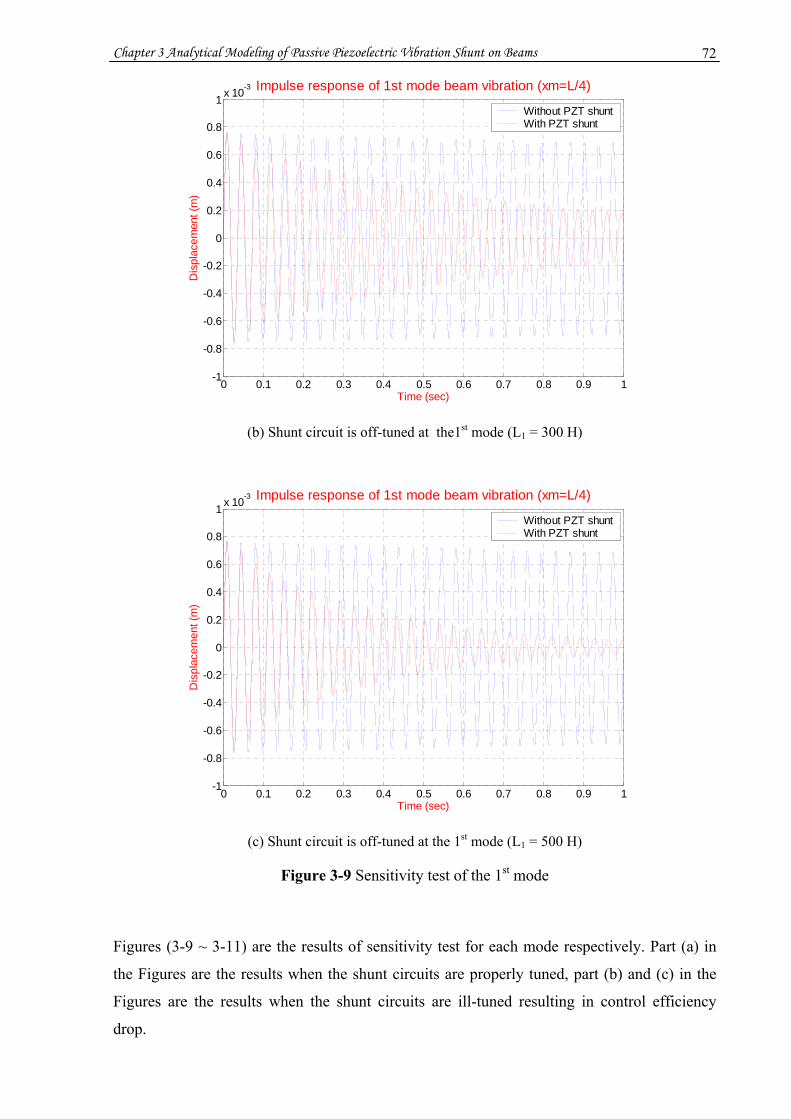
Chapter 3 Analytical Modeling of Passive Piezoelectric Vibration Shunt on Beams 72
0 0.1 0.2 0.3 0.4 0.5 0.6 0.7 0.8 0.9 1-1
-0.8
-0.6
-0.4
-0.2
0
0.2
0.4
0.6
0.8
1 x 10⁻³ Impulse response of 1st mode beam vibration (xm=L/4)
Time (sec)
Dis
plac
emen
t (m
)
Without PZT shuntWith PZT shunt
(b) Shunt circuit is off-tuned at the1st mode (L1 = 300 H)
0 0.1 0.2 0.3 0.4 0.5 0.6 0.7 0.8 0.9 1-1
-0.8
-0.6
-0.4
-0.2
0
0.2
0.4
0.6
0.8
1 x 10⁻³ Impulse response of 1st mode beam vibration (xm=L/4)
Time (sec)
Dis
plac
emen
t (m
)
Without PZT shuntWith PZT shunt
(c) Shunt circuit is off-tuned at the 1st mode (L1 = 500 H)
Figure 3-9 Sensitivity test of the 1st mode
Figures (3-9 ~ 3-11) are the results of sensitivity test for each mode respectively. Part (a) in
the Figures are the results when the shunt circuits are properly tuned, part (b) and (c) in the
Figures are the results when the shunt circuits are ill-tuned resulting in control efficiency
drop.

Chapter 3 Analytical Modeling of Passive Piezoelectric Vibration Shunt on Beams 73
0 0.1 0.2 0.3 0.4 0.5 0.6 0.7 0.8 0.9 1-1
-0.8
-0.6
-0.4
-0.2
0
0.2
0.4
0.6
0.8
1 x 10⁻³ Impulse response of 2nd mode beam vibration (xm=L/4)
Time (sec)
Dis
plac
emen
t (m
)
Without PZT shuntWith PZT shunt
(a) Shunt circuit is tuned to the 2nd mode (L2 = 24.64 H)
0 0.1 0.2 0.3 0.4 0.5 0.6 0.7 0.8 0.9 1-1
-0.8
-0.6
-0.4
-0.2
0
0.2
0.4
0.6
0.8
1 x 10⁻³ Impulse response of 2nd mode beam vibration (xm=L/4)
Time (sec)
Dis
plac
emen
t (m
)
Without PZT shuntWith PZT shunt
(b) Shunt circuit is off-tuned at 2nd mode (L2 = 22 H)
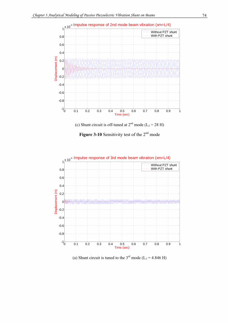
Chapter 3 Analytical Modeling of Passive Piezoelectric Vibration Shunt on Beams 74
0 0.1 0.2 0.3 0.4 0.5 0.6 0.7 0.8 0.9 1-1
-0.8
-0.6
-0.4
-0.2
0
0.2
0.4
0.6
0.8
1 x 10⁻³ Impulse response of 2nd mode beam vibration (xm=L/4)
Time (sec)
Dis
plac
emen
t (m
)
Without PZT shuntWith PZT shunt
(c) Shunt circuit is off-tuned at 2nd mode (L2 = 28 H)
Figure 3-10 Sensitivity test of the 2nd mode
0 0.1 0.2 0.3 0.4 0.5 0.6 0.7 0.8 0.9 1-1
-0.8
-0.6
-0.4
-0.2
0
0.2
0.4
0.6
0.8
1 x 10⁻³ Impulse response of 3rd mode beam vibration (xm=L/4)
Time (sec)
Dis
plac
emen
t (m
)
Without PZT shuntWith PZT shunt
(a) Shunt circuit is tuned to the 3rd mode (L3 = 4.846 H)
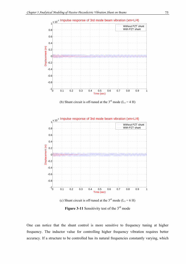
Chapter 3 Analytical Modeling of Passive Piezoelectric Vibration Shunt on Beams 75
0 0.1 0.2 0.3 0.4 0.5 0.6 0.7 0.8 0.9 1-1
-0.8
-0.6
-0.4
-0.2
0
0.2
0.4
0.6
0.8
1 x 10⁻³ Impulse response of 3rd mode beam vibration (xm=L/4)
Time (sec)
Dis
plac
emen
t (m
)
Without PZT shuntWith PZT shunt
(b) Shunt circuit is off-tuned at the 3rd mode (L3 = 4 H)
0 0.1 0.2 0.3 0.4 0.5 0.6 0.7 0.8 0.9 1-1
-0.8
-0.6
-0.4
-0.2
0
0.2
0.4
0.6
0.8
1 x 10⁻³ Impulse response of 3rd mode beam vibration (xm=L/4)
Time (sec)
Dis
plac
emen
t (m
)
Without PZT shuntWith PZT shunt
(c) Shunt circuit is off-tuned at the 3rd mode (L3 = 6 H)
Figure 3-11 Sensitivity test of the 3rd mode
One can notice that the shunt control is more sensitive to frequency tuning at higher
frequency. The inductor value for controlling higher frequency vibration requires better
accuracy. If a structure to be controlled has its natural frequencies constantly varying, which

Chapter 3 Analytical Modeling of Passive Piezoelectric Vibration Shunt on Beams 76
is quite possible in reality, it is desirable to have the control frequency of the shunt circuit
track the natural frequency of the structure to prevent the frequency mismatch problem. This
requires real-time estimation of structure’s excitation frequencies. This is discussed in
Chapter 7.
3.5 Chapter summary
In this chapter, an analytical study of resistor-inductor piezoelectric vibration shunt control on
a beam structure has been carried out. The motion equation of the composite beam made of a
cantilever beam with a PZT patch attached has been derived by using the Hamilton’s principle
and Galerkin’s method. The piezoelectric shunt networks have been coupled into the beam
equation by means of the constitutive piezoelectric relation and electrical circuit theory as a
mechanism to control beam vibration. A numerical example of the parallel R-L piezoelectric
vibration shunt control for beam vibration by solving the state space equation has been given.
The simulation results with Matlab® have shown that significant vibration reduction can be
achieved when the control circuit is tuned to the natural frequency to be controlled. The
results have also shown that the control efficiency is sensitive to the location where the PZT
patch is placed and the accuracy of the shunt circuit being tuned.
Chapter 4 Composite Beam Analysis and Design 77
Chapter 4
Composite Beam Analysis and Design
Composite beams, made of more than one material, have different properties and
characteristics from beams made of a single material. Strain and stress distributions in the
composite beams are determined by the geometry size, material properties and beam
structure. To understand the strain/stress distribution in the composite beams is important for
effectively removing vibration energy from the structure using passive piezoelectric vibration
control technique. In this chapter, the influence of neutral surface location on strain
distribution in the composite beam will be discussed. The equations of neutral surface
location, area moment of inertia, strain and stress distribution of a two-layer composite beam
made of the PZT and a uniform beam will be derived respectively. Simulations of the derived
equations with different thickness ratios and Young’s modulus ratios are presented. Some
FEA simulation and experimental results of the piezoelectric vibration shunt control for the
beams made of various materials are presented. Carbon fibre composite material and its
layout are also briefly introduced. Finally, the design of the Cricket bat handle is proposed in
order to maximize the conversion of vibration energy to electrical energy to be dissipated by
an electrical network and the benefits of using carbon-fibre materials in Cricket bats will also
be described.
4.1 Stress and Strain in Composite Beams
Beams made of more than one material are known as composite beams. The examples of the
composite beams are bimetallic beams, sandwich beams and laminated beams, which consist
of multi-layer beams of different materials. Figure 4-1(a) shows a simple composite beam that
is made of a PZT layer bonded on the outer surface of a uniform cantilever beam. It is
assumed that the PZT layer and the beam are firmly bonded together, the PZT and beam
models are linear and elastic, and the material properties of the PZT and beam are
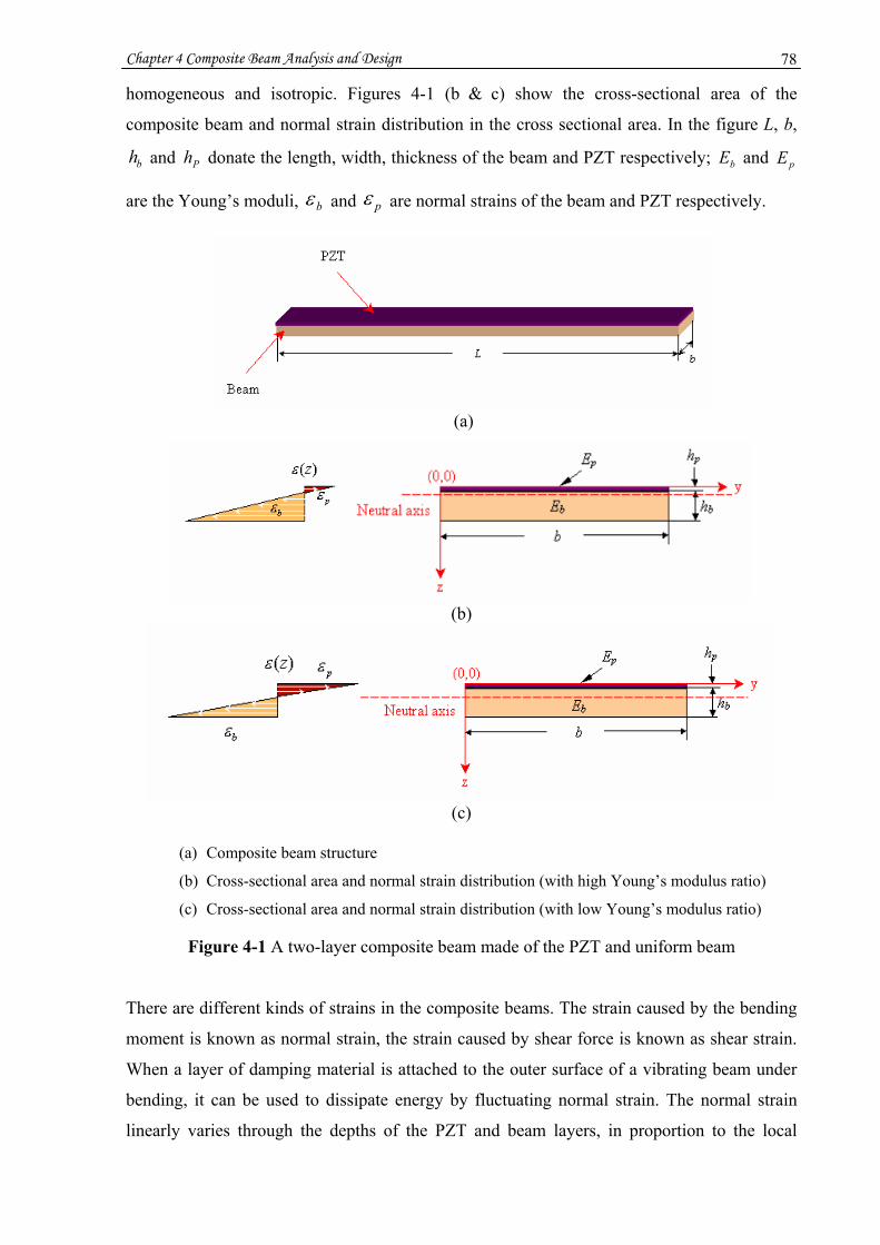
Chapter 4 Composite Beam Analysis and Design 78
homogeneous and isotropic. Figures 4-1 (b & c) show the cross-sectional area of the
composite beam and normal strain distribution in the cross sectional area. In the figure L, b,
bh and Ph donate the length, width, thickness of the beam and PZT respectively; bE and pE
are the Young’s moduli, bε and pε are normal strains of the beam and PZT respectively.
(a)
(b)
(c)
(a) Composite beam structure
(b) Cross-sectional area and normal strain distribution (with high Young’s modulus ratio)
(c) Cross-sectional area and normal strain distribution (with low Young’s modulus ratio)
Figure 4-1 A two-layer composite beam made of the PZT and uniform beam
There are different kinds of strains in the composite beams. The strain caused by the bending
moment is known as normal strain, the strain caused by shear force is known as shear strain.
When a layer of damping material is attached to the outer surface of a vibrating beam under
bending, it can be used to dissipate energy by fluctuating normal strain. The normal strain
linearly varies through the depths of the PZT and beam layers, in proportion to the local

Chapter 4 Composite Beam Analysis and Design 79
bending moment and the distance from the neutral surface of bending. The further the
distance of a surface from the neutral surface, the greater the normal strain of the surface. The
greatest normal strain occurs along the surface furthest from the neutral surface. In order to
dissipate more energy in bending, the damping layer should be attached as far from the
neutral surface as possible, or the neutral surface of the composite beam should be located as
far from the damping layer as possible. This configuration, known as free/unconstrained layer
treatment/damping, can maximize normal strain but is free from shear strain as it is free from
shear force. On the contrary, another configuration where the damping layer is sandwiched in
the middle of two beams, known as constrained treatment/damping, can maximize the shear
strain but produce very little normal strain due to a damping layer close to the neutral surface
(Mead, 2000). In order to dissipate one type of strain energy or the other efficiently, the
material properties and location of the damping layer should be selected accordingly. In this
study, only normal strain is considered.
Although made of different materials, the normal strain distribution through the depth of the
composite beams is still linear, same as the normal strain distribution of the beams made of a
single material. However, unlike the beams made of a single material, the stress distribution in
the composite beams is not linear but piecewise linear. The stress of individual layer is the
product of the strain and the Young’s modulus of the material of the layer. The level of
normal strain in the layer can be different depending on the location of the neutral surface of
the composite beam. The neutral surface is the surface where strain/stress is zero. The
strains/stresses below the neutral surface and above the neutral surface have opposite signs. In
pure bending, the normal strain xε and normal stress xσ in x-direction can be expressed as,
respectively,
zRz
x κε −=−= , (4.1)
zEE ixix κεσ −== . (4.2)
where
R1
=κ is the radius of curvature of the composite beam due to bending, R is the radius
of curvature, iE is the Young’s modulus, and z is the distance on z-coordinate from the
neutral surface. For small deflections of the beam compared to the length of the beam, the
radius of curvature can be determined from the following equation (assume the composite
Chapter 4 Composite Beam Analysis and Design 80
beam is under pure bending, that is the x-direction displacement x
txwztxDx ∂∂
=),(),( and y-
direction displacement 0),( =txDy ) and ),(),,( txwtzxDz = ):
2/32
2
2
2
2
),(1
),(1
⎥⎥⎦
⎤
⎢⎢⎣
⎡⎟⎟⎠
⎞⎜⎜⎝
⎛∂
∂+
∂∂
−=
xtxw
xtxw
R. (4.3)
If the composite beam is slightly bent, then 1),(2
2
<<∂
∂x
txw , Equation (4.3) can be
approximated as:
IEM
xtxw
R i
−=∂
∂−== 2
2 ),(1κ . (4.4)
where
IEdAzEdAzM iAA x κκσ −=−=−= ∫∫∫∫
2 , (4.5)
∫∫=A
dAzI
2 . (4.6)
M and I are the bending moment and the area moment of inertia of the composite beam
respectively.
4.2 Parameters of the two-layer piezoelectric composite beam
In this section, some important parameters of the two-layer piezoelectric composite beam
depicted in Figure 4-1, such as the location of neutral surface, area moment of inertia, and
normal strain/stress will be derived.
4.2.1 Neutral surface location
The neutral surface location of the composite beams is determined by the geometry sizes and
the Young’s moduli of all layers. Considering the cross sectional area of a multi-layer
composite beam as shown in Figure 4-2, where iA and iE are the cross-sectional area and
Young’s modulus of the ith layer respectively.

Chapter 4 Composite Beam Analysis and Design 81
Stress is a measure of the intensity of internal forces. If the body is in equilibrium, the sum of
x-axial forces xF on the cross sectional area is zero, that is ∑=
==N
iixx FF
10)( , where
∫∫=iA ixix dAF
)()( σ .
So
0)()()(1
1 =++++= ∫∫∫∫∫∫Ni A NxA ixA xx dAdAdAF
σσσ . (4.7a)
Figure 4-2 Cross sectional area of a multi-layer composite beam
Substituting Equations (4.2 & 4.1) to Equation (4.7a) obtain:
0)()()(1
11 =++++ ∫∫∫∫∫∫Ni A NxNA ixiA x dAEdAEdAE
εεε , (4.7b)
Or
01
1 =−−−−− ∫∫∫∫∫∫Ni ANAiAzdAEzdAEzdAE
. (4.7c)
where z is the z-coordinate value of the distance from neutral surface.
Let zzz −= ˆ , then Equation (4.7c) becomes:
0)ˆ()ˆ()ˆ(1
1 =−++−++− ∫∫∫∫∫∫Ni ANAiA
dAzzEdAzzEdAzzE
. (4.7d)
For the ith term in Equation (4.7d),
][ 1 zhzhz ii −∈ − - ∵ ,
1h2h
1−ihih
1−NhNh
by
z
)0,0(
Layer N, AN, EN
Layer i, Ai, Ei
Layer 2, A2, E2
Layer 1, A1, E1
Chapter 4 Composite Beam Analysis and Design 82
][ˆ 1 ii hhz −∈∴ .
∫∫∫∫∫−−−
−=−=− i
i
i
i
i
ii
h
hi
h
hi
h
hiAi zdzbEzdzbEzdzzbEdAzzE
111
ˆˆˆˆ)ˆ()ˆ(
zAEhhbEhhzbEzbE iiiii
iii
h
hi
i
i
−−=−−= −−
−
)(2
)(2ˆ 2
12
1
2
1
zAEzAEzAEhhhhbE iiiiiiiiiii
i −=−−+
= −− )(
2 11 . (4.8)
where,
2
1−+= ii
ihhz is the value of the centeroid, and )( 1−−= iii hhbA is the area of the ith
layer (i = 1, 2, ..., N) respectively.
Applying Equation (3.8) to each term of Equation (4.7d), Equation (4.7d) can be rewritten as
011111 =−++−++− zAEzAEzAEzAEzAEzAE NNNNNiiiii ,
Or
011
=− ∑∑==
N
iii
N
iiii AEzzAE . (4.9)
From Equation (4.9), the neutral surface location of the multi-layer composite beam can be
found by
∑
∑
=
== N
iii
N
iiii
EA
zEAz
1
1 . (4.10)
For the composite beam shown in Figure 4-1, we define a thickness ratio μ that is the ratio of
the PZT thickness over the beam thickness, and a Young’s modulus ratio n that is the ratio of
the Young’s modulus of the PZT over the Young’s modulus of the beam respectively, that is,
b
p
hh
=μ –– Thickness ratio of PZT over beam,
b
p
EE
n = –– Young’s modulus ratio of PZT over beam.
The composite beams in Figure 4-1 (b & c) have the same thickness ratio but different
Young’s modulus ratio. The Young’s modulus ratio in Figure 4-1 (b) is larger than that in
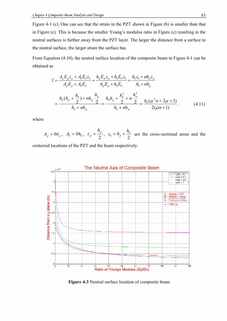
Chapter 4 Composite Beam Analysis and Design 83
Figure 4-1 (c). One can see that the strain in the PZT shown in Figure (b) is smaller than that
in Figure (c). This is because the smaller Young’s modulus ratio in Figure (c) resulting in the
neutral surfaces is further away from the PZT layer. The larger the distance from a surface to
the neutral surface, the larger strain the surface has.
From Equation (4.10), the neutral surface location of the composite beam in Figure 4-1 can be
obtained as
pb
ppbb
bbpp
bbbppp
bbpp
bbbppp
nhhznhzh
EhEhzEhzEh
EAEAzEAzEA
z+
+=
+
+=
+
+=
)1(2)12(222
)2
( 2
22
+++
=+
++=
+
++=
nnh
nhh
hnhhh
nhh
hnhhhh
b
pb
pbpb
pb
pp
bpb
μμμ
. (4.11)
where
pp bhA = , bb bhA = , 2
pp
hz = ,
2b
pbhhz += are the cross-sectional areas and the
centeroid locations of the PZT and the beam respectively.
Figure 4-3 Neutral surface location of composite beam
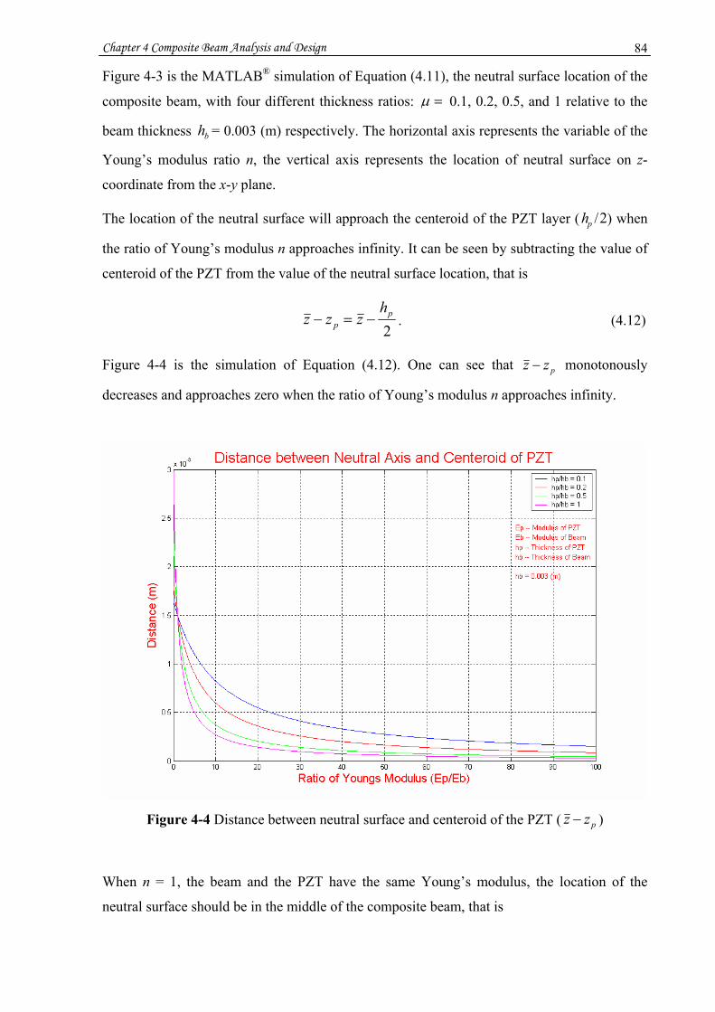
Chapter 4 Composite Beam Analysis and Design 84
Figure 4-3 is the MATLAB® simulation of Equation (4.11), the neutral surface location of the
composite beam, with four different thickness ratios: =μ 0.1, 0.2, 0.5, and 1 relative to the
beam thickness bh = 0.003 (m) respectively. The horizontal axis represents the variable of the
Young’s modulus ratio n, the vertical axis represents the location of neutral surface on z-
coordinate from the x-y plane.
The location of the neutral surface will approach the centeroid of the PZT layer ( 2/ph ) when
the ratio of Young’s modulus n approaches infinity. It can be seen by subtracting the value of
centeroid of the PZT from the value of the neutral surface location, that is
2
pp
hzzz −=− . (4.12)
Figure 4-4 is the simulation of Equation (4.12). One can see that pzz − monotonously
decreases and approaches zero when the ratio of Young’s modulus n approaches infinity.
Figure 4-4 Distance between neutral surface and centeroid of the PZT ( pzz − )
When n = 1, the beam and the PZT have the same Young’s modulus, the location of the
neutral surface should be in the middle of the composite beam, that is
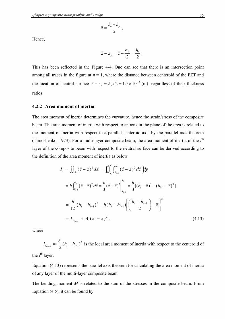
Chapter 4 Composite Beam Analysis and Design 85
2pb hh
z+
= ,
Hence,
22bp
phh
zzz =−=− .
This has been reflected in the Figure 4-4. One can see that there is an intersection point
among all traces in the figure at n = 1, where the distance between centeroid of the PZT and
the location of neutral surface (m)105.12/ 3 −×==− bp hzz regardless of their thickness
ratios.
4.2.2 Area moment of inertia
The area moment of inertia determines the curvature, hence the strain/stress of the composite
beam. The area moment of inertia with respect to an axis in the plane of the area is related to
the moment of inertia with respect to a parallel centeroid axis by the parallel axis theorem
(Timoshenko, 1973). For a multi-layer composite beam, the area moment of inertia of the ith
layer of the composite beam with respect to the neutral surface can be derived according to
the definition of the area moment of inertia as below
dyzdzzdAzzIb h
hAii
ii∫ ∫∫∫ ⎟
⎠⎞⎜
⎝⎛ −=−=
−
0
22
1
ˆ)ˆ()ˆ(
])()[(3
)ˆ(3
ˆ)ˆ( 31
332
11
zhzhbzzbzdzzb ii
h
h
h
h
i
i
i
i
−−−=−=−= −
−−
∫
2
11
31 2
)()(12 ⎥
⎦
⎤⎢⎣
⎡−⎟
⎠⎞
⎜⎝⎛ +
−+−= −−− zhhhhbhhb ii
iiii
2)( zzAI iiiLocal−+= . (4.13)
where
31)(
12 −−= iii hhbILocal
is the local area moment of inertia with respect to the centeroid of
the ith layer.
Equation (4.13) represents the parallel axis theorem for calculating the area moment of inertia
of any layer of the multi-layer composite beam.
The bending moment M is related to the sum of the stresses in the composite beam. From
Equation (4.5), it can be found by

Chapter 4 Composite Beam Analysis and Design 86
∫∫∫∫∫∫ −−−−−=Ni A NxA ixA x zdAzdAzdAM
)()()(
11 σσσ
∫∫∫∫∫∫ −−−−−=Ni ANAiA
dAzEdAzEdAzE
2221
1
κκκ
EIIEIEIEIE i
N
iiNNii κκκκκ −=−=−−−−−= ∑
=111 . (4.14)
where EI donates the equivalent flexural rigidity of the N-layer composite beam,
∑∑∑===
=⎟⎟⎠
⎞⎜⎜⎝
⎛==
N
iii
N
ii
iN
iii InEI
EEEIEEI
11
1 11
1 . (4.15)
The moment of inertia of the entire cross-sectional area of the N-layer composite beam can be
calculated as
∑=
=N
iiit InI
1 . (4.16)
where
tI is the total area moment of inertia of the composite beam, iI and in are the area
moment of inertia and the Young’s modulus ratio relative to 1E of the ith layer respectively.
1E is assumed to be the Young’s modulus of the first layer.
For the composite beam in Figure 4-1, one can have
00 =h , phh =1 , bp hhh +=2 ,
pp bhAA == 1 , bb bhAA == 2 ,
21p
p
hzz == ,
22b
pbhhzz +== .
The local area moments of inertia of the PZT and beam layers are, respectively,
12
3
1p
p
bhII
LocalLocal== ,
12
3
2b
bbhII
LocalLocal== .
Therefore, from Equation (4.13), the area moments of inertia of the PZT layer and the beam
layer about the neutral surface can be derived, respectively,
ppp
pppp bhzzbh
AzzIILocal
23
2 )(12
)( −+=−+= , (4.17)
Chapter 4 Composite Beam Analysis and Design 87
bb
pb
bbbb bhhhzbhAzzIILocal
232
212)( ⎟
⎠⎞
⎜⎝⎛ −−+=−+= . (4.18)
Since
bbpp
pbbbp
bbpp
bbbpppp EhEh
zzEhz
EhEhzEhzEh
zz+−
=−++
=−)(
)1(2)1(
)(2)(
nh
EhEhhhEh b
bbpp
pbbb
μμ
++
=+
+= , (4.19)
bbpp
bpppppb
bbpp
bbbpppb EhEh
zEhzEhz
EhEhzEhzEh
zz+
−=−
+
+=−
)(2)()(
bbpp
pbbb
bb
pp
bbpp
bppp
EhEhhhEh
EhEh
EhEhzzEh
+
+⎟⎟⎠
⎞⎜⎜⎝
⎛−=
+
−=
)1(2)1()(
nhnzzn b
p μμμμ
++
−=−−= . (4.20)
Substituting Equation (4.19) into Equation (4.17) obtains
ppp
pppp bhzzbh
AzzIILocal
23
2 )(12
)( −+=−+=
23
)1(2)1(
12 ⎥⎦
⎤⎢⎣
⎡++
+=n
hbhbh b
pp
μμ
23
33
)1(21
12 ⎥⎦
⎤⎢⎣
⎡++
+=n
hbhbb
b
μμμ
μ
12)364(2
12 22
234253
++++++
=nn
nnbhb
μμμμμμμ
. (4.21)
Figure 4-5 is the plot of Equation (4.21), the area moment of inertia of the PZT layer about
the neutral surface with four different thickness ratios.

Chapter 4 Composite Beam Analysis and Design 88
Figure 4-5 Area moment of inertia of the PZT layer about the neutral surface
Similarly, substituting Equation (4.20) into Equation (4.18) obtains the area moments of
inertia of the beam layer about the neutral surface
bb
pb
bbbb bhhhzbhAzzIILocal
232
212)( ⎟
⎠⎞
⎜⎝⎛ −−+=−+=
223
2)1(2)12(
12 ⎥⎦
⎤⎢⎣
⎡−−
+++
+= bp
bb
b hhn
nhbhbhμ
μμ
223
3
21
)1(212
12 ⎥⎦
⎤⎢⎣
⎡−−
+++
+= μμ
μμn
nbhbhb
b
1212)463(
12 22
22343
++++++
=nn
nnbhb
μμμμμμ
. (4.22)
Figure 4-6 is the plot of Equation (4.22) with four different thickness ratios.
Chapter 4 Composite Beam Analysis and Design 89
Figure 4-6 Area moment of inertia of the beam layer about the neutral surface
The equivalent flexural rigidity of the composite beam is
tbpbbppbb IEnIIEIEIEEI =+=+= )( . (4.23)
where
pbt nIII += . (4.24)
is the total area moment of inertial of the composite beam.
Substituting Equations (4.21, 4.22) into Equation (4.24) obtains,
⎟⎟⎠
⎞⎜⎜⎝
⎛++
+++++
++++++
=12
)364(212
12)463(12 22
23425
22
22343
nnnnn
nnnnbhI b
t μμμμμμμ
μμμμμμ
12
1)564()465(12 22
232234353
+++++++++
=nn
nnnbhb
μμμμμμμμμ
. (4.25)
Figure 4-7 is the plot of Equation (4.25), the total area moment of inertia of the composite
beam about the neutral surface with four different thickness ratios.

Chapter 4 Composite Beam Analysis and Design 90
Figure 4-7 Total area moment of inertia of the composite beam about the neutral surface
4.2.3 Average normal strain and stress
From Equation (4.1) and Equation (4.4), the normal strain along the x-coordinate can be
calculated as:
IEMz
Rz
ix −=−=ε . (4.26)
For the PZT layer, the strain in the middle (centeroid) surface of the PZT is
)()()(
)(pbb
p
ppbb
pAvep nIIE
zzMIEIEzzM
+
−=
+
−−=ε
⎟⎟⎠
⎞⎜⎜⎝
⎛−++−+
−⎟⎟⎠
⎞⎜⎜⎝
⎛=
ppp
bbb
p
b bhzzbh
nbhzzbh
zzEM
23
23
)(12
)(12
22
33
)()(12 ppbb
pb
p
b zznhzzhnhh
zzbEM
−+−++
−⎟⎟⎠
⎞⎜⎜⎝
⎛= . (4.27)
Substituting Equations (4.19, 4.20) into Equation (4.27) obtains:
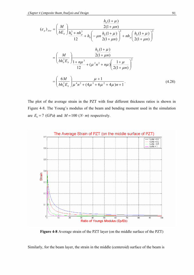
Chapter 4 Composite Beam Analysis and Design 91
2233
)1(2)1(
)1(2)1(
12
)1(2)1(
)(
⎟⎟⎠
⎞⎜⎜⎝
⎛++
+⎟⎟⎠
⎞⎜⎜⎝
⎛++
−++
++
⎟⎟⎠
⎞⎜⎜⎝
⎛=
nhnh
nhnh
nhhn
h
bEM
bp
bb
pb
b
bAvep
μμ
μμμ
μμ
ε
222
33
)1(21)(
121
)1(2)1(
⎟⎟⎠
⎞⎜⎜⎝
⎛++
+++
++
⎟⎟⎠
⎞⎜⎜⎝
⎛=
nnnn
nh
EbhM
b
bb
μμμμμ
μμ
1)464(16
23242 +++++
⎟⎟⎠
⎞⎜⎜⎝
⎛=
nnEbhM
bb μμμμμ
. (4.28)
The plot of the average strain in the PZT with four different thickness ratios is shown in
Figure 4-8. The Young’s modulus of the beam and bending moment used in the simulation
are )(7 GPaEb = and )(100 mNM ⋅= respectively.
Figure 4-8 Average strain of the PZT layer (on the middle surface of the PZT)
Similarly, for the beam layer, the strain in the middle (centeroid) surface of the beam is

Chapter 4 Composite Beam Analysis and Design 92
)()()()(pbb
b
ppbb
bAveb nIIE
zzMIEIE
zzM+−
=+−
−=ε
⎟⎟⎠
⎞⎜⎜⎝
⎛−++−+
−⎟⎟⎠
⎞⎜⎜⎝
⎛=
ppp
bbb
b
b bhzzbh
nbhzzbhzz
EM
23
23
)(12
)(12
2233
)1(2)1(
)1(2)1(
12
)1(2)1(
⎟⎟⎠
⎞⎜⎜⎝
⎛++
+⎟⎟⎠
⎞⎜⎜⎝
⎛++
−++
++
−
⎟⎟⎠
⎞⎜⎜⎝
⎛=
nhnh
nhnh
nhhn
hn
bEM
bp
bb
pb
b
b
μμ
μμμ
μμμ
222
33
)1(21)(
121
)1(2)1(
⎟⎟⎠
⎞⎜⎜⎝
⎛+++++
++
⎟⎟⎠
⎞⎜⎜⎝
⎛ −=
nnnn
nhn
EbhM
b
bb
μμμμμ
μμμ
1)464()(62324
2
2 +++++
⎟⎟⎠
⎞⎜⎜⎝
⎛ −=
nnn
EbhM
bb μμμμμμ
. (4.29)
Figure 4-9 Average strain of the beam layer (on the middle surface of the beam)
The plot of average strain in the beam with four different thickness ratios is shown in Figure
4-9. Figure 4-8 and Figure 4-9 show that the strain in the beam and the strain in the PZT have

Chapter 4 Composite Beam Analysis and Design 93
opposite sign, and when n is not too large, the average strain of the PZT is much larger than
that of the beam.
The stress σ can be obtained from equation εσ iE= , where iE is the Young’s modulus
(unit: Newton/Meter2 or Pascal).
The average stress of the PZT layer is
1)464()1(6)()()( 23242 ++++
+⎟⎟⎠
⎞⎜⎜⎝
⎛===
nnn
bhMnEE
bAvepbAveppAvep μμμμ
μεεσ . (4.30)
The average stress of the beam layer
1)464()1(6)()( 23242 ++++
+⎟⎟⎠
⎞⎜⎜⎝
⎛ −==
nnn
bhMEb
AvebbAveb μμμμμμεσ . (4.31)
One can notice that the ratio of average stress in the beam over average stress in the PZT is
equal to the thickness ratio μ but in opposite sign, i.e. μσσ
−=Avep
Aveb
)()( . When 1=μ , this
means the average stress in the beam and the PZT are the same but with negative sign.
Negative sign means that one is in compression and the other is in extension or vice versa.
This is consistent with beam theory.
Figure 4-10 Average stress of the PZT layer (on the middle surface of the PZT)

Chapter 4 Composite Beam Analysis and Design 94
Figure 4-10 and Figure 4-11 are the plots of the average stress in the PZT and the average
stress in the beam respectively.
Figure 4-11 Average stress of the beam layer (on the middle surface of the beam)
4.3 Discussion of composite beam design for maximizing strain in the
PZT
In this section, the relationship between the electrical field and the mechanical strain of
piezoelectric materials and how to select the Young’s modulus ratio and thickness ratio based
on maximizing the strain in the PZT are discussed. Some FEA simulation and experimental
results of the piezoelectric vibration shunt control for an aluminium beam, a wooden beam
and a carbon-fibre beam are presented. Carbon-fibre composite materials and their layout
configuration are briefly introduced. A preferable design of the Cricket bat handle is
proposed. The benefits of using carbon-fibre material in the Cricket bat handle are described.
4.3.1 The relation between electrical field and mechanical strain in the PZT
As mentioned in Chapter 2, the essence of “piezoelectric effect” is the relation between
electric polarization and mechanical strain in crystals. When mechanically strained, the
piezoelectric materials produce electric polarization that is in proportion to the strain. When
electrically polarized, the piezoelectric materials produce mechanical strain that is in

Chapter 4 Composite Beam Analysis and Design 95
proportion to the polarizing field. For the passive piezoelectric vibration control, the former
mechanism is used; for the active vibration control, the latter mechanism is used. The focus
here will be on how to maximize the mechanical strain in the PZT for the passive control. The
larger strain the PZT has, the larger electrical field it can produce from electric polarization.
This can be reflected by the h-form constitutive relation of piezoelectric materials (IEEE
1987)
DhhDE
Ep
βεεσ+−−
==
⎩⎨⎧
. (4.32)
where
E –– Electrical field (V/m)
pE –– Young’s modulus of PZT (N/m2 or Pa)
β –– Dielectric impermeability (m/F or V-m/C)
D –– Electrical displacement (C/m2)
ε –– Mechanical strain
h –– Electrical field-strain coefficient of PZT (V/m or N/C)
N –– Newton, m –– Meter, V –– Volt, C –– Coulomb, F –– Farad
Reorganize the first equation of Equation (4.32)
εεσ pp EhDE '=−= . (4.33)
From Equation (4.33), one can have
εh
EED pp '−= . (4.34)
If D = 0, pp EE =' , which is the Young’s modulus without considering electrical field or the
electrodes of the PZT at short circuit.
Substituting Equation (4.34) into the second equation of Equation (4.32) obtains
εβ
εβε ⎟⎟⎠
⎞⎜⎜⎝
⎛−
−=
−+−= h
hEE
hEE
hE pppp )'('. (4.35)
Equation (4.35) indicates that the electrical field E produced in the PZT is in proportion to its
strain ε . Larger strain will produce larger electrical field and lead to a larger output voltage,
therefore, more mechanical energy can be converted into electrical energy that can be
dissipated by an electrical network. Figure 4-8 has shown that the average strain in the PZT
layer monotonously decreases when the ratio of Young’s modulus n increases but the average
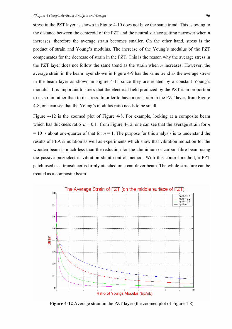
Chapter 4 Composite Beam Analysis and Design 96
stress in the PZT layer as shown in Figure 4-10 does not have the same trend. This is owing to
the distance between the centeroid of the PZT and the neutral surface getting narrower when n
increases, therefore the average strain becomes smaller. On the other hand, stress is the
product of strain and Young’s modulus. The increase of the Young’s modulus of the PZT
compensates for the decrease of strain in the PZT. This is the reason why the average stress in
the PZT layer does not follow the same trend as the strain when n increases. However, the
average strain in the beam layer shown in Figure 4-9 has the same trend as the average stress
in the beam layer as shown in Figure 4-11 since they are related by a constant Young’s
modulus. It is important to stress that the electrical field produced by the PZT is in proportion
to its strain rather than to its stress. In order to have more strain in the PZT layer, from Figure
4-8, one can see that the Young’s modulus ratio needs to be small.
Figure 4-12 is the zoomed plot of Figure 4-8. For example, looking at a composite beam
which has thickness ratio 1.0=μ , from Figure 4-12, one can see that the average strain for n
= 10 is about one-quarter of that for n = 1. The purpose for this analysis is to understand the
results of FEA simulation as well as experiments which show that vibration reduction for the
wooden beam is much less than the reduction for the aluminium or carbon-fibre beam using
the passive piezoelectric vibration shunt control method. With this control method, a PZT
patch used as a transducer is firmly attached on a cantilever beam. The whole structure can be
treated as a composite beam.
Figure 4-12 Average strain in the PZT layer (the zoomed plot of Figure 4-8)

Chapter 4 Composite Beam Analysis and Design 97
This can be explained that because the Young’s modulus of wood is about one-tenth of the
Young’s modulus of the PZT (i.e. n = 10) while the Young’s modulus of the aluminium and
carbon-fibre beam is close to the Young’s modulus of the PZT (i.e. n ≈ 1), the average strain
in the PZT layer is much smaller when the PZT is attached to the wooden beam compared to
the average strain in the PZT layer when the PZT is attached to the aluminium or carbon-fibre
beam. The FEA simulation and experimental results of the piezoelectric vibration shunt
control for the beam with different material are illustrated in the next two subsections. The
results have shown that the vibration reduction is only about 8% for the wooden beam and
40% ~ 90% for the aluminium and carbon-fibre beam. The thickness ratio of the composite
beam μ used in simulations and experiments is around 0.1 ~ 0.15.
In order to maximize the strain in the PZT layer, the Young’s modulus ratio should be as
small as possible, especially for the composite beams with a large thickness ratio. Figure 4-13
is the further zoomed plot of Figure 4-12 (for 1≤n ). One can see that in this region, the
average strains are much larger than those in other regions but falls sharply with large
thickness ratios such as 1=μ . The Young’s modulus ratio 1≤n means the base material is
stiffer than the PZT material. So the piezoelectric vibration shunt control can have better
effect on stiffer structures. If the Young’s modulus ratio is extremely small (say n < 0.04), the
composite beam with a large thickness can attract much more strain in the PZT.
Figure 4-13 Average strain in the PZT layer (the zoomed plot of Figure 4-12)
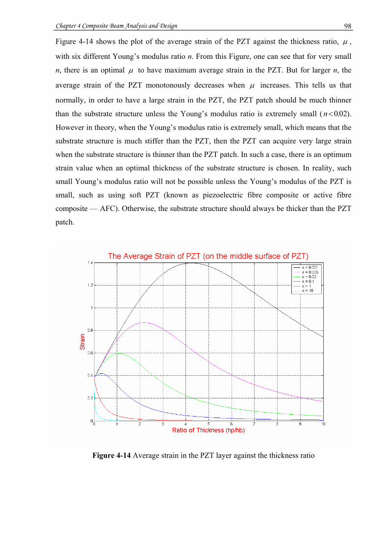
Chapter 4 Composite Beam Analysis and Design 98
Figure 4-14 shows the plot of the average strain of the PZT against the thickness ratio, μ ,
with six different Young’s modulus ratio n. From this Figure, one can see that for very small
n, there is an optimal μ to have maximum average strain in the PZT. But for larger n, the
average strain of the PZT monotonously decreases when μ increases. This tells us that
normally, in order to have a large strain in the PZT, the PZT patch should be much thinner
than the substrate structure unless the Young’s modulus ratio is extremely small ( 02.0<n ).
However in theory, when the Young’s modulus ratio is extremely small, which means that the
substrate structure is much stiffer than the PZT, then the PZT can acquire very large strain
when the substrate structure is thinner than the PZT patch. In such a case, there is an optimum
strain value when an optimal thickness of the substrate structure is chosen. In reality, such
small Young’s modulus ratio will not be possible unless the Young’s modulus of the PZT is
small, such as using soft PZT (known as piezoelectric fibre composite or active fibre
composite –– AFC). Otherwise, the substrate structure should always be thicker than the PZT
patch.
Figure 4-14 Average strain in the PZT layer against the thickness ratio

Chapter 4 Composite Beam Analysis and Design 99
4.3.2 Analytical precursor to the strain analysis in the PZT Patch
In this study, a few different analysis methods had been tried to understand why the
piezoelectric vibration shunt control had worked well for aluminium and carbon-fibre beams
but not for wooden beams before the strain analysis method was used. One of them was the
strain energy method that focused on the strain energy contained of the PZT. The result was
not quite convincing and did not match the simulation and experiment very well. However, as
part of this study, it is worthwhile to document it here. The method focused on strain energy
rather than strain. The method analyzed the strain energy contained in the PZT relative to the
total energy of the composite beam.
With the Euler-Bernoulli beam model, the strain energy of a uniform beam due to bending is
dxdAxwzzEdxdAEdVU
L
bA b
L
A bbbV bbbbbbb
∫ ∫∫∫ ∫∫∫∫∫ ⎟⎟
⎠
⎞
⎜⎜
⎝
⎛⎥⎦
⎤⎢⎣
⎡∂∂
−=⎟⎠⎞⎜
⎝⎛==
0
2
2
2
0
2 )ˆ(21
21
21 εσε
dxxwIEdx
xwdAzzE
L
bb
L
A bbb
∫∫ ∫∫ ⎟⎟⎠
⎞⎜⎜⎝
⎛∂∂
=⎟⎟⎠
⎞⎜⎜⎝
⎛∂∂
⎟⎠⎞⎜
⎝⎛ −=
0
2
2
22
2
2
0
2
21)ˆ(
21
. (4.36)
According to Equation (4.4), the radius of curvature of the composite beam due to bending
can be expressed as
ppbb IEIEM
EIM
xw
+−=−=
∂∂
−= 2
2
κ . (4.37)
From Equation (4.37), one can see that κ is independent of x for uniform beams, applying
Equations (4.37, 4.22 & 4.25) to Equation (4.36) obtain the strain energy of the beam,
2
2
2
2
2
2
0
2
2
2
2)(2)(21
21
t
b
bpb
b
bppbbbb
L
bbb II
ELM
nIII
ELM
IEIELMIEdx
xwIEU =
+=
+=⎟⎟
⎠
⎞⎜⎜⎝
⎛∂∂
= ∫
223223435
222234
3
2
]1)564()465([)12](12)463[(6+++++++
++++++⎟⎟⎠
⎞⎜⎜⎝
⎛=
nnnnnnn
EbhLM
bb μμμμμμμμμμμμμ
. (4.38)
Similarly, the strain energy of the PZT is
dxdAxwzzEdxdAEdVU
L
pA p
L
A pppV ppppppp
∫ ∫∫∫ ∫∫∫∫∫ ⎟⎟
⎠
⎞
⎜⎜
⎝
⎛⎥⎦
⎤⎢⎣
⎡∂∂
−=⎟⎠⎞⎜
⎝⎛==
0
2
2
2
0
2 )ˆ(21
21
21
εσε

Chapter 4 Composite Beam Analysis and Design 100
dxxwIEdx
xwdAzzE
L
pp
L
A ppp
∫∫ ∫∫ ⎟⎟⎠
⎞⎜⎜⎝
⎛∂∂
=⎟⎟⎠
⎞⎜⎜⎝
⎛∂∂
⎟⎠⎞⎜
⎝⎛ −=
0
2
2
22
2
2
0
2
21)ˆ(
21
2
2
2
2
2
2
2)(2)(21
t
p
bpb
p
bppbbpp I
nIE
LMnII
nIE
LMIEIE
LMIE =+
=+
=
223223435
22232435
3
2
]1)564()465([)12]()364(2[6
+++++++++++++
⎟⎟⎠
⎞⎜⎜⎝
⎛=
nnnnnnnn
EbhLM
bb μμμμμμμμμμμμμμ
. (4.39)
The total strain energy of the composite beam then is:
∫∫ ⎟⎟⎠
⎞⎜⎜⎝
⎛∂∂
+=⎟⎟⎠
⎞⎜⎜⎝
⎛∂∂
+=+=L
ppbb
L
ppbbpb dxxwIEIEdx
xwIEIEUUU
0
2
2
22
2
2
0)(
21)(
21
]1)564()465([
)12(623223435
22
3
2
+++++++++
⎟⎟⎠
⎞⎜⎜⎝
⎛=
nnnnn
EbhLM
bb μμμμμμμμμ
. (4.40)
From Equations (4.36, 4.37, & 4.38), the ratio of the strain energy of the PZT over the strain
energy of the beam and the ratio of the strain energy of the PZT over the total strain energy of
the composite beam can be expressed respectively, as:
12)463()364(2
2234
232435
++++++++
=nn
nnnUU
b
p
μμμμμμμμμ
(4.41)
1)564()465()364(2
23223435
232435
+++++++++++
=nnn
nnnUU p
μμμμμμμμμμμμ . (4.42)
Figures (4-15, 4-16 & 4-17) are the plots of the strain energy of the PZT (Equation (4.39)),
the strain energy of the beam (Equation (4.38)), and the total strain energy of the composite
beam (Equation (4.40)) with )(7 GPaEb = and )(100 mNM ⋅= respectively.
Figure 4-18 is the plot of Equation (4.41) and Figure 4-19 is the plot of Equation (4.42)
respectively.

Chapter 4 Composite Beam Analysis and Design 101
Figure 4-15 Strain energy of the PZT ( pU )
Figure 4-16 Strain energy of the beam ( bU )
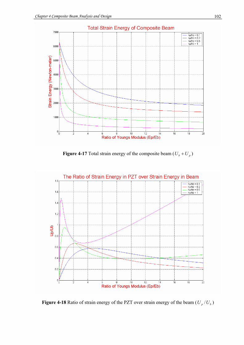
Chapter 4 Composite Beam Analysis and Design 102
Figure 4-17 Total strain energy of the composite beam ( pb UU + )
Figure 4-18 Ratio of strain energy of the PZT over strain energy of the beam ( bp UU / )

Chapter 4 Composite Beam Analysis and Design 103
Figure 4-19 Ratio of strain energy of the PZT over total strain energy of the composite beam
( UU p / )
Figure 4-15 has shown that for each composite beam with different thickness ratios, there is
an optimal value of strain energy contained in the PZT at certain Young’s modulus ratio,
which means that if the Young’s moduli of the beam and the PZT are selected properly, the
strain energy in the PZT can be optimized. However, one can find that the strain energy in the
PZT, for example a composite beam of 1.0=μ , at n = 1 and that at n = 10 do not differ a
great deal. The difference is not big enough to explain the vibration control efficiency
mentioned previously. The reason is that the strain energy of the PZT, similar to stress, is not
only in proportion to its strain, but also to its Young’s modulus. The reduction of the strain in
the PZT layer when n increases is compensated by the increase in the Young’s modulus.
Large strain energy of the PZT does not necessarily mean large strain in the PZT, as there is a
Young’s modulus influence as seen in Equation 4.35a, for example.
bp UU / and UU p / as shown in Figure 4-18 and Figure 4-19 will approach infinity and 100%
respectively when n approaches infinity. This means that the PZT will ultimately possess all
the strain energy when n becomes infinity. This is understandable since when the PZT is
much stiffer than the beam, the beam structure can be totally neglected. Certainly the PZT
layer will possess all the strain energy although there is little strain in it. Since the electrical
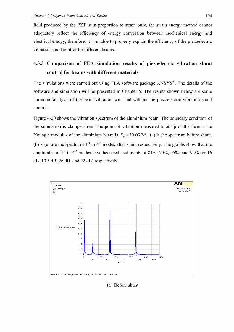
Chapter 4 Composite Beam Analysis and Design 104
field produced by the PZT is in proportion to strain only, the strain energy method cannot
adequately reflect the efficiency of energy conversion between mechanical energy and
electrical energy, therefore, it is unable to properly explain the efficiency of the piezoelectric
vibration shunt control for different beams.
4.3.3 Comparison of FEA simulation results of piezoelectric vibration shunt
control for beams with different materials
The simulations were carried out using FEA software package ANSYS®. The details of the
software and simulation will be presented in Chapter 5. The results shown below are some
harmonic analysis of the beam vibration with and without the piezoelectric vibration shunt
control.
Figure 4-20 shows the vibration spectrum of the aluminium beam. The boundary condition of
the simulation is clamped-free. The point of vibration measured is at tip of the beam. The
Young’s modulus of the aluminium beam is )( GPaEb 70= . (a) is the spectrum before shunt,
(b) ~ (e) are the spectra of 1st to 4th modes after shunt respectively. The graphs show that the
amplitudes of 1st to 4th modes have been reduced by about 84%, 70%, 95%, and 92% (or 16
dB, 10.5 dB, 26 dB, and 22 dB) respectively.
(a) Before shunt

Chapter 4 Composite Beam Analysis and Design 105
(b) Shunt 1st mode
(c) Shunt 2nd mode
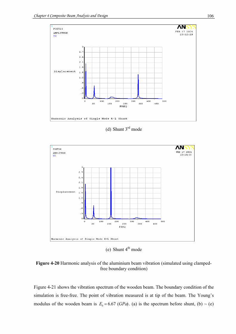
Chapter 4 Composite Beam Analysis and Design 106
(d) Shunt 3rd mode
(e) Shunt 4th mode
Figure 4-20 Harmonic analysis of the aluminium beam vibration (simulated using clamped-
free boundary condition)
Figure 4-21 shows the vibration spectrum of the wooden beam. The boundary condition of the
simulation is free-free. The point of vibration measured is at tip of the beam. The Young’s
modulus of the wooden beam is )(67.6 GPaEb = . (a) is the spectrum before shunt, (b) ~ (e)
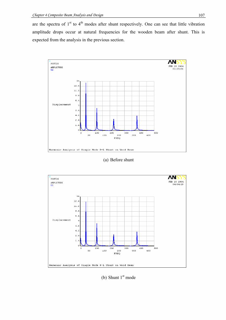
Chapter 4 Composite Beam Analysis and Design 107
are the spectra of 1st to 4th modes after shunt respectively. One can see that little vibration
amplitude drops occur at natural frequencies for the wooden beam after shunt. This is
expected from the analysis in the previous section.
(a) Before shunt
(b) Shunt 1st mode
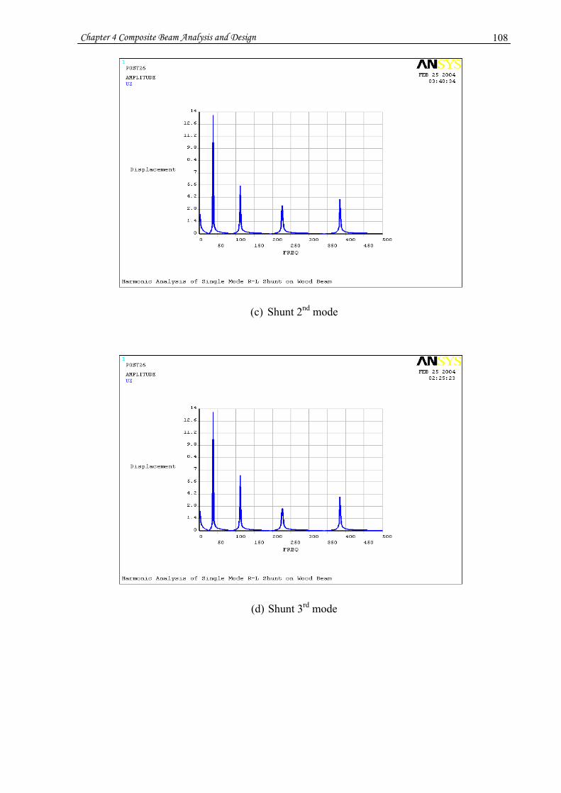
Chapter 4 Composite Beam Analysis and Design 108
(c) Shunt 2nd mode
(d) Shunt 3rd mode

Chapter 4 Composite Beam Analysis and Design 109
(e) Shunt 4th mode
Figure 4-21 Harmonic analysis of the wooden beam vibration (simulated using free-free boundary condition)
In order to improve the efficiency of vibration shunt control, a composite beam was
constructed as shown in Figure 4-22. The left section is the wooden beam, the right section is
the carbon-fibre beam. The Young’s modulus of the carbon-fibre beam is )(66 GPaEc = .
The PZT patch is attached on the upper surface of the carbon-fibre beam.
Figure 4-22 Composite beam with a PZT patch attached
Figure 4-23 shows the first four bending modes of the joint beam obtained from modal
analysis and Figure 4-24 shows the vibration spectrum of the joint beam obtained from
harmonic analysis. (a) shows the spectrum before shunt, (b) ~ (d) show the spectra of 1st to 3rd
Wood
Carbon-fibre PZT

Chapter 4 Composite Beam Analysis and Design 110
modes after shunt respectively. The boundary condition of both simulation is free-free. The
point of vibration measured in Figure 4-24 is at tip of the beam.
Figure 4-23 Modal analysis of the carbon-fibre beam (simulated using free-free boundary condition)
(a) Before shunt

Chapter 4 Composite Beam Analysis and Design 111
(b) Shunt 1st mode
(c) Shunt 2nd mode

Chapter 4 Composite Beam Analysis and Design 112
(d) Shunt 3rd mode
Figure 4-24 Harmonic analysis of the carbon-fibre beam vibration (simulated using free-free
boundary condition)
The graphs show that the amplitudes of 1st to 3rd modes have been reduced by about 48%,
50%, and 83% (or 5.68 dB, 6 dB, and 15.4 dB) respectively. The reduction of vibration
amplitude at natural frequencies is markedly improved from the wooden beam. However, it is
not as good as for the aluminium beam since the carbon-fibre beam is only a part of the joint
beam, much shorter than the length of the aluminium beam. The carbon-fibre beam section
has been bent much less than the aluminium beam has. Nevertheless, the PZT can still get
more strain when attached on the carbon-fibre beam than when attached on the wooden beam.
The result of vibration reduction for the joint beam is between the reduction for the
aluminium beam and the reduction for the wooden beam. During the experiment, the PZT was
attached on the carbon-fibre beam that has similar physical size and Young’s modulus as the
aluminium beam. The results of vibration reduction for the aluminium beam and for the
carbon-fibre beam were comparable which will be shown in Chapter 6.

Chapter 4 Composite Beam Analysis and Design 113
4.3.4 Application of the PZT-composite beam technology and analysis of the
handle of the Cricket bat - Introduction of carbon-fibre composite material
Carbon-fibre materials can be an alternative for many materials in structures. The properties
of the carbon-fibre materials can be specified by designers. Carbon fibre materials are stiff,
light, strong and rust free.
The Young’s modulus of carbon fibre materials, classified as engineering composites in
Figure 4-25 (Cebon, et al, 1994), can be from a few GPa to several hundred GPa, even greater
than that of steel while the density is much lower than steel (for example, the unidirectional
multi-layer CFRP shown in Figure 4-25 has a density about 1600 Kg/m3 in comparison with
7850 Kg/m3 of steel). As the carbon density is low, the specific rigidity is very high.
Figure 4-25 The Young’s modulus of materials against density (Cebon, et al, 1994)

Chapter 4 Composite Beam Analysis and Design 114
Carbon fibre materials usually consist of a multi-layer of thin, unidirectional carbon fibre
sheets. The unidirectional carbon fibre sheets are a mixture of epoxy and carbon fibres, which
are made out of long, thin filaments of carbon similar to graphite. These layers are then
compacted together and subjected to a curing process involving raised temperatures and
pressures to obtain the rigid and light weight final product
The fibre orientation of the multi-layer carbon fibre sheets can be of different combinations,
such as a combination of (0, +45, -45, +90, +90, -45, +45, 0) as shown in Figure 4-26.
Figure 4-26 Structure of a multi-layer carbon-fibre material
The combination is selected based on the stiffness required. 0 degrees is parallel to the long
axis of the frame member. Naturally, this gives the largest stiffness. +90 degrees is vertical to
the long axis of the frame member. It gives least stiffness. Other degrees give stiffness
varying between the two.
In order to remove more vibration energy from Cricket bat handle, the carbon fibre strips
were used as a part of the Cricket bat handle. The carbon-fibre strips are unidirectional
laminates using a 120 °C curing unidirectional carbon fibre prepreg tape (unidirectional fibres
in an epoxy matrix in tape form) manufactured by Advanced Composites Group. Variable
stiffness polymeric composite strips were designed and manufactured in order to locate the
first anti-node of the Cricket bat in the handle area. The lower 1/3 of the strip (part A in the
Figure 4-27, at the blade-handle interface) is one 12-pile with a combination of (0, -45, +45,
+90, +45, -45)s which is softer. The upper 2/3 of the strip (part B in the Figure 4-27, at the

Chapter 4 Composite Beam Analysis and Design 115
handle area) is another 12 plies with a stiffer combination of (0, 0, 0, -45, +45, -45)s which is
stiffer. 0 degrees fibre orientation is in-line with the handle’s longitudinal axis. The subscript
‘s’ represents a symmetric laminate and the orientation with other 6 plies repeated in
symmetric order.
Figure 4-27 The variable stiffness lay-up combination for a 12-ply carbon-fibre strip
It needs to be mentioned here that the ply arrangement described above evolved after
numerous experimental trials with various arrangements for obtaining the optimal PZT patch-
shunt circuit effectiveness.
4.3.5 Proposed design of Cricket bat handle
Cricket bat vibration control is produced by controlling the vibration at the bat handle. The
handle of Cricket bats is traditionally made of wood. As demonstrated in the preceding
subsection in this chapter, if the PZT is directly attached to wood, little strain can be
transferred into the PZT. The solution is to use the carbon-fibre strip attached to the whole
handle area as PZT-shunt circuit effectiveness interfacing medium, and then attach the PZT
patch somewhere on the carbon-fibre strip. Since the stiffness of carbon-fibre material can be
very large and is specified by the designer, enhanced vibration control effects can be achieved
by using the carbon-fibre strip. The results of FEA simulations and experiments have shown
remarkable vibration reduction for the carbon-fibre beam using the passive piezoelectric
vibration method. However, if the carbon-fibre strip is attached to one side of the wooden
beam, there is still the problem of little strain being produced in the carbon-fibre beam such as
when the PZT patch is attached to the wooden beam. In order to have high strain in the
carbon-fibre layer, two identical carbon-fibre strips were attached at both sides of a wooden
beam, which makes a sandwich beam. The cross sectional area of the sandwich beam is
shown in Figure 4-28. Wooden material is sandwiched between two carbon-fibre strips
attached to both outer side surfaces of the wooden beam.
A B
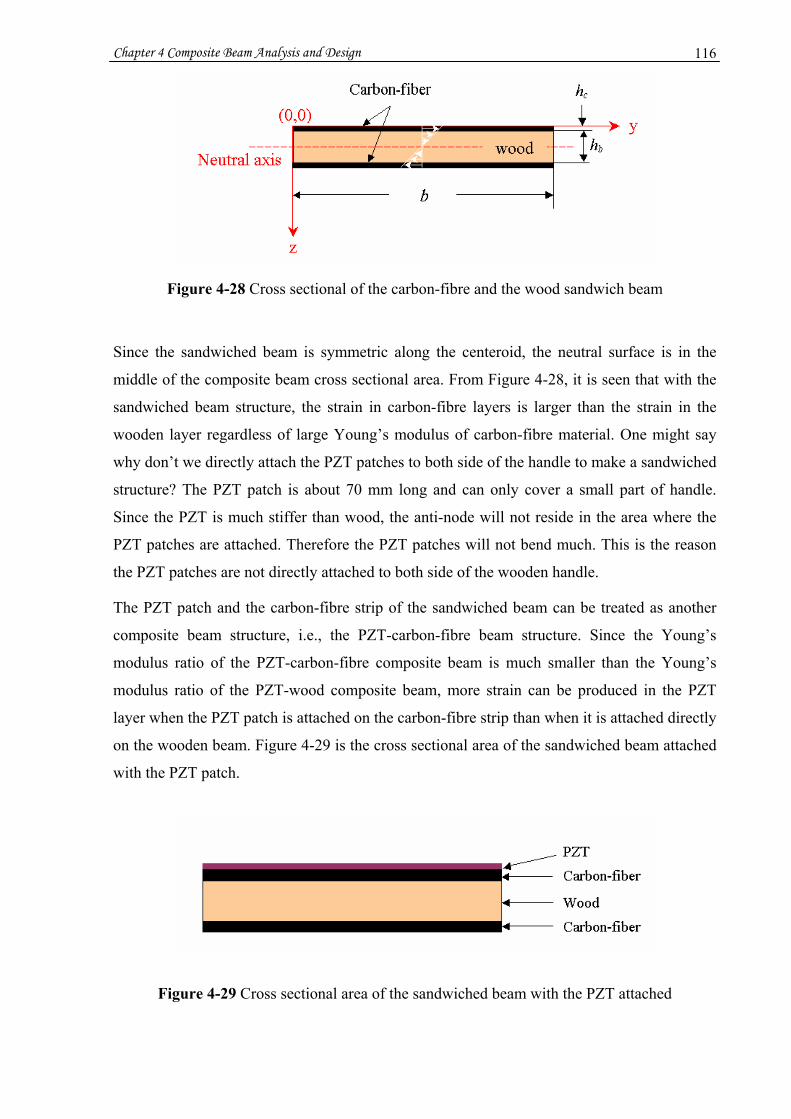
Chapter 4 Composite Beam Analysis and Design 116
Figure 4-28 Cross sectional of the carbon-fibre and the wood sandwich beam
Since the sandwiched beam is symmetric along the centeroid, the neutral surface is in the
middle of the composite beam cross sectional area. From Figure 4-28, it is seen that with the
sandwiched beam structure, the strain in carbon-fibre layers is larger than the strain in the
wooden layer regardless of large Young’s modulus of carbon-fibre material. One might say
why don’t we directly attach the PZT patches to both side of the handle to make a sandwiched
structure? The PZT patch is about 70 mm long and can only cover a small part of handle.
Since the PZT is much stiffer than wood, the anti-node will not reside in the area where the
PZT patches are attached. Therefore the PZT patches will not bend much. This is the reason
the PZT patches are not directly attached to both side of the wooden handle.
The PZT patch and the carbon-fibre strip of the sandwiched beam can be treated as another
composite beam structure, i.e., the PZT-carbon-fibre beam structure. Since the Young’s
modulus ratio of the PZT-carbon-fibre composite beam is much smaller than the Young’s
modulus ratio of the PZT-wood composite beam, more strain can be produced in the PZT
layer when the PZT patch is attached on the carbon-fibre strip than when it is attached directly
on the wooden beam. Figure 4-29 is the cross sectional area of the sandwiched beam attached
with the PZT patch.
Figure 4-29 Cross sectional area of the sandwiched beam with the PZT attached

Chapter 4 Composite Beam Analysis and Design 117
If the carbon-fibre strip is made much stiffer and thicker than the PZT patch, the structure
alternation of the sandwiched beam due to the PZT patch attached can be neglected. Besides,
for the PZT-carbon-fibre composite beam structure, a softer and thinner PZT patch can result
in more strain in the PZT layer than that in the carbon-fibre beam layer. In order to maximize
the strain in the PZT layer, the analysis above as shown in Figure 4-12 will dictate the
following for maximizing the strain in the PZT patch for a given young’s modulus ratio:
1) Small Young’s modulus ratio between the PZT patch and carbon-fibre strip, which
means the carbon-fibre strip should be made as stiff as possible.
2) Small thickness ratio between the PZT patch and the carbon-fibre strip, which means the
carbon-fibre strip should be made thicker than the PZT patch unless their Young’s
modulus ratio is extremely small (in the case of soft PZT being used).
Practically, if the carbon-fibre strip is made too stiff, the anti-nodes of the Cricket bat,
especially that of first mode, will not be present in the handle but in the blade area, which
means that the Cricket bat handle will barely bend. This will reduce the strain in the PZT
patch since the PZT patch is only allowed to be placed in the handle area. This is the reason
why it is preferred to use the variable stiffness carbon-fibre strips to control the anti-node
positions. There is a compromise between stiffening the carbon-fibre strip and positioning the
first anti-node within the handle area. On the other hand, if the carbon-fibre strip is made too
thick, it will also shift the first anti-node out of the bat handle. So the design should be made
accordingly.
4.3.6 Other benefits of using carbon-fibre material in the Cricket bat
The benefit of using carbon-fibre strips in the Cricket bat handle mentioned in the last section
is that it can increase the normal strain in the PZT patch. Another benefit of using the carbon-
fibre material is that the carbon-fibre material can help to increase the natural frequencies of
the Cricket bats, as a result of increasing the stiffness of the bat handle. Structural vibration is
caused by the excitation force that contains frequency components matching the natural
frequencies of the structure. When the carbon-fibre strips are stiff enough, the stiffness of the
bat handle will be determined mainly by the carbon-fibre strips. The influence of the wooden
material in the bat handle can almost be neglected. High frequency vibration usually feels
more comfortable than low frequency vibration and is also easier for the materials to absorb.
In terms of shunt circuit technology, high vibration frequency is easier to use than a large
inductor which should be avoided.

Chapter 4 Composite Beam Analysis and Design 118
Last but not least is that it can help to shift some natural frequencies from the inside of
excitation frequency to the outside of excitation frequency and reduce the excitation energy at
natural frequencies of the Cricket bat. When a batsman hits a ball, the ball-bat collision
produces an excitation impulse of force. The bat vibration is the impulse response of the
excitation impulse. The frequency range of the excitation impulse is related to the ball-bat
contact time and is in inverse proportion to the contact time. The contact time of an ideal
impulse is zero corresponding to infinity frequency range. However, in reality the contact
time is nonzero, is about 1 millisecond (Grant, C. 1998). The frequency range of the
excitation impulse therefore is about 1 kHz.
Figure 4-30 shows an impulse with width 1=wT millisecond and the corresponding power
spectrum. The power spectrum is the square of the Fourier transform of the impulse. The first
zero crossing frequency of the spectrum is 1/1 == wc Tf kHz. The narrower the impulse is, the
larger the cf will be.
It is seen that the magnitude of the power spectrum declines when frequency increases in the
first lobe (within 1 kHz range). This means the energy of the impulse is lower for higher
frequency components. The excitation energy of impulse signals mainly resides in the first
lobe. Considering the Cricket bat as a linear system, lower excitation energy certainly causes
smaller vibration response. When the energy of the frequency components is lower than a
certain threshold, the vibration response caused by these frequency components can be
neglected. One can set a threshold, such as 1/3 of maximum energy, for a structure. The
frequency at this threshold is defined as an excitation frequency. The vibration outside the
excitation frequency can be neglected. So the vibration of the Cricket bat caused by the
natural frequencies outside the excitation frequency can be neglected. Lifting up the natural
frequencies can firstly, shift some natural frequencies from the inside of the excitation
frequency to the outside of the excitation frequency, and secondly, relatively reduce the
excitation energy at the natural frequencies, and therefore ease the vibration response.

Chapter 4 Composite Beam Analysis and Design 119
Figure 4-30 Impulse signal and its corresponding power spectrum
4.4 Chapter summary
In this chapter, strain distribution in the composite beams has been analyzed in detail. The
average strain in each layer is decided by the physical size of the layers as well as the
Young’s modulus of materials used. This is a result of the neutral surface location of the
composite beams which plays an important role in the strain distribution. If the neutral surface
is close to the centeroid of a layer, the average strain of the layer will be reduced. In order to
allocate more strain in a preferred layer, the composite beam should be designed to bring the
neutral surface away from this layer. Simulations with different thickness ratio and Young’s
modulus ratio of a two-layer composite beam have been conducted. The simulation results
help us to understand why the FEA simulation and experimental results of the passive
piezoelectric vibration shunt control all showed that the vibration control for the aluminium or
carbon-fibre beam is more effective than that for the wooden beam. The analysis provides an
analytical tool for applying the passive piezoelectric vibration shunt control method to multi-
material- based substrate structures. The FEA simulations and experimental results of
piezoelectric vibration shunt control for the aluminium, wooden and carbon-fibre beams are
presented. Carbon-fibre materials and the layer structure are briefly introduced.

Chapter 4 Composite Beam Analysis and Design 120
Finally, the design of the Cricket bat handle has been proposed in order to maximize the
removal of vibration energy from the Cricket bat handle with the passive piezoelectric
vibration shunt control method and the benefits of using carbon-fibre strips in the Cricket bat
handle are also described. Other advantages of the inherent increase in the natural frequency
of the structure when using carbon-fibre strips are presented. This is argued from the
drastically reduced power spectrum characteristics for frequencies above a threshold value.

Chapter 5 Numerical Modeling of Passive Piezoelectric Vibration Control using FEA Software ANSYS® 121
Chapter 5
Numerical Modelling of
Passive Piezoelectric Vibration
Control using the FEA Software ANSYS®
In previous chapters, analytical modelling and analysis of the structure and vibration control
have been conducted. However, the mathematical equations of accurate analytical models of
complex geometry structures are usually very difficult to be solved. Instead of solving a
complex structure as a whole, numerical methods based on the idea of dividing the complex
structure into many simply shaped portions are often used to approximate the accurate model.
The small portions are solved individually and then combined. Finite element analysis (FEA)
is one of the major numerical solutions. With today’s powerful computer capabilities and
sophisticated algorithms, most engineering problems can be solved accurately with the FEA
method. There are many commercially available FEA software packages, such as ANSYS®
(General purpose on PC and workstations), NASTRAN® (General purpose on mainframes),
ABAQUS® (Non-linear and dynamic analyses), PATRAN® (Pre/Post processor), etc.
Efficient vibration control involves obtaining the optimum geometry size, material property of
a structure and the effective placement of the piezoelectric transducer. The piezoelectric
materials are quite expensive at the moment and are not reusable after being bonded to an
object. Therefore, it will be quite costly in both time and resources rely purely on experiment.
A computer simulation method of the passive piezoelectric vibration shunt control with
ANSYS® has been developed. It is a useful alternative to an experimental approach. The
method can help us to analyze, design and optimize the structure and control system prior to
actual physical experimentation and implementation. It has many advantages, such as
flexibility, re-programmability, time and cost efficiency.
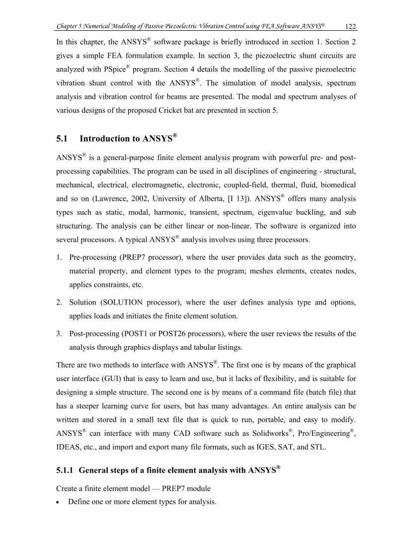
Chapter 5 Numerical Modeling of Passive Piezoelectric Vibration Control using FEA Software ANSYS® 122
In this chapter, the ANSYS® software package is briefly introduced in section 1. Section 2
gives a simple FEA formulation example. In section 3, the piezoelectric shunt circuits are
analyzed with PSpice® program. Section 4 details the modelling of the passive piezoelectric
vibration shunt control with the ANSYS®. The simulation of model analysis, spectrum
analysis and vibration control for beams are presented. The modal and spectrum analyses of
various designs of the proposed Cricket bat are presented in section 5.
5.1 Introduction to ANSYS®
ANSYS® is a general-purpose finite element analysis program with powerful pre- and post-
processing capabilities. The program can be used in all disciplines of engineering - structural,
mechanical, electrical, electromagnetic, electronic, coupled-field, thermal, fluid, biomedical
and so on (Lawrence, 2002, University of Alberta, [I 13]). ANSYS® offers many analysis
types such as static, modal, harmonic, transient, spectrum, eigenvalue buckling, and sub
structuring. The analysis can be either linear or non-linear. The software is organized into
several processors. A typical ANSYS® analysis involves using three processors.
1. Pre-processing (PREP7 processor), where the user provides data such as the geometry,
material property, and element types to the program; meshes elements, creates nodes,
applies constraints, etc.
2. Solution (SOLUTION processor), where the user defines analysis type and options,
applies loads and initiates the finite element solution.
3. Post-processing (POST1 or POST26 processors), where the user reviews the results of the
analysis through graphics displays and tabular listings.
There are two methods to interface with ANSYS®. The first one is by means of the graphical
user interface (GUI) that is easy to learn and use, but it lacks of flexibility, and is suitable for
designing a simple structure. The second one is by means of a command file (batch file) that
has a steeper learning curve for users, but has many advantages. An entire analysis can be
written and stored in a small text file that is quick to run, portable, and easy to modify.
ANSYS® can interface with many CAD software such as Solidworks®, Pro/Engineering®,
IDEAS, etc., and import and export many file formats, such as IGES, SAT, and STL.
5.1.1 General steps of a finite element analysis with ANSYS®
Create a finite element model — PREP7 module
• Define one or more element types for analysis.

Chapter 5 Numerical Modeling of Passive Piezoelectric Vibration Control using FEA Software ANSYS® 123
• Assign appropriate physical properties to each type.
• Define one or more sets of materials used in the model.
• Define mass distribution for dynamic analysis
• Create geometry
• Mesh elements
• Apply loads and boundary conditions
Solution — SOLUTION module
• Choose appropriate analysis type and solution algorithm
• Initiate solution
Post-processing — POST1 and POST26 modules
• View results
• Export results
5.1.2 Some elements used for implementation
There are hundreds of elements in the element library of ANSYS®. They are categorized as
being LINK, BEAM, PLANE, SHELL, SOLID, MASS, VISCO, CONTACT, FLUID,
CIRCU elements and so on, which can be either one-dimensional, two-dimensional or three-
dimensional elements.
In general, four characteristic element shapes are possible: point, line, area or volume. A point
element is typically defined by one node, e.g., a mass element. A line element is typically
represented by a line or arc connecting two or three nodes. Examples are beams, spars, pipes
and axisymmetric shells. An area element has a triangular or quadrilateral shape and may be a
2-D solid element or a shell element. A volume element has a tetrahedral or brick shape and is
usually a 3-D solid element.
The degrees of freedom of the element determine the discipline for which the element is
applicable: structural, thermal, fluid, electric, magnetic or coupled-field. In the piezoelectric
vibration shunt control, 3-D structural, 3-D coupled-field and 2-D electric elements are used.
They are briefly summarized below. Details can be found in the ANSYS® Element Reference.
SOLID45 — SOLID45 is used for three-dimensional modelling of solid structures such as
beams. The element is defined by eight nodes having three degrees of freedom at each node:
translations in the nodal x, y, and z directions, and orthotropic material properties. The
element has plasticity, creep, swelling, stress stiffening, large deflection, and large strain
capabilities. The geometry, node locations and the coordinate system for this element are
shown in Figure 5-1 (ANSYS 6.1 Documentation, [I 3]).
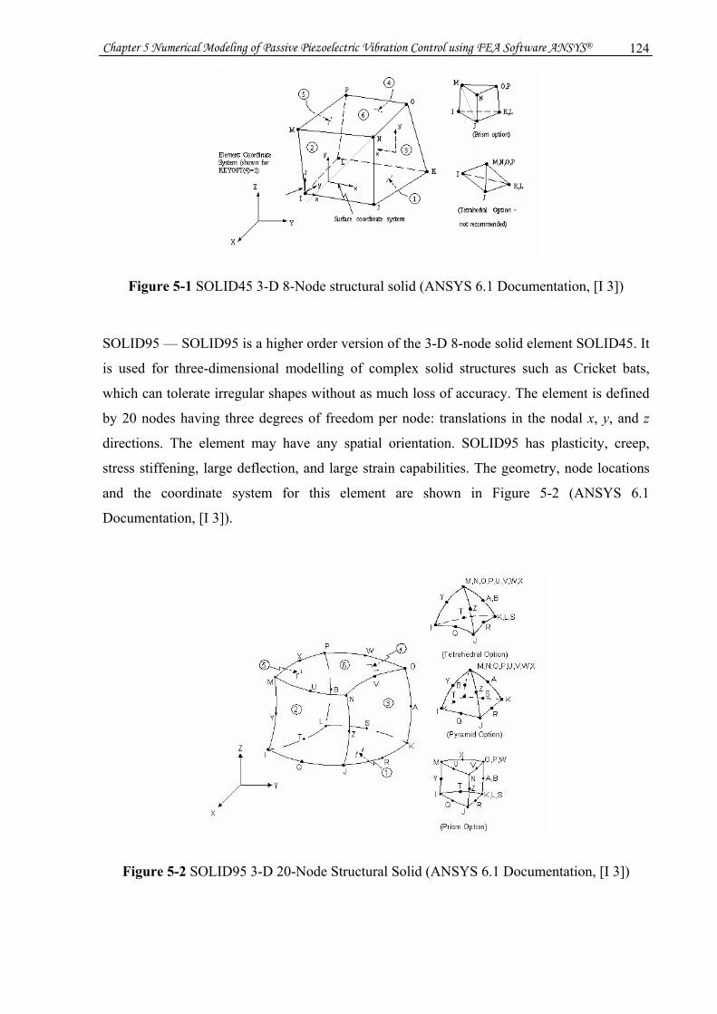
Chapter 5 Numerical Modeling of Passive Piezoelectric Vibration Control using FEA Software ANSYS® 124
Figure 5-1 SOLID45 3-D 8-Node structural solid (ANSYS 6.1 Documentation, [I 3])
SOLID95 — SOLID95 is a higher order version of the 3-D 8-node solid element SOLID45. It
is used for three-dimensional modelling of complex solid structures such as Cricket bats,
which can tolerate irregular shapes without as much loss of accuracy. The element is defined
by 20 nodes having three degrees of freedom per node: translations in the nodal x, y, and z
directions. The element may have any spatial orientation. SOLID95 has plasticity, creep,
stress stiffening, large deflection, and large strain capabilities. The geometry, node locations
and the coordinate system for this element are shown in Figure 5-2 (ANSYS 6.1
Documentation, [I 3]).
Figure 5-2 SOLID95 3-D 20-Node Structural Solid (ANSYS 6.1 Documentation, [I 3])

Chapter 5 Numerical Modeling of Passive Piezoelectric Vibration Control using FEA Software ANSYS® 125
SOLID5 — SOLID5 has a three-dimensional magnetic, thermal, electric, piezoelectric and
structural field capability with limited coupling between the fields. The element has eight
nodes with up to six degrees of freedom at each node. Various combinations of nodal loading
are available for this element depending upon the KEYOPT(1) value used for the degree of
freedom selected. KEYOPT (or key option) is a switch, used to turn various element options
on or off.
UX, UY, UZ, TEMP, VOLT, MAG if KEYOPT (1) = 0
TEMP, VOLT, MAG if KEYOPT (1) = 1
UX, UY, UZ if KEYOPT (1) = 2
TEMP if KEYOPT (1) = 8
VOLT if KEYOPT (1) = 9
MAG if KEYOPT (1) = 10
The geometry, node locations, and the coordinate system for this element are shown in Figure
5-3.
Figure 5-3 SOLID5 3-D coupled-field solid (ANSYS 6.1 Documentation, [I 3])
CIRCU94 — CIRCU94 is a piezoelectric circuit element and simulates basic linear electric
circuit components that can be directly connected to the piezoelectric FEA domain (through
interfacing with SOLID5, SOLID98, or PLANE13 coupled-field elements). The element has
two or three nodes to define the circuit component and one or two degrees of freedom to
model the circuit response. It is applicable to full harmonic and transient analyses. The
element model and circuit options, indicating node locations and degrees of freedom are
shown in Figure 5-4.
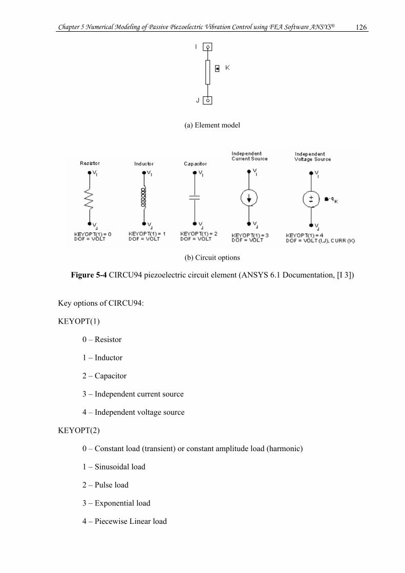
Chapter 5 Numerical Modeling of Passive Piezoelectric Vibration Control using FEA Software ANSYS® 126
(a) Element model
(b) Circuit options
Figure 5-4 CIRCU94 piezoelectric circuit element (ANSYS 6.1 Documentation, [I 3])
Key options of CIRCU94:
KEYOPT(1)
0 – Resistor
1 – Inductor
2 – Capacitor
3 – Independent current source
4 – Independent voltage source
KEYOPT(2)
0 – Constant load (transient) or constant amplitude load (harmonic)
1 – Sinusoidal load
2 – Pulse load
3 – Exponential load
4 – Piecewise Linear load
Chapter 5 Numerical Modeling of Passive Piezoelectric Vibration Control using FEA Software ANSYS® 127
For example,
ET, 1, CIRCU94, 0, 0 ! Set up element 1 as a resistor (Constant)
ET, 2, CIRCU94, 1, 0 ! Set up element 2 as a inductor (Constant)
ET, 3, CIRCU94, 2, 0 ! Set up element 3 as capacitor (Constant)
ET, 4, CIRCU94, 3, 1 ! Set up element 4 as independent current source (Sinusoid)
ET, 5, CIRCU94, 4, 2 ! Set up element 5 as independent voltage source (Pulse)
5.1.3 Coupled-field analysis
The implementation of the piezoelectric vibration shunt control being made possible in the
ANSYS® is thanks to the coupled-field capability of the software. The Coupled-field analysis
is an analysis that takes into account the interaction (coupling) between two or more
disciplines (fields) of engineering. A piezoelectric analysis, for example, handles the
interaction between the structural and electric fields: it solves for the voltage distribution due
to applied displacements, or vice versa.
5.2 A Simple example of the finite element formulation
Finite element analysis is to discretize an object of arbitrary geometry into many
interconnected small regular shape elements. The matrices of mass, stiffness of these small
elements are then superimposed to approximate the characteristics of the whole object. In this
section, a simple example of finite element formulation for the Euler-Bernoulli beam is
illustrated to give some insight of the FEA.
The Euler-Bernoulli beam motion equation of vibration under pure bending is
)(),(),(2
2
4
4
xpt
txwx
txwEI =∂
∂+
∂∂ ρ . (5.1)
where
),( txw is the transverse displacement of the beam, ρ is the mass density per unit
length, EI is the beam flexural rigidity, and )(xp is the external applied force respectively.
For free vibration, 0)( =xp , according to the relations (Timoshenko, 1973),
0),()( 4
4
2
2
=∂
∂===
xtxwEI
dxMd
dxdQxp . (5.2)
where
Q and M denote the shear force and bending moment respectively.
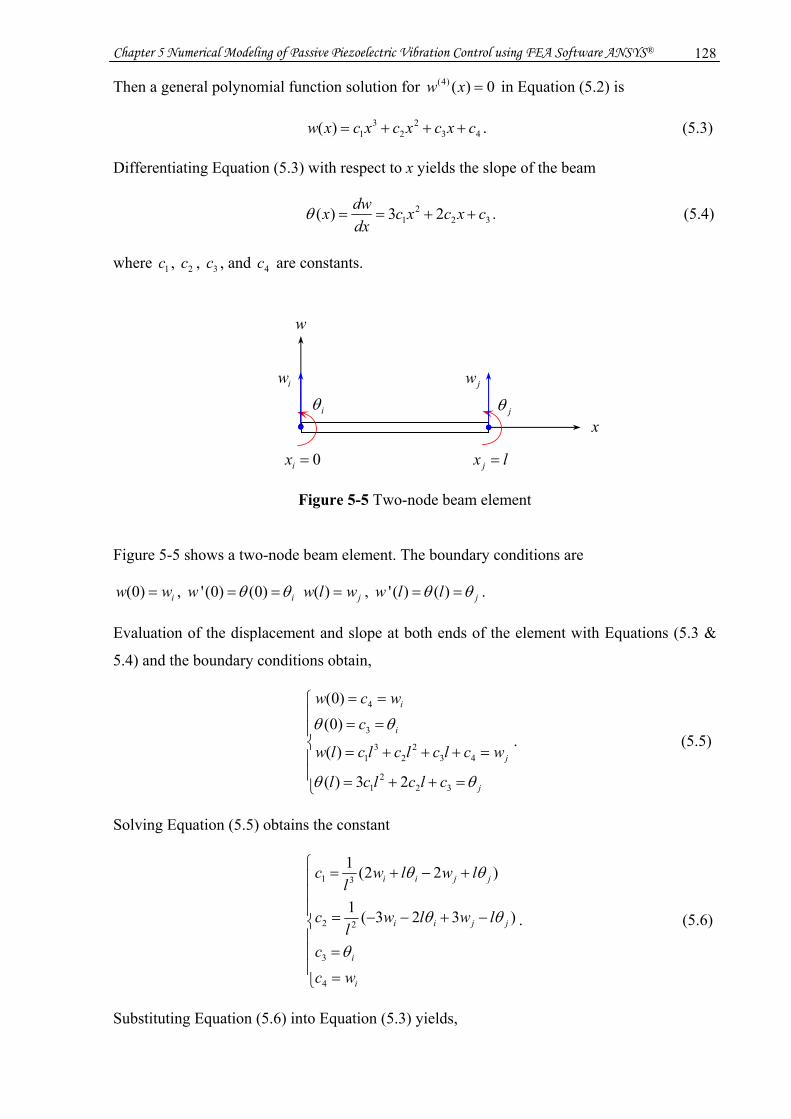
Chapter 5 Numerical Modeling of Passive Piezoelectric Vibration Control using FEA Software ANSYS® 128
Then a general polynomial function solution for 0)()4( =xw in Equation (5.2) is
432
23
1)( cxcxcxcxw +++= . (5.3)
Differentiating Equation (5.3) with respect to x yields the slope of the beam
322
1 23)( cxcxcdxdwx ++==θ . (5.4)
where 1c , 2c , 3c , and 4c are constants.
Figure 5-5 Two-node beam element
Figure 5-5 shows a two-node beam element. The boundary conditions are
iww =)0( , iw θθ == )0()0(' jwlw =)( , jllw θθ == )()(' .
Evaluation of the displacement and slope at both ends of the element with Equations (5.3 &
5.4) and the boundary conditions obtain,
⎪⎪
⎩
⎪⎪
⎨
⎧
=++=
=+++=
==
==
j
j
i
i
clclcl
wclclclclw
cwcw
θθ
θθ
322
1
432
23
1
3
4
23)(
)(
)0()0(
. (5.5)
Solving Equation (5.5) obtains the constant
⎪⎪⎪
⎩
⎪⎪⎪
⎨
⎧
=
=
−+−−=
+−+=
i
i
jjii
jjii
wcc
lwlwl
c
lwlwl
c
4
3
22
31
)323(1
)22(1
θ
θθ
θθ
. (5.6)
Substituting Equation (5.6) into Equation (5.3) yields,
iw jw
iθ jθx
0=ix lx j =
w
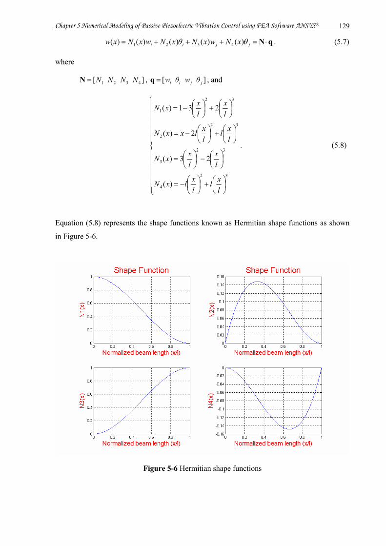
Chapter 5 Numerical Modeling of Passive Piezoelectric Vibration Control using FEA Software ANSYS® 129
qN ⋅=+++= jjii xNwxNxNwxNxw θθ )()()()()( 4321 . (5.7)
where
][ 4321 NNNN N = , ][ jjii θwθw q = , and
⎪⎪⎪⎪⎪⎪
⎩
⎪⎪⎪⎪⎪⎪
⎨
⎧
⎟⎠⎞
⎜⎝⎛+⎟
⎠⎞
⎜⎝⎛−=
⎟⎠⎞
⎜⎝⎛−⎟
⎠⎞
⎜⎝⎛=
⎟⎠⎞
⎜⎝⎛+⎟
⎠⎞
⎜⎝⎛−=
⎟⎠⎞
⎜⎝⎛+⎟
⎠⎞
⎜⎝⎛−=
32
4
32
3
32
2
32
1
)(
23)(
2)(
231)(
lxl
lxlxN
lx
lxxN
lxl
lxlxxN
lx
lxxN
. (5.8)
Equation (5.8) represents the shape functions known as Hermitian shape functions as shown
in Figure 5-6.
Figure 5-6 Hermitian shape functions

Chapter 5 Numerical Modeling of Passive Piezoelectric Vibration Control using FEA Software ANSYS® 130
The transverse deflection function including time t and spatial x is
)()()()()()()()()()(),( 4321 txtxNtwxNtxNtwxNtxw jjiiTqN ⋅=+++= θθ . (5.9)
where
)]()()()([ 4321 xNxNxNxN N = , )]()()( )([ tθtwtθtw jjii q = .
The kinetic energy of the beam is
qmq1qNNq TTT
2221
00
2
=⋅=⎟⎠⎞
⎜⎝⎛∂∂
= ∫∫ dxdxtwT
l
b
l
bb ρρ . (5.10)
where
dxl
b NNm T∫= 0ρ , q is the matrix of the differentiating of q with respect to time t.
Since
⎥⎥⎥⎥⎥
⎦
⎤
⎢⎢⎢⎢⎢
⎣
⎡
=⋅=
24434241
43233231
42322221
41312121
4321T
4321 ][][
NNNNNNNNNNNNNNNNNNNNNNNNNNNN
N N NN N N NNNNT ,
From Equation (5.8), the mass matrix can be obtained as
⎥⎥⎥⎥
⎦
⎤
⎢⎢⎢⎢
⎣
⎡
−−−−−−
== ∫22
22
0
422313221561354313422135422156
420llll
llllllll
ldx bl
bρρ NNm T , (5.11)
The strain energy of the beam can be expressed as
kqq1q'N')'(N'q TTT
2221
00
2
2
2
=⋅=⎟⎟⎠
⎞⎜⎜⎝
⎛∂∂
= ∫∫ dxEIdxxwEIU
ll
b . (5.12)
where
dxEIl
'N')'(N'k T∫= 0.
From Equation (5.8), one can have
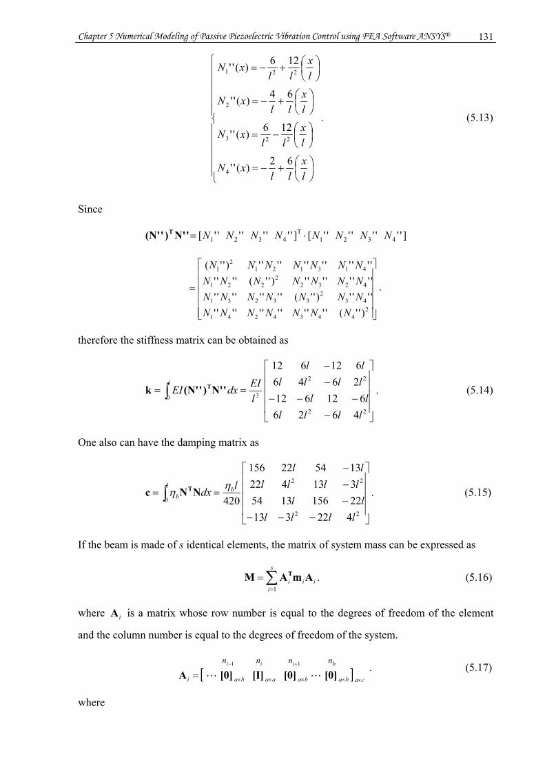
Chapter 5 Numerical Modeling of Passive Piezoelectric Vibration Control using FEA Software ANSYS® 131
⎪⎪⎪⎪⎪
⎩
⎪⎪⎪⎪⎪
⎨
⎧
⎟⎠⎞
⎜⎝⎛+−=
⎟⎠⎞
⎜⎝⎛−=
⎟⎠⎞
⎜⎝⎛+−=
⎟⎠⎞
⎜⎝⎛+−=
lx
llxN
lx
llxN
lx
llxN
lx
llxN
62)(''
126)(''
64)(''
126)(''
4
223
2
221
. (5.13)
Since
]''''''''[]''''''''[ 4321T
4321 N N NN N N NN ⋅='N')'(N' T
⎥⎥⎥⎥⎥
⎦
⎤
⎢⎢⎢⎢⎢
⎣
⎡
=
24434241
432
33231
42322
221
4131212
1
)''('''''''''''''''')''('''''''''''''''')''('''''''''''''''')''(
NNNNNNNNNNNNNNNNNNNNNNNNNNNN
.
therefore the stiffness matrix can be obtained as
⎥⎥⎥⎥
⎦
⎤
⎢⎢⎢⎢
⎣
⎡
−−−−
−−
== ∫22
22
30
4626612612
2646612612
llllll
llllll
lEIdxEI
l'N')'(N'k T . (5.14)
One also can have the damping matrix as
⎥⎥⎥⎥
⎦
⎤
⎢⎢⎢⎢
⎣
⎡
−−−−−−
== ∫22
22
0
422313221561354313422135422156
420llll
llllllll
ldx bl
bηη NNc T . (5.15)
If the beam is made of s identical elements, the matrix of system mass can be expressed as
ii
s
ii AmAM T∑
=
=1
. (5.16)
where iA is a matrix whose row number is equal to the degrees of freedom of the element
and the column number is equal to the degrees of freedom of the system.
[ ] cababaaabai
bnnnn iii
×××××=+−
[0] [0] [I] [0] A 11 . (5.17)
where

Chapter 5 Numerical Modeling of Passive Piezoelectric Vibration Control using FEA Software ANSYS® 132
a, b, and c represent the number of the degrees of freedom of the element, the number
of the nodes of the element, and the number of the degrees of freedom of the system
respectively; ba× 0][ is a zero matrix and aa× I][ is the unit matrix.
Figure 5-7 Two-element beam
For example, the beam is made of two elements as shown in Figure 5-7. Since the element has
two nodes (b = 2) and four degrees of freedom (a = 4). The system has three nodes and six
degrees of freedom (c = 6), the matrices of iA (i = 1, 2) are
⎥⎥⎥⎥
⎦
⎤
⎢⎢⎢⎢
⎣
⎡
=
001000000100000010000001
1A ,
⎥⎥⎥⎥
⎦
⎤
⎢⎢⎢⎢
⎣
⎡
=
100000010000001000000100
2A .
The matrix of the system mass is
222111
2
1AmAAmAAmAM TTT +==∑
=ii
ii .
where
⎥⎥⎥⎥
⎦
⎤
⎢⎢⎢⎢
⎣
⎡
−−−−−−
==
22
22
21
422313221561354313422135422156
420llll
llllllll
lbρmm .
Similarly, the matrix of the system stiffness is
ii
s
ii AkAK T∑
=
=1
, (5.18)
and the matrix of the system damping is
ii
s
ii AcAC T∑
=
=1
. (5.19)
For the two element beams
222111
2
1AkAAkAAkAK TTT +==∑
=ii
ii ,
E1 E2
1n 2n 3n

Chapter 5 Numerical Modeling of Passive Piezoelectric Vibration Control using FEA Software ANSYS® 133
and
222111
2
1AcAAcAAcAC TTT +==∑
=ii
ii .
where
⎥⎥⎥⎥
⎦
⎤
⎢⎢⎢⎢
⎣
⎡
−−−−
−−
==
22
22
321
4626612612
2646612612
llllll
llllll
lEIkk ,
⎥⎥⎥⎥
⎦
⎤
⎢⎢⎢⎢
⎣
⎡
−−−−−−
==
22
22
21
422313221561354313422135422156
420llll
llllllll
lbηcc .
The motion equation of free vibration of the beam is
0=++ KqqCqM . (5.20)
where T q )](),(),(),(),(),([ 332211 ttwttwttw θθθ= .
Solving Equation (5.20), the natural frequencies of the beam can be obtained. This is a simple
example of obtaining a system’s characteristics using the finite element method. Details can
be found in books of the finite element analysis (Lepi, 1998 and Pilkey et al, 2000, etc.).
5.3 Modelling of passive piezoelectric shunt circuit with PSpice®
5.3.1 Single mode resistor-inductor shunt (R-L shunt)
Resistor-inductor piezoelectric vibration shunt is to control single vibration frequency. A
resistor-inductor branch is connected either in series or parallel across the electrodes of PZT.
(a) Series R-L shunt (b) Parallel R-L shunt
Figure 5-8 PSpice® model of single mode series resistor-inductor piezoelectric shunt

Chapter 5 Numerical Modeling of Passive Piezoelectric Vibration Control using FEA Software ANSYS® 134
For the series R-L shunt circuit in (a), the transfer function is:
222 2
211)(
n
pp
sss
LCs
LRs
LRs
RsLsC
RsHωσ
σ++
=++
=++
= . (5.21)
22 22)(
njjjH
ωσωωσωω
++−= . (5.22)
When
0=ω , 0)( =ωjH , nωω = , 1)( =ωjH , and ∞→ω , 0)( =ωjH .
The impulse response of Equation (5.21) is,
)()sin()cos(2)( tUettth td
dd
⋅−⋅⎥⎦
⎤⎢⎣
⎡−= σωωσωσ . (5.23)
where
222,12
σωωωσ −=== ndp
n LCLR , ,
00
10
)( t t
tU><
⎩⎨⎧
= is the step function.
For the parallel shunt in (b), the transfer function is:
22
2
2
2
21111
11
111
)(n
ppp
sss
LCs
RCs
s
sLRsC
sLRsHωσ ++
=++
=
++
+= . (5.24)
22
2
2)(
njjH
ωσωωωω
++−−
= . (5.25)
When
0=ω , 0)( =ωjH , nωω = , σωω2
)( njH = , and ∞→ω , 1)( =ωjH .
The impulse response of Equation (5.24) is,
)()sin()cos(2)()(22
tUetttth td
d
dd
⋅−⋅⎥⎦
⎤⎢⎣
⎡⋅
−+−= σω
ωσωωσδ . (5.26)
where
222,12
1 σωωωσ −=== ndp
np LCRC
, .
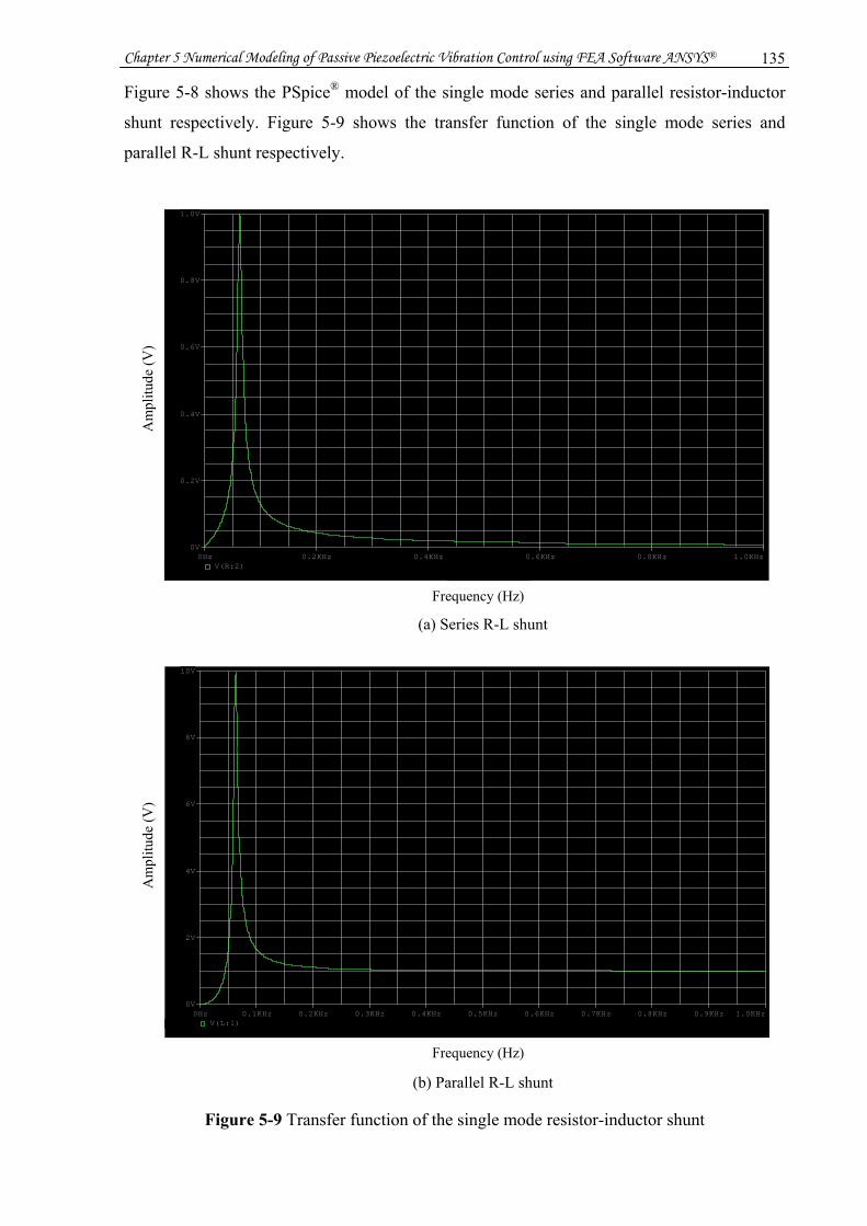
Chapter 5 Numerical Modeling of Passive Piezoelectric Vibration Control using FEA Software ANSYS® 135
Figure 5-8 shows the PSpice® model of the single mode series and parallel resistor-inductor
shunt respectively. Figure 5-9 shows the transfer function of the single mode series and
parallel R-L shunt respectively.
(a) Series R-L shunt
(b) Parallel R-L shunt
Figure 5-9 Transfer function of the single mode resistor-inductor shunt
Am
plitu
de (V
)
Frequency
0Hz 0.2KHz 0.4KHz 0.6KHz 0.8KHz 1.0KHzV(R:2)
0V
0.2V
0.4V
0.6V
0.8V
1.0V
Frequency (Hz)
Am
plitu
de (V
)
Frequency
0Hz 0.1KHz 0.2KHz 0.3KHz 0.4KHz 0.5KHz 0.6KHz 0.7KHz 0.8KHz 0.9KHz 1.0KHzV(L:1)
0V
2V
4V
6V
8V
10V
Frequency (Hz)

Chapter 5 Numerical Modeling of Passive Piezoelectric Vibration Control using FEA Software ANSYS® 136
One can see that the R-L shunt has narrow band characteristics. They act as a bandpass filter.
The resonant frequency of the filter is determined by
pc LC
fπ2
1= .
5.3.2 Multi-mode parallel resistor-inductor shunt
Practically however, there are often more than one vibration modes that need to be controlled
simultaneously. In order to control the multi-frequency vibration with a single piezoelectric
patch, requires designing an analogue filter-bank. The resonant frequencies of the filter-bank
match the natural frequencies of the structure to be controlled. Each frequency is aimed at
suppressing one structural vibration mode with the others simultaneously. Fleming et al
(2003) proposed multiple parallel single mode shunt circuits in series using single PZT. Each
parallel single mode shunt circuit also had a “blocking” circuit in parallel (Fleming et al,
2003). Figure 5-10 shows the concept. The switch in the circuit acts as the “blocking” circuit.
If all the switches are “Close” except one, the circuit becomes a single mode parallel R-L
shunt circuit.
Figure 5-10 Multiple parallel single mode shunt circuits in series with “blocking” switch
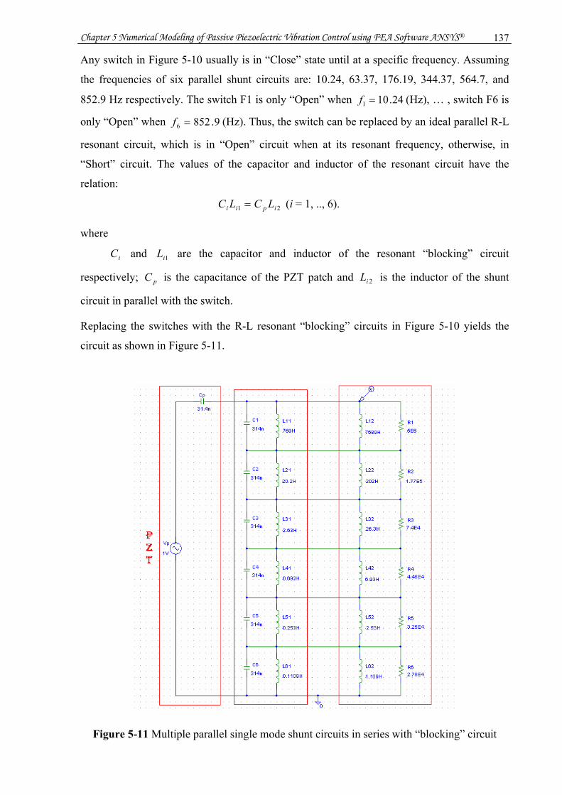
Chapter 5 Numerical Modeling of Passive Piezoelectric Vibration Control using FEA Software ANSYS® 137
Any switch in Figure 5-10 usually is in “Close” state until at a specific frequency. Assuming
the frequencies of six parallel shunt circuits are: 10.24, 63.37, 176.19, 344.37, 564.7, and
852.9 Hz respectively. The switch F1 is only “Open” when 24.101 =f (Hz), … , switch F6 is
only “Open” when 9.8526 =f (Hz). Thus, the switch can be replaced by an ideal parallel R-L
resonant circuit, which is in “Open” circuit when at its resonant frequency, otherwise, in
“Short” circuit. The values of the capacitor and inductor of the resonant circuit have the
relation:
21 ipii LCLC = (i = 1, .., 6).
where
iC and 1iL are the capacitor and inductor of the resonant “blocking” circuit
respectively; pC is the capacitance of the PZT patch and 2iL is the inductor of the shunt
circuit in parallel with the switch.
Replacing the switches with the R-L resonant “blocking” circuits in Figure 5-10 yields the
circuit as shown in Figure 5-11.
Figure 5-11 Multiple parallel single mode shunt circuits in series with “blocking” circuit
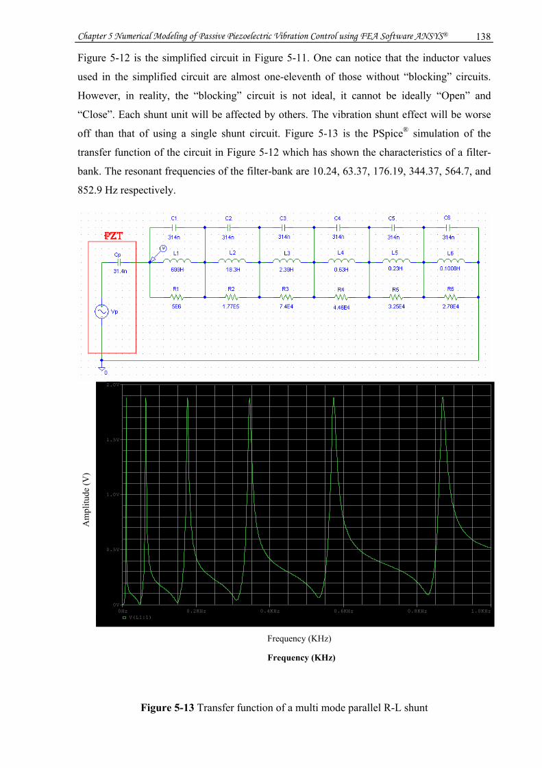
Chapter 5 Numerical Modeling of Passive Piezoelectric Vibration Control using FEA Software ANSYS® 138
Figure 5-12 is the simplified circuit in Figure 5-11. One can notice that the inductor values
used in the simplified circuit are almost one-eleventh of those without “blocking” circuits.
However, in reality, the “blocking” circuit is not ideal, it cannot be ideally “Open” and
“Close”. Each shunt unit will be affected by others. The vibration shunt effect will be worse
off than that of using a single shunt circuit. Figure 5-13 is the PSpice® simulation of the
transfer function of the circuit in Figure 5-12 which has shown the characteristics of a filter-
bank. The resonant frequencies of the filter-bank are 10.24, 63.37, 176.19, 344.37, 564.7, and
852.9 Hz respectively.
Figure 5-12 Equivalent circuit of multi-mode parallel shunt
Figure 5-13 Transfer function of a multi mode parallel R-L shunt
Frequency (KHz)
Am
plitu
de (V
)
Frequency
0Hz 0.2KHz 0.4KHz 0.6KHz 0.8KHz 1.0KHzV(L1:1)
0V
0.5V
1.0V
1.5V
2.0V
Frequency (KHz)

Chapter 5 Numerical Modeling of Passive Piezoelectric Vibration Control using FEA Software ANSYS® 139
5.4 Modelling of passive piezoelectric shunt circuit with ANSYS®
The subject used for ANSYS® modelling comprises a 0.5×0.025×0.003 m3 aluminium beam
with a 0.05×0.025×0.0005 m3 PZT patch attached. The boundary condition of the beam is
“clamped-free”. The PZT is attached at the clamped end. This analysis is linear elastic one
without considering internal damping. The element employed for modelling the aluminium
beam is a SOLID45, the 3-D structural solid element. The Young’s modulus for the beam is
66 GPa and the density is 2790 kg/m3. The element for modelling the piezoelectric transducer
is a SOLID5, the 3-D coupled field solid element. The density of the transducer is 7730
kg/m3. The element for modelling the shunt circuit components (resistor, capacitor and
inductor) is CIRCU94, the circuit element.
5.4.1 Single mode resistor-inductor shunt
Figure 5-14 shows the ANSYS® model of the single mode parallel R-L piezoelectric shunt for
a cantilever beam. The parallel R-L circuit is connected across the electrodes of PZT. The
inherent static capacitance of the PZT measured by the software is about 31.4 nF. The arrow
at the tip of the beam indicates where external force applied.
Figure 5-14 ANSYS® modelling of the parallel R-L piezoelectric shunt for beam
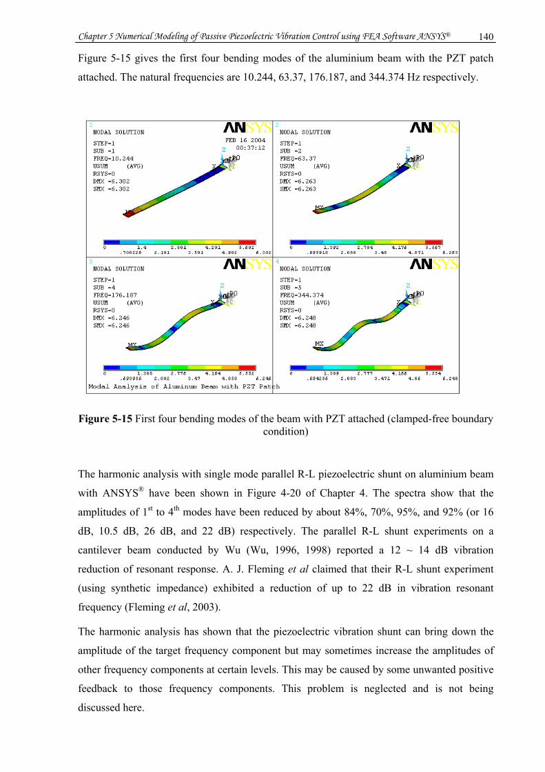
Chapter 5 Numerical Modeling of Passive Piezoelectric Vibration Control using FEA Software ANSYS® 140
Figure 5-15 gives the first four bending modes of the aluminium beam with the PZT patch
attached. The natural frequencies are 10.244, 63.37, 176.187, and 344.374 Hz respectively.
Figure 5-15 First four bending modes of the beam with PZT attached (clamped-free boundary condition)
The harmonic analysis with single mode parallel R-L piezoelectric shunt on aluminium beam
with ANSYS® have been shown in Figure 4-20 of Chapter 4. The spectra show that the
amplitudes of 1st to 4th modes have been reduced by about 84%, 70%, 95%, and 92% (or 16
dB, 10.5 dB, 26 dB, and 22 dB) respectively. The parallel R-L shunt experiments on a
cantilever beam conducted by Wu (Wu, 1996, 1998) reported a 12 ~ 14 dB vibration
reduction of resonant response. A. J. Fleming et al claimed that their R-L shunt experiment
(using synthetic impedance) exhibited a reduction of up to 22 dB in vibration resonant
frequency (Fleming et al, 2003).
The harmonic analysis has shown that the piezoelectric vibration shunt can bring down the
amplitude of the target frequency component but may sometimes increase the amplitudes of
other frequency components at certain levels. This may be caused by some unwanted positive
feedback to those frequency components. This problem is neglected and is not being
discussed here.

Chapter 5 Numerical Modeling of Passive Piezoelectric Vibration Control using FEA Software ANSYS® 141
5.4.2 Multi-mode parallel resistor-inductor shunt
Multi-mode vibration shunt uses a single PZT patch and an analogue filter-bank. The
ANSYS® modelling is shown in Figure 5-16. The model is the same as the single mode
except it has more electronic components in the shunt circuit, which is similar to the
equivalent circuit in Figure 5-14. It has four parallel R-L-C resonant circuits in series
designed for shunting the 1st to 4th vibration bending modes of the beam.
Figure 5-17 is the beam vibration spectrum after multi-mode shunting. Comparing with the
spectrum of Figure 4-20(a), the 1st to 4th modes were reduced by about 85%, 52%, 86%, and
77% (or 16.5 dB, 6.4 dB, 17 dB, and 12.8 dB) respectively. The experiment of multi-mode
shunt with a single PZT patch, by using a “current blocking” circuit in series with shunt
circuit, conducted by Wu had a vibration reduction from 7 dB to 15 dB (Wu, 1998). Similar
experiments carried out by A. J. Fleming et al by using “current blocking” circuit in parallel
with shunt circuit, had vibration reductions of up to18 dB (Fleming et al, 2003). The results
obtained from multi-mode shunt to particular frequency is about 3 ~ 6 dB worse than that
obtained from the single mode shunt.
Figure 5-16 ANSYS® modelling of the multi-mode piezoelectric shunt for beam (clamped-free boundary condition)

Chapter 5 Numerical Modeling of Passive Piezoelectric Vibration Control using FEA Software ANSYS® 142
Figure 5-17 Harmonic analysis of beam vibration with multi-mode piezoelectric shunt (clamped-free boundary condition)
5.4.3 Shunt effectiveness related to the placement of the PZT patch
The location of the PZT patch on the beam will significantly affect the effectiveness of the
vibration shunt. The PZT patch is best to be placed at the anti-node area where the beam has
the largest bending and strain to achieve optimum effectiveness of the vibration shunt. It can
be verified by the simulation below.
Figure 5-18 shows a PZT patch attached in the middle of an aluminium beam with free-free
boundary conditions. Figure 5-19 shows the first four bending modes of the beam. One can
see that the anti-node of the 1st and 3rd bending modes and the node of the 2nd and 4th bending
modes occur in the middle of the beam. Therefore, the 1st and 3rd bending modes have the
highest strain while the 2nd and 4th bending modes have the lowest strain in the PZT patch.

Chapter 5 Numerical Modeling of Passive Piezoelectric Vibration Control using FEA Software ANSYS® 143
Figure 5-18 Beam with PZT patch attached in the middle of the beam (free-free BC)
Figure 5-19 First four bending modes of the beam in Figure 5-16
We can predict that the vibration shunt control has high effectiveness to reduce the 1st and 3rd
vibration modes but has little effectiveness to reduce the 2nd and 4th vibration modes. This can
be verified by the harmonic analysis in Figure 5-20. The 1st mode in (b) and the 3rd mode in
(d) almost disappear, while the 2nd mode in (c) and 4th mode in (e) show almost no reduction
compared with the same components in (a).
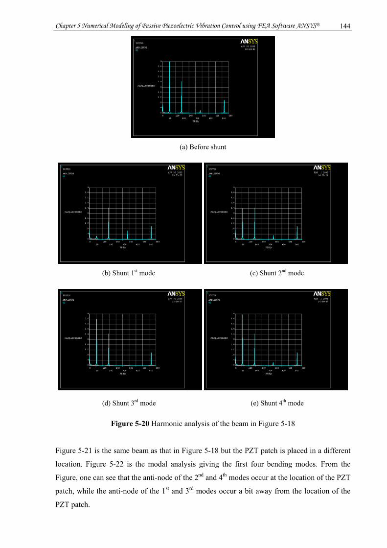
Chapter 5 Numerical Modeling of Passive Piezoelectric Vibration Control using FEA Software ANSYS® 144
(a) Before shunt
(b) Shunt 1st mode (c) Shunt 2nd mode
(d) Shunt 3rd mode (e) Shunt 4th mode
Figure 5-20 Harmonic analysis of the beam in Figure 5-18
Figure 5-21 is the same beam as that in Figure 5-18 but the PZT patch is placed in a different
location. Figure 5-22 is the modal analysis giving the first four bending modes. From the
Figure, one can see that the anti-node of the 2nd and 4th modes occur at the location of the PZT
patch, while the anti-node of the 1st and 3rd modes occur a bit away from the location of the
PZT patch.
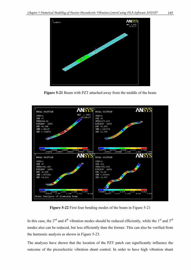
Chapter 5 Numerical Modeling of Passive Piezoelectric Vibration Control using FEA Software ANSYS® 145
Figure 5-21 Beam with PZT attached away from the middle of the beam
Figure 5-22 First four bending modes of the beam in Figure 5-21
In this case, the 2nd and 4th vibration modes should be reduced efficiently, while the 1st and 3rd
modes also can be reduced, but less efficiently than the former. This can also be verified from
the harmonic analysis as shown in Figure 5-23.
The analyses have shown that the location of the PZT patch can significantly influence the
outcome of the piezoelectric vibration shunt control. In order to have high vibration shunt

Chapter 5 Numerical Modeling of Passive Piezoelectric Vibration Control using FEA Software ANSYS® 146
efficiency, the PZT patch has to be placed at a high strain area. To properly identify or locate
the nodes and anti-nodes of the structure to be controlled and the area where strains occur is
critical in implementing the vibration control. The geometry sizes and material properties of
the structure and PZT patch have also influenced the effectiveness of the vibration shunt
control. The simulation results have already been demonstrated in Chapter 4.
(a) Before shunt
(b) Shunt 1st mode (c) Shunt 2nd mode
(d) Shunt 3rd mode (e) Shunt 4th mode
Figure 5-23 Harmonic analysis of the beam in Figure 5-21

Chapter 5 Numerical Modeling of Passive Piezoelectric Vibration Control using FEA Software ANSYS® 147
5.5 Modelling and analysis of the Cricket bat
The major change in the newly designed Cricket bat is the use of high stiffness to weight ratio
advanced fibre composites as part of the material variation to the handle. The purposes of this
include:
(a) To enhance the strain distribution in the PZT patch, and
(b) To increase the natural frequencies of the bat.
Cricket bats with different handle materials and geometry shapes have been modelled.
However, due to the limitation of computer capabilities (very significant memory capacity is
needed to perform piezoelectric vibration shunt control for a large object), vibration shunt
control for the Cricket bat has not been simulated. The simulations help to identify the anti-
nodes, strain of the Cricket bats to make sure that the PZT patch is placed at the high strain
area.
5.5.1 Cricket bat with a wooden handle
A Cricket bat model as shown in Figure 5-24 was constructed by using Solidworks®, CAD
software. The model then was imported into ANSYS®.
Figure 5-24 Cricket bat model built with Solidworks®
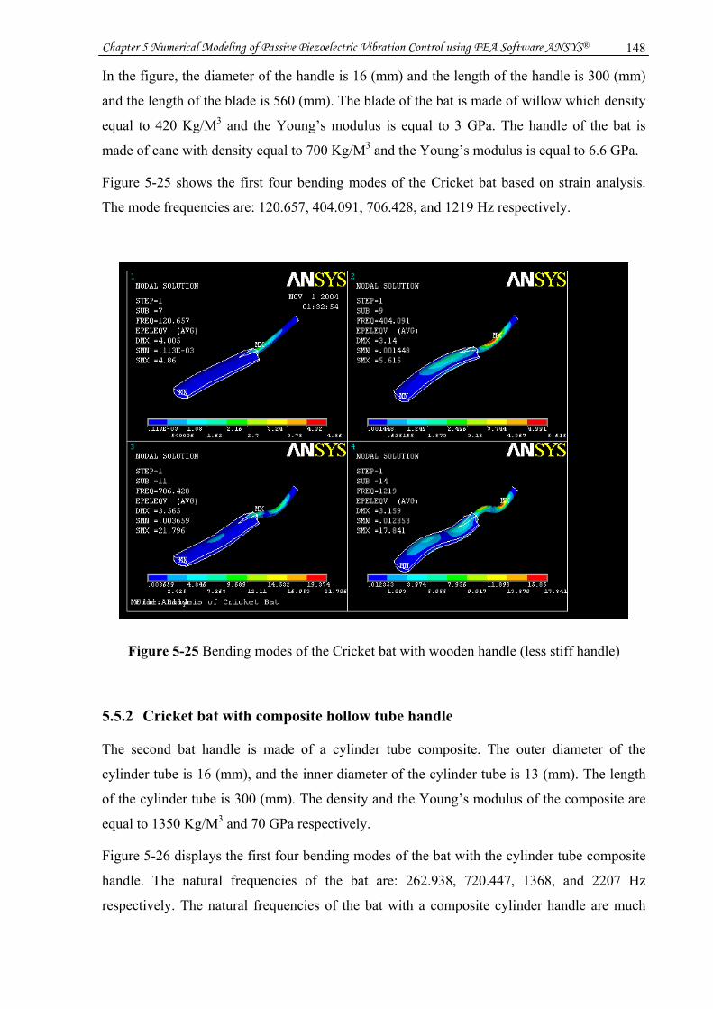
Chapter 5 Numerical Modeling of Passive Piezoelectric Vibration Control using FEA Software ANSYS® 148
In the figure, the diameter of the handle is 16 (mm) and the length of the handle is 300 (mm)
and the length of the blade is 560 (mm). The blade of the bat is made of willow which density
equal to 420 Kg/M3 and the Young’s modulus is equal to 3 GPa. The handle of the bat is
made of cane with density equal to 700 Kg/M3 and the Young’s modulus is equal to 6.6 GPa.
Figure 5-25 shows the first four bending modes of the Cricket bat based on strain analysis.
The mode frequencies are: 120.657, 404.091, 706.428, and 1219 Hz respectively.
Figure 5-25 Bending modes of the Cricket bat with wooden handle (less stiff handle)
5.5.2 Cricket bat with composite hollow tube handle
The second bat handle is made of a cylinder tube composite. The outer diameter of the
cylinder tube is 16 (mm), and the inner diameter of the cylinder tube is 13 (mm). The length
of the cylinder tube is 300 (mm). The density and the Young’s modulus of the composite are
equal to 1350 Kg/M3 and 70 GPa respectively.
Figure 5-26 displays the first four bending modes of the bat with the cylinder tube composite
handle. The natural frequencies of the bat are: 262.938, 720.447, 1368, and 2207 Hz
respectively. The natural frequencies of the bat with a composite cylinder handle are much

Chapter 5 Numerical Modeling of Passive Piezoelectric Vibration Control using FEA Software ANSYS® 149
higher than those of the bat with the wooden handle, almost doubled. These results were
verified by experiments which will be illustrated in Chapter 6.
However, comparing Figure 5-25 with Figure 5-26, one can notice that the strain distribution
is different between the two bats. For the wooden handle bat, the high strain resides in the
handle section. For the composite handle bat, the high strain shifts to the blade section,
especially for the first mode, there is little strain appearing at the joint area of blade and
handle (known as shoulder area). This is a result of increasing the handle stiffness.
Figure 5-26 Bending modes of the Cricket bat with hollow composite handle (stiffer handle)
PZT patch cannot be directly placed on the tube handle. In order to place the PZT patch on the
tube handle, a small segment is mounted on the handle, then the PZT patch is bonded on the
segment as shown in Figure 5-27. The segment adds stiffness to where it is placed. It reduces
bending in the area.
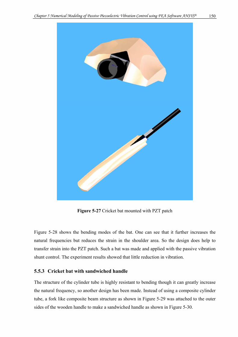
Chapter 5 Numerical Modeling of Passive Piezoelectric Vibration Control using FEA Software ANSYS® 150
Figure 5-27 Cricket bat mounted with PZT patch
Figure 5-28 shows the bending modes of the bat. One can see that it further increases the
natural frequencies but reduces the strain in the shoulder area. So the design does help to
transfer strain into the PZT patch. Such a bat was made and applied with the passive vibration
shunt control. The experiment results showed that little reduction in vibration.
5.5.3 Cricket bat with sandwiched handle
The structure of the cylinder tube is highly resistant to bending though it can greatly increase
the natural frequency, so another design has been made. Instead of using a composite cylinder
tube, a fork like composite beam structure as shown in Figure 5-29 was attached to the outer
sides of the wooden handle to make a sandwiched handle as shown in Figure 5-30.
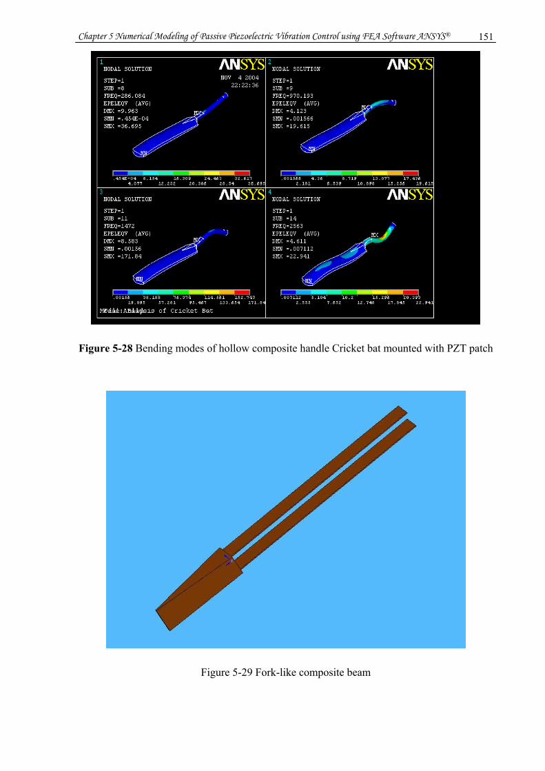
Chapter 5 Numerical Modeling of Passive Piezoelectric Vibration Control using FEA Software ANSYS® 151
Figure 5-28 Bending modes of hollow composite handle Cricket bat mounted with PZT patch
Figure 5-29 Fork-like composite beam

Chapter 5 Numerical Modeling of Passive Piezoelectric Vibration Control using FEA Software ANSYS® 152
Figure 5-30 Cricket bat with sandwiched handle
Figure 5-31 is the strain analysis of the Cricket bat with the sandwiched handle. It is seen that
this design can induce strain to occur at the shoulder while the natural frequencies of the bat
are increased.
In order to minimize the change in the appearance of the Cricket bat, the preferred model of
the Cricket bat handle should be that as shown in Figure 5-32. The composite beams are
embedded in the handle. The PZT patches are then bonded on the composite beams. It should
just feel like a normal Cricket bat when the batsman holds it. The strain analysis of the bat in
5-31 is shown in Figure 5-33.
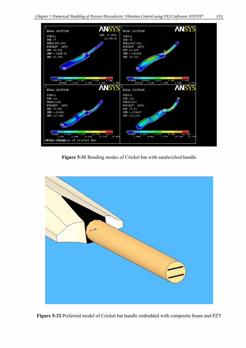
Chapter 5 Numerical Modeling of Passive Piezoelectric Vibration Control using FEA Software ANSYS® 153
Figure 5-31 Bending modes of Cricket bat with sandwiched handle
Figure 5-32 Preferred model of Cricket bat handle embedded with composite beam and PZT
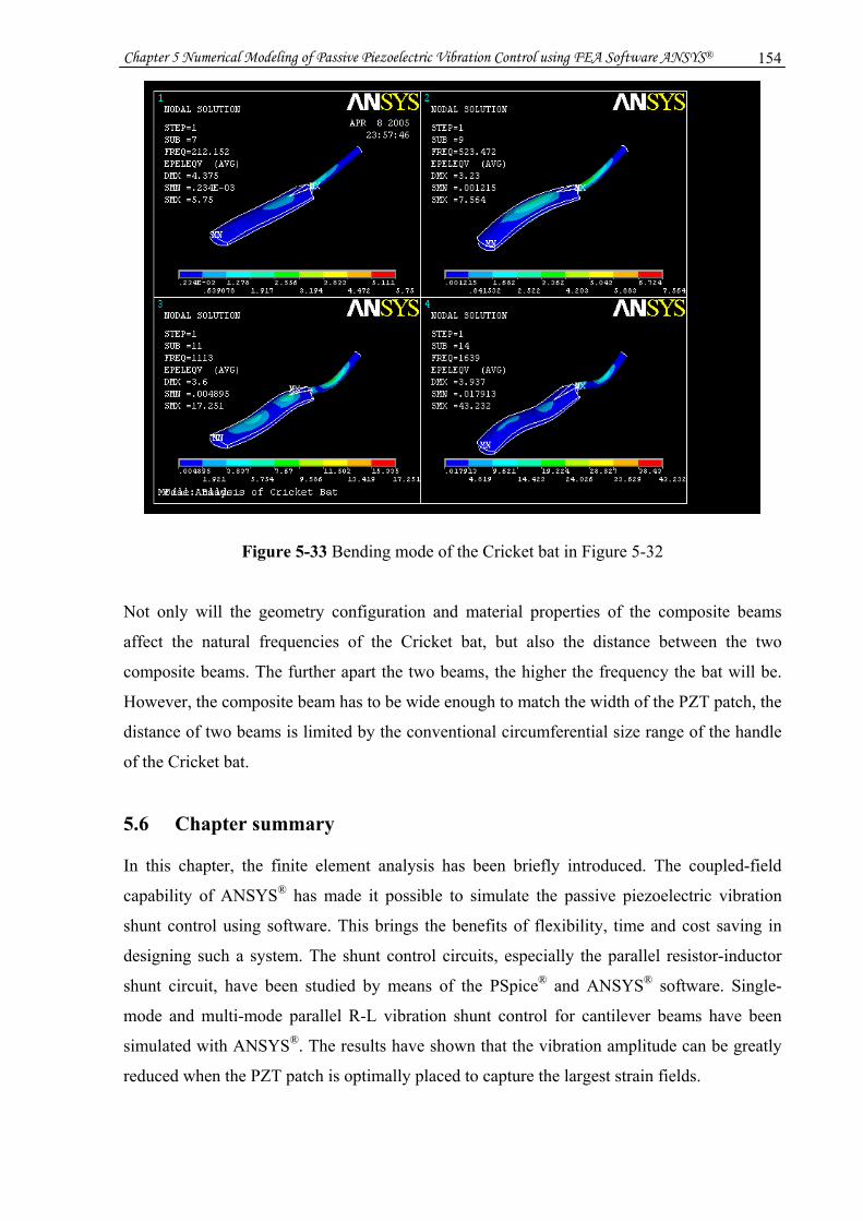
Chapter 5 Numerical Modeling of Passive Piezoelectric Vibration Control using FEA Software ANSYS® 154
Figure 5-33 Bending mode of the Cricket bat in Figure 5-32
Not only will the geometry configuration and material properties of the composite beams
affect the natural frequencies of the Cricket bat, but also the distance between the two
composite beams. The further apart the two beams, the higher the frequency the bat will be.
However, the composite beam has to be wide enough to match the width of the PZT patch, the
distance of two beams is limited by the conventional circumferential size range of the handle
of the Cricket bat.
5.6 Chapter summary
In this chapter, the finite element analysis has been briefly introduced. The coupled-field
capability of ANSYS® has made it possible to simulate the passive piezoelectric vibration
shunt control using software. This brings the benefits of flexibility, time and cost saving in
designing such a system. The shunt control circuits, especially the parallel resistor-inductor
shunt circuit, have been studied by means of the PSpice® and ANSYS® software. Single-
mode and multi-mode parallel R-L vibration shunt control for cantilever beams have been
simulated with ANSYS®. The results have shown that the vibration amplitude can be greatly
reduced when the PZT patch is optimally placed to capture the largest strain fields.

Chapter 5 Numerical Modeling of Passive Piezoelectric Vibration Control using FEA Software ANSYS® 155
Several Cricket bat designs were analyzed. A new Cricket bat model was proposed.
Unfortunately, the vibration shunt control for the Cricket bat was not preformed because of
the high computational demand due to the complex geometric configuration of the Cricket
bat. However, the structural analysis of the bat has enabled the identification of the nodes and
anti-nodes of (hence largest strain fields) for various modes of vibration. The ANSYS® code
of the passive piezoelectric vibration shunt for beams developed in this study can be applied
to many large objects including Cricket bats as long as the PC can handle a large amount of
elements to perform coupled-field analysis. Extensive simulations with various handle-blade
configurations were analysed in this study but due to the brevity requirements of the thesis,
not all the simulations have been reported in this thesis.
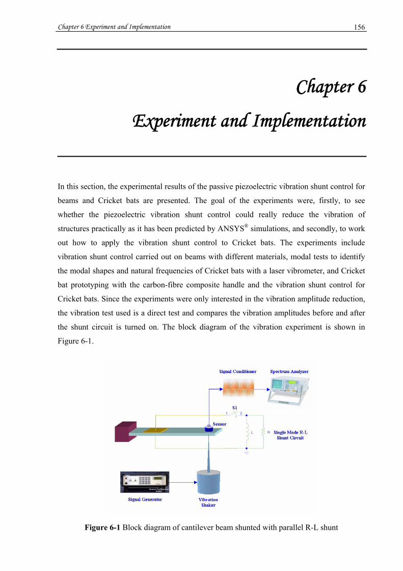
Chapter 6 Experiment and Implementation 156
Chapter 6
Experiment and Implementation
In this section, the experimental results of the passive piezoelectric vibration shunt control for
beams and Cricket bats are presented. The goal of the experiments were, firstly, to see
whether the piezoelectric vibration shunt control could really reduce the vibration of
structures practically as it has been predicted by ANSYS® simulations, and secondly, to work
out how to apply the vibration shunt control to Cricket bats. The experiments include
vibration shunt control carried out on beams with different materials, modal tests to identify
the modal shapes and natural frequencies of Cricket bats with a laser vibrometer, and Cricket
bat prototyping with the carbon-fibre composite handle and the vibration shunt control for
Cricket bats. Since the experiments were only interested in the vibration amplitude reduction,
the vibration test used is a direct test and compares the vibration amplitudes before and after
the shunt circuit is turned on. The block diagram of the vibration experiment is shown in
Figure 6-1.
Figure 6-1 Block diagram of cantilever beam shunted with parallel R-L shunt
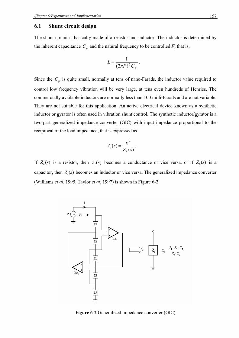
Chapter 6 Experiment and Implementation 157
6.1 Shunt circuit design
The shunt circuit is basically made of a resistor and inductor. The inductor is determined by
the inherent capacitance pC and the natural frequency to be controlled F, that is,
pCFL 2)2(
1π
= .
Since the pC is quite small, normally at tens of nano-Farads, the inductor value required to
control low frequency vibration will be very large, at tens even hundreds of Henries. The
commercially available inductors are normally less than 100 milli-Farads and are not variable.
They are not suitable for this application. An active electrical device known as a synthetic
inductor or gyrator is often used in vibration shunt control. The synthetic inductor/gyrator is a
two-part generalized impedance converter (GIC) with input impedance proportional to the
reciprocal of the load impedance, that is expressed as
)()(
2
sZgsZL
i = .
If )(sZL is a resistor, then )(sZi becomes a conductance or vice versa, or if )(sZL is a
capacitor, then )(sZi becomes an inductor or vice versa. The generalized impedance converter
(Williams et al, 1995, Taylor et al, 1997) is shown in Figure 6-2.
Figure 6-2 Generalized impedance converter (GIC)

Chapter 6 Experiment and Implementation 158
Let,
11 RZ = , 2
21
sCZ = , 33 RZ = , 44 RZ = , and 55 RZ = ,
then the input impedance iZ is
eqi sLR
CRRRsZZ
ZZZZ =⋅⋅⋅
=⋅⋅⋅
=4
2531
42
531 .
where
4
2531
RCRRRLeq⋅⋅⋅
= .
Figure 6-3 is the PSpice® model of the parallel piezoelectric R-L shunt circuit with a gyrator-
based inductor.
Figure 6-3 Parallel R-L piezoelectric shunt circuit with a gyrator-based inductor
The equivalent inductor value in Figure 6-3 is
)(5010
1010010100105103
9333
HLeq =×⋅×⋅×⋅
=−
.
Then the frequency to be controlled is
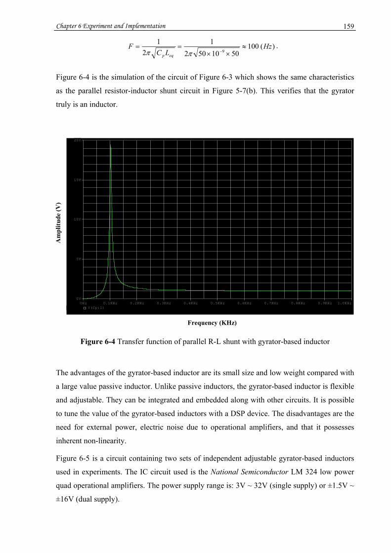
Chapter 6 Experiment and Implementation 159
)(1005010502
12
19
HzLC
Feqp
≈××
==−ππ
.
Figure 6-4 is the simulation of the circuit of Figure 6-3 which shows the same characteristics
as the parallel resistor-inductor shunt circuit in Figure 5-7(b). This verifies that the gyrator
truly is an inductor.
Figure 6-4 Transfer function of parallel R-L shunt with gyrator-based inductor
The advantages of the gyrator-based inductor are its small size and low weight compared with
a large value passive inductor. Unlike passive inductors, the gyrator-based inductor is flexible
and adjustable. They can be integrated and embedded along with other circuits. It is possible
to tune the value of the gyrator-based inductors with a DSP device. The disadvantages are the
need for external power, electric noise due to operational amplifiers, and that it possesses
inherent non-linearity.
Figure 6-5 is a circuit containing two sets of independent adjustable gyrator-based inductors
used in experiments. The IC circuit used is the National Semiconductor LM 324 low power
quad operational amplifiers. The power supply range is: 3V ~ 32V (single supply) or ±1.5V ~
±16V (dual supply).
Am
plitu
de (V
)
Frequency
0Hz 0.1KHz 0.2KHz 0.3KHz 0.4KHz 0.5KHz 0.6KHz 0.7KHz 0.8KHz 0.9KHz 1.0KHzV(Cp:1)
0V
5V
10V
15V
20V
Frequency (KHz)
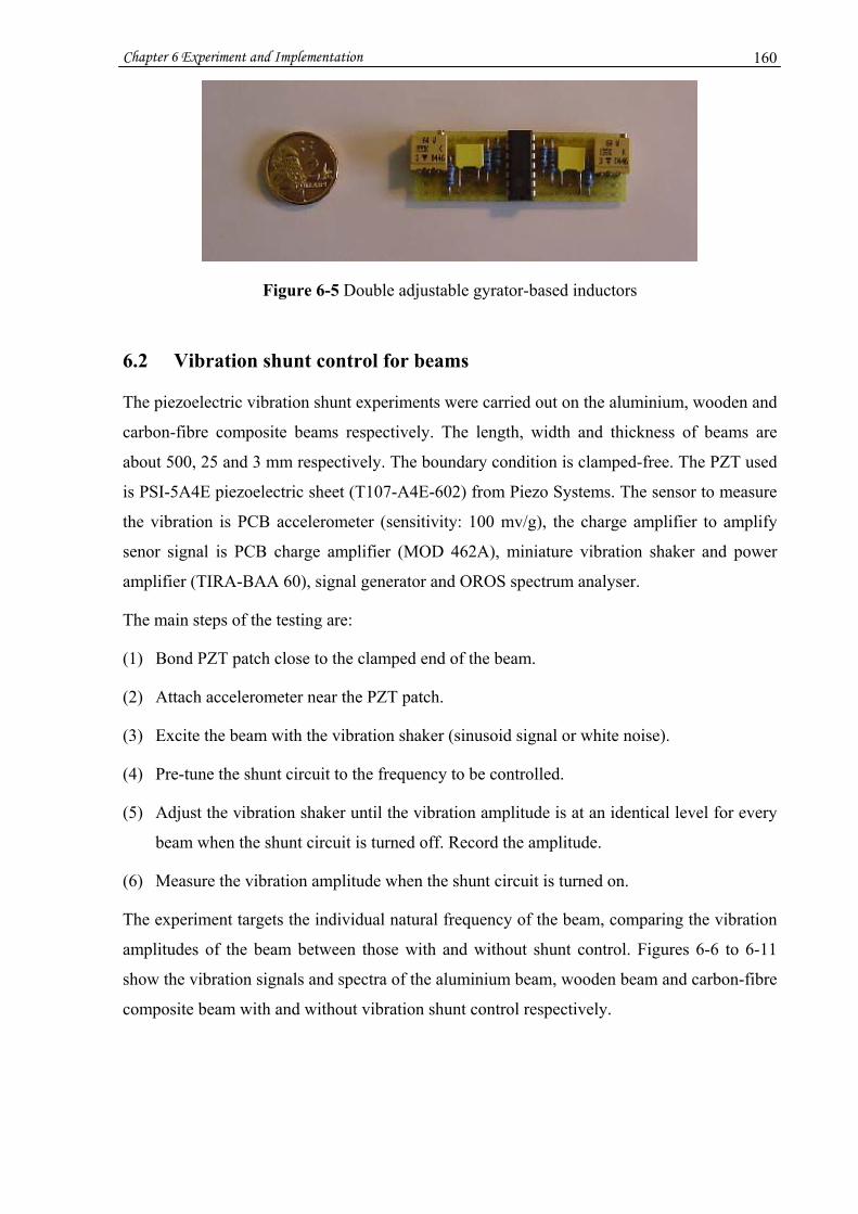
Chapter 6 Experiment and Implementation 160
Figure 6-5 Double adjustable gyrator-based inductors
6.2 Vibration shunt control for beams
The piezoelectric vibration shunt experiments were carried out on the aluminium, wooden and
carbon-fibre composite beams respectively. The length, width and thickness of beams are
about 500, 25 and 3 mm respectively. The boundary condition is clamped-free. The PZT used
is PSI-5A4E piezoelectric sheet (T107-A4E-602) from Piezo Systems. The sensor to measure
the vibration is PCB accelerometer (sensitivity: 100 mv/g), the charge amplifier to amplify
senor signal is PCB charge amplifier (MOD 462A), miniature vibration shaker and power
amplifier (TIRA-BAA 60), signal generator and OROS spectrum analyser.
The main steps of the testing are:
(1) Bond PZT patch close to the clamped end of the beam.
(2) Attach accelerometer near the PZT patch.
(3) Excite the beam with the vibration shaker (sinusoid signal or white noise).
(4) Pre-tune the shunt circuit to the frequency to be controlled.
(5) Adjust the vibration shaker until the vibration amplitude is at an identical level for every
beam when the shunt circuit is turned off. Record the amplitude.
(6) Measure the vibration amplitude when the shunt circuit is turned on.
The experiment targets the individual natural frequency of the beam, comparing the vibration
amplitudes of the beam between those with and without shunt control. Figures 6-6 to 6-11
show the vibration signals and spectra of the aluminium beam, wooden beam and carbon-fibre
composite beam with and without vibration shunt control respectively.

Chapter 6 Experiment and Implementation 161
(a) Before Shunt (b) After shunt
Figure 6-6 Vibration shunt for aluminium beam (test 1)
(a) Before Shunt (b) After shunt
Figure 6-7 Vibration shunt for aluminium (test 2)
(a) Before Shunt (b) After shunt
Figure 6-8 Vibration shunt for wooden beam (test 1)

Chapter 6 Experiment and Implementation 162
(a) Before Shunt (b) After shunt
Figure 6-9 Vibration shunt for wooden beam (test 2)
(a) Before Shunt (b) After shunt
Figure 6-10 Vibration shunt for carbon-fibre composite beam (test 1)
(a) Before Shunt (b) After shunt
Figure 6-11 Vibration shunt for carbon-fibre composite beam (test 2)
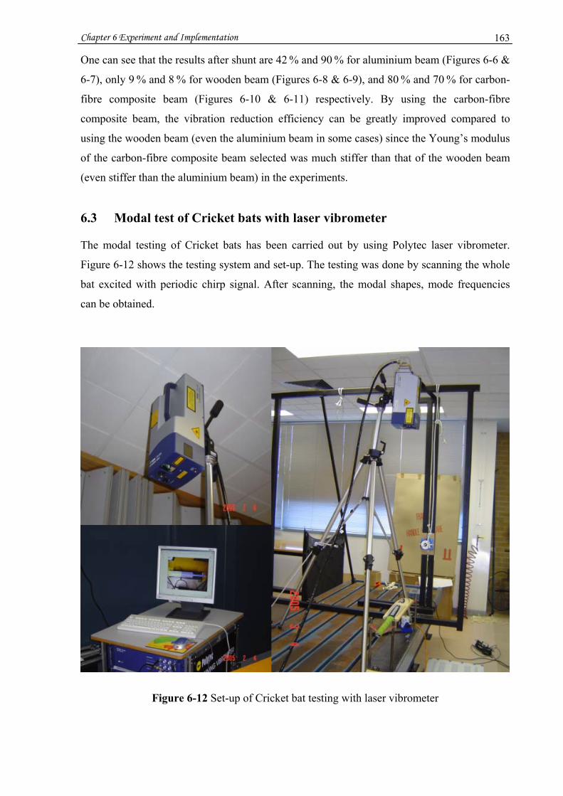
Chapter 6 Experiment and Implementation 163
One can see that the results after shunt are 42 % and 90 % for aluminium beam (Figures 6-6 &
6-7), only 9 % and 8 % for wooden beam (Figures 6-8 & 6-9), and 80 % and 70 % for carbon-
fibre composite beam (Figures 6-10 & 6-11) respectively. By using the carbon-fibre
composite beam, the vibration reduction efficiency can be greatly improved compared to
using the wooden beam (even the aluminium beam in some cases) since the Young’s modulus
of the carbon-fibre composite beam selected was much stiffer than that of the wooden beam
(even stiffer than the aluminium beam) in the experiments.
6.3 Modal test of Cricket bats with laser vibrometer
The modal testing of Cricket bats has been carried out by using Polytec laser vibrometer.
Figure 6-12 shows the testing system and set-up. The testing was done by scanning the whole
bat excited with periodic chirp signal. After scanning, the modal shapes, mode frequencies
can be obtained.
Figure 6-12 Set-up of Cricket bat testing with laser vibrometer

Chapter 6 Experiment and Implementation 164
Several Cricket bats were tested, one of them is the normal wooden handle bat, two are the
carbon-fibre composite tube handle bats, and two are the carbon-fibre composite sandwiched
handle bats. The results are given below.
6.3.1 Wooden handle Cricket bat
The wooden handle Cricket bat is the traditional bat commonly used in the Cricket game.
Figure 6-13 is the bat to be tested.
Figure 6-13 Wooden handle Cricket bat
Figure 6-14 shows the first three bending modes (from top to bottom) of the bats obtained by
the laser vibrometer. Their frequencies are: 125, 395, and 654 Hz respectively. One can notice
that the maximum strain of the 1st mode is almost concentrated at the shoulder area.

Chapter 6 Experiment and Implementation 165
Figure 6-14 Bending modes of the wooden handle Cricket bat
6.3.2 Carbon-fibre composite tube handle Cricket bat
Two carbon-fibre composite tube handle Cricket bats as shown in Figures 6-15 and 6-16 have
been tested. The handle material of the bat in Figure 6-15 is less stiff than that of the bat in
Figure 6-16.
Figure 6-15 Carbon-fibre composite tube handle Cricket bats #1 (less stiff handle)

Chapter 6 Experiment and Implementation 166
Figure 6-16 Carbon-fibre composite tube handle Cricket bat #2 (stiffer handle)
Figure 6-17 shows the first three bending modes of the bat #1 in Figure 6-15. The mode
frequencies of the bat are 237, 678, and 1237 Hz respectively.
Figure 6-17 First three bending modes of the bat in Figure 6-15
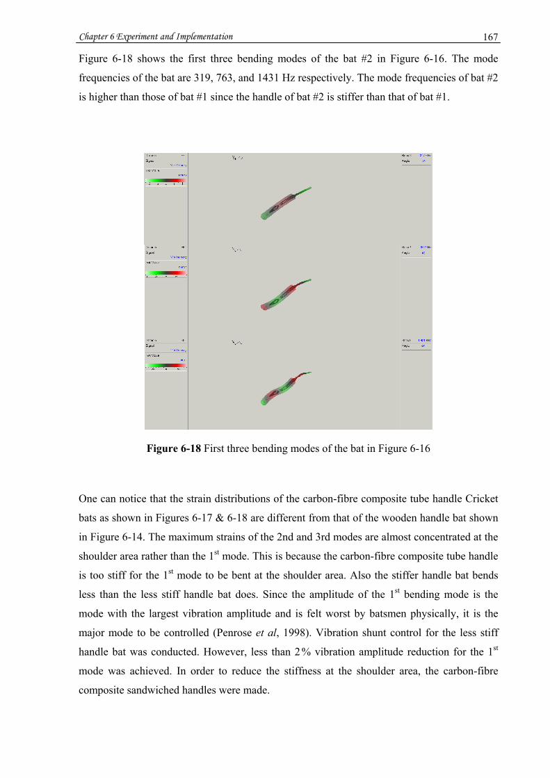
Chapter 6 Experiment and Implementation 167
Figure 6-18 shows the first three bending modes of the bat #2 in Figure 6-16. The mode
frequencies of the bat are 319, 763, and 1431 Hz respectively. The mode frequencies of bat #2
is higher than those of bat #1 since the handle of bat #2 is stiffer than that of bat #1.
Figure 6-18 First three bending modes of the bat in Figure 6-16
One can notice that the strain distributions of the carbon-fibre composite tube handle Cricket
bats as shown in Figures 6-17 & 6-18 are different from that of the wooden handle bat shown
in Figure 6-14. The maximum strains of the 2nd and 3rd modes are almost concentrated at the
shoulder area rather than the 1st mode. This is because the carbon-fibre composite tube handle
is too stiff for the 1st mode to be bent at the shoulder area. Also the stiffer handle bat bends
less than the less stiff handle bat does. Since the amplitude of the 1st bending mode is the
mode with the largest vibration amplitude and is felt worst by batsmen physically, it is the
major mode to be controlled (Penrose et al, 1998). Vibration shunt control for the less stiff
handle bat was conducted. However, less than 2 % vibration amplitude reduction for the 1st
mode was achieved. In order to reduce the stiffness at the shoulder area, the carbon-fibre
composite sandwiched handles were made.

Chapter 6 Experiment and Implementation 168
6.3.3 Carbon-fibre composite sandwiched handle Cricket bat
Figure 6-19 is the first carbon-fibre composite sandwiched handle Cricket bat. The handle is
sandwiched by two pieces of carbon-fibre composite beams. The carbon-fibre composite
beam is the variable stiffness polymeric composite strip as shown in Figure 4-26 in Chapter 4.
The carbon-fibre material at the shoulder area where the PZT patch will be attached, is less
stiff although theoretically it should be made stiffer in this area to transfer more strain into the
PZT patch. This is actually a compromise in order to shift the 1st bending mode to the
shoulder area.
Figure 6-19 Carbon-fibre composite sandwiched handle Cricket bat #1
Figure 6-20 shows the first three bending modes of the sandwiched handle bat #1. The mode
frequencies are: 203, 503, and 784 Hz. They are lower than the carbon-fibre tube handle bats
but higher than the wooden handle bat. The location of the 1st bending mode is closer to the
shoulder area of the bat.
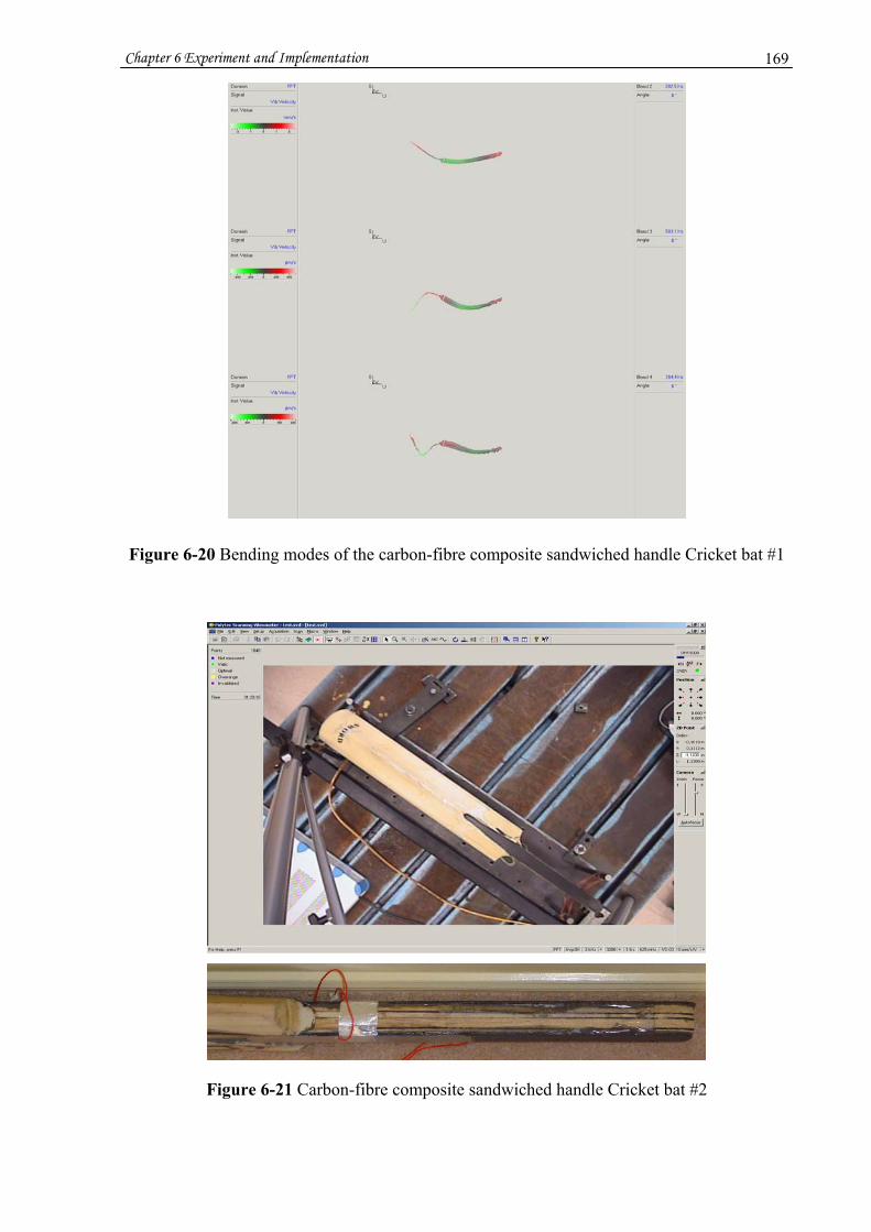
Chapter 6 Experiment and Implementation 169
Figure 6-20 Bending modes of the carbon-fibre composite sandwiched handle Cricket bat #1
Figure 6-21 Carbon-fibre composite sandwiched handle Cricket bat #2

Chapter 6 Experiment and Implementation 170
The bat in Figure 6-21 is the second carbon-fibre composite sandwiched handle Cricket bat.
The difference from the first handle is that the wooden material sandwiched between the
carbon-fibre composite strips has uniform thickness as shown in the bottom picture of Figure
6-21. Figure 6-22 is the 1st bending mode and the acceleration spectrum of the sandwiched
handle bat #2. The 1st bending mode shows it even closer to the shoulder area of the bat.
Figure 6-22 Accelerate spectrum of the #2 sandwiched handle Cricket bat
Figure 6-23 shows the first four bending modes of the sandwiched handle bat #2. It gives
clearer picture of where the anti-node locations of the bat are. The mode frequencies are: 156,
438, 655, and 1009 Hz respectively. The frequencies are further dropped and are closer to the
frequencies of the wooden handle bat. The frequency drop is partly due to the gap between
composite strips of bat #2 handle is narrower (hence lower flexural rigidity) than that of bat
#1 handle. However, the frequency drop is not what was desired. It is certainly something that
needs to be improved. The constraint here is that due to the laws of the game (MCC, [I 8]),
attachments are not allowed anywhere except the handle of the bat. We need to find a break
(soft) point along the handle to maximize the bending of the 1st mode. The only likely position
is at the shoulder area. It is possible to increase the frequencies as well as have the anti-node
of the 1st bending mode close to the shoulder area by optimising the geometry size, Young’s
modulus of the carbon-fibre strips and the thickness of the wood material sandwiched
between the two strips. It requires more simulations and experiments. A third sandwiched
handle Cricket bat was made as shown in Figure 6-24 (before assembly, the blade and pre-
made sandwiched handle).

Chapter 6 Experiment and Implementation 171
Figure 6-23 Bending modes of the carbon-fibre composite sandwiched handle Cricket bat #2
Figure 6-24 Blade and pre-made sandwiched handle for sandwiched handle Cricket bat #3
Slot to hold circuit Slot to hold batteries

Chapter 6 Experiment and Implementation 172
The sandwiched handle bat #3 was tested after assembly. The mode frequencies, especially
the 1st mode, have been improved compared to those of sandwiched handle bat #2. The first
three mode frequencies are: 180, 444, and 710 Hz. Table 6-1 lists the natural frequencies of
various bats.
Table 6-1 Natural frequency comparison among various Cricket bats
Natural Frequency (Hz)
Bending
Mode
Wooden bat
Carbon-fibre tube
bat #1
Carbon-fibre tube
bat #2
Carbon -fibre
sandwiched bat #1
Carbon- fibre
sandwiched bat #2
Carbon -fibre
sandwiched bat #3
1st 125 237 317 202 156 180
2nd 395 678 763 503 438 440
3rd 654 1237 1431 784 655 712
4th 960 –– –– 1102 1009 1070
Due to the time and resource limitations, only three carbon-fibre composite sandwiched
handle bats were made. The tests have shown that the vibration shunt control efficiency has
been improved for the carbon-fibre sandwiched bats compared to wooden bat and composite
tube bat. They are discussed in next section.
6.3.4 Vibration shunt control for the Cricket bat
The vibration shunt control was carried out for the bat with the carbon-fibre tube handle but
the vibration reduction is very little. It also is a problem to attach the PZT patch on the tube
handle. So the carbon-fibre composite sandwiched handle bat was designed and tested. The
PZT patches are attached to both sides of the handle as shown in Figure 6-25. The pair at the
shoulder area aims to reduce the vibration of the 1st and 3rd modes and the other pair aims to
reduce the vibration of the 2nd and 4th modes based on the mode distribution as shown in
Figure 6-23. The PZT patches in each pair are connected in parallel then connected to a shunt
circuit. There are two parallel R-L shunt circuits for the bat.
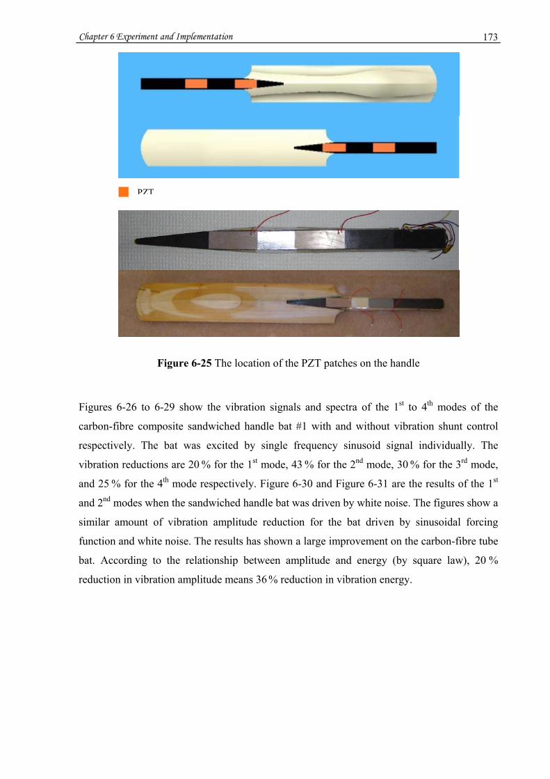
Chapter 6 Experiment and Implementation 173
Figure 6-25 The location of the PZT patches on the handle
Figures 6-26 to 6-29 show the vibration signals and spectra of the 1st to 4th modes of the
carbon-fibre composite sandwiched handle bat #1 with and without vibration shunt control
respectively. The bat was excited by single frequency sinusoid signal individually. The
vibration reductions are 20 % for the 1st mode, 43 % for the 2nd mode, 30 % for the 3rd mode,
and 25 % for the 4th mode respectively. Figure 6-30 and Figure 6-31 are the results of the 1st
and 2nd modes when the sandwiched handle bat was driven by white noise. The figures show a
similar amount of vibration amplitude reduction for the bat driven by sinusoidal forcing
function and white noise. The results has shown a large improvement on the carbon-fibre tube
bat. According to the relationship between amplitude and energy (by square law), 20 %
reduction in vibration amplitude means 36 % reduction in vibration energy.
PZT

Chapter 6 Experiment and Implementation 174
(a) Before Shunt (b) After shunt
Figure 6-26 Vibration of the sandwiched handle Cricket bat #1 (1st mode)
(a) Before Shunt (b) After shunt
Figure 6-27 Vibration of the sandwiched handle Cricket bat #1 (2nd mode)
(a) Before Shunt (b) After shunt
Figure 6-28 Vibration of the sandwiched handle Cricket bat #1 (3rd mode)

Chapter 6 Experiment and Implementation 175
(a) Before Shunt (b) After shunt
Figure 6-29 Vibration of the sandwiched handle Cricket bat #1 (4th mode)
(a) Before Shunt (b) After shunt
Figure 6-30 Vibration of the sandwiched handle Cricket bat #1 (1st mode, random excitation)
(a) Before Shunt (b) After shunt
Figure 6-31 Vibration of the sandwiched handle Cricket bat #1 (2nd mode, random excitation)
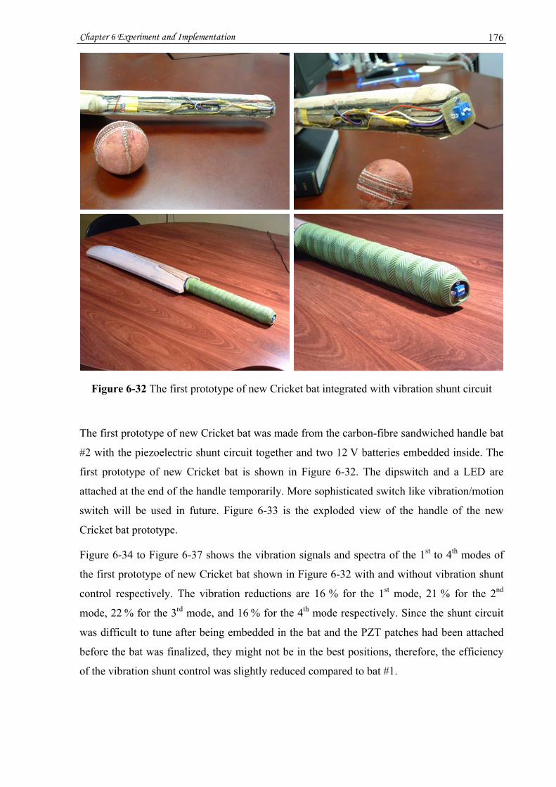
Chapter 6 Experiment and Implementation 176
Figure 6-32 The first prototype of new Cricket bat integrated with vibration shunt circuit
The first prototype of new Cricket bat was made from the carbon-fibre sandwiched handle bat
#2 with the piezoelectric shunt circuit together and two 12 V batteries embedded inside. The
first prototype of new Cricket bat is shown in Figure 6-32. The dipswitch and a LED are
attached at the end of the handle temporarily. More sophisticated switch like vibration/motion
switch will be used in future. Figure 6-33 is the exploded view of the handle of the new
Cricket bat prototype.
Figure 6-34 to Figure 6-37 shows the vibration signals and spectra of the 1st to 4th modes of
the first prototype of new Cricket bat shown in Figure 6-32 with and without vibration shunt
control respectively. The vibration reductions are 16 % for the 1st mode, 21 % for the 2nd
mode, 22 % for the 3rd mode, and 16 % for the 4th mode respectively. Since the shunt circuit
was difficult to tune after being embedded in the bat and the PZT patches had been attached
before the bat was finalized, they might not be in the best positions, therefore, the efficiency
of the vibration shunt control was slightly reduced compared to bat #1.
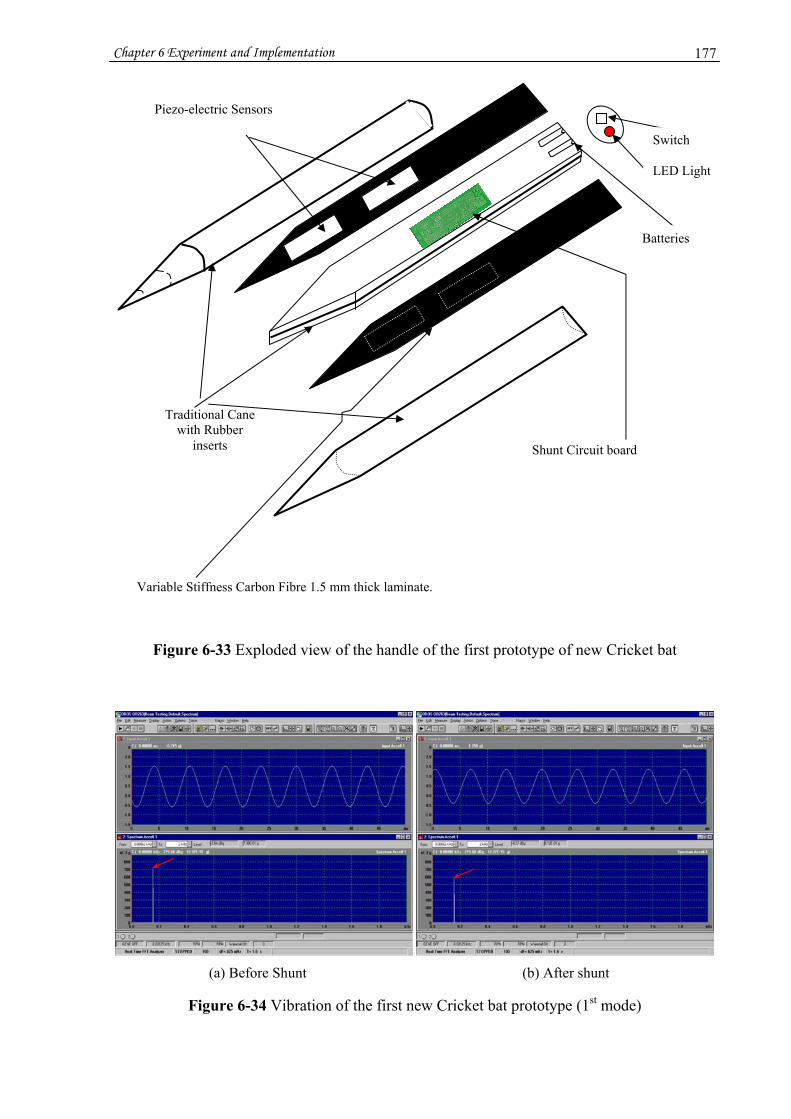
Chapter 6 Experiment and Implementation 177
Figure 6-33 Exploded view of the handle of the first prototype of new Cricket bat
(a) Before Shunt (b) After shunt
Figure 6-34 Vibration of the first new Cricket bat prototype (1st mode)
Shunt Circuit board
Variable Stiffness Carbon Fibre 1.5 mm thick laminate.
Traditional Cane with Rubber
inserts
Piezo-electric Sensors
Switch LED Light
Batteries

Chapter 6 Experiment and Implementation 178
(a) Before Shunt (b) After shunt
Figure 6-35 Vibration of the first new Cricket bat prototype (2nd mode)
(a) Before Shunt (b) After shunt
Figure 6-36 Vibration of the first new Cricket bat prototype (3rd mode)
(a) Before Shunt (b) After shunt
Figure 6-37 Vibration of the first new Cricket bat prototype (4th mode)

Chapter 6 Experiment and Implementation 179
Comparing the vibration shunt results between the Cricket bats and for the beams, the
percentage of vibration amplitude reduction of the former is clearly much less than the latter.
This is because the volume of the Cricket bats is much larger than the volume of the beams.
The Cricket bats certainly contain more vibration energy than the beams do. A single PZT
patch can only absorb a limited amount of vibration energy. However, when multiple PZT
patches can be placed and connected in parallel, the vibration energy to be absorbed is almost
in proportion to the number of PZT patches. It was verified by attaching one PZT patch and
two PZT patches to the Cricket bat respectively. The vibration reduction for using two PZT
patches is doubled compared with that for using one PZT patch. The other thing that needs to
be mentioned is that the shunt efficiency is in inverse proportion to the magnitude of
vibration. The larger the vibration, the lower percentage of vibration reduction. This is
understandable since the PZT has a finite energy absorption capability.
One phenomenon that was noticed during the experiments is that the efficiency of the shunt
control is related to the power supply of the shunt circuit. The efficiency of the shunt control
is proportional to the power supply. It is probably because the inductor used is the gyrator-
based inductor, which is built with operational amplifiers. The operational amplifiers have a
certain dynamic range to operate within. The larger the power supply, the larger the dynamic
range of the operational amplifiers. Since the parallel shunt control is an inherent parallel
resonant circuit, when the shunt circuit is tuned to the frequency to be controlled, the resonant
phenomenon happens and the voltage at the input of the shunt circuit will be very large. The
operational amplifiers can be saturated when the input vibration signal exceeds the dynamic
range of the operational amplifiers. In such case, the inductor will not be at the right value and
the shunt circuit will hence not function correctly.
Figure 6-38 shows an example of the influence of the power supply over the efficiency of the
shunt control. Figure 6-38 (a) is the vibration signal before shunt, (b) shows the vibration
signal after shunt with 10 voltage power supply to the shunt circuit, (c) show the vibration
signal after shunt with 15 voltage power supply to the shunt circuit. Comparing the
magnitudes between the signals in Figure 6-38 (b) and Figure 6-38 (c), the vibration reduction
is about 6.5 % in (b) and is about 10 % in (c). The percentage increase in efficiency is about
the same as the percentage increase of power supply at this power supply level. Since the
power supply of the operational amplifier used is limited to ±16V, no further test has been
made. However, the efficiency of the shunt control is expected to rise when the gyrator-based
inductor is built with power operational amplifiers and powered with a higher voltage.
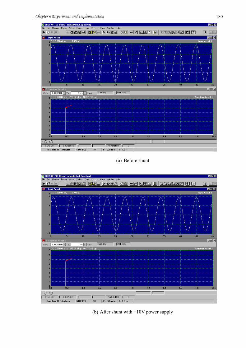
Chapter 6 Experiment and Implementation 180
(a) Before shunt
(b) After shunt with ±10V power supply

Chapter 6 Experiment and Implementation 181
(c) After shunt with ±15V power supply
Figure 6-38 The influence of power supply to the effectiveness of shunt control
The vibration reduction shown in Figure 6-38 is not very significant because:
1. The vibration energy was relatively significant.
2. The shunt circuit was slightly out-of-tune at the frequency to be controlled which is
evident in Figure 6-40 since the circuit had already been embedded in the Cricket bat. It
was thus difficult to tune manually.
Figure 6-39 shows the second prototype of new Cricket bat made from the carbon-fibre
sandwiched handle bat #3. Figure 6-40 shows its vibrations under random excitation where:
Figure 6-40(a) is the vibration without shunt control and Figures 6-40 (b & c) show the
vibration with shunt control. One can see from the vibration spectrum in Figures (b & c), the
magnitude dip of the mode 1 is not at the centre of the peak. It means that the shunt circuit
was not tuned to the natural frequency accurately therefore the shunt control effectiveness was
reduced.
Since the passive R-L piezoelectric shunt control possesses narrow-band characteristics, when
the shunt circuit is not tuned appropriately, it will lose performance. The sophisticated control
system should be able to automatically tune to the natural frequency to be controlled. It

Chapter 6 Experiment and Implementation 182
should firstly have a mechanism to detect the natural frequency of the structure to be
controlled. Hence, an adaptive algorithm to detect multiple frequencies embedded in the
signal will be discussed in the next chapter.
Figure 6-39 The second prototype of new Cricket bat integrated with vibration shunt circuit
(a) Before Shunt

Chapter 6 Experiment and Implementation 183
(b) After shunt
(c) Similar to Figure (b) but with simulated with smaller frequency range
Figure 6-40 Vibration of the second new Cricket bat prototype (1st mode, random excitation)
6.4 Field testing of the Smart bat
The Smart bat shown in Figure 6.39 was field tested by experienced Cricket players both
within RMIT University and Kookaburra Sports. The preliminary feedback from these
experienced players indicates that the feel of the bat was comfortable for most strokes and
there was a perceived enhancement of the Sweet Spot towards the handle. This rather
subjective finding could be linked to the higher frequency induced by the carbon-fibre strips
in the Smart bat since the displacement is inverse proportion to the mode frequency:
222 FgADπ
= (Space Age Control, [I 11]),
Chapter 6 Experiment and Implementation 184
where,
D, A and F denote displacement, acceleration and mode frequency respectively. g is a
constant that is equal to 9.80665 m/s².
Also, it was immediately obvious if the activated shunt circuit provided a ‘better feel’ of the
batting stroke compared to when the circuit was not activated. The overall perception
however was that the bat did not feel any worse than the traditional Cricket bat. This was a
very comforting outcome and it augers well for further development of the Smart bat provided
the law makers see it fit to accommodate technological advances in the sport of Cricket.
6.5 Chapter summary
In this chapter, the experimental results of the passive piezoelectric vibration shunt control for
various beams and Cricket bats have been shown. Excellent vibration reductions have been
achieved for the aluminium and carbon-fibre composite beams, except for the wooden beam,
as predicted by the ANSYS® simulation. A few modifications have been made on the
traditional wooden Cricket bat. The carbon-fibre sandwiched handle Cricket bats were
prototyped after tubular handle designs were extensively trialled. A certain vibration
reduction was achieved although the Cricket bat design was restricted by the laws of the
game. It is possible to increase the mode frequencies and maintain the anti-node of the 1st
bending mode close to the shoulder area by optimising the geometry size, Young’s modulus
of the carbon-fibre strips and the thickness of the wood material sandwiched between the two
strips. The high power supply of the shunt circuit can help to increase the shunt control
efficiency. An important thing is that the natural frequencies of the Cricket bat will shift more
or less in reality when boundary conditions change. This will reduce the shunt efficiency due
to the narrow-band characteristic of the shunt circuit. Because of this, it was critical to
develop a way to online-detect the natural frequency to be controlled and real-time adjust the
value of the inductor to track that frequency. The analytical work in this regard is presented in
the next chapter.
The field testing of the bat was carried out and the perception of the Smart bat was that it
generally felt good to play with.

Chapter 7 Frequency Estimation and Tracking 185
Chapter 7
Frequency Estimation and Tracking
As mentioned in previous chapters, the R-L passive piezoelectric vibration shunt control is the
narrowband control that targets the natural frequency of structures. It is very sensitive to the
shift of the natural frequency to be controlled. When the frequency of a shunt circuit does not
match the natural frequency to be controlled, the effectiveness of the shunt control will
worsen dramatically. In reality, the natural frequencies of structures often shift when
boundary conditions, material properties or environments change. The natural frequencies of
Cricket bats will be affected with or without being held by the batsman. Even the hand
location and grip of the batsman will affect the natural frequencies. So it is important to have
a mechanism to detect and track the natural frequencies in real-time to automatically adjust
the parameters of the shunt circuit instantly in order to maintain the effectiveness of the shunt
control. In this chapter, a method of detecting multiple sinusoid frequencies buried in noise by
using adaptive Infinite Impulse Response (IIR) notch filters is presented. In first section,
filters are briefly reviewed. Section 2 gives an example of generic notch filter. The adaptive
notch filter for frequency estimation is discussed, and an example is given in section 3. The
frequency estimation and tracking is a possible option for future Smart Cricket bats.
7.1 Introduction of filters
Filters are used to remove unwanted frequency components and noise from signals. There are
two types of filters, i.e. analogue filters and digital filters. Analogue filters are implemented in
electronic hardware, such as resistors, capacitors, and operational amplifiers, etc. Digital
filters can be implemented either in hardware or software or both. Since the adaptive
algorithms are usually implemented in software, digital filters are often the choice for
adaptive filters. The digital filters can be classified as having either finite impulse response
(FIR) or infinite impulse response (IIR). FIR filters are non-recursive filters, which means

Chapter 7 Frequency Estimation and Tracking 186
they have no feedback paths. IIR filters are recursive filters that have feedback paths. FIR
filters have the advantage of stability and linear phase response if desired, whereas IIR filters
have the advantage of being very computationally efficient. Figure 7-1 shows the diagram of a
direct realization of an Nth order non-recursive FIR digital filter.
Figure 7-1 Direct realization of an Nth order non-recursive FIR digital filter
Given an input sequence, )(nx , and a finite length impulse response sequence, )(nh , the
output sequence, )(ny can be obtained according to:
∑−
=
−⋅==1
0)()()(*)()(
N
kknxkhnxnhny . (7.1)
where * denotes convolution, N is the length of the impulse response, and 0)( =nh for n < 0
which means that the filter is a causal system.
The transfer function of the above Nth order FIR filter in the z-domain is:
∑−
=
−⋅=1
0)()(
N
k
kzkhzH . (7.2)
Figure 7-2 shows the diagram of a direct realization of an Nth order recursive IIR digital filter.
The IIR filter’s output depends not only on the previous M inputs but also on the previous N
outputs. The differential equation of an IIR filter can be expressed as:
∑ ∑=
−
=
−⋅=−⋅+N
k
M
kkk knxbknyany
1
1
0
)()()( . (7.3)
The transfer function in the z-domain is:
NN
MM
zazazbzbbzH −−
+−−
−
⋅++⋅+⋅++⋅+
=……
11
11
110
1)( . (7.4)
+
z-1 z-1 z-1 z-1
+ + +
)2( −nx)1( −nx)(nx
)2( +−Nnx )1( +−Nnx
)0(h )1(h )2(h )2( −Nh )1( −Nh
)(ny

Chapter 7 Frequency Estimation and Tracking 187
The IIR filter has zeros as well as poles. The pole positions are determined by the recursive
feedback coefficients ka . In order for the filter to be stable, the poles must be located within
the unit circle for a causal system.
Figure 7-2 Direct realization of an Nth order recursive IIR digital filter
Adaptive filters are the filters that, in a sense, can self-design their filter coefficients in real-
time to optimum values based on certain rules according to the time varying input signal. An
adaptive digital filter consists of a programmable digital filter and an adaptive algorithm to
update the coefficients of the digital filter. The programmable digital filter can be a FIR or IIR
type. Figure 7-3 shows a block diagram of the digital filter.
Figure 7-3 Block diagram of the general adaptive digital filter
Adaptive Algorithm
∑Programmable Digital Filter A/D
+−)(nx )(ne)(ny
)(nd
z-1
z-1
z-1
z-1
z-1
z-1
+
+
+
+
+
+
+
+
+
+ )(ny)(nx0b
1b
2b
2−Mb
1−Mb
1a
2a
1−Na
Na
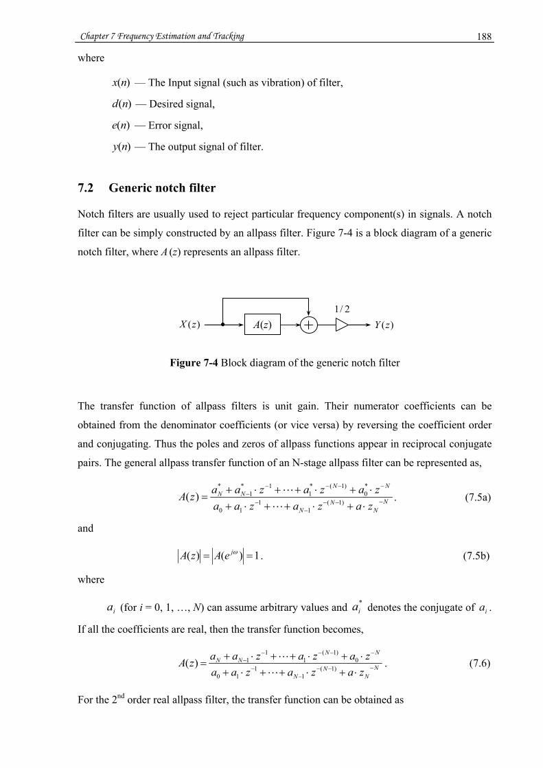
Chapter 7 Frequency Estimation and Tracking 188
where
)(nx — The Input signal (such as vibration) of filter,
)(nd — Desired signal,
)(ne — Error signal,
)(ny — The output signal of filter.
7.2 Generic notch filter
Notch filters are usually used to reject particular frequency component(s) in signals. A notch
filter can be simply constructed by an allpass filter. Figure 7-4 is a block diagram of a generic
notch filter, where A (z) represents an allpass filter.
Figure 7-4 Block diagram of the generic notch filter
The transfer function of allpass filters is unit gain. Their numerator coefficients can be
obtained from the denominator coefficients (or vice versa) by reversing the coefficient order
and conjugating. Thus the poles and zeros of allpass functions appear in reciprocal conjugate
pairs. The general allpass transfer function of an N-stage allpass filter can be represented as,
NN
NN
NNNN
zazazaazazazaazA −−−
−−
−−−−−
⋅+⋅++⋅+⋅+⋅++⋅+
=)1(
11
10
*0
)1(*1
1*1
*
)( . (7.5a)
and
1)()( == ωjeAzA . (7.5b)
where
ia (for i = 0, 1, …, N) can assume arbitrary values and *ia denotes the conjugate of ia .
If all the coefficients are real, then the transfer function becomes,
NN
NN
NNNN
zazazaazazazaazA −−−
−−
−−−−−
⋅+⋅++⋅+⋅+⋅++⋅+
=)1(
11
10
0)1(
11
1)( . (7.6)
For the 2nd order real allpass filter, the transfer function can be obtained as
A(z) 2/1
)(zY)(zX

Chapter 7 Frequency Estimation and Tracking 189
22
121
21212
)1(1)1()( −−
−−
++++++
=zazaazzaaazA . (7.7)
Therefore the transfer function of the 2nd order notch filter is,
22
121
2112
)1(121
21)](1[
21
)()()( −−
−−
++++++
=+==zazaa
zzaazAzXzYzH . (7.8)
The zeros of Equation (7.8) are
211
211
2,1 12
442aja
aaz −±−=
−±−= ( 11 ≤a ).
One can notice that the radiuses of the zeros are 12,1 =z which means the zeros are always on
the unit circle. The location of the zeros reflects the notch frequency in frequency domain.
The relationship of the notch frequency and the zeros in Equation (7.8) is
)arccos(2 1aTfT nn −== πω .
where
nω is the notch normalized angular frequency ( nn f×= πω 2 ), T is the sampling
interval. If T = 1, then )arccos( 1an −=ω .
The poles of Equation (7.8) are
24)]1([)1( 2
22121
2,1
aaaaap
−+±+−=
.
The radius of the poles determines the bandwidth of the notch filter. The closer the pole to the
unit circle, the narrower the bandwidth and the sharper the notch filter is.
The filter coefficients of the notch filter in Equation (7.8) can be obtained by
⎪⎩
⎪⎨
⎧
=+−
=
=−=
22
1
)2/tan(1)2/tan(1
)1(assume)cos(
rBWBWa
Ta n ω
. (7.9)
where BW is 3 dB bandwidth, and r is the pole radius.
For example, )2(15.0 πω ×=n , r = 0.95, then,
587785.0)3.0cos(1 −=−= πa , 9025.022 == ra ,
According to Equation (7.8), the transfer function of the notch filter becomes,
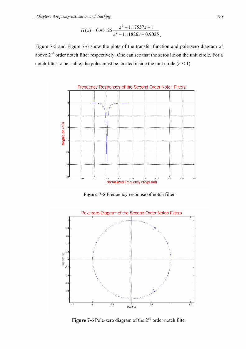
Chapter 7 Frequency Estimation and Tracking 190
9025.011826.1117557.195125.0)( 2
2
+−+−
=zz
zzzH.
Figure 7-5 and Figure 7-6 show the plots of the transfer function and pole-zero diagram of
above 2nd order notch filter respectively. One can see that the zeros lie on the unit circle. For a
notch filter to be stable, the poles must be located inside the unit circle (r < 1).
Figure 7-5 Frequency response of notch filter
Figure 7-6 Pole-zero diagram of the 2nd order notch filter

Chapter 7 Frequency Estimation and Tracking 191
7.3 Adaptive notch filter
An adaptive notch filter (ANF) is a notch filter where the notch frequency is determined by a
series of observed signal samples to detect and remove sinusoid components buried in the
signal. The sinusoid components are usually unknown or time varying. Vibration a signals of
flexible structures are often modelled as the combination of harmonic (natural frequency
components) signals and additive noise. A second order ANF can be used for detecting single
natural frequency. For detecting multiple natural frequencies, the structure of cascaded second
order ANFs can be used. When the vibration signal passes though each second order ANF
stage, one of the frequency components is detected and removed. The output of preceding 2nd
order ANF is the input of succeeding 2nd order ANF.
Figure 7-7 shows a block diagram of a high order adaptive notch filter by cascading multiple
2nd order ANF sections. The selected 2nd order notch filter structure is the IIR filter.
Figure 7-7 Adaptive notch filter by cascading multiple 2nd order ANF sections
7.3.1 Simplified adaptive notch filter
The 2nd order notch filter can be designed by Equation (7.8). However, since there are
multiple filter coefficients in Equation (7.8), it requires estimating multiple parameters for the
adaptive filter. It increases the complexity of adaptation and the scale of filter stability
monitoring. A minimal parameter adaptive notch filter with constrained poles and zeros was
proposed by Nehorai (1985) which is an approximation of the generic notch filter. With
Nehorai’s method, there are n parameters to be estimated for n sinusoid components rather
than 2n for many other adaptive notch filter algorithms. The general transfer function of the
2nth order Nehorai’s notch filter is (Nehorai, 1985),
nnnnnn
n
nnnn
zrzarzarzrazzazaza
rzAzAzH 2212
1121
1
2121
11
1
11
11
)()()( −−−−−
−−−−
−
−−
++++++++++++
==. (7.10)
where r is the pole contraction factor, 0 < r < 1.

Chapter 7 Frequency Estimation and Tracking 192
The coefficients of the transfer function in Equation (7.10) has the following relation,
ini aa −= 2 (i = 0, 1, …, n-1), and
120 == naa .
The ith angular notch frequency given by Equation (7.10) can be obtained as,
)2/arccos( ii aθ = (i = 1, …, n). (7.11a)
or the filter coefficient represented by iθ
ii θa cos2= ( 2] [-2, ∈ia ). (7.11b)
The vector of the angular notch frequency is
T ][ 1 nθθ=θ . (7.12)
Assume the input signal )(ty is composed of n sinusoid components plus white noise )(tn as
below,
)()cos()(1
tntCty ii
n
ii ++=∑
=
φθ .
Let the output signal of the notch filter be
)()()( 1 tyqHte −= , (7.13a)
where 1−q is a unit delay. Hence,
)()()()( 1
1
tyrqAqAte −
−
= . (7.13b)
where
nn
inin
ii
nnnn qaqqaqqaqaqaqA −+−−
−
=
−+−−−− ++=++++++= ∑ )(1)( 21
0
2121
11
1 (7.14a)
nnnn qrqraqraqrarqA 21121
1111
11 )()()()(1)( −−+−−−−−−− ++++++=
nn
nininin
i
ii qarqrqra −+−−−
−
=
++=∑ )( 221
0 . (7.14b)
Equation (7.13b) can be rewritten as,
)()()()( 11 tyqAterqA −− = , (7.15a)
that is,
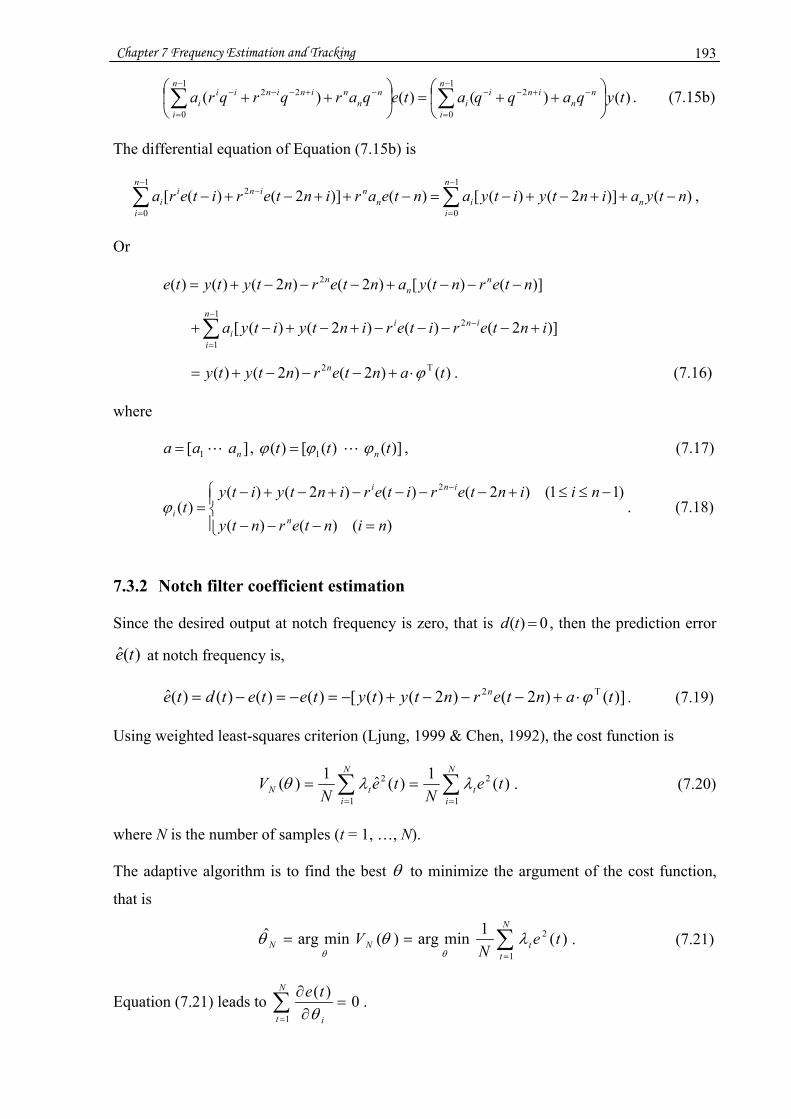
Chapter 7 Frequency Estimation and Tracking 193
)()()()( 21
0
221
0
tyqaqqateqarqrqra nn
inin
ii
nn
nininin
i
ii ⎟
⎠
⎞⎜⎝
⎛++=⎟
⎠
⎞⎜⎝
⎛++ −+−−
−
=
−+−−−−
=∑∑ . (7.15b)
The differential equation of Equation (7.15b) is
)()]2()([)()]2()([1
0
21
0ntyaintyityantearinteritera n
n
iin
ninn
i
ii −++−+−=−++−+− ∑∑
−
=
−−
=
,
Or
)]()([)2()2()()( 2 nterntyanterntytyte nn
n −−−+−−−+=
∑−
=
− +−−−−+−+−+1
1
2 )]2()()2()([n
i
inii interiterintyitya
)()2()2()( T2 tanterntyty n ϕ⋅+−−−+= . (7.16)
where
][ 1 naaa = , )]()([)( 1 ttt nϕϕϕ = , (7.17)
⎪⎩
⎪⎨⎧
=−−−
−≤≤+−−−−+−+−=
−
)()()(
)11()2()()2()()(
2
ninternty
niinteriterintyityt
n
ini
i
ϕ . (7.18)
7.3.2 Notch filter coefficient estimation
Since the desired output at notch frequency is zero, that is 0)( =td , then the prediction error
)(ˆ te at notch frequency is,
)]()2()2()([)()()()(ˆ T2 tanterntytytetetdte n ϕ⋅+−−−+−=−=−= . (7.19)
Using weighted least-squares criterion (Ljung, 1999 & Chen, 1992), the cost function is
)(1)(ˆ1)(1
2
1
2 teN
teN
VN
it
N
itN ∑∑
==
== λλθ . (7.20)
where N is the number of samples (t = 1, …, N).
The adaptive algorithm is to find the best θ to minimize the argument of the cost function,
that is
∑=
==N
ttNN te
NV
1
2 )(1minarg)(minargˆ λθθθθ
. (7.21)
Equation (7.21) leads to 0)(1
=∂∂∑
=
N
t i
teθ
.

Chapter 7 Frequency Estimation and Tracking 194
Let the vector of error gradient be
)]()([)( 1 ttt nψψψ = . (7.22a)
where
i
i
iii
aatetet
θθψ
∂∂⋅
∂∂
=∂∂
−=)()()( (i = 1,…, n). (7.22b)
From Equation (7.11b), one can have,
ii
ia θθ
sin−=∂∂ . (7.23)
For i
teθ∂
∂ )( , differentiating both sides of Equation (7.15a) with respect to ia and considering
Equation (7.14), for 11 −≤≤ ni ,
)()()()()()( 2221 tyqqteqrqraterqA iniininii
i
+−−+−−−− +=++∂∂ . (7.24a)
for i = n,
)()()()( 1 tyqteqraterqA nnn
i
−−− =+∂∂ . (7.24b)
or
⎪⎩
⎪⎨⎧
=−−−
−≤≤+−−−−+−+−=
∂∂
−
−
)()()(
)11()2()()2()()()(2
1
ninternty
niinteriterintyity
aterqA
n
ini
i
)(tiϕ= . (7.25a)
Hence,
)()()(1−=
∂∂
rqAt
ate i
i
ϕ . (7.25b)
Substituting Equations (7.23, 7.25b) into Equation (7.22b) obtains the error gradient with
respect to iθ is,
ii
i rqAtt θϕψ sin
)()(2)( 1 ⋅−= − (i = 1,…, n). (7.26)
The adaptive algorithm is the recursive least-squares (RLS) algorithm (Ljung, 1999) that is
summarized as
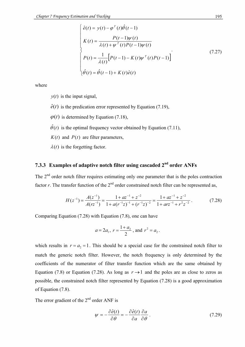
Chapter 7 Frequency Estimation and Tracking 195
[ ]⎪⎪⎪⎪
⎩
⎪⎪⎪⎪
⎨
⎧
+−=
−−−=
−+−
=
−−=
)(ˆ)()1(ˆ)(ˆ
)1()()()1()(
1)(
)()1()()()()1()(
)1(ˆ)()()(ˆ
tetKtt
tPttKtPt
tP
ttPttttPtK
tttyte
T
T
T
θθ
ψλ
ψψλψ
θϕ
. (7.27)
where
)(ty is the input signal,
)(ˆ te is the predication error represented by Equation (7.19),
)(tϕ is determined by Equation (7.18),
)(ˆ tθ is the optimal frequency vector obtained by Equation (7.11),
)(tK and )(tP are filter parameters,
)(tλ is the forgetting factor.
7.3.3 Examples of adaptive notch filter using cascaded 2nd order ANFs
The 2nd order notch filter requires estimating only one parameter that is the poles contraction
factor r. The transfer function of the 2nd order constrained notch filter can be represented as,
221
21
2111
21
1
11
11
)()(11
)()()( −−
−−
−−−−
−−
−
−−
++++
=++++
==zrarz
zazzrzra
zazrzAzAzH . (7.28)
Comparing Equation (7.28) with Equation (7.8), one can have
12aa = , 2
1 2ar += , and 2
2 ar = .
which results in 12 == ar . This should be a special case for the constrained notch filter to
match the generic notch filter. However, the notch frequency is only determined by the
coefficients of the numerator of filter transfer function which are the same obtained by
Equation (7.8) or Equation (7.28). As long as 1→r and the poles are as close to zeros as
possible, the constrained notch filter represented by Equation (7.28) is a good approximation
of Equation (7.8).
The error gradient of the 2nd order ANF is
θθψ
∂∂
∂∂
−=∂∂
−=a
atete )(ˆ)(ˆ . (7.29)

Chapter 7 Frequency Estimation and Tracking 196
where 2] [-2,cos2 ∈= θa .
The differential equation of Equation (7.28) is,
)2()1()2()1()()( 2 −−−−−+−+= tertaretytaytyte . (7.30)
Figure 7-8 is the direct realization of the constrained 2nd order IIR notch filter represented by
Equation (7.30).
Figure 7-8 Direct realization of the constrained 2nd order IIR notch filter
The predication error is
)2()1()()2()1()()()()(ˆ 2 −−−−−−+−=−=−= tytaytytertaretetetdte . (7.31)
Let the derivative of Equation (7.31) with respect to “a” be zero, that is 0)(ˆ=
∂∂
ate
, obtains
)1()1()2()1()( 2 −−−=∂−∂
+∂−∂
+∂∂ trety
ater
atear
ate . (7.32)
Then let,
ate
atetE
∂∂
−=∂
∂=
)()(ˆ)( ,
Equation (7.32) becomes,
)1()1()(]1[ 221 −−−=++− −− tretytEqrarq . (7.33)
Therefore derivative can be represented by,
z-1
a
z-1
+ +
+
z-1
z-1
+
ra−
2r−
)(ty)1( −ty )2( −ty
)(te
)1( −te
)2( −te

Chapter 7 Frequency Estimation and Tracking 197
)()1()1(
1)1()1()(ˆ
)( 1221 −−−
−−−−=
++−−−
−=∂∂
=rqA
tretyqrarq
tretyatetE . (7.34)
Since θθ
sin2−=∂∂a , substituting
θ∂∂a and Equation (7.18) to Equation (7.12) obtain the
gradient as,
θψ sin)(
)1()1(2 1−
−−−−=
rqAtrety
. (7.35)
Figure 7-9 to Figure 7-12 are the simulations of the frequency estimation using the three
cascaded 2nd order IIR adaptive notch filter. Figure 7-9 shows the input signal to the ANF that
contains three sinusoid frequency components and white noise (top left), and the output
signals of three 2nd order ANF stages respectively. The sinusoid frequencies of the input
signal are 0.05, 0.1 and 0.2 of sampling frequency respectively. The power of the white
Gaussian noise added )(tn , which is independent of the signal component, is 0 dBW. The
signal to noise ratio (SNR) of individual frequency component is 0 dB, i.e.
)()22.0cos()21.0cos()205.0cos()( tntttty +××+××+××= πππ
Figure 7-9 Input signal and the output signals of each 2nd order ANF (SNR = 0 dB)
Figure 7-10 shows the adaptation progress of the ANF that shows that the estimation
converges to three sinusoid frequency components of the input signal after about 100
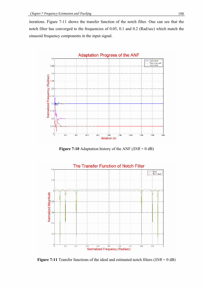
Chapter 7 Frequency Estimation and Tracking 198
iterations. Figure 7-11 shows the transfer function of the notch filter. One can see that the
notch filter has converged to the frequencies of 0.05, 0.1 and 0.2 (Rad/sec) which match the
sinusoid frequency components in the input signal.
Figure 7-10 Adaptation history of the ANF (SNR = 0 dB)
Figure 7-11 Transfer functions of the ideal and estimated notch filters (SNR = 0 dB)

Chapter 7 Frequency Estimation and Tracking 199
Figure 7-12 shows spectra of the input signal and the output signal of the individual 2nd order
ANF. The spectra show that each 2nd order notch filter removes one frequency component.
Figure 7-12 Spectra of the input signal and the output signals of each 2nd order ANF
(SNR = 0 dB)
Figure 7-13 Input signal and the output signals of each 2nd order ANF (SNR = –10 dB)
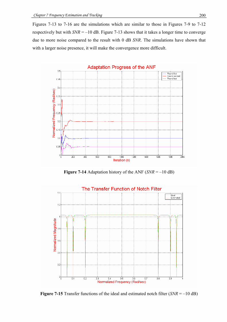
Chapter 7 Frequency Estimation and Tracking 200
Figures 7-13 to 7-16 are the simulations which are similar to those in Figures 7-9 to 7-12
respectively but with SNR = –10 dB. Figure 7-13 shows that it takes a longer time to converge
due to more noise compared to the result with 0 dB SNR. The simulations have shown that
with a larger noise presence, it will make the convergence more difficult.
Figure 7-14 Adaptation history of the ANF (SNR = –10 dB)
Figure 7-15 Transfer functions of the ideal and estimated notch filter (SNR = –10 dB)
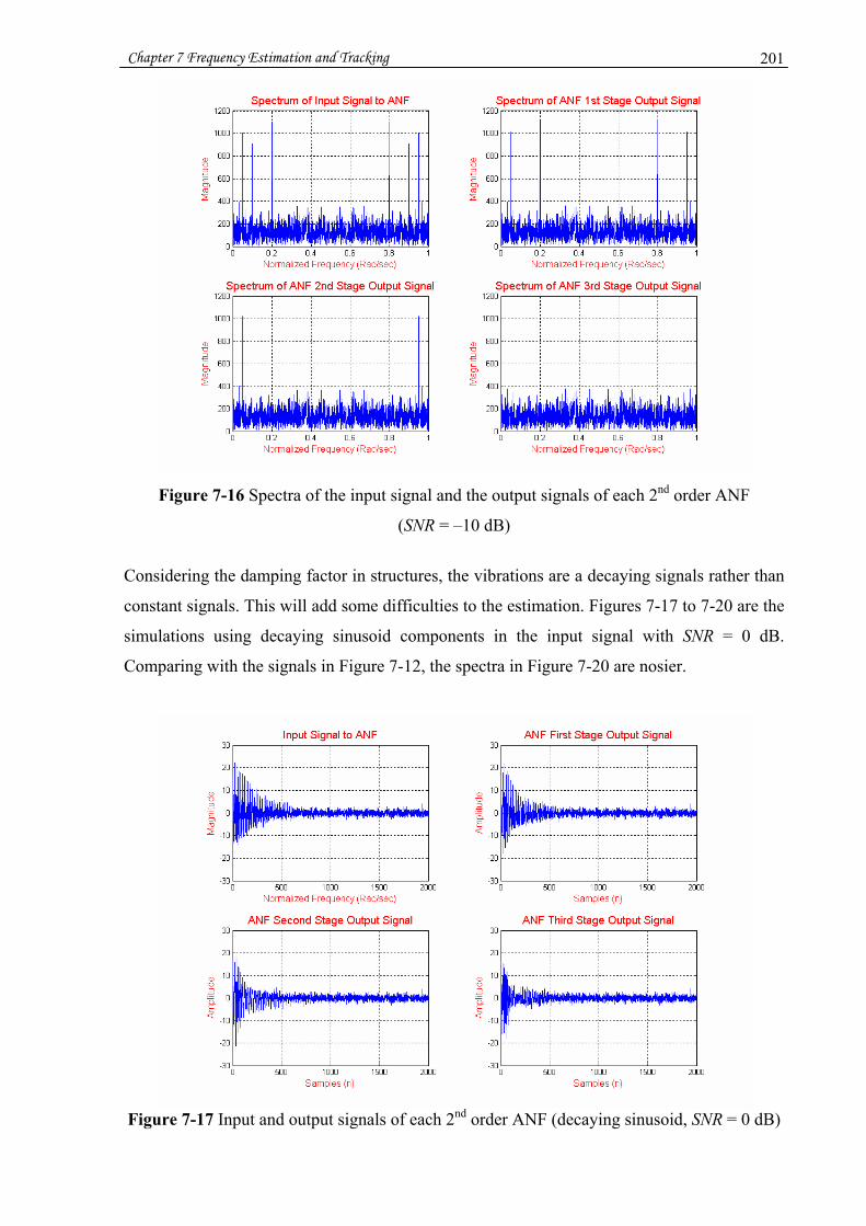
Chapter 7 Frequency Estimation and Tracking 201
Figure 7-16 Spectra of the input signal and the output signals of each 2nd order ANF
(SNR = –10 dB)
Considering the damping factor in structures, the vibrations are a decaying signals rather than
constant signals. This will add some difficulties to the estimation. Figures 7-17 to 7-20 are the
simulations using decaying sinusoid components in the input signal with SNR = 0 dB.
Comparing with the signals in Figure 7-12, the spectra in Figure 7-20 are nosier.
Figure 7-17 Input and output signals of each 2nd order ANF (decaying sinusoid, SNR = 0 dB)
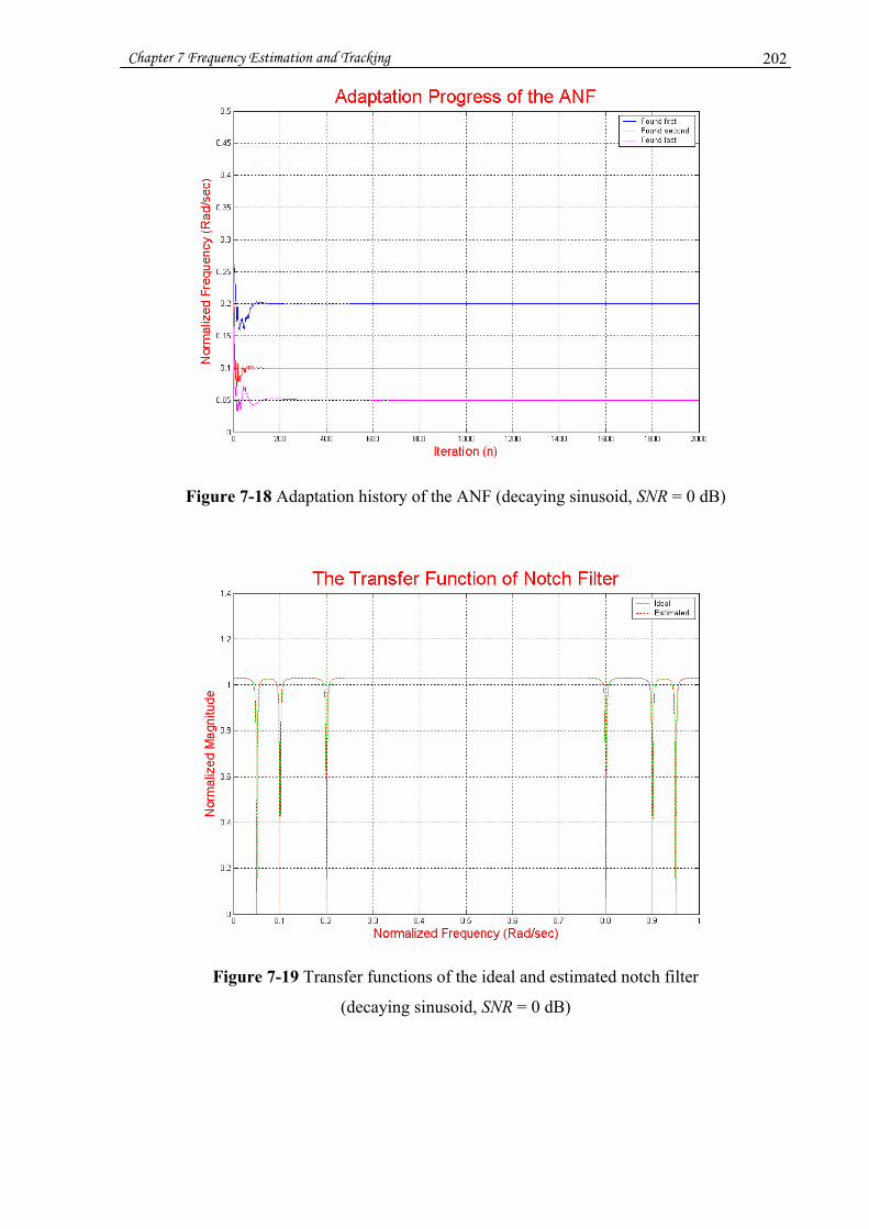
Chapter 7 Frequency Estimation and Tracking 202
Figure 7-18 Adaptation history of the ANF (decaying sinusoid, SNR = 0 dB)
Figure 7-19 Transfer functions of the ideal and estimated notch filter
(decaying sinusoid, SNR = 0 dB)

Chapter 7 Frequency Estimation and Tracking 203
Figure 7-20 Spectra of the input signal and the output signals of each 2nd order ANF
(decaying sinusoid, SNR = 0 dB)
7.4 Chapter summary
In this chapter, a frequency estimation method using an adaptive notch filter has been
presented. The notch filter structure adopted is a constrained poles and zeros IIR structure,
which is an approximation of the ideal notch filter but needs only half parameters to be
adapted compared with using an ideal one. To estimate n frequency components, n number of
2nd order IIR adaptive notch filter can be cascaded. Each of them is responsible for estimating
one frequency component. The adaptive algorithm used is the recursive least-squares (RLS)
algorithm. It is a fast and efficient algorithm. An example of three cascaded 2nd order adaptive
notch filters was given and simulated. The results show that the notch filter was correctly
converged to the frequency components contained in the input signals. With the help of
frequency estimation, it is possible to tune the gyrator-based inductor in the passive
piezoelectric shunt control automatically with the frequency controlled resistor or capacitor to
track the natural frequency shift of the Cricket bat.
This remained an analytical study into frequency tracking for use in a digital control system
for a Cricket bat and was hence not implemented in the analogue shunt control system
designed and implemented in the prototype Smart Cricket bat described in the previous
chapters.
Chapter 8 Conclusions and Future work 204
Chapter 8
Conclusions and Future Work
Overview
This research project has explored the possibility of vibration control using Smart materials in
combination with electronics and signal processing techniques to reduce the vibration of
Cricket bats. The emphasis has been on the passive piezoelectric vibration shunt control
method so far. Substantial analytical analyses, numerical simulations and practical
experiments have been carried out. The prototype of the newly designed Cricket bat has been
designed, evaluated and fabricated.
Although some vibration reduction of the Cricket bat has been achieved, it is the best that
could be achieved given the technology used and the restrictions dictated by the rules of the
game of Cricket. There are two major reasons which make the task difficult. One is that the
governing rules of the Cricket game prevent the radical modification of the Cricket bat. The
other is that unlike tennis, the racket or baseball bat, made of thin carbon-fibre or aluminium
materials (which are light and have small inherent damping factor), the Cricket bat (made of a
thick wooden chunk) has a much larger mass which will acquire much more mechanical
energy after the collision with a Cricket ball. Also, the large inherent damping factor of wood
makes the external damping less significant as a result. This requires much more control
energy being applied to the Cricket bat to achieve a reasonable and notable vibration
reduction. In spite of these restrictions, the vibration reductions reported are nevertheless
significant when compared to technological improvements in the field of sporting
implements.
The work carried out is an initial trial and has paved the way for future work. The conclusions
from work undertaken so far and suggestions for future work are described in the following
subsections.
Chapter 8 Conclusions and Future work 205
8.1 Conclusions
8.1.1 Analytical work on the PZT-based vibration shunt circuit
In chapter 3, an analytical study of resistor-inductor piezoelectric vibration shunt control on a
cantilever beam was carried out. The equation of motion of the beam attached with the PZT
patch and coupled with electrical shunt network has been derived by using Hamilton’s
principle and solved with the help of Galerkin’s method. The analysis has shown the physical
interaction between mechanical energy and electrical energy related by the constitutive
equations of piezoelectric materials. This augments the theoretical understanding of the
passive piezoelectric vibration shunt control.
8.1.2 Field-coupled simulations
Extensive numerical simulations with the FEA software package ANSYS® have been
conducted. Significant effort has been spent on developing the ANSYS® program for the
passive piezoelectric vibration shunt control which can help to analyse, design and optimise
the structure and control system prior to actual physical experimentation and implementation.
Some simulation results have been presented in chapters 4 & 5. With the help of the ANSYS®
simulations, it was found that the material properties and geometrical sizes of the structure
and piezoelectric transducer have significant influence on the effectiveness of the passive
piezoelectric vibration shunt control.
8.1.3 Cricket bat innovations
Chapter 4 has been a thorough analysis of the strain generated in the piezoelectric transducer
with respect to the geometry sizes and material properties of the transducer and the structure
to be controlled. It was found that the neutral axis/surface of the composite structure
determines the amount of strain produced in the transducer. Carbon-fibre material has been
suggested to be a medium between the structure and the piezoelectric transducer in order to
produce more strain in the piezoelectric transducer. The simulation and experimental results
have shown that the passive piezoelectric vibration shunt control is markedly effective with
respect to the vibration control of carbon-fibre materials.
A comparative experimental study of the passive piezoelectric vibration shunt controls of
aluminium, wooden and carbon-fibre composite beams was carried out. The experimental
results have shown that excellent vibration reduction can be achieved with the carbon-fibre
composite beam that matches the results of analytical analyses and numerical simulations.
This finding is significant and can result in several other applications for structural vibration

Chapter 8 Conclusions and Future work 206
control. The proposed Cricket bat handle, partially made of carbon-fibre composite material,
is one of the possible applications.
A novel sandwiched Cricket bat handle has been designed. The handle, incorporated with
specifically designed high stiffness-to-weight ratio advanced carbon-fibre composites strips
and a shunted piezoelectric sensor/actuator, has produced a reduction in the transient vibration
in the Cricket bat upon impact with a Cricket ball. In addition, another advantage of using the
carbon-fibre strips is that the natural frequencies of the Cricket bat have been increased.
The piezoelectric vibration shunt control circuit has been made and used for vibration control
for beams and Cricket bats. It has found that the efficiency of the vibration shunt control
(vibration reduction) is in proportion to the power supply of the shunt circuit. The higher the
supply voltage, the better the vibration reduction. A small circuit, such as this, has been
embedded in the Cricket bat handle to control the Cricket bat vibration.
8.1.4 Frequency tracking analysis
To account for the variable natural frequencies of Cricket bats due to the natural variability of
wood types and the time dependency of this variation due to the usage of the bat, it become
necessary to track and identify these changing frequencies using built-in hardware. The
method of fast estimating and tracking multiple frequency components buried in a noisy
signal by using cascaded 2nd order adaptive notch filters has been presented in chapter 7. The
method can be used for detecting the natural frequency of structures, such as Cricket bats and
adjust the control frequency in real-time which is crucial for achieving a high efficiency in the
piezoelectric vibration shunt control. It is possible to implement the adaptive notch filter in
hardware and embed it in the structure to automatically tune the control frequency of the
shunt circuit by adjusting some kind of variable resistors and capacitors to track the natural
frequencies of the structure.
8.1.5 Power amplifier proposal
In appendix 4, a novel power amplifier for driving the piezoelectric actuator, by using an
amplitude modulation technique and a piezoelectric transformer, has been proposed.
8.1.6 Cricket bat prototyping and field testing
Two Smart Cricket bats have been prototyped and field tested. The preliminary feedback has
been positive from these field tests undertaken by experienced Cricket players. However,
before the merits of the Smart bat can be declared, more robust batting at the nets and

Chapter 8 Conclusions and Future work 207
evaluation will be needed from top-class batsmen. Future work to improve the bat is
suggested in the next section.
8.2 Future work
There are many new aspects which could be pursued in the future to improve the Smart
Cricket bat.
On Smart Cricket bat technology improvements
To optimise the thickness and the Young’s modulus of the carbon-fibre strips to maximize
the strain produced in the PZT patch.
To increase the natural frequencies of the Cricket bat by selecting the material property
and geometry size of the carbon-fibre strips but in the meantime maintain the anti-node of
the first mode residing in the handle area.
To try to use the soft piezoelectric transducer (piezoelectric fibre composite) instead of the
hard piezoelectric transducer for the shunt control.
To implement the adaptive notch filter into a digital-based hardware together with an
automatic tuning mechanism to tune the gyrator-based inductor according to the frequency
being estimated.
To improve the engineering work in making the bat handle, including finding a proper
location to embed the shunt circuit, battery, and using automatic switches such as a
motion switch to turn the control circuit OFF and ON.
To increase the supply voltage of the shunt circuit. To replace battery power by a self-
powered system that is a challenging task.
If both the self-powered system and miniature power amplifier for driving the
piezoelectric actuator can be developed, the active piezoelectric vibration control will be a
better alternative to the passive piezoelectric vibration shunt control.
On the developed Smart Cricket bat
To investigate which bending mode does the most damage to cricket players.
More field testing by top class batsmen will be needed on the developed Smart Cricket bat
in order to comprehensively evaluate the performance of the bat.
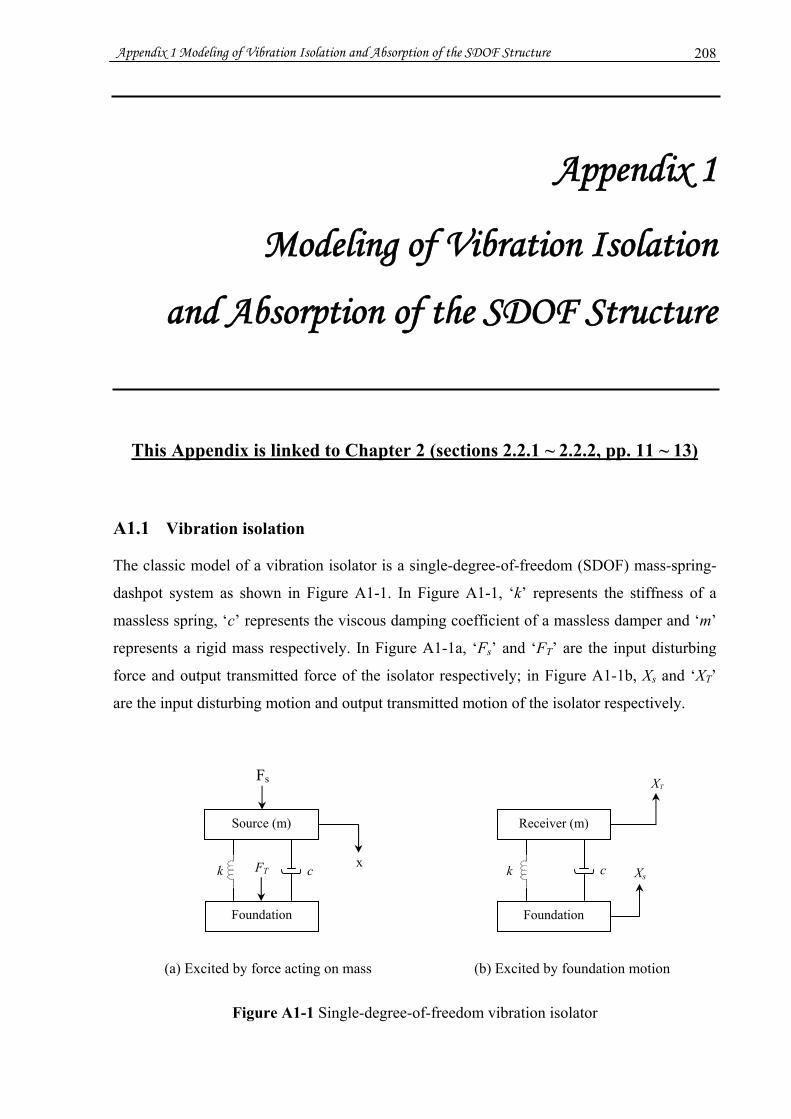
Appendix 1 Modeling of Vibration Isolation and Absorption of the SDOF Structure 208
Appendix 1
Modeling of Vibration Isolation
and Absorption of the SDOF Structure
This Appendix is linked to Chapter 2 (sections 2.2.1 ~ 2.2.2, pp. 11 ~ 13)
A1.1 Vibration isolation
The classic model of a vibration isolator is a single-degree-of-freedom (SDOF) mass-spring-
dashpot system as shown in Figure A1-1. In Figure A1-1, ‘k’ represents the stiffness of a
massless spring, ‘c’ represents the viscous damping coefficient of a massless damper and ‘m’
represents a rigid mass respectively. In Figure A1-1a, ‘Fs’ and ‘FT’ are the input disturbing
force and output transmitted force of the isolator respectively; in Figure A1-1b, Xs and ‘XT’
are the input disturbing motion and output transmitted motion of the isolator respectively.
(a) Excited by force acting on mass (b) Excited by foundation motion
Figure A1-1 Single-degree-of-freedom vibration isolator
FT
Fs
x
Source (m)
c k
Foundation
XT
Xs c k
Foundation
Receiver (m)

Appendix 1 Modeling of Vibration Isolation and Absorption of the SDOF Structure 209
The purpose of the isolator is to make the amplitude of TF (or TX ) less than the amplitude of
SF (or SX ). The SDOF isolator in Figure A1-1a can be described by differential equations,
)()( tFtkxxcxm s=++ . (A1.1)
)()( tkxxctFT += . (A1.2)
Where dot (·) represents time derivation.
The Laplace transform of the Equations (A1.1) and (A1.2) are
( ) )()(2 sFsXkcsms s=++ . (A1.3)
( ) )()( sXkcssFT += . (A1.4)
Transmissibility ( FT ), which is used to describe the effectiveness of a vibration isolation
system, is defined by the ratio of the transmitted force ( TF ) of an isolated system to the input
disturbing force (F) (Dimarogonas, 1996). From Equations (A1.3) and (A1.4), one can obtain,
22
2
22
2
2 22
22
)()(
)()(
)()()(
nn
nn
n
nT
s
TF ss
sss
skcsms
kcssFsX
sXsF
sFsFsT
ωζωωζω
ωσωσ
+++
=++
+=
+++
=== . (A1.5)
where
mk
n =ω –– Undamped natural frequency of the isolation system.
nmc ζωσ ==
2 –– Damping factor.
kmc
cc
c 2== ζ –– Damping ratio.
nc mc ω2= –– Critical damping.
The frequency response of the transmissibility can be expressed as:
222
2
2222
22
22
2
)2()1()2(1
)2()(
)2(2)(
2)(rr
rjj
jjTnn
nn
nn
nnF ζ
ζωζωωω
ζωωωωωζωω
ωωζωω+−
+=
+−
+=
+++
= . (A1.6)
Where nn ffr ==
ωω is the ratio of the disturbing force frequency to the natural frequency of
the isolation system.
Similarly, the transmissibility of the isolation system in Figure A1-1b, )()()(
sXsXsT
s
TX = , will
have the same result.
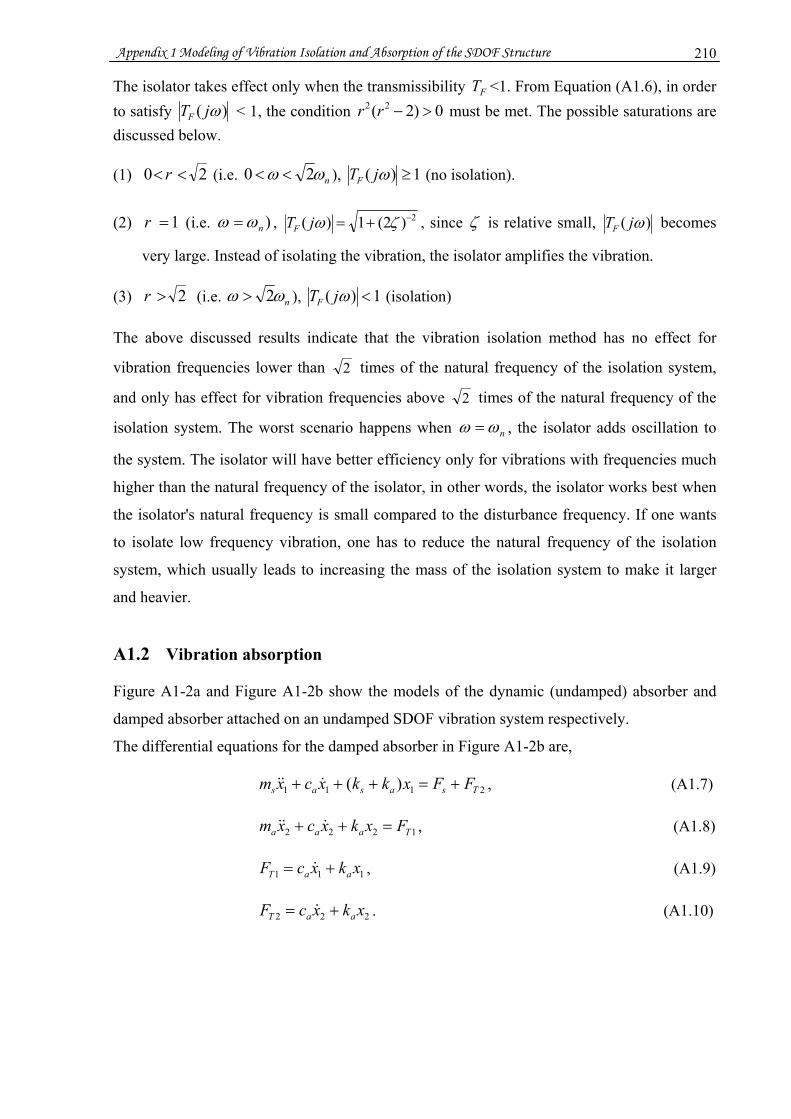
Appendix 1 Modeling of Vibration Isolation and Absorption of the SDOF Structure 210
The isolator takes effect only when the transmissibility FT <1. From Equation (A1.6), in order to satisfy )( ωjTF < 1, the condition 0)2( 22 >−rr must be met. The possible saturations are discussed below.
(1) 20 << r (i.e. nωω 20 << ), 1)( ≥ωjTF (no isolation).
(2) 1= r (i.e. )nωω = , 2)2(1)( −+= ζωjTF , since ζ is relative small, )( ωjTF becomes
very large. Instead of isolating the vibration, the isolator amplifies the vibration.
(3) 2> r (i.e. nωω 2> ), 1)( <ωjTF (isolation)
The above discussed results indicate that the vibration isolation method has no effect for
vibration frequencies lower than 2 times of the natural frequency of the isolation system,
and only has effect for vibration frequencies above 2 times of the natural frequency of the
isolation system. The worst scenario happens when nωω = , the isolator adds oscillation to
the system. The isolator will have better efficiency only for vibrations with frequencies much
higher than the natural frequency of the isolator, in other words, the isolator works best when
the isolator's natural frequency is small compared to the disturbance frequency. If one wants
to isolate low frequency vibration, one has to reduce the natural frequency of the isolation
system, which usually leads to increasing the mass of the isolation system to make it larger
and heavier.
A1.2 Vibration absorption
Figure A1-2a and Figure A1-2b show the models of the dynamic (undamped) absorber and
damped absorber attached on an undamped SDOF vibration system respectively.
The differential equations for the damped absorber in Figure A1-2b are,
2111 )( Tsasas FFxkkxcxm +=+++ , (A1.7)
1222 Taaa Fxkxcxm =++ , (A1.8)
111 xkxcF aaT += , (A1.9)
222 xkxcF aaT += . (A1.10)

Appendix 1 Modeling of Vibration Isolation and Absorption of the SDOF Structure 211
(a) Dynamic (undamped) absorber (b) Damped absorber
Figure A1-2 Models of vibration absorber
Substituting Equation (A1.9) and Equation (A1.10) into Equation (A1.7) and Equation (A1.8)
obtains Equation (A1.11) and Equation (A1.12),
saasaas Fxkxkkxcxcxm =−++−+ 21211 )( , (A1.11)
021212 =+−+− xkxkxcxcxm aaaaa . (A1.12)
Equation (A1.11) and Equation (A1.12) can be written as matrix format in Equation (A1.13),
⎥⎦
⎤⎢⎣
⎡=⎥
⎦
⎤⎢⎣
⎡⎥⎦
⎤⎢⎣
⎡+⎥
⎦
⎤⎢⎣
⎡⎥⎦
⎤⎢⎣
⎡+⎥
⎦
⎤⎢⎣
⎡⎥⎦
⎤⎢⎣
⎡02
1
2221
1211
2
1
2221
1211
2
1
2221
1211 sFxx
kkkk
xx
cccc
xx
mmmm
. (A1.13)
where
smm =11 , 02112 == mm , amm =22 ,
accc == 2211 , accc −== 2112 ,
as kkk +=11 , akkk −== 2112 , akk =22 .
Equation (A1.13) can be simplified as,
FKXXCXM =++ . (A1.14)
where
⎥⎦
⎤⎢⎣
⎡=
2221
1211
mmmm
M , ⎥⎦
⎤⎢⎣
⎡=
2221
1211
cccc
C , ⎥⎦
⎤⎢⎣
⎡=
2221
1211
kkkk
K , ⎥⎦
⎤⎢⎣
⎡=
2
1
xx
X , ⎥⎦
⎤⎢⎣
⎡=
2
1
xx
X , ⎥⎦
⎤⎢⎣
⎡=
2
1
xx
X ,
Absorber x2
ma
ca ka
x1
ks
ms
sF
1TF
2TF
Absorber x2
ma
ka
x1
ks
ms
sF
1TF
2TF
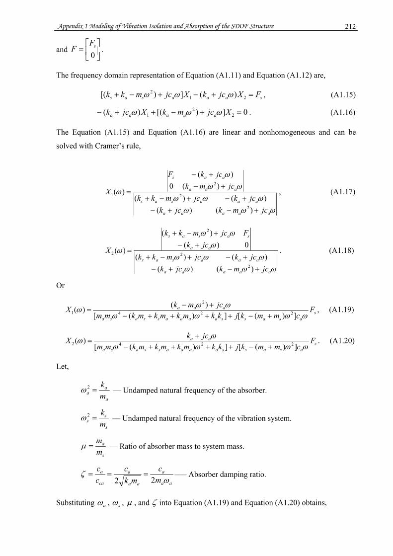
Appendix 1 Modeling of Vibration Isolation and Absorption of the SDOF Structure 212
and ⎥⎦
⎤⎢⎣
⎡=
0sF
F .
The frequency domain representation of Equation (A1.11) and Equation (A1.12) are,
saaasas FXjckXjcmkk =+−+−+ 212 )(])[( ωωω , (A1.15)
0])[()( 22
1 =+−++− XjcmkXjck aaaaa ωωω . (A1.16)
The Equation (A1.15) and Equation (A1.16) are linear and nonhomogeneous and can be
solved with Cramer’s rule,
ωωωωωω
ωωω
ω
aaaaa
aaasas
aaa
aas
jcmkjckjckjcmkk
jcmkjckF
X
+−+−+−+−+
+−+−
=
)()()()(
)(0)(
)(
2
2
2
1 , (A1.17)
ωωωωωω
ωωω
ω
aaaaa
aaasas
aa
sasas
jcmkjckjckjcmkk
jckFjcmkk
X
+−+−+−+−+
+−+−+
=
)()()()(
0)()(
)(
2
2
2
2 . (A1.18)
Or
sasassaaaassasa
aaa Fcmmkjkkmkmkmkmm
jcmkXωωωω
ωωω])([])([
)()( 224
2
1 +−++++−+−
= , (A1.19)
sasassaaaassasa
aa Fcmmkjkkmkmkmkmm
jckXωωωω
ωω])([])([
)( 2242 +−++++−+
= . (A1.20)
Let,
a
aa m
k=2ω –– Undamped natural frequency of the absorber.
s
ss m
k=2ω –– Undamped natural frequency of the vibration system.
s
a
mm
=μ –– Ratio of absorber mass to system mass.
aa
a
aa
a
ca
a
mc
mkc
cc
ωζ
22=== ––– Absorber damping ratio.
Substituting aω , sω , μ , and ζ into Equation (A1.19) and Equation (A1.20) obtains,
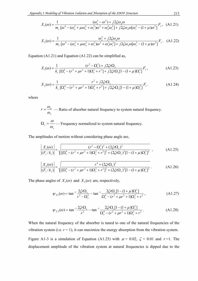
Appendix 1 Modeling of Vibration Isolation and Absorption of the SDOF Structure 213
ssasasaa
aa
s
Fj
jm
X])1([2])([
2)(1)( 222222224
22
1 ωμωωζωωωωωμωωωωζωωωω
+−++++−+−
= , (A1.21)
ssasasaa
aa
s
Fj
jm
X])1([2])([
21)( 222222224
2
2 ωμωωζωωωωωμωωωωζωωω
+−++++−+
= . (A1.22)
Equation (A1.21) and Equation (A1.22) can be simplified as,
sssss
ss
s
Frjrrr
rjrk
X])1(1[2])1([
2)(1)( 222224
22
1 Ω+−Ω++Ω++−ΩΩ+Ω−
=μζμ
ζω , (A1.23)
sssss
s
s
Frjrrr
rjrk
X])1(1[2])1([
21)( 222224
2
2 Ω+−Ω++Ω++−ΩΩ+
=μζμ
ζω . (A1.24)
where
s
arωω
= –– Ratio of absorber natural frequency to system natural frequency.
ss ω
ω=Ω –– Frequency normalized to system natural frequency.
The amplitudes of motion without considering phase angle are,
222222224
22221
])1(1[)2(])1([)2()(
)/()(
ssss
ss
ss rrrrrr
kFX
Ω+−Ω++Ω++−ΩΩ+Ω−
=μζμ
ζω , (A1.25)
222222224
242
])1(1[)2(])1([)2(
)/()(
ssss
s
ss rrrrrr
kFX
Ω+−Ω++Ω++−ΩΩ+
=μζμ
ζω . (A1.26)
The phase angles of )(1 ωX and )(2 ωX are, respectively,
22224
21
221
1 )1(])1(1[2tan2tan)(
rrrr
rr
ss
ss
s
sX +Ω++−Ω
Ω+−Ω−
Ω−Ω
= −−
μμζζωψ , (A1.27)
22224
21
21
2 )1(])1(1[2tan2tan)(
rrrr
rr
ss
sssX +Ω++−Ω
Ω+−Ω−
Ω= −−
μμζζωψ . (A1.28)
When the natural frequency of the absorber is tuned to one of the natural frequencies of the
vibration system (i.e. r = 1), it can maximize the energy absorption from the vibration system.
Figure A1-3 is a simulation of Equation (A1.25) with μ = 0.02, ζ = 0.01 and r =1. The
displacement amplitude of the vibration system at natural frequencies is dipped due to the
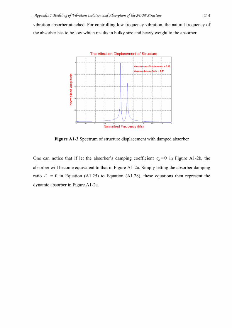
Appendix 1 Modeling of Vibration Isolation and Absorption of the SDOF Structure 214
vibration absorber attached. For controlling low frequency vibration, the natural frequency of
the absorber has to be low which results in bulky size and heavy weight to the absorber.
Figure A1-3 Spectrum of structure displacement with damped absorber
One can notice that if let the absorber’s damping coefficient 0=ac in Figure A1-2b, the
absorber will become equivalent to that in Figure A1-2a. Simply letting the absorber damping
ratio ζ = 0 in Equation (A1.25) to Equation (A1.28), these equations then represent the
dynamic absorber in Figure A1-2a.

Appendix 2 Estimation of System Damping 215
Appendix 2
Estimation of System Damping
This Appendix is linked to Chapter 2 (section 2.2.3, pp. 13 ~ 16)
The system damping can be estimated either in frequency domain or in time domain. In this
appendix, the damping estimation of a single degree of freedom (SDOF) structure is
described. The methods may work with a bandpass filter to estimate the damping ratio of each
individual mode of a MDOF system separately.
A2.1 Frequency domain estimation
The basic model for the SDOF system is shown in Figure A2-1. The system consists of a
mass (m), a spring (k) and a viscous dashpot (c), where )(tf and )(tx are general time-
varying force and displacement response quantities respectively (Ewins, 2002).
Figure A2-1 Single-degree-of-freedom (SDOF) system (Ewins, 2002)
f
x (t)
m
ck

Appendix 2 Estimation of System Damping 216
According to Newton’s law, the differential motion equation of the SDOF system can be
derived as
)()()()( tftkxtxctxm =++ . (A2.1)
From Equation (A2.1), the Laplace transfer function of the SDOF system can be expressed as,
mks
mcs
mkcsmssF
sXsH++
=++
==2
2
/11)()()(
2222 2/1
2/1
nnn ssm
ssm
ωζωωσ ++=
++= . (A2.2)
where
mk
n =ω –– Undamped natural frequency of the isolation system.
nmc ζωσ ==
2 –– Damping factor.
kmc
cc
c 2== ζ –– Damping ratio.
nc mc ω2= –– Critical damping.
The frequency domain transfer function of the Equation (A2.2) is
ωζωωω
ωnn j
mjH2)(
/1)( 22 +−= . (A2.3)
The amplitude of the transfer function without considering phase angle is
222222 4)(
/1)(ωωζωω
ωnn
mjH+−
= . (A2.4)
At the centre frequency nω ,
221)(
nn m
jHζω
ω = . (A2.5)
Assume 1ω and 2ω are the 3 dB frequencies and 1ω < nω < 2ω . According to the definition
that the amplitude at 3 dB frequency points are equal to 2/1 times the amplitude at centre
frequency which is represented by Equation (A2.5), that is,

Appendix 2 Estimation of System Damping 217
)2(21
4)(/1)( 22
122222
11
nnn mmjH
ζωωωζωωω =
+−= ,
)2(21
4)(/1)(
222
222222
2nnn m
mjHζωωωζωω
ω =+−
= .
Since
)( 1ωjH = )( 2ωjH ,
that is
22
222222
21
222221 4)(4)( ωωζωωωωζωω nnnn +−=+− ,
or
)(4))(2( 21
22
2221
22
22
21
2 ωωωζωωωωω −−=−−− nn ,
or
))(())(()()(4 221122
221
222nnnnnnn ωωωωωωωωωωωωωζ +−−+−=−+−=− .
For a small damping system, which has narrow frequency bandwidth, has the following
relation,
nnn ωωωωω ≈−=− )()( 21 ,
then,
)())(()]())[((4 2121121122 ωωωωωωωωωωωωωωζ −≈−−=+−+−=− nnnnnn .
Therefore, the damping ratio ζ can be expressed as,
nnn ff
fff
2221212 Δ=
−=
−=
ωωωζ ( 1f < 2f ). (A2.6)
Equation (A2.6) indicates that the damping ratio of a lightly damped SDOF system ccc /=ζ
can be estimated in frequency domain by measuring the centre frequency nf and its
bandwidth fΔ . This method is often used in experiments to determine the damping ratio of
vibration modes in frequency domain. Figure A2-2 shows the zoomed frequency response of
a SDOF system.
where 50=nf Hz, 158.1==Δ dff Hz, using Equation (A2.6), the damping ratio can be
estimated as
01.050*2
158.12
≈==nf
dfζ .

Appendix 2 Estimation of System Damping 218
Figure A2-2 Frequency response of a SDOF system
A2.2 Time domain estimation
The SDOF system represented by Equation (A2.2) can be rewritten as,
2222 )(/1
2/1)(
dnnn sm
ssmsH
ωζωωζω ++=
++= . (A2.7)
where
nd ωζω 21−= –– Damped natural frequency of the system.
By inverse the Laplace transform, the impulse response of the SDOF system can be obtained
as,
)sin()(~)sin(1)( tthtem
th ddt
d
n ωωω
ζω == − )0( ≥t . (A2.8)
where
tt
d
nn ehem
th ζωζω
ω−− == )0(~1)(~
and )0(~h is the value of )(~ th at t = 0.

Appendix 2 Estimation of System Damping 219
)(th decays along with time and the speed of the decay reflects the amount of damping in the
system which is only influenced by the )(~ th . Applying logarithmic on )(~ th , thus the damping
ratio can be estimated by the following equation,
⎟⎟⎠
⎞⎜⎜⎝
⎛=
)(~)0(~
ln1
11 thh
tnωζ . (A2.9)
where “ ln ” donates the logarithm to base e. Therefore, in time domain by measuring two
amplitudes of )(~ th , such as )0(~h at 0=t and )(~1th at 1tt = . Then the damping ratio ζ can
be obtained by Equation (A2.9).
The Figure A2-3 is an impulse response of the SDOF system which shows that at 0=t ,
1)0(~=h , and at 11 == tt (s), 0432.0)(~
1 =th . By Equation (A2.9), the damping ratio can be
estimated as,
01.00432.01ln
1*50**21
)(~)0(~
ln1
11
≈⎟⎠⎞
⎜⎝⎛=⎟⎟
⎠
⎞⎜⎜⎝
⎛=
πωζ
thh
tn.
which matches the result estimated in frequency domain previously.
Figure A2-3 Impulse response of a SDOF system

Appendix 3 Positive Position Feedback (PPF) Control 220
Appendix 3
Positive Position Feedback (PPF) Control
This Appendix is linked to Chapter 2 (section 2.3.4, p. 36)
In the section below, a brief description about PPF control applied to a structure is given. The
homogeneous differential equations representing a SDOF structure and a second order
bandpass filter can be represented as,
Structure: 02 2 =⋅+⋅⋅⋅+ ξωξωςξ sss , (A3.1)
Filter: 02 2 =⋅+⋅⋅⋅+ ηωηωςη ccc . (A3.2)
where ξ , η , sς , cς , sω , cω are modal coordinators, damping ratios, resonant frequencies of
the structure and electronic filter respectively.
The block diagram of the SDOF structure with a PPF controller applied is as shown in Figure
A3-1 (Song et al, 2000).
Figure A3-1 Block diagram of SDOF structure with PPF control (Song et al, 2000)
The differential equations to describe the SDOF structure with PPF control shown in Figure
A3-1 are,
Disturbance
Electronic Filter
Structure
02 2 =++ ξωξωςξ sss
02 2 =++ ηωηωςη ccc
2sGω 2
cω
ξ
η
++

Appendix 3 Positive Position Feedback (PPF) Control 221
ηωξωξωςξ ⋅⋅=⋅+⋅⋅⋅+ 222 ssss G , (A3.3)
ξωηωηωςη ⋅=⋅+⋅⋅⋅+ 222 cccc . (A3.4)
where G is a gain factor.
Combine the Fourier transform of Equations (A3.3) and (A3.4) one can have
)()(2)(
)( 22
2
ωξωωςωω
ωωη jjj
jccc
c ⋅+⋅⋅⋅+
= . (A3.5)
The unforced vibration of the structure can be expressed as tj set ωαξ −=)( , the Equation
(A3.5) then becomes
)(21
)()(2)(
)(
2
222
2
s
c
sc
s
ss
ccc
c
jjj
j ωωδ
ωως
ωω
αωωδωωςωω
ωαωη −
⎟⎟⎠
⎞⎜⎜⎝
⎛+⎟⎟
⎠
⎞⎜⎜⎝
⎛−
=−++
⋅= . (A3.6)
where α is a constant and )(ωδ is Dirac’s delta function.
The inverse Fourier transform of Equation (A3.6) is
)(1 )()( ϕωβωηη +− ⋅=ℑ= tj sejt . (A3.7)
with
22
2
2
2
41 ⎟⎟⎠
⎞⎜⎜⎝
⎛+⎟⎟
⎠
⎞⎜⎜⎝
⎛−
=
c
sc
c
s
ωως
ωω
αβ and
⎟⎟⎟⎟⎟
⎠
⎞
⎜⎜⎜⎜⎜
⎝
⎛
−−= −
2
21
1
2tan
c
s
c
sc
ωωωως
ϕ .Equation (A3.7) can be
discussed in following three different saturations:
(1) When the structure vibrates at a frequency much lower than the filter’s resonant
frequency (i.e. sω << cω ) the phase angle ϕ approaches to zero according to Equation
(A3.7). Then, )()( )( teet titi ξββη ωϕω =⋅≈⋅= ⋅+⋅ . (A3.8)
Substitute Equation (A3.8) into Equation (A3.3) results in
0)(2 22 =⋅⋅⋅−+⋅⋅⋅+ ξωβωξωςξ ssss G . (A3.9)
Equation (A3.9) shows that the PPF controller in this case results in the stiffness term of the
structure being decreased, which is called active flexibility.

Appendix 3 Positive Position Feedback (PPF) Control 222
(2) When the filter’s resonant frequency is equal to the structure natural frequency (i.e. sω =
cω ), the phase angle ϕ in Equation (A3.7) equals to 2/π− . Then
)()()( )2/( teieiets
tis
s
titi ss ξωβω
ωβββη ωωπω ⋅−=⋅⋅−=⋅⋅−≈⋅= ⋅⋅⋅⋅−⋅ . (A3.10)
Substitute Equation (A3.10) into Equation (A3.3) results in
0)2( 2 =⋅+⋅⋅⋅+⋅⋅+ ξωξωβωςξ ssss G . (A3.11)
Equation (A3.11) shows that the PPF controller in this case results in an increase in the
damping term of the structure, which is called active damping.
(3) When the structure frequency is much greater than that of the filter (i.e. sω >> cω ), the
phase angle ϕ approaches π− . Then,
)()( )( teet titi s ξββη ωπω −=⋅−=⋅≈ ⋅⋅⋅−⋅ . (A3.12)
Substitute Equation (A3.12) into Equation (A3.3) results in
0)(2 22 =⋅⋅⋅++⋅⋅⋅+ ξωβωξωςξ ssss G . (A3.13)
Equation (A3.13) shows that the PPF controller in this case results in an increase in the
stiffness term of the structure, which is called active stiffness.
Figure A3-2 is the simple SIMULINK model of a SDOF structure applied with PPF control
under the condition: Hz100 == sc ff , sς = 0.02 and cς = 0.48, the input signal is an
impulse (created by the difference of two step signals).
Figure A3-2 SIMULINK model of SDOF structure with positive position feedback
Figure A3-3 shows the simulation results of the SIMULINK model in Figure A3-2. The graph
in (a) and (b) are the impulse response and frequency response respectively. Blue colour
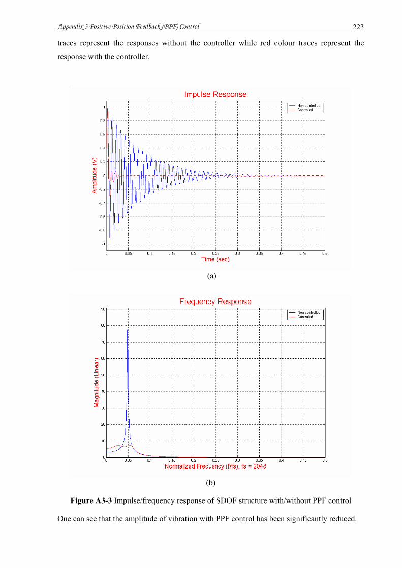
Appendix 3 Positive Position Feedback (PPF) Control 223
traces represent the responses without the controller while red colour traces represent the
response with the controller.
(a)
(b)
Figure A3-3 Impulse/frequency response of SDOF structure with/without PPF control
One can see that the amplitude of vibration with PPF control has been significantly reduced.

Appendix 3 Positive Position Feedback (PPF) Control 224
Figure A3-4 is the SIMULINK model of a 4-DOF structure applied with PPF control under
the condition: cf = sf = 50, 100, 200, and 500 Hz, sς = 1.6E-3, 8E-4, 4E-4, and 1.6E-4, cς =
0.32, 0.32, 0.24, and 0.16 respectively.
Figure A3-4 SIMULINK model of 4-DOF structure with positive position feedback
Figure A3-5 is the simulation results of the 4-DOF structure with/without PPF control. The
graph in (a) and (b) are the impulse response and frequency response respectively. Blue
colour traces represent the responses without PPF control while red colour traces represent the
response with PPF control.
The frequency response shows that the magnitudes of the structure’s vibration at natural
frequencies have been reduced simultaneously when multiple PPF control is applied. A real
complex flexible structure often can be modelled approximately with a finite number degree
of freedom. Each of them can be targeted with a second order bandpass filter using PPF
method.
Appendix 3 Positive Position Feedback (PPF) Control 225
(a)
(b)
Figure A3-5 Impulse/frequency response of 4-DOF structure with/without PPF control

Appendix 4 Proposed Power Amplifier using Amplitude Modulation and Piezoelectric Transformer for Active Vibration Control
226
Driver section Generator section
Appendix 4
Proposed Power Amplifier using
Amplitude Modulation and Piezoelectric
Transformer for Active Vibration Control
This Appendix is linked to Chapter 2 (sections 2.3.5 ~ 2.3.6, pp. 40 ~ 43)
Since a piezoelectric transformer (PT) is a very promising alternative to the traditional
electromagnetic transformer for active vibration control as demonstrated by Carazo et al in
(Carazo, 2001), we here propose a novel design of a power amplifier using amplitude
modulation (AM) and a piezoelectric transformer for driving the piezoelectric actuator which
can be compact and energy efficient. The purpose of using the amplitude modulation
technique is to shift the frequency of actuation signal to the resonant frequency of the
piezoelectric transformer to achieve maximum voltage step-up.
Figure A4-1 Rosen type piezoelectric transformer

Appendix 4 Proposed Power Amplifier using Amplitude Modulation and Piezoelectric Transformer for Active Vibration Control
227
PT is ultrasonic resonators with two pairs of electrodes provided on the surface of a
piezoelectric material, in which electrical energy is carried in the mechanical form. The PT
uses both the direct and indirect piezoelectric effects; an applied voltage results in vibration,
which in turn generates the output voltage. The input and output electrodes are arranged to
provide the impedance transformation, which results in the voltage transformation. PT
consists of two piezoelectric material parts, which are driver and generator section with
different polarization as shown in Figure A4-1.
Figure A4-2 shows (a) the Transoner® PT with 25 mm diameter, 6 mm total thickness and
power capability higher than 70 W, made by FACE Electronics, LC, and (b) the PT
characteristics, voltage step-up voltage ratio vs. load (Carazo, 2001).
(a) (b)
Figure A4-2 (a) Transoner® piezoelectric transformer, (b) step-up voltage ratio vs. load
The PTs have many advantages, in addition to being EMI-free, they are generally lighter,
smaller, non-flammable, have high efficiency (over 95 %), high power capacity per unit
volume leading to smaller size, high Q factor, large voltage step-up at resonant frequency, and
a high degree of insulation.
However, PTs have large voltage step-up only at their resonant frequencies, while the
electrical actuation signals to drive actuators can have any frequency, usually there are much
lower than the resonant frequencies of PTs. The main idea behind the proposed design is to
use amplitude modulation (AM) technique to modulate the actuation signal by a carrier which
frequency matches the resonant frequency of a PT, thus the AM signal can be largely
amplified by the PT. The amplified AM signal must be demodulated to reconstruct the
actuation signal before driving the actuator. The demodulation procedure is simply by passing

Appendix 4 Proposed Power Amplifier using Amplitude Modulation and Piezoelectric Transformer for Active Vibration Control
228
the amplified AM signal through a rectifier then to a lowpass filter. With a design such as this,
the active electronic components may only be needed for the low voltage part of the circuit
while the high voltage section can use only passive electronic components. Figure A4-3 is the
block diagram of the proposed AM power amplifier.
Figure A4-3 Block diagram of an AM power amplifier
Figure A4-4 PSpice® functional model of an AM amplifier
Figure A4-4 is the PSpice® functional model of the proposed AM amplifier, where its
assumed that the actuation signal to be amplified is 1V/100 Hz, carrier signal is 1V/100 kHz,
Vb is a bias voltage to adjust the percentage of modulation, the transformer used here is the
electromagnetic transformer of PSpice® model (TX1) for function verification, the coupling
coefficient and ratio of transformation of the transformer are 1 and 1:2500 (i.e. voltage step-
A
B
C
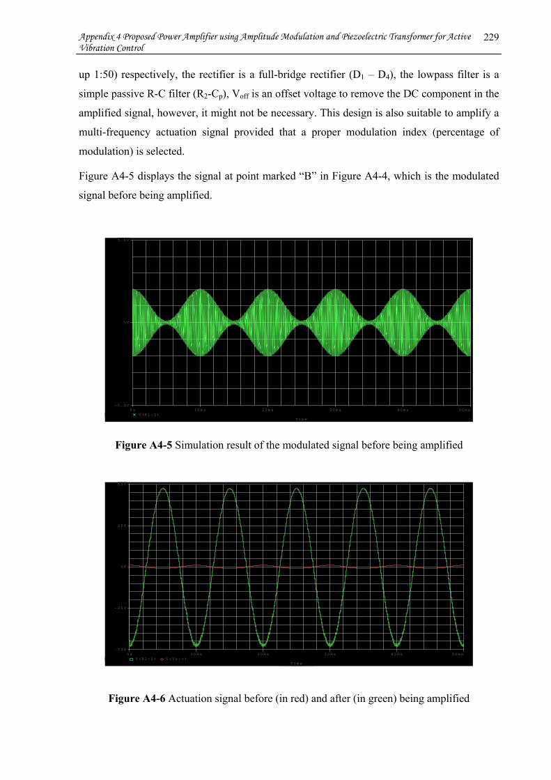
Appendix 4 Proposed Power Amplifier using Amplitude Modulation and Piezoelectric Transformer for Active Vibration Control
229
up 1:50) respectively, the rectifier is a full-bridge rectifier (D1 – D4), the lowpass filter is a
simple passive R-C filter (R2-Cp), Voff is an offset voltage to remove the DC component in the
amplified signal, however, it might not be necessary. This design is also suitable to amplify a
multi-frequency actuation signal provided that a proper modulation index (percentage of
modulation) is selected.
Figure A4-5 displays the signal at point marked “B” in Figure A4-4, which is the modulated
signal before being amplified.
T i m e
0 s 1 0 m s 2 0 m s 3 0 m s 4 0 m s 5 0 m sV ( R 1 : 2 )
- 5 . 0 V
0 V
5 . 0 V
Figure A4-5 Simulation result of the modulated signal before being amplified
T i m e
0 s 1 0 m s 2 0 m s 3 0 m s 4 0 m s 5 0 m sV ( R 2 : 2 ) V ( V s : + )
- 5 0 V
- 2 5 V
0 V
2 5 V
5 0 V
Figure A4-6 Actuation signal before (in red) and after (in green) being amplified
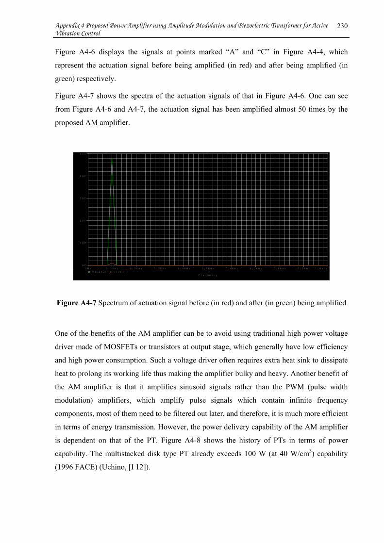
Appendix 4 Proposed Power Amplifier using Amplitude Modulation and Piezoelectric Transformer for Active Vibration Control
230
Figure A4-6 displays the signals at points marked “A” and “C” in Figure A4-4, which
represent the actuation signal before being amplified (in red) and after being amplified (in
green) respectively.
Figure A4-7 shows the spectra of the actuation signals of that in Figure A4-6. One can see
from Figure A4-6 and A4-7, the actuation signal has been amplified almost 50 times by the
proposed AM amplifier.
F r e q u e n c y
0 H z 0 . 1 K H z 0 . 2 K H z 0 . 3 K H z 0 . 4 K H z 0 . 5 K H z 0 . 6 K H z 0 . 7 K H z 0 . 8 K H z 0 . 9 K H z 1 . 0 K H zV ( R 2 : 2 ) V ( V s : + )
0 V
1 0 V
2 0 V
3 0 V
4 0 V
5 0 V
Figure A4-7 Spectrum of actuation signal before (in red) and after (in green) being amplified
One of the benefits of the AM amplifier can be to avoid using traditional high power voltage
driver made of MOSFETs or transistors at output stage, which generally have low efficiency
and high power consumption. Such a voltage driver often requires extra heat sink to dissipate
heat to prolong its working life thus making the amplifier bulky and heavy. Another benefit of
the AM amplifier is that it amplifies sinusoid signals rather than the PWM (pulse width
modulation) amplifiers, which amplify pulse signals which contain infinite frequency
components, most of them need to be filtered out later, and therefore, it is much more efficient
in terms of energy transmission. However, the power delivery capability of the AM amplifier
is dependent on that of the PT. Figure A4-8 shows the history of PTs in terms of power
capability. The multistacked disk type PT already exceeds 100 W (at 40 W/cm3) capability
(1996 FACE) (Uchino, [I 12]).
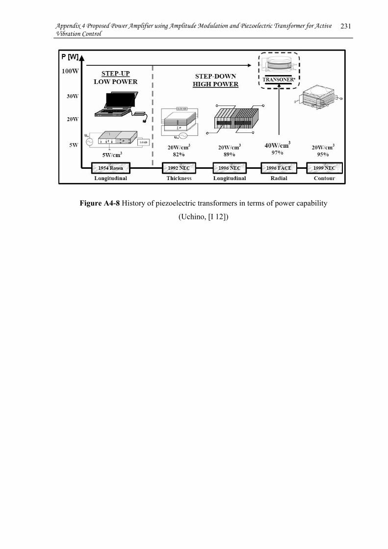
Appendix 4 Proposed Power Amplifier using Amplitude Modulation and Piezoelectric Transformer for Active Vibration Control
231
Figure A4-8 History of piezoelectric transformers in terms of power capability
(Uchino, [I 12])

Appendix 5 Beam Modelling and Modal Analysis 232
Appendix 5
Beam Modelling and Modal Analysis
This Appendix is linked to Chapter 3 (Sections 3.1, pp. 46 ~ 55)
Here we first derive the motion equation of a cantilever beam using energy principles and
variational methods with the general consideration that the beam is not only affected by the
bending moment, but also by shear force and rotary inertia. Then simplify the motion
equation gradually to the Euler-Bernoulli modal and give an example of the modal shape of
the Euler-Bernoulli beam.
A5.1 Potential energy and kinetic energy of a vibration beam
Two types of energies are usually used to describe the beam vibration, i.e. potential energy
and kinetic energy. Part of the potential energy is due to bending moment and part of it is due
to shear force. The kinetic energy is partly from the displacement of a beam element parallel
to the axis perpendicular to the beam principle plane, and partly from the rotation of the same
element. Figure A5-1 depicts the vibration of a beam element with moment inertia, rotary
inertia and shear deformation (Tse, 1978).
In the Figure A5-1, xw∂∂ is the slope due to bending moment M , Sθ is the slope due to shear
force Q , and bθ is the slope combining bending moment and shear force, i.e. Sbxw θθ −=∂∂ .
Neglecting the interaction between the shear and the bending moment, the shear force Q will
cause a rectangular element to become a parallelogram (in broken line) without a rotation of
the faces (Tse, 1978).

Appendix 5 Beam Modelling and Modal Analysis 233
Figure A5-1 Vibration of beam element with rotary inertia and shear deformation
The potential energy or strain energy for the small neutral axis deflections along z axis due to
the bending moment is defined as document
( ) dxdAx
txzEdxdAEdVUL
Ab
b
L
A xbV xxb ∫ ∫∫ ∫∫ ⎟⎟⎠
⎞⎜⎜⎝
⎛⎟⎠⎞
⎜⎝⎛
∂∂
===0
2
0
2 ),(21
21
21 θεσε
( ) dxx
txIEdxdAzx
txEL b
bb
L
Ab
b ∫∫ ∫ ⎟⎠⎞
⎜⎝⎛
∂∂
=⎥⎥⎦
⎤
⎢⎢⎣
⎡⎟⎠⎞
⎜⎝⎛
∂∂
=0
2
0
22 ),(
21),(
21 θθ . (A5.1)
where bE is the Young’s modulus, xσ is the axial stress, L, A, and V are the length, cross-
sectional area, and volume of the beam respectively. bI is the moment of inertia of the beam
cross-sectional area with respect to z axis, dAzIAb ∫= 2 .
The potential energy due to shear force is defined as
∫∫ ⎟⎠⎞
⎜⎝⎛
∂∂
−=⎟⎠⎞
⎜⎝⎛
∂∂
=L
b
L ss dx
xtxwtxGAkdx
xtxGAkU
0
22
0
),(),('21),('
21 θθ . (A5.2)
where
'k and G are the shear stiffness factor and shear modulus of the beam respectively
(Fung, 2001). The shear stiffness factor is the inverse of shape factor that is ratio of the plastic
section modulus to the elastic section modulus and depends on the cross-sectional shape
(Young et al, 2002).
The potential energy of the beam is then,
Q
z
x
),( txw
Normal to cross- sectional area
(Total slope)
(Bending slope)
(Shear slope)Sθ
xw∂∂M
dxx
MM∂∂
+
dxxQQ∂∂
+
bθ

Appendix 5 Beam Modelling and Modal Analysis 234
∫∫ ⎟⎠⎞
⎜⎝⎛
∂∂
−+⎟⎠⎞
⎜⎝⎛
∂∂
=+=L
b
L bbbsb dx
xtxwtxGAkdx
xtxIEUUU
0
2
0
2 ),(),('21),(
21 θθ . (A5.3)
The kinetic energy from the displacement of the beam element parallel to z coordinate is
defined as
dxt
txwATL
bd
2
0
),(21∫ ⎟
⎠⎞
⎜⎝⎛
∂∂
= ρ , (A5.4)
The kinetic energy from the rotation of the same beam element about an axis perpendicular to
the neutral axis is defined as
dxt
txJTL b
br
2
0
),(21∫ ⎟
⎠⎞
⎜⎝⎛
∂∂
=θ , (A5.5)
where bρ is the density of the beam, bbb IJ ρ= (Dimarogonas, 1996) donates the mass
moment of inertia about neutral axis per unit length of the beam, xtxw ∂∂ /),( is the
translational velocity and xtxb ∂∂ /),(θ is the angular velocity of the beam.
The kinetic energy of the beam is then,
dxt
txJdxt
txwATTTL b
b
L
brd
2
0
2
0
),(21),(
21
∫∫ ⎟⎠⎞
⎜⎝⎛
∂∂
+⎟⎠⎞
⎜⎝⎛
∂∂
=+=θρ . (A5.6)
The potential energy due to external transverse load ),( txp , the bending moment and shear
force at the beam ends x = 0 and x = L, i.e. 0M , LM , 0Q , LQ , is
00000),(),( wQwQMMdxtxwtxpA LLLL
L−++−−= ∫ θθ . (A5.7)
A5.2 Motion equation derivation of beam using Hamilton’s principle
The motion equation of beam can be derived by the Hamilton’s principle
∫ =+−2
1
0)t
tdtATU
δ (A5.8)
that is
dxpwt
JtwA
xwGAk
xIE
t
t
L bbbb
sbbb∫ ∫
⎪⎩
⎪⎨⎧
⎥⎥⎦
⎤
⎢⎢⎣
⎡−⎟
⎠⎞
⎜⎝⎛∂∂
−⎟⎠⎞
⎜⎝⎛∂∂
−⎟⎠⎞
⎜⎝⎛
∂∂
−+⎟⎠⎞
⎜⎝⎛∂∂2
1 0
2222
21
21
221
θρθθδ
00000 =⎭⎬⎫
−++ dtwQwQMM LLLL θθ . (A5.9)

Appendix 5 Beam Modelling and Modal Analysis 235
For the first potential energy term in Equation (A5.9) due to bending moment, there is
dtdxxx
IEdtdxx
IEdtdxx
IEt
t
L bbbb
t
t
L bbb
t
tbL
bb
∫ ∫∫ ∫∫ ∫ ⎟⎠⎞
⎜⎝⎛
∂∂
∂∂
=⎟⎟⎠
⎞⎜⎜⎝
⎛⎟⎠⎞
⎜⎝⎛∂∂
=⎟⎟⎠
⎞⎜⎜⎝
⎛⎟⎠⎞
⎜⎝⎛∂∂ 2
1
2
1
2
1 00
22
0
)(21
21 δθθθδθδ .
Let
,)(',)()(x
xgx
xf bb
∂∂
=∂
∂=
θδθ
Using integration by parts (i.e. ∫ ∫−= dxxfxgxgxfdxxgxf )(')()()()(')( ), we obtain,
dtdxxx
IEdtdxxx
IEt
t
L
bb
L
bb
bb
t
t
L bbbb
∫ ∫∫ ∫ ⎟⎟⎠
⎞⎜⎜⎝
⎛
∂∂
−∂
∂=⎟⎟
⎠
⎞⎜⎜⎝
⎛⎟⎠⎞
⎜⎝⎛
∂∂
⎟⎠⎞
⎜⎝⎛∂∂ 2
1
2
1 0 2
2
00
)()()()()( θδθθδθδθθ ,
Thus,
dtdxxx
IEdtdxx
IEt
t
L
bb
L
bb
bb
t
tbL
bb
∫ ∫∫ ∫ ⎟⎟⎠
⎞⎜⎜⎝
⎛
∂∂
−∂∂
=⎟⎟⎠
⎞⎜⎜⎝
⎛⎟⎠⎞
⎜⎝⎛∂∂ 2
1
2
1 0 2
2
0
2
0)()(
21 δθθδθθθδ . (A5.10)
For the second potential energy term in Equation (A5.9) due to shear force, there is
dtdxxw
xwkdtdx
xwk
t
t
L
bb
t
t
L
b ∫ ∫∫ ∫ ⎥⎦
⎤⎢⎣
⎡⎟⎠⎞
⎜⎝⎛
∂∂
−⎟⎠⎞
⎜⎝⎛
∂∂
−=⎥⎥⎦
⎤
⎢⎢⎣
⎡⎟⎠⎞
⎜⎝⎛
∂∂
− 2
1
2
1 00
2 )(21
δδθθθδ
dtdxxwdx
xw
xwk
t
t
L L
bbb∫ ∫ ∫ ⎥⎦
⎤⎢⎣
⎡⎟⎠⎞
⎜⎝⎛ −
∂∂
−⎟⎠⎞
⎜⎝⎛ −
∂∂
∂∂
= 2
1 0 0
)()(
δθδθδθδ
.
where GAkk '= .
Let
⎟⎠⎞
⎜⎝⎛ −
∂∂
= bxwxf δθδ )()( ,
xwxg∂∂
=)(' ,
Using integrating by parts to the first integration yields
dtdxwxx
wwxwkdt
xw
xwk
t
t
L bL
b
t
t
L
b ∫ ∫∫ ∫⎥⎥⎦
⎤
⎢⎢⎣
⎡⎟⎟⎠
⎞⎜⎜⎝
⎛∂∂
−∂∂
−⎟⎠⎞
⎜⎝⎛ −∂∂
=⎟⎠⎞
⎜⎝⎛ −
∂∂
∂∂ 2
1
2
1 0 2
2
00
)()()(
δθδθδθδ ,
Therefore, the second potential energy term is
dtdxxwkt
t
L
b∫ ∫⎥⎥⎦
⎤
⎢⎢⎣
⎡⎟⎠⎞
⎜⎝⎛ −∂∂2
1 0
2
2
θδ
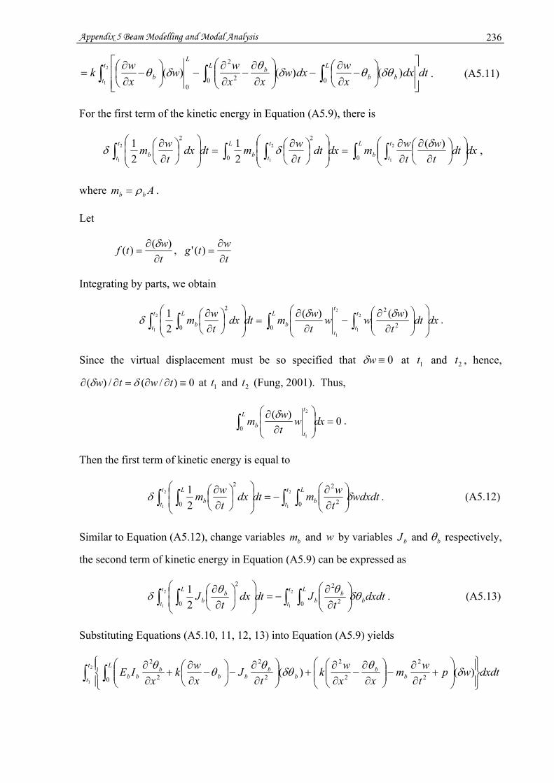
Appendix 5 Beam Modelling and Modal Analysis 236
dtdxxwdxw
xxww
xwk
t
t
L L
bbb
L
b∫ ∫ ∫⎥⎥⎦
⎤
⎢⎢⎣
⎡⎟⎠⎞
⎜⎝⎛ −∂∂
−⎟⎟⎠
⎞⎜⎜⎝
⎛∂∂
−∂∂
−⎟⎠⎞
⎜⎝⎛ −∂∂
= 2
1 0 02
2
0
)()()(
δθθδθδθ . (A5.11)
For the first term of the kinetic energy in Equation (A5.9), there is
dxdttw
twmdxdt
twmdtdx
twm
L t
tb
L t
tb
t
t b ∫ ∫∫ ∫∫ ⎟⎟⎠
⎞⎜⎜⎝
⎛⎟⎠⎞
⎜⎝⎛
∂∂
∂∂
=⎟⎟⎠
⎞⎜⎜⎝
⎛⎟⎠⎞
⎜⎝⎛∂∂
=⎟⎟⎠
⎞⎜⎜⎝
⎛⎟⎠⎞
⎜⎝⎛∂∂
00
22 )(21
21 2
1
2
1
2
1
δδδ ,
where Am bb ρ= .
Let
twtg
twtf
∂∂
=∂
∂= )(' ,)()( δ
Integrating by parts, we obtain
dxdtt
wwwtwmdtdx
twm
L t
t
t
tb
t
t
L
b ∫ ∫∫ ∫ ⎟⎟⎠
⎞⎜⎜⎝
⎛⎟⎟⎠
⎞⎜⎜⎝
⎛∂
∂−
∂∂
=⎟⎟⎠
⎞⎜⎜⎝
⎛⎟⎠⎞
⎜⎝⎛∂∂
0 2
22
0
)()(21 2
1
2
1
2
1
δδδ .
Since the virtual displacement must be so specified that 0≡wδ at 1t and 2t , hence,
0)/(/)( ≡∂∂=∂∂ twtw δδ at 1t and 2t (Fung, 2001). Thus,
0)(0
2
1
=⎟⎟⎠
⎞⎜⎜⎝
⎛
∂∂
∫ dxwtwm
Lt
tb
δ .
Then the first term of kinetic energy is equal to
wdxdttwmdtdx
twm
t
t
L
b
t
t
L
b δδ ∫ ∫∫ ∫ ⎟⎟⎠
⎞⎜⎜⎝
⎛∂∂
−=⎟⎟⎠
⎞⎜⎜⎝
⎛⎟⎠⎞
⎜⎝⎛∂∂ 2
1
2
1 0 2
2
0
2
21
. (A5.12)
Similar to Equation (A5.12), change variables bm and w by variables bJ and bθ respectively,
the second term of kinetic energy in Equation (A5.9) can be expressed as
dxdtt
Jdtdxt
J b
t
t
L bb
t
t
L bb δθθθδ ∫ ∫∫ ∫ ⎟⎟
⎠
⎞⎜⎜⎝
⎛∂∂
−=⎟⎟⎠
⎞⎜⎜⎝
⎛⎟⎠⎞
⎜⎝⎛∂∂ 2
1
2
1 0 2
2
0
2
21
. (A5.13)
Substituting Equations (A5.10, 11, 12, 13) into Equation (A5.9) yields
dxdtwptwm
xxwk
tJ
xwk
xIE
t
t
L
bb
bb
bbb
bb∫ ∫ ⎪⎭
⎪⎬⎫
⎪⎩
⎪⎨⎧
⎟⎟⎠
⎞⎜⎜⎝
⎛+
∂∂
−⎟⎟⎠
⎞⎜⎜⎝
⎛∂∂
−∂∂
+⎟⎟⎠
⎞⎜⎜⎝
⎛∂∂
−⎟⎠⎞
⎜⎝⎛ −∂∂
+∂∂2
1 0 2
2
2
2
2
2
2
2
)()(
δθδθθθθ

Appendix 5 Beam Modelling and Modal Analysis 237
0)()(0
=⎪⎭
⎪⎬⎫
⎟⎟⎠
⎞⎜⎜⎝
⎛⎟⎟⎠
⎞⎜⎜⎝
⎛+⎟
⎠⎞
⎜⎝⎛ −∂∂
+⎟⎠⎞
⎜⎝⎛ −
∂∂
+ dtwQxwkM
xIE
L
bbb
bb δθδθθ . (A5.14)
In order for Equation (A5.14) to be true for any virtual displacements bδθ and wδ , the
following partial differential equations can be obtained
02
2
2
2
=∂∂
−⎟⎠⎞
⎜⎝⎛ −∂∂
+∂∂
tJ
xwk
xIE b
bbb
bbθθθ , (A5.15)
02
2
2
2
=+∂∂
−⎟⎟⎠
⎞⎜⎜⎝
⎛∂∂
−∂∂ p
twm
xxwk b
bθ , (A5.16)
Reorganize the Equation (A5.16) as
⎟⎟⎠
⎞⎜⎜⎝
⎛+
∂∂
−∂∂
=∂∂ p
twm
xwk
kx bb
2
2
2
21θ . (A5.17)
Perform a derivate of x to Equation (A5.15) once and then substitute the derivation xb ∂∂ /θ
by Equation (A5.17) to eliminate the variable bθ as below
⎟⎟⎠
⎞⎜⎜⎝
⎛⎟⎟⎠
⎞⎜⎜⎝
⎛+
∂∂
−∂∂
−∂∂
+⎟⎟⎠
⎞⎜⎜⎝
⎛+
∂∂
−∂∂
∂∂ p
twm
xwk
kxwkp
twm
xwk
xkIE
bbbb
2
2
2
2
2
2
2
2
2
2
2
2 1
– 02
2
2
2
2
2
=⎟⎟⎠
⎞⎜⎜⎝
⎛+
∂∂
−∂∂
∂∂ p
twm
xwk
tkJ
bb .
or
2
2
2
2
2
2
22
4
4
4
4
4
tp
kJ
xp
kIEp
twm
txw
kmIEJ
tw
kmJ
xwIE bbb
bbbb
bb
bbb ∂∂
+∂∂
−=∂∂
+∂∂
∂⎟⎠⎞
⎜⎝⎛ +−
∂∂
+∂∂ . (A5.18)
with boundary conditions at beam ends
either Mx
IE bbb −∂∂θ = 0 or bδθ = 0. (A5.19a)
and
either 0=+⎟⎠⎞
⎜⎝⎛ −∂∂ Q
xwk bθ or wδ = 0. (A5.19b)
Equation (A5.18) is the Timoshenko equation for lateral vibration of beams, which has
included not only the displacement due to the bending moment, but also the displacements
affected by shear deformation and rotary inertia. However, the effects of shear and rotation
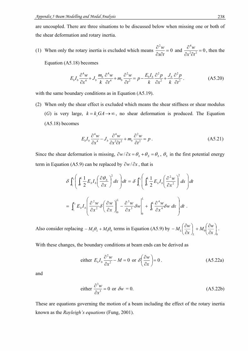
Appendix 5 Beam Modelling and Modal Analysis 238
are uncoupled. There are three situations to be discussed below when missing one or both of
the shear deformation and rotary inertia.
(1) When only the rotary inertia is excluded which means 02
=∂∂
∂tx
w and 022
4
=∂∂
∂tx
w , then the
Equation (A5.18) becomes
2
2
2
2
2
2
4
4
4
4
tp
kJ
xp
kIEp
twm
tw
kmJ
xwIE bbb
bb
bbb ∂∂
+∂∂
−=∂∂
+∂∂
+∂∂ . (A5.20)
with the same boundary conditions as in Equation (A5.19).
(2) When only the shear effect is excluded which means the shear stiffness or shear modulus
(G) is very large, ∞→= GAkk s , no shear deformation is produced. The Equation
(A5.18) becomes
ptwm
txwJ
xwIE bbbb =
∂∂
+∂∂
∂−
∂∂
2
2
22
4
4
4
. (A5.21)
Since the shear deformation is missing, bSbxw θθθ =+=∂∂ / , bθ in the first potential energy
term in Equation (A5.9) can be replaced by xw ∂∂ / , that is
=⎟⎟⎠
⎞⎜⎜⎝
⎛⎟⎠⎞
⎜⎝⎛∂∂
∫ ∫ dtdxx
IEt
tbL
bb 2
1
2
0 21 θδ dtdx
xwIE
t
t
L
bb ∫ ∫ ⎟⎟
⎠
⎞
⎜⎜
⎝
⎛⎟⎟⎠
⎞⎜⎜⎝
⎛∂∂2
1
2
2
2
0 21δ
dtdxwxww
xw
xw
xwIE
t
t
LLL
bb ∫ ∫ ⎟⎟⎟
⎠
⎞
⎜⎜⎜
⎝
⎛
∂∂
+∂∂
−⎟⎠⎞
⎜⎝⎛∂∂
∂∂
=2
1 0 4
4
0
3
3
02
2
δδδ .
Also consider replacing 00θθ MM LL +− terms in Equation (A5.9) by 0
0 ⎟⎠⎞
⎜⎝⎛∂∂
+⎟⎠⎞
⎜⎝⎛∂∂
−xwM
xwM
LL .
With these changes, the boundary conditions at beam ends can be derived as
either 02
2
=−∂∂ M
xwIE bb or 0=⎟
⎠⎞
⎜⎝⎛∂∂
xwδ . (A5.22a)
and
either 03
3
=∂∂
xw or wδ = 0. (A5.22b)
These are equations governing the motion of a beam including the effect of the rotary inertia
known as the Rayleigh’s equations (Fung, 2001).
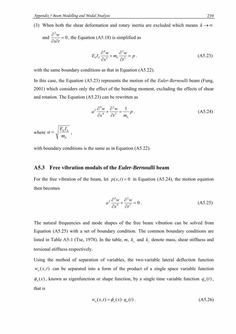
Appendix 5 Beam Modelling and Modal Analysis 239
(3) When both the shear deformation and rotary inertia are excluded which means ∞→k
and 02
=∂∂
∂tx
w , the Equation (A5.18) is simplified as
ptwm
xwIE bbb =
∂∂
+∂∂
2
2
4
4
. (A5.23)
with the same boundary conditions as that in Equation (A5.22).
In this case, the Equation (A5.23) represents the motion of the Euler-Bernoulli beam (Fung,
2001) which considers only the effect of the bending moment, excluding the effects of shear
and rotation. The Equation (A5.23) can be rewritten as
pmt
wxwa
b
12
2
4
42 =
∂∂
+∂∂ . (A5.24)
where b
bb
mIEa = ,
with boundary conditions is the same as in Equation (A5.22).
A5.3 Free vibration modals of the Euler-Bernoulli beam
For the free vibration of the beam, let 0),( =txp in Equation (A5.24), the motion equation
then becomes
02
2
4
42 =
∂∂
+∂∂
tw
xwa . (A5.25)
The natural frequencies and mode shapes of the free beam vibration can be solved from
Equation (A5.25) with a set of boundary condition. The common boundary conditions are
listed in Table A5-1 (Tse, 1978). In the table, m, sk and tk denote mass, shear stiffness and
torsional stiffness respectively.
Using the method of separation of variables, the two-variable lateral deflection function
),( txwn can be separated into a form of the product of a single space variable function
)(xnφ , known as eigenfunction or shape function, by a single time variable function )(tqn ,
that is
)()(),( tqxtxw nnn ⋅= φ . (A5.26)
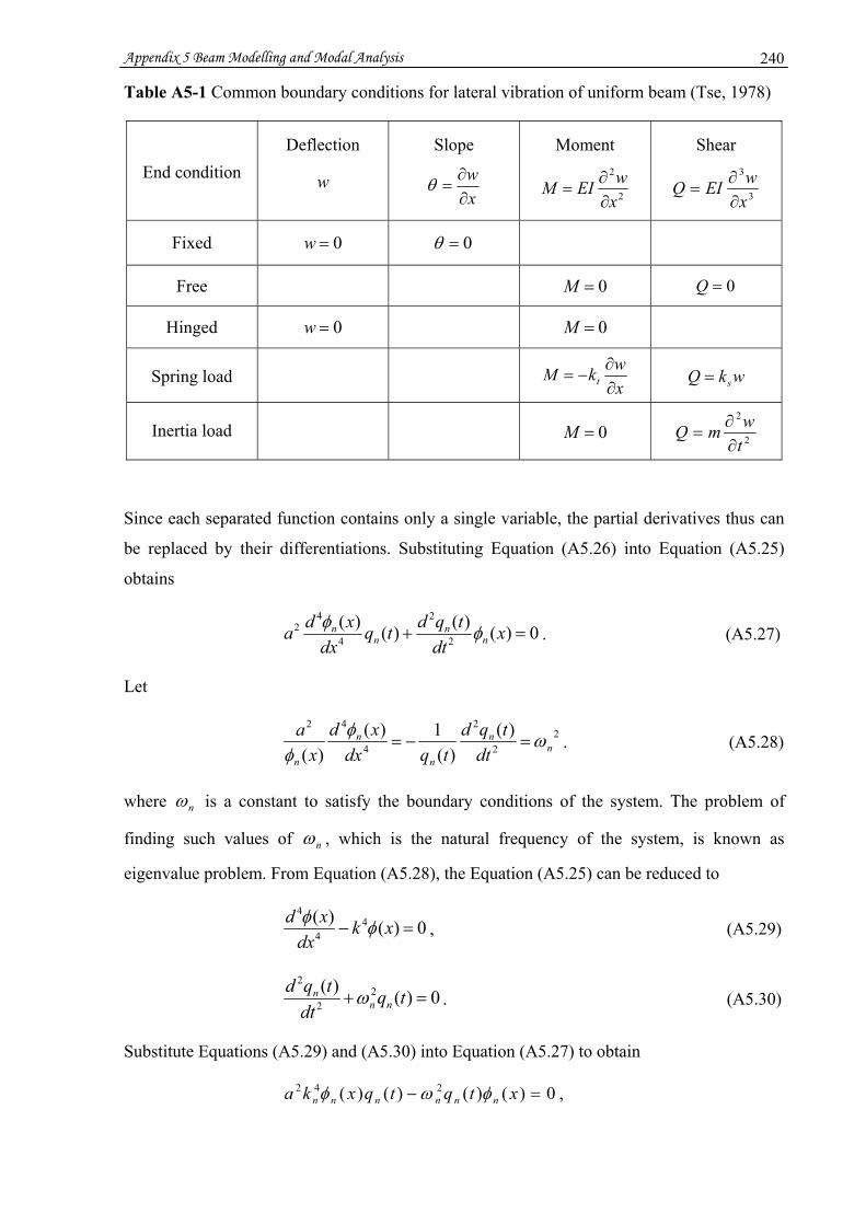
Appendix 5 Beam Modelling and Modal Analysis 240
Table A5-1 Common boundary conditions for lateral vibration of uniform beam (Tse, 1978)
End condition Deflection
w
Slope
xw∂∂
=θ
Moment
2
2
xwEIM
∂∂
=
Shear
3
3
xwEIQ
∂∂
=
Fixed 0=w 0=θ
Free 0=M 0=Q
Hinged 0=w 0=M
Spring load xwkM t ∂∂
−= wkQ s=
Inertia load 0=M 2
2
twmQ
∂∂
=
Since each separated function contains only a single variable, the partial derivatives thus can
be replaced by their differentiations. Substituting Equation (A5.26) into Equation (A5.25)
obtains
0)()()()(2
2
4
42 =+ x
dttqdtq
dxxda n
nn
n φφ. (A5.27)
Let
22
2
4
42 )()(
1)()( n
n
n
n
n dttqd
tqdxxd
xa ωφ
φ=−= . (A5.28)
where nω is a constant to satisfy the boundary conditions of the system. The problem of
finding such values of nω , which is the natural frequency of the system, is known as
eigenvalue problem. From Equation (A5.28), the Equation (A5.25) can be reduced to
0)()( 44
4
=− xkdx
xd φφ, (A5.29)
0)()( 22
2
=+ tqdt
tqdnn
n ω . (A5.30)
Substitute Equations (A5.29) and (A5.30) into Equation (A5.27) to obtain
0)()()()( 242 =− xtqtqxka nnnnnn φωφ ,

Appendix 5 Beam Modelling and Modal Analysis 241
results in
222nnka ω= ,
Thus
nn
bb
bnn IE
ma
kλπωω 2
4/12
4/1
2
2
=⎟⎟⎠
⎞⎜⎜⎝
⎛⋅=⎟⎟
⎠
⎞⎜⎜⎝
⎛= . (A5.31)
The parameters nk and nλ are the bending wavenumber and wavelength that have the units of
(1/Meter) and (Meter) respectively.
The neutral frequency is the function of nk
b
bbnn m
IEk 2=ω (n = 1, 2, …). (A5.32)
The solution for the free vibration of the Euler-Bernoulli beam is
)()()cos()sin()( 4321 xkchCxkshCxkCxkCx nnnnnnnnn +++=φ , (A5.33)
)cos()sin()( 65 tCtCtq nnnnn ωω += . (A5.34)
For example, for the clamped-free boundary conditions given in Table A2-1 ( 0)0( =w ,
0)0(' =w , 0)('' =Lw , 0)(''' =Lw ), the boundary conditions for Equation (A5.25) can be
expressed as
0)()()()(0
0====
====
Lx
n
x
nLxnxn dx
xddx
xdxx φφφφ . (A5.35)
Apply Equation (A5.35) to Equation (A5.33) to obtain,
0)(0=
=xn xφ leads to nn CC 24 −= .
0)(
0
==x
n
dxxdφ leads to nn CC 13 −= .
0)(2
2
==Lx
n
dxxd φ leads to 0)]()[cos()]()[sin( 21 =+++ nnnnnn CLkchLkCLkshLk .
0)(3
3
==Lx
n
dxxd φ
leads to 0)]()[sin()]()[cos( 21 =−−+ nnnnnn CLkshLkCLkchLk .
The matrix representation of the constants is

Appendix 5 Beam Modelling and Modal Analysis 242
⎥⎦
⎤⎢⎣
⎡=⎥
⎦
⎤⎢⎣
⎡⋅⎥
⎦
⎤⎢⎣
⎡+−+++
00
)()sin()()cos()()cos()()sin(
2
1
n
n
nnnn
nnnn
CC
LkshLkLkchLkLkchLkLkshLk
.
The non-zero solution of the constants nC1 and nC2 can be determined by solving the
following determinant
0)()sin()()cos(
)()cos()()sin(=
+−+++
LkshLkLkchLkLkchLkLkshLk
nnnn
nnnn
.
One can obtain the frequency equation
1)()cos( −=LkchLk nn . (A5.36)
Since
0)]()[cos()]()[sin( 21 =+++ nnnnnn CLkchLkCLkshLk and
0)]()[sin()]()[cos( 21 =−−+ nnnnnn CLkshLkCLkchLk , thus
)()cos()()sin(
)()sin()()cos(
2
1
LkchLkLkshLk
LkshLkLkchLk
CC
nn
nn
nn
nn
n
n
+−
=++
−= ,
From Equation (A5.33) and the coefficients nC1 , nC 2 , nC3 , nC 4 , the eigenfunction can be
obtained as
)]cos()([)]sin()([)( 21 xkxkchCxkxkshCx nnnnnnn −−−−=φ
⎥⎦
⎤⎢⎣
⎡−
++
−−−= )]sin()([)()sin()()cos()cos()(2 xkxksh
LkshLkLkchLkxkxkchC nn
nn
nnnnn . (A5.37)
Substitute from Equations (A5.34), (A5.37) to Equation (A5.36)
)()(),( tqxtxw nnn φ= =
)]cos()sin([)]sin()([)()sin()()cos()cos()( tBtAxkxksh
LkshLkLkchLkxkxkch nnnn
nn
nnnn ωω +⋅⎟⎟
⎠
⎞⎜⎜⎝
⎛−
++
−−.
(A5.38)
where nnCCA 52= and nnCCB 62−= .
The roots Lkn can be solved numerically from the frequency equation 1)()cos( =LkchLk nn .
The first six approximate values of Lkn are 1.8751, 4.6941, 7.8548, 10.9955, 14.1372, and

Appendix 5 Beam Modelling and Modal Analysis 243
17.2788. From Equation (A5.32), the natural frequencies of the clamped-free Euler-Bernoulli
beam can be calculated as
bb
bbn
b
bbnnn A
IEL
Lkm
IEkfρπππ
ω2
22
2)(
22 ⋅=== . (A5.39)
where bA is the cross-sectional area of the beam.
When the shear and rotation effects are considered, the value nk will decrease thus the natural
frequency nω will decrease as well. However, the influence is more pronounced for the
higher modes (Fung, 2001).
Figure A5-2 shows the first six normalized bending mode shapes of a clamped-free Euler-
Bernoulli beam.
Figure A5-2 Bending mode shapes of a clamped-free Euler-Bernoulli beam
A5.4 An example of obtaining mode shapes from experiment
Since the frequency response function (FRF) becomes purely imaginary at the modal
frequency (or natural frequency). Its amplitude is proportional to the modal displacement, and
its sign is positive if displacement is in phase with the excitation. The mode shapes can be
determined by exciting a set of FRFs at selected locations on the structure with one of them is

Appendix 5 Beam Modelling and Modal Analysis 244
fixed as a reference to measure the FRF responses. The imaginary parts of the measured the
FRFs can be "picked" at the modal frequencies at which they represent the modal
displacement for that specific DOF (Døssing, 1988). Figure A5-3 illustrates an example
explaining the method. In the example, DOF #2 is used as the response reference. A set of
FRFs is then measured by exciting each of the four defined DOFs in turn. The four imaginary
parts of the FRF for each modal frequency represent the associated mode shape. If the
measurements were made with calibrated instrumentation, the mode shapes could then be
scaled (Døssing, 1988).
Figure A5-3 Illustration of obtaining mode shapes of a structure from the imaginary part of
the FRFs (Døssing, 1988)
An experiment has been carried out on a steel beam which has size )(0030025050 3m ... ×× ,
the Young’s modulus )(1006.2 11 Pa Eb ×= , and the density )(7830 3kg/mb =ρ . The 1st to 6th
theoretical natural frequencies are: 9.943, 62.312, 174.475, 341.896, 565.185, and 844.284 Hz
respectively. The natural frequencies obtained from the experiment are: 10.0, 61.87, 171.88,
335.0, 561.25, and 834.38 Hz respectively.

Appendix 5 Beam Modelling and Modal Analysis 245
Figure A5-4 and A5-5 show the first six bending mode shapes of a clamped-free beam
obtained from experiments. Figure A5-4 is that before curve fitting and Figure A5-5 is that
after curve fitting.
Figure A5-4 Experimental mode shapes of a clamped-free beam before curve fitting
Figure A5-5 Experimental mode shapes of a clamped-free beam after curve fitting

Appendix 5 Beam Modelling and Modal Analysis 246
Figure A5-6 shows the comparison between theoretical and experimental mode shapes. The
1st to 3rd modes are given in Figure (a) and the 4th to 6th modes are given in Figure (b)
respectively. The two match reasonably well.
(a)
(b)
Figure A5-6 Comparison between theoretical and experimental mode shapes

Appendix 6 Derivation of the Equations in Chapter 3 247
Appendix 6
Derivation of the Equations in Chapter 3
This Appendix is lnked to Chapter 3 (section 3.1.5, p. 52 ~ 53 and section
3.2, p. 55)
A6.1 Derivation of the Equations (3.24 ~ 3.28) in Chapter 3.
Equation (3.24),
dxdttwAdtdx
twA
L t
tbb
t
t
L
bb ∫ ∫∫ ∫ ⎟⎟⎠
⎞⎜⎜⎝
⎛⎟⎠⎞
⎜⎝⎛∂∂
=⎟⎟⎠
⎞⎜⎜⎝
⎛⎟⎠⎞
⎜⎝⎛∂∂
0
22
0
2
1
2
1 21
21 δρρδ
dxdttw
twAdxdt
tw
twA
L t
tbb
L t
tbb ∫ ∫∫ ∫ ⎟⎟⎠
⎞⎜⎜⎝
⎛⎟⎠⎞
⎜⎝⎛
∂∂
∂∂
=⎟⎟⎠
⎞⎜⎜⎝
⎛⎟⎠⎞
⎜⎝⎛∂∂
∂∂
=
00
)(2
1
2
1
δρδρ (δ acts on ),( txw )
Let
twtg
twtf
∂∂
=∂
∂= )(' ,)()( δ
By integration by parts (that is ∫ ∫−= dttftgtgtfdttgtf )(')()()()(')( ), one obtains
dxdtt
wwwtwAdxdt
tw
twA
L t
t
t
tbb
L t
tbb ∫ ∫∫ ∫ ⎟⎟⎠
⎞⎜⎜⎝
⎛⎟⎟⎠
⎞⎜⎜⎝
⎛∂
∂−
∂∂
=⎟⎟⎠
⎞⎜⎜⎝
⎛⎟⎠⎞
⎜⎝⎛
∂∂
∂∂
0 2
2
0
)()()( 2
1
2
1
2
1
δδρδρ
dxdtwtwAdxdtw
twA
t
t
L
bb
L t
tbb
∫ ∫∫ ∫ ⎟⎟⎠
⎞⎜⎜⎝
⎛∂∂
−=⎟⎟⎠
⎞⎜⎜⎝
⎛⎟⎟⎠
⎞⎜⎜⎝
⎛∂∂
−= 2
1
2
1 0 2
2
0 2
2
δρδρ
0
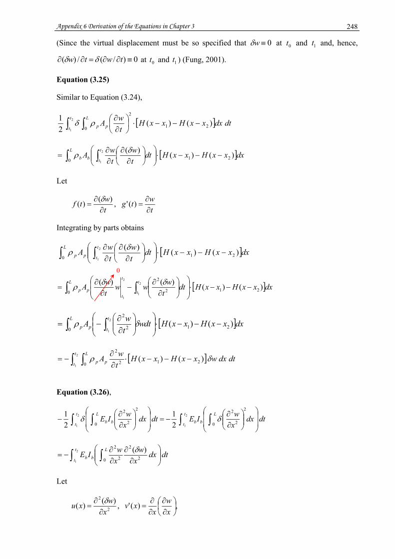
Appendix 6 Derivation of the Equations in Chapter 3 248
(Since the virtual displacement must be so specified that 0≡wδ at 0t and 1t and, hence,
0)/(/)( ≡∂∂=∂∂ twtw δδ at 0t and 1t ) (Fung, 2001).
Equation (3.25)
Similar to Equation (3.24),
[ ] dtdxxxHxxHtwA
t
t
L
pp
∫ ∫ −−−⋅⎟⎠⎞
⎜⎝⎛∂∂2
1 0 21
2
)()(21 ρδ
[ ]dxxxHxxHdttw
twA
L t
tbb )()()(210
2
1
−−−⋅⎟⎟⎠
⎞⎜⎜⎝
⎛⎟⎠⎞
⎜⎝⎛
∂∂
∂∂
= ∫ ∫
δρ
Let
twtg
twtf
∂∂
=∂
∂= )(' ,)()( δ
Integrating by parts obtains
[ ]dxxxHxxHdttw
twA
L t
tpp )()()(210
2
1
−−−⋅⎟⎟⎠
⎞⎜⎜⎝
⎛⎟⎠⎞
⎜⎝⎛
∂∂
∂∂
∫ ∫
δρ
[ ]dxxxHxxHdtt
wwwtwA
L t
t
t
tpp )()()()(
210 2
22
1
2
1
−−−⋅⎟⎟⎠
⎞⎜⎜⎝
⎛⎟⎟⎠
⎞⎜⎜⎝
⎛∂
∂−
∂∂
= ∫ ∫
δδρ
[ ]dxxxHxxHdtwtwA
L t
tpp )()( 210 2
22
1
−−−⋅⎟⎟⎠
⎞⎜⎜⎝
⎛⎟⎟⎠
⎞⎜⎜⎝
⎛∂∂
−= ∫ ∫
δρ
[ ] dtdxwxxHxxHtwA
t
t
L
pp∫ ∫ −−−⋅∂∂
−= 2
1 0 212
2
)()(
δρ
Equation (3.26),
dtdxxwIEdtdx
xwIE
t
t
L
bb
t
t
L
bb ∫ ∫∫ ∫ ⎟⎟
⎠
⎞
⎜⎜
⎝
⎛⎟⎟⎠
⎞⎜⎜⎝
⎛∂∂
−=⎟⎟
⎠
⎞
⎜⎜
⎝
⎛⎟⎟⎠
⎞⎜⎜⎝
⎛∂∂
− 2
1
2
1 0
2
2
22
2
2
0 21
21 δδ
dtdxx
wxwIE
t
t
L
bb ∫ ∫ ⎟⎟⎠
⎞⎜⎜⎝
⎛∂
∂∂∂
−= 2
1 0 2
2
2
2 )(δ
Let
,)(',)()( 2
2
⎟⎠⎞
⎜⎝⎛∂∂
∂∂
=∂
∂=
xw
xxv
xwxu δ
0

Appendix 6 Derivation of the Equations in Chapter 3 249
Integrating by parts obtain,
dtdxx
wxw
xw
xwIEdtdx
xw
xwIE
t
t
LL
bb
t
t
L
bb
∫ ∫∫ ∫ ⎟⎟
⎠
⎞
⎜⎜
⎝
⎛
∂∂
∂∂
−∂
∂∂∂
−=⎟⎟⎠
⎞⎜⎜⎝
⎛∂
∂∂∂
− 2
1
2
1 0 3
3
02
2
0 2
2
2
2 )()()( δδδ
Then let,
,)(' ,)()( 3
3
xwxg
xwxf
∂∂
=∂
∂=
δ
Again integrating by parts, one can have Equation (3.26) as
dttdxx
wxwIE
t
t
L
bb
∫ ∫ ⎟⎟⎠
⎞⎜⎜⎝
⎛∂
∂∂∂
− 2
1 0 2
2
2
2 )(δ
ddxwx
wwx
wx
wxwIE
t
t
LLL
bb
∫ ∫ ⎟⎟⎟
⎠
⎞
⎜⎜⎜
⎝
⎛
∂∂
+∂
∂−
∂∂
∂∂
−= 2
1 0 4
4
0
3
3
02
2 )()()( δδδ
dtdxwxww
xw
xw
xwIE
t
t
LLL
bb
∫ ∫ ⎟⎟⎟
⎠
⎞
⎜⎜⎜
⎝
⎛
∂∂
+∂∂
−⎟⎠⎞
⎜⎝⎛∂∂
∂∂
−= 2
1 0 4
4
0
3
3
02
2
δδδ
Equation (3.27),
[ ] dtdxxxHxxHxwIE
t
t
L
pp
)()(
21
21
2
2
2
0
2
1
−−−⎟⎟⎠
⎞⎜⎜⎝
⎛∂∂
− ∫ ∫δ
[ ] dtdxxxHxxHxw
xwIE
t
t
L
pp
∫ ∫ −−−⎟⎟⎠
⎞⎜⎜⎝
⎛∂∂
∂∂
−= 2
1 0 212
2
2
2
)()(δ
Let
[ ])()()( 212
2
xxHxxHxwxu −−−
∂∂
= δ , ⎟⎠⎞
⎜⎝⎛∂∂
∂∂
=xw
xxv )(' ,
By integration by parts, one obtains
[ ] dtdxxxHxxHxw
xwIE
t
t
L
pp
∫ ∫ −−−⎟⎟⎠
⎞⎜⎜⎝
⎛∂∂
∂∂
− 2
1 0 212
2
2
2
)()(δ
Lt
t pp xwxxHxxH
xwIE
0
212
2 )()]()([2
1 ⎩⎨⎧
∂∂
−−−∂∂
−= ∫δ
0
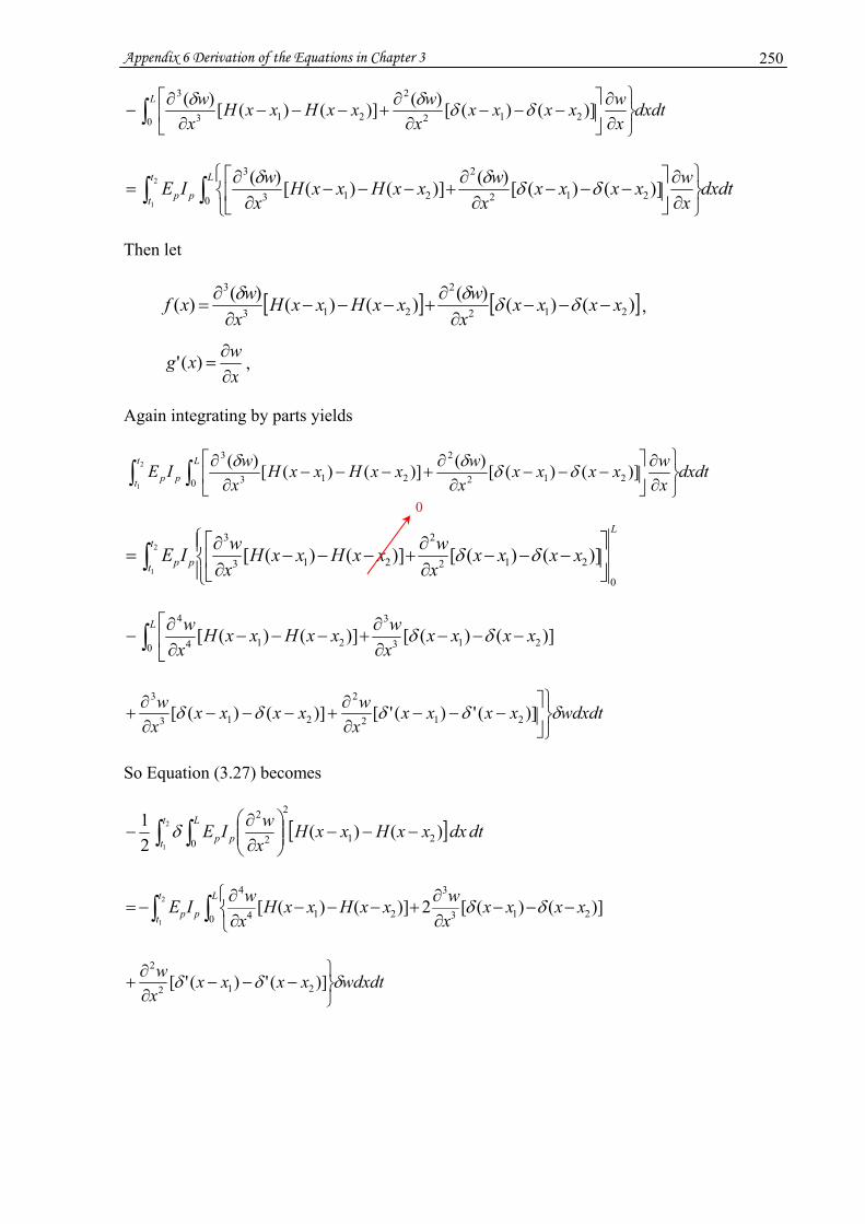
Appendix 6 Derivation of the Equations in Chapter 3 250
dxdtxwxxxx
xwxxHxxH
xwL
∫⎭⎬⎫
∂∂
⎥⎦
⎤⎢⎣
⎡−−−
∂∂
+−−−∂
∂−
0 212
2
213
3
)]()([)()]()([)( δδδδ
∫ ∫⎭⎬⎫
⎩⎨⎧
∂∂
⎥⎦
⎤⎢⎣
⎡−−−
∂∂
+−−−∂
∂= 2
1 0 212
2
213
3
)]()([)()]()([)(t
t
L
pp dxdtxwxxxx
xwxxHxxH
xwIE
δδδδ
Then let
[ ] [ ])()()()()()()( 212
2
213
3
xxxxx
wxxHxxHx
wxf −−−∂
∂+−−−
∂∂
= δδδδ,
xwxg∂∂
=)(' ,
Again integrating by parts yields
∫ ∫⎭⎬⎫
∂∂
⎥⎦
⎤⎢⎣
⎡−−−
∂∂
+−−−∂
∂2
1 0 212
2
213
3
)]()([)()]()([)(t
t
L
pp dxdtxwxxxx
xwxxHxxH
xwIE
δδδδ
Lt
t pp xxxxxwxxHxxH
xwIE
0
212
2
213
3
)]()([)]()([2
1 ⎪⎩
⎪⎨⎧
⎥⎦
⎤⎢⎣
⎡−−−
∂∂
+−−−∂∂
= ∫ δδ
∫ ⎢⎣
⎡−−−
∂∂
+−−−∂∂
−L
xxxxxwxxHxxH
xw
0 213
3
214
4
)]()([)]()([ δδ
wdxdtxxxxxwxxxx
xw δδδδδ
⎭⎬⎫⎥⎦
⎤−−−
∂∂
+−−−∂∂
+ )](')('[)]()([ 212
2
213
3
So Equation (3.27) becomes
[ ] dtdxxxHxxHxwIE
t
t
L
pp
)()(
21
21
2
2
2
0
2
1
−−−⎟⎟⎠
⎞⎜⎜⎝
⎛∂∂
− ∫ ∫δ
∫∫⎩⎨⎧
−−−∂∂
+−−−∂∂
−=Lt
t pp xxxxxwxxHxxH
xwIE
0 213
3
214
4
)]()([2)]()([2
1
δδ
wdxdtxxxxxw δδδ
⎭⎬⎫
−−−∂∂
+ )](')('[ 212
2
0
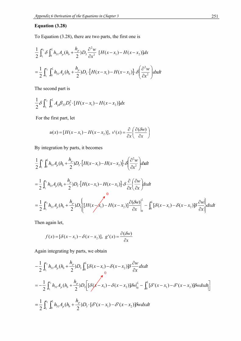
Appendix 6 Derivation of the Equations in Chapter 3 251
Equation (3.28)
To Equation (3.28), there are two parts, the first one is
∫ ∫ −−−∂∂
+2
1 0 212
2
331 )]()([)2
(21 t
t
L pbp dxxxHxxH
xwD
hhAh
δ
[ ] dtdxxwxxHxxHD
hhAh
t
t
pb
L
p∫ ∫ ⎟⎟⎠
⎞⎜⎜⎝
⎛∂∂
⋅−−−⋅+= 2
12
2
2130 31 )()()2
(21
δ
The second part is
∫ ∫ −−−⋅2
1 0 212333 )]()([
21 t
t
L
p dxxxHxxHDA
βδ
For the first part, let
)]()([)( 21 xxHxxHxu −−−= , ⎟⎠⎞
⎜⎝⎛
∂∂
∂∂
=xw
xxv )()(' δ
By integration by parts, it becomes
[ ] dtdxxwxxHxxHD
hhAh
t
t
L pbp∫ ∫ ⎟⎟
⎠
⎞⎜⎜⎝
⎛∂∂
⋅−−−⋅+2
1 0 2
2
21331 )()()2
(21
δ
[ ] dxdtxw
xxxHxxHD
hhAh
t
t
pbp ⎟
⎠⎞
⎜⎝⎛∂∂
∂∂
⋅−−−⋅+= ∫ δ2
1
)()()2
(21
21331
dxdtxwxxxx
xwxxHxxHD
hhAh
t
t
LL
pbp∫ ∫ ⎪⎭
⎪⎬⎫
⎪⎩
⎪⎨⎧
∂∂
−−−−∂
∂−−−+= 2
1 0 210
21331 )]()([)()]()([)2
(21
δδδδ
Then again let,
xwxgxxxxxf
∂∂
=−−−=)()(')],()([)( 21
δδδ
Again integrating by parts, we obtain
dxdtxwxxxxD
hhAh
Lt
t
pbp ∂
∂−−−+− ∫∫ δδδ
0 21331 )]()([)2
(21 2
1
⎥⎦⎤
⎢⎣⎡ −−−−−−−+−= ∫∫ wdxdtxxxxwxxxxD
hhAh
LLt
t
pbp δδδδδδ
0 21021331 )](')('[)]()([)2
(21 2
1
∫ ∫ −−−⋅+= 2
1 0 21331 )](')('[)2
(21 t
t
L pbp wdxdtxxxxD
hhAh
δδδ
0
0

Appendix 6 Derivation of the Equations in Chapter 3 252
So the first part of Equation (3.28) can be expressed as
∫ ∫ −−−∂∂
+2
1 0 212
2
331 )]()([)2
(21 t
t
L pbp dxxxHxxH
xwD
hhAh
δ
∫ ∫ −−−⋅+= 2
1 0 21331 )](')('[)2
(21 t
t
L pbp wdxdtxxxxD
hhAh
δδδ
The second part of Equation (3.28) can be obviously expressed as
∫∫ −−−=−−−L
p
L
p dxDxxHxxHDAdxxxHxxHDA
0 3213330 212333 )]()([)]()([
21 δββδ
Finally obtaining the Equation (3.28)
∫ −−−⎟⎟⎠
⎞⎜⎜⎝
⎛+
∂∂
+−L p
bp dxxxHxxHDxwD
hhhA
0 2123332
2
331 )]()([)2
( βδ
∫ ∫ −−−⋅+−= 2
1 0 21331 )](')('[)2
(21 t
t
L pbp wdxdtxxxxD
hhAh
δδδ
∫ −−−−L
p dxDxxHxxHDA
0 321333 )]()([ δβ
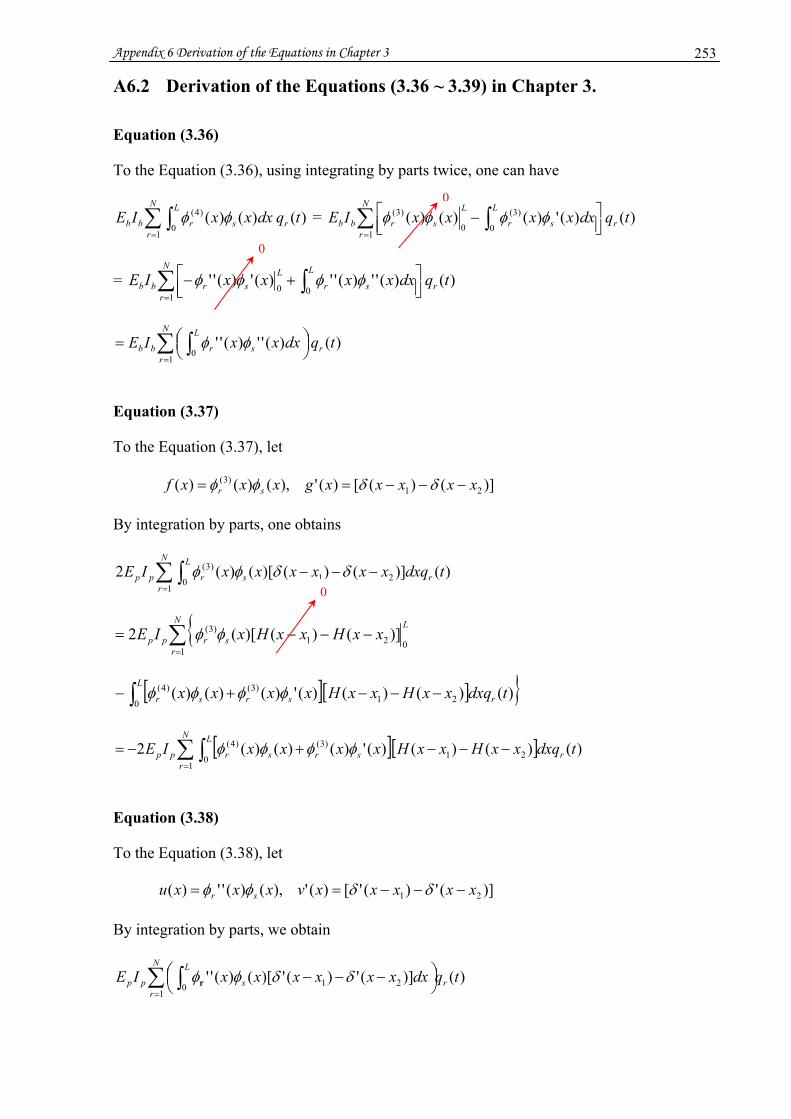
Appendix 6 Derivation of the Equations in Chapter 3 253
A6.2 Derivation of the Equations (3.36 ~ 3.39) in Chapter 3. Equation (3.36)
To the Equation (3.36), using integrating by parts twice, one can have
)()()(1
0
)4( tqdxxxIE rs
N
r
L
rbb
φφ∑∫
=
= )()(')()()(1
0
)3(
0
)3( tqdxxxxxIE r
N
r
L
sr
L
srbb ∑ ∫=
⎥⎦⎤
⎢⎣⎡ −
φφφφ
= )()('')('')(')(''1
00tqdxxxxxIE r
N
r
L
srL
srbb ∑ ∫=
⎥⎦⎤
⎢⎣⎡ +−
φφφφ
)()('')(''1
0tqdxxxIE r
N
r
L
srbb ∑ ∫=
⎟⎠⎞⎜
⎝⎛=
φφ
Equation (3.37)
To the Equation (3.37), let
)]()([)(' ),()()( 21)3( xxxxxgxxxf sr −−−== δδφφ
By integration by parts, one obtains
)()]()()[()(2 211
0
)3( tdxqxxxxxxIE rs
N
r
L
rpp −−−∑∫=
δδφφ
∑=
−−−=N
r
L
srpp xxHxxHxIE1
021)3( )]()()[(2 φφ
[ ][ ]
∫ −−−+−L
rsrsr tdxqxxHxxHxxxx0 21
)3()4( )()()()(')()()( φφφφ
[ ][ ]
∑∫=
−−−+−=N
r
L
rsrsrpp tdxqxxHxxHxxxxIE1
0 21)3()4( )()()()(')()()(2 φφφφ
Equation (3.38)
To the Equation (3.38), let
)](')('[)(' ),()('')( 21 xxxxxvxxxu sr −−−== δδφφ
By integration by parts, we obtain
)()](')(')[()(''1
210tqdxxxxxxxIE r
N
rs
L
pp ∑ ∫=
⎟⎠⎞⎜
⎝⎛ −−− δδφφ
r
0
0
0

Appendix 6 Derivation of the Equations in Chapter 3 254
∑= ⎩⎨⎧ −−−=
N
r
Lsrpp xxxxxxIE
1021 )]()()[()('' δδφφ
)()]()()][(')('')()([ 210
)3( tqdxxxxxxxxx rsrs
L
r ⎭⎬⎫−−−+− ∫ δδφφφφ
)()]()()][(')('')()([1
210
)3( tqdxxxxxxxxxIE r
N
rsrs
L
rpp ∑ ∫=
⎟⎠⎞⎜
⎝⎛ −−−+−= δδφφφφ
Again, let
)]()([)(' ),(')('')()()( 21)3( xxxxxgxxxxxf srsr −−−=+= δδφφφφ
Integrating by parts obtains
)()]()()][(')('')()([1
210
)3( tqdxxxxxxxxxIE r
N
rsrs
L
rpp ∑ ∫=
⎟⎠⎞⎜
⎝⎛ −−−+− δδφφφφ
∑=
−−−+−=N
r
Lssrpp xxHxxHxxxxIE
1021
)3( )]()()][(')('')()([ φφφφ
)()]()()][('')('')(')(2)()([ 21)3(
0
)4( tqdxxxHxxHxxxxxx rsrsrs
L
r ⎭⎬⎫−−−+++ ∫ φφφφφφ
Therefore the Equation (3.38) is
)()](')(')[()(''1
210tqdxxxxxxxIE r
N
rs
L
pp ∑ ∫=
⎟⎠⎞⎜
⎝⎛ −−− δδφφr
∑∫=
−−−++=N
rrsrsrs
L
rpp tdxqxxHxxHxxxxxxIE1
21)3(
0
)4( )()]()()][('')('')(')(2)()( φφφφφφ
Equation (3.39)
To the Equation (3.39), since )(')(')( 00 xfdxxxxf −=−∫+∞
∞−δ , thus
∫ −−−+−L
sp
bp dxxxxxxDh
hAh0 21331 )](')(')[()
2( δδφ
∫+−=+−+− 2
1
)('')2
()](')('[)2
( 33121331
x
x sp
bpssp
bp dxxDh
hAhxxDh
hAh
φφφ
0
0

Appendix 7 Partial List of ANSYS® and MATLAB® Simulation Codes 255
Appendix 7
Partial List of ANSYS®
and MATLAB® Simulation Codes
A7.1 ANSYS® code of modal analysis for aluminium beam with PZT
attached
! *** Modal analysis of Aluminium beam with PZT attached *** ! Written by Jia Long Cao /CLEAR /VIEW,1,1,1,1 /VUP,,Z /PREP7 ! ET,1,5 ! 8-node solid with all DOF, used ! for piezoceramic transducer ET,2,45 ! 8-node solid with UX,UY,UZ DOF,
! used for aluminium beam
MP,DENS,1,7730 ! Density of piezoceramic MP,PERX,1,8.7969E-9 ! Permittivity of piezoceramic MP,PERY,1,8.7969E-9 MP,PERZ,1,8.7969E-9 TB,PIEZ,1 ! Piezoelectric "e" matrix of piezoceramic TBDATA,3,-6.1 TBDATA,6,-6.1 TBDATA,9,15.7 TB,ANEL,1 ! Stiffness "c" matrix of piezoceramic TBDATA,1,12.8E10,6.8E10,6.6E10 TBDATA,7,12.8E10,6.6E10 TBDATA,12,11.0E10 TBDATA,16,2.1E10 TBDATA,19,2.1E10 TBDATA,21,2.1E10

Appendix 7 Partial List of ANSYS® and MATLAB® Simulation Codes 256
MP,EX,2,6.6E10 ! Modulus of Elasticity of aluminium MP,NUXY,2,.345 ! Poisson's ratio of aluminium MP,DENS,2,2790 ! Density of aluminium BTHK= 0.003 ! Beam thickness CVTHK= 0.0005 ! Piezoceramic covering thickness DEPTH= 0.025 ! Depth of assembly BLNGTH= 0.5 ! Beam length CVLNGTH=0.05 ! Length of covering ! BLOCK,,CVLNGTH,,DEPTH,0,BTHK ! Defines covered beam volume BLOCK,CVLNGTH,BLNGTH,,DEPTH,0,BTHK ! Defines uncovered beam volume VATT,2,,2 ! Associates material 2 and type 2 ! with beam volume BLOCK,,CVLNGTH,,DEPTH,BTHK,BTHK+CVTHK ! Defines piezoceramic cover ESIZE,BLNGTH/30 ! Defines default element size NUMMRG,KP ! Merges duplicate solid model ! entities numstr,node,14 ! Set starting node number for the ! solid model VMESH,ALL ! Generates nodes and elements ! within the volumes NSEL,S,LOC,Z, BTHK NSEL,R,LOC,X,,CVLNGTH CP,1,VOLT,ALL ! Couples volt DOF at beam interface CM,INTRFC,NODE ! Creates a component for the ! interface (Face to beam) *GET,BOT_ELECTRODE,NODE,,NUM,MIN NSEL,S,LOC,Z,BTHK+CVTHK NSEL,R,LOC,X,,CVLNGTH CP,2,VOLT,ALL ! Couples volt DOF at piezoceramic ! outer surface CM,OUTSIDE,NODE ! Creates a component for the outer ! surface *GET,TOP_ELECTRODE,NODE,,NUM,MIN !NSEL,S,LOC,X !D,ALL,UX,,,,,UY,UZ ! Fixes nodes at x=0 NSEL,ALL FINISH ! /COM, **** OBTAIN THE MODAL SOLUTION UNDER SHORT-CIRCUIT CONDITIONS **** ! /SOLU ANTYPE,MODAL ! Modal analysis nmodes = 20 modopt,LANB,nmodes ! Block Lanczos solver mxpand,nmodes,,,yes ! Calculate element results and ! reaction forces TOTAL,30,1 ! Requests automatic generation of ! (structural) DOF D,BOT_ELECTRODE,VOLT,0.0 D,TOP_ELECTRODE,VOLT,0.0 ! Add boundary condition will change ! the modal frequency TOTAL,30,1 ! Requests automatic generation of ! (structural) DOF SOLVE FINISH ! /COM, **** REVIEW THE RESULTS OF THE MODAL SOLUTION **** ! /POST1 SET,LIST ! Lists all frequencies /WINDOW,1,LTOP ! Defines four windows /WINDOW,2,RTOP

Appendix 7 Partial List of ANSYS® and MATLAB® Simulation Codes 257
/WINDOW,3,LBOT /WINDOW,4,RBOT /WINDOW,ALL,OFF ! All windows off *DO,I,1,4 /VUP,I,Z /VIEW,I,1,1,1 ! View for all windows /WINDOW,I,ON ! Turns on window i SET,1,I+6 ! Reads in data for mode I+4*K /TITLE,Aluminium Beam with PZT Patch !PLNSOL,U,SUM,0,1 PLNSOL,EPEL,EQV,0,1 ! Plot Von Mises strain /NOERASE ! No screen erase after plot /WINDOW,I,OFF ! Turns off window i *ENDDO FINISH
A7.2 ANSYS® code of harmonic analysis for aluminium beam with PZT
attached
! *** Harmonic analysis of aluminium beam *** ! Written by Jia Long Cao /VIEW,1,1,1,1 /VUP,,Z /PREP7 ET,1,5 ! 8-node solid with all DOF, used for ! piezoceramic transducer ET,2,45 ! 8-node solid with UX,UY,UZ DOF, used ! for aluminium beam MP,DENS,1,7730 ! Density of piezoceramic MP,PERX,1,8.7969E-9 ! Permittivity of piezoceramic MP,PERY,1,8.7969E-9 MP,PERZ,1,8.7969E-9 TB,PIEZ,1 ! Piezoelectric "e" matrix of piezoceramic TBDATA,3,-6.1 TBDATA,6,-6.1 TBDATA,9,15.7 TB,ANEL,1 ! Stiffness "c" matrix of piezoceramic TBDATA,1,12.8E10,6.8E10,6.6E10 TBDATA,7,12.8E10,6.6E10 TBDATA,12,11.0E10 TBDATA,16,2.1E10 TBDATA,19,2.1E10 TBDATA,21,2.1E10 MP,EX,2,6.6E10 ! Modulus of Elasticity of aluminium MP,NUXY,2,.345 ! Poisson's ratio of aluminium MP,DENS,2,2790 ! Density of aluminium ! BTHK= 0.003 ! Beam thickness CVTHK= 0.0005 ! Piezoceramic covering thickness DEPTH= 0.025 ! Depth of assembly BLNGTH= 0.5 ! Beam length CVLNGTH=0.05 ! Length of covering

Appendix 7 Partial List of ANSYS® and MATLAB® Simulation Codes 258
BLOCK,,CVLNGTH,,DEPTH,,BTHK ! Defines covered beam volume BLOCK,CVLNGTH,BLNGTH,,DEPTH,,BTHK ! Defines uncovered beam volume VATT,2,,2 ! Associates material 2 and type 2 ! with beam volume BLOCK,,CVLNGTH,,DEPTH,BTHK,BTHK+CVTHK ! Defines piezoceramic cover ESIZE,BLNGTH/30 ! Defines default element size NUMMRG,KP ! Merges duplicate solid model ! entities numstr,node,14 ! Set starting node number for the ! solid model VMESH,ALL ! Generates nodes and elements ! within the volumes NSEL,S,LOC,Z, BTHK NSEL,R,LOC,X,,CVLNGTH CP,1,VOLT,ALL ! Couples volt DOF at beam interface CM,INTRFC,NODE ! Creates a component for the ! interface (Face to beam) *GET,BOT_ELECTRODE,NODE,,NUM,MIN NSEL,S,LOC,Z,BTHK+CVTHK NSEL,R,LOC,X,,CVLNGTH CP,2,VOLT,ALL ! Couples volt DOF at piezoceramic ! outer surface CM,OUTSIDE,NODE ! Creates a component for the outer ! surface *GET,TOP_ELECTRODE,NODE,,NUM,MIN NSEL,ALL FORCENODE = node(BLNGTH,DEPTH/2,BTHK) ! Node where force applied DISPNODE = node(BLNGTH,DEPTH/2,BTHK) ! Node where deflection detected FINISH /SOLU ANTYPE,HARM ! Harmonic analysis HARFRQ,0,1000, ! Frequency range of analysis NSUBST,500, ! Number of frequency steps KBC,0 ! Impulse loads F,FORCENODE,FZ,-1e3 ! Applying force D,BOT_ELECTRODE,VOLT,0.0 ! Assigns zero voltage to bottom ! electrode D,TOP_ELECTRODE,VOLT,0.0 ! Assigns zero voltage to top ! electrode D,2,VOLT,0.0 ! Assigns zero voltage to node 2 CNVTOL,F,,,,1E-5 ! Small convergence value for force CNVTOL,VOLT ! Default convergence value for ! current flow NSEL,S,LOC,X D,ALL,UX,,,,,UY,UZ ! Fixes nodes at x=0 NSEL,ALL SOLVE FINISH /POST26 NSOL,2,DISPNODE,U,Z ! Get z-direction deflection at node DISPNODE ! and store it into variable 2 /ERASE /axlab,y,Displacement !/YRANGE,0,14 PLVAR,2 ! Plot variable 2 vs. Freq /window,1,off /noerase FINISH

Appendix 7 Partial List of ANSYS® and MATLAB® Simulation Codes 259
A7.3 ANSYS® code of single mode, parallel R-L piezoelectric vibration
shunt control for aluminium beam
! *** R-L Parallel Shunt Circuit for Vibration Control *** ! Written by Jia Long Cao !/SHOW,JPEG /VIEW,1,1,1,1 /VUP,,Z /PREP7 *dim,F,array,6 ! Array to store natural frequencies *dim,L,array,6 ! Array to store inductor values *dim,R,array,6 ! Array to store resistor values *set,i,1 ! Index of the modal to be controlled !Cp = 31.14E-9 ! Capacitor of PZT F(1) = 57.391 ! First modal frequency F(2) = 161.987 ! Second modal frequency F(3) = 324.152 ! Third modal frequency F(4) = 546.799 ! Fourth modal frequency F(5) = 834.393 ! Fifth modal frequency L(1) = 229.9 ! Inductor value for F(1) L(2) = 29.5 ! Inductor value for F(2) L(3) = 7.27 ! Inductor value for F(3) L(4) = 2.58 ! Inductor value for F(4) L(5) = 1.11 ! Inductor value for F(5) R(1) = 1E9 ! Resistor value for F(1) R(2) = 5E7 ! Resistor value for F(2) R(3) = 5E6 ! Resistor value for F(3) R(4) = 4E5 ! Resistor value for F(4) R(5) = 18E4 ! Resistor value for F(5) ET,1,5 ! 8-node solid with all DOF, used for ! piezoceramic transducer ET,2,45 ! 8-node solid with UX,UY,UZ DOF, ! used for aluminum beam MP,DENS,1,7730 ! Density of piezoceramic MP,PERX,1,8.7969E-9 ! Permittivity of piezoceramic MP,PERY,1,8.7969E-9 MP,PERZ,1,8.7969E-9 TB,PIEZ,1 ! Piezoelectric "e" matrix of ! piezoceramic TBDATA,3,-6.1 TBDATA,6,-6.1 TBDATA,9,15.7 TB,ANEL,1 ! Stiffness "c" matrix of piezoceramic TBDATA,1,12.8E10,6.8E10,6.6E10 TBDATA,7,12.8E10,6.6E10 TBDATA,12,11.0E10 TBDATA,16,2.1E10 TBDATA,19,2.1E10 TBDATA,21,2.1E10 MP,EX,2,6.6E10 ! Modulus of Elasticity of aluminium MP,NUXY,2,.345 ! Poisson's ratio of aluminium

Appendix 7 Partial List of ANSYS® and MATLAB® Simulation Codes 260
MP,DENS,2,2790 ! Density of aluminium ! BTHK= 0.003 ! Beam thickness CVTHK= 0.0005 ! Piezoceramic covering thickness DEPTH= 0.025 ! Depth of assembly BLNGTH= 0.5 ! Beam length CVLNGTH=0.05 ! Length of covering BLOCK,,CVLNGTH,,DEPTH,,BTHK ! Defines covered beam volume BLOCK,CVLNGTH,BLNGTH,,DEPTH,,BTHK ! Defines uncovered beam volume VATT,2,,2 ! Associates material 2 and type 2 with beam volume BLOCK,,CVLNGTH,,DEPTH,BTHK,BTHK+CVTHK ! Defines piezoceramic cover ESIZE,BLNGTH/30 ! Defines default element size NUMMRG,KP ! Merges duplicate solid model entities numstr,node,14 ! Set starting node number for the solid model VMESH,ALL ! Generates nodes and elements within the volumes ! NSEL,S,LOC,Z, BTHK NSEL,R,LOC,X,,CVLNGTH CP,1,VOLT,ALL ! Couples volt DOF at beam interface CM,INTRFC,NODE ! Creates a component for the interface (Face to beam) *GET,BOT_ELECTRODE,NODE,,NUM,MIN NSEL,S,LOC,Z,BTHK+CVTHK NSEL,R,LOC,X,,CVLNGTH CP,2,VOLT,ALL ! Couples volt DOF at piezoceramic outer surface CM,OUTSIDE,NODE ! Creates a component for the outer surface *GET,TOP_ELECTRODE,NODE,,NUM,MIN N,1,-0.03,DEPTH/2, 0.03 N,2,-0.03,DEPTH/2,-0.03 ET,3,CIRCU94,1,0 ! Set up the inductor R,1,L(i) RMOD,1,15,0,0 ! Subscript of inductor is 0, i.e. L0 TYPE,3 $ REAL,1 E,TOP_ELECTRODE,BOT_ELECTRODE ! Parallel the inductor to the ! electrodes of PZT E,1,2 ! Parallel the inductor between ! node 1 and 2 ET,4,CIRCU94,0,0 ! Set up the resistor R,2,R(i) RMOD,2,15,0,0 ! Subscript of resistor is 0, i.e. R0 TYPE,4 $ REAL,2 E,TOP_ELECTRODE,BOT_ELECTRODE ! Parallel the resistor to the ! electrodes of PZT E,1,2 ! Parallel the resistor between node 1 and 2 NSEL,ALL FORCENODE = node(BLNGTH,DEPTH/2,BTHK) ! Node where force applied DISPNODE = node(BLNGTH,DEPTH/2,BTHK) ! Node where deflection detected FINISH /SOLU ANTYPE,HARM ! Harmonic analysis HARFRQ,0,1000, ! Frequency range of analysis NSUBST,500, ! Number of frequency steps KBC,0 ! Impulse loads F,FORCENODE,FZ,-1e3 ! Applying force D,BOT_ELECTRODE,VOLT,0.0 ! Assigns zero voltage to bottom electrode !D,TOP_ELECTRODE,VOLT,0.0 ! Assigns zero voltage to top electrode D,2,VOLT,0.0 ! Assigns zero voltage to node 2

Appendix 7 Partial List of ANSYS® and MATLAB® Simulation Codes 261
CNVTOL,F,,,,1E-5 ! Small convergence value for force CNVTOL,VOLT ! Default convergence value for current flow !NSEL,S,LOC,X !D,ALL,UX,,,,,UY,UZ ! Fixes nodes at x=0 !NSEL,ALL SOLVE FINISH /POST26 NSOL,2,DISPNODE,U,Z ! Get z-direction deflection at node DISPNODE ! and store it into variable 2 /ERASE /axlab,y,Displacement /YRANGE,0,4 PLVAR,2 ! Plot variable 2 vs. Freq /window,1,off /noerase FINISH
A7.4 ANSYS® code of modal analysis of carbon-fibre composite sandwich
cricket bat with rubber layers (blade built in Solidworks® is
imported into ANSYS®)
! Modal analysis of carbon-fibre composite sandwich cricket bat with ! rubber layers ! Written by Jia Long Cao ! The handle consists of two beam composite material sandwiched with wood, ! There are two rubber layers in wood part as well ! The triangle part overlapping with blade is solid wood, not composite. /BATCH /CONFIG,NRES,50000 ! Maximum substep is 50000 /input,menust,tmp,'',,,,,,,,,,,,,,,,1 /GRA,POWER /GST,ON /PLO,INFO,3 /GRO,CURL,ON ~PARAIN,Blade,x_t,,SOLIDS,0,0 ! Access Blade.x_t file built in Solidworks !* ! A triangle volume to be used as a subtracter K,480,0,-0.016,-0.025, K,481,0,0.016,-0.025, K,482,0,0.016,0.025, K,483,0,-0.016,0.025, K,484,0.12,-0.001,-0.025, K,485,0.12,0.001,-0.025, K,486,0.12,-0.001,0.04, K,487,0.12,0.001,0.04, V,480,481,482,483,484,485,487,486 ! Subtract the triangle volume from blade FLST,2,2,6,ORDE,2 FITEM,2,1 FITEM,2,2 VSBV,P51X,2

Appendix 7 Partial List of ANSYS® and MATLAB® Simulation Codes 262
! Create a triangle volume to be fit in the blade K,480,0,-0.016,-0.0175, K,481,0,0.016,-0.0175, K,482,0,0.016,0.0145, K,483,0,-0.016,0.0145, K,484,0.12,-0.001,-0.0165, K,485,0.12,0.001,-0.0165, K,486,0.12,-0.001,0.0245, K,487,0.12,0.001,0.0245, V,480,481,482,483,484,485,487,486 wpoff,0,0,-0.0016 ! Shift current centre point by (x0,y0,z0) wpro,,,-90.000000 ! Rotate –90 degrees CYL4,,,,,0.016,,0.3 ! Create CYLINDER1 FLST,2,2,6,ORDE,2 ! Make cylinder1 and triangle volumes as one part FITEM,2,1 ! Pick up volume 1 FITEM,2,-2 ! to 2 VADD,P51X ! Add all ! BLOCK1 & BLOCK2 are used to make space for embedding composite beams BLOCK,0.0095,0.011,-0.0105,0.0105,0,0.3 BLOCK,-0.0095,-0.011,-0.0105,0.0105,0,0.3 ! BLOCKs are used to make space for embedding rubber layers BLOCK,-0.0005,0.0005,-0.015,0.015,,0.3 BLOCK,-0.0045,-0.0055,-0.014,0.014,,0.3 BLOCK,0.0045,0.0055,-0.014,0.014,,0.3 FLST,3,5,6,ORDE,4 FITEM,3,1 FITEM,3,-2 FITEM,3,5 FITEM,3,-7 VSBV,4,P51X ! BLOCKS are used for making composite beams BLOCK,0.0095,0.011,-0.0105,0.0105,0,0.3 BLOCK,-0.0095,-0.011,-0.0105,0.0105,0,0.3 ! BLOCKs are used for making rubber layers BLOCK,-0.0005,0.0005,-0.015,0.015,,0.3 BLOCK,-0.0045,-0.0055,-0.014,0.014,,0.3 BLOCK,0.0045,0.0055,-0.014,0.014,,0.3 FLST,2,7,6,ORDE,3 FITEM,2,1 ! Pick up volume 1 FITEM,2,-6 ! to 6 FITEM,2,8 ! Pick up volume 8 VGLUE,P51X ! Glue all /VIEW,1,1,1,1 VPLOT ET,1,SOLID95 !* ! Material property of Blade (willow) MPTEMP,,,,,,,, MPTEMP,1,0 MPDATA,EX,1,,6.67E9 ! Young's modulus of willow MPDATA,NUXY,1,,.35 MPTEMP,,,,,,,, MPTEMP,1,0 MPDATA,DENS,1,,420 ! Density of willow ! Material property of wood cane

Appendix 7 Partial List of ANSYS® and MATLAB® Simulation Codes 263
MPTEMP,,,,,,,, MPTEMP,1,0 MPDATA,EX,2,,3E9 ! Young's modulus of wood cane MPDATA,NUXY,2,,.32 MPTEMP,,,,,,,, MPTEMP,1,0 MPDATA,DENS,2,,700 ! Density of wood cane ! Material property of composite MPTEMP,,,,,,,, MPTEMP,1,0 MPDATA,EX,3,,7E10 ! Young's modulus of composite MPDATA,NUXY,3,,.32 MPTEMP,,,,,,,, MPTEMP,1,0 MPDATA,DENS,3,,1350 ! Density of composite ! Material property of rubber MPTEMP,,,,,,,, MPTEMP,1,0 MPDATA,EX,4,,6E6 ! Young's modulus of rubber MPDATA,NUXY,4,,.42 MPTEMP,,,,,,,, MPTEMP,1,0 MPDATA,DENS,4,,1113 ! Density of rubber ESIZE,0.0098 MSHAPE,1,3D MSHKEY,0 ! Select the composite part of the handle CM,_Y,VOLU VSEL,S,VOLU,,1,2 CM,_Y1,VOLU CHKMSH,'VOLU' CMSEL,S,_Y VATT,3,,1 !* VMESH,_Y1 !* CMDELE,_Y CMDELE,_Y1 CMDELE,_Y2 !* ! Select the rubber part of the handle CM,_Y,VOLU VSEL,S,VOLU,,4,5 VSEL,A,VOLU,,6 CM,_Y1,VOLU CHKMSH,'VOLU' CMSEL,S,_Y VATT,4,,1 !* VMESH,_Y1 !* CMDELE,_Y CMDELE,_Y1 CMDELE,_Y2 !* ! Select the wood part of the handle CM,_Y,VOLU VSEL,S,VOLU,,9 CM,_Y1,VOLU CHKMSH,'VOLU'

Appendix 7 Partial List of ANSYS® and MATLAB® Simulation Codes 264
CMSEL,S,_Y VATT,2,,1 !* VMESH,_Y1 !* CMDELE,_Y CMDELE,_Y1 CMDELE,_Y2 !* ! Select Blade Volume CM,_Y,VOLU VSEL,S,VOLU,,7 CM,_Y1,VOLU CHKMSH,'VOLU' CMSEL,S,_Y VATT,1,,1 !* VMESH,_Y1 !* CMDELE,_Y CMDELE,_Y1 CMDELE,_Y2 FINI /SOLU ANTYPE,MODAL ! Modal analysis nmodes = 14 modopt,LANB,nmodes ! Block Lanczos solver ! Calculate element results and reaction forces mxpand,nmodes,,,yes ! Requests automatic generation of (structural) DOF TOTAL,14,1 SOLVE FINI ! /COM, **** REVIEW THE RESULTS OF THE MODAL SOLUTION **** /POST1 /Triad,off SET,LIST ! Lists all frequencies /WINDOW,1,LTOP ! Defines four windows /WINDOW,2,RTOP /WINDOW,3,LBOT /WINDOW,4,RBOT /WINDOW,ALL,OFF ! All windows off /VUP,1,Z /VIEW,1,1,1,1 ! View for window 1 !/VIEW,1,0,-1 ! View for window 1 /WINDOW,1,ON ! Turns on window i SET,1,7 ! Reads in data for mode i /TITLE,Modal Analysis of Cricket Bat !PLNSOL,U,SUM,0,1 PLNSOL,EPEL,EQV,0,1 ! Plot Von Mises strain /NOERASE ! No screen erase after plot /WINDOW,1,OFF ! Turns off window 1 /VUP,2,Z /VIEW,2,1,1,1 ! View for window 2 !/VIEW,2,0,-1 ! View for window 2 /WINDOW,2,ON ! Turns on window i SET,1,9 ! Reads in data for mode i !PLNSOL,U,SUM,0,1 PLNSOL,EPEL,EQV,0,1 ! Plot Von Mises strain /NOERASE ! No screen erase after plot
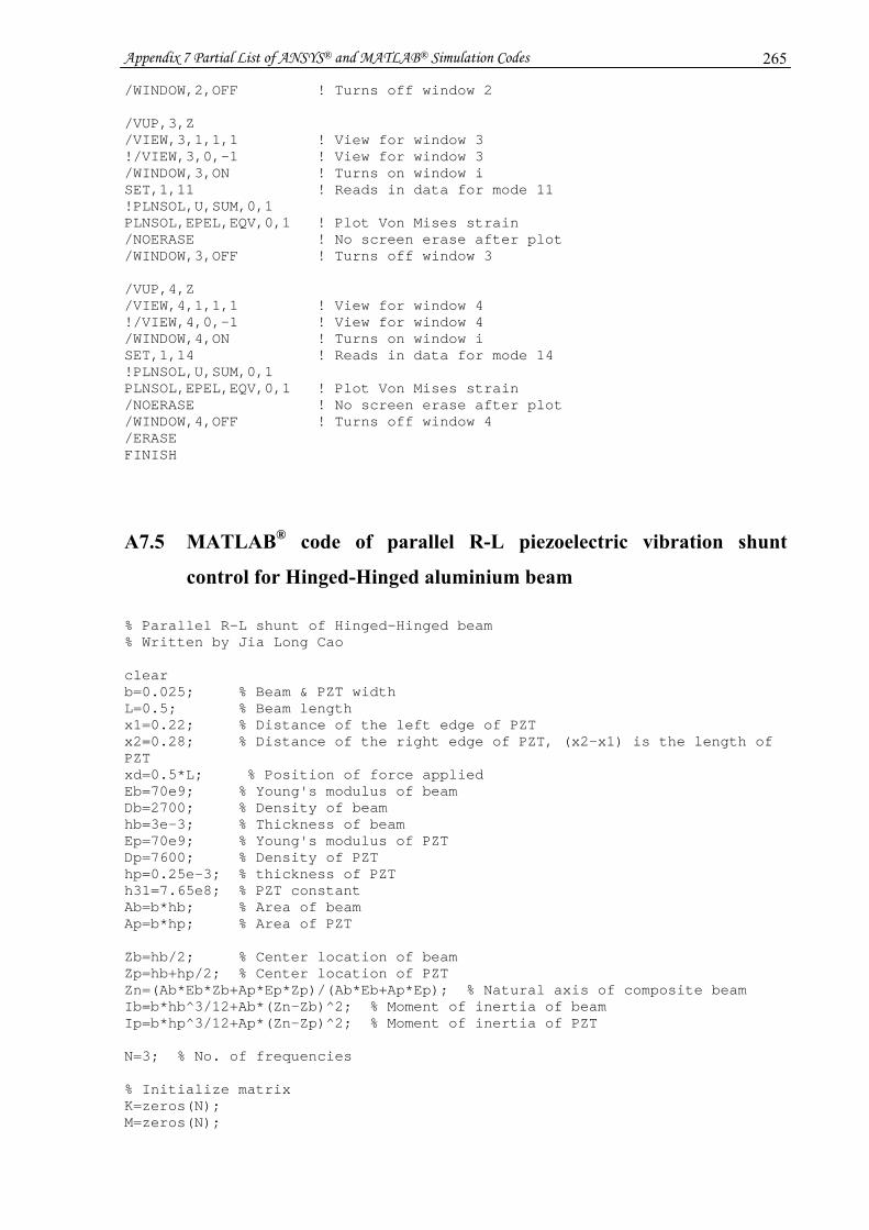
Appendix 7 Partial List of ANSYS® and MATLAB® Simulation Codes 265
/WINDOW,2,OFF ! Turns off window 2 /VUP,3,Z /VIEW,3,1,1,1 ! View for window 3 !/VIEW,3,0,-1 ! View for window 3 /WINDOW,3,ON ! Turns on window i SET,1,11 ! Reads in data for mode 11 !PLNSOL,U,SUM,0,1 PLNSOL,EPEL,EQV,0,1 ! Plot Von Mises strain /NOERASE ! No screen erase after plot /WINDOW,3,OFF ! Turns off window 3 /VUP,4,Z /VIEW,4,1,1,1 ! View for window 4 !/VIEW,4,0,-1 ! View for window 4 /WINDOW,4,ON ! Turns on window i SET,1,14 ! Reads in data for mode 14 !PLNSOL,U,SUM,0,1 PLNSOL,EPEL,EQV,0,1 ! Plot Von Mises strain /NOERASE ! No screen erase after plot /WINDOW,4,OFF ! Turns off window 4 /ERASE FINISH
A7.5 MATLAB® code of parallel R-L piezoelectric vibration shunt
control for Hinged-Hinged aluminium beam
% Parallel R-L shunt of Hinged-Hinged beam % Written by Jia Long Cao clear b=0.025; % Beam & PZT width L=0.5; % Beam length x1=0.22; % Distance of the left edge of PZT x2=0.28; % Distance of the right edge of PZT, (x2-x1) is the length of PZT xd=0.5*L; % Position of force applied Eb=70e9; % Young's modulus of beam Db=2700; % Density of beam hb=3e-3; % Thickness of beam Ep=70e9; % Young's modulus of PZT Dp=7600; % Density of PZT hp=0.25e-3; % thickness of PZT h31=7.65e8; % PZT constant Ab=b*hb; % Area of beam Ap=b*hp; % Area of PZT Zb=hb/2; % Center location of beam Zp=hb+hp/2; % Center location of PZT Zn=(Ab*Eb*Zb+Ap*Ep*Zp)/(Ab*Eb+Ap*Ep); % Natural axis of composite beam Ib=b*hb^3/12+Ab*(Zn-Zb)^2; % Moment of inertia of beam Ip=b*hp^3/12+Ap*(Zn-Zp)^2; % Moment of inertia of PZT N=3; % No. of frequencies % Initialize matrix K=zeros(N); M=zeros(N);

Appendix 7 Partial List of ANSYS® and MATLAB® Simulation Codes 266
C=zeros(N); BL=zeros(N,1); BR=zeros(N,1); Fd=zeros(N,1); Cp=82e-9; % capacitance of PZT %L0=[400 4.788 1]; % shunt inductors %R0=[3e5 1e4 1]; % shunt resistors L0=[400 24.64 4.846]; % shunt inductors R0=[3.4e5 1e5 7e4]; % shunt resistors % Coefficient of BL %BL=h31*(hb+0.5*hp)*(L0/R0)*(pi/L)*(cos(pi*x2/L)-cos(pi*x1/L)); % Coefficient of BR %BR=h31*(hb+0.5*hp)*(pi/L)*(cos(pi*x2/L)-cos(pi*x1/L)); % Coefficient of BL %BL=h31*(hp/(x2-x1))*(hb+0.5*hp)*(L0/R0)*(pi/L)*... %(cos(pi*x2/L)-cos(pi*x1/L)); % Coefficient of BR %BR=h31*(hp/(x2-x1))*(hb+0.5*hp)*(pi/L)*(cos(pi*x2/L)-cos(pi*x1/L)); CR=inv(diag(R0*Cp)); % Coefficient of CR CL=inv(diag(L0*Cp)); % Coefficient of CL for r=1:N; Q1(r)=-(h31*hp*(hb+0.5*hp)*(r*pi/L)*abs(cos(r*pi*x2/L)-... cos(r*pi*x1/L)))/((x2-x1)); for s=1:N; BL(s)=h31*(hp/(x2-x1))*(hb+0.5*hp)*(L0(s)/R0(s))*... (s*pi/L)*(cos(pi*x2/L)-cos(pi*x1/L)); % Coefficient of BL BR(s)=h31*(hp/(x2-x1))*(hb+0.5*hp)*(s*pi/L)*... (cos(pi*x2/L)-cos(pi*x1/L)); % Coefficient of BR if r == s K(r,s)=(pi*r/L)^4*(Eb*Ib*L/2+Ep*Ip*(x2-x1)/2+... Ep*Ip*L/(4*pi*r)*(sin(2*pi*r*x1/L)-sin(2*pi*r*x2/L))); M(r,s)=(Db*Ab*L/2+Dp*Ap*(x2-x1)/2+Dp*Ap*L/... (4*pi*r)*(sin(2*pi*r*x1/L)-sin(2*pi*r*x2/L))); else K(r,s)=Ep*Ip*L/pi*(pi^2*r*s/L^2)^2*((r*sin(s*pi*x2/L)... *cos(r*pi*x2/L))/(s^2-r^2)+(s*sin(r*pi*x2/L)*... cos(s*pi*x2/L))/(r^2-s^2)-((r*sin(s*pi*x1/L)*... cos(r*pi*x1/L))/(s^2-r^2)+(s*sin(r*pi*x1/L)*... cos(s*pi*x1/L))/(r^2-s^2))); M(r,s)=Dp*Ap*L/pi*((r*sin(s*pi*x2/L)*cos(r*pi*x2/L))/... (s^2-r^2)+(s*sin(r*pi*x2/L)*cos(s*pi*x2/L))/(r^2-s^2)-... ((r*sin(s*pi*x1/L)*cos(r*pi*x1/L))/(s^2-r^2)+... (s*sin(r*pi*x1/L)*cos(s*pi*x1/L))/(r^2-s^2))); end; end; %Fd(r)=1/100*sin(r*pi*xd/L); % due to discrete force with magnitude 1/100 end; Fd = (1/100)*[1; 1; 1]; % applied force Cd=0.2*M+1e-7*K; % Internal damping coefficient Q=Q1*inv(diag(L0)); % Q1/L0 Q=diag(Q); % Make Q as a diagonal matrix BL=diag(BL); BR=diag(BR); % state-space model AK=-inv(M)*K; % -K/M AC=-inv(M)*Cd; % -C/M

Appendix 7 Partial List of ANSYS® and MATLAB® Simulation Codes 267
% A matrix without shunt A1=[zeros(N) eye(N) zeros(N) zeros(N); AK AC zeros(N) zeros(N); ... zeros(N) zeros(N) zeros(N) eye(N); -Q zeros(N) -CL -CR]; % A matrix with shunt A2=[zeros(N) eye(N) zeros(N) zeros(N); AK AC -inv(M)*BR -inv(M)*BL; ... zeros(N) zeros(N) zeros(N) eye(N); -Q zeros(N) -CL -CR]; B=[zeros(N,1); inv(M)*Fd; zeros(N,1); zeros(N,1)]; for r=1:N; C1(1,r)=sin(r*pi/4); % displacement w at midpoint (x=L/2) end; C=[C1 zeros(1,3*N)]; D=[0]; % impulse response t=linspace(0,1,1e5); IU=1; [y,x,t]=impulse(A1,B,C,D,IU,t); % uncontrolled response [yc,x,t]=impulse(A2,B,C,D,IU,t); % controlled response figure(1); plot(t,y,'b--',t,yc,'r') % unit (mm) legend('Without PZT shunt','With PZT shunt'); title('Impulse response of beam transverse displacement at xm=L/4', 'Fontsize', 18, 'Color', 'r') xlabel('Time (sec)', 'Fontsize', 16, 'Color', 'r') ylabel('Displacement (m)', 'Fontsize', 16, 'Color', 'r') axis([0 1 -1e-3 1e-3]) grid; zoom on; figure(2); plot(20*log10(abs(fft(y))),'b--'); hold on; plot(20*log10(abs(fft(yc))), 'r'); legend('Without PZT shunt','With PZT shunt'); title('Frequency response of beam transverse displacement at xm=L/4', 'Fontsize', 20, 'Color', 'r'); xlabel('Frequency (Hz)', 'Fontsize', 16, 'Color', 'r'); ylabel('Magnitude (dB)', 'Fontsize', 16, 'Color', 'r'); axis([0 1000 -80 40]); grid; zoom on; hold off;

Appendix 7 Partial List of ANSYS® and MATLAB® Simulation Codes 268
A7.6 MATLAB® code for analysing neutral axis, moment inertia, strains,
stresses, strain energies etc. illustrated in Chapter 4
% Written by Jia Long Cao clear; M = 100; % Bending moment Ew = 7E9; % Young's modulus of wood L = 0.5; b = 0.025; % Width of the composite beam hw = 0.003; % Wood beam thickness hp(1) = 0.1*hw; % PZT thickness hp(2) = 0.2*hw; % PZT thickness hp(3) = 0.5*hw; % PZT thickness hp(4) = hw; % PZT thickness N = 10000; % Number of samples dN = 20/N; % Sampling resolution for i = 1:4 u(i) = hp(i)/hw; % Thickness ratio of PZT and wood beam for j = 1:N n = j*dN; % n = Ep/Ew, n is from dN to N*dN % Neutral axis of composite beam, the distance from top edge of PZT % (assume that z (z = 0) starts at top edge of PZT and downwords) Zn(i,j) = (hw/2)*((u(i)^2*n+2*u(i)+1)/(1+u(i)*n)); Zp(i) = hp(i)/2; Zb(i) = hp(i)+hw/2; Zn_Minus_Zp(i,j) = (hw/2)*((u(i)^2*n+2*u(i)+1)/(1+u(i)*n))-Zp(i); % Moment of inertia of wood part of the composite beam %Iw(i,j) = (b*hw^3/12)*(1+3*u(i)^2*n^2*((1+u(i))/(1+u(i)*n))^2); %Iw(i,j) = b*hw^3/12 + b*hw*(Zn(i,j)-Zb(i))^2; Iw(i,j)=(b*hw^3/12)*(((3*u(i)^4+6*u(i)^3+4*u(i)^2)*... n^2+2*u(i)*n+1))/(u(i)^2*n^2+2*u(i)*n+1); % Moment of inertia of PZT part of the composite beam %Ip(i,j) = (b*hw^3/12)*(u(i)^3+3*u(i)*((1+u(i))/(1+u(i)*n))^2); %Ip(i,j) = b*hp(i)^3/12 + b*hp(i)*(Zn(i,j)-Zp(i))^2; Ip(i,j)=(b*hw^3/12)*((u(i)^5*n^2+2*u(i)^4*n+4*u(i)^3+... 6*u(i)^2+3*u(i)))/(u(i)^2*n^2+2*u(i)*n+1); % Overall moment of inertia %I(i,j) = Iw(i,j)+n*Ip(i,j); I(i,j)=(b*hw^3/12)*((u(i)^5*n^3+(5*u(i)^4+6*u(i)^3+... 4*u(i)^2)*n^2+(4*u(i)^3+6*u(i)^2+5*u(i))*n+1))/... (u(i)^2*n^2+2*u(i)*n+1); Iw_over_Ip(i,j) = Iw(i,j)/Ip(i,j); % Ib/Ip Ip_over_Iw(i,j) = Ip(i,j)/Iw(i,j); % Ip/Ib Iw_over_I(i,j) = Iw(i,j)/I(i,j); % Ib/I % Average strain of PZT PZT_strain(i,j) = (6*M/(b*hw^2*Ew))*(1+u(i))/... ((u(i)^4*n^2+4*u(i)^3*n+6*u(i)^2*n+4*u(i)*n+1)); % Average strain of beam beam_strain(i,j) = (-6*M/(b*hw^2*Ew))*(u(i)^2+u(i))*n/... ((u(i)^4*n^2+4*u(i)^3*n+6*u(i)^2*n+4*u(i)*n+1)); %beam_strain(i,j) = M*(Zn(i,j)-Zb(i))/(Ew*I(i,j));

Appendix 7 Partial List of ANSYS® and MATLAB® Simulation Codes 269
% Average stress of PZT PZT_stress(i,j) = (6*M/(b*hw^2))*(1+u(i))*n/... ((u(i)^4*n^2+4*u(i)^3*n+6*u(i)^2*n+4*u(i)*n+1)); % Average stress of beam beam_stress(i,j) = (-6*M/(b*hw^2))*(u(i)^2+u(i))*n/... ((u(i)^4*n^2+4*u(i)^3*n+6*u(i)^2*n+4*u(i)*n+1)); %beam_strain(i,j) = M*(Zn(i,j)-Zb(i))/(Ew*I(i,j)); EI(i,j) = Ew*I(i,j); % EI = Ew*Iw + Ep*Ip % Maximum strain of PZT (the upper-most edge) %Sp_max(i,j) = (-M*n*Ew)*(0-Zn(i,j))/EI(i,j); % Maximum strain of PZT (the upper-most edge) Sp_max(i,j) = -n*M*(0-Zn(i,j))/I(i,j); %Sp_max(i,j) = (6*M/(b*hw^2))*(u(i)^2*n+2*u(i)+1)*n/... %(u(i)^4*n^2+(4*u(i)^3+6*u(i)^2+4*u(i))*n+1); % Maximum strain of wood (the lower-most edge %Sw_max(i,j) = (M*Ew)*(hp(i)+hw-Zn(i,j))/EI(i,j); % Maximum strain of wood (the lower-most edge Sw_max(i,j) = M*(hp(i)+hw-Zn(i,j))/I(i,j); %Sw_max(i,j) = (6*M/(b*hw^2))*(u(i)^2*n+2*u(i)*n+1)/... %(u(i)^4*n^2+(4*u(i)^3+6*u(i)^2+4*u(i))*n+1); % Strain of PZT at juncture %Sp_int(i,j) = (-M*n*Ew)*(hp(i)-Zn(i,j))/EI(i,j); Sw_int(i,j) = M*(hp(i)-Zn(i,j))/I(i,j); % Strain of PZT at juncture %Sw_int(i,j) = Sp_int(i,j)/n; % Strain of wood at juncture Sp_int(i,j) = -n*Sw_int(i,j); % Strain of wood at juncture % The ratio of strain energy in PZT over total strain % energy of the composite beam %Ub(i,j) = (M^2*L/(2*Ew))*Iw(i,j)./I(i,j)^2; Ub(i,j)=(6*M^2*L/(Ew*b*hw^3))*((3*u(i)^4+6*u(i)^3+... 4*u(i)^2)*n^2+2*u(i)*n+1)*(u(i)^2*n^2+2*u(i)*n+1) ... /(u(i)^5*n^3+(5*u(i)^4+6*u(i)^3+4*u(i)^2)*n^2+... (4*u(i)^3+6*u(i)^2+5*u(i))*n+1)^2; %Up(i,j) = (M^2*L/(2*Ew))*n*Ip(i,j)./I(i,j)^2; Up(i,j)=(6*M^2*L/(Ew*b*hw^3))*(u(i)^5*n^3+2*u(i)^4*n^2+... (4*u(i)^3+6*u(i)^2+3*u(i))*n)*(u(i)^2*n^2+2*u(i)*n+1) ... /(u(i)^5*n^3+(5*u(i)^4+6*u(i)^3+4*u(i)^2)*n^2+(4*u(i)^3+... 6*u(i)^2+5*u(i))*n+1)^2; U(i,j) = Ub(i,j) + Up(i,j); Up_over_Ub(i,j) = Up(i,j)./Ub(i,j); Up_over_U(i,j) = Up(i,j)./U(i,j); Strain_ratio(i,j) = -PZT_strain(i,j)./beam_strain(i,j); end end % n is the last value of looping or the maximum value of Ep/Ew w = linspace(0, n, N); figure(1); plot(w, Zn(1,:), w, Zn(2,:), 'r', w, Zn(3,:), 'g', w, Zn(4,:), 'm'); legend('hp/hb = 0.1', 'hp/hb = 0.2', 'hp/hb = 0.5', 'hp/hb = 1', 1); xlabel('Ratio of Youngs Modulus (Ep/Eb)', 'Fontsize', 16, 'Color', 'r'); ylabel('Distance from x-y plane (m)', 'Fontsize', 16, 'Color', 'r'); title('The Neutral Axis of Composite Beam', 'Fontsize', 20, 'Color', 'r'); grid; text(81, 34E-4, 'Ep -- Modulus of PZT', 'Fontsize', 10, 'Color', 'r'); text(81, 33E-4, 'Eb -- Modulus of Beam', 'Fontsize', 10, 'Color', 'r'); text(81, 32E-4, 'hp -- Thickness of PZT', 'Fontsize', 10, 'Color', 'r'); text(81, 31E-4, 'hb -- Thickness of Beam', 'Fontsize', 10, 'Color', 'r'); text(81, 29E-4, 'hb = 0.003 (m)', 'Fontsize', 10, 'Color', 'r'); zoom on;

Appendix 7 Partial List of ANSYS® and MATLAB® Simulation Codes 270
figure(2); plot(w, Zn_Minus_Zp(1,:), w, Zn_Minus_Zp(2,:), 'r', ... w, Zn_Minus_Zp(3,:), 'g', w, Zn_Minus_Zp(4,:), 'm'); legend('hp/hb = 0.1', 'hp/hb = 0.2', 'hp/hb = 0.5', 'hp/hb = 1', 1); xlabel('Ratio of Youngs Modulus (Ep/Eb)', 'Fontsize', 16, 'Color', 'r'); ylabel('Distance (m)', 'Fontsize', 16, 'Color', 'r'); title('Distance between Neutral Axis and Centeroid of PZT',... 'Fontsize', 20, 'Color', 'r'); grid; text(81, 24E-4, 'Ep -- Modulus of PZT', 'Fontsize', 10, 'Color', 'r'); text(81, 23E-4, 'Eb -- Modulus of Beam', 'Fontsize', 10, 'Color', 'r'); text(81, 22E-4, 'hp -- Thickness of PZT', 'Fontsize', 10, 'Color', 'r'); text(81, 21E-4, 'hb -- Thickness of Beam', 'Fontsize', 10, 'Color', 'r'); text(81, 19E-4, 'hb = 0.003 (m)', 'Fontsize', 10, 'Color', 'r'); zoom on; figure(3); plot(w, Iw(1,:), w, Iw(2,:), 'r', w, Iw(3,:), 'g', w, Iw(4,:),'m'); legend('hp/hb = 0.1', 'hp/hb = 0.2', 'hp/hb = 0.5', 'hp/hb = 1', 1); xlabel('Ratio of Youngs Modulus (Ep/Eb)', 'Fontsize', 16, 'Color', 'r'); ylabel('Ib (m^4)', 'Fontsize', 16, 'Color', 'r'); title('Area Moment of Inertia of Beam about Neutral Surface',... 'Fontsize', 20, 'Color', 'r'); grid; zoom on; figure(4); plot(w, Ip(1,:), w, Ip(2,:), 'r', w, Ip(3,:), 'g', w, Ip(4,:),'m'); legend('hp/hb = 0.1', 'hp/hb = 0.2', 'hp/hb = 0.5', 'hp/hb = 1', 1); xlabel('Ratio of Youngs Modulus (Ep/Eb)', 'Fontsize', 16, 'Color', 'r'); ylabel('Ip (m^4)', 'Fontsize', 16, 'Color', 'r'); title('Area Moment of Inertia of PZT about Neutral Surface',... 'Fontsize', 20, 'Color', 'r'); grid; zoom on; figure(5); plot(w, I(1,:), w, I(2,:), 'r', w, I(3,:), 'g', w, I(4,:),'m'); legend('hp/hb = 0.1', 'hp/hb = 0.2', 'hp/hb = 0.5', 'hp/hb = 1', 1); xlabel('Ratio of Youngs Modulus (Ep/Eb)', 'Fontsize', 16, 'Color', 'r'); ylabel('It (m^4)', 'Fontsize', 16, 'Color', 'r'); title('Total Area Moment of Inertia of Composite Beam about Neutral Surface',... 'Fontsize', 17, 'Color', 'r'); grid; zoom on; figure(6); plot(w, PZT_strain(1,:), w, PZT_strain(2,:), 'r',... w, PZT_strain(3,:), 'g', w, PZT_strain(4,:),'m'); legend('hp/hb = 0.1', 'hp/hb = 0.2', 'hp/hb = 0.5', 'hp/hb = 1', 1); xlabel('Ratio of Youngs Modulus (Ep/Eb)', 'Fontsize', 16, 'Color', 'r'); ylabel('Strain', 'Fontsize', 16, 'Color', 'r'); title('The Average Strain of PZT (on the middle surface of PZT)',... 'Fontsize', 20, 'Color', 'r'); grid; zoom on; figure(7); plot(w, beam_strain(1,:), w, beam_strain(2,:), 'r',... w, beam_strain(3,:), 'g', w, beam_strain(4,:),'m'); legend('hp/hb = 0.1', 'hp/hb = 0.2', 'hp/hb = 0.5', 'hp/hb = 1', 1); xlabel('Ratio of Youngs Modulus (Ep/Eb)', 'Fontsize', 16, 'Color', 'r'); ylabel('Strain', 'Fontsize', 16, 'Color', 'r');

Appendix 7 Partial List of ANSYS® and MATLAB® Simulation Codes 271
title('The Average Strain of Beam (on the middle surface of beam)',... 'Fontsize', 20, 'Color', 'r'); grid; zoom on; figure(8); plot(w, PZT_stress(1,:), w, PZT_stress(2,:), 'r', w,... PZT_stress(3,:), 'g', w, PZT_stress(4,:),'m'); legend('hp/hb = 0.1', 'hp/hb = 0.2', 'hp/hb = 0.5', 'hp/hb = 1', 1); xlabel('Ratio of Youngs Modulus (Ep/Eb)', 'Fontsize', 16, 'Color', 'r'); ylabel('Stress (10^9 N/m^2)', 'Fontsize', 16, 'Color', 'r'); title('The Average Stress of PZT (on the middle surface of PZT)',... 'Fontsize', 20, 'Color', 'r'); grid; zoom on; figure(9); plot(w, beam_stress(1,:), w, beam_stress(2,:), 'r',... w, beam_stress(3,:), 'g', w, beam_stress(4,:),'m'); legend('hp/hb = 0.1', 'hp/hb = 0.2', 'hp/hb = 0.5', 'hp/hb = 1', 1); xlabel('Ratio of Youngs Modulus (Ep/Eb)', 'Fontsize', 16, 'Color', 'r'); ylabel('Stress (10^8 N/m^2)', 'Fontsize', 16, 'Color', 'r'); title('The Average Stress of Beam (on the middle surface of beam)',... 'Fontsize', 20, 'Color', 'r'); grid; zoom on; figure(10); %plot(w, Ip_over_Iw(1,:), w, Ip_over_Iw(2,:), 'r',... %w, Ip_over_Iw(3,:), 'g', w, Ip_over_Iw(4,:),'m'); plot(w, Ub(1,:), w, Ub(2,:), 'r', w, Ub(3,:), 'g', w, Ub(4,:),'m'); legend('hp/hb = 0.1', 'hp/hb = 0.2', 'hp/hb = 0.5', 'hp/hb = 1', 1); xlabel('Ratio of Youngs Modulus (Ep/Eb)', 'Fontsize', 16, 'Color', 'r'); ylabel('Strain Energy (Newton-meter)', 'Fontsize', 16, 'Color', 'r'); title('Strain Energy of Beam', 'Fontsize', 20, 'Color', 'r'); grid; zoom on; figure(11); %plot(w, Sw_max(1,:), w, Sw_max(2,:), 'r'); %plot(w, Sw_max(1,:), w, Sw_max(2,:), 'r', ... %w, Sw_max(3,:), 'g', w, Sw_max(4,:),'m'); plot(w, Up(1,:), w, Up(2,:), 'r', w, Up(3,:), 'g', w, Up(4,:),'m'); legend('hp/hb = 0.1', 'hp/hb = 0.2', 'hp/hb = 0.5', 'hp/hb = 1', 1); xlabel('Ratio of Youngs Modulus (Ep/Eb)', 'Fontsize', 16, 'Color', 'r'); ylabel('Strain Energy (Newton-meter)', 'Fontsize', 16, 'Color', 'r'); title('Strain Energy of PZT', 'Fontsize', 20, 'Color', 'r'); grid; zoom on; figure(12); %plot(w, Sw_max(1,:), w, Sw_max(2,:), 'r'); %plot(w, Sw_max(1,:), w, Sw_max(2,:), 'r', ... %w, Sw_max(3,:), 'g', w, Sw_max(4,:),'m'); plot(w, U(1,:), w, U(2,:), 'r', w, U(3,:), 'g', w, U(4,:),'m'); legend('hp/hb = 0.1', 'hp/hb = 0.2', 'hp/hb = 0.5', 'hp/hb = 1', 1); xlabel('Ratio of Youngs Modulus (Ep/Eb)', 'Fontsize', 16, 'Color', 'r'); ylabel('Strain Energy (Newton-meter)', 'Fontsize', 16, 'Color', 'r'); title('Total Strain Energy of Composite Beam', ... 'Fontsize', 20, 'Color', 'r'); grid; zoom on;

Appendix 7 Partial List of ANSYS® and MATLAB® Simulation Codes 272
figure(13); plot(w, Up_over_Ub(1,:), w, Up_over_Ub(2,:), 'r', ... w, Up_over_Ub(3,:), 'g', w, Up_over_Ub(4,:),'m'); legend('hp/hb = 0.1', 'hp/hb = 0.2', 'hp/hb = 0.5', 'hp/hb = 1', 1); xlabel('Ratio of Youngs Modulus (Ep/Eb)', 'Fontsize', 16, 'Color', 'r'); ylabel('Up/Ub', 'Fontsize', 16, 'Color', 'r'); title('The Ratio of Strain Energy of PZT over Strain Energy in Beam',... 'Fontsize', 20, 'Color', 'r'); grid; zoom on; figure(14); plot(w, 100*Up_over_U(1,:), w, 100*Up_over_U(2,:), 'r',... w, 100*Up_over_U(3,:), 'g', w, 100*Up_over_U(4,:),'m'); legend('hp/hb = 0.1', 'hp/hb = 0.2', 'hp/hb = 0.5', 'hp/hb = 1', 1); xlabel('Ratio of Youngs Modulus (Ep/Eb)', 'Fontsize', 16, 'Color', 'r'); ylabel('Up/U (Percentage)', 'Fontsize', 16, 'Color', 'r'); title('The Ratio of Strain Energy of PZT over Total Strain Energy',... 'Fontsize', 20, 'Color', 'r'); axis([0 n 0 100]); grid; zoom on;

References 273
References
[1] Alexander, S. Thomas, “Adaptive Signal Processing, Theory and Applications”,
Springer-Verlag New York Inc. 1986. ISBN: 0-540-96380-4.
[2] Bai, M. R. and Lin, G. M., “The development of a DSP-based active small amplitude
vibration control system for flexible beams by using the LQG algorithms and
intelligent materials,” Journal of Sound and Vibration, Vol. 198, No. 4, pp. 411-427,
1996.
[3] Bailey, T., “A history of cricket”, Allen and Unwin, 1979, London.
[4] Balas, M. J., “Active control of flexible systems,” Jounal of Optimization Theory and
Applications, Vol. 25, No. 3, July 1978.
[5] Belloli, A., Niederberger, D., Kornmann, X., Ermanni, P., Morari, M. and Pietrzko, S.,
“Vibration Control via Shunted Embedded Piezoelectric Fibers”, Proc SPIE 11th
Annual International Symposium on Smart Structures and Materials, San Diego, 14-
18 March, 2004.
[6] Beranek, Leo L. and Ver, Istvan L., “Noise and Vibration Control Engineering ––
Principles and Applications”, John Wiley & Sons, Inc. 1992. ISBN: 0471617512.
[7] Bianchini, E., Spangler, R. L. and Pandell, T., “Use of piezoelectric dampers for
improving the feel of golf clubs,” in SPIE Smart Structures and Materials, Smart
Structures and Integrated Systems, N. M. Wereley, ed., SPIE Vol. 3668, pp. 824 –
834, SPIE – The Interregnal Society for Optical Engineering, (Newport Beach, USA),
Mar. 1999.
[8] Bor-Sen Chen, Tsang-Yi Yang, and Bin-Hong Lin, “Adaptive notch filter by direct
frequency estimation”, Signal Processing, vol. 27, pp. 161-176, 1992.
[9] Brooks, R., Mather, J. S. B., and Knowles, S., “The influence of impact vibration
modes and frequencies on cricket bat performance”, special issue paper, Proc. ImechE
Vol. 220 Part L: J. Materials: Design and Applications 2006.
[10] Brooks, R., Knowles, S. and Mather, J. S. B., “Design and construction of a high
performance composite Cricket Bat”, Proceedings of ICCM-11, Gold Coast, Australia,
14th – 18th July 1997.
References 274
[11] Carazo, A. V. and Uchino, Kenji, “Novel piezoelectric-based power supply for driving
piezoelectric actuators designed for active vibration damping applications,” Journal of
Electoceramics, Vol. 7, pp. 179-210, 2001.
[12] Cebon, D. and Ashby, M. F., “Materials Selection for Precision Instruments”, Meas.
Science and Technology, Vol. 5, pp296-306, 1994.
[13] Crawley, E. F. and Luis, J. D., “Use of Piezo electric actuators and elements of
Intelligent Structures”, AIAA Journal, Vol.25, pp.1373-1385. 1987.
[14] Culshaw, Brian, “Smart Structure and Materials”, Artech House, Inc. 1996. ISBN: 0-
89006-681-7.
[15] Davis, C. L. and Lesieutre, G. A., “A modal strain energy approach to the prediction of
resistively shunt piezoceramic damping”, Journal of Sound and Vibration (1995),
184(1), pp. 129-139.
[16] Dimarogonas, Andrew, “Vibration for Engineers”, Second Edition, Prentice Hall,
1996. ISBN: 0-13-456229-1.
[17] Dosch, Jeffrey J., Inman, Daniel J. and Garcia, E., “A self-sensing piezoelectric
actuator for collocated control,” Journal of Intelligent Material, System and Structure,
Vol. 3, January, pp. 166 – 185, 1992.
[18] Døssing, Ole, “Structural testing, Part II: Modal Analysis and Simulation”,
Brüel&Kjær, 2850 Nærum, Denmark, 1988.
[19] Dowling, Norman E., “Mechanical behaviour of materials – Engineering methods for
deformation, fracture, and fatigue,” 1993 by Prentice-Hall, Inc. ISBN 0135790468.
[20] Edberg, D. L., Bicos, A. S., Fuller, C. M. and Tracy, J. J., “Theoretical and
experimental studies of a truss incorporating active members,” J. of Intell. Mater. Syst.
and Struct., Vol. 3rd, April 1992.
[21] Ewins, D. J., “Modal testing – theory, practice and application”, 2nd Edition, Research
Studies Press Ltd., 2002. ISBN: 0-86380-218-4.
[22] Fleming, A. J., Behrens, S. and Moheimani, S. O. R., “Reducing the inductance
requirements of piezoelectric shunt damping systems”, Smart Materials and
Structures, Vol. 12, pp. 57-64, 2003.
[23] Forward, Robert L., “Electronic damping of vibrations in optical structures”, Applied
Optics, Vol.18, No.5, March 1979, pp. 690-697.
References 275
[24] Fung, Y. C. and Tong, Pin, “Classical and Computational Solid Mechanics,” World
Scientific Publishing Co. Pty. Ltd. 2001, ISBN: 9810239122.
[25] Gandhi, M. V. and Thompson, B. S., “Smart Materials and Structures”, Chapman &
Hall, 1992. ISBN: 0412370107.
[26] Goh, C. J. and Caughey, T. K., “On the stability problem caused by finite actuator
dynamic in the collocated control of large space structures,” Int. J. Control, Vol. 41,
No. 3, pp. 787-802, 1985.
[27] Grant, C., “The Role of Materials in the Design of an Improved Cricket Bat”, MRS
Bulletin, March 1998, Materials Research Society, Warrendale PA.
[28] Grant, C. and Nixon, S. A., “Parametric modeling of the dynamic performance of a
cricket bat”, The Engineering of Sport, Haake (ed), Balkema, 1996, Rotterdam, 245-
249.
[29] Grant, C. and Nixon, S. A., The effect of microstructure on the impact dynamics of a
cricket bat, The Engineering of Sport, Haake (ed), Balkema, 1996, Rotterdam, 169-
173.
[30] Hagood, N. W., Chung, Walter H. and Von, Flotow Andreas, “Modelling of
piezoelectric actuator dynamics for active structural control,” Journal of Intelligent
Material System and Structure, Vol. 1, pp. 327-354, July 1990.
[31] Hagood, N. W. and Von Flotow, A., "Damping of Structural Vibrations with
Piezoelectric Materials and Passive Electrical Networks", Journal of Sound and
Vibration, (1991) 146 (2), pp. 243 – 268.
[32] Harris, Cyril M. and Piersol, Allan G., “Harris’ Shock and Vibration Handbook”, Fifth
Edition, McGraw-Hill, 2002. ISBN: 0071370811.
[33] Hollkamp, Joseph J., “Multimodal passive vibration suppression with piezoelectrics”,
AIAA paper, AIAA-93-1683-CP, pp. 3227-3237.
[34] Ikeda, Takuro, “Fundamentals of Piezoelectricity”, Oxford Science Publications,
Oxford University Press, 1996. ISBN: 0-19-856339-6.
[35] Jaffe, B., Cook, R. and Jaffe, H., “Piezoelectric Ceramics”, Academic Press Inc. 1971.
ISBN: 0123795508.
[36] Janocha, H. and Stiebel, C., “New approach to a switching amplifier for piezoelectric
actuators,” In: Proc. Of the 6th International Conf. On New Actuators, Messe Bremen
GmbH. pp. 198-192, Bremen, Germany, 1998.
References 276
[37] John, S. and Li, Z. B., “Multi-directional Vibration Analysis of Cricket Bat”, The
Engineering of Sport 4, Blackwell Science Ltd, pp. 96-103, 2002.
[38] Knowles, S., Mather, J. S. B. and Brooks, R., "Cricket bat design and analysis through
impact vibration modeling", The Engineering of Sport, Haake (ed), Balkema, 1996,
Rotterdam, 339-346.
[39] Kwon, Young W. and Bang, Hyochoong, “The Finite Element Method using
MATLAB”, 2nd Edition, CRC Press 2000. ISBN: 0-8493-0096-7.
[40] Law, H. H. and Koss, L. L., “Characterization of mechanical vibration damping by
piezoelectric materials”, Journal of Sound and Vibration, 197(4), pp. 489-513, 1996.
[41] Lawrence, Kent L., “ANSYS Tutorial”, releases 5.7 & 6.0, SDC Publications 2002.
ISBN: 1-58503-082-1.
[42] Lay, A. and Kroplin, B. H., “Active vibration control of a cantilever beam:
experimental verification of different controller designs,” Proceedings of ISMA23,
Vol.3, pp. 1269-1278, 1998.
[43] Lee, C. K., “Modal sensors/actuators,” Transactions of the ASME, Vol. 57, pp. 434-
441, June 1990.
[44] Lepi, Steven M., “Practical guide to finite elements: a solid mechanics approach”,
CRC Press, 1998. ISBN: 0824700759.
[45] Lesieutre, George A., “Vibration damping and control using shunted piezoelectric
materials”, The Shock and Vibration Digest, Vol. 30, No. 3, pp. 187-195, May 1998.
[46] Lindner, D. K., Zhu, H. Y., Song, C. P., Huang, W. X. and Cheng, D. L., “Low input
voltage switching amplifiers for piezoelectric actuators,” Proceedings of SPIE’s 2002
North American Symposium on Smart Structures and Materials: Industrial and
Commercial Applications of Smart Structures Technologies, Anne-Marie McGowen,
Ed., San Diego, CA, March 18-21, 2002.
[47] Ljung, Lennart, “System Identification – Theory for the user”, 2nd edition, Prentice Hall
PTR, 1999. ISBN: 0-13-656695-2.
[48] Luan, J. and Lee, F. C., “Design of a high frequency switching amplifier for smart
material actuators with improved current mode control”, PESC 98, Vol. 1, pp. 59 – 64,
Fukuoka, May 1998.
[49] McKinnell, R. J., “Active vibration isolation by canceling bending waves,” Proc. R.
Soc. Lond. A421, pp. 357-391, 1989.
References 277
[50] Mead, Denys J., “Passive Vibration Control”, John Wiley & Sons, Ltd., 2000, ISBN:
0471942030.
[51] Naruo, T. and Sato, F., An experimental study of baseball bat performance,
Engineering of Sport, Haake (ed), Blackwell Science, 1998, Cambridge, 49-56.
[52] Nehorai, A., “A minimal parameter adaptive notch filter with constrained poles and
zeros”, IEEE Trans. Acoust. Speech Signal Process., Vol. ASSP-33, 1985, pp. 983-
996.
[53] Oslear, Dun, “Wisden The Laws of Cricket: The 2000 code and its interpretation”,
Ebury Press, London, Great Britain, 2000. ISBN: 0091877903.
[54] Parnes, Raymond, “Solid mechanics in engineering,” John Wiley & Sons, Ltd., 2001,
ISBN: 0471493007.
[55] Penrose, J. M. T. and Hose, D. R., "Finite element impact analysis of a flexible cricket
bat for design optimisation", The Engineering of Sport, Haake (ed), Blackwell
Science, 1998, Cambridge, 531-540.
[56] Perkins, Sid, “Calming Bad Vibes, From microscopes to skyscrapers, smart structures
help control vibration”, Science News, Vol. 152, No. 21, pp. 328 – 331, November 22,
1997.
[57] Pilkey, Walter D. and Wunderlich, Walter, “Mechanics of Structures Variational and
Computational Methods”, CRC Press Inc., 2000. ISBN: 0-8493-4435-2.
[58] Pratomo, D. [S John- Supervisor] (2001), "Dynamic Analysis of Cricket Bats", MEng
Thesis, Dept of Mech. & Manu. Eng., RMIT University, Melbourne, Australia.
[59] Preumont, Andre, “Vibration control of active structures, an introduction”, Solid
Mechanics and its Applications, volume 50, Kluwer Academic Publishers, 1997.
ISBN: 0-7923-4392-1.
[60] Rao, Mohan D., “Recent Applications of Viscoelastic Damping for Noise Control in
Automobiles and Commercial Airplanes”, India-USA Symposium on Emerging Trends
in Vibration and Noise Engineering 2001.
[61] Ruzicka, Jerome E., “Structural Damping”, a colloquium on structural damping held at
the ASME annual meeting in Atlantic City, N. J., in December 1959.
[62] Sears, Francis Weston, “Mechanics, wave motion, and heat”, Addison-Wesley
Publishing Company, INC. 1958.

References 278
[63] Song, G., Schmidt, S. P. and Agrawal, B. N., “Active vibration suppression of a
flexible structure using smart material and a modular control patch”, Proc. Instn.
Mech. Engrs. vol. 214 Part G, pp. 217 – 229, G02899 © ImechE 2000.
[64] Suleman, Afzal, “Smart Structures –– Applications and related technologies”,
International centre for mechanical sciences, Courses and lectures – No.429, 2001 by
CISM, Udine, Springer-Verlag Wien New York. ISBN: 3-211-83681-0.
[65] Sun, C. T. and Lu, Y. P., “Vibration Damping of Structural Elements”, Prentice Hall
PTR, Englewood Cliffs, New Jersey, 1995.
[66] Taylor, John T. and Huang, Qiuting, “CRC Handbook of Electrical Filters”, CRC Press
LLC, 1997. ISBN: 0-8493-8951-8.
[67] Bailey, Thomas and Hubbard, James E. Jr., “Distributed piezoelectric polymer active
vibration control of a cantilever beam,” Journal of Guidance, Vol. 8, No. 5, Sept.-Oct.
1985.
[68] Timoshenko, Stephen P. and Gere, James M., “Mechanics of Materials”, Van Nostrand
Reinhold Company, 1973. ISBN: 0442299966.
[69] Tse, Francis S., Morse, Ivan E. and Hinkle, Rolland T., “Mechanical Vibrations –
theory and applications,” second edition, Allyn and Bacon, Inc. 1978, ISBN:
0205059406.
[70] Tzou, H. S. and Tseng, C. I., “Distributed piezoelectric sensor/actuator design for
dynamic measurement/control of distributed parameter systems: a piezoelectric finite
element approach,” Journal of Sound and Vibration, Vol. 138, No. 1, pp. 17-34, 1990.
[71] Uchino, K. and Ishii, T., 1988, “Mechanical damper using piezoelectric ceramics”,
Journal of the Ceramic Society of Japan 96(8), 863 – 867.
[72] Vessonen, Ismo, “Smart materials and structures, VTT research program 2000 – 2002”,
2003 VTT Industrial Systems, VTT Symposium 225, Espoo, Finland, 4th December
2002. ISBN: 951-38-6278-X; 951-38-6279-8.
(URL: http://virtual.vtt.fi/inf/pdf/symposiums/2003/S225.pdf).
[73] Wang, K. W., Lai, J. S. and Yu, W. K., “An energy-based parametric control approach
for structural vibration suppression via semi-active piezoelectric networks”, Journal of
Vibration and Acoustics, July 1996, Vol. 118, pp.505-509.
[74] Williams, Arthur B. and Taylor, Fred J., “Electronic Filter Design Handbook”, 3rd
Edition, McGraw-Hill Inc. 1995. ISBN: 0-07-070441-4.

References 279
[75] Wu, Shu-yan, “Piezoelectric shunts with a parallel R-L circuit for structural damping
and vibration control”, SPIE Vol. 2720, pp. 259-269, 1996.
[76] Wu, Shu-yan, “Method for multiple mode shunt damping of structural vibration using a
single PZT transducer”, SPIE Vol. 3327, pp. 159-168, 1998.
[77] Young, Warren C. and Budynas, Richard G., “Roark’s Formulas for Stress and
Strain”, 7th Edition, McGraw-Hill 2002. ISBN: 0-07-072542-X.
Internet References [I 1] ACI Technology, “Active Fibre Composite Materials”,
http://www.advancedcerametrics.com/acitechnology.htm (2006).
[I 2] Akhras, Georges, “Smart materials and smart systems for the future”,
http://www.journal.forces.gc.ca/engraph/Vol1/no3/pdf/25-32_e.pdf (2006).
[I 3] ANSYS 6.1 Documentation,
http://www.oulu.fi/atkk/tkpalv/unix/ansys-6.1/content/Hlp_E_SOLID95.html (2006).
[I 4] APC International Ltd, “Piezo theory”,
http://www.americanpiezo.com/piezo_theory/index.html (2006).
[I 5] Head_a, Head Tennis racquet technology,
http://www.head.com/tennis/technology.php?region=eu (2006).
[I 6] Head_b, Head Ski & Boots technology,
http://www.head.com/ski/technology.php?region=eu (2006).
[I 7] Head_c, Head Intelligent snowboards technology,
http://www.ridehead.com/main?UID=intelligence&lang=en (2006).
[I 8] MCC, Law of cricket, http://www.abcofcricket.com/bet/bet.htm (2006).
[I 9] Noble, Larry, “Inertial and vibrational characteristics of softball and baseball bats:
research and design implications”,
http://combat.atomicmotion.com/uploads/pdfs/bat%20physics%20-
%20larry%20noble.pdf (2006).
[I 10] PI Ceramic “Tutorial”, http://www.piceramic.com/pdf/PIC_Tutorial.pdf (2006).
[I 11] Russell, Dan, “Vibrational Modes of a Baseball Bat”,
http://www.kettering.edu/~drussell/Demos/batvibes.html (2006).

References 280
[I 12] Space Age Control, “Sinusoidal motion calculator”,
http://www.spaceagecontrol.com/calcsinm.htm (2006).
[I 13] Uchino, Kenji and Carazo, A. V., “High Power Piezoelectric Transformers – Their
Applications to Smart Actuator Systems”,
http://www.mecheng.sun.ac.za/aboutus/damping/Uchino.pdf (2006).
[I 14] University of Alberta, “ANSYS Tutorials”,
http://www.mece.ualberta.ca/tutorials/ansys/index.html (2006).