H'

CBI CB2 CB3 CB4 CBS

-60 -30 0 30 60

0-MLD

TT-BT

BT-300 m

300-500 m

500-1000 m

■ 0-MLD ■ TT-BT ❑ 200- 300 • 300- 500 ■ 500- 1000

0-40

40-200

200-300

300-500

500-1000

9 11 13 15 17 19

Mesozooplankton Community Structure: Its Seasonal Shifts, Grazing and Growth Potential in the Bay of Bengal

Thesis submitted to Goa University for the degree of

'Doctor of Philosophy in-Marine Sciences

Veronica Fernandes

National Institute of Oceanography Council of Scientific and Industrial Research

Dona Paula, Goa- 403 004, India

June 2008

CERTIFICATE

This is to certify that Ms. Veronica Fernandes has duly completed the thesis entitled

`Mesozooplankton community Structure: Its seasonal shifts, grazing and growth

potential in the Bay of Bengal ' under my supervision for the award of the degree of

Doctor of Philosophy.

This thesis being submitted to the Goa University, Taleigao Plateau, Goa for the award

of the degree of Doctor of Philosophy in Marine Sciences is based on original studies

carried out by her.

The thesis or any part thereof has not been previously submitted for any other degree or

diploma in any Universities or Institutions.

Date: June 16, 2008 Place: Dona Paula

N. Ramaiah Research Guide Scientist National Institute of Oceanography Dona Paula, Goa-403 004

yikazit -44 jr-

N t e. \, t '

P1114 /414 Ko-ce'dP

o 578 , 77

4 2 ci F EA/ e--5

DECLARATION

As required under the University Ordinance 0.19.8 (iv), I hereby declare that the

present thesis entitled `Mesozooplankton community structure: Its seasonal shifts,

grazing and growth potential in the Bay of Bengal ' is my original work carried out

in the National Institute of Oceanography, Dona-Paula, Goa and the same has not been

submitted in part or in full elsewhere for any other degree or diploma. To the best of

my knowledge, the present research is the first comprehensive work of its kind from the

area studied.

Veronica Fernandes

ACKNOWLEDGEMENT

I express my deep sense of gratitude and sincere thanks to my research guide

Dr. N. Ramaiah, Scientist, National Institute of Oceanography, Goa, for his continuous

support and encouragement throughout my research tenure. I also gratefully thank him

for critically reviewing the thesis work. His broad understanding of science, scientific

experience and consideration for perfection has helped in completing this piece of

work.

I thank the former director Dr. E. Desa for giving me an opportunity to be associated

with this institute. I also thank Dr. S. R. Shetye, Director, National Institute of

Oceanography for the necessary laboratory facilities.

I take this opportunity to thank Late Dr. M. Madhupratap- Coordinator-Bay of Bengal

Process Studies (From 2002-2004) who has inspired me to take up this interesting

subject of research for doctoral studies.

I thank Dr. K. Althaff and his students for their patience in teaching me the basics of

copepodology and identification techniques. I also thank Dr. R. Stephen for training me

in copepod identification. I thank Dr. Conway and Dr. Achuthankutty for organizing

the zooplankton identification workshop that has gone a long way in sharpening my

zooplankton identification skills.

I __e this opportunity to Dr. S. Prasannakumar- Coordinator- Bay of Bengal Process

Studies (from 2004- 2007) for providing the physical oceanography data that has been

used in this thesis and also for encouragement.

I acknowledge Dr. S. Sardessai for providing the chemical data that has been used in

this thesis.

I also take this opportunity to thank Dr. N. B. Bhosle for his encouragement especially

towards writing and publishing more papers.

I express my sincere thanks to Dr. M. P. Tapaswi, Librarian, and his staff for their

efficient support in procuring the literature and maintaining the best of oceanography

journals. I also acknowledge the help rendered for all the HRDG work provided by Dr.

V. K. Banakar.

I thank Dr. G.N. Nayak, Head, Department of Marine Science, my co-guide for support

and guidance in my work. I take this opportunity to thank the members of the FRC

panel for their critical and valuable reviews. Thanks also to my VC's nominee Dr. P.A.

Lokabharathi for the suggestions provided in helping me to make this thesis better.

I thank the DOD, for providing financial assistance while working in the DOD funded

Bay of Bengal Process Studies (BOBPS) project. I also acknowledge CSIR for an

award of Senior Research Fellowship that has helped me to carry out this thesis work to

completion.

I thank Drs. Manguesh Gauns, Godhantaraman N.(Madras University), Madhu N. V

(RC-Kochi), Jyothibabu (RC-Kochi) and P. V Bhaskar for their help and goodwill

during various stages of my career. I also thank my oldest colleague Mrs Jane T. Paul

with whom I worked in the first project when I joined NIO. With a large life-experience

that she used to always share and, tough-to-approach shell but a soft core, she was a

great company in my research career. I thank my colleagues, Veera Victoria Rodrigues,

Sanjay Kumar Singh, Sagar Nayak, Abdulsalam A.S. Alkawri, Venecia Catul for being

around in a team spirit, helpful, understanding each other and living in the lab like 'its

our own home' attitude. I also thank Mrs. Sujata Kurtarkar for the help rendered.

Thanks are also due to Jasmine, Muraleedharan, Pramod and Martin from Kochi RC,

for helping me during the experiments on board. For all help rendered at different

stages of the experiments during the cruise a special thanks to all crew of FORV Sagar

Sampada (cruise no SS-240). I further acknowledge the support of the crew members of

ORV Sagar Kanya (SK182 and 191). Thanks to all the BOBPS team members. I take

this time to acknowledge the ITG group for their instant efforts to attend to any of my

pc complaints.

I also thank my friends Jayu Narvekar and Ranjita Harji for whatever help rendered

during my research career.

I am deeply indebted to my husband Remy, without his co-operation and constant support,

it would have been difficult for me to attain this target. Here, I also would like to mention

my sincere thanks to my parents, who always wanted me to achieve great heights in my

educational career and, my in-laws who believed and were very supportive in all that I did.

I also thank my other family members and well-wishers who were always concerned for

my work and me.

Last but not the least; I thank GOD, Almighty, for being with me unfailingly, for his

constant grace, mercy, love and umpteen blessings that He has provided me.

Veronica Fernandes

Dedicated - To 9frly Beloved - Parents

Table of Contents Page No.

Chapter 1 Introduction 1-11

Chapter 2 Review of Literature 12-27

Chapter 3 General Hydrography and Distribution of Chlorophyll a 28-41

Chapter 4 Different Groups of Mesozooplankton from Central Bay 42-54

Chapter 5 Different Groups of Mesozooplankton from Western Bay 55-69

Chapter 6 Copepoda in Central Bay of Bengal 70-95

Chapter 7 Copepoda in Western Bay of Bengal 96-111

Chapter 8 Vital Rates of Copepods in the Bay 112-136

Chapter 9 Summary 137-142

References 143-175

Publications 176

Number of Tables 57

Number of Figures 64

Number of Plates 8

Chapter 1

Chapter 1

Introduction

Ocean biology is complex, profound and, enigmatic. With all its forms known to

mankind, life exists from the 'skin' [surface micro-layer] to the deepest zones of the

marine domain. Ocean thus is the cradle of wide spectrum of organisms ranging from

teeming, tiny autotrophic phytoplankton to heterotrophic bacteria; and from

microfauna to fish to macrofauna including the gigantic whales.

Victor Hensen (1887) coined the term "plankton" for all those organisms drifting

in the water and those unable to move against the currents. The animal constituent of

the plankton is known as zooplankton. Some of these are herbivorous, carnivorous,

detritivorous or omnivorous (Metz and Schnack-Schiel 1995). Some foraminiferans,

radiolarians and also some metazoans (cnidarians and mollusks) are mixotrophic, the

combination of auto- and heterotrophy (Tittel et al. 2003). Some calanoids and

cyclopoids are known to be coprophagous, feeding on zooplankton feces (Noji et al.

1991; Gonzales et al.1994).

Depending on the lifetime spent in the planktonic form, zooplankton are either

holoplanktonic, spending their entire life in plankton or meroplanktonic, drifting as

plankton only for a part of their life before becoming benthic or nektonic (Martin et

al. 1996, 1997). Foraminifers, radiolarians, siphonophores, ctenophores, pelagic

polychaetes, heteropods, pteropods, ostracods, copepods with few exceptions,

hyperiids, euphausiids, most chaetognaths, appendicularians and salps are

holoplanktonic. Examples of meroplankton are larvae of cephalopods and fish that

become part of nekton when adult. Cladocerans and some copepods produce resting

eggs that are part of benthos during unfavorable conditions (Weider et al. 1997;

Blumenshine et al. 2000). Hydrozoans and scyphozoans alternate between the

planktic medusae during summer and benthic polyp stage during winter (Hartwick

1991). Also, larvae of benthic polychaetes, mollusks, echinoderms, barnacles and

decapods are seen in the plankton for a short span of time (Raymont 1983). Animal

phyla normally encountered in plankton are listed in Table 1.1.

1

1.1. Significance of Zooplankton

In aquatic ecosystems, zooplankton form an important link between primary and

tertiary level in the food chain leading to the production of fishery. About 90% of the

world's fisheries occur in rich coastal areas, where dense populations of plankton

grow (O'Driscoll 2000). It has been well established that potentials of pelagic fishes

viz. fin fishes; crustaceans, mollusks and marine mammals either directly or indirectly

depend on zooplankton (Arai 1988; Ates 1988; Harbison 1993; Plounevez and

Champalbert 2000; Dalpadado et al. 2003; Sabates et al. 2007). The herbivorous

zooplankton are efficient grazers of the phytoplankton and have been referred to as

living machines transforming plant material into animal tissue. By virtue of sheer

abundance and intermediary role between phytoplankton and fish (Hays et al. 2005),

they are considered as the chief index of utilization of aquatic biome at the secondary

trophic level. The high protein content of plankton covets them to be potential food

source for people (Omori 1978).

The shell or tests of protozoan plankton, such as foraminifers, radiolarians and

gastropod mollusks contributing to the formation of "globigerina ooze" and

"radiolarian ooze" occurring over wide areas of the sea floor is of great economic

value. For e.g. Radiolarian ooze is utilized as a filler and extender in paint, paper,

rubber and in plastics; as an anti-caking agent; thermal insulating material; catalyst

carrier; as support in chromatographic columns and polish, abrasive and pesticide

extender (Kadey 1983).

Due to their abundance and distribution in oceanic and coastal waters, certain

zooplankton species are important indicators of water masses (Webber et al. 1992,

1996). For instance off Plymouth, Thysanoessa sp., Aglantha sp., Meganyctiphanes

sp. and Clione limacina were found to be the indicator species of Atlantic cold water

mass, while the presence of Agalma elegans and Sagitta serratodentata indicated the

arrival of warmer Gulf Stream in the area (Russel 1935; Russel and Yonge 1936).

Doliolum is also known as an indicator of the North Atlantic warm water current.

Mesopelagic species of chaetognaths such as Sagitta Lyra, S. planctonis, S. decipiens

and Eukrohnia hamata were observed, ascending to near surface waters by upwelling

events off Chile (Alvarino 1965,1992; Ulloa et al.2004) and on the West coast of India

(Srinivasan 1976). The association of copepods, in particular Calanus species, with

rich herring shoals (Kiorboe and Munk 1986) is also worth mentioning. Euphausia

2

superba, commonly called as krill, forms not only the principal diet of baleen whales

but also of seabirds and pinnipeds in the Antarctic (Croxall et al. 1985).

1.2. Ecological Adaptations

Physical factors such as light, food, oxygen, temperature and salinity are known to

affect zooplankton distributions (Breitburg 1997; Nybakken 2003; Kimmel et al.

2006). Some zooplankton feed at surface during the night, and migrate deeper during

the day, forming the 'deep scattering layer' (Kinzer 1969). Such diel vertical

migrations are followed possibly to escape the predators that can see and capture them

(De Robertis 2002). It could also save them energy by reduced metabolic rate in

colder, deeper water (Enright 1977). The neuston of the warmer seas is particularly

blue to purple in color due to presence of carotenoid proteins as in Labidocera

(Herring 1967, 1977). With no surfaces to match or hide behind in the open sea,

transparency of tissues provides camouflage. Since phytoplankton is present in the

euphotic zone, zooplankton too must avoid sinking out of this zone. In many

zooplankton, which are incapable of active movement, buoyancy is achieved by

means of morphological adaptations which increase/decrease frictional resistance

(Power 1989). The increase in surface body area due to feather like projection or

development of long spines or extreme flattening of the body helps them to float

passively. In warmer waters, animals are smaller and have more body projections for

buoyancy. These projections are adjustable when needed during downward migration.

Tropical zooplankton have more species, grow faster, live shorter and reproduce

often (Briggs 1995; Hirst et al. 2003). In the case of medusae, siphonophores,

ctenophores, tunicates and fish larvae, flotation is mainly achieved by the inclusion of

more fluids and oil droplets in the body, which reduce the specific gravity. With

gelatinous watery body, arrow worms and other jellyfishes increase buoyancy by

eliminating heavy ions and replacing them with chloride or ammonium ions (Bone et

al. 1991). The buoyancy of hydrozoans, such as Physalia, Velella and Porpita, is due

to the presence of pneumatophores. Foamy mucous substance secreted by the

planktonic gastropod, Janthina, facilitates its floatation. The shells of Janthina and

pteropods are very delicate and fragile that does not allow the animals to sink. Bivalve

veliger larvae can swim into the oceanic currents for transport and close their two

3

shells together to sink to the ocean floor. Salps, tunicates, and echinoderm larvae have

specialized ciliary structures to propel through the water.

1.3. Feeding Ecology

Herbivorous and omnivorous filter feeders like copepods, euphausiids and pelagic

tunicates feed on large spectra of food: phytoplankton, detritus as well as on nano-

and microzooplankton (Alldredge and Madin 1982). Depending on their feeding

habit, zooplankton occupy the second (primary herbivores) or third level (primary

carnivores) in the food chain. In feeding techniques, copepods use their highly

structured feeding appendages to create a feeding current, the food/phytoplankton

caught is then broken by the tooth-like mandibles (Koehl and Strickler 1981).

Appendicularians have a fine-meshed funnel net inside their house (Paffenhofer 1976;

Alldredge 1981) and thaliaceans, a ciliary mucous net inside their barrel shaped body.

Many meroplanktic larvae feed by means of ciliary currents, while the pteropods

employ large mucous nets for trapping their prey.

Raptorial predators like cnidarians paralyze their prey by nematocyst on their

tentacles. Pelagic polychaetes, heteropods, gymnosome pteropods, cephalopods,

hyperiids and fish larvae are active hunters. Chaetognaths however, are ambush

predators. Cladocerans, ostracods and mysids occupy an intermediate position

between the raptorial and filter feeders. Appendicularians and salps may be important

only in some areas, due to their seasonal and non-ubiquitous occurrence. Ctenophores

and scyphomedusae may be significant top predators as observed in the Black Sea

(Harbison 1993) and Baltic Sea (Behrends and Schneider 1995) respectively.

For an effective functioning of food web, there has to be a balance between the

predators and the prey availability. In the pelagic realm, it is essentially a bottom-up

control (Dufour and Torreton 1996), where the availability of nutrients in the surface

layer determines the primary productivity. Top-down control is marked in a microbial

food web where ciliates are the main consumers, whose population is controlled by

the mesozooplankton devouring them. Both types of food webs exist in the ocean but

their relative importance changes with region and season. While the classical food

chain operates in the eutrophic, cold, upwelling systems, the microbial loop (top-

down control) operates in the warm, oligotrophic regions and especially during

summer stratification.

4

1.4. Community Structure and Distribution

Communities are defined as associations of different populations co-existing in space

and time (Begon et al. 1990). These associations have specific properties, e.g.

composition, diversity, ratio of rare to common species, indicator species and biomass

production. Knowledge of plankton community structure functioning depends on

answering which, how much, where and when plankton occurs.

Zooplankton inhabit all the oceans, from surface, down to their greatest depths

sampled (Banse 1964, Vinogradov 1962, 1968, 1972). Their distribution is governed

by water depth, trophic status of the area and temperature regime. Water depth

separates the oceanic from the neritic plankton. Deeper open ocean regions, beyond

the 200 m have a higher proportion of holoplankton compared to the coastal regions

with relatively low salinities. The epipelagic (0-200 m) and mesopelagic (200-1000

m) zones are the main domains of zooplankton. Below 1000 m, their abundance

decreases logarithmically (Vinogradov 1977). However, copepods usually dominate

the samples irrespective of the region.

Like all ecological entities, zooplankton exhibit variability of populations or

communities over a broad range of spatial and temporal scales (Legendre et al. 1986;

Pinel-Alloul 1995; Currie et al. 1998). Several investigations have highlighted

environmental processes that generate and maintain the spatial patterns of marine

zooplankton. These processes are of two types: i) physical processes mainly generated

by climatic and hydrodynamic regimes (Haury et al. 1978; Denman and Powell 1984;

Davis et al. 1991; Piontkovski et al. 1995 a, b; Leising and Yen 1997; Noda et al.

1998; Huntley et al. 2000; Roman et al. 2001), and ii) biological processes (Haury and

Wiebe 1982; Mackas et al. 1985; Tiselius 1992; Buskey 1998; Folt and Burns 1999;

Rollwagen-Bollens and Landry 2000) arising due to varieties of physiological and

metabolic as well as due to inter relationships between the organismic component in a

given biotope.

Zooplankton associated with tropical environments display ecological features

that diverge from associations in temperate areas. In tropical areas, seasons are

difficult to predict and are usually less pronounced, compared to temperate zones

(Webber and Roff 1995). The smaller biomass in the tropics is offset by higher

growth rates (Hoperoft and Roff 1998 b; Hoperoft et al. 1998 a). With the seasonal

5

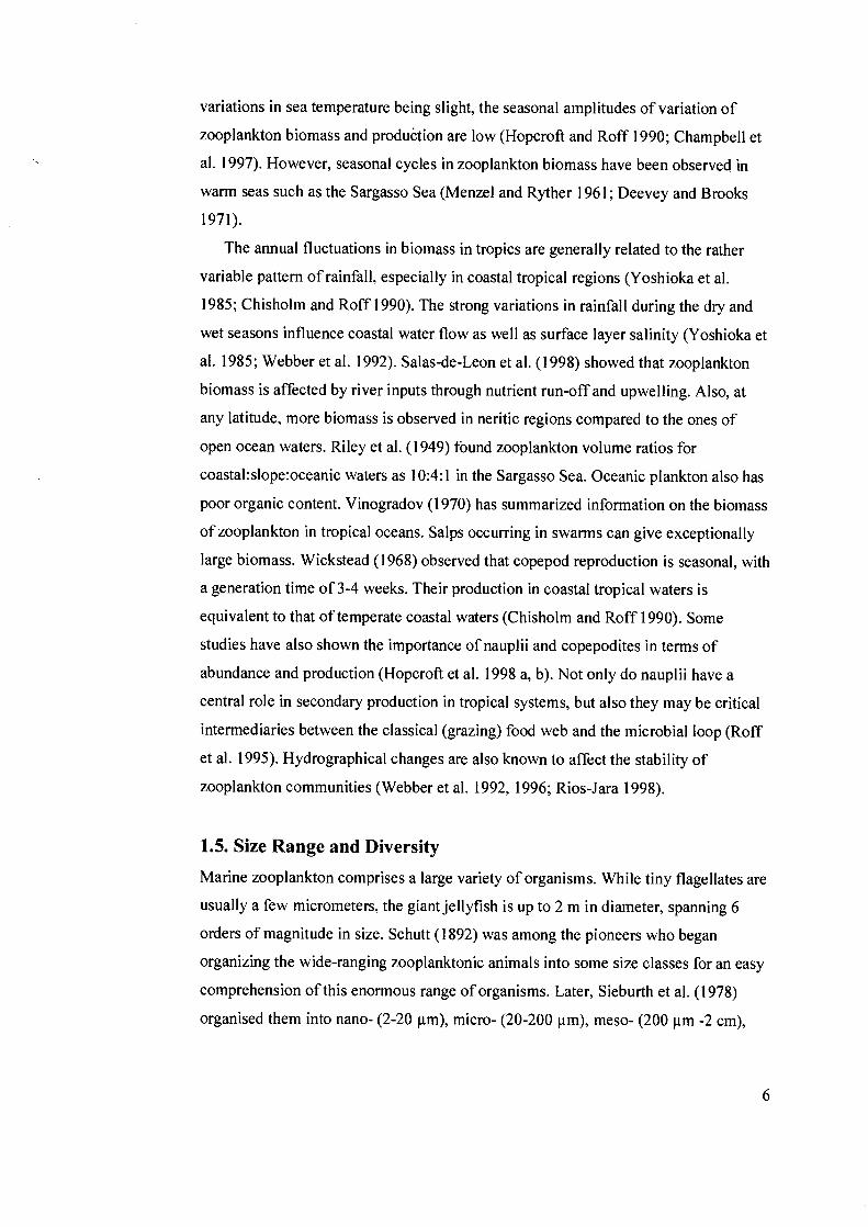
variations in sea temperature being slight, the seasonal amplitudes of variation of

zooplankton biomass and produCtion are low (Hoperoft and Roff 1990; Champbell et

al. 1997). However, seasonal cycles in zooplankton biomass have been observed in

warm seas such as the Sargasso Sea (Menzel and Ryther 1961; Deevey and Brooks

1971).

The annual fluctuations in biomass in tropics are generally related to the rather

variable pattern of rainfall, especially in coastal tropical regions (Yoshioka et al.

1985; Chisholm and Roff 1990). The strong variations in rainfall during the dry and

wet seasons influence coastal water flow as well as surface layer salinity (Yoshioka et

al. 1985; Webber et al. 1992). Salas-de-Leon et al. (1998) showed that zooplankton

biomass is affected by river inputs through nutrient run-off and upwelling. Also, at

any latitude, more biomass is observed in neritic regions compared to the ones of

open ocean waters. Riley et al. (1949) found zooplankton volume ratios for

coastal:slope:oceanic waters as 10:4:1 in the Sargasso Sea. Oceanic plankton also has

poor organic content. Vinogradov (1970) has summarized information on the biomass

of zooplankton in tropical oceans. Salps occurring in swarms can give exceptionally

large biomass. Wickstead (1968) observed that copepod reproduction is seasonal, with

a generation time of 3-4 weeks. Their production in coastal tropical waters is

equivalent to that of temperate coastal waters (Chisholm and Roff 1990). Some

studies have also shown the importance of nauplii and copepodites in terms of

abundance and production (Hoperoft et al. 1998 a, b). Not only do nauplii have a

central role in secondary production in tropical systems, but also they may be critical

intermediaries between the classical (grazing) food web and the microbial loop (Roff

et al. 1995). Hydrographical changes are also known to affect the stability of

zooplankton communities (Webber et al. 1992, 1996; Rios-Jara 1998).

1.5. Size Range and Diversity

Marine zooplankton comprises a large variety of organisms. While tiny flagellates are

usually a few micrometers, the giant jellyfish is up to 2 m in diameter, spanning 6

orders of magnitude in size. Schutt (1892) was among the pioneers who began

organizing the wide-ranging zooplanktonic animals into some size classes for an easy

comprehension of this enormous range of organisms. Later, Sieburth et al. (1978)

organised them into nano- (2-20 [tm), micro- (20-200 gm), meso- (200 gm -2 cm),

6

macro- (2-20 cm) and mega- (20-200 cm) plankton. Since body size governs the

growth rate, the doubling time for zooplankton in the range of 100-1500 gm is —2-12

days (Sheldon et al. 1972; Steele 1977).

The enormous diversity of animals in the plankton is well recognized. The

zooplankton is characterized by having representatives of almost every taxon of the

animal kingdom. Marine zooplankton is comprised of---36000 species (ICES 2000).

Only 27% of these are holoplanktonic with the remaining meroplanktonic. Their

species diversity is governed by temperature and evolutionary age of the oceans.

Their highest diversity is thus found in the tropics. The diversity of copepods is

usually higher in warm, oceanic waters. From the wide variety of taxa observed,

Copepoda forms the dominant fraction and is therefore justifiable to study them in

detail. Several aspects of biology of this Group are described in Chapter 6. Be (1966;

1967) and Be and Toderlund (1971) report 27-30 species of foraminiferans of which

22 are warm water species, living mainly in the upper 100 m (Berger 1969).

Similarly, 4500 species of Radiolaria, 900 of Cnidaria, 80 of Ctenophora, 100 of

Polychaeta, 10600 of Mollusca, 9000 of Crustacea, 2000 of Echinodermata, 50 of

Chaetognatha, 100 of Tunicata and 3000 species of fish larvae, are estimated to be in

the plankton (ICES 2000).

1.6. Grazing, Growth and Metabolism

Mesozooplankton grazing is a main factor in removing phytoplankton from the water

column (Steele 1974; Banse 1994). Zooplankton grazing and metabolism in the open

ocean waters have received growing attention in recent years, particularly in the

Pacific within the JGOFS equatorial Pacific study (Dam et al. 1995; Zhang et al.

1995; Le Borgne and Rodier 1997; Roman and Gauzens 1997; Zhang and Dam 1997;

Roman et al. 2002 b; Le-Borgne and Landry 2003) and the Atlantic Oceans (Le

Borgne 1977, 1981, 1982). A quantitative assessment of the effects of zooplankton

grazing and nutrient regeneration on the standing crop and growth of the

phytoplankton community is important for an understanding of aquatic ecosystem

dynamics. A common, and increasingly popular, approach for the estimation of

ingestion rates of herbivores and predators is based on the use of gut contents and

estimated gut passage times (Baars and Helling 1985).

7

Due to the variety in the diet of zooplankton, it is important to carry out

experimental analysis in order to understand their feeding ecology. Many

experimental studies aiming to understand trophic interactions are available (Calbet

and Landry 1999; Landry et al. 2003; Sautour et al. 2000; Stibor et al. 2004). Most of

the organic matter originated through primary production in the surface layers is fated

to mineralize through in situ planktonic respiration (Hernandez-Leon and Ikeda 2005).

As a convenient measure of zooplankton metabolism, oxygen consumption rate has

often been used. Early investigations on zooplankton respiration were mostly carried

out on Calanus finmarchicus (Marshall et al.1935; Clarke and Bonnet 1939). A

respiration rate determination indicates the amount of carbon being oxidized

(Marshall and Orr 1962) and allows the calculation of a first-order approximation to

the rate of nutrient recycling (Harris 1959; Satomi and Pomeroy 1965; Martin 1968;

Ganf and Blaika 1974).

Growth and metabolism of zooplankton depends on the interaction of a number of

external and internal factors. The external factors include food supply, nutritional

quality of food, predation, temperature, salinity and oxygen. The internal factors are

body size and physiological state. Potential growth rate is possible under ideal

conditions, however in reality, it may be limited by one of the above factors as well as

top down control. Since metabolic rate is also a function of body size, smaller

organisms have a comparatively higher rate and grow faster than the larger ones. In

marine copepods, where dominant copepods seldom vary in body size, temperature

has been demonstrated as the main factor governing their growth rate (Huntley and

Lopez 1992). In warmer waters, it is possible to build up a large population from a

low standing stock rather sooner due to the high growth rate. The ratio between

production and biomass is an important index of population dynamics indicating

turnover rate of organic matter. Under optimal conditions, the highest turnover is

observed in the tropics.

1.7. Sampling Methods

Most mesozooplankton sampling methods rely on the use of fine mesh nets, originally

made of bolting silk, now made of nylon and/or other synthetic material. Mesh size is

a critical factor in selecting organisms. The quantity of plankton passing through the

net is variable, depending on factors such as elasticity of the net, towing speed,

8

clogging (especially in phytoplankton-rich coastal areas), animal shape and,

possession of spines and projecting appendages by animals (Raymont 1983). The use

of vertically hauled closing nets has been of great value in plankton sampling in a

particular section of water column and its quantification on regional and seasonal

scales. One of the chief problems in quantitative sampling is estimation of the water

filtered through the net. For this purpose, a number of flow meters have been devised.

Avoidance of net by larger organisms such as euphausiids may be in response to

visual stimuli (net should not be shiny), pressure changes, acceleration or turbulence

or actual contact with the towing apparatus (Brinton 1967). The Hardy Continuous

Plankton Recorder (Hardy 1939) conceived in the1920s has proved to be an important

tool in sampling large areas of the open ocean and is especially useful in monitoring

long-term faunistic changes in surface layers (Reid et al. 2003). Galliene et al. (2001)

have shown a good agreement between biovolume using optical plankton counter and

carbon content using vertical plankton hauls in the North Atlantic.

There are two main types of quantitative procedures for zooplankton, biomass

determination and counting methods. Biomass/biovolume is generally expressed as

mass per unit volume of water i.e. mg m-3 , or related to the sea surface as mg m -2 .

There are a variety of methods for biovolume/biomass measurements. However, the

volumetric and gravimetric methods are rapid compared to the biochemical methods.

In the first one, displacement volume is the most reliable hence, most commonly used.

The other, settling volume is less precise when gelatinous organisms and, ones with

long appendages of higher buoyancy are present in the mixed plankton sample

(Hensen 1887). In the gravimetric method involving wet mass measurement of

samples after being preserved by formalin, slight to large loss of biomass is possible.

Dry mass and biochemical measurements cause destruction of sample. Measuring

abundance, the number of individuals per unit volume/surface of water (individuals

M-3 or m-2) though laborious, demanding experience, allows parallel quantification

and species identification. It is generally the most accepted basis of community

analysis.

1.8. Study Area and Objectives

The Bay of Bengal (BoB) is a unique embayment receiving large river inflow (-1.62

x 1012 m 3 year-1 ) from Godavari, Krishna, Cauvery, Mahanadi, Ganges, Brahmaputra

9

and Irrawaddy. Precipitation (ca. 2 m year t ) exceeding evaporation (-1 m year -1 ; Han

and Webster 2002), low-saline surface waters (28— 33 psu), warmer sea-surface

temperatures (SST, 29-30°C) and weak winds (<7 m s -1 ) stratify the upper 30-40 m

column of the Bay (Prasannakumar et al. 2002). Further, absence of marked

upwelling limits nutrient injection into euphotic layer. Apart from this, the high

terrigenous input (ca. 1.4 x 109 tons Subramanian 1993) by rivers and

prolonged cloud cover cause light limitation leading to low photosynthetic production

(Prasannakumar et al. 2002).

In the Bay, quantitative and qualitative surveys examining the seasonal cycle of

zooplankton are limited mostly to inshore waters. Using the opportunity of the Bay of

Bengal Process Studies (BOBPS) programme, it was planned to decipher the spatio-

temporal variability of zooplankton community. This first time study was planned for

a comparative analysis from the open-ocean and near-coastal waters from the surface

to 1000 m with the main idea of understanding its relation with the physico-chemical

parameters.

For this study, the following objectives were planned:

■ To measure the vertical distribution of mesozooplankton biomass and population

density with the main idea to decipher spatio-temporal variability and to

characterize the mesozooplankton community structure as well as to carry out a

detailed taxonomic analysis to obtain species identification wherever possible.

The rationale behind this objective is the following. The surface primary

production in the Bay varies with seasonally reversing monsoon currents. It

ultimately governs the amount of organic matter produced and transported to

deeper depths. This might also be reflected in the biomass and composition of

zooplankton species at deeper depths. This set of analyses was to provide

answers to the questions as to: a) how the zooplankton biomass responds to

low-saline upper waters that make the Bay to be low to moderate in

phytoplankton biomass and, b) how their populations in terms of abundance

and type vary during different seasons when physical, chemical and

chlorophyll characteristics change. As oligotrophic regions are known to

harbor larger diversity of organisms, it was pondered over that the

zooplankton group/species diversity would be more. In the near-estuarine

surface condition of the Bay, there is scarce photosynthetic food and relatively

more detrital matter through allochthonous inputs from the rivers. With

10

warmer sea-surface temperature of almost always > 28°C, it was also intended

to examine whether there is any predominance of a single or a few species,

location-, depth- or season-wise.

■ To understand the influences of environmental and biological factors on the

mesozooplankton population dynamics through experimental alterations of

nutrients, salinity, phytoplankton density, microzooplankton and bacteria. Further,

to estimate mesozooplankton ingestion, egestion, grazing, respiration and potential

growth rates.

There have been no experimental studies to realize the grazing potential of

mesozooplankton assemblages in the Bay of Bengal. Mesozooplankton with

diverse food habits are known to be the major consumers of phytoplankton as

well as microzooplankton and bacteria. Since salinity, nutrients and

phytoplankton abundance and type vary regionally in the Bay, the rationale

was to set up microcosm experiments at different latitudes to get basic

information on the environmental effects on zooplankton, potential grazing,

predation and omnivory.

Since strong latitudinal gradients in salinity are observed in the top 50 m in

central as well as western Bay, measurements of mesozooplankton gut

fluorescence were also carried out at various latitudes to obtain the ingestion

and defecation rates. Similarly, respiration rate through dissolved oxygen

measurements were also done at these stations to obtain estimations of overall

metabolic activity.

Since growth is temperature dependant, standard growth rate equations were

used to obtain estimates of mesozooplankton growth potential in the warm

pool environment of the Bay.

11

Table 1.1. Taxonomic Classification of Marine Zooplankton (Garrison 2004)

KINGDOM PROTISTA: Eukaryotic single-celled, colonial, and a few multicellular heterotrophs # PHYLUM SARCODINA: Amoebas and their relatives Class Rhizopodea: Foraminiferans Class Actinopodea: Radiolarians

KINGDOM ANIMALIA: Mostly multicellular heterotrophs # PHYLUM PORIFERA: Sponges # PHYLUM CNIDARIA: Jellyfish and their kin; all are equipped with stinging cells Class Hydrozoa: Polyp-like animals that often have a medusa-like stage in their life cycle, such as Portuguese man-of-war (Physalia physalis) Class Scyphozoa: Jellyfish with no (or reduced) polyp stage in life cycle Class Cubozoa: Sea wasps; commonly called box jellyfishes (e.g. Chironexfleckeri) Class Anthozoa: Sea anemones, coral # PHYLUM CTENOPHORA: "Sea gooseberries/ comb jellies"; round, gelatinous, predatory # PHYLUM MOLLUSCA: Mollusks Class Monoplacophora: Rare, deep-water forms with limpet-like shells Class Polyplacophora: Bearing many plates e.g. 8-piece shells in Chitons Class Aplacophora: Shell-less; sand burrowing e.g. Helicoradomenia, Chaetoderma Class Gastropoda: Snails, limpets, abalones, sea slugs, pteropods Class Bivalvia: Clams, oysters, scallops, mussels and shipworms Class Cephalopoda: Squid, octopuses, and nautiluses Class Scaphopoda: Tooth shells e.g. Dentalium pretiosum # PHYLUM ARTHROPODA: jointed-foot invertebrates Subphylum Crustacea: Copepods, barnacles, krill, isopods, amphipods, shrimp, lobsters, crabs Subphylum Chelicerata: Horseshoe crabs, sea spiders Subphylum Uniramia: Insects, e.g. Halobates # PHYLUM SIPUNCULA: Peanut worms; all marine # PHYLUM ANNELIDA: Segmented worms; e.g. polychaetes PHYLUM ECHINODERMATA: Radially symmetrical, most with a water-vascular system, spiny-skinned, benthic Class Asteroidea: Sea stars Class Ophiuroidea: Brittle stars, basket stars Class' Echinoidea: Sea urchins, sand dollars, and sea biscuits Class Holothuroidea: Sea cucumbers Class Crinoidea: Sea lilies, feather stars Class Concentricycloidea: Sea daisies # PHYLUM CHAETOGNATHA: Arrow worms; stiff-bodied, planktonic and predaceous # PHYLUM CHORDATA: Having at some stage of development a dorsal nerve cord, a notochord, and gill slits Subphylum Urochordata: Sea squirts, tunicates (Appendicularia),Thaliacea(Doliolida, Pyrosomida, Salpida) Subphylum Cephalochordata: Lancelets, Amphioxus Subphylum: Vertebrata Class Agnatha: Jawless fishes such as lampreys, hagfishes; cartilaginous skeleton Class Chondrichthyes: jawed cartilaginous fish with paired fins and nostrils, scales, two-chambered hearts; &larks, skates, rays, chimaeras and sawfish Class Osteichthyes: Bony fishes

Chapter 2

Chapter 2

Review of Literature

Mesozooplankton are the main link between planktonic primary producers and

consumers such as fish. Such a key component in the structure and functioning of marine

planktonic food webs (Fig. 2.1) has other roles too. For instance, their role of

regeneration of inorganic nutrients, especially ammonia that is ideally suited to promote

phytoplankton growth into surface waters is highly recognized (Saiz et al. 2007).

Regeneration of nutrients in the photic zone via the "microbial loop" during the low

chlorophyll times has also been appreciated (Nybakken 1997; Fig. 2.2). Their diel

vertical migration (DVM) in all oceans is a universally known feature (Hays 2003). By

the process of DVM, they feed near surface at night, migrate to deeper depth during the

day (Fig. 2.3) where they continue to defecate, respire, excrete, and thus export the

ingested carbon and nitrogen out of the photic zone (Longhurst and Harrison 1989; Hays

et al. 1997; Schnetzer and Steinberg 2002 b). About 20 species of marine zooplankton are

commercially utilized as food or feed. These are mainly planktonic crustaceans

comprising —11% of the crustacean fishery in the world (Omori 1978). Due to their large

density, shorter life span, drifting nature, high group/species diversity and different

tolerance to varying environmental conditions, some of them are also used as indicators

of physical, chemical and biological processes in the aquatic ecosystems (Beaugrand

2005).

Approximately 36000 zooplankton species exist in the oceans, out of which —11500

belong to subclass Copepoda (ICES 2000). Hardy (1970) and Turner (2004) proposed

that the copepods are the most numerous metazoan animals in the world, even

outnumbering the insects, despite the latter having more species. Well-fed copepods

produce larger batches of eggs (Steidinger and Walker 1984). Therefore the successful

reproduction of herbivorous zooplankton depends on adequate supply of phytoplankton.

Owing to their abundance, their fecal pellets, which are produced at rates of up to 150

individual day"' (Pinto et al. 2001), represent an ecologically important energy source

12

Figure 2.1. An un-assorted sample of mesozooplankton

Motors noviirws y Microbiology

Figure 2.2. Schematic presentation of a marine food web (Azam and Malfattti 007)

Figure 2.3. Schematic diagram of diel vertical migration in zooplankton .

While downward movement (left side arrow) is begun at dawn, the upward movement begins by dusk

for detritus feeders. The flux of fecal pellets —50-100 m day -I (Suess 1980) to the ocean

floor may have a significant impact on nutrient cycling and sedimentation rates.

Ecologically, copepods are important links in the food chain linking the microscopic

algal cells to juvenile fish to whales. They constitute the biggest source of protein in the

oceans. Most of the economically important fishes depend on copepods and even the

whales in the northern hemisphere feed on them. Some copepods like Branchiura

(commonly referred to as sea lice) are known parasites of fish. Copepod fecal pellets

contribute greatly to the marine snow and therefore accelerate the flow of nutrients and

minerals from surface waters to the bottom of the seas. The sheer abundance of copepods

in marine plankton secures them a vital role in the marine ecosystem.

Several investigators have documented various aspects of mesozooplankton biology

(Raymont 1983). For instance, from spatio-temporal studies, it has been evidenced that

mesozooplankton populations in the Northeast Pacific have undergone a regime shift

possibly following changes in climatic conditions (Batten and Welch 2004). Fernandez-

Alamo and Farber-Lorda (2006) have shown that zooplankton spatio-temporal variations

coincide with water circulations, water-masses and upwelling. They also found that they

were directly related to the regime shifts of commercial fisheries in the eastern tropical

Pacific. From a 50- year historic record, these authors have observed a shift from the

sardine regime during low zooplankton biomass to anchovy regime during high

zooplankton biomass. Similarly, the interannual changes in zooplankton communities

were directly linked to the growth of sardine larvae in the Mediterranean Sea (Mercado et

al. 2007). High zooplankton production off Saurashtra coast in the Indian Ocean region

corresponds to the rich fisheries (Govindan et al. 1982). These physical processes affect

primary productivity and, thus play a prominent role in structuring of zooplankton

communities, as a consequence, affecting the recruitment of pelagic fisheries.

2.1. Spatio-temporal Distribution of Biomass and Abundance

Nutrients and, primary and secondary productivity ultimately determine the sustainable

harvest of fish resources (Cushing 1971). A change in phytoplankton production does

affect the biomass at the higher trophic levels including fishery yield (Nixon 1988;

Gucinski et al.1990). Environmental parameters like salinity, dissolved oxygen and

13

nutrients directly influence the abundance and diversity (Siokou-Frangou et al. 1998) as

well as the distribution (Nasser et al. 1998) of zooplankton. However, Irigoien et al.

(2004 a) have shown that zooplankton diversity, which is a unimodal function of its

biomass, is not related to phytoplankton biomass.

Mixed zooplankton is assumed to contain carbon comprising — 35- 45% of the dry

weight in the North Pacific (Omori 1969) and —34% in the Indian Ocean (Madhupratap et

al. 1981; Madhupratap and Haridas 1990). Their biomass is reported to be higher in

boreal and polar waters, intermediate in equatorial waters and the lowest in subtropical

gyres (Hernandez-Leon and Ikeda 2005). Mesozooplankton represent a major, but

neglected component of the carbon cycle in the ocean. Also, climate change

manifestation in terms of local-scale temperature variations seem to affect and alternate

zooplankton life histories (Costello et al. 2006).

2.1.1. Depth-wise distribution

Mesozooplankton abundance in the Arabian Sea (AS) is fairly high in the mixed layer

depth (MLD) all through the year (Madhupratap et al. 1996 a). Padmavati et al. (1998)

found higher standing stocks of zooplankton in the MLD and the lowest in the 500-1000

m (deepest sampled strata) in the central and eastern AS. Higher biomass in the upper

200 m was related to potentially higher food levels in this depth zone (Wishner et al.

1998). Their biovolumes decrease with increasing depth in all seasons in the northern AS

(Pieper et al. 2001), in phase with the primary production in the top 150 m (Koppelmann

et al. 2003). In the mesopelagic realm (150-1050 m), the seasonal coupling was less clear

and there was no such evidence in the bathypelagic zone below 1050 m (Koppelmann et

al. 2003). At two sites (one each in the central and western Arabian Sea), zooplankton

biomass and abundance that were measured up to 4000 m were elevated in the

oxygenated surface waters, decreased sharply in the oxygen minimum zone (OMZ)

before decreasing gradually below 1000 m (Koppelmann et al. 2005).

In a study from upper 4440 m in the eastern Mediterranean, maximum abundance of

zooplankton was observed at 100 m, where maximum phytoplankton was present (Kimor

and Wood 1975). At 1000 m, the biomass was — 1% of the surface zooplankton, at 5000

14

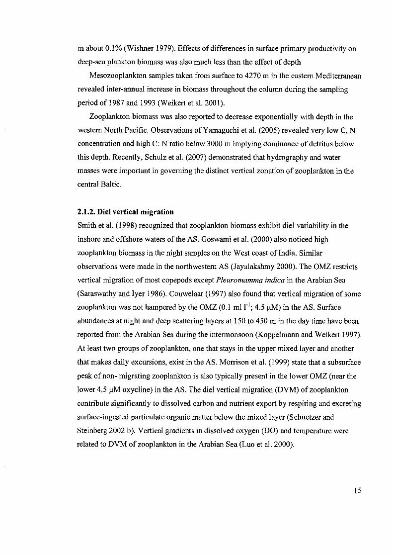
m about 0.1% (Wishner 1979). Effects of differences in surface primary productivity on

deep-sea plankton biomass was also much less than the effect of depth

Mesozooplankton samples taken from surface to 4270 m in the eastern Mediterranean

revealed inter-annual increase in biomass throughout the column during the sampling

period of 1987 and 1993 (Weikert et al. 2001).

Zooplankton biomass was also reported to decrease exponentially with depth in the

western North Pacific. Observations of Yamaguchi et al. (2005) revealed very low C, N

concentration and high C: N ratio below 3000 m implying dominance of detritus below

this depth. Recently, Schulz et al. (2007) demonstrated that hydrography and water

masses were important in governing the distinct vertical zonation of zooplankton in the

central Baltic.

2.1.2. Diel vertical migration

Smith et al. (1998) recognized that zooplankton biomass exhibit diel variability in the

inshore and offshore waters of the AS. Goswami et al. (2000) also noticed high

zooplankton biomass in the night samples on the West coast of India. Similar

observations were made in the northwestern AS (Jayalakshmy 2000). The OMZ restricts

vertical migration of most copepods except Pleuromamma indica in the Arabian Sea

(Saraswathy and Iyer 1986). Couwelaar (1997) also found that vertical migration of some

zooplankton was not hampered by the OMZ (0.1 ml 1 -1 ; 4.5 µM) in the AS. Surface

abundances at night and deep scattering layers at 150 to 450 m in the day time have been

reported from the Arabian Sea during the intermonsoon (Koppelmann and Weikert 1997).

At least two groups of zooplankton, one that stays in the upper mixed layer and another

that makes daily excursions, exist in the AS. Morrison et al. (1999) state that a subsurface

peak of non- migrating zooplankton is also typically present in the lower OMZ (near the

lower 4.5 1,1M oxycline) in the AS. The diel vertical migration (DVM) of zooplankton

contribute significantly to dissolved carbon and nutrient export by respiring and excreting

surface-ingested particulate organic matter below the mixed layer (Schnetzer and

Steinberg 2002 b). Vertical gradients in dissolved oxygen (DO) and temperature were

related to DVM of zooplankton in the Arabian Sea (Luo et al. 2000).

15

Saltzman and Wishner (1997) studied vertical distribution of copepods in the upper

1230 m, in relation to the OMZ in the eastern tropical Pacific. Diel variations were also

observed in zooplankton biomass at the Bermuda Atlantic time-series (BATS) site in the

North Atlantic (Madin et al. 2001). The average biomass at night within the upper 200 m

exceeded that at day by 3.5 times in the Angola Benguela coastal upwelling zone and the

OMZ (0.2 ml 1-1 ) was no barrier to migrating zooplankon (Postel et al. 2007). While some

chaetognaths and species of copepods were found to perform DVM, over 60% of the

zooplankton did not perform significant DVM in the Irish Sea (Irigoien at al. 2004 b). In

the near-shore areas where DO reduction to< 1.0 ml 1 1 may be sudden, widespread, or

unpredictable, the patterns of reduced copepod abundance in bottom waters may

primarily be due to mortality rather than avoidance (Stalder and Marcus 1997).

2.1.3. Seasonal and latitudinal variability

Copepod distribution was found to vary seasonally in the Tapong Bay off Taiwan (Lo et

al. 2004 a). Kang et al. (2004) attributed zooplankton distribution patterns to the spatial

variations in chlorophyll (chl) a. Yamaguchi et al. (2005) found that diversity increased

offshore. Spatial variability of zooplankton species richness, abundance and biomass was

ascribed to salinity gradient in estuarine waters of China (Li et al. 2006).

Ramfos et al. (2006) found strong seasonal changes in dominant copepods in the

surface layer in the eastern Mediterranean Sea, where strong variations in hydrography

was evident with biomass and abundance decreasing offshore. In a monthly sampling at

the BATS, zooplankton biomass showed seasonal variations (Madin et al. 2001). Salinity

was found to control the spatio- temporal changes in mesozooplankton community

structure in the Seine Estuary (Mauny and Dauvin 2002), Bristol Channel and Severn

Estuary (Collins and Williams 1981). Seasonal and spatial variation in mesozooplankton

biomass correlating positively with chlorophyll, primary production and organic

particulate matter and, negatively with temperature and salinity was observed in the

Northwest Mediterranean (Gaudy et al. 2003). Abundance of zooplankton increased with

increasing temperature, salinity and chlorophyll a values in a temperate estuary in

western Portugal (Vieira et al. 2003). Uncoupling between phytoplankton and

zooplankton consumers was observed in the Waquoit Bay (Lawrence et al. 2004).

16

Temperature, salinity and suspended matter seem to regulate the seasonal and annual

variability of zooplankton density in the turbid Gironde Estuary (David et al. 2005).

Vidjak et al. (2006) observed high mesozooplankton abundance and low diversity in the

eastern Adriatic Sea during the warmer part of the year. On the contrary, a 10- year

survey in the western Mediterranean revealed seasonal and interannual changes in

zooplankton biomass and assemblages, with the warmer years having lesser biomass

compared to the cooler years (De-Puelles et al. 2007). Alcaraz et al. (2007) found that the

deep chl a maxima during summer stratification allows the formation of deep

zooplankton maxima in the Mediterranean.

The eastern Arabian Sea is rich in zooplankton production (Menon and George 1977)

mainly due to coastal upwelling. Along the West coast of India, accelerated zooplankton

production was documented during periods of high salinity (Madhupratap 1986; Tiwari

and Nair 1993). The phytoplankton to zooplankton carbon ratio has been higher during

the periods of low salinity in Cochin backwaters (Madhu et al. 2007). Zooplankton

diversity that was inversely related to abundance showed variability between the

monsoons in the western Indian Ocean (Mwaluma et al. 2003). Changes observed in

zooplankton biomass using an Acoustic Doppler Current Profiler were associated with

monsoonal oscillations in the AS (Ashjian et al. 2002). Madhupratap and Haridas (1975)

noticed that zooplankton displacement volumes were higher at those stations where

swarms of hydromedusae and ctenophores occurred. Zooplankton biovolumes varied

seasonally, with the lowest biovolumes during the summer monsoon (SUM), intermediate

during the fall intermonsoon (FIM) and the highest during the winter (Northeast)

monsoon (WM) in the northern AS (Pieper et al. 2001). High biomass was observed off

Oman, the upwelling zone during SUM (Hitchcock et al. 2002). They also observed high

biomass of zooplankton coinciding with the large phytoplankton blooms in the Red Sea

and Gulf of Aden during WM, and in the Somali Current and northern Somali Basin

coinciding with the high primary production during SUM. Smith and Madhupratap

(2005) found high standing stocks of zooplankton in the AS being sustained during low

chlorophyll period L e. the WM by the microbial loop. They also reported that by the end

of SUM, at least one abundant epipelagic copepod species goes through diapause in the

subsurface. However, Padmavati et al. (1998) did not find much variation between

17

coastal and offshore standing stocks of zooplankton in the AS. However, Smith et al.

(1998) and Stelfox et al. (1999) found that zooplankton differed in the inshore and

offshore waters with the seasonally reversing monsoons in the AS.

In a study carried out in the neritic and estuarine waters off Coromandel Coast, Bay

of Bengal (BoB), during the period from January 1960 to December 1967, a steady-

increasing trend in plankton production was evident from months of March to October,

correlating with the salinity and rainfall (Subbaraju and Krishnamurthy 1972). Higher

zooplankton standing stocks were reported in the upwelling area in the western Bay of

Bengal (Nair et al.1981). Piontkovski et al. (1995 b) stated that zooplankton abundance-

spectra change with hydrodynamic regimes of water in the Indian Ocean. In a study from

the western Bay of Bengal during January and May, Rakhesh et al. (2006), recorded 58

copepod species dominating the zooplankton sample collections in the top layers. Basin-

scale and mesoscale processes such as warm-core eddies, cold-core eddies and upwelling

areas influence the abundance and spatial heterogeneity of plankton populations across a

wide spatial scale in the BoB (Muraleedharan et al. 2007). Spatial differences in

zooplankton were also found in the Malacca Strait (Rezai et al. 2004).

2.2. Composition

Achuthankutty and Selvakumar (1979) observed high abundance of Acetes larvae during

pre- and post monsoon in the estuarine systems of Goa. Nair and Paulinose (1980)

recorded elevated abundance of decapod larvae near to the coast, decreasing gradually

towards the open ocean. Copepods dominate the marine zooplankton community and

often contribute over 80-90% of the total zooplankton in near-shore and estuarine habitats

(Ramaiah and Nair 1993). Most herbivores in the AS are either small filter feeders like

copepods or large mucous filters feeders like tunicates that are able to feed on very small

particles (Nair et al. 1999). Kidwai and Amjad (2000) reported 38 taxonomic groups

from the samples collected during SUM and WM in the Arabian Sea. Copepoda was the

most dominant group, followed by chaetognaths and siphonophores in their collection.

The size structure of zooplankton was related to the spatio- temporal variation in size

spectra of dominant phytoplankton (Stelfox et al. 1999). Increased abundances of

Calanoides carinatus were observed off Oman, the upwelling zone during SUM

is

(Hitchcock et al. 2002). Among the preponderant Calanoida, the members of families

Clausocalanidae and Paracalanidae were the most abundant among copepods in the Gulf

of Aqaba. As Cornils et al. (2007) propose, this abundance is strongly linked to the

annual temperature cycle.

Zooplankton composition was homogenous and diversity low irrespective of season

in the subtropical Inland Sea of Japan (Madhupratap and Onbe 1986). Vertical

distribution of zooplankton community was closely linked with the hydrographic

structure in East Japan Sea (Ashjian et al. 2005). Across the continental margin of the

Northeast Pacific, zooplankton show a typical gradient in community composition from

near-shore to oceanic. This gradient is usually the steepest near the continental shelf

break (Mackas and Coyle 2005). Numerical abundance of copepod fraction in the smaller

size-range of 100-300 gm was seven times greater than the larger size fraction of >330

gm in Tapong Bay (Lo et al. 2004 a). Oithona, the most ubiquitous and abundant

copepod in the world's oceans increased in abundance during the FIM and WM in the AS

(Smith and Madhupratap 2005). According to Bottger-Schnack (1994), Calanoida,

Cyclopoida (Oithona and Paroithona) and Poecilostomatoida (mainly Oncaea) are the

three most abundant copepod orders in the eastern Mediterranean, Arabian Sea and Red

Sea. In the epipelagic zone (0-100 m), these orders are reported to occur at similar

abundance levels, whereas in the meso- and bathypelagic zones, Oncaea dominates

numerically (60-80%). Nakata et al. (2004) suggest that an increase in temperature and

decrease in primary production (PP) would reduce the reproduction of the oncaeids in the

surface layer. Among the 178 copepod-species identified off northern Taiwan, western

North Pacific during spring, Paracalanus aculeatus, Oncaea venusta and Clausocalanus

furcatus were the three dominant species (Lo et al. 2004 b). These three species

contributed 43% of the total copepod numbers during their study. The deep-dwelling

detritivorous copepod, Lucicutia grandis was found in high numbers at the lower

interface of the OMZ (400-1100 m) at one station in the Arabian Sea during spring

intermonsoon and summer monsoon (Gowing and Wishner 1998). Nishikawa et al.

(2007) recorded dominance of Eucalanidae, Metridinidae and Lucicutiidae in the OMZ of

the Sulu Sea. Ramfos et al. (2006) found strong seasonal changes in the dominant

copepods in surface layer of the eastern Mediterranean.

19

Siphonophora are the major and regular constituents of the marine zooplankton,

which occupy fourth or fifth place in the order of abundance in the tropical community

(Yamazi 1971). However, unlike other zooplankton, it is very difficult to obtain an

accurate estimation of siphonophore population in an area because of its structure,

complexities and fragile nature (Rengarajan 1983). Hydromedusae represent an important

and exclusive carnivorous zooplankton group in the coastal zones of India (Santhakumari

1977). Factors such as salinity, temperature, currents, food availability and seasons

regulate the distribution of medusae (Santhakumari and Nair 1999). The abundance of

fish larvae and salinity showed a significant negative correlation (p<0.001) indicating that

the fish larval abundance decreased as salinity increased (Devi 1977). Occurrence of fish

eggs and larvae during summer indicates the spawning periods of various fishes of the

inshore waters of the Tuticorin (Marychamy et al. 1985).

The protozoan Acantharia, containing zooxanthellae and chl a, was recorded as deep

as 4000 m and below for the first time in the eastern Mediterranean (Kimor and Wood

1975). Batistic et al. (2003) found that chaetognath abundance was high in the upper 100

m and decreased with increasing depth. From the Southern Ocean, Hempel (1985)

described three very different large-scale subsystems, the ice-free West Wind Drift

dominated by copepods, the seasonal pack-ice zone with the hill Euphausia superba as

the main component, and the permanent pack-ice zone where copepods and the ice-hill

Euphausia crystallorophias are the major plankton-elements. Both copepods and

larvaceans are sources of fluorescent- and chromophoric dissolved organic matter in

marine coastal systems (Urban-Rich et al. 2006).

Higher concentrations of pteropods were observed in the center of a cold-core eddy

compared to the ambient water in the northeastern Atlantic, with large sized specimens

occurring in 100-400 m depth than in the surface (Beckmann et al. 1987). The high

abundance of filter-feeders (ostracods, cladocerans, doliolids and salps) was ascribed to

elevated chlorophyll concentrations in the cyclonic eddy in the southwestern

Mediterranean Sea, during summer (Riandey et al. 2005). Data from continuous plankton

recorder (CPR) surveys demonstrate that zooplankton communities have undergone

geographical as well as size shifts off the Northwest European shelf (Pitois and Fox

2006).

20

In the northern Indian Ocean, plankton communities differed in zones of intensive

divergence, poor divergence and stratified waters in terms of their biomass, species

diversity, and trophic group ratios (Timonin 1976). The disproportionately high

abundance of very few species of mesozooplankton in the epipelagic zone of the Red Sea

than the bathypelagic zone was related to high temperature (>21.5°C) and salinity (> 40

psu; Weikert 1982) in the later zone. A faunistic change was also observed in the bathy-

to abysso- pelagic zone in the eastern Mediterranean (Weikert et al. 2001). The

mesozooplankton composition is noted to vary with space and season in the Indian Ocean

sector of the Southern Ocean (Mayzaud et al. 2002 a).

2.3. Grazing- and Growth- Rates

The small sized mesozooplankton (200-500 pm) contributing >50% to the total grazing

rates by mesozooplankton showed latitudinal differences in central tropical Pacific

(Zhang et al. 1995). Their rates of ingestion, egestion and production in the equatorial

Pacific 140°W and 180° are maximal in the high-nutrient low-chlorophyll (HNLC) zone

associated with equatorial upwelling (5°S-5°N) as compared to the more oligotrophic

regions to the north and south of it (Roman et al. 2002 b). In the equatorial upwelling

region of the Atlantic, high primary production rates and low phytoplankton biomass

were suggestive of a strong top-down control of primary producers by zooplankton

(Perez et al. 2005). Sautour et al. (2000) found that 26% of the total PP was grazed by

mesozooplankton in the Gironde Estuary. Their average grazing rates varying from 19 to

92 mg C m 2 d" 1 in the AS during September-December resulted in the removal of 4-12%

of daily PP (Edwards et al. 1999). Hernandez-Leon et al. (2002) observed high gut

fluorescence in zooplankton along an upwelling filament extending from Northwest

African coast to offshore. Grazing was also estimated by using 14C- radiolabeled natural

(i.e., mixed) phytoplankton populations (Griffiths and Caperon 1979). However, the

reliability of the results is better when the experimental time is short enough to prevent

recycling of the isotope, and growth of the phytoplankton substrate.

Using the gut fluorescence (GF) technique, Pakhomov and Froneman (2004) showed

that copepods were the most conspicuous grazers in the upper 200 m. Along an eastern

transect of the southern Atlantic Ocean, GF accounted for —40% of total zooplankton

21

grazing. The grazing impact of the copepods (>73 % of total zooplankton) changed

seasonally and spatially in the Pearl River Estuary and, varied between <0.3% and 75%

of the chlorophyll standing stock, and up to 21-104% of the daily phytoplankton

production (Tan et al. 2004). In the Atlantic (Huskin et al. 2001 a), copepod gut

evacuation rate averaged 0.03 min -1 irrespective of latitude or body size. Their grazing

impact averaged —6% of the integrated chlorophyll (chl) a concentration and 22% of the

primary production in the subtropical Atlantic during spring (Huskin et al. 2001 b) with

higher gut content during night.

Paffenhofer (2002) has revealed that many species of diatoms in bloom

concentrations can negatively affect the nauplii of many calanoid copepods. Exudates and

transparent exopolymer particles from Phaeocystis globosa are known to drastically

reduce the microalgal feeding rates of naupliar stages of copepods (Dutz et al. 2005). Gut

content analysis of the copepods Pleuromamma xiphias (Giesbrecht), Euchirella

messinensis (Claus) and of the euphausiid Thysanopoda aequalis (Hansen) indicated that

all three species fed on a wide variety of phytoplankton, zooplankton, and detrital

material. Diet changes generally reflected seasonal trends in phytoplankton community

structure. However, species-specific feeding preferences and differences in feeding

selectivity among the three species, all with distinct mouthpart morphology, were evident

(Schnetzer and Steinberg 2002 a).

Wu et al. (2004) studied the gut contents of the poecilostomatoids, Oncaea venusta,

0. mediterranea, and 0. conifera from the southern Taiwan Strait. Copepod gut contents

comprising diatoms (Chaetoceros sp. and Thalassiothrix sp.), radiolaria and,

microzooplanktonic- and copepod debris suggests the kind of food components available

in the study area. Such analyses are useful in suggesting non-selectively and diversity in

feeding habits. As copepods feeding on coccolithophores are known to egest only 27-

50% of the ingested coccolith calcite, there are strong possibilities of its acid digestion in

their guts (Harris 1994). Oncaea venusta is known to attack and feed on chaetognaths

(Go et al. 1998). From the fatty acid and alcohol composition of oncaeids and oithoniids,

it has been concluded that feeding behaviour of all their species is omnivorous and/or

carnivorous (Kattner et al. 2003). Copepods are also known to be highly adept at

consuming their own fecal pellets, a process called coprohexy (coprophagy), by

22

removing the peritrophic membrane with its attached bacterial flora leaving behind

"ghost" pellets, consisting of only a membrane with little or no apparent solid content

(Lampitt et al. 1990).

The preponderant —21.1m sized phytoplankton in warm oligotrophic open oceans are

too small for direct consumption efficiently by mesozooplankton (Calbet and Landry

1999). Food chain analysis suggests that a significant fraction of the microzooplankton is

probably consumed by mesozooplankton (Dam et al. 1995; Calbet and Landry 1999). An

estimated 28% of the carbon demand of mesozooplankton is met by ciliates and

heterotrophic dinoflagellates in coastal waters off Zanzibar during May-June (Lugomela

et al. 2001). Schnetzer and Caron (2005) observed that the copepods were responsible for

removing 5-36 % of the microzooplankton standing stocks in the San Pedro Channel,

California resulting in increased abundance of nanozooplankton. Umani et al. (2005)

demonstrated that mesozooplankton consume —76% of the daily PP in the mesotrophic

northern Adriatic Sea. Further, microzooplankton also formed substantial portion in their

diet.

In the Arabian Sea, mesozooplankton were mostly omnivorous consuming detritus

and protozoa (Richardson et al. 2006). However, they mainly grazed upon large

phytoplankton whenever they prevailed. Heterotrophic prey constitutes a relevant fraction

of zooplankton diet, as an alternative to the scarce phytoplankton in the Northwest

Mediterranean Sea (Saiz et al. 2007). Seasonal and inter-annual variations in

mesozooplankton grazing were observed in the upwelling region, off northern California

(Slaughter et al. 2006). Zooplankton grazing on bacterioplankton populations was found

to be insignificant in some studies (Boak and Goalder 1983). However, from the

experimental addition of nutrients in the eastern Mediterranean (Pasternak et al. 2005),

gut fullness of herbivores suggested the rapid utilization of the enhanced stocks of

bacterio-and phyto-plankton.

While planktivorous fish are known to be important predators of fish eggs and larvae

(Steidinger and Walker 1984), some zooplankton are known to be predators on

ichtyoplankton (Brewer at al. 1984). Scyphomedusae are known to consume a variety of

zooplankton such as larvaceans, cladocerans, fish eggs and hydromedusae (Fancett

1988). Terazaki (1996) inferred that the diet of Sagitta enflata consists of —52% copepods

23

and a small percentage each of foraminiferans, chaetognaths, pteropods, ostracods,

crustacean and fish larvae, corresponding to a daily feeding rate of 8% of the secondary

production in the central equatorial Pacific. Though copepods were the main diet of

chaetognaths, cannibalism was common in the South Adriatic (Batistic et al. 2003). Salps

have a fine-mesh filter, on which they can retain even the smallest phytoplankton. In

contrast, pteropods ingest mostly larger phytoplankton and the fecal pellets of both these

epipelagic herbivores, large in size are source of food for the deeper living animals.

Zooplankton growth rate averaging 0.12 d -I, varying only slightly with seasons in the

northern AS was the highest in inshore waters (Roman et al. 2000). The higher

mesozooplankton biomass and derived growth-rate parameters at stations of Hawaiian

ocean time-series (HOT) than those of BATS were attributed to episodic nutrient inputs

at BATS and mismatches between phytoplankton production and the grazing/production

response by mesozooplankton in addition to periodic salp swarms (Roman et al. 2002 a).

Mean instantaneous growth rates (g) ranged from as high as 0.90 d -I for Parvocalanus

crassirostris to as low as 0.41 d -I for Corycaeus spp. (Hoperoft and Roff 1998 b).

Cyclopoids were found to grow more slowly compared to calanoids of the same size

(Hoperoft et al. 1998 a). Growth rate in Sagitta elegans was observed to be of the order

of 2-3 mm per month (Brodeur and Terazaki 1999).

2.4. Mesozooplankton Respiration Rates

The average values of zooplankton respiration rates obtained in the morning hours

oscillated between 0.015 and 0.016 mg 0 2 mg dry weight-I (DW) hr-I (light and dark

incubations). At night, these rates were higher probably due to increased swimming

speeds and filtration rates and ranged from 0.020 to 0.035 mg 02 mg DW I hr-1 (Macedo

and Pinto-Coelho 2000). They also opine that increase in zooplankton biomass and,

longer incubation produce lower respiration rates. The average mesozooplankton

respiration rate in open oceans amounts to 3 Gt C yr -I (Del Giorgio and Duarte 2002).

Respiration rates measured for 13 species of copepods varied from 0.5-0.6 ml 02 ind -I

day -I for smaller species to 20-62 ml 02 ind -I day -I for the larger ones in the Indian sector

of the Antarctic Ocean (Mayzaud et al. 2002 b). Assuming a respiratory quotient of 0.8

and digestion efficiency of 0.7, the carbon requirement for respiration of Oithona similis

24

was calculated to be 125-143 ng C animal -1 day-1 off Massachusetts (Nakamura and

Turner 1997). According to Hernandez-Leon and Ikeda (2005), specific respiration rates

were the highest in equatorial waters and rapidly decreased pole ward. The global

community respiration estimate for mesozooplankton in the upper 200 m of the oceans

integrated over all the latitudes is 10.4 ± 3.7(n = 838), 2.2 ± 0.4 (n = 57) and 0.40 ± 0.2 (n

= 12) Gt C yr-l in the epipelagic (top 200 m), mesopelagic (200-1000 m) and

bathypelagic (below 1000 m) zones respectively. Global depth-integrated

mesozooplankton respiration (13.0 ± 4.2 Gt C yr -I ) was 17-32% of global primary

production. Body weight, temperature and the extent of motion will affect energy

expenditures and thus, the respiration rates of zooplankton. Ikeda (1985) revealed that 84

- 96% of variation in metabolic rates of marine epipelagic zooplankton is due to body

mass and habitat temperature. Owing to relatively low organic matter content in the

gelatinous forms, it was found that there was no significant difference in the dry weight-

specific respiration rates of gelatinous- (cnidarians, ctenophores and salps) and non-

gelatinous zooplankton. The spatial distribution of zooplankton metabolic rates appears

to be closely related to hydrographic features as demonstrated by Alcaraz et al. (2007) in

the Mediterranean regions.

2.5. Zooplankton Studies in the Bay of Bengal

The general hydrography and circulation of the Bay of Bengal have been well studied

(Shetye et al. 1991, 1996; Varkey et al. 1996; Shankar et al. 2002). These studies

highlight the low sea surface salinities, particularly in the northern region of the BoB as a

result of the heavy monsoonal precipitation that exceeds evaporation by over 70 cm

annually (Gill 1982) and large freshwater influxes (1.6 x 10 12 m3 yf'; UNESCO 1988)

from the Ganges, Brahmaputra and Irawaddy rivers. The voluminous freshwater in the

Bay (Prasad 1997) generates highly stable stratification in the upper layers of the

northern BoB (Prasannakumar et al. 2002, 2004). The stratification forms a strong

`barrier layer' to the re-supply of nutrients from deeper waters (Lukas and Lindstrom

1991; Sprintall and Tomczak 1992; Prasannakumar et al. 2002; Vinayachandran et al.

2002). This barrier persists throughout the late summer and post monsoon periods, and

25

the associated hydrographic characteristics have a profound influence on the biological

productivity.

The BoB is generally considered to have a lower biological productivity than the

Arabian Sea. Nutrients brought in by the rivers are thought to be removed to the deeper

waters because of the narrow shelf (Qasim 1977; Sengupta et al. 1977). The poor solar

irradiance during the summer monsoon because of the heavy cloud cover leads to poorer

primary productivity. It is evident from the literature that most of the studies on

zooplankton distribution and related hydrography are available from the Atlantic and the

Pacific Oceans. In the Indian Ocean, they are mainly from the Arabian Sea. Little was

known of the oceanography of the Indian Ocean including the Bay of Bengal before the

International Indian Ocean Expedition (HOE). With participation from 20 nations and 40

research vessels; physical, chemical, biological as well as geological studies were carried

out during the HOE (1960-65; Zeitzschel 1973).

Studies are available on the hydrography (La Fond 1957; Varadachari et al. 1967;

Rao and Jayraman 1968; Rao et al. 1986; Murty et al. 1992; Shetye et al. 1996; Varkey et

al. 1996; Schott and McCreary 2001; Prasannakumar et al. 2002; Shankar et al. 2002) and

a few on the nutrient distributions (Sengupta et al. 1977; De Sousa et al. 1981; Rao et al.

1994; Sarma et al. 1994; Naqvi 2001; Madhupratap et al. 2003; Sardessai et al. 2007) in

the Bay. Spatio-temporal variations in chlorophyll a, primary- and bacterial productivity

are also available from the BoB (Radhakrishna et al. 1978, 1982; Bhattathiri et al. 1980;

Devassy et al. 1983; Sarma and Kumar 1991; Madhupratap et al. 2003; Prasannakumar et

al. 2002, 2004, 2007; Paul et al. 2007; Fernandes et al. 2008). However, most

zooplankton studies are from the upper 200 m; confining mostly to the coastal areas.

Pioneering research in zooplankton from the East coast of India is from the Madras

University (Menon 1930, 1931; Aiyar et al. 1936). Menon (1930, 1932) gave a brief

account of scyphomedusae and hydromedusae off Madras coast. Panikkar (1936) gave a

general account of anthozoan larvae. John (1933, 1937) described seasonal variations of

Sagitta. Alikunhi (1949, 1951, 1967) described stomatopod and phyllosoma larvae;

Krishnaswamy (1953, 1957), the copepods; Nayar (1959) the amphipods and Nair (1946,

1952), fish eggs and larvae. Nair and Aiyar (1943) studied theThaliacea off Madras. At

the Andhra University, Waltair, Professor Ganapati and colleagues made quantitative

26

study of plankton in Lawson's Bay (Ganapati and Rao 1954, 1958). Distribution of

Physalia (Ganapati and Rao 1962), polychaetes (Ganapati and Radhakrishna 1958),

pelagic tunicates (Ganapati and Bhavanarayana 1958), fish eggs and larvae (Ganapati and

Raju 1961, 1963) and copepods (Chandramohan and Rao 1969), and feeding habits of

Janthina (Ganapati and Rao 1959) have been reported. Seasonal study of zooplankton

was carried out in the Bahuda Estuary, off South Orissa coast (Mishra and Panigrahy

1998). Ecological aspects of zooplankton have also been studied from the neritic and

estuarine waters of Porto Novo (Krishnamurthy 1967; Subbaraju and Krishnamurthy

1972). In the Gulf of Mannar too, some studies on zooplankton are available (Prasad

1954, 1956, 1969). However, data on abundance and composition of mesozooplankton in

the open waters of the Bay after -and even during- HOE (Panikkar and Rao 1973; Pati

1980; Nair et al. 1981; Achuthankutty et al. 1980; Madhupratap et al. 2003; Rakhesh et

al. 2006) is relatively scarce.

For instance, as is inferable from Rao (1973), the data on mesozooplankton during the

HOE was from a very few locations and not consistent to obtain a seasonal picture.

Zooplankton, comprising of a large number of foraminiferans, radiolarians and sponge

larvae have been reported off Barren Islands, Andamans (Eashwar et al. 2001). Studies of

Madhupratap et al. (1981), Madhu et al. (2003), Munk et al. (2004), Satapoomin et al.

(2004) and Ik (2007) describe the zooplankton from the Andaman Sea. From the Malacca

Strait, Rezai et al. (2005) reported spatio-temporal variability in calanoid copepods. From

all these studies, it is clearly suggestive that there are no investigations on seasonal

variability of zooplankton from surface to1000 m in the BoB. Also, detailed analyses of

copepod species, grazing and metabolic rates from the open ocean have not been carried

out earlier.

27

Chapter 3

Chapter 3

General Hydrography and Distribution of Chlorophyll a

It is well known that physical processes that make the nutrients available to the upper

layers control biological production in warm tropical waters. The hydrography and

circulation of the Bay of Bengal is complex due to the interplay of semi-annually

reversing monsoon winds and perennial warm and fresh water pool (Vinayachandran and

Shetye 1991). Inflow of warm high saline waters of the Arabian Sea, the Persian Gulf and

of the Red Sea origin (Jensen 2001) may affect the zooplankton biomass and assemblages

in the Bay. In addition, a number of cyclonic disturbances during both pre-monsoon

(May) and post-monsoon (October) also bear an influence on zooplankton.

Physical oceanographic studies following the International Indian Ocean Expedition

(HOE 1960-65) have gathered considerable amount of information on hydrographic

characteristics and general circulation of the Bay (Shetye et al. 1991, 1996; Varkey et al.

1996; Schott and McCreary 2001; Shankar et al. 2002). These studies have described in

detail the monsoon circulation of the Bay of Bengal and to an extent, the mixed layer

dynamics and stratification. During the summer monsoon, the current (Summer Monsoon

Current) flows eastward as a continuous current from the western Arabian Sea to the Bay

of Bengal; during the winter monsoon, it (Winter Monsoon Current) flows westward,

from the western Bay to the western Arabian Sea (Shankar et al. 2002). It is these

currents, which transfer water masses between the two highly dissimilar arms of the

North Indian Ocean, the Bay of Bengal and the Arabian Sea. With a positive net heat flux

from the atmosphere (Murty et al. 2000), sea surface temperatures are mostly warmer i.e.

>28°C except during winter. Surface winds are generally weak (<10 m s -1 ) and variable

with seasons. The stratification due to low salinity (ranging from 24-34 psu) in the upper

100 m, a consequence of water debouched by rivers (1.6 x 10 12 m3 yr-1 ; Subramanian

1993; from Ganges, Brahmaputra, Irrawady, Mahanadi, Godavari, Krishna, Cauvery and

Pennar) and precipitation in excess of evaporation (2 m yr -1 ; Prasad 1997) is the most

interesting feature about the hydrography of the Bay of Bengal (Shetye et al. 1996).

28

Chemical properties (Sengupta et al. 1977; De Sousa et al. 1981; Rao et al. 1994;

Sardessai et al. 2007) and distribution of chlorophyll a (chl a) and primary production

(PP) in the Bay (Radhakrishna et al. 1978, 1982; Devassy et al. 1983; Sarma and Kumar

1991; Prasannakumar et al. 2002, 2004, 2007; Madhupratap et al. 2003) are also reported.

The mean concentrations of nitrate were 1.2±0.55[1g at and that of phosphate was

2.80±2.46 [ig at 14 during summer monsoon (Bhattathiri et al. 1980). Sardessai et al.

(2007) have shown that the top 20 m is mostly devoid of nitrate except in regions of cold-

core eddies. Bhattathiri et al. (1980) reported that chl a varied from 0.02 to 0.93 mg 111-3

at inshore stations and, from 0.01 to 1.01 mg 111-3 at the offshore stations during summer

monsoon. Similarly, primary production (PP) ranges are from 120 to 310 mg C m -2 d"' in

the open ocean, and 10-2160 mg C 111-2 Cr ' from the shelf region (Qasim 1979). Though

there is a general understanding about the general circulation, hydrography,

biogeochemistry and primary productivity characteristics in the Bay, their role in

governing the zooplankton biomass and abundance on spatial and seasonal scale is yet to

be understood.

3.1. Materials and Methods

As a part of the Bay of Bengal Process Studies (BOBPS) programme to understand the

biogeochemistry associated with the seasonal variability of the upper ocean, in situ

measurements were carried out onboard ORV Sagar Kanya along two transects—in the

central Bay (CB) and along the western Bay (WB; Fig. 3.1) during summer monsoon

(SUM; July 10-August 10, 2001), fall intermonsoon (FIM; September 14-October 12,

2002), spring intermonsoon (SpIM; April 12-May 7, 2003) and winter monsoon (WM;

November 26, 2005 - January 7, 2006). Due to narrow shelf and sudden sloping in the

WB, depths varied between 150 and –1200 m at the sampled stations.

Data on temperature, salinity, dissolved oxygen and nutrients at all the nine stations

were collected by the physical and chemical oceanographers. They are duly

acknowledged for, and these data are used to understand the effect they bear on

biological parameters detailed in the thesis. A Sea-Bird conductivity–temperature–depth

(CTD) having a rosette sampler fitted with 10/30-1 Go-Flo bottles was used to obtain

profiles of temperature and salinity in the upper 1000 m. CTD salinity was calibrated

29

70 75 80 85 90

95

100 Longitude (E)

Fig. 3.1: Map showing the sampling locations in the central (along 88°F) and western Bay of Bengal. The data on physical and many chemical parameters presented in the thesis are also from stations in between the locations in this drawing. The biological parameters described in the thesis are from the locations shown here.

against water samples collected simultaneously and analyzed with a Guideline 8400

Autosal. Water samples from various depths were collected in glass bottles and analyzed

for dissolved oxygen by Winkler method. Similarly, water samples for nutrients collected

in glass and plastic bottles were estimated by autoanalyser (Skalar) as well as standard

manual methods (Grasshoff et al. 1983).

For chlorophyll a (chl a) measurements, one-litre sub-samples of water collected

from 8 discrete depths (near-surface, 10, 20, 40, 60, 80, 100 and 120 m) were filtered

through 47mm GF/F filters (Whatman, UK, 0.7 pm pore size). Filters were taken

individually into 20 ml polycarbonate vials and 10 ml 90% acetone (v/v) was added to

extract chl a in the dark for 24 h in refrigerator. Chl a concentration was measured using

a fluorometer (AU 10 Turner Designs, USA) following the JGOFS Protocols (UNESCO

1994). A factor of 50 was used to convert chl a to carbon biomass (Banse 1988).

Statistical analyses such as one-way and two-way ANOVA (Excel software program)

was carried out for various hydrographical parameters in order to decipher the spatio-

temporal variability.

3.2. Results

3.2.1. Temperature

Central Bay

The sea surface temperature (SST) along the open ocean transect (88°E) during SUM was

29°C between CB1 (9°N) and CB3 (15°N) that decreased to 28°C between CB4 (18°N)

and CBS (20°N; Fig. 3.2). The mixed layer depth (MLD) calculated using density criteria

(Levitus 1982) was about 15 m at CB1; was in excess of 50 m at CB2 (12°N), but shoaled

gradually under the influence of increased freshening to <4 m at 20°N (Table 3.1). Along

the CB, thermocline oscillated in the upper 300 m. An upheaval of isotherms was noticed

at CB1 where the 28°C isotherm shoaled from —50 m to 20 m. This was clearly a

signature of a subsurface cold-core eddy seen below 15 m, which depressed the ambient

temperature at 60 m (27°C) by about 5°C. Similar changes were observed at the northern

cold-core eddy at CBS. Below 300 m, the thermal structure did not show any special

feature.

30

10 12 14 16 18 20

10 12 14 20 10 12 14 16 18

0 -50

-100

-150 •.@., -200

-250 -300 -400

-600

-800

-1000

0 -50

-100 -150

-200 -250 -300 -400

-600

-800

-1000 16 18 20

Summer monsoon

0 0

-50 -50

-100 -100

i• -150 -150

\-4 -200 -200

A -250 -250

-300 -300 -400 -400

-600 -600

-800 -800

-1000 -1000 10 12 14 16 18 20

Winter monsoon

Fall intermonsoon

Spring intermonsoon

CB1 CB2 CB3 CB4 CB5 Station (N)

CB1 CB2 CB3 CB4 CB5 Station (N)

Fig 3.2: Spatio-vertical sections of temperature (°C) in the upper 1000 m of the central Bay during different seasons

Table 3.1.Variations in mixed layer depth (MLD) during summer monsoon (SUM), fall intermonsoon (FIM), winter monsoon (WM) and spring intermonsoon (SpIM) along central and western Bay of Bengal

Central Bay Sampling Mixed layer depth (m) Station

SUM FIM WM SpIM CB 1 15 25 40 40 CB2 51 60 40 30 CB3 29 26 40 15 CB4 13 3 30 40 CBS 4 5 10 30

Western Bay Sampling Mixed layer depth (m) Station

SUM FIM WM SpIM WB1 29 30 40 36 WB2 30 6 20 44 WB3 14 5 52 17 WB4 2 7 30 26

During FIM, the SST was —.28°C between CB1 and CBS. The MLD was about 25 m

at CB1; deepened to 60 m at CB2, and then shoaled to <5 m at CBS. Thermocline

oscillations were present within the upper 300 m and signatures of cold-core eddies were

implicit at CB1 and CB5.

During WM, the SST was 28°C south of CB3 and, decreased north of it. The vertical

thermal structure showed signature of cold-core eddies and thermocline oscillation within

the upper 300m. Similar to the observations during SUM and FIM, isotherms shoaled at

CB1 and CBS, indicating the persistence of cold-core eddies in CB. MLD was —40 m

between CB1 and CB3, which decreased to 10 m at CBS.

During SpIM, the uppermost 10 m thick isothermal layer showed temperature in

excess of 30°C between CB1 and CB3 and was a couple of degrees colder (28°C)

between CB4 and CBS. MLD was about 40 m at CBI, was variable at the different

stations before becoming shallow once again at CBS. Thermocline oscillations were not

very pronounced along the track.

Western Bay

In the WB, the SSTs varied between 29° and 30°C during SUM and, were higher than

those in the central transect (Fig. 3.3). MLD was 25 m at WB1 and almost non-existent in

the northernmost location (Table 3.1). The thermal structure in the upper 300 m also

exhibited oscillations within the thermocline as was the case with the open ocean

transect. A noteworthy feature was, uplifting of isotherms centered near WB3. The 28°C

isotherm shoaled from 60 m to 10 m. This vertical displacement of about 50 m in the

upper thermocline depressed the ambient temperature by about 5°C.

During FIM, SST was on an average 30°C (range, 29.2-30.5°C). MLD decreased from

about 30 m in the south to <5 m in the north. Cold-core eddy signature could be inferred

with its center near WB3, where the 27°C isotherm shoaled from 60 m to —15 m

depressing the ambient temperature by —3°C.

Averaging 26°C, SST was 2-3°C cooler in the WM compared to that in the other three

seasons. Thermal structure showed the presence of oscillations. A cold-core eddy near

WB 1 could be discerned.

31

Winter monsoon 0

-50 -100 -150

\.4 -200 -200

A -250 -250

0

-50 -100

-150

Spring intermonsoon

-300 -300 -400 -400

-600 -600

-800 -800

-1000 -1000 12 13 14 15 16 17 18 19 12 13 14 15 16 17 18 19

WB1 WB2 WB3 WB4 WB1 WB2 WB3 WB4

Station (N) Station(N)

Summer monsoon Fall intermonsoon

0

0

-50 -50 -100 -100

'R -150 -150

-200 -200

g -250 -250

-300 -300 -400 -400

-600 -600

-800 -800

-1000 -1000 12 13 14 15 16 17 18 19 12 13 14 15 16 17 18 19

Fig 3.3: Spatio-vertical sections of temperature (°C) in the upper 1000 m of the western Bay during different seasons

Varying between 30.5°C and 29°C. SST showed a decreasing trend from south to

north during SpIM. The MLD shoaled from 36 m in south to 26 m in the north.

Signatures of cold-core eddies were observed around WB2 and WB3.

3.2.2. Salinity

Central Bay

Sea surface salinity (SSS) in the CB was about 33.5 psu (practical salinity unit) between

CB 1 and CB3 during SUM (Fig. 3.4) but reduced rapidly towards north reaching a low of

28 psu at CB5. The salinity gradient in the upper 50m at CB1 was about 1.5 psu while

that at CB5 was about 7 psu. Between 50 and 200 m, salinity was close to 34.99 psu.

During FIM, surface salinity showed a slow and steady decrease from —34.0 psu at

CB1 to 32.0 psu at CB3. From CB3, the salinity dropped to 28 psu at CB5. The salinity

gradient in the upper 50m was about 1 psu in the south (CB 1) and 7 psu in the north.

Water mass of 34.99 psu, which existed from surface to 280 m depth at CB2, reduced to a

narrow band of 80-200 m at CBS.

SSS ranged between 33.5 in the south (CB1) and 30 psu in the north (CBS) during

WM. Salinity gradient was 0.5 psu in the top 50 m in the south, which increased to 3 psu

in the north. The halocline was located between 40 and 100 m.

Surface salinity during SpIM (32.7 psu) was higher than in the other three seasons.

Salinity gradient of 1 psu in the top 50 m was observed throughout the CB.

In all four seasons in the CB, high salinity water mass of 35.01 psu was observed

between 250 and 600 m, below which, water mass of <35 psu existed till 1000 m.

Western Bay

Surface salinity varied from 34 psu at WB1 to 24 psu at WB4 during SUM. Strong

salinity gradient was observed in the top 50m especially at WB4 (10 psu) compared to

south of WB2 (0.5 psu). Below 50 m, homogeneous waters with 34.99 psu were seen till

200 m (Fig 3.5).

Salinity distribution during FIM was similar but the vertical stratification towards

north was much stronger than during SUM.

32

0

-50

-100

IN -150

-200

cS' -250

-300 -400

-600

-800

-10001 10 12 14 16 18 20

0

-50

-100

IN -150

.‘g -200

6) -250

-300 -400

-600

-800

-1000

0

-50

-100

-150

-200

-250

-300 -400

-600

-800

-1000 10 I 12 1 1 14 1 16 I 1 18 20

0

-50

-100

-150

-200

-250

-300 -400

-600

-800

1000

Summer monsoon

Winter monsoon

Fall intermonsoon

Spring intermonsoon

10 12 14 16 18 20

10 12 14 16 18 20

CB1 CB2 CB3 CB4 CB5

CB1 CB2 CB3 CB4 CB5 Station (N)

Station (N)

Fig 3.4 Distribution pattern of salinity (psu) in the upper 1000 m of the central Bay during different seasons

0 -50

-100 1% -150 ,e -200 6) -250

-300 -400

-600

-800

-1000

0— ----41-.740 -50-

-100 -150

.g -200 6) -250

-300 -400

-600

-800

-1000 12 13

WB1 14 15 16 17 18 19 20

WB2 WB3 WB4 Station (N)

-50 -100 -150 -200 -250 -300 -40

-60

-80

-100

0 -50

-100 -150 -200 -250 -300 -400

-600

-800

-1000 12 13 14 15 16 17 18 19 20

WB1 WB2 WB3 WB4

Station (N)

Summer monsoon

12 13 14 15 16 17 18 19

Winter monsoon

Fall intermonsoon

12 13 14 15 16 17 18 19

Spring intermonsoon

Fig 3.5: Distribution pattern of salinity (psu) in the upper 1000 m of the western Bay during different seasons

During WM, it varied from 33.2 psu in the south to 31.8 in the north. The vertical

gradient in salinity in the top 50 m was 1.5 psu at WB1 and, 3 psu at WB4.

Surface salinity was the highest during SpIM without much variation between

sampling locations. It decreased by 0.5 psu from south (33.9 psu at WB1) to north (33.4

psu at WB4). Accordingly, the vertical gradient of salinity in the upper 50 m was only 0.4

psu in the south and 0.9 psu in the north. Consistent with thermal structure, salinity

distribution also showed prominent isohaline displacements centered near WB 1 and

WB3.

The water mass of 34.99 psu was observed between 50 and 180 m during SUM and

FIM; between 100 and 200 m during WM and SpIM. During all the four seasons, high

salinities of 35.01-35.03 psu persisted at depths of 200- 600 m, below which were the low

salinity layers of <35 psu till 1000 m.

3.2.3. Dissolved oxygen

Central Bay

During SUM, dissolved oxygen (DO) concentration in the surface varied from 180 RM

(180/44.6 = 4 ml 14 ) at CB1 to 200 IAA at CBS. An intense oxygen minimum zone

(OMZ) with <10 µM DO extended from —100-150 m to —700 m mostly between CB2

and CBS. Suboxic/low oxygen waters (5 ii,M) were observed between 100 and 200 m

from CB3 to CBS. Intrusion of waters with relatively higher oxygen concentrations of 15-

35 p,M was observed at depth of 350-700 m between CB1 and CB2. Below 700 m, the

DO gradually increased to register 35 RM at 1000 m (Fig. 3.6).

During FIM, surface oxygen hardly varied from south to north ranging narrowly from

200 µM at CB1 to 195 1.IM at CBS. The oxygen minimum layer of 1011M was seen at

depths of 100-600 m between CB2 and CBS (Fig 3.6). The suboxic zone was also seen at

similar between CB3 and CBS. The intermediate waters between 400 and 600 m had DO

in the range of 5-20 µM whereas the deeper waters had relatively higher oxygen content

(20-25 p,M).

During winter season, DO concentration varied from 215 1.1M (4.8 ml 1 -1 ) at the

surface, which gradually decreased to 30 1.1M by 200 m. Lowest concentration of 25 p.M

33

Summer monsoon

Fall intermonsoon 0

-50

-100

-150

-200

'6) -250

-300 -400

-600

-800

-1000

0

-50

-100

I -150

\-4 -200

gi -250

-300 -400

-600

-800

-1000

0

-50

-100

-150

-200

-250

-300 -400

-600

-800

-1000 20 10 12 14 16 18

Winter monsoon

10 12 14 16 18 20 CBI CB2 CB3 CB4 CB5

Station (N)

0-

-50

-100

-150

-200

-250

-300 -400

-600

-800

-1000

10 12 14 16 18 20

Spring intermonsoon

10 12 14 16 18 20 CB 1 CB2 CB3 CB4 CB5

Station (N)

Fig 3.6: Distribution of dissolved oxygen (ttM) in the upper 1000 m of the central Bay during different seasons

was observed between CB 1 and CB3 in the depth range of 270 to 500 m. There was a

gradual increase in oxygen levels below this depth to 50 pM by 1000 m.

During spring intermonsoon, surface oxygen concentration of 195 pM decreased to

50 pM at 80 m. At CB4 and CBS, the dissolved oxygen was significantly lower due to

the upheaval of the subsurface water mass in this region. The oxygen minimum layer was

mostly confined to 100-500 m between CB3 and CBS. A narrow band of near-suboxic

waters was seen from 200 to 400 m at the same latitudes. Intermediate waters between

400 and 600 m had oxygen content in the range of 5-20 tiM, which increased in the deep

water to 20-40 p.M.

Western Bay

The up-sloping of the low oxygen waters along the western margin (Fig. 3.7) was

observed at WB3 in all the seasons except WM. During SUM, the DO. of 190 tiM in the

surface decreased to 10 gM at 100m. Suboxic water was observed between 150-400 m

throughout the WB. Between 400 and 600 m, the DO concentration was 10 pM. In the

deeper waters, it increased gradually from 10 to 50 p,M.

During FIM, surface oxygen concentration increased from 200p,M at WB1 to 205 pM

at WB4. The narrow band of suboxic waters was seen at shallower depths of 200 and 400

m at WB1, was between 300 and 400 m until WB3, and was between 100 and 400 m at

WB3-WB4. Between 400 and 600 m, the oxygen concentration was in the range of 10-25

p,m. Below 600 m, the DO increased gradually to 45 p,M.

In WM, the surface oxygen with decreasing concentration from south to north (230-

200 [IM) was higher than in any other season. Sinking of the water mass with relatively

higher oxygenwas observed between WB3 and WB4. Oxygen minimum zone (10 pM)

was observed between 100 and 150 m. Suboxic waters were not observed in this season.

Oxygen concentration decreased from 195 pM in the south to 190 p,M in the north

during SpIM. The oxygen minimum layer extended from 170 to 500 m between WB3

and WB4. Suboxic waters, prominently seen during SUM and FIM, were absent during

SpIM. Below 600 m, the DO increased from 25-50 pM by 1000 m.

34

Summer monsoon Fall intermonsoon

0

0

-50 -50

-100 -100

IN -150 -150

s-4 -200 -200

6) -250 -250 -300 -300 -400 -400

-600 -600

-800 -800

-1000 -1000 12 13 14 15 16 17 18 19 12 13 14 15 16 17 18 19

Winter monsoon

0 0

-50 -50

-100 -100

fa, -150 -150

6) -200 -200

-250 -250

-300 -300 -400 -400

-600 -600

-800 -800

-1000 -1000

12 13 14 15 16 17 18 19 12 13 14 15 16 17 18 19 WB 1 WB2 WB3 WB4 WB I WB2 WB3 WB4

Station (N) Station (N)

Fig 3.7: Variation of dissolved oxygen (1.1,M) in the upper 1000 m of the western Bay during different seasons

Spring intermonsoon

3.2.4. Nutrients

Central Bay

During SUM, the nitrate (NO3) concentration in the top 40 m was below detection limit

(-=0) to 9.011M at CB1, was below detection limit from CB2 to CB4, and was 0-2.8 pM at

CB5. It was generally higher in the deeper layers. Phosphate (PO4) was not detectable in

the top 120 m at CB1. It was observed only below 60 m from CB2 to CB4. Its

concentration was 0-0.3 p,M in the top 40 m at CB5. Silicate (SiO3) was higher in the top

40 m at CB1 (1-3.8 p,M) and CB5 (0.6-2.9 p,M) and, increased in the deeper layer (Table

3.2).

Unlike during SUM, all the three nutrients were observed in greater concentrations in

the upper 40 m at all stations during FIM, especially at CB1 (NO3: 0.2-9.6 pM; PO4: 0.4-

1.2 pM; SiO3: 0.4-4.2 p,M), CB4 (NO3: 0.1-8.8 p,M; PO4: 0.2-1.2 p,M; SiO3: 0.9-5.0 p,M)

and CB5 (NO3: 0.1-14.8 p,M; PO4: 0.2-1.5 pM; SiO3: 2.3-9.3 pM).

During WM, the NO3 concentration in the top 40 m (<0.2 pM) was the lowest among

the four seasons observed in the CB. NO3 and SiO3 (< 2 pM) were higher at CB1, CB4

and CB5. In the top 40 m, PO 4 was observed to be higher at CB2 and CB4.

Higher concentration of all three nutrients was observed during SpIM at CB1 (NO3:

0.2-1.2 p.M; PO4: 0.1-0.2 p.M; SiO 3 : 1.7-2.2 p,M). PO4 concentration was the least

observed during this season (<0.2 p.M).

Western Bay

In the SUM, the highest concentrations of nutrients (Table 3.3) were observed at WB3

(NO3: 0-14.4 pM; PO4: 0-1.0 1.1M; SiO3: 0-6.0 pM) in the upper 46m.

While NO3 (0.1-17 ;AM) and PO4 (0.4-1.7 p.M) concentrations were the highest again

at WB3 during FIM, the SiO 3 was only moderate (1.4-7.6 p,M) with its highest

concentration being at WB4 (4.3-9.7 p,M).

During WM, a decreasing gradient in nutrient concentration was discernible in the

120 m towards the northern Bay.

During SpIM again, the highest values of nutrients were obtained at WB3 (NO3: 0.2-

14 p.M; PO4 : 0.3-1.4 p.M; SiO3: 2.0-6.3 !AM).

35

Table 3.2. Ranges of nutrient concentrations (Nitrate- NO3, Phosphate-PO4 and Silicate- SiO4) in the top 40 m (bold) and 60-120 m in the central Bay of Bengal during summer monsoon (SUM), fall intermonsoon (FIM), winter monsoon (WM) and spring intermonsoon (SpIM)

Station NO3 (M) PO4 (µM) SiO4 (PM) NO3 (ILIM) PO4 (AM) SiO4 (PM)

SUM FIM

CBI 0*- 9.00 0* 1.00-3.80 0.16-9.61 0.35-1.19 0.43-4.25 17.10-25.00 0 * 7.50-14.80 13.90-22.60 1.20-1.70 6.80-14.80

CB2 0* 0* 0* 0.02-1.27 0.06-0.18 1.05-1.68 0-25.40 d-2.15 6-12.80 5.02-28.54 0.56-1.72 3.57-15.7

CB3 0* 0* 0* 0.03- 0.07 0.19-0.35 0.81-1.09 3.70-25.80 0.16-1.82 1.80-17.2 5.58-27.76 0.84-2.22 3.45-20.9

CB4 0* 0* 0*-0.80 0.07- 8.77 0.21-1.19 0.89-4.99 8.00-27.40 0.53-1.88 4.60-27.6 21.43-36.9 2.02-2.36 11.44-21.9

CBS 0*- 2.80 0*-0.31 0.60- 2.90 0.11-14.82 0.19-1.51 2.28- 9.28 12.80-27.00 0.95-2.18 4.70-22.10 21.2-30.69 2.19-2.37 13.79-26.50

WM SpIM

CB 1 0.11-0.16 0.19-0.97 1.79-1.82 0.20-1.20 0.10-0.21 1.71-2.23 1.70-17.90 0.28-0.90 3.00-12.20 15.70-22.80 1.02-1.70 10.20-21.20

CB2 0*-0.06 0.21-0.46 0.48-0.56 0*-0.20 0.02-0.27 1.60-2.13 4.18-21.3 0.68-1.74 3.60-14.40 2.10-26.30 0.39-2.21 2.2-19.5

CB3 0*-0.05 0.14-0.30 0.86-0.96 0.30-0.40 0.02-0.06 1.86-1.94 0.21-21.7 0.27-1.72 1.98-13.7 2.90-30.6 0.34-1.96 2.71-21.3

CB4 0.09-0.14 0.30-0.56 1.27-1.57 0.20-0.30 0.03-0.06 1.77-2.02 0.16-17.50 0.25-1.58 1.28-9.57 0.50-25.6 0.13-1.644 1.67-15.9

CBS 0.12-0.17 0.20-0.31 1.18-1.52 0.20-0.20 0*-0.08 1.60-1.64 0.20-26.80 0.14-1.80 1.24-15.70 6.80-30.20 0.63-2.09 4.59-24.8

*denotes non-detectable levels of nutrients

Table 3.3. Ranges of nutrient concentrations (Nitrate- NO3, Phosphate-PO4 and Silicate- SiO4) in the top 40 m (bold) and 60-120 m in the western Bay of Bengal during summer monsoon (SUM), fall intermonsoon (FIM), winter monsoon (WM) and Spring intermonsoon (SpIM)

Station NO3 (AM) PO4 (AM) SiO4 (PM) NO3 (p.M) PO4 OIND SiO4 (µM)

SUM FIM

WB1 0* 0%0.08 0* 0.15-0.40 0.11-0.64 1.05-1.10 9.70-23.30 0.37-0.95 2.70-13.7 19.41-29.5 1.68-2.4 9.58-26.9

WB2 0* 0* 0* 0.11-5.36 0.03-0.52 1.49-3.96 0*-20.60 0.11-1.53 0 * -11.90 14.02-27.49 1.22-2.13 8.04-22.5

WB3 0*-14.40 0*-0.96 0*-6.00 0.13-17.04 0.37-1.69 1.38-7.58 19.00-24.80 1.41-1.80 10.20-15.80 21.46-32.25 1.95-2.43 11.86-28.00

WB4 0*-0.20 0* 0.10-4.00 0.22-4.52 0.99-1.39 4.28-9.69 5.70-21.60 0.41-1.52 2.00-9.70 11.48-32.88 2.09-3.37 7.39-25.10

WM SpIM

WB1 0.22-0.70 0.03-0.10 3.07-4.71 0.30-0.50 0.03-1.08 1.67-2.04 23.10-30.40 1.79-2.36 37.35-45.5 0.30-26.20 0*-1.68 1.75-18.5

WB2 0.18-0.60 0.11-1.04 2.41-2.98 0.20-0.20 0.05-0.12 1.76-2.02 19.5-27.3 0.95-2.44 21.19-42.5 0.20-19.9 0.14-1.29 1.66-13.7

WB3 0.01-0.04 0.05-0.20 1.14-1.28 0.20-14.00 0.27-1.42 1.97-6.30 0.01-24.80 0.02-1.99 1.11-18.3 22.8-32.7 2.13-2.55 14.83-28.30

WB4 0*-0.10 0*-0.16 1.27-1.42 0.10-1.00 0.26-0.40 1.3-2.46 0.05-20.6 0.09-1.68 1.14-16.1 12.2-30.6 1.09-2.27 7.63-28.7

*denotes non-detectable levels of nutrients

3.2.5. Chlorophyll a

Central Bay

Chlorophyll a (chl a) concentrations ranged from 0.01 to 0.28 mg m -3 in the CB during

SUM. The deep chl a maximum (DCM) was between 40 and 60 m (Fig. 3.8). Integrated

chl a varied from 9 to 11.5 mg m -2 with its highest concentration at CB1 (Fig. 3.9 A).

During FIM, it was in the range of 0.001-0.42 mg I11-3 . The DCM was between 40 and

60 m. Integrated chl a varied from 13.8 to 23.4 mg m2 with the highest concentration

again at CB1 and also at CB2.

Ranging from 0.01 to 0.25 mg m -3 during WM, its concentration was higher than

other seasons. The DCM was at depths of 40-60 m and the integrated concentrations

varied from 17.3 to 21.3 mg m 2 .

During SpIM (range: 0.02-0.44 mg m -3), the DCM was at 80 m; deepest in

comparison with other seasons. Column concentrations varied from 13.4- to 18.3 mg m 2

with the values increasing northwards.

The 0-120 m integrated chl a carbon (mg C m2; Fig. 3.9 B) was lower during SUM

(518) and SpIM (789) compared to FIM (904) and WM (1023).

Western Bay

Chl a concentrations ranged from 0.01 to 0.36 mg m -3 in the WB during SUM. The DCM

was between 20 and 60 m (Fig. 3.10). Integrated chl a concentration varied from 12 to

18.7 mg m2, with the highest value observed at WB4 (Fig. 3.11 A).

During FIM, it was in the range of -0.01- 0.77 mg m -3 . The DCM was between 20 and

40 m. Integrated chl a concentration varied between 11.3 and 18.7 mg m 2, with higher

values at WB1 and WB3.

Ranging from 0.005-0.44 mg m -3 , its concentration during WM was the maximum at

40 m. Integrated chl a concentration varied between 17 and 27 mg m 2, with the highest

concentration observed at WB2.

During SpIM (range: 0.02-to1.00 mg m 3), the DCM was generally at 80 m, again

deepest compared to that during other seasons. Column concentrations were varying

between 11 and 43 mg m2 with the highest value at WB3.

36

-120 ° -120

0 028

0.26

0.24 -20 0.22

0.2 -40 0.18

0.16

0.14 -60 0.12

0.1 -80 0.08

0.06

0.04 - 100

0.02

0

-20

-40

t -60

-80

-100

0

-20

pi. -40

t -60

A) -80

-100

-120

0 0.45

0.4

0.35

0.3

0.25

0.2

0.15

0.1

0.05

0

-20

-40

-60

-80

-100

-120

0.3

0.27

0.24

0.21

0.18

0.15

0.12

0.09

0.06

0.03

0

ummer monsoon Fall intermonsoon 0.43

0.4

0.37

0.34

0.31

0.28

025

0.22

0.19

0.18

0.13

0.1

0.07

0.04

0.01

-0.02

10 12 14 16 18 20

10 12 14 16 18 20 Winter monsoon Spring intermonsoon

10 12 14 16 18 20

10 12 14 16 18 20

CB1 CB2 CB3 CB4 CB5

CB1 CB2 CB3 CB4 CB5

Station (N)

Station (N)

Fig 3.8: Variation of chlorophyll a (mg m-3) in the upper 120 m of the central Bay during different seasons

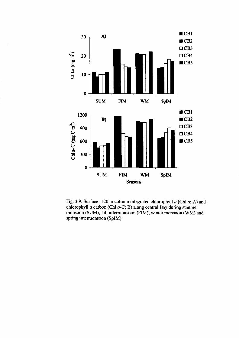
30 -

A) ■CBI ■CB2 ❑CB3 ❑C134 ■CB5

'E 20 - ao E

.74 10 - u

0 SUM FIM WM SpIM

1200

5 900 - U

600 U

300 - U

0

■ CB1 ■ CB2 ❑CB3 O C134 ■ CB5

SUM FIM WM SpIM Seasons

Fig. 3.9. Surface -120 m column integrated chlorophyll a (Chl a; A) and chlorophyll a carbon (Chl a-C; B) along central Bay during summer monsoon (SUM), fall intermonsoon (FIM), winter monsoon (WM) and spring intermonsoon (SpIM)

Winter monsoon Spring intermonsoon 0 0

-20

-40

-60

-80

-100

0.36

0.32

0.28

0.24

0.2

0.16

0.12

0.04

-20

-40

-60

-80

" 8 - 1 c

-120 o -120 12 13 14 15 16 17 18 19 12 13 14 15 16 17 18 19

Summer monsoon

Fall intermonsoon 0

0 0.8

0.6

0.55

0.5

0.45

0.4

0.35

0.3

0.25

0.2

0.15

0.1

0.05

0

-0.05

0.36

-20 1 0.32 -20 0.28

" -40 0.24

-40

--S -60 0.2 -60

6 -80 0.16

0.12 -80

-100 0.08 -100 0.04

-120 • 0 -120 12 13 14 15 16 17 18 19 12 13 14 15 16 17 18 19

0.9

0.8

0.7

0.6

0.5

0.4

0.3

0.2

0.1

0

WB1 WB2 WB3 WB4

Station (N) WB1 WB2 WB3 WB4

Station (N)

Fig 3.10: Variation of chlorophyll a (mg m-3) in the upper 120 m of the western Bay during different seasons

30 -

25 -

20 -

15 -

10 -

5-

0

1200

's 900

U 600

U 3

0

SUM FIM WM SpIM

2 46 B)

-

-

■ WB1 • WB2 D WB3 0 W134

• WB1 • WB2 DWB3 0 W134

SUM FIM WM SpIM Seasons

Fig. 3.11. Surface -120 m column integrated chlorophyll a (CM a; A) and chlorophyll a carbon (Chl a-C; B) along western Bay during summer monsoon (SUM), fall intermonsoon (FIM), winter monsoon (WM) and spring intermonsoon (SpIM)

The 0-120 m integrated chl a carbon (mg C m-2 ; Fig 3.11B) increased from SUM

(688), FIM (767), WM (1057) to SpIM (1212).

3.2.6. Statistical analyses

There was no significant difference in the SST and SSS between stations in the CB as

well as in the WB. Between seasons, only SST varied significantly along both transects

(Table 3.4). Dissolved oxygen varied significantly with depths and stations in the CB

(Table 3.5 CB). In the WB, although the DO decreased significantly with depth in all

seasons, its variation between stations during FIM and WM was not significant (Table

3.5 WB). Also there was no significant difference in the DO concentrations between

seasons or between CB and WB.

The chl a varying significantly between seasons in the CB also varied significantly

with depth. However, between stations, a significant difference was observed only during

FIM (Table 3.6 CB). In the WB, there was no significant difference in the chl a between

depths during SUM and SpIM. During SpIM, a significantly higher proportion of chl a

was observed in the DCM at WB3. In all other seasons, the difference between stations

was statistically insignificant (Table 3.6 WB).

Nutrients (NO3, PO4, SR/0 varied significantly with depth in all seasons in the CB.

Nitrate varied significantly between stations only during FIM. Between stations, PO4 and

SiO4 were significantly different during all seasons except during WM. However,

between seasons, only PO4 varied significantly (Table 3.7 CB). In WB, all the nutrients

varied significantly with depths and stations. However, between seasons, this difference

was significant only in case of PO4 and SiO 3 (Table 3.7 WB).

3.3. Discussion

The hydrography of the typically tropical ocean basin, the Bay of Bengal, is influenced

by semi-annually reversing monsoon wind system. During SUM, the strong (10 m s -1 )

southwesterly winds bring humid maritime air from Southwest Indian Ocean into the Bay

of Bengal. In contrast, during WM, the weak northeasterly winds (5 m s -1 ) bring in cool

and dry continental air from the Asian landmass to the Bay of Bengal

(http://en.wikipedia.org/wiki/Monsoon) . The surface circulation within the basin reverses

37

Table 3.4. One-way ANOVA for understanding the spatio-temporal variation in sea surface temperature (SST) and sea surface salinity (SSS) in the central (CB) and western Bay (WB)

Groups

SST

SSS

CB Between stations

F (4 , 19)=0.5, p>0.05

F (4 , 19)=2.25, p>0.05

Between seasons

F (3, 19)=9.7, p<0.001

F (3 , 19)=0.9, p>0.05

WB Between stations

F (3, 15)=0. 1 , p>0.05

F (3, 15)= 1.1, p>0.05

Between seasons

F (3 , 15)=54.9, p<0.001 F (3, 15)=3.0, p>0.05 Significant results are marked bold

Table 3.5. One-way ANOVA (between seasons) and two-way ANOVA (between depths and also stations) for understanding the spatio-temporal variation in dissolved oxygen concentration in the top 1000 m in the central and western Bay during summer monsoon (SUM), fall intermonsoon (FIM), winter monsoon (WM) and spring intermonsoon (SpIM)

Groups ANOVA

Central Bay

Between depths Between stations

Between depths Between stations

SUM

F (14, 74)=57.6, p<0.001 F (14, 74)=57.6, p<0.001

WM F (13, 69)=73 . 7, p<0.001 F (4, 59)=4.0, p<0.05

FIM

F (13, 69)=43 . 7 , p<0.001 F (4, 69)=8.5, p<0.001

SpIM

F (14,74)=80.9, p<0.001 F (4, 74)=2.5, p<0.05

Between seasons F (3, 302)=1 .4, p>0.05

Western Bay

SUM

FIM

Between depths

F (13 , 55)=37.6, p<0.001 F (13 , 55)=61.1, p<0.001 Between stations F (3 , 55)=4.5, p<0.05

F (3 , 55)=1.4, p>0.05

Between depths F Between stations F

WM (13 , 55)=53.4, p<0.001 (3 , 55)= 1.7, p>0.05

SpIM F (13, 41)=9.0, p<0.001 F (z 41)=7.2, p<0.05

Between seasons F

Between transects F (3, 241)=0 .9 , p>0.05

(1,153)=0.3, p>0.05 are marked bold

Significant results

Table 3.6. One-way ANOVA (between seasons) and two-way ANOVA (between depths and also stations) to decipher the spatio-temporal variations in chlorophyll a concentration in the central and western Bay during summer monsoon (SUM), fall intermonsoon (FIM), winter monsoon (WM) and spring intermonsoon (SpIM)

Groups ANOVA Central

SUM

Bay

FIM

Between depths F (7, 39)=5.9, p<0.001 F (7 , 39)= 14.3, p<0.00I Between stations F (4 , 39)= 1. 1 , p>0.05 F (4, 39)=4.2, p<0.05

WM SpIM

Between depths F (7 , 39)= 12.3, p<0.001 F (7, 39)= 13.2, p<0.001 Between stations F (4, 39)=0.5, p>0.05 F (4, 39)=1 .52, p>0.05

Between seasons F (3 , 150=3.2, p<0.05

Western Bay

SUM FIM

Between depths F (7, 30=1.9, p>0.05 F (7 , 31)=4.3, p<0.05 Between stations F (3 , 30= 1.2, p>0.05 F (3, 31)=1.6, p>0.05

WM SpIM

Between depths F (6 , 27)= 14.4, p<0.001 F (7 , 31)=1.7, p>0.05 Between stations F (3 , 27)=3.5, p<0.05 F (3 , 30=2.1, p>0.05

Between seasons F (3, 120)=1 .2, p>0.05 Between transects F (1.305)=0.6, p>0.05

Significant results are marked bold

Table 3.7. One-way ANOVA (between seasons) and two-way ANOVA (between depths and also stations) to decipher the spatio-temporal variation in nutrient (Nitrate; NO3, Phosphate: PO4, Silicate: SiO3) concentration in the central and western Bay of Bengal during summer monsoon (SUM), fall intermonsoon (FIM), winter monsoon (WM) and spring intermonsoon (SpIM)

Parameter Groups SUM FIM WM SpIM

NO3

PO4

SiO4

Depths Stations Seasons Depths Stations Seasons Depths Stations

F (7 , 39) =71, p<0.01 F (4,39) =2.5, p>0.05 F (3, 159) = 1.5, p>0.05 F (7,39) =13.1, p<0.01 F (4, 39) =5.2, p<0.01 F (3,159)=3 . 8 , p<0.05

F (7,39)3 1 , p<0.01 F (4 39)=5, p<0.01

Central Bay

F (7 , 39)=48, p<0.01 F (4, 39)=5.2, p<0.01

F (7 , 39)=34.4, p<0.01 F (4, 39)=8.7, p<0.01

F (7 , 39)=49, p<0.01 F (4 , 39)-12, p<0.01

F (7, 39)=51.9, p<0.01 F (4 , 39)=2.3, p>0.05

F (7, 39)=2 I .7, p<0.01 F (4 , 39)=1.0, p>0.05

F (7 , 39)=60.8, p<0.01 F (4, 39)=0.5, p>0.05

F (7, 39)=44.8, p<0.01 F (4 , 39)=2.3, p>0.05

F (7, 39)=45, p<0.01 F (4, 39)=3.5, p>0.05

F (7, 39)=47, p<0.01 F (4, 39)=39, p<0.01

Seasons F (3 , 159)= 1 .7, p>0.05

Western Bay

NO3 Depths F (7, 31) 3 1, p<0.01 F (7, 31)=88.7, p<0.01 F (7, 30=21.8,p<0.01 F (7, 30= 14.7,p<0.01

Stations F (3 , 31)5, p<0.01 F (3 , 30=3.7, p<0.05 F (3 , 31)=5, p<0.01 F (3 , 30=8, p<0.01 Seasons F (3,127)=0 . 5 , p>0.05

PO4 Depths F (7, 31)=21, p<0.01 F (7 , 31)=44, p<0.01 F (7 , 31)=24, p<0.01 F (7, 30=1 1 .6, p<0.01 Stations F (3 , 31)7, p<0.01 F (3, 30=25.4, p<0.01 F (3, 31)=5.4, p<0.01 F (3, 31 )=1 1.8, p<0.01 Seasons F (3127)=4 . 7, p<0.01

SiO4 Depths F (7, 31)19, p<0.01 F (7, 31)=63, p<0.01 F (7, 31)=8, p<0.01 F (7, 30= 15, p<0.01 Stations F (3, 30= 5.3, p<0.01 F (3 , 30=5, p<0.01 F (3 , 31)=4.4, p<0.01 F (7, 31)=7.3, p<0.01 Seasons F (3, 127)=3 .5, p<005

Significant results are marked bold

semi-annually, in accordance with the wind reversal. During SUM, the Summer Monsoon

Current advects warm, high-salinity water mass at shallower depths (40-100 m) from the

Arabian Sea into the southwestern CB up to 14°N (Sastry et al. 1985; Murty et al. 1992).

The East India Coastal Current (EICC) along the western boundary weakens and even

reverses in the northern part to a southward flow (Shetye et al. 1991). The open-ocean

circulation at this time of the year consists of multiple gyres, re-circulations, meanders

and eddies.

During FIM, the EICC reverses completely, flowing towards the south carrying BoB

low-salinity water almost along the entire coast, forming a part of the cyclonic gyre. The

southward EICC peaks in December and decays in January, completing its annual cycle.

By end of February (WM), EICC again reverses carrying the Arabian Sea high-salinity

waters towards north. EICC peaks during March—April (spring intermonsoon), when the

winds are weak (Shetye et al. 1993) and the open-ocean circulation during this period is

anticyclonic.

The estimated freshwater influxes into the BOB from local precipitation and through

river discharge are 4700 and 3000 km 3 yr" I respectively. Ganges, Brahmaputra, Mahanadi

and Irrawady are the major rivers that discharge in the head Bay whereas Godavari,

Krishna and Pennar along the WB. The loss due to evaporation is — 3600 km 3 Thus,

on an annual scale, freshwater input exceeds the loss due to evaporation substantially

(Rajamani et al. 2006). This tends to make the water of the BOB relatively less saline

compared to the rest of the Indian Ocean (Wyrtki 1971). The salinity (-24-33 psu) in the

top —10-20 m layer decreases from south to north (Gallagher 1966). The top —30 m layer

is highly stratified and cannot be eroded by the weaker winds that prevail over the Bay

(Shenoi et al. 2002). Below this low-salinity water mass, three water masses can be

identified in the Bay of Bengal, which include the layer between 50-200 m characterized

by Arabian Sea high-salinity water mass in the southern central Bay. The layer between

200-600 m is the Bay of Bengal subsurface water mass (Salinity 34.9 to 35.05). Below

600 m, where salinity decreases gradually to lower values (<35.0) at deeper depths is

identified as the Indian equatorial intermediate water (Gallagher 1966).

During the study period that covered different seasons, most of the Bay remained a

warm pool as SSTs were >28°C. Being land-locked in the north and in the absence of

38

wind-induced upwelling, pole ward transport of the surface heat is restricted, thereby

giving rise to Bay of Bengal warm pool (Vinayachandran and Shetye 1991). While the

SpIM SSTs were the highest (>30°C), the lowest were during winte;mostly in the WB.

Inspite of low SST in the north, winter cooling during WM did not lead to convective

mixing. As reported by many authors (Prasannakumar and Prasad 1996; Madhupratap et

al. 1996 b; Jyothibabu et al. 2004), the intense stratification by freshwater that hardly

changes with seasons in the Bay, prevents such mixing. The thermal structures obtained

from the in situ hydrographic measurements clearly indicated the presence of cyclonic

eddies (cold-core) by way of doming isopleths/thermocline oscillation, in the CB and WB

during both monsoons (Prasannakumar et al. 2004) as well as intermonsoons

(Prasannakumar et al. 2007).

Mixed layer depths (MLD) varied seasonally between CB 1 and CB3. They were

deeper during the SUM and WM owing to higher wind forcing in addition to intrusion of

Arabian Sea high salinity water, in particular during SUM. The shallower MLDs during

intermonsoons were due to light winds, and primary/secondary solar heating.

Surprisingly at CB1, where cold-core eddy was present, the MLD was relatively

shallower. North of CB3, MLD was mostly shallower due to the increased stability

caused by perennial fresh water capping (Narvekar and Prasannakumar 2006).

Oxygen distribution is generally governed by physical processes like atmospheric

interaction, fresh water influx, upwelling, water mass transport and, biological processes

like photosynthesis and respiration. The seasonal variability and distribution of dissolved

oxygen in the surface layer in the Bay of Bengal appears to be significantly influenced by

physical processes like eddies and water circulation in the intermediate and deeper layers

(Sardessai et al. 2007). The pronounced OMZ at depths between 100 and 700 m is typical

of the northern Indian Ocean. As explained by Naqvi (2006), the presence of Asian

landmass restricts adequate ventilation of the thermocline from the north. To a smaller

extent, a porous eastern boundary (openings between the Indonesian islands), also

facilitates exchange of water with the Pacific Ocean.

Although large influx of freshwater adds biogenic matter to the Bay (Khodse et al.

2007) along with the mineral particles, the biological demand for oxygen does not lead to

anoxic or oxygen depleted conditions as is prevalent in the Arabian Sea (De Sousa et al.

39

1996; Naqvi et al. 2000). Ittekkot et al. (1991) through their study of particle fluxes using

sediment traps estimate 40-50% of the total annual flux to occur during the SUM,

probably leading to a larger OMZ compared to the other seasons. This zone was thicker

in the WB due to the higher remineralization rates (Sardessai et al. 2007) observed in this

season. However, the seasonal variations in the overall oxygen concentrations in the CB

as well as WB are insignificant.

In the CB, in the region of eddies, high concentrations of chl a was observed in

response to the enhanced levels of nitrate and silicate, more significantly during fall

intermonsoon. Cyclonic eddies cause upward displacement of nutricline therefore making

the essential nutrients available into the impoverished euphotic zone, thus enhancing chl

a concentrations (Falkowski et al. 1991; McGillicuddy et al. 1998; Seki et al. 2001;

Vaillancourt et al. 2003). The average concentrations of surface and column integrated

chl a were similar to those reported from offshore waters by Madhu et al. (2006) and

Gomes et al. (2000). The DCM seated between 40 and 80 m, deepest during SpIM,

reflect oligotrophy (intense solar heating, stratified upper layer and weak winds) in the

Bay during all the sampled seasons. The occurrence of DCM in the nitracline is essential

feature of the typical tropical structure in the Atlantic (Herbland and Voituriez 1979) and

in the Arabian Sea (Madhupratap et al. 1996 a). Eddy-pumping of nutrients not only

helps increase the chl a concentrations to >1.5 times but also pushes the DCM to

shallower depths as can be discerned at —CB 1 and CB4/5. The 0-120 m column

integrated chl a and PP were maximum during WM and minimum during SUM, probably

due to the higher suspended particulate matter (0.2-15 mg 1 -1 ; Sardessai et al. 2007) and

persistent cloud cover during the latter season (Madhupratap et al. 2003). Also the top 40

m was impoverished of nutrients during SUM except in the region of eddies.

In the WB, enhanced chl a was observed between WB3 and WB4 and, to an extent, at

WB 1. The higher phytoplankton biomass production in the northern region appears to be

due to combined effect of nutrient input from cold-core eddy and riverine source albeit

the input from latter is very meager. Unlike in the open ocean, the column integrated chl

a in this transect was maximum during SpIM. Sengupta et al. (1977) reported that rivers

did not contribute to the inorganic nutrient pool of the western BoB during SpIM.

Contrary to this, high nutrient concentrations were observed in the upper 40 m at all the

40

stations in the WB during this season. Also, it appears that the cold-core eddy and the

deep-seated nutrients enhanced the chl a concentration in the deeper DCM to more than

double. The chl a minimum during SUM could be related to the high-suspended matter

and stratified upper waters (temperature: >30°C, salinity: 23-33 psu).

Seasonal variations in chl a were associated with the seasonally changing

hydrographical and meteorological conditions. Differences were also evident between

transects, with the central transect becoming more productive in phytoplankton biomass

during winter monsoon, compared to the western transect which is most productive

during SpIM. Cold-core eddies at CM, CB4/5 and WB3 seem to govern the overall

productivity of the Bay. Though the subsurface oxygen minimum zone is the largest

during SUM, especially in the WB, there is no prevalence of anoxia (<0.5 11M) during

any season.

41

Chapter 4

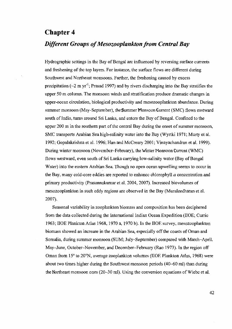
Chapter 4

Different Groups of Mesozooplankton from Central Bay

Hydrographic settings in the Bay of Bengal are influenced by reversing surface currents

and freshening of the top layers. For instance, the surface flows are different during

Southwest and Northeast monsoons. Further, the freshening caused by excess

precipitation (-2 m yr -1 ; Prasad 1997) and by rivers discharging into the Bay stratifies the

upper 50 m column. The monsoon winds and stratification produce dramatic changes in

upper-ocean circulation, biological productivity and mesozooplankton abundance. During

summer monsoon (May-September), the Summer Monsoon Current (SMC) flows eastward

south of India, turns around Sri Lanka, and enters the Bay of Bengal. Confined to the

upper 200 m in the southern part of the central Bay during the onset of summer monsoon,

SMC transports Arabian Sea high-salinity water into the Bay (Wyrtki 1971; Murty et al.

1992; Gopalakrishna et al. 1996; Han and McCreary 2001; Vinayachandran et al. 1999).

During winter monsoon (November—February), the Winter Monsoon Current (WMC)

flows westward, even south of Sri Lanka carrying low-salinity water (Bay of Bengal

Water) into the eastern Arabian Sea. Though no open ocean upwelling seems to occur in

the Bay, many cold-core eddies are reported to enhance chlorophyll a concentration and

primary productivity (Prasannakumar et al. 2004, 2007). Increased biovolumes of

mesozooplankton in such eddy regions are observed in the Bay (Muraleedharan et al.

2007).

Seasonal variability in zooplankton biomass and composition has been deciphered

from the data collected during the International Indian Ocean Expedition (IIOE; Currie

1963; HOE Plankton Atlas 1968, 1970 a, 1970 b). In the IIOE survey, mesozooplankton

biomass showed an increase in the Arabian Sea, especially off the coasts of Oman and

Somalia, during summer monsoon (SUM; July—September) compared with March—April,

May—June, October—November, and December—February (Rao 1973). In the region off

Oman from 15° to 20°N, average zooplankton volumes (IIOE Plankton Atlas, 1968) were

about two times higher during the Southwest monsoon periods (40-60 ml) than during

the Northeast monsoon ones (20-30 ml). Using the conversion equations of Wiebe et al.

42

(1975), this would correspond to average dry weights of 11-18 and 5-8 g, respectively.

Off Somalia, Smith (1982) also found that zooplankton stocks varied with monsoon

reversal. Zooplankton stocks during the upwelling period of the Southwest monsoon

ranged from 0.8-7.0 g dry weight m -2 . There are indications that the currents associated

with the Somali upwelling area are so swift that mesozooplankton is advected into the

central Arabian Sea before achieving the biomass that could be supported by the

upwelled nutrients if the Somali area had a less vigorous circulation (Baars 1999; Baars

and Oosterhuis 1998; Hitchcock et al. 2002). High zooplankton standing stocks in the

mixed layer are known to occur in the central Arabian Sea irrespective of seasons

(Madhupratap et al. 1996 a) due to open ocean upwelling during SUM, convective

mixing during winter and/or through the microbial loop during the intermonsoon. Many

studies on the seasonal cycles of mesozooplankton are available for the Arabian Sea

(Madhupratap et al. 1996 a, b; Wishner et al. 1998; Smith 1982, 1998, 1999, 2000, 2001;

Smith et al. 1998; Stelfox et al. 1999; Hitchcock et al. 2002; Koppelmann et al. 2005;

Smith and Madhupratap 2005).

Zoogeographic aspects of many groups and species in the Indian Ocean have been

published (UNESCO 1965-72; IOBC Atlas and Handbook 1-5, 1968-73; Zeitzschel

1973). Later studies by Nair et al. (1977, 1978) and Peter and Nair (1978) also augment

this. Almost all of the zooplankton taxa studied in detail showed patterns of increased

abundance during SUM. These included polychaete worms (Peter 1969 a), fish larvae

(Peter 1969 b), euthecosome molluscs (Sakthivel 1969), cephalopod juveniles

(Aravindakshan and Sakthivel 1973), amphipods (Nair et al. 1973) and euphausiids

(Gopalakrishnan and Brinton 1969; Brinton and Gopalakrishnan 1973). Euphausiids have

probably been under-sampled in most studies. The HOE collections contained mainly

larvae and immature adults (Gopalakrishnan and Brinton 1969). While zooplankton

biomass showed a seasonal increase during the SUM (Rao 1973), the concentration of

copepods (total number per volume), the main zooplanktonic taxa, did not (Panikkar

1970). The two other common forms, ostracods (George 1969) and chaetognaths (Nair

1969; Nair and Rao 1973), also did not show marked increases during the SUM season.

An upwelling specialized copepod species, Calanoides carinatus, was found in the

mesopelagic layers of the central Arabian Sea during winter. Diel- (Smith et al. 1998;

43

Goswami et al. 2000; Jayalakshmy 2000; Madin et al. 2001; Schnetzer and Steinberg

2002 b), depth-wise (Madhupratap et al. 1996 a; Padmavati et al. 1998; Pieper et al.

2001; Koppelmann et al. 2003, 2005) and latitudinal- (Mauny and Dauvin 2002; Gaudy

et al. 2003; Kang et al. 2004; Roman et al. 1995; Yamaguchi et al. 2005; Li et al. 2006;

Fernandez-Alamo and Farber-Lorda 2006; Alcaraz et al. 2007) variability in zooplankton

has been studied in many parts of the world oceans. However, even after the HOE (1960-

1965), the Bay of Bengal still remains one of the sparsely investigated regions of the

Indian Ocean especially in terms of zooplankton below 200 m depth from the open ocean

region.

Secondary producers, the zooplankton, are the major consumers linking primary

production to tertiary production. Thus, they are important contributors of vertical flux of

organic matter (Wishner et al. 1998). Knowledge of their abundance and distribution and

composition in space and time is important for understanding the carbon budgets and, to

decipher the effects of climate change on marine fauna. Keeping the first objective of this

study in the fore, the spatial and seasonal differences in mesozooplankton biomass, their

numerical abundance, and group composition in the upper 1000 m were studied from five

stations in the central Bay during summer monsoon, fall intermonsoon, winter monsoon

and spring intermonsoon.

4.1. Methods

4.1.1. Sampling

Sampling was carried out in the central Bay (CB) between 9°N and 20°N along 88°E (Fig.

3.1) during the cruises 166, 182 and 191 onboard ORV "Sagar Kanya" and cruise 240 on

ORV "Sagar Sampada". The four seasons covered were summer monsoon (SUM, July 6

to August 2, 2001), fall inter monsoon (FIM, September 14 to October 12, 2002), spring

inter monsoon (SpIM, April 10 to May 10, 2003) and winter monsoon (w, NovernberzG

2005 to January 7, 2006). Mesozooplankton samples were collected from five stations.

Sample collections were made around noon and midnight at each station by vertical hauls

from five discrete depths in the upper 1000 m using a multiple plankton net (MPN-

Hydro-Bios, mouth area 0.25 m 2, mesh size 200 gm). Sampling strata were decided

according to temperature profiles obtained from CTD. The five strata sampled were:

44

mixed layer, top of thermocline (TT) to base of thermocline (BT), BT - 300 m, 300 - 500

m, and 500 - 1000 m. During SpIM, only the first four strata were sampled due to non-

functionality of one net. The net was hauled up at 0.8 m s -1 and the volume of water

filtered was calculated by multiplying the sampling depth by mouth area of the net. The

wire angle was taken into account by the pressure sensors fitted on the MPN.

4.1.2. Biovolume measurements

Biovolume (ml) was estimated by the standard displacement volume method (ICES

2000). For this, samples from each stratum were filtered on to a 200-[im mesh-piece;

excess water blotted out using a wad of absorbent paper and transferred to a measuring

cylinder with known volume of water to determine the volume displaced. Thereafter, the

samples were fixed with 4% buffered formaldehyde-seawater solution and brought to the

laboratory for further analyses. The conversion factor provided for tropical zooplankton

by Madhupratap and Haridas (1990) was used to calculate the dry weight. In that, 1 ml

displacement volume is equivalent to 0.075 g dry wt. As also provided by these authors

34.2% of the dry weight was used to calculate gram equivalent of carbon biomass.

4.1.3. Numerical abundance

When the sample size was large, usually in the first and second strata, it was split using a

Folsom splitter and, in general, 25% aliquots were taken up for enumeration (abundance)

and identification. Entire sample was analyzed for enumeration and speciation from other

three deeper layers where the volumes were usually small or negligible. All the samples

were sorted group-wise and the groups identified by following standard references

(UNESCO 1968). A stereo zoom microscope (Zeiss, Germany) with 90X magnification

was used for differentiating the groups and, most genera.

4.1.4. Statistics

In order to detect variability if any, arising due to day and night differences, biomass,

abundance and groups data were subjected to Wilcoxon matched pair test. Friedman

ANOVA (non parametric test; Zar 1974; Conover 1980) was carried out to test for

variability between depths, stations and seasons. Bray-Curtis similarity indices (Bray-

45

Curtis 1957) for cluster analysis and non-metric multidimensional scaling (NMDS; Gray

et al. 1988) were done to understand similarity in distribution of biovolume and

abundance of zooplankton between seasons. Correlation analysis (Excel software

program or STATISTICA 6.0) was carried out between zooplankton and the abioticibiotic

parameters to understand the relation between the two.

4.2. Results

4.2.1. Biovolume

Mesozooplankton biovolume (ml 100 m -3) was the highest in the mixed layer (MLD)

during all four seasons (Fig. 4.1-4.4; Table 4.1). Diel difference in biovolume from the

entire column was not significant except during SUM. Biovolume decreased significantly

with increasing depth (Table 4.12). Nearly 95 - 99% of the biovolume during SUM and

SpIM was in the MLD. It was mostly negligible below this depth. During FIM and WM,

the biovolume in MLD was relatively less i.e., average 73 and 53% respectively.

In the upper 1000 m, biovolume ranged from 0.2 to 404 (mean: 39 ml 100 m -3) during

SUM, from negligible to 120 (12.7 ml 100 m -3) during FIM, 0.3-75 (13.8 ml 100 m -3)

during WM and 1.3-230 (40.4 ml 100 m -3) during SpIM. Pyrosoma swarms and

scyphomedusae contributed to the higher biovolumes during SUM and SpIM

respectively. The average biovolumes for the upper 1000 m were higher during SUM and

SpIM compared to either FIM and/or WM. Seasonal differences in the biovolumes were

highly significant (Table 4.12). The biovolumes were greater at CB 1 and CB5 during

SUM; at CB 1 and CB4 during FIM; at CBS during WM and; at CB3 and CB4 during

SpIM. This heterogeneity in biovolume distribution between stations was however

significant only during FIM.

Though higher biovolumes were recorded at locations in the vicinities of cold-core

eddies, negative correlation between biovolume and temperature was observed only

during SUM and WM (Table 4.13). It had a good positive correlation with chlorophyll

(chl) a during all seasons, however was significant during FIM and SpIM.

46

i

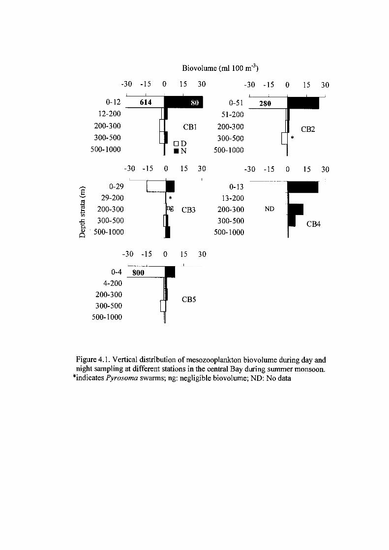
0-12 614 12-200

200-300

300-500

500-1000

CB1

❑ D ■ N

-30 -15 0 15 30

0-29

29-200

200-300 CB3 300-500

500-1000

0-51

51-200

200-300

300-500

500-1000

-30 -15 0 15 30

0-13

13-200

200-300 ND

300-500

500-1000 6)

Biovolume (ml 100 m -3)

-30 -15 0 15 30 -30 -15 0 15 30

-30 -15 0 15 30

0-4 800 4-200

200-300 CB5

300-500

500-1000

Figure 4.1. Vertical distribution of mesozooplankton biovolume during day and night sampling at different stations in the central Bay during summer monsoon.

*indicates Pyrosoma swarms; ng: negligible biovolume; ND: No data

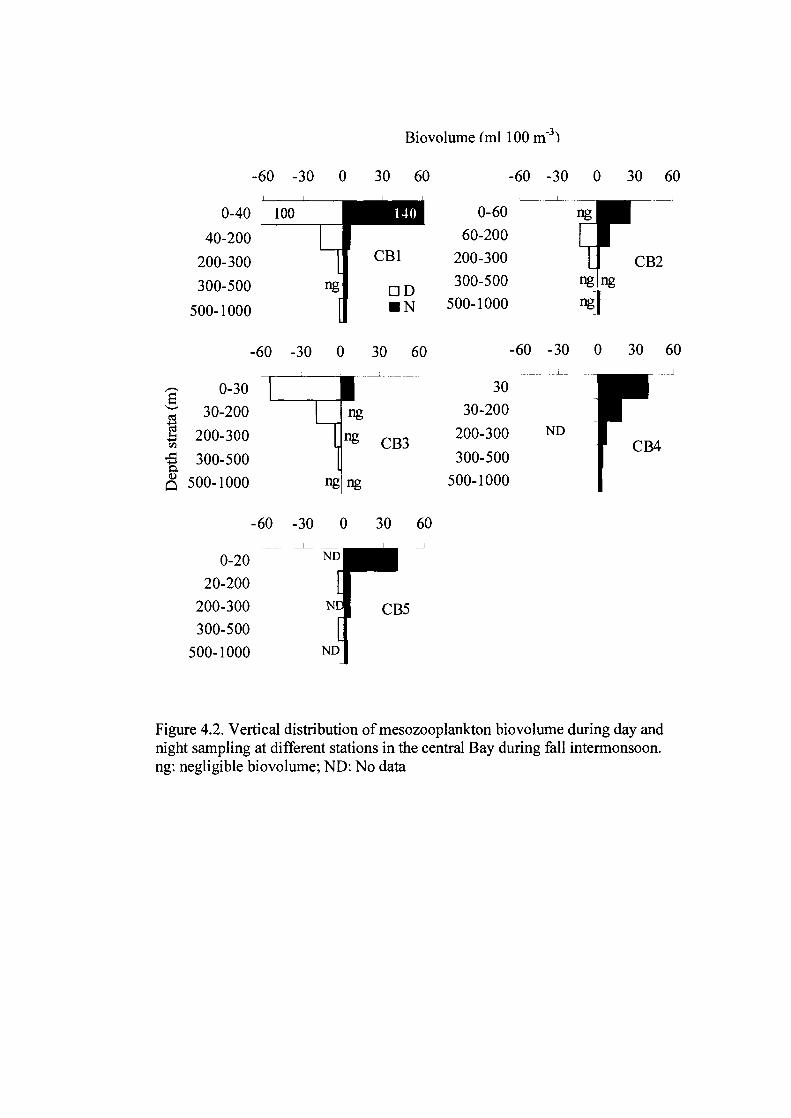
Biovolume (ml 100 m-3 1

-60 -30 0 30 60 -60 -30 0 30 60

0-40

40-200

200-300

300-500

500-1000

0-60 ng

60-200

200-300 CB2

300-500 ng ng

500-1000 ng

-60 -30 0 30 60 -60 -30 0 30 60

0-30

,71 30-200

200-300

300-500 s. 6' 500-1000

30

30-200

200-300

300-500

500-1000 ng ng

-60 -30 0 30 60 J

0-20 NEr,

20-200

200-300 CB5 300-500

500-1000 ND

Figure 4.2. Vertical distribution of mesozooplankton biovolume during day and night sampling at different stations in the central Bay during fall intermonsoon. ng: negligible biovolume; ND: No data

Biovolume (ml 100 m-3)

-80 -40 0 40 80 -80 -40 0 40 80

I 1

0-40

40-150

150-300

300-500

500-1000

0-40

40-150

150-300

300-500

500-1000

CB1

0 D • N

CB2

-80 -40 0 40 80 -80 -40 0 40 80

IT

0-40

ct 40-150 150-300 300-500

A 500-1000

0-60 60-150

150-300

300-500 500-1000

CB3 C134

-80 -40 0 40 80

0-40

40-200

200-300

300-500

Figure 4.3. Vertical distribution of mesozooplankton biovolume during day and night sampling at different stations in the central Bay during winter monsoon. ng: negligible biovolume

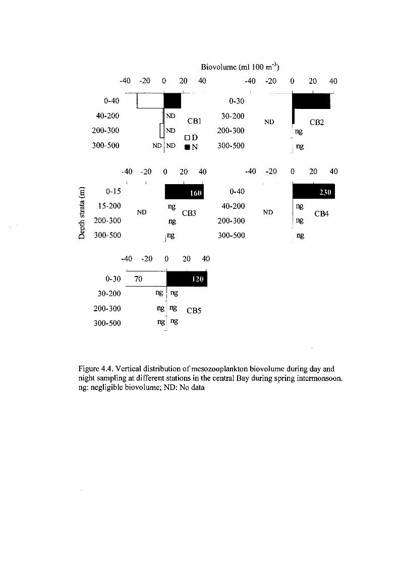
-40 -20 0 20 40

CB2 ng

ng

-40 -20 0 20 40

0-40

40-200

200-300

300-500

0-30

30-200

200-300

300-500

ND

Biovolume (ml 100 m-3 )

-40 -20 0 20 40 -40 -20 0 20 40

0-15 as 15-200

200-300

cd,) 300-500

ND

L L _OMEN 0-40

40-200 ng ND C134

200-300 ng

300-500 ng

-40

0-30

-20

70

0 20 40

30-200 lig ng

200-300 ng ng CB5

300-500 lig ng

Figure 4.4. Vertical distribution of mesozooplankton biovolume during day and night sampling at different stations in the central Bay during spring intermonsoon. ng: negligible biovolume; ND: No data

Table 4.1. Mesozooplankton biovolume (ml 100 m -3) and carbon biomass (mM C t11-2 ; in parentheses) in the central Bay of Bengal during different seasons

Sampling Stations

Depth (m) CB1 CB2 CB3 CB4 CB5 Summer monsoon

0-MLD *347.2 (65.9) * 152.5 (38.1) 11.4 (10.7) 24.0 (25.7) *404 (89.8 TT-BT 2.3 (8.5) 1.4 (3.8) 0.4 (1.1) 0.7 (2.2) 1.3 (3.8) BT-300 2.3 (4.8) 1.4 (2.9) 0.4 (1.2) 12.0 (21.4) 1.5 (3.3) 300-500 3.3 (13.9) *4.5 (19.2) 1.8 (7.5) 6.0 (25.7) 2.2 (9.2) 500-1000 0.2 (2.1) 0.3 (2.7) 1.9 (20.3) ng (ng) 0.5 (4.8)

Fall intermonsoon 0-MLD 120.0 (102.6) 20.0 (34.1) 31.7 (38.5) 40.0 (25.7) 20.0 (25.7) TT-BT 11.3 (37.6) 7.9 (34.9) 9.6 (56.3) 18.8 (68.3) 4.6 (17.0) BT-300 3.5 (7.5) 1.0 (8.2) 2.4 (8.6) 7.0 (15.0) 2.5 (10.7) 300-500 1.5 (12.8) ng (ng) 0.6 (5.1) 3.5 (15.0) 3.0 (12.8) 500-1000 2.8 (29.9) 1.6 (17.1) 0.6 (0.0) 2.8 (29.9) 1.2 (12.8)

Winter monsoon 0-MLD 20.0 (17.1) 30.0 (13.3) 25.0 (21.4) 26.7 (34.2) 75.0 (64.1) TT-BT 8.2 (19.2) 10.9 (15.4) 10.9 (25.7) 8.9 (26.6) 50.9 (106.4) BT-300 2.7 (5.7) 2.3 (7.3) 5.3 (17.1) 2.7 (7.8) 24.0 (32.7) 300-500 8.0 (28.6) 4.0 (17.1) 3.0 (12.8) 3.0 (12.8) 5.0 (21.4) 500-1000 0.3 (2.7) 1.7 (18.0) 0.9 (9.4) 0.8 (8.6) ND (ND)

Spring intermonsoon 0-MLD 22.5 (19.2) 36.6 (15.6) 160.0 (51.3) 230.0 (196.7) 95.0 (55.6) TT-BT 1.3 (2.1) 2.4 (8.5) ng (ng) ng (ng) ng (ng) BT-300 4.0 (4.3) ng (ng) ng (ng) ng (ng) ng (ng) 300-500 ng (ng) ng (ng) ng (ng) ng (ng) ng (ng) MLD: mixed layer depth; TT: Top of thermocline; BT: Base of thermocline

*high volumes due to swarms of Pyrosoma; ng- negligible biovolume; ND- no data (due to shallower depth at the northern most station)

4.2.2. Abundance

Similar to the biovolume distribution, the mesozooplankton abundance (No. x 10 3

individuals 100 m-3 ) observed was more in the MLD during all seasons (Table 4.2). The

diel difference in abundance was also negligible (Table 4.12). However, unlike that of the

biovolume, the abundance decreased significantly with increasing depth only during FIM

and SpIM. In these two seasons, the abundance in MLD accounted respectively for 87

and 96% of total numbers. During SUM and WM, it accounted for 79 and 66%

respectively. The abundance ranged from 0.04 to 35.8 (mean: 7 x 10 3 ind. 100 m-3) during

SUM, 0.2 to 356 (29.3 x 10 3 ind. 100 m-3) during FIM, 0.4 to 308 (24.5 x 10 3 ind. 100 m-

3) during WM and 0.04 to 248 (28 x 10 3 ind. 100 ni3) during SpIM.

The abundance in the upper 1000 m differed significantly between seasons (Table

4.12), with higher averages during FIM and, SpIM, followed by WM and least during

SUM. Station-wise differences in abundance were also noticeable. During SUM, the

abundance was higher at CB1, CB2 and CBS. During FIM, it was very high at CB1

followed by CB4. While during WM, it was found to be very high at CB5, during SpIM,

it was higher at CB3 and CB5. Higher abundances were at locations in the vicinities of

cold-core eddies as is also implicit from the negative correlations with temperature (Table

4.13). It also had strong positive correlation with salinity and chl a during FIM.

4.2.3. Cluster and non-metric multidimensional scaling analysis (NMDS)

Results from cluster and NMDS analyses imply that during the seasons FIM and WM,

the distribution pattern of both biovolume and abundance at depths as well as stations is

similar. This differed from other two seasons (Fig. 4.5).

4.2.4. Column (1000-surface) integrated carbon biomass and abundance

The abundance during SUM, FIM, WM and SpIM ranged respectively from 6 to 37

(mean: 24 x 10 3 ind. m-2), 33 to 166 (80 x 103 ind. m-2), 40 to 223 (88 x 10 3 ind. m-2) and

7 to 50 (33 x 10 3 ind. m-2). Similarly, calculated carbon biomass during these seasons

ranged respectively from 95 to 111 (mean: 78 mM C m -2); 79 to 190 (112 mM C m -2); 71

to 225 (134 mM C m2) and from 24 to 197 (75 mM C r11-2 ; Fig. 4.6). Overall, numerical

abundance and carbon biomass in the upper 1000 m were higher during WM and FIM.

47

Table 4.2. Mesozooplankton numerical abundance (x 10 3 individuals 100 m-3) in the central Bay of Bengal during different seasons

Depth (m) CB1 Sampling stations

CB2 CB3 CB4 CB5 Summer monsoon 0-MLD 35.8 35.8 5.2 19.9 34.8 TT-BT 0.5 0.5 0.2 1.5 2.0 BT-300 0.3 0.3 0.2 0.2 16.7 300-500 0.7 5.4 2.5 3.0 0.0 500-1000 0.1 0.1 0.2 0.0 1.2

Fall intermonsoon 0-MLD 355.9 66.1 47.9 96.5 72.1 TT-BT 8.6 18.8 8.5 26.4 7.3 BT-300 3.7 1.5 0.7 2.4 2.8 300-500 0.7 0.2 0.7 2.2 1.8 500-1000 2.0 0.5 0.8 1.9 1.1

Winter monsoon 0-MLD 16.0 12.3 26.9 27.6 308.2 TT-BT 32.4 16.2 37.6 21.4 43.7 BT-300 6.0 3.4 4.4 2.0 9.4 300-500 5.4 4.6 1.6 1.7 5.6 500-1000 0.4 0.7 0.8 0.4 ND

Spring intermonsoon 0-MLD 3.8 48.3 248.0 85.7 124.5 TT-BT 0.8 6.6 0.8 0.8 0.6 BT-300 3.8 3.6 0.6 2.2 0.4 300-500 ng 0.3 0.1 0.4 ng

MLD: mixed layer depth; TT: Top of thermocline; BT: Base of thermocline

Only at one depth in northernmost station, there was no data (ND) due to shallower depth; ng- negligible abundance

cyss:0

II

VVM1 I

II

III

I

II

III

FIM

SUM

SpIM

40

a)

Abundance

60

Bray-Curtis

80

Similarity (%)

100

WM

FIM

SUM

SpIM

50 60; 70 80 90

100 Bray-Curtis Similarity (%)

a) bl

b)

Biovolume

•

Figure 4.5. a) Cluster dendrograms depicting similarity between seasons based on biovolume and abundance of zooplankton in the central Bay. b) Non- metric multidimensional scaling (NMDS) ordination based on the Bray- Curtis similarity coefficients.

250 -

200 -

'rs 150

100 - ixt

50 -

0 SUM FIM WM SpIM

Season

Figure 4.6. Latitudinal variations in the 0-1000 m column integrated mesozooplankton abundance (10 3 individuals m-2) and biomass in the central Bay during different seasons (SUM: summer monsoon, FIM: fall intermonsoon, WM: winter monsoon; SpIM: spring intermonsoon)

4.2.5. Groups

A total of 37 groups were identified from CB (Table 4.3). The number of groups varied

significantly between seasons as well as between depths but not between stations (Table

4.14). Of these, 21 groups viz. Amphipoda, Appendicularia, Chaetognatha, crustacean

nauplii, Copepoda, Decapoda, Doliolida, Euphausiacea, fish larvae, Foraminifera,

Gastropoda, invertebrate eggs, Isopoda, Medusae, Mysida, Ostracoda, Polychaeta,

Pteropoda, Radiolaria, Salpida and Siphonophora were recorded during all four sampling

seasons. As can be seen from Tables 4.4- 4.11, not all groups were recorded from all the

stations during any given season.

Cirripedia and Sipuncula were recorded only during SUM. Pyrosoma swarms in

MLD and in deeper depths contributed much of the biomass during SUM. Only a few of

its colonies were observed during WM. Anthozoa and Pterotrachea were observed only

during FIM. Echinoderm larvae were in large numbers during WM. Carinaria was rare,

that too was found only during SpIM. Acantharia was observed during WM and SpIM.

Members of Ctenophora and Stomatopoda were present during all seasons except SpIM.

The least numbers of groups were recorded during SpIM and, the highest during WM.

As many as eight groups i.e., Acantharia, Anthozoa, Bivalvia, Carinaria, Cephalopoda,

Echinodermata, Pterotrachea and Stomatopoda were absent during SUM (Table 4.4, 4.5)

and six (Acantharia, Carinaria, Cirripedia, Echinodermata, Pyrosomida and Sipuncula;

Table 4.6, 4.7) were absent during FIM. During WM, Anthozoa, Carinaria, Cirripedia,

Halobates, Pterotrachea and Sipuncula were not found in any samples (Table 4.8, 4.9).

Since as many as nine groups (Anthozoa, Cephalochordata, Cirripedia, Echinodermata,

fish eggs, Pterotrachea, Pyrosomida Sipuncula and Stomatopoda; Table 4.10, 4.11) were

absent during SpIM, the incidence of groups was the lowest.

The number of groups decreased rapidly below MLD. Interestingly however, their

number was more in the 500-1000 m column, in particular during SUM and FIM. The

lowest number of groups during these seasons occurred in the thermocline (range: 2-9)

and the 300-500 m stratum (range: 7-16) respectively (Fig. 4.7; Table 4.5, 4.7). During

SUM, 23 of the 37 groups were absent in the samples collected from the thermocline.

During FIM, 14 groups were absent in the 300-500 m strata. However, during WM and

SpIM, the number decreased gradually till 1000/500 m (Fig. 4.7; Table 4.9, 4.11).

48

Table 4.3. List of groups found in the central Bay

Gr. No: Group Gr. No: Group Gr. No: Group

1 Acantharia Callianasa 22 Gastropoda 2 Amphipoda Lucifer 23 Halobates 3 Anthozoa Lucifer mysis 24 Invertebrate eggs 4 Appendicularia Lucifer protozoea 25 Isopoda 5 Bivalvia Megalopa 26 Medusae 6 Carinaria Palaemon 27 Mysida 7 Cephalochordata Sergestes larvae 28 Ostracoda 8 Cephalopoda Thalassocaris 29 Polychaeta 9 Chaetognatha Unidentified larvae 30 Pteropoda 10 Cirrripedia 16 Doliolida 31 Pterotrachea 11 Cladocera 17 Echinodermata 32 Pyrosomida

Evadna 18 Euphausiacea 33 Radiolaria 12 Crustacean larvae Euphausiid larvae 34 Salpida 13 Copepoda Euphausiid protozoea 35 Siphonophora 14 Ctenophora Euphausiids 36 Sipuncula 15 Decapoda 19 Fish eggs 37 Stomatopoda

Alpheid 20 Fish larvae Brachyuran zoea 21 Foraminifera

Gr. No: Group Number

Table 4.4. Percent abundance of different groups of mesozooplankton in central Bay during summer monsoon (SUM)

Gr No: Groups Various depth strata (m) at the stations sampled

0-12 12-200

CB1

200-300 300-500 500-1000 0-51 51-200

CB2

200-300 300-500 500-1000

2 Amphipoda A A 0.27 A A 0.27 1.06 A 0.74 0.70 4 Appendicularia 1.06 A A A 0.64 A A A A A

7 Cephalochordata A A A A A 0.22 A A A A 9 Chaetognatha 1.83 1.99 A 2.38 0.64 7.12 2.75 28.95 5.50 12.40 12 Crustacean larvae 0.24 A A A A A A A A A 13 Copepoda 92.76 93.63 94.81 94.29 95.54 88.27 85.65 48.68 75.78 79.91 15 Decapoda 0.13 0.40 A 0.16 A 0.49 A A 0.30 0.21

Lucifer A A A A A 0.45 A A 0.30 0.21 Unidentified larvae 0.13 0.40 A 0.16 A 0.04 A A A A

16 Doliolida A A A A A 0.06 A A 0.15 A 18 Euphausiacea A A 0.82 A 2.55 1.20 2.34 15.79 0.45 2.29

Euphausiid protozoea A A A A 0.64 A A A A A

Euphausiids A A 0.82 A 1.91 1.20 2.34 15.79 0.45 2.29 19 Fish eggs 0.13 A A A A A A A A A

20 Fish larvae A 0.40 0.54 0.16 A A A 1.32 0.30 A 23 Halobates A A A 0.16 A A A A A A 24 Invertebrate eggs 0.36 A A 2.06 A A A A A A 25 Isopoda A A A A A A A A A 0.70 27 Mysida A A A A A 0.06 A A 0.15 0.21 28 Ostracoda 0.59 3.19 3.56 0.48 A 1.44 7.99 3.95 1.49 1.33 29 Polychaeta 0.12 0.40 A A 0.64 0.71 0.21 1.32 0.15 0.21

30 Pteropoda A A . A A A A A A 14.86 0.21

32 Pyrosomida * A A A A * A A * A

33 Radiolaria 0.12 A A A A A A A A A 34 Salpida 0.13 A A 0.16 A 0.15 A A 0.15 1.83

35 Siphonophora A A A 0.16 A A A A A A

36 Sipuncula 2.53 A A A A A A A A A Number of groups 13 6 5 9 5 12 6 6 13 11

Individuals 100 111-3 35840 469 253 673 124 35840 469 253 5384 124

*swarms of Pyrosoma that could not be counted; 'A' denotes absent

Table 4.4. Contd.

Gr No: Groups Various depth strata (m) at the stations sampled

0-29 29-200

CB3

200-300 300-500 500-1000 0-13 13-200

CB4

200-300 300-500

2 Amphipoda A A A 0.33 A 0.48 A A A 4 Appendicularia 0.57 A 4.55 A 0.65 2.01 A A A 7 Cephalochordata A A A A A A 0.17 A A 9 Chaetognatha 11.88 5.26 10.62 4.40 11.07 5.58 3.12 5.00 0.27 10 Circripedia 0.97 A A A A A A A A 11 Cladocera 0.04 A A A A 0.96 A A A 12 Crustacean larvae A A A A A 0.88 A A A 13 Copepoda 77.91 78.95 76.86 91.21 81.43 84.41 95.15 70.00 98.14 14 Ctenophora A A A A A 0.04 A A A 15 Decapoda 0.16 A A 0.16 A 1.00 A A A

Lucifer 0.16 A A 0.16 A 0.76 A A A Unidentified larvae A A A A A 0.24 A A A

16 Doliolida A A A A A 0.08 A A A 18 Euphausiacea A A A 0.16 0.98 0.60 0.17 12.50 0.27

Euphausiids A A A 0.16 0.98 0.60 0.17 12.50 0.27 19 Fish eggs 2.21 A A A A A A A A 20 Fish larvae 0.12 A A 0.16 A 0.28 A A 0.27 21 Foraminifera A A A A 0.65 A 0.17 A A 22 Gastropoda 0.08 A A A A 0.24 A A A 24 Invertebrate eggs A A 0.38 A A A A A A 26 Medusae 2.17 A A A 0.33 0.12 0.17 A 0.27 27 Mysida A A A A 0.33 A A 2.50 A 28 Ostracoda 0.24 3.95 3.05 3.09 2.28 0.84 0.35 7.50 0.53 29 Polychaeta 0.08 11.84 4.55 0.49 0.33 1.00 0.52 A A 30 Pteropoda 0.04 A A A A 0.40 A A A 32 Pyrosomida A * A A A A A A A 34 Salpida 2.13 A A A 0.33 0.04 A A A 35 Siphonophora 1.88 A A A 1.63 1.00 0.17 2.50 0.27

Number of groups 15 5 6 8 11 18 9 6 7 Individuals 100 M-3 5237 234 168 2456 246 19912 1539 160 3016

*swarms of Pyrosoma that could not be counted; 'A' denotes absent

Table 4.4. Contd.

Gr No: Groups Various depth strata (m) sampled at CB5

0-13 13-200 200-300 300-500 500-1000

4 Appendicularia 1.08 6.60 0.37 A 2.31 9 Chaetognatha 1.40 A 2.01 8.33 2.31 12 Crustacean larvae 0.08 A A A A 13 Copepoda 92.72 83.02 91.11 91.67 79.62 15 Decapoda 0.25 0.94 0.18 A A

Lucifer 0.08 0.94 0.09 A A Unidentified larvae 0.17 A 0.09 A A

16 Doliolida 0.08 A A A A 18 Euphausiacea A A 0.82 A 0.38

Euphausiids A A 0.82 A 0.38 19 Fish eggs 0.08 A 0.09 A A 20 Fish larvae 0.08 A 0.37 A A 21 Foraminifera 0.58 A A A A 24 Invertebrate eggs A A 0.18 A A 26 Medusae 0.25 A 0.09 A 0.38 28 Ostracoda A 2.83 1.75 A 3.08 29 Polychaeta 2.57 6.60 2.67 A 10.77 30 Pteropoda 0.17 A 0.09 A A 32 Pyrosomida A A A A 34 Salpida A A 0.09 A A 35 Siphonophora 0.66 A 0.18 A 1.15

Number of groups 14 5 14 2 8 Individuals 100 I11-3 34792 1957 16734 38 1248

*swarms of Pyrosoma that could not be counted; `A' denotes absent

Table 4.5. Mesozooplankton groups absent from different depth strata in the central Bay during summer monsoon. Refer to Table 4.3 for the names of individual groups corresponding to the group numbers

Sampling station

CB1

0-MLD

1-3, 5-8, 10, 11, 14, 16-18, 20-23, 25-27, 30-32, 35, 37

Groups absent in different depth strata (m)

TT-BT 200-300 300-500

1-8, 10-12, 14-19, 1, 3-12, 14-17, 1-8, 10-12, 14, 16-19, 21-27, 30-37 19, 21-27, 29-37 21, 22, 25-27, 29-33,

36, 37

500-1000

1-3, 5-8, 10-12, 14- 17, 19-28, 30-37

1, 3-8, 10-12, 14, 15, 17, 19, 21-26, 31-33, 35-37

1, 3-8, 10-12, 14, 16, 17, 19, 21-27, 30-37

1, 3-6, 8, 10-12, 14, 17, 19-27, 30- 33, 35-37

1-3, 5-8, 12, 14, 16-18, 21, 23-25, 27, 31-33, 36, 37

1, 3, 5-8, 10, 17, 19, 21, 23-25, 27, 31-33, 36, 37

1-3, 5-8, 10, 11, 14, 17, 18, 22-25, 27, 28, 31-34, 36, 37

1,3-8, 10-12, 14- , 17, 19-27, 30-37

1-8, 10-12, 14-27, 30-37

1-6, 8, 10-12, 14-17, 19, 20, 22-25, 27, 30-34, 36, 37

1-3, 5-12, 14, 16- 27, 30-37

1-8, 10-12, 14-17, 19, 21-27, 30-37

1-3, 5-8, 10-12, 14-23, 25-27, 30-37

1-8, 10-12, 14-17, 19-26, 29-34, 36, 37

1-3, 5-8, 10-12, 14, 16, 17, 21-23, 25, 27, 31-33, 36, 37

1, 3-8, 10-12, 14- 17, 19-24, 26, 31- 33, 35-37

1-3, 5-8, 10-12, 14- 17,19, 20, 22-25, 30-33, 36, 37

NO DATA

1-3, 5-8, 10-12, 14- 17, 19-25, 27, 30- 34, 36, 37

CB2

CB3

CB4

CB5

1-8, 14-17, 19, 21-25, 27, 29-34, 36, 37

1-8, 10-12, 14-37

MLD: mixed layer depth; TT: Top of thermocline; BT: Base of thermocline

Table 4.6. Percent abundance of different groups of mesozooplankton in central Bay during fall intermonsoon

Gr. No: Groups Various depth strata (m) at the stations sampled

0-40 40-200

CB1

200-300 300-500 500-1000 0-60 60-200

CB2

200-300 300-500 500-1000

2 Amphipoda 0.28 A A A A 0.05 0.08 A A A 4 Appendicularia 1.24 0.20 0.12 0.13 0.16 0.81 0.38 0.41 A 0.08 5 Bivalvia 0.05 A A A A A 0.02 A 0.33 0.16 7 Cephalochordata A A A A 0.05 A A A A A 8 Cephalopoda A A A A A A 0.01 A A A 9 Chaetognatha 3.99 10.73 4.60 3.52 1.93 10.51 7.11 4.84 10.43 1.43 12 Crustacean larvae 0.03 A 5.41 A A 0.01 0.06 A A A 13 Copepoda 74.75 64.88 77.59 72.08 85.61 75.43 78.49 87.31 80.56 94.89 15 Decapoda 0.24 A A A A 1.76 0.67 A A 0.08

Callianasa A A A A A 0.01 0.05 A A A Lucifer 0.08 A A A A 0.53 0.16 A A A Lucifer mysis 0.03 A A A A 0.06 0.03 A A A Lucifer protozoea 0.06 A A A A 0.05 0.26 A A 0.08 Megalopa 0.02 A A A A A A A A A Palaemon A A A A A 0.46 0.07 A A A Sergestes larvae 0.04 A A A A 0.01 A A A A Thalassocaris 0.02 A A A A 0.64 0.09 A A A

16 Doliolida 0.12 0.07 A 0.13 0.10 0.06 A A A A 18 Euphausiacea 0.61 5.52 2.11 1.13 1.57 0.25 1.11 1.27 4.23 A

Euphausiid larvae 0.01 A A A A A 0.06 A A A Euphausiid protozoea 0.33 A A A A 0.04 0.24 0.14 A A Euphausids 0.27 5.52 2.11 1.13 1.57 0.22 0.81 1.13 4.23 A

19 Fish eggs 0.03 A A 0.16 A 0.09 0.10 A A A 20 Fish larvae 0.07 A 0.13 1.28 0.24 0.07 0.11 A 1.41 0.24 21 Foraminifera 5.18 5.16 1.44 5.84 7.13 1.62 1.99 0.25 A 1.11 22 Gastropoda 0.07 A 0.34 3.27 A 0.32 0.48 1.51 A A 24 Invertebrate eggs 0.63 2.61 2.71 1.71 1.10 8.09 5.12 0.76 0.98 0.48 25 Isopoda 0.01 A A A A A 0.01 A A A 26 Medusae 0.01 1.04 0.59 0.29 0.26 0.01 0.03 A A A 27 Mysida 0.08 A A A A 0.03 0.04 A A A 28 Ostracoda 0.39 3.08 5.95 2.37 1.44 0.43 3.74 4.14 0.65 1.58 29 Polychaeta 0.38 0.65 0.33 0.13 0.43 0.28 0.32 0.14 0.70 A 30 Pteropoda 11.20 4.43 1.13 0.81 A 0.03 0.02 A A A 33 Radiolaria 0.33 0.92 A A A A A A A A 34 Salpida 0.08 A A 0.16 A A A A 0.70 A 35 Siphonophora 0.24 1.18 0.44 8.64 0.24 0.15 0.10 1.26 A A 37 Stomatopoda 0.02 A A A A A A A A A

Number of groups 24 13 14 16 13 19 21 10 9 9 Individuals 100 M-3 355940 8630 3698 707 1984 66120 18796 1532 224 505

`A' denotes absent

Table 4.6. Contd.

Gr. No: Groups Various depth strata (m) at the stations sampled

0-30 30-200

CB3

200-300 300-500 500-1000 0-30 30-200

CB4

200-300 300-500 500-1000

2 Amphipoda 0.24 0.34 A A 0.27 0.22 0.18 A 0.09 0.04 3 Anthozoa A A 0.48 A A A A A A A 4 Appendicularia 13.24 2.07 0.64 A 1.37 10.53 2.39 3.36 1.19 2.35 5 Bivalvia 0.03 A A A 0.12 0.04 0.04 A A A 8 Cephalopoda 0.01 A A A A A A A A A 9 Chaetognatha 6.48 5.14 0.32 A 2.02 3.91 1.96 1.51 1.10 1.03 11 Cladocera A 0.03 A A A 0.51 A A A A 12 Crustacean larvae 0.01 0.03 A A A 0.03 A 0.17 0.09 0.04 13 Copepoda 68.15 76.97 87.46 81.93 83.44 74.36 86.49 88.93 95.53 94.49 14 Ctenophora 0.01 A A A A A A A A A 15 Decapoda 0.17 0.15 A A 0.01 0.35 0.11 A 0.09 A

Alpheid 0.01 A A A A A A A A A Brachyuran zoea A A A A A 0.01 A A A A Callianasa A 0.06 A A A 0.01 0.04 A A A Lucifer 0.03 A A A 0.01 0.14 A A 0.09 A Lucifer mysis 0.08 0.03 A A A A A A A A Lucifer protozoea A A A A A A 0.04 A A A Megalopa 0.03 A A A A A A A A A Palaemon 0.03 0.06 A A A A A A A A Sergestes larvae 0.01 A A A A 0.18 0.04 A A A

16 Doliolida 0.07 0.26 0.16 A 0.01 0.26 0.43 A A 0.08 18 Euphausiacea 0.41 0.42 4.47 7.23 0.55 2.36 0.39 A A 0.37

Euphausiid larvae A 0.13 A A 0.11 A A A A A Euphausiid protozoea 0.20 A A A A 0.06 A A A A Euphausiids 0.21 0.29 4.47 7.23 0.44 2.31 0.39 A A 0.37

19 Fish eggs 0.03 0.13 A A A 0.01 A A A A 20 Fish larvae 0.57 0.28 A A 0.22 0.19 0.04 A A A 21 Foraminifera 0.50 1.06 1.60 2.41 4.19 A 0.25 0.84 0.82 0.37 22 Gastropoda 0.27 0.09 1.52 A 0.04 0.28 0.11 0.17 A 0.04 23 Halobates 0.02 A A A A 0.03 A A A A 24 Invertebrate eggs 0.85 0.16 0.48 A 0.28 0.99 0.18 2.01 0.27 A 25 Isopoda 0.05 0.06 A A A A A A A A 26 Medusae 0.23 0.85 1.12 A 0.24 0.43 0.39 1.01 0.09 0.08 27 Mysida 0.05 A A A 0.01 0.04 0.04 A A A 28 Ostracoda 6.01 9.94 0.96 3.61 4.84 2.53 4.31 0.34 0.27 A 29 Polychaeta 1.68 1.03 A 1.20 0.33 0.86 1.11 1.34 0.46 0.86 30 Pteropoda A A 0.32 2.41 A 0.11 A A A A 31 Pterotrachea A A A 1.20 A 0.04 A A A A 33 Radiolaria 0.15 A A A 0.01 A A 0.17 A A 34 Salpida 0.08 A 0.16 A A 0.12 A A A A 35 Siphonophora 0.69 0.98 0.32 A 2.09 1.80 1.60 0.17 A 0.25 37 Stomatopoda A 0.03 A A A A A A A A

Number of groups 25 20 14 7 18 23 17 12 11 12 Individuals 100 m -3 47907 8495 692 737 798 96520 26400 2384 2190 1943

`A' denotes absent Table 4.6. Contd.

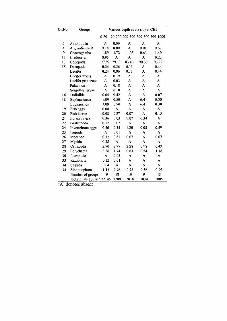
Gr.No: Groups Various depth strata (m) at CB5

0-20 20-200 200-300 300-500 500-1000

2 Amphipoda A 0.09 A A A 4 Appendicularia 9.18 8.80 A 0.08 0.67 9 Chaetognatha 1.89 3.72 11.35 0.63 1.40 11 Cladocera 0.93 A A A 0.22 13 Copepoda 77.97 79.11 83.43 90.37 93.77 15 Decapoda 0.24 0.56 0.11 A 0.44

Lucifer 0.24 0.06 0.11 A 0.44 Lucifer mysis A 0.19 A A A Lucifer protozoea A 0.03 A A A Palaemon A 0.18 A A A Sergestes larvae A 0.10 A A A

16 Doliolida 0.64 0.42 A A 0.07 18 Euphausiacea 1.09 0.50 A 6.41 0.30

Euphausiids 1.09 0.50 A 6.41 0.30 19 Fish eggs 0.08 A A A A 20 Fish larvae 0.08 0.27 0.07 A 0.15 21 Foraminifera 0.36 0.03 0.07 0.34 A 22 Gastropoda 0.12 0.02 A A A 24 Invertebrate eggs 0.56 0.35 1.20 0.08 0.59 25 Isopoda A 0.01 A A A 26 Medusae 0.32 0.81 0.07 A 0.07 27 Mysida 0.28 A A A A 28 Ostracoda 2.70 2.77 2.28 0.98 6.43 29 Polychaeta 2.26 1.74 0.63 0.54 1.18 30 Pteropoda A 0.03 A A A 33 Radiolaria 0.12 0.01 A A A 34 Salpida 0.04 A A A A 35 Siphonophora 1.13 0.76 0.78 0.56 0.96

Number of groups 19 18 10 9 13 Individuals 100 m-3 72145 7280 2818 1834 1085

`A' denotes absent

Table 4.7. Mesozooplankton groups absent from different depth strata in the central Bay during fall intermonsoon. Refer to Table 4.3 for the names of individual groups corresponding to the group numbers

Groups absent in different depth strata (m) Sampling station 0-MLD

TT-BT BT-300 300-500 500-1000

CB1 1, 3, 6-8, 10-11,14, 17, 23, 31, 32, 36

1-3, 5-8, 10-12, 1-3, 5-8, 10, 1-3, 5-8, 10-12, 14, 1-3, 5-6, 8, 10- 14, 15, 17, 19, 11, 14-17, 19, 15, 17, 23, 25, 27, 12, 14-17, 19, 20, 22, 23, 25, 23, 25, 27, 31- 31-33, 36, 37 22, 23, 25, 27, 27, 31, 32, 34, 34, 36, 37 30-34, 36,37 36, 37

1, 3, 5-8, 10, 11, 1, 3, 6, 7, 10, 11, 1-3, 5-8, 10- 1-4, 6-8, 10-12, 14- 1-3, 6-8, 10-12, 14, 17, 23, 25, 14, 17, 23, 31- 12, 14-17, 19, 17, 19, 21-23, 25- 14, 16-19, 22, 31-34, 36, 37 34, 36, 37 20, 23, 25-27, 27, 30-33, 35-37 23, 25-27, 29-37

30-34, 36, 37

1, 3, 6, 7, 10, 11, 1, 3, 5-8, 10, 14, 1,2, 5-8, 10- 1-12, 14-17, 19, 20, 1, 3, 6-8, 10-12, 17, 30-32, 36, 17, 23, 27, 30- 12, 14, 17, 19, 22-27, 32-37 14, 17, 19, 23, 37 34, 36 20, 23, 25, 27, 25, 30-32, 34,

29, 31-33, 36, 36, 37 37

1, 3, 6-8, 10, 14, 1, 3, 6-8, 10-12, 1-3, 5-8, 10, 1, 5-8, 10, 11, 14- 1, 3, 5-8, 10-11, 17, 21, 25, 32, 14, 17, 19, 23, 11, 14-20, 23, 20, 22, 23, 25, 27, 14, 15, 17, 19, 33, 36, 37 25, 30-34, 36, 37 25, 27, 30-32, 30-37 20, 23-25, 27,

34, 36, 37 28, 30-34, 36, 37

1-3, 5-8, 10, 11, 1, 3, 5-8, 10-12, 1-8, 10-12, 14, 1-3, 5-8, 10-12, 14- 1-3, 5-8, 10, 12, 12, 14, 17, 23, 14, 17, 19, 23, 16-19, 22, 23, 17, 19, 20, 22, 23, 14, 17, 21-23, 25, 30-32, 36, 27, 31, 32, 34, 25, 27, 30-34, 25-27, 30-34, 36, 25, 27, 30-34, 37 36, 37 36, 37 37 36, 37

MLD: mixed layer depth; TT: Top of thermocline; BT: Base of thermocline

CB2

CB3

CB4

CB5

Table 4.8. Percent abundance of different groups of mesozooplankton in central Bay during winter monsoon

Gr. No: Groups Various depth strata (m) at the stations sampled

0-40 40-150

CB1

150-300 300-500 1000-500 0-40 40-150

CB2

150-300 300-500 1000-500

1 Acantharia A A A A A A 0.17 A 0.10 A 2 Amphipoda 0.81 0.03 0.02 0.05 A 0.08 0.07 A 0.05 A 4 Appendicularia 1.88 0.79 A 0.28 0.47 2.80 A 0.05 0.16 A 5 Bivalvia A A 0.05 A A A A A A A 7 Cephalochordata A A A A A A A 0.02 A A 8 Cephalopoda A A A A A A 0.14 A 0.03 A 9 Chaetognatha 9.22 2.06 0.68 0.93 0.35 11.42 2.66 1.42 2.98 0.50 11 Cladocera 0.36 0.02 A 0.19 A 0.33 A A A 0.11 12 Crustacean larvae 0.24 A A 0.46 A A 0.11 A 0.03 0.11 13 Copepoda 68.95 90.89 87.22 90.04 94.88 58.97 91.18 85.93 89.83 94.18 15 Decapoda 1.47 0.09 0.04 0.05 0.07 1.01 0.14 A 0.03 0.24

Lucifer 0.16 A A A A 0.39 0.02 A 0.03 A Lucifer mysis A A A A A 0.08 A A A A Thalassocaris 1.31 0.09 0.04 A 0.07 0.46 0.12 A A A Unidentified larvae A A A 0.05 A 0.08 A A A 0.24

16 Doliolida A A A 0.05 0.07 A A A A A 17 Echinoderm larvae A A A A A 3.09 0.07 0.05 0.14 A 18 Euphausiacea 1.33 0.30 0.74 0.65 A 1.18 0.38 0.76 1.21 0.04

Euphausiid larvae 0.28 0.05 A A A 0.63 0.07 0.22 0.05 0.04 Euphausiids 1.05 0.24 0.74 0.65 A 0.55 0.31 0.54 1.16 A

19 Fish eggs A A A A A 0.26 A A A A 20 Fish larvae 0.13 0.07 A 0.05 A 0.15 0.11 0.02 0.44 0.26 21 Foraminifera 0.34 0.29 0.09 1.21 0.40 0.39 1.63 1.25 0.61 1.18 22 Gastropoda A A A A A A A 0.02 0.03 A 24 Invertebrate eggs 2.19 0.18 0.02 0.65 A 0.31 0.12 0.22 0.12 0.22 25 Isopod A 0.02 A A A A A A A A 26 Medusae A A A 0.14 A 0.51 0.02 A A A 27 Mysida A 0.02 0.02 A A A 0.14 0.07 A A 28 Ostracoda 11.23 4.62 10.91 3.89 3.28 11.52 1.66 8.24 3.81 2.95 29 Polychaeta 0.71 0.27 0.08 0.70 0.07 2.14 1.11 0.24 0.32 0.17 30 Pteropoda 0.46 0.15 0.11 A 0.20 0.15 A 0.05 A A 32 Pyrosomida A A A A A 0.17 A A A A 33 Radiolaria A 0.02 A A A 1.54 0.17 1.50 A 0.04 34 Salpida 0.24 0.09 A 0.05 0.20 0.32 0.07 0.05 0.05 A 35 Siphonophora 0.43 0.08 0.02 0.65 A 0.66 0.09 0.07 0.06 A

Number of groups 16 18 13 17 10 20 19 17 18 12 Individuals100 111-3 16025 32411 6016 5410 368 12310 16187 3385 4605 656

`A' denotes absent

Table 4.8. Contd.

Gr. No: Groups Various depth strata (m) at the stations sampled

0-40 40-150

CB3

150-300 300-500 1000-500 0-60 60-150

CB4

150-300 300-500 1000-500

1 Acantharia A 0.11 A A A 0.04 0.05 A A A 2 Amphipoda 0.11 0.05 0.05 A A 0.48 0.20 A A 0.36 4 Appendicularia 0.99 0.89 0.24 A A 0.28 0.35 A A 0.42 5 Bivalvia 0.22 0.01 A A A A A 0.10 A 0.18 7 Cephalochordata A 0.05 A A A 0.06 0.12 A A A 8 Cephalopoda 0.04 0.02 A A A A 0.14 A A A 9 Chaetognatha 5.96 4.22 0.62 0.99 0.83 8.31 3.58 1.83 0.74 4.02 I1 Cladocera 0.04 A A A A 0.21 A A A A 12 Crustacean larvae A A 0.11 A A 0.06 0.15 A A A 13 Copepoda 80.02 87.69 87.67 91.72 95.94 75.32 84.92 86.08 95.95 87.19 15 Decapoda 0.34 0.03 0.09 A A 0.50 0.04 A 0.06 0.18

Lucifer 0.19 A A A A 0.34 A A A 0.18 Megalopa 0.04 A 0.05 A A A A A A A Sergestes larvae 0.04 0.01 A A A A A A A A Thalassocaris 0.08 0.01 0.04 A A 0.16 0.04 A 0.06 A

16 Doliolida 0.08 0.04 A A A 0.10 0.04 A A A 17 Echinoderm larvae 0.66 0.26 0.08 A A 0.25 0.34 A A A 18 Euphausiacea 0.48 0.13 0.42 1.21 0.16 0.64 0.53 0.99 0.47 0.08

Euphausiid larvae 0.07 0.02 0.08 A 0.03 0.04 0.05 A A A Euphausiid protozoea 0.15 A A 0.06 A A A A A A Euphausiids 0.26 0.11 0.34 1.15 0.13 0.60 0.48 0.99 0.47 0.08

19 Fish eggs 0.15 A 0.04 0.06 A A 0.05 A A A 20 Fish larvae 0.19 0.22 0.08 0.44 0.12 A 0.14 A A 0.16 21 Foraminifera 1.63 0.58 2.06 0.19 0.03 6.23 0.25 2.29 0.22 2.09 22 Gastropoda 0.22 0.10 A A A A A A A A 24 Invertebrate eggs 1.10 0.31 0.04 A A 0.94 A 0.52 0.11 0.18 25 Isopoda A A 0.05 A A A A A A A 26 Medusae A 0.05 0.05 0.19 A 0.13 0.09 0.20 0.17 A 27 Mysida A 0.06 0.05 A A 0.06 0.17 0.30 A A 28 Ostracoda 6.18 3.91 6.88 4.30 2.90 3.41 6.03 6.99 2.14 2.11 29 Polychaetes 0.86 0.76 0.62 0.24 A 1.81 2.55 0.30 0.12 2.43 30 Pteropoda 0.29 0.03 A 0.06 0.03 0.06 A A A A 32 Pyrosomida A A A A A 0.33 A A A A 33 Radiolaria A A 0.83 0.06 A 0.11 0.05 0.31 A A 34 Salpida 0.04 0.14 0.04 A A 0.23 0.05 A A 0.08 35 Siphonophora 0.41 0.34 A 0.54 A 0.45 0.19 0.09 A 0.36

Number of groups 21 23 19 12 7 23 22 12 9 14 Individuals 100 ni3 26910 37622 4364 1621 843 27627 21431 1997 1718 362

`A' denotes absent

Table 4.8. Contd.

Gr. No: Groups Various depth strata (m) at CI35

0-20 20-200 200-300 300-500 500-1000

2 Amphipoda A 0.09 A A A 4 Appendicularia 9.18 8.80 A 0.08 0.67 9 Chaetognatha 1.89 3.72 11.35 0.63 1.40 11 Cladocera 0.93 A A A 0.22 13 Copepoda 77.97 79.11 83.43 90.37 93.77 15 Decapoda 0.24 0.56 0.11 A 0.44

Lucifer 0.24 0.06 0.11 A 0.44 Lucifer mysis A 0.19 A A A Lucifer protozoea A 0.03 A A A Palaemon A 0.18 A A A Sergestes larvae A 0.10 A A A

16 Doliolida 0.64 0.42 A A 0.07 18 Euphausiacea 1.09 0.50 A 6.41 0.30

Euphausiids 1.09 0.50 A 6.41 0.30 19 Fish eggs 0.08 A A A A 20 Fish larvae 0.08 0.27 0.07 A 0.15 21 Foraminifera 0.36 0.03 0.07 0.34 A 22 Gastropoda 0.12 0.02 A A A 24 Invertebrate eggs 0.56 0.35 1.20 0.08 0.59 25 Isopoda A 0.01 A A A 26 Medusae 0.32 0.81 0.07 A 0.07 27 Mysida 0.28 A A A A 28 Ostracoda 2.70 2.77 2.28 0.98 6.43 29 Polychaeta 2.26 1.74 0.63 0.54 1.18 30 Pteropoda A 0.03 A A A 33 Radiolaria 0.12 0.01 A A A 34 Salpida 0.04 A A A A 35 Siphonophora 1.13 0.76 0.78 0.56 0.96

Number of groups 19 18 10 9 13 Individuals 100 m-3 72145 7280 2818 1834 1085

`A' denotes absent

Table 4.9. Mesozooplankton groups absent from different depth strata in the central Bay during winter monsoon. Refer to Table 4.3 for the names of individual groups corresponding to the group numbers

Groups absent in different depth strata (m) Sampling station 0-MLD TT-BT BT-300 300-500 500-1000

1, 3, 5-8, 10, 12, 1, 3, 5-8, 10, 12, 1, 3, 4, 6-8, 1, 3, 5-8, 10, 14, 1-3, 5-8, 10-12, 14-17, 19, 22, 14, 16, 17, 19, 10-12, 14, 16, 17, 19, 22, 23, 25, 14, 17-20, 22-27, 23, 26, 31, 32, 22, 23, 26, 31, 17, 19, 20, 22, 27, 30-33, 36,37 31-33, 35-37 36, 37 32, 36, 37 23, 25, 26, 31-

34, 36, 37

1, 3,5-8, 10, 14, 3-7, 10, 11, 14, 1-3, 5-6, 8, 10- 1, 3, 5-8, 10, 11, 1-8, 10, 14, 16, 16, 22, 23, 25, 16, 19, 22, 23, 12, 14-16, 19, 14, 16, 19, 23, 25- 17, 19, 22, 23, 27, 31, 36, 37 25, 30-32, 36, 37 23, 25, 26, 31, 27, 30-33, 36, 37 25-27, 30-32, 35-

32, 36, 37 37

1, 3,6, 7, 10, 12, 3, 6, 10-12, 14, 1, 3, 5-8, 10, 1-8, 10-12, 14-17, 1-8, 10-12, 14- 14, 23, 25-27, 15, 19, 23, 25, 11, 14, 16, 22, 22-25, 27,31, 32, 17, 19, 22-27, 31-33, 36, 37 31-33, 36, 37 23, 30-32, 35- 34, 36, 37 29, 31-37

37

3, 5, 6, 8, 10, 14, 1, 3, 5, 6, 10, 11, 1-4, 6-8, 10- 1-8, 10-12, 14, 16, 1, 3, 6-8, 10-12, 19, 20, 22, 23, 14, 22-25, 30-32, 12, 14-17, 19, 17, 19, 20, 22, 23, 14, 16, 17, 19, 25, 31, 36, 37 36, 37 20, 22, 23, 25, 25, 27, 30-37 22, 23, 25-27,

30-32, 34, 36, 30-33, 36-37 37

3, 6-8, 10, 11, 1, 3, 6-8, 10, 11, 3, 5-8, 10-12, 1, 3, 6-8, 10-12, 14, ND 14, 16, 17, 23, 16, 17, 23, 25, 14,17, 22, 23, 16, 22, 23, 25, 31, 31, 33, 36 31-33, 36, 37 25, 31-33, 36, 32, 34-37

37

ND: No data due to shallower depth; MLD: mixed layer depth; TT: Top of thermocline; BT: Base of thermocline

CB1

CB2

CB3

CB4

CB5

Table 4.10. Percent abundance of different groups of mesozooplankton in central Bay during spring intermonsoon

Gr. No:

Groups Various depth strata (m) at the stations sampled

0-40

CBI

40-200 200-300 0-30 30-200

CB2

200-300 300-500

1 Acantharia A 0.40 A A A A A 2 Amphipoda A 0.10 A 0.28 0.96 A A 4 Appendicularia 1.41 A 0.03 0.55 2.02 0.33 A 5 Bivalvia 0.20 A A 0.06 0.04 A A 6 Carinaria A A A 0.19 A A A 8 Cephlaopoda 0.20 A A A A A A 9 Chaetognatha 1.91 2.87 1.74 2.71 8.95 1.75 0.67 11 Cladocera A A A 0.75 0.04 A A 12 Crustacean larvae A A 0.59 A 0.07 1.86 A 13 Copepoda 71.83 71.94 87.40 82.04 70.17 67.54 75.84 15 Decapoda A A 0.15 1.02 0.14 0.11 A

Brachyuran zoea A A A 0.14 A A A Lucifer A A A 0.33 A A A Lucifer protozoea A A A 0.08 0.14 A A Megalopa A A A 0.39 0.00 A A Sergestes larvae A A A 0.08 A A A Unidentified A A 0.15 A A 0.11 A

16 Doliolida A A A 0.03 0.14 A A 18 Euphausiacea 0.20 2.80 0.99 0.17 0.96 0.66 A

Euphausiid protozoea 0.20 A A 0.11 0.67 0.22 A Euphausiids A 2.80 0.99 0.06 0.28 0.44 A

21 Foraminifera 8.76 2.35 1.59 0.66 1.35 0.33 4.03 22 Gastropoda 0.57 A A 0.53 0.07 A A 24 Invertebrate egg 10.03 2.88 0.31 8.07 7.42 20.50 4.70 25 Isopoda A 0.10 A 0.03 0.21 A A 26 Medusae 0.20 0.20 0.03 0.47 0.36 A A 27 Mysida A A A 0.66 A A A 28 Ostracoda 2.72 12.50 3.76 0.33 4.62 5.59 14.09 29 Polychaeta 0.20 0.10 0.34 0.75 1.31 0.77 0.67 30 Pteropoda A A A 0.11 0.39 A A 33 Radiolaria 0.20 3.77 2.38 A 0.25 0.44 A 34 Salpida A A 0.15 0.08 0.04 A A 35 Siphonophora 1.58 A A 0.36 0.25 A A

Number of groups 14 12 13 21 21 11 6 Individuals 100 111-3 3840 831 3820 48253 6626 3648 298

`A' denotes absent

Table 4.10. Contd.

Gr. No: Groups Various depth strata (m) at the stations sampled

0-15 15-200

CB3

200-300 300-500 0-40 40-200

CB4

200-300 300-500

I Acantharia 0.15 A A A A A A A 2 Amphipoda 0.43 A A A 0.40 0.33 0.37 A 4 Appendicularia 3.10 A A 5.13 1.31 A 1.66 A 9 Chaetognatha 3.51 0.26 0.68 A 8.29 0.33 4.79 2.11 11 Cladocera 0.37 A A A 0.16 A 0.18 0.53 12 Crustacean larvae 0.02 A A A A A A A 13 Copepoda 81.48 87.63 87.16 87.18 74.70 86.60 83.06 88.42 15 Decapoda 0.39 0.26 A A 0.28 A A A

Brachyuran zoea 0.02 A A A A A A A Lucifer 0.15 A A A 0.19 A A A Lucifer protozoea 0.09 0.26 A A 0.05 A A A Megalopa A A A A 0.02 A A A Sergestes larvae 0.13 A A A A A A A Unidentified larvae A A A A 0.02 A A A

16 Doliolida 0.09 A A A 0.09 A A A 18 Euphausiacea 0.13 0.26 A A 0.72 A 0.37 A

Euphausiid larva A A A A 0.02 A A A Euphausiid protozoea 0.06 A A A 0.49 A A A Euphausiids 0.06 0.26 A A 0.21 A 0.37 A

21 Foraminifera 0.43 3.61 0.68 2.56 0.47 7.19 0.37 A 22 Gastropoda 0.32 0.26 A A 0.02 A 0.55 1.05 23 Halobates A A A A 0.02 A A A 24 Invertebrate egg 5.10 1.80 1.35 A 6.37 A . 2.39 A 25 Isopoda 0.02 A A A 0.02 A A A 26 Medusae 0.39 A A A 0.28 A 0.18 A 28 Ostracoda 1.12 3.87 8.78 5.13 5.14 0.98 3.50 4.74 29 Polychaeta 1.01 1.03 1.35 A 0.75 4.58 1.84 2.63 30 Pteropoda 0.30 A A A 0.19 A 0.55 A 33 Radiolaria 0.19 0.77 A A 0.05 A 0.18 0.53 34 Salpida 0.43 0.26 A A 0.28 A A A 35 Siphonophora 0.56 A A A 0.42 A A A

Number of groups 21 11 6 4 20 6 14 7 Individuals 100 m 3 248000 839 592 78 85680 765 2172 380

`A' denotes absent

Table 4.10. Contd.

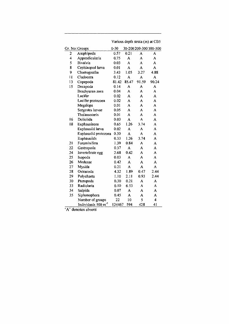
Various depth strata (m) at CB5

Gr. No: Groups 0-30 30-200 200-300 300-500 2 Amph ipoda 0.57 0.21 A A 4 Appendicularia 0.75 A A A 5 Bivalvia 0.03 A A A 8 Cephlaopod larva 0.01 A A A 9 Chaetognatha 3.43 1.05 3.27 4.88 11 Cladocera 0.12 A A A 13 Copepoda 81.42 85.47 91.59 90.24 15 Decapoda 0.14 A A A

Brachyuran zoea 0.04 A A A Lucifer 0.02 A A A Lucifer protozoea 0.02 A A A Megalopa 0.01 A A A Sergestes larvae 0.05 A A A Thalassocaris 0.01 A A A

16 Doliolida 0.03 A A A 18 Euphausiacea 0.65 1.26 3.74 A

Euphausiid larva 0.02 A A A Euphausiid protozoea 0.30 A A A Euphausiids 0.33 1.26 3.74 A

21 Foraminifera 1.39 0.84 A A 22 Gastropoda 0.37 A A A 24 Invertebrate egg 2.68 0.42 A A 25 Isopoda 0.03 A A A 26 Medusae 0.42 A A A 27 Mysida 0.21 A A A 28 Ostracoda 4.32 1.89 0.47 2.44 29 Polychaeta 1.10 2.11 0.93 2.44 30 Pteropoda 0.30 0.21 A A 33 Radiolaria 0.10 6.53 A A 34 Salpida 0.07 A A A 35 Siphonophora 0.45 A A A

Number of groups 22 10 5 4 Individuals 100 rif 3 124467 594 428 41

`A' denotes absent

CB3

CB4

Groups absent in different depth (m)strata Sampling station 0-MLD

TT-BT

200-300 300-500

1-3, 6, 7, 10-12, 14- 3-8, 10-12, 14-17, 17, 19, 20, 23, 25, 19, 20, 22, 23, 27, 27, 30-32, 34, 36, 37 30-32, 34-37

1, 3, 7, 8, 10, 12, 14, 1, 3, 6-8, 10, 14, 17, 19, 23, 31-33, 36,17, 19, 23, 27, 31, 37 32,36, 37

3, 5-8, 10, 14, 17, 19,1-8, 10-12, 14, 16, 23, 27, 31, 32, 36, 37 17, 19, 20, 23, 25-

27, 30-32, 35-37

1-3, 5-8, 10, 11, ND 14, 16, 17, 19, 22, 23, 25, 27, 30-32, 35-37

1-3, 5-8, 10, 11, 1-8, 10-12, 14-20, 22, 14, 16, 17, 22, 23, 23, 25-27, 30-37 25-27, 30-32, 34- 37

1-8, 10-12, 14-20, 1-3, 5-12, 14-20, 22- 22, 23, 25-27, 30- 27, 29-37 37

CB1

CB2

1, 3, 5-8, 10, 12, 14, 17, 19, 27, 31, 32, 36, 37

CB5 1, 3, 6, 7, 10, 12, 14, 17, 19, 23, 31, 32, 36, 37

1, 3-8, 10-12, 14- 20, 22-27, 30-37

1, 3-8, 10-12, 14-17, 19, 20, 22, 23, 25-27, 31-32, 34-37

1, 3, 5-8, 10, 12, 1-8, 10, 12, 14-21, 14-17, 19, 20, 23, 23-27, 30-32, 34-37 25, 27, 31, 32, 34- 37

1-8, 10-12, 14-17, 1-8, 10-12, 14-27, 30- 19-27, 30-37 37

Table 4.11. Mesozooplankton groups absent from different depth strata in the central Bay during spring intermonsoon. Refer to Table 4.3 for the names of individual groups corresponding to the group numbers

ND: No data as no zooplankton was present MLD: mixed layer depth; TT: Top of thermocline; BT: Base of thermocline

FIM

25

20

15

10

5

0

0-MID TT-BT BT-300 111

500-1000 in 00 C..)°

300-500

25

20

15

10

5

0 N

umbe

r of G

roup

s

■ 500-1000

■ 300-500

0 BT-300

0 TT-BT

■ 0-MID

25 -

20 -

15 -

10

5

WM

0

0-MID TT-BT BT-300 300-500 roSto2 500-1000 en Cei r ,u(.)

C.) C.)‘"

SpIM

25

20

15

10

5

0

0-MID TT-BT BT-300 Trial Station

300-500 500-1000 WI gn 1400 C.) (-)U

Figure 4.7. Depth-wise variation in the number of groups at each station in the central Bay during different seasons (SUM: summer monsoon, FIM: fall intermonsoon, WM: winter monsoon; SpIM: spring intermonsoon)

Depth strata

Only four to six of the 37 groups observed dominated numerically in the CB ( Fig.

4.8). Groups having an abundance >2% of the total mesozooplankton abundance were

considered as dominant. Some salient features on their spatio-temporal distribution are

listed below. In the overall, Copepoda was predominant during all the seasons, at all

stations and depths. Distribution (depth-wise and latitudinal) of the predominant groups is

described below.

4.2.6. Vertical distribution of predominant groups

Copepods ranged from 76 to 90% of the total abundance during SUM (Fig. 4.8). Their

percentage decreased to a minimum in the 200-300 m stratum, where the abundance of

chaetognaths (range: 2.6-9.3%), the second abundant group, was the maximum.

Euphausiacea (0.5-6%) and ostracods (0.6-4%) were also abundant in this stratum.

Polychaetes (0.1-4%) were the most abundant in the thermocline.

During FIM too, copepods contributed 74 to 90% of total abundance. Abundance of

second major group, Chaetognatha (1.6-5.7%), decreased with increasing depth.

Ostracods contributing 1.6-4.8% were most abundant in the thermocline. Euphausiids

(0.6-1.6%) were preponderant in the 300-500 m column. Appendicularia (0.3-7%) were

more in the first two-strata. Foraminifera (0.8-2.6%) were observed in all the sampled

strata.

Copepods accounted for 74 to 93% of the abundance during WM. Ostracods (2.8-

7.2%) and chaetognaths (1.4-7.6%) decreased relatively with increasing depth. High

abundance of medusae (none-7%) was found only in the 150-300 m stratum.

During SpIM, abundance of Copepoda ranged from 78 to 85%. Ostracoda (2.7-6.6%)

was the second major group with its percentage increasing from surface to 500 m. In

contrast, chaetognaths (1.9-4%) decreased. Foraminifera (0.6-3.1%) and invertebrate

eggs (1.2-6.5%) were the other major groups throughout the upper 500 m.

4.2.7. Latitudinal distribution of the predominant groups

Except for CB1 during SUM, copepods showed an increasing trend towards northern Bay

during SUM, FIM and SpIM (Fig. 4.9). Similar trend was also observed in case of

Appendicularia during FIM. Medusae were dominant at the northernmost station, CBS

49

SUM

■ Copepoda 0-MLD I

TT-BT II ■ Chaetognatha 0 Euphausiacea

200-300 MIN 0 Ostracoda ■ Polychaeta 300-500 I

500-1000 II

FIM 0-MLD IN

■ Copepoda TT-BT I- ■ Chaetognatha

0 Euphausiacea 200-300 I M 0 Ostracoda

■ Appendicularia 300-500 NI ■ Foraminifera

E g tg

500-1000 In

WM A. 0-MLD MIll ■ Copepoda

TT-BT ■ Chaetognatha 0 Ostracoda MI

150-300 ■ Medusae ■

300-500 ■

500-1000 ■

0-MLD SpIM ■ Copepoda ■ ME

■ Chaetognatha IM ■ TT-BT 0 Ostracoda

■ Foraminifera 200-300 = MO 0 Inv. eggs

300-500 ME

500-1000

60 80 100 %

Figure 4.8. Distribution of dominant groups (> 2%) in each stratum in the central Bay during different seasons (SUM: summer monsoon, FIM: fall intermonsoon, WM: winter monsoon; SpIM: spring intermonsoon). Inv. eggs: invertebrate eggs

■Poly chaeta O Ostracoda 0 Euphausiacea ■Chaetognatha ■Copepoda

13 Foraminifera ■Appendicularia O Ostracoda 0 Euphausiacea

, ■ Chaetognatha ■Copepoda

100 -

80 -

60

■Medusae Ostracoda

■Chaetognatha ■Copepoda

0 Inv.eggs ■Foraminifera

Ostracods ■Chaetognatha ■Copepoda

80

60

SUM 100

80 1

60

100 - FIM

80

60 , i , i

WM 0

C'S 100 -

CB1 CB2 CB3 C134 CB5

Station

Figure 4.9. Distribution of dominant groups (> 2%) at different stations in the central Bay during different seasons (SUM: summer monsoon, FIM: fall intermonsoon, WM: winter monsoon; SpIM: spring intermonsoon). Inv. eggs: invertebrate eggs

Table 4.12. Various statistical (non-parametric tests) analyses to distinguish diel, spatial and temporal differences in mesozooplankton biovolume and abundance in the central Bay of Bengal

Wilcoxon Matched Pairs Test between day and night

Seasons SUM FIM WM SpIM

Biovolume N T Z p 18 26.5 2.4 p<0.05 20 81.0 0.2 p>0.05 24 106.0 0.7 p>0.05

Abundance N T Z p 20 66 1.5 p>0.05 18 62 1.0 p>0.05 25 121 0.8 p>0.05

Friedman ANOVA to test difference between depths Biovolume Abundance

Seasons

Chi Sqr. N df p Chi Sqr. N df p SUM

14.5 5 5 p<0.05 14.2 5 4 p<0.05 FIM

18 5 5 p<0.05 17.1 5 4 p<0.05 WM

15.4 4 4 p<0.05 18.4 4 4 p<0.05 SpIM

8.4 5 2 p<0.05 12 4 3 p<0.05

Friedman ANOVA to test the difference between stations Biovolume Abundance

Seasons

Chi Sqr. N df p Chi Sqr. N df p SUM

3.8 5 4 p>0.05 5.3 5 4 p>0.05 FIM

11.1 5 4 p<0.05 10.4 5 4 p<0.05 WM

6.7 4 4 p>0.05 5.6 5 4 p>0.05 SpIM

0.7 4 4 p>0.05 1.3 3 4 p>0.05

Friedman ANOVA to test the difference between seasons

Chi Sqr. N df p Biovolume 9.5 20 3 p<0.05

Abundance 22.6 19 3 P< 0 ' a5

The Wilcoxon test could not be obtained during SpIM due to insufficient data values in day-night pairs; Significant results are marked bold

Table 4.13. Correlation coefficients between mesozooplankton biomass, abundance and number of groups (from mixed layer depth) and temperature, salinity, chl a (average from upper 120 m) in the central Bay of Bengal

Parameters Biovolume Abundance Groups

SUM Temp -0.714 -0.425 -0.035 Salinity 0.168 0.262 -0.336 Chl a 0.659 0.175 0.231

FIM Temp 0.387 0.395 0.117 Salinity 0.769 0.840 -0.098 Chl a 0.939 0.908 0.441

WM Temp -0.452 -0.297 -0.245 Salinity -0.375 -0.478 -0.674 Chl a 0.528 0.580 -0.255

SpIM Temp 0.703 -0.131 -0.078 Salinity -0.349 -0.673 -0.497 Chl a 0.876 0.394 0.475

Bold r-values are significant at p<0.05

Table 4.14. Spatio-temporal variation in number of zooplankton groups in the central Bay as determined through one/two way ANOVA

Groups

Between depths Between stations

Between depths Between stations

Between seasons

ANOVA Two-way ANOVA

SUM FIM F (4, 24)-4.0, p<0.05 F (4, 24)-12.7, p<0.001 F (4, 24)=0.4, p>0.05 F (4, 24)=0.9, p>0.05

WM SpIM F (4, 24)=19.7, p<0.001 F (3, 19)=11.3, p<0.001 F (4, 2a)=0.7, p>0.05 F (4, 19)=0.9, p>0.05

One-way ANOVA

F (3, 90=10.9, p<0.001 Significant results are marked bold

during WM. High abundance of chaetognaths was observed at stations CB2 and CB3

during SUM coinciding with the lowest copepod abundance. However, they did not show

any latitudinal variability during other seasons. Euphausiids and polychaetes did not

show any latitudinal trend in any season when they were dominant. Ostracods occurring

in higher percentage during WM and SpIM were more in the southern Bay. Similar was

the case of Foraminifera and invertebrate eggs during the intermonsoons, FIM and SpIM.

4.3. Discussion

4.3.1. Spatio-temporal variations in biovolume, biomass and abundance

On a seasonal basis, the average zooplankton biovolume (ml 100 m -3) in the 1000 m was

higher during SUM (39.3) and SpIM (40.4) compared to FIM (12.7) and WM (13.8).

Historical data from the HOE show that biovolume in the Bay range between 0.1 and 9.9

ml per standard haul during WM (Duing 1970). During March- April (SpIM), large

patches in the Bay with volumes ranging from 10 to 19.9 ml have been reported. In other

areas in the CB, the volumes were low (in the range of 0.1-9.9 ml). The results from this

study indicate that the central Bay has higher mesozooplankton biovolume during SUM

and SpIM. In these two seasons, the integrated chl a in the upper 120 m was lower (10

and 16 mg 111-2 ; Chapter 3) probably due to elevated grazing pressure than that was

observed during either FIM or WM (18 and 27 mg m -2). Similar results are reported from

Arabian Sea by many authors (Smith 1982; Baars and Oosterhuis 1998; Ashjian et al.

2002). They also suggest that the low chl a was due to grazing by zooplankton. Also,

large swarms of Pyrosoma, observed during SUM could have also reduced the

phytoplankton.

The HOE data suggests that the Bay is more productive during WM (Panikkar and

Rao 1973). Though this is not reflected in the zooplankton biovolumes, the integrated

carbon biomass and abundance in the upper 1000 m in the central Bay is higher during

WM and FIM compared to the two other seasons SUM and SpIM. Cold-core eddies are

known to pump in or re-supply nutrients into the euphotic layer and, enhance

phytoplankton production within such eddies (Falkowski et al. 1991; Vaillancourt et al.

2003). The stations CB1 and CB5 during SUM as well as FIM, CB5 during WM and

CB3 and CB4 during SpIM were located in the vicinity of cold-core eddies. At these

50

stations, there was higher biovolume and numerical abundance of mesozooplankton

having positive correlations with chl a. This observation is similar to one reported earlier

by Wiebe (1976), Beckmann et al. (1987) and Huntley et al. (1995).

4.3.2. Seasonal variations in community structure

As mentioned earlier, the hydrography of the Bay undergoes seasonal changes. The

central Bay experiences a warm pool and low surface salinities throughout the seasons.

The SST (28.7, 28.8, 28.1 and 29.9 °C during SUM, FIM, WM and SpIM respectively)

and SSS (31.4, 31.5, 32.8 and 32.9 psu respectively for the same seasons) did show minor

variations seasonally. The dissolved oxygen concentrations and the thickness of the low

oxygen (5-10 p,M) zone also varied. It was larger during SUM (roughly between 100-700

m), thinner during FIM (100-600 in particular between CB3 and CBS) as well as during

SpIM (200-500 m between CB3 and C135) and was absent during WM. Similarly, the

standing stocks and groups of zooplankton are known to vary in the northern Indian

Ocean seasonally (Rao 1973, 1979). Jyothibabu et al. (2004) showed that zooplankton

biomass from the open waters of BoB was lesser than in the central Arabian Sea by 50%.

However, results from present study (75-134 mM C m -2) imply that they are closely

comparable to those in the Arabian Sea (73-158 mM C m 2; Madhupratap et al. 1996 a).

To avoid visual predators in the surface during the day, zooplankton have been

reported to move subsurface (Longhurst and Williams 1992; Goswami et al. 2000).

During this study, diel variations were insignificant during most seasons. During SUM,

the diel difference in biovolume was significant due to the occurrence of large swarms of

herbivorous Pyrosoma in the surface during day-time. Most of the biovolume was

concentrated in the MLD and decreased significantly with increasing depth as also

observed in previous studies (Vinogradov 1970, 1997; Banse 1994 and Wishner et al.

1998; Padmavati et al. 1998; Madhupratap et al. 2001). Mesozooplankton are the

maximum in the uppermost stratum where concentrations of chlorophyll are more and

primary production takes place (Longhurst and Harrison 1989; White et al. 1995). Thus

the decrease in their abundance at subsurface depths is a universal feature in tropical

oceans (Vinogradov 1997). This was also reflected in the number of groups, which was

the largest only in the MLD.

(1 2 51

Since only 21 groups occurred during all the seasons, this means that a significant

number, i.e. — 50% of the groups occurred only seasonally. Stereozoom and light

microscopy photographs of some groups identified from the Bay are given in Plates 1-5.

The number of groups recorded during SUM and SpIM (27) were lower compared to

those recorded during FIM and WM (31). Also, in spite of higher biovolumes of

zooplankton, their carbon biomass was lower during the former two seasons (SUM: 78,

SpIM: 75 mM C ni2) than in the latter seasons (FIM: 112 WM: 134 mM C m -2).

Pyrosoma, the holoplanktonic colonial tunicates appeared in dense aggregations and

contributed to most of the biovolume during SUM. They are known to be restricted to

warmer waters (Van Soest 1981). Their trophic function in the ocean, as well as their

ecology and physiology are extremely poorly known (Perissinotto et al. 2007).

During SpIM large biovolumes in the surface were due to scyphomedusae. Though

gelatinous zooplankton such as pyrosomes and scyphomedusae have large biovolumes,

their carbon content is low compared to crustaceans (Clarke et al. 1992). This might be

the major cause for lower carbon biomass during these two seasons in the CB. During

SUM, the lowest number of groups was found in the thermocline, which gradually

increased in the deeper strata. Also the seasonal difference in the decrease of number of

groups with depth seems to be a direct reflection of variations in subsurface oxygen

concentration. This can be confirmed from the drastic decrease in the number of groups

in the subsurface during SUM, which coincided with the thickest OMZ.

Copepods are the most abundant and diverse metazoans in all pelagic ecosystems

(Longhurst 1985). As also reported in many earlier studies (Padmavati et al. 1998;

Madhupratap and Haridas 1990; Madhupratap et al. 2001; Koppelmann and Weikert

2000; Rakhesh et al. 2006), it was the dominant taxon in the CB during all the seasons.

Carnivorous chaetognaths and omnivorous ostracods were the other major groups present

during all the seasons. These three groups were also found to be dominant in the Arabian

Sea (Padmavati et al.1998; Madhupratap and Haridas 1990; Madhupratap et al. 2001).

Chaetognath abundance in the upper 200 m (Ulloa et al. 2000) and progressive

decrease with increasing depth has already been reported (Nair 1977; Batistic et al.

2003). Their population density is thought to reduce with rapidly decreasing temperature

(Nair et al. 2000). Further, their population did not show much of latitudinal variation, as

52

was also found during the HOE (Nair and Rao 1971). It is very probable that the

distribution of chaetognaths in the offshore waters is also severely affected by the

reversal of currents caused by monsoon (Tokioka 1962). Contrary to the observations in

the HOE (Panikkar and Rao 1973), ostracod abundance was more in the southern Bay.

Albeit poorer in abundance than the Arabian Sea, ostracods showed seasonal fluctuations

and were more abundant during WM and SpIM. Latitudinal zonation patterns in ostracod

distributions were observed in the Southern Ocean (Angel and Blachowiak-Samolyk

2007). Numerically, they are often the second or third most abundant group in

mesoplankton samples and play a significant role in the recycling of organic matter in the

marine snow and fecal pellets within subthermocline. Similar to the observations in the

Northeast Atlantic (Angel et al. 2007), ostracod abundances increased in the CB rapidly

below the thermocline during most seasons, reaching maxima at 200-400 m before

declining again with depth.

Investigations on the pelagic polychaetes of the Indian Ocean are few (Fauvel 1953).

In general, they are adapted for tubiculous, burrowing or bottom dwelling life style with

planktonic larval stages. However, only a few polychaete species are planktonic even in

their adult stages, e.g., Tomopteridae and Alciopidae. Pelagic polychaetes were found

abundantly in the Bay as well as in the AS (Peter 1973 a, b) with some species in high

numbers in the surface waters though with marked seasonal and diurnal variations. In this

study, they were present throughout the water column only during SUM. The

appendicularians were present in the upper 200 m in the northern CB. They are reported

to be remarkably efficient in capturing food particles of nano-and pico-size categories

(0.2-20 j.tm; Flood 1978; King et al. 1980; Alldredge 1981), which can hardly be captured

by copepods. From the higher abundance of medusae in the northernmost station

observed during the WM, it appears that the Bay of Bengal harbors a peculiar assortment

of species/genera of medusae that prefer or tolerate a combination of high temperature

and low salinity as also suggested by Vannucci and Navas (1973).

Though diel differences were not clearly evident in biomass values, higher percentage

of euphausiids at subsurface depths was a noticeable feature during SUM and FIM.

Kinzer (1969) found deep scattering layers (DSL) to be rich in zooplankton biovolumes

mostly composed of euphausiids and copepods. Dominance of euphausiids in certain

53

depth levels has been observed in other studies also (Moore 1950; Tucker 1951; Brinton

1967 and Longhurst 1967). Foraminifera became a major group during the warm, high-

saline period of SpIM. They also were abundant in the southern Bay in particular during

FIM.

As Ryther (1969) pointed out, it has been increasingly apparent that the bulk of

primary productivity in oceanic waters is by the nanophytoplankton, which range in size

between —5 and 25 gm. In general, the nanoplanktonic organisms are too small to be

captured by most metazoan herbivores. Before the energy they embody can be utilized, it

must be assimilated by small herbivores, and these are chiefly the planktonic protozoans,

such as Foraminifera. During the intermonsoons, the foraminifers may be preyed upon in

turn by small carnivorous zooplankton, including chaetognaths (Croce 1963), thecosome

pteropods (Boas 1886), and others. Thus, as also observed in the Arabian Sea

(Madhupratap et al. 1996 a, b), the microbial loop may play an important role in

sustaining high biomass of zooplankton in the surface in particular during the

intermonsoons.

From the foregoing, it can be summarized that the variability in biomass and

abundance of zooplankton is affected directly by the seasonal changes in physical

parameters, and also indirectly by alterations in nutrient (chemical) and chl a (biological)

concentrations. During SUM and SpIM, the CB had higher biovolumes consisting of

Pyrosoma and cnidarians with lower carbon biomass. However, during FIM and WM,

despite lower biovolumes, the carbon content was higher. Further, the number of groups

was found to be lower during SUM and SpIM than those recorded either during FIM

and/or WM. Also, cyclonic eddies play a crucial role in supporting higher zooplankton

biomasses (75-134 mM C m -2), the values of which nearly match those in the central

Arabian Sea (73 —158 mM C m 2). From the HOE data, the zooplankton biomass in the

central Bay was estimated to aid in producing tertiary production of 0.5 Million tons per

5X5° square (Cushing et al. 1971). With India's annual fish catch of — 30% (CMFRI

1970) coming from the Bay of Bengal, the large amounts of zooplankton carbon in the

offshore are indicative of supporting rich pelagic fisheries.

54

Chapter 5

Chapter 5

Different Groups of Mesozooplankton from Western Bay

As described in Chapter 4, the hydrography of the Bay of Bengal is influenced by semi

annually reversing monsoon winds, river runoff (1.6 x 10 12 m3 yr-1 ; Subramanian 1993)

and annual precipitation (--1m yr -1 ; Baumgartner and Reichel 1975) exceeding

evaporation. These physical forcings keep the upper layers in the western bay (WB)

highly stratified and the surface salinity is lower in particular in the northern parts. As

mentioned earlier, the seasonally reversing EICC (East India Coastal Current) is

northward during summer monsoon (SUM) and Equator-ward during fall intermonsoon

(Wyrtki 1971; Murty et al. 1992; Gopalakrishna et al. 1996; Han and McCreary 2001).

The southwesterly winds prevalent during SUM are favourable for offshore Ekman

transport and vertical advection in the WB. La Fond (1957), Murty and Varadachari

(1968), Shetye et al. (1991) and Rao (2002) have reported upwelling along the near-shore

WB during this season. Wind driven vertical advection and mixing have been observed to

transport nutrients from within and below the thermocline up into the euphotic zone.

These processes replenish nutrient concentrations in the upper layers during the SUM

(Bhavanarayana and La Fond 1957; Thirupad et al. 1959). Madhu et al. (2002) reported

primary production and chlorophyll (chl) a distribution in the upwelling regions of the

southern WB during SUM.

Most previous biological studies in the WB have focused on the seasonal variation in

primary productivity. Abundance and composition of mesozooplankton are addressed by

a very few studies (Panikkar and Rao 1973; Achuthankutty et al.1980; Nair et al. 1981;

Madhupratap et al. 2003; Muraleedharan et al. 2007; Rakhesh et al. 2006). In the

stratified layers of the Bay, cyclonic eddy-pumping is thought to be a possible

mechanism for transferring nutrients into the euphotic zone and increasing biological

production during most part of the year (Gomes et al. 2000; Prasannakumar et al. 2004,

2007). Eddy-mediated elevated zooplankton biovolumes associated with increased

primary production has been reported in the Bay (Muraleedharan et al. 2007). As also

mentioned in Chapter 4, many studies from the Atlantic and Pacific regions are available

55

on the spatio-temporal distribution of zooplankton (Roman et al. 1995; Smith et al. 1998;

Madin et al. 2001; Mauny and Dauvin 2002; Schnetzer and Steinberg 2002 b; Gaudy et

al. 2003; Koppelmann et al. 2003; Kang et al. 2004; Yamaguchi et al. 2005; Fernandez-

Alamo and Farber-Lorda 2006; Li et al. 2006; Alcaraz et al. 2007).

In the Indian Ocean, investigations of Madhupratap et al. (1996), Padmavati et al.

(1998), Goswami et al. (2000) and Jayalakshmy (2000) among many others have

addressed these aspects mostly from the Arabian Sea. In particular, a large number of

studies on seasonal cycles of mesozooplankton are available from the western Arabian

Sea (Wishner et al. 1998; Smith 1998, 1999, 2000, 2001; Smith et al. 1998; Stelfox et al.

1999; Hitchcock et al. 2002; Koppelmann et al. 2005). High zooplankton standing stocks

in the mixed layer are known to occur in the eastern Arabian Sea throughout the year

(Madhupratap et al. 1996 a) due to coastal upwelling during SUM, convective mixing in

winter and through the microbial loop in the intermonsoon.

As also pointed out in Chapter 4, after the HOE (International Indian Ocean

Expedition; 1960-1965), the western Bay of Bengal also remains one of the sparsely

investigated regions of the Indian Ocean especially in terms of zooplankton biomass and

composition below 200 m depth. The seasonal studies on the distributional patterns of

mesozooplankton from the upper 1000 m and their response to primary production

associated with basin-scale hydrographic processes in the WB are not yet reported.

Knowledge of mesozooplankton abundance, distribution and composition in space and

time is important for understanding regime shifts in their communities, their possible

effect on fisheries, carbon budgets and climate change. In this chapter, spatial and

seasonal variations in mesozooplankton biomass, their numerical abundance, and group

composition in the upper 1000 m, at four stations in the western Bay during summer

monsoon (SUM), fall intermonsoon (FIM), winter monsoon (WM) and spring

intermonsoon (SpIM) would be addressed.

5.1. Methods

5.1.1. Sampling

Sampling sites in the western Bay (WB) of Bengal were from four locations viz. WB 1 to

WB4 (12°N 81°E,15°N 82°E,17°N 83°E, 19°N 85°E). All other details of collection,

56

biovolume measurements and group-wise enumeration of mesozooplankton and

statistical analyses are as described in Chapter 4.

5.2. Results

5.2.1. Biovolume

As also recorded from central Bay (CB), zooplankton biovolume during all four seasons

was the highest in the mixed layer depth (MLD; Fig. 5.1-5.4; Table 5.1). It decreased

significantly with increasing depth during both monsoons and FIM. Nearly 93, 69, 63 and

80% of the biovolume was present in the MLD during the SUM, FIM, WM and SpIM

respectively. In the WM, up to 11% biovolume was observed in the 300-500 m stratum.

In the upper 1000 m, biovolume ranged from 0.2 to 120 (mean: 10.0 ml 100 m -3) during

SUM, negligible to 115 (15.4 ml 100 m 3) during FIM, 1.0-142 (34.0 ml 100 m 3) during

WM and negligible to 533 (76.4 ml 100 m 3) during SpIM. The higher biovolumes during

SUM and SpIM were due to Pyrosoma swarms and scyphomedusae respectively. With

the average biovolumes in the top1000 m increasing from SUM to SpIM, seasonal

differences were highly significant (Table 5.12). Also, vertical migration patterns were

not evident as there was no significant difference in biovolumes between the day and

night in any season (Table 5.12).

Biovolumes were higher at WB3 during SUM and FIM, at WB1 and WB2 during

WM and at WB3 and WB4 during SpIM. However, these differences were not

statistically significant. When compared with the temperature in the top 120 m in

different seasons, it was found to correlate negatively (Table 5.13). Temperature was

lower and biovolumes higher at stations with cold-core eddies. However the relation with

chlorophyll (chl) a was negative during all seasons but was significant only during SUM.

5.2.2. Abundance

Similar to biovolumes, the abundance (No.x 1000 individuals 100 m -3) observed was

greatest in the MLD during all seasons (Table 5.2) and decreased significantly with

increasing depth. The diel difference in abundance was also negligible except during

SpIM (Table 5.12). It ranged from negligible to 462 (mean: 31.8 x 10 3 ind. 100 m3)

during SUM, 0.7 to 136.3 (35.2 x 10 3 ind. 100 m-3) during FIM, 0.4 to 161.8 (38.4 x 10 3

57

1

ng WB1

0-14 14-200

200-300 300-500

500-1000

0-29 29-200

200-300 300-500

500-1000

ng W134

ng 0 D • N

L_ [

Biovolume (ml 100 m-3 )

-30 -15 0 15 30 -30 -15 0

15 30

Dep

th s

trata

(m)

-30 -15 0 15 30

0-2 2-200

200-300 300-500

500-1000

Figure 5.1. Vertical distribution of mesozooplankton biovolume during day and night sampling at different stations in the western Bay of Bengal during summer monsoon. `ng' denotes negligible biovolume

-60 -30 0 30 60

Biovolume (ml 100 m-3)

-60 -30 0 30 60 -60 -30 0 30 60

0-30

30-200

200-300

300-500

500-1000 r-6

15 a.„,) 0-20

20-200 200-300 300-500

500-1000

0-20

20-200

200-300

300-500

500-1000

0-40 40-200

200-300 300-500

500-1000

-60 -30 0 30 60

_L.

Figure 5.2. Vertical distribution of mesozooplankton biovolume during day and night sampling at different stations in the western Bay of Bengal during fall intermonsoon. 'lig' denotes negligible biovolume and 'NO DATA' is where net failed to open/close

0-20

20-171

171-300

300-500

500-1000

0-30

30-156

156-300 WB1

300-500

35-135

0-35

WB4

Biovolume (ml 100 m-3)

-80 -40 0 40 80 -80 -40 0 40 80

V, -80 -40 0 40 80

-E.

200-300

300-500 JO D

■ Dusk

fa' 0-60 Q

60-200 WB3

-80 -40 0 40 80

OD • N

Figure 5.3. Vertical distribution of mesozooplankton biovolume during day and night sampling at different stations in the western Bay of Bengal during winter monsoon

-40 -20 0 20 40 -40 -20 0 20 40

0-40

40-200

200-300

300-500

0-30

30-200

200-300

300-500

0-30

30-200

200-300

300-500

0-30

30-200

200-300

300-500

Dep

th s

trat

a (m

)

Biovolume (ml 100 m-3)

-40 -20 0 20 40 -40 -20 0

20 40

Figure 5.4. Vertical distribution of mesozooplankton biovolume during day and night sampling at different stations in the western Bay of Bengal during spring intermonsoon. 'rig' denotes negligible biovolume and 'NO DATA' is where net failed to open/close

Table 5.1. Mesozooplankton biovolume (ml 100 rn-3) and carbon biomass (mM C IT1-2 ; in parentheses) in the western Bay of Bengal during different seasons

Sampling stations Depth (m) WB1 WB2 WB3 WB4

Summer monsoon 0-MLD 14.0 (15.0) ND (ND) * 120.0 (53.4) 5.0 (5.3) TT-BT 0.3 (0.8) ND (ND) ng (ng) 0.6 (0.6) BT-300 1.1 (2.2) ND (ND) ng (ng) 3.5 (6.2) 300-500 0.15 (0.6) ND (ND) 0.4 (1.7) 0.3 (0.6) 500-1000 0.15 (0.5) ND (ND) 3.0 (32.1) 0.5 (1.7)

Fall intermonsoon 0-MLD 26.6 (17.1) 30.0 (12.8) 115.0 (49.2) 42.0 (18.0) TT-BT 30.6 (111.2) 14.4 (55.4) 6.6 (25.4) 5.0 (19.3) BT-300 ng (ng) 4.0 (8.6) 4.6 (9.8) 13.0 (27.8) 300-500 2.0 (8.6) ng (ng) 4.0 (17.1) 1.8 (7.7) 500-1000 1.6 (17.1) 2.2 (23.5) 1.8 (19.2) 3.0 (23.5)

Winter monsoon 0-MLD 142.0 (51.2) 140.0 (59.9) 33.7 (34.2) 25.7 (19.2) TT-BT 12.3 (28.6) 26.1 (67.1) 11.6 (37.3) 18.0 (38.5) BT-300 35.6 (58.9) 2.1 (6.4) 15.3 (44.7) ND (ND) 300-500 12.0 (51.3) 24.0 (27.6) 10.0 (27.8) ND (ND) 500-1000 ND (ND) 1.0 (10.7) ND (ND) ND (ND)

Spring tintermonsoon 0-MLD 13.3 (5.7) 20.0 (17.1) 246.7 (86.7) 533.3 (228.0) TT-BT 4.4 (16.0) 17.5 (59.9) 107.6 (391.2) 11.8 (21.4) BT-300 12.0 (12.8) 8.0 (17.1) ng (ng) 11.5 (24.6) 300-500 ng (ng) ng (ng) 1.0 (2.1) 6.5 (14.1) MLD: mixed layer depth; TT: Top of thermocline; BT: Base of thermocline

*high volumes due to swarms of Pyrosoma; ng- negligible biovolume; ND- no data (probably due to failure of net or due to shallower depth)

Table 5.2. Mesozooplankton numerical abundance (x 10 3 individuals 100 m-3) in the western Bay of Bengal during different seasons

Sampling stations Depth (m) WB1 WB2 WB3 WB4

Summer monsoon 0-MLD 6.7 ND 462.1 1.71

TT-BT 0.0 ND 2.5 0.08 BT-300 1.0 ND 0.0 0.90 300-500 0.0 ND 1.9 0.04 500-1000 0.0 ND 0.5 0.01

Fall intermonsoon 0-MLD 136.3 99.1 129.1 131.3

TT-BT 41.2 39.1 8.7 7.9

BT-300 5.5 4.8 44.3 15.1 300-500 2.8 0.8 15.8 13.4

500-1000 0.7 2.3 2.1 3.6

Winter monsoon 0-MLD 161.8 139.6 72.9 35.3 TT-BT 7.3 17.8 41.6 31.8

BT-300 34.3 3.1 5.2 ND

300-500 12.5 1.6 10.8 ND

500-1000 ND 0.4 ND ND

Spring intermonsoon 0-MLD 31.0 37.3 49.5 533.8 TT-BT 15.6 23.0 39.9 8.2

BT-300 3.1 4.2 1.4 5.1 300-500 0.2 0.8 1.6 1.7

MLD: mixed layer depth; TT: Top of thermocline; BT: Base of thermocline

At some depths, there was no data (ND) either due to failure of the net to open/close or due to shallower depth in northernmost station

ind. 100 m-3) during WM and 0.2 to 533.8 (47.3 x 103 ind. 100 m-3) during SpIM. The

abundance in MLD was 98.6, 70.4, 68.3, and 86.1% during SUM, FIM, WM and SpIM

respectively.

The average abundance in the upper 1000 m increased from SUM to SpIM and

differed significantly between seasons. Though the station-wise differences in abundance

were noticeable during some seasons, they were not statistically significant. During the

SUM, the abundance was the highest at WB3; during FIM, it did not vary much. While

during WM, the higher abundance was found at WB1, it was at WB4 during SpIM. These

locations were in the vicinities of cold-core eddies as is also implicit from the negative

correlations with temperature (Table 5.13). Similar to biovolume, abundance too

correlated negatively with chl a, but significantly during SUM.

5.2.3. Cluster analyses and non-metric multidimensional scaling (NMDS)

Cluster and NMDS analyses imply that zooplankton biovolume and abundance

distribution at various depths and stations (Fig. 5.5) during SUM were different compared

to that during the other three seasons. Among the other three seasons, biovolume

distribution was similar during the intermonsoons. However, the numerical abundance

was similar during FIM and WM.

5.2.4. Column (0-1000 m) integrated abundance and carbon biomass

The integrated abundance during SUM, FIM, WM and SpIM respectively ranged from 2

to 53 (mean: 20 x 103 ind. 100 m-2), 108 to 128 (120 x 10 3 ind. 100 m2), 44 to 155 (95 x

103 ind. 100 m-2) and 38 to 182 (96 x 103 ind. 100 m-2). It was the least during SUM,

moderate during WM and SpIM, and the highest during FIM (Fig 5.6).

Similarly, the integrated carbon biomass (mM C m -2) was 14-90 (mean: 42 mM C m

2); 96-54 (118 mM C m -2); 58-190 (141 mM C m 2); and 35-480 (224 mM C m-2) during

the respective seasons (Fig. 5.6). It was found to increase from SUM to SpIM.

5.2.5. Groups

A total of 33 groups were identified from the western Bay (Table 5.3). Acantharia,

Carinaria, Pterotrachea and Sipuncula that were present in rare numbers in the CB were

58

20 40 60 ! 80 Bray-Curtis Similarity (%)

Abundance

a) bl

W1

M I FI

SpIM II

SUM III

100

Biovolume

a) bl

SUM III

100

Sp11 I

FIM

WM II

40 60 80 Bray-Curtis Similarity (%)

Figure 5.5. a) Cluster dendrograms depicting similarity between seasons based on biovolume and abundance of zooplankton in the western Bay. b) Non- metric multidimensional scaling (NMDS) ordination based on the Bray- Curtis similarity coefficients

Abu

ndan

ce (x

1d

ind.

ni2)

■ WBI

• WB2

0 WB3

■ WB4

SUM FIM WM SpIM

300 480 ■ WBI

■ WB2 D WB3

N 200 - • WB4

8 U 2 ^ 100 -

• 0 r i SUM FIM WM SpIM

Season

Figure 5.6. Latitudinal variations in the 0-1000 m column integrated mesozooplankton abundance (10 3 individuals m'2) and biomass in the western Bay during different seasons (SUM: summer monsoon, FIM: fall intermonsoon, WM: winter monsoon ; SpIM : spring intermonsoon)

Table 5.3. List of groups found in the western Bay

Gr. No Group Gr. No Group Gr. No Group 2 Amphipoda Hippolyte 19 Fish eggs 3 Anthozoa Lucifer 20 Fish larvae 4 Appendicularia Lucifer mysis 21 Foraminiferida 5 Bivalvia Lucifer protozoea 22 Gastropoda 7 Cephalochordata Megalopa 23 Halobates 8 Cephalopoda Palaemon 24 Invertebrate eggs 9 Chaetognatha Phyllosoma larvae 25 Isopoda 10 Cirripedia Porcellanid zoea 26 Medusae 11 Cladocera Sergestes larvae 27 Mysida

Evadna Stenopus larvae 28 Ostracoda 12 Crustacean larvae Thalassocaris 29 Polychaeta 13 Copepoda Unidentified larvae 30 Pteropoda 14 Ctenophora 16 Doliolida 32 Pyrosomida 15 Decapoda 17 Echinodermata 33 Radiolaria

Acetes 18 Euphausiacea 34 Salpida Alpheid Euphausiid larvae 35 Siphonophora Brachyuran zoea Euphausiid protozoea 37 Stomatopoda Callianasa Euphausiids

Gr. No: Group Number; As can be noted, Groups 1 (Acantharia), 6(Carinaria), 31 (Pterotrachea) and 36 (Sipuncula) were absent in this transect

not detected in any of the samples from the WB. The number of groups varied

significantly with seasons and depth but not between stations (Table 5.14; Fig. 5.7).

Twenty groups viz. Amphipoda, Appendicularia, Cephalochordata, Chaetognatha,

Crustacean larvae, Copepoda, Decapoda, Doliolida, Euphausiiacea, fish eggs, fish larvae,

Foraminifera, Gastropoda, invertebrate eggs, Medusae, Ostracoda, Polychaeta,

Pteropoda, Salpida and Siphonophora occurred during all seasons (Table 5.4-5.11).

Cirripedia was found only during SUM. Pyrosomida that occurred in swarms in the MLD

contributed much of the biomass during SUM and a few of its colonies were observed

during WM. Bivalvia, Cephalopoda, Isopoda, Mysida and Radiolaria were present during

all seasons except SUM. Anthozoa and Ctenophora were observed only during FIM.

Stomatopods were observed in FIM and WM. Cladocera were not seen during WM.

Halobates was recorded only during SpIM.

The least number of groups were recorded during SUM, and the highest during FIM.

As much as nine groups i.e. Anthozoa, Bivalvia, Cephalopoda, Ctenophora, Halobates,

Isopoda, Mysida, Radiolaria and Stomatopoda were not found during SUM (Table 5.4;

5.5). Only three groups (Cirripedia, Halobates and Pyrosomida; Table 5.6; 5.7) were

absent during FIM. During WM, Anthozoa, Cirripedia, Cladocera, Ctenophora and

Halobates were not present in samples (Table 5.8; 5.9). During SpIM, six groups

(Anthozoa, Cirripedia, Ctenophora, Echinodermata, Pyrosomida and Stomatopoda; Table

5.10; 5.11) were absent at all stations.

As also in the CB, most number of groups were present in the MLD during SUM.

During the other three seasons, they also populated the thermocline. The groups in the

MLD were not found to have any correlation trend either with temperature, salinity or chl

a (Table 5.12).The number of groups occurring decreased with increasing depth during

most seasons except WM. The lowest number of groups during SUM occurred in the

thermocline (range: 1-6) and the strata between 300 and 500 m (range: 1-5) respectively

(Fig. 5.7, Table 5.4-5.11). Except for the six groups i.e. chaetognaths, copepods,

medusae, ostracods, polychaetes and siphonophores, all the other groups were absent in

the thermocline at all stations during SUM. Similarly, these groups plus cephalochordates

and euphausiids were the only groups present in the 300-500 m stratum during FIM.

59

Table 5.4. Percent abundance of different groups of mesozooplankton in western Bay during summer monsoon (SUM)

Various depth strata (m) at the stations sampled

Gr. No: Groups 0-29 29-200

WB1

200-300 300-500 500-1000 0-14 14-200

WB3

300-500 500-1000

2 Amphipoda 0.06 A 0.24 A A 0.22 A A 0.17 4 Appendicularia 0.18 A 1.03 A A 0.44 A A 0.23 7 Cephalochordata A A A 1.43 A 0.07 A A 0.17 9 Chaetognatha A A 3.34 2.86 A 6.16 0.12 0.84 5.27 10 Cirripedia A A 3.10 A A 1.32 A A A 11 Cladocera A A 0.16 A A 0.14 A A A 12 Crustacean larvae A A 0.08 A A A A A A 13 Copepoda 93.53 100.00 89.28 85.71 100 88.72 99.14 93.72 89.49 15 Decapoda 0.18 A 0.16 A A 0.42 A A A

Brachyuran zoea A A A A A 0.14 A A A Lucifer A A A A A 0.28 A A A Megalopa 0.06 A A A A A A A A Sergestes larvae 0.06 A A A A A A A A Unidentified larvae 0.06 A 0.16 A A A A A A

16 Doliolida 0.06 A A A A A A A A 17 Echinodermata A A A A A 0.44 A A A 18 Euphausiacea 0.06 A 0.08 A A 0.71 A 3.35 1.50

Euphausiid protozoea A A A A A 0.14 A A 0.35 Euphausiids 0.06 A 0.08 A A 0.57 A 3.35 1.15

19 Fish eggs 0.06 A A A A 0.15 A A A 20 Fish larvae 0.24 A A A A A A A 0.52 21 Foraminifera 0.06 A A A A A A A A 24 Invertebrate eggs 0.06 A A A A A A A A 26 Medusae A A 0.24 A A 0.37 0.12 A A 28 Ostracoda 3.60 A 0.79 7.14 A 0.64 0.24 1.26 1.89 29 Polychaeta 0.36 A 0.48 2.86 A 0.28 0.24 A 0.75 32 Pyrosomida A A A A A * A A A 35 Siphonophora 0.06 A 1.03 A A 0.80 0.12 0.84 A

Number of groups 13 1 13 5 1 16 6 5 10 Individuals 100 111-3 6672 ng 1007 ng 3 462080 2514 1912 458

`A' denotes absent *swarms of Pyrosoma that could not be counted; ng: negligible

Table 5.4. Contd.

Various depth strata (m) sampled at WB4 Gr. No: Groups 0-2 2-200 200-300 300-500 500-1000

4 Appendicularia 2.73 A 3.65 A A 9 Chaetognatha 1.87 A 3.08 A A 10 Cirripedia 2.59 A A A A 12 Crustacean larvae 1.29 A A A A 13 Copepoda 82.33 100.00 85.23 100.00 100.00 15 Decapoda 0.72 A A A A

Lucifer 0.86 A A A A Unidentified larvae 0.57 A A A A

16 Doliolida 0.29 A 0.24 A A 17 Echinodermata 0.14 A 0.24 A A 18 Euphausiacea 0.72 A A A A

Euphausiids 0.72 A A A A 22 Gastropoda 0.29 A A A A 26 Medusae 1.01 A A A A 28 Ostracoda 0.86 A 2.96 A A 29 Polychaeta 2.44 A 4.36 A A 30 Pteropoda 0.86 A A A A 34 Salpida 0.14 A A A A 35 Siphonophora 1.01 A 0.24 A A

Number of groups 16 1 8 1 1 Individuals 100 111-3 1712 80 896 ng ng

`A' denotes absent; ng: negligible

Table 5.5. Mesozooplankton groups absent from different depth strata in the western Bay during summer monsoon. Refer to Table 5.3 for the names of individual groups corresponding to the group numbers

Sampling station 0-MLD

Groups absent in different depth strata (m)

TT-BT 200-300 300-500 500-1000

WB 1

WB2

WB3

WB4

1, 3, 5-8, 10-12, 14, 17, 22, 23, 25-27, 30-34, 36, 37

NO DATA

1, 3, 5, 6, 8, 12, 14, 16, 18, 20- 25, 27, 30-34, 36, 37

1-3, 5-8, 14, 19, 20, 21, 23-25, 27, 31, 32, 36, 37

1-12, 14-37

NO DATA

1-8, 10-12, 14- 25, 27, 30-34, 36-37

1-12, 14-37

1, 3, 5-8, 14, 16, 17, 19, 25, 27, 30-34, 36, 37

NO DATA

NO DATA

1-3, 5-8, 10- 12, 14, 15, 18-27, 30-34, 36, 37

1-6, 8, 10-12, 14- 27, 30-37

NO DATA

1-8, 10-12, 14-17, 19-27, 29-34, 36, 37

1-12, 14-37

1-12, 14-37

NO DATA

1, 3, 5, 6, 8, 10- 12, 14-17, 19, 21-27, 30-37

1-12, 14-37

MLD: mixed layer depth; TT: Top of thermocline; BT: Base of thermocline

ND: No data due to failure of the net to open/close

Table 5.6. Percent abundance of different groups of mesozooplankton in western Bay during fall intermonsoon (FIM)

Various depth strata (m) at the stations sampled

Gr. No: Group 0-30 30-200 WB1

200-300 300-500 500-1000 0-20 20-200 WB2

200-300 300-500 500-1000 2 Amphipoda 0.12 0.02 A A A 0.15 0.12 A A A 3 Anthozoa A 0.30 A A A A A A A A 4 Appendicularia 2.54 1.83 0.36 1.97 A 7.92 3.05 1.65 A 0.56 5 Bivalvia 0.16 0.02 A A A 0.01 A A A A 7 Cephalochordata 0.20 A A A A A 0.05 A A A 8 Cephalopoda A 0.05 A A A 0.01 0.05 A A 0.01 9 Chaetognatha 3.95 1.92 0.15 1.97 1.53 3.33 3.60 0.89 1.25 1.45 11 Cladocera 0.08 A A A A 0.97 A A A A 12 Crustacean larvae 0.04 A A A A 0.02 0.01 A A 0.07 13 Copepoda 88.93 89.22 33.60 90.23 87.74 67.90 78.67 72.37 95.19 88.26 14 Ctenophora A A A A A 0.03 A A A A 15 Decapoda 0.20 0.02 A A A 0.30 0.09 A A 0.03

Brachyuran zoea A A A A A A 0.01 A A 0.01 Callianasa 0.04 A A A A A A A A A Hippolyte A A A A A 0.01 A A A A Lucifer A A A A A 0.12 0.01 A A A Lucifer mysis A 0.02 A A A 0.05 A A A A Luciferprotozoea A A A A A 0.01 0.04 A A A Megalopa A A A A A A 0.01 A A 0.01 Palaemon 0.04 A A A A A A A A A Sergestes larvae 0.04 A A A A 0.08 0.02 A A A Stenopus larva A A A A A 0.01 A A A A Thalassocaris 0.08 A A A A 0.01 A A A A

16 Doliolida A 0.23 0.07 A A 0.12 0.18 0.25 A 0.11 18 Euphausiacea 0.90 0.65 A 0.14 0.11 0.22 0.42 0.87 A 0.34

Euphausiid larvae 0.04 A A A A 0.01 0.05 A A A Euphausiid protozoea 0.55 A A 0.14 A 0.11 0.12 A A 0.14 Euphausiids 0.31 0.65 A A 0.11 0.10 0.25 0.87 A 0.20

19 Fish eggs A A A A A 0.03 0.12 A A 0.05 20 Fish larvae A 0.05 A 0.07 A 0.14 0.07 A A 0.01 21 Foraminifera 0.27 0.48 0.07 0.14 A 0.30 1.25 12.47 0.43 0.27 22 Gastropoda 0.23 0.07 A 0.42 A 0.21 0.12 0.23 A 0.01 24 Invertebrate eggs 0.94 1.96 65.17 1.26 A 14.55 5.54 2.30 0.43 1.10 25 Isopoda A A A A A 0.02 A A A A 26 Medusae 0.08 0.02 A 0.14 A 0.15 0.85 0.60 0.14 0.08 27 Mysida 0.04 A A A A 0.03 0.14 A A 0.05 28 Ostracoda 0.27 0.37 0.22 2.39 9.48 1.22 2.40 6.01 1.75 6.42 29 Polychaeta 0.51 0.84 0.29 0.28 1.09 0.75 1.21 1.90 1.25 0.73 30 Pteropoda 0.04 0.16 A A A 0.08 0.16 0.05 A A 33 Radiolaria A 0.02 A A A A A A A 0.06 34 Salpida 0.08 0.23 A 0.14 A 0.20 0.06 A A 0.09 35 Siphonophora 0.43 1.51 0.07 0.84 A 1.34 1.80 0.41 0.14 0.28 37 Stomatopoda A 0.05 A A A A 0.01 A A 0.01

Number of groups 20 22 9 13 5 25 23 13 8 21 Individuals 100 m-3 136320 41237 5512 2846 734 99130 39124 4760 794 2340

`A' denotes absent

Table 5.6. Contd.

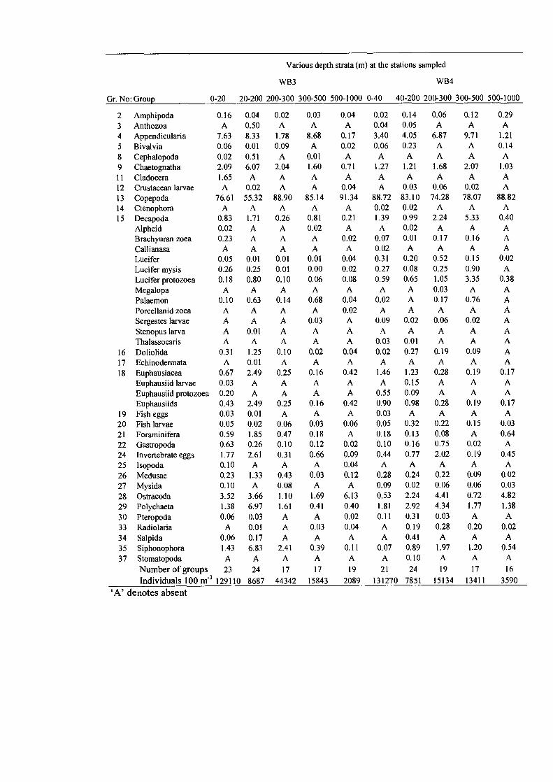
Various depth strata (m) at the stations sampled

Gr. No: Group 0-20 20-200

WB3

200-300 300-500 500-1000 0-40 40-200

WB4

200-300 300-500 500-1000

2 Amphipoda 0.16 0.04 0.02 0.03 0.04 0.02 0.14 0.06 0.12 0.29 3 Anthozoa A 0.50 A A A 0.04 0.05 A A A 4 Appendicularia 7.63 8.33 1.78 8.68 0.17 3.40 4.05 6.87 9.71 1.21 5 Bivalvia 0.06 0.01 0.09 A 0.02 0.06 0.23 A A 0.14 8 Cephalopoda 0.02 0.51 A 0.01 A A A A A A 9 Chaetognatha 2.09 6.07 2.04 1.60 0.71 1.27 1.21 1.68 2.07 1.03 11 Cladocera 1.65 A A A A A A A A A 12 Crustacean larvae A 0.02 A A 0.04 A 0.03 0.06 0.02 A 13 Copepoda 76.61 55.32 88.90 85.14 91.34 88.72 83.10 74.28 78.07 88.82 14 Ctenophora A A A A A 0.02 0.02 A A A 15 Decapoda 0.83 1.71 0.26 0.81 0.21 1.39 0.99 2.24 5.33 0.40

Alpheid 0.02 A A 0.02 A A 0.02 A A A Brachyuran zoea 0.23 A A A 0.02 0.07 0.01 0.17 0.16 A Callianasa A A A A A 0.02 A A A A Lucifer 0.05 0.01 0.01 0.01 0.04 0.31 0.20 0.52 0.15 0.02 Lucifer mysis 0.26 0.25 0.01 0.00 0.02 0.27 0.08 0.25 0.90 A Lucifer protozoea 0.18 0.80 0.10 0.06 0.08 0.59 0.65 1.05 3.35 0.38 Megalopa A A A A A A A 0.03 A A Palaemon 0.10 0.63 0.14 0.68 0.04 0.02 A 0.17 0.76 A Porcellanid zoea A A A A 0.02 A A A A A Sergestes larvae A A A 0.03 A 0.09 0.02 0.06 0.02 A Stenopus larva A 0.01 A A A A A A A A Thalassocaris A A A A A 0.03 0.01 A A A

16 Doliolida 0.31 1.25 0.10 0.02 0.04 0.02 0.27 0.19 0.09 A 17 Echinodermata A 0.01 A A A A A A A A 18 Euphausiacea 0.67 2.49 0.25 0.16 0.42 1.46 1.23 0.28 0.19 0.17

Euphausiid larvae 0.03 A A A A A 0.15 A A A Euphausiid protozoea 0.20 A A A A 0.55 0.09 A A A Euphausiids 0.43 2.49 0.25 0.16 0.42 0.90 0.98 0.28 0.19 0.17

19 Fish eggs 0.03 0.01 A A A 0.03 A A A A 20 Fish larvae 0.05 0.02 0.06 0.03 0.06 0.05 0.32 0.22 0.15 0.03 21 Foraminifera 0.59 1.85 0.47 0.18 A 0.18 0.13 0.08 A 0.64 22 Gastropoda 0.63 0.26 0.10 0.12 0.02 0.10 0.16 0.75 0.02 A 24 Invertebrate eggs 1.77 2.61 0.31 0.66 0.09 0.44 0.77 2.02 0.19 0.45 25 Isopoda 0.10 A A A 0.04 A A A A A 26 Medusae 0.23 1.33 0.43 0.03 0.12 0.28 0.24 0.22 0.09 0.02 27 Mysida 0.10 A 0.08 A A 0.09 0.02 0.06 0.06 0.03 28 Ostracoda 3.52 3.66 1.10 1.69 6.13 0.53 2.24 4.41 0.72 4.82 29 Polychaeta 1.38 6.97 1.61 0.41 0.40 1.81 2.92 4.34 1.77 1.38 30 Pteropoda 0.06 0.03 A A 0.02 0.11 0.31 0.03 A A 33 Radiolaria A 0.01 A 0.03 0.04 A 0.19 0.28 0.20 0.02 34 Salpida 0.06 0.17 A A A A 0.41 A A A 35 Siphonophora 1.43 6.83 2.41 0.39 0.11 0.07 0.89 1.97 1.20 0.54 37 Stomatopoda A A A A A A 0.10 A A A

Number of groups 23 24 17 17 19 21 24 19 17 16 Individuals 100 al3 129110 8687 44342 15843 2089 131270 7851 15134 13411 3590

`A' denotes absent

Table 5.7. Mesozooplankton groups absent from different depth strata in the western Bay during fall intermonsoon. Refer to Table 5.3 for the names of individual groups corresponding to the group numbers

Groups absent in different depth strata (m) Sampling station 0-MLD TT-BT 200-300 300-500 500-1000

1, 3, 6, 8, 10, 14, 1, 2, 6, 7, 10, 12, 1-3, 5-8, 10- 1-3, 5-8, 10-12, 14- 1-8, 10-12, 14- 16, 17, 19, 20, 14, 17, 19, 23, 12, 14, 15, 17- 17, 19, 23, 25, 27, 17, 19-27, 30-37 23, 25, 31-33, 25, 27, 31, 32, 3620, 22, 23, 25- 30-33, 36, 37 36, 37 27, 30-34, 36,

37

1, 3, 6, 7, 10, 11, 1, 3, 5, 6, 10-12, 1-3, 5-8, 10- 1-8, 10-12, 14-20, 1-3, 5-7, 10, 14, 17,23, 31-33, 14, 17, 23, 25, 12, 14, 15, 17, 22, 23, 25, 27, 30- 17, 18, 23, 25, 36, 37 31-33, 36 19, 20, 23, 25, 34, 36, 37 30, 31, 32, 36

27, 31-34, 36, 37

1, 3, 6, 7, 10, 12, 1, 6, 7, 10-12, 1, 3, 6-8, 10- 1, 3, 5-7, 10-12, 14, 1, 3, 6-8, 10, 11, 14, 17, 23, 31- 14, 23, 27, 31, 12, 14, 17, 19, 17, 19, 23, 25, 27, 14, 17, 19, 21, 33, 36, 37 32, 36, 37 23, 25, 30-34, 30-32, 34, 36, 37 23, 27, 31, 32,

36, 37 34, 36-37

1, 6-8, 10-12, 1, 6-8, 10, 11, 1, 3, 5-8, 10, 1, 3, 5-8, 10, 11, 1, 3, 6-8, 10-12, 14, 17, 23, 25, 17, 19, 23, 25, 11, 14, 19, 23, 14, 17, 19, 21, 23, 14, 16, 17, 19, 31, 34, 36, 37 31, 32, 36 25, 31, 34, 36- 25, 30, 31, 32, 34, 22, 23, 25, 30,

37 36, 37 31, 32, 34, 36-37

MLD: mixed layer depth; TT: Top of thermocline; BT: Base of thermocline

WB1

WB2

WB3

WB4

Table 5.8. Percent abundance of different groups of mesozooplankton in western Bay during winter monsoon (WM)

Various depth strata (m) at the stations sampled

WB I WB2 Gr. No: Groups 0-30 30-156 156-300 300-500 0-20 20-171 171-300 300-500 500-1000

2 Amphipoda 0.13 0.05 0.12 0.07 0.16 0.60 A 0.10 A 4 Appendicularia 0.83 0.33 0.13 0.34 12.39 2.93 0.37 0.54 0.31 5 Bivalvia A A A A A A 0.05 A 0.22 7 Cephalochordata A A A 0.04 A A A A A 9 Chaetognatha 2.32 1.68 3.03 4.64 4.55 9.13 2.80 2.45 1.99 12 Crustacean larvae A A A A A 0.09 A A A 13 Copepoda 90.72 85.43 91.00 81.81 78.52 72.56 82.41 90.08 91.29 15 Decapoda 0.05 0.09 0.13 0.19 0.48 0.63 A 0.18 0.08

Brachyuran zoea 0.03 A A A A A A A A Lucifer A A 0.06 0.04 A A A 0.10 0.08 Lucifer mysis A 0.04 A 0.11 0.26 A A A A Megalopa 0.03 A A A A A A A A Sergestes larvae A A A A 0.05 0.15 A A A Thalassocaris A A 0.03 A A A A A A Unidentified larvae A 0.05 0.04 0.04 0.18 0.48 A 0.08 A

16 Doliolida A 0.04 0.02 0.04 A 0.06 A A A 18 Euphausiacea 0.73 2.38 0.16 0.83 0.50 0.46 0.59 1.30 0.08

Euphausiid larvae 0.15 A 0.13 A 0.07 0.28 A 0.08 A Euphausiid protozoea 0.51 2.38 0.03 0.57 0.43 0.18 0.59 1.22 0.08 Euphausiids 0.06 A A 0.26 A A A A A

19 Fish eggs 0.10 0.14 0.03 A 0.07 0.09 0.05 0.35 A 20 Fish larvae 0.49 0.63 0.22 0.82 0.35 1.53 3.27 0.08 0.87 21 Foraminifera A A A A A 0.07 A A 0.11 22 Gastropoda 0.05 0.14 A A 0.15 1.87 0.13 0.08 0.11 25 Isopoda 0.10 0.23 0.58 0.07 A 0.41 0.05 0.08 A 26 Medusae A A 0.03 A A A 0.08 A A 27 Mysida 0.21 A 0.11 0.07 0.07 0.44 A 0.08 A 28 Ostracoda 2.64 8.12 2.54 10.25 0.52 4.14 8.08 3.59 3.82 29 Polychaeta 0.41 0.34 0.78 0.60 1.29 1.29 0.19 0.18 0.22 30 Pteropoda 0.38 0.27 0.66 0.07 0.19 1.58 1.06 0.18 0.27 32 Pyrosomida 0.05 A A A 0.11 0.07 0.05 0.17 A 33 Radiolaria A A 0.02 A A A A A A 34 Salpida 0.54 0.14 0.02 0.11 0.44 1.18 0.72 0.44 0.47 35 Siphonophora 0.18 A 0.39 0.04 0.20 0.81 0.08 0.10 0.16 37 Stomatopoda 0.05 A 0.03 A A 0.06 A A A

Number of groups 18 15 19 16 16 21 16 17 14 Individuals 100 M-3 161827 7316 34335 12472 139600 17845 3122 1620 434

`A' denotes absent

Table 5.8. Contd.

Various depth strata (m) at the stations sampled

Gr. No: Groups 0-60

WB3

60-200 200-300 300-500

WB4

0-35 35-135 2 Amphipoda 0.20 0.20 0.13 0.15 0.69 0.42 4 Appendicularia 0.64 0.34 0.26 0.15 2.98 1.95 5 Bivalvia 0.14 0.11 0.18 A 0.08 0.05 7 Cephalochordata A A A A 1.94 0.05 8 Cephalopoda A A A A 0.01 A 9 Chaetognatha 2.66 1.74 2.83 2.75 3.92 3.42 12 Crustacean larvae A 0.07 A A A A 13 Copepoda 88.90 86.68 86.67 72.44 68.83 85.11 15 Decapoda 0.31 A 0.77 0.59 0.05 0.02

Brachyuran zoea A A 0.09 A 0.01 A Lucifer 0.08 A 0.18 0.37 A A Lucifer mysis 0.18 A 0.23 0.07 A A Megalopa A A 0.09 A A A Palaemon A A A 0.07 A 0.02 Sergestes larvae 0.05 A 0.09 0.07 A A Thalassocaris A A 0.09 A 0.04 A

16 Doliolida 0.09 A 0.04 A 0.04 0.05 17 Echinodermata A 0.02 A A A 0.05 18 Euphausiacea 0.45 0.51 0.60 0.22 0.32 0.25

Euphausiid larvae A 0.38 A A 0.08 0.05 Euphausiid protozoea 0.35 0.13 0.60 0.22 A 0.07 Euphausiids 0.10 A A A 0.24 0.13

19 Fish eggs A 0.26 A 0.07 0.04 A 20 Fish larvae 2.18 0.68 2.05 1.78 0.65 0.10 21 Foraminifera 0.03 0.05 A A 10.94 1.51 22 Gastropoda 0.22 0.22 0.09 A 1.21 0.05 24 Invertebrate eggs A A A A 0.68 0.53 25 Isopoda 0.03 0.16 0.68 A A A 26 Medusae A A A A A 0.10 27 Mysida 0.03 0.25 A A A 0.27 28 Ostracoda 2.16 5.59 3.32 2.38 1.38 4.42 29 Polychaeta 0.52 1.75 0.35 A 0.48 0.62 30 Pteropoda 1.19 1.04 1.77 19.32 4.72 0.54 32 Pyrosomida 0.05 0.02 A 0.07 0.04 A 33 Radiolaria A A 0.09 A 0.65 A 34 Salpida 0.03 A A A A 0.03 35 Siphonophora 0.12 0.26 0.09 A 0.36 0.43 37 Stomatopoda 0.05 0.04 0.04 0.07 A A

Number of groups 20 20 17 12 21 21 Individuals 100 1113 72891 41559 5239 10768 35343 31770

`A' denotes absent

Table 5.9. Mesozooplankton groups absent from different depth strata in the western Bay during winter monsoon. Refer to Table 5.3 for the names of individual groups corresponding to the group numbers

Groups absent in different depth strata (m) Sampling station 0-MLD

TT-BT 200-300

300-500 500-1000

1, 3, 5-8, 10-12, 1, 3, 5-8, 10-12, 1, 3, 5-8, 10- 1, 3, 5, 6, 8, 10-12, NO DATA 14, 16, 17, 21, 14, 17, 21, 23, 12, 14, 17, 21- 14, 17, 19, 21-24, 23, 24, 26, 31, 24, 26, 27, 31- 24, 31, 32, 36 26, 31-33, 36, 37 33, 36 33, 35-37

1, 3, 5-8, 10-12, 1, 3, 5-8, 10, 11, 1-3, 6-8, 10- 1, 3, 5-8, 10-12, 14, 1-3, 6-8, 10-12, 14, 16, 17, 21, 14, 17, 23, 24, 12, 14-17, 21, 16, 17, 21, 23, 24, 14, 16, 17, 19, 23-26, 31, 33, 26, 31, 33, 36 23, 24, 27, 31, 26, 31, 33, 36, 37 23-27, 31-33, 36, 36, 37 33, 36, 37 37

1, 3, 6-8, 10-12, 1, 3, 6, 7, 8, 10, 1, 3, 6-8, 10- 1, 3, 5-8, 10-12, 14, NO DATA 14, 17, 19, 23, 11, 14-16, 23, 12, 14, 17, 19, 16, 17, 21-27, 29, 24, 26, 31, 33, 24, 26, 31, 33, 21, 23, 24, 26, 31, 33-36 36 34, 36 27, 31, 32, 34,

36

1, 3, 6, 8, 10-12, 1, 3, 6, 8, 10-12, NO DATA NO DATA NO DATA 14, 17, 23, 25- 14, 19, 23, 25, 27, 31, 34, 36, 31-33, 36, 37 37

MLD: mixed layer depth; TT: Top of thermocline; BT: Base of thermocline

There was NO DATA in some deeper depths due to shallow water depth

WB1

WB2

WB3

WB4

Table 5.10. Percent abundance of different groups of mesozooplankton in western Bay during spring intermonsoon (SpIM)

Various depth strata (m) at the stations sampled

Gr. No: Groups 0-30 30-200

WB1

200-300 300-500 0-40 40-200

WB2

200-300 300-500

2 Amphipoda 0.33 0.36 A A A 0.24 A A 4 Appendicularia 0.79 0.16 A 0.46 0.54 0.30 A A 7 Cephalochordata 0.04 0.01 A A A A A A 8 Cephlaopoda 0.04 A A A A A A A 9 Chaetognatha 9.39 3.34 0.64 4.63 2.52 1.91 1.14 3.93

11 Cladocera 0.43 0.10 A A 0.08 A A A 12 Crustacean larvae 0.23 A A A A 0.04 A A 13 Copepoda 79.95 83.57 48.70 87.50 89.78 90.95 65.11 90.58 15 Decapoda 0.07 0.01 0.02 A 0.09 0.02 0.02 A

Brachyuran zoea A A A A A 0.02 A A Lucifer 0.20 0.01 A A 0.35 A A A Lucifer protozoea 0.36 0.08 A A 0.40 0.11 A A Phyllosoma larva A 0.01 A A A A A A Sergestes A 0.01 A A A A A A Unidentified larvae 0.02 0.01 0.14 A 0.03 0.02 0.20 A

16 Doliolida A 0.01 A A A A A A 18 Euphausiacea 1.66 1.13 0.81 A 1.39 1.30 2.00 0.52

Euphausiid larva 0.05 A A A 0.08 A 0.10 A Euphausiid protozoea 1.38 0.42 A A 1.13 1.11 A A Euphausiids 0.22 0.71 0.81 A 0.19 0.20 1.90 0.52

19 Fish eggs A A A A 0.16 A A A 20 Fish larvae 0.13 0.17 0.06 A 0.08 0.09 0.29 A 21 Foraminifera 0.62 0.33 36.90 1.85 0.38 0.37 7.98 A 22 Gastropoda 0.02 0.02 0.14 A A A A A 24 Invertebrate eggs 0.55 0.82 0.12 0.46 0.88 A A 0.26 25 Isopoda A 0.03 A A A A A A 26 Medusae 0.02 A A A A 0.02 A A 27 Mysida A A A A 0.03 A A A 28 Ostracoda 3.34 8.76 9.58 4.17 1.47 3.00 22.81 2.88 29 Polychaeta 1.00 0.51 0.67 0.93 0.67 0.61 0.19 1.05 30 Pteropoda 0.66 0.20 0.25 A 0.99 0.41 0.10 0.52 33 Radiolaria A 0.01 0.07 A A 0.33 A A 34 Salpida 0.13 0.09 1.91 A 0.08 0.04 0.10 A 35 Siphonophora 0.11 0.25 0.07 A 0.16 0.22 A 0.26

Number of groups 20 20 14 7 16 16 10 8 Individuals 100 1113 31013 15564 3056 216 37290 22995 4208 764

`A' denotes absent

Table 5.10. Contd.

Various depth strata (m) at the stations sampled

Gr. No: Groups 0-30 30-200

WB3

200-300 300-500 0-30

WB4

30-200 200-300 300-500

2 Amphipoda 0.33 0.03 A 0.09 0.34 0.13 0.24 0.06 4 Appendicularia 6.35 2.22 3.34 5.80 2.60 0.21 0.07 0.11 5 Bivalvia 0.11 0.09 0.44 0.09 0.04 0.21 1.07 0.22 7 Cephalochordata A A A A A A 0.02 A 8 Cephlaopoda 0.06 A A A A 0.02 0.02 A 9 Chaetognatha 2.00 0.94 1.68 1.62 3.25 1.61 2.58 2.54 11 Cladocera 0.13 0.03 A 0.05 0.29 0.01 A A 12 Crustacean larvae 0.03 A 0.11 A 0.05 A 0.02 A 13 Copepoda 77.62 81.03 85.77 84.50 78.81 80.24 80.51 80.96 15 Decapoda 0.16 0.05 0.01 0.05 0.11 0.05 0.04 0.01

Acetes A 0.02 A A A A A A Brachyuran zoea 0.07 A A A 0.05 0.01 0.05 A Lucifer 0.68 0.16 A 0.18 0.51 0.04 0.10 A Lucifer protozoea 0.35 0.13 A 0.09 0.24 A 0.02 A Megalopa A A A A 0.01 0.04 0.02 A Phyllosoma larvae A 0.02 A A A A A 0.06 Sergestes A 0.02 A A A 0.01 A A Thalassocaris 0.29 0.03 A A A 0.04 0.05 A Unidentified larvae 0.05 0.05 0.11 0.14 0.22 0.31 0.15 A

16 Doliolida 1.82 6.40 0.21 0.50 0.01 0.24 0.34 0.66 18 Euphausiacea 1.15 0.76 0.43 0.51 1.84 2.71 1.53 0.18

Euphausiid larvae A A A A 0.13 A A A Euphausiid protozoea 0.66 0.11 0.32 0.14 0.83 0.19 A 0.06 Euphausiids 0.48 0.65 0.11 0.37 0.89 2.52 1.53 0.12

19 Fish eggs 0.01 0.23 A 0.18 0.66 0.08 0.05 A 20 Fish larvae 0.12 A A A 0.17 0.04 0.19 0.06 21 Foraminifera 0.36 0.79 0.62 0.14 1.01 0.92 0.68 2.37 22 Gastropoda A A 0.11 0.05 A 0.01 A 0.11 23 Halobates A A A A A A A 0.01 24 Invertebrate eggs 1.17 0.28 0.41 0.61 2.09 0.53 0.34 1.07 25 Isopoda A A A A A 0.01 0.02 A 26 Medusae 0.31 0.18 0.21 0.05 0.20 0.21 2.02 5.31 27 Mysida 0.01 A A A 0.05 A 0.02 A 28 Ostracoda 1.80 2.51 2.06 1.63 3.73 7.89 3.50 4.40 29 Polychaeta 0.64 0.76 1.28 0.55 0.83 1.86 2.57 0.91 30 Pteropoda 0.27 0.13 0.55 0.23 0.49 0.07 0.12 0.50 33 Radiolaria 0.05 0.03 A A 0.01 A A A 34 Salpida 3.50 2.42 2.26 3.00 1.78 0.91 A 0.12 35 Siphonophora 0.70 0.18 0.41 A 0.66 1.42 3.67 0.22

Number of groups 23 19 17 18 22 22 22 18 Individuals 100 m-3 49486 39918 1388 1606 533840 8193 5134 1721

`A' denotes absent

Table 5.11. Mesozooplankton groups absent from different depth strata in the western Bay during spring intermonsoon. Refer to Table 5.3 for the names of individual groups corresponding to the group numbers

Groups in different depth strata (m) Sampling station 0-MLD TT-BT 200-300 300-500

1, 3, 5, 6, 10, 14, 1, 3, 5, 6, 8, 10, 1-8, 10-12, 14, 1-3, 5-8, 10-12, 14- 16, 17, 19, 23, 12, 14, 17, 19, 16, 17, 23, 25- 20, 22, 23, 25-27, 25, 27, 31-33, 23, 26, 27, 31, 27, 31, 32, 36, 30-37 36, 37 32, 36, 37 37

1-3, 5-8, 10, 12, 1, 3, 5-8, 10, 11, 1-8, 10-12, 14, 1-8, 10-12, 14-17, 14, 16, 17, 22, 14, 16, 17, 19, 16, 17, 19, 22, 19-23, 25-27, 31- 23, 25, 26, 31- 22-25, 27, 31, 23, 25-27, 31- 34, 36-37 33, 36, 37 32, 36, 37 33, 35-37

1, 3, 6, 7, 10, 14, 1, 3, 6-8, 10, 12, 1-3, 6-8, 10, 1, 3, 6-8, 10, 12, 17, 22, 23, 25, 14, 17, 20, 22, 11, 14, 17, 19, 14, 17, 20, 23, 25, 31, 32, 36, 37 23, 25, 27, 31, 20, 23, 25, 27, 27, 31-33, 35-37

32, 36, 37 31-33, 36, 37

1, 3, 6-8, 10, 14, 1, 3, 6, 7, 10, 12, 1, 3, 6, 10, 11, 1, 3, 6-8, 10-12, 14, 17, 22, 25, 31, 14, 17, 23, 27, 14, 17, 22, 23, 17, 19, 23, 25, 27, 32, 36, 37 31-33, 36, 37 31-34, 36, 37 31-33, 36, 37

WB1

WB2

WB3

WB4

MLD: mixed layer depth; TT: Top of thermocline; BT: Base of thermocline

WM

300-500

Num

ber o

f Gro

ups

0-MLD TT-BT BT-300

30

500-1000 -§§

NM

301

20 SUM

10

0

0-MID TT-BT 13T-300 1 300-500 500-1000

■ 500-1000

■ 300-500

CI BT-300

CI TT-13T

■0-MID

0-MLD TT-BT BT-300 300-500 500-1000 0§

Station

Figure 5.7. Depth-wise variation in the number of groups at each station in the western Bay during different seasons (SUM: summer monsoon, FIM: fall intermonsoon, WM: winter monsoon; SpIM: spring intermonsoon)

Among the 33 groups identified, only two to six of them were found to be dominating

numerically (forming >2% of the total mesozooplankton abundance; Fig. 5.8) in this

transect. Some salient points on their spatio-temporal distribution are listed below. In all

seasons, Copepoda was the most predominant group at all stations and depths.

5.2.6. Vertical distribution of the dominant groups

During SUM, only two of the 24 groups recorded were dominant (Fig. 5.8). Copepoda

ranging from 88 to 99.7% was the most abundant group, especially in the thermocline.

The second most major group was Chaetognatha (range: 0.04-2.87%).

During FIM, six groups were dominant (Fig. 5.8). Copepods ranging from 67 to 89 %

exhibited a subsurface minimum in the 200-300 m stratum. In this stratum, invertebrate

eggs (0.5-17.5%) were most important. Chaetognaths (1.2-3.2%) decreased in percentage

with increasing depth. Though polychaetes (1-3%) were observed throughout the water

column, they were relatively more abundant in the thermocline. Appendicularians (0.5-

5.4%) occurred in higher percentage in the upper 500 m. Ostracods (1.4-6.7%) were more

in the deepest stratum.

Copepods ranged from 82 to 91 % among the five groups that dominated during WM

(Fig. 5.8). The relative abundance of this group increased with depth. Ostracoda (1.7-

5.6%) was the second most-dominant group that was more abundant below MLD.

Chaetognath (2-4%) percentage did not vary much with depth. Appendicularia (0.3-

4.2%) were dominant in the two uppermost strata. Pteropods increased from surface to

the 300- 500 m stratum where they attained a maximum percentage.

During SpIM, copepods ranging from 70 to 85 % at different depths were least

abundant in the 200-300 m stratum (Fig. 5.8). In this stratum, Ostracoda (range: 2.6-

9.5%) and Foraminifera (0.6-11.5%) increased to their maximum percentages.

Chaetognatha (1.5-4.3%) that was highly abundant in the surface was present throughout

the upper 500 m.

5.2.7. Latitudinal distribution of the dominant groups

Latitudinally, copepods were distributed homogenously at all stations except during WM,

where their percentage apparently decreased northwards (Fig. 5.9). Appendicularia, one

60

FIM

1 II

■ ■

1

WM

II I

0-MLD

TT-BT

200-300

300-500

500-1000

SUM ■Copepoda ■Chaetognatha

0-MLD

200-300

00-500

0-1000 ca

)-MLD

TT-BT

150-300

300-500

500-1000

0-MLD

TT-BT

200-300

300-500

500-1000

■Copepoda ■Chaetognaths 0 Ostracoda ■Appendicularia ■Polychaeta O Inv.eggs

■Copepoda ■Chaetognatha 0 Ostracoda ■Appendicularia 0 Pteropoda

■Copepoda ■Chaetognatha 0 Ostracoda ■Foraminifera

60

80

100 11/0

Figure 5.8. Distribution of dominant groups (> 2%) in each stratum in the western Bay during different seasons (SUM: summer monsoon, FIM: fall intermonsoon, WM: winter monsoon; SpIM: spring intermonsoon)

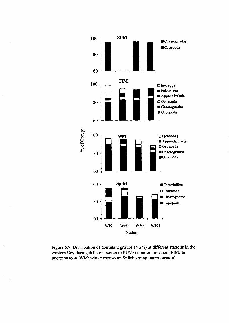
100 -

80 -

60

100 -

80 -

60

100 -

80 -

60

0 Inv. eggs ■ Poly chaeta ■ Appendicularia O Ostracoda ■ Chaetognatha ■ Copepoda

OPteropoda ■ Appendicularia

I0 Ostracoda ■ Chaetognatha ■ Copepoda

SpIM ■ Foraminifers

i 1 I 0 Ostracoda

■ Chaetognatha

■ Copepoda

I I I

WB1 WB2 WB3 WB4

■ Chaetognatha

■Copepoda

Station

Figure 5.9. Distribution of dominant groups (> 2%) at different stations in the western Bay during different seasons (SUM: summer monsoon, FIM: fall intermonsoon, WM: winter monsoon; SpIM: spring intermonsoon)

Table 5.12. Various statistical (non-parametric tests) analyses to distinguish diel, spatial and temporal differences in mesozooplankton biovolume and abundance in the western Bay of Bengal through non-parametric statistical tests

Wilcoxon Matched Pairs Test between day and night

Seasons N Biovolume

N Abundance

T Z p T Z

SUM 13 23.0 1.6 p>0.05 10 2 1.1 p>0.05

FIM 15 43.5 0.1 p>0.05 15 47 0.7 p>0.05

WM 14 50.0 0.2 p>0.05 20 47 0.7 p>0.05

SpIM 12 12.0 1.6 p>0.05 10 5 2.3 p<0.05

Friedman ANOVA to test difference between depths

Seasons Chi Sqr. Biovolume

p Chi Sqr. Abundance

N df N df

SUM 6.0 3 2 p <0.05 7.7 3 4 p<0.05

FIM 10.9 3 4 p<0.05 12.6 4 4 p<0.05

WM 3 2 3 p >0.05 11.1 4 3 p<0.05

SpIM 8.1 4 3 p<0.05 12.8 4 4 p<0.05

Friedman ANOVA to test the difference between stations Biovolume Abundance

Seasons Chi Sqr. N df p Chi Sqr. N df p

SUM 0.4 5 2 p>0.05 4.4 5 2 p>0.05

FIM 0.9 4 3 p>0.05 2 5 3 p>0.05

WM 5.8 4 3 p>0.05 3.6 4 3 p>0.05

SpIM 4.2 2 3 p>0.05 3.8 5 3 p>0.05

Friedman ANOVA to test the difference between seasons

Chi Sqr. N df p

Biovolume 8.1 9 3 p<0.05

Abundance 14.9 12 3 p<0.05

Significant results are marked bold

' Table 5.13. Correlation coefficients between mesozooplankton biovolume, abundance and number of groups (from the mixed layer) and temperature,

salinity, chl a (average from upper 120 m) in the western Bay of Bengal

Parameters Biovolume Abundance Groups SUM Temp 0.064 0.003 -0.869

Salinity 0.416 0.360 -0.635

Chl a -0.758 -0.717 0.254

FIM Temp -0.631 -0.574 -0.180

Salinity -0.391 -0.202 0.991

Chl a -0.188 -0.121 -0.734

WM Temp -0.945 -0.989 0.781

Salinity 0.878 0.964 -0.824

Chl a 0.215 -0.020 -0.442

SpIM Temp -0.586 -0.205 -0.896

Salinity 0.851 0.576 0.815

Chl a 0.404 0.004 0.613

Significant r values at p<0.05 are marked bold

Table 5.14. Spatio-temporal variation in number of zooplankton groups in the central Bay as determined through one/two way anova in the western Bay of Bengal

Groups

ANOVA

Two-way anova

Between depths Between stations

SUM F (4,14 =5 .8, p<0.05 F (2, 14)-0.8, p>0.05

WM F (3, 11)=0.6, p>0.05 F (2, 10=0.1, p>0.05

F (4,

F (3,

F (3,

F (3,

FIM 19)=6.1, p<0.05 19)=1.7, p>0.05

SpIM 15)=10.6, p<0.01 15)=12.7, p<0.01

One-way anova Between seasons

F (3, 64)=15.9, p<0.001

Significant results are marked bold

of the dominant groups during FIM and WM, registered higher percentage in the northern

Bay during FIM. Pteropods were also more abundant in the northern stations during WM.

Chaetognaths did not show any latitudinal trend during any season. In contrast to the

above-mentioned groups, invertebrate eggs were proportionately higher in the southern

stations, with their highest abundance of 14% at WB1 during FIM. Similar was the case

of ostracods during WM and SpIM.

5.3. Discussion

5.3.1. Variation of Biovolume, Biomass and Abundance

Most of the studies reporting zooplankton biovolumes from the Bay of Bengal (BoB) are

from the top 200 m. These are cited in the Table below.

Region Sampling period

Biovolume (ml 100 m-3)

Reference

Western Bay SUM 7.8 to 8.4 Nair et al. (1977)

Western Bay SUM 2.5-to 15.4 Achuthankutty et al. (1980)

Western Bay FIM 8.9 to 32.2 Nair et al. (1981)

Andaman Sea WM 1.8 to 14.4 Madhupratap et al. (1981)

Andaman Sea SpIM 1.0 to 13.5 Madhupratap et al. (1981)

Results from HOE for the upper 200 m (Duing 1970), using the Indian Ocean

Standard Net suggest that during WM, few spots of > 80 ml per standard haul off

Madras, and from 0.1to19.9 ml in the rest of the area were observed in WB. During

transitional period i.e. March-April, large patches in the WB show values from 10-19.9

ml and the rest, 0.1-9.9 ml. During commencement of SUM, i.e. during May-June,

biovolume ranged from 10 to 19.9 ml. Values ranging from 20 to 39.9 ml were present

south of Andaman Sea. From HOE studies, it is evident that the BoB becomes highly

productive during WM, while the Arabian Sea during SUM (Prasad 1969).

Biovolume (ml 100 m-3) was lowest during SUM (10), intermediate during FIM

(15.4) and WM (34), and the highest during SpIM (76.4). Results from this study in part

61

agree with the earlier observations. For instance, the average biovolume and carbon

biomass in WB during WM is three times more than during SUM. Further, the highest

biovolumes were during SpIM. The HOE studies suggest that Bay is rich in zooplankton

especially off Madras and Orissa coasts. Upwelling of weak intensity has been reported

in these areas during February-April (La Fond 1954; Varadachari 1961) resulting in high

plankton production during April-July (Panikkar and Rao 1973). Subsequent studies

(Anand et al. 1968; Murty and Varadachari 1968) have confirmed upwelling in these

areas during SpIM and SUM and also intense subsurface upwelling off the mouths of

Godavari and Krishna rivers. Sankaranarayanan and Reddy (1968) show evidence for

upwelling in coastal areas of northwestern Bay as early as in January. However, no signs

of upwelling were evidenced during any of the sampling periods in the WB during this

study. Panikkar and Rao (1973) described two peaks in plankton biovolume i. e. one

during spring and the other during fall in the Gulf of Mannar. On the Southwest coast of

India, peak in biomass/abundance is during May, when the SUM induces upwelling

early.

Mean biovolumes of zooplankton ranging from 10 to 76.4 ml 100 r11-3 in the upper

1000 m during the four different seasons of this study are comparable to those observed

in the eastern Arabian Sea (Madhupratap et al. 1996 a). However, unlike the results of

Madhupratap et al. (1996), results from this study show quite a high variability in

biovolumes as well as numerical abundance between seasons. Also, the seasonal averages

of zooplankton biovolume relate quite closely to the seasonal distribution of integrated

chlorophyll a in the upper 120 m, with its concentration increasing from SUM to SpIM

(Table 5.15; also in Chapter 3). High chlorophyll a and zooplankton abundance are found

to co-occur on the offshore and downstream edges of the upwelling area off Peru (Boyd

and Smith 1983). At many of the stations, high biovolumes coincided with the occurrence

of cold-core eddies, i.e. at WB3 during SUM and SpIM. During WM, it was observed at

WB1 and around WB2. Similar to the CB, the cyclonic eddies appear to play a significant

role in the re-supply of nutrients to the photic zone, which enhances primary production

inside them (Falkowski et al. 1991). Muraleedharan et al. (2007) reported biovolume up

to 67 ml 100 111-3 in the center of a cyclonic eddy and, up to 112 ml 100 m -3 in the regions

62

of coastal upwelling. They also observed higher biovolumes in the WB compared to the

CB.

Mesozooplankton biovolumes were high in the MLD and decreased rapidly with

increasing depth during all seasons except WM. These results are similar to those of

Madhu et al. (2003) for the Andaman Sea and, of Padmavati et al. (1998) and

Madhupratap et al. (2001) for the Arabian Sea. Rapid decrease in biomass is a universal

feature in tropical oceans (Vinogradov 1997). Some zooplankton are known to move

through narrow suboxic zones, live anaerobically for short intervals or, reduce

metabolism for diapause (Boyd et al. 1980). The critical lower limit for aerobic

metabolism in mesozooplankton is about 6p,M (Wishner et al. 1990). Since the oxygen

concentrations in the subsurface did not fall below 10 1.1M during WM, up to 10% of the

biovolume and —5% of the numerical abundance could be seen in the 300-500 m stratum,

suggesting that zooplankton abundance reduces drastically when oxygen concentrations

are at nadir as also observed by Madhupratap et al. (2001). Diel variations with higher

biovolumes in the night are reported from the Arabian Sea (Padmavati et al. 1998;

Goswami et al. 2002). However, in the Bay and even in the Arabian Sea, it seems to be a

manifestation of the oxygen minimum zone.

The deep oxygen minimum zone strongly influenced the vertical distribution of

zooplankton in the Arabian Sea (Madhupratap et al. 2001) and Andaman Sea (Madhu et

al. 2003). Similar studies conducted in the Arabian Sea and the eastern Pacific also

suggest that diel vertical migration (DVM) would be limited by low oxygen, and most

zooplankton would remain in the mixed layer both day and night (Wishner et al. 1998;

Saltzman and Wishner 1997). Insignificant DVM observed during this study is suggestive

of the fact that the existing oxygen minimum levels in the subsurface hinder the vertical

migration of mesozooplankton in the BoB.

5.3.2. Seasonal variation in community structure

Though the currents reverse with seasons, the sea surface temperature in the WB was

always >29°C during all seasons except during WM with — 26°C. The sea surface salinity,

which showed a horizontal gradient, was lower during SUM and FIM ranging from 24 to

34, intermediate during WM and the highest during SpIM. Similar to that in the CB, the

63

thickness of the low oxygen (5-10 p.M) zone also varied with seasons. It was the largest

during SUM, decreased in thickness during FIM and SpIM and was absent during WM.

All the groups reported in this study were reported earlier from the WB (Panikkar and

Rao 1973; Achuthankutty et al. 1980; Nair et al. 1981; Rakhesh et al. 2006), Andaman

Sea (Madhu et al. 1999; Ik 2007) as well as the eastern Arabian Sea (Padmavati et al.

1998; Madhupratap and Haridas 1990). The standing stocks and groups of zooplankton

are known to vary in the northern Indian Ocean according to seasons (Rao 1973, 1979).

Zoogeographically, the WB recorded lower number of groups than those in the CB. For

instance, four minor/rare groups in CB, viz. Acantharia, Carinaria, Pterotrachea and

Sipuncula, did not occur in the WB during any of the seasons. The non- occurrence of

these groups could be related to patchiness and their numerical rarity in the WB during

the study period. Abundance of Carinaria and Pterotrachea was reported to be higher in

the WB than the central parts of the Bay (Aravindakshan 1969). Abundance of

Acantharia was ascribed directly to primary productivity (Bottazzi and Andreoli 1982 a).

Spatially, most Acantharia were found between the tropics and the Equator and, vertically

they increased in abundance from the surface to 300 m and then decreased, although

juvenile forms were most numerous from 500-900 m. More Acantharia were found in the

daytime than at night, and the seasonal period of greatest abundance was spring (Bottazzi

and Andreoli 1982 b). It is thus suggested that their size of < 200p,m could have caused

their exclusion from the samples in this study.

The total number of groups that occurred was 24, 30, 28 and 27 during SUM, FIM,

WM and SpIM. As pointed out, the least number of groups occurring during SUM was

probably due to the occurrence of a large number of swarms of Pyrosoma that

contributed most of the biovolume in the samples. The lowest number of groups in the

thermocline during SUM and in the 300-500 m layer during FIM (Chapter 3) could have

been caused due to drastic decrease in the dissolved oxygen concentration in these zones.

As also reported in many earlier studies including the HOE, Copepoda was the

dominant taxon during all the seasons examined. Chaetognaths, ostracods and

invertebrate eggs were the other most dominant group during different seasons for

reasons already explained in Chapter 4. It has been observed that during the upwelling

period, when phytoplankton is abundant, copepods are sparse in the eastern Arabian Sea.

64

However, copepods and carnivorous chaetognaths become dominant during the low

chlorophyll time, from November to April. Ganapati and Rao (1958) have indicated that

only a few chaetognaths and tunicates occur in the WB during the low chl a periods

between August and December. An abundance of appendicularians and copepods were

observed during the high chl a period between January and August. Such a difference

was not evident in this study. A noteworthy observation of Rao (1973) is that the deeper

living chaetognath, Pterosagitta draco is found in the surface samples only in February-

April when upwelling is prominent in the Bay. It is thus apparent that the essentially

marine chaetognath fauna is affected quite adversely by monsoon in the inshore and low-

saline waters in the WB.

Ostracods were an important group after copepods in numerical abundance. Unlike

the observations during HOE, there was no notable difference in the ostracod abundance

in the WB compared to the CB. Compared to the Bay, the Arabian Sea is richer in

ostracod abundance (Panikkar and Rao 1973). As many as 30 species of ostracods were

observed in the Arabian Sea during HOE. Known to inhabit all depths and play a

significant role in detrital cycles, they were abundantly seen throughout the 1000 m

during the study period. Clear latitudinal zonation patterns were observed during WM

and SpIM, with a southward increase in proportion. Such a distribution pattern has also

been recently observed in the Southern Ocean with the majority of species occupying the

polar seas having circumpolar distributions (Angel and Blachowiak-Samolyk 2007).

Appendicularia, which was abundant mostly in the upper 500 m during FIM and

upper 150 m during WM, are thought to avoid very cold and very warm temperatures.

These animals occur from the ocean surface to at least 1000 m (Alldredge and Madin

1982). Also known as sea butterflies, these marine pelagic gastropods were dominant in

the 300-500 m stratum only during WM. Because they may reproduce rapidly, their

population dynamics may sometimes closely reflect seasonal or spatial changes in

phytoplankton. Foraminifera was one of the major groups during the warm, high-saline

period of SpIM, when phytoplankton food was adequate as observed from some higher

chl a concentration levels. They were found in all strata in the upper 500 m during SpIM.

Peak abundances of various pteropods and foraminifers might indicate the presence of

65

local upwelling processes as reported for Bab el Mandeb area (Auras- Schudnagies et al.

1989).

5.3.3. Differences between transects

To bring out some of the common and contrasting features in the CB and WB, their

physical, chemical and biological characteristics are listed in Table 5.15. In a nutshell,

biomass, abundance and composition of zooplankton are influenced by seasonal changes

in physico-chemical parameters. These in turn affect the nutrient and chl a

concentrations. The WB is least productive in terms of zooplankton biovolume and

abundance during SUM and most productive during SpIM. In contrast, the CB supported

higher biovolumes during both these seasons. However, the number of groups occurring

was lower in both these seasons along both transects. WB had higher biovolume and

numerical abundances than the CB during all seasons except SUM. The average carbon

biomass in both transects was similar during FIM and WM. Compared to the CB

however, the carbon biomass was lower during SUM, and higher during SpIM in the

WB. In the other two seasons, it was similar in both transects. Also, cyclonic eddies play

a crucial role in elevating the zooplankton biomasses in the WB (seasonal average: 42-

224 mM C m-2) and CB (75-134 mM C m-2) to values that even exceeded those reported

from the eastern Arabian Sea (75-83 mM C m -2) and nearly matched those in the central

Arabian Sea (73-158 mM C m -2). From the fewer groups i.e. only 33 that were present in

the WB compared to 37 in the CB, it is discernible that group diversity increases from

coastal to open waters in the Bay. Copepods, chaetognaths, ostracods, appendicularians,

polychaetes, invertebrate eggs and foraminifera were the major groups common in both

transects during different seasons. However, certain differences did prevail in the

dominance of a few groups. For instance, medusae and Euphausiacea were dominant only

in CB and, Pteropoda in the WB.

5.3.4. Salient biological features of the dominant groups in the Bay of Bengal

The following is a brief description of the main biological features of the dominant

groups recorded in the BoB. This is included to provide an insight into the possible roles

these mesozooplankton groups play in the trophic structure of the BoB.

66

Table 5.15. Ranges of physical, chemical and biological parameters in the central and western Bay of Bengal

Parameters SUM CB

FIM WM SpIM SUM FIM WB

SpIM WM

SST (°C) 28.4-29 28.4-29.1 26.8-28.7 29.3-30.5 28.6-29.4 29.8-30.6 26.5-27.1 29.1-30.5

SSS (psu) 27.7-33.3 28.1-33.9 32.2-33.3 32.6-33.3 29.6-33.9 20.7-34.0 32.0-33.3 33.3-33.9 Chi a (mg m-3) 9.0-11.5 13.8-23.4 17.3-22.2 13.4-18.26 11.7-18.7 11.3-18.7 16.7-26.7 11.18-42.92 DO (p,M) 3-201 3-206 5.1-220.9 3.5-200 3-194 3-219 5.2-231 5.6-194 Biovolume (ml 100 m -3) 0.2-404 ng-120 0.3-75 ng-230 0.2-120 ng-115 1.0-142 1.0-533

Biomass (mM C M-2 ; 1000 m) 41-111 79-190 71-225 24-197 14-90 96-154 58-190 35-480 Abundance (x 10 3 100 m-3) 0.1-35.8 0.2-356 0.4-308 0.1-248 0.5-462 0.7-136 0.4-162 0.2-534 Number of groups (range) 4-14 9-25 9-24 4-25 1-16 9-25 14-21 7-25 Major groups (>2%) Copepoda 75-90 74-90 74-93 78-85 88.2-99.7 67.3-89 81-91 70-86 Chaetognatha 2.6-9.3 1.6-5.7 1.4-7.6 1.9-4 0.04-3.2 1.2-3.2 2.0-4.0 1.5-4.3

Euphausiacea 0.2-6 0.6-3.8 Ostracoda 0.6-4 1.6-4.8 2.8-7.2 2.7-6.6 1.4-6.7 1.7-5.6 2.6-9.5

Polychaeta 0.1-3.9 0.9-3.0 Appendicularia 0.3-7 0.5-5.4 0.3-4.2

Medusae 0-7 Foraminifera 0.8-2.6 0.6-3.1 0.6-11.6 Invertebrate eggs 1.2-6.5 0.6-17.5

Pteropoda 0.3-6.5

Ng: negligible

It is well understood that occurrence and relative abundance of zooplankton

assemblages is governed by hydrographical characteristics of the region (Fager and

McGowan 1963; Ashjian and Wishner 1993). With diverse forms and varied roles, they

are important in the marine food web. Since it was not the aim of this study (except

copepods) to undertake detailed taxonomic analyses of all the groups, it would be out of

scope of this discussion to provide an opinion on the possible species of carnivores or,

other groups except copepods.

Pyrosoma, the holoplanktonic colonial tunicates are known to be restricted to warmer

waters (Van Soest 1981). Their trophic function in the ocean, as well as their ecology and

physiology are extremely poorly known (Perissinotto et al. 2007). Harbison (1998) has

shown that, in oceanic ecosystems, they are actually a very important prey item in the

diet of many marine animals, vertebrates in particular. Harbison (1998) lists 62 fish and 3

turtle species worldwide that devour pyrosomes as a significant food source. Amongst the

invertebrates, at least one species of sapphirinid copepod (Harbison 1998), two genera of

hyperiid amphipods (Tregouboff and Rose 1957) and another two of penaeid shrimps

(Monticelli and Lo Bianco 1901, Lindley et al. 2001) have been found inside Pyrosoma

colonies.

Chaetognatha are extremely abundant in the sea and, constitute an important part of

the marine plankton. Their vertical distribution is known to show a strong association

with water masses (Ulloa et al. 2000). Occasionally mesopelagic species like Sagitta

decipiens and Eukrohnia hamata are found in surface waters during coastal upwelling

events (Bieri 1959; Fagetti 1968). All of them except Spadella sp. are planktonic with

majority of these species being oceanic. These arrow worms are mostly holoplanktonic

carnivores preying on copepods and other small zooplankton. They have mechanosensory

hair fans along the body, which are capable of detecting prey in the form of water borne

vibrations; however the range of prey detection is limited only to 2-3 mm (Horridge and

Boulton 1967; Feigenbaum and Reeve 1977). The use of a tetrodotoxin (TTX) venom,

found in at least six species of chaetognaths greatly enhances their success rate of prey

capture and may be essential for the ingestion process to begin when the prey item is

large or spiniferous (Thuesen et al. 1988). They found that in general, larger chaetognath

species tended to possess higher quantities of toxin. The widespread abundance of

67

planktonic chaetognaths in the pelagic and neritic waters of the world suggests that they

may act as a vector in the distribution of TTX producing bacteria through marine food

webs. Cannibalism was evident in all species studied by Batistic et al. (2003) in the

Mediterranean. Around 30 species of chaetognaths have been recorded from the Indian

Ocean. Sagitta enflata is the dominant species and, S. bombayensis is considered to be

endemic. In general, chaetognath fauna of the Indian Ocean resembles that of the Pacific.

Appendicularians are marine filter-feeders that live and consume particulate food

inside an elaborate mucoid house (Fenaux 1986). They form an important constituent of

food for carnivorous zooplankton (King et al. 1980) and fish (Shelbourne 1962; Ryland

1964; Last 1978 a, b). When epipelagic appendicularians are numerous, they can

consume the total daily production of phytoplankton (Alldredge 1981). A single

individual produces as many as 5-16 houses a day depending on food and temperature

conditions (Taguchi 1982; Gorsky et al. 1984; Fenaux 1985). Such particle-laden

material constitutes one kind of marine snow aggregate, a substratum on which active

microbial communities develop (Davoll and Silver 1986; Caron et al. 1986). Due to an

elaborate apparatus for feeding, the weight-specific filtering rates and growth rates of

appendicularians are higher and generation times shorter than those of copepods (Fenaux

1976; Paffenhofer 1976; Alldredge 1981). In a nutshell, appendicularians also have

greater potentials as secondary producers. However their role in carbon transformation

and transport to the deep water is not yet well understood (Barham 1979; Galt 1979;

Youngbluth 1984).

Planktonic especially halocyprid ostracods are an important, but poorly studied

component of open ocean plankton communities. They inhabit all depths and play a

significant role in detrital cycles. Numerically, they are often the second or third most

abundant group in mesoplankton samples and play a significant role in the recycling of

marine snow and fecal pellets within thermocline waters. Their species occupying the

polar seas were observed to have circumpolar distributions (Angel and Blachowiak-

Samolyk 2007). The species that are predominantly temperate with occasional records in

polar waters have either circumpolar distributions or are restricted to either the Atlantic

or the Indo-Pacific Oceans. The tropical Cypria tigris has a wide distribution in the

Indian Ocean region (Rao 1973).

68

Euthecosomatous pteropods are widespread in the world oceans secreting aragonitic

tests. After their death, together with the skeletal remains of other calcareous planktonic

organisms, they contribute to the calcareous ooze on the sea floor (Herman 1968). When

pteropods constitute a high percentage of the ooze, the deposit is called pteropod ooze

(Herman 1998). Certain species of pteropods are believed to have great potential as

bathymetric indicators due to the restricted depth ranges of certain species and to rapid

settling velocities, which should lead to deposition close to their habitat (Herman and

Rosenberg 1969).

Foraminifera, the single-celled amoeboid protists are abundant all over the ocean with

—40 planktonic species. In tropical euphotic waters, where trophic resources are highly

competitive and sunlight is plentiful, several families of foraminifera harbor a host of

unicellular photoautotrophs such as dinoflagellates, diatoms, green algae, red algae and

even chrysophytes and prymnesiophytes. They derive carbohydrates (energy) from their

symbionts. Owing to the diversity of endosymbionts or their photopigments, the

symbiont bearing foraminifera are successful to utilize a wider range of the light

spectrum and water depths. Other species mostly being omnivorous consume foods

ranging from dissolved organic molecules, bacteria, diatoms and other single celled

phytoplankton, to small animals such as copepods. They move and catch their food with a

network of thin extensions of the cytoplasm called reticulopodia.

Scyphomedusae represent a conspicuous component of the plankton, especially

during the summer months (Brodeur et al. 2002). They devour on a wide spectrum of

zooplankton prey and can have a strong impact on zooplankton standing stocks (Omori et

al. 1995; Ishii and Tanaka 2001; Brodeur et al. 2002). Their mass occurrence has been

found to reduce local stocks of copepods (Hulsizer 1976).

In the Bay, the herbivorous copepods, foraminifers and appendicularians; the

carnivorous chaetognaths and, the omnivorous ostracods and pteropods prevailed during

most seasons. It can thus be proposed that these groups of mesozooplankton populating

the MLD consume most of the primary and microbial (bacterial and microzooplankton)

production in the surface layers of the BOB. This is also implicit from the close seasonal

coupling of their biovolume with chlorophyll concentration in the MLD.

69

Plate 1

Different crustacean zooplankton groups from the Bay of Bengal

Key: A: Mysid: B: Mysid; C: Euphausiid: D: Thalassocaris: E: Pasiphaeid; F: Stomatopod: G: Megalopa: H: Lucifer: I: Isopod: 1-L: Atnphipods

rI

Plate 2

Various cnidarian zooplankton identified from the Bay of Bengal

Key: A-F: Medusae. G-K: Siphonophores

AR. $AL Ay'

yak

• • 110 V.

Plate 3

Various Chordates identified from mesozooplankton samples in the Bay

Key: A: Appendicularia: B: Doliolum, C. D: Salps, E: Pyrosoma colony: F: Amphioxus: G-J: Fish larvae: K. L: Fish eggs

\I

Plate 4

Various mesozooplankton groups in the Bay

Key: A: Foraminifera: B: Chaetognath: C: Gastropod: D. E: Cephalopod larvae: F: Ostracod: G: Echinoderm larvae: H: Carinaria: I: Halobates: J. K: Pteropod: L-0: Polychaetes

Chapter 6

Chapter 6 Copepoda in Central Bay of Bengal

Copepods, the very diverse aquatic crustaceans, are the most numerous metazoans

(Hardy 1970) in aquatic ecosystems. Their habitats range from freshwater to super

hypersaline conditions, from subterranean caves to water collected on leaves or leaf litter

on the ground and from streams, rivers, and lakes to the sediment layer in the open ocean.

Their habitats also range from the aquatic bodies in the highest mountains (Loffler 1968)

to the deepest ocean trenches (Wolff 1960), and from the cold polar ice-water interface to

the hot active hydrothermal vents (Tsurumi and Tunnicliffe 2003).

The subclass Copepoda comprises 10 Orders: Calanoida, Cyclopoida, Gelyelloida,

Harpacticoida, Misophrioida, Monstrilloida, Mormonilloida, Platycopioida,

Poecilostomatoida and Siphonostomatoida (Boxshall and Hasley 2004) covering

approximately 210 described families, 2,280 genera and over 14,000 species. More than

11000 of these known species live in the sea (Bowman and Abele 1982; Humes 1994).

As they form the biggest biomass in the oceans, they are also called as the insects of the

sea. They may be free-living, symbiotic, or internal or external parasites on almost every

phylum of aquatic animals. Evolved presumably in the post-Precambrian (Sharov 1966;

Boxshall 1983, Huys and Boxshall 1991), they are typically small and fragile. The

copepods do not fossilize well; the first true fossils were of harpacticoids and cyclopoids

and were reported by Palmer (1960, 1969) in North and South America. One of these

forms was identified as Cletocamptus Schmankewitsch species. The most spectacular

fossil copepod is undoubtedly Kabatarina pattersoni Cressey and Boxshall, a fish

parasite from the Lower Cretaceous (Cressey and Patterson 1973; Cressey and Boxshall

1989).

The name copepod is derived from the Greek words Kope meaning 'oar' and podos

meaning 'foot' and literally means 'oar-footed'. This name refers to their broad, paddle-

like swimming legs. Morphological and other biological features are described briefly in

the following paragraphs.

70

GYMNOPLEA PODOPLEA

Erelcd Al

A2

111 z 0 cn

,

p4

Lil eopmeet

0

0 Ansi segment

FureA

Eye

Al

Mow

Figure 6.1. Schematic diagram of typical copepods showing different morphological

features (http://www.luciopesce.net/copepods/intro.htm)

Morphology: There are two basic plans of body organization or tagmosis in copepods,

gymnoplean and podoplean, differentiated by the position of the major body articulation.

In the gymnoplean plan, this is behind the fifth pedigerous somite whereas in the

podoplean plan (Harpacticoida) it is between the fourth and fifth pedigerous somites. The

major articulation divides the body into an anterior prosome and a posterior urosome

(Figure 6.1). Theoretically, the body comprises of 16 segments. The prosome is further

divided into two sub-regions. It consists of the anterior cephalosome (head) comprising

of six somites, and thorax (metasome). The first thoracic somite bears the maxillipeds.

All copepods have their first thoracic somite fully incorporated into the cephalosome.

The head has a central naupliar eye and a pair of uniramous antennules (Al) that are

generally very long and comprise up to 27 segments. The antennae (A2), mandible (Md)

and maxilla 1(Mx1; maxillule) are biramous whereas the maxilla 2 (Mx2) and

maxillipeds (Mxp) are uniramous without exopod. Each of the second to sixth thoracic

somites bears a pair of biramous swimming legs (P1 to P5). These legs are often reduced

and, sometimes missing, especially in parasitic forms. The fifth leg is often modified, by

reduction or loss of the endopod or by fusion of the endopod to the basis. The fifth leg is

absent in some species. The sixth pair of pereopods is reduced and included into the

71

genital apparatus that is present on the seventh thoracic somite in both sexes. The

posterior urosome consists of the abdomen. The four abdominal somites are limbless,

although the anal somite bears terminally paired caudal rami of seven setae each (Huys

and Boxshall 1991).

Size: Copepods are typically small with size of 1-2 mm. In the marine planktonic forms,

total body length is usually between 0.5 and 5.0 mm, although the full range is from

about 0.2 mm (some species of Oncaea Philippi) to about 28 mm (a species of Valdiviella

Steuer; Huys and Boxshall 1991). Adult males of Sphaeronellopsis monothrix, a parasite

of marine ostracods are the smallest copepods attaining length of 0.11 mm (Bowman and

Kornicker 1967). However Pennella balaenopterae, an ectoparasite of fin whale,

measuring 28±3 cm is the largest copepod in the world (Cicek et al. 2007).

Locomotion: Their long and feathered antennae are ideal for drifting in the free water.

Some species show daily migrations, ascending to the surface layer during the night and

descending to several hundred meters depth during daytime. These tiny creatures (1-2

mm length) reach a speed of up to 90 meters per hour (this is — 45000 body lengths per

hour and would equal a speed of 81 km/h for a human of 1.80 m height; Enright 1977).

The movement of the mouth appendages provides the propulsion and for faster

movements, the swimming legs are used (Alcaraz and Strickler 1998; Durbaum and

Kunnemann; http://www.uni-oldenburg.de/zoomorphology/Biologyintro.htm).

Nutrition: Planktonic copepods are mainly suspension feeders on phytoplankton and/or

bacteria; the food items being collected by the second maxillae. As such, copepods are

therefore selective filter feeders (Frost 1972, 1974; Wilson 1973). Water current is

generated by the appendages over the stationary second maxillae, which actively captures

the food particles. Calanoida are typical particle feeders (Gauld 1966). As soon as food

receptors detect the approach of a suitable algal cell, the maxillae are opened. Water with

the cell is sucked into the chamber between the maxillae. When the chamber is closed the

water is pressed out again. The algal cells are trapped between the bristles of the

maxillae. In this chamber, particles of 5-gm diameter can be retained. Many

harpacticoids feed on algae or microbes that cover the substrate. Most predatory

72

copepods can be found in the Calanoida and Cyclopoida (Gauld 1966). Some of the latter

are able to tear pieces out of the body of their victims (small fishes) with their strong

mandibles.

Life cycle: The life cycle includes up to six naupliar and five copepodid stages prior to

the adult. The male copepods are commonly smaller than the females and appear in lower

abundance then the latter. Locating a mate is the most difficult task for planktonic

copepods in oligotrophic environments (Buskey 1998). Reproductive success can be

found in swarming copepods such as Dioithona oculata, which swarm in densities of tens

of copepods per ml (Ambler et al. 1991; Buskey et al. 1996). Usually, copepods swarm at

dawn and disperse at dusk (Buskey 1998). It has been evidenced that in planktonic

copepods, the male searches for the female (Katona 1973; Blades 1977; Uchima and

Murano 1988; Ambler et al. 1996). The virgin females are usually preferred (Snell and

Carmona 1994). They may use distance-pheromones (Katona 1973; Griffiths and Frost

1976) and contact-pheromones (Snell and Morris 1993; Snell and Carmona 1994) or even

mechanosensory information in mate recognition (Strickler and Bal 1973; Yen et al.

1995).

During copulation, the male grasps the female with its first antennae (Figure 6.2),

sperm is transferred by the male through spermatophores

that are placed on the female and glued by means of

special cement (Strickler 1998). The spermatophores

discharge the sperm via paired copulatory pores into

paired seminal receptacles within the genital somite

of the female where they are stored. Some female

copepods are reportedly observed with multiple Figure 6.2. Copepod mating

spermatophore attachments (Katona 1975; Hopkins (Jurine 1820)

and Machin 1977) suggesting that multiple mating has occurred. It has been found that

the female Oithona davisae needs to be mated only once to remain fertile during the rest

of its adult life (Uchima 1985). However, female members of the family Centropagidae

require frequent re-mating to stay fertile (Ohtsuka and Huys 2001). Inter-species

73

breeding, found in some experiments is not well studied (Katona 1973; Jacoby and

Youngbluth 1983; Maly 1984).

A few hours or days after copulation, egg-sacks are formed in females. Eggs typically

carried in paired egg sacs outside the body under the abdomen are usually embedded into

a mass of secretions. In some groups, there is a single egg sac or a loose egg mass. In

others, the eggs are released directly and are not carried by the female. Calanoids shed

their eggs singly into the water. Depending on size and life style, a few to several dozen

eggs develop inside their protective cover. Some parasites produce several thousand eggs.

Studies in the Atlantic and Indian waters have shown fecundity in planktonic copepods

ranging from 80-130 eggs.female -1 clutch-1 (Sazhina 1980, 1982, 1985). It was also found

that most of these species bear their eggs-sacs with small number of large eggs (20-25) or

great number of small eggs (50-150 eggs.female -1 . clutch-1 ). Reproduction of copepods is

associated with temperature, size of females and food (Marshall and On 1955; McLaren

1978; Durbin et al. 1983).

The females nourish the eggs and after a few days the larvae hatch and the egg sack is

cast off. The production of non-hatching eggs is often ascribed to insufficiency of food

(Ban et al. 1997; Miralto et al. 1999), or to production of resting eggs (Castellani and

Lucas 2003). It is also possible that the eggs are unfertilized (Ianora et al. 1989) and the

females unmated since virgin copepod females may produce sterile eggs (Parrish and

Wilson 1978; Uchima 1985). Sazhina (1987) reported that up to 20-30 % of copepods,

out of all species available were found to reproduce in productive and coastal zones,

while only 10 % pertained to oligotrophic zones. The duration of clutch development was

rather short in surface waters of high temperature (25-30°C). While the species laying

eggs into water showed a lower duration (0.5-2 days), the development time of eggs in

egg sacs was found to be 3-6 days.

Larval stages: The first larvae of copepods are called nauplii (Figure 6.3). They are very

small (sometimes 20 [tm) and like the adults, are found in very different habitats.

Usually copepods pass six naupliar stages, which are separated by moulting. The first

stages have only three pairs of appendages that are responsible for locomotion and

74

feeding. The older nauplii already show buds of further mouth appendages and

swimming legs.

The sixth naupliar stage moults into the first

copepodid. With the increasing number of body segments

more appendages become functional. After the fifth

moult, adulthood is reached and reproduction can take

place. The development may take from less than one

week to as long as one year. Life span of a copepod

ranges from six months to one year. Figure 6.3: Copepod nauplii

(http://www.fao.org/DOCREP/003/W3732E/w3732e0t.htm) (Durbaum and Kunnemann)

Diapause: Under unfavorable conditions some copepod species can produce thick-

shelled dormant eggs or resting eggs. Such cysts can withstand desiccation and also

provide means for dispersal when these are carried to other places by birds or other

animals. In higher latitudes, a diapause stage is present in the development of the

copepods so as to survive adverse environmental conditions, such as freezing. Diapause

usually taking place between the copepodite stage II and adult females, are recognized by

an empty alimentary tract, the presence of numerous orange oil globules in the tissue and

an organic, cyst-like covering. The major diapause habitat is the sediment, although a

minor part of the diapausing individuals may stay in the planktonic fraction, the so-called

"active diapause" (Dussart and Defaye 2001; http://www.uni-oldenburg.de/zoomorphology/Biology.litml).

Significance of copepods in marine ecosystems: Planktonic copepods, calanoids in

particular, are the main consumers of diatoms. Copepods in general, can be credited as

the biological entities linking microscopic algal cells to juvenile fish to whales in the

marine food chain. Notably, this group constitutes the biggest source of protein in the

oceans (http://www.uni-oldenburg.de/zoomorphology/Biology.html.) . The sheer

abundance of this most diverse group in marine plankton secures them a vital role in the

marine economy. Most of the commercially harvested fishes and even the whales in the

northern hemisphere directly feed on them. Due to their widespread distribution

throughout the world oceans, they largely contribute to its secondary productivity, and to

carbon sink. Through their extensive diel and seasonal vertical migrations, they also

75

make some matter from the euphotic layer available to deeper layers (Longhurst and

Williams 1992). Their fecal pellets contribute greatly to the marine snow and therefore

accelerate the downward flux of organic matter from surface waters.

Advancing the understanding of the distribution of marine copepod communities in

oceanic/ coastal regions has been one of the focuses of the ICES (International Council

for Exploration of Seas), JGOFS (Joint Global Ocean Flux Study) and GLOBEC (Global

Ocean Ecosystem Dynamics). Studies on copepods from many oceanic regions like the

tropical Pacific (Grice 1961; Longhurst 1967, 1985; Vinogradov and Shushkina 1976;

Dessier and Donguy 1985; Roman et al. 1995), Subarctic Pacific (Miller 1993; Mackas et

al. 1993; Shih and Chiu 1998;Yamaguchi et al. 2002), the Sargasso Sea (Deevey and

Brooks 1971, 1977; Roman et al. 1993), the North Atlantic (Hulsemann and Grice 1963;

Deevey 1964; Morales et al. 1991; Hays et al. 1997; Berasategui et al. 2005) and the

Arabian Sea (Smith 1998; 2000; Madhupratap et al. 2000) have been carried out.

The copepod assemblages in the oceanic environments are very diverse, for instance,

Hayward and McGowan (1979) found over 200 copepod species in the North Pacific

gyre. Sameoto (1986) reported 118 species in the eastern tropical Pacific and, Webber

and Roff (1995) recorded 69 species at an oceanic site off Jamaica. More recently,

Berasategui et al. (2005) observed 35 species of copepods in 23 genera and 13 families in

the upper 50 m of the southwestern Atlantic. Along a transect extending from 60°N to

41 °N over the mid Atlantic ridge, a total of 68 genera and 117 species were identified

from the upper 2500 m (Gaard et al. 2008). They found 57 genera of calanoid copepods

dominating the generic richness. Also, there was a clear equator-ward increase in the

number of genera.

The Indian Ocean harbors the greatest copepod diversity (http://copepodes.obs-

banyuls.fr/en) . In the Arabian Sea, up to 98 species of only calanoid copepods were

identified by Padmavati et al. (1998). Similarly, 86 calanoid species were identified in the

central Arabian Sea (Madhupratap et al. 2001).

After the HOE (International Indian Ocean Expedition), the Bay of Bengal has

remained relatively unexplored. Further, in addition to being sparsely sampled during

HOE, data on copepod species abundance was limited to the upper 200 m. A few other

studies carried out thereafter were mostly from the coastal areas (Achuthankutty et

76

al.1980; Nair et al. 1981; Rakhesh et al. 2006). The main aim was to advance our

knowledge on the abundance and distribution of copepods in the oceanic regions of the

Bay of Bengal. It was also aimed to understand the seasonal variability in existence of

copepod species at various depths in the upper 1000 m.

6.1. Materials and Methods

As described in Chapter 4, zooplankton samples were collected from five strata at five

stations from the central Bay of Bengal (CB) using a multiple plankton closing net. After

biovolume measurements, zooplankton samples were preserved in 4% formaldehyde-

seawater solution. In the laboratory, the plankton samples were sorted out group-wise.

From the copepods, all adult specimens were identified up to generic and up to species

level in most cases. To confirm the species of calanoids, the 5 th leg of many individual

specimens were dissected out whenever felt necessary. The unidentifiable copepodites

and nauplii were included in total copepod counts. Statistical analyses have been carried

out as mentioned in Chapter 4.

Many standard identification keys were referred to for taxonomic confirmation

(Tanaka 1956; Kasturirangan 1963; Owre and Foyo 1967; Bradford and Jillett 1980;

Bradford-Grieve 1994). Also integrated taxonomic information system (ITIS;

http://www.itis.gov ) was used for confirmation of currently used species names.

6.1.1. Diversity indices

Diversity index is a mathematical measure of species diversity in a community. Diversity

indices provide more information about community composition than simply species

richness (L e. the number of species present); they also take the relative abundances of

different species into account.

The Shannon diversity index (Omori and Ikeda 1984) for copepod species was

calculated for comparing the species diversity among copepod communities at various

depths and locations in the Bay, using the formula:

H'= - g=isE Pi log2Pi

where, S.-- total number of species and

77

Pi = proportion of the numbers of individuals of species i to the total number of

individuals (Pi= ni/N).

H' accounts for both abundance and evenness of the species present. Its maximum value

for fixed species richness is therefore ln(S). Therefore, HT increases dramatically with

increasing numbers of species.

Species Evenness (J') was calculated according to Pielou (1966):

.1= HI Loge S

Where, TT is the Shannon diversity index and, S= total number of species. Evenness is the

ratio of observed diversity to maximum diversity (Log2S). The latter is achieved when

most species in a collection are equally abundant (Margalef 1951; Pielou 1966).

Evenness assumes a value between 0 and 1, with 1 being complete evenness.

Species Richness (d; Margalef 1951) is defined as the number of species recorded

from a region. Higher the number of species, higher will be the richness. It is an indirect

method of calculating diversity. It was determined by the formula:

d= (S-1)/loge N

d does not use information on species proportions. According to it, when total abundance

is larger, species will be less evenly distributed, which is often the case in natural

communities.

6.2. Results

6.2.1. Abundance

Copepod abundance (Fig. 6.1) varied respectively from 35 to 86796 (average, 8773

individuals 100 m-3), 136 to 103253 (23643 ind. 100 m -3), 321 and 273588 (21150 ind.

100 m-3) and 68 to 202080 (22246 ind. 100 m -3) during summer monsoon (SUM), fall

intermonsoon (FIM), winter monsoon (WM) and spring intermonsoon (SpIM). There was

significant difference (p<0.05) in the abundance between the stations during SUM, FIM

and WM iri the CB (Table 6.1). During the former two seasons, abundance was higher in

the mixed layer depth (MLD) at CB1 and CB5. During WM and SpIM however, it was

highest only at CBS and CB3 respectively. However, the abundance decreased

significantly with increasing depth during all seasons. The seasonal variation in copepod

abundance was significant but the diel variation was not (Table 6.1). Cluster analysis

78

SUM FIM WM SpIM

300000

200000

100000 -

0 Air

SUM F114 WM Sp IM

2 O

c/1

air /1

SUM FIM WM SpIM

1111 11 (-ca.) .42

S mc..) UM FIM WM

1

5 00-1000 m

SUM FJM

40000-

30000 -

20000 -

V)

10000 - max.)

NM) 0

Cop

epod

abu

ndan

ce (

indi

vidu

als

100

m-3

)

Bail: n

80

6000 -

5000 -

4000

3000

2000

1000

0

300-500

ANN,

m

WM SpIM,

FigE.9uo

15000 -

10000-

5000 -

0 en.

2000 -

1500

1000 -

500 -

0

Seasons

Figure 6.1. Spatio-temporal variation in copepod abundance at different depths in the central Bay of Bengal. SUM - Summer monsoon, FIM: fall intermonsoon, WM: winter monsoon and SpIM: spring intermonsoon. Scales are different for each graph

Table 6.1. Diel, spatial and seasonal difference in copepod abundance in the central Bay of Bengal during summer monsoon (SUM), fall intermonsoon (FIM), winter monsoon (WM) and spring intermonsoon (SpIM) as deciphered through non-parametric tests

Wilcoxon Matched Pairs Test between day and night

Seasons N T Z p SUM 25 130 0.57 p >0.05 FIM 18 67 0.81 p >0.05 WM 25 119 0.89 p >0.05 SpIM ND

Friedman ANOVA Seasons Chi Sqr. N df

Between stations p

SUM 8.8 4 4 p= 0.05 FIM 8.32 5 4 p= 0.05 WM 10.6 4 4 p < 0.05 SpIM 4.2 3 3 p >0.05

Between depths SUM 13.4 4 4 p< 0.05 FIM 18.08 5 4 p< 0.05 WM 14.8 4 4 p < 0.05 SpIM 5.8 3 3 p> 0.05

Between Seasons 15.63 17 3 p< 0.05

Significant results are marked bold

WM

FIM

SUM

SpIM

70 80 90 100

50 i 60

Bray- Curtis Similarity (%)

Figure 6.2. Cluster dendrogram based on Bray- Curtis similarity coefficients, depicting similarity in copepod abundance between seasons in the central Bay. SUM: Summer monsoon, FIM: fall intermonsoon, WM: winter monsoon and SpIM: spring intermonsoon

revealed that the copepod abundance was spatially similar during SUM, FIM and WM,

differing from that during SpIM (Fig. 6.2).

6.2.2. Orders

Five orders viz. Calanoida, Cyclopoida, Harpacticoida, Mormonilloida and

Poecilostomatoida were identified during all seasons in the CB (Fig. 6.3; Tables 6.2 -6.6).

Overall, Calanoida was always the most dominant order (49.4%), followed by

Poecilostomatoida (26.2%), Mormonilloida (9.1%), Cyclopoida (7.6%) and

Harpacticoida (3.8%). For the ease of comparison, seasonal variations in the abundance

of individuals from different families under these orders are described below.

Calanoida: Members of Calanoida ranging from 33 to 61 % of total copepods during

SUM was higher in the subsurface (200-300 m) and the deepest layer (Fig. 6.3). It also

attained a subsurface maximum in the 300-500 m stratum during FIM (44-79 %) and

150-500 m stratum during WM (18-63 %). During SpIM however, it (35-59%) decreased

from the surface to the 200-300 m stratum.

In this transect, 25 calanoid families were recorded (Tables 6.2 -6.6). The individual

species belonging to the families Metridinidae (average 8.7%) and Eucalanidae (7.5%)

were the largest during SUM, followed by Paracalanidae (15.6%), Lucicutiidae (10.3%)

and Augaptilidae (9.0%) during FIM, Metridinidae (13%) during WM and

Clausocalanidae (10.2%) and Metridinidae (9.3%) during SpIM.

Cyclopoida: This order (3.5-13%) comprising exclusively of Oithonidae was abundant in

the 200-300 m layer during SUM. It was found in the upper 300 m and especially the

thermocline during FIM (0.4-11.3%). It was abundant above 500 m during WM (2.6-

15%), and was most abundant again in the thermocline (5-19%) during SpIM.

Harpacticoida: Observed at all depths, this order ranging from 2.3 to 9.5% was most

abundant during SUM. In the other three seasons, it was present throughout the water

column in minor concentrations ranging from 2.3 to 3.9 %. Species in the families

Clyemnestridae and Miraciidae were generally abundant among the five families

recorded under this order.

79

II

IM1

11 it

0-M LD

TT-BT

200-300

300-500

500-1000 cis

0-MLD

TT-BT

200-300

300-500

500-1000

SUM

FIM

1

❑ Calanoida

■ Cyclopoida

❑Harpacticoida

011111110MIEDMIE ❑ Mormonilloida

■Poecilostomatoida

SpIM

I

WM

0%

50%

100% 0%

50% 100%

Percentage of Copepoda Orders

Figure 6.3. Vertical distribution of Copepoda orders at different depths during summer monsoon (SUM), fall intermonsoon (FIM), winter monsoon (WM) and spring intermonsoon (SpIM) in the central Bay of Bengal

Mormonilloida: Mormonilloida represented by single family Mormonillidae was mostly

abundant below MLD during all seasons (SUM 3.1-31.0; FIM: 0.04-8.7; WM: 0.2-21.4;

SpIM: 2.0-30.9%).

Poecilostomatoida: Poecilostomatoida ranging from 15.3 to 47.5% was abundant in the

surface, decreased subsurface showing a secondary peak in the 300-500 m layer during

SUM. Similarly, it relatively increased below subsurface minima at 300-500 m during

FIM (6.0 to 41.1%), 150-300 m during WM (15.3-52.9%) and thermocline during SpIM

(14.1-26.7%). Though six families were recorded, only two viz. Oncaeidae and

Corycaeidae were the most dominant.

6.2.3. Families

From the 37 families (Tables 6.2-6.6) that were recorded from the CB during the study,

members of only eight families (Clausocalanidae, Eucalanidae, Lucicutiidae,

Metridinidae, Paracalanidae, Oithonidae, Mormonillidae and Oncaeidae) contributed >5

%. Another eight families (Aetideidae, Augaptilidae, Euchaetidae, Scolecithrichidae,

Heterorhabdidae, Clytemnestridae, Miraciidae and Corycaeidae) were minor, occurring

between one and five percent. The percentage contribution of the remaining 21 families

(Acartiidae, Arietellidae, Calanidae, Candaciidae, Centropagidae, Fosshageniidae,

Mecynoceridae, Megacalanidae, Nullosetigeridae, Phaennidae, Pontellidae,

Rhincalanidae, Spinocalanidae, Temoridae, Tharybidae, Aegisthidae, Ectinosomatidae,

Euterpinidae, Clausidiidae, Lubbockidae and Sapphirinidae) was <1% of total copepods.

In the mixed layer, the number of families occurring was 29, 25, 27 and 28 during

SUM, FIM, WM and SpIM respectively (Table 6.2). Members of Oncaeidae (15-40%),

Corycaeidae (8.5-9.4%) and Paracalanidae (6.8-38.9%) were preponderant during all

seasons. Clausocalanidae (8.6-23.5%) and Oithonidae (7-12.5%) were dominant during

most seasons except FIM. Comprising six and five percent of the total abundance,

Miraciidae and Eucalanidae were most abundant only during SUM and FIM respectively.

Similarly, members of Metridinidae and Lucicutiidae contributed to 5.8% and 7.7%

respectively only during SpIM. Arietellidae, Megacalanidae, Aegisthidae, Clausiidae and

Lubbockidae were absent from the MLD during all seasons.

80

In the thermocline, the number of families reduced during SUM compared to that in

the MLD (SUM: 22, FIM: 27, WM: 31, SpIM: 25; Table 6.3). Representatives of the

families Oncaeidae (11-22%) and Metridinidae (7-11%) were in high abundance during

all seasons. Members of Paracalanidae (9.5-21%) and Oithonidae (11.3-19.2%) were

preponderant during most seasons except SUM. Mormonillidae (6-31%) and Eucalanidae

(4.8-9.4%) were dominant in most seasons except during FIM and WM respectively.

Peaks of Lucicutiidae (10.3%) and Clausocalanidae (12.1%) in this stratum were found

during FIM and WM only. Two families, Megacalanidae and Clausiidae were absent

during all seasons from this stratum.

In the 200-300 m stratum too the number of families varied with seasons (SUM: 22,

FIM: 29, WM: 28, SpIM: 20; Table 6.4). Cohorts of four families viz. Oncaeidae (12.0-

25.6%), Oithonidae (4.7-12.7%), Metridinidae (11-39.2%) and Eucalanidae (5.1-14.1%)

dominated during all the seasons in this stratum. The dominant family Euchaetidae

accounted for 10.7% of the total abundance only during SUM. Both Paracalanidae (9.3

and 14.2%) and Lucicutiidae (6.1 and 8.4%) were relatively abundant during SUM and

FIM. Similarly, representatives of Mormonillidae (7.4 and 31%) were dominant during

WM and SpIM in particular. Members of families Arietellidae, Megacalanidae,

Nullosetigeridae, Phaennidae and Temoridae were absent from this stratum during all

seasons.

In the stratum between 300 and 500 m, the highest number of families was recorded

during WM (SUM: 25, FIM: 24, WM: 31; Table 6.5). Members of Oncaeidae (5.7-

40.6%), Mormonillidae (7.1-8.7%), Metridinidae (8.4-9.6%) and Lucicutiidae (5.3-

19.9%) were highly abundant during all the sampled seasons. Representatives of

Miraciidae, Augaptilidae and Eucalanidae attained their highest abundance during SUM

(6.2%), FIM (33%) and WM (14.6%) respectively. Oithonidae accounted for 5% of the

abundance during SUM and WM. Families such as Megacalanidae, Nullosetigeridae,

Tharybidae, Euterpinidae and Clausiidae were absent from this stratum during all

seasons.

In the deepest stratum sampled during this study, the numbers of families present

were 27, 26 and 26 in SUM, FIM and WM respectively (Table 6.6). The dominant family

Oncaeidae (18.7-51.7%) was preponderant during all seasons in this stratum. Members of

81

Table 6.2. Seasonal variations in abundance (individuals 100 different copepod species in the mixed layer depth in central

3) and percentage (%) of

Bay of Bengal SpIM

% Abundance % Species CALANOIDA Acartiidae Acartia amboinensis A. danae A. erythraea A. negligens A. spinicauda Acartiella sewelli Aetideidae Aetideus acutus Euchirella amoena E. galeata E. indica E. rostromagna E. speciosa E. truncata Euchirella sp. Gaidius pungens Augaptilidae Centraugaptilus horridus Haloptilus longicornis H. mucronatus H. spiniceps Pseudhaloptilus pacificus Calanidae Canthocalanus pauper Mesocalanus tenuicornis Nannocalanus minor Undinula vulgaris Candaciidae Candacia bispinosa Candacia bradyi C. catula C. discaudata C. pachydacryla Candacia sp. Paracandacia truncata P. simplex Centropagidae Centropages alcocki C. calaninus C. dorsispinatus C. furcatus C. gracilis C. orsinii Centropages sp. Clausocalanidae Clausocalanus arcuicornis C. furcatus C. pergens Drepanopsis orbus Eucalanidae Eucalanus crassus E. subcrassus E. elongatus E. monachus E. mucronatus E. pseudattenuatus Eucalanus sp.

88.16 0.26 A - A A A 130.12 0.13 A A

71.90 0.21 A - A A A 214.33 0.21 270.83 0.40 164.57 0.51 A 27.89 0.03 A A A 245.80 0.24 A A

388.79 1.13 A A A A 101.32 0.10 A A

8.34 0.02 A A A -

28.82 0.08 A 21.23 0.03 83.00 0.26

33.37 0.10 A A A

44.08 0.13 A A A A - A 25.13 0.04 A - A A A 87.16 0.27

44.08 0.13 A 246.66 0.37 A -

16.69 0.05 A - A A

201.34 0.58 65.06 0.06 46.35 0.07 2.08 0.01 A - 14.01 0.01 A A

44.08 0.13 A - A A A - 65.06 0.06 A - A

160.05 0.46 83.68 0.08 453.70 0.68 202.96 0.63

A - 42.04 0.04 A - A -

A 74.73 0.07 A - A

14.41 0.04 738.42 0.72 1372.79 2.05 515.97 1.60

A - A - A - 2.60 0.01

14.41 0.04 14.01 0.01 802.85 1.20 100.65 0.31

A - 47.48 0.05 A - A

44.08 0.13 74.73 0.07 11.94 0.02 A -

44.08 0.13 A - A - 13.03 0.04

A - 108.20 0.11 A 227.28 0.71

A 199.85 0.19 A 1.04 0.00

A A - A A -

A 191.76 0.19 A - A -

A A 366.90 0.55 15.11 0.05

A - A - 8.22 0.01 A -

109.75 0.32 130.12 0.13 201.23 0.30 347.63 1.08

A - 81.93 0.08 A - 39.49 0.12

A 765.29 0.74 A A -

27.82 0.08 849.74 0.83 A A

981.26 2.85 2093.99 2.04 6415.77 9.58 6956.63 21.60

1586.81 4.61 1094.62 1.06 2087.69 3.12 599.48 1.86

352.62 1.02 266.24 0.26 A A

44.08 0.13 A A A

27.82 0.08 1372.61 1.33 25.13 0.04 A

132.23 0.38 327.24 0.32 25.13 0.04 A -

298.97 0.87 A A - 85.59 0.27

503.60 1.46 3037.20 2.95 592.14 0.88 421.49 1.31

A 130.12 0.13 A - 13.03 0.04

16.69 0.05 A A A -

301.12 0.87 338.75 0.33 A 187.80 0.58

SUM FIM

WM

Abundance % Abundance % Abundance

Pareucalanusattenuatus 64.99 0.19 A 336.88 0.50 419.54 1.30 Euchaetidae Euchaeta concinna 27.82 0.08 A - 139.78 0.21 A E. indica 88.16 0.26 1372.15 1.33 31.95 0.05 13.03 0.04 E. marina 190.72 0.55 540.79 0.53 770.53 1.15 666.60 2.07 E. media A - A A A - E. plan A - 27.89 0.03 A A Euchaeta sp. 109.75 0.32 95.95 0.09 253.54 0.38 A Fosshageniidae Temoropia mayumbaensis 55.64 0.16 A A 168.59 0.52 Heterorhabdidae Heterorhabdus abyssalis 16.69 0.05 A A A H. pacificus 14.41 0.04 A A A H. papilliger 11.22 0.03 A 36.32 0.05 A H. spinfrons 2.88 0.01 A A A Heterostylites major A - A A 2.59 0.01 Lucicutiidae Lucicutia bicornuta 16.69 0.05 A - A A - L. flavicornis 632.06 1.83 943.72 0.92 720.92 1.08 2380.27 7.39 L. maxima 131.30 0.38 A - 6.88 0.01 A - L. ovalis 194.64 0.56 A A 101.66 0.32 Mecynoceridae Mecynocera clausii 44.08 0.13 489.49 0.48 34.98 0.05 39.49 0.12 Metridinidae Gaussia princeps 8.34 0.02 A A 5.17 0.02 Metridia brevicauda 39.44 0.11 A A 2.59 0.01 Metridia sp. 44.08 0.13 A A - A Pleuromamma abdominalis A - 16.59 0.02 45.80 0.07 A - P. gracilis 154.99 0.45 A 91.30 0.14 259.90 0.81 P. indica 866.34 2.51 1251.95 1.22 956.98 1.43 1598.42 4.96 P. quadrangulata 8.34 0.02 33.47 0.03 A A - P. robusta A - 134.51 0.13 45.80 0.07 A P. xiphias A A 15.10 0.02 2.59 0.01 Pleuromamma sp. A A 91.60 0.14 A Nullosetigeridae Nullosetigera bidentata 250.38 0.73 A A A Paracalanidae Acrocalanus gibber 132.23 0.38 262.32 0.26 A - 257.50 0.80 A. gracilis 377.91 1.10 1345.45 1.31 246.66 0.37 489.96 1.52 A. longicornis A - 2807.40 2.73 1608.64 2.40 564.22 1.75 A. monachus A - A 23.88 0.04 A - Calocalanus pavo 63.65 0.18 1848.87 1.80 1542.97 2.30 979.91 3.04 C. plumulosus A - A 158.60 0.24 85.59 0.27 Paracalanus indicus 969.72 2.81 26244.18 25.52 4757.19 7.10 613.62 1.91 P. aculeatus 55.64 0.16 3931.57 3.82 60.80 0.09 A - P. crassirostris A 3386.11 3.29 A A P. parvus 741.90 2.15 163.87 0.16 2197.19 3.28 A Phaennidae Amallophora conifer 27.82 0.08 A A A Xanthocalanus pectinatus 36.16 0.10 A A A Pontellidae Calanopia aurivilli A 101.32 0.10 A A C. elliptica 27.82 0.08 881.95 0.86 A - A C. minor A A 45.80 0.07 A - Labidocera acuta 55.64 0.16 A 386.44 0.58 83.00 0.26 L. pavo A A 48.86 0.07 2.59 0.01 Pontellina plumata A 28.03 0.03 85.18 0.13 168.08 0.52 Rhincalanidae Rhincalanus cornutus 88.16 0.26 A A A I?. nasutus 25.03 0.07 A A A R. rostrifrons 96.50 0.28 65.06 0.06 4.25 0.01 A Scolecitrichidae Amallothrix gracilis A A A 168.59 0.52 Lophothrixfrontalis 14.41 0.04 A A 1.04 0.00 Scaphocalanus elongatus A A A 2.08 0.01

Scolecithricella bradyi A A A 257.50 0.80 Scolecithricella sp. A A A 275.07 0.85 Scolecithrichopsis ctenopus 27.82 0.08 A A 83.78 0.26 Scolecithrix bradyi A A A 39.49 0.12 S. danae 39.44 0.11 1141.01 1.11 542.64 0.81 42.08 0.13 Spinocalanidae Monacilla gracilis A A 25.13 0.04 A M typica 69.11 0.20 A A A Spinocalanus spinosus A A A A Temoridae Temora turbinata A 346.84 0.34 A - A T. discaudata A 129.21 0.13 293.01 0.44 2.59 0.01 T. sty!ifera A 101.32 0.10 666.26 0.99 A Tharybidae Undinella brevipes 52.42 0.15 A A A U. spinifer 44.08 0.13 A A A CYCLOPOIDA Oithonidae Oithona brevicornis 153.83 0.45 255.20 0.25 514.54 0.77 A - O. plumtfera 433.36 1.26 65829 0.64 1605.16 2.40 783.52 2.43 0. similis 1392.24 4.04 3103.10 3.02 6236.92 9.31 1549.39 4.81 0. spinirostris 308.55 0.90 218.86 0.21 A - A - Oithona sp. 83.46 024 224.20 0.22 A A HARPACTICOIDA Clytemnestridae Clytemnestra scutellata 763.37 2.22 324.39 0.32 203.68 0.30 A Ectinosomatidae Microsetella roses A A 246.66 0.37 13.03 0.04 Euterpinidae Euterpina acutifrons A 202.64 0.20 386.44 0.58 A Miraciidae Macrosetella gracilis 2124.26 6.17 928.01 0.90 762.04 1.14 270.53 0.84 Miracia efferata A - 14.01 0.01 334.29 0.50 2.08 0.01 Oculosetella gracilis A 65.06 0.06 A - A -

MORMONILLOIDA Mormonillidae Mormonilla minor 810.19 2.35 44.49 0.04 116.76 0.17 640.08 1.99 M. phasma 271.71 0.79 A A A -

POECILOSTOMATOIDA Corycaeidae Corycaeus catus 1308.15 3.80 2710.68 2.64 3522.39 526 1532.52 4.76 C. danae 1368.47 3.97 5822.05 5.66 1649.01 2.46 176.90 0.55 C. longistylis A - 264.40 0.26 46.35 0.07 A - C. speciosus 176.31 0.51 610.96 0.59 609.88 0.91 908.99 2.82 C. typicus A - 28.03 0.03 A - 302.16 0.94 Corycaeus sp. 44.08 0.13 A 246.66 0.37 93.90 0.29 Farranula carinata 44.08 0.13 163.87 0.16 24.66 0.04 A -

Oncaeidae Conaea gracilis 406.55 1.18 A 75.10 0.11 A - Oncaea mediterranea A - A 853.72 1.27 660.12 2.05 O. notopus A - A 116.32 0.17 A 0. venusta 12637.47 36.68 23280.88 22.64 13287.60 19.84 4215.53 13.09 Triconia conifera 27.82 0.08 377.83 0.37 93.82 0.14 A Sapphirinidae Copilia longistylis A 44.49 0.04 A A C. mirabilis A - A A - A - C. quadrats 263.59 0.77 108.20 0.11 513.78 0.77 114.18 0.35 Sapphirina auronitens 27.82 0.08 101.32 0.10 296.91 0.44 94.94 0.29 S. metallina A 74.73 0.07 A - A - S. nigromaculata A A 31.95 0.05 13.03 0.04 S. opalina A A 21.23 0.03 A - S. ovatolanceolata 52.42 0.15 A A 2.59 0.01 Sapphirina sp. A 16.59 0.02 45.65 0.07 83.00 0.26 Unidentified 224.46 0.65 2250.79 2.19 5874.15 8.77 436.54 1.36 Total individuals 100 nf3 34453 102850 66961 32200

Table 6.3. Seasonal variations in abundance (individuals 100 m -3) and percentage (%) of different copepod species in the thermocline in central Bay of Bengal

Species

SUM FIM WM SpIM Abundance % Abundance % Abundance % Abundance %

CALANOIDA Acartiidae Acartia dance A 14.32 0.13 A A A. negligens A A 26.31 0.10 3.98 0.23 A. southwelli A 0.96 0.01 A A Aetideidae Aetideus acutus 3.46 0.30 0.96 0.01 45.52 0.17 A A. armatus A A 17.83 0.07 3.56 0.21 Aetideus sp. A 0.53 0.00 A A Chiridiella sp. A 18.42 0.16 A A A Euchirella amoena A 18.42 0.16 0.86 0.00 A E. bella A - 0.96 0.01 A A E. bitumida 1.34 0.12 A A A E. indica 1.73 0.15 A 1.55 0.01 A E. messinensis A A A 28.56 0.11 A E. similis 4.01 0.35 A A A E. speciosa 1.34 0.12 A A A E. venusta 0.67 0.06 A A A Euchirella sp. 2.73 0.24 A 101.23 0.38 7.65 0.45 Pseudochirella mawsoni A - A 26.31 0.10 A Gaetanus miles A 0.96 0.01 A - A G. minor A A 0.52 0.00 A Gaidius pungens 1.73 0.15 A A A Undeuchaeta major A A - 25.17 0.09 A U. plumosa A 221.06 1.95 A A Arietellidae Arietellus giesbrechtii A A 0.86 0.00 A Augaptilidae Augaptilus sp. A 55.27 0.49 A A Centraugaptilus horridus A A - 0.71 0.00 A Centraugaptilus sp. A A 16.97 0.06 A Euaugaptilusfacilis A A A 3.56 0.21 Haloptilus acutifrons A - 18.42 0.16 A - 3.49 0.20 H. longicornis 2.24 0.19 0.96 0.01 165.85 0.63 23.11 1.36 H. ornatus 1.34 0.12 A A - A H. spiniceps A - A 21.09 0.08 A Pseudhaloptilus abbreviatus A 3.15 0.03 A - A P. pacYlcus A 0.96 0.01 A A Calanidae Canthocalanus pauper A 14.38 0.13 162.27 0.61 7.65 0.45 Cosmocalanus darwinii A 14.03 0.12 A A Mesocalanus tenuicornis A 10.75 0.09 A A Nannocalanus minor A - 19.18 0.17 A A Undinula vulgaris 9.81 0.85 33.19 0.29 307.71 1.16 19.62 1.15 Candaciidae Candacia bispinosa A A - 0.86 0.00 A C. bradyi 0.20 0.02 26.03 0.23 254.80 0.96 A C. catula A 20.70 0.18 A - A C. discaudata A 0.53 0.00 18.69 0.07 A C. pachydactyla 0.33 0.03 7.01 0.06 29.41 0.11 A - Candacia sp. 0.33 0.03 A 21.42 0.08 3.98 0.23 Paracandacia truncata A - 30.22 0.27 A - 19.37 1.14 P. simplex A 0.53 0.00 A A - Centropagidae Centropages calaninus A 7.16 0.06 61.18 0.23 A - C. furcatus A 29.05 0.26 18.69 0.07 7.65 0.45 C. orsinii A 7.16 0.06 A - A - Centropages sp. A 1.91 0.02 A A Clausocalanidae

Clausocalanus arcuicornis 19.62 1.70 274.76 2.43 1831.50 6.91 65.32 3.83 C. furcatus A 3.15 0.03 1377.92 5.20 6.96 0.41 C. pergens 13.92 1.20 47.49 0.42 A A Clausocalanus sp. 9.32 0.81 A A A Drepanopsisfrigidus A - 18.42 0.16 A A Eucalanidae Eucalanus crassus A 123.55 1.09 A 3.56 0.21 E. subcrassus A - 1.48 0.01 32.63 0.12 A E. elongatus 91.59 7.92 51.40 0.45 68.75 0.26 39.58 2.32 E. monachus 13.49 1.17 796.56 7.04 136.98 0.52 A E. mucronatus A - 23.50 0.21 121.59 0.46 19.37 1.14 Eucalanus sp. A 44.38 0.39 40.69 0.15 A Pareucalanus attenuatus 1.73 0.15 25.18 0.22 154.44 0.58 19.37 1.14 Euchaetidae Euchaeta concinna A - 7.02 0.06 78.24 0.30 A E. indica 1.73 0.15 22.32 0.20 58.86 0.22 A E. marina 6.91 0.60 49.55 0.44 396.91 1.50 19.37 1.14 Euchaeta sp. 9.81 0.85 A - 25.17 0.09 3.98 0.23 Fosshageniidae Temoropia mayumbaensis A A 209.38 0.79 10.52 0.62 Heterorhabdidae Heterorhabdus papilliger 029 0.02 30.22 0.27 A 6.96 0.41 H. spinifrons A A - A 23.18 1.36 H. vipera A A 20.34 0.08 A - Heterorhabdus sp. 1.05 0.09 A 22.97 0.09 11.15 0.65 Heterostylites longicornis A A A 11.45 0.67 H. major A A A 15.43 0.90 Lucicutiidae Lucicutiaflavicornis 17.02 1.47 1135.15 10.03 879.04 3.32 39.03 2.29 L. lucida A - 5.88 0.05 A - A - L. magna A - 2.10 0.02 A A L. maxima 0.48 0.04 18.42 0.16 1.55 0.01 2.98 0.17 L. ovalis 15.22 1.32 A - 18.69 0.07 A Mecynoceridae Mecynocera clausii A 79.39 0.70 224.82 0.85 2.98 0.17 Metridinidae Gaussia princeps 0.20 0.02 A 0.52 - 0.50 0.03 Metridia brevicauda 5.18 0.45 A - 12.38 0.05 3.56 0.21 Pleuromamma abdomirtalis A 21.50 0.19 A - A - P. gracilis 32.88 2.84 0.53 0.00 174.65 0.66 12.51 0.73 P. indica 69.47 6.01 855.12 7.56 1370.16 5.17 152.70 8.95 P. quadrangulata A 14.03 0.12 A - A - P. robusta A 43.73 0.39 A - 6.54 0.38 P. xiphias 3.46 0.30 0.96 0.01 62.50 0.24 A - Pleuromamma sp. A 2.74 0.02 269.52 1.02 11.93 0.70 Nullosetigeridae Nullosetigera sp. 0.33 0.03 A A A Paracalanidae Bestiolina similis A A - 28.56 0.11 A - Acrocalanus gibber A 18.70 0.17 28.56 0.11 19.37 1.14 A. gracilis A 53.31 0.47 26.31 0.10 80.98 4.75 A. longicornis A 95.22 0.84 151.55 0.57 A - A. monachus A 10.96 0.10 A - A Calocalanus longispinus 0.29 0.02 A A - A - C. pavo 0.33 0.03 49.69 0.44 292.98 1.11 3.49 0.20 C. plumulosus A - 22.66 0.20 227.66 0.86 A - Paracalanus indicus 40.96 3.54 1608.21 14.21 1374.46 5.19 66.51 3.90 P. aculeatus A 264.13 2.33 185.37 0.70 A -

P. crassirostris A 235.95 2.08 A A P. parvus 1.73 0.15 9.44 0.08 207.02 0.78 A Phaennidae Amallophora conifer A A 19.38 0.07 A A. oculata A A 85.68 0.32 A Pontellidae Calanopia aurivilli A 2.74 0.02 A A

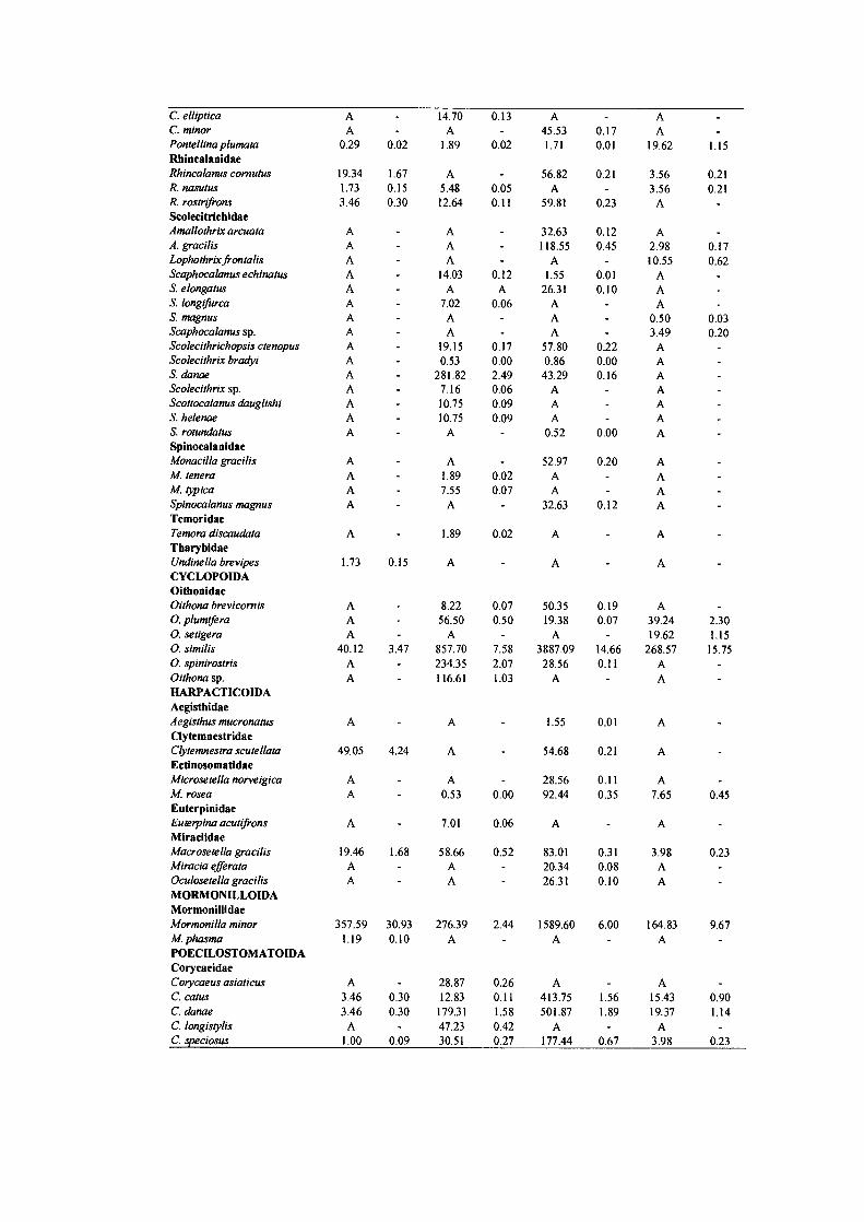
C. elliptica A 14.70 0.13 A A C. minor A A 45.53 0.17 A Pontellina plumata 0.29 0.02 1.89 0.02 1.71 0.01 19.62 1.15 Rhincalanidae Rhincalanus cornutus 19.34 1.67 A 56.82 0.21 3.56 0.21 R. nasutus 1.73 0.15 5.48 0.05 A 3.56 0.21 R. rostrifrons 3.46 0.30 12.64 0.11 59.81 0.23 A - Scolecitrichidae Amallothrix arcuata A A 32.63 0.12 A - A. gracilis A A 118.55 0.45 2.98 0.17 Lophothrixfrontalis A A - A - 10.55 0.62 Scaphocalanus echinatus A 14.03 0.12 1.55 0.01 A - S. elongatus A A A 26.31 0.10 A S. longifurca A 7.02 0.06 A - A - S. magnus A A - A 0.50 0.03 Scaphocalanus sp. A A - A - 3.49 0.20 Scolecithrichopsis ctenopus A 19.15 0.17 57.80 0.22 A - Scolecithrix bradyi A 0.53 0.00 0.86 0.00 A S. danae A 281.82 2.49 43.29 0.16 A Scolecithrix sp. A 7.16 0.06 A - A Scottocalanus dauglishi A 10.75 0.09 A A S. helenae A 10.75 0.09 A - A S. rotundatus A A - 0.52 0.00 A Spinocalanidae Monacilla gracilis A A - 52.97 0.20 A Al. tenera A 1.89 0.02 A A Al. typica A 7.55 0.07 A A Spinocalanus magnus A A - 32.63 0.12 A Temoridae Temora discaudata A 1.89 0.02 A A Tharybidae Undinella brevipes 1.73 0.15 A A A CYCLOPOIDA Oithonidae Oithona brevicornis A 8.22 0.07 50.35 0.19 A - O. plumifera A 56.50 0.50 19.38 0.07 39.24 2.30 O. setigera A A - A - 19.62 1.15 0. similis 40.12 3.47 857.70 7.58 3887.09 14.66 268.57 15.75 0. spinirostris A 234.35 2.07 28.56 0.11 A - Oithona sp. A 116.61 1.03 A - A HARPACTICOIDA Aegisthidae Aegisthus mucronatus A A 1.55 0.01 A Clytemnestridae Clytemnestra scutellata 49.05 4.24 A 54.68 0.21 A Ectinosomatidae Microsetella norveigica A A 28.56 0.11 A - M. roses A 0.53 0.00 92.44 0.35 7.65 0.45 Euterpinidae Eutemina acutifrons A 7.01 0.06 A A Miraciidae Macrosetella gracilis 19.46 1.68 58.66 0.52 83.01 0.31 3.98 0.23 Miracia efferata A A 20.34 0.08 A - Oculosetella gracilis A A 26.31 0.10 A MORMONILLOIDA Mormonillidae Mormonilla minor 357.59 30.93 276.39 2.44 1589.60 6.00 164.83 9.67 Al. phasma 1.19 0.10 A A A - POECILOSTOMATOIDA Corycaeidae Corycaeus asiaticus A 28.87 0.26 A - A - C. catus 3.46 0.30 12.83 0.11 413.75 1.56 15.43 0.90 C. danae 3.46 0.30 179.31 1.58 501.87 1.89 19.37 1.14 C. longistylis A 47.23 0.42 A A C. speciosus 1.00 0.09 30.51 0.27 177.44 0.67 3.98 0.23

C. typicus A A - A 7.47 0.44 Corycaeus sp. A 75.12 0.66 A 3.49 0.20 Farranula carinata A 2.74 0.02 33.95 0.13 A -

Lubbockidae Lubbockia aculeata A A 1.37 0.01 2.98 0.17 L. squillimana A A 28.56 0.11 A Oncaeidae Conaea gracilis 5.57 0.48 A 111.91 0.42 23.77 1.39 Oncaea mediterranea A - A 340.52 1.28 11.94 0.70 0. notopus A A - 105.34 0.40 A - O. venusta 249.57 21.59 2004.44 17.71 4381.95 16.53 142.09 8.33 Triconia conifera 0.23 0.02 67.12 0.59 145.34 0.55 10.61 0.62 Sapphirinidae Copilia quadrats 1.73 0.15 7.01 0.06 119.75 0.45 A C. vitrea A A 20.34 0.08 A Sapphirina intestinata A 9.75 0.09 A A S. nigromaculata A A 65.25 0.25 A S. ovatolanceolata A A 75.64 0.29 A Sapphirina sp. A A - 84.03 0.32 A - Unidentified 11.73 1.02 183.29 1.62 1941.91 7.33 152.49 8.94 Total individuals 100 in -3 1156 11318 26508 1705

Table 6.4. Seasonal variations in abundance (individuals 100 I11-3 ) and percentage (%) of different copepod species in the base of the thermocline-300 m stratum in central Bay of Bengal Species

SUM FIM WM SpIM Abundance % Abundance % Abundance % Abundance %

CALANOIDA Acartiidae Acartia negligens A A A 20.02 1.04 Aetideidae Aetideus acutus 1.60 0.05 6.86 0.38 A A A. armatus A 0.75 0.04 0.66 0.02 5.35 0.28 Euchirella amoena A 3.27 0.18 5.63 0.14 A - E. bella 1.60 0.05 A - A A - E. bitumida A A A 12.69 0.66 E. curticauda A A - 0.53 0.01 A - E. galeata A 9.32 0.52 A A E. indica 59.32 1.76 A - 19.17 0.46 A E. messinensis 1.60 0.05 A A A E. rostrata 1.60 0.05 A A A E. venusta A A 2.29 0.06 A - Euchirella sp. 1.30 0.04 A A 8.14 0.20 A A Gaetanus arminger A 0.75 0.04 A A - G. kruppii A A A 13.18 0.69 G. miles A 9.38 0.52 2.05 0.05 A - Undeuchaeta sp. A 0.20 0.01 A A Augaptilidae Augaptilus glacialis 0.50 0.01 A A A Centraugaptilus horridus 50.58 1.50 A A A Euaugaptilus bullifer 1.60 0.05 86.28 4.80 A A - E. facilis A - A A 6.69 0.35 E. longimanus 1.60 0.05 A A A - E. oblongus 1.60 0.05 A A A - Haloptilus acutifrons 29.48 0.88 A A 22.69 1.18 H. longicornis A 1.01 0.06 21.18 0.51 22.69 1.18 H. ornatus A A 4.00 0.10 A - H. spiniceps 0.65 0.02 A 20.38 0.49 A Calanidae Canthocalanus pauper A A 9.91 0.24 A Mesocalanus tenuicornis A 5.97 0.33 A A Undinula vulgaris 55.75 1.66 6.86 0.38 40.22 0.97 A Candaciidae Candacia bradyi A A 6.46 0.16 A C. catula A 1.01 0.06 A A C. discaudata A A 0.53 0.01 A C. pachydactyla A A 16.88 0.41 A - Candacia sp. A A A 12.69 0.66 Paracandacia truncata 0.65 0.02 71.34 3.97 A A - P. simplex A 0.75 0.04 A A Centropagidae Centropages calaninus A 5.97 0.33 0.53 0.01 A C. dorsispinatus A 6.86 0.38 A A Centropages sp. A 6.86 0.38 6.46 0.16 A Clausocalanidae Clausocalanus arcuicornis 27.88 0.83 16.63 0.92 104.36 2.51 55.40 2.89 C. furcatus 27.88 0.83 21.16 1.18 51.20 1.23 A - C. pergens 27.88 0.83 A A - A Eucalanidae Eucalanus crassus 1.60 0.05 28.30 1.57 3.50 0.08 68.78 3.59 E. subcrassus A 7.45 0.41 A A - E. elongatus 17.72 0.53 29.08 1.62 101.79 2.45 62.73 3.27 E. monachus 256.56 7.62 114.48 6.36 35.01 0.84 A - E. mucronatus 1.60 0.05 20.28 1.13 60.46 1.46 10.01 0.52 E. pseudattenuatus A - 7.62 0.42 A - A -

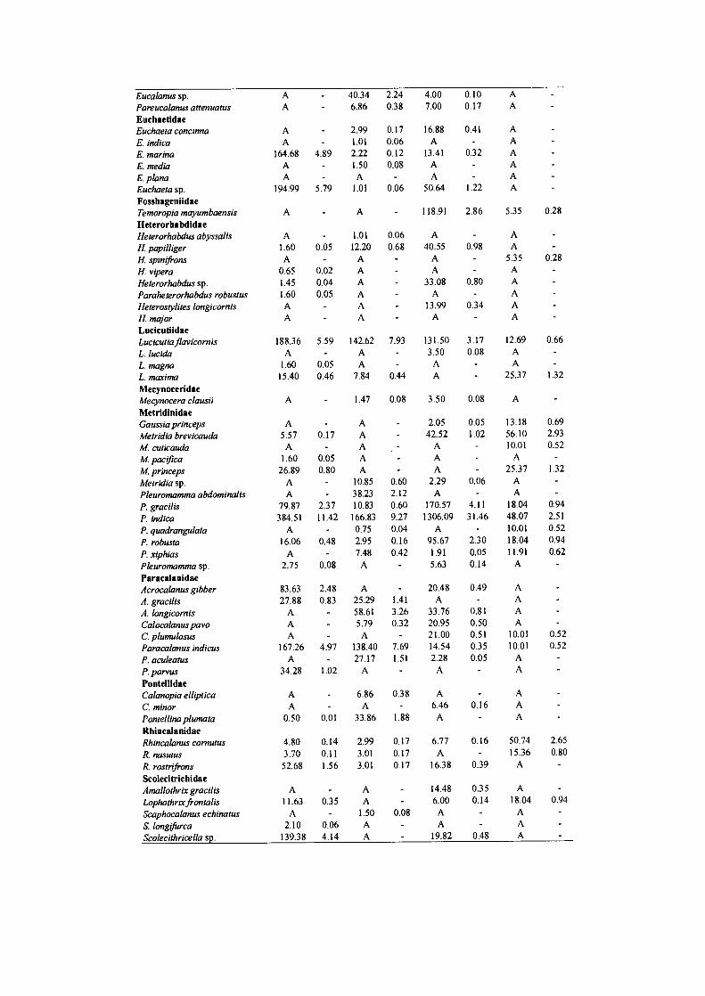
Eucalanus sp. A 40.34 2.24 4.00 0.10 A Pareucalanus attenuatus A 6.86 0.38 7.00 0.17 A Euchaetidae Euchaeta concinna A 2.99 0.17 16.88 0.41 A E. indica A - 1.01 0.06 A A E. marina 164.68 4.89 2.22 0.12 13.41 0.32 A E. media A - 1.50 0.08 A - A E. plans A - A - A - A Euchaeta sp. 194.99 5.79 1.01 0.06 50.64 1.22 A Fosshageniidae Temoropia mayumbaensis A A 118.91 2.86 5.35 0.28 Heterorhabdidae Heterorhabdus abyssalis A 1.01 0.06 A A H. papilliger 1.60 0.05 12.20 0.68 40.55 0.98 A -

H. spinifrons A A - A 5.35 0.28

H. vipera 0.65 0.02 A A A - Heterorhabdus sp. 1.45 0.04 A 33.08 0.80 A Paraheterorhabdus robustus 1.60 0.05 A A A Heterostylites longicornis A A 13.99 0.34 A H. major A A A A Lucicutiidae Lucicutia flavicornis 188.36 5.59 142.62 7.93 131.50 3.17 12.69 0.66 L. lucida A A 3.50 0.08 A -

L. magna 1.60 0.05 A A A -

L. maxima 15.40 0.46 7.84 0.44 A 25.37 1.32

Mecynoceridae Mecynocera clausii A 1.47 0.08 3.50 0.08 A Metridinidae Gaussia princeps A - A 2.05 0.05 13.18 0.69 Metridia brevicauda 5.57 0.17 A 42.52 1.02 56.10 2.93

M. cuticauda A - A A - 10.01 0.52

M pacifica 1.60 0.05 A A A

M. princeps 26.89 0.80 A A - 25.37 1.32

Metridia sp. A - 10.85 0.60 2.29 0.06 A Pleuromamma abdominalis A - 38.23 2.12 A - A

P. gracilis 79.87 2.37 10.83 0.60 170.57 4.11 18.04 0.94

P. indica 384.51 11.42 166.83 9.27 1306.09 31.46 48.07 2.51

P. quadrangulata A 0.75 0.04 A - 10.01 0.52

P. robusta 16.06 0.48 2.95 0.16 95.67 2.30 18.04 0.94

P. xiphias A 7.48 0.42 1.91 0.05 11.91 0.62

Pleuromamma sp. 2.75 0.08 A - 5.63 0.14 A

Paracalanidae Acrocalanus gibber 83.63 2.48 A - 20.48 0.49 A

A. gracilis 27.88 0.83 25.29 1.41 A - A

A. longicornis A - 58.61 3.26 33.76 0.81 A Calocalanus pavo A 5.79 0.32 20.95 0.50 A C. plumulosus A - A - 21.00 0.51 10.01 0.52

Paracalanus indicus 167.26 4.97 138.40 7.69 14.54 0.35 10.01 0.52

P. aculeatus A 27.17 1.51 2.28 0.05 A -

P. parvus 34.28 1.02 A - A A

Pontellidae Calanopia elliptica A 6.86 0.38 A A

C. minor A A - 6.46 0.16 A

Pontellina plumata 0.50 0.01 33.86 1.88 A A

Rhincalanidae Rhincalanus cornutus 4.80 0.14 2.99 0.17 6.77 0.16 50.74 2.65

R. nasutus 3.70 0.11 3.01 0.17 A 15.36 0.80

R. rostrifrons 52.68 1.56 3.01 0.17 16.38 0.39 A -

Scolecitrichidae Amallothrix gracilis A A 14.48 0.35 A -

Lophothrix frontalis 11.63 0.35 A 6.00 0.14 18.04 0.94

Scaphocalanus echinatus A 1.50 0.08 A A -

S. longifurca 2.10 0.06 A A - A Scolecithricella sp. 139.38 4.14 A 19.82 0.48 A

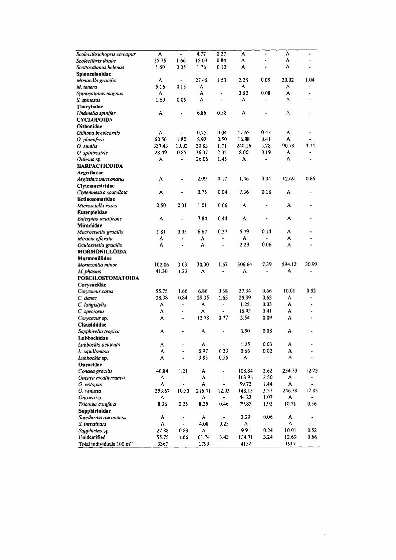
Scolecithrichopsis ctenopus A - 4.77 0.27 A A Scolecithrix dance 55.75 1.66 15.09 0.84 A A Scottocalanus helenae 1.60 0.05 1.76 0.10 A A Spinocalanidae Monacilla gracilis A 27.45 1.53 2.28 0.05 20.02 1.04 M. tenera 5.16 0.15 A - A A Spinocalanus magnus A A 3.50 0.08 A S. spinosus 1.60 0.05 A A A Tharybidae Undinella spinifer A 6.86 0.38 A A CYCLOPOIDA Oithonidae Oithona brevicornis A - 0.75 0.04 17.65 0.43 A O. plumifera 60.56 1.80 8.92 0.50 16.88 0.41 A 0. similis 337.43 10.02 30.83 1.71 240.16 5.78 90.78 4.74 0. spinirostris 28.49 0.85 36.37 2.02 8.00 0.19 A Oithona sp. A - 26.06 1.45 A - A HARPACTICOIDA Aegisthidae Aegisthus mucronatus A 2.99 0.17 1.46 0.04 12.69 0.66 Clytemnestridae Clytemnestra scutellata A 0.75 0.04 7.36 0.18 A Ectinosomatidae Microsetella rosea 0.50 0.01 1.01 0.06 A A Euterpinidae Eutetpina acutifrons A 7.84 0.44 A A Miraciidae Macrosetella gracilis 1.81 0.05 6.67 0.37 5.79 0.14 A Miracia efferata A A - A A Oculosetella gracilis A A 2.29 0.06 A MORMONILLOIDA Mormonillidae Mormonilla minor 102.06 3.03 30.00 1.67 306.64 7.39 594.12 30.99 M. phasma 41.30 1.23 A A A - POECILOSTOMATOIDA Corycaeidae Corycaeus catus 55.75 1.66 6.86 0.38 27.34 0.66 10.01 0.52 C. danae 28.38 0.84 29.35 1.63 25.99 0.63 A - C. longislylis A A 1.25 0.03 A C. speciosus A A 16.93 0.41 A Corycaeus sp. A 13.78 0.77 3.54 0.09 A Clausidiidae Sapphirella tropica A A 3.50 0.08 A Lubbockidae Lubbockia aculeata A A 1.25 0.03 A L. squillimana A 5.97 0.33 0.66 0.02 A Lubbockia sp. A 9.85 0.55 A - A Oncaeidae Conaea gracilis 40.84 1.21 A 108.84 2.62 234.39 12.23 Oncaea mediterranea A A 103.95 2.50 A - O. notopus A A 59.72 1.44 A O. venusta 353.67 10.50 216.41 12.03 148.15 3.57 246.38 12.85 Oncaea sp. A A 44.22 1.07 A Triconia conifera 8.36 0.25 8.25 0.46 79.85 1.92 10.71 0.56 Sapphirinidae Sapphirina auronitens A A 2.29 0.06 A S. intestinata A - 4.08 0.23 A - A - Sapphirina sp. 27.88 0.83 A 9.91 0.24 10.01 0.52 Unidentified 55.75 1.66 61.74 3.43 134.71 3.24 12.69 0.66 Total individuals 100 m-3 3367 1799 4152 1917

Miraciidae (6%) and Spinocalanidae (7.2%) registered their highest percentage in this

stratum only during SUM. Similarly, Augaptilidae (6.4%) and Metridinidae (7.6%)

showed higher abundant in this stratum only during FIM. Eucalanidae (11.2 and 5.8%)

and Lucicutiidae (13.4 and 12.1%) contributed to relatively higher abundances during

SUM and FIM respectively. Mormonillidae also accounted for 6.4 and 12.4% of the total

during SUM and WM respectively. Clausiidae was the only family that was absent during

all seasons from this stratum.

6.2.4. Genera and species

A total of 83 genera were identified during the study (Tables 6.2-6.6). The numbers of

genera found in MLD, TT-BT, BT-300 m, 300-500 m and 500-1000 m were, 63, 71, 61,

62 and 62 respectively. Not only did the total number of genera in the water column vary

seasonally (SUM: 64, FIM: 66, WM: 70 and SpIM: 50) but they varied also in each

sampled strata. The highest number of genera in the thermocline was due to the presence

of many deep -water genera such as Chiridiella, Pseudochirella, Gaetanus, Undeuchaeta,

Arietellus, Augaptilus, Scottocalanus, Aegisthus and Lubbockia that occurred only below

MLD and two other genera viz. Bestiolina and Cosmocalanus that were exclusively

present in this stratum.

The most dominant genera were Oncaea (17%), Mormonilla (9.0%), Pleuromamma

(8.6%), Oithona (7.6%), Clausocalanus (6.0%), Lucicutia (6.0%), Eucalanus (5.5%) and

Paracalanus (5.5%) accounting for 68% of the total abundance in the 1000 m water

column in the CB (Table 7.9; Chapter 7).

From the total of 251 species that were identified in the CB, 69 species occurred

during all the seasons. From these, only two viz. Oithona similis and Oncaea venusta

were preponderant at all depths and stations. Varying distinctly with depths, the number

of species occurring was 150, 169, 145, 170 and 145 in MLD, TT-BT, BT-300 m, 300-

500 m and 500-1000 m respectively. In the topmost stratum, the largest number of

species of Sapphirina and Corycaeus were observed. Similarly, the largest number of

species of Aetideidae, Augaptilidae, Scolecithrichidae and Spinocalanidae were observed

in the 300-500 m stratum. While some species never surfaced in any of the seasons,

species such as Conaea gracilis were found to increase in abundance with depth.

82

Table 6.5. Seasonal variations in abundance (individuals 100 I11-3 ) and percentage (%) of different copepod species in the 300-500 m stratum in central Bay of Bengal

SUM FIM WM Species Abundance % Abundance % Abundance %

CALANOIDA Acartiidae Acartia negligens 28.31 1.01 0.25 0.03 6.35 0.18 A. southwelli A 5.64 0.61 A Aetideidae Aetideus acutus A A 2.79 0.08 A. armatus A A 17.76 0.51 A. bradyi A A 8.02 0.23 Aetideus sp. A A 17.76 0.51 Chiridiella sp. A A 4.20 0.12 Euchirella amoena A 0.60 0.07 A E. bitumida A A 8.47 0.24 E. galeata A - 0.27 0.03 11.38 0.33 E. indica 15.78 0.56 A 2.79 0.08 E. maxima A - 0.10 0.01 A - E. rostrata A 5.64 0.61 A - E. rostromagna A A 10.86 0.31 E. speciosa A A 1.48 0.04 E. venusta A A - 3.33 0.10 Euchirella sp. 6.98 0.25 3.20 0.35 6.44 0.19 Gaetanus arminger A 2.12 0.23 A - G. kruppii A - 2.15 0.23 1.09 0.03 G. miles 6.98 0.25 5.64 0.61 5.47 0.16 G. minor 10.28 0.37 A - 0.74 0.02 G.pileatus 4.00 0.14 A A - Undeuchaeta sp. A - 0.35 0.04 A Arietellidae Arietellus setosus A A 0.89 0.03 Augaptilidae Augaptilus sp. A A 2.44 0.07 Centraugaptilus rattrayi A A 0.40 0.01 C. horridus 3.43 0.12 A - A Euaugaptilus bullifer A 282.42 30.66 A E. hecticus A A - 2.44 0.07 E. laticeps A A - 17.76 0.51 E. magnus A 0.71 0.08 A E mixtus A 1.42 0.15 A E. nodifrons A A 1.48 0.04 E. oblongus 1.71 0.06 11.33 1.23 A E. rigidus A 1.42 0.15 A Haloptilus acutifrons A A - 10.86 0.31 H. longicornis 8.20 0.29 0.71 0.08 9.02 0.26 H. spiniceps 2.10 0.07 A A Pseudhaloptilus abbreviatus A - 5.92 0.64 A P. eurygnathus 1.71 0.06 A A P. pacificus 1.71 0.06 A A Calanidae Undinula vulgaris 6.98 0.25 A 12.64 0.36 Candaciidae Candacia bradyi 8.69 0.31 A 25.10 0.72 C. catula A A 6.29 0.18 C. discaudata A A 6.35 0.18 C. pachydactyla A 0.25 0.03 A - Candacia sp. A 0.71 0.08 10.86 0.31 Paracandacia truncata 1.71 0.06 0.25 0.03 A - P. simplex A A - A Centropagidae Centropages calaninus 6.98 0.25 A 6.29 0.18

C dorsispinatus C. furcatus

C. gracilis Clausocalanidae

A 0.24

A 0 01

5.17 A

1.07

0.56

0.12

A A A

Clausocalanus arcuicornis 47.41 1.69 22.42 2.43 66.15 1.90 C. furcatus 6.98 0.25 0.84 0.09 20.31 0.58 C. pergens 4.20 0.15 0.17 0.02 A Eucalanidae Eucalanus crassus 6.85 0.24 0.50 0.05 6.35 0.18 E. subcrassus A 0.10 0.01 A E. elongatus 74.90 2.66 6.26 0.68 384.01 11.03 E. monachus 22.27 0.79 0.10 0.01 18.98 0.55 E. mucronatus 7.86 0.28 7.81 0.85 92.36 2.65 E. pseudattenuatus 15.42 0.55 1.07 0.12 A Eucalanus sp. 5.53 0.20 0.25 0.03 A Pareucalanus attenuatus 3.43 0.12 0.10 0.01 6.35 0.18 Euchaetidae Euchaeta concinna A 0.10 0.01 A E. indica A 1.18 0.13 A E. marina 18.24 0.65 2.41 0.26 4.91 0.14 E. media A A - A E. plan 6.98 0.25 0.10 0.01 A Euchaeta sp. 15.67 0.56 0.10 0.01 8.77 0.25 Pareuchaeta malayensis A 1.07 0.12 A Fosshageniidae Temoropia mayumbaensis A A 41.10 1.18 Heterorhabd id ae Disseta palumboi A A 0.45 0.01 Heterorhabdus abyssalis A 6.37 0.69 6.87 0.20 H fistulosus A A A H. pacificus A 0.10 0.01 4.20 0.12 H. papilliger 26.29 0.93 45.70 4.96 31.39 0.90 H. spinifrons 12.29 0.44 A 6.29 0.18 H. subspinifrons A - A 020 0.01 H. vipera 2.10 0.07 A 4.84 0.14 Heterorhabdus sp. 4.23 0.15 A 21.96 0.63 Heterostylites longicornis 0.40 0.01 A 4.20 0.12 Lucicutiidae Lucicutiaflavicornis 119.67 4.25 134.37 14.59 107.79 3.10 L. longispina 1.71 0.06 A A L. maxima 50.67 1.80 48.59 5.28 74.96 2.15 L. ovalis 15.54 0.55 A A Mecynoceridae Mecynocera clausii A 5.17 0.56 6.29 0.18 Metridinidae Gaussia princeps A 12.85 1.40 1.34 0.04 Metridia brevicauda 6.85 0.24 1.52 0.17 94.94 2.73 M. cuticauda 11.99 0.43 A A - M. pacifica 3.43 0.12 A A M. princeps 3.43 0.12 A 0.74 0.02 Metridia sp. A - 5.98 0.65 A Pleuromamma abdominalis A 3.54 0.38 A - P. gracilis 9.40 0.33 1.90 0.21 121.65 3.49 P. indica 233.67 8.31 40.66 4.41 153.84 4.42 P. quadrangulata A 6.14 0.67 17.76 0.51 P. robusta A 0.81 0.09 55.64 1.60 P. xiphias 1.71 0.06 2.65 0.29 25.89 0.74 Pleuromamma sp. A 7 1.00 0.11 5.65 0.16 Paracalanidae Acrocalanus gibber 20.93 0.74 5.67 0.62 12.69 0.36 A. gracilis 7.77 028 0.10 0.01 A A. longicornis 0.40 0.01 A - 6.35 0.18 A. monachus 6.98 0.25 A A -

Calocalanus pavo A - 0.50 0.05 55.28 1.59 C. pavoninus 6.98 025 A A -

C. plumulosus A A - 36.19 1.04 Paracalanus indices 21.57 0.77 14.32 1.55 12.69 0.36 P. aculeatus 0.40 0.0I 2.96 0.32 8.59 0.25 P. crassirostris A - A - A - P. parvus 6.98 0.25 A A -

Phaennidae Xanthocalanus sp. A A 2.44 0.07 Pontellidae Calanopia elliptica A 1.57 0.17 20.55 0.59 Pontellina plumata 13.96 0.50 1.96 0.21 A Rhincalanidae Rhincalanus cornutus 1.71 0.06 1.07 0.12 8.59 0.25 R. nasutus 10.40 0.37 0.50 0.05 8.09 0.23 R. rostrtfrons A A - 25.90 0.74 Scolecitrichidae Amallothrix gracilis 6.98 0.25 A 2.24 0.06 Pseudoamallothrix emarginata A A 0.40 0.01 Lophothrixfrontalis 24.67 0.88 0.50 0.05 60.80 1.75 L. humiltfrons A A 8.14 0.23 Scaphocalanus echinatus 2.10 0.07 0.50 0.05 A - S. longifurca A A 2.79 0.08 S. magnus 2.10 0.07 A - A Scaphocalanus sp. 4.83 0.17 0.55 0.06 2.79 0.08 Scolecithricella abyssalis A 0.31 0.03 A S. dentata A 1.07 0.12 A Scolecithricella sp. A 021 0.02 26.85 0.77 Scolecithrichopsis ctenopus A 1.28 0.14 6.35 0.18 Scolecithrix danae A 2.80 0.30 18.93 0.54 S. nicobarica 6.98 0.25 A A - Scolecithrix sp. A 11.33 1.23 2.24 0.06 Scottocalanus helenae A 12.94 1.40 3.72 0.11 Spinocalanidae Monacilla gracilis 1.19 0.04 A 78.66 226 M. tenera 36.87 1.31 A 65.78 1.89 M typica 2.21 0.08 0.06 0.01 A Spinocalanus magnus 0.40 0.01 A A Spinocalanus sp. A A 2.44 0.07 Temoridae Temora turbinata 6.98 0.25 A A T. srylifera A 0.71 0.08 A CYCLOPOIDA Oithonidae Oithona brevicornis 6.98 0.25 A A O. plumtfera 6.98 0.25 0.10 0.01 17.16 0.49 O. setigera 2.10 0.07 A 5.65 0.16 0. similis 130.00 4.62 3.33 0.36 150.02 4.31 0. spinirostris 6.98 0.25 0.63 0.07 A HARPACTICOIDA Aegisthidae Aegisthus mucronatus A A 10.58 0.30 Clytemnestridae Clytemnestra scutellata A A 10.55 0.30 Ectinosomatidae Microsetella rosea A 0.10 0.01 20.55 0.59 Miraciidae Macrosetella gracilis 174.60 6.21 1.19 0.13 33.03 0.95 Miracia efferata A A 6.35 0.18 MORMONILLOIDA Mormonillidae Mormonilla minor 184.23 6.55 80.25 8.71 246.03 7.07 POECILOSTOMATOIDA Corycaeidae Corycaeus catus 14.75 0.52 A 25.33 0.73 C. danae 58.04 2.06 2.06 0.22 24.36 0.70 C. longistylis A - 0.25 0.03 6.35 0.18

C. speciosus 7.37 0.26 A 12.69 0.36 Corycaeus sp. A - 0.21 0.02 A Farranula carinata A A 18.88 0.54 Lubbockidae Lubbockia aculeata A A 0.74 0.02 Oncaeidae Conaea gracills 118.78 4.22 A 139.82 4.02 Oncaea mediterranea A - A 54.68 1.57 0. notopus A - A - 8.59 0.25 0. venusta 1023.28 36.37 52.15 5.66 324.03 9.31 Triconia comfera A - 0.56 0.06 49.89 1.43 Sapphirinidae Copilia quadrata 7.37 0.26 A 10.86 0.31 C. vitrea 7.37 0.26 A A Sapphirina auronitens 0.40 0.01 A A S. ovatolanceolata 13.96 0.50 A - A - Unidentified 0.24 0.01 19.75 2.14 186.46 5.36 Total individuals 100 nf3 2813 921 3481

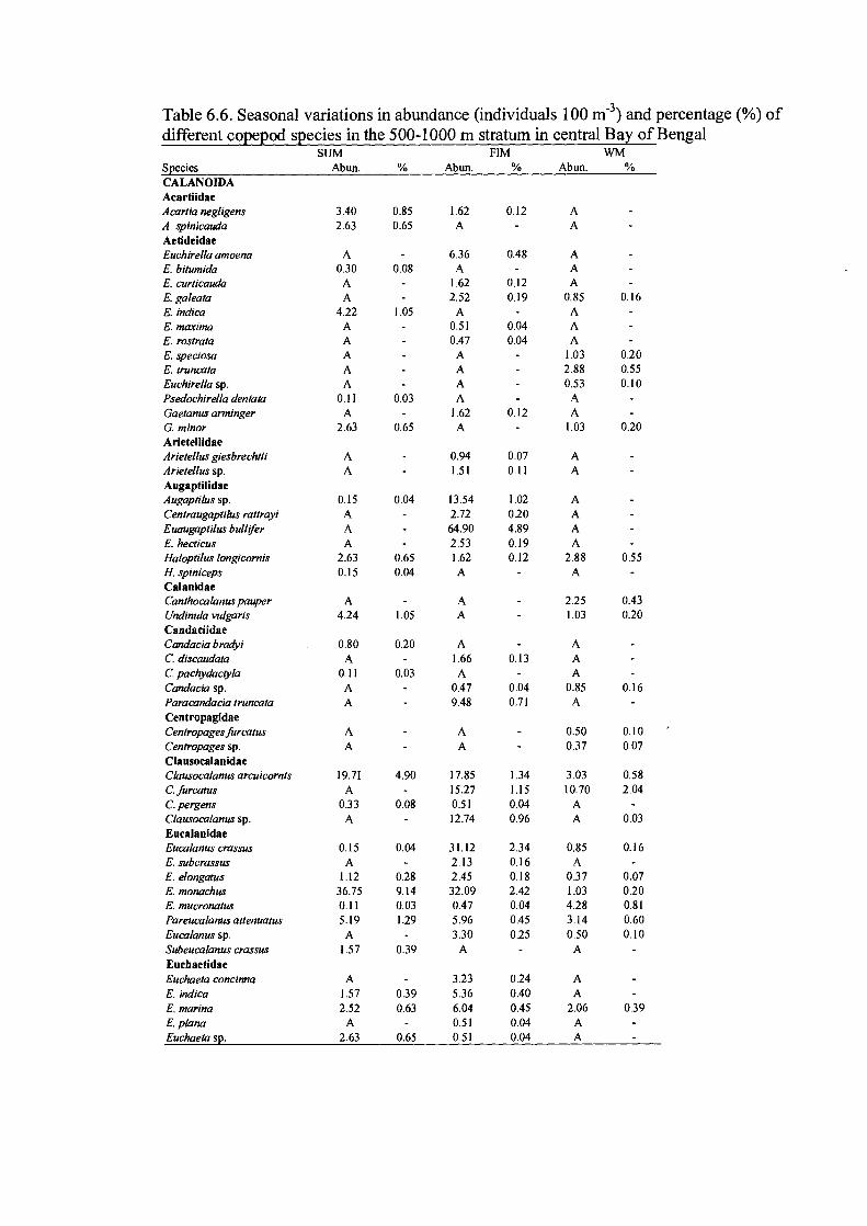
Table 6.6. Seasonal variations in abundance (individuals 100 m -3 ) and percentage (%) of different copepod species in the 500-1000 m stratum in central Bay of Bengal

SUM FIM WM Species Abun. % Abun. % Abun. % CALANOIDA Acartiidae Acartia negligens 3.40 0.85 1.62 0.12 A A. spinicauda 2.63 0.65 A A Aetideidae Euchirella amoena A 6.36 0.48 A E. bitumida 0.30 0.08 A A E. curticauda A 1.62 0.12 A E. galeata A 2.52 0.19 0.85 0.16 E. indica 4.22 1.05 A A E. maxima A 0.51 0.04 A E. rostrata A 0.47 0.04 A - E. speciosa A A 1.03 0.20 E. truncata A A 2.88 0.55 Euchirella sp. A - A 0.53 0.10 Psedochirella dentata 0.11 0.03 A A - Gaetanus arminger A - 1.62 0.12 A G. minor 2.63 0.65 A 1.03 0.20 Arietellidae Arietellus giesbrechtii A 0.94 0.07 A Arietellus sp. A 1.51 0.11 A Augaptilidae Augaptilus sp. 0.15 0.04 13.54 1.02 A Centraugaptilus rattrayi A 2.72 0.20 A Euaugaptilus bullifer A 64.90 4.89 A E. hecticus A 2.53 0.19 A - Haloptilus longicornis 2.63 0.65 1.62 0.12 2.88 0.55 H. spiniceps 0.15 0.04 A - A - Calanidae Canthocalanus pauper A A 2.25 0.43 Undinula vulgaris 4.24 1.05 A 1.03 0.20 Candaciidae Candacia bradyi 0.80 0.20 A - A C. discaudata A 1.66 0.13 A C. pachydactyla 0.11 0.03 A - A Candacia sp. A 0.47 0.04 0.85 0.16 Paracandacia truncata A 9.48 0.71 A Centropagidae Centropages furcatus A A 0.50 0.10 Centropages sp. A A 0.37 0.07 Clausocalanidae Clausocalanus arcuicornis 19.71 4.90 17.85 1.34 3.03 0.58 C. furcatus A 15.27 1.15 10.70 2.04 C. pergens 0.33 0.08 0.51 0.04 A - Clausocalanus sp. A 12.74 0.96 A 0.03 Eucalanidae Eucalanus crassus 0.15 0.04 31.12 2.34 0.85 0.16 E. subcrassus A 2.13 0.16 A E. elongatus 1.12 0.28 2.45 0.18 0.37 0.07 E. monachus 36.75 9.14 32.09 2.42 1.03 0.20 E. mucronatus 0.11 0.03 0.47 0.04 4.28 0.81 Pareucalanus attenuatus 5.19 1.29 5.96 0.45 3.14 0.60 Eucalanus sp. A 3.30 0.25 0.50 0.10 Subeucalanus crassus 1.57 0.39 A - A Euchaetidae Euchaeta concinna A 3.23 0.24 A E. indica 1.57 0.39 5.36 0.40 A E. marina 2.52 0.63 6.04 0.45 2.06 0.39 E. plans A 0.51 0.04 A Euchaeta sp. 2.63 0.65 0.51 0.04 A

Fosshageniidae Temoropia mayumbaensis A A 7.59 1.45 Heterorhabdidae Heterorhabdus abyssalis 7.88 1.96 A 0.85 0.16 H. pacificus 0.80 0.20 0.51 0.04 A H. papilliger 0.27 0.07 17.76 134 A - H. spinfrons 0.16 0.04 2.72 0.20 0.36 0.07 Heterorhabdus sp. A - A 2.06 0.39 Heterostylites longicornis A A 0.17 0.03 Lucicutiidae Lucicutiaflavicornis 46.21 11.49 107.08 8.06 12.57 2.39 L. maxima 7.72 1.92 51.30 3.86 10.44 1.99 L. ovalis A - 2.53 0.19 0.85 0.16 Mecynoceridae Mecynocera clausii A 4.23 0.32 A Megacalanidae Megacalanus princeps A 0.47 0.04 A Metridinidae Gaussia princeps 0.15 0.04 3.04 0.23 A - Metridia brevicauda 0.95 0.24 0.51 0.04 2.25 0.43 M cuticauda A A 2.88 0.55 M.princeps A 5.06 0.38 A - Metridia sp. A 19.25 1.45 0.26 0.05 Pleuromamma abdominalis A 1.52 0.11 A -

P. gracilis 0.80 0.20 4.75 0.36 3.90 0.74 P. indica 21.50 5.35 54.14 4.08 3.10 0.59 P. quadrangulata A 5.44 0.41 1.03 0.20 P. robusta A 4.74 0.36 A - P. xiphias A A 2.88 0.55 Pleuromamma sp. A 1.98 0.15 0.17 0.03 Nullosetigeridae Nullosetigera bidentata 0.30 0.08 A A Nullosetigera sp. 0.22 0.06 A A Paracalanidae Acrocalanus gibber 0.15 0.04 A - A - A. gracilis 0.46 0.11 0.51 0.04 0.17 0.03 A. longicornis 0.26 0.07 6.66 0.50 2.09 0.40 Calocalanus pavo 2.03 0.51 A - 0.85 0.16 C. pavoninus 0.22 0.06 A A C. plumulosus A - A 0.17 0.03 Paracalanus indicus 6.38 1.59 8.10 0.61 A P. aculeatus 2.78 0.69 1.52 0.11 A P. parvus 1.68 0.42 A A Phaennidae Amallophora conifer A A 1.03 0.20 Pontellidae Calanopia aurivilli 1.57 0.39 A - A - C. elliptica A 0.94 0.07 A A C. minor 0.61 0.15 A - A A Pontellina plumata A 11.67 0.88 0.17 0.03 Rhincalanidae Rhincalanus cornutus A 0.94 0.07 A R. nasutus A 0.47 0.04 A R. rostrifrons 1.57 0.39 3.29 0.25 1.29 0.25 Scolecitrichidae Amallothrix gracilis A A - 0.10 0.02 Lophothrixfrontalis 1.10 0.27 0.47 0.04 5.17 0.98 L. humilifrons A A - 0.26 0.05 Scaphocalanus echinatus A 5.06 0.38 A - S. elongatus A A - 0.26 0.05 Scaphocalanus sp. 0.15 0.04 A 0.50 0.10 Scolecithricella abyssalis A 1.52 0.11 A S. bradyi 4.20 1.04 A A S. dentata A A 0.10 0.02 S. vittatta A A 2.09 0.40

Scolecithricella sp. A - 1.01 0.08 A Scolecithrichopsis ctenopus 2.63 0.65 13.84 1.04 A Scolecithrix bradyi 2.78 0.69 A - A - S. danae 0.95 0.24 24.64 1.86 1.22 0.23 S. nicobarica A - 0.47 0.04 A - Scolecithrix sp. A 1.89 0.14 0.17 0.03 Scottocalanus helenae A 13.20 0.99 2.88 0.55 Spinocalanidae Monacilla tenera 28.91 7.19 A A M. typica A A 0.52 0.10 Spinocalanus sp. A A 2.09 0.40 Temoridae Temora discaudata 0.15 0.04 2.53 0.19 A Tharybidae Thwybis sp. A 0.47 0.04 A Undinella sp. A 3.13 0.24 A CYCLOPOIDA Oithonidae Oithona brevicornis 0.15 0.04 1.66 0.13 1.03 0.20 O. plumifera 3.07 0.76 0.51 0.04 A O. setigera A A - 0.85 0.16 0. similis 9.88 2.46 27.81 2.09 10.85 2.07 0. spinirostris 6.27 1.56 10.84 0.82 0.90 0.17 HARPACTICOIDA Aegisthidae Aegisthus aculeatus A A 0.26 0.05 A. mucronatus 5.26 1.31 A A Clytemnestridae Clytemnestra scutellata 0.11 0.03 A 1.02 0.19 Ectinosomatidae Microsetella rosea 0.11 0.03 0.51 0.04 A Miraciidae Macrosetella gracilis 23.88 5.94 5.03 0.38 0.70 0.13 Miracia efferata 0.15 0.04 A - A MORMONILLOIDA Mormonillidae Mormonilla minor 25.80 6.42 57.26 4.31 112.28 21.38 POECILOSTOMATOIDA Corycaeidae Cotycaeus catus 2.44 0.61 3.00 0.23 1.99 0.38 C. danae 0.98 0.24 8.97 0.68 1.53 0.29 C. longistylis A - A - 0.43 0.08 C. speciosus 2.74 0.68 0.47 0.04 0.17 0.03 Cotycaeus sp. A A - 2.09 0.40 Farranula gibbula 1.57 0.39 0.47 0.04 A - Lubbockidae Lubbockia sp. A 1.51 0.11 A Oncaeidae Conaea gracilis 44.87 11.16 2.83 0.21 255.55 48.67 Oncaea mediterranea A A 1.39 0.27 0. notopus A A - 5.03 0.96 0. venusta 27.74 6.90 514.61 38.76 4.80 0.91 Oncaea sp. A 0.94 0.07 A - Triconia conifera 2.63 0.65 12.97 0.98 4.52 0.86 Sapphirinidae Copilia quadrata 0.52 0.13 A A Sapphirina metallina 1.57 0.39 A A S. ovatolanceolata A A 0.17 0.03 Sapphirina sp. 2.63 0.65 A - A Unidentified 1.68 0.42 28.25 2.13 6.69 1.28 Total individuals 100 ni3 402 1328 525

In each of these strata mentioned above, the species were further found to vary

seasonally. In the MLD, species of Acartia were most abundant during FIM, while only

A. negligens was found during months of FIM and SpIM (Table 6.2). Many deep-water

species showed seasonal appearance in this stratum. For instance, Conaea gracilis and

species of Spinocalanidae were absent during both the intermonsoons. Fewer species of

Aetideidae were noticed during FIM, WM and SpIM. During these seasons again, no

species of Undinella, Rhincalanus, Nullosetigera and Phaennidae were present. Similarly,

species of Heterorhabdidae were absent during FIM and just one species each was found

during WM and SpIM.

In the thermocline stratum, species of Acartia, Centropages, Acrocalanus, all species

of Scolecithrichidae, Spinocalanidae and Temoridae were absent during SUM (Table

6.3). During SpIM, all species of Sapphirinidae, Spinocalanidae, Temoridae and most

species of Aetideidae and Scolecithrichidae were absent.

In the TT-300 m stratum, the lowest number of species was observed during SpIM

(Table 6.4). During this season, species of Calanidae, Centropagiidae, Euchaetidae and

Pontellidae were absent. Also the least number of species of Aetideidae, Candaciidae,

Clausocalanidae, Paracalanidae, Corycaeidae, Clausiidae, Lubbockidae and harpacticoids

was notable.

In the 300-500 m stratum, the most number of species, particularly those of

Aetideidae were present during WM (Table 6.5). Seasonal changes in species were also

felt in the deepest stratum (Table 6.6).

Seasonally, the number of species occurring in the upper 1000 m was the least during

SpIM (SUM: 162, FIM: 170, WM: 172, SpIM: 96).

6.2.5. Dominant species

All the species accounting for >2% of the total copepod abundance were considered as

dominant ones. During SUM, Oncaea venusta, Mormonilla minor, Pleuromamma indica,

Oithona similis, Macrosetella gracilis, Lucicutia flavicornis, Paracalanus indicus,

Corycaeus danae, Conaea gracilis, Clausocalanus furcatus, Corycaeus catus and

Eucalanus monachus dominated the collections (Table 6.7). These 12 species together

contributed to 71.4% of the total copepod abundance in the 0-1000 m column. Based on

83

Table 6.7. Copepod species contributing >2% of total abundance (individuals m -2) in the upper 1000 m of the central Bay during summer monsoon (SUM), fall intermonsoon (FIM), winter monsoon (WM) and spring intermonsoon (SpIM)

Season Species

Abundance in 1000 m (ind ni2) %

SUM Oncaea venusta 5688 31.3 Mormonilla minor 1287 7.1 Pleuromamma indica 1056 5.8 Oithona similis 922 5.1 Macrosetella gracilis 889 4.9 Lucicutia flavicornis 643 3.5 Paracalanus indicus 462 2.5 Corycaeus danae 453 2.5 Conaea gracilis 416 2.3 Clausocalanus furcatus 393 2.2 Corycaeus catus 380 2.1 Eucalanus monachus 377 2.1

FIM Oncaea venusta 16770 21.4 Paracalanus indicus 15026 19.2 Lucicutia flavicornis 3724 4.8 Eucalanus monachus 3575 4.6 Corycaeus danae 3097 4.0 Oithona similis 2816 3.6 Paracalanus aculeatus 2332 3.0 Pleuromamma indica 2293 2.9

WM Oncaea venusta 11042 15.4 Oithona similis 7437 10.3 Clausocalanus arcuicornis 4999 7.0 Pleuromamma indica 4225 5.9 Paracalanus indicus 3486 4.8 Mormonilla minor 3114 4.3 Clausocalanus furcatus 2587 3.6 Corycaeus catus 2215 3.1 Lucicutia flavicornis 1722 2.4 Conaea gracilis 1631 2.3

SpIM Clausocalanus arcuicornis 4113 15.9 Oncaea venusta 3871 15.0 Oithona similis 1547 6.0 Lucicutia flavicornis 1306 5.1 Pleuromamma indica 1225 4.7 Mormonilla minor 951 3.7 Corycaeus catus 891 3.4 Oncaea mediterranea 672 2.6 Acrocalanus gracilis 592 2.3 Calocalanus pavo 586 2.3 Clausocalanus furcatus 583 2.3 Corycaeus speciosus 576 2.2

Clausocakmusfurcatus Zucalams MOYZIC;215 liecicutiaflavie ormis Pcracakons htllcus

10 12 14 16 18 20 10 12 14 16 18 20 10 12 14 16 18 20 10 12 14 16 18 20 Pleuramamma ineica 01010,32 Macrceetella gracilis MOr711041L2 minor

10 12 14 16 18 20 10 12 14 16 18 20 10 12 14 16 18 20 10 12 14 16 18 20 COnaea gracilis Corycaeus cdus anycaeus & ►we Owaea venusta

-1

-2

-3

-4

-5 10 12 14 16 18 20 10 12 14 16 18 20 10 12 14 16 18 20 10 12 14 16 18 20

CB1 CB2 CB3 CB4 CB5 CB1 CB2 CB3 CB4 CB5 CB1 CB2 CB3 CB4 CB5 CB1 CB2 CB3 CB4 CB5

Station

Figure 6.4. Distribution of major copepod species along central Bay during summer monsoon. Abundance (number 100 tri i; on labeled contours) is indicated in log numbers

Det)/1-- 'k.° 6 fri• e- dVp11-1!inl i;r4.2, cj 41 )0ro:(A. 1#'( .1 1

04 -0-ietn)ocA,rie -3; iv. -2., nor - _3C C • 6c( t CC. re

Paracalanus aculeatus

Paracalanus indicus

Eucalanus monachus

10 12 14 16 18 20 10 12 14 16 18 20 10 12 14 16 18 20

Lucicutiaflavicornis

Pleuromamma indica Oithona similis

10 12 14 16 18 20 10 12 14 16 18 20 10 12 14 16 18 20 Corycaeus danae Oncaea venusta 031 CB2 CB3 CB4 CB5

10 12 14 16 18 20 10 12 14 16 18 20 CB1 CB2 CB3 034 CB5 CB1 CB2 CB3 CB4 CB5

Station

Figure 6.5. Distribution of major copepod species along central Bay during fall inter monsoon. Abundance (number 100 m-3 ; on labeled contours) is indicated in log numbers

geclia ; - - (lc - rr; xect a,wk L t e pc'f ( fel , lsoc.6 010(1.,0e1T-0-

11-1,5e oS t 6 ; zc . 5 c c 1 nct rn

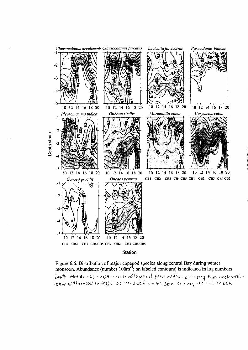
Clausocalanus arcuicornis Clausocalanus furcatus -1

Lucicutiaflavicornis Paracalanus indicus

1.1

10 12 14 16 18 20

10 12 14 16 18 20 10 12 14 16 18 20 10 12 14 16 18 20

Pleuromamma indica

Oithona similis

Mormonilla minor Corycaeus catus

10 12 14 16 18 20 10 12 14 16 18 20 10 12 14 16 18 20 10 12 14 16 18 20

Conaea gracilis Oncaea venusta CBI CB2 CB3 CB4 CB5 CB1 CB2 CB3 CB4 CB5

10 12 14 16 18 20 10 12 14 16 18 20

CB1 CB2 CB3 CB4 CB5 CB1 CB2 CB3 CB4 CB5

Station

Figure 6.6. Distribution of major copepod species along central Bay during winter monsoon. Abundance (number 100m-i ; on labeled contours) is indicated in log numbers.

Z.e4;41, "1: LAC,: .mce - e-4 det)q-, 1, rn" 04 11,-l et

oei (el) 't s!;:) ." - 3COM', 4. 3c- r 010 - • p- c

10 12 14 16 18 20 10 12 14 16 18 20

CB1 CB2 CB3 CB4 CB5 CB1 CB2 CB3 CB4 CB5

- 1 Acrocalanus gracilis Calocalanus pavo Clausocalanus arcuicornis Clausocalanus furcatus

1 -2-

-3-

10 12 14 16 18 20 10 12 14 16 18 20 10 12 14 16 18 20

Corycaeus speciosus Corycaeus catus Lucicutiaflavicornis

10 12 14 16 18 20

Mormonilla minor

a -

1 7 1 1 , i'f'

10 12 14 16 18 20 10 12 14 16 18 20

_ 1 Oncaea venusta Oncaea mediterranea

2:43 !

10 12 14 16 18 20 10 12 14 16 18 20

CB1 CB2 CB3 CB4CB5 CB1 CB2 CB3 CB4 CB5

-4 10 12 14 16 18 20

Oithona similis

f -r7

10 12 14 16 18 20

Pleuromamma indica

Station

Figure 6.7. Distribution of major copepod species along central Bay during spring inter monsoon. Abundance (number 100m -i ; on labeled contours) is indicated in log numbers.

Dery t: '; Ate (», iCA Cr'-ti tr, 04 tht ,

4-4,.ornoc 1 ;r1t, /31),, c't)",

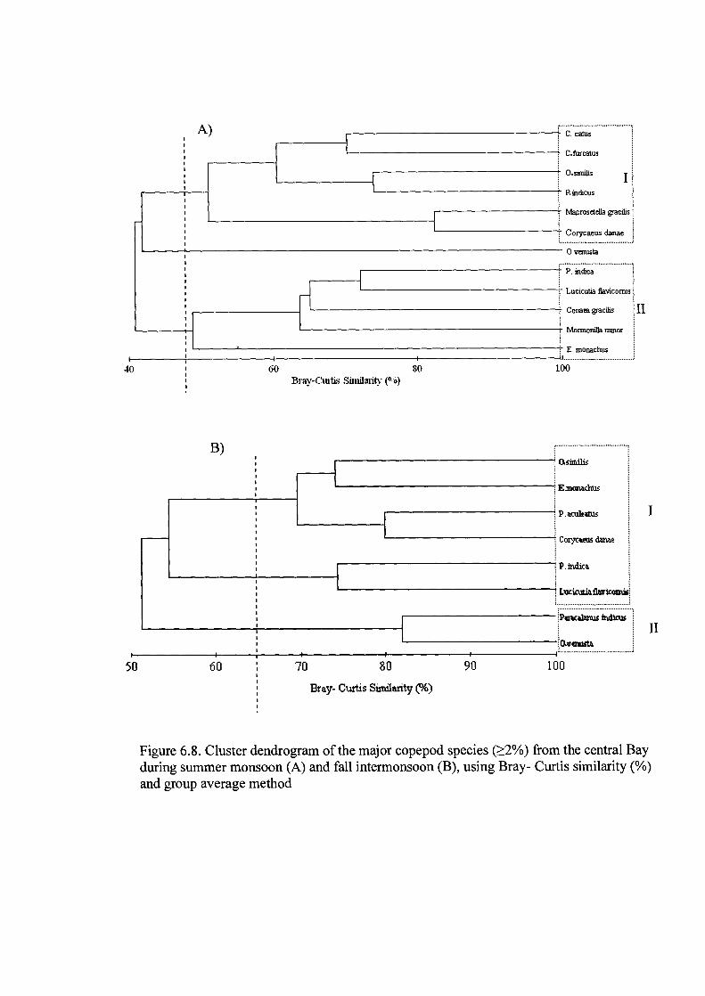
II

A) C. catus

Cdurcatus

0.simihs

P. indicus

Macrosetella gracilis

Corycaeus danae

0 venusta

P. indica

Lucicutia flavicornis

Conaea gracilis

Mormonilla minor

E. monachus

40

60 SO

100 Bray-Cutts Similarity ( 0 0

B) 0.similis

Emonachus

P .a.culemus

Corycaeus dume

Lucicutimflancanus.

Paracalanus indicus

avalustm

I

II

50 60 70 80 90 100

Bray- Curtis Similarity (%)

Figure 6.8. Cluster dendrogram of the major copepod species (?2%) from the central Bay during summer monsoon (A) and fall intermonsoon (B), using Bray- Curtis similarity (%) and group average method

A) C. catus

C. furcatus

0.similis

I Carcuicomis

o venusta

Paracalanus indicus

P. indica

Lucicutia flavicomis II

Mormonilla minor

Comm gracilis

100 20 40 60 80

Bray- Outs Similarity (0 0

40

Lucicutia flavicornis

C. catus

P. indica

0.simihs

C.speciosus

Calocalanus pavo

avenusta

C.arcuicornis

Mormon to minor

C. furcatus

A. gracilis II O.mediterranea

60

80 100

Bray- Cults Simibilly (%)

Figure 6.9. Cluster dendrogram of the major copepod species (>2%) from the central Bay during winter monsoon (A) and spring inter monsoon (B), using Bray- Curtis similarity (%) and group average method

B)

their distribution pattern, they fell into two distinct clusters plus a single (`stand-alone')

species (Fig. 6.8 A). Species with usually higher surface abundances e.g. Corycaeus

catus, Clausocalanus furcatus, 0. similis, P. indicus, M gracilis and C. danae formed

one cluster. In the other cluster were, P. indica, L. flavicornis, Conaea gracilis, M minor

and E. monachus, usually with higher abundances at various depths below MLD.

Standing alone, Oncaea venusta was abundant at all depths except at station CB3 (Fig.

6.4; 6.8 A).

During FIM, eight dominant species, Oncaea venusta, Paracalanus indicus, Lucicutia

flavicornis, Eucalanus monachus, Corycaeus danae, Oithona similis, Paracalanus

aculeatus and Pleuromamma indica contributed to 64% of the total abundance (Table

6.7). Pleuromamma indica, L. flavicornis, 0. similis, E. monachus, P. aculeatus and C.

danae which clustered in group I had higher abundances in the MLD at CB1 and CB4.

Paracalanus indicus and 0. venusta in cluster II, were abundant in the MLD and

decreased gradually with increasing depth (Fig. 6.5; 6.8 B).

During WM, 10 species were dominant with 0. venusta, 0. similis, Clausocalanus

arcuicornis, P. indica, P. indicus, Mormonilla minor, Clausocalanus furcatus, C. catus,

L. flavicornis and Conaea gracilis forming 59% of the total copepod abundance (Table

6.7). Corycaeus catus, C. furcatus, 0. similis, Clausocalanus arcuicornis, 0. venusta and

P. indicus in cluster I, had moderate abundance in the upper two strata at CB1, CB3 and

CB5 and decreased with increasing depth. Most of them were absent from the 300-1000

m layers at CB4. At all stations, P. indicus was absent in these strata. Pleuromamma

indica, L. flavicornis and M minor in cluster II, were abundant even in the deepest

stratum though their core abundance was in the thermocline. The single species Conaea

gracilis that did not cluster with others was dominant in the deepest layer at CB3,

decreasing in abundance at shallower depths (Fig. 6.6; 6.9 A).

Contributing to 65.4%, 12 species viz. Clausocalanus arcuicornis, 0. venusta, 0.

similis, L. flavicornis, P. indica, M minor, C. catus, Oncaea mediterraneana,

Acrocalanus gracilis, Calocalanus pavo, Clausocalanus furcatus and Corycaeus

speciosus were dominant during SpIM (Table 6.7). Lucicutia flavicornis, C. catus, P.

indica, 0. similis, C. speciosus, C. pavo, 0. venusta and C. arcuicornis in cluster I were

most abundant in the MLD especially at CB3 and dwindled with increasing depth.

84

6 A)

5

4

If 3

2

1

0

CB1 CB2 CB3 CB4 CB5

7 6

5 4

d 3 2

1 0

CB1 CB2 CB3 CB4 CBS

B)

CB1 CB2 CB3 CB4 CBS

■ 0-MLD

■ TT-BT

0 200-300

0 300-500

■ 500-1000

CB1 CB2 CB3 CB4 CB5

1.0

.17

0.5

0.0 111-111ffill 111111111 CB1 CB2 CB3 CB4 CB5 CB1 CB2 CB3 CB4 CB5

Stations

Figure 6.10. Depth-wise variation of copepod species diversity (H'), richness (d), and evenness (J') at different sampling stations in central Bay of Bengal during summer monsoon (A) and fall intermonsoon (B)

Mormonilla minor that stood apart was abundant in the MLD as well as in the 200-300 m

stratum between CB1 and CB2. Falling into cluster II, Acrocalanus gracilis,

Clausocalanus furcatus and 0. mediterranea were present in the uppermost two strata

except at CB3 (Fig. 6.7; 6.9 B).

6.2.6. Species diversity, evenness and species richness

Shannon diversity (H'), richness (d) and evenness (J') for copepod species varied greatly

with depth and between stations. During SUM, H' varied from 0.6 to 4.9, d from 0.8 to

6.9 and J' from 0.30-0.94 in the CB. Diversity, richness and evenness were higher in

some surface strata and mostly in the deepest stratum. All these parameters showed

seemed to decrease towards the northern Bay (Fig. 6.10 A).

During FIM, H' ranged from 2.0 to 4.3 and was higher in the upper three strata and

some deepest strata. In the MLD and thermocline, it did not vary between stations. In the

two strata between 200 and 500 m, it decreased towards north but in the deepest layer it

increased northward. Ranging from 1 to 4.9, the d was higher in the thermocline and

again in the deepest layer. Overall, there was a clear northward decrease. Evenness (0.61-

0.91) was higher in the subsurface depths of 300 m and remained similar at all stations

(Fig. 6.10 B).

The H' ranging from 2.8 to 4.4 during WM, was higher in the surface and 300-500 m

stratum. Ranging from 1.9 to 4.4, d was mostly higher in the 300-500 m strata with an

overall decrease northwards. Evenness ranging from 0.49 to 0.90 decreased with depth.

Similar to H', J' varied with depth and was uniform at all stations (Fig. 6.11 A).

During SpIM, H' ranged from 1.0 to 5.0. It decreased with increasing depth

especially between CB3 and CBS. Similar trend was seen in the d, which ranged from 0.5

to 4.8. J' (0.71-0.97) seemed to decrease with increasing depth in the first two stations,

however, it showed an increasing trend from CB3 to CBS (Fig. 6.11 B).

6.2.7. Correlation analysis

Copepod abundance correlated negatively with temperature during both monsoons and

positively with salinity during SUM and FIM. Though it was positively correlated with

chl a in all seasons, it was significant only during FIM.

85

5 -

4

3 -

2 -

1 -

0

A)

H'

CB1 CB2 CB3 CB4 CB5

I I B) ■ 0-MLD

■ TT-BT

0 200-300

O 300-500

■ 500-1000

CB1 CB2 CB3 CB4 CB5

d

5

4 -

3

2

1

0

CB1 CB2 CB3 CB4 CB5 CB1 CB2 CB3 CB4 CB5

1 .0

tilitilit 0.5

0.0

CB1 CB2 CB3 CB4 CB5 CB1 CB2 CB3 CB4 CB5

Station

Figure 6.11. Depth-wise variation of copepod species diversity (H'), richness (d), and evenness (J') at different sampling stations in central Bay of Bengal during winter monsoon (A) and spring intermonsoon (B)

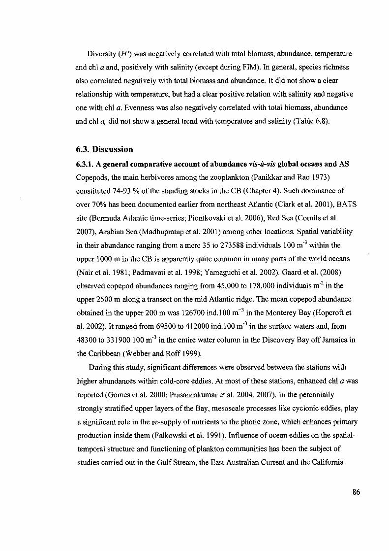
Diversity (H') was negatively correlated with total biomass, abundance, temperature

and chl a and, positively with salinity (except during FIM). In general, species richness

also correlated negatively with total biomass and abundance. It did not show a clear

relationship with temperature, but had a clear positive relation with salinity and negative

one with chl a. Evenness was also negatively correlated with total biomass, abundance

and chl a, did not show a general trend with temperature and salinity (Table 6.8).

6.3. Discussion

6.3.1. A general comparative account of abundance vis-à-vis global oceans and AS

Copepods, the main herbivores among the zooplankton (Panikkar and Rao 1973)

constituted 74-93 % of the standing stocks in the CB (Chapter 4). Such dominance of

over 70% has been documented earlier from northeast Atlantic (Clark et al. 2001), BATS

site (Bermuda Atlantic time-series; Piontkovski et al. 2006), Red Sea (Cornils et al.

2007), Arabian Sea (Madhupratap et al. 2001) among other locations. Spatial variability

in their abundance ranging from a mere 35 to 273588 individuals 100 111-3 within the

upper 1000 m in the CB is apparently quite common in many parts of the world oceans

(Nair et al. 1981; Padmavati et al. 1998; Yamaguchi et al. 2002). Gaard et al. (2008)

observed copepod abundances ranging from 45,000 to 178,000 individuals 111-2 in the

upper 2500 m along a transect on the mid Atlantic ridge. The mean copepod abundance

obtained in the upper 200 m was 126700 ind.100 r11-3 in the Monterey Bay (Hoperoft et

al. 2002). It ranged from 69500 to 412000 ind.100 r11-3 in the surface waters and, from

48300 to 331900 100 111-3 in the entire water column in the Discovery Bay off Jamaica in

the Caribbean (Webber and Roff 1999).

During this study, significant differences were observed between the stations with

higher abundances within cold-core eddies. At most of these stations, enhanced chl a was

reported (Gomes et al. 2000; Prasannakumar et al. 2004, 2007). In the perennially

strongly stratified upper layers of the Bay, mesoscale processes like cyclonic eddies, play

a significant role in the re-supply of nutrients to the photic zone, which enhances primary

production inside them (Falkowski et al. 1991). Influence of ocean eddies on the spatial-

temporal structure and functioning of plankton communities has been the subject of

studies carried out in the Gulf Stream, the East Australian Current and the California

86

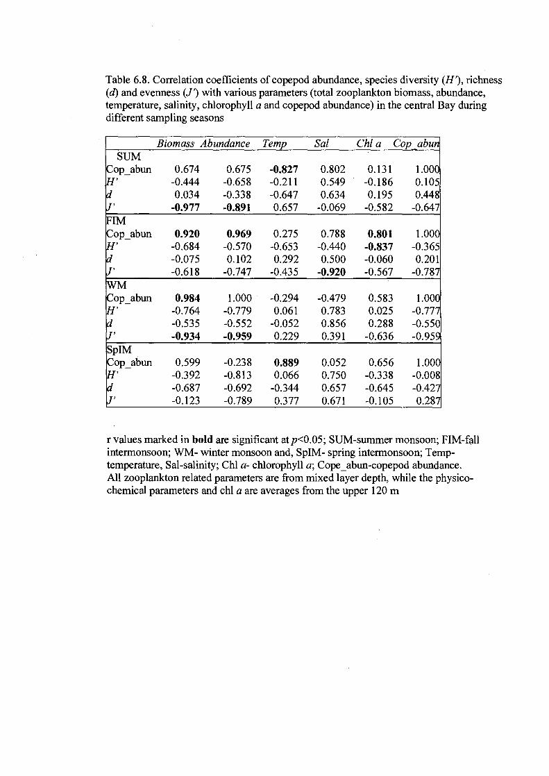
Table 6.8. Correlation coefficients of copepod abundance, species diversity (H'), richness (d) and evenness (J') with various parameters (total zooplankton biomass, abundance, temperature, salinity, chlorophyll a and copepod abundance) in the central Bay during different sampling seasons

Biomass Abundance Temp Sal Chl a Cop_abun SUM

Cop_abun 0.674 0.675 -0.827 0.802 0.131 1.000 H' -0.444 -0.658 -0.211 0.549 -0.186 0.105 d 0.034 -0.338 -0.647 0.634 0.195 0.448 J' -0.977 -0.891 0.657 -0.069 -0.582 -0.647 FIM Cop_abun 0.920 0.969 0.275 0.788 0.801 1.000 H' -0.684 -0.570 -0.653 -0.440 -0.837 -0.365 d -0.075 0.102 0.292 0.500 -0.060 0.201 J' -0.618 -0.747 -0.435 -0.920 -0.567 -0.787 WM Cop_abun 0.984 1.000 -0.294 -0.479 0.583 1.000 H' -0.764 -0.779 0.061 0.783 0.025 -0.777 d -0.535 -0.552 -0.052 0.856 0.288 -0.550 I' -0.934 -0.959 0.229 0.391 -0.636 -0.959 SpIM Cop_abun 0.599 -0.238 0.889 0.052 0.656 1.000 H' -0.392 -0.813 0.066 0.750 -0.338 -0.008 d -0.687 -0.692 -0.344 0.657 -0.645 -0.427 J' -0.123 -0.789 0.377 0.671 -0.105 0.287

r values marked in bold are significant at p<0.05; SUM-summer monsoon; FIM-fall intermonsoon; WM- winter monsoon and, SpIM- spring intermonsoon; Temp-temperature, Sal-salinity; Chl a- chlorophyll a; Cope_abun-copepod abundance. All zooplankton related parameters are from mixed layer depth, while the physico-chemical parameters and chl a are averages from the upper 120 m

Current System (Wiebe et al. 1976; Ortner et al. 1979; Kosnirev and Shapiro 1981; The

Ring Group 1981; Bradford et al. 1982; Tranter et al. 1983; Haury 1984; Piontkovski et

al. 1985).

As mentioned in Chapter 4 and 5, copepods are known to migrate near surface to feed

during night and stay subsurface during daytime. Unlike in other oceanic regions,

copepod diel vertical migration (DVM) was not significant in this study. Oxygen

minimum zone (OMZ) restricts vertical migration of most copepods (Saltzman and

Wishner 1997), except Pleuromamma indica in the eastern Arabian Sea. Low oxygen

waters, common in low latitudes, below the near-surface layer with higher biological

productivity, extending to over 600 m in the Bay could have prevented significant DVM.

Highest copepod abundance was always in the MLD and similar to other studies

(Wishner and Allison 1986), their numbers decreased with depth. However the relative

contribution of copepods increased with depth (Chapter 4) as also reported from the

Arabian Sea (Madhupratap and Haridas 1990). In the Gulf Stream too, the abundance

ranging from 3200 to 7500 ind.100 ni3 in the upper 75 m, fell to <300 ind. 100 111-3 below

200 m (Wishner and Allison 1986). Copepod eggs and nauplii (Chapter 4) were found at

all depths, indicating that spawning and hatching occurred throughout the water column

(Fernandez de Puelles et al. 1996).

6.3.2. Influence of hydrography on copepod distribution, abundance and type

Tropical oceanic waters are generally regarded as relatively stable environments, typified

by small seasonal changes in physical and chemical parameters (Longhurst and Pauly

1987). Calef and Grice (1967) identified seasonal changes in zooplankton abundance off

Barbados. Moore and Sander (1977) conducted a similar investigation of zooplankton

and environmental conditions in the tropical western Atlantic, near Barbados, noting a

lack of seasonal pattern. Within such an steady-state environment, planktonic

communities may be expected to demonstrate minimal seasonal variation, with standing

stocks of organisms changing by only a factor of two or three over an annual cycle

(Blackburn 1981). Highly significant seasonal variation in copepod abundance was

observed during this study. The CB was abundant with copepods during FIM (av: 23643

individuals 100 m-3), SpIM (22246) and WM (21150) compared to SUM (8773). As

87

mentioned in Chapters 4 and 5, SUM season favored the development of large Pyrosoma

swarms causing the overall reduction of other plankton including copepods.

In tropical oceans, where the "seasons" are difficult to predict and usually less

pronounced compared to temperate waters, annual fluctuations are generally related to

the rather variable pattern of annual rainfall (Chisholm and Roff 1990). In estuaries on

the west coast of India, copepods that dominate the mesozooplankton groups

(Madhupratap 1979), showed strong seasonality in accordance with the changes in

salinity (Pillai et al. 1973; Madhupratap 1987). Madhu et al. (2007) also found that the

zooplankton was less abundant during the SUM and FIM months owing to the reduction

in salinity following rains and runoff. Similar results during this study showing positive

correlation of copepod abundance and salinity during the SUM and FIM months of lower

surface salinity indicate that the assemblages are mostly marine.

From the generally positive correlation with chlorophyll a in the euphotic zone, it is

evident that consistent relationships exist between copepods and other physical and

biological variables e.g. maximum copepod biomass is generally at the depth of the chl a

maximum, or at the depth of maximum primary production (Hobson and Lorenzen 1972;

Ortner et al. 1980; Herman 1983, 1989; Roman et al. 1986) as also pointed out by many

authors.

6.3.3. Prominent orders, families, genera and species in the CB

Five orders of Copepoda viz. the Calanoida, Cyclopoida, Harpacticoida, Mormonilloida

and Poecilostomatoida identified during this study in the CB have all been previously

reported from the Arabian Sea (Madhupratap and Haridas 1990; Bottger-Sclmack 1995).

In spite of the seasonal differences in the distribution patterns of these orders in the upper

1000 m, Calanoida was always dominant, as has also been reported from all the oceans

(Pacific: Farran 1936; Atlantic: Deevey and Brooks 1977; Indian Ocean: Madhupratap

and Haridas 1990). Further, all the calanoid (Madhupratap et al. 1990; Padmavati et al

1998; Madhupratap et al 2001) as well as non-calanoid (Bottger-Schnack 1995) families

of copepods observed in this study have been reported previously from the Arabian Sea.

Characteristic pattern in most seasons was subsurface maxima in calanoid abundance at

200-500 m. This was mainly due to abundance of omnivorous families such as

88

Mormonillidae, Lucicutiidae, Metridinidae, Eucalanidae and Spinocalanidae. Apparently

the members of these families are not restricted by low oxygen in the OMZ.

Although a large number of families prevail in the Bay, only a few are numerically

dominant (>5%), with the maximum number of them accounting <1% of total copepods.

Clear vertical partitioning of families was evidenced from this study. As reported earlier,

dominant herbivorous calanoid assemblages of Paracalanidae (Stephen and Kunjamma

1987; Padmavati et al. 1998), Clausocalanidae (Kouwenberg 1994; Cornils et al. 2007)

and Eucalanidae (Saltzman and Wishner 1997) were generally dominant in the top 200

m. While the relative abundance of the former two families decreased with increasing

depth, that of Eucalanidae increased with depth during SpIM in particular. As recorded

during this study, species of Eucalanus have been commonly reported to occupy the

upper and lower OMZ interface in the eastern tropical Pacific (Fernandez-Alamo and

Faber-Lorda 2006).

Cyclopoida comprising exclusively the members of Oithonidae was most abundant in

the thermocline - 300 m stratum, although scarce in other strata. This observation is in

agreement with the studies of Nishida and Marumo (1982) and Padmavati et al. (1998).

According to Kellermann (1987), adults of Oithona spp. prefer to stay in deeper waters,

supposedly to avoid "visual hunters" such as predatory fish larvae.

The warm water families Corycaeidae, Oncaeidae and Sapphirinidae (Raymont 1983)

in the order Poecilostomatoida, the second-most dominant were also abundant in the

MLD and decreased in particular in the OMZ. Similar to observations of Bottger-

Schnack (1995), members of Oncaeidae were more again in deeper depths.

Mormonilloida, comprising a sole mesopelagic family Mormonillidae (Boxshall 1986)

was abundant at all depths below MLD. Similar to observations of Weikert (1982),

Macrosetella gracilis the dominant harpacticoid was most abundant in the MLD during

SUM, although was present throughout the 1000 m.

As also observed by Deevey (1964) and, Deevey and Brooks (1977) smaller species

were more numerous at the surface and larger copepods occurred mainly in the deeper

waters. Species in the genera such as Acartia, Paracalanus, Clausocalanus were mostly

surface living. Acartia, a major constituent of the holozooplankton communities in many

semi-enclosed marine areas (Abraham 1969; Lakkis 1994), showed high degree of

89

seasonality in the MLD. For instance, during WM and SpIM when vertical salinity

gradients were lesser, only the oceanic species i.e. Acartia negligens was observed.

Deeper-living calanoid copepods such as Conaea gracilis, Megacalanus princeps

(bathypelagic), Eucalanus elongatus, and those belonging to the families Aetideidae

(Chiridiella, Pseudochirella, Gaetanus, Undeuchaeta), Scolecitrichidae (Scottocalanus),

Metridinidae (Metridia princeps), Lucicutiidae (Lucicutia ovalis) Augaptilidae

(Augaptilus, Euaugaptilus spp.), Arietellidae (Arietellus) and Aegisthus were generally

found in mesopelagic depths and rarely in MLD (Madhupratap and Haridas 1986;

Padmavati et al. 1998; Stephen and Rao 1980). Lucicutia maxima that has been described

as a possible seasonal migrant, inhabiting the OMZ (Vinogradov and Voronina 1962),

was abundant at these mesopelagic depths during FIM. The bathypelagic species Gaussia

princeps was observed only within the upper 300 m during all seasons except FIM.

Gueredrat (1969) explains that this warm water species, recorded in the equatorial Pacific

has a wider vertical migration in the region of weak upwelling. Never being reported

from the upwelling areas of the Arabian Sea, several specimens were recorded from the

Bay of Bengal during the SUM coinciding with the surfacing of intermediate waters

within 200 m (Saraswathy 1973) thus bringing up the rare deep-water inhabitants. From

this occurrence it is suggested that this is the first report of G. princeps from the deep

waters of the Bay of Bengal.

Deevey and Brooks (1977) found 326 species of copepods in the upper 2000 m of the

water column in the Sargasso Sea. Padmavati et al (1998) reported 98 species of

calanoids in the Arabian Sea. With 55 species found in the upper 200 m, copepod

diversity was reported to be low in the Alboran Mediterranean Sea (Youssara and Gaudy

2001).

As many as 251 species were recorded during the present investigation. The

assemblages contained the least number of species during SpIM (96), moderate numbers

during SUM (162) and the highest numbers during FIM (170) and WM (172). Various

theories about the co-existence of so many copepod species have been advanced.

McGowan and Walker (1979) indicated that many similar species coexist, and that,

selective predation or density-independent predation as the reason for such coexistence.

Most species identified during this study in the CB are tropical-subtropical recorded

90

earlier from Atlantic, Pacific and Indian Oceans (Table 7.9, Chapter 7; Bradford-Grieve

1994; Owre and Foyo 1967; Tanaka 1956; Bradford and Jillett 1980; Razouls et al. 2005-

http://copepodes.obs-banyuls.fr/en) . Some cosmopolitan species such as Clausocalanus

arcuicornis, Pontellina plumata and Eucalanus elongatus (Fleminger and Hulsemann

1973) with circumglobal distribution were also found.

Most of the available data on copepod distribution in the Bay during HOE

(Kasturirangan et al. 1973, Fleminger and Hulsemann 1973, Stephen et al. 1992,

Gopalakrishnan and Balachandran 1992) are mostly pertaining to large calanoid

copepods. The HOE samples were also typically limited to the 0-200 m strata and

therefore, under-represent forms, which have deeper distributions. Unfortunately, the

details of distribution and abundance are only for a few species; notably for Gaussia

princeps (Saraswathy 1973 a, b), Euchaeta spp. (Tanaka 1973) and, Haloptilus acutifrons

(Stephen and Saraladevi 1973). Further, lack of identification and enumeration of the

entire copepod assemblage from samples collected within a defined region and season

during the HOE plankton does not give any idea about the dominant copepod species and

their diversity regionally or seasonally.

6.3.4. First Reports from this study and significance

From this extensive analysis, as many as 15 species identified from the CB are recorded

for the first time from the Indian Ocean. While species such as Chirudiella sp.,

Euchirella speciosa, Euaugaptilus mixtus, Pseudhaloptilus abbreviatus, Drepanopsis

orbus, Metridia pacifica, Amallophora conifer, A. oculata and Tharybis sp. were

exclusively present in the CB, Euchirella rostromagna, Heterorhabdus pacificus,

Xanthocalanus pectinatus, Scottocalanus rotundatus, Monacilla gracilis, and Undinella

spinifer were present in the WB as well (Table 7.9; Chapter 7).

The following species were recorded previously from open waters of the Bay:

Pleuromamma indica, Acartia negligens, Scolecithrix danae, Scolecithrichopsis

ctenopus, Rhincalanus cornutus, Euchirella sp. (Nair et al. 1981), Haloptilus acutifrons

(Stephen and Saraladevi 1973), Gaussia princeps (Saraswathy 1973), Acartia erythraea,

Lucicutia flavicornis, Euchaeta indica, Centropages calaninus, C. gracilis, Pontellina

plumata, Undinula vulgaris, Cosmocalanus darwinii, Labidocera acuta, L. pavo,

91

Pareucalanus attenuatus, Eucalanus pseudattenuatus, Calanopia elliptica, C. minor,

Acrocalanus gibber, Temora discaudata, T. turbinata, Nannocalanus minor,

Canthocalanus pauper, Sapphirina nigromaculata, Corycaeus speciosus, C. catus, C.

danae, Farrannula gibbula, Miracia efferata, Oncaea venusta, Macrosetella gracilis

(Rakhesh et al. 2006), Paracandacia truncata, P. simplex, Candacia catula, C. bispinosa,

C. discaudata (Lawson 1977) and Ratania flava (Saraswathy 1982).

Other than these 41 species, all the rest identified in this study have been reported for

the first time from the central Bay of Bengal. It is a point of significance to note that the

unfolding of copepod assemblages only means that there is so much yet to be learnt from

the BoB for its zooplankton diversity. Stereozoom- and light microscopy photographs for

some of the species identified from the Bay are in Plates 5-8.

The copepod assemblages reported in the Bay are very similar to those reported from

the Arabian Sea. As Rao and Madhupratap (1986) suggest, the North Indian Ocean is

biogeographically a single unit. From this total of 251 species recorded in this study, only

a fraction i.e. 69 species were present at all stations during all seasons. This means that

more than two thirds of the species occurred seasonally. An intriguing question

concerning the ephemeral species is where did they go in certain seasons and, how did

they get back? Apart from the deficiencies of sampling (no duplicate hauls), entry into

diapause is a common trait of many species of marine copepods (Grice and Marcus

1981). Some copepods are found to produce diapause eggs that will not hatch until the

end of a refractory period (Marcus 1989; Chen and Marcus 1997). Having diapause as

part of a life history is clearly advantageous under a number of circumstances, especially

when environmental conditions are periodically adverse for an organism (De Stasio

2004).

A few calanoids especially Calanus (e.g. Pseudocalanus in particular) are typically

abundant in colder high latitudes. Calanus finmarchicus is a dominant, large copepod in

temperate and boreal waters in the North Atlantic (Williams 1988). Similarly, Calanus

cristatus inhabits the North Pacific (Johnson and Brinton 1963). In this study, the

predominance of 0. venusta during all seasons suggests its continuous breeding

throughout the year in the CB as Hopkins (1977) proposed. Deevey (1971) too observed

the predominance of Oncaea in the Sargasso Sea. In addition to this species, herbivorous

92

Clausocalanus arcuicornis was also predominant during SpIM. Similarly, its other

relative, C. furcatus, one of the dominant species in most seasons in CB, is known to

benefit in low phytoplankton conditions (Mazzocchi and Paffenhofer 1998). They are

reported to be widespread (Frost and Fleminger 1968) with maximum occurrence in

subtropical and tropical waters (Deevey 1971; Schulz 1986; Webber and Roff 1995).

They are also represented to be an important numerical component of the copepod

communities throughout the year in the Gulf of Naples, dominating when the autotrophic

biomass was particularly scarce (Peralba and Mazzochi 2004).

The dominant species accounting to >2% of the total copepods also displayed a wide

range of vertical distribution patterns, such as shallow, intermediate and deep-water

distribution. The mesopelagic species, Eucalanus elongatus, varying seasonally, was

deeper from summer to autumn and shallower in winter and spring in the Sargasso Sea

(Deevey and Brooks 1977). The Bay being a warm tropical region, this species was

always in the deeper depths irrespective of seasons. The dominant species, Oncaea

venusta, 0. mediterranea, Clausocalanus arcuicornis, C. furcatus, Mormonilla minor,

Paracalanus aculeatus, P. indicus, Oithona similis, Macrosetella gracilis, Corycaeus

catus, C. danae, C. speciosus, Acrocalanus gracilis, Eucalanus monachus, Calocalanus

pavo, Conaea gracilis and Pleuromamma indica in various seasons were a mix of

oceanic as well as coastal forms reflecting the euryhaline nature of these organisms.

Paracalanus spp. can sustain themselves even when their food type and concentrations

are low as in the offshore waters (Paffenhofer and Stearns 1988).

Affirming their cosmopolitan nature (Bigelow 1926; Rose 1929, 1933; Wilson 1942;

Sewell 1947), Oithona similis and Oncaea venusta with mostly higher abundance in top

200 m were also present at all sampled depths and stations during all the seasons.

Lucicutia flavicornis and Pleuromamma indica as seen in this study, are known to occur

throughout the 1000 m water column (Saltzman and Wishner 1997). As they also

propose, P. indica, Eucalanus elongatus and M minor being able to survive low-oxygen

conditions, were observed to have higher abundances at subsurface depths. Conaea

gracilis with a truly deeper distribution as reported by Raymont (1983) was found in

increased abundances in the deeper waters of the CB.

93

6.3.5. Diversity

Estimating diversity in the pelagic realm is particularly relevant when examining

relationships between hydrography and the pelagic biota. Diversity varied not only with

depth but also seasonally. Akin to earlier observations (Deevey and Brooks 1977),

copepod diversity in the CB was higher in the warmer surface waters and also in deeper

waters. This trend could not be ascertained during SpIM where there was little or no

biomass below 300 m. Longhurst (1985) in an observation from the eastern tropical

Pacific Ocean suggested that a stable vertical structure of the water column might be one

of the more important causes of variation in regional plankton diversity in the euphotic

zone.

Padmavati et al. (1998) attributed the high diversity in the deepest layer to the stable

environment there. From this study, it is possible to suggest that the high diversity in the

deeper strata is ascribable to marked chemical and physical gradients, providing a stable

structured environment (Angel 1993).

The species richness was higher in the surface and the deepest stratum during SUM,

in the thermocline during FIM, in the 300-500 m stratum during WM, and in the surface

during SpIM. Peak occurrence of species at various depths has been documented in

earlier studies (Roe 1972, 1984; Deevey and Brooks 1977; Scotto di Carlo et al. 1984;

Richter 1994; Kosobokova and Hirche 2000). Hayward and McGowan (1979) observed

the species do not seem to be specialists and niche separation is much more subtle than

expected. Species richness was higher in all seasons except the SpIM. In the overall, H'

and d did not show much latitudinal variation. Evenness, a major component of diversity

(Ortner et al. 1982), generally increased with depth registering its highest during SpIM

(0.97).

Both H' and J' are reported to plateau out at 200-300 m depth layers (Shimode et al.

2006). Species richness (<2.4) and evenness (<0.5) reported from the subtropical Inland

Sea of Japan (Madhupratap and Onbe 1986) are lower than those observed during this

study. The numbers of copepod species found from the Kuroshio range from 8 to 94 (He

and Yang 1990). Also, H' values varying from 1.39 to 3.13 reported from the Southeast

China Sea (Shih and Chiu 1998) are lower than the values observed during this study.

Changes in water temperature; salinity and spring phytoplankton bloom (Davis 1987;

94

Siokou-Frangou 1996) are considered to be the primary factors that induce internal

changes in community structure and biodiversity.

6.3.6. Conclusion

The mesozooplankton community in the Bay of Bengal is copepod dominated. Though

the Bay is a tropical basin, high seasonal variability in copepod abundance was observed

with the highest abundance during the intermonsoons and the least during SUM,

generally concurrent with primary production rates (lowest during SUM). Indeed, the

overall abundance (and production) of copepod community appears to be food limited.

However, the coexistence of as many as 69 species throughout the year is suggestive that

the degree of limitation is different both within and between species (Webber and Roff

1995). Well adapted to the low primary production situation, opportunistic feeders such

as Clausocalanus species can be extremely successful in the oligotrophic open waters of

the BoB. Although small copepods such as Oithona spp. are among the main dietary

sources for many commercially important fish, their role in the pelagic trophic dynamics

has traditionally been underestimated due to larger mesh sizes of the nets used for

mesozooplankton sampling (Porri et al. 2007; Gallienne and Robin 2001; Hoperoft et al.

2005). Oithona similis, despite being a smaller sized (500-70011m) species, its

considerable dominance in the Bay is an intriguing phenomenon. Fine tuned studies are

advocated for resolving such issues of zooplankton ecology in the BoB.

In this region, species coexistence seems to be particularly important for copepods,

which seem to have successfully populated the sampled water column and dominate

(numerically) the zooplankton communities under a very large variety of ecological

conditions of the BoB. Large variations in salinity (22-35 psu), warm pool during most

part of the year and lower chl a (0.01-0.44 mg m-3) notwithstanding, the high diversity

and numerical abundance of copepods are first reports from this sparingly studied tropical

basin. In particular, small sized Oncaea venusta, an carnivorous-omnivorous

poecilostomatoid seems to be well adapted to the low-moderate chlorophyll a regime in

the central Bay.

95

Chapter 7

Chapter 7

Copepoda in Western Bay of Bengal

Planktonic copepods are the main consumers of diatoms, in general linking microscopic

algal cells to juvenile fish to whales in the marine food chain. Their distribution in coastal

as well as oceanic regions has been extensively studied by several authors and, under

several programmes such as ICES, JGOFS and GLOBEC in all the three oceans. Many

details of these are provided in Chapter 6.

The Indian Ocean harbors the greatest copepod diversity (http://copepodes.obs-

banyuls.fr/en) . Yet, after the HOE (International Indian Ocean Expedition), the Bay of

Bengal has remained relatively unexplored. To meet up one of the objectives of

understanding the abundance and distribution of copepods in the coastal regions,

sampling was carried out in the western margin of the Bay of Bengal. It was also aimed

to understand the seasonal variability in abundance of copepod species at various depths

in the upper 1000 m along the western Bay.

7.1. Materials and Methods

As described in Chapter 5, zooplankton samples were collected from five strata from four

stations in the western Bay of Bengal (WB) using a multiple plankton closing net. All

other details of collection, identification, statistical analyses and calculation of diversity

indices are as described in Chapter 6.

7.2. Results

7.2.1. Abundance

In the WB, the copepod abundance (individuals 100 r11-3 ; Fig. 7.1) varied from 0.8 to

213540 (average: 16161 ind. 100 in -3), 764 to 114067 (26761 ind. 100 m -3), 394 to

147965 (33047 ind. 100 m3) and 186 to 417920 (36778 ind. 100 m -3) during SUM

(summer monsoon), FIM (fall inter monsoon), WM (winter monsoon) and SpIM (spring

inter monsoon) respectively. While the abundance was significantly higher at WB3

during SUM, the station-wise difference was insignificant during the rest of the seasons

96

0-M LD 500000

400000 -

300000-

200000

1000001

0

SUM FIM

0 0

+vs

tvpl v t wilf3

WM Sp fM I

300-500 m

Ir

40000 ,

30000 -

20000

10000

TT-BT

WM SpIM FIM

0

SUM

FIM SUM SUM

Cop

epod

abu

ndan

ce (

indi

vidu

als

100

m-3

)

WM SpIM

20000-

15000

10000

5000

0

40000-

30000-

20000 -

10000

0

j BT-300 m i

ar

nif er

Sp IM 14/3/ FIM WM

4000 - 500-1000 m

3000 -

2000

1000 111-

0

SUM FIM WM

Season

Figure 7.1. Spatio-temporal variation in copepod abundance at different depths in the western Bay of Bengal. SUM: Summer monsoon, FIM: fall intermonsoon, WM: winter monsoon and SpIM: spring intermonsoon. Scales are different for each graph

(Table 7.1). It decreased significantly with increasing depth only during the

intermonsoons.

Compared to that in the CB, the abundance was higher during all seasons in the WB,

but was significantly higher only during SUM. With the average abundance increasing

from SUM to SpIM, the seasonal variation was also statistically significant. The diel

variation was significant only during SpIM (Table 7.1). Cluster analysis revealed that

spatial distribution of copepod abundance during SpIM, FIM and WM, differed from that

during SUM (Fig. 7.2).

7.2.2. Orders

Six orders viz. Calanoida, Cyclopoida, Harpacticoida, Mormonilloida, Poecilostomatoida

and Siphonostomatoida were identified from the WB (Fig. 7.3; Tables 7.2-7.6). For the

ease of comparison, seasonal variations in the abundance of individuals from different

families under these orders are described below.

Calanoida: During SUM, Calanoida ranging from 34 to 88% showed two subsurface

peaks, one at 200-300 m and the other in the deepest stratum. During FIM (range: 42-

67%) and SpIM (43-71%), it decreased relatively in the 200-300 m stratum before

increasing again in the strata below. Calanoid abundance accounting for 34-56.4% of the

total copepods, decreased from the surface to 1000 m during WM.

As in the CB, this order comprised as many as 24 families in the WB. The individual

species belonging to the family Paracalanidae (17.7%) and Metridinidae (14.5%) during

SUM, Paracalanidae (14.9%) during FIM, Paracalanidae (10.4%) and Clausocalanidae

(9.1%) during WM and, Eucalanidae (19.1%) and Metridinidae (9.8%) during SpIM were

highly preponderant.

Cyclopoida: Comprising a single family, Oithonidae, Cyclopoida (2.1-32%) was

abundant in the thermocline and the 300-500 m stratum during SUM (Fig. 7.3). It was

most abundant in the TT-300 m during FIM (1.4-15.6%), and SpIM (4-15%). During

WM, accounting for 2.4-12.6% of the total copepods, cyclopoids were mostly in the

upper 500 m.

97

Table 7.1. Diel, spatial and temporal difference in copepod abundance in the western Bay of Bengal during summer monsoon (SUM), fall intermonsoon (FIM), winter monsoon (WM) and spring intermonsoon (SpIM) as deciphered through non-parametric tests

Wilcoxon Matched Pairs Test between day and night

Seasons N T Z p SUM 20 27 1.60 p >0.05 FIM 15 49 0.62 p >0.05 WM 20 47 0.74 p >0.05 SpIM 12 11 2.20 p< 0.05

Friedman ANOVA Seasons Chi Sqr. N df p

Between stations SUM 6.5 4 2 p < 0.05 FIM 1.2 5 2 p >0.05 WM 0.6 2 3 p >0.05 SpIM 3.6 4 3 p >0.05

Between depths SUM 7.2 2 4 p > 0.05 FIM 9.33 3 4 p= 0.05 WM 5.8 3 3 p > 0.05 SpIM 11.1 4 3 p < 0.05

Between Seasons 20.14 14 3 p< 0.05

Between transects SUM 4.57 14 1 p< 0.05 FIM 0 .60 15 1 p >0.05 WM 0 .06 15 1 p >0.05 SpIM 2.25 16 1 p >0.05

Significant results are marked bold

SpIM

FIM

WM

SUM

100

40

60 80

Bray- Curtis Similarity (%)

Figure 7.2. Cluster dendrogram based on Bray- Curtis similarity coefficients, depicting similarity in copepod abundance between seasons in the western Bay.

SpIM

I

II

II

Dep

th s

trata

(m)

0-MLD

TT-BT

200-300

300-500

500-1000

SUM

II

11

I

IN

I I

0-MLD

TT-BT

200-300

300-500

500-1000

FIM

I

IN

I I

t

INN

)1111■6nomvm ■ Calanoida

■ Cyclopoida

o Harpacticoida

■ Mormonilloida

■ Poecilostomatoida

■ Siphonostomatoida

I-

IIMINE011=11111111

0%

50%

100% 0%

50% 100%

Percentage of Copepoda Orders

Figure 7.3. Vertical distribution of Copepoda orders at different depths during summer monsoon (SUM), fall intermonsoon (FIM), winter monsoon (WM) and spring intermonsoon (SpIM) in the western Bay of Bengal

Harpacticoida: Present throughout the sampled column, harpacticoids registered a range

of 3.1-13.3% and were the most abundant during SUM. In the other three seasons, they

accounted for <4% of total copepods at all sampled depths.

Mormonilloida: This order consisting of a single family Mormonillidae, was observed in

the upper two layers during SUM (2.6-4.2%). In other three seasons, it was prominently

observed below the MLD (FIM: 0.5-10.8%; WM: 0.5-14.6%; SpIM: 0.7-28.2%).

Poecilostomatoida: Contributing widely to 5-22% of the total copepods, members of this

order occurred at all depths. They were the most dominant in the surface and the strata

between 200-500 m during SUM. Their contribution to total copepods ranged from 22.7

to 38.3% during FIM with the highest percentage in the 200-300 m stratum. Varying

from 25.4 to 46.2%, poecilostomatoids relatively increased with depth during WM.

During SpIM, they accounted for 13.9-23.6% of the total copepods. They were more in

upper two and the lowermost strata sampled. Five families were identified under this

order, with Oncaeidae as the most dominant one during all easons.

Siphonostomatoida: This order was observed with just one family, Rataniidae in the

thermocline region during WM only.

Overall, Calanoida was almost always the most dominant order (53%), followed by

Poecilostomatoida (24.3%), Cyclopoida (9.6%), Mormonilloida (6.0%) and

Harpacticoida (3.7%). Siphonostomatoida (0.01%) was rare among the 6 orders

identified.

7.2.3. Families

From a total of 38 families (Tables 7.2-7.6) that occurred during the study period, the

numerical abundance of individuals of only eight families (Clausocalanidae, Eucalanidae,

Metridinidae, Paracalanidae, Oithonidae, Mormonillidae, Corycaeidae and Oncaeidae)

was greater than five. Twelve families (Acartiidae, Calanidae, Candaciidae,

Centropagidae, Euchaetidae, Lucicutiidae, Scolecithrichidae, Spinocalanidae,

Clytemnestridae, Euterpinidae, Miraciidae and Sapphirinidae) were minor, comprising 1-

5% of total individuals. The remaining 18 families (Aetideidae, Arietellidae,

Augaptilidae Fosshageniidae Heterorhabdidae Mecynoceridae, Megacalanidae,

Nullosetigeridae, Phaennidae, Pontellidae, Rhincalanidae, Temoridae, Tharybidae,

98

Table 7.2. Seasonal variations in abundance (individuals 100 IT1-3 ) and percentage (%) of different copepod species in the mixed layer depth in western Bay of Bengal

SUM FIM WM SpIM

Species Abundance % Abundance °A) Abundance % Abundance % CALANOIDA Acartiidae Acartia amboinens s A - 316.20 0.34 A - A - A. negligens 401.71 0.55 752.21 0.82 92.51 0.11 2295.23 1.80 A. spinicauda A - 7919.12 8.64 A A Aetideidae Aetideus armatus A A 1.67 0.00 A Chirundina streetsi A A 1.67 0.00 A - Euchirella amoena A A A 99.14 0.08 E. bitumida A A 1.67 0.00 713.01 0.56 E. curticauda A 104.33 0.11 A - A E. galeata A A 1.67 0.00 A E. indica 724.81 1.00 A A A -

Euchirella sp. A A 1.00 0.00 2882.77 2.26 Arietellidae Arietellus giesbrechtii A 316.20 0.34 A A Augaptilidae Haloptilus longicornis A A 57.84 0.07 29.06 0.02 H. ornatus A 60.01 0.07 A A Pseudhaloptilus pacificus A A A 1.67 0.00 Calanidae Canthocalanus pauper 401.71 0.55 912.02 0.99 2476.36 2.86 988.08 0.77 Cosmocalanus danvinii A A - 616.71 0.71 102.75 0.08 Mesocalanus tenuicornis A 119.81 0.13 A - A -

Undinula vulgaris 1528.22 2.11 1908.63 2.08 2636.31 3.04 994.07 0.78 Candaciidae Candacia bradyi 724.81 1.00 692.42 0.76 754.53 0.87 166.88 0.13 C. discaudata A A 0.83 0.00 742.07 0.58 C. pachydactyla A 873.07 0.95 A 3.34 0.00 Candacia sp. 401.71 0.55 A - 75.73 0.09 800.07 0.63 Paracandacia truncata 401.71 0.55 A A 49.80 0.04 Centropagidae Centropages calaninus A A A 1046.78 0.82 C. dorsispinatus A A A - A - C. furcatus 724.81 1.00 A 1264.05 1.46 4544.16 3.55 C. gracilis A A 92.51 0.11 A - Clausocalanidae Clausocalanus arcuicornis 724.81 1.00 A - 6603.53 7.62 8826.99 6.91 C. furcatus A 3213.97 3.50 2774.73 3.20 356.82 0.28 C. pergens A A - A - 720.94 0.56 Clausocalanus sp. A A 149.46 0.17 A - Eucalanidae Eucalanus crassus A 436.53 0.48 A 2923.92 2.29 E. subcrassus A A A A - E. elongatus A 164.34 0.18 A - A - E. monachus 5955.68 8.21 2533.82 2.76 3532.54 4.08 A 17.36 E. mucronatus A A - 60.00 0.07 52.68 0.04 E. pseudattenuatus A A - A - A Eucalanus sp. A 1264.81 1.38 A - 52.68 0.04 Pareucalanus attenuatus A A - 1044.53 1.21 1522.37 1.19 Subeucalanus crassus A A A A -

Euchaetidae Euchaeta concinna 323.10 0.45 119.81 0.13 A A - E. indica 401.71 0.55 316.20 0.34 233.33 0.27 713.01 0.56 E. marina 969.30 1.34 599.03 0.65 754.89 0.87 2437.72 1.91 Euchaeta sp. A - A - 113.53 0.13 29.06 0.02 Fosshageniidae Temoropia mayumbaensis A 857.07 0.93 A 932.57 0.73 Heterorhabdidae Hemirhabdus grimaldi A 104.33 0.11 A A Heterorhabdus abyssalis A 104.33 0.11 A A H. pacificus A 240.03 0.26 A A - H. papilliger A A - 21.02 0.02 720.94 0.56 H. spinifrons 401.71 0.55 A 756.20 0.87 A Lucicutiidae tucicutia flavicornis 1528-22 211 3393.20 3 70 141 02 0.16 3239.33 2.53 L. magna A 60.01 0.07 A A

L. maxima 401.71 0.55 224.35 0.24 120.00 0.14 A

L. ovalis A 164.34 0.18 A - A Mecynoceridae Mecynocera clausii A A 484.61 0.56 108.19 0.08

Megacalanidae Megacalanus prfnceps A A A 720.94 0.56

Metridinidae Metridia brevicauda A 120.02 0.13 1.67 0.00 720.94 0.56 Pleuromamma gracilis A 493.02 0.54 1846.22 2.13 1491.94 1.17

P. indica 2733.35 3.77 1635.01 1.78 210.35 0.24 8791.38 6.88

P. quadrangulata A A - A 29.06 0.02 P. robusta A A - A - 6789.76 5.31

Pleuromamma sp. A 316.20 0.34 92.51 0.11 A -

Nullosetigeridae Nullosetigera sp. A A A 713.01 0.56

Paracalanidae Acrocalanus gibber 724.81 1.00 316.20 0.34 405.52 0.47 155.43 0.12

A. gracilis 803.42 1.11 718.83 0.78 2088.00 2.41 3038.88 2.38 A. longicornis 646.20 0.89 600.87 0.66 4158.77 4.80 2228.70 1.74 A. monachus A A - 57.84 0.07 383.83 0.30 Calocalanus pavo 724.81 1.00 239.61 0.26 1714.21 1.98 289.80 0.23

C. pavoninus A 479.22 0.52 A - A - C. plumulosus A - A - 324.51 0.37 0.00 0.00 Paracalanus indices 12383.01 17.07 2786.43 3.04 6969.85 8.04 1789.64 1.40

P. aculeatus 1371.01 1.89 2541.04 2.77 754.53 0.87 A P. parvus 724.81 1.00 3887.16 4.24 393.20 0.45 A Phaennidae Amallophora crassirostris A 104.33 0.11 A A A. irritans 803.42 1.11 A - A A Cephalophanes frigidus A A - A 50.07 0.04

Phaenna spinifera A - 1897.22 2.07 A A Xanthocalanus pectinatus 323.10 0.45 1264.81 1.38 A A

Pontellidae Calanopia elliptica A A - 754.53 0.87 713.01 0.56

Labidocera acuta A 180.02 0.20 A 1433.95 1.12

L. minuta A - 316.20 0.34 5.00 0.01 A

L. pectinata A A - A A -

L. pavo A - 436.53 0.48 754.53 0.87 75.52 0.06

Pontellina plumata A 239.61 0.26 1128.46 1.30 294.14 0.23

Pontellopsis scotti A 436.53 0.48 A - A Rhincalanidae Rhincalanus cornutus A - A 230.00 0.27 713.01 0.56

Scolecitrichidae Amallothrix gracilis A - 60.01 0.07 230.00 0.27 166.88 0.13

Lophothrix frontalis 401.71 0.55 164.34 0.18 1.67 0.00 A A Scaphocalanus magnus A - A A 713.01 0.56 S. major A 60.01 0.07 A A - Scaphocalanus sp. A A 60.00 0.07 713.01 0.56

S. dentata A A - A 713.01 0.56 Scolecithricella sp. A 632.41 0.69 A 102.75 0.08 Scolecithrichopsis ctenopus A A A 219.57 0.17

S. cianae 724.81 1.00 A 21.02 0.02 887.82 0.69

S. nicobarica A 239.61 0.26 A A -

Scolecithrix sp. A A A 52.68 0.04

Scottocalanus helenae A A - A 29.06 0.02 Spinocalanidae Monacilla gracilis A 6324.07 6.90 A A Temoridae Temora turbinata A A - A - 208.11 0.16

T. discaudata A 660.67 0.72 1278.73 1.48 829.13 0.65 T. stylifera A A - 1048.73 1.21 958.24 0.75 Tharybidae Undinella brevipes A A A - A CYCLOPOIDA Oithonidae Oithona brevicomis 401.71 0.55 119.81 0.13 A - A -

O. plumifera A 1634.59 1.78 2608.55 3.01 2244.56 1.76 0. simi/is 5632.58 7.76 1377.87 1.50 4713.22 5.44 5923.76 4.63 0. spinirostris 401.71 0.55 436.01 0.48 A A -

Oithona sp. A 312.99 0.34 A A HARPACTICOIDA Aegisthidae Aegisthus mucronatus A 632.41 0.69 A A Clytemnestridae

Clytemnestra scutellata A A 904.88 1.04 A Ectinosomatidae Microsetella rosea A 119.81 0.13 A 50.07 0.04 Euterpinidae Euterpina acutifrons 323.10 0.45 316.20 0.34 1509.07 1.74 A Miraciidae Macrosetella gracilis 1528.22 2.11 817.74 0.89 1215.97 1.40 99.14 0.08 Miracia efferata A A 95.76 0.11 168.44 0.13 MORMONILLOIDA Mormonillidae Mormonilla minor 2410.25 3.32 493.02 0.54 450.35 0.52 871.27 0.68 M. phasma 401.71 0.55 A - A - A -

POECILOSTOMATOIDA Corycaeidae Corycaeus asiaticus A 316.20 0.34 A - A - C. catus 803.42 1.11 2044.70 2.23 2589.21 2.99 2019.59 1.58 C. danae 724.81 1.00 3669.46 4.00 396.45 0.46 1551.61 1.21 C. longistylis A 436.53 0.48 A - A C. speciosus 1126.52 1.55 2947.15 3.21 582.04 0.67 2058.63 1.61 C. typicus A A - 964.00 1.11 A -

Corycaeus sp. A A 57.84 0.07 750.00 0.59 Lubbockidae Lubbockia aculeata A A A 166.88 0.13 Oncaeidae Conaea gracilis A A - 300.00 0.35 A -

Oncaea mediterranea A - A - 1166.57 1.35 157.27 0.12 O. venusta 11265.16 15.53 12292.27 13.40 A 19.43 9579.13 7.49 Triconia conifera A - 765.00 0.83 57.84 0.07 713.01 0.56 Sapphirinidae Copilia longistylis 803.42 1.11 A - 74.73 0.09 A - C. mirabilis A 119.81 0.13 A 153.53 0.12 C. quadrata A - 539.23 0.59 1231.86 1.42 1653.51 1.29 C. vitrea 401.71 0.55 119.81 0.13 A A Sapphirina auronitens 323.10 0.45 A 2.50 0.00 A S. nigromaculata A - 239.61 0.26 A A 166.88 0.13 S. ovatolanceolata 803.42 1.11 A - 92.51 0.11 A Sapphirina sp. A - A - 60.00 0.07 1555.93 1.22 Unidentified 6829.04 9.41 6848.29 7.47 1349.89 1.56 1463.01 1.14 Total individuals 100 ni3 72560 91706 86652 127830

Table 7.3. Seasonal variations in abundance (individuals 100 m -3) and percentage (%) of different copepod species in the thermocline in western Bay of Bengal

SUM FIM WM SpIM

Species Abundance % Abundance % Abundance % Abundance % CALANOIDA Acartiidae Acartia etythraea A 72.59 0.49 A A A. negligees A 7.73 0.05 0.50 0.00 48.67 0.30 A. spinicauda 12.11 1.41 A - A A Aetideidae Aetideus acutus A 7.73 0.05 A A A. armatus A A 0.42 0.00 A - A. giesbrechtii A A A 10.11 0.06 Euchirella bitumida A A - 0.50 0.00 10.73 0.07 E. galeata A - 73.55 0.50 A A E. indica A - A 16.68 0.08 10.11 0.06 E. latirostris A A A 0.28 0.00 E. rostromagna A 7.73 0.05 A A E. venusta A A 9.83 0.05 A Euchirella sp. A 3.66 0.02 20.42 0.10 13.01 0.08 Gaetanus miles A A 0.40 0.00 A Undeuchaeta sp. A 23.20 0.16 A A Arietellidae Arietellus giesbrechtii A A A 0.28 0.00 Augaptilidae Euaugaptilus hecticus A A A - 0.28 0.00 E. laticeps A A - 0.42 0.00 0.28 0.00 Haloptilus longicornis A 30.56 0.21 1.40 0.01 84.64 0.52 H. spiniceps A 30.19 0.20 0.86 0.00 A Pseudhaloptilus pacificus A A 0.42 0.00 A Calanidae Canthocalanus pauper A - 15.10 0.10 124.79 0.60 149.45 0.93 Cosmocalanus darwinii A A 15.89 0.08 25.25 0.16 Mesocalanus tenuicornis A 72.59 0.49 A - A Undinula vulgaris A 4.43 0.03 158.81 0.77 417.62 2.59 Candaciidae Candacia bradyi A 15.47 0.10 47.87 0.23 124.79 0.77 C. catula A A A 10.11 0.06 C. discaudata A 145.17 0.98 82.13 0.40 9.87 0.06 C. pachydactyla A A A 35.36 0.22 Candacia sp. 12.11 1.41 A A 253.61 1.57 Paracandacia truncata A A A 35.94 0.22 P. simplex A A A A Centropagidae Centropages calaninus A A 0.50 0.00 A C. furcatus 24.23 2.82 30.93 0.21 493.06 2.39 198.65 1.23 Clausocalanidae Clausocalanus arcuicornis 24.23 2.82 0.96 0.01 2942.13 14.24 1124.47 6.97 C. furcatus A 840.16 5.68 233.86 1.13 195.04 1.21 C. pergens A 176.10 1.19 A A Drepanopsis frigidus A 72.59 0.49 A A Eucalanidae Eucalanus crassus A 45.29 0.31 30.18 0.15 0.28 0.00 E. subcrassus A A - A A E. elongatus A - 162.38 1.10 272.31 1.32 44.57 0.28 E. monachus 96.91 11.27 981.53 6.64 206.81 1.00 2519.60 15.61 E. mucronatus 12.11 1.41 1.92 0.01 24.12 0.12 144.77 0.90 E. pseudattenuatus A 0.96 0.01 A A Eucalanus sp. A 219.49 1.49 63.56 0.31 19.59 0.12 Pareucalanus attenuatus A A 171.52 0.83 169.71 1.05 Euchaetidae Euchaeta concinna 24.23 2.82 A A A E. indica A A - 0.42 0.00 10.38 0.06 E. marina A 238.93 1.62 302.43 1.46 10.38 0.06 Euchaeta sp. A 95.33 0.65 139.79 0.68 119.57 0.74 Fosshageniidae Temoropia mayumbaensis A 194.09 1.31 255.46 1.24 154.66 0.96 Heterorhabdidae Heterorhabdus abyssalis A 29.92 0.20 A A H. papilliger A 30 19 0.20 10 85 0.51 144 42 0.89 H. spinifrons A A - 37.90 0.18 44.83 0.28

Heterorhabdus sp. Heterostylites longicornis Lucicutiidae

A A

A A

A A

2.62 0.28

0.02 0.00

Lucicutiaflavicornis 36.34 4.23 564.81 3.82 262.82 1.27 561.37 3.48 L. lucida A 0.96 0.01 A - A - L. maxima A A 77.23 0.37 2.62 0.02 L. ovalis A 4.80 0.03 63.56 0.31 10.11 0.06 Mecynoceridae Mecynocera clausii A 80.32 0.54 82.27 0.40 20.22 0.13 Metridinidae Metridia brevicauda A 15.10 0.10 23.95 0.12 A Metridia sp. A 2.70 0.02 A - A Pleuromamma gracilis A - 31.52 0.21 232.11 1.12 32.08 0.20 P. indica 24.23 2.82 943.30 6.38 984.50 4.76 969.32 6.00 P. robusta A 145.17 0.98 115.75 0.56 64.97 0.40 Pleuromamma sp. A 54.13 0.37 167.14 0.81 A Nullosetigeridae Nullosetigera sp. A 7.73 0.05 A A Paracalanidae Acrocalanus gibber 36.34 4.23 16.83 0.11 16.77 0.08 A A. gracilis 24.23 2.82 72.59 0.49 77.43 0.37 372.61 2.31 A. longicornis 24.23 2.82 3.47 0.02 336.70 1.63 144.55 0.90 A. monachus A A A 10.11 0.06 Calocalanus pavo A 30.19 0.20 373.76 1.81 161.60 1.00 C. plumulosus A A 147.39 0.71 10.11 0.06 Paracalanus indicus 84.80 9.86 279.59 1.89 837.75 4.05 267.99 1.66 P. aculeatus A 177.06 1.20 A A P. crassirostris A A A - A P. parvus A 264.29 1.79 94.10 0.46 50.50 0.31 Phaennidae Amallophora crassirostris A 7.73 0.05 A A Cephalophanes frigidus A A A 25.25 0.16 Onchocalanus affinis A 0.96 0.01 A A Phaenna spinifera A 23.20 0.16 A A Xanthocalanus pectinatus A 30.93 0.21 A A Pontellidae Calanopia minor A A A 26.22 0.16 Labidocera acuta A A - A 19.59 0.12 Pontellina plumata A 72.59 0.49 A 25.52 0.16 Rhincalanidae Rhincalanus cornutus A A - 31.71 0.15 20.81 0.13 R. nasutus A A 0.38 0.00 A R. rostrfrons A A 9.33 0.05 9.87 0.06 Scolecitrichidae Amallothrix gracilis A A 162.41 0.79 119.30 0.74 Lophothrix frontalis A A - 0.83 0.00 A - Scaphocalanus echinatus A 0.96 0.01 A - A S. major A 0.96 0.01 A - A Scaphocalanus sp. A A - 0.40 0.00 A Scolecithricella dentata A 1.92 0.01 15.89 0.08 A - Scolecithricella sp. A 72.59 0.49 A - 12.73 0.08 Scolecithrichopsis ctenopus A 7.73 0.05 30.56 0.15 10.11 0.06 Scolecithrix bradyi A 7.73 0.05 A A S. danae 12.11 1.41 273.81 1.85 19.40 0.09 10.11 0.06 S. nicobarica A 22.83 0.15 A A Scolecithrix sp. A A - A 19.59 0.12 Spinocalanidae Monacilla gracilis A 23.20 0.16 65.33 0.32 A M. typica A 7.73 0.05 A - A Spinocalanus magnus A 9.47 0.06 A - A Temoridae Temora turbinata A 72.59 0.49 A 10.11 0.06 T. discaudata A 74.32 0.50 0.38 0.00 44.83 0.28 T. stylifera A A A A 10.11 0.06 CYCLOPOIDA Oithonidae Oithona brevicornis A 72.59 0.49 A - A - O. plumijkra A - 247.95 1.68 188.06 0.91 297.99 1.85 0. similis 266.51 30.99 1112.04 7.52 1573.26 7.61 2130.82 13.20 O. spinirostris 12.11 1.41 247.95 1.68 A - 25.25 0.16 Oithona sp. A 16.83 0.11 A A -

HARPACTICOIDA Aegisthidae Aegisthus mucronatus A 108.26 0.73 17.58 0.09 A

Clytemnestridae Clytemnestra scutellata A A 63.94 0.31 0.28 0.00 Ectinosomatidae Microsetella norveigica A A 15.89 0.08 A M. rosea A A 81.39 0.39 A Euterpinidae Euterpina acutifrons A A 16.77 0.08 A Miraciidae Macrosetella gracilis 12.11 1.41 72.29 0.49 82.27 0.40 25.83 0.16 Miracia efferata A - A 10.33 0.05 144.55 0.90 Oculosetella gracilis A A 0.38 0.00 A MORMONILLOIDA Mormonillidae Mormonilla minor 36.34 4.23 1089.07 7.37 2697.18 13.05 204.15 1.26 M. phasma A - 149.55 1.01 A - A POECILOSTOMATOIDA Corycaeidae Corycaeus catus 12.11 1.41 248.32 1.68 357.91 1.73 235.24 1.46 C. danae 24.23 2.82 337.33 2.28 254.97 1.23 70.48 0.44 C. longistylis A - 72.59 0.49 0.33 0.00 A C. speciosus A 190.46 1.29 36.84 0.18 418.38 2.59 C. typicus A A 48.85 0.24 A Lubbockidae Lubbockia aculeata A A 0.50 0.00 25.25 0.16 L. squillimana A A 15.89 0.08 A Oncaeidae Conaea gracilis A A 69.99 0.34 2.62 0.02 Oncaea mediterranea A A 684.17 3.31 358.28 2.22 O. notopus A A A A 0. venusta 24.23 2.82 2152.05 14.56 3529.31 17.08 1928.40 11.95 Pachos punctatum A A A 0.55 0.00 Triconia conifera A A 61.61 0.30 134.31 0.83 Sapphirinidae Copilia mirabilis A 72.59 0.49 A 144.55 0.90 C. quadrats A A - 66.69 0.32 57.56 0.36 C. vitrea A 72.59 0.49 131.00 0.63 A Sapphirina auronitens A 103.15 0.70 0.90 0.00 A S. intestinata A 7.73 0.05 A A S. nigromaculata 12.11 1.41 87.68 0.59 A 119.30 0.74 S. ovatolanceolata A A 1.00 0.00 10.11 0.06 Sapphirina sp. A 15.10 0.10 A 64.42 0.40 SIPHONOSTOMATOIDA Rataniidae Ratania (lava A A - 47.33 0.23 A Unidentified 12.11 1.41 1266.53 8.57 615.89 2.98 558.66 3.46 Total individuals 100 m 4 860 14780 20663 16143

Aegisthidae, Ectinosomatidae, Clausidiidae, Lubbockidae and Rataniidae) accounted for

less than 1% of total copepods.

In the MLD, the largest number of families occurred during most seasons (SUM: 21,

FIM: 29, WM: 26 and SpIM: 30;Table 7.2). Members of Oncaeidae contributing from 8.2

to 21.2%, Paracalanidae from 6.2 to 24.0%, Eucalanidae from 4.8-20.9% and Oithonidae

from 4.2 to 8.9% were dominant in this stratum during all seasons. Representatives of

Corycaeidae (4.9-10.3%) were in higher abundance during FIM, WM and SpIM.

Members of Acartiidae (9.8%), Calanidae (6.6%) and Metridinidae (14%) were the most

abundant in MLD during FIM, WM and SpIM respectively. Clausocalanidae was

observed in greater abundance during WM (11%) and SpIM (7.8%).

The number of families occurring in the thermocline (SUM: 17, FIM: 29, WM: 31,

SpIM: 30; Table 7.3) decreased during SUM and increased during WM compared to that

in the MLD. Paracalanidae (5.7-20%) and Oithonidae (8.5-32.4%) were preponderant

during all seasons. Eucalanidae accounting to 10-18% was dominant in most seasons

except WM. Similarly; members of Clausocalanidae (7.4-15.4%), Oncaeidae (15-21%)

and Metridinidae (6.6-8%) were preponderant during all seasons except SUM.

Mormonillidae was dominant during FIM (8.4%) and WM (13%).

In the stratum between the bottom of the thermocline and 300 m, lesser number of

families occurred compared to the strata above (SUM: 13, FIM: 26, WM: 29, SpIM: 24;

Table 7.4). Only the members of Eucalanidae (5-18.4%) were preponderant during all

four seasons. Families, Metridinidae (4.5-7.4%), Oithonidae (7.5-15.6%) and Oncaeidae

(10.6-33.8%) were dominant during all seasons in this stratum except SUM.

Paracalanidae, accounting to 9.2-33.3% decreased in abundance from SUM to WM and

was not dominant during SpIM. Members of Mormonillidae accounted for 13% during

WM and 28% during SpIM. In the same seasons, Metridinidae accounted for 7.4 and 6%

respectively. Maximum percentage of members of Clausocalanidae (11.3%) and

Corycaeidae (19.4%) was during WM and SUM.

Compared to other seasons (FIM: 28, WM: 27, SpIM: 23), the numbers of families

were only six during SUM in the 300-500 m stratum (Table 7.5). Families such as

Acartiidae, Augaptilidae, Centropagidae, Clausocalanidae, Eucalanidae, Euchaetidae,

Heterorhabdidae, Lucicutiidae, Metridinidae, Pontellidae, Rhincalanidae and Temoridae

99

Table 7.4. Seasonal variations in abundance (individuals 100 m -3) and percentage (%) of different copepod species in the base of the thermocline to 300 m stratum in western Bay

SUM FIM WM SpIM

Species Abundance % Abundance % Abundance % Abundance % CALANOIDA Acartiidae Acartia amboinensis A 1.61 0.01 A A A. centrura A - A 0.50 0.00 A A. elythraea 52.27 2.78 A A A A. negligens A 27.41 0.16 A 2.57 0.11 A. spinicauda A 4.82 0.03 A A Aetideidae Aetideus armatus A A 0.89 0.01 A Euchirella bitumida A A A 0.98 0.04 E. indica A A 30.34 0.24 A Euchirella sp. A A 25.29 0.20 A Gaetanus miles A A - 6.97 0.05 2.57 0.11 Valdiviella brevicornis A 54.82 0.32 A A Augaptilidae Euaugaptilus angustus A A A A 0.23 Haloptilus longicornis A 15.60 0.09 32.11 0.25 23.01 0.97 H. ornatus A 27.41 0.16 A A - Calanidae Canthocalanus pauper A 15.60 0.09 98.61 0.78 A Undinula vulgaris A 295.25 1.71 129.83 1.02 A Candaciidae Candacia bradyi A 1.61 0.01 99.50 0.78 0.49 0.02 C. discaudata A A 24.40 0.19 A C. pachydactyla A A 5.93 0.05 A Candacia sp. A A 5.93 0.05 A Paracandacia truncata A 25.70 0.15 A - 2.57 0.11 Centropagidae C. furcatus 52.27 2.78 31.19 0.18 A - 16.25 0.68 Centropages sp. A A 25.42 0.20 A - Clausocalanidae Clausocalanus arcuicornis 26.13 1.39 A 1218.17 9.59 46.01 1.94 C. furcatus A 94.26 0.54 212.66 1.67 7.39 0.31 C. pergens A 3.21 0.02 A - A - Eucalanidae Eucalanus crassus 26.13 1.39 15.60 0.09 A - A - E. elongatus A 999.77 5.78 350.49 2.76 9.95 0.42 E. monachus 52.27 2.78 2.29 0.01 247.93 1.95 410.38 17.26 E. mucronatus A 31.19 0.18 33.60 0.26 8.76 0.37 Eucalanus sp. 52.27 2.78 A A - A -

Pareucalanus attenuatus A A 1.03 0.01 7.39 0.31 Euchaetidae Euchaeta concinna A 15.60 0.09 A - A - E. indica A 1.61 0.01 74.07 0.58 23.01 0.97 E. marina A 155.97 0.90 148.66 1.17 3.05 0.13 Euchaeta sp. A 15.60 0.09 5.93 0.05 A - Fosshageniidae Temoropia mayumbaensis A 3.89 0.02 A 7.92 0.33 Heterorhabdidae Heterorhabdus abyssalis A 17.18 0.10 A - A H. fistulosus A A - 6.40 0.05 A H. pacificus A 0.68 0.00 5.93 0.05 A - H. papilliger A 114.21 0.66 30.34 0.24 6.36 0.27 H. spinifrons A A A 80.90 0.64 13.28 0.56 Heterorhabdus sp. A 54.82 0.32 6.40 0.05 7.92 0.33 HeterosOilites longicornis A A A 24.92 0.20 A - H. major A A A 1.03 0.01 A Lucicutiidae Lucicutiaflavicornis A 229.09 1.32 298.25 2.35 107.04 4.50 L. maxima 104.54 5.56 2.05 0.01 5.93 0.05 A - L. ovalis A 295.25 1.71 A - A Mecynoceridae Mecynocera clausii A A 6.40 0.05 7.39 0.31 Metridinidae Gaussia princeps A A 0.89 0.01 1.47 0.06 Metridia brevicauda A 136 0 01 15.24 0 12 A Metridia sp. A 2.98 0.02 A A

Pleuromamma gracilis A 9.59 0.06 278.93 2.20 20.08 0.84 P. indica 26.13 1.39 704.59 4.07 460.26 3.62 109.20 4.59 P. robusta A 56.42 0.33 128.77 1.01 12.74 0.54 P. xiphias A A 24.40 0.19 A - Pleuromamma sp. A A 31.36 0.25 A Paracalanidae Acrocalanus gibber 26.13 1.39 979.33 5.66 . A - 5.36 0.23 A. gracilis 26.13 1.39 0.68 0.00 173.57 1.37 2.57 0.11 A. longicornis 104.54 5.56 621.69 3.59 376.30 2.96 A Calocalanus pavo 26.13 1.39 A - 204.37 1.61 12.74 0.54 C. plumulosus A A - 74.07 0.58 16.34 0.69 Paracalanus indices 418.15 22.22 1671.16 9.65 260.11 2.05 31.76 1.34 P. aculeatus A 31.88 0.18 A - A P. parvus 26.13 1.39 529.21 3.06 74.07 0.58 A Phaennidae Onchocalanus affinis A 31.19 0.18 A A Phaenna spinifera A 1.61 0.01 A A Pontellidae Labidocera acuta A A 48.81 0.38 A Pontellina plumata A A 74.07 0.58 A Rhincalanidae Rhincalanus cornutus A A 83.38 0.66 39.11 1.65 R. rostrYi.ons A A 0.89 0.01 A Scolecitrichidae Amallothrix arcuata A 1.61 0.01 A - A Pseudoamallothrix ovata A 27.41 0.16 A - A Lophothrixfrontalis A 0.68 0.00 65.06 0.51 0.98 0.04 Scaphocalanus magnus A A A - 0.98 0.04 Scaphocalanus sp. A A - 34.72 0.27 A Scolecithricella sp. A 29.43 0.17 A - A Scolecithrichopsis ctenopus A - 15.60 0.09 A A Scolecithrix danae A - 124.78 0.72 A A S. nicobarica A 0.68 0.00 A A Spinocalanidae Monacilla gracilis A 3.21 0.02 A A M. tenera A A A - 14.78 0.62 M Oka A A 109.48 0.86 A Temoridae Temora turbinata 52.27 2.78 A - A - A - T. discaudata A - 15.60 0.09 83.38 0.66 29.36 1.24 T. stylifera A A 25.42 0.20 7.39 0.31 CYCLOPOIDA Oithonidae Oithona brevicornis A 295.25 1.71 A - A O. plumifera A 295.25 1.71 86.87 0.68 30.93 1.30 O. setigera A - 27.41 0.16 A - A 0. similis 52.27 2.78 237.38 1.37 824.56 6.49 270.84 11.39 0. spinirostris A - 70.41 0.41 25.42 0.20 A Oithona sp. A - 1771.50 10.23 9.30 0.07 A HARPACTICOIDA Aegisthidae Aegisthus mucronatus A - A 6.40 0.05 A Clytemnestridae Clytemnestra scutellata A 1.61 0.01 151.23 1.19 A Ectinosomatidae Microsetella norveigica A A - 0.52 0.00 A Euterpinidae Euterpina acutifrons 287.48 15.28 A 99.50 0.78 A Miraciidae Macrosetella gracilis 52.27 2.78 63.42 0.37 1.35 0.01 A MORMONILLOIDA Mormonillidae Mormonilla minor A 247.58 1.43 1651.72 13.00 662.59 27.87 M phasma A 31.30 0.18 A - 7.92 0.33 POECILOSTOMATOIDA Corycaeidae Coiycaeus agilis A 15.60 0.09 A A C. asiaticus A - 17.20 0.10 A - A C. catus A - 43.69 0.25 102.21 0.80 36.28 1.53 C. danae 365.88 19.44 1.61 0.01 181.70 1.43 14.28 0.60 C. speciosus A - 354.53 2.05 5.93 0.05 15.85 0.67 C. typicus A A - 249 84 1.97 A Farranula carinata A 46.79 0.27 A - A Lubbockidae

Lubbockia aculeata A A A 2.57 0.11 Oncaeidae Conaea gracilis A - A 6.40 0.05 A Oncaea mediterranea A - A - 1014.98 7.99 32.29 1.36 0. venusta 52.27 2.78 5843.50 33.76 2278.03 17.94 220.25 9.26 Triconia conifera A - A - 31.82 0.25 A Sapphirinidae Copilia quadrats A 1.61 0.01 9.77 0.08 0.49 0.02 C. vitrea A A 5.93 0.05 A Sapphirina nigromaculata A A - 0.46 0.00 A - S. ovatolanceolata A 15.60 0.09 A 7.88 0.33 Sapphirina sp. A 295.25 1.71 A - A Vettoria granulosa A A - 6.40 0.05 A Unidentified A 219.26 1.27 78.82 0.62 50.86 2.14 Total individuals 100 111-3 1882 17311 12701 2378

that were present in this stratum during other seasons were absent during SUM. Like in

the upper three strata, Oncaeidae ranging from 16.4 to 33.3% was major family.

Members of Paracalanidae contributing from 8.4 to 32.2% were abundant during SUM,

FIM and WM. Representatives of Eucalanidae (4.7-19%) and Corycaeidae (6.5-11.4%)

dominated from FIM to SpIM. Members of Candaciidae and Miraciidae contributing to

11% each were the most dominant in this stratum only during SUM. Calanidae formed

11-12% of the total abundance only during SUM and FIM. Clausocalanidae (8%) and

Metridinidae (5.2 and 12.6%) were more abundant only during WM and SpIM.

Oithonidae comprised 22- and 13% of the total abundance during SUM and WM

respectively.

In the deepest stratum sampled in this study, the numbers of families occurring were

19, 28 and 16 during SUM, FIM and WM respectively (Table 7.6). While the relative

abundance of Metridinidae (5-67%) decreased from SUM to WM, that of Lucicutiidae

(11-12%) did not change over seasons. Higher abundance of Oncaeidae (22 and 46%)

and Mormonillidae (11 and 15%) was observed only during FIM and WM. Augaptilidae

reached a maximum abundance of 9% during FIM. Members of Paracalanidae (6%) and

Spinocalanidae (7%) were abundant in this stratum only during WM.

In the overall, members of Arietellidae, Megacalanidae, Rhincalanidae, Tharybidae,

Aegisthidae, Ectinosomatidae, Clausiidae, Lubbockidae and Rataniidae were absent in

the samples during SUM. Members of the families Megacalanidae, Clausiidae,

Lubbockidae and Rataniidae were absent during FIM. Representatives of families such as

Arietellidae, Megacalanidae, Nullosetigeridae, Phaennidae, Tharybidae and Clausiidae

were not found during WM. Members of Arietellidae, Tharybidae, Aegisthidae,

Euterpinidae Clausiidae and Rataniidae were not recorded from any sample during SpIM.

7.2.4. Genera and species

A total 82 genera was identified during the study period (Table 7.2-7.6). Though number

of genera occurring did not vary much with depth (MLD: 65, TT-BT: 68, BT-300 m: 57,

300-500 m: 58, 500-1000 m: 54), it did vary with seasons (SUM: 37, FIM: 70, WM: 55

and SpIM: 53). Within each of the strata too, seasonal differences were evident.

100

Table 7.5. Variations in abundance (individuals 100 111-3 ) and percentage (%) of different copepod species in the 300-500 m stratum in western Bay

SUM FIM WM SpIM

Species Abundance % Abundance % Abundance % Abundance % CALANOIDA Acartiidae Acartia amboinensis A 46.60 0.61 A - A - A. negligens A 1.21 0.02 48.01 0.52 24.57 3.22 A. spinicauda A 73.39 0.96 A - A - Aetideidae Aetideus armatus A A 0.67 0.01 A Chirundina streetsi A 7.53 0.10 A A Euchirella bitumida A A 7.95 0.09 A Euchirella sp. A 2.41 0.03 0.67 0.01 A Gaetanus kruppii A A 0.33 0.00 A Augaptilidae Euaugaptilus bullifer A 5.27 0.07 0.33 0.00 A E. hecticus A 31.36 0.41 0.33 0.00 A - Haloptilus longicornis A A 11.87 0.13 5.50 0.72 Calanidae Canthocalanus pauper A 470.71 6.19 162.02 1.74 4.59 0.60 Cosmocalanus darwinii A A 40.50 0.43 A Undinula vulgaris 68.93 11.11 457.75 6.02 55.97 0.60 A Candaciidae Candacia bradyi A 90.78 1.19 47.68 0.51 5.50 0.72 C. catula A 1.21 0.02 A A C. discaudata A 45.39 0.60 95.36 1.02 4.59 0.60 Candacia sp. A 45.39 0.60 A - A Paracandacia truncata 68.93 11.11 1.21 0.02 A A Centropagidae Centropages alcocki A 28.00 0.37 A - A C. furcatus A 7.53 0.10 48.01 0.52 7.39 0.97 Clausocalanidae Clausocalanus arcuicornis A A 610.11 6.55 34.32 4.50 C. furcatus A 213.41 2.81 136.86 1.47 25.02 3.28 C. pergens A 6.48 0.09 A - A Eucalanidae Eucalanus elongatus A 29.83 0.39 227.85 2.45 19.47 2.55 E. monachus A 326.02 4.29 324.10 3.48 110.53 14.50 E. mucronatus A - A 8.28 0.09 4.59 0.60 Eucalanus sp. A A 47.68 0.51 4.59 0.60 Pareucalanus attenuatus A A 0.67 0.01 5.50 0.72 Euchaetidae Euchaeta concinna A A A 5.50 0.72 E. marina A - 46.60 0.61 8.28 0.09 22.00 2.89 Fosshageniidae Temoropia mayumbaensis A A A 12.89 1.69 Heterorhabdidae Heterorhabdus papilliger A 14.92 0.20 7.73 0.08 4.59 0.60 H. spinifrons A A 19.48 0.21 A Heterorhabdus sp. A 5.27 0.07 A A Heterosodites longicornis A A 0.33 0.00 5.50 0.72 H. major A A A 11.00 1.44 Lucicutiidae Lucicutia jlavicornis A 111.73 1.47 298.07 3.20 39.19 5.14 L. lucida A - 15.68 0.21 A - A L. magna A 1.21 0.02 A - A L. maxima A 7.52 0.10 71.21 0.76 A L. (walls A 12.80 0.17 A - A Mecynoceridae Mecynocera clausii A 10.10 0.13 A A Metridinidae Gaussia princeps A A - 1.33 0.01 1.89 0.25 Metridia brevicauda A - 4.82 0.06 78.49 0.84 A - Pleuromamma gracihs A - 16.42 0.22 31.35 0.34 13.00 1.71 P. indica A 80.49 1.06 297.08 3.19 54.11 7.10 P. robusta A 21.69 0.29 27.33 0.29 17.59 2.31 Pleuromamma sp. A A - 47.68 0.51 9.18 1.20 Paracalanidae Acrocalanus gibber A - 209.57 2.76 A - A A. gracitis A 213.41 2.81 40.50 0.43 A

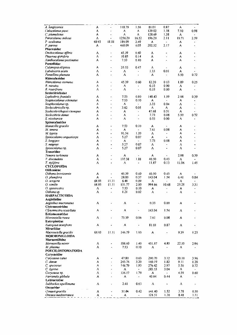
A. longicornis A 118.79 1.56 81.01 0.87 A -

Calocalanus pavo A A A 129.02 1.38 7.50 0.98 C. plumulosus A A A 128.69 1.38 A -

Paracalanus indicus A 1256.29 16.52 196.29 2.11 19.71 2.59 P. aculeatus 68.93 11.11 189.09 2.49 A - A - P. parvus A 460.09 6.05 202.52 2.17 A Phaennidae Onchocalanus affinis A 45.39 0.60 A A Phaenna spinifera A 10.85 0.14 A A Xanthocalanus pectinatus A 7.53 0.10 A A Pontellidae Calanopia elliptica A 35.53 0.47 A A Labidocera acuta A A 1.33 0.01 A - Pontellina plumata A A A 5.50 0.72 Rhincalanidae Rhincalanus cornutus A 45.39 0.60 12.20 0.13 1.89 0.25 R. nasutus A A 0.33 0.00 A R. rostrifrons A A 0.33 0.00 A Scolecitrichidae Lophothriv frontalis A 7.53 0.10 148.43 1.59 2.98 0.39 Scaphocalanus echinatus A 7.53 0.10 A A Scaphocalanus sp. A A 3.33 0.04 A Scolecithricella sp. A 3.62 0.05 A A A Scolecithrichopsis ctenopus A A 47.68 0.51 A Scolecithrix danae A A 7.73 0.08 5.50 0.72 S. nicobarica A A 0.33 0.00 A Spinocalanidae Monacilla gracilis A 7.53 0.10 A A M. tenera A A 7.61 0.08 A M. typica A 91.54 1.20 A A Spinocalanus angusticeps A 5.27 0.07 A A S. longipes A A 7.73 0.08 A S. magnus A 5.27 0.07 A A Spinocalanus sp. A 5.27 0.07 A A Temoridae Temora turbinata A A A - 2.98 0.39 T discaudata A 137.38 1.81 40.50 0.43 A T. stylifera A A 11.87 0.13 11.06 1.45 CYCLOPOIDA Oithonidae Oithona brevicornis A 45.39 0.60 40.50 0.43 A O. plumifera A 28.00 0.37 143.04 1.54 6.41 0.84 O. setigera 68.93 11.11 6.48 0.09 A - A 0. similis 68.93 11.11 151.77 2.00 994.66 10.68 25.25 3.31 0. spinirostris A 7.53 0.10 A A Oithona sp. A 1.21 0.02 A - A HARPACTICOIDA Aegisthidae Aegisthus mucronatus A - A 0.33 0.00 A Clytemnestridae Clytemnestra scutellata A A 143.04 1.54 A Ectinosomatidae Microsetella rosea A 73.39 0.96 7.61 0.08 A Euterpinidae Euterpina acutifrons A A 81.01 0.87 A Miraciidae Macrosetella gracilis 68.93 11.11 146.79 1.93 A 9.39 1.23 MORMONILLOIDA Mormonillidae Mormonilla minor A 106.60 1.40 451.87 4.85 22.55 2.96 M. phasma A 7.53 0.10 A - A POECILOSTOMATOIDA Corycaeidae Corycaeus catus A - 47.80 0.63 290.70 3.12 30.18 3.96 C. danae A 243.76 3.20 169.19 1.82 9.11 1.20 C. speciosus A 146.79 1.93 276.42 2.97 5.50 0.72 C. typicus A A 283.53 3.04 A Corycaeus sp. A 136.17 1.79 A 4.59 0.60 Farranula gibbula A A - 40.84 0.44 A Lubbockidae Lubbockia squillimana A 2.41 0.03 A A Oncaeidae Conaea gracilis A 31.64 0.42 141.40 1.52 3.78 0.50 Oncaea mediterranea A A - 121.51 1.30 8.48 1.11

0. venusta Oncaea sp. Triconia conifera Sapphirinidae Copilia mirabilis C. quadrata Sapphirina nigromaculata Unidentified Total individuals 100 tri -3

206.78 A A

A A A A

620

33.33 1095.16 A

84.01

A 7.53 28.00 96.06 7606

14.40

1.10

- 0.10 0.37 1.26

1879.65 A

11.87

A 88.18 47.68 271.73 9316

20.18 -

0.13

- 0.95 0.51 2.92

105.22 4.59 2.98

5.50 A A

9.05 762

13.80 0.60 0.39

0.72

1.19

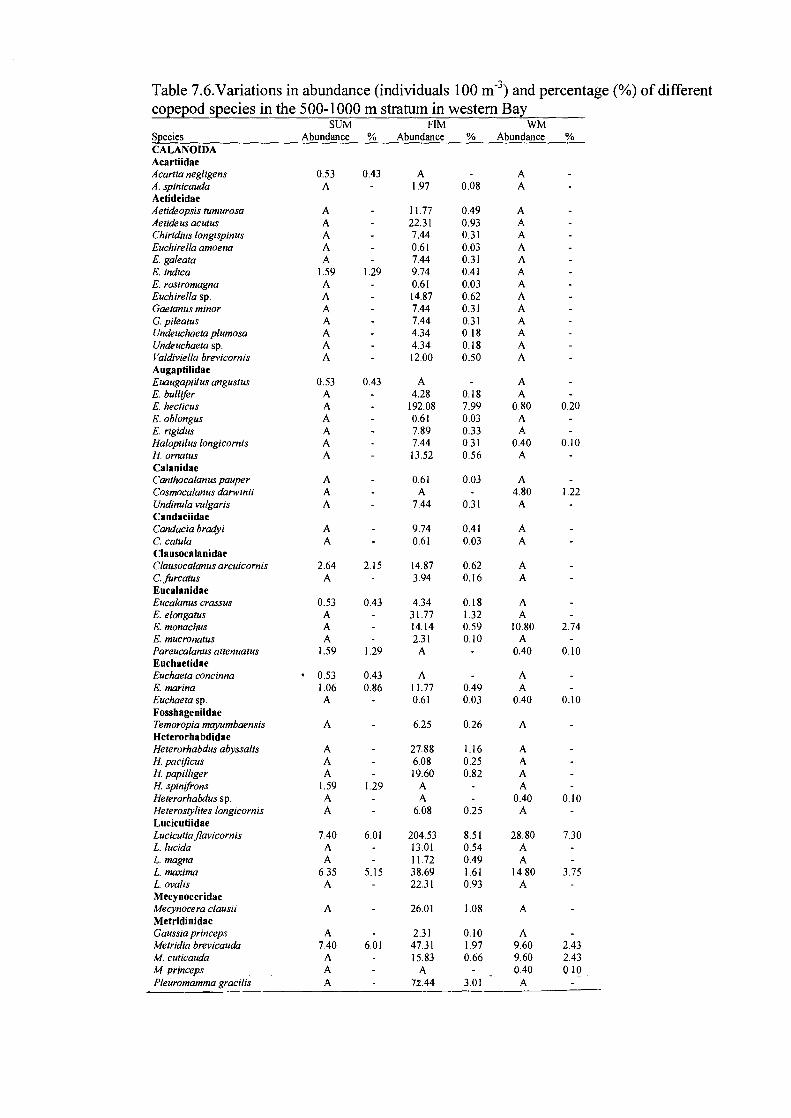
Table 7.6.Variations in abundance (individuals 100 m -3) and percentage (%) of different copepod species in the 500-1000 m stratum in western Bay

Species SUM

Abundance % FIM

Abundance % WM

Abundance % CALANOIDA Acartiidae Acartia negligens 0.53 0.43 A A A. spinicauda A 1.97 0.08 A Aetideidae Aetideopsis tumurosa A 11.77 0.49 A Aetideus acutus A - 22.31 0.93 A Chiridius longispinus A 7.44 0.31 A Euchirella amoena A 0.61 0.03 A E. galeata A - 7.44 0.31 A E. indica 1.59 1.29 9.74 0.41 A E. rostromagna A - 0.61 0.03 A Euchirella sp. A 14.87 0.62 A Gaetanus minor A 7.44 0.31 A G. pileatus A 7.44 0.31 A Undeuchaeta plumosa A 4.34 0.18 A Undeuchaeta sp. A 4.34 0.18 A Valdiviella brevicornis A 12.00 0.50 A Augaptilidae Euaugaptilus angustus 0.53 0.43 A A E. bullifer A 4.28 0.18 A E. hecticus A 192.08 7.99 0.80 0.20 E. oblongus A 0.61 0.03 A E. rigidus A 7.89 0.33 A Haloptilus longicornis A 7.44 0.31 0.40 0.10 H. ornatus A 13.52 0.56 A Calanidae Canthocalanus pauper A 0.61 0.03 A Cosmocalanus darwinii A A 4.80 1.22 Undinula vulgaris A - 7.44 0.31 A Candaciidae Candacia bradyi A 9.74 0.41 A C. catula A 0.61 0.03 A Clausocalanidae Clausocalanus arcuicornis 2.64 2.15 14.87 0.62 A C. furcatus A 3.94 0.16 A Eucalanidae Eucalanus crassus 0.53 0.43 4.34 0.18 A E. elongatus A - 31.77 1.32 A E. monachus A 14.14 0.59 10.80 2.74 E. mucronatus A - 2.31 0.10 A Pareucalanus attenuatus 1.59 1.29 A 0.40 0.10 Euchaetidae Euchaeta concinna • 0.53 0.43 A A E. marina 1.06 0.86 11.77 0.49 A Euchaeta sp. A 0.61 0.03 0.40 0.10 Fosshageniidae Temoropia mayumbaensis A 6.25 0.26 A Heterorhabdidae Heterorhabdus abyssalis A 27.88 1.16 A H. pacificus A - 6.08 0.25 A H. papilliger A - 19.60 0.82 A H. spinifrons 1.59 1.29 A A Heterorhabdus sp. A - A 0.40 0.10 Heterostylites longicornis A 6.08 0.25 A Lucicutiidae Lucicutia flavicornis 7.40 6.01 204.53 8.51 28.80 7.30 L. lucida A 13.01 0.54 A - L. magna A - 11.72 0.49 A L. maxima 6.35 5.15 38.69 1.61 14.80 3.75 L. ovalis A - 22.31 0.93 A Mecynoceridae Mecynocera clausii A 26.01 1.08 A Metridinidae Gaussia princeps A 2.31 0.10 A Metridia brevicauda 7.40 6.01 47.31 1.97 9.60 2.43 M. cuticauda A 15.83 0.66 9.60 2.43 M princeps A A - ._ 0.40 0 10 Pleuromamma gracilis A 72.44 3.01 A

P. indica 72.97 59.23 44.20 1.84 A P. robusta 1.59 1.29 24.16 1.01 A Pleuromamma sp. A - 1.97 0.08 A Paracalanidae Acrocalanus gracilis A 13.52 0.56 A Calocalanus pavoninus A 4.34 0.18 A - Paracalanus indicus A - 7.44 0.31 24.00 6.09 P. parvus 0.53 0.43 28.39 1.18 A -

Phaennidae Amallophora crassirostris A 20.55 0.86 A Onchocalanus affinis A 9.41 0.39 A Phaenna spinifera A 1.97 0.08 A Pontellidae Calanopia elliptica 0.53 0.43 A A Labidocera pectinata A - 7.44 0.31 A Pontellina plumata A A 0.40 0.10 Scolecitrichidae Acrocalanus gracilis A - A 4.80 1.22 Lophothrix frontalis 0.53 0.43 32.16 1.34 A -

Scaphocalanus echinatus A - 15.83 0.66 A Scaphocalanus sp. 0.53 0.43 0.61 0.03 A Scolecithrix vittatta A - 2.31 0.10 A Scolecithrix bradyi A 4.34 0.18 A S. danae A - 21.51 0.90 A Scottocalanus rotundatus 0.53 0.43 A A Spinocalanidae Monacilla gracilis A 7.44 0.31 A - M. tenera A - 4.61 0.19 4.80 1.22 M. typica 0.53 0.43 36.49 1.52 14.40 3.65 Spinocalanus longipes A - A - 9.60 2.43 Tharybidae Undinella spintfer A 2.31 0.10 A CYCLOPOIDA Oithonidae Oithona similis 2.64 2.15 27.04 1.12 9.60 2.43 0. spinirostris A - 0.00 0.00 A -

Oithona sp. A - 6.31 0.26 A HARPACTICOIDA Aegisthidae Aegisthus aculeatus A A - 0.80 0.20 A. mucronatus A 11.72 0.49 A Clytemnestridae Clytemnestra scutellata A 2.31 0.10 A Ectinosomatidae Microsetella rosea A 0.61 0.03 4.80 1.22 Euterpinidae Euterpina acutifrons 0.53 0.43 A A Miraciidae Macrosetella gracilis 1.06 0.86 1.97 0.08 A MORMONILLOIDA Mormonillidae Mormonilla minor 3.17 2.58 218.84 9.10 57.60 14.60 M. phasma A 40.44 1.68 A -

POECILOSTOMATOIDA Corycaeidae Corycaeus catus 0.53 0.43 7.44 0.31 A C. danae A 19.82 0.82 A C. speciosus 0.53 0.43 A - A Oncaeidae Conaea gracilis 3.17 2.58 215.29 8.96 139.20 35.29 Oncaea mediterranea A - A 4.80 1.22 0. venusta 2.12 1.72 301.01 12.52 38.40 9.74 Oncaea sp. A 8.95 0.37 A Triconia conifera A 3.94 0.16 A Sapphirinidae Copilia quadrata A 1.97 0.08 A Unidentified A 277.46 11.54 A Total individuals 100 ni3 123 2404 394

The most dominant genera Oncaea (15.4%), Oithona (9.6%), Pleuromamma (8.3%),

Eucalanus (8.0%), Pleuromamma (8.0%), Paracalanus (7.8%), Mormonilla (6.1%),

Corycaeus (5.1%) and Clausocalanus (5.0%) contributed to 69% of the total copepod

abundance in the WB.

From the total of 201 species that were identified, 40 species (Acartia negligens,

Euchirella indica, Canthocalanus pauper, Undinula vulgaris, Candacia bradyi,

Candacia sp., Centropages furcatus, Clausocalanus arcuicornis, Eucalanus crassus, E.

monachus, E. mucronatus, Eucalanus sp., Euchaeta indica, E. marina, Lucicutia

flavicornis, L. maxima, Metridia brevicauda, Pleuromamma indica, P. robusta,

Acrocalanus gibber, A. gracilis, A. longicornis, Calocalanus pavo, Paracalanus indicus,

P. parvus, Calanopia elliptica, Lophothrix frontalis, Scaphocalanus sp., Scolecithrix

danae, Oithona similis, 0. spinirostris, Macrosetella gracilis, Mormonilla minor,

Corycaeus catus, C. danae, C. speciosus, Conaea gracilis, Oncaea venusta, Sapphirina

nigromaculata and S. ovatolanceolata) occurred during all seasons in the WB.

However, only two of these viz. Oithona similis and Oncaea venusta were present at

all depths and stations. The total number of species occurring decreased below the

thermocline (MLD: 137, TT-BT: 145, BT-300 m: 117, 300-500: 112, 500-1000 m: 101).

The season-wise variation in the total number of species was also distinct with 59, 151,

128 and 113 species observed respectively during SUM, FIM, WM and SpIM.

Stereozoom and light microscopy photographs of some species identified from the Bay

are given in Plates 5-8.

7.2.5. Dominant species

Least number of species occurred during SUM. Ten species viz. 0. venusta, C.

arcuicornis, E. monachus, Acrocalanus gracilis, Phyllopus indicus, Oithona similis,

Mormonilla minor, Pleuromamma indica, Corycaeus danae and Oithona sp. contributed

to 76.2% of the total copepods identified (Table 7.7). Due to many missing samples, the

spatial distribution of the dominant species could not be analyzed for this season.

During FIM again, 10 dominant species (0. venusta, Paracalanus indicus, P. parvus,

Oithona sp., Acrocalanus gibber, Lucicutia flavicornis, Pleuromamma indica, Undinula

vulgaris, Eucalanus elongatus and E. monachus) contributed to 50% abundance (Table

101

Table 7.7. Copepod species contributing >2% of total abundance (individuals m -2) observed in the upper 1000 m of the western Bay during summer monsoon (SUM), fall intermonsoon (FIM), winter monsoon (WM) and spring intermonsoon (SpIM)

Season Species

Abundance in 1000 m (ind. m -2) %

SUM Oncaea venusta 5582 18.3 Clausocalanus arcuicornis 4222 13.8 Eucalanus monachus 3848 12.6 Acrocalanus gracilis 2813 9.2 Phyllopus indicus 2094 6.9 Oithona similis 1323 4.3 Mormonilla minor 995 3.3 Pleuromamma indica 914 3.0 Corycaeus danae 769 2.5 Oithona sp. 698 2.3

FIM Oncaea venusta 13562 18.6 Paracalanus indicus 6243 8.6 Oithona sp. 2662 3.6 Paracalanus parvus 2483 3.4 Acrocalanus gibber 2128 2.9 Lucicutia flavicornis 1972 2.7 Pleuromamma indica 1941 2.7 Undinula vulgaris 1907 2.6 Eucalanus elongatus 1845 2.5 Eucalanus monachus 1779 2.4

WM Oncaea venusta 14803 18.8 Clausocalanus arcuicornis 7915 10.1 Oithona similis 6028 7.7 Mormonilla minor 5388 6.9 Paracalanus indicus 3659 4.7 Oncaea mediterranea 2356 3.0 Pleuromamma indica 2087 2.7 Acrocalanus longicornis 2004 2.6 Eucalanus monachus 1987 2.5 Corycaeus catus 1913 2.4 Oithona plumifera 1697 2.2

SpIM Eucalanus monachus 47508 17.3 Oncaea venusta 25872 9.4 Oithona similis 22572 8.2 Clausocalanus arcuicornis 18679 6.8 Pleuromamma indica 18103 6.6 Pleuromamma robusta 8743 3.2 Lucicutia flavicornis 8299 3.0 Centropages furcatus 7020 2.6 Acrocalanus gracilis 6152 2.2

Paracalcvms Inelcus 15 16 17 18

Oifhorm sp. 15 16 17 18 19

Oncaea 'cyan -1

-5 15 16 17 18 19

Fleuromamma iraca

15 16 17 18 19 15 Undinula vu geris WB2

19 15 16 17 18 19 15 16 17 18 19 Paracalanus parvus

16 17 18 19 15 16 17 18 19 WB3 WB4 WB2 WB3 WB4

-5 15 16 17 18 19 15 16 17 18 19 WB2 WB3 WB4 WB2 WB3 WB4

Station

Figure 7.4. Distribution of major copepod species along western Bay during fall inter monsoon. Abundance (number 100m-i ; on labeled contours) is indicated in log numbers.

Depti, strata: sue-Oct - rnix e liner depth (mid) : -2: top 04 then-mclinecn)-

lase o4 Me-rm "Jule (-1); 3 `. 3orrn; --1-1-`;30C-5com ,,,—S: 5 to - lee orn

14 12 16 18 12

Oithona plumifera Oithona similis Pleuromamma indica Mormonilla minor

-5 12 14

I ' f

14 16 18 12 14 16 18 '---

16 18

- 1

-5 12 14 16 18

Corycaeus catus

r 7

12 14 16 18 12 14 16 18 12 14 16 18 Oncaea mediterranea Oncaea venusta WB1 WB2 WB3 WB4

Clausocalanus arcuicornis Eucalanus monachus Acrocalanus longicornis Paracalanus indicus

12 14 16 18 12 14 16 18 12 14 16 18

WB1 WB2 WB3 WB4 WB1 WB2 WB3 WB4 WB1 WB2 WB3 WB4

Station

Figure 7.5. Distribution of major copepod species along western Bay during winter monsoon. Abundance (number 100m -3 ; on labeled contours) is indicated in log numbers ,

De_pfill Strata: r.0 e nit e a ( rn I ci)., —2 top c4 thermoclwr. (fs) --aliSe 04- tine-et-nod% ne u3,1) ) 131- - 3 o Cm e, -if 3 Co - SOO - 5-6 c -1000m

Lucicutia flavicornis Oncaea venusta Eucalanus monachus

Acrocalanus gracilis Centropages furcatus Clausocalanus arcuicornis

12 14 16 18

12 14 16 18

12 14 16 18

Oithona similis Pleuromamma indica

Pleuromamma robusta

-1

-2

-3

-4 12 14 16 18 12

14 16 18 12

14 16 18

WB1 WB2 WB3 WB4 WB1

WB2 WB3 WB4 WB1

WB2 WB3 WB4

Station

Figure 7.6. Distribution of major ,copepod species along western Bay during spring inter-monsoon. Abundance (number 100m -3 ; on labeled contours) is indicated in log numbers

Sac( Ace - m Ye d depih( mlet) tip the vrnoctne

tri) - Sase o4 I karnodi ne, CEO; -3 t _ET-3ootrv) 30C -cOttn

Acrocalanus longiconus

E. monachus

Pitman= adieus

C. catus

Oithona plunders

meditenanea

B)

20

P. indica

Lucicutia flavicornis

E monachus

0. venusta

parvus

Paracalanus indicus

Undinula vulgaris

E. elongatus

A_gibber II

Oithona sp

60 80 100

Bray- Curtis Similarity (%)

A)

40

0. smuhs

C arcuicomis

0,venusta

II

Morntonilla minor

P. indica

50 60 70 80 90 100

Btay- Curtis Similarity (°o)

Figure 7.7. Cluster dendrogram of the major copepod species (>2%) from the western Bay during fall intermonsoon (A) and winter monsoon (B), using Bray- Curtis similarity (%) and group average method.

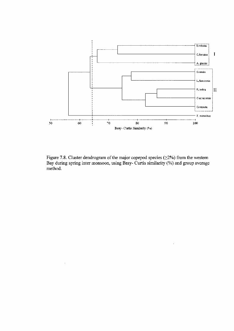
I

P. robusta

C. furcatus

A, gracihs

0. similis

flavic ornis

P. Mdica

C,arcuicomis

0„ venusta

II

90 50 60 '0 $0

Bray- Curtis Similarity (°..0)

E. monachus

100

Figure 7.8. Cluster dendrogram of the major copepod species (>2%) from the western Bay during spring inter monsoon, using Bray- Curtis similarity (%) and group average method.

7 .7). Pleuromamma indica, L. flavicornis, E. monachus, 0. venusta, P. parvus, P. indicus

and U. vulgaris formed cluster I. They occurred throughout the 1000 m column mostly at

WB3 and WB4. Being dominant in the 200-300 m layer at WB3, Group II comprising E.

elongatus, A. gibber and Oithona sp. formed cluster II (Fig. 7.4; Fig. 7.7 A).

During WM, 0. venusta, Clausocalanus arcuicornis, Oithona similis, Mormonilla

minor, Paracalanus indicus, Oncaea mediterranea, Pleuromamma indica, Acrocalanus

longicornis, E. monachus, Corycaeus catus and Oithona plumifera in WM accounted for

63.4% of the total copepods (Table 7.7). Acrocalanus longicornis, E. monachus, P.

indicus, C. catus, 0. plumijera and 0. mediterranea comprising cluster I were abundant

in the MLD. They decreased drastically with depth and some were absent below the

second or the third stratum at some stations. In cluster II, 0. similis, C. arcuicornis and

0. venusta were abundant in the upper two strata but decreased gradually with depth. In

cluster III, M minor and P. indica were more in the thermocline to 300 m especially at

WB1 and WB3 (Fig. 7.5; Fig. 7.7 B).

During SpIM, nine species, E. monachus, 0. venusta, 0. similis, C. arcuicornis, P.

indica, P. robusta, L. flavicornis, Centropages furcatus and Acrocalanus gracilis were

dominant contributing 59% of the total copepods (Table 7.7). Pleuromamma robusta, C.

furcatus and A. gracilis that formed cluster I were observed mostly at WB 1 and WB4.

While the first two species were observed even in the 500-1000 m stratum at WB3, the

last species was confined to the upper two strata only. In cluster II, 0. similis, L.

flavicornis, P. indica, and 0. venusta were present throughout the 1000 m except that C.

arcuicornis was absent from the 300-1000 m stratum at WB1 and WB2. Eucalanus

monachus did not group with any species and was abundant throughout the 1000 m at

WB3 and WB4 (Fig. 7.6; Fig. 7.8).

7.2.6. Species diversity, evenness and richness

Shannon diversity (II ') , richness (d) and evenness (J') for copepod species varied greatly

with depth and stations. The ranges for the three indices during SUM are: H' (0.7-4.0), d

(1.5-4.9), J' (0.21-0.94; Fig. 7.9A).

102

6 -

4 -

2 -

0

1.0

J' " 0.0

d LI WB1 WB2

WB1 WB2 WB3 WB4 WB1 WB2 WB3 WB4

Station

Figure 7.9. Depth-wise variation of copepod species diversity (H'), richness (d), and evenness (J') at different sampling stations in the western Bay of Bengal during summer monsoon (A) and fall intermonsoon (B)

B) A) 5

4

H'

WB1 WB2

■ 0-MID

■ TT-BT

0 200-300

O 300-500

■ 500-1000

WB1 WB2 WB3 WB4

11 WB1 WB2 WB3 WB4

During FIM, H' ranged from 3.4 to 4.8, d from 2.3 to 4.8 with their lowest values at

WB3. J' ranging from 0.76 to 0.93 was higher at WB2. H' and J' did not vary much with

depth. In general, d was higher below the MLD (Fig. 7.9B).

H' ranged from 3.4 to 4.2 and was higher in the upper two strata during WM. Varying

from 2.0 to 3.9, d was higher in subsurface depths and seemed to decrease northwards. J'

varied from 0.72 to 0.88 and was more or less similar over depths and stations (Fig. 7.10

A).

During SpIM, H' varying from 1.7 to 4.4, was high in the MLD and also mostly in

the lowest strata. It was the lowest in the 200-300 m stratum and increased northwards.

Similar distribution trend was observed in case of d, which varied from 1.5 to 4.4, with an

overall northward decrease. Varying from 0.44 to 0.95, J' showed a northward increase

in the third stratum (Fig. 7.10 B).

7.2.7. Correlation analysis

The mixed layer copepod abundance correlated: a) mostly negatively with temperature;

b) positively with salinity during most seasons, and c) positively with chlorophyll (chl) a

only during FIM. Diversity (H') correlated mostly negatively with total abundance and

temperature; mostly positively with chl a and salinity. Species richness also correlated

negatively with total biomass and abundance except during SUM. It correlated positively

with temperature and salinity and, negatively with chl a. Evenness was negatively

correlated with total biomass, abundance and, temperature. It correlated positively with

chl a in the monsoons and negatively during inter monsoons (Table 7.8).

7.3. Discussion

7.3.1. Comparative account of copepod abundance

The following comparative accounts are from different parts of the world oceans mostly

from the neritic waters. Spatial variation in their numerical abundance (Nair et al. 1981;

Padmavati et al. 1998) ranging from 0.8 to 417920 individuals 100 111-3 in the upper 1000

m was also obtained in earlier studies in the Indian Ocean.

In the western Mediterranean, values ranging from 60000-120000 ind. 100 111-3 were

obtained in the upper 200 m (Fernandez de Puelles et al. 2003). They varied from 1.64 x

103

WB1 WB2 WB3 WB4

H'

A) 4

3

2

1

0

5 -

4

3

2

1

0

d

WB1 WB2 WB3 WB4 WB1 WB2 WB3 WB4

WB1 WB2 WB3 WB4

1.0

J' 0.5

0.0 Etat

WB1 WB2 WB3 WB4 WB1 WB2 W133 WB4

Stations

Figure 7.10. Depth-wise variation of copepod species diversity (H'), richness (d), and evenness (J') at different sampling stations in western Bay of Bengal during winter monsoon (A) and spring intermonsoon (B)

■ 0-MLD

■ TT-BT

O 200-300

0 300-500

■ 500-1000

Table 7.8. Correlation coefficients of copepod abundance, species diversity (H'), richness (d) and evenness (J') with various parameters (total zooplankton biomass, abundance, temperature, salinity, chlorophyll a and copepod abundance) in the western Bay during different sampling seasons

Biomass Abundance Temp Sal Chl a Cop_abun SUM Cop_abun 0.998 1.000 0.001 0.358 -0.716 1.000 H' -0.900 -0.925 0.377 0.021 0.399 -0.926 d 0.842 0.807 0.593 0.841 -0.990 0.806 J -0.475 -0.420 -0.909 -0.998 0.934 -0.418 FIM Cop_abun 0.236 0.937 -0.127 -0.995 0.589 1.000 H' 0.080 -0.781 -0.191 0.977 -0.813 -0.950 d -0.539 -1.000 0.442 0.907 -0.295 -0.946 J 0.778 -0.084 -0.843 0.517 -0.982 -0.426

WM Cop_abun 0.920 0.985 -0.996 0.957 -0.182 1.000 H' 0.799 0.619 -0.567 0.443 0.730 0.502 d -0.206 0.050 -0.080 0.274 -0.864 0.164 J 0.211 -0.042 0.062 -0.277 0.826 -0.147 SpIM Cop_abun 0.908 1.000 -0.200 0.577 0.005 1.000 H' 0.120 -0.009 -0.115 0.448 0.550 0.005 d -0.663 -0.800 0.125 -0.211 0.300 -0.792 J -0.771 -0.804 0.368 -0.408 0.060 -0.794

r values marked in bold are significant at p<0.05 SUM-summer monsoon; FIM-fall intermonsoon; WM- winter monsoon and, SpIM- spring intermonsoon ; Temp-temperature, Sal-salinity; Chl a- chlorophyll a; Cope_abun-copepod abundance All zooplankton related parameters are from mixed layer depth, while the physico-chemical parameters and chl a are averages from the upper 120 m.

105 to 6.40 x 107 ind.100 111-3 in the Fukuyama Harbor, an eutrophic inlet of the Inland

Sea of Japan (Uye and Liang 1998). Their mean abundance was 12300 ± 6900 ind.100 m -

3 in the coastal waters off southwestern Taiwan (Lo et al. 2001). Varying seasonally, the

abundance ranged from 200 to 18300 ind 100 111-3 in the Atlantic coast of southern

Morocco (Somoue et al. 2005). Rakhesh et al. (2006) observed high abundance of

copepods ranging from 9300 to 14,00400 ind.100 m -3 in the shelf waters (50-200 m) of

the WB.

As already detailed in Chapter 5, copepods constituted 67-99.7% of the total

mesozooplankton standing stocks in the WB. Despite the fact that the stations sampled in

this study were in shelf/slope waters (with the maximum depth sometimes exceeding

1000 m), the total number of copepods is comparable to many above listed studies from

the near-shore waters. In the upper 100 m, their abundance was in the range of 0.8 to

213540 ind. 100 m -3 during SUM, 764 to 114067 ind. 100 IT1-3 during FIM, 394 to 147965

ind. 100 III-3 during WM and from 186 to 417920 ind. 100 111-3 during SpIM.

7.3.2. Influence of hydrography on the abundance and type

Significant differences were observed in abundance between the stations during SUM in

particular. The higher abundance in MLD at WB3 during SUM, and WB 1 during WM

coincided with the existence of cold-core eddies (Chapter 3). In cold-core eddies,

enhanced chl a was reported earlier in the Bay (Gomes et al. 2000; Prasannakumar et al.

2004, 2007). Increased plankton production in eddies has been observed in many parts of

the world oceans (Chapter 6).

As also observed during the HOE (Panikkar and Rao 1973), rich patches of copepod

abundance were observed along the northern Andhra coast during SUM, Orissa coast

during intermonsoons and off Madras during the winter monsoon in this study. Off

Visakhapatnam, the hydrographical conditions are largely influenced by southerly

(August—December, salinity 20.79-32.97 psu) and northerly (January—July, salinity

30.06-34.57) currents, which run skirting the coast. Upwelling during March—May leads

to increased phytoplankton production (La Fond 1958; Murty and Varadachari 1968; Rao

et al. 1986; Ganapati 1973; Raju 1988; Gomes et al. 2000; Schott and McCreary 2001;

Madhupratap et al. 2003;). Chl a up to 42 mg m -2 was observed at WB3 during SpIM

104

with a dominant diatom community (>90%; Paul 2007). Marked increase in nutrients and

salinity at this time of the year compared to offshore waters appears to enhance

zooplankton biomass.

As mentioned in Chapter 6, copepod diel vertical migration (DVM; Hays 2003) has

been reported from many oceans (Saltzman and Wishner 1997; Smith et al. 1998;

Goswami et al. 2000; Jayalakshmy 2000; Madin et al. 2001). However, no significant

DVM of copepods was observed in this study except during SpIM. Pronounced oxygen

minimum zone (OMZ) in the Bay would have restricted vertical migration of most

copepods (Saltzman and Wishner 1997). Highest copepod abundance was always in the

MLD, the strata of maximum chlorophyll and primary production (Hobson and Lorenzen

1972; Ortner et al. 1980; Herman 1983, 1989; Roman et al. 1986). Their generally

negative correlation with chl a in this study appears to be due to their grazing activity.

Similar to that in the CB and also in other studies (Wishner and Allison 1986; Padmavati

et al. 1998), their numbers decreased with depth. From their relatively higher proportion

at deeper depths in the Bay and also in the Arabian Sea (Madhupratap and Haridas 1990),

it appears that they are important in waters where food is scarce.

Tropical waters being warmer and relatively stable compared to temperate waters,

little seasonal changes are expected in hydrography (Longhurst and Pauly 1987) and in

plankton (Blackburn 1981; Moore and Sander 1977). Though some studies in the tropics

do find seasonal variability in zooplankton (Calef and Grice 1967), in coastal tropical

oceans, such patterns are generally related to variability of annual rainfall (Chisholm and

Roff 1990). The North Indian Ocean is unique in this aspect where the seasonal

variability is driven primarily by the monsoons. In the WB, highly significant seasonal

variation in copepod abundance was observed, with the entire transect becoming more

productive during SpIM (36778 ind. 100 m -3), followed by WM (33047 ind. 100 m -3),

FIM (26761 ind. 100 m-3) and SUM (16161 ind. 100 m-3). Seasonal changes in copepod

abundance with a spring maximum have been found in many parts of tropical oceans

(Moore 1949; Bsharah 1957; Menzel and Ryther 1961; Madhu et al. 2007). Similar to

studies from estuaries on the West coast of India (Pillai et al. 1973; Madhupratap 1987,

1979; Madhu et al. 2007), copepod abundance correlated positively with surface salinity

in this study from the East coast of India.

105

7.3.3. Prominent orders and families in the Bay of Bengal

Six orders of Copepoda i.e. Calanoida, Cyclopoida, Harpacticoida, Mormonilloida,

Poecilostomatoida and Siphonostomatoida identified in this study are all previously

reported from the Arabian Sea (Madhupratap and Haridas 1990; Bottger-Schnack 1995).

In spite of the seasonal differences in the distribution patterns of these orders in the upper

1000 m, Calanoida was always dominant irrespective of seasons, as has also been

reported in all oceans (Pacific: Farran 1936; Atlantic: Deevey and Brooks 1977; Indian

Ocean: Madhupratap and Haridas 1990). All the calanoid (Madhupratap et al. 1990;

Padmavati et al. 1998; Madhupratap et al. 2001) as well as non-calanoid (Bottger-

Schnack 1995) families of copepods observed in this study have been reported previously

from the Arabian Sea. Increased percentage of calanoids in the 300-500 m layer during

intermonsoons and, in the deepest layer during SUM was largely due to the contribution

of low-oxygen- tolerant species of the families Lucicutiidae, Metridinidae, Augaptilidae

and Spinocalanidae. The oxygen content in these depths was relatively more during WM.

Only a few families were numerically dominant, contributing >5% of the total

copepods in a total of 38 families. A clear dominance in their pattern of distribution was

evident during all seasons. Sometimes, families such as Megacalanidae, Rataniidae,

Clausiidae were so poor in abundance that as less as just one specimen per whole sample

was recorded. At least four to nine of such rare families, due to lower abundance were

absent from the samples in every season. Vertical partitioning as well as seasonal

variation of predominant families was evident from this data.

The abundance of herbivorous calanoids like Paracalanidae, Eucalanidae, Acartiidae

and Clausocalanidae is commonly reported in the surface waters in oceans (Stephen and

Kunjamma 1987; Kouwenberg 1994; Padmavati et al. 1998; Saltzman and Wishner 1997;

Cornils et al. 2007). Metridinidae comprised largely of Pleuromamma indica, an

omnivorous, low-oxygen tolerant and vertically migrating species (Saraswathy and Iyer

1986) in the Indian Ocean.

Cyclopoida comprising exclusively Oithonidae, though present throughout the

column, was mostly abundant in the thermocline. Oithonids are known to be eurythermal,

euryhaline and globally occurring omnivorous species. This observation agrees with the

106

studies of Nishida and Marumo (1982) and Padmavati et al. (1998). The warm water

families Corycaeidae, Oncaeidae and Sapphirinidae (Raymont 1983) belonging to the

second dominant order Poecilostomatoida were also abundant in the MLD and their

abundance/occurrence decreased with depth. However, similar to observations of

Bottger-Schnack (1995), Oncaeidae mostly increased again in deeper depths.

Mormonillidae, the mesopelagic family (Boxshall 1986) was abundant at all depths

below MLD. The most abundant species among harpacticoids, Macrosetella gracilis, was

present throughout the 1000 m as observed by Weikert (1982) was abundant in the 300-

500 m stratum (11%) in SUM.

As also demonstrated by Deevey and Brooks (1977), larger copepods occurred

mainly in deeper waters with smaller species being more numerous at the surface.

7.3.4. First Reports from this study and significance

A total of 201 species were recorded in the present investigation from the WB that

covered four different seasons. They are mostly tropical-subtropical with some of them

having cosmopolitan and circumglobal distribution (Fleminger and Hulsemann 1973;

Table 7.9). Most of these species identified have been recorded in previous studies in the

Indian Ocean. However, 11 species from this transect are recorded for the first time in the

Indian Ocean. Aetideopsis tumurosa, Chiridius longispinus, Amallophora crassirostris,

A. irritans and Pseudoamallothrix ovata occurred only in the WB. Six species i.e.

Euchirella rostromagna, Heterorhabdus pacificus, Xanthocalanus pectinatus,

Scottocalanus rotundatus, Monacilla gracilis and Undinella spinifer were found in the

central transect as well.

The following species are reported previously from the coastal waters of the Bay:

Paracalanus aculeatus, Pareucalanus attenuatus, Eucalanus crassus, E. monachus, E.

pseudattenuatus, Canthocalanus pauper, Euchaeta concinna, E. marina, E. indica,

Temora discaudata, T. turbinata, Acartia erythraea, Mesocalanus tenuicornis, Lucicutia

flavicornis, Candacia bradyi, C. pachydactyla, Centropages calaninus, C. furcatus, C.

gracilis, Pontellina plumata, Undinula vulgaris, Cosmocalanus darwini, Labidocera

acuta, L. pavo, Calanopia elliptica, C. minor, Acrocalanus gibber, Sapphirina

nigromaculata, Corycaeus catus,C. danae, C. speciosus, Farranula gibbula, Oncaea

107

Table 7.9. List of copepod species from the central and western Bay of Bengal recorded during this study. Their previous records and other relevant information also included

Sr. No Species CB av % WB av % Previous records 1 Acartia amboinensis Carl, 1907 0.013 0.048 Arabian Sea; Malacca strait

@2 A. centrura Giesbrecht, 1889 A 0.025 Arabian Sea; BoB @3 A. danae Giesbrecht, 1889 0.013 A Arabian Sea; BoB @4 A. erythraea Giesbrecht, 1889 0.010 0.163 Arabian Sea, BoB @5 A. negligens Dana, 1849 0.294 0.472 Arabian Sea; BoB @6 A. southwelli Sewell, 1914 0.031 A Arabian Sea; BoB @7 A. spinicauda Giesbrecht, 1889 0.034 0.556 Arabian Sea; Malacca strait; BoB @8 Acartiella sewelli Steuer, 1934 0.012 A Arabian Sea; BoB $9 Aetideopsis tumurosa Sars, 1903 A 0.024 Sub-antarctic Pacific 10 Aetideus acutus Farran, 1929 0.106 0.049 Trop, sub-trop 11 A. armatus Boeck, 1872 0.072 0.001 I0 12 A. bradyi A Scott, 1909 0.012 A Indo Pacific, 10 13 A. giesbrechtii Cleve, 1904 A 0.004 Trop, sub-trop; I0 14 Aetideus sp. 0.026 A

$ 15 Chiridius longispinus Tanaka, 1957 A 0.015 W Pacific $ 16 Chiridiella sp. 0.014 A Atlantic

17 Chirundina streetsi Giesbrecht, 1895 A 0.005 SW Pacific; JO 18 Euchirella amoena Giesbrecht, 1888 0.056 0.006 SW Pacific; JO 19 E. bella Giesbrecht, 1888 0.003 A Arabian Sea 20 E. bitumida With, 1915 0.077 0.046 N Atlantic; SW Pacific, JO 21 E. curticauda Giesbrecht, 1888 0.007 0.006 I, A, P 22 E. galeata Giesbrecht, 1888 0.063 0.040 N Pacific, 10 23 E. indica Vervoort, 1949 0.231 0.154 Trop, sub-trop; Indo Pacific 24 E. latirostris Farran, 1929 A 0.0001 Warm Sub-antarctic waters; JO 25 E. maxima Wolfenden, 1905 0.002 A Atlantic; 10 26 E. messinensis Claus, 1863 0.008 A Trop, sub- trop; temperate; I0 27 E. rostrata Claus, 1866 0.035 A I, A, P

$28 E. rostromagna Wolfenden, 1911 0.020 0.004 Antarctic convergence 29 E. similis Wolfenden, 1911 0.017 A I, A, P

$30 E. speciosa Grice and Hulsemann, 1968 0.024 A Sub-tropical Pacific 31 E. truncata Esterly, 1911 0.029 A SW Pacific, JO 32 E. venusta Giesbrecht, 1888 0.010 0.002 Indo Pacific

@33 Euchirella sp. 0.147 0.195 Bay of Bengal 34 Psedochirella dentata A. Scott, 1909 0.001 A Indo Pacific 35 P. mawsoni Vervoort, 1957 0.005 A 10, Pacific 36 Gaetanus arminger Giesbrecht, 1888 0.020 A I, A, P 37 G. kruppii Giesbrecht, 1903 0.071 0.0002 I, A, P 38 G. miles Giesbrecht, 1888 0.080 0.010 Trop, sub-trop; temp; I, A, P 39 G. minor Farran, 1905 0.062 0.015 SW Pacific, JO 40 G. pileatus Farran, 1903 0.007 0.015 I, A, P 41 Gaidius pungens Giesbrecht, 1895 0.032 A All oceans 200-1000m 42 Undeuchaeta major Giesbrecht, 1888 0.005 A SW Pacific; I0 43 U plumosa Lubbock, 1856 0.098 0.009 Trop, sub-trop, temp; I, A, P 44 Undeuchaeta sp. 0.002 0.017 45 Valdiviella brevicornis Sars, 1905 A 0.041 10; N Atlantic; bathypelagic 46 Arietellus giesbrechtii Sars, 1905 0.004 0.017 NW Atlantic; eq Pac; JO 47 A. setosus Giesbrecht, 1892 0.001 A Trop Atlantic, I0 48 Arietellus sp. 0.006 A 49 Augaptilus glacialis Sars, 1900 0.001 A N Atlantic; Arctic; Pacific; I0 50 Augaptilus sp. 0.081 A Arabian Sea 51 Centraugaptilus rattrayi T. Scott, 1894 0.011 A I, A, P 52 C. horridus Farran, 1908 0.084 A Arabian Sea, Pacific 53 Centraugaptilus sp. 0.003 A 54 Euaugaptilus angustus Sars, 1905 0.001 0.036 Atlantic, Arabian Sea 55 E. bullifer Giesbrecht, 1889 2.020 0.013 I, A, P, Arabian Sea

56 E. facilis Farran, 1908 0.046 A N Atlantic, Arabian Sea 57 E. hecticus Giesbrecht, 1889 0.013 0.431 I, A, P; Arabian Sea 58 E. laticeps Sars, 1905 0.026 0.0002 Atlantic; Arabian Sea 59 E. longimanus Sars, 1905 0.002 A Temp; Atlantic; Pacific; W 10 60 E. magnus Wolfenden, 1904 0.004 A N Atlantic, Antarctic; 10

$61 E. mixtus Brodsky, 1950 0.008 A Bering Sea; Pacific; Med 62 E. nodifrons Sars, 1905 0.002 A N Atlantic; 10 63 E. oblongus Sars, 1905 0.067 0.001 N Atlantic; IO; Arabian Sea 64 E. rigidus Sars, 1907 0.008 0.016 Pacific; IO

@65 Haloptilus acutifrons Giesbrecht, 1892 0.183 A 10; Med; Arabian Sea; BoB 66 H. longicornis Claus, 1863 0.415 0.198 Med; Arabian Sea; USSR 67 H. mucronatus Claus, 1863 0.001 A S Atlantic; Mediterranean 68 H. ornatus Giesbrecht, 1892 0.011 0.039 Atlantic; Med; W IO; Malay 69 H. spiniceps Giesbrecht, 1892 0.042 0.010 Warm currents of I, A, P

570 Pseudhaloptilus abbreviatus Sars, 1905 0.034 A N Atlantic 71 P. eurygnathus Sars, 1920 0.003 A N Atlantic; Arabian Sea 72 P. pacificus MW Johnson, 1936 0.007 0.0002 N Pacific; Japanese coast; W 10

@73 Canthocalanus pauper Giesbrecht, 1888 0.132 0.840 I, A, P; BoB @74 Cosmocalanus darwinii Lubbock, 1860 0.006 0.137 Trop, sub-trop Oceans; 10; BoB @75 Mesocalanus tenuicornis Dana, 1849 0.023 0.031 Trop, sub-trop oceans; 10; BoB @76 Nannocalanus minor Claus, 1863 0.012 A Trop, sub-trop oceans; 10; BoB @77 Undinula vulgaris Dana, 1849 0.728 1.650 Neretic; trop; IO; BoB @78 Candacia ethiopica Dana, 1849 A 0.003 Cosmopotitan; trop; IO, BoB @79 C. bispinosa Claus, 1863 0.001 A 10; BoB @80 Candacia bradyi A Scott, 1902 0.218 0.396 Trop; IO; BoB @81 C. catula Giesbrecht, 1889 0.023 0.006 Trop; IO; BoB @82 C. discaudata A Scott, 1909 0.031 0.237 Trop; IO; BoB @83 C. pachydactyla Dana, 1849 0.043 0.064 Cosmopolitan; trop; 10; BoB @84 Paracandacia truncata Dana, 1849 0.357 0.615 IO; BoB @85 P. simplex Giesbrecht, 1889 0.002 A IO; BoB

86 Candacia sp. 0.174 0.272 87 Centropages alcocki Sewell, 1912 0.009 0.018 Trop

@88 C. calaninus Dana, 1849 0.085 0.051 Cosmopolitan; trop; BoB @89 C. dorsispinatus Thompson & Scott, 1903 0.048 A Trop; BoB @90 C. furcatus Dana, 1849 0.186 0.974 Trop; BoB @91 C. gracilis Dana, 1849 0.020 0.005 Trop; BoB

92 C. orsinii Giesbrecht, 1889 0.040 A IO; Malacca strait 93 Centropages sp. 0.077 0.010 94 Clausocalanus arcuicornis Dana, 1849 4.491 3.568 Cosmopolitan; trop, I0 95 C. furcatus Brady, 1883 1.257 1.327 Cosmopolitan; trop, sub-tropic 96 C. pergens Farran, 1926 0.201 0.100 Trop; sub-trop 97 Clausocalanus sp. 0.090 0.009 98 Drepanopsis frigidus Wolfenden, 1911 0.008 0.025 10

599 D. orbus sp. 0.006 A Sagami Bay; Japan @100 E. crassus Giesbrecht, 1888 0.680 0.294 BoB @101 E. subcrassus Giesbrecht, 1888 0.073 A BoB @102 E. elongatus Dana, 1849 1.939 0.968 W Atlantic; Arabian Sea; BoB @103 E. monachus Giesbrecht, 1888 2.206 6.535 W Atlantic; Gulf of Mexico; BoB 104 E. mucronatus Giesbrecht, 1888 0.546 0.231 Florida current; Arabian Sea

@105 E. pseudattenuatus Sewell, 1947 0.057 0.0003 BoB 106 Eucalanus sp. 0.281 0.371

@107 Pareucalanus attenuatus Dana, 1849 0.446 0.377 SW Pacific; BoB 108 Subeucalanus crassus Giesbrecht, 1888 0.020 A IO; Arabian Sea

@109 Euchaeta concinna Dana, 1849 0.074 0.241 10; Pacific @110 E. indica Wolfenden, 1905 0.163 0.187 Malay; Maldives archipelago; I0 @111 E. marina Prestandrea, 1833 0.898 0.815 I, A, P; BoB

112 E. media Giesbrecht, 1888 0.004 A I, A, P 113 E. plana Mori, 1937 0.016 A Arabian Sea 114 Euchaeta sp. 0.535 0.134

115 Pareuchaeta malayensis Sewell, 1929 0.006 A Arabian Sea 116 Temoropia mayumbaensis T. Scott, 1894 0.440 0.420 NW Atlantic, Arabian Sea 117 Disseta palumboi Giesbrecht, 1889 0.001 A I, A, P 118 Hemirhabdus grimaldi Richard, 1893 A 0.006 I, A, P, Arabian Sea 119 Heterorhabdus abyssalis Giesbrecht, 1889 0.156 0.079 I, A, P 120 H. fistulosus Tanaka, 1964 A 0.003 NW Pacific; 10

$ 121 H. pacificus Brodsky, 1950 0.021 0.028 NW Pacific 122 H. papilliger Claus, 1863 0.548 0.282 All oceans 123 H. spinifrons Claus, 1863 0.184 0.239 All oceans 124 H. subspinifrons Tanaka, 1964 0.000 A S JO; S Atlantic; NW Pacific 125 H. vipera Giesbrecht, 1889 0.015 A I, A, P 126 Heterorhabdus sp. 0.164 0.049 127 Paraheterorhabdus robustus, Farran 1908 0.081 0.068 Atlantic; Antarctic; Indo Pacific 128 Heterostylites longicornis Giesbrecht 1889 0.076 0.091 I, A, P; Arabian Sea; Malay 129 H. major F. Dahl, 1894 0.002 A Atlantic; JO; Antarctic; USSR 130 Lucicutia bicornuta Wolfenden, 1905 0.002 A Atlantic; JO; Malay; Antarctic

@131 L. jlavicornis Claus, 1863 4.823 3.251 Trop I, A, P; Arabian Sea; BoB 132 L. longispina Tanaka, 1963 0.003 A W Pacific; I0 133 L. lucida Farran, 1908 0.007 0.038 Atlantic; Pacific; I0 134 L. magna Wolfenden, 1903 0.003 0.028 Atlantic; Med; Antarctic; I0 135 L. maxima Steuer, 1904 1.050 0.916 IO; Malay 136 L. ovalis Giesbrecht, 1889 0.169 0.170 I, A, P 137 Mecynocera clausii Thompson, 1888 0.196 0.171 Trop, sub-trop, temp; epipelagic; JO 138 Megacalanus princeps Brady, 1883 0.002 0.035 I, A, P; Antarctic

@139 Gaussia princeps T. Scott, 1894 0.151 0.025 Pacific; USSR; 10; BoB 140 Metridia brevicauda Giesbrecht, 1889 0.544 0.625 Atlantic; 10; Malay 141 M cuticauda Giesbrecht, 1889 0.092 0.155 Pacific; Atlantic; Malay; I0

$ 142 M pacflca Brodsky, 1950 0.008 A N Pacific; Atlantic 143 M princeps Giesbrecht, 1889 0.176 0.005 Atlantic; JO; Malay 144 Metridia sp. 0.147 0.002 145 Pleuromamma abdominalis Lubbock 1856 0.145 A I, A, P 146 P. gracilis Claus, 1863 1.032 0.736 1, A, P

@147 P. indica Wolfenden, 1905 6.529 6.244 Indo Pacific; BoB 148 P. quadrangulata F. Dahl, 1893 0.144 0.001 I0 149 P. robusta F. Dahl, 1893 0.389 0.822 I0 150 P. xiphias Giesbrecht, 1889 0.186 0.010 10 151 Pleuromamma sp. 0.151 0.199 152 Nullosetigera bidentata Brady, 1883 0.040 A Arabian Sea 153 Nullosetigera sp. 0.004 0.037 154 Bestiolina similis Sewell 1914 0.005 A W 10; SW Pacific; Malacca strait

@155 A. gibber Giesbrecht, 1888 F,M 0.444 0.823 SW Pacific; BoB @156 A. gracilis Giesbrecht, 1888 0.825 1.027 Tropical oceans; Bay of Bengal @157 A. longicornis Giesbrecht, 1888 0.735 1.433 SW Pacific; Malacca strait; BoB @158 A. monachus Giesbrecht, 1888 0.019 0.026 SW Pacific; BoB

159 Calocalanus longispinus Shmeleva, 1978 0.001 A SW Pacific; 10 @160 C. pavo Dana, 1849 0.721 0.653 Trop, sub-trop, temp; BoB

161 C. pavoninus Farran, 1936 0.015 0.035 Trop I, A, P 162 C. plumulosus Claus, 1863 0.209 0.199 Trop, sub-trop, temp; Med 163 Paracalanus indicus Wolfenden, 1905 4.341 5.581 Trop, sub-trop, temp; Med; W 10

@164 P. aculeatus Giesbrecht, 1888 0.503 1.026 Arabian Sea; IO; BoB @165 P. crassirostris Dahl, 1894 0.269 A SW Pacific; JO; BoB @166 P. parvus Claus, 1863 0.415 1.159 Arabian Sea; IO; BoB

$ 167 Amallophora conifer sp. 0.018 A 400-600m W Pacific $ 168 A. crassirostris sp. A 0.051 0-1000m W Pacific $ 169 A. irritans sp. A 0.055 0-1000m W Pacific $ 170 A. oculata sp. 0.016 A 0-1000m W Pacific 171 Cephalophanes frigidus Wolfenden, 1911 A 0.012 IO, Atlantic; Antarctic 172 Onchocalanus affinis With, 1915 A 0.059 N Atlantic; Arabian Sea 173 Phaenna spinifera Claus, 1863 A 0.123 I, A, P; Med; Arabian Sea

5 1 74 Xanthocalanus pectinatus sp. 0.005 0.107 0-1000m W Pacific 175 Xanthocalanus sp. 0.004 A 176 Calanopia aurivilli Cleve, 1901 0.026 A NW Atlantic; Arabian Sea

@177 C. elliptica Dana, 1849 0.114 0.123 NW Atlantic; Arabian Sea; BoB @178 C. minor A. Scott, 1902 0.027 0.010 NW Atlantic; Arabian Sea; BoB @179 Labidocera acuta Dana, 1849 0.058 0.107 C Atlantic; oceanic or coastal; BoB @180 L. minuta Giesbrecht, 1889 A 0.018 IO; BoB @181 L. pectinata Thompson and Scott, 1903 A 0.015 10; BoB @182 L. pavo Giesbrecht, 1889 0.004 0.071 IO; BoB @183 Pontellina plumata Dana, 1849 0.325 0.206 10; BoB

184 Pontellopsis scotti Sewell, 1932 A 0.024 I0 @185 Rhincalanus cornutus Dana, 1849 0.393 0.251 Atlantic; IO; BoB @186 R. nasutus Giesbrecht, 1888 0.146 0.000 Atlantic; 10; BoB

187 R. rostrifrons Dana, 1849 0.237 0.007 Indo Pacific 188 Amallothrix arcuata Sars, 1920 0.006 0.000 I, A, P; Arabian Sea 189 A. gracilis Sars, 1905 0.115 0.171 Atlantic; Arabian Sea; Indo Pacific 190 Pseudoamallothrix emarginata Farran 1905 0.001 A Pacific; IO; Arabian Sea

$ 191 P. ovata Farran, 1905 A 0.008 S Pacific; Antarctic; Cosmopolitan 192 Lophothrix frontalis Giesbrecht, 1895 0.355 0.263 I, A, P, 193 L. humilifrons Sars, 1905 0.014 A Arabian Sea; Pacific 194 Scaphocalanus echinatus Farran, 1905 0.036 0.038 Atlantic; W Pacific; Arabian Sea 195 S. elongatus A. Scott, 1909 0.008 A 10; Malay 196 S. longifurca Giesbrecht, 1888 0.010 A N Pacific; 10 197 S. magnus T. Scott, 1894 0.006 0.037 W Pacific; I0 198 S. major T. Scott, 1894 A 0.004 I, A, P 199 Scaphocalanus sp. 0.039 0.077 200 Scolecithricella abyssalis Giesbrecht, 1888 0.007 A Atlantic; Pacific; Med; Malay 201 S. bradyi Giesbrecht, 1888 0.119 A Trop, sub-trop, I, A, P 202 S. dentata Giesbrecht, 1892 0.007 0.039 1, A, P 203 S. vittatta Giesbrecht, 1892 0.020 0.005 Atlantic; Med; 10 204 Scolecithricella sp. 0.346 0.080

@205 Scolecithrichopsis ctenopus Giesbrecht1888 0.159 0.055 IO; S Pac; Malay; BoB 206 Scolecithrix bradyi Giesbrecht, 1888 0.045 0.012 Trop, sub-trop, oceans; 10

@207 S. danae Lubbock, 1856 0.529 0.396 10; BoB 208 S. nicobarica Sewell, 1929 0.014 0.021 IO; Pacific 209 Scolecithrix sp. 0.077 0.010 210 Scottocalanus dauglishi Sewell, 1929 0.005 A I0 211 S. helenae Lubbock, 1856 0.165 0.001 I, A, P; Arabian Sea; Malay $212 S. rotundatus sp. 0.0001 0.021 W Pacific $213 Monacilla gracilis Wolfenden, 1911 0.293 0.390 W Pacific 214 M tenera Sars, 1907 0.528 0.113 Bathypelagic; Atlantic; 10 215 M typica Sars, 1905 0.023 0.386 I, A, P 216 Spinocalanus angusticeps Sars, 1920 A 0.003 Atlantic; 10 217 S. longipes Tanaka, 1956 A 0.126 W Pacific; I0 218 S. magnus Wolfenden, 1904 0.011 0.007 I, A, P 219 S. spinosus Farran, 1908 0.002 A Deep water; all oceans 220 Spinocalanus sp. 0.023 0.003

@221 Temora turbinata Dana, 1849 0.029 0.202 10; BoB @222 T discaudata Giesbrecht, 1889 0.041 0.420 IO; BoB

223 T stylifera Dana, 1849 0.059 0.238 Atlantic; 10; Malacca strait

$224 Tharybis sp. 0.002 A W Pacific 225 Undinella brevipes Farran, 1908 0.015 A Upper 1000 m; N Atlantic; I0

$226 U spinifer sp. 0.025 0.005 Upper 1000 m; N Atlantic; 227 Undinella sp. 0.012 A Arabian Sea

@228 Oithona brevicornis Giesbrecht, 1891 0.140 0.196 IO; Malacca strait; BoB @229 0. plumifera Baird, 1843 0.851 0.943 Epipelagic; all oceans; BoB

230 0. setigera Dana, 1849 0.116 0.568 Atlantic; 10 @231 0. similis Claus, 1866 5.884 7.081 10; BoB

232 0. spinirostris Claus, 1863 0.461 0.251 10

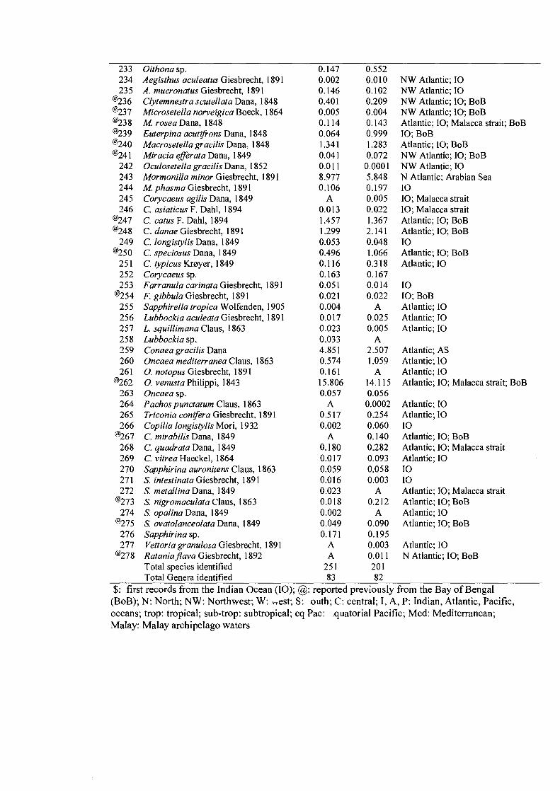
233 Oithona sp. 0.147 0.552 234 Aegisthus aculeatus Giesbrecht, 1891 0.002 0.010 NW Atlantic; JO 235 A. mucronatus Giesbrecht, 1891 0.146 0.102 NW Atlantic; 10

@236 Clytemnestra scutellata Dana, 1848 0.401 0.209 NW Atlantic; JO; BoB @237 Microsetella norveigica Boeck, 1864 0.005 0.004 NW Atlantic; IO; BoB @238 M rosea Dana, 1848 0.114 0.143 Atlantic; JO; Malacca strait; BoB @239 Euterpina acutifrons Dana, 1848 0.064 0.999 JO; BoB @240 Macrosetella gracilis Dana, 1848 1.341 1.283 Atlantic; 10; BoB @241 Miracia efferata Dana, 1849 0.041 0.072 NW Atlantic; 10; BoB

242 Oculosetella gracilis Dana, 1852 0.011 0.0001 NW Atlantic; 10 243 Mormonilla minor Giesbrecht, 1891 8.977 5.848 N Atlantic; Arabian Sea 244 M. phasma Giesbrecht, 1891 0.106 0.197 10 245 Corycaeus agilis Dana, 1849 A 0.005 IO; Malacca strait 246 C. asiaticus F. Dahl, 1894 0.013 0.022 IO; Malacca strait

@247 C. catus F. Dahl, 1894 1.457 1.367 Atlantic; 10; BoB @248 C. danae Giesbrecht, 1891 1.299 2.141 Atlantic; IO; BoB

249 C. longistylis Dana, 1849 0.053 0.048 10 @250 C. speciosus Dana, 1849 0.496 1.066 Atlantic; IO; BoB

251 C. typicus Kroyer, 1849 0.116 0.318 Atlantic; I0 252 Corycaeus sp. 0.163 0.167 253 Farranula carinata Giesbrecht, 1891 0.051 0.014 10

@254 F. gibbula Giesbrecht, 1891 0.021 0.022 IO; BoB 255 Sapphirella tropica Wolfenden, 1905 0.004 A Atlantic; 10 256 Lubbockia aculeata Giesbrecht, 1891 0.017 0.025 Atlantic; I0 257 L. squillimana Claus, 1863 0.023 0.005 Atlantic; 10 258 Lubbockia sp. 0.033 A 259 Conaea gracilis Dana 4.851 2.507 Atlantic; AS 260 Oncaea mediterranea Claus, 1863 0.574 1.059 Atlantic; I0 261 0. notopus Giesbrecht, 1891 0.161 A Atlantic; I0

@262 0. venusta Philippi, 1843 15.806 14.115 Atlantic; 10; Malacca strait; BoB 263 Oncaea sp. 0.057 0.056 264 Pachos punctatum Claus, 1863 A 0.0002 Atlantic; 10 265 Triconia conifera Giesbrecht, 1891 0.517 0.254 Atlantic; JO 266 Copilia longistylis Mori, 1932 0.002 0.060 10

@267 C. mirabilis Dana, 1849 A 0.140 Atlantic; JO; BoB 268 C. quadrata Dana, 1849 0.180 0.282 Atlantic; IO; Malacca strait 269 C. vitrea Haeckel, 1864 0.017 0.093 Atlantic; I0 270 Sapphirina auronitens Claus, 1863 0.059 0.058 JO 271 S. intestinata Giesbrecht, 1891 0.016 0.003 10 272 S. metallina Dana, 1849 0.023 A Atlantic; 10; Malacca strait

@273 S. nigromaculata Claus, 1863 0.018 0.212 Atlantic; 10; BoB 274 S. opalina Dana, 1849 0.002 A Atlantic; JO

@275 S. ovatolanceolata Dana, 1849 0.049 0.090 Atlantic; JO; BoB 276 Sapphirina sp. 0.171 0.195 277 Vettoria granulosa Giesbrecht, 1891 A 0.003 Atlantic; 10

@278 Ratania flava Giesbrecht, 1892 A 0.011 N Atlantic; 10; BoB Total species identified 251 201 Total Genera identified 83 82

$: first records from the Indian Ocean (10); @: reported previously from the Bay of Bengal (BoB); N: North; NW: Northwest; W: ,vest; S: outh; C: central; I, A, P: Indian, Atlantic, Pacific, oceans; trop: tropical; sub-trop: subtropical; eq Pac: ,quatorial Pacific; Med: Mediterranean; Malay: Malay archipelago waters

venusta, Euterpina acutifrons, Microsetella norveigica, Macrosetella gracilis, Miracia

efferata (Nair et al. 1981; Rakhesh et al. 2006), Acrocalanus gracilis, Clytemnestra

scutellata, (Pati 1980), Eucalanus elongatus, Calocalanus pavo, Sapphirina

ovatolanceolata (Krishnamurty 1967), Rhincalanus nasutus, Oithona plumifera

(Subbaraju and Krishnamurty 1972), Paracandacia truncata, Candacia catula, C.

discaudata (Lawson 1977), Microsetella rosea, Oithona similis, Paracalanus parvus,

Acrocalanus longicornis, Acartia spinicauda,Oithona brevicornis (Godhantaraman 1994)

and Acartia centrura (White et al. 2006).

Other than these 54 species, the remaining species identified in this study are the first-

time reports from the western Bay of Bengal. Since only 40 out of 201 species in the WB

were present in all seasons, a significant number of species occurred only seasonally.

Various possible reasons for their seasonal occurrence are detailed in Chapter 6.

7.3.5. Dominant species

As described in Chapter 6, the apparent predominance of 0. venusta during most part of

the year in both CB and also in WB might suggest a continuous breeding throughout the

year (Hopkins 1977). In other oligotrophic regions such as the Sargasso Sea too, a

predominance of Oncaea was observed (Deevey 1971). During SpIM, E. monachus was

the predominant species. The occurrence of E. monachus in large numbers coinciding

with spring blooms in temperate seas or upwelling events in the tropical zone is well

documented (Gapishko 1980; Heinrich 1986; Smith 1995). As an adaptation to

intermittent food supply, the species diapause at mesopelagic depths at lower latitudes

(Boucher 1984; Heinrich 1986; Smith 1992) and the massive lipid storage by pre-adult

resting stages fuels respiration (Conover 1988). It may be presumed that episodic new

production as indicated by the higher populations of the large sized opportunistic coarse

filter feeding E. monachus would have contributed appreciably to the total biomass

during SpIM.

The other dominant species with >2% of the total populations also displayed a wide

range of distribution patterns, such as preponderance in the shallow, intermediate and /or

deep-water distribution. Eucalanus elongatus, the mesopelagic resident (Deevey and

Brooks 1977) was always in deeper depths irrespective of seasons in this warm tropical

108

basin. The species C. arcuicornis, Acrocalanus gracilis, 0. mediterranea P. indicus,

Eucalanus monachus, C. catus, C. danae and 0. similis were common along this transect

as well as in the CB. Paracalanus spp. known to obtain sufficient food at the low food

concentrations (Paffenhofer and Stearns 1988) were also preponderant in this transect.

Compared to the other abundant species in WB such as Paracalanus spp., Clausocalanus

spp., Oithona spp. and Oncaea spp., the relatively large and warm water species

Centropages furcatus constituted a significant part of the zooplankton biomass as also

reported for other coastal areas especially the South east Atlantic coast (Turner 1987;

Turner and Tester 1989). As Ikeda (1974) and Anraku and Omori (1963) suggest, the

omnivorous—carnivorous character allows the successful maintenance of this species

allowing it to compensate for seasonal variations of phytoplankton abundance.

Similar to that in the CB and many previous observations (Bigelow 1926; Rose 1929,

1933; Wilson 1942; Sewell 1947), Oithona similis and Oncaea venusta were ubiquitous

in this study with mostly higher abundances in top 200 m. Lucicutia flavicornis and

Pleuromamma indica as seen in this study, are reported to occur throughout the water

column of over 1000 m (Saltzman and Wishner 1997). Pleuromamma indica, Eucalanus

elongatus and M minor seem to tolerate low oxygen concentrations (Saltzman and

Wishner 1997) since they were observed in higher proportion at subsurface depths.

7.3.6. Diversity

Estimating diversity in the pelagic realm is particularly relevant when examining

relationships between hydrography and the pelagic biota. Similar to observations of

Deevey and Brooks (1977), diversity was high in the MLD and the deeper depths in the

WB. Padmavati et al. (1998) attributed the high diversity in the deepest layer to the stable

environment there. Overall, H' did not show much latitudinal variation in the WB. On an

average, diversity was very high during FIM as was also seen in the CB. A very stable

water column in this season of marked chemical and physical gradients, providing a

structured environment but with low input of nutrients for phytoplankton production

could be a reason for high diversity (Angel 1993). As Lasserre (1994) suggest, the high

diversity in the phytoplankton community in the Bay (Paul et al. 2007) appear to be a

mechanism generating diversity among zooplankton.

109

The details of evenness and species richness in the WB were not very different from

those already discussed in Chapter 6 but for minor deviations. Copepod diversity showed

a negative correlation with chl a indicating inverse relation with primary production

(Huston 1994).

7.3.7. Compositional differences in WB and CB

Undoubtedly, the Bay of Bengal is a copepod-dominated biome. Collectively, the

copepod population in low latitudes has its intense breeding activity during July and

October. But, individual species may reach their maximum densities in different months

of the year (Reeve 1964; Raymont 1983), a characteristic feature of the warm seas.

Though the average abundance in the WB was greater than in the CB, there was no

significant difference between coastal and oceanic waters but for one season (SUM). This

is probably because the stations in WB were mostly in depths over 1000 m.

The WB was significantly more productive than the CB only during SUM. Such

difference in the inshore and offshore waters was also observed with the seasonally

reversing monsoons in the Arabian Sea (Smith et al. 1998; Stelfox et al. 1999). One

additional order, Siphonostomatoida comprising a member of family Rataniidae was

identified only in the WB. The number of genera (82) and species (201) observed in the

WB were lower compared to CB (83 genera and 251 species). Species diversity was

higher in the CB. While Paracalanus parvus, Acrocalanus gibber, A. longicornis, 0.

plumifera and Centropages furcatus were the dominant epipelagic species in the WB,

Macrosetella gracilis, Paracalanus aculeatus, P. crassirostris, Corycaeus speciosus and

Clausocalanus furcatus were in the CB, suggesting that dominant epipelagic assemblages

vary in coastal and oceanic waters.

Though Calanoida was the dominant order, the poecilostomatoid, 0. venusta formed

the key species in most seasons, depths and stations along both transects. With only a

moderate chl a regime in the Bay, this carnivore-omnivore seems to be well adapted for

survival in the environmental variabilities oscillating in the Bay under the influences of

physics (monsoonal currents and wind forcing), chemistry (salinity and nutrient changes)

and biology (chl a; primary production).

110

Vertical partitioning of food and space resources is evident with different families

dominating different zones of the upper 1000 m water column and only a few ubiquitous

forms like Oithona and Oncaea seeming to be versatile. The wide distribution of Oithona

species is partly due to the fact that some of them have euryhaline (Torres-Sorando et al.

2003 and Hansen et al. 2004), and eurythermal characteristics (Turner 2004), in addition

to low respiration and metabolic rates (Paffenhofer 1993). Fransz and Gonzalez (1995)

report that egg production of Oithona is spread over the seasons than reported for

calanoid copepods. They also seem to be spawning and hatching throughout the water

column (Fernandez de Puelles et al. 1996) as observed from the occurrence of copepod

eggs and nauplii (Chapter 5) at all sampling depths. According to Kellermann (1987),

Oithona adults are important food items for fish larvae ("visual hunters"), so that the

adults prefer to stay in deeper water layers supposedly to avoid predators. Pleuromamma

indica showed a significant positive correlation with salinity and phosphate and a

negative relationship with dissolved oxygen in the Bay of Bengal and Arabian Sea

(Saraswathy 1986). Being able to adapt readily to OMZ in the northern Indian Ocean in

particular, its increased abundance over the past thirty years is suggestive of the growing

size and/or intensity of the OMZ in the Arabian Sea (Smith and Madhupratap 2005).

This study has brought out the occurrence of a large number of copepod species

(>200) not reported so far from the BoB. High diversity not only in the deep but also in

the surface is a significant observation of this study. Besides being useful to notify such

diversity of copepods from the Bay of Bengal, it is also reflecting the distribution pattern

of predominant species (e.g. 0. venusta), from this least studied region. The fact that the

deep-strata sampling was carried out systematically for the first time which is the main

reason for revealing such a lot of new records (20 species are new to the Indian Ocean) of

copepod species, need to be kept in the fore. This was possible mainly because of the

sampling from deeper than the usual 200 m column. In addition, the extensive and careful

analysis of all the collected samples led to such discoveries. It is certain that there are far

more number of zooplankton in the deeper realms of the BoB unknown to marine

biologists. Notwithstanding the meagerness of the least abundant species, another

highlight from this study is that there is more to know of copepods from the Bay of

Bengal.

111

Plate 5

Photographs of some epipelagic calanoid copepod species (scale is in micrometer) from the Bay of Bengal

Key: A: Labidocera pavo: B: L. acura: C: Pontella sp.: D: Candacia conifer, E: C. pachydacryla:F. G: Candacia sp.: H: Dm-claims crassus: I: E. mucronants: J: Ericalanus elongants: K: Pareucalanus attenuants: L: Rhincalanus cornunts

700

Plate 6

Photographs of some epipelagic calanoid copepod species (scale is in micrometer) from the Bay of Bengal

Key: A: Acrocalanus longicornis: B: Undinula vulgaris: C: Cosmocalanus darwinii; D: Scolecithrix (Jamie; E: Calocalanus paro: F: Acartia spinicauda: G: Aetideus acutus: H: Euchaeta marina: I: Clausocalanus Arcatus: J: Centropages fiaratus; K: Canthocalanus pauper; L: Temora discaudata; M: Paracalanus indicus

2000 500

3000

Plate 7

Photographs of some mesopelagic copepod species (scale is in micrometer) from the Bay of Bengal

Key: A: Euchirella bitumida: B: Euchirella sp.: C: Gaetanus miles: D: Euaugaptilus facilis: E: Eitaugapti/us sp_: F: Haloprilus longicornis; G: Gattssia princeps; H: Merridia pr inceps: I: Merridia bre ► icauda: Pleuromamma indica: K: P xiphias: L: Lucicutia maxima;

M: Lophothrix frontalis; N: Scottocalanus helenae: 0: MegacaIanus princeps

150

1) 250

300

Plate 8

Photographs of some non- calanoid copepod species (scale is in micrometer) from the Bay of Bengal

Key: A: Aegisthus ',flimflams: B: Euterpina actin:tons: C: Microsetella rosea: D: M norveigica: E: Mormonilla minor: F: Colycaeus cants: G: Colycaeus sp.: H: Sapphiiina ovatolanceolata: I: Sapphirina sp.: J: Pachos punctaturn: K: Lubbockia actileara: L: Conaea gracilis: M: Oncaea venom: N: Oithona similis: 0: Ratania flaw,

Chapter 8

Chapter 8

Measurements of Vital Rates of Copepods in the Bay

There is a growing awareness of the important contribution of mesozooplankton to

carbon cycling in the ocean (Zhang and Dam 1997; Steinberg et al. 2000). The transfer of

primary production to secondary producers not only involves ingestion of phytoplankton,

but also the respiratory demand of zooplankton that utilizes a large proportion of the

ingested matter (Hernandez- Leon and Ikeda 2005). The ubiquitous distribution, high

abundance and trophic importance of copepods form important criteria for estimating

their vital rates in the elucidation of marine carbon cycling (Aristegui et al. 2005;

Hernandez- Leon and Ikeda 2005; Buitenhuis et al. 2006). The activities of planktonic

copepods range from occasional motion to continuous, rapid swimming (Gauld 1966;

Paffenhofer et al. 1996; Mazzocchi and Paffenhofer 1999). According to modeling

studies, increased motion results in increased metabolic expenditures (Klyashtorin and

Yarzombek 1973).

Zooplankton grazing is an important process controlling phytoplankton populations in

the oceans (Banse 1994). However, studies on zooplankton carried out in the open ocean

are concerning mostly their distribution (Finenko et al. 2003). During the last decade,

investigations on zooplankton grazing have been carried out in more productive coastal

areas (Morales et al. 1991; Pakhomov and Perissinotto 1997; Gowen et al. 1999).

Although the vast oligotrophic regions contribute up to 80% of the global ocean

production and 70% of the total export production (Karl et al. 1996), information on

zooplankton vital rates in general, is lacking from these ecosystems (Dam et al.1995;

Zhang et al. 1995).

Method of Gut fluorescence as a measure of chlorophyll pigments was developed by

Yentsch and Menzel (1963). The fundamental factor in estimation of the ingestion rate is

the careful measurement of the gut evacuation rate (Peterson et al.1990). The gut

evacuation rate constant (k) is usually derived from a model of exponential decrease in

gut fluorescence over time, assuming that a constant proportion of the gut content is

112

evacuated per unit time (Baars and Oosterhuis 1984; Kiorboe et al. 1985, Christoffersen

and Jespersen 1986).

From studies of Campbell and Vaulot (1993), Letelier et al. (1993) and Campbell et

al. (1994, 1997), it is evident that warm oligotrophic regions support a complex

planktonic community with pico-sized (0.2-2 um) phytoplankton and, auto- and hetero-

trophic bacteria dominating the community biomass. Such organisms are reported to be

largely unavailable to direct utilization by the Crustacea-dominated mesozooplankton

because of size constraints on feeding mechanisms (Rassoulzadegan and Etienne 1981;

Conover 1982; Berggreen et al. 1988; Hansen et al. 1994). Nonetheless, they are linked in

principle to higher order animals by the cascading influences of mesozooplankton

grazing on consumers of intermediate size (Sherr et al. 1986; Sherr and Sherr 1988;

Wilmer and Hagstrom 1988).

Oxygen consumption of copepods has been related to body mass, temperature (Ikeda

1985; Hiromi et al. 1988; Castellani et al. 2005), feeding behavior (Klekowski et al.

1977), and to diel cycles (Pavlova 1994). In the subtropical to tropical open-ocean,

abundances of potential food organisms for planktonic copepods are usually low

compared to neritic regions (Paffenhofer et al. 2003). This is indicative that their

metabolic and growth demands may not always be met (Dam et al. 1995; Roman and

Gauzens 1997). Most of the organic matter originated through primary production in the

surface layers is fated to mineralize through planktonic respiration in situ or during the

course of sinking. Only a small fraction is buried in the ocean floor. Recently Del Giorgio

and Duarte (2002) provided an assessment of respiration in the ocean. From this, it

appears that respiration consumes more organic matter than seems to be produced in the

ocean.

Mesozooplankton respiration can be calculated as the product of their specific

respiration rates and biomass. Specific respiration rates have been shown to vary with

temperature and body mass, with relatively modest or no taxonomic differences (Ikeda

1985). Zooplankton biomass in the epipelagic zone of a given water mass being highly

variable in space and time by one to three orders of magnitude (Huntley and Lopez 1992),

the subsequent respiration rates are likely to vary concurrently.

113

Metabolic processes of zooplankton such as grazing, respiration and growth in the

open ocean waters have received growing attention in recent years, particularly in the

Pacific and Atlantic (Dam et al. 1995; Zhang et al. 1995; Le Borgne and Rodier 1997;

Roman and Gauzens 1997; Zhang and Dam 1997; Roman et al. 2002; Le Borgne and

Landry 2003; Le Borgne 1977, 1981, 1982; Welschmeyer and Lorenzen 1985; Harrison

et al. 2001; Ruskin et al. 2001 a, b; Woodd-Walker et al. 2002).

Respiration measurements were carried out in the early 1930s mainly on the copepod

Calanus finmarchicus (Marshall et al. 1935, Clarke and Bonnet 1939). To date there has

not been a single documented report of respiration rate from the Bay of Bengal.

Assessing the magnitude of respiration by the preponderant epipelagic copepods in the

warm, moderately productive waters of the Bay of Bengal is essential for relating their

organic matter requirement vis a vis its production through photosynthetic process. This

set of measurements was thus aimed at not only obtaining information on zooplankton

respiration rate but also to calculate the carbon consumption rates using relevant

respiration quotients available in literature.

To understand the grazing pressure of different trophic levels on phytoplankton,

nutrient enrichments of size-fractionated seawater have been carried out in microcosm

experiments in oligotrophic eastern Mediterranean (Kress et al. 2005; Zohary et al. 2005)

and at Hawaiian Ocean time-series station (HOTS; Calbet and Landry 1999). In tropical

ecosystems such as the Bay of Bengal (BoB), the upper waters are mostly devoid of any

nutrients due to almost perennial warm pool and low saline lens in the upper 30 m

(Prasannakumar et al. 2002, 2007). The thermohaline stratification causes nutrient

limitation and keeps the Bay low to moderate in chl a levels throughout the year. In the

present study, the effect of nutrient enrichment on the dynamics of chlorophyll a,

phytoplankton cell numbers, microzooplankton and the mesozooplankton abundance was

investigated in microcosm experiments. The main objective of this experiment was to

evaluate mesozooplankton grazing or ingestion effect on phytoplankton under natural sea

water-, nutrient altered- and, size fractionated- microcosms set up onboard.

Zooplankton growth-rate measurements in situ in open waters have been carried out

as early as 1963 (Cushing and Tungate 1963), but they are extremely time-consuming.

Shipboard incubation techniques have been used for growth estimates for individual

114

copepod species based on molting frequency (Miller et al. 1984) and egg production

(Kiorboe and Johansen 1986; Berggreen et al. 1988). But these techniques are subject to a

variety of containment effects and are of limited value for overall copepod community

growth estimates in tropical seas where the species diversity of copepods is great (Grice

and Hart 1962; Timonin 1971).

Another approach to estimating copepod growth is based on regression models that

use temperature (McLaren and Corkett 1981; Huntley and Lopez 1992), resource

concentration (Vidal 1980; Berggreen et al. 1988) or temperature and body size

(McLaren 1965; Ikeda and Motoda 1975; Hirst and Sheader 1997; Hirst and Lampitt

1998) to predict copepod growth rates. These models assume that all copepod species of

the same size grow at the same rate at a given temperature.

Using a regression equation, growth rates for the 200-500 pm fraction of copepods

have been estimated during this study from the upper mixed layer.

8.1. Materials and Methods

These sets of microcosm and rate measurement experiments were carried out onboard

during the winter monsoon cruise (November 26, 2005 to January 7, 2006) of FORV

Sagar Sampada.

8.1.1. Collection of zooplankton samples

A Bongo (two-nets set; mouth area 0.28 m 2 of each net; mesh size 300 pm; Hydrobios)

net was hauled obliquely at 2 knots speed for 10-15 min for collecting surface (0-5 m)

zooplankton at all the nine stations shown in Fig. 3.1 in Chapter 3. The initial and final

digital flowmeter (FMR; Hydrobios Model 438 110) readings were noted in order to

calculate the volume of water filtered. The volume of water filtered was calculated using:

V (m3) =A x R x K; Where, A= mouth area (for circular net, A = it x r 2 where r is the

radius of the net, it = 3.14); R = flow meter reading; K = calibration constant;

V = Volume of water filtered.

115

8.1.2. Measurement of gut fluorescence

This technique was carried out by following the available methods (Mackas and Bohrer

1976; Baars and Oosterhuis 1984; Kiorboe et al. 1985, Christoffersen and Jespersen

1986; Dam et al. 1995). Upon retrieval of the net, the contents of one net were used to

measure the biovolume and preserved as described in Chapter 4 for enumerating the

mesozooplankton and total copepods. The contents of the second net were immediately

transferred into llitre 0.45-pm filtered seawater taken from 10 m depth. This was done to

avoid crowding and undue stress. At zero time itself, 25 ml of this diluted zooplankton

sample was transferred into a wide petridish to pick up actively moving copepods. Under

dim light, —30 medium sized copepods were picked with a dropper and filtered onto

GF/C filter paper and added to 8 ml of 90 % acetone. Similar procedure was carried out

for the rest of the zooplankton samples every 15 min generally for 150 min. The samples

were kept for extraction at zero degree in the freezer for 24 h in the dark. After

extraction, the sample was thawed for half an hour and chlorophyll (chl) a was measured

using Fluorometer (AU-10 Turner designs, USA).

Concentrations of chl a and phaeopigments (phaeo) in the copepod guts were calculated

using the following equations (Parsons et al. 1984 ):

Chl a Gig ind-1 ) = (T/(T-1)) * (Rb - Ra) * Fd * Vol ex /no of individuals

Phaeo Gig ind-I ) = (T/(T-1)) * ((T*Ra) - Rb) * Fd * Vol ex / no of individuals

where; T = acidification coefficient (Rb/Ra obtained through the calibration of the

fluorometer); Rb = reading before acidification; Ra = reading after acidification

Fd = flourometer calibration factor Gig liter -I ); Vol ex = volume of extraction (ml);

The Gut content was calculated as: G = (1.51 x conc. of phaeopigment)+ conc. of chl a

The gut evacuation rate constant (k) was calculated from the equation: Gt= Go x e tc`

Where; Gt = pigment concentration at time t; Go = pigment concentration at time to

The ingestion rate was then calculated as: I = G * k (ICES 2000)

116

Copepod egestion (fecal pellet production; E) was estimated by assuming that 70% of

the ingested material (I) was partitioned to growth and respiration and 30% was egested

as fecal pellets (Conover 1978).

The amount of chl a grazed daily by copepods was estimated by multiplying

their numerical abundance in a tow (ind m -3) with the corresponding ingestion rate. The

phytoplankton carbon ingested was calculated by applying a carbon to chl a ratio as 50

(Banse 1988).

8.1.3. Measurement of respiration rates

The respiration or oxygen consumption rate was measured following essentially Mayzaud

and Dallot (1973). From the assortment of mesozooplankton collected from the oblique

hauls, mostly copepods were separated and transferred to a beaker with 0.22 pm filtered

seawater (FSW) and allowed to acclimatize for one hour. Five sets of bottles of 125 ml

capacity (in duplicate) were used in the experiment as follows:

A set of two bottles was filled gently with 0.20 pm FSW avoiding air bubble

formation. These were used for measuring initial concentration of dissolved oxygen (DO)

by fixing it immediately with Winkler A and B reagents. Copepods (-30 1 -1 ) and

streptomycin (50 mg 1 -1 ) were added to the experimental bottles filled with 0.20 pm

FSW. The antibiotic was added to arrest uptake by bacteria. Another set of two bottles

was incubated with copepods (-30 1 -1 ) without the antibiotic to derive the oxygen

consumption both by bacteria and copepods (positive control). One more set of two

bottles with streptomycin but without copepods (negative controls) were used to check

whether the addition of streptomycin is contributing to any DO consumption. A final set

of two bottles served as negative controls and, was without copepods and antibiotics to

examine if FSW itself contributed to any variation in DO concentration.

But for the bottles initially fixed, the other sets of bottles were topped up with FSW to

the brim and covered with aluminium foil and incubated for 12 h at RT. After 12 h, the

bottles were fixed with Winkler A and B and dissolved oxygen estimated by the standard

Winkler method (Grasshoff et al. 1983; using 665 Dosimat Metrohm, Switzerland). After

the experiment, the contents of the incubation bottles were filtered over 200-pm mesh

and the retained plankton counted using a magnifying lens.

117

Oxygen consumption rate was calculated by using the equation (Omori and Ikeda

1984):

R = ((Co-Ct)-(C0-00) x (Ve-V,)/ (t x N)

Where Co = Oxygen concentration at time 0, C t = oxygen concentration in experimental

bottle, Ct' = oxygen concentration in control, V e = volume of experimental bottle, V, =

volume of zooplankton, t = incubation time, N = number of copepods.

A respiration quotient of 1.0 provided by Baars and Franz (1984) was used to convert

oxygen consumption into carbon mineralization. The derived respiration rates at each

sampling location were applied to calculate the total copepod respiration in the mixed

layer using the copepod abundance data presented in Chapters 6 and 7.

8.1.4. Evaluation of responses of plankton assemblages to nutrient amendments

The experiment was conducted at three locations (CBI, CB5 and WB2) in the BoB. The

first location was the southernmost station in the open waters, the second the

northernmost and the last, in the western Bay. At these locations, over 200 1 of seawater

was collected from 10 m depth by several casts of 301 Go Flo bottles. After collecting the

water, zooplankton were collected as described in section 8.1.1., transferred in 0.45µm-

filtered seawater to considerably thin down the concentration and held for an hour before

using in the experiments below.

Set up of Microcosms

Ten transparent polythene tubs of 20 litre capacity were used as microcosms. In brief,

the experimental set up and nutrient amendments is as follows:

Microcosm /:Twenty litres of whole seawater (WSW)- Normal control

Microcosm 2: WSW (20 1) amended with nutrients (NO3: 15 p.M, SiO3: 5pM and PO4:

1p.M). Such nutrient concentrations were usually deep-seated at =40-80 m, where deep

chlorophyll maxima form in the Bay of Bengal. Thus, the amendment was done to

examine the response of phytoplankton to increased nutrient levels without the added

population of grazers, i.e. copepods.

Microcosm 3 was the same as the above but with added copepods at a concentration of 10

ind. 14 to check the effect of grazing on phytoplankton under nutrient enrichment.

118

Microcosm 4: Twenty litres of 200 1AM filtered seawater (FSW) and added nutrients at

the concentrations in microcosms 2 and 3. Passing through 200 p.m was done for

excluding mesozooplankton grazers while still retaining the microzooplankton. These

alterations were made to check out whether the phytoplankton population increased and,

grew rapidly without the mesozooplankton grazing pressure, or decreased owing to

overwhelming microzooplankton grazing pressure.

Microcosm 5 consisted of 200 pm FSW sans addition of nutrients and grazers. This was

done to observe the effect of natural community of micro-zooplankton grazers on the

natural phytoplankton population.

Microcosm 6 consisted of 100 pm FSW and added nutrients, in order to see the response

of phytoplankton and consequently of the smaller fraction of the microzooplankton when

nutrient concentrations are increased.

Microcosm 7 had 20 1 100 pm FSW sans added nutrients to serve as control to

microcosm 6.

Microcosm 8 was set up with 20 1 20 p.m FSW to check the grazing effect of

nanozooplankton if any on phytoplankton fraction < 20pm.

Microcosm 9 had 20 1 20 p.m FSW with added nutrients. This microcosm was set up to

examine the response of the HNF if the nanophytoplankton increased as consequence of

added nutrients.

Microcosm 10 was with 20 1 20 pm FSW, and copepods. In this treatment, it was aimed

at finding out whether the <20pm phyto-fraction can support the survival of

mesozooplankton grazers or not.

All the microcosms were maintained at shipboard temperature (-26°C) under 12:12 h

light (1000 lux = —200 pE): dark cycle for a period of 7 days. Samples were drawn daily

for seven days and, nine different parameters were measured from all the microcosms.

These were: nutrients- nitrate (NO3), silicate (SiO 3) and phosphate (PO4), phytoplankton

(PCC), microzooplankton (Mzp), mesozooplankton (MsZP), total bacterial abundance

(BA), chlorophyll (chl) a and phaeopigments (phaeo). Everyday, the water samples were

collected around the same time, analysed soon after collection or, fixed appropriately and

stored for later analyses in the laboratory. The parameters measured are as follows:

119

Nutrients

100 ml water sample from each microcosm was filled in clean plastic bottles and frozen

at 0°C until analyses. Nutrients (NO3-N, PO4-P and Sia t-Si) were analyzed as soon as

the experiment was terminated, using a SKALAR autoanalyser following the procedures

given in Grasshoff et al. (1983).

Phytoplankton/Microzooplankton

From all the 10 microcosms, 250 ml of water sample was fixed in Lugol's iodine (1%

w/v), 3% formaldehyde and 2 mg r I strontium sulphate, and stored in dark until taken up

for analyses. A settling and siphoning procedure was followed to concentrate samples

from 250 ml to 10 ml (Utermohl 1958). A few replicates of one-ml concentrated aliquots

were taken into a Sedgwick-Rafter plankton counting chamber and examined

microscopically at 200-400X magnification. Some taxa of phytoplankton were identified

to generic level by referring to various keys (Tomas 1997; ICES 2000).

Mesozooplankton abundance

Another 250 ml of water sample from each microcosm was collected and fixed with

formalin to a final concentration of 4% and stored. In the laboratory, the water was

siphoned out to keep behind —10 ml, which was poured into Bogorov chamber and total

mesozooplankton were counted (UNESCO 1968; ICES 2000).

Chlorophyll a and phaeopigments

Samples of 500 ml of water were collected dailyfor measurement of these pigments.Their

measurements were carried out following the JGOFS Protocols (UNESCO 1994)

described in Chapter 3.

Bacterial Abundance

From each microcosm, 10 ml samples were fixed with 0.22 lam pre-filtered formaldehyde

(final concentration of 3.7%) and stored at 4°C in dark as per JGOFS Protocols

(UNESCO 1994) until analysis. The procedure followed for enumerating bacterial counts

was according to Parsons et al. (1984). Three milliliter of each sample was stained with

120

acridine orange (final concentration 0.01%) for 3 mM, filtered onto 0.22 pm black

Nuclepore filters, mounted on glass slides using non-fluorescent oil and observed under

100X oil immersion objective of epifluorescence microscope (E400 Nikon, Japan). The

slides were viewed using a blue excitation (450-490 nm) filter, 510 nm beam splitter and

a 520 nm emission filter. Bacterial cells in ca. 25 microscopic fields were counted, mean

cell numbers per field calculated and used for estimating total abundance by using the

formula detailed in Parsons et al. (1984):

Bacterial cells m1 -1 = Xb x Ct N; where

Xb = mean bacteria per field

Ct = conversion factor (filtration area/grid area)

V = volume of sample filtered (ml)

8.1.5. Derivation of growth rates

The regression equation of Hirst and Sheader (1997) given below, was used to calculate

the potential growth rate of mesozooplankton. This equation uses published data on

copepod growth rates, a wide range of body weights (0.002-43 p.M C) and habitat

temperatures (0-29.8°C).

G = 0.0732 x 00.0246 w c 0.2962

where,

g (dH ) = intrinsic growth rate; T; °C = temperature and Wc; pg C individual-1 = copepod

carbon weight

Temperature data obtained from CTD at each sampling location were averaged from the

upper 120 m in the central (CB) and western Bay of Bengal (WB). It was assumed that

the predominant copepods (70 to 90%) comprised all of the measured mesozooplankton

biomass. Individual copepod weight for the 200-500 pm fraction was taken as 2.04 [is C

(Roman et al. 2000).

Copepod production was derived using:

P (mg C m-2 C I ) = B x g,

where B is biomass (mM C m-2).

121

Biomass values of zooplankton collected during four different seasons (summer

monsoon: SUM; fall intermonsoon: FIM; winter monsoon: WM; spring interttonsoon:

SpIM) during this study from the Bay were used for deriving the copepod production.

8.2. Results

8.2.1. Composition of Copepoda

The predominant copepods differed at each station sampled in both transects (Table 8.1).

At CB1, the dominant copepods were Undinula vulgaris (17.2%), Corycaeus longistylis

and C. speciosus (10.3%). At CB2, Sapphirina spp. (18%), Undinula vulgaris (11%) and

Acrocalanus spp. (9.4%) were dominant. At CB3, U. vulgaris (31.5%), Sapphirina spp.

(11%) and Candacia bradyi (9.3%) were abundant. At CB4, U. vulgaris, Pleuromamma

indica (22.7%) and C. bradyi (13.6%) were dominant. At CBS, Temora stylifera (28%),

Oncaea spp. (17%), Candacia sp. (13.2%) and Scottocalanus helenae (9.4%) were the

dominant species.

In the WB, Acrocalanus longicornis (17.7%), Temora discaudata (11.3%) and T.

stylifera (9.7%) were the dominant species at WB1 (Table 8.1). At WB2, Oithona spp.

(24.4%), T stylifera and A. longicornis (16.3%) were dominant. At WB3, Oithona spp.

(15.2%), T stylifera and Centropages furcatus (12.1%) were dominant. At WB4, Temora

stylifera (26.1%) was the most abundant.

8.2.2. Gut evacuation, ingestion and egestion rates of copepods

The initial chl a concentrations in copepod guts from the measurements of gut

fluorescence at various stations were found to be varying from 2 to 14 ng per individual

(Fig. 8.1). Similarly, the phaeopigment concentration varied from 0.2 to 6.6 ng per

individual. In the gut evacuation experiment, the copepod gut chl a decreased rapidly in

the experimental duration of 150 min. The decline was rapid especially in the first hour.

A conspicuous feature observed was the steady-state to steep increase in phaeopigments

towards the end of the experiment. Minor peaks could also be noticed in the chl a after

the first 30-60 mins.

Copepod abundance varying from 72 to 2736 ind. T11-3 were higher in the WB (Fig.

8.2). The gut evacuation rate constant varied only narrowly from 4.02 to 4.08 II I between

122

Table 8.1. Distribution of Copepod species at different stations in the central and western Bay of Bengal

% abundance at different stations Species CB1 CB2 CB3 CB4 CB5 WB1 WB2 WB3 WB4

Acrocalanus longicornis 7.69 7.55 17.74 16.28 Acrocalanus spp 9.37 3.70 1.89 3.03 4.35 Calanopia elliptica 1.61 Calaocalanus pctvo 4.55 1.89 1.16 6.06 4.35 Candacia bradyi 6.25 9.26 13.64 1.61 Candacia pachydactyla 7.69 3.12 Candacia spp. 1.56 13.21 3.23 4.65 Canthocalanus pauper 3.85 7.81 1.85 Centropages calaninus 3.85 1.85 1.61 2.33 Centropages furcatus 3.12 1.85 12.12 4.35 Clausocalanus spp. 1.56 3.77 1.16 4.35 Copilia quadrata 4.55 Copilia sp. 1.56 1.85 1.89 3.23 3.49 Corycaeus catus 3.85 4.35 Corycaeus danae 4.69 4.55 1.61 Corycaeus longistylis 11.54 4.69 3.70 1.89 1.61 Corycaues speciosus 11.54 3.03 Corycaeus spp. 1.85 4.55 1.89 1.61 2.33 4.35 Cosmocalanus darwinii 1.85 1.61 9.09 4.35 Eucalanus crassus 8.06 6.98 3.03 E elongatus 1.85 1.61 1.16 E mucronatus 1.61 E pseudoattenuatus 1.61 Pareucalanus attenuatus 3.85 1.56 1.85 1.61 3.03 4.35 Euchaeta indica 1.56 1.85 1.89 1.61 1.16 Euchaeta marina 1.56 1.85 6.06 4.35 Euchaeta spp. 4.69 1.85 1.89 1.61 Farrannula carinata 1.85 Labidocera pavo 1.56 1.89 4.35 Macrosetella gracilis 1.85 Oithona spp. 1.85 4.55 3.23 24.42 15.15 Oncaea sp. 3.85 16.98 6.45 3.49 9.09 8.70 Oncaea venusta 7.69 4.69 7.41 3.77 1.61 3.03 8.70 Paracalanus indicus 2.33 3.03 Paracalanus parvus 3.85 4.35 Paracalanus spp. 3.85 3.12 4.84 3.03 Pleuromamma indica 22.73 1.89 1.61 2.33 4.35 Pleuromamma sp. 1.61 Pontellina plumata 1.56 1.85 4.55 1.61 1.16 4.35 Rhincalanus cornutus 1.61 Sapphirina sp. 3.85 18.75 11.11 4.55 6.06 Scolecithrix danae 1.56 5.56 4.55 Scottocalanus helenae 1.56 9.43 1.61 3.49 3.03 Temora discaudata 11.29 4.65 Temora stylifera 3.12 4.55 28.30 9.68 16.28 12.12 26.09 Undinula vulgaris 19.23 10.94 31.48 22.73 Total ind 100 I11-3 4232 24896 14428 6741 53341 857274 221464 72265 37720 Number of species 14 23 22 12 16 28 18 16 16

Dominant copepods at each station are marked bold

Chl a

, pha

eopi

gmen

t (ng

. cop

epod

ind.

-1)

0

0

1

1

2

2

CB2

3

0

0

1

1

2

2

WB3

3

3

4 CB5 CB4

WB1

—*— Chl a

—0-- phaeo

0 1 2

3

0 1 2

3

Figure 8.1. Variation in copepod gut pigments (ng. chl a and phaeopigments. copepod ind-1 ) with increasing starvation time

K (h

il);

I, E

(lig

CM

eq

ind.

,0)

G

NMI E

PP

3000

0, 2500

2000

1500

1000 - L.)

500 -

0

CB1 CB2 CB3 CB4 CB5 WB1 WB3 WB4

Station

90 tly MJ

60

30 -

0

F

Figure 8.2. Copepod abundance (individuals 100 m 3); their gut evacuation rate constant (K), ingestion (I), egestion (E; fecal pellet production) and, grazing rate (G) and primary production (PP) in the mixed layer

stations. Using these values, the gut clearance time was estimated to be 14.7-14.9 min.

Ingestion rates on chlorophyll ranging from g.s . to 685ng chl eq. ind -I were the

highest at WB3, followed by vlBi. Egestion of fecal pellets, which is assumed to be 30%

of ingestion varied from 2.9 to 20.6 ng chl eq. ind-I

The calculated ingestion rates corresponded to a daily grazing rate of 1.3-87 mg C 111-3

d-I in the mixed layer depth (MLD; Fig. 8.2). Similarly, the carbon lost through their

fecal pellets ranged from 0.4 to 26.1 mg C 111-3 d 1 . Both grazing and egestion rates were

higher in the WB. The grazing rate ranged from 39 to >100% of the daily primary

production (PP) in the MLD. The grazing rate exceeded the daily PP at all the stations in

WB.

8.2.3. Respiration rate

Respiratory oxygen consumption (RO) rates for the 200-500 p.m fraction of surface living

copepods varied from 0.15 to 0.38 pl 0 2 ind-I h-I (Fig. 8.3) at different stations. The

corresponding body carbon respired (RC) was 79-205 ng C ind -1 h-1 . The total copepod

community at various stations contributed to daily respiration rates (RD) of 0.3- 5.2 mg C

111-3 & I . This accounted for 6-141% of the daily primary production (PP). It exceeded that

of PP at CB1 and WB1.

Seasonally, the carbon loss due to mesozooplankton respiration in the MLD ranged

from 0.08 to 96.14 mg C r112 d-I during SUM, 6.92 to 209.11 mg C r11-2 d-I during FIM,

9.25 to 190.34 mg C 111-2 d-I during WM and 1.26 to 349.45 mg C 111-2 d-I during SpIM

(Fig. 8.4). The highest rates were during SpIM and the lowest during SUM. On an

average, the daily respiration rates were 22, 15, 36 and 63% of the daily PP in upper 40 m

during SUM, FIM, WM and SpIM respectively.

8.2.4. Responses of plankton assemblages to nutrient amendments

Variation of the chemical and biological factors with time

The following is a brief account of quantitative details of chemical and biological

parameters in whole seawater used in the experiments. The variations during the

experimental period are presented in Fig. 8.5-8.10.

123

0.4 -

0.0

250

200 - —ro

-5 150 -

100 -

p4 50 -

0

CB1 CB2 CB3 CB4 CBS 1 WB1 WB3 WB4

CB1 CB2 CB3 CB4 CB5 I WB1 WB3 WB ,

- - PP

—IF— RD ■•

CB1 CB2 CB3 CB4 CB5 WB1 WB3 WB4

Station

Figure 8.3. Station-wise variation in the rates of oxygen consumption (RO), body carbon respired (RC), daily carbon respiration (RD) and daily primary production (PP) in the central and western Bay of Bengal.

MJ

a,

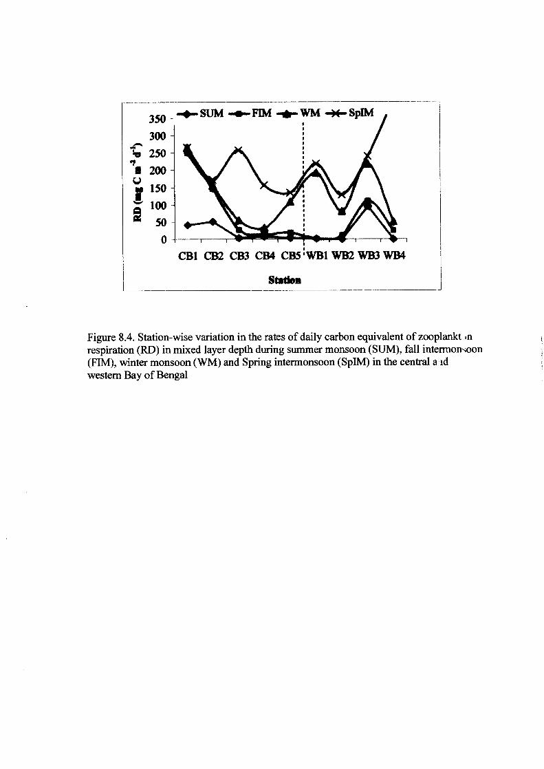
350

300

la 250

• 200

ao 150

Q 100

50

0

Station

...mi. SUM milloo. FIM WM -44.- SpIM

CB1 CB2 CB3 CM CB5'WB1 WB2 WB3 W134

Figure 8.4. Station-wise variation in the rates of daily carbon equivalent of zooplankt .n respiration (RD) in mixed layer depth during summer monsoon (SUM), fall intermonsoon (FIM), winter monsoon (WM) and Spring intermonsoon (SpIM) in the central a id western Bay of Bengal

The ambient nutrient concentrations in seawater were below detection limit for NO3;

21.1,M of SiO3, and 1 p.M of PO4 at CB1. At CB5, their concentrations were 0.3, 4.7 and

0.3 1.1.M respectively. At WB2, the respective concentrations were 2.2, 4.8 and 1.6 p.M.

Phytoplankton abundance in whole seawater ranged from 0.32 x 10 3 cells F 1 at CB1, 0.1

x 104cells F 1 at CB5 to 0.36 x 103 cells F 1 for respective locations on day zero. Microzoo-

plankton numbers varied from 12 ind. r' at CB1 to 8 ind. 1 -1 each at CB5 and WB2.

Similarly, mesozooplankton numbers on day zero at CB1, CB5 and WB1 were 4, 4 and 8

individuals 1-1 . Bacterioplankton numbers (no.x 10 9 cells 1 -1 ) were 0.03, 0.1 and 0.2 at

CB1, CB5 and WB2 respectively. Chl a concentration varied from 0.14 at CB1, 0.3 at

CB5 to 0.26 mg 111-3 at WB2. Phaeopigment values were 0.04, 0.03 and 0.15 mg M.-3 at

the same stations.

Phytoplankton abundance differed considerably (p<0.05) between the experimental

treatments (different size fractionated water) with the lowest numbers in the microcosms

with 20 pun filtered seawater. Bacterial numbers were significantly higher in microcosms

containing added zooplankton. Chlorophyll a and phaeo-pigment concentrations

decreased in the smaller size fractions. While numbers of mesozooplankton significantly

reduced in the <200 1.1M fraction of seawater, that of microzooplankton were negligible in

the 20 p,m fractionated seawater (Table 8.2).

Between the nutrient-amended and non-amended microcosms, most of the measured

biological parameters did not not show a significant difference except for chl a and

phaeopigments at all stations and microzooplankton at CBS and WB2. The 7-day

variation of the measured parameters in treatments with and without nutrient additions is

described below.

Observations from microcosms without nutrient addition

At CB 1, from day zero to day seven, nutrients generally showed a significant variation in

most microcosms. In WSW (Microcosm 1), the phytoplankton cell counts ranging from

0.08 to 0.48 (x 103 cells 1 -1 ) remained high between day zero and day four and drastically

decreased later (Fig. 8.5). However, the decrease in chl a concentration ranging from 0.1

to 0.19 mg M-3 was not drastic. The phaeopigment concentration seemed to increase from

0.03 to 0.06 mg M.-3 with increasing number of days. Micro- (4-12 ind. 1 -1 ) and meso-( 4-8

124

0.8

0.6 1

0.4 U

02 .4 co

0.0 MsZP

--NE— Phaeo

0.6

2 0.4

Li 02

0 PCC

—6-13A NMI nizp

Chl a

0

.8. NO3 t SiO3 PO4

2 — — 2

1

0

1

2 0.6

0.4

02 —

100 pin FSW

2

1

0 1.67."14.741.7487.11.141° 0

3— - 0.8

0.6

0.4

0.2

0.0

0.6

0.4

02

0

2 0.6 0.8

0.6

0.4

0.2

0.0

3 — 20 prn FSW + zoo

0.4 1

0.2

0 ti 0 0 0 1 2 3 4 5 6 7

2

0 1 2 3 4 5 6 7 Days

Figure 8.5. Variation of nitrate (NO3), silicate (SiO 3) and phosphate (PO 4) concentrations (11M), phytoplankton cell counts (PCC; 10 3 cells 1- '), microzooplankton (mzp; 10 2 ind. mesozooplankton (MsZP; 102 ind. 1-1), bacteria (BA; 10 9 cells 14), chlorophyll a (chl a; mg m-3) and phaeopigments (phaeo; mg m-3) in the microcosms with different size fractions of nutrient un-amended seawater over a 7-day period at CB1. (WSW: whole seawater, FSW: filtered seawater, Zoo: zooplankton).

PCC mzp —0—BA —os— Chl a

MsZP -11E-- Phsco

0.6

0.4

02

0.0

15

10

6 Z 5

0

WSW + Nut 2

1

0 SiO3 --dr- PO4

200 um FSW + Nut

• •

.4? FSW + Nut • • • •■■•

15

10

5

0 0 1 2 3 4 5 6 7

15

10

5

0

15

10

5

0

WSW +Nut+ zno 0.6

0.4

0.2

0

2 0.6

0.4 1

0.2

0 0

2 0.6

0.4 1

0.2

0 0

2

0.4 1

02

0 0

Days

-E_ 0.6

- 0.4

02

1- 0.0

T 0.6

0.4

0.2

I f 4 0.0 0 1 2 3 4 5 6 7

0.6 —

Figure 8.6. Variation of nitrate (NO 3), silicate (SiO 3) and phosphate (PO4) concentrations (11M), phytoplankton cell counts (PCC; 10 3 cells 1- '), microzooplankton (mzp; 10 2 ind. mesozooplankton (MsZP; 102 ind. 1- '), bacteria (BA; 109 cells r), chlorophyll a (chl a; mg m-3) and phaeopigments (phaeo; mg m3) in the microcosms with different size fractions of nutrient amended seawater over a 7-day period at CB1. (WSW: whole seawater, FSW: filtered seawater, Zoo: zooplankton, Nut: nutrients).

200pm FSW

Inb,lo. •

20pm FSW

—6.4.41.4.6.4.40+0,014111411-

20pm FSW-+-Zoo

•

• •■■••••••• 8 re rll I I I I I

0 1 2 3 4 5 6 7

6

4

2

0

6

4

2

0

MOM PCC nup MIN MsZP —or— BA Oil► a —111— Phaeo

3

2

—3

— 2 le

1

— 0

1.0 0.6

13.1 2 0.4 -

0.5 g (5 0.2

+- 0.0

0

1.0

0.6

0.4 - 0.5

0.2

0.0 0

1.0 0.6

OA 0.5

02

0.0

1.0 0.6

0.4 0.5

0.2

0.0 0

1.0 0.6

0.4 0.5

0.2

0.0

Days

cn 4

Z 2

0

0 1 2 3 4 5 6 7

Figure 8.7. Variation of nitrate (NO3), silicate (SiO 3) and phosphate (PO 4) concentrations (1 1M), phytoplankton cell counts (PCC; 10 4 cells 1-1 ), microzooplankton (mzp; 10 2 ind. mesozooplankton (MsZP; 102 ind. 1- '), bacteria (BA; 10 9 cells 1- '), chlorophyll a (chl a; mg m-3) and phaeopigments (phaeo; mg m-3) in the microcosms with different size fractions of nutrient un-amended seawater over a 7-day period at CBS. (WSW: whole seawater, FSW: filtered seawater, Zoo: zooplankton)

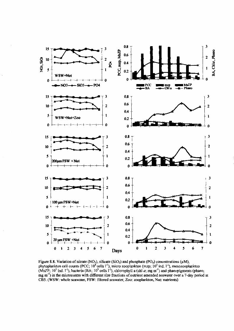
3

2

1

0

15

10

5

0

3

2

1

0

15

10

5

0

15T

0

5—

100 pm FSW+Nut

ill""01•■•••••••••■••■.....• — 3

20 pm FSW +Nut 1 I I t

0 1 2 3 4 5 6 7

2

0

3

2

1

0

Days

1

0.8

0.6

0.4

0.2

0

0.8 15 3

0 6 '

10 2

3

2

1

0

0.4 i73

BA

, Chl

a , P

haeo

Z 5 1 ELS; 0.2 WSW+Nut

0 I 1 I 1 1 0 0

rsw—NO3-4-- 8103—*-- PO4 mom PCC MIN mzp NMI MaZP —o—BA Chia Phaeo

Figure 8.8. Variation of nitrate (NO 3), silicate (SiO 3) and phosphate (PO 4) concentrations (11M), phytoplankton cell counts (PCC; 10 4 cells p'), micro zooplankton (mzp; 10 2 ind. r), mesozooplankton (MsZP; 102 ind. r), bacteria (BA; 10 9 cells r), chlorophyll a (chl a; mg rif 3) and phaeopigments (phaeo; mg m-3) in the microcosms with different size fractions of nutrient amended seawater over a 7-day period at CBS. (WSW: whole seawater, FSW: filtered seawater, Zoo: zooplankton, Nut: nutrients)

ind. zooplankton were present throughout. Bacterial numbers (0.03-0.36 x 10 9 cells 1 -

1 ) increased by an order of magnitude with increasing number of days.

The 200 gm filtered seawater (Microcosm 5) was devoid of mesozooplankton. Thus,

microzooplankton ranging from 4 to 32 (ind. 0 were abundant on all days.

Phytoplankton concentrations were lower, and varied from 0.12 to 0.3 (x 10 3 cells 1 1 ).

The chl a concentration reduced from a maximum of 0.14 on day zero to 0.01 mg m -3 by

day six. Similar trend was noticed in the phaeopigment concentrations (0.01-0.04 mg m -

3). Bacterial numbers increased by an order from 0.02 to 0.2 (x 10 9 cells 1 -1 ) by day seven.

In the 100 gm fraction (Microcosm 7), both microzooplankton (3-20 ind. and PCC

(0.04-0.28 x 103 cells 1 -1 ) were much less. Chl a varied from 0.07 to 0.13 mg m -3 and

phaeopigments from 0.03 to 0.07 mg 111-3 . As chl a decreased, a slight increase was

observed in the phaeopigment concentrations. Bacteria varying from 0.02 to 0.25 (x 10 9

cells 11 ) showed two peaks, one on day three and the other on day seven.

In the 20 gm passed fraction (Microcosm 8), microzoo-, mesozoo- and

microphytoplankton were absent. Bacterial numbers varied from 0.03 to 0.38 (x 10 9 cells

Chl a varying from 0.03 to 0.12 mg m -3 , decreased with time. Phaeopigments varied

from 0.02 to 0.05 mg /11-3 and was higher during day two to day five.

In the 20 gm passed seawater fraction (Microcosm 10), the extra zooplankton which

were added did not survive after day 2. The number of bacteria varying from 0.4 to 0.5 (x

109 cells 1 -1 ) did not change much till the seventh day. Chl a concentrations varying from

0.04 to 0.09 mg m-3 were the lowest among the non-amended microcosms. Phaeo-

pigment concentrations varied from 0.02 to 0.09 mg m -3 . The concentrations of both

decreased with time.

Observations from nutrient added microcosms

Upon nutrient addition to the whole seawater (Microcosm 2), a prominent increase in

phytoplankton cells ( 0.1-0.64 x 10 3 cells 1 -1 ) and chl a (0.06-0.52 mg m -3) was observed

on the second day, decreasing drastically by the seventh day (Fig. 8.6). Phaeo-pigments

varying from 0.07 to 0.15 mg m -3 , were found to peak at the chl a minimum. Micro-(8-24

ind. 1 1 ) and meso-(0-4 ind. 1" 1 ) zooplankton grazers were present throughout the

125

Table 8.2. Two-way anova of various parameters measured in the experiments carried out in different microcosms incubated at ship temperature over a period of seven days.

Source of variation

Variables CB 1 CB5 WB2 Between experimental treatments

Nitrate

Silicate

Phosphate

Phytoplankton

Chlorophyll a

Phaeopigments

F (9, 79)= 1277; p<0.05

F (9, 79)=352; p<0.05

F (9 , 79)=25.6; p<0.05

F (9, 79)=7.03, p<0.05

F (9, 79)= 13.07, p<0.05

F (9, 79)=7.9; p<0.05

F (9, 79)=363.5; p<0.05

F (9, 79)=27.5; p<0.05

F (9, 79)=28.6; p<0.05

F (9 , 79)= 17; p<0.05

F (9, 79)=6.5; p<0.05

F (9, 79)= 1.49; p>0.05

F (9 , 79)=7.6; p<0.05

F (9, 79)=42.2; p<0.05

F (9, 79)=4.8; p<0.05

F (9, 79)=449; p<0.05

F (9, 79)=617; p<0.05

F (9, 79)=57; p<0.05

F (9, 79)= 14.5; p<0.05

F (9, 79)=6.1; p<0.05

F (9, 79)=5.0; p<0.05

F (9, 79)=9.3; p<0.05

F (9, 79)=8.5; p<0.05

F (9, 79)=3.7; p<0.05

Microzooplankton F (9, 79)=7.19; p<0.05

Mesozooplankton F (9, 79)=7.5; p<0.05

Bacteria F 79)=2.4; p<0.05

Between nutrient amended and the non-amended

F (1 , 78)=2.4; p>0.05

F (I , 78)=4.0; p<0.05

F 78)=0.28; p>0.05

F 78)=0.75; p>0.05

F 78)=8.3; p<0.05

F (1 , 78)=5.4; p<0.05

F (I , 78)=0.17; p>0.05

F (1 , 78)=4.9; p<0.05

F (1 , 78)=0.1; p>0.05

F (I , 78)=2.1; p>0.05

F t1 , 78)=29.7; p<0.05

F (1 , 78)= 15.8; p<0.05

Between Days

F (7, 79)= 11.57; p<0.05

F (7, 79)= 18.6; p<0.05

F (7, 79)=9.8; p<0.05

F (7, 79)=4.2; p<0.05

F (7, 79)=4.0; p<0.05

F (7 , 79)= 1.0; p>0.05

F (7 , 79)=8.2; p<0.05

F (7, 79)=5.3; p<0.05

F (7 , 79)=5.0; p<0.05

Between experiments

F (2, 1439).=103 ; p<0.05

Phytoplankton

F (1 , 78)=3.6; p>0.05

Microzooplankton F 78)=3.2; p>0.05

Mesozooplankton F (1 , 78)= 1.3; p>0.05

Bacteria

F (1 , 78)= 1.5; p>0.05

Chlorophyll a

F (1 , 78)= 10.9; p<0.05

Phaeopigment

F (1 , 78)=13.3; p<0.05

Nitrate

F (7, 79)= 1 .2; p>0.05

Silicate

F (7, 79)=1 1 .54; p<0.05

Phosphate

F (7, 79)=6.61; p<0.05

Phytoplankton

F (7, 79)=2.6; p<0.05

Microzooplankton F (7, 79)=2.8; p<0.05

Mesozooplankton F (7, 79)=- 1.7; p>0.05

Bacteria

F (7 , 79)=2.6; p<0.05

Chlorophyll a

F (7, 79)= 10, p<0.05

Phaeopigments F (7, 79)=4.8; p<0.05

F (7, 79)=7.4; p<0.05

F (7, 79)=3.09; p<0.05

F (7, 79)=5.37; p<0.05

F (7, 79)=7.6; p<0.05

F (7 , 79)=4.5; p<0.05

F (7, 79)=2.0; p>0.05

F (7, 79)=9.5; p<0.05

F (7, 79)=38.7; p<0.05

F (7, 79)=5.8; p<0.05

Significant results are marked bold

experiment. The dwindling chl a and phytoplankton cells were accompanied by a rise in

bacterial numbers.

In the microcosms where nutrients and zooplankton were added to whole seawater

(Microcosm 3), PCC (0.04-0.32 x 10 3 cells I . ') and chl a concentrations (0.006-0.126 mg

m-3) were found to be lower and without a prominent peak. Phaeopigments showed a

peak near the chl a minimum. Bacterial numbers increased quite a lot from 0.03 to 0.6 (x

109 cells 1 -1 ) by day five.

In the 200 pm passed seawater (Microcosm 4), without mesozooplankton and

amended with nutrients, it was seen that phytoplankton cells (0.12-0.38 x 10 3 cells 1-1 ),

chl a (0.05-0.38 mg m-3) and phaeopiments (0.03-0.27 mg m -3) nearly doubled when

compared to the microcosm No.7 containing whole sea water, extra nutrients and extra

mesozooplankton. Bacterial counts which also increased from 0.05 to 0.32 (x 10 9 cells 1-1 )

were lower than in the amended whole seawater (microcosm No. 7). While

mesozooplankton were hardly observed, microzooplankton ranged from 4 to 28 ind. F'.

In the nutrient amended 100 pm passed seawater(Microcosm 6), the increase in

phytoplankton cells (0.04-0.28 x 10 3 cells 1 -1 ), chl a ( 0.07-0.18 mg m-3) and

phaeopigments (0.04-0.08 mg m -3) was smaller. Microzooplankton ranged in abundance

from 4-10 ind. ri. Bacteria increased in abundance from 0.03 to 0.27 ( x 10 9 cells 1 - ') by

the end of the experiment.

In the 20 pm passed fraction (Microcosm 9), chl a concentration remained stable

throughout the experimental period while bacteria showed a steady increase as the

experiment progressed. Phaeopigment concentration was —50% of the chl a

concentration.

Akin to this experiment, the measured parameters were almost similar in their

quantitative comparison in the other two experiments at CBS (Fig. 8.7, 8.8) and WB2

(Fig. 8.9, 8.10). However, the response of large phytoplankton and the chl a to the

nutrient amendments was significant (p<0.05) at CB5.

Correlation analyses

Phytoplankton cell counts (PCC) correlated significantly positively with chl a,

phaeopigments and microzooplankton at all the stations from where these experiments

126

4t1 6

4

-c 2

0

2.0 0

13 g

1.0

05 .4 co 0.0

§ 4 C/3

z 2

6

0 1 1 1 1 1

-a- NO3 SiO3 PO4

2

1

0

—PCC mzp MsZP

BA al a Phaeo

20 tun FSW

1111111

PP1nF/w+P°1

2.0

1.5

1.0

0.5

0.0

6 200 pm

4

2 tetclItl:'411°>4"

0

6 T 100 tun FSW

4

1114=3==11104=4 2

0 1

6

4

2

0

6

4

2

0

2

6

1 4

2

0

2

6

1 4

2

0

2

6

1 4

2

0

2 6

1 4

2

0 0

2.0

1.5

1.0

0.5

0.0

2.0

1.5

1.0

0.5

0.0

2.0

1.5

1.0

0.5

0.0 0 1 2 3 4 5 6 7 Days

0 1 2 3 4 5 6 7

Figure 8.9. Variation of nitrate (NO 3), silicate (SiO 3) and phosphate (PO4) concentrations (PM), phytoplankton cell counts (PCC; 10 2 cells ir'), micro zooplankton (mzp; ind. mesozooplankton (MsZP; ind. 1- '), bacteria (BA; 10 9 cells 1- '), chlorophyll a (chl a; mg m-3) and phaeopigments (phaeo; mg m -3) in the microcosms with different size fractions of nutrient un-amended seawater over a 7-day period at WB2. (WSW: whole seawater, FSW: filtered seawater, Zoo: zooplankton)

20

15

.1;31 to 5 z 5

0

0.5

0

1.5

1

BA

, Ch

ia, P

haeo

— 1.5

1

0.5

0

8

6

4

2

3

2

1

0

20

15

10

5

0

1.5

0.5

0

1.5 3

2

1

0

20

15

10

5

0

1

0.5

0

20,4 1=3=ilimmo=z1zug

■••■•••■■••••"""4' 411

100 um+Nut

20 T T 3

15— 2 10

5

0

8

6

4

2

0

20

15

10

5

0

1.5

1

0.5

0

3

2

1

0

Days

a"—."-••• ■•"`"11%

et 20 jun FSW+Nut

0 1 2 3 4 5 6 7 0 1 2 3 4 5 6 7

1 WSW+Nut+Zoo

I 0

--a—NO3 --4- SA3 --a- PO4 PCC fmzp FMsZP —o—BA --)4- Chl a --RE-- Phaeo

Figure 8.10. Variation of nitrate (NO 3), silicate (SiO3) and phosphate (PO4) concentrations (tiM), phytoplankton cell counts (PCC, 10 2 cells 1 -1), microzooplankton (mzp; ind. 1 -1), mesozooplankton (MsZP; ind. p'), bacteria (BA; 10 9 cells 17 1), chlorophyll a (chl a; mg m-3) and phaeopigments (phaeo; mg m -3) in the microcosms with different size fractions of nutrient amended seawater over a 7-day period at WB2. (WSW: whole seawater, FSW: filtered seawater, Zoo: zooplankton, Nut: nutrients)

Table 8.3. Spearman correlation coefficient (R) of the various parameters measured in the experiments.

Pair of Variables N R

CB1

t(N-2) p R

CB5

t(N-2) p R

WB2

t(N-2) p

PCC & chl a 80 0.61 6.71 0.00 0.70 8.68 0.00 0.54 5.71 0.00 PCC & phaeo 80 0.42 4.12 0.00 0.30 2.80 0.01 0.24 2.16 0.03 PCC & mzp 80 0.58 6.25 0.00 0.61 6.77 0.00 0.60 6.70 0.00 PCC & MsZP 80 0.22 1.96 0.05 0.32 2.99 0.00 0.52 5.34 0.00 PCC & BA 80 -0.41 -2.95 0.01 -0.31 -2.85 0.01 -0.44 -4.29 0.00 PCC & PO4 80 0.08 0.75 0.46 0.22 2.01 0.05 -0.14 -1.29 0.20 mzp & chl a 80 0.45 4.40 0.00 0.45 4.44 0.00 0.37 3.51 0.00 mzp & phaeo 80 0.48 4.81 0.00 0.20 1.84 0.07 0.11 1.00 0.32 mzp & BA 80 -0.16 -1.43 0.16 -0.34 -3.24 0.00 -0.33 -3.04 0.00 mzp & MsZP 80 0.15 1.36 0.18 0.31 2.86 0.01 0.37 3.48 0.00 MsZP & NO3 80 0.02 0.14 0.89 0.38 3.59 0.00 0.03 0.24 0.81 MsZP & PO4 80 0.03 0.30 0.76 0.30 2.75 0.01 -0.07 -0.65 0.52 MsZP & phaeo 80 0.48 4.81 0.00 0.14 1.20 0.23 0.12 1.11 0.27 MsZP & BA 80 -0.12 -1.08 0.28 -0.17 -1.5 0.14 -0.24 -2.21 0.03 BA & chl a 80 -0.25 -2.28 0.03 -0.07 -0.65 0.52 -0.37 -3.49 0.00 BA & phaeo 80 0.23 2.10 0.04 0.12 1.08 0.29 0.20 -1.84 0.07 BA & NO 3 80 0.14 1.28 0.21 0.20 1.84 0.07 0.23 2.08 0.04 BA & SiO3 80 0.24 2.17 0.03 0.07 0.63 0.53 0.14 1.21 0.23 BA & PO4 80 0.04 0.38 0.71 0.20 1.78 0.08 0.46 4.57 0.00 chl a & phaeo 80 0.47 4.74 0.00 0.35 3.32 0.00 0.21 1.93 0.06 chl a & NO3 80 0.15 1.35 0.18 0.38 3.59 0.00 0.26 2.41 0.02 chl a & SiO3 80 0.20 1.77 0.08 0.37 3.50 0.00 0.14 1.23 0.22 chl a & PO4 80 0.16 1.46 0.15 0.44 4.33 0.00 0.08 0.75 0.46 phaeo & NO3 80 0.21 1.92 0.06 0.31 2.91 0.00 0.11 1.00 0.32 phaeo & SiO3 80 0.34 3.24 0.00 0.29 2.68 0.01 0.30 2.74 0.01 phaeo & PO4 80 0.21 1.86 0.07 0.37 3.52 0.00 0.06 0.55 0.58 The significant (p<0.05) relationships are marked in bold

were done (Table 8.3). At at all three stations, PCC showed significant positive

correlation with mesozooplankton and negative with bacterial abundance. However, it

correlated positively with phosphate only at CB5.

Microzooplankton was observed to have significant positive correlation with chl a, at

all stations. At some stations, it correlated positively with phaeopigments and

mesozooplankton numbers, and negatively with bacterial numbers. Mesozooplankton

correlated positively (p<0.05) with nitrate, phosphate and phaeopigments and, negatively

with bacterial abundance. At some stations, bacterial abundance had a strong positive

correlation with phaeopigments and nutrients, and negative with chl a.

Correlation between chlorophyll a, phaeopigment concentrations and the three

nutrients was significantly positive at CB5 in particular.

8.2.5. Empirical growth rates

The derived growth rates ranged in the CB from 0.21 to 0.26 (0.24±0.01 d -i ) during SUM

and FIM, 0.21 to 0.27 (0.26 . ±0.01 d-1 ) during WM and 0.25 to 0.29 (0.26 ±0.02 d -1 )

during SpIM (Fig. 8.11). Similarly, in the WB, they ranged respectively from 0.25 to 0.26

(0.26 ±0.01 d-1 ), 0.23 to 0.26 (0.25 ±0.01 d-1 ), 0.21 to 0.26 (0.23 ±0.02 d -1 ) and 0.22 to

0.29 (0.26 ±0.03 d-1 ) during the seasons listed above. They did not show significant

spatial variation during any season in the CB or WB. However, they varied significantly

(p<0.05) with seasons in the CB. The lowest calculated growth rates were from WB

during WM.

In terms of carbon, the biomass in the mixed layer varied from a minimum of 128 in

SUM to a maximum of 2360 mg C 111-2 during SpIM in the CB (Fig. 8.11). In the WB, it

varied from a low of 64 to the highest value of 2736 mg C m -2 in the corresponding

seasons. It can be noticed that the biomass was stable throughout, showing no or least

spatio-temporal variability.

The mesozooplankton production calculated from the copepod growth rates did not

show significant spatio-temporal variation either (Fig. 8.11). For the CB, it averaged

127±84, 133±104, 94±64, and 225±266 mg C m 2 d-1 during SUM, FIM, WM and SpIM

respectively. In the WB, it was 76±78, 70±45, 113±43 and 247±303 mg C m 2 di

respectively. On an annual scale, the average daily production of mesozooplankton in the

127

CB2 CB3 CB4 035 WB1 WB2 WB3 CB1 WB4

0.30 -

0.25 - .11

2 0.20 -C7

0.15 + 1

3000

2500 -

U 2000 -

1500 -

1000 - 0

cr-1 500 -

0

SUM

—0— FIM

--0- WM

SpIM

800 - b

600 - C..)

ffs 400 -

200

2 a. 0

Station

Figure. 8.11. Station-wise variation of mesozooplankton growth rates, biomass and production during summer monsoon (SUM), fall intermonsoon (FIM), winter monsoon (WM) and spring intermonsoon (SpIM) in the central and western Bay of Bengal

mixed layer for the CB and WB is 145±129 and 126±117 mg C m -2 Considering that

the surface mesozooplankton production varies little with seasons, these values would

correspond to an annual production rate of 53 g C m 2 yr-I in the CB and 46 g C m -2 yr-1

in the WB. This production averaged 86 and 59% of primary production in both transects.

8.3. Discussion

8.3.1. Copepod composition

Zooplankton samples collected for experiments from the various stations, consisted

mostly the warm water copepod species of Corycaeus and Sapphirina and coastally

occurring herbivorous-omnivorous species such as Undinula vulgaris, Temora stylifera,

Acrocalanus and Oithona spp. These species were also recorded from MLD during

different seasons sampled.

8.3.2. Ingestion rate

The method of gut fluorescence adapted for this first study from BoB has certainly

been useful to obtain a reasonable estimate of grazing rates and presents clear advantages

over alternative incubation methods, minimizing potential sources of stress due to

experimental handling and manipulation of animals discussed previously by Head and

Harris (1996).

The gut fluorescence technique has been the most popular and widely used procedure

to estimate in situ zooplankton grazing rates in the last decades. The principle behind

measuring gut fluorescence is that the pigments from ingested algae can be quantitatively

recovered from the animals by extracting them in an organic solvent. This gives the

amount of gut contents, and knowing the turnover rate of gut contents or the gut

evacuation rate, the rate of ingestion can be calculated. Uncertainty about the pigment

destruction and its restriction to chl a bearing feed are the limitations of the method. This

method assumes that the chlorophyll molecule does not degrade to undetectable products

within the copepod gut (Penry and Frost 1991; Head and Harris 1996; McLeroy-

Etheridge and McManus 1999). Dam and Peterson (1988) proposed an average

destruction value of chl a in copepod guts as 33%. Penry and Frost (1991) suggested that

128

pigment destruction is low (<20%) at low food concentrations, such as those found in the

study area.

The chl a pigment concentrations ranging from 2 to 14 ng chl a indi in freshly caught

animals in this study is similar to that obtained in the Black Sea by Besiktepe (2001).

This experiment has shown that, when copepods are transferred to seawater devoid of

available phytoplankton, there was drastic and/or very steady decline in their gut

pigments especially of chl a indicating rapid metabolic activity in these animals.

Intermittent increases in the pigment concentrations, especially of the phaeophytin,

implied that the animals were re-ingesting some of the egested matter (Goes et al. 1999).

This suggests that the animals in the surface layers of the Bay of Bengal not only feed on

the phytoplankton that is available but also resort to coprophagy especially in times of

low chi a concentrations. Such a behaviour has also been reported for the tropical

planktonic herbivores (Frankenberg and Smith 1967). Since sinking fecal pellets rapidly

acquire bacterial flora (Lampitt 1985), it would increase the calorific value of the pellets

when ingested (Goes et al. 1999). Ingestion of such pellets would be an important means

of survival for the copepods in the warm, moderately to highly oligotrophic surface layers

of the Bay.

The gut evacuation rate constants obtained during this study (4.02-4.08h -1 ) are high.

Dam and Peterson (1988) have shown that the rate increases exponentially with

increasing temperature. They also demonstrated that the rate doubles with every 10°C

increase in temperature. For instance, they found a gut evacuation rate constant of 3.6 If'

at a temperature of 20°C. The k-values obtained in this study account for gut clearance

times ranging from 14.7 to 14.9 mins. Comparatively, much slower gut evacuation rates

were found in many previous studies in the temperate oceans (Dagg and Grill 1980; Dagg

and Wyman 1983; Kleppel et al. 1985; Simard et al.1985; Tsuda and Nemoto 1987).

These rates are strongly linked to temperature (Kiorboe et al. 1982; Dagg and Wyman

1983) especially in coastal regions, where food availability may be adequate.

In oceanic regions however, where temperature does not fluctuate rapidly, Kiorboe et

al. (1982) showed that it varied with food concentration. Shorter gut clearance time with

increasing food concentration was shown in cladocerans (Murtaugh 1985), and in

copepods (Baars and Oosterhuis 1984). It is predicted that gut passage time should be

129

longer at lower food concentrations (Penry and Jumars 1986, 1987). The higher gut

evacuation rate constants and shorter gut transit times obtained in this study appear to be

related to higher metabolic rates that are a manifestation of warmer temperatures in the

Bay. Further, in starvation experiments, coprophagy may bias the results and, under such

conditions, k would be underestimated (Baars and Helling 1985). Gut evacuation rate

constants, showing no particular trend either with temperature or body size, have also

been shown to range from 1.044 to 0.96611 1 in spring and autumn in the Bohai Sea (Li et

al. 2003).

One of the most remarkable characteristics of the open-ocean oligotrophic regions is

the steady-state of phytoplankton biomass through out the year (Venrick 1990).

Zooplankton grazing has been suggested as the main reasons for this steady state (Cullen

et al. 1992). As already mentioned in Chapter 2, the grazing impact of copepods is

reported to account for 8-14% of PP in the Atlantic (Huskin et al. 2001 a), 26% in the

Gironde Estuary (Sautour et al. 2000) and 21.4-91.4% in the Pacific Ocean (Li et al.

2003). The average daily grazing by the medium size fraction was 16.7% of primary

production in the Black Sea (Besiktepe 2001) and 40% in the Arabian Sea (Roman et al.

2000). The large range of grazing impact of 39->100% of daily PP in the Bay appears to

imply that copepods in this warm pool evacuate their food rather rapidly. It is also

probable that there are other sources of food (bacteria/microbes-laden aggregates of

suspended particulate matter from allochthonous, riverine inputs and, coprophagy) to

meet up the grazing rate exceeding the daily PP.

8.3.3. Respiration rates

The respiration rates obtained in this study are comparable closely to those obtained by

Gauld (1951). However, these rates ranging from 0.15 to 0.38 pl 02 ind -1 h-1 are far more

than those reported by Thor et al. (2003) for the copepod, Acartia tonsa in temperate

waters. They found that its respiratory oxygen consumption (RO) decreased from

0.057±0.01 Ill 02 ind-1 11-1 in well-fed animals to 0.023±0.003 µ1O2 ind -1 h-1 in animals

starved for 12 h. The elevated respiration rates typical of animals inhabiting in the tropics

impose a higher demand in terms of energy resources to be allocated to the maintenance

of basal metabolism. Higher oxygen consumption rates of Calanus sinicus (0.21-0.84 pi

130

02 ind.-I h-I ) in the Yellow Sea were often associated with high temperature (Li et al.

2004).

Environmental temperature, body size and locomotion play an enormous role in

deciding the respiration rates (Ikeda 1985; Mazzocchi and Paffenhofer 1999). Lampert

(1984) suggested that at Qio coefficient, the metabolic rate doubles for every 10°C. The

respiration rate is shown to increase from 0.84 to 7.4 nl 02 individual - ' h-I with

increasing weight (2.0 to 32 ti,g) even when the temperatures are as low as 3°C. Andrew

et al. (1989) suggested that respiration activity can greatly increase at night time due to

increased swimming activity of the animals to reach the surface layers. Greater specific

respiration rates of tropical zooplankton as Hernandez-Leon and Ikeda (2005) highlight,

are due to the combined effects of warm water temperature and smaller body size of

individuals, both of which are associated with increased rates.

Dam et al. (1995) found mesozooplankton respiration averaging 55 mg C tn -2 day',

equivalent to 20% of the daily PP at the JGOFS Bermuda Atlantic time-series station

(BATS). As Valiela (1984) suggest, if it is assumed that respiration roughly accounts for

33% of total carbon ingestion, the estimates of copepod respiration in this study exceed

those of ingestion rate. Though, the daily loss by zooplankton respiration (0.3-5.2 mg C

m-3 d-I ; 6-142% of PP) exceeded that of daily PP at some stations, it was —3-41% of the

zooplankton grazing on PP. Akin to the RO observed during this study, Li et al. (2004)

also estimated the daily loss of copepod respiratory carbon to be exceeding the estimates

of their carbon ingestion rates for reasons of high temperature.

Rates of respiration in the surface layer of the ocean are typically high, averaging

—1.2 g C m2 d-I (Duarte and Agusti 1998; Williams 1998). They represent a global

respiration of about 143 Gt C yr -I in the open oceans. This estimate is about three to four

times the accepted estimates of primary production (35-65 Gt C yr -I ; Field et al. 1998).

Epipelagic respiration was found to be 144±21 mg C m 2 d-I between 10°N and S

(Hernandez-Leon and Ikeda 2005). They also found that specific respiration rates were

the highest in equatorial waters and decreased rapidly, pole-ward. With seasonally

varying abundance of zooplankton, the carbon loss due to their respiration also varied

seasonally in the mixed layer depths in the Bay. It was the highest during SpIM (1.26 to

349.45 mg C m2 d-I ) and lowest during SUM (0.08 to 96.14 mg C m 2 d-I ).

131

8.3.4. Evaluation of grazing through microcosm experiments

Microcosm experiments have a long tradition in ecological studies and are still a

powerful research tool, which can increase our understanding of trophic interactions

(Fraser and Keddy 1997). Size fractionation as done during this study led to a significant

reduction of phytoplankton cell counts in the size fraction of 20 pm passed seawater. For

instance, in the 20 pm fractionated sample, the cells were mostly negligible to <10% of

those in the whole seawater. However, a comparison of chl a values showed upto 30-60

% reduction in the <20 pm fraction. This indicates that nano- or picophytoplankton

contributed up to 60% of the total phytoplankton biomass. Bacteria were higher in the

microcosms with added zooplankton. As Kirchman and Rich (1997) pointed out, bacteria

responded quickly to the substrate additions that would have been as particulate and,

dissolved organic matter from zooplankton.

Chlorophyll a concentration as well as phytoplankton numbers greatly increased with

nutrient addition, especially in the whole seawater at CB5, where micro- and meso-

zooplankton communities were in moderate quantities. Diatoms and dinoflagellates are

the most abundant classes of marine phytoplankton (Lalli and Parsons 1993). Diatoms

that are generally known to have rapid growth rates (Furnas 1990), even under nutrient-

depleted conditions, were abundant in the surface waters of the BoB (Paul et al. 2007).

Many chains of diatoms such as Chaetoceros and Thalassiosira that were found in the

northern region of the Bay are known to prevent grazing without sacrificing nutrient

uptake ability (Munk and Riley 1952).

When extra zooplankton were added to nutrient amended whole seawater, the

microzooplankton numbers as well as chl a levels were low throughout the experiment,

indicating that mesozooplankton grazed on a significant amount of phytoplankton as well

as microzooplankton. High positive correlation between microzooplankton and

mesozooplankton at CB5 also explains the dependance of mesozooplankton on

microzooplankton for food.

The moderate increase in chl a in the nutrient amended 200 pm and 100 gm passed

seawater is suggestive of microzooplankton being important grazers of the

microphytoplankton (McManus and Ederington-Cantrell 1992; Ruiz et al. 1998). As

132

Calbet and Landry (2004) propose, these microherbivores in oceanic regions consume up

to 70% of the phytoplankton produced. This view is also supported from the highly

positive correlation between their numbers and those of phytoplankton as well as chl a

concentration.

It is apparent that size is an important characteristic in determining both nutrient

uptake and efficiency in phytoplankton. The chl a in the nutrient amended 201-1,M fraction

did not respond much to nutrient increment. The smaller sized phytoplankton offers

increased nutrient uptake efficiency at very low ambient nutrient concentrations, through

a greater surface area to volume ratio (Malone 1980). However, the fact that nutrients

were present in concentrations well above detection limits (NO3: 0-2.2, SiO3: 2.0-4.8,

PO4: 0.3-1.6 [tM) during this season, there was negligible effect of additional nutrients

here. Even though —30-60% of chl a and abundant bacteria were present in the 20

passed FSW, most mesozooplankton added died after the 2 ❑d day of the experiment. One

reason might be that of size constraint in feeding on these smaller-sized feed organisms.

Diatom growth in marine waters is likely to be limited by dissolved silica (DSi) when

DSi/DIN (Dissolved inorganic nitrogen) ratios are less than 1 (Redfield et al. 1963 and

Brzezinski 1985). The DSi concentrations >2 IAM already found in the ambient seawater

during this season was enough to support diatom growth without any more addition as

Dortch and Whitledge (1992) proposed. Nitrogen can also stimulate chlorophyll

production without necessarily influencing growth (Meeks 1974). However, the

significantly positive relation of phytoplankton cell counts with chlorophyll a suggests

that the contribution of microphytoplankton growth to the chlorophyll is substantial.

Phytoplankton responses to nutrients may depend in part on bacteria. Bacteria are

effective competitors for phosphorus (P; Currie and Kalff 1984), and may sequester P or,

delay its availability to phytoplankton. However, the high concentrations (> 1µM) of

phosphate in these experiments appear to be sufficient for phytoplankton growth.

Microzooplankton numbers reportedly very low in the Bay (Gauns et al. 2005), were

found to be few and also highly variable between samples analyzed on each day. They

showed a negative relationship with bacteria. This is probably because bacteria make up a

large proportion of their diet (Richard et al. 2005). Higher bacterial abundance during the

133

lag phase of phytoplankton and its significant positive relationship with nutrients

suggests that bacteria play active role in remineralization of organic matter

8.3.5. Empirical growth rates

During this study high growth rates ranging from 0.23 ±0.02 to 0.26±0.01 d -1 were

obtained in the Bay of Bengal. These are higher than those obtained in the Arabian Sea,

at HOTS and at BATS, but lower than those from the equatorial Indian Ocean as detailed

below.

The growth rate for the Arabian Sea zooplankton community comprising all size-

fractions estimated with the Hirst and Sheader (1997) model ranged from 0.08 to 0.18 d 1 ,

with a mean of 0.12 d -1 (Roman et al. 2000). Sazhina (1985) reported higher growth rates

(0.33-0.45 (14 ) for smaller copepod species in the equatorial countercurrent of the Indian

Ocean. The growth rates for the 200-500 Rm mesozooplankton fraction averaged 0.17 d -1

at HOTS and 0.15 eat BATS respectively (Roman et al. 2002 a). As Huntley and Lopez

(1992) argue, temperature is a major factor determining the high growth rates in the Bay.

For instance, g, as high as 1.2 d-l was found in the near shore waters off Jamaica, at

temperatures of 28 °C (Hoperoft et al. 1998 a).

The zooplankton production estimates made using zooplankton biomass and

calculated growth rates in this study (CB: 145±129 and WB: 126±117 mg C m -2 d-1 )

match the estimates in the Arabian Sea (156 mg C m -2 d-1 ; Roman et al. 2000). However,

the annual production rates (53 g C 111-2 yr-1 in the CB and 46 g C 111-2 yr-1 ) are much

higher than those observed at HOTS (9.5 g C m 2 yr-1 ) and BATS (4 g C r112 yf l ; Roman

et a12002 a).

The average zooplankton: primary production ratios estimated for the Arabian Sea

(0.12; Roman et al. 2000), HOTS (0.05; Roman et al., 2002) and BATS (0.03; Roman et

al. 2002) are lower than those obtained during this study (0.55 and 0.33). Smith et al.

(1998) demonstrated that over 200 mg C m 2 d-1 of zooplankton was consumed by

myctophid fishes in the western Arabian Sea. Such zooplanktivore fishes in the surface

waters of the Bay (Dalpadado and Gjosaeter 1988) may be responsible for removing a

considerable amount of zooplankton.

134

Presuming that phytoplankton production and grazing are in balance or, in steady

state, the mesozooplankton grazing should equal primary production. During this study,

the copepod grazing:PP ratio (carbon ingested by zooplankton : primary production) was

39->l00% in the Bay. Since the ingestion rates measured in this study are based on

phytoplankton consumption alone, it means that non-fluorescent organic matter including

protozoans (Kleppel 1992; Dam et al. 1995; Verity and Paffenhoffer 1996; Roman and

Gauzens 1997) constitutes an important part of the copepod diet in the Bay of Bengal. In

many oceanic waters, >90% of total chlorophyll is due to <2 pm phytoplankton cells and

therefore, too small to be efficiently grazed by copepods. Thus, it may be concluded that

a significant proportion of the primary production in the CB is rooted through the

microzooplankton. More studies need to be done to understand the effect of episodic

occurrences of chl a levels as in bloom conditions. Nevertheless, the direct estimates of

copepod grazing rates obtained in this study are the first reports from the Bay of Bengal.

With the low numbers of microzooplankton, the mesozooplankton appear to sustain

mostly on the low to moderate chl a production in this warm pool region. As Berggreen

et al. (1988) propose, a wide size spectrum and diversity of copepods occur in the tropics

where food resources are typically low. My estimates of mesozooplankton growth and

production would then be overestimates if the actual in situ mesozooplankton growth

rates were food-limited.

8.4. Conclusions

It can be summarized that higher growth rates of zooplankton in the Bay of Bengal are

associated with the warmer temperature. The reason being: Bay is a warm pool region

during most months of the year. Thus, seasonal variations in growth rates were not

marked. In tropical ecosystems, thermal variation is of little consequence. Microcosm

experiments have been useful to suggest that the mesozooplankton in the Bay are

perpetually dependant on phytoplankton as their major diet. Similar to reports from the

Arabian Sea their high biomass in the surface waters is invariable during different

seasons. Further, their production rates also appear to be invariable in the surface layers

of the Bay. In the Bay, the mesozooplankton represents a major component, contributing

significantly to the carbon cycle. These first ever mesozooplankton respiration rates

135

derived under non-feeding conditions during winter of 2005 from the Bay of Bengal

might be underestimates. Estimation of such rates over a seasonal cycle and range of

feeding conditions would be greatly helpful in understanding carbon cycle in the Bay of

Bengal. While this study is providing newer understanding on mesozooplankton biology

in terms of vital rates, more such studies are essential for deriving far reaching insights.

136

Chapter 9

Chapter 9

Summary

Bay of Bengal, sprawling on the east of Indian peninsula is important for the Indian

subcontinent. For, it is a region analogous to the Arabian Sea on the west that has

shaped our cultures from time immemorial. The instantaneous thoughts that come to

mind when we think of the Bay are: its fishery resources, navigable waters, the

world's vast Sundarban mangroves (and all the remaining Royal Bengal Tigers

therein), the Indian horse-shoe crab, the Bengali-relishing Hilsa and, occasional super

cyclones. Above all, thoughts will also be of the rains that irrigate, vitalize, sustain

and govern the life and, livelihoods of all flora and fauna on the terrain falling under

the Bay's monsoonal swath. For science and research, the Bay is still a virgin domain

to explore.

In its geographical setting, the Bay of Bengal (BoB) is quite akin to the Arabian

Sea (AS). Both of these regions are landlocked in the north and, experience seasonally

reversing monsoon winds as well as surface currents. However, they differ vastly in

their hydrographic and hydro-chemical characteristics, and thereby in their biological

processes. Bay receives much larger freshwater discharges (1.6 x 10 12 m3 yr-1 ) than

the AS (0.3 x 10 12 m3 yr- 5. Also the precipitation in the Bay is in excess of

evaporation; making its surface waters at least 3-7 psu less saline. The low-salinity,

and warmer surface temperatures (>28°C) make the surface layers of the Bay strongly

stratified. With mild/sporadic coastal upwelling and absence of any open ocean

upwelling, the entrainment of nutrients into the mixed layer is restricted. All these

physico-chemical settings make it to remain moderately oligotrophic.

A comparative analysis of mesozooplankton collected from five pre-decided

locations in the open-ocean (central Bay; CB) and four in western Bay (WB) has been

made for this study. To obtain information on spatio-temporal variability in the

mesozooplankton biomass, abundance, taxonomic groups and species of copepods,

sampling was carried out during summer monsoon (SUM), fall intermonsoon (FIM),

winter monsoon (WM) and spring intermonsoon (SpIM) from the CB and WB. To

decipher the mesozooplankton in response to physico-chemical parameters, various

hydrographic parameters collected during the cruises were correlated.

137

Stratified sampling was carried out using multiple plankton net in the upper 1000

m. Vertical hauls from discrete depths (1000-500m; 500-300m; 300m-base of

thermocline (BT); BT to top of thermocline (TT) and, TT to surface) were made.

Mesozooplankton biovolume and biomass was measured and samples sorted to

various taxonomic groups. The copepod species taxonomic identification was carried

out to understand the variation in species composition and diversity spatio-temporally.

Rates of copepod ingestion and respiration were estimated experimentally onboard

during the winter monsoon cruise. Onboard microcosm experiments were also set up

at three different salinity regimes in the Bay for understanding the plankton dynamics

in size fractionated and nutrient altered conditions. Parameters such as chlorophyll a,

phytoplankton abundance and type, micro- and mesozooplankton abundance and

bacterial total counts were measured on all days in the experimental duration of 7

days.

Salient observations:

■ Except during WM, the SST usually persisting at >28°C, kept the Bay a warm

pool. The lower surface salinity (-24-29 psu) at most northern stations,

varying only slightly between the seasons signified stratification.

■ Prominent oxygen minimum zone (OMZ) was observed during all seasons

along both transects between depths of 150 and 600 m. The dissolved oxygen

(DO) in this zone was quite low in the northern locations in CB during all the

seasons. A thick band of suboxic water (5gM) was observed between 150 and

300 m throughout the WB during SUM. The intensity of OMZ was variable

between seasons.

■ Chlorophyll a (chl a) concentrations were <0.9 mg m -3 throughout the study

period and varied significantly with seasons in CB, not in WB. Prominent

deep chl a maxima were observed in all seasons, signifying lack of nutrients in

upper 30 m. There was no difference in chl a concentration between transects.

Higher nutrients and chl a in mixed layer depth (MLD) at stations CB 1, CB5

and WB3 were associated with cold-core eddies.

■ Highest mesozooplankton biovolume was observed during SUM and SpIM in

the CB. In the WB, the biovolume was lowest during SUM and the greatest

during SpIM. In general, maximum biovolume occurred in the MLD, during

SUM and SpIM in particular, and decreased with increasing depth. From the

138

negligible differences in biovolume and numerical abundance between the day

and the night, diel vertical migration among mesozooplankton in the Bay was

not evident.

■ Among the notable observations, mesozooplankton standing stocks in terms of

their carbon biomass are comparable to those in the high primary productivity

regions of central and eastern Arabian Sea. Their carbon biomass in mixed

layer depth (MLD) is stable throughout the year in both transects, as was also

notified from the Arabian Sea.

■ Total numbers of mesozooplankton groups recoded during the study are 33 in

WB, 37 in CB. While the highest number of groups was observed during

SpIM the least were during SUM. Their number decreased with increasing

depth along both transects. Predominance of groups changed with seasons and

showed variable vertical and latitudinal gradients.

■ Major groups such as copepods, chaetognaths, ostracods, appendicularians,

polychaetes, invertebrate eggs and foraminifera were common in both

transects during different seasons.

■ Large Pyrosoma swarms occurred along both transects during SUM.

Scyphomedusae were abundant during SpIM. Both these warm water groups

contributed significantly to the overall biovolume in these two seasons.

■ The Bay is essentially copepod dominated. They contribute 67-88 % to the

total mesozooplankton abundance. Copepod individuals belonging to five

Orders (Calanoida, Cyclopoida, Harpacticoida, Mormonilloida and

Poecilostomatoida) were identified from the CB and one additional Order

(Siphonostomatoida) from the WB. Calanoida was the most dominant in both

transects.

■ A total of 38 copepod families were recorded (CB: 37; WB: 38) in the Bay.

With eight of them viz. Clausocalanidae, Eucalanidae, Metridinidae,

Paracalanidae, Oithonidae, Mormonillidae, Corycaeidae and Oncaeidae being

preponderant. Vertical partitioning of copepod families was quite distinct.

■ The numerical abundance of copepods was in general similar along both

transects during all the seasons; implying that CB is similar in terms of

copepod populations. Their diversity was mostly higher in the mixed layer

depth (MLD) and, in some deeper strata. The numbers of copepod species

139

were less in WB (in 82 genera, 20I species) compared to that in the CB (83,

251).

■ Copepod species diversity showed spatio-temporal variability. Along both

transects, the species rich ness generally decreased northwards. This study

brings out the fact that both warmer temperature and oligotrophic regimes of

the Bay are responsible for the high copepod diversity.

■ Forty copepod species in WB, and, 69 in CB occurred during all the seasons.

The dominant epipelagic species in various seasons in CB are: Macrosetella

gracilis, Paracalanus aculeatus, P. crassirostris, Corycaeus speciosus and

Clausocalanus furcatus; in WB are: Paracalanus parvus, Acrocalanus gibber,

A. longicornis, Oithona plumifera and Centropages furcatus. The

poecilostomatoid copepod Oncaea venusta is the key species in the Bay.

■ Estimates of copepod ingestion, egestion, gut transit time and respiration rates

were measured onboard using on live copepods collected from the surface

waters. Due to warmer water temperatures,high gut evacuation rate constants 1

(4.05 h') and faster gut transit times (15 min) were found in the surface living

copepods. Their ingestion rates (.9..5'-‘ts'ng chl eq. ind -.1 h-1 ) corresponded to

1.3-87 mg C m -3 d' (i.e. 39 ->100% of daily primary production: PP).

■ It appears that the carbon demands of zooplankton are not met by PP alone.

Their egestion through fecal pellets in the range of 2.9 - 20.6 ng chl eq. ind ' h-

corresponds to 0.4-26.1 mg C m -3 d-1 .

■ From the microcosm experiments, it was found that the large phytoplankton

especially in the northern stations of the Bay respond faster to increased

nutrient pulses within a span of 2-3 days. Mesozooplankton were found to be

mostly omnivorous, feeding on microzoo- as well as large phyto-plankton.

Increased microzooplankton in abundance under reduced predation pressure of

mesozooplankton appears to suggest that the microzooplankton grazing on

microphytoplankton is considerable.

■ Mesozooplankton respiration accounted for 79-205 ng C ind.1 h ' ; their

respiratory carbon loss from MLD varied seasonally and ranged from 0.008 to

350 mg C m -2 d ' i.e. 15 -63 % of daily PP in MLD. The highest rates were

during SpIM and the lowest during SUM.

140

■ High growth rates (0.21-0.29 d -1 ) of mixed layer mesozooplankton in the Bay

are linked to the warmer temperatures in the surface layers. Zooplankton 2

1 in 2

1 i annual production amounts to 53 g C m yr n CB and 46 g C m yr in

WB, which is —86% and 59% of PP.

■ In the overall, seasonal changes in mesozooplankton biovolume, abundance

and groups are clearly evident. Temporal shifts in the occurrence of major

groups including copepod species are also imminent.

■ From the total of 278 copepod species recorded in this study; 172 species were

common for both transects. As many as, 20 species are the first records from

the Indian Ocean. Since only 75 species were reported previously from the

Bay; >200 copepod species recorded during this study are first reports from

the Bay.

This study is the first detailed investigation on zooplankton that systematically

covered the same locations during four seasons from the hither-to poorly studied Bay

of Bengal. Further, the measurements of ingestion, egestion, respiration rates and

derivation of growth rates have been carried for the first time from the Bay. This rater

exhaustive study has brought to the fore many details of mesozooplankton ecology,

diversity and their vital rates from this part of the world oceans.

A few suggestions for future studies

1. The classical taxonomy must give way to advanced methods of biodiversity

analyses. One of the ways is the use of molecular techniques to decipher the

level(s) of genetic dissimilarity needed to differentiate species described

through morphological analyses. It would be ideal to recognize the genetic

trait(s) responsible for speciation of copepods that are most diverse and,

inhabit a wide array of habitats.

2. As the grazing rates derived in this study are based on phytoplankton alone,

development of a quantitative method estimating the feeding patterns

simultaneously on phytoplankton, microzooplankton, mesozooplankton would

be greatly helpful. Direct measurements of growth, fecundity and survival

rates also need to be understood.

141

3. Searches for newer, bioactive, biotechnologically potent and industrially

useful molecules are sure to benefit by including deepwater forms of

zooplankton.

4. Techniques of culturing some truly marine copepods are also necessary.

5. There is a strong need for continuous monitoring of zooplankton abundance

and preponderant copepod species from a select set of locations on weekly,

monthly, seasonal, annual and decadal basis to understand their biological

variability and the impact of climate change they experience. Their shifts in

abundance or, group/species dominance would be indicative of possible

changes in fisheries both in terms of composition and harvestable yields from

the Bay of Bengal.

142

REFERENCES

Abraham S (1969) A preliminary systematic survey of the family Acartiidae with special reference to Cochin backwaters. First All-India Symposium on Estuarine Biology, December 27-30, Madras (Abstract), p 6

Achuthankutty CT and Selvakumar RA (1979) Larval distribution of sergestid shrimp Acetes, in the estuarine system of Goa. Mahasagar-Bulletin of National Institute of Oceanography 12:169-174

Achuthankutty CT, Madhupratap M, Nair VR, Nair SRS and Rao TSS (1980) Zooplankton biomass and composition in the western Bay of Bengal during late Southwest monsoon. Indian Journal of Marine Sciences 9: 201-206

Aiyar RG, Menon KS and Menon MGK (1936) Plankton records for the year 1929 and 1930. Journal of the Madras University 8(1): 97-139

Alcaraz M and Stickler JR (1988) Locomotion in copepods: pattern of movements and energetics of Cyclops. Hydrobiologia 167/168: 409-414

Alcaraz M, Calbet A, Estrada M, Marrase C, Saiz E and Trepat I (2007) Physical control of zooplankton communities in the Catalan Sea. Progress in Oceanography 74: 294-312

Alikunhi KH (1949) Note on the metamorphosis of phyllosoma larvae from Madras. Proceedings of the Indian Science Congress (35 th session) Pt. 3:193

Alikunhi KH (1951) An account of the stomatopod larvae of the Madras plankton. Records of the Indian Museum 49: 239-319

Alikunhi KH (1967) An account of the stomatopod larvae of the postlarval development, moulting and growth of the common stomatopods of the Madras Coast. Proceedings of the Symposia Crustacea. Marine Biological Association of India II: 824-945

Alldredge AL (1981) The impact of appendicularian grazing on natural food concentrations in situ. Limnology and Oceanography 26: 247-257

Alldredge AL and Madin LP (1982) Pelagic Tunicates: Unique herbivores in the marine plankton. BioScience 32(8): 655-663 doi: 10.2307/1308815

Alvarino A (1965) Chaetognaths. Oceanography and Marine Biology Annual Review 3: 115-194 Alvarino A (1992) 22. Chaetognatha. In: Adiyodi KG and Adiyodi RG (eds) Reproductive biology of

invertebrates: V: Sexual differentiation and behaviour. Wiley and Sons Ltd, Chichester, pp 425-470 Ambler JW, Ferrari FD and Fornshell JA (1991) Population structure and swarm formation of the

cyclopoid copepod Dioithona oculata near mangrove cays. Journal of Plankton Research 13: 1257- 1272

Ambler JW, Broadwater SA, Buskey EJ, Peterson JO (1996) Mating behavior in swarms of Dioithona oculata. In: Lenz PH, Hartline DK, Purcell JE, MacMillan D (eds) Zooplankton: Sensory ecology and physiology. Gordon and Breach, Basel, pp 287-299

Anand SP, Murty CB, Jayaraman R and Aggarwal DM (1968) Distribution of temperature and oxygen in the Arabian Sea and Bay of Bengal during the monsoon season. Proceedings of Symposium on Indian Ocean, Bulletin of the National Institute of Sciences of India 38: 1-24

Andrew TE, Cabrera S and Montecino V (1989) Diurnal changes in zooplankton respiration rates and the phytoplankton activity in two Chilean lakes. Hydrobiologia 175: 121-135

Angel MV (1993) Biodiversity of the pelagic ocean. Conservation Biology 7: 760-772 Angel MV, Blachowiak-Samolyk K (2007) Insights gained from a web-based atlas of halocyprid ostracods

of the Southern Ocean. Revue de micropaleontologie, in Press, Corrected proof Angel MV, Blachowiak-Samolyk K, Drapun I and Castillo R (2007) Changes in the composition of

planktonic ostracod populations across a range of latitudes in the Northeast Atlantic. Progress in Oceanography 73: 60-78

Anraku M and Omori M (1963) Preliminary survey of the relationship between the feeding habit and the structure of the mouthparts of marine copepods. Limnology and Oceanography 8: 116-126

Arai MN (1988) Interactions of fish and pelagic coelenterates. Canadian Journal of Zoology 66: 1913-1927 Aravindakshan PN (1969) Preliminary report on the geographical distribution of the species of Carinariidae

and Pterotracheidae (Heteropoda. Mollusca) from the International Indian Ocean Expedition. Bulletin of the National Institute of Sciences of India 38 Pt. II: 575-584

143

Aravindakshan PN and Sakthivel M (1973) The location of cephalopod nurseries in the Indian Ocean, Handbook to the International Zooplankton Collections, Volume V, National Institute of Oceanography, Cochin pp 70-75

Aristegui J, Agusti S, Middleburg JJ and Duarte CM (2005) Zooplankton respiration. In: Del Giorgio PA, Williams PJ1eB (eds) Respiration in aquatic ecosystems. Oxford University Press, Oxford, pp 181-205

Ashjian CJ and Wishner KF (1993) Temporal consistency of copepod species groups in the Gulf Stream. Deep-Sea Research 40: 483-516

Ashjian CJ, Smith SL, Flagg CN and Idrisi N (2002) Distribution, annual cycle, and vertical migration of acoustically derived biomass in the Arabian Sea during 1994-1995. Deep-Sea Research II 49 (12): 2377-2402

Ashjian CJ, Davis CS, Gallager SM and Alatalo P (2005) Characterization of the zooplankton community, size composition, and distribution in relation to hydrography in the Japan/East Sea. Deep-Sea Research II 52(11-13): 1363-1392

Ates RML (1988) Medusivorous fishes, a review. Zoologische Mededelingen 62: 29-42 Auras-Schudnagies A, Kroon D, Ganssen GM, Hemleben C and Hinte JE (1989) Distributional pattern of

planktonic foraminifers and pteropods in surface waters and top core sediments of the Red Sea, and adjacent areas controlled by the monsoonal regime and other ecological factors. Deep-Sea Research 36(10): 1515-1533

Azam F and Malfatti F (2007) Microbial structuring of marine ecosystems. Nature Reviews Microbiology 5: 782-791

Baars MA (1999) On the paradox of high mesozooplankton biomass, throughout the year in the western Arabian Sea: re-analysis of HOE data and comparison with newer data. Indian Journal of Marine Sciences 28: 125-137

Baars and Franz (1984) Grazing pressure of copepods on the phytoplankton stock of the central North Sea. Netherlands Journal of Sea Research 18 (1/2): 120-142

Baars MA and Helling GR (1985) Methodical problems in the measurement of phytoplankton ingestion rate by gut fluorescence. Hydrobiological Bulletin 19: 81-88

Baars MA and Oosterhuis SS (1984) Diurnal feeding rhythms in North Sea copepods measured by gut fluorescence, digestive enzyme activity and grazing on labelled food. Netherlands Journal of Sea Research 18 (1/2): 97-119

Baars MA and Oosterhuis SS (1998) Zooplankton biomass in the upper 200 m in and outside the seasonal upwelling areas of the western Arabian Sea. In: Pierrot-Bults, AC, Van der Spoel S. (eds) Pelagic Biogeography ICOBP II. Proceedings of the Second International Conference. IOC/UNESCO Workshop Report 142, Paris, pp 36-49

Ban S, Burns C, Castel J, Chaudron Y, Christou E, Escribano R, Umani SF, Gasparini S, Ruiz FG, Hoffineyer M, Ianora A, Kang HK, Laabir M, Lacoste A, Miraltolo A, Ning X, Poulet S, Rodriguez V, Runge J, Shi J, Starr M, Uye S and wang Y (1997) The paradox of diatom-copepod interactions. Marine Ecology Progress Series 157: 287-293

Banse K (1964) On the vertical distribution of zooplankton in the sea. Progress in Oceanography 2: 53-125 Banse K (1988) Estimates of average phytoplankton division rates in the open Arabian Sea. Indian Journal

of Marine Sciences 17: 31-36 Banse K (1994) On the coupling of hydrography, phytoplankton, zooplankton offshore in the Arabian Sea

and organic particles settling to depth. In: Lal D (ed) Biogeochemistry of the Arabian Sea. Indian Academy of Sciences, Bangalore, pp 125-161

Barham EG (1979) Giant larvacean houses: observations from deep submersibles. Science 205:1129-1131 Batistic M, Mikus J and Njire J (2003) Chaetognaths in the South Adriatic: Vertical distribution and

feeding. Journal of the Marine Biological Association of the United Kingdom 83: 1301-1306 Batten SD, Welch DW (2004) Changes in oceanic zooplankton populations in the Northeast Pacific

associated with the possible climatic regime shift of 1998/1999. Deep-Sea Research II 51: 863-873 Baumgartner A and Reichel E (1975). The world water balance: Annual, global, continental and maritime

precipitaion, evaporation and runoff, 31 Charts, Elsevier Science, New york pp 179 Be AWH (1966) Abstracts of papers 2 nd International Oceanographic Congress Publication Nauka,

Moscow, pp 26 Be AWH (1967) Foraminifera families: Globigerinidae and Globorotaliidae In: Fraser JH (ed) Fiches

d'Identification du Zooplancton. Conseil Internat. l'Exploration Mer, Charlottenlund, Sheet 108

144

Be AWH and Toderlund DS (1971) Distribution and ecology of living planktonic foraminifera in surface waters of the Atlantic and Indian Oceans. In: Funnel BM and Riedel WR (eds) The micropaleontology of oceans. Cambridge (Cambridge University Press), pp 105-149

Beaugrand G (2005) Monitoring pelagic ecosystems using plankton indicators. ICES Journal of Marine Science 62(3): 333-338

Beckmann W, Auras A and Hemleben Ch (1987) Cyclonic cold-core eddy in the eastern North Atlantic. 111. Zooplankton. Marine Ecology Progress Series 39: 165-173

Begon M, Harper JL and Townsend CR (1990) Ecology - Individuals, populations and communities, Blackwell Scientific Publications, London, UK, 2 nd edition. Chapter 4

Behrends G and Schneider G (1995) Impact of Aurelia aurita medusae (Cnidaria, Schyphozoa) on the standing stock and community composition of mezozooplankton in the Kiel Bight (western Baltic Sea). Marine Ecology Progress Series 127:39-45

Berasategui AD, Ramirez FC and Schiariti A (2005) Patterns in diversity and community structure of epipelagic copepods from the Brazil-Malvinas Confluence area, southwestern Atlantic. Journal of Marine Systems 56: 309— 316

Berger WH (1969) Ecologic patterns of living planktonic foraminifera. Deep-Sea Research 16: 1-24 Berggreen U, Hansen B and Kioboe T (1988) Food size spectra, ingestion and growth of the copepod

Acartia tonsa during development: Implications for determination of copepod production. Marine Biology 99: 341-352

Besiktepe S (2001) Diel vertical distribution, and herbivory of copepods in the southwestern part of the Black Sea. Journal of Marine Systems 28: 281-301

Bhattathiri PMA, Devassy VP and Radhakrishna K (1980) Primary production in the Bay of Bengal during Southwest monsoon of 1978. Mahasagar-Bulletin of the National Institute of Oceanography 13: 315-323

Bhavanarayana PV and La Fond EC (1957) On the replenishment of some plant nutrients during the upwelling period on the East coast of India. Indian Journal of Fisheries 4 (1): 75-79

Bieri R (1959) The distribution of the planktonic Chaetognatha and their relationship to the water masses. Limnology and Oceanography 4: 1-28

Bigelow HB (1926) Plankton of the offshore waters of the Gulf of Maine. Bureau of Fisheries Bulletin 40(2): 1-509

Blackburn M (1981) Low latitude gyral regions. In: Longhurst AR (ed) Analysis of marine ecosystems. Academic Press, London, pp 3-29

Blades PI (1977) Mating behavior of Centropages typicus (Copepoda: Calanoida). Marine Biology 40: 57-64

Blumenshine SC, Lodge DM and Hodgson JR (2000) Gradient of fish predation alters body size distributions of lake benthos. Ecology 81:374-386

Boak AC and Goulder R (1983) Bacterioplankton in the diet of the calanoid copepod Eurytemora sp. in the Humber Estuary. Marine Biology 73: 139-149

Boas JEV (1886) Zur Systematik and Biologie der Pteropoden. Zoologische Jahrbuecher 1: 311-340 Bone Q, Kapp H and Pierrot-Bults (eds) (1991) The biology of the chaetognaths. Oxford University Press,

New York, p 173 Bottazzi EM and Andreoli MG (1982 a) Distribution of Acantharia in the western Sargasso Sea in

correspondence with 'thermal fronts'. Journal of Protozoology 29(2): 162-169 Bottazzi EM and Andreoli MG (1982 b) Distribution of adult and juvenile Acantharia (Protozoa Sarcodina)

in the Atlantic Ocean. Journal of Plankton Research 4(4): 757-777 Bottger-Schnack R (1994) The microcopepod fauna in the eastern Mediterranean and Arabian Seas: a

comparison with the Red Sea fauna. Hydrobiologia 292/293: 271-282 Bottger-Schnack R (1995) Summer distribution of micro- and small mesozooplankton in the Red Sea and

Gulf of Aden, with special reference to non-calanoid copepods. Marine Ecology Progress Series 118:81-102

Boucher J (1984) Localisation of zooplankton populations in the Ligurian marine front: role of ontogenetic migration. Deep-Sea Research 31: 469-478

Bowman TE, Kornicker LS (1967) Two new crustaceans: the parasitic copepod Sphaeronellopsis monothrix (Choniostomatidae) and its myodocopid ostracod host Parasterope pollex (Cylindroleberidae) from the southern New England coast. Proceedings of the United States National Museum 123:1-28

145

Bowman TE, Abele LG (1982) The classification of Crustacea. In: Abele LG (ed) The biology of Crustacea, Vol. 1. Systematics, the fossil record and biogeography. New York, Academic Press pp 1-27

Boxshall GA (1983) A comparative functional analysis of the major maxillopodan groups. In: Schram FR (ed) Crustacean Phylogeny, Balkema AA: Rotterdam, pp 121-143

Boxshall GA (1986) Phylogeny of Mormonilloida and Siphonostomatoida. Syllogeus 58: 173-176 Boxshall GA and Halsey SH (2004) An introduction to copepod diversity. The Ray Society, pp 966 Boyd DM and Smith SL (1983) Plankton, upwelling and coastally trapped waves off Peru. Deep-Sea

Research I 30:723-742 Boyd DM, Smith SL and Cowles TJ (1980) Grazing patterns of copepods in the upwelling systems off

Peru. Limnology and Oceanography 2: 583-596 Bradford JM and Jillett JB (1980) The marine fauna of New Zealand: pelagic calanoid copepods: Family

Aetidiidae. New Zealand Oceanographic Institute Memoirs: 86:1-102 Bradford JM, Heath RA, Chang FH and Hay CH (1982) The effect of warm- core eddies on oceanic

productivity of northern New Zealand. Deep-Sea Research 29(12A): 1501-151 Bradford-Grieve JM (1994) Pelagic Calanoid Copepoda: Megacalanidae, Calanidae, Paracalanidae,

Mecynoceridae, Eucalanidae, Spinocalanidae, Clausocalanidae. New Zealand Oceanographic Institute Memoirs 102: 1-160

Bray JR, Curtis JT (1957) An ordination of the upland forest communities of Southern Wisconsin. Ecological Monographs 27: 325-349

Breitburg DL, Loher T, Pacey CA and Gerstein A. (1997) Varying Effects of Low dissolved oxygen on trophic interactions in an estuarine food web. Ecological Monographs 67(4): 489-507

Brewer GD, Kleppe] GS and Dempsey M (1984) Apparent predation on ichthyoplankton by zooplankton and fishes in nearshore waters of southern California. Marine Biology 80: 17-28

Briggs JC (1995) Species diversity: land and sea developments. In: Palaeontology and stratigraphy. Chapter 13, Global Biogeography 14: 371-389

Brinton E (1967) Vertical migration and avoidance capability of euphausiids in the California Current. Limnology and Oceanography 12 (3): 451-483

Brinton E and Gopalakrishnan K (1973) The distribution of Indian Ocean euphausiids. In: Zeitzschel B and Gerlach SA (eds) The biology of the Indian Ocean. Springer-Verlag, Berlin, pp 357-382

Brodeur R and Terazaki M (1999) Springtime abundance of chaetognaths in the shelf region of the northern Gulf of Alaska, with observations on the vertical distribution and feeding of Sagitta elegans. Fisheries Oceanography 8: 93-103

Brodeur RD, Sugisaki H and Hunt GL (2002) Increases in jellyfish biomass in the Bering Sea: implications for the ecosystem. Marine Ecology Progress Series 233:89-103

Brzezinski MA (1985) The Si: C: N ratio of marine diatoms: interspecific variability and the effect of some environmental variables. Journal of Phycology 21:347-357

Bsharah L (1957) Plankton of the Florida Current. V. Environmental conditions, standing crop, seasonal and diurnal changes at a station forty miles east of Miami. Bulletin of Marine Science of the Gulf and Caribbean 7: 201-251

Buitenhuis E, Quere CL, Aumont Q, Beaugrand G, Bunker A, Hirst A, Ikeda T, O'Brien T, Piontkovski S and Straile D (2006) Biogeochemical fluxes through mesozooplankton. Global Biogeochem Cycles 20:GB2003, doi: 10.1029/2005GB002511

Buskey EJ (1998) Components of mating behavior in planktonic copepods. Journal of Marine Systems 15: 13-21

Buskey EJ, Peterson JO and Ambler JW (1996) The swarming behavior of the copepod Dioithona oculata: in situ and laboratory studies. Limnology and Oceanography 41: 513-521

Calbet A and Landry MR (1999) Mesozooplankton influences on the microbial food web: Direct and indirect trophic interactions in the oligotrophic open ocean. Limnology and Oceanography 44: 1370-1380

Calbet A and Landry MR (2004) Phytoplankton growth, microzooplankton grazing, and carbon cycling in marine systems. Limnology and Oceanography 49: 51-57

Calef GW and Grice GD (1967) Influence of the Amazon river outflow on the ecology of the western tropical Atlantic. 2. Zooplankton abundance, copepod distribution, with remarks on the fauna of low salinity areas. Journal of Marine Research 25:84-94

146

Campbell L and Vaulot D (1993) Photosynthetic picoplankton community structure in the subtropical central North Pacific Ocean near Hawaii (Station ALOHA). Deep-Sea Research 40: 2043-2060

Campbell L, Nolla HA and Vaulot D (1994) The importance of Prochlorococcus to community structure in the central North Pacific Ocean. Limnology and Oceanography 39: 954-961

Campbell L, Liu HB, Nolla HA and Vaulot D (1997) Annual variability of phytoplankton and bacteria in the subtropical North Pacific Ocean at Station ALOHA during the 1991-1994 ENSO event. Deep-Sea Research 4:167-192

Caron DA, Davis PG, Madin LP and Sieburth JM (1986) Enrichment of microbial populations in macroaggregates (marine snow) from surface waters of the North Atlantic. Journal of Marine Research 44:543-565

Castellani C and Lucas IAN (2003) Seasonal variation in egg morphology and hatching success in the calanoid copepods Temora longicornis, Acartia clausi and Centropages hamatus. Journal of Plankton Research 25:527-537

Castellani C, Robinson C, Smith T and Lampitt RS (2005) Temperature affects respiration rate of Oithona similis. Marine Ecology Progress Series 285:129-135

Champbell L, Liu H, Nolla HA and Vaulot D (1997) Annual variability of phytoplankton and bacteria in the subtropical North Pacific Ocean at station ALOHA during the 1991-1994 ENSO event. Deep-Sea Research 44: 167-192

Chandramohan P and Rao TSS (1969) Copepoda of the Godavary Estuary. Abstract. First All India Symposium on Estuarine Biology, Madras: 19

Chen F and Marcus NH (1997) Subitaneous, diapause, and delayed hatching eggs of planktonic copepods from the northern Gulf of Mexico: morphology and hatching success. Marine Biology 127:587-597

Chisholm LA, Roff JC (1990) Abundance, growth rates and production of tropical neritic copepods off Kingston, Jamaica. Marine Biology 106: 79-89

Christoffersen K, Jespersen AM (1986) Gut evacuation rates and ingestion rates of Eudiaptomus graciloides measured by means of the gut fluorescence method. Journal of Plankton Research 8: 973-983

Cicek E, Oktener A and Capar OB (2007) First Report of Pennella balaenopterae Koren and Danielssen, 1877 (Copepoda: Pennelidae) from Turkey. Turkiye Parazitoloji Dergisi 31 (3): 239-241

Clarke GI and Bonnet DD (1939) The influence of temperature on the survival, growth and respiration of Calanus finmarchicus. The Biological Bulletin, Woods Hole 76: 371-383

Clarke A, Holmes LJ and Gore DJ (1992) Proximate and elemental composition of gelatinous zooplankton from the Southern Ocean. Journal of Experimental Marine Biology and Ecology 155: 55-68

Clark DR, Aazem KV and Hays GC (2001) Zooplankton abundance and community structure over a 4000 km transect in the Northeast Atlantic. Journal of Plankton Research 23(4): 365-372

CMFRI (1970) Annual report of Central Marine Fisheries Research Institute, ICAR, 1970 Collins NR and Williams R (1981) Zooplankton of the Bristol Channel and Severn Estuary. The

distribution of four copepods in relation to salinity. Marine Biology 64: 273-283 Conover R (1978) Transformations of organic matter. In: Kinne 0 (ed) Marine Ecology 4. Dynamics.

Wiley, Chichester, pp 221-499 Conover WJ (1980) Practical nonparametric statistics. John Wiley and Sons, New York, pp 493 Conover RJ (1982) Interactions between microzooplankton and to maintain stability at low levels of

phytoplankton other plankton organisms. Annales de l'Institut Oceanographique (Paris) 58 (Suppl): 31-46

Conover RJ (1988) Comparative life histories in the genera Calanus and Neocalanus in high latitudes of the northern hemisphere. Hydrobiologia 167/168: 127-142

Cornils A, Schnack-Schiel SB, Boer M, Graeve M, Struck U, Al-Najjar T, Richter C (2007) Feeding of Clausocalanids (Calanoida, Copepoda) on naturally occurring particles in the northern Gulf of Aqaba (Red Sea). Marine Biology 151:1261-1274

Costello JH, Sullivan BK and Gifford DJ (2006) Physical—Biological underlying variable responses to climate change by coastal zooplankton. Journal of Plankton Research 28 (11): 1099-1105

Couwelaar MV (1997) Zooplankton and micronekton biomass off Somalia and in the southern Red Sea during the SW monsoon of 1992 and the NE monsoon of 1993. Deep-Sea Research II 44 (6-7): 1213- 1234

Cressey RF and Boxshall GA (1989) Kabatarina pattersoni, a fossil parasitic copepod from a Lower Cretaceous fish, Cladocyclus gardneri Agassiz. Micropalaeontology 35:150-167

147

Cressey R and Patterson C (1973) Fossil parasitic copepods from a Lower Cretaceous fish. Science 180: 1203-1285

Croce LC (1963) Osservazoni sul'alimentazione di Sagitta. Rapports et Proces-Verbaux des Reunions 17: 627-30

Croxall JP, Prince PA and Rickets C (1985) Relationships between prey life-cycles and the extent, nature and timing of seal and seabird predation in the Scotia Sea. In: Siegfried WR, Condy PR, Laws RM (eds) Antarctic Nutrient Cycles and Food Webs. Springer, Berlin and Heidelberg, pp 516-533

Cullen JJ, Lewis MR, Davis CO and Barber RT (1992) Photosynthetic characteristics and estimated growth rates indicate grazing is the proximate control of primary production in the equatoraial Pacific. Journal of Geophysical Research 97: 639-654

Currie RI (1963) The Indian Ocean standard net. Deep-Sea Research 10: 27-32 Currie DJ and Kalff J (1984) A comparison of the abilities of freshwater algae and bacteria to acquire and

retain phosphorus. Limnology and Oceanography 29: 298-310 Currie WJS, Claereboudt MR and Roff JC (1998) Gaps and patches in the ocean: a one-dimensional

analysis of planktonic distributions. Marine Ecology Progress Series 171: 15-21 Cushing DH (1971) Upwelling and production of fish. Advances in Marine Biology 9:255-334 Cushing DH and Tungate DS (1963) Studies on a Calanus patch. 1. The identification of a Calanus patch.

Journal of the Marine Biological Association of the United Kingdom 43: 327-337 Dagg MJ and Grill DW (1980) Natural feeding rates of Centropages typicus females in the New York

Bight. Limnology and Oceanography 25: 597-609 Dagg MJ and Wyman KD (1983) Natural ingestion rates of the copepods Neocalanus plumchrus and N.

cristatus calculated from gut contents. Marine Ecology Progress Series 13: 37-46 Dalpadado P and Gjosaeter J (1988) Feeding Ecology of the Lanternfish Benthosema pterotum from the

Indian Ocean. Marine Biology 99:555-567 Dalpadado P, Ingvaldsen R and Hassel A (2003) Zooplankton biomass variation in relation to climatic

conditions in the Barents Sea. Polar Biology 26(4): 233-241 Dam HG, Roman MR and Youngbluth MJ (1995) Downward export of respiratory carbon and dissolved

inorganic nitrogen by diel-migrant mesozooplankton at the JGOFS Bermuda time-series station. Deep-Sea Research I 42(7): 1187-1197

Dam HG and Peterson WT (1988) The effect of temperature on the gut clearance rate constant of planktonic copepods. Journal of Experimental Marine Biology and Ecology 13: 37-46

David V, Sautour B, Chardy P and Leconte M (2005) Long-term changes of the zooplankton variability in a turbid environment: The Gironde Estuary (France). Estuarine, Coastal and Shelf science 64 (2-3): 171-184

Davis CS (1987) Components of the zooplankton production cycle in the temperate ocean. Journal of Marine Research 45: 947-983

Davis CS, Flierl GR, Wiebe PH and Franks PJS (1991) Micropatchiness, turbulence and recruitment in plankton. Journal of Marine Research 49: 109-152

Davoll PJ and Silver MW (1986) Marine snow aggregates: life history sequence and microbial community of abandoned larvacean houses from Monterey Bay, California. Marine Ecology Progress Series 33:111-120

Deevey G (1964) Annual variations in the length of copepods in the Sargasso Sea off Bermuda: 1964. Journal of the Marine Biological Association of the United Kingdom 44 (3): 589-600

Deevey GB (1971) The annual cycle in quantity and composition of the zooplankton of the Sargasso Sea off Bermuda. I. The upper 500 m. Limnology and Oceanography 16: 219-240

Deevey GB and Brooks AL (1971) The annual cycle in quantity and composition of the zooplankton of the Sargasso Sea off Bermuda. 2. The surface to 2000 m. Limnology and Oceanography 16: 927-943

Deevey GB and Brooks AL (1977) Copepods of the Sargasso Sea off Bermuda: species composition, and vertical and seasonal distribution between the surface and 2000 m. Bulletin of Marine Science 27:256-291

De-Puelles MLF, Alemany F and Jansa J (2007) Zooplankton time-series in the Balearic Sea (western Mediterranean): Variability during the decade 1994-2003. Progress in Oceanography 74: 329-354

De Robertis A (2002) Size-dependent visual predation risk and the timing of vertical migration: An optimization model. Limnology and Oceanography 47(4): 925-933

De Sousa SN, Naqvi SWA and Reddy CVG (1981) Distribution of nutrients in the western Bay of Bengal. Indian Journal of Marine Sciences 10:327-331

148

De Sousa SN, Dileep-Kumar M, Sardessai S, Sarma VVSS and Shirodkar PV (1996) Seasonal variability of oxygen and nutrients in the central and eastern Arabian Sea. Current Science 71: 847-851

De Stasio BT (2004) Diapause in calanoid copepods: within-clutch hatching patterns. Journal of Limnology 63 (Suppl. 1): 26-31

Del Giorgio PA and Duarte CM (2002) Respiration in the open ocean. Nature 420 (28): 379-384 Denman KL and Powell TM (1984) Effect of physical processes on zooplankton ecosystems in the coastal

ocean. Oceanography and Marine Biology, An Annual Review 22: 125-168 Dessier A and Donguy JR (1985) Planktonic copepods and environmental properties of the eastern

equatorial Pacific: seasonal and spatial variations. Deep-Sea Research 32 (9): 1117-1133 Devassy VP, Bhattathiri PMA and Radhakrishna K (1983) Primary production in the Bay of Bengal during

August 1977. Mahasagar-Bulletin of the National Institute of Oceanography 16: 443-447 Devi CBL (1977) Distribution of larva of flatfishes (Heterostomata) in Indian Ocean. Proceeding of the

Symposium on Warm Water Zooplankton, [NIO/UNESCO], pp 18 — 20 Duarte CM and Agusti S (1998) The CO2 balance of unproductive aquatic ecosystems. Science 281: 234-

236 Dortch Q and Whitledge TE (1992) Does nitrogen or silicon limit phytoplankton production in the

Mississippi plume and nearby regions? Continental and Shelf Research 12:1293-1309 Dufour PH and Torreton JP (1996) Bottom-up and top-down control of bacterioplankton from eutrophic to

oligotrophic sites in the tropical northeastern Atlantic Ocean Deep-Sea Research I 43 (8): 1305-1320 Duing W (1970) The monsoon regime of the currents in the Indian Ocean. HOE Oceanographic

Monograph No 1: 1-68 Durbaum J and Kunnemann TD. Zoosystematics and morphology, Biology of copepods: An introduction.

http://www.uni-oldenburg.de/zoomorphology/Biology.html Durbin EG, Durbin AG, Smayda TJ, Verity PG (1983) Food limitation of production by Acartia tonsa in

Narragansett Bay, Rhode Island. Limnology and Oceanography 28: 1199-1213 Dussart BH and Defaye D (2001) Introduction to the Copepoda (2nd edition) (revised and enlarged). In:

Dumont HJF (ed) Guides to the Identification of the microinvertebrates of the continental waters of the world. SPB Academic Publishing, The Hague, pp 289

Dutz J, Klein-Breteler WCM and Kramer G (2005) Inhibition of copepod feeding by exudates and transparent exopolymer particles (TEP) derived from a Phaeocystis globosa dominated phytoplankton community. Harmful Algae 4(5): 929-940

Eashwar M, Keberaj K, Nallathambi T and Govindarajan G (2001) A note on the plankton from Barren Island region, Andamans. Current Science 81(6): 651-654

Edwards ES, Burkill PH and Stelfox CE (1999) Zooplankton herbivory in the Arabian Sea during and after the SW monsoon, 1994. Deep-Sea Research II 46: 843-863

Enright JT (1977) Diurnal vertical migration: Adaptive significance and timing. Part 1. Selective advantage: A metabolic model. Limnology and Oceanography 22(5): 856-872

Fager EW and McGowan JA (1963) Zooplankton species groups in the North Pacific. Science NY 140: 453-460

Fagetti E (1968) Quetognatos de la expediciOn "Marchile I" con observaciones acerca del posible valor de algunas especies como indicadoras de las masas de agua frente a Chile. Revista de Biologia Marina (Chile) 13: 85-171

Falkowski PG, Ziemann D, Kolber Z and Bienfang PK (1991) Role of eddy pumping in enhancing primary production in the ocean. Nature 352: 55-58

Fancett MS (1988) Diet and prey selectivity of scyphomedusae from Port Phillip Bay, Australia. Marine Biology 98: 503-509

Farran GP (1936) Copepoda. Scientific Reports of the Great Barrier Reef Expedition 5: 73-142 Fauvel P (1953) The fauna of India. Annelida Polychaeta. The Indian Press Limited, Allahabad, p 507 Feigenbaum D and Reeve MR (1977) Prey detection in the Chaetognatha: response to a vibrating probe and

experimental attack distance in large aquaria. Limnology and Oceanography 22: 1052-1058 Fenaux R (1976) Cycle vital d'un appendiculaire Oikopleura dioica Fol, 1872 description et chronologie.

Annales de l'Institut Oceanographique 52:89-101 Fenaux R (1985) Rhythm of secretion of oikopleurid's houses. Bulletin of Marine Science 37:498-503 Fenaux R (1986) The house of Oikopleura dioica (Tunicata. Appcndicularia): Structure and functions.

Zoomorphology 106: 224-231

149

Fernandes V, Ramaiah N, Paul JT, Sardessai S, Jyothibabu R and Gauns M (2008) Strong variability in bacterioplankton abundance and production in central and western Bay of Bengal. Marine Biology 153:975-985 doi 10.1007/s00227-007-0873-z

Fernandez-Alamo MA and Farber-Lorda J (2006) Zooplankton and the oceanography of the eastern tropical Pacific: A review. Progress in Oceanography 69 (2-4): 318-359

Fernandez de Puelles, Valdes L, Varela M, Alvarez-Ossorio MT and Halliday N (1996) Diel variations in the vertical distribution of copepods off the north coast of Spain. ICES. Journal of Marine Sciences 53: 97-106

Fernandez de Puelles ML, Pinot JM and Valencia J (2003) Seasonal and interannual variability of zooplankton community in waters off Mallorca Island: 1994-1999. Oceanologica Acta 26:673-686

Field CB, Behrenfeld MJ, Randerson JT and Falkowski P (1998) Primary production of the biosphere: integrating terrestrial and oceanic components. Science 281: 237-239

Finenko GA, Romanova ZA, Abolmasova GI, Anninsky BE, Svetlichny LS, Hubareva ES, Bat L and Kideys AE (2003) Ingestion, growth and reproduction rates of the alien Beroe ovata and its impact on plankton community in Sevastopol Bay (The Black Sea). Journal of Plankton Research 25:539-549

Fleminger A and Hulsemann K (1973) Relationship of Indian Ocean epiplanktonic calanoids to the world ocean. In: Zeitzschel B (ed) The Biology of the Indian Ocean. Springer-Verlag, Berlin, pp 339-347

Flood PR (1978) Filter characteristics of appendicularian food catching nets. Experientia 34: 173-175 Folt CL and Burns CW (1999) Biological drivers of zooplankton patchiness. Trends in Ecology and

Evolution 14:300-305 Frankenberg D and Smith KL Jr (1967) Coprophagy in marine animals. Limnology and Oceanography 12:

443-450 Fransz HG and Gonzalez SR (1995) The production of Oithona similis (Copepoda: Cyclopoida) in the

Southern Ocean. ICES Journal of Marine Science 52: 549-555 Fraser LH and Keddy P (1997) The role of experimental microcosms in ecological research. Trends in

Ecology and Evolution 12: 478-481 Frost BW (1972) Effects of size and concentration of food particles on the feeding behaviour of the marine

planktonic copepod Calanus pacificus. Limnology and Oceanography 17: 805-815 Frost BW (1974) Feeding processes at lower trophic levels in pelagic communities. In: Miller CB (ed) The

biology of the oceanic Pacific. Oregon State University Press, Corvallis, pp 59-77 Frost B and Fleminger A (1968) A revision of the genus Clausocalanus (Copepoda Calanoida) with

remarks on distributional patterns in diagnostic characters Bulletin of the Scripps Institution of Oceanography 12: 1-235

Furnas MJ (1990) Insitu growth rates of marine phytoplankton: Approaches to measurement, community and species growth rates. Journal of Plankton Research 12: 1117-1151

Gaard E, Gislason A, Falkenhaug T, Soiland H, Musaeva E, Vereshchaka A and Vinogradov G (2008) Horizontal and vertical copepod distribution and abundance on the Mid-Atlantic Ridge in June 2004. Deep-Sea Research II 55(1-2): 59-71

Gallagher JF (1966) The variability of water masses in the Indian Ocean. Washington DC: National Oceanographic Data Centre (General Series, Publication G-11) pp 74

Gallienne CP and Robin DB (2001) Is Oithona the most important copepod in the world's oceans?. Journal of Plankton Research 23:1421-1432

Galliene CP, Robins DB and Woodd-Walker RS (2001) Abundance, distribution and size structure of zooplankton along a 20° west meridional transect of the Northeast Atlantic Ocean in July. Deep-Sea Research II 48:925-949

Galt CP (1979) First records of a giant pelagic tunicate, Bathochordaeus charon (Urochordata, Larvacea), from the eastern Pacific Ocean, with notes on its biology. Fisheries Bulletin 77(2): 514-519

Ganapati PN (1973) Biological oceanography of the Bay of Bengal. Mahasagar- Bulletin of the National Institute of Oceanography 6(2): 84-94

Ganapati PN and Rao TSS (1954) Studies on Chaetognatha of the Vishakapatnam coast, Pt 1. Seasonal fluctuations in relation to salinity and temperature. Andhra University Memoirs in Oceanography 1: 143-150

Ganapati PN and Rao DVS (1958) Quantitative study of plankton off Lawson's Bay, Waltair. Proceedings of the Indian Academy of Sciences B. 48: 189-209

Ganapati PN and Rao DVS (1959) Notes on the feeding habits of Janthina janthina Linn. Journal of the Marine Biological Association of India 1(2): 251-252

150

Ganapati PN and Rao DVS (1962) On the distribution of Physalia in the Indian waters. Proceedings, All India Congress, Zoology, Jabalpur (1959), Part 2: 324-328

Ganapati PN and Bhavanarayana PV (1958) Pelagic tunicates as indicators of water movements off Waltair coast. Current Science 27: 57-58

Ganapati PN and Radhakrislma Y (1958) Studies on the polychaetes larve in the plankton off the Vishakapatnam coast. Andhra University Memoirs in Oceanography 2:210-237

Ganapati PN and Raju NS (1961) On the occurrence of pelagic spawn. Current Science 30: 61 Ganapati PN and Raju NS (1963) Fish eggs off Waltair coast. Current Science 32: 361-362 Ganf GG and Blaika P (1974) Oxygen uptake, ammonia and phosphate excretion by zooplankton of a

shallow equatorial lake (Lake George, Uganda). Limnology and Oceanography 19 (2): 313-325 Gapishko AI (1980) Relationships between trophic groups in the zooplankton of the Gulf of Aden.

Hydrobiological Journal 16: 36-41 Garrison T (2004) Oceanography: An Invitation to Marine Science, Brooks/Cole Pub Co 5 th edition,

Appendix VI, pp 475-476 Gaudy R, Youssara F, Diaz F and Raimbault P (2003) Biomass, metabolism and nutrition of zooplankton in

the Gulf of Lions (NW Mediterranean). Oceanologica Acta 26: 357-372 Gauld DT (1951) The grazing rate of planktonic copepods. Journal of the Marine Biological Association of

the United Kingdom 29: 695-706 Gauld DT (1966) The swimming and feeding of planktonic copepods In: Barnes H (ed) Some

contemporary studies in marine science. London Allen G and Unwin, pp 313-334 Gauns M, Madhupratap M, Ramaiah N, Jyothibabu R, Fernandes V, Paul JT and Prasannakumar S (2005)

Comparative accounts of biological productivity characteristics and estimates of carbon fluxes in the Arabian Sea and the Bay of Bengal. Deep-Sea Research II 52:2003-2017

George J (1969) A preliminary report on the distribution and abundance of planktonic ostracods in the Indian Ocean, Proceedings of the symposium on Indian Ocean, National Institute of Sciences of India, New Delhi, pp 641-647

Gill AE (1982) Atmosphere — Ocean Dynamics. Academic press, New York, p 662 Go YB, Oh BC and Terazaki M (1998) Feeding behavior of the poecilostomatoid copepods Oncaea spp on

chaetognaths. Journal of Marine Systems 15(1-4): 475-482 Godhantaraman N (1994) Species composition and abundance of tintinnids and copepods in the

Pichavaram mangroves (South India). Ciencias Marinas 20(3): 371-391 Gomes HR, Goes JI and Saino T (2000) Influence of physical processes and freshwater discharge on the

seasonality of phytoplankton regimes in the Bay of Bengal. Continental Shelf Research 20: 313-330 Gonzales HE, Kurbjeweit F and Bathmann UV (1994) Occurrence of cyclopoid copepods and faecal

material in the Halley Bay region, Antarctica, during January—February 1991. Polar Biology 14: 331-342

Gopalakrishna VV, Pednekar SM and Murty VSN (1996) T-S variability and volume transport in the central Bay of Bengal during Southwest monsoon. Indian Journal of Marine Sciences 25:50-55

Gopalakrishnan K and Brinton E (1969) Preliminary observations on the distribution of Euphausiacea from the International Indian Ocean Expedition. Proceedings of the symposium on Indian Ocean, National Institute of Sciences of India, New Delhi pp 594-611

Gopalakrishnan TC and Balachandran T (1992) North-south diversity of Scolecithricidae species (Copepoda: Calanoida) in the Indian Ocean. In: Desai BN (ed) Oceanography of the Indian Ocean. Oxford and IBH Publishing Company, New Delhi, pp 167-176

Goswami SC, Krishna Kumari L and Shrivastava Y (2000) Diel variations in zooplankton and their biochemical composition from Vengurla to Ratnagiri, west coast of India. Indian Journal of Marine Sciences 29: 277-280

Govindan K, Kasinath R and Desai BN (1982) Biomass and composition of zooplankton in and around Gulf of Kutch. Journal of the Indian Fisheries Association 7: 64-76

Gowen RJ, McCullough G, Kleppel GS, Houchin L and Elliott P (1999) Are copepods important grazers of the spring phytoplankton bloom in the western Irish Sea?. Journal of Plankton Research 21(3): 465-483

Gowing MM and Wishner KF (1998) Feeding ecology of the copepod Lucicutia aff. L. grandis near the lower interface of the Arabian Sea oxygen minimum zone. Deep-Sea Research II 45: 2433-2459

Goes JI, Caeiro S and Gomes H do R (1999) Phytoplankton-zooplankton inter relationships in tropical waters- Grazing and gut pigment dynamics. Indian Journal of Marine Sciences 28: 116-124

151

Gorsky G, Fisher NS and Fowler SW (1984) Biogenic debris from the pelagic tunicate Oikopleura dioica, and its role in the vertical transport of a transuranium element. Estuarine and Coastal Shelf Science 18:

13-23 Grasshoff K, Ehrhardt M and Kremling K (1983) Methods of seawater analysis. In: Ehrhardt M, Kremling

K (eds) second revised, extended edition. Verlag Chemie, Weinheim, Germany, pp 419 Gray JS, Aschan M, Carr MR, Clarke KR, Green RH, Pearson TH, Rosenberg R and Warwick RM (1988)

Analysis of community attributes of the benthic macrofauna of Frierfjord/Langesundfjord and in a mescosm experiment. Marine Ecology Progress Series 46: 151-165

Grice GD (1961) Calanoid copepods from equatorial waters of the Pacific Ocean. Fisheries Bulletin 61: 172-246

Grice GD and Hart AD (1962) The abundance, seasonal occurrence and distribution of the epizooplankton between New York and Bermuda. Ecological Monographs 34: 287-309

Grice GD and Marcus NH (1981) Dormant eggs of marine Copepods. Oceanography and Marine Biology. An Annual Review 19: 125-140

Griffiths AM and Frost BW (1976) Chemical communication in the marine planktonic copepods Calanus pacificus and Pseudocalanus sp. Crustaceana 30:1-8

Griffiths FB and Caperon J (1979) Description and use of an improved method for determining estuarine zooplankton grazing rates on phytoplankton. Marine Biology 54:301-309

Gucinski H, Lackey RT and Spence BC (1990) Global climate change: policy implications for fisheries. Fisheries 15: 33-38

Gueredrat JA (1969). Distribution de quatre aspeces de copepods bathypelagiques dans l'ouest du Pacifique equatorial et tropical sud. Deep-Sea Research 16: 361-375

Han W and McCreary JP (2001) Modeling salinity distribution in the Indian Ocean. Journal of Geophysical Research 106: 859-877

Han W and Webster PJ (2002) Forcing mechanisms of sea level interannual variability in the Bay of Bengal. Journal of Physical Oceanography 32(1): 216-239

Hansen B, Koefoed Bjornsen P and Hansen PJ (1994) The size ratio between predators and their prey. Limnology and Oceanography 39: 395-403

Hansen FC, Mollmann C, Schutz U and Hinrichsen HH (2004) Spatio-temporal distribution of Oithona similis in the Bornholm Basin (Central Baltic Sea). Journal of Plankton Research 26: 659-668

Harbison GR (1993) The potential of fishes for the control of gelatinous zooplankton. ICES (International Council for Exploration of Seas) CMS (1993/L: 74): 1-10

Harbison GR (1998) The parasites and predators of Thaliacea. In: Bone Q (ed) The biology of pelagic tunicates. Oxford University Press, Oxford, p 187-214

Hardy AC (1939) Ecological investigations with the Continuous Plankton Recorder: object, plan, methods. Hull Bulletin of Marine Ecology 1: 1-57

Hardy A (1970) The open sea. The world of plankton. Collins, London pp 335 Harris E (1959) The nitrogen cycle in Long Island Sound. Bulletin of the Bingham Oceanographic

collection 17: 31-65 Harris RR (1994) Zooplankton grazing on the coccolithophore Emiliania huxleyi and its role in inorganic

carbon flux. Marine Biology 119: 431-439 Harrison WG, Aristegui J, Head EJH, Li WKW, Longhurst AR and Sameoto DD (2001) Basin-scale

variability in plankton biomass and community metabolism in the sub-tropical North Atlantic Ocean. Deep-Sea Research II 48: 2241-2269

Hartwick RF (1991) Distributional ecology and behaviour of the early life stages of the box jellyfish Chironex fleckeri. Hydrobiologia 216-217(1): 181-188

Haury LR (1984) An offshore eddy in the California Current System, Part IV, Plankton distributions. Progress in Oceanography 13: 95-111

Haury LR and Wiebe PH (1982) Fine-scale multi-species aggregations of oceanic zooplankton. Deep-Sea Research I 29: 915-921

Haury LR, McGowan JS and Wiebe P (1978) Patterns and Processes in the time-space scales of plankton distributions. In: Steele JH (ed) Spatial pattern in plankton communities. Plenum Press, New York, pp 277-327

Hays GC (2003) A review of the adaptive significance and ecosystem consequences of zooplankton diel vertical migrations. Hydrobiologia 503: 163-170

152

Hays GC, Harris RP and Head RN (1997) The vertical nitrogen flux caused by zooplankton diel vertical migration. Marine Ecology Progress Series 160: 57-62

Hays GC, Richardson AJ and Robinson C (2005) Climate change and marine plankton. Trends in Ecology and Evolution. 20(6): 337-344

Hayward TL and McGowan JA (1979) Pattern and structure in an oceanic zooplankton community. American Zoologist 19: 1045-1055

He D and Yang G (1990) Distribution of the pelagic copepods in the Kuroshio upstream and adjacent waters in spring, 1986. In: Sun X (ed) Essay on the Investigation of Kuroshio. Ocean Press, Beijing, pp 329-334

Head EJH and Harris LR (1996) Chlorophyll destruction by Calanus spp grazing on phytoplankton: kinetics, effects of ingestion rate and feeding history and a mechanistic interpretation. Marine Ecology Progress Series 135: 223-235

Heinrich AK (1986) Mass species of oceanic phytophagous copepods and their ecology. Oceanology 26: 213-217

Hempel G (1985) On the biology of polar seas, particularly the Southern Ocean. In: Gray JS, Christiansen ME (eds) Marine biology of polar regions and effects of stress on marine organisms. Wiley and Sons, New York, pp 3-33

Hensen V (1887) Uber die Bestimmung des Planktons oder des im Meere treibenden Materials an Pfanzen and Tieren. V. Bericht der Commision zur wissenschaftlichen Untersuchung der deutschen Meere in Kiel. Paul Parey, Berlin, 12-16: 1-108

Herbland A and Voituriez B (1979) Hydrological structure analysis for estimating the primary production in the tropical Atlantic Ocean. Journal of Marine Research 37: 87-101

Herman AW (1983) Vertical distribution patterns of copepods, chlorophyll, and production in northeastern Bay. Limnology and Oceanography 28(4): 709-719

Herman AW (1989) Vertical relationships between chlorophyll, production and copepods in the eastern tropical Pacific. Journal of Plankton Research 11(2): 243-261

Herman Y (1968) Evidences of Climatic Changes in Red Sea Cores. In: Morrison RB and Wrights HE (eds) Means of Correlation of Quaternary Sequences. 7th INQUA Congress Proceedings (International Union for Quarternary Research, Paris 8: 325-348

Herman Y (1998) Introduction to marine micropaleontology (Second edition) Pages 151-159 Herman Y and Rosenberg PE (1969) Pteropods as bathymetric indicators. Marine Geology 7: 169-173 Hernandez-Leon S, Almeida C, Portillo-Hahnefeld A, Gomez M, Rodroguez JM and Aristegui J (2002)

Zooplankton biomass and indices of feeding and metabolism in relation to an upwelling off Northwest Africa. Journal of Marine Research 60: 327-346

Hernandez-Leon S and Ikeda T (2005) A global assessment of mesozooplankton respiration in the ocean. Journal of Plankton Research 27(2): 153-158; doi: 10.1093/plankt/fbh166

Herring PJ (1967) The pigments of plankton at the sea surface. Symposia of the Zoological Society of London 19:215-235

Herring PJ (1977) Bioluminescence of marine organisms. Nature 267:788-793 Hiromi J, Nagata T and Katoda S (1988) Respiration of the small planktonic copepod Oithona davisae at

different temperatures. Bulletin of the Plankton Society of Japan 35:143-148 Hirst AG and Lampitt RS (1998) Towards a global model on in situ weight-specific growth rates in marine

planktonic copepods. Marine Biology 132: 247-257 Hirst AG, Sheader M (1997) Are in situ weight-specific growth rates body-size independent in marine

planktonic copepods? A re-analysis of the global syntheses and a new empirical model. Marine Ecology Progress Series 154: 155-165

Hirst AG, Roff JC and Lampitt RS (2003) A synthesis of growth rates in marine epipelagic invertebrate zooplankton. Advances in Marine Biology 44: 1-142

Hitchcock GL, Lane P, Smith S, Luo J and Ortner PB (2002) Zooplankton spatial distributions in coastal waters of the northern Arabian Sea, August, 1995. Deep-Sea Research II 49 (12): 2403-2423

Hobson LA and Lorenzen CJ (1972) Relationships of chlorophyll maxima to density structure in the Atlantic Ocean and Gulf of Mexico. Deep-Sea Research 19: 277-306

Hoperoft RR and Roff JC (1998 a) Zooplankton growth rates: the influence of female size and resources on egg production of tropical marine copepods. Marine Biology 132: 79-86

Hoperoft RR and Roff JC (1998 b) Zooplankton growth rates: the influence of size in nauplii of tropical marine copepods. Marine Biology 132: 87-96

153

Hoperoft RR and Roff JC (1990) Phytoplankton size fractions in a tropical neritic ecosystem near Kingston, Jamaica. Journal of Plankton Research 12: 1069-1088

Hoperoft RR, RoffJC, Webber MK and Witt JDS (1998 a) Zooplankton growth rates: the influence of size and resources in tropical marine copepodites. Marine Biology 132: 67-77

Hoperoft RR, Roff JC, Lombard D (1998 b) Production of tropical copepods in Kingston Harbour, Jamaica: the importance of small species. Marine Biology 130: 593-604

Hoperoft RR, Clarke C and Chavez FP (2002) Copepod communities in Monterey Bay during the 1997 to 1999 El Nino and La Nina. Progress in Oceanography 54:251-263

Hoperoft RR, Clarke C, Nelson RJ and Raskoff KA (2005) Zooplankton Communities of the Arctic's Canada Basin: the contribution by smaller taxa. Polar Biology 28: 197-206

Hopkins CCE (1977) The relationship between maternal body size and clutch size, development time and egg mortality in Euchaeta norvegica (Copepoda, Calanoida) from Loch Etive, Scotland. Journal of the Marine Biological Association of the United Kingdom 57:723-733

Hopkins CCE and Machin D (1977) Patterns of spermatophore distribution and placement in Euchaeta norvegica (Copepoda: Calanoida). Journal of the Marine Biological Association of the United Kingdom 57: 113-131

Horridge GA and Boulton PS (1967) Prey detection by Chetognatha via a vibration sense. Proceeding of Royal Soceity, London 168: 413-419

Hulsemann K and Grice GD (1963) A new genus and species of bathypelagic calanoid copepod from the North Atlantic. Deep-Sea Research 10: 724-734

Hulsizer EE (1976) Zooplankton of lower Narragansett Bay, 1972-1973. Chesapeake Science 17: 260-270 Humes AG (1994) How many copepods? Hydrobiologia 292/293: 1-7 Huntley ME and Lopez MDG (1992) Temperature-dependent production of marine copepods: A global

synthesis. The American Naturalist 140: 201-242 Huntley ME, Zhou M and Nordhausen W (1995) Mesoscale distribution of zooplankton in the California

Current in late spring, observed by optical plankton counter. Journal of Marine Research 53:647-674 Huntley ME, Gonzalez A, Zhu Y, Zhou M and Irigoien X (2000) Zooplankton dynamics in a mesoscale

eddy jet system off California. Marine Ecology Progress Series 201: 165-178 Huskin I, Anadon R, Woodd-Walker RS and Harris RP (2001 a) Basin-scale latitudinal patterns of copepod

grazing in the Atlantic Ocean. Journal of Plankton Research 23(12): 1361-1371 Huskin I, Anadon R, Medina G, Head RN and Harris RP (2001 b) Mesozooplankton distribution and

copepod grazing in the subtropical Atlantic near the Azores: Influence of mesoscale structures. Journal of Plankton Research 23(7): 671-691

Huston MA (1994) Biological Diversity. Cambridge University Press, Cambridge, UK, pp 681 Huys R and Boxshall GA (1991) Copepod evolution. The Ray Society, London, 159: 1-468 Ianora A, Scotto Di Carlo B, and Mascellaro P (1989) Reproductive biology of the planktonic copepod

Temora stylifera. Marine Biology 101: 187-194 ICES (2000) Zooplankton methodology manual. Harris RP, Wiebe PH, Lenz J, Skjoldal HR, Huntley M

(eds) California, USA, Academic Press HOE Plankton Atlas (1968) Maps on total zooplankton biomass in the Arabian Sea and the Bay of Bengal,

Vol. I, Fascicle 1. Indian Ocean Biological Centre, National Institute of Oceanography, New Delhi HOE Plankton Atlas (1970 a) Distribution of copepods and decapod larvae in the Indian Ocean, Vol. II,

Fascicle 1. Indian Ocean Biological Centre, Cochin, National Institute of Oceanography, Goa HOE Plankton Atlas (1970 b) Distribution of Fish Eggs and Larvae in the Indian Ocean, Vol. II, Fascicle 2.

Indian Ocean Biological Centre, Cochin, National Institute of Oceanography, Goa Ik P (2007) Ecology of Andaman Sea: past, present and future. Journal of Cell and Animal Biology 1 (1):

011-014 Ikeda T (1974) Nutritional ecology of marine zooplankton. Memoirs of the Faculty of Fisheries Hokkaido

University 22: 1-97 Ikeda T (1985) Metabolic rates of epipelagic marine zooplankton as a function of body mass and

temperature. Marine Biology 85:1-11 Ikeda T, Motoda S (1975) An approach to the estimation of zooplankton production in the Kuroshio and

adjacent regions. In: Morton B (ed), Special Symposium on Marine Sciences. Pacific Science Association, Hong Kong, pp 24-28

IOBC (1968-73) `HOE Zooplankton Atlases' 1-5; NIO, CSIR, India IOBC (1968-73) 'Handbook to the international zooplankton collections' 1-5; NIO, CSIR, India

154

Irigoien X, Huisman J and Harris RP (2004 a) Global biodiversity patterns of marine phytoplankton and zooplankton. Nature 429: 863-867

Irigoien X, Conway DVP, Harris RP (2004 b) Flexible diel vertical migration behaviour of zooplankton in the Irish Sea. Marine Ecology Progress Series 67: 85-97

Ishii H and Tanaka F (2001) Food and feeding of Aurelia aurita in Tokyo Bay with an analysis of stomach contents and a measurement of digestion times. Hydrobiologia 451:311-320

Ittekkot V, Nair RR, Honjo S, Ramaswamy V, Bartsch M, Manginini S and Desai BN (1991) Enhanced Particle fluxes in Bay of Bengal induced by injection of fresh water. Nature 351: 385-387

Jacoby CA and Youngbluth MJ (1983) Mating behavior in three species of Pseudodiaptomus (Copepoda: Calanoida). Marine Biology 76: 77-86

Jayalakshmy KV (2000) Spatial zonation of zooplankton in the northwestern Arabian Sea: A multivariate approach. International Journal of Ecology and Environmental Sciences 26: 253-268

Jensen TG (2001) Arabian Sea and Bay of Bengal exchange of salt and tracers in an ocean model. Geophysical Research Letters 28(20): 3967-3970

John CC (1933) Sagitta of the Madras coast. Bulletin of the Madras Government Museum (new Series Natural History) 3 (4): 1-10

John CC (1937) Seasonal variation in the distribution of Sagitta of the Madras coast. Records of Indian Museum 39: 83-97

Johnson MW and Brinton E (1963) Biological species, watermasses and currents. In: Hill M (ed) The Sea. Volume 2. Interscience Publishers, New York, p 381-414

Jurine L (1820) Histoire des monocles, qui se trouvent aux environs deGeneve. Geneve, CH: Paschoud. Jyothibabu R, Maheswaran PA, Madhu NV, Mohammed Ashraf TT, Gerson VJ, Haridas PC, Venugopal P,

Revichandran C, Nair KKC and Gopalakrishnan TC (2004) Differential response of winter cooling on biological production in the northeastern Arabian Sea and northwestern Bay of Bengal. Current Science 87(6): 783-791

Kadey FL (1983) "Diatomite", Industrial Minerals and Rocks, 5 th ed, Lefond SJ (ed), AIME, New York, pp 677-708

Kang Jung-Hoon, Kim Woong-Seo, Chang KH and Noh JH (2004) Distribution of plankton related to the mesoscale physical structure within the surface mixed layer in the southwestern East Sea, Korea. Journal of Plankton Research 26(12): 1515-1528; doi: 10.1093/plankt/fbh140

Karl DMM, Christian JR, Dore JE, Hebei DV, Letelier RM, Tupas LM and Winn CW (1996) Seasonal and interannual variability in primary production and particulate flux at Station ALOHA. Deep-Sea Research II 43: 359-568

Kasturirangan LR (1963) A key for the identification of the more common planktonic Copepoda of Indian coastal waters. Indian National Committee on Oceanic Research, Panikkar NK (ed), Council of Scientific and Industrial Research, New Delhi Publication No 2, pp 1-87

Kasturirangan LR, Sarawathy M and Gopalakrishnan TC (1973) Distribution of Copepoda in the Indian Ocean. In: Zeitschel B (ed) The biology of the Indian Ocean. Springer, Berlin, pp 331-333

Katona SK (1973) Evidence for sex pheromones in planktonic copepods. Limnology and Oceanography 18:574-583

Katona SK (1975) Copulation in the copepod Eurytemora affinis (Poppe 1880). Crustaceana 28: 89-95 Kattner G, Albers C, Graeve M and Schnack-Schiel SB (2003) Fatty acid and alcohol composition of the

small polar copepods, Oithona and Oncaea: indication on feeding modes. Polar Biology 26: 666-671 Kellermann A (1987) Food and feeding ecology of postlarval and juvenile Pleurogramma antarcticum

(Pisces; Notothenioidei) in the seasonal pack ice zone off the Antarctic Peninsula. Polar Biology 7: 307-315

Kidwai S and Amjad S (2000) Zooplankton: pre-southwest and Northeast monsoons of 1993 to 1994, from the North Arabian Sea. Marine Biology 136: 561-571

Kimmel DG, Roman MR and Zhang X (2006) Spatial and temporal variability in factors affecting mesozooplankton dynamics in Chesapeake Bay: Evidence from biomass size spectra. Limnology and Oceanography 51(1): 131-141

Kimor B and Wood EJF (1975) A plankton study in the eastern Mediterranean Sea. Marine Biology 29: 321-333

King RK, Hollibaugh JT and Azam F (1980) Predator-prey interactions between the larvacean Oikopleura dioica and bacterioplankton in enclosed water columns. Marine Biology 56: 49-57

155

Kinzer J (1969) On the quantitative distribution of zooplankton in deep scattering layers. Deep-Sea Research 16: 117-125

Kiorboe T, Mohlenberg F and Nicolajsen H (1982) Ingestion rate and gut clearance in the planktonic copepod Centropages hamatus (Lilljeborg) in relation to food concentration and temperature. Ophelia 21: 181-194

Kiorboe T, Mehlenberg F and Hamburger K (1985) Bioenergetics of the planktonic copepod Acartia tonsa: Relation between feeding, egg-production and respiration, and composition of specific dynamic action. Marine Ecology Progress Series 26: 85-97

Kiorboe T and Johansen K (1986) Studies of a larval herring (Clupea harengus L) patch in the Buchan area. IV. Zooplankton distribution and productivity in relation to hydrographic features. Dana 6: 37-51

Kiorboe T and Munk P (1986) Feeding and growth of larval herring, Clupea harengus, in relation to density of copepod nauplii. Environmental Biology of Fishes 17(2): 133-139

Kirchman DL and Rich JH (1997) Regulation of bacterial growth rates by dissolved organic carbon and temperature in the equatorial Pacific Ocean. Microbial Ecology 33:11-17

Khodse VB, Fernandes L. Gopalkrishna VV, Bhosle NB, Fernandes V, Prabhu Matondkar SG and Bhushan R (2007) Distribution and seasonal variation of concentrations of particulate carbohydrates and uronic acids in the northern Indian Ocean. Marine Chemistry 103:327-346

Klekowski RZ, Kukina IV and Tumanseva NI (1977) Respiration in the microzooplankton of the equatorial upwellings in the eastern Pacific Ocean. Polish Archives of Hydrobiology 24(Suppl): 467-489

Kleppel GS (1992) Environmental regulation of feeding and egg production by Acartia tonsa off southern California. Marine Biology 112: 57-65

Kleppel GS, Willbanks L and Pieper RE (1985) Diel variation in body carotenoid content and feeding activity in marine zooplankton assemblages. Journal of Plankton Research 7: 569-580

Klyashtorin LB and Yarzombek AA (1973) Energy consumption inactive movements of planktonic organisms. Oceanology 13:575-580 (English translation)

Koehl MAR and Stickler JR (1981) Copepod feeding currents: Food capture at low Reynolds number. Limnology and Oceanography 26: 1062-1073

Koppelmann R and Weikert H (1997) Deep Arabian Sea mesozooplankton distribution. Intermonsoon, October 1995. Marine Biology 129: 549-560

Koppelmann R and Weikert H (2000) Transfer of organic matter in the deep Arabian Sea zooplankton community: insights from d 15N analysis Deep-Sea Research II 47: 2653-2672

Koppelmann R, Fabian H and Weikert H (2003) Temporal variability of deep-sea zooplankton in the Arabian Sea. Marine Biology 142: 959-970

Koppelmann R, Zimmermann-Timm H and Weikert H (2005) Bacterial and zooplankton distribution in deep waters of the Arabian Sea. Deep-Sea Research I 52 (11): 2184-2192

Kosnirev VK and Shapiro NB (1981) Synoptical variability of the northeastern part of the Indian Ocean (Synopticheskaya izmenchivost severo-zapadnoi chasti Indiiskogo okeana). Marine Hydrophysical Institute, Sevastopol

Kosobokova K and Hirche HJ (2000) Zooplankton distribution across the Lomonosov Ridge, Arctic Ocean: species inventory, biomass and vertical structure. Deep-Sea Research I 47: 2029-2060

Kouwenberg JHM (1994) Copepod distribution in relation to seasonal hydrographics and spatial structure in the northwestern Mediterranean [Golfe du Lion]. Estuarine, Coastal and Shelf Science 38: 69-90

Kress N, Thingstad TF, Pitta P, Psarra S, Tanaka T, Zohary T, Groome S, Heruta B, Mantoura RFC, Polychronaki T, Rassoulzadegan F and Spyres G (2005) Effect of P and N addition to oligotrophic Eastern Mediterranean waters influenced by near-shore waters: A microcosm experiment. Deep-Sea

Research II 52: 3054-3073 Krishnamurthy K (1967) Seasonal variation in the plankton of Porto Novo waters, India. Hydrobiologia 29

(1/2): 226-238 Krishnaswamy S (1953) Pelagic Copepoda of the Madras coast. Journal of the Madras University (b) 23:

61-75 Krishnaswamy S (1957) Studies on the copepods of Madras. University of Madras, Madras 1-168 La Fond EC (1954) On upwelling and sinking off the East coast of India. Andhra University Memoirs in

Oceanography I: 94-101 La Fond EC (1957) Oceanographic studies in the Bay of Bengal. Proceedings of the Indian Academic

Sciences (Earth and Planetary Sciences) 46B: 1-46

156

La Fond EC (1958) Seasonal cycle of the sea surface temperatures and salinities along the East coast of India. Andhra University Memoirs in Oceanography 2: 12-21

Lakkis S (1994) Coexistence and competition within Acartia (Copepoda, Calanoida) congeners from Lebanese coastal water: niche overlap measurements. Hydrobiologia 292/293:481-492

Lalli CM and Parsons TR (1993) Biological Oceanography: An Introduction. Butterworth-Heinemann, Oxford, pp 301

Lampert W (1984) The measurement of respiration. In: Downing JA, Rigler FH (eds) A manual on methods for the assessment of secondary productivity in freshwaters. Oxford, Blackwell Scientific Publications, pp 413-468

Lampitt R (1985) Evidence for the seasonal deposition of detritus to the deep-sea floor and its subsequent resuspension. Deep-Sea Research 32:885-897

Lampitt RS, Noji T and Bodungen V (1990) What happens to zooplankton faecal pellets? Implications for material flux. Marine Biology 104: 15-23

Landry MR, Brown SL, Neveux J, Dupouy C, Blanchot J, Christensen S and Bidigare RR (2003) Phytoplankton growth and microzooplankton grazing in high: nutrient, low- chlorophyll waters of the equatorial Pacific: Community and taxon- specific rate assessments from pigment and flowcytometric analyses. Journal of Geophysical Research 108 (C12): 8142, doi10.1029/2000JC00074

Last JM (1978 a) The food of four species of pleuronectiform larvae in the eastern English Channel and southern North Sea. Marine Biology 45: 359-368

Last JM (1978 b) The food of three species of gadoid larvae in the eastern English Channel and southern North Sea. Marine Biology 48: 377-386

Lawrence D, Valiela I and Tomasky G (2004) Estuarine calanoid copepod abundance in relation to season, salinity, and land-derived nitrogen loading, Waquoit Bay MA. Estuarine, Coastal and Shelf Science 61: 547-557

Lawson TJ (1977) Community interactions and zoogeography of the Indian Ocean Candaciidae (Copepoda: Calanoida). Marine Biology 43 (1): 71-92

Le Borgne R (1977) Etude de la production pelagique de la zone equatoriale de l'Atlantique a 4°W - IV -Production et role du zooplancton dans le reseau trophique. Cah Orstom, ser Oceanogr XV (4): 363-374

Le Borgne R (1981) Relationships between the hydrological structure, chlorophyll and zooplankton biomasses in the Gulf of Guinea. Journal of Plankton Research 3 (4): 577-592

Le Borgne R (1982) Zooplankton production in the eastern tropical Atlantic Ocean: net growth efficiency and P: B in terms of carbon, nitrogen and phosphorus. Limnology and Oceanography 27 (4): 681-698

Le Borgne R and Rodier M (1997) Net zooplankton and the biological pump: a comparison between the oligotrophic and mesotrophic equatorial Pacific. Deep-Sea Research II 44: 2003-2023

Le Borgne R and Landry MR (2003) EBENE: A JGOFS investigation of plankton variability and trophic interactions in the equatorial Pacific (180°). Journal of Geophysical Research 108 (C12): 8136, doi: 10.1029/2001JC001252

Legendre L, Demers S and Lefaivre D (1986) Biological production at marine ergoclines. In: Nihoul JC (ed) Marine interfaces ecohydrodynamics. Elsevier, Amsterdam, pp 1-29

Leising AW and Yen J (1997) Spacing mechanisms within light-induced copepod swarms. Marine Ecology Progress Series 155: 127-135

Letelier RM, Bidigare RR, Hebei DV, Ondrusek M, Winn CD and Karl DM (1993) Temporal variability of phytoplankton community structure based on pigment analysis. Limnology and Oceanography 38:1420-1437

Levitus S (1982) Climatological atlas of the world ocean NOAA, Professional paper 13. National Oceanic and Atmospheric Administration, Rockville, MD, pp 173

Li C, Wang R and Sun S (2003) Horizontal distribution and feeding activities of Calanus sinicus in the anchovy spawning ground in the southern Yellow Sea. Journal of Fisheries of China 27 (Suppl): 55-63

Li C, Sun S, Wang R and Wang X (2004) Feeding and respiration rates of a planktonic copepod (Calanus sinicus) oversummering in Yellow Sea cold bottom waters. Marine Biology 145: 149-157

Li KZ, Yin JQ, Huang LM and Tan YH (2006) Spatial and temporal variations of mesozooplankton in the Pearl River Estuary China. Estuarine, Coastal and Shelf Science 67(4): 543-552

Lindley JA (ed) (2001) Numerical and taxonomic index of ICES Plankton Identification Leaflets, 1939-2001 (including Fiches d'Identification du Zooplancton and ICES Identification Leaflets for Plankton,

157

1-186, and Fiches d'Identification des Eufs et Larves de Poissons, 1-6). ICES. Identification Leaflets for Plankton 187: 1-8

Lo WT, Hwang JS and Chen QC (2001) Identity and abundance of surface-dwelling, coastal copepods of southwestern Taiwan. Crustaceana 74: 1139-1157

Lo WT, Chung CL and Shih CT (2004 a) Seasonal distribution of copepods in Tapong Bay, southwestern Taiwan. Zoological Studies 43(2): 464-474

Lo WT, Shih CT and Hwang JS (2004 b) Diel vertical migration of the planktonic copepods at an upwelling station north of Taiwan, western North Pacific. Journal of Plankton Research 26 (1): 89-97

Loftier H (1968) Die Crustaceenfauna der Binnengewasser Ostafrikanischer Hochberge. Hochgebirgsforschung 1: 107-170

Longhurst AR (1967) Vertical distribution of zooplankton in relation to the eastern Pacific oxygen minimum. Deep-Sea Research 14: 51-63

Longhurst AR (1985) Relationship between diversity and the vertical structure of the upper ocean. Deep-Sea Research 32: 1535-1570

Longhurst A and Harrison WG (1989) The biological pump: profiles of plankton production and consumption in the upper ocean. Progress in Oceanography 22: 47-123

Longhurst A and Pauly D (1987) Ecology of tropical oceans Academic Press, San Diego, pp 407 Longhurst AR and Williams R (1992) Carbon flux by seasonal vertical migrant copepods is a small

number. Journal of Plankton Research 14: 1495-1509 Lugomela C, Wallberg P and Nielsen TG (2001) Plankton composition and cycling of carbon during the

rainy season in a tropical coastal ecosystem, Zanzibar, Tanzania. Journal of Plankton Research 23 (10): 1121-1136

Lukas R and Lindstrom E (1991) The mixed layer of the western equatorial Pacific Ocean. Journal of Geophysical Research 96: 3343-3357

Luo J, Ortner PB, Forcucci D and Cummings SR (2000) Diel vertical migration of zooplankton and mesopelagic fish in the Arabian Sea. Deep-Sea Research II 47: 1451-1473

Macedo CF and Pinto-Coelho RM (2000) Diel variations in respiration, excretion rates, and nutritional status of zooplankton from the Pampulha Reservoir, Belo Horizonte, MG. Journal of Experimental Zoology 286:671-682

Mackas D and Bohrer R (1976) Fluorescence analysis of zooplankton gut contents and an investigation of diel feeding patterns. Journal of Experimental Marine Biology and Ecology 25:77-85

Mackas DL and Coyle KO (2005) Shelf-offshore exchange processes, and their effects on mesozooplankton biomass and community composition patterns in the Northeast Pacific. Deep-Sea Research 52 (5-6): 707-725

Mackas DL, Denman KL and Abbott MR (1985) Plankton patchiness: biology in the physical vernacular. Bulletin of Marine Science 37: 652-674

Mackas DL, Sefton H, Miller CB and Raich A (1993) Vertical habitat partitioning by large calanoid copepods in the oceanic Subarctic Pacific during spring. Progress in Oceanography 32: 259-294

Madhu NV, Jyothibabu R, Ramu K, Sunil V, Gopalakrishnan TC and Nair KKC (1999) Vertical distribution of mesozooplankton biomass in relation to oxygen minimum layer in the Andaman Sea during February. Indian Journal of Fisheries 50 (4): 533-538

Madhu NV, Maheswaran PA, Jyothibabu R, Sunil V, Revichandran C, Balasubramanian T, Gopalakrishnan TC and Nair KKC (2002) Enhanced biological production off Chennai triggered by October 1999 super cyclone Orissa. Current Science 82: 1472-1479

Madhu NV, Jyothibabu R, Ramu K, Sunil V, Gopalakrishnan TC and Nair KKC (2003) Vertical distribution of mesozooplankton biomass in relation to oxygen minimum layer in the Andaman Sea during February 1999. Indian Journal of fisheries 50 (4): 533-538

Madhu NV, Jyothibabu R, Maheswaran PA, Gerson VT, Gopalakrishnan TC and Nair KKC (2006) Lack of seasonality in phytoplankton standing stock (chlorophyll a) and production in the western Bay of Bengal. Continental and Shelf Research 26: 1868-1883

Madhu NV, Jyothibabu R, Balachandran KK, Honey UK, Martin GD, Vijay JG, Shiyas CA, Gupta GVM and Achuthankutty CT (2007) Monsoonal variability in planktonic standing stock and abundance in a tropical estuary (Cochin Backwaters —India). Estuarine, Coastal and Shelf Science 3: 54-64

Madhupratap M (1979) Distribution, community structure and species succession of copepods from Cochin backwaters. Indian Journal of Marine Sciences 8: 1 - 8

158

Madhupratap M (1986) Zooplankton standing stock and diversity along an oceanic track in the western Indian Ocean. Mahasagar- Bulletin of the National Institute of Oceanography 16: 463-467

Madhupratap M (1987) Status and strategy zooplankton of tropical Indian estuaries: a review. Bulletin of Plankton Society of Japan 34: 65-81

Madhupratap M and Haridas P (1975) Composition and variations in the abundance of zooplankton of backwaters from Cochin to Alleppey. Indian Journal of Marine Sciences 4: 77-85

Madhupratap M and Haridas P (1986) Epipelagic calanoid copepods of the northern Indian Ocean. Oceanologica Acta 9 (2): 105-117

Madhupratap M and Haridas P (1990) Zooplankton, especially calanoid copepods, in the upper 1000 m off the Southeast Arabian Sea. Journal of Plankton Research 12: 305-321

Madhupratap M and Onbe T (1986) Structure and species diversity of the zooplankton community of the Inland Sea of Japan. Estuarine, Coastal and Shelf Science 23:725-737

Madhupratap M, Achuthankutty CT, Nair SRS and Nair VR (1981) Zooplankton abundance of the Andaman Sea. Indian Journal of Marine Sciences 10: 258-261

Madhupratap M, Nair SRS, Haridas P, Padmavati G (1990) Response of zooplankton to physical changes in the environment: coastal upwelling along the central West coast of India. Journal of coastal Research 6:413-426

Madhupratap M, Gopalakrishnan TC, Haridas P, Nair KKC, Aravindakshan PN, Padmavati G and Shiney P (1996 a) Lack of seasonal and geographical variation in mesozooplankton biomass in the Arabian Sea and its structure in the mixed layer. Current Science 71: 863-868

Madhupratap M, Prasanna Kumar S, Bhattathiri PMA, Dileep Kumar M, Raghukumar S, Nair KKC and Ramaiah N (1996 b) Mechanism of the biological response to winter cooling in the northeastern Arabian Sea. Nature 384: 549-552

Madhupratap M, Gopalakrishnan TC, Haridas P and Nair KKC (2001) Mesozooplankton biomass, composition and distribution in the Arabian Sea during the fall Intermonsoon: implications of oxygen gradients. Deep-Sea Research II 48: 1345-1368

Madhupratap M, Gauns M, Ramaiah N, Prasannakumar S, Muraleedharan PM, De Sousa SN, Sardessai S and Muraleedharan U (2003) Biogeochemistry of the Bay of Bengal: physical, chemical and primary productivity characteristics of the central and western Bay of Bengal during summer monsoon 2001. Deep-Sea Research II 50: 881-896

Madin LP, Erich FH and Steinberg DK (2001) Zooplankton at the Bermuda Atlantic time-series study (BATS) station: diel, seasonal and interannual variation in biomass, 1994-1998. Deep-Sea Research II 48: 2063-2082

Malone TC (1980) Size fractionated primary productivity of marine phytoplankton. In: Falkowski P (ed) Primary productivity in the sea. Plenum Press, New York, pp 301-319

Maly EJ (1984) Interspecific copulation in and co-occurrence of similar-sized freshwater centropagid copepods. Australian Journal of Marine and Freshwater Research 35:153-165

Marcus NH (1989) Abundance in bottom sediments and hatching requirements of eggs of Centropages hamatus (Copepoda: Calanoida) from the Alligator Harbor Region, Florida. The Biological Bulletin 176:142-146

Margalef R (1951) Diversidad de especies en las communidades naturals. Publicaciones del Insitute de Biologia Aplicada 9: 5-27

Marshall SM, Nicholls AG and On Al (1935) On the biology of Calanus finmarchicus. VI. Oxygen consumption in relation to environmental conditions. Journal of the Marine Biological Associaton of the United Kingdom 20: 1-27

Marshall SM and On AP (1955) The biology of a marine copepod, Calanus finmarchicus (Gunnerus), Oliver and Boyd, Edinburgh, p 188

Marshall SM and On AP (1962) Food and feeding in copepods. Rapports et Proces-verbaux des Reunions du Conseil (permanent) international pour l'Exploration de la Mer 153: 92-98

Martin JH (1968) Phytoplankton-zooplankton relationships in Narragansett Bay. III. Seasonal changes in zooplankton excretion rates in relation to phytoplankton abundance. Limnology and Oceanography 13(1): 63-71

Martin D, Pinedo S and Sarda R (1996) Grazing by meroplanktonic polychaete larvae may contribute to control the nanoplankton in the NW Mediterranean littoral: In situ experimental evidence. Marine Ecology Progress Series 143: 239-246

159

Martin D, Claret M, Pinedo S and Sarda R (1997) Vertical and spatial distribution of the near-shore littoral meroplankton off the Bay of Blanes (NW Mediterranean Sea). Journal of Plankton Research 19 (12): 2079-2089

Marychamy R, Gopinathan CP and Siraimeetan P (1985) Studies on primary and secondary production in relation to hydrography in the inshore waters of Tuticorin. Journal of the Marine Biological Association of India 27:129-137

Mauny P and Dauvin JC (2002) Environmental control of mesozooplankton community structure in the Seine Estuary. Oceanologica Acta 25 (1): 13-22

Mayzaud P and Dallot S (1973) Respiration and nitrogen excretion of zooplankton. I. Evaluation of the metabolic rates of some western Mediterranean species. Marine Biology 19: 307-314

Mayzaud P, Tirellia V, Errhifa A, Labata JP, Razouls S and Perissinotto R (2002 a) Carbon intake by zooplankton. Importance and role of zooplankton grazing in the Indian sector of the Southern Ocean. Deep-Sea Research II 49: 3169-3187

Mayzaud P, Razouls S, Errhif A, Tirellia V and Labat JP (2002 b) Feeding, respiration and egg production rates of copepods during austral spring in the Indian sector of the Antarctic Ocean: role of the zooplankton community in carbon transformation. Deep-Sea Research I 49: 1027-1048

Mazzocchi MG and Paffenhofer GA (1998) First observations on the biology of Clausocalanus furcatus (Copepoda, Calanoida). Journal of Plankton Research 20: 331-342

Mazzocchi MG and Paffenhofer GA (1999) Swimming and feeding behavior of the planktonic copepod Clausocalanus furcatus. Journal of Plankton Research 21:1501-1518

McGillicuddy DJJr, Robinson AR, Siegel DA, Jannasch HW, Johnson R, Dickey TD, McNiel J, Michaels AF and Knap AH (1998) Influence of mesoscale eddies on new production in the Sargasso Sea. Nature 394: 263-266

McGowan JA and Walker PW (1979) Structure in the copepod community of the North Pacific Central Gyre. Ecological Monographs 49: 195-226

Mclaren IA (1965) Some relationships between temperature and egg size, body size, development, rate, and fecundity of the copepod Pseudocalanus. Limnology and Oceanography 10:528-538

McLaren IA (1978) Generation lengths of some temperate marine copepods: estimation, production and implications. Journal of the Fisheries Research Board of Canada 345: 1330-1342

McLaren IA and Corkett CJ (1981) Temperature-dependent growth and production by a marine copepod. Canadian Journal of Fisheries and Aquatic Sciences 38: 77-83

McLeroy-Etheridge SL and McManus GB (1999) Food type and concentration affect chlorophyll and carotenoid destruction during copepod feeding. Limnology and Oceanography 44(8): 2005-2011

McManus GB and Ederington-Cantrell M (1992) Phytoplankton pigments and growth rates, and microzooplankton grazing in a large temperate estuary. Marine Ecology Progress Series 87:77-85

Meeks JC (1974) Chlorophylls. In: Stewart WDP (ed) Algal Physiology and Biochemistry. Blackwell Scientific Publications, Oxford, pp 161-175

Menon MGK (1930) The scyphomedusae of the Madras and neighbouring coast. Bulletin of the Madras Government Museum (new Series Natural History) 3(1): 1-28

Menon MGK (1932) The hydromedusae of Madras. Bulletin of the Madras Government Museum (new Series Natural History) 3(2): 1-28

Menon KS (1931) A preliminary account of the Madras plankton. Records of the Indian Museum 33:489-516

Menon MD and George KC (1977) On the abundance of zooplankton along the Southwest coast of India during the year 1971-75. Proceeding of the symposium on warm water zooplankton: 205-214

Menzel DW and Ryther JH (1961) Zooplankton in the Sargasso Sea off Bermuda, and its relation to organic production. Journal du Conseil 26:250-258

Mercado JM, Cortes D, Garcia A and Ramirez T (2007) Seasonal and inter-annual changes in the planktonic communities of the Northwest Alboran Sea (Mediterranean Sea). Progress in Oceanography 74: 273-293

Metz C and Schnack-Schiel SB (1995) Observations on carnivorous feeding in Antarctic calanoid copepods. Marine Ecology Progress Series 129: 71-75

Miller CB (1993) Pelagic production processes in the Subarctic Pacific. Progress in Oceanography 32: 1-15 Miller CB, Frost BW, Batchelder HP, Clemons MJ and Conway RE (1984) Life histories of large, grazing

copepods in aSubarctic Ocean gyre: Neocalanus plumchrus, Neocalanus cristatus and Eucalanus bungii in the Northeast Pacific. Progress in Oceanography 13: 201-243

160

Miralto A, Barone G, Romano G, Poulet SA, Ianora A, Russo GL, Buttino I, Mazzarella G, Laabir M, Cabrini M and Giacobbe MG (1999). The insidious effect of diatoms on copepod reproduction. Nature 402:173 —176

Mishra S and Panigrahy RC (1998) Zooplankton ecology of the Bahuda estuary (Orissa), East coast of India. Indian Journal of Marine Sciences 28(3): 297-301

Monticelli FS, and Lo Bianco S (1901) Sullo svilupo dei Penneidi del Golfo di Napoli. Monitore Zoologico Italian() 11: 205-206

Moore HB (1949) The zooplankton of the upper waters of the Bermuda area of the North Atlantic. Bulletin of the Bingham Oceanographic Collection 12 (2): 97

Moore HB (1950) The relation between the scattering layer and the Euphausiacea. Biological Bulletin, Marine Biology Laboratory, Woods Hole, 99 (2): 181-212

Moore E and Sander F (1977) A study of the offshore zooplankton of the tropical western Atlantic near Barbados. Ophelia 16: 77-96

Morales CE, Bedo A, Harris RP and Tranter PRG (1991) Grazing of copepod assemblages in the Northeast Atlantic: the importance of the small size fraction. Journal of Plankton Research 13: 455-472

Morrison JM, Codispoti LA, Smith SL, Wishner K, Flagg C, Gardner WD, Gaurin S, Naqvi SWA, Manghnani V, Prosperie L and Gundersen JS (1999) The oxygen minimum zone in the Arabian Sea during 1995. Deep-Sea Research II 46: 1903-1931

Munk WH and Riley GA (1952) Absorption of nutrients by aquatic plants. Journal of Marine Research 11: 215-240

Munk P, Bjornsen PK, Boonruang P, Fryd M, Hansen PJ, Janekarn V, Limtrakulvong V, Nielsen TG, Hansen OS, Satapoomin S, Sawangarreruks S, Thomsen HA and Ostergaard JB (2004) Assemblages of fish larvae and mesozooplankton across the continental shelf and shelf slope of Andaman Sea (NE Indian Ocean). Marine Ecology Progress Series 274:87-97

Muraleedharan KR, Jasmine P, Achuthankutty CT, Revichandran C, Dinesh-Kumar PK, Anand P and Rejomon G (2007) Influence of basin-scale and mesoscale physical processes on biological productivity in the Bay of Bengal during the summer monsoon. Progress in Oceanography 72 (4): 364-383

Murtaugh PA (1985) The influence of food concentration and feeding rate on the gut residence time of Daphnia. Journal of Plankton Research 7:413-420

Murty CS and Varadachari VVR (1968) Upwelling along the East coast of India. Bulletin of National Institute of Sciences of India 361: 80-86

Murty VSN, Sarma YVB, Rao DP and Murty CS (1992) Water characteristics, mixing and circulation in the Bay of Bengal during Southwest monsoon. Journal of Marine Research 50: 207-228

Murty VSN, Sarma MSS, Lambata BP, Gopalakrishna VV, Pednekar SM, Suryachanra Rao A., Luis AJ, Kaka AR and Rao LVG (2000) Seasonal variability of upper layer geostrophic transport in the tropoical Indian Ocean during 1992-1996 along TOGA - I XBT tracklines. Deep-Sea Research I 47: 1569-1582

Mwaluma J, Osore M, Kamau J and Wawiye P (2003) Composition, abundance and seasonality of zooplankton in Mida Creek, Kenya. Western Indian Ocean Journal of Marine Science 2(2): 147-155

Nair RV (1946) Fish eggs and larvae of the Madras plankton. Abstract. Proceedings of the Indian Science Congress, 33 rd Session Pt. 3:127

Nair RV (1952) Studies on fish eggs and larvae of the Madras Plankton. Proceedings of the Indian Academy of Sciences B 35: 181-208

Nair VR (1969) A preliminary report on the biomass of chaetognaths in the Indian Ocean comparing the Southwest and Northeast monsoon periods. Proceedings of the symposium on Indian Ocean, National Institute of Sciences of India, New Delhi, pp 747-752

Nair VR (1977) Chaetognaths of the Indian Ocean. Proceedings of the Symposium on warm water zooplankton, Special Publication, NIO. 168-195

Nair RV and Aiyar RG (1943) On the Thaliacea of the Madras plankton. Current Science 12: 121-122 Nair VR and Paulinose VT (1980) Decapod larvae from the nearshore waters of Karwar. Mahasagar-

Bulletin of the National Institute of Oceanography 13:277-280 Nair VR and Rao TSS (1971) Distribution of chaetognaths in the Arabian Sea. Proceedings of the

Symposium on Biology of the Indian Ocean, HOE, Kiel, W. Germany Nair VR and Rao TSS (1973) Chaetognaths of the Arabian Sea. In: Zeitzschel B and Gerlach SA (eds) The

biology of the Indian Ocean. Springer-Verlag, Berlin, pp 281-290

161

Nair VR, Peter G and Paulinose VT (1977) Zooplankton studies in the Indian Ocean, from Bay of Bengal during Southwest monsoon period. Mahasagar- Bulletin of the National Institute of Oceanography 10: 45-54

Nair VR, Peter G and Paulinose VT (1978) Zoolankton studies in the Indian Ocean. II. From the Arabian Sea during the postmonsoon period. Mahasagar- Bulletin of the National Institute of Oceanography 11:35-43

Nair VR, Krishnamurti Al and Gajbhiye SN (1999) Trophic structure and levels of selected metals in the zooplankton community of Thane-Bassein Creek, Bombay. Indian Journal of Marine Sciences 28:173-183

Nair VR, Jayalakshmy KV and Terazaki M (2000) Abundance and diversity of chaetognaths from the Rodriguez Triple Junction area of the Indian Ocean. Deccan Geography 38(1-2): 41-51

Nair KKC, Jacob PG and Kumaran S (1973) Distribution and abundance of planktonic amphipods in the Indian Ocean. In: Zeitzschel B and Gerlach SA (eds) The biology of the Indian Ocean, Springer-Verlag, Berlin, pp 349-356

Nair SSR, Nair VR, Achuthankutty CT and Madhupratap M (1981) Zooplankton composition and diversity in western Bay of Bengal. Journal of Plankton Research 3(4): 493-508

Nakamura Y and Turner JT (1997) Predation and respiration by the small cyclopoid copepod Oithona similis: How important is feeding on ciliates and heterotrophic flagellates? Journal of Plankton Research 19 (9): 1275-1288

Nakata K, Itoh H, Ichikawa T and Sasaki K (2004) Seasonal changes in the reproduction of three oncaeid copepods in the surface layer of the Kuroshio Extension. Fisheries Oceanography 13 (Suppl. 1): 21-33

Naqvi SWA (2001) Chemical Oceanography. In: Sengupta R, Desa E (eds) The Indian Ocean: A perspective. Oxford and IBH; New Delhi (India) 1: 159-236

Naqvi SWA (2006) Oxygen deficiency in the north Indian Ocean. Suplemento Gayana 70: 53-58 Naqvi SWA, Jayakumar DA, Narvekar PV, Naik H, Sarma VVSS, D'Souza W, Joseph S and George MD

(2000) Increased marine production of N 20 due to intensifying anoxia on the Indian continental shelf. Nature 408: 346-349

Narvekar J and Prasannakumar S (2006) Seasonal variability of the mixed layer in the central Bay of Bengal and associated changes in nutrients and chlorophyll. Deep-Sea Research I 53: 820-835

Nasser AKV, Pon S and Aboobaker PM (1998) Zooplankton abundance and distribution at Minicoy lagoon, Lakshdweep. Indian Journal of Marine Sciences 27:346-350

Nayar KN (1959) The amphipoda of the Madras coast. Bulletin of the Madras Government Museum (new Series Natural History) 6(6): 1-59

Nishida S and Marumo S (1982) Vertical distribution of cyclopoid copepods of the family Oithonidae in the western Pacific and eastern Indian Oceans. Bulletin of the Plankton Soceity of Japan 29: 99-118

Nishikawa J, Matsuura H, Castillo LV, Campos WL and Nishida S (2007) Biomass, vertical distribution and community structure of mesozooplankton in the Sulu Sea and its adjacent waters. Deep-Sea Research II 54: 114-130

Nixon SW (1988) Physical energy inputs and the comparative ecology of lake and marine ecosystems. Limnology and Oceanography 33:1005-1025

Noda M, Ikeda I, Ueno S, Hashimoto H and Gushima K (1998) Enrichment of coastal zooplankton communities by drifting zooplankton patches from the Kuroshio front. Marine Ecology Progress Series 170: 55-65

Noji TT, Estep KW, Maclntyre F and Norrbin F (1991) Image analysis of faecal material grazed upon by three species of copepods: evidence for coprorhexy, coprophogy, and coprochaly. Journal of the Marine Biological Association of the United Kingdom 71: 465-480

Nybakken JW (1997) Marine biology: An ecological approach, 4 th edition. Addison-Wesley Educational Publishers Inc., USA, p 446

Nybakken JW (2003) Marine biology: An ecological approach, 6 th edition. Benjamin Cummings O'Driscoll KA (2000) The Great Plankton Race.

http://marinediscovery.arizona.edu/lessonsF00/bryozoans/2.html Ohtsuka S, and Huys R (2001) Sexual dimorphism in calanoid copepods: Morphology and function.

Hydrobiologia 453/454: 441-466 Omori M (1969) Weight and chemical composition of some important oceanic zooplankton in the North

Pacific Ocean. Marine Biology 3: 4-10 Omori M (1978) Zooplankton fisheries of the world: A review. Marine Biology 48: 199-205

162

Omori M and Ikeda T (1984) Methods in marine zooplankton ecology. Wiley, New York, pp 332 Omori M, Ishii H and Fujinaga Ai (1995) Life history strategy of Aurelia aurita (Cnidaria,

Scyphomedusae) and its impact on the zooplankton community of Tokyo Bay. ICES Journal of Marine Science 52:597-603

Ortner PB, Hulbert EM and Wiebe PH (1979) Phytohydrography, Gulf Stream rings, and herbivore habitat contrasts. Journal of Experimental and Marine Biology and Ecology 39: 101-124

Ortner PB, Weibe PH and Cox JL (1980) Relationships between oceanic epizooplankton distributions and the seasonal deep chlorophyll maximum in the northwestern Atlantic Ocean. Journal of Marine Research 38: 507-531

Ortner PB, Hill LC and Cummings SR (1982) Variation in copepod species assemblage distributions The utility of the log-normal approach. Marine Pollution Bulletin 13(6): 195-197

Owre HB and Foyo M (1967) Copepods of the Florida Current. Fauna Caribaea No. 1. Crustacea, Part 1: Copepoda. Institute of Marine Science, University of Miami, Miami, pp 1-137

Padmavati G, Haridas P, Nair KKC, Gopalakrishnan TC, Shiney P and Madhupratap M (1998) Vertical distribution of mesozooplankton in the central and eastern Arabian Sea during the winter monsoon. Journal of Plankton Research 20 (2): 343-354

Paffenhofer GA (1976) On the biology of Appendicularia of the southeastern North Sea. In: Persoone G and Jaspers E (eds) 10 th European Symposium on Marine Biology, Universa Press, Wetteren, Belgium, pp 437-455

Paffenhofer GA (1993) On the ecology of marine cyclopoid copepods (Crustacea, Copepoda). Journal of Plankton Research 15: 37-55

Paffenhofer GA (2002) An assessment of the effects of diatoms on planktonic copepods. Marine Ecology Progress Series 227:305-310

Paffenhofer GA and Stearns DE (1988) Why is Acartia tonsa (Copepoda: Calanoida) restricted to nearshore environments? Marine Ecology Progress Series 42: 33-38

Paffenhofer GA, Stickler JR, Lewis KD and Richman S (1996) Motion behavior of nauplii and early copepodid stages. Journal of Plankton Research 18:1699-1715

Paffenhofer GA, Tzeng M, Hristov R Smith CL and Mazzocchi MG (2003) Abundance and distribution of nanoplankton in the epipelagic subtropical/tropical open Atlantic Ocean. Journal of Plankton Research 25: 1535-1549

Pakhomov EA and Perissinotto R (1997) Spawning success and grazing impact of Euphausia crystallorophias in the Antarctic shelf region. In: Battaglia B, Valencia J, Walton DWH (eds) Antarctic communities species, structure and survival. Cambridge: Cambridge University Press, pp 187-192

Pakhomov EA and Froneman PW (2004) Zooplankton dynamics in the eastern Atlantic sector of the Southern Ocean during the austral summer 1997/1998-Part 2: Grazing impact. Deep-Sea Research II 51: 2617-2631

Palmer AR (1960) Miocene arthropods from the Mojave Desert, California. United States Geological Soceity, Professional paper 294G: 235-277

Palmer AR (1969) Copepoda. In: Moore RC (ed) Treatise on invertebrate paleontology. Part R. Arthropoda. 4 (1). Geologica Soceity of America and University of Kansas Press, Lawrence, pp 200-203

Panikkar NK (1936) Observations on Arachnachtis of the Madras plankton together with a general account of the anthozoan larvae of the Madras coast. Abstract. Proceedings of the Indian Science Congress 24 th

Session, Pt. 3: 293 also1947. Annales des Sciences Naturelles Zoologia 9:230-250 Panikkar NK (1970) Distribution of Copepoda and decapod larvae in the Indian Ocean. International Indian

Ocean Plankton Atlas, Volume II, Fascicle 1, Indian Ocean Biological Center, Cochin, pp 15 Panikkar NK and Rao TSS (1973) Zooplankton investigation in Indian waters and the role of the Indian

Ocean Biological Centre, Handbook to the international zooplankton collections Volume V, National Institute of Oceanography, Cochin (1973), pp 111-162

Parrish KK and Wilson DF (1978) Fecundity studies on Acartia tonsa (Copepoda: Calanoida) in standardized cultures. Marine Biology 46: 65-81

Parsons TR, Takahashi M and Hargrave B (1984) Biological oceanographic processes. 3 rd ed, Pergamon Press, Oxford, UK, pp 330

Pasternak A, Wassmann P and Riser CW (2005) Does mesozooplankton respond to episodic P inputs in the eastern Mediterranean? Deep-Sea Research II 52: 2975-2989

163

Pati S (1980) Observations on the hydrography and inshore plankton of the Bay of Bengal off Balasore, India. Hydrobiologia 70: 123-132

Paul JT (2007) Ecological and experimental analyses of phytoplankton dynamics in the Bay of Bengal. PhD thesis, Goa University

Paul JT, Ramaiah N, Gauns M and Fernandes V (2007) Preponderance of a few diatom species among the highly diverse microphytoplankton assemblages in the Bay of Bengal. Marine Biology 152:63-75 DOI 10.1007/s00227-007-0657-5

Pavlova EV (1994) Diel changes in copepod respiration rates. Hydrobiologia 292/293:333-339 Penry JJL and Frost BW (1991) Chlorophyll a degradation by Calanus pacificus: dependence on ingestion

rate and digestive acclimation to food resources. Limnology and Oceanography 36:147-159 Penry DL and Jumars PA (1986) Chemical reactor analysis and optimal digestion theory. Bioscience 36:

310-315 Penry DL and Jumars PA (1987) Modeling animal guts as chemical reactors. American Naturalist 129: 69-

96 Peralba U and Mazzocchi MG (2004) Vertical and seasonal distribution of eight Clausocalanus species

(Copepoda: Calanoida) in oligotrophic waters. ICES Journal of Marine Science 61: 645-653 Perez V, Fernandez E, Maranon E, Serreta P, Varela R, Bode A, Varela M, Varela MM, Anxelu X, Moran

G, Woodward EMS, Kitidis V and Garcia-Soto C (2005) Latitudinal distribution of microbial plankton abundance, production, and respiration in the Equatorial Atlantic in autumn 2000. Deep-Sea Research I 52: 861-880

Perissinotto R, Mayzaud P, Nichols PD and Labat JP (2007) Grazing by Pyrosoma atlanticum (Tunicata, Thaliacea) in the South Indian Ocean. Marine Ecology Progress Series 330: 1-11

Peter G (1969 a) A preliminary report on the general distribution and variation in abundance of the planktonic polychaetes in the Indian Ocean, Proceedings of the symposium on Indian Ocean, National Institute of Sciences of India, New Delhi pp 718-726

Peter KJ (1969 b) Preliminary report on the density of fish eggs and larvae of the Indian Ocean, Proceedings of the symposium on Indian Ocean, National Institute of Sciences of India, New Delhi pp 854-863

Peter G (1973 a) On the ecology of pelagic polychaetes newly recorded from Indian Ocean. Handbook to the International zooplankton collections, Indian Ocean Biological Center, Volume V, pp 81-86

Peter G (1973 b) Latitudinal distribution of a few species of pelagic polychaetes in the upper 200 m water of the Indian Ocean. Handbook to the International zooplankton collections, Indian Ocean Biological center, Volume V, 76-80

Peter G and Nair VR (1978) Vertical distribution of zooplankton in relation to thermocline. Mahasagar-Bulletin of the National Institute of Oceanography 11:169-175 '

Peterson WT, Painting S and Barlow R (1990) Feeding rates of Calanoides carinatus: a comparison of five methods including evaluation of the gut fluorescence method. Marine Ecology Progress Series 63:85-92

Pielou EC (1966) Species-diversity and pattern-diversity in the study of ecological succession. Journal of Theoretical Biology 10: 370-383

Pieper RE, McGehee DE, Greenlaw CF and Holliday DV (2001) Acoustically measured seasonal patterns of zooplankton in the Arabian Sea. Deep-Sea Research II 48 (6-7): 1325-1343

Pinel-Alloul B (1995) Spatial heterogeneity as a multiscale characteristic of zooplankton community. Hydrobiologia 300/301: 17-42

Pinto CSC, Souza-Santos LP and Santos PJP (2001) Development and population dynamics of Tisbe biminiensis (Copepoda: Harpacticoida) reared on different diets. Aquaculture 198(3-4): 253-267

Pillai P, Qasim SZ and Kesavan N (1973) Copepod component of zooplankton in a tropical estuary. Indian Journal of Marine Sciences 2: 38 - 46

Piontkovski SA, Melnik TA, Sidko AF, Plotnikov VA and Chistenko VM (1985) Elements of spatial structure of pelagic communities in the surface layer of the Indian Ocean. Polish Archives of Hydrobiology 32: 385-393

Piontkovski SA, Williams R, Peterson W and Kosnirev V K (1995 a) Relationship between oceanic mesozooplankton and energy of eddy fields. Marine Ecology Progress Series 128: 35-41

Piontkovski SA, Williams R and Melnik TA (1995 b) Spatial heterogeneity, biomass and size structure of plankton of the Indian Ocean: some general trends. Marine Ecology Progress Series 117: 219-227

164

Piontkovski SA, O'brien TD, Umani SF, Krupa EG, Stuge TS, Balymbetov KS, Grishaeva OV and Kasymov AG (2006) Zooplankton and the North Atlantic Oscillation: a basin-scale analysis. Journal of Plankton Research 28(11): 1039-1046

Pitois SG and Fox CJ (2006) Long-term changes in zooplankton biomass concentration and mean size over the Northwest European shelf inferred from Continuous Plankton Recorder data. ICES. Journal of Marine Sciences: 785-798

Plounevez S and Champalbert G (2000) Diet, feeding behaviour and trophic activity of the anchovy (Engraulis encrasicolus L) in the Gulf of Lions (Mediterranean Sea). Oceanologica Acta 23: 175-192

Porri F, McQuaid CD and Froneman WP (2007) Spatio-temporal variability of small copepods (especially Oithona plumifera) in shallow nearshore waters off the south coast of South Africa. Estuarine, Coastal and Shelf Science 72(4): 711-720

Postel L, Jose da Silva A, Mohrholz V and Lass HU (2007) Zooplankton biomass variability off Angola and Namibia investigated by a lowered ADCP and net sampling. Journal of Marine Systems 68(1-2): 143-166

Power JH (1989) Sink or swim: Growth dynamics and zooplankton hydromechanics.The American Naturalist 133(5): 706-721

Prasad RR (1954) The characteristics of marine plankton at an inshore station in the Gulf of Mannar. Indian Journal of Fisheries 1: 1-36

Prasad RR (1956) Further studies on the plankton of the inshore waters of Mandapam. Indian Journal of Fisheries 3: 1-42

Prasad RR (1969) Zooplankton biomass in Arabian Sea and Bay of Bengal with a discussion on the fisheries of the region. Proceedings of the National Institute of Science India, 35B (5): 399-437

Prasad TG (1997) Annual and seasonal mean buoyancy fluxes for the tropical Indian Ocean. Current Science 73: 667-674

Prasannakumar S, Prasad TG (1996) Winter cooling in the northern Arabian Sea. Current Science 71: 834-841

Prasannakumar S, Muraleedharan PM, Prasad TG, Gauns M, Ramaiah N, DeSouza SN, Sardessai S and Madhupratap M (2002) Why is the Bay of Bengal less productive during the summer monsoon compared to the Arabian Sea. Geophysical Research Letters 29(24): 2235,doi:10.1029/2002GL016013

Prasannakumar S, Nuncio M, Narvekar J, Kumar A, Sardessai S, DeSouza SN, Gauns M, Ramaiah N and Madhupratap M (2004) Are eddies nature's trigger to enhance biological productivity in the Bay of Bengal? Geophysical Research Letters 31: L07309, doi: 10.1029/2003GL019274

Prasannakumar S, Nuncio M, Ramaiah N, Sardessai S, Narvekar J, Fernandes V and Paul JT (2007) Eddy-mediated biological productivity in the Bay of Bengal during fall and spring intermonsoons Deep-Sea Research I 54: 619-1640

Qasim SZ (1977) Biological productivity of the Indian Ocean. Indian Journal of Marine Sciences 6: 122-137

Qasim SZ (1979) Primary production in some tropical environments. In: Dunbar MJ (ed) Marine production mechanisms. International Biological Programme 20, Cambridge University Press, Great Britain, pp 31-69

Radhakrishna K, Devassy VP, Bhargava RMS and Bhattathiri PMA (1978) Primary production in the Northern Arabian Sea. Indian Journal of Marine Sciences 7: 271-275

Radhakrishna K, Bhattathiri PMA and Devassy VP (1982) Chlorophyll a, phaeopigments and particulate organic carbon in the northeastern Arabian Sea. Indian Journal of Marine Sciences 11: 287-291

Rajamani V, Ramesh R, Bhat GS, Vinayachandran PN, Sengupta D, Prasannakumar S and Kolli RK (2006) Linking Indian rivers vs Bay of Bengal monsoon activity. Current Science 90(1): 12-13

Raju GRK (1988) Studies on some hydrochemical characteristics of coastal waters of Visakhapatnam (Bay of Bengal). Ph.D. Thesis, Andhra University, India.

Rakhesh M, Raman AV and Sudarsan D (2006) Discriminating zooplankton assemblages in neritic and oceanic waters: A case for the Northeast coast of India, Bay of Bengal. Marine Environmental Research 61 (1): 93-109

Ramaiah N and Nair VR (1993) Population abundance and species composition of chaetognaths in the Bombay harbour-Thana and Bassein Creek Estuarine Complex. Indian Journal of Marine Sciences 22: 89-93

165

Ramfos A, Isari S, Somarakis S, Georgopoulos D, Koutsikopoulos C and Fragopoulu N (2006) Mesozooplankton community structure in offshore and coastal waters of the Ionian Sea (eastern Mediterranean) during mixed and stratified conditions. Marine Biology 150:29-44

Rao CK, Naqvi SWA, Kumar MD, Varaprasad SJD, Jayakumar DA, George MD and Singbal SYS (1994) Hydrochemistry of the Bay of Bengal: possible reasons for a different water-column cycling of carbon and nitrogen from the Arabian Sea. Marine Chemistry 47: 279-290

Rao LVG and Jayaraman R (1968) Hydrographical features of the southern and central Bay of Bengal during the transition period between winter and summer. Bulletin of National Institute of Sciences of India 38: 184-205

Rao TSS (1973) Zooplankton studies in the Indian Ocean. In: Zeitschel B (ed) The biology of the Indian Ocean. Springer-Verlag, Berlin, p 243-255

Rao TSS (1979) Zoogeography of the Indian Ocean. In: Van der Spoel S and Pierrot-Bults (eds) Zoogeography and diversity in plankton. Bunge Scientific Publishers, Utrecht 254-292

Rao TSS and Madhupratap M (1986) Zoogeography of the Indian Ocean zooplankton: concepts and restraints. pp 235-236 In: Pierrot-Bults AC, van der Spoel S, Zahuranec BJ and Johnson RK (eds) Pelagic Biogeography. Proceedings of an International Conference, The Netherlands, 28 th May 5th June 1985. UNESCO Technical Papers in Marine Science 49

Rao TVN, Rao DP, Rao BP and Raju VS (1986) Upwelling and sinking along Visakhapatnam coast. Indian Journal of Marine Sciences 15: 84-87

Rao TVN (2002) Spatial distribution of upwelling off the central East coast of India. Estuarine, Coastal and Shelf Science 542:141-156

Rassoulzadegan F and Etienne M (1981) Grazing rate of the tintinnid Stenosemella ventricosa (Clap. and Lachm) Jorg. on the spectrum of the naturally occurring particulate matter from a Mediterranean neritic area. Limnology and Oceanography 26: 258-270

Raymont JEC (1983) Plankton and productivity in the oceans 2 nd edition, Volume 2- Zooplankton, Pergamon Press; 1-824 pp

Razouls C, de Bovee F, Kouwenberg J. et Desreumaux N. 2005-2008. - Diversity and Geographic Distribution of Marine Planktonic Copepods. See http://copepodes.obs-banyuls.fr/en

Redfield AC, Ketchum BH and Richards FA (1963) The Influence of organisms on the composition of sea-water. In: Hitt MN (ed) The sea. Wiley and Sons, New York, pp 26-77

Reeve MR (1964) Studies on the seasonal variation of the zooplankton on a marine subtropical in-shore environment. Bulletin of Marine Science 14: 103-122

Reid PC, Colebrook JM, Matthews JBL, Aiken J and Continuous Plankton Recorder Survey Team (2003) The Continuous Plankton Recorder: concepts and history, from plankton indicator to undulating recorders. Progress in Oceanography 58: 117-173

Rengarajan K (1983) Quantitative and seasonal abundance of siphonophore along the southwest coast of India and the Laccadive Sea. Journal of the Marine Biological Association of India 25(1 and 2): 17-40

Rezai H, Yusoff MF, Arshad A, Kawamura A, Nishida S and Ross OBH (2004) Spatial and temporal distribution of copepods in the Straits of Malacca. Zoological Studies 43(2): 486-497

Rezai H, Yusoff FMd, Arshad A and Ross 0 (2005) Spatial and temporal variations in calanoid copepod distribution in the Straits of Malacca. Hydrobiologia 537: 157-167

Riandey V, Champalbert G, Carlotti F, Taupier-Letage I and Thibault-Botha D (2005) Zooplankton distribution related to the hydrodynamic features in the Algerian Basin (western Mediterranean Sea) in summer 1997. Deep-Sea Research I 52 (11): 2029-2048

Richards TA, Vepritskiy AA, Gouliamova DE and Nierzwicki-Bauer SA (2005) The molecular diversity of freshwater picoeukaryotes from an oligotrophic lake reveals diverse, distinctive and globally dispersed lineages. Environmental Microbiology 7: 1413-1425

Richardson TL, Jackson GA, Ducklow HW and Roman MR (2006) Spatial and seasonal patterns of carbon cycling through planktonic food webs of the Arabian Sea determined by inverse analysis Deep-Sea Research II 53: 555-575

Richter C (1994) Regional and seasonal variability in the vertical distribution of mesozooplankton in the Greenland Sea. Berichte zur Polarforschung 154: 1-87

Riley GA, Stommel H and Bumpus DF (1949) Quantitative ecology of the plankton of the western North Atlantic. Bulletin of the Bingham Oceanographic Collection 12(3): 1-169

Rios-Jara E (1998) Spatial and temporal variations in the zooplankton community of Phosphorescent Bay, Puerto Rico. Estuarine, Coastal and Shelf Science 46: 797-809

166

Roe HSJ (1972) The vertical distributions and diurnal migrations of calanoid copepods collected on the SOND cruise, 1965. I. The total population and general discussion. Journal of the Marine Biological Association of the United Kingdom 52: 277-314

Roe HSJ (1984) The diel migrations and distributions within mesopelagic community in the Northeast Atlantic. 4. The copepods. Progress in Oceanography 13:353-388

Roff JC, Turner JT, Webber MK and Hoperoft RR (1995) Bacterivory by tropical copepod nauplii: extent and possible significance. Aquatic Microbial Ecology 9: 165-175

Rollwagen-Bollens GC and Landry MR (2000) Biological response to iron fertilization in the eastern equatorial Pacific (IronEx II). II. Mesozooplankton abundance, biomass, depth distribution and grazing. Marine Ecology Progress Series 201: 43-56

Roman MR, Yentsch CS, Gauzens AL and Phinney DA (1986) Grazer control of the fine-scale and distribution of phytoplankton m warm-core Gulf Stream rings. Journal of Marine Research 44:795-813

Roman MR, Dam HG, Gauzens AL and Napp JM (1993) Zooplankton biomass and grazing at the JGOFS Sargasso Sea time-series station. Deep-Sea Research II 40: 883-901

Roman MR, Dam HG, Gauzens AL, Urban-Rich J, Foley DG and Dickey TD (1995) Zooplankton variability on the equator at 140°W during the JGOFS EqPac study. Deep-Sea Research II 42 (2-3): 673-693

Roman MR and Gauzens AL (1997) Copepod grazing in the equatorial Pacific. Limnology and Oceanography 42: 623-634

Roman M, Smith S, Wishner K, Zhang X and Gowing M (2000) Mesozooplankton production and grazing in the Arabian Sea. Deep-Sea Research II 47 (7-8): 1423-1450

Roman MR, Holliday DV and Sanford LP (2001) Temporal and spatial patterns of zooplankton in the Chesapeake Bay turbidity maximum. Marine Ecology Progress Series 213: 215-227

Roman MR, Adolf HA, Landry MR, Madin LP, Steinberg DK and Zhang X (2002 a) Estimates of oceanic mesozooplankton production: a comparison using the Bermuda and Hawaii time-series data. Deep-Sea Research II 49: 175-192

Roman MR, Dam HG, Le Borgne R and Zhang X (2002 b) Latitudinal comparisons of equatorial Pacific zooplankton. Deep-Sea Research II 49: 2695-2711

Rose M (1929) La Question des Tropismes. Les Presses Universitaires de France, Paris, pp 469 Rose M (1933) Copepodes Pelagiques. Faune de France 26: 1-374 Ruiz A, Franco J and Villate F (1998) Microzooplankton grazing in the Estuary of Mundaka, Spain, and its

impact on phytoplankton distribution along the salinity gradient. Aquatic Microbial Ecology 14: 281-288

Russel FS (1935) On the value of certain plankton animals as indicators of water movements in the English Channel and North Sea. Journal of the Marine Biological Association of the United Kingdom 20: 507-522

Russel FS and Yonge CM (1936) The Seas. Frederick Warne and Co. Ltd., London, p 235 Ryland JS (1964) The feeding of plaice and sand-eel larvae in the southern North Sea. Journal of Marine

Biological Association of the United Kingdom 44: 343-364 Ryther JH (1969) Photosynthesis and fish production in the sea. Science 166: 72-76 Sabates A, Olivar MP, Salat J, Palomera I and Alemany F (2007) Physical and biological processes

controlling the distribution of fish larvae in the NW Mediterranean. Progress in Oceanography 74: 355-376

Saiz E, Calbet A, Atienza D and Alcaraz M (2007) Feeding and production of zooplankton in the Catalan Sea (NW Mediterranean). Progress in Oceanography 74: 313-328

Sakthivel M (1969) A preliminary report on the distribution and relative abundance of Euthecosomata with a note on the seasonal variation of Limacina species in the Indian Ocean. Proceedings of the symposium on Indian Ocean, National Institute of Sciences of India, New Delhi, pp 700-717

Salas-de-Leon DA, Monreal-Gomez MA, Sanvicente-Aftorve L and Flores-Coto C (1998) Influence de la circulation a long terme sur la repartition des organismes zooplanctoniques dans la Baie de Campeche, Mexique. Oceanologica Acta 21: 87-93

Saltzman J and Wishner KF (1997) Zooplankton ecology in the eastern tropical Pacific oxygen minimum zone above a seamount: 2. Vertical distribution of copepods. Deep-Sea Research I 44 (6): 931-954

Sameoto DD (1986) Influence of the biological and physical environment on the vertical distribution of mesozooplankton and micronekton in the eastern tropical Pacific. Marine Biology 93: 263-279

167

Sankaranarayanan VN and Reddy CVG (1968) Nutrients of the northwestern Bay of Bengal. Proceedings of the Symposium on Indian Ocean, New Delhi, 1967. Bulletin of the National Institute of Sciences of India, No 38, Part I: 148-163

Santhakumari V (1977) Distribution of hydromedusae along the Southwest coast of India. Mahasagar-Bulletin of the National Institute of Oceanography 10: 83-86

Santhakumari V and Nair VR (1999) Distribution of hydromedusae from the exclusive economic zone of the West and East Coast of India. Indian Journal of Marine Sciences 28:150 - 157

Saraswathy M (1973 a) The genus Gaussia (Copepoda-Calanoida) with a description of G. sewelli sp. nov. from the Indian Ocean. Hand Book to the International Zooplankton Collections, Indian Ocean Biological Centre 5: 190-5

Saraswathy M (1973 b) - Distribution of Gaussia (Copepoda, Metridiidae) in the upper 200 m in the Indian Ocean. In: Zeitschel B (ed) The Biology of the Indian Ocean 4. 10: 335-338

Saraswathy M (1982) Siphonostomes (Copepoda - Cyclopoida) from the Indian Ocean. Journal of Plankton Research 4 (3): 633-641

Saraswathy M (1986) Pleuromamma (Copepoda- Calanoida) in the Indian Ocean. Mahasagar—Bulletin of the National Institute of Oceanography 19: 185-201

Saraswathy M and Iyer HK (1986) Ecology of Pleuromamma indica Wolfenden (Copepoda-Calanoida) in the Indian Ocean. Indian Journal of Marine Sciences 15: 219-222

Sardessai S, Ramaiah N, Prasannakumar S, and De Souza SN (2007) Influence of environmental forcings on the seasonality of dissolved oxygen and nutrients in the Bay of Bengal. Journal of Marine Research 65(2): 301-316

Sarma VV and Kumar VA (1991) Subsurface chlorophyll maxima in the northwestern Bay of Bengal. Journal of Plankton Research 13:339-352

Sarma NS, Rao IN, Annapurna K (1994) Ammonium ion and organic phosphorous as major in-situ contributors to dissolved fluorescence of the near northwestern Bay of Bengal. Marine Chemistry 47: 255-267

Sastry JS, Rao DP, Murty VSN, Sarma YVB, Suryanarayana A and Babu MT (1985) Water mass structure in the Bay of Bengal. Mahasagar-Bulletin of the National Institute of Oceanography 18: 153-162

Satapoomin S, Nielsen TG and Hansen PJ (2004) Andaman Sea copepods: spatio-temporal variations in biomass and production, and role in the pelagic food web. Marine Ecology Progress Series 274:99-122

Satomi M and Pomeroy LR (1965) Respiration and phosphorus excretion in some marine populations. Ecology 46 (6): 877-881

Sautour B, Artigas LF, Delmas D, Herbland A and Laborde P (2000) Grazing impact of micro- and mesozooplankton during a spring situation in coastal waters off the Gironde Estuary. Journal of Plankton Research 22 (3): 531-552

Sazhina LI (1980) Fecundity, growth rate, and specific production of some copepods of the Atlantic Ocean. The Soviet Journal of Marine Biology 6: 154-159

Sazhina LI (1982) Peculiarities of the Atlantic Ocean copepod reproduction. Ekologiya moray 11: 21-28 (in Russian)

Sazhina LI (1985) Fecundity and growth rate of copepods in different dynamic zones of equatorial countercurrent of the Indian Ocean. Polish Archives of Hydrobiology 32:491-505

Sazhina LI (1987) Reproduction, development and production of pelagic copepods. Naukova Dumka, Kiev, pp 156

Schnetzer A and Caron DA (2005) Copepod grazing impact on the trophic structure of the microbial assemblage of the San Pedro Channel, California. Journal of Plankton Research 27 (10): 959-971

Schnetzer A and Steinberg DK (2002 a) Natural diets of vertically migrating zooplankton in the Sargasso Sea. Marine Biology 141: 89-99

Schnetzer A and Steinberg DK (2002 b) Active transport of particulate organic carbon and nitrogen by vertically migrating zooplankton in the Sargasso Sea. Marine Ecology Progress Series 234: 71-84

Schott F and McCreary JrJP (2001) The monsoon circulation of the Indian Ocean. Progress in Oceanography 51:1-123

Schulz K (1986) Aspects of calanoid copepod distribution in the upper 200 m of the central and southern Sargasso Sea in spring 1979. Syllogeus 58:459-466

Schulz J, Mollmann C and Hirche RI (2007) Vertical zonation of the zooplankton community in the central Baltic Sea in relation to hydrographic stratification as revealed by multivariate discriminant function and canonical analysis. Journal of Marine Systems 67: 47-58

168

Schutt F (1892) Analytische Planktonstudien. Lipsius and Tischer, Kiel, p 117 Scotto di Carlo B, Ianora A, Fresi E and Hure J (1984) Vertical zonation patterns for Mediterranean

copepods from the surface to 3000m at a fixed station in the Tyrrhenian Sea. Journal of Plankton Research 6: 1031-1056

Seki M P, Polovina JJ, Brainard RE, Bidigare RR, Leonard CL and Foley DG (2001) Biological enhancement at cyclonic eddies tracked with GOES thermal imagery in Hawaiian waters. Geophysical Research Letters 28:1583-1586

Sengupta R, De Sousa SN and Reddy CVG (1977) On nitrogen and phosphorous in the western Bay of Bengal. Indian Journal of Marine Sciences 6: 107-110

Sewell RBS (1947) The free-swimming planktonic copepoda, systematic account. Scientific Reports, The John Murray Expedition 8 (1): 1-303

Sharov AG (ed) (1966) Basic arthropodan stock, with special reference to insects. Pergamon Press, p 271 Shankar D, Vinayachandran PV and Unnikrishnana AS (2002) The monsoon currents in the North Indian

Ocean. Progress in Oceanography 52: 63-120 Shelbourne JE (1962) A predator-prey size relationship for plaice larvae feeding on Oikopleura. Journal of

the Marine Biological Association of the United Kingdom 42: 243-252 Shenoi SSC, Shankar D and Shetye SR (2002) Differences in heat budget of the near surface Arabian Sea

and Bay of Bengal: Implications for the summer monsoon. Journal of Geophysical Research 107 (C6): 3052, doi: 10.1029/2000 JC000679

Sherr EB and Sherr BF (1988) Role of microbes in pelagic food webs: a revised concept. Limnology and Oceanography 33:1225-1227

Sherr BF, Sherr EB, Andrew TL, Fallon RD and Newell SY (1986) Trophic interactions between heterotrophic Protozoa and bacterioplankton in estuarine water analyzed using selective metabolic inhibitors. Marine Ecology Progress Series 32:169-180

Shetye SR, Shenoi SSC, Gouveia AD, Michael GS, Sundar D and Nampoothiri G (1991) Wind driven coastal upwelling along the western boundary of the Bay of Bengal during the southwest monsoon. Continental Shelf Research 11: 1397-1408

Shetye SR, Gouveia AD, Shenoi SSC, Sunder D, Michael GS and Nampoothiri G (1993) The western boundary current of the seasonal subtropical gyre in the Bay of Bengal. Journal of Geophysical Research 98 (CI): 945-954

Shetye S, Gouveia A, Shankar D, Shenoi S, Vinayachandran P, Sundar D, Michael G, and Nampoothiri G (1996) Hydrography and circulation in the western Bay of Bengal during the Northeast monsoon. Journal of Geophysical Research 101: 114011-14025

Shih CT and Chiu TS (1998) Copepod diversity in the water masses of the southern East China Sea north of Taiwan. Journal of Marine Systems 15:533-542

Shimode S, Toda T and Kikuchi T (2006) Spatio-temporal changes in diversity and community structure of planktonic copepods in Sagami Bay, Japan. Marine Biology 148: 581-597 DOI 10.1007/s00227-005-0093-3

Sieburth JMcN, Smetacek V and Lenz J (1978) Pelagic ecosystem structure: heterotrophic compartments of the plankton and their relationship to plankton size fractions. Limnology and Oceanography 23: 1256-1263

Simard Y, Lacroix G and Legendre L (1985) In situ twilight grazing rhythm during vertical migrations of a scattering layer of Cal anus finmarchicus. Limnology and Oceanography 30: 598-606

Siokou-Frangou I (1996) Zooplankton annual cycle in a Mediterranean coastal area. Journal of Plankton Research 18:203-223

Siokou-Frangou I, Papathanassiou E, Lepretre A and Frontier S (1998) Zooplankton assemblages and influence of environmental parameters on them in a Mediterranean coastal area. Journal of Plankton Research 20 (5): 847-870

Slaughter AM, Bollens SM and Rollwagen-Bollens G (2006) Grazing impact of mesozooplankton in an upwelling region off northern California, 2000-2003. Deep-Sea Research II 53 (25-26): 3099-3115

Smith SL (1982) The northwestern Indian Ocean during the monsoon of 1979: Distribution, abundance and feeding of zooplankton. Deep-Sea Research 29: 1331-1353

Smith SL (1992) Secondary production in waters influenced by upwelling off the coast of Somalia. In: Desai BN (ed) Oceanography of the Indian Ocean. Oxford and IBH Publishing, New Delhi, pp 191-199

169

Smith SL (1995) The Arabian Sea: mesozooplankton response to seasonal climate in a tropical ocean. ICES. Journal of Marine Science 52: 427-438

Smith SL (ed) (1998) 1994-1996 Arabian Sea Expedition: Oceanic response to monsoonal forcing Part 1. Deep-Sea Research II 45: 1905-2501

Smith SL (ed) (1999) 1994-1996 Arabian Sea Expedition: Oceanic response to monsoonal forcing Part 2. Deep-Sea Research II 46: 1531-1964

Smith SL (ed) (2000) 1994-1996 Arabian Sea Expedition: Oceanic response to monsoonal forcing Part 3. Deep-Sea Research II 47: 1177-1677

Smith SL (ed) (2001) 1994-1996 Arabian Sea Expedition: Oceanic response to monsoonal forcing Part 4. Deep-Sea Research II 48: 1069-1402

Smith SL and Madhupratap M (2005) Mesozooplankton of the Arabian Sea: Patterns influenced by seasons, upwelling, and oxygen concentrations. Progress in Oceanography 65 (2-4): 214-239

Smith SL, Roman M, Prusova I, Wishner K, Gowing M, codispoti LA, Barber R, Marra J and Flagg C (1998) Seasonal response of zooplankton to monsoonal reversals in the Arabian Sea. Deep-Sea Research II 45: 2369-2403

Snell TW and Carmona MJ (1994) Surface glycoproteins in copepods: potential signals for mate recognition. Hydrobiologia 292/293 pp. 255-264

Snell TW and Morris PD (1993) Sexual communication in copepods and rotifers. Hydrobiolgia 255/256: 105-116

Somoue L, Elkhiati N, Ramdani M, Hoai LT, Ettahiri 0, Berraho A and Chi TD (2005) Abundance and structure of copepod communities along the Atlantic coast of southern Morocco. Acta Adriatica 46 (1): 63 - 76

Sprintall J and Tomczak M (1992) Evidence of the barrier layer in the surface layer of the tropics. Journal of Geophysical Research 97 C5: 7305-7316

Srinivasan M (1976) Distribution of chaetognaths, with special reference to Sagitta decipiens as an indicator of upwelling along the West coast of India. Journal of the Marine Biological Association of India 16: 127-142

Stalder LC and Marcus NH (1997) Zooplankton responses to hypoxia: behavioral patterns and survival of three species of calanoid copepods. Marine Biology 127: 599-607

Steele JH (1974) The structure of marine ecosystems. Blackwell, Oxford, pp 128 Steele JH (1977) Some comments on plankton patches. In: Steele JH (ed) Spatial pattern in plankton

communities, Plenum Press, New York, pp 1-20 Steidinger KA and Walker LM (eds) (1984) Marine plankton life cycle strategies. CRC Press, Inc., Boca

Raton, Florida Steinberg DK, Carlson CA, Bates NR, Goldthwait SA, Madin LP and Michaels AF (2000) Zooplankton

vertical migration and the active transport of dissolved organic and inorganic carbon in the Sargasso Sea. Deep-Sea Research I 47: 137-158

Stelfox CE, Burkill PH, Edwards ES, Harris RP and Sleigh MA (1999) The structure of zooplankton communities, in the 2-to 2000 gm size range, in the Arabian Sea during and after the SW monsoon, 1994. Deep-Sea Research II 46: 815-842

Stephen R and Saraladevi K (1973) Distribution and Haloptilus acutifrons (Copepods Calanoida) in the Indian Ocean with a description of an unknown male. Handbook to the International zooplankton collections 5: 172-179

Stephen R and Kunjamma PPM (1987) Vertical distribution of calanoid copepods in the equatorial Indian Ocean. Paper presented at the third conference on Copepoda, London 63 pp (abstract)

Stephen R and Rao TSS (1980) Distribution of the bathypelagic family Arietellidae (Copepoda: Calanoida) in the upper 200 m in the Indian Ocean. Journal of Plankton Research 2 (4): 239-247

Stephen R, Saraladevi K, Meenakshikunjamma PP, Gopalakrishnan TC and Saraswathy M (1992) Calanoid copepods of the International Indian Ocean Expedition collections. In: Desai BN (ed) Oceanography of the Indian Ocean. Oxford and IBH Publishing Company, New Delhi pp 143-156

Stibor H, Vadstein 0, Lippert B, Roederer W and Olsen Y (2004) Calanoid copepods and nutrient enrichment determine population dynamics of the appendicularian Oikopleura dioica: a mesocosm experiment. Marine Ecology Progress Series 270: 209-215

Stickler JR (1998) Observing free-swimming copepods mating. Philosophical Transactions of the Royal Society of London Series B. Biological Sciences 353: 671-680

170

Strickler JT and Bal AK (1973) Setae of the first antennae of the copepod Cyclops scutifer (Sars): their structure and importance. Proceedings of the National Academy of Sciences 70:2656-2659

Subbaraju RC and Krishnamurthy K (1972) Ecological aspects of plankton production. Marine Biology 14: 25-31

Sheldon RW, Prakash A and Sutcliffe Jr WH (1972) The size distribution of particles in the Ocean. Limnology and Oceanography 17: 327-340

Subramanian V (1993) Sediment load of the Indian Rivers. Current Science 64: 928-930 Suess E (1980) Particulate organic carbon flux in the oceans-surface productivity and oxygen utilization.

Nature (London) 288:260-263 Taguchi S (1982) Seasonal study of fecal pellets and discarded houses of appendicularia in a subtropical

inlet, Kaneohe Bay, Hawaii. Estuarine, Coastal and Shelf Science 14:545-555 Tan Y, Huang L, Chen Q and Huang X (2004) Seasonal variation in zooplankton composition and grazing

impact on phytoplankton standing stock in the Pearl River Estuary, China. Continental shelf Research 24 (16): 1949-1968

Tanaka 0 (1956) The pelagic copepods of the Izu region, middle Japan. Systematic Account I. Families Calanidae and Eucalanidae. Publications of the Seto marine Biological Laboratory, Volume V (2)

Tanaka 0 (1973) On Euchaeta (Copepoda, Calanoida) of the Indian Ocean. Indian Ocean Biological Center, Cochin, India, handbook, Volume 4: 126-149

Terazaki M (1996) Vertical distribution of pelagic chaetognaths and feeding of Sagitta enflata in the central equatorial Pacific. Journal of Plankton Research 18 (5): 673-682

The Ring Group (1981) Gulf Stream cold-core rings: their physics, chemistry and biology. Science 212: 1091-1100

Thirupad P, Vanua PU and Reddy GCV (1959) Seasonal variations of the hydrological factors of the Madras coastal waters. Indian Journal of Fisheries 6(2): 298-305

Thor P, Dam HG and Rogers DR (2003) Fate of organic carbon release from decomposing copepod fecal pellets in relation to bacterial production and ectoenzymatic activity. Marine Ecology Progress Series 33: 279-288

Thuesen EV, Nagasawa S, Bieri R and Nemoto T (1988) Transvestibular pores of chaetognaths with comments on the function and nomenclature of the vestibular anatomy. Bulletin of the Plankton Soceity of Japan 35: 11 1-120

Timonin AG (1971) The structure of plankton communities of the Indian Ocean. Marine Biology 9: 281-289

Tiselius P (1992) Behavior of Acartia tonsa in patchy food environments. Limnology and Oceanography 37:1640-1651

Tittel J, Bissinger V, Zippel B, Gaedke U, Bell E, Lorke A and Kamjunke N (2003) Mixotrophs combine resource use to outcompete specialists: Implications for aquatic food webs. Proceedings National Academy of Sciences USA 100(22): 12776-12781

Tiwari RL and Nair VR (1993) Zooplankton composition in Dharamtar Creek adjoining Bombay harbour. Indian Journal of Marine Sciences 22: 63-69

Tokioka T (1962) The outline of the investigations made on chaetognaths in the Indian Ocean. (In Japanese and English). Information Bulletin of Planktology in Japan 8: 5-11

Tomas CR (ed) (1997) Marine Diatoms. Identifying Marine Phytoplankton. Academic Press Limited, 24-28 Oval Road, London, NW1 7DX, UK, pp 857

Torres-Sorando U, Zacarias D, Zoppi de Roa E and Rodriguez DJ (2003) Population dynamics of Oithona hebes, (Copepoda: Cyclopoida) in a coastal estuarine lagoon of Venezuela: a stage-dependent matrix growth model. Ecological Modelling 161:159-168

Tranter DJ, Tafe DJ and Sandland RL (1983) Some zooplankton characteristics of a warm-core eddy shed by the East Australian current, with particlular reference to copepods. Australian Journal of Marine and Freshwater Research 34 (4): 597-608

Tregouboff G and Rose M (1957) Manuel de planctonologie Mediterraneenne. Vol. I. Centre National de la Recherche Scientifique, Paris, p 587

Tsuda A and Nemoto T (1984) The feeding of a marine copepod Acartia clausi on cultured red-tide phytoplankton. Bulletin of the Plankton Soceity of Japan 31: 79-80

Tsurumi M and Tunnicliffe V (2003) Tubeworm-associated communities at hydrothermal vents on the Juan de Fuca Ridge, Northeast Pacific. Deep-Sea Research I 50: 611-629

171

Tucker GI (1951) Relation of fishes and other organisms to the scattering of underwater sound. Journal of marine Research 10: 215-238

Turner JT (1987) Zooplankton feeding ecology: contents of fecal pellets of the copepod Centropages velificatus from waters near the mouth of the Mississippi River. Biological Bulletin, Marine Biology Laboratory, Woods Hole 173: 377-386

Turner JT (2004) The importance of small planktonic copepods and their roles in pelagic marine food webs. Zoological Studies 43(2): 255-266

Turner JT and Tester PA (1989) Zooplankton feeding ecology: Copepod grazing during an expatriate red tide. In: Cosper EM, Bricelj VM, Carpenter EJ (eds) Novel phytoplankton blooms: Causes and impacts of recurrent brown tides and other unusual blooms. Springer, Berlin Heidelberg New York, pp 359-374

Uchima M (1985) Copulation in the marine copepod Oithona davisae Ferrari and Orsi, I. Mate discrimination. Bulletin of the Plankton Soceity of Japan 32: 23-30

Uchima M and Murano M (1988) Mating behavior of the marine copepod Oithona davisae. Marine Biology 99: 39-45

Ulloa R, Palma S, Silva N (2000) Bathymetric distribution of chaetognaths and their association with water masses of the coast of Valparaiso, Chile. Deep-Sea Research I 47: 2009-2027

Ulloa R, Palma S and Silva N (2004) Relationship between spatial distribution of chaetognaths and oceanographic conditions off ConcepciOn Bay, Chile. Deep Sea Research Part II: Topical Studies in Oceanography 51(6-9): 537-550

Umani SF, Tirelli V, Beran A and Guardiani B (2005) Relationships between microzooplankton and mesozooplankton: competition versus predation on natural assemblages of the Gulf of Trieste (northern Adriatic Sea). Journal of Plankton Research 27 (10): 973-986

UNESCO (1965-72) International Indian Ocean Expedition Collected Reprints 1-8, Paris UNESCO (1968) Zooplankton sampling. Monographs on oceanographic methodology, UNESCO

Publication No. 2, pp 174 UNESCO (1988) River inputs into Ocean systems: status and recommendations for research. UNESCO

Technical papers in marine science, No. 55, Final report of SCOR Working Group 46, Paris, pp 25 UNESCO (1994) Protocols for the Joint Global Ocean Flux Study (JGOFS). Manual and Guides 29, pp 170 Urban-Rich J, McCarty JT, Fernandez D and Acuna JL (2006) Larvaceans and copepods excrete

fluorescent dissolved organic matter (FDOM). Journal of Experimental and Marine Biology 332 (1, 2): 96-105

Utermohl H (1958) Zur vervollkommnung der quantitativen phytoplankton- methodic. Mitteran International Ver Limnologie 9: 1-38

Uye S and Liang D (1998) Copepods attain high abundance, biomass and production in the absence of large predators but suffer cannibalistic loss. Journal of Marine Systems 15:495-501

Valiela I (1984) Marine ecological processes. Springer-Verlag. New York, p 546 Van Soest RWM (1981) A monograph of the order Pyrosomatida (Tunicata, Thaliacea). Journal of

Plankton Research 3: 603-631 Vannucci M and Navas D (1973) On the ecology of Indian Ocean hydromedusae. Handbook to the

International zooplankton collections, Indian Ocean Biological Center, Volume V, 1-54 Vaillancourt RD, Marra J Barber RT and Smith WOJr (2003) Primary productivity and in situ quantum

yields in the Ross Sea and Pacific Sector of the Antarctic Circumpolar Current Deep-Sea Research Part II: Topical Studies in Oceanography 50 (3-4): 559-578

Varadachari VVR and Sharma GS (1967) Circulation of the surface waters in the North Indian Ocean. Journal of Indian Geophysical Union 4: 61-74

Vardachari VVR (1961) On the process of upwelling and sinking off the East coast of India, Prof Mahadevan Shastabdyapurti Commemoration 159-162

Varkey MJ, Murty VSN and Suryanarayana A (1996) Physical oceanography of Bay of Bengal and Andaman Sea In: Ansell AD, Gibson RN, Barnes M (eds) Oceanography and marine biology: an annual review. Vol 34 UCL Press, pp. 1-70

Venrick GL (1990) Phytoplankton in an oligotrophic ocean: species structure and interannual variability. Ecology 71: 1547-1563

Verity PG and Paffenhofer GA (1996) On assessment of prey ingestion by copepods. Journal of Plankton Research 18:1767-1779

172

Vidal J (1980) Physioecology of zooplankton. I. Effects of phytoplankton concentration, temperature and body size on the growth rate of Calanus pacificus and Pseudocalanus sp. Marine Biolosy 56: 111-134

Vidjak 0, Bojanic N, Kuspilic G, Marasovic I, Gladan NZ and Brautovic I (2006) Annual variability and trophic relations of the mesozooplankton community in the eutrophicated coastal area (Vranjic Basin, eastern Adriatic Sea). Journal of the Marine Biological Association of the United Kingdom 86: 19-26

Vieira L, Azeiteiro U, Rd P, Pastorinho R, Marques JC and Morgado F (2003) Zooplankton distribution in a temperate estuary (Mondego Estuary southern arm: western Portugal). Acta Oecologica -International Journal of Ecology 24 (1): S163-S173

I? • i: - i e ra 1

y Vinayachandran PN and Shetye SR (1991) The warm pool in the Indian Ocean. Proceedings of the Indian

Academy of Sciences (Earth and Planetary Sciences) 100: 165-175 Vinayachandran PN, Saji HN and Yamagata T (1999) Response of the equatorial Indian Ocean to an

anomalous wind event during 1994. Geophysical Research Letters 26: 1613-1616 Vinayachandran PN, Murty VSN and Babu VR (2002) Observations of barrier layer formation in the Bay

of Bengal during summer monsoon. Journal of Geophysical Research C. Oceans. 107 C12,8018, doi: 10.1029/2001JC000831

Vinogradov ME (1962) Feeding of the deep-sea zooplankton. Rapports et Proces-Verbaux des Reunions 153: 114-120

Vinogradov ME (1968) Vertical distribution of the oceanic zooplankton. Nauka, Moscow, 320 pp. (in Russian); translation (1970): Publication of USA Department of the Interior and National Science Foundation, Washington DC, Jerusalem, pp 339

Vinogradov ME (1970) Vertical distribution of plankton in the surface and subsurface layers. In: Vinogradov ME (ed) Vertical distribution of the oceanic zooplankton. Jerusalem: Israel Program for Scientific Translations, pp 47-92

Vinogradov ME (1972) Vertical distribution of zooplankton in the Kurile-Kamchatka area of the Pacific Ocean. Proceedings of the Shirshov Institute of Oceanology 86: 104-123

Vinogradov ME (1977) Spatial and temporal aspects of the existence of pelagic communities. In Vinogradov ME (ed) Biology of the Ocean. Vol. 2. Biological Productivity of the Ocean. Nauka, Moscow, pp 14-23 (in Russian)

Vinogradov ME (1997) Some problems of vertical distribution of meso- and macroplankton in the ocean. Advances in Marine Biology 32: 1-92

Vinogradov MY and Shushkina EA (1976) Some characteristics of the vertical structure of a planktonic community in the equatorial Pacific upwelling region. Oceanology (USSR), 16: 389-393

Vinogradov ME and Voronina NM (1962) Influence of the oxygen deficit on the distribution of plankton in the Arabian Sea. Deep-Sea Research 9: 523-530

Webber MK and Roff JC (1995) Annual structure of the copepod community and its associated pelagic environment off Discovery Bay, Jamaica. Marine Biology 123:467-479

Webber DF, Webber MK and Roff JC (1992) Effects of floodwaters on the planktonic community of the Hellshire coast, southeast coast Jamaica. Biotropica 24:362-374

Webber MK, Roff CJ, Chisholm LA and Clarke C (1996) Zooplankton distributions and community structure in an area of the south coast shelf of Jamaica. Bulletin of Marine Science 59:259-270

Weider LJ, Lampert W, Wessels M, Colbourne JK and Limburg P (1997) Long-term genetic shifts in a microcrustacean egg bank associated with anthropogenic changes in Lake Constance ecosystem. Proceedings of the Royal Society B: Biological Sciences 264:1613-1618

Weikert H (1982) The vertical distribution of zooplankton in relation to habitat zones in the area of the Atlantis II Deep, central Red Sea. Marine Ecology Progress Series 8: 129-143

Weikert H, Koppelmann R and Wiegratz S (2001) Evidence of episodic changes in deep-sea mesozooplankton abundance and composition in the Levantine Sea (eastern Mediterranean). Journal of Marine Systems 30: 221-239

Welschmeyer NA and Lorenzen CJ (1985) Chlorophyll budgets: zooplankton grazing and phytoplankton growth in a temperate fjord and the central Pacific gyres. Limnology and Oceanography 30: 1-21

White JR, Zhang X, Welling LA, Roman MR and Dam HG (1995) Latitudinal gradients in zooplankton biomass in the tropical Pacific at 140°W during the JGOFS EqPac study: Effects of El Nino. Deep-Sea Research II 42(2-3): 715-733

- - : : . . • • L' t : : t

173

White S, Rakhesh M, Sarma VS, Rajanna B and Raman AV (2006) Discriminating zooplankton assemblages through multivariate methods: A case for a tropical polluted harbour and Bar-built estuary. Chemistry in ecology 22 (3): 225-237

Wickstead JH (1968) Temperate and tropical plankton; a quantitive comparison. Journal of Zoology, London 155: 253-269

Wiebe PH (1976) The biology of cold-core rings. Oceanus 19: 69-76 Wiebe PH, Boyd S and Cox JL (1975) Relationship between zooplankton displacement volume, wet

weight, dry weight and carbon. Fishery Bulletin 73:777-786 Wiebe PH, Burt KH, Boyd SH and Morton AW (1976) A multiple opening/closing net and environmental

sensing system for sampling zooplankton. Journal of Marine Research 34: 313-326 Wikner J and Hagstrom A (1988) Evidence for a tightly coupled nanoplanktonic predator—prey link

regulating the bacterivores in the marine environment. Marine Ecology Progress Series 50: 137-145 Williams PJB (1998) The balance of plankton respiration and photosynthesis in the open oceans. Nature

394:55-57 Williams R (1988) Spatial heterogeneity and niche differentiation in oceanic zooplankton. Hydrobiologia

167/168: 151-159 Wilson CB (1942) Description of a new genus and species of copepod parasitic in a shipworm. Journal of

the Washington Academy of Sciences 32(2): 60-2 Wilson DS (1973) Food size selection among copepods. Ecology 54: 969-914 Wishner KF (1979) The biomass of the deep-sea benthopelagic plankton. Deep-Sea Research 27A: 203-

216 Wishner KF and Allison S K (1986) The distribution and abundance in relation to the physical structure of

the Gulf Stream. Deep-Sea Research 33: 705-731 Wishner KF, Levin L, Gowing M and Mullineaux L (1990) The involvement of the oxygen minimum in

benthic zonation on a deep seamount. Nature 346: 57-59 Wishner KF, Gowing MM and Gelfman C (1998) Mesozooplankton biomass in the upper 1000 m in the

Arabian Sea: overall seasonal and geographic patterns, and relationship to oxygen gradients. Deep-Sea Research II 45: 2405-2432

Wolff T (1960) The hadal community, an introduction. Deep-Sea Research 6: 95-124 Woodd-Walker RS, Ward P and Clarke A (2002) Large-scale patterns in diversity and community structure

of surface water copepods from the Atlantic Ocean. Marine Ecology Progress Series 236: 189-203 Wyrtki K (1971) Oceanographic atlas of the International Indian Ocean Expedition. National Science

Foundation, Washington, DC, pp 531 Wu CH, Hwang JS and Yang JS (2004) Diets of three copepods (Poecilostomatoida) in the southern

Taiwan Strait. Zoological Studies 43(2): 388-392 Yamaguchi A, Watanabe Y, Ishida H, Harimoto T, Furusawa K, Suzuki S, Ishizaka J, Ikeda T and

Takahashi MM (2002) Structure and size distribution of plankton communities down to the greater

depths in the western North Pacific Ocean. Deep-Sea Research II 49:5513-5529 Yamaguchi A, WatanabeY, Ishida H, Harimoto T, Maeda M, Ishizaka J, Ikeda T and Takahashi MM

(2005) Biomass and chemical composition of net-plankton down to greater depths (0-5800 m) in the western North Pacific Ocean. Deep-Sea Research I 52 (2): 341-353

Yamazi I (1971) Data report and distributional maps of the CSK standard zooplankton samples. Miscellaneous report of the National Science Museum 6:1-703

Yen J, Colin S, Doall M, Moore P, Okubo A and Strickler JR (1995) Mate tracking in copepods: pheromones or species-specific wakes? Abstract. Symposium on the sensory ecology and physiology of zooplankton. University of Hawaii at Manoa, January 1995

Yentsch CS and Menzel DW (1963) A method for the determination of phytoplankton chlorophyll and phaeophytin by fluorescence. Deep-Sea Research 10: 221-231

Yoshioka PM, Owen GP and Pesante D (1985) Spatial and temporal variations in Caribbean zooplankton near Puerto Rico. Journal of Plankton Research 7:733-751

Youngbluth MJ (1984) Water column ecology: In situ observations of marine zooplankton from a manned submersible. In: Fleming NC (ed) Divers, submersibles and marine science, Vol. 9, Memorial University of Newfoundland, Occasional Papers in Biology, pp 45-57

Youssara F and Gaudy R (2001) Variations of zooplankton in the frontal area of the Alboran Sea (Mediterranean Sea) in winter 1997. Oceanologica Acta 24(4): 361-376

174

Zar JH (1974) Biostatistical Analysis. Prentice-Hall, Inc, Englewood Cliffs, NJ, pp 620 Zeitzschel B (ed) (1973) The Biology of the Indian Ocean. Springer, New York, pp 549 Zhang X, Dam HG, White JR and Roman MR (1995) Latitudinal varistions in mesozooplankton grazing

and metabolism in the central tropical Pacific during the US JGOFS EqPac study. Deep-Sea Research II 42 (2-3): 695-714

Zhang X and Dam HG (1997) Downward export of carbon by diel migrant mesozooplankton in the central equatorial Pacific. Deep-Sea Research II 44: 2191-2202

Zohary T, Herut B, Krom MD, Mantoura RFC, Pitta P, Psarra S, Rassoulzadegan F, Stambler N, Tanaka T, Thingstad TF and Woodward EMS (2005) Is the eastern Mediterranean N and P co-limited in summer? The response of P supplemented water to added ammonia in an on-board microcosm experiment. Deep- Sea Research II 52: 3024-3040

175

Publications

Veronica Fernandes, Spatial distribution of mesozooplankton in eddy- extant regions in central Bay of Bengal. Journal of Marine Research (accepted)

Veronica Fernandes and Ramaiah N, Spatial variability in mesozooplankton community during the 2001 summer monsoon in the central and western Bay of Bengal. Aquatic Ecology (revision requested)

Mangesh Gauns, Madhupratap M, Ramaiah N, Jyothibabu R, Veronica Fernandes, Jane T Paul, Prasannakumar S, Comparative accounts of biological productivity characteristics and estimates of carbon fluxes in the Arabian Sea and the Bay of Bengal. Deep-Sea Research II 52 (2005): 2003-2017

176