Technical Report Documentation Page 1. Report No.

FHWA/TX-03/2119-1

2. Government Accession No.

3. Recipient’s Catalog No.

5. Report Date

October 2002

4. Title and Subtitle

VEHICLE DETECTOR EVALUATION 6. Performing Organization Code

7. Author(s)

Dan Middleton and Ricky Parker

8. Performing Organization Report No.

Report 2119-1 10. Work Unit No. (TRAIS)

9. Performing Organization Name and Address

Texas Transportation Institute The Texas A&M University System College Station, Texas 77843-3135

11. Contract or Grant No.

Project No. 0-2119

13. Type of Report and Period Covered

Research: February 1999-August 2002

12. Sponsoring Agency Name and Address

Texas Department of Transportation Research and Technology Implementation Office P. O. Box 5080 Austin, Texas 78763-5080

14. Sponsoring Agency Code

15. Supplementary Notes

Research performed in cooperation with the Texas Department of Transportation and the U.S. Department of Transportation, Federal Highway Administration. Research Project Title: Evaluation of Vehicle Detection Systems 16. Abstract Most vehicle detection today relies on inductive loop detectors. However, problems with installation and maintenance of these detectors have necessitated evaluation of alternative detection systems. Replacing loops with better detectors requires a thorough evaluation of the alternatives. This research included examination of the performance characteristics, reliability, and cost of these technologies. The detection technologies included in this study were: video image detection, radar, Doppler microwave, passive acoustic, and a system based on inductive loops. Research results clearly indicate promising non-intrusive alternatives to loops, but their limitations must be understood. This research solicited information from a variety of agencies pertaining to installation and use of non-intrusive technologies and conducted field tests on a high volume freeway to determine their suitability for implementation. Findings indicate that non-intrusive detectors have improved since recent detector research sponsored by the Texas Department of Transportation. Count accuracies of 95 percent and speed accuracies within 5 mph of true values are common during free-flow conditions. During slower congested flow traffic, all non-intrusive device count accuracies degraded to the range of 70 to 90 percent, and most speed accuracies worsened as well – differing by 10 to 30 mph from the baseline system. 17. Key Words

Non-intrusive Detectors, Inductive Loops, Data Collection, Vehicle Counts, Vehicle Speeds, Occupancy, Vehicle Classification

18. Distribution Statement No restrictions. This document is available to the public through NTIS: National Technical Information Service 5285 Port Royal Road Springfield, Virginia 22161

19. Security Classif.(of this report)

Unclassified

20. Security Classif.(of this page)

Unclassified

21. No. of Pages

170

22. Price

Form DOT F 1700.7 (8-72) Reproduction of completed page authorized

VEHICLE DETECTOR EVALUATION

by

Dan Middleton, P.E. Program Manager

and

Ricky Parker

Engineering Research Associate

Report 2119-1 Project Number 0-2119

Research Project Title: Evaluation of Vehicle Detection Systems

Sponsored by Texas Department of Transportation

In Cooperation with the U.S. Department of Transportation Federal Highway Administration

October 2002

TEXAS TRANSPORTATION INSTITUTE The Texas A&M University System College Station, Texas 77843-3135

v

DISCLAIMER

The contents of this report reflect the views of the authors, who are solely responsible for the facts and accuracy of the data, the opinions, and the conclusions presented herein. The contents do not necessarily reflect the official view or policies of the Texas Department of Transportation (TxDOT), Federal Highway Administration (FHWA), the Texas A&M University System, or the Texas Transportation Institute (TTI). This report does not constitute a standard or regulation, and its contents are not intended for construction, bidding, or permit purposes. The use of names or specific products or manufacturers listed herein does not imply endorsement of those products or manufacturers. The engineer in charge of the project was Dan Middleton, P.E. # 60764.

vi

ACKNOWLEDGMENTS

This project was conducted in cooperation with the Texas Department of Transportation and the Federal Highway Administration. The authors wish to gratefully acknowledge the contributions of several persons who made the successful completion of this research possible. This especially includes the program coordinators, Mr. Abed Abukar and Mr. Larry Colclasure, and the project director, Mr. Brian Burk. Special thanks are also extended to the following members of the Technical Advisory Committee: Mr. Al Kosik, Mr. Richard Reeves, Mr. Jeff Reding, Mr. Brian St. John, Ms. Catherine Wolff, and Mr. Billy Manning of the Texas Department of Transportation. Personnel in the Austin district who provided significant support over the duration of this project were Mr. Jimmy Blackwell and Mr. Carl Johnson.

vii

TABLE OF CONTENTS Page LIST OF FIGURES................................................................................................................ x LIST OF TABLES ................................................................................................................. xi 1.0 INTRODUCTION........................................................................................................ 1

1.1 PURPOSE ........................................................................................................ 1 1.2 BACKGROUND.............................................................................................. 1 1.3 OBJECTIVES .................................................................................................. 1 1.4 ORGANIZATION OF THE REPORT ............................................................ 1

2.0 INDUCTIVE LOOP DETECTOR PRACTICE .......................................................... 3 2.1 INTRODUCTION............................................................................................ 3 2.2 METHODOLOGY........................................................................................... 3 2.3 TEXAS PRACTICE......................................................................................... 3

2.3.1 Examples of Typical Texas Practice .................................................... 3 2.3.2 Examples of Above-Average Texas Practice....................................... 6 2.3.3 Texas Standard Plans for Loops......................................................... 11

2.4 LOOP PRACTICE OUTSIDE OF TEXAS................................................... 12 2.4.1 Arizona DOT...................................................................................... 12 2.4.2 Caltrans............................................................................................... 12 2.4.3 City of Los Angeles............................................................................ 14 2.4.4 Florida DOT ....................................................................................... 14 2.4.5 Minnesota DOT.................................................................................. 16 2.4.6 New Jersey Turnpike Authority ......................................................... 16 2.4.7 Indiana DOT....................................................................................... 16 2.4.8 The Netherlands ................................................................................. 18 2.4.9 Utah DOT........................................................................................... 19 2.4.10 Washington State DOT ...................................................................... 20

2.5 SUMMARY ................................................................................................... 21 3.0 NON-INTRUSIVE DETECTOR PRACTICE........................................................... 23

3.1 INTRODUCTION.......................................................................................... 23 3.2 METHODOLOGY......................................................................................... 23 3.3 TEXAS PRACTICE....................................................................................... 23

3.3.1 Bryan District ..................................................................................... 23 3.3.2 Corpus Christi District ....................................................................... 24 3.3.3 Dallas District..................................................................................... 24 3.3.4 Lufkin District .................................................................................... 25 3.3.5 Paris District....................................................................................... 25

viii

TABLE OF CONTENTS (Continued) Page

3.4 NON-TEXAS PRACTICE............................................................................. 26 3.4.1 Arizona DOT...................................................................................... 26 3.4.2 Caltrans............................................................................................... 28 3.4.3 City of Los Angeles............................................................................ 29 3.4.4 Florida DOT ....................................................................................... 31 3.4.5 Minnesota DOT.................................................................................. 32 3.4.6 New Jersey Turnpike Authority ......................................................... 34 3.4.7 Purdue University............................................................................... 35 3.4.8 Utah DOT........................................................................................... 36 3.4.9 Virginia DOT ..................................................................................... 37 3.4.10 Washington State DOT ...................................................................... 37 3.4.11 Tacoma Traffic Management Center ................................................. 38 3.4.12 Washington State Detector Tests in Spokane .................................... 39 3.4.13 City of Lynnwood, Washington ......................................................... 41

3.5 SUMMARY ................................................................................................... 43 3.5.1 Presence and Speed Performance....................................................... 43 3.5.2 Cost..................................................................................................... 45 3.5.3 Ease of Setup...................................................................................... 45 3.5.4 Interface with Other Devices.............................................................. 46 3.5.5 Overarching Considerations............................................................... 46

4.0 EQUIPMENT EVALUATION PLAN ...................................................................... 47

4.1 INTRODUCTION.......................................................................................... 47 4.2 METHODOLOGY......................................................................................... 47

4.2.1 Selection of Technologies .................................................................. 47 4.2.2 Preliminary Activities ........................................................................ 48

4.3 FIELD TEST SITE......................................................................................... 51 4.3.1 Criteria for Location........................................................................... 51 4.3.2 Process of Establishing the Site ......................................................... 52 4.3.3 Site Details ......................................................................................... 54 4.3.4 I-35 Testbed Remote Data Acquisition System ................................. 56 4.3.5 Pre-Test Preparation........................................................................... 59

4.4 SUMMARY ................................................................................................... 65 5.0 FIELD TEST RESULTS............................................................................................ 67

5.1 INTRODUCTION.......................................................................................... 67 5.2 METHODOLOGY......................................................................................... 67

ix

TABLE OF CONTENTS (Continued) Page

5.3 TEST RESULTS............................................................................................ 68 5.3.1 Peek ADR-6000 ................................................................................. 68 5.3.2 Autoscope Solo Pro............................................................................ 69 5.3.3 Iteris Vantage ..................................................................................... 72 5.3.4 RTMS by EIS ..................................................................................... 73 5.3.5 SAS-1 by SmarTek............................................................................. 73

6.0 IMPLEMENTATION OF FINDINGS ...................................................................... 75

6.1 INTRODUCTION.......................................................................................... 75 6.2 IMPLEMENTATION .................................................................................... 75

6.2.1 Peek ADR-6000 ................................................................................. 75 6.2.2 Autoscope Solo Pro............................................................................ 75 6.2.3 Iteris Vantage ..................................................................................... 76 6.2.4 RTMS by EIS ..................................................................................... 76 6.2.5 SAS-1 by SmarTek............................................................................. 76 6.2.6 3M Microloops................................................................................... 77

REFERENCES....................................................................................................................... 79 APPENDIX A. CALTRANS INDUCTIVE LOOP SPECIFICATION ............................... 81 APPENDIX B. WASHINGTON STATE INDUCTIVE LOOP SPECIFICATION ............ 93 APPENDIX C. DATA PLOTS ............................................................................................. 97 APPENDIX D. NON-INTRUSIVE DETECTOR FUNCTIONAL SPECIFICATION ..... 121 APPENDIX E. SMART CLASSIFIER FUNCTIONAL SPECIFICATION ..................... 135 APPENDIX F. STATISTICAL COMPARISON OF COUNT AND SPEED DATA FOR LANES 1 AND 3............................................................................... 149

x

LIST OF FIGURES

Figure Page 1 Indiana DOT Traffic Signal Inductive Loop Configuration ...................................... 17 2 Hand Hole Used by Indiana DOT.............................................................................. 17 3 SAS-1 Mounting Location for Tests by City of LA .................................................. 30 4 ADR-6000 Loop Layout ............................................................................................ 49 5 TTI Occupancy Program User Interface .................................................................... 51 6 Layout of I-35 Site ..................................................................................................... 55 7 Photo of I-35 Testbed................................................................................................. 56 8 I-35 Testbed Remote Data Acquisition System ......................................................... 58 9 Example Quad Video Image ...................................................................................... 59 10 Test of ADR-6000 Speed Accuracy Using Radar...................................................... 70 11 Speed Comparison Peek ADR-6000, RTMS Doppler Radar, and Autoscope........... 70

xi

LIST OF TABLES Table Page 1 Comparison of TxDOT and The Netherlands Inductive Loop Specification for Freeways......................................................................................... 19 2 Detectors Used on Phoenix Freeways........................................................................ 27 3 City of LA Test Results.............................................................................................. 31 4 Comparison between Inductive Loops and Video Detectors ..................................... 35 5 Device Data Collection Locations.............................................................................. 40 6 Detector Test Information .......................................................................................... 40 7 Detectors Originally Considered for Test .................................................................. 47 8 ADR-6000 Southbound Inductive Loop Parameters ................................................. 53 9 Loop Wire and Sealant Characteristics ...................................................................... 53 10 Austin Testbed Activities ........................................................................................... 60 11 Peek ADR-4000/6000 Activities................................................................................ 61 12 Autoscope Solo Pro Activities ................................................................................... 63 13 Iteris Vantage Activities............................................................................................. 64 14 IVS-2000 Activities.................................................................................................... 64 15 ADR-6000 Classification Accuracy Comparison for May 8, 2002, 15-minute Interval Beginning at 8:15 a.m................................................................................... 69

1

CHAPTER 1.0 INTRODUCTION 1.1 PURPOSE The purpose of this project was to identify and test promising detectors that have the potential of replacing inductive loops and to learn about successful inductive loop practice from within Texas and elsewhere. 1.2 BACKGROUND

Most vehicle detection today relies on inductive loop detectors; however, problems with installation and maintenance of loops have made it necessary to evaluate alternative vehicle detection systems. Several “non-intrusive” detection systems are becoming more prominent, being viewed as cost-effective replacements of inductive loops. However, as new detectors are introduced or as existing devices are improved, there needs to be continued research to document performance. Past research indicates that testing needs to occur in a variety of traffic, weather, and lighting conditions to arrive at definitive conclusions that are useful to the Texas Department of Transportation (TxDOT).

The Texas Transportation Institute (TTI) has been involved in detector research for more than 10 years, with research projects 0-1715 and 0-1439 making recent contributions to the detector knowledge base (1, 2). Early TTI research focused primarily on inductive loops and video image detection systems, then TTI field-tested other devices in low-volume conditions, so continuing tests in the more demanding environment of I-35 in Austin adds substantially to what was already known from previous research. 1.3 OBJECTIVES

The project objectives were to: 1) determine in-state and out-of-state practice related to vehicle detection, 2) identify promising new or relatively untested detectors, and 3) conduct field tests of selected detectors to identify prospects for implementation. 1.4 ORGANIZATION OF THE REPORT

This research report consists of six chapters organized by topic. Chapter 2 provides a summary of inductive loop practice from selected agencies around the country. Chapter 3 presents non-intrusive detector practice in Texas and elsewhere. Chapter 4 is the equipment evaluation plan, emphasizing the testbed setup on I-35 in Austin, the test methodology, and other activities required to begin field-testing. Chapter 5 presents field test results based mostly on testing at the I-35 testbed. Chapter 6 presents an implementation of findings from this research.

3

CHAPTER 2.0 INDUCTIVE LOOP DETECTOR PRACTICE 2.1 INTRODUCTION This chapter investigates current TxDOT detector practice, focusing on non-intrusive detector use, but also including information on inductive loops. The scope of this research was not intended to include an in-depth study of inductive loops, but to look for and report on “success stories” that could be useful to TxDOT or others in improving the ongoing use of loops. Since many thousands of inductive loops are still functionally adequate and agencies will continue their use throughout the state of Texas, there is a need to disseminate information based on successful practice. 2.2 METHODOLOGY

Information in this chapter came from telephone contacts with several TxDOT districts and the City of Arlington, Texas. Not all contacts provided information, and not all jurisdictions that cooperated fully provided what was considered to be better than average, successful loop practice. This chapter quickly summarizes the latter results followed by results from entities that provided more useful results. 2.3 TEXAS PRACTICE

The research team solicited information from TxDOT districts on inductive loops to identify “success stories” and found some that were considered average and some that were above average. In most cases, agencies had not thoroughly documented requested information, so agency representatives had to estimate many answers to interviewer questions.

Information for this section came from TxDOT districts and from the city of Arlington, Texas. Districts providing some information were Abilene, Austin, Bryan, Corpus Christi, Dallas, Lufkin, and Paris. Researchers contacted other jurisdictions, but they either did not participate or their information was redundant. First, this section provides information on what was considered to be typical but not above-average loop practice, followed by above-average practice, or the “success stories.” The loop installation procedure, the loop specification used, thorough and timely inspection of contractor installation, and the loop sealant are all important in achieving a high success rate with loops, so this section provides information on all of these factors where the information was available. 2.3.1 Examples of Typical Texas Practice 2.3.1.1 Abilene District

For inductive loop installations, the Abilene District uses the statewide specification. The district occasionally installs quadrapoles for detecting motorcycles, but otherwise it uses

4

square or rectangular shapes. This district only needs detection for intersections because it does not monitor freeways. This district has not used preformed loops at all.

Based on comments, district personnel consider inductive loops a significant maintenance problem, and the district is very anxious to find an alternative with longer life. However, based on district estimates, their annual failures due to “natural” failures only averaged approximately two to three per year and their total number of loops district wide was approximately 350. This represents an annual failure percentage of approximately 1 percent. Performance of loops in terms of accuracy is acceptable. The possible exception to this failure rate was 12 loops installed on one job at a cost of $5000 and three were destroyed shortly after that, followed by one natural failure. The district loses as many from external damage as to natural failures.

The installation process used by the district involves mostly visual inspection, even though a frequency tester is available for district personnel to use. When no traffic is passing over the loop, the frequency should be stable. If not, technicians know something is wrong. The district recently bought a megger, but it still uses its frequency tester more than the megger. However, the primary test is to simply connect the loop leads and see if the loop functions properly. The district has experienced acceptable results with the loop sealant currently being used, Chemque “Q-Seal 290-S.” The same result has come from the 3M product used before. Saw cuts are an average of 3 inches deep, but depth depends on pavement thickness and the material underneath the asphalt. There are a few streets that are asphalt pavement over brick. Milling and utility work cause many of the district’s loop failures. Poor pavements are a significant problem, and there are many loop failures near stop lines. 2.3.1.2 Austin District

The Austin District currently operates an estimated 9100 inductive loops throughout the district that serve the freeway and signalized intersection needs. None of these installations use preformed loops.

For traffic signal applications, the district has experienced the best presence detection

accuracy from loops, with video image vehicle detection systems (VIVDS) being second. The average number of “natural” loop failures experienced annually at traffic signals is 25 to 30. Milling operations damage more loops at as well, but the district contract includes replacement of damaged loops. For detecting small vehicles at the stop bar such as motorcycles, the Austin District uses an angle smaller than 90 degrees (exact angle not specified) on the entering and exiting sides of the loop. Using this acute angle reduces the number of motorcycles crossing a loop and not being detected. The district does not inspect loops at traffic signals unless there is a problem reported. There are only four persons to cover the 11 county area that makes up the district. Therefore, the district does not have the resources to check all loops on a periodic basis.

In the Austin District, the contractor is responsible for loops for a period of 30 days.

At traffic signals, district personnel work inside the cabinet hooking up loops and other

5

components, so they normally detect any problems with loops within this 30-day period. The District Signal Shop gets involved early in this process, no matter what the detection technology is. For VIVDS, the contractor installs all the hardware, then the signal shop personnel set all the controller settings. A similar process happens for other detectors. Freeway loop installations in the Austin District must follow TxDOT’s Special Specification 6574 entitled “Loop Detector for Surveillance, Communication, and Control (SC&C).” It requires, among other things, that loop detectors on overlay or new pavement locations be cut before the final pavement lift so that the final pavement layer covers and seals the saw cuts. Each test report from freeway loop inspections must include: the date of installation, date of test, location, manufacturer, number of turns, environmental conditions at installation, environmental conditions at time of test, inductance, resistance, leakage, frequency (20 to 50 Hz), sensitivity, phasing, and the quality factor (Q factor). The district requires that the contractor furnish to the Department test data forms containing the sequence of conducting tests, data to be taken, quantitative results for all tests, and certification blocks for signatures. The contractor must submit the test data forms to the Department at least 30 days prior to the day the tests are to begin in order to get approval of test procedures. 2.3.1.3 Bryan District

The Bryan District has experienced very few failures from inductive loops. The average annual failure rate is less than 1 percent. District personnel could only recall three to five failures that have occurred in the past 5 years district wide. The total number of loops installed in the district was unknown. Even with this positive experience with loops, the Bryan District is installing non-intrusive detectors to overcome some of the problems such as motorcycle detection, pavement weakening, and interference with traffic experienced with loops.

The Bryan District uses the statewide specification for loop detector installation. The district allows either wet or dry cut as desired by the contractor. Only one of the contractors that work in the district uses a wet-cut process. As for saw-cut depth, the specification calls for a 1-inch thickness of sealant over the wire so the cut depth must be sufficient to provide this thickness. District personnel were uncertain as to the sealant used. The Area office inspects loop installations, but the inspection is only visual. The district can require contractors to “meg” the loop wires, but current success with loops causes district personnel to think there is no need to do this. The district does not keep records of loop parameters. For detection of small vehicles, the district has heard only one complaint from a motorcycle rider regarding not being detected by loops. District personnel simply instructed the rider to ride over one of the longitudinal saw cuts to be detected. 2.3.1.4 Dallas District

The Dallas District installed 80 to 100 loops at ½ mile spacings along a 10-mile section of the North Central Expressway (U.S. 75) during its reconstruction. TxDOT’s initial design for this roadway occurred in 1992 or 1993 when less intrusive devices were not as viable as they are today. The district has not closely monitored the U.S. 75 loop system’s

6

failure rate or other performance parameters thus far; however, there will probably be more attention given upon completion of the remainder of the reconstructed freeway and loop system. When that time comes, there will be another 315 loops added to the current number along this 10-mile segment of freeway. The district uses the statewide specification when it installs loops.

The district does not plan on installing additional inductive loops on freeways that are

already open because of the interference with traffic that their installation and maintenance causes. The district’s philosophy is to optimize freeway throughput and minimize traffic interference. On existing freeways, the district generally installs non-intrusive detectors as loops fail because of public sensitivity to any delays such as those caused by loop installation and maintenance. The district also tries to avoid the use of contact closures, but chooses instead to use the full functionality of selected detectors. For example, the district intends to use the incident detection feature of Autoscope detectors. 2.3.1.5 Lufkin District The Lufkin District has 93 actuated signalized intersections, with 30 of them utilizing video image vehicle detection systems. The total number of inductive loops serving the other 60 intersections is not known. For several reasons, the Lufkin district is no longer installing new loops or using a loop installation contractor to maintain loops as it did in the past. One reason for converting to video image detection is the relatively short life of loops, which historically has been about 5 years. Much of the district’s loop problems result from milling and the fact that all pavements are asphalt. None of the cities in the district have a population over 50,000, meaning that the district has to do all of the traffic signal and detector installation and maintenance. The loop specification used by the district calls for saw-cut depth of 3 inches, but pavement thickness in these cities is less than 3 inches. Therefore, the district had to install them at less than 3 inches to avoid cutting completely through the pavement and into the base material. Other factors contributing to loop problems were the large number of timber trucks, loop sealant problems, and quality of loop inspections. 2.3.2 Examples of Above-Average Texas Practice 2.3.2.1 The City of Arlington, Texas

The City of Arlington, Texas, signal shop maintains electronically controlled traffic control devices on streets and roadways within its jurisdiction, including traffic signals and school zones. The city believes it gets around 95 to 98 percent accuracy at its 268 traffic signals located throughout the city. All of the signals are actuated during some time periods of a typical day, but some are on closed-loop systems, controlled from the master controller during peak periods.

The city’s goal is to maintain 90 percent of its loops in good operating condition at all times. The city conducts an annual test of all loops and responds to problems based on user complaints or observed problems such as short phase lengths. They may need to adjust sensitivity at the site or other minor repair, or replace the loop. The city currently has 85 to

7

88 percent of its loops operating. The city currently only installs and maintains 6 ft by 50 ft loops at the stop bar. Because of a lack of resources to maintain upstream loops, the city has not installed or maintained upstream 6 ft by 6 ft loops in 2 to 3 years.

The city of Arlington currently uses only standard loops, not preformed loops. The city is considering using preformed loops in future construction or on overlay jobs to be installed as part of the construction process. The city also has tested only one non-loop detector, a microwave product. The spokesperson was not specific about that detector except to say that it was experimental and had only been tested once.

While not all requirements in a city’s loop specification will be applicable to freeways, some elements of the Arlington specification are worthy of serious consideration. The information provided below is organized under the following subheadings: loop layout and sawing, saw slot cleaning and wiring, loop testing and sealing, and connection of loop wires to lead-in cable. This information is intended for an informed audience that already knows the basics of loop installation.

Loop Layout and Sawing. Installers should center loops in the lane, desirably no closer than 30 inches (24 inches minimum) to a curb line or lane line. Loop widths are typically 6 ft; if more than 6 ft the loop will not detect properly but if less than 4 ft the loop will not stay in tune. The depth of the saw cut in concrete is 1 inch minimum and 1¼ inch maximum. In asphalt, the saw cut is 1½ inch minimum and 2 inches maximum (3).

Saw Slot Cleaning and Wiring. The inside corner of all intersecting saw cuts has to be smooth to prevent chafing of the loop wire insulation. Installers can use a drill (preferred) or cold chisel to break and smooth the inside corner edge. Asphalt or concrete dust is a natural abrasive, so the area around the saw cuts and the saw cuts must be cleaned. Installers can use a push broom to clean the pavement and either water or compressed air to clean the saw cuts. Installers should then mark loop wires to avoid mismatching during splicing. Each pair of wires should be a designated color and the “beginning” of each wire should be marked (e.g., with colored tape). Installers should wire loops clockwise and use a blunt tool to push wire gently to the bottom of the saw cut. They should leave slack at the corners when possible. For 6-ft by 6-ft loops, there should be four turns of wire in asphalt and four turns in concrete. There should be three twists of the wire leads per foot and installers should tape the wires together at the end to retain the twist (3).

Loop Testing and Sealing. Installers should test new loops before sealing to make sure the frequency and inductance are within the desirable range. Loop inductance (tested at the side of the road) is a function of number of turns of wire and size of the loop. Check the frequency of the loop tester output against a calculated or tabulated value but allow a maximum of 10 percent variance from expected values. Using backer rod can keep the loop wire in place at the bottom of the saw-cut slot. Installers should use a wheeled insertion tool to place the right amount of pressure on the backer rod. Seal the saw cuts using an appropriate sealant for the pavement type, temperature, humidity, and so forth. Sealed loops have less frequency drift and less detection problems than unsealed loop installations. Sealant

8

should fill the voids completely without overfilling the slot, and it should expand as it dries. It should remain ���������¼ inch below the surface of the road (3).

Connection of Loop Wires to Lead-In Cable. Installers should connect the marked (colored tape) beginning loop to the “black” wire of the loop lead-in cable and the ending wire to the white wire of the loop lead-in cable. Then connect the black wire to the “D” detector input terminal in the cabinet. Connect the white wire to the “E” detector input terminal. Solder loop to lead-in connections and apply a connection sealing kit such as 3M #3570 Connector Sealing packs to form a watertight connection. Test loop lead-in at cabinet and record the results on the cabinet maintenance card. Acceptable loop frequency drift must not exceed 10 Hz in a 1 minute time period. The Arlington specification also provides the following other considerations (3):

• Overlapping inductive fields produce unstable readings. • An inductive field too near an adjacent lane will be disturbed by the wrong vehicles. • Concrete has rebar, so a loop in concrete requires more turns of wire. • Avoid placing a loop around a cast iron sewer drain hole as cast iron interferes with

inductive loop operation. • Loose connections produce unstable readings.

2.3.2.2 Paris District The Paris District has 98 actuated signalized intersections out of a total of 176 signalized intersections. Many of these 98 intersections have multiple inductive loops. One of the intersections has preformed loops, four use Peek VideoTrak 900, and three use Autoscope. A few intersections have only a single long presence loop in each lane. These numbers can provide an estimate of the total number of standard inductive loops. Paris District personnel believe that their loop specification is the same as the TxDOT statewide specification for loops.

Loop sealant has been a problem in the Paris District. The specification for loop sealant used by Paris (and possibly the rest of TxDOT) may undergo some changes, even though nothing is in writing yet. The district currently uses either the Chemque brand or 3M (the contractor can decide). The district allows the Chemque black pigment, but not the gray. For a time, the Chemque product was a problem, forming bubbles that expanded above the pavement surface while curing. A Chemque representative thought he solved the problem, concluding that humidity was the cause of bubbles forming as the sealant cured. However, the next year the problem recurred and the vendor found that it was dealing with a bad batch of sealant. The other finding by the district was that opening to traffic a little earlier and allowing traffic to “agitate” the sealant while curing reduced the amount of bubbles. This earlier opening caused some tracking of the sealant but was not bad enough to sling onto vehicles.

The district has experienced problems with the saw cutting process at loop corners. At one time, the district drilled the corners with a 1¼-inch drill bit. The purpose of this drilling was to “round” the corner and reduce the likelihood of pavement aggregate cutting loop wire

9

insulation. The district then adopted a process that allowed chipping out the corners such as with a pneumatic tool (chisel) to remove sharp edges. However, contractors tended to remove too much material, creating a large hole to fill with sealant. This void often formed a weakened area that eventually became a pothole and caused loop failure as well. The district went back to 45-degree cuts on corners. The problem with the diagonals was excessive cutting and forming a connected triangle that eventually failed.

Problems that account for 90 percent of loop failures are construction of new driveways, utility companies digging near the pavement edge, or pavement milling to resurface the roadway. One of the solutions to the remaining 10 percent (natural failures) is the use of loop duct. There are examples where saw-cut lines are still visible near intersection stop lines and the lines have been distorted due to pavement shoving, but the loop still functions. This positive finding is thought to be the result of loop duct. Another situation for (non-duct) loops, which was causing one to three failures per year, was the interface between asphalt and concrete when the pavement is concrete and the shoulder is asphalt. Loop duct has greatly reduced this problem.

Life expectancy for loops is highly variable. If installed properly in concrete pavement with loop duct, its life could be indefinite provided the pavement does not buckle at the loop or utilities do not disturb the pavement. In asphalt pavement, if the pavement is good, the loop usually remains good in the Paris District.

Loop amplifiers can also be a source of problems. The district has had many problems with Detector System amplifiers. Their shelf-mount unit is heat sensitive, with false detection occurring with temperature changes. Sometimes, these detectors get a call and hold it until manually reset. The Paris District has had problems with Naztec amplifiers associated with speed traps for detection of large tractor-semitrailers. The challenge for the rack-mounted amplifiers is setting the sensitivity high enough to detect trucks without getting false calls. The false calls are probably due to cross talk in each detector card with two amplifier channels. Field personnel can spend a great deal of time trying to set the sensitivity. Sometimes, reversing the loop polarity in the cabinet for adjacent loops is enough to solve the problem. The district is pursuing an even better solution – getting better amplifiers. They begin each new installation by setting the sensitivity at a medium setting, then adjusting the sensitivity until successfully detecting trucks. (The problem is not always just detecting the trailer; the tractor is also difficult to detect.) For long presence loops with power headers, the district uses two turns except in the power header, where it uses four turns. This configuration helps in detecting small compact vehicles and motorcycles.

The Paris District winds loops clockwise and marks the beginning of each loop lead. The district reverses the polarity in the cabinet for adjacent lanes. A lot of contractors do not understand the need to mark the beginning of the loop lead because the loops seem to work fine without marking and connecting in series (beginning of loop “A” to the white or clear wire in the lead-in cable and the ending of loop “A” to the beginning of the loop “B” and the ending of loop “B” to the black wire in the lead-in cable). Eighty percent of the time, district personnel clear a problem by changing the polarity to be opposite of the adjacent lane loops.

10

The Paris District normally wires loops in series, so the inductance is additive. If several loops are connected to a single lead-in cable, the inductance becomes a factor. Typical loop amplifiers have a range of inductance approximately 20 µH to 200 µH. Loop lead-in cable has an inductance of 0.22 µH per foot of run. The main thing to consider is to have the total inductance of the loops greater than the total inductance of the lead-in cable. The district has found that inductance of 200 to 1000 µH performs best. Sometimes working with long runs of lead-in cable such as 1500 feet, the inductance can be more than the total inductance of the loops. For 1500 ft of lead-in, the inductance is 330 µH.

The district checks several parameters in the cabinet before it accepts a new

installation from a contractor. They record frequency, inductance, resistance, Q factor, insulation (megohm), and delta L on a form created by district personnel and kept in the cabinet for subsequent troubleshooting. The district checks these parameters with a meter purchased at a cost of $800 from Intersection Development Corporation, called ILA-550. This unit comes with a coil sensor that plugs into the meter and measures the magnetic field. One instance where it was really useful involved testing a power header that did not perform as intended. The district’s meter indicated that the field strength was less over the power-header than over the other part, whereas it should have been greater. After talking with the installer, district personnel discovered that the power header had been wired improperly (wound in a figure eight). The district has only one of these meters at the present time, but it plans on buying one or two additional units to be used at their two satellite offices.

Splices of loop wire and lead-ins in the pull box must be done very carefully to be trouble free over a long time period. At one time, the district used an epoxy product, which encapsulated the splice, and all outer jackets were inside a plastic bag. The problem with this technique was it used so much wire length and all of it had to be cut off to make a new splice. This process wasted a lot of wire and left insufficient wire the second or third time a new splice was required. The district changed to a 3M product (DBY-6), which has non-conductive grease. Now, a new splice only requires losing the soldered end.

The district also at one time encapsulated the end of the loop duct and outer jacket of the lead-in in the splice area. However, the duct did not allow moisture to escape, so now the procedure cuts the loop duct and the outer jacket of lead-in back away from the splice area. If captured moisture is not allowed to drain, it will cause problems at the splice. The loop amplifier shows an erratic blinking light in these cases, sometimes producing false calls due to moisture in the lead-in or splice joint. The district uses 3M Scotch-Coat to seal the end of the outer jacket, as it is not encapsulated with the splice. A wicking action in the lead-in cable can cause water to penetrate an entire run.

Another problem the district experienced with contractors had to do with grounding the lead-in shielded drain wire. The district’s intent was only to ground at the cabinet. However, at splice points, shielded wire can form a ground loop if not insulated, which defeats the purpose. Conduit will eventually get water inside, so it is absolutely necessary to seal the ends of the loop lead-in and loop duct before installation.

11

Only one intersection in the Paris District has preformed loops. This intersection used paving brick for aesthetics, so a preformed loop under the brick provided loop integrity. The installation process involved removing some of the bricks to install the detector then replacing the bricks. The loops have been installed for approximately 8 years with no problems.

2.3.3 Texas Standard Plans for Loops TxDOT’s Standard Plans include LD1-98 entitled “Loop Detector Installation Details” for installation of inductive loops. The general notes on this standard sheet are as follows (4):

1. Installers are to make the pavement cut with a concrete saw to neat lines and remove loose material. They must clean and dry the cut before placing the wire and sealing compound.

2. Loop wire shall be 14 AWG Stranded, Type XHHW. Installers must twist wire from the loop to the ground box a minimum of five turns per foot. There shall be no splices in the loop or in the run to the ground box.

3. The home run cable from the pull box to the controller shall be IMSA 50-2 shielded cable or equivalent. Installers shall solder home run cable to the loop wire and seal with Scotchcast or other method acceptable to the Engineer. Installers shall ground the shield only at the controller end. The loop home run cable must be two conductor 14 AWG Shielded, Type XHHW.

4. Installers must seal all wire placed in the saw cut by fully encapsulating it in a sealant acceptable to the Engineer. Sealing compound shall be in accordance with special specification Item 6003.

5. The loop location, configuration, and number of turns shall be as indicated on the plans or as directed by the Engineer.

Recommended Number of Turns for Loop Detectors:

Loop Perimeter Size (ft)

Number of Turns

Approximate Loop Sizes Included

24 ft or less 25 ft – 110 ft 110 ft or more

3 or 4 2 or 3 1 or 2

5 ft by 5 ft, 6 ft by 6 ft 6 ft by 10 ft to 6 ft by 45 ft 6 ft by 50 ft or longer

6. The installer shall make a separate saw cut from each loop to the edge of pavement or

as specified by the Engineer. 7. Installers shall make splices between the loop lead-in cable and loop detector only in

the ground box near the loop it is serving. 8. For installing circular loops, installers may use prewound loops encased in continuous

polyvinyl chloride tubing. They may adjust saw-cut width to accommodate tubing. 9. Installers must coil the lead-in wire in the circular loop at the 3-inch drilled corner to

reduce bending stress.

12

10. The installer may use loop duct as specified by the Engineer. Note: For additional information refer to “Texas Traffic Signal Detector” manual, TTI Report 1163-1 (5). 2.4 LOOP PRACTICE OUTSIDE OF TEXAS

The out-of-state agencies contacted were: Arizona Department of Transportation (ADOT), California Department of Transportation (Caltrans), the City of Los Angeles, Florida DOT (FDOT), Indiana DOT (INDOT), Minnesota DOT (MinnDOT), New Jersey Turnpike Authority (NJTA), Purdue University, Utah DOT (UDOT) and Washington State DOT (WSDOT). 2.4.1 Arizona DOT Arizona Department of Transportation has not conducted formal validation of (baseline) loop speeds but has observed some very consistent patterns in loop speeds on I-10 and I-17. Loop speeds reported by accurately saw-cut 18-ft speed trap pairs agree very well with operations personnel expectations and experience. Speeds are highest in the inside lanes (nearest the median) and drop progressively in lanes to the right. The speed differences are generally about 2 mph per lane moving left to right. 2.4.2 Caltrans

Caltrans conducts limited testing on selected sensor technologies as well as loop sealants. It conducts loop sealant tests in Arcadia in a wet environment similar to a rain forest. Caltrans examines a cross-section of the loop wire to determine how well the sealant bonded. The sensor testbed focuses on various detector tests, including standard loops.

Ninety percent of Caltrans detectors are inductive loops. Caltrans uses preformed

loops primarily where pavements are poor. Their cost is approximately double the cost of a normal saw-cut loop and is considered too expensive to use everywhere. There are two types of preformed loops that Caltrans uses. One is the typical type that is purchased intact from a vendor such as “Never Fail.” With the other type, the process actually assembles the loop in the roadway. It first requires cutting the pavement, then placing the polyvinyl chloride material and wire assembly in the saw cut. Then, it requires forcing the sealant material inside the jacket to hold the wires in place.

When Caltrans cuts square loops, they use a small diagonal in the corners that is perhaps 1 foot on a side. They do not have significant problems with these triangular sections breaking and forming potholes. Caltrans does not use long loops like 6 ft by 50 ft, instead choosing multiple smaller loops such as 6 ft round or 6 ft square. The circular loop is preferred, but districts make their own decisions on what is used. Caltrans usually uses a wire system comparable to preformed

13

loops for this circular pattern to keep individual loop wires in close proximity to each other and bonded together. The home runs are also pre-twisted. Caltrans specifies a certain home run length such as 50 ft or maybe 75 ft. The wire fits almost perfectly in the 6-ft round loop cut.

Caltrans practice emphasizes installation procedure and inspection very heavily, in addition to shapes. Three things improve performance and longevity of circular loops: 1) leave nothing in the saw cut to sever insulation, 2) use insulation thickness of 0.044 inch instead of the thinner ones often used, and 3) check to ensure 100 megohms reading throughout the day. Megger readings commonly differ from morning to afternoon (may drop in the afternoon). Therefore, check to ensure a reading of 100 megohms in the afternoon.

Caltrans specifies that the saw cut be cleaned out following the cut to remove any residue. The typical method is to blow it out, but vacuum is also acceptable. Another very important item is pre-winding the wire system and pre-twisting home runs. The contractor will ignore the pre-twist requirement if the work is not inspected. Caltrans also uses separate home run slots to remove cross-talk. It is important to twist loop wires that run outside the detection area (Caltrans uses two turns per foot). If they are not twisted, they may trigger detections outside the targeted detection area (due to mutual coupling of magnetic fields). Substandard installations most often experience cross-talk around the home runs. In the ground box, always solder and never crimp the connections, never use wire nuts, and never simply twist the wires together and tape. The typical loop will have three turns of wire in the loop.

Shape affects sensitivity. Loops will operate in the range from 50 µH to 700 µH. Desirable minimum Q factor is five, but it needs to be as high as possible. Water from natural sources or from irrigation will penetrate the surface of the roadway and change the properties of the loop system.

Reno AE detectors are excellent for detecting problems. Caltrans uses them to slide into the slot and observe for short time periods, then replaces them with a less expensive amplifier for permanent operation. Fifty percent of the problems are outside the cabinet. Trucks passing on the roadway can vibrate the pavement and cause drift in the resonant frequency. The following information on loop installation comes from Caltrans Standard Plans (6). Appendix A provides detail sheets showing a number of loop shapes and winding and other details.

1. Installers must center loops in lanes. 2. The distance between the side of a loop and a lead-in saw cut from adjacent detectors

must be no less than 2 ft (600 mm), and the distance between lead-in saw cuts must be no less than 6 inches (150 mm).

3. The bottom of the saw cut must be smooth with no sharp edges.

14

4. Installers must wash saw slots until clean, blow out the cuts, and thoroughly dry the cuts before installing loop conductors.

5. Installers must wind adjacent loops on the same sensor unit channel in opposite directions.

6. Installers must identify and tag loop circuit pairs in the termination pull box, showing the loop number, start (S), and finish (F) of the conductor. Installers must identify and tag lead-in cable with sensor number and phase.

7. Installers must use a 5- to 6-mm thick wood paddle for installing the loop conductor in the slot and hold loop conductors with wood paddles (at the bottom of the sawed slot) during sealant placement.

8. There shall be no more than two twisted pairs installed in one sawed slot. 9. Installers must allow additional length of conductor for the run to the termination pull

box plus 5 ft of slack in pull box. 10. Installers must twist together the additional length of each conductor for each loop

into a pair (two turns per ft minimum) before placing it in the slot and conduit leading to the termination pull box.

11. Installers must test each loop circuit for continuity, circuit resistance, and insulation resistance at the pull box before filling slots (as shown in details).

12. Installers must splice loop conductors to the lead-in cable, soldering all splices using resin-core solder.

13. Installers must waterproof the end of the lead-in cable and Type 2 loop wire prior to installing in the conduit to prevent moisture from entering the cable.

14. Installers must not splice lead-in cable between the termination pull box and the controller cabinet terminals.

15. Installers must test each loop circuit for continuity, circuit resistance, and insulation resistance at the controller cabinet.

16. In cases where installers do not splice loop conductors to a lead-in cable, they must tape and waterproof the ends of the conductors with electrical insulating coating.

2.4.3 City of Los Angeles

The City of Los Angeles has sites where it needs circular loops to detect bicycles so city personnel wrote the software to be able to do this. The only piece of ferrous metal in some bikes is the derailleur, so detection with inductive loops is difficult. Some modifications in the city’s detection system would be needed to detect motorcycles. The city had one location near a beach where it installed hex-shaped loops 5-ft across. This site required two loops to cover the full width of the bikeway. The city has found no difference in performance between circular and hexagonal loops. 2.4.4 Florida DOT Section 660 of the Florida Department of Transportation’s Standard Specifications for Road and Bridge Construction has a section entitled “Inductive Loop Detectors,” which covers some aspects of inductive loop installation (7). Subsections covered below are saw cuts, loop wire, lead-in cable, splicing and termination requirements, and testing requirements.

15

2.4.4.1 Saw Cuts Installers should use a chalk line or equivalent to outline the perimeter of the loop on the pavement and routes for lead-in cables. The pavement saw must not deviate more than 1 inch from the chalked line. Ensure that all saw cuts are free from dust, dirt, or other debris and completely dry prior to installation of the loop wire. Ensure that the top conductor of the loop wire or lead-in cables is at least 1 inch below the final surface of the roadway (7). 2.4.4.2 Loop Wire Installers must wind all loops in a clockwise manner, and they must place the first turn of the loop wire in the bottom of the saw cut, placing each subsequent turn on top of the preceding turn. Push the loop wire to the bottom of the saw cut with a non-metallic tool which will not damage the insulation. Mark the clockwise “lead” of each loop. Use alternate polarity on adjacent loops. The hold-down material must be non-metallic and no longer than 1 inch and positioned no less than ¾ inch below the final surface of the road. The installer must twist loop wires a minimum of five turns per foot from the edge of the loop to the pull box and must not place more than one loop wire twisted pair in a saw cut. The minimum distance between twisted loop wire pairs within the roadway is 6 inches until they are within 1 ft of the edge of the pavement or curb, at which point installers may place them closer together. Installers must ensure that the loop sealant has cured completely before allowing traffic to travel over the sealant (7). 2.4.4.3 Lead-In Cable Installers must be careful not to damage the insulation when placing the lead-in cable in the saw cut. Gently force the cable to the bottom of the saw cut. Install no more than four lead-in cables in a saw cut and ensure that the hold-down material is no longer than 1 inch. Also make sure that the hold-down material is at least ¾ inch below the finished surface (7). 2.4.4.4 Splicing and Termination Requirements Splicing must be done off the roadway, not in the roadway itself. FDOT references its Roadway and Traffic Design Standards, Index No. 17781 for splicing lead-in cable. Installers must splice the black conductor of the lead-in cable to the clockwise “lead” of the loop. Installers must encase the ends of the cable jackets, twisted pair, and lead-in in the loop splice material. They must also ensure that each loop has an individual return to the cabinet and perform series splicing on a separate terminal block in the cabinet (7). 2.4.4.5 Testing Requirements Measure and record series resistance and insulation resistance and leave a copy of the results in the controller cabinet. If the series resistance of a loop assembly is greater than 10 ohms, inspect the loop assembly to determine the cause of the excessive resistance. Use a 500 VDC insulation megger to make sure the insulation resistance is greater than 100 megohms. Reference all measurements to a good earth ground with a resistance to ground of

16

less than 25 ohms. If the insulation resistance is less than 100 megohms, determine the problem and replace the defective cable or loop wire. 2.4.5 Minnesota DOT Phase II of the non-intrusive tests (NIT) by MinnDOT utilized inductive loops for baseline vehicle counts, speeds, and occupancy along with a Peek ADR-3000 vehicle classifier. In order to test the accuracy of this system, NIT researchers used manual observations and a full-stop-motion videocassette recorder (VCR) to manually control the video on a per-frame basis. The analysis used a total of 36 hours of videotaped traffic to determine the accuracy of the classifier-loop system. The hourly percent difference ranged from 0.1 percent to a worst case of 3.5 percent during one observation period. For vehicle speed verification, this MinnDOT research found that inductive loops, once calibrated, were as accurate as radar. The research used a qualified probe vehicle (apparently with a highly accurate speedometer), with speed calculated by driving a predetermined distance. Using results from 21 runs of the probe vehicle, the average percent difference between the loop speed and probe vehicle was 1.2 percent in the left and right lanes and 3.3 percent for the center lane of the freeway (8). 2.4.6 New Jersey Turnpike Authority

The New Jersey Turnpike Authority has non-intrusive detectors along with a total of 965 inductive loops. Its loop system has been operational since 1976, involving loops every ½ mile in the center lane, on each ramp, and in every lane before and after each interchange. The NJTA wants to discontinue use of intrusive roadway sensors, so it has installed Remote Traffic Microwave System (RTMS) and Autoscope devices. Traffic operations personnel collect volume, speed, and classification (car vs. truck), but the main factor is occupancy (percent of each 1-minute period that each loop is occupied).

Failures in the detector system are quite extensive on the turnpike, but much of the

problem stems from the communication system that links detectors with the Traffic Management Center (TMC). The authority is considering fiber-optic communication, but it is not likely to install fiber for some time in the future. The current system is a combination of hard wire and wireless modes. In April 2001, there were only 49 detectors working, resulting in an extremely high failure rate of 95 percent. There is a high failure rate among inductive loops, with failures often detected by comparing the output from one loop to others. Operations personnel use four closed-circuit television (CCTV) cameras to further verify failures; they can also dispatch a mobile unit to verify sensor output. Even when they are working, loops often double count, resulting in high occupancy rates. Other causes of problems and failures in loops are construction, weather, salt, and traffic. 2.4.7 Indiana DOT

Figure 1 shows the loop scheme based on the INDOT inductive loop specification. The specification calls for wiring the first three loops nearest the stop bar in parallel and wiring the fourth loop (farthest from stop bar) separately. The intent is to preclude total

17

failure of all loops. All loops and spaces measured in the direction of traffic flow are 6 ft. Rather than install one long loop, INDOT has chosen instead to install several short loops that maintain the “call” as vehicles pass over the system. The other element of the specification that is unusual is the use of a small hand hole in the traffic lane as shown by Figure 2. Saw cuts from each loop in that direction of traffic flow lead from the individual loop to the hand hole. It has a small, approximately 6-inch square metal cover to keep out debris. Beneath this cover are wire splices and conduit leading to the side of the road. One advantage of this hand hole location is, if a loop fails, the agency only has to re-cut one loop.

Figure 1. Indiana DOT Traffic Signal Inductive Loop Configuration.

Figure 2. Hand Hole Used by Indiana DOT (9).

In recent research by Purdue University, videotape replays indicated errors in both video and loop systems. The Purdue University School of Civil Engineering has on- and nearby off-campus traffic detector test sites. From the Northwestern and Stadium Avenue intersection’s four approaches, fiber-optic communications feeds live video images and

18

traffic controller status to campus. In the civil engineering laboratory video from the intersection is split and used to test different video detector’s presence accuracy vs. inductive loops. The video from the intersection has text overlaid on the image allowing the viewer to see the signal phase status and presence detection from the two video and inductive loop detectors from four approaches. The live comparison is useful to demonstrate the use, accuracy, and errors of video and inductive loop detection. The setup also streams the video feed and text overlay from the intersection to the Internet and archives it in a compressed video format (9).

One of the primary inductive loop errors was cross-talk from adjacent lanes. A

vehicle in the left-turn bay sometimes actuated a through-lane loop when no vehicle was over that loop. In addition to the loops at the test beds, there were installations on the Purdue campus to test different shapes and different configurations to see how well they detect bicycles (9). 2.4.8 The Netherlands

The Federal Highway Administration sponsored a scanning tour of several European countries to learn how those countries performed traffic monitoring (10). The tour included visits to the Netherlands, Switzerland, Germany, France, and the United Kingdom. In the United Kingdom, the information pertained almost exclusively to roadways in England.

There is widespread use of loop detector systems in Europe for traffic detection and monitoring. The Dutch report an extremely high reliability rate for inductance loops, perhaps because they developed their own specifications after determining that commercially available systems did not meet requirements for reliability and long-term operations. The failure rate number of loops inoperable at any given time reported for the loop system is 1 per 1500. The AVV, which is the Ministry of Transport, Public Works and Water Management’s Transport Research Center, indicated that attempts to purchase loop detector systems from commercial vendors resulted in loop failure and reliability problems. Subsequently, the AVV decided to create its own specifications for all loop detector hardware and software components. These specifications are apparently responsible for the high reliability levels and employ fail-safe designs, including battery backup, hierarchical controls, and progressive failure levels. Three companies currently manufacture loop detectors that meet the Dutch specifications (10).

In order to learn from this specification from The Netherlands, TTI acquired a copy to compare with the TxDOT specification. Table 1 is a comparison of the two specifications, but the result is somewhat inconclusive because The Netherlands specification is not clearly superior in most aspects. One might conclude that if TxDOT’s contractors followed the present specification during installation, fewer loops would fail. Also the comparison of the two specifications suggests some other things that would improve current specification. These items follow:

• Make the saw cut larger for the loop lead-in than the loop saw cut to accommodate twisting five turns per foot.

19

• After saw cutting, make sure that there are no sharp edges and that the bottom is smooth and flat.

• To clean the saw cut, use a pressure washer, then use clean compressed air free of water and oil to dry the saw cut, and finish by drying with a gas burner.

• The use of better loop sealant, namely 3-M brand and new Spec 51-7 loop detector wire with an extra polyethylene outer jacket, might also help. Obviously, other factors besides the specification affect the performance life of loops.

These factors include inspection of the loop during installation, pavement thickness and condition, subgrade type, installation and maintenance procedure, and the loop amplifier.

Table 1. Comparison of TxDOT and The Netherlands Inductive Loop Specification for Freeways.

Inductive Loop Practice The Netherlands TxDOT Wire size 2.3 x 10-3 in2 (four times

smaller than TxDOT) 14 AWG

Insulation thickness 0.0295 inch 0.0299 inch Insulation material Polyethylene Polyethylene Maximum depth 2.36 inch 2.00 inch Minimum depth of uppermost wire

0.985 inch 1.00 inch

Minimum saw cut width 0.32 inch or 0.04 to 0.08 inch > cable

0.375 inch minimum

Lead-in to shoulder cut Fiberglass reinforced flexible polyester tube

1.00 inch PVC conduit

Number of turns for lead-in 2.5 per ft 4 per ft Clean out saw cut Use filtered compressed air

and dry with gas burner Use compressed air

Placement of wire in saw cut

Place tight and flat on the bottom

Lay in bottom

Use backer rod Entire cable covered 4 inch sections for every 12 inches

Test wire before sealing Check resistance and meg Check resistance and meg Loop sealant Bitumen (85/25) Spec 6003 Source: TxDOT Specification (4), The Netherlands Specification (11). 2.4.9 Utah DOT

UDOT is primarily using inductive loops for vehicle detection, both on freeways and at intersections. The loop detectors are either preformed in rectangular-shaped polyvinyl chloride (PVC), and placed in saw cut trenches or are installed the traditional way with a pavement saw and saw cuts filled with sealant. UDOT has recently started using circular loops, in addition to the more traditional rectangular shapes.

20

There is a new project that will install loop wire inside a ¾-inch rigid preformed 6-ft by 6-ft PVC with rounded corners embedded into the pavement. UDOT places this loop assembly into a “trench” and backfills with a flowable concrete mix.

Negative factors associated with loops include high cost of traffic control on freeways, natural failures, milling damage, and utility work damage. The high cost of traffic control on freeways has made replacement with new loops almost prohibitive. Traffic control is not as expensive at traffic signals.

The agency keeps loop systems working by using other functioning loops near failed

loops by splicing leads or other relatively easy fixes when possible. UDOT has not used the pave-over type preformed loops where hot-mix asphalt cement (HMAC) covers the loops. The agency probably has 5 percent of its loops that are inoperable at any given time. UDOT has begun to use some circular loops. They are easier to install than the conventional rectangular shape. There was concern at first regarding the detection characteristics compared to rectangular loops, but this has not been a valid concern. 2.4.10 Washington State DOT

WSDOT has had good experience with inductive loops, especially when placed in concrete pavement. There have been cases where loops lasted longer than 15 years in concrete pavement. A concrete pavement works well for loops until it starts to crack and induce significant stress in the loop wire. Recently, with much more freeway construction, loops now only last approximately 10 years in concrete, and less in asphalt. WSDOT has problems similar to those in Texas in asphalt, especially at traffic signals near the stop line. Again, the overall experience with loops has been good, but there is a need to find something as accurate as loops that does not require lane closures for installation and repair.

WSDOT uses a 14-gage stranded copper wire with XHHW insulation conforming to International Municipal Signal Association (IMSA) 51-3 requirements, encased in ¼-inch outside diameter polyurethane tubing conforming to IMSA 51-5 requirements. The width of the saw cut within the loop proper has to be at least wider than the diameter of the loop wire, up to a maximum of ¼ inch. The width of the “home run” cuts must be at least 1/25 inch wider than twice the diameter of the loop wire, up to a maximum of ½ inch. The agency began cutting round loops in 1998, and these loops became standard in 1999. It now cuts nothing but round loops both on freeways and at intersections to reduce the corner stress and failures previously experienced. There is insufficient hard evidence to prove that the shape makes a difference in loop life, but the agency believes it does. There are no preformed loops being used because of the success of the IMSA standard loop and the additional cost for preformed loops. The agency installed one preformed loop in the I-90 bridge deck over Lake Washington, which is still functional. It was cast in place during the construction process. WSDOT loops currently cost approximately $1500 each, including traffic control. Appendix B shows the Washington State DOT specification. The Washington State Intelligent Transportation System (ITS) detail for saw cuts shows the saw cuts wider than ¼

21

inch. It is wide enough to fill with sealant around loop wires. Corners require a radius instead of a diagonal. The requirement for the 1.6-inch radius is met by using a chisel to remove sharp edges. The WSDOT spokesman preferred the “cookie cutter” method for cutting circular loops, but it is no longer allowed by the WSDOT specification. He noted that it was faster and could cut a wider cut (½ inch). The method used today is to mark the circle first then simply follow the line with a special saw that is equipped to cut in a circle. This process, like the cookie cutter, is also very fast; another saw must be used to cut the “home runs.” The “ID loop locator” is an adhesive device (must be similar to a temporary raised pavement marker (RPM)) that is placed on existing pavement such that the paving machine passes over it and the loop locater returns to the top of the new pavement and is visible after the pavement is rolled and finished. At first the agency used white, but motorists would swerve to avoid it, so they are now using gray. 2.5 SUMMARY Findings from around the state of Texas and around the country point out some items that might improve TxDOT practice related to inductive loops. One of the “success stories” is the TxDOT Paris district. A key finding is that 90 percent of the Paris district loop failures have nothing to do with the installation process, but with damage due to utility work and milling operations. Perhaps TxDOT should consider marking loop conduit and pull box locations to reduce the occurrence of damage along the roadside. A way to reduce damage due to milling in thicker pavement is to place the loop wires deeper in the pavement. The Lufkin District has many pavement sections that are only 3 inches thick, so loops are probably not the best choice among detection alternatives. Other problems result from passage of certain vehicles or from the environment. Caltrans has found that 50 percent of the problems are outside the cabinet. Trucks passing on the roadway can vibrate the pavement and cause drift in the resonant frequency. Irrigation systems or rainfall causing water penetration into and around the loop wires change the properties of the loops. Other key findings are as follows:

• Most successful loop installers cite treatment of loop corners as critical to success with inductive loops. The primary objective is make corners smooth and rounded and completely free of sharp edges and abrasive materials.

• Loop duct has reduced failures at the interface between concrete lanes and asphalt shoulders in the Paris District.

• Several jurisdictions use backer rod; some use it around the entire loop perimeter, while others evenly space short strips around the loop.

• Successful installers (e.g., Paris district, FDOT, and Caltrans) wind loops clockwise and mark the beginning and end.

• It is important to check frequency, quality, and resistance before sealing the loop. Use an instrument such as the IDC ILA-550 as used by the Paris District.

• The only splice must be at the pull box. The Paris District uses a 3M DBY-6 splice kit.

• WSDOT success emphasized its wire specification. WSDOT uses a 14-gage stranded copper wire with XHHW insulation conforming to IMSA 51-3 requirements, encased

22

in ¼-inch outside diameter polyurethane tubing conforming to IMSA 51-5 requirements.

• The sealant is extremely important in ensuring an adequate bond with the pavement, but most of the information references a specification rather than a product. Use a loop sealant that adheres properly in the presence of moisture (e.g., 3M). Saw cuts have moisture residue even though they may appear to be dry after using compressed air to clean the saw cut. Caltrans conducts loop sealant tests in a wet environment, then examines a cross-section of the loop wire to evaluate sealant bonding.

• Loop detector amplifiers are not all the same. Caltrans has discovered that Reno AE detectors are excellent for detecting problems in the loop system. Caltrans uses the Reno amplifiers to slide into the slot and observe and troubleshoot for short time periods, then replaces them with a less expensive amplifier for permanent operation.

• The WSDOT spec notes that the width of the saw cut within the loop proper has to be at least wider than the diameter of the loop wire, up to a maximum of ¼ inch. The width of the “home run” cuts must be at least 1/25 inch wider than twice the diameter of the loop wire, up to a maximum of ½ inch. Home run saw cuts need to be double the saw cut width of the loop proper. The reason is the wire needs to be twisted and this saw cut has to be wide enough for the wire to easily slip down to the bottom of the cut.

• One effective way to test loop wire is by submerging in water to meg the wire before placing in the saw cuts.

• Preformed loops maintain inter-wire spacing without the tension necessary for non-preformed wires. This tension creates stress at corners that may eventually cause failure.

• FDOT allowed a maximum of 1 inch in the horizontal variation of the saw cuts compared to an accurately marked line. This variation has implications on speed accuracy of inductive loop traps.

• FDOT specifies that if the resistance of loops connected in series is greater than 10 ohms, the installer must identify and correct the problem. Also, if the insulation resistance is greater than 100 megohms, the FDOT specification requires determining and fixing the problem.

• The Netherlands specification requires using a pressure washer to clean the saw cut, then using clean compressed air free of water and oil to dry the saw cut and finish by drying with a gas burner.

23

CHAPTER 3.0 NON-INTRUSIVE DETECTOR PRACTICE 3.1 INTRODUCTION This chapter reports on non-intrusive detector experience of selected agencies both within and outside of Texas. Results relied upon phone calls to the following TxDOT districts: Abilene, Austin, Brownwood, Corpus Christi, Dallas, El Paso, Ft. Worth, Houston, Paris, and San Antonio. Out-of-state contacts were: Arizona DOT, California Department of Transportation, Michigan ITS Center, Minnesota DOT, New Jersey Turnpike Authority, Utah DOT, Virginia Polytechnic University, Washington State DOT, and the City of Los Angeles. 3.2 METHODOLOGY

Information documented in this chapter comes primarily from telephone contacts of agencies not previously contacted or not recently contacted in earlier detector research. The focus of information gathered for this chapter is non-intrusive detectors. TTI proposed the organizations to contact based on previous research and an extensive knowledge base pertaining to current installations. Researchers proposed and submitted to the Project Director (PD), the Program Coordinator (PC), and the Project Monitoring Committee (PMC) a general set of items they would discuss during the phone calls to these jurisdictions. Upon approval, TTI moved forward with phone calls. The objective in making these contacts was to determine the state-of-the-practice regarding non-intrusive detectors. Visits to Purdue University and Minnesota DOT followed the phone calls to learn more about each agency’s detector research. 3.3 TEXAS PRACTICE

Even though researchers contacted more districts than are reported below, the ones that provided the most useful information were Bryan, Corpus Christi, Dallas, Lufkin, and Paris. 3.3.1 Bryan District

The district installed a TC-30 Microwave detector in 1996, but it failed within a year. The district also installed a Siemens PIR-1 passive infrared detector in 1999 and is very pleased with its performance so far. The only negative feature expressed by district personnel was its cost, at approximately $1000.

In May 2000, the district was in the process of installing an Odetics VIVDS at the diamond interchange of Briarcrest and S.H. 6 in Bryan. The VIVDS consists of two processors and six cameras. The district proposed to mount cameras on risers fastened to the signal pole mast arms. The cost of the VIVDS was estimated to be $43,500, and the loop option would have cost approximately the same. In discussing costs with an Odetics representative later, he commented that contractors sometimes use change orders to simply

24

provide an alternative at the same cost. In reality, according to the vendor, VIVDS would cost less than the loop system. He quoted a processor-plus-camera installation cost for a four-leg intersection of approximately $15,000. 3.3.2 Corpus Christi District

The district is using exclusively Odetics video image detection, although TxDOT buys according to low bid so there will probably be other vendors winning bids in the future. The district has bought a total of 53 Odetics VIVDS processors, which have been in use for a period of more than a year and a half.

Other devices the district is using are Naztec’s Accuwave and MicroSense TC-20 and TC-26. The difference in the two MicroSense Doppler microwave products is the TC-20 only detects approaching traffic and the TC-26 is switchable to detect either approaching or receding traffic. The accuracy of the Accuwave approaches 100 percent when it is in tune. The units are in the process of retuning perhaps 5 to 10 percent of the time. The previous traffic engineer in the Corpus Christi District liked long max times, but the current one has a different philosophy and is more sensitive to minimizing delays to motorists. Max times are not set as high now. The Accuwave has problems retuning often and because of this sometimes causes long delays to motorists. The Corpus Christi District intends to phase out their Accuwaves and MicroSense detectors over time. 3.3.3 Dallas District

The district has installed 34 Autoscope Solos on freeways, and the contractor began testing the Autoscopes on August 1, 2001. TTI’s Dallas office will be responsible for characterizing the accuracy of the Autoscope through manual checks. One of the Autoscope features that the district needs is its incident detection algorithm. The district is installing Autoscopes at approximately 1-mile spacings, with two units at each monitoring station, one to monitor each direction of the freeway. Each of these detectors will feed information to a communication hub at the site, with two or three Solos connected to each hub. A fiber-optic network links these hubs, and a multiplex system sends information from multiple hubs to satellite communication servers located at approximately 10-mile intervals or where major freeways intersect. The sole purpose of these satellite workstations is to poll the individual Autoscope Solos via individual T1 links and make this information available to the Traffic Management Center, performing as an emulated Local Area Network. The TMC houses a true server that polls all the individual satellite workstations. The only other non-intrusive detector system that the Dallas District is planning on installing is the RTMS by EIS. Its sole purpose will be to generate speeds for populating a speed map, not for incident detection. The North Central Texas Council of Governments (NCTCOG) is encouraging the speed map development for various jurisdictions in the metroplex area, to include those in the Ft. Worth District. The Dallas design calls for mounting these RTMS units sidefire to monitor all lanes. The RTMS speed accuracy in

25

sidefire orientation is not a critical issue because the district only wants perhaps three speed categories for display. Its cost on a per lane basis and its immunity to weather and lighting conditions were also positive elements contributing to its selection.

The TTI Dallas office conducted an evaluation of the Autoscope Solo units that TxDOT installed at the 34 sites in Dallas. To determine classification count accuracy of these units, TTI conducted multiple manual counts from videotapes from each site. The evaluation randomly selected 10-minute intervals from the 2-hour videotape from each site and used two or three manual counts until manual data collection counts agreed with each other. The speed evaluation, done by another agency, used a “marked vehicle” traveling at a predetermined speed and time-of-day through the detection zone. The TTI evaluation concluded that the Autoscope Solo units as installed could provide good estimates of speed of random vehicles but they could not provide accurate vehicle classification or speed estimates on a lane-specific basis at most of the 34 sites. For sites that included high occupancy vehicle (HOV) lanes, the Autoscopes could not provide accurate speeds or classification of vehicles on the HOV lanes. The reason for inaccurate detection of HOV vehicles was double recording of B/C vehicle classes from the inside (non-HOV) lane to the HOV lane. (Autoscopes classify vehicles by length categories called A, B, C, etc.). This occlusion factor affected both speeds and classifications (12). 3.3.4 Lufkin District

The Lufkin District has 93 actuated signalized intersections, with 30 of them utilizing video image vehicle detection systems. Of these 30 intersections, 29 utilize Iteris and one uses an Autoscope 2004. In April 2002, the district was just beginning three additional installations of VIVDS in Diboll, which will push the total intersections controlled by VIVDS to 33. The total number of inductive loops serving the other 60 intersections is not known. The district has found that its own personnel can install the Iteris systems, although it also uses contractors. District personnel can set up the Iteris system in about 30 minutes, once it is installed. The Autoscope is more complex, requiring an hour or more for setup. The accuracy of these two VIVDS products is in the upper 90 percent range, although the district has not conducted formal tests to determine this accuracy. They have experienced some problems due to placement of cameras. The district mounts side-street cameras at the “center of the intersection” so there are problems due to large trucks passing on the main street and blocking the view of the cameras. Use of the “delay” setting in the controller can minimize the problem. District personnel are not aware of any problems with the VIVDS systems due to weather or lighting. Besides the detectors already noted, there is one Accuwave detector being used for left-turn detection at an intersection that has worked reasonably well. 3.3.5 Paris District

The district has 98 actuated signalized intersections out of a total of 176 that are signalized. Many of these 98 have multiple inductive loops. One of the intersections has preformed loops, four use Peek VideoTrak 900, and three use Autoscope. One can estimate the total number of standard inductive loops based on these numbers. A few intersections

26

have only a single long presence loop in each lane. The district is currently designing a new intersection that will use two more Autoscopes, and another is upcoming that will use VIVDS. The accuracy of the VIVDS products has not been tested, even though the Peek can generate vehicle counts.

The Paris District is also still using Rockwell TraffiCam detectors, 10 Accuwaves, and three Microwave TC-26B detectors. The Accuwaves are fairly unreliable, becoming somewhat unstable due to weather factors. They generate continuous calls during rain but reset when the rain ends. They are also tricky to set up due to site factors. They must be set in “locking” mode.

The district spokesman was unaware of anything new that should be detected other than possibly the Autoscope Solo. As for a test location for non-intrusive detectors, the district would be willing to support this activity. The district has three bucket trucks and other support. Costs, loop specification, and failure rate information should be available from maintenance contracts.

One of the problems that concerns the district is that VIVDS vendors are not all totally compatible with signal controller hardware and software. Some vendors say they are “plug-and-play” with TS-2 architecture, but that is not true. The district has not been able to get the Peek VideoTrak 900 to interface with TS-2. Also, Autoscope is designed to work with four cameras but can accommodate eight cameras with the addition of another processor. This setup requires another communication cable and some effort to make it work. 3.4 NON-TEXAS PRACTICE

Some of the out-of-state agencies that were most informative were not on the original list of contacts. On the final list was Arizona DOT, California Department of Transportation, the City of Los Angeles, Florida DOT, Minnesota DOT, New Jersey Turnpike Authority, Purdue University, Utah DOT, Virginia DOT, Washington State DOT, and the city of Lynnwood, Washington. Because of the lack of response of some agencies, researchers contacted substitutes. 3.4.1 Arizona DOT

Currently, the primary detector used by Arizona Department of Transportation is

inductive loops, but problems with loops have resulted in ADOT testing and using alternative detectors. These problems include milling operations that destroy whole sections of freeway loops, pavement problems caused by saw-cutting, lane shifts resulting in loops being between lanes, and poor or incomplete contractor installation.

Table 2 indicates the number of detectors planned or installed by phase. The total

number of inductive loops currently being used by ADOT on Phoenix freeways is now 1762. ADOT numbered the phases based on its planned implementation schedule. Phase 4 was not completed on time because of various problems with the contract/contractor. Construction resumed in early 2001, with estimated completion in late 2001 or early 2002. Also, some

27

loops implemented in a “phase” have been replaced with passive acoustic detectors, but in ADOT’s vocabulary, the replacement project is not a “phase.”

Table 2. Detectors Used on Phoenix Freeways. Phase No. Detectors Type Detectors Comments

1 1018 49

Inductive loops SAS-1

Replaced 282 existing loops

2 376 120

Inductive loops Smartsonic

3A 42 SAS-1 4 440 Inductive loops Not installed 5 368 Inductive loops

TOTALS 1762 91 120

Inductive loops SAS-1

Smartsonic

Source: Arizona DOT One of the problems in loop installation is that the installation contractors typically

only “meg” and check inductance on newly installed loops, but these tests do not detect all problems. This means that even if new loops pass the megger and inductance tests, the operations office sometimes does not get reliable output from the loops. The percent of loop failures in May 2001 totaled 28 percent, but ADOT personnel did not know the number of these failures that were “natural” as opposed to external causes (e.g., utility work and milling).

The first non-intrusive detector used by ADOT was the Smartsonic (passive acoustic) detector around 1998 on freeways in Phoenix, and these detectors are still operational. However, a problem with Smartsonic resulted in ADOT not buying additional units for new projects and buying instead the newer SAS-1 detectors by SmarTek.

ADOT conducted a short-term 5-day evaluation of the SAS-1 passive acoustic detectors by SmarTek in late January 2000, which resulted in the purchase and installation of the detectors on two freeways. On the full-scale freeway implementation, the SAS-1 detects speeds within ± 5 percent of loop speeds. The exception is during very low traffic volumes, when the SAS-1 might underestimate speeds by as much as 10 to 15 mph. During high-volume congested traffic, the SAS-1 counts up to 8 percent less traffic than loops, and during low-volume periods the SAS-1 counts up to 5 percent more traffic than loops. Twenty-four-hour volumes are within 5 percent of loop volumes.

The SAS-1 standard deviation on speed data is slightly higher than loops. ADOT uses the speed data for generating a speed map and for incident detection, so the discrepancy is not a problem.

Two projects in Phoenix currently utilize SAS-1 detectors; one project is on I-17 and

the other is on I-10. The total number for both projects is 91 units. There are some units covering five lanes, but ADOT has not closely evaluated the accuracy of the SAS-1 units on

28

the fifth lane (farthest from the detector). However, ADOT reports speeds and counts to be “reasonable” in the fifth lane.

ADOT had its contractor install SAS-1 detectors 34 feet above the roadway on poles located in the median on both projects. Each pole supports two detectors, one for each direction of travel in most cases. The output of both loops and the SAS-1 detection systems (contact closure only) goes into “179 Controller” cabinets to feed data to create a real-time speed display map. Typical detector trap distances are 18 feet and the typical architecture uses two loops per slot in the cabinet.

ADOT has not done life-cycle cost comparisons of detectors. Initial installed costs of SAS-1 and Smartsonics were a couple of thousand dollars more per station than loops, but the agency probably recoups the additional cost if the lanes shift.

3.4.2 Caltrans

Caltrans is testing a number of devices to replace loops. One is SafeTran magnetometers. Testing of this unit by Caltrans test personnel indicates that its response and drop-out is as sensitive as a standard loop. It is different from the 3M product because it does not have to be aligned (vertically). It worked well at 12 inches deep, but not at the 21 inches recommended by vendor. Expected mean-time-between-failures is 25 years. Its detection area depends on how it is set by the user. Its detection area can be as small as 4 ft or as large as 24 ft, depending on how the gain is set. Therefore, it can detect either one or two lanes of traffic as needed.

Caltrans uses the SafeTran detector in combination with inductive loops at signalized intersections. Extension detection comes from the magnetic detectors, whereas stop bar (presence) detection comes from inductive loops. Tests are underway on another magnetic detector, the Roadrunner. It uses a radio frequency (RF) transmitter and battery power. However, Caltrans intends to reject it because of its limited number of channels for RF.

Other Caltrans tests included radar, infrared, microwave, video image detectors (Autoscope and Odetics), and the Roadrunner (self-powered magnetometer). The Roadrunner goes into a drilled hole, and then installers backfill the hole with sand and patch the pavement. The battery in the Roadrunner lasts 4 years then has to be replaced. This unit would not work well for a 50-ft turn bay since its detection zone is only 3 to 4 ft in diameter. A 6-ft by 50-ft loop would require 32 of these units for full coverage.

Testing by Caltrans of video image detection systems includes Omron, Autoscope, and Odetics. Their test personnel do not recommend devices for intersection application unless it is at least as accurate as inductive loops. VIVDS products sometimes count two vehicles as one. Even 95 percent or 97 percent is not accurate enough for Caltrans. Their personnel believe that if loops are working properly, their accuracy is 100 percent.

29

Caltrans has tested radar devices and finds that the technology has some weaknesses. To use technologies like radar and ultrasonic extensively, Caltrans believes there is a need to have experts on staff to solve problems as they occur. Caltrans test results showed that ultrasonic detectors could be set up properly in the morning, but in the afternoon, the detector footprint would drift outside the desired area. Caltrans observed that RTMS error rates increased significantly on lanes away from the detector due to occlusion of nearer vehicles.

An important observation is the trend by ITS personnel to have all processing in a central unit, such as the 2070 Controller. If the current trend continues, detectors will only send contact closure information to the processor rather than functioning as a “smart” sensor doing its own processing.

When Caltrans first started testing detectors, it was looking for the best detector to use everywhere. After more tests, the agency decided to simply publish findings and facilitate decisions based on site-specific needs or strengths of a particular detector.

Omron “Silhouette” is a video image detection system that has apparently been used extensively in Japan. The Caltrans tests showed that it had serious shadow and light transition problems. Caltrans has found that VIVDS has problems achieving more than about 90 percent accuracy if all conditions are considered.

The Caltrans experience with 3M microloops suggests that the probes are very accurate for count and speed information, perhaps as accurate as standard inductive loops. The estimate of accuracy was within 5 percent for speed and 2 to 3 percent for counts. However, there was a problem in the horizontal bore being too deep in spots, requiring the agency to increase amplifier sensitivity to the point that adjacent lane detection may have occurred. One of the more positive things that the manufacturer is considering is extending the warranty. 3.4.3 City of Los Angeles The city of Los Angeles tested the SAS-1 by SmarTek using inductive loops for baseline data and found some appealing features for application at urban intersections. The SAS-1 detector is a side-mounted, overhead type detector that detects a vehicle using the sound generated by the vehicle and road noises. Installation of the detector required the use of a boom truck in the curb lane. Figure 3 shows a photo of the detector as installed by city personnel. The setup used by LA required a relay interface unit in the controller cabinet. The test unit’s replay interface did not use a standard input file slot interface, but SmarTek representatives say that one is available. Calibration required a laptop computer running a Windows-based program. Preliminary findings by city evaluation staff indicate that the SAS-1 is as good as loops in detecting vehicle traffic in curb lanes with adjacent parking. Strengths and weaknesses are as follows. Strengths: • This unit is relative easy to install. Since it is a side-mounted overhead detector,

installation will only interfere with traffic flow in the curb lane.

30

• The unit has demonstrated a high degree of accuracy and precision in vehicle detection. • There were no detectable errors due to vehicle occlusion at this site. Weaknesses: • The unit requires some degree of manual calibration. The manufacturer could improve

the unit by incorporating more intelligence to reduce the amount of manual calibration needed.

• City personnel considered the detector to be relatively expensive at $3500 for a single unit, $3000 apiece for 10 units, and $2500 apiece for 25 to 50 units.

Figure 3. SAS-1 Mounting Location for Tests by City of LA.

City of LA representatives stated that they evaluated the SAS-1 as a count and system detector alternative. In that context, city staff recommended that the SAS-1 detector should be a candidate for locations where they cannot install loops. Personnel who evaluated the SAS-1 found that its detection accuracy equals that of inductive loop detectors for a two- to three-lane roadway. The unit is also able to detect traffic flow across a painted median when mounted at sufficient height. This ability can allow a single unit to provide advance detection between two closely spaced intersections (e.g., a diamond interchange). City of LA staff concluded that the SAS-1 can achieve a peak daily accuracy relative to loop detectors as high as 99.99 percent, and peak daily accuracy relative to adjusted true traffic volume1 was 99.8 percent. Table 3 summarizes these findings. 1 Adjusted True Traffic volume is the real-world traffic volume adjusted for the accuracy of the loop detector. If a loop detector measures 100 vehicles per hour at 98% accuracy, the Adjusted True Traffic volume is 102 vehicles per hour.

SAS-1

31

The manual calibration of the detection zone in lane 1 had a 1-pixel gap in the calibration software between lane 1 and lane 2. This translated into an error in the angle of the detection and did not cover parts of the lane. This phenomenon contributed to the below-average daily accuracy for the lane. Note the difference between the accuracy variance for lane 3 between the loop and actual traffic flow. It appears that the SAS-1 is better than the loop in detection of vehicle traffic in the curb lane with adjacent parking lane. However, city personnel will need to conduct additional tests to verify this observation.

Table 3. City of LA Test Results. MON TUE WED THUR FRI SAT SUN Mean

Lane 1 (Median Lane) Average Accuracy 76.24% 77.30% 79.04% 76.67% 77.26% 77.58% 79.79% 77.70% Standard Deviation 0.155% 0.140% 0.139% 0.144% 0.146% 0.139% 0.157% 0.146% Confidence Level 0.10% 0.09% 0.09% 0.09% 0.09% 0.09% 0.10% 0.09% Ghost Signals 3 0 2 3 1 4 3 2.29 Variance from Loop 23.7% 22.7% 20.9% 23.3% 22.7% 22.4% 20.2% Variance from Flow 23.8% 22.8% 21.0% 23.4% 22.8% 22.5% 20.3% Lane 2 (Center Lane) Average Accuracy 99.94% 97.71% 98.59% 98.58% 99.71% 99.99% 99.13% 99.09% Standard Deviation 0.066% 0.088% 0.072% 0.056% 0.066% 0.073% 0.088% 0.073% Confidence Level 0.04% 0.06% 0.05% 0.04% 0.04% 0.05% 0.06% 0.05% Ghost Signals 0 0 0 0 0 0 0 - Variance from Loop -2.0% 0.2% -0.7% -0.7% -1.8% -2.1% -1.2% Variance from Flow 2.2% 4.4% 3.5% 3.6% 2.4% 2.1% 3.0% Lane 3 (Curb Lane) Average Accuracy 103.73% 101.79% 103.32% 101.14% 102.43% 104.79% 102.00% 102.74% Standard Deviation 0.097% 0.073% 0.153% 0.100% 0.069% 0.134% 0.071% 0.100% Confidence Level 0.06% 0.05% 0.10% 0.06% 0.04% 0.09% 0.05% 0.06% Ghost Signals 0 0 0 0 0 0 0 - Variance from Loop -7.1% -5.2% -6.7% -4.5% -5.8% -8.2% -5.4% Variance from Flow -0.2% 1.7% 0.2% 2.3% 1.1% -1.3% 1.5% Source: City of Los Angeles 3.4.4 Florida DOT The Florida Department of Transportation installed the 3M Canoga® microloop detection system, model 702, in Tallahassee on September 14, 1999, to perform a field evaluation. FDOT installed two sets of three probes in the southbound lane of a two-lane roadway, with probes installed 21 inches deep and evenly spaced across the lane. The reason for the two stations was to generate speed and length data. The narrow lane width of 10 ft and using three probes per station were probably factors resulting in detection of some northbound vehicles. Findings of this research indicate that 3M microloops detect the presence of vehicles traveling at normal speeds very well. However, microloops did not detect the presence of

32

stopped vehicles. Its estimates of average speeds were very close to those of inductive loops. Researchers questioned its ability to accurately detect length. For more information on this detector, see test results from TTI in Research Project 0-1715 (1). 3.4.5 Minnesota DOT The Minnesota DOT was completing its Phase II report entitled “NIT Phase II: Evaluation of Non-Intrusive Technologies for Traffic Detection” near the end of the contract period for Project 0-2119 in August, 2002 (8). The Phase II MinnDOT tests apply mostly to freeways, using the same site in Minneapolis at I-394/Penn Avenue as Phase I tests. The goals of Phase II were to develop standardized test methodologies, conduct extensive field tests of non-intrusive technologies, and evaluate costs and deployment issues associated with the technologies. Test systems were evaluated for applications in both historic and real-time data collection applications. Technologies or combinations of technologies in each detector housing were as follows: passive infrared, active infrared, magnetic, microwave, passive acoustic, pulse ultrasonic/passive infrared, pulse ultrasonic/passive infrared/Doppler microwave, and video. Testing occurred in 24-hour periods, followed by moving the sensors to a new mounting location. The following bulleted items summarize findings of these tests:

• The ASIM IR 254 is a passive infrared sensor that can be mounted either above the roadway or to the side of the road to monitor one traffic lane. Setup and calibration were simple, but in sidefire the calibration was more difficult. Speed and count results were good during off-peak periods of free-flow traffic, but count accuracy degraded during congested flow conditions.

• The ASIM DT 272 sensor utilizes two technologies, ultrasonic and passive infrared, to detect vehicles in a single lane of traffic from above or from the side of the freeway. Setup and calibration were simple, and sidefire count results were accurate. In the overhead position, the DT 272 count accuracy was less than in sidefire and worse yet during congested conditions.

• The ASIM TT 262 sensor utilizes three technologies: ultrasonic, passive infrared, and Doppler microwave. It monitors vehicles in a single traffic lane from above the roadway. Installation and calibration were easy, and the sensor provided accurate speed and count results at the freeway test site.

• The Autosense II by Schwartz Electro-Optics (SEO) is an active infrared sensor that is installed above a single lane of traffic. It was easy to set up and calibrate and was very reliable during test periods. Installers must be careful to aim the sensor 5 degrees from vertical. The sensor generated accurate speed and count results.

• The ECM Loren is a Doppler microwave sensor designed to monitor multiple lanes from a sidefire location. Repeated attempts to calibrate and repair the sensor’s interface unit failed to achieve the desired results. The technology showed promise, but the detector needs refinement.

• 3M microloop magnetic sensors can be installed in conduit underneath pavement or under a bridge deck to detect traffic in several lanes. Installation can be expensive, but the detection system was easy to install and results indicated accurate speed and count output.

33

• SmarTek SAS-1 is a passive acoustic sensor that can monitor multiple lanes of traffic from a sidefire location. Even though sensor aiming and mounting are flexible, the best performance is with the sensor at 45 degrees from vertical. During most periods, speeds and counts were accurate but congested traffic caused a reduction in accuracy.

• The ISS Autoscope Solo is a video image detection sensor that can monitor multiple lanes of traffic from overhead or in sidefire. The sensor was easy to install and was very reliable during these tests. Calibration is an iterative process that takes time to learn effectively. The sensor provided accurate speed and count results at both the freeway and intersection test sites.

• The Traficon Video image detection system monitors multiple lanes of traffic from either overhead or sidefire. It was easy to install and was reliable during tests. Calibration is an iterative process that takes time to accomplish effectively. The sensor provided accurate speed and count results at both the freeway and intersection test sites.

One of the unique aspects of the MinnDOT NIT tests in Phase II was the assessment

of detector performance in a variety of mounting configurations. Some of the conclusions pertaining to mounting follow (8):

• In some cases, the effect of changing the mounting locations was intuitive. For example, mounting video imaging cameras as near the freeway as possible and as high above the freeway as feasible improves performance.

• Mounting the SAS-1 acoustic sensor at a distance that is the same height and lateral offset from the center of the monitored lanes yielded the best results. This fact requires that the sensor be mounted at a 45-degree angle with vertical and aimed at the center of the detection area.

• Sensors with the best count accuracy were SEO Autosense II, ASIM TT 262, and 3M microloops, followed by the two video image detectors.

• Speed data on the eight detectors that generate this data were generally within 8 percent of baseline data. The most accurate speed detectors were the ASIM TT 262 and the 3M microloops.

• The SAS-1 acoustic detector undercounted vehicles during periods of heavy traffic congestion.

• Four of the nine detectors tested can detect multiple lanes; five can operate in sidefire orientation.

• An advantage of video imaging detection over other technologies is that it provides an image of traffic operations at the test site.

• The 3M microloop can detect traffic from underneath a bridge deck. • Study findings did not recommend the ECM Loren for deployment at the present

time.

The next phase of the MinnDOT project will test non-intrusive detectors for bicycle and pedestrian detection. A future phase will build and test a portable non-intrusive detection system.

34

3.4.6 New Jersey Turnpike Authority

The New Jersey Turnpike Authority has a detection system that includes the following detectors: 12 RTMS, 92 Autoscope video image detection systems, and 965 inductive loops. Its loop system has been operational since 1976, with loops installed every half-mile in the center lane, on each ramp, and in every lane before and after each interchange.

The NJTA wants to stop relying on intrusive roadway sensors, so it has installed

RTMS and Autoscope non-intrusive devices. The authority mounted RTMS and Autoscopes overhead on bridges looking straight down on the roadway. The authority places RTMS units directly over the center lane, so it does not monitor all lanes. Traffic operations personnel collect volume, speed, and classification (car vs. truck), but the main factor is occupancy (percent of each 1-minute period that each loop is occupied). The accuracy of these devices is acceptable, although the authority has not conducted a rigorous test to thoroughly evaluate the detection systems.

Turnpike operators monitor occupancy rates to determine incidents and then relay this information to Dynamic Message Signs (DMS) along the turnpike. They also control speed before an incident through the use of changeable speed signs. They can also change the lane restrictions on trucks to avoid upcoming incidents.

Failures in the detector system are quite extensive on the turnpike, but much of the problem stems from the communication system that links detectors with the Traffic Management Center. The authority is considering fiber-optic communication, but it is not likely to install fiber for some time in the future. The current system is a combination of hard-wire and wireless modes. In April 2001, there were only 49 detectors working, resulting in a high failure rate.

There is a high failure rate among inductive loops, with failures often detected by

comparing the output from one loop to others. Operations personnel use CCTV cameras to further verify failures; they can also dispatch a mobile unit to verify sensor output. Even when they are working, loops often double count, resulting in high occupancy rates. Other causes of problems and failures in loops are construction, weather, salt, and traffic. The only problem they have had with their RTMS and Autoscope sensors is with vandals knocking the sensor out of alignment.

The authority has used magnetometers in the past, but these detectors were not effective and either failed outright or were taken off line by the operator of the system because of inaccurate results. The NJTA has also used Smartsonic acoustic detectors with reasonable results, but has not continued their use. With the recent installation of the PrePass® system, the NJTA could possibly use it to replace some of the existing detection systems.

35

3.4.7 Purdue University Research conducted at Purdue University during the course of Research Project 0-2119 evaluated video image detection for use at signalized intersections. Many of its findings pertain to freeways as well as traffic signals. The Purdue research utilized a high-volume intersection near campus – Northwestern Avenue and Stadium Avenue. Fiber-optic cables connected the intersection and the Traffic Signal Laboratory in the Purdue University Civil Engineering building. Researchers installed five video cameras, four of which were fixed base and focal length cameras, and one with pan-tilt-zoom capability. Besides cameras and fiber-optic cable, other equipment installed at this testbed included an Indiana Department of Transportation traffic cabinet and a Purdue University traffic cabinet. The two test video imaging systems were the Econolite Autoscope and the Peek VideoTrak 905. Two elements of the Purdue research have high value to other researchers and to jurisdictions considering non-intrusive detection. One of these elements is the performance finding related to the two video systems and the other is the methodology developed for comparing baseline system data to test system data. The second element must be discussed first, as it is part of the performance evaluation. The Purdue research utilized the terms “error” and “discrepancy.” Error is an absolute term, meaning that results have been compared to the actual true baseline results. Because results of this research compare two test systems with inductive loops, which themselves have errors, the term discrepancy is used. This term is not an absolute term, but is instead a relative term. Significant discrepancies between test systems and inductive loops indicate that there may be problems with the test system. Table 4 compares the different outcomes that may be possible in the test scenario. In the table, L stands for loops and V stands for video detector. The 0 and 1 are Boolean operators where 0 indicates “does not indicate presence” and 1 means “indicates presence.” Of the four possibilities, two are discrepancies as defined above.

Table 4. Comparison between Inductive Loops and Video Detectors.

Status Description Discrepancy L0V1 Loop does not indicate presence and video

indicates presence Yes

L1V0 Loop indicates presence and video does not indicate presence

Yes

L0V0 Loop does not indicate presence and video does not indicate presence

No

L1V1 Loop indicates presence and video indicates presence

No

36

With use of the loop-video discrepancy model, results of this research indicate the following (the Purdue report maintained anonymity by using “System 1” and “System 2”):

• System 2 was more than twice as likely to have an L0V1 discrepancy than System 1, • System 1 and System 2 are both 7 to 8 percent likely to have an L1V0 discrepancy,

and • System 1 performed better than System 2.

Likewise, the loop-video discrepancy model showed that under worst-case

conditions, the following occurred:

• System 1 missed vehicle presence approximately 16 percent of the time and generated false presence more than 40 percent of the time, and

• System 2 missed vehicle presence approximately 20 percent of the time and generated false presence more than 40 percent of the time as well. As a result of this detector research at Purdue, INDOT policy-makers suspended

further use of video image detection for signalized intersection control. Reasons cited for this change in policy identified shortcomings with the use of this technology. One reason was difficulties providing accurate presence detection during less than optimal conditions. For example, detection occurs in the illuminated portion of the pavement ahead of the vehicle’s headlights, but then it drops the call. In addition, variable weather conditions such as high wind, fog, and rain further degrade video detection’s performance. INDOT also cited another major shortcoming of video detection – its inability to provide dilemma zone detection (13).

The directive went on to say that INDOT would not allow video detection unless

inductive loops were not compatible with the installation. There would also be no further design and deployment of video detection systems until their shortcomings were adequately addressed. Furthermore, the directive asked the INDOT Division of Design not to include video detection systems on projects not yet let to contract (unless loops were not an alternative). The directive stopped short of requiring removal of installed video detection systems. To the contrary, it stated that the new research findings did not necessarily mean that existing video systems were not safe and need to be converted to loop detection. INDOT needed time “… to determine maintenance and operating procedures that will allow the existing and possible future video systems to operate in the most efficient manner possible.” Finally, exceptions to this suspension could only be made by a consensus of a committee composed of a representative of the district and of the Divisions of Design and Operations Support (13). 3.4.8 Utah DOT

Non-intrusive detectors that UDOT has installed in the past, generally on a trial basis, were Peek video detection, 3M microloops, and RTMS detectors. There has only been one short formal evaluation of non-intrusive detectors, which included only the Peek VideoTrak, but no published report came from the evaluation. The evaluation of the Peek VideoTrak was in 1998 and indicated reduced accuracy at dusk and dawn. The count accuracy during

37

daylight conditions and good weather was consistently in the 95 percent range. The agency is now in the process of installing a few Iteris VIVDS units. UDOT installed 3M microloops on a high-speed freeway, but the installation was so recent that no significant results were available. The impression generated by the detectors was generally favorable. One of the differences in this installation compared to the manufacturer’s recommendation was the depth; UDOT installed them 24 to 27 inches below the surface compared to the 18 inches recommended.

The agency bought 10 RTMS detectors on an experimental basis and compared count accuracy with inductive loops. Again, the result was favorable, but UDOT no longer uses output from these sensors. 3.4.9 Virginia DOT The Smart Road is a partnership between the Virginia Department of Transportation, the Virginia Transportation Research Council, Virginia Tech, and the Federal Highway Administration. The Smart Road was conceived as a testbed for research in safety and human factors, pavement, structures, ITS sensors, and others; it will connect Blacksburg, Virginia and I-81. Its research on traffic sensors will include both intrusive and non-intrusive sensors, focusing on detection, classification, and weigh-in-motion.

When Project 0-2119 staff contacted Smart Road representatives, the sensor testing had not begun at the Smart Road. However, a Faculty Research Scientist at the University of Virginia was just beginning a related research project entitled, “Camera Positioning and Calibration Techniques for Integrating Existing Camera Technologies with Machine Vision Traffic Detection Devices.” The project will address issues related to precise realignment of cameras for pre-calibrated video detection applications. It will seek ways to integrate VDOT’s numerous existing CCTV systems with commercially available video image detection applications. It will determine if a software solution to camera realignment is feasible and will explore methods for dynamic calibration of video detection systems. 3.4.10 Washington State DOT

In April 2001, WSDOT was installing 30 RTMS units at seven sites. Each site had either four or five traffic lanes. WSDOT was installing the RTMS units over lanes instead of sidefire and using one per lane. WSDOT’s experience with VIVDS only covers about 2 years, but so far, the impression is favorable. The VIVDS currently being purchased is either Traficon or Iteris. The agency also bought Autoscope 2004 units a few years ago, but it favors the two newer units over the 2004. The primary factors that affect detection accuracy in video image units are related to visibility such as snow, fog, and heavy dust storms.

Washington State DOT only has two Self-Powered Vehicle Detectors (SPVD) in use at the present time, but the agency plans on buying 12 more. DOT personnel installed the two detectors in a left-turn bay and indicated good performance as of April 2001 after being in

38

use since December 1998. Installation requires a 6-inch vertical core drill to depth of 18 inches, followed by cold-mix backfill.

The SPVD is a fairly advanced sensor in its ability to self-adjust to the environment in which it is placed. Placement on a bridge does not appear to be a problem, according to Washington experience (although state personnel had only installed two of these detectors in April 2001). Some of the literature results from years past indicate unacceptable performance, but the problems may have been corrected by now.

Battery life is a function of the amount of traffic over the detector and whether it is set for sending both arrivals and departures. At 10,000 arrivals and 10,000 departures, the nominal battery life is 4 years. If the user deactivates departures, the life is increased to 5 years. Upon failure of the battery, the user agency can replace the battery and start the system again for another 4 or more years. The manufacturer is trying to increase battery life with a new design. 3.4.11 Tacoma Traffic Management Center

Besides the Traficon VIVDS, the Tacoma Traffic Management Center has video cameras, Highway Advisory Radio (for incident notification), and other equipment that provides information to the TMC from a network along Interstate 5. The primary purpose of the video imaging system was to generate a traffic condition or flow map. The Tacoma I-5 traffic flow map is available via a link from Seattle’s web site. The Tacoma TMC operates five stations (using 10 cameras) on I-5 using the TrafiCon system. The system uses detection zone occupancy to determine congestion. A phone line connects each station with the TMC to continuously poll traffic information. The system does not transmit video from these cameras back to the TMC. The five stations consist of poles to support cameras, two cameras (one for each direction of traffic flow), and a processor for each station. Installers placed 20-ft poles on overpass bridges at each location, using hinges at the pole base to facilitate maintenance of cameras. The bases of the poles are typically approximately 15 ft above the roadway being monitored, putting the cameras at a total of 35 ft above the detection areas. The TrafiCon system places each camera on its own pole, with one facing oncoming traffic and the other facing departing traffic. Each pole is centered over the four lanes that each camera is monitoring.

The vertical angle of the cameras and camera focal length were critical in achieving

good performance. During the initial operation of the system, results indicated double counting of headlights at night when the pavement was wet. Raising the cameras to their current height, changing the focal length of the lens, and using a steeper camera angle solved the problem, although the TMC Traffic Operations Engineer still recommended viewing the back of vehicles instead of the front to avoid headlight problems.

The agency recommends a vertical angle of approximately 45 degrees down from

horizontal, even though the current angles are somewhat flatter than that. The focal length

39

was initially 12 mm, but a 6-mm lens worked better with the cameras raised to their final position. One thing the Tacoma installation did to assist in calibrating the system when a camera has to be removed and replaced was to place buttons along the roadway at known locations to serve as reference markers. There were only three problems with the TrafiCon system when it was first installed. One was the problem of double counting as noted above. The second problem occurred just after installation and was associated with the power supply. System assembly is in Belgium where the standard power supply is 50 Hz. Upon changing the system to 60 Hz, it worked flawlessly. One other problem occurred at a site near an industrial area with many heavy trucks. The agency installed the original camera on a short (2 to 3 ft) arm, which made vibrations from trucks even worse. The contractor removed the arm and strapped the camera directly to the pole, reducing the vibration and solving the problem.

Cost and accuracy are items that are critical to other agencies that might consider

purchasing this system. The cost of the TrafiCon system was $10,000 per station, excluding traffic control for the installation. Traffic control was approximately one-third of the total contract cost. Inductive loops would have cost about $8,000 to $10,000 per station as well (excluding traffic control). Loop cost in the Tacoma area is approximately $1,000 per loop excluding traffic control. The operating agency did not conduct a rigorous accuracy evaluation of this system, but generally believes that the system is sufficiently accurate for this application.

The system operator had very positive comments about the TrafiCon system based on

3 years of operation. Its user interface is good, and the units have been virtually maintenance-free. The TrafiCon system has required no lens cleaning and no reorienting of cameras beyond what was mentioned above.

3.4.12 Washington State Detector Tests in Spokane WSDOT, in collaboration with the City of Spokane, Spokane County, the Spokane Regional Transportation Council (Spokane area Metropolitan Planning Organization (MPO)), and the Spokane Transit Authority, entered into a multi-agency effort to implement a system to acquire and manage freeway traffic data. The team effort utilized locations along I-90 in the downtown Spokane area that linked the test devices to a traffic management center via a central communications trunk line. The evaluation explored the benefits of the data generated for both freeway operations and planning or other purposes. The evaluation compared sampled device measurements from four test systems with baseline data. The primary objective was to develop a better understanding of the accuracy and utility of the installed traffic measurement devices; the secondary objective was to explore the utility of adapting performance measures developed for WSDOT Northwest Region’s “Flow” freeway monitoring and management system to the Spokane device data. Flow is the name given to the group of techniques (hardware, facilities, operational strategies, etc.) used by WSDOT for freeway management in the central Puget Sound region.

40

The device data analysis took place as follows. Researchers from WSDOT installed the four test devices at three locations along Interstate 90 in Spokane, taking measurements that reflected a range of traffic characteristics by vehicle volume, speed, lane occupancy, and other measures of traffic flow. The study focused on the accuracy with which the test devices measured average vehicle speeds and vehicle volume counts. Each site had one or more test devices that were operational there and baseline data that were available for the tests. Table 5 indicates the devices tested and site characteristics (14).

Table 5. Device Data Collection Locations. Location Milepost No. Lanes Traffic Measurement Device

I-90 at Garden Springs 278.2 4 RTMS X2 (microwave radar) Peek Videotrak 900 (VIVDS)

I-90 at Arthur 282.1 3 Traficon CCATS VIP7 (VIVDS) I-90 at Custer 284.6 2 Autoscope 2004 (VIVDS)

Source: Washington State DOT The Traficon had a Burl TC 9912A 12-mm lens with focal length of 8 mm. Project

personnel thought that the Peek and Autoscope had cameras with 12-mm lenses. All cameras had fixed focal length lenses. Mounting locations on this east-west freeway for all video image devices were all over the shoulder oriented at a small angle with the roadway centerline, whereas the RTMS was 90 degrees with the roadway alignment oriented in sidefire. Contractors installed and calibrated all devices; WSDOT staff did not install any of them. The RTMS did not have a loop emulation board installed; it generated output via a serial interface.

WSDOT originally planned a follow-up study to evaluate the effects of weather and

lighting conditions on the performance characteristics of these devices, but then postponed that phase. In the phase one effort, there were no tests at night and no tests in inclement weather (14). Installers configured each detector system to continuously measure and record traffic attributes in 5-minute intervals during the test period, which varied from one day to one week for either eastbound or westbound or both directions of travel. Table 6 shows direction of travel and measurement period.

Table 6. Detector Test Information. Location Device Dir. of Travel Measurement Period I-90 at Garden Springs RTMS EB and WB Jan 22-29, 2001 I-90 at Garden Springs Peek Videotrak WB Jan 23, 2001 I-90 at Arthur Traficon EB Jan 22-30, 2001 I-90 at Custer Autoscope EB and WB Jan 19-30, 2001

Source: Washington State DOT

41

The two parameters of interest for these test devices were average vehicle speed and vehicle volume (count). WSDOT staff collected baseline speed data with the help of Washington State Patrol. Speed tests used a total of 11 weekday sessions of field observations. During each observation session, observers sampled vehicles during the morning, midday, and afternoon traffic periods using a laser-based speed detection gun. Collecting the speed data required three observers, one to operate the speed gun and two others who recorded the time and speed of selected vehicles on a laptop computer as well as manually (14). WSDOT staff used videotape recordings of traffic to evaluate the traffic count accuracy of each device. Count comparisons used approximately 9 hours of videotape from the midday time period (roughly 8:00 a.m. to 5:00 p.m.), always using direct comparisons of each device against the same videotaped time interval. Actual comparison intervals within the full data collection time period were: morning (8:00 a.m. to 10:00 a.m.), midday (11:00 a.m. to 1:30 p.m.), and afternoon (1:30 p.m. to 4:30 p.m.). In most cases, speed and count tests occurred simultaneously to compare accuracies of each device simultaneously (14). Results of WSDOT tests show that the Autoscope 2004 produced consistently accurate count and speed estimates at all levels of aggregation (5 minute, 15 minute, and summing across lanes). Both differences and standard deviations were small and there was no obvious bias (toward over- or underestimating counts or speeds) in its data. Output from the Peek VideoTrak system, on the other hand, showed significant variations from measured values (even though the average speed difference was less than 8 percent) and significant temporal fluctuations in estimated values. The Traficon and RTMS generally produced results that were within approximately 10 percent of baseline values, but count accuracy varied with the level of aggregation (14). There were variations in lane-to-lane count accuracies on the RTMS, Traficon, and Peek. The results did not suggest consistent time of day variation in device accuracy, but tests did not include the effects of dusk and dawn lighting effects (applicable to the video image devices). In general, as count results were aggregated from 5-minute values to 15-minute values, apparent device accuracy and standard deviations improved. Also, as count results were aggregated from single lane values to values summed across lanes, apparent device accuracy and standard deviation usually improved (14). 3.4.13 City of Lynnwood, Washington

The City of Lynnwood, Washington, in the Seattle area has installed 120 cameras that

are elements of Traficon systems in various projects throughout the city. The city based its selection of Traficon on the following factors: • the city wanted a modular design and the card-rack system used by Traficon was most

conducive to this architecture, • the city did not want a commitment to a particular camera in order to take advantage of

camera improvements,

42

• the city wanted the processing that determined detections to occur in the cabinet because its architecture allowed the cabinet to serve as a hub and detections could more easily be sent back to the Traffic Management Center, and

• the Traficon only required a keypad for setup rather than a laptop computer. With respect to the third bullet, the city can use its cameras for remotely monitoring or changing detection configuration. It can also record detections during off hours if there is a complaint, and it can utilize the central system to download upgrades and patches to the detection algorithms.

One of the alternative detectors, the Autoscope Solo, processes detections in the camera/processor unit and not in the cabinet, so it would not meet Lynnwood’s needs. At the time the city was evaluating video image detection systems, decision-makers considered the Traficon to be significantly ahead of other products. These other products included Iteris and Autoscope Solo. One of the innovative elements of the Lynnwood design for moderate-speed approaches (up to 45 to 50 mph) is the use of two cameras per approach, one near the stop bar and covering approximately 200 ft along the approach, and one at an upstream point for dilemma-zone detection. Each card in the Traficon system can handle two cameras, so these two-camera approaches feed detection information to one card in the cabinet. The video detection card is a standard four-channel card that can be used in existing racks and has four outputs. With an additional card, essentially an I/O device, the number of outputs increases to 16. The city uses TS-1 cabinets, so outputs go from the detector to the controller, allowing more of the features of the detection system to be used. Traficon outputs include presence, speeds, and counts. The addition of the upstream camera is easier because the city is now installing 2070 controllers at intersections. The 2070 pin assignments facilitate camera outputs being directed to a particular input, resulting in proper controller operation on the higher-speed approaches. This detection system allows the use of logic assignments as well as assigning multiple outputs from one detector zone. The city has not tried the turning movement count feature, but it is starting to use the counting detectors and the data collection features on the cards and the computer retrieval. Camera locations are important for achieving optimum results. The city places stop-bar cameras on a 6-ft riser supported by the mast arm approximately centered over the approach lanes. The placement and orientation of the camera favors the left-turn lane, sometimes in lieu of the right-turn lane. The right-turn lane in many cases emphasizes transit, and detecting right-turning vehicles is not as critical as detecting left-turning vehicles. Therefore, the detector in the right-turn lane may be at some distance from the stop line. The city tries to limit the number of lanes covered by each camera to four. This factor is more a function of the optics than processing requirements. Zooming out too far (to cover more lanes) may bring cross-street traffic into view and reduces the size of vehicles being detected. For upstream cameras, the city again places cameras over lanes by either using existing poles and adding a short mast arm or by installing a pole assembly designed for optimum placement of cameras.

43

The cost of the Traficon system with only the features that are typically provided by a loop system would usually be less expensive than loops. For example, the cost of a Traficon system to cover an intersection that has up to four approach lanes (e.g., two through lanes, a left-turn lane, and a right-turn lane) with two cards and four cameras (one camera per approach and one card for two cameras) would be $12,000. The cost of a comparable inductive loop system would likely require three 6-ft by 6-ft loops in each lane, resulting in an approximate cost per approach of $4000, or $16,000 for the intersection. 3.5 SUMMARY 3.5.1 Presence and Speed Performance 3.5.1.1 3M Microloops

The Caltrans experience with 3M microloops suggests that the probes are very accurate for count and speed information. The estimate of accuracy was within 5 percent on speed and 2 to 3 percent on counts. However, there was a problem in the horizontal bore being too deep in spots, requiring the agency to increase amplifier sensitivity to the point that adjacent lane detection may have occurred. One of the more positive things that the manufacturer is considering is extending the warranty.

Findings of FDOT research indicate that 3M microloops detect the presence of vehicles traveling at normal speeds very well, but microloops did not detect the presence of stopped vehicles. Its estimates of average speeds were very close to those of inductive loops, while its ability to accurately detect length was questionable (1).

MinnDOT research found that 3M microloops could function in conduit underneath pavement or under a bridge deck to detect traffic in several lanes. Installation can be expensive, but the detection system was easy to install and results indicate accurate speed and count output. 3M microloops were among the most accurate count detectors, along with the SEO Autosense II and ASIM TT 262. For the most accurate speed detectors, researchers also named the 3M microloops, along with the ASIM TT 262. 3.5.1.2 RTMS

The Dallas District design calls for mounting its RTMS units sidefire to monitor all lanes. The RTMS speed accuracy in sidefire orientation is not a critical issue because the district only wants perhaps three speed categories for display. Its cost on a per lane basis and its immunity to weather and lighting conditions were also positive elements contributing to its selection. 3.5.1.3 SAS-1

Arizona DOT found that the SAS-1 detects speeds within ± 5 percent of loop speeds except during very low traffic volumes, when the SAS-1 underestimated speeds by as much as 10 to 15 mph. During high-volume congested traffic the SAS-1 counts up to 8 percent less

44

traffic than loops, and during low-volume periods the SAS-1 counts up to 5 percent more traffic than loops. Twenty-four-hour volumes are within 5 percent of loop volumes. The SAS-1 standard deviation on speed data is slightly higher than loops. ADOT uses the speed data for generating a speed map and for incident detection, so the discrepancy is not a problem.

The city of LA found that the SAS-1 demonstrated a reasonable degree of accuracy across three lanes on a city street. City tests indicated that its average relative presence detection accuracy over a period of 7 days in lane 1 (median lane, farthest from the detector) lane 2, and lane 3 (curb lane) was 78 percent, 99 percent, and 103 percent, respectively. MinnDOT research discovered that the best performance from the SAS-1 was with the sensor at 45 degrees from vertical. During most periods, speeds and counts were accurate but congested traffic caused a reduction in accuracy. 3.5.1.4 Video Image Detection

The TTI evaluation of the Autoscope Solo units at 34 sites in Dallas found that the units could provide good estimates of speed of random vehicles, but they could not provide accurate vehicle classification or speed estimates on a lane-specific basis at most sites. The reason for inaccurate speeds of HOV vehicles was double recording of two vehicle classes from the inside (non-HOV) lane to the HOV lane. Occlusion affected both speeds and classifications (12).

The Lufkin District believes that the accuracy of Autoscope 2004 and Iteris is in the upper 90 percent range, although the district has not conducted formal tests to determine this accuracy.

As a result of detector research at Purdue, INDOT policy-makers suspended further installations of video image detection for signalized intersection control. One reason for this change in policy was the difficulty in providing accurate presence detection during less than optimal conditions such as high wind, fog, and rain. Another perceived fault was its inability to provide dilemma zone detection (13). However, in Lynnwood, Washington, city engineers design for moderate-speed approaches (up to 45 to 50 mph) by using two cameras per approach, one near the stop bar, covering approximately 200 ft along the approach, and one at an upstream point for dilemma-zone detection. Each card in the Traficon system can handle two cameras, so these two-camera approaches feed detection information to one card in the cabinet.

Another aspect of findings from the city of Lynnwood pertains to the limit of the number of traffic lanes per camera. Limiting to four lanes per camera is more a function of the optics than processing requirements. Zooming out too far (to cover more lanes) may bring cross-street traffic into view and reduces the size of vehicles being detected. For upstream cameras, the city again places cameras over lanes by using existing poles and adding a short mast arm or by installing a pole assembly designed for optimum placement of cameras.

45

Results of WSDOT tests in Spokane show that the Autoscope 2004 produced consistently accurate count and speed estimates at all levels of aggregation. Both differences and standard deviations were small and there was no obvious bias in its data. The Traficon and RTMS generally produced results that were within approximately 10 percent of baseline values, but count accuracy varied with the level of aggregation (14).

3.5.2 Cost

The Bryan District installed an Odetics video imaging system at a diamond interchange in May 2000, consisting of two processors and six cameras. The cost of this video image system was $43,500, and the loop option would have cost approximately the same. A vendor later stated that for that project, the updated price for the Odetics system would be less than the loop system because prices were dropping. Also, TxDOT issued a change order on that project, which might have allowed the contractor a higher profit margin. The vendor quoted a processor-plus-camera installation cost for a four-leg intersection of approximately $15,000.

The cost of the SAS-1 to the City of LA was $3500 for a single unit, $3000 each for 10 units, and $2500 each for 25 to 50 units.

In the Tacoma, Washington, system, the cost of the Traficon system was $10,000 per station, excluding traffic control for the installation. Traffic control was approximately one-third of the total contract cost. Inductive loops would have cost about $8000 to $10,000 per station as well (excluding traffic control). Loop cost in the Tacoma area is approximately $1000 per loop excluding traffic control.

The cost of the Traficon system in Lynnwood, Washington, with only the features that are typically provided by a loop system would usually be less expensive than loops. For example, the cost of a Traficon system to cover an intersection that has up to four approach lanes (two through lanes, a left-turn lane, and a right-turn lane) with two cards and four cameras (one camera per approach and one card for two cameras) would be $12,000. The cost of a comparable inductive loop system in this city would likely require three 6-ft by 6-ft loops in each lane, resulting in an approximate cost per approach of $4000 or $16,000 for the intersection. 3.5.3 Ease of Setup

Lufkin District personnel can set up the Iteris system in about 30 minutes, once it is installed. The Autoscope is more complex, requiring an hour or more for setup. The City of LA found the SAS-1 relatively easy to install. A weakness was its need for some degree of manual calibration and therefore the need for more intelligence from the unit to assist in the setup.

46

3.5.4 Interface with Other Devices

Video imaging vendors are not all totally compatible with signal controller hardware and software. Some vendors claim their products are “plug-and-play” with TS-2 architecture, but the Paris District has found that is not true. The district has not been able to get the Peek VideoTrak 900 to interface with TS-2. Also, Autoscope is designed to work with four cameras but can add another processor and accommodate eight cameras. This setup requires another communication cable and some effort to make it work. 3.5.5 Overarching Considerations

When Caltrans first started testing detectors, it was looking for the best detector to use everywhere. After more tests, the agency decided to simply publish findings and allow decisions to be made based on site-specific needs or strengths of a particular detector. A note of warning is in order for use of the findings of any short-term research such as findings from MinnDOT (or Project 0-2119, see Chapters 5 and 6). Research evaluations typically allow detector manufacturers almost unrestricted access to their test units until actual tests began. In some cases, researchers send data showing comparison of test units with the baseline system to facilitate improvements. Vendors spend an inordinate amount of resources optimizing their detector’s performance since positive results have significant marketing implications. Also, in short-term tests of a few months, some weaknesses of detectors go undetected. There may be significant maintenance needs that do not show up within a short-term test period. Therefore, longer-term ongoing research needs to be considered at various appropriate locations around the state to supplement short-term tests. On a related note, the newer non-intrusive products are changing at a seemingly ever-increasing pace. The list of activities in Chapter 4 for each of the test systems is a clear indication that hardware and software changes should be expected. One of the problems with the numerous changes is the fact that vendors do not always provide upgrades to their customers. Even if customers find out about upgrades and request them, there is no guarantee that the upgrade will be provided. The interval between changes is sometimes a matter of only a few weeks.

47

CHAPTER 4.0 EQUIPMENT EVALUATION PLAN

4.1 INTRODUCTION This chapter covers the methods used to evaluate selected detector systems. There was input from Texas users and from jurisdictions across the country. Information gathered from others preceded a full-scale field data collection effort. There were attempts to compare the test equipment with the Austin District’s Advanced Traffic Management System (ATMS) output, but attempts to coordinate clocks on all systems were unsuccessful. 4.2 METHODOLOGY

TTI developed a plan for collecting information from agencies in Texas and elsewhere that was subsequently approved by the Project Director, the Program Coordinator, and the Project Monitoring Committee. Chapter 3 findings are very relevant to the topic of equipment evaluation, but some of the detector devices evaluated by others were not the most recent releases and some evaluations were less formal than desired or did not follow fully acceptable scientific methodologies. Therefore, this research placed considerable emphasis on its field tests. For most of the field tests, TTI and TxDOT installed monitoring equipment at a site on I-35 in Austin for testing detectors selected in this research project. Building the testbed to the point where devices could be accurately tested was a significant part of the effort expended on this project, but it will remain a viable test site for years to come as TxDOT districts, divisions, new research projects, and perhaps other jurisdictions have need to test new detectors. 4.2.1 Selection of Technologies

Criteria used to select the detectors that should be included in this research included detectors suitable for freeways, needs of the sponsor, detectors not fully tested in Texas, and modified or new detectors. Table 7 is a list of devices, tentative locations for testing, and parameters to be evaluated in Project 0-2119. There were early discussions of different locations and other devices. For example, the MBB SensTech was another device that the Ft. Worth district wanted to test, but its availability did not materialize. The two video image detectors, the Autoscope Solo Pro and the Iteris Vantage, came along after the original list, but both seemed appropriate for this project. The timing of construction on U.S. 290 precluded testing of the 3M microloops as originally planned.

Table 7. Detectors Originally Considered for Test.

Detector Location Parameter to Measure Peek ADR-6000 I-35 Austin Classification, speed 3M microloop U.S. 290 Austin Presence, speed, occupancy

SAS-1 I-35 Austin Presence, speed, occupancy RTMS I-35 Austin Presence, speed, occupancy

Autoscope Solo Pro I-35 Austin Presence, speed, occupancy Iteris Vantage I-35 Austin Presence, speed, occupancy

48

4.2.2 Preliminary Activities Procurement of detectors was a significant issue at the beginning of this research. There were initially two major options – TTI could assume a budget amount and buy the detectors to be tested or TxDOT could buy the detectors. Since TTI’s proposal recommended that detector selection be a joint effort between researchers and TxDOT, the number and type of detectors could not be established until later. The final decision required TxDOT to purchase the equipment unless vendors were willing to donate one or two units for testing. However, that decision created some challenges, leading to project delays since the TxDOT procurement system is set up to buy on a “low-bid” basis and not on a “sole-source” basis. TTI had to write specifications for two of the devices, the RTMS and the SAS-1 in order to get the procurement process moving. Because of delays early in the project pertaining to test sensor procurement and time required to install the I-35 testbed, researchers conducted preliminary tests in College Station to evaluate speed performance of the Autoscope Solo Pro and the RTMS. TTI had installed the testbed in College Station before the beginning of Project 0-2119 largely using its own resources, so the S.H. 6 testbed’s availability was an opportunity to expedite early testing of some devices. Some of the most recent research pertaining to detectors is available in Research Reports 1715-S (1) and 1439-7(2). The reason the College Station site was not appropriate for further tests was that there are only two monitored lanes and the traffic volume on S.H. 6 is light. Even before Project 0-2119 officially began, a representative from the Transportation Planning and Programming Division asked that an intrusive device, the Peek ADR-6000 (formerly Idris®) be part of the tests. The TTI Research Supervisor and TxDOT’s Project Director agreed that this classification system could be included. Early in the process of selecting test devices, the idea of using the ADR-6000 as the baseline system for at least vehicle speeds and counts began to surface. However, it would have to prove itself first, since it had never been fully tested as a vehicle classifier in a roadside cabinet and with a non-toll classification algorithm. Its previous use was abroad as a toll application where it used a completely different classification scheme than the FHWA 13-class scheme. Also, for tolling, it was evidently housed in a more benign environment than the sweltering heat and humidity of a Texas equipment cabinet. 4.2.2.1 ADR-6000 Description

The Peek ADR-6000 is a high-end vehicle classifier that uses four inductive loops per lane, two that are 6.5 ft by 6.5 ft and two that are smaller (5 ft by 18 inches) axle loops. The bottom half of Figure 4 shows the configuration of these four loops and the top half shows a detail of an axle loop. The two axle loops are wound as quadrapoles for greater sensitivity in detecting steel belted tires or the metal in each wheel that passes over it. The classifier has special inductive loop amplifiers for the axle loops and standard trap loops that require onsite manual tuning for each lane before the system is operational. Field personnel had no written procedure for setting up the loop amplifiers so a Peek factory representative had to set up and

49

Figure 4. ADR-6000 Loop Layout.

5’

B

B

18”

9”

6.5’ 6.5’ 3.5’ 3’

6.5’

13’

Notes • Saw-cut depth: A – 1.25 in, B – 2

inches deep. Depth for main loops is 2 inches. Subject to change.

• Saw cuts are typically ¼ inch wide. Subject to change.

• Wire length needed for a 5-ft axle loop is 103.5 ft plus the twisted lead-in (two wires in a lead-in). Subject to change.

• Wire length needed for a 7-ft axle loop is 139.5 ft plus the twisted lead-in (two wires in a lead-in). Subject to change.

• Wire length needed for a 6.5 ft main loop is 78 ft plus the twisted lead-in (2 wires in a lead-in). Subject to change.

A B C

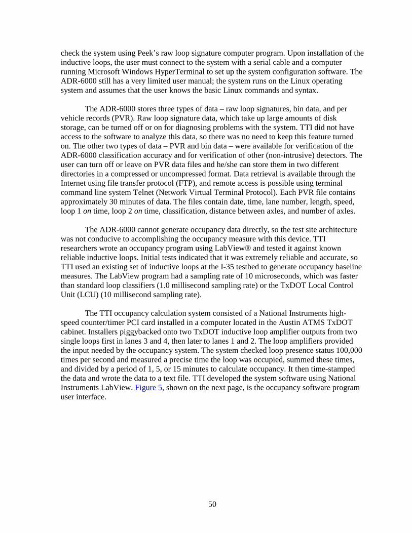
50

check the system using Peek’s raw loop signature computer program. Upon installation of the inductive loops, the user must connect to the system with a serial cable and a computer running Microsoft Windows HyperTerminal to set up the system configuration software. The ADR-6000 still has a very limited user manual; the system runs on the Linux operating system and assumes that the user knows the basic Linux commands and syntax.

The ADR-6000 stores three types of data – raw loop signatures, bin data, and per vehicle records (PVR). Raw loop signature data, which take up large amounts of disk storage, can be turned off or on for diagnosing problems with the system. TTI did not have access to the software to analyze this data, so there was no need to keep this feature turned on. The other two types of data – PVR and bin data – were available for verification of the ADR-6000 classification accuracy and for verification of other (non-intrusive) detectors. The user can turn off or leave on PVR data files and he/she can store them in two different directories in a compressed or uncompressed format. Data retrieval is available through the Internet using file transfer protocol (FTP), and remote access is possible using terminal command line system Telnet (Network Virtual Terminal Protocol).�Each PVR file contains approximately 30 minutes of data. The files contain date, time, lane number, length, speed, loop 1 on time, loop 2 on time, classification, distance between axles, and number of axles.

The ADR-6000 cannot generate occupancy data directly, so the test site architecture was not conducive to accomplishing the occupancy measure with this device. TTI researchers wrote an occupancy program using LabView® and tested it against known reliable inductive loops. Initial tests indicated that it was extremely reliable and accurate, so TTI used an existing set of inductive loops at the I-35 testbed to generate occupancy baseline measures. The LabView program had a sampling rate of 10 microseconds, which was faster than standard loop classifiers (1.0 millisecond sampling rate) or the TxDOT Local Control Unit (LCU) (10 millisecond sampling rate).

The TTI occupancy calculation system consisted of a National Instruments high-speed counter/timer PCI card installed in a computer located in the Austin ATMS TxDOT cabinet. Installers piggybacked onto two TxDOT inductive loop amplifier outputs from two single loops first in lanes 3 and 4, then later to lanes 1 and 2. The loop amplifiers provided the input needed by the occupancy system. The system checked loop presence status 100,000 times per second and measured a precise time the loop was occupied, summed these times, and divided by a period of 1, 5, or 15 minutes to calculate occupancy. It then time-stamped the data and wrote the data to a text file. TTI developed the system software using National Instruments LabView. Figure 5, shown on the next page, is the occupancy software program user interface.

51

Figure 5. TTI Occupancy Program User Interface. 4.3 FIELD TEST SITE This section includes major details about the installation of a testbed in a freeway environment with many details that are transferable to other sites. The TTI test plan involved testing all devices simultaneously, so synchronizing the clocks on each device was critical. This section covers the methods used to achieve this goal. 4.3.1 Criteria for Location Designing and implementing a state-of-the-art non-intrusive freeway detector testbed requires special infrastructure and full cooperation from the local TxDOT district and possibly other local jurisdictions such as city officials. To reduce the initial cost of a test bed, installers should find a location where most of the infrastructure already exists with items such as equipment cabinets, fully functioning inductive loops in the proper location relative to test device mounting, conduit that is not fully utilized, high-bandwidth communications, and 110 VAC power. The selected detector test site needs the following structures: a sign bridge or overpass (preferably with catwalks), sturdy poles close to the first monitored lane,

52

space to bore under the roadway, and safe access to the side of the roadway beside the equipment. A multi-lane roadway with a total of five or more lanes with high volumes of traffic is desirable, to include traffic conditions that vary by time of day. It is desirable to have free-flow traffic during part of the day and some stop-and-go traffic once or twice a day. Weather is a factor as well in that it should be representative of the area for deployment of the test detector systems. Roadway alignment needs to be reasonably level and straight so that surveillance cameras do not have blind spots. Retaining walls and median barriers can cause reflection of energy, so installers must consider them for certain detector technologies. Bridges and tunnels can deflect sound energy and so can ground-mounted highway signs. The surface texture of the roadway may affect the performance of some passive acoustic devices, and the ability of acoustic sensors to compensate for such reflective surfaces will probably be important. The I-35 site near 47th Street was an excellent prospect because it had high traffic volume, inductive loops in all lanes, an overhead sign bridge (for mounting overhead detectors), a phone line, 110 VAC power, an equipment cabinet (although it was relatively full), conduit, and two luminaire supports for mounting charged couple display (CCD) cameras. For the ADR-6000, new loops had to be installed anyway, but having fully functional loops provided a means to measure occupancy independently of the ADR-6000 system. Initially, researchers primarily needed the southbound side, so they installed the infrastructure for testing, including the baseline ADR-6000 system, a new cabinet, conduit, and two CCD surveillance cameras. Full testing of the ADR-6000 baseline system required a traffic stream with some stop-and-go conditions. The morning and afternoon peaks at the I-35 site sometimes met this requirement. Speeds almost always dropped to the 15- to 30-mph range during morning and afternoon peak periods, but stop-and-go conditions were not as common. Researchers wanted to confirm that the Peek could accurately classify a vehicle that stopped over the inductive loops then started again. 4.3.2 Process of Establishing the Site

TxDOT and TTI jointly developed a plan for equipment installation at the testbed, although parts of the plan changed as time went on. TxDOT offered two CCD cameras, but closer evaluation indicated they would not work for the purposes of this research, so TTI installed its own cameras. Later, images from the two video image detectors replaced one of the cameras. Therefore, one surveillance camera remained on one of the two poles used to support traffic monitoring equipment. It was downstream of the cabinet, while the two VIVDS units monitored traffic from the pole closer to the cabinet. TxDOT installed the second cabinet at the site and ran most of the conduit; TTI was responsible for almost all of the wiring and connections to equipment.

TxDOT installed all the southbound lane inductive loops for the ADR-6000 in one night, beginning at 9:00 p.m. on February 15, 2000. Representatives from TTI and Peek were

53

on site to support the operation. Table 8 summarizes the loop parameters from readings taken immediately after installation. Table 9 is a summary of wire and sealant characteristics.

Table 8. ADR-6000 Southbound Inductive Loop Parameters.

Inductive Loop No.

Inductance �� ��

Resistance (ohm)

Quality

Frequency (kHz)

1 116.0 1.5 22.0 45 A1 94.4 1.4 19.0 45 2 91.8 1.3 20.0 45

A2 115.4 1.3 24.0 45

3 114.0 1.3 25.0 45 A3 92.3 1.3 20.0 45 4 92.2 1.3 20.5 45

A4 112.7 1.3 24.0 45 5 111.8 1.3 25.5 45

A5 87.8 1.1 22.5 45

6 89.6 1.1 24.0 45 A6 110.5 1.5 27.0 45 7 109.0 1.0 29.0 45

A7 88.0 1.1 23.0 45 8 85.4 1.0 24.0 45

A8 106.5 1.0 30.0 45

9 97.8 1.0 28.0 45 A9 84.5 0.9 26.0 45 10 84.2 0.8 29.0 45

A10 101.3 0.7 40.0 45

Table 9. Loop Wire and Sealant Characteristics. Loop wire AWG 14 41/30

Type UL 1015 Loop sealant Q-SEAL

Sealant Type 290S

Polyurethane

For the ADR-6000 to perform its best, the saw-cut depth and the dimensions for the

axle and main loops had to be precisely maintained. The depth from the top of the pavement to the top quadrapole wire could be a maximum of 0.375 inch, but 0.25 inch was preferable for maximum sensitivity. This close tolerance meant that saw-cut depth had to be maintained to 1.25 inches for the outside of the quadrapole and 2 inches for the inside cut. The depth for the main loops was 2 inches. The Peek on-site factory representative marked all the saw cuts

54

for TxDOT. As an indication of the precision needed in the saw-cutting, after completing the first axle loop cuts the Peek representative asked the saw operator to raise the saw blade ¼ inch on the next center cut for the axle loops. 4.3.3 Site Details

Figure 6 is a schematic of the I-35 testbed site. The freeway has four through-lanes in each direction and a fifth lane on the southbound side is an exit lane to Airport Boulevard. This site is near the old Austin airport and near 47th Street and just north of the elevated section of I-35. The elevated section is a factor in dispersion of traffic by type and by lane because an unusually high percentage of trucks use the left two lanes to stay on the two lower lanes of the freeway and avoid the two elevated lanes. On most multilane roadways, a higher percentage of trucks are in the right lanes.

Before installation of the ADR-6000 loops, there were already 6-ft by 6-ft inductive

loops under the overhead sign bridge. In the through lanes, there were two loops (traps), whereas on the exit lane there was only one 6-ft by 6-ft loop. TTI tested all loops prior to installing test equipment and found them all to be in good working order. As shown in Figure 6, the equipment installed on the sign bridge was an RTMS on the west side facing south, an RTMS on the east side facing west (sidefire), and a SAS-1 on the east side oriented sidefire to the direction of traffic. Installers positioned one RTMS unit on the sign bridge to monitor only one lane in Doppler mode. On the luminaire pole 85 ft south of the southbound cabinets (west side of the freeway), TTI and TxDOT mounted two Autoscope Solo Pros, the Iteris Vantage, an RTMS, and a SAS-1. The TxDOT and TTI field installation crew mounted one Autoscope to the pole at 38.5 ft above the freeway and one to the mast arm supporting the luminaire. The reason for placing them at two locations was to determine the effect of different offsets. Figure 7 is a photograph of the site looking northward with an enlargement of the pole showing the detectors mounted on it for testing. Both Autoscopes faced oncoming traffic, whereas the Iteris (placed right beside the pole Autoscope) faced receding traffic. The RTMS on this same pole was 17 ft above the freeway and positioned in sidefire. The SAS-1 on this same pole was 35 ft above the freeway. As shown by Figure 6, the detection area for all pole-mounted devices was very close to the baseline ADR-6000 loops to minimize the effect of lane changing and changes in vehicle speeds. The field test plan for the northbound side of the freeway included mounting the RTMS and SAS-1 on the east side of the sign bridge and sending wireless data to the cabinets on the west side of the freeway. Even though most wireless applications would probably send data over a longer distance, the tests were envisioned more as a test of latency or other factors than determining the range of the wireless systems. Other items installed for northbound traffic included an equipment cabinet between the mainline and the northbound service road, 110 VAC power from the sign bridge to the cabinet, and conduit across the sign bridge. Installation of equipment for monitoring northbound traffic will be useful for Austin District functions and to future research, but installation came too late for application in this research project.

55

Figure 6. Layout of I-35 Site.

12345 4321

Cabinets

Light PoleSurveillance

Camera

Light Pole

Cabinet

WirelessRTMS 17’SAS-1 30’

RTMS 20’

Sign Bridge

Light Pole

Autoscope 45’

Autoscope, Iteris on pole 38.5’

RTMS 17’SAS-1 35’

35’

50’

ADR-6000 Loops

13’

TxDOT Loops

56

Figure 7. Photo of I-35 Testbed. TTI researchers chose high-speed Internet access to remotely monitor detector systems, upload data, check sensor configurations, and stream live video. This research project revealed many benefits of using Internet communications. One benefit was far fewer trips to the site and the associated travel and labor costs. The result was more productive use of staff time and increased monitoring of detector systems. Another very important benefit was allowing detector manufacturers and vendors remote access to the detector test site. Some of the manufacturers accessed their system remotely from across the U.S. and other parts of the world to check detector setup programs and upgrade algorithms and software. This cooperation with manufacturers helped them and TxDOT get a better product in the end. 4.3.4 I-35 Testbed Remote Data Acquisition System The remote data acquisition system was located in two roadside traffic cabinets on the west side of I-35. This system required using a small amount of space in TxDOT’s ATMS cabinet plus a second small cabinet, with the two cabinets interconnected with conduit. The test site’s Internet communication system consisted of a Local Area Network connected to an asymmetrical digital subscriber line (ADSL). The ADSL modem connected to a six-port 10-MB hub with five static Internet Protocol (IP) addresses assigned to it. The three computers, digital video recorder, and ADR-6000 each had static IP addresses. Anyone from outside the area who had the right access information could connect to the three TTI networked

Sidefire RTMS

SAS-1

Iteris

Autoscope Solo Pro

Weather Station

57

computers using pcAnywhere. This software allowed file transfer and remote Windows desktop admission. TTI also installed two telephone devices to remotely cycle power on the three computers and ADSL power supply when necessary if a computer or ADSL modem locked up. The ADR-6000 also had a hardware firewall connected between the hub and Ethernet port because, at one point in time, its Linux operating system became inundated with denial of service attacks causing the system to frequently shut down and restart. The hardware firewall completely solved the Internet hacker problem, allowing authorized persons 24-hour access to the ADR-6000 data and operating system. Figure 8 shows the relationship of these components.

Project staff recorded video for count and classification verification using a digital video recorder with sufficient memory to record full-motion video for three days. The digital video recorder’s setup and recording controls could also be accessed through its Internet IP address. TTI mounted a pan-tilt-zoom CCD surveillance camera, controlled from one of the computers, 30 ft high on a downstream pole for one camera angle. The Solo Pro mounted on the luminaire pole facing upstream and the Iteris camera mounted on the same pole facing downstream provided two additional camera angles. The three cameras and a National Television Standards Committee (NTSC) video image generated from the computer scan converter were all displayed on the digital quad simultaneously. TTI researchers wrote a Visual Basic program to display real-time serial data coming from the ADR-6000 containing time, date, lane number, length, speed, classification, and axle count. Installation personnel also connected the digital quad displaying the three camera angles and synchronized data to a video capture card on another computer, and this computer streamed the video to the Internet using Real Producer and Real Server software. This setup allowed TTI to remotely spot-check the ADR-6000’s classification accuracy.

Figure 9 shows an actual quad video image. In this quad image, the upper left image

comes from the downstream pole’s CCD surveillance camera, the upper right is from the Iteris Vantage camera, and the lower right is from the Autoscope Solo Pro. Information provided in the lower left quad is output from the ADR-6000 from the TTI software. The first set of numbers separated by colons is time stamps indicating vehicle passage; the single digit numbers just to the right of the time stamp are lane numbers (1 through 5). The next column is total vehicle length, followed by the speed in miles per hour. Finally, the next to last column is the FHWA vehicle classification and to its right is the number of axles.

TxDOT and TTI researchers installed a Campbell Scientific weather station on the

west end of the sign bridge that recorded wind speed and direction, air temperature, humidity, solar radiation, and rainfall amount. Authorized persons could access weather station data remotely through a serial connection to one of the computers in the small cabinet. The TxDOT cabinet contained an ADR-3000 classifier that had 14 contact closure inputs and an accurate clock to record contact closure outputs for count and speed verification. The RTMS and Iteris serial data were not usable because of internal clock drift or inability to set the system clock through software. Research staff had to record data from these two systems using the ADR-3000 connected serially to TTI’s computer in the TxDOT cabinet.

58

Figure 8. I-35 Testbed Remote Data Acquisition System.

59

Figure 9. Example Quad Video Image. 4.3.5 Pre-Test Preparation There were many activities that this research required before TTI actually began to evaluate performance attributes of the test devices. The list of activities is important in understanding the readiness of both the entire test site and the readiness of the various detectors. Table 10 is a list of activities related to preparing the testbed for beginning to install detectors. Following this table are Tables 11 through 14 pertaining to individual detectors. Table 14 summarizes activities on the IVS-2000, a device that was subsequently dropped from further tests. As noted earlier, TTI elected to test all devices simultaneously so all non-intrusive devices would experience exactly the same weather, lighting, and traffic conditions. The challenging part of this scenario was keeping all the clocks synchronized. To keep the computer clocks accurate, the three networked computers connected to the LAN were automatically synchronized to an atomic clock on the Internet every minute. A computer program running in the background that connected to the atomic clock performed the automatic synchronization and set the computer’s time. Each detector system connected to

60

Table 10. Austin Testbed Activities. Date Events for Austin Test Site

05/19/2000 Ordered ADSL and telephone line 07/13/2000 Installed surveillance camera and digital video quad 09/05/2000 ADSL installed and working 09/07/2000 Installed ADSL router 02/05/2001 Ordered five static IP addresses for ADSL replace router with hub 04/17/2001 Installed new P III 700 MHz computer to stream video from Austin 09/06/2001 Inventoried detectors to be installed at test site RTMS, SAS-1 10/01/2001 Pulled wire from plastic conduit so it could be replaced with steel conduit 12/19/2001 Installed another PC and ADR-3000 in TxDOT’s ATMS cabinet 12/20/2001 Connected RTMS and Iteris to ADR-3000 for counts 12/20/2002 Installed digital video recorder in cabinet 12/21/2001 Connected occupancy detection system to TxDOT loops on lanes 3 & 4 02/11/2002 Replaced power supply on PC in TxDOT’s ATMS cabinet 04/10/2002 TTI checked out weather station to be installed 04/24/2002 Installed weather station on side of overhead sign bridge 05/03/2002 ADSL quit working for 5 days 05/09/2002 Brought digital video recorder back to home base to use in data verification 05/28/2002 Installed new Peek software on ADR-3000 to collect count data from RTMS and

Iteris 05/31/2002 Changed remote access passwords on all computers for security and added extra

padlock to cabinet door 06/07/2002 Set up TxDOT ATMS database for 12 trap inputs on LCU 1 southbound I-35 06/14/2002 Repaired LCU 1 had 2 bad EEPROMS 06/23/2002 Configured ADR-3000 to collect count and speed data from RTMS for four lanes

and Iteris for three lanes of trap output 06/27/2002 Lost communication with ADSL 06/28/2002 Discovered TxDOT turned off power to test site, TTI restored power 07/05/2002 Remotely uploaded weather data 07/08/2002 UPS for test cabinet computers not working 08/05/2002 Replaced UPS

the TTI computer had a different method for setting its internal clock; some used software and required manual setting, and some could set their time automatically to the host computer’s clock. The following paragraphs indicate the method for setting the clock for each device. 4.3.5.1 ADR-6000 and ADR-3000

Synchronizing the ADR-6000 clock requires connecting through HyperTerminal using the serial port from PC1. Once logged into the system the user must stop the classification application by typing the command STOPAPPLICATION. Upon stopping the application, the user sets the clock by typing in the command SYNCTIME followed by CENTURY, DATE, AND TIME. The user then restarts the application. After installing and configuring the hardware firewall, field personnel were able to use the ADR-6000’s Linux

61

Table 11. Peek ADR-4000/6000 Activities.

Date Events for ADR-4000/6000 02/16/2000 Installed loops in five lanes, 20 loops total 05/15/2000 Installed first ADR-4000 and recorded all loop electrical parameters 07/13/2000 Diamond Consulting checking system returned with data and video 09/07/2000 Changed ADR-4000 processor, contact closures would not work with LCU 09/27/2000 ADR-4000 hard drive not working 10/05/2000 TTI wrote VB program to view per vehicle records on monitor 10/18/2000 ADR-4000 running out of memory 10/26/2000 Connected contact closures for lanes 3, 4, & 5 11/01/2000 Collected data and recorded traffic video from site 11/03/2000 Manually checked data 12/01/2000 ADR-4000 quit working 03/06/2001 Diamond Consulting remotely updated class table and system software 05/14/2001 ADR-4000 quit working until 05/22/2001 06/11/2001 ADR-4000 quit working 06/14/2001 Began collecting data 08/08/2001 ADR-4000 quit working 12/14/2001 After meeting with Peek discovered we actually had ADR-4000 02/06/2002 Installed ADR-6000 connected to Ethernet LAN and computer serial port 02/14/2002 Misclassifying Class 9 vehicles with five axles in lane 5 02/22/2002 Ran out of memory and stopped collecting data 02/26/2002 Creating multiple daily bin files causing gaps in data 03/07/2002 Lost communications with main detector cards 03/08/2002 Diamond Consulting remotely reestablished communications with cards 03/19/2002 Installed UPS for system and fan for processor 03/25/2002 Peek said new ADR-6000 ready for classification and count verification 03/26/2002 TTI is able to collect one daily bin file for the first time 04/09/2002 Creating multiple daily bin files causing gaps in data 04/15/2002 System locked up, had to cycle power 04/16/2002 Peek said system is being overcome by Internet hackers, so disabled Ethernet 04/19/2002 Remotely uploaded data 04/26/2002 Data directory memory full, cannot connect remotely 05/01/2002 Ethernet port enabling itself after system restart allowing hackers access 05/10/2002 Manually verified count and classification data from digital video 05/01/2002 Ethernet port still enabling itself after system restart allowing hackers access 05/28/2002 Peek installed hardware firewall on LAN to block hackers 05/31/2002 Still creating multiple daily bin files, changed remote access password 06/03/2002 Still creating multiple daily bin files causing gaps in data 06/05/2002 Installed another new system, Peek reused flash memory from old system 06/06/2002 Peek installed new flash memory because data was not binning correctly

Connected contact closures for all five lanes to LCU trap inputs 06/10/2002 System quit collecting data because clock was not synchronized correctly 06/11/2002 System ran out of memory and stopped collecting data 06/14/2002 Uploaded data and synchronized clock 06/21/2002 Manually verified count and classification data from digital video

62

Table 11. Peek ADR-4000/6000 Activities (continued). Date Events for ADR-4000/6000

06/22/2002 Remotely uploaded data and synchronized clock 06/28/2002 Remotely synchronized clock started data collection 07/01/2002 Remotely uploaded data 07/02/2002 Remotely uploaded data 07/03/2002 Remotely uploaded data 07/04/2002 Remotely uploaded data 07/05/2002 Remotely synchronized clock started data collection 07/08/2002 Remotely synchronized clock started data collection 07/09/2002 Remotely uploaded data 07/10/2002 Remotely uploaded data 08/07/2002 Remotely synchronized clock started data collection 08/09/2002 Remotely uploaded data 08/10/2002 Remotely uploaded data, discovered gaps in data on lane 2 08/11/2002 Remotely synchronized clock started data collection 08/12/2002 Remotely uploaded data 08/14/2002 Peek remotely installed new classification algorithm and system software 08/15/2002 Remotely synchronized clock started data collection 08/17/2002 Remotely uploaded data 08/18/2002 Remotely synchronized clock started data collection 08/19/2002 Remotely uploaded data 08/20/2002 Remotely uploaded data 08/21/2002 Remotely uploaded data

operating system FTP server software to upload data. They could transfer data directly from the ADR-6000 in Austin to an office computer in College Station using FTP and TTI’s high- speed Internet connection. Before TTI installed the firewall, field personnel used the serial connection to transfer files with HyperTerminal but at a much lower baud rate. It first involved transferring data to TTI’s local Austin computer, then using pcAnywhere to transfer the data to College Station.

TTI manually set the clock on the ADR-3000 through Peek’s software to match the clock on one of the LAN computers. Research staff collected the ADR-3000 data using the Peek TOPS software running on the same local computer connected to the ADR-3000 with a serial cable. Once data were downloaded to the computer’s hard drive they could be transferred to College Station using pcAnywhere.

63

Table 12. Autoscope Solo Pro Activities. Date Events for Autoscope Solo Pro

04/10/2001 Installed on 40 ft high mast arm at S.H. 6 test site College Station 05/09/2001 Had water inside camera processor enclosure and needs a replacement unit 05/23/2001 Installed replacement unit at S.H. 6 test site College Station 05/29/2001 Collected speed data at S.H. 6 test site College Station 07/10/2001 Upgraded software at S.H. 6 test site College Station 07/12/2001 Observed the unit undercounting at night 08/16/2001 Installed replacement unit at S.H. 6 test site College Station 08/20/2001 Collected speed and count data at S.H. 6 test site College Station 10/23/2001 Vendor installed on pole in Austin 38.5 ft above road surface 10/30/2001 Autoscope factory representative set up software 01/06/2002 Vendor installed on luminaire arm 45 ft above road surface 02/14/2002 Upgraded software and calibrated speeds on both 04/04/2002 Checking count data on both 04/19/2002 Remotely uploaded data 05/01/2002 Upgraded software version from 5.0 to 5.1 06/12/2002 Outputs to LCU stopped working reconfigured software to fix problem 06/27/2002 Serial connection broke on communication panel 06/28/2002 Replaced communication panel 07/01/2002 Remotely uploaded data 07/02/2002 Remotely uploaded data 07/03/2002 Remotely uploaded data 07/04/2002 Remotely uploaded data 07/09/2002 Remotely uploaded data 07/10/2002 Remotely uploaded data 08/05/2002 Calibrated speed on lane 5 for pole mounted Solo Pro 08/09/2002 Remotely uploaded data 08/10/2002 Remotely uploaded data 08/11/2002 Remotely uploaded data 08/18/2002 Remotely uploaded data 08/19/2002 Remotely uploaded data 08/20/2002 Remotely uploaded data 08/21/2002 Remotely uploaded data

4.3.5.2 Autoscope Solo Pro (Pole and Luminaire)

The latest Solo Pro software facilitated time synchronization automatically with the supervisor computer (one of TTI’s local Austin computers) every hour. Data storage occurred two ways using the Solo Pro – as flash data or by using Autoscope’s real-time data manager software running on a computer connected with a serial cable to the Autoscope communications panel. TTI used the Solo Pro software for data upload to the local Austin computer to transfer flash data stored inside the detector to the local computer. From this local computer’s hard drive, TTI transferred the data to College Station using pcAnywhere.

64

4.3.5.3 Iteris Vantage

The Iteris Vantage requires time to be set manually using the mouse and menu on the video monitor. Unfortunately, the time could not be set to the exact second using this method. Because of this shortcoming, TTI could only test short speed, count, and occupancy data intervals from the Iteris VRAS software running on TTI’s local computer connected serially to the Iteris. The remainder of the data collected for test purposes relied on contact closure outputs fed into the contact closure inputs of the Peek ADR-3000.

Table 13. Iteris Vantage Activities. Date Events for Iteris

04/09/2001 Freeway model still not in production for tests in College Station 10/23/2001 Local vendor installed on pole 38.5 ft above road surface 01/31/2002 Installed new VRAS software on TTI computer 02/13/2002 Local vendor calibrated speeds and occupancy 03/12/2002 Discovered that speed calibration was lost following power failure 06/14/2002 Local vendor installed new firmware to fix speed calibration problem 06/20/2002 Speed still not calibrated correctly 06/24/2002 Requested local vendor to calibrate speed and occupancy 06/28/2002 Iteris factory representative calibrated speed and occupancy 07/01/2002 Remotely uploaded data 07/02/2002 Remotely uploaded data 07/03/2002 Remotely uploaded data 07/04/2002 Remotely uploaded data 07/09/2002 Remotely uploaded data 07/10/2002 Remotely uploaded data 08/06/2002 Local vendor calibrated speed and occupancy in all four lanes 08/09/2002 Remotely uploaded data 08/10/2002 Remotely uploaded data 08/11/2002 Remotely uploaded data 08/18/2002 Remotely uploaded data 08/19/2002 Remotely uploaded data 08/20/2002 Remotely uploaded data 08/21/2002 Remotely uploaded data

Table 14. IVS-2000 Activities. Date Events for IVS-2000

03/06/2001 Installed IVS-2000 using TxDOT loops in lane 3 04/18/2001 Collected classification data in lane 3 to compare to ADR-4000 data 06/14/2001 Collecting data 06/18/2001 Checking data against ADR-4000

65

4.3.5.4 RTMS Sidefire Lane 1-4 and Rearfire Lane 5

The fact that the RTMS internal clock was not accurate required collecting count and speed data using the ADR-3000’s contact closure inputs. TTI wrote custom software to enable the collection of raw serial data from the RTMS over lane 5. Data analysts binned, time stamped, and stored to the local computer’s hard drive each vehicle speed in 1-minute and 15-minute intervals. The RTMS Doppler radar could not lock onto every vehicle, causing its counts to be low. TTI collected some count data using the contact closures for zone one in this configuration and achieved better results. 4.3.5.5 SAS-1

TTI used the SAS-1 software to synchronize time to the local serially connected computer. There were two options for data storage – it could be stored internally (archived data) or logged to the connected computer using the SAS-1 interface and serial cable. The SAS-1’s internal clock was very accurate and only drifted 1 to 2 seconds each month. TTI used the internal sensor’s archive data and uploaded it to the local Austin computer. Once the data was on the local computer’s hard drive, TTI transferred it to College Station using pcAnywhere. 4.4 SUMMARY

The equipment evaluation plan for this research relied on researcher experience and TxDOT needs. Criteria used to select detectors that should be included in this research included: detectors suitable for freeways, needs of the sponsor, and detectors not fully tested in the Texas environment. Detectors selected for field-testing under the rigors of I-35 traffic near downtown Austin were the Peek ADR-6000 and the following non-intrusive detectors: 3M microloops (magnetic), SAS-1 by SmarTek (acoustic), RTMS by Electronic Integrated Systems (Doppler radar), Autoscope Solo Pro (video imaging) and Iteris Vantage (video imaging). The I-35 testbed site was not appropriate for testing the 3M microloops, so the Project Director modified the U.S. 290 construction project to add horizontal conduit under new pavement at a location with inductive loops for verification. Unfortunately, the construction did not progress to the point where Project 0-2119 could test the microloops at that location. Pre-test activities focused on procuring, designing, and implementing the I-35 testbed facility, acquiring and preparing ancillary equipment, and conducting short-term evaluations to prove the readiness of selected systems. These preliminary tests made results available to manufacturer representatives so they could make last minute adjustments. Procurement was a challenge that caused minor delays early in this research. Future research that requires equipment purchase should consider a fixed budget for all bidders (to make that part of the bidding process fair to all) to use for purchases, then adjust later as needed. TTI wrote two programs to help test detectors at the I-35 site. One was for use on a baseline occupancy system, and the other was for use in testing the Peek ADR-6000. Other actions necessary to bring the testbed on-line included adding a cabinet, installing detectors,

66

installing CCD surveillance cameras and a weather station, moving a Peek ADR-3000 classifier and high-speed computers to the site, and installing services like an asynchronous digital subscriber line for high-bandwidth communication. TTI spent considerable time working with the TxDOT legacy system components such as the LCU as well as components to allow TxDOT to receive output from test devices at the Austin TMC.

TTI first began testing the Peek ADR-6000 near the beginning of the project and worked for the entire almost three-year research period to test its capabilities as a vehicle classifier. During time periods while it was stable, TTI found that it was extremely accurate for speeds and counts, but its stability problems and its accuracy as a classifier needed attention. Some of the major actions required during this research were multiple software changes, installing two new replacement units (the first unit was actually an ADR-4000), installing a contact closure board for all five lanes, installing an Uninterrupted Power Supply (UPS), adding a hardware firewall to improve security, and troubleshooting to identify causes for unexplained lapses in data collection. The scenario chosen by TTI for the field tests was to simultaneously test all non-intrusive devices under identical traffic, weather, and lighting conditions, and allow vendor accessibility. Testing multiple systems simultaneously requires either using the contact closure outputs (outputs are independent of internal clock) or synchronizing clocks on test systems with the baseline system.

67

CHAPTER 5.0 FIELD TEST RESULTS

5.1 INTRODUCTION This chapter covers the field test results for the baseline ADR-6000, along with the non-intrusive detectors – the Autoscope Solo Pro, the Iteris Vantage, the RTMS (sidefire and overhead), and the SAS-1. Parameters tested on the ADR-6000 were classification, count, and speed. For the non-intrusive devices, the desired parameters were speed, count, and occupancy, although in some cases capturing occupancy from the test system was not feasible. Some of the non-intrusive devices classify vehicles according to length, but this series of tests did not include classification for anything other than the ADR-6000. These results pertain to the detectors installed on the southbound side only because of delays in the northbound installation process. 5.2 METHODOLOGY

Evaluation of field test results for the southbound detectors began with the Peek ADR-6000. Its evaluation required at least one person to monitor each traffic lane by viewing recorded videotape. TTI used specialized equipment to record three camera views on a digital video quad, allowing review staff to watch different views of the same vehicle to ensure accuracy. The fourth view in the quad was the ADR-6000 output from the custom software written by TTI staff (see Figure 9 on page 59). The most efficient method of evaluating a block of data was to assemble a group of five or more people in the TransLink® Lab all at one time and assign each one a freeway lane to monitor. The first thing the viewers had to learn (if they did not know it already) was the FHWA classification scheme, so an instructor handed each person a copy of example vehicles for all classes on an 8½-inch by 11-inch sheet. Each person also had a printout from a Microsoft Excel spreadsheet to check against each vehicle passing in that lane. Each person closely watched his/her assigned lane as vehicles passed and mentally checked off each vehicle. If there was uncertainty about any vehicle in any lane, the videotape operator paused, reversed, and then forwarded the tape in slow motion until the group was certain of the classification of that vehicle. In rare cases where the vehicle was partially hidden in all camera views, the group of reviewers gave the ADR-6000 the benefit of the doubt. This process was very time-consuming, requiring 3 to 4 hours to process each 15-minute interval of real-time data.

The count and speed accuracy of the ADR-6000 was also important to its viability as a

baseline system. Its count accuracy came from the same process described above. Field personnel verified its speed accuracy using a laser radar unit at the Austin site. The process used two persons, one with a laser radar speed device and the other monitoring the ADR-6000 output and worked best in low to moderate traffic volume by selecting only large trucks. The two operators communicated using radios to overcome freeway noise as a target vehicle approached. They used only lane 4 Class 9 vehicles to minimize error on the laser device and ensure that each person was targeting the same vehicle. The process continued until researchers reached a sample size of 80.

After analyzing sufficient data from the ADR-6000 to confirm its count and speed

accuracy, field personnel synchronized its clock with other clocks and began collecting data for

68

comparison. For non-intrusive detectors, the data analysis required storing count and speed data in ASCII format and converting the data to an Excel spreadsheet for comparison with the baseline system’s data. There were 1-minute, 5-minute, and 15-minute intervals to be used for comparison purposes.

For occupancy comparisons, TTI used its occupancy program and the older TxDOT inductive loops that were installed close to the sign bridge. Each test device requires calibration for occupancy and is largely a measure of each device’s vehicle speed accuracy. Some devices do not generate an easily measurable occupancy value, so the results in this chapter do not include these data.

5.3 TEST RESULTS

The following comparisons of the test systems against baseline counts, speeds, and occupancies use 5-minute intervals unless noted otherwise. The results start with the Peek ADR-6000 in order to show its viability as a baseline speed and count device. Discussion of the Autoscope Solo Pro, the Iteris Vantage, the RTMS, and SAS-1 follow the ADR-6000. TTI did not test 3M microloops as originally planned because the construction project where they were to be deployed did not finish in time. Appendix C provides a sample of the data plots upon which these discussions are based. Some plots reflect ideal conditions and others represent less than ideal conditions such as rain, changing light intensity, and congested flow traffic with slow speeds. 5.3.1 Peek ADR-6000 5.3.1.1 Classification Accuracy This research conducted several evaluations of the classification accuracy of the Peek ADR-6000. Among the large vehicles, the ADR-6000 had the highest number of classification errors in Classes 4, 5 and 9. It could not always distinguish between two-axle single unit trucks and large buses (Class 4 and Class 5). Class 9 errors seemed to result from missing an axle, so it sometimes classified five-axle tractor-semitrailers as Class 8 with four axles. Table 15 summarizes the errors during one of these count periods for 12 classes of vehicles over all five lanes. This time interval included a short period of stop-and-go traffic, making classification more difficult. During periods of free-flow, the ADR-6000 still misclassified about the same number of vehicles. The overall classification accuracy based on this dataset of 1923 vehicles was 98.9 percent. Its highest error rate by lane was 1.8 percent on lane 2, and its highest error rate by vehicle class was for Class 4 (buses), but fortunately they represented only 0.4 percent of the traffic stream. The next highest error rates were for Class 5 then Class 9 vehicles, in which case it misclassified 8.3 and 7.3 percent, respectively. 5.3.1.2 Count Accuracy

The count accuracy of the ADR-6000 is almost perfect, missing only one vehicle in each of three 15-minute samples of data. In the dataset of 1923 vehicles represented by Table 15, the ADR-6000 missed only one vehicle.

69

Table 15. ADR-6000 Classification Accuracy Comparison for May 8, 2002, 15-minute Interval Beginning at 8:15 a.m.

Class 1 2 3 4 5 6 7 8 9 10 11 12 Total Errors Lane 1 Count 0 330 118 1 9 0 0 2 15 0 1 0 476 Errors 0 0 0 0 1 0 0 0 2 0 0 0 3 Lane 2 Count 0 299 84 0 16 3 1 11 23 0 1 0 438 Errors 2 1 3 1 1 8 Lane 3 Count 2 306 96 1 11 3 0 7 6 0 0 0 432 Errors 1 2 1 1 5 Lane 4 Count 0 312 88 1 14 1 0 4 2 0 0 0 422 Errors 1 1 1 1 4 Lane 5 Count 0 106 36 0 5 3 0 0 5 0 0 0 155 Errors 1 1 Totals 4 1356 423 7 60 12 1 24 55 0 2 0 1923

Total Errors 2 3 1 4 5 2 0 0 4 0 0 0 21 5.3.1.3 Speed Accuracy

Researchers tested the speed accuracy on the Peek ADR-6000 by using a laser device to select large trucks in lane 4. Figure 10 indicates the results of this comparison. Also, Figure 11 compares a larger sample of vehicles in lane 5 using the RTMS in its overhead Doppler radar mode to verify results in the smaller hand picked sample. Figure 11 shows excellent agreement between all three systems except when speeds drop below 20 mph in the 1-minute intervals. This finding indicates that the RTMS, even in the overhead (rearfire) mode, does not generate accurate speeds below approximately 20 mph. Both the RTMS and the Autoscope Solo Pro overestimate speeds during periods of very slow traffic. 5.3.2 Autoscope Solo Pro 5.3.2.1 Count Accuracy To better quantify the accuracy of the non-intrusive test systems, researchers calculated descriptive statistics that are tabulated in Appendix F. These values came from differences in 5-minute samples of count and speed data where the test device parameter was subtracted from the baseline parameter for the corresponding time interval. These statistics facilitate testing of

70

Lane 4 Speed Histogram

0

5

10

15

20

25

30

35

40

45

-5 -4 -3 -2 -1 0 1 2 3 4 5

Bin

Freq

uenc

y

Figure 10. Test of ADR-6000 Speed Accuracy Using Radar.

Lane 5 p.m. Peak Speeds I-35 (7/3/02)

0

5

10

15

20

25

30

35

40

45

50

16:4

5

16:4

8

16:5

1

16:5

4

16:5

7

17:0

0

17:0

3

17:0

6

17:0

9

17:1

2

17:1

5

17:1

8

17:2

1

17:2

4

17:2

7

17:3

0

17:3

3

17:3

6

17:3

9

17:4

2

17:4

5

Time

1 M

inut

e A

vera

ge S

peed

(mph

)

ADR6000 RTMS Solo Pro Luminaire

Figure 11. Speed Comparison Peek ADR-6000, RTMS Doppler Radar, and Autoscope.

71

detector accuracy during congested flow versus free flow, lane 1 versus lane 3, and for the Autoscope Solo Pro, its mounting location on the pole versus its location closer to the monitored lanes on the luminaire mast arm.

The Autoscope Solo Pro count accuracy in lane 1 is correlated with speed. Differences

between the Solo Pro and baseline counts on both lane 1 and lane 3 were much greater in congested flow than in free flow conditions. The graphics in Appendix C indicate that as speed during the morning peak dropped to 40 mph (5-min intervals), it undercounted by less than 5 percent. Below 40 mph, the Solo Pro undercounted vehicles in the range of 10 to 25 percent. As speed increased again after the morning peak, the Autoscope error centered on zero with no 5-minute interval errors greater than 5 percent. During the afternoon peak in lane 1 (all speed intervals over 45 mph), the Autoscope was usually within 5 percent of baseline counts with a maximum undercount of 12 percent.

In lane 2 during the morning peak, the Autoscope undercounted every time interval except one, and the undercount errors increased with slower speeds. Count errors reached 20 percent during one of the slow intervals, but during the remainder of the peak period it was between -2 and -14 percent. Lane 3 morning peak count intervals by the Autoscope were almost all in the 0 to -5 percent range, with one interval at -15 percent during the slowest speed. Again, it undercounted in all except one interval. Lane 3 afternoon peak count intervals were all within 0 to -10 percent, and many were within 5 percent. The Autoscope’s lane 4 morning peak counts were all between 0 and -10 percent (undercounts), with the data points centered on -5 percent. Its afternoon peak counts were 0 to -10 percent from 4:00 p.m. to 5:00 p.m. but then the trend changed to predominately overcounting from 5:00 p.m. to 6:00 p.m. in the range of -5 to +10 percent. In summary, the Autoscope Solo Pro count accuracy was within 5 percent of baseline counts in lane 1 until speeds dropped below 40 mph. Then, its counts were low by a range of 10 to 25 percent. It undercounted in all other lanes almost always in the range of 0 to -10 percent. 5.3.2.2 Speed Accuracy Appendix F statistics indicate very little difference in speed accuracy for the Solo between lane 1 and lane 3, between free flow and congested flow conditions, and between the luminaire-mounted versus the pole-mounted unit. In all cases, the Solo Pro excelled in its speed estimation. Appendix C plots show that in lane 1 during the morning peak, the Autoscope Solo Pro’s speeds were within 0 to 3 mph of the baseline system and did not seem to vary with the speed of traffic. During the afternoon peak on lane 1, it was always within 0 to 3 mph. On lane 2 during both the morning and afternoon peaks, the Autoscope was always within 0 to 2 mph of the baseline. On lane 3 during the morning peak, it was within 1 mph of the baseline, and during the afternoon peak it was within 2 mph. On lane 4, the Autoscope underestimated speeds in the range of 0 to 5 mph during the morning peak and by 1 to 5 mph during the afternoon peak. Figure 11 is also an indication of its accuracy.

72

5.3.2.3 Occupancy Of the three non-intrusive devices tested for occupancy output in lanes 3 and 4, the Autoscope Solo Pro was the most accurate. Its 15-minute cumulative occupancy values differed from loops by as much as 3.9 percent, but during most intervals its difference was less than 1 percent. 5.3.3 Iteris Vantage 5.3.3.1 Count Accuracy Comparing Appendix F statistics for Iteris counts indicates that the Iteris had the highest standard deviation during free flow of all test devices on both lanes 1 and 3. Overall, the Iteris count accuracy was not as dependent on prevailing freeway speeds as some other devices. Appendix C plots show that its calibration was apparently better than the Autoscope because it did not have a significant bias toward overcounting or undercounting. Its lane 1 morning peak counts were between -1 and -22 percent during slow speeds (20 to 30 mph); then it overcounted by as much as 10 percent when speeds increased. It mostly overcounted in lane 1 during the afternoon peak with a range from -4 to +10 percent. Lane 2 Iteris morning peak counts were all within the range of 0 to -10 percent except one and that one was at +5 percent. In the afternoon, its range was -5 to +10 percent, and all but four of its intervals were within +5 percent. Lane 3 Iteris morning peak counts were all within the range of +2 to -7 percent. In the afternoon peak, the Iteris was +5 to -10 percent. Lane 4 counts were not available. 5.3.3.2 Speed Accuracy Statistics tabulated in Appendix F show that the standard deviation for the Iteris was among the lowest of the devices tested on both lanes 1 and 3. Its mean values were lowest on lane 3, perhaps indicating better calibration than on lane 1. Appendix C graphics indicate that the Iteris Vantage was both over and under the baseline speeds but usually within 5 mph in lane 1 during the morning peak. During the afternoon peak, it was always within 5 mph on lane 1. On lane 2, its morning peak speeds exceeded the baseline by as much as 15 mph. During the afternoon peak, it was always within 5 mph on lane 2. On lane 3 during the morning peak, its speeds were excellent in all intervals showing speeds within 0 to 2 mph of the baseline. During the afternoon peak, it was within 5 mph. On lane 4, the Iteris was consistently within 5 mph of baseline during the morning peak. Speeds during the afternoon peak were not available. 5.3.3.3 Occupancy

Of the three non-intrusive devices tested for occupancy output in lanes 3 and 4, the Iteris Vantage was the second most accurate. Its 15-minute cumulative occupancy values differed from loops by as much as 8.1 percent, but during most intervals its difference was less than 6 percent.

73

5.3.4 RTMS by EIS Results of this research indicate that the RTMS is much more accurate in both counts and speeds in the overhead position where it covers one lane. Figure 11 supports this finding, indicating that its speed accuracy from the overhead position closely tracks the baseline speed. Values for Appendix C and F and the discussion below are therefore focused on its sidefire accuracy. 5.3.4.1 Count Accuracy Count statistics in Appendix F verify expected findings that the RTMS counts are better in lane 3 than in lane 1. Findings based on RTMS serial output indicate that the detector’s count accuracy was best on lanes 2, 3, and 4, where its counts were almost always within 5 percent of loop counts. On lane 1, its counts were always within 10 percent of loops during the off-peak periods. During peak periods on all lanes, RTMS counts varied more from baseline counts than during off-peak periods, but it was still usually within 10 percent. TTI encountered problems with the interface cards provided by EIS and these problems may not have been totally resolved at the end of the project. Appendix C graphics came from data collected using these interface cards and not from serial output. 5.3.4.2 Speed Accuracy Appendix C graphics indicate that speed estimates by the RTMS were better on lanes 3 and 4 than on lanes 1 and 2 and better during free-flow conditions than during slow speeds. On lane 3, its morning peak speeds were between 0 and 5 mph different from the baseline speed. During the afternoon peak, it overestimated speeds, but only by 2 to 5 mph until speeds dropped below 50 mph and it was 10 mph over the baseline. On lane 4, its morning peak speeds were consistently over the baseline speeds by 2 to 5 mph. As an example of its speed accuracy on lane 1, the RTMS overestimated speeds during the morning peak usually in the range of 5 to 10 mph and especially during periods of slow traffic when a few intervals were off by as much as 15 mph. 5.3.4.3 Occupancy This research did not include occupancy tests on the RTMS. 5.3.5 SAS-1 by SmarTek 5.3.5.1 Count Accuracy Appendix F statistics show that the SAS-1 count accuracy was reduced during congested flow on lane 1 compared to free flow, but on lane 3 the accuracy was similar for the two conditions. Appendix C plots show that the SAS-1 generally undercounted almost all intervals. In lane 1 during the a.m. peak and while speeds were over 40 mph its count range was 0 to -10 percent. During slower speeds, its range was -12 to -32 percent. Its range for lane 1 afternoon peak intervals was +2 to -20 percent with all but two intervals between 0 and -10 percent. The

74

SAS-1 lane 2 ranges for the morning and afternoon peaks were +5 to -18 percent and 0 to -10 percent, respectively. Lane 3 counts fell in the range of +6 to -12 percent during the morning peak and -2 to -14 percent during the afternoon peak. In lane 4, it undercounted during both the morning and afternoon peak by the range of -3 to -15 percent and 0 to -12 percent, respectively. 5.3.5.2 Speed Accuracy Appendix F tabulations show that the SAS-1 speed accuracy was similar in either congested flow or free flow on lane 1. For lane 3, its mean and standard deviations indicate its accuracy was better in free flow than in congested flow. Appendix C graphics show that the SAS-1 consistently overestimated speeds in lane 1 during the morning peak by 5 to 10 mph. During the afternoon peak, it overestimated speed by as much as 20 to 25 mph during slow speeds then improved to within 5 mph as speeds reached free-flow conditions. On lane 2 during both the morning and afternoon peaks, the SAS-1 was almost always over the baseline system by 0 to 5 mph with a maximum of 10 mph. On lane 3 this detector was consistently within 2 to 5 mph of the baseline system. On lane 4, its morning peak speed estimates were consistently within 5 mph and its afternoon peak speed estimates were less consistent but still within ±5 mph. 5.3.5.3 Occupancy

Of the three non-intrusive devices tested for occupancy output in lanes 3 and 4, the SAS-1 was the third most accurate. Its 15-minute cumulative occupancy values differed from loops by as much as 14.7 percent, but during most intervals its difference was less than 4 percent.

75

CHAPTER 6.0 IMPLEMENTATION OF FINDINGS

6.1 INTRODUCTION This chapter covers recommendations from researchers pertaining to implementation of the findings of Research Project 0-2119. These recommendations come from both contacts of detector practitioners across the country and from full-scale field tests conducted by the Texas Transportation Institute. 6.2 IMPLEMENTATION

Implementation involves the baseline Peek ADR-6000, along with non-intrusive detectors – the Autoscope Solo Pro, the Iteris Vantage, the RTMS (sidefire and overhead), the SAS-1, and 3M microloops. 6.2.1 Peek ADR-6000 The research team recommends continued efforts by the manufacturer to refine this classifier system. Recommended improvements are as follows: 1) it needs a user-friendly interface based on Microsoft Windows or other platform more common to DOT installers than the Linux system it now uses, 2) Peek needs to package the unit as a stand-alone system with sufficient internal cooling to stay operational without external cooling devices (except the normal cabinet fans), 3) it must be capable of being externally polled to upload its data, and 4) it must be able to sustain brown-outs and power outages and lose minimal amounts of data.

A critical issue for the ADR-6000 to achieve optimum performance is the saw-cut depth and the dimensions for the axle and main loops. The depth from the top of the pavement to the top quadrapole wire could be a maximum of 0.375 inches, but 0.25 inches is preferable for maximum sensitivity. This close tolerance means that saw-cut depth has to be maintained to 1.25 inches for the outside of the quadrapole and 2.00 inches for the inside cut. The depth for the main loops was 2.00 inches. Two obvious conclusions pertaining to implementation pertain to the depth of the saw cuts. The first is that a knowledgeable inspector must be available on site to inspect the depth of every saw cut. The second is that loops installed in asphalt stand a high probability of being milled and overlaid in a relatively short time period, rendering the existing loops ineffective. A more desirable long-term solution is to install ADR-6000 loops in concrete pavement. 6.2.2 Autoscope Solo Pro The Autoscope Solo Pro exhibited overall the most consistent count, speed, and occupancy performance of all non-intrusive detectors tested in this research project. Based on these short-term tests, it is ready for implementation in its current configuration on Texas freeways. Its cost is higher than some competitors, but additional features such as providing a view of the roadway may be sufficient to justify the additional cost. Its consistent accuracy,

76

along with a previous product line that move it up on the learning curve, should make it viable as an inductive loop replacement for many applications. For mounting location, the test statistics did not make a strong case for mounting on the mast arm rather than mounting on the pole. 6.2.3 Iteris Vantage The Iteris Vantage is relatively new on the market for freeway detection. Its newness is a factor to consider, since most new devices require modifications. Its accuracy during most tests indicates that it is a promising video image detector. Congested flow conditions do not seem to compromise its speed and count accuracy as much as some other detectors in this research. Its count accuracy was almost always within 10 percent of baseline and often within 5 percent. Its speed accuracy was almost always within 5 mph of the baseline system. The research staff recommends that its progress continue to be monitored, because it could be an even better detector as the manufacturer makes more refinements. One of the problems found in this research is that it loses calibration after a short time. 6.2.4 RTMS by EIS The positive features of the RTMS in sidefire are its ability to generate speeds and counts for five or more lanes with reasonable accuracy. Its advantages also include ease of setup, being mounted only 17 ft above the roadway, and its good user interface. Its coverage makes the RTMS an economical means of monitoring this number of lanes. In fact, in previous research, TTI found it to have the lowest life-cycle cost for freeway applications of those detectors included in that research (1). In Project 0-2119, researchers discovered defects with the loop emulation boards provided by EIS, but the manufacturer is addressing the problems. Researchers anticipate that results from this research would be the same even with new and improved boards because they only used data for time intervals when the current boards were functioning properly. In sidefire under free-flow conditions, the RTMS can count with 95 percent accuracy and detect speeds within 5 mph in 1-minute intervals. However, during congested flow, the RTMS showed occasional count errors of up to 15 percent and speed errors in the 5- to 15-mph range. The RTMS in the overhead position generated excellent speeds until prevailing traffic speeds dropped below about 20 mph. It is an accurate count device as well in the overhead position, but it only covers one lane. As long as errors at very slow speeds are not critical, TxDOT should give this device serious consideration. It is a mature product and is not affected by weather or lighting conditions. 6.2.5 SAS-1 by SmarTek The SAS-1 is a fairly recent addition to the list of non-intrusive detectors. Its ease of setup and its per-lane cost make it very attractive as a freeway detector. Even though it is fairly new on the market, the manufacturer has aggressively incorporated recommendations from previous research and from installations elsewhere. The only weather condition found in the Project 0-2119 research to affect its performance was heavy rain. During free-flow

77

traffic, the SAS-1 generally counted traffic within 5 to 10 percent of the baseline system and detected speeds within 5 mph. During slow moving traffic, its accuracy degraded to the point that its counts were off by as much as 30 percent and speeds were off by 20 to 25 mph. In summary, the SAS-1 has undergone many improvements and will perform well in free-flowing traffic, but its slow-speed accuracy and its degraded performance in rain need to be addressed. 6.2.6 3M Microloops Even though this research project did not field-test 3M microloops, research personnel gathered information from Caltrans, FDOT, and MinnDOT, and conducted their own research on a lower volume facility as reported elsewhere (2). The following points are helpful in determining the future use of this detector on freeways.

The two options for installation of 3M microloop sensors are in conduit underneath pavement and under a bridge deck. Its high installation cost where boring is required is at least partially offset by its ease of installation, its accurate speed and count output, its ability to be adjusted if traffic lanes shift, and possibly its long life. There is no known long-term research that indicates life-cycle costs of microloops, although TTI continues to monitor six probes installed on S.H. 6 in College Station in November 1999. These microloop probes and amplifiers have required no maintenance whatsoever in the three years they have been installed. TTI researchers anticipate that their service life will be an attractive attribute, given their benign environment. The most recent MinnDOT detector research results listed the 3M product as one of the best count and speed detectors.

79

REFERENCES 1. Middleton, D., D. Jasek, and R. Parker, Evaluation of the Existing Technologies for

Vehicle Detection, Report No. FHWA/TX-99/1715-S, Texas Transportation Institute, College Station, TX, September 1998.

2. Middleton, D., and R. Parker, Initial Evaluation of Selected Detectors to Replace

Inductive Loops on Freeways, Report No. FHWA/TX-00/1439-7, Texas Transportation Institute, College Station, TX, April 2000.

3. Specification for Installation of Inductive Loops, City of Arlington, Texas. 4. Texas Department of Transportation Standard Plans, Loop Detector Installation

Details, LD1-98, October 1998. 5. Woods, D.L. Texas Traffic Signal Detector Manual, Report No. FHWA/TX-90/1163-

1, Texas Transportation Institute, College Station, TX, July 1992. 6. State of California, California Department of Transportation, Standard Plans, Sh. ES-

5A, ES-5B, ES-5E, Sacramento, CA, July 1999. 7. Florida Department of Transportation’s Standard Specifications for Road and Bridge

Construction, Section 660, Tallahassee, FL, 2000. 8. Evaluation of Non-Intrusive Technologies for Traffic Detection, NIT Phase II, Draft

Final Report, Minnesota Department of Transportation, St. Paul, MN, August 2002. 9. Purdue University: http://bridge.ecn.purdue.edu/~darcy/researchprojects.html, July

2002. 10. Federal Highway Administration Scanning Team, FHWA Study Tour for European

Traffic Monitoring Programs and Technologies, Federal Highway Administration, U.S. Department of Transportation, Washington, D.C., August 1997.

11. Urban Traffic Systems Installation and User Manual EuroDetector ED 16. A

publication of Peek Traffic B.V., Amersfoort, The Netherlands, December 1999. 12. Texas Transportation Institute Memorandum, “Autoscope Solo Video Detection

Evaluation,” Dallas, TX, February 2002. 13. Grenard, J., D. Bullock, and A. Tarko. Evaluation Of Selected Video Detection

Systems At Signalized Intersections, Report No. FHWA/IN/JTRP-2001/22, Purdue University, West Lafayette, IN, Final Draft, November 2001.

80

��� Washington State Department of Transportation, “Spokane Freeway Data Collection:

Measurement Device Analysis,” Draft Report, University of Washington, Seattle, WA, November 2001.�

���� National Electrical Manufacturers Association, National Transportation

Communications for ITS Protocol (NTCIP) Object Definitions for Actuated Traffic Signal Controller Units, NEMA Standards Publication No. TS 3.5-1996, Washington, D.C., 1996.�

�

81

APPENDIX A

CALTRANS INDUCTIVE LOOP SPECIFICATION

83

84

85

86

87

88

89

90

91

92

93

APPENDIX B

WASHINGTON STATE INDUCTIVE LOOP SPECIFICATION

95

Induction Loop Vehicle Detectors Section 8-20.3(14)C is supplemented with the following:

ITS Round Loops Round loops shall be constructed in accordance with the following requirements.

Loop wire shall be No. 14 stranded copper with XHHW insulation conforming

to IMSA 51-3 requirements, encased in ¼ inch outside diameter polyurethane tubing conforming to IMSA 51-5 requirements.

Round sawcuts shall be 6 feet in diameter and shall be constructed using

equipment designed for cutting round loops. The equipment shall use a concave, diamond-segmented blade. The sawcuts shall be vertical and shall be a minimum of 0.25 inches wide. The sawcut depth shall be a minimum of 2 ½ inches and a maximum of 3 inches measured at any point along the perimeter, except on bridge decks. Other methods of constructing the round sawcut, such as anchoring a router or flat blade saw, will not be allowed.

The bottom of the sawcut shall be smooth. No edges created by differences

in sawcut depths will be allowed. All sawcut corners shall be rounded to a minimum 1.6 inch radius. All sawcuts shall be cleaned with a 100 psi high pressure washer as specified

in this Special Provision. Wash water and slurry shall be vacuumed out and blown dry with compressed air. Sawcutting shall be subject to the requirements set forth in Section 1-07.5(3) and the subsection Fish And Wildlife and Ecology Regulations of the Special Provision LEGAL RELATIONS AND RESPONSIBILITIES TO THE PUBLIC.

In areas where new pavement will be placed, loops shall be installed after all

grinding and prior to paving the final lift of asphalt. An ID loop locator shall be installed in the center of each loop prior to paving the final lift of asphalt.

The loop shall constructed using 4 turns of conductor. The conductor shall be

installed one turn on top of the previous turn. All turns shall be installed in a clockwise direction. The conductors shall be secured to prevent floating with 2 inch lengths of high temperature foam backer rod sized for a snug fit. The backer rod shall be spaced at 2 foot intervals around the perimeter of the sawcut and at corners.

Sealant for Portland cement concrete pavement shall be one of those listed in

the Qualified Products List meeting the requirements for Standard Specification 8-20.3(14)C.

96

Sealant for ACP pavement shall be one of those listed in the Qualified Products List meeting the requirements for Standard Specification 8-20.3(14)C.

Loop sealant shall be installed in 2 layers. The first layer shall be allowed to

cool before the second layer is applied. Installation of the sealant shall completely encapsulate the loop conductors. A minimum of 1 inch of sealant shall be provided between the top of the conductors and the top of the sawcut. The twisted polypropylene rope noted in Standard Plan J-8a is not allowed.

Section A-A and B-B of the Standard Plan J-8a are revised to read:

The width of the sawcut for Section A-A shall be at least wider than the diameter of the loop wire, up to a maximum of ¼ inch. The width of Sections B-B and C-C shall be at least 1/25 inch wider than twice the diameter of the loop wire, up to a maximum of ½ inch

Induction loop splice shall be in accordance with Section 9-29.12(2) or shall

be one of the following:

1. 3M Splice Tape 2. Plymouth Splice Tape 3. Raychem Heat Shrink Splice Kit

Testing For Induction Loops and Lead - In Cables Section 8-20.3 (14D) is supplemented with the following: Test A The resistance shall not exceed values calculated using the given formula.

Resistance per 1000 ft of #14 AWG, R = 3.16 ohms / 1000 ft

R = 3.16 x distance of lead-in cable (ft) 1000 ft

97

APPENDIX C

DATA PLOTS

99

Lane 1 Morning Peak Speeds I-35 (7/2/02)

0

5

10

15

20

25

30

35

40

45

50

55

60

65

07:0

0

07:1

0

07:2

0

07:3

0

07:4

0

07:5

0

08:0

0

08:1

0

08:2

0

08:3

0

08:4

0

08:5

0

09:0

0

09:1

0

09:2

0

09:3

0

09:4

0

09:5

0

10:0

0

Time

5 M

inut

e av

erag

e Sp

eed

(mph

)

0

0.02

0.04

0.06

0.08

0.1

0.12

0.14

0.16

0.18

0.2

Rai

n in

/ 15

min

ADR6000 RTMS Iteris SAS-1 Solo Pro Rain

Lane 1 Free Flow Speeds I-35 (7/2/02)

10

15

20

25

30

35

40

45

50

55

60

65

70

11:0

0

11:1

5

11:3

0

11:4

5

12:0

0

12:1

5

12:3

0

12:4

5

13:0

0

13:1

5

13:3

0

13:4

5

14:0

0

14:1

5

14:3

0

14:4

5

15:0

0

15:1

5

15:3

0

15:4

5

16:0

0

Time

5 M

inut

e A

vera

ge S

peed

(mph

)

0

0.1

0.2

0.3

0.4

0.5

0.6

0.7

0.8

0.9

1

Rai

n in

/ 15

min

ADR6000 RTMS Iteris SAS-1 SoloPro Rain

100

Lane 1 Morning Peak Count Error I-35 (7/2/02)

-40.0%

-30.0%

-20.0%

-10.0%

0.0%

10.0%

20.0%

07:0

0

07:1

0

07:2

0

07:3

0

07:4

0

07:5

0

08:0

0

08:1

0

08:2

0

08:3

0

08:4

0

08:5

0

09:0

0

09:1

0

09:2

0

09:3

0

09:4

0

09:5

0

10:0

0

Time

% E

rror

Fro

m B

asel

ine

0

10

20

30

40

50

60

5 M

inut

e A

vera

ge S

peed

(mph

)

Iteris SAS-1 Solo Pro Baseline Speed

Lane 2 Free Flow Count Error I-35 (7/2/02)

-30.0%

-20.0%

-10.0%

0.0%

10.0%

20.0%

30.0%

40.0%

50.0%

60.0%

11:0

0

11:1

5

11:3

0

11:4

5

12:0

0

12:1

5

12:3

0

12:4

5

13:0

0

13:1

5

13:3

0

13:4

5

14:0

0

14:1

5

14:3

0

14:4

5

15:0

0

15:1

5

15:3

0

15:4

5

16:0

0

Time

% E

rror

Fro

m B

asel

ine

0

10

20

30

40

50

60

70

5 M

inut

e A

vera

ge S

peed

(mph

)

Iteris SAS-1 Solo Pro Baseline Speed

101

Lane 2 Morning Peak Speeds I-35 (7/2/02)

0

5

10

15

20

25

30

35

40

45

50

55

60

65

07:0

0

07:1

0

07:2

0

07:3

0

07:4

0

07:5

0

08:0

0

08:1

0

08:2

0

08:3

0

08:4

0

08:5

0

09:0

0

09:1

0

09:2

0

09:3

0

09:4

0

09:5

0

10:0

0

Time

5 M

inut

e A

vera

ge S

peed

(mph

)

0

0.02

0.04

0.06

0.08

0.1

0.12

0.14

0.16

0.18

0.2

Rai

n in

/ 15

min

ADR6000 RTMS Iteris SAS-1 Solo Pro Rain

Lane 2 Free Flow Speeds I-35 (7/2/02)

10

15

20

25

30

35

40

45

50

55

60

65

70

11:0

0

11:1

5

11:3

0

11:4

5

12:0

0

12:1

5

12:3

0

12:4

5

13:0

0

13:1

5

13:3

0

13:4

5

14:0

0

14:1

5

14:3

0

14:4

5

15:0

0

15:1

5

15:3

0

15:4

5

16:0

0

Time

5 M

inut

e A

vera

ge S

peed

(mph

)

0

0.1

0.2

0.3

0.4

0.5

0.6

0.7

0.8

0.9

1

Rai

n in

/ 15

min

ADR6000 RTMS Iteris SAS-1 SoloPro Rain

102

Lane 2 Morning Peak Count Error I-35 (7/2/02)

-40.0%

-30.0%

-20.0%

-10.0%

0.0%

10.0%

20.0%

07:0

0

07:1

0

07:2

0

07:3

0

07:4

0

07:5

0

08:0

0

08:1

0

08:2

0

08:3

0

08:4

0

08:5

0

09:0

0

09:1

0

09:2

0

09:3

0

09:4

0

09:5

0

10:0

0

Time

% E

rror

Fro

m B

asel

ine

0

10

20

30

40

50

60

5 M

inut

e A

vera

ge S

peed

(mph

)

Iteris SAS-1 Solo Pro Baseline Speed

Lane 2 Free Flow Count Error I-35 (7/2/02)

-30.0%

-20.0%

-10.0%

0.0%

10.0%

20.0%

30.0%

40.0%

11:0

0

11:1

5

11:3

0

11:4

5

12:0

0

12:1

5

12:3

0

12:4

5

13:0

0

13:1

5

13:3

0

13:4

5

14:0

0

14:1

5

14:3

0

14:4

5

15:0

0

15:1

5

15:3

0

15:4

5

16:0

0

Time

% E

rror

Fro

m B

asel

ine

0

10

20

30

40

50

60

70

5 M

inut

e A

vera

ge S

peed

(mph

)

Iteris SAS-1 Solo Pro Baseline Speed

103

Lane 3 Morning Peak Speeds I-35 (7/2/02)

0

5

10

15

20

25

30

35

40

45

50

55

60

07:0

0

07:1

0

07:2

0

07:3

0

07:4

0

07:5

0

08:0

0

08:1

0

08:2

0

08:3

0

08:4

0

08:5

0

09:0

0

09:1

0

09:2

0

09:3

0

09:4

0

09:5

0

10:0

0

Time

5 M

inut

e A

vera

ge S

peed

(mph

)

0

0.02

0.04

0.06

0.08

0.1

0.12

0.14

0.16

0.18

0.2

Rai

n in

/ 15

min

ADR6000 RTMS Iteris SAS-1 Solo Pro Rain

Lane 3 Free Flow Speeds I-35 (7/2/02)

5

10

15

20

25

30

35

40

45

50

55

60

65

11:0

0

11:1

5

11:3

0

11:4

5

12:0

0

12:1

5

12:3

0

12:4

5

13:0

0

13:1

5

13:3

0

13:4

5

14:0

0

14:1

5

14:3

0

14:4

5

15:0

0

15:1

5

15:3

0

15:4

5

16:0

0

Time

5 M

inut

e A

vera

ge S

peed

(mph

)

0

0.1

0.2

0.3

0.4

0.5

0.6

0.7

0.8

0.9

1

Rai

n in

/ 15

min

ADR6000 RTMS Iteris SAS-1 Solo Pro Rain

104

Lane 3 Morning Peak Count Error I-35 (7/2/02)

-40.0%

-30.0%

-20.0%

-10.0%

0.0%

10.0%

20.0%

07:0

0

07:1

0

07:2

0

07:3

0

07:4

0

07:5

0

08:0

0

08:1

0

08:2

0

08:3

0

08:4

0

08:5

0

09:0

0

09:1

0

09:2

0

09:3

0

09:4

0

09:5

0

10:0

0

Time

% E

rror

Fro

m B

asel

ine

0

10

20

30

40

50

60

5 M

inut

e A

vera

ge S

peed

(mph

)

Iteris SAS-1 Solo Pro Baseline Speed

Lane 3 Free Flow Count Error I-35 (7/2/02)

-30.0%

-20.0%

-10.0%

0.0%

10.0%

20.0%

30.0%

40.0%

11:0

0

11:1

5

11:3

0

11:4

5

12:0

0

12:1

5

12:3

0

12:4

5

13:0

0

13:1

5

13:3

0

13:4

5

14:0

0

14:1

5

14:3

0

14:4

5

15:0

0

15:1

5

15:3

0

15:4

5

16:0

0

Time

% E

rror

Fro

m B

asel

ine

0

10

20

30

40

50

60

70

5 M

inut

e A

vera

ge S

peed

(mph

)

Iteris SAS-1 Solo Pro Baseline Speed

105

S

Lane 1 Morning Peak Speeds I-35 (8/15/02)

15

20

25

30

35

40

45

50

55

60

65

70

07:0

0

07:1

0

07:2

0

07:3

0

07:4

0

07:5

0

08:0

0

08:1

0

08:2

0

08:3

0

08:4

0

08:5

0

09:0

0

09:1

0

09:2

0

09:3

0

09:4

0

09:5

0

10:0

0

Time

5 M

inut

e A

vera

ge S

peed

(mph

)

ADR6000 RTMS Iteris SAS-1 Solo Pro

Lane 1 Afternoon Peak Speeds I-35 (8/16/02)

5

10

15

20

25

30

35

40

45

50

55

60

65

70

16:0

0

16:0

5

16:1

0

16:1

5

16:2

0

16:2

5

16:3

0

16:3

5

16:4

0

16:4

5

16:5

0

16:5

5

17:0

0

17:0

5

17:1

0

17:1

5

17:2

0

17:2

5

17:3

0

17:3

5

17:4

0

17:4

5

17:5

0

17:5

5

18:0

0

Time

5 M

inut

e A

vera

ge S

peed

(mph

)

ADR6000 RTMS Iteris SAS-1 Solo Pro

106

Lane 1 Morning Peak Count Error I-35 (8/16/02)

-40.0%

-30.0%

-20.0%

-10.0%

0.0%

10.0%

20.0%

07:0

0

07:1

0

07:2

0

07:3

0

07:4

0

07:5

0

08:0

0

08:1

0

08:2

0

08:3

0

08:4

0

08:5

0

09:0

0

09:1

0

09:2

0

09:3

0

09:4

0

09:5

0

10:0

0

Time

% E

rror

Fro

m B

asel

ine

0

10

20

30

40

50

60

70

5 M

inut

e A

vera

ge S

peed

(mph

)

RTMS Iteris SAS-1 Solo Pro Baseline Speed

Lane 1 Afternoon Peak Count Error I-35 (8/15/02)

-40.0%

-30.0%

-20.0%

-10.0%

0.0%

10.0%

20.0%

30.0%

16:0

0

16:1

0

16:2

0

16:3

0

16:4

0

16:5

0

17:0

0

17:1

0

17:2

0

17:3

0

17:4

0

17:5

0

18:0

0

Time

% E

rror

Fro

m B

asel

ine

5

15

25

35

45

55

65

75

5 M

inut

e A

vera

ge S

peed

(mph

)

RTMS Iteris SAS-1 Solo Pro Baseline Speed

107

Lane 2 Morning Peak Speeds I-35 (8/15/02)

15

20

25

30

35

40

45

50

55

60

65

70

07:0

0

07:0

5

07:1

0

07:1

5

07:2

0

07:2

5

07:3

0

07:3

5

07:4

0

07:4

5

07:5

0

07:5

5

08:0

0

08:0

5

08:1

0

08:1

5

08:2

0

08:2

5

08:3

0

08:3

5

08:4

0

08:4

5

08:5

0

08:5

5

09:0

0

Time

5 M

inut

e A

vera

ge S

peed

(mph

)

ADR6000 RTMS Iteris SAS-1 Solo Pro

Lane 2 Afternoon Peak Speeds I-35 (8/15/02)

25

30

35

40

45

50

55

60

65

70

75

16:0

0

16:0

5

16:1

0

16:1

5

16:2

0

16:2

5

16:3

0

16:3

5

16:4

0

16:4

5

16:5

0

16:5

5

17:0

0

17:0

5

17:1

0

17:1

5

17:2

0

17:2

5

17:3

0

17:3

5

17:4

0

17:4

5

17:5

0

17:5

5

18:0

0

Time

5 M

inut

e A

vera

ge S

peed

(mph

)

ADR6000 RTMS Iteris SAS-1 Solo Pro

108

Lane 2 Morning Peak Count Error I-35 (8/15/02)

-40.0%

-30.0%

-20.0%

-10.0%

0.0%

10.0%

20.0%

30.0%

40.0%

07:0

0

07:1

0

07:2

0

07:3

0

07:4

0

07:5

0

08:0

0

08:1

0

08:2

0

08:3

0

08:4

0

08:5

0

09:0

0

Time

% E

rror

Fro

m B

asel

ine

0

10

20

30

40

50

60

70

5 M

inut

e A

vera

ge S

peed

(mph

)

RTMS Iteris SAS-1 Solo Pro Baseline Speed

Lane 2 Afternoon Peak Count Error I-35 (8/15/02)

-40.0%

-30.0%

-20.0%

-10.0%

0.0%

10.0%

20.0%

30.0%

16:0

0

16:1

0

16:2

0

16:3

0

16:4

0

16:5

0

17:0

0

17:1

0

17:2

0

17:3

0

17:4

0

17:5

0

18:0

0

Time

% E

rror

Fro

m B

asel

ine

5

15

25

35

45

55

65

75

5 M

inut

e A

vera

ge S

peed

(mph

)

RTMS Iteris SAS-1 Solo Pro Baseline Speed

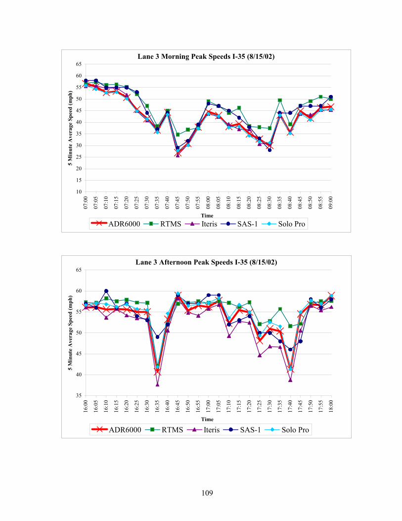
109

Lane 3 Morning Peak Speeds I-35 (8/15/02)

10

15

20

25

30

35

40

45

50

55

60

65

07:0

0

07:0

5

07:1

0

07:1

5

07:2

0

07:2

5

07:3

0

07:3

5

07:4

0

07:4

5

07:5

0

07:5

5

08:0

0

08:0

5

08:1

0

08:1

5

08:2

0

08:2

5

08:3

0

08:3

5

08:4

0

08:4

5

08:5

0

08:5

5

09:0

0

Time

5 M

inut

e A

vera

ge S

peed

(mph

)

ADR6000 RTMS Iteris SAS-1 Solo Pro

Lane 3 Afternoon Peak Speeds I-35 (8/15/02)

35

40

45

50

55

60

65

16:0

0

16:0

5

16:1

0

16:1

5

16:2

0

16:2

5

16:3

0

16:3

5

16:4

0

16:4

5

16:5

0

16:5

5

17:0

0

17:0

5

17:1

0

17:1

5

17:2

0

17:2

5

17:3

0

17:3

5

17:4

0

17:4

5

17:5

0

17:5

5

18:0

0

Time

5 M

inut

e A

vera

ge S

peed

(mph

)

ADR6000 RTMS Iteris SAS-1 Solo Pro

110

Lane 3 Morning Peak Count Error I-35 (8/15/02)

-20.0%

-15.0%

-10.0%

-5.0%

0.0%

5.0%

10.0%

15.0%

20.0%

07:0

0

07:1

0

07:2

0

07:3

0

07:4

0

07:5

0

08:0

0

08:1

0

08:2

0

08:3

0

08:4

0

08:5

0

09:0

0

Time

% E

rror

Fro

m B

asel

ine

0

10

20

30

40

50

60

5 M

inut

e A

vera

ge S

peed

(mph

)

RTMS Iteris SAS-1 Solo Pro Baseline Speed

Lane 3 Afternoon Peak Count Error I-35 (8/15/02)

-20.0%

-15.0%

-10.0%

-5.0%

0.0%

5.0%

10.0%

15.0%

20.0%

16:0

0

16:1

0

16:2

0

16:3

0

16:4

0

16:5

0

17:0

0

17:1

0

17:2

0

17:3

0

17:4

0

17:5

0

18:0

0

Time

% E

rror

Fro

m B

asel

ine

5

15

25

35

45

55

65

5 M

inut

e A

vera

ge S

peed

(mph

)

RTMS Iteris SAS-1 Solo Pro Baseline Speed

111

Lane 4 Morning Peak Speeds I-35 (8/15/02)

15

20

25

30

35

40

45

50

55

60

65

70

07:0

0

07:0

5

07:1

0

07:1

5

07:2

0

07:2

5

07:3

0

07:3

5

07:4

0

07:4

5

07:5

0

07:5

5

08:0

0

08:0

5

08:1

0

08:1

5

08:2

0

08:2

5

08:3

0

08:3

5

08:4

0

08:4

5

08:5

0

08:5

5

09:0

0

Time

5 M

inut

e A

vera

ge S

peed

(mph

)

ADR6000 RTMS SAS-1 Solo Pro

Lane 4 Afternoon Peak Speeds I-35 (8/15/02)

35

40

45

50

55

60

65

16:0

0

16:0

5

16:1

0

16:1

5

16:2

0

16:2

5

16:3

0

16:3

5

16:4

0

16:4

5

16:5

0

16:5

5

17:0

0

17:0

5

17:1

0

17:1

5

17:2

0

17:2

5

17:3

0

17:3

5

17:4

0

17:4

5

17:5

0

17:5

5

18:0

0

Time

5 M

inut

e A

vera

ge S

peed

(mph

)

ADR6000 RTMS SAS-1 Solo Pro

112

Lane 4 Morning Peak Count Error I-35 (8/15/02)

-20.0%

-15.0%

-10.0%

-5.0%

0.0%

5.0%

10.0%

15.0%

20.0%

07:0

0

07:1

0

07:2

0

07:3

0

07:4

0

07:5

0

08:0

0

08:1

0

08:2

0

08:3

0

08:4

0

08:5

0

09:0

0

Time

% E

rror

Fro

m B

asel

ine

0

10

20

30

40

50

60

5 M

inut

e A

vera

ge S

peed

(mph

)

RTMS SAS-1 Solo Pro Baseline Speed

Lane 4 Afternoon Peak Count Error I-35 (8/15/02)

-20.0%

-15.0%

-10.0%

-5.0%

0.0%

5.0%

10.0%

15.0%

20.0%

16:0

0

16:1

0

16:2

0

16:3

0

16:4

0

16:5

0

17:0

0

17:1

0

17:2

0

17:3

0

17:4

0

17:5

0

18:0

0

Time

% E

rror

Fro

m B

asel

ine

5

15

25

35

45

55

65

5 M

inut

e A

vera

ge S

peed

(mph

)

RTMS SAS-1 Solo Pro Baseline Speed

113

Lane 1 Morning Peak Speeds I-35 (8/16/02)

15

20

25

30

35

40

45

50

55

60

65

70

07:0

0

07:1

0

07:2

0

07:3

0

07:4

0

07:5

0

08:0

0

08:1

0

08:2

0

08:3

0

08:4

0

08:5

0

09:0

0

09:1

0

09:2

0

09:3

0

09:4

0

09:5

0

10:0

0

Time

5 M

inut

e A

vera

ge S

peed

(mph

)

ADR6000 RTMS Iteris SAS-1 Solo Pro

Lane 1 Afternoon Peak Speeds I-35 (8/16/02)

5

10

15

20

25

30

35

40

45

50

55

60

65

70

16:0

0

16:0

5

16:1

0

16:1

5

16:2

0

16:2

5

16:3

0

16:3

5

16:4

0

16:4

5

16:5

0

16:5

5

17:0

0

17:0

5

17:1

0

17:1

5

17:2

0

17:2

5

17:3

0

17:3

5

17:4

0

17:4

5

17:5

0

17:5

5

18:0

0

Time

5 M

inut

e A

vera

ge S

peed

(mph

)

ADR6000 RTMS Iteris SAS-1 Solo Pro

114

Lane 1 Morning Peak Count Error I-35 (8/16/02)

-40.0%

-30.0%

-20.0%

-10.0%

0.0%

10.0%

20.0%

07:0

0

07:1

0

07:2

0

07:3

0

07:4

0

07:5

0

08:0

0

08:1

0

08:2

0

08:3

0

08:4

0

08:5

0

09:0

0

09:1

0

09:2

0

09:3

0

09:4

0

09:5

0

10:0

0

Time

% E

rror

Fro

m B

asel

ine

0

10

20

30

40

50

60

70

5 M

inut

e A

vera

ge S

peed

(mph

)

RTMS Iteris SAS-1 Solo Pro Baseline Speed

Lane 1 Afternoon Peak Count Error I-35 (8/16/02)

-40.0%

-30.0%

-20.0%

-10.0%

0.0%

10.0%

20.0%

30.0%

16:0

0

16:1

0

16:2

0

16:3

0

16:4

0

16:5

0

17:0

0

17:1

0

17:2

0

17:3

0

17:4

0

17:5

0

18:0

0

Time

% E

rror

Fro

m B

asel

ine

5

15

25

35

45

55

65

75

5 M

inut

e A

vera

ge S

peed

(mph

)

RTMS Iteris SAS-1 Solo Pro Baseline Speed

115

Lane 1 Free Flow Speeds I-35 (8/16/02)

55

60

65

70

75

19:0

0

19:0

5

19:1

0

19:1

5

19:2

0

19:2

5

19:3

0

19:3

5

19:4

0

19:4

5

19:5

0

19:5

5

20:0

0

20:0

5

20:1

0

20:1

5

20:2

0

20:2

5

20:3

0

20:3

5

20:4

0

20:4

5

20:5

0

20:5

5

21:0

0

Time

5 M

inut

e A

vera

ge S

peed

(mph

)

0

50

100

150

200

250

300

350

400

450

Ave

rage

Lig

ht in

tens

ity

(W/m

^2)

ADR6000 RTMS Iteris SAS-1 SoloPro Light Level

Lane 1 Free Flow Count Error I-35 (8/16/02)

-20.0%

-15.0%

-10.0%

-5.0%

0.0%

5.0%

10.0%

15.0%

20.0%

19:0

0

19:1

0

19:2

0

19:3

0

19:4

0

19:5

0

20:0

0

20:1

0

20:2

0

20:3

0

20:4

0

20:5

0

21:0

0

Time

% E

rror

Fro

m B

asel

ine

0

50

100

150

200

250

300

350

400

450

Ave

rage

Lig

ht in

tens

ity (W

/m^2

)

RTMS Iteris SAS-1 Solo Pro Light Intensity

116

Lane 2 Morning Peak Speeds I-35 (8/16/02)

15

20

25

30

35

40

45

50

55

60

65

70

07:0

0

07:0

5

07:1

0

07:1

5

07:2

0

07:2

5

07:3

0

07:3

5

07:4

0

07:4

5

07:5

0

07:5

5

08:0

0

08:0

5

08:1

0

08:1

5

08:2

0

08:2

5

08:3

0

08:3

5

08:4

0

08:4

5

08:5

0

08:5

5

09:0

0

Time

5 M

inut

e A

vera

ge S

peed

(mph

)

ADR6000 RTMS Iteris SAS-1 Solo Pro

Lane 2 Afternoon Peak Speeds I-35 (8/16/02)

101520253035404550556065707580

16:0

0

16:0

5

16:1

0

16:1

5

16:2

0

16:2

5

16:3

0

16:3

5

16:4

0

16:4

5

16:5

0

16:5

5

17:0

0

17:0

5

17:1

0

17:1

5

17:2

0

17:2

5

17:3

0

17:3

5

17:4

0

17:4

5

17:5

0

17:5

5

18:0

0

Time

5 M

inut

e A

vera

ge S

peed

(mph

)

ADR6000 RTMS Iteris SAS-1 Solo Pro

117

Lane 2 Morning Peak Count Error I-35 (8/16/02)

-40.0%

-30.0%

-20.0%

-10.0%

0.0%

10.0%

20.0%

30.0%

40.0%

07:0

0

07:1

0

07:2

0

07:3

0

07:4

0

07:5

0

08:0

0

08:1

0

08:2

0

08:3

0

08:4

0

08:5

0

09:0

0

Time

% E

rror

Fro

m B

asel

ine

0

10

20

30

40

50

60

70

5 M

inut

e A

vera

ge S

peed

(mph

)

Iteris SAS-1 Solo Pro Baseline Speed

Lane 2 Afternoon Peak Count Error I-35 (8/16/02)

-40.0%

-30.0%

-20.0%

-10.0%

0.0%

10.0%

20.0%

30.0%

16:0

0

16:1

0

16:2

0

16:3

0

16:4

0

16:5

0

17:0

0

17:1

0

17:2

0

17:3

0

17:4

0

17:5

0

18:0

0

Time

% E

rror

Fro

m B

asel

ine

5

15

25

35

45

55

65

75

5 M

inut

e A

vera

ge S

peed

(mph

)

RTMS Iteris SAS-1 Solo Pro Baseline Speed

118

Lane 2 Free Flow Speeds I-35 (8/16/02)

55

60

65

70

75

19:0

0

19:0

5

19:1

0

19:1

5

19:2

0

19:2

5

19:3

0

19:3

5

19:4

0

19:4

5

19:5

0

19:5

5

20:0

0

20:0

5

20:1

0

20:1

5

20:2

0

20:2

5

20:3

0

20:3

5

20:4

0

20:4

5

20:5

0

20:5

5

21:0

0

Time

5 M

inut

e A

vera

ge S

peed

(mph

)

0

50

100

150

200

250

300

350

400

450

Ave

rage

Lig

ht in

tens

ity

(W/m

^2)

ADR6000 RTMS Iteris SAS-1 SoloPro Light Level

Lane 2 Free Flow Count Error I-35 (8/16/02)

-20.0%

-15.0%

-10.0%

-5.0%

0.0%

5.0%

10.0%

15.0%

20.0%

19:0

0

19:1

0

19:2

0

19:3

0

19:4

0

19:5

0

20:0

0

20:1

0

20:2

0

20:3

0

20:4

0

20:5

0

21:0

0

Time

% E

rror

Fro

m B

asel

ine

0

50

100

150

200

250

300

350

400

450

Ave

rage

Lig

ht in

tens

ity (W

/m^2

)

Iteris SAS-1 Solo Pro Light Intensity

119

Lane 3 Morning Peak Speeds I-35 (8/16/02)

10

15

20

25

30

35

40

45

50

55

60

65

07:0

0

07:0

5

07:1

0

07:1

5

07:2

0

07:2

5

07:3

0

07:3

5

07:4

0

07:4

5

07:5

0

07:5

5

08:0

0

08:0

5

08:1

0

08:1

5

08:2

0

08:2

5

08:3

0

08:3

5

08:4

0

08:4

5

08:5

0

08:5

5

09:0

0

Time

5 M

inut

e A

vera

ge S

peed

(mph

)

ADR6000 RTMS Iteris SAS-1 Solo Pro

Lane 3 Afternoon Peak Speeds I-35 (8/16/02)

5

10

15

20

25

30

35

40

45

50

55

60

65

16:0

0

16:0

5

16:1

0

16:1

5

16:2

0

16:2

5

16:3

0

16:3

5

16:4

0

16:4

5

16:5

0

16:5

5

17:0

0

17:0

5

17:1

0

17:1

5

17:2

0

17:2

5

17:3

0

17:3

5

17:4

0

17:4

5

17:5

0

17:5

5

18:0

0

Time

5 M

inut

e A

vera

ge S

peed

(mph

)

ADR6000 RTMS Iteris SAS-1 Solo Pro

121

APPENDIX D

NON-INTRUSIVE DETECTOR FUNCTIONAL SPECIFICATION

123

TEXAS DEPARTMENT OF TRANSPORTATION FUNCTIONAL SPECIFICATION

NON-INTRUSIVE VEHICLE DETECTION SYSTEM

1.0 GENERAL

This Specification sets forth the functional requirements for a non-intrusive vehicle detection system that monitors vehicles on a roadway via technologies that do not significantly interfere with traffic. Technologies that can be used include, but are not limited to, acoustic (passive or active), magnetic, radar, and video imaging. The detector shall be capable of being mounted above, beside, or below the pavement and away from the traffic stream being monitored. It shall also be reasonably standardized and be capable of providing detector outputs to a traffic controller or similar device. Applications for these devices include freeway main lanes, freeway ramp metering, and traffic signals. The system must be able to integrate with TxDOT’s existing hardware and software system(s). The detector to be supplied shall consist of a data gathering system using actual traffic to detect individual vehicles and generate information about vehicle presence, speed, and (lane) occupancy of motor vehicles and to generate alarms for certain abnormal conditions. Components comprising the detector include, but are not limited to, a processing unit, standard serial data output devices, camera image sensors (if appropriate), computer server hardware, configuration computer hardware and software interface, and graphic user interface. The processing unit shall communicate asynchronously to a serial expansion device located as described in the plans and that shall communicate by an Ethernet and TCP/IP (transmission control protocol/Internet protocol) connection to TxDOT server(s) provided under other contract or funding. The system shall be composed of these principal items: the sensor unit(s), the processing unit (along with any PC, monitor or associated equipment required to set up the detector), and the field communications link between the sensor unit and the local system.

1.1 Definitions 1.1.1 Occlusion

Occlusion can occur in either of two ways. The first is when the view of a vehicle in the detection zone is blocked or obstructed from the sensor by another vehicle. This

124

type of occlusion can result in a missed count. The second type of occlusion occurs when a vehicle in one lane enters the detection zone of an adjacent lane. This type of occlusion results in single vehicles being counted in more than one lane. In verification tests of accuracy, occlusion shall be considered as follows. In instances in which a vehicle has been significantly occluded (with respect to a camera’s field of view) by another vehicle, that vehicle’s count shall not be used in the calculation of the overall accuracy. For purposes of this test, “significant occlusion” defines a target vehicle’s image that has been occluded by more than 50 percent.

1.1.2 Supervisor Computer

The supervisor computer is a portable microcomputer (e.g., laptop) used to set up and monitor the operation of the detector processor unit. If required to interface with the processor unit, the supervisor computer with associated peripherals shall be supplied as part of the sensor.

1.1.3 Field Communications Link

The Field Communications Link is the communications connection between the sensor unit and the roadside cabinet where the processor unit is located. The primary communications link media may be coaxial cable or fiber optic cable.

1.1.4 Remote Communications Link

Remote Communications Link is the communications connection between the detector’s processor unit and the central control.

1.1.5 Sensor Unit

The sensor unit is the complete assembly beside, above, or below the roadway used to send and/or receive energy from vehicles passing through the detection zone. It could be a camera or optical device assembly used to collect a visual image. The sensor unit consists of an environmental enclosure, temperature control mechanism, and all necessary mounting hardware. Power to the sensor unit shall be provided by a three (3) conductor sensor unit power cable, or appropriate cable as approved by the Engineer.

1.1.6 Detection Zone

The detection zone is the area selected through the processor unit that when occupied by a vehicle, sends a vehicle detection to the freeway management system.

125

1.1.7 Detection Accuracy

Detection accuracy is the measure of the basic operation of a detection system (shows detection when a vehicle is in the detection zone AND shows no detection when there is not a vehicle in the detection zone).

1.1.8 Statewide Traffic Analysis and Reporting System (STARS)

The Statewide Traffic Analysis and Reporting System is an Internet-accessible, relational database system owned and maintained by the Traffic Analysis Section. STARS streamlines the inclusion of traffic data, its analysis both by preceded screening tools and by traffic analysts, and expedites availability by departmental staff and the general public to the analyzed and approved statewide traffic data. It is designed with the greatest amount flexibility and functionality for interfacing with other departmental relational database systems.

2.0 FUNCTIONAL REQUIREMENTS 2.1 Functional Detection Requirements

The detector shall be capable of performing the following functions:

• Vehicle counting • Vehicle speed measurement • Lane occupancy • Either individual vehicle data or parameter summaries of 10 seconds or greater

2.2 Functional Output Parameters

The sensor shall output the following functional detection parameters:

• Volume—vehicles per hour total all lanes • Speed—time mean and space mean vehicle speed in MPH. • Occupancy—lane occupancy measured in percent of time. • Flow Rate— number of vehicles detected during a specific time interval (< 1 hr). • Vehicle Classification—number of vehicles in each of at least two categories: 1)

automobiles/vehicles less than 25 feet long, 2) trucks and buses greater than 25 feet long.

• Alarm—a function where output is triggered when an abnormal situation is detected (such as continuous presence on a detector or a detection against the flow of traffic), used to warn operators of wrong way vehicles or stopped vehicles.

126

2.3 Sensor Operating Location

There are anticipated to be many locations where an overhead sensor cannot be placed directly over traffic lanes. Therefore, performance requirements are based on an overhead sensor being placed a minimum of 30 ft over the traffic lanes and 20 ft away (measured horizontally) from the nearest traffic lane. The detector shall be capable of monitoring five lanes and two shoulders and to measure the appropriate parameters (see section 3.0) from this location. For sidefire devices, the height and offset will depend on the manufacturer’s requirements.

2.4 Demonstration and Test Requirements

The proposed Detection System equipment or software will be subject to the following criteria.

2.4.1 Demonstration (Test)

Once the Certification Documentation has been confirmed and TxDOT staff has delivered a letter of approval of the certification, the sensor manufacturer and/or supplier shall demonstrate and operate a test system. Demonstration and operational performance verification of said system equipment and software (or sub components) will be on a site designated by TxDOT or their representative and will be conducted in the presence of TxDOT personnel or their representatives. The demonstration field installation shall meet the requirements of Section 2.4, unless stipulated otherwise by the plans. The locations for the test installations shall be determined by the Department. If the Department chooses to allow the demonstration to be performed at a currently instrumented site using existing communication links and installed cameras, the equipment vendor shall concur with the use of the existing Department equipment. Otherwise the equipment supplier/manufacturer shall provide all required equipment, installation, setup, and calibration to effectively perform the demonstration. The initial operational sensor demonstration test shall last thirty (30) days. At the beginning of the initial thirty (30) day test period, the manufacturer or supplier shall submit catalog cut sheets of the individual components for approval.

2.4.2 Acceptance Test Performance of an acceptance test after system installation shall be required. Prior to the Department’s acceptance of the installation of the sensor system, the vendor shall perform the acceptance test under observation by Department personnel. The

127

acceptance test shall last at least 30 days, commencing on a date to be specified by the Department, and the sensor performance shall meet the accuracy requirements stipulated in Section 3.0. The vendor shall prepare a written report of the results of the test and submit the report to the Department within fourteen (14) calendar days of the completion of the test.

3.0 FUNCTIONAL ACCURACY REQUIREMENTS

The functional detection outputs identified in above shall meet overall accuracy requirements specified herein under the following environmental and installed location conditions. • During both day and night periods and transitions from dark to daylight to dusk, • Under all weather conditions normally experienced in the local area (if not

specified, bright sunlight to one (1) inch per hour rainfall), and • Mounting locations as described in Section 2.4. Testing to determine and verify accuracy shall be conducted for at least two separate 4 hour periods which encompass a transition from night-to-day (dawn) and day-to-night (dusk), except as may be amended by the accuracy specifications and measurement conditions described for each parameter below. These 4 hour periods will be chosen to evaluate worst case conditions including peak traffic and sun blindness intervals. Additional testing requirements specific to a particular detection parameter shall be individually discussed. The following specified accuracies are stated as the minimum acceptable values.

3.1 Volume

Average vehicle count during a testing period shall have a 90 percent overall accuracy in test locations meeting the conditions described in Section 2.4. This accuracy shall be accomplished with traffic volume of at least 500 vehicles per hour per lane (VPHPL) during off-peak periods and over 1,000 VPHPL during peak periods. Verification of compliance with the accuracy requirement shall be confirmed by performance of a videotape recording (and/or manual or mechanical count confirmation) that pass through each sensor’s detection area.

3.2 Speed

Average vehicle speed throughout the sensor’s detection area shall meet an overall accuracy of 85 percent for locations specified in Section 2.4. These accuracies shall be valid for traffic moving at speeds between 10 and 75 MPH. This test shall be conducted either through the use of videotape equipment or via other electronic

128

methods (e.g., radar detectors used as a speed standard) at the Department’s discretion. The tests shall be conducted at three range speeds: 1) slow congested traffic which occurs during rush hour (10-30 MPH), 2) moderate traffic flow during non-rush hour conditions (30-50 MPH) and 3) unimpeded traffic flow (50-75 MPH). Additionally, the testing shall be accomplished for these three speed ranges for both day and night time conditions.

3.3 Occupancy

Lane occupancy calculation for each defined detector within a sensor’s field of view shall have an accuracy of 85 percent for Section 2.4 conditions. Verification of accuracy shall be accomplished using a videotape recording or other electronic methods as used for speed accuracy determination.

3.4 Flow Rate

Flow rate accuracy shall be 85 percent in all lanes required to be monitored.

3.5 Headway

Headway accuracy shall be 85 percent. Verification of headway determination accuracy shall be considered valid when volume, speed, classification and occupancy accuracies have been tested and determined “within-specification” and the vendor has provided certification of the headway calculation to the Department. For purposes of this test, the vendor certification shall contain a detailed description of the headway occupancy calculation to include all pertinent calculation variables.

3.6 Alarm

The sensor shall detect wrong-way and stopped vehicles to at least 90 percent accuracy. Verifications of accuracy compliance shall be conducted using a test vehicle located on a shoulder/emergency lane. The verification test shall be conducted for both day and night tine periods lasting at least 1 hour each. For safety purposes, the Department may elect to only test stopped vehicle detection or to test wrong way detection at a slower speed within the confines of the shoulder/emergency lane detector as traffic conditions permit.

4.0 SENSOR EQUIPMENT AND SOFTWARE FUNCTIONAL REQUIREMENTS

Certain major functional capabilities will be required for use of particular sensor equipment and software in addition to the functional output requirements for the system as a whole.

129

4.1 Sensor Equipment and Software

The sensor equipment shall have the capability to enable a TxDOT operator to define multiple detection zones within each individual sensor’s field of view via the configuration software. Because the quantity and type of zones will vary within the detection area of each sensor, flexibility in definition of the zones and response and processing time of each zone is required.

4.1.1 Data Collection and Storage

The detector shall be capable of storing data internally at a minimum in 20 second, 1 minute, and 5 minute intervals. The user shall be able to download data using software made available by the equipment manufacturer.

4.1.2 Detection Parameters

The sensor shall independently compute the following traffic parameters, as defined in Section 3.0, over user-defined time interval durations. This data shall be readily accessible ASCII format. Software on the configuration computer shall provide a means for retrieving, reporting, and filing the collected traffic parameter data. The sensor shall be capable of storing these data in remote non-volatile memory.

• Volume • Speed • Occupancy • Flow Rate • Headway

4.1.3 Interval Duration

The sensor shall be capable of computing and storing all traffic parameters in selectable time intervals of 10, 20, or 30 seconds, and 1, 5, 15, or 60 minutes. For historical data, the sensor shall be able to store data in 1, 5, 15, or 60-minute intervals.

4.1.4 Memory

All setup and traffic parameter data shall be stored in non-volatile memory within the sensor. This data shall be capable of being retrieved using the configuration computer at a later time. Non-volatile memory size shall be at least 4 MB.

130

4.1.5 Data Retrieval

Transfer of traffic parameter data from the sensor’s non-volatile memory to the configuration computer (or other computer) shall be via a serial communications port. Transfer of data shall be by any or all of the following modes: modem and dial-up telephone lines, fiber optic network, or direct connection to another computer.

4.1.6 Communications

Communications between the configuration computer and the sensor shall be via either a direct or multi-drop architecture. An error-checking and retransmission protocol shall be employed during file and data downloads and uploads.

5.0 VEHICLE DETECTION PROGRAMMING REQUIREMENTS 5.1 Detection Zone Placement

It shall be possible to place vehicle detection zones anywhere within the field if view of the sensors. Detection zones may be lines or boxes within the traffic lane or area of desired detection. Detectors may overlap if necessary.

5.1.1 Placement and Manipulation

The configuration computer shall allow the user to place detection zones through the Microsoft Windows or equivalent graphics environment with a mouse interface. It shall be possible to create detection zones of varying size and shape to allow best coverage of the viewable roadway lanes, ramps, and shoulders. Once set up, all the detection zones in a particular sensor image may be saved as a detector file on the configuration computer for immediate or future downloading to the sensor. It shall be possible for the user to retrieve the current active detector file from the sensor.

5.1.2 Detection Zone Editing

It shall be possible to edit existing detector configuration files using the configuration computer. Once edited, the new detector file shall be viewable on the configuration computer’s monitor.

6.0 HARDWARE REQUIREMENTS

For simplification, standardization, and maintenance purposes, the specifications shall apply to any equipment offered as part of the procurement.

131

The maximum weight shall be 15 lb including mounting hardware.

The sensor assembly and associated enclosure shall be capable of being mounted without specialized tools, fixtures, or holding devices. The sensor bracket shall be supplied with the sensor unit and shall be adjustable, then remain stationary upon fixing the field of detection.

6.1 Environmental Issues

Operating ambient temperature range: -30°F to 140°F. Humidity: 5-95% humidity per NEMA TS2 (15). Vibration: Performance shall not be impaired by vibration when mounted on 80 ft or shorter pole. The video camera sensor and enclosure shall maintain their functional capability and physical integrity when subjected to a vibration of 5 to 30 Hertz up to 0.5 gravity applied to each of three mutually perpendicular axes (NEMA TS-2 (15)). Shock: The video camera sensor and enclosure shall withstand a 10G-±1G shock. Neither permanent physical deformation nor inoperability of the video camera sensor and enclosure shall be sustained as a result of this shock level. Acoustic Noise: The video camera sensor and enclosure shall withstand 150 dB for 30 minutes continuously, and their function and accuracy shall not be reduced.

6.2 Electrical Issues

6.2.1 Serial Communications

Serial communications to the configuration computer shall be through RS-232/RS-422 serial port for downloading traffic data stored in non-volatile memory and for receiving detection information. This connector shall be on the front of the VPU for easy access when rack remounted.

132

6.2.2 Sensor Software

The VPU software shall be stored within the sensor in non-volatile memory. Software updates shall be performed either through the configuration computer or direct computer communication through a serial port.

6.2.3 Input Power 115 VAC +/- 10%, 60 Hz nominal ±3Hz. Power conductors from the power source to the camera input shall be sized so that no more than a 3% voltage drop is experienced (NEC 210-19a., FPN No. 4). The camera enclosure shall include a provision at the rear of the enclosure for connection of power and video signal cables.

7.0 CONFIGURATION COMPUTER SYSTEM

7.1 Windows Software

If required by TxDOT, the configuration computer system shall consist of a computer with Windows-based interface software. This system will be used to configure detection zones, and retrieve stored data. For each sensor system, TxDOT may require one complete configuration computer system and a spare (for a total of two complete configuration systems and two spares) be provided at a location to be specified by the Department.

7.2 Optional Computer Specifications

Minimum specifications for the configuration desktop or laptop computer are:

• Intel Pentium II Processor 200 MHz or higher with a full-size AT-compatible

expansion slot capability • At least 1 PCI and 1 ISA expansion slot • Microsoft Windows (latest version) or equivalent • 128 MB of RAM • 3.5” floppy disk drive • 4 GB or higher hard disk drive • 32x CD ROM or faster • PCI 10/100 Twisted Pair Ethernet adapter

7.3 Software

If required, the configuration computer shall include a Windows-based program to interface with any models/versions of the supplied sensor. The software shall provide

133

an easy to use graphical interface and support all models/versions of the supplied sensor. The software shall support either still image or real-time viewing of video images within a window. Still image views shall not require the use of a video digitizer board.

8.0 WARRANTY, MAINTENANCE, AND SUPPORT

8.1 Warranty

The complete sensor system equipment and software shall be warranted by its supplier for a minimum of two (2) years. The two (2) year warranty period shall begin when the project has received final acceptance from the Department OR when the Prime Contractor requests and receives a partial acceptance of the sensor system from the Department. When the Department detects a failure of any component of the system during the warranty period, the Department shall notify the supplier in writing of the problem. The supplier shall have a maximum of seven calendar days after receiving the notification to correct the problem or liquidated damages in the amount of $500 per day will be assessed until the problem is corrected. The supplier shall repair or replace the defective device(s) and ensure that all vehicle detection affected by the problem is brought within original accuracy parameters. Once the Department has verified accuracy, the problem will be considered resolved.

8.1.1 Maintenance

Normal, routine maintenance (camera lens cleaning, periodic inspections, etc.) shall be performed by Department personnel two times per year. However, malfunction conditions that affect overall detection performance that can be attributed to a specific component or item-level components of the sensor shall be repaired under warranty at no cost to the Department.

8.1.2 Support

During the warranty period, any software upgrades of the sensor and/or configuration management software shall be supplied to the Department at no charge. In addition, phone consultation as needed shall be provided at no cost during the warranty period for operating questions or problems that arise.

8.1.3 Future Support

If the Department desires, it may enter into a separate agreement with the suppliers for technical support and software upgrades. The supplier shall make available a program

134

of technical support and software upgrades to the Department beyond the original warranty period.

135

APPENDIX E

SMART CLASSIFIER FUNCTIONAL SPECIFICATION

137

TEXAS DEPARTMENT OF TRANSPORTATION FUNCTIONAL SPECIFICATION SMART CLASSIFIER SYSTEM

1.0 GENERAL

This Specification sets forth the functional requirements for a vehicle classification system that monitors vehicles on a roadway via intrusive technologies. Technologies that can be used include inductive loops. The sensors shall be capable of being mounted in the pavement being monitored. It shall also generate output that is consistent with the standardized protocols established by NTCIP and be capable of simultaneously providing contact closure detector outputs to a traffic controller or similar device. Applications for these devices include freeway main lanes in both free flow and stop-and-go conditions. The detector to be supplied shall consist of a data gathering system using actual traffic to detect individual vehicles and generate information about vehicle presence, speed, and classification using either the FHWA and Texas classification schemes. Components comprising the detector include, but are not limited to, a processing unit, standard serial data output devices, software interface, and graphic user interface to configure the studies. The processing unit shall communicate asynchronously to a serial expansion device located as described in the plans and that shall communicate by an Ethernet and TCP/IP (transmission control protocol/Internet protocol) connection to TxDOT server(s) provided under other contract or funding. The system must be able to integrate with TxDOT’s existing hardware and software system(s). The system shall be composed of these principal items: the sensor unit(s) in or on the pavement, the processing unit (along with any PC, monitor or associated equipment required to set up the detector), and the field communications link between the sensor unit and the local system.

1.1 Definitions 1.1.1 Supervisor Computer

The supervisor computer is a portable microcomputer (e.g., laptop) used to set up and monitor the operation of the detector processor unit. If required to interface with the processor unit, the supervisor computer with associated peripherals shall be supplied as part of the sensor.

138

1.1.2 Field Communications Link

The Field Communications Link is the communications connection between the sensor unit and the roadside cabinet where the processor unit is located. The primary communications link media may be coaxial cable or fiber optic cable.

1.1.3 Remote Communications Link

Remote Communications Link is the communications connection between the detector’s processor unit and the central control.

1.1.4 Sensor Unit

The sensor unit is the complete assembly located within the roadway used to send and/or receive energy from vehicles passing through the detection zone. It could be an inductive loop and interface assembly, but it must detect all axles of a vehicle and determine spacings between axles to accurately classify vehicles. The sensor unit consists of an environmental enclosure, temperature control mechanism, and all necessary mounting hardware in a vendor-approved cabinet. Power to the sensor unit shall be provided by a three (3) conductor sensor unit power cable, or appropriate cable as approved by the Engineer.

1.1.5 Detection Zone

The detection zone is the area selected through the processor unit that when occupied by a vehicle, sends a vehicle detection to the freeway management system.

1.1.6 Detection Accuracy

Detection accuracy is the measure of the basic operation of a detection system (shows detection when a vehicle is in the detection zone AND shows no detection when there is not a vehicle in the detection zone).

1.1.7 Statewide Traffic Analysis and Reporting System (STARS)

The Statewide Traffic Analysis and Reporting System is an Internet-accessible, relational database system owned and maintained by the Traffic Analysis Section. STARS streamlines the inclusion of traffic data, its analysis both by preceded screening tools and by traffic analysts, and expedites availability by departmental staff and the general public to the analyzed and approved statewide traffic data. It is designed with the greatest amount flexibility and functionality for interfacing with other departmental relational database systems.

139

2.0 FUNCTIONAL REQUIREMENTS 2.1 Functional Detection Requirements

The detector shall be capable of performing the following functions: • Vehicle counting • Vehicle speed measurement • Vehicle classification of FHWA or TxDOT scheme • Contact closure outputs for all lanes detected (simultaneous with classification) • Lane occupancy

2.2 Functional Output Parameters

The sensor shall internally store and serially output in real-time the following functional detection parameters:

• Volume – vehicles per hour total all lanes • Speed – time mean and space mean vehicle speed (mph). • Classification – all 13 classes used by FHWA and TxDOT • Occupancy – per lane occupancy (percent)

2.3 Demonstration and Test Requirements

The proposed Detection System equipment or software will be subject to the following criteria.

2.3.1 Demonstration (Test)

Once the Certification Documentation has been confirmed and TxDOT staff has delivered a letter of approval of the certification, the sensor manufacturer and/or supplier shall demonstrate and operate a test system. Demonstration and operational performance verification of said system equipment and software (or sub components) will be on a site designated by TxDOT or their representative and will be conducted in the presence of TxDOT personnel or their representatives. The locations for the test installations shall be determined by the Department. If the Department chooses to allow the demonstration to be performed at a currently instrumented site using existing communication links and installed cameras, the equipment vendor shall concur with the use of the existing Department equipment. Otherwise the equipment supplier/manufacturer shall provide all required equipment, installation, setup, and calibration to effectively perform the demonstration.

140

The initial operational sensor demonstration test shall last thirty (30) days. At the beginning of the initial thirty (30) day test period, the manufacturer or supplier shall submit catalog cut sheets of the individual components for approval.

2.3.2 Acceptance Test Performance of an acceptance test after system installation shall be required. Prior to the Department’s acceptance of the installation of the sensor system, the vendor shall perform the acceptance test under observation by Department personnel. The acceptance test shall last at least 30 days, commencing on a date to be specified by the vendor shall prepare a written report of the results of the test and submit the report to the Department within fourteen (14) calendar days of the completion of the test.

3.0 FUNCTIONAL ACCURACY REQUIREMENTS

The functional detection outputs identified above shall meet overall accuracy requirements specified herein under the following environmental and installed location conditions. • During both day and night periods and transitions from dark to daylight to dusk, • Under all weather conditions normally experienced in the local area (if not

specified, bright sunlight to one (1) inch per hour rainfall), and • Mounting locations as defined by the Department. The following specified accuracies are stated as the minimum acceptable values.

3.1 Volume

Average vehicle count during a testing period shall have a 99 percent overall accuracy in test locations designated by the Department. This accuracy shall be accomplished with traffic volume of at least 900 vehicles per hour per lane (VPHPL) during off-peak periods and at least 1,800 VPHPL during peak periods or during periods when there is stop-and-go traffic. Verification of compliance with the accuracy requirement shall be confirmed by performance of a videotape recording (and/or manual or mechanical count confirmation) that pass through each sensor’s detection area.

3.2 Speed

Average vehicle speed throughout the sensor’s detection area shall meet an overall accuracy of 95 percent for locations designated by the Department. These accuracies shall be valid for traffic moving at speeds between 10 mph and 75 mph. This test shall be conducted either through the use of videotape equipment or via other electronic methods (e.g., radar detectors used as a speed standard) at the Department’s

141

discretion. The tests shall be conducted at three range speeds: 1) slow congested traffic which occurs during rush hour (10-30 mph), 2) moderate traffic flow during non-rush hour conditions (30-50 mph) and 3) unimpeded traffic flow (50-75 mph). Additionally, the testing shall be accomplished for these three speed ranges for both day and night time conditions.

3.3 Classification

Vehicle classification during a testing period shall achieve 85 percent in each of 12 vehicle classes except Class 1 and 2. The overall classification error percentage (number of all misses divided by the number of vehicles in the data set shall be no more than 3 percent.

3.4 Lane Occupancy

Lane occupancy during a test period shall achieve a 99 percent overall accuracy in test locations designated by the Department. This accuracy shall be accomplished with traffic volume of at least 900 vehicles per hour per lane (VPHPL) during off-peak periods and over 1,800 VPHPL during peak periods or during periods when there is stop-and-go traffic. Verification of compliance with the accuracy requirement shall be confirmed by performance of a videotape recording (and/or manual or mechanical occupancy confirmation) that pass through each sensor’s detection area.

4.0 SENSOR EQUIPMENT AND SOFTWARE FUNCTIONAL REQUIREMENTS

Certain major functional capabilities will be required for use of particular sensor equipment and software in addition to the functional output requirements for the system as a whole.

4.1 Sensor Equipment and Software

The sensor equipment shall have the capability to enable a TxDOT operator to monitor the equipment on-site and remotely. Modifications to the system software shall be available via an on-site or TMC-based computer through the classifier’s serial data interface.

4.1.1 Data Collection and Storage

The sensor shall have auto-polling capability and file format compatible with the current TxDOT Statewide Traffic Analysis and Reporting System database or other appropriate database as specified by the Engineer. The communication medium shall be telephone modem and or TCP/IP through the Internet.

142

4.1.2 Detection Parameters

The sensor shall independently compute the following traffic parameters, as defined in Section 3.0, in real-time and over user-defined time interval durations. This data shall be readily accessible ASCII format. Software on the classifier shall provide a means for serially streaming, retrieving, reporting, and filing the collected traffic parameter data. The sensor shall be capable of storing these data in remote non-volatile memory. • Volume • Speed • Classification • Occupancy

4.1.3 Classification Data Recording

The device shall be capable of logging bin and pvr (per vehicle record) data for at least 30 days before being downloaded. This capacity shall be sized according to 70,000 bins per day and a total of 500,000 pvrs. The device shall keep at least 30 days of data for new files, and up to 180 days of archived data. The archive data ability may be limited to 0 (zero) days if the maximum bin and pvr limits are used.

4.1.4 BIN Studies The device shall have user configurable bin studies. The device shall support study setting by one or more of the following headings: Lane, Direction, Speed. The device shall support a maximum of 8 studies. The device shall support up to three headings per study.

4.1.5 PVR Studies

The device shall have the capability to perform post-processing of pvr files. The device shall have user configurable pvr reporting capability. The device shall collect only one pvr report at any one time. The device shall provide a number of criteria to determine the pvr report from the following: lane, time, date, and vehicle number, relative to current bin period. The device shall record pvr studies as ASCII text files, both compressed and uncompressed.

4.1.6 PVR Display The classifier’s real time per vehicle records display shall contain: date, time of day in 24 hr format, lane number, direction, length, speed, loop occupancy of the main loops, class, and number of axles (if enabled). The device shall provide a short form .pvr for output to a video overlay unit. The device real time short form display shall be limited

143

to 40 characters including any terminating characters and shall contain: vehicle number in the range 00 to 99, time of day in 24 hr format, lane relative to unit, direction, length, speed, class, number of axles (if enabled), and raw data as per vehicle records at the same time. Display units for the device shall be able to display records in both metric and imperial units. The imperial units shall be: length (feet), speed (mph). The metric units shall be: length (meters or centimeters), speed (m/s or kph).

4.1.7 User Interface The device must provide the facilities that allow the user to access the recorder for configuration and operational checks. This access will be for the user and Peek. The device user interface shall allow: Easy downloading of data easily configurable reports. The device user interface shall configure: time and date, classification table, station number, configuration type of file(s) stored and required sensor calibration. It shall allow multiple selection of reporting schemes to include: FWMA Scheme “F” as the default and be user configurable and selectable.

4.1.8 Interval Duration

The sensor shall be capable if computing and storing all traffic parameters in selectable time intervals of 1, 5, 15, or 60 minutes.

4.1.9 Memory

All setup and traffic parameter data shall be stored in non-volatile memory within the sensor. This data shall be capable of being retrieved using the configuration computer at a later time. Non-volatile memory size shall be at least 100 MB or the classifier shall utilize flash memory for data and program storage and provide sufficient data storage space to accommodate TxDOT requirements. The unit should have at least 64MB of memory capacity, compact flash or Smart Media, expandable and have an option to have a PCMCIA slot for memory expansion. It should be able to record and store one (1) minute data increments for a minimum of 30 days before being downloaded. It should be able to record and store one (1) hour data increments for a minimum of 30 days before being downloaded. The data is stored for up to 30 days for new files, and up to 180 days for archive data. The device shall provide sufficient raw data storage space to accommodate at least 8 hours of raw data capture with 4 main and 4 axle detectors fitted and assuming an average data compression ratio of 5:1.

144

4.1.10 Data Retrieval

Transfer of traffic parameter data from the sensor’s non-volatile memory to the configuration computer (or other computer) shall be via a serial communications port. Transfer of data shall be by any or all of the following modes: modem and dial-up telephone lines, fiber optic network, or direct connection to another computer.

4.1.11 Communications

Communications between the configuration computer and the classifier shall be via either a direct or multi-drop architecture. An error-checking and retransmission protocol shall be employed during file and data downloads and uploads.

5.0 HARDWARE REQUIREMENTS

For simplification, standardization, and maintenance purposes, the specifications shall apply to any equipment offered as part of the procurement. The maximum weight shall be less than 30 lb including mounting hardware. The sensor assembly and associated enclosure shall be capable of being mounted without specialized tools, fixtures, or holding devices.

5.1 Environmental Issues

Operating ambient temperature range: -30°F to 140°F. Humidity: 5-95% humidity per NEMA TS2 (15). Vibration: Performance shall not be impaired by vibration when mounted on 80 ft or shorter pole. The video camera sensor and enclosure shall maintain their functional capability and physical integrity when subjected to a vibration of 5 to 30 Hertz up to 0.5 gravity applied to each of three mutually perpendicular axes (NEMA TS2 (15)). Shock: The video camera sensor and enclosure shall withstand a 10G-±1G shock. Neither permanent physical deformation nor inoperability of the video camera sensor and enclosure shall be sustained as a result of this shock level.

145

Acoustic Noise: The video camera sensor and enclosure shall withstand 150 dB for 30 minutes continuously, and their function and accuracy shall not be reduced.

5.2 Electrical Issues

5.2.1 Serial Communications

Serial communications to the configuration computer shall be through RS-232/RS-422 serial port for downloading traffic data stored in non-volatile memory and for receiving real-time detection information. This connector shall be on the front of the VPU for easy access when rack remounted.

5.2.2 Input Power

115 VAC +/- 10%, 60 Hz nominal ±3Hz. Power conductors from the power source to the camera input shall be sized so that no more than a 3% voltage drop is experienced (NEC 210-19a., FPN No. 4). The camera enclosure shall include a provision at the rear of the enclosure for connection of power and video signal cables.

6.0 CONFIGURATION COMPUTER SYSTEM

6.1 Windows Software

If required by TxDOT, the configuration computer system shall consist of a computer with Windows-based interface software. This system will be used to configure detection zones, and retrieve stored data. For each sensor system, TxDOT may require one complete configuration computer system and a spare (for a total of two complete configuration systems and two spares) be provided at a location to be specified by the Department.

6.2 Optional Computer Specifications

Minimum specifications for the configuration desktop or laptop computer are:

• Intel Pentium II Processor 200 MHz or higher with a full-size AT-compatible

expansion slot capability • At least 1 PCI and 1 ISA expansion slot • Microsoft Windows (latest version) or equivalent • 128 MB of RAM • 3.5” floppy disk drive • 4 GB or higher hard disk drive

146

• 32x CD ROM or faster • PCI 10/100 Twisted Pair Ethernet adapter

6.3 Software

If required, the configuration computer shall include a Windows-based program to interface with any models/versions of the supplied sensor. The software shall provide an easy to use graphical interface and support all models/versions of the supplied sensor. The software shall support either still image or real-time viewing of video images within a window. Still image views shall not require the use of a video digitizer board.

7.0 WARRANTY, MAINTENANCE, AND SUPPORT

7.1 Warranty

The complete sensor system equipment and software shall be warranted by its supplier for a minimum of two (2) years. The two (2) year warranty period shall begin when the project has received final acceptance from the Department OR when the Prime Contractor requests and receives a partial acceptance of the sensor system from the Department. When the Department detects a failure of any component of the system during the warranty period, the Department shall notify the supplier in writing of the problem. The supplier shall have a maximum of seven calendar days after receiving the notification to correct the problem or liquidated damages in the amount of $500 per day will be assessed until the problem is corrected. The supplier shall repair or replace the defective device(s) and ensure that all vehicle detection affected by the problem is brought within original accuracy parameters. Once accuracy has been verified by the Department, the problem will be considered resolved.

7.2 Maintenance

Normal, routine maintenance (camera lens cleaning, periodic inspections, etc.) shall be performed by Department personnel two times per year. However, malfunction conditions that affect overall detection performance that can be attributed to a specific component or item-level components of the sensor shall be repaired under warranty at no cost to the Department.

7.3 Support

During the warranty period, any software upgrades of the sensor and/or configuration management software shall be supplied to the Department at no charge. In addition, phone consultation as needed shall be provided at no cost during the warranty period for operating questions or problems that arise.

147

7.4 Future Support

If the Department desires, it may enter into a separate agreement with the suppliers for technical support and software upgrades. The supplier shall make available a program for technical support and software upgrades to the Department beyond the original warranty period.

149

APPENDIX F

STATISTICAL COMPARISON OF COUNT AND SPEED DATA FOR LANES 1 AND 3

151

Lane 1 Free-flow Counts 10:00 AM TO 2:00 PM RTMS Iteris SAS

Column2 Column1 Column1 Mean -17.0612 Mean -2.816 Mean -8.18367Standard Error 0.708553 Standard Error 3.6638 Standard Error 0.748964Median -16 Median -4 Median -9Mode -15 Mode -12 Mode -10Standard Deviation 4.959873 Standard Deviation 25.646 Standard Deviation 5.242747Sample Variance 24.60034 Sample Variance 657.74 Sample Variance 27.48639Kurtosis 2.258577 Kurtosis 1.1196 Kurtosis -0.02591Skewness -1.0396 Skewness 0.3816 Skewness 0.25567Range 27 Range 140 Range 24Minimum -35 Minimum -70 Minimum -19Maximum -8 Maximum 70 Maximum 5Sum -836 Sum -138 Sum -401Count 49 Count 49 Count 49Largest(1) -8 Largest(1) 70 Largest(1) 5Smallest(1) -35 Smallest(1) -70 Smallest(1) -19Confidence Level(95.0%) 1.424641

Confidence Level(95.0%) 7.3665

Confidence Level(95.0%) 1.505892

SOLO LUM SOLO Pole

Column1 Column1 Mean -2.34694 Mean 0.0408 Standard Error 0.445643 Standard Error 0.5609 Median -2 Median 0 Mode -1 Mode -2 Standard Deviation 3.119502 Standard Deviation 3.9262 Sample Variance 9.731293 Sample Variance 15.415 Kurtosis -0.3292 Kurtosis 0.2314 Skewness -0.20805 Skewness 0.1964 Range 14 Range 18 Minimum -9 Minimum -9 Maximum 5 Maximum 9 Sum -115 Sum 2 Count 49 Count 49 Largest(1) 5 Largest(1) 9 Smallest(1) -9 Smallest(1) -9 Confidence Level(95.0%) 0.896025

Confidence Level(95.0%) 1.1277

152

Lane 1 Congested Counts 7:30 AM TO 9:30 AM RTMS Iteris SAS

Column1 Column1 Column1 Mean -24 Mean -12.92 Mean -30.4 Standard Error 1.256981 Standard Error 1.444438 Standard Error 2.284002 Median -24 Median -13 Median -32 Mode -20 Mode -13 Mode -32 Standard Deviation 6.284903 Standard Deviation 7.222188 Standard Deviation 11.42001 Sample Variance 39.5 Sample Variance 52.16 Sample Variance 130.4167 Kurtosis -0.76846 Kurtosis 2.360253 Kurtosis -0.93223 Skewness -0.35903 Skewness -0.631 Skewness -0.16903 Range 21 Range 37 Range 39 Minimum -36 Minimum -34 Minimum -52 Maximum -15 Maximum 3 Maximum -13 Sum -600 Sum -323 Sum -760 Count 25 Count 25 Count 25 Largest(1) -15 Largest(1) 3 Largest(1) -13 Smallest(1) -36 Smallest(1) -34 Smallest(1) -52 Confidence Level(95.0%) 2.59428

Confidence Level(95.0%) 2.981172

Confidence Level(95.0%) 4.713948

SOLO LUM SOLO Pole

Column1 Column1 Mean -18.08 Mean -28.28 Standard Error 1.431689 Standard Error 2.028563 Median -19 Median -29 Mode -24 Mode -25 Standard Deviation 7.158445 Standard Deviation 10.14281 Sample Variance 51.24333 Sample Variance 102.8767 Kurtosis 0.259166 Kurtosis 0.467867 Skewness 0.822177 Skewness 0.600165 Range 28 Range 43 Minimum -28 Minimum -45 Maximum 0 Maximum -2 Sum -452 Sum -707 Count 25 Count 25 Largest(1) 0 Largest(1) -2 Smallest(1) -28 Smallest(1) -45 Confidence Level(95.0%) 2.95486

Confidence Level(95.0%) 4.186747

153

Lane 1 Free-flow Speeds 10:00 AM TO 2:00 PM RTMS Iteris SAS

Column1 Column1 Column1 Mean -2.61163 Mean -3.587 Mean 2.612653Standard Error 1.671329 Standard Error 0.1722 Standard Error 0.27339Median -0.51 Median -3.64 Median 2.71Mode 1.22 Mode -3.45 Mode 0.52Standard Deviation 11.6993 Standard Deviation 1.2052 Standard Deviation 1.913731Sample Variance 136.8737 Sample Variance 1.4525 Sample Variance 3.662366Kurtosis 29.91467 Kurtosis -0.336 Kurtosis 1.562555Skewness -5.23878 Skewness 0.3163 Skewness -0.66001Range 77.16 Range 5.14 Range 9.95Minimum -73.51 Minimum -6.02 Minimum -3.97Maximum 3.65 Maximum -0.88 Maximum 5.98Sum -127.97 Sum -175.8 Sum 128.02Count 49 Count 49 Count 49Largest(1) 3.65 Largest(1) -0.88 Largest(1) 5.98Smallest(1) -73.51 Smallest(1) -6.02 Smallest(1) -3.97Confidence Level(95.0%) 3.36043

Confidence Level(95.0%) 0.3462

Confidence Level(95.0%) 0.549687

SOLO LUM SOLO Pole

Column1 Column1 Mean 0.976652 Mean 0.1366 Standard Error 0.083128 Standard Error 0.0855 Median 0.931406 Median 0.2373 Mode #N/A Mode #N/A Standard Deviation 0.581898 Standard Deviation 0.5983 Sample Variance 0.338605 Sample Variance 0.358 Kurtosis -0.45805 Kurtosis -0.595 Skewness 0.299433 Skewness -0.445 Range 2.515469 Range 2.2747 Minimum -0.17141 Minimum -1.145 Maximum 2.344063 Maximum 1.1292 Sum 47.85594 Sum 6.6919 Count 49 Count 49 Largest(1) 2.344063 Largest(1) 1.1292 Smallest(1) -0.17141 Smallest(1) -1.145 Confidence Level(95.0%) 0.167141

Confidence Level(95.0%) 0.1719

154

Lane 1 Congested Speeds 7:30 AM TO 9:30 AM RTMS Iteris SAS

Column1 Column1 Column1 Mean 9.0396 Mean 4.6032 Mean 2.7028Standard Error 0.69341 Standard Error 0.277014 Standard Error 1.240062Median 8.51 Median 4.54 Median 0.98Mode 7.92 Mode #N/A Mode #N/A Standard Deviation 3.467048 Standard Deviation 1.385071 Standard Deviation 6.200312Sample Variance 12.02042 Sample Variance 1.918423 Sample Variance 38.44387Kurtosis 1.324065 Kurtosis 0.389355 Kurtosis 0.486189Skewness 0.351327 Skewness 0.21944 Skewness 1.135011Range 15.68 Range 5.82 Range 22.04Minimum 1.34 Minimum 1.93 Minimum -4.28Maximum 17.02 Maximum 7.75 Maximum 17.76Sum 225.99 Sum 115.08 Sum 67.57Count 25 Count 25 Count 25Largest(1) 17.02 Largest(1) 7.75 Largest(1) 17.76Smallest(1) 1.34 Smallest(1) 1.93 Smallest(1) -4.28Confidence Level(95.0%) 1.431127

Confidence Level(95.0%) 0.571729

Confidence Level(95.0%) 2.559363

SOLO LUM SOLO Pole

Column1 Column1 Mean 1.492956 Mean 0.857488 Standard Error 0.168789 Standard Error 0.178545 Median 1.535938 Median 0.89 Mode #N/A Mode #N/A Standard Deviation 0.843946 Standard Deviation 0.892727 Sample Variance 0.712246 Sample Variance 0.796962 Kurtosis 0.504725 Kurtosis -0.35543 Skewness 0.541515 Skewness 0.354143 Range 3.604218 Range 3.432812 Minimum 0.081563 Minimum -0.48141 Maximum 3.685781 Maximum 2.951406 Sum 37.32391 Sum 21.43719 Count 25 Count 25 Largest(1) 3.685781 Largest(1) 2.951406 Smallest(1) 0.081563 Smallest(1) -0.48141 Confidence Level(95.0%) 0.348364

Confidence Level(95.0%) 0.3685

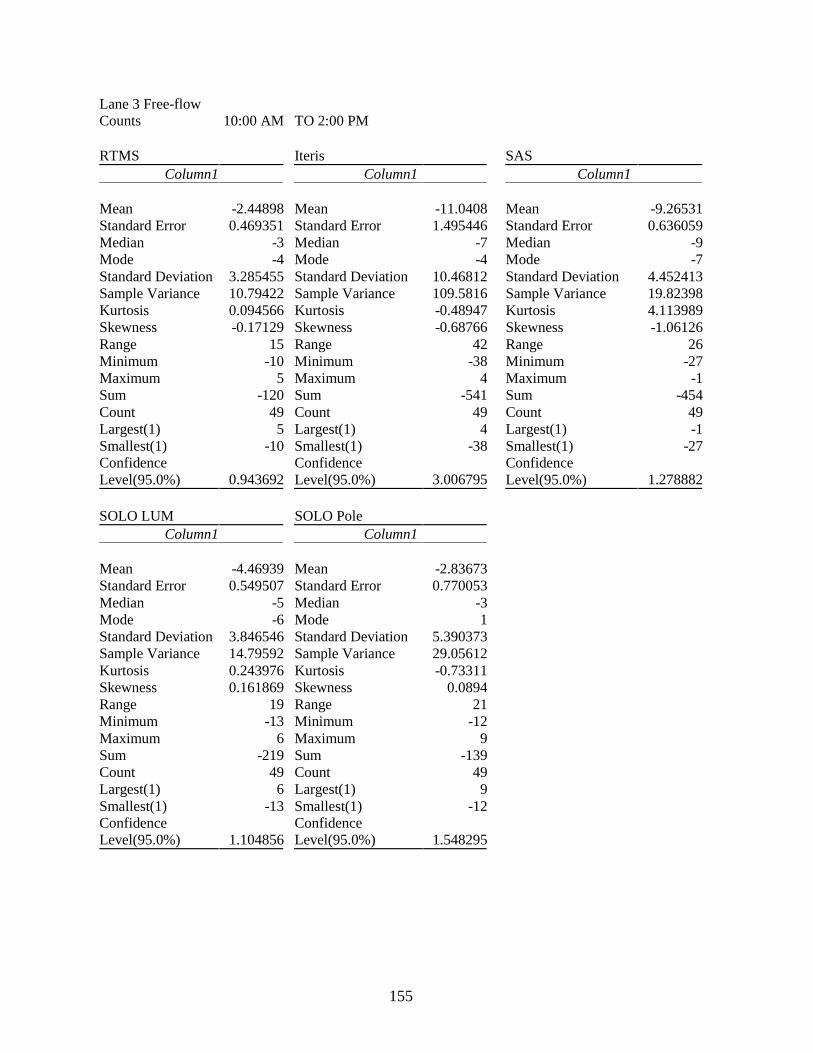
155

Lane 3 Free-flow Counts 10:00 AM TO 2:00 PM RTMS Iteris SAS

Column1 Column1 Column1 Mean -2.44898 Mean -11.0408 Mean -9.26531Standard Error 0.469351 Standard Error 1.495446 Standard Error 0.636059Median -3 Median -7 Median -9Mode -4 Mode -4 Mode -7Standard Deviation 3.285455 Standard Deviation 10.46812 Standard Deviation 4.452413Sample Variance 10.79422 Sample Variance 109.5816 Sample Variance 19.82398Kurtosis 0.094566 Kurtosis -0.48947 Kurtosis 4.113989Skewness -0.17129 Skewness -0.68766 Skewness -1.06126Range 15 Range 42 Range 26Minimum -10 Minimum -38 Minimum -27Maximum 5 Maximum 4 Maximum -1Sum -120 Sum -541 Sum -454Count 49 Count 49 Count 49Largest(1) 5 Largest(1) 4 Largest(1) -1Smallest(1) -10 Smallest(1) -38 Smallest(1) -27Confidence Level(95.0%) 0.943692

Confidence Level(95.0%) 3.006795

Confidence Level(95.0%) 1.278882

SOLO LUM SOLO Pole

Column1 Column1 Mean -4.46939 Mean -2.83673 Standard Error 0.549507 Standard Error 0.770053 Median -5 Median -3 Mode -6 Mode 1 Standard Deviation 3.846546 Standard Deviation 5.390373 Sample Variance 14.79592 Sample Variance 29.05612 Kurtosis 0.243976 Kurtosis -0.73311 Skewness 0.161869 Skewness 0.0894 Range 19 Range 21 Minimum -13 Minimum -12 Maximum 6 Maximum 9 Sum -219 Sum -139 Count 49 Count 49 Largest(1) 6 Largest(1) 9 Smallest(1) -13 Smallest(1) -12 Confidence Level(95.0%) 1.104856

Confidence Level(95.0%) 1.548295

156

Lane 3 Congested Counts 7:30 AM TO 9:30 AM RTMS Iteris SAS

Column1 Column1 Column1 Mean -3.16 Mean -8.88 Mean -9.44Standard Error 1.2051 Standard Error 1.003859 Standard Error 1.741723Median -4 Median -9 Median -11Mode -5 Mode -7 Mode -5Standard Deviation 6.025501 Standard Deviation 5.019296 Standard Deviation 8.708616Sample Variance 36.30667 Sample Variance 25.19333 Sample Variance 75.84Kurtosis 6.966512 Kurtosis 0.247827 Kurtosis 1.808235Skewness 2.101784 Skewness -0.14782 Skewness 0.804755Range 31 Range 21 Range 42Minimum -12 Minimum -19 Minimum -26Maximum 19 Maximum 2 Maximum 16Sum -79 Sum -222 Sum -236Count 25 Count 25 Count 25Largest(1) 19 Largest(1) 2 Largest(1) 16Smallest(1) -12 Smallest(1) -19 Smallest(1) -26Confidence Level(95.0%) 2.487204

Confidence Level(95.0%) 2.071863

Confidence Level(95.0%) 3.594739

SOLO LUM SOLO Pole

Column1 Column1 Mean -15.96 Mean -17.64 Standard Error 1.070016 Standard Error 1.668213 Median -16 Median -17 Mode -15 Mode -10 Standard Deviation 5.350078 Standard Deviation 8.341063 Sample Variance 28.62333 Sample Variance 69.57333 Kurtosis 1.638076 Kurtosis 2.255818 Skewness -0.46416 Skewness 0.097281 Range 26 Range 44 Minimum -31 Minimum -39 Maximum -5 Maximum 5 Sum -399 Sum -441 Count 25 Count 25 Largest(1) -5 Largest(1) 5 Smallest(1) -31 Smallest(1) -39 Confidence Level(95.0%) 2.208403

Confidence Level(95.0%) 3.443021

157

Lane 3 Free-flow Speeds 10:00 AM TO 2:00 PM RTMS Iteris SAS

Column1 Column1 Column1 Mean 0.834286 Mean 0.119 Mean 0.594898Standard Error 0.198218 Standard Error 0.1063 Standard Error 0.317141Median 0.63 Median 0.17 Median 0.74Mode 2.49 Mode -0.57 Mode -2.72Standard Deviation 1.387528 Standard Deviation 0.7444 Standard Deviation 2.219988Sample Variance 1.925233 Sample Variance 0.5541 Sample Variance 4.928346Kurtosis -0.89217 Kurtosis -0.382 Kurtosis -0.56815Skewness 0.132708 Skewness 0.1877 Skewness -0.1555Range 5.32 Range 3.18 Range 9.13Minimum -1.61 Minimum -1.27 Minimum -4.28Maximum 3.71 Maximum 1.91 Maximum 4.85Sum 40.88 Sum 5.83 Sum 29.15Count 49 Count 49 Count 49Largest(1) 3.71 Largest(1) 1.91 Largest(1) 4.85Smallest(1) -1.61 Smallest(1) -1.27 Smallest(1) -4.28Confidence Level(95.0%) 0.398544

Confidence Level(95.0%) 0.2138

Confidence Level(95.0%) 0.637655

SOLO LUM SOLO Pole

Column1 Column1 Mean -2.75722 Mean 0.8434 Standard Error 0.156765 Standard Error 0.1451 Median -2.56922 Median 0.8547 Mode #N/A Mode #N/A Standard Deviation 1.097356 Standard Deviation 1.0157 Sample Variance 1.204191 Sample Variance 1.0317 Kurtosis -0.72472 Kurtosis -0.731 Skewness -0.55059 Skewness -0.136 Range 3.894219 Range 4.0767 Minimum -5.14172 Minimum -1.295 Maximum -1.2475 Maximum 2.7814 Sum -135.104 Sum 41.326 Count 49 Count 49 Largest(1) -1.2475 Largest(1) 2.7814 Smallest(1) -5.14172 Smallest(1) -1.295 Confidence Level(95.0%) 0.315197

Confidence Level(95.0%) 0.2917

158

Lane 3 Congested Speeds 7:30 AM TO 9:30 AM RTMS Iteris SAS

Column1 Column1 Column1 Mean 6.1456 Mean -1.62 Mean -9.44Standard Error 0.915129 Standard Error 0.365488 Standard Error 1.741723Median 5.12 Median -1.93 Median -11Mode #N/A Mode #N/A Mode -5Standard Deviation 4.575645 Standard Deviation 1.827439 Standard Deviation 8.708616Sample Variance 20.93653 Sample Variance 3.339533 Sample Variance 75.84Kurtosis 6.08233 Kurtosis -0.0723 Kurtosis 1.808235Skewness 1.878304 Skewness 0.472452 Skewness 0.804755Range 22.84 Range 7.51 Range 42Minimum -0.31 Minimum -4.79 Minimum -26Maximum 22.53 Maximum 2.72 Maximum 16Sum 153.64 Sum -40.5 Sum -236Count 25 Count 25 Count 25Largest(1) 22.53 Largest(1) 2.72 Largest(1) 16Smallest(1) -0.31 Smallest(1) -4.79 Smallest(1) -26Confidence Level(95.0%) 1.888733

Confidence Level(95.0%) 0.75433

Confidence Level(95.0%) 3.594739

SOLO LUM SOLO Pole

Column1 Column1 Mean -0.25007 Mean 0.609307 Standard Error 0.258393 Standard Error 0.16331 Median -0.19031 Median 0.649688 Mode #N/A Mode #N/A Standard Deviation 1.291963 Standard Deviation 0.816548 Sample Variance 1.669168 Sample Variance 0.666751 Kurtosis 1.647811 Kurtosis -0.55136 Skewness -0.88627 Skewness 0.050587 Range 5.755625 Range 3.115156 Minimum -3.76938 Minimum -0.98328 Maximum 1.98625 Maximum 2.131875 Sum -6.25172 Sum 15.23266 Count 25 Count 25 Largest(1) 1.98625 Largest(1) 2.131875 Smallest(1) -3.76938 Smallest(1) -0.98328 Confidence Level(95.0%) 0.533296

Confidence Level(95.0%) 0.337054