Variations in normal color vision. II. Unique hues

Webster et al. Vol. 17, No. 9 /September 2000 /J. Opt. Soc. Am. A 1545

Variations in normal color vision. II.Unique hues

Michael A. Webster

Department of Psychology, University of Nevada, Reno, Reno, Nevada 89557

Eriko Miyahara

Department of Psychology, Rochester Institute of Technology, Rochester, New York 14623

Gokhan Malkoc and Vincent E. Raker

Department of Psychology, University of Nevada, Reno, Reno, Nevada 89557

Received October 14, 1999; revised manuscript received May 17, 2000; accepted May 25, 2000

We examined individual differences in the color appearance of nonspectral lights and asked how they might berelated to individual differences in sensitivity to chromatic stimuli. Observers set unique hues for moderatelysaturated equiluminant stimuli by varying their hue angle within a plane defined by the LvsM and SvsLMcone-opponent axes that are thought to characterize early postreceptoral color coding. Unique red settingswere close to the 1L pole of the LvsM axis, while green, blue, and yellow settings clustered along directionsintermediate to the LvsM and SvsLM axes and thus corresponded to particular ratios of LvsM to SvsLM ac-tivity. Interobserver differences in the unique hues were substantial. However, no relationship was foundbetween hue settings and relative sensitivity to the LvsM and SvsLM axes. Moreover, interobserver varia-tions in different unique hues were uncorrelated and were thus inconsistent with a common underlying factorsuch as relative sensitivity or changes in the spectral sensitivities of the cones. Thus for the moderately satu-rated lights we tested, the unique hues appear largely unconstrained by normal individual differences in thecone-opponent axes. In turn, this suggests that the perceived hue for these stimuli does not depend on fixed(common) physiological weightings of the cone-opponent axes or on fixed (common) color signals in the envi-ronment. © 2000 Optical Society of America [S0740-3232(00)01809-3]

OCIS codes: 330.1690, 330.1720, 330.1730, 330.5020, 330.7310.

1. INTRODUCTIONHuman color vision is thought to depend on two generalstages: Light is initially absorbed by the long-, medium-,or short-wavelength sensitive (L-, M-, or S-) cone recep-tors, and the signals from the receptors are then com-bined to form different types of postreceptoral channels.However, the number and nature of these postreceptoraltransformations remain poorly defined. The principal di-mensions underlying postreceptoral color vision were firstsuggested by measures of color appearance. Any aper-ture color can be described by a combination of the fourperceptually unique hues: red, green, blue, or yellow, yetno light appears both red and green or both blue andyellow.1,2 Such observations led Hering to postulate thatthe sensation of color directly reflects the responses in twoopponent channels coding red–green or blue–yellowsensations.3 Because a single channel signaled eitherred or green depending on the polarity of its response,these two hues could not be perceived simultaneously.By this account, most hues (e.g., orange) appear mixed be-cause they reflect the component responses from bothchannels (e.g., red plus yellow), while the unique hues ap-pear pure because they stimulate one channel but leavethe second channel in equilibrium.

Such models account well for the phenomenology ofcolor vision but predict cone transformations different

0740-3232/2000/091545-11$15.00 ©

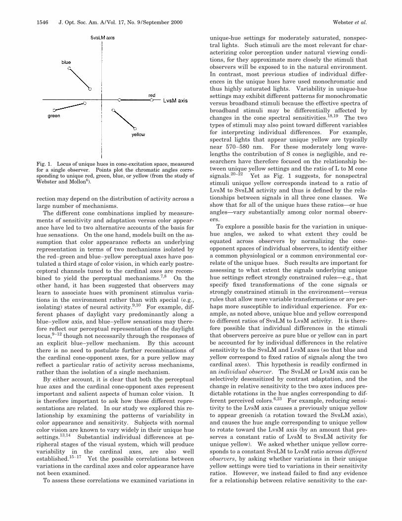
from those that are typically observed in physiological re-cordings or in psychophysical measurements of sensitiv-ity and adaptation.4 These types of studies suggest thatpostreceptoral color coding is organized in terms of two di-mensions that correspond to opposing signals from the Land M cones (LvsM) or to signals from the S cones op-posed by a combination of signals from the L and M ones(SvsLM). Any color can be represented in an opponent-modulation space whose two chromatic axes correspond tothe level of SvsLM or LvsM activity.5 Yet within thisspace the four unique hues do not lie along the four polesof the cardinal axes. For example, Fig. 1 plots theunique-hue settings for a single observer (MW) within theLvsM versus SvsLM plane (from the study of Webster andMollon6). Only the 1L pole of the LvsM axis may beclose to a perceptually pure color (unique red), while theremaining poles appear as mixtures of the primary hues(blue–green for the 1M pole, blue–red for the 1S pole,and yellow–green for the 2S pole). Thus—with the pos-sible exception of unique red—the unique hues do not cor-respond to activity along a single cardinal axis. More-over, whether any suprathreshold stimuli can isolate asingle postreceptoral color mechanism is doubtful, for avariety of results suggest that postreceptoral color codinginvolves multiple mechanisms tuned to different colordirections.4 Thus the perceived hue at any stimulus di-

2000 Optical Society of America

1546 J. Opt. Soc. Am. A/Vol. 17, No. 9 /September 2000 Webster et al.

rection may depend on the distribution of activity across alarge number of mechanisms.

The different cone combinations implied by measure-ments of sensitivity and adaptation versus color appear-ance have led to two alternative accounts of the basis forhue sensations. On the one hand, models built on the as-sumption that color appearance reflects an underlyingrepresentation in terms of two mechanisms isolated bythe red–green and blue–yellow perceptual axes have pos-tulated a third stage of color vision, in which early postre-ceptoral channels tuned to the cardinal axes are recom-bined to yield the perceptual mechanisms.7,8 On theother hand, it has been suggested that observers maylearn to associate hues with prominent stimulus varia-tions in the environment rather than with special (e.g.,isolating) states of neural activity.9,10 For example, dif-ferent phases of daylight vary predominantly along ablue–yellow axis, and blue–yellow sensations may there-fore reflect our perceptual representation of the daylightlocus,9–12 though not necessarily through the responses ofan explicit blue–yellow mechanism. By this accountthere is no need to postulate further recombinations ofthe cardinal cone-opponent axes, for a pure yellow mayreflect a particular ratio of activity across mechanisms,rather than the isolation of a single mechanism.

By either account, it is clear that both the perceptualhue axes and the cardinal cone-opponent axes representimportant and salient aspects of human color vision. Itis therefore important to ask how these different repre-sentations are related. In our study we explored this re-lationship by examining the patterns of variability incolor appearance and sensitivity. Subjects with normalcolor vision are known to vary widely in their unique huesettings.13,14 Substantial individual differences at pe-ripheral stages of the visual system, which will producevariability in the cardinal axes, are also wellestablished.15–17 Yet the possible correlations betweenvariations in the cardinal axes and color appearance havenot been examined.

To assess these correlations we examined variations in

Fig. 1. Locus of unique hues in cone-excitation space, measuredfor a single observer. Points plot the chromatic angles corre-sponding to unique red, green, blue, or yellow (from the study ofWebster and Mollon6).

unique-hue settings for moderately saturated, nonspec-tral lights. Such stimuli are the most relevant for char-acterizing color perception under natural viewing condi-tions, for they approximate more closely the stimuli thatobservers will be exposed to in the natural environment.In contrast, most previous studies of individual differ-ences in the unique hues have used monochromatic andthus highly saturated lights. Variability in unique-huesettings may exhibit different patterns for monochromaticversus broadband stimuli because the effective spectra ofbroadband stimuli may be differentially affected bychanges in the cone spectral sensitivities.18,19 The twotypes of stimuli may also point toward different variablesfor interpreting individual differences. For example,spectral lights that appear unique yellow are typicallynear 570–580 nm. For these moderately long wave-lengths the contribution of S cones is negligible, and re-searchers have therefore focused on the relationship be-tween unique yellow settings and the ratio of L to M conesignals.20–22 Yet as Fig. 1 suggests, for nonspectralstimuli unique yellow corresponds instead to a ratio ofLvsM to SvsLM activity and thus is defined by the rela-tionships between signals in all three cone classes. Weshow that for all of the unique hues these ratios—or hueangles—vary substantially among color normal observ-ers.

To explore a possible basis for the variation in unique-hue angles, we asked to what extent they could beequated across observers by normalizing the cone-opponent spaces of individual observers, to identify eithera common physiological or a common environmental cor-relate of the unique hues. Such results are important forassessing to what extent the signals underlying uniquehue settings reflect strongly constrained rules—e.g., thatspecify fixed transformations of the cone signals orstrongly constrained stimuli in the environment—versusrules that allow more variable transformations or are per-haps more susceptible to individual experience. For ex-ample, as noted above, unique blue and yellow correspondto different ratios of SvsLM to LvsM activity. It is there-fore possible that individual differences in the stimulithat observers perceive as pure blue or yellow can in partbe accounted for by individual differences in the relativesensitivity to the SvsLM and LvsM axes (so that blue andyellow correspond to fixed ratios of signals along the twocardinal axes). This hypothesis is readily confirmed inan individual observer. The SvsLM or LvsM axis can beselectively desensitized by contrast adaptation, and thechange in relative sensitivity to the two axes induces pre-dictable rotations in the hue angles corresponding to dif-ferent perceived colors.6,23 For example, reducing sensi-tivity to the LvsM axis causes a previously unique yellowto appear greenish (a rotation toward the SvsLM axis),and causes the hue angle corresponding to unique yellowto rotate toward the LvsM axis (by an amount that pre-serves a constant ratio of LvsM to SvsLM activity forunique yellow). We asked whether unique yellow corre-sponds to a constant SvsLM to LvsM ratio across differentobservers, by asking whether variations in their uniqueyellow settings were tied to variations in their sensitivityratios. However, we instead failed to find any evidencefor a relationship between relative sensitivity to the car-


dinal axes and unique hue settings across observers.Moreover, in contrast to the predictions for relative sen-sitivity differences across the cones or for changes in thespectral sensitivities of the cones, there was no correla-tion between hue angles corresponding to differentunique hues. These results thus suggest that normalvariations in peripheral factors may place little constrainton the perceived hues of the moderately saturated lightswe tested.

2. METHODSA detailed description of the display and stimulus specifi-cation is given in the accompanying paper.17 As de-scribed there, stimuli were shown on a monitor and con-sisted of equiluminant (30 cd/m2) pulses of colorpresented in a 2-deg square field, centered on a 6.43 8.4 deg neutral gray background (30 cd/m2 and chro-maticity of Illuminant C). The chromatic contrasts of thepulses were defined by their variations relative to thisneutral point within a threshold-scaled version of theMacLeod–Boynton24 r,b chromaticity diagram, scaled sothat

LvsM contrast 5 ~rmb 2 0.6568! * 2754

SvsLM contrast 5 ~bmb 2 0.01825! * 4099.

Observers made unique-hue judgments for conditionsand stimuli that were very similar to those described inthe accompanying paper for measuring chromaticsensitivity.17 The monitor was viewed binocularly in anotherwise dark room from 250 cm. Observers firstadapted for 3 min to the gray background. Test stimuliwere then presented while subjects made forced-choicejudgments about their perceived color (e.g., responding ei-ther ‘‘too red’’ or ‘‘too green’’ for unique yellow settings.)The pulsed tests were shown at full contrast for 280 msand ramped on and off with Gaussian envelopes (s5 80 ms). During a run the contrast (;saturation) ofthe stimulus was fixed, while the chromatic angle wasvaried across trials by using two randomly interleavedstaircases to define the angle at which the alternate re-sponses occurred with equal probability. The field re-turned to gray for 3 s between each presentation. Con-trol runs with longer intertrial intervals (up to 8 s)yielded very similar settings, suggesting that the hueangles were not biased by adaptation to the test pulses.Hue angles were measured over a range of contrasts forsix observers (the authors and two additional subjects) forwhom we also collected measures of sensitivity to theLvsM and SvsLM axes.17 Further unique-hue settings ata single contrast were collected for an additional 45 sub-jects who participated for course credit. All subjects hadnormal color vision as assessed by the Ishihara pseudo-isochromatic plates.

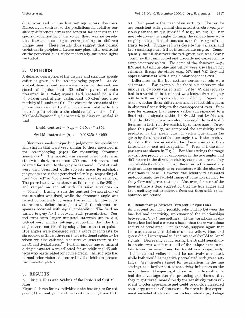
3. RESULTSA. Unique Hues and Scaling of the LvsM and SvsLMAxesFigure 2 shows for six individuals the hue angles for red,green, blue, and yellow at contrasts ranging from 10 to

60. Each point is the mean of six settings. The resultsare consistent with general characteristics observed pre-viously for the unique hues6,25–29 (e.g., see Fig. 1). Formost observers the angles defining the unique hues wereroughly independent of contrast over the range of con-trasts tested. Unique red was close to the 1L axis, andthe remaining hues fell at intermediate angles. Conse-quently, for all observers the red–green axis was clearly‘‘bent,’’ so that unique red and green do not correspond tocomplementary colors. For some of the observers (e.g.,EM and JS) unique blue and yellow were also clearly notcollinear, though for others (e.g., MW and VR) they didappear consistent with a single color-opponent axis.

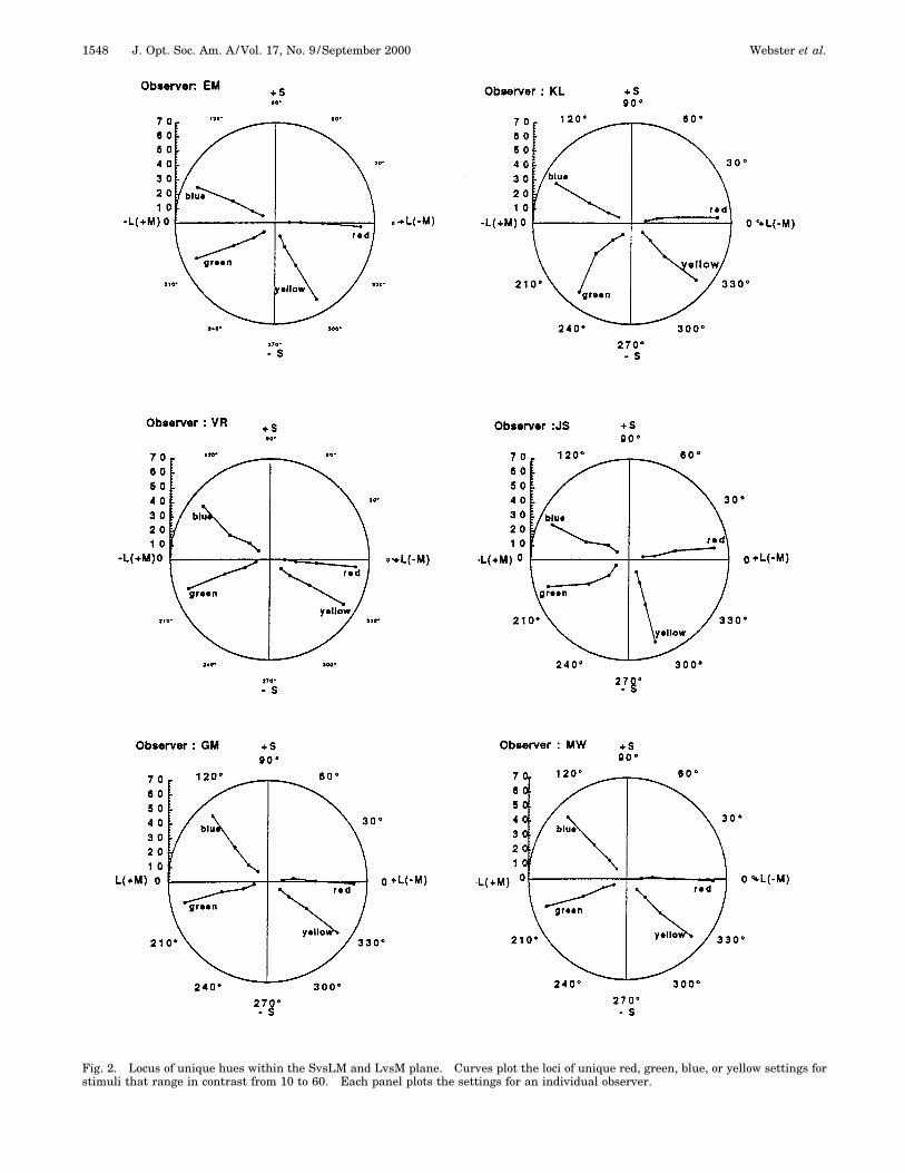
Differences in the hue settings across subjects weresubstantial. For example, for these six observers theunique yellow locus varied from 232 to 269 deg (equiva-lent to a variation in dominant wavelength from roughly580 to 570 nm, respectively; see Table 1). Again, weasked whether these differences might reflect differencesin observers’ sensitivity to the cone-opponent axes. Sup-pose for example that unique yellow corresponded to afixed ratio of signals within the SvsLM and LvsM axes.Then the differences across observers might be tied to dif-ferences in their relative sensitivity to these axes. To ex-plore this possibility, we compared the sensitivity ratiopredicted by the green, blue, or yellow hue angles (asgiven by the tangent of the hue angles), with the sensitiv-ity ratio that we estimated for these observers fromthresholds or contrast adaptation.17 Plots of these com-parisons are shown in Fig. 3. For blue settings the rangeof variation predicted by differences in the hue angles anddifferences in the direct sensitivity estimates are roughlycomparable (twofold). Thus differences in the sensitivityratio are large enough to be consistent with the observedvariations in blue. However, the sensitivity estimatesunderestimate the fourfold range of variation implied bythe yellow and green settings. Moreover, for none of thehues is there a clear suggestion that the hue angles andthe sensitivity ratios inferred from the thresholds or ad-aptation are related.

B. Relationships between Different Unique HuesAs a second test for a possible relationship between thehue loci and sensitivity, we examined the relationshipsbetween different hue settings. If the variations in dif-ferent hue loci had a common basis, then these variationsshould be correlated. For example, suppose again thatthe chromatic angles defining unique yellow, blue, andgreen did all correspond to fixed ratios of SvsLM to LvsMsignals. Decreasing or increasing the SvsLM sensitivityin an observer would cause all of the unique hues to ro-tate toward or away from the SvsLM axis, respectively.Thus blue and yellow should be positively correlated,while both would be negatively correlated with green set-tings. We therefore tested for covariations in the huesettings as a further test of sensitivity influences on theunique hues. Comparing different unique hues directlyhad the advantage over the preceding experiments thatthey might reveal more directly the sensitivity ratios rel-evant to color appearance and could be quickly measuredon a large number of observers. Subjects in this experi-ment included students in an undergraduate psychology


Fig. 2. Locus of unique hues within the SvsLM and LvsM plane. Curves plot the loci of unique red, green, blue, or yellow settings forstimuli that range in contrast from 10 to 60. Each panel plots the settings for an individual observer.


Fig. 3. S/LM sensitivity ratios estimated from hue angles compared with estimates from thresholds (circles) or adaptation (triangles).Estimates from unique hues are based on the tangent of the observer’s mean unique hue angle.

Table 1. Unique-Hue Settings for All Subjects (n Ä 51)a

Hue Angle

Unique Hue

Yellow Blue Red Green

Mean Hue Angle 250.3 144.6 0.4 205.1Dominant Wavelength 574 477 545Standard Deviation 9.2 10.3 5.4 12.6Range 270.6 to 231.3 121.0 to 163.3 29.0 to 12.3 172.6 to 241.1Dominant Wavelength 570 to 580 465 to 486 491 to 562

a Values give chromatic angle in degrees within the threshold-scaled LvsM and SvsLM space.

course who participated for course credit. During asingle session each of the unique hues at a contrast of 30was measured four times (following an initial, discardedpractice run). A subset of subjects repeated the samemeasures during a second session as a test for reliability.The settings for some students were highly variable, pre-sumably for reasons unrelated to their color vision (e.g.,estimating the wrong hue on some trials). We thereforeexcluded subjects whose range was greater than one stan-dard deviation above the mean range for the group forany single hue. Thirteen observers were excluded by thiscriterion.

Figure 4 plots the hue angles for each subject withinthe LvsM and SvsLM space, and Fig. 5 shows histogramsof the chromatic angles for each hue. The figures illus-trate large variations in all of the hue angles. Within ourchromatic plane the loci for red were the most constrained(covering a range of 20 deg centered on the 1L axis),whereas unique green varied over a range of 60 deg(Tables 1 and 2). Tables 1 and 2 also give the dominantwavelength of the hue angles for blue, green, and yellow.For blue and yellow the means and range are comparableto previous measurements of the unique hues in mono-chromatic lights,14,22,30 consistent with the largely linearequilibrium axes for these hues.25,28 Alternatively, ourunique green settings were biased toward longer wave-lengths than unique green estimates for spectral lights,consistent with a curvature in the loci for uniquegreen.25,29

Despite the large interobserver differences in each ofthe hues, the variations across different hues were in allcases unrelated. The correlation matrix for the four huesis given in Table 3. Surprisingly, none of the correlationsbetween different hues reaches significance. In Table 3the values in the upper-right cells were calculated from

the data of all 51 observers. The diagonals show the cor-relations between the same hues over two different daysbased on 31 observers who participated in two sessions.These values show that red, blue, and yellow were setwith good reliability, whereas settings for green werehighly variable (even relative to the large differencesacross observers). Uncertainty in the settings for indi-vidual hues could thus mask a weak relationship betweendifferent hues. To give the sensitivity hypothesis thebest chance for succeeding, we therefore further restrictedthe analysis to the subset of subjects who made the mostreliable hue settings, by selecting subjects whose totalrange of hue settings was at or below the median range

Fig. 4. Locus of unique hues within the SvsLM and LvsM plane.Each point plots the chromatic angle that appeared unique red,green, blue, or yellow for one of the 51 observers. All stimulihad a fixed contrast of 30.


Fig. 5. Histograms of the distributions of hue angles. For each of the four hues, the upper panel plots the measured hue settings, forthe full set of 51 observers (unshaded bars) or for the subset of 26 observers who set the hues most consistently (shaded histogram). Thelower panel for each hue shows the range of hue angles predicted by assuming that all observers with different spectral sensitivitieschoose hues that match the same physiological weightings of the cardinal axes (unshaded bars) or choose hues that match the sameenvironmental stimuli (shaded bars). The predictions were based on reconstructing the sensitivities of the 49 Stiles and Burch observ-ers.

Table 2. Unique-Hue Settings for the Most Consistent Subjects (n Ä 26)a

Hue Angle

Unique Hue


Mean Hue Angle 250.2 146.1 21.83 203.3Dominant Wavelength 574 478 542Standard Deviation 9.5 9.1 4.3 10.9Range 263.5 to 231.3 125.6 to 162.4 29.0 to 6.17 186.6 to 232.1Dominant Wavelength 571 to 580 468 to 486 504 to 560

a Total variability in hue settings equal to or below the median range for all observers. Values give chromatic angle in degrees within the threshold-scaled LvsM and SvsLM space.

Table 3. Correlations between Different Unique-Hue Settingsa

Unique Hue

Unique Hue


Yellow 0.97 0.88 20.24 20.23 20.22Blue 0.31 0.93 0.88 20.03 20.12Red 0.30 0.38 0.92 0.80 0.0

Green 0.15 20.13 20.01 0.54 0.44

a Values give the correlations between hue angles for all observers (n 5 51, upper-right cells) or for the subset of observers who made the most consistentsettings (n 5 26, lower-left cells, in boldface). Values along the diagonal show the correlations for the same hue measured across two daily sessions. Noneof the measured correlations across different unique hues is significant.


for the entire group. For these subjects the repeated set-tings of each individual varied over a range of 10 deg orless for red, blue, and yellow and over 20 deg or less forunique green. This resulted in high reliabilities for red,blue, and yellow, though consistency for the green set-tings was still marginal (Table 3). Yet even for this sub-set of observers the correlations across different hues re-mained in all cases insignificant. Thus our resultssuggest that variations across the unique hues are sur-prisingly independent.

C. Unique Hues and Individual Differences in SpectralSensitivityThe preceding results suggested that there is little rela-tionship between the chromatic angles that are perceivedas unique hues and the relative sensitivity to the SvsLMand LvsM axes. As a final analysis we examined thevariations in unique hues that would be predicted bychanges in the spectral sensitivities of the cone mecha-nisms rather than by their relative scaling. To assessnormal variations in the cone sensitivities, we used theanalysis of MacLeod and Webster16,31 to reconstruct indi-vidual spectral sensitivities for the 49 observers in thecolor matching study of Stiles and Burch.32 (Details ofthis reconstruction are described in the accompanyingpaper.17) We then calculated the unique hues for theseindividuals predicted by two different assumptions: (1)that the hue angles are determined by fixed physiologicalsignals in the observer or (2) that the unique hues corre-spond to fixed color signals in the environment. We con-sider these alternatives in turn.

1. Fixed Physiological SignalIn this case we assumed that the unique hues were set byfixed directions within the SvsLM and LvsM plane. Wethen calculated how the stimulus directions required toproduce these ratios would be biased by changes in thecone sensitivities, owing to differences in preretinalscreening or photopigment absorption spectra. Notethat, like the sensitivity-ratio hypothesis we rejectedabove, this approach essentially assumes that the uniquehues are determined by a fixed weighting of the cone sig-nals (as might occur if these weightings were specified ge-netically). For the calculations, we assumed that theseweightings were given by the S/LM ratio implied by themean hue settings for our observers (Table 1). We thencalculated for each Stiles and Burch observer the stimu-

lus angle (relative to their individual responses to thewhite point) at which this ratio occurred.

Figure 5 plots the distribution of hues predicted by thevariations in color matching among the Stiles–Burch ob-servers. These are shown by the unshaded histogramsplotted below the empirical distributions for each hue.Because these predictions are based on finding constantdirections within each individual’s cone-opponent plane,they are similar in principle to analyzing how changes inspectral sensitivity alter the stimulus directions deter-mining the cardinal axes (see Fig. 5 of the accompanyingpaper.17) In fact, the distribution for unique red is iden-tical to the distribution defining the LvsM axis, since weassumed an angle of 0 deg (the 1L axis) for unique red.This distribution is very narrow, spanning a range of only2 deg, and thus clearly fails to account for the 20-degrange of variation in the observed unique red settings.Alternatively, the predicted range of angles for the otherhues is large and thus comes much closer to the spread ofhue angles actually observed. However, as Table 4shows, the predicted variations in the different hues arevery highly correlated. Thus, like the scaling hypothesis,the changes in spectral sensitivity again fail to accountfor the independence of the different unique hues.

2. Fixed Environmental StimulusA dissociation between color sensations and chromaticsensitivity could arise if the hue loci for the conditions weexamined are tied more to physical properties of the out-side world than to physiological properties of theobserver.9,10 Jordan and Mollon18,19 suggested thatthere might in fact be comparatively little interobservervariability in hue judgements for natural reflectancefunctions (though focal colors named in Munsell chips doshow some individual differences.33) They suggestedthat observers might learn to associate concordant huepercepts with real-world reflectances. These perceptswould correspond to different physiological signals de-pending on the specific makeup of the observer (e.g.,whether the observer had a higher or lower density of pre-retinal pigments). By this argument, variations in thehues of monochromatic lights arise because narrowbandlights are no longer subjected to the spectrally selectivefiltering by the individual’s visual system and thus nolonger produce the same ratio of cone signals.

The hypothesis of Jordan and Mollon points to the im-portance of searching for the basis of color appearance

Table 4. Correlations between Different Unique-Hue Settings Predicted by Individual Differencesin Color Matching a

Unique Hue

Unique Hue Yellow Blue Red Green

Yellow 0.99 20.77 20.93Blue 0.97 20.77 20.97Red 0.62 0.77 0.80

Green 0.19 0.37 0.84

a Values give the correlations between hue angles for observers with different spectral sensitivities, based on reconstructing sensitivities for the 49 Stilesand Burch observers. Upper-right cells show the correlations predicted if the unique hues correspond to constant S/LM ratios equal to the mean observedratios. Lower-left cells (in boldface) show the correlations predicted if the unique hues correspond to a constant color signal in the environment, simulatedby spectra for Munsell chips viewed under Illuminant C.


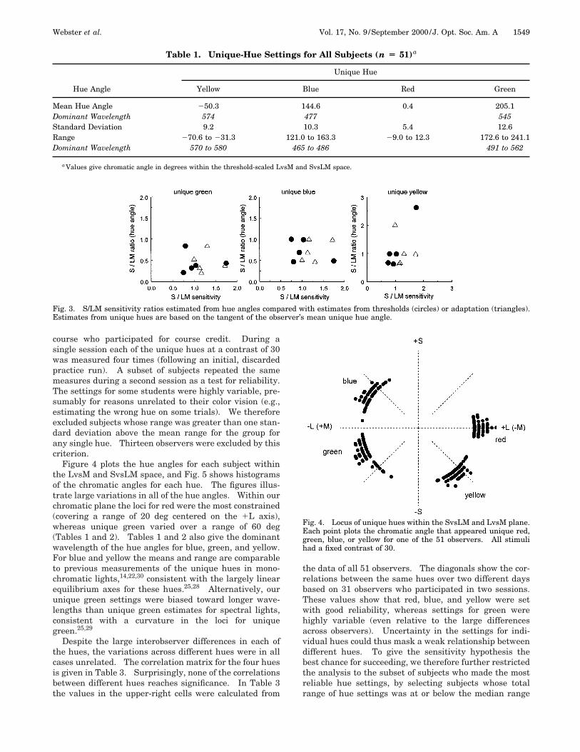
Fig. 6. Spectra used to calculate how the variations in the hue settings depend on the stimulus color signal. Naturalistic color signalswere constructed by simulating Munsell chips viewed under Illuminant C (dashed curves). Solid curves show the monitor spectra withthe equivalent chromaticity.

within the context of the stimuli to which observers arenormally exposed. The spectra for our monitor stimuliare obviously much broader than the monochromaticlights traditionally used to measure the unique hues, yetthey vary much less smoothly than typical natural colorsignals. Could differences in hue settings on our monitorreflect differences in the spectral filtering characteristicsof observers who would have agreed on the perceived hueof natural surfaces? To assess this possibility, we againused the hypothetical Stiles–Burch observers, but thistime we calculated how these observers would encodenatural surfaces viewed under natural illumination.Since our reference chromaticity equaled Illuminant C,we approximated an Illuminant-C source from the firstthree basis functions that Judd et al.34 derived for naturaldaylight. Surfaces were simulated Munsell chips basedon the first three basis functions derived for Munsell re-flectance spectra by Cohen.35 The chips were chosen sothat the color signals under the illuminant had a contrastof 30 and again equaled the mean angle chosen for eachhue by our observers. The resulting spectra are illus-trated in Fig. 6, along with the monitor phosphor spectragiving the same chromaticity. For each observer we cal-culated the S/LM ratio for each unique hue based on theMunsell spectra (given by the hue angle relative to theirresponse to the Illuminant C spectrum). Finally, we cal-culated the color angle that was necessary to give thesame S/LM ratio for the phosphor spectra (again relativeto their response to the Illuminant-C reference, which weassumed represents their ‘‘learned’’ white point).

Again, if observers with different spectral sensitivitiesagreed on the hues of the Munsell surfaces, then the coneratios corresponding to these hues must differ, and thusfor the monitor stimuli different phosphor combinationswould be necessary to equate these cone ratios. Notethat in this case the observers’ settings should be unaf-

fected by differences in the scaling of their cone-opponentaxes, for this scaling would affect the Munsell and moni-tor stimuli in the same way. However, Fig. 5 shows thatthe monitor stimuli are dispersed by changes in theshapes of the cone spectra (see shaded histograms in thepanels for the predicted distributions). Interestingly, inthis case the range of angles predicted for each of the huesis comparable (;7 deg) but underestimates the range of20 to 40 deg that we actually measured. Moreover, thechanges in spectral sensitivity again predict highly corre-lated changes in some pairs of hues, such as blue and yel-low (Table 4), although, notably, the relationships be-tween the green and blue or yellow are now weak. Thusthe predicted relationships between the different hues areagain inconsistent with the pattern that we found. Ofcourse, the environmental stimuli defining the uniquehues may be different from the spectra that we chose (forIlluminant C itself appears slightly bluish under neutraladaptation), but the relevant spectra should be similarlybroad and thus should similarly account for only a smallproportion of the variance in the hue settings, while againpredicting strong correlations between the hues.

The implication of these analyses is that the variationsin the unique hues are too large and too independent to beaccounted for by either a fixed physiological weighting ora fixed color signal in the environment. In turn, this im-plies that the hue loci for our moderately saturatedstimuli are largely unconstrained by normal variations inthe peripheral factors that we considered, even thoughthese factors substantially alter an observer’s sensitivityto chromatic stimuli.

4. DISCUSSIONThe LvsM and SvsLM axes are often loosely described as‘‘red–green’’ and ‘‘blue–yellow’’ axes, respectively, yet the


discrepancies between the cardinal cone-opponent andcolor-appearance axes are large. Understanding thesediscrepancies and their basis remains a central questionin color science. It is well recognized that variations inS-cone excitation do not correspond to a blue–yellowvariation, for S-cone signals also contribute substantiallyto red–green sensations.36,37 The relationship betweenthe LvsM axis and red–green appearance is less clear.Unique green is clearly shifted off the LvsM axis, requir-ing less S-cone excitation than the equiluminantwhite.6,25,27 On the other hand, we found that uniquered judgements do tend to cluster around the LvsM axis.For our observers, the range of unique red settings wasan order of magnitude too large to be accounted for by ex-pected individual differences in the LvsM axis, yet themean locus across observers was not significantly differ-ent from the 1L axis. This result differs from that of DeValois et al.,27 who found that unique red was insteadsystematically shifted off the LvsM axis toward angles re-quiring increasing S-cone excitation.

While red versus green and blue versus yellow repre-sent mutually exclusive sensations, our results supportprevious evidence indicating that the opponent pairs arenot strongly coupled. For example, judgments of red andgreen or blue and yellow scale differently with eccentric-ity, suggesting that they do not depend on a single under-lying process.38,39 The independence of the color-opponent poles is further suggested by the observationthat red versus green or blue versus yellow are not collin-ear within cone-opponent space.25–27 Our results rein-force the conclusion that the different hue sensations aredecoupled, because they suggest that there is little corre-lation across observers between the settings for the fourunique hues. This result is particularly surprising in thecase of blue and yellow settings, for at least in some ob-servers they fall very close to defining complementarypoles of a single linear axis25,28 (see Fig. 2).

The weak relationships between the hue settings alsoimply that the hue judgments are not strongly con-strained by normal variations in color sensitivity, whichshould lead to correlated changes in different axes of colorspace. In particular, our results failed to show a rela-tionship between the hue loci and the relative sensitivityto the SvsLM and LvsM axes or between the hue loci andperipheral factors that modify the shapes of the cone spec-tral sensitivities. Again, differences in a factor such asthe S/LM sensitivity ratio could plausibly have affectedthe hue judgments on a number of grounds. First,changing the scaling in a single observer (e.g., throughcontrast adaptation) does induce corresponding changesin the chromatic angles defining the unique hues.6 Sec-ond, the variability in the relative scaling across observ-ers may, for some hues at least, be comparable in range tothe range implied by the variations in the unique hues(see Fig. 3). Third, we showed that if the rules definingthe axes of color experience reflected a specific, fixedweighting of the cardinal-axis signals or reflected a com-mon learned feature of the environment, then the stimulirequired for the hue judgments should reflect variationsin the weightings imposed by factors affecting the cone-opponent axes. Finally, under some conditions theunique-hue settings have been found to be systematically

related to individual differences in peripheral color vision,such as in the relative number of cones21 (but see Refs. 20and 22), or the eye pigmentation of the observer.18

Yet despite such a priori arguments, the absence ofmeasurable correlations between the hue loci for ourstimuli suggest that the variations in the unique hues arelargely independent of the sensitivity differences acrossobservers. Because of the low reliability for some set-tings (e.g., unique green), we cannot reject a pattern ofweak correlations, but then the implied influence of thefactors that we considered must be correspondingly weak.Independent variations in different unique hues have alsobeen observed by others,40,41 as has independence be-tween measurements of observers’ hue settings and spec-tral sensitivities.18 Moreover, a similar result is sug-gested by studies showing largely normal colorjudgements in observers with highly compromised colorsensitivity. For example, Schefrin et al.42 found thatmost diabetic observers that they tested made unique-huesettings within the range of normal controls despite largemeasured losses in S-cone sensitivity. Miyahara et al.43

found that carriers of anomalous trichromacy had highlybiased L/M cone ratios but nevertheless made unique yel-low settings that were within the range of normal observ-ers. Further, Crognale et al.44 examined color vision in asubject with congenital cone dystrophy. This subjectlacked L cones and had abnormally low M- and S-conesensitivity but made unique-hue settings that werewithin normal limits for green and blue (though uniqueyellow and red fell outside the range we have found fornormal observers). Thus even observers with markedlydifferent chromatic sensitivities may make concordantappearance judgments.

Such results are difficult to reconcile with a fixed physi-ological transformation (i.e., a fixed, common weighting ofthe cone signals) as the basis for the unique hues. It re-mains possible that the hue loci depend in a simple wayon variations in a physiological factor that we have notconsidered (e.g., in the degree of rod intrusion); yet thendifferent factors that selectively affect specific hues wouldbe required to account for the independent variations inthe different hues. This constraint eliminates many ofthe known peripheral sources of variation in normal colorvision, since these sources instead have more global influ-ences on the cone signals for the desaturated lights thatwe tested. Moreover, variations in hue-specific factorsthat arise at more central levels of the visual systemcould dilute the influence of more-peripheral factors, butthey should not remove that influence entirely.

The alternative of a fixed environmental basis for theunique hues (e.g., a common learned color signal) also ap-pears inconsistent with the large range of hue settingsthat we observed. Specifically, our results do not point toa substantial decrease in interobserver differences in per-ceived hue as the spectra become more broadband ornaturalistic. It is possible that observers do show moreconsistent judgments for real surfaces under naturalviewing conditions, but our analysis suggests that this isunlikely to result from changes in the color signal that de-fines the surface (though it could conceivably result fromthe much richer context in which these color signals arejudged).


On the other hand, if hue judgments do depend onlearned characteristics of the environment, then differ-ences in these judgments could plausibly be expectedfrom differences in the visual diets of observers.Shepard12 noted that natural daylight provides a consis-tent environmental variable that could underlie a com-mon color organization. However, the color statistics ofnatural images—of collections of natural surfaces viewedunder daylight—vary substantially, and thus differentnatural contexts may be characterized by very differentcolor signatures.45 Adaptations to these statistics shapethe signals underlying color vision45 and thus could shapethe stimulus dimensions that define an individual’s per-ceptual organization of color. However, it remains to betested whether differences in the color environment arecorrelated with hue judgments and whether the environ-ment varies in ways that predict independent variationsin the loci for different hues. We are currently exploringthese questions.

ACKNOWLEDGMENTSThis research was supported by National Eye Institutegrant EY-10834. We are grateful to David Brainard andJohn Werner for helpful comments on the manuscript.

The corresponding author is Michael A. Webster, De-partment of Psychology, University of Nevada, Reno,Reno, Nevada 89557; email: [email protected].

REFERENCES1. I. Abramov and J. Gordon, ‘‘Color appearance: on seeing

red—or yellow, or green, or blue,’’ Annu. Rev. Psychol. 45,451–485 (1994).

2. L. M. Hurvich and D. Jameson, ‘‘An opponent-processtheory of color vision,’’ Psychol. Rev. 64, 384–404 (1957).

3. E. Hering, Outlines of a Theory of the Light Sense (HarvardU. Press, Cambridge, Mass., 1964).

4. M. A. Webster, ‘‘Human colour perception and its adapta-tion,’’ Network Comput. Neural Systems 7, 587–634 (1996).

5. D. H. Brainard, ‘‘Cone contrast and opponent modulationcolor spaces,’’ in Human Color Vision, P. Kaiser and R. M.B. Boynton, eds. (Optical Society of America, WashingtonD.C., 1996), pp. 563–579.

6. M. A. Webster and J. D. Mollon, ‘‘The influence of contrastadaptation on color appearance,’’ Vision Res. 34, 1993–2020(1994).

7. R. L. De Valois and K. K. De Valois, ‘‘A multi-stage colormodel,’’ Vision Res. 33, 1053–1065 (1993).

8. S. L. Guth, ‘‘Model for color vision and light adaptation,’’ J.Opt. Soc. Am. A 8, 976–993 (1991).

9. J. Pokorny and V. C. Smith, ‘‘Evaluation of single-pigmentshift model of anomalous trichromacy,’’ J. Opt. Soc. Am. 67,1196–1209 (1977).

10. J. D. Mollon, ‘‘Color vision,’’ Annu. Rev. Psychol. 33, 41–85(1982).

11. H.-C. Lee, ‘‘A computational model for opponent color en-coding,’’ in Advanced Printing of Conference Summaries,SPSE’s 43rd Annual Conference (Society for Imaging Sci-ence and Technology, Springfield, Va., 1990), pp. 178–181.

12. R. N. Shepard, ‘‘The perceptual organization of colors: anadaptation to regularities of the terrestrial world?’’ in TheAdapted Mind, J. Barkow, L. Cosmides, and J. Tooby, eds.(Oxford U. Press, Oxford, UK, 1992), pp. 495–532.

13. D. M. Purdy, ‘‘Spectral hues as a function of intensity,’’ J.Psychol. 43, 541–559 (1931).

14. B. Schefrin and J. S. Werner, ‘‘Loci of spectral unique huesthroughout the lifespan,’’ J. Opt. Soc. Am. A 7, 305–311(1990).

15. V. C. Smith and J. Pokorny, ‘‘Chromatic discriminationaxes, CRT phosphor spectra, and individual variation incolor vision,’’ J. Opt. Soc. Am. A 12, 27–35 (1995).

16. M. A. Webster and D. I. A. MacLeod, ‘‘Factors underlyingindividual differences in the color matches of normal ob-servers,’’ J. Opt. Soc. Am. A 5, 1722–1735 (1988).

17. M. A. Webster, E. Miyahara, G. Malkoc, and V. E. Raker,‘‘Variations in normal color vision. I. Cone-opponentaxes,’’ J. Opt. Soc. Am. A 17, 1535–1544 (2000).

18. G. Jordan and J. D. Mollon, ‘‘Rayleigh matches and uniquegreen,’’ Vision Res. 35, 613–620 (1995).

19. J. D. Mollon and G. Jordan, ‘‘On the nature of unique hues,’’in John Dalton’s Colour Vision Legacy, C. Dickenson, I.Murray, and D. Carden, eds. (Taylor & Francis, London,1997), pp. 381–392.

20. D. H. Brainard, A. Roorda, Y. Yamauchi, J. B. Calderone,A. Metha, M. Neitz, J. Neitz, D. R. Williams, and G. H.Jacobs, ‘‘Functional consequences of the relative numbersof L and M cones,’’ J. Opt. Soc. Am. A 17, 607–614 (2000).

21. S. Otake and C. M. Cicerone, ‘‘L and M cone relative numer-osity and red–green opponency from fovea to midperipheryin the human retina,’’ J. Opt. Soc. Am. A 17, 615–627(2000).

22. J. Pokorny and V. C. Smith, ‘‘L/M cone ratios and the nullpoint of the perceptual red/green opponent system,’’ Farbe34, 53–57 (1987).

23. M. A. Webster and J. D. Mollon, ‘‘Changes in colour appear-ance following post-receptoral adaptation,’’ Nature 349,235–238 (1991).

24. D. I. A. MacLeod and R. M. Boynton, ‘‘Chromaticity dia-gram showing cone excitation by stimuli of equal lumi-nance,’’ J. Opt. Soc. Am. 69, 1183–1186 (1979).

25. S. A. Burns, A. E. Elsner, J. Pokorny, and V. C. Smith, ‘‘TheAbney effect: chromaticity of unique and other constanthues,’’ Vision Res. 24, 479–489 (1984).

26. E. J. Chichilnisky and B. A. Wandell, ‘‘Trichromatic oppo-nent color classification,’’ Vision Res. 39, 3444–3458 (1999).

27. R. L. De Valois, K. K. De Valois, E. Switkes, and L. Mahon,‘‘Hue scaling of isoluminant and cone-specific lights,’’ VisionRes. 37, 885–897 (1997).

28. J. Larimer, D. H. Krantz, and C. M. Cicerone, ‘‘Opponent-process additivity I. Red/green equilibria,’’ Vision Res. 14,1127–1140 (1974).

29. J. Larimer, D. H. Krantz, and C. M. Cicerone, ‘‘Opponent-process additivity—II. Yellow/blue equilibria and nonlin-ear models,’’ Vision Res. 15, 723–731 (1975).

30. C. M. Cicerone, ‘‘Constraints placed on color vision modelsby the relative numbers of different cone classes in humanfovea centralis,’’ Farbe 34, 59–66 (1987).

31. D. I. A. MacLeod and M. A. Webster, ‘‘Factors influencingthe color matches of normal observers,’’ in Colour Vision:Physiology and Psychophysics, J. D. Mollon and L. T.Sharpe, eds. (Academic, London, 1983), pp. 81–92.

32. W. S. Stiles and J. Burch, M., ‘‘N.P.L. colour matching in-vestigation: final report (1958),’’ Opt. Acta 6, 1–26 (1959).

33. P. Kay, B. Berlin, L. Maffi, and W. Merrifield, ‘‘Color nam-ing across languages,’’ in Color Categories in Thought andLanguage, C. L. Hardin and L. Maffi, eds. (Cambridge U.Press, Cambridge, UK, 1997), pp. 21–56.

34. D. B. Judd, D. L. MacAdam, and G. Wyszecki, ‘‘Spectral dis-tribution of typical daylight as a function of correlated colortemperature,’’ J. Opt. Soc. Am. 54, 1031–1040 (1964).

35. J. Cohen, ‘‘Dependency of the spectral reflectance curves ofthe Munsell color chips,’’ Psychon. Sci. 1, 369–370 (1964).

36. S. K. Shevell and R. A. Humanski, ‘‘Color perception underchromatic adaptation: red/green equilibria with adaptedshort-wavelength-sensitive cones,’’ Vision Res. 28, 1345–1356 (1988).

37. J. S. Werner and B. R. Wooten, ‘‘Opponent chromaticmechanisms: relation to photopigments and hue naming,’’J. Opt. Soc. Am. 69, 422–434 (1979).


38. I. Abramov, J. Gordon, and H. Chan, ‘‘Color appearance inthe peripheral retina: effects of stimulus size,’’ J. Opt. Soc.Am. A 8, 404–414 (1991).

39. C. F. I. Stromeyer, J. Lee, and R. T. Eskew, ‘‘Peripheralchromatic sensitivity for flashes: a post-receptoral red–green asymmetry,’’ Vision Res. 32, 1865–1873 (1992).

40. C. E. Harlow, V. J. Volbrecht, and J. L. Nerger, ‘‘What de-termines the population variability in the locus of uniquegreen?’’ Invest. Ophthalmol. Visual Sci. Suppl. 40, S355(1999).

41. I. Abramov, J. Gordon, B. E. Schefrin, and J. S. Werner,‘‘Spectral loci of unique hues: population statistics,’’ In-vest. Ophthalmol. Visual Sci. Suppl. 35, 2166 (1994).

42. B. E. Schefrin, A. J. Adams, and J. S. Werner, ‘‘Anomaliesbeyond sites of chromatic opponency contribute to sensitiv-ity losses of an S-cone pathway in diabetes,’’ Clin. VisionSci. 6, 219–228 (1991).

43. E. Miyahara, J. Pokorny, V. C. Smith, R. Baron, and E.Baron, ‘‘Color vision in two observers with highly biasedLWS/MWS cone ratios,’’ Vision Res. 38, 601–612 (1998).

44. M. A. Crognale, J. B. Nolan, M. A. Webster, M. Neitz, and J.Neitz, ‘‘Color vision and genetics in a case of congenital op-tic nerve dystrophy,’’ Color Res. Appl. (to be published).

45. M. A. Webster and J. D. Mollon, ‘‘Adaptation and the colorstatistics of natural images,’’ Vision Res. 37, 3283–3298(1997).

Variations in normal color vision. II. Unique hues

Documents

Transcript of Variations in normal color vision. II. Unique hues