VARIABILITY OF THE STABLE AND UNSTABLE ATMOSPHERICBOUNDARY-LAYER HEIGHT AND ITS SCALES OVER A BOREAL

FOREST

S. M. JOFFRE, M. KANGAS, M. HEIKINHEIMO and S. A. KITAIGORODSKIIFinnish Meteorological Institute, P.O.B. 503, FIN-00101 Helsinki, Finland

(Received in final form 1 November 2000)

Abstract. Radiosondes releases during the NOPEX-WINTEX experiment carried out in late winterin Northern Finland were analysed for the determination of the heighth of the atmospheric boundarylayer. We investigate various possible scaling approaches, based on length scales using micromet-eorological turbulence surface measurements and the background atmospheric stratification aboveh. Under stable conditions, the three previously observed turbulence regimes delineated by valuesof z/L (L is the Obukhov length) appears as a blueprint for understanding the departures foundfor the suitability of the Ekman scaling based onLE = u∗/f (u∗ is the friction velocity andfthe Coriolis parameter). The length scaleLN = u∗/N (whereN is the Brunt–Väisälä frequency)appears to be a useful scale under most stable conditions, especially in association withL. Underunstable conditions, shear production of turbulence is still significant, so that the three scalesL, LNandLE are again relevant and the dimensionless ratiosµN = LN/L andLN/LE = N/f describewell the WINTEX data. Furthermore, in the classical scaling framework, the unstable domain mayalso be divided into three regimes as reflected by the dependence ofu∗ on instability (z/L).

Keywords: Background stratification length, Boundary-layer height, Friction velocity, Scale lengths,Stable boundary layer, Unstable boundary layer.

1. Introduction

The height of the atmospheric boundary layer (ABL) is a key to the understandingand prediction of other processes taking place within the ABL, such as profilesof mean and turbulent quantities (including wind shear determination for aircrafttraffic), surface fluxes (including wind dry deposition of natural and anthropogenicspecies), the prediction of surface values (frost prediction and weather forecasts),or the assessment of pollutant dispersion from local or regional sources. Anotherincentive for ABL research is the fact that the ABL parameterisation is one ofthe main flaws identified in various numerical weather/climate models and thisleads to errors in certain parameter predictions (e.g., Beljaars, 1995; Betts et al.,1998). The ABL height is not observed by standard measurements and there is nosuch device as the ABL meter (Seibert et al., 2000). Nevertheless, its importancefor theory and applications has promoted many studies yielding various simple ormore sophisticated methods for its characterisation and determination (for a recentreview see, e.g., Seibert et al., 1998).

Boundary-Layer Meteorology99: 429–450, 2001.© 2001Kluwer Academic Publishers. Printed in the Netherlands.

430 S. M. JOFFRE ET AL.

In spite of the substantial experimental and theoretical work performed on theABL height, most studies are individual works covering a limited range of con-ditions at a specific time only. Furthermore, boundary-layer model developmentvalidations are generally based on a very limited number of measurements. It isnoteworthy that the ABL height is probably the only meteorological parameterabout which there is no comprehensive climatology in spite of its importance.Thus, there is a need for analysing new and versatile sets of data characterisingvarious conditions of the atmospheric boundary layer. The variety of natural con-ditions makes it also essential to have a theoretical framework to determine andcharacterise the ABL height.

The present study is aimed at bringing more insight into the variability of theABL height in terms of surface flux parameters and background atmospheric con-ditions under late winter-early spring conditions (March–April, 1997) at a northlatitude site (Sodankylä, Finland, 67◦ N). The snow cover resulting from the longnorthern winter, together with an already pronounced daily solar cycle (aroundthe equinox), ensures that the selected set of data covered an extended range ofunstable to stable conditions. One objective was to try to delineate the domain ofapplication of specific ABL height schemes.

2. The Data

The present study used new high-quality data from the internationalNOPEX/WINTEX programme (Northern Hemisphere Climate-Processes Land-Surface Experiment/Land-surface atmosphere interaction in a winter-time boreallandscape) performed by several scientific groups from the Nordic countries withadditional support by groups from the UK and Germany. WINTEX is a full-scaleConcentrated Field Effort (CFE) within NOPEX. The first WINTEX campaign washeld between 3 March and 11 April, 1997, around Sodankylä, Finland (67.4◦ N,26.7◦ E, 180 m a.m.s.l.), with the intensive period CFE3 held between 10–21March (Halldin, 1999).

The data set is based on an intensive campaign of radiosoundings performedduring CFE3 at the observatory of Sodankylä. The terrain topography around thesite is mostly flat, characterised by isolated gently rolling hills (altitude differences50–150 m). The nearest hill (240 m a.m.s.l.) was on the southwest side at a distanceof about 3 km from the site. In order to characterise and scale the radiosonde profiledata we used turbulence parameters near the surface consisting of turbulent fluxmeasurements performed from a 18-m mast, at a distance of about 80 m from thesonde launching site. This area of Lapland is covered by sparse forest (mean treeheight of about 8 m around the site). A detailed description of the experimentalset-up and meteorological conditions during the WINTEX experiment is found inHalldin (1999).

VARIABILITY OF STABLE AND UNSTABLE ATMOSPHERIC BOUNDARY-LAYER HEIGHT 431

During the CFE3 campaign, soundings were launched three-hourly at synoptichours excluding the 0000 UTC and 1200 UTC soundings for which the regularPTU data were available. In addition, a research oriented sounding was launchedeach day at ca. 1100 UTC (1300 local time, i.e., 30 min before the regularsounding) to provide a continuous daytime record of the structure of the loweratmosphere. This resulted in more than 70 radiosoundings for analysis. The PTUsoundings were made with the Väisälä RS-80 sonde with lower speed ascent (3–5m s−1) obtained using smaller than normal balloons (Totex TA, 200 g), resulting ina vertical resolution of 5–10 m. The new RS-90, with significantly faster responsetime of sensors, was also used in 10 soundings.

The surface turbulence measurements were performed on a 18-m mast in-strumented with four three-component acoustic anemometer-thermometers (SolentResearch 3D sonic anemometer) placed at 2, 6, 10 and 18 m heights above groundsurface and an open-path infrared hygrometer (OPHIR) placed at the 18-m level.All measurements were performed at 10 Hz. The turbulent parameters such as thefriction velocity u∗ and the sensible heat fluxQs were derived as 30-min averagesfrom the sonic anemometer measurements. From these values we calculated theObukhov lengthL = −u3∗(gβκQs)

−1 wheregβ is the buoyancy parameter andκ= 0.4 is the von Karman constant. In addition the latent heat flux was derived fromthe measurements of the sonic anemometer and the OPHIR instrument placed atthe 18-m level. In this paper, we only use those micrometeorological data sampledat the time of the radiosoundings.

The immediate vicinity of the mast was characterised by semi-open pine forest.The mean heightHr of the major roughness elements, the trees, around the mastwas 8 m. A rough estimate of the displacement heightd is generallyd/Hr ≈ 2/3(e.g., Brutsaert, 1982) yieldingd = 5.3 m. Considering near-neutral situations(|z/L| < 10−2), the roughness lengthz0 of the forest was inferred from the meas-ured drag coefficientC1/2

D = u∗/V18 ≈ 0.18 (Batchvarova et al., 2001) and ourabove-mentioned estimate of the displacement heightd,

z0 = (z− d)exp[−κC−1/2D ] (1)

yielding z0 ≈ 1.4 m. This value is somehow high compared to typical dense forestvalues but agrees with values found for sites with sparse tree distribution (Mahrt etal., 1997).

3. Determination of the Boundary-Layer Height

The heighth of the boundary layer was subjectively determined by examiningvertical profiles of temperature, humidity and wind from the radiosoundings and of

432 S. M. JOFFRE ET AL.

Figure 1.Mean profiles of the stable ABL on 17 March 1997, 2300 UTC. The arrow indicates theABL height identified ath = 170 m.

the Richardson number calculated from the observed meteorological parameters.The Richardson number profile was determined from the expression

Ri(zi+1) = (g/Ts)(θi+2− θi)(zi+2− zi)(Vi+2− Vi)2 , (2)

whereTs is the near-surface air temperature and the sub-indexi refers to the num-ber of the layer of the profile. The algorithm of Equation (2) computes Ri overlayers of approximately 20 metres.

Under unstable conditions (defined as when the turbulent heat flux from themast was upwards, i.e.,z/L < 0), it was generally sufficient to only considervertical profiles of temperature and humidity. The base of the inversion or jump invirtual potential temperature2v and/or specific humidityq determined the heightof the ABL. Then we identified aboveh a significant layer (i.e., of depth of a fewhundred metres) with a quasi-homogeneous lapse rateγ , in order to determine thebackground stratification into which the ABL should rise. This background strat-ification was then used to compute the Brunt–Väisälä frequencyN = (gβγ )1/2,whereγ = (∂2v/∂z)z>h.

For stable conditions, since the surface inversion is determined by both turbulentand radiative cooling, the observed surface inversion was an indication of an abso-lute maximum for the ABL heighth. Then, the stable ABL height was identifiedby inspecting together the wind, humidity and Ri profiles for clear changes belowthis inversion height that would indicate a change in the structure of the loweratmosphere. The adopted criteria were a wind maximum, a change in the winddirection or humidity profiles slope, and/or persistent large departures of Ri valuesbeyond a critical value of about 1 as illustrated in Figure 1.

In the absence of turbulence profiles, as is generally the case, the determin-ation of the ABL height from profiles of mean quantities contains obviously a

VARIABILITY OF STABLE AND UNSTABLE ATMOSPHERIC BOUNDARY-LAYER HEIGHT 433

certain amount of subjectivity. This adds to the other uncertainties embedded indata sets and makes the evaluation of various models somewhat uncertain. On theother hand, this is partly reduced by the fact that the present subjective analysisis applied concomitantly to different profiles (wind, temperature, humidity andRi), thus forcing the results towards some converging physical criterion. Even so-called objective algorithms such as threshold values can misinterpret certain profilefeatures if they are not overseen by a subjective check (Seibert et al., 2000).

The ABL height varied between 60 and 730 m under stable conditions with amean of 281± 170 m (n = 34). Under daytime unstable conditions (z/L < 0), theABL height varied between 190 and 1080 m with a mean of 588± 227 m (n = 26).

4. Characteristic Conditions during the Experiment

Considering only the values of the surface kinematic heat fluxQs and of the frictionvelocity u∗ observed at the radiosounding time, a clear diurnal cycle occurred dueto the fact that although the area was still covered by snow, the study took placebefore and after the equinox and the sunshine amount was already significant.

The distribution of friction velocity according to stability shows a monotonicdecrease with increasing stratification (Figure 2), but a slower decrease under un-stable conditions, so that shear production of turbulence was always significant.Note that this decrease can be divided into three parts for both stability conditions.A slow decrease under near-neutral conditions, a strong decrease under moderateconditions of both stability regimes, and seemingly a slower decrease for bothstrong stability and instability conditions. Note that such a graph is subject to self-correlation withu∗ intervening on both axis (Hicks, 1978). Nevertheless, this isnot a distracting issue here since we are not aiming at quantifying power laws butrather at delineating different regimes.

Under stable conditions, according to a suggestion by Mahrt et al. (1998), thereshould exist three different regimes, determined by the value of the dimension-less stability parameterζ = z/L (L is the Obukhov length). Mahrt et al. (1998)proposed that the limits for delineating these regimes would be:ζ < 0.06 (weaklystable regime), 0.06< ζ < 1 (intermediate stability regime) andζ > 1 (very stableregime). The transition between the weakly stable regime and the intermediatestability regime corresponds to the maximum heat flux. Malhi (1995) proposed aformula for determining the value ofz/L at which such a transition occurs, namely:

z − dL=

ln[z−dz0

]2βm

, (3)

whereβm ≈ 5 is the coefficient of the linear part of the wind profile. Using hisquoted values for the HAPEX-Sahel data (Hydrological Atmospheric Pilot Ex-periment), we obtain a value ofL = 20 m for the maximum heat flux. As to the

434 S. M. JOFFRE ET AL.

Figure 2.Dependence of the friction velocityu∗ on the stability parameterz/L under stable (+) andunstable (#) conditions.

Microfront experiments of Mahrt et al. (1998), we derive from their reported near-neutral values of the drag coefficientCD (their Figure 1e) thatz0 ≈ 0.1 m andd ≈ 0.7 m, leading to a value ofL = 22 m for the maximum heat flux. As toour experiment, the above estimates ofz0 andd lead to a maximum heat flux atL ≈ 57 m. This would indicate that, contrary to the conclusion of Mahrt et al.(1998), there exists some tendency towards universality for the stability condi-tions corresponding to maximum downward heat flux. This convergence may beimproved by including latent heat flux effects inL.

We plot in Figures 3 the stability dependence of the heat fluxQs , the drag coef-ficient CD = (u∗/V18)

2, and the eddy diffusivity coefficientKm = u2∗/(∂V/∂z)computed over the layer 40-18 m. Although the scatter of individual data is largeand the data do not cover well the strong stability case (ζ > 1), these plots seem tocorroborate the three above-mentioned regimes with, moreover, grossly the sametransition values as obtained by Mahrt et al. (1998), i.e.,ζ ≈ 0.05 andζ ≈ 1.Starting from neutral conditions, the heat flux increases as turbulent fluctuationsincrease up toζ ≈ 0.05 and then decreases as stratification dampens those fluctu-ations up toζ ≈ 1 when this decrease seems to level off. Both the drag coefficientand the eddy transfer coefficient are nearly constant up toζ ≈ 0.05 and thendecrease monotonically. A slower decrease beyondζ ≈ 1 is apparent only forKmdue to insufficient data coverage. Note also that the transitionζ ≈ 0.05 in Figure2 grossly corresponds to the start of the steeper decrease ofu∗ with increasing

VARIABILITY OF STABLE AND UNSTABLE ATMOSPHERIC BOUNDARY-LAYER HEIGHT 435

stability, whileζ ≈ 1 indicates the end of the quick decrease ofu∗ with increasingstability.

The simple scaling laws that will be tested in this paper assume a quasi-steady state. Most of our data were sampled under conditions where mech-anical production of turbulence was significant. A typical scale for turbulenceis τ∗ = h/u∗ ≈ 103 s. Time scales associated with synoptical and ABL non-stationarity would be, respectively:t1V = V (∂V/1t)−1, and tE = h(∂h/∂t)−1.Taking the maximum observed values for(∂V /∂t) = 1/3600 s−1, and(∂h/∂t) =0.05 m s−1, yieldst1V ≈ 18×103 s, andtE ≈ 10× 103 s. Thus, the assumption ofquasi-steady state is in general fulfilled. There were only a couple of cases whereτ∗ andtE were of the same order of magnitude, and as these points did not appearas clear outliers they were retained in the analysis.

5. Variability of the Boundary-Layer Height

5.1. THEORETICAL FRAMEWORK

There are basically two approaches to estimate the ABL height from other met-eorological parameters: either 1-D and 3-D modelling using actual meteorologicalfields or parameterisation schemes using diagnosed/observed surface values. In theformer approachh is inferred either through a criterion on the value of a Richard-son number or as the height where local turbulent quantities (e.g., the heat flux orturbulent kinetic energy) are a pre-selected small percentage of the correspondingsurface value. In the latter parameterisation approach,h is determined as a certainfraction of one or several characteristic scales assumed to describe the relevantphysical processes. Classically, at large values of the roughness Rossby number Ro=G/f z0 (G being the geostrophic wind andf the Coriolis parameter),h is scaledby any one of the length scalesLE = u∗/f (Rossby and Montgomery, 1935),L (Kitaigorodskii, 1960),LN = u∗/N (Kitaigoroskii, 1988; Kitaigoroskii andJoffre, 1988), a limited combination of them such as(LEL)

1/2 (Zilitinkevich, 1972;Nieuwstadt, 1981),(LELN)1/2 (Pollard et al., 1973), or all of them (Zilitinkevichand Mironov, 1998). These different scaling options and the other models used inthis section are summarised in Table I.

Zilitinkevich and Mironov (1998) presented a simple interpolation frameworkto identify the stable ABL regime under scrutiny in a phase space described by thedimensionless scale ratiosµ0 = LE/L and3 = LE/LN = N/f . In this format,however, the Ekman scaleLE appears in both dimension though it should haveonly a limited role due to its small range of variability and to the fact that generallyit is much larger thanL orLN , thus not being able to influence the ABL dynamics(Seibert et al., 1998). Since it is more probable that background stratification ratherthan rotation will impede boundary-layer development, and following theoreticalworks of Kitaigoroskii (1988) and Kitaigorodskii and Joffre (1988), we postulate

436 S. M. JOFFRE ET AL.

Figure 3.Dependence of (a) the heat fluxQs (Km s−1), (b) the drag coefficientCD, and (c) the eddydiffusivity coefficientKm (m2 s−1) on the stability parameterz/L under stable conditions.

VARIABILITY OF STABLE AND UNSTABLE ATMOSPHERIC BOUNDARY-LAYER HEIGHT 437

TABLE I

Overview of the various definitions or scaling for the stable ABL height used in this paper

Model code Functional relationship Bibliographical reference

RM35 h = cnLE Ross and Montgomery (1935)

Z72 h = csr (LEL)1/2, (Equation (5) Zilitinkevich (1972)

N81 Equation (6) Nieuwstadt (1981)

K60 h = csL Kitaigorodskii (1960)

KJ88 h = ciLN Equation (9) Kitaigorodskii and Joffre (1988)

PRT73 h = cir (LELN)1/2, Equation (11) Pollard, Rhines and Thompson (1973)

ZM96 Equation (4) Zilitinkevich and Mironov (1996)

Z00 Equation (8) Zilitinkevich and Calanca (2000)

that the domains of variability ofh would rather be determined by the ratiosµN =LN/L and3 = N/f . The former one can be interpreted as a stability parameterembedding the relative strength of surface buoyancy versus the entrainment fluxaloft, whereas the latter ratio measures the relative strength of the two counteractingeffects of rotation and stratification aloft.

The positioning of our data with respect to the different regimes is illustrated inFigure 4 where the curves delineate domains where the corresponding asymptoticregime is at least 55% of the value ofh determined from the general equation(Zilitinkevich and Mironov, 1998),(

h

cnLE

)2

+ h

csL+ h

ciLN+ h

csr√LEL

+ h

cir√LELN

= 1. (4)

In accordance with our results below, we choosecn = 0.2, cs = 2.5, ci = 10,csr = 0.4 andcir = 1.2. Based on our data, the domain of variation ofµN and3 (depicted by the rectangles in Figure 4) shows that actual conditions do notgenerally belong to any specific asymptotic case and all length scales should playa role. Nevertheless, the Kitaigoroskii and Joffre (1988) regime KJ88 seems tobe the most relevant, while the Kitaigorodskii (1960) L-scaling K60 is an appro-priate alternative descriptor. On the other hand, we note that regimes involvingthe length scaleLE, such as Z72 (Zilitinkevich, 1972) and RM35 (Rossby andMontgomery, 1935), are less probable, corroborating conclusions of other studies(e.g., Seibert et al., 2000), mainly becauseLE requires too long a spin-up time inmost real situations. Other data sets, such as the ICE data taken from over the frozenBaltic Sea and the Wangara data analysed in Kitaigoroskii and Joffre (1988), coverroughly the same phase domain as the present WINTEX data withµN ∈ (10−2,102] and3 ∈ [30,200], thus indicating that the present conclusions have a widerapplication.

438 S. M. JOFFRE ET AL.

Figure 4.Allocation of observed boundary-layer structure conditions during WINTEX (delineated byrectangles) in the phase space described by the dimensionless scale ratiosLN/L andLE/LN = N/ffor stable and unstable conditions.

5.2. NEAR-NEUTRAL AND STABLE CONDITIONS

For near-neutral conditions (i.e., shear is the main turbulence generation process),the ABL height has traditionally been set as proportional toLE with a coefficientvarying between 0.1 and 0.5. The dimensionless ratioh/LE is shown in Figure 5 asa function ofz/L, which appeared above to be an indicator of the stability regime.It appears that the coefficientcn = h/LE does vary as a function ofz/L but,moreover, its behaviour changes roughly at the same above-mentioned transitions.As stability increases slowly from neutrality up toζ ≈ 0.05, the coefficientcndecreases from a value of≈0.15–0.2 down to 0.05. Under moderate stability con-ditions, it increases back to 0.15 and eventually seems to remain constant beyondζ ≈ 1. With increasing stratification, the actual ABL height becomes expectedlya decreasing part of the boundary layer defined by rotational constraint only. Onthe other hand, under more substantial stability conditions, the effects of upperlayer shear and turbulence bursts from above, together withLE much lower due toweaker values of the friction velocity, makescn increase again. Eventually, underextreme stably-stratified conditions, whereu∗ cannot decrease much more from itssmall value,cn remains roughly constant at a value of 0.15. In a general manner,naturally,cn should not be extrapolated beyond near-neutral conditions, and Figure6 is a clear illustration of the deficiency of the simple Ekman scaling. This alsoindicates that there exists some non-local interactions between the bottom and topregions of the ABL that are not embedded in classical scales.

VARIABILITY OF STABLE AND UNSTABLE ATMOSPHERIC BOUNDARY-LAYER HEIGHT 439

Figure 5.Dependence of the Ekman-scaling ratioh/LE on the intensity of stratification as depictedby the parameterz/L under stable conditions.

Figure 6.Dependence of the scaled stable ABL heighth/L on the so-called Monin–Kazanski stabil-ity parameterµ0 = LE/L. The continuous line illustrates Equation (5) with the constantcsr = 0.35,while the dashed line depicts Equation (6). The dotted line illustrates Equation (8).

440 S. M. JOFFRE ET AL.

For stable conditions, the following formulae proposed by Zilitinkevich (1972)and Nieuwstadt (1981), respectively, have been most widely used,

h

L= csr

√LE

L= csrµ1/2

0 , (5)

h

L= 0.26[−1+√1+ 2.28µ0]. (6)

According to empirical studies, the constantcsr varies between 0.1 and 0.8. Wetested the application of both these expressions to our data set (Figure 6); this showsthat both models fit the data only for an intermediate range of weak to moderate sta-bility conditions in the intervalµ0 = 10–30. In this range the best fit with Equation(5) is obtained withcsr = 0.35. Note that several experimental studies defined thestable ABL as the surface inversion, thus leading to larger fitting coefficients. BothEquations (5) and (6) overestimate the data at weak stability (µ0 < 10), but mostnotably underestimate data at stronger stability with their square-root dependence,whereas overall our data sample follows a quasi-linear trend under intermediatestable conditions with

h

L= 0.082µ1.07

0 . (7)

The transition from weak to moderate stability observed atz/L ≈ 0.05 can bealso expected asLE/L evolves becauseLE brings very little additional variabilitysince the Coriolis parameter is constant at a specific site and the variability of thefriction velocity is already embedded inL (with a power 3). Figure 2 indicatesthatu∗ = 0.5 m s−1 at ζ ≈ 0.05 so that the transition from weak to intermediatestability should occur atµ0 = LE/L = (u∗/f z)(z/L) = 10. In spite of the scatter,the data in Figure 6 do seem to display a steepening of the slope from≈2/3 to≈3/2 atµ0 = 10. The other transition atζ ≈ 1, from moderate to strong stability,should occur atµ0 ≈ 40 with probably a weaker slope of the dependenceh/L(µ0).Unfortunately our data do not cover sufficiently this range of strong stability toconfirm this trend.

Zilitinkevich and Calanca (2000) derived an expression for the stably-stratifiedEkman ABL by extending a formulation of the surface-layer similarity theory thatalso includes the free flow stability through the Brunt-Väisälä frequency. Theiranalysis yields for the equilibrium ABL height,

h

L= cnµ0

[1+

(cn

csr

)2

µ0

(1+ cu

µN

)]−1/2

. (8)

This expression is also depicted in Figure 6 withcn = 0.5, csr = 0.7 andcu = 0.3 (Zilitinkevich and Calanca, 2000), whereµN = µ0/3 with the mean

VARIABILITY OF STABLE AND UNSTABLE ATMOSPHERIC BOUNDARY-LAYER HEIGHT 441

value3 = N/f = 150 characterising our observations. It appears that Equation(8) fits the present data for a wider range of stability than Equations (5) and (6),by covering both near-neutral conditions and moderate stability up toµ0 ≈ 30.This fact also corroborates the assumption thatLE is not a good scale alone, evenunder near-neutral conditions, since it is the incorporation ofLN that improves theagreement. At larger stability Equation (8) has the same behaviour as (5) and (6)and does not fit the WINTEX data.

Kitaigorodskii (1988) and Kitaigorodskii and Joffre (1988) presented argumentsthat the ABL height variability should also depend on the background stratificationinto which the ABL evolves and introduced the scaleLN = u∗/N . They found thatunder moderate stability conditionh can be simply scaled withLN , i.e.

h = ciLN. (9)

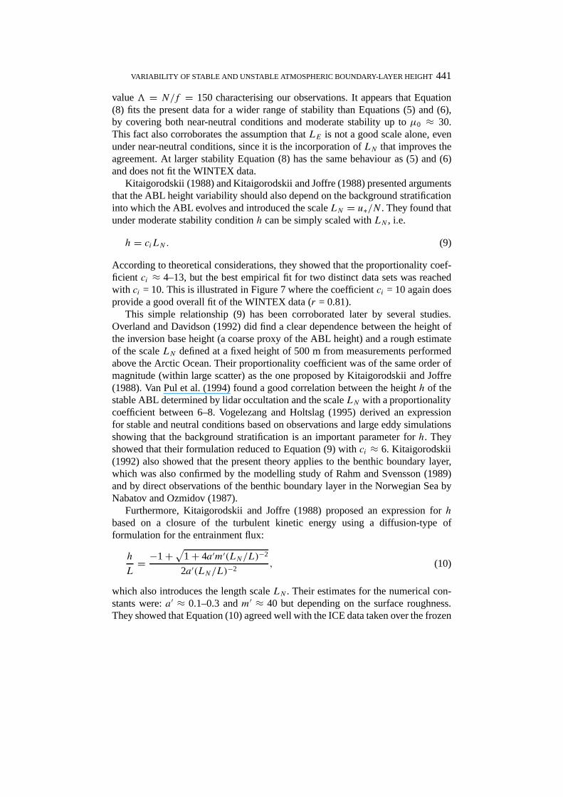
According to theoretical considerations, they showed that the proportionality coef-ficient ci ≈ 4–13, but the best empirical fit for two distinct data sets was reachedwith ci = 10. This is illustrated in Figure 7 where the coefficientci = 10 again doesprovide a good overall fit of the WINTEX data (r = 0.81).

This simple relationship (9) has been corroborated later by several studies.Overland and Davidson (1992) did find a clear dependence between the height ofthe inversion base height (a coarse proxy of the ABL height) and a rough estimateof the scaleLN defined at a fixed height of 500 m from measurements performedabove the Arctic Ocean. Their proportionality coefficient was of the same order ofmagnitude (within large scatter) as the one proposed by Kitaigorodskii and Joffre(1988). Van Pul et al. (1994) found a good correlation between the heighth of thestable ABL determined by lidar occultation and the scaleLN with a proportionalitycoefficient between 6–8. Vogelezang and Holtslag (1995) derived an expressionfor stable and neutral conditions based on observations and large eddy simulationsshowing that the background stratification is an important parameter forh. Theyshowed that their formulation reduced to Equation (9) withci ≈ 6. Kitaigorodskii(1992) also showed that the present theory applies to the benthic boundary layer,which was also confirmed by the modelling study of Rahm and Svensson (1989)and by direct observations of the benthic boundary layer in the Norwegian Sea byNabatov and Ozmidov (1987).

Furthermore, Kitaigorodskii and Joffre (1988) proposed an expression forh

based on a closure of the turbulent kinetic energy using a diffusion-type offormulation for the entrainment flux:

h

L= −1+√1+ 4a′m′(LN/L)−2

2a′(LN/L)−2, (10)

which also introduces the length scaleLN . Their estimates for the numerical con-stants were:a′ ≈ 0.1–0.3 andm′ ≈ 40 but depending on the surface roughness.They showed that Equation (10) agreed well with the ICE data taken over the frozen

442 S. M. JOFFRE ET AL.

Figure 7.Dependence of the stable ABL heighth on the background stratification scaleLN = u∗/N .The continuous line illustrates Equation (9) withci = 10.

VARIABILITY OF STABLE AND UNSTABLE ATMOSPHERIC BOUNDARY-LAYER HEIGHT 443

Figure 8.Dependence of the scaled stable ABL heighth/L on the dimensionless stratification para-meterµN = LN/L for the WINTEX data. The continuous lines illustrate Equation (10) witha′ = 0.1and 0.3, respectively. The dashed line depicts the relationshiph = 10LN . The dotted line illustratesEquation (11) for:J = 0.25 andN/f = 100 (lower curve), andJ = 2 andN/f = 170 (upper curve).

Baltic Sea and the Wangara data from Australia over a wide range of stabilityconditions (except strongly stable), though overestimating some of them, but thiscould be due to the uncertainty in the numerical parameterisation constants. Usingthe same numerical constants, this expression (10) agrees qualitatively well withthe present WINTEX data, though it quantitatively fits slightly better the high edgeof our h/L values (Figure 8). We can also notice that, as expected earlier, theinternal scatter of the data is detailed by the values of the secondary scale ratio3 = LN/LE. Spurious correlation due to the presence ofL on both axes naturallyoccurs but is only secondary here becauseLN already explains 66% of the varianceof h (see Figure 7).

Note that for a wide range of intermediate stable conditions Equation (10) re-duces to (0.6 . . . 0.2)µ0, which is equivalent to Equation (7). This also implies alinear dependence ofh on u∗, corroborated by their strong correlation (r = 0.75),in opposition to the 3/2-power dependence of the practical formula of Venkatram(1980), which, however, has Equation (5) as its basis and thus should have a limiteddomain of applicability.

Closing the turbulent kinetic energy equation with a critical bulk Richard-son number criterion for the slab ABL, Joffre (1981) obtained a time-dependentsolution forh in terms ofµN . For an equilibrium ABL away from his initial de-

444 S. M. JOFFRE ET AL.

velopment this leads to a solution equivalent to the Pollard et al. (1973) regime,i.e.,

h

L= 1.7J 1/4 (LELN)

1/2

L= 1.7J 1/4µN

√3 (11)

whereJ is the critical value of the bulk Richardson number over the whole ABL.Diagnosed values ofJ vary from the classical 0.25 up to values of 1.3 or 2 (Joffre,1981; Maryon and Best, 1992), increasing with values ofh/LE. Equation (11)does provide an envelope for our empirical WINTEX data using the same range ofvariability for values ofJ , namely 0.25 and 2 (Figure 8). We also found a very goodcorrelation betweenh and (LELN)1/2 (which includes no self-correlation) withcir = 1.7J 1/4 = 1.08±0.35, that is very close to values observed in oceanographicstudies (Pollard et al., 1973). This sets the critical Ri number close to unity withJ ≈ 0.9. These numerical values also represent an indirect support to our ABLheight determination.

Inspection of Figure 4 indicated thatL andLN are, a priori, the most relevantscales forh. Thus, a pure heuristic model forh that forces the turbulent volume tobe proportional tou∗ and inversely proportional toN andQs would yield

h = ch1

√LLN. (12)

This is corroborated by the strong linear correlation (r ≈ 0.9) between the twosides of Equation (12), while the coefficientch1 has a mean value of 4.9± 3.5.Additionally, forcing the same model forh to be inversely proportional tof wouldyield

h = ch2(LLN)1/4(LELN)

1/4, (13)

with a correlation only marginally improved (r ≈ 0.93), and the coefficientch2 =2.2± 1.1.

5.3. UNSTABLE CONDITIONS

The unstable ABL is generally treated in terms of prognostic equations computingthe growth of the inversion lid during the accumulative warming phase of thediurnal cycle. Though these models have been very successful for well-definedexperiments, they may be sensitive to initial conditions provided by radiosound-ings. These latter are seldom available on a routine basis at the desired site andanyway are performed only twice a day so that many applications may wish to usediagnostic methods that represent an approximate quasi-equilibrium relationshipbetween relevant variables. The fact that the simplest prognostic models do as wellas more sophisticated models also supports the use of only a limited number ofvariables to characterise actual quasi-stationary conditions.

VARIABILITY OF STABLE AND UNSTABLE ATMOSPHERIC BOUNDARY-LAYER HEIGHT 445

Leaving aside free convective conditions whereinu∗ loses its significance andw∗ = (gβQsh)

1/3 is the relevant velocity scale, on the other hand, under moderateunstable conditions, the same length scales as under stable conditions should play asignificant role as they are associated with physical processes that are still relevant.The observed domain of variability of the dimensionless ratiosµN = LN/L and3 = LN/LE under unstable conditions is roughly the same as for stable conditions(cf. Figure 4). Examining Figure 2 indicates that a key parameter for the dynamicsof the ABL, the friction velocity, has a similar behaviour under stable and unstableconditions. Friction velocity is involved in all three scalesL, LN andLE. Thus,it may be expected that unstable conditions may be split also into three regimes:weak, moderate and strong (or free convective).

Plotting h/LE as a function ofz/|L| indicates, with a rather large scatter, adecrease from a near-neutral value of 0.15 down to 0.07 atz/|L| ≈ 0.004. Thisquick transition would also indicate that departures from quasi-neutrality are ex-pectedly more quickly felt under unstable than stable conditions. This transitioncorresponds in Figure 2 also to the start of the steepening decrease ofu∗. Thisvalue ofz/|L| = 0.004 can be translated intoµ0 = LE/|L| = 1.5. As instabilityfurther increases,h/LE seems to increase back to 0.15–0.2, but the scatter is solarge that it is difficult to say objectively whether this trend stops atz/|L| = 0.1 or1. Beyond|µ0| = 1 the scatter is even larger, indicating expectedly thatLE is nota suitable scale. It is noteworthy that in Figure 2 the valuez/|L| = 1 correspondsalso to the end of the abrupt decrease ofu∗ with z/|L|. A value ofz/|L| = 1 wouldcorrespond to|µ0| ≈ 100.

Examining the dependence ofh/L on µ0 (Figure 9), we may detect the twoabove-mentioned transitions at the predictedµ0 values. The first one at|µ0| ≈ 1.5seems to reflect a change in the slope from 1/2 to 1, whereas there is only a fainthint of a transition at|µ0| = 100–200 as a weakening of the slope. Again, the lackof data coverage calls for further investigations to check this hypothesis.

For the non-free convective unstable ABL (u∗ still relevant), Kitaigorodskii andJoffre (1988) proposed an expression for the height of the unstable ABL based ona dimensionless form of the turbulence kinetic energy equation. This formula reads

h

L= 1+√1+ 4a′m"(LN/L)−2

2a′(LN/L)−2, (14)

wherea′ andm" are parameterisation constants (a′ ≈ 0.1–0.3 andm" ≈ 6). Ourdata fall well within these conditions since ourh values correlate much better withu∗ than with the heat fluxQs . The dependence ofh/L on the stratification para-meterµN for the WINTEX data is plotted in Figure 10 and Equation (14) appearsto represent well our data set over a wide range of unstable conditions. The limitedinternal scatter also supports the applicability of the scaling. The missing scaleLEis introduced to explain this internal scatter of the data through the dimensionlessratio3 = N/f , with the upper edge of the data described by high values of this

446 S. M. JOFFRE ET AL.

Figure 9.Dependence ofh/L on the classical stratification parameterµN = LE/L for the WINTEXdata under unstable conditions.

ratio and the lower edge by low values. On the other hand, note that this parameterN/f did not help to stratify the internal scatter in the framework based onµ0 inFigure 9.

Expression (14) derived in Kitaigorodskii and Joffre (1988) described well alsothree different data sets characterised by smallz0 values (Wangara, Joint Air-SeaInteraction Experiment JASIN and ICE data) analysed by the authors, thus sup-porting the universality of the approach based onh ∝ LN . An improved fit couldbe obtained by optimising the parametrisation constantsa′ andm" of Equation (14)with respect to the different roughness conditions.

Since, as hydrostatic instability grows stronger, the velocity scale shifts pro-gressively fromu∗ to w∗, a homogeneous treatment of unstable conditions wouldrequire use of a scale combining both of them, such aswm = (25u3∗ + w3∗)1/3(Driedonks and Tennekes, 1984). When we ploth/L′ vs. L′N/L

′ (the prime in-dicates thatwm was substituted foru∗ in the length scale), we observed a similardependence as in Figure 10 but with more scatter, thus not helpful for our applic-ations. This may indicate thatu∗ is a sufficient scale under non-free convectiveconditions. Surprisingly, for the regime of large values of the parameterL′N/|L′|(≥ 0.3), the observed trend possibly indicates a levelling off ofh/|L′| towards avalue of≈0.2–0.3 and not an enhanced growth with increased convection as inFigure 10 (see Appendix A).

According to Kitaigorodskii and Joffre (1988), under stronger unstable con-ditions the behaviour ofh/L changes from a linear (µN -dependence to aµ3/2

N -dependence. The outmost range of our data may indicate the start of this phase,

VARIABILITY OF STABLE AND UNSTABLE ATMOSPHERIC BOUNDARY-LAYER HEIGHT 447

Figure 10.Dependence ofh/L on the stratification parameterµN = LN/L for the WINTEX dataunder unstable conditions. The continuous line illustrates Equation (14) witha′ = 0.1 and 0.3, andm" = 6.

meaning that the transition between shear-forced convection and free convectiondoes occur at roughlyh/|L| ≈ 50 orLN/|L| ≈ 2. However, more data for strongunstable conditions are necessary to confirm this and to investigate the regimeprevailing forµN > 1.

6. Conclusions

We empirically determined the height of the ABL from radiosoundings performedabove a forested terrain in late winter in Northern Finland. We used both surface-layer turbulence parameters and the background stratification above the ABL todetermine relevant scales describing the variability of the ABL height. The subject-ive determination of the ABL height from mean profiles is somewhat uncertain butcan be safer sometimes than an objective approach or the use of algorithms. Thiscalls for undertaking comprehensive surveys of the ABL height determined fromradiosonde profiles, together with turbulence profiles, by relating selected featuresof the available profiles to physical criteria in order to provide climatology of theABL height at various sites under a wide spectrum of meteorological conditions.

For stable conditions, we came to the same conclusion as Mahrt et al. (1998)that the stable case can be divided into three different regimes according to thevalue of the parameterz/L. Though this reflects conditions in the surface layer, itappears that this affects the whole ABL as was witnessed in the behaviour of the

448 S. M. JOFFRE ET AL.

dimensionless parameterh/LE. Our analysis of the data indicates that the paradigmof Kitaigorodskii and Joffre (1988) seems to apply very well with the scalesLN =u∗/N andL (Obukhov length) explaining a great deal of the variability ofh understable conditions.

For unstable conditions, we found that for a dual regime of turbulence pro-duction (mechanical and buoyant), the model of Kitaigorodskii and Joffre (1988)seemed to apply very well forh scaled byL and depending on the stability para-meterµN = LN/L and onN/f . The classical similarity framework seems to havealso a three-regime structure as determined byu∗.

One important implication from this study is that friction velocity is a surrogatefor a great deal of the prevailing conditions affecting the ABL depth, sinceu∗ doesnot only reflect surface stress and shear conditions but is also strongly modulatedby surface buoyancy fluxes. Thus,u∗ can characterise a great deal of the behaviourof the ABL. Delineation of the different regimes identified in the present workshould still be tested against other data sets, preferably with different externalconditions (latitude, roughness, soil moisture, albedo). The previously observedagreement between classical Monin–Kazanski similarity scaling and observationswas partly due to the induced strong correlation of the ABL height with the fric-tion velocity itself. Put in other words, this prominent role ofu∗ may reflect theimportant role of non-local effects coupling the surface layer with the top regionof the ABL. Thus, taking into account the practical range of variability of physicalparameters, ABL variability is mainly constrained by the scalesL andLN , whilethe scale ratioN/f brings a second-order correction.

Since our data did not cover well the transition towards free convectiveand strong stability cases, it would be interesting to compare other extensivemeasurements presented in our framework with the present WINTEX data.

Acknowledgements

We are thankful to Mette Mannonen who compiled and plotted the PTU profilesfrom the WINTEX observations. We thank Sven-Erik Gryning for providing uswith the micrometeorological data of WINTEX. Prof. S.A. Kitaigorodskii acknow-ledged financial support from the Academy of Finland to spend one year at theFinnish Meteorological Institute to contribute to this work. The European Com-mission partly supported the WINTEX-project within its Environment and ClimateProgramme through contract ENV4-CT96-0324.

VARIABILITY OF STABLE AND UNSTABLE ATMOSPHERIC BOUNDARY-LAYER HEIGHT 449

Appendix A

If we substitutewm = (25u3∗ + w3∗)1/3 for u∗ in the definitions ofL andLN , weobtain for the new scales

L′ = −w3m

gβκQs

= L[25− h

κL

], (A1)

L′N =wm

N= LN

[25− h

κL

]1/3

. (A2)

Thus, using expressions (A1) and (A2), an asymptotic behaviour of the typeh/L ∝(LN/L)

3/2 would have a similar functional form, such as

h

L′∝(L′NL′

)3/2

, (A3)

which has the same slope as Equation (14).

References

Batchvarova, E., Gryning, S.-E., and Hasager, C. B.: 2001, ‘Regional Fluxes of Momentum andSensible Heat over a Sub-Arctic Landscape during Late Winter’,Boundary-Layer Meteorol.99,489–507.

Beljaars, A. C. M.: 1995, ‘The Impact of Some Aspects of the Boundary Layer Scheme in theECMWF Model’, in Proceedings of the ECMWF Seminar on the Parametrization of Subgrid-Scale Physical Processes, September 1994, European Centre for Medium-Range WeatherForecasts, Shinfield Park, Reading, U.K., pp. 125–161.

Betts, A. K., Viterbo, P., Beljaars, A., Pan, H-L., Hong, S-Y., Goulden, M., and Wofsy, S.: 1998,‘Evaluation of Land-Surface Interaction in ECMWF and NCEP/NCAR Reanalysis Models overGrassland (FIFE) and Boreal Forest (BOREAS)’,J. Geophys. Res.103(D18), 23079–23085.

Driedonks, A. G. M. and Tennekes, H.: 1984, ‘Entrainment Effects in the Well-Mixed AtmosphericBoundary Layer’,Boundary-Layer Meteorol.30, 75–105.

Halldin (ed.): 1999, Final Report for WINTEX, NOPEX Technical Report No. 29, 70 pp. (Availablefrom: NOPEX Central Office, Institute of Earth Sciences, Uppsala University, Norbyvägen 18B,SE-75236 Uppsala, Sweden.)

Hicks, B. B.: 1978, ‘Some Limitations of Dimensional Analysis and Power Laws’,Boundary-LayerMeteorol.14, 567–569.

Joffre, S. M.: 1981,The Physics of the Mechanically-Driven Atmospheric Boundary Layer as anExample of Air-Sea Ice Interactions, Ph.D. Thesis, University of Helsinki, Dept. of Meteorology,Report No. 20, 75 pp.

Kitaigorodskii, S. A.: 1960, ‘Calculating the Thickness of the Wind-Induced Mixing Layer in theOcean’,Izv. Acad. Sci. SSSR. Ser. Geofiz.3, 425–431 (English edition 284–287).

Kitaigorodskii, S. A.: 1988, ‘A Note on Similarity Theory for Atmospheric Boundary Layers in thePresence of Background Stable Stratification’,Tellus40A, 434–438.

Kitaigorodskii, S. A.: 1992, ‘The Location of Thermal Shelf Fronts and the Variability of the Heightsof Tidal Benthic Boundary Layers’,Tellus44A, 425–433.

450 S. M. JOFFRE ET AL.

Kitaigorodskii, S. A. and Joffre, S. M.: 1988, ’In Search of a Simple Scaling for the Height of theStratified Atmospheric Boundary Layer’,Tellus40A(5), 419–433.

Mahrt, L., Sun, L., Blumen, W., Delany, T., and Oncley, S.: 1998, ‘Nocturnal Boundary-LayerRegimes’,Boundary-Layer Meteorol.88, 255–278.

Mahrt, L., Sun, J., MacPherson, J. I., Jensen, N. O., and Desjardins, R. L.: 1997, ‘Formulation ofSurface Heat Flux: Application to BOREAS’,J. Geophys. Res.102(D24), 29641–29649.

Malhi, Y. S.: 1995, ‘The Significance of the Dual Solutions for Heat Fluxes Measured bythe Temperature Fluctuations Method in Stable Conditions’,Boundary-Layer Meteorol.74,389–396.

Maryon, R. H. and Best, M. J.: 1992, ‘NAME, ATMES and the Boundary Layer Problem’,Met O(APR) Turbulence and Diffusion Note, No. 204 (U.K. Met. Office).

Nabatov, V. N. and Ozmidov, R. V.: 1987, ‘Investigation of the Bottom Boundary Layer in theOcean’,OceanologiaXXVII , 5–11.

Nieuwstadt, F. T. M.: 1981, ‘The Steady State Height and Resistance Laws of the NocturnalBoundary Layer: Theory Compared with Cabauw Observations’,Boundary-Layer Meteorol.20,3–17.

Overland, J. E. and Davidson, K. L.: 1992, ‘Geostrophic Drag Coefficients over Sea Ice’,Tellus44A,54–66.

Pollard, R. T., Rhines, P. B., and Thompson, R. O. R. Y.: 1973, ‘The Deepening of the Wind-MixedLayer’, Geophys. Fluid Dyn.3, 381–404.

Rahm, L. and Svensson, U.: 1989, ‘Dispersion in a Stratified Benthic Boundary Layer’,Tellus41A,148–161.

Rossby, C. G. and Montgomery, R. B.: 1935, ‘The Layer of Frictional Influence in Wind and OceanCurrents’,Pap. Phys. Oceanog. Meteorol.3(3), 1–101. (M.I.T. and Woods Hole Oceanog. Inst.)

Seibert, P., Beyrich, F, Gryning, S-E, Joffre, S., Rasmussen, A., and Tercier, Ph.: 1998, ’MixingHeight Determination for Dispersion Modelling’, in Fisher et al. (eds.), Final Report of COST-710 (Harmonisation of the Pre-processing of Meteorological Data for Atmospheric DispersionModels), EUR18195 En, European Commission, DGXII, Brussels (B), 431 pp. (ISBN 92-828-3302-X.)

Seibert, P., Beyrich, F, Gryning, S-E, Joffre, S., Rasmussen, A., and Tercier, Ph.: 2000, ‘Review andIntercomparison of Operational Methods for the Determination of the Mixing Height’,Atmos.Environ.34, 1001–1027.

Van Pul, W. A. J., Holtslag, A. A. M., and Swart, D. P. J.: 1994, ‘A Comparison of ABL HeightsInferred Routinely from Lidar and Radiosondes at Noontime’,Boundary-Layer Meteorol.68,173–191.

Vogelezang, D. H. P. and Holtslag, A. A. M.: 1996, ‘Evaluation and Model Impacts of AlternativeBoundary-Layer Height Formulations’,Boundary-Layer Meteorol.81, 245–269.

Zilitinkevich, S. S.: 1972, ‘On the Determination of the Height of the Ekman Boundary Layer’,Boundary-Layer Meteorol.3, 141–145.

Zilitinkevich, S. and Calanca, P.: 2000, ‘An Extended Similarity-Theory Formulation for the StablyStratified Atmospheric Surface layer’,Quart. J. Roy. Meteorol. Soc.126, 1913–1923.

Zilitinkevich, S. and Mironov, D. V.: 1996, ‘A Multi-Limit Formulation for the Equilibrium Depth ofa Stably Stratified Boundary Layer’,Boundary-Layer Meteorol.81, 325–351.