ORIGINAL ARTICLE

Validation of metabolomics for toxic mechanism of actionscreening with the earthworm Lumbricus rubellus

Qi Guo Æ Jasmin K. Sidhu Æ Timothy M. D. Ebbels Æ Faisal Rana ÆDavid J. Spurgeon Æ Claus Svendsen Æ Stephen R. Sturzenbaum ÆPeter Kille Æ A. John Morgan Æ Jacob G. Bundy

Received: 12 August 2008 / Accepted: 15 December 2008! Springer Science+Business Media, LLC 2009

Abstract One of the promises of environmental meta-bolomics, together with other ecotoxicogenomic approaches,

is that it can give information on toxic compound mechanism

of action (MOA), by providing a specific response profile orfingerprint. This could then be used either for screening in the

context of chemical risk assessment, or potentially in con-

taminated site assessment for determining what compoundclasses were causing a toxic effect. However for either of

these two ends to be achievable, it is first necessary to know if

different compounds do indeed elicit specific and distinctmetabolic profile responses. Such a comparative study has

not yet been carried out for the earthworm Lumbricus

rubellus. We exposed L. rubellus to sub-lethal concentrationsof three very different toxicants (CdCl2, atrazine, and fluo-

ranthene, representing three compound classes with different

expected MOA), by semi-chronic exposures in a laboratorytest, and used NMR spectroscopy to obtain metabolic pro-

files. We were able to use simple multivariate pattern-

recognition analyses to distinguish different compounds tosome degree. In addition, following the ranking of individual

spectral bins according to their mutual information with

compound concentrations, it was possible to identify bothgeneral and specific metabolite responses to different toxic

compounds, and to relate these to concentration levels

causing reproductive effects in the worms.

Keywords Environmental biomarker ! Atrazine !Cadmium ! Fluoranthene ! Ecotoxicogenomics !Metabonomics

1 Introduction

The major application of metabolomics in the environ-

mental sciences to date has been in ecotoxicology. Within

this, a majority of groups are working in aquatic ecotoxi-cology, recently reviewed by Lin et al. (2006) and Viant

(2007). In contrast, fewer studies have been carried out on

terrestrial models; to date, most of the examples of appli-cation of metabolomics in terrestrial ecotoxicology are in

earthworms. Earthworms have, of course, been widely used

for assessing soil contamination for many years (Spurgeonet al. 2003b; Sanchez-Hernandez 2006). A host of different

biochemical and biomolecular endpoints have been used as

measures of earthworm response, and so it is not surprisingthat metabolite profiles have been added to the arsenal of

molecular biomarkers used by terrestrial ecotoxicologists.

Qi Guo and Jasmin K. Sidhu contributed equally to this paper.

Electronic supplementary material The online version of thisarticle (doi:10.1007/s11306-008-0153-z) contains supplementarymaterial, which is available to authorized users.

Q. Guo ! J. K. Sidhu ! T. M. D. Ebbels ! F. Rana !J. G. Bundy (&)Department of Biomolecular Medicine, Division of Surgery,Oncology, Reproductive Biology, and Anaesthetics, Facultyof Medicine, Imperial College London, Sir Alexander FlemingBuilding, London SW7 2AZ, UKe-mail: j.bundy@imperial.ac.uk

D. J. Spurgeon ! C. SvendsenCentre for Ecology and Hydrology, Maclean Building, BensonLane, Crowmarsh Gifford, Wallingford OX10 8BB, UK

S. R. SturzenbaumPharmaceutical Science Division, King’s College London,School of Biomedical & Health Sciences, Franklin WilkinsBuilding, Stamford Street, London SE1 9NH, UK

P. Kille ! A. J. MorganUniversity of Cardiff, School of Biosciences, Main Building,Park Place, Cardiff CF10 3TL, UK

123

Metabolomics

DOI 10.1007/s11306-008-0153-z

Recent publications have used NMR-based profiling for

assessing field and semi-field studies on Lumbricus rubel-lus (Bundy et al. 2004, 2007, 2008; Jones et al. 2008). This

species also has EST sequence data available (Owen et al.

2008), meaning that it is suitable for parallel transcriptomicstudies. Furthermore, a project is ongoing to sequence the

entire L. rubellus genome (see www.earthworms.org for

more information). In addition, L. rubellus is widely dis-tributed and can often be found at field sites, making it a

useful choice for both lab and field studies. Eisenia fetida isanother important terrestrial model, because it is required

for regulatory testing (OECD 1984), although as an

extreme epige it is less relevant for soil testing than L.rubellus. Brown et al. (2008) have evaluated different

sample preparation methods with E. fetida which, coupled

with additional genomic information in the form of an ESTlibrary and resultant cDNA microarrays (Gong et al. 2007),

makes it, like L. rubellus, a very suitable organism to

combine future metabolomic research with other post-genomic analyses.

For metabolomics (and other toxicogenomic methods)

to be adopted as a useful monitoring tool in ecotoxicology,it is not enough to do as well as existing methods: sub-

stantial improvements are needed (van Straalen and

Roelofs 2008). Hence an important question is, whatadvantages are there to using ecotoxicogenomic methods in

addition to current approaches based on chemical residue

analysis? If biological response information is needed, whynot make use of a known biomarker response? One pos-

sibility is that omic methods can potentially discriminate

between specific compounds/toxic mode of action (MOA);it then becomes clear that being able to discriminate and

assign MOAs is a critical need for environmental meta-

bolomics studies. Metabolic profiling has been widely usedfor classifying or discriminating MOA in toxicology

(Gartland et al. 1989, 1990, 1991; Ebbels et al. 2007), and

has also been applied to earthworm multiple-toxicantstudies (Bundy et al. 2002). However, there are currently

no studies comparing the metabolic effect of toxicants with

different MOA for the species L. rubellus. It is alsoimportant that enough baseline data are available to give a

context for interpreting metabolic responses—i.e. is a

metabolite change really a biomarker of a specific MOA, oris it instead a more general stress response (van Straalen

and Roelofs 2008)?

Field exposure data are important in ecotoxicology, aslaboratory exposures cannot fully model the complexity of

the natural environment, particularly for a highly hetero-

geneous matrix such as soil. Nonetheless controlledexposures to single toxicants are still essential, in order to

provide a context for field observations. Here, we present

data for NMR-based profiling of tissue extracts ofL. rubellus following chronic soil exposure to three

different toxicants: Cd, fluoranthene (FA), and atrazine

(AZ), i.e. a toxic metal, a common organic pollutant, andan agrochemical (herbicide). We have identified both

general and toxicant-specific biomarkers in the dataset. In

addition, we tested if the profiles could be used to distin-guish the effects of different toxicants, and thus potentially

assign MOA. These data will provide a useful baseline for

future metabolomic experiments using L. rubellus.

2 Materials and methods

2.1 Chemical exposures

A full description of the exposure protocol was given by

Owen et al. (2008), and so we will give only a summaryhere. Briefly, earthworms were exposed in a spiked natural

soil, using an existing 28-day test protocol (Spurgeon et al.

2003a). The toxicants Cd, fluoranthene (FA), and atrazine(AZ) were mixed with a commercially available loam soil

(soil characteristics described by Spurgeon et al. 2004) at a

range of concentrations, using an experimental design withreplicated concentrations (n = 8 for controls, and n = 5

for replicated toxicant concentrations), supplemented by

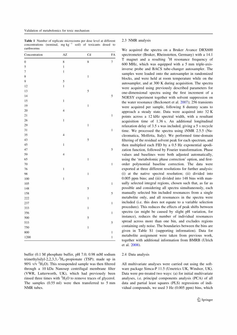
individual non-replicated exposures at intermediate andadditional concentrations (Table 1). The concentrations

were chosen based on previous experiments to cover the

same sub-lethal effect range for each toxicant, as shownby similar reductions in reproduction for each toxicant

across the concentration ranges used. Each replicate

comprised a group of 8 clitellate earthworms in 1 kg ofsoil. Exposure was for 28 days, and survival, weight

change, and cocoon production at the end of the period

were all recorded. At the end of the 28 days, three indi-viduals from each replicate were then pooled, snap-frozen,

and ground, to give a single sample. In total, 104 samples

were analysed.

2.2 Sample preparation for NMR analysis

We lyophilized ground tissues without allowing them to

thaw, and then stored them at -80"C until extraction. We

extracted the tissues by homogenizing approx. 80 mg dryweight into 4 ml of 70% ice-cold acetonitrile solution,

using a Heidolph SilentCrusher homogenizer. One ml of

each of the extracts was then subjected to solid-phaseextraction, using Strata-X-AW mixed-mode 6 ml car-

tridges with 200 mg adsorbent (Phenomenex, Macclesfield,

UK), in order to remove 2-hexyl-5-ethyl-furan-3-sulfonicacid (HEFS). The extracts were diluted with water, loaded

onto the cartridges, and eluted with 6 ml of HPLC-grade

methanol. The eluate was then dried using a rotary vacuumconcentrator at 45"C, and resuspended in 0.65 ml of NMR

Q. Guo et al.

123

buffer (0.1 M phosphate buffer, pH 7.0; 0.98 mM sodium

trimethylsilyl-2,2,3,3,-2H4-propionate (TSP); made up in

90% v/v 2H2O). This resuspended sample was then filteredthrough a 10 kDa Nanosep centrifugal membrane filter

(VWR, Lutterworth, UK), which had previously been

rinsed three times with 2H2O to remove traces of glycerol.The samples (0.55 ml) were then transferred to 5 mm

NMR tubes.

2.3 NMR analysis

We acquired the spectra on a Bruker Avance DRX600spectrometer (Bruker, Rheinstetten, Germany) with a 14.1

T magnet and a resulting 1H resonance frequency of

600 MHz, which was equipped with a 5 mm triple-axis-inverse probe and BACS tube-changer autosampler. The

samples were loaded onto the autosampler in randomized

blocks, and were held at room temperature while on theautosampler, and at 300 K during acquisition. The spectra

were acquired using previously described parameters for

one-dimensional spectra using the first increment of aNOESY experiment together with solvent suppression on

the water resonance (Beckonert et al. 2007); 256 transients

were acquired per sample, following 8 dummy scans toapproach a steady state. Data were acquired into 32 K

points across a 12 kHz spectral width, with a resultant

acquisition time of 1.36 s. An additional longitudinalrelaxation delay of 3.5 s was included, giving a 5 s recycle

time. We processed the spectra using iNMR 2.5.5 (Nu-

cleomatica, Molfetta, Italy). We performed time-domainfiltering of the residual solvent peak for each spectrum, and

then multiplied each FID by a 0.5 Hz exponential apodi-

zation function, followed by Fourier transformation. Phasevalues and baselines were both adjusted automatically,

using the ‘metabolomic phase correction’ option, and first-

order polynomial baseline correction. The data wereexported at three different resolutions for further analysis:

(i) at the native spectral resolution; (ii) divided into

0.005 ppm bins; and (iii) divided into 148 bins with man-ually selected integral regions, chosen such that, as far as

possible and considering all spectra simultaneously, each

manually selected bin included resonances from a singlemetabolite only, and all resonances in the spectra were

included (i.e. this does not equate to a variable selection

procedure). This reduces the effects of peak shifts betweenspectra (as might be caused by slight pH variation, for

instance), reduces the number of individual resonances

spread across more than one bin, and excludes regionscontaining only noise. The boundaries between the bins are

given in Table S1 (supporting information). Data for

metabolite assignment were taken from previous work,together with additional information from BMRB (Ulrich

et al. 2008).

2.4 Data analysis

All multivariate analyses were carried out using the soft-ware package Simca-P 11.5 (Umetrics UK, Windsor, UK).

Data were pre-treated two ways: (a) for initial multivariateanalyses, i.e. principal components analysis (PCA) of all

data and partial least squares (PLS) regressions of indi-

vidual compounds, we used 3 Hz (0.005 ppm) bins, which

Table 1 Number of replicate microcosms per dose level at differentconcentrations (nominal, mg kg-1 soil) of toxicants dosed toearthworms

Concentration AZ Cd FA

0 8 8 7

5 1

7 1

8 1

9 5

12 1

13 5

14 5

15 1

19 1

20 4

21 1

26 1

29 1

31 1

35 4

43 5

45 1

47 5

59 4

65 1

70 1

76 1

98 1

100 1

105 1

148 5

158 5

222 1

237 1

333 1

356 1

500 5

533 5

750 1

800 1

1200 1

Validation of metabolomics for toxic mechanism

123

have previously been used for pattern-recognition of NMR

data, and considered to give advantages over broaderbins (Warne et al. 2000; Viant 2003). Difference profiles

were then calculated for each of the separate toxicant

groups by subtracting the mean control profile (by ‘dif-ference profile’ we mean the equivalent of a difference

spectrum, but for the binned data, not for the full resolu-

tion spectra).The data were then mean-centred, and analysed both

with and without scaling to unit variance. (b) For SIMCAand PCA of the data for the two highest replicated con-

centration levels for each toxicant (Table 1), the manually

selected bins were used. Difference profiles were scaledsuch that the three independent control groups of the ori-

ginal data would have been converted to unit variance

(Malmendal et al. 2006).In this study, we also used mutual information to

investigate relationships between metabolites and external

variables. Mutual information is a general informationtheoretic approach to measure the statistical dependence

between variables. It has been applied in many areas such

as analysis of gene expression data (Steuer et al. 2002;Daub et al. 2004; Meyer et al. 2008), independent com-

ponent analysis (Hyvarinen et al. 2001), and image

processing (Thevenaz and Unser 2000). The conventionalmethod to quantify the linear dependence between vari-

ables is Pearson correlation. However, a vanishing Pearson

correlation does not imply that two variables are indepen-dent (Steuer et al. 2002). Inter-metabolite relationships are

frequently nonlinear (Camacho et al. 2005), and linear

models are also often inadequate to describe biologicaldose-responses (Calabrese 2008; May and Bigelow 2005).

We previously observed nonlinear responses of metabolites

to copper in L. rubellus (Bundy et al. 2008). Therefore, it ishighly desirable to investigate both the linear and nonlinear

dependence between the metabolites and external vari-

ables, especially those nonlinear relations which cannot bedetected by linear measures. Mutual information is able to

detect any type of functional relationship and extends

conventional methods, such as Pearson correlation.Let A be a system with m finite states {a1, a2, …, am}

and pi be a probability of state ai, then the Shannon entropy

H(A) is given as

H"A# $ %Xm

i$1

p"ai# log p"ai# "1#

The Shannon entropy measures the uncertainty of the stateof the system A. The entropy of the system A is zero if

p(aj) = 1 and p(ai) = 0 for all i = j, whereas the entropy

becomes maximal if pi = pj for all i and j. The jointentropy H(A,B) of two systems A and B (with n finite

states) is defined as

H"A;B# $ %Xm;n

i$1;j$1

p"ai; bj# log p"ai; bj# "2#

So we have

H A;B" #&H A" # ' H B" # "3#

The above equation fulfils equality only if A and B areindependent. The mutual information MI(A,B) can be

defined as

MI A;B" # $ H A" # ' H B" # % H A;B" #( 0 "4#

Since mutual information is defined in terms of discretedata, its application to continuous data, such as metabolo-

mics data, requires a binning procedure. Here, wecalculated MI following the method of Daub et al. (2004)

which is based on B-spline functions, and the results were

visualized by plotting MI against Pearson correlation. Theseplots allow one to visually identify individual variables with

high MI and/or correlation for further inspection.

The statistical significance of the MI was estimatedusing the method proposed by Steuer et al. (2002). A

surrogate dataset is generated by random permutations of

the original data. From the mutual information of the ori-ginal dataset MI(X,Y)data, the average value obtained from

surrogate data\MI(Xsurr, Ysurr)[, and its standard devia-

tion rsurr, the significance S can be given as

S $ MI"X; Y#data %\MI"Xsurr; Ysurr#[rsurr

"5#

In this study, S for each variable was estimated by

resampling the data 30 times and then visualized by colour-

scale.

3 Results and discussion

The NMR spectra showed a typical mixture of smallmolecule metabolites, as expected from extracts of earth-

worm tissue (Fig. S1, supporting information). We have

previously assigned metabolites from proton spectra of L.rubellus tissue extracts (Bundy et al. 2008), so will not here

present extensive data on assignment. We did observe a

novel unassigned compound (with triplet resonances at2.98 and 3.15 ppm) in all samples, that we had not previ-

ously seen in earthworm tissue extracts.

We removed the compound HEFS from earthworm tis-sue extracts before NMR analysis, for two reasons: firstly,

as this is found in very high concentration in earthworms,

and has seven separate 1H resonances, it may obscureresponses of other low-concentration metabolites. Sec-

ondly, our preliminary results indicated that, at least for

this set of samples, the tissue extracts were not stable, with

Q. Guo et al.

123

visible changes when the samples were left for several

hours at room temperature (i.e. when running samplesusing an autosampler), including a decrease in HEFS and

increase in resonances from a suspected HEFS degradation

product at 6.60 and 1.16 ppm. We surmised that, given itsamphiphilic properties, HEFS might stabilize macromole-

cules even in the solvent extracts, which could include

degradative enzymes. In addition, we filtered samplesthrough a 10 kDa-cutoff membrane filter. The extracts

treated in this way were stable over the period of acquisi-tion, as observed by NMR.

3.1 The three compounds induced distinct and well-defined metabolic responses at sub-lethal

concentrations

Clear dose-responsive effects were observed for all toxi-

cants at the whole profile level. All exposures were at a

sub-lethal level, but sufficient to cause a significantreduction in an ecologically important endpoint (repro-

duction, as measured by rate of cocoon production).

Pattern-recognition analysis showed that there were bio-logical differences between the control groups for the three

toxicants (data not shown), which was not surprising as,

because of logistical constraints, the three toxicant expo-sures were carried out sequentially rather than in parallel.

Because of this, we used difference spectra for further

comparative analyses.Initially, we analysed the effects of each toxicant sepa-

rately. The supervised method partial least squares (PLS)

regression offers the advantage of modelling the multi-variate response across different concentrations, as

opposed to just class discrimination. All three toxicants had

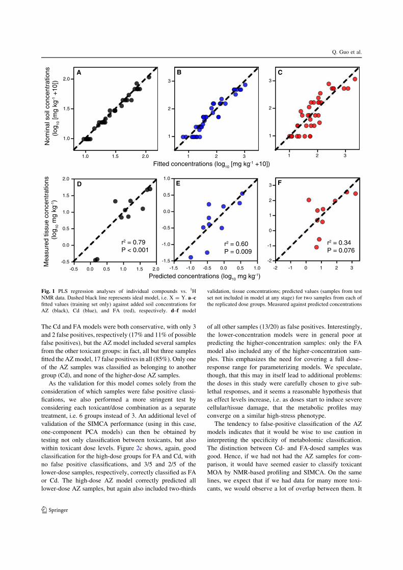
highly significant PLS models for exposure (soil) concen-trations (Fig. 1), for data both scaled and not scaled to unit

variance (not shown). It is important to validate these

models beyond fit alone (Broadhurst and Kell 2006); per-mutation plots show that for each compound, Q2Y

distributions fall to zero as the data are randomized (Fig.

S2, supporting information).In addition to the PLS models for soil toxicant con-

centrations, we fitted models for the tissue concentration

data, shown in Fig. 1d–f as predictions for data from anindependent test set (data for training set are shown in Fig.

S3, supporting information). This was with the aim of

mimicking a more realistic scenario for use with earth-worms sampled from contaminated sites (e.g. during

monitoring of exposure to persistent organic pollutants in

top predators), where (a) tissue concentrations might beused in preference to soil concentrations, because of con-

taminant heterogeneity; and (b) one would want to predict/

classify samples based on existing data. Weak relationshipswere shown for all three toxicants. These were significant

for AZ and Cd (P\ 0.001 and P = 0.009, respectively),

and approached significance at the 5% level for FA(P = 0.076). In our current study, which used well-mixed

soil microcosms, the soil toxicant concentrations were

generally a better indicator of exposure than tissue con-centrations. The tissue levels could have been affected by

either contaminant excretion, for all toxicants, or bio-

transformation, for FA and AZ, either of which phenomenawould underestimate total exposure.

Metabolic profiling can be used as a biomarker discov-ery tool. Environmental biomarkers have great potential as

a tool for effect-based rather than residue-based monitor-

ing—although have also been criticized as not translatingto useful regulatory or monitoring tools (Forbes et al.

2006). Nonetheless, there is interest in ecotoxicogenomic

techniques, including metabolomics, from regulators(Ankley et al. 2006). One reason is that the use of a highly

multivariate profile as an endpoint promises the ability to

distinguish between different chemicals; or, more plausi-bly, different toxicant/MOA classes. Thus, in order to

prove usefulness beyond existing biomarkers, one impor-

tant consideration for environmental metabolomics of L.rubellus is to ask if individual toxicants can be distin-

guished on the basis of their NMR spectral fingerprints.

3.2 Classification of individual samples

An initial unsupervised analysis of all data (PCA) did notseparate the dosed samples into three groups in a

straightforward manner, although there were dose- and

concentration-related effects on different PC axes (sup-porting information, Fig. S4), and so we analysed a sub-set

of the data in more detail. We chose the two highest-con-

centration sets of replicate dosed samples for each toxicant(dose levels given in Table 1), as we assumed the between-

toxicant metabolic differences would be most distinct at the

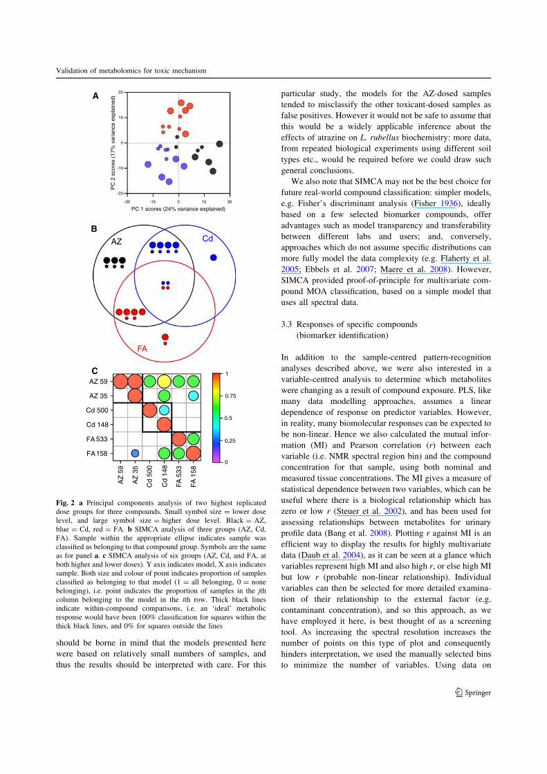
higher concentrations. A PCA of this reduced dataset didindeed show that the different exposed samples tended to

cluster in toxicant-specific groups (Fig. 2a); in addition, the

higher-concentration dose samples fell further from theorigin than the lower-concentration samples. Given that

PCA alone is not a classification method, we also used

SIMCA (statistical isolinear multiple component analysis;or, soft independent modelling of class analogy (Wold

1974, as cited in Duewer et al. 1975; Wold 1976)) to

perform a simple classification.Our initial SIMCAwas based on a PCA (two components)

of each separate toxicant. Figure 2b shows, unsurprisingly,

that each toxicant model successfully predicted all its ownsamples (with the exception of one AZ sample at the higher

dose level, which fell outside all models, and is not shown in

the figure). Four samples were classed as belonging to allthreemodels (two FA and twoCd, both from the lower dose).

Validation of metabolomics for toxic mechanism

123

The Cd and FA models were both conservative, with only 3

and 2 false positives, respectively (17% and 11% of possiblefalse positives), but the AZ model included several samples

from the other toxicant groups: in fact, all but three samples

fitted the AZmodel, 17 false positives in all (85%). Only oneof the AZ samples was classified as belonging to another

group (Cd), and none of the higher-dose AZ samples.

As the validation for this model comes solely from theconsideration of which samples were false positive classi-

fications, we also performed a more stringent test by

considering each toxicant/dose combination as a separatetreatment, i.e. 6 groups instead of 3. An additional level of

validation of the SIMCA performance (using in this case,

one-component PCA models) can then be obtained bytesting not only classification between toxicants, but also

within toxicant dose levels. Figure 2c shows, again, good

classification for the high-dose groups for FA and Cd, withno false positive classifications, and 3/5 and 2/5 of the

lower-dose samples, respectively, correctly classified as FA

or Cd. The high-dose AZ model correctly predicted alllower-dose AZ samples, but again also included two-thirds

of all other samples (13/20) as false positives. Interestingly,

the lower-concentration models were in general poor atpredicting the higher-concentration samples: only the FA

model also included any of the higher-concentration sam-

ples. This emphasizes the need for covering a full dose–response range for parameterizing models. We speculate,

though, that this may in itself lead to additional problems:

the doses in this study were carefully chosen to give sub-lethal responses, and it seems a reasonable hypothesis that

as effect levels increase, i.e. as doses start to induce severe

cellular/tissue damage, that the metabolic profiles mayconverge on a similar high-stress phenotype.

The tendency to false-positive classification of the AZ

models indicates that it would be wise to use caution ininterpreting the specificity of metabolomic classification.

The distinction between Cd- and FA-dosed samples was

good. Hence, if we had not had the AZ samples for com-parison, it would have seemed easier to classify toxicant

MOA by NMR-based profiling and SIMCA. On the same

lines, we expect that if we had data for many more toxi-cants, we would observe a lot of overlap between them. It

1.0 1.5 2.0

1.0

1.5

2.0

Nom

inal

soi

l con

cent

ratio

ns (

log 10

[mg

kg-1 +

10])

1 2 3

1

2

3

-1.5 -1.0 -0.5 0.0 0.5 1.0-1.5

-1.0

-0.5

0.0

0.5

1.0

1 2 3

1

2

3

-2 -1 0 1 2 3-2

-1

0

1

2

3

Fitted concentrations (log10 [mg kg-1 +10])

Mea

sure

d tis

sue

conc

entr

atio

ns (

log 10

mg

kg-1)

Predicted concentrations (log10 mg kg-1)

D

A

E

B

F

C

r2 = 0.60P = 0.009

r2 = 0.34P = 0.076

r2 = 0.79P < 0.001

-0.5 0.0 0.5 1.0 1.5 2.0-0.5

0.0

0.5

1.0

1.5

2.0

Fig. 1 PLS regression analyses of individual compounds vs. 1HNMR data. Dashed black line represents ideal model, i.e. X = Y. a–cfitted values (training set only) against added soil concentrations forAZ (black), Cd (blue), and FA (red), respectively. d–f model

validation, tissue concentrations; predicted values (samples from testset not included in model at any stage) for two samples from each ofthe replicated dose groups. Measured against predicted concentrations

Q. Guo et al.

123

should be borne in mind that the models presented herewere based on relatively small numbers of samples, and

thus the results should be interpreted with care. For this

particular study, the models for the AZ-dosed samples

tended to misclassify the other toxicant-dosed samples asfalse positives. However it would not be safe to assume that

this would be a widely applicable inference about the

effects of atrazine on L. rubellus biochemistry: more data,from repeated biological experiments using different soil

types etc., would be required before we could draw such

general conclusions.We also note that SIMCA may not be the best choice for

future real-world compound classification: simpler models,e.g. Fisher’s discriminant analysis (Fisher 1936), ideally

based on a few selected biomarker compounds, offer

advantages such as model transparency and transferabilitybetween different labs and users; and, conversely,

approaches which do not assume specific distributions can

more fully model the data complexity (e.g. Flaherty et al.2005; Ebbels et al. 2007; Maere et al. 2008). However,

SIMCA provided proof-of-principle for multivariate com-

pound MOA classification, based on a simple model thatuses all spectral data.

3.3 Responses of specific compounds(biomarker identification)

In addition to the sample-centred pattern-recognitionanalyses described above, we were also interested in a

variable-centred analysis to determine which metabolites

were changing as a result of compound exposure. PLS, likemany data modelling approaches, assumes a linear

dependence of response on predictor variables. However,

in reality, many biomolecular responses can be expected tobe non-linear. Hence we also calculated the mutual infor-

mation (MI) and Pearson correlation (r) between each

variable (i.e. NMR spectral region bin) and the compoundconcentration for that sample, using both nominal and

measured tissue concentrations. The MI gives a measure of

statistical dependence between two variables, which can beuseful where there is a biological relationship which has

zero or low r (Steuer et al. 2002), and has been used for

assessing relationships between metabolites for urinaryprofile data (Bang et al. 2008). Plotting r against MI is an

efficient way to display the results for highly multivariate

data (Daub et al. 2004), as it can be seen at a glance whichvariables represent high MI and also high r, or else high MI

but low r (probable non-linear relationship). Individual

variables can then be selected for more detailed examina-tion of their relationship to the external factor (e.g.

contaminant concentration), and so this approach, as we

have employed it here, is best thought of as a screeningtool. As increasing the spectral resolution increases the

number of points on this type of plot and consequently

hinders interpretation, we used the manually selected binsto minimize the number of variables. Using data on

AZ Cd

FA

B

C

A

AZ

59

AZ

35

Cd

500

Cd

148

FA 5

33

FA 1

58

AZ 59

AZ 35

Cd 500

Cd 148

FA 533

FA 1580

0.25

0.5

0.75

1

-30 -15 0 15 30

PC 1 scores (24% variance explained)

-20

-10

0

10

20

PC

2 s

core

s (1

7% v

aria

nce

expl

aine

d)

Fig. 2 a Principal components analysis of two highest replicateddose groups for three compounds. Small symbol size = lower doselevel, and large symbol size = higher dose level. Black = AZ,blue = Cd, red = FA. b SIMCA analysis of three groups (AZ, Cd,FA). Sample within the appropriate ellipse indicates sample wasclassified as belonging to that compound group. Symbols are the sameas for panel a. c SIMCA analysis of six groups (AZ, Cd, and FA, atboth higher and lower doses). Y axis indicates model, X axis indicatessample. Both size and colour of point indicates proportion of samplesclassified as belonging to that model (1 = all belonging, 0 = nonebelonging), i.e. point indicates the proportion of samples in the jthcolumn belonging to the model in the ith row. Thick black linesindicate within-compound comparisons, i.e. an ‘ideal’ metabolicresponse would have been 100% classification for squares within thethick black lines, and 0% for squares outside the lines

Validation of metabolomics for toxic mechanism

123

individual fitted compounds would have been better still

(Wishart 2008), but was not practicable in the currentstudy. It should also be borne in mind that more data are

required to calculate MI accurately than Pearson r, andideally we would have had more samples, especially for thesingle-toxicant analyses (Camacho et al. 2005; Khan et al.

2007). However, our use of the permutation procedure in

the MI calculation protects against spuriously high valuesof the MI being interpreted as a significant relationship.

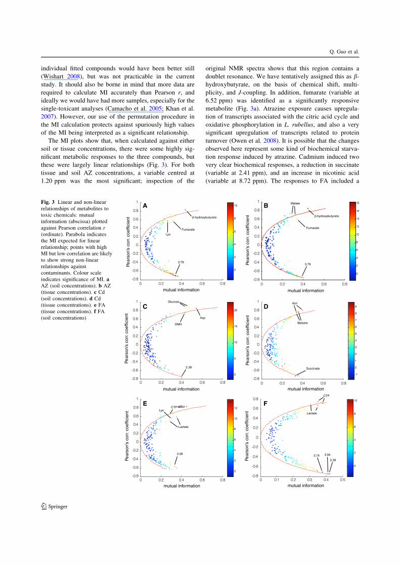
The MI plots show that, when calculated against eithersoil or tissue concentrations, there were some highly sig-

nificant metabolic responses to the three compounds, but

these were largely linear relationships (Fig. 3). For bothtissue and soil AZ concentrations, a variable centred at

1.20 ppm was the most significant; inspection of the

original NMR spectra shows that this region contains a

doublet resonance. We have tentatively assigned this as b-hydroxybutyrate, on the basis of chemical shift, multi-

plicity, and J-coupling. In addition, fumarate (variable at

6.52 ppm) was identified as a significantly responsivemetabolite (Fig. 3a). Atrazine exposure causes upregula-

tion of transcripts associated with the citric acid cycle and

oxidative phosphorylation in L. rubellus, and also a verysignificant upregulation of transcripts related to protein

turnover (Owen et al. 2008). It is possible that the changesobserved here represent some kind of biochemical starva-

tion response induced by atrazine. Cadmium induced two

very clear biochemical responses, a reduction in succinate(variable at 2.41 ppm), and an increase in nicotinic acid

(variable at 8.72 ppm). The responses to FA included a

!-hydroxybutyrate

Fumarate

Succinate2.39

Betaine

CTP

Lactate

CTP

Lactate

A B

C D

E F

Asn

Lys

Asp

DMH

Glucose

Lys

3.39

2.39

3.553.74

3.79

!-hydroxybutyrate

Fumarate

3.79

Malate

mutual information

mutual information mutual information

mutual information

mutual informationmutual information

Pear

son’

s co

rr. c

oeffi

cien

tPe

arso

n’s

corr

. coe

ffici

ent

Pear

son’

s co

rr. c

oeffi

cien

t

Pear

son’

s co

rr. c

oeffi

cien

tPe

arso

n’s

corr

. coe

ffici

ent

Pear

son’

s co

rr. c

oeffi

cien

t

Fig. 3 Linear and non-linearrelationships of metabolites totoxic chemicals: mutualinformation (abscissa) plottedagainst Pearson correlation r(ordinate). Parabola indicatesthe MI expected for linearrelationship; points with highMI but low correlation are likelyto show strong non-linearrelationships againstcontaminants. Colour scaleindicates significance of MI. aAZ (soil concentrations). b AZ(tissue concentrations). c Cd(soil concentrations). d Cd(tissue concentrations). e FA(tissue concentrations). f FA(soil concentrations)

Q. Guo et al.

123

variable at 4.11 ppm (lactate; the methyl resonance at

1.33 ppm was not here identified as significantly different,presumably because at neutral pH this overlaps with a

resonance from threonine in 1D NMR spectra), and a group

of variables at 6.00, 6.13, 7.94, and 7.96 ppm. (The indi-vidual relationships for these variables listed here are all

shown in supporting information, Fig. S5.) These last four

variables correspond to three resonances (7.94 and 7.96represent two halves of a doublet, binned separately

because of partial overlap with another resonance): thechemical shifts, multiplicities, relative intensities, and

J-couplings are all consistent with cytidine triphosphate

(CTP), and the statistical correlation between these threeresonances across all spectra is high, indicating they belong

to a single compound, and so we have assigned this as

CTP. (The 7.4 Hz J-coupling of the resonance at 6.13 ppmis particularly diagnostic, indicating this is not an anomeric

ribose proton resonance.) This analysis clearly shows that

the response of L. rubellus to the three toxicants does notjust involve the same metabolites in each case, again

supporting the future potential of metabolomics for MOA

classification in earthworms.Multivariate analysis of sample differences (pattern

recognition) is especially useful as a screening tool for

metabolic biomarker discovery. However, actual imple-mentation of the results may well be better done through

selection of a small number of robust biomarkers, rather

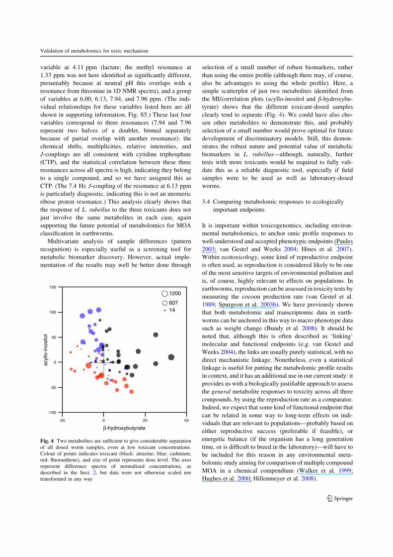
than using the entire profile (although there may, of course,also be advantages to using the whole profile). Here, a

simple scatterplot of just two metabolites identified from

the MI/correlation plots (scyllo-inositol and b-hydroxybu-tyrate) shows that the different toxicant-dosed samples

clearly tend to separate (Fig. 4). We could have also cho-

sen other metabolites to demonstrate this, and probablyselection of a small number would prove optimal for future

development of discriminatory models. Still, this demon-strates the robust nature and potential value of metabolic

biomarkers in L. rubellus—although, naturally, further

tests with more toxicants would be required to fully vali-date this as a reliable diagnostic tool, especially if field

samples were to be used as well as laboratory-dosed

worms.

3.4 Comparing metabolomic responses to ecologically

important endpoints

It is important within toxicogenomics, including environ-

mental metabolomics, to anchor omic profile responses towell-understood and accepted phenotypic endpoints (Paules

2003; van Gestel and Weeks 2004; Hines et al. 2007).

Within ecotoxicology, some kind of reproductive endpointis often used, as reproduction is considered likely to be one

of the most sensitive targets of environmental pollution and

is, of course, highly relevant to effects on populations. Inearthworms, reproduction can be assessed in toxicity tests by

measuring the cocoon production rate (van Gestel et al.

1989; Spurgeon et al. 2003b). We have previously shownthat both metabolomic and transcriptomic data in earth-

worms can be anchored in this way to macro phenotype data

such as weight change (Bundy et al. 2008). It should benoted that, although this is often described as ‘linking’

molecular and functional endpoints (e.g. van Gestel and

Weeks 2004), the links are usually purely statistical, with nodirect mechanistic linkage. Nonetheless, even a statistical

linkage is useful for putting the metabolomic profile results

in context, and it has an additional use in our current study: itprovides us with a biologically justifiable approach to assess

the general metabolite responses to toxicity across all three

compounds, by using the reproduction rate as a comparator.Indeed, we expect that some kind of functional endpoint that

can be related in some way to long-term effects on indi-

viduals that are relevant to populations—probably based oneither reproductive success (preferable if feasible), or

energetic balance (if the organism has a long generation

time, or is difficult to breed in the laboratory)—will have tobe included for this reason in any environmental meta-

bolomic study aiming for comparison of multiple compound

MOA in a chemical compendium (Walker et al. 1999;Hughes et al. 2000; Hillenmeyer et al. 2008).

-25 0 25 50

!-hydroxybutyrate

-100

-50

0

50

100

150

scyl

lo-in

osito

l

1200

60714

Fig. 4 Two metabolites are sufficient to give considerable separationof all dosed worm samples, even at low toxicant concentrations.Colour of points indicates toxicant (black: atrazine; blue: cadmium;red: fluoranthene), and size of point represents dose level. The axesrepresent difference spectra of normalized concentrations, asdescribed in the Sect. 2, but data were not otherwise scaled nortransformed in any way

Validation of metabolomics for toxic mechanism

123

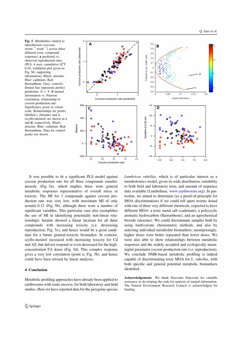
It was possible to fit a significant PLS model againstcocoon production rate for all three compounds simulta-

neously (Fig. 5a), which implies there were general

metabolic responses representative of overall stress ortoxicity. The MI for 3 compounds against cocoon pro-

duction rate was very low, with maximum MI of only

around 0.12 (Fig. 5b), although there were a number ofsignificant variables. This particular case also exemplifies

the use of MI in identifying potentially non-linear rela-

tionships: betaine showed a linear increase for all threecompounds with increasing toxicity (i.e. decreasing

reproduction; Fig. 5c), and hence would be a good candi-

date for a future general-toxicity biomarker. In contrast,scyllo-inositol increased with increasing toxicity for Cd

and AZ, but did not respond or even decreased for the high-

concentration FA doses (Fig. 5d). This complex responsegives a very low correlation (point ii, Fig. 5b), and hence

could have been missed by linear analyses.

4 Conclusion

Metabolic profiling approaches have already been applied to

earthworms with some success, for both laboratory and field

studies. Here we have reported data for the peregrine species

Lumbricus rubellus, which is of particular interest as ametabolomics model, given its wide distribution, suitability

to both field and laboratory tests, and amount of sequence

data available (Lumbribase, www.earthworms.org). In par-ticular, we aimed to determine (as a proof-of-principle for

MOA discrimination) if we could tell apart worms dosed

with one of three very different chemicals, expected to havedifferent MOA: a toxic metal salt (cadmium), a polycyclic

aromatic hydrocarbon (fluoranthene), and an agrochemical

biocide (atrazine). We could discriminate samples both byusing multivariate chemometric methods, and also by

selecting individual metabolite biomarkers; unsurprisingly,

higher doses were better separated than lower doses. Wewere also able to show relationships between metabolic

responses and the widely accepted and ecologically mean-

ingful parameter cocoon production rate (i.e. reproduction).We conclude NMR-based metabolic profiling is indeed

capable of discriminating toxic MOA for L. rubellus, withboth specific and general potential metabolic biomarkersidentified.

Acknowledgements We thank Slawomir Zukowski for valuableassistance in developing the code for analysis of mutual information.The Natural Environment Research Council is acknowledged forfunding.

0 1 2

Cocooon production rate (predicted)

0

1

2

Coc

oon

prod

uctio

n ra

te (

obse

rved

)

0.0 0.5 1.0 1.5 2.0

Cocoon production rate

-200

0

200

400

600

Bet

aine

0.0 0.5 1.0 1.5 2.0

-100

-50

0

50

100

150

Var

iabl

e at

3.3

5 pm

A B

C D

Fig. 5 Metabolites related toreproduction (cocoonsworm-1 week-1) across threedifferent toxic compoundresponses. a predicted vs.observed reproduction rates(PLS, 4 axes, cumulative Q2Y0.54; validation plot given asFig. S6, supportinginformation). Black: atrazine.Blue: cadmium. Red:fluoranthene. Grey: controls.Dotted line represents perfectprediction, X = Y. b mutualinformation vs. Pearsoncorrelation, relationship tococoon production rate.Significance given as colourscale. Relationships for pointslabelled i. (betaine) and ii.(scyllo-inositol) are shown in cand d, respectively. Black:atrazine. Blue: cadmium. Red:fluoranthene. Data for controlpoints not shown

Q. Guo et al.

123

References

Ankley, G. T., et al. (2006). Toxicogenomics in regulatory ecotoxi-cology. Environmental Science and Technology, 40, 4055–4065.doi:10.1021/es0630184.

Bang, J. W., et al. (2008). Integrative top-down system metabolicmodeling in experimental disease states via data-driven Bayesianmethods. Journal of Proteome Research, 7, 497–503. doi:10.1021/pr070350l.

Beckonert, O., et al. (2007). Metabolic profiling, metabolomic andmetabonomic procedures for NMR spectroscopy of urine,plasma, serum and tissue extracts. Nature Protocols, 2, 2692–2703. doi:10.1038/nprot.2007.376.

Broadhurst, D. I., & Kell, D. B. (2006). Statistical strategies for avoidingfalse discoveries in metabolomics and related experiments. Meta-bolomics, 2, 171–196. doi:10.1007/s11306-006-0037-z.

Brown, S. A., Simpson, A. J., & Simpson, M. J. (2008).Evaluation of sample preparation methods for nuclear mag-netic resonance metabolic profiling studies with Eiseniafetida. Environmental Toxicology and Chemistry, 27, 828–836. doi:10.1897/07-412.1.

Bundy, J. G., et al. (2002). Metabonomic assessment of toxicity of 4-fluoroaniline, 3,5-difluoroaniline and 2-fluoro-4-methylaniline tothe earthworm Eisenia veneta (Rosa): Identification of newendogenous biomarkers. Environmental Toxicology and Chem-istry, 21, 1966–1972. doi:10.1897/1551-5028(2002)021\1966:MAOTOF[2.0.CO;2.

Bundy, J. G., et al. (2004). Environmental metabonomics: Applyingcombination biomarker analysis in earthworms at a metalcontaminated site. Ecotoxicology (London, England), 13, 797–806. doi:10.1007/s10646-003-4477-1.

Bundy, J. G., et al. (2007). Metabolic profile biomarkers of metalcontamination in a sentinel terrestrial species are applicableacross multiple sites. Environmental Science and Technology,41, 4458–4464. doi:10.1021/es0700303.

Bundy, J. G., et al. (2008). ‘Systems toxicology’ approach identifiescoordinated metabolic responses to copper in a terrestrial non-model invertebrate, the earthworm Lumbricus rubellus. BMCBiology, 6, 25. doi:10.1186/1741-7007-6-25.

Calabrese, E. J. (2008). Hormesis: Why it is important to toxicologyand toxicologists. Environmental Toxicology and Chemistry, 27,1451–1474. doi:10.1897/07-541.1.

Camacho, D., de la Fuente, A., & Mendes, P. (2005). The origin ofcorrelations in metabolomics data. Metabolomics, 1, 53–63. doi:10.1007/s11306-005-1107-3.

Daub, C. O., Steuer, R., Selbig, J., & Kloska, S. (2004). Estimatingmutual information using B-spline functions—an improvedsimilarity measure for analysing gene expression data. BMCBioinformatics, 5, 118. doi:10.1186/1471-2105-5-118.

Duewer, D. L., Kowalski, B. R., & Schatzki, T. F. (1975). Sourceidentification of oil spills by pattern recognition analysis ofnatural elemental composition. Analytical Chemistry, 47, 1573–1583. doi:10.1021/ac60359a051.

Ebbels, T. M., et al. (2007). Prediction and classification of drugtoxicity using probabilistic modeling of temporal metabolic data:The consortium on metabonomic toxicology screening approach.Journal of Proteome Research, 6, 4407–4422. doi:10.1021/pr0703021.

Fisher, R. A. (1936). The use of multiple measures in taxonomicproblems. Annals of Eugenics, 7, 179–188.

Flaherty, P., Giaever, G., Kumm, J., Jordan, M. I., & Arkin, A. P.(2005). A latent variable model for chemogenomic profiling.Bioinformatics (Oxford, England), 21, 3286–3293. doi:10.1093/bioinformatics/bti515.

Forbes, V. E., Palmqvist, A., & Bach, L. (2006). The use and misuseof biomarkers in ecotoxicology. Environmental Toxicology andChemistry, 25, 272–280. doi:10.1897/05-257R.1.

Gartland, K. P., Beddell, C. R., Lindon, J. C., & Nicholson, J. K.(1990). A pattern recognition approach to the comparison ofPMR and clinical chemical data for classification of nephrotox-icity. Journal of Pharmaceutical and Biomedical Analysis, 8,963–968. doi:10.1016/0731-7085(90)80151-E.

Gartland, K. P., Beddell, C. R., Lindon, J. C., & Nicholson, J. K.(1991). Application of pattern recognition methods to theanalysis and classification of toxicological data derived fromproton nuclear magnetic resonance spectroscopy of urine.Molecular Pharmacology, 39, 629–642.

Gartland, K. P., Bonner, F. W., & Nicholson, J. K. (1989).Investigations into the biochemical effects of region-specificnephrotoxins. Molecular Pharmacology, 35, 242–250.

Gong, P., et al. (2007). Toxicogenomic analysis provides new insightsinto molecular mechanisms of the sublethal toxicity of 2,4,6-trinitrotoluene in Eisenia fetida. Environmental Science andTechnology, 41, 8195–8202. doi:10.1021/es0716352.

Hillenmeyer, M. E., et al. (2008). The chemical genomic portrait ofyeast: Uncovering a phenotype for all genes. Science, 320, 362–365. doi:10.1126/science.1150021.

Hines, A., Oladiran, G. S., Bignell, J. P., Stentiford, G. D., & Viant,M. R. (2007). Direct sampling of organisms from the field andknowledge of their phenotype: Key recommendations forenvironmental metabolomics. Environmental Science and Tech-nology, 41, 3375–3381. doi:10.1021/es062745w.

Hughes, T. R., et al. (2000). Functional discovery via a compendiumof expression profiles. Cell, 102, 109–126. doi:10.1016/S0092-8674(00)00015-5.

Hyvarinen, A., Karhunne, J., & Oja, E. (2001). IndependentComponent Analysis. New York: Wiley.

Jones, O. A., Spurgeon, D. J., Svendsen, C., & Griffin, J. L. (2008). Ametabolomics based approach to assessing the toxicity of thepolyaromatic hydrocarbon pyrene to the earthworm Lumbricusrubellus.Chemosphere, 71, 601–609. doi:10.1016/j.chemosphere.2007.08.056.

Khan, S., et al. (2007). Relative performance of mutual informationestimation methods for quantifying the dependence among shortand noisy data.Physical Review E: Statistical, Nonlinear, and SoftMatter Physics, 76, 026209. doi:10.1103/PhysRevE.76.026209.

Lin, C. Y., Viant, M. R., & Tjeerdema, R. S. (2006). Metabolomics:Methodologies and applications in the environmental sciences.Journal of Pesticide Science, 31, 245–251. doi:10.1584/jpestics.31.245.

Maere, S., Van Dijck, P., & Kuiper, M. (2008). Extracting expressionmodules from perturbational gene expression compendia. BMCSystems Biology, 2, 33. doi:10.1186/1752-0509-2-33.

Malmendal, A., et al. (2006). Metabolomic profiling of heat stress:Hardening and recovery of homeostasis in Drosophila. AmericanJournal of Physiology: Regulatory, Integrative and Compara-tive Physiology, 291, R205–R212. doi:10.1152/ajpregu.00867.2005.

May, S., & Bigelow, C. (2005). Modeling nonlinear dose–responserelationships in epidemiologic studies: Statistical approaches andpractical challenges. Dose Response, 3, 474–490. doi:10.2203/dose-response.003.04.004.

Meyer, P. E., Lafitte, F., & Bontempi, G. (2008). minet: A R/Bioconductor package for inferring large transcriptional net-works using mutual information. BMC Bioinformatics, 9, 461.doi:10.1186/1471-2105-9-461.

OECD. (1984). Guidelines for the testing of chemicals. 207.Earthworm acute toxicity tests. Paris: OECD.

Validation of metabolomics for toxic mechanism

123

Owen, J., et al. (2008). Transcriptome profiling of developmental andxenobiotic responses in a keystone soil animal, the oligochaeteannelid Lumbricus rubellus. BMC Genomics, 9, 266. doi:10.1186/1471-2164-9-266.

Paules, R. (2003). Phenotypic anchoring: Linking cause and effect.Environmental Health Perspectives, 111, A338–A339.

Sanchez-Hernandez, J. C. (2006). Earthworm biomarkers in ecologicalrisk assessment. Reviews of Environmental Contamination andToxicology, 188, 85–126. doi:10.1007/978-0-387-32964-2-3.

Spurgeon, D. J., Svendsen, C., Kille, P., Morgan, A. J., & Weeks, J.M. (2004). Responses of earthworms (Lumbricus rubellus) tocopper and cadmium as determined by measurement of juveniletraits in a specifically designed test system. Ecotoxicology andEnvironmental Safety, 57, 54–64. doi:10.1016/j.ecoenv.2003.08.003.

Spurgeon, D. J., Svendsen, C., Weeks, J. M., Hankard, P. K.,Stubberud, H. E., & Kammenga, J. E. (2003a). Quantifyingcopper and cadmium impacts on intrinsic rate of populationincrease in the terrestrial oligochaete Lumbricus rubellus.Environmental Toxicology and Chemistry, 22, 1465–1472.doi:10.1897/1551-5028(2003)22\1465:QCACIO[2.0.CO;2.

Spurgeon, D. J., Weeks, J. M., & van Gestel, C. A. M. (2003b). Asummary of eleven years progress in earthworm ecotoxicology.Pedobiologia, 47, 588–606.

Steuer, R., Kurths, J., Daub, C. O., Weise, J., & Selbig, J. (2002). Themutual information: Detecting and evaluating dependenciesbetween variables. Bioinformatics (Oxford, England), 18(Suppl2), S231–S240.

Thevenaz, P., & Unser, M. (2000). Optimization of mutual informa-tion for multiresolution image registration. IEEE Transactionson Image Processing, 9, 2083–2099. doi:10.1109/83.887976.

Ulrich, E. L., et al. (2008). BioMagResBank. Nucleic Acids Research,36, D402–D408. doi:10.1093/nar/gkm957.

van Gestel, C. A., van Dis, W. A., van Breemen, E. M., &Sparenburg, P. M. (1989). Development of a standardized

reproduction toxicity test with the earthworm species Eiseniafetida andrei using copper, pentachlorophenol and 2,4-dichloro-aniline. Ecotoxicology and Environmental Safety, 18, 305–312.doi:10.1016/0147-6513(89)90024-9.

van Gestel, C. A., & Weeks, J. M. (2004). Recommendations of the3rd international workshop on earthworm ecotoxicology, Aar-hus, Denmark, August 2001. Ecotoxicology and EnvironmentalSafety, 57, 100–105.

van Straalen, N. M., & Roelofs, D. (2008). Genomics technology forassessing soil pollution. Journal of Biology (Online), 7, 19. doi:10.1186/jbiol80.

Viant, M. R. (2003). Improved methods for the acquisition andinterpretation of NMR metabolomic data. Biochemical andBiophysical Research Communications, 310, 943–948. doi:10.1016/j.bbrc.2003.09.092.

Viant, M. R. (2007). Metabolomics of aquatic organisms: The new‘omics’ on the block. Marine Ecology Progress Series, 332,301–306. doi:10.3354/meps332301.

Walker, M. G., Volkmuth, W., Sprinzak, E., Hodgson, D., & Klingler,T. (1999). Prediction of gene function by genome-scale expres-sion analysis: Prostate cancer-associated genes. GenomeResearch, 9, 1198–1203. doi:10.1101/gr.9.12.1198.

Warne, M. A., Lenz, E. M., Osborn, D., Weeks, J. M., & Nicholson, J.K. (2000). An NMR-based metabonomic investigation of thetoxic effects of 3-trifluoromethyl-aniline on the earthwormEisenia veneta. Biomarkers, 5, 56–72. doi:10.1080/135475000230541.

Wishart, D. S. (2008). Quantitative metabolomics using NMR. Trendsin Analytical Chemistry, 27, 228–237. doi:10.1016/j.trac.2007.12.001.

Wold, S. (1976). Pattern recognition by means of disjoint principalcomponents models. Pattern Recognition, 8, 127–139. doi:10.1016/0031-3203(76)90014-5.

Q. Guo et al.

123