valence transitions and interplay of Kondo effect and disorder
159
HAL Id: tel-01308512 https://tel.archives-ouvertes.fr/tel-01308512v2 Submitted on 3 Nov 2017 HAL is a multi-disciplinary open access archive for the deposit and dissemination of sci- entific research documents, whether they are pub- lished or not. The documents may come from teaching and research institutions in France or abroad, or from public or private research centers. L’archive ouverte pluridisciplinaire HAL, est destinée au dépôt et à la diffusion de documents scientifiques de niveau recherche, publiés ou non, émanant des établissements d’enseignement et de recherche français ou étrangers, des laboratoires publics ou privés. Theory of lanthanide systems : valence transitions and interplay of Kondo effect and disorder Jose Luiz Ferreira da Silva Jr To cite this version: Jose Luiz Ferreira da Silva Jr. Theory of lanthanide systems: valence transitions and interplay of Kondo effect and disorder. Condensed Matter [cond-mat]. Université Grenoble Alpes, 2016. English. NNT : 2016GREAY077. tel-01308512v2
-
Upload
khangminh22 -
Category
Documents
-
view
2 -
download
0
Transcript of valence transitions and interplay of Kondo effect and disorder

HAL Id: tel-01308512https://tel.archives-ouvertes.fr/tel-01308512v2
Submitted on 3 Nov 2017
HAL is a multi-disciplinary open accessarchive for the deposit and dissemination of sci-entific research documents, whether they are pub-lished or not. The documents may come fromteaching and research institutions in France orabroad, or from public or private research centers.
L’archive ouverte pluridisciplinaire HAL, estdestinée au dépôt et à la diffusion de documentsscientifiques de niveau recherche, publiés ou non,émanant des établissements d’enseignement et derecherche français ou étrangers, des laboratoirespublics ou privés.
Theory of lanthanide systems : valence transitions andinterplay of Kondo effect and disorder
Jose Luiz Ferreira da Silva Jr
To cite this version:Jose Luiz Ferreira da Silva Jr. Theory of lanthanide systems : valence transitions and interplay ofKondo effect and disorder. Condensed Matter [cond-mat]. Université Grenoble Alpes, 2016. English.�NNT : 2016GREAY077�. �tel-01308512v2�
!
THÈSE Pour obtenir le grade de
DOCTEUR DE LA COMMUNAUTÉ UNIVERSITÉ GRENOBLE ALPES Spécialité : Physique de la matière condensée & rayonnement
Arrêté ministériel : 7 août 2006
Présentée par
José Luiz FERREIRA DA SILVA JUNIOR
Thèse dirigée par Claudine LACROIX et codirigée par Sébastien BURDIN
préparée au sein du Laboratoire Institut Néel dans l'École Doctorale de Physique
Théorie des systèmes de lanthanide: transitions de valence et effet Kondo en présence de désordre Thèse soutenue publiquement le 23 mars 2016, devant le jury composé de :
M. Daniel MALTERRE Professeur, Institut Jean Lamour, CNRS et Université de Lorraine, Président du jury Mme. Anuradha JAGANNATHAN Professeure, Laboratoire de Physique des Solides, CNRS et Université Paris-Sud, Rapporteur M. Indranil PAUL Chargé de recherches, Laboratoire Matériaux et Phénomènes Quantiques, CNRS et Université Paris-Diderot, Rapporteur Mme. Gertrud ZWICKNAGL Professeure, Institut für Mathematische Physik, Technische Universität Braunschweig, Examinatrice M. Ilya SHEIKIN Directeur de recherches, Laboratoire National des Champs Magnétiques Intenses, CNRS et Université Grenoble Alpes, Examinateur Mme. Claudine LACROIX Directrice de recherches, Institut Néel, CNRS et Université Grenoble Alpes, Directrice de thèse M. Sébastien BURDIN Maître de conférences, Laboratoire Ondes et Matières d’Aquitaine (LOMA), CNRS et Université de Bordeaux, Co-Directeur de thèse

Abstract
The topics of the thesis concerns two theoretical aspects of the physics of 4f electron systems.In the first part the topic of intermediate valence and valence transitions in lanthanide
systems is explored. For that purpose, we study an extended version of the Periodic AndersonModel which includes the Coulomb interaction between conduction electrons and the localizedf electrons (Falicov-Kimball interaction). If it is larger than a critical value, this interactioncan transform a smooth valence change into a discontinuous valence transition. The model istreated in a combination of Hubbard-I and mean-field approximations, suitable for the energyscales of the problem. The zero temperature phase diagram of the model is established. Itshows the evolution of the valence with respect to the model parameters. Moreover, theeffects of an external magnetic field and ferromagnetic interactions on the valence transitionsare investigated. Our results are compared to selected Yb- and Eu-based compounds, such asYbCu2Si2, YbMn6Ge6−xSnx and Eu(Rh1−xIrx)2Si2.
In the second part of the thesis, we study lanthanide systems in which the number oflocal magnetic atoms is tuned by substitution of non-magnetic atoms, also known as KondoAlloys. In such systems it is possible to go from the single Kondo impurity to the Kondo latticeregime, both characterized by different type of Fermi liquids. The Kondo Alloy model is studiedwithin the Statistical Dynamical Mean-Field Theory, which treats different aspects of disorderand is formally exact in a Bethe lattice of any coordination number. The distributions of themean-field parameters, the local density of states and other local quantities are presented asa function of model parameters, in particular the concentration of magnetic moments x, thenumber of conduction electrons per site nc and the Kondo interaction strength JK . Our resultsshow a clear distinction between the impurity (x� 1) and the lattice (x≈ 1) regimes for astrong Kondo interaction. For intermediate concentrations (x≈nc), the system is dominatedby disorder effects and indications of Non-Fermi liquid behavior and localization of electronicstates are observed. These features disappear if the Kondo interaction is weak. We furtherdiscuss the issue of low dimensionality and its relation to the percolation problem in suchsystems.
1

Résumé
Cette thèse a comme sujet général l’etude théorique de deux aspects de la physique des systèmesd’electrons 4f .
La première partie est consacrée aux systèmes intermétalliques de lanthanides à valenceintermédiaire ou possédant une transition de valence. Dans ce but, nous étudions une versionétendue du modèle d’Anderson périodique, auquel est ajoutée une interaction coulombienneentre les électrons de conduction et les électrons f localisés (intéraction de Falicov-Kimball).Si cette interaction est plus forte qu’une valeur critique, le changement de valence n’est pluscontinu, mais devient discontinu. Le modèle est traité par un ensemble de approximationsappropriées aux échelles d’énergie du problème : Hubbard-I et le champ moyen. Le diagrammede phases du modèle à température nulle et l’évolution de la valence avec les paramètresdu modèle sont déterminés. En plus, les effets d’un champ magnétique extérieur et des in-teractions ferromagnétiques entre les électrons localisés sont examinés. Nos résultats sontcomparés à quelques composés à base de Yb et Eu, comme YbCu2Si2, YbMn6Ge6−xSnx etEu(Rh1−xIrx)2Si2.
Dans la deuxième partie nous étudions des systèmes de lanthanides dans lesquels le nom-bre d’atomes magnétiques localisés peut être modifié par substitution par des atomes non-magnétiques (Alliages Kondo). Dans ces systèmes il est possible de passer du régime d’impuretéKondo au régime de réseau Kondo ; à basse température ces deux régimes sont des liquidesde Fermi dont les caractéristiques sont différentes. Le modèle d’alliage Kondo est étudié dansla théorie du champ moyen dynamique statistique, qui traite différents aspects du désordreet qui est formellement exacte dans un arbre de Bethe avec un nombre de coordination quel-conque. Les distributions des paramètres de champ moyen, des densité d’états locales etd’autres quantités locales sont présentées en fonction des paramètres du modèle, en particulierla concentration de moments magnétiques x, le nombre d’électrons de conduction par site nc,et la valeur de l’interaction Kondo JK . Nos résultats montrent une différence nette entre lesrégimes d’impureté (x� 1) et de réseau (x≈ 1) pour une interaction Kondo forte. Pour desconcentrations intermédiaires (x≈nc), le système est dominé par le désordre et des indicationsd’un comportement non-liquide de Fermi et d’une localisation des états électroniques sont ob-servés. Ces caractéristiques disparaissent quand l’interaction Kondo est faible. Nous discutonsaussi la question d’une basse dimensionnalité et la relation avec le problème de percolationdans ces systèmes.
3

Remerciements
Tout d’abord je voudrais remercier le président du jury Daniel Malterre, les rapporteurs Anu-radha Jagannathan et Indranil Paul, et les examinateurs Gertrud Zwicknagl et Ilya Sheikin pouravoir accepté de faire partie de mon jury de thèse et pour le temps qu’ils ont consacré à lalecture de ce manuscrit et pour leur participation lors de la soutenance.
Je remercie chaleureusement mes deux directeurs de thèse Claudine Lacroix et SébastienBurdin. Pendent cette période j’ai eu le plaisir de profiter de leur expérience, leurs compétencesscientifiques et humaines et je les remercie pour tout ce que j’ai appris. Je remercie Claudinepour avoir accepté de diriger mon doctorat en France et avoir été disponible pendant cesannées. Je remercie Sébastien pour les nombreux échanges, surtout par mail ou par téléphone,pour m’avoir accueilli dans son laboratoire lors mes visites à Bordeaux et pour le temps dédiéà mes recherches et à ma thèse.
Je remercie Vladimir Dobrosavljevic, notre collaborateur pour la deuxième partie de cettethèse, pour tous ses conseils et pour les connaissances qu’il m’a fait partager. D’autre part, pourla première partie de cette thèse, j’ai eu le plaisir d’avoir de nombreuses discussions intéressantesavec des expérimentateurs du domaine. Dans ce contexte, je remercie particulièrement DanielBraithwaite, Daniel Malterre, Thomas Mazet, Olivier Isnard et William Knafo pour les échangesque nous avons eus et qui m’ont permis de mieux connaitre les aspects expérimentaux liés àla mesure de la valence et aux différents composés.
Je remercie l’ensemble des personnels de l’Institut Néel que j’ai côtoyé pendant ces années,les membres de l’équipe Théorie de la Matière Condensée et du département Matière Condenséeet Basse Temperature, en particulier le directeur du département Pierre-Etienne Wolff et leresponsable de l’équipe Simone Fratini. Un très grand merci à tous les doctorants et postdocsque j’ai pu rencontrer au laboratoire, et plus spécialement à tous ceux avec qui j’ai eu le plaisirde partager le bureau.
Je remercie mes collègues et professeurs de Porto Alegre: Acirete Simões, Roberto Iglesias,Miguel Gusmão, Christopher Thomas et Edgar Santos pour m’avoir encouragé à venir faire mathèse à Grenoble.
Je remercie Glaucia pour les bons moments que nous avons partagés à Grenoble, ma famillepour son soutien « à longue portée » et mes amis pour leur sympathie.
Enfin, je suis reconnaissant envers le CNPq, qui a financé ma bourse de thèse en France,pour son soutien.
5


Contents
1 Introduction 111.1 Magnetic Impurities in metals . . . . . . . . . . . . . . . . . . . . . . . . . . 11
1.1.1 The impurity Anderson model . . . . . . . . . . . . . . . . . . . . . . 121.1.2 The Kondo model . . . . . . . . . . . . . . . . . . . . . . . . . . . . 13
1.2 Lattice models . . . . . . . . . . . . . . . . . . . . . . . . . . . . . . . . . . 151.3 Thesis presentation . . . . . . . . . . . . . . . . . . . . . . . . . . . . . . . 17
I Model for valence transitions in lanthanide systems 19
2 Valence of lanthanides 212.1 Introduction . . . . . . . . . . . . . . . . . . . . . . . . . . . . . . . . . . . 21
2.1.1 Valence of lanthanide ions . . . . . . . . . . . . . . . . . . . . . . . . 212.1.2 Two historical examples . . . . . . . . . . . . . . . . . . . . . . . . . 232.1.3 General aspects of intermediate valence states . . . . . . . . . . . . . 24
2.2 Experimental techniques to measure valence . . . . . . . . . . . . . . . . . . 252.2.1 Time-scales of valence fluctuation . . . . . . . . . . . . . . . . . . . . 252.2.2 Static measurements . . . . . . . . . . . . . . . . . . . . . . . . . . . 262.2.3 Dynamical measurements . . . . . . . . . . . . . . . . . . . . . . . . 27
2.3 Models for valence transitions . . . . . . . . . . . . . . . . . . . . . . . . . . 312.3.1 Anderson impurity and lattice models . . . . . . . . . . . . . . . . . . 312.3.2 The Falicov-Kimball model . . . . . . . . . . . . . . . . . . . . . . . 322.3.3 Models explicitly including volume effects . . . . . . . . . . . . . . . . 33
2.4 Summary . . . . . . . . . . . . . . . . . . . . . . . . . . . . . . . . . . . . . 34
3 The Extended Periodic Anderson Model 353.1 Energy scales in EPAM . . . . . . . . . . . . . . . . . . . . . . . . . . . . . 363.2 Previous works . . . . . . . . . . . . . . . . . . . . . . . . . . . . . . . . . . 373.3 Approximations for the Extended Periodic Anderson Model . . . . . . . . . . . 38
3.3.1 Ufc term: the mean-field approximation . . . . . . . . . . . . . . . . . 383.3.2 U term: Hubbard-I approximation . . . . . . . . . . . . . . . . . . . . 393.3.3 Green’s functions . . . . . . . . . . . . . . . . . . . . . . . . . . . . . 41
3.4 Properties of the model . . . . . . . . . . . . . . . . . . . . . . . . . . . . . 42
7

CONTENTS 8
4 Results 474.1 Results for non-magnetic phases . . . . . . . . . . . . . . . . . . . . . . . . . 47
4.1.1 Self-consistent solutions . . . . . . . . . . . . . . . . . . . . . . . . . 474.1.2 Valence as a function of model parameters . . . . . . . . . . . . . . . 484.1.3 Summary . . . . . . . . . . . . . . . . . . . . . . . . . . . . . . . . . 55
4.2 Magnetic Phases . . . . . . . . . . . . . . . . . . . . . . . . . . . . . . . . . 564.2.1 Intrinsic Magnetism . . . . . . . . . . . . . . . . . . . . . . . . . . . 564.2.2 Magnetism induced by an external magnetic field . . . . . . . . . . . . 604.2.3 Ferromagnetism induced by f-f exchange . . . . . . . . . . . . . . . . 644.2.4 Summary . . . . . . . . . . . . . . . . . . . . . . . . . . . . . . . . . 67
4.3 Connection with experiments . . . . . . . . . . . . . . . . . . . . . . . . . . 684.3.1 Pressure effects . . . . . . . . . . . . . . . . . . . . . . . . . . . . . 684.3.2 YbCu2Si2 . . . . . . . . . . . . . . . . . . . . . . . . . . . . . . . . 694.3.3 YbMn6Ge6−xSnx . . . . . . . . . . . . . . . . . . . . . . . . . . . . 724.3.4 Eu(Rh1−xIrx)2Si2 . . . . . . . . . . . . . . . . . . . . . . . . . . . . 764.3.5 Summary . . . . . . . . . . . . . . . . . . . . . . . . . . . . . . . . . 78
5 Conclusions and perspectives 79
II Disorder in Kondo systems 81
6 Introduction 836.1 Kondo effect: from the impurity to the lattice . . . . . . . . . . . . . . . . . 83
6.1.1 Local versus Coherent Fermi Liquid . . . . . . . . . . . . . . . . . . . 846.1.2 Strong-coupling picture of Kondo impurity and lattice models . . . . . 85
6.2 Substitutional disorder in Kondo systems . . . . . . . . . . . . . . . . . . . . 876.2.1 Non-Fermi liquid behavior from disorder . . . . . . . . . . . . . . . . . 876.2.2 Kondo Alloys: experimental motivation . . . . . . . . . . . . . . . . . 88
7 Model and method 917.1 The Kondo Alloy model . . . . . . . . . . . . . . . . . . . . . . . . . . . . . 91
7.1.1 State-of-art . . . . . . . . . . . . . . . . . . . . . . . . . . . . . . . . 927.1.2 The JK→∞ limit . . . . . . . . . . . . . . . . . . . . . . . . . . . . 92
7.2 Mean-field approximation for the Kondo problem . . . . . . . . . . . . . . . . 947.2.1 Green’s functions . . . . . . . . . . . . . . . . . . . . . . . . . . . . . 967.2.2 Hopping expansion . . . . . . . . . . . . . . . . . . . . . . . . . . . . 97
7.3 Statistical DMFT . . . . . . . . . . . . . . . . . . . . . . . . . . . . . . . . 997.4 Summary . . . . . . . . . . . . . . . . . . . . . . . . . . . . . . . . . . . . . 103
8 Results 1058.1 Important quantities and their distributions . . . . . . . . . . . . . . . . . . . 1058.2 Concentration effects . . . . . . . . . . . . . . . . . . . . . . . . . . . . . . 109
8.2.1 Strong Coupling . . . . . . . . . . . . . . . . . . . . . . . . . . . . . 110

CONTENTS 9
8.2.2 Weak coupling . . . . . . . . . . . . . . . . . . . . . . . . . . . . . . 1148.3 Neighboring effects . . . . . . . . . . . . . . . . . . . . . . . . . . . . . . . . 1178.4 Lower dimensions and percolation problem . . . . . . . . . . . . . . . . . . . 1198.5 Summary . . . . . . . . . . . . . . . . . . . . . . . . . . . . . . . . . . . . . 123
9 Conclusions and perspectives 125
A Hubbard-I approximation for the EPAM 127
B Magnetic Susceptibility for the EPAM 131
C Some results on Bethe lattices 135
D Matsubara’s sum at zero temperature 139
E Some limits of φi(ω) 141
F Renormalized Perturbation Expansion 145
Bibliography 149

Chapter 1
Introduction
This thesis has as general topic the description of anomalous lanthanides materials, an im-portant class of strongly correlated systems. In general, strongly correlated materials presentpartially filled d or f orbitals, which have a small spacial extension compared to s and p or-bitals. It leads to interactions among electrons on them that are stronger than the electronicbandwidths. For such reason, the conventional band theory fails in these materials and novelmethods have been developed in the last 50 years to deal with them.
In lanthanide systems the relevant orbitals are 4f orbitals, which are the most localizedamong all types of orbitals. Such degree of localization produces extreme phenomena as inheavy fermions, for example[1].
Through the whole work the mathematical formalism of second quantization and Green’sfunctions are employed and the notations are most often the usual ones. For that we refer totextbooks in References [2], [3] and [1]. The physical constants kB (Boltzmann’s constant)and ~ (reduced Planck’s constant) are implicitly taken as one, so energies and temperature arein the same unities.
In this chapter some key concepts on the subject of 4f -electron systems will be introduced.The basis of such systems is the formation (or not) of stable magnetic moments in lanthanideions, which can be described theoretically by the impurity Anderson model (Section 1.1.1).
1.1 Magnetic Impurities in metals
Magnetic impurities exist in a metal if the impurity ions have partially filled d or f orbitals. Ex-amples of such behavior are Fe impurities in Cu and Au, in which the impurities contributes tothe magnetic susceptibility through a Curie-Weiss term, typical of local moments. In addition,transport measurements showed an electrical resistivity minimum in the same metals. Theappearance of these features not only depends on the impurity atom but also on the metallichost.
11
CHAPTER 1. INTRODUCTION 12
1.1.1 The impurity Anderson model
The explanation for the local moment formation was put forward by Anderson[4]. He introduceda simple model to explain it, known nowadays as the Single Impurity Anderson model (SIAM):
H =∑k,σ
ε(k)c†k,σck,σ + Ef∑σ
f †σfσ + Uf †↑f↑f†↓f↓ +
V√N
∑k,σ
(c†k,σfσ + h.c.
)(1.1)
The operator ck,σ (c†k,σ) creates(annihilates) one conduction electron in the band with awave-vector k and spin orientation σ. Its energy is given by the electronic dispersion ε(k). Theimpurity site is represented by a non-degenerate local level with energy Ef and its electronsby the operators fσ and f †σ. The doubly occupied impurity state has an extra energy U(electronic repulsion)., which will be the key ingredient to moment formation. The last termis the hybridization V between the impurity and the conduction band and it can be taken ask-independent in a good approximation.
The impurity site behaves as a local moment as long as it is occupied by one electron only,which will happen if Ef <µ and Ef +U >µ, being µ the Fermi level of conduction electrons(Figure 1.1) . We adopt the mean-field description of the problem proposed by Anderson [4],employing the Hartree-Fock approximation for the Coulomb repulsion:
Uf †↑f↑f†↓f↓ → U 〈nf,↓〉 nf,↑ + 〈nf,↑〉 n↓ − U 〈nf,↑〉 〈nf,↓〉 , (1.2)
The operators nf,σ = f †σfσ are replaced by their averaged values that must be calculatedself-consistently.
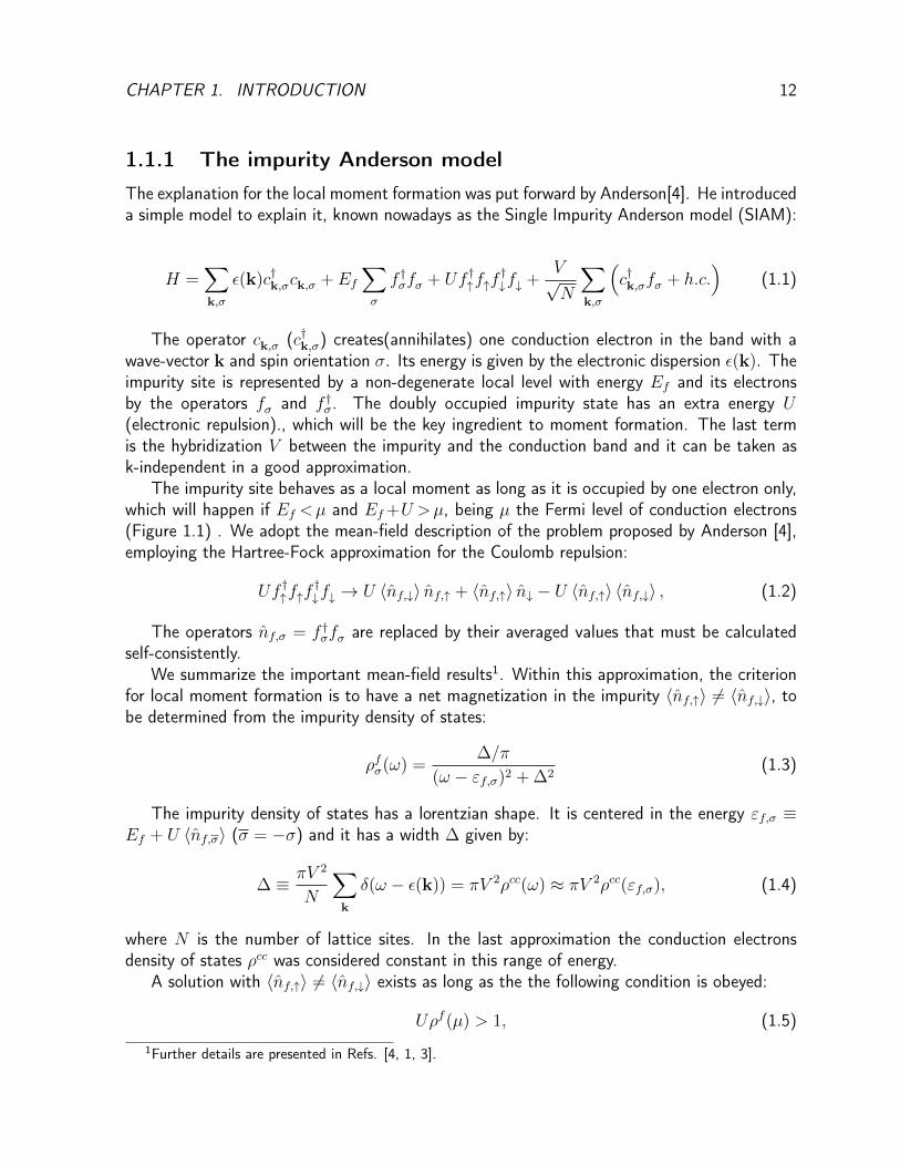
We summarize the important mean-field results1. Within this approximation, the criterionfor local moment formation is to have a net magnetization in the impurity 〈nf,↑〉 6= 〈nf,↓〉, tobe determined from the impurity density of states:
ρfσ(ω) =∆/π
(ω − εf,σ)2 + ∆2(1.3)
The impurity density of states has a lorentzian shape. It is centered in the energy εf,σ ≡Ef + U 〈nf,σ〉 (σ = −σ) and it has a width ∆ given by:
∆ ≡ πV 2
N
∑k
δ(ω − ε(k)) = πV 2ρcc(ω) ≈ πV 2ρcc(εf,σ), (1.4)
where N is the number of lattice sites. In the last approximation the conduction electronsdensity of states ρcc was considered constant in this range of energy.
A solution with 〈nf,↑〉 6= 〈nf,↓〉 exists as long as the the following condition is obeyed:
Uρf (µ) > 1, (1.5)
1Further details are presented in Refs. [4, 1, 3].

CHAPTER 1. INTRODUCTION 13
This condition is a local version of the Stoner criterion, that is used as a criterion for bandferromagnetism in metals[5]. The local moment is stable if the f (or d) density of states issufficiently large for a given U , that, on its turn, must be finite. An equivalent form of theStoner criterion is U/π∆> 1, where it becomes evident that the local moment formation isfavored if the hybridization V or the conduction electrons density of states close to the impuritylevel energy is small. That is the reason why moment formation depends on the characteristicsof the impurities and the metallic host.
Mixed-valence regime
The local moment formation occurs when the singly occupied level is stable and all the othersimpurity configurations (empty or the doubly occupied) have energies much higher than theresonant level width ∆. However, if the position of the empty level approaches the Fermilevel (−Ef → µ) and becomes comparable to ∆, the local moment becomes unstable. Thissituation (Fig. 1.1.b) corresponds to the mixed-valence regime of Anderson model, in whichthe average occupation of the impurity site is less than one. A similar situation arises whenthe doubly occupied state becomes close to the Fermi level, the impurity average occupation(or valence) being between one and two. Two other non-magnetic regimes of the SIAM ariseswhen the local levels are completely empty or full. The physics of mixed-valence regime willbe explored in details in the Part I.
1.1.2 The Kondo model
Taking as granted that the local moment is formed, we can ask now how does it interacts withthe conduction electrons and what are the consequences of such interaction. For that purpose,Schrieffer and Wolff performed a canonical transformation of the Anderson model (Eq. 1.1)known as Schrieffer-Wolff transformation[6]. It is a projection of the Anderson model into itsnf = 1 subspace, so that the other impurity configurations (nf = 0 and nf = 2) are treatedas virtual states.
The resulting hamiltonian is known as the Kondo model:
H =∑k,σ
ε(k)c†k,σck,σ + JKS · s (1.6)
In this model, the impurity magnetic moment interacts locally with the conduction electronspin through an exchange interaction. The Kondo coupling JK is related to the parameters ofAnderson model by
JK = V 2
(1
µ−Ef+
1
Ef+U−µ
)(1.7)
and it is a positive quantity. Then the Kondo interaction has an antiferromagnetic nature.The Kondo model was first predicted by Kondo[7] already in 1964, who used it to explain
the resistivity minimum observed in normal metals with a very low concentration of magneticimpurities, which was firstly reported in gold samples by de Haas, de Boer and van der Berg[8]

CHAPTER 1. INTRODUCTION 14
Figure 1.1: Schematic representation of SIAM parameters in (a) the Kondo and (b) the mixedvalence regime. The conduction band is represented by the blue area and it is filled up to theFermi energy µ. The impurity levels are located at Ef and Ef+U and they are broadened by∆ (Eq. 1.4). In the Kondo limit (a), the impurity level Ef is well below the Fermi energyµ, while the doubly occupied state is above with an energy Ef +U . Virtual processes inwhich conduction electrons hops on and off the impurity levels generate a peak in the Fermienergy (Abrikosov-Suhl resonance) for T < TK . In the mixed valence regime (b), the levelEf , broadened by the hybridization, approaches µ. The impurity level is partially filled with anon-integer number of electrons. Both situations lead to an enhanced density of states at theFermi energy, but the underlying mechanism is different.
thirty years before. Kondo used perturbation theory to determine a log T dependence responsi-ble for the minimum. The perturbation theory remains valid for temperatures above the Kondotemperature,
TK = De−1/JKρc(µ), (1.8)
where D is the conduction electrons bandwidth.The solution of the T < TK regime required non-perturbative methods inexistent at that
time. The key concept that emerges from this problem is the gradual screening of the magneticimpurities with decreasing temperature, which leads to an effective non-magnetic impurity asT→0. This idea came from the Anderson’s "poor man scaling" [9, 1] and it was later formallydeveloped by Wilson in his pioneer work on Numerical Renormalization Group[10].
For T � TK the conduction electrons scattering on the impurity progressively screens itsmagnetic moment. The many-body process creates a sharp peak in the density of stateslocated at the Fermi energy, known as Abrikosov-Suhl (or Kondo resonance). The width of theKondo resonance is proportional to TK , which leads to enhanced contribution on the magneticsusceptibility and specific heat at low temperatures. The physical picture of the Kondo regimefor T < TK is presented in Figure 1.1, including the Kondo resonance. We stress that this
CHAPTER 1. INTRODUCTION 15
situation is different from the mixed-valent regime shown in the right, which is discussed indetails in Section 2.3.1.
1.2 Lattice models
In the last section it was discussed the consequences of having isolated magnetic impurities innon-magnetic metals. In systems with a periodical lattice of magnetic ions, it is necessary togeneralize the above picture.
The simplest model to describe metals containing both itinerant and localized electrons isthe Periodic Anderson model (PAM):
H =∑k,σ
ε(k)c†k,σck,σ + Ef∑i,σ
f †iσfiσ + U∑i
f †i↑fi↑f†i↓fi↓ + V
∑i,σ
(c†iσfσ + h.c.
)(1.9)
This is a generalization of the Anderson Impurity model (Eq. 1.1) in which every lattice sitecontains a non-degenerate local level with energy Ef . The local nature of these levels impliesthat the Coulomb repulsion U between two f-electrons on the same site is large.
The Periodic Anderson model possesses several regime of parameters. The two most rele-vant are the mixed valence and the local moment (or Kondo) regimes, which are characterizedby the same parameters than in the SIAM. Nevertheless, the nature of both regimes is differentin the lattice: in the mixed valence regime of PAM, the system Fermi energy depends on thef-levels occupation given that the total number of electrons (c+f) is conserved (see Section2.3.1). In the Kondo limit the difference lies in the fact that the impurity scattering becomescoherent due to the periodicity of local moments, giving a coherent state at low temperatures(Section 6.1).
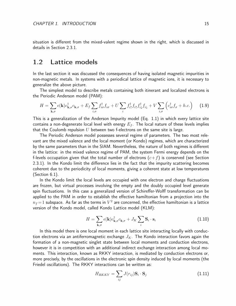
In the Kondo limit the local levels are occupied with one electron and charge fluctuationsare frozen, but virtual processes involving the empty and the doubly occupied level generatespin fluctuations. In this case a generalized version of Schireffer-Wolff transformation can beapplied to the PAM in order to establish the effective hamiltonian from a projection into thenf =1 subspace. As far as the terms in V 2 are concerned, the effective hamiltonian is a latticeversion of the Kondo model, called Kondo Lattice model (KLM):
H =∑k,σ
ε(k)c†k,σck,σ + JK∑i
Si · si (1.10)
In this model there is one local moment in each lattice site interacting locally with conduc-tion electrons via an antiferromagnetic exchange JK . The Kondo interaction favors again theformation of a non-magnetic singlet state between local moments and conduction electrons,however it is in competition with an additional indirect exchange interaction among local mo-ments. This interaction, known as RKKY interaction, is mediated by conduction electrons or,more precisely, by the oscillations in the electronic spin density induced by local moments (theFriedel oscillations). The RKKY interactions can be written as:
HRKKY =∑ij
J(rij)Si · Sj (1.11)

CHAPTER 1. INTRODUCTION 16
where the magnetic coupling J(rij) at large distance rij is proportional to
J(rij) ∼ J2Kρ(µ)
cos (2kF rij)
(kF rij)3. (1.12)
Here rij is the distance between the moments Si and Sj and kF is the Fermi wave-vector ofconduction electrons (the interaction strength decays with the distance rij and its sign dependson 2kF rij). The RKKY interaction alone can lead to ferro-, antiferro- or helimagnetism. Inheavy fermions the magnetic order is often antiferromagnetic, for example, in CeAl2 [11].
The Doniach’s diagram
The competition of the Kondo effect and magnetic order has been considered first by Doniach[12],who proposed a phase diagram known now as Doniach diagram (Figure 1.2)[13, 14]. It acomparison between the energy scales of the two phases: the Kondo temperature TK ∼exp (−1/JKρ
c(µ)) and the magnetic ordering temperature TN ∼ J2Kρ
c(µ). For a particularsystem, if the parameter Jρc(µ) is such that TK > TN (i.e. if JKρc(µ) is small enough),the local magnetic moments will be quenched and the system ground state is non-magnetic.On the other hand, for TN >TK , i.e. for large JKρc(µ), the magnetic order is stable at lowtemperatures.
Figure 1.2: Doniach diagram for the Kondo Lattice, illustrating the competition betweenantiferromagnetism(AFM) and the heavy fermion regime. These phases are separated by aQuantum Critical Point (QCP) at zero temperature. Non-Fermi Liquid (NFL) behavior appearsin the vicinity of the QCP.
By tuning the parameter Jρc(µ), which can be done experimentally with pressure or dop-ing, the system can pass from one ground-state to the other. The two phases are separatedat zero temperature by a quantum critical point(QCP), i.e. a second-order phase transition,

CHAPTER 1. INTRODUCTION 17
where quantum fluctuations are large[14, 15, 16]. The QCP is often "hidden" by a supercon-ducting dome as in CeCu2Si2[17] and close to this QCP can be observed a Non-Fermi Liquidbehavior(NFL)[18, 19].
Heavy-fermions
Let us discuss in more details the non-magnetic ground-state of the Kondo Lattice. It is a FermiLiquid phase characterized by an extremely large effective mass of charge carriers. Systemsin this phase are called heavy electrons systems[14, 20]. One example is CeAl3, which has aSommerfeld coefficient γ=1620mJ/mol.K2 [21], which corresponds to an electronic effectivemass three orders of magnitude larger than the electron mass. The key concept to understandthis behavior is the coherent nature of Kondo effect in the lattice. The coherence is achievedby the periodic electronic scattering on the Kondo singlets, which generates quasiparticles witha very narrow bandwidth. It is in contrast with the incoherent scattering in the single impurityscenario that leads to a large resistivity at low temperatures[14]. The "heavy" nature of quasi-particles can be interpreted as a partial delocalization of f-electrons due to the hybridizationto conduction electrons via Kondo effect. In Chapter 6.1 we will cover these aspects in moredetails.
1.3 Thesis presentation
In this thesis we are interested in two different aspects of the physics described in this intro-duction. Part I covers the study of valence transitions in lanthanide intermetallics, focusingon the valence dependence on pressure, doping, external magnetic fields and ferromagnetism.In Part II the topic is the study of magnetic-nonmagnetic substitutions in Kondo alloys andthe effect of disorder in such systems. Both parts present theoretical studies on these subjectsusing methods appropriated for each case.
A common interest of both subjects is to provide a different perspective on the physics of4f electron systems, departing from the Doniach’s conjecture on Kondo Lattices. Althoughextensively used to understand the behavior of concentrated lanthanide systems, the Doniachdiagram has strong limitations, since it is valid only in the Kondo Lattice limit.


Part I
Model for valence transitions inlanthanide systems
19


Chapter 2
Generalities on valence transitions inlanthanides
In the first part of this thesis we will discuss the problem of valence transitions in some inter-metallic lanthanide compounds from a theoretical perspective. The objective is to understandthe different effects that play a role in such transitions and compare the results with the inter-play of lanthanide valence, pressure, temperature, applied magnetic field and ferromagnetismpresent in real systems.
In the following three introductory sections some general aspects on the valence transitionproblem will be presented, starting from an overview of the intermediate valence states inrare-earth systems. Then we will show the characterization of intermediate valence statesby experimental measurements, including both static and dynamic probes of valence states.In the third introductory section some models for the description of valence transitions andintermediate valence states will be introduced, having in mind their pertinence with respect tothe model that will be used in this work.
2.1 Introduction
2.1.1 Valence of lanthanide ions
Before entering in the physics of intermetallic lanthanides and their valence states, let mebriefly discuss some chemical and physical properties of lanthanides in their atomic and ionicform1. In the lanthanide series 4f orbitals are very localized penetrating the xenon-like coreconsiderably, and do not overlap with outer orbitals (like 5s and 5p). Therefore they almostdo not participate in chemical bonding and they are weakly affected by different environments.
Most lanthanides have atomic configuration [Xe]4fn6s2. Exceptions include lanthanum,cerium, gadolinium and lutetium, having [Xe]4fn5d16s2 configuration. When forming ions,all lanthanides loose their 6s electrons easily and the first and second ionization energies are
1For a complete discussion check Reference [22]
21
CHAPTER 2. VALENCE OF LANTHANIDES 22
almost constant in the whole series. In most cases a third electron is also lost and a trivalentconfiguration is stable, corresponding (without any exception) to electronic configurations[Xe]4fn from the lanthanum (n = 0) until the lutetium (n = 14). All lanthanides can betrivalent, but divalent and tetravalent configurations are possible if the extra stability fromempty, half-filled and complete 4f subshell is achieved.
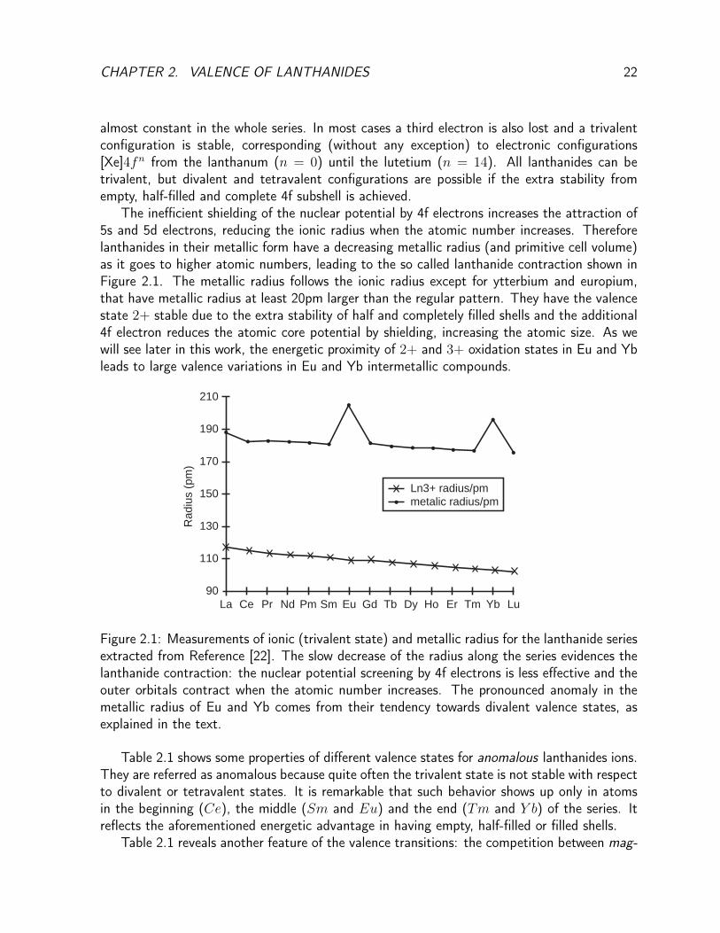
The inefficient shielding of the nuclear potential by 4f electrons increases the attraction of5s and 5d electrons, reducing the ionic radius when the atomic number increases. Thereforelanthanides in their metallic form have a decreasing metallic radius (and primitive cell volume)as it goes to higher atomic numbers, leading to the so called lanthanide contraction shown inFigure 2.1. The metallic radius follows the ionic radius except for ytterbium and europium,that have metallic radius at least 20pm larger than the regular pattern. They have the valencestate 2+ stable due to the extra stability of half and completely filled shells and the additional4f electron reduces the atomic core potential by shielding, increasing the atomic size. As wewill see later in this work, the energetic proximity of 2+ and 3+ oxidation states in Eu and Ybleads to large valence variations in Eu and Yb intermetallic compounds.
SPH SPH
JWBK057-02 JWBK057-Cotton December 9, 2005 14:3 Char Count=
14 The Lanthanides – Principles and Energetics
2.7 Atomic and Ionic Radii
These are listed in Table 2.3 and shown in Figure 2.4. It will be seen that the atomicradii exhibit a smooth trend across the series with the exception of the elements europiumand ytterbium. Otherwise the lanthanides have atomic radii intermediate between thoseof barium in Group 2A and hafnium in Group 4A, as expected if they are representedas Ln3+ (e−)3. Because the screening ability of the f electrons is poor, the effective nu-clear charge experienced by the outer electrons increases with increasing atomic number,so that the atomic radius would be expected to decrease, as is observed. Eu and Yb areexceptions to this; because of the tendency of these elements to adopt the (+2) state, theyhave the structure [Ln2+(e−)2] with consequently greater radii, rather similar to barium.In contrast, the ionic radii of the Ln3+ ions exhibit a smooth decrease as the series iscrossed.
The patterns in radii exemplify a principle enunciated by D.A. Johnson: ‘The lanthanideelements behave similarly in reactions in which the 4f electrons are conserved, and verydifferently in reactions in which the number of 4f electrons change’ (J. Chem. Educ., 1980,57, 475).
Table 2.3 Atomic and ionic radii of the lanthanides (pm)
Ba La Ce Pr Nd Pm Sm Eu Gd Tb Dy Ho Er Tm Yb Lu Hf
217.3 187.7 182.5 182.8 182.1 181.0 180.2 204.2 180.2 178.2 177.3 176.6 175.7 174.6 194.0 173.4 156.4La3+ Ce3+ Pr3+ Nd3+ Pm3+ Sm3+ Eu3+ Gd3+ Tb3+ Dy3+ Ho3+ Er3+ Tm3+ Yb3+ Lu3+ Y3+
103.2 101.0 99.0 98.3 97.0 95.8 94.7 93.8 92.3 91.2 90.1 89.0 88.0 86.8 86.1 90.0
2.8 Patterns in Hydration Energies (Enthalpies) for the Lanthanide Ions
Table 2.4 shows the hydration energies (enthalpies) for all the 3+ lanthanide ions, and alsovalues for the stablest ions in other oxidation states. Hydration energies fall into a patternLn4+ > Ln3+ > Ln2+, which can simply be explained on the basis of electrostatic attraction,
210
190
170
150
130
110
90La Ce Pr Nd Pm Sm Eu Gd Tb Dy Ho Er Tm Yb Lu
Ln3+ radius/pmmetalic radius/pm
Rad
ius
(pm
)
Figure 2.4Metallic and ionic radii across the lanthanide series.Figure 2.1: Measurements of ionic (trivalent state) and metallic radius for the lanthanide seriesextracted from Reference [22]. The slow decrease of the radius along the series evidences thelanthanide contraction: the nuclear potential screening by 4f electrons is less effective and theouter orbitals contract when the atomic number increases. The pronounced anomaly in themetallic radius of Eu and Yb comes from their tendency towards divalent valence states, asexplained in the text.
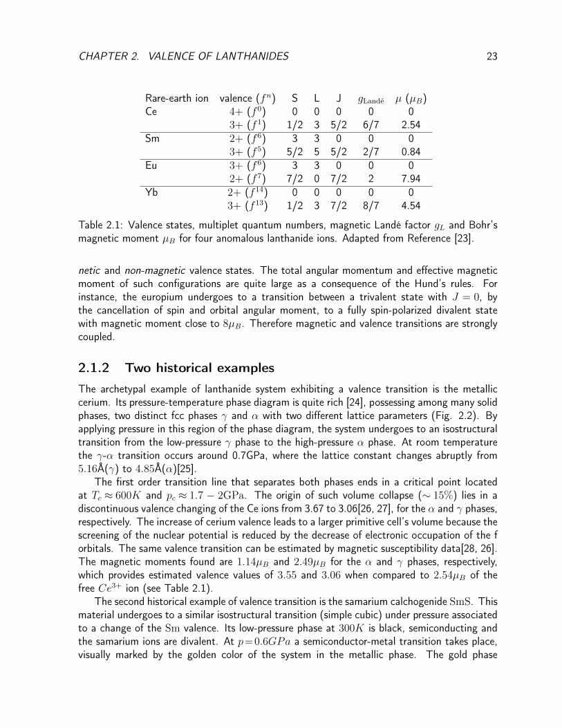
Table 2.1 shows some properties of different valence states for anomalous lanthanides ions.They are referred as anomalous because quite often the trivalent state is not stable with respectto divalent or tetravalent states. It is remarkable that such behavior shows up only in atomsin the beginning (Ce), the middle (Sm and Eu) and the end (Tm and Y b) of the series. Itreflects the aforementioned energetic advantage in having empty, half-filled or filled shells.
Table 2.1 reveals another feature of the valence transitions: the competition between mag-
CHAPTER 2. VALENCE OF LANTHANIDES 23
Rare-earth ion valence (fn) S L J gLande µ (µB)Ce 4+ (f 0) 0 0 0 0 0
3+ (f 1) 1/2 3 5/2 6/7 2.54Sm 2+ (f 6) 3 3 0 0 0
3+ (f 5) 5/2 5 5/2 2/7 0.84Eu 3+ (f 6) 3 3 0 0 0
2+ (f 7) 7/2 0 7/2 2 7.94Yb 2+ (f 14) 0 0 0 0 0
3+ (f 13) 1/2 3 7/2 8/7 4.54
Table 2.1: Valence states, multiplet quantum numbers, magnetic Landé factor gL and Bohr’smagnetic moment µB for four anomalous lanthanide ions. Adapted from Reference [23].
netic and non-magnetic valence states. The total angular momentum and effective magneticmoment of such configurations are quite large as a consequence of the Hund’s rules. Forinstance, the europium undergoes to a transition between a trivalent state with J = 0, bythe cancellation of spin and orbital angular moment, to a fully spin-polarized divalent statewith magnetic moment close to 8µB. Therefore magnetic and valence transitions are stronglycoupled.
2.1.2 Two historical examples
The archetypal example of lanthanide system exhibiting a valence transition is the metalliccerium. Its pressure-temperature phase diagram is quite rich [24], possessing among many solidphases, two distinct fcc phases γ and α with two different lattice parameters (Fig. 2.2). Byapplying pressure in this region of the phase diagram, the system undergoes to an isostructuraltransition from the low-pressure γ phase to the high-pressure α phase. At room temperaturethe γ-α transition occurs around 0.7GPa, where the lattice constant changes abruptly from5.16Å(γ) to 4.85Å(α)[25].
The first order transition line that separates both phases ends in a critical point locatedat Tc ≈ 600K and pc ≈ 1.7 − 2GPa. The origin of such volume collapse (∼ 15%) lies in adiscontinuous valence changing of the Ce ions from 3.67 to 3.06[26, 27], for the α and γ phases,respectively. The increase of cerium valence leads to a larger primitive cell’s volume because thescreening of the nuclear potential is reduced by the decrease of electronic occupation of the forbitals. The same valence transition can be estimated by magnetic susceptibility data[28, 26].The magnetic moments found are 1.14µB and 2.49µB for the α and γ phases, respectively,which provides estimated valence values of 3.55 and 3.06 when compared to 2.54µB of thefree Ce3+ ion (see Table 2.1).
The second historical example of valence transition is the samarium calchogenide SmS. Thismaterial undergoes to a similar isostructural transition (simple cubic) under pressure associatedto a change of the Sm valence. Its low-pressure phase at 300K is black, semiconducting andthe samarium ions are divalent. At p=0.6GPa a semiconductor-metal transition takes place,visually marked by the golden color of the system in the metallic phase. The gold phase

CHAPTER 2. VALENCE OF LANTHANIDES 24
4 J M Lawrence, P S Riseborough and R D Parks
I I I I 1
Ce SmS 750 - -
- 8
-
1 I 1 I
density (a0=4.85 A) 01 state; it is an isomorphic phase transition (there is no change in the crystal symmetry) and the phase boundary terminates at a critical point (figure 1). The large (15 %) cell volume change associated with the lattice collapse arises from a change in electronic structure. In the y state the cerium ions primarily have the trivalent 4fl(5d6s)3 structure; application of pressure increasingly favours the tetravalent 4f0(5d6s)4 structure. There is a large decrease in radius for the tetravalent atoms because removal of the 4f electron decreases the screening of the nuclear charge so that the outer 5d6s valence electrons are sucked in closer to the nucleus. The valence (z) in the 01 state is not four, however. One form of evidence, based on the empirical correlations between valence and metallic radius which are found in the periodic table, suggests a non-integral valence, midway between z = 3 and z = 4 (Gschneidner and Smoluchowksi 1963). In a plot of metallic radius against atomic number (figure 2) a-Ce does not lie on the smooth extrapolated curve for tetravalent elements, but at an intermediate position, such that one would assign by linear interpolation an intermediate valence (IV), z = 3.67.
A similar isomorphic valence transition occurs in SmS (figure 1) which is an ionic solid with the rock-salt structure. In the low-pressure phase (B-SmS) it is a black, divalent 4f6(5d6s)2 semiconductor; under application of 6 kbar pressure the lattice collapses as the material undergoes an insulator-metal transition to a metallic phase (M-SmS) where the material turns golden as the plasma edge moves into the visible. The valence/radius correlations (figure 2) suggest that in the M phase the material is not fully trivalent 4f5(5d6s)3 but rather has a non-integral valence z=2.75 (for a review see Jayaraman et a1 1975b).
Valence transitions can also be driven at ambient pressure by alloying in Cel-2RE2, Sml-sRE5S or SmSl-%M,. (we will use the notation of RE to represent a rare earth or related solute; M represents a pnictide.) The phase diagrams are similar to figure 1 with x replacing P. Hence for x > xo z 0.15 at ambient conditions the alloy Sml-,GdzS is in an IV state. In addition, many compounds of cerium, samarium, europium, thulium and ytterbium exhibit non-integral valence at ambient conditions, e.g. CeN, SmBs, EuRh2, TmSe or YbAIz.
1.2.2. The mixed-valent state. A necessary condition for non-integral valence is that two bonding states 4f%(Sd6s)m and 4f%-1(5d6s)"+x of the rare earth be nearly degenerate. A
Figure 2.2: Phase diagram for metallic Ce (left) and SmS (right) extracted from Reference[23].
(M-SmS) has an intermediate valence Sm2.75+ determined by lattice measurements.Metallic Ce, SmS and other mixed valence have been studied intensively between the
decades of 1970 and 1980. For further details on these experiments and on the differentaspects of the problem covered in this chapter the reviews of Varma[29], Khomskii[30] andLawrence et al.[23] are suggested.
2.1.3 General aspects of intermediate valence states
First of all, an important distinction should be made between homogeneous and inhomogeneousmixed-valence states2. In both cases the lanthanide average valence is different from a integervalue, but locally the valence behavior is completely different. In an inhomogeneous mixed-valence state each ion in the lattice is in a well defined (integer) valence state and ionswith different valences occupy inequivalent positions, generating a charge ordered state. Twoexamples of rare-earth materials with charge ordered states are Eu3S4 and Sm3S4[31].
In homogeneous mixed-valence systems all the ions occupy equivalent lattice sites, theaverage valence in each ion is the same and it is not an integer value. The valence state is in aquantum mechanical state described by a linear combination of two different valence states:
|ψ〉=a |fn〉+b∣∣fn+1
⟩, (2.1)
Other states are excluded in the combination due to the large Coulomb repulsion inside forbitals.
The condition to have an intermediate valence state is that both atomic levels En andEn+1 are close to each other and both close to the Fermi energy. In reality, since the f levelsweakly hybridize with the other electronic states (spd bands), there is a finite width ∆ (Eq.
2The nomenclature employed here follow the same lines present in Varma’s review on mixed valence[29].

CHAPTER 2. VALENCE OF LANTHANIDES 25
1.4) for these states. So it is required that |En−En+1|<∆ in order that the mixed valencestate exists.
It is important from the beginning to differentiate the mixed-valence state from the Kondostate formed in magnetic impurities (see Figure 1.1). Contrary to the Kondo state, the for-mation of the local moment in the mixed valence state is forbidden by the very large chargefluctuations in the f level. The valence is related to the coefficients in a wave-function as inEq. 2.1 and its value ranges between two integers. Since one can go continuously from theKondo to the mixed valence case , it is very hard (if not impossible) to characterize a systemas ”purely” Kondo or mixed-valence. An attempt to separate the two physical scenarios is theanalysis of valence transitions. Given that the Kondo regime requires a nearly integer valencestate, while in a mixed-valent state it is not necessary, one could naively state that everytransition in which the valence variation is small, the dominant effect for valence changing isKondo effect. However, if the valence variation is large, it is connected to the competition oftwo different atomic ground states for f electrons (mixed-valence). Unfortunately the physicalsituation is much more complex than that and such classification can not be taken as granted.
2.2 Experimental techniques to measure valence
In Section 2.1 we reviewed some general aspects of valence fluctuation and chemical propertiesof lanthanide ions and monoatomic metallic systems. In this section we discuss some relevantexperimental features observed in lanthanide systems with valence fluctuations that motivateour theoretical work.
The purpose of this chapter is to give a brief introduction to experimental techniques from atheorist point of view, which is far from being complete and rigorous. In Section 4.3 we presentanother experimental discussion, focused on specific systems, where we may recall some pointsdiscussed below.
2.2.1 Time-scales of valence fluctuation
If the valence state of a given ion in the metallic environment is a linear superposition oftwo nearly degenerate valence configurations, it means that it is possible to associate a time-scale to the fluctuation between these configurations. As we saw in Section 1.1.1, the chargefluctuation of a f level has a characteristic energy ∆ (Eq. 1.4), the f-level width, and it isinversely proportional to the characteristic time of fluctuations.
Let us suppose, for the sake of the argument, that ∆∼ 1meV for two nearly degeneratevalence states in a rare-earth atom. Then a good estimative for the characteristic time ofvalence fluctuations is given by
τvf∼h
∆∼10−12s, (2.2)
where h=4.135× 10⁻¹⁵eV · s is the Planck constant.The characteristic time of valence fluctuations is an important issue regarding the experi-
mental observation of this phenomenon. If the experiment probes the system in a time larger

CHAPTER 2. VALENCE OF LANTHANIDES 26
than τvf , then the observed valence is an average of two valence configurations. On the otherhand, if the experiment operates in a time-scale smaller than τvf , one can resolve both valencestates independently. Hence there are two possible types of measurements for the valence:slow and fast measurements.
The experimental time-scale τext depends on many factors, which include the energy of theprobe (for example, photons or neutrons) and the underlying physical mechanisms occurring inthe system during and after the interaction with the probe. Since in many cases the estimateτext is rather imprecise or dubious and a deeper discussion on the experimental techniques isout of the scope of the present work, we restrict ourselves to the division between static anddynamic measurements.
2.2.2 Static measurements
Structural analysis by X-ray diffraction
As we saw in Section 2.1.1, there is a direct relation between the metallic radius and thevalence state. If one can synthesize a family of compounds with different rare-earth ions, forexample ReO (being Re a lanthanide) or a metallic Re, it would be possible to compare thelattice parameters (measured, for instance, from X-ray diffraction) and extrapolate the averagevalence. One example of this comparative analysis was employed to explain the anomalousbehavior of Eu and Yb seen in Figure 2.1. In another type of experiment one could measurethe variation of unit-cell parameters for the same compound in different external conditions(temperature, external pressure and others). For instance, the well-known α-γ transition ofmetallic cerium, in which a substantial volume variation is detected.
The basic hypothesis employed in lattice measurements is that any volume change is mainlyan effect of a valence variation, but other mechanisms can modify the lattice parameters. Forinstance, in real materials the application of pressure (or doping) can modify the band structureeven if the valence keeps constant.
Lattice constant measurements is a comparative method which requires an initial knowledge(or guess) for the valence in a given compound or under certain conditions, which is anotherimportant limitation. Nevertheless, this method is useful to predict phase transitions andanomalous valence states and it has its historical importance in the field that makes it worthto mention.
Magnetic measurements
Other possible experiments that reveal intermediate valence states are the magnetic suscepti-bility measurements. In an homogeneous mixed valence state containing one magnetic and onenonmagnetic configuration as present in Equation 2.1, it is expected that fluctuations wouldprevent magnetic ordering at low temperatures. For example, SmS in its intermediate valencephase (metallic) is non-magnetic at very low temperatures [32, 33].
The temperature behavior of magnetic susceptibility in a true mixed valent state is thefollowing: at high temperatures, the susceptibility follows a Curie’s law χ(T ) = C/T , where Cis proportional to the average between the magnetic moments in the two valence states weighted

CHAPTER 2. VALENCE OF LANTHANIDES 27
by the contribution of each one in the valence. This behavior is also seen in inhomogeneousmixed-valence states, so both types of intermediate valence can not be distinguished from themagnetic susceptibility in this range of temperatures.
Homogeneous mixed-valence states generally do not order at low temperature. One ex-ception is thulium, since the two relevant valence states are magnetic. The magnetic orderis inhibited by the strong local charge fluctuations. When the system approaches the zerotemperature the magnetic susceptibility reaches a constant value.
A phenomenological expression for the magnetic susceptibility of intermediate valence sys-tems was given by Sales and Wohleben[34]:
χ(T ) =µ2nv(T ) + µ2
n−1(1− v(T ))
T + Tvf(2.3)
Here µn and µn−1 are the magnetic moments for the 4fn and 4fn−1 states, respectively.v(T ) represents the average valence of the rare-earth ion that, in principle, depends on thetemperature. This formula has a Curie-Weiss behavior in which the characteristic energy scaleof valence fluctuation Tvf (proportional to the width of the virtual level ∆) acts as a Curietemperature. Note that at zero temperature it predicts χ(0)=µ2v(0)/Tsf if there is only onemagnetic valence state (with moment µ) in the mixture.
2.2.3 Dynamical measurements
Mössbauer spectroscopy
Mössbauer spectroscopy[31] probes the shifts in nuclear transition energies due to differentenvironments for the atomic nucleus, through the atomic absorption and emission of energeticgamma rays. One part of this effect comes from the difference of s electron densities that,in the context of interest here, can be attributed to the addition or removal of 4f electrons.With less electrons in the 4f orbitals there is less nuclear screening and, consequently, the 5selectronic shell comes closer to the nuclear core. This is called isomer shift 3.
There are at least two important features in Mössbauer spectra in the context of valencedetermination. The average line shift is a measure of the average f orbitals occupation, whilethe linewidth is related to its fluctuations. Since it probes several ions in the crystal, thistechnique is capable of differentiate the inhomogeneous from the homogeneous intermediatevalence states. In the former case it is seen as the apparition of two separated spectral linescorresponding to two valence states. Contrastingly, the homogeneous case gives a singlespectral line positioned between those of well defined valence states are expected (Figure 2.3).
The isomer shift measurement is considered a slow technique since it does not separate thetwo states that compose the mixed-valence. Estimation of characteristic time provided by Coeyand Massenet [31] is on the order of 10−9s, which is well above the estimated τvf∼10−12s.
In addition to the fact that the Mössbauer technique is suitable enough to rule out theexistence of inhomogeneous mixed-valence states, it has a good experimental resolution even
3It is also named chemical shift, since it is sensitive to different covalent bondings (formed from s electrons).

CHAPTER 2. VALENCE OF LANTHANIDES 28
Figure 2.3: Mössbauer spectra for Eu on the inhomogeneous mixed-valent Eu3S4 (left) [31] andthe homogeneous EuRb2 (right) [35] as a function of the temperature. In the inhomogeneouscase two peaks appear in the spectrum at low temperatures, corresponding to two differentvalence states of europium in inequivalent lattice sites. For an homogeneous mixed-valencestate only one peak is seen and its position varies with the temperature, signaling a variationin the average valence. Figure extracted from Reference [30].
in early measurements. One of the issues is again the necessity to compare the isomer shift fora given system with a similar one, which is very bad to extract quantitative results. Finally, thistechnique can only be applied to Mössbauer active elements, that includes all the lanthanideelements with the important exception of cerium.
Neutron scattering
Techniques involving neutrons are very useful to determine the existence and the propertiesof magnetic ordering in solids and the characteristics of many types of excitations. Thereare two types of neutron scattering measurements: neutron diffraction and inelastic neutronscattering. Neutron diffraction allows, among other things, to determine magnetic peaksassociated to magnetic order and the magnetic moment values. This technique is, in mostcases, not particularly relevant for intermediate valence compounds, since very often thesesystems are in non-magnetic ground states dominated by strong charge fluctuations.
Contrary to the former example, the inelastic (and quasielastic4) neutron scattering revealsimportant aspects of the intermediate valence regime[23, 36]. The mixed-valence state man-ifests itself through a temperature-independent large linewidth of the quasielastic peak thatis claimed [36] to be proportional to ∆ (Eq. 1.4). For instance, the values of ∆ obtained
4Even that the two techniques are different from the experimental point of view, the physical interpretationcan be thought as the same in a superficial consideration.
CHAPTER 2. VALENCE OF LANTHANIDES 29
from the spectra of YbCu2Si2 and CePd3 are ∼ 30meV and ∼ 40meV , respectively. Theselinewidths are two orders of magnitude larger than those of a rare-earth material in a stablevalence configuration[36].
Inelastic neutron scattering can also determine whether the spin dynamics is related tothe charge fluctuations or the Kondo effect. While in the former case the linewidth does notdepend on the temperature, in the latter it increases considerably with T . This behavior is seenin both Kondo lattice (CeCu2Si2 and CeAl3) and Kondo impurity (Fe in Cu) systems[36].
Resonant Inelastic X-Ray Scattering
Among all the techniques to measure the valence of materials, the most accurate is the resonantinelastic X-ray scattering[37]. It is a spectroscopic technique in which a very energetic photoninteracts with electrons in deep-lying electronic levels, promoting them to empty states thatlater decay, emitting another photon with different momentum and energy. Through theanalysis of the energy, momentum and polarization of the scattered photon it is possible todetermine the properties of excitations in the system.In order to enhance the scattering crosssection, it is crucial to choose the photon energy to be in one of the atomic X-ray transitionsof the system (the resonant character). RIXS is element dependent, since one can select eachatom on the material through the photon energy. Also it is orbital dependent from the selectionrules involving the photon’s emission and absorption.
The accuracy on the valence measurements by RIXS technique comes from the fact thatone can identify each valence state by a peak in the spectrum. Both peaks are fitted bygaussian functions and their integrated weights are compared in order to extract the averagevalence. For instance, if two valence states 4fn and 4fn+1 forms an intermediate valence state,then the valence extracted from RIXS experiment is (I(n) is the integrated weight of the peakassociated to the 4fn state):
v = n+I(n+ 1)
I(n) + I(n+ 1)(2.4)
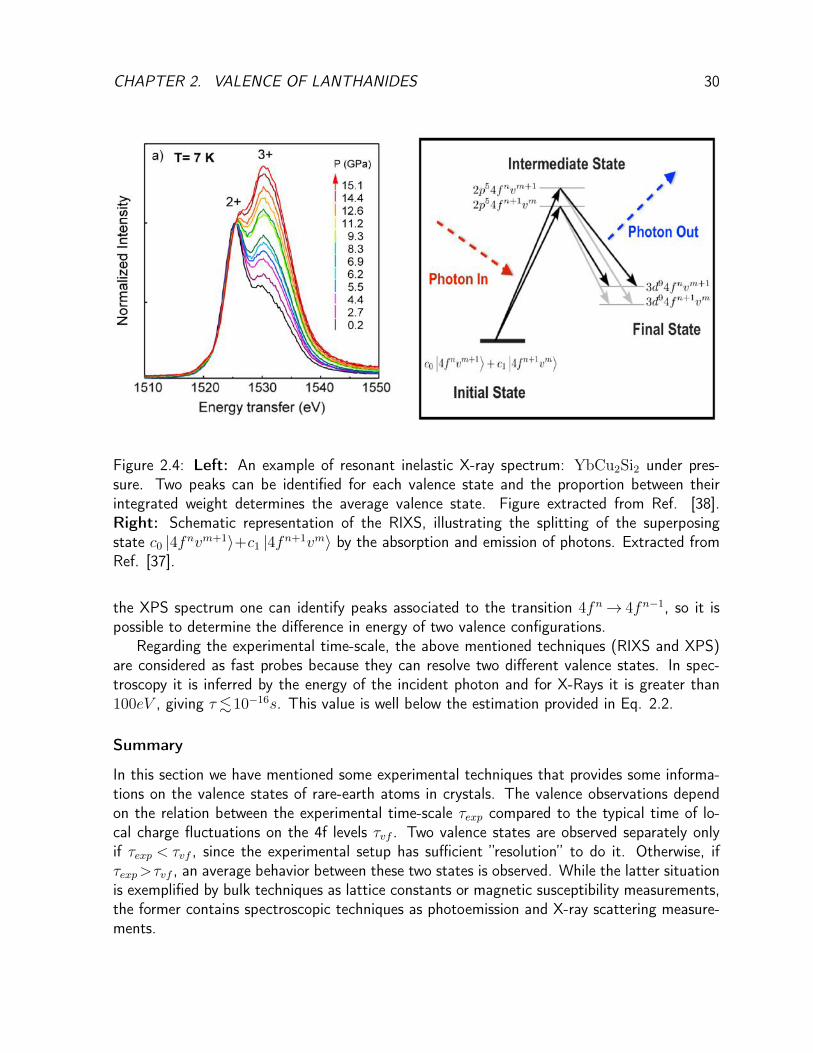
Let us see in more detail the resonant X-ray technique for the case of ytterbium. In Figure2.4 (right) the processes occurring in the Yb atom are schematically depicted. The initial stateis an intermediate valence state between 4fn and 4fn+1 (v are the other valence electronscoming from spd orbitals). A highly energetic photon is absorbed by the atom and a 2p coreelectron is excited above the Fermi level, generating the excited state. The energy of suchstate depends on the number of 4f electrons through their interaction with the 2p core-holestate. Then a second core electron, here from 3d orbital, fills the core-hole and excited statedecays by the emission of a photon. The energy of the final states also depend on the amountof f electrons, so the initially mixed state is separated in two. This separation is seen in thespectra on Figure 2.4(left).
RIXS is the most precise spectroscopic technique for valence transition, nevertheless thereare other examples. The pioneer example in this context is X-Ray Photoemission Spectroscopy(XPS)[39]. Photoemisson consists in sending a high energetic photon to the material andmeasure the energy of the electron taken from the interaction with the absorbed photon. From
CHAPTER 2. VALENCE OF LANTHANIDES 30
Figure 2.4: Left: An example of resonant inelastic X-ray spectrum: YbCu2Si2 under pres-sure. Two peaks can be identified for each valence state and the proportion between theirintegrated weight determines the average valence state. Figure extracted from Ref. [38].Right: Schematic representation of the RIXS, illustrating the splitting of the superposingstate c0 |4fnvm+1〉+c1 |4fn+1vm〉 by the absorption and emission of photons. Extracted fromRef. [37].
the XPS spectrum one can identify peaks associated to the transition 4fn→ 4fn−1, so it ispossible to determine the difference in energy of two valence configurations.
Regarding the experimental time-scale, the above mentioned techniques (RIXS and XPS)are considered as fast probes because they can resolve two different valence states. In spec-troscopy it is inferred by the energy of the incident photon and for X-Rays it is greater than100eV , giving τ.10−16s. This value is well below the estimation provided in Eq. 2.2.
Summary
In this section we have mentioned some experimental techniques that provides some informa-tions on the valence states of rare-earth atoms in crystals. The valence observations dependon the relation between the experimental time-scale τexp compared to the typical time of lo-cal charge fluctuations on the 4f levels τvf . Two valence states are observed separately onlyif τexp < τvf , since the experimental setup has sufficient ”resolution” to do it. Otherwise, ifτexp>τvf , an average behavior between these two states is observed. While the latter situationis exemplified by bulk techniques as lattice constants or magnetic susceptibility measurements,the former contains spectroscopic techniques as photoemission and X-ray scattering measure-ments.
CHAPTER 2. VALENCE OF LANTHANIDES 31
2.3 Models for valence transitions
Having reviewed in Section some experimental manifestations of the intermediate valence statesof rare-earth ions, we put in perspective the theoretical models proposed to describe the valenceproperties. Since the literature on the subject is vast, we limit ourselves to the presentation ofmodels that we consider the most pertinent.
In the first subsection the mixed valence regime on the single impurity (SIAM) and periodicAnderson(PAM) models is discussed. While the PAM describes well the crossover from theKondo to the intermediate valence regimes and continuous valence transitions, it fails in providea mechanism to the discontinuities observed in many materials. For that purpose, we discussin the last two subsections the Falicov-Kimball model, which is historically the first model thatdescribes the discontinuous valence transitions, and models containing explicit volume effects(Kondo Volume Collapse), which are a second route to understand the pressure dependence invalence for some compounds.
2.3.1 Anderson impurity and lattice models
The single impurity Anderson model (Eq. 1.1) has an intermediate valence regime dependingon its parameters, as it was discussed in Section 1.1.1. The rough criterion for intermediatevalence in SIAM depends on the position of the impurity levels (Ef and Ef+U) with respectto the Fermi level µ and their width ∆ (defined in Eq.1.4) due to the hybridization with theconduction electrons. If |Ef−µ|<∆ or if |Ef+U−µ|<∆, then the broaded level "cuts" theFermi energy and the electronic occupation on the impurity level is non-integer5. The situationcorresponding to the condition |Ef−µ|<∆ was depicted in Fig. 1.1.b and the impurity hasnf<1 electrons.
The intermediate valence case corresponds to the asymmetric regime of Anderson model(U�|Ef |,∆) and it was studied by Haldane using scaling theory[40]. He had shown that thecriterium for a mixed-valence regime in this model is |E∗f |.∆, where
E∗f = Ef +∆
πln
(D
∆
)is the scaling-invariant "effective position" of the local level Ef . In this regime the chargefluctuations do not disappear by the scaling procedure and the occupation on the impurity sitenf is not integer at T = 0.
The situation above should be contrasted to −E∗f � ∆, in which the charge fluctuationsare frozen for T �∆ and a local moment is stable. In this case the system is in the Kondolimit, where the Kondo model is valid. The passage from the two situations described here iscontinuous and the physical quantities, such as the occupation nf , susceptibility and specificheat, are smooth universal functions of E∗f/∆. As a consequence, it is hard to separate bothregimes from the experimental point of view. Besides, the SIAM is unable to describe coherent
5Given the large value of U in f orbitals, the second condition is not expected in real systems

CHAPTER 2. VALENCE OF LANTHANIDES 32
effects from the dense regime, which play a very important role at low temperatures. For thatreason it is appropriate to discuss the lattice model.
Regarding the local charge fluctuations on the f level, the condition to obtain a mixed-valence state in the Periodic Anderson Model (Eq. 1.9) is the same as in single impuritymodel, i.e. |Ef−µ|<∆. The difference comes from the fact that the Fermi energy µ is fixed.In the SIAM, µ does not depend on the impurity occupation and it is determine purely by theconduction electrons concentration nc. In the PAM, the Fermi level depends on the local levelsoccupation, since the total number of electrons is conserved, independently if they are in locallevels or in the band.
In the intermediate valence state of PAM the Fermi energy is pinned in the 4f level peak (lo-cated in Ef ). Any large change in the valence leads to a feedback in the chemical potential[1],restoring the valence value. It occurs because the conduction electron density of states ismuch smaller than the contribution from the f electrons, so it is difficult to accommodate theelectrons leaving the f orbitals in the band. As a consequence, the valence variation describedby the PAM is always small if other effects are not taken into account.
From the experimental point of view two situations may arise: the valence variation canbe continuous or not. The discontinuity can accentuate the passage from the Kondo to theintermediate valence regime if one of the valence configurations is close to the magnetic one,as in the α phase of metallic Ce. For continuous variations the passage is not marked, howeverone estimative can be done through the Sommerfeld coefficient γ of specific heat, that isexpected to be one order of magnitude higher in the Kondo regime (since it is a heavy fermion)than in the intermediate valence. The coefficient γ in the mixed valence regime is larger thanthose in ordinary metals, since the density of states at the Fermi energy is enhanced by itsproximity to the f level.
The major drawback in the PAM is the absence of mechanisms allowing large valencechanges, which is in contrast to the experimental examples presented in Section 2.1.2. Forthat reason, we present in the next subsection the Falicov-Kimball model, which describescontinuous and discontinuous valence variations. Lastly, the Kondo Volume Collapse modeland its description of volume instabilities in metallic Ce are discussed.
2.3.2 The Falicov-Kimball model
The first model used to describe the behavior of valence transitions in rare-earth materialswas proposed by L. Falicov and J. Kimball in 1969 [41]. Their purpose was to study thesemiconductor-metal transition of some transition-metal oxides and SmB6
6 by the analysis ofdifferent intra-atomic interactions involving Bloch (conduction electrons) and Wannier statesfrom 4f orbitals (or 3d for the transition metals). The hamiltonian is written as:
HFK =∑kσ
ε(k)c†kσckσ +∑iσ
Eff†iσfiσ + Ufc
∑iσσ′
nfiσnciσ′ (2.5)
The notation is the same as in the PAM (Eq. 1.9), defined in Chapter 1. The last term in Eq.
6SmB6 is nowadays classified as a Kondo Insulator [42].

CHAPTER 2. VALENCE OF LANTHANIDES 33
(2.5) describes the repulsive interaction Ufc between conduction and local electrons 7. Falicovand Kimball [41] established that critical interaction value U∗fc separates continuous variations ofthe local levels occupation (Ufc<U∗fc) as a function of Ef to first-order transitions(Ufc>U∗fc),where occupation jumps appeared.
The model in Equation 2.5 was studied using several approximations (analytical and nu-merical) and for different dimensions and lattice structures. Early works from Gonçalves daSilva and Falicov [43], Khomskii and Kocharjan [44], Hewson and Riseborough[45] and Singhet al. [46] pointed out the role of an additional hybridization in the Falicov-Kimball modelusing Hartree-Fock approximation. As a general result, these papers have confirmed the as-sertion that the repulsive interaction Ufc, if sufficiently large, would lead to valence jumps asa function of external parameters (incorporated by Ef ) at T =0.
Recently the Falicov-Kimball model was subject of several other studies, mainly becauseits spin-less version can be seen as a simplified Hubbard model in which DMFT equations areexactly solvable. These considerations are out of the scope of the present thesis and the reviewarticle by Freericks and Zlatić [47] is recommended in this context.
2.3.3 Models explicitly including volume effects
Models containing explicitly volume effects were proposed to understand the unusual behavior inthe γ-α transition of metallic Ce (cf. Section 2.1.2). In this compound a pressure-induced firstorder transition at 0.7GPa appears with a volume change close to 15%, as it was discussedin Section 2.1.2. The general idea of such models comes from the empirical fact that theKondo temperature is strongly dependent on the volume[48, 49, 50]. Neutron scatteringmeasurements of the resonant level width Γ, which is proportional to the Kondo temperature,give Γγ =6−16meV and Γα>70meV for the γ and α phases of Ce, respectively[50].
The Kondo Volume Collapse model was proposed in 1982 concurrently by two differentgroups[51, 52]. Allen and Martin [51] have shown that an additional contribution to the free-energy from the coupling between 4f and conduction electrons must be considered. They haveobtained from the equation of state, fed by experimental values, a first order transition with acritical endpoint close to pc=0.7GPa and Tc=850K. The estimated Kondo temperature areTKγ =54K and TKα=765K, which are close to the experimental results mentioned above.
In the work of Lavagna and collaborators[52] the Kondo lattice model was studied in themean-field approximation[53] with a volume-dependent Kondo coupling TK(V)∼ e−(V−V0)/V0
(V0 is the volume at zero pressure). Following the same reasoning as above, they have obtainedthe isotherms in the p-V phase diagram.
The issue of Kondo Volume Collapse in the γ-α transition was later addressed from ab initiocalculations using a combination of density functional theory (DFT) and dynamical mean-fieldtheory[54, 55, 56]. Within this approach it is possible to incorporate the full set of f orbitalsand the realistic band structure in the presence of strong correlations [57]. The results can besummarized by the figure 8 in Reference [55]. It shows an increasing spectral weight in the
7In the original work by Falicov and Kimball the local states represents holes, and not electrons, and Ufc isan attractive interaction instead of a repulsive one. Nevertheless it will be adopted the electronic version hereto simplify the connection to our work later.

CHAPTER 2. VALENCE OF LANTHANIDES 34
Fermi energy when the lattice volume is reduced, accompanied by a reduction of spectral weightin the Hubbard satellites. This corresponds to an increasing valence for Ce and a delocalizationof the 4f electrons, as observed in experiments.
2.4 Summary
Let us summarize the aspects of valence transitions in lanthanide systems presented in thischapter. Firstly we have discussed the anomalous behavior of some lanthanide ions (such asCe, Yb and Eu) in a crystalline environment that possesses two valence configurations veryclose in energy. It leads to an intermediate valence value that can be modified by applyingpressure or doping the system. One example of such behavior is the metallic Ce (Section2.1.2), in which the Ce valence vary discontinuously (at room temperature) from 3.06 to 3.67by the application of pressure.
In Section 2.3 some techniques to perform valence measurements were presented. We haveseparated the techniques with respect to static and dynamic measurements. The former typerelates the lanthanide valence to crystallographic and magnetic properties of the compound.In the latter group are placed more accurate and "modern" techniques, allowing a precisedetermination of valence. From this group we highlight the resonant inelastic X-ray scatteringtechnique, which has been largely employed in the latest experimental works on the subject.
Lastly the most relevant models for valence transitions in rare-earth systems were discussed.The standard description is given by the Periodic Anderson model, which contains the Kondoand the intermediate valence regime and coherence among f electrons is taken in account(contrary to the single impurity model). Its major problem in the context of valence transitionsis the absence of mechanisms to make it discontinuous, required to describe the compoundslike the metallic Ce.
Two possible improvements on the issue of discontinuous transitions are the inclusion of alocal electronic repulsion among conduction and localized electrons (Falicov-Kimball interac-tion) or explicit volume effects (volume collapse models). While the volume collapse approachis focused on the Kondo lattice regime, the Falicov-Kimball interaction plays a big role in themixed-valence phase and it might be the origin of first-order transitions for compounds withlarge valence changes. Having it on mind, we will present in details the model chosen todescribe valence transitions in the thesis.
Chapter 3
The Extended Periodic AndersonModel
In this chapter we present the model that will be employed in the description of valencetransitions of lanthanide compounds. The basic idea is to include in the Periodic Andersonmodel (Eq.1.9) an additional Falicov-Kimbal interaction (Section 2.3.2) in order to have thecombined effects of Coulomb repulsions (intraorbital and interobital) and the hybridizationbetween the two orbitals. As we shall confirm in the next chapter results, the Falicov-Kimballinteraction will be the driving mechanism to render valence transitions discontinuos, what isnot expected in the original PAM.
The Extended Periodic Anderson model (EPAM) hamiltonian is the following:
HEPAM =∑kσ
ε(k)c†kσckσ + Ef∑iσ
f †iσfiσ + U∑i
nfi↑nfi↓
+ V∑iσ
(c†iσfiσ + f †iσciσ
)+ Ufc
∑iσσ′
nfiσnciσ′ (3.1)
In this hamiltonian, ε(k) is the kinetic energy of conduction electrons (being D its band-width), Ef is the energy of local (f ) level in each site of the lattice, U is the Coulomb repulsiongiven that the local level in the site i is doubly occupied, V is the hybridization between theconduction band and f orbitals and Ufc is the local Coulomb repulsion among conduction and felectrons. We will consider a fixed total (c+f) number of electrons per lattice site ntot, whichdetermine the chemical potential µ.
The model above retains a priori the most relevant physical aspects of the problem. Forinstance, we are keeping only a single f orbital instead of the seven possible in the case (L=3),which is justifiable by the considerations of the Hund’s rules and crystal field done in Section4.2.2. The hybridization is assumed constant, even though it may have a k-dependence forsymmetry reasons.
The EPAM hamiltonian in Eq. 3.1 cannot be solved without using approximations for theinteracting terms. Obviously the approximation scheme must be consistent with the energy
35

CHAPTER 3. THE EXTENDED PERIODIC ANDERSON MODEL 36
magnitudes of the system that we want to describe, then let us point out briefly the energyscales of the problem, and afterwards we present our approximation scheme to solve thisproblem.
3.1 Energy scales in EPAM
The kinetic energy of conduction electrons is roughly proportional to the bandwidth of eachmaterial, which depends (among other things) on the type of relevant orbitals that combineto form the conduction band. In a common metal, containing mainly s and p orbitals, thebandwidths are as large as 10eV . However these typical values are one order of magnitudesmaller (1eV ) for intermetallic systems, since the composition of the relevant conduction bands(those that are close to the Fermi energy) contain an important amount of d orbitals.
Regarding the hybridization values, it also depends on the material band structure. It corre-sponds to the overlap between the atomic 4f wave-functions and the Bloch states representingconduction electrons. Its typical values are 0.1eV .
The f level energy, Ef , is not a simple quantity to be measured experimentally. In order toachieve an intermediate valence state it is crucial that the local level lies inside the conductionband, otherwise one would obtain only integer values for the valence. In this case Ef must bein the same range of energy as the electronic bandwidth (1eV ). One would expect that thevalence variations in this model happen when Ef is close to the chemical potential, a picturethat will be verified in the results of Chapter 4.
Lastly the energy scales of the two Coulomb interactions, U and Ufc, must be analyzed.Even if they share the same physical origin, the electromagnetic interaction between pairs ofelectrons, their magnitudes are quite different. The intra-orbital interaction U is, by far, thelargest energy involved in the problem. Its values observed by photoemission and absorptionexperiments in rare-earth ions are in the range of 5 to 10eV .
Term Energy scaleD 1 eVEf 1 eVV 0.1 eVU 5-10 eVUfc ? eV
Table 3.1: The energy magnitude of each term in hamiltonian 3.1.
The value of Ufc interaction
The most important question that arises in the analysis of the energy scales of the EPAM isthe value of the interaction Ufc. This question, as far as I know, is still open and there is notmuch information in the literature.

CHAPTER 3. THE EXTENDED PERIODIC ANDERSON MODEL 37
Within a first principle approach, Ufc should be calculated from an expression of the type:
Ufc =
∫φ∗c(r
′)φ∗f (r)e2
|r− r′|φc(r′)φf (r)drdr′ (3.2)
Here φc(r) and φf (r) are the Wannier functions corresponding to conduction and localizedelectrons. This direct Couloumb interaction is strongly reduced by screening effects and quiteoften is neglected in other compounds. In lanthanides it might be relevant if φc(r) contains alarge contribution from d orbitals.
The simple argument that relates the magnitude of Ufc to the amount of d orbitals thatform the conduction band is qualitatively verified in two cerium compounds: metallic Ce andCeCu2Si2. The former compound possesses d states close to the Fermi energy, while in thelatter s and p orbitals from the anionic part are dominant. Then Ufc is expected to be largerin Ce than in CeCu2Si2, and only one of them, Ce, shows a first-order valence transition. Adetailed discussion of several compounds will be done in Section 4.3 and the point made hereto justify the addition of the Falicov-Kimball interaction will be reviewed.
3.2 Previous works
The EPAM was studied in several works. An early study [46] on the context of Falicov-Kimballmodel have pointed out the suitability of EPAM for the valence transitions in SmS. Therebirth of the model came in 2000 when Onishi and Miyake proposed [58, 59] its use to explainthe unusual superconductivity of CeCu2Si2[60], in which the superconducting dome has ananomalous pressure dependence.
Further investigations using different methods were made. The magnetic field dependenceof valence transitions was studied in slave-boson mean-field theory [61] and applied to com-pounds as CeRhIn5 [62] and YbXCu4 (X=In,Ag,Cd)[63]. In unidimensional systems DMRGwas employed to analyse charge, spin and superconducting correlations [64, 65], confirming theconnection between valence fluctuations and superconductivity in the model. Other approachesinclude DMFT [66], variational Monte Carlo [59] and projector-based renormalization method[67].
In all the works mentioned in this section, the effect of Ufc is observed: a continuousvalence variation as a function of other model parameters (for instance, Ef ) becomes a first-order valence transition above a critical value of Ufc. This critical value defines a quantumcritical endpoint in Ef -Ufc phase diagram, whose generic form (see Figure 4.1) is independentof the dimensionality or method employed. In the next section we describe the approximationswe have used for the EPAM.

CHAPTER 3. THE EXTENDED PERIODIC ANDERSON MODEL 38
3.3 Approximations for the Extended PeriodicAnderson Model
3.3.1 Ufc term: the mean-field approximation
Following the discussions in Section 3.1, we might safely assume that the Falicov-Kimballinteraction is weaker than the Coulomb repulsion U and, possibly, smaller or of the sameorder as the electronic bandwidth D. In this case the simplest treatment is the mean-fieldapproximation for this interaction.
The mean-field approximation for a two-body interaction term is based on the substitutionof the one-body operators by their average value (denoted by <nfiσ>) and a fluctuation aroundit:
nfiσ ≡<nfiσ> +δnfiσ
Then:
nfiσnciσ′ =<nfiσ>< nciσ > + <nfiσ> δnciσ′+ <nciσ′> δnfiσ + δnfiσδn
ciσ′ (3.3)
Assuming that the fluctuations are small, the term in (δn)2 can be neglected and it ispossible to write:
nfiσnciσ′ =<nciσ′> nfiσ+ <nfiσ> nciσ′− <nfiσ><n
ciσ′> (3.4)
We are interested in homogeneous mixed valence states, then the average occupation of cand f electrons in all lattice sites must be exactly the same. It implies that the averages onEquation 3.4 are site independent. With this restriction, the Falicov-Kimball interaction to beconsidered from now is:
VFK = Ufc∑iσ
(ncn
fiσ + nf n
ciσ
)−NUfcnfnc (3.5)
We have defined the averages nf =< nfi↑ >+< nfi↓ > and nc =< nci↑ >+< nci↓ >, forshortness. Note that the effect of VFK in mean-field approximation is to shift the positions ofthe f-level and the conduction band center. The shift for each type of orbital (c or f) dependson the average charge on the other orbital, as expected by hand-waving arguments concerningthe electrostatic nature of this interaction.
Replacing the Falicov-Kimball term VFK in Eq.3.1, it reads:
HEPAM =∑kσ
εc(k)c†kσckσ + εf∑iσ
f †iσfiσ + U∑iσ
nfi↑nfi↓
+ V∑iσ
(c†iσfiσ + f †iσciσ
)−NUfcnfnc (3.6)

CHAPTER 3. THE EXTENDED PERIODIC ANDERSON MODEL 39
The definitions of εc(k) and εf are:
εc(k) = ε(k) + Ufcnf (3.7)εf = Ef + Ufcnc (3.8)
The Hartree-Fock approximation for the Falicov-Kimball interaction in the context discussedhere was employed before[45, 46]. Even at this level of approximation the valence change isstrongly enhanced by Ufc and first-order valence transitions are possible[46]. In fact the role ofUfc in the valence transitions is qualitatively captured in this level of approximation, since it isan interaction with local origin[68]. Then it is appropriate to keep this level of approximation ifone is not interested on the critical behavior of the model or features connected to fluctuations(as the valence fluctuation mechanism to superconductivity[68]).
3.3.2 U term: Hubbard-I approximation
The strong correlation effects due to the local Coulomb repulsion inside the f orbitals requiresdifferent treatment than the mean-field approximation that was carried out for the Falicov-Kimball term Ufc. The simpler and first approximation proposed to deal with it was madeby Hubbard[69, 70] in the context of the Hubbard model, which is nowadays called Hubbard-Iapproximation.
The core of Hubbard-I approximation consist in substituting the self-energy term for theCoulomb interaction in the electronic propagator by the atomic self-energy of the problem1
[71]. Since the Hilbert space of the atomic problem contains only four states, it is simple towrite down the self-energy in this limit. So the starting point is to consider local 4f levelssplitted in two well separated levels with energy Ef and Ef +U 2, with the spectral weightcorrectly divided between those levels. After that we will take the infinite U limit only thelower sub-band survives and its integrated spectral weight is at most one, once the doubleoccupation is forbidden in this limit. For this reason, the hybridization between conduction andf electrons is modified because conduction electrons cannot hybridized with f electrons fromthe upper subband.
The main reason to adopt the Hubbard-I scheme relies on its correct treatment of thespectral weight in the mixed-valence regime of EPAM. The spectral weight is a crucial quantityin valence transitions since it is precisely the integrated spectral weight that yields the occupa-tion of f orbitals (the valence). The Hubbard-I approximation for the EPAM has an importantlimitation: it cannot describe the crossover from the mixed-valent to the Kondo lattice regime.The reason for that is the absence of the quasiparticle peak at the Fermi energy (see discussionin Section 1.2) within this approximation, which is inherent to all the physics of Kondo effect.
In the present subsection we will present the Hubbard-I approximation for EPAM in apedagogical form, by following the steps described above. A second derivation, based on theequation of motions for the Green’s functions, is presented in Appendix A.
1The atomic limit is formally obtained when the electronic bandwidth is taken to zero (for the Hubbardmodel).
2If the f electrons had dispersion, it would correspond to the center of the lower and upper Hubbardsub-bands or satellites.
CHAPTER 3. THE EXTENDED PERIODIC ANDERSON MODEL 40
Let us start by the f-electron "atomic" hamiltonian:
Hf =∑iσ
εfσf†iσfiσ + U
∑i
f †i↑fi↑f†i↓fi↓ (3.9)
Here the one electron energy εfσ (Eq. 3.8) is modified to take into account a possible spindependence of the atomic levels, what will be important when magnetism is present (Section4.2).
The equation of motion for the Green’s function3 gffii,σ(ω) ≡� fiσ ; f †iσ� with respect tothe hamiltonian Hat yields:
ω �fiσ ; f †iσ�= 1 + εfσ �fiσ ; f †iσ� +U � nfiσfiσ ; f †iσ� (3.10)
On the right side of equation above it appears a higher-order Green’s function� nfiσfiσ; f †iσ�,which has an equation of motion given by:
ω � nfiσfiσ ; f †iσ�=<nfiσ> + (εfσ + U)� nfiσfiσ ; f †iσ� (3.11)
This equation gives:
� nfiσfiσ ; f †iσ�=<nfiσ>
ω − εfσ − U(3.12)
Plugging it on Equation 3.10 and performing some algebra, gffii,σ(ω) is obtained:
gffσ (ω) =1− <nfiσ>
ω − εfσ+
<nfiσ>
ω − εfσ − U(3.13)
The interpretation of this expression is very simple. Basically it says that an electron withspin σ in a f orbital would have an energy εfσ if there is no other electron on site i, which has aprobability 1−<nfiσ> to happen. Otherwise it will interact with the other spin and its energywould be εfσ + U . This local approach is exact for the hamiltonian in Eq. 3.9. In a lattice,the approximation is made when the local term <nfiσ> is replaced by its average over all theN lattice sites:
nf,σ =1
N
∑i
<nfiσ>
In this case translational invariance is imposed, as in Equation 3.5, in order to describe homo-geneous intermediate valence states.
In Section 3.1 it was mentioned that the Coulomb interaction U is the largest energy of theproblem (∼ 10eV ). Therefore the energetic separation between the two poles of �fiσ ; f †iσ�is much larger than the bandwidth of conduction electrons and the doubly occupied state(associated to the pole εfσ + U) is rarely reached. So, in a good approximation, one canneglect the second term in Eq.3.13 by taking the limit U → +∞.
3We use the Zubarev’s notation[72] for Green’s functions in the derivation present here and in the AppendixB.
CHAPTER 3. THE EXTENDED PERIODIC ANDERSON MODEL 41
In the limit U →∞, Eq. 3.13 is written as:
gffσ (ω) = limU→+∞
�fiσ ; f †iσ�≡pσ
ω − εfσ, (3.14)
beingpσ ≡ 1− nf,σ (3.15)
For the non-magnetic case Efσ, pσ and gffσ (ω) are independent of spin. Then:
gff (ω) =p
ω − εf(3.16)
andp ≡ p↑ = p↓ = 1− nf
2. (3.17)
Summarizing the important results in this section: from the f-electron local hamiltonianin Eq.3.9, we computed the local Green’s function gffσ (ω) (Eq. 3.13), which has a two-polestructure. This function can be further simplified if we take the limit U → +∞ and assumea paramagnetic phase. In its final expression, gffσ (ω) has a single pole in Ef and its spectralweight is p, which is reminiscent of the strong correlation from U and provides the constraintnf ≤ 1 for the f-level occupation.
3.3.3 Green’s functions
Once explained the approximations for the interacting terms Ufc and U , the next step is towrite the Green’s function for the complete EPAM hamiltonian. We first note that the EPAMhamiltonian from Eq. 3.6 has the following form:
HEPAM = Hf +Hc +HV − Ufcncnf
The f-electrons term Hf was treated in the Hubbard-I with U → ∞ and its associatedGreen’s function gffσ (ω) is given in Eq. 3.14. The second term is the c-electron part of thehamiltonian:
Hc =∑kσ
εc,σ(k)c†kσckσ (3.18)
Defining gccσ (k, ω) as the conduction electrons Green’s function for the Hc term, we have:
gccσ (k, ω) =1
ω − εc(k)(3.19)
The Green’s functions gffσ (ω) and gccσ (k, ω) correspond to the GF in the absence of hy-bridization. In order to include the hybridization term HV , we proceed by writing two Dysonequations for the complete GF Gcc
σ (k, ω) and Gffσ (k, ω):
[Gccσ (k, ω)]−1 = [gccσ (k, ω)]−1 − Σc
σ(k, ω), (3.20)

CHAPTER 3. THE EXTENDED PERIODIC ANDERSON MODEL 42
[Gffσ (k, ω)
]−1=[gffσ (k, ω)
]−1 − Σfσ(k, ω), (3.21)
The self-energy Σcσ(k, ω) denotes the process that an c-electron hops on and off the f-level
(and vice-versa for Σfσ(k, ω)). The self-energies are given by:
Σ(ω)cσ = gffσ (ω)V 2 (3.22)
Σ(ω)fσ = gccσ (ω)V 2 (3.23)
Substituting Eqs.3.14,3.19,3.22 and 3.23 in Eqs. 3.20 and 3.21, one obtains:
Gccσ (k, ω) =
1
ω − εc(k)− pσV 2
ω−εf,σ
(3.24)
Gffσ (k, ω) =
pσ
ω − εf,σ − pσV 2
ω−εc,σ(k)
(3.25)
The parameters εc(k), εf and p are given by Eqs. 3.7, 3.8 and 3.17, respectively.
3.4 Properties of the model
The approximations presented in Section 3.3 enable us to write down the Green’s functionsfor the present problem. In the current section we will show some results using a generic formfor the conduction band. For the numerical calculations, it will be later simplified under theassumption of a constant density of states for the non-interacting conduction band.
Quasiparticles spectra
The excitation energies of quasiparticles correspond to the poles of the Green’s functions(Eqs.3.24 and 3.25). These poles are the solutions of:
(ω − εc(k))(ω − εf )− pV 2 = 0
We find two branches of poles:
ωα(k) =εc(k) + εf
2+ α
√(εc(k)− εf
2
)2
+ pV 2, (3.26)
in which α = −1,+1.If V = 0, then the problem is completely separable in terms of conduction and f electrons
and the quasiparticles’ energies corresponds to εc(k) and εf (defined in Eqs.3.7 and 3.8), asexpected. For finite V , the quasiparticles wave functions are linear combination of c and felectrons and the spectrum exhibit features of both types of electrons. In the region aroundthe initial f-level εf an hybridization gap appears and the quasiparticles have a prevailing

CHAPTER 3. THE EXTENDED PERIODIC ANDERSON MODEL 43
local character. Far from the gap the quasiparticle bands are wider and close to the initialconduction band. This is a general feature of the Periodic Anderson model and it will reappearin the discussion of the Kondo Lattice model in Part 2.
The Green’s functions in Eqs. 3.24 and 3.25 can be rewritten in terms of the two quasi-particle energy given in Eq.3.26. The decomposition of Gcc
σ (k, ω) and Gffσ (k, ω) in partial
fractions immediately shows the spectral function of each quasiparticle branch:
Gccσ (k, ω) =
(εf−ω−(k)
ω+(k)−ω−(k)
)ω − ω−(k)
+
(− εf−ω+(k)
ω+(k)−ω−(k)
)ω − ω+(k)
(3.27)
Gffσ (k, ω) =
p(εc(k)−ω−(k)ω+(k)−ω−(k)
)ω − ω−(k)
+p(− εc(k)−ω+(k)ω+(k)−ω−(k)
)ω − ω+(k)
(3.28)
The total spectral function is Atot± (k) defined by
Gccσ (k, ω) +Gff
σ (k, ω) ≡ Atot− (k)
ω − ω−(k)+
Atot+ (k)
ω − ω+(k), (3.29)
one obtain:Atot− (k) =
p (εc(k)− ω−(k)) + εf − ω−(k)
ω+(k)− ω−(k)(3.30)
Atot+ (k) =−p (εc(k)− ω+(k))− εf + ω+(k)
ω+(k)− ω−(k)(3.31)
Simplifying these expressions:
Atot− (k) =(1 + p)(ω+ − εf )− (εc(k)− εf )
ω+(k)− ω−(k)(3.32)
Atot+ (k) =(1 + p)(ω+ − εf )− p(εc(k)− εf )
ω+(k)− ω−(k)(3.33)
Note that only the second term in the expression above is different by a factor p. It meansthat the total density of states is asymmetrical with respect to εf . This results contrasts withthe non-interacting case (U=0), since in the absence of the renormalization of V both spectralweights Atot± (k) would be equal.
Density of states
Let us suppose that we know the non-interacting density of states for the conduction electrons.This quantity is defined as
ρ0(ω) =1
N
∑k
δ(ω − εc(k)), (3.34)
where N is the total number of sites and δ is the Dirac distribution. The function ρ0(ω) isassumed to be compact, i.e. it is non-zero in a limited region of the real space (ω ∈ [−D;D],

CHAPTER 3. THE EXTENDED PERIODIC ANDERSON MODEL 44
D is the half bandwidth). This assumption is not restrictive, since physically the bandwidthsmust be in a finite interval of energies.
Thanks to the monotonicity of the quasiparticle spectra in Equation 3.26, it is possible touse the non-interacting density ρ0 and the other parameters in the problem to write down thedensities of states ρcc and ρff associated to the Green’s functions Gcc and Gff , respectively.The trick[73] involves a change of variables that highlights all the generic properties of thesefunctions without appealing to a specific form of ρ0.
The expressions for ρcc and ρff are:
ρcc(ω) = ρ0
(ω − pV 2
ω − εf
)(3.35)
ρff (ω) =
(pV
ω − εf
)2
ρ0
(ω − pV 2
ω − εf
)(3.36)
From the density of state it is possible to obtain the occupation numbers and the energyper site of the ground-state at zero temperature. The latter quantity is expressed as
EtotN
= 2
µ∫−∞
dωω (ρcc(ω) + ρff (ω))− Ufcncnf , (3.37)
where the second term comes from the mean-field approximation on the Ufc term(Eq. 3.5).
Particular case: constant ρ0(ω)
After the discussion of the general properties of the density of states, I want to focus on theapproximations made in order to determine the core results that will appear in the next chapter.For that reason we will further simplify the expressions, using a constant density of states inthe interval ω ∈ [−D;D] and normalized to 1:
ρ0(ω) =
{1
2Dif |ω| ≤ D
0 otherwise
The advantage of considering such form lies on the simple expressions for ρcc(ω) andρff (ω) that it yields, leaving them easy to be integrated. The plots of ρcc(ω) and ρff (ω) areschematically represented in Figure 3.1 for arbitrary values of parameter. These functions are

CHAPTER 3. THE EXTENDED PERIODIC ANDERSON MODEL 45
non-zero inside two disconnected energy regions defined by their extrema:
ω1 =εc(−D) + εf
2−√(
εc(−D)− εf2
)2
+ pV 2 (3.38)
ω2 =εc(+D) + εf
2−√(
εc(+D)− εf2
)2
+ pV 2 (3.39)
ω3 =εc(−D) + εf
2+
√(εc(−D)− εf
2
)2
+ pV 2 (3.40)
ω4 =εc(+D) + εf
2+
√(εc(+D)− εf
2
)2
+ pV 2 (3.41)
Here we have used εc(±D) = ±D + Ufcnf .
Figure 3.1: Schematic plot of partial densities of states ρff (ω) (red) and ρcc(ω) (blue) in theconstant ρ0 approximation. The position of the f level εf is indicated in the dashed grey lineand lies inside the hybdridization gap. Plot using arbitray parameters.
From now on, we will call the regions in the intervals [ω1;ω2] and [ω3;ω4] as the lowerand upper energy bands, respectively. In Eqs. 3.38-3.41 the labels ωi are defined to obey therelation:
ω1<ω2<ω3<ω4
The two peaks appearing on the edges of the hybridization gap in ρff (ω) are displayed inFigure 3.1. Their position with respect to the chemical potential is the crucial aspect of thevalence transitions as we will see in the next chapter.


Chapter 4
Results
4.1 Results for non-magnetic phases
In this section some results obtained with the model developed in Chapter 3 will be presented.The interest here is to establish the valence dependence on the model parameters at zeroand finite temperatures. The objective is to establish a theoretical background on the valencetransition phenomenon that will be later applied to lanthanide compounds displaying suchbehavior.
4.1.1 Self-consistent solutions
All the results shown in this section were obtained through the solution of self-consistentequations. For the particular case of non-magnetic solutions, there are only two coupledequations involving the total number of electrons ntot and the number of f electrons nf in eachsite of the lattice. They are calculated from integrals over the density of states in Eqs.3.35and 3.35,
Explicitly the self-consistent equations are:
ntot = nc + nf = 2
+∞∫−∞
dωf(ω) (ρff (ω) + ρcc(ω)) (4.1)
and
nf = 2
+∞∫−∞
dωf(ω)ρff (ω). (4.2)
The integrals are weighted by the Fermi distribution
f(ω) =1
1 + e(ω−µ)/T, (4.3)
where T is the temperature.
47

CHAPTER 4. RESULTS 48
The densities of states to be integrated in the equations above depend themselves on thevalues of nf and nc in Eqs. 4.1 and 4.2 should be solved self-consistently. Their solutionsare found using the bisection method for nonlinear equations[74]. The algorithm for numericalintegration uses the Simpson rule with adaptive step and an absolute error of 10−7 is demandedfor the integral.
4.1.2 Valence as a function of model parameters
The first result to be discussed is the phase diagram at zero temperature. As mentioned before,we are interested in the behavior of the valence by changing external parameters (as pressure,doping or temperature), so the relevant quantity for the moment will be the occupation numbernf .
Let us concentrate first on the case with constant concentration of electrons ntot andhybridization V . In Figure 4.1 we have set V = 0.1D and ntot = 1.5 and we vary the f-levelposition Ef and interaction Ufc.
The generic form of this phase diagram can be divided in two regions with respect to Ufc.If Ufc is smaller than a critical value U∗fc, the variation of nf with respect to Ef occurs in acontinuous form, from the complete occupation (nf =1) to the empty level(nf =0). Then thisparticular region is named a valence crossover region. When Ufc is larger than U∗fc the valencejumps abruptly from its largest (nf ≈ 1) to its smallest (nf ≈ 0) value by increasing Ef (seeFig. 4.4). This corresponds to a first-order valence transition.
The first-order valence transition line ends up in a quantum critical endpoint(QCEP) locatedat Ef =−0.23D and Ufc=0.53D. The position of the critical endpoint depends on the otherparameters (V and ntot), but the general shape of the phase diagram is rather universal.
In the crossover regime there are at least two important things to be observed. Firstly, U∗fcis always finite and the case with zero Falicov-Kimball interaction, which corresponds to the"pure" Periodic Anderson model, is always a valence crossover. This interaction is responsibleto turn the valence crossover to a discontinuously valence transition. Increasing Ufc fromits zero value enhances the transition and narrows the parameter window where the valencechanges.
The valence transition can be understood from the evolution of the total density of statesρtot(ω) = ρff (ω) + ρcc(ω) with respect to Ef or Ufc. In Figure 4.2, ρtot is presented forthree different points in the phase diagram of Fig.4.1, corresponding to the valence crossoverregion(Ufc=0). For the sake of comparison the energy axis is shifted by the chemical potentialµ. The f peak in ρtot, located around εf =Ef+ncUfc, gradually crosses the Fermi energy whenEf is increased. For Ef =0 the peak coincides with the chemical potential, which characterizesthe intermediate valence regime.
The physical interpretation of the Ufc effect is seen directly from the mean-field approxi-mation employed for this term. Since the effective f-level is measured by εf =Ef +Ufcnc, itsposition depends on nf for a non-zero Ufc interaction. So there is an additional feedback inthe nf variation proportional to Ufc. This feedback becomes critical for Ufc=U∗fc and abovethis point there is a discontinuity in εf . From the point of view of the total density of statesin Fig. 4.2, the discontinuity in εf represents a direct passage between the nf ≈ 1 (top) to
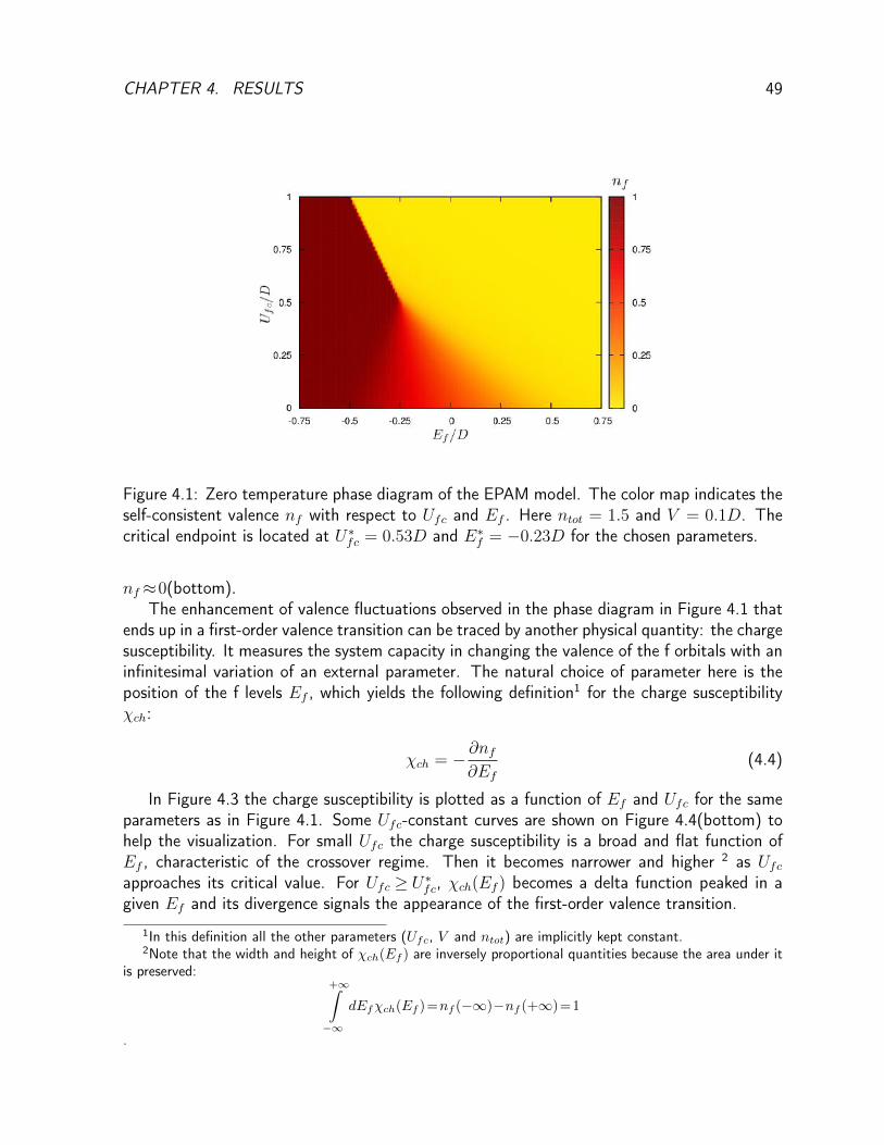
CHAPTER 4. RESULTS 49
Figure 4.1: Zero temperature phase diagram of the EPAM model. The color map indicates theself-consistent valence nf with respect to Ufc and Ef . Here ntot = 1.5 and V = 0.1D. Thecritical endpoint is located at U∗fc = 0.53D and E∗f = −0.23D for the chosen parameters.
nf≈0(bottom).The enhancement of valence fluctuations observed in the phase diagram in Figure 4.1 that
ends up in a first-order valence transition can be traced by another physical quantity: the chargesusceptibility. It measures the system capacity in changing the valence of the f orbitals with aninfinitesimal variation of an external parameter. The natural choice of parameter here is theposition of the f levels Ef , which yields the following definition1 for the charge susceptibilityχch:
χch = − ∂nf∂Ef
(4.4)
In Figure 4.3 the charge susceptibility is plotted as a function of Ef and Ufc for the sameparameters as in Figure 4.1. Some Ufc-constant curves are shown on Figure 4.4(bottom) tohelp the visualization. For small Ufc the charge susceptibility is a broad and flat function ofEf , characteristic of the crossover regime. Then it becomes narrower and higher 2 as Ufcapproaches its critical value. For Ufc ≥ U∗fc, χch(Ef ) becomes a delta function peaked in agiven Ef and its divergence signals the appearance of the first-order valence transition.
1In this definition all the other parameters (Ufc, V and ntot) are implicitly kept constant.2Note that the width and height of χch(Ef ) are inversely proportional quantities because the area under it
is preserved:+∞∫−∞
dEfχch(Ef )=nf (−∞)−nf (+∞)=1
.

CHAPTER 4. RESULTS 50
Figure 4.2: Total density of states ρtot(ω) for three points in the phase diagram (Ufc = 0):Ef =−0.5D (top), Ef =0.0D (middle) and Ef =0.5D (bottom). The energy is measured withrespect to the Fermi level, which is different in the three cases. The intermediate valence statecorrespond to the situation where the Fermi level is located in the peak of ρtot, as discussed inthe text. Other parameters are V =0.1D and ntot=1.5.
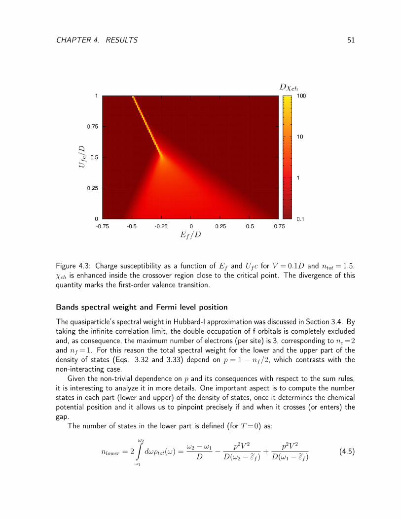
CHAPTER 4. RESULTS 51
Figure 4.3: Charge susceptibility as a function of Ef and Ufc for V = 0.1D and ntot = 1.5.χch is enhanced inside the crossover region close to the critical point. The divergence of thisquantity marks the first-order valence transition.
Bands spectral weight and Fermi level position
The quasiparticle’s spectral weight in Hubbard-I approximation was discussed in Section 3.4. Bytaking the infinite correlation limit, the double occupation of f-orbitals is completely excludedand, as consequence, the maximum number of electrons (per site) is 3, corresponding to nc=2and nf = 1. For this reason the total spectral weight for the lower and the upper part of thedensity of states (Eqs. 3.32 and 3.33) depend on p = 1 − nf/2, which contrasts with thenon-interacting case.
Given the non-trivial dependence on p and its consequences with respect to the sum rules,it is interesting to analyze it in more details. One important aspect is to compute the numberstates in each part (lower and upper) of the density of states, once it determines the chemicalpotential position and it allows us to pinpoint precisely if and when it crosses (or enters) thegap.
The number of states in the lower part is defined (for T =0) as:
nlower = 2
ω2∫ω1
dωρtot(ω) =ω2 − ω1
D− p2V 2
D(ω2 − εf )+
p2V 2
D(ω1 − εf )(4.5)

CHAPTER 4. RESULTS 52
Figure 4.4: Valence nf (top) and charge susceptibility χch (bottom) as a function of Ef forfour different values of Ufc.
Figure 4.5: Total number of states (c+f) in the lower sub-band nlower as a function of Effor three Ufc values: Ufc = 0 (red solid), Ufc = 0.4D (blue dashed) and Ufc = 0.6D (greendot-dashed). For comparison ntot is shown in the grey dashed line. The condition nlower=ntotis satisfied only if Ufc<U∗fc and represents an insulating phase (see text). Other parametersare V =0.1D and ntot=1.5 .
In Figure 4.5 nlower (determined self-consistenly) is plotted as a function of Ef for threedistinct values of Ufc. We consider ntot=1.5 and V =0.1D, as in Figure 4.1. The grey dashed

CHAPTER 4. RESULTS 53
line indicates the position of ntot=1.5. We see that the relation nlower=ntot is satisfied in onepoint only if the inter-orbital repulsion is smaller that its critical value U∗fc. For these precisevalues of Ef the chemical potential lies in the hybridization gap and the system is an insulator.If Ufc >U∗fc, then the position of the chemical potential jumps from the upper to the lowerpart of the density of states. Note that nlower is bounded between 1 and 2 for any value ofntot. It means that for ntot < 1 and ntot > 2 the chemical potential cannot move from onepart of the DOS to the other , no matter what it the Ufc value. As a conclusion, the systembehaves differently if ntot is fixed between 1 and 2 (the case analysed so far) or if ntot< 1 orntot>2.
Electronic filling effects
Two different situations can happen in the EPAM with respect to the total electronic fillingntot. If 1<ntot ≤ 2, then all the electrons in the system can be allocated in the conductionband (in the case of large Ef ) and the occupation nf varies between zero and one. This casewas depicted in Figure 4.1.
Figure 4.6: The same phase diagram as in Figure 4.1, but for a different electronic fillingntot = 2.5. Note that the color map has a different scale and the lowest valence value is 0.5,indicated by the yellow region. The positions of the crossover region, the first-order transitionline and the critical endpoint depend on ntot. For these parameters, the critical endpoint islocated at U∗fc = 0.55D and E∗f = 0.23D.

CHAPTER 4. RESULTS 54
The situation is modified if ntot > 2. In this case the total number of electrons is largerthan the maximal occupation of the conduction band (2 electrons per site). It means that it isimpossible to get an empty f level, even if Ef is much higher in energy than the non-interactingconduction band (Ef�D), so the minimum value for nf is ntot−2. Moreover, the Fermi leveldoes not cross the hybridization gap as discussed in the last subsubsection.
In Figure 4.6 the valence is shown for ntot = 2.5 and V = 0.1D. The yellow region on thetop right of the figure corresponds to the minimum value for nf (0.5). Note that the crossoverregion and the first-order critical line are now obtained for bigger values of Ef . Despite thesedifferences, the generic shape of the phase diagram is the same as before.
In the region with nf =0.5, the chemical potential is pinned in the f peak of the density ofstates, as it happens in the intermediate valence region. However, since the conduction bandis completely filled, the f peak and the hybridization gap are located close to the upper bandedge.
Hybridization effects
Next, let us investigate the behavior of the Ef -Ufc phase diagram for different values ofhybridization V . In Figure 4.7 the valence phase diagram is shown for V = 0.01D (left) andV =0.5D (right) with a fixed ntot=1.5, in a comparison to the diagram presented in Fig. 4.1(V = 0.1D). A bigger hybridization enlarges the width of the f peak, resulting in a smoothervariation of valence. Consequently the position of the critical endpoint is pushed to a larger Ufcvalue and the valence crossover happens in a wider range of Ef values. The inverse situationis observed for smaller values of V (with respect to V = 0.1D), but the variations are lessmarked.
Figure 4.7: Valence phase diagram as in Fig. 4.1 for two distinct hybridizations: V = 0.01D(left) and V =0.5D (right). The crossover region grows as V increases and the critical pointmoves to larger Ufc values.
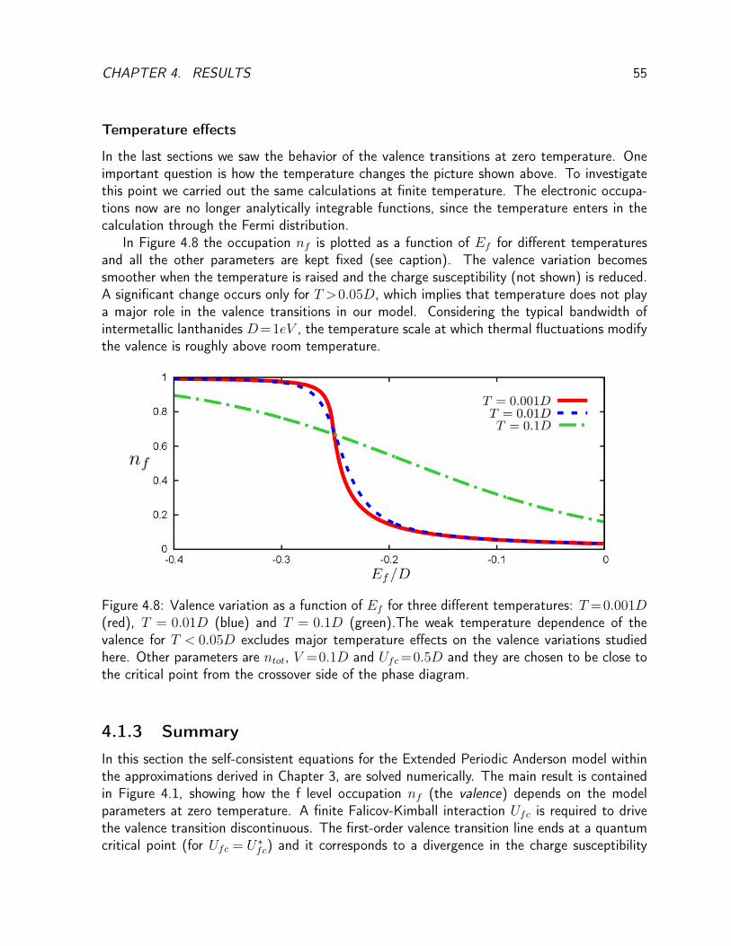
CHAPTER 4. RESULTS 55
Temperature effects
In the last sections we saw the behavior of the valence transitions at zero temperature. Oneimportant question is how the temperature changes the picture shown above. To investigatethis point we carried out the same calculations at finite temperature. The electronic occupa-tions now are no longer analytically integrable functions, since the temperature enters in thecalculation through the Fermi distribution.
In Figure 4.8 the occupation nf is plotted as a function of Ef for different temperaturesand all the other parameters are kept fixed (see caption). The valence variation becomessmoother when the temperature is raised and the charge susceptibility (not shown) is reduced.A significant change occurs only for T >0.05D, which implies that temperature does not playa major role in the valence transitions in our model. Considering the typical bandwidth ofintermetallic lanthanides D=1eV , the temperature scale at which thermal fluctuations modifythe valence is roughly above room temperature.
Figure 4.8: Valence variation as a function of Ef for three different temperatures: T =0.001D(red), T = 0.01D (blue) and T = 0.1D (green).The weak temperature dependence of thevalence for T < 0.05D excludes major temperature effects on the valence variations studiedhere. Other parameters are ntot, V =0.1D and Ufc=0.5D and they are chosen to be close tothe critical point from the crossover side of the phase diagram.
4.1.3 Summary
In this section the self-consistent equations for the Extended Periodic Anderson model withinthe approximations derived in Chapter 3, are solved numerically. The main result is containedin Figure 4.1, showing how the f level occupation nf (the valence) depends on the modelparameters at zero temperature. A finite Falicov-Kimball interaction Ufc is required to drivethe valence transition discontinuous. The first-order valence transition line ends at a quantumcritical point (for Ufc = U∗fc) and it corresponds to a divergence in the charge susceptibility

CHAPTER 4. RESULTS 56
χch = −∂nf/∂Ef . For Ufc < U∗fc the valence variation is a continuous crossover, stronglyenhanced close to the critical point.
4.2 Magnetic Phases
In Section 4.1 we analyzed the system in a nonmagnetic state where the pressure and thetemperature are the only external parameters used to modify the valence in lanthanide ions.However the valence state nf = 1 corresponds to a magnetic configurations with large ef-fective magnetic moments (since J = 7/2 or J = 5/2), one would expect that the magneticmeasurements in these systems could bring interesting information about the valence states.
In what follows the magnetic phases of the Extended Periodic Anderson model will bestudied. The discussions start with the possibility of having intrinsic magnetism in the model,corresponding to spontaneous magnetization in the absence of magnetic field. Later we willdiscuss the magnetic solutions restricted to two different types of magnetic effects: the presenceof an external magnetic field and ferromagnetism.
4.2.1 Intrinsic Magnetism
One relevant physical observable is the magnetic susceptibility at zero field. This quantity isformally defined as:
χmag =∂mf
∂hext
∣∣∣∣hext→0+
(4.6)
Here mf is the f-electron magnetization mf =nf,↑−nf,↓ and hext is a small magnetic fieldapplied to the system. As the charge susceptibility, χmag is here a function of all the parametersof the system.
We present below two ways to calculate χmag from the self-consistent equations. The firstone is to include a infinitesimal magnetic field hext in the model through a Zeeman term,
HZ = −hext∑i
gfSzi , (4.7)
and analytically expand mf with respect to hext. It results directly in a formal expression forχmag in terms of the self-consistent parameters calculated before. For practical purposes, thiscalculation is shown in the Appendix B and only the main results will be presented here. Inthe second method the limit hext→0 is performed by numerical means using the calculationsthat will be presented in Section 4.2.2.
First Method
From the expansions carried on in Appendix B, it is seen that the generic form of the magneticsuscetibility (Eqs.B.10 and B.16) is given by:
χ0 =C0
1− C1
(4.8)

CHAPTER 4. RESULTS 57
The exact expressions for the coefficients C0 and C1 are shown in Appendix B. They arecalculated, for a given set of model parameters, from the self-consistent solutions in the non-magnetic case discussed in Section 4.1.
A magnetic transition is expected when the magnetic susceptibility diverges. Since C0 isa positive finite quantity, it implies that the condition to enter in a magnetic phase is C1 =1,which is a kind of Stoner criterion. An unphysical χ0<0 is obtained inside the ferromagneticphase, when C1>1, indicating that the ground state is ferromagnetic if C1>1.
In Figure 4.9 we plot the value of 1−C1 as a function of Ef for three different Ufc values:0, 0.4D and 0.6D (keeping V =0.1D and ntot=1.5). The intrinsic ferromagnetism exists forthe intervals in which 1−C1 is negative. For Ufc = 0 it corresponds to −0.3<Ef <−0.17.The magnetic region shrinks by increasing Ufc to Ufc=0.4D, ranging from -0.27 to -0.25, anddisappears when Ufc is larger than the critical value U∗fc. So we conclude that the ferromagneticinstability occurs inside the crossover region of the valence transitions only.
Figure 4.9: Value of 1−C1 as a function of Ef for three different values of Ufc: 0,0.4 and 0.6.Other parameters are V =0.1D and ntot=1.5. The spontaneous ferromagnetism exists in theregion where 1−C1 < 0 as discussed in the text. The instability occurs only in the crossoverregime (Ufc<U∗fc) and its region size decreases with increasing Ufc. The jumps in the curvesoccur when the chemical potential jumps from one band to the other.
Another notable aspect of the intrinsic ferromagnetism is the dependence of its region sizeand position with respect to the occupation number ntot. In Figure 4.10 the ferromagneticregion (its range in terms of Ef ) is plotted for different values of ntot between 1 and 2, havingfixed Ufc = 0 and all the other parameters as in Figure 4.9. The ferromagnetic region existsonly for ntot<1.7 and it becomes wider by decreasing ntot. When ntot → 1 the region extendsto a very large range of negative Ef values, which is visually indicated close to the horizontalaxis.
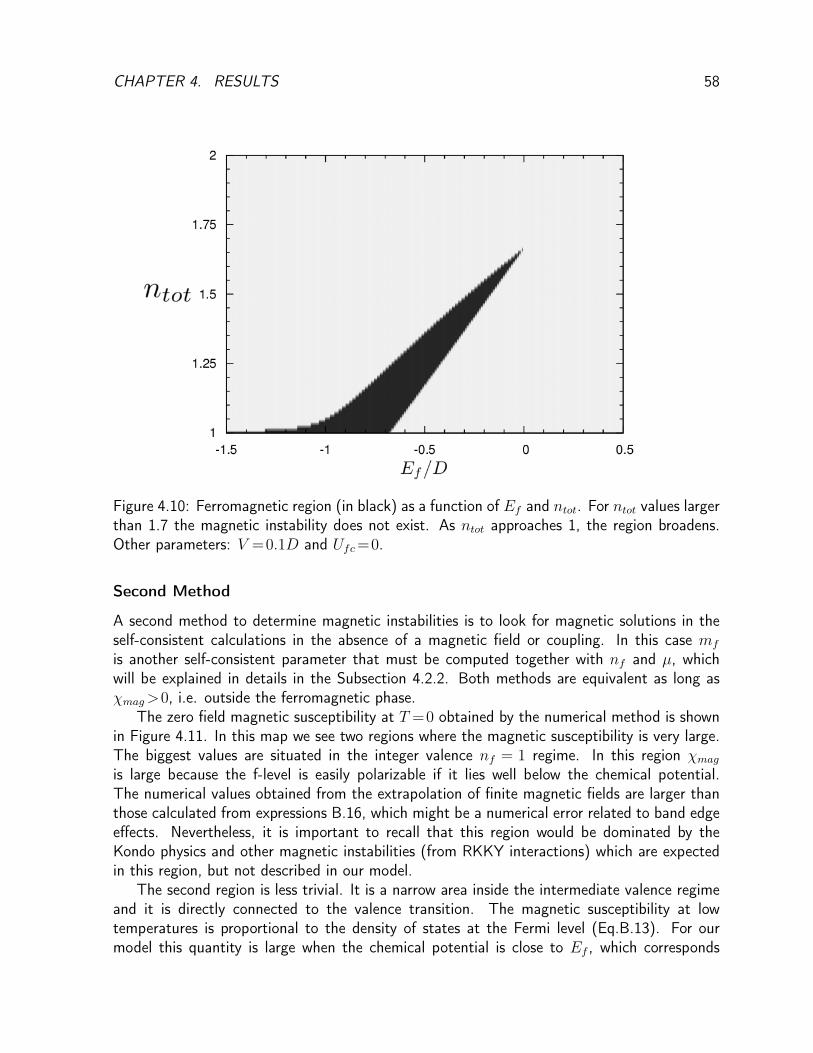
CHAPTER 4. RESULTS 58
Figure 4.10: Ferromagnetic region (in black) as a function of Ef and ntot. For ntot values largerthan 1.7 the magnetic instability does not exist. As ntot approaches 1, the region broadens.Other parameters: V =0.1D and Ufc=0.
Second Method
A second method to determine magnetic instabilities is to look for magnetic solutions in theself-consistent calculations in the absence of a magnetic field or coupling. In this case mf
is another self-consistent parameter that must be computed together with nf and µ, whichwill be explained in details in the Subsection 4.2.2. Both methods are equivalent as long asχmag>0, i.e. outside the ferromagnetic phase.
The zero field magnetic susceptibility at T =0 obtained by the numerical method is shownin Figure 4.11. In this map we see two regions where the magnetic susceptibility is very large.The biggest values are situated in the integer valence nf = 1 regime. In this region χmagis large because the f-level is easily polarizable if it lies well below the chemical potential.The numerical values obtained from the extrapolation of finite magnetic fields are larger thanthose calculated from expressions B.16, which might be a numerical error related to band edgeeffects. Nevertheless, it is important to recall that this region would be dominated by theKondo physics and other magnetic instabilities (from RKKY interactions) which are expectedin this region, but not described in our model.
The second region is less trivial. It is a narrow area inside the intermediate valence regimeand it is directly connected to the valence transition. The magnetic susceptibility at lowtemperatures is proportional to the density of states at the Fermi level (Eq.B.13). For ourmodel this quantity is large when the chemical potential is close to Ef , which corresponds

CHAPTER 4. RESULTS 59
Figure 4.11: Magnetic susceptibility as a function of Ef and Ufc for V =0.1D and ntot=1.5.A ferromagnetic transition exists inside the intermediate valence region around Ef =−0.25D,corresponding to the situation in which the f part of the density of states is enhanced (closeto the hybridization gap).
exactly to the situation with large valence variations in the crossover regime. The calculationsshown in Appendix B yield negative values for χ0 in this region, signaling a ferromagneticinstability, which was not obtained by the numerical method.
One interesting question is whether there is a ferromagnetic instability in this model at zerotemperature. It is well-known for the Hubbard model that the ground state is not ferromagneticin the zero bandwidth limit [69]. Moreover, Hubbard-I approximation does not lead to anyferromagnetic instability for a rectangular density of states3. Then the Coulomb repulsion byitself does not seem to be the driving mechanism leading to instabilities.
In Periodic Anderson model the situation is more complex. Apart from the possible ferro-magnetic states in the localized limit due to RKKY interactions, instabilities are also observedin the intermediate valence regime. For instance, Reddy and collaborators [76] shown thatferromagnetism is expected in this regime, depending on the position of f level and the totalnumber of electrons. Hybridization is the key mechanism for ferromagnetism, once it slightlydelocalizes the f levels and it generates strongly asymmetric density of states. Remarkably theyhave found ferromagnetism around Ef =−0.25D for the same parameters as in Figure 4.11,advocating in favor of a ferromagnetic instability inside the intermediate valence region of our
3For further details, check Section 8.5 of Ref. [75]
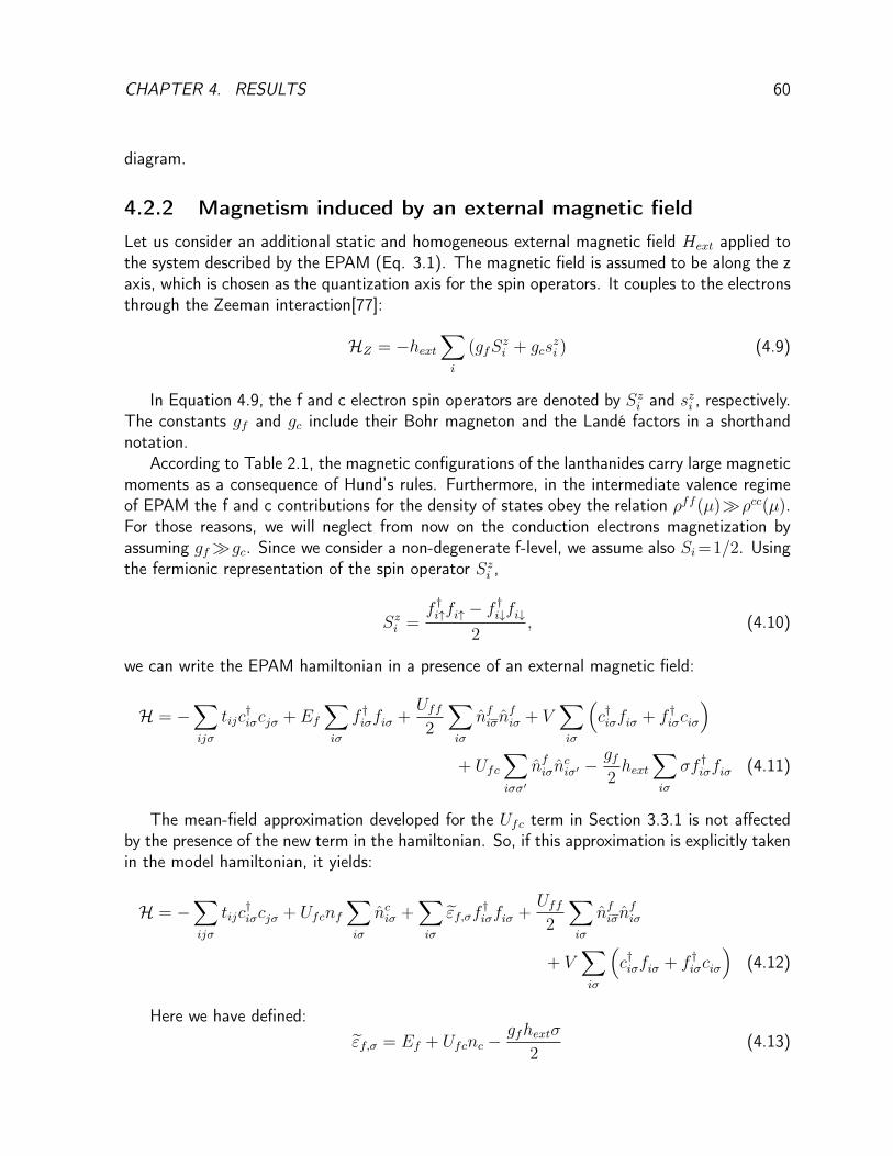
CHAPTER 4. RESULTS 60
diagram.
4.2.2 Magnetism induced by an external magnetic field
Let us consider an additional static and homogeneous external magnetic field Hext applied tothe system described by the EPAM (Eq. 3.1). The magnetic field is assumed to be along the zaxis, which is chosen as the quantization axis for the spin operators. It couples to the electronsthrough the Zeeman interaction[77]:
HZ = −hext∑i
(gfSzi + gcs
zi ) (4.9)
In Equation 4.9, the f and c electron spin operators are denoted by Szi and szi , respectively.The constants gf and gc include their Bohr magneton and the Landé factors in a shorthandnotation.
According to Table 2.1, the magnetic configurations of the lanthanides carry large magneticmoments as a consequence of Hund’s rules. Furthermore, in the intermediate valence regimeof EPAM the f and c contributions for the density of states obey the relation ρff (µ)�ρcc(µ).For those reasons, we will neglect from now on the conduction electrons magnetization byassuming gf�gc. Since we consider a non-degenerate f-level, we assume also Si=1/2. Usingthe fermionic representation of the spin operator Szi ,
Szi =f †i↑fi↑ − f †i↓fi↓
2, (4.10)
we can write the EPAM hamiltonian in a presence of an external magnetic field:
H = −∑ijσ
tijc†iσcjσ + Ef
∑iσ
f †iσfiσ +Uff2
∑iσ
nfiσnfiσ + V
∑iσ
(c†iσfiσ + f †iσciσ
)+ Ufc
∑iσσ′
nfiσnciσ′ −
gf2hext
∑iσ
σf †iσfiσ (4.11)
The mean-field approximation developed for the Ufc term in Section 3.3.1 is not affectedby the presence of the new term in the hamiltonian. So, if this approximation is explicitly takenin the model hamiltonian, it yields:
H = −∑ijσ
tijc†iσcjσ + Ufcnf
∑iσ
nciσ +∑iσ
εf,σf†iσfiσ +
Uff2
∑iσ
nfiσnfiσ
+ V∑iσ
(c†iσfiσ + f †iσciσ
)(4.12)
Here we have defined:εf,σ = Ef + Ufcnc −
gfhextσ
2(4.13)
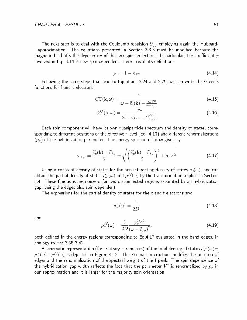
CHAPTER 4. RESULTS 61
The next step is to deal with the Couloumb repulsion Uff employing again the Hubbard-I approximation. The equations presented in Section 3.3.3 must be modified because themagnetic field lifts the degeneracy of the two spin projections. In particular, the coefficient pinvolved in Eq. 3.14 is now spin-dependent. Here I recall its definition:
pσ = 1− nfσ (4.14)
Following the same steps that lead to Equations 3.24 and 3.25, we can write the Green’sfunctions for f and c electrons:
Gccσ (k, ω) =
1
ω − εc(k)− pσV 2
ω−εfσ
(4.15)
Gffσ (k, ω) =
pσ
ω − εfσ − pσV 2
ω−εc(k)
(4.16)
Each spin component will have its own quasiparticle spectrum and density of states, corre-sponding to different positions of the effective f level (Eq. 4.13) and different renormalizations(pσ) of the hybridization parameter. The energy spectrum is now given by:
ω±,σ =εc(k) + εfσ
2±√(
εc(k)− εfσ2
)2
+ pσV 2 (4.17)
Using a constant density of states for the non-interacting density of states ρ0(ω), one canobtain the partial density of states ρccσ (ω) and ρffσ (ω) by the transformation applied in Section3.4. These functions are nonzero for two disconnected regions separated by an hybridizationgap, being the edges also spin-dependent.
The expressions for the partial density of states for the c and f electrons are:
ρccσ (ω) =1
2D(4.18)
and
ρffσ (ω) =1
2D
p2σV
2
(ω − εfσ)2 , (4.19)
both defined in the energy regions corresponding to Eq.4.17 evaluated in the band edges, inanalogy to Eqs.3.38-3.41.
A schematic representation (for arbitrary parameters) of the total density of states ρtotσ (ω)=ρccσ (ω)+ρffσ (ω) is depicted in Figure 4.12. The Zeeman interaction modifies the position ofedges and the renormalization of the spectral weight of the f peak. The spin dependence ofthe hybridization gap width reflects the fact that the parameter V 2 is renormalized by pσ inour approximation and it is larger for the majority spin orientation.

CHAPTER 4. RESULTS 62
Figure 4.12: Total density of states ρtotσ (ω) = ρccσ (ω) + ρffσ (ω) for each spin direction. Notethat all the features in ρtotσ (ω) are spin-dependent: the with of hybridization gap, the bandedges and the height of the f peak. The parameters are chosen to exaggerate the differencebetween the spin bands.
Results
The self-consistent equations for the magnetization, valence and chemical potential are solvednumerically using the same method as in Section 4.1. For simplicity, we define gf = 2 as thenumerical value for the g-factor.
In Figure 4.13 we show the valence and the magnetization of the f electrons as a functionof hext. Three points in the Ef -Ufc phase diagram are considered: Ef =−0.15D;Ufc=0.4D(Point A, solid red line), Ef = −0.2D;Ufc = 0.5D (point B, blue dashed line) and Ef =−0.25D;Ufc = 0.6D (point C, green dot-dashed line). The other parameters are kept fixed:V =0.1D and ntot=1.5. Their positions in the Ef -Ufc phase diagram (for hext=0) are shownon the inset. The magnetic field leads always to an increase of both valence and magnetization,or in other words, it always drives the system towards a more localized behavior.
When the system is in the crossover region (curves A and B), both parameters nf andmf vary continuously with the external field. For an Ufc larger than the critical value, a first-order valence transition appears by the effect of the external field and it is accompanied bya magnetization jump in a critical field (curve C). Above the transition the magnetization isclose to its saturated value, in which mf/nf =1. The critical field h∗ext reflects the distance (interms of Ef ) from the valence critical line. For instance, when Ufc=0.6D and Ef =−0.25D(curve C) the critical field is h∗ext=0.05D, which is exactly the difference between Ef and thecritical Ef =−0.3D for Ufc=0.6D.
The increase of valence with a magnetic field can be understood conceptually from simplearguments. The external magnetic field acts in detriment of the spin degeneracy of the f-level,which acquires a polarization energy proportional to hext (see the band splitting in Figure 4.12).

CHAPTER 4. RESULTS 63
Figure 4.13: Valence nf (top) and f-electron magnetization mf (bottom) as a function of theexternal magnetic field hext for three points in the Ef -Ufc phase diagram: Ef =−0.15D;Ufc=0.4D(point A), Ef =−0.2D;Ufc = 0.5D (point B) and Ef =−0.25D;Ufc = 0.6D (point C).Other parameters are V =0.1D and ntot=1.5. Inset: position of the three set of parameterswith respect to the Ef -Ufc phase diagram (Fig. 4.1).
Then one of the spin components (here the positive Sz=+1/2) has an effective f-level positionthat decreases progressively with respect to Ef (Eq. 4.13), while for the other component itincreases. This separation is associated to a larger occupation of the up-spin component,increasing the f-electron magnetization and the valence.
Next let us see how the magnetic field affects the dependence of nf and mf on the positionof the f-level Ef in the crossover and the first-order valence transition regions. This will beimportant for discussions on the pressure dependence of mixed-valence compounds under amagnetic field. This dependence is shown in Figure 4.14 in the crossover(left) and first-order(right) regions for three values of hext: hext=0.01D (red solid line), hext=0.1D (blue dashedline) and hext=0.5D (green dot-dashed line). In both cases the external magnetic field leadsthe valence variation region towards larger values of Ef . The displacement with respect tothe case without external field is given by hext itself, in agreement with the arguments givenin the last paragraph. We remark, based on these results, that the external field is unable tochange the nature of the valence transition, i.e. it does not transform the valence crossoverinto a discontinuous transition. The magnetization curves in Figure 4.14 for hext = 0.1D andhext=0.5D present some kinks as a function of Ef , which are caused by the chemical potentialcrossing the hybridization gap for one or both spin orientations (see Figure 4.12).
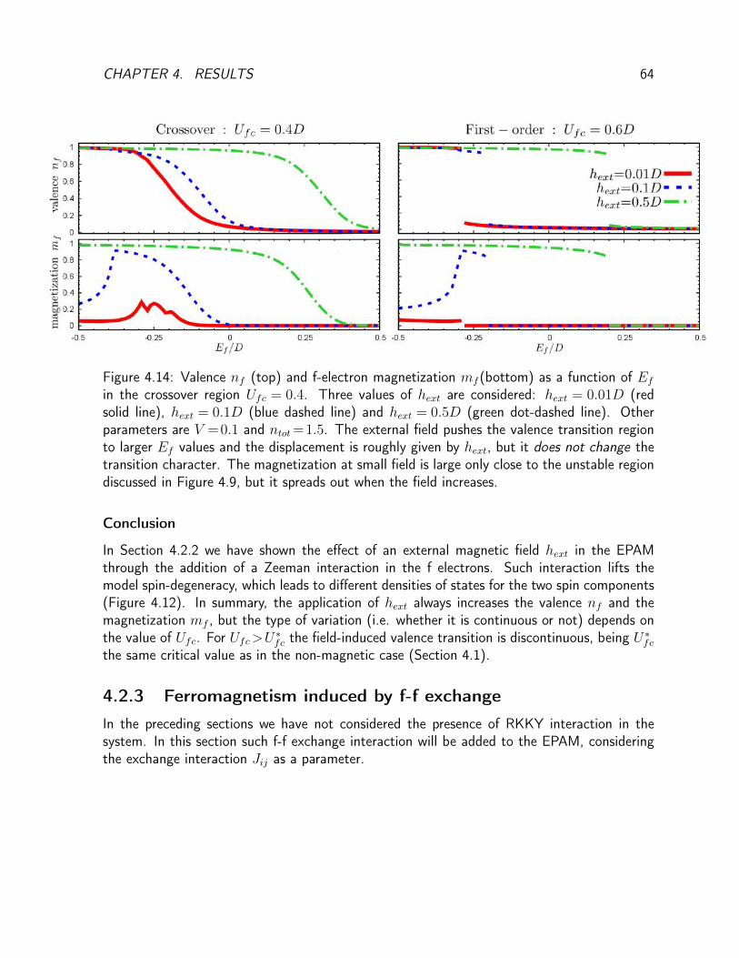
CHAPTER 4. RESULTS 64
Figure 4.14: Valence nf (top) and f-electron magnetization mf (bottom) as a function of Efin the crossover region Ufc = 0.4. Three values of hext are considered: hext = 0.01D (redsolid line), hext = 0.1D (blue dashed line) and hext = 0.5D (green dot-dashed line). Otherparameters are V =0.1 and ntot=1.5. The external field pushes the valence transition regionto larger Ef values and the displacement is roughly given by hext, but it does not change thetransition character. The magnetization at small field is large only close to the unstable regiondiscussed in Figure 4.9, but it spreads out when the field increases.
Conclusion
In Section 4.2.2 we have shown the effect of an external magnetic field hext in the EPAMthrough the addition of a Zeeman interaction in the f electrons. Such interaction lifts themodel spin-degeneracy, which leads to different densities of states for the two spin components(Figure 4.12). In summary, the application of hext always increases the valence nf and themagnetization mf , but the type of variation (i.e. whether it is continuous or not) depends onthe value of Ufc. For Ufc>U∗fc the field-induced valence transition is discontinuous, being U∗fcthe same critical value as in the non-magnetic case (Section 4.1).
4.2.3 Ferromagnetism induced by f-f exchange
In the preceding sections we have not considered the presence of RKKY interaction in thesystem. In this section such f-f exchange interaction will be added to the EPAM, consideringthe exchange interaction Jij as a parameter.
CHAPTER 4. RESULTS 65
Ferromagnetic Interactions and Mean-Field approximation
Here we will restrict ourselves to the analysis of nearest neighbor ferromagnetic interactions,described by the following hamiltonian:
HJ = −J∑<i,j>
Si · Sj (4.20)
In this hamiltonian < i, j > represents the sum over all pairs of neighboring sites in thelattice and J is the strength of magnetic interaction (J > 0 for ferromagnetism). This termwill be treated in mean-field approximation. The spin operators are replaced by their averagevalues plus fluctuations, that are kept to first order only. If the magnetization is along the zaxis, then:
Szi Szj ≈ 〈Szi 〉Szj +
⟨Szj⟩Szi − 〈Szi 〉
⟨Szj⟩
(4.21)
In the ferromagnetic state the system is homogeneous and the average value 〈Szi 〉 is thesame for all lattice sites. Using this invariance explicitly in the mean-field approximation, thehamiltonian in Eq. 4.20 yields:
HJ = −Jmf
∑iσ
σf †iσfiσ + Jm2fN (4.22)
Here the spin operator is rewritten in terms of fermionic operators Szi =1/2(f †i↑fi↑−f †i↓fi↓),we used the definition mf = 2 < Sz > and N is the number of lattice sites. The prefactorin the sum (Jmf ) is named Weiss molecular field once it acts in the same way as an externalmagnetic field (as in Eq. 4.9), apart from the constant Jm2
fN . For this reason, we can use thesame equations as in Section 4.2.2 to calculate nf andmf , but nowmf must be computed self-consistently since it is proportional to the Weiss field. Moreover, the trivial solution mf = 0is always present in this case, so it is crucial to compare its energy to other self-consistentsolutions. The expression for the total energy in the presence of the f-f magnetic exchange is:
EtotN
=∑σ
µ∫−∞
dωω(ρccσ (ω) + ρffσ (ω)
)− Ufcncnf + Jm2
f , (4.23)
Results
Let us present the numerical results that we have obtained in the presence of a ferromagneticexchange. The bisection method was employed again and the good solution is chosen amongthe self-consistent results by energy comparison. The valence and magnetization dependenceon the exchange parameter J is shown in the Figure 4.15 for three different points in theEf -Ufc phase diagram: Ef =−0.15D;Ufc=0.4D (point A), Ef =−0.2D;Ufc=0.5D (pointB) and Ef =−0.25D;Ufc=0.6D (point C). These points are chosen to be close to the criticalpoint (see Figure 4.1) and are the same of Fig. 4.13. Differently from the case of an externalmagnetic field (Figure 4.13), the increase of J always leads to a discontinuity in the valence andthe magnetization, irrespective to the value of Ufc. For the points A and B the magnetization

CHAPTER 4. RESULTS 66
jumps are smaller than in point C and mf does not reach its maximum value after it. For thepoint C the magnetization jump happens at J = 0.31D and mf is close to the saturation forJ >0.31D (where the three curves superimpose).
Next we analyze the variations of nf and mf as a function of Ef in Figure 4.16, followingthe same lines as in Section 4.2.2. The results are shown for Ufc=0.4D (left) and Ufc=0.6D(right), which are also classified as crossover and first-order scenarios in terms of the criticalUfc value for the paramagnetic phase diagram in Figure 4.1. Here the results are presented fortwo exchange values: J=0.1D and J=0.5. For Ufc=0.4D, the magnetization is finite in theinterval between Ef =−0.4D and Ef =−0.15D when J=0.1D. This region is placed aroundEf =−0.25D, that corresponds to the ferromagnetic instability in the paramagnetic case (seeFig.4.9), widened by the additional exchange interaction. The mf 6= 0 region can be furtherwidened by increasing J or decreasing Ufc.
Figure 4.15: Valence nf (top) and f-electron magnetization mf (bottom) as a function of theexchange parameter J for three points in the Ef -Ufc phase diagram: Ef = −0.15D;Ufc =0.4D(point A), Ef =−0.2D;Ufc = 0.5D (point B) and Ef =−0.25D;Ufc = 0.6D (point C).Other parameters are V =0.1D and ntot=1.5. Inset: position of the three set of parameterswith respect to the Ef -Ufc phase diagram (Fig. 4.1).
Conclusion
In Section 4.2.3 we considered the addition of a ferromagnetic exchange interaction betweenthe f-electrons in the EPAM. Such interaction was treated in mean-field approximation, whichyields the same equations as in Section 4.2.2 but in the presence of a self-consistent (Weiss)

CHAPTER 4. RESULTS 67
Figure 4.16: Valence nf (top) and f-electron magnetization mf (bottom) as a function ofEf in the crossover region Ufc = 0.4 (left) and in the first-order transition region Ufc = 0.6.Three values of J are considered:J = 0 (red solid line), J = 0.1D (blue dashed line) andJ = 0.5D (green dot-dashed line). Other parameters are V = 0.1 and ntot = 1.5.
magnetic field. The results are shown in Figures 4.15 and 4.16, representing the valenceand magnetization as a function of J (for a fixed point in the Ef -Ufc phase diagram) andas a function of Ef (for fixed J and Ufc), respectively. As a general result, we have seenthat the valence dependence on J is always a discontinuous curve, independent of the Ufcvalue. This is in contrast to the valence dependence on hext observed in last section, so weargue that ferromagnetism may enhance the valence transition. The discontinuities mightalso be an artifact of the mean-field approximation. In Figure 4.16 it is observed how theferromagnetic unstable region presented in Section 4.2.1 is increased in the presence of theadditional exchange interaction, as one should expect. These results will be revisited when theferromagnetic transition of YbCu2Si2 will be discussed (Section 4.3.2).
4.2.4 Summary
In this section the role of magnetism in valence transitions was discussed through three differentscenarios: the intrinsic magnetism provided by a ferromagnetic instability of the system, themagnetism induced by an external magnetic field and the magnetism provided by f-f exchangeinteractions. In the first case it was shown that a ferromagnetic instability exists in a small partof the intermediate valence region (Figure 4.11) as long as the electronic filling ntot does notexceed a critical value, as indicated in Figure 4.10. The self-consistent magnetization obtainedin the absence of fields can be as high as mf ≈ 0.35 inside this region. This instability canbe explained by the means of the Stoner criterion, which predicts an instability when densityof states in the Fermi level is sufficiently high, that happens in our model precisely when the

CHAPTER 4. RESULTS 68
Fermi level crosses the hybridization gap.In the second scenario an external magnetic field was included in the system by addition of
a Zeeman interaction on the f-electrons. Since this interaction breaks the spin-symmetry, theself-consistent equations were modified to take it into account. The major result is the fielddependence of the valence nf and magnetization mf : they both increase with an increasinghext, but the nature of these transitions (continuous or not) depends on the value of Ufc as inthe non-magnetic case. A discontinuous valence transition is seen only if Ufc is larger than itscritical value in the absence of fields (defined as U∗fc). As a conclusion, the application of anexternal field could be a god tool to control experimentally valence variations, since it allowsus to identify quantitatively the Ufc interaction for a given system.
In the last scenario we studied the effect of a ferromagnetic exchange interaction between felectrons in neighboring sites. The interaction was included in the mean-field level. The resultsshow that the first-order transition is enhanced by the exchange interaction, since it drives thevalence transition discontinuous for any value of Ufc interaction. Whether it is a consequenceof the mean-field or not is still an open question, nevertheless the existence of intermetalliclanthanides that display first-order ferromagnetic transitions (for example YbCu2Si2, discussedin the next section) may advocate in favor of it.
4.3 Connection with experiments
In this chapter we will establish some connections between the theory developed for the EPAMand some selected materials showing valence transitions. The choice of compounds is far frombeing exhaustive, still they were chosen carefully to make a point in every aspect discussedin the theoretical part: application of pressure and magnetic fields, ferromagnetism and thenature of the valence variations (crossover or first-order transition).
4.3.1 Pressure effects
Pressure reduces the system size, increasing the overlap between the wave-functions of con-duction electrons and the 4f orbitals. In the case of Ce-based compounds the negative ionsare pushed in the direction of the tails in the 4f wave-function, which produces an increase ofEf in our model[68]. The hybridization V and the inter-orbital repulsion Ufc also increase dueto the larger overlap. As a consequence, pressure tends to favor the nonmagnetic valence con-figuration of cerium (Ce4+, corresponding to 4f 0) with respect to the magnetic configuration(Ce3+ or 4f 1)
Ytterbium compounds are often seen as the "hole" analogous to cerium, once it has a4f 13 (one hole) configuration in its valence state Y b3+ in competition with the Y b2+(4f 14)state. In this case pressure favours the magnetic state Y b3+, which amounts to decreasing Efand V in the Periodic Anderson model. The particle-hole analogy is useful to compare similarcompounds (as in CeCu2Si2 and YbCu2Si2), although important differences exists betweenCe-based and Yb-based materials[78].
As a practical rule, pressure favours larger valencies in lanthanides. For Ce and Yb it
CHAPTER 4. RESULTS 69
corresponds to Ce4+ (nonmagnetic) and Y b3+ (magnetic). For europium, for which someexamples will be discussed in this section, pressure a priori induces a transition from themagnetic divalent state (Eu2+) to the nonmagnetic J=0 trivalent state (Eu3+).
Recalling that volume effects are not explicitly considered in the model and the pressure isnot a parameter in the model, it is clear that pressure effects must be encoded in terms of theother model parameters, such as Ef and V . For this purpose, some hypothesis on the relationbetween pressure and parameters are done.
First we assume that the pressure can be translated as a continuous and monotonic variationof the model parameters Ef , Ufc and V . In this case, we choose Ef as the control parameterand use its variation ∆Ef =Ef−E0
f (with respect to the initial value E0f ) to write the variation
of Ufc and V :
Ufc = U0fc + α∆Ef (4.24)
V = V 0 + β∆Ef (4.25)
For comparison purposes, two different scenarios for the parameter variations are proposed.In both scenarios Ufc varies weakly with ∆Ef and we fix α = 0.1. The difference comesfrom the hybridization dependence: in scenario A the hybridization is kept fixed at V 0 =0.1D(β = 0), while in scenario B V has a weak dependence on ∆Ef and β = 0.1. We considertwo different values of U0
fc for each scenario, U0fc=0.4D and U0
fc=0.6D, in order to describethe crossover and the first-order valence transition regions, respectively.
In Figure 4.17 the valence dependence on pressure is schematically shown for the two sce-narios proposed above. For both scenarios the crossover and the first-order valence transitionsare shown in the red and blue curves, respectively, and corresponds to different values of U0
fc
as indicated. The inset of Fig.4.17 presents schematically the parametrized curves with respectto the phase diagram in Figure 4.1(with a fixed V =0.1).
The situation described by scenario A is qualitatively the same as in Figure 4.1.On theother hand, if the hybridization dependence on pressure is included (bottom figure), the va-lence variation is strongly reduced. In this case a discontinuous transition still exists, howeverthe valence jumps is smaller than for a fixed V . This picture is more consistent with theexperimental results showing that valence variations are small (on the order of 0.1) even if thetransition is discontinuous.
4.3.2 YbCu2Si2
The first Yb-based compound of interest is YbCu2Si2[38, 79]. It has a tetragonal crystalstructure with lattice parameters a=3.92 Åand c=9.99 Å. The Sommerfeld parameter aroundγ≈150mJ/mol.K2 evidences a moderate heavy-fermion character established below 40K.
This material was meticulously studied in Ref. [38], where a substantial set of experimentalresults under extreme conditions and their respective analysis were performed. Some of theseresults will be summarized and their connection with the theory developed in this part of thethesis will be debated.
Figure 4.18 shows the P-T phase diagram of YbCu2Si2 with emphasis on the valence values.The highlighted feature of this diagram is a ferromagnetic transition at p=8GPa with ordering

CHAPTER 4. RESULTS 70
Figure 4.17: Pressure effects on the valence when passing through the crossover (red) or thefirst order transition line (blue), as indicated on the inset. On the top the hybridization is keptfixed with the increasing pressure (scenario A), while on the bottom V increases linearly withit (scenario B).
temperature TM =8K[79] and it is believed to have a first-order nature, which contrast to thesecond-order antiferromagnetic critical point from the Doniach diagram (Fig.1.2) and oftenseen in Ce compounds. For the temperature of 7K (below TM), the Yb valence varies linearlywith the pressure, from 2.75 at ambient pressure to 2.92 at p=15GPa[80].
The appearance of a pressure-induced ferromagnetic transition with an increasing valenceis also observed in our model. YbCu2Si2 does not show any evidence of discontinuous valencetransitions, then it should be placed in the crossover region of the phase diagram in Figure4.1. It has an intermediate valence Y b2.75+ at room pressure that goes towards the magneticconfiguration Y b3+ under pressure, as expected for Yb compounds (see Figure 4.17). Whatis remarkable is the existence of magnetic transitions for a very small exchange interactionJ in this particular region of parameters, which includes also the maximum in the zero-fieldmagnetic susceptibility presented in Figure 4.11.
Other interesting feature of this compound is its comparison to YbCu2Ge2[81, 82]. Ger-manium has a larger atomic radius than silicon, having similar electronic configurations. ThenGe substitution acts as a negative pressure, dilating the crystal structure without any othersignificant modification. In YbCu2Ge2 at low temperatures, the ytterbium valence is close to

CHAPTER 4. RESULTS 71
(P � T ) 2 2 TM TMax / TK
TFL 2 2
P T 2 2
Figure 4.18: Phase diagram of YbCu2Si2 under pressure. A ferromagnetic transition is seen at8GPa with a Curie temperature on the order of 10K. The ytterbium valence is continuous forthe whole phase diagram and increases with the pressure, as expected for Yb-based materials.Extracted from Ref.[38].
Figure 4.19: Schematic comparison between the EPAM and YbCu2(Si/Ge)2 compounds. Thepressure dependence of the valence (red solid line) and f-electron magnetization (blue dashedline) follows from the discussion in Section 4.3.1 (using scenario A) and the experimentalvalues are extracted from Refs. [81] and [80]. Theoretical parameters: V = 0.1D,ntot = 1.2,Ufc=0.4D,J=0.01D and Ef varying from Ef =−0.1D to Ef =−0.5D.

CHAPTER 4. RESULTS 72
2 (4f 14 configuration) and the system behaves as a common metal with small effective mass(γ≈10mJ/mol.K2) and Pauli paramagnetism[81]. Under pressure the valence increases andheavy quasiparticles are formed (γ≈80mJ/mol.K2 at p=16.8GPa). It is expected that thissystem recovers all the features of the Si-based material in a higher pressure range, but it isexperimentally unachievable.
The behavior of YbCu2(Si/Ge)2 at low temperatures seems to follow the theory presentedin Section 4.2.3. At low pressures Yb is almost divalent. Increasing the pressure the f-levelenergy decreases and approaches the Fermi level, which leads to increasing valence fluctuations.The enhancement of 4f 13 configuration produces a ferromagnetic transition with a quite higheffective moment. Since there is no sign of discontinuities in valence or in the volume underthe applied pressure, we can conclude that Ufc plays a minor role in the valence variations.
To illustrate this specific point, we compare in Figure 4.19 the experimental data to resultsobtained from EPAM suitable for this particular compound. The pressure dependence onthe model parameters follows the scenario A in Figure 4.17 and the calculation is done atzero temperature. Since the valence variation is continuous in YbCu2(Si/Ge)2, we placedthe compound in the crossover region. For YbCu2Ge2 the corresponding valence is close to2+ and increases with pressure, while in YbCu2Si2 the valence is already in an intermediatevalue (2.75) at zero pressure and a finite spontaneous magnetization is seen in the model andexperimentally when the valence tends to 3.
The EPAM, treated with the approximations described in Section 3.3, misses a relevantphenomenon in the Y b3+ state: the Kondo effect. It would originate a large quasiparticle peakin the electronic density of states at the Fermi energy, what tends to increase the magneticsusceptibility close to the nf =1 region. Nevertheless, it is interesting to see that in any casethe valence variation with the pressure cannot be explained only by the delocalization of felectrons from Kondo effect. If it was the case, the heavy fermion behavior would persist evenwhen Yb valence is close to 2, which is in disagreement with the small Sommerfeld coefficient(γ≈10mJ/mol.K2) of YbCu2Ge2.
4.3.3 YbMn6Ge6−xSnx
The next compound to be analyzed in terms of our theory is YbMn6Ge6−xSnx. It crystallizesin a hexagonal (P6/mmm) structure with a minor disorder from x= 0 to x= 6. The largeratomic radius of Sn implies that there is a negative pressure effect by doping with this atom.Then it is expected a valence drop (towards Y b2+ configuration) when the concentration ofSn is increased.
YbMn6Ge6−xSnx is a rare example of lanthanide intermetallics containing also magnetictransition metals. The presence of manganese in the crystal structure affects the Yb valence innontrivial ways, as it was studied in Reference [83, 84]. Contrary to many examples of Yb-basedcompounds, for instance YbCu2(Si/Ge)2 discussed in Section 4.3.2, the Yb valence decreaseswith the temperature for YbMn6Ge1.6Sn4.4. For the same composition, the Yb is magneticallyordered up to 90K (which is unusual), while Mn is ordered up to room temperature. Theexistence of highly polarized Mn states acts as a very strong magnetic field (close to 100T) onthe Yb sites.
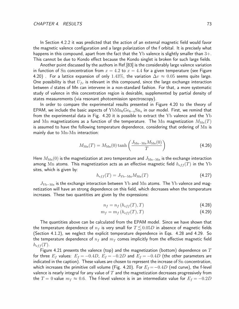
CHAPTER 4. RESULTS 73
In Section 4.2.2 it was predicted that the action of an external magnetic field would favorthe magnetic valence configuration and a large polarization of the f orbital. It is precisely whathappens in this compound, apart from the fact that the Yb valence is slightly smaller than 3+.This cannot be due to Kondo effect because the Kondo singlet is broken for such large fields.
Another point discussed by the authors in Ref.[83] is the considerably large valence variationin function of Sn concentration from x = 4.2 to x = 4.4 for a given temperature (see Figure4.20) . For a lattice expansion of only 1.43%, the variation ∆v ≈ 0.05 seems quite large.One possibility is that Ufc is relevant in this compound, since the large exchange interactionbetween d states of Mn can intervene in a non-standard fashion. For that, a more systematicstudy of valence in this concentration region is desirable, supplemented by partial density ofstates measurements (via resonant photoemission spectroscopy).
In order to compare the experimental results presented in Figure 4.20 to the theory ofEPAM, we include the basic aspects of YbMn6Ge6−xSnx in our model. First, we remind thatfrom the experimental data in Fig. 4.20 it is possible to extract the Yb valence and the Yband Mn magnetizations as a function of the temperature. The Mn magnetization MMn(T )is assumed to have the following temperature dependence, considering that ordering of Mn ismainly due to Mn-Mn interaction:
MMn(T ) = MMn(0) tanh
(JMn−MnMMn(0)
T
)(4.26)
HereMMn(0) is the magnetization at zero temperature and JMn−Mn is the exchange interactionamong Mn atoms. This magnetization acts as an effective magnetic field heff (T ) in the Ybsites, which is given by:
heff (T ) = JYb−MnMMn(T ) (4.27)
JYb−Mn is the exchange interaction between Yb and Mn atoms. The Yb valence and mag-netization will have an strong dependence on this field, which decreases when the temperatureincreases. These two quantities are given by the expressions:
nf = nf (heff (T ), T ) (4.28)mf = mf (heff (T ), T ) (4.29)
The quantities above can be calculated from the EPAM model. Since we have shown thatthe temperature dependence of nf is very small for T . 0.05D in absence of magnetic fields(Section 4.1.2), we neglect the explicit temperature dependence in Eqs. 4.28 and 4.29. Sothe temperature dependence of nf and mf comes implicitly from the effective magnetic fieldheff (T ).
Figure 4.21 presents the valence (top) and the magnetization (bottom) dependence on Tfor three Ef values: Ef =−0.4D, Ef =−0.2D and Ef =−0.4D (the other parameters areindicated in the caption). These values are chosen to represent the increase of Sn concentration,which increases the primitive cell volume (Fig. 4.20). For Ef =−0.4D (red curve), the f-levelvalence is nearly integral for any value of T and the magnetization decreases progressively fromthe T = 0 value mf ≈ 0.6. The f-level valence is in an intermediate value for Ef =−0.2D
CHAPTER 4. RESULTS 74
(blue curve) and slightly decreases with T . Note that mf decreases in a similar way as forEf =−0.4D, but its value is always larger when Ef =−0.2D. Finally, if the valence is closeto zero (Ef =−0.0D, green curve), than the f-level magnetization vanishes.
The results presented above qualitatively agree with the temperature dependence on thevalence and the magnetization of YbMn6Ge6−xSnx (Figure 4.20, right). For x= 3.8 the Y bvalence is nearly integral and the Y b magnetization decreases and vanishes at T ≈ 50K. Forx = 4.2 and x = 4.4 the valence is closer to an intermediate value and the Yb sites has avanishing magnetization only at T ≈ 100K. The difference between the total magnetizationclose to T =0 and at T =100K for x=4.2 is almost three times larger that for x=3.8, whichindicates that Yb magnetization is larger in the former case. Comparing to the results in 4.21,we see that the Yb in its intermediate valence regime has a larger magnetization than for thenearly integral valence state. For x= 5.5 the Yb has zero magnetization, even if the Mn ispolarized up to 300K, which can be explained by the fact that the Yb valence is smaller inthis alloy.
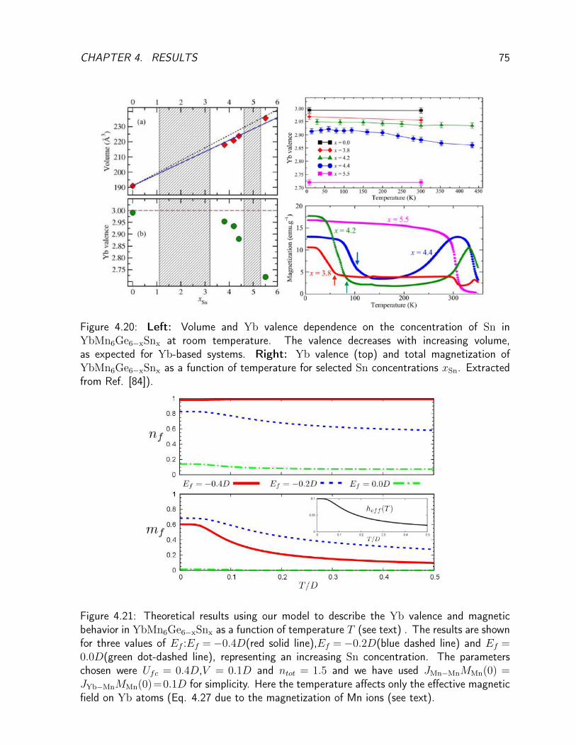
CHAPTER 4. RESULTS 75
Figure 4.20: Left: Volume and Yb valence dependence on the concentration of Sn inYbMn6Ge6−xSnx at room temperature. The valence decreases with increasing volume,as expected for Yb-based systems. Right: Yb valence (top) and total magnetization ofYbMn6Ge6−xSnx as a function of temperature for selected Sn concentrations xSn. Extractedfrom Ref. [84]).
Figure 4.21: Theoretical results using our model to describe the Yb valence and magneticbehavior in YbMn6Ge6−xSnx as a function of temperature T (see text) . The results are shownfor three values of Ef :Ef =−0.4D(red solid line),Ef =−0.2D(blue dashed line) and Ef =0.0D(green dot-dashed line), representing an increasing Sn concentration. The parameterschosen were Ufc = 0.4D,V = 0.1D and ntot = 1.5 and we have used JMn−MnMMn(0) =JYb−MnMMn(0)=0.1D for simplicity. Here the temperature affects only the effective magneticfield on Yb atoms (Eq. 4.27 due to the magnetization of Mn ions (see text).
CHAPTER 4. RESULTS 76
4.3.4 Eu(Rh1−xIrx)2Si2
Europium-based intermetallics are not studied as much as the Ce- and Yb-based materials,but they present a very interesting behavior with respect to valence. Contrary to Ce andYb materials, the importance of Kondo effect in Eu systems is not so evident and the lowtemperature behavior very often deviates from the predictions based on the Doniach’s diagram.
In intermetallic compounds, Eu possesses two valence configurations. The magnetic oneis Eu2+(4f 7), which has a purely spin angular momentum J = 7/2, according to the Hund’srules. By giving one electron to the conduction band, the Eu ion becomes trivalent and itsangular momentum cancels out exactly(J=0). This situation does not happen for lanthanidessituated in the beginning and the end of the series and one should wonder if it leads to differentbehavior than Ce and Yb.
Experimental evidences suggest that the valence transitions are enhanced in several Eu-based compounds[85, 86, 87]. One of these compounds is Eu(Rh1−xIrx)2Si2, which crystalizesin a tetragonal (I4/mmm) structure[88]. The unit cell volume goes from 171Å3 at x= 0 to169.5Å3 at x=1, corresponding to a volume reduction close to 1.5%.
The x-T phase diagram of Eu(Rh1−xIrx)2Si2 is presented in Figure 4.22. At low iridiumconcentrations the divalent configuration is stable and antiferromagnetic order takes placebelow TN ≈ 25K. For x ≈ 0.3 the AF order disappears abruptly and the low temperaturevalence increases. At T =Tv, a first-order valence transition happens and the system is againdivalent at higher temperatures. The first-order transition is unambiguously seen by the bighysteresis in thermodynamic quantities (for instance, the magnetic susceptibility)[88]. Forx≥0.75 the valence transition becomes a crossover.
The most impressive feature of the phase diagram discussed above is the existence of acritical endpoint that separates the first-order from the crossover valence transition. To ourknowledge, apart from the "historical" metallic Ce and SmS, it is the only compound thatshows such point on its phase diagram. Note that these two other examples have substantialvolume variations through the first-order line, which does not seem to be the case in thisexample, since the volume variation is close to 1%[88].
In order to establish the connection between the experimental phase diagrams and theEPAM, we plot in Figure 4.23 the valence dependence on the pressure and temperature closeto the critical point. Here we have considered that the applied pressure (or the Ir doping) onEuRh2Si2 is translated in an increasing Ef in the model. Ufc is chosen to be slightly abovethe zero-temperature critical endpoint, i.e. Ufc>U∗fc
4. In this case, at very low temperaturethe valence transition is first-order, but by temperature effects (as discussed in Section 4.1.2)the transition is softened and becomes a crossover. The valence jump in the first-order lineis overestimated in our approach using mean-field theory, being five times larger than what isseen experimentally (∆v≈0.19 [89]).
The real system presents an antiferromagnetic phase at low pressure with TN≈20K, whichdisappears close to p= 1GPa (xIr ≈ 0.25), when an intermediate valence state is stabilized.In the present work the question of antiferromagnetic order was not addressed, but from the
4We remind that the critical value for Ufc for V =0.1D and ntot=1.5 is U∗fc=0.53D (see Figure 4.1 andSection 4.1.2 for details.

CHAPTER 4. RESULTS 77
J. Phys.: Condens. Matter 23 (2011) 375601 S Seiro and C Geibel
shown in figure 9. At low Ir content (x 0.25), Eu isstable divalent from room temperature down to the lowesttemperatures achieved in this work (⇠0.35 K) and ordersantiferromagnetically below ⇠25 K. Increasing the Ir contentto x = 0.3 results in an abrupt change of the ground stateto an intermediate-valence state which is similar to that ofEuIr2Si2, where a valence of 2.8 has been established byMossbauer spectroscopy [30, 31]. For x � 0.3 increasing thetemperature restores the Eu2+ state through a pronouncedfirst-order transition. The valence transition temperatureincreases steeply with x, from about Tv = 30 K at x = 0.3to about Tv = 80 K at x = 0.5. At even larger Ir contents x �0.75, the valence transition evolves into a crossover behaviour,with a continuous valence decrease on increasing temperatureand a signature of Kondo-like behaviour in the resistivity.Accordingly, at room temperature the Eu valence as deducedfrom lattice parameters moderately increases up to ⌫ = 2.3with increasing x. In contrast, at low temperatures, the specificheat data show that the electronic properties of the groundstate change abruptly between x = 0.25 and 0.30, withoutevidence for critical fluctuations or diverging correlationeffects. Thus the phase diagram that we determined forthe alloy system Eu(Rh1�xIrx)2Si2 based on our study ofsingle crystals is very similar to those reported previously onpolycrystals of other Eu alloy systems [8–10], and supportsthe generic character of the phase diagram in figure 1(b).However, as discussed above, the actual control parameterin this case is not the volume difference between Rh andIr atoms, which is small and positive and would yield aEu2+ state for the Ir compound in a pure chemical pressurescenario. The evolution of the properties from x = 0 to 1 iscontrolled by a purely electronic effect: the binding energyfor the Eu 5d and the transition metal valence electronsis obviously higher for the case of 5d Ir than for 4d Rh,promoting the transfer of an electron from the 4f to the 5dshell of Eu in the former case. Considering that EuCo2Si2is a stable trivalent compound [48], the tendency to a higherrare earth valence increases from 4d Rh to 5d Ir to 3d Co.The same tendency is also observed in the homologue Cecompounds: CeRh2Si2 is an antiferromagnet with a Neeltemperature of 36 K [49], while CeIr2Si2 and CeCo2Si2 areintermediate-valence compounds [50], the Ce valence beinghigher for the Co system than for the Ir system. Surprisingly,the Yb homologues present the reverse order for Rh and Ir:the valence increases from YbIr2Si2 (Kondo scale ⇠40 K,paramagnetic) to YbRh2Si2 (Kondo scale ⇠20 K, weak AFMorder at 70 mK) to YbCo2Si2 (stable trivalent Yb, AFMorder at 1.7 K) [26, 47, 51]. The reason for this differenceis not clear. Moreover, pressure experiments indicate thatthe difference in the Kondo scale between YbIr2Si2 andYbRh2Si2 is larger than expected from the volume differencebetween Ir and Rh atoms [52], which implies that theelectronic effect is of different sign than for the Eu-based orCe-based systems, i.e. it pushes the Ir compound towards thelower Yb valence.
The origin of the pronounced difference between thegeneric phase diagram of Eu and Ce/Yb systems is still poorlyunderstood. Considerations based both on cohesive energies
Figure 9. Phase diagram for Eu(Rh1�xIrx)2Si2. Red open symbolswere obtained from resistivity data and black full symbols fromsusceptibility data. For first-order transitions, the average betweencooling and warming runs is plotted. The lines are a guide to the eye.
and high-energy electron spectroscopy results [53] proposestrong similarities between Yb and Eu, and strong differencesto the case of Ce. On the other hand, the huge magneticentropy S = R ln 8 of the J = 7/2 Eu2+ state, which undergoesno crystal electric field (CEF) splitting since L = 0, contrastswith the much smaller S = R ln 2 for the CEF-split groundstate doublet in Ce or Yb systems. However, if degeneracywas the determining factor, Yb systems with a small CEFsplitting, like YbT2Zn20 [54], should behave like Eu systemsat temperatures above 50 K since Yb3+ has also J = 7/2. Inaddition, RKKY exchange in Eu systems is much larger thanin Yb, but only slightly larger than in Ce. A more likely originis the 4f intrashell coupling energy due to spin polarization,orbital polarization and spin–orbit coupling (corresponding toHund’s first, second and third rules, respectively) [55]. Fortrivalent Ce and Yb, with a single electron or a single hole inthe f shell, this polarization energy is small. Thus the valencechange involves mainly a change in the chemical bondingenergy. In contrast, the (nearly) half-filled f shell of Eu impliesa huge polarization energy (of the order of 10 eV), with adifference in polarization energy between 4f6 and 4f7 thatis also large (of the order of 1 eV) [55]. Thus, a valencechange in Eu systems involves a huge energy transfer frompurely chemical interatomic bonding energy to intra-4f shellpolarization energy. It is readily conceivable that this shouldfavour a first-order transition.
4. Conclusions
We have demonstrated that high-quality single crystals notonly of divalent EuRh2Si2, but also of valence-fluctuatingEuIr2Si2 and their alloy series can be grown using an In-fluxgrowth method. We have studied the evolution of the Euvalence and the magnetic behaviour of these crystals asa function of the Ir content x by means of susceptibility,specific heat and resistivity measurements. The phase diagramdescribing the transition from the stable Eu2+ state at x = 0,showing antiferromagnetic order at low temperatures, to a
7
Figure 4.22: Left: x-T phase diagram for Eu(Rh1−xIrx)2Si2 from Ref.[88]. The passage froma first-order valence transition to a crossover happens at x ≈ 0.75 (not specifically shown).Right: p-T phase diagram for EuRh2Si2 from Ref.[89].
Figure 4.23: Valence phase diagram for EuRh2Si2 under pressure (or Ir doping) using theEPAM model. Parameters are chosen to enforce the proximity to the zero temperature quantumcritical point (see text). Parameters in the model: V = 0.1D, ntot = 1.5, Ufc = 0.55D, Efranging from Ef =−0.6D to Ef = 0.2D. The temperature range is indicated in the verticalaxis.

CHAPTER 4. RESULTS 78
points discussed in what concerns ferromagnetism (Section 4.2.3) it can be sustained thatmagnetic order is very sensitive to first-order valence transitions. Then it is expected that thefirst-order transition lines on Fig. 4.22 (represented by TV ) coincide with the antiferromagnetictransition line.
The existence of a critical point as in Figure 4.1 raises a natural question: how importantis Ufc in Eu-based materials? If valence transitions are enhanced and eventually first-order inEu intermetallics, one would expect a large Ufc interaction, especially if volume effects are notappreciable. On the other hand, Ce and Yb materials in a similar structure do not show thisremarkable changing in the transition behavior, even that the electronic structure should be apriori similar.
The answer for the puzzle above is still open. It is most likely related to the energeticdifferences between the magnetic Eu2+ and the nonmagnetic Eu3+ configurations[90]. Thelarge spin polarization energy (close to 1eV ) between these states would favor a first-ordertransition, which does not happen in Ce(Yb) transitions since it involves states with zero andone electron (hole). Obviously it is a multiorbital effect not described by the single orbitalhamiltonian considered in this work, so Ufc acts here as an effective parameter that modelsthis interaction.
Further analysis of this compound are highly desirable. For instance, spectroscopic mea-surements like RIXS could determine with precision the valence states through the transitionsand clearly identify the location of the critical point in the phase diagram of Figure 4.22. Ex-periments under pressure and external magnetic field as those realized for YbCu2Si2 could alsohelp to understand the discrepancies between Eu and Ce/Yb-based intermetallics.
4.3.5 Summary
In Section 4.3 the comparison between the results obtained for EPAM in Sections 4.1 and4.2 and some compounds is made. The first compound is YbCu2Si2[79], which presents aferrromagnetic transition at p= 8GPa for T < 10K. The Yb valence increases continuouslywith the applied pressure even inside the ferromagnetic phase. We propose that the ferromag-netic transition of YbCu2Si2 under pressure can be accounted in the EPAM, which possesses aferromagnetic instability in the intermediate valence region (see Section 4.2.1). For the secondcompound, YbMn6Ge6−xSnx, we have used the EPAM model in the presence of a magneticfield developed in Section 4.2.2, given that the manganese magnetization acts as a large exter-nal field in the Yb site. For that reason, we have proposed a temperature-dependent magneticfield (Figure 4.21) that describes well the valence variations with temperature for differentSn concentrations. Lastly, we have discussed the case of Eu-based compounds, that usuallypresent larger valence variations in comparison to Ce and Yb materials. The experimentalphase diagram of EuRh2Si2 as a function of Ir doping (in Rh sites) or pressure shows theexistence of a first-order valence transition line that terminates in a critical point, which is alsopresent in the EPAM phase diagram.
Chapter 5
Conclusions and perspectives
In Part I we have covered the topic of valence transitions in intermetallic lanthanide systemsfrom a theoretical perspective. The description of valence transitions was made using anextended version of the Periodic Anderson model (Eq.3.1) that includes the repulsion betweenconduction and localized (f) electrons, represented by Ufc. This interaction is responsible forchanging the character of valence variations from continuous (if Ufc is small) to discontinuous, ifUfc is large. The Extended Periodic Anderson model was treated by a combination of mean-fieldapproximation for the Ufc term and infinite-U Hubbard-I approximation. These approximationsyield a simple self-consistent calculation of the valence at zero and finite temperatures and itallows us to study additional effects, as the inclusion of an external magnetic field (Section4.2.2) and ferromagnetic exchange interactions (Section 4.2.3).
The first important result obtained in Part I is the zero-temperature Ef -Ufc phase diagramin Figure 4.1: it shows how the valence crossover is transformed in a first-order valence transi-tion line by Ufc interaction. This result is in agreement with other works on the EPAM usingmore sophisticated methods, which means that the mean-field approximation is a good choiceof treatment. A second interesting result is the ferromagnetic instability predicted inside theintermediate valence region (Figure 4.11), which is explained by the large density of statesat the Fermi level. Obviously such instability is reinforced in the presence of ferromagneticinteractions (see results of Section 4.2.3), which we have suggested as an explanation of theferromagnetic transition in YbCu2Si2 (Section 4.3.2). An open question is to know if antifer-romagnetic instabilities exist in the EPAM, but for this particular point we need to provide aspecific lattice structure (for example, a cubic lattice). Besides, we have investigated how thevalence is affected by the application of an external magnetic field (Section 4.2.2). As expected,the magnetic field always favors the magnetic valence state (nf =1 in the EPAM), however itdoes not change the nature of the valence variation. Then it provides an experimental tool toinvestigate intermediate valence states and valence transitions.
Apart from the antiferromagnetic instabilities, some open questions deserves to be addressedand are perspectives for future works. One of them concerns the inclusion (or maintenance)of Kondo physics in the problem of valence transitions, allowing to go from the intermediatevalence phase (studied here) to the Kondo limit by decreasing the f level energy Ef . The
79

CHAPTER 5. CONCLUSIONS AND PERSPECTIVES 80
Kondo limit is a particular case of the PAM (see Section 1.2) and is initially included in theEPAM, however the choice of Hubbard-I approximation "killed" the Kondo effect since it doesnot describe the quasiparticle peak that emerges at the Fermi level. This is particularly evidentfrom the Hubbard model: the Hubbard-I approximation describes the lower and upper Hubbardsub-bands only and it is appropriate for the insulating phase. The inclusion of the Kondo peakin the density of states is granted in more sophisticated approximations, as the DynamicalMean-Field Theory.
A second point that may be promising in the context of the EPAM is the inclusion of orbitaleffects. The motivation is based on the discrepancies between the valence phase diagrams ofCe/Yb and Eu materials, highlighted in Refs. [87, 88]. The "competing" valence configura-tions in Ce (4f 0 and 4f 1) and Yb (4f 13 and 4f 14) are composed of a completely empty (orfull 4f orbital) and a one electron (one hole) state, being the non-magnetic configuration com-pletely trivial. In europium the valence configurations are more "exotic": the magnetic state4f 7 is fully polarized (J=S=7/2) and has a large magnetic moment, while the non-magneticstate has L=S=3, but the third Hund’s rule yields J=0. In order to study the quantitiativedifference between Ce/Yb and Eu compounds via orbital effects, one can study an improvedversion of the EPAM with three local orbitals, which is a simplification of the seven 4f orbitals,but provides non-trivial configurations in which J=0.
Part II
Disorder in Kondo systems
81

Chapter 6
Introduction
In the second part of this thesis we will address the problem of disorder in Kondo systems froma theoretical perspective, more specifically the effect of magnetic-nonmagnetic substitutions inlanthanide (or actinide) metallic systems. Before entering in the details of our calculations, wewill discuss some introductory aspects of the problem: the evolution from the Kondo impurityto the Kondo lattice, the effect of disorder in Kondo systems and some experimental resultsthat motivate our work.
6.1 Kondo effect: from the impurity to the lattice
In Chapter 1 some aspects of the Kondo impurity (Eq.1.6) and the Kondo lattice (Eq.1.10)models were introduced. They correspond to particular cases of the single impurity and periodicAnderson models, respectively, in which the localized levels are occupied by one electron andthe charge degrees of freedom are quenched. The passage from the Anderson to Kondo modelsis done through the Schrieffer-Wolff transformation [6], in which the f electrons retain onlytheir magnetic degrees of freedom.
Kondo model describes the antiferromagnetic interaction between local moments and con-duction electrons. Local moments are screened by conduction electrons below the Kondotemperature:
TK = De− 1JKρ
c(µ) , (6.1)
that depends exponentially on the Kondo coupling JK and the conduction electrons density ofstates at the Fermi level ρc(µ).
The Kondo screening is indirectly observed through a logarithmic dependence of the elec-trical resistivity at T & TK that appears both in the impurity and in the concentrated regimes.For lower temperatures, impurity and lattice have a different resistivity behavior: in the impurityregime, the scattering of conduction electrons by impurities is incoherent and it approaches theunitary limit, then the resistivity saturates as T → 0. For the lattice the scattering becomesprogressively elastic as the temperature is reduced [91] and the system achieves a coherentstate below the coherence temperature Tcoh. Then, for T < Tcoh, the resistivity is given in
83

CHAPTER 6. INTRODUCTION 84
Figure 6.1: Magnetic contribution to the resistivity (normalized by the number of Ce atoms)of CexLa1−xCu6 [92] as a function of temperature for different Ce concentrations. The curvescorresponding to the single impurity and the lattice regime are highlighted in red and blue,respectively. Adapted from Ref.[92].
terms of the Fermi liquid expression R(T ) =R0 +AT 2, in which R0 is the residual resistivityand A (the coefficient of electron-electron scattering contribution) is extremely large comparedto common metals.
The development of coherence is clearly seen in the alloy CexLa1−xCu6[92, 93]. Themagnetic resistivity measurements from room temperature up to T =0.01K (Figure 6.1) showthe difference between the impurity and the lattice regimes as the concentration of Ce is tuned.At high temperatures T > 10K there is a clear logarithmic dependence on the temperaturethat is almost independent of concentration, signaling the Kondo effect. For T < 10K thebehavior depends on the concentration: in the diluted regime (x<0.5), resistivity increases bydecreasing temperature until saturation to a residual resistivity at T ≈1K, which correspondsto the unitary limit of scattering. For the concentrated regime (x > 0.5), resistivity has amaximum around 10K and decreases at lower temperatures, until it achieves the residualresistivity.
6.1.1 Local versus Coherent Fermi Liquid
It was mentioned in Chapter 1 that the Kondo impurity and lattice models (Eqs. 1.6 and 1.10)have Fermi liquid (FL) fixed points at zero temperature. While in the impurity the FL behavioris universal, in the lattice other ground states are possible and the low temperature behaviordepends on specific details of each system. In many dense systems, the FL ground state ofthe lattice is in competition with antiferromagnetic order, which is described by the Doniachdiagram (Fig. 1.2).
The FL description of the single impurity Kondo problem was developed by Nozières[94]and it is known as Local Fermi Liquid (LFL). The starting point of Nozières theory is that

CHAPTER 6. INTRODUCTION 85
JK→∞ at low temperatures, as shown by scaling arguments by Anderson[9]. In this limit,the magnetic impurity moment forms a rigid singlet state with one conduction electron spinand an infinite energy is required to break it. The impurity acts as a non-magnetic scatteringsite with infinite repulsion. Including the virtual excitations of the singlet, he has shown thatadditional interactions are irrelevant in a 1/JK expansion.
The Fermi liquid regime of the Kondo lattice, sometimes denote Coherent Fermi Liquid(CFL), corresponds to the heavy fermion behavior introduced in Section 1.2. The strikingproperty of the CFL is the extremely high effective mass of its quasiparticles, which can beexplained by the two (s-f) band picture given by mean-field theory: the Kondo Lattice modelis transformed in a model with two hybridized bands, representing the conduction and the(dispersionless) f electrons (see Section 7.2).
The "exhaustion" problem
In order to achieve a non-magnetic ground (CFL) state in the Kondo lattice, conduction elec-trons must quench the spin degrees of freedom of an outnumbered local moments. Consideringthat the effective number of conduction electrons participating in the screening are located ina energy window of TK(TK�D), then the magnetic moments largely outnumber it and thepicture of individual Kondo cloud must be reconsidered. This "exhaustion problem" was firstproposed by Nozières [95, 96], who used an entropy argument to estimate that the coherencetemperature Tcoh∼ρcT 2
K .Nozières estimation was proven to be wrong by mean-field calculations[97, 98, 99]: the
ratio Tcoh/TK depends only on band structure details, but not on TK (or JK) [97, 98]. Thephysical argument to explain it is the following: in a Kondo Lattice, the "true" quasiparticlesat low temperature are a combination of the conduction and the localized electrons, so the felectrons are (in some sense) "screening themselves"[14].
6.1.2 Strong-coupling picture of Kondo impurity and latticemodels
The strong-coupling limit JK → ∞ of the Kondo impurity and lattice models is a simpleway to understand their low temperature behavior and Fermi liquid properties. According toRenormalization Group calculations[10], JK →∞ is the low temperature fixed-point of theimpurity problem. In the lattice, the ground state is expected to be magnetic for large JK .Here, we are interested in non-magnetic states of the Kondo lattice in the limit JK→∞, sinceit yields an interesting physical picture that can help to understand the CFL for lower JK .
The JK →∞ picture for the Kondo impurity model is represented in Figure 6.2. Themagnetic impurity forms a rigid singlet state with one conduction electron and an infiniteenergy is required to break it. Consequently, the impurity site is forbidden for the remainingconduction electrons. The Nc−1 (Nc is the total number of conduction electrons) remainingconduction electrons are the system quasiparticles, moving in a lattice depleted by one site.
In this picture [100, 96], the Nc=ncN conduction electrons form local singlet states with afraction of the N local moments in the lattice (assuming that Nc<N), while N−Nc moments

CHAPTER 6. INTRODUCTION 86
Figure 6.2: Strong coupling picture of single impurity Kondo problem. The impurity and theconduction electron spins are represented by the red thick and the blue thin arrows, respectively.The impurity local moment forms a singlet state (represented in yellow) with one conductionelectron. The impurity site is "forbidden" for the other conduction electrons, since it requiresinfinite energy to break the singlet. The remaining conduction electrons move freely in thedepleted lattice.
are unscreened (the bachelor spins). Thanks to the electronic mobility, conduction electronswill hop to bachelors spins and the CFL ground state is assured to be non-magnetic by thisdynamical effect. Effectively the bachelor spins behave as holes of a lattice containing a singletper site (a Kondo insulator), having an infinite repulsion between them since two holes cannotoccupy the same lattice site. This situation is depicted in Figure 6.3.
Figure 6.3: Strong coupling picture of Kondo lattice problem. Every conduction electron inthe lattice forms a local singlet (in yellow) with a local moment, while the remaining moments(represented by the thick red arrows surrounded by red dots) stay unscreened. Hopping pro-cesses of conduction electrons are possible only toward sites with unscreened spins. One canequally think that the charge carriers in the system are holes in unscreened spin sites, havingan effective repulsive interaction (see text).
It is possible to check two important results from the analysis above. First, the number
CHAPTER 6. INTRODUCTION 87
of quasiparticles in the system is 2N − (N −Nc) = N +Nc, since holes are moving in thelattice. This verifies the Luttinger’s theorem[2] for the Kondo lattice[101], which states thatconduction electrons and local moments contribute to the Fermi surface.
The second result is the formal equivalence between the JK→∞ Kondo lattice with Nc
electrons and the U→∞ Hubbard model with N −Nc electrons[100, 96]. We can compare itto the LFL for the impurity (Fig. 6.2), where the effective quasiparticles interaction is zero andthe only modification with respect to the "clean" system is the depletion of the impurity site.So, from the JK→∞ point of view, the Local and the Coherent Fermi Liquids have different"types" of quasiparticles: non-interacting electrons in LFL and "hard-core" interacting holesin CFL.
The strong-coupling picture presented in this section can be generalized for a system withan arbitrary numbers of local moments (Kondo Alloys). Such generalization will be discussedin Section 7.1.2.
6.2 Substitutional disorder in Kondo systems
In this section we briefly review some aspects of substitutional disorder in Kondo systems in aglobal perspective. From the stoichiometric point of view there are two non-equivalent formsof substitution in heavy fermion families of materials1, depending on the atom that is replaced.For a f site substitution, the magnetic rare-earth atom is replaced by a non-magnetic one, as inCexLa1−xCu6 [92, 93] or UxTh1−xPd2Al3 [102, 103]. Distinctively, a ligand substitution occurswhen atoms other than the rare-earth (ligand atoms) are replaced, as in CeCu6−xAux [19] orUCu5−xPdx [104]. Here we are going to focus on the f site substitution.
6.2.1 Non-Fermi liquid behavior from disorder
A frequent consequence of substitution in heavy fermions systems is the appearance of Non-Fermi Liquid (NFL) behavior[18], characterized by a violation of Fermi Liquid theory withrespect to the temperature dependence of physical quantities. Many scenarios for Non-Fermiliquid behavior in heavy fermions have been proposed[105, 106], including the proximity of thequantum critical point of the Doniach’s diagram[107] or a quantum critical point associatedto valence transitions[68], models for multichannel Kondo effect [108, 109] and theories ondisorder effects[110, 111, 112]. The pertinence of these theories relies on the specific detailsof the compounds that are meant to be described.
Here we will focus on theories in which disorder is considered to be the driving force ofNon-Fermi liquid behavior. The common aspect of these theories [113, 110, 111] is thatdisorder induces different local environments for the magnetic moments and, consequently, adistribution of Kondo temperatures p(TK). Because TK has an exponential dependence on thelocal energy scale, p(TK) is a skewed distribution.
1By heavy fermion family we mean compounds that possess heavy fermion behavior in a given composition.For a known example, CexLa1−xCu6 enters in this classification, since it is a heavy fermion forx =1.

CHAPTER 6. INTRODUCTION 88
Following the analysis of Refs.[110, 114], we can estimate the thermodynamic behavior ofa system displaying such distribution p(TK). For example, the average magnetic susceptibilitycan be calculated. For a single Kondo impurity expression, we adopt the form from Wilson[1]:
χ(T, TK) =A
T + bTK(6.2)
Here A and b are constants. The average susceptibility with respect to p(TK) is given by:
χ(T ) '+∞∫0
dTKp(TK)A
T + bTK(6.3)
The upper limit of the integral above does not contribute, since p(TK) does not extendentirely to infinite, so the interest is in the low-TK limit. Let us first suppose that p(TK) is afinite quantity as TK→0. Then, using the leading term from the Taylor expansion p(TK)=p0
and introducing a cutoff Γ, we have:
χ(T ) 'Γ∫
0
dTKp0A
T + bTK∼ p0A
blog
(Γ
T
)(6.4)
So a logarithm divergence appears in the low temperature behavior of the magnetic suscepti-bility, in a clear contrast to the Fermi liquid behavior χ=χ0+AT 2. As a conclusion, if thereis a finite distribution of moments having TK→ 0, it leads immediately to Non-Fermi Liquidbehavior. The divergence is stronger in the case of a singularity in p(TK). In the case of apower-law distribution[115, 114] for p(TK)∼Tα−1
K , we have:
χ(T ) 'Γ∫
0
dTK(TK)α−1 A
T + bTK∼{
χ0 , if α > 1Tα−1 , if α < 1
(6.5)
For α> 1, the distribution p(TK) does not diverge as TK→ 0 and χ(T ) remains finite whenT → 0, as in a Fermi liquid. On the other hand, Non-Fermi liquid behavior is observed inχ(T ) if α < 1. In a similar way, NFL behavior of the specific heat coefficient γ = C/T canbe deduced from a distribution of TK . Further details on these calculations, for instance thedisorder dependence of α in Kondo systems, the References [114, 115, 116] are recommended.
6.2.2 Kondo Alloys: experimental motivation
Kondo alloys are systems where the concentration of local moments is tuned by the amountof the magnetic ion. The typical example is the substitution of lanthanum (in La3+ valencestate) by cerium (Ce3+ valence state), but there are examples with other atoms involved. Oneissue of this type of substitution is the multiple effects that can appear when it is performed.For instance, there are volume effects inherent to different ionic radius (RLa3+ =103.2pm and

CHAPTER 6. INTRODUCTION 89
RCe3+ =101.0pm [22]). Furthermore, the substitution affects not only the electrical properties(as the resistivity), but also the magnetic properties (susceptibility).
A first example of Kondo alloy is CexLa1−xCu6 shown in Figure 6.1. The low T behavior ofits resistivity was discussed in the context of coherence formation and the evolution from theimpurity to lattice regimes. Other examples are CexLa1−xCoIn5 [117, 118], CexLa1−xPd3[119],Ce1−xLaxPtGa[120], CexLa1−xB6[121], Ce1−xLaxCu2Ge2[122], (CexLa1−x)7Ni3 [123] orU1−xThxPd2Al3[102, 103].
Figure 6.4: Experimental phase diagram of CexLa1−xNi2Ge2 as a function of Ce concentrationx.The two Fermi Liquids regions indicated in blue (Local FL) and yellow (Coherent FL) aredetermine by specific heat, resistivity and thermopower measurements and the points charac-terize different system energy scales, namely the Kondo and the coherence temperatures. TheFermi Liquid regions are separated by a Non-Fermi Liquid region that spans a large range ofintermediate concentrations. Figure adapted from Ref. [124].
Let us focus on a particular example of compound: CexLa1−xNi2Ge2 [124]. It is a heavyfermion system in the Ce-rich phase (CeNi2Ge2) with a large Sommerfeld coefficient γ ≈350mJ/K2mol [125, 126]. Anomalous behavior of the specific heat of CeNi2Ge2 in mKscales suggests that it is very close to a magnetic quantum critical point. While the magnetictransition is observed via the Ni-Pd or Ge-Cu substitution, the same is not seen when Ce isreplaced by La. Instead, a coherent Fermi Liquid regime is obtained in the range 0.95<x<0.6.For 0.5< x < 0.02 Non-Fermi liquid behavior is reported, while the system is again a Fermiliquid (local FL) for x<0.02 (Figure 6.4).
The compound CexLa1−xNi2Ge2 is non-magnetic in the whole range of substitution andit has two different Fermi Liquid phases well separated by a large region of Non-Fermi Liquid
CHAPTER 6. INTRODUCTION 90
behavior. Moreover, the results in Refs. [124, 127] indicate that the Kondo temperature isindependent of x. The interpretation of these results leads us to propose that the Non-FermiLiquid behavior in the range 0.5< x < 0.02 is induced by disorder, in a possible associationwith the loss of coherence by La doping.
In the next chapter we will propose a model to describe non-magnetic phases of KondoAlloys as CexLa1−xCu6 or CexLa1−xNi2Ge2 using a method suitable to treat the combinedeffects of coherence and disorder.

Chapter 7
Model and method
In this chapter we will introduce the model hamiltonian that describes the physics of alloyscontaining randomly displaced magnetic moments and the numerical method used to solve it.We start from the presentation of the model and its relation with the compounds discussedin Section 6.2.2. Then the approximations employed in this work are shown in details: themean-field approximation for the Kondo problem (Section 7.2) and the statistical DMFT fordisorder effects (Section 7.3).
7.1 The Kondo Alloy model
Our goal is to describe rare-earth systems in which the concentration of magnetic moments canbe tuned by substitution. One example is the La-Ce substitution, supposing that the ceriumconfiguration is magnetic. The model hamitonian is the Kondo Alloy model (KAM):
H = −∑ijσ
(tij + µδij)c†iσcjσ + JK
∑i ∈ K
Si · si (7.1)
The first term describes the kinetic energy of conduction electrons given by the hoppingintegral tij. The number of conduction electrons per lattice site is fixed by the chemicalpotential µ. The second term is the Kondo interaction, i.e. a local antiferromagnetic couplingbetween the local moment, described by the spin operator Si, and the spin of conductionelectrons (si). The Kondo interaction takes place only in a subset K of the N lattice sites,which is composed by the sites containing local moments that are randomly distributed alongthe lattice (quenched disorder). The interaction strength JK is the same for all the Kondosites and it is a positive quantity. We have supposed that the hopping integral tij does notdepend on the nature of the sites i and j.
Apart from the lattice geometry (given by tij) and the Kondo interaction JK , there are twoother controlled parameters: the concentration of magnetic moments x, ranging from x=0 tox=1, and the concentration of conduction electrons nc, from nc=0 to nc=2. In the absenceof magnetic moments (x= 0), the system behaves as a normal metal with a single electronicband. In the presence of one magnetic impurity (xN=1), the KAM corresponds to the single
91

CHAPTER 7. MODEL AND METHOD 92
impurity Kondo model, discussed in Section 1.1.2. Otherwise, if the number of local momentsis maximum (x=1), i.e. every lattice has a local moment, the KAM is equivalent to the KondoLattice model (Eq. 1.10).
We assume that the only variation occurring in the system under the substitution is thepresence/absence of a local moment and the Kondo interaction. In reality, this type of sub-stitutions produces disorder in the conduction electrons energy and lattice distortions, sincethe electronic levels and ionic volumes are different from one rare-earth atom to other. Herewe neglect these effects for simplicity. We are also considering a S = 1/2 spin for the localmoment and only one conduction electron band.
7.1.1 State-of-art
The Kondo Alloy model was previously studied by several authors. Early works of Kurata[128,129] using the Coherent Potential Approximation (CPA) were focused on the analytical calcu-lations for the density of states and the resistivity within this approximation.
More recently, Burdin and Fulde [130] have employed a matrix form of CPA, showing thatit is equivalent to a matrix dynamical mean-field theory, and mean-field interaction for theKondo interaction. They have focused the analysis of the relation between the Fermi liquidand the Kondo temperatures, T0 and TK , for different concentration x of magnetic moments.In particular, the ratio T0/TK exhibits a different behavior when x<nc and x>nc.
Kaul and Vojta[131] combined the mean-field approximation for the Kondo interactionwith exact diagonalization in a 20 × 20 square lattice to investigate the same model. Thisapproach allows to study the spatial distribution of local quantities for a disorder realization.In particular, they have shown that the mean-field energy scale T ∗, defined from the averagedvalue of the mean-field parameter r2 (see Section 7.2), has a sharp change around the pointx=nc, as it is shown in Figure 7.1. A similar change was found by Watanabe and Ogata[62]using Variational Monte Carlo calculations. Besides, many studies using a disordered versionof the Periodic Anderson model were made in a similar context[132, 133, 134, 135], most ofthem employing CPA.
7.1.2 The JK→∞ limit
The JK→∞ limit of the Kondo Alloy model was recently studied by Burdin and Lacroix[136].In this work, the existence of a "Lifshitz-like" transition separating the Local and the CoherentFermi liquids at x = nc. In Section 6.1.2 the physical picture of the strong coupling limitwas presented for the impurity and the lattice cases. If we generalize this picture for anyconcentration x of local moments, we have the following situations:
• Situation I (x < nc): The Ns = xN magnetic moments form rigid singlets with thesame number of conduction electrons and an infinite energy is required to break any ofthese singlets. The remaining electrons ((nc−x)N) are free carriers in a lattice depletedby xN sites, assuming that the former percolates1. The number of quasiparticles is
1The issue of percolation will be discussed in more details in Section 8.4

CHAPTER 7. MODEL AND METHOD 93
Figure 7.1: Dependence of the coherent temperature T ∗ on the concentration of magneticimpurities for the KAM. The point x=nc marks the crossover from the diluted (x<nc) to theconcentrated (x>nc) regime. Figure adapted from Ref.[131].
Nqp=Nc−Ns=(nc−x)N .
• Situation II(x>nc): The Nc=ncN conduction electrons in the lattice form singlet stateswith local moments, leaving (x−nc)N unscreened moments (the bachelor spins). Theelectronic hopping occurs only between Kondo sites (as in Fig. 6.3), what can be seenas the movement of bachelor spins in a lattice depleted by (1−x)N Non-Kondo sites.The number of quasiparticles in this regime is Nqp = Ns+Nc = (nc+x)N , given theholelike character or the carriers. The electronic correlation comes not only from thelattice depletion, but also by an infinite repulsion that prevents the double occupation ofholes (following Ref.[100]).
Figure 7.2: Strong coupling picture of the Kondo Alloy model for x < nc (left) and x > nc(right).
By increasing the concentration x, one should expect to pass from the former to the lattersituation when x= nc. In this point there is a discontinuity in the number of quasiparticles(from (nc−x)N to (nc+x)N), in the effective number of lattice sites (from N−Ns to Ns)

CHAPTER 7. MODEL AND METHOD 94
and in the effective Hubbard repulsion (from zero to infinity). According to Ref. [136] thissingularity is related to a singular change of the Fermi surface (a Lifshitz transition[137]), andnot to a symmetry breaking.
7.2 Mean-field approximation for the Kondo problem
The mean-field approximation here employed follows Reference [53] and it is equivalent to theslave boson mean-field theory[138, 139, 140].
We use the relation:
Si · si = Szi szi +
1
2
(S+i s−i + S−i s
+i
)(7.2)
and write the spin operators in their fermionic representation:
Szi =1
2
∑σ
σf †iσfiσ ; S+i = f †i↑fi↓ ; S−i = f †i↓fi↑ (7.3)
szi =1
2
∑σ
σc†iσciσ ; s+i = c†i↑ci↓ ; s−i = c†i↓ci↑ (7.4)
The hamiltonian in Eq. 7.1 then becomes (σ ≡ −σ):
H = −∑ijσ
tijc†iσcjσ + JK
∑i ∈ K
[Szi σ
zi +
1
2
∑σ
f †iσfiσc†iσciσ
](7.5)
The mean-field approximation consists in approximating the terms with four operators inEq. 7.5 by:
Szi σzi = 〈Szi 〉σzi + 〈σzi 〉Szi − 〈Szi 〉 〈σzi 〉 (7.6)
and∑σ
f †iσfiσc†iσciσ = −
∑σ
(⟨f †iσciσ
⟩c†iσfiσ +
⟨c†iσfiσ
⟩f †iσciσ −
⟨f †iσciσ
⟩⟨c†iσfiσ
⟩)(7.7)
By replacing the local spin operators Szi for fermions, one must assure local charge conservation:∑σ
f †iσfiσ = 1 , ∀ i ∈ K (7.8)
This is done by the inclusion of a local Lagrange multiplier λi, that might be different at eachKondo site.
The mean-field approximation introduces average values[141]: 〈Szi 〉, 〈szi 〉 and <f †iσciσ >.The first two averages measure the local polarization of f and c electrons, respectively, and arenonzero in magnetic phases only. The third average, <f †iσciσ>, measures the local degree ofhybridization between conduction and f electrons and it is related to the local singlet formation

CHAPTER 7. MODEL AND METHOD 95
by Kondo effect.We assume from now on that the system is in a non-magnetic state. Thenthe second term in Eq. 7.5 will not be considered. The third term in Eq. 7.5 simplifies sincethe averages <f †iσciσ> are spin-independent under this assumption. Defining:
ri ≡ −JK⟨f †iσciσ
⟩, (7.9)
and considering ri as a real quantity, the hamiltonian reads:
H = −∑ijσ
tijc†iσcjσ − µ
∑iσ
(c†iσciσ −
nc2
)+∑i ∈ K
∑σ
ri
(c†iσfiσ + f †iσciσ
)−∑i ∈ K
∑σ
λi
(f †iσfiσ −
1
2
)+∑i ∈ K
2r2i
JK(7.10)
In Eq. 7.10, two Lagrange multipliers were included. The first one is the chemical potentialµ that fixes the average number of conduction electrons nc in the lattice (a global constraint).The second is a local multiplier λi, which constraint the number of f electrons to one in eachKondo site.
The hamiltonian in Eq. 7.10 describes hybridized s and f bands. The hybridization ri is alocal quantity, as well as the position of the f-level λi, reflecting the disorder. Both ri and λiare self-consistent parameters determined by Eqs. 7.8 and 7.9.
The determination of the mean-field parameters λi and ri comes from the solution oflocal self-consistent equations. Introducing the finite temperature Green’s functions in siterepresentation[3, 2],
Gcciσ,jσ′(τ) ≡ −
⟨Tτciσ(τ)c†jσ′(0)
⟩, (7.11)
Gffiσ,jσ′(τ) ≡ −
⟨Tτfiσ(τ)f †jσ′(0)
⟩, (7.12)
Gcfiσ,jσ′(τ) ≡ −
⟨Tτciσ(τ)f †jσ′(0)
⟩, (7.13)
(7.14)
defined for the imaginary time τ (Tτ is the imaginary-time ordering operator). Thermal averagesas⟨f †i ci
⟩and
⟨f †i fi
⟩are computed2 in the limit τ → 0−,⟨
f †i ci
⟩= Gcf
i,i(τ = 0−)⟨f †i fi
⟩= Gff
i,i (τ = 0−),
leading to the following equations for ri and λi (if i ∈ K):1
2= Gff
ii (τ = 0−) (7.15)
ri = −JKGcfii (τ = 0−) (7.16)
2From now on spin indices are dropped for shortness.
CHAPTER 7. MODEL AND METHOD 96
The evaluation of Gffii (τ = 0−) and Gcf
ii (τ = 0−) are done via a sum over fermionic Mat-subara’s frequencies, which are presented in details in Appendix D. At T = 0, we have fromEquations D.7 and D.9:
Gffii (τ = 0−) =
1
π
+∞∫0
dωRe(Gffii (ω)
)+
1
2(7.17)
Gcfii (τ = 0−) =
1
π
+∞∫0
dωRe(Gcfii (ω)
)(7.18)
7.2.1 Green’s functions
The hamiltonian in Eq. 7.10 can be rewritten as:
H = −∑ijσ
tijc†iσcjσ +
∑i
H0i + cts. (7.19)
This expression contains only one non-local term: the kinetic energy of conduction electrons.It corresponds to conduction electrons hopping in and out of a particular site. The local partcontains the chemical potential for the conduction electrons, equal in all the sites, and thef-operators contribution, present if i is a Kondo site. For Non-Kondo sites ri = 0 and weartificially introduce an f energy level λi = −E0 that will be considered as infinite in orderto enforce the local constraint nf,i = 0 if i 6∈ K. This procedure is equivalent to introduceprojection operators for the two different type of sites, as it was performed in Ref. [130]. Itallows to describe H0
i equally for Kondo and Non-Kondo sites with the same matrix form:
H0i =
∑σ
(c†iσ f †iσ
)( −µ riri −λi
)(ciσfiσ
)(7.20)
Here:ri = 0
λi = −E0, if i 6∈ K. (7.21)
In the following we study only non-magnetic phases. We can thus consider an effectivespin-less problem and the index σ is dropped in the remaining of this chapter.
Defining gii(iωn) as the matrix Green’s function for the local term H0i , we have:
gii(iωn) =
(gccii (iωn) gcfii (iωn)
gfcii (iωn) gffii (iωn)
)=[iωnI−H0
i
]−1 (7.22)
Here I is the 2 × 2 identity matrix. The matrix inversion leads to the explicit form ofgii(iωn):
gii(iωn) =
1
iωn+µ−r2i
iωn+λi
ri(iωn+µ)(iωn+λi)−r2
i
ri(iωn+µ)(iωn+λi)−r2
i
1
iωn+λi−r2i
iωn+µ
(7.23)

CHAPTER 7. MODEL AND METHOD 97
7.2.2 Hopping expansion
We perform an infinite expansion of the hybridization function (sometimes called self-energy 3)associated with the electronic hopping[143]. The suitable expansion is given by the Feenberg’sperturbation theory[144] largely discussed in the context of Anderson localization[145, 146].
The hybridization function ∆i(iωn) describes processes where a conduction electron hopsout the initial site i, move through a given path in the lattice and returns to the initial site inthe end. For convenience, we define it in the matrix form
∆i(iωn) =
(∆i(iωn) 0
0 0
), (7.24)
so that we can write the full Green’s functions Gii(iωn) (also in a matrix form) as:
Gii(iωn) =[(gii(iωn))−1 −∆i(iωn)
]−1(7.25)
Explicitly:
Gii(iωn) =
1
iωn+µ−r2i
iωn+λi−∆i(iωn)
ri(iωn+µ−∆i(iωn))(iωn+λi)−r2
i
ri(iωn+µ−∆i(iωn))(iωn+λi)−r2
i
1
iωn+λi−r2i
iωn+µ−∆i(iωn)
(7.26)
The expansion of ∆i(iωn) for an arbitrary lattice is presented in Appendix F. Here werestrict ourselves to the results obtained for a Bethe lattice. A Bethe lattice 4 is a loop-freenetwork characterized only by its coordination number Z, as shown in Figure 7.3. We alsoconsider that all the nearest-neighbors hoppings are equal (tij = t, for all pair of neighborsi, j), disregarding the type of sites (Kondo or non-Kondo).
Figure 7.3: Finite representation of a Z = 4 Bethe lattice.3We adopt the former denomination to link it to Dynamical Mean-Field Theory[142], where hybridization
function is used for the same quantity.4We refer to Appendix C for additional results on the Bethe lattice, including the analytical expression of
the non-interacting density of states.

CHAPTER 7. MODEL AND METHOD 98
Given that loops are absent, there is only one path connecting two different sites in thislattice and the expansion in Equation F.7 contains only the first term. The equation obtainedfor ∆i(iωn) is (Eq. F.11):
∆i(iωn) = t2Z∑j 6=i
Gcc (i)jj (iωn), (7.27)
The sum extends over the Z neighbors of i (Z is the lattice coordination number). Gcc (i)jj (iωn)
is the Green’s function in the site j with the site i removed, or a cavity Green’s function, havinga similar form as Gcc
ii (iωn):
Gcc (i)jj (iωn) =
1
iωn + µ− r2j
ω+λj−∆
(i)jj (iωn)
(7.28)
The hybridization function ∆(i)j (iωn) for the cavity Green’s function Gcc (i)
jj (iωn) (given byEq. 7.28) has a similar structure (see Figure 7.4):
∆(i)j (iωn) = t2
Z−1∑k 6=j,i
Gcc (j)kk (iωn), (7.29)
although the sum extends over Z−1 terms only. Note that in the Bethe lattice all the "higher-orders" cavity Green’s functions and their hybridization functions have exactly the same formas Gcc (i)
jj (iωn) and ∆(i)j (iωn).
Figure 7.4: Schematic diagram of the hopping expansion in a Z = 4 Bethe lattice. (a)Starting from the central site i, the hybridization function ∆i(iωn) is written in terms of theGreen’s functions of its Z neighbouring sites with the central site excluded (the cavity Green’sfunctions). In this procedure, the branch labeled by its first site j (highlighted in (b)) isseparated from the others.(c) The cavity hybridization function ∆
(i)j (iωn) is obtained in the
same manner, except that it is a sum over Z − 1 sub-branches, labeled by k.

CHAPTER 7. MODEL AND METHOD 99
7.3 Statistical DMFT
The statistical DMFT is a variation of Dynamical Mean-Field Theory adapted to treat disor-dered problems. The idea is to map an interacting fermionic problem in a disordered latticeto an ensemble of single impurity problems embedded in their own self-consistent baths. Theself-consistency is taken in the statistical distribution of baths, which is obtained from an algo-rithm that generates it iteratively. This method was introduced by Dobrosavljevic and Kotliar[147, 148, 149] for the Hubbard model with a disordered local energy in the context of theMott-Anderson metal-insulator transition.
In all following, the Bethe lattice will be considered. Let us take some results from the lastsection to explain the method. Supposing that the site i is a Kondo site. Its Green’s functionis given by the matrix Eq.7.26 and
Gccii (iωn) =
1
iωn + µ− r2i
ω+λi− t2
Z∑j 6=i
Gcc (i)jj (iωn)
, (7.30)
where the sum over j is taken on the Z nearest neighbors of site i.Here we have written explicitlythe hybridization function ∆i(iωn) from Eq.7.27. The cavity Green’s function Gcc (i)
jj (iωn) aregiven by (using Eq.7.28 and 7.29)
Gcc (i)jj (iωn) =
1
iωn + µ− r2j
ω+λj− t2
Z−1∑k 6=j,i
Gcc (j)kk (iωn)
, (7.31)
where the sum over k is taken on the Z−1 nearest neighbors of j, having excluded site i (seeFigure 7.4).
Since we are dealing with a disordered problem, we expect that local quantities as Gccii (iωn)
will follow some distribution (unknown, in principle) and our goal is to determine them. Thisis done in the statistical DMFT by considering Eq. 7.31 above as a self-consistent equationfor the distribution of cavity Green’s functions. This idea was first considered by Abou-Chacra,Anderson and Thouless [146] for non-interacting electrons in their self-consistent treatment ofdisorder, discussed in the context of Anderson localization. The statistical DMFT then is ageneralization of their approach for interacting problems.
We remind that the method presented here is exact for a Bethe lattice of any coordinationnumber Z. Approximations in this work are performed in two different levels. The first one isthe solution of the local Kondo problem5 in a mean-field approximation. The second one takesplace when we sample the distribution of cavity Green’s functions by a numerical procedure,which introduces statistical errors.
In the next section we will show a numerical procedure to implement a stochastic methodthat achieves the convergence from the self-consistent relation in Eq.7.30 for finite Z.
5The solution of the single impurity Anderson model is required in the general case.

CHAPTER 7. MODEL AND METHOD 100
Numerical procedure
Let us concentrate now on the numerical procedure that implements the statistical DMFT. Thekey point lies in the iterative procedure to generate new cavity hybridization functions (or cavitybaths) from the cavity Green’s functions in the last step of iteration, as it is mathematicallydescribed in Eq. 7.31.
For clarity purposes, we discuss separately the parts containing the self-consistent calcula-tion for the Fermi level and how the statistics are made. The numerical implementation coreis the following6:
1. Enter an initial guess for the cavity baths ∆(0)i (iωn). A good approach to speed up
convergence is to use an ansatz that interpolates between its value on the lattice (x = 1)and the impurity (x→ 0):
∆(0)i (iωn) = x∆
(0)i,Lattice(iωn) + (1− x)∆
(0)i,Impurity(iωn).
These quantities are easily computed for a given JK and Z. For instance, ∆(0)i,Impurity(iωn)
is the same as in the non-interacting problem and its expression is given in Eq. C.7.
2. Solve xNsite mean-field equations numerically for every Kondo site of the ensemble usingthe baths ∆
(0)i (iωn). The mean-field equations for ri and λi (Eqs. 7.15 and 7.16) can
be written as:
2
π
∫ +∞
0
dωRe
1
ω + λi − r2i
ω+µ−∆(0)i (ω)
= 0 (7.32)
− 1
π
∫ +∞
0
dωRe
[1
(ω + µ−∆(0)i (ω))(ω + λi)− r2
i
]= 1 (7.33)
After that, update the cavity Green’s functions with the mean-field parameters and thecavity baths.
3. Generate new cavity baths from the previous ones from the following procedure:
(a) Creates Z − 1 copies of each cavity Green’s function from the previous step G(0)ii .
The system will have (Z − 1)Nsites sites after this step.
(b) For a given site j(= 1, ..., Nsites), pick up randomly Z − 1 functions G(0)jj and
compute the new cavity baths as:
∆(0)i (ω) = t2
Z−1∑j
G(0)jj (ω) (7.34)
6In this subsection we employ the notation from Appendix C for the cavity Green’s function (Gcc (0)ii ) and
hybridization function (∆(0)i (ω)), instead of Gcc (i)
jj and ∆(i)j . The reason is to avoid misleading idea that the
sampling procedure is performed in a real lattice for a fixed disorder realization.

CHAPTER 7. MODEL AND METHOD 101
4. Go back to step 2 using ∆(0)i (ω) as baths. Proceed by iteration until you achieve the
statistical convergence of ∆(0)i (ω).
5. After the convergence: The last step is to get ∆j(ω) from ∆(0)j (ω). It corresponds in
our construction to Eq. 7.30. It is done by the step 3 above, but now copying Z timeseach function and combining Z functions to construct ∆j(ω).
6. Store all the local quantities whose statistics will be analyzed.
In Figure 7.5 we illustrate the statistical DMFT procedure, in particular, the generation ofrandom cavity baths is described in the diagram on the bottom.
The determination of the Fermi level is based on the requirement that the average numberof conduction electrons per site is fixed at a given value nc, which is calculated using Eq.D.8:
nc = 2∑i
<c†ici>= 2∑i
Gccii (τ = 0−) (7.35)
Since it is a disordered system, in principle each site has a different occupation and theaverage value varies at each iteration, due to statistical fluctuations inherent to the method.Then the criterion to achieve a self-consistent value for the Fermi energy must be loose enoughto account for these fluctuations. In all the results in the next chapter we have taken asnumerical error 0.01 and the chemical potential is determined for a nc fixed to a given value±0.01.
The numerical procedure to perform reliable statistical analysis is based on an artifact toincrease the sample size. The number of sites Nsite increases the computational time in twoways: the number of impurity problems to be solved at each iteration is proportional to Nsite,as it is the size of arrays that store the local quantities numerically7. Then the following trickis proposed: instead of using a large array and compute the statistics at the end of the finaliteration, we gather data in Nstat iterations counted after the convergence is achieved. So weeffectively sample Nsite×Nstat different sites.
7In practice we are constrained to use Nsite=104−105 in a serial implementation on a PC.

CHAPTER 7. MODEL AND METHOD 102
Figure 7.5: Illustration of Statistical DMFT procedure for Z = 4 Bethe lattice. Top: Thedisordered interacting problem in the lattice (represented by a single branch) is replaced byan ensemble of single site problems in which the local environment is encoded by the bathfunctions ∆
(0)i (iωn). The cavity Green’s functions Gcc,(0)
ii (iωn) are obtained after the solutionof xN impurity problems. Bottom: New bath functions are constructed from the randomcombination of Z−1 cavity Green’s functions. The iteration stops when convergence is achievedfor the Gcc,(0)
ii (iωn) probability distribution.

CHAPTER 7. MODEL AND METHOD 103
7.4 Summary
In Chapter 7 we have introduced the Kondo Alloy model (KAM) hamiltonian (Eq. 7.1). Theformalism employed to study this model is the Statistical DMFT described in Section 7.3,which is a generalization of the standard DMFT procedure designed for disordered problems.The core of Statistical DMFT is to map an interacting problem in a disordered lattice ina large ensemble of Anderson Impurity (Section 1.1.1) problems with different hybridizationfunctions, whose probability distribution through the lattice sites is obtained self-consistently.The self-consistent procedure is implemented numerically, as discussed in Section 7.3. In thenext chapter some results obtained for the KAM using statistical DMFT will be presented.


Chapter 8
Results
In this chapter we will present some results for the Kondo Alloy model obtained from thestatistical DMFT calculations described in the last chapter. The statistical feature of themethod implies that distributions of local quantities are the central results. This chapter isorganized as follows. In Section 8.1 we present the relevant quantities to be used in thediscussion of our results. Section 8.2 contains an analysis of the system behavior as a functionof x in the strong and weak coupling regimes. Finally, in Sections 8.3 and 8.4 we discussthe influence of different local environments and we address the issues of low dimensionality,respectively.
8.1 Important quantities and their distributions
Let us start by presenting some local quantities whose distributions will be analyzed in thischapter. I start by the two local mean-field parameters r2
i and λi. The first parameter measuresthe degree of hybridization between c and f electrons (Equation 7.9) and is related to the Kondocoupling JK . The second parameter is the position of the f level with respect to the Fermienergy, computed self-consistently from the local constraint (Equation 7.8).
Both parameters come from the solution of the mean-field equations (the "impurity solver")in every Kondo site of the problem. Its implementation is explained in Section 7.2. For thenumerical calculations we have used standard subroutines to solve non-linear equations (bythe bisectional method) and numerical integration. Energy scales are all normalized to thehalf-bandwidth D of the non-interacting electrons in a Bethe lattice with fixed Z, given byD=2
√Z − 1t.
In Figure 8.1 the distributions of r2i and λi are shown as examples. In these plots we have
fixed the local moments concentration to x = 0.1, the electronic filling to nc = 0.5 and theKondo interaction to JK =D and the calculation was performed using a Z= 5 Bethe lattice.The first notable feature of these distributions is that they are often multi-modal, as it canbe seen for the distribution of λi. Due to this complex form, we cannot characterize thesedistributions by invoking only their first statistical moments (average and standard deviation).As it will be shown in the following, this multipeaked structure results from the different
105
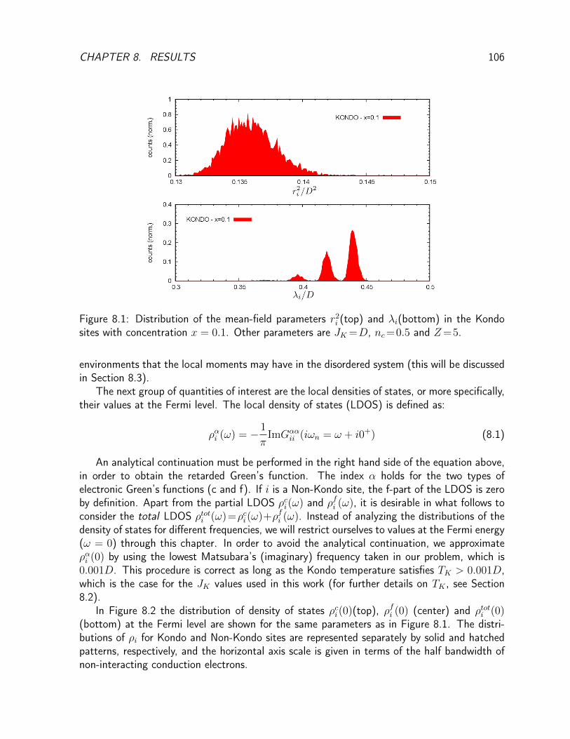
CHAPTER 8. RESULTS 106
Figure 8.1: Distribution of the mean-field parameters r2i (top) and λi(bottom) in the Kondo
sites with concentration x = 0.1. Other parameters are JK =D, nc=0.5 and Z=5.
environments that the local moments may have in the disordered system (this will be discussedin Section 8.3).
The next group of quantities of interest are the local densities of states, or more specifically,their values at the Fermi level. The local density of states (LDOS) is defined as:
ραi (ω) = − 1
πImGαα
ii (iωn = ω + i0+) (8.1)
An analytical continuation must be performed in the right hand side of the equation above,in order to obtain the retarded Green’s function. The index α holds for the two types ofelectronic Green’s functions (c and f). If i is a Non-Kondo site, the f-part of the LDOS is zeroby definition. Apart from the partial LDOS ρci(ω) and ρfi (ω), it is desirable in what follows toconsider the total LDOS ρtoti (ω)=ρci(ω)+ρfi (ω). Instead of analyzing the distributions of thedensity of states for different frequencies, we will restrict ourselves to values at the Fermi energy(ω = 0) through this chapter. In order to avoid the analytical continuation, we approximateραi (0) by using the lowest Matsubara’s (imaginary) frequency taken in our problem, which is0.001D. This procedure is correct as long as the Kondo temperature satisfies TK > 0.001D,which is the case for the JK values used in this work (for further details on TK , see Section8.2).
In Figure 8.2 the distribution of density of states ρci(0)(top), ρfi (0) (center) and ρtoti (0)(bottom) at the Fermi level are shown for the same parameters as in Figure 8.1. The distri-butions of ρi for Kondo and Non-Kondo sites are represented separately by solid and hatchedpatterns, respectively, and the horizontal axis scale is given in terms of the half bandwidth ofnon-interacting conduction electrons.

CHAPTER 8. RESULTS 107
Figure 8.2: Distribution of the local density of states ρci(0)(top), ρfi (0) (center) and ρtoti (0)(bottom). Kondo and Non-Kondo sites distributions are plotted separately. Parameters areJK =D, x=0.1, nc=0.5 and Z=5.
In the top figure of Fig. 8.2, ρci(0) is distributed very close to zero for Kondo sites becauseconduction electrons in these sites are participating in the screening of local moments throughKondo effect (as already indicated by the distribution of ri) and electronic excitations costa large energy. For Non-Kondo sites the distribution is peaked at a finite value close to 0.5,indicating that conduction electrons in this sublattice have excitations close to the Fermi energyas in the non-interacting case. The value ρci(0)D≈ 0.5 is close to the value in the middle ofthe non-interacting DOS for Z=5 Bethe lattice (see Figure C.1). The values of ρfi (0) (middlefigure in Fig. 8.2) for Kondo sites are distributed around the value 1.2. This quantity roughlycorresponds to the Kondo peak height and it is inversely proportional to the Kondo temperature.
CHAPTER 8. RESULTS 108
φ-function
Another important quantity that will be largely discussed in this chapter is the function φi(ω),defined by the relation:
Gccii (ω) ≡ G0(ω−φi(ω)) (8.2)
Here φi(ω) is employed to relate the site dependent c-electron Green’s function Gccii (ω) to
the free electron Green’s function in a Bethe lattice G0(ω), which has an analytic expression(Eq. C.9):
G0(ω) =(Z − 2)ω − Zω
√1− 4t2(Z−1)
ω2
2 (Z2t2 − ω2)(8.3)
Using the reciprocal function of G0, R [G0(ω)](Eq. C.12), we have:
ω − φi(ω) = R [Gccii (ω)] (8.4)
φi(ω) is a complex function defined as:
φi(ω) = ω +
(Z − 2
2Gccii (ω)
)−(
Z
2Gccii (ω)
)√1 + 4t2 (Gcc
ii (ω))2 (8.5)
Let us restrict ourselves to the analysis of this quantity at the Fermi energy. φi(ω = 0) isa complex number. The interpretation is the following1: the real part of φi(0) can be thoughtas an effective position of the conduction electron level with respect to the non-interactingdensity of states. The latter is bounded in the interval [−D;D], since the energy scale is thehalf-bandwidth of the non-interacting problem. Then, if Re[φi(0)] belongs to this interval fora given site, it means that the local electronic level lies in a region with a non-zero density ofstates for conduction electrons and the conduction electrons have an itinerant behavior. Onthe other hand, if Re[φi(0)] lies outside the interval [−D;D], the f-level energy lies outsidethe conduction band, being almost localized since the hybridization effect on it is small. Thislocalization is reminiscent of a Kondo insulating state (from a local point of view), even if thesystem is neither periodic nor half-filled.
The interpretation to Re[φi(0)] described above is exemplified in Figure 8.3. It representsthe dilute regime of the Kondo Alloy (x = 0.1 and nc = 0.5). In that case, the conductionelectrons in Kondo sites form local singlets with the local moments, "pushing" the effectivelevel to lower values and Re[φi(0)]<−D. The conduction electrons engaged in these boundstates are blocked and do not contribute to the low-energy excitations. The remaining electronsare free to move in the depleted lattice of Non-Kondo sites, which is represented by values ofRe[φi(0)] lying inside the non-interacting conduction band. The quasiparticles in the systemare the conduction electrons in Non-Kondo sites and their existence guarantees the metallicbehavior of the system.
For completeness we also show in Fig. 8.3 the imaginary part of φi(0) in order to establishthat φi(ω) cannot be interpreted as the "local self-energy" of the interacting disordered prob-lem. Our claim is based on the numerical finding that Im[φi(0)] can assume positive values,
1In Appendix E φi(ω) is shown in two limiting cases in which it has a simpler interpretation.

CHAPTER 8. RESULTS 109
Figure 8.3: Distribution of the real (top) and imaginary (bottom) parts of φi(ω) at the Fermilevel. The value of parameters are JK = D, x = 0.1 and nc = 0.5.
while for a self-energy the relation Im[Σ(k, ω)]≤0 must be fulfilled to respect causality [3, 2].But even if Im[φi(0)] can be positive, the local density of states ρci(0) remains non-negative inall cases. In Appendix E we present the expression for Im[φi(0)] in the Z→∞ limit and wediscuss the origin of such sign.
8.2 Concentration effects
Let us now present the results concerning the evolution of the distributions introduced inSection 8.1 as a function of the local moments concentration x. We consider two regimes,depending on the strength of Kondo interaction: the strong coupling and weak coupling case.A qualitative criterion to distinguish both regimes is given by the comparison between theanalytical expression for the Kondo temperature (Eq.1.1.2) and its numerical estimative fromthe mean-field parameter r2.The single impurity Kondo temperature follows the exponentialformula TK = D exp (−1/ρc0(µ)JK) only in the weak coupling case. In the strong couplingcase, TK is proportional to JK , which is the energy required to break the singlet state betweenone conduction electron and the impurity spin.
Since our mean-field calculations are done at zero temperature, we can estimate numericallyits value from the mean-field parameter r2
imp for the single impurity case. We compare it toT
(1)K = D exp (−1/ρc0(µ)JK), computed from the non-interacting density of states for the
Bethe lattice (Figure C.1) with Z = 5. This expression of TK gives a rough estimate of theKondo temperature when JK is small. Nevertheless Figure 8.4 shows the dependence of theratio (r2
imp/D)/T(1)K for a single impurity as a function of JK for a Z = 5 Bethe lattice with a
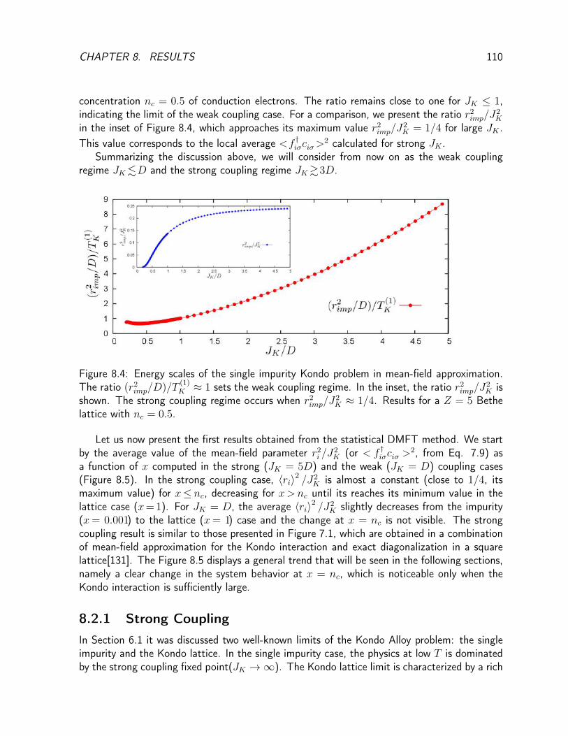
CHAPTER 8. RESULTS 110
concentration nc = 0.5 of conduction electrons. The ratio remains close to one for JK ≤ 1,indicating the limit of the weak coupling case. For a comparison, we present the ratio r2
imp/J2K
in the inset of Figure 8.4, which approaches its maximum value r2imp/J
2K = 1/4 for large JK .
This value corresponds to the local average <f †iσciσ>2 calculated for strong JK .
Summarizing the discussion above, we will consider from now on as the weak couplingregime JK.D and the strong coupling regime JK&3D.
Figure 8.4: Energy scales of the single impurity Kondo problem in mean-field approximation.The ratio (r2
imp/D)/T(1)K ≈ 1 sets the weak coupling regime. In the inset, the ratio r2
imp/J2K is
shown. The strong coupling regime occurs when r2imp/J
2K ≈ 1/4. Results for a Z = 5 Bethe
lattice with nc = 0.5.
Let us now present the first results obtained from the statistical DMFT method. We startby the average value of the mean-field parameter r2
i /J2K (or < f †iσciσ >
2, from Eq. 7.9) asa function of x computed in the strong (JK = 5D) and the weak (JK = D) coupling cases(Figure 8.5). In the strong coupling case, 〈ri〉2 /J2
K is almost a constant (close to 1/4, itsmaximum value) for x≤ nc, decreasing for x>nc until its reaches its minimum value in thelattice case (x= 1). For JK = D, the average 〈ri〉2 /J2
K slightly decreases from the impurity(x= 0.001) to the lattice (x= 1) case and the change at x = nc is not visible. The strongcoupling result is similar to those presented in Figure 7.1, which are obtained in a combinationof mean-field approximation for the Kondo interaction and exact diagonalization in a squarelattice[131]. The Figure 8.5 displays a general trend that will be seen in the following sections,namely a clear change in the system behavior at x = nc, which is noticeable only when theKondo interaction is sufficiently large.
8.2.1 Strong Coupling
In Section 6.1 it was discussed two well-known limits of the Kondo Alloy problem: the singleimpurity and the Kondo lattice. In the single impurity case, the physics at low T is dominatedby the strong coupling fixed point(JK →∞). The Kondo lattice limit is characterized by a rich

CHAPTER 8. RESULTS 111
Figure 8.5: Average value of the mean field parameter r2i as a function of x for JK = D (red
circles) and JK = 5D (blue triangles). A kink is observed at x = nc (nc = 0.5).
phase diagram where the Fermi liquid Kondo phase compete with RKKY dominated phases (seethe Doniach diagram in Fig. 1.2). Here we consider only the FL ground states for the Kondolattice regime. Besides, one of our motivations is to understand from numerical calculations theproposition of a "Lifshitz transition" done in Ref. [136] (Section 7.1.2), predicted in the strongcoupling limit. Then, in this section we will discuss the possible signatures of this transition interms of the statistics of local quantities and see if it is retained at smaller values of the Kondoparameter.
We focus on the the local density of states at the Fermi level. In Figure 8.6 we plot thedistribution of the total density of states at the Fermi energy for different values of x and fixednc = 0.5. The distributions for Kondo and Non-Kondo sites are plotted separately in order tohighlight the difference between the types of sites. For x = 0.1 (x � nc) the distribution ofρtoti (0) has a peak close to ρtoti (0) = 0 for Kondo sites and is distributed at finite values forNon-Kondo sites. This corresponds to the dilute regime of the model, where the Kondo sitesare "locked" in singlet states while charge carriers can move almost freely on Non-Kondo sites.In this situation the Kondo sites locally behave as in an insulator.
By increasing the concentration of Kondo sites, assuming fixed nc, the number of carriers inthe lattice tends to reduce when x approaches nc and the distribution of ρtoti (0) in Non-Kondosites is broadened by this effect. For x = nc all the conduction electrons are located in Kondosites and ρtoti (0)=0 is equal to zero for both Kondo and Non-Kondo sites. It corresponds to aKondo Insulator regime exactly as predicted in Ref. [136]. Note that this state is more generalthan the insulating phase of the Kondo Lattice model at half-filling (nc=1), where periodicitycreates a gap at the zone boundary and enhances the insulating behavior.
For x=0.9 the distribution of ρtoti (0) for Kondo sites is located around ρtoti (0)≈1.2, whilethe distribution for Non-Kondo sites is close to zero. This result indicates that the chargecarriers are now moving in the sublattice of Kondo sites, while the Non-Kondo sites are empty,as it is expected from the analysis made in Section 7.1.2.
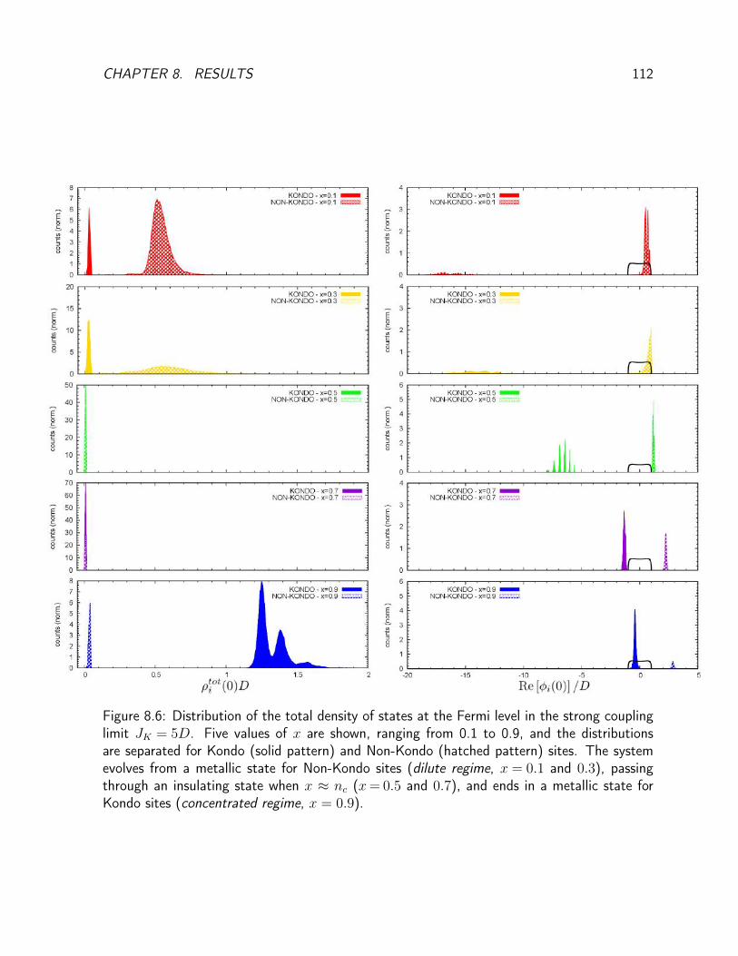
CHAPTER 8. RESULTS 112
Figure 8.6: Distribution of the total density of states at the Fermi level in the strong couplinglimit JK = 5D. Five values of x are shown, ranging from 0.1 to 0.9, and the distributionsare separated for Kondo (solid pattern) and Non-Kondo (hatched pattern) sites. The systemevolves from a metallic state for Non-Kondo sites (dilute regime, x = 0.1 and 0.3), passingthrough an insulating state when x ≈ nc (x= 0.5 and 0.7), and ends in a metallic state forKondo sites (concentrated regime, x = 0.9).

CHAPTER 8. RESULTS 113
Figure 8.7: Concentration x dependence on the ratios of Kondo (red) and Non-Kondo (blue)sites in which Re [φi(0)] lies inside the non-interacting conduction band. The point x=nc ismarked by the vanishing ratio RNK (Non-Kondo sites) when it is approched from the dilutedside x < nc. Both ratios are zero between x = 0.5 and x ≈ 0.75, where the strong disorderand interactions leads to an insulating phase (see text). Other parameters are JK = 5D andnc=0.5 and lines are guides for the eyes.
The features depicted by the density of state can be further analyzed with respect tothe function φi(0) introduced in Section 8.1. The sites in which the density of states aredistributed at non-zero values have |Re [φi(0)] | ≤D, while for sites with ρtoti (0)≈ 0 we have|Re [φi(0)] |>D.
Contrary to what happens in the JK→∞ limit, the insulating regime is stable not onlywhen x=nc, but in a finite region around it. For instance, in Figure 8.6, an insulating phase isstill observed at x=0.7. Note that the insulating phase in not symmetric with respect to thepoint x=nc, since at x= 0.3 the distribution is not peaked at zero and |Re [φi(0)] | ≤ D forNon-Kondo sites. The reason is the treatment of disorder by the Statistical DMFT employedhere, in comparison to the treatment given by CPA and related methods.
One practical way to visualize the system dependence on the concentration x is to calculatethe concentration of Kondo and Non-Kondo sites at which |Re [φi(0)] | ≤ D, since it is anestimate of the fraction of sites containing extended states at the Fermi energy. Their formaldefinition are:
RK =1
xN
∑i∈K
Θ (D − |Re [φi(0)] |) (8.6)
RNK =1
(1− x)N
∑i 6∈K
Θ (D − |Re [φi(0)] |) (8.7)
Here Θ(x) is the Heaviside function. In Figure 8.7 we plot the ratios RK and RNK as afunction of the concentration x using the same parameters as in Figure 8.6. When x<nc theratio RNK is very close to unity, but it vanishes when x=nc. Above this point the conductionelectrons are all in the sublattice of Kondo sites. The ratio RK is zero when x < nc, sinceconduction electrons in Kondo sites are locked in singlets.

CHAPTER 8. RESULTS 114
Remarkably the value of RK is still zero above the transition point x= nc until x ≈ 0.8.One would expect that the coherence effects should appear immediately at this point and RK
would increase with increasing x by the same reason as RNK decreases at this point. Thisissue is related to a fundamental asymmetry between the diluted (x<nc) and the concentrated(x > nc) regime, indicating that the effective disorder seen by conduction electrons is largerin the concentrated case. Given that strong disorder leads to localization of electronic states(Anderson localization[145, 146]), it seems that two metal-insulator transitions occur, at x=nc = 0.5 and at x= 0.8.This result, obtained only in the strong coupling regime, needs to befurther studied.
8.2.2 Weak coupling
The strong coupling results serve as a bridge between our numerical calculations and theanalytical considerations done in References [100, 96, 136], but it does not correspond tothe physical limit. For that reason we further investigate concentration effects with a smallerKondo interaction JK = D. In Figure 8.8 we plot again the total density of states ρtoti (0) andRe [φi(0)] for different concentrations of local moments, as in Figure 8.6. The electronic fillingand the coordination number are fixed to nc = 0.5 and Z = 5, respectively.
Firstly, we note that ρtoti (0) has a non-zero average value in any case, differently from thepeaks ρtoti (0) ≈ 0 that appear in the strong coupling case. Since the Kondo effect is weakerhere, the local singlets in Kondo sites are weakly bounded and the electronic states are neverlocalized.
The distributions of Re [φi(0)] show a smooth evolution from the diluted (x�nc) to theconcentrated (x�nc) regime and we do not observe the "insulating phase" separating bothregimes for JK =D. Instead, at the point x= nc the distributions of Re [φi(0)] are peakednear the band edges for both Kondo and Non-Kondo sites and there is a finite amount ofsites for which Re [φi(0)] is distributed inside the range [−D;D]. Considering the definitionof Re [φi(0)] (Eq. 8.2) and invoking the fact that the non-interacting Green’s function G0 issingular near the band edges, we may speculate that the presence of peaks at ±D for Re [φi(0)]could lead to non-analyticities in the energy or temperature dependence of physical quantities,leading to Non-Fermi liquid behavior[150, 151, 152].
According to the discussion on Section 6.2.1 and references therein, an evidence for disorder-induced NFL behavior is a power-law distribution of Kondo temperatures, which gives a similarsingularity in thermodynamical quantities. In Figure 8.9 the distribution of local Kondo tem-peratures is shown for JK =D and two local moment concentrations: x=nc=0.5 and x=0.9.The local Kondo temperatures are obtained with the expression (ρci(0) is the c-electrons localdensity of states)
TKi = D exp
(− 1
JKρci(0)
), (8.8)
which is valid in the weak coupling regime. The statistical DMFT method provides the fulldistribution of ρci(0) and, consequently, of TKi . Since the later has an exponential dependence,it is clear that it can be a broad distribution. For x = nc, which marks the concentrationregion where NFL is expected from the analysis of Figure 8.8, a power-law distribution of TKi

CHAPTER 8. RESULTS 115
Figure 8.8: Distribution of the total density of states in the Fermi level at the weak couplingregime JK = D. Five values of x are shown, ranging from 0.1 to 0.9, and the distributionsare separated for Kondo (solid pattern) and Non-Kondo (hatched pattern) sites. The evolutionaround the point x = nc is smooth and Re [φi(0)] of Kondo (Non-Kondo) progressively en-ters(quits) the non-interacting density of states. For 0.3≤x≤0.7 the distribution of Re [φi(0)]for both type of sites have a finite value. Other parameters are nc=0.5 and Z=5.
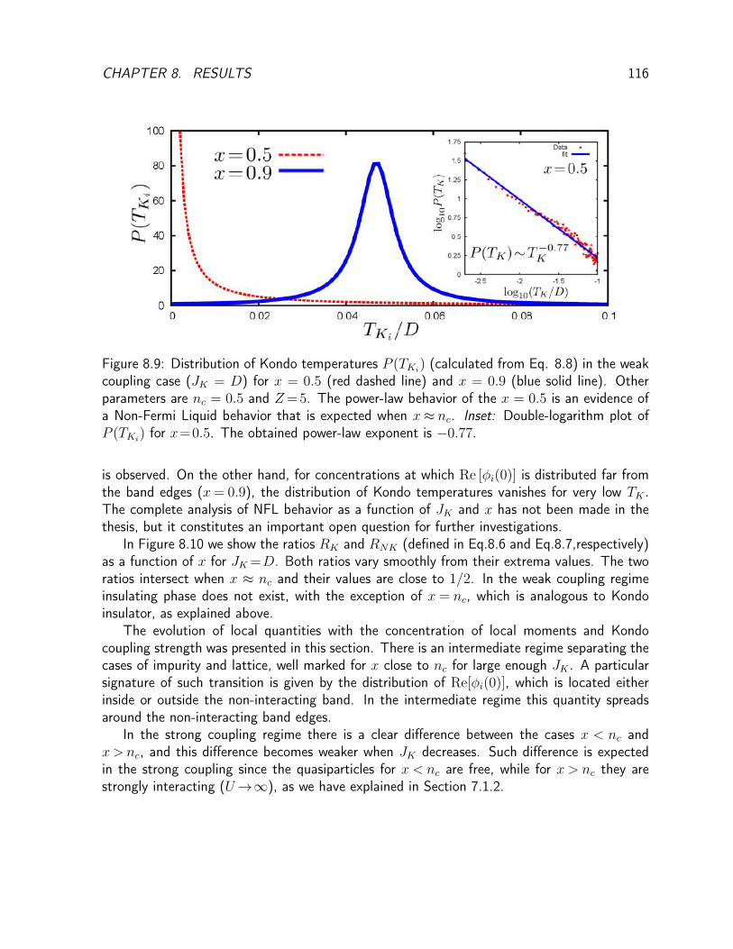
CHAPTER 8. RESULTS 116
Figure 8.9: Distribution of Kondo temperatures P (TKi) (calculated from Eq. 8.8) in the weakcoupling case (JK = D) for x = 0.5 (red dashed line) and x = 0.9 (blue solid line). Otherparameters are nc = 0.5 and Z=5. The power-law behavior of the x = 0.5 is an evidence ofa Non-Fermi Liquid behavior that is expected when x≈ nc. Inset: Double-logarithm plot ofP (TKi) for x=0.5. The obtained power-law exponent is −0.77.
is observed. On the other hand, for concentrations at which Re [φi(0)] is distributed far fromthe band edges (x= 0.9), the distribution of Kondo temperatures vanishes for very low TK .The complete analysis of NFL behavior as a function of JK and x has not been made in thethesis, but it constitutes an important open question for further investigations.
In Figure 8.10 we show the ratios RK and RNK (defined in Eq.8.6 and Eq.8.7,respectively)as a function of x for JK =D. Both ratios vary smoothly from their extrema values. The tworatios intersect when x ≈ nc and their values are close to 1/2. In the weak coupling regimeinsulating phase does not exist, with the exception of x = nc, which is analogous to Kondoinsulator, as explained above.
The evolution of local quantities with the concentration of local moments and Kondocoupling strength was presented in this section. There is an intermediate regime separating thecases of impurity and lattice, well marked for x close to nc for large enough JK . A particularsignature of such transition is given by the distribution of Re[φi(0)], which is located eitherinside or outside the non-interacting band. In the intermediate regime this quantity spreadsaround the non-interacting band edges.
In the strong coupling regime there is a clear difference between the cases x < nc andx > nc, and this difference becomes weaker when JK decreases. Such difference is expectedin the strong coupling since the quasiparticles for x < nc are free, while for x > nc they arestrongly interacting (U→∞), as we have explained in Section 7.1.2.

CHAPTER 8. RESULTS 117
Figure 8.10: Ratios RK and RNK . Parameters are the same as in Fig. 8.8 and lines are guidesfor the eyes.
8.3 Neighboring effects
Interesting informations can be obtained by the analysis of distributions with respect to the localenvironment. Although the stochastic method that provides the construction of baths (with itsappropriate probability distribution) does not allow to trace the full "genealogy" of each site,we have at least access to informations concerning the nearest neighbours and it is possibleto decompose all the distributions defined in Section 8.1 in terms of the site environment.Defining NK as the number of Kondo neighbors for a given site i, i.e. the number of sitescomposing the bath function ∆i(ω) that contains local moments, it is possible to compute thepartial statistics by separating sites with different NK (0 ≤ NK ≤ Z).
In Figure 8.11 the distributions of Re[φi(0)] are plotted for different number of neighboringKondo sites for x = nc = 0.5 and JK = D. This set of parameters corresponds to theintermediate regime of weak coupling scenario (central plot(s) in Fig. 8.8) where Re[φi(0)]is distributed around the band edges (partially inside, partially outside the non-interactingconduction band) for both Kondo and Non-Kondo sites. Since it was taken Z = 5 as in thelast section, there are six possible values for NK displayed in ascending order from the top(NK = 0) to the bottom (NK = 5).
The interpretation of Figure 8.11 is straightforward. The sites with NK = 0 have a biggerprobability to belong to a very large cluster (infinite, in the thermodynamic limit) of Non-Kondosites, which possesses extended electronic states. This probability decreases progressively forincreasing NK and it becomes zero for NK = 5, when all the Non-Kondo sites have localizedstates for their conduction electrons (Re[φi(0)] lies outside [−D;D]. For Kondo sites thesituation is precisely the opposite and extended states are most likely to exist for large NK .
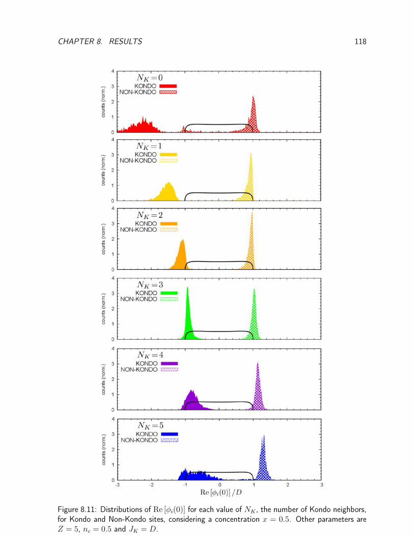
CHAPTER 8. RESULTS 118
Figure 8.11: Distributions of Re [φi(0)] for each value of NK , the number of Kondo neighbors,for Kondo and Non-Kondo sites, considering a concentration x = 0.5. Other parameters areZ = 5, nc = 0.5 and JK = D.

CHAPTER 8. RESULTS 119
8.4 Lower dimensions and percolation problem
Since the method introduced in Section 7.3 is valid for a Bethe lattice with any coordinationnumber Z, we can address the issue of the KAM in low dimensions. In particular there aresignificant effects related to the absence of percolation of the two existent sublattices, formedby Kondo and Non-Kondo sites, that we will discuss in this section.
Percolation is an important concept in a classical description of conductivity in randommedia. For general aspects of percolation theory and physical examples, we refer to References[153, 154]. Here we will briefly explain its consequences for our problem of Kondo Alloys.The physical picture is the following: in the strong coupling analysis of the model and in theresults presented in Section 8.2.1, we have argued that some sites behave as insulators. Forinstance, in the diluted regime (characterized by nc >x) the Kondo sites play this role sinceconduction electrons are participating in singlets, as it was claimed by Nozières in Ref. [94]. Inthis case, the remaining electrons move in the lattice of Non-Kondo sites. Now there are twopossible scenarios for the behavior of the remaining electrons: if the depleted lattice percolatesthese electrons will move in infinitely large clusters and their states (or their wave-functions)will be extended through the whole system, as it happens in a metal. On the other hand, ifthe depleted lattice does not percolate, electronic states are constrained to a finite region ofthe system. So a different behavior is expected whether the concentration of Non-Kondo sitesexceeds the percolation threshold or not. The same issue is present in the concentrated regime(nc<x), except that in this case it is the percolation (or not) of Kondo sites that matters.
Figure 8.12: Percolation in the Kondo Alloy model for three different cases: (a) nc<xp, (b)xp<nc< 1 − xp and (c) 1 − xp<nc. The shadowed yellow areas indicate intervals in whichpercolation does not take place for one type of lattice sites. For instance, in case (a) theKondo sites do not percolate in the interval nc < x < xp, while in (c) the same happens toNon-Kondo sites in the interval 1 − xp<x<nc. In case (b) percolation is never an issue, asexpected for lattices with low percolation threshold and an intermediate nc. Note that in ourfurther example (using Z=3) xp=1− xp, then the case (b) can only occur for nc=xp.
The percolation threshold for a Bethe lattice is xp=1/(Z−1)[153]. In the diluted regimex<nc of the Kondo Alloy model the absence of percolation takes place if the concentration

CHAPTER 8. RESULTS 120
of Non-Kondo sites 1 − x is smaller than the percolation threshold xp. This gives the firstcondition:
1− xp<x<nc (8.9)
In the concentrated regime x > nc, the absence of percolation of Kondo sites happens forx<xp.This gives the second condition:
nc<x<xp. (8.10)
When one of these two conditions (in Eqs.8.9 and 8.10) is realized, there is a percolationproblem.
For a lattice with a low percolation threshold, one of the two conditions presented abovecan be satisfied only in extreme cases, when nc is close to the half-filling or almost zero. Inthe usually employed infinity Z Bethe lattice these conditions are never satisfied. So far, wehave shown results for a lattice with Z=5 and nc=0.5, in which percolation always happens.Then, in order to investigate the possible issue of the lack of percolation, we need to considera lattice with a bigger percolation threshold and different concentrations nc.
Our analysis is based again on the quantity Re[φi(0)], defined in Eq.8.2. According to thediscussions in Section 8.1, the distinction between localized and extended electronic states atthe Fermi energy can be simplified by the comparison of Re[φi(0)] and the non-interactingdensity of states.
In Figure 8.13 we present the ratios RK and RNK , given by Eqs.8.6 and 8.7, as a functionof the local moment concentration x for JK =5D (left) and JK =2D (right). Three differentelectronic fillings are chosen: nc=0.25, nc=0.5 (the percolation threshold) and nc=0.75.
For nc=0.25 and JK =5D, RNK progressively decreases with increasing x, being close tozero for x=nc, while in Kondo sites RK is zero through this range of concentrations. Betweenx=nc and x=xp=0.5 the ratios RK and RNK are zero for both type of sites and RK increasesonly for x≈0.55>xp. This is related to the lack of Kondo sites percolation when nc<x<xp,indicating the absence of extended states close to the Fermi energy in both sub-lattices. Theabsence of percolation in the interval nc<x<xp is still visible for JK = 2D and both ratiosare very small in this region.
For nc = 0.75 the same effect appears in the Non-Kondo sites. RNK decreases until itreaches a value close to zero for x= 1 − xp. For 1 − xp<x<nc the Non-Kondo sub-latticedoes not percolate and the metallic behavior is expected to be lost. Extended states will appearin Kondo sites after crossing the point x= nc. This clearly happens for JK = 2D, while forJK =5D the interval in x in which both ratios vanish extends for x > nc due to the very strongKondo interaction. An insulating phase is seen up to x= 0.95. The ratio RK is expected toincrease above this value and for x=1 (not shown) it must be equal to one again.
When nc is chosen to be the percolation threshold none of these effects are visible, sincepercolation issues are not reachable. Instead there is a dip for both curves at the crossingpoint nc =x for JK = 2D. It corresponds to an insulating phase that marks this transition inthe strong coupling limit. For JK = 5D there are two metal-insulator transitions for x= 0.45and x= 0.8, but they are probably related to the Anderson localization (see Figure 8.7 anddiscussions therein) and not to the lack of percolation. We note that the asymmetry between
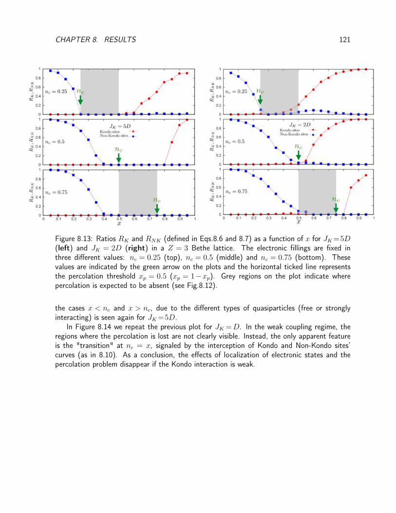
CHAPTER 8. RESULTS 121
Figure 8.13: Ratios RK and RNK (defined in Eqs.8.6 and 8.7) as a function of x for JK =5D(left) and JK = 2D (right) in a Z = 3 Bethe lattice. The electronic fillings are fixed inthree different values: nc = 0.25 (top), nc = 0.5 (middle) and nc = 0.75 (bottom). Thesevalues are indicated by the green arrow on the plots and the horizontal ticked line representsthe percolation threshold xp = 0.5 (xp = 1−xp). Grey regions on the plot indicate wherepercolation is expected to be absent (see Fig.8.12).
the cases x < nc and x > nc, due to the different types of quasiparticles (free or stronglyinteracting) is seen again for JK =5D.
In Figure 8.14 we repeat the previous plot for JK =D. In the weak coupling regime, theregions where the percolation is lost are not clearly visible. Instead, the only apparent featureis the "transition" at nc = x, signaled by the interception of Kondo and Non-Kondo sites’curves (as in 8.10). As a conclusion, the effects of localization of electronic states and thepercolation problem disappear if the Kondo interaction is weak.

CHAPTER 8. RESULTS 122
Figure 8.14: Ratios RK and RNK as a function of x for JK = D in a Z = 3 Bethe lattice.The electronic fillings are fixed in three different values: nc = 0.25 (top), nc = 0.5 (middle)and nc = 0.75 (bottom).

CHAPTER 8. RESULTS 123
8.5 Summary
In this chapter we have presented the results of the Kondo Alloy model (Eq. 7.1) obtainedfrom the Statistical Dynamical Mean-Field Theory presented in Section 7.3. This method hasas a principal feature the ability to access the distributions of local quantities in the model,being some of them introduced in Section 8.1. In this work we restrict ourselves mainly in thedistributions of quantities at the Fermi energy, in special, the density of states (Eq. 8.1) andthe φ-function (Eq. 8.2).
In Section 8.2 we have shown how these two quantities evolved from the dilute (x�nc)to the concentrated (x�nc) regimes in the strong (JK = 5D) and weak (JK =D) couplingscenarios. In the strong coupling we could identify two metal-insulator transitions at x=nc=0.5and x= 0.75 separating both regimes. While the system was expected to be an insulator atthe point x=nc from the JK→∞ limit analysis (Section 7.1.2), the insulating region abovethis point is a new feature of the KAM and we believe that it is connected to the localizationof electronic states due to strong disorder. In the weak coupling scenario the metal-insulatortransitions disappear and the passage from the dilute to the concentrated regimes is smooth.For intermediate concentrations (x≈nc), we have seen that te distributions of Re [φi(0)] arepeaked in the band edges. This result suggests that disorder for weak interactions can leadto a Non-Fermi liquid behavior, which is a precursor of the metal-insulator transition seen atstrong interaction. The case x= nc was further investigated in Section 8.3, where we haveshown the partial distributions of Re [φi(0)] for sites containing different numbers of Kondosites as neighbors. The results indicate that Kondo sites have a behavior closer to the densecase (x > nc) the more they are surrounded by other Kondo sites (forming clusters). Thiscorroborates the idea that the disorder provided by different local environments dominates theintermediate concentration regimes.
In Section 8.4 we have addressed the percolation issue in the context of the Kondo Alloymodel. The absence of percolation can affect the formation of metallic states in both regimes(dilute and dense) of the model, as it is discussed in Figure 8.12. For this purpose, we havepresented results for the Bethe lattice with Z=3 (whose percolation threshold is xp=0.5) anddifferent concentrations of conduction electrons. Using the ratios RK and RNK (Eqs. 8.6 and8.7), we have shown that the lack of percolation introduces new insulating regions in the phasediagram of KAM for intermediate and strong JK interactions. These regions can be furtherincreased by disorder, as seen in Section 8.2.


Chapter 9
Conclusions and perspectives
In Part II we have studied the Kondo Alloy model within the Statistical Dynamical Mean-FieldTheory and a mean-field approximation for the Kondo interaction. The method allows togo beyond the Coherent Potential Approximation and includes inhomogeneities from differentlocal environments. The procedure is shown to be exact [146, 115] in a Bethe lattice of finitecoordination number.
The central results presented in this work are distributions of local quantities that allow acomplete characterization of the problem, even if physical observables are given in terms ofaveraged quantities. Apart from the usual quantities discussed in the context of Kondo physics,as the mean-field parameters ri and λi or the local density of states ρi(ω)=(−1/π)Im[Gii(ω+i0+)], we have introduced a new function φi(ω) and we have analyzed it close to the Fermienergy. This function is interpreted as a measure of the extended/localized nature of the localelectronic states.
In a first step we have examined the distributions of ρtoti (0) and Re [φi(0)] by changingthe concentration of local moments x and the strength of the Kondo interaction JK . In thestrong coupling scenario we have found two metal-insulator transitions in the intermediateconcentration range (x≈nc) that separate the dilute and dense regimes of KAM. Our resultsshow an asymmetry around the point x = nc if Kondo interaction is strong, what can beunderstood in terms of the different nature of the quasiparticles (free or strongly correlated)seen in the JK→∞ limit. In particular, we have suggested that the insulating phase observedfor x& nc is related to the combined effects of disorder and the strong correlations, leadingto localization of electronic states. For smaller JK disorder is expected to produce Non-Fermiliquid behavior, which is suggested from our results of Re [φi(0)] when x ≈ nc. These twofeatures will be analyzed in more details in future works.
In order to determine in which region Non-Fermi Liquid behavior could occur due to disorderwithin our theoretical approach, it is crucial to calculate the temperature dependence of physicalquantities such as the magnetic susceptibility, the specific heat or the electrical conductivity.It can be done after an adaptation of the method to perform finite temperature calculationsof the mean-field parameters or by using a different impurity solver.
A second aspect discussed in this work is the dimensionality effects. We remind that such
125

CHAPTER 9. CONCLUSIONS AND PERSPECTIVES 126
effects are enhanced in the case of a big percolation threshold and a large Kondo interaction,which is usually not the case of the typical Kondo systems which have been experimentallystudied up to now. Nevertheless such issues might be useful for the study of Kondo effect innanostructures, which have a higher degree of controllability.
Apart from the calculations of physical observables at finite temperature, another highlydesirable perspective is to take into account the effects of magnetism in the Kondo Alloy model,neglected in the present work. While it is well stablished that magnetic ordered ground statesare possible in the Kondo Lattice and spin glass behavior is observed in many systems withdiluted impurities, it is unknown how these phases evolve with the concentration of magneticmoments. It would be interesting to study the interplay between magnetism and Kondo effectin the KAM. Also it is fair to speculate that the magnetism would be more sensitive to thepercolation issues. The study of magnetic phases in KAM is a priori beyond the scope of thestatistical DMFT method.

Appendix A
Hubbard-I approximation for theEPAM
The method chosen to solve the Extended Periodic Anderson model hamiltonian (Equation3.1) is based on the truncation of the equation of motion for the electronic propagators. Inprinciple the equation of motion for a given Green’s function leads to higher-order terms forhamiltonian containing two(or high)-body terms. The truncation will be inspired by the socalled Hubbard-I approximation[69, 70, 71]. The major drawback of this approximation in thecontext of the Hubbard model is the existence of a Mott-insulating regime for the half-filledcorrelated band for a finite value of U . For the Periodic Anderson model this issue does nothold since the f-orbitals are dispersionless.
In Section 3.3.2 the complete Green’s functions for the EPAM were derived in a morepedagogical form. Here we will perform the same approximations directly in the equation ofmotion of the EPAM. A similar derivation is done for the Periodic Anderson model (Eq. 1.9)in Ref. [155].
For convenience we will consider the following form of the hamiltonian in Eq.3.1:
HEPAM = −∑i,jσ
(tij − εcδij)c†iσcjσ +∑iσ
εf,σf†iσfiσ +
U
2
∑iσ
nfiσnfiσ
+ V∑iσ
(c†iσfiσ + f †iσciσ
)− Ufcncnf (A.1)
The hamiltonian above is written in its site representation, tij being the hopping integral.The mean-field approximation for Ufc term is already included, as discussed in Section 3.3.1,and we define εc ≡ Ufcnf for shortness. The relation between tij and the band dispersion ε(k)(defined in Eq. 3.1) is given through a Fourier transformation:
−∑i,jσ
tijc†iσcjσ =
∑kσ
ε(k)c†kσckσ
The equation of motion for a fermionic propagator1 Gabiσ,jσ′(ω) ≡�aiσ ; b†jσ′� in frequency
1We recall that the Zubarev’s notation[72] for Green’s functions is used in this Appendix.
127

APPENDIX A. HUBBARD-I APPROXIMATION FOR THE EPAM 128
representation is:
ω �aiσ ; b†jσ′�=⟨{aiσ; b†jσ′}
⟩+� [aiσ;H] ; b†jσ′� . (A.2)
For the conduction electrons we have:
ω �ciσ ; c†iσ�= 1−∑j
tij �cjσ ; c†iσ� +εc �ciσ ; c†iσ� +V �fiσ ; c†iσ� (A.3)
For f-electrons the equation of motion is:
ω �fiσ ; f †iσ�= 1 + εfσ �fiσ ; f †iσ� +U � nfiσfiσ ; f †iσ� +V �ciσ ; f †iσ� (A.4)
In a similar way, for the mixed Green’s FunctionsGcfσ (k, ω) ≡�ciσ; f †iσ� andGfc
σ (k, ω) ≡�fiσ ; c†iσ�:
ω �ciσ ; f †iσ�= −∑j
tji �cjσ ; f †iσ� +εc �ciσ ; f †iσ� +V �fiσ ; f †iσ� (A.5)
ω �fiσ ; c†iσ�= εfσ �fiσ ; c†iσ� +U � nfiσfiσ ; c†iσ� +V �ciσ ; c†iσ� (A.6)
Note that in Eqs. A.4 and A.6 it appears higher-orders Green’s functions. Their equationsof motion are:
ω � nfiσfiσ ; f †iσ�=< nfiσ > +εfσ � nfiσfiσ ; f †iσ� +U � nfiσfiσ ; f †iσ�+ V �nf,iσciσ ; f †iσ� +V �(f †iσciσ − c†iσfiσ)fiσ ; f †iσ�
(A.7)
ω � nf,iσfiσ ; c†iσ�=εfσ � nfiσfiσ ; c†iσ� +U � nfiσfiσ ; c†iσ�+ V � nfiσciσ ; c†iσ� +V �(f †iσciσ − c†iσfiσ)fiσ ; c†iσ�
(A.8)
In this generic Hubbard-I approximation we settle (a† standing for both c† and f †):
� nfiσciσ ; a†iσ�= nf,iσ �ciσ ; a†iσ��(f †iσciσ − c†iσfiσ)fiσ ; a†iσ�= 0
Using these relations, Eqs. A.7 and A.8 express the high-order Green’s functions in termsof Green’s functions with two operators, allowing the set of equations in Eqs. A.3-A.6 to besolved after a Fourier transformation in k-space. Explicitly:
(ω − εc(k))Gccσ (k, ω) = 1 + V Gfc
σ (k, ω) (A.9)
(ω − εfσ)Gffσ (k, ω) = 1 + V Gcf
σ (k, ω) + U < nfσ >
(1 + V Gcf
σ (k, ω)
ω − εfσ − U
)(A.10)
(ω − εc(k))Gcfσ (k, ω) = V Gff
σ (k, ω) (A.11)
(ω − εfσ)Gfcσ (k, ω) = V Gcc
σ (k, ω) + U < nfσ >
(V Gcc
σ (k, ω)
ω − εfσ − U
)(A.12)
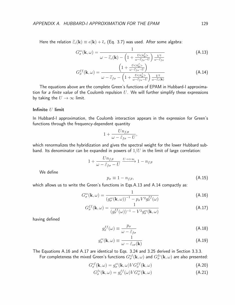
APPENDIX A. HUBBARD-I APPROXIMATION FOR THE EPAM 129
Here the relation εc(k) ≡ ε(k) + εc (Eq. 3.7) was used. After some algebra:
Gccσ (k, ω) =
1
ω − εc(k)−(
1 +U<nfσ>
ω−εfσ−U
)V 2
ω−εfσ
(A.13)
Gffσ (k, ω) =
(1 +
U<nfσ>
ω−εfσ−U
)ω − εfσ −
(1 +
U<nfσ>
ω−εfσ−U
)V 2
ω−εc(k)
(A.14)
The equations above are the complete Green’s functions of EPAM in Hubbard-I approxima-tion for a finite value of the Coulomb repulsion U . We will further simplify these expressionsby taking the U →∞ limit.
Infinite U limit
In Hubbard-I approximation, the Coulomb interaction appears in the expression for Green’sfunctions through the frequency-dependent quantity
1 +Unf,σ
ω − εfσ − U,
which renormalizes the hybridization and gives the spectral weight for the lower Hubbard sub-band. Its denominator can be expanded in powers of 1/U in the limit of large correlation:
1 +Unf,σ
ω − εfσ − UU→+∞−−−−→ 1− nf,σ
We definepσ ≡ 1− nf,σ, (A.15)
which allows us to write the Green’s functions in Eqs.A.13 and A.14 compactly as:
Gccσ (k, ω) =
1
(gccσ (k, ω))−1 − pσV 2gffσ (ω)(A.16)
Gffσ (k, ω) =
1
(gffσ (ω))−1 − V 2gccσ (k, ω)(A.17)
having defined
gffσ (ω) ≡ pσω − εfσ
(A.18)
gccσ (k, ω) ≡ 1
ω − εcσ(k)(A.19)
The Equations A.16 and A.17 are identical to Eqs. 3.24 and 3.25 derived in Section 3.3.3.For completeness the mixed Green’s functions Gcf
σ (k, ω) and Gfcσ (k, ω) are also presented:
Gcfσ (k, ω) = gccσ (k, ω)V Gff
σ (k, ω) (A.20)
Gfcσ (k, ω) = gffσ (ω)V Gcc
σ (k, ω) (A.21)


Appendix B
Magnetic Susceptibility for theEPAM
Here we will derive the analytical expression of the magnetic susceptibility in the paramagneticphase of the EPAM (Eq.4.11) at zero temperature. This derivation is based on an expansionof the equations for nf,↑ and nf,↓ when an infinitesimal external magnetic field hext is appliedto the system. It is possible to write the magnetic response χ0 = mf/hext in terms of theparameters of the problem in the absence of magnetic fields. χ0 can be evaluated using theself-consistent results obtained in Chapter 4.1.
For practical matters, it is easier to separate the calculation in two cases, depending onthe chemical potential position µ with respect to the lower and upper energy band (defined inEqs.3.38-3.41.
µ in the lower energy band
Let us consider first that the chemical potential µ lies below the hybridization gap. In thiscase, the integration must be performed only in the lower part of the density of states, definedbetween ω1 and ω2 (Eqs.3.38 and 3.39). The f-electron magnetization is given by:
mf =
µ∫ω1,↑
dωρff↑ (ω)−µ∫
ω1,↓
dωρff↓ (ω) (B.1)
Using Eq.4.19, the expression for the f-electron density of states is
ρffσ (ω) =1
2D
p2σV
2
(ω − εfσ)2 , (B.2)
The parameters εfσ and pσ are defined by the equations 4.13 and 4.14, respectively. Per-forming the integrals in Eq.B.1, one gets:
mf =p2↑V
2
2D
(1
ω1,↑ − εf,↑− 1
µ− εf,↑
)−p2↓V
2
2D
(1
ω1,↓ − εf,↓− 1
µ− εf,↓
)(B.3)
131

APPENDIX B. MAGNETIC SUSCEPTIBILITY FOR THE EPAM 132
We consider now the application of a very small magnetic field hext that will polarize thesystem. It will produce a magnetization mf = χ0hext to be calculated from the expressionabove, which depends on hext through the spin-dependent coefficients pσ, εf,σ and ω1,σ. Thedependence in hext is direct for the first two parameters1:
pσ = 1− nfσ = 1− nf2− σmf
2≡ p0 + σ
χ0hext2
εf,σ = εf,0 − σgfhextIn the same order, we have:
p2σ ≈ p2
0 + σhextχ0p0 (B.4)
The dependence on hext in ωi,σ comes from the parameters above, but a Taylor expansionis required. Up to the first order in hext, we have (from Eqs. 3.38):
ω1,σ − εf,σ = ω1,0 − εf,0 + σhext
[gf2− gfE0(−D)
2∆0(−D)− χ0V
2
4∆0(−D)
]For shortness, the following definitions are employed in the expression above:
E0(−D) =εc(−D)− εf,0
2(B.5)
∆0(−D) =
√[E0(−D)]2 + p0V 2 (B.6)
After a first-order Taylor expansion in hext, the denominators in Eq. B.3 are:
1
ω1,σ − εfσ=
1
ω1,0 − εf,0
[1− σhext
(gf2− gfE0(−D)
2∆0(−D)− χ0V
2
4∆0(−D)
)(1
ω1,0 − εf,0
)](B.7)
1
µ− εfσ=
1
µ− εf,0
[1− σhext
(1
µ− εf,0
)](B.8)
Gathering all the terms up to the first order in hext and defining χ0 ≡ mf/hext, we get theclosed expression:
χ0 =p2
0V2
2D
[−2
(1
ω1,0 − εf,0
)2(gf2− gfE0(−D)
2∆0(−D)− χ0V
2
4∆0(−D)
)+ 2gf
(1
µ− εf,0
)2]
+p0χ0V
2
2D2
[1
ω1,0 − εf,0− 1
µ− εf,0
](B.9)
1Through this section the parameters indexed by the subscript 0 correspond to the values in the absence ofmagnetic field.

APPENDIX B. MAGNETIC SUSCEPTIBILITY FOR THE EPAM 133
The solution of the equation above for χ0 is:
χ0 =C0
1− C1
(B.10)
The coefficients C0 and C1 are given by:
C0 =p2
0V2
D
[−(
1
ω1,0 − εf0
)2(gf2− gfE0(−D)
2∆0(−D)
)+ gf
(1
µ− εf,0
)2]
(B.11)
C1 =p2
0V2
D
(1
ω1,0 − εf,0
)2V 2
4∆0(−D)+p0V
2
D
[1
ω1,0 − εf,0− 1
µ− εf,0
](B.12)
The expressions above can be further simplified by using the expression for ρff0 (ω) and nf :
C0 = gfρff0 (ω1,0)
(E0(−D)−∆0(−D)
∆0(−D)
)+ 2gfρ
ff0 (µ) (B.13)
C1 = ρff0 (ω1,0)V 2
2∆0(−D)+nfp0
(B.14)
µ in the upper energy band
Let us now deal with the case in which the chemical potential µ in the absence of magneticfield lies in the upper energy band. In this case the expression for the f-electron magnetizationis:
mf =
ω2,↑∫ω1,↑
dωρff↑ (ω) +
µ∫ω3,↓
dωρff↑ (ω)−
ω2,↓∫ω1,↓
dωρff↓ (ω) +
µ∫ω3,↓
dωρff↓ (ω)
(B.15)
Performing a similar calculation as done in the previous case, one gets the following equa-tion:
χ0 =B0
1−B1
(B.16)
In this case the coefficients are:
B0 = gf
[ρff0 (ω1,0)
(E0(−D)−∆0(−D)
∆0(−D)
)− ρff0 (ω2,0)
(E0(+D)−∆0(+D)
∆0(+D)
)
+ ρff0 (ω3,0)
(E0(−D) + ∆0(−D)
∆0(−D)
)+ 2ρff0 (µ)
](B.17)
B1 =V 2
2
[ρff0 (ω1,0)
1
∆0(−D)− ρff0 (ω2,0)
1
∆0(+D)− ρff0 (ω3,0)
1
∆0(−D)
]+nfp0
(B.18)
In both cases the expressions for χ0 must be evaluated numerically from the self-consistentparameters determined in Section 4.1.

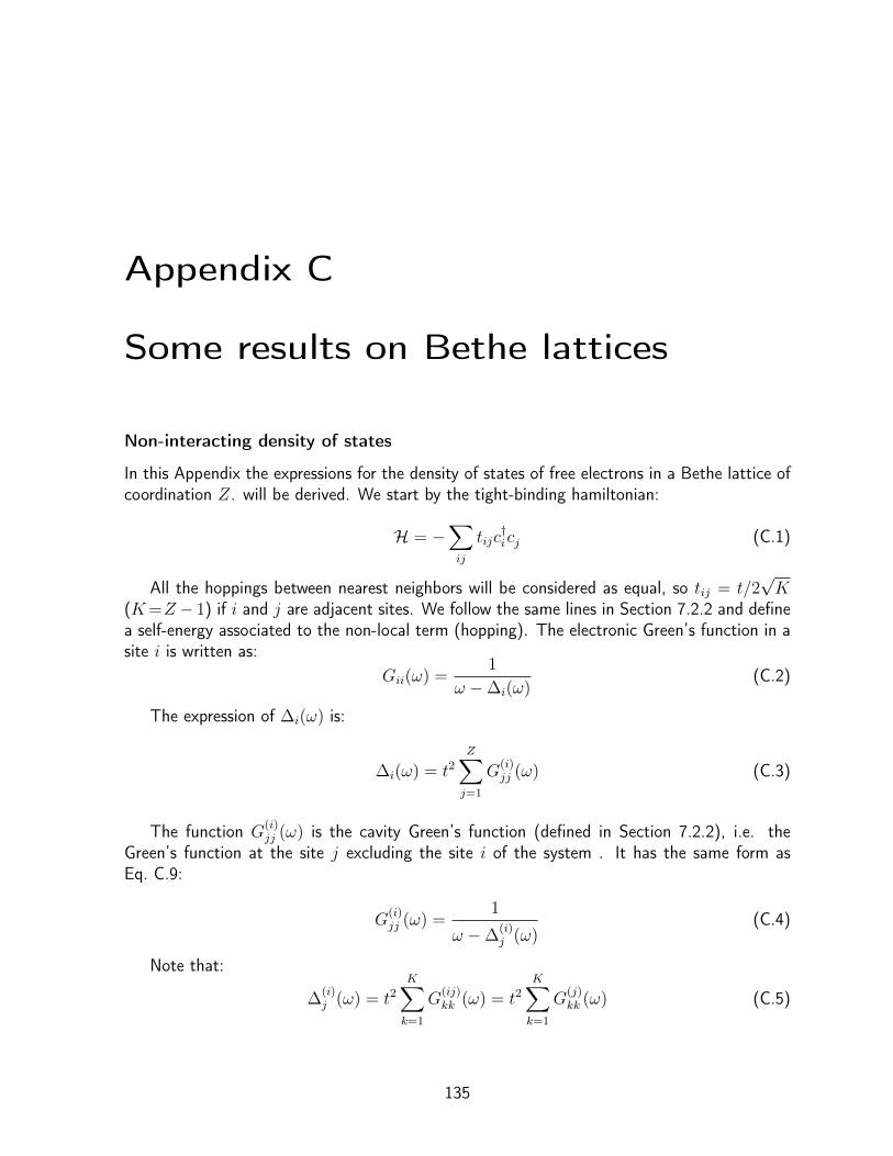
Appendix C
Some results on Bethe lattices
Non-interacting density of states
In this Appendix the expressions for the density of states of free electrons in a Bethe lattice ofcoordination Z. will be derived. We start by the tight-binding hamiltonian:
H = −∑ij
tijc†icj (C.1)
All the hoppings between nearest neighbors will be considered as equal, so tij = t/2√K
(K=Z − 1) if i and j are adjacent sites. We follow the same lines in Section 7.2.2 and definea self-energy associated to the non-local term (hopping). The electronic Green’s function in asite i is written as:
Gii(ω) =1
ω −∆i(ω)(C.2)
The expression of ∆i(ω) is:
∆i(ω) = t2Z∑j=1
G(i)jj (ω) (C.3)
The function G(i)jj (ω) is the cavity Green’s function (defined in Section 7.2.2), i.e. the
Green’s function at the site j excluding the site i of the system . It has the same form asEq. C.9:
G(i)jj (ω) =
1
ω −∆(i)j (ω)
(C.4)
Note that:
∆(i)j (ω) = t2
K∑k=1
G(ij)kk (ω) = t2
K∑k=1
G(j)kk (ω) (C.5)
135

APPENDIX C. SOME RESULTS ON BETHE LATTICES 136
Here the sum is performed over K = Z− 1 neighboring sites, since one neighbor is alreadyexcluded. The last equality holds because in a Bethe lattice there is only one path that connectsthe sites i and k (through the site j), so G(ij)
kk (ω) = G(j)kk (ω).
For an homogeneous system (no disorder), we can re-express G(i)jj (ω) = G
(0)ii (ω) and
∆(i)j (ω) = ∆
(0)i (ω) for all i and j. We can combine Eqs. C.4 and C.5 in a closed expres-
sion
∆(0)i (ω) =
t2K
ω −∆(0)i (ω)
, (C.6)
whose solution is
∆(0)i (ω) =
ω
2
[1−
√1− 4t2K
ω2
]. (C.7)
The negative sign of the square root is chosen to give ∆(0)i (ω) = 0 if t= 0. Equation C.3
now gives:
∆i(ω) =2t2Z
ω
[1 +
√1− 4t2K
ω2
] =Zω
2K
[1−
√1− 4t2K
ω2
](C.8)
Finally, one can get the expression for the local Green’s function as:
Gii(ω) =1
ω − Zω2K
[1−
√1− 4t2K
ω2
]=
2K
(Z − 2)ω + Zω√
1− 4t2Kω2
=(Z − 2)ω − Zω
√1− 4t2K
ω2
2 (Z2t2 − ω2)
(C.9)
The density of states is obtained from the imaginary part of the retarded Green’s function:
ρ(ω) = − 1
πIm(Gii(ω + i0+)
)=
√ω2 − 4Kt2
2π(Zt2 − ω2/Z)(C.10)
In Figure C.1 we plot the density of states for Bethe lattices of different coordinationnumbers, including the semi-elliptic density of states (for Z → ∞). Interestingly, the densityof states for Z = 5 is quite similar to the flat density of states.
Lastly, the reciprocal function of G(ω), defined as R[G(x)] = x, is given by the solution of
R2 +Z − 2
GR−
(Z2t2 +
Z − 1
G2
)= 0, (C.11)
which gives:
R = −(Z − 2
2G
)+
Z
2G
√1 + 4t2G2 (C.12)

APPENDIX C. SOME RESULTS ON BETHE LATTICES 137
Figure C.1: Density of states for free-electrons in a Bethe lattice of different coordinationnumber Z. The energy is renormalized by the half-bandwidth D=2
√Kt (K=Z−1).
Limit of infinite coordination number
The expressions above simplify in the Z → ∞ limit. In this case one must renormalize thehopping parameters t→ t/
√Z to keep the kinetic energy finite. Using this scaling and taking
Z→∞ in Equation C.9, the following Green’s function is obtained:
Gii(ω) =ω −
√1− 4t2
ω2
2t2(C.13)
The corresponding density of states for the expression above has the well-known semi-ellipticform:
ρi(ω) =
√ω2 − 4t2
2πt2(C.14)
Lastly, one can show that the reciprocal function of G(ω) in the limit of infinite coordinationnumber is simply:
R = t2G+1
G(C.15)


Appendix D
Matsubara’s sum at zerotemperature
In this Appendix it is shown how to calculate Matsubara’s sums at zero temperature in order tosolve the mean-field equations for the Kondo problem (Eqs. 7.15 and 7.16). The calculationsperformed here are developed in details in Chapter 3 of Ref.[2].
Let us take for example Gffii (τ = 0−). Using its Fourier transformation, we have (β ≡ 1/T
is the inverse temperature):
Gffii (τ=0−) = lim
τ→0−
1
β
∑iωn
e−iωnτGffii (iωn), (D.1)
The sum in the right hand side extends over the infinite set of fermionic Matsubara’sfrequencies:
iωn = i(2n+ 1)π
β. (D.2)
Using the property Gffii (iωn) =
(Gffii (−iωn)
)∗and trigonometric relations, the sum can be
restricted to positive frequencies
Gffii (τ=0−) = lim
τ→0−
2
β
∑ωn>0
[cos (ωnτ)Re
(Gffii (iωn)
)+ sin (ωnτ)Im
(Gffii (iωn)
)](D.3)
The limit τ→0− can be taken directly in the first term of the sum, sinceGffii (iωn)∼1/(iωn)
for large ωn and Re(Gffii (iωn)
)tends to zero faster than 1/ωn as ωn tends to infinity. The
second term has important contributions only when ωn is large (i.e., ωnτ ∼ 1), so we canreplace the imaginary part of Gff
ii (iωn) by its asymptotic value 1/(iωn) and transforms thesum into an integral (if T =0) through:
1
β
∑ωn>0
→+∞∫0
d(iω)
2π(D.4)
139

APPENDIX D. MATSUBARA’S SUM AT ZERO TEMPERATURE 140
Then1:
limτ→0−
2
β
∑ωn>0
sin (ωnτ)Im(Gffii (iωn)
)= lim
τ→0−
− 1
π
+∞∫0
sin (ωτ)
ω
=1
2(D.5)
After the considerations above, one can finally write:
Gffii (τ = 0−) =
2
β
∑ωn>0
Re(Gffii (iωn)
)+
1
2(D.6)
In principle the sum in Equation D.6 can be performed numerically for a given temperatureT , although the convergence can be an issue at low temperatures. We are interested in thezero temperature behavior of the system, therefore it is desirable to transform the sum at finiteT into its zero temperature equivalent. This is done by the relation in Eq. D.4, leading to:
Gffii (τ = 0−) =
1
π
+∞∫0
dωRe(Gffii (ω)
)+
1
2(D.7)
Here the integration is performed along the positive imaginary axis and the index n wasdropped to explicit that it a continuous variable (in contrast to the finite T frequencies).Analogously one can evaluate
⟨c†ici
⟩, which determines the local occupation of conduction
electrons, by: ⟨c†ici
⟩= Gcc
ii (τ = 0−) =1
π
+∞∫0
dωRe (Gccii (ω)) +
1
2(D.8)
The third average to be computed is < f †i ci >. The only difference from the other twoaverages comes from the asymptotic limit of the mixed Green’s function 2 Gcf
ii (iωn) ∼ 1/(iωn)2
for large ωn. Based on the same lines of the argument given between Eq.D.3 and Eq.D.4, onecan show that the factor asymptotic limit of the first term in Eq.D.3 is zero (instead of 1/2).Then:
Gcfii (τ = 0−) =
1
π
+∞∫0
dωRe(Gcfii (ω)
)(D.9)
1Here it was used+∞∫0
sin (ωτ)ω = π
2 sign(τ)
2The functional form of the Green’s function is presented in its matrix form in Eqs.7.26.

Appendix E
Some limits of φi(ω)
In Chapter 8 we have introduced a site-dependent complex function φi(ω) formally definedthrough the relation:
Gccii (ω) ≡ G0(ω−φi(ω)) (E.1)
The interpretation of its real part at the Fermi energy was provided in Section 8.1: it mea-sures the effective position of the conduction electron level with respect to the non-interactingdensity of states, indicating if the site behaves locally as a "conductor" or "insulator". Giventhat the expression for φi(ω) in Equation 8.5 is not simple to understand, it is desirable toanalyze in details some limiting cases in which φi(ω) has a simpler form. In this Appendix, twocases will be considered: the Kondo Lattice limit (x= 1) and the Z→∞ limit. The formercase served as the starting point for the definition of φi(ω), although it corresponds to theclean case (without disorder).
Kondo Lattice
The first example that shows what is φi(ω) comes from the Kondo lattice within the mean-fieldapproximation. In this case the system possesses translational invariance and the local Green’sfunctions are the same for all sites, namely:
GccKL(ω) =
1
ω + µ−∆KL(ω)− r2KL
ω+λKL
(E.2)
GffKL(ω) =
1
ω + λKL − r2KL
ω+µ−∆KL(ω)
(E.3)
Here r2KL and λKL are the mean-field parameters for the Kondo lattice to be determined
self-consistently and ∆KL(ω) is the bath function given by:
∆KL(ω) = Zt2Gcc,(o)KL (ω) (E.4)
The structure of these equations for GccKL(ω) is the same as seen in Equations C.9 to C.6
in Appendix C. In fact, performing the change of variable ω → ω+ µ− r2KL
ω+λKL, one concludes
141

APPENDIX E. SOME LIMITS OF φi(ω) 142
that:
GccKL(ω) = G0
(ω + µ− r2
KL
ω + λKL
)(E.5)
The equation above permit us to write the complete c-electron Green’s function for the KondoLattice in terms of the non-interacting c-electrons Green’s function. This result, here explicitlydeveloped for the Bethe Lattice, is independent of the lattice structure, being a general propertyof the mean-field approximation. Comparing Eqs.E.5 and E.1, we have:
φKL(ω) =r2KL
ω + λKL+ µ (E.6)
Note that φKL(0) is a real number at the Fermi energy. If the shift φKL(0) = r2KL/λKL is
sufficiently large so that G0 in Eq. E.5 is zero, then the chemical potential for the Kondolattice lies in the hybridization gap and the system is in an insulating state (Kondo Insulator).For instance, this situation happens in the half-filled(nc = 1) Kondo lattice: the mean-fieldparameter λKL is zero and the shift −r2
KL/λKL diverges 1. As a consequence, the functionφi(0) can be seen as a local generalization of this parameter in which not only the Kondointeraction is considered, but also different environments.
Limit of large coordination number
A second limit in which φi(ω) has a simple expression (and, equivalently, a simple interpretation)is when the coordination number is Z → ∞. In this limit, the Bethe lattice relations derivedin Appendix C are simpler. For instance, using the reciprocal function in Eq. C.15, one getsfor a Kondo site i:
φi(ω) = ∆i(ω)− t2Gccii (ω) +
r2i
ω + λi+ µ (E.7)
If Z→∞, then the bath function ∆i(ω) is a sum over infinity lattice sites, which is theaverage value of Gcc(ω).
∆i(ω) = t2Gccii (ω) (E.8)
This limit corresponds to the so called Coherent Potential Approximation. The expression ofφi(ω) in a Kondo site is then:
φi(ω) = t2(Gccii (ω)−Gcc
ii (ω))
+r2i
ω + λi+ µ (E.9)
From the expression above we see that φi(ω) has two contributions. The first one measuresthe difference between the local Green’s function Gcc
ii (ω) and its average value. The secondcontribution is non-zero only for Kondo sites and measures the scattering potential from thelocal moment on the conduction electrons. This term is a real quantity at the Fermi energy.
The imaginary part of φi(0) at the Fermi energy has the following expression:
Imφi(0) = πt2 (ρci(0)− ρc(0)) (E.10)1This argument can be extended for nc>1 by invoking particle-hole symmetry.

APPENDIX E. SOME LIMITS OF φi(ω) 143
The sign of Imφi(0) can be whether positive or negative, depending on how much the localdensity of states is shifted with respect to its average. For a finite value of Z, the expression ofφi(ω) is complicated, but one can speculate from its Z→∞ value that Imφi(0) would measurethe local density of states shift compared to the local bath at the Fermi energy (∆i(0)), beingthe last quantity also site-dependent in a disordered system.

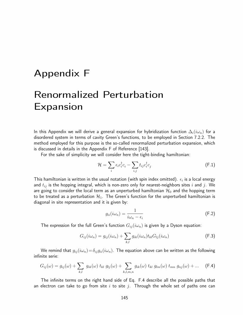
Appendix F
Renormalized PerturbationExpansion
In this Appendix we will derive a general expansion for hybridization function ∆i(iωn) for adisordered system in terms of cavity Green’s functions, to be employed in Section 7.2.2. Themethod employed for this purpose is the so-called renormalized perturbation expansion, whichis discussed in details in the Appendix F of Reference [143].
For the sake of simplicity we will consider here the tight-binding hamiltonian:
H =∑i
εic†ici −
∑i,j
tijc†icj (F.1)
This hamiltonian is written in the usual notation (with spin index omitted). εi is a local energyand tij is the hopping integral, which is non-zero only for nearest-neighbors sites i and j. Weare going to consider the local term as an unperturbed hamiltonian H0 and the hopping termto be treated as a perturbation H1. The Green’s function for the unperturbed hamiltonian isdiagonal in site representation and it is given by:
gii(iωn) =1
iωn − εi(F.2)
The expression for the full Green’s function Gij(iωn) is given by a Dyson equation:
Gij(iωn) = gij(iωn) +∑k,l
gik(iωn)tklGlj(iωn) (F.3)
We remind that gij(iωn)=δijgii(iωn). The equation above can be written as the followinginfinite serie:
Gij(ω) = gij(ω) +∑k,l
gik(ω) tkl glj(ω) +∑k,l,m,n
gik(ω) tkl glm(ω) tmn gnj(ω) + ... (F.4)
The infinite terms on the right hand side of Eq. F.4 describe all the possible paths thatan electron can take to go from site i to site j. Through the whole set of paths one can
145

APPENDIX F. RENORMALIZED PERTURBATION EXPANSION 146
Figure F.1: Schematic picture representing paths connecting the sites i and j in a squarelattice, which is related to Gij(iωn) in Eq.F.5. The skeleton path i → k → l → j (red thickarrows) is a path that does not contain any loop. Three loops corrections to this particularskeleton path are shown in the thin arrows and renormalizes this path, as it is explained in thetext. Note that the loop correction in green cannot be taken into account twice in sites i andk, then cavity Green’s functions as G(i)
kk(iωn) must be used to avoid double counting.
identify skeleton paths, in which each site is visited by the electron one time only (the path isself-avoiding). The paths containing loops can be "decomposed" in terms of a skeleton pathmultiplied by a loop correction, then the expansion in Eq.F.4 can be resummed in terms ofskeleton paths with appropriate loops corrections.
The loops corrections correspond to all intermediate paths that start and return to thesame visited site in the skeleton path, as represented bu the thin lines in Fig. F.1. They mustbe computed systematically in order to avoid double-counting. For example, let us considerthe skeleton path i → k → l → j in Gij(iωn) (the thick red lines in Fig. F.1). The loopcorrections for the first site(i) correspond to all the paths starting and ending in this site, whichcorresponds to Gii(iωn). The corrections for the next visited site contain all the paths startingand ending in k, except those passing through i, which are already accounted in the correctionfor i (for example, the green path in Figure F.1). For that reason, the loop corrections in k isgiven by the cavity Green’s function G(i)
kk(iωn), which is the local Green’s function in k havingexcluded the site i of the problem 1. The corrections in the other visited sites follow the sameprocedure and Eq. F.4 can be written as:
Gij(iωn) =∑
skeleton pathsi→j
Gii(iωn)tikG(i)kk(iωn)tklG
(i,k)ll (iωn)tlm...G
(i,k,l,m,...)jj (iωn) (F.5)
For Gii(iωn), we can write Eq.F.5 as
Gii(iωn) = gii(iωn) +Gii(iωn)∆i(iωn)gii(iωn), (F.6)
1The exclusion of i can be formally done for the hamiltonian in Eq. F.1 by taking εi →∞

APPENDIX F. RENORMALIZED PERTURBATION EXPANSION 147
in which we have defined ∆i(iωn) as:
∆i(iωn) ≡∑
skeleton pathsi→i
tikG(i)kk(iωn)tklG
(i,k)ll (iωn)tlm...tzi (F.7)
Equation F.6 can be rewritten by using Eq.F.2:
Gii(iωn) =1
iωn − εi −∆i(iωn)(F.8)
The Equations F.7 and F.8 are the principal result of this appendix. The function ∆i(iωn)takes into account all the hopping terms starting and ending in the site i through a summationover self-avoiding paths in the lattice. The drawback of writing such sum is in its coefficients,which contains cavity Green’s functions of many (infinite) "orders". However the same proce-dure described above can be used to determine G(i)
kk(iωn) or any other cavity Green’s function.Explicitly:
G(i)kk(iωn) =
1
iωn − εk −∆(i)k (iωn)
(F.9)
∆(i)kk(iωn) =
∑skeleton paths
k→k
tklG(i,k)ll (iωn)tlmG
(i,k,l)mm (iωn)tmn...tzk (F.10)
In general, there is an infinite number of equations needed to determine all Green’s functionsfor an infinite and regular lattice, then the equations above are not very useful. One way tosimplify them is to consider a Bethe lattice[146, 143], what we will do in the following.
Particular case: Bethe lattice
Bethe lattice is a loop-free structure, which means that there is a unique path connecting twosites i and j in the lattice. Thus the only skeleton path that keeps in Eq.F.7 is i→ j → i, so:
∆i(iωn) =Z∑j=1
tijG(i)jj (iωn)tji =
Z∑j=1
t2G(i)jj (iωn) (F.11)
In this equation, the sum is performed on the j sites neighbors of i (Z is the lattice coordinationnumber). We also considered that all the hopping integrals are equal to t. Similarly, we havefor ∆
(i)jj (iωn):
∆(i)j (iωn) =
Z−1∑k=1
t2G(ij)kk (iωn) =
Z−1∑k=1
t2G(j)kk (iωn) (F.12)
Here the sum is over Z − 1 sites, given that one neighboring site was excluded. In the lastequality we use the relation G(ij)
kk (iωn) = G(j)kk (iωn), which is valid in the Bethe lattice since the
exclusion of site j automatically excludes i. All the cavity Green’s functions with two or moreexcluded sites are equivalent to one with a single site removed and the hierarchy of equationsis reduced to Eqs. F.11 and F.12.


Bibliography
[1] A. C. Hewson, The Kondo problem to heavy fermions, Vol. 2 (Cambridge UniversityPress, 1997).
[2] A. A. Abrikosov, L. P. Gorkov, and I. E. Dzyaloshinski, Methods of quantum field theoryin statistical physics (Dover Publications, 1975).
[3] G. D. Mahan, Many-Particle Physics (Springer Science & Business Media, 2000).
[4] P. W. Anderson, Phys. Rev. 124, 41 (1961).
[5] E. C. Stoner, Proc. R. Soc. A , 372 (1938).
[6] J. R. Schrieffer and P. A. Wolff, Phys. Rev. 149, 491 (1966).
[7] J. Kondo, Progress of Theoretical Physics 32, 37 (1964).
[8] W. de Haas, J. de Boer, and G. van dën Berg, Physica 1, 1115 (1934).
[9] P. W. Anderson, J. Phys. C: Solid State Phys. 3, 2436 (1970).
[10] K. G. Wilson, Rev. Mod. Phys. 47, 773 (1975).
[11] B. Barbara, J. Boucherle, J. Buevoz, M. Rossignol, and J. Schweizer, Solid StateCommunications 24, 481 (1977).
[12] S. Doniach, Physica B+ C 91, 231 (1977).
[13] S. Doniach, in Theoretical and Experimental Aspects of Valence Fluctuations and HeavyFermions (Springer, 1987) pp. 179–185.
[14] P. Coleman, “Heavy fermions: Electrons at the edge of magnetism,” in Handbook ofMagnetism and Advanced Magnetic Materials (John Wiley & Sons, Ltd, 2007).
[15] P. Gegenwart, Q. Si, and F. Steglich, nature physics 4, 186 (2008).
[16] Q. Si and F. Steglich, Science 329, 1161 (2010).
[17] F. Steglich, J. Aarts, C. D. Bredl, W. Lieke, D. Meschede, W. Franz, and H. Schäfer,Phys. Rev. Lett. 43, 1892 (1979).
149
BIBLIOGRAPHY 150
[18] G. R. Stewart, Rev. Mod. Phys. 73, 797 (2001).
[19] H. v. Löhneysen, T. Pietrus, G. Portisch, H. G. Schlager, A. Schröder, M. Sieck, andT. Trappmann, Phys. Rev. Lett. 72, 3262 (1994).
[20] G. R. Stewart, Rev. Mod. Phys. 56, 755 (1984).
[21] K. Andres, J. E. Graebner, and H. R. Ott, Phys. Rev. Lett. 35, 1779 (1975).
[22] S. Cotton, Lanthanide and actinide chemistry (John Wiley & Sons, 2013).
[23] J. Lawrence, P. Riseborough, and R. Parks, Reports on Progress in Physics 44, 1 (1981).
[24] K. Gschneidner, L. Eyring, and G. Lander, Handbook on the physics and chemistry ofrare earths, Vol. 32 (Elsevier, 2002).
[25] E. Franceschi and G. L. Olcese, Phys. Rev. Lett. 22, 1299 (1969).
[26] K. Gschneidner and R. Smoluchowski, Journal of the Less Common Metals 5, 374 (1963).
[27] J.-P. Rueff et al., Phys. Rev. Lett. 96, 237403 (2006).
[28] J. M. Lock, Proc. Phys. Soc. B 70, 566 (1957).
[29] C. Varma, Rev. Mod. Phys. 48 (1976).
[30] D. Khomskii, Physics-Uspekhi 879 (1979).
[31] J. Coey and O. Massenet, in Valence Instabilities and Related Narrow-Band Phenomena,edited by R. Parks (Springer US, 1977) pp. 211–228.
[32] M. B. Maple and D. Wohlleben, Phys. Rev. Lett. 27, 511 (1971).
[33] M. B. Maple and D. Wohlleben, AIP Conference Proceedings 18, 447 (1974).
[34] B. Sales, Journal of Low Temperature Physics 28, 107 (1977).
[35] I. Nowik, in Valence Instabilities and Related Narrow-Band Phenomena, edited byR. Parks (Springer US, 1977) pp. 261–273.
[36] M. Löwenhaupt and E. Holland-Moritz, Journal of Applied Physics 50, 7456 (1979).
[37] J.-P. Rueff, Strongly Correlated Electrons at High Pressure, Habilitation à diriger desrecherches, Université Pierre et Marie Curie - Paris VI (2007).
[38] A. Fernandez-Pañella, Ytterbium-based heavy fermion compounds under extreme condi-tions : a new instrumentation to tackle fundamental questions, Ph.D. thesis, Universitéde Grenoble (2012).

BIBLIOGRAPHY 151
[39] M. Campagna, G. Wertheim, and E. Bucher, in Rare Earths, Structure and Bonding,Vol. 30 (Springer Berlin Heidelberg, 1976) pp. 99–140.
[40] F. D. M. Haldane, Phys. Rev. Lett. 40, 416 (1978).
[41] L. Falicov and J. Kimball, Phys. Rev. Lett. 22, 997 (1969).
[42] M. Neupane et al., Nature Comm. 4 (2013), 10.1038/ncomms3991.
[43] C. G. Da Silva and L. Falicov, Solid State Communications 17, 1521 (1975).
[44] D. Khomskii and A. Kocharjan, Solid State Communications 18, 985 (1976).
[45] A. Hewson and P. Riseborough, Solid State Communications 22, 379 (1977).
[46] I. Singh, A. Ahuja, and S. Joshi, Solid State Communications 34, 65 (1980).
[47] J. Freericks and V. Zlatić, Rev. Mod. Phys. 75, 1333 (2003).
[48] M. Croft, J. H. Weaver, D. J. Peterman, and A. Franciosi, Phys. Rev. Lett. 46, 1104(1981).
[49] A. Franciosi, J. H. Weaver, N. Martensson, and M. Croft, Phys. Rev. B 24, 3651 (1981).
[50] S. M. Shapiro, J. D. Axe, R. J. Birgeneau, J. M. Lawrence, and R. D. Parks, Phys. Rev.B 16, 2225 (1977).
[51] J. W. Allen and R. M. Martin, Phys. Rev. Lett. 49, 1106 (1982).
[52] M. Lavagna, C. Lacroix, and M. Cyrot, Physics Letters A 90, 210 (1982).
[53] C. Lacroix and M. Cyrot, Phys. Rev. B 20, 1969 (1979).
[54] K. Held, A. K. McMahan, and R. T. Scalettar, Phys. Rev. Lett. 87, 276404 (2001).
[55] A. K. McMahan, K. Held, and R. T. Scalettar, Phys. Rev. B 67, 075108 (2003).
[56] A. K. McMahan, Phys. Rev. B 72, 115125 (2005).
[57] G. Kotliar, S. Y. Savrasov, K. Haule, V. S. Oudovenko, O. Parcollet, and C. A. Mari-anetti, Rev. Mod. Phys. 78, 865 (2006).
[58] Y. Onishi and K. Miyake, J. Phys Soc. Jpn. 69, 3955 (2000).
[59] Y. Onishi and K. Miyake, Physica B: Condensed Matter 281, 191 (2000).
[60] A. Holmes, D. Jaccard, and K. Miyake, Phys. Rev. B 69, 024508 (2004).
[61] S. Watanabe, A. Tsuruta, K. Miyake, and J. Flouquet, Phys. Rev. Lett. 100, 236401(2008).
BIBLIOGRAPHY 152
[62] S. Watanabe and K. Miyake, J. Phys Soc. Jpn. 79, 033707 (2010).
[63] S. Watanabe, A. Tsuruta, K. Miyake, and J. Flouquet, J. Phys Soc. Jpn. 78, 104706(2009).
[64] S. Watanabe, M. Imada, and K. Miyake, J. Phys Soc. Jpn. 75, 043710 (2006).
[65] I. Hagymási, J. Sólyom, and O. Legeza, Phys. Rev. B 90, 125137 (2014).
[66] Y. Saiga, T. Sugibayashi, and D. Hirashima, J. Phys Soc. Jpn. 77, 114710 (2008).
[67] V.-N. Phan, A. Mai, and K. Becker, Phys. Rev. B 82, 045101 (2010).
[68] S. Watanabe and K. Miyake, J. Phys.: Condens. Matter 23, 094217 (2011).
[69] J. Hubbard, Proc. R. Soc. A 276, 238 (1963).
[70] J. Hubbard, Proc. R. Soc. A 277, 237 (1964).
[71] F. Gebhard, Metal-Insulator Transitions (Springer, 1997).
[72] D. Zubarev, Soviet Physics Uspekhi 3, 320 (1960).
[73] S. Burdin, Le réseau Kondo à basse température : du liquide de Fermi au liquide de spin,Ph.D. thesis, Université de Grenoble (2001).
[74] R. L. Burden and J. D. Faires, Numerical Analysis. Prindle, Weber & Schmidt, Boston,MA., pp. x 676 (1985).
[75] W. Nolting and A. Ramakanth, Quantum theory of magnetism (Springer Science &Business Media, 2009).
[76] G. G. Reddy, D. Meyer, S. Schwieger, A. Ramakanth, and W. Nolting, J. Phys.: Condens.Matter 12, 7463 (2000).
[77] N. Majlis, The quantum theory of magnetism (World Scientific, 2000).
[78] J. Flouquet and H. Harima, ArXiv e-prints (2009).
[79] A. Fernandez-Pañella, D. Braithwaite, B. Salce, G. Lapertot, and J. Flouquet, Phys.Rev. B 84, 134416 (2011).
[80] A. Fernandez-Pañella, V. Balédent, D. Braithwaite, L. Paolasini, R. Verbeni, G. Lapertot,and J.-P. Rueff, Phys. Rev. B 86, 125104 (2012).
[81] A. Miyake, F. Honda, R. Settai, K. Shimizu, and Y. Onuki, J. Phys Soc. Jpn. 81, SB054(2012).

BIBLIOGRAPHY 153
[82] A. Yasui, S.-I. Fujimori, I. Kawasaki, T. Okane, Y. Takeda, Y. Saitoh, H. Yamagami,A. Sekiyama, R. Settai, T. D. Matsuda, Y. Haga, and Y. Onuki, Phys. Rev. B 84,195121 (2011).
[83] T. Mazet, D. Malterre, M. François, C. Dallera, M. Grioni, and G. Monaco, Phys. Rev.Lett. 111, 096402 (2013).
[84] T. Mazet, D. Malterre, M. François, L. Eichenberger, M. Grioni, C. Dallera, andG. Monaco, Phys. Rev. B 92, 075105 (2015).
[85] C. Segre, M. Croft, J. Hodges, V. Murgai, L. Gupta, and R. Parks, Physical ReviewLetters 49, 1947 (1982).
[86] L. Fournes, B. Chevalier, B. Lloret, and J. Etourneau, Zeitschrift für Physik B CondensedMatter 75, 501 (1989).
[87] V. Guritanu, S. Seiro, J. Sichelschmidt, N. Caroca-Canales, T. Iizuka, S. Kimura,C. Geibel, and F. Steglich, Physical review letters 109, 247207 (2012).
[88] S. Seiro and C. Geibel, J. Phys.: Condens. Matter 23, 375601 (2011).
[89] A. Mitsuda, S. Hamano, N. Araoka, H. Yayama, and H. Wada, J. Phys Soc. Jpn. 81,023709 (2012).
[90] J. Melsen, J. Wills, B. Johansson, and O. Eriksson, Journal of Alloys and Compounds209, 15 (1994).
[91] P. Coleman, AIP Conference Proceedings 629, 79 (2002).
[92] A. Sumiyama, Y. Oda, H. Nagano, Y. Onuki, K. Shibutani, and T. Komatsubara, J.Phys Soc. Jpn. 55, 1294 (1986).
[93] Y. Onuki and T. Komatsubara, Journal of magnetism and magnetic materials 63, 281(1987).
[94] P. Nozières, Journal of Low Temperature Physics 17, 31 (1974).
[95] P. Nozières, Ann. Phys. Fr. 10, 19 (1985).
[96] P. Nozières, Eur. Phys. J. B 6, 447 (1998).
[97] S. Burdin, A. Georges, and D. R. Grempel, Phys. Rev. Lett. 85, 1048 (2000).
[98] S. Burdin and V. Zlatić, Phys. Rev. B 79, 115139 (2009).
[99] T. Costi and N. Manini, Journal of Low Temperature Physics 126, 835 (2002).
[100] C. Lacroix, Solid State Communications 54, 991 (1985).

BIBLIOGRAPHY 154
[101] M. Oshikawa, Phys. Rev. Lett. 84, 3370 (2000).
[102] P. d. V. du Plessis, A. Strydom, R. Troc, T. Cichorek, C. Marucha, and R. Gers, J.Phys.: Condens. Matter 11, 9775 (1999).
[103] M. Maple, M. de Andrade, J. Herrmann, Y. Dalichaouch, D. Gajewski, C. Seaman,R. Chau, R. Movshovich, M. Aronson, and R. Osborn, Journal of Low TemperaturePhysics 99, 223 (1995).
[104] B. Andraka and G. R. Stewart, Phys. Rev. B 47, 3208 (1993).
[105] H. v. Löhneysen, A. Rosch, M. Vojta, and P. Wölfle, Rev. Mod. Phys. 79, 1015 (2007).
[106] P. Misra, in Heavy-Fermion Systems, Handbook of Metal Physics, Vol. 2, edited byP. Misra (Elsevier, 2008) pp. 51 – 86.
[107] M. A. Continentino, Phys. Rev. B 47, 11587 (1993).
[108] P. Nozières and A. Blandin, Journal de Physique 41, 193 (1980).
[109] D. L. Cox, Phys. Rev. Lett. 59, 1240 (1987).
[110] E. Miranda, V. Dobrosavljević, and G. Kotliar, Phys. Rev. Lett. 78, 290 (1997).
[111] A. H. Castro Neto, G. Castilla, and B. A. Jones, Phys. Rev. Lett. 81, 3531 (1998).
[112] O. O. Bernal, D. E. MacLaughlin, H. G. Lukefahr, and B. Andraka, Phys. Rev. Lett.75, 2023 (1995).
[113] V. Dobrosavljević, T. R. Kirkpatrick, and B. G. Kotliar, Phys. Rev. Lett. 69, 1113(1992).
[114] D. Tanasković, E. Miranda, and V. Dobrosavljević, Phys. Rev. B 70, 205108 (2004).
[115] E. Miranda and V. Dobrosavljevic, Reports on Progress in Physics 68, 2337 (2005).
[116] E. Miranda, V. Dobrosavljevic, and G. Kotliar, J. Phys.: Condens. Matter 8, 9871(1996).
[117] S. Nakatsuji, S. Yeo, L. Balicas, Z. Fisk, P. Schlottmann, P. G. Pagliuso, N. O. Moreno,J. L. Sarrao, and J. D. Thompson, Phys. Rev. Lett. 89, 106402 (2002).
[118] S. Nakatsuji, D. Pines, and Z. Fisk, Phys. Rev. Lett. 92, 016401 (2004).
[119] P. Scoboria, J. Crow, and T. Mihalisin, J. Appl. Phys. 50, 1895 (1979).
[120] F. Ragel, P. d. V. du Plessis, and A. Strydom, J. Phys. Chem. Solids 71, 1694 (2010).
[121] S. Nakamura, M. Endo, H. Yamamoto, T. Isshiki, N. Kimura, H. Aoki, T. Nojima,S. Otani, and S. Kunii, Phys. Rev. Lett. 97, 237204 (2006).
BIBLIOGRAPHY 155
[122] H. Hodovanets, S. L. Bud’ko, W. E. Straszheim, V. Taufour, E. D. Mun, H. Kim, R. Flint,and P. C. Canfield, Phys. Rev. Lett. 114, 236601 (2015).
[123] Y. Itoh, K. Umeo, and H. Kadomatsu, Journal of alloys and compounds 315, 11 (2001).
[124] A. P. Pikul, U. Stockert, A. Steppke, T. Cichorek, S. Hartmann, N. Caroca-Canales,N. Oeschler, M. Brando, C. Geibel, and F. Steglich, Phys. Rev. Lett. 108, 066405(2012).
[125] G. Knopp, A. Loidl, R. Caspary, U. Gottwick, C. Bredl, H. Spille, F. Steglich, andA. Murani, Journal of Magnetism and Magnetic Materials 74, 341 (1988).
[126] G. Knebel, M. Brando, J. Hemberger, M. Nicklas, W. Trinkl, and A. Loidl, Phys. Rev.B 59, 12390 (1999).
[127] A. P. Pikul, C. Geibel, N. Oeschler, M. E. Macovei, N. Caroca-Canales, and F. Steglich,Phys. Status Solidi B 247, 691 (2010).
[128] K. Hoshino and Y. Kurata, J. Phys. F: Met. Phys. 9, 131 (1979).
[129] Y. Kurata, J. Phys. F: Met. Phys. 10, 893 (1980).
[130] S. Burdin and P. Fulde, Phys. Rev. B 76, 104425 (2007).
[131] R. K. Kaul and M. Vojta, Phys. Rev. B 75, 132407 (2007).
[132] C. Grenzebach, F. B. Anders, G. Czycholl, and T. Pruschke, Phys. Rev. B 77, 115125(2008).
[133] J. Otsuki, H. Kusunose, and Y. Kuramoto, J. Phys Soc. Jpn. 79, 114709 (2010).
[134] Z.-z. Li and Y. Qiu, Phys. Rev. B 43, 12906 (1991).
[135] S. Wermbter, K. Sabel, and G. Czycholl, Phys. Rev. B 53, 2528 (1996).
[136] S. Burdin and C. Lacroix, Phys. Rev. Lett. 110, 226403 (2013).
[137] I. Lifshitz, Soviet Physics JEPT 11, 1130 (1960).
[138] N. Read and D. M. Newns, J. Phys. C: Solid State Phys. 16, 3273 (1983).
[139] D. M. Newns and N. Read, Advances in Physics 36, 799 (1987).
[140] P. Coleman, Phys. Rev. B 29, 3035 (1984).
[141] C. Lacroix, Journal of Magnetism and Magnetic Materials 100, 90 (1991).
[142] A. Georges, G. Kotliar, W. Krauth, and M. Rozenberg, Rev. Mod. Phys. 68, 13 (1996).
BIBLIOGRAPHY 156
[143] E. N. Economou, Green’s Functions in Quantum Physics, Vol. 7 (Springer Science &Business Media, 2006).
[144] E. Feenberg, Phys. Rev. 74, 206 (1948).
[145] P. W. Anderson, Phys. Rev. 109, 1492 (1958).
[146] R. Abou-Chacra, D. Thouless, and P. Anderson, J. Phys. C: Solid State Phys. 6, 1734(1973).
[147] V. Dobrosavljević and G. Kotliar, Phys. Rev. Lett. 71, 3218 (1993).
[148] V. Dobrosavljević and G. Kotliar, Phys. Rev. Lett. 78, 3943 (1997).
[149] V. Dobrosavljević and G. Kotliar, Phil. Trans. R. Soc. A 356, 57 (1998).
[150] E. Miranda and V. Dobrosavljević, Physica B: Condensed Matter 259-261, 359 (1999).
[151] E. Miranda and V. Dobrosavljević, Phys. Rev. Lett. 86, 264 (2001).
[152] M. C. O. Aguiar, E. Miranda, and V. Dobrosavljević, Phys. Rev. B 68, 125104 (2003).
[153] D. Stauffer and A. Aharony, Introduction to percolation theory (CRC press, 1994).
[154] V. Shante and S. Kirkpatrick, Advances in Physics 20, 325 (1971).
[155] B. H. Bernhard and C. Lacroix, Phys. Rev. B 60, 12149 (1999).