Available at www.sciencedirect.com

journal homepage: www.elsevier.com/locate/watres

Using satellite imagery for stormwater pollutionmanagement with Bayesian networks

Mi-Hyun Park�, Michael K. Stenstrom

Department of Civil and Environmental Engineering, UCLA, 5714 Boelter Hall, Los Angeles, CA, 90095-1593, USA

a r t i c l e i n f o

Article history:

Received 24 June 2005

Received in revised form

19 May 2006

Accepted 30 June 2006

Available online 7 September 2006

Keywords:

Stormwater pollutant loading

Remote sensing

Satellite image classification

Bayesian networks

A B S T R A C T

Urban stormwater runoff is the primary source of many pollutants to Santa Monica Bay, but

its monitoring and modeling is inherently difficult and often requires land use information

as an intermediate process. Many approaches have been developed to estimate stormwater

pollutant loading from land use. This research investigates an alternative approach, which

estimates stormwater pollutant loadings directly from satellite imagery. We proposed a

Bayesian network approach to classify a Landsat ETM+ image of the Marina del Rey area in

the Santa Monica Bay watershed. Eight water quality parameters were examined,

including: total suspended solids, chemical oxygen demand, nutrients, heavy metals,

and oil and grease. The pollutant loads for each parameter were classified into six levels:

very low, low, medium low, medium high, high, and very high. The results provided spatial

estimates of each pollutant load as thematic maps from which the greatest pollutant

loading areas were identified. These results may be useful in developing best management

strategies for stormwater pollution at regional and global scales and in establishing total

maximum daily loads in the watershed. The approach can also be used for areas without

ground-survey land use data.

& 2006 Elsevier Ltd. All rights reserved.

1. Introduction

The Santa Monica Bay watershed has been studied for the last

two decades to restore and protect its water quality. Recent

efforts have focused mainly on stormwater runoff because

most point sources have been addressed (Bay et al., 1999,

2003; Ackerman and Schiff, 2003). Stormwater runoff is

recognized to be the major source of many pollutants in this

watershed (Wong et al., 1997; Bay et al., 1999). Many drainage

areas in this watershed are highly urbanized. Continuing

urbanization has increased stormwater runoff and identify-

ing urban land use has become important for properly

managing stormwater runoff pollution.

Monitoring stormwater runoff is inherently difficult due to

the uncertain temporal and spatial characteristics of its

domain (Wong et al., 1997). Stormwater discharges to Santa

Monica Bay through 30 major and hundreds of minor storm

drains. For example, the small catchment (22 km2) considered

in this paper may have as many as 2000 small storm

discharges.

To overcome the monitoring and computational difficulty of

the direct approach, alternatives based on land use informa-

tion have been used (Stenstrom et al., 1984; Wong et al., 1997).

Determining land use from traditional ground surveys is

expensive and time consuming. New approaches are being

developed to estimate land cover/land use from satellite

imagery because it provides an inexpensive and repetitive

information base (Haack et al., 1987; Kanellopoulos et al.,

1993; Paola and Schowengerdt, 1995; Stefanov et al., 2001; Pal

and Mather, 2003; Park and Stenstrom, 2003).

In this research, we explored an alternative approach

that estimates stormwater pollutant loadings directly from

ARTICLE IN PRESS

0043-1354/$ - see front matter & 2006 Elsevier Ltd. All rights reserved.doi:10.1016/j.watres.2006.06.041

�Corresponding author. Tel.: +1 310 825 1408.E-mail address: mhpark@seas.ucla.edu (M.-H. Park).

WAT E R R E S E A R C H 4 0 ( 2 0 0 6 ) 3 4 2 9 – 3 4 3 8

satellite imagery, which does not require land use or event

mean concentration (EMC) thematic maps as intermediate

processes. In order to facilitate this task, we used Bayesian

networks, an artificial intelligence (AI) algorithm, to predict

stormwater pollutant loads.

Bayesian networks are powerful probabilistic approaches to

knowledge representation and handling problems under

uncertainty. A Bayesian network is a graphical representation

in conjunction with probabilistic theory. Bayesian networks

have been successfully applied to pattern recognition, lan-

guage understanding, computer vision, medical informatics,

and decision-making (Charniak, 1991; Sucar and Gillies, 1994;

Lucas and Abu-Hanna, 1999; Bang and Gillies, 2002). Bayesian

networks have also been adopted in environmental areas,

such as risk assessment, water quality management, and

wastewater treatment system (Varis, 1995; Chong and Wally,

1996; Sanguesa and Burrell, 2000; Borsuk and Stow, 2000;

Sahely and Bagley, 2001; Borsuk et al., 2004). Bayesian

networks have been compared with other AI techniques,

such as rule-based systems and neural networks, which have

been widely used in the environmental engineering area.

Previous research proved that Bayesian networks outper-

formed rule-based systems for diagnosis in wastewater

treatment systems (Chong and Wally, 1996; Sanguesa and

Burrell, 2000). Unlike decision trees (Breiman et al., 1984;

Quinlan, 1986), Bayesian networks do not need a priori rules.

Bayesian networks were reported to be an alternative to

neural networks in wastewater treatment modeling (Hiirsal-

mi, 2000).

The main objective of this research is to spatially estimate

stormwater pollutant loadings using satellite imagery in

order to better develop management strategies in a reliable

and consistent way. Our goal is to identify the areas that

generate high pollutant loads into receiving waters. Identify-

ing areas contributing to high pollutant loads will be useful in

developing best management practices (BMPs). This will be

also useful in establishing total maximum daily load (TMDL)

because TMDLs for stormwater pollutants in this watershed

have not yet been determined. In general, we hope to gain a

better understanding of stormwater pollution using satellite

imagery and propose new guidelines for BMPs for stormwater

runoff.

2. Background

2.1. Stormwater pollution

Based on land use data, many researchers have developed

empirical models for stormwater runoff and pollutant loading

(Stenstrom et al., 1984; Guay, 1990; Stenstrom and Strecker,

1993; Wong et al., 1997; Burian and McPherson 2000; Acker-

man and Schiff, 2003). The concept uses runoff coefficients

(RCs) and pollutant concentrations in the runoff. The RC is

the fraction of rainfall that actually reaches the receiving

water and is the main component in determining annual

average storm runoff. As shown in Eq. (1), the annual average

storm runoff can be calculated from the rainfall information,

R ¼ RC�A� CF� RF�Nstorm, (1)

where R is the annual average storm runoff (m3/yr), RC is

the runoff coefficient (ranges from 0 to 1), A is the catchment

area (m2), CF is the conversion factor, RF is the average storm

rainfall (mm), and Nstorm is the average number of storms

per year (yr�1). As shown in Eq. (2), the pollutant loading

can be calculated from the EMC for each water quality

parameter

PLi ¼ R� EMCi, (2)

where PLi and EMCi are the annual pollutant loading and the

EMCs for water quality for each parameter i.

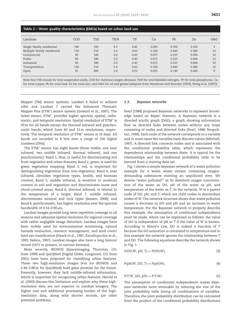
Tables 1 and 2 show RCs and EMCs for various land uses in

the Santa Monica Bay watershed (Wong et al., 1997). The

EMCs shown in Table 2 are higher than those reported in the

US EPA’s Nationwide Urban Runoff Program (NURP). Wong et

al. (1997) found that the median EMCs for the Santa Monica

Bay watershed corresponded to the 90th percentile NURP

concentrations (Driscoll et al., 1990). These simple models

using constant RCs and EMCs were restricted to longer

periods of observation or estimation because the parameters

are independent of antecedent dry periods and other event-

specific parameters.

The approach taken in this paper is to use annual loads. In

more sensitive or impacted areas with less stormwater

dilution than occurs in Santa Monica Bay, short-term impacts

of individual storms may also be important. The time of the

year, especially for Mediterranean climates may need to be

considered. A previous research (Lee et al., 2004) showed that

the first large storm of each wet year may have several times

the concentration of pollutants. Also pollutant concentra-

tions may change as a function of time between storms and

progress of the storm (Khan et al. 2006).

2.2. Satellite imagery: Landsat

The Landsat system is the first unmanned satellite system

for land observation (Jensen, 2000). Since 1972, seven

Landsat satellite series have been launched. The first three

Landsat satellites with Multi-Spectral Scanner (MSS) sensors

were the first generation of the series. Landsat 4 and 5

were the second-generation satellites and employ Thematic

ARTICLE IN PRESS

Table 1 – Runoff coefficients and imperviousness basedon urban land use

Landuse Imperviousness Runoffcoefficient

Single family

residential

0.42 0.39

Multiple family

residential

0.68 0.58

Commercial 0.95 0.74

Public 0.80 0.66

Industrial 0.91 0.74

Transportation 0.80 0.66

Open 0.00 0.1

Adapted from Stenstrom and Strecker (1993); Wong et al. (1997).

WAT E R R E S E A R C H 4 0 ( 2 0 0 6 ) 3 4 2 9 – 3 4 3 83430

Mapper (TM) sensor systems. Landsat 6 failed to achieve

orbit and Landsat 7 carried the Enhanced Thematic

Mapper Plus (ETM+) sensor system (Goward et al., 2001). The

latest sensor, ETM+, provides higher spectral, spatial, radio-

metric, and temporal resolution. Spatial resolution of ETM+ is

30 m for all bands except the thermal infrared and panchro-

matic bands, which have 60 and 15 m resolutions, respec-

tively. The temporal resolution of ETM+ sensor is 16 days. All

bands are recorded in 8 bits over a range of 256 digital

numbers (DNs).

The ETM+ sensor has eight bands (three visible, one near

infrared, two middle infrared, thermal infrared, and one

panchromatic): Band 1, blue, is useful for discriminating soil

from vegetation and urban features; Band 2, green, is used for

green vegetation mapping; Band 3, red, is important for

distinguishing vegetation from non-vegetation; Band 4, near

infrared, identifies vegetation types, health, and biomass

content; Band 5, middle infrared, is sensitive to moisture

content in soil and vegetation and discriminates snow and

cloud-covered areas; Band 6, thermal infrared, is related to

the temperature of a target; Band 7, middle infrared,

discriminates mineral and rock types (Jensen, 2000); and

Band 8, panchromatic, has higher resolution over the spectral

bandwidth of 0.52–0.90mm.

Landsat images provide long-term repetitive coverage in all

seasons and adequate spatial resolution for regional coverage

with rather negligible image distortion. Landsat images have

been widely used for environmental monitoring, natural

hazards evaluation, resource management, and land cover/

land use classification (Haack et al., 1987; Kanellopoulos et al.,

1993; Sabins, 1997). Landsat images also have a long historic

record (1972 to present, in various formats).

More recently, IKONOS (Spaceimaging, Thornton, CO,

from 1999) and Quickbird (Digital Globe, Longmont, CO, from

2001) have been proposed for classifying urban features.

These two high-resolution images (4 m for IKONOS and

2.44–2.88 m for Quickbird) hold great promise for the future.

Presently, however, they lack middle-infrared information,

which is important for recognizing urban features. Herold et

al. (2003) discuss this limitation and explain why these high-

resolution data are not superior to Landsat imagery. The

higher cost and additional processing burden of the high-

resolution data, along with shorter records, are other

potential problems.

2.3. Bayesian networks

Pearl (1988) proposed Bayesian networks to represent knowl-

edge based on Bayes’ theorem. A Bayesian network is a

directed acyclic graph (DAG), a graph showing information

flow as directed links between nodes without any loops

consisting of nodes and directed links (Pearl, 1988; Neapoli-

tan, 1990). Each node of the network corresponds to a variable

and in most cases the variables have discrete values (Mitchell,

1997). A directed link connects nodes and is associated with

the conditional probability table, which represents the

dependence relationship between them. It is typical for the

relationships and the conditional probability table to be

learned from a training data set.

Fig. 1 shows a simple Bayesian network of a water pollution

example for a warm waste stream containing oxygen-

demanding substances entering an unpolluted river. We

denote ‘‘water polluted?’’ as W, dissolved oxygen concentra-

tion of the water as DO, pH of the water as pH, and

temperature of the water as T. In the network, W is a parent

node of DO, pH, and T, which are child nodes or descendant

nodes of W. The network structure shows that water pollution

causes a decrease in DO and pH and an increase in water

temperature. For the Bayesian network to properly describe

this example, the assumption of conditional independence

must be made, which can be explained as follows: the value

of DO is independent of pH or T if the value of W is known.

According to Henry’s Law, DO is indeed a function of T

because the DO saturation is correlated to temperature and in

this example the network ignores the relationship between T

and DO. The following equations describe the network shown

in Fig. 1:

PðDOjW; pH; TÞ ¼ PðDOjWÞ, (3)

PðpHjW; DO; TÞ ¼ PðpHjWÞ, (4)

PðTjW; DO; pHÞ ¼ PðTjWÞ. (5)

The assumption of conditional independence makes Baye-

sian networks more attainable by reducing the size of the

joint probability table listing all combinations of variables.

Therefore, the joint probability distribution can be calculated

from the product of the conditional probability distributions

ARTICLE IN PRESS

Table 2 – Water quality characteristics (EMCs) based on urban land use

Landuse COD TSS TKN TP Cu Pb Zn O&G

Single family residential 140 290 4.3 0.85 0.095 0.350 0.350 3

Multiple family residential 130 210 2.4 0.62 0.100 0.440 0.380 22

Commercial 90 180 2.0 0.43 0.072 0.225 0.694 22

Public 90 180 2.0 0.43 0.072 0.225 0.694 22

Industrial 90 180 2.0 0.43 0.072 0.225 0.694 22

Transportation 130 210 2.4 0.62 0.100 0.440 0.380 22

Open 95 490 2.8 0.52 0.055 0.140 0.440 0

Note that TSS stands for total suspended solids, COD for chemical oxygen demand, TKN for total Kjeldahl nitrogen, TP for total phosphorus, Cu

for total copper, Pb for total lead, Zn for total zinc; and O&G for oil and grease (adapted from Stenstrom and Strecker (1993); Wong et al. (1997)).

WAT E R R E S E A R C H 40 (2006) 3429– 3438 3431

of all nodes given their parent nodes, assuming conditional

independence.

Water pollution, W, for this example can be inferred from

the observation of DO, pH, and T as follows,

PðWjDO; pH; TÞ ¼ aPðDOjWÞPðpHjWÞ

�PðTjWÞPðWÞ, ð6Þ

where a is a normalizing constant to set the probabilities to 1.

Because the prior probability of P(W) can be calculated from

training data or can be obtained from experts, the likelihoods

of P(DO|W), P(pH|W) and P(T|W) must be calculated from

training data. We can calculate the posterior probability

distribution over W for any observed values of DO, pH, and

T. We can then predict whether the water is polluted with the

highest posterior probability.

This example uses a naive Bayesian classifier, which are the

simplest Bayesian networks with only one class node. The

network can easily be constructed by setting one class node

(i.e., W in Fig. 1) and all other nodes (i.e., DO, pH, and T in Fig.

1) as its child nodes. The relative contribution of each node

cannot be inferred by the network structure.

The naive Bayesian classifiers are limited by the strong

conditional independence assumption. Although the condi-

tional independence assumption provides computational

simplicity, it is not often completely satisfied in real world

situations. Modified naive Bayesian classifiers partially over-

come this problem by providing more flexibility among child

nodes. For example, selective naive Bayesian classifiers, joint

naive Bayesian classifiers, and tree-augmented naive Bayesian

classifiers, which are beyond the scope of this paper, were

developed to overcome the limit of naive Bayesian classifiers

(Langley and Sage, 1994, Pazzani, 1995, Friedman et al., 1997).

An alternative and usually more powerful structure is a

maximum weight spanning tree (MWST). MWSTs can be

constructed from data based on mutual information

or weight between variables, which provides a measure

of dependency between variables as follows (Chow and

Liu, 1968):

MIðXi;XjÞ ¼X

Pðxi; xjÞ logPðxi; xjÞ

PðxiÞPðxjÞ

!, (7)

where MI(Xi,Xj) is the mutual information of random variables

of Xi and Xj, P(xi,xj) is a joint probability of xi and xj, and P(xi)

and P(xj) are the probabilities of each random variable. For

example, in this paper, pairs of satellite bands are the Xi and

Xj’s. The pairs of nodes having the greatest mutual informa-

tion are connected while avoiding loops. When completing

the network, the sum of the mutual information will be

maximized. The MWST structure explicitly shows the rela-

tionships among nodes and the less contributing nodes can

sometimes be eliminated to simplify the problem.

3. Methods

3.1. Study area and data

The study area focused on Marina del Rey and its vicinity

(latitudes 3315604200–3315904500 and longitudes 11812404200

–11812703400) in the Santa Monica Bay watershed. The size of

the study area is 22 km2. The area is dominated by residential

and open areas and urbanization is continuing.

We used land use data from the Southern California

Association of Governments (SCAG) (2003) and geospatial

ancillary data, i.e., X and Y coordinate values of each pixel in

the imagery. Land use pixels that are misclassified for

environmental purposes in the SCAG data were reclassified

based upon ground truth. For example, the open areas around

the Los Angeles International Airport and Loyola Marymount

University were classified as transportation and public,

respectively. They were also reclassified as open land use.

The land use data were transformed into pollutant loadings

for each water quality parameter per unit pixel area and unit

rainfall using Eq. (8), as follows:

PLi ¼ b� RC� EMCi, (8)

where PLi is pollutant loads per unit pixel and unit rainfall for

each water quality parameter i, and b is a normalization

factor that depends on units and CFs. The study area was

small and the rainfall and number of storms per year were

assumed equal for all pixels. It was also assumed that all

stormwater runoff discharges to Santa Monica Bay. Eight

water quality parameters were used to estimate pollutant

loading: chemical oxygen demand (COD); total suspended

solids (TSS); nutrients, i.e., total Kjeldahl nitrogen (TKN) and

total phosphorus (TP); total copper (Cu); total lead (Pb); total

zinc (Zn); and oil and grease (O&G).

We used a Landsat ETM+ image (obtained on August 11,

2002) of the study area. All bands except the panchromatic

band were examined for our study (the panchromatic band

overlaps with other bands from visible to near infrared, and

provides redundant information). Selected pixels from the

satellite image corresponding to the pollutant loading data

set were used as the training and test data sets. The test data

were used for accuracy assessment. Pixels for the training

data and test data were randomly collected from each class to

avoid undersampling of the small classes, which can occur if

the pixels are selected randomly from the entire dataset

(Jensen, 1996). The total number of training data pixels was

2067 and the total number of test data pixels was 1033, which

corresponded to 8.5% and 4.3% of total data, respectively. The

ARTICLE IN PRESS

P(T|W)

W

pHDO T

P(W)

P(DO|W)

P(pH|W)

Fig. 1 – An example of a Bayesian network for water

pollution. Note that W is ‘‘Is water polluted?’’, DO is

dissolved oxygen concentration in the water, pH is the pH of

the water, and T is water temperature.

WAT E R R E S E A R C H 4 0 ( 2 0 0 6 ) 3 4 2 9 – 3 4 3 83432

probabilistic relationships defined by Eqs. (6) and (7) were

calculated using a C++ program, although commercial soft-

ware could have been used (Hugin; Netica). The detailed

information of the satellite image data is given in Table 3.

This approach differs from other approaches (Stenstrom et

al., 1984; Guay, 1990; Stenstrom and Strecker, 1993; Wong et

al., 1997; Burian and McPherson 2000; Ackerman and Schiff,

2003) in that pollutant loads are identified as opposed to land

use. This is advantageous because land uses that have the

same pollutant loads do not need to be recognized indepen-

dently. For example, commercial, public, and industrial land

uses tend to have similar pollutant loads and are often

misclassified in land use classification. These land uses can

be lumped in our approach, which improves the classification

accuracy.

3.2. Bayesian networks

Both naive Bayesian classifiers and MWSTs were developed by

selecting unit pollutant loading as a class node. All data

values used here were discretized to 15 values based on equal

frequency interval. The class node had six states correspond-

ing to the degree of pollutant loading for each water quality

parameter: very low, low, medium low, medium high, high,

and very high. In this case, the ‘‘very low’’ state indicated that

no pollutant was discharged. The state of ‘low’ was the

minimum pollutant loading for each water quality parameter

except zero loading. As shown in Table 4, the rest of the states

were normalized based on ‘low’ state of pollutant loading

values.

3.3. Accuracy assessment

In order to evaluate the performance of Bayesian networks,

overall accuracy was calculated. However, overall accuracy

has a limitation in that it does not provide individual class

accuracy (Foody, 2002). In the remote sensing community,

individual class accuracy is measured by using a confusion

matrix also called contingency table, which compares the

predicted pixel labels from the final map with the correspond-

ing actual class labels from ground truth (Jensen, 1996;

Richards and Jia, 1999; Foody, 2002). Two different errors were

measured: (1) omission error corresponding to the percentage

of the pixels actually belonging to a class, but failed to be

assigned to the class and (2) commission error corresponding

to the percentage of the pixels that are incorrectly assigned to

the class, but actually belong to other classes. These errors

are expressed as

omission error ¼ 1�nijPinij

!� 100, (9)

commission error ¼ 1�nijPjnij

!� 100, (10)

where nij is the number of pixels of each element in the

matrix and i and j are the indices for row and column,

respectively, when the labels in the column are original ones.

The overall accuracy in conjunction with the confusion

matrix is expressed as

overall accuracy ¼

Pknkk

N� 100, (11)

where N is the total number of test pixels in the confusion

matrix.

Table 5 shows an example of a confusion matrix, which can

be used to calculate the omission error, commission error,

ARTICLE IN PRESS

Table 3 – Landsat ETM+ image data statistics for the study area

Band Wave length (mm) Min Max Median Mean Standard deviation

1 (blue) 0.45–0.52 80 255 111 114 15

2 (green) 0.52–0.60 50 255 94 96 17

3 (red) 0.63–0.69 43 255 102 105 22

4 (near IR) 0.76–0.90 20 155 63 63 12

5 (IR) 1.55–1.75 9 255 96 101 28

6 (thermal IR) 10.4–12.5 138 210 180 179 9

7 (IR) 2.08–2.35 8 255 75 79 25

Table 4 – Classification states for water quality parameter

State Normalized loading values

Very low �0 loading

Low Minimum loading

Medium low p4� low loading

Medium high p8� low loading

High p12� low loading

Very high 412� low loading

Table 5 – An example of confusion matrix

Ground truth

Class A B C Total

Map class A 35 2 2 39

B 10 37 3 50

C 5 1 41 47

Total 50 40 46 136

WAT E R R E S E A R C H 40 (2006) 3429– 3438 3433

and the overall accuracy. Omission error of class B is 7%,

which is derived from (1–37/40)100, and commission error is

26%, which is derived from (1–37/50)100. Overall accuracy is

83%, which is derived from (35+37+41)/136.

4. Results

The correlations of each Band in the Landsat ETM+ data are

presented in Table 6. All visible Bands 1, 2, and 3 and middle

infrared Bands 5 and 7 exhibited high correlation. The near

infrared, Band 4 and thermal infrared, Band 6 were not highly

correlated with the other Bands. The distribution of each

Band is shown in Fig. 2. Most of the distributions of the DN

values of each Band were skewed.

The resulting Bayesian network structures are shown in Fig.

3. In naive Bayesian classifiers, the relative contribution of

each band and the geospatial inputs is not known for the

previously stated reasons. Conversely, the structure of

MWSTs shows that Bands 1 and 5 mainly contributed to the

class node values. In addition, Band 6 was also connected to

the class node in the MWST structure for Zn and O&G. The

structure of MWSTs presented strong dependency between

visible Bands (1–3) and middle infrared bands (5 and 7), which

were consistent with their high correlations.

The resulting thematic maps using MWSTs are shown in

Fig. 4. Each water quality parameter shows a different level of

classification: TSS, TP, and TKN were classified into two

classes; COD, Cu, and Pb were classified into three classes;

and Zn and O&G were classified into four classes. The maps of

Pb and O&G displayed the level of ‘‘very high’’ and/or ‘‘very

low’’ loading, which is distinctive. Table 7 shows the percen-

tage of area assigned to the different pollutant loadings.

The overall accuracies for each case are given in Fig. 5. The

dotted line represents the accuracies with spectral data only,

whereas the solid line represents the accuracies with both

spectral and geospatial data. When geospatial data were

included, overall accuracies for COD, TSS, TKN, and TP were

all above 90%. Overall accuracies for heavy metals, such as

Cu, Pb, and Zn, as well as O&G ranged from 83% to 88% with

geospatial data depending on the network structure. Includ-

ing geospatial data improved the accuracies of COD, heavy

metals, and O&G up to 7%. This probably occurs because of

zoning rules which tend to locate similar land uses together.

However, overall accuracies between naive Bayesian classi-

fiers and MWSTs for a specific water quality parameter were

only slightly different. This was especially true when includ-

ing geospatial data and the MWSTs were only 3% better.

In order to validate the accuracy improvement, the overall

accuracies of Bayesian networks were compared with the

accuracy by random classification. For example, classification

with two states can provide 50% of accuracy even with

random prediction. The comparison between these two

accuracies is given in Fig. 6. The top figure shows the overall

accuracy as a percent. While the best random accuracy was

only 50%, the various Bayesian networks were 77% to over

90% accurate depending upon the water quality parameter.

The bottom part of the figure shows the ratios of the Bayesian

accuracies to the random accuracy. The Bayesian network

accuracy of TSS, TP, and TKN was approximately 1.9 times

better than the random classification accuracy. Likewise,

Bayesian network accuracy of COD, Cu, and O&G was 2.5–2.7

times better, and that of Pb and Zn was 3.4 times better than

random classification accuracy. The difference between these

ratios among network structures was almost negligible

(p1.5%).

Omission error of the highest pollutant loading varied

depending upon the water quality parameters. Omission

errors for TSS, TKN, and TP were the lowest—from 4% to

6%. Depending on the network structure, the omission errors

for Cu and Zn were from 9% to 18%. The errors for COD, Pb,

and O&G were mostly above 20%, with the largest error of

35%. In regards to the network structures, most omission

errors of naive Bayesian classifiers were larger than those of

MWSTs except TSS, TKN, and TP. In addition, the inclusion of

geospatial data reduced omission errors.

ARTICLE IN PRESS

Table 6 – Correlation of Landsat ETM+ bands from training data

Band 1 Band 2 Band 3 Band 4 Band 5 Band 6 Band 7

Band 1 1

Band 2 0.98 1

Band 3 0.95 0.97 1

Band 4 0.25 0.34 0.31 1

Band 5 0.24 0.32 0.47 0.36 1

Band 6 0.21 0.20 0.27 �0.18 0.25 1

Band 7 0.51 0.58 0.70 0.25 0.90 0.30 1

0

500

1000

1500

2000

0 50 100 150 200 250

digital number

coun

t

B1

B2

B3

B4

B5

B6

B7

Fig. 2 – Distribution of each ETM+ band.

WAT E R R E S E A R C H 4 0 ( 2 0 0 6 ) 3 4 2 9 – 3 4 3 83434

ARTICLE IN PRESS

C

B1 B5 X YB7B2 B3 B4 B6

(a)

C

B1 B5 X Y

B7B2

B3 B4

B6

(b)

C

B1 B5 X Y

B7B2

B3 B4

B6

(c)

Fig. 3 – The resulting structure of Bayesian networks for pollutant loading estimation (a) naive Bayesian networks, (b) MWSTs

for COD, TSS, TKN, TP, Cu, and Pb, (c) MWSTs for Zn and oil and grease.

Fig. 4 – Thematic maps of pollutant loading for water quality parameters using MWSTs including geospatial data (a) COD, (b)

TSS, (c) TP, TKN, (d) Cu, (e) Pb, (f) Zn, (g) oil and grease, (h) landuse.

WAT E R R E S E A R C H 40 (2006) 3429– 3438 3435

Commission error of the lowest pollutant loading from other

areas showed little variation for different water quality

parameters compared with the omission errors. When com-

pared with omission errors, the magnitudes of commission

errors of COD, Pb, and Zn became smaller, whereas those of

TSS, TKN, and TP became larger. The commission errors of

COD ranged from 6% to 8%; those of TSS, TKN, and TP were

from 9% to 11%; and those of heavy metals and O&G were

between 6% and 14%. Including geospatial data reduced the

commission errors, but it was not as significant as with

omission errors.

5. Discussion

The methodology proposed here is different from conven-

tional land use-based stormwater models and appears to be a

valuable alternative. By estimating pollutant loads directly

from satellite imagery, potential errors in land use classifica-

tion are avoided. Land use classifications not developed for

environmental purposes often group environmentally differ-

ent land uses into the same category. For example, the buffer

zone around the Los Angeles International Airport is classi-

ARTICLE IN PRESS

Table 7 – Percentage of pollutant loading area of each water quality parameter

COD TSS TKN TP Cu Pb Zn O&G

Very low 0 0 0 0 0 0 0 30.9

Low 28.6 27.7 27.7 27.7 29.9 29.4 32.8 30.3

Med-low 0 72.3 0 0 0 0 32.1 0

Med-high 64.3 0 72.3 72.3 33.0 0 19.2 0

High 7.1 0 0 0 37.1 53.5 15.9 14.3

Very high 0 0 0 0 0 17.1 0 24.5

70

80

90

100

COD TSS TP/TKN Cu Pb Zn O&G

over

all a

ccur

acy

(%)

Naïve XYMWST XYNaïve no XYMWST no XY

0

20

40

60

omis

sion

err

or (

%)

0

5

10

15

20

com

mis

sion

err

or (

%)

COD TSS TP/TKN Cu Pb Zn O&G

COD TSS TP/TKN Cu Pb Zn O&G

Naïve XYMWST XYNaïve no XYMWST no XY

MWST XYNaïve no XYMWST no XY

Naïve XY

(a)

(b)

(c)

Fig. 5 – Accuracy of Bayesian networks (a) overall accuracy

(b) omission error of the highest pollutant loading area (c)

commission error of the lowest pollutant loading area.

0

25

50

75

100

COD TSS TP/TKN Cu Pb Zn O&G

COD TSS TP/TKN Cu Pb Zn O&G

over

all a

ccur

acy

(%)

Naïve XY

Naïve no XYMWST no XYrandom accuracy

(a)

(b)0

1

2

3

4

ratio

Naïve XY

MWST XY

Naïve no XY

MWST no XY

MWST XY

Fig. 6 – Bayesian network accuracy compared with random

classification accuracy (a) plot of Bayesian network accuracy

with random classification accuracy (b) ratio of Bayesian

network accuracy to random classification accuracy.

WAT E R R E S E A R C H 4 0 ( 2 0 0 6 ) 3 4 2 9 – 3 4 3 83436

fied as transportation, but has the environmental properties

of open land use. In addition, parks are classified as public

land use along with environmentally different land use, such

as government buildings (e.g., schools, post offices, libraries).

Furthermore, there are many areas of interest where there are

no land use data.

An alternate method employs land use classification

instead of pollutant loadings and calculates pollutant loading

from land use definitions. This approach was used in an

earlier project by the authors Park and Stenstrom (2006) but

was less accurate, yielding only 79–81% accuracy with

geospatial data and 69–71% without geospatial data. The

new methodology used in this paper predicted pollutants for

the various parameters with accuracies ranging from 80% (Pb

and Zn) to 94% (TSS, TKN, and TP). Therefore, the new

methodology improved accuracy up to 15% when using

geospatial data and up to 25% without geospatial data. The

new methodology provides better prediction and is a promis-

ing method for future environmental planning and manage-

ment. Moreover, the new method does not require potentially

expensive land use data based on ground surveys for the

entire watershed.

The examples described in this paper show important

differences among pollutant types. The loadings are shown in

fuzzy categories (see Fig. 4) from very low to very high, but the

numerical values (not shown) vary by 10–20 fold for Zn and Pb

emission rates and only by 3–9 fold for TSS, TKN, TP, and COD

emission rates. This suggests that there is greater opportunity

to impact Zn and Pb emission rates by identifying high

emitters. Environmental planners and regulators need to be

aware of these important differences. The new strategy

provides this information along with spatial information to

locate environmental opportunities.

The thematic maps show that the lowest pollutant loading

areas mostly corresponded to open land use. Transportation

land use corresponded to the highest pollutant loading areas

for all water quality parameters except Zn, which was highest

in commercial and industrial land uses. This shows the

significance of transportation land use for stormwater

management. Multiple-family residential land use is also

important for Pb, which may result from greater numbers of

vehicles associated with multiple-family residential land use.

Fig. 6 shows the performance of the Bayesian network.

Compared to random classification, the network performed

especially well for Pb and Zn, although the absolute accura-

cies were less than the accuracies of other water quality

parameters. This results from more states for Pb and Zn.

Similar ratios among different networks show that the

Bayesian network performance was effective even with the

increased number of class node states, which required higher

level of classification.

The results of omission error and commission error show

that MWSTs outperformed naive Bayesian classifiers. This

confirms that MWSTs are more useful not only because of the

reduced number of the input variables for classification, but

also because of reducing the risk of mismatching the highest

pollutant loading area with the lower pollutant loading area

and vice versa. Moreover, the omission errors demonstrate

that including geospatial data considerably improves the

classification in locating the highest pollutant loading areas.

Including geospatial data was inexpensive because the X and

Y coordinate values can be calculated from the image. The

only cost for including the geospatial data was the computing

time, which was relatively small.

6. Conclusions

This paper has shown that Bayesian classification of satellite

imagery is useful for estimating pollutant loading in a

watershed. Both naive Bayesian classifiers and MWSTs were

useful, but MWSTs were better for the following reasons: (1)

they reveal the relationships among variables; (2) they

identify the most informative input variables to classification;

(3) they reduce the number of input variables required for

classification; and (4) they reduce the risk of overestimating or

underestimating of pollutant loading in the given area.

Incorporating geospatial data improved accuracy—especially

in identifying areas with higher metal loadings.

The new approach in this paper is to estimate stormwater

pollutant loads directly from satellite imagery. This has

advantages over approaches based upon land use from

ground surveys. Such land use classifications were usually

performed for other purposes and are not optimized for

environmental uses. For example, transportation classifica-

tion often includes large open areas, and parks and ceme-

teries and golf courses are included in classifications that are

primarily associated with developed, impervious areas.

Training and classification based upon pollutant emission

rates are promising alternatives to conventional land use

models and have the added advantage of applicability to

areas without land use data based on ground surveys.

Acknowledgment

This work was partially supported by the US Environmental

Protection Agency under Grant R825831.

R E F E R E N C E S

Ackerman, D., Schiff, K., 2003. Modeling storm water massemissions to the Southern California Bight. J. Environ. Eng.,ASCE 129 (4), 308–317.

Bang, J., Gillies, D. F., 2002. Using Bayesian networks to model theprognosis of hepatitis C. In: Proceedings of the seventhIntelligent Data Analysis and Pharmacology (IDAMAP) work-shop, 15th European Conference on Artificial Intelligence,Lyon, France, pp. 7–12.

Bay, S., Jones, B. H., Schiff, K., 1999. Study of the impact ofstormwater discharge on the beneficial uses of Santa MonicaBay, Executive summary prepared for Los Angeles County,Department of Public Works, Alhambra, CA.

Bay, S., Jones, B.H., Schiff, K., Washburn, L., 2003. Water qualityimpacts of stormwater discharges to Santa Monica Bay. Mar.Environ. Res. 56, 205–223.

Breiman, L., Friedman, J.H., Olshen, R.A., Stone, C.J., 1984.Classification and Regression Trees. Wadsworth, Belmont, CA.

Borsuk, M.E., Stow, C.A., 2000. Bayesian parameter estimation in amixed-order model of BOD decay. Water Res. 34, 1830–1836.

ARTICLE IN PRESS

WAT E R R E S E A R C H 40 (2006) 3429– 3438 3437

Borsuk, M.E., Stow, C.A., Reckhow, K.H., 2004. A Bayesian networkof eutrophication models for synthesis, prediction, anduncertainty analysis. Ecol. Modeling 173, 219–239.

Burian, S. J., McPherson, T. N., 2000. Water quality modeling ofBallona Creek and the Ballona Creek estuary. In: Proceedingsof AWRA’s Annual Water Resources Conference, AmericanWater Resources Association, Bethesda, MD.

Charniak, E., 1991. Bayesian network without tears. AI Mag. 12 (4),50–63.

Chong, H.G., Wally, W.J., 1996. Rule-based versus probabilisticapproached to the diagnosis of faults in wastewater treatmentprocesses. Artif. Intell. Eng. 1, 265–273.

Chow, C.K., Liu, C.N., 1968. Approximating discrete probabilitydistributions with dependence trees. IEEE Trans. Inform. Theo-ry 14 (3), 462–467.

Digital Globe http://www.digitalglobe.com/.Driscoll, E. D., Shelly, P. E., Strecker, E. W., 1990. Pollutant loadings

and impacts from stormwater runoff, vol. III: Analyticalinvestigation and research report, FHWA-RD-88-008, FederalHighway Administration.

Foody, G.M., 2002. Status of land cover classification accuracyassessment. Remote Sens. Environ. 80 (1), 185–201.

Friedman, N., Geiger, D., Goldszmidt, M., 1997. Bayesian networkclassifiers. Mach. Learn. 29 (2–3), 131–163.

Goward, S.N., Masek, J., Williams, D.L., Irons, J.R., Thompson, R.J.,2001. The Landsat 7 mission: terrestrial research for the 21stcentury, Special Issue on Landsat 7. Remote Sens. Environ. 78(1–2), 3–12.

Guay, J. R., 1990. Simulation of urban runoff and river waterquality in the San Joaquin River near Fresno, California. In:Proceedings of American Water Resources Association Sym-posium on Urban Hydrology, Denver, CO, pp. 177–181.

Haack, B., Bryant, N., Adams, S., 1987. An assessment of LandsatMSS and TM data for urban and near-urban land-cover digitalclassification. Remote Sens. Environ. 21, 201–213.

Herold, M., Gardner, M.E., Roberts, D.A., 2003. Spectral resolutionrequirements for mapping urban areas. IEEE Trans. Geosci.Remote Sens. 41 (9), 1907–1919.

Hiirsalmi, M., 2000. Method feasibility study: Bayesian networks.MODUS-Project Waste Water Case Study, Research ReportTTE1-2000-29, VTT Information Technology, Espoo, Finland.

Hugin http://www.hugin.com.Jensen, J.R., 1996. Introductory Digital Image Processing: A Remote

Sensing Perspective. Prentice Hall, Upper Saddle River, NJ.Jensen, J.R., 2000. Remote Sensing of the Environment: An Earth

Resource Perspective. Prentice Hall, Upper Saddle River, NJ.Kanellopoulos, I., Wilkinson, G. G., Megier, J., 1993. Integration of

neural network and statistical image classification for landcover mapping. In: Proceedings of IGARSS, Tokyo, Japan,511–513

Khan, S., Lau, S-L., Kayhanian, M., Stenstrom, M.K., 2006. Oil andgrease measurement in highway runoff-sampling time andevent mean concentrations. J. Environ. Eng., ASCE 132, 415–422.

Langley, P., Sage, S., 1994. Induction of selective Bayesianclassifiers. In: Proceedings of the 10th Conference on Un-certainty in Artificial Intelligence, Seattle, WA.

Lee, H., Lau, S.-L., Kayhanian, M., Stenstrom, M.K., 2004. Seasonalfirst flush phenomenon of urban stormwater discharges.Water Res. 38, 4153–4163.

Lucas, P., Abu-Hanna, A., 1999. Prognostic methods in medicine.Artif. Intell. Med. 15, 105–119.

Mitchell, T.M., 1997. Machine Learning. McGraw Hill, Singapore.Neapolitan, R.E., 1990. Probabilistic Reasoning in Expert Systems:

Theory and Algorithms. Wiley, New York.Netica http://www.norsys.com.Pal, M., Mather, P.M., 2003. An assessment of the effectiveness of

decision tree methods for land cover classification. RemoteSens. Environ. 86 (4), 554–565.

Paola, J.D., Schowengerdt, R.A., 1995. A detailed comparison ofback propagation neural network and maximum-likelihoodclassification for urban land use classification. IEEE Trans.Geosci. Remote Sens. 33, 981–996.

Park, M., Stenstrom, M. K., 2003. Land use classification forstormwater modeling using Bayesian networks. In: Proceed-ings of the Seventh International Specialised IWA Conference,Diffuse Pollution and Basin Management, Dublin, Ireland.

Park, M., Stenstrom, M.K., 2006. Spatial estimates of stormwaterpollutant loading using Bayesian networks and geographicinformation systems. Water Environ. Res. 78 (4), 421–429.

Pazzani, M. J., 1995. An iterative improvement approach for thediscretization of numeric attributes in Bayesian classifiers. In:Proceedings of the First International Conference on Knowl-edge Discovery and Data Mining, Montreal, Canada.

Pearl, J., 1988. Probabilistic Reasoning in Intelligent Systems: Net-works of Plausible Inference. Morgan Kaufmann, San Mateo, CA.

Quinlan, J.R., 1986. Induction of decision trees. Mach. Learning 1,81–106.

Richards, J.A., Jia, X., 1999. Remote sensing digital image analysis:an introduction, 3rd ed. Springer, New York.

Sabins, F.F., 1997. Remote Sensing: Principles and Interpretation.Freeman and company, USA.

Sahely, B.S.G.E., Bagley, D.M., 2001. Diagnosing upsets in anaero-bic wastewater treatment using Bayesian belief networks. J.Environ. Eng., ASCE 127 (4), 302–310.

Sanguesa, R., Burrell, P., 2000. Application of Bayesian networklearning methods to waste water treatment plants. Appl.Intell. 13, 19–40.

Southern California Association of Governments, 2003. http://wagsdata.scag.ca.gov.

Spaceimaging http://www.spaceimaging.com/.Stefanov, W.L., Ramsey, M.S., Christensen, P.R., 2001. Monitoring

urban land cover change; An expert system approach to landcover classification of semiarid to arid urban centers. RemoteSens. Environ. 77 (2), 173–185.

Stenstrom, M.K., Silverman, G.S., Bursztynsky, T.A., 1984. Oil andgrease in urban stormwaters. J. Environ. Eng. Div., ASCE 110 (1),58–72.

Stenstrom, M. K., Strecker, E., 1993. Assessment of storm drainsources of contaminants to Santa Monica Bay, Vol. I, AnnualPollutants Loadings to Santa Monica Bay from StormwaterRunoff, UCLA-ENG-93-62, I, 1-248.

Sucar, L.E., Gillies, D.F., 1994. Probabilistic reasoning in high-levelvision. Image Vis. Comput. 12 (1), 42–60.

Varis, O., 1995. Belief networks for modeling and assessment ofenvironmental change. Environmetrics 6, 439–444.

Wong, K., Strecker, E.W., Stenstrom, M.K., 1997. A geographicinformation system to estimate stormwater pollutant massloadings. J. Environ. Eng., ASCE 123, 737–745.

ARTICLE IN PRESS

WAT E R R E S E A R C H 4 0 ( 2 0 0 6 ) 3 4 2 9 – 3 4 3 83438