Using Phylogenomic Data to Untangle the Patterns ... - CORE

Using Phylogenomic Data to Untangle the Patterns and Timescale of Flowering Plant Evolution

Charles Stuart Piper Foster

The University of Sydney Faculty of Science

2018

A thesis submitted in fulfilment of the requirements for the

degree of Doctor of Philosophy

ii

Authorship Attribution Statement

During the course of my doctoral candidature, I published a series of

stand-alone manuscripts in peer-reviewed international journals. In

agreement with the University of Sydney’s policy for doctoral theses,

these publications form the research chapters of this thesis. These

publications are linked by the theme of using comprehensive state-

of-the-art phylogenetic techniques and/or genome-scale data to

unravel the patterns and timescale of flowering plant evolution.

Therefore, there is inevitably some repetition and overlap between

each of the chapters of this thesis. Additionally, there is cross-

referencing between chapters, particularly in Chapter 1 (which refers

to the results from Chapter 2), and in Chapter 6 (which builds on the

results of Chapter 5).

The first-person singular (“I”) is used for the Introduction and

Discussion since I was the sole author of these chapters. All other

research chapters were co-authored. Hence, for each of these

chapters (and their relevant appendices) I use the first-person plural

(“we”). I contributed significantly to each of these publications.

Further details can be found below.

Parts of Chapter 1 of this thesis are published as: Foster, CSP (2016)

The evolutionary history of flowering plants, Journal & Proceedings of

the Royal Society of New South Wales 149, 65–82. I designed the

study, extracted and analysed the data, and wrote drafts of the

manuscript. I was the sole and corresponding author of the paper.

iii

Chapter 2 of this thesis is published as: Foster, CSP, Sauquet, H,

van der Merwe, M, McPherson, H, Rossetto, M, Ho, SYW (2017)

Evaluating the impact of genomic data and priors on Bayesian

estimates of the angiosperm evolutionary timescale, Systematic

Biology 66, 338–351. SYWH and I conceived and designed the

project. MvdM, HM, MR, and I collected the data. I analysed the data

and drafted the manuscript. SYWH, HS, and I finalised the

manuscript. I was the first and corresponding author of the paper.

Chapter 3 of this thesis is published as: Duchêne, S, Foster, CSP,

Ho, SYW (2016) Estimating the number and assignment of clock

models in analyses of multigene data sets, Bioinformatics 32, 1281–

1285. SYWH, SD and I conceived and designed the project. SD and

I collected the data. SD and I analysed the data and drafted the

manuscript. SYWH, SD, and I finalised the manuscript. I was the

second author of the paper.

Chapter 4 of this thesis is published as: Foster, CSP, Ho, SYW

(2017) Strategies for partitioning clock models in phylogenomic

dating: application to the angiosperm evolutionary timescale,

Genome Biology and Evolution 9, 2752–2763. SYWH and I

conceived and designed the project. I collected the data, analysed

the data, and drafted the manuscript. SYWH and I finalised the

manuscript. I was the first and corresponding author of the paper.

iv

Chapter 5 of this thesis is published as: Foster, CSP, Cantrill, DJ,

James, EA, Syme, AE, Jordan, R, Douglas, R, Ho, SYW, Henwood,

MJ (2016) Molecular phylogenetics provides new insights into the

systematics of Pimelea and Thecanthes (Thymelaeaceae),

Australian Systematic Botany 29, 185–196. MJH and I conceived

and designed the project. DJC, EAJ, RJ, RD, and I collected the

data. I analysed the data and drafted the manuscript. SYWH, MJH,

and I finalised the manuscript. I was the first and corresponding

author of the paper.

Chapter 6 of this thesis has been submitted for publication as: Foster,

CSP, Henwood, MJ, Ho, SYW (under review) Plastome-scale data

and exploration of phylogenetic tree space help to resolve the

evolutionary history of Pimelea (Thymelaeaceae). SYWH, MJH and I

conceived and designed the project. I collected the data, analysed

the data, and drafted the manuscript. SYWH, MJH, and I finalised the

manuscript. I will be the first and corresponding author of the paper.

Parts of the abstracts of the papers listed above are also used within

Chapter 7 of this thesis.

v

In addition to the statements above, in cases where I am not the

corresponding author of a published item, permission to include the

published material has been granted by the corresponding author.

Charles Stuart Piper Foster 2018

As supervisor for the candidature upon which this thesis is based, I

can confirm that the authorship attribution statements above are

correct.

Simon. Y.W. Ho

2018

vi

Statement of Originality

I certify that, to the best of my knowledge, the content of this thesis is

my own work, except where specifically acknowledged. This thesis

has not been submitted for any degree or other purposes.

I certify that the intellectual content of this thesis is the product of my

own work and that all the assistance received in preparing this thesis

and sources have been acknowledged.

Charles Stuart Piper Foster

2018

vii

Acknowledgements

I’ve heard the process of completing a PhD described in many ways,

but one of the most common phrases is that "it's not a sprint, it's a

marathon". To a degree, I've found this to be true, but, if pressed, I'd

describe my PhD experience as being that of an Ironman contest.

There were both mad dashes towards goals and prolonged tests of

endurance, as well as plenty of hurdles to overcome. However, the

whole adventure has been rewarding, and there are plenty of people

without whom it would not have been possible.

First and foremost, I would like to thank my primary supervisor

Simon Ho. From the first time I met Simon back in 2012, I was

inspired by the wealth of knowledge that was hidden behind his

humble and unassuming demeanour. It was almost by accident that

Simon came to be my primary supervisor for my Honours degree

back then, and it was a similar situation when I began my PhD. I

originally intended to be back in the Molecular Ecology,

Phylogenetics and Evolution (MEEP) lab for a few months before

starting a PhD overseas, but, as fate conspired, that opportunity

passed, and Simon took me under his wing for the complete PhD

journey. I could not have asked for a better “accident” to happen to

me. Simon has been one of the best supervisors one could hope for

by providing sage advice, constant encouragement, and financial

assistance to complete projects and attend conferences. As a result,

I really do feel like I have successfully integrated into the academic

world throughout the past few years and am set up for my future

career. So, to Simon: thank you.

viii

I also thank Murray Henwood for agreeing to be my auxiliary

supervisor for the past few years. Murray has been part of my

education and progression to a career in academia from my first year

of undergraduate study at the University of Sydney. It was through

Murray’s passionate teaching and encouragement that I began to

develop a love for botany, and then delve deeper into the arcane

world of systematics and molecular evolution. Throughout my PhD,

Murray has provided nuanced botanical advice, and has also helped

me to develop contacts within the botanical community within

Australia. Cheers, Murray!

Science has always worked best as a collaborative discipline,

and this has become especially apparent to me over the past few

years. I’d like to thank the Directors of the many herbaria within

Australia for providing permission to collect from both herbarium

specimens and living collections, and the staff from these institutions

for helping with the collecting. I also thank all of the collaborators and

co-authors who have worked with me throughout my PhD

candidature, as well as those researchers who have given up their

time to review manuscripts that I have submitted. I would like to give

a special mention to Hervé Sauquet, who has almost functioned as

an international supervisor to me for the past few years. Your critical

feedback as a co-author has proved immensely helpful, and I truly

appreciate the assistance you have given to me.

Undertaking a PhD is an expensive process, so I would like to

acknowledge the funding sources that allowed me to complete my

various projects. These are: the University of Sydney Merit

Scholarship, the Australian Government Research Training Program

ix

Scholarship, the Hansjorg Eichler Scientific Research Fund

(administered by the Australasian Systematic Botany Society), and

the Australian Conservation Taxonomy Awards (administered by The

Nature Conservancy and The Thomas Foundation). I would also like

to acknowledge the Sydney Informatics Hub at the University of

Sydney for their technical assistance, and, in particular, providing

access to the high-performance computing facility Artemis.

I have been lucky to be a part of such a great group of people

for the past few years at MEEP. Throughout my time in the lab, I

have overlapped with many other researchers, some of whom were

part of the way through their time in MEEP when I joined, others who

joined at roughly the same time as me, and others who joined the lab

later into my candidature. It’s been a pleasure to work with all of you,

and develop many memories that I’ll never forget (even if, perhaps, I

wanted to.) So, in no particular order, thank you to Nathan Lo, Mark

de Bruyn, David Duchêne,Toshihisa Yashiro, Arong Luo, Fangluan

Gao, Thomas Bourguignon, Sarah Vargas, Tim Lee, Martyna Molak,

Cara Van Der Wal, Evelyn Todd, Daej Arab, Perry Beasley-Hall,

Niklas Mather, and Sally Potter. Additionally, I must give particular

thanks to several other people who were my friends and colleagues

during my time at MEEP.

Sebastián Duchêne, your work ethic, coding skills, and

general brilliance were an immense inspiration to me at the

beginning of my PhD.

Luana Lins, the bond that we developed during my PhD was a

large part of what kept me sane. I appreciate the kindness you

x

showed me, and the many times you lent me your couch and your

cats.

Kyle Ewart, I thoroughly appreciate the solid banter we’ve had

for the last couple of years. Cheers, Supertramp.

Andrew Ritchie, our friendship has been rather understated,

but has been exactly what it needed to be. The knowing glances we

shared said more than what could have been expressed in words. I

will also forever feel guilt for locking us out of the apartment in

Vienna, so sorry about that.

Jun Tong, I feel lucky to have counted you as a close friend

ever since our near-death experience in Darwin all those years ago.

Starting our PhDs at the same time, we both got to experience the

many highs and lows together. I appreciate the times we shared

together both inside and outside of the lab, although I probably would

have finished the PhD a couple of years ago without your

distractions... I look forward to our many years of friendship to come.

For all of the hours spent within the lab during my PhD, I also

spent countless hours participating in fun activities to preserve my

sanity. Thanks to all of my friends from school, who I still treasure as

parts of my life. To all at Mosman Cricket Club, thanks for the great

times over the past few seasons. With the submission of this thesis, it

seems like I finally will be “Doc” soon!

I thank all of those within the university who helped to make

the PhD experience more fun through countless coffee breaks,

through trips to the pub, and through games of soccer and ultimate

frisbee. I have made too many friends with other postgraduate

students and staff to list all of you here, but I thank all of you for

xi

making my time at university special. However, there are several

people I must draw attention to.

I couldn’t have completed the PhD milestones, nor had so

much fun at university events, without the assistance of the brilliant

Joanna Malyon and Richard Withers. Thanks guys!

To Mel Laird, thanks for always being ready to meet up near

the Gilgamesh statue to de-stress over a cup of coffee, and for

inspiring me with your humility.

Thanks, too, to Sam McCann, for always being so positive

and caring, and an all-round great person.

To Nick Smith, despite starting your own PhD adventure

relatively late into my candidature, I value the strong friendship we’ve

quickly forged. I can’t figure out if this is because of or in spite of all

the times you’ve thrown me under the metaphorical bus, whether at

university or elsewhere.

To Rebecca Gooley, I can’t thank you enough for being one of

the kindest and most caring people that I’ve ever met. Your own

triumphs over the many challenges life has thrown at you will always

act as a source of inspiration for me. You’re a beautiful, talented,

brilliant, powerful musk-ox, and may we always hate people together.

To “Dr” Ryan Keith, thank you for being a great friend ever

since near the beginning of our undergraduate degrees. We’ve

shared a lot of experiences together, including many nights out in the

city, house parties, and events at university, including the all-

important annual University of Sydney Book Fair. I place a very high

value on our friendship, and I’m sure it will continue strong for many

xii

years to come. I truly hope that at least some of our crazy ideas

come to fruition.

Finally, I must give some very special shout-outs to my family,

who have supported me in many ways for the past few years. Of

course, I’m including my many pets as part of the family – thanks

guys! To my extended family, thanks for always expressing interest

in my studies and showing me your love.

To my sister, Christie, thanks for being an inspiration. I

originally only chose to study science to copy you, and you showed

me what is possible through hard work and dedication. I appreciate

the time you’ve spent driving me around, keeping me company on

public transport, and all of the delicious meals you’ve cooked (there, I

said it!)

To my father, Greg, thank you for the financial support, and for

not complaining (at least, not too much) all the times you’ve picked

me up late at night from the bus stops or train stations. I appreciate

everything you’ve done for me.

Lastly, I must give the biggest thanks of all to my mum,

Robyn. For my whole life you have been fiercely protective of me,

and all you have ever wanted is for me to be happy. I thoroughly

appreciate every moment we spend together, whether at a café, in

the garden at home, or watching cheesy TV series with the cats. One

of my biggest motivations in life is to make you proud, and I really

hope that I have done so.

xiii

Table of Contents

Authorship Attribution Statement ............................................................... ii

Statement of Originality ............................................................................... vi

Acknowledgements .................................................................................... vii

Table of Contents ....................................................................................... xiii

List of Figures ............................................................................................ xvi

List of Tables ............................................................................................... xx

Abstract .......................................................................................................... 1

Chapter 1 — General Introduction .............................................................. 3

1.1. The evolutionary history of flowering plants ........................................... 3

1.2. Higher relationships of angiosperms and the origin of flowers .............. 8

1.3. Major relationships within Angiospermae ............................................. 12

1.4. Evolutionary timescale of angiosperms ................................................ 18

1.5. Future directions for angiosperm research .......................................... 25

1.6. Motivation for this thesis ........................................................................ 27

Chapter 2 — Evaluating the Impact of Genomic Data and Priors on

Bayesian Estimates of the Angiosperm Evolutionary Timescale ....... 31

2.1. Introduction ............................................................................................ 31

2.2. Materials and methods ......................................................................... 36

2.3. Results and discussion ......................................................................... 47

2.4. Conclusions ........................................................................................... 65

xiv

Chapter 3 — Estimating the Number and Assignment of Clock Models

in Analyses of Multigene Data Sets ......................................................... 68

3.1. Introduction ............................................................................................ 68


3.3. Results ................................................................................................... 74

3.4. Discussion ............................................................................................. 79

Chapter 4 — Strategies for Partitioning Clock Models in Phylogenomic

Dating: Application to the Angiosperm Evolutionary Timescale ........ 83

4.1. Introduction ............................................................................................ 83


4.3. Results ................................................................................................... 95

4.4. Discussion ........................................................................................... 104

4.5. Conclusions ......................................................................................... 110

Chapter 5 — Molecular Phylogenetics Provides New Insights into the

Systematics of Pimelea and Thecanthes (Thymelaeaceae) ............... 112

5.1. Introduction .......................................................................................... 112

5.2. Materials and methods ....................................................................... 117

5.3. Results ................................................................................................. 126

5.4. Discussion ........................................................................................... 133

5.5. Taxonomy ............................................................................................ 143

Chapter 6 — Plastome-Scale Data and Exploration of Phylogenetic

Tree Space Help to Resolve the Evolutionary History of Pimelea

(Thymelaeaceae) ...................................................................................... 145

6.1. Introduction .......................................................................................... 145

xv

6.2. Materials and methods ....................................................................... 149

6.3. Results ................................................................................................. 159

6.4. Discussion ........................................................................................... 169

6.5. Conclusions ......................................................................................... 177

Chapter 7 — General Discussion ........................................................... 179

7.1. Thesis overview and significance ....................................................... 179

7.2. Additional studies ................................................................................ 185

7.3. Future directions .................................................................................. 186

References ................................................................................................ 189

Appendix 1 — Supplementary Material for Chapter 2 ......................... 217


Appendix 2.1. Chloroplast Genome Data Sets ......................................... 218

Appendix 2.2. Mammalian Genome Data Set .......................................... 223




Appendix 6 — List of Additional Publications ..................................... 228

xvi

List of Figures

Chapter 1 — General Introduction

Figure 1.1. The relationships among seed plant lineages, scaled to

geological time based on fossil ages ........................................................... 11

Figure 1.2. A comparison of several different estimates of the relationships

among eudicots, magnoliids, monocots, Ceratophyllum, Chloranthales, and

ANA-grade angiosperms .............................................................................. 17

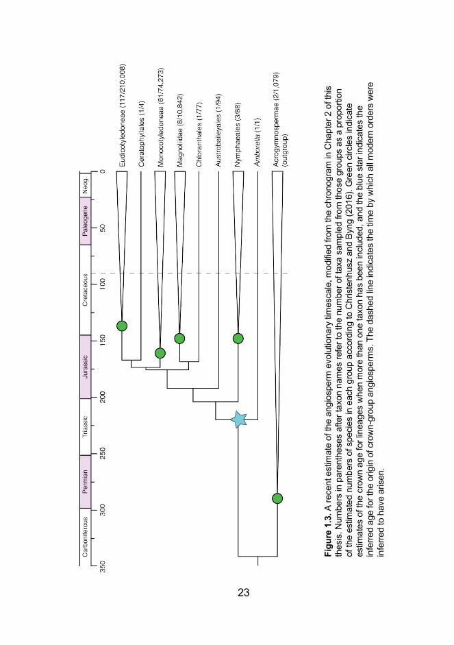
Figure 1.3. A recent estimate of the angiosperm evolutionary timescale,

modified from the chronogram in Chapter 2 of this thesis ........................... 23


Bayesian Estimates of the Angiosperm Evolutionary Timescale

Figure 2.1. A comparison of the taxon and gene sampling in a selection of

previous estimates of the angiosperm evolutionary timescale, based on

data sets including ≥50 angiosperm taxa and/or ≥4 genes ......................... 33

Figure 2.2. Chronogram depicting the angiosperm evolutionary timescale,

as estimated using Bayesian (MCMCTREE) analysis of 76 chloroplast

genes from 195 taxa with 35 minimum and two maximum fossil constraints

...................................................................................................................... 50

Figure 2.3. A comparison of the ages inferred for important nodes across

different analyses, based on different clock models, dating methods, and

rate priors ...................................................................................................... 52

Figure 2.4. A comparison of the ages inferred for important angiosperm

nodes across different analyses, based on different subsamples of genes

...................................................................................................................... 55

xvii


nodes across different analyses, based on various parameter values for the

birth–death prior on the tree ......................................................................... 57


nodes across different analyses, based on different calibration schemes

...................................................................................................................... 61


in Analyses of Multigene Data Sets

Figure 3.1. Illustration of cluster assignment using the model with highest

statistical fit for genes shared between the five chloroplast data sets ........ 76


Dating: Application to the Angiosperm Evolutionary Timescale

Figure 4.1. Gap statistic values for different numbers of clock-subsets (k)

for the plastome-scale angiosperm data set, inferred using partitioning

around medoids in ClockstaR ...................................................................... 96

Figure 4.2. Chronogram depicting the evolutionary timescale of 52

angiosperm taxa and two gymnosperm outgroup taxa ............................... 97

Figure 4.3. Mean posterior age estimates and associated 95% credibility

intervals for six nodes in the angiosperm phylogeny with increasing

numbers of clock-subsets (k), as inferred using an uncorrelated lognormal

relaxed clock, clock-partitioning according to the optimal schemes identified

in ClockstaR, and uniform calibration priors .............................................. 100




xviii

relaxed clock, clock-partitioning according to relative rates of substitution,

and uniform calibration priors ..................................................................... 101




relaxed clock, clock-partitioning according to random assignment of genes

to clock subsets, and uniform calibration priors ......................................... 102


Systematics of Pimelea and Thecanthes (Thymelaeaceae)

Figure 5.1. Majority-rule consensus tree of 230 taxa within Thymelaeaceae,

as inferred through Bayesian analysis of a five-gene (nuclear + plastid)

dataset using MrBayes ............................................................................... 127

Figure 5.2. Phylogram of 230 taxa within Thymelaeaceae, as inferred

through maximum-likelihood analysis of a five-gene (nuclear + plastid)

dataset using RAxML ................................................................................. 128

Chapter 6 — Plastome-Scale Data and Exploration of Phylogenetic

Tree Space Help to Resolve the Evolutionary History of Pimelea

(Thymelaeaceae)

Figure 6.1. Phylogram depicting the relationship among 33 Pimelea taxa

and eight outgroup taxa, as estimated using maximum-likelihood analysis of

134 molecular markers (75 protein-coding and 59 non-coding) in IQ-TREE

.................................................................................................................... 161

Figure 6.2. Phylogram depicting the relationship among 33 Pimelea taxa

and eight outgroup taxa, as estimated using Bayesian inference of 134

molecular markers (75 protein-coding and 59 non-coding) in MrBayes ... 162

xix

Figure 6.3. Chronogram depicting the evolutionary timescale of 33 Pimelea

taxa and eight outgroup taxa, as estimated using Bayesian inference of 134

molecular markers (75 protein-coding and 59 non-coding) in MCMCTREE

.................................................................................................................... 168

Appendix 2 — Supplementary Material for Chapter 3

Figure A2.1. The number of clusters estimated for Angiospermae,

Monocotyledoneae, Eudicotyledoneae, Rosidae, and Asteraceae .......... 222

xx

List of Tables


Bayesian Estimates of the Angiosperm Evolutionary Timescale

Table 2.1. Marginal likelihoods of different clock models, estimated using

the smoothed harmonic-mean estimator ..................................................... 39


in Analyses of Multigene Data Sets

Table 3.1. Number of clusters (k) of branch-length patterns among genes in

five chloroplast data sets, estimated using different clustering methods and

covariance matrices ...................................................................................... 75

Table 3.2. Estimated number of clusters (k) of branch-length patterns

among genes in simulated data sets ........................................................... 78


Dating: Application to the Angiosperm Evolutionary Timescale

Table 4.1. The calibration priors used within this study to estimate the

angiosperm evolutionary timescale.. ........................................................... 93


Systematics of Pimelea and Thecanthes (Thymelaeaceae)

Table 5.1. Primers used for polymerase chain reaction (PCR) amplification

of DNA from five markers ........................................................................... 121

Table 5.2. The optimal partitioning scheme for our five-marker data set, as

determined using a greedy search in PartitionFinder ................................ 123

xxi


Table A2.1. The sample of taxa used in analyses of chloroplast sequence

data in Chapter 3 ........................................................................................ 219

Table A2.2. Estimated number of clusters (k) of branch-length patterns

among genes in 431 mammalian genes, estimated using different clustering

methods and covariance matrices ............................................................. 224

Table A2.3. Estimated number of clusters (k) of branch-length patterns

among genes in data simulated under two (k=2) and eight (k=8) clusters

.................................................................................................................... 224

1

Abstract

Angiosperms are one of the most dominant groups on Earth, and

have fundamentally changed global ecosystem patterns and

function. Therefore, unravelling their evolutionary history is key to

understanding how the world around us was formed, and how it

might change in the future. In this thesis, I use genome-scale data to

investigate the evolutionary patterns and timescale of angiosperms at

multiple taxonomic levels, ranging from angiosperm-wide to genus-

level data sets.

I begin by using the largest combination of taxon and gene

sampling thus far to provide a novel estimate for the timing of

angiosperm origin in the Triassic period. Through a range of

sensitivity analyses, I demonstrate that this estimate is robust to

many important components of Bayesian molecular dating.

I then explore tactics for phylogenomic dating using multiple

molecular clocks. I evaluate methods for estimating the number and

assignment of molecular clock models, and strategies for partitioning

molecular clock models in analyses of multigene data sets. I also

demonstrate the importance of critically evaluating the precision in

age estimates from molecular dating analyses.

Finally, I assess the utility of plastid data sets for resolving

challenging phylogenetic relationships, focusing on Pimelea Banks &

Sol. ex Gaertn. Through analysis of a multigene data set, sampled

from many taxa, I provide an improved phylogeny for Pimelea and its

close relatives. I then generate a plastome-scale data set for a

representative sample of species to further refine the Pimelea

2

phylogeny, and characterise discordant phylogenetic signals within

their chloroplast genomes.

The work in this thesis demonstrates the power of genome-

scale data to address challenging phylogenetic questions, and the

importance of critical evaluation of both methods and results. Future

progress in our understanding of angiosperm evolution will depend

on broader and denser taxon sampling, and the development of

improved phylogenetic methods.

3

Chapter 1 — General Introduction

1.1. The evolutionary history of flowering plants

The diversity and interactions of life on Earth have long been of

scientific interest. Quantifying biodiversity and the timescale over

which it arose allows inferences about the biological history of the

planet to be made, and can provide insight into how ecosystems

might change in response to events such as climate change (Thuiller

et al. 2011; Bellard et al. 2012). Flowering plants (angiosperms)

have been of particular focus because of their important economic

and cultural roles within society, as well as their ubiquity and

importance within natural ecosystems. Specifically, angiosperms

sequester large amounts of carbon from the atmosphere, and act as

primary producers of food for many animal groups, with their spread

and appearance shaping habitat structure globally (Brodribb and

Feild 2010; Magallón 2014). In addition, angiosperms have

developed important mutualistic relationships with many groups of

organisms, such as pollination interactions with insects, birds, and

small mammals (van der Niet and Johnson 2012; Rosas-Guerrero et

al. 2014).

However, to properly quantify the extent and impact of groups

such as angiosperms, biological entities must first be recognised and

described into distinct groups such as species, and, ideally, placed

into higher-order classifications. The goal is to recognise groups that

contain only the descendants of a common evolutionary ancestor

(monophyletic groups), which represent natural evolutionary groups.

4

For most of history, biological groups and the relationships

between them have been recognised through observations of the

form and structure of organisms. When these features are shared

between two or more taxa after being inherited from their most recent

common ancestor, they are known as synapomorphies. In addition

to aiding the classification of extant taxa, these morphological

features are also able to link extant and extinct diversity through

comparison with the fossil record, which can suggest a timescale of

evolution. However, analysis of morphological data sets often cannot

reliably distinguish between competing taxonomic hypotheses

because of a lack of informative characters, or can be misled by the

independent evolution of similar traits in organisms that are not

closely related (convergent evolution). Morphological data have

been supplemented by molecular data since the inception of

molecular phylogenetics in the mid-20th Century.

Molecular data typically comprise sequences of the nucleotides of

DNA, or the amino acids that they encode. Each nucleotide or amino

acid within a sequence represents a character that can be used for

phylogenetic analysis. Therefore, molecular data sets can contain

millions of characters for phylogenetic reconstruction, which makes

such data sets especially useful for evaluating the taxonomic

hypotheses that have been suggested by morphology. Analysis of

molecular data is also useful for estimating the evolutionary timescale

of organisms using molecular clocks (Lee and Ho 2016), especially

for groups with poor fossil records.

Both morphological and molecular data have been used

extensively to evaluate the diversity of angiosperms. Angiosperms

5

are among the most species-rich groups of organisms on the planet,

and are by far the largest group of plants. The exact number of

species is difficult to determine because of high amounts of

taxonomic synonymy, and the fact that many species potentially

remain to be discovered (Bebber et al. 2010; Pimm and Joppa 2015).

Despite this, we can be fairly certain that there are at least 350,000

species of angiosperms, and probably c. 400,000 in total (Pimm and

Joppa 2015). As expected in a group of this size, there is extreme

variation in morphology, life history characteristics, and growth form.

Angiosperms variously exist as herbaceous annuals, vines, lianas,

shrubs or trees, and can be found growing in aquatic or terrestrial

environments, or even growing on and/or parasitising other plants.

Similarly, there is large variation in genome size and content

within angiosperms. For example, it is estimated that throughout

their evolutionary history over 70% of angiosperms have had an

increase in the number of copies of chromosomes contained within

each cell (ploidy level) from the typical diploid state (Levin 2002).

Most of the functions essential for growth and development are

controlled by genes located within the cell nucleus, which are

collectively known as the nuclear genome. Paris japonica Franch., a

small herbaceous plant native to Japan, has the largest accurately

measured genome known to science (Pellicer et al. 2010). At nearly

150 billion nucleotides, its octoploid genome is more than 50 times

larger than the human genome, and nearly 2500 times larger than

the smallest known plant nuclear genome of Genlisea tuberosa

Rivadavia, Gonella & A.Fleischm., a carnivorous angiosperm from

Brazil (Fleischmann et al. 2014).

6

Plant cells also contain specialised organelles known as

chloroplasts and mitochondria, which are responsible for the

essential processes of photosynthesis and cellular respiration,

respectively. Both of these organelles are predominantly

uniparentally inherited and contain their own independent genomes,

which is thought to be because of their origins as free-living

organisms that were engulfed by early eukaryotic cells in separate

endosymbiotic events (Sagan 1967; Schwartz and Dayhoff 1978).

The chloroplast genome varies substantially among angiosperms,

with the order of genes differing between groups, and with some

genes being lost completely. For example, the chloroplast genome is

drastically reduced in many parasitic plants, with many genes

important for photosynthesis having been lost (Bungard 2004).

The mitochondrial genome of plants is more enigmatic, and is

disproportionally less studied than the nuclear and chloroplast

genomes. Plant mitochondrial genomes are large compared with

animal mitochondrial genomes, and their content is highly dynamic,

with many gene gains, losses, transfers, duplications and

rearrangements, as well as a large proportion of repeated elements

and introns (Kitazaki and Kubo 2010; Galtier 2011). Of direct

importance for reconstructing the evolutionary history of plants is that

the three genomes have very different nucleotide substitution rates.

The nuclear genome evolves at the highest rate, the chloroplast

genome evolves at an intermediate rate, and, in contrast to its

dynamic nature, the mitochondrial genome has by far the lowest

evolutionary rate (Wolfe et al. 1987).

7

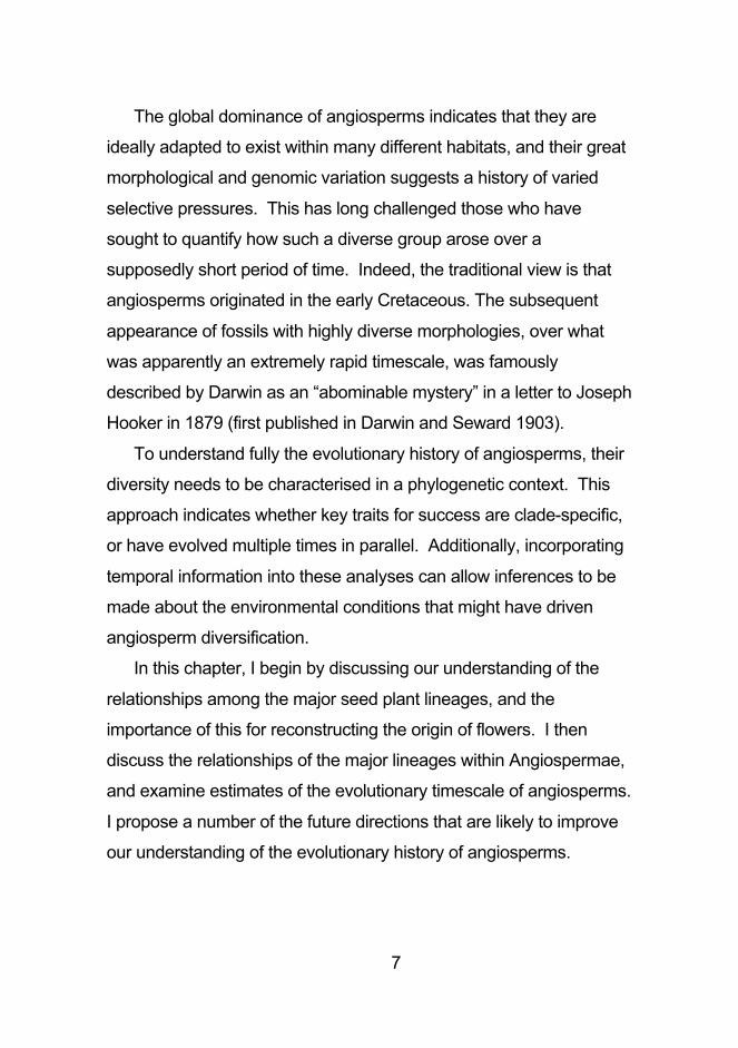
The global dominance of angiosperms indicates that they are

ideally adapted to exist within many different habitats, and their great

morphological and genomic variation suggests a history of varied

selective pressures. This has long challenged those who have

sought to quantify how such a diverse group arose over a

supposedly short period of time. Indeed, the traditional view is that

angiosperms originated in the early Cretaceous. The subsequent

appearance of fossils with highly diverse morphologies, over what

was apparently an extremely rapid timescale, was famously

described by Darwin as an “abominable mystery” in a letter to Joseph

Hooker in 1879 (first published in Darwin and Seward 1903).

To understand fully the evolutionary history of angiosperms, their

diversity needs to be characterised in a phylogenetic context. This

approach indicates whether key traits for success are clade-specific,

or have evolved multiple times in parallel. Additionally, incorporating

temporal information into these analyses can allow inferences to be

made about the environmental conditions that might have driven

angiosperm diversification.

In this chapter, I begin by discussing our understanding of the

relationships among the major seed plant lineages, and the

importance of this for reconstructing the origin of flowers. I then

discuss the relationships of the major lineages within Angiospermae,

and examine estimates of the evolutionary timescale of angiosperms.

I propose a number of the future directions that are likely to improve

our understanding of the evolutionary history of angiosperms.

8

1.2. Higher relationships of angiosperms and the origin of flowers

Angiosperms are recognised as members of the superdivision

Spermatophyta along with cycads, conifers, gnetophytes, and

Ginkgo. The last four extant cone-bearing lineages are known as

acrogymnosperms, whereas extant and extinct cone-bearing

lineages combined are known as gymnosperms (Cantino et al.

2007). The five extant spermatophyte lineages are united by the

synapomorphy of seed production. Estimates of the number of seed

plant species vary, but are consistently in the region of many hundred

thousand species (Govaerts 2001; Scotland and Wortley 2003).

Among other potential factors, the success of these lineages is

perhaps due to the diversification of regulatory genes important for

seed and floral development following ancient whole-genome

duplication events along the lineages leading to seed plants and

angiosperms (Jiao et al. 2011).

Angiosperms can be readily distinguished from gymnosperms

through a suite of synapomorphies. These include the presence of

flowers with at least one carpel, which develop into fruit (cf. the

“naked” seeds of gymnosperms); stamens with two pairs of pollen

sacs (cf. the larger, heavier corresponding organs of gymnosperms);

a range of features of gametophyte structure and development,

including drastically reduced male and female gametophytes

compared with gymnosperms; and phloem tissue with sieve tubes

and companion cells (cf. sieve cells without companion cells in

gymnosperms) (Doyle and Donoghue 1986; Soltis and Soltis 2004).

9

The production of endosperm through double fertilisation was

previously considered to be a further synapomorphy of angiosperms,

but this phenomenon has also been observed in some gnetophyte

lineages (Friedman 1992; Carmichael and Friedman 1996).

Collectively, the synapomorphies of angiosperms are thought to

be responsible for providing the evolutionary advantages that led to

their global dominance, which coincided with a decline in

gymnosperm diversity (Bond 1989). However, to reconstruct the

evolution of these characters and evaluate their importance for

angiosperm evolution, it is necessary to determine which lineage of

seed plants is most closely related to angiosperms. The majority of

earlier studies focused on evaluating the seed plant phylogeny,

including determining the sister lineage to angiosperms, using

comparative morphology to assess homology of the reproductive and

vegetative structures of the seed plant lineages (e.g., Doyle and

Donoghue 1986).

One major hope was that determining the sister lineage to

angiosperms might prove especially useful for inferring the origin and

structure of the first flowers. Throughout the 20th century, the two

main hypotheses for the origin of flowers were that they evolved from

branched, unisexual reproductive structures found in most

gymnosperms ("pseudanthial" theory, Wettstein 1907), or that

flowers evolved from bisexual, flower-like structures, such as in the

extinct group Bennettitales ("euanthial" theory, Arber and Parkin

1907). The inferred homology of morphological structures

consistently suggested that gnetophytes were the extant sister

lineage to angiosperms, with several potential close (non-

10

angiosperm) fossil relatives. Specifically, various features of wood

anatomy and flower-like structures seemed to suggest a close

relationship between angiosperms, gnetophytes, and the extinct

order Bennettitales, with this group being the sister lineage to the rest

of the gymnosperms (Crane 1985; Doyle and Donoghue 1986).

Therefore, based on the strength of morphological evidence, the

euanthial theory was the most popular view in the 20th Century.

The acceptance of the euanthial theory, coupled with the

predominance of Cretaceous Magnolia-like fossils at the time, led to

suggestions that the ancestral flowers were similar to present-day

magnolias. This implies that magnolias and their close relatives were

some of the earliest-diverging angiosperm lineages (Endress 1987).

However, most molecular phylogenetic studies from the 1990s

onwards have recovered different relationships between the extant

seed plant lineages. The dominant theme in these modern studies is

that all extant gymnosperm lineages form a monophyletic sister

group to angiosperms (Chaw et al. 1997; Bowe et al. 2000; Chaw et

al. 2000; Ruhfel et al. 2014; Wickett et al. 2014) (Figure 1.1).

Particularly strong evidence has emerged for a close relationship

between gnetophytes and conifers (Qiu et al. 1999; Winter et al.

1999). Indeed, the evidence seems to suggest that gnetophytes

might even be nested within conifers and the sister group to

Pinaceae (Bowe et al. 2000; Chaw et al. 2000; Zhong et al. 2010).

Overall, because none of the extant gymnosperm lineages is

more closely related to angiosperms than to other gymnosperms,

they cannot directly inform hypotheses on the homologies of

angiosperm characters, or on the sequence of development of these

11

Figu

re 1

.1. T

he re

latio

nshi

ps a

mon

g se

ed p

lant

linea

ges,

sca

led

to g

eolo

gica

l tim

e ba

sed

on fo

ssil

ages

. N

umbe

rs in

gre

en c

ircle

s re

fer t

o th

e fo

llow

ing:

(1) o

ldes

t Gin

kgo

foss

il (Ya

ng e

t al.

2008

); (2

) old

est c

ycad

foss

il (G

ao a

nd T

hom

as 1

989)

; (3)

old

est g

neto

phyt

e fo

ssil (

Ryd

in e

t al.

2006

); (4

) old

est c

onife

r fos

sils

(Wie

land

19

35);

(5) o

ldes

t ang

iosp

erm

foss

ils (d

iscu

ssed

in D

oyle

201

2); (

6) o

ldes

t acr

ogym

nosp

erm

foss

il (d

iscu

ssed

in

Cla

rke

et a

l. 20

11);

(7) a

n es

timat

ed m

axim

um a

ge fo

r cro

wn-

grou

p se

ed p

lant

s (d

iscu

ssed

in C

hapt

er 2

; M

agal

lón

and

Cas

tillo

2009

).

12

characters (Doyle 2012). Therefore, while the relationships among

the major seed plant lineages have been largely resolved, the

structural origin of flowers, and the affinity of the earliest flowers to

modern species, remains controversial. Progress in this area is likely

to be achieved through improved understanding of the relationships

among the major angiosperm groups.

1.3. Major relationships within Angiospermae

The major relationships within angiosperms have historically proved

difficult to determine, and have long been in a state of flux. This has

largely been due to differing ideas of the characters, initially

morphological but later molecular, needed to reconstruct the

angiosperm phylogeny. An early discovery was that flowering plants

have either one or two embryonic leaves (Ray 1686–1704). While

John Ray was the first to observe this dichotomy, he later followed

Marcello Malpighi in referring to these leaves as ‘cotyledons’.

Accordingly, flowering plants with one cotyledon have subsequently

been referred to as monocotyledons or ‘monocots’, and those with

two cotyledons have been called dicotyledons or ‘dicots’.

Although the most widely known early classification scheme by

Linnaeus was based solely on floral reproductive characters, the

division into monocots and dicots has since been recognised as an

important diagnostic feature to inform classification, with varying

implications for the angiosperm phylogeny. A minority of early

authors argued that some key morphological differences between

monocots and dicots, such as vascular bundle anatomy, were

13

irreconcilable with a monophyletic origin of angiosperms. Instead,

these authors argued that angiosperms should be recognised as a

polyphyletic group (= derived from more than one common

evolutionary ancestor) (e.g., Meeuse 1972; Krassilov 1977).

However, the predominant view was that angiosperms are

monophyletic, and the division into monocots and dicots constitutes a

natural split within flowering plants. This was echoed in many

angiosperm classification systems developed in the 20th century,

including the highly influential Takhtajan (1980) and Cronquist (1981)

systems.

To infer the evolutionary relationships within monocots and

dicots, many cladistic analyses were undertaken in the latter half of

the 20th century using pollen, floral, and vegetative characters. This

approach led to many informal subgroups being proposed. For

example, Donoghue and Doyle (1989b) recognised five major groups

of angiosperms, corresponding to Magnoliales, Laurales,

Winteraceae-like plants, ‘paleoherbs’ (‘primitive’ herbaceous lineages

including water lilies and Amborella), and plants with tricolpate pollen.

Although the constituent members of the subgroups varied across

studies, the recognition of tricolpates as a monophyletic group was a

consistent finding (e.g., Donoghue and Doyle 1989b; Donoghue and

Doyle 1989a), leading to suggestions that dicots had multiple

evolutionary origins (Endress et al. 2000; Endress 2002). Indeed,

stratigraphical studies in which triaperturate pollen (tricolpate) fossils

were consistently found to originate in younger sediments than both

monocots and non-tricolpate dicots had already hinted that dicots did

not form a monophyletic group (Doyle 1969). Consequently, Doyle

14

and Hotton (1991) chose to recognise tricolpates as distinct from the

rest of the dicots, coining the term ‘eudicots’ for this group.

Taxonomic concepts for the major angiosperm groups have

changed over time, which makes it difficult to chronicle concisely the

changing opinions about the earliest-diverging angiosperms. For

example, the group Magnoliidae now has a very different

circumscription compared with the past, so statements in earlier

studies regarding the relationships between magnoliids and other

groups might no longer be applicable. Nevertheless, it is clear that

the most common view historically was that Magnolia-like flowers

probably occupied a position at or near the root of the angiosperm

phylogeny. However, there were other suggestions for the earliest-

diverging angiosperm lineages, including Piperales+Chloranthales,

several of the lineages in the formerly recognised paleoherb group,

or even monocots (Burger 1977, 1981).

Attempts to clarify the relationships within the angiosperm

phylogeny have since been greatly strengthened by the inclusion of

molecular data. Some aspects of early classification schemes based

on morphology have been strongly supported by molecular data

(reviewed by Endress et al. 2000; Endress 2002). For example, the

key concepts of the monophyly of angiosperms, monocots and

eudicots, the polyphyly of dicots, and the position of magnoliids as an

early diverging angiosperm lineage, were all further supported by

molecular data (Endress et al. 2000). However, many molecular

estimates of angiosperm evolutionary relationships have contradicted

estimates based on morphological data. For example, molecular

data have firmly resolved the family Hydatellaceae within

15

Nymphaeales, rather than within Poales as former morphology-

based studies had concluded (Saarela et al. 2007). Molecular data

have also helped to clarify the extent of convergent evolution within

angiosperms, such as C4 photosynthesis evolving independently at

least 60 times (Sage et al. 2011).

Arguably the most important finding from analyses of molecular

data has been the rooting of the angiosperm phylogeny. Consensus

was not immediate, with disagreements being found among the

results of molecular analyses, depending on the choice of molecular

markers. An influential early attempt with molecular data to resolve

the seed plant phylogeny and, necessarily, to determine the earliest-

diverging angiosperm lineage, analysed sequences for the

chloroplast rbcL gene from nearly 500 seed plant taxa using

maximum parsimony (Chase et al. 1993). In this case, the

widespread aquatic genus Ceratophyllum was found to be the sister

lineage to all other flowering plants. However, this has subsequently

been found to be an anomalous result seemingly unique to single-

gene parsimony analyses of rbcL. A series of studies in 1999 found

that the monotypic genus Amborella is strongly supported as being

the sister lineage to all other flowering plants (Mathews and

Donoghue 1999; Parkinson et al. 1999; Qiu et al. 1999; Soltis et al.

1999), and this finding has subsequently been supported by nearly

all large multigene analyses (Moore et al. 2007; Soltis et al. 2011;

Ruhfel et al. 2014; Wickett et al. 2014), with some notable exceptions

(Goremykin et al. 2013; Xi et al. 2014; Goremykin et al. 2015).

These studies have also revealed that the base of the angiosperm

phylogeny constitutes a grade of several successive lineages,

16

originally referred to as the ANITA

(Amborella/Nymphaeales/Illiciaceae-Trimeniaceae-Austrobaileya)

grade, but now known as the ANA

(Amborella/Nymphaeales/Austrobaileyales) grade.

The remaining ~99.95% of angiosperms are collectively referred

to as Mesangiospermae (clade names here are standardised to

Cantino et al. 2007). Within this group, five major lineages are

recognised: Chloranthales, Magnoliidae, Ceratophyllales, monocots,

and eudicots (Cantino et al. 2007). Unfortunately, despite large

increases in the amount of available genetic data and improved

analytical techniques, the relationships among these mesangiosperm

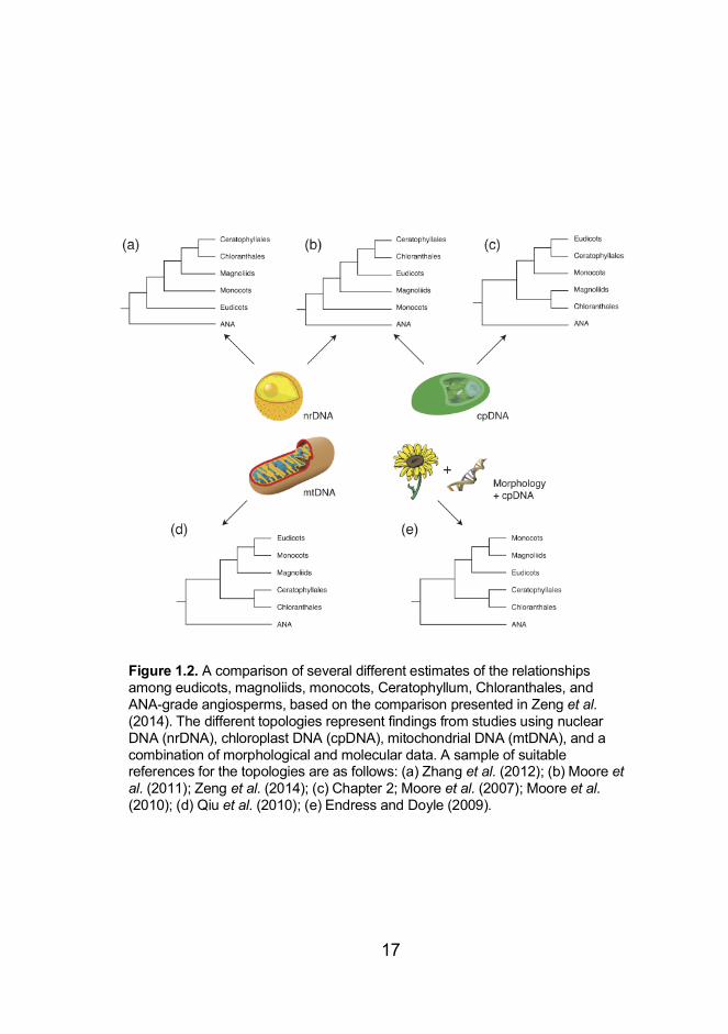
groups have remained uncertain (Figure 1.2). When analysing

chloroplast genome sequences, the most common finding is that

eudicots+Ceratophyllum form the sister group to monocots, with

these three lineages being the sister group to

magnoliids+Chloranthales. Large nuclear DNA data sets, which

have only become available in recent years, tend to resolve different

relationships. For example, they have supported a sister relationship

between eudicots and magnoliids+Chloranthales, with monocots

being the sister group to these three lineages (Wickett et al. 2014).

However, the number and choice of nuclear DNA markers can affect

inferred relationships within Mesangiospermae. For example,

analysis of a selection of 59 low-copy nuclear genes inferred a

grouping of Ceratophyllum+Chloranthales and eudicots, with

successive sister relationships to magnoliids and monocots (Zeng et

al. 2014). Additionally, the choice of phylogeny reconstruction

17

Figure 1.2. A comparison of several different estimates of the relationships among eudicots, magnoliids, monocots, Ceratophyllum, Chloranthales, and ANA-grade angiosperms, based on the comparison presented in Zeng et al. (2014). The different topologies represent findings from studies using nuclear DNA (nrDNA), chloroplast DNA (cpDNA), mitochondrial DNA (mtDNA), and a combination of morphological and molecular data. A sample of suitable references for the topologies are as follows: (a) Zhang et al. (2012); (b) Moore et al. (2011); Zeng et al. (2014); (c) Chapter 2; Moore et al. (2007); Moore et al. (2010); (d) Qiu et al. (2010); (e) Endress and Doyle (2009).

18

method can lead to the estimation of different topologies (Xi et al. 2014).

Nevertheless, despite conflicting topologies sometimes being

inferred, we currently have an understanding of the angiosperm

phylogeny that is greater than at any other time in history. The power

of molecular data and modern probabilistic methods to resolve the

historically challenging relationships among flowering plants is now

well established. In response to the rapid advances in the field, a

cosmopolitan consortium of researchers regularly collaborate to

release timely summaries of the state of knowledge of the

angiosperm phylogeny (Angiosperm Phylogeny Group 1998, 2003;

Angiosperm Phylogeny Group 2009; Angiosperm Phylogeny Group

2016). We now have a viable framework to allow fields related to

phylogenetics to flourish and provide a greater understanding of the

important evolutionary steps that have contributed to the

overwhelming success of angiosperms, such as through evolutionary

developmental biology (evo-devo) studies (Preston and Hileman

2009). However, to gain a fuller understanding of the evolutionary

history of angiosperms, it is necessary to know more than just the

relationships among the major flowering plant groups; a reliable

estimate of the angiosperm evolutionary timescale is also needed.

1.4. Evolutionary timescale of angiosperms

To understand how angiosperms came to dominance, including how

the crucial morphological traits that led to their success first evolved,

it is necessary to have some idea of the timescale of angiosperm

evolution. Traditionally, the evolutionary timescale of organisms has

19

been elucidated through study of the fossil record. In this approach,

the first appearance of each taxon in the fossil record, as determined

by morphology, provides an indication of when it first evolved. When

considering the fossil record, it is important to distinguish between

“crown” and “stem” groups. A crown group is the least inclusive

monophyletic group that contains all extant members of a clade, as

well as any extinct lineages that diverged after the most recent

common ancestor of the clade (Magallón and Sanderson 2001). In

contrast, a stem group is the most inclusive monophyletic group that

contains all extant members of a clade, as well as any extinct

lineages that diverged from the lineage leading to the crown group

(Magallón and Sanderson 2001).

The fossil record of seed plants is ancient, with the oldest fossils

of progymnosperms occurring in sediments from the Late Devonian,

~365 million years ago (Ma) (Fairon-Demaret and Scheckler 1987;

Rothwell et al. 1989; Fairon-Demaret 1996). The fossil record of

gymnosperms is rich, with fossils becoming common from the Late

Carboniferous to Early Triassic (Magallón 2014), and revealing an

extinct diversity far greater than the extant diversity. Unfortunately,

the fossil record of angiosperms is not as extensive or informative.

The oldest known fossils that can probably be assigned to the

stem group of angiosperms are pollen microfossils, and have

suggested that angiosperms arose as early as 247.2–242.0 Ma

(million years ago) (Hochuli and Feist-Burkhardt 2013). Monosulcate

columellate tectate pollen fossils (microfossils of angiospermous

affinity) suggest that crown-group angiosperms first appeared in the

Valanginian to early Hauterivian (Early Cretaceous, ~139.8–129.4

20

Ma), albeit in sparse amounts, followed by an increase in

angiospermous microfossils occurring by the Barremian (~129.4–125

Ma) (Doyle 2012; Herendeen et al. 2017). There is a noticeable

disparity in the number and presence of fossils between lineages,

particularly at the family level and below, with many excellent fossils

being present for some groups but none for others (Magallón 2014).

While fossil data have traditionally provided the only source of

information about the evolutionary timescale of major groups,

molecular dating techniques provide a compelling alternative,

especially for groups that lack fossils. In these approaches,

evolutionary timescales can be estimated using phylogenetic

methods based on molecular clocks. When the concept of the

molecular clock was first proposed, evolutionary change was

assumed to correlate linearly with time and to remain constant across

lineages (“strict” molecular clock) (Zuckerkandl and Pauling 1962).

However, it has since become clear that strictly clocklike evolution is

the exception, rather than the rule (Welch and Bromham 2005).

Rates of molecular evolution vary substantially across vascular

plant lineages (Soltis et al. 2002), and are often strongly correlated

with life history strategies. For example, substitution rates in

herbaceous annual lineages of angiosperms are known to be

substantially higher than in woody perennial plants (Smith and

Donoghue 2008; Lanfear et al. 2013). Consequently, a variety of

molecular clock models have been developed to account for

evolutionary rate variation among lineages (Ho and Duchêne 2014).

Fossil data are still intricately linked with these methods, because

fossils are used to provide temporal information to calibrate the

21

molecular clock, thereby providing absolute rather than relative ages

of nodes. For example, in Bayesian analyses, temporal information

is incorporated through calibrations priors, which can take the form of

a variety of probability distributions (Ho and Phillips 2009). In the

absence of fossils for a particular group being studied, biogeographic

events and rate estimates from other groups can be used as

calibrations, but these are subject to a wide range of errors (Ho et al.

2015b).

Collectively, molecular dating studies have yielded remarkably

disparate estimates for the age of crown-group angiosperms

(summarised in Chapter 2; Bell et al. 2010; Magallón 2014)). Inferred

ages have ranged from the extreme values of 86 Ma (when

considering only the 3rd codon positions of rbcL; Sanderson and

Doyle 2001) to 332.6 Ma (Soltis et al. 2002). Most age estimates fall

between 140 and 240 Ma, but this still represents a substantial

amount of variation. Additionally, the earliest analyses found that

crown-group angiosperms were considerably older than implied by

the fossil record, in some cases by more than 100 million years (Martin et al. 1989). Smaller disparities between molecular and fossil

estimates were obtained in later studies (e.g., Sanderson and Doyle

2001). However, some more recent estimates have tended to

support a more protracted timescale for angiosperm evolution (e.g.,

Chapter 2; Smith et al. 2010), echoing the results of the earliest

molecular studies.

Progress in molecular dating can be characterised in terms of

increasing methodological complexity and improving sampling of taxa

and genes (Ho 2014). A persistent problem, however, has been the

22

need for a trade-off between taxon sampling and gene sampling.

Low gene sampling has been typical of studies of angiosperm

evolution, albeit with some other exceptions, including the 12

mitochondrial genes analysed by Laroche et al. (1995), 58

chloroplast genes analysed by Goremykin et al. (1997), 61

chloroplast genes analysed by Moore et al. (2007), and the 83

chloroplast genes analysed by Moore et al. (2010). However, most of

these studies had sparse angiosperm taxon sampling. Among the

few other studies that have included more than 50 taxa, the largest

number of genes sampled was five. The largest taxon samples have

been those of Zanne et al. (2014), which used a staggering 32,223

species, and Magallón et al. (2015), which included 792 angiosperm

taxa and one of the largest samples of fossil calibration points ever

used. An exception to the above trade-off between taxon and gene

sampling is the study detailed in Chapter 2, which analysed 76

chloroplast genes from 193 angiosperm taxa.

The most controversial aspect of angiosperm molecular dating

studies has been an apparent incongruence between molecular

estimates and those extrapolated purely from fossil occurrence data.

Many modern molecular dating estimates without strongly informative

temporal calibrations tend to suggest that crown-group angiosperms

arose in the early to mid-Triassic (Figure 1.3) (Chapter 2), which

implies a considerable gap in the fossil record (Doyle 2012). This

contradicts the claim that the evolutionary history of crown-group

angiosperms is well represented in the fossil record (Magallón 2014),

despite several lines of evidence supporting this suggestion: the

gradual increase in abundance, diversity, and distribution of fossil

23

Figu

re 1

.3. A

rece

nt e

stim

ate

of th

e an

gios

perm

evo

lutio

nary

tim

esca

le, m

odifi

ed fr

om th

e ch

rono

gram

in C

hapt

er 2

of t

his

thes

is. N

umbe

rs in

par

enth

eses

afte

r tax

on n

ames

refe

r to

the

num

ber o

f tax

a sa

mpl

ed fr

om th

ose

grou

ps a

s a

prop

ortio

n of

the

estim

ated

num

bers

of s

peci

es in

eac

h gr

oup

acco

rdin

g to

Chr

iste

nhus

z an

d By

ng (2

016)

. Gre

en c

ircle

s in

dica

te

estim

ates

of t

he c

row

n ag

e fo

r lin

eage

s w

hen

mor

e th

an o

ne ta

xon

has

been

incl

uded

, and

the

blue

sta

r ind

icat

es th

e in

ferre

d ag

e fo

r the

orig

in o

f cro

wn-

grou

p an

gios

perm

s. T

he d

ashe

d lin

e in

dica

tes

the

time

by w

hich

all

mod

ern

orde

rs w

ere

infe

rred

to h

ave

aris

en.

24

angiosperms; the ordered progression of both morphological and

functional diversification; and the agreement between the

stratigraphic record and molecular data in the sequential appearance

of angiosperm lineages.

If the fault lies instead with the molecular estimates, then it has

been suggested that the substantial disparity between molecular and

fossil-based estimates of the age of crown angiosperms might be a

result of the choices of molecular markers, taxa, calibrations, or

models of rate variation (Magallón 2014). Particular blame has been

placed on the inability of molecular dating methods to account

properly for non-representative sampling of angiosperms and life

history-associated rate heterogeneity (Beaulieu et al. 2015).

However, comprehensive investigations of the impact of models,

priors, and gene sampling on Bayesian estimates of the angiosperm

evolutionary timescale, using a genome-scale data set and

numerous, widely distributed fossil calibrations, have still yielded

remarkably robust estimates of a Triassic origin of crown-group

angiosperms (Chapter 2). This implies a long period of no

angiosperm fossilisation, or that fossils of this age simply remain to

be discovered (but see Wang et al. 2007; Gang et al. 2016).

Despite the disparate estimates for the origin of crown-group

angiosperms, the timescale of evolution within this group is beginning

to be understood with increased precision. Of particular note is that

estimates for the origin of most modern angiosperm orders seem to

be consistent regardless of the age inferred for the angiosperm

crown group (Chapter 2; Magallón et al. 2015). Ordinal diversification

is most commonly estimated to have begun in the early Cretaceous,

25

and is concentrated predominantly from this time through to the mid-

Cretaceous (Chapter 2; Magallón et al. 2015). Modern angiosperm

families are estimated to have originated steadily from the early

Cretaceous, with the peak of family genesis occurring from the late

Cretaceous to the early Paleogene (Magallón et al. 2015). During this

time, the supercontinent Pangaea largely completed its breakup into

the continents of the present day. Concurrently, there were dramatic

shifts in climate, with global temperatures and CO2 levels far higher

than in the present day (Hay and Floegel 2012). These changes,

particularly in temperature, would have had significant impacts on the

levels and efficiency of photosynthesis (Ellis 2010; Hay and Floegel

2012). Selective pressures would have been high, ultimately

influencing the evolution of angiosperms and, presumably, other taxa

that interacted with them.

1.5. Future directions for angiosperm research

The substantial diversity and global dominance of flowering plants

have puzzled and intrigued many researchers throughout history.

The classification of angiosperms has long proved difficult because of

the monumental size and such varied morphologies within this group.

Subsequently, the key evolutionary innovations that first occurred to

produce flowers, as well as the reasons for the overwhelming

success of angiosperms, have historically been obscured.

Therefore, it is reasonable to surmise that for most of history, the

relationship of angiosperms to other seed plants, the relationships

within angiosperms, the timescale of angiosperm evolution, and the

26

reasons for the relative success of angiosperms compared to

gymnosperms were all largely unknown or not understood.

Thankfully, we have now made great progress in the quest to

answer these questions. Work remains to identify potential stem-

group relatives of seed plants, but we now have reliable estimates of

the phylogeny of extant seed plants. However, the most widely

accepted seed plant phylogeny suggests that no extant gymnosperm

lineage preserves the evolutionary steps that led to the origin of the

first flowers. Therefore, in some respects the resolution of the seed

plant phylogeny has been somewhat of a disappointment for those

wanting to reconstruct the development of the flower (Doyle 2012).

While this might be considered a setback, our greatly improved

knowledge of the angiosperm phylogeny, including a strongly

supported position for the root, allows increasingly sophisticated

questions to be asked about angiosperm macroevolution (e.g.,

Turcotte et al. 2014; Zanne et al. 2014). Similarly, our modern

estimates for the timescale of angiosperm evolution allow us to

explore further the selective pressures that might have shaped the

present-day distribution and diversity of flowering plants.

Despite our significant improvements in understanding the

patterns and timescale of angiosperm evolution, the field is far from

settled. The celebrated consistent, strongly supported phylogeny

based on chloroplast markers is increasingly being recognised as

only one estimate of the angiosperm phylogeny. The alternative

phylogenies inferred through analysis of nuclear markers, and

through the choice of phylogeny reconstruction methods, suggests

that more work is needed to reconcile potentially conflicting

27

evolutionary histories. Additionally, the controversy surrounding the

age of flowering plants shows no signs of abating. Modern

knowledge of the fossil record suggests that the rapid radiation of

angiosperm lineages was not quite as explosive as implied by

Darwin’s “abominable mystery” proclamation, yet a new mystery is

why molecular date estimates still generally far pre-date the oldest

angiosperm fossils. It is unlikely that increasing the amount of

genetic data will solve this problem (Chapter 2); instead, increased

sampling from underrepresented groups and methodological

improvements in incorporating fossil data appear to be the way

forward. The last point appears to be an especially promising

avenue of research, with new methods being developed for the

simultaneous analysis of extant and extinct taxa (Ronquist et al.

2012a; Gavryushkina et al. 2014; Heath et al. 2014). Overall, it is

clear that our understanding of the evolutionary history of

angiosperms has changed considerably over time, and we are now

in an exciting new era of angiosperm research.

1.6. Motivation for this thesis

Over the past few decades, the field of molecular phylogenetics has

been at the forefront of evolutionary biology. This has been driven by

improvements in computational power, the development of

increasingly sophisticated analytical methods, and, perhaps most

importantly, advances in sequencing technologies. However, the best

ways to take advantage of these advances in combination has

remained to be thoroughly examined. In this thesis, I critically explore

28

how analysis of phylogenomic data using state-of-the-art

phylogenetic techniques can be used to revolutionise our

understanding of important biological questions. In particular, I focus

on the use of chloroplast sequence data to unravel the patterns and

timescale of flowering plant evolution.

In Chapter 2, I estimate the angiosperm evolutionary

timescale with unprecedented rigour, using the largest combination

of taxon and gene sampling to date. I was motivated to do so by the

fact that although there have been many attempts to estimate the

angiosperm timescale in recent years (e.g., Bell et al. 2010; Smith et

al. 2010; Clarke et al. 2011; Magallón et al. 2013; Magallón et al.

2015), there is still no consensus about when angiosperms most

likely first appeared. To do so, I assemble a plastome-scale data set

for nearly 200 angiosperm taxa and estimate the evolutionary

timescale. I then estimate the sensitivity of the inferred timescale to

different data-partitioning schemes, different levels of data

subsampling, and potential disparities in branch rates, and to the

choice of clock models, priors, and fossil constraints.

Many methods have been developed to accommodate the

vast amounts of molecular data generated through high-throughput

sequencing. These include efficient programs to rapidly estimate the

phylogeny (Stamatakis 2014; Nguyen et al. 2015), the evolutionary

timescale (Yang 2007), or the optimal partitioning scheme for

substitution models (Kalyaanamoorthy et al. 2017). However,

methods to partition clock models to account for among-lineage rate

heterogeneity have been somewhat neglected, despite the

demonstrated benefits of clock-partitioning (Duchêne and Ho 2014).

29

I aimed to assess the possible methods for choosing an

appropriate number of clock-partitions for multilocus data, and the

methods of assigning genes to these clock-partitions. In Chapter 3, I

validate the use of clustering methods to determine clock-partitioning

schemes. Then, in Chapter 4, I demonstrate that increasing the

degree of clock-partitioning can lead to age estimates with vastly

higher precision, but that the meaning of this increased precision

needs to be critically evaluated.

The majority of the work in this thesis focuses on questions

deep in evolutionary time, including estimating the evolutionary

timescale of angiosperms as a whole, and critically evaluating

methods to best analyse such deep divergences. However, the

methodological, technical and computational advancements in recent

years also have great power to resolve relationships at a much finer

scale. Therefore, in Chapter 5 and 6 I chose to focus on using

chloroplast sequence data to investigate the molecular systematics

of Pimelea Banks & Sol. (Thymelaeaceae), a large genus of

angiosperms that is predominantly distributed in Australia.

In Chapter 5, I assemble a data set comprising a relatively

small number of genes from a large taxon sample to infer the

phylogeny of Pimelea. I analyse the data set using a comprehensive

range of phylogenetic techniques. The resulting phylogeny

represented the best estimates for the relationships within Pimelea at

the time of publication. Despite this, many relationships within

Pimelea remained unresolved, particularly when considering the

backbone of the Pimelea clade. Therefore, in Chapter 6 I address the

same question, but instead use a plastome-scale data set. This

30

allows me to resolve the backbone of the Pimelea clade, as well as

many relationships within the genus. Additionally, I demonstrate the

many types of phylogenetic questions that can be addressed with

plastome-scale data sets, including investigating discordance among

gene trees.

This thesis represents a synthesis of many of the types of

questions that can be addressed using the vast quantities of data

produced by high-throughput sequencing. I advance the theoretical

knowledge behind many phylogenetic techniques, and apply this

knowledge to questions in angiosperm evolution at multiple

taxonomic scales. By doing so, I hope I have produced a body of

work that will guide many researchers in one of the most exciting

eras of evolutionary biology.

31

Chapter 2 — Evaluating the Impact of Genomic Data and Priors on Bayesian Estimates of the

Angiosperm Evolutionary Timescale

2.1. Introduction

Flowering plants (Angiospermae) are among the most successful

groups on Earth, in terms of both the rate and scale of their

diversification. Estimates of angiosperm diversity range from 223,300

(Scotland and Wortley 2003) to 422,127 (Govaerts 2001) described

species, with perhaps 20% more yet to be discovered (Joppa et al.

2011). Angiosperms play an important role in the environment and

have important mutualistic relationships with many groups of

organisms, the most obvious being pollination interactions with

insects, birds, and small mammals (Thien et al. 2009; Rosas-

Guerrero et al. 2014). To understand how angiosperms rose to

dominance, including how the crucial morphological traits that led to

their success first evolved, requires both precise and accurate

estimates of the angiosperm evolutionary timescale.

Prior to the availability of genetic data, evolutionary timescales

were inferred exclusively using fossil occurrence data. The oldest

known fossil that can be confidently assigned to the stem group of

angiosperms has been dated to 247.2–242.0 million years ago (Ma)

(Hochuli and Feist-Burkhardt 2013). However, since these fossils

cannot be attributed safely to the crown group of angiosperms, they

do not inform us on their crown-group age. Monosulcate pollen

microfossils with reticulate-columellar structure have been found in

Valanginian to early Hauterivian sediments (~139.8–129.4 Ma).

32

Although these fossils might belong to the stem group of

angiosperms, they have usually been interpreted as evidence that

crown-group angiosperms already existed in the early Cretaceous

(~139.4–130.8 Ma), with many other angiospermous microfossils

occurring by the Barremian (~130.8–126.3 Ma) (Doyle 2012). Within

the crown group, there are noticeable disparities among the fossil

records of different lineages, particularly at the family level and

below.

Molecular dating techniques provide complementary means of

estimating the evolutionary timescale of angiosperms. However,

methodological complexity and resource limitations usually forced a

trade-off between taxon sampling and gene sampling (Figure 2.1;

Appendix 1: Table A1.1). Maximising the number of taxa, rather than

the number of loci, is beneficial for investigations of diversification

rates (Heath et al. 2008), but a small sample of loci might fail to

capture sufficient phylogenetic signal or to allow reliable estimation of

evolutionary rates. Maximising the number of genes at the expense

of taxon sampling increases the number of informative sites, and can

allow more accurate estimation of evolutionary rates. Phylogenomic

studies of plants have provided important insights into the

relationships among angiosperms (Wickett et al. 2014; Zeng et al.

2014), but, in general, increasing the amount of data leads to a rapid

decline in the marginal improvements in the uncertainty of age

estimates (dos Reis and Yang 2013). However, the sparse taxon

sampling that is normally required for phylogenomic studies can

reduce the number of nodes available for fossil calibration, and affect

the estimation of macroevolutionary parameters, the degree of

33

Figure 2.1. A comparison of the taxon and gene sampling in a selection of previous estimates of the angiosperm evolutionary timescale, based on data sets including ≥50 angiosperm taxa and/or ≥4 genes. The sizes of the circles are proportional to the number of genes sampled. The shade of circles represent the type of analysis used, with lightest circles representing Bayesian analyses, darkest circles representing penalised- likelihood analyses, and intermediate-shaded circles representing other methods. The letters correspond to the following studies: (a) Magallón et al. (2015), (b) Bell et al. (2010), (c) Magallón and Castillo (2009), (d) this study, (e) Smith et al. (2010), (f) Schneider et al. (2004), (g) Magallón et al. (2013), (h) Moore et al. (2007), (i) Magallón and Sanderson (2005), (j) Laroche et al. (1995), (k) Clarke et al. (2011), (l) Goremykin et al. (1997), and (m) Soltis et al. (2002). Despite meeting our criteria for this plot, the study by Zanne et al. (2014) is omitted to allow a clearer comparison of the chosen studies.

34

tree balance, and the performance of phylogenetic inference (Heath

et al. 2008). Therefore, there is uncertainty about the impact of

phylogenomic data on our understanding of the age of the

angiosperms in particular, and on inferring their timescale of

diversification in general.

As a result of differences in sampling, model choice, and

calibrations, previous studies have yielded disparate estimates for

the age of angiosperms, with up to fourfold variation. The earliest

molecular dating analyses found that crown-group angiosperms were

considerably older than implied by the fossil record, in some cases by

more than 100 million years (Martin et al. 1989). Subsequent studies

have produced date estimates ranging from 86 Ma (when

considering only the 3rd codon positions of rbcL; Sanderson and

Doyle 2001) to 332.6 Ma (Soltis et al. 2002), although most age

estimates fall between 140 and 240 Ma. Most molecular dating

studies have suggested that angiosperms arose well before the early

Cretaceous, which implies a considerable gap in the fossil record

(Doyle 2012).

All molecular dating studies require the incorporation of temporal

information to calibrate the estimates of rates and divergence times.

This is usually done using fossil evidence, and the manner in which

calibrations are implemented is known to have a strong influence on

inferred ages (e.g., Inoue et al. 2010; Sauquet et al. 2012; Tong et al.

2015). Another important aspect of molecular dating is the model of

rate variation across branches. Relaxed-clock models are often used

in order to account for this form of rate heterogeneity (reviewed by

Ho and Duchêne 2014), but these models might provide a poor fit to

35

certain patterns of rate variation (Dornburg et al. 2012; Bellot and

Renner 2014). This is a particular concern for analyses of the

angiosperm timescale, because of the possibility that there have

been major shifts in evolutionary rates near the base of angiosperms

(Beaulieu et al. 2015). Additionally, when a Bayesian approach is

used, a prior for the tree topology and node times needs to be

specified. These models typically do not account for potential shifts in

angiosperm diversification rates over time (but see Hagen et al.

2015), which might lead to biases in age estimates (Beaulieu et al.

2015). As a result, the choice of tree prior can have a significant

impact on Bayesian estimates of branch rates and node times (Ho et

al. 2005; Condamine et al. 2015).

In this study, we use Bayesian relaxed-clock and penalised

likelihood methods to estimate the timing of the origin and

diversification of angiosperms. Our data set consists of 76 protein-

coding genes from the chloroplast genomes of a diverse selection of

195 taxa, calibrated by a core set of 35 minimum and two maximum

age constraints based on fossil evidence. We test the sensitivity of

our results to different data-partitioning schemes, different levels of

data subsampling, and potential disparities in branch rates, and to

the choice of clock models, priors, and fossil constraints. By doing so,

we are able to investigate the robustness of our estimate of the

angiosperm evolutionary timescale, using the most comprehensive

combination of taxon and gene sampling so far.

36

2.2. Materials and methods

2.2.1. Data set

We obtained chloroplast genome sequences for 182 angiosperm

taxa from GenBank. These were chosen so that our data set

included only one representative per genus, reduced from an initial

sample of 438 chloroplast genomes. Additionally, we obtained novel

chloroplast genome sequences from 11 angiosperm taxa to fill

taxonomic gaps and allow additional fossil calibrations to be used.

These chloroplast genome sequences were extracted in silico from

whole-genome shotgun libraries sequenced on the Illumina platform

(Appendix 1.1). Our total data set consisted of chloroplast genome

sequences from 193 angiosperm taxa, representing 86 families from

45 orders, and two gymnosperm outgroup taxa (Appendix 1: Tables

A1.2–A1.3).

We extracted 79 protein-coding genes from the chloroplast

genomes for analysis, although this number varied among taxa. All

genes were initially aligned using MUSCLE v3.5 (Edgar 2004),

followed by manual adjustments. We excluded three genes (infA,

ycf1, and ycf2) due to alignment ambiguities, leaving 76 genes for

phylogenetic analysis. We then created two data sets, one with all

sites included (CP123: 61,242 nucleotides) and another with all 3rd

codon sites removed (CP12: 40,828 nucleotides). This allowed us to

examine the effect of saturation at 3rd codon positions. We also

filtered out any sites in the alignment at which a gap was present in

≥80% of the taxa to eliminate some alignment ambiguities, and

37

because missing data can have unpredictable effects on

phylogenetic inference and molecular dating (Lemmon et al. 2009;

Filipski et al. 2014). This represented 12.43% of the sites (CP12:

5076 nucelotides; CP123: 7615 nucleotides). Our final sequence

alignments consisted of 53,627 and 35,752 nucleotides for the full

and reduced data sets, respectively, with the proportion of gaps and

completely undetermined characters in the alignment being only

3.43%.

2.2.2. Phylogenetic analyses

We inferred the phylogeny using maximum likelihood in RAxML v8.0

(Stamatakis 2014), with topological support estimated using 1000

bootstrap replicates with the rapid bootstrapping algorithm. The

chloroplast genome is typically non-recombining (Birky 1995), so we

assumed that all genes shared the same tree topology. We analysed

the full data set (CP123) and reduced data set (CP12) with two main

partitioning schemes: with and without partitioning by codon position.

Additionally, we analysed data set CP12 using PartitionFinder v1.1.1

(Lanfear et al. 2012) to determine the optimal partitioning scheme.

We specified 152 data blocks to be compared, corresponding to the

first and second codon positions of every gene, and used the greedy

search algorithm with GTR+Γ as the specified model of nucleotide

substitution. We then implemented the optimal partitioning scheme

(28 data subsets) in RAxML, with the GTRGAMMA model of

nucleotide substitution applied to each data subset.

38

For further analyses, we chose to focus on data set CP12 to

minimise any negative effects of saturation, but we ran replicate

analyses of data set CP123 and an additional data set comprising

only 3rd codon positions as a form of comparison. The size of our

data set precluded the use of some computationally intensive dating

methods such as BEAST; instead, we used MCMCTREE in PAML

v4.8 (Yang 2007), which is able to reduce computational load by

using approximate likelihood calculation (dos Reis and Yang 2011).

MCMCTREE requires a fixed tree topology, so for each data set we

used the best-scoring trees estimated in RAxML. To investigate the

presence of rate variation among branches, we compared the strict-

clock model against an unconstrained (free-rates) model using a

likelihood-ratio test in PAML, and found that the strict-clock model

was strongly rejected (p<10-307). We analysed the data using the

autocorrelated lognormal relaxed clock (Thorne et al. 1998; Kishino

et al. 2001) and the uncorrelated lognormal relaxed clock

(Drummond et al. 2006; Yang and Rannala 2006), as well as the

strict clock as a form of comparison. We compared the marginal

likelihoods of duplicate runs of these clock models, and found

decisive support for the uncorrelated relaxed clock (Table 2.1).

Hence, all subsequent sensitivity analyses were conducted using this

clock model.

In MCMCTREE it is not possible to link the clock model prior

across data subsets; the branch rates are effectively estimated

separately for each data subset, which precluded any partitioning by

clock model. Analysing the data using the partitioning scheme

selected by PartitionFinder was not computationally feasible.

39

Table 2.1. Marginal likelihoods of different clock models, estimated using the smoothed harmonic-mean estimator.

Clock model Marginal log likelihood

Replicate 1 Replicate 2 Mean

Strict -16894.21 -16893.38 -16893.80

Autocorrelated -450.51 -459.25 -454.88

Uncorrelated -439.34 -445.05 -442.20

40

Instead, we chose to focus on partitioning by codon position. We

used the GTR+Γ model of nucleotide substitution, the most general

model permitted by MCMCTREE, with among-site rate heterogeneity

modelled using a gamma distribution with four rate categories.

Posterior distributions of divergence times were estimated using

Markov chain Monte Carlo sampling, with samples drawn every 500

steps over a total of 2×107 steps, after a discarded burn-in of 2×105

steps. We ran each analysis in duplicate and visually inspected

results in Tracer v1.6 (Rambaut et al. 2014), ensuring that the

effective sample sizes of all parameters were above 200. In total, we

ran five different maximum-likelihood analyses in RAxML, one

penalised-likelihood dating analysis in r8s, and 39 different Bayesian

analyses in MCMCTREE (as described below).

MCMCTREE incorporates a gamma-Dirichlet prior for the

overall rate parameter (µ). First, the average substitution rate across

all loci is assigned a gamma prior. A Dirichlet distribution with

concentration parameter α is then used to partition the rate across

loci (Yang 2007; dos Reis et al. 2014). To investigate the sensitivity

of our date estimates to the priors, we ran further analyses and

varied the mean of this gamma-Dirichlet prior for the overall rate

parameter by increasing or decreasing it 10-fold from what we

considered to be the optimal setting of 0.1 substitutions per site per

108 years.

MCMCTREE also incorporates a gamma-Dirichlet prior for the

degree of rate variation across branches (σ2), which has a different

meaning in the two relaxed-clock models. In the uncorrelated relaxed

clock, rates for branches are independent variables from a lognormal

41

distribution, whereas in the autocorrelated relaxed clock the density

of any particular branch rate is calculated while taking into account

the ancestral rate and the time elapsed (Yang 2007). Despite the

different implementations, in both clock models this parameter is

used to represent the variance of the logarithm of the rate. We

investigated the effect of a 10-fold increase in the mean of this

gamma prior for rate variation across branches.

We also investigated the effect of varying the birth rate (λ),

death rate (µ), and sampling proportion (s) parameters of the birth-

death-process tree prior. In MCMCTREE, the values of λ=1, µ=1, and

s=0 represent an extreme limit giving the uniform kernel. Under these

conditions, each node has a uniform prior between ancestral and

descendant nodes. Varying the birth- and death-rate parameters

requires a fixed, non-zero value for s. We chose a value of 0.0005,

representing a sampling proportion of 0.05% based on our sample

size of 193 angiosperm taxa compared with an upper estimate of the

number of angiosperm species (422,127; Govaerts 2001). First, we

set λ to 1 and varied µ to represent no extinction (µ=0), medium

extinction (µ=0.5), and high extinction (µ=0.9). We then used a

published estimate of the angiosperm diversification rate by Magallón

and Castillo (2009), from their analysis assuming a relaxed crown

age with either low or high relative death rates (ε), to obtain values for

λ and µ. This led to values of λ=0.0489 and µ=0 when assuming a

relative death rate of 0, and λ=0.42 and µ=0.378 when assuming a

relative death rate of 0.9. It is worth noting that under the birth-death-

process tree prior, extinction occurs with an equal probability across

all lineages. This implies random sampling of extant lineages after

42

non-biased extinction, which might not always be true. To test the

influence of the sampling fraction parameter (s), representing

different proportions of sampling, we changed its value to 0.001,

0.01, 0.1, and 1. Increasing the value of s embodies an expectation

of longer internal branches (Yang and Rannala 1997).

Amborella trichopoda is generally recognised as the sister

taxon to all other extant angiosperms, but there remain some

suggestions that, instead, Amborella and Nymphaeales form the

sister clade to all other angiosperms (Barkman et al. 2000;

Goremykin et al. 2013; Drew et al. 2014; Xi et al. 2014; Goremykin et

al. 2015). To investigate the effect of this alternative placement of

Amborella on the estimated age of angiosperms, we replicated our

main analysis with Amborella constrained to be the sister taxon to

Nymphaeales.

Recently, Beaulieu et al. (2015) suggested that age estimates

for crown-group angiosperms have been misled because of a failure

to account for large shifts in evolutionary rates near the base of

angiosperms. Many early-diverging lineages of angiosperms are

herbaceous annuals, a life-history trait that is suggested to lead to a

higher evolutionary rate compared with woody, perennial taxa (Gaut

et al. 1992; Smith and Donoghue 2008; Lanfear et al. 2013; Beaulieu

et al. 2015). We investigated the effect of this potentially confounding

factor using two different methods. First, we looked for shifts in

branch rates in the results of our optimal MCMCTREE analysis. This

was initially done by examining rategrams, in which each branch

length is proportional to the corresponding branch rate. These branch

rates were plotted against the midpoint ages of branches from the

43

corresponding chronogram, as obtained using the R package NELSI

v0.21 (Ho et al. 2015a). Second, we performed an analysis in which

we excluded herbaceous lineages. To do this, we first coded all taxa

as being either woody perennials or herbaceous annuals based on

the Global Woodiness Database (Zanne et al. 2013; Zanne et al.

2014). Ancestral state reconstruction was carried out using the

make.simmap function, implementing the SYM model, in the R

package Phytools v0.3-10 (Revell 2012). We removed all taxa that

are currently herbaceous or were inferred to be ancestrally

herbaceous, leaving 74 taxa in the data set. The resulting tree was

analysed in MCMCTREE with the same parameter choices as in our

main analysis of data set CP12.

As a means of assessing the impact of increased gene

sampling on divergence-time estimates, we repeated our analyses

using subsamples of the genes within our data set. First, we sampled

only three of the most commonly used plastid genes: atpB, matK,

and rbcL (3rd codon positions excluded). Second, we sampled only

the 11 plastid genes used by Soltis et al. (2011): atpB, matK, ndhF,

psbB, psbT, psbN, psbH, rbcL, rpoC2, rps16, and rps4 (3rd codon

positions excluded). Third, we drew a random subsample of 20, 30,

40, 50, 60, and 70 genes to examine how our date estimates

responded to increases in the size of the data set. We analysed all

data subsamples in MCMCTREE using the same tree topology and

parameter choices as in our main analysis of data set CP12.

We compared our Bayesian estimates of the angiosperm

evolutionary timescale with those made using penalised likelihood.

To do this, we used RAxML to obtain 100 bootstrap phylograms from

44

data set CP12. We then estimated the divergence times on these

trees using r8s v1.8 (Sanderson 2003), using the same fossil

calibration scheme as in our main Bayesian analyses. The optimal

value of the smoothing parameter was estimated using cross-

validation on the best-scoring tree from RAxML.

2.2.3. Fossil calibrations

The accuracy of molecular dating relies on the careful selection of

calibrations. We only included fossils that (i) have been placed in

groups based on phylogenetic analysis, (ii) can unequivocally be

placed in a group based on synapomorphies, and/or (iii) have had

their phylogenetic placement reviewed or critically examined in

previous studies (Magallón and Castillo 2009; Martínez-Millán 2010;

Massoni et al. 2015b). We chose primarily to include calibrations as

uniform age priors with soft or hard bounds (see below), with fossils

providing minimum age constraints. By doing so, we recognised that

a lineage existed at a certain point in time, but might have arisen well

before that time (Warnock et al. 2012). Based on these criteria, we

chose 35 minimum age constraints (Appendix 1: Table A1.4), using

fossils that each represents the oldest known member of a group.

For all analyses, this included the oldest angiosperm fossil pollen

grains from the Valanginian–Hauterivian as a minimum constraint on

the age of crown-group angiosperms (Magallón et al. 2015). To

investigate the joint prior on node times, we ran a replicate of our

main analysis in which we sampled only from the prior (Warnock et

al. 2012).

45

For all of our main analyses, we implemented two soft

maximum age constraints: (i) 126.7 Ma for the origin of eudicots

(reviewed by Massoni et al. 2015a), and (ii) 350 Ma for the root

(divergence between angiosperms and gymnosperms). Magallón

and Castillo (2009) argued that the latter maximum constraint is

justifiable because it is younger than the Upper Devonian age of the

oldest known fossil seeds (Elkinsia polymorpha) and older than the

Lower-Upper Carboniferous age of the oldest presumed crown-group

seed plants (Cordaitales). This age also corresponds approximately

to the upper end of the 95% credibility interval of the age inferred for

crown seed plants across a number of molecular-clock analyses of a

data set representing major vascular plant lineages (Magallón et al.

2013).

We replicated our main analysis of data set CP12 using

different maximum age constraints to see the impact on inferred

ages. First, we tested maximum ages of 300 Ma, an arbitrary value

roughly corresponding to the end of the Carboniferous; 330 Ma,

based on the estimated mean age of the seed plant crown group by

Magallón et al. (2013); and 366.8 Ma, following Clarke et al. (2011).

We then tested the extreme maximum ages of 454 Ma,

corresponding to the hypothesised oldest tracheophytes based on

the oldest recorded trilete spores (Steemans et al. 2009), and 1024

Ma, corresponding to the oldest proposed age for land plants (Clarke

et al. 2011). Additionally, we tested the effect of retaining the original

maximum age of 350 Ma for the root, but implemented an additional

maximum constraint for crown-group angiosperms of 248.4 Ma,

which is based on the age of the first sediments preceding the oldest

46

occurrence of angiosperm-like pollen (Clarke et al. 2011; Hochuli and

Feist-Burkhardt 2013). Finally, we used a much stronger maximum

age constraint of 139.35 Ma for the angiosperm crown node. This

corresponds to the upper bound of the 95% confidence interval on

crown-group angiosperms based on fossil data, as implemented by

Magallón et al. (2015). As with our main analysis of data set CP12,

we looked for evidence of accelerated substitution rates in basal

branches of the angiosperm clade. We did this by visual inspection of

the rategrams from this analysis, and by plotting branch rates against

the midpoint ages of branches from the corresponding chronogram.

All calibrations were implemented as uniform priors with soft

bounds. These assign equal prior probability for all ages between

specified minimum and maximum constraints, but have a 2.5%

probability that the age is beyond each bound, with a heavy-tailed

probability density based on a truncated Cauchy distribution (Yang

and Rannala 2006; Inoue et al. 2010). Compared with hard bounds,

this approach has the advantage of allowing the molecular data to

overcome poor calibrations, brought about by misinterpretations of

the fossil record, when other good calibrations are present (Yang and

Rannala 2006). However, because most other molecular dating

studies of plants have exclusively utilised hard bounds, we ran

replicate analyses with calibrations implemented as hard bounds as

a means of comparison. Most of the absolute ages used here as

calibrations follow Gradstein et al. (2012), including the most recent

comprehensive synthesis of absolute dates for the Cretaceous (Ogg

and Hinnov 2012). The exceptions were two ages that were derived

47

from 40Ar–39Ar radioisotope analysis of the locality in which fossils

were found (Table S3).

We investigated the impact of using a non-uniform prior for

fossil constraints. We used gamma priors (exponential and lognormal

priors are not available in MCMCTREE), with each calibration having

a mean equal to the age of each fossil +10% and an arbitrary

standard deviation of 2 (Appendix 1: Table A1.4). In all analyses

using uniform calibration priors, our calibration for the angiosperm

crown node provided a minimum constraint. However, once we

implemented this constraint as a gamma prior using the method

above, it effectively created a strong constraint on the age of this

node. Therefore, as a form of comparison we replicated our analysis

using gamma priors without any direct constraint on this node.

2.3. Results and discussion

2.3.1. Phylogenetic relationships

The results from the RAxML analyses were consistent across the

different data-partitioning schemes and were robust to the inclusion

or exclusion of 3rd codon positions. Each treatment yielded a

strongly supported tree topology, with the majority of nodes receiving

100% bootstrap support (b.s.) (Appendix 1: Figures A1.1–A1.5). The

inferred topologies were largely congruent across analyses, with the

exception of a few poorly supported and very short internal branches.

These topologies also corresponded closely to the currently

48

accepted, well supported angiosperm tree (Angiosperm Phylogeny

Group 2009; Moore et al. 2010; Soltis et al. 2011; Ruhfel et al. 2014). Few nodes were weakly supported (<80% b.s.), and these

were generally restricted to deeper parts of the tree. One such

example is the relationship between monocots, Ceratophyllum, and

eudicots, which reflects the long-standing uncertainty about the

placement of Ceratophyllum among angiosperms (discussed in

Moore et al. 2007). There has also been uncertainty about whether

Amborella or Amborella+Nymphaeales is the sister lineage to all

other angiosperms (Wickett et al. 2014; Xi et al. 2014). The most

comprehensive analysis of the relationships among angiosperms (17

genes from 640 taxa) strongly supports a sister relationship between

Amborella and all other angiosperms (Soltis et al. 2011). Our analysis

of the chloroplast genome agrees with this, with all non-Amborella

angiosperms forming a strongly supported clade, except in the

analysis using the partitioning scheme from PartitionFinder (71%

b.s.). The relationships of other early-diverging lineages were also

well supported, with Amborella, Nymphaeales, Austrobaileyales, and

magnoliids+Chloranthales being resolved as successive sister

lineages, all with 100% bootstrap support. However, it is worth noting

that two recent phylotranscriptomic studies based on the nuclear

genome inferred a different topology for Mesangiospermae (i.e., all

angiosperms except Amborellales, Nymphaeales, and

Austrobaileyales), with monocots being placed outside a clade

containing magnoliids, Chloranthales, and eudicots (Wickett et al.

2014; Zeng et al. 2014). It is possible that such phylogenetic

49

uncertainty might affect inferred ages in subsequent molecular dating

analyses, which were based on a fixed tree topology.

2.3.2. Evolutionary timescale of angiosperms

We used a Bayesian relaxed-clock method to estimate the

evolutionary timescale of angiosperms. Here, we report the results of

our analyses of data set CP12, comprising the 1st and 2nd codon

positions of 76 protein-coding chloroplast genes, using an

uncorrelated lognormal relaxed clock and what we considered to be

the optimal settings (Figure 2.2; Appendix 1: Figure A1.6). Our

analysis yielded a mean estimate of 221 Ma (95% credibility interval:

253–192 Ma) for the age of crown angiosperms, suggesting an origin

in the Triassic. This reflects the findings of many recent molecular

dating studies of angiosperms (e.g. Bell et al. 2010; Magallón 2010;

Clarke et al. 2011; Zeng et al. 2014; Beaulieu et al. 2015). Our mean

age estimates for the crown groups of Mesangiospermae,

Chloranthales, magnoliids, and monocots suggest that diversification

of these groups occurred over a period of approximately 27 million

years from the early Jurassic (Appendix 1: Figure A1.6). We inferred

crown-group eudicots to have arisen in the Late Jurassic to Early

Cretaceous 154–136 Ma (we discuss further below the implications

of this result with respect to the soft maximum age constraint applied

to this node), with crown-group Rosidae and

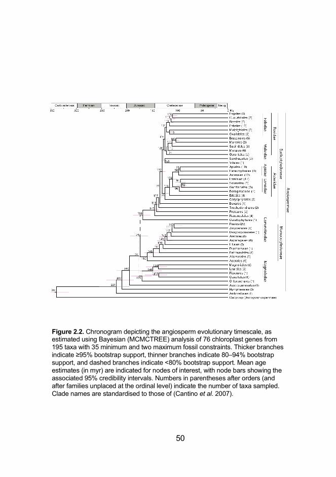
50

Figure 2.2. Chronogram depicting the angiosperm evolutionary timescale, as estimated using Bayesian (MCMCTREE) analysis of 76 chloroplast genes from 195 taxa with 35 minimum and two maximum fossil constraints. Thicker branches indicate ≥95% bootstrap support, thinner branches indicate 80–94% bootstrap support, and dashed branches indicate <80% bootstrap support. Mean age estimates (in myr) are indicated for nodes of interest, with node bars showing the associated 95% credibility intervals. Numbers in parentheses after orders (and after families unplaced at the ordinal level) indicate the number of taxa sampled. Clade names are standardised to those of (Cantino et al. 2007).

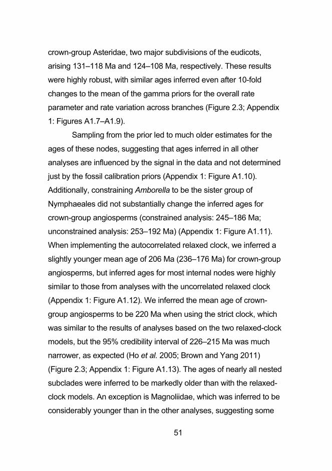
51

crown-group Asteridae, two major subdivisions of the eudicots,

arising 131–118 Ma and 124–108 Ma, respectively. These results

were highly robust, with similar ages inferred even after 10-fold

changes to the mean of the gamma priors for the overall rate

parameter and rate variation across branches (Figure 2.3; Appendix

1: Figures A1.7–A1.9).

Sampling from the prior led to much older estimates for the

ages of these nodes, suggesting that ages inferred in all other

analyses are influenced by the signal in the data and not determined

just by the fossil calibration priors (Appendix 1: Figure A1.10).

Additionally, constraining Amborella to be the sister group of

Nymphaeales did not substantially change the inferred ages for

crown-group angiosperms (constrained analysis: 245–186 Ma;

unconstrained analysis: 253–192 Ma) (Appendix 1: Figure A1.11).

When implementing the autocorrelated relaxed clock, we inferred a

slightly younger mean age of 206 Ma (236–176 Ma) for crown-group

angiosperms, but inferred ages for most internal nodes were highly

similar to those from analyses with the uncorrelated relaxed clock

(Appendix 1: Figure A1.12). We inferred the mean age of crown-

group angiosperms to be 220 Ma when using the strict clock, which

was similar to the results of analyses based on the two relaxed-clock

models, but the 95% credibility interval of 226–215 Ma was much

narrower, as expected (Ho et al. 2005; Brown and Yang 2011)

(Figure 2.3; Appendix 1: Figure A1.13). The ages of nearly all nested

subclades were inferred to be markedly older than with the relaxed-

clock models. An exception is Magnoliidae, which was inferred to be

considerably younger than in the other analyses, suggesting some

52

Figu

re 2

.3. A

com

paris

on o

f the

age

s in

ferre

d fo

r im

porta

nt n

odes

acr

oss

diffe

rent

ana

lyse

s, b

ased

on

diffe

rent

clo

ck m

odel

s,

datin

g m

etho

ds, a

nd ra

te p

riors

. All a

naly

ses

used

an

unco

rrela

ted

rela

xed

cloc

k w

ith u

nifo

rm c

alib

ratio

n pr

iors

, unl

ess

othe

rwis

e st

ated

. “U

ncor

rela

ted

- CP1

2” a

nd “U

ncor

rela

ted

- CP1

23” c

olum

ns re

fer t

o an

alys

es o

f the

firs

t tw

o co

don

posi

tions

an

d al

l thr

ee c

odon

pos

ition

s, re

spec

tivel

y, u

sing

the

unco

rrela

ted

logn

orm

al re

laxe

d cl

ock

with

opt

imal

set

tings

. “A

utoc

orre

late

d” a

nd “S

trict

” ref

er to

the

diffe

rent

aut

ocor

rela

ted

rela

xed

cloc

k an

d st

rict c

lock

mod

els,

resp

ectiv

ely,

that

are

av

aila

ble

in M

CM

CTR

EE. “

PL” r

efer

s to

age

s in

ferre

d us

ing

the

pena

lised

-like

lihoo

d m

etho

d in

r8s.

“Hig

her r

ate”

and

“Low

er

rate

” ref

er to

ana

lyse

s in

whi

ch th

e m

ean

of th

e ga

mm

a pr

ior f

or th

e ov

eral

l rat

e pa

ram

eter

was

var

ied

by a

n or

der o

f m

agni

tude

hig

her a

nd lo

wer

from

its

optim

al s

ettin

g. “H

ighe

r σ2 ” r

efer

s to

our

ana

lysi

s in

whi

ch th

e m

ean

of th

e ga

mm

a pr

ior

for r

ate

varia

tion

acro

ss b

ranc

hes

was

var

ied

to b

e an

ord

er o

f mag

nitu

de h

ighe

r tha

n its

opt

imal

set

ting.

53

form of potential rate heterogeneity between this group and the rest

of the tree. Additionally, the age of the root, corresponding to the

divergence between angiosperms and gymnosperms, was inferred to

be unreasonably high (480–451 Ma), far beyond the soft maximum

constraint of 350 Ma. However, because the strict-clock model was

rejected, these ages are unreliable. Our results, taken collectively,

point to an evolutionary timescale for angiosperms that is more

protracted than suggested by the fossil record.

Our age estimates are also robust to the inclusion or exclusion

of 3rd codon positions. Our analysis of data set CP123 yielded mean

age estimates that were slightly older than those from our analysis of

data set CP12, although with generally narrower 95% credibility

intervals (Appendix 1: Figure A1.14). This suggests that saturation

and heterogeneities in nucleotide composition are not substantially

affecting our inferences, and that the additional data provided by the

third positions might help to bracket the true ages more accurately

(by increasing precision in estimates of branch lengths). However,

we still found evidence of substantial saturation at 3rd codon

positions (Appendix 1: Figure A1.15). Analysis of only third codon

positions led to a far older mean age for crown-group angiosperms

and several early-diverging lineages (Appendix 1: Figure A1.16),

which reflects suggestions that 3rd codon sites might produce

underestimates of basal branch lengths (Phillips 2009). Taking this

into consideration, we chose to focus on data set CP12 for all

subsequent analyses.

Our estimate of the angiosperm evolutionary timescale is

based on a large data set, reducing the stochasticity associated with

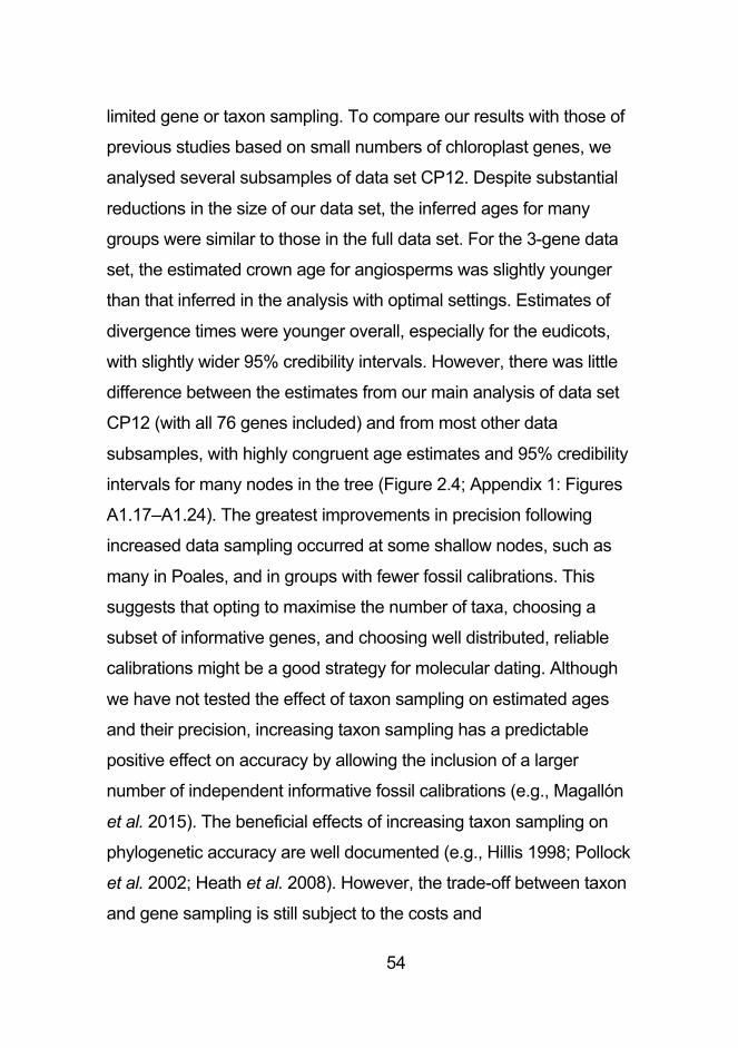
54

limited gene or taxon sampling. To compare our results with those of

previous studies based on small numbers of chloroplast genes, we

analysed several subsamples of data set CP12. Despite substantial

reductions in the size of our data set, the inferred ages for many

groups were similar to those in the full data set. For the 3-gene data

set, the estimated crown age for angiosperms was slightly younger

than that inferred in the analysis with optimal settings. Estimates of

divergence times were younger overall, especially for the eudicots,

with slightly wider 95% credibility intervals. However, there was little

difference between the estimates from our main analysis of data set

CP12 (with all 76 genes included) and from most other data

subsamples, with highly congruent age estimates and 95% credibility

intervals for many nodes in the tree (Figure 2.4; Appendix 1: Figures

A1.17–A1.24). The greatest improvements in precision following

increased data sampling occurred at some shallow nodes, such as

many in Poales, and in groups with fewer fossil calibrations. This

suggests that opting to maximise the number of taxa, choosing a

subset of informative genes, and choosing well distributed, reliable

calibrations might be a good strategy for molecular dating. Although

we have not tested the effect of taxon sampling on estimated ages

and their precision, increasing taxon sampling has a predictable

positive effect on accuracy by allowing the inclusion of a larger

number of independent informative fossil calibrations (e.g., Magallón

et al. 2015). The beneficial effects of increasing taxon sampling on

phylogenetic accuracy are well documented (e.g., Hillis 1998; Pollock

et al. 2002; Heath et al. 2008). However, the trade-off between taxon

and gene sampling is still subject to the costs and

55

Figu

re 2

.4. A

com

paris

on o

f the

age

s in

ferre

d fo

r im

porta

nt a

ngio

sper

m n

odes

acr

oss

diffe

rent

ana

lyse

s, b

ased

on

diffe

rent

sub

sam

ples

of g

enes

. All

anal

yses

use

an

unco

rrela

ted

rela

xed

cloc

k w

ith u

nifo

rm c

alib

ratio

n pr

iors

. Est

imat

es

are

mad

e us

ing

betw

een

3 an

d 70

gen

es, s

ubsa

mpl

ed fr

om th

e to

tal d

ata

set o

f 76

gene

s. T

he d

ashe

d ho

rizon

tal l

ines

in

dica

te th

e es

timat

ed a

ge o

f eac

h no

de fr

om th

e m

ain

anal

ysis

of d

ata

set C

P12.

56

benefits of each approach. While the analytical cost is low in terms of

raw computational hours, and the cost of generating large amounts

of genetic data is decreasing rapidly, the expense of collecting

material remains considerable.

The age of crown angiosperms can be overestimated when

there is inadequate modelling of heterogeneous rates of molecular

evolution and diversification (Beaulieu et al. 2015). In particular,

molecular-clock models might be unable to handle the rate variation

associated with angiosperm life history, such as the herbaceous

habit in some early-diverging lineages (Beaulieu et al. 2015).

However, our plots did not indicate any elevation of substitution rates

in the early branches of the angiosperm tree (Appendix 1: Figure

A1.25). The rategrams for each locus, corresponding to the 1st and

2nd codon positions, did not reveal any clear patterns of elevated

substitution rates along herbaceous lineages when compared with

woody lineages (Appendix 1: Figures A1.26–A1.27). When we

removed all ancestrally or currently herbaceous taxa from the data

set, we once again obtained age estimates that matched those from

our analysis with the optimal settings (Appendix 1: Figure A1.28).

Additionally, we inferred highly congruent ages for crown-group

angiosperms and most internal nodes across all analyses where we

varied the parameters of the tree prior to reflect different

diversification rates (Figure 2.5, Appendix 1: Figure A1.29–A1.37).

Improved models of rate variation, including those that incorporate

information from life-history traits, might lead to a clearer and more

detailed picture of rate heterogeneity across angiosperms.

57

Figu

re 2

.5. A

com

paris

on o

f the

age

s in

ferre

d fo

r im

porta

nt a

ngio

sper

m n

odes

acr

oss

diffe

rent

ana

lyse

s, b

ased

on

vario

us

para

met

er v

alue

s fo

r the

birt

h–de

ath

prio

r on

the

tree.

All

anal

yses

use

d an

unc

orre

late

d re

laxe

d cl

ock

with

uni

form

cal

ibra

tion

prio

rs; “

0.1%

Sam

plin

g,” “

1% S

ampl

ing,

” “10

% S

ampl

ing,

” and

“100

% S

ampl

ing”

refe

r to

diffe

rent

val

ues

of th

e sa

mpl

ing

prop

ortio

n (s

) par

amet

er fo

r the

birt

h–de

ath

proc

ess

tree

prio

r. “N

o Ex

tinct

ion,

” “H

alf E

xtin

ctio

n,” a

nd “H

igh

Extin

ctio

n” re

fer t

o di

ffere

nt p

aram

eter

izat

ions

of t

he b

irth–

deat

h pr

oces

s tre

e pr

ior w

ith a

dea

th ra

te o

f zer

o, a

dea

th ra

te 5

0% o

f the

birt

h ra

te, a

nd

a de

ath

rate

90%

of t

he b

irth

rate

, res

pect

ivel

y. “M

C09

ε0”

and

“MC

09 ε

0.9”

refe

r to

diffe

rent

par

amet

eriz

atio

ns o

f the

birt

h–de

ath

proc

ess

tree

prio

r with

low

and

hig

h re

lativ

e ex

tinct

ion

rate

s, re

spec

tivel

y, b

ased

on

a pu

blis

hed

estim

ate

of th

e di

vers

ifica

tion

rate

by

Mag

alló

n an

d C

astill

o (2

009)

. The

das

hed

horiz

onta

l line

s in

dica

te th

e es

timat

ed a

ge o

f eac

h no

de fr

om

the

mai

n an

alys

is o

f dat

a se

t CP1

2.

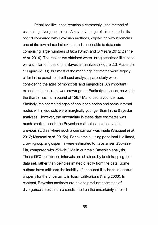
58

Penalised likelihood remains a commonly used method of

estimating divergence times. A key advantage of this method is its

speed compared with Bayesian methods, explaining why it remains

one of the few relaxed-clock methods applicable to data sets

comprising large numbers of taxa (Smith and O’Meara 2012; Zanne

et al. 2014). The results we obtained when using penalised likelihood

were similar to those of the Bayesian analyses (Figure 2.3; Appendix

1: Figure A1.38), but most of the mean age estimates were slightly

older in the penalised-likelihood analysis, particularly when

considering the ages of monocots and magnoliids. An important

exception to this trend was crown-group Eudicotyledoneae, on which

the (hard) maximum bound of 126.7 Ma forced a younger age.

Similarly, the estimated ages of backbone nodes and some internal

nodes within eudicots were marginally younger than in the Bayesian

analyses. However, the uncertainty in these date estimates was

much smaller than in the Bayesian estimates, as observed in

previous studies where such a comparison was made (Sauquet et al.

2012; Massoni et al. 2015a). For example, using penalised likelihood,

crown-group angiosperms were estimated to have arisen 236–229

Ma, compared with 251–192 Ma in our main Bayesian analysis.

These 95% confidence intervals are obtained by bootstrapping the

data set, rather than being estimated directly from the data. Some

authors have criticised the inability of penalised likelihood to account

properly for the uncertainty in fossil calibrations (Yang 2006). In

contrast, Bayesian methods are able to produce estimates of

divergence times that are conditioned on the uncertainty in fossil

59

calibrations, the priors, and the model parameters (dos Reis et al.

2016).

Our estimated age for crown-group angiosperms is noticeably

older (~85 million years) than the oldest angiosperm crown fossils,

which is consistent with previous molecular estimates and indicates

either an incomplete fossil record or a bias in molecular dating

analyses, or both. This problem has been addressed by many

previous studies (e.g., Magallón 2010; Doyle 2012; Beaulieu et al.

2015; Magallón et al. 2015) and is unlikely to be resolved unless

additional, older fossils are discovered, or new molecular dating

methods produce younger age estimates. Considering this, it is

crucial to investigate the impacts of fossil calibrations using the

available molecular dating methods.

2.3.3. Evaluating the impact of the fossil calibrations

There are three main approaches that can be used to calibrate the

angiosperm crown node for molecular dating. First, uniform

calibration priors can be used to constrain the divergence between

angiosperms and gymnosperms rather than to place a maximum

constraint on the angiosperm crown node (e.g., Bell et al. 2010).

Uniform priors are comparatively uninformative because the node

has an equal probability of taking any age between the minimum and

maximum bounds. Using this approach typically leads to large 95%

credibility intervals on date estimates, as observed in the present

study. However, it is worth noting that well calibrated data sets using

uniform priors in a Bayesian relaxed-clock framework tend to

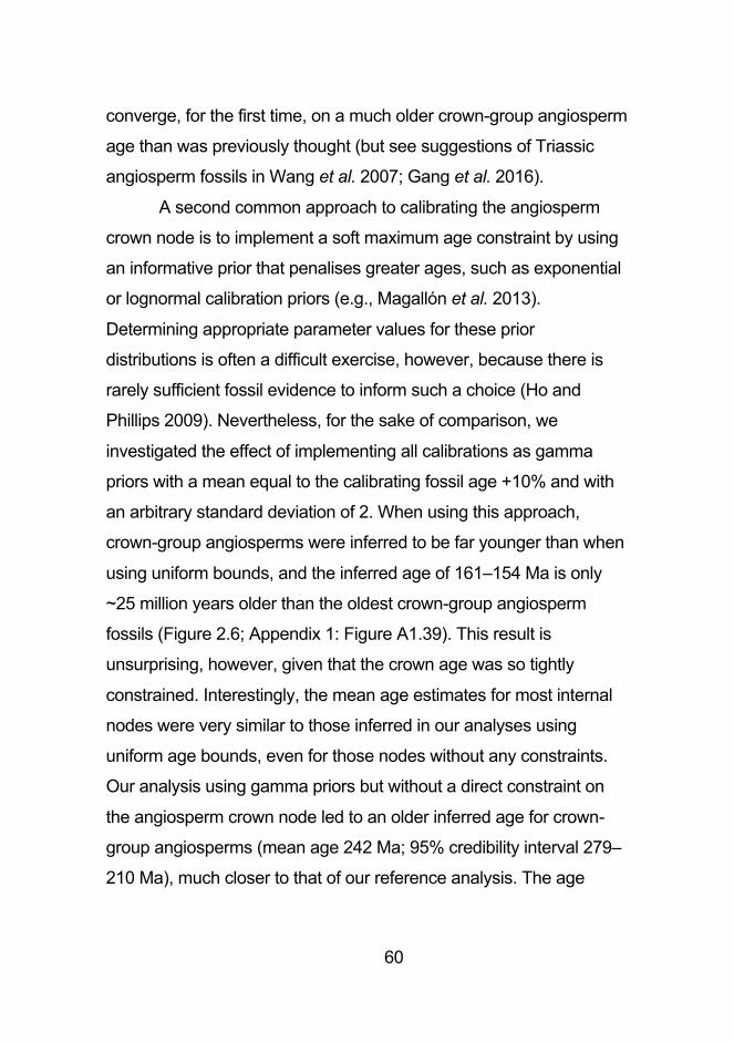
60

converge, for the first time, on a much older crown-group angiosperm

age than was previously thought (but see suggestions of Triassic

angiosperm fossils in Wang et al. 2007; Gang et al. 2016).

A second common approach to calibrating the angiosperm

crown node is to implement a soft maximum age constraint by using

an informative prior that penalises greater ages, such as exponential

or lognormal calibration priors (e.g., Magallón et al. 2013).

Determining appropriate parameter values for these prior

distributions is often a difficult exercise, however, because there is

rarely sufficient fossil evidence to inform such a choice (Ho and

Phillips 2009). Nevertheless, for the sake of comparison, we

investigated the effect of implementing all calibrations as gamma

priors with a mean equal to the calibrating fossil age +10% and with

an arbitrary standard deviation of 2. When using this approach,

crown-group angiosperms were inferred to be far younger than when

using uniform bounds, and the inferred age of 161–154 Ma is only

~25 million years older than the oldest crown-group angiosperm

fossils (Figure 2.6; Appendix 1: Figure A1.39). This result is

unsurprising, however, given that the crown age was so tightly

constrained. Interestingly, the mean age estimates for most internal

nodes were very similar to those inferred in our analyses using

uniform age bounds, even for those nodes without any constraints.

Our analysis using gamma priors but without a direct constraint on

the angiosperm crown node led to an older inferred age for crown-

group angiosperms (mean age 242 Ma; 95% credibility interval 279–

210 Ma), much closer to that of our reference analysis. The age

61

Figu

re 2

.6. A

com

paris

on o

f the

age

s in

ferre

d fo

r im

porta

nt a

ngio

sper

m n

odes

acr

oss

diffe

rent

ana

lyse

s, b

ased

on

diffe

rent

cal

ibra

tion

sche

mes

. All

anal

yses

wer

e ba

sed

on a

n un

corre

late

d re

laxe

d cl

ock

with

uni

form

cal

ibra

tion

prio

rs,

unle

ss o

ther

wis

e st

ated

. Her

e “G

amm

a” re

fers

to a

naly

ses

with

gam

ma

calib

ratio

n pr

iors

, with

“Gam

ma

WAC

” (ga

mm

a w

ithou

t ang

iosp

erm

cal

ibra

tion)

ana

lyse

s la

ckin

g a

cons

train

t on

the

angi

ospe

rm c

row

n no

de. “

Angi

o 24

8” re

fers

to

anal

yses

with

a m

axim

um c

onst

rain

t of 2

48 M

a on

the

angi

ospe

rm c

row

n no

de b

ased

on

the

age

of th

e fir

st s

edim

ents

pr

eced

ing

the

olde

st o

ccur

renc

e of

ang

iosp

erm

-like

pol

len

(Cla

rke

et a

l. 20

11; H

ochu

li an

d Fe

ist-B

urkh

ardt

201

3). “

Max

30

0,” a

n ar

bitra

ry v

alue

roug

hly

corre

spon

ding

to th

e en

d of

the

Car

boni

fero

us; “

Max

330

,” ba

sed

on th

e es

timat

ed m

ean

age

of th

e se

ed p

lant

cro

wn

grou

p by

(Mag

alló

n et

al.

2013

); “M

ax 3

66,”

follo

win

g (C

lark

e et

al.

2011

); “M

ax 4

54,”

corre

spon

ding

to th

e hy

poth

esis

ed o

ldes

t tra

cheo

phyt

es b

ased

on

the

olde

st re

cord

ed tr

ilete

spo

res

(Ste

eman

s et

al.

2009

); an

d “M

ax 1

024”

, cor

resp

ondi

ng to

the

olde

st p

ropo

sed

age

for l

and

plan

ts (C

lark

e et

al.

2011

), re

fer t

o th

e di

ffere

nt

max

imum

age

con

stra

ints

pla

ced

on th

e no

de c

orre

spon

ding

to c

row

n-gr

oup

seed

pla

nts.

The

das

hed

horiz

onta

l lin

es

indi

cate

the

estim

ated

age

of e

ach

node

from

the

mai

n an

alys

is o

f dat

a se

t CP1

2.

62

estimates of other internal nodes were similar to those produced by

the other analyses (Appendix 1: Figure A1.40).

A third way to constrain the age of the angiosperm crown

node is to implement priors based on assumptions about fossil

preservation. Marshall (2008) proposed a method to establish the

confidence interval that contains the true age of the clade in the tree

with the most complete fossil record. The confidence interval is

calculated using the minimum age of this clade (given by the oldest

fossil), the number of branches in the phylogenetic tree represented

in the fossil record, and the average number of localities from which

each branch represented in the fossil record is known (see Marshall

2008; Magallón et al. 2015). It is also possible to analyse fossil

occurrence data in a Bayesian framework to estimate probability

distributions for the timing of the origin of clades based on

assumptions of fossil preservation (Silvestro et al. 2015). The

effectiveness of this approach is contingent upon the number of

fossils, but it could be used to generate informative calibration priors

for fossil-rich clades for use in molecular dating analyses.

The fossil-bracketing method of Marshall (2008) was the main

approach used by Magallón et al. (2015), who estimated a 95%

confidence interval of 139.35–136 Ma for the angiosperm crown

node and used this to specify a uniform calibration prior in a

Bayesian uncorrelated relaxed-clock analysis. Their analysis yielded

precise age estimates for deeper divergences in the tree. When we

repeated our analyses with an age constraint of 139.35–138.7 Ma for

crown angiosperms, for many nodes we inferred ages with a similar

precision to those estimated by Magallón et al. (2015) (Appendix 1:

63

Figures A1.41–A1.42). This precision was to be expected, given the

tight constraints placed upon all calibrating nodes in this analysis.

However, the estimated ages for some nodes had low precision,

such as that for crown-group Magnoliaceae (86.6–8.9 Ma), perhaps

due to differences in taxon sampling and the smaller number of fossil

calibrations in our analyses compared with that of Magallón et al.

(2015). When we plotted branch rates against their midpoint ages

using this strong maximum constraint, we did not find any unusual

trend of highly accelerated rates in early-diverging angiosperms

(Appendix 1: Figure A1.43). The rategram for codon position 1

indicates a potential large rate jump along the branch leading to

crown-group Mesangiospermae, and another along the branch

leading to the crown node of all non-Ranunculales eudicots

(Appendix 1: Figure A1.44). In contrast, the rategram for codon

position 2 indicates a potential large rate jump along the branch

leading to all non-Amborella angiosperms, and another along the

branch leading to the crown node of Rosidae (Appendix 1: Figure

A1.45). It is also worth noting that in this analysis the soft bounds

were not overcome. Although the fossil-bracketing method yielded

estimates for divergence times within angiosperms that were

congruent with those inferred in our unconstrained analyses, it forces

an estimate of the angiosperm crown age that is probably too

precise.

Maximum age constraints are often criticised because of their

perceived arbitrariness and because they involve strong assumptions

about the absence of taxa. For the majority of our analyses, we

placed a conservatively high maximum bound of 350 Ma on the root

64

of the tree. Substantial changes to this maximum age constraint did

not strongly affect the estimated age of crown-group angiosperms.

All of our mean age estimates for this node fell within the range of

227–217 Ma, despite being produced by analyses with maximum

constraints that ranged from 248 Ma for crown-group angiosperms to

1024 Ma for crown-group seed plants (Figure 6; Appendix 1: Figures

A1.46–51). However, the 95% credibility interval on the crown-group

age of angiosperms slightly increased in width with an increasing

maximum age constraint on seed plants. The same pattern was

observed with the 95% credibility interval on the estimated age of the

root. Additionally, with increasing maximum age constraints the

estimated mean age of this node increased substantially. For

example, when the maximum constraint of 1024 Ma was used, we

inferred the age of the root to be 518 Ma.

We also chose a maximum age for the eudicots of 126.7 Ma,

corresponding to the first appearance of tricolpate pollen grains in the

Barremian–Aptian boundary (126.3±0.4 Ma). This calibration has

been widely used in the past (e.g., Soltis et al. 2002; Anderson et al.

2005; Magallón and Castillo 2009; Massoni et al. 2015a), albeit with

some controversy (Smith et al. 2010). There is a complete absence

of any tricolpate pollen before this time, despite its conspicuous

nature, and its abundance and diversity steadily increases worldwide

from the Aptian onwards. This suggests that its usage as a maximum

bound is justified if the assumptions of this approach are

acknowledged (Doyle 2012). However, we inferred an age of 145 Ma

(154–136 Ma) for eudicots, suggesting that they arose earlier than

believed, with the signal in the data and the other fossil calibrations

65

overcoming the soft maximum age of 126.7 Ma that we imposed. In

contrast, there did not appear to be sufficient signal in the data to

overcome a soft maximum of 139.35 Ma when placed upon crown-

group Angiospermae.

Additionally, we replaced the soft bounds with hard bounds to

investigate the effect on the resulting age estimates. This had the

greatest effect on the inferred age of the eudicots, leading to a

younger mean age estimate with a narrower 95% credibility interval.

The mean age estimate for monocots was also slightly younger than

when soft bounds were used, but mean age estimates for magnoliids

and ANA-grade angiosperms were slightly older (Appendix 1: Figure

A1.52). It is worth noting that, despite hard maximum constraints

being applied to both eudicots and the root, there was little impact on

the inferred age for crown-group angiosperms. For a summary of

inferred ages of important groups across all analyses within this

study, see Appendix 1: Table A1.5.

2.4. Conclusions

Using analyses of near-complete chloroplast genomes, we have

estimated that crown-group Angiospermae arose 221 Ma (251–192

Ma), in the mid-Triassic. This inferred age is at least ~50 million

years, and up to ~110 million years, older than the oldest known

fossils attributed to crown-group angiosperms. However, an inferred

Triassic origin of angiosperms is a common finding in modern, well

calibrated studies based on relaxed molecular clocks that do not

directly constrain the age of the angiosperm crown node. Hence, we

66

assessed a range of methodological factors that could lead to biased

age estimates.

We found that our estimate of the angiosperm evolutionary

timescale was robust to large reductions in the number of loci we

sampled, and to substantial changes to most models and priors.

However, age estimates remain dependent on the choice of fossil

calibration priors, with informative gamma priors generally leading to

younger, highly precise inferred ages compared with those inferred

using less informative uniform priors. Collectively, these findings

suggest that future studies should consider focusing on increased

taxon sampling, especially in relatively undersampled clades, rather

than aiming for large increases in the number of loci. Increased taxon

sampling benefits molecular dating estimates by allowing a larger

number of fossil calibrations for a broader range of taxonomic groups

(e.g., Magallón et al. 2015). Additionally, possible improvements in

the accuracy of inferred ages through more representative taxon

sampling might improve the ability to detect rate shifts within

phylogenies (Beaulieu et al. 2015).

In addition to increased taxon sampling, revision and

refinement of the angiosperm evolutionary timescale are likely to

come with significant methodological changes or with new

information from the fossil record, including improvements in

methods of modelling and incorporating fossil data. Recently

developed methods are able to reconcile extinct and extant taxa in

the same phylogenetic framework, allowing temporal information to

be derived from fossils without the need for ad hoc calibration priors

(Ronquist et al. 2012a; Gavryushkina et al. 2014; Heath et al. 2014).

67

This approach has been applied to Monocotyledoneae by analysing

genetic data from 118 monocot taxa while incorporating temporal

information from 247 fossils using the fossilised-birth-death tree prior

(Eguchi and Tamura 2016). It is interesting to note that the ages

inferred by Eguchi and Tamura (2016) are congruent with those we

inferred in the present study, particularly for crown monocots (Eguchi

and Tamura: 153 [174–134] Ma; present study: 160 [179–142] Ma).

However, these methods require many morphological characters to

be scored from both extinct and extant taxa. Until such morphological

data are available, comprehensive evaluations of existing methods

remain valuable, particularly given that the genomic era has brought

a renewed focus on many historically challenging questions in

biology. By utilising genome-scale data for a large taxon sample with

many fossil calibrations, and examining the effects of various priors,

calibrations, and phylogenetic methods, we have been able to

present a detailed evaluation of many of the potential methodological

impacts on age estimates of one of the most important biological

groups on the planet.

68

Chapter 3 — Estimating the Number and Assignment of Clock Models in Analyses of

Multigene Data Sets

3.1. Introduction

Evolutionary rates and timescales can be estimated from nucleotide

sequences using molecular-clock models, which describe the pattern

of rate variation among lineages. The various clock models share a

reliance on age calibrations, but they differ in their assumptions about

the number and distribution of distinct evolutionary rates (reviewed by

Ho and Duchêne 2014). For example, the strict molecular clock

assumes a single rate across all lineages (Zuckerkandl and Pauling

1962), whereas uncorrelated relaxed clocks allow branches to have

distinct rates that are drawn from the same distribution (Drummond

et al. 2006; Rannala and Yang 2007). There are various model-

selection methods for identifying the best-fitting clock model for a

data set of interest (e.g., using marginal likelihoods; Baele et al.

2013). The choice of clock model can have substantial impacts on

phylogenetic estimates, particularly those of evolutionary rates and

timescales.

Rates of molecular evolution often vary among lineages, but this

pattern of variation can differ across sites and across genes (Muse

and Gaut 1997; Gaut et al. 2011). Therefore, when complex

sequence data are being analysed, the use of multiple clock models

might provide a better fit (e.g. higher marginal likelihood) than a

single clock model. For example, separate clock models might be

applied to different genes or codon positions.

69

In analyses of multigene data sets, there are usually many

possible partitioning schemes. Identifying the best-fitting schemes

involves two components: determining the optimal number of

clusters, and assigning the genes to these clusters. In Bayesian

analyses, this can be done using Bayes factors to compare different

clock-partitioning schemes (Ho and Lanfear 2010). However, such

an approach is impractical when there are many candidate schemes,

as is often the case for multigene or genome-scale data sets,

because the statistical fit of every possible scheme would need to be

assessed.

Clustering methods provide a computationally feasible means of

identifying appropriate clock-partitioning schemes, by grouping

subsets of the data according to their pattern of among-lineage rate

variation (Duchêne et al. 2014). Similar approaches are available for

selecting partitioning schemes for substitution models (Frandsen et

al. 2015). The software ClockstaR, which was designed to identify

the best-fitting clock-partitioning scheme for multigene data sets

(Duchêne et al. 2014), employs a k-medoids clustering algorithm

known as partitioning around medoids (Kaufman and Rousseeuw

2005). However, other clustering methods, such as k-means and

Gaussian mixture modeling, have not been tested in the context of

clock-model selection. One advantage of Gaussian mixture models is

that they can represent the shapes of clusters flexibly by using

covariance matrices. For example, they can use a diagonal

covariance matrix to identify clusters with ellipsoidal shapes, such

that they might have higher accuracy than k-medoids.

70

Here we test the performance of three different clustering

methods for identifying the clusters of patterns of among-lineage rate

variation in multigene data sets: variational inference Gaussian

mixture model (VBGMM), Dirichlet process Gaussian mixture model

(DPGMM), and partitioning around medoids (PAM). We evaluate

these three methods using simulated data and apply them to

chloroplast genome sequences from angiosperms. We find that the

optimal number of clusters for these data sets range from one to

three. Our results also reveal that mixture models, such as VBGMM

and DPGMM, tend to detect a larger number of clusters than

methods based on partitioning, such as PAM. Mixture models also

appear to be more robust than PAM in that they can detect the

correct number of clusters in a broader range of simulation

conditions.


3.2.1. Clustering methods

We compared the performance of three different methods: VBGMM

and DPGMM, as implemented in the Python module Scikit-learn

v0.16 (Pedregosa et al. 2012), and PAM implemented in the R

package Cluster v1.15 (Maechler et al. 2005). The PAM algorithm,

also known as k-medoids, is very similar to the k-means algorithm. It

involves randomly choosing k data points from the data, known as

the ‘medoids’. The remaining data points are assigned to their closest

medoid to form k clusters. In the next step, the medoids are replaced

71

by the data points that are closest to the center of each cluster,

resulting in new medoids. The data points are reassigned to the new

medoids. The last two steps are repeated until the medoids are the

same for successive iterations. To select the optimal value of k, we

use the Gap statistic, which uses the ratio of cluster width to distance

between clusters, as a measure of goodness-of-fit (Tibshirani et al.

2001). In our analyses, each cluster represents a group of genes that

have similar patterns of among-lineage rate variation.

The VBGMM and DPGMM assume that the data were

generated from a mixture of Gaussian probability distributions, also

known as ‘components’, with unknown parameters. Both of these

methods incorporate information about the covariance structure of

the data. The most commonly used are the spherical and the

diagonal covariance matrices. The spherical covariance matrix

assumes that each cluster has the same variance across

dimensions, resulting in spherical clusters. In contrast, in the diagonal

covariance matrix the variance can differ among dimensions, such

that clusters can take ellipsoidal shapes. The number of components

for VBGMM is finite, so they need to be specified a priori. To select

the optimal value, we calculate the Bayesian Information Criterion

(BIC) for values of k from 1 to n−1, where n is the number of data

points. In DPGMM, the number of components is infinite, but the

number of clusters to which the data are assigned is defined by a

Dirichlet process. In practice, the implementation of DPGMM requires

an upper bound for the number of components, which we set as n−1.

For both the VBGMM and the DPGMM algorithms, we used the BIC

to compare the fit of diagonal and spherical covariance matrices.

72

However, the BIC cannot be computed for PAM, such that the

performance of this method cannot be assessed using this metric.

3.2.2. Chloroplast genome data

We obtained complete chloroplast genome sequences of

angiosperms from GenBank (Appendix 2.1: Table A2.1). The

advantage of analysing genes from the non-recombining chloroplast

genome is that they all share the same topology, which is an

important requirement of these methods. We initially aligned all

protein-coding genes using MUSCLE v3.5 (Edgar 2004), followed by

visual inspection. Three genes (infA, ycf1 and ycf2) were excluded

because of alignment ambiguities, leaving 76 genes for subsequent

analysis, although this number varied among taxonomic groups. To

reduce potential impacts of missing data, we excluded any sites in

the alignment at which a gap was present for ≥80% of taxa.

Our initial data set contained 183 taxa, including

representatives of all major angiosperm groups. We drew

subsamples to form five data sets representing different taxonomic

levels: (i) angiosperms (18 taxa); (ii) eudicots (15 taxa); (iii) rosids (13

taxa); (iv) Poaceae (20 taxa); and (v) Asteraceae (7 taxa). For the

Poaceae and Asteraceae data sets, some gene alignments

consisted primarily of missing data, so we removed these alignments

and used 61 and 74 genes, respectively, instead of the 76 genes in

the complete set of gene alignments. For each of the five taxonomic

data sets, we concatenated all of the genes to infer the topology

using maximum likelihood in PhyML v3.1 (Guindon et al. 2010) with

73

the GTR+Γ nucleotide substitution model. We then estimated

individual gene trees while constraining the tree topology to that

inferred from the concatenated data, which is equivalent to optimising

the branch lengths.

Clustering algorithms typically cluster data points represented

in an n-dimensional space. Previous studies have used individual

branch lengths as dimensions in which to represent gene trees as

data points (e.g., dos Reis et al. 2012; Duchêne et al. 2014; Duchêne

and Ho 2015). We used the same approach by treating the branch

lengths as a proportion of the total tree length and using a log10

transformation. Our empirical data and example code are available

online

(https://github.com/sebastianduchene/pacemaker_clustering_method

s).

3.2.3. Simulations

To test the performance of the clustering methods under known

conditions, we first generated data sets by simulating data points

using the mixture model with the highest fit according to the BIC. This

involved sampling data points from the mixture of distributions

inferred by the model. We also simulated data under optimal

conditions for the PAM algorithm. To do this, we estimated the mean

and standard deviation of each dimension for each cluster inferred

using the mixture models to represent the clusters as multivariate

normal distributions. We then sampled data points from these

distributions. In both simulation scenarios, the simulations have the

74

same dimensions as the chloroplast genome data described above,

but they differ in the shape and spread of the clusters. We conducted

100 simulations for each of the chloroplast data sets and analysed

them using all of the clustering algorithms. We analysed the

simulated data sets using the mixture models, then we selected the

model with the highest statistical fit and noted the optimal value of k.

We also estimated k using the Gap statistic under the PAM

algorithm.

Our simulations serve two specific purposes. First, they allow

us to assess the stability, or reproducibility, of the methods; that is,

whether the same model and value of k is recovered for data sets

generated under the same simulation conditions. Second, the

simulations can be interpreted as parametric bootstrap replicates: if

the inferences of the model are robust, the simulated data sets

should have the same optimal model and number of clusters as

those inferred for the empirical data.

3.3. Results

In our analyses of five chloroplast data sets, the VBGMM with a

spherical covariance matrix had higher fit than the other mixture

models (Table 3.1). Using this method, the optimal number of

clusters ranged from one to three across the five data sets (Figure

3.1; Appendix 2.1: Figure A2.1). The PAM algorithm inferred one

cluster for Poaceae, rosids, and eudicots, and two clusters for

Asteraceae and angiosperms. Although the number of clusters

inferred by all of the methods was similar, VBGMM with a spherical

75

Table 3.1. Number of clusters (k) of branch-length patterns among genes in five chloroplast data sets, estimated using different clustering methods and covariance matrices

Data set Model Covariance

matrix BIC k

Angiosperms VBGMM Diagonal 10126.0 2 VBGMM Spherical 9474.2 1 DPGMM Diagonal 31939.1 2 DPGMM Spherical 20823.2 2 PAM – – 2 Poaceae VBGMM Diagonal 9856.7 2 VBGMM Spherical 9191.5 2 DPGMM Diagonal 28274.2 1 DPGMM Spherical 18606.3 2 PAM – – 1 Eudicots VBGMM Diagonal 8521.9 2 VBGMM Spherical 7657.2 2 DPGMM Diagonal 26545.8 2 DPGMM Spherical 17265.2 2 PAM – – 1 Asteraceae VBGMM Diagonal 3728.3 2 VBGMM Spherical 3465.6 3 DPGMM Diagonal 10756.2 2 DPGMM Spherical 7584.7 2 PAM – – 2 Rosids VBGMM Diagonal 7218.9 2 VBGMM Spherical 6336.5 2 DPGMM Diagonal 22633.8 3 DPGMM Spherical 14539.2 3 PAM – – 1

Data sets were analysed with the variational inference Gaussian mixture model (VBGMM), Dirichlet

process Gaussian mixture model (DPGMM), and partitioning around medoids (PAM). The Bayesian

information criterion (BIC) was used to compare the fit of the mixture models to each data set, with the

best-fitting model shown in bold.

76

Figu

re 3

.1. I

llust

ratio

n of

clu

ster

ass

ignm

ent u

sing

the

mod

el w

ith h

ighe

st s

tatis

tical

fit f

or g

enes

sha

red

betw

een

the

five

chlo

ropl

ast d

ata

sets

. The

row

s co

rresp

ond

to th

e fiv

e da

ta s

ets,

and

eac

h co

lum

n re

pres

ents

a g

ene.

Col

ours

indi

cate

the

clus

ter a

ssig

nmen

ts o

f the

gen

es in

eac

h da

ta s

et

77

covariance matrix tended to infer the largest number of clusters. The

exception was the angiosperm data set, for which VBGMM with a

spherical covariance matrix only identified one cluster, whereas the

other methods identified two clusters. Importantly, for all data sets

there were at least some discrepancies in the number of clusters

inferred by the methods. The PAM algorithm inferred the smallest

number of clusters for almost all of the data sets.

Our analyses of data simulated under mixture models showed

that the algorithms with mixture models correctly identified the model

used to generate the data and the number of clusters for a majority of

the simulations (Table 3.2). In all cases, the VBGMM with a spherical

covariance matrix presented the highest statistical fit for all 100

simulations. For the chloroplast data from angiosperms, Poaceae

and eudicots, the estimated value of k matched the true value in all

100 simulation replicates. For rosids, the correct value of k was

recovered for 97% of the simulated data sets. The mixture model

fitted to the Asteraceae data set performed the most poorly. In this

case, the correct value of k was recovered for only 69% of the

simulated data sets. The fact that the frequency of the optimal k is

overall high for the mixture model also indicates that it is stable,

yielding similar estimates for data simulated under the same

conditions.

For the simulations based on mixture models, the PAM

algorithm performed more poorly (Table 3.2). It only recovered the

true value of k for the simulations using the model fitted to the

angiosperms. For the other simulations, it tended to estimate a larger

number of clusters, from five in the simulations using the model fitted

78

Data set True k

kmixture Frequency of kmixture

kPAM Frequency of kPAM

VBGMM simulations Angiosperms 1 1 1.00 1 1.00 Poaceae 2 2 1.00 5 0.66 Eudicots 2 2 1.00 7 0.30 Asteraceae 3 3 0.69 7 0.20 Rosids 2 2 0.97 8 0.32 PAM simulations Angiosperms Poaceae

1 2

1 2

1.00 1.00

1 2

1.00 1.00

Eudicots Asteraceae

2 3

2 3

1.00 1.00

2 3

1.00 1.00

Rosids 2 2 1.00 2 1.00 Results are based on analyses of 100 simulations under the model fitted to each of the five chloroplast

data sets. In all cases, the most frequently chosen mixture model was the VGBMM with a spherical

covariance matrix (frequency of 1.00). kmixture is the most frequent k for analyses of the data simulated

using mixture models. kPAM is the most frequent k for the analyses using the PAM algorithm, with its

corresponding frequency.

Table 3.2. Estimated number of clusters (k) of branch-length patterns among genes in simulated data sets

79

to Poaceae to eight for the simulations under the model fitted to the

rosids. The stability of this algorithm was also much lower than that of

the mixture models for most data sets. For example, for the

Asteraceae data, the most frequent value of k was present in 20 of

the 100 simulated data sets, with many different values of k being

inferred for the remaining 80 simulated data sets. This probably

occurred because this data set contains a small number of points,

such that there is greater variation among simulation replicates. The

simulations using the model fitted to the angiosperm data had more

stable results, with a frequency of 1.00 for k = 1.

In our analyses of data simulated under conditions consistent

with the assumptions of the PAM algorithm, we found that both

mixture models and PAM recovered the correct number of clusters

with a frequency of 1.00. As with the data simulated using mixture

models, the VGBMM with a spherical covariance matrix had the

highest statistical fit among the mixture models. Collectively, our

analyses of simulated data show that mixture models and the PAM

algorithm perform well when the model used to generate the data

matches that used to infer the number of clusters. However, mixture

models performed well even when the data were simulated using a

scenario based on PAM, such that they provide more robust

estimates.

3.4. Discussion

We investigated the performance of three different clustering

methods for grouping genes according to their patterns of among-

80

lineage rate variation. We have found that the VBGMM with a

spherical covariance matrix provides the best fit among the mixture

models to a range of chloroplast data sets, and our simulation study

confirms the stability of this method. The PAM algorithm failed to

recover the simulation conditions under VBGMM in most cases,

probably because the shape of the clusters is difficult to capture

using this method. In contrast, VBGMM frequently estimated the

correct number of clusters irrespective of the simulation method. This

differs from the results of previous studies of clustering methods for

branch-length patterns, which found that the PAM algorithm

appeared to perform well (Duchêne et al. 2014; Duchêne and Ho

2015). However, we reanalysed a mammalian genome data set from

our previous study (Duchêne and Ho 2015) and found a similar

number of clusters (Appendix 2.2); the most stable mixture model

(DPGMM) supported seven clusters, compared with 13 using PAM in

the original study. This suggests that, in empirical studies, it is

important to compare the inferences from different clustering

algorithms. In this study, for example, the estimated numbers of

clusters for the empirical data are very similar among clustering

algorithms. We find that mixture models provide a powerful

alternative that can flexibly accommodate different cluster shapes.

The results from these models also appear more stable under

different simulation conditions, at least for the data sets analysed

here. Another advantage of these methods is that their parametric

nature offers a simple framework for conducting simulations, which

should be done routinely to assess the robustness of the results.

Importantly, the shape of the clusters and choice of covariance

81

structure do not necessarily have biological implications. Rather, they

provide a convenient mathematical description of the cluster shapes.

The clusters identified in our analyses represent groups of

genes that have similar patterns of among-lineage rate variation

(pacemakers). All of the clustering algorithms suggest that the

evolution of chloroplast genomes in angiosperms and nuclear

genomes in mammals has been governed by a small number of

pacemakers, each of which leads to a distinct pattern of rate variation

among lineages (Snir et al. 2012; Ho 2014). This is consistent with

previous findings from prokaryotes (Snir 2014), Drosophila, and

yeast (Snir et al. 2014). Furthermore, comparing the gene clusters

across our five angiosperm data sets reveals that there is some

consistency in pacemakers across different taxonomic scales (Figure

1). However, additional work will be needed to understand the

biological bases of these pacemakers.

Identifying genes with similar patterns of among-lineage rate

variation has important applications in phylogenetic analyses.

Notably, in molecular dating studies, estimates of divergence times

have been shown to be more accurate if a separate relaxed-clock

model is assigned to each cluster of genes (Duchêne and Ho 2014).

Our results indicate that multigene data sets might only exhibit a

small number of distinct patterns of rate variation among lineages.

This has notable implications for analyses of genome-scale data

sets, for which only a small number of relaxed-clock models might be

sufficient to capture the key components of evolutionary rate

variation. To this end, clustering methods provide a feasible and

reliable alternative to more computationally demanding approaches

82

to selecting clock-partitioning schemes for molecular dating analyses.

In particular, mixture models might have better performance than

the k-medoids and k-means algorithms for genomic data because

they can model clusters of different shapes. Increasing the adoption

of these methods will help to improve estimates of evolutionary rates

and timescales from genome-scale data sets.

83

Chapter 4 — Strategies for Partitioning Clock Models in Phylogenomic Dating: Application to

the Angiosperm Evolutionary Timescale

4.1. Introduction

Evolutionary timescales can be estimated from molecular sequence

data using phylogenetic methods based on the molecular clock (Ho

and Duchêne 2014; dos Reis et al. 2016; Bromham et al. in press). In

practice, most data sets exhibit substantial rate heterogeneity among

lineages. These “lineage effects” can be caused by variation in life-

history traits, generation time, or exposure to mutagens (Smith and

Donoghue 2008; Gaut et al. 2011; Lanfear et al. 2013). Among-

lineage rate variation can be taken into account using Bayesian

relaxed-clock models, in which the rates can be assumed to be either

correlated between neighbouring branches (Thorne et al. 1998;

Kishino et al. 2001) or drawn independently from a chosen

distribution (Drummond et al. 2006; Rannala and Yang 2007).

A number of factors can cause rates to vary across loci in the

genome (Wolfe et al. 1987). These “gene effects” can be taken into

account by allowing each locus to have a distinct relative rate. Less

certain is the best way to deal with interactions between gene effects

and lineage effects, which can be caused by differences in selective

pressure and other processes (Gaut et al. 2011). In this case, the

extent and patterns of among-lineage rate heterogeneity vary across

genes or other subsets of the data. This form of rate variation can be

captured by assigning separate clock models to different subsets of

84

the data (Ho and Duchêne 2014), a process that we refer to here as

clock-partitioning.

Appropriate clock-partitioning can improve the precision of

Bayesian date estimates (as measured by the associated 95%

credibility intervals), but it is rarely done in practice. This is also

despite widespread adoption of partitioning schemes for substitution

models (Lanfear et al. 2012). The most likely explanation is that the

use of clock-partitioning in Bayesian phylogenetics greatly increases

the risk of overparameterisation, and thus to reduced Markov chain

Monte Carlo performance. Overparameterisation has been

previously addressed in light of the bias-variance trade-off, which is

well established in statistical theory (Burnham and Anderson 2003).

Compared with a complex, parameter-rich model, a simple model

that underfits data is expected to have low accuracy (high bias) but

high precision (low variance). Conversely, a parameter-rich model

that overfits the data is likely to have higher accuracy, but this comes

at the cost of reduced precision. The best model is an intermediate

one that simultaneously maximises accuracy and precision

(Wertheim et al. 2010)

It is useful to consider the bias-variance trade-off in the

context of molecular dating with partitioned clock models. Patterns of

among-lineage rate variation are likely to differ across genes (Muse

and Gaut 1994), so increasing the number of relaxed clocks will

better capture these patterns of rate heterogeneity and should lead to

more accurate age estimates (Duchêne and Ho 2014). However,

each clock-subset has parameters that need to be estimated,

including a distinct set of branch rates. As a consequence, increasing

85

the degree of clock-partitioning should lead to a widening of the

posterior distributions of parameters.

Contrary to the expectations of the bias-variance trade-off,

increasing the degree of clock-partitioning tends to improve the

precision of Bayesian age estimates (Zhu et al. 2015). One possible

explanation for this lies in the treatment of the uncertainty in the

estimates of genetic branch lengths. The accuracy and precision of

evolutionary rate estimates depend on the accurate inference of

branch lengths (in substitutions per site). In the case of molecular

dating, branch rates for each clock-subset are combined with node

times to give the branch lengths. Therefore, as the number of clock-

subsets increases, the node times in the chronogram are estimated

from an increasing number of data points, leading to increasing

precision. Although branch-length estimation generally improves as

the amount of sequence data increases, branch lengths can be

estimated with reasonable accuracy even with fairly small amounts of

sequence data (Yang and Rannala 2006). This suggests that for a

data set of a (large) fixed size, increasing the number of clock-

subsets should lead to improved precision in divergence-time

estimates until the amount of sequence data in each clock-subset

decreases to a critical point.

Zhu et al. (2015) explain this phenomenon in their “finite sites”

theory, although they use the term “loci” to refer to clock-subsets.

Even with sequences of infinite length, there will still be uncertainty in

the age estimates, corresponding to the uncertainty in the fossil

calibrations ("infinite data limit"; Yang and Rannala 2006; dos Reis

and Yang 2013). As the number of clock-subsets (L) increases, the

86

finite-sites theory suggests that the uncertainty in age estimates

decreases to the infinite-data limit at the rate of 1/L (Zhu et al. 2015).

This property has important consequences for analyses of genome-

scale data sets, whereby many genes are analysed concurrently.

Therefore, it is important that both the finite-sites theory and the bias-

variance trade-off are tested comprehensively on a genome-scale

data set with clock-partitioning.

Persistent uncertainty in molecular date estimates is perhaps

best exemplified by studies of the origins of flowering plants

(angiosperms) (Chapter 1). The earliest unequivocal angiosperm

fossils are tricolpate pollen grains from the Barremian–Aptian

boundary, from approximately 125.9 million years ago (Ma) (Hughes

1994). Older pollen grains from the Hauterivian provide some

evidence of crown-group angiosperms, and are usually accepted as

belonging to this group, albeit with less confidence than for the

tricolpate pollen grains (Herendeen et al. 2017). Patterns of

diversification in the broader fossil record suggest that angiosperms

are unlikely to have arisen much earlier than this time (Magallón et al.

2015; Sauquet et al. 2017). The majority of molecular dating

analyses tell a vastly different story, with most recent analyses

inferring an origin within the Triassic (Chapter 2). Estimates of the

angiosperm evolutionary timescale appear to be largely robust to the

source of genetic markers, despite the choice between chloroplast-

derived markers or nuclear-derived markers potentially affecting the

deep nodes of the angiosperm phylogeny (Wickett et al. 2014; Zeng

et al. 2014). However, the uncertainty surrounding the age of the

angiosperm crown node is large, often spanning an interval of many

87

tens of millions of years, unless strong age constraints are placed on

the node. This uncertainty could be masking any interesting

biological processes driving the age estimates for deep nodes.

Improving the accuracy and precision of estimates of the age of

crown angiosperms thus represents a key goal of molecular dating.

In this study, we use a Bayesian phylogenetic approach to

investigate the impact of clock-partitioning on the precision of

divergence-time estimates. We also investigate whether the criteria

used to assign genes to different clocks has an impact on estimation

error. To do so, we infer the evolutionary timescale of angiosperms

using a plastome-level data set. In analyses with clock-partitioning

schemes comprising up to 20 clock-subsets, we allocate genes to

clock-subsets based on patterns of among-lineage rate heterogeneity

or relative substitution rate, or through random assignment. In all

cases, we confirm that increasing the degree of clock-partitioning can

lead to vast improvements in the precision of Bayesian date

estimates.


4.2.1. Data sets and clock-partitioning

We obtained full chloroplast genome sequences for 52 angiosperm

taxa and two gymnosperm outgroup taxa from GenBank (Appendix

3: Table A3.1). Each angiosperm taxon was chosen to represent a

different order, with our sampling designed to include as many as

possible of the 63 angiosperm orders recognised by the Angiosperm

88

Phylogeny Group (2016). We extracted all 79 protein-coding genes

from the chloroplast genomes, although some genes were missing

from some taxa. We initially translated all genes into amino acid

sequences using VirtualRibosome (Wernersson 2006) and aligned

them using MAFFT v7.305b (Katoh and Standley 2013). We then

translated the aligned amino acid sequences back into nucleotide

sequence alignments using PAL2NAL (Suyama et al. 2006), made

manual adjustments, and filtered out any sites in the alignment at

which a gap was present in ≥80% of the taxa. Our total core data set

consisted of 68,790 nucleotides, of which only 7.54% sites contained

gaps or missing data (Appendix 3: File A3.1).

Our primary strategy for clock-partitioning based on patterns

of among-lineage rate heterogeneity was to analyse the genes using

ClockstaR v2 (Duchêne et al. 2014). ClockstaR takes predefined

subsets of the data, along with the estimated gene tree for each

subset, and determines the optimal clock-partitioning scheme for the

data set. This involves identifying the optimal number of clock-

subsets (k), as well as the optimal assignment of the data subsets to

each of these clock-subsets. We used the partitioning around

medoids (PAM) algorithm within ClockstaR for this purpose, which

identifies k objects (medoids) that are centrally located within clusters

(Kaufman and Rousseeuw 2005). In our case, this strategy identifies

groups of genes that have the most similar patterns of among-

lineage rate heterogeneity for increasing numbers of clusters (clock-

subsets). Comparison of clock-partitioning schemes is done by

comparing the patterns of among-lineage rate heterogeneity across

the gene trees and clustering the gene trees according to the gap

89

statistic (Gapk) (Tibshirani et al. 2001). The gap statistic method

evaluates the goodness-of-clustering for each value of k by

comparing the mean within-cluster dispersion of the data with that of

bootstrap reference data sets. Higher values for Gapk indicate a

better statistical fit, and the optimal number of clusters (clock-

subsets) is selected as the smallest value of k that yields a peak in

Gapk (Tibshirani et al. 2001). ClockstaR can also determine the

optimal clock-partitioning scheme for any value of k. In our case,

each of the 79 protein-coding genes was considered as a separate

data subset for the ClockstaR analysis.

ClockstaR requires all data subsets to share the same tree

topology. Since the chloroplast genome does not typically undergo

recombination (Birky 1995), all of its genes should share the same

topology. Therefore, we first inferred the phylogeny for the

concatenated data set using maximum-likelihood analysis in IQ-

TREE v1.50a (Nguyen et al. 2015), with node support estimated

using 1000 bootstrap replicates with the ultrafast bootstrapping

algorithm (Minh et al. 2013). We partitioned the data set by codon

position using the edge-linked partition model (Chernomor et al.

2016), and implemented the GTR+Γ4 model of nucleotide substitution

for each subset. The best-scoring tree was very similar to previous

estimates of the angiosperm phylogeny based on chloroplast data

(Moore et al. 2010; Soltis et al. 2011), and we found strong support

for most nodes in the tree (Appendix 3: Figure A3.1). We used this

tree for ClockstaR and optimised the branch lengths for each gene

alignment. Finally, we determined the optimal value of k, and then

created 12 clock-partitioning schemes using the optimal assignment

90

of genes to clock-subsets for values of k from 1 to 10, 15, and 20

(“PCSTAR” schemes).

As a means of comparison with the ClockstaR partitioning

schemes, we also chose clock-partitioning schemes based on

relative substitution rates across genes (dos Reis et al. 2012). To do

so, we focused on a subset of 20 taxa for which sequences of all 79

protein-coding genes were available (Appendix 3: Table A3.1). We

then analysed each gene using maximum likelihood in IQ-TREE, in

each case partitioning by codon position and implementing the GTR+

Γ4 model of nucleotide substitution for each codon position. Using the

tree lengths as a proxy for the overall substitution rate of each gene,

we created 11 partitioning schemes based on relative rates of

substitution (“PRATE” schemes), in which we assigned genes to clock-

subsets for values of k from 2 to 10, 15, and 20.

For an additional form of comparison, we generated clock-

partitioning schemes with genes randomly allocated to clock-subsets.

Genes were randomly sampled without replacement in R v3.3.2 (R

Core Team 2016) and assigned to clock-subsets for values of k from

2 to 10, 15, and 20. We repeated this process three times, resulting

in a total of 33 clock-partitioning schemes in which genes were

randomly assigned to clock-subsets (“PRAND” schemes).

4.2.2. Molecular dating

We inferred the evolutionary timescale using MCMCTREE in PAML

v4.8 (Yang 2007) with the GTR+Γ4 model of nucleotide substitution.

A key requirement of MCMCTREE is a fixed tree topology, so we

91

used the best-scoring tree that we estimated from the total

concatenated data set using IQ-TREE. We primarily analysed our

data sets with the uncorrelated lognormal (UCLN) relaxed clock

(Drummond et al. 2006; Rannala and Yang 2007), but replicated all

analyses to check for any differences under the autocorrelated

lognormal (ACLN) relaxed clock (Thorne et al. 1998; Kishino et al.

2001).

We estimated the overall substitution rate for each clock-

partitioning scheme by running baseml under a strict clock, with a

single point calibration at the root. We then used this estimate to

select the shape (α) and scale (β) parameters for the gamma-

Dirichlet prior on the overall substitution rate across loci in the

MCMCTREE analysis according to the formulae α = (m/s)2 and β =

m/s2, where m and s are the mean and standard deviation of the

substitution rate, respectively. For all analyses, we set the shape and

scale parameters for the gamma-Dirichlet prior on rate variation

across branches to 1 and 3.3, respectively. The posterior distribution

of node ages was estimated with Markov chain Monto Carlo

sampling, with samples drawn every 103 steps across a total of 107

steps, after a discarded burn-in of 106 steps. We ran all analyses in

duplicate to assess convergence, and confirmed sufficient sampling

by checking that the effective sample sizes of all parameters were

above 200.

We repeated the MCMCTREE analysis for all PCSTAR, PRATE,

and PRAND schemes. An advantage of MCMCTREE is the option to

use approximate likelihood calculation, which is much faster than full

likelihood calculation (Thorne et al. 1998; dos Reis and Yang 2011).

92

However, this precludes the calculation of marginal likelihoods using

path sampling and similar methods, which require the full likelihood to

be computed. Instead, we compared the means and 95% credibility

intervals of the posterior estimates of divergence times across our

partitioning strategies. We chose to focus on six nodes in the

angiosperm phylogeny: the crown groups of all angiosperms,

magnoliids, monocots, eudicots, campanulids, and Liliales. The first

four of these were chosen because they define major clades in the

angiosperm phylogeny. The other two nodes were chosen because

they do not have explicit fossil-based calibration priors.

For each of the 12 numbers of clock-subsets, we sampled

from the joint prior by running the analysis without data. This allowed

us to compare the prior and posterior distributions of node ages and

to observe the influence of changing the number of clock-subsets.

The PCSTAR, PRATE, and PRAND schemes are all treated as identical

because the sequence data are not taken into account.

4.2.3. Fossil calibrations

Calibrations are the most important component of Bayesian

molecular dating, with critical impacts on posterior estimates of

divergence times. Therefore, we selected a set of 23 calibration

priors primarily based on recent studies that carefully considered the

phylogenetic affinities of angiosperm fossils (Table 4.1). We also

applied two calibration priors to the gymnosperm outgroup. Fossils

can strictly only provide a minimum age for the divergence of

lineages from their common ancestor, so we chose to implement

93

Cal

ibra

tion

node

U

nifo

rm P

riors

G

amm

a Pr

iors

Fo

ssil

Ref

eren

ce

M

in. (

Ma)

M

ax. (

Ma)

α

β

C

G A

lism

atal

es

120.

7 35

0 43

32.8

32

64.4

M

ayoa

por

tuga

llica

M

agal

lón

et a

l. (2

015)

CG

Ang

iosp

erm

ae

136

350

5245

.7

3507

.2

Ear

ly C

reta

ceou

s po

llen

grai

ns

Mag

alló

n et

al.

(201

5)

CG

Are

cale

s 83

.6

350

1992

.0

2167

.7

Sab

olite

s ca

rolin

ensi

s Ile

s et

al.

(201

5)

CG

Bor

agin

ales

47

.8

126.

7 80

6.6

1535

.4

Ehr

etia

cla

usen

tia

Mar

tinez

-Mill

án 2

010

CG

Bra

ssic

ales

89

.3

126.

7 25

30.9

25

77.0

D

ress

iant

ha b

icar

pela

ta

Mag

alló

n et

al.

(201

5)

CG

Car

yoph

ylla

les

70.6

12

6.7

1495

.4

1926

.2

Coa

huila

carp

on

phyt

olac

coid

es

Mag

alló

n et

al.

(201

5)

CG

Cor

nale

s 89

.3

126.

7 25

30.9

25

77.0

Ty

leria

nthu

s cr

ossm

anen

sis

Mag

alló

n et

al.

(201

5)

CG

Eric

ales

89

.3

126.

7 25

30.9

25

77.0

P

enta

peta

lum

tri

fasc

icul

andr

icus

M

agal

lón

et a

l. (2

015)

C

G F

abal

es

55.8

12

6.7

897.

6 14

62.5

P

aleo

secu

ridac

a cu

rtiss

i M

agal

lón

et a

l. (2

015)

C

G F

agal

es

96.6

12

6.7

2689

.9

2532

.0

Nor

map

olle

s po

llen

Mag

alló

n et

al.

(201

5)

CG

Gen

tiana

les

37.2

12

6.7

445.

7 10

86.9

E

mm

enop

tery

s di

lche

ri M

agal

lón

et a

l. (2

015)

C

G M

agno

liale

s 11

2.6

350

4197

.7

3390

.7

End

ress

inia

bra

silia

na

Mas

soni

et a

l. (2

015)

C

G M

yrta

les

87.5

12

6.7

2534

.2

2632

.6

Esg

ueiri

a fu

tabe

nsis

M

agal

lón

et a

l. (2

015)

C

G O

xalid

ales

10

0.1

126.

7 29

18.4

26

51.4

Tr

opid

ogyn

e pi

kei

Cha

mbe

rs e

t al.

(201

0)

CG

Pan

dana

les

86.3

35

0 22

89.8

24

11.3

M

abel

ia c

onna

tifila

Ile

s et

al.

(201

5)

CG

Par

acry

phia

les

79.2

12

6.7

1926

.6

2209

.7

Silv

iant

hem

um s

ueci

cum

M

agal

lón

et a

l. (2

015)

C

G R

anun

cula

les

112.

6 12

6.7

3867

.5

3124

.8

Texe

iraea

lusi

tani

ca

Mag

alló

n et

al.

(201

5)

CG

Sax

ifrag

ales

89

.3

126.

7 25

30.9

25

77.0

M

icro

altin

gia

apoc

arpe

la

Mag

alló

n et

al.

(201

5)

CG

Zin

gibe

rale

s 72

.1

350

1663

.3

2096

.8

Spi

rem

atos

perm

um

chan

dler

ae

Iles

et a

l. (2

015)

S

G B

uxal

es

99.6

12

6.7

3306

.3

3019

.9

Spa

nom

era

mar

ylan

dens

is

Mag

alló

n et

al.

(201

5)

SG

Cyc

adal

es

268.

3 35

0 21

939.

8 74

34.1

C

ross

ozam

ia

Nag

alin

gum

et a

l. (2

011)

S

G g

ymno

sper

ms

306.

8 35

0 28

377.

3 84

08.2

C

orda

ixyl

on io

wen

sis

Cla

rke

et a

l. (2

011)

S

G P

lata

nace

ae

107.

7 12

6.7

3362

.6

2837

.3

Sap

indo

psis

var

iabi

lis

Mag

alló

n et

al.

(201

5)

SG

Win

tera

ceae

12

5 35

0 47

38.5

34

19.5

W

alke

ripol

lis g

abon

ensi

s M

asso

ni e

t al.

(201

5)

Tabl

e 4.

1. T

he c

alib

ratio

n pr

iors

use

d w

ithin

this

stu

dy to

est

imat

e th

e an

gios

perm

evo

lutio

nary

tim

esca

le. "

CG

" and

"S

G" r

efer

to th

e cr

own

and

stem

gro

ups,

resp

ectiv

ely,

of t

he c

lade

of i

nter

est.

94

fossil calibrations primarily as uniform distributions with soft bounds

This approach assigns an equal prior probability for all ages between

specified minimum and maximum ages, with a 2.5% probability that

the age surpasses each bound (Yang and Rannala 2006).

We implemented two maximum age constraints: 1) 350 Ma for

the divergence between angiosperms and gymnosperms (the root), a

well accepted upper bound for this divergence (Chapter 2); and 2)

126.7 Ma for the origin of crown eudicots, corresponding to the upper

bound of the Barremian–Aptian boundary (reviewed by Massoni et

al. 2015a). The latter constraint is widely used and is justified by the

complete absence of tricolpate pollen before the latest Barremian, yet

some molecular dating results have suggested an earlier origin for

eudicots (Chapter 2; Smith et al. 2010; Zeng et al. 2017).

Ranunculales, one of the earliest-diverging eudicot orders, has a

fossil record dating back to the late Aptian/early Albian. Therefore,

implementing the eudicot maximum constraint results in a strong

prior being placed on crown-group eudicots appearing between

~126.7 and 112.6 Ma. As a result, including the eudicot maximum

constraint leads to the eudicot crown node being a useful example of

a heavily constrained node for downstream comparisons of the

uncertainty in posterior age estimates.

For comparison, we also performed analyses with our PCSTAR

schemes using gamma calibration priors and the UCLN relaxed

clock. In this case, the mean of each gamma prior was set to the age

of each fossil +10%, with an arbitrary standard deviation of 2 (Table

4.1). This effectively brackets the age estimates of calibrated nodes

within a very narrow interval. In such a calibration scheme, the

95

precision of age estimates is not expected to improve substantially

with increased clock-partitioning.

4.3. Results

4.3.1. Angiosperm evolutionary timescale

Our ClockstaR analysis identified the optimal value of k to be 1,

suggesting that a single pattern of among-lineage rate heterogeneity

is shared across protein-coding genes from the chloroplast genomes.

However, despite k=1 being optimal, the values of the gap statistic

were still higher for all values of k>5 (Figure 4.1). Based on our

analysis using the optimal clock-partitioning scheme (k=1) and the

UCLN relaxed clock, we estimated the time to the most recent

common ancestor of angiosperms to be 196 Ma (95% credibility

interval 237–161 Ma; Figure 4.2). We inferred that crown magnoliids

first appeared 171–115 Ma, and that crown monocots arose

contemporaneously, 167–120 Ma. Crown eudicots were inferred to

have arisen 128–124 Ma, with this precise estimate reflecting the

strong calibration prior placed upon this node. Finally, our estimates

for the time to the most recent common ancestors of campanulids

and Liliales were 101–91 Ma and 108–91 Ma, respectively.

The true age of crown angiosperms is unknown, so we cannot

assess the absolute accuracy of our date estimates. Instead, we

consider the consistency of mean age estimates across analyses

(Hillis 1995). The mean age estimates for all crown angiosperms,

magnoliids, and monocots varied slightly across values of k from 1 to

96

Figure 4.1. Gap statistic values (open circles) and associated variance (red vertical lines) for different numbers of clock-subsets (k) for the plastome-scale angiosperm data set, inferred using partitioning around medoids in ClockstaR. The asterisk indicates the optimal number of clock-subsets.

97

Figure 4.2. Chronogram depicting the evolutionary timescale of 52 angiosperm taxa and two gymnosperm outgroup taxa. The chronogram was estimated using Bayesian analysis of 79 genes from the 54 taxa in MCMCTREE, implementing the optimal clock-partitioning scheme (k = 1) and the uncorrelated lognormal relaxed clock. Tip labels indicate the taxa sampled in our study, with the orders they belong to in parentheses. Numbers in circles correspond to our six nodes of interest, as follows: 1) Angiospermae, 2) Magnoliidae, 3) Monocotyledoneae, 4) Liliales, 5) Eudicotyledoneae, and 6) Campanulidae.

98

3, but estimates remained stable across all other values of k. Mean

age estimates for crown eudicots only varied by approximately 2 myr

across all values of k. Mean age estimates for crown Liliales were

stable across all clock-partitioning schemes. However, mean

estimates for crown campanulids steadily declined by approximately

10–15 myr as the number of loci increased. We observed the same

broad trends in accuracy for all nodes of interest when using the

ACLN relaxed clock, although mean age estimates were consistently

slightly younger than in analyses with the UCLN relaxed clock. In our

analyses with the PCSTAR schemes and with gamma calibration priors,

mean age estimates for crown angiosperms steadily increased with

increasing numbers of clock-subsets, but the mean estimates were

stable for all other nodes of interest.

4.3.2. Precision in estimates of divergence times

We focus first on our results when using the UCLN relaxed clock,

uniform calibration priors, and with clock-partitioning according to

ClockstaR. We report improvements in the precision of node-age

estimates by calculating the decrease in 95% CI width, which we

standardised by dividing by the posterior mean. The optimal clock-

partitioning scheme was inferred to be k=1, matching the results of

previous analyses (Chapter 3). However, increasing the number of

clock-subsets generally led to large increases in the precision of

node-age estimates. The impact of this is perhaps most striking in the

inferred age of crown angiosperms. Increasing the number of clock-

subsets from k=1 to k=2 led to a reduction in statistical fit (Figure

99

4.1), but also reduced the width of the 95% CI for the inferred age of

crown angiosperms from 77 myr to 46 myr (an improvement in

precision of 35.4%).

Greater clock-partitioning led to further improvement in

precision (Figure 4.3). For example, implementing a clock-partitioning

scheme with k=20 reduced the width of the 95% CI for the inferred

age of crown angiosperms to only 20 myr, representing a 73.1%

improvement in precision. However, the rate of improvement in

precision declined rapidly for increasing numbers of clock-subsets

(Figure 4.3).

An improvement in precision with the number of clock-subsets

can also be observed in the age estimates for both magnoliids and

monocots. For example, increasing k from 1 to 20 results in

respective increases of 76.1% and 68% in precision in the age

estimates for crown magnoliids and crown monocots (Figure 4.3).

When considering the nodes corresponding to the crown groups of

campanulids and Liliales, a similar trend can be observed, albeit with

a less drastic increase in precision. Increasing the number of clock-

subsets led to 29.7% and 37.7% increases in precision for the crown

groups of campanulids and Liliales, respectively. However, there is a

vastly different trend in the age estimate for crown eudicots. In this

case, the age estimate for k=1 is already precise (95% credibility

interval: 128–124 Ma) and increasing the number of clock-subsets

actually led to a slight decrease in precision of 0.02%.

Compared with the PCSTAR clock-partitioning schemes, very

similar trends in precision were observed for both the PRATE scheme

(Figure 4.4) and PRAND scheme (Figure 4.5). The only differences

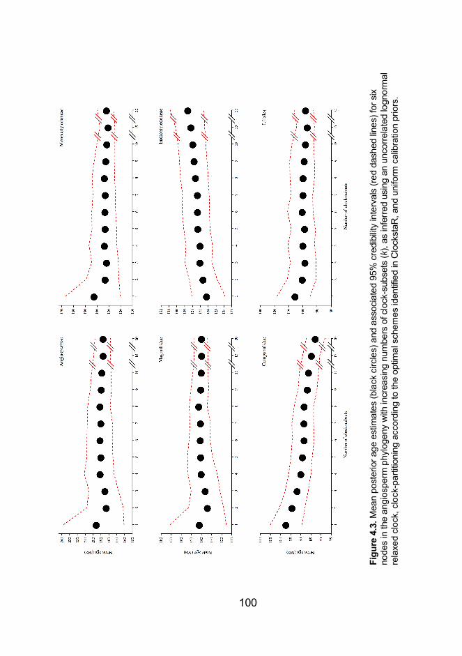
100

Figu

re 4

.3. M

ean

post

erio

r age

est

imat

es (b

lack

circ

les)

and

ass

ocia

ted

95%

cre

dibi

lity

inte

rval

s (re

d da

shed

line

s) fo

r six

no

des

in th

e an

gios

perm

phy

loge

ny w

ith in

crea

sing

num

bers

of c

lock

-sub

sets

(k),

as in

ferre

d us

ing

an u

ncor

rela

ted

logn

orm

al

rela

xed

cloc

k, c

lock

-par

titio

ning

acc

ordi

ng to

the

optim

al s

chem

es id

entif

ied

in C

lock

staR

, and

uni

form

cal

ibra

tion

prio

rs.

101

Figu

re 4

.4. M

ean

post

erio

r age

est

imat

es (b

lack

circ

les)

and

ass

ocia

ted

95%

cre

dibi

lity

inte

rval

s (re

d da

shed

line

s) fo

r six

no

des

in th

e an

gios

perm

phy

loge

ny w

ith in

crea

sing

num

bers

of c

lock

-sub

sets

(k),

as in

ferre

d us

ing

an u

ncor

rela

ted

logn

orm

al re

laxe

d cl

ock,

clo

ck-p

artit

ioni

ng a

ccor

ding

to re

lativ

e ra

tes

of s

ubst

itutio

n, a

nd u

nifo

rm c

alib

ratio

n pr

iors

.

102

Figu

re 4

.5. M

ean

post

erio

r age

est

imat

es (b

lack

circ

les)

and

ass

ocia

ted

95%

cre

dibi

lity

inte

rval

s (re

d da

shed

line

s) fo

r six

no

des

in th

e an

gios

perm

phy

loge

ny w

ith in

crea

sing

num

bers

of c

lock

-sub

sets

(k),

as in

ferre

d us

ing

an u

ncor

rela

ted

logn

orm

al

rela

xed

cloc

k, c

lock

-par

titio

ning

acc

ordi

ng to

rand

om a

ssig

nmen

t of g

enes

to c

lock

sub

sets

, and

uni

form

cal

ibra

tion

prio

rs. T

he

estim

ates

pre

sent

ed h

ere

are

the

aver

ages

of t

hree

rand

om a

ssig

nmen

ts o

f gen

es to

clo

ck-s

ubse

ts fo

r eac

h va

lue

of k

.

103

were that there was less variation in mean age estimates for smaller

values of k compared with the ClockstaR partitioning scheme, and

standardised improvements in precision were consistently slightly

greater (Appendix 3: Table A3.2). For example, the widths of the

95% CIs, and the mean age estimates, declined monotonically in

both classes of clock-partitioning schemes.

We observed the same broad trends across all clock-

partitioning schemes when using the ACLN relaxed clock. With

increasing numbers of clock-subsets, the uncertainty in age

estimates rapidly decreased, with the exception of the age estimate

for the eudicot crown node. Even with k=1, however, the precision of

the age estimates was much greater than in the corresponding

analysis with the UCLN relaxed clock. For example, when

implementing the PCSTAR clock-partitioning schemes, the 95%

credibility interval of the age estimate for crown angiosperms

spanned 77 myr when using the UCLN relaxed clock, but only 59

myr when using the ACLN relaxed clock. Additionally, age estimates

for crown eudicots became less precise as the degree of clock-

partitioning increased. We observed the same trend for the other

nodes of interest across analyses, and the apparent limit to

uncertainty appeared to be reached much more rapidly than with the

UCLN relaxed clock (Appendix 3: Figures A3.2–3.4).

When using highly informative gamma calibration priors in our

additional analyses of the PCSTAR schemes, we found that for the

crown groups of angiosperms, monocots, and magnoliids, the

increases in precision with greater clock-partitioning were much lower

than with uniform calibration priors (Appendix 3: Figure A3.5 and

104

Table A3.2). For example, an improvement of only 18.5% occurred in

the precision of the age estimate for crown angiosperms. The

opposite trend occurred for the crown nodes of eudicots,

campanulids and Liliales.

When we implemented uniform calibration priors, greater

clock-partitioning led to either no change or decreases in precision

for age estimates of crown-group eudicots, but when using gamma

calibration priors the precision improved by 36% with greater clock-

partitioning. For crown-group Liliales, increasing k from 1 to 20 led to

a 64.3% increase in the precision of age estimates, the greatest

improvement of all six key nodes. However, it is worth noting that our

age estimates for all six nodes of interest were very precise even

when k=1. Therefore, in terms of absolute time units, there was

generally little improvement in precision with increasing numbers of

clock-subsets.

In most cases, there is a clear difference between the

posterior and prior distributions for our six nodes of interest

(Appendix 3: Figures A3.6–3.8). Additionally, while the shapes of the

prior distributions are nearly identical with increasing values of k, the

shapes of the posterior distributions closely mirror the trends

described above based on 95% CIs, as expected.

4.4. Discussion

The goal of all molecular dating studies is to estimate the

evolutionary timescale with a useful degree of precision and

accuracy. We demonstrated that increasing the degree of clock-

105

partitioning leads to increasingly precise age estimates, which has

recently been shown in an independent study by Angelis et al.

(2018), and is predicted by the finite-sites theory (Zhu et al. 2015).

Additionally, clock-partitioning schemes based on patterns of among-

lineage rate heterogeneity or relative substitution rates did not have

any measurable advantage over randomly assigning genes to clock-

subsets, at least in terms of the accuracy and precision of the

resulting estimates of divergence times.

The near-identical patterns of precision across all clock-

partitioning schemes stands in contrast with some previous

suggestions that the assignment of genes to clock-subsets is more

important than the number of clock-subsets (Duchêne and Ho 2014).

However, through simulations it has been demonstrated that different

partitioning schemes only tend to have large impacts on the accuracy

of posterior divergence times when the molecular clock is seriously

violated, when the rate prior is misspecified, or when fossil

calibrations are in conflict or incorrect (Angelis et al. 2018). In such

cases, it is possible for increased clock-partitioning to yield highly

precise age estimates, but for the 95% CIs of these estimates to

exclude the true age. This goes some way to explaining why we

observed such consistent age estimates across nearly all partitioning

schemes, since we carefully chose appropriate values for the rate

prior and implemented appropriate fossil calibrations that were not in

conflict.

Our results demonstrate that to improve the precision of age

estimates, one could simply increase the degree of clock-partitioning

by assigning genes to an arbitrarily large number of clock-subsets,

106

until the marginal benefit of increasing the number of clocks is close

to zero (Zhu et al. 2015). An obvious consequence of this is that one

must consider whether such an increase is desirable or biologically

meaningful. If there is evidence that a data set conforms to a single

pattern of rate variation among lineages, an increase in precision

from clock-partitioning is not justifiable because the clock-subsets do

not constitute independent realisations of the process of rate

variation (Zhu et al. 2015). Our analysis using ClockstaR indicates

that within our data set, all genes exhibit the same pattern of rate

heterogeneity among lineages, such that they should be analysed

using a single clock model. In this case, increasing the degree of

clock-partitioning leads to a model that overfits the data, does not

appear to accurately predict the data, and is insensitive to the

sampled data. Normally this would be expected to occur when a

model underfits the data, but the increasing sets of “independent”

branch-rate estimates for each clock-subset ensure that estimates of

node times remain precise.

The uncertainty in posterior divergence times can be divided

into three components: 1) uncertainty in branch lengths due to limited

sequence length (N); 2) among-lineage rate variation for each clock-

subset, as well as the evolutionary rate variation among clock-

subsets; and 3) uncertainty in fossil calibrations (Zhu et al. 2015). If

the number of clock subsets (L) is large, then the uncertainty caused

by limited sequence length approaches zero at the rate of 1/N.

Additionally, the uncertainty attributable to the second component

approaches zero at the rate of 1/L. As Nà∞ and Là∞, the

uncertainty in divergence-time estimates should be wholly

107

attributable to uncertainty in the fossil calibrations (Zhu et al. 2015).

For a data set of fixed size, such as our angiosperm data set,

increasing L will reduce N, and vice versa. We found that partitioning

the data set into increasing numbers of clock-subsets led to

improvements in precision, which implies that increasing L has a

larger impact on precision than decreasing N has on reducing

precision. However, it is likely that for very small values of N, the

estimation error in branch lengths will grow rapidly.

An important exception to the overall trend was the age

inferences for the crown eudicot node. The most common calibration

strategy for this node has been to place a maximum bound or a

highly informative prior on the age of this node, based on the

absence of tricolpate pollen before the Barremian–Aptian boundary

(~126 Ma) (Chapter 2; Magallón and Castillo 2009; Sauquet et al.

2012; Massoni et al. 2015a). Additionally, many of the earliest-

diverging eudicot lineages have relatively old fossils dating to the late

Aptian (~113 Ma). These lines of evidence provide a narrow age

bracket for the eudicot crown, often causing age estimates for the

eudicot crown node to be necessarily highly precise. As a result, the

limit in uncertainty of the fossil calibrations should be reached rapidly.

Therefore, the age of the eudicot crown node is useful to evaluate in

light of the finite-sites theory. We found that increasing the number of

clock-subsets had essentially no effect on the uncertainty in the age

estimate of this node. A very similar pattern was observed when

using tightly constrained gamma calibration priors, and we expect

that the general trend extends to other cases in which calibrated

nodes have strongly constrained ages, for example when lognormal

108

or exponential priors are chosen (Smith et al. 2010; Magallón et al.

2015).

Our results are especially important for analyses of genome-

scale data sets. The size of phylogenomic data sets generally

precludes molecular dating with computationally intensive

phylogenetic software, such as BEAST (Bouckaert et al. 2014) or

MrBayes (Ronquist et al. 2012b), unless work-around methods are

employed (Ho 2014). For example, some researchers have chosen

to analyse each gene or data subset separately and then take the

average of the results (Zeng et al. 2017). However, this methodology

effectively assigns to each gene its own model of nucleotide

substitution and its own clock model. Not only does this run the risk

of severe overparameterisation, but it also raises the question of how

the estimates should be combined in a way that takes full account of

estimation error. Another method is to apply data filtering to select

only a subset of a data set, such as those that are the most clocklike

(Jarvis et al. 2014) or the most informative (Tong et al. 2016).

In cases where data-filtering approaches are not feasible, less

computationally intensive methods can be employed, such as the

approximate-likelihood method of MCMCTREE. There are also non-

Bayesian alternatives to phylogenomic dating, such as penalised

likelihood (Sanderson 2002), that have been used to analyse large

data sets (Zanne et al. 2014). Additionally, a number of rapid dating

methods that can account for among-lineage rate heterogeneity

without an explicit statistical model of branch-rate variation have

been developed specifically for phylogenomic data sets (Kumar and

Hedges 2016). Although these methods appear to have accuracy

109

comparable to that of Bayesian methods, they cannot produce

reliable estimates of the uncertainty in the inferred ages (Kumar and

Hedges 2016). It is also unclear how well the results of these

analyses will conform to the finite-sites theory.

In the context of clock-partitioning, an important final

consideration is that comparison of clock-partitioning schemes only

provides an indication of relative fit. It does not indicate whether any

of the partitioning schemes actually provides an adequate description

of the process that generated the data (Duchêne et al. 2015). For

example, even the most parameter-rich clock-partitioning scheme

might be an inadequate description of the data. There have been

recent developments in methods for evaluating clock-model

adequacy, but these techniques involve thresholds that depend on

the lengths of the sequences across the clock-subsets (Duchêne et

al. 2015). Further refinement of methods for testing clock-model

adequacy will be required before they can be readily applied to clock-

partitioning schemes.

The primary aim of the present study was not to provide a

novel estimate for the angiosperm evolutionary timescale, but it is still

useful to consider our results in the context of previous estimates.

Our inferred origin for crown-group angiosperms in the late Triassic

to early Jurassic is consistent with most modern molecular dating

estimates (Chapter 2; Bell et al. 2010; Magallón 2010; Clarke et al.

2011; Zeng et al. 2014; Beaulieu et al. 2015). Similarly, our age

estimate for crown magnoliids of 171–115 Ma is very similar to a

previous estimate of 179–127 Ma based on the most comprehensive

molecular dating analyses of Magnoliidae (Massoni et al. 2015a).

110

Our estimate of 167–120 Ma for the age of crown monocots is

compelling, because a recent study of monocots using the fossilised-

birth-death model inferred a very similar age of 174–134 Ma (Eguchi

and Tamura 2016). Our age estimate for crown eudicots of 128–124

Ma suggests that there was not enough signal within the data to

overcome the strong calibration priors placed upon this node. Finally,

although our age estimate for the appearance of crown campanulids

101–91 Ma is very similar to those of recent studies (Chapter 2;

Magallón et al. 2015), our age estimate of 108–91 Ma for the time to

the most recent common ancestor of Liliales was slightly younger

than recent estimates.

4.5. Conclusions

In this study, we have demonstrated that the finite-sites theory for

molecular dating applies to a typical genome-scale data set from

angiosperms, with the exception of nodes that have strong age

constraints. In contrast with previous suggestions, the choice of

strategy for assigning genes to clocks does not appear to be

important. These results imply that the data set can be arbitrarily

partitioned into a large number of clock-subsets, up to the point at

which there is little marginal benefit in increasing the degree of clock-

partitioning. However, we caution that all molecular date estimates

should be critically interpreted to determine whether their precision is

meaningful or not. To this end, the best approach is to identify the

patterns of among-lineage rate heterogeneity in a data set and to

111

apply a clock-partitioning scheme that appropriately captures this

variation.

112

Chapter 5 — Molecular Phylogenetics Provides New Insights into the Systematics of Pimelea

and Thecanthes (Thymelaeaceae)

5.1. Introduction

Thymelaeaceae is a family of flowering plants comprising ~900

species in ~50 genera (Z.S. Rogers, see http://www.tropicos.org/

Project/Thymelaeaceae). Most species are trees or shrubs, but some

are herbaceous perennials or annuals. Resolving the position of

Thymelaeaceae within the angiosperm phylogeny has been

challenging. Various interpretations of morphological and

biochemical properties have led to the family being placed within its

own order (Thymelaeales), or within Myrtales, Euphorbiales or

Malvales. Molecular data strongly support the monophyly of

Thymelaeaceae and its placement within Malvales (van der Bank et

al. 2002). Although the subfamilial classification is equivocal, the

following four subfamilies are recognised: Aquilarioideae,

Gonystyloideae, Synandrodaphnoideae and Thymelaeoideae.

Thymelaeoideae, the largest of the subfamilies, has a widespread

distribution throughout the southern hemisphere, with the majority of

diversity being found in southern Africa and extending to Australasia

(Rye and Heads 1990; van der Bank et al. 2002). Molecular

phylogenetic analyses have found strong support for the monophyly

of Thymelaeoideae (van der Bank et al. 2002; Beaumont et al. 2009;

Motsi et al. 2010).

In Australia, Thymelaeaceae (revised by Threlfall 1982; Rye

1988; Rye and Heads 1990) is represented by ~108 species in six

113

genera of Thymelaeoideae, and two species in two genera of

Gonystyloideae. Pimelea Banks & Sol. ex Gaertn. was first described

in 1788 and, with ~90 species in seven sections, is the largest genus

of Australian Thymelaeoideae. The genus is widespread throughout

Australia, with species occurring in all states and territories. Pimelea

is economically important, with some Australian species being

cultivated for their fragrant flowers (Rye and Heads 1990), whereas

others have been reported to poison livestock (Everist 1981; Fletcher

et al. 2014).

Attempts to clarify the relationships among Australian Pimelea

using molecular phylogenetics have not been entirely successful

(Motsi et al. 2010). The lack of phylogenetic resolution is presumed

to be because of low nucleotide sequence variation, which is

somewhat surprising, given that the genus has a high degree of

morphological and ecological variation. While the Australian species

comprise the majority of the genus, ~35 species and 18 subspecies

of Pimelea have been described from New Zealand (Burrows

2011b). Despite comprehensive taxonomic treatments of New

Zealand species of Pimelea (Burrows 2008, 2009a, 2009b, 2011a,

2011b), the phylogenetic relationships among these taxa have

largely been untested using molecular data.

Another notable, predominantly Australian genus within

Thymelaeaceae is Thecanthes Wikstr., comprising five species and

extending from the Philippines and New Ireland to northern Australia

(Rye and Heads 1990). All five species occur within northern

Australia, three of which are endemic to this region. The relationship

between Pimelea and Thecanthes has long been debated (e.g.,

114

Threlfall 1982, 1984; Rye 1988; Motsi et al. 2010). Thecanthes was

originally described by Wikström in 1818, but was later reduced to a

section of Pimelea by Bentham (1873). Subsequent authors followed

Bentham in treating Thecanthes at the infrageneric level (Gilg 1894;

Threlfall 1982, 1984), until Rye (1988) reinstated Thecanthes as a

genus and simultaneously classified Pimelea into seven sections.

The decision to reinstate Thecanthes was based on several

morphological characteristics and life-history traits. The

inflorescences of Pimelea vary from racemose to head-like structures

with convex to flat, rarely concave, receptacles; the pedicels are

terete, and usually hairy, and the number of involucral bracts varies

greatly among species (Rye 1988). In contrast, the inflorescences of

Thecanthes are always head-like with concave receptacles; the

pedicels are always glabrous and dorsiventrally compressed, and

there are always four involucral bracts (Rye 1988). Additionally,

Thecanthes has an annual life history, and its species are always

hermaphrodite, whereas species of Pimelea are almost exclusively

perennial and are variously dioecious, gynodioecious or

hermaphrodite (Burrows 1960; Rye 1988; Rye and Heads 1990).

Both genera have a reduced androecium of two stamens, which is

the only constant morphological character separating Pimelea sens.

lat. (Pimelea + Thecanthes) from other genera within the tribe

Gnidieae (Heads 1994). Previous authors have referred to Pimelea

sens. lat. as the subtribe Pimeleinae (e.g., Beaumont et al. 2009;

Motsi et al. 2010). Therefore, despite this not being a formally

accepted taxonomic category, we follow this terminology for

convenience.

115

The first investigation of the phylogenetic relationships among

Pimelea and Thecanthes using molecular data, as part of a larger

study, provided strong support for the monophyly of the Pimeleinae,

but suggested that Thecanthes could be included within a more

broadly circumscribed Pimelea (Beaumont et al. 2009). However, the

authors also established that Gnidia L., the largest genus of

Thymelaeaceae, is polyphyletic. Further complicating the taxonomy

of Thymelaeoideae was the finding that many of the larger genera

within the subfamily, including Passerina L., Lachnaea L., Struthiola

L. and Pimelea + Thecanthes, were nested within four distinct

lineages of Gnidia. Motsi et al. (2010) built on the data sets of van der

Bank et al. (2002) and Beaumont et al. (2009) by increasing taxon

sampling within Pimelea. They also found strong support for

Pimeleinae, and that Thecanthes appears to be nested within

Pimelea, having a sister relationship with P. haematostachya

F.Muell. and P. decora Domin. These authors stopped short of

formally synonymising Thecanthes with Pimelea, suggesting instead

a need for stronger bootstrap support for the resolution of

Thecanthes within Pimelea. Adding to the reluctance of these

authors to take this nomenclatural action was the possibility of

Pimeleinae being reduced to a subgeneric rank within Gnidia, which

has been suggested previously as one solution to the polyphyletic

circumscription of Gnidia (Beaumont et al. 2009).

Despite the lack of resolution within Pimeleinae, the findings

of Beaumont et al. (2009) and Motsi et al. (2010) suggested some

possible biogeographic scenarios. Pimeleinae were inferred to be

monophyletic, with Thecanthes nested within Pimelea, and the sister

116

taxa of Pimelea were inferred to be Gnidia phaeotricha Gilg and G.

squarrosa (L.) Druce. Both of these species of Gnidia are endemic to

southern Africa, whereas Pimeleinae are restricted to Australasia.

This suggests that there was a single origin of Pimeleinae within

Australasia, possibly from Africa, followed by radiation into the

diversity of species known today. Additionally, Motsi et al. (2010)

found that their sample of four New Zealand species formed a sister

clade to P. alpina F.Muell. ex Meisn., which is restricted to the alpine

and subalpine regions of the Snowy Mountains in New South Wales

and eastern highland region of Victoria (Rye and Heads 1990). The

nested position of the New Zealand clade within the Pimelea

phylogeny is consistent with a single colonisation of New Zealand,

possibly from Australia, but the authors acknowledged that any

biogeographic trends could change with broader taxon sampling

(Motsi et al. 2010).

Obtaining an accurate understanding of the biogeographic

and evolutionary history of Pimeleinae is important for conservation

agencies, bioprospecting and ecological studies, particularly given

the threatened nature of many species of Pimelea. For example,

under the Environment Protection and Biodiversity Conservation Act

1999, two subspecies of Pimelea spinescens Rye are listed as

Critically endangered, P. spicata R.Br. and P. venosa Threlfall are

listed as Endangered, and P. curviflora R.Br. var. curviflora, P.

leptospermoides F.Muell. and P. pagophila Rye are listed as

Vulnerable. Additionally, as of 2014, the Department of Environment,

Land, Water and Planning (DELWP) in Victoria lists 16 Pimelea taxa

117

as being rare or threatened. The placement of many of these species

within the phylogeny of Pimeleinae is yet to be evaluated.

In the present study, we perform maximum-likelihood and

Bayesian phylogenetic analyses to estimate the relationships

between and within Pimelea and Thecanthes, as well as the

relationships between these genera and other lineages in

Thymelaeaceae. In particular, we aim to improve the resolution of the

relationships within Pimelea, which have traditionally been

unsupported, while determining whether Thecanthes should remain

as a segregate genus. Our phylogenetic analyses are based on one

nuclear ribosomal and four plastid markers. We build on the data set

of Motsi et al. (2010) by extending the sampling of Pimelea from 45

taxa to 81 taxa, including 29 taxa from New Zealand. By doing so,

our data set currently represents the most complete sampling of

Pimelea.


5.2.1. Taxon sampling

Thymelaeaceae has been the focus of several molecular

phylogenetic studies in recent years (van der Bank et al. 2002;

Beaumont et al. 2009; Motsi et al. 2010), resulting in a large amount

of sequence data on GenBank. The first attempt to clarify the generic

relationships within the family analysed two markers, namely, rbcL,

because of the large number of sequences available for this marker

on GenBank, and the trnL–F region (trnT–trnL intergenic spacer +

118

tRNA-Leu + trnL–F intergenic spacer; van der Bank et al. 2002).

Beaumont et al. (2009) increased the Thymelaeaceae taxon

sampling for rbcL and trnL–F, and added sequence data for the

internal transcribed spacer of nuclear rDNA (ITS). Motsi et al. (2010)

then built on these data sets by increasing taxon sampling for rbcL,

trnL–F and ITS, and adding sequence data for the rps16 intron and

matK. Despite these additional data, the species relationships within

Pimelea remained largely unresolved, with many internal nodes

remaining unsupported. We aimed to improve the resolution of these

relationships by maximising taxon sampling.

We chose to focus on the same five markers as used in these

previous studies because the combination of coding and non- coding

markers from both the plastid and nuclear genomes should provide

enough signal to clarify relationships at both the genus and species

levels. Thus, we downloaded from GenBank all available sequences

from Thymelaeaceae for ITS, matK, rbcL, rps16 and trnL–F, and

generated new sequences for additional taxa of Pimelea. After

removing some taxa that did not meet our minimum selection criteria

(see ‘Phylogenetic analysis’ section below), our data set comprised

224 taxa from 19 genera of Thymelaeoideae, two taxa from two

genera of Aquilariodeae, and four taxa from four genera of

Gonystyloideae, for a total of 230 taxa (Appendix 4: Table A4.1). We

wanted to obtain replicates for taxa of interest, so there was some

overlap between the data from GenBank and the taxa that we chose

to sequence. We used the six taxa of Aquilarioideae and

Gonystyloideae as the outgroup. Including such a broad range of

taxa allowed us to examine the relationships among Pimelea and

119

Thecanthes, while also inferring the placement of these genera in the

broader context of the subfamily. This is important in view of the

extensive polyphyly of Gnidia (Beaumont et al. 2009; Motsi et al.

2010), which still requires taxonomic treatment.

5.2.2. Molecular methods

Samples were collected from both fresh (silica-dried) plant material

and herbarium specimens lodged within the past 40 years at the

National Herbarium of Victoria (Royal Botanic Gardens, Victoria) and

the Allan Herbarium (Lincoln, New Zealand) (Appendix 4: Table

A4.1). Fifty-one taxa of Pimelea from Australia and New Zealand

were sampled for five molecular markers, including nuclear ITS, and

chloroplast matK, rbcL, rps16 and the trnL–F region. Our sequences

for the trnL–F region contained the trnT–trnL intergenic spacer and

trnL gene, but did not contain the same trnL–F intron partial

sequence that was present in sequences derived from GenBank.

Nevertheless, for consistency, we refer to this gene as trnL–F within

this paper. DNA was isolated from all collections using the QIAGEN

DNeasy Plant Mini Kit (QIAGEN, Melbourne, Vic., Australia) following

the manufacturer’s protocol. Variations on the method prescribed

include the addition of 3 µL of RNAse at Step 7 (rather than the

specified 4 µL) and final elution from the spin column membrane with

two 80-µL additions of elution buffer (to a final volume of 160 µL).

The target regions were amplified using the polymerase chain

reaction (PCR) and the primers used by Motsi et al. (2010) (Table

5.1). PCR was carried out in 25 µL reactions comprising 0.5 µL of

120

QIAGEN Hotstar Taq DNA polymerase (5 U µL–1), 2.5 µL of supplied

buffer, 2.0 µL of dNTPs (10 mM), 1 µL of each primer (10 mM) and

2.5 µL of DNA sample. Additionally, when amplifying ITS, 0.8 µL of

bovine serum albumen (10 mg mL–1) and 1.125 µL of dimethyl

sulfate was added per 25 µL reaction to reduce enzymatic effects,

following Motsi et al. (2010). Conditions for all reactions (both nuclear

and chloroplast) were as follows: 95°C 15 min (single cycle); 94°C 30

s, 52°C 1 min, 72°C 2 min (for 35 cycles); and 72°C 10 min (single

cycle).

Purification of PCR product and sequencing reactions were

performed by Macrogen (Seoul, South Korea). Raw sequence pairs

for each species were aligned using the data-handling and analysis

program Geneious ver. 5.3 (Kearse et al. 2012). Consensus

sequences were then generated for each specimen using the

‘Geneious alignment’ pairwise distance matrix with a gap-open

penalty of 12 and gap-extension penalty of three.

5.2.3. Phylogenetic analysis

We used Bayesian and maximum-likelihood phylogenetic methods to

analyse our data, because these have several desirable statistical

properties (Yang and Rannala 2012). Our main data set comprised a

concatenation of all five markers, but we also chose to analyse a

reduced data set of only the plastid markers, as well as each marker

separately. This allowed us to examine the relative signal provided by

each marker, and to observe any differences between the

relationships inferred by analysis of markers from the nuclear and chloroplast genomes.

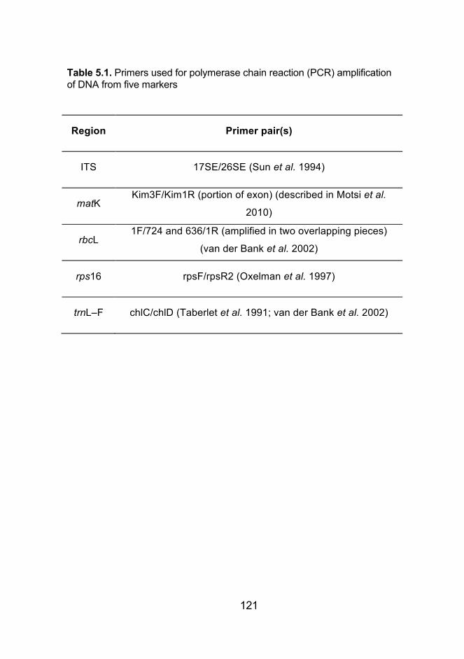
121

Table 5.1. Primers used for polymerase chain reaction (PCR) amplification of DNA from five markers

Region Primer pair(s)

ITS 17SE/26SE (Sun et al. 1994)

matK Kim3F/Kim1R (portion of exon) (described in Motsi et al.

2010)

rbcL 1F/724 and 636/1R (amplified in two overlapping pieces)

(van der Bank et al. 2002)

rps16 rpsF/rpsR2 (Oxelman et al. 1997)

trnL–F chlC/chlD (Taberlet et al. 1991; van der Bank et al. 2002)

122

We aligned the sequences of all markers initially by using

MUSCLE ver. 3.5 (Edgar 2004), followed by manual adjustments.

Not all markers were available for all taxa, so we removed taxa that

did not have data available for ITS and two or more plastid markers,

because the effect of missing data on phylogenetic inference can be

unpredictable (Lemmon et al. 2009; Filipski et al. 2014). We allowed

several exceptions to our selection criteria (Arnhemia cryptantha Airy

Shaw, Gnidia pilosa, Gonystylus macrophyllus (Miq.) Airy Shaw,

Lachnaea macrantha Meisn., Lethedon cernua (Baill.) Kosterm.,

Pimelea suteri Kirk, and Solmsia calophylla Baill.) to retain our

outgroup taxa and other taxa of interest. So as to reduce the effect of

alignment ambiguities, we filtered the data to remove any site at

which a gap was present in ≥80% of the taxa. After concatenating the

sequences of the five markers, the data set contained a total of 4544

sites (Appendix 4: File A4.1).

Partitioning the data set is an important step in phylogenetic

analyses, because this process is known to affect the accuracy of

phylogenetic inference (Lanfear et al. 2012). Accordingly, we

selected the best-fitting partitioning scheme by using the greedy

search algorithm in PartitionFinder ver. 1.1.1 (Lanfear et al. 2012).

The optimal partitioning scheme split the sequence alignment into six

subsets (Table 5.2).

We first analysed all five markers in a concatenated data set.

We inferred the phylogeny in a Bayesian framework by using

MrBayes ver. 3.2.2 (Ronquist et al. 2012b), implementing a uniform

prior on the tree topology and an exponential prior on branch lengths.

Posterior distributions of parameters, including the tree, were

123

Table 5.2. The optimal partitioning scheme for our five-marker data set, as determined using a greedy search in PartitionFinder

Subset Marker Substitution model

1 ITS SYM + Γ

2 matK 1st codon position, matK 2nd codon position, rps16

GTR + Γ

3 matK 3rd codon position, trnL–F GTR + Γ

4 rbcL 1st codon position GTR + Γ

5 rbcL 2nd codon position SYM + Γ

6 rbcL 3rd codon position GTR + Γ

124

estimated by Markov chain Monte Carlo sampling. We ran two

independent analyses with four Markov chains each for 40 000 000

steps, sampling every 4000 steps, then removed the first 25% of

samples as burnin. We then checked for convergence in the

estimates of model parameters by using Tracer ver. 1.6 (A. Rambaut,

M. A. Suchard, D. Xie and A. J. Drummond, see

http://beast.bio.ed.ac.uk/Tracer). The effective sample sizes of all

parameters were above 200, indicating adequate sampling to provide

a reliable estimate of the posterior distribution. To check that the

chains were sampling from the stationary distribution of tree

topologies, we inspected the average standard deviation of split

frequencies in MrBayes.

In addition to the Bayesian analysis, we inferred the

phylogeny using maximum likelihood in RAxML ver. 8.0 (Stamatakis

2014). We implemented the rapid bootstrapping algorithm with 1000

bootstrap pseudoreplicates to infer topological support, which results

in 200 fast maximum- likelihood searches followed by a final,

thorough search (Stamatakis et al. 2008). We used the optimal

partitioning scheme from PartitionFinder; however, because of the

limited nucleotide substitution models available, we implemented the

GTR+Γ model of nucleotide substitution for each data subset.

In both Bayesian and maximum-likelihood analyses, each

node support value refers to a precise hypothesis of the monophyly

of a group of potentially many members. As a result, the support

values can be sensitive to one or a few taxa whose position within a

group is unstable (Sanderson and Shaffer 2002). These taxa that are

placed in varying and contradictory positions within a tree are termed

125

‘rogue’ taxa (Wilkinson 1996), and their instability is thought to be

caused by missing data, an elevated substitution rate causing

homoplasy, or extremely low rates inside and outside the clade of

interest (Sanderson and Shaffer 2002). The negative effect of rogue

taxa on support values is well documented, particularly in the case of

majority-rule consensus trees (Trautwein et al. 2011). Therefore, we

tested for the presence of rogue taxa by analysing the 1000

bootstrap replicates from our maximum-likelihood analysis by using

RogueNaRok ver. 1.0 (Aberer et al. 2013). Rather than re-analyse a

data set without rogue taxa included, it is best to prune them from the

sets of trees resulting from the original analyses. This allows the

rogue taxa to inform the estimates of the topology, without having a

negative effect on support values or resolution (Cranston and

Rannala 2007). We removed the putative rogue taxa from the best-

scoring tree from RAxML and the corresponding bootstrap replicate

trees, and then calculated the support for the newly pruned tree. We

also removed the putative rogue taxa from the set of sampled trees

from our Bayesian analysis, and then produced a new consensus

tree.

We repeated the Bayesian and maximum-likelihood

phylogenetic analyses using a reduced data set comprising only the

four plastid markers with the same partitioning scheme (without ITS),

and then for all five markers separately. When analysing the

individual markers using MrBayes, we used the same approach as

for the full data set, except for reducing the analysis to consist of two

chains, each for 20 000 000 steps, sampling every 2000 steps.

126

5.3. Results

5.3.1. Nuclear and plastid concatenated data set

Phylogenetic analysis of our five-gene concatenated data set using

both Bayesian and maximum-likelihood methods produced very

similar results, with strong support for the monophyly of

Thymelaeoideae (p.p. = 1, b.s. = 100%; Figures 5.1 and 5.2,

Appendix 4: Figures A4.1–A4.2). Consistent with the findings of

Beaumont et al. (2009) and Motsi et al. (2010), Pimeleinae were

resolved as monophyletic with strong support (p.p. = 1, b.s. = 100%),

and Pimelea was resolved as paraphyletic with respect to

Thecanthes, with a strongly supported sister relationship inferred

between Thecanthes and a clade comprising P. decora and P.

haematostachya (p.p. = 1, b.s. = 86%). The branches leading to

Thecanthes and to P. decora + P. haematostachya were relatively

long compared to the majority of branches within the trees, so we ran

additional analyses to determine whether the sister relationship

between these groups was the product of long-branch attraction. We

first re-analysed the five-gene data set after removing all Thecanthes

taxa. Under this scenario, we found that the position of P. decora +

P. haematostachya within the phylogeny did not change (Appendix 4:

Figures A4.3–A4.4). We then re-analysed the data set after instead

removing P. decora + P. haematostachya, but this did not cause any

change in the phylogenetic placement of Thecanthes (Appendix 4:

Figures A4.5–A4.6).

127

Figure 5.1. Majority-rule consensus tree from our analysis of 230 taxa within Thymelaeaceae, as inferred through Bayesian analysis of a five-gene (nuclear + plastid) dataset using MrBayes. The scale bar represents substitutions per site. Taxon names ending with an asterisk are those that were newly sequenced for the present study, and named clades correspond to those discussed in the text. The tree is truncated to focus on the relationships between Pimeleinae and several closely related species of Gnidia. Black circles indicate nodes with a posterior probability (p.p.) of 1, grey circles indicate nodes with a p.p. of ≥0.9–0.99, and white circles indicate nodes with a p.p. of ≥0.8–0.89. Nodes without circles have a p.p. of <0.8.

128

Figure 5.2. Phylogram from our analysis of 230 taxa within Thymelaeaceae, as inferred through maximum-likelihood analysis of a five-gene (nuclear + plastid) dataset using RAxML. The scale bar represents substitutions per site. Taxon names ending with an asterisk are those that were newly sequenced for the present study, and named clades correspond to those discussed in the text. The tree is truncated to focus on the relationships between Pimeleinae and several closely related species of Gnidia. Black circles indicate nodes with bootstrap support (b.s.) of ≥95%, grey circles indicate nodes with b.s. of ≥80–94%, and white circles indicate nodes with b.s. of ≥50–79%. Nodes without circles have b.s. of <50%.

129

Despite the increase in sampling of Pimelea, species

relationships within the genus remained largely unresolved, with

many branches having very low or zero support. Although the overall

lack of resolution within Pimelea precludes many strong conclusions,

some trends were apparent, such as all New Zealand taxa falling into

one clade. There was very little sequence variation, indicated by very

short branches, among most of the Pimelea taxa from New Zealand,

especially within the P. prostrata (J.R.Forst. et G.Forst.) Willd.

complex. Unusually, P. longiflora subsp. eyrei (F.Muell.) Rye and P.

sylvestris R.Br. were nested within this otherwise New Zealand

clade, despite both being endemic to Western Australia.

Within the broader subfamily, Dais L., Daphnopsis Mart.,

Diarthron Turcz., Dirca L., Drapetes Banks ex Lam., Edgeworthia

Meisn., Kelleria Endl., Lachnaea, Passerina, Peddiea Harv. ex

Hook., Stellera L., Stephanodaphne Baill., Struthiola and Thymelaea

Mill. were each inferred to be monophyletic, with strong support (p.p.

= 1, b.s. ≥95%). Wikstroemia Endl. was found to be paraphyletic with

respect to Daphne gemmata E.Pritz. ex Diels, which, in turn,

rendered Daphne L. polyphyletic. This agrees with previous

observations of a high degree of morphological similarity between

Wikstroemia and Daphne, with the need for taxonomic revision (Ding

Hou 1960). However, it is worth noting that, in our data set, the taxon

sampling for many of these genera was low; increasing the taxon

sampling might lead to differences in the inferred relationships

among these genera. The resolution of the relationships among the

various genera of Thymelaeoideae was also markedly improved from

that in previous studies, with support for most backbone nodes and

130

other internal branches separating the genera receiving strong

support in the Bayesian analysis (p.p. ≥0.95) and moderate to strong

support in the maximum-likelihood analysis (b.s. = ~50–100%).

Importantly, Gnidia was resolved, once again, as polyphyletic, with

each of the component lineages being strongly supported (p.p. = 1,

b.s. = 100%), similar to previous findings (Beaumont et al. 2009;

Motsi et al. 2010).

Our analysis using RogueNaRok identified 23 putative rogue

taxa that could be contributing to the poor support for many clades

within Pimeleinae. However, the cumulative effect of removing all 23

taxa results only in an improvement of the relative bipartition

information criterion (RBIC) optimality, the measure of improvement

given by RogueNaRok, from 0.593 to 0.616 (Appendix 4: Table

A4.2). Nevertheless, we removed all identified rogue taxa to observe

the effect on support values within both our Bayesian and maximum-

likelihood trees (Appendix 4: Figures A4.7–A4.8). The largest

increase in statistical support occurred within Lachnaea after the

removal of L. oliverorum Beyers., with support for some nodes

increasing by as much as 43% b.s. (from 51 to 94%) and 0.36 p.p.

(from 0.64 to 1.00). Within Pimeleinae, the largest increase in support

in the maximum-likelihood tree was for the node uniting the

subspecies of P. ligustrina and P. axiflora (b.s. from 49 to 82%),

followed by the node representing the common ancestor of the New

Zealand taxa (b.s. from 56 to 76%). Nodes that previously had

posterior probabilities of 0.50 in our Bayesian majority- rule

consensus tree received a slight increase in support after removing

the rogue taxa; therefore, there were some changes in tree topology.

131

However, these changes mostly did not have strong statistical

support. Additionally, most nodes received only a very small increase

in statistical support, if any change occurred, even after all rogue taxa

were removed.

5.3.2. Plastid data set

Phylogenetic analysis of the plastid-only data set produced results

similar to the analysis of the five-gene data set, with Thymelaeoideae

again inferred to be monophyletic with strong support (p.p. = 1, b.s. =

100%; Appendix 4: Figures A4.9–A4.10). Pimeleinae was strongly

supported as monophyletic (p.p. = 1, b.s. = 99%), and Thecanthes

was still nested within Pimelea. However, there was no longer a

strongly supported sister relationship between Thecanthes and P.

haematostachya + P. decora. Instead, Thecanthes was resolved

within a clade comprising P. holroydii F.Muell., P. ammocharis

F.Muell., P. haematostachya, P. decora, P. strigosa Gand., P.

sericostachya F.Muell. subsp. sericostachya and P. latifolia subsp.

elliptifolia Threlfall with weak support (p.p. = 0.84, b.s. = 33%).

Pimelea longiflora subsp. eyrei, P. sylvestris and the taxa from New

Zealand formed a clade again, but, unlike in the five-gene analyses,

additional non-New Zealand taxa were also placed within this group.

These included P. stricta Meisn., P. physodes Hook., P. venosa

Threlfall and P. imbricata var. piligera (Benth.) Diels. The last two

taxa were previously not resolved as being closely related, and, in

these analyses of the combined plastid data set, the branch leading

to them, and the branch for P. venosa, were noticeably long. This

132

different relationship might be a result of the plastid data for P.

venosa being poor. The sequence for rbcL has a large proportion of

missing data, as well as many apparent substitutions relative to the

rest of Pimelea. Additionally, the trnL sequence for P. venosa has

very low variation compared with the other Pimelea spp., and there

are no data for matK or rps16. It cannot be ruled out that the change

in position of P. venosa and P. imbricata var. piligera might instead

be due to long- branch attraction rather than a different signal in the

chloroplast genome. However, likelihood-based methods generally

perform well in the presence of long branches (i.e. are not particularly

sensitive to long-branch attraction) when an appropriate, well fitting

evolutionary model is used (Huelsenbeck 1995; Ho and Jermiin

2004; Bergsten 2005). As in the analysis of all five genes, the

branches among the New Zealand taxa were inferred to be very

short. The same relationships were estimated among Dais,

Daphnopsis, Diarthron, Dirca, Drapetes, Edgeworthia, Kelleria,

Lachnaea, Passerina, Peddiea, Stellera, Stephanodaphne, Struthiola

and Thymelaea, with each of these genera again being found to be

monophyletic with strong support (p.p. = 1, b.s. ≥95%), although the

support for some internal nodes decreased. Gnidia was again

inferred to be polyphyletic, with each Gnidia lineage receiving strong

support (p.p. = 1, b.s. 100%).

5.3.3. Single-gene analyses

Separate analyses of the five genes included in the study

demonstrated the relative utility of each gene in resolving the

133

relationships within Thymelaeoideae. The topology inferred in the

analysis of ITS was very similar to those inferred from the five-gene

and plastid data sets, but with generally weaker support (Appendix 4:

Figures A4.11–A4.12). However, a key difference was that Gnidia

aberrans C.H.Wright, G. wikstroemiana Meisn. and G. setosa Wikstr.

were nested within Pimeleinae, rather than as sister lineages.

Thecanthes was again inferred to be nested within Pimelea and the

sister group to P. haematostachya + P. decora (p.p. = 0.86, b.s. =

49%). Analysis of matK also yielded a topology that is largely

congruent with that inferred in our five-gene analysis (Appendix 4:

Figures A4.13–A4.14). Pimeleinae were strongly supported (p.p. = 1,

b.s. = 96%), but the relationships within this group were generally

unresolved. Thecanthes was recovered as the sister lineage to P.

ammocharis, but this relationship was only weakly supported (p.p. =

0.82, b.s. = 38%). The results from analysis of trnL–F support the

monophyly of Pimeleinae (p.p. = 1, b.s. = 93%), but resolution within

the subtribe is poor (Appendix 4: Figures A4.15–A4.16). Although

many of the relationships in the trees inferred in analyses of rbcL and

rps16 are congruent with those inferred in our analysis of the other

data sets, the very low support and resolution, and low sequence

variation, preclude any meaningful interpretation (Appendix 4:

Figures A4.17–A4.20).

5.4. Discussion

Molecular phylogenetic studies of Thymelaeaceae in recent years

have each found strong support for the monophyly of the subfamily

134

Thymelaeoideae (van der Bank et al. 2002; Beaumont et al. 2009;

Motsi et al. 2010), an outcome that was strengthened by the results

of the present study. After finding evidence for the complicated

nature of the relationships within Thymelaeoideae, van der Bank et

al. (2002) suggested increasing sampling within the subfamily to help

better delimit the generic relationships. Beaumont et al. (2009)

followed this approach by increasing sampling of both genes and

taxa to further clarify the extent of polyphyly within Gnidia, and this

data set was extended by Motsi et al. (2010) by increasing taxon

sampling within Pimeleinae. Most genera within Thymelaeoideae

were found to be monophyletic in these studies, but the relationships

among them were mostly unclear or unsupported. On the basis of

our analyses of a five-gene data set, we present a moderately to

strongly supported improvement in understanding of the relationships

among the genera of Thymelaeoideae that were included in our

broad taxon sample. This will prove important in guiding the

taxonomic decisions necessary to redefine Gnidia as a monophyletic

group. However, our finding of a polyphyletic Gnidia is congruent with

the results of these previous studies, and will require extensive

attention to resolve.

Support varied between analyses; however, in all cases, we

found support for the monophyly of Pimeleinae. Although our

analysis using RogueNaRok identified 23 putative rogue taxa,

removing all 23 taxa had very little effect on the support for

relationships within Pimeleinae. Some previously unsupported or

poorly supported nodes received a small increase in support;

however, the backbone of Pimeleinae remained poorly supported.

135

Here, we focus on the results from analyses of our five-gene

concatenated data set with all taxa included to discuss the

relationships within Pimeleinae. Despite including many more

species of Pimelea than in previous studies, the resolution of the

Pimeleinae backbone remains poor. In the maximum- likelihood tree,

there is no bootstrap support for most of these backbone branches.

The same lack of support can be observed in our tree inferred by

Bayesian analysis, with nearly all backbone branches having a

posterior probability of less than 0.5. Another potential cause of the

low support values is the presence of only a small number of

informative sites within the data set that are influencing the

maximum-likelihood estimate of the phylogeny and are being missed

during bootstrap resampling. Low signal in the data could also

explain the lack of support inferred in our Bayesian analysis.

Although there was little to no support for the phylogenetic

backbone of Pimeleinae, many internal clades were found, with

support varying from moderate to strong. All New Zealand taxa were

inferred to form a clade with strong support in the Bayesian analysis

(p.p. = 1), but with moderate support in our maximum- likelihood

analysis (b.s. = 56%). Three main clades were resolved within the

broader New Zealand clade. The first consisted of P. gnidia and P.

longifolia; the second consisted of a putative undescribed species

(‘Pimelea cf. oreophila Norton 36852’), P. pseudolyallii Allan, P.

buxifolia Hook.f., P. longiflora subsp. eyrei and P. sylvestris; and the

third consisted of all other New Zealand species that were sampled,

corresponding largely to those recently described by Burrows (2008,

2009a, 2009b, 2011a, 2011b). The nested position of P. longiflora

136

subsp. eyrei and P. sylvestris within the second clade is somewhat

strange because the two species are restricted to Western Australia.

This suggests a complicated biogeographic history for Pimelea that

should be explored further when a more strongly resolved tree is

obtained. Many of the branches within the third clade are extremely

short and support for many relationships is very low, indicating

relatively little sequence variation. For example, the sequences for all

markers for Pimelea orthia C.J.Burrows & Thorsen subsp. orthia and

Pimelea prostrata subsp. prostrata are identical. Many of these

species were described on the basis of distinct morphological

characteristics; however, the molecular data indicated that there may

be fewer, morphologically variable species than was proposed by

Burrows (2008, 2009a, 2009b, 2011a, 2011b). Additionally, Burrows

sampled several populations that exhibited morphological

characteristics that were intermediate between the species he

described, and proposed that these may represent hybrids. An

example is ‘Pimelea sp. Burrows 38838’, an accession that Burrows

(2011a) considered to be a hybrid between P. pseudolyallii and P.

oreophila C.J.Burrows. While these three taxa resolved within our NZ

clade, they were not especially closely related. Therefore, although

the lack of resolution within this group hinders any firm conclusions,

the resulting phylogenetic trees did not appear to provide any

evidence for the proposed hybrid nature of this taxon.

Throughout the rest of Pimeleinae, we found many smaller,

moderately to strongly supported clades; however, the sectional

classification proposed by Rye (1988) was not upheld. Each of the

sections was inferred to be polyphyletic, as found by Motsi et al.

137

(2010). We inferred the presence of a large clade that comprised

only western Australian taxa (p.p. = 0.84, b.s.= 23%). The

relationships within this clade were strongly supported in the

Bayesian analysis, but only moderately supported in the maximum-

likelihood analysis. Likewise, we found several clades comprising

predominantly eastern Australian taxa, as well as a clade comprising

taxa found only in Tasmania, whereas the Australian alpine species

did not group together. There were also suggestions of a northern

Australian grade that might reflect Asian interchange. Although there

were suggestions of biogeographic trends, the low resolution and

support for many branches prevented firm conclusions. It is also

worth noting that P. trichostachya Lindl. and P. simplex F.Muell.

subsp. simplex, two of the three species of Pimelea known to cause

livestock poisoning (Fletcher et al. 2014), were resolved as sister

taxa. This suggests a possible single origin of toxic Pimelea spp.,

which may aid in future attempts to understand and characterise the

nature of livestock poisoning. However, further investigation is

necessary, especially because other species have been proposed to

be potentially toxic.

At the species level, there were several important findings. We

found that P. sylvestris and P. calcicola Rye are somewhat distantly

related on the basis of molecular data. This is surprising, because

these species are morphologically highly similar, and were once

considered to be conspecific (Rye 1984). However, it is now

appropriate to consider that the similar morphological characteristics

of P. sylvestris and P. calcicola might be a result of convergent

evolution. This process has been hypothesised to have led to the

138

high degree of morphological similarity throughout Thymelaeoideae

(Beaumont et al. 2009), and hinders efforts to identify clear

synapomorphies. Pimelea curviflora is known to be a morphologically

variable species much in need of further study (Rye and Heads

1990). Six varieties are currently accepted; we included four P.

curviflora accessions, representing at least three of the recognised

varieties, with one accession not being identified to this level. Our

results indicated that P. curviflora var. divergens Threlfall might best

be described as a distinct species, given its position as the sister

lineage to P. micrantha F.Muell. ex Meisn.; however, stronger

support and resolution is needed before this action can be taken

formally.

Our results also indicated that the infraspecific circumscription

of some Pimelea taxa is generally well founded, although in some

cases might need revision. The most obvious example of this is P.

longiflora R.Br. We inferred P. longiflora R.Br. subsp. longiflora to be

nested within a clade of western Australian taxa with strong support,

whereas P. longiflora subsp. eyrei, the other recognised subspecies,

was nested deep within a clade of New Zealand taxa (with the

exception of the western Australian P. sylvestris), also with strong

support. The disjunct position of the two subspecies within the

phylogeny differed between data sets, as did the statistical support

for their inferred positions. However, the two subspecies of P.

longiflora were never inferred as sister taxa. This lends strong

support to reinstating P. longiflora subsp. eyrei at the species level as

P. eyrei F.Muell.

139

The complicated taxonomic history of Pimelea and

Thecanthes is indicative of the close relationship between the two

genera, as is the strong support we find for Pimeleinae across most

of our analyses. After a comprehensive treatment of Pimelea based

on morphological data, Rye (1988) concluded that the annual life

history and specialised inflorescence of Thecanthes were enough to

justify resurrecting it as a genus. However, recent attempts to clarify

the relationships between these genera by using molecular

phylogenetics have indicated that Thecanthes is nested within

Pimelea, with varying levels of support (Beaumont et al. 2009; Motsi

et al. 2010). Our results supported these findings, with analyses of

our five-gene data set indicating strong support for Thecanthes being

nested within Pimelea (p.p. = 1, b.s. = 86%). This finding was

consistent across all other analyses, albeit with decreased statistical

support.

The exact placement of Thecanthes within Pimelea was

variable across analyses, and requires additional work. However, the

best estimate from the present study is that Thecanthes is the sister

group to a clade comprising at least P. decora and P.

haematostachya. Motsi et al. (2010) acknowledged that there is good

molecular evidence for synonymising Thecanthes with Pimelea, but

were hesitant to make the taxonomic changes unless there was

strong bootstrap support for Thecanthes. We have achieved an

appropriate level of support for the sister relationship between

Thecanthes and P. decora + P. haematostachya. Additionally,

removing the Thecanthes sequences from the data set did not

change the inferred position of P. decora + P. haematostachya within

140

the phylogeny. Likewise, removing the sequences for P. decora + P.

haematostachya from the data set did not change the inferred

position of Thecanthes within the phylogeny. Therefore, despite the

branches leading to P. decora + P. haematostachya and Thecanthes

being long, we can be confident that long-branch attraction is not

causing these two groups to be inferred as sister lineages.

It is also important to consider any morphological similarities

between Thecanthes and P. decora + P. haematostachya. Several of

the synapomorphies for Thecanthes identified by Rye (1988) are

shared with these two species. Both groups are hermaphroditic with

a herbaceous habit, and both possess sessile involucral bracts,

although the number and persistence of bracts differs (Thecanthes:

4, persistent; P. decora: 5–8, deciduous; P. haematostachya: 7–12,

deciduous; Rye and Heads 1990). However, the life-history strategy

and inflorescence structures differ between the groups. Thecanthes

has an annual life-history strategy, with head-like inflorescences and

glabrous, dorsiventrally compressed pedicels, whereas species of

the P. decora + P. haematostachya group are perennials, with

terminal racemose inflorescences and hairy, terete pedicels (Rye and

Heads 1990). Some morphological characters suggested to be

distinctive to Thecanthes are also seen elsewhere in other species of

Pimelea, although the whole suite of characters is not found outside

Thecanthes. For example, similar to Thecanthes, P. gilgiana E.Pritz.

possesses head-like inflorescences with concave receptacles

(female flowers) and glabrous pedicels (male flowers), although this

species differs in several key characteristics (e.g., dioecious with

shrub habit; Rye and Heads 1990). Overall, taking our results and

141

those of previous studies into account, we believe that the most

appropriate action is to reduce Thecanthes to synonymy with

Pimelea. This would suggest that the synapomorphies for

Thecanthes should instead be treated as variation within Pimelea, an

approach that seems reasonable considering the extensive

morphological variation of the genus.

Unfortunately, for the reduction of Thecanthes to synonymy of

Pimelea to be a long-term solution, the extensive polyphyly of Gnidia

will still need to be addressed. Beaumont et al. (2009) proposed two

options for dealing with the polyphyly of Gnidia, both of which would

require extensive taxonomic changes. Option 1 proposes broadening

the circumscription of Gnidia to also include Pimelea, Thecanthes,

Struthiola, Passerina and Lachnaea, as well as resurrecting the

genus Lasiosiphon Fresen. Option 2 proposes broadening the

circumscription of Pimelea to include the several sister species of

Gnidia, while reducing several other genera to sections within new

subgenera of Gnidia. Beaumont et al. (2009) remained agnostic as to

the preferred course of action, but we align more closely with Option

2, which would subsume the Gnidia sister lineages into Pimelea

(including the newly synonymised Thecanthes).

We acknowledge that this option generates additional

difficulties for generic delimitation within Thymelaeoideae. At present,

Pimeleinae can be distinguished readily from the South African

species of Gnidia only by the almost constant reduction in the

number of stamens to (1)2 per flower (Beaumont et al. 2009).

However, this seems to be a weak diagnostic character, considering

that the number of stamens per flower is highly variable within

142

Thymelaeaceae (Rye and Heads 1990; van der Bank et al. 2002).

Nevertheless, expanding Pimelea to include the sister species of

Gnidia would remove this sole consistent morphological difference,

and would leave no known synapomorphies for Pimelea. This is

especially troubling, given that previous attempts to find additional

synapomorphies have been largely unsuccessful (Beaumont et al.

2009), presumably because of significant morphological

convergence.

There remains an additional course of action. Gnidia could be

substantially reduced to conserve strongly supported monophyletic

groups such as Lachnaea and Passerina. For this to occur, sampling

within Lachnaea, Passerina, Struthiola, Drapetes and Kelleria would

need to be increased to allow further understanding of these genera.

This approach would also be hindered by the difficulty of finding

synapomorphies for each newly circumscribed genus, which reflects

the lack of informative morphological characters within the broader

family (Peterson 1959; Ding Hou 1960).

It is clear that the relationships within and between the genera

of Thymelaeoideae are far from settled, and clarifying the

circumscription of Gnidia in particular will probably result in many

taxonomic changes. Even if it is ultimately only an interim measure, it

is appropriate to perform the reduction of Thecanthes to synonymy

with Pimelea here, because a taxonomic revision of Gnidia is unlikely

to occur in the immediate future. Nevertheless, the uncertainty

surrounding the relationships within Thymelaeoideae has diminished

with each study that has increased taxon and gene sampling.

Therefore, cost-effective generation of large amounts of genetic data,

143

as can be achieved through high-throughput sequencing, will be the

next step towards a well resolved phylogeny for Thymelaeoideae.

5.5. Taxonomy

We reduce Thecanthes to synonymy of Pimelea, and reinstate its

constituent species (in Pimelea) and Pimelea eyrei F.Muell., as

follows.

Pimelea filifolia (Rye) C.S.P.Foster et M.J.Henwood, comb. nov. Thecanthes filifolia Rye, B.L. Rye, in A.S. George (ed.) Fl. Australia 18: 213–214, 325, fig. 80G I, map 303 (1990). Type: Magela Creek, N.T., 25 Feb. 1973, C.R. Dunlop 3357 (holo: CANB; iso: BRI, DNA, NSW; n.v.). Pimelea concreta F.Muell., Fragm. 5: 73 (1865) Banksia concreta (F.Muell.) Kuntze, Revis. Gen. Pl. 2: 583 (1891); Thecanthes concreta (F.Muell.) Rye, Nuytsia 6: 262 (1988). Type: Camden Harbour, W.A., J.S.Roe (holo: MEL; n.v.). Pimelea brevituba Fawcett in H.O.Forbes, A Naturalist’s Wanderings 516 (1885). Type: Mount Sobale, Samoro, Timor, 28 Apr.–3 May 1883, H.O. Forbes 3828 (holo: BM; n.v.). Pimelea cornucopiae Vahl, Enum. Pl. 1: 305 (1804) Thecanthes cornucopiae (Vahl) Wikstr., Kongl. Vetensk. Acad. Handl. 271 (1818); Calyptostregia cornucopiae (Vahl) Endl., Gen Pl. Suppl. 4(2): 60 (1848); Banksia cornucopiae (Vahl) Kuntze, Revis. Gen. Pl. 2: 583 (1891). Type: Australia, D.Montin (holo: C, n.v., fide S.Threlfall, Brunonia 5: 123 (1983)). Pimelea ramosissima Schumann in K.Schumann & K.Lauterbach, Nachtr. Fl. Deutsch. Schutzgeb. Südsee 324 (1905).

144

Type: New Britain, Bismarck Archipelago, Jan. 1902, R. Parkinson, n.v. Pimelea philippinensis C.Robinson, Philipp. J. Sci. 6: 345 (1911). Type: Sanchez Mira, Province of Cagayan, Luzon, Philippines, Ramos 7410 (holo: K; n.v.). Pimelea punicea R.Br., Prodr. 359 (1810) Thecanthes punicea (R.Br.) Wikstr., Kongl. Vetensk. Acad. Handl. 272 (1818); Calyptostregia punicea (R.Br.) Endl., Gen Pl. Suppl. 4(2): 60 (1848); Banksia punicea (R.Br.) Kuntze, Revis. Gen. Pl. 2: 583 (1891). Type: North Bay, Arnhem Land, [N.T.], 16 Feb. 1803, R.Brown (lecto: BM, fide B.L.Rye, Nuytsia 6: 264 (1988); isolecto: MEL). Pimelea punicea var. breviloba F.Muell. ex Benth., Fl. Austral. 6: 6 (1873). Type: Purdie Ponds, N.T., J.McDouall Stuart (lecto: K, fide B.L.Rye, op. cit. 264; isolecto: MEL; n.v.). Pimelea sanguinea F.Muell., Fragm. 1: 84 (1859) Banksia sanguinea (F.Muell.) Kuntze, Revis. Gen. Pl. 2: 583 (1891); Thecanthes sanguinea (F.Muell.) Rye, Nuytsia 6: 267 (1988). Type: Pandanus Springs, upper Roper R., N.T., 20 July 1856, F.Mueller (holo: MEL; n.v.). Pimelea eyrei F.Muell., Fragm. 5: 109 (1866) Banksia eyrei (F.Muell.) Kuntze, Revis. Gen. Pl. 2: 583 (1891); Pimelea longiflora subsp. eyrei (F.Muell.) Rye, Nuytsia 6: 196 (1988). Type: Eyre Ra., Phillip R. and Fitzgerald R., W.A., G.Maxwell (holo: MEL; n.v.). Note: The nomenclature here largely follows that presented by Rye and Heads (1990).

145

Chapter 6 — Plastome-Scale Data and Exploration of Phylogenetic Tree Space Help to

Resolve the Evolutionary History of Pimelea (Thymelaeaceae)

6.1. Introduction

Since its inception, the molecular systematics of plants has been

dominated by analyses of chloroplast genes (Clegg and Zurawski

1992). For several decades, however, evolutionary rates have been

known to vary among the genes in the chloroplast genome (Wolfe et

al. 1987). Accordingly, it was recognised that a combination of

chloroplast genes could potentially be used to resolve evolutionary

relationships at multiple taxonomic scales. For example, one of the

most commonly sequenced chloroplast genes has been rbcL, which

was prominently used to estimate the phylogeny of seed plants

(Chase et al. 1993). The value of chloroplast genes for molecular

systematics is also reflected in the recommendation that rbcL and

matK be used in tandem for DNA barcoding (Hollingsworth et al.

2009).

Chloroplast genes have provided an indisputably valuable

source of data for plant systematics. However, there are cases in

which chloroplast genes have only offered limited phylogenetic

resolution for challenging taxa, even when combined with more

rapidly evolving nuclear markers such as the internal transcribed

spacer (ITS). One such example is Pimelea Banks & Sol. ex Gaertn.

(Thymelaeaceae), a genus of flowering plants comprising ca. 150

species (Z.S. Rogers, see

146

www.tropicos.org/Project/Thymelaeaceae). As expected in a genus

of this size, Pimelea exhibits extensive morphological variation, both

in terms of habit and inflorescence structure (Rye and Heads 1990).

For example, some species are small and herbaceous, whereas

others range from woody procumbent shrubs to large trees.

Additionally, Pimelea has a number of life-history strategies, ranging

from annual species that are always hermaphroditic, to perennial

species that are variously dioecious, gynodioecious or

hermaphroditic (Burrows 1960; Rye 1988; Rye and Heads 1990).

Pimelea occurs in a variety of habitats, ranging from arid to alpine.

Some species are restricted to relatively small geographic areas, but

others are far more widespread (Rye and Heads 1990).

Most of the taxonomic diversity in this genus can be found

within Australia, with ca. 95 endemic species, and, after the recent

reduction of Thecanthes to synonymy with Pimelea (Chapter 5),

another two species extending into New Ireland and the Philippines

(Rye and Heads 1990). About 35 species and 18 subspecies of

Pimelea are also recognised within New Zealand (Burrows 2011b).

The taxonomy of Pimelea has a long history and has undergone

many revisions, particularly with respect to the relationship between

Pimelea and the recently synonymised Thecanthes (Chapter 5;

Bentham 1873; Gilg 1894; Threlfall 1982, 1984; Rye 1988; Rye and

Heads 1990; Motsi et al. 2010).

The first molecular systematic study to focus on Pimelea

sampled five markers from 50 species (including the five species

formerly recognised as Thecanthes), and found strong support for

the monophyly of the genus (Motsi et al. 2010). However, the

147

phylogenetic resolution within Pimelea was poor overall, especially

along the backbone of the tree. More recently, we attempted to

resolve the relationships within Pimelea by sampling the same

molecular markers as Motsi et al. (2010), but extending the sampling

of Pimelea to 86 taxa (Chapter 5). By employing a range of statistical

and phylogenetic techniques, including data partitioning, we resolved

many of the sister-species groupings within the genus with strong

support. We also found enough statistical support to reduce

Thecanthes to a synonym of Pimelea. However, the backbone of the

Pimelea phylogeny remained unresolved, with many of the internal

branches appearing to be extremely short.

Pimelea is economically important, with some species being

popular in floriculture (Rye and Heads 1990), and other toxic species

causing serious losses to the pastoral cattle industry through the

poisoning of livestock (Fletcher et al. 2014). Additionally, many

species of Pimelea are under some degree of threat. The Australian

Environment Protection and Biodiversity Conservation (EPBC) Act

1999 lists both subspecies of P. spinescens as critically endangered,

P. venosa and P. spicata as endangered, and P. curviflora var.

curviflora, P. leptospermoides, and P. pagophila as vulnerable. The

Department of Environment, Land, Water and Planning in Victoria

lists 16 Pimelea taxa as being rare or threatened, and the New South

Wales Scientific Committee has recently supported a proposal to list

P. cremnophila as critically endangered under the Australian

Threatened Species Conservation Act 1995. Therefore, obtaining a

stable nomenclature and phylogeny of Pimelea is valuable for

floricultural and horticultural breeding programmes, for understanding

148

the evolutionary history of the toxic species, and for improving our

knowledge of the genetics of many threatened species.

There are many possible causes of poor phylogenetic

resolution. The chosen molecular markers might lack the signal

needed to resolve the evolutionary relationships. We posited that this

was the case for Pimelea, with the low phylogenetic resolution likely

to be a consequence of the low genetic variation in the chosen

molecular markers (Chapter 5). This stands in contrast with the

extensive morphological variation within the genus (Rye and Head

1990). Alternatively, the molecular markers might have conflicting

information as a result of the interactions between evolutionary

processes, rates, and phylogenetic signal (Revell et al. 2008).

Introgression and incomplete lineage sorting can lead to discordant

gene trees and a resulting lack of support for species relationships

(Vogl et al. 2003; Maddison and Knowles 2006). Extremely short

branches, as are expected from a rapid or recent radiation, can also

have a negative impact on phylogenetic resolution because of a lack

of accumulated substitutions during the speciation process (Wiens et

al. 2008). However, the potential causes of low phylogenetic

resolution and conflicting phylogenetic signals are difficult to explore

when the data set consists of only a few genetic markers.

In this study, we aim to resolve the backbone of the Pimelea

phylogeny using a plastome-scale data set. We take advantage of

advances in sequencing technology to generate plastome sequences

for 41 taxa, including 33 species of Pimelea and eight outgroup taxa.

We conduct a series of Bayesian and maximum-likelihood analyses

to estimate the phylogeny and evolutionary timescale of Pimelea. We

149

also perform a comprehensive set of analyses to examine the

phylogenetic signal in our data set, and explore the difficult nature of

unravelling recent radiations.


6.2.1. Taxon sampling

We aimed to obtain a representative sample of the evolutionary

diversity of Pimelea by selecting from clades that were previously

found to have moderate to strong support (Chapter 5). We also

prioritised sampling from taxa that have been identified as vulnerable

or threatened under the Australian Environment Protection and

Biodiversity Conservation Act 1999, with the hope of improving the

knowledge of the genetics of these species. We chose eight

outgroup taxa from Thymelaeoideae. Leaves were sampled from

herbarium specimens of Gnidia squarrosa, Kelleria dieffenbachii,

Passerina montana, Struthiola thomsoni, Wikstroemia indica, and

Jedda multicaulis. Chloroplast genome sequences for Aquilaria

sinensis (Aquilarioideae, Thymelaeaceae) and Theobroma cacao

(Malvaceae) were obtained from GenBank. In total, we sampled 41

taxa (Appendix 5: Table A5.1).

6.2.2. Molecular methods

We obtained leaf samples for the majority of our chosen species from

herbarium specimens lodged at the National Herbarium of New

South Wales (NSW; Royal Botanic Gardens, Sydney), National

150

Herbarium of Victoria (VIC; Royal Botanic Gardens, Victoria), and the

Queensland Herbarium (BRI; Brisbane Botanic Gardens,

Queensland). We aimed to sample from the most recent and/or best-

preserved collections for each species. Fresh leaf samples were

collected for several species of Pimelea from cultivated collections at

the Australian National Botanic Gardens (CANB; Canberra,

Australian Capital Territory). Additionally, we obtained samples of

genomic DNA for some species of Pimelea from the National

Herbarium of Victoria.

We extracted genomic DNA from the leaf samples using the

QIAGEN DNeasy Plant Mini Kit (QIAGEN, Melbourne, Australia),

following the manufacturer’s protocol. The samples of total genomic

DNA were prepared for sequencing by two different experimental

methods. In both cases, we aimed to recover full chloroplast

sequences in a genome-skimming approach. For our first approach,

we sent samples for sequencing at the Ramaciotti Centre for

Genomics (University of New South Wales, Australia). Each sample

contained only genomic DNA from a single taxon. Nextera libraries

were prepared according to the Nextera® XT DNA Sample

Preparation kit from Illumina, before paired-end (2×150 bp) shotgun

sequencing was performed on the Illumina NextSeq 500 platform.

Our second experimental sequencing approach was to pool

DNA samples from the present study with those from animal taxa

from an unrelated study. Sequencing was performed by BGI

(Shenzhen, China) and Macrogen (Seoul, South Korea). At both

facilities, Nextera libraries were prepared using the Nextera® XT

DNA Sample Preparation kit from Illumina. At BGI, paired-end

151

(2×150 bp) sequencing was performed on the Illumina HiSeq 2500

platform. At Macrogen, paired-end (2×150 bp) sequencing was

performed on the Illumina Hiseq X-Ten platform.

The raw data from both BGI and Macrogen contained reads

from multiple taxa (one plant, ≥2 animals). To obtain the plant-

specific reads, we mapped all reads to a reference chloroplast

genome from Aquilaria sinensis Gilg using BWA-mem v0.7.12 (Li

2013), and then extracted all mapped reads using SAMtools v1.3.1

(Li et al. 2009).

6.2.3. Chloroplast genome assembly

We attempted initial assembly of chloroplast genomes from non-

pooled samples using NOVOPlasty v2.5.9 (Dierckxsens et al. 2017),

with A. sinensis as the reference genome. This method was highly

successful for some taxa, and generated complete or near-complete

circular chloroplast genome sequences. For other taxa, however,

only small fragments of the chloroplast genomes were assembled. In

these cases, we instead carried out de novo assembly using CLC

Genomics Workbench 10 (available from http://www.clcbio.com).

Next, we mapped the assembled contigs with ≥5× coverage for each

species to a reference chloroplast genome. For the reference, we

chose the chloroplast genome from Pimelea simplex subsp. simplex

F.Muell. that was successfully assembled using NOVOplasty. Finally,

we produced consensus sequences for each taxon.

For all pooled samples, we exercised additional caution to

ensure that the sequences were of plant origin, despite the initial

152

mapping step with BWA-mem. To do so, we carried out de novo

assembly of each taxon using CLC as above. We then searched

assembled contigs against the total Genbank nucleotide database

with the BLASTn algorithm, and removed any contigs from highly

conserved regions that were of non-plant origin. Finally, we mapped

the remaining contigs against the Pimelea simplex subsp. simplex

reference genome and extracted consensus sequences, as with the

non-pooled sequences.

We annotated all 41 chloroplast genomes using the Dual

Organellar Genome Annotator (Wyman et al. 2004). In each case,

we corrected the automatic annotation of start and stop codons by

comparison with homologous chloroplast genes. Our previous

mapping approach led to us recovering two copies of some genes,

corresponding to those that would be found in the inverted repeats of

the chloroplast genomes. After ensuring that both copies were

identical, we discarded one copy of each of these genes prior to

phylogenetic analysis. We recovered 75 out of 79 plastid protein-

coding genes for most taxa, but fewer genes for some taxa from the

pooled samples (Appendix 5: File A5.1; Table A5.2). This is

presumably because of uneven sequencing coverage across the

pooled taxa, rather than the actual absence of these genes from their

chloroplast genomes. Although this prevented us from identifying and

recovering all possible intergenic regions, we were able to assemble

a set of 55 intergenic regions and four intronic regions.

153

6.2.4. Phylogenetic analysis

We aligned the protein-coding genes at the amino acid level using

MAFFT v7.305b (Katoh and Standley 2013), then back-translated

them into nucleotide sequences using PAL2NAL (Suyama et al.

2006). All non-coding markers were aligned using MAFFT. We made

manual adjustments to all sequence alignments. Three main

concatenated data sets were assembled for phylogenetic analysis: (i)

all protein-coding genes and non-coding regions (86,941

nucleotides), (ii) all protein-coding genes (62,088 nucleotides), and

(iii) all non-coding regions (24,853 nucleotides) (Appendix 5: File

A5.1).

Our main approach for inferring the phylogeny was the same

for each data set. First, we inferred the phylogeny using maximum

likelihood in IQ-TREE v1.5.5 (Nguyen et al. 2015), with branch

support estimated using 1000 replicates of both the SH-like

approximate likelihood-ratio test (SH-aLRT; Guindon et al. 2010),

and the ultrafast bootstrapping algorithm (Minh et al. 2013). We used

the ModelFinder option to identify the optimal partitioning scheme

and substitution models (Chernomor et al. 2016; Kalyaanamoorthy et

al. 2017), but for computational reasons we did not allow the

probability-distribution-free model of rate heterogeneity among sites.

Bayesian phylogenetic analysis was performed using

MrBayes v3.2.2 (Ronquist et al. 2012b), using the same partitioning

schemes and model for among-site rate heterogeneity as in the IQ-

TREE analyses. There are far fewer nucleotide substitution models

available in MrBayes than in IQTREE. Therefore, the best

compromise was to implement a GTR substitution model, the most

154

general model available, to each subset of the data. Posterior

distributions of parameters, including the tree, were estimated by

Markov chain Monte Carlo (MCMC) sampling. We ran two

independent analyses with four Markov chains each for 107 steps,

sampling every 103 steps. After removing the first 25% of samples as

burn-in, we checked that the effective sample sizes of model

parameters were above 200. To check that the chains were sampling

from the stationary distribution of tree topologies, we inspected the

average standard deviation of split frequencies to ensure that they

were below 0.01.

Preliminary assessments of our estimated trees revealed

some strongly supported clades, but also many weakly supported

nodes. Support values in both Bayesian and maximum-likelihood

analyses can be sensitive to ‘rogue’ taxa whose phylogenetic

placements are unstable (Wilkinson 1996). Rogue taxa might have

large amounts of missing data or elevated substitution rates

compared with other taxa in the data set, or there might be extremely

low substitution rates inside and outside the clade being considered

(Sanderson and Shaffer 2002). We tested for the presence of rogue

taxa in all data sets using RogueNaRok v1.0 (Aberer et al. 2013). We

maintained the default settings, but in each case we optimised the

bootstrap support for the best-known (maximum-likelihood) tree for

each data set.

Chloroplast genomes are predominantly non-recombining

(Birky 1995), so it is appropriate to concatenate their genes for

phylogenetic analysis. Nevertheless, some have found evidence of

conflicting topological signal between plastid genes (Zeng et al.

155

2014), which leads to low support for nodes. Therefore, we used a

clustering approach to test whether topological discordance was

leading to the low support in our inferred trees. The gene tree for

each protein-coding gene was inferred using 10 searches in IQ-

TREE, in each case partitioning by codon position. Since the

relationships among the outgroup taxa in the concatenated analyses

were resolved with strong support, we pruned these taxa from the

inferred gene trees. We also removed some genes and some

Pimelea taxa to minimise the proportion of missing data and to

achieve an optimal balance between gene and taxon sampling

(Appendix 5: Table A5.1).

We estimated the topological distance between each of the

gene trees using the modified Robinson-Foulds metric of Penny and

Hendy (1985) in the ape R package (Paradis et al. 2004). Using the

CLARA algorithm in the cluster R package (Maechler et al. 2016), we

clustered the gene trees based on their topological distances. The

optimal number of clusters was determined using the gap statistic

(Tibshirani et al. 2001). This approach recovered three clusters of

genes that supported different tree topologies. We concatenated the

genes within each of these clusters, and then inferred the phylogeny

again using IQ-TREE and MrBayes. In each case we used the

optimal partitioning scheme determined by IQ-TREE.

To compare potential biological explanations for the clustering

of gene trees, we investigated several properties of the clusters. First,

we analysed each gene using codeml (Yang 2007) to estimate the

ratio of nonsynonymous to synonymous substitution rates (ω), which

can indicate the direction and strength of selection. The method in

156

codeml does not take into account any nucleotide site that has

missing or ambiguous data for any taxon. Therefore, we excluded

taxa for which we had only fragmentary gene sequences. We then

compared the mean ω values across the three clusters of genes. We

also calculated the mean length of each gene tree, using this as a

proxy for substitution rate, to see whether gene clustering was

associated with evolutionary rate (Duchêne and Ho 2015). Finally,

we calculated the average GC content of each gene, because this

was found to be associated with gene-tree clustering in a study of

marsupials (Duchêne et al. in press). In each case, we tested for

differences between clusters using a Kruskal-Wallis rank sum test,

and determined which clusters differed using Dunn’s test with a

Bonferroni correction for multiple tests.

Our data set contains several species that have not previously

been included in phylogenetic analyses of Pimelea. Therefore, we

combined sequence data from the present study with those of

Chapter 5 to place these species in the context of the broader

phylogeny of Pimelea. The resulting data matrix of 3528 nucleotides

from 271 taxa combined the protein-coding genes matK and rbcL,

and a partial sequence of the trnT–trnL intergenic spacer. We

analysed this data set using IQ-TREE and MrBayes with a separate

GTR+Γ substitution model for each codon position and for the non-

coding marker.

157


We estimated the evolutionary timescale of Pimelea using

MCMCTREE v4.8 (Yang 2007). Unfortunately, very few reliable

fossils are available for calibrating molecular date estimates for

Pimelea. No macrofossils of Thymelaeaceae are known, and the

identification of pollen fossils from this family is notoriously difficult

because their crotonoid morphology can also be found in other

distantly related lineages (Herber 2002). Three main pollen types

have been recognised in Thymelaeaceae: Phaleria-type (lower

Miocene), Daphne-type (lower Eocene), and Gonystylus-type

(Oligocene) (Muller 1981). There are crotonoid pollen fossil taxa that

can be reliably assigned to Thymelaeoideae, dating from the

Miocene onwards (Muller 1981), and Gonystyloideae fossils are

known from the Eocene (Venkatachala and Kar 1968). Within

Pimelea, the oldest microfossils are from the mid-Pliocene of New

Zealand (Mildenhall 1980), but are uninformative for molecular dating

because of this young age. A pollen fossil from the Paleocene of

Texas has been attributed to Pimelea, but probably belongs to

another group of Thymelaeaceae or elsewhere (Muller 1981).

The taxonomy of Thymelaeaceae has changed considerably

in the several decades since the last detailed reviews of the fossil

record of the broad group. This suggests a need for caution in the

assignment of fossils to lineages. Therefore, we took a conservative

approach to fossil calibration. We placed a minimum age of 33.9

million years ago (Ma) on the crown node of Thymelaeaceae based

on Daphne-type pollen from the lower Eocene (Krutzsch 1966;

Gruas-Cavagnetto 1976). We chose to assign this age to crown

158

Thymelaeaceae rather than the more nested Daphne clade

(represented by Wikstroemia in our study), because the latter

assignment has been challenged based on a lack of definitive

synapomorphies in the pollen (Herber 2002). We also placed a

minimum age of 7.25 Ma on the stem node of Wikstroemia, based on

fossil pollen from the Daphne-Thymelaea evolutionary lineage from

the Tortonian (Barrón 1996). Finally, we placed a minimum age of

55.8 Ma on the root, corresponding to the oldest macrofossils of

stem-group Malvaceae from the Cerrejón Formation (middle to late

Paleocene) (Carvalho et al. 2011).

All calibrations were implemented as uniform priors with soft

bounds. We ran two replicate analyses, each with a different

maximum age constraint on the root. First, we conservatively

assigned a maximum age of 126.7 Ma, corresponding to the first

appearance of tricolpate pollen at the upper age limit of the

Barremian–Aptian boundary (Friis et al. 2006). This has frequently

been used as a maximum age bound for eudicots in studies of

angiosperm evolution (Sauquet et al. 2012; Massoni et al. 2015a;

also discussed in Chapter 2). Second, we used a more informative

maximum age of 77.61 Ma, corresponding to the upper bound of the

95% credibility interval for the divergence of Malvaceae and

Thymelaeaceae from their most recent common ancestor in a recent

molecular dating analysis (Magallón et al. 2015).

MCMCTREE requires a fixed tree topology, so we chose the

maximum-likelihood tree from our analysis of the combined protein-

coding and non-coding data set. We estimated the overall

substitution rate by running baseml (Yang 2007) under a strict clock,

159

with a single point calibration of 59.8 million years ago (Ma) at the

root. We based this calibration on a recent mean estimate for the

divergence of Malvaceae and Thymelaeaceae from their most recent

common ancestor (Magallón et al. 2015). We used the substitution

rate estimate to set the prior on the overall substitution rate across

loci in the MCMCTREE analysis, and we set the shape and scale

parameters for the prior on rate variation across branches to 1 and

1.3, respectively.

Judicious partitioning of molecular clock models is an

important component of molecular dating (Chapter 4; Angelis et al.

2018). We partitioned the data set into four subsets, one for each

codon position of the protein-coding genes and one for the non-

coding data. This applies a separate relaxed clock to each data

partition. The posterior distribution of node ages was estimated by

MCMC sampling, with samples drawn every 500 steps across a total

of 2.5×106 steps, after a discarded burn-in of 2×105 steps. We ran the

analysis in duplicate to assess convergence, and confirmed sufficient

sampling by checking that the effective sample sizes of all

parameters were above 200.

6.3. Results

6.3.1. Phylogenetic relationships: plastome-scale data set

We report first on the relationships that we inferred using maximum-

likelihood and Bayesian analyses of the combined protein-coding and

160

non-coding sequences. Consistent with previous findings (Chapter 5;

van der Bank et al. 2002; Beaumont et al. 2009; Motsi et al. 2010),

we found maximum support for a monophyletic Thymelaeoideae

(Figures 6.1 and 6.2). Our study is the first to use molecular data to

assess the phylogenetic position of Jedda multicaulis, a monotypic

genus within Thymelaeoideae (Clarkson 1986). We found maximum

support for a sister relationship between Jedda multicaulis and the

rest of Thymelaeoideae. The relationships that we resolved along the

Thymelaeoideae backbone, including those among Passerina,

Kelleria, Struthiola, and Wikstroemia, are consistent with previous

findings (Chapter 5; Beaumont et al. 2009). However, we provide the

strongest support for these relationships so far (p.p. = 1, SH-aLRT =

100%, UFboot = 100%). As in previous studies, we inferred a close

relationship between Gnidia squarrosa and Pimelea. Additionally, we

found maximum support for a monophyletic Pimelea.

Within Pimelea, the relationships inferred in the maximum-

likelihood and Bayesian analyses are predominantly the same,

although the level of support differs between methods. In the

maximum-likelihood analysis, some nodes received strong UFboot

support (≥95%), but many are only moderately supported (80–94%).

In contrast, all but five nodes have strong support based on SH-aLRT

values (≥80%). In the Bayesian analysis, most nodes have posterior

probabilities of 1.00, and only six nodes have posterior probabilities

below 0.95. In both maximum-likelihood and Bayesian analyses,

branches were generally very short, particularly along the backbone,

indicative of a recent or rapid radiation.

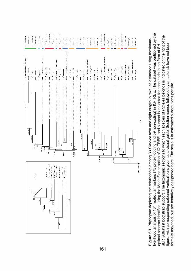
161

Figu

re 6

.1. P

hylo

gram

dep

ictin

g th

e re

latio

nshi

p am

ong

33 P

imel

ea ta

xa a

nd e

ight

out

grou

p ta

xa, a

s es

timat

ed u

sing

max

imum

-lik

elih

ood

anal

ysis

of 1

34 m

olec

ular

mar

kers

(75

prot

ein-

codi

ng a

nd 5

9 no

n-co

ding

) in

IQ-T

REE

. The

dat

aset

was

par

titio

ned

by th

e op

timal

sch

eme

iden

tifie

d us

ing

the

Mod

elFi

nder

opt

ion

of IQ

-TR

EE, a

nd s

uppo

rt is

indi

cate

d fo

r eac

h no

de in

the

form

of S

H-

aLR

T/ul

trafa

st b

oots

trap

supp

ort.

The

taxo

nom

ic s

ectio

ns to

whi

ch e

ach

spec

ies

of P

imel

ea b

elon

gs is

indi

cate

d on

the

right

of t

he

figur

e, w

ith c

orre

spon

ding

col

oure

d ve

rtica

l bar

s gi

ven

as a

vis

ual g

uide

. Sec

tion

nam

es fo

llow

ed b

y an

ast

eris

k ha

ve n

ot b

een

form

ally

ass

igne

d, b

ut a

re te

ntat

ivel

y de

sign

ated

her

e. T

he s

cale

is in

est

imat

ed s

ubst

itutio

ns p

er s

ite.

162

Figu

re 6

.2. P

hylo

gram

dep

ictin

g th

e re

latio

nshi

p am

ong

33 P

imel

ea ta

xa a

nd e

ight

out

grou

p ta

xa, a

s es

timat

ed u

sing

Bay

esia

n in

fere

nce

of 1

34 m

olec

ular

mar

kers

(75

prot

ein-

codi

ng a

nd 5

9 no

n-co

ding

) in

MrB

ayes

. The

dat

aset

was

par

titio

ned

by th

e op

timal

sc

hem

e id

entif

ied

usin

g th

e M

odel

Find

er o

ptio

n of

IQ-T

REE

, and

sup

port

is in

dica

ted

for e

ach

node

in th

e fo

rm o

f pos

terio

r pr

obab

ilitie

s. T

he ta

xono

mic

sec

tions

to w

hich

eac

h sp

ecie

s of

Pim

elea

bel

ongs

is in

dica

ted

on th

e rig

ht o

f the

figu

re, w

ith

corre

spon

ding

col

oure

d ve

rtica

l bar

s gi

ven

as a

vis

ual g

uide

. Sec

tion

nam

es fo

llow

ed b

y an

ast

eris

k ha

ve n

ot b

een

form

ally

as

sign

ed, b

ut a

re te

ntat

ivel

y de

sign

ated

her

e. T

he s

cale

is in

est

imat

ed s

ubst

itutio

ns p

er s

ite.

163

The evolutionary relationships of Pimelea aquilonia, P.

cremnophila, P. elongata, P. penicillaris, and P. umbratica have not

been evaluated previously. Pimelea aquilonia was resolved as the

sister species to Pimelea sanguinea, which was considered as part

of the segregate genus Thecanthes until its recent synonymisation

with Pimelea (Chapter 5). Pimelea elongata was resolved as the

sister taxon to P. trichostachya and P. simplex subsp. simplex, with

this clade of three species representing all Pimelea species that have

so far been confirmed to be toxic to livestock (Fletcher et al. 2014).

Both P. penicillaris and P. umbratica were grouped with P.

leptospermoides, P. ligustrina subsp. ligustrina, P. venosa, and P.

cremnophila. In all analyses, there was maximum support for a sister

relationship between P. cremnophila and P. venosa. However, the

relationships among the other species within this clade are

unresolved, and represent the only differences between the trees

inferred using Bayesian and maximum-likelihood methods.

6.3.2. Phylogenetic relationships: other data sets

Separate analyses of the protein-coding and non-coding data sets

yielded trees that were mostly congruent with those estimated from

the combined data set, but with less support overall (Appendix 5:

Figures A5.1–A5.4). The only differences between the trees

estimated from the combined and protein-coding data sets occur in

poorly supported parts of the phylogeny. This is also the case for

some of the incongruent relationships between the combined and

non-coding data sets, but there are also some strongly supported

164

differences. For example, analyses of the non-coding data set

resolve P. haematostachya as the sister taxon to all other Pimelea

taxa with strong support in the Bayesian analysis (p.p. = 0.99), and

moderate support in the maximum-likelihood analysis (SH-aLRT =

74.2%, UFboot = 90%). This is in contrast with the results from

analyses of the combined data set, where P. haematostachya

occupies a more nested position as the sister taxon to a clade

comprising P. ammocharis, P. aquilonia, and P. sanguinea, with

strong to moderate support (p.p. = 1, SH-aLRT = 90.4%, UFboot =

91%). Nevertheless, combining the two sources of data leads to the

best-supported trees, including both along the backbone and at the

tips.

We found very little evidence for rogue taxa having an impact

on our results, with no rogue taxa detected in the protein-coding and

combined data sets. When analysing the non-coding data set,

however, we found Pimelea physodes to be a putative rogue taxon.

Nevertheless, pruning P. physodes had no impact on the UFboot or

SH-aLRT support values for any nodes in the inferred phylogeny,

and only increased the posterior probability of one node from 0.99 to

1.

Analysis of the data matrix combining sequences from three

molecular markers from the present study with those of Chapter 5

yielded a phylogeny that is mostly poorly supported (Appendix 5:

Figures A5.5–A5.6). Additionally, in the maximum-likelihood analysis,

some taxa were resolved in unusual positions in the phylogeny,

including two species of Passerina that were resolved within

Pimelea. This is probably because of the sequences for some taxa

165

being fragmentary, with large amounts of missing data. Nevertheless,

the expanded Pimelea phylogeny can still be used as a preliminary

test of the placement of the taxa in this study that have not previously

been subject to phylogenetic analysis. Jedda multicaulis was again

inferred to be the sister lineage to all other taxa in Thymelaeoideae,

with strong to moderate support (p.p. = 0.89, SH-aLRT = 75.5%,

UFboot = 92%). Pimelea aquilonia was found to group with P.

haematostachya, P. decora, P. argentea, P. strigosa, P. latifolia

subsp. elliptifolia, and P. sericostachya subsp. sericostachya, but

with only moderate to low support (p.p. = 0.56, SH-aLRT = 83.2%,

UFboot = 75%). As in our main analyses, we found a sister

relationship between P. cremnophila and P. venosa with strong

support (p.p. = 1, SH-aLRT = 96.4%, UFboot = 100%). In the

maximum-likelihood analysis, P. penicillaris was resolved as the

sister taxon to P. curviflora var. gracilis with moderate support (SH-

aLRT = 79.9%, UFboot = 88%), but in the Bayesian analysis P.

penicillaris was instead resolved as the sister taxon to P. curviflora

var. divergens with maximum support. Finally, the phylogenetic

placement of P. umbratica was comparable with that inferred in our

main analyses.

6.3.3. Exploration of phylogenetic tree space

Our topology-clustering approach identified three clusters of gene

trees for the protein-coding data set (Appendix 5: Table A5.2; Figure

A5.7). The most striking difference between clusters was in tree

length (Kruskal-Wallis rank sum test; p<0.01; H=13.356; df=2)

166

(Appendix 5: Figure A5.8). Trees from Cluster 1 were significantly

longer than those in Cluster 2 and Cluster 3 (Dunn’s test; p<0.05 and

p<0.001, respectively), but there was no significant difference in tree

length between Cluster 2 and Cluster 3.

We found a significant difference in GC content between

clusters (Kruskal-Wallis rank sum test; p<0.01; H=10.912; df=2)

(Appendix 5: Figure A5.9). The genes in Cluster 2 had a significantly

higher GC content than those in the other two clusters (Dunn’s test;

p<0.05 and p<0.001, respectively), but there was no significant

difference between Cluster 1 and Cluster 3. However, the difference

was small enough not to warrant further investigation. When

considering the ratio of nonsynonymous to synonymous substitution

rates for each gene, there was no significant difference between any

of the clusters (Kruskal-Wallis rank sum test; p>0.05; H=3.5508;

df=2) (Appendix 5: Figure A5.10).

When we re-estimated the phylogeny for each of the three

clusters of genes, there were noticeable differences in topology

between trees, as expected (Appendix 5: Figures A5.11–A5.16). The

tree inferred from the genes in Cluster 1 has generally higher node

support, especially when considering SH-aLRT support values for the

backbone nodes. Based on this higher support, and the smaller

number of short branches, we consider the tree from Cluster 1 to be

the most reliable. There are many cases in which the longer tree

from Cluster 1 closely resembles the trees estimated from the

protein-coding data set, such as in the resolution of a clade

comprising P. biflora, P. micrantha, and P. spicata. There are also

some differences in topology, but these are generally unsupported. In

167

all analyses in this study, a clade comprising the toxic Pimelea

species P. elongata, P. simplex subsp. simplex, and P. trichostachya

is resolved as the sister group to a clade comprising P.

haematostachya, P. ammocharis, P. aquilonia, and P. sanguinea,

with this combined clade being the sister group to the rest of

Pimelea. In the trees estimated separately for each cluster, the sister

relationship between these two clades is strongly supported (p.p. = 1,

UFBoot ≥95%, SH-aLRT ≥80%), despite this relationship being only

moderately to poorly supported by the protein-coding, non-coding,

and combined data sets.


Our various molecular dating analyses yielded generally similar

estimates of node ages, except for some of the deeper divergences

when we implemented a conservative maximum bound of 126.7 Ma

for the age of the root (Appendix 5: Figure A5.17). Here, we report

the results of our analysis using a maximum age constraint of 77.61

Ma (Fig. 6.3, Appendix 5: Figure A5.18). We inferred that crown-

group Thymelaeaceae arose 51.23–32.19 Ma, and crown-group

Thymelaeoideae arose 38.34–22.32 Ma. Crown-group Pimelea was

inferred to have arisen in the mid to late Miocene, 9.44–5.42 Ma.

Diversification within the genus occurred over a short time period,

with the majority of mean age estimates falling between ca. 6–4 Ma,

and with the most recent divergence between P. trichostachya and P.

simplex subsp. simplex occurring 2.76–1.13 Ma. The two New

Zealand taxa that we included in our data set, P. ignota and P. xenica

168

Figu

re 6

.3. C

hron

ogra

m d

epic

ting

the

evol

utio

nary

tim

esca

le o

f 33

Pim

elea

taxa

and

eig

ht o

utgr

oup

taxa

, as

estim

ated

usi

ng

Baye

sian

infe

renc

e of

134

mol

ecul

ar m

arke

rs (7

5 pr

otei

n-co

ding

and

59

non-

codi

ng) i

n M

CM

CTr

ee. W

e us

ed fo

ur d

ata

parti

tions

, one

for e

ach

codo

n po

sitio

n of

the

prot

ein-

codi

ng g

enes

and

one

for t

he n

on-c

odin

g da

ta, a

nd im

plem

ente

d an

in

form

ativ

e m

axim

um a

ge o

f 77.

61 M

a. H

oriz

onta

l bar

s in

dica

te 9

5% c

redi

bility

inte

rval

s fo

r inf

erre

d ag

es, a

nd m

ean

age

estim

ates

are

pro

vide

d fo

r sev

eral

nod

es o

f int

eres

t. C

olou

red

verti

cal b

ars

indi

cate

the

dist

ribut

ion

of ta

xa, w

ith th

e co

rresp

ondi

ng g

eogr

aphi

c re

gion

s in

dica

ted.

Num

bers

in c

ircle

s co

rresp

ond

to th

ree

node

s of

inte

rest

, as

follo

ws:

1) T

hym

elae

acea

e, 2

) Thy

mel

aeoi

deae

, and

3) P

imel

ea. A

bbre

viat

ions

: “Pl

io.”

= Pl

ioce

ne, “

Plei

.” =

Plei

stoc

ene.

169

were inferred to have split from each other 3.8–1.3 Ma.

6.4. Discussion

6.4.1. Phylogenetic relationships within Pimelea

Resolving the phylogenetic relationships within Pimelea, particularly

along the backbone of the phylogeny, has been a long-standing

challenge. In the present study, we have provided the best estimate

of the early evolutionary history of Pimelea through the sequencing

and analysis of chloroplast genomes. We also offer a vast

improvement in phylogenetic resolution within Pimelea. Previous

attempts to resolve the relationships within the genus used a

maximum of five molecular markers, with little success. This is

despite the inclusion of protein-coding and non-coding chloroplast

genes alongside nuclear ribosomal genes. It is only after increasing

the sampling to a total of 134 molecular markers (75 protein-coding

and 59 non-coding) that we have been able to achieve a satisfactory

resolution of the relationships within Pimelea. Previously, the best-

resolved phylogeny of Pimelea only included support for some sister-

species relationships and some other small clades (Chapter 5), but

here we have improved the phylogenetic resolution both at the tips

and along the backbone.

Within Pimelea, our phylogenetic analyses yielded support for

several clades of interest. Pimelea lehmanniana subsp. nervosa, P.

ferruginea, P. rosea, P. avonensis, and P. physodes are all endemic

to Western Australia, and were found to form a clade with strong

170

support. The two New Zealand taxa that we sampled, Pimelea ignota

and P. xenica, grouped together with maximum support. We found

moderate to strong support for P. curviflora var. curviflora, which is

restricted to Sydney, NSW, as the sister taxon to the two New

Zealand taxa. This clade was nested within the Pimelea phylogeny,

and implies a single arrival of Pimelea into New Zealand from

Australia, although broader taxon sampling and explicit

biogeographic modelling is needed to confirm this.

Our phylogenetic analysis has clarified the phylogenetic

position of several species of Pimelea that, under the Australian

EPBC Act List of Threatened Flora, are critically endangered (P.

cremnophila and P. spinescens subsp. pubiflora), endangered (P.

spicata and P. venosa), or vulnerable (P. curviflora var. curviflora, P.

leptospermoides, and P. pagophila). Knowledge of the genetics of

these species could help to guide future conservation efforts. For

example, since P. cremnophila and P. venosa are sister lineages and

under threat, losing both of these taxa would represent a significant

loss of evolutionary diversity.

The results of our analyses might also have economic

implications, by confirming the monophyly of the group including P.

elongata, P. simplex subsp. simplex, and P. trichostachya, the three

species of Pimelea that are confirmed to be toxic to livestock

(Fletcher et al. 2014). However, it should be noted that other Pimelea

species have also been found to contain the simplexin toxin, but

have not yet been linked definitively to livestock poisoning (Chow et

al. 2010). Some of these other species are closely related to our

“toxic” clade, including P. haematostachya and P. decora, but others

171

are more distantly related, including P. microcephala and P.

penicillaris. Therefore, it is possible that toxicity has evolved multiple

times independently in this genus, or that all or most taxa have

various levels of underlying toxicity.

Our results reinforce several important findings from previous

studies of Pimelea. Despite indications that Thecanthes should be

reduced to synonymy with Pimelea, Motsi et al. (2010) were reluctant

to do so without stronger bootstrap support for a sister relationship

between species of Thecanthes and Pimelea. In a more recent

study, we achieved bootstrap support for a sister relationship

between Thecanthes and P. decora + P. haematostachya that we

deemed sufficient, so we synonymised Thecanthes with Pimelea

(Chapter 5). However, the bootstrap support for this relationship was

still only 86%. In the present study, we have provided stronger

evidence for the synonymisation by demonstrating a sister

relationship between P. sanguinea (formerly Thecanthes sanguinea)

and P. aquilonia with strong support (p.p. = 1, SH-aLRT = 95.9%,

UFboot = 97%).

Rye (1988) classified Pimelea into seven sections based on

morphological evidence, but the sectional classification has not been

upheld in either of the recent molecular systematic studies of Pimelea

(Chapter 5; Motsi et al. 2010). The present study included

representatives of six of the seven sections, and we have found

again that, overall, the sectional classification is not supported by

molecular data. Although we inferred a monophyletic P. sect.

Heterolaena, we only sampled four out of ca. 15 species from this

section (Appendix 5: Table A5.1). All other sections were found to be

172

polyphyletic. However, much greater taxon sampling would be

required before we can propose an alternative stable infrageneric

classification for Pimelea. The infrageneric classification of the

species of Pimelea that were formerly included in Thecanthes also

remains to be assessed.

6.4.2. Implications for the broader subfamily

Several recent studies have focused on the molecular systematics of

Thymelaeaceae, either at the family level or with a focus on its

constituent genera (Chapter 5; Beaumont et al. 2009; Motsi et al.

2010). There have been a number of consistent findings in these

studies with respect to the subfamily Thymelaeoideae. Most genera

within Thymelaeoideae are found to be monophyletic with strong

support, with Gnidia being an important exception. Gnidia is the

largest genus in Thymelaeaceae and exhibits extensive polyphyly

(Chapter 5; Motsi et al. 2010). Since Gnidia has nomenclatural

priority over many Thymelaeoideae, resolving the circumscription of

this genus has implications for the nomenclature of nearly all other

genera within the subfamily. We do not address the issue of the

polyphyly of Gnidia in the present study, because this will require a

much larger taxon sample from throughout Thymelaeoideae.

However, we do confirm a close relationship between Gnidia

squarrosa and Pimelea, as identified previously (Chapter 5; Motsi et

al. 2010).

The relationships among the genera of Thymelaeoideae have

not been certain, despite some recent improvement in support

173

(Chapter 5). In the present study, we fully resolve the backbone of

the Thymelaeoideae phylogeny. Although we did not include all of

the genera in the subfamily, we included representatives from

several of the major clades that have been identified previously

(Chapter 5; Beaumont et al. 2009; Motsi et al. 2010). Additionally, we

have inferred the phylogenetic placement of Jedda multicaulis for the

first time, and demonstrated that the divergence of the evolutionary

lineage leading to this taxon was one of the earliest divergences in

Thymelaeoideae.

6.4.3. Evolutionary timescale of Pimelea

All of our inferred phylogenies revealed many extremely short

branches within Pimelea, particularly along the backbone of the

phylogeny. Short internal branches can indicate a rapid or recent

radiation (Crisp and Cook 2009), but an estimate of the evolutionary

timescale is necessary to confirm either possibility. We are the first to

provide an estimate of the evolutionary timescale of Pimelea and

Thymelaeoideae. Based on the distribution of the taxa we sampled,

we tentatively infer an origin of Thymelaeoideae in Australia 39.8–

23.3 Ma, followed by at least two independent dispersals to South

Africa 22.8–12.7 Ma (the clade comprising Struthiola and Passerina)

and 18.1–9.7 Ma (Gnidia squarrosa). However, denser sampling

from Thymelaeoideae is necessary for more definitive conclusions.

Our inferred evolutionary timescale suggests that none of the extant

species of Pimelea arose particularly recently, but that the genus

underwent a rapid radiation in the mid-Miocene.

174

The Miocene was a time of increasing aridification in Australia

(Byrne et al. 2008), and has been hypothesised to have promoted

speciation in many Australian taxa as habitats fragmented (Byrne

and Hopper 2008). A rapid radiation in the early evolutionary history

of Pimelea goes some way to explaining the difficulty behind

estimating a well resolved phylogeny for the genus. Rapid radiations

have challenged phylogenetic estimation at multiple taxonomic

scales (Wang et al. 2009; Fior et al. 2013; Straub et al. 2014). We

also inferred a recent origin of the New Zealand species of Pimelea

during the Pliocene–Pleistocene, consistent with a single arrival by

long-distance dispersal.

6.4.4. The importance of critically assessing methods

The improvements in phylogenetic resolution achieved in our study

only became evident after careful consideration of the best ways to

analyse our data set. Analysing only protein-coding data or only non-

coding data led to conflicting topologies. Some of the inferred

evolutionary relationships only had moderate to poor support, but

there were also some strongly supported incongruences between the

two sources of data. Although this might be a true signal from the

data, it could also be due to a greater amount of missing data and/or

fragmentary sequences in the non-coding data set compared with

the protein-coding data set.

It is also important to consider critically the different methods

that can be used to assess the support for inferred relationships. In

this study, we assessed support for phylogenetic relationships using

175

Bayesian posterior probabilities, the SH-like approximate likelihood-

ratio test (SH-aLRT), and the ultrafast bootstrap (UFboot). There are

cases in which the Bayesian estimates of the trees contained nodes

with maximum posterior probabilities, yet the same relationships

received only moderate to low ultrafast bootstrap support. It is difficult

to determine why this might be, since posterior probabilities and

bootstrap support are calculated differently, and, therefore, cannot be

directly compared. Nevertheless, it has been suggested that

posterior probabilities can overestimate branch support, or bootstrap

support can be overly conservative, or both (Douady et al. 2003).

In a phylogeny such as the one inferred in this study, with very

short branches corresponding to a rapid radiation, there might have

been inadequate time for many substitutions to accumulate (Wiens et

al. 2008). As a result, bootstrap replicates might fail to recover the

few substitutions that do exist. However, SH-aLRT values are robust

to short branches and should provide more accurate estimates of

support in these situations (Guindon et al. 2010). An important caveat

is that SH-aLRT values can fail to account for competing highly likely

topologies that differ greatly from the maximum-likelihood tree. In

cases where there is not a good estimate of the maximum-likelihood

topology, a bootstrapping approach might be preferable because

support values are based on a better sample of topologies (Guindon

et al. 2010). Therefore, in the case of our data set, where a rapid

radiation has led to a challenging phylogenetic problem, it is best to

consider different support indices in combination.

We found evidence of conflicting signal across chloroplast

genes in Pimelea, despite the chloroplast genome being non-

176

recombining. We identified three clusters of protein-coding gene

trees based on Robinson-Foulds topology distances. Although the

trees estimated from each cluster of genes were not better resolved

or more highly supported than the tree estimated from all protein-

coding genes combined, we still observed some trends of note.

Despite the common assumption that all chloroplast genes share the

same topology, we demonstrate that gene trees from the chloroplast

genome can have different topologies, as has been suggested

previously (Delwiche and Palmer 1996; Vogl et al. 2003; Shepherd et

al. 2008; Zeng et al. 2014).

Recombination is unlikely to be the cause of the discordance

among chloroplast gene trees, because this process has only rarely

been observed in any plants (Birky 1995). Horizontal gene transfer is

a common explanation for discordance between nuclear and

chloroplast phylogenies, and has been observed in plants previously

in the form of chloroplast capture (Soltis et al. 1991; Jackson et al.

1999; Stegemann et al. 2012). However, because the chloroplast is

inherited as a single locus, chloroplast capture should not lead to

discordance among genes within the chloroplast. Alternative

explanations for discordance between chloroplast gene trees include

mutational saturation, covarion effects, and paralogy (Vogl et al.

2003). Given the relatively young age that we inferred for Pimelea,

both saturation and covarion effects are unlikely. Paralogy of

chloroplast genes is hypothesised to occur through gene duplication

as genes are recruited into the chloroplast inverted repeat, followed

by loss of one of the gene copies (Vogl et al. 2003). The duplicate

protein-coding genes that we identified, corresponding to those that

177

would be in the inverted repeats, were identical within species; this

indicates that paralogy was not a problem.

Since we have inferred a relatively recent origin for Pimelea, it

is possible that the protein-coding genes, which represent the largest

component of our data set, have evolved too slowly to allow

resolution of the evolutionary relationships within the genus.

Therefore, the discordance between gene trees might be caused by

a lack of resolution in some gene trees, with those of a similar

evolutionary rate and phylogenetic signal clustering together. This

hypothesis is supported by our finding that the three clusters of gene

trees differ in terms of tree length, which reflects the relative

substitution rate. When comparing the three clusters, the tree

estimated from Cluster 1 most closely resembles our best estimate of

the Pimelea phylogeny, has overall far greater support than the trees

estimated from the other two clusters, and its constituent genes are

significantly longer than in the other two clusters. The implications of

this are especially evident when considering the SH-aLRT support

values, because many of the short branches in the trees estimated

from Cluster 2 and Cluster 3 receive SH-aLRT support values of 0%.

6.5. Conclusions

It is clear that the phylogeny of Pimelea represents a challenging

problem. Previously, we posited that the lack of phylogenetic

resolution for this genus was largely due to a lack of genetic variation

within the chosen molecular markers (Chapter 5). However, through

sequencing of chloroplast genomes we have revealed that the

178

difficulty can also be attributed to a rapid radiation early within the

evolutionary history of Pimelea. Additionally, discordance among

gene trees might be contributing to the difficulty in phylogeny

estimation.

Future phylogenomic studies of Pimelea should include much

broader taxon sampling both within the genus and within

Thymelaeoideae, and sampling from the nuclear genome. This will

allow a more definitive understanding of the evolutionary history of

Pimelea, including the potential presence of confounding factors

such as incomplete lineage sorting. Increased sampling will also help

to clarify the taxonomic problems caused by the extensive polyphyly

of Gnidia, which we have not addressed here. Nevertheless, the

improvements that we have made to the phylogeny of Pimelea

through plastome-scale sequencing and in-depth phylogenetic

analyses reveal the power of these methods, and will assist with

future revisions of the genus.

179

Chapter 7 — General Discussion

7.1. Thesis overview and significance

Molecular phylogenetics has revolutionised research into angiosperm

evolution. In the early days of the molecular revolution, many

answers to key questions in angiosperm evolution based on

morphological data were overturned. For example, gnetophytes were

sometimes proposed to be the closest extant relatives to

angiosperms based on comparative morphology (Crane 1985; Doyle

and Donoghue 1986; but see Foster and Gifford 1959), but molecular

data have shown this not to be true (Qiu et al. 1999; Winter et al.

1999). Before long, molecular data also resolved further questions

such as the identity of the sister lineage to all angiosperms (Mathews

and Donoghue 1999; Parkinson et al. 1999; Qiu et al. 1999; Soltis et

al. 1999), and began to refine the evolutionary timescale of

angiosperms. However, many of the early key findings were based

on very small numbers of genes (e.g., Chase et al. 1993).

The increasing availability of high-performance computational

facilities, and the ability to generate massive quantities of sequence

data in a cost-effective manner, present a golden opportunity for

fundamental questions in biology to be addressed with

unprecedented rigour (Metzker 2010). However, these data sets also

present many analytical and theoretical challenges, especially since

our knowledge of the best ways to analyse molecular data, and the

assumptions behind many methods, are largely based on data sets

of only a few genes (Tong et al. 2016). In the studies presented in

this thesis, I aimed to address many of these challenges. I focused

180

on uncovering the ways in which the many methodological

components of phylogenetic analysis might affect the estimates of

evolutionary relationships and timescales, and demonstrated the

utility of plastome-scale data sets for answering key questions in

biology.

In Chapter 2, I investigated the angiosperm evolutionary

timescale. The timing of the origin of angiosperms and their

subsequent diversification has long been a key question in biology

(Magallón 2014). Molecular estimates of this timescale have shown

considerable variation, being influenced by differences in taxon

sampling, gene sampling, fossil calibrations, evolutionary models,

and choices of priors (summarised in Chapter 1 and Chapter 2).

I analysed a data set comprising 76 protein-coding genes

from the chloroplast genomes of 195 taxa spanning 86 families,

including novel genome sequences for 11 taxa, to evaluate the

impact of models, priors, and gene sampling on Bayesian estimates

of the angiosperm evolutionary timescale. Using a Bayesian relaxed

molecular-clock method, with a core set of 35 minimum and two

maximum fossil constraints, I estimated that crown angiosperms

arose 221 (251–192) Ma during the Triassic. Based on a range of

additional sensitivity and subsampling analyses, I found that the date

estimates were generally robust to large changes in the parameters

of the birth–death tree prior and of the model of rate variation across

branches. I found an exception to this when I implemented fossil

calibrations in the form of highly informative gamma priors rather than

as uniform priors on node ages. Under all other calibration schemes,

including trials of seven maximum age constraints, I consistently

181

found that the earliest divergences of angiosperm clades

substantially predate the oldest fossils that can be assigned

unequivocally to their crown group.

Overall, my extensive analyses of genome-scale data in

Chapter 2 have provided one of the most rigorous estimates of the

angiosperm evolutionary timescale so far. More broadly, my results

suggest that incorporating plastome-scale data into molecular dating

analyses might not necessarily lead to improvements in estimates of

evolutionary timescales. Instead, reliable age estimates will require

increased taxon sampling, significant methodological changes, and

new information from the fossil record.

Chapters 3 and 4 provide assessments of phylogenetic

methods for partitioning genome-scale data for molecular dating

analyses. Clock-partitioning is an important, and arguably under-

utilised, component of phylogenetic analysis, and allows phenomena

like among-lineage rate-heterogeneity to be taken into account

(Duchêne and Ho 2014; Angelis et al. 2018). In Chapter 3, I

investigated the performance of different clustering methods to

assign genes to molecular-clock-partitions using data from

chloroplast genomes and data generated by simulation. My results

show that mixture models provide a useful alternative to traditional

partitioning algorithms. I found only a small number of distinct

patterns of among-lineage rate variation among chloroplast genes,

which were consistent across taxonomic scales. This suggests that

the evolution of chloroplast genes has been governed by a small

number of genomic pacemakers. My study also demonstrates that

182

clustering methods provide an efficient means of identifying clock-

partitioning schemes for genome-scale data sets.

In Chapter 4, I investigated how the accuracy and precision of

Bayesian divergence-time estimates improve with increased clock-

partitioning of genome-scale data into clock-subsets. I focused on a

data set comprising plastome-scale sequences of 52 angiosperm

taxa. There was little difference among the Bayesian date estimates

whether I chose clock-subsets based on patterns of among-lineage

rate heterogeneity or relative rates across genes, or by random

assignment. Increasing the degree of clock-partitioning usually led to

an improvement in the precision of divergence-time estimates, but

this increase was asymptotic to a limit presumably imposed by fossil

calibrations. My clock-partitioning approaches yielded highly precise

age estimates for several key nodes in the angiosperm phylogeny.

For example, when partitioning the data into 20 clock-subsets based

on patterns of among-lineage rate heterogeneity, I inferred crown

angiosperms to have arisen 198-178 Ma. This demonstrates that

judicious clock-partitioning can improve the precision of molecular

dating based on phylogenomic data, but I caution that the meaning of

this increased precision should be considered critically.

I demonstrated the power of comprehensive phylogenetic

analyses to resolve difficult phylogenetic problems in Chapters 5 and

6. In Chapter 5, I investigated the molecular systematics of Pimelea

Banks & Sol. (Thymelaeaceae), including its close relationship with

Thecanthes Wikstr. Previous attempts to resolve the relationships

within Pimelea have been largely unsuccessful (Beaumont et al.

2009; Motsi et al. 2010), with a lack of molecular variation leading to

183

most relationships within the genus remaining unclear. However,

these previous studies still uncovered some trends of note, such as

the possibility of Thecanthes being nested within Pimelea. Relatively

low phylogenetic resolution and low statistical support prevented

potentially necessary taxonomic changes from occurring (Motsi et al.

2010)

Through careful and exhaustive Bayesian and maximum-

likelihood phylogenetic analyses of four plastid markers (matK, rbcL,

rps16, trnL–F) and one nuclear ribosomal marker (ITS), I recovered

an improved estimate of the phylogeny of Pimelea, including strong

support for the nested position of Thecanthes within Pimelea. My

results also indicated that P. longiflora R.Br. subsp. longiflora and P.

longiflora subsp. eyrei (F.Muell.) Rye are best considered as distinct

species. Therefore, I reduced Thecanthes to a synonym of Pimelea,

and reinstated Pimelea eyrei F.Muell. However,my estimate of the

phylogeny was still poorly resolved overall with low support,

particularly with respect to the backbone of the Pimelea clade. I

demonstrated that careful and considered approaches to analysis are

able to lead to improved phylogenetic estimates, but concluded that

the phylogeny of Pimelea would most likely need genome-scale data

to be resolved.

Accordingly, in Chapter 6 I generated and analysed a

plastome-scale data set for 33 Pimelea taxa and eight outgroup taxa.

Through comprehensive Bayesian and maximum-likelihood

analyses, I successfully resolved the backbone of the Pimelea

phylogeny. I also provided even stronger support for my previous

decision to reduce Thecanthes to a synonym of Pimelea. However,

184

some relationships within Pimelea received only moderate to poor

support, and the Pimelea clade contained extremely short internal

branches.

By using topology-clustering analyses, I demonstrated that

conflicting phylogenetic signals can be found across the gene trees

estimated from chloroplast protein-coding genes. This approach has

recently successfully recovered important, phylogenetically

informative topological discordance in other groups, including

marsupials (Duchêne et al. in press). Additionally, a relaxed-clock

dating analysis revealed that Pimelea arose in the mid-Miocene, with

most divergences occurring during a rapid radiation. The

incongruence between gene trees and the rapid radiation early in the

evolutionary history of Pimelea could both be contributing to the

difficulty in resolving the Pimelea phylogeny.

Overall, I have provided a greatly improved estimate of the

Pimelea phylogeny, which will guide conservation of threatened

species within the genus, and assist in future taxonomic treatments

of both the genus and the family Thymelaeaceae. More broadly,

while plastome-scale data did not lead to substantial improvements

in estimates of the evolutionary timescale of angiosperms in Chapter

2, in Chapter 6 I have demonstrated the substantial improvements in

phylogenetic resolution that can be achieved using plastome-scale

data sets in plant molecular systematics.

185

7.2. Additional studies

During the course of my doctoral candidature, I was involved in

additional projects that were not directly related to this thesis. I was

the lead author on two resulting publications, and a co-author on two

others. I will briefly describe these publications in this section; a full

list of the publications can be found in Appendix 6.

The first project involved synthesising the results from an

investigation into the molecular systematics and biogeography of

Logania R.Br. (Loganiaceae). In its traditional circumscription,

Logania was divided into two taxonomic sections (Conn 1994; Conn

1995). All extant taxa are endemic to Australia, and there are several

examples of disjunct distributions between sister groups occurring in

the east and west of Australia. I demonstrated that each of the

sections should instead be recognised as distinct genera, and

provided some potential biogeographic explanations for the

distribution of the taxa (Foster et al. 2014b). Subsequently, I made

the necessary taxonomic changes to elevate L. sect. Stomandra to

the genus level as Orianthera C.S.P.Foster & B.J.Conn, and made

new combinations for all constituent species (Foster et al. 2014a).

The implementation of temporal calibrations is the most

important component of molecular dating analyses (Ho and Philips

2009; Sauquet et al. 2012). There are established best-practice

approaches for calibrating analyses using fossil data (e.g., Ho and

Phillips 2009; Parham et al. 2012), but the best approach to

calibration when fossils are not available has been less well studied.

Therefore, a group of co-authors and I published an overview of the

different geological and climatic events that can provide informative

186

calibrations, and explained how such temporal information can be

incorporated into dating analyses (Ho et al. 2015b).

Finally, in addition to the mystery surrounding the timing of the

origin and diversification of angiosperms, it has also remained

uncertain what the first angiosperms looked like (Bateman et al.

2006; Specht and Bartlett 2009; Doyle 2012). I participated in a

collaborative study with many researchers from around the world to

reconstruct the flower of the most recent common ancestor of all

flowering plants. Using state-of-the-art methods, we provided a

reconstruction of 27 key morphological traits for our inferred ancestral

flower, and used this to model the early floral macroevolution of

angiosperms (Sauquet et al. 2017).

7.3. Future directions

In recent years, our understanding of flowering plant evolution has

improved greatly. We now have more strongly supported estimates

of the relationships among the major angiosperm lineages than ever

before, which has allowed broad classification schemes to be

developed (Angiosperm Phylogeny Group 2016). Additionally, our

understanding of the angiosperm evolutionary timescale has been

substantially improved in recent years (Chapter 2; Magallón et al.

2015). Despite these improvements, however, our knowledge of

angiosperm evolution is far from complete.

The majority of estimates of both the angiosperm phylogeny

and evolutionary timescale have been based on chloroplast data, but

several recent studies have begun to carry out phylogenetic analyses

187

of angiosperms using nuclear data (Zhang et al. 2012; Wickett et al.

2014; Zeng et al. 2014; Zeng et al. 2017). Nuclear phylogenies have

sometimes agreed with those from chloroplast data, but often there

are strongly supported conflicts (e.g., Folk et al. 2017; Vargas et al.

2017). Therefore, while chloroplast genomes continue to offer

valuable insight into plant evolution, it is critical that future studies

continue to delve into the nuclear genome as well. In addition to

being far more numerous than chloroplast data, nuclear data are

beneficial by having the power to resolve relationships at both deep

and shallow nodes, and by having the ability to reveal processes

such as incomplete lineage sorting or hybridisation (Vargas et al.

2017).

Improvements to our knowledge of the evolutionary timescale

of angiosperm taxa are unlikely to come only through incorporating

more nuclear data. I have demonstrated that even with plastome-

scale data, the most important component of molecular dating

remains the implementation of temporal calibrations (Chapter 2),

reinforcing previous findings based on smaller multigene data sets

(Sauquet et al. 2012). Several alternative forms of calibration to

node-dating approaches already exist, including total-evidence dating

(TED) and the fossilised-birth-death (FBD) tree prior. TED allows

fossil taxa to be incorporated into divergence-time analyses, with the

phylogenetic position of the fossils inferred based on morphological

characters, and the ages of the fossils informing divergence-time

estimates (Ronquist et al. 2012a; O’Reilly et al. 2015). While this

approach has been praised for not requiring ad hoc calibration priors,

age estimates from TED are often less precise (Wood et al. 2012;

188

Arcila et al. 2015), and potentially less accurate (O’Reilly et al. 2015),

than node-dating alternatives. The FBD approach is also able to

explicitly incorporate fossil taxa in analyses, but has the benefit of not

requiring a morphological data matrix or a model of morphological

evolution (Heath et al. 2014).

Both the TED and FBD approaches can potentially

incorporate many fossils from a particular lineage to inform age

estimates. This compares favourably to traditional node-dating

approaches, in which only the oldest fossils from a particular lineage

can be used to calibrate nodes. However, it is unlikely that node-

dating approaches will be completely superseded by alternative

approaches. Some authors have argued for node-dating approaches

to be combined with total-evidence approaches (O'Reilly and

Donoghue 2016), and, in general, total-evidence methods to node-

dating still require further refinement (O’Reilly et al. 2015). Therefore,

it is uncertain what impact that alternative calibration approaches will

have on estimates of the evolutionary timescale of angiosperms.

The continued generation and analysis of genome-scale data

clearly represents the future of studies into angiosperm evolution. An

increase in data from relatively undersampled clades, and

advancements in phylogenetic methods, will both be of benefit for

improving our understanding of the evolutionary history of

angiosperms. I hope that the in-depth methodological assessments

and novel empirical findings that are presented in this thesis will

provide a foundation for these future studies.

189

References

Aberer, AJ, Krompass, D, Stamatakis, A (2013) Pruning rogue taxa improves phylogenetic accuracy: an efficient algorithm and webservice. Systematic Biology 62, 162–166.

Anderson, CL, Bremer, K, Friis, EM (2005) Dating phylogenetically basal eudicots using rbcL sequences and multiple fossil reference points. American Journal of Botany 92, 1737–1748.

Angelis, K, Álvarez-Carretero, S, Dos Reis, M, Yang, Z (2018) An evaluation of different partitioning strategies for Bayesian estimation of species divergence times. Systematic Biology 67, 61–77.

Angiosperm Phylogeny Group (2009) An update of the Angiosperm Phylogeny Group classification for the orders and families of flowering plants: APG III. Botanical Journal of the Linnean Society 165, 105–121.

Angiosperm Phylogeny Group, APG (1998) An ordinal classification for the families of flowering plants. Annals of the Missouri Botanical Garden 85, 531–553.

Angiosperm Phylogeny Group, APG (2003) An update of the Angiosperm Phylogeny Group classification for the orders and families of flowering plants. Botanical Journal of the Linnean Society 141, 399–436.

Angiosperm Phylogeny Group, APG (2016) An update of the Angiosperm Phylogeny Group classification for the orders and families of flowering plants: APG IV. Botanical Journal of the Linnean Society 181, 1–20.

Arber, EA, Parkin, J (1907) On the origin of angiosperms. Journal of the Linnean Society of London, Botany 38, 29–80.

Arcila, D, Pyron, RA, Tyler, JC, Ortí, G, Betancur-R, R (2015) An evaluation of fossil tip-dating versus node-age calibrations in tetraodontiform fishes (Teleostei: Percomorphaceae). Molecular Phylogenetics and Evolution 82, 131–145.

Baele, G, Li, WLS, Drummond, AJ, Suchard, MA, Lemey, P (2013) Accurate model selection of relaxed molecular clocks in Bayesian phylogenetics. Molecular Biology and Evolution 30, 239–243.

Barkman, TJ, Chenery, G, McNeal, JR, Lyons-Weiler, J, Ellisens, WJ, Moore, G, Wolfe, AD (2000) Independent and combined

190

analyses of sequences from all three genomic compartments converge on the root of flowering plant phylogeny. Proceedings of the National Academy of Sciences of the USA 97, 13166–13171.

Barrón, E (1996) Estudio tafonómico y análisis paleoecológico de la macro y microflora miocena de la cuenca de la Cerdaña. Universidad Complutense de Madrid, PhD thesis.

Bateman, RM, Hilton, J, Rudall, PJ (2006) Morphological and molecular phylogenetic context of the angiosperms: contrasting the ‘top-down’ and ‘bottom-up’ approaches used to infer the likely characteristics of the first flowers. Journal of Experimental Botany 57, 3471–3503.

Beaulieu, JM, O’Meara, B, Crane, P, Donoghue, MJ (2015) Heterogeneous rates of molecular evolution and diversification could explain the Triassic age estimate for angiosperms. Systematic Biology 64, 869–878.

Beaumont, AJ, Edwards, TJ, Manning, J, Maurin, O, Rautenbach, M, Motsi, MC, Fay, MF, Chase, MW, Van Der Bank, M (2009) Gnidia (Thymelaeaceae) is not monophyletic: taxonomic implications for Thymelaeoideae and a partial new generic taxonomy for Gnidia. Botanical Journal of the Linnean Society 160, 402–417.

Bebber, DP, Carine, MA, Wood, JRI, Wortley, AH, Harris, DJ, Prance, GT, Davidse, G, Paige, J, Pennington, TD, Robson, NKB (2010) Herbaria are a major frontier for species discovery. Proceedings of the National Academy of Sciences of the USA 107, 22169–22171.

Bell, CD, Soltis, DE, Soltis, PS (2010) The age and diversification of the angiosperms re-revisited. American Journal of Botany 97, 1296–1303.

Bellard, C, Bertelsmeier, C, Leadley, P, Thuiller, W, Courchamp, F (2012) Impacts of climate change on the future of biodiversity. Ecology Letters 15, 365–377.

Bellot, S, Renner, SS (2014) Exploring new dating approaches for parasites: the worldwide Apodanthaceae (Cucurbitales) as an example. Molecular Phylogenetics and Evolution 80, 1–10.

Bentham, G (1873) 'Flora Australiensis: a description of the plants of the Australian territory. Vol VI. Thymeleae to Dioscoridaea.' (L. Reeve & Co.: London)

191

Bergsten, J (2005) A review of long-‐branch attraction. Cladistics 21, 163–193.

Birky, CW (1995) Uniparental inheritance of mitochondrial and chloroplast genes: mechanisms and evolution. Proceedings of the National Academy of Sciences of the USA 92, 11331–11338.

Bond, WJ (1989) The tortoise and the hare: ecology of angiosperm dominance and gymnosperm persistence. Biological Journal of the Linnean Society 36, 227–249.

Bouckaert, R, Heled, J, Kühnert, D, Vaughan, T, Wu, C-H, Xie, D, Suchard, MA, Rambaut, A, Drummond, AJ (2014) BEAST 2: a software platform for Bayesian evolutionary analysis. PLOS Computational Biology 10, e1003537.

Bowe, LM, Coat, G, dePamphilis, CW (2000) Phylogeny of seed plants based on all three genomic compartments: Extant gymnosperms are monophyletic and Gnetales' closest relatives are conifers. Proceedings of the National Academy of Sciences of the USA 97, 4092–4097.

Brodribb, TJ, Feild, TS (2010) Leaf hydraulic evolution led a surge in leaf photosynthetic capacity during early angiosperm diversification. Ecology Letters 13, 175–183.

Bromham, L, Duchêne, S, Hua, X, Ritchie, AM, Duchêne, DA, Ho, SYW (in press) Bayesian molecular dating: opening up the black box. Biological Reviews.

Brown, RP, Yang, Z (2011) Rate variation and estimation of divergence times using strict and relaxed clocks. BMC Evolutionary Biology 11, 1–12.

Bungard, RA (2004) Photosynthetic evolution in parasitic plants: insight from the chloroplast genome. BioEssays 26, 235–247.

Burger, WC (1977) The piperales and the monocots. The Botanical Review 43, 345–393.

Burger, WC (1981) Heresy revived: the monocot theory of angiosperm origin. Evolutionary Theory 5, 189-226.

Burnham, KP, Anderson, DR (2003) 'Model selection and multimodel inference: a practical information-theoretic approach.' (Springer New York)

Burrows, CJ (1960) Studies in Pimelea I. The breeding system. Transactions of the Royal Society of New Zealand 88, 29–45.

192

Burrows, CJ (2008) Genus Pimelea (Thymelaeaceae) in New Zealand 1. The taxonomic treatment of seven endemic, glabrous-‐leaved species. New Zealand Journal of Botany 46, 127–176.

Burrows, CJ (2009a) Genus Pimelea (Thymelaeaceae) in New Zealand 2. The endemic Pimelea prostrata and Pimelea urvilliana species complexes. New Zealand Journal of Botany 47, 163–229.

Burrows, CJ (2009b) Genus Pimelea (Thymelaeaceae) in New Zealand 3. The taxonomic treatment of six endemic hairy-‐leaved species. New Zealand Journal of Botany 47, 325–354.

Burrows, CJ (2011a) Genus Pimelea (Thymelaeaceae) in New Zealand 4. The taxonomic treatment of ten endemic abaxially hairy-leaved species. New Zealand Journal of Botany 49, 41–106.

Burrows, CJ (2011b) Genus Pimelea (Thymelaeaceae) in New Zealand 5. The taxonomic treatment of five endemic species with both adaxial and abaxial leaf hair. New Zealand Journal of Botany 49, 367–412.

Byrne, M, Hopper, SD (2008) Granite outcrops as ancient islands in old landscapes: evidence from the phylogeography and population genetics of Eucalyptus caesia (Myrtaceae) in Western Australia. Biological Journal of the Linnean Society 93, 177–188.

Byrne, M, Yeates, D, Joseph, L, Kearney, M, Bowler, J, Williams, M, Cooper, S, Donnellan, S, Keogh, J, Leys, R (2008) Birth of a biome: insights into the assembly and maintenance of the Australian arid zone biota. Molecular Ecology 17, 4398–4417.

Cantino, PD, Doyle, JA, Graham, SW, Judd, WS, Olmstead, RG, Soltis, DE, Soltis, PS, Donoghue, MJ (2007) Towards a phylogenetic nomenclature of Tracheophyta. Taxon 56, 1E–44E.

Carmichael, JS, Friedman, WE (1996) Double fertilization in Gnetum gnemon (Gnetaceae): its bearing on the evolution of sexual reproduction within the Gnetales and the anthophyte clade. American Journal of Botany 83, 767–780.

Carvalho, MR, Herrera, FA, Jaramillo, CA, Wing, SL, Callejas, R (2011) Paleocene Malvaceae from northern South America

193

and their biogeographical implications. American Journal of Botany 98, 1337–1355.

Conn, BJ (1994) Revision of Logania R.Br. section Stomandra (R.Br.) DC (Loganiaceae). Telopea 5, 657–692.

Conn, BJ (1995) Taxonomic revision of Logania section Logania (Loganiaceae). Australian Systematic Botany 8, 585–665.

Chase, MW, Soltis, DE, Olmstead, RG, Morgan, D, Les, DH, Mishler, BD, Duvall, MR, Price, RA, Hills, HG, Qiu, Y-L (1993) Phylogenetics of seed plants: an analysis of nucleotide sequences from the plastid gene rbcL. Annals of the Missouri Botanical Garden 80, 528–580.

Chaw, S-M, Parkinson, CL, Cheng, Y, Vincent, TM, Palmer, JD (2000) Seed plant phylogeny inferred from all three plant genomes: monophyly of extant gymnosperms and origin of Gnetales from conifers. Proceedings of the National Academy of Sciences of the USA 97, 4086–4091.

Chaw, S-M, Zharkikh, A, Sung, H-M, Lau, T-C, Li, W-H (1997) Molecular phylogeny of extant gymnosperms and seed plant evolution: analysis of nuclear 18S rRNA sequences. Molecular Biology and Evolution 14, 56–68.

Chernomor, O, von Haeseler, A, Minh, BQ (2016) Terrace aware data structure for phylogenomic inference from supermatrices. Systematic Biology 65, 997–1008.

Chow, S, Fletcher, MT, McKenzie, RA (2010) Analysis of daphnane orthoesters in poisonous Australian Pimelea species by Liquid Chromatography−Tandem Mass Spectrometry. Journal of Agricultural and Food Chemistry 58, 7482–7487.

Christenhusz, MJ, Byng, JW. (2016) The number of known plants species in the world and its annual increase. Phytotaxa 261, 201–17.

Clarke, JT, Warnock, R, Donoghue, PCJ (2011) Establishing a time-scale for plant evolution. New Phytologist 192, 266–301.

Clarkson, JR (1986) Jedda, a new genus of Thymelaeaceae (subtribe Linostomatinae) from Australia. Austrobaileya 203–210.

Clegg, MT, Zurawski, G (1992) Chloroplast DNA and the study of plant phylogeny: present status and future prospects. In 'Molecular Systematics of Plants.' (Eds PS Soltis, DE Soltis, JJ Doyle.) pp. 1–13. (Springer US: Boston, MA)

194

Condamine, FL, Nagalingum, NS, Marshall, CR, Morlon, H (2015) Origin and diversification of living cycads: a cautionary tale on the impact of the branching process prior in Bayesian molecular dating. BMC Evolutionary Biology 15, 65.

Crane, PR (1985) Phylogenetic analysis of seed plants and the origin of angiosperms. Annals of the Missouri Botanical Garden 72, 716–793.

Cranston, KA, Rannala, B (2007) Summarizing a posterior distribution of trees using agreement subtrees. Systematic Biology 56, 578–590.

Crisp, MD, Cook, LG (2009) Explosive radiation or cryptic mass extinction? Interpreting signatures in molecular phylogenies. Evolution 63, 2257–2265.

Cronquist, A (1981) 'An integrated system of classification of flowering plants.' (Columbia University Press: New York City, USA)

Darwin, F, Seward, AC (1903) 'More letters of Charles Darwin: a record of his work in a series of hitherto unpublished letters.' (John Murray: London, UK)

Delwiche, CF, Palmer, JD (1996) Rampant horizontal transfer and duplication of rubisco genes in eubacteria and plastids. Molecular Biology and Evolution 13, 873–882.

Dierckxsens, N, Mardulyn, P, Smits, G (2017) NOVOPlasty: de novo assembly of organelle genomes from whole genome data. Nucleic Acids Research 45, e18.

Ding Hou, L (1960) Thymelaeaceae. Flora Malesiana 6, 1–48. Donoghue, MJ, Doyle, JA (1989a) Phylogenetic analysis of

angiosperms and the relationships of Hamamelidae. In 'Evolution, Systematics, and Fossil History of the Hamamelidae. Vol. 1. Introduction and "Lower" Hamamelidae.' (Eds PR Crane, S Blackmore.) (Clarendon Press: Oxford)

Donoghue, MJ, Doyle, JA (1989b) Phylogenetic studies of seed plants and angiosperms based on morphological characters. In 'The hierarchy of life: molecules and morphology in phylogenetic analysis.' (Eds B Fernholm, K Bremer, H Jörnvall.) pp. 181–193. (Elsevier Science: Amsterdam)

Dornburg, A, Brandley, MC, McGowen, MR, Near, TJ (2012) Relaxed clocks and inferences of heterogeneous patterns of

195

nucleotide substitution and divergence time estimates across whales and dolphins (Mammalia: Cetacea). Molecular Biology and Evolution 29, 721–736.

dos Reis, M, Donoghue, PCJ, Yang, Z (2016) Bayesian molecular clock dating of species divergences in the genomics era. Nature Reviews Genetics 17, 71–80.

dos Reis, M, Inoue, J, Hasegawa, M, Asher, RJ, Donoghue, PCJ, Yang, Z (2012) Phylogenomic datasets provide both precision and accuracy in estimating the timescale of placental mammal phylogeny. Proceedings of the Royal Society of London B: Biological Sciences 279, 3491–3500.

dos Reis, M, Yang, Z (2011) Approximate likelihood calculation on a phylogeny for Bayesian estimation of divergence times. Molecular Biology and Evolution 28, 2161–2172.

dos Reis, M, Yang, Z (2013) The unbearable uncertainty of Bayesian divergence time estimation. Journal of Systematics and Evolution 51, 30–43.

dos Reis, M, Zhu, T, Yang, Z (2014) The impact of the rate prior on Bayesian estimation of divergence times with multiple loci. Systematic Biology 63, 555–565.

dos Reis, M, Donoghue, PCJ, Yang, Z (2016) Bayesian molecular clock dating of species divergences in the genomics era. Nature Reviews Genetics 17, 71–80.

Douady, CJ, Delsuc, F, Boucher, Y, Doolittle, WF, Douzery, EJP (2003) Comparison of Bayesian and maximum likelihood bootstrap measures of phylogenetic reliability. Molecular Biology and Evolution 20, 248–254.

Doyle, JA (1969) Cretaceous angiosperm pollen of the Atlantic Coastal Plain and its evolutionary significance. Journal of the Arnold Arboretum 50, 1–35.

Doyle, JA (2012) Molecular and fossil evidence on the origin of angiosperms. Annual Review of Earth and Planetary Sciences 40, 301–326.

Doyle, JA, Donoghue, MJ (1986) Seed plant phylogeny and the origin of angiosperms: an experimental cladistic approach. The Botanical Review 52, 321–431.

Doyle, JA, Hotton, CL (1991) Diversification of early angiosperm pollen in a cladistic context. In 'Pollen and spores: patterns of

196

diversification.' (Eds S Blackmore, SH Barnes.) pp. 169–195. (Clarendon Press: Oxford)

Drew, BT, Ruhfel, BR, Smith, SA, Moore, MJ, Briggs, BG, Gitzendanner, MA, Soltis, PS, Soltis, DE (2014) Another look at the root of the angiosperms reveals a familiar tale. Systematic Biology 63, 368–382.

Drummond, AJ, Ho, SYW, Phillips, MJ, Rambaut, A (2006) Relaxed phylogenetics and dating with confidence. PLOS Biology 4, e88.

Duchêne, DA, Bragg, JG, Duchene, S, Neaves, LE, Potter, S, Moritz, C, Johnson, RN, Ho, SYW, Eldridge, MDB (in press) Analysis of phylogenomic tree space resolves relationships among marsupial families. Systematic Biology.

Duchêne, DA, Duchêne, S, Holmes, EC, Ho, SYW (2015) Evaluating the adequacy of molecular clock models using posterior predictive simulations. Molecular Biology and Evolution 32, 2986–2995.

Duchêne, S, Ho, SYW (2014) Using multiple relaxed-clock models to estimate evolutionary timescales from DNA sequence data. Molecular Phylogenetics and Evolution 77, 65–70.

Duchêne, S, Ho, SYW (2015) Mammalian genome evolution is governed by multiple pacemakers. Bioinformatics 31, 2061–2065.

Duchêne, S, Molak, M, Ho, SYW (2014) ClockstaR: choosing the number of relaxed-clock models in molecular phylogenetic analysis. Bioinformatics 30, 1017–1019.

Edgar, RC (2004) MUSCLE: multiple sequence alignment with high accuracy and high throughput. Nucleic Acids Research 32, 1792–1797.

Eguchi, S, Tamura, MN (2016) Evolutionary timescale of monocots determined by the fossilized birth-death model using a large number of fossil records. Evolution 70, 1136–1144.

Ellis, RJ (2010) Biochemistry: Tackling unintelligent design. Nature 463, 164–165.

Endress, PK (1987) The early evolution of the angiosperm flower. Trends in Ecology & Evolution 2, 300–304.

Endress, PK (2002) Morphology and angiosperm systematics in the molecular era. The Botanical Review 68, 545–570.

197

Endress, PK, Baas, P, Gregory, M (2000) Systematic plant morphology and anatomy: 50 Years of progress. Taxon 49, 401–434.

Endress, PK, Doyle, JA (2009) Reconstructing the ancestral angiosperm flower and its initial specializations. American Journal of Botany 96, 22–66.

Everist, SL (1981) 'Poisonous plants of Australia.' (Angus & Robertson: Sydney, Australia)

Fairon-Demaret, M (1996) Dorinnotheca streelii Fairon-Demaret, gen. et sp. nov., a new early seed plant from the upper Famennian of Belgium. Review of Palaeobotany and Palynology 93, 217–233.

Fairon-Demaret, M, Scheckler, SE (1987) Typification and redescription of Moresnetia zalesskyi Stockmans, 1948, an early seed plant from the Upper Famennian of Belgium. Bulletin-Institut royal des sciences naturelles de Belgique. Sciences de la terre 57, 183–199.

Filipski, A, Murillo, O, Freydenzon, A, Tamura, K, Kumar, S (2014) Prospects for building large timetrees using molecular data with incomplete gene coverage among species. Molecular Biology and Evolution 31, 2542–2550.

Fior, S, Li, M, Oxelman, B, Viola, R, Hodges, SA, Ometto, L, Varotto, C (2013) Spatiotemporal reconstruction of the Aquilegia rapid radiation through next-generation sequencing of rapidly evolving cpDNA regions. New Phytologist 198, 579–592.

Fleischmann, A, Michael, TP, Rivadavia, F, Sousa, A, Wang, W, Temsch, EM, Greilhuber, J, Müller, KF, Heubl, G (2014) Evolution of genome size and chromosome number in the carnivorous plant genus Genlisea (Lentibulariaceae), with a new estimate of the minimum genome size in angiosperms. Annals of Botany 114, 1651–1663.

Fletcher, MT, Chow, S, Ossedryver, SM (2014) Effect of increasing low-dose simplexin exposure in cattle consuming Pimelea trichostachya. Journal of Agricultural and Food Chemistry 62, 7402–7406.

Folk, RA, Mandel, JR, Freudenstein, JV (2017) Ancestral gene flow and parallel organellar genome capture result in extreme phylogenomic discord in a lineage of angiosperms. Systematic Biology 66, 320–337.

198

Foster, AS, Gifford, EM (1959) 'Comparative morphology of vascular plants' (W.H. Freeman and Company: San Francisco, USA)

Foster, CSP, Conn, BJ, Henwood, MJ, Ho, S (2014a) Molecular data support Orianthera: a new genus of Australian Loganiaceae. Telopea 16, 149–158.

Foster, CSP, Ho, SYW, Conn, BJ, Henwood, MJ (2014b) Molecular systematics and biogeography of Logania R.Br. (Loganiaceae). Molecular Phylogenetics and Evolution 78, 324–333.

Frandsen, PB, Calcott, B, Mayer, C, Lanfear, R (2015) Automatic selection of partitioning schemes for phylogenetic analyses using iterative k-means clustering of site rates. BMC Evolutionary Biology 15, 13.

Friedman, WE (1992) Evidence of a pre-angiosperm origin of endosperm: implications for the evolution of flowering plants. Science 255, 336–339.

Friis, EM, Pedersen, KR, Crane, PR (2006) Cretaceous angiosperm flowers: innovation and evolution in plant reproduction. Palaeogeography, Palaeoclimatology, Palaeoecology 232, 251–293.

Galtier, N (2011) The intriguing evolutionary dynamics of plant mitochondrial DNA. BMC Biology 9, 61.

Gang, HAN, Zhongjian, LIU, Xueling, LIU, Limi, MAO, Jacques, F, Xin, W (2016) A whole plant herbaceous angiosperm from the middle Jurassic of China. Acta Geologica Sinica (English Edition) 90, 19–29.

Gao, Z, Thomas, BA (1989) A review of fossil cycad megasporophylls, with new evidence of Crossozamia Pomel and its associated leaves from the Lower Permian of Taiyuan, China. Review of Palaeobotany and Palynology 60, 205–223.

Gaut, B, Yang, L, Takuno, S, Eguiarte, LE (2011) The patterns and causes of variation in plant nucleotide substitution rates. Annual Review of Ecology, Evolution, and Systematics 42, 245–266.

Gaut, BS, Muse, SV, Clark, WD, Clegg, MT (1992) Relative rates of nucleotide substitution at the rbcL locus of monocotyledonous plants. Journal of Molecular Evolution 35, 292–303.

Gavryushkina, A, Welch, D, Stadler, T, Drummond, AJ (2014) Bayesian inference of sampled ancestor trees for

199

epidemiology and fossil calibration. PLOS Computational Biology 10, e1003919.

Gilg, E (1894) Thymelaeaceae. In 'Die Naturlichen Pflanzenfamilien III, 6a.' (Eds A Engler, K Prantl.) pp. 216–245. (Wilhelm Engelmann: Leipzig, Germany)

Goremykin, VV, Hansmann, S, Martin, WF (1997) Evolutionary analysis of 58 proteins encoded in six completely sequenced chloroplast genomes: revised molecular estimates of two seed plant divergence times. Plant Systematics and Evolution 206, 337–351.

Goremykin, VV, Nikiforova, SV, Biggs, PJ, Zhong, B, Delange, P, Martin, W, Woetzel, S, Atherton, RA, McLenachan, PA, Lockhart, PJ (2013) The evolutionary root of flowering plants. Systematic Biology 62, 50–61.

Goremykin, VV, Nikiforova, SV, Cavalieri, D, Pindo, M, Lockhart, P (2015) The root of flowering plants and total evidence. Systematic Biology 64, 879–891.

Govaerts, R (2001) How many species of seed plants are there? Taxon 50, 1085–1090.

Gradstein, F, Ogg, J, Schmitz, M, G., O (2012) 'The geologic time scale 2012.' (Elsevier: Amsterdam)

Gruas-Cavagnetto, C (1976) Étude palynologique du Paléogène du Sud de l'Angleterre. Cahiers de Micropaléontologie 1, 1–49.

Guindon, S, Dufayard, J-F, Lefort, V, Anisimova, M, Hordijk, W, Gascuel, O (2010) New algorithms and methods to estimate maximum-likelihood phylogenies: assessing the performance of PhyML 3.0. Systematic Biology 59, 307–321.

Hagen, O, Hartmann, K, Steel, M, Stadler, T (2015) Age-dependent speciation can explain the shape of empirical phylogenies. Systematic Biology 64, 432–440.

Hay, WW, Floegel, S (2012) New thoughts about the Cretaceous climate and oceans. Earth-Science Reviews 115, 262–272.

Heads, MJ (1994) Biogeography and biodiversity in New Zealand Pimelea (Thymelaeaceae). Candollea 49, 37–53.

Heath, TA, Huelsenbeck, JP, Stadler, T (2014) The fossilized birth–death process for coherent calibration of divergence-time estimates. Proceedings of the National Academy of Sciences 111, E2957–E2966.

200

Heath, TA, Zwickl, DJ, Kim, J, Hillis, DM (2008) Taxon sampling affects inferences of macroevolutionary processes from phylogenetic trees. Systematic Biology 57, 160–166.

Herber, BE (2002) Pollen morphology of the Thymelaeaceae in relation to its taxonomy. Plant Systematics and Evolution 232, 107–121.

Herendeen, PS, Friis, EM, Pedersen, KR, Crane, PR (2017) Palaeobotanical redux: revisiting the age of the angiosperms. Nature Plants 3, 17015.

Hillis, DM (1995) Approaches for assessing phylogenetic accuracy. Systematic Biology 44, 3–16.

Hillis, DM (1998) Taxonomic sampling, phylogenetic accuracy, and investigator bias. Systematic Biology 47, 3–8.

Ho, SYW (2014) The changing face of the molecular evolutionary clock. Trends in Ecology & Evolution 29, 496–503.

Ho, SYW, Duchêne, S (2014) Molecular-clock methods for estimating evolutionary rates and timescales. Molecular Ecology 23, 5947–5965.

Ho, SYW, Duchêne, S, Duchêne, D (2015a) Simulating and detecting autocorrelation of molecular evolutionary rates among lineages. Molecular Ecology Resources 15, 688–696.

Ho, SYW, Jermiin, LS (2004) Tracing the decay of the historical signal in biological sequence data. Systematic Biology 53, 623–637.

Ho, SYW, Lanfear, R (2010) Improved characterisation of among-lineage rate variation in cetacean mitogenomes using codon-partitioned relaxed clocks. Mitochondrial DNA 21, 138–146.

Ho, SYW, Phillips, MJ (2009) Accounting for calibration uncertainty in phylogenetic estimation of evolutionary divergence times. Systematic Biology 58, 367–380.

Ho, SYW, Phillips, MJ, Drummond, AJ, Cooper, A (2005) Accuracy of rate estimation using relaxed-clock models with a critical focus on the early metazoan radiation. Molecular Biology and Evolution 22, 1355–1363.

Ho, SYW, Tong, KJ, Foster, CSP, Ritchie, AM, Lo, N, Crisp, MD (2015b) Biogeographic calibrations for the molecular clock. Biology Letters 11, 20150194.

201

Hochuli, PA, Feist-Burkhardt, S (2013) Angiosperm-like pollen and Afropollis from the Middle Triassic (Anisian) of the Germanic Basin (Northern Switzerland). Frontiers in Plant Science 4, 344.

Hollingsworth, PM, Forrest, LL, Spouge, JL, Hajibabaei, M, Ratnasingham, S, van der Bank, M, Chase, MW, Cowan, RS, Erickson, DL, Fazekas, AJ, Graham, SW, James, KE, Kim, K-J, Kress, WJ, Schneider, H, van AlphenStahl, J, Barrett, SCH, van den Berg, C, Bogarin, D, Burgess, KS, Cameron, KM, Carine, M, Chacón, J, Clark, A, Clarkson, JJ, Conrad, F, Devey, DS, Ford, CS, Hedderson, TAJ, Hollingsworth, ML, Husband, BC, Kelly, LJ, Kesanakurti, PR, Kim, JS, Kim, Y-D, Lahaye, R, Lee, H-L, Long, DG, Madriñán, S, Maurin, O, Meusnier, I, Newmaster, SG, Park, C-W, Percy, DM, Petersen, G, Richardson, JE, Salazar, GA, Savolainen, V, Seberg, O, Wilkinson, MJ, Yi, D-K, Little, DP, CBOL Plant Working Group (2009) A DNA barcode for land plants. Proceedings of the National Academy of Sciences of the USA 106, 12794–12797.

Huelsenbeck, JP (1995) Performance of phylogenetic methods in simulation. Systematic Biology 44, 17–48.

Hughes, NF (1994) 'The enigma of angiosperm origins.' (Cambridge University Press: Cambridge)

Inoue, J, Donoghue, PCJ, Yang, Z (2010) The impact of the representation of fossil calibrations on Bayesian estimation of species divergence times. Systematic Biology 59, 74–89.

Jackson, HD, Steane, DA, Potts, BM, Vaillancourt, RE (1999) Chloroplast DNA evidence for reticulate evolution in Eucalyptus (Myrtaceae). Molecular Ecology 8, 739–751.

Jarvis, ED, Mirarab, S, Aberer, AJ, Li, B, Houde, P, Li, C, Ho, SYW, Faircloth, BC, Nabholz, B, Howard, JT, Suh, A, Weber, CC, da Fonseca, RR, Li, J, Zhang, F, Li, H, Zhou, L, Narula, N, Liu, L, Ganapathy, G, Boussau, B, Bayzid, MS, Zavidovych, V, Subramanian, S, Gabaldón, T, Capella-Gutiérrez, S, Huerta-Cepas, J, Rekepalli, B, Munch, K, Schierup, M, Lindow, B, Warren, WC, Ray, D, Green, RE, Bruford, MW, Zhan, X, Dixon, A, Li, S, Li, N, Huang, Y, Derryberry, EP, Bertelsen, MF, Sheldon, FH, Brumfield, RT, Mello, CV, Lovell, PV, Wirthlin, M, Schneider, MPC, Prosdocimi, F, Samaniego, JA, Velazquez, AMV, Alfaro-Núñez, A, Campos, PF,

202

Petersen, B, Sicheritz-Ponten, T, Pas, A, Bailey, T, Scofield, P, Bunce, M, Lambert, DM, Zhou, Q, Perelman, P, Driskell, AC, Shapiro, B, Xiong, Z, Zeng, Y, Liu, S, Li, Z, Liu, B, Wu, K, Xiao, J, Yinqi, X, Zheng, Q, Zhang, Y, Yang, H, Wang, J, Smeds, L, Rheindt, FE, Braun, M, Fjeldsa, J, Orlando, L, Barker, FK, Jønsson, KA, Johnson, W, Koepfli, K-P, O’Brien, S, Haussler, D, Ryder, OA, Rahbek, C, Willerslev, E, Graves, GR, Glenn, TC, McCormack, J, Burt, D, Ellegren, H, Alström, P, Edwards, SV, Stamatakis, A, Mindell, DP, Cracraft, Jet al. (2014) Whole-genome analyses resolve early branches in the tree of life of modern birds. Science 346, 1320–1331.

Jiao, Y, Wickett, NJ, Ayyampalayam, S, Chanderbali, AS, Landherr, L, Ralph, PE, Tomsho, LP, Hu, Y, Liang, H, Soltis, PS (2011) Ancestral polyploidy in seed plants and angiosperms. Nature 473, 97–100.

Joppa, LN, Roberts, DL, Pimm, SL (2011) How many species of flowering plants are there? Proceedings of the Royal Society of London B: Biological Sciences 278, 554–559.

Kalyaanamoorthy, S, Minh, BQ, Wong, TKF, von Haeseler, A, Jermiin, LS (2017) ModelFinder: fast model selection for accurate phylogenetic estimates. Nature Methods 14, 587–589.

Katoh, K, Standley, DM (2013) MAFFT multiple sequence alignment software version 7: improvements in performance and usability. Molecular Biology and Evolution 30, 772–780.

Kaufman, L, Rousseeuw, PJ (2005) 'Finding groups in data: an introduction to cluster analysis.' (Wiley: Hoboken, NJ, USA)

Kearse, M, Moir, R, Wilson, A, Stones-Havas, S, Cheung, M, Sturrock, S, Buxton, S, Cooper, A, Markowitz, S, Duran, C, Thierer, T, Ashton, B, Mentjies, P, Drummond, A (2012) Geneious Basic: an integrated and extendable desktop software platform for the organization and analysis of sequence data. Bioinformatics 28, 1647-1649.

Kishino, H, Thorne, JL, Bruno, WJ (2001) Performance of a divergence time estimation method under a probabilistic model of rate evolution. Molecular Biology and Evolution 18, 352–361.

203

Kitazaki, K, Kubo, T (2010) Cost of having the largest mitochondrial genome: evolutionary mechanism of plant mitochondrial genome. Journal of Botany 2010, 620137.

Krassilov, VA (1977) The origin of angiosperms. The Botanical Review 43, 143–176.

Krutzsch, W (1966) Zur Kenntnis der präquartären periporaten Pollenformen. Geologie 15, 16–71.

Kumar, S, Hedges, SB (2016) Advances in time estimation methods for molecular data. Molecular Biology and Evolution 33, 863–869.

Lanfear, R, Calcott, B, Ho, SYW, Guindon, S (2012) PartitionFinder: combined selection of partitioning schemes and substitution models for phylogenetic analyses. Molecular Biology and Evolution 29, 1695–1701.

Lanfear, R, Ho, SYW, Davies, TJ, Moles, AT, Aarssen, L, Swenson, NG, Warman, L, Zanne, AE, Allen, AP (2013) Taller plants have lower rates of molecular evolution. Nature Communications 4, 1879.

Laroche, J, Li, P, Bousquet, J (1995) Mitochondrial DNA and monocot-dicot divergence time. Molecular Biology and Evolution 12, 1151–1156.

Lee, MSY, Ho, SYW (2016) Molecular clocks. Current Biology 26, R399–R402.

Lemmon, AR, Brown, JM, Stanger-Hall, K, Lemmon, EM (2009) The effect of ambiguous data on phylogenetic estimates obtained by maximum likelihood and Bayesian inference. Systematic Biology 58, 130–145.

Levin, DA (2002) 'The role of chromosomal change in plant evolution.' (Oxford University Press: New York)

Li, H (2013) Aligning sequence reads, clone sequences and assembly contigs with BWA-MEM. arXiv 1303.3997.

Li, H, Handsaker, B, Wysoker, A, Fennell, T, Ruan, J, Homer, N, Marth, G, Abecasis, G, Durbin, R, 1000 Genome Project Data Processing Subgroup (2009) The Sequence Alignment/Map format and SAMtools. Bioinformatics 25, 2078–2079.

Maddison, WP, Knowles, LL (2006) Inferring phylogeny despite incomplete lineage sorting. Systematic Biology 55, 21–30.

204

Maechler, M, Rousseeuw, P, Struyf, A, Hubert, M, Hornik, K (2005) Cluster analysis basics and extensions. R Statistics Package.

Maechler, M, Rousseeuw, P, Struyf, A, Hubert, M, Hornik, K (2016) Cluster: cluster analysis basics and extensions. R package version 2.0.5.

Magallón, S (2010) Using fossils to break long branches in molecular dating: a comparison of relaxed clocks applied to the origin of angiosperms. Systematic Biology 59, 384–399.

Magallón, S (2014) A review of the effect of relaxed clock method, long branches, genes, and calibrations in the estimation of angiosperm age. Botanical Sciences 92, 1–22.

Magallón, S, Castillo, A (2009) Angiosperm diversification through time. American Journal of Botany 96, 349–365.

Magallón, S, Gómez-Acevedo, S, Sánchez-Reyes, LL, Hernández-Hernández, T (2015) A metacalibrated time-tree documents the early rise of flowering plant phylogenetic diversity. New Phytologist 207, 437–453.

Magallón, S, Hilu, KW, Quandt, D (2013) Land plant evolutionary timeline: gene effects are secondary to fossil constraints in relaxed clock estimation of age and substitution rates. American Journal of Botany 100, 556–573.

Magallón, S, Sanderson, MJ (2001) Absolute diversification rates in angiosperm clades. Evolution 55, 1762–1780.

Magallón, SA, Sanderson, MJ (2005) Angiosperm divergence times: the effect of genes, codon positions, and time constraints. Evolution 59, 1653–1670.

Marshall, CR (2008) A simple method for bracketing absolute divergence times on molecular phylogenies using multiple fossil calibration points. The American Naturalist 171, 726–742.

Martin, W, Gierl, A, Saedler, H (1989) Molecular evidence for pre-Cretaceous angiosperm origins. Nature 339, 46–48.

Martínez-Millán, M (2010) Fossil record and age of the Asteridae. The Botanical Review 76, 83–135.

Massoni, J, Couvreur, TLP, Sauquet, H (2015a) Five major shifts of diversification through the long evolutionary history of Magnoliidae (angiosperms). BMC Evolutionary Biology 15, 49.

205

Massoni, J, Doyle, JA, Sauquet, H (2015b) Fossil calibration of Magnoliidae, an ancient lineage of angiosperms. Palaeontologia Electronica 18.1.2FC, 1–25.

Mathews, S, Donoghue, MJ (1999) The root of angiosperm phylogeny inferred from duplicate phytochrome genes. Science 286, 947–950.

Meeuse, ADJ (1972) Facts and fiction in floral morphology with special reference to the Polycarpicae 1. A general survey. Acta Botanica Neerlandica 21, 113–127.

Metzker, ML (2010) Sequencing technologies—the next generation. Nature Reviews Genetics 11, 31–46.

Mildenhall, DC (1980) New Zealand Late Cretaceous and Cenozoic plant biogeography: a contribution. Palaeogeography, Palaeoclimatology, Palaeoecology 31, 197–233.

Minh, BQ, Nguyen, MAT, von Haeseler, A (2013) Ultrafast approximation for phylogenetic bootstrap. Molecular Biology and Evolution 30, 1188–1195.

Moore, MJ, Bell, CD, Soltis, PS, Soltis, DE (2007) Using plastid genome-scale data to resolve enigmatic relationships among basal angiosperms. Proceedings of the National Academy of Sciences of the USA 104, 19363–19368.

Moore, MJ, Hassan, N, Gitzendanner, MA, Bruenn, RA, Croley, M, Vandeventer, A, Horn, JW, Dhingra, A, Brockington, SF, Latvis, M (2011) Phylogenetic analysis of the plastid inverted repeat for 244 species: insights into deeper-level angiosperm relationships from a long, slowly evolving sequence region. International Journal of Plant Sciences 172, 541–558.

Moore, MJ, Soltis, PS, Bell, CD, Burleigh, JG, Soltis, DE (2010) Phylogenetic analysis of 83 plastid genes further resolves the early diversification of eudicots. Proceedings of the National Academy of Sciences of the USA 107, 4623–4628.

Motsi, MC, Moteetee, AN, Beaumont, AJ, Rye, BL, Powell, MP, Savolainen, V, van der Bank, M (2010) A phylogenetic study of Pimelea and Thecanthes (Thymelaeaceae): evidence from plastid and nuclear ribosomal DNA sequence data. Australian Systematic Botany 23, 270–284.

Muller, J (1981) Fossil pollen records of extant angiosperms. The Botanical Review 47, 1–142.

206

Muse, SV, Gaut, BS (1994) A likelihood approach for comparing synonymous and nonsynonymous nucleotide substitution rates, with application to the chloroplast genome. Molecular Biology and Evolution 11, 715–724.

Muse, SV, Gaut, BS (1997) Comparing patterns of nucleotide substitution rates among chloroplast loci using the relative ratio test. Genetics 146, 393–399.

Nguyen, L-T, Schmidt, HA, von Haeseler, A, Minh, BQ (2015) IQ-TREE: a fast and effective stochastic algorithm for estimating maximum-likelihood phylogenies. Molecular Biology and Evolution 32, 268–274.

O'Reilly, JE, Donoghue, PCJ (2016) Tips and nodes are complementary not competing approaches to the calibration of molecular clocks. Biology Letters 12, 20150975.

O’Reilly, JE, dos Reis, M, Donoghue, PCJ (2015) Dating tips for divergence-time estimation. Trends in Genetics 31, 637–650.

Ogg, JG, Hinnov, LA (2012) Cretaceous. In 'The geologic time scale 2012.' (Ed. FM Gradstein.) pp. 793–853. (Elsevier: Amsterdam)

Oxelman, B, Lidén, M, Berglund, D (1997) Chloroplast rps16 intron phylogeny of the tribe Sileneae (Caryophyllaceae). Plant Systematics and Evolution 206, 393–410.

Paradis, E, Claude, J, Strimmer, K (2004) APE: analyses of phylogenetics and evolution in R language. Bioinformatics 20, 289–290.

Parham, JF, Donoghue, PCJ, Bell, CJ, Calway, TD, Head, JJ, Holroyd, PA, Inoue, JG, Irmis, RB, Joyce, WG, Ksepka, DT (2012) Best practices for justifying fossil calibrations. Systematic Biology 61, 346–359.

Parkinson, CL, Adams, KL, Palmer, JD (1999) Multigene analyses identify the three earliest lineages of extant flowering plants. Current Biology 9, 1485–1491.

Pedregosa, F, Varoquaux, G, Gramfort, A, Michel, V, Thirion, B, Grisel, O, Blondel, M, Prettenhofer, P, Weiss, R, Dubourg, V (2012) Scikit-learn: Machine learning in Python. Journal of Machine Learning Research 12, 2825–2830.

Pellicer, J, Fay, MF, Leitch, IJ (2010) The largest eukaryotic genome of them all? Botanical Journal of the Linnean Society 164, 10–15.

207

Penny, D, Hendy, MD (1985) The use of tree comparison metrics. Systematic Zoology 34, 75–82.

Peterson, B (1959) Some interesting species of Gnidia. Botaniska Notiser 112, 465–480.

Phillips, MJ (2009) Branch-length estimation bias misleads molecular dating for a vertebrate mitochondrial phylogeny. Gene 441, 132–140.

Pimm, SL, Joppa, LN (2015) How many plant species are there, where are they, and at what rate are they going extinct? Annals of the Missouri Botanical Garden 100, 170–176.

Pollock, DD, Zwickl, DJ, McGuire, JA, Hillis, DM (2002) Increased taxon sampling is advantageous for phylogenetic inference. Systematic Biology 51, 664–671.

Preston, JC, Hileman, LC (2009) Developmental genetics of floral symmetry evolution. Trends in Plant Science 14, 147–154.

Qiu, Y-L, Lee, J, Bernasconi-Quadroni, F, Soltis, DE, Soltis, PS, Zanis, M, Zimmer, EA, Chen, Z, Savolainen, V, Chase, MW (1999) The earliest angiosperms: evidence from mitochondrial, plastid and nuclear genomes. Nature 402, 404–407.

Qiu, YL, Li, L, Wang, B, Xue, JY, Hendry, TA, Li, RQ, Brown, JW, Liu, Y, Hudson, GT, Chen, ZD (2010) Angiosperm phylogeny inferred from sequences of four mitochondrial genes. Journal of Systematics and Evolution 48, 391–425.

R Core Team (2016) R: A language and environment for statistical computing. Vienna, Austria: R Foundation for Statistical Computing.

Rambaut, A, Suchard, MA, Xie, D, Drummond, AJ (2014) Tracer v1.6. Available from http://beast.bio.ed.ac.uk/Tracer

Rannala, B, Yang, Z (2007) Inferring speciation times under an episodic molecular clock. Systematic Biology 56, 453–466.

Ray, J (1686–1704) 'Historia Plantarum.' (H. Faithorne: London) Revell, LJ (2012) phytools: an R package for phylogenetic

comparative biology (and other things). Methods in Ecology and Evolution 3, 217–223.

Revell, LJ, Harmon, LJ, Collar, DC (2008) Phylogenetic signal, evolutionary process, and rate. Systematic Biology 57, 591–601.

208

Ronquist, F, Klopfstein, S, Vilhelmsen, L, Schulmeister, S, Murray, DL, Rasnitsyn, AP (2012a) A total-evidence approach to dating with fossils, applied to the early radiation of the Hymenoptera. Systematic Biology 61, 973–999.

Ronquist, F, Teslenko, M, van der Mark, P, Ayres, DL, Darling, A, Höhna, S, Larget, B, Liu, L, Suchard, MA, Huelsenbeck, JP (2012b) MrBayes 3.2: efficient Bayesian phylogenetic inference and model choice across a large model space. Systematic Biology 61, 539–542.

Rosas-Guerrero, V, Aguilar, R, Martén-Rodríguez, S, Ashworth, L, Lopezaraiza-Mikel, M, Bastida, JM, Quesada, M (2014) A quantitative review of pollination syndromes: do floral traits predict effective pollinators? Ecology Letters 17, 388–400.

Rothwell, GW, Scheckler, SE, Gillespie, WH (1989) Elkinsia gen. nov., a Late Devonian gymnosperm with cupulate ovules. Botanical Gazette 150, 170–189.

Ruhfel, BR, Gitzendanner, MA, Soltis, PS, Soltis, DE, Burleigh, JG (2014) From algae to angiosperms–inferring the phylogeny of green plants (Viridiplantae) from 360 plastid genomes. BMC Evolutionary Biology 14, 23.

Rydin, C, Wu, SQ, Friis, EM (2006) Liaoxia Cao et SQ Wu (Gnetales): ephedroids from the Early Cretaceous Yixian Formation in Liaoning, northeastern China. Plant Systematics and Evolution 262, 239–265.

Rye, BL (1984) Four new names for Pimelea species (Thymelaeaceae) represented in the Perth region [Western Australia]. Nuytsia 5, 1–11.

Rye, BL (1988) A revision of western Australian Thymelaeaceae. Nuytsia 6, 129–278.

Rye, BL, Heads, MJ (1990) Thymelaeaceae. Flora of Australia 18, 122–215.

Saarela, JM, Rai, HS, Doyle, JA, Endress, PK, Mathews, S, Marchant, AD, Briggs, BG, Graham, SW (2007) Hydatellaceae identified as a new branch near the base of the angiosperm phylogenetic tree. Nature 446, 312–315.

Sagan, L (1967) On the origin of mitosing cells. Journal of Theoretical Biology 14, 225–274.

209

Sage, RF, Christin, P-A, Edwards, EJ (2011) The C4 plant lineages of planet Earth. Journal of Experimental Botany 62, 3155–3169.

Sanderson, MJ (2002) Estimating absolute rates of molecular evolution and divergence times: a penalized likelihood approach. Molecular Biology and Evolution 19, 101–109.

Sanderson, MJ (2003) r8s: inferring absolute rates of molecular evolution and divergence times in the absence of a molecular clock. Bioinformatics 19, 301–302.

Sanderson, MJ, Doyle, JA (2001) Sources of error and confidence intervals in estimating the age of angiosperms from rbcL and 18S rDNA data. American Journal of Botany 88, 1499–1516.

Sanderson, MJ, Shaffer, HB (2002) Troubleshooting molecular phylogenetic analyses. Annual Review of Ecology and Systematics 33, 49–72.

Sauquet, H, Ho, SYW, Gandolfo, MA, Jordan, GJ, Wilf, P, Cantrill, DJ, Bayly, MJ, Bromham, L, Brown, GK, Carpenter, RJ (2012) Testing the impact of calibration on molecular divergence times using a fossil-rich group: the case of Nothofagus (Fagales). Systematic Biology 61, 289–313.

Sauquet, H, von Balthazar, M, Magallon, S, Doyle, JA, Endress, PK, Bailes, EJ, Barroso de Morais, E, Bull-Herenu, K, Carrive, L, Chartier, M, Chomicki, G, Coiro, M, Cornette, R, El Ottra, JHL, Epicoco, C, Foster, CSP, Jabbour, F, Haevermans, A, Haevermans, T, Hernandez, R, Little, SA, Lofstrand, S, Luna, JA, Massoni, J, Nadot, S, Pamperl, S, Prieu, C, Reyes, E, Dos Santos, P, Schoonderwoerd, KM, Sontag, S, Soulebeau, A, Staedler, Y, Tschan, GF, Wing-Sze Leung, A, Schonenberger, J (2017) The ancestral flower of angiosperms and its early diversification. Nature Communications 8, 16047.

Schneider, H, Schuettpelz, E, Pryer, KM, Cranfill, R, Magallón, S, Lupia, R (2004) Ferns diversified in the shadow of angiosperms. Nature 428, 553–557.

Schwartz, RM, Dayhoff, MO (1978) Origins of prokaryotes, eukaryotes, mitochondria, and chloroplasts. Science 199, 395–403.

Scotland, RW, Wortley, AH (2003) How many species of seed plants are there? Taxon 52, 101–104.

210

Shepherd, LD, Holland, BR, Perrie, LR (2008) Conflict amongst chloroplast DNA sequences obscures the phylogeny of a group of Asplenium ferns. Molecular Phylogenetics and Evolution 48, 176–187.

Silvestro, D, Cascales-Miñana, B, Bacon, CD, Antonelli, A (2015) Revisiting the origin and diversification of vascular plants through a comprehensive Bayesian analysis of the fossil record. New Phytologist 207, 425–436.

Smith, SA, Beaulieu, JM, Donoghue, MJ (2010) An uncorrelated relaxed-clock analysis suggests an earlier origin for flowering plants. Proceedings of the National Academy of Sciences of the USA 107, 5897–5902.

Smith, SA, Donoghue, MJ (2008) Rates of molecular evolution are linked to life history in flowering plants. Science 322, 86–89.

Smith, SA, O’Meara, BC (2012) treePL: divergence time estimation using penalized likelihood for large phylogenies. Bioinformatics 28, 2689–2690.

Snir, S (2014) On the number of genomic pacemakers: a geometric approach. Algorithms for Molecular Biology 9, 26.

Snir, S, Wolf, YI, Koonin, EV (2012) Universal pacemaker of genome evolution. PLOS Computational Biology 8, e1002785.

Snir, S, Wolf, YI, Koonin, EV (2014) Universal pacemaker of genome evolution in animals and fungi and variation of evolutionary rates in diverse organisms. Genome Biology and Evolution 6, 1268–1278.

Soltis, DE, Smith, SA, Cellinese, N, Wurdack, KJ, Tank, DC, Brockington, SF, Refulio-Rodriguez, NF, Walker, JB, Moore, MJ, Carlsward, BS (2011) Angiosperm phylogeny: 17 genes, 640 taxa. American Journal of Botany 98, 704–730.

Soltis, DE, Soltis, PS, Collier, TG, Edgerton, ML (1991) Chloroplast DNA variation within and among genera of the Heuchera group (Saxifragaceae): evidence for chloroplast transfer and paraphyly. American Journal of Botany 78, 1091–1112.

Soltis, PS, Soltis, DE (2004) The origin and diversification of angiosperms. American Journal of Botany 91, 1614–1626.

Soltis, PS, Soltis, DE, Chase, MW (1999) Angiosperm phylogeny inferred from multiple genes as a tool for comparative biology. Nature 402, 402–404.

211

Soltis, PS, Soltis, DE, Savolainen, V, Crane, PR, Barraclough, TG (2002) Rate heterogeneity among lineages of tracheophytes: integration of molecular and fossil data and evidence for molecular living fossils. Proceedings of the National Academy of Sciences of the USA 99, 4430–4435.

Specht, CD, Bartlett, ME (2009) Flower evolution: the origin and subsequent diversification of the angiosperm flower. Annual Review of Ecology, Evolution and Systematics 40, 217–243.

Stamatakis, A (2014) RAxML version 8: a tool for phylogenetic analysis and post-analysis of large phylogenies. Bioinformatics 30, 1312–1313.

Stamatakis, A, Hoover, P, Rougemont, J (2008) A rapid bootstrap algorithm for the RAxML web servers. Systematic Biology 57, 758–771.

Steemans, P, Le Hérissé, A, Melvin, J, Miller, MA, Paris, F, Verniers, J, Wellman, CH (2009) Origin and radiation of the earliest vascular land plants. Science 324, 353–353.

Stegemann, S, Keuthe, M, Greiner, S, Bock, R (2012) Horizontal transfer of chloroplast genomes between plant species. Proceedings of the National Academy of Sciences of the USA 109, 2434–2438.

Straub, SCK, Moore, MJ, Soltis, PS, Soltis, DE, Liston, A, Livshultz, T (2014) Phylogenetic signal detection from an ancient rapid radiation: Effects of noise reduction, long-branch attraction, and model selection in crown clade Apocynaceae. Molecular Phylogenetics and Evolution 80, 169–185.

Sun, Y, Skinner, DZ, Liang, GH, Hulbert, SH (1994) Phylogenetic analysis of Sorghum and related taxa using internal transcribed spacers of nuclear ribosomal DNA. Theoretical and Applied Genetics 89, 26–32.

Suyama, M, Torrents, D, Bork, P (2006) PAL2NAL: robust conversion of protein sequence alignments into the corresponding codon alignments. Nucleic Acids Research 34, W609–W612.

Taberlet, P, Gielly, L, Pautou, G, Bouvet, J (1991) Universal primers for amplification of three non-coding regions of chloroplast DNA. Plant Molecular Biology 17, 1105–1109.

Takhtajan, AL (1980) Outline of the classification of flowering plants (Magnoliophyta). The Botanical Review 46, 225–359.

212

Thien, LB, Bernhardt, P, Devall, MS, Chen, Z-d, Luo, Y-b, Fan, J-H, Yuan, L-C, Williams, JH (2009) Pollination biology of basal angiosperms (ANITA grade). American Journal of Botany 96, 166–182.

Thorne, JL, Kishino, H, Painter, IS (1998) Estimating the rate of evolution of the rate of molecular evolution. Molecular Biology and Evolution 15, 1647–1657.

Threlfall, S (1982) The genus Pimelea (Thymelaeaceae) in eastern mainland Australia. Australian Systematic Botany 5, 113–201.

Threlfall, S (1984) Pimelea, the eastern mainland species. Australian Plants 12, 246–258.

Thuiller, W, Lavergne, S, Roquet, C, Boulangeat, I, Lafourcade, B, Araujo, MB (2011) Consequences of climate change on the tree of life in Europe. Nature 470, 531–534.

Tibshirani, R, Walther, G, Hastie, T (2001) Estimating the number of clusters in a data set via the gap statistic. Journal of the Royal Statistical Society: Series B (Statistical Methodology) 63, 411–423.

Tong, KJ, Duchêne, S, Ho, SYW, Lo, N (2015) Comment on “Phylogenomics resolves the timing and pattern of insect evolution”. Science 349, 487–487.

Tong, KJ, Lo, N, Ho, SYW (2016) Reconstructing evolutionary timescales using phylogenomics. Zoological Systematics 41, 343–351.

Trautwein, MD, Wiegmann, BM, Yeates, DK (2011) Overcoming the effects of rogue taxa: Evolutionary relationships of the bee flies. PLOS Currents 3, RRN1233.

Turcotte, MM, Davies, TJ, Thomsen, CJM, Johnson, MTJ (2014) Macroecological and macroevolutionary patterns of leaf herbivory across vascular plants. Proceedings of the Royal Society of London B: Biological Sciences 281, 20140555.

van der Bank, M, Fay, MF, Chase, MW (2002) Molecular phylogenetics of Thymelaeaceae with particular reference to African and Australian genera. Taxon 51, 329–339.

van der Niet, T, Johnson, SD (2012) Phylogenetic evidence for pollinator-driven diversification of angiosperms. Trends in Ecology & Evolution 27, 353–361.

Vargas, OM, Ortiz, EM, Simpson, BB (2017) Conflicting phylogenomic signals reveal a pattern of reticulate evolution in

213

a recent high-Andean diversification (Asteraceae: Astereae: Diplostephium). New Phytologist 214, 1736–1750.

Venkatachala, BS, Kar, RK (1968) Palynology of the Tertiary sediments of Kutch-1. Spores and pollen from bore-hole no. 14. Paleobotanist 17, 157–178.

Vogl, C, Badger, J, Kearney, P, Li, M, Clegg, M, Jiang, T (2003) Probabilistic analysis indicates discordant gene trees in chloroplast evolution. Journal of Molecular Evolution 56, 330–340.

Wang, H, Moore, MJ, Soltis, PS, Bell, CD, Brockington, SF, Alexandre, R, Davis, CC, Latvis, M, Manchester, SR, Soltis, DE (2009) Rosid radiation and the rapid rise of angiosperm-dominated forests. Proceedings of the National Academy of Sciences of the USA 106, 3853–3858.

Wang, X, Duan, S, Geng, B, Cui, J, Yang, Y (2007) Is Jurassic Schmeissneria an angiosperm? Acta Palaeontologica Sinica 46, 490.

Warnock, RCM, Yang, Z, Donoghue, PCJ (2012) Exploring uncertainty in the calibration of the molecular clock. Biology Letters 8, 156–159.

Welch, JJ, Bromham, L (2005) Molecular dating when rates vary. Trends in Ecology & Evolution 20, 320–327.

Wernersson, R (2006) Virtual Ribosome—a comprehensive DNA translation tool with support for integration of sequence feature annotation. Nucleic Acids Research 34, W385–W388.

Wertheim, JO, Sanderson, MJ, Worobey, M, Bjork, A (2010) Relaxed molecular clocks, the bias–variance trade-off, and the quality of phylogenetic inference. Systematic Biology 59, 1–8.

Wettstein, R (1907) 'Handbuch der systematischen Botanik.' (Franz Deuticke: Leipzig)

Wickett, NJ, Mirarab, S, Nguyen, N, Warnow, T, Carpenter, E, Matasci, N, Ayyampalayam, S, Barker, MS, Burleigh, JG, Gitzendanner, MA (2014) Phylotranscriptomic analysis of the origin and early diversification of land plants. Proceedings of the National Academy of Sciences of the USA 111, E4859–E4868.

Wieland, GW (1935) The Cerro Cuadrado petrified forest. Carnegie Institute of Washington Publication 449, 1–183.

214

Wiens, JJ, Kuczynski, CA, Smith, SA, Mulcahy, DG, Sites Jr, JW, Townsend, TM, Reeder, TW (2008) Branch lengths, support, and congruence: testing the phylogenomic approach with 20 nuclear loci in snakes. Systematic Biology 57, 420–431.

Wilkinson, M (1996) Majority-rule reduced consensus trees and their use in bootstrapping. Molecular Biology and Evolution 13, 437–444.

Winter, K-U, Becker, A, Münster, T, Kim, JT, Saedler, H, Theissen, G (1999) MADS-box genes reveal that gnetophytes are more closely related to conifers than to flowering plants. Proceedings of the National Academy of Sciences of the USA 96, 7342–7347.

Wolfe, KH, Li, W-H, Sharp, PM (1987) Rates of nucleotide substitution vary greatly among plant mitochondrial, chloroplast, and nuclear DNAs. Proceedings of the National Academy of Sciences of the USA 84, 9054–9058.

Wood, HM, Matzke, NJ, Gillespie, RG, Griswold, CE (2012) Treating fossils as terminal taxa in divergence time estimation reveals ancient vicariance patterns in the palpimanoid spiders. Systematic Biology 62, 264–284.

Wyman, SK, Jansen, RK, Boore, JL (2004) Automatic annotation of organellar genomes with DOGMA. Bioinformatics 20, 3252–3255.

Xi, Z, Liu, L, Rest, JS, Davis, CC (2014) Coalescent versus concatenation methods and the placement of Amborella as sister to water lilies. Systematic Biology 63, 919–932.

Yang, X-J, Friis, EM, Zhou, Z-Y (2008) Ovule-bearing organs of Ginkgo ginkgoidea (Tralau) comb. nov., and associated leaves from the Middle Jurassic of Scania, South Sweden. Review of Palaeobotany and Palynology 149, 1–17.

Yang, Z (2006) 'Computational molecular evolution.' (Oxford University Press: Oxford, UK)

Yang, Z (2007) PAML 4: phylogenetic analysis by maximum likelihood. Molecular Biology and Evolution 24, 1586–1591.

Yang, Z, Rannala, B (1997) Bayesian phylogenetic inference using DNA sequences: a Markov chain Monte Carlo method. Molecular Biology and Evolution 14, 717–724.

Yang, Z, Rannala, B (2006) Bayesian estimation of species divergence times under a molecular clock using multiple fossil

215

calibrations with soft bounds. Molecular Biology and Evolution 23, 212–226.

Yang, Z, Rannala, B (2012) Molecular phylogenetics: principles and practice. Nature Reviews Genetics 13, 303–314.

Zanne, A, Tank, D, Cornwell, W, Eastman, J, Smith, S, FitzJohn, R, McGlinn, D, O'Meara, B, Moles, A, Reich, P, Royer, D, Soltis, D, Stevens, P, Westoby, M, Wright, I, Aarssen, L, Bertin, R, Calaminus, A, Govaerts, R, Hemmings, F, Leishman, M, Oleksyn, J, Soltis, P, Swenson, N, Warman, L, Beaulieu, J, Ordonez, A (2013) Data from: Three keys to the radiation of angiosperms into freezing environments. Dryad Digital Repository.

Zanne, AE, Tank, DC, Cornwell, WK, Eastman, JM, Smith, SA, FitzJohn, RG, McGlinn, DJ, O’Meara, BC, Moles, AT, Reich, PB, Doyer, DL, Soltis, D, Stevens, P, Westoby, M, Wright, I, Aarssen, L, Bertin, R, Calaminus, A, Govaerts, R, Hemmings, F, Leishman, J, Soltis, PS, Swenson, NG, Warman, L, Beaulieu, JM (2014) Three keys to the radiation of angiosperms into freezing environments. Nature 506, 89–92.

Zeng, L, Zhang, N, Zhang, Q, Endress, PK, Huang, J, Ma, H (2017) Resolution of deep eudicot phylogeny and their temporal diversification using nuclear genes from transcriptomic and genomic datasets. New Phytologist 214, 1338–1354.

Zeng, L, Zhang, Q, Sun, R, Kong, H, Zhang, N, Ma, H (2014) Resolution of deep angiosperm phylogeny using conserved nuclear genes and estimates of early divergence times. Nature Communications 5, 4956.

Zhang, N, Zeng, L, Shan, H, Ma, H (2012) Highly conserved low-‐copy nuclear genes as effective markers for phylogenetic analyses in angiosperms. New Phytologist 195, 923–937.

Zhong, B, Yonezawa, T, Zhong, Y, Hasegawa, M (2010) The position of Gnetales among seed plants: overcoming pitfalls of chloroplast phylogenomics. Molecular Biology and Evolution 27, 2855–2863.

Zhu, T, Dos Reis, M, Yang, Z (2015) Characterization of the uncertainty of divergence time estimation under relaxed molecular clock models using multiple loci. Systematic Biology 2015, 267–280.

216

Zuckerkandl, E, Pauling, L (1962) Molecular disease, evolution and genic heterogeneity. In 'Horizons in biochemistry.' (Eds M Kasha, B Pullman.) pp. 189–225. (Academic Press.: New York).

217


The supplementary material from Chapter 2 includes the following: • Appendix 1.1. Supplementary materials and methods, including the

protocols used for DNA extraction, library preparation, and high-throughput

sequencing.

• File A1.1. DNA sequence alignment (in NEXUS format) of 76 protein-

coding chloroplast genes from 193 angiosperm (including 11 novel taxa)

and two gymnosperm outgroup taxa. Gene boundaries are indicated in the

character set block under the alignment.

• Figures A1.1–A1.52. Supplementary figures, including 48 NEXUS-format

tree files (five phylograms, four rategrams, 39 chronograms) that can be

read in FigTree or a similar program. There is also a PDF with figure

captions for each of the supplementary figures.

• Tables A1.1–A1.5. Five supplementary tables, including a table comparing

previous studies investigating the angiosperm timescale, a table of taxa

chosen for novel sequencing, a table of all taxa sampled for the study, a

table of all fossil calibrations used for molecular dating (with appropriate

references for fossils), and a table comparing the inferred ages for

important nodes across all analyses within the study.

All supplementary material from Chapter 2 is available from:

https://github.com/charlesfoster/PhD_Thesis_SupplementaryFiles/tre

e/master/Chapter2_Supplement

218


Appendix 2.1. Chloroplast Genome Data Sets

In Chapter 3, we analysed sequence data from the chloroplasts of

many angiosperm taxa. The full taxon list and associated GenBank

accession numbers can be found in Table A2.1. Plots showing the

number of clusters estimated for Angiospermae, Monocotyledoneae,

Eudicotyledoneae, Rosidae, and Asteraceae can be seen in Figure

A2.1.

219

Table A2.1. The sample of taxa used in analyses of chloroplast sequence data in Chapter 3

Data set Species Accession Angiospermae Alstroemeria aurea KC968976

Arabidopsis thaliana NC_000932

Calycanthus floridus var. glaucus NC_004993

Camellia sinensis KC143082

Ceratophyllum demersum EF614270

Chloranthus spicatus NC_009598

Cocos nucifera KF285453 Colocasia esculenta NC_016753

Drimys granadensis DQ887676

Illicium oligandrum NC_009600

Liquidambar formosana NC_023092 Nuphar advena DQ354691

Piper cenocladum DQ887677

Platanus occidentalis NC_008335

Ranunculus macranthus NC_008796 Solanum lycopersicum DQ347959

Typha latifolia GU195652

Zingiber spectabile JX088661

Eudicotyledoneae Arabidopsis thaliana NC_000932 Carica papaya EU431223

Citrus sinensis DQ864733

Coffea arabica EF044213

Daucus carota DQ898156 Helianthus annuus NC_007977

Liquidambar formosana NC_023092

Nelumbo lutea FJ754269

Oenothera argillicola EU262887 Platanus occidentalis NC_008335

Ranunculus macranthus NC_008796

Salvia miltiorrhiza JX312195

220

Solanum lycopersicum DQ347959

Tetracentron sinense NC_021425 Trochodendron aralioides KC608753

Monocotyledoneae Acidosasa purpurea HQ337793

Aegilops cylindrica KF534489

Agrostis stolonifera EF115543 Anomochloa marantoidea GQ329703

Arundinaria appalachiana KC817462

Bambusa emeiensis HQ337797

Brachypodium distachyon EU325680 Dendrocalamus latiflorus FJ970916

Deschampsia antarctica KF887484

Ferrocalamus rimosivaginus HQ337794

Festuca altissima JX871939 Hordeum vulgare NC_008590

Indocalamus longiauritus HQ337795

Leersia tisserantii JN415112

Lolium multiflorum JX871942 Oryza rufipogon JN005832

Panicum virgatum HQ822121

Pharus lappulaceus KC311467

Phragmites australis KF730315 Phyllostachys edulis HQ337796

Rosidae Arabidopsis thaliana NC_000932

Azadirachta indica KF986530

Brassica napus NC_016734 Carica papaya EU431223

Citrus sinensis DQ864733

Cucumis sativus NC_007144

Fragaria chiloensis JN884816 Liquidambar formosana NC_023092

Manihot esculenta NC_010433

Morus indica DQ226511

221

Oenothera argillicola EU262887

Pentactina rupicola JQ041763 Theobroma cacao HQ336404

Asteraceae Ageratina adenophora JF826503

Artemisia frigida JX293720

Chrysanthemum indicum JN867592 Guizotia abyssinica EU549769

Helianthus annuus NC_007977

Jacobaea vulgaris HQ234669

Lactuca sativa AP007232

222

Figu

re A

2.1.

The

num

ber o

f clu

ster

s es

timat

ed fo

r Ang

iosp

erm

ae, M

onoc

otyl

edon

eae,

Eud

icot

yled

onea

e, R

osid

ae, a

nd

Aste

race

ae.

223

Appendix 2.2. Mammalian Genome Data Set

We tested the performance of the VBGMM and the DPGMM models

in an analysis of a mammalian genome data set from Duchêne and

Ho (2015), using the method described in the main text. The data set

consists of 431 gene trees with the same topology from 29

mammalian taxa. The mixture model with highest statistical fit,

according to the BIC, was the DPGMM with a diagonal covariance

matrix, with eight clusters. The number of clusters inferred by the

different methods ranged from two in the VBGMM with spherical

covariance matrix, to 13 using the PAM algorithm (Table A2.2). We

assessed the robustness of these estimates by simulating data from

DPGMM with seven clusters and a diagonal covariance matrix. We

conducted 100 simulation replicates, and we analysed each replicate

using the DPGMM and PAM algorithms. The DPGMM algorithm

recovered the correct number of clusters (k=7) in 60% of the

simulations. In contrast, the PAM algorithm estimated six clusters for

51% of the simulations, resulting in a slight underestimation of the

number of clusters (Table A2.3).

224

Table A2.2. Estimated number of clusters (k) of branch-length patterns among genes in 431 mammalian genes, estimated using different clustering methods and covariance matrices.

Model Covariance matrix BIC k

VBGMM Diagonal 75396.8 3

VBGMM Spherical 57622.3 2

DPGMM Diagonal 36236.1 8

DPGMM Spherical 206216.1 3

PAM – – 13

Data sets were analysed with the variational inference Gaussian mixture model (VBGMM), Dirichlet process Gaussian mixture model (DPGMM), and partitioning around medoids (PAM). The Bayesian information criterion (BIC) was used to compare the fit of the mixture models to each data set, with the best-fitting model shown in bold.

Table A2.3. Estimated number of clusters (k) of branch-length patterns among genes in data simulated under two (k=2) and eight (k=8) clusters.

Simulation model True k kmixture Frequency of

kmixture kPAM

Frequency

of kPAM

DPGMM

(Diagonal) 7 7 0.60 6 0.51

Results are based on analyses of 100 simulations under the model fitted to each of the five chloroplast data sets. In all cases, the most frequently chosen mixture model was the VGBMM with a spherical covariance matrix (frequency of 1.00). kmixture is the most frequent k for analyses of the data simulated using mixture models. kPAM is the most frequent k for the analyses using the PAM algorithm, with its corresponding frequency.

225


The supplementary material from Chapter 4 includes the following: • File A3.1. DNA sequence alignment (in NEXUS format) of 79 protein-

coding chloroplast genes from 52 angiosperm and two gymnosperm

outgroup taxa. Gene boundaries are indicated in the character set block

under the alignment.

• Figures A3.1–A3.8. Eight supplementary figures in PDF format.

Corresponding figure captions can also be found in a PDF document.

• Tables A3.1–A3.2. Two supplementary tables: 1) A table of all taxa

sampled for the study; and 2) A table with the mean age estimates and

associated measurements of precision across all values of k for all clock-

partitioning schemes, as well as the standardised percentage improvement

between k=1 and k=20.




226


The supplementary material from Chapter 5 includes the following: • File A4.1. DNA sequence alignment (in NEXUS format) of five protein-

coding chloroplast genes from 230 Thymelaeaceae taxa. Gene boundaries

are indicated in the character set block under the alignment.

• Figures A4.1–A4.20. The 20 supplementary figures referred to in Chapter

4, provides as NEXUS-format tree figures. Corresponding figure captions

for each are provided in a PDF document.

• Tables A4.1–A4.2. Two supplementary tables: 1) A table of all taxa

sampled for the study; and 2) A table with the putative rogue taxa identified

by RogueNaRok.




227


The supplementary material from Chapter 6 includes the following: • File A5.1. DNA sequence alignment (in NEXUS format) of protein-coding

genes and non-coding molecular markers (86,941 nucleotides) from the

chloroplasts of 33 Pimelea taxa and eight Thymelaeaceae outgroup taxa.

Gene boundaries are indicated in the character set block under the

alignment.

• Figures A5.1–A5.18. 14 supplementary figures in PDF format, and four

NEXUS-format tree figures. Corresponding figure captions can also be

found in a PDF document.

• Tables A5.1–A5.2. Two supplementary tables: 1) A table listing the taxa

used within the study and their corresponding vouchers and GenBank

accessions, where appropriate; and 2) A table listing the genes analysed in

the study, including the assignment of our subset of protein-coding genes

to clusters within a topology-clustering analysis.




228

Appendix 6 — List of Additional Publications

During my PhD candidature, I was a lead or co-author on four

publications that were not directly related to this thesis. These

publications are listed below.

Foster, CSP, Conn, BJ, Henwood, MJ, Ho, SYW (2014a) Molecular

data support Orianthera: a new genus of Australian Loganiaceae. Telopea 16, 149–158.

Foster, CSP, Ho, SYW, Conn, BJ, Henwood, MJ (2014b) Molecular

systematics and biogeography of Logania R.Br. (Loganiaceae). Molecular Phylogenetics and Evolution 78, 324–333.

Ho, SYW, Tong, KJ, Foster, CSP, Ritchie, AM, Lo, N, Crisp, MD

(2015) Biogeographic calibrations for the molecular clock. Biology Letters 11, 20150194.

Sauquet, H, von Balthazar, M, Magallon, S, Doyle, JA, Endress, PK,

Bailes, EJ, Barroso de Morais, E, Bull-Herenu, K, Carrive, L, Chartier, M, Chomicki, G, Coiro, M, Cornette, R, El Ottra, JHL, Epicoco, C, Foster, CSP, Jabbour, F, Haevermans, A, Haevermans, T, Hernandez, R, Little, SA, Lofstrand, S, Luna, JA, Massoni, J, Nadot, S, Pamperl, S, Prieu, C, Reyes, E, Dos Santos, P, Schoonderwoerd, KM, Sontag, S, Soulebeau, A, Staedler, Y, Tschan, GF, Wing-Sze Leung, A, Schonenberger, J (2017) The ancestral flower of angiosperms and its early diversification. Nature Communications 8, 16047.

Using Phylogenomic Data to Untangle the Patterns ... - CORE

Documents

Transcript of Using Phylogenomic Data to Untangle the Patterns ... - CORE