Using genetic algorithms to improve the performance of classification rules produced by symbolic...
10
Six:h inlt!rnaJiona/ Symposium on jor ifllelligefICt! SYSlt!ms Char/oue, .vC.. OClober 16·19, 1991 ALGORITHi\1S TO IMPROVE THE PERFORMANCE OF CLASSIFICATION RULES PRODUCED BY SYMBOLIC INDUCTIVE METHODS Jerzy Bala Kenneth Dejong Peter Pachowicz Center for Artificial Intelligence, George Mason University 4400 University Drive, Fairfax, VA 22030 Abstract: In this paper we present a novel way 0/ combining symbolic inductive methods and genetic algorithms (GAs) applied to produce high-performance classification rules. The presented method consists 0/ two phases. In the first one the algorithm induvtively learns a set of classification rules from noisy input examples. In the second phase the worst performing rule is optimized by GAs techniques. Experimental results are presented/or twelve classes o/noisy data obtained/rom textured images. 1 Introduction One fundamental weakness of inductive learning (except for special cases) is the fact that the acquired knowledge cannot be validated. Traditional inquiries into inductive inference have therefore dealt with questions of what are the best criteria for guiding the selection of inductive assertions, and how these assertiops can be confirmed. The goal of inference is to formulate plausible general assertions that explain the given facts and are able to predict new facts. For a given set of facts, a potentially infinite number of hypotheses can be generated that imply these facts. A preference criterion is therefore necessary to provide constraints and reduce the infinite choice to one hypothesis or a few more preferable ones. A typical way of defining such criterion is to specify the preferable propenies of the hypothesis, for example, to require that the hypothesis is the shonest or the most economical description consistent with all the facts. Even if the preferred criterion is defined it can generate other problems: e.g. performance on the future data. This is especially imponant if the initial data has some distribution of noisy and irrelevant examples. We propose a novel hybrid approach in which, frrst, a classic rule induction system (AQ) produces shon, simple, complete and, consistent rules; and then GAs are used to improve the performance of the rule via an evolutionary mechanism. By dropping the requirement for a rule
-
Upload
independent -
Category
Documents
-
view
4 -
download
0
Transcript of Using genetic algorithms to improve the performance of classification rules produced by symbolic...

~-t5 Sixh inltrnaJiona Symposium on ~fehodgies jor ifllelligefICt SYSltms 7-~ Charoue vC OClober 16middot19 1991
USI~G GE~ETIC ALGORITHi1S TO IMPROVE THE PERFORMANCE OF CLASSIFICATION RULES PRODUCED BY SYMBOLIC INDUCTIVE METHODS
Jerzy Bala Kenneth Dejong Peter Pachowicz
Center for Artificial Intelligence George Mason University
4400 University Drive Fairfax VA 22030
Abstract In this paper we present a novel way 0 combining symbolic inductive methods and genetic algorithms (GAs) applied to produce high-performance classification rules The presented method consists 0 two phases In the first one the algorithm induvtively learns a set of classification rules from noisy input examples In the second phase the worst performing rule is optimized by GAs techniques Experimental results are presentedor twelve classes onoisy data obtainedrom textured images
1 Introduction
One fundamental weakness of inductive learning (except for special cases) is the fact that
the acquired knowledge cannot be validated Traditional inquiries into inductive inference have
therefore dealt with questions of what are the best criteria for guiding the selection of inductive
assertions and how these assertiops can be confirmed The goal of inference is to formulate
plausible general assertions that explain the given facts and are able to predict new facts For a
given set of facts a potentially infinite number of hypotheses can be generated that imply these
facts A preference criterion is therefore necessary to provide constraints and reduce the infinite
choice to one hypothesis or a few more preferable ones A typical way of defining such criterion
is to specify the preferable propenies of the hypothesis for example to require that the
hypothesis is the shonest or the most economical description consistent with all the facts Even if
the preferred criterion is defined it can generate other problems eg performance on the future
data This is especially imponant if the initial data has some distribution of noisy and irrelevant
examples
We propose a novel hybrid approach in which frrst a classic rule induction system (AQ)
produces shon simple complete and consistent rules and then GAs are used to improve the
performance of the rule via an evolutionary mechanism By dropping the requirement for a rule
to be complete and consistent with respect to the initial learning dara we reduce the coverage of
noisy and irrelevant components in the rule structure Since the AQ learning algorithm is the
induction learning method in our method the next section presents a short overview of this
learning method Section 3 presents the GA phase of our method and the experimental results are
presented in section 4
2 AQ learning algorithm
The AQ algorithm [Michalski et al 1986] learns atuibutional description from examples
When building a decision rule AQ performs a heuristic search through a space of logical
expressions to determine those that account for all positive examples and no negative examples
Because there are usually many such complete and consistent expressions the goal of AQ is to
find the most preferred one according to some criterion Learning examples are given in the
form of events which are vectors of attribute values Events represent different decision classes
For each class a decision rule is produced that covers all examples of that class and none of other
classes The concept descriptions learned by AQ algorithm are represented in VL 1 the Variableshy
Valued Logic System 1 [Michalski 1972] and are used to represent attributional concept
descriptions A description of a concept is a disjunctive normal form which is called a cover A
cover is a disjunction of complexes A complex is a conjunction of selectors A selector is a
form [LR] (1)
where L is called the referee which is an attribute R is called the referent which is a set of values in the domain of the attribute L is one of the following relational symbols = lt gt gt= lt= ltgt
The following is an example of the five selectors AQ complex (equality is used as a relational
symbol)
[xl=1 3][x2=1][x4=O][x6=17][x8=1]
Dots in the description represent a range of possible values of a given attribute An example of
simple four complexes AQ description is presented below
1 [xl=78] [x2=8 19] [x3-8 13] [x5=4 54] [x6=O3] 2 [xl=15 54] [x3=1114] [x4=14 17] [x6=O 9] [x7=O111 3 [xl=9 18] [x3=16 21] [x4=9 10] 4 [xl=1O 14] [x3=13 16] [x4=14 54] [x7=4 5]
2
3 Genetic Algorithms Phase
The rules generated by the AQ algorithm have the propeny of being complete and
consistent with respect to the learning examples These properties mean that each class covers its
learning examples (positive examples) and does not cover any negative examples (negative
examples are all examples belonging to other classes) hen the AQ algorithm is applied to finershy
grained and noisy symbolic representations the consistency and completeness conditions
overconstrain the generated class description This in turn leads to poorer predictive accuracy
on future data Conversely by relaxing the requirement of consistency and completeness
predictive accuracy in noisy domains can be improved In the proposed method we use GAs to
improve the performance of initially consistent and complete rules via the evolutionary
mechanism
A genetic algorithm [De Jong 1988] maintains a constant-sized population of candidate
solutions known as individuals At each iteration each individual is evaluated and recombined
with others on the basis of its overall qUality or fitness The expected number of times an
individual is selected for recombination is proportional to its fitness relative to the rest of
population The power of a genetic algorithm lies in its ability to exploit in a highly efficient
manner information about a large number of individuals By allocating more reproductive
occurrences to above average individuals the overall affect is an increase of the populations
average fitness New individuals are created using two main genetic recombination operators
known as crossover and mutation Crossover operates by selecting a random location in the
genetic saing of the parents (crossover point) and concatenating the initial segments of one parent
with the final segment parent to create a new child A second child is simultaneously generated
using the remaining segments of the two parents Mutation provides for occasional disturbances
in the crossover operation to insure diversity in the genetic strings over long periods of rime and
to prevent stagnation in the convergence of the optimizations technique In order to apply GAs
one needs to choose a representation defme the operators and the performance measure In
traditional GAs individuals in the population are typically represented using a binary string
notation to promote efficiency and application independence in the genetic operations The
mathematical analysis of GAs shows that they work best when the internal representation
encourages the emergence of useful building blocks that can be subsequently combined with
others to produce improved performance and string representations are just one of many ways of
achieving this In olD application of GAs we do not use string representations Each individual of
the population is represented in VLl (previous section) as the different version of a given rule
that is a subject for the optimization The VL 1 representation is very natural for the
optimization problem defined in this paper (search for a better performing rule) and can easily be
manipulated by GA operators The next section describes GA operators chosen for our method
3
31 GA operators
An initial population of rules is created by causing small variations to an existing rule
Then a population of different variations of this rule is evolved by using GAs operators Each
rule in the population is evaluated based on its peIiormance within the set of initial rules To
evaluate the rule we use the tuning data which are pan of the set of learning examples The
perfonnance of the best rule in the population is monitored by matching this rule with the testing
examples
Mutation is performed by introducing small changes to the condition pans (selectors) of a
selected disjunct (rule complex) of a given rule The selectors to be changed are chosen by
randomly generating two pointers the first one that points to the rule disjunct complex and the
second one points to the selector of this disjunct Random changes are introduced to the left-most
or right-most (this is also chosen randomly) value of this selector For example the selector
[x5=310bullbull23] can be changed to one of the following [x5=3IO 201 [x5=3IO241
[x5=510 23] or [x5=210 23] Such a mutation process samples the space of possible
boundaries between rules to minimize the coverage of noisy and irrelevant components of a given
rule The crossover operation is performed by splitting rule disjuncts into two parts upper
disjuncts and lower disjuncts These parts are exchanged between parent rules to produce new
child rules Since degree of match of a given instance depends on the degree of match of this
instance to each disjunct of that rule this exchange process enables inheritance of information
about strong disjuncts (suongly matching) in the individuals of the next evolved population An
example ofcrossover applied to short four disjuncts rules is depicted below
Parent rule I I [xl=78] [x2=8 19] [x3=8 13] [xS=454] [x6=O3] 2 [xl=IS 54] [x3=1114] [x4=14 17] [x6=O 9] [x7=O11] ------------------ crossover position ---------------- shy3 [xl=918] [x3=16 21] [x4=9 10] 4 [xl=IO 14] [x3=13 16] [x4=1454] [x7=4 5]
Parent rule 2 I [x3=18 54] [x4=16 54] [xS=O 6] [x7=5 12] 2 [xl=8 25] [x3=8 13] [x4=9 11] [x5=O 3] ------------------ crossover position --------------------shy3 [x4=O bull 22] [x5=8 9] [x6=O 7] [x7=1148] 4 [x2=S bull 8] [x3=7 8] [x4=8 11] [x5=O 3]
Result of the crossover operation (one of two child rules) I [xl=7bull8] [x2=8 19] [x3=8 13] [xS=454] [x6=O 3] 2 [xl=IS 54] [x3=1114] [x4=14 17] [x6=O9] [x7=O 11] 3 [x4=O 22] [x5=8 9] [x6=O 7] [x7=1148] 4 [x2=5 8] [x3=7 8] [x4=8 11] [xS=O bull 3]
4
The GA operators as described above are very effective in situations where no a priori
infonnation is given on the distribution of attribute values Son-nonnal distribution of attribute
values complicates the AQ generated descriptions especially if the learned rules consistently and
completely cover input instances of the data Graph 1 presents the most representative samples of
non-normal attribute distribution obtained from the experiment with textured image classes
described in section 4
Class C9 Attribute 5 Class C8 Attribute xl 8~--~-------~-------~~
O--~~~-r----r-~-+~~~ O~~--~---+--P-~~--+--r-~
o 10 AUribute value 40 50 o 10 AUribute value 40 50 Class C8 Attribute x3
~ g -l---+---t-_r--Ii--1t--+---+--4 a ~ -+--I-----t--+--tfo~___+__t
i+---~--~~~--+---~~--~~ l+---~~--r---~--~~r-~ O~~--+--p--P-~~-----+--~~~
o 10 AUribuae value 40 50
Class Cll Attribute 7 4-----~--~----~----~--~~
O~~~--~~~~--~~-r~~
o 10 AUribute value 40 50
Graph 1 Examples of non-nonnal attribute distribution
The solid line corresponds to smoothed distribution of an attribute and the dotted line
corresponds to the approximated nonnal distribution The left hand diagrams of Graph 1 present
a relatively simple attribute distribution However the right hand diagrams of Graph I present
two cases of more complex attribute distributions The upper right diagram indicates the possible
formation of more than one cluster of training data The lower right diagram presents very
complex distribution of an attribute without distinction of regular clusters One can notice that x7
5
attribute does not carry significant information about CII class Considering the above
complexity of the attributes we postulate that this domain (data in a representation space
expressed by such attributes) is a good candidate for the GA type of searches where random
changes (mutation) and some directional sampling (crossover) can yield high performance
solutions (optimized rules)
32 Rule performance evaluation
Each rule candidate in the population is evaluated by plugging it into the set of other rules
and calculating the confusion mattix for the tuning examples The confusion matrix represents
infonnation on correct and incorrect classification results This matrix is obtained by calculating a
degree of flexible match between a tuning instance and a given class description The row entries
it) the matrix represent a percentage of matched instances from a given class (row index) to all
class descriptions (column index) The following is an example of the confusion matrix for 12
classes
Cl C2 C3 C4 C5 C6 Cl C8 C9 CIO Cl1 C12
Cl 45 S 31 0 0 9 0 28 16 0 6 2 C2 S 51 3 12 0 16 1 17 7 0 17 2 C3 31 0 80 0 7 1 0 2 10 0 6 S C4 0 25 0 72 0 14 0 12 0 0 1 10 C5 0 0 2 0 99 0 0 0 0 0 0 7 C6 8 11 3 25 0 62 0 28 0 0 12 1 C7 0 2 0 0 0 0 98 0 0 0 0 0 C8 19 14 8 2 1 59 0 59 3 0 5 0 C9 16 0 8 0 0 5 0 5 87 0 I 2 CI0 0 0 I 0 0 0 0 0 2 95 0 0 Cll 16 4 32 10 0 4 0 4 2shy 0 44 7 C12 0 0 0 4 0 0 1 0 0 0 2 98
Average recognition=7467 Average mis-classitication=483
The above confusion matrix represents classification results on data extracted from
textured images The method of extraction and texture classification by inductive learning is not
the subject of research presented in this paper The reader can find various information on the
method of learning texture descriptions in the following papers [Bala and Pachowicz 1991]
Let us suppose that the class Cll is the one chosen to be evolved by GAs mechanism
First we mutate this class representation multiple times to produce an initial population of
different individuals of that class To test the performance of a given individual we calculate the
confusion matrix The confusion matrix shows us how this specific variation of class Cll
6
perfonns when tested with other classes using the set of tuning examples For example we can
see from me above confusion matrix mat the class C11 has me following performance
Cl C2 C3 C4 C5 C6 C7 C8 C9 ClO Cll Cl2 CII 16 4 32 10 0 4 0 4 2 0 44 7
The above values represent percentage of instances of class C 11 (set of tuning instances)
matched to learned descriptions of all 12 classes If class CII is to be optimized by GAs we have
to evaluate the performance of each individual from the population of that class by calculating the
performance measure of different candidates of that class with respect to other classes Thus as
the performance evaluation measure of each individual of the population we use the ratio of
correct recognition rates to incorrect recognition rates CCMC where CC is an average
recognition for correctly recognized classes (an average of entries on the diagonal of the
confusion matrix) and MC is an average mis-classification (an average of entries outside the
diagonal of the confusion matrix) For the above confusion matrix CCMC=7467483=1545
The next section describes how the distance measure between an example (tuning or testing) and
a rule is calculated
321 Reeoampnizinamp class membership throuamph nexible matehinamp
Flexible matching measures the degree of closeness between an instance and the
conditional pan of a rule Such closeness is computed as distance value between an instance and
rule complex within the attribute space This distance measure takes any value in the range from
o (Le does not match) to 1 (Lebull matches) Calculation of this distance measure for a single
test instance is executed according to the following schema For a given condition of a rule
[ Xn =valjl and an instance where Xn = valk the normalized distance measure is
1 bull ( I valj bull valk II levels ) (2)
where levels is the total number of attrib1te values The confidence level of a rule is computed
by multiplying evaluation values of each condition of the rule The total evaluation of class
membership of a given test instance is equal to the confidence level of the best matching rule ie
the rule of the highest confidence value For example the confidence value c for matching the
following complex of a rule [ xl =0 ] [ x7 =10 ] [ x8 = 10 20]
with a given instance x = lt 4 S 24 34 O 12 6 25 gt and the number of attribute values levels=55 is computed as follows
cx = 1middot ( 10 - 4155) = 928 Cx7 = 1 - ( 110 - 61 55) = 928 cx8 = 1- ( 120middot 511 55) = 91 Cx2 cx3 cx4 cxs cx6 = 1
7
c = cxl Cx2 Cx) Cx4 Cx5 Cx6 Cx7 Cx8 = 078
The recognition process yields class membership for which the confidence level is the highest
among matched rules Calculated confidence level however is not a probability measure and it
can yield more than one class membership It means that for a given preclassified test dataset the
system recognition effectiveness is calculated as the number of correctly classified instances to
the total number of instances of the dataset The above described method of rule evaluation by
flexible matching and confidence level calculation has imponant consequences for the crossover
operation Since the degree of match of an instance to a rule depends on the confidence level of
this instance to each disjunct of that rule the swapping process introduced by crossover operator
enables inheritance of infonnation represented in the strong disjuncts (with high confidence level)
of rule candidates through generations of a population
4 Experimental results
In the experiment we used 12 classes of texture data The initial deSCriptions were
generated by the AQ module using 200 examples per class Another set of 100 examples was
used to calculat the perfonnance measure for the GAs cycle The testing set had 200 examples
extracted from different image areas other than training and tuning data Examples of a given
class were constructed using 8 attributes and an extraction process based on Laws mask [Bala
and Pachowicz 1991] The weakest class (with the lowest matching results with testing data)
chosen for the experiment was class Cll (like in the confusion matrix example in section 32)
with 40 disjuncts Graph 2 represents results of the experiment White circles of the diagrams
represent characteristics obtained for tuning data used to guide the genetic search Characteristics
mapped by black circles were obtained for testing data Upper diagram monitors the performance
of genetically evolved description of Cll texture When all 300 examples were used to generate
rules the average classification rate for this class (when tested with 200 examples) was below
45 When the set of 300 examples was split into two parts 200 for the initial inductive learning
and 100 as the tuning data for GAs cycle the correct classification rates obtainedtin the 30th
evolution was above 60 That is a significant increase in comparison with 45 obtained from
inductive learning only The bottom diagrams represent the evaluation function used by genetic
algorithm (COMe section 32) in order to guide the genetic seanh The evaluation function was
calculated as a rate of the correct classifications to mis-classifications for all twelve texture
classes These diagrams are depicted for both testing and tuning data The increases of CCMC
on both diagrams represent an overall improvement of system recognition performance The
system performance was investigated for a larger number of GA generation steps However it
appears that the substantial increase was reached both for the CII class description and for the
overall system performance in a very few generation steps (Le in 10 steps)
8
o
bull Results for tuning data Results for testing data
30~----~A+--------+-------~
20---~--~----~--~~--~--~
o 10 Generations 30
208
-~ 0
r 1
~
MM II be
roo J
248
207
247206
205
246 204
203 shy245
202
244201 o 10 Generations 30
Graph 2 Results of experiment with 12 classes
u
~
bullJ
0 10 Generations 30
f
- ~
s Conclusion
This paper presents a novel approach to the optimization of the classification rule
descriptions through GAs techniques We recognize rule optimization as an emerging research
area in the creation of autonomous intelligent systems Two issues appear to be important for this
research First rule optimization is absolutely necessary in such problems where the system
must be protected against the accumulation of noisy components and where attributes used to
describe initial data have complex non-nonna distributions The method can be augmented by
9
optimizing input data formation (searching for the best subset of attributes) prior to rule
generation [Vafaie De Jong 1991] Secondly for inducti ely generated rules (falsity preserving
rules) there should be some method of validating these rules (or choosing the most preferred
inductive rule) before applying them to future data The methoo presented in this paper tries to
offer some solutions to these problems
The presented experiments on applying this hybrid methoo to finer-grained symbolic
representations of vision data are encouraging Highly disjunctive descriptions obtained by
inductive learning from this data were easily manipulated by chosen GA operators and a
substantial increase in the overall system perfonnance was observed in a few generations
Although there exists substantial differences between GAs and symbolic induction methods
(learning algorithm performance elements knowledge representation) this method serves as a
promising example that a better understanding of abilities of each approach (identifying common
building blocks) can lead to novel and useful ways of combining them This paper concentrates
primarily on the proposed methodology More experiments are needed to draw concrete
conclusions Future research will attempt to thoroughly test this approach on numerous data sets
We will also examine more thoroughly mutation and crossover operators
Acknowledgement This research was supponed in pan by the Office of Naval Research under grants No NOOOI4-88-K-0397 and No NOOO14-88-K-0226 and in pan by the Defense Advan~ed Research Projects Agency under the grant administered by the Office of Naval Research No NOOOI4-K-85-0878 The authors wish to thank Janet Holmes and Haleh Vafaie for editing suggestions
References
Bala IW and Pachowicz PW Application of Symbolic Machine Learning to the Recognition ofTexture Concepts 7th IEEE Conference on Artificial Intelligence Applications Miami Beach FL February 1991
De Jong K bullbull Learning with Genetic Algorithms An Overview Machine Learning vol 3 123shy138 Kluwer Academic Publishers 1988
Vafaie Hand De Jong K Improving the Performance of a Rule Induction System Using Genetic Algorithms in preparation(Center for AI GMU 1991)
Fitzpatrick JM and Grefenstette I Genetic Algorithms in Noisy Environments Machine Leaming 3 pp 101-12-(1988)
MichalskiR S AQVAUI--ComputerImplementation ofa Variable-Valued Logic System VLl and Examples of Its Application to Pattern Recognition First International Joint Conference on Pattern Recognition October 30 1973 Washington DC
Michalski RS bull Mozetic I Hong IR Lavrac N bull The AQ15 Inductive Learning System Report No UIUCDCS-R-86-1260 Department of Computer Science University of Illinois at Urbane-Champaign July 1986
10
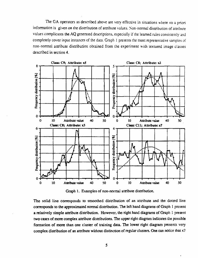