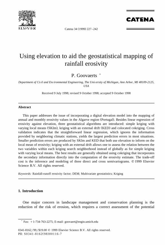
Ž .Catena 34 1999 227–242

Using elevation to aid the geostatistical mapping ofrainfall erosivity

P. Goovaerts )

Department of CiÕil and EnÕironmental Engineering, The UniÕersity of Michigan, Ann Arbor, MI 48109-2125,USA

Received 9 July 1998; revised 9 October 1998; accepted 9 October 1998

Abstract

This paper addresses the issue of incorporating a digital elevation model into the mapping ofŽ .annual and monthly erosivity values in the Algarve region Portugal . Besides linear regression of

erosivity against elevation, three geostatistical algorithms are introduced: simple kriging withŽ . Ž .varying local means SKlm , kriging with an external drift KED and colocated cokriging. Cross

validation indicates that the straightforward linear regression, which ignores the informationprovided by neighboring climatic stations, yields the largest prediction errors in most situations.Smaller prediction errors are produced by SKlm and KED that both use elevation to inform on thelocal mean of erosivity; kriging with an external drift allows one to assess the relation between thetwo variables within each kriging search neighborhood instead of globally as for simple krigingwith varying local means. The best results are generally obtained using cokriging that incorporatesthe secondary information directly into the computation of the erosivity estimate. The trade-offcost is the inference and modeling of three direct and cross semivariograms. q 1999 ElsevierScience B.V. All rights reserved.

Keywords: Rainfall-runoff erosivity factor; DEM; Multivariate geostatistics; Kriging

1. Introduction

One major concern in landscape management and conservation planning is thereduction of the risk of erosion, which requires a correct assessment of the potential

) Fax: q1-734-763-2275; E-mail: goovaert@engin.umich.edu

0341-8162r99r$19.00 q 1999 Elsevier Science B.V. All rights reserved.Ž .PII: S0341-8162 98 00116-7

( )P. GooÕaertsrCatena 34 1999 227–242228

transport capabilities of runoff generated by erosive storms. A preliminary step is to mapthe rainfall erosivity in the area under management. The rainfall-runoff erosivity factorŽ . Ž .R of the Revised Universal Soil Loss Equation RUSLE is generally recognized as

Žone of the best indicators of the erosive potential of raindrops impact Renard et al.,.1991a,b . Because rainfall erosivity is not distributed uniformly through the year, the

assessment of soil erosion requires knowledge of the seasonal distribution of R, hencethe existence of rainfall measurements with high temporal resolution. Daily-read rain-gauge stations are expensive, and so rainfall erosivity is typically known only at alimited number of locations. It is thus critical to capitalize on any source of informationto predict erosivity values at unmonitored locations.

Until the late 80s, techniques such as the inverse distance, Thiessen polygons, orisohyetals have been used to interpolate rainfall data. Geostatistics, which is based on

Ž .the theory of regionalized variables Journel and Huijbregts, 1978; Goovaerts, 1997 , isincreasingly used because it allows one to capitalize on the spatial correlation betweenneighboring observations to predict attribute values at unsampled locations. Several

Ž .authors Tabios and Salas, 1985; Phillips et al., 1992 have shown that geostatisticsprovides better estimates of precipitation than conventional methods. A major advantage

Ž .of geostatistical prediction kriging is that sparsely sampled observations of the primaryattribute can be complemented by secondary attributes that are more densely sampled. A

Fig. 1. Location of the study area and positions of the 36 climatic stations.

( )P. GooÕaertsrCatena 34 1999 227–242 229

valuable and cheap source of information for many climatic attributes is provided byŽ .digital elevation models. Martinez-Cob and Cuenca 1992 used cokriging to incorporate

Ž .elevation into the mapping of evapotranspiration. Hevesi et al. 1992a,b applied asimilar approach to the mapping of precipitation using a network of 62 stations

Ž .complemented by a digital elevation model. Hudson and Wackernagel 1994 usedanother geostatistical technique, known as kriging with an external drift, to map Januarymean temperature for the whole of Scotland combining the information provided by 145climate stations with a digital elevation model.

ŽIn this paper, three geostatistical algorithms simple kriging with varying local means,.kriging with an external drift, colocated ordinary cokriging are introduced to incorpo-

Ž .rate an exhaustive secondary information digital elevation model into the spatialprediction of rainfall erosivity. The techniques are illustrated using annual and monthlyrainfall data from the Algarve region in Portugal. Cross validation is used to comparethe prediction performances of the three geostatistical interpolation algorithms with thestraightforward linear regression.

2. Setting the problem

The Algarve is the most southern region of Portugal, with an area of approximately5000 km2. Fig. 1 shows the location of 36 daily-read raingauge stations where thefollowing three rainfall parameters were measured from January 1970 to March 1995:

Fig. 2. Information available for mapping of annual erosivity: observations at 36 climatic stations and a digitalelevation model.

( )P. GooÕaertsrCatena 34 1999 227–242230

Ž .monthly rainfall, monthly rainfall for days where precipitation exceeds 10 mm rain ,10Ž .and the monthly number of days where precipitation exceeds 10 mm days . At each10

of these stations, the monthly erosive storm empirical index EI was computed30month

using the regression equation:

EI s6.56 rain y75.09 days r 2 s0.92 1Ž .30 month 10 10

As expected, the more rainfall within a smallest number of days, the larger theŽ .rainfall erosivity. Relation 1 was calibrated from measurements recorded at 17

Ž .tipping-bucket raingauges time resolutions1 min between October 1992 and March1995; 12 of these high resolution raingauges are located in the daily-read stationsaforementioned. For each erosive storm occurring during this period, EI values were30

Žcomputed according to the RUSLE handbook instructions Wischmeier and Smith, 1978;. Ž .Renard et al., 1991b in SI units of MJ.mmrha.h Foster et al., 1981 . Monthly values

were computed as the sum of EI for each erosive storm during this month. Because30Ž .the Algarve is an homogeneous rainfall region, Eq. 1 was applied to the 25 years time

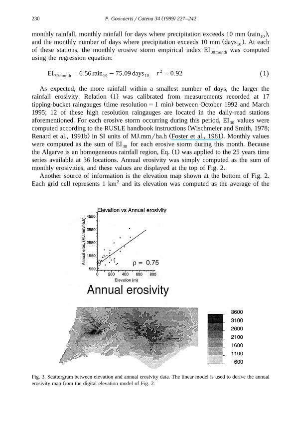
series available at 36 locations. Annual erosivity was simply computed as the sum ofmonthly erosivities, and these values are displayed at the top of Fig. 2.

Another source of information is the elevation map shown at the bottom of Fig. 2.Each grid cell represents 1 km2 and its elevation was computed as the average of the

Fig. 3. Scattergram between elevation and annual erosivity data. The linear model is used to derive the annualerosivity map from the digital elevation model of Fig. 2.

( )P. GooÕaertsrCatena 34 1999 227–242 231

elevations at four discrete points within the cell. The relief is dominated by the two mainŽ . Ž . Ž .Algarve’s mountains: the Monchique left and the Caldeirao right . Fig. 3 top graph˜

shows that the annual erosivity is positively correlated with elevation, hence, it seemsworth accounting for this exhaustive secondary information into the mapping of rainfallerosivity.

3. Mapping of the erosivity index

� Ž . 4Let z u , as1, . . . ,n be the set of erosivity values measured at ns36 locationsa

u . Elevation is denoted by y and is available at all primary data locations u and at alla a

locations u being estimated. Using this information, one aims at estimating the erosivityz at any grid node u.

3.1. Linear regression

A straightforward approach consists of modeling the relation between elevation anderosivity, e.g., using a linear function of the type:

) )z u s f y u sa qa y u . 2Ž . Ž . Ž . Ž .0 1

This relation is then used to convert each elevation into an erosivity value. ForŽ .example, the relation between annual erosivity and elevation was modeled as z u s

Ž .968.2q3.8087 y u , leading to the erosivity map shown at the bottom of Fig. 3. Amajor shortcoming of this type of regression is that the erosivity at a particular grid nodeu is derived only from the elevation at u, regardless of the erosivity value at thesurrounding climatic stations u . Such an approach amounts at assuming that erosivitya

values are independent from one another, which is rarely the case in practice.Spatial dependence between observations can be detected using the semivariogram

which is a measure of average dissimilarity between observations as a function of theŽ .separation vector h. The experimental semivariogram g h is computed as half theˆ

average squared difference between the components of every data pair:

Ž .N h1 2g h s z u yz u qh , 3Ž . Ž . Ž . Ž .ˆ Ý a a2 N hŽ .

as1

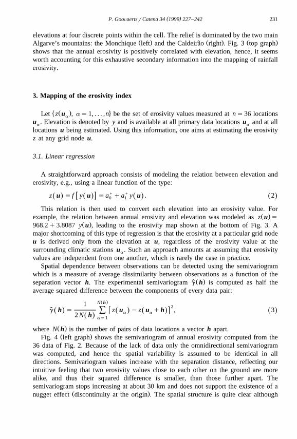
Ž .where N h is the number of pairs of data locations a vector h apart.Ž .Fig. 4 left graph shows the semivariogram of annual erosivity computed from the

36 data of Fig. 2. Because of the lack of data only the omnidirectional semivariogramwas computed, and hence the spatial variability is assumed to be identical in alldirections. Semivariogram values increase with the separation distance, reflecting ourintuitive feeling that two erosivity values close to each other on the ground are morealike, and thus their squared difference is smaller, than those further apart. Thesemivariogram stops increasing at about 30 km and does not support the existence of a

Ž .nugget effect discontinuity at the origin . The spatial structure is quite clear although

( )P. GooÕaertsrCatena 34 1999 227–242232

Fig. 4. Experimental semivariograms of annual erosivity and elevation computed from the information of Fig.2.

only a few observations are available to compute the semivariogram. Such spatialpattern of erosivity is, to a large extent, imparted by elevation that varies smoothlythrough the study area, as illustrated by the absence of nugget effect on the semivari-

Ž .ogram of Fig. 4 right graph .

3.2. The geostatistical approach

Geostatistical interpolation allows one to account for the spatial dependence betweenobservations in the prediction of attribute values. Most of geostatistics is based on theconcept of a random function, whereby the set of unknown values is regarded as a set of

Ž .spatially dependent random variables. Each measurement z u is thus interpreted as aa

Ž .particular realization of a random variable Z u . Interested readers should refer toa

Ž . Ž . Ž . Žtextbooks such as Isaaks and Srivastava 1989 pp. 196–236 or Goovaerts 1997 pp..59–74 for a detailed presentation of the theory of random functions.

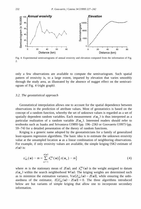
Kriging is a generic name adopted by the geostatisticians for a family of generalizedleast-squares regression algorithms. The basic idea is to estimate the unknown erosivityvalue at the unsampled location u as a linear combination of neighboring observations.

Ž .For example, if only erosivity values are available, the simple kriging SK estimate ofŽ .z u is:

Ž .n u) SKz u yms l u z u ym 4Ž . Ž . Ž . Ž .ÝSK a a

as1

Ž . SK Ž .where m is the stationary mean of Z u , and l u is the weight assigned to datuma

Ž . Ž .z u within the search neighborhood W u . The kriging weights are determined sucha

� ) Ž . Ž .4as to minimize the estimation variance, Var Z u yZ u , while ensuring the unbi-SK� ) Ž . Ž .4asedness of the estimator, E Z u yZ u s0. The three algorithms introducedSK

below are but variants of simple kriging that allow one to incorporate secondaryinformation.

( )P. GooÕaertsrCatena 34 1999 227–242 233

3.2.1. Simple kriging with Õarying local meansŽ .Simple kriging with varying local means SKlm amounts at replacing the known

Ž Ž .. ) Ž .stationary mean in the SK estimate Eq. 4 by known varying means m u derivedSKŽ .from the secondary information Goovaerts, 1997, pp. 190–191 :

Ž .n u) ) SK )z u ym u s l u z u ym u . 5Ž . Ž . Ž . Ž . Ž . Ž .ÝSKlm SK a a SK a

as1

Ž .If the local means are derived using a linear regression of type 2 , the SKlm estimatew Ž .x ) Ž .can be rewritten as the sum of the regression estimate f y u sm u and the SKSK

estimate of the residual value at u:

Ž .n u) ) SKz u sm u q l u r uŽ . Ž . Ž . Ž .ÝSKlm SK a a , 6Ž .as1

)s f y u qr uŽ . Ž .SK

Ž . Ž . w Ž .x SK Ž .where the residual r u is defined as z u y f y u . The weights l u area a a a

obtained by solving the simple kriging system:

Ž .n uSKl u C u yu sC u yu as1, . . . ,n u 7Ž . Ž . Ž . Ž . Ž .Ý b R a b R a

bs1

Ž . Ž . Ž . Ž .where C h is the covariance function of the residual RF R u sZ u ym u , not thatRŽ . Ž .of Z u itself. If the residuals are uncorrelated, C h s0 ; h, hence all krigingR

Ž .weights in Eq. 6 are zero and the SKlm estimate is but the value provided by linearregression.

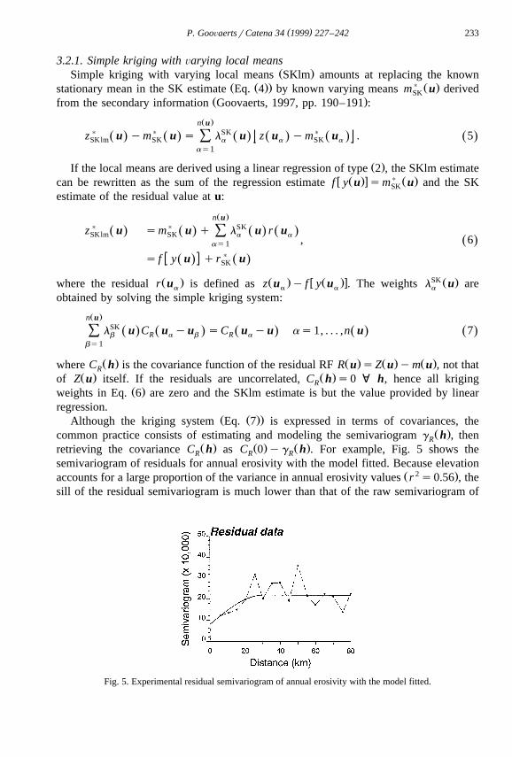
Ž Ž ..Although the kriging system Eq. 7 is expressed in terms of covariances, theŽ .common practice consists of estimating and modeling the semivariogram g h , thenR

Ž . Ž . Ž .retrieving the covariance C h as C 0 yg h . For example, Fig. 5 shows theR R R

semivariogram of residuals for annual erosivity with the model fitted. Because elevationŽ 2 .accounts for a large proportion of the variance in annual erosivity values r s0.56 , the

sill of the residual semivariogram is much lower than that of the raw semivariogram of

Fig. 5. Experimental residual semivariogram of annual erosivity with the model fitted.

( )P. GooÕaertsrCatena 34 1999 227–242234

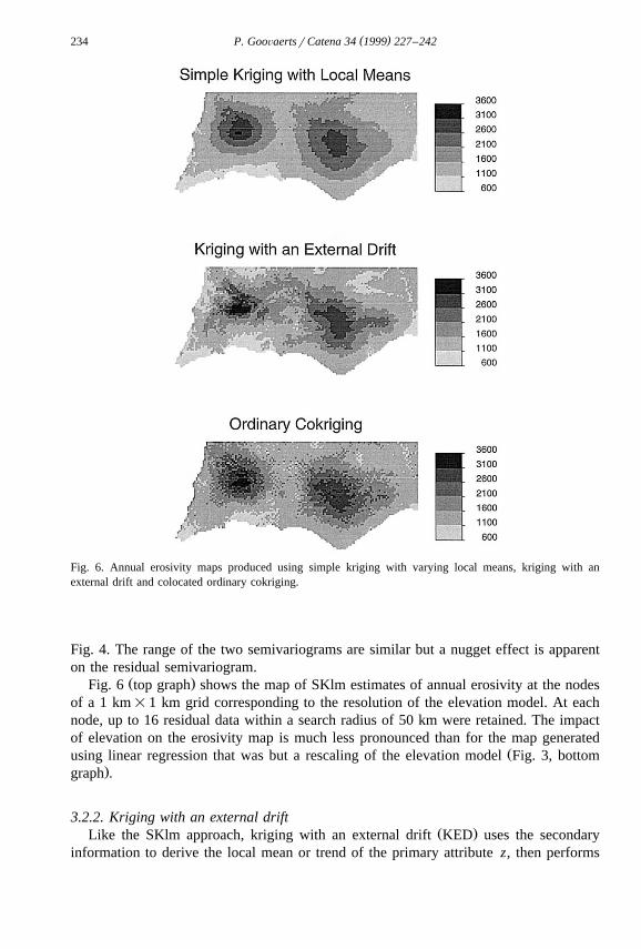
Fig. 6. Annual erosivity maps produced using simple kriging with varying local means, kriging with anexternal drift and colocated ordinary cokriging.

Fig. 4. The range of the two semivariograms are similar but a nugget effect is apparenton the residual semivariogram.

Ž .Fig. 6 top graph shows the map of SKlm estimates of annual erosivity at the nodesof a 1 km=1 km grid corresponding to the resolution of the elevation model. At eachnode, up to 16 residual data within a search radius of 50 km were retained. The impactof elevation on the erosivity map is much less pronounced than for the map generated

Žusing linear regression that was but a rescaling of the elevation model Fig. 3, bottom.graph .

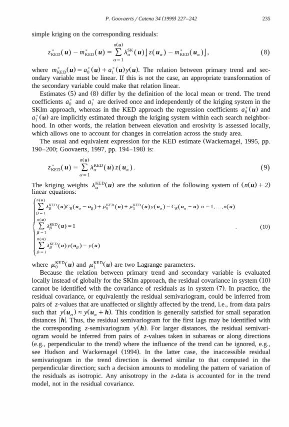
3.2.2. Kriging with an external driftŽ .Like the SKlm approach, kriging with an external drift KED uses the secondary

information to derive the local mean or trend of the primary attribute z, then performs

( )P. GooÕaertsrCatena 34 1999 227–242 235

simple kriging on the corresponding residuals:

Ž .n u) ) SK )z u ym u s l u z u ym u , 8Ž . Ž . Ž . Ž . Ž . Ž .ÝKED KED a a KED a

as1

) Ž . ) Ž . ) Ž . Ž .where m u sa u qa u y u . The relation between primary trend and sec-KED 0 1

ondary variable must be linear. If this is not the case, an appropriate transformation ofthe secondary variable could make that relation linear.

Ž . Ž .Estimates 5 and 8 differ by the definition of the local mean or trend. The trendcoefficients a) and a) are derived once and independently of the kriging system in the0 1

) Ž .SKlm approach, whereas in the KED approach the regression coefficients a u and0) Ž .a u are implicitly estimated through the kriging system within each search neighbor-1

hood. In other words, the relation between elevation and erosivity is assessed locally,which allows one to account for changes in correlation across the study area.

ŽThe usual and equivalent expression for the KED estimate Wackernagel, 1995, pp..190–200; Goovaerts, 1997, pp. 194–198 is:

Ž .n u) KEDz u s l u z u . 9Ž . Ž . Ž . Ž .ÝKED a a

as1

KEDŽ . Ž Ž . .The kriging weights l u are the solution of the following system of n u q2a

linear equations:Ž .n u°

KED KED KEDl u C u y u qm u qm u y u sC u y u a s1, . . . ,n uŽ . Ž . Ž . Ž . Ž . Ž . Ž .Ý b R a b 0 1 a R a

b s1

Ž .n uKED~ l u s1Ž . . 10Ž .Ý b

b s1

Ž .n uKEDl u y u s y uŽ . Ž . Ž .Ý b b¢

b s1

KEDŽ . KEDŽ .where m u and m u are two Lagrange parameters.0 1

Because the relation between primary trend and secondary variable is evaluatedŽ .locally instead of globally for the SKlm approach, the residual covariance in system 10

Ž .cannot be identified with the covariance of residuals as in system 7 . In practice, theresidual covariance, or equivalently the residual semivariogram, could be inferred frompairs of z-values that are unaffected or slightly affected by the trend, i.e., from data pairs

Ž . Ž .such that y u fy u qh . This condition is generally satisfied for small separationa a

< <distances h . Thus, the residual semivariogram for the first lags may be identified withŽ .the corresponding z-semivariogram g h . For larger distances, the residual semivari-

ogram would be inferred from pairs of z-values taken in subareas or along directionsŽ .e.g., perpendicular to the trend where the influence of the trend can be ignored, e.g.,

Ž .see Hudson and Wackernagel 1994 . In the latter case, the inaccessible residualsemivariogram in the trend direction is deemed similar to that computed in theperpendicular direction; such a decision amounts to modeling the pattern of variation ofthe residuals as isotropic. Any anisotropy in the z-data is accounted for in the trendmodel, not in the residual covariance.

( )P. GooÕaertsrCatena 34 1999 227–242236

ŽA more sophisticated alternative consists of estimating the parameters range, sill,.nugget effect of the residual semivariogram model using restricted maximum likelihood

Ž .Gotway and Hartford, 1996 . This method requires, however, a prior assumptionregarding the shape of the semivariogram model, e.g., spherical, exponential, etc.

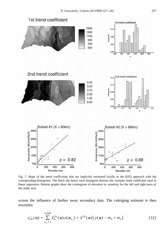
Because of the small size of the Algarve data set and the absence of a systematictrend along a particular direction, it was not possible to compute an experimentalresidual semivariogram. The residual semivariogram model was then built empiricallyusing a spherical scheme with a zero nugget effect and a range of 30 km as thesemivariogram of annual erosivity. The sill has no impact on the kriging weights andwas arbitrarily set to the sill of the semivariogram of residuals displayed in Fig. 5. Fig. 6Ž .middle graph shows the map of KED estimates of annual erosivity. It bears moreresemblance to the elevation map of Fig. 2 than does the map of SKlm estimates. Theimpact of elevation is particularly pronounced in the left part of the study area, while thevariation is much smoother in the right part. Such spatial difference in the contribution

) Ž .of secondary information can be depicted by mapping the two trend coefficients a u0) Ž . Ž .and a u using the procedure described in Goovaerts 1997, pp. 196–197 .1

Fig. 7 shows that the slope of the local linear regression between elevation andŽ .erosivity i.e., second trend coefficient , and so the influence of the secondary informa-

tion, decreases from left to right. The first trend coefficient exhibits a reverse trend. Thetwo histograms emphasize the large range of the local trend coefficients, as opposed tothe constant coefficients used in the SKlm approach and depicted by black dots. Thelarge value of the regression slope in the left part of the Algarve arises from the

Ž .coexistence of the smallest and largest Monchique Mountain erosivity values there.This regional difference is illustrated by plotting the scattergrams of elevation vs.

Ž .erosivity for the climatic stations with x-coordinates-80 km subset a1 and the onesŽ . Ž .with x-coordinates)80 km subset a2 , see Fig. 7 bottom graph .

3.2.3. Ordinary cokrigingAnother approach for incorporating secondary information is cokriging, a multivari-

Ž . Ž .ate extension of kriging Goovaerts, 1997, pp. 203–248 . The cokriging CK estimate isa linear combination of neighboring primary and secondary data:

Ž . Ž .n u n u1 2

) CK CKz u s l u z u q l u y u ym qm , 11Ž . Ž . Ž . Ž . Ž . Ž .Ý ÝCK a a a a Y Z1 1 2 2a s1 a s11 2

where m and m are the means of the primary and secondary variables, respectively.Z Y

Note that one uses a particular formulation of ordinary cokriging whereby the secondaryvariable is rescaled so that its mean equals that of the primary variable. The so-called‘standardized’ ordinary cokriging enhances the contribution of the secondary variable

Žand reduces the risk of getting aberrant estimates such as negative erosivity Goovaerts,.1998 .

Ž .When the secondary variable is known everywhere e.g., elevation there is little lossin retaining in the cokriging system only the secondary datum colocated with the

Ž . Ž .location u being estimated Xu et al., 1992 . Indeed the colocated datum y u tends to

( )P. GooÕaertsrCatena 34 1999 227–242 237

Fig. 7. Maps of the trend coefficients that are implicitly estimated locally in the KED approach with thecorresponding histograms. The black dot below each histogram denotes the constant trend coefficient used inlinear regression. Bottom graphs show the scattergram of elevation vs. erosivity for the left and right parts ofthe study area.

screen the influence of further away secondary data. The cokriging estimate is thenrewritten:

Ž .n u1

) CK CKz u s l u z u ql u y u ym qm . 12Ž . Ž . Ž . Ž . Ž . Ž .ÝCK a a Y Z1 1a s11

( )P. GooÕaertsrCatena 34 1999 227–242238

The main difference between cokriging and the two previous geostatistical algorithmslies in how the colocated y-datum is handled. Whereas that datum directly influencesthe cokriging estimate, in the SKlm and KED approaches that secondary datum providesinformation only about the primary trend at location u.

Ž Ž . .The cokriging weights are solutions of the following system of n u q2 linear1equations:

Ž .n u1°CK CK CKl u C u y u q l u C u y u qm u sC u y u a s1, . . . ,n uŽ . Ž . Ž . Ž . Ž . Ž . Ž .Ý b ZZ a b Z Y a ZZ a 1 11 1 1 1 1

b s11

Ž .n u1

CK CK CK~ l u C uy u q l u C 0 qm u sC 0Ž . Ž . Ž . Ž . Ž . Ž .Ý b Y Z b Y Y Z Y1 1b s11

Ž .n u1

CK CKl u q l u s1Ž . Ž .Ý a1¢a s11

Ž .where C u yu is the cross covariance between primay and secondary variables atZ Y a1

locations u and u, respectively.a1

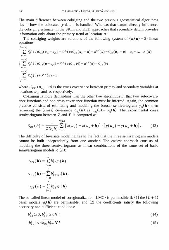
Cokriging is more demanding than the other two algorithms in that two autocovari-ance functions and one cross covariance function must be inferred. Again, the common

Ž . Ž .practice consists of estimating and modeling the cross semivariogram g h , theni jŽ . Ž . Ž . Ž .retrieving the cross covariance C h as C 0 yg h . The experimental crossi j i j i j

semivariogram between Z and Y is computed as:

Ž .N h1g h s z u yz u qh P y u yy u qh . 13Ž . Ž . Ž . Ž . Ž . Ž .ˆ ÝZ Y a a a a2 N hŽ .

as1

The difficulty of bivariate modeling lies in the fact that the three semivariogram modelscannot be built independently from one another. The easiest approach consists ofmodeling the three semivariograms as linear combinations of the same set of basic

Ž .semivariogram models g h :l

Llg h s b g hŽ . Ž .ÝZZ ZZ l

ls0

Llg h s b g hŽ . Ž . .ÝY Y Y Y l

ls0

Llg h s b g hŽ . Ž .ÝZ Y Z Y l

ls0

Ž . Ž . Ž .The so-called linear model of coregionalization LMC is permissible if: 1 the Lq1Ž . Ž .basic models g h are permissible, and 2 the coefficients satisfy the followingl

necessary and sufficient conditions:

bl G0, bl G0 ; l 14Ž .ZZ Y Y

l l l< < (b F b b ; l 15Ž .Z Y ZZ Y Y

( )P. GooÕaertsrCatena 34 1999 227–242 239

Fig. 8. Experimental semivariograms of annual erosivity and elevation and their cross semivariogram, with thelinear model of coregionalization fitted.

In practice, the modeling is performed in two steps:1. both direct semivariograms are first modeled as linear combinations of selected basic

Ž .structures g h ,l

2. the same basic structures are then fitted to the cross semivariogram under theŽ .constraint 15 .

This approach was used to fit visually a spherical scheme with a 30 km range to theŽ .cross semivariograms of annual erosivity and elevation displayed in Fig. 8.

Ž .Fig. 7 bottom graph shows the map of cokriging estimates of annual erosivity. Asfor the SKlm approach, the details of the elevation map do not appear in the erosivitymap.

4. Comparative performance of the different estimators

The performances of the different kriging algorithms were assessed and comparedŽ .using cross validation Isaaks and Srivastava, 1989, pp. 351–368 . The idea consists of

removing temporarily one datum at a time from the data set and ‘re-estimate’ this valuefrom remaining data using the alternative algorithms. All computations have been

Ž .performed using the geostatistical software Gslib Deutsch and Journel, 1998 .

( )P. GooÕaertsrCatena 34 1999 227–242240

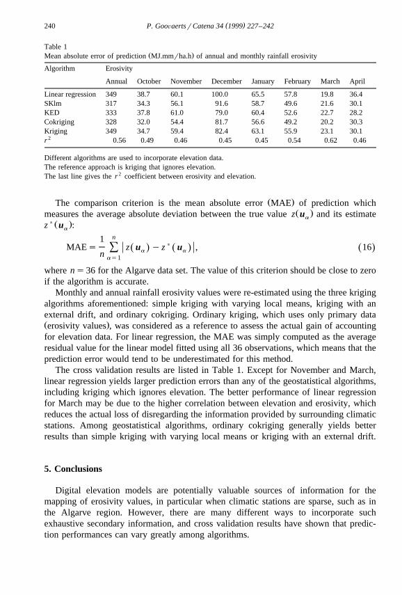
Table 1Ž .Mean absolute error of prediction MJ.mmrha.h of annual and monthly rainfall erosivity

Algorithm Erosivity

Annual October November December January February March April

Linear regression 349 38.7 60.1 100.0 65.5 57.8 19.8 36.4SKlm 317 34.3 56.1 91.6 58.7 49.6 21.6 30.1KED 333 37.8 61.0 79.0 60.4 52.6 22.7 28.2Cokriging 328 32.0 54.4 81.7 56.6 49.2 20.2 30.3Kriging 349 34.7 59.4 82.4 63.1 55.9 23.1 30.1

2r 0.56 0.49 0.46 0.45 0.45 0.54 0.62 0.46

Different algorithms are used to incorporate elevation data.The reference approach is kriging that ignores elevation.The last line gives the r 2 coefficient between erosivity and elevation.

Ž .The comparison criterion is the mean absolute error MAE of prediction whichŽ .measures the average absolute deviation between the true value z u and its estimatea

) Ž .z u :a

n1)MAEs z u yz u , 16Ž . Ž . Ž .Ý a an

as1

where ns36 for the Algarve data set. The value of this criterion should be close to zeroif the algorithm is accurate.

Monthly and annual rainfall erosivity values were re-estimated using the three krigingalgorithms aforementioned: simple kriging with varying local means, kriging with anexternal drift, and ordinary cokriging. Ordinary kriging, which uses only primary dataŽ .erosivity values , was considered as a reference to assess the actual gain of accountingfor elevation data. For linear regression, the MAE was simply computed as the averageresidual value for the linear model fitted using all 36 observations, which means that theprediction error would tend to be underestimated for this method.

The cross validation results are listed in Table 1. Except for November and March,linear regression yields larger prediction errors than any of the geostatistical algorithms,including kriging which ignores elevation. The better performance of linear regressionfor March may be due to the higher correlation between elevation and erosivity, whichreduces the actual loss of disregarding the information provided by surrounding climaticstations. Among geostatistical algorithms, ordinary cokriging generally yields betterresults than simple kriging with varying local means or kriging with an external drift.

5. Conclusions

Digital elevation models are potentially valuable sources of information for themapping of erosivity values, in particular when climatic stations are sparse, such as inthe Algarve region. However, there are many different ways to incorporate suchexhaustive secondary information, and cross validation results have shown that predic-tion performances can vary greatly among algorithms.

( )P. GooÕaertsrCatena 34 1999 227–242 241

The most straightforward approach consists of deriving the erosivity value directlyŽ .from the colocated elevation through a non linear regression. By so doing, one ignores

the information provided by surrounding climatic stations which is critical when thecorrelation between the two variables is not too strong. An easy way to account for suchinformation is to interpolate the residuals using geostatistics, that is to use simple krigingwith varying local means. The SKlm approach reduces the influence of elevation on theerosivity map and, except for one month, yields smaller prediction errors than directregression.

Kriging with an external drift is more sophisticated than simple kriging with varyinglocal means in that the relation between elevation and erosivity is evaluated locally. Thecase study showed that the trend coefficients vary substantially across the study area andthat elevation tends to influence strongly the KED estimate, especially when the

Ž .estimated slope a u of the local trend model is large. Cross validation indicates,1

however, that this additional complexity does not pay off for this data set.Whereas the SKlm and KED approaches use elevation only to inform on the local

mean of erosivity, cokriging incorporates the secondary datum directly into the computa-tion of the estimate. Also, as opposed to the local assessment of the correlation betweenerosivity and elevation performed by kriging with an external drift, colocated cokrigingaccounts for the global linear correlation between primary and secondary variables ascaptured by the cross semivariogram. Cokriging may seem more demanding in that threesemivariograms must be inferred and jointly modeled, yet the linear model of coregion-alization allows flexible fitting, in particular for the case of two variables. Crossvalidation shows this additional complexity pays off in that the smallest prediction errorsare usually obtained using cokriging.

Acknowledgements

The author thanks Mr. Nuno de Santos Loureiro for the Algarve data set.

References

Deutsch C.V., Journel, A.G., 1998. GSLIB: Geostatistical Software Library and User’s Guide: Second edition.Oxford Univ. Press, New York, 369 pp.

Foster, G.R., McCool, D.K., Renard, K.G., Moldenhauer, W.C., 1981. Conversion of the universal soil lossŽ .equation to SI metric units. Journal of Soil and Water Conservation 36 6 , 355–359.

Goovaerts, P., 1997. Geostatistics for natural resources evaluation. Oxford Univ. Press, New York, 483 pp.Ž .Goovaerts, P., 1998. Ordinary cokriging revisited. Mathematical Geology 30 1 , 21–42.

Gotway, C.A., Hartford, A.H., 1996. Geostatistical methods for incorporating auxiliary information in theŽ .prediction of spatial variables. Journal of Agricultural, Biological and Environmental Statistics 1 1 ,

17–39.Hevesi, J.A., Istok, J.D., Flint, A.L., 1992a. Precipitation estimation in mountainous terrain using multivariate

geostatistics: I. Structural analysis. Journal of Applied Meteorology 31, 661–676.Hevesi, J.A., Flint, A.L., Istok, J.D., 1992b. Precipitation estimation in mountainous terrain using multivariate

geostatistics: II. Isohyetal maps. Journal of Applied Meteorology 31, 677–688.

( )P. GooÕaertsrCatena 34 1999 227–242242

Hudson, G., Wackernagel, H., 1994. Mapping temperature using kriging with an external drift: theory and anexample from Scotland. International Journal of Climatology 14, 77–91.

Isaaks, E.H., Srivastava, R.M., 1989. An introduction to applied geostatistics. Oxford Univ. Press, New York,561 pp.

Journel A.G., Huijbregts, C.J., 1978. Mining geostatistics. Academic Press, New York, 600 pp.Martinez-Cob, A., Cuenca, R.H., 1992. Influence of elevation on regional evapotranspiration using multivari-

ate geostatistics for various climatic regimes in Oregon. Journal of Hydrology 136, 353–380.Phillips, D.L., Dolph, J., Marks, D., 1992. A comparison of geostatistical procedures for spatial analysis of

precipitations in mountainous terrain. Agricultural and Forest Meteorology 58, 119–141.Renard, K.G., Foster, G.R., Weesies, G.A., Porter, J.P., 1991a. RUSLE—Revised Universal Soil Loss

Ž .Equation. Journal of Soil and Water Conservation 46 1 , 30–33.Renard, K.G., Foster, G.R., Weesies, G.A., McCool, D.K., 1991b. Predicting soil erosion by water—a guide

Ž .to conservation planning with the revised universal soil loss equation RUSLE . U.S. Department ofAgriculture, Agricultural Research Service, Draft 6r92.

Tabios, G.Q., Salas, J.D., 1985. A comparative analysis of techniques for spatial interpolation of precipitation.Water Resources Bulletin 21, 365–380.

Wackernagel, H., 1995. Multivariate Geostatistics. Springer, Berlin, 256 pp.Wischmeier, W.H., Smith, D.D., 1978. Predicting rainfall erosion losses—a guide to conservation planning.

U.S. Department of Agriculture, Science and Education Administration, Agricultural Research, AgricultureHandbook No. 537, 58 pp.

Xu, W., Tran, T.T., Srivastava, R.M., Journel, A.G., 1992. Integrating seismic data in reservoir modeling: thecollocated cokriging alternative. Society of Petroleum Engineers, paper no. 24742.