Using derivative estimates to describe intraindividual variability at multiple time scales

Intraindividual Variability 1

Running head: INTRAINDIVIDUAL VARIABILITY

Describing Intraindividual Variability at Multiple Time Scales Using Derivative Estimates

Pascal R. Deboeck

University of Notre Dame

Mignon A. Montpetit


C. S. Bergeman


Steven M. Boker

University of Virginia


Abstract

The study of intraindividual variability is central to the study of individuals in psychology.

Previous research has related the variance observed in repeated measurements (time

series) of individuals to trait–like measures that are logically related. The use of

intraindividual measures such as intraindividual standard deviation or the coefficient of

variation are likely to be incomplete representations of intraindividual variability. This

paper shows that studying intraindividual variability can be made more productive by

examining variability of interest at specific time scales, rather than considering the

variability of entire time series. Furthermore, examination of variance in observed scores

may not be sufficient, as these neglect the time scale dependent relationships between

observations. The current paper outlines a method to examine intraindividual variability

through estimates of the variance and other distributional properties at multiple time

scales using estimated derivatives. In doing so, this paper encourages more nuanced

discussion about intraindividual variability and highlights that variability and variance are

not equivalent. An example with simulated data and an example relating variability in

daily measures of negative affect to neuroticism are provided.


Describing Intraindividual Variability at Multiple Time

Scales Using Derivative Estimates

As psychological methods have evolved, a movement has been made “to

conceptualize key behavioral and behavioral change matters in more dynamical,

change–oriented terms rather than the static, equilibrium–oriented terms that have tended

to dominate our history” (Nesselroade, 2004, p.45); this shift has brought with it a focus

on intraindividual variability. Individual data are the combination of many different

sources of variability (Nesselroade, 1991; Nesselroade & Boker, 1994). Constructs may

fluctuate within days, within weeks (e.g., weekend effect), within months (e.g., hormonal

effects), within years (e.g., seasonal effects), and within a lifetime. At each time scale,

variables may differentially affect constructs such as mood; consider, for example the effect

of work demands at a within–day scale, global stress at a weekly scale, socioeconomic

status at a monthly scale, resilience resources at an annual scale, and personality over the

course of a lifetime. Some commonly used methods for modeling intraindividual change

may not be ideal for modeling intraindividual variability; for example, growth curve

modeling (McArdle & Epstein, 1987; Meredith & Tisak, 1990) and hierarchical linear

modeling (HLM; Bryk & Raudenbush, 1987; Lairde & Ware, 1982; Pinheiro & Bates,

2000), because these fit a trend to the data and thus may average over intraindividual

variability or partition this variability into the error terms of the models.

One common way that intraindividual variability has been examined is by

calculating the intraindividual standard deviation or coefficient of variation (standard

deviation divided by the mean) of a time series (e.g., Christensen et al., 2005; Cranson et

al., 1991; Eid & Diener, 1999; Eizenman, Nessleroade, Featherman, & Rowe, 1997; Finkel

& McGue, 2007; MacDonald, Hultsch, & Dixon, 2003; Mullins, Bellgrove, Gill, &

Robertson, 2005). Although such studies provide initial insights into intraindividual


variability, particularly as the standard deviation of a time series would seem intuitively to

describe intraindividual variability, this approach is incomplete. These approaches have

two limitations: 1) the standard deviation neglects the ordering of the observations, and

2) the sampling rate and time over which measurements are collected are frequently not

considered, which may result in differing conclusions between researchers.

Consideration of Observation Ordering

When a standard deviation is calculated from a time series, the ordering of the

information is not taken into account. To see why the ordering of observations is

important, consider the following thought experiment. A researcher is interested in

assessing whether three individuals differ in their variability on a construct. Three time

series, such as those in Figure 1, are collected and the standard deviation of each time

series is calculated for each. These time series seem to correspond to individuals who

differ in their variability; for example individual “c” might be considered more variable

than individual “a.” The researcher, however, will be disappointed to find that the

standard deviation of each of these time series is exactly equal, as the time series consist

of the same observations rearranged in different orders.

While this likely would not occur in practice, the example highlights that the

standard deviation may not differentiate between individuals that appear to differ in

variability. The information the standard deviation neglects is the rate at which

individuals are changing, information which cannot be captured unless one considers the

ordering of the observations. Most descriptions of highly variable individuals involve not

just a wide range of scores, but also that high scores and low scores follow each other in

quick succession. That is, it is desirable to also consider the change in scores with respect

to a change in time.

The change in one variable with respect to another is called a derivative. On a


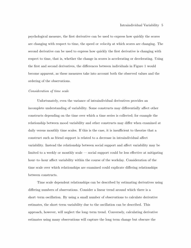
psychological measure, the first derivative can be used to express how quickly the scores

are changing with respect to time, the speed or velocity at which scores are changing. The

second derivative can be used to express how quickly the first derivative is changing with

respect to time, that is, whether the change in scores is accelerating or decelerating. Using

the first and second derivatives, the differences between individuals in Figure 1 would

become apparent, as these measures take into account both the observed values and the

ordering of the observations.

Consideration of time scale

Unfortunately, even the variance of intraindividual derivatives provides an

incomplete understanding of variability. Some constructs may differentially affect other

constructs depending on the time over which a time series is collected; for example the

relationship between mood variability and other constructs may differ when examined at

daily versus monthly time scales. If this is the case, it is insufficient to theorize that a

construct such as friend support is related to a decrease in intraindividual affect

variability. Instead the relationship between social support and affect variability may be

limited to a weekly or monthly scale — social support could be less effective at mitigating

hour–to–hour affect variability within the course of the workday. Consideration of the

time scale over which relationships are examined could explicate differing relationships

between constructs.

Time scale dependent relationships can be described by estimating derivatives using

differing numbers of observations. Consider a linear trend around which there is a

short–term oscillation. By using a small number of observations to calculate derivative

estimates, the short–term variability due to the oscillation can be described. This

approach, however, will neglect the long–term trend. Conversely, calculating derivative

estimates using many observations will capture the long term change but obscure the


short–term oscillation. Calculation of derivative estimates at different time scales will

allow relationships that occur at differing time scales to emerge. This tradeoff between

being able to resolve finer detail and smoothing to enhance global features, is well known

in the time series literature; the principle is used in low and high pass filtering to focus on

features that occur over a particular length of time (Gasquet & Witomski, 1999; Kwok &

Jones, 2000; Rothwell, Chen, & Nyquist, 1998).

Multiple Time Scale Derivative Estimation

By examining the derivative estimates of a time series in addition to the observed

scores, and by examining multiple time scales rather than a single time scale, researchers

will be able to understand intraindividual variability in significantly more detail. To

accomplish this goal, it is necessary to first identify a method that can be used to estimate

derivatives using differing numbers of observations. While several options exist (e.g., see

Boker & Nesselroade, 2002; Boker, Neale, & Rausch, 2004; Ramsay & Silverman, 2005),

this paper uses a technique called Generalized Local Linear Approximation (GLLA)

(Boker, Deboeck, Edler, & Keel, in press; Savitzky & Golay, 1964). Although selection of

this method is tangential to the primary objective of this paper, the rationale for using

GLLA includes: 1) its ability to use any number of observations to estimate a derivative

(e.g., 3, 4, 5, 6...) thereby automatically smoothing over different time scales, 2) it tends

to produce a narrower sampling distribution than its predecessor (LLA, Boker &

Nesselroade, 2002), 3) it produces observed rather than latent estimates (e.g., Boker et

al., 2004), and 4) it can be adapted to accommodate non–equally spaced observations

(although we will assume equally spaced observations in this paper). Depending on the

analytic needs imposed by one’s data, alternative choices for derivative estimation may be

warranted.


The calculation of derivative estimates using GLLA, can be expressed as

Y = XL(L′L)−1. (1)

Matrix X is a reorganization of an individual’s observed time series and is called an

embedded matrix. Matrix L is used to produce the weights that will calculate the desired

derivative estimates. The resulting matrix Y contains estimates of both the observed

scores and derivatives of a time series.

The embedded matrix X is constructed using replicates of an individual time series

that are offset from each other in time. Creation of X requires a time series

X = {x1, x2, . . . , xT } and the the number of observations to be used for each derivative

estimation (number of embedding dimensions)1. If we were interested in using 4 observed

values to estimate each derivative, X would consist of rows of 4 adjacent observations,

with no pair of rows containing the same set of observations. For a time series with N

observations, a matrix of embedding dimension four would have the form:

X(4) =

x1 x2 x3 x4

x2 x3 x4 x5

......

...

x(N−3) x(N−2) x(N−1) xN

. (2)

For example, consider a time series X = {49, 50, 51, 52, 53, 54, 55, 56} which consists of 8


observations (N = 8). The embedded matrix X(4), with four embeddings, would look like:

X(4) =

49 50 51 52

50 51 52 53

51 52 53 54

52 53 54 55

53 54 55 56

. (3)

The number of embedded dimensions determines the number of observations used to

calculate each derivative estimate. For additional examples related to the use of embedded

matrices in psychology, see Boker et al. (2004) and Boker and Laurenceau (2006).

The L matrix produces weights that express the relationship between X and Y.

Each column requires three pieces of information: 1) a vector ν consisting of values from 1

to the number of embeddings (columns in X(4)), 2) the time between successive

observations in the time series ∆t, and 3) the order α of the derivative estimate of interest

(observed score order = 0, first derivative estimate order = 1, second derivative estimate

order = 2, etc.). The values of each column can then be calculated using

Lorder =(∆t(ν − ν))α

α!, (4)

where ν is the mean of ν, and ! is standard notation for a factorial. If one wanted to

calculate estimates up to the second derivative, one would calculate three column vectors

(0th, 1st and 2nd order) using Equation 4 and bind these vectors together to form L. For

example, if one were to calculate up to the second order, using four embeddings


(ν = {1, 2, 3, 4}) and ∆t = 1,

L =

1 −1.5 1.125

1 −0.5 0.125

1 0.5 0.125

1 1.5 1.125

. (5)

It should be noted that the number of embeddings must be at least one greater than the

maximum derivative order examined; this is related to the fact that calculating a linear or

quadratic trend requires a minimum of two and three observations respectively (Singer &

Willett, 2003, p. 217). In addition, even if one is interested only in a higher–order

derivative, columns for all lower–order derivatives must be included in L.

Using Equation 1 and the X and L that have been generated, one can calculate

Y = XL(L′L)−1 =

50.5 1.0 0

51.5 1.0 0

52.5 1.0 0

53.5 1.0 0

54.5 1.0 0

. (6)

The first, second and third columns correspond, respectively, to estimates of the observed

scores, first derivative and second derivative for each row of X. The estimates of observed

scores are equal to the average for the observations in each row of X. The first derivative

estimates, which are all equal to 1.0, indicate that for all rows the scores are changing 1

unit with each 1 unit increase in time; this is equivalent to the slope within each row. The

second derivative estimates are all equal to zero, indicating that within each row the rate

at which scores are changing is neither accelerating or decelerating.


Using GLLA Derivative Estimates

Using GLLA to calculate estimates of observed scores and derivatives at multiple

time scales, subsequent analysis steps could proceed much as previous studies and

depending on the questions of the researcher. The primary change that occurs is a need

for more specific hypotheses regarding intraindividual variability. A hypothesis would

need to include the order of the derivative estimates, the distributional property that

would be examined, and the time scale over which relationships are expected. One might

hypothesize, for example, that more neurotic individuals tend to show higher variance in

the first derivative estimates of negative affect over time scales of a several days. Such a

study would regress estimates of neuroticism against estimates of first derivative variance

at a range of daily to weekly time scales.

The selection of the order of derivative estimates to examine will depend on the

statement one hopes to make about intraindividual variability. (For now, we will focus on

examining the variance of a distribution and ignore the specific time scale at which

relationships may be observed.) A researcher who believes that a trait may relate to

individuals using a wider or narrower range of scores on a scale would be able to examine

such a relationship using the variance of the observed scores. A researcher who believes a

trait may relate to some individuals not changing much between two occasions and other

individuals having rapid increases and/or decreases in score would be able to examine

such a relationship using first derivative estimates; the first derivative expresses the rate of

change, or velocity, of scores and therefore low variance would correspond to a small range

of velocities while a high variance would correspond to a large range of velocities. A

researcher who believes a trait may be related to whether or not individuals show quick

increases in scores followed by quick decreases (or vice versa) would be able to examine

such a relationship using the second derivative estimates. The second derivative, or

acceleration, is highest when scores either rapidly increase and then decrease, or vice versa.


Individuals with high variance in second derivative estimates would show a wide range of

accelerations, while low variance individuals would show more consistent acceleration.

Variability and Variance

It is also important to distinguish between variability and variance. Variance is one

distributional property that could be used to describe intraindividual variability but other

distributional properties, such as skewness and kurtosis, may also be informative. When

applied to observed scores, differences in skewness and kurtosis take on the expected

interpretations; however these alternative distributional properties offer unique

substantive interpretations when applied to derivative estimates rather than the observed

scores. Consider a time series with little overall trend. When the distribution of first

derivative estimates is positively skewed this would suggest an individual who exhibits

only a few large positive slopes and but many smaller negative slopes. This person would

appear to quickly become very distressed, and require much more time to slowly reduce

his or her distress. When the distribution of first derivative estimates is negatively skewed

this would suggest an individual with who exhibits many, smaller positive slopes and only

a few, large negative slopes. This person would appear to require a lot of time to build up

distress, but is then able to quickly alleviate their distress by “blowing off steam.” It

would be interesting to see if a trait could be used to predict individuals who display first

derivative estimates with more positive or negative skew.

The kurtosis of the first derivative estimates also offers an intriguing avenue for

characterizing intraindividual variability. Consider an individual with a leptokurtic

distribution, which would correspond to many more small changes over time (peaked), and

a few extra very large changes over time (additional observations in tails). An individual

with a platykurtic distribution would display fewer very large changes over time and fewer

small changes over time, primarily showing moderate changes most of the time. This first


person, then, would appear not to change their distress level very much from day-to-day

(fairly consistent amount of distress), although occasionally large positive and negative

changes in distress occur (e.g., days punctuated with good/bad luck). The second person,

however, does not have the extreme changes and also has many fewer days with small

changes in distress. Rather, this second person’s distress level changes by a more

moderate amount almost every single day (e.g., most days a new drama arises).

In practice we cannot assume that distributional properties, such as the mean of the

first derivative, are on average equal to zero for all individuals. Consequently, when

interpreting the results from a particular distributional property, the lower distributional

properties must be kept in mind. For example, imagine that one finds that a trait is

related to variance of the first derivative estimates. Individuals may still have differing

means for the first derivative estimates; that is some individuals may have an upwards

trend and others a downwards trend. The relationship between the trait and variance only

conveys information regarding the variance around each individual’s central tendency.

Similarly, if a significant relationship were shown between a trait and skewness, this does

not rule out the potential that within individuals high and low on the trait there could be

a variety of distributions with differing means and variances. Consideration of this point

will be further discussed in the applied example.

Relationship to Time Series Methods

Using GLLA to estimate derivatives can be broadly categorized into the class of

linear filters that are common in much of the time series analysis and signal processing

literatures(Gasquet & Witomski, 1999; Gottman, 1981). In signal processing, linear filters

are often used to eliminate frequencies or components that may be undesirable, such as

those associated with noise. For example, the time scale over which derivatives are

estimated will serve a similar function to low and high pass filters. Unlike typical linear


filters, however, we are not utilizing the filters merely to remove a component from the

data, such as “noise.” GLLA derivative estimates will focus on a specific time scale

depending on the embedding dimension and time lag selected. By doing so, we are

purposefully attempting to extract a derivative estimate at a particular time scale.

When estimating the 0th order derivatives, that is the observed scores, the estimates

produced by GLLA will be similar to those of moving average algorithms. It is the use of

filters corresponding to higher order derivatives that should be of particular interest in

psychology. Rather than decomposing a signal into components, such as sine waves, a

derivative filter will literally provide information regarding how people are changing at a

particular time scale. This substantive interpretation, which seems to map well onto how

people discuss individual changes over time, motivates the selection of this particular filter.

Proposed Application

The combination of derivative estimates selected, and distributional properties

examined, should directly relate to a researcher’s conceptualization of variability. This

poses the question for theory: What does high intraindividual variability mean? Although

answers are seemingly intuitive, consider the following example. You are told that

someone you know is a driver with high intraindividual variability. One way a driver could

show large variability is by having large variations in the distance from home that person

drives on any given occasion (high variance in observed scores). The driver also could

display a great deal of variance in his or her speed by using the entire range on the

speedometer (high variance in the first derivative). That person also could have large

variance in speed changes by slamming on the brakes or flooring the gas pedal (high

variance in the second derivative). Due to the variety of possible interpretations, there is a

need to be more specific when conceptualizing intraindividual variability.

We will utilize GLLA as one of several possible methods to produce derivative


estimates using a range of time scales. The analysis of the distributional properties of

derivatives across multiple time scales will be referred to as Derivative Variability Analysis

(DVA). In the following sections we pose questions such as: At what time scales (daily?

weekly?) are individuals who are higher/lower on some trait more variable in their time

series scores and its derivative estimates? The first application consists of a simulation

study, in which two types of time series are created. To each of these time series are added

random events, the amplitude of which are related to a trait–like variable. Analysis of

these data demonstrate the ability of derivative–based analyses at multiple time scales to

detect this relationship and the time scale at which it occurs. In the second application,

we apply the method described to examine the relationships between intraindividual

variability in negative affect and the trait of neuroticism.

Application I: Simulation Study

We will first consider an example with simulated data. Unlike typical simulations,

we do not seek to define the parameter space over which a statistic is applicable. Rather,

we create two different types of trajectories composed of many different, overlapping

sources of variability which are used to generate individual time series. Within the

variability and measurement error of each time series is a component of the intraindividual

variability that relates to a trait variable. With these examples we will explore whether

DVA can be used to detect the portion of the intraindividual variability related to the

trait variable, even though it is highly obscured.

For this simulation, time series are created with known characteristics. The variance

of the observed scores of the time series, and variance of estimated derivatives, are

examined in relation to an exogenous predictor. The simulation will demonstrate that

some relationships may not be apparent in observed score variance, but can be observed

when using the variance of derivative estimates. The simulation also will demonstrate that


relationships occurring at specific time scales can be highlighted using DVA.

Methods

Two very different types of time series were examined; the parameters selected for

these time series are arbitrary, but this does not alter the substance of these examples.

The first type of time series consisted of the linear combination of four sources of

variability, which can be imagined to correspond to a construct that consists of an overall

trend, with an approximately monthly oscillation that occasionally changes phase,

combined with a few random life events that perturb the system for about a week, plus

measurement error.

The oscillating trend was selected such that it would correspond to a cycle longer

than one month, assuming the space between observations is equal to one day. The

oscillating trend was defined using 5 sin(ω ∗ time+ δ), in which ω ∼ N(0.15, 0.02); the 95%

confidence interval for ω corresponds to cycles of 33.2 to 56.7 days. The parameter δ

equaled zero at t = 1 and had a 5% chance at each subsequent point in time of randomly

resetting to a value drawn from a uniform distribution bounded by 0 and 2π; the reset

chance of 5% was selected to represent a moderate probability of a serious disruption

occurring on any particular day. A linear trend with a slope randomly drawn from a

normal distribution with mean of zero and standard deviation of 0.13. The mean of zero

was selected to allow for both positive and negative slopes. The standard deviation was

selected such that the contributions of both the oscillating trend and linear trend were

similar in amplitude for many time series; the oscillation has an amplitude from −5 to +5,

while time series at one standard deviation from the mean on slope will be expected to

change 13 points over the 100 observations observed. The third source of variability

consisted of randomly placed “events” that perturbed the system for about 7 days; this

particular length was selected with the intension of representing a moderately disruptive


event in one’s life. This perturbation was created using approximately one–half of an

oscillation, defined by the equation sin(0.53 ∗ tw), where tw = {0, 1, . . . , 6} and 0.53

corresponds to the approximate ω value required for one–half cycle of the desired length.

The events were multiplied by a random uniform distribution consisting of the values −1

and 1, to allow for both positive and negative perturbations. Finally, independent,

normally distributed errors were added to each time series with mean of zero and a

standard deviation of 12.4, corresponding to a signal to noise ratio of approximately 5 to

1; these values were selected to represent a scale with reasonable reliability. Figure 2a

and 2b depicts two examples of these simulated data.

The second type of time series consisted of a linear combination of three sources of

variability, which can be imagined to correspond to a construct where today’s value is

highly related to yesterday’s value and somewhat related to the value of the day before, a

few random life events that perturb the system for about a week, plus measurement error.

The first source was a second–order autoregressive process, that is,

xt = a1xt−1 + a2xt−2 + γi. The random variable γi, often called the innovation, was drawn

from a normal distribution with mean of zero and variance of one. The autoregressive

parameters a1 and a2 were set to 0.7 and 0.31 respectively; in selecting these parameters

the considerations were that a1 should be relatively large such that adjacent observations

are moderately to highly correlated, and that a1 + a2 > 1 so that the process would not be

stationary. The second and third sources of variability, randomly placed “events” and

independent, normally distributed errors, were specified exactly as they were in the

overlapping variability time series described above. Figure 2c and 2d depicts two examples

of these simulated data.

For both types of times series, each individual time series was paired with a value yi

drawn from a normal distribution (µ = 3, σ = 1). Two conditions were considered for each

type of time series. In one condition, the amplitude of the randomly placed “events” for a


particular time series was multiplied by the value yi. In the other condition, the amplitude

of the randomly placed “events” for a particular time series was multiplied by a value

randomly drawn from the same distribution as yi. In the first condition the time series

should display a small amount of additional intraindividual variability related to the trait

variable y. In the second condition no such relationships should occur. Moreover, as we

know that the events are about 7 observations in length, this is the time scale at which

observation of relationships between the time series x variability and the trait score y are

expected.

To be able to examine the expected results in the long run, a sufficiently large

number of time series and single trait score sets must be analyzed. We examined 50, 000

sets, with the assumption that this was sufficiently large, for each of the four conditions:

overlapping variability related to trait, overlapping variability unrelated to trait,

autoregressive related to trait, and autoregressive unrelated to trait. Time series were

each 100 observations long. Each of the four groups were analyzed as a single sample

using the procedure described in the next section. Although it would be unusual to

acquire such a large sample, the analysis results should reflect the central tendency of

expected results if this simulation were replicated using many smaller samples.

Analysis.

The following outlines the broad conceptual steps that are taken in applying DVA to

the simulated data, and later the set of applied data. Readers interested in applying DVA

are referred to Appendices A and B, which include R syntax and a detailed description of

how to apply the syntax (R, 2008). This analysis focuses on applying the ideas from the

introduction, that is applying DVA in the context of correlating properties of time series

with a specific trait; DVA could be adapted to consider other derivatives, distributional

properties, time scales and even the relationships between pair of time series.

Step 1: First, researchers need to select the conditions to be studied, including 1)


the embedding dimension(s), 2) the order of the derivatives, and 3) the distributional

property or properties. In selecting embedding dimensions, there are several factors to

consider. On the low end, an embedding dimension of 3 is required for estimation of

derivatives up to the second derivative. The highest recommendable embedding dimension

will depend on the length of the time series and the amount of missing data. Note, when

using GLLA, an embedding dimension of 10 will require 10 consecutive observations to

estimate a single derivative; one will require several estimates to produce an estimate of a

distribution. Consequently, even small amounts of missing data can rapidly reduce the

number of estimates that can be generated from the data. It is important to consider the

number of estimates that will be produced by GLLA for each individual for a particular

embedding, and the number of individuals for whom enough estimates can be produced

such that a distributional property can be examined.

The second decision is in regard to the order of the derivatives to be examined; as

described in the introduction, the selection of the derivative order should be related to a

researcher’s conceptualization of intraindividual variability — whether conceptualized as

variability in observed scores, the rate at which scores change, or the rate at which scores

accelerate and decelerate. Finally the distributional property to be examined must be

selected. As discussed in the introduction, the choice of distributional properties should

also relate to a researcher’s conceptualization of intraindividudal variability, whether just

variance or also including features such as skewness and/or kurtosis. For the simulated

data example, the variance of the observed scores and first derivative estimates will be

examined. The embedding dimensions were selected both to encompass the length of the

random events related to the trait of interest, and to mimic the analysis of the applied

data example; embedding dimensions from 3 to 30 will be examined.

Step 2: The next step is to calculate a distributional property for an order of

derivative at a particular embedding for each individual time series. Since each


combination of distributional property, derivative order, and embedding dimension must

be considered as an individual set of conditions, let us consider a specific example where

the variance of the first derivative estimates is being calculated using an embedding

dimension. For example, let us assume that we are calculating values associated with an

embedding dimension of 10. For each individual time series, one creates an embedded

matrix Xi. GLLA, as described in the introduction, is then used to produce the matrix of

derivative estimates Yi. From Yi the column corresponding to the first derivative

estimates is selected. The variance can then be calculated from these estimates. The

process of embedding matrices and calculating a distributional property is performed for

each individual time series. The result will be one estimate per individual, where the

estimate will equal a distributional property of interest, for a particular derivative order,

at a particular embedding.

Step 3: The previous step produces a vector of estimates N individuals in length,

which can then be correlated with a vector of trait scores for the corresponding

individuals. For the specific example in Step 2, the resulting correlation will address

whether a trait is related to the variance of first derivative estimates at a time scale

equivalent to the time spanned by 10 observations (i.e., and embedding dimension of 10).

Correlations have been selected in the current paper due to their interpretability, however

other applications of these methods may warrant the calculation of other statistics (e.g.,

slope estimates); regardless of the statistic selected in this step, the other steps for

analysis will remain unchanged.

Step 4: The standard errors produced when calculating a correlation may not be

accurate when using DVA, as the assumptions may be violated. Consequently hypothesis

tests and confidence intervals produced by statistical programs should be ignored when

using DVA. Rather, confidence intervals that do not require distributional assumptions,

that is non–parametric confidence intervals, should be calculated using the bootstrap


(Efron & Tibshirani, 1994). To bootstrap the data, pairs of variability and trait estimates

are randomly drawn from the original data, with replacement, to form a bootstrap sample.

The correlation is then calculated on this sample, and the process is repeated a large2

number of time such that a distribution of correlations is formed. In the example

provided, the percentile confidence intervals are reported; for a 95% confidence interval,

this method only requires one to sort the results from the bootstrap samples and select

the upper and lower values for the middle 95% of the distribution3.

DVA will typically involve a large number of statistical tests, as correlations will be

calculated for each embedding dimension multiplied by the number of orders of derivatives

and the number of distributional properties considered. Therefore, applications of this

method should adopt stricter criteria than the typical 95% confidence interval, so as to

limit the frequency of Type I errors; not doing so could produce a large number of Type I

errors and consequently mislead researchers. Until further research is done, we encourage

the use of the conservative Bonferroni correction (α = 0.05/comparisons) so as to

maintain the Type I error rate at 0.05 within a each family of comparisons (Maxwell &

Delaney, 2000). We have selected a family of comparisons to consist of all of the

comparisons within a particular derivative order and distributional property; that is, all

the tests conducted across the range of embedding dimensions. With the range of

embedding dimensions selected for the simulation, 3 to 30, there will be 28 tests conducted

for each combination of distribution property and derivative order. Our corrected α level

would then be equal to 0.00179 (0.05/28), and we would form a 99.82% confidence interval

for each embedding. Consequently, the probability of making a Type I error for the 28

comparisons will still be less than 0.05. As with all statistical tests, users are encouraged

to judiciously select a priori the tests to be performed; such a choice determines the

extent to which results can be considered confirmatory, rather than exploratory.

Step 5: In Steps 2 through 4 focus was placed on calculating the correlation and


confidence intervals for one specific combination of distributional property, derivative

order, and embedding dimension. The last step is to repeat the process for each

combination of conditions which were selected in Step 1.

In summary, the steps involve the following: 1) select distributional properties

(variance, skewness, kurtosis), derivatives (observed score, first derivative, second

derivative) and time scales (embedding dimensions) for analysis; 2) for a specific

derivative and time scale, calculate a distributional property for each individual; 3)

calculate the correlation or statistic of interest between a trait and the estimates from

Step 2; 4) use a non–parametric procedure and a multiple–testing procedure to get

accurate confidence intervals, 5) repeat for all combinations of distributional properties,

derivative orders and time scales selected in step 1.

Results

Figure 3 shows the DVA results for both types of time series. Although a typical

application of DVA would include confidence intervals, they are not shown in the figure as

the lines are expected to reflect the results in the population due to the simulation

design4. The upper and lower pairs of graphs correspond to the conditions in which the

trait y are respectively unrelated and related to the amplitude of the random “events”

added to each system. If we had regressed the trait against estimates of the standard

derivation of time series, the results would be most similar to the results for the observed

scores (solid line) at the lowest embedding dimension. That is, commonly used analyses

would be the equivalent of only one point on one of the lines which we have shown,

ignoring a substantial amount of potentially interesting information.

Using DVA, no relationships were expected when the trait and the “event”

amplitude were unrelated, as observed in the upper pair of graphs. Relationships were

expected when the trait and the “event” amplitude were related, as observed in the lower


pair of graphs. When the trait is regressed on the observed score variance these

relationships are not apparent due to the many other sources of variability in each time

series. The variances of the first and second derivative estimates reflect that there is a

short–term relationship between the trait and the intraindividual variability; this result

was present in each of the two types of time series that were simulated, suggesting that

the result is not unique to a type of time series. In creating the time series, the random

“events” were created to be 5 to 7 days in length. This feature of the data seems to

correspond well with the peak of the relationship observed in the first derivative estimates.

The peak of the relationship with second derivative variance is less well defined than first

derivative variance; this is likely to be related to the variance of the sampling distribution

of the second derivative estimates as well as the shape of the random events added to each

system.

Conclusions

While simulated data, this application highlighted several aspects of DVA. First, it

demonstrated the examination of the relationship between a trait and a particular

distributional property (variance) of different derivatives (0th to 2nd order) over multiple

time scales (3 to 30 embeddings). Second, the results highlight the possibility that

differing relationships can be observed depending on the derivative order and time scales

examined. Third, examination of the standard deviation or coefficient of variation of the

observed scores would yield results similar to the lowest embedding for the observed score

variance; those result suggests that no relationships exist between the trait and time series.

Specification of the time scale, derivatives and distributional properties will impact

the conclusions one can draw about relationships with other constructs when examining

intraindividual variability. It is tenable that relationships in applied research may occur at

specific time scales. For example, if one considered the relationships between


intraindividual variability on stress and the personality trait of dispositional resilience

(Maddi & Kobasa, 1984), the application of DVA might suggest whether lability in stress

is related to dispositional resilience, and whether these effects are universal or whether

they occur at some specific time scale (e.g., daily, weekly, or monthly). It might be that

the ability to shift efficiently between mood states in the short–term is adaptive, but that

maintaining this lability over time may cease to be helpful and even be related to poor

psychological functioning when considered over a longer time span.

It should be noted that even events of a specific length in time will alter the

estimation of derivatives at both longer and shorter time scales; consequently adjacent

embedding dimensions tend to produce similar correlation estimates. This blending of

time scales is important to keep in mind when considering results, as the time scale of a

relationship may actually be narrower than portrayed using DVA based on GLLA. Future

research may better illuminate under which conditions differing derivative estimation

techniques may be used for more precise estimation of the time scale of a relationship.

Application II: Applied Data Example

This applied example, exploring the relationship between neuroticism and negative

affect, will demonstrate the information that can be garnered using DVA. Given that

neuroticism is either defined as an inherent propensity to experience negative affectivity or

as a greater tendency for emotional lability (Costa & McCrae, 1980), the example

examines the relationships between a trait measure of neuroticism and daily

intraindividual variability in negative affect. Research has resulted in considerable debate

surrounding these variables; some authors propose that there is conceptual and

measurement overlap in neuroticism and negative affect (Ormel, Rosmalen, & Farmer,

2004) or negative affectivity (Watson & Clark, 1984; Fujita, 1991), suggesting redundancy

in the constructs. That is, neuroticism is highly correlated with an individuals’ typical


level of distress. Others consider predictive relationships among the constructs, implying

that the constructs are related, but are not the same (Bolger & Zuckerman, 1995; Mrocek

& Almeida, 2004). In other words, neuroticism may make people more vulnerable to the

negative consequences of stress, an indirect, rather than direct, effect (Suls & Martin,

2005). Using DVA, we can ultimately disentangle the extent to which neuroticism relates

to the level of distress (negative affect) or to the volatility (change in negative affect), and

whether the relationship between these constructs changes over a variety of timeframes.

Methods

Participants.

Participants consisted of a subsample from the Notre Dame Longitudinal Study of

Aging (see Wallace, Bergeman, & Maxwell, 2002 for details). Following the initial

questionnaires assessing various aspects of the aging process, participants were invited to

participate in a 56–day daily diary study. Of the 86 people invited, 66 (77%) participated

in the daily data collection. The individuals who provided daily data were, on average,

three years younger than those who declined to participate (t = 2.17; p < .05), but there

were no significant differences by gender, race, marital status, or living situation (e.g.,

alone or with others). The participants who participated in the daily data collection were

predominantly older (Mage = 79 years; SD = 6.21 years), female (75%), living either alone

(54%) or with a spouse (45%), educated (98% through high school, 61% some post–high

school), and white (90%, 5% African–American, 5% Hispanic.)

Measures.

Daily negative affect was measured using the Positive and Negative Affect Schedule

(PANAS; Watson, Clark, & Tellegan, 1988). Participants were asked to select from a

5–point scale for each of the 20 affect items, examples of which include

“irritable,”“distressed,” “attentive” and “inspired.” Internal consistency reliability


assessed on Day 1 was high (Cronbach’s α = .85). The sum of the 10 negative items on

any given day was used as an index of negative affect, with higher scores indicating more

negative affect. Daily data were collected over 56 days, with one, two, and three–week

packets counterbalanced within and between subjects

Neuroticism was assessed using a subscale of the Revised NEO Personality

Inventory (NEO PI–R; Costa & McCrae, 1991). The twelve items were scored such that

higher scores indicated higher levels of Neuroticism. Internal consistency reliability was

high (Cronbach’s α = .88).

Analysis.

In these analyses, the distributional properties variance, skewness and kurtosis were

examined using both observed score and the first derivative estimates. Estimates were

examined from embedding dimension of 3 days (the shortest value that can be using

GLLA if allowing for estimates up to the second derivative) to an embedding dimension of

30 days (approximately the longest value that seemed advisable given the length of the

data and the presence of missing observations). As with the simulation, for each

individual time series an estimate was made for each combination of distributional

property (3 levels), derivative order (2 levels) and embedding dimension (28 levels, i.e., the

number of embedding dimensions from 3 to 30). Each combination of estimates (e.g.,

skewness of first derivative at embedding dimension of 12) was then correlated with the

neuroticism measure. Due to potential violations of assumptions, standard errors

produced for the correlation estimates may be inaccurate, and so confidence intervals were

generated for each correlation using bootstrapping. A minimum of 5 observed scores or

derivative estimates was required to estimate a distributional property for an individual;

this is very close to the minimum number of observations required to estimate kurtosis

and may lead poor estimates of distributional properties. A low minimum was used so as

to include as much of the sample as possible, even at higher embedding dimensions, at the


cost of larger standard errors around distributional estimates.

Due to the large number of relationships being examined (3 ∗ 2 ∗ 28 = 168 tests),

there was a very high probability of making a Type I error. Each combination of

distributional property and derivative order was therefore treated as a family of analyses

(3 ∗ 2 = 6 families). Within each family, each of the 28 comparisons were made using a

99.82% confidence interval. This confidence interval corresponds to the Bonferroni

corrected alpha to maintain a family–wise Type I error rate of 0.05 for 28 independent

tests (Maxwell & Delaney, 2000), which will be overly conservative in this case as tests

within family are correlated. By using the 99.82% confidence interval in this example, the

sum of all of our tests should be equivalent to making only 6 statistical tests using an

alpha much less than 0.05. Percentile confidence intervals were generated using 100,000

pair–wise boostrap samples5 of the data within each combination of distributional

property, derivative order and embedding dimension.

Results

Figure 4 plots the results for each combination of conditions, with the six figures

each corresponding to a combination of derivative order and distributional property. The

confidence intervals suggest only a few occasions at which the correlations between

negative affect distributional properties and neuroticism significantly differ from zero;

these are in the skewness of the first derivative estimates at an embedding dimension of 25,

the kurtosis of the observed scores at an embedding dimension of 10, and the kurtosis of

the first derivative estimates at embedding dimensions of 7, 9, 10 and 12. In interpreting

the results, two cautions are recommended. The first is regarding the results consisting of

a singular significant observation (skewness first derivative estimates 25, and kurtosis

observed score estimates 10). It is odd that the adjacent values are not also significant

and so these results may be due to some chance fluctuation; that being said, these may be


areas that could be more likely to produce significant results in future research. The

second caution is that null results should be interpreted with caution, as these results have

a high probability of being Type II errors given the Type I error corrections.

The kurtosis of the first derivative estimates suggest a relationship not apparent in

the other distributional properties or in the observed scores. These results suggest a

negative correlation between the estimated kurtosis of first derivative estimates of

Negative Affect and Neuroticism. Of the 7 embeddings that are near the zero correlation

line (embeddings 7 to 13), four of the confidence intervals do not contain zero. Given the

correction used on the confidence intervals, the probability of a Type I error rate has been

controlled to be much less than 0.05 for the entire set of 28 tests; the probability of four

significant results by chance is extremely small. These results suggest that at a weekly

time scale, as Neuroticism increases the first derivative estimates tend to become more

platykutic, while as Neuroticism decreases the first derivative estimates tend to be more

leptokurtic. More Neurotic individuals typically have distributions that include more

moderate rates of change over most weeks, compared to less Neurotic individuals who

experience smaller amounts of change on weekly basis with the occasional more extreme

change. Individuals with high or low neuroticism may still differ greatly in their means,

variances, and skewness.

Conclusions

The results provide some interesting information regarding the conceptualization of

Neuroticism. Based on the definition of neuroticism, it was expected that the variance of

the observed score or first derivative estimates would be correlated with neuroticism,

particularly at shorter time scales. As the results do not suggest such a relationship, it is

unclear whether there is no such relationship, or whether this is a Type II error.

Interestingly, a result was observed at short time scales in the kurtosis of the first


derivative estimates, which is concurrent with the definition of neuroticism. The results

suggest that less Neurotic individuals, relative to their mean rate of change, tend to have

more weeks with small change and the occasional larger change. More neurotic

individuals, however, are more likely to have moderate amounts of change each week

(most weeks a new drama arises), relative to their mean rate of change.

It should be cautioned that individuals both high and low in neuroticism may have

differences in their means, variances and skewness. So in interpreting the data, it is

possible that one neurotic individual may have scores with a positive trend and another

with a negative trend; the kurtosis results cannot inform us of this, but can inform us that

around each individuals’ central tendency (whether positive or negative), the rates of

change tend to be distributed around that trend in a more heavy–shouldered distribution

compared to a less neurotic individual.

For contrast, one may consider regressing Neuroticism against the standard

deviation of each individual time series, as has been done in previous studies of

intraindividual variability. With the results presented, one does not need to conduct this

analysis, as the results should be very similar to those for the variance of the observed

scores at the lowest embedding dimension — that is the first point on Figure 4a. While

one would have additional power if conducting only a single statistical test, from the other

figures it is clear that there is significantly more information that can be garnered from a

time series. Given the cost and time associated with collection of psychological data, it is

important to learn as much as possible from these time series.

There are several limitations to the present work, several of which must be

considered in all statistical applications but which are explicitly stated here because of the

method’s novelty. First, one must be cautious about the interpretation of the correlations

without regard to the confidence intervals because this may lead to misinterpretation or

over–interpretation of results. As distributional properties such as variance are often


skewed, spurious results can occur due to factors such as bivariate outliers; therefore, the

calculation and interpretation of bootstrapped confidence intervals are important to deal

with potential issues with distributional properties. Second, the results are subject to

standard correlation assumptions, namely that the error in measurement of the two

constructs are uncorrelated and that the constructs have a linear relationship. Third, for

proper interpretation of results it is critical that one considers the Type I error rate,

power due to sample size, and number of statistical tests performed. We have presented,

and suggested, a conservative approach that is unlikely to yield Type I errors, but could

result in many Type II errors. Fourth, the current sample had 66 people measured on 56

days. This study is likely then to be underpowered. Power for such studies could be

increased by carefully selecting which statistical tests are conducted such that less

correction is required to avoid Type I errors, collecting multivariate indicators, and

increasing either sample size or time series length.

The results presented here are unique from other applications where the standard

deviation or the coefficient of variation of an entire time series is used to represent

intraindividual variability. The information related to time scale of relationships will be

helpful in the designing of future studies, as valuable research resources can be saved by

sampling at rates corresponding to the relationships of interest. Through the richness of

interpretation by examining multiple distributional properties, combined with derivatives,

theory can move away from discussing individuals as more “variable” and discussing

specifically how they are more variable (i.e., Over which time scale? In their scores or

derivatives? In their variance, skewness or kurtosis?).

General Discussion

As research progresses towards a better understanding of the interface between

method and theory, the understanding of intraindividual variability has moved toward a


dynamic conceptualization of change (Nesselroade, 2006). Although fields such as

developmental psychology have often described long–term trends in adaptation to life’s

demands, increasingly the challenge is to understand intraindividual variability around

those trends. Because, presumably, those long–term trends result from constituent

experiences (e.g., momentary, daily, weekly, etc.), a natural scientific progression might be

to unite findings across levels of analysis, investigating how daily life experience

corresponds to the well-documented macroscopic trends observed using traditional

developmental methods.

Examination of the distributions of derivative estimates provides a methodology

that will begin to untangle the complexity of intraindividual variability. DVA highlights

the importance of specifically considering the time scales at which relationships occur.

Through the examination of derivative estimates, DVA detects relationships that might

otherwise be obscured by other sources of variability. Furthermore, through the

examination of distributional properties in addition to variance, nuanced understanding

can be gained about differences in how different individuals change over time.

The applications of DVA and the theoretical insights that may result are much

broader than the trait–state variability relationships presented. DVA could illuminate

relationships between daily process and life–span changes. This could be accomplished by

melding the concepts presented in this paper with the life–span modeling ability of

techniques such as HLM. One could then address questions regarding how the regulation

of daily fluctuations is related to long–term outcomes. DVA would also allow for the

consideration of coupled time series more broadly than is currently available with other

methods, including larger numbers of simultaneously coupled variables or consideration of

constructs that may differentially affect each other at different time scales. The

conceptual underpinnings of DVA can also be expanded in the future to accommodate

unequally spaced data, as derivative estimation does not require equidistant observations.


DVA also has the potential for far–reaching consequences in informing theory. These

include probing the relationships between traits and states or between short and longer

term intraindividual variability; informing the conceptualization of constructs; and

refining investigation of process–oriented models of change. The application of DVA

concepts is primarily constrained only by the type and way in which data are collected,

including the sampling rate and the length of time series collected.

Weekly measures, for example, will only allow for estimation of the second

derivative using 3 or more weeks; consequently weekly measures will only allow for

statements at approximately monthly scales or longer, depending on how long data are

collected. Because these limitations are inherent to study design, rather than to the

concepts presented, the flexible nature of DVA is likely to encourage more creative

sampling of constructs that change.

The information DVA provides may also be valuable in understanding how to pick a

model to describe intraindividual variability. Many areas of psychology begin to

understand the relationships between variables through the examination of correlations.

Differing distributional properties over time may motivate the selection of one model over

another; the time scale over which relationships with exogenous variable occur may also

inform how exogenous variables should be included in a model. As an increasing diversity

of methodologies for modeling intraindividual variability become available, the translation

of DVA results into models should become increasingly apparent.

As psychologists move toward more dynamic understandings of change over time,

additional methodological advances will be required to untangle the many sources of

variability that contribute to observed time series. Methods flexible enough to allow for

the examination of relationships at multiple time scales, and able to identify and partial

out variability of interest, will become increasingly important as we try to disentangle

antecedents, correlates, and sequelae of – as well as relationships between – long–term


trends and short–term variability. DVA provides a tool for the understanding of

intraindividual variability that parallels the first step taken in most psychological research:

gaining nuanced understanding of the correlations between constructs. By providing a

tool to further understand intraindividual variability, DVA will help inform both the

collection of data (i.e., ideal sampling rates for particular relationships) and the modeling

of data. Novel methods, such as those presented here, will allow psychological research to

consider the causes, effects, and interrelation of the waves, tides and currents of the

seemingly chaotic sea of intraindividual variability.


Appendix A

The following presents syntax that allows one to examine whether a particular trait

is related to a specific distributional property of a time series, for a particular order of

derivative, over a selected number of embeddings. The code presented is for the statistical

program R (2008), which is available for free through the internet and can be used on a

wide variety of computer platforms.

The lines marked with the symbol # consist of comments regarding the function or

implementation of this code. It is presumed that data have been scanned into R as two

variables: 1) “Data.Trait” consisting of a vector with length N , and 2) “Data.TimeSeries”

an N by T matrix containing the time series for each individual. The variables N and T

correspond to the total number of individuals, and the total number of observations in

each time series. The functions in Appendix B need to be copied and pasted into an active

R Console prior to application of the code presented in this appendix.

The code will be presented in five steps, corresponding to the five steps described in

the “Analysis” section of Application I. After the time series and trait data have been

loaded into R, the first step for derivative variability analysis requires one to select 1) the

embeddings (the time scale over which derivatives will be estimated), 2) the order of the

derivatives to be examined (Observed Scores, First Derivatives, or Second Derivatives),

and the distributional properties that will be examined (Variance, Skewness, Kurtosis).

For now, assume that a single embedding dimension, a single derivative order, and a single

distributional property have been selected for analysis.

The second step involves estimating the derivatives for each individual’s time series,

using a particular embedding dimension, and then calculating the distributional property

of interest from the estimates. This step can be accomplished by submitting to R,

temp <- CalculateProperty(Data.TimeSeries,Embedding,DerivativeOrder,Property)


with the values you selected in Step 1 substituted for the values between the parentheses.

That is, Data.TimeSeries should be the matrix containing your time series data, Embedding

should be replaced with a value for an embedding dimension, DerivativeOrder should be

replaced with ”Observed Scores”, ”First Derivative”, or ”Second Derivative”, and Property

should be replaced with ”Variance”, ”Skewness”, or ”Kurtosis”. For example one might use

temp <- CalculateProperty(Data.TimeSeries,5,"Observed Scores","Skewness")

to calculate the observed score skewness at an embedding dimension of 5. The sample

syntax, as written, will save the estimates to a variable call temp. Additional details about

the function CalculateProperty are included in Appendix B, following the comment

characters.

The third step involves calculating the correlation between the distributional

property estimates generated in Step 2 and a trait of interest. In the fourth step, a

bootstrapped confidence interval is produced for the estimate. Both steps are

accomplished by submitting to R,

result <- TestRelationship(temp,Data.Trait,alpha,Bootsamples)

where temp are the estimates from the previous step and Data.Trait is the vector with the

trait estimates for each individual6. The third value, alpha, corresponds to the Type I

error rate desired for the confidence intervals. If one were selecting a single test, one could

type 0.05 in place of alpha. If multiple tests are being conducted, to control the Type I

error rate, alpha should be divided by the number of tests within a family or experiment

(see Maxwell & Delaney, 2000 for a discussion of family–wise and experiment–wise control

of Type I errors). In the applied example provided, Type I error rates were controlled

within each family of comparisons involving 28 different embedding dimensions, so alpha

was set equal to 0.05/28. The selection of the number of times to resample the data while


bootstrapping (Bootsamples) will depend on the value selected for alpha. See Footnote 2

regarding the number of bootstrap samples. One might submit to R

result <- TestRelationship(temp,Data.Trait,.05/28,100000)

with 0.05/28 filled in for alpha and 100000 filled in for the number of Bootsamples. The

saved variable result will contain the information about the correlation between the trait

and the distributional property for the derivative estimates at a particular embedding.

The correlation can be accessed by typing result$Correlation and the confidence interval

can be accessed by typing result$ConfidenceInterval.

This process will only produce a single correlation and confidence interval. As in the

applied example one may wish to examine a range of conditions, for example a range of

embedding dimensions. So, corresponding to Step 5, the code presented can be easily

extended to such situations. For example, if one wished to examine the variance of the

first derivative over a range on embedding dimensions from 3 to 15, one might use the

following syntax:

MinEmbedding <- 3MaxEmbedding <- 15results <- matrix(NA,MaxEmbedding,3)

for(value in MinEmbedding :MaxEmbedding ) {temp <- CalculateProperty(Data.TimeSeries,value,"Observed Scores","Skewness")temp2 <- TestRelationship(temp,Data.Trait,.05/28,100000)results[value,] <- c(temp2$Correlation,temp2$ConfidenceInterval)}

This would produce a matrix results where the row number will correspond to the

embedding dimension, and the columns will correspond to the correlation (column 1) and

confidence interval (columns 2 and 3).


Appendix B

#Load library containing required functions. Prior to making this call, be#sure that the e1071 package has been installed from the CRAN libraries.#See ‘‘Package Installer’’ in R menus.library(e1071)

#Function to Embed DataEmbed <- function(x,Dimen) {

out <- matrix(NA,(length(x)-Dimen+1),Dimen)for(i in 1:Dimen) { out[,i] <- x[i:(length(x)-Dimen+i)] }return(t(out))}

#Function to Calculate properties of distribution of derivative estimatesCalculateProperty <- function(TimeSeries,Embedding,DerivativeOrder,Property)

{N <- dim(TimeSeries)[1]estimates <- rep(NA,N)

#Create L matrix to calculate derivative estimatesL1 <- rep(1,Embedding)L2 <- c(1:Embedding)-mean(c(1:Embedding))L3 <- (L2^2)/2L <- cbind(L1,L2,L3)W <- L%*%solve(t(L)%*%L)

#Set "DerivativeOrder" equal to a valueif(DerivativeOrder=="Observed Scores") whichDerivative <- 1if(DerivativeOrder=="First Derivative") whichDerivative <- 2if(DerivativeOrder=="Second Derivative") whichDerivative <- 3

#Apply following to each individual time seriesfor(i in 1:N) {#Embed time seriesEMat <- Embed(TimeSeries[i,],Embedding)#Estimate deriatives and select derivative order of interestDerivativeEstimates <- (t(W)%*%EMat)[whichDerivative,]#If there are very few derivative estimates, don’t create estimateif(sum(!is.na(DerivativeEstimates))<10) next

#Calculate the requested distributional property for the time seriesif(Property=="Variance") estimates[i] <- var(DerivativeEstimates,na.rm=TRUE)if(Property=="Skewness") estimates[i] <- skewness(DerivativeEstimates,na.rm=TRUE)


if(Property=="Kurtosis") estimates[i] <- kurtosis(DerivativeEstimates,na.rm=TRUE)}

#Return distribution estimates for all individualsreturn(estimates)}

#Function to calculate the correlation between a trait and the distributional#property of a selected derivative at a selected embedding dimensionTestRelationship <- function(Estimates,Trait,alpha,Bootsamples) {

#If there are very few pairs, don’t create estimatepercentdata <- sum((!is.na(Trait))*(!is.na(Estimates)))/length(Estimates)if(percentdata<0.5) {cat("ERROR: You have more missing pairs of data than observed pairs.")return(list(Correlation=NA,ConfidenceInterval=c(NA,NA)))}

OriginalResult <- cor(Trait,Estimates,use="complete.obs")ResampledResults <- rep(NA,Bootsamples)Start <- Sys.time()

#Bootstrap Resultsfor(i in 1:Bootsamples) {#Select from pairs of Trait & Estimate scores with replacementselect <- floor(runif(length(Trait),1,(length(Trait)+1)))#Calculate and save correlation on boostrap sampleResampledResults[i] <- cor(Trait[select],Estimates[select],use="complete.obs")

#If it has been a while, give an estimate as to how long this is going to take.#This "if" statement can be deleted without altering performance.if((i%%50000)==0) {

time <- as.numeric(difftime(Sys.time(),Start,units="mins"))time <- round(time/i*(Bootsamples-i),2)cat("Approximate time to complete bootstrap: ",time," minutes\n")}

}

#Calculate percentile confidence intervalsCI <- sort(ResampledResults)[c(floor(alpha/2*Bootsamples),

ceiling((1-(alpha/2))*Bootsamples))]

#Return estimate or correlation in original data, and confidence intervalreturn(list(Correlation=OriginalResult,ConfidenceInterval=CI))}


References

Boker, S. M., Deboeck, P. R., Edler, C., & Keel, P. K. (in press). Generalized local linear

approximation of derivatives from time series. In S. Chow, E. Ferrer, & F. Hsieh

(Eds.), Statistical methods for modeling human dynamics: An interdisciplinary

dialogue. Lawrence Erlbaum Associates.

Boker, S. M., & Laurenceau, J. P. (2006). Dynamical systems modeling: An application

to the regulation of intimacy and disclosure in marriage. In T. A. Walls &

J. L. Schafer (Eds.), Models for intensive longitudinal data (p. 195218). Oxford:

Oxford University Press.

Boker, S. M., Neale, M. C., & Rausch, J. R. (2004). Latent differential equation modeling

with multivariate multi-occasion indicators. In K. V. Montfort, J. Oud, &

A. Satorra (Eds.), Recent developments on structural equation models: Theory and

applications (p. 151-174). Amsterdam, Kluwer: Kluwer Academic Publishers.

Boker, S. M., & Nesselroade, J. R. (2002). A method for modeling the intrinsic dynamics

of intraindividual variability: Recovering the parameters of simulated oscillators in

multi-wave panel data. Multivariate Behavioral Research, 37 (1), 127-160.

Bolger, N., & Zuckerman, A. (1995). A framework for studying personality in the stress

process. Journal of Personality and Social Psychology , 69 , 890–902.

Bryk, A. S., & Raudenbush, S. W. (1987). Application of hierarchical linear models to

assessing change. Psychological Bulletin, 101 , 147–158.

Christensen, H., Dear, K. B. G., Anstey, K. J., Parslow, R. A., Sachdev, P., & Jorm, A. F.

(2005). Within–occasion intraindividual variability and preclinical diagnostic status:

In intraindividual variability an indicator of mild cognitive impairment?

Neuropsychology , 19 (3), 3009–3017.

Costa, P. T., & McCrae, R. R. (1980). Influence of extraversion and neuroticism on

subjective well being: Happy and unhappy people. Journal of Personality and Social

Psychology , 38 , 668–678.

Costa, P. T., & McCrae, R. R. (1991). Revised NEO personality inventory (NEO PI-R)


and neo five-factor inventory (neo-ffi) professional manual. Odessa, FL:

Psychological Assessment Resources, Inc.

Cranson, R. W., Orme-Johnson, D. W., Gackenback, J., Dillbeck, M. C., Jones, C. H., &

Alexander, C. N. (1991). Transcendental mediation and improved performance on

intelligence–related measures: A longitudinal study. Personality and Individual

Differences, 12 (10), 1105–1116.

Efron, B., & Tibshirani, R. J. (1994). An introduction to the bootstrap. Boca Raton:

Chapman & Hall/CRC.

Eid, M., & Diener, E. (1999). Intraindividual variability in affect: Reliability, validity, and

personality correlates. Journal of Personality and Social Psychology , 74 (4),

662–676.

Eizenman, D. R., Nessleroade, J. R., Featherman, D. L., & Rowe, J. W. (1997).

Intraindividual variability in perceived control in an older sample: The MacArthur

Successful Aging Studies. Psychology and Aging , 12 (3), 489–502.

Finkel, D., & McGue, M. (2007). Genetic and environmental influences on intraindividual

variability in reaction time. Experimental Aging Research, 33 , 13–35.

Fujita, F. (1991). An investigation of the relation between extraversion, neuroticism,

positive affect, and negative affect. Unpublished master’s thesis, University of Illinois

at Urbana–Champaign.

Gasquet, C., & Witomski, P. (1999). Fourier analysis and applications: Filtering,

numberical computation, wavelets. New York: Springer.

Gottman, J. M. (1981). Time-series analysis: A comprehensive introduction for social

scientists. New York: Cambridge University Press.

Hall, P. (1992). The bootstrap and edgeworth expansion. New York: Springer.

Kwok, H. K., & Jones, D. L. (2000). Improved instantaneous frequency estimation using

an adaptive short-time fourier transform. IEEE Transactions on Signal Processing ,

48 (10), 2964-2972.

Lairde, N. M., & Ware, J. H. (1982). Random-effects models for longitudinal data.


Biometrics, 38 , 963–974.

MacDonald, S. W. S., Hultsch, D. F., & Dixon, R. A. (2003). Performance variability if

related to change in cognition: Evidence from the victoria longitudinal study.

Psychology & Aging , 18 (3), 510–523.

Maddi, S. R., & Kobasa, S. C. (1984). The hardy executive: Health under stress.

Homewood, IL: Dow Jones-Irwin.

Maxwell, S. E., & Delaney, H. D. (2000). Designing experiments and analyzing data: A

model comparison perspective. Mahwah, NJ: Lawrence Erlbaum Associates.

McArdle, J. J., & Epstein, D. (1987). Latent growth curves within developmental

structural equation models. Child Development , 58 , 110–133.

Meredith, W., & Tisak, J. (1990). Latent curve analysis. Psychometrika, 55 (1), 107–122.

Mrocek, D. K., & Almeida, D. M. (2004). The effect of daily stress, personality, and age

on daily negative affect. Journal of Personality , 72 , 355–378.

Mullins, C., Bellgrove, M. A., Gill, M., & Robertson, I. H. (2005). Variability in time

reproduction: Difference in adhd combined and inattentive subtypes. Journal of the

American Academy of Child & Adolescent Psychiatry , 44 (2), 169–176.

Nesselroade, J. R. (1991). Interindividual differences in intraindividual change. In

L. M. Collins & J. L. Horn (Eds.), Best methods for the analysis of change

(p. 92-105). Washington, D.C.: American Psychological Association.

Nesselroade, J. R. (2004). Intraindividual variability and short–term change.

Geronotology , 50 , 44–47.

Nesselroade, J. R. (2006). Quantitative modeling in adult development and aging:

Reflections and projections. In C. S. Bergeman & S. M. Boker (Eds.), Methodological

issues in aging research (pp. 1–18). Mahwah, NJ: Erlbaum.

Nesselroade, J. R., & Boker, S. M. (1994). Assessing constancy and change. In

T. F. Heatherton & J. L. Weinberger (Eds.), Can personality change? (p. 121-147).

Washington, D.C.: American Psychological Association.

Ormel, J., Rosmalen, J., & Farmer, A. (2004). Neuroticism: A non-informative marker of


vulnerability to psychopathology. Social Psychiatry and Psychiatric Epidemiology ,

39 , 906–912.

Pinheiro, J. C., & Bates, D. M. (2000). Mixed–Effects Models in S and S–Plus. New York:

Springer–Verlag.

R. (2008, August). software. http://www.r-project.org/.

Ramsay, J., & Silverman, B. W. (2005). Functional data analysis. New York: Springer.

Rothwell, E. J., Chen, K. M., & Nyquist, D. P. (1998). An adaptive-window-width

short-time fourier transform for visualization of radar target substructure

resonances. IEEE Transactions on Antennas and Propagation, 46 (9), 1393-1395.

Savitzky, A., & Golay, M. J. E. (1964). Smoothing and differentiation of data by

simplified least squares. Analytical Chemistry , 36 , 1627–1639.

Singer, J. D., & Willett, J. (2003). Applied longitudinal data analysis: Modeling change

and event occurrence. New York: Oxford University Press.

Suls, J., & Martin, R. (2005). The daily life of the garden variety neurotic: Reactivity,

stressor exposure, mood spillover, and maladaptive coping. Journal of Personality ,

73 , 1485–1509.

Wallace, K. A., Bergeman, C. S., & Maxwell, S. E. (2002). An application of classification

and regression tree (cart) analyses: Predicting outcomes in later life. In S. P. Shohov

(Ed.), Advances in psychology research, vol 17 (pp. 71–92). New York: Nova Science

Publishers.

Watson, D., & Clark, L. A. (1984). Negative affectivity: The disposition to experience

aversive emotional states. Psychological Bulletin, 96 , 465–490.

Watson, D., Clark, L. A., & Tellegan, A. (1988). Development and validation of brief

measures of positive and negative affect: The panas scales. Journal of Personality

and Social Psychology(54), 1063-1070.


Author Note

Address correspondence to Pascal R. Deboeck, University of Kansas, Department of

Psychology, 1415 Jayhawk Blvd., Lawrence, KS 66045; email: [email protected]. As of

August, 2009, Dr. Montpetit will be affiliated with Illinois Wesleyan University.


Footnotes

1It should be noted that there is an additional parameter τ discussed by Boker et al.

(in press). This parameter specifies the number of observations to offset successive

embeddings. A τ of one has been selected in this paper, so that adjacent observations are

used in the derivative estimation.

2In this paper 100,000 bootstrap samples was selected to ensure stable confidence

interval results. For most bootstrapping applications, 100,000 bootstraps would be

excessive. Due to our multiple–testing correction, the confidence intervals required will be

much larger than 95%; for example with 30 tests one would need a 99.83% confidence

interval to correct the Type I error rate using the Bonferroni correction. Using a typically

recommended number of bootstraps, such as 5,000 or 10,000 bootstraps, will result in

confidence interval estimates that are not very stable due to the small number of

observations contained in the 0.17% of the distribution’s tails. Increasing the number of

bootstrap replications will remedy this problem and produce more stable confidence

interval estimates.

3The percentile bootstrap has been shown to be conservative under many conditions;

A less conservative option would be to use another method such as Hall’s Percentile

Interval (Hall, 1992) or bias–corrected and accelerated confidence intervals (Efron &

Tibshirani, 1994).

4As described in the methods section, these results were produced using 50,000

simulated individuals per condition. Consequently, confidence intervals would be

non–informative in this situation as the results presented are expected to be equal to the

population results. That is, these are the results that would be expected, on average, if

the experiment were repeated numerous time using smaller samples.

5See Footnote 2.

6This does assume that the scores for a particular individual are saved in the same

location for each vector; for example, that temp[6] and Data.Trait[6] correspond to the data

for the same individual. This will be the case if the row number for an individual in the


Data.TimeSeries matrix correspond to the vector position of an individual in Data.Trait.


Figure Captions

Figure 1. Three figures with widely different characteristics based on different

arrangements of 20 observations. The variance of each of the three time series is exactly

the same (s2 = 3.64). If one calculates difference scores for each time series (xt − xt−1) ,

which are related to estimates of the first derivative, the variances of the differences score

differ dramatically (s2a = 0.41, s2b = 4.53, s2c = 10.55).

Figure 2. Examples of the data generated for the simulation study in Application I. The

points, which include the true signal plus error, are the data that would be analyzed. The

black line represents the true scores. The grey parts of the line represent the original

trajectory, before the random events were added to the trajectories. Examples of times

series generated by overlapping sources of variability are shown in a and b, while c and d

correspond to time series generated using an auto–regressive process.

Figure 3. Correlation for a given embedding dimension between trait scores and variance

of the observed scores (line), first derivative estimates (filled–circles) and second derivative

estimates (open–diamonds). Upper two figures correspond to the condition where the trait

and random events are unrelated; In the lower two figures, the trait and amplitude of the

random events are related.

Figure 4. These figures represent the correlations (solid line) and 99.82% confidence

intervals (circles) for observed scores (left–hand figures) and first derivative (right–hand

scores) estimates. The three rows correspond to the distributional properties variance,

skewness, and kurtosis respectively. Filled circles represent confidence intervals that do

not contain zero. A horizontal line is provided at a correlation of zero for visual reference.

● ●

●

●

●● ●

●

●

● ●

●

●

●

●

●●

●

●●

5 10 15 20

12

34

56

7a

time

scor

e

●

●

● ●

●

●

●

●

●

●

●●

● ●

●

●●

●

●

●

5 10 15 201

23

45

67

b

time

scor

e

●

●

●

●

●

●

●

●

●

●

●

●

●

●

●

●

●

●

●

●

5 10 15 20

12

34

56

7

c

time

scor

e

●

●

●

●

●●

●

●●

●

●

●●

●●

●

●●

●

●

●

●

●

●

●

●

●

●

●

●●

●●

●

●

●

●

●

●

●

●

●

●

●

●●

●

●

●

●

●

●●

●

●

●

●

●

●

●

●

●

●

●●

●

●

●

●

●

●

●

●

●

●

●

●

●

●

●

●●

●

●

●

●

●

●●

●

●●

●

●

●

●

●

●

●

●

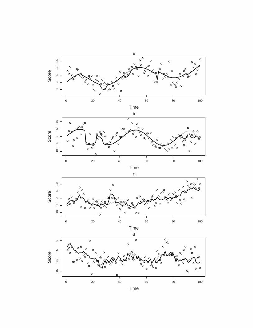
0 20 40 60 80 100

−5

05

1015

a

Time

Sco

re

●

●

●

●

●

●

●

●

●●

●

●

●●

●

●

●

●

●

●●

●

●

●

●●

●

●

●

●●

●

●

●●

●

●

●

●

●●

●●

●

●

●

●●

●

●

●

●

●

●

●

●

●

●●

●●

●

●

●

●●●

●

●●

●●●

●

●

●

●

●

●

●

●

●

●

●●

●

●

●

●

●

●

●

●

●

●

●

●

●

●

●

0 20 40 60 80 100

−10

−5

05

10

b

Time

Sco

re

●

●

●

●

●●

●●

●

●

●

●

●

●

●

●

●

●

●

●

●

●●

●

●

●

●

●

●

●

●●

●

●

●

●●

●

●

●

●

●

●

●

●●

●●

●●

●

●

●

●

●

●

●●

●●

●

●

●

●●

●

●

●

●

●

●●

●

●

●

●

●

●●

●●

●

●

●

●

●

●

●

●

●

●●

●

●

●●

●

●

●

●

0 20 40 60 80 100

−10

−5

05

10

c

Time

Sco

re

●

●

●

●

●●

●

●

●

●

●

●

●

●

●

●

●

●

●

●

●

●

●

●

●●

●

●

●

●

●

●●

●

●

●

●

●

●

●●

●

●

●●

●

●

●●

●●

●

●●

●

●●

●

●

●

●

●

●●●

●

●

●

●

●

●

●

●

●

●●

●●

●●

●●

●

●

●●

●

●

●

●●

●

●

●

●

●

●

●●

●

0 20 40 60 80 100

−15

−10

−5

0

d

Time

Sco

re

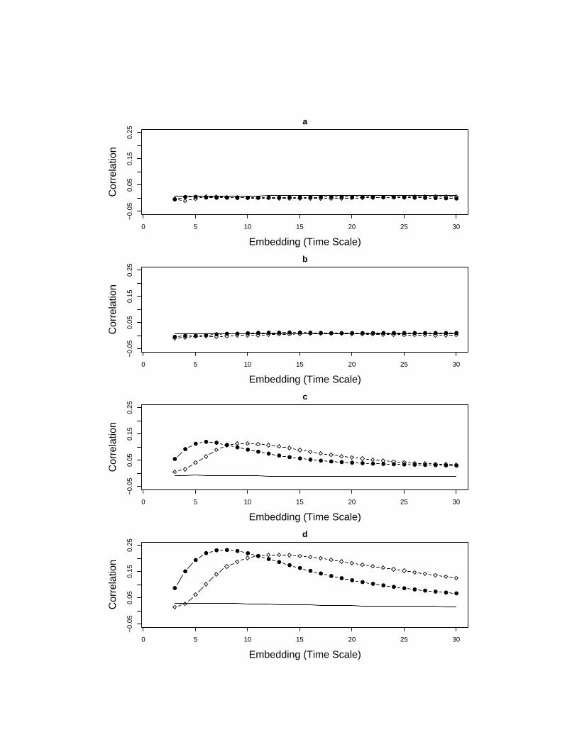
0 5 10 15 20 25 30

−0.

050.

050.

150.

25a

Embedding (Time Scale)

Cor

rela

tion

●● ● ● ● ● ● ● ● ● ● ● ● ● ● ● ● ● ● ● ● ● ● ● ● ● ● ●

0 5 10 15 20 25 30

−0.

050.

050.

150.

25

b


Cor

rela

tion

● ● ● ● ● ● ● ● ● ● ● ● ● ● ● ● ● ● ● ● ● ● ● ● ● ● ● ●

0 5 10 15 20 25 30

−0.

050.

050.

150.

25

c


Cor

rela

tion

●

●

● ● ●●

●●

● ● ● ● ● ● ● ● ● ● ● ● ● ● ● ● ● ● ● ●

0 5 10 15 20 25 30

−0.

050.

050.

150.

25

d


Cor

rela

tion

●

●

●

●● ● ●

●●

●●

●●

●●

●●

● ● ● ● ● ● ● ● ● ● ●

0 5 10 15 20 25 30

−1.

0−

0.5

0.0

0.5

1.0

a

Embedding

Cor

rela

tion

●

●

●

●

●

●

●

●

●

●

●

●

●

●

●

●

●

●

●

●

●

●

●

●

●

●

●

●

●

●

●

●

●

●

●

●

●

●

●

●

●

●

●

●

●

●

●

●

●

●

●

●

●

●

●

●

0 5 10 15 20 25 30

−1.

0−

0.5

0.0

0.5

1.0

b

Embedding

Cor

rela

tion

●

●

●

●

●

●

●

●

●

●

●

●

●

●

●

●

●

●

●

●

●

●

●

●

●

●

●

●

●

●

●

●

●

●

●

●

●

●

●

●

●

●

●

●

●

●

●

●

●

●

●

●

●

●

●

●

0 5 10 15 20 25 30

−1.

0−

0.5

0.0

0.5

1.0

c

Embedding

Cor

rela

tion

●

●

●

●

●

●

●

●

●

●

●

●

●

●

●

●

●

●

●

●

●

●

●

●

●

●

●

●

●

●

●

●

●

●

●

●

●

●

●

●

●

●

●

●

●

●

●

●

●

●

●

●

●

●

●

●

0 5 10 15 20 25 30

−1.

0−

0.5

0.0

0.5

1.0

d

Embedding

Cor

rela

tion

●

●

●

●

●

●

●

●

●

●

●

●

●

●

●

●

●

●

●

●

●

●

●

●

●

●

●

●

●

●

●

●

●

●

●

●

●

●

●

●

●

●

●

●

●

●

●

●

●

●

●

●

●

●

●

●

●

●

0 5 10 15 20 25 30

−1.

0−

0.5

0.0

0.5

1.0

e

Embedding

Cor

rela

tion

●

●

●

●

●

●

●

●

●

●

●

●

●

●

●

●

●

●

●

●

●

●

●

●

●

●

●

●

●

●

●

●

●

●

●

●

●

●

●

●

●

●

●

●

●

●

●

●

●

●

●

●

●

●

●

●

●

●

0 5 10 15 20 25 30

−1.

0−

0.5

0.0

0.5

1.0

f

Embedding

Cor

rela

tion

●

●

●

●

●

●

●

●

●

●

●

●

●

●

●

●

●

●

●

●

●

●

●

●

●

●

●

●

●

●

●

●

●

●

●

●

●

●

●

●

●

●

●

●

●

●

●

●

●

●

●

●

●

●

●

●

●

●

●

●

●

●

●

●

Using derivative estimates to describe intraindividual variability at multiple time scales

Documents

Transcript of Using derivative estimates to describe intraindividual variability at multiple time scales