Bulletin of Indonesian Economic Studies, Vol. 40, No. 3, 2004: 355–77

ISSN 0007-4918 print/ISSN 1472-7234 online/04/030355-23 © 2004 Indonesia Project ANUDOI: 10.1080/0007491042000231520

Carfax PublishingTaylor & Francis Group

USING CLIMATE MODELS TO IMPROVE INDONESIAN FOOD SECURITY

Walter P. Falcon, Rosamond L. Naylor, Whitney L. Smith, Marshall B. Burke and Ellen B. McCullough*

Stanford University

El Niño Southern Oscillation (ENSO) events exert significant influence on South-east Asian rice output and markets. This paper measures ENSO effects on Indo-nesia’s national and regional rice production and on world rice prices, using theAugust Niño 3.4 sea surface temperature anomaly (SSTA) to gauge climate vari-ability. It shows that each degree Celsius change in the August SSTA produces a1,318,000 metric ton effect on output and a $21/metric ton change in the worldprice for lower quality rice. Of the inter-annual production changes due to SSTAvariation, 90% occur within 12 provinces, notably Java and South Sulawesi. Newdata and models offer opportunities to understand the agricultural effects of ENSOevents, to reach early consensus on coming ENSO effects, and to use forecasting toimprove agencies’ and individuals’ capacity to mitigate climate effects on foodsecurity. We propose that Indonesia hold an ‘ENSO summit’ each September toanalyse the food-security implications of upcoming climate events.

INTRODUCTIONFood policy in Indonesia has changed substantially since the end of the Soehartoregime in 1998. With these policy changes have come associated alterations indecision-making processes and in the institutions serving food and agriculture.International developments have also affected Indonesia’s food system. Theworld market for rice is larger in volume and more stable with respect to pricesthan in earlier periods; the Asian financial crisis of the late 1990s is more or lessover; and new climate data and models for the Indo-Pacific region have shiftedspeculation on El Niño Southern Oscillation (ENSO) impacts on agriculture fromshamans to computers. Collectively, these changes have enhanced the role of theprivate sector in Indonesia’s rice trade, and have altered the manner in whichvarious actors use available instruments to deal with annual variations in paddyproduction.1

The central concern of this paper is to estimate the magnitude of year-to-yearchanges in paddy production—nationally and regionally—caused by ENSO vari-ables. Since these estimated magnitudes turn out to be large, our second, morenormative, focus is on how improved production forecasts can best be used toimprove food security in an evolving rice system—one that is more decentralisedand privatised than the system that prevailed during the Soeharto era.

CBIEDec04 27/10/04 4:23 PM Page 355

The Climate ContextThe recurring pattern of climate variability in the eastern equatorial Pacific ischaracterised by anomalies in both sea surface temperature (referred to as ElNiño and La Niña for warming and cooling periods, respectively) and sea levelpressure (Southern Oscillation). During El Niño events, the prevailing easterlyPacific winds slacken or reverse direction. As a consequence, the warmer oceanwater shifts eastward away from Indonesia, causing rain to fall over the centralPacific Ocean and simultaneously causing drought to occur over large parts ofthe Indonesian archipelago.

Previous research by the authors demonstrated the specific impacts of ENSOevents on Indonesian agriculture (Naylor et al. 2001, 2002). Although Indonesiahas long been known to receive strong ENSO signals, quantitative relationshipsamong sea surface temperature anomalies (SSTAs) in the central Pacific Ocean,rainfall patterns, and rice production were obscured by data and cropping-system complexities. However, when rice production data were retabulated on acrop-year (September–August) rather than on a calendar-year basis, and whenfocus shifted from yield to area variables, simple econometric models provedremarkably robust in quantifying climate–production linkages.

Several conclusions emerged from the earlier research, which in turn provideunderpinnings for the extensions explored in this paper. First, August SSTAs (asmeasured by the Niño 3.4 SSTA index in the Pacific Ocean) are central to anunderstanding of subsequent rainfall patterns in Indonesia.2 Second, most of theclimate-induced variation in paddy production occurs as a consequence ofchanges in the area harvested rather than in the yield of paddy per hectare. Third,extreme El Niño events, of the type that occurred in 1982/83 and 1997/98, shiftboth the timing of plantings and the total amount of paddy produced, thoughthere appears to be some ‘catching up’ of paddy production later in the crop year.The difference in magnitudes in Indonesian paddy area between the mostextreme El Niño and La Niña years (1982/83 and 1975/76, respectively) is about800 thousand hectares, roughly equivalent to 3,500 thousand metric tons (tmt) orabout 7% of annual paddy production (Naylor et al. 2002). Climate variability isthus a (and perhaps the) primary determinant of year-to-year variation in Indo-nesian rice production.

The models presented in the second portion of this paper extend our earlierresearch in three important dimensions. First, we reformulate the basic modelusing level rather than first-difference forms of the variables, and analysewhether models that best predict variations in national paddy production arealso effective and appropriate for use at the provincial level. We subsequentlyassess the extent and nature of feedbacks to the world rice price caused by climatevariability in the Indo-Pacific region. Understanding these price feedbacks isespecially important in gauging the food-security implications of our model. Thefinal portion of the article illustrates the forecasting capacity of the model, andshows how such forecasts might be used to promote food security.

ENSO EFFECTS ON PADDY YIELDS, AREA AND PRODUCTION Estimating ENSO impacts for Indonesia and then conveying the implications ofthose results would be much easier if climatic episodes corresponded well with

356 Walter P. Falcon et al.

CBIEDec04 27/10/04 4:23 PM Page 356

calendar years. However, none of the statistical formulations we have tried on acalendar-year basis has proven successful. We have thus used trimester agricul-tural data and have retabulated the data into crop years that begin on 1 Septem-ber of year (t) and end on 31 August of year (t + 1).3 As it happens, the trimestersthemselves are of interest, especially the first trimester of each calendar year,since the January–April period corresponds well with the large (wet-season) har-vest of paddy throughout much of Indonesia (figure 1).

Problems with time trends in the various production series further complicatestatistical procedures. Our earlier climate–rice production models were based onthe years 1983/84–1998/99, the period for which tri-yearly national data werethen available. These models were formulated in first-difference form, i.e.changes in paddy production from year (t) to (t + 1) were estimated as a functionof changes in the SSTA for August from year (t – 1) to (t).4 This formulation solvedmost of the troubling statistical problems associated with serial correlationamong the residuals, and the resulting equation was both simple and clear in itsdemonstration of climatic effects on rice production. It was also easy to explain topolicy analysts and practitioners. However, in this statistical formulation, timetrends in the production series end up being captured by the constant term in theestimation process. If these time trends are decelerating, as empirically they are,using a first-difference model for actual forecasting purposes becomes increas-ingly problematic, as the equation tends to underestimate the changes caused bythe SSTA variable.

In an effort to solve this problem, we reformulated the base equation using lev-els for SSTA, production, area harvested and yields, rather than first differences.We also extended the data series through 2001/02. The SSTA variable exhibitedno trend through time; however, we found it necessary to include time and time-

Using Climate Models to Improve Indonesian Food Security 357

Calendar year

Sep Oct Nov Dec Jan Feb Mar Apr May Jun Jul Aug Sep Oct Nov Dec

Aug SSTA

t

Aug SSTAt+1

Harvest Harvest

Growing season

Modal planting date,normal years,dry season

Crop year

Growing season

Modal planting date,normal years,wet season

FIGURE 1 Time-line Used for ENSO Models

CBIEDec04 27/10/04 4:23 PM Page 357

squared variables to accommodate trends in production—thereby ensuring thatthe resulting residuals were stationary.5 Accounting for trends in this mannerensured that both the production and SSTA variables were balanced.6

Equation (1) represents the new formulation for Indonesia’s paddy productionon a crop-year basis. It shows a production effect of –1,318 tmt per degree Celsiusrise in the SSTA. That coefficient is virtually identical to the –1,400 tmt per degreeCelsius change predicted by first-difference methods. However, equation (1) pro-vides for considerably more flexibility in estimating technology effects. In partic-ular, the squared time term allows for the possibility of an acceleration ordeceleration of productivity increases in paddy production.

Paddy production = 35,311 – 1,318 AugSSTA + 1,675 time – 45.0 time2 (1)t-statistic values (40.44) (–4.40) (8.26) (–4.57)Adj. R2 = 0.94 Durbin–Watson = 2.00 Time is measured in years, where 1 = 1983/84

ENSO Effects at the National LevelNational Crop-Year Models. Table 1, which for completeness contains equation (1),presents an array of national results for the crop year. For each of the area, yieldand production equations, intercept and slope coefficients are followed by theirrespective t-statistics in succeeding rows. Adjusted R2, root mean square error,and Durbin–Watson statistics are also provided.

A number of important conclusions emerge from these results. First and fore-most, SSTAs are important determinants of both area harvested and productionof paddy. Each degree Celsius increase in the SSTA results in an area effect of –261thousand hectares and a production effect of –1,318 tmt. (These results are sym-metric—a decline of one-degree Celsius in the SSTA results in an increase of 261thousand hectares and of 1,318 tmt of production.) The root mean square error forthe production equation is 1,132 tmt, or roughly 2% of current yearly paddy pro-

358 Walter P. Falcon et al.

TABLE 1 Effects of ENSO Events on Paddy Area Harvested, Yield and Production (1983/84–2001/02 Crop Years)a

Intercept August Time Time2 Adj. R2 RMSEb D.W.b

SSTA

Area harvested 9,359 –261 200 –4.0 0.90 246 2.04(‘000 ha) (49.13) (–4.00) (4.52) (–1.84)

Production (tmt) 35,311 –1,318 1,675 –45.0 0.94 1,132 2.00(40.44) (–4.40) (8.26) (–4.57)

Yield (mt/ha) 3.80 –0.02 0.08 –0.003 0.82 0.08 0.94(65.59) (–0.98) (6.16) (–4.42)

at-statistics in parentheses.bRMSE = root mean square error; D.W. = Durbin–Watson statistic; tmt = ‘000 metric tons.

CBIEDec04 27/10/04 4:23 PM Page 358

duction. Moreover, both the production and area-harvested equations are stable,with no serious outlier observations. To test the latter proposition, we droppedone observation sequentially, re-estimated the equation each time, and then usedthe new equation to ‘forecast’ the observation that was omitted. The correlationsbetween the actual dependent variables and their forecast values using this pro-cedure were 0.95 and 0.91 for production and area harvested, respectively.7

We also tested the model’s stability by calculating it using a subset of observa-tions and verifying its ability to predict production and area harvested for theomitted, ‘out-of-sample’ observations. The model performed well out of samplefor both the production and area-harvested variables. Decreases in both variableswere correctly predicted for the 1987/88 El Niño event when the first six yearswere omitted from the model calculation. Similarly, the model predicteddecreased production and area harvested in the 1997/98 El Niño event when thelast six years were forecast out of sample. The correlation coefficients betweenout-of-sample predicted production and actual production were 0.93 and 0.75when the first six observations and last six observations were left out of themodel, respectively. Out-of-sample calculations with the area harvested variableyielded similar results.

The effect of SSTAs on the yield component was of the expected sign, but wasstatistically insignificant. Nonetheless, all three equations—area harvested, pro-duction and yield—have adjusted R2s that are very high. In addition, theDurbin–Watson tests are reassuring for the key production and area harvestedequations. Finally, the significance of the time variable in the yield equation(which then carries over as a determinant for the production equation) under-scores the importance of technology and infrastructure improvements in the1980s and 1990s, though the highly significant t-statistic on the time-squared termalso emphasises the slowdown of productivity increases in recent years.

National Models for the September–December Trimester. The estimates in table 2for the September–December period show a qualitative pattern very similar to

Using Climate Models to Improve Indonesian Food Security 359

TABLE 2 Effects of ENSO Events on Paddy Area Harvested, Yield and Production (1983/84–2001/02, September–December)a

Intercept August Time Time2 Adj. R2 RMSEb D.W.b

SSTA

Area harvested 1,619 –142 48 –0.59 0.75 138 2.24(‘000 ha) (15.15) (–3.88) (1.94) (–0.49)

Production (tmt) 6,200 –556 280 –4.24 0.83 556 2.25(14.45) (–3.78) (2.81) (–0.87)

Yield (mt/ha) 3.85 0.02 0.05 –0.001 0.80 0.07 1.36(74.26) (1.13) (4.10) (–2.23)

at-statistics in parentheses.bAs for table 1.

CBIEDec04 27/10/04 4:23 PM Page 359

that for the total crop year. Perhaps most surprising is the magnitude of the ENSOeffects. A one-degree Celsius change in the SSTA from the previous crop yearalters area harvested by 142 thousand hectares (more than half of the total 261thousand hectares for the entire crop year), and production by some 556 tmt. Theclimate effect on paddy yield was again insignificant for the trimester. In short,the August SSTA is a key indicator of paddy production in the subsequent fourmonths, September–December, which constitute the beginning phase of the cropyear.

National Models for the January–April Trimester. Table 3 is of particular interestbecause of its correspondence with the wet-season harvest for most parts of thecountry. The production-related ENSO effect is large (some 938 tmt per degreeCelsius change in the SSTA), owing mainly to the very significant area effect.Overall, more than 70% of the climate-induced changes in both area harvestedand production for the entire crop year occur during the January–April trimester.The yield coefficient of 30 kg per degree change is significant at only the 85% levelof confidence, yet at the margin it also adds to the significance of the productionequation relative to the area equation.

National Models for the May–August Trimester. In some fundamental sense,table 4 is qualitatively different from tables 1–3. By May of year (t + 1), the effectsof the previous August SSTA are diminishing, as reflected by the lower adjustedR2s. The May–August period is also the ‘catch-up’ season. In El Niño years, rainsare both late and limited, which in turn shifts more of the cropping schedule intothe May–August trimester. (The cropping schedule for West Java, a representa-tive province, is shown in figure 2.) In contrast with the two other subperiods, thekey SSTA slope coefficients for production and area harvested are positive ratherthan negative, although the production coefficient is significant at only about the75% level of confidence. Table 4 thus helps to underscore an important timingpoint relevant for policy making and policy makers.8 Crop prospects in El Niñoyears appear bleakest in about February. It is at that point that the crop is furthest

360 Walter P. Falcon et al.

TABLE 3 Effects of ENSO Events on Paddy Area Harvested, Yield and Production (1983/84–2001/02, January–April)a

Intercept August Time Time2 Adj. R2 RMSEb D.W.b

SSTA

Area harvested 4,503 –188 179 –6.49 0.78 190 1.84(‘000 ha) (30.70) (–3.74) (5.26) (–3.90)

Production (tmt) 16,552 –938 1,210 –43.26 0.86 952 1.85(22.54) (–3.72) (7.09) (–5.20)

Yield (mt/ha) 3.73 –0.03 0.09 –0.003 0.86 0.07 1.06(70.88) (–1.46) (7.29) (–5.27)

at-statistics in parentheses.bRMSE = root mean square error; D.W. = Durbin–Watson statistic; tmt = ‘000 metric tons.

CBIEDec04 27/10/04 4:23 PM Page 360

behind. By July, at least some of the shortfall has been recovered. This point,while important, is obviously less than completely consoling to poor familieswho must deal with a prolonged hungry season (paceklek) due to the delayed wet-season harvest.

Using Climate Models to Improve Indonesian Food Security 361

FIGURE 2 Average Monthly Plantings, West Java, 1971–2001(‘000 hectares)

Sep Oct Nov Dec Jan Feb Mar Apr May Jun Jul Aug0

100

200

300

400

500

1971–2001

El Niño years 1982/83, 1987/88, 1997/98

La Niña years 1988/89, 1992/93, 1998/99

TABLE 4 Effects of ENSO Events on Paddy Area Harvested, Yield and Production (1983/84–2001/02, May–August)a

AugustIntercept SSTA Time Time2 Adj. R2 RMSEb D.W.b

Area harvested 3,237 69 –27 3.11 0.73 128 2.50(‘000 ha) (32.82) (2.05) (–1.19) (2.78)

Production (tmt) 12,558 176 185 2.33 0.83 586 2.13(27.81) (1.14) (1.76) (0.46)

Yield (mt/ha) 3.87 –0.04 0.1 –0.004 0.68 0.11 1.10(45.23) (–1.24) (4.86) (–0.37)

at-statistics in parentheses.bAs for table 3.

CBIEDec04 27/10/04 4:23 PM Page 361

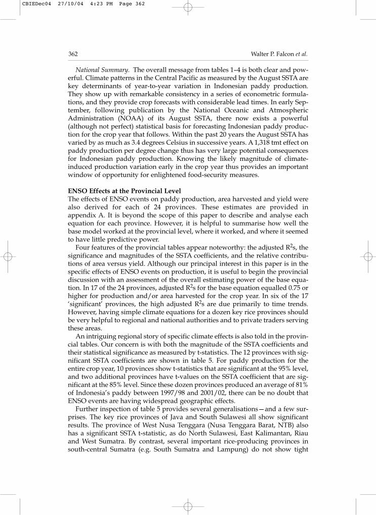
National Summary. The overall message from tables 1–4 is both clear and pow-erful. Climate patterns in the Central Pacific as measured by the August SSTA arekey determinants of year-to-year variation in Indonesian paddy production.They show up with remarkable consistency in a series of econometric formula-tions, and they provide crop forecasts with considerable lead times. In early Sep-tember, following publication by the National Oceanic and AtmosphericAdministration (NOAA) of its August SSTA, there now exists a powerful(although not perfect) statistical basis for forecasting Indonesian paddy produc-tion for the crop year that follows. Within the past 20 years the August SSTA hasvaried by as much as 3.4 degrees Celsius in successive years. A 1,318 tmt effect onpaddy production per degree change thus has very large potential consequencesfor Indonesian paddy production. Knowing the likely magnitude of climate-induced production variation early in the crop year thus provides an importantwindow of opportunity for enlightened food-security measures.

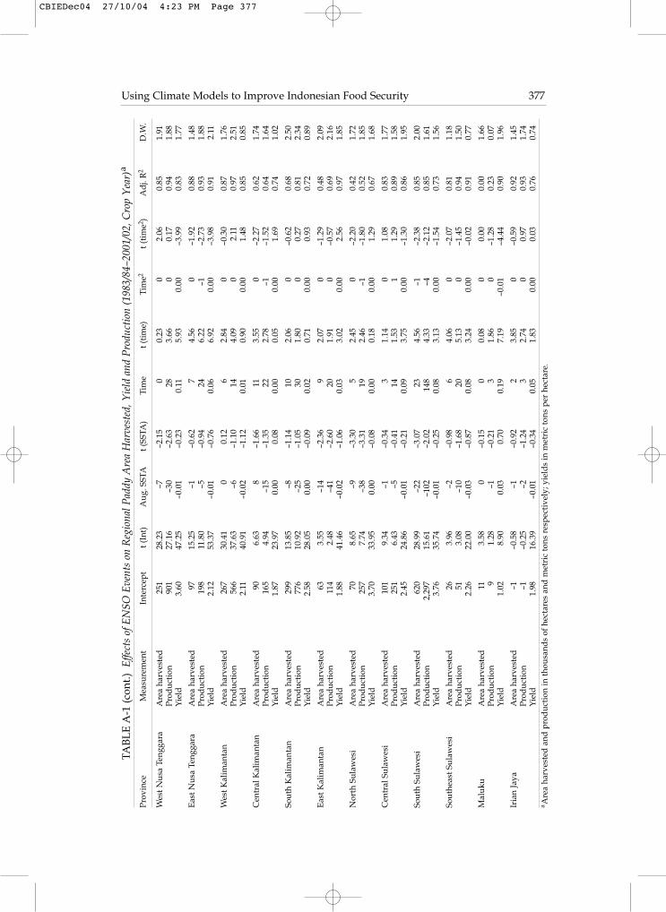
ENSO Effects at the Provincial Level The effects of ENSO events on paddy production, area harvested and yield werealso derived for each of 24 provinces. These estimates are provided inappendix A. It is beyond the scope of this paper to describe and analyse eachequation for each province. However, it is helpful to summarise how well thebase model worked at the provincial level, where it worked, and where it seemedto have little predictive power.

Four features of the provincial tables appear noteworthy: the adjusted R2s, thesignificance and magnitudes of the SSTA coefficients, and the relative contribu-tions of area versus yield. Although our principal interest in this paper is in thespecific effects of ENSO events on production, it is useful to begin the provincialdiscussion with an assessment of the overall estimating power of the base equa-tion. In 17 of the 24 provinces, adjusted R2s for the base equation equalled 0.75 orhigher for production and/or area harvested for the crop year. In six of the 17‘significant’ provinces, the high adjusted R2s are due primarily to time trends.However, having simple climate equations for a dozen key rice provinces shouldbe very helpful to regional and national authorities and to private traders servingthese areas.

An intriguing regional story of specific climate effects is also told in the provin-cial tables. Our concern is with both the magnitude of the SSTA coefficients andtheir statistical significance as measured by t-statistics. The 12 provinces with sig-nificant SSTA coefficients are shown in table 5. For paddy production for theentire crop year, 10 provinces show t-statistics that are significant at the 95% level,and two additional provinces have t-values on the SSTA coefficient that are sig-nificant at the 85% level. Since these dozen provinces produced an average of 81%of Indonesia’s paddy between 1997/98 and 2001/02, there can be no doubt thatENSO events are having widespread geographic effects.

Further inspection of table 5 provides several generalisations—and a few sur-prises. The key rice provinces of Java and South Sulawesi all show significantresults. The province of West Nusa Tenggara (Nusa Tenggara Barat, NTB) alsohas a significant SSTA t-statistic, as do North Sulawesi, East Kalimantan, Riauand West Sumatra. By contrast, several important rice-producing provinces insouth-central Sumatra (e.g. South Sumatra and Lampung) do not show tight

362 Walter P. Falcon et al.

CBIEDec04 27/10/04 4:23 PM Page 362

SSTA connections (appendix table A-1). The answer almost surely lies with par-ticular wind movements, and perhaps with the physical locations of theseprovinces vis-à-vis peninsular Malaysia and Kalimantan. Based on the work ofFox (2000), we had also expected to see an SSTA association with paddy produc-tion in East Nusa Tenggara (Nusa Tenggara Timur, NTT). However, Fox also indi-cates that in NTT (and in several other eastern provinces) SSTA effects play outmore importantly for crops other than paddy, such as corn.

For the crop year as a whole, the largest production effects from a one-degreeCelsius change in the SSTA take place on Java. Indeed, the impact in West Java isby far the greatest of any province. Table 5 shows that when the coefficients forthese 12 provinces are summed (1,191 tmt), they account for 90% of the nationalimpact (1,318 tmt).

Table 5 also illustrates one other regional point of importance. Although thelargest adjustments take place on Java, the percentage effect of a one-degree Cel-sius change relative to provincial production is substantially higher in the off-Java provinces of East Kalimantan and North Sulawesi. Since those provinceshave rice systems that are less well integrated than the Java provinces into boththe national and international rice markets, advance warnings of production

Using Climate Models to Improve Indonesian Food Security 363

TABLE 5 Significant Provincial Production Effects Caused by a 1°C Increase in the August SSTA

Province Crop-Year Percentage Significance Ratio of Production of of Production

Effect National Production Effect (September–August) Effect Effect to Average

(tmt) (t-statistic) Yearly Production 1997/98–2001/02

West Java –380 28.83 –3.01 –0.037Central Java –238 18.06 –3.67 –0.026East Java –232 17.60 –4.06 –0.026South Sulawesi –102 7.74 –2.02 –0.033North Sumatra –54 4.10 –1.57 –0.016West Sumatra –46 3.49 –2.18 –0.026East Kalimantan –41 3.11 –2.60 –0.118North Sulawesi –38 2.88 –3.31 –0.104West Nusa Tenggara –30 2.28 –2.63 –0.021Riau –17 1.29 –2.14 –0.041Southeast Sulawesi –10 0.76 –1.68 –0.033Bali –3 0.23 –2.82 –0.003

Subtotal –1,191 90.36Coefficient for all-

Indonesia (table 1) –1,318 100.00

CBIEDec04 27/10/04 4:23 PM Page 363

variations may be particularly helpful to them from a regional food-security per-spective.

Finally, the provincial results in appendix A demonstrate that almost all of theENSO impacts are via changes in area harvested. In only one province is theyield–SSTA linkage statistically significant: in South Sumatra, yields are affectedby about 60 kg/ha per degree Celsius change in the SSTA. We are puzzled by thisresult, especially because the SSTA variable does not significantly affect area har-vested or production in South Sumatra.

The provincial ENSO story is remarkably consistent and straightforward. Mostof the large effects on paddy production arising from changes in the SSTA are infour provinces, even though a total of 12 provinces are significantly affected.Moreover, even on a provincial basis, virtually all of the ENSO production effectsare via the amount and timing of areas harvested and almost none are via yields.

Climate and Price LinkagesThe significant effect of ENSO on rice production begs the question of what roleprices play in the dynamics of the system. We examined the role of prices, first asa causal variable influencing Indonesian rice supply along with climate, and sec-ond as a dependent variable being affected by changes in climate. In attemptingto build farm prices into the foregoing paddy production models, we usednumerous price alternatives, including deflated paddy prices, the ratio of paddyprices to corn prices, and the ratio of government-announced floor prices to theprice of urea. In the end, none of the price variables proved statistically signifi-cant on a consistent basis.

Better measures of expected prices might solve some of the estimation prob-lems in the Indonesia rice-supply equations. However, such measures areunlikely to overcome the fundamental econometric problem for the period underreview. Stabilising the real price of rice was a cornerstone of food policy in the1980s and most of the 1990s, and there is insufficient variation in the relevantprice variables to permit the successful econometric estimations of supplyresponse that could supplement the equations of tables 1–4. Obviously prices areimportant to farmers, and our finding does not suggest otherwise. Paddy hasgenerally been the most profitable of the major crops for farmers to grow(Heytens 1991; Pearson, Bahri and Gotsch 2003), and paddy prices have thus beena key determinant of farm income, even if their variation has been insufficientlylarge to induce significant changes in cropping patterns.

The combination of policy decisions in Indonesia and climatic variability in theIndo-Pacific region has had important effects on world prices. After a period ofself-sufficiency on a trend basis (and even substantial exports in the crop year1984/85), Indonesia has become a consistent importer of rice. In addition, thevariation in Indonesian imports has been very large. In the decade of the 1990s,for example, the range of rice import tonnages went from a low of 24 tmt in 1993to a high of 4,748 tmt in 1999 (FAOSTAT 2003).9 Import quantities depended ondomestic stocks of rice, domestic prices, world prices, exchange rates and a seriesof other policy variables. However, there can be no doubt that the ENSO effectsdescribed in previous sections play a big role in determining the amount of riceimported. Dawe (2002) has had some success in isolating specific country effectson world prices. Our intention here is to link SSTAs directly to the world price of

364 Walter P. Falcon et al.

CBIEDec04 27/10/04 4:23 PM Page 364

rice. While the logic of this procedure is clear enough, the data constraints are for-midable.

The world rice market is very different from the markets for wheat and corn.The latter have active futures markets, and virtually all international contracts arewritten with reference to Chicago or one of the other organised markets. Rice, bycontrast, has no comparable market.10 The reasons have much to do with thepolitical nature of rice, especially in Asia, and the high percentage of internationaltrade that was historically completed via government-to-government (G-to-G)transactions. Partly as cause and partly as consequence of these arrangements,international rice trade has been a small percentage of total output (usually lessthan 4%). The private trade that has existed internationally has tended to beamong friends and families, in no small measure because this facilitated contractenforcement. However, with the liberalisation of rice policy in the 1990s in coun-tries like India and Vietnam, both of which went on to become substantialexporters, the world rice market roughly doubled in size and became much lessvariable with respect to prices. Increasingly, private trade has replaced G-to-Gsales. In short, a real international market for rice has begun to develop (Dawe2002).

One historical by-product of the marketing arrangements has been the lack ofreliable international price data. Over the years, the ‘government-posted price’ ofrice in Bangkok has been the predominant indicator price, but increasingly therehave been complaints that these posted prices were ‘desired outcomes’ ratherthan actual transaction prices. Notwithstanding difficulties with official Bangkokprices, the data show a clear and surprisingly strong link between ENSO eventsand world rice prices. Equation (2) below is representative. It shows the changein export prices of A1 Special (A1S) rice (a lower-quality indica rice) from thefourth quarter of one year to the fourth quarter of the next as a function of theprevious year’s change in the August SSTA.

∆A1S price (4Qt – 4Qt + 1) = –2.40 + 21.08 ∆AugSSTA [(t–1) to (t)] (2)t-statistic values (–0.29) (3.72)Adjusted R2 = 0.46 Durbin–Watson = 2.02

This simple first-difference formulation indicates that a one-degree Celsiuschange in the SSTA has resulted in an increase of about $21 per metric ton in theprice of rice more than a year later, and the equation explains nearly half of thevariation in year-to-year changes in nominal world prices for the period January1986 to December 2003.11 A1 Special rice traded between 1986 and 2003 at anaverage price of $180 per metric ton f.o.b. Bangkok, and thus in this case theENSO feedback on the low-quality rice market is very significant. By contrast,change in the SSTA variable is not a good predictor of changes in the price ofhigh-quality rice; the adjusted R2 of a similar first-difference formulation for Thai5% brokens, a representative high-quality variety, is only 0.003.

Two conclusions emerge from the analysis. The first is that the strong relation-ship between ENSO events and world rice prices only holds for the lower quali-ties, namely 35% brokens and A1 Special. This result is entirely logical—Indonesia is consistently one of the largest importers of rice on the world market,and it imports primarily the lower qualities. Thus it would appear likely that the

Using Climate Models to Improve Indonesian Food Security 365

CBIEDec04 27/10/04 4:23 PM Page 365

SSTA mechanism operates principally through Indonesia, although preliminarywork by Dawe (2003) and Mastrandrea (2003) suggests that similar but smallerSSTA effects also operate via the Philippines and Vietnam, respectively. Second,El Niño episodes alter the relative prices of various grades of rice. Markets forlower-quality and higher-quality rice generally tend to move somewhat inde-pendently—the correlation coefficient between changes in the price of A1 Specialand the price of Thai 5% brokens, for example, is only about 0.64—and in post ElNiño situations the price of lower-quality rice tends to rise relative to higher-quality rice prices. In ‘normal’ years, the price ratio of A1 Special to Thai 5% bro-kens is about 0.68, whereas in El Niño years it is about 0.80. In other words, ElNiño events cause the price difference between the high- and low-quality vari-eties to shrink by around $25/metric ton.

USING CLIMATE DATA TO IMPROVE PLANNINGThe power of our model rests on four attributes: the large percentage of variationthat it explains, which is indicated by the high values of the adjusted R2s; its addi-tive nature, which permits disaggregation by season and province; its long leadtime, which provides quantitative forecasts in sufficient time for decision makersto engage in discussion and take meaningful action; and its logical simplicity,which makes it easily understood by policy makers. In the following section, wediscuss how the equations outlined in the preceding sections can be employed toimprove public and private sector activities in Indonesia.

Even if the utmost care is taken, there are some inherent uncertainties associ-ated with production forecasts based on ENSO data. The fact that the estimatesare probabilistic and therefore rarely perfectly accurate might be seen by some asa reason to limit their transparent use. That would be a great mistake, for theadvantage of using formalised models such as the one presented here lies pre-cisely in their ability to reduce uncertainty.

There is also a tendency among some analysts within Indonesia to disregardmore aggregated models that use time as a proxy for a number of variables. Theyargue instead for models that are more complex and that add variables such asfertiliser usage, irrigation volumes, areas damaged by pests, and factor and prod-uct prices. However, these models are typically cumbersome to build, they tendto be specific to one or two regions, and they are difficult to update on a time-relevant basis because of data constraints. As a consequence, their usefulnessturns out to be limited across time and space. Our primary concern, by contrast,is with forecasts that clearly delineate the effects of climate and that can beupdated consistently on an annual basis.

The Mechanics of ForecastingAll of the equations in tables 1–4 are similar in structure. For any particulartrimester or crop year, they depend on the year’s sequence number (e.g. 1983/84= 1; 2001/02 = 19) and the August SSTA datum of the Niño 3.4 series compiled byNOAA. During the two decades covered by the equations, the August SSTAranged from a high of 2.14 degrees Celsius above the long-run average to a lowof –1.46 degrees Celsius below average.12 By about 10 September of each year,NOAA posts the August value. At that time, all of the equations in this paper can

366 Walter P. Falcon et al.

CBIEDec04 27/10/04 4:23 PM Page 366

be used to forecast the upcoming crop year or a particular trimester, either forIndonesia as a whole or for a specific province. In September 2002, for example,we estimated that, as a consequence of the moderate El Niño indicated by theAugust 2002 SSTA, the paddy crop in 2002/03 would be down by about 1,300 tmt(about 850 tmt of rice) from our forecast of the preceding crop year. In October2003, we forecast that total paddy production for 2003/04 would be 50,430 tmt,or up about 1,040 tmt over 2002/03.

Figure 3 displays estimated versus actual paddy production plotted by cropyear, with prediction confidence intervals provided for the in-sample predictions(1982/83–2001/02) and forecasting confidence intervals provided for the out-of-sample, ‘future’ predictions (2002/03 and 2003/04). A plot of monthly SSTAmeasurements shares the time axis so that the powerful effect of SSTA on produc-tion can be observed. Figure 3 also emphasises that the model is robust but inher-ently probabilistic, and thus its forecasting ability cannot be expected to be exact.

Crop Year versus Calendar YearWe noted earlier that climatic episodes do not correspond well with calendaryears. This limitation is unfortunate analytically, because of the way historical

Using Climate Models to Improve Indonesian Food Security 367

�

����

����

���

��

�

������

��

��

�

����

���

��

�

����

��

�

���

�

���

�

���

���

����

��

�

�

���

����

���

��

�

����

��

�

����

����

���

��

�

�����

�

83/84 86/87 89/90 92/93 95/96 98/99 01/0235

40

45

50

55

FIGURE 3 Crop-year Production, Actual vs Predicted (million metric tons)

����������������������������������������������������������

�������������������������������������������������������������������������������������������������������������������������

���������������������������������������������������������������������

-3

-2

-1

0

1

2

3

El Niño 3.4 SSTA

Anomaly in degrees C

J Actual

�Estimated

Forecast

�95% confidence

75% confidence

CBIEDec04 27/10/04 4:23 PM Page 367

data have been recorded and preserved. Although we cannot provide calendar-year forecasts, we are able, after the fact, to reconstruct estimates on a calendar-year basis for the post-1983 era. The process is somewhat tedious but verystraightforward. In the case of national paddy production, for example, tables 2–4can be used to estimate every trimester in the series, beginning with September1983. After those forecasts have been estimated by trimester, it is then possible toretabulate the estimates on a calendar-year basis. For any given calendar year,SSTA data from two years are required to form the composite estimate.

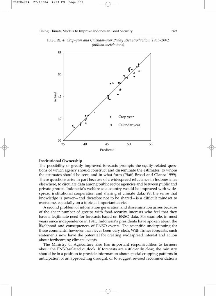
Figure 4 plots actual production against production estimates calculated forboth the crop year and the calendar year. The figure shows that both methodsarrive at a similar result. If the estimates were perfect for all years, a plot of actualversus estimated paddy production would lie exactly along the 45-degree line. Asit stands, the fits for both are extraordinarily good, and the plot in figure 4 simplyreaffirms visually the very high adjusted R2s of the national estimating equations.

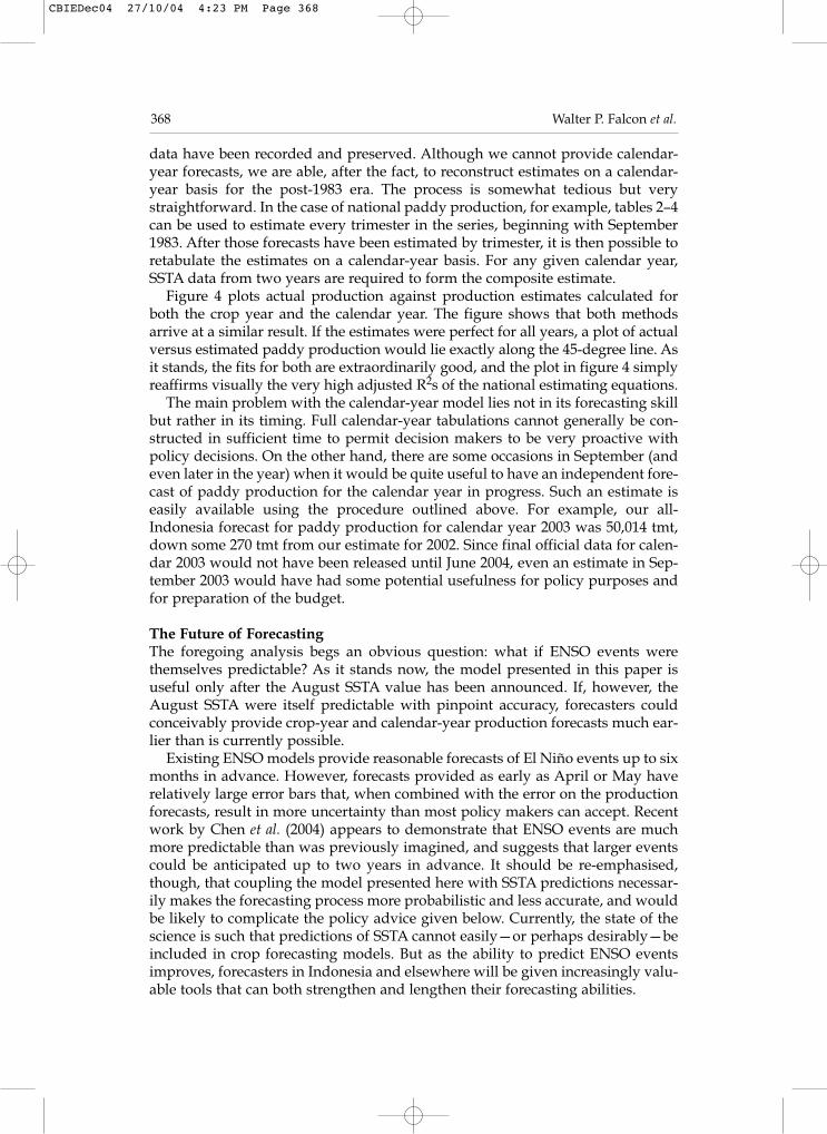
The main problem with the calendar-year model lies not in its forecasting skillbut rather in its timing. Full calendar-year tabulations cannot generally be con-structed in sufficient time to permit decision makers to be very proactive withpolicy decisions. On the other hand, there are some occasions in September (andeven later in the year) when it would be quite useful to have an independent fore-cast of paddy production for the calendar year in progress. Such an estimate iseasily available using the procedure outlined above. For example, our all-Indonesia forecast for paddy production for calendar year 2003 was 50,014 tmt,down some 270 tmt from our estimate for 2002. Since final official data for calen-dar 2003 would not have been released until June 2004, even an estimate in Sep-tember 2003 would have had some potential usefulness for policy purposes andfor preparation of the budget.

The Future of ForecastingThe foregoing analysis begs an obvious question: what if ENSO events werethemselves predictable? As it stands now, the model presented in this paper isuseful only after the August SSTA value has been announced. If, however, theAugust SSTA were itself predictable with pinpoint accuracy, forecasters couldconceivably provide crop-year and calendar-year production forecasts much ear-lier than is currently possible.

Existing ENSO models provide reasonable forecasts of El Niño events up to sixmonths in advance. However, forecasts provided as early as April or May haverelatively large error bars that, when combined with the error on the productionforecasts, result in more uncertainty than most policy makers can accept. Recentwork by Chen et al. (2004) appears to demonstrate that ENSO events are muchmore predictable than was previously imagined, and suggests that larger eventscould be anticipated up to two years in advance. It should be re-emphasised,though, that coupling the model presented here with SSTA predictions necessar-ily makes the forecasting process more probabilistic and less accurate, and wouldbe likely to complicate the policy advice given below. Currently, the state of thescience is such that predictions of SSTA cannot easily—or perhaps desirably—beincluded in crop forecasting models. But as the ability to predict ENSO eventsimproves, forecasters in Indonesia and elsewhere will be given increasingly valu-able tools that can both strengthen and lengthen their forecasting abilities.

368 Walter P. Falcon et al.

CBIEDec04 27/10/04 4:23 PM Page 368

Institutional OwnershipThe possibility of greatly improved forecasts prompts the equity-related ques-tions of which agency should construct and disseminate the estimates, to whomthe estimates should be sent, and in what form (Pfaff, Broad and Glantz 1999).These questions arise in part because of a widespread reluctance in Indonesia, aselsewhere, to circulate data among public sector agencies and between public andprivate groups. Indonesia’s welfare as a country would be improved with wide-spread institutional cooperation and sharing of climate data. Yet the sense thatknowledge is power—and therefore not to be shared—is a difficult mindset toovercome, especially on a topic as important as rice.

A second problem of information generation and dissemination arises becauseof the sheer number of groups with food-security interests who feel that theyhave a legitimate need for forecasts based on ENSO data. For example, in mostyears since independence in 1945, Indonesia’s presidents have spoken about thelikelihood and consequences of ENSO events. The scientific underpinning forthese comments, however, has never been very clear. With firmer forecasts, suchstatements now have the potential for creating widespread interest and actionabout forthcoming climate events.

The Ministry of Agriculture also has important responsibilities to farmersabout the ENSO-related outlook. If forecasts are sufficiently clear, the ministryshould be in a position to provide information about special cropping patterns inanticipation of an approaching drought, or to suggest revised recommendations

Using Climate Models to Improve Indonesian Food Security 369

FIGURE 4 Crop-year and Calendar-year Paddy Rice Production, 1983–2002(million metric tons)

35

40

45

50

55

35 40 45 50 55

Crop year

Calendar year

Predicted

Act

ual

CBIEDec04 27/10/04 4:23 PM Page 369

on such inputs as fertiliser. The ministry is well aware of its responsibilities andhas already begun to use formal methods of ENSO estimation as a regular part ofits planning and informational processes.

In an earlier era, the food logistics agency, Bulog, would have been the primaryuser of ENSO-based forecasts. During much of the 1980s and 1990s, Bulog hadresponsibility for supporting paddy prices to farmers, for ensuring that consumerprices did not exceed a policy-determined band, and for rice imports, over whichit held a monopoly (Bappenas et al. 2002). The more decentralised and privatisedsystem now in place has appropriately diminished Bulog’s role in the rice econ-omy. Yet Bulog still has responsibility for procuring domestic paddy (withinbudget-constrained limits) and for distributing rice both to the military andselected segments of the civil service, and to poor households. The latter is a par-ticularly important responsibility, especially in El Niño years, when the hungryseason is prolonged and rice prices increase. In such years, the number of desti-tute households expands proportionately even more than paddy productiondeclines (Molyneaux 2003). Food security deteriorates as a result of delayedincome, depleted rice stocks, greater reliance of households on markets, and agreater than normal rise in seasonal prices for the staple food commodity.

Because our model is in the public domain, any of a number of groups couldin principle use it to provide updated estimates. Nevertheless, it seems to us as apractical matter that some semi-formal mechanism is needed now within Indo-nesia to improve the connections among this network of concerned agencies andindividuals.

A PROPOSALNew data and models now combine to provide Indonesia with opportunities forunderstanding the effects of ENSO events on rice production, for forming a timelyconsensus on likely ENSO effects for the coming year, and for using forecasts inways that permit agencies and individuals to do a more credible job in mitigatingnegative climate effects. We suggest, therefore, that an ‘ENSO Summit’ be heldeach year, as close as possible to 15 September, to discuss the food-security impli-cations of forecasts based on newly released ENSO data. This meeting could alsobe used as a vehicle for outlining the types of forecasts that are most useful fordifferent user groups.

Modelling efforts now show clearly that the August 3.4 SSTA value is impor-tant for understanding annual rainfall and climate scenarios in Indonesia. SSTAdata before August do not provide the precision required by decision makers ineither the public or the private sector. Data after August help to refine the model,but at a serious cost in terms of the loss in lead times for the results. We believe,therefore, that the optimal time for a workshop is shortly after the August SSTAhas been posted by NOAA, and hence our call for a September summit.

There is a further corollary on timing. The results of the modelling efforts todate indicate that much more can be said about likely ENSO effects on rice pro-duction after 15 September even relative to what can be said two months earlier.The power of good forecasts will be sharply diminished if there is idle specula-tion before 15 September about likely El Niños, or if there is a wide range ofguesses presented as fact or analysis. The scientific basis for forecasting El Niños

370 Walter P. Falcon et al.

CBIEDec04 27/10/04 4:23 PM Page 370

is improving significantly, but we nonetheless urge various Indonesianspokespersons to limit their El Niño conjectures until after the August SSTAdatum is available.

Participation in the proposed two-day workshop should be broadly based,with strong representation from both the public and the private sector. The dis-cussion should be focused and rigorous. Not all of the interested groups will needto be on the program, even though all will have something useful to learn fromthe workshop. The list of speakers might well include climate scientists from out-side the country, e.g. from Singapore, Australia and the US, and it is also possiblethat one or more of the larger multinational grain firms might be willing to shareinsights based on their considerable climate and weather expertise. In our view,this workshop should focus on climate-based rice production forecasts and theirpossible food-security implications. It should not be used as an occasion for fight-ing jurisdictional battles or debating other food and agricultural issues such astariff and subsidy levels, which may be important, but are not central to the cli-mate issues at hand. Given such a food-security focus, and given also the Min-istry of Agriculture’s ongoing activities in forecasting ENSO effects, the ministryseems well positioned to take the leadership in establishing the annual work-shop. It might make sense for other bodies such as the Central Statistics Agency(BPS) or the Bureau of Meteorology to co-host the event.

The primary goal of the workshop should be to forge a high-level consensusestimate of likely climate impacts, which could then serve as a useful guide forthe dissemination of information and for follow-up activities by various agenciesand groups. At least initially the program should probably deal only with paddy.With additional experience and research, further crops could be added in subse-quent years.

Even though some degree of uncertainty will remain, farmers, poor house-holds, traders and agency managers will be much better off than they presentlyare if the best forecasting skills in the world can be brought to bear on the topic.Indonesia now stands poised to make much better forecasts than in the past. Newscience provides an opportunity for improved action, an opportunity whoseloss—either by inattention or by jurisdictional fights among competing organisa-tions—would be regrettable.

Using Climate Models to Improve Indonesian Food Security 371

CBIEDec04 27/10/04 4:23 PM Page 371

NOTES* Corresponding author: phone 1 650 723 6367; fax 1 650 725 1992; email wpfalcon@stan-

ford.edu. Funding from the National Science Foundation, Stanford’s Office for Tech-nology Licensing and the Agency for International Development (via DevelopmentAlternatives’ Indonesian Food Policy Support Project) is gratefully acknowledged. Theauthors thank David Battisti, Steven Block, Ashley Dean, Matthew Evans, James Gin-gerich, Carl Gotsch, Jack Molyneaux, Scott Pearson, Anne Peck, Ning Pribadi, PeterRosner, James Sanchirico, Karen Seto, Kacek Suryanto, Lester Taylor, Peter Timmer andRoger von Haefen for suggestions and helpful assistance. The usual disclaimers apply.

1 In this essay, ‘paddy’ (gabah) refers to unhusked rice, and ‘rice’ refers to milled whiterice (beras). Typical milling ratios result in about 66 kg of milled rice from 100 kg ofpaddy.

2 The Niño 3.4 SSTA index is one of the leading measures of Central Pacific sea surfacetemperatures used in climate models. It is composed of temperature measurementsfrom 170 degrees West to 120 degrees West and from 5 degrees North to 5 degreesSouth. The Niño 3.4 data are maintained by the National Oceanic and AtmosphericAdministration (NOAA) and are updated on a weekly basis (NOAA 2003). All futurereferences to SSTA in this article refer to the August value of the Niño 3.4 data series,unless specifically noted otherwise.

3 All yield, area, production and area damaged data used in this article come from BadanPusat Statistik (various years), Produksi Tanaman Padi dan Palawija di Indonesia [Produc-tion of Paddy and Secondary Crops in Indonesia], Jakarta. Unless otherwise noted, allarea data are for harvested area.

4 The most interesting crop-year equation from the earlier research is:

∆Paddy production = 839 – 1,400 ∆AugSSTA (in tmt for all of Indonesia)t-values (1.91) (–4.79)Adj. R2 = 0.61 Durbin–Watson = 2.09

5 Both time and time-squared are used in all equations. Use of the same regressors acrossequations permits the sum of the trimester coefficients to equal those for the entire cropyear. By the same logic, only three of the four equations, i.e. the three trimesters andthe total, contain ‘real’ statistical information, since any one of the equations could beobtained by knowing the other three. In the sets of equations that follow, however, wepresent all four in tables 1–4 for ease of interpretation.

6 The Dickey–Fuller statistic was used to test whether the errors from the regression ofproduction on t and t-squared were stationary or non-stationary. The test statistic, Z(t),was –5.38, which allowed us to reject the null hypothesis of non-stationarity at a 99%confidence level. The deviations from the t and t-squared equation would also havebeen an appropriate dependent variable to regress against the August SSTA. We ranthese regressions, and the results were virtually identical with those for equation (1).The latter, however, is easier to manipulate econometrically and also easier to explainto policy makers.

7 This approach is sometimes referred to as a ‘jackknife’ procedure to evaluate skill(Kleinbaum, Kupper and Muller 1988).

8 We have intentionally kept the regressors the same across tables 1–4 to permit additionacross trimesters. For the May–August trimester, however, there is one other effect thatshould be noted. This trimester is also being affected by the ‘new’ ENSO conditionsthat are developing. If the SSTA variable for both the previous and current year areincluded in the estimating equation for area harvested, both coefficients are statistically

372 Walter P. Falcon et al.

CBIEDec04 27/10/04 4:23 PM Page 372

significant; they are almost identical in magnitude; they are of different signs; and theadjusted R2 is unaffected.

Area harvested (May–Aug) = 3,460 + 82 AugSSTAt–1 – 83 AugSSTAt – 68 time + 4 time2

t-values (35.56) (2.44) (–2.49) (–3.20) (4.56)Adjusted R2 = 0.74 Durbin–Watson = 2.04

While the ‘current’ August SSTA obviously provides limited lead time for forecastingpurposes, including this variable in table 4 after the fact may provide additional expla-nations of how climate affects paddy area. These explanations may be particularly use-ful given that official estimates are available only in June of the following year.

9 Private sources indicate that Indonesian rice imports peaked in 1998 rather than 1999,at a volume of slightly more than 6,000 tmt (Slayton 2002).

10 A tiny futures market for rough rice (paddy) currently exists at Chicago’s Board ofTrade. It is used primarily for domestic marketing in the US. This market’s history hasbeen disjointed, and it has never been a significant feature in contracts for rice beingtraded internationally.

11 Official Bangkok price data are from USDA (2003).12 The mean and standard deviations of the August 3.4 SSTA over that time period are

0.04 and 0.91, respectively.

Using Climate Models to Improve Indonesian Food Security 373

CBIEDec04 27/10/04 4:23 PM Page 373

374 Walter P. Falcon et al.

REFERENCESBappenas/Departemen Pertanian/USAID/DAI Food Policy Advisory Team (2002), ‘Food

Security in an Era of Decentralization: Historical Lessons and Policy Implications forIndonesia’, accessed October 2004 at <www.macrofoodpolicy.com/docs/wp/07_secu-rity.pdf>.

Chen, D., et al. (2004), ‘Predictability of El Niño Over the Past 148 Years’, Nature 428: 733–6.Dawe, D. (2002), ‘The Changing Structure of the World Rice Market, 1950–2000’, Food Pol-

icy 27: 355–70.Dawe, D. (2003), Personal communication, ‘Philippine ENSO Effects’, International Rice

Research Institute (IRRI), Los Baños, Philippines.FAOSTAT (2003), FAO Statistical Database, accessed August 2003 at <apps.fao.org>. Fox, J.J. (2000), ‘The Impact of the 1997–98 El Niño on Indonesia’, in R.H. Grove and J.

Chappell (eds), El Niño—History and Crisis: Studies from the Asia–Pacific Region, TheWhite Horse Press, Cambridge: 171–90.

Heytens, P. (1991), ‘Rice Production Systems’, in S. Pearson, W. Falcon, P. Heytens, E.Monke and R. Naylor, Rice Policy in Indonesia, Cornell University Press, Ithaca: 38–57.

Kleinbaum, D.G, L.L. Kupper and K.E. Muller (1988), Applied Regression Analysis and OtherMultivariable Methods, Duxbury Press, Belmont CA.

Mastrandrea, M. (2003), Personal communication, ‘Vietnam ENSO Effects’, Stanford Uni-versity, Stanford CA.

Molyneaux, J. (2003), ‘Starchy Staple Consumption and Household Nutrition: A FreshLook at Indonesian Welfare’, accessed October 2004 at <www.macrofoodpolicy.com/docs/ misc/starchy_stapel_consumption_Feb%2003a.pdf>.

Naylor, R.L., W.P. Falcon, D. Rochberg and N. Wada (2001), ‘Using El Niño/SouthernOscillation Climate Data to Predict Rice Production in Indonesia’, Climatic Change 50:255–65.

Naylor, R.L., W.P. Falcon, N. Wada and D. Rochberg (2002), ‘Using El Niño–SouthernOscillation Climate Data to Improve Policy Planning in Indonesia’, Bulletin of IndonesianEconomic Studies 38: 75–91.

NOAA (National Oceanic and Atmospheric Administration) (2003), Monthly Atmosphericand SST Indices, accessed August 2003 at <www.cpc.ncep.noaa.gov/data/indices/>.

Pearson, S.R., S. Bahri and C. Gotsch (2003), ‘Is Rice Production in Indonesia Still Prof-itable?’, accessed August 2003 at <www.macrofoodpolicy.com/htm/pubcaser.htm>.

Pfaff, A., K. Broad and M. Glantz (1999), ‘Who Benefits from Seasonal-to-International Cli-mate Forecasts’, Nature 397: 645–6.

Slayton, T. (2002), Personal communication, ‘Indonesia Rice Trade’, Slayton and Associ-ates, Alexandria VA.

USDA (United States Department of Agriculture) (2003), Rice Situation and Outlook Year-book, Economic Research Service, USDA, Washington DC, November.

CBIEDec04 27/10/04 4:23 PM Page 374

APPENDIX AAppendix table A-1 (below) shows SSTA effects on paddy production, area har-vested and yields for the September–August crop year. Estimates are providedfor each of 24 provinces for the period 1983/84 to 2001/02. Readers should bewarned that the province of West Java includes provincial paddy data fromJakarta and, since 2001, also data from the new province of Banten, which hadformerly been a part of West Java. Similarly, Central Java contains the data forYogyakarta. In addition, data since 2001 for the new province of Gorantolo havebeen re-added into North Sulawesi and for Bangka Belitung into South Suma-tra. No estimates are provided for East Timor, and for the early years of theseries, paddy data for East Timor have been removed from the national totals soas to maintain a consistent data set for the entire period.

Using Climate Models to Improve Indonesian Food Security 375

CBIEDec04 27/10/04 4:23 PM Page 375

376 Walter P. Falcon et al.

TABL

E A

-1E

ffect

s of

EN

SO E

vent

s on

Reg

iona

l Pad

dy A

rea

Har

vest

ed, Y

ield

and

Pro

duct

ion

(198

3/84

–200

1/02

, Cro

p Y

ear)

a

Prov

ince

Mea

sure

men

tIn

terc

ept

t (In

t)A

ug. S

STA

t (SS

TA)

Tim

et (

time)

Tim

e2t (

time2 )

Adj

. R2

D.W

.

Ace

hA

rea

harv

este

d24

014

.99

–5–0

.85

133.

390

–2.2

90.

601.

39Pr

oduc

tion

767

11.8

6–2

5–1

.14

815.

37–3

–3.6

90.

831.

15Yi

eld

3.31

67.0

8–0

.02

–1.2

30.

119.

590.

00–6

.83

0.92

1.98

Nor

th S

umat

raA

rea

harv

este

d50

324

.98

–8–1

.23

357.

57–1

–4.3

60.

931.

70Pr

oduc

tion

1,63

416

.39

–54

–1.5

717

97.

73–5

–4.1

80.

941.

56Yi

eld

3.33

71.0

0–0

.03

–1.5

70.

087.

060.

00–3

.84

0.92

1.96

Wes

t Sum

atra

A

rea

harv

este

d31

623

.60

–9–2

.07

92.

830

–1.2

60.

741.

89Pr

oduc

tion

1,17

983

.46

–46

–2.1

883

5.87

–3–3

.98

0.86

1.83

Yiel

d3.

8596

.37

–0.0

1–0

.74

0.12

13.3

1–0

.01

–11.

660.

920.

83

Ria

uA

rea

harv

este

d12

616

.63

–5–1

.99

52.

600

–2.6

20.

261.

55Pr

oduc

tion

271

11.5

6–1

7–2

.14

274.

99–1

–3.9

70.

691.

46Yi

eld

2.23

33.6

5–0

.02

–0.6

80.

106.

220.

00–3

.52

0.90

0.81

Jam

biA

rea

harv

este

d14

621

.54

–2–0

.95

85.

380

–5.1

50.

591.

97Pr

oduc

tion

386

17.5

2–8

–1.0

932

6.29

–1–5

.26

0.74

1.89

Yiel

d2.

6945

.29

–0.0

1–0

.41

0.04

2.82

0.00

–1.0

40.

762.

19

Sout

h Su

mat

ra

Are

a ha

rves

ted

393

18.5

94

0.55

40.

880

1.11

0.79

1.72

Prod

uctio

n1,

044

18.0

6–1

7–0

.84

413.

070

0.27

0.92

1.55

Yiel

d2.

6654

.27

–0.0

6–3

.35

0.07

6.40

0.00

–3.7

20.

902.

27

Beng

kulu

Are

a ha

rves

ted

719.

53–2

–0.8

35

2.83

0–1

.80

0.55

1.77

Prod

uctio

n20

09.

15–6

–0.7

718

3.48

0–1

.67

0.78

1.71

Yiel

d2.

8642

.67

0.01

0.37

0.03

1.96

0.00

0.34

0.84

1.37

Lam

pung

Are

a ha

rves

ted

294

12.4

62

0.19

173.

070

–1.0

90.

801.

49Pr

oduc

tion

837

11.6

51

0.05

975.

83–2

–2.3

00.

931.

70Yi

eld

2.95

38.2

2–0

.01

–0.3

40.

116.

190.

00–3

.53

0.89

0.63

Wes

t Jav

aA

rea

harv

este

d2,

031

29.4

8–7

4–3

.13

140.

850

–0.5

50.

342.

27Pr

oduc

tion

8,19

922

.31

–380

–3.0

138

44.

49–1

5–3

.62

0.66

1.65

Yiel

d4.

0433

.68

–0.0

2–0

.42

0.16

5.57

–0.0

1–4

.66

0.68

1.04

Cen

tral

Java

Are

a ha

rves

ted

1,60

543

.12

–45

–3.5

09

1.06

00.

260.

712.

28Pr

oduc

tion

7,10

737

.54

–238

–3.6

722

55.

12–7

–3.0

60.

852.

13Yi

eld

4.44

76.2

3–0

.01

–0.5

50.

118.

030.

00–6

.51

0.84

1.13

East

Java

Are

a ha

rves

ted

1,56

949

.03

–38

–3.4

61

0.11

01.

120.

691.

79Pr

oduc

tion

7,33

343

.93

–232

–4.0

614

83.

81–4

–1.8

60.

831.

93Yi

eld

4.68

72.5

7–0

.02

–1.0

80.

096.

050.

00–4

.84

0.75

1.56

Bali

Are

a ha

rves

ted

175

61.1

7–3

–3.0

0–2

–2.5

60

0.66

0.80

2.59

Prod

uctio

n75

444

.75

–16

–2.8

214

3.68

–1–3

.36

0.49

2.15

Yiel

d4.

3014

5.09

–0.0

1–0

.68

0.13

19.4

40.

00–1

2.60

0.98

1.30

CBIEDec04 27/10/04 4:23 PM Page 376

Using Climate Models to Improve Indonesian Food Security 377

TABL

E A

-1 (c

ont.)

Effe

cts

of E

NSO

Eve

nts

on R

egio

nal P

addy

Are

a H

arve

sted

, Yie

ld a

nd P

rodu

ctio

n (1

983/

84–2

001/

02, C

rop

Yea

r)a

Prov

ince

Mea

sure

men

tIn

terc

ept

t (In

t)A

ug. S

STA

t (SS

TA)

Tim

et (

time)

Tim

e2t (

time2 )

Adj

. R2

D.W

.

Wes

t Nus

a Te

ngga

ra

Are

a ha

rves

ted

251

28.2

3–7

–2.1

50

0.23

02.

060.

851.

91Pr

oduc

tion

901

27.1

6–3

0–2

.63

283.

660

0.17

0.94

1.88

Yiel

d3.

6047

.25

–0.0

1–0

.23

0.11

5.93

0.00

–3.9

90.

831.

77

East

Nus

a Te

ngga

ra

Are

a ha

rves

ted

9715

.25

–1–0

.62

74.

560

–1.9

20.

881.

48Pr

oduc

tion

198

11.8

0–5

–0.9

424

6.22

–1–2

.73

0.93

1.88

Yiel

d2.

1253

.37

–0.0

1–0

.76

0.06

6.92

0.00

–3.9

80.

912.

11

Wes

t Kal

iman

tan

Are

a ha

rves

ted

267

30.4

10

0.12

62.

840

–0.3

00.

871.

76Pr

oduc

tion

566

37.6

3–6

–1.1

014

4.09

02.

110.

972.

51Yi

eld

2.11

40.9

1–0

.02

–1.1

20.

010.

900.

001.

480.

850.

85

Cen

tral

Kal

iman

tan

Are

a ha

rves

ted

906.

638

–1.6

611

3.55

0–2

.27

0.62

1.74

Prod

uctio

n16

54.

94–1

5–1

.35

222.

78–1

–1.5

20.

641.

64Yi

eld

1.87

23.9

70.

000.

080.

000.

050.

001.

690.

741.

02

Sout

h K

alim

anta

n A

rea

harv

este

d29

913

.85

–8–1

.14

102.

060

–0.6

20.

682.

50Pr

oduc

tion

776

10.9

2–2

5–1

.05

301.

800

0.27

0.81

2.34

Yiel

d2.

5828

.05

0.00

–0.0

90.

020.

710.

000.

930.

720.

89

East

Kal

iman

tan

Are

a ha

rves

ted

633.

55–1

4–2

.36

92.

070

–1.2

90.

482.

09Pr

oduc

tion

114

2.48

–41

–2.6

020

1.91

0–0

.57

0.69

2.16

Yiel

d1.

8841

.46

–0.0

2–1

.06

0.03

3.02

0.00

2.56

0.97

1.85

Nor

th S

ulaw

esi

Are

a ha

rves

ted

708.

65–9

–3.3

05

2.45

0–2

.20

0.42

1.72

Prod

uctio

n25

77.

74–3

8–3

.31

192.

46–1

–1.8

00.

521.

85Yi

eld

3.70

33.9

50.

00–0

.08

0.00

0.18

0.00

1.29

0.67

1.68

Cen

tral

Sul

awes

iA

rea

harv

este

d10

19.

34–1

–0.3

43

1.14

01.

080.

831.

77Pr

oduc

tion

251

6.43

–5–0

.41

141.

531

1.29

0.89

1.58

Yiel

d2.

4524

.86

–0.0

1–0

.21

0.09

3.75

0.00

–1.3

00.

861.

95

Sout

h Su

law

esi

Are

a ha

rves

ted

620

28.9

9–2

2–3

.07

234.

56–1

–2.3

80.

852.

00Pr

oduc

tion

2,29

715

.61

–102

–2.0

214

84.

33–4

–2.1

20.

851.

61Yi

eld

3.76

35.7

4–0

.01

–0.2

50.

083.

130.

00–1

.54

0.73

1.56

Sout

heas

t Sul

awes

iA

rea

harv

este

d26

3.96

–2–0

.98

64.

060

–2.0

70.

811.

18Pr

oduc

tion

513.

08–1

0–1

.68

205.

130

–1.4

50.

941.

50Yi

eld

2.26

22.0

0–0

.03

–0.8

70.

083.

240.

00–0

.02

0.91

0.77

Mal

uku

Are

a ha

rves

ted

113.

580

–0.1

50

0.08

00.

000.

001.

66Pr

oduc

tion

91.

28–1

–0.2

13

1.86

0–1

.28

0.23

0.07

Yiel

d1.

028.

900.

030.

700.

197.

19–0

.01

–4.4

40.

901.

96

Iria

n Ja

yaA

rea

harv

este

d–1

–0.5

8–1

–0.9

22

3.85

0–0

.59

0.92

1.45

Prod

uctio

n–1

–0.2

5–2

–1.2

43

2.74

00.

970.

931.

74Yi

eld

1.98

16.3

9–0

.01

–0.3

40.

051.

830.

000.

030.

760.

74a A

rea

harv

este

d an

d pr

oduc

tion

in th

ousa

nds

of h

ecta

res

and

met

ric

tons

res

pect

ivel

y; y

ield

s in

met

ric

tons

per

hec

tare

.

CBIEDec04 27/10/04 4:23 PM Page 377