Using amplitude variation with offset and normalized residual polarization analysis of ground...

Journal of Applied Geophysics 56 (2004) 41–58

Using amplitude variation with offset and normalized residual

polarization analysis of ground penetrating radar data to

differentiate an NAPL release from stratigraphic changes

Thomas E. Jordana,*, Gregory S. Bakera, Keith Hennb, Jean-Pierre Messierc

aDepartment of Geology, University at Buffalo, Buffalo, NY, USAbTetra Tech NUS, Pittsburgh, PA, USA

cUnited States Coast Guard Support Center, Elizabeth City, NC, USA

Received 19 May 2003; accepted 12 March 2004

Abstract

Amplitude variation with offset analysis of ground penetrating radar data (AVO/GPR) may improve the differentiation of

nonaqueous phase liquid (NAPL) from stratigraphic changes. Previous controlled experiments have shown that common offset

(CO) GPR methods can detect the presence of NAPL in soil by examining amplitude and travel time (velocity) anomalies.

Unfortunately, stratigraphic changes such as the presence of a silt or clay lens or perched water table may produce similar

amplitude and velocity anomalies. Therefore, it is difficult to delineate NAPL in a terrain with unknown stratigraphy

exclusively using CO data collection methods. Forward models based on the Fresnel equations predict that amplitude responses

exist at various incidence angles that will allow for differentiating NAPL from hydrogeologic changes. Models generated as part

of this study indicate that analyzing the difference in amplitude responses from linearly polarized electric field vertically

oriented (EV) to the horizontally oriented (EH) signals at various incidence angles improves target discrimination. A case

history is presented demonstrating that collecting common-midpoint (CMP) GPR data using EH and EV polarized signals at

anomalous CO amplitude responses and analyzing the data using AVO and normalized residual polarization (NRP) methods

may improve the detection and differentiation of NAPL from stratigraphic changes in the subsurface. These results are

corroborated using a capacitively coupled resistivity instrument and subsequent intrusive sampling.

D 2004 Elsevier B.V. All rights reserved.

Keywords: NRP; AVO; NAPL

1. Introduction and background information

Over the past 10 years, many researchers have

investigated the feasibility of using ground penetrat-

0926-9851/$ - see front matter D 2004 Elsevier B.V. All rights reserved.

doi:10.1016/j.jappgeo.2004.03.002

* Corresponding author. Key Environmental, Inc. 1200 Arch

Street, Suite 200, Carnegie, PA 15106, USA.

E-mail address: [email protected] (T.E. Jordan).

ing radar (GPR) for detection of nonaqueous phase

liquid (NAPL) in soil (e.g. Olhoeft, 1992; Brewster

and Annan, 1994; Sander and Olhoeft, 1994; Dan-

iels et al., 1995; Baker, 1998; Kim et al., 2000).

These papers have identified that amplitude anoma-

lies (bright spots and dim spots), travel time (ve-

locity) anomalies, and occasional phase anomalies

are associated with the presence of NAPL. Unfor-

T.E. Jordan et al. / Journal of Applied Geophysics 56 (2004) 41–5842

tunately, the presence of stratigraphic and hydro-

geologic changes may also result in similar ampli-

tude, velocity, or phase anomalies that are indis-

tinguishable from the presence of NAPL (Brewster

and Annan, 1994). Forward models developed for

this research are based on the Fresnel equations

and indicate that stratigraphic changes may produce

anomalous GPR responses similar to NAPL

responses when data are collected at closely spaced

transmitter and receiver offsets. Therefore, this and

previous research indicates that in order to apply

GPR methods to NAPL identification and delinea-

tion, one must either characterize the stratigraphy

in advance of the survey, or have a secondary

method to determine if the anomaly is due to a

known stratigraphic change or from the presence of

NAPL.

Baker (1998) first investigated modeling ampli-

tude variation with offset (AVO) analysis of GPR

data for the purpose of differentiating NAPL from

stratigraphic changes. Work presented here

expands on those previously developed models

and presents field data demonstrating the merits

of amplitude variation with offset AVO/GPR

techniques. The forward models used here gener-

ate the reflection coefficients (R) for linearly

polarized GPR signals. The results of the forward

models indicate that amplitude and phase data

collected at a range of incidence angles can be

used to assist in differentiating stratigraphic

changes from the presence of NAPL contamina-

tion. This is the premise of the AVO/GPR

technique.

This research was initiated to determine the ap-

plicability of AVO/GPR techniques for delineation of

jet propellant-4 (JP-4) and jet propellant-5 (JP-5),

which are both a light NAPL (LNAPL). Data were

collected at a JP-4 and JP-5 release at a United

States Coast Guard (USCG) Support Center facility

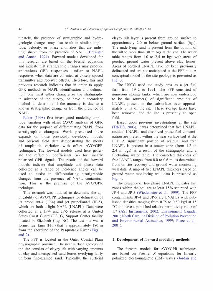
located in Elizabeth City, NC. The test site was a

former fuel farm (FFF) that is approximately 180 m

from the shoreline of the Pasquotank River (Figs. 1

and 2).

The FFF is located in the Outer Coastal Plain

physiographic province. The near surface geology of

the site consists of clayey silt with varying amounts

of clay and interspersed sand lenses overlying fairly

uniform fine-grained sand. Typically, the surficial

clayey silt layer is present from ground surface to

approximately 2.0 m below ground surface (bgs).

The underlying sand is present from the bottom of

the silt to more than 30 m bgs at the site. The water

table ranges from 1.0 to 2.4 m bgs with areas of

perched ground water present above clay lenses.

Areas of perched LNAPL have not been previously

delineated and are not anticipated at the FFF site. A

conceptual model of the site geology is presented as

Fig. 3.

The USCG used the study area as a jet fuel

farm from 1942 to 1991. The FFF consisted of

numerous storage tanks, which are now understood

to be the source(s) of significant amounts of

LNAPL present in the subsurface over approxi-

mately 3 ha of the site. These storage tanks have

been removed, and the site is presently an open

field.

Based upon previous investigations at the site

(TtNUS, 2003), it was determined that free LNAPL,

residual LNAPL, and dissolved phase fuel contami-

nation are present within the near surface soil at the

FFF. A significant portion of residual and free

LNAPL is present in a smear zone (from 1.2 to

2.4 m bgs) as a result of the stratigraphy and a

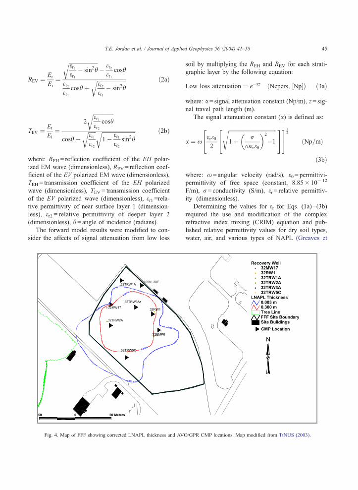
fluctuating water table. The corrected thickness of

free LNAPL ranges from 0.0 to 0.6 m, as determined

from on-site recovery and ground water monitoring

well data. A map of free LNAPL thickness based on

ground water monitoring well data is presented as

Fig. 4.

The presence of free phase LNAPL indicates that

zones within the soil are at least 15% saturated with

JP-4 and JP-5 (Wiedemeier et al., 1999). The FFF

contaminants JP-4 and JP-5 are LNAPLs with pub-

lished densities ranging from 0.75 to 0.80 kg/l at 15

jC and have a published relative permittivity value of

1.7 (ASI Instruments, 2002; Environment Canada,

2001; North Carolina Division of Pollution Prevention

and Environmental Assistance, 1999; Place et al.,

2001).

2. Development of forward modeling methods

The forward models for AVO/GPR techniques

are based on Fresnel R equations for linearly

polarized electromagnetic (EM) waves (Jordan and

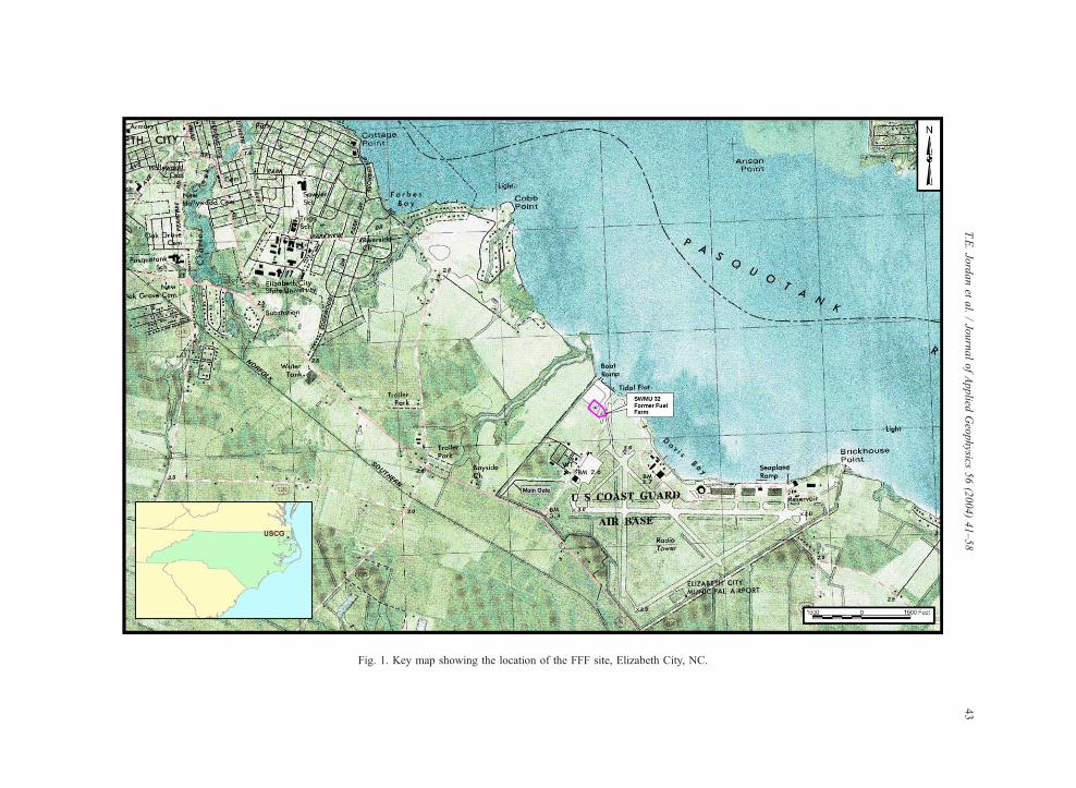
Fig. 1. Key map showing the location of the FFF site, Elizabeth City, NC.

T.E.Jordanet

al./JournalofApplied

Geophysics

56(2004)41–58

43

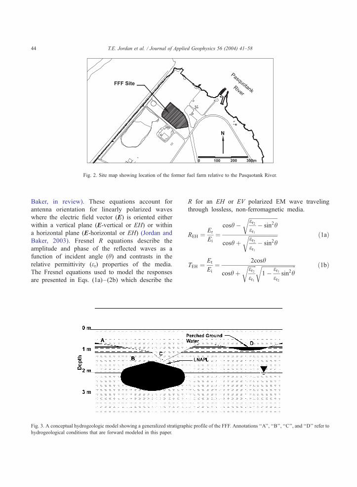
Fig. 2. Site map showing location of the former fuel farm relative to the Pasquotank River.


Baker, in review). These equations account for

antenna orientation for linearly polarized waves

where the electric field vector (E) is oriented either

within a vertical plane (E-vertical or EH) or within

a horizontal plane (E-horizontal or EH) (Jordan and

Baker, 2003). Fresnel R equations describe the

amplitude and phase of the reflected waves as a

function of incident angle (h) and contrasts in the

relative permittivity (er) properties of the media.

The Fresnel equations used to model the responses

are presented in Eqs. (1a)–(2b) which describe the

Fig. 3. A conceptual hydrogeologic model showing a generalized stratigrap

hydrogeological conditions that are forward modeled in this paper.

R for an EH or EV polarized EM wave traveling

through lossless, non-ferromagnetic media.

REH ¼ Er

Ei

¼cosh �

ffiffiffiffiffiffiffiffiffiffiffiffiffiffiffiffiffiffiffiffiffier2er1

� sin2hr

cosh þffiffiffiffiffiffiffiffiffiffiffiffiffiffiffiffiffiffiffiffiffier2er1

� sin2hr ð1aÞ

TEH ¼ Et

Ei

¼ 2cosh

cosh þffiffiffiffiffiffier2er1

r ffiffiffiffiffiffiffiffiffiffiffiffiffiffiffiffiffiffiffiffiffiffiffiffiffi1� er1

er2sin2h

r ð1bÞ

hic profile of the FFF. Annotations ‘‘A’’, ‘‘B’’, ‘‘C’’, and ‘‘D’’ refer to

T.E. Jordan et al. / Journal of Applied Geophysics 56 (2004) 41–58 45

REV ¼ Er

Ei

¼

ffiffiffiffiffiffiffiffiffiffiffiffiffiffiffiffiffiffiffiffiffier2er1

� sin2hr

� er2er1

cosh

er2er1

cosh þffiffiffiffiffiffiffiffiffiffiffiffiffiffiffiffiffiffiffiffiffier2er1

� sin2hr ð2aÞ

TEV ¼ Et

Ei

¼2

ffiffiffiffiffiffiffiffiffiffiffiffiffiffiffier1er2

coshr

cosh þffiffiffiffiffiffier1er2

r ffiffiffiffiffiffiffiffiffiffiffiffiffiffiffiffiffiffiffiffiffiffiffiffiffi1� er1

er2sin2h

r ð2bÞ

where: REH = reflection coefficient of the EH polar-

ized EM wave (dimensionless), REV = reflection coef-

ficient of the EV polarized EM wave (dimensionless),

TEH = transmission coefficient of the EH polarized

wave (dimensionless), TEV = transmission coefficient

of the EV polarized wave (dimensionless), er1 =rela-tive permittivity of near surface layer 1 (dimension-

less), er2 = relative permittivity of deeper layer 2

(dimensionless), h = angle of incidence (radians).

The forward model results were modified to con-

sider the affects of signal attenuation from low loss

Fig. 4. Map of FFF showing corrected LNAPL thickness and AV

soil by multiplying the REH and REV for each strati-

graphic layer by the following equation:

Low loss attenuation ¼ e�az ðNepers; ½Np�Þ ð3aÞ

where: a = signal attenuation constant (Np/m), z = sig-

nal travel path length (m).

The signal attenuation constant (a) is defined as:

a ¼ xere02

ffiffiffiffiffiffiffiffiffiffiffiffiffiffiffiffiffiffiffiffiffiffiffiffiffiffiffiffiffiffiffiffiffiffiffi1þ r

xere0

� �2

�1

s24

35

24

35

12

ðNp=mÞ

ð3bÞ

where: x = angular velocity (rad/s), e0 = permittivi-

permittivity of free space (constant, 8.85� 10� 12

F/m), r = conductivity (S/m), er = relative permittiv-

ity (dimensionless).

Determining the values for er for Eqs. (1a)–(3b)

required the use and modification of the complex

refractive index mixing (CRIM) equation and pub-

lished relative permittivity values for dry soil types,

water, air, and various types of NAPL (Greaves et

O/GPR CMP locations. Map modified from TtNUS (2003).


al., 1996; Ulriksen, 1982). Eq. (4) is modified from

the three-phase CRIM equation to consider fractional

saturation of air, water, and NAPL in the pore

spaces.

er ¼ /SNAPLffiffiffiffiffiffiffiffiffiffiffieNAPL

p þ ð1� /Þ ffiffiffiffiffiem

p

þ /ð1� SNAPL � SairÞffiffiffiffiffiew

p þ /Sairffiffiffiffiffiffieair

p

ð4Þ

where: eNAPL= relative permittivity of NAPL (dimen-

sionless), em = relative permittivity of soil matrix

(dimensionless), ew = relative permittivity of water

(dimensionless), eair = relative permittivity of air (di-

mensionless), / = porosity (dimensionless), SNAPL=

fractional NAPL saturation (dimensionless), Sair =

fractional air saturation (dimensionless).

The variable em can be roughly approximated

based on soil density by Eq. (5) where

em ¼ q1:93 ð5Þ

However, not having soil density values we used

published values of relative permittivity for dry soils

from Ulriksen (1982) and input them into a simple

ratio relationship to estimate the variable em where

em ¼/ � ffiffiffiffiffiffiffiffiffiffiffiffiffiffiffiffi

er dry soilp

/ � ffiffiffiffiffiffieair

p� �2

ð6Þ

Published values of relative permittivity from

Ulriksen (1982) and estimated values from Eqs.

(4)–(6) were used to model the stratigraphy and

hydrogeology of the FFF and are presented in Table 1.

The relative permittivity values from Table 1 and

Eqs. (1a)–(3b) were used to develop four forward

Table 1

Values of relative permittivity used for the conceptual model for the

FFF

Soil type Porosity Estimated relative permittivity values

Water saturation NAPL saturation

0% 15% 100% 15% 30% 50%

Loose, mixed

grain sand

0.40 6.00 8.58 34.45 29.67 24.89 18.51

Soft, slightly

organic clay

0.66 2.40 9.47 54.35 46.46 38.57 28.05

Values of porosity are from Dunn et al. (1980). The NAPL is

assumed to be present at the water table and have a relative

permittivity value of 1.70.

AVO/GPR models for the FFF (Figs. 5–8). The

thickness for each forward model was constant and

is presented in Table 2.

The AVO/GPR forward models are based on

Eqs. (1a)–(3b), and the er values presented in Table

1. These forward models account for the reflected

versus transmitted energy at each and subsequently

deeper interfaces. The forward models also consider

the impact of signal attenuation using Eqs. (3a) and

(3b). Travel path length for the multilayered models

is calculated using Snell’s Law and the offset

distance between the transmitter and receiver. How-

ever, the AVO/GPR forward model results are

presented as incidence angle versus reflection coef-

ficient where incidence angle is based on a simple

geometric path from the transmitter to the target

layer and return.

The reflection coefficient results of the AVO/GPR

forward models were independently normalized

(REH/REHMax) and (REV/REVMax

) with care taken to

preserve phase. The independently normalized polar-

ization differences (REH�REV) were then calculated

and used to assist in data interpretation. The inde-

pendently normalized polarization differences are

henceforth referred to as normalized residual polar-

ization (NRP) and are plotted versus incidence angle

for each target reflector. The forward modeled NRP

values were plotted versus incidence angle for four

hydrogeologic scenarios common to the FFF site as

follows:

(A) Clayey soils with and without the presence of a

sand lens.

(B) Sandy soils with and without NAPL present

beneath a clay lens.

(C) Sandy soils with and without NAPL present at the

water table (without an overlying clay lens).

(D) Sandy soils with perched ground water with and

without NAPL above a clay lens.

The parameters for the four models are presented

in Table 3 and the results are presented in Figs. 5–

8. The conductivity values used are our best esti-

mate of the subsurface conditions at this site.

Conductivity values of 1 mS/m were used to repre-

sent unsaturated dry sandy or clayey soils. Conduc-

tivity values of 3 mS/m were used to represent

moist sandy soils and values of 6 mS/m were used

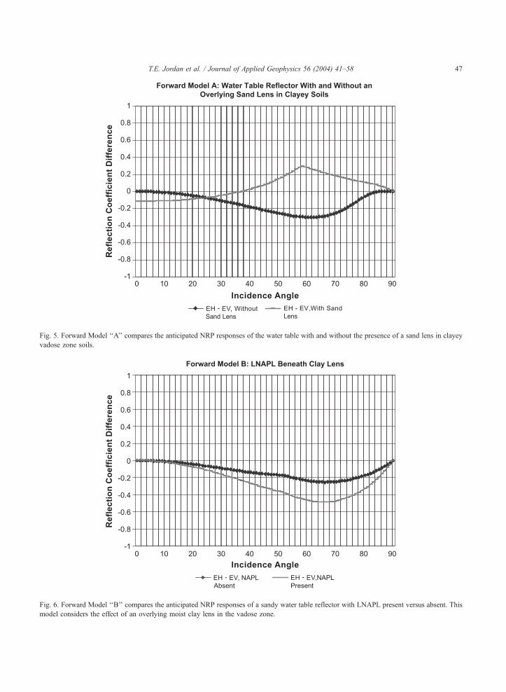
Fig. 5. Forward Model ‘‘A’’ compares the anticipated NRP responses of the water table with and without the presence of a sand lens in clayey

vadose zone soils.

Fig. 6. Forward Model ‘‘B’’ compares the anticipated NRP responses of a sandy water table reflector with LNAPL present versus absent. This

model considers the effect of an overlying moist clay lens in the vadose zone.


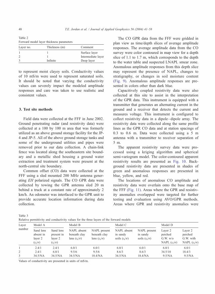
Table 2

Forward model layer thickness parameters

Layer no. Thickness (m) Comment

1 1 Surface layer

2 1 Intermediate layer

3 Infinite Deep layer


to represent moist clayey soils. Conductivity values

of 10 mS/m were used to represent saturated soils.

It should be noted that varying the conductivity

values can severely impact the modeled amplitude

responses and care was taken to use realistic and

consistent values.

3. Test site methods

Field data were collected at the FFF in June 2002.

Ground penetrating radar (and resistivity data) were

collected at a 100 by 100 m area that was formerly

utilized as an above ground storage facility for the JP-

4 and JP-5. All of the above ground storage tanks and

some of the underground utilities and pipes were

removed prior to our data collection. A chain-link

fence was located along the southeastern site bound-

ary and a metallic shed housing a ground water

extraction and treatment system were present at the

north-central site boundary.

Common offset (CO) data were collected at the

FFF using a sled mounted 200 MHz antenna gener-

ating EH polarized signals. The CO GPR data were

collected by towing the GPR antenna sled 20 m

behind a truck at a constant rate of approximately 2

km/h. An odometer was interfaced to the GPR unit to

provide accurate location information during data

collection.

Table 3

Relative permittivity and conductivity values for the three layers of the fo

Layer Model A Model B

numberSand lens

absent in

layer 2

(er/r)

Sand lens

present in

layer 2

(er/r)

NAPL absent

beneath clay

lens (er/r)

NAPL present

beneath clay

lens (er/r)

1 2.4/1 2.4/1 6.0/1 6.0/1

2 2.4/1 6.0/1 9.5/6 9.5/6

3 34.5/NA 34.5/NA 34.5/NA 18.4/NA

Values of conductivity are presented in units of mS/m.

The CO GPR data from the FFF were gridded in

plan view as time/depth slices of average amplitude

responses. The average amplitude data from the CO

survey were color contoured in map view for a depth

slice of 1.1 to 1.7 m, which corresponds to the depth

to the water table and suspected LNAPL smear zone.

Anomalous amplitude responses from this depth slice

may represent the presence of NAPL, changes to

stratigraphy, or changes in soil moisture content

(Fig. 9). Anomalous amplitude responses are pre-

sented in colors other than dark blue.

Capacitively coupled resistivity data were also

collected at this site to assist in the interpretation

of the GPR data. This instrument is equipped with a

transmitter that generates an alternating current in the

ground and a receiver that detects the current and

measures voltage. This instrument is configured to

collect resistivity data in a dipole–dipole array. The

resistivity data were collected along the same profile

lines as the GPR CO data and at station spacings of

0.3 to 0.6 m. Data were collected using a 5 m

antenna with a transmitter to receiver separation of

5 m.

The apparent resistivity survey data were pro-

cessed using a kriging algorithm and spherical

semi-variogram model. The color-contoured apparent

resistivity results are presented as Fig. 10. Back-

ground resistivity data are presented in shades of

green and anomalous responses are presented in

blue, yellow, and red.

The locations of anomalous CO amplitude and

resistivity data were overlain onto the base map of

the FFF (Fig. 11). Areas where the GPR and resistiv-

ity anomalies overlapped were targeted for further

testing and evaluation using AVO/GPR methods.

Areas where GPR and resistivity anomalies were

rward models

Model C Model D

NAPL absent

in sandy

soils (er/r)

NAPL present

in sandy

soils (er/r)

Layer 2

perched

G.W. w/o

NAPL (er/r)

Layer 2

perched

G.W. with

NAPL (er/r)

6.0/1 6.0/1 6.0/1 6.0/1

8.6/3 8.6/3 34.5/10 18.4/3

34.5/NA 18.4/NA 9.5/NA 9.5/NA

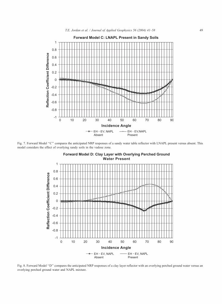
Fig. 7. Forward Model ‘‘C’’ compares the anticipated NRP responses of a sandy water table reflector with LNAPL present versus absent. This

model considers the effect of overlying sandy soils in the vadose zone.

Fig. 8. Forward Model ‘‘D’’ compares the anticipated NRP responses of a clay layer reflector with an overlying perched ground water versus an

overlying perched ground water and NAPL mixture.


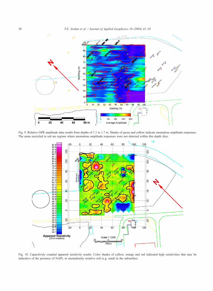
Fig. 9. Relative GPR amplitude data results from depths of 1.1 to 1.7 m. Shades of green and yellow indicate anomalous amplitude responses.

The areas encircled in red are regions where anomalous amplitude responses were not detected within this depth slice.

Fig. 10. Capacitively coupled apparent resistivity results. Color shades of yellow, orange and red indicated high resistivities that may be

indicative of the presence of NAPL or anomalously resistive soil (e.g. sand) in the subsurface.



absent appeared to correspond, suggesting that mini-

mal additional data collection were necessary in those

regions of the site.

Eight locations were selected for further analysis.

These locations were revisited using common-mid-

point (CMP) GPR methods. The CMP data were

collected using perpendicular broadside and parallel

end-fire antenna orientations to generate EH and EV

polarized signals, respectively. Common-midpoint da-

ta were also collected in suspected LNAPL and non-

LNAPL impacted areas to obtain signal velocity

information and geo-electric stratigraphic information

for this site.

4. AVO/GPR data processing and analysis

The raw CO and CMP data were processed using

commercially available software. Raw amplitude

values versus transmitter to receiver separation dis-

tances were extracted from EH and EV CMP data

using software that assisted in the selection of the

maximum relative amplitude value within a 5 ns

window for each trace. Care was taken to preserve

the original CMP amplitudes and not corrupt them

with automatic gain control (AGC) or other process-

ing/interpretation steps.

Velocity data for each reflector were extracted

from the CMP data for depth correlation purposes

through the use of the Dix equation. The Dix

equation was used to convert apparent velocity (Va)

and travel time (t) data to interval velocity (V), layer

thickness, and layer depth. The Dix equation for

determining the root mean square velocity (Vrms) is

presented as Eq. (7), and the interval velocity equa-

tion is presented as Eq. (8).

Vrms ¼

ffiffiffiffiffiffiffiffiffiffiffiffiffiffiffiffiffiffiffiffiXni¼1

V 2aiDti

Xni¼1

Dti

vuuuuuuut ð7Þ

V1 ¼

ffiffiffiffiffiffiffiffiffiffiffiffiffiffiffiffiffiffiffiffiffiffiffiffiffiffiffiffiffiffiffiffiffiffiffiV 2rms2

t02 � V 2rms1

t01

t02 � t01

sð8Þ

The velocity results were converted to layer thick-

ness and depth and then calibrated to test boring data

provided by the USCG for this experiment. The

results from the velocity analysis indicate that the

total Vrms from surface to 2.0 m varies from 0.76 to

0.11 ns/m across the site. These variable Vrms values

may be indicative of changes in moisture content

related to heterogeneous soil texture or stratigraphic

changes at the FFF.

The maximum raw amplitude data versus trans-

mitter/receiver separation distance for each reflec-

tion event were extracted from the EH and EV

CMP data and archived into a database. The EH

and EV polarization data were individually normal-

ized to account for the inability to simultaneously

collect multi-polarized GPR data. Therefore, EH

polarization data were normalized to EH data and

EV polarized data were normalized to EV data.

The NRP data (EH–EV) were then calculated and

plotted versus incidence angle. The NRP AVO/

GPR results are presented as incidence angle

versus reflection coefficient difference where inci-

dence angle is based on a simple geometric path

down from the transmitter and back to the receiver

(Figs. 12–19).

5. Results

The NRP AVO/GPR responses are presented

from the eight CMP locations (Figs. 12–19) and

are summarized in Table 4. The absence, presence,

and thickness of LNAPL were confirmed after the

completion of data interpretation using several in-

trusive approaches. Confirmation methods included

the used of a membrane interface probe/electrical

conductivity (MIP/EC) unit followed by collection

of soil samples and ground water monitoring well

installation. The MIP/EC was used to identify the

location of soil samples and the placement of

NAPL monitoring wells. Soil samples and an oil/

water interface meter were used to confirm the

presence and apparent thickness of the free NAPL.

The apparent thickness of the free NAPL was

corrected based upon accepted methods (USEPA,

1996).

The first location analyzed using AVO/GPR tech-

niques is situated adjacent to ground water monitor-

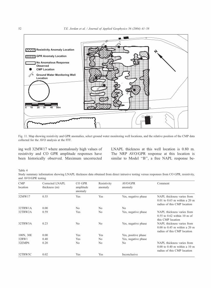
Fig. 11. Map showing resistivity and GPR anomalies, select ground water monitoring well locations, and the relative position of the CMP data

collected for the AVO analysis at the FFF.


ing well 32MW17 where anomalously high values of

resistivity and CO GPR amplitude responses have

been historically observed. Maximum uncorrected

Table 4

Study summary information showing LNAPL thickness data obtained from

and AVO/GPR testing

CMP

location

Corrected LNAPL

thickness (m)

CO GPR

amplitude

anomaly

Resistivit

anomaly

32MW17 0.55 Yes Yes

32TRW1A 0.00 No No

32TRW2A 0.59 Yes No

32TRW3A 0.23 No No

100N, 30E 0.00 Yes Yes

32RW1 0.40 Yes No

32EMP6 0.20 No No

32TRW5C 0.02 Yes Yes

LNAPL thickness at this well location is 0.80 m.

The NRP AVO/GPR response at this location is

similar to Model ‘‘B’’, a free NAPL response be-

direct intrusive testing versus responses from CO GPR, resistivity,

y AVO/GPR

anomaly

Comment

Yes, negative phase NAPL thickness varies from

0.01 to 0.63 m within a 20 m

radius of this CMP location

No


0.55 to 0.62 within 10 m of

this CMP location


0.00 to 0.45 m within a 20 m


Yes, positive phase

Yes, negative phase

No NAPL thickness varies from

0.00 to 0.40 m within a 10 m


Inconclusive

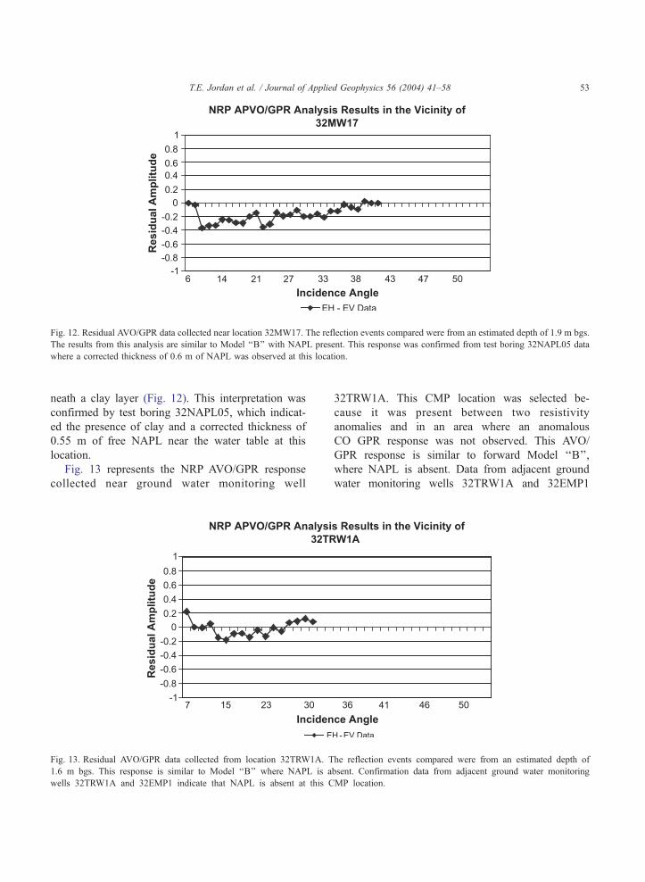
Fig. 12. Residual AVO/GPR data collected near location 32MW17. The reflection events compared were from an estimated depth of 1.9 m bgs.

The results from this analysis are similar to Model ‘‘B’’ with NAPL present. This response was confirmed from test boring 32NAPL05 data

where a corrected thickness of 0.6 m of NAPL was observed at this location.


neath a clay layer (Fig. 12). This interpretation was

confirmed by test boring 32NAPL05, which indicat-

ed the presence of clay and a corrected thickness of

0.55 m of free NAPL near the water table at this

location.

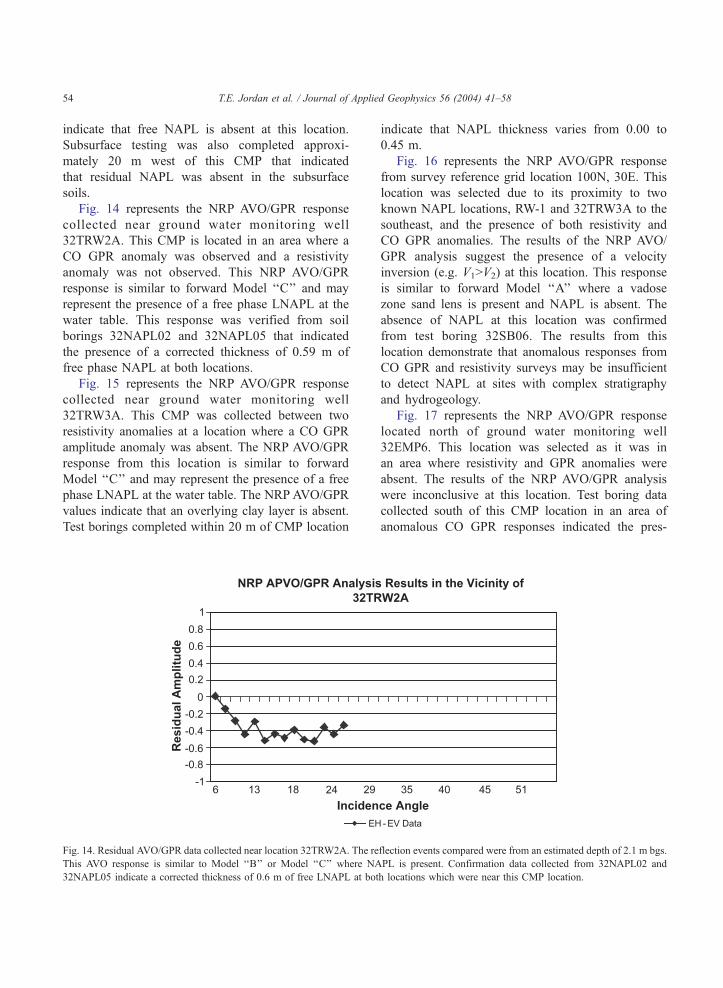
Fig. 13 represents the NRP AVO/GPR response

collected near ground water monitoring well

Fig. 13. Residual AVO/GPR data collected from location 32TRW1A. T

1.6 m bgs. This response is similar to Model ‘‘B’’ where NAPL is a

wells 32TRW1A and 32EMP1 indicate that NAPL is absent at this C

32TRW1A. This CMP location was selected be-

cause it was present between two resistivity

anomalies and in an area where an anomalous

CO GPR response was not observed. This AVO/

GPR response is similar to forward Model ‘‘B’’,

where NAPL is absent. Data from adjacent ground

water monitoring wells 32TRW1A and 32EMP1

he reflection events compared were from an estimated depth of

bsent. Confirmation data from adjacent ground water monitoring

MP location.


indicate that free NAPL is absent at this location.

Subsurface testing was also completed approxi-

mately 20 m west of this CMP that indicated

that residual NAPL was absent in the subsurface

soils.



32TRW2A. This CMP is located in an area where a

CO GPR anomaly was observed and a resistivity

anomaly was not observed. This NRP AVO/GPR

response is similar to forward Model ‘‘C’’ and may

represent the presence of a free phase LNAPL at the

water table. This response was verified from soil

borings 32NAPL02 and 32NAPL05 that indicated

the presence of a corrected thickness of 0.59 m of

free phase NAPL at both locations.



32TRW3A. This CMP was collected between two

resistivity anomalies at a location where a CO GPR

amplitude anomaly was absent. The NRP AVO/GPR

response from this location is similar to forward

Model ‘‘C’’ and may represent the presence of a free

phase LNAPL at the water table. The NRP AVO/GPR

values indicate that an overlying clay layer is absent.

Test borings completed within 20 m of CMP location

Fig. 14. Residual AVO/GPR data collected near location 32TRW2A. The re

This AVO response is similar to Model ‘‘B’’ or Model ‘‘C’’ where NA

32NAPL05 indicate a corrected thickness of 0.6 m of free LNAPL at bot

indicate that NAPL thickness varies from 0.00 to

0.45 m.


from survey reference grid location 100N, 30E. This

location was selected due to its proximity to two

known NAPL locations, RW-1 and 32TRW3A to the

southeast, and the presence of both resistivity and

CO GPR anomalies. The results of the NRP AVO/

GPR analysis suggest the presence of a velocity

inversion (e.g. V1>V2) at this location. This response

is similar to forward Model ‘‘A’’ where a vadose

zone sand lens is present and NAPL is absent. The

absence of NAPL at this location was confirmed

from test boring 32SB06. The results from this

location demonstrate that anomalous responses from

CO GPR and resistivity surveys may be insufficient

to detect NAPL at sites with complex stratigraphy

and hydrogeology.


located north of ground water monitoring well

32EMP6. This location was selected as it was in

an area where resistivity and GPR anomalies were

absent. The results of the NRP AVO/GPR analysis

were inconclusive at this location. Test boring data

collected south of this CMP location in an area of

anomalous CO GPR responses indicated the pres-

flection events compared were from an estimated depth of 2.1 m bgs.

PL is present. Confirmation data collected from 32NAPL02 and

h locations which were near this CMP location.

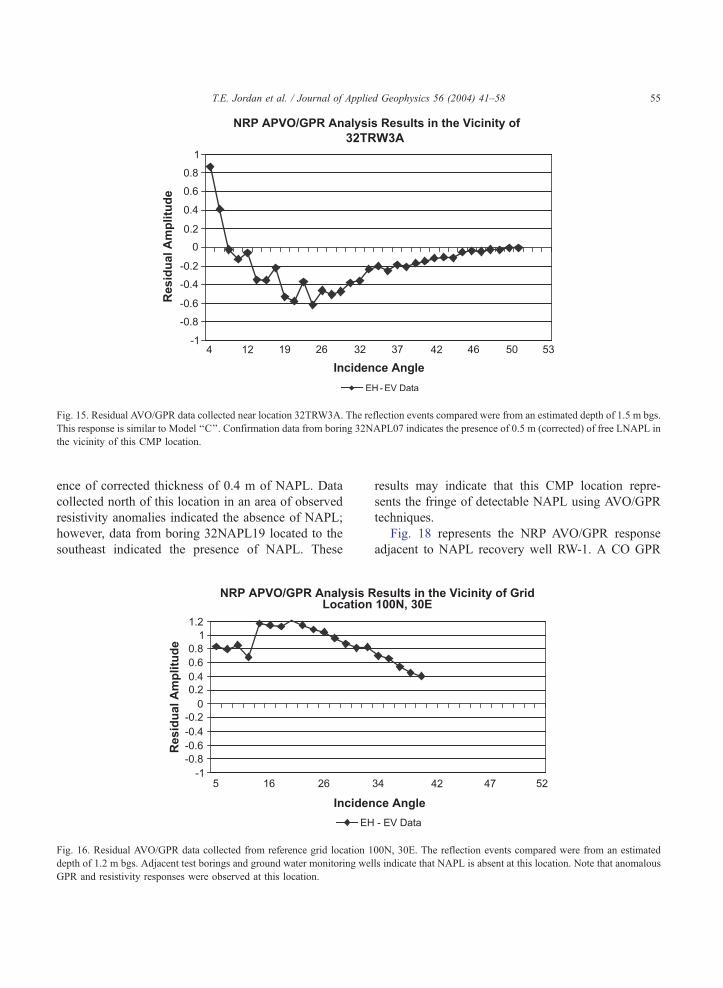
Fig. 15. Residual AVO/GPR data collected near location 32TRW3A. The reflection events compared were from an estimated depth of 1.5 m bgs.

This response is similar to Model ‘‘C’’. Confirmation data from boring 32NAPL07 indicates the presence of 0.5 m (corrected) of free LNAPL in

the vicinity of this CMP location.


ence of corrected thickness of 0.4 m of NAPL. Data

collected north of this location in an area of observed

resistivity anomalies indicated the absence of NAPL;

however, data from boring 32NAPL19 located to the

southeast indicated the presence of NAPL. These

Fig. 16. Residual AVO/GPR data collected from reference grid location 1

depth of 1.2 m bgs. Adjacent test borings and ground water monitoring wel

GPR and resistivity responses were observed at this location.

results may indicate that this CMP location repre-

sents the fringe of detectable NAPL using AVO/GPR

techniques.


adjacent to NAPL recovery well RW-1. A CO GPR

00N, 30E. The reflection events compared were from an estimated

ls indicate that NAPL is absent at this location. Note that anomalous

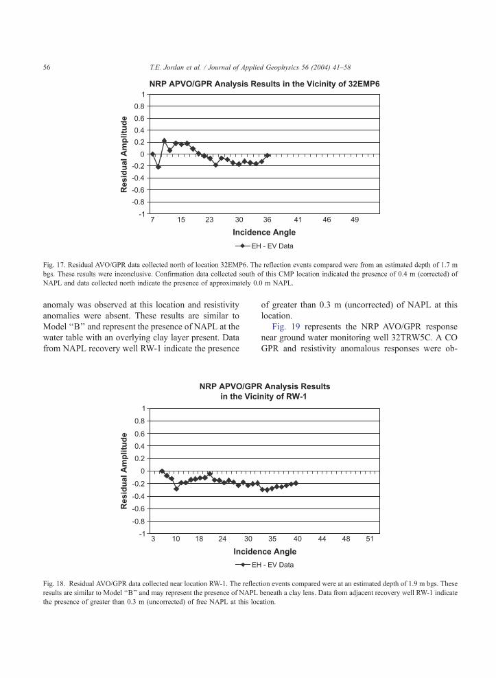
Fig. 17. Residual AVO/GPR data collected north of location 32EMP6. The reflection events compared were from an estimated depth of 1.7 m

bgs. These results were inconclusive. Confirmation data collected south of this CMP location indicated the presence of 0.4 m (corrected) of

NAPL and data collected north indicate the presence of approximately 0.0 m NAPL.


anomaly was observed at this location and resistivity

anomalies were absent. These results are similar to

Model ‘‘B’’ and represent the presence of NAPL at the

water table with an overlying clay layer present. Data

from NAPL recovery well RW-1 indicate the presence

Fig. 18. Residual AVO/GPR data collected near location RW-1. The reflec

results are similar to Model ‘‘B’’ and may represent the presence of NAPL

the presence of greater than 0.3 m (uncorrected) of free NAPL at this loc

of greater than 0.3 m (uncorrected) of NAPL at this

location.


near ground water monitoring well 32TRW5C. A CO

GPR and resistivity anomalous responses were ob-

tion events compared were at an estimated depth of 1.9 m bgs. These

beneath a clay lens. Data from adjacent recovery well RW-1 indicate

ation.

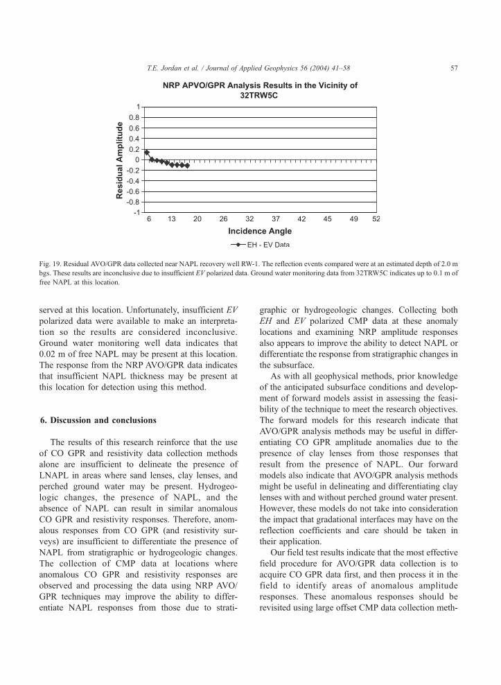
Fig. 19. Residual AVO/GPR data collected near NAPL recovery well RW-1. The reflection events compared were at an estimated depth of 2.0 m

bgs. These results are inconclusive due to insufficient EV polarized data. Ground water monitoring data from 32TRW5C indicates up to 0.1 m of

free NAPL at this location.


served at this location. Unfortunately, insufficient EV

polarized data were available to make an interpreta-

tion so the results are considered inconclusive.

Ground water monitoring well data indicates that

0.02 m of free NAPL may be present at this location.

The response from the NRP AVO/GPR data indicates

that insufficient NAPL thickness may be present at

this location for detection using this method.

6. Discussion and conclusions

The results of this research reinforce that the use

of CO GPR and resistivity data collection methods

alone are insufficient to delineate the presence of

LNAPL in areas where sand lenses, clay lenses, and

perched ground water may be present. Hydrogeo-

logic changes, the presence of NAPL, and the

absence of NAPL can result in similar anomalous

CO GPR and resistivity responses. Therefore, anom-

alous responses from CO GPR (and resistivity sur-

veys) are insufficient to differentiate the presence of

NAPL from stratigraphic or hydrogeologic changes.

The collection of CMP data at locations where

anomalous CO GPR and resistivity responses are

observed and processing the data using NRP AVO/

GPR techniques may improve the ability to differ-

entiate NAPL responses from those due to strati-

graphic or hydrogeologic changes. Collecting both

EH and EV polarized CMP data at these anomaly

locations and examining NRP amplitude responses

also appears to improve the ability to detect NAPL or

differentiate the response from stratigraphic changes in

the subsurface.

As with all geophysical methods, prior knowledge

of the anticipated subsurface conditions and develop-

ment of forward models assist in assessing the feasi-

bility of the technique to meet the research objectives.

The forward models for this research indicate that

AVO/GPR analysis methods may be useful in differ-

entiating CO GPR amplitude anomalies due to the

presence of clay lenses from those responses that

result from the presence of NAPL. Our forward

models also indicate that AVO/GPR analysis methods

might be useful in delineating and differentiating clay

lenses with and without perched ground water present.

However, these models do not take into consideration

the impact that gradational interfaces may have on the

reflection coefficients and care should be taken in

their application.

Our field test results indicate that the most effective

field procedure for AVO/GPR data collection is to

acquire CO GPR data first, and then process it in the

field to identify areas of anomalous amplitude

responses. These anomalous responses should be

revisited using large offset CMP data collection meth-


ods. The CMP data should be collected using antenna

orientations to generate both EH and EV polarized

signals. The CMP results should be processed using a

procedure to extract maximum raw amplitude values

for each value, which are then compared to the

incidence angle of the target reflector. The amplitude

versus incidence angle results should be independent-

ly normalized to account for the inability to simulta-

neously collect EH and EV polarized data. Subtracting

the independently normalized EV from EH polarized

amplitude signal appears to substantially improve the

interpretation process.

It was also observed that the use of a secondary

geophysical technique that measures the electrical

properties of soils improves the development of a

strategy for focusing on a specific set of anomalies.

Various geophysical techniques such as EM induction

and capacitively coupled resistivity devices are avail-

able for rapidly measuring the apparent resistivity or

conductivity of the near surface soil.

The preliminary results of this research indicate

that the NRP AVO/GPR technique is a promising

method that here is shown to assist in the detection

of near surface LNAPL and differentiate the responses

from changes in shallow subsurface stratigraphy and

hydrogeology.

References

ASI Instruments, Dielectric constant reference guide. Retrieved Au-

gust 12, 2002 from the World Wide Web: http://www.asiinstr.

com/dc1.html.

Baker, G.S., 1998. Applying AVO analysis to GPR data. Geophys-

ical Research Letters 25, 397–400.

Brewster, M.L., Annan, A.P., 1994. Ground-penetrating radar mon-

itoring of a controlled DNAPL release: 200 MHz radar. Geo-

physics 59, 1211–1221.

Daniels, J., Roberts, R., Vendl, M., 1995. Ground penetrating radar

for the detection of liquid contaminants. Journal of Applied

Geophysics 33, 195–207.

Dunn, I.S., Anderson, L.R., Kiefer, F.W., 1980. Fundamentals of

Geotechnical Analysis. John Wiley & Sons, New York.

Environment Canada, 2001. Environmental Technology Centre. Re-

trieved August 12, 2002 from the World Wide Web: http://

www.etc.ec.gc.ca.

Greaves, R.J., Lesmes, D.P., Lee, J.M., Toksoz, M.N., 1996. Ve-

locity variations and water content estimated from multi-offset,

ground penetrating radar. Geophysics 61, 683–695.

Jordan, T.E., Baker, G., 2003. Recommendation for new terminol-

ogy for linear polarized components of ground penetrating radar

waves. Journal of Environmental and Engineering Geophysics

8, 38–42.

Jordan, T.E., Baker, G.S., in review. Amplitude and Phase Variation

with Offset (APVO). Analysis of Ground Penetrating Radar

Data: Theory and Forward Modeling: Environmental and Engi-

neering Geoscience Journal.

Kim, C., Daniels, J., Guy, E., Radzevicius, S., Holt, J., 2000.

Residual hydrocarbons in a water saturated medium: a detec-

tion strategy using ground penetrating radar. American Asso-

ciation of Petroleum Geologists, Environmental Geosciences 7,

169–176.

North Carolina Division of Pollution Prevention and Environmental

Assistance, 1999. Fact Sheet, Petroleum Fuels: Basic Composi-

tion and Properties. 1639 Mail Service Center-Raleigh, NC

27699-1639.

Olhoeft, G.R., 1992. Geophysical detection of hydrocarbon and

organic chemical contamination. In: Bell, R.S.Proceedings on

Application of Geophysics to Engineering, and Environmental

Problems. EEGS, Oakbrook, IL, pp. 587–595.

Place, M.C., Coonfare, C.T., Chen, A.S.C., Hoeppel, R.E., Rosan-

sky, S.H., 2001. Principles and Practices of Bioslurping. Battelle

Press, Columbus.

Sander, K.A., Olhoeft, G.R., 1994. 500-MHz ground penetrating

radar data collected during an intentional spill of tetrachloro-

ethylene at Canadian Forces Base Borden in 1991. U.S. Geo-

logical Survey Digital Data Series DDS 25.

Tetra Tech NUS, 2003. Corrective action plan addendum 6, Former

Fuel Farm (SMMU No. 32) United States Coast Guard Support

Center, Elizabeth City, NC.

Ulriksen, P.C., 1982. Application of impulse radar to civil engineer-

ing. PhD Dissertation. Lund University.

USEPA, 1996. How to effectively recover free product at leaking

underground storage tank sites, USEPA 510-R-96-001.

Wiedemeier, T.H., Hanadi, H.S., Wilson, J.T., Newel, C., 1999.

Natural Attenuation of Fuels and Chlorinated Solvents in the

Subsurface. Wiley, New York.

http:\\www.asiinstr.com\dc1.html

http:\\www.etc.ec.gc.ca

Using amplitude variation with offset and normalized residual polarization analysis of ground...

Documents

Transcript of Using amplitude variation with offset and normalized residual polarization analysis of ground...