Using a Broadband ADCP in a Tidal Channel. Part II: Turbulence

1568 VOLUME 16J O U R N A L O F A T M O S P H E R I C A N D O C E A N I C T E C H N O L O G Y

q 1999 American Meteorological Society

Using a Broadband ADCP in a Tidal Channel. Part II: Turbulence

YOUYU LU* AND ROLF G. LUECK

School of Earth and Ocean Sciences, University of Victoria, Victoria, British Columbia, Canada

(Manuscript received 16 July 1997, in final form 12 August 1998)

ABSTRACT

A four-transducer, 600-kHz, broadband acoustic Dopple current profiler (ADCP) was rigidly mounted to thebottom of a fully turbulent tidal channel with peak flows of 1 m s21. Rapid samples of velocity data are usedto estimate various parameters of turbulence with the covariance technique. The questions of bias and errorsources, statistical uncertainty, and spectra are addressed. Estimates of the Reynolds stress are biased by themisalignment of the instrument axis with respect to vertical. This bias can be eliminated by a fifth transducerdirected along the instrument axis. The estimates of turbulent kinetic energy (TKE) density have a systematicbias of 5 3 1024 m2 s22 due to Doppler noise, and the relative statistical uncertainty of the 20-min averages isusually less than 20%–95% confidence. The bias in the Reynolds stress due to Doppler noise is less than 643 1025 m2. The band of zero significance is never less than 1.5 3 1025 m2 s22 due to Doppler noise, and thisband increases with increasing TKE density. Velocity fluctuations with periods longer than 20 min contributelittle to either the stress or the TKE density. The rate of production of TKE density and the vertical eddy viscosityare derived and in agreement with expectations for a tidal channel.

1. Introduction

Turbulence is ubiquitous in coastal waters and playsimportant roles in the transfer of momentum and themixing of water properties. Turbulence parameters andtheir statistics vary both in space and time. Conven-tionally, turbulent velocity fluctuations in the ocean aremeasured by two types of instruments: shear probes(e.g., Osborn and Crawford 1980) and point current me-ters (e.g., Gross and Nowell 1983, 1985; McPhee 1994).Turbulent measurement with acoustic Doppler currentprofilers (ADCPs) is a relatively new technique and pos-sesses the advantages of remote sensing.

Several approaches have been developed to estimateturbulent quantities with an ADCP by taking advantageof the rapid sampling of this instrument. Gargett (1988,1994) reported a ‘‘large-eddy’’ approach that providesestimates of the turbulent kinetic energy (TKE) dissi-pation rate by using a narrowband ADCP with a truevertical beam. Van Haren et al. (1994) applied a ‘‘direct-correlation’’ approach to estimate the velocity covari-ance (Reynolds stress) in the internal wave frequency

* Current affiliation: Department of Oceanography, Dalhousie Uni-versity, Halifax, Nova Scotia, Canada.

Corresponding author address: Dr. Rolf G. Lueck, School of Earthand Ocean Sciences, University of Victoria, P.O. Box 1700, 3800Finnerty Road, Victoria, BC V8W 2Y2, Canada.E-mail: [email protected]

band by using a moored narrowband ADCP with a stan-dard beam configuration. The third method is the ‘‘var-iance technique’’ that derives Reynolds stress and TKEdensity from the autocovariances of along-beam veloc-ities. This method was first explored by Lohrmann etal. (1990) with a pulse-to-pulse coherent sonar and wasrecently applied by Stacey (1996) with a broadbandADCP. The advantages of using a broadband ADCP arethat the noise level in velocity profiling is lower thanthat of a narrowband unit and the profiling range is muchlarger than that of a pulse-to-pulse coherent sonar.

In this paper, we address the issue of obtaining re-liable estimates of turbulent quantities with the ‘‘vari-ance technique’’ and, thereby, extend the work on first-order moments presented in the companion paper (Luand Lueck 1999, hereafter Part I). Section 2 provides abrief introduction of the computation algorithm. In sec-tions 3–5, we present analyses of bias and error sources,statistical uncertainty of the estimates and its causes, aswell as spectra. Section 6 addresses the measurementresults of Reynolds stresses, the TKE density, the TKEproduction rate, and viscosity coefficient. Section 7 of-fers a summary.

2. Deriving turbulent products from variances ofalong-beam velocities

The transducer geometry and beam orientation of theADCP, manufactured by RD Instruments (RDI), is il-lustrated in Fig. 1 of Part I. Each of the four beams isinclined by u 5 308 from the axis of the instrument,

NOVEMBER 1999 1569L U A N D L U E C K

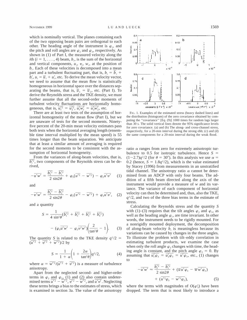
FIG. 1. Examples of the estimated stress (heavy dashed lines) andthe distribution (histogram) of the zero covariance obtained by com-puting the ‘‘covariance’’ [Eq. (9)] 1000 times for random lags largerthan 30 s. The solid vertical lines denote the 95% significance levelsfor zero covariance. (a) and (b) The along- and cross-channel stress,respectively, for a 20-min interval during the strong ebb; (c) and (d)the same components for a 20-min interval during the weak flood.

which is nominally vertical. The planes containing eachof the two opposing beam pairs are orthogonal to eachother. The heading angle of the instrument is w1, andthe pitch and roll angles are w2 and w3, respectively. Asshown in (1) of Part I, the measured velocity along theith (i 5 1, . . . , 4) beam, bi, is the sum of the horizontaland vertical components, ui, y i, wi, at the position ofbi. Each of these velocities is decomposed into a meanpart and a turbulent fluctuating part, that is, bi 5 b i 1

, ui 5 u i 1 , etc. To derive the mean velocity vector,b9 u9i i

we need to assume that the mean flow is statisticallyhomogeneous in horizontal space over the distances sep-arating the beams, that is, u 1 5 u 2, etc. (Part I). Toderive the Reynolds stress and the TKE density, we mustfurther assume that all the second-order moments ofturbulent velocity fluctuations are horizontally homo-geneous, that is, 5 , 5 , etc.2 2u9 u9 u9w9 u9w91 2 1 1 2 2

There are at least two tests of the assumption of hor-izontal homogeneity of the mean flow (Part I), but weare unaware of tests for the second moments. Ninety-five percent of the 20-min mean velocity estimates passboth tests when the horizontal averaging length (ensem-ble time interval multiplied by the mean speed) is 55times longer than the beam separation. We anticipatethat at least a similar amount of averaging is requiredfor the second moments to be consistent with the as-sumption of horizontal homogeneity.

From the variances of along-beam velocities, that is,, two components of the Reynolds stress can be de-2b9i

rived,

2 2b9 2 b92 1 2 22u9w9 5 1 w (u9 2 w9 ) 2 w u9y9 (1)3 22 sin2u

and2 2b9 2 b94 3 2 22y9w9 5 2 w (y9 2 w9 ) 1 w u9y9, (2)2 32 sin2u

and a quantity

12 2 2 2S 5 (b9 1 b9 1 b9 1 b9 )1 2 3 424 sin u

22 (w u9w9 2 w y9w9) 2 1 . (3)3 2 21 2tan u

The quantity S is related to the TKE density q2/2 5(u92 1 y92 1 w92 )/2 by

1 2a2S 5 1 1 q /2, (4)

21 21 1 a tan u

where a 5 w92 /(u92 1 y92 ) is a measure of turbulenceanisotropy.

Apart from the neglected second- and higher-orderterms in w2 and w3, (1) and (2) also contain undeter-mined terms u92 2 w92 , y92 2 w92 , and u9y9 . Neglectingthese terms brings a bias to the estimates of stress, whichis examined in section 3a. The value of the anisotropy

ratio a ranges from zero for extremely anisotropic tur-bulence to 0.5 for isotropic turbulence. Hence S 5(1;2.7)q2/2 (for u 5 308). In this analysis we use a 50.2 (hence, S 5 1.8q2/2), which is the value estimatedby Stacey (1996) from measurements in an unstratifiedtidal channel. The anisotropy ratio a cannot be deter-mined from an ADCP with only four beams. The ad-dition of a fifth beam directed along the axis of theinstrument would provide a measure of w and its var-iance. The variance of each component of horizontalvelocity can then be determined and, thus, also the TKE,q2/2, and two of the three bias terms in the estimate ofstress.

Calculating the Reynolds stress and the quantity Swith (1)–(3) requires that the tilt angles w2 and w3, aswell as the heading angle w1, are time invariant. In otherwords, the instrument needs to be rigidly mounted. Fora nonrigidly mounted deployment, the decompositionof along-beam velocity bi is meaningless because itsvariations can be caused by changes in the three angles.To illustrate the problem with tilt–eddy correlation inestimating turbulent products, we examine the casewhen only the roll angle w3 changes with time, the head-ing angle is constant, and the pitch angle w2 5 0. Byassuming that w3 5 w3 5 u9w3 , etc., (1) changesu9 u91 2

to

2 2b9 2 b92 12u9w9 ø 1 (u u9w 2 w w9w )3 32 sin2u

2 21 (u9 w 2 w9 w ), (5)3 3

where the terms with magnitudes of O( ) have been2w 3

dropped. The term that is most likely to introduce a


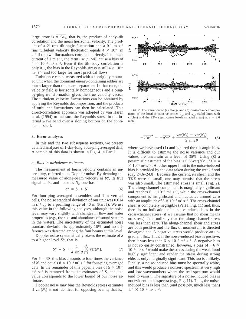
FIG. 2. The variation of (a) along- and (b) cross-channel compo-nents of the local friction velocities u

*s and u*n (solid lines with

circles) and the 95% significance levels (shaded areas) at z 5 3.6mab.

large error is u u9w3 , that is, the product of eddy–tiltcorrelation and the mean horizontal velocity. The prod-uct of a 28 rms tilt-angle fluctuation and a 0.1 m s21

rms turbulent velocity fluctuation equals 4 3 1023 ms21 if the two fluctuations correlate perfectly. In a meancurrent of 1 m s21, the term u u9w3 will cause a bias of4 3 1023 m2 s22. Even if the tilt–eddy correlation isonly 0.1, the bias in the Reynolds stress is still 4 3 1024

m2 s22 and too large for most practical flows.Turbulence can be measured with a nonrigidly mount-

ed unit when the dominant energy-containing eddies aremuch larger than the beam separation. In that case, thevelocity field is horizontally homogeneous and a ping-by-ping transformation gives the true velocity vector.The turbulent velocity fluctuations can be obtained byapplying the Reynolds decomposition, and the productsof turbulent fluctuations can then be calculated. Thisdirect-correlation approach was adopted by van Harenet al. (1994) to measure the Reynolds stress in the in-ternal wave band over a sloping bottom on the conti-nental shelf.

3. Error analyses

In this and the two subsequent sections, we presentdetailed analyses of 1-day-long, four-ping averaged data.A sample of this data is shown in Fig. 4 in Part I.

a. Bias in turbulence estimates

The measurement of beam velocity contains an un-certainty, referred to as Doppler noise. By denoting themeasured value of along-beam velocity as , its trueb*isignal as bi, and noise as Ni, one has

5 bi 1 Ni.b*i (6)

For four-ping averaged ensembles and 1-m verticalcells, the noise standard deviation of our unit was 0.014m s21 up to a profiling range of 40 m (Part I). We usethis value in the following analyses, although the noiselevel may vary slightly with changes in flow and waterproperties (e.g., the size and abundance of sound scattersin the water). The uncertainty of the estimated noisestandard deviation is approximately 15%, and no dif-ference was detected among the four beams at this level.

Doppler noise systematically biases the estimate of Sto a higher level S*, that is,

41S* 5 S 1 var(N ). (7)O i24 sin u i51

For u 5 308 this bias amounts to four times the varianceof Ni and equals 8 3 1024 m2 s22 for four-ping averageddata. In the remainder of this paper, a bias of 5 3 1024

m2 s22 is removed from the estimates of S, and thisvalue corresponds to the lower bound of our noise es-timate.

Doppler noise may bias the Reynolds stress estimatesif var(Ni) is not identical for opposing beams; that is,

var(N ) 2 var(N )2 1*2u9w9 5 2u9w9 1 , (8)2 sin2u

where we have used (1) and ignored the tilt-angle bias.It is difficult to estimate the noise variance and ourvalues are uncertain at a level of 35%. Using (8) apessimistic estimate of the bias is 0.35var(N)/1.73 5 43 1025 m2 s22. Another upper limit to the noise-inducedbias is provided by the data taken during the weak flood(day 24.6–24.8). Because the current, its shear, and theTKE were all small, one may surmise that the stresswas also small. The estimated stress is small (Fig. 2).The along-channel component is marginally significantand reaches 6 3 1025 m2 s22, while the cross-channelcomponent is insignificant and fluctuates around zerowith an amplitude of 3 3 1025 m2 s22. The cross-channelshear is completely negligible (Part I, Fig. 11) and, thus,there is no indication of a noise-induced bias in thecross-channel stress (if we assume that no shear meansno stress). It is unlikely that the along-channel stresswas less than zero. The along-channel shear and stressare both positive and the flux of momentum is directeddowngradient. A negative stress would produce an up-gradient flux. Thus, if the noise-induced bias is positive,then it was less than 6 3 1025 m2 s22. A negative biasis not so easily constrained; however, a bias of 26 31025 m2 s22 would make the stress during the weak floodhighly significant and render the stress during strongebbs as only marginally significant. This too is unlikely.Finally, a noise-induced bias must be spectrally white,and this would produce a nonzero spectrum at very highand low wavenumbers where the real spectrum wouldtend to vanish. The signature of a noise-induced bias isnot evident in the spectra (e.g., Fig. 11). Thus, the noise-induced bias is less than (and possibly, much less than)64 3 1025 m2 s22.


TABLE 1. Estimates of Reynolds stress and S, the 95% significancelevel (D95) for stress, and two estimates of the 95% confidence in-tervals [(d95)1 and (d95)2] for both stress and S (all quantities are inunits of 1024 m2 s22). The estimates are for two 20-min intervals atz 5 3.6 mab.

Mean D95 (s95)1 (d95)2

Strong ebb (2u9w9)s

(2v9w9)n

S

213.05.72

102

65.7265.44

63.3462.4668.12

68.3265.66619.0

Weak flood (2u9w9)s

(2v9w9)n

S

0.3670.1484.08

60.3360.32

60.2760.2560.71

60.3760.3560.96

In section 2, we have noticed that neglecting the termsassociated with tilt angles introduces another type ofbias to the Reynolds stress estimates. From (1) and (2),this bias is proportional to the magnitudes of the tiltangles and the undetermined terms u92 2 w92 , y92 2w92 , and u9y9 . If turbulence tends to be isotropic, u92

2 w92 and y92 2 w92 are small. For anisotropic tur-bulence, w3(u92 2 w92 ) 5 O(w3q2/2). The magnitudeof q2/2 is approximately five times larger than the Reyn-olds stress (e.g., Gross and Nowell 1983). Hence, atmost, the bias due to w3(u92 2 w92) amounts to 17%of the magnitude of 2u9w9 for w3 5 22.08, as in thisexperiment. Similarly, if the magnitude of 2u9y9 is notsignificantly larger than that of 2u9w9 or 2y9w9 , thenneglecting w2u9y9 and w3u9y9 will not cause a significantbias. However, for pitch and roll angles exceeding a fewdegrees and for strongly anisotropic turbulence, this willbe the largest bias in the estimates of Reynolds stress.

b. Statistical uncertainties

In this analysis, we choose 20 min as the ensembleaveraging time to calculate the turbulent quantities. Thelow- and high-frequency velocity components are sep-arated by a low-pass fourth-order Butterworth filter atzero phase. Variances of beam velocity fluctuations arethen calculated and smoothed with the same filter andaveraged over 20-min intervals to give estimates ofReynolds stress and the quantity S.

To test if a stress estimate is statistically different fromzero, we apply the nonparametric approach outlined byFleury and Lueck (1994) and Lueck and Wolk (1999).Differences of the beam velocity variances in (1) and(2) are rearranged into a ‘‘covariance’’ form, for ex-ample,

2 5 ( 1 )( 2 ) .2 2b9 b9 b9 b9 b9 b92 1 2 1 2 1 (9)

Hence, the Reynolds stress 2u9w9 is proportional to thecovariance of the two time series ( 1 ) and ( 2b9 b9 b92 1 2

) at zero lag. The decorrelation timescales of the beamb91velocities are typically 15 s during strong flows and 6s during weak flows (see Fig. 5 in Part I). If we shiftone time series, say ( 1 ), by a lag (or lead) largerb9 b92 1

than 30 s, then its statistical nature is unchanged, but itwill have no correlation with the other time series,( 2 ), on average. A histogram of this zero co-b9 b92 1

variance is obtained by randomly choosing the lag manytimes (e.g., 1000) and then computing the covariances.If the zero-lag covariance, that is, the stress is outsideof the 95% confidence levels of the zero covariance,then this estimate is accepted as statistically differentfrom zero. Figure 1 illustrates the examples of applyingthis method to two 20-min intervals of data, one duringthe strong ebb around day 23.91 and one during theweak flood around day 24.65. For each interval we cal-culate the 95% significance levels (denoted as D95) forboth the along- and cross-channel components of thestress separately. During the strong ebb, the along-chan-

nel stress is significantly different from zero, and thecross-channel stress is marginally different from zero,at the 95% significance levels. During the weak flood,the along-channel stress is comparable to the size of the95% significance levels (and marginally significant),whereas the cross-channel stress is not different fromzero.

We have also applied a bootstrap method (Efron andTibshirani 1993, chapter 13) to determine the statisticaluncertainties for both the stress and S estimates. Foreach 20-min interval, time sequences of the vectors( , , , ) are randomly resampled at identical timeb9 b9 b9 b91 2 3 4

indices to construct a new matrix of beam velocity fluc-tuations. In the first calculation, the new matrix has thesame length as the original data, which is tantamountto assuming that all original samples are independent.In the second calculation, the length of the resampledmatrix is reduced by a factor corresponding to the de-correlation time of the original data: 15 s for the intervalduring the strong ebb and 6 s for the interval duringthe weak flood. The ‘‘stress’’ and ‘‘S’’ for the resampleddata are calculated according to Eqs. (1)–(3). By re-peating the above calculations 1000 times, distributionsof the ‘‘stress’’ and ‘‘S’’ are constructed. The 95% con-fidence intervals for the stress and the quantity S, de-noted as (d95)1 for the first calculation and (d95)2 for thesecond calculation, are derived from the distributions.

Table 1 compares the 95% zero-stress significancelevels (D95) against the 95% confidence intervals [(d95)1,and (d95)2] for the two 20-min intervals. The first con-fidence interval (d95)1 is smaller than (d95)2 because ofits inflated degrees of freedom and it provides a lowerlimit to the confidence interval. The second confidenceinterval (d95)2 is based upon the appropriate degrees offreedom and usually equals the interval of zero signif-icance, D95. The second confidence interval for S isapproximately 20% of S.

In the following, we take D95 as a measure of bothstatistical significance and uncertainty for the stress es-timates. Time variations of the Reynolds stresses at z5 3.6 mab, as well as the corresponding estimates ofD95, are shown in Fig. 2. For clarity in linear coordi-nates, we plot the ‘‘local friction velocities,’’


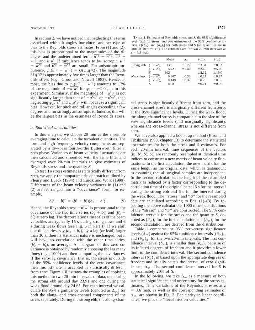
FIG. 3. Variations of stress magnitude (heavy solid lines), the sizeof its 95% significance intervals (dashed lines), and TKE density S(thinner solid lines) at (a) z 5 27.6, (b) z 5 15.6, and (c) z 5 3.6mab. FIG. 4. Scatter diagram (open circles) of |D95| vs S at three levels

(z 5 3.6, 15.6, and 27.6 mab). The two solid lines represent (12)and (13).

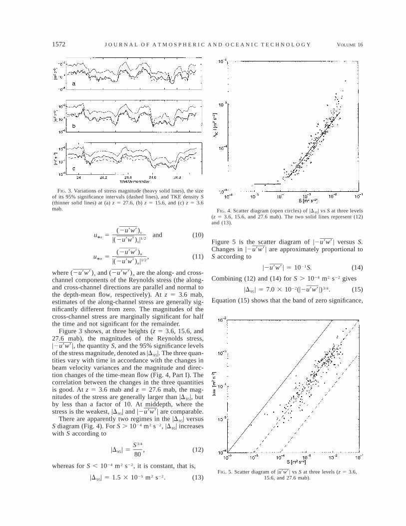
FIG. 5. Scatter diagram of |u9w9 | vs S at three levels (z 5 3.6,15.6, and 27.6 mab).

(2u9w9)su 5 and (10)s 1/2* |(2u9w9) |s

(2u9w9)nu 5 , (11)n 1/2* |(2u9w9) |n

where (2u9w9)s and (2u9w9)n are the along- and cross-channel components of the Reynolds stress (the along-and cross-channel directions are parallel and normal tothe depth-mean flow, respectively). At z 5 3.6 mab,estimates of the along-channel stress are generally sig-nificantly different from zero. The magnitudes of thecross-channel stress are marginally significant for halfthe time and not significant for the remainder.

Figure 3 shows, at three heights (z 5 3.6, 15.6, and27.6 mab), the magnitudes of the Reynolds stress,|2u9w9 |, the quantity S, and the 95% significance levelsof the stress magnitude, denoted as |D95|. The three quan-tities vary with time in accordance with the changes inbeam velocity variances and the magnitude and direc-tion changes of the time-mean flow (Fig. 4, Part I). Thecorrelation between the changes in the three quantitiesis good. At z 5 3.6 mab and z 5 27.6 mab, the mag-nitudes of the stress are generally larger than |D95|, butby less than a factor of 10. At middepth, where thestress is the weakest, |D95| and |2u9w9 | are comparable.

There are apparently two regimes in the |D95| versusS diagram (Fig. 4). For S . 1024 m2 s22, |D95| increaseswith S according to

3/4S|D | 5 , (12)95 80

whereas for S , 1024 m2 s22, it is constant, that is,

|D95| 5 1.5 3 1025 m2 s22. (13)

Figure 5 is the scatter diagram of |2u9w9 | versus S.Changes in |2u9w9 | are approximately proportional toS according to

|2u9w9 | 5 1021S. (14)

Combining (12) and (14) for S . 1024 m2 s22 gives22 3/4|D | 5 7.0 3 10 (|2u9w9 |) . (15)95

Equation (15) shows that the band of zero significance,


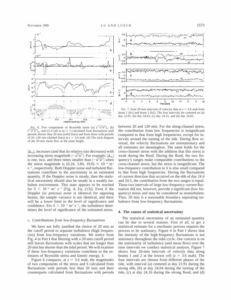
FIG. 6. Two components of Reynolds stress (a) (2u9w9)s, (b)(2u9w9)n, and (c) S (all in m2 s22) calculated from fluctuations withperiods shorter than 20 min (solid lines) and from those with periodsof 20–120 min (dashed lines) at z 5 3.6 mab. (d) The stick diagramof the 20-min mean flow at the same height.

FIG. 7. Four 20-min intervals of velocity data at z 5 3.6 mab frombeam 1 (b1) and beam 2 (b2). The four intervals are centered on (a)day 23.91, (b) day 24.03, (c) day 24.15, and (d) day 24.65.

|D95|, increases (and that its relative size decreases) withincreasing stress magnitude |2u9w9 |. For example, |D95|is one, two, and three times smaller than |2u9w9 | whenthe stress magnitude is (0.24, 3.84, 19.0) 3 1024 m2

s22, respectively. Both Doppler noise and turbulent fluc-tuations contribute to the uncertainty in an estimatedquantity. If the Doppler noise is steady, then the statis-tical uncertainty should also be steady in a weakly tur-bulent environment. This state appears to be reachedfor S , 1024 m2 s22 [Fig. 4; Eq. (13)]. Even if theDoppler (or process) noise is identical for opposingbeams, the sample variance is not identical, and therewill be a lower limit to the level of significance andconfidence. For S . 1024 m2 s22, the turbulence deter-mines the level of significance of the estimated stress.

c. Contributions from low-frequency fluctuations

We have not fully justified the choice of 20 min asthe cutoff period to separate turbulence (high frequen-cies) from low-frequency variations. We notice fromFig. 4 in Part I that filtering with a 20-min cutoff periodstill leaves fluctuations with scales that are longer than20 min but shorter than the tidal period. We will examineif these low-frequency variations contribute to the es-timates of Reynolds stress and kinetic energy, S.

Figure 6 compares, at z 5 3.6 mab, the magnitudesof two components of the stress and S calculated fromfluctuations with periods less than 20 min and theircounterparts calculated from fluctuations with periods

between 20 and 120 min. For the along-channel stress,the contribution from low frequencies is insignificantcompared to that from high frequencies, except for in-tervals around the turning of the tide. During flow re-versal, the velocity fluctuations are nonstationary andall estimates are meaningless. The same holds for thecross-channel stress with the addition that this stress isweak during the flood. During the flood, the two fre-quency’s ranges make comparable contributions to thecross-channel stress, but the stress is insignificant. Thelow-frequency contribution to S is also small comparedto that from high frequencies. During the fluctuationsof current direction that occurred on the ebb of day 24.4and 24.5, the contribution from the two ranges is equal.These two intervals of large low-frequency current fluc-tuation did not, however, provide a significant (low fre-quency) stress and may be considered as nonturbulent.Thus, 20 min is a reasonable boundary separating tur-bulence from low-frequency fluctuations.

4. The causes of statistical uncertainty

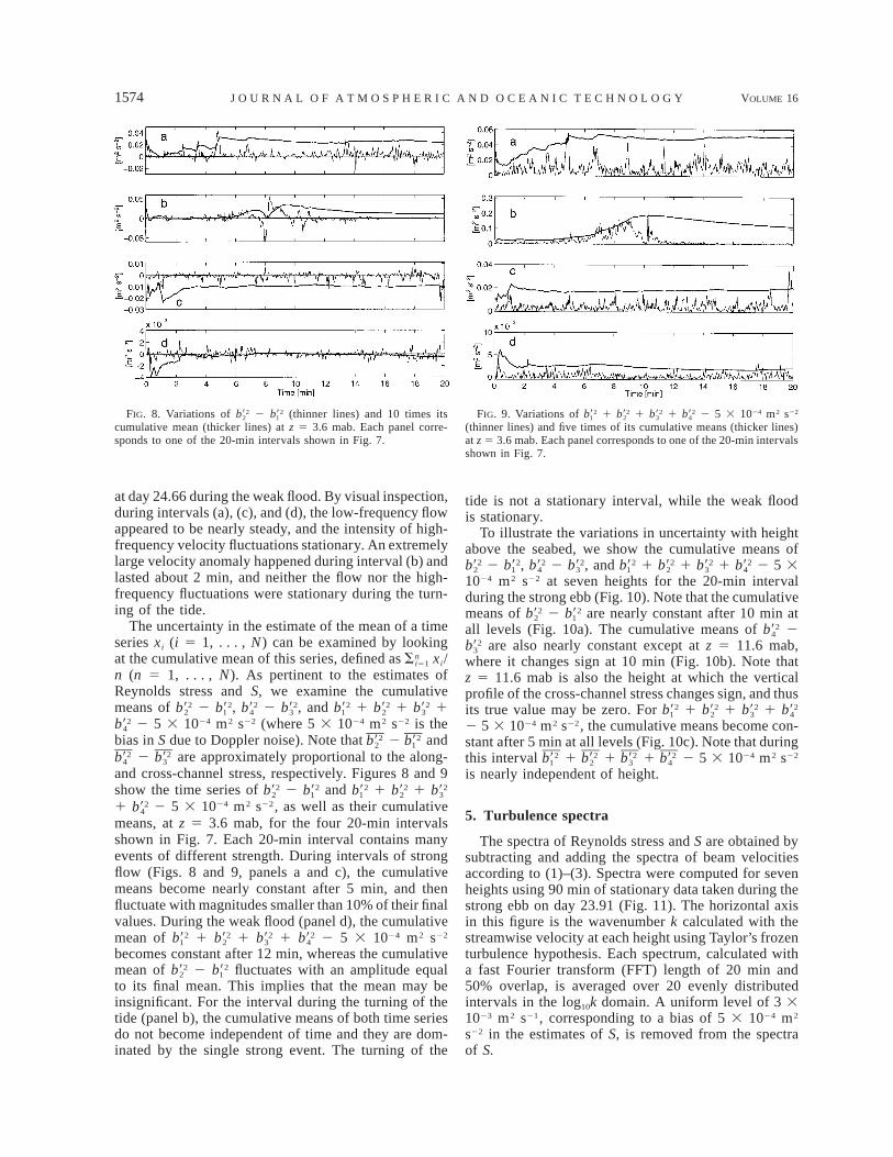
The statistical uncertainty of an estimated quantitycan be due to several reasons. First of all, to get astatistical estimate for a stochastic process requires theprocess to be stationary. Figure 4 in Part I shows thatthe intensity of the high-frequency fluctuations is notstationary throughout the tidal cycle. Our concern is onthe stationarity of turbulence (and mean flow) over thetime intervals we conduct statistical analysis. Figure 7shows four 20-min intervals of velocity data alongbeams 1 and 2 at the lowest cell (z 5 3.6 mab). Thefour intervals are chosen from different phases of thetide, with interval (a) centered at day 23.91 during thestrong ebb, (b) at day 24.04 during the turning of thetide, (c) at day 24.16 during the strong flood, and (d)


FIG. 8. Variations of 2 (thinner lines) and 10 times its2 2b9 b92 1

cumulative mean (thicker lines) at z 5 3.6 mab. Each panel corre-sponds to one of the 20-min intervals shown in Fig. 7.

FIG. 9. Variations of 1 1 1 2 5 3 1024 m2 s222 2 2 2b9 b9 b9 b91 2 3 4

(thinner lines) and five times of its cumulative means (thicker lines)at z 5 3.6 mab. Each panel corresponds to one of the 20-min intervalsshown in Fig. 7.

at day 24.66 during the weak flood. By visual inspection,during intervals (a), (c), and (d), the low-frequency flowappeared to be nearly steady, and the intensity of high-frequency velocity fluctuations stationary. An extremelylarge velocity anomaly happened during interval (b) andlasted about 2 min, and neither the flow nor the high-frequency fluctuations were stationary during the turn-ing of the tide.

The uncertainty in the estimate of the mean of a timeseries xi (i 5 1, . . . , N) can be examined by lookingat the cumulative mean of this series, defined as xi/nSi51

n (n 5 1, . . . , N). As pertinent to the estimates ofReynolds stress and S, we examine the cumulativemeans of 2 , 2 , and 1 1 12 2 2 2 2 2 2b9 b9 b9 b9 b9 b9 b92 1 4 3 1 2 3

2 5 3 1024 m2 s22 (where 5 3 1024 m2 s22 is the2b94bias in S due to Doppler noise). Note that 2 and2 2b9 b92 1

2 are approximately proportional to the along-2 2b9 b94 3

and cross-channel stress, respectively. Figures 8 and 9show the time series of 2 and 1 12 2 2 2 2b9 b9 b9 b9 b92 1 1 2 3

1 2 5 3 1024 m2 s22, as well as their cumulative2b94means, at z 5 3.6 mab, for the four 20-min intervalsshown in Fig. 7. Each 20-min interval contains manyevents of different strength. During intervals of strongflow (Figs. 8 and 9, panels a and c), the cumulativemeans become nearly constant after 5 min, and thenfluctuate with magnitudes smaller than 10% of their finalvalues. During the weak flood (panel d), the cumulativemean of 1 1 1 2 5 3 1024 m2 s222 2 2 2b9 b9 b9 b91 2 3 4

becomes constant after 12 min, whereas the cumulativemean of 2 fluctuates with an amplitude equal2 2b9 b92 1

to its final mean. This implies that the mean may beinsignificant. For the interval during the turning of thetide (panel b), the cumulative means of both time seriesdo not become independent of time and they are dom-inated by the single strong event. The turning of the

tide is not a stationary interval, while the weak floodis stationary.

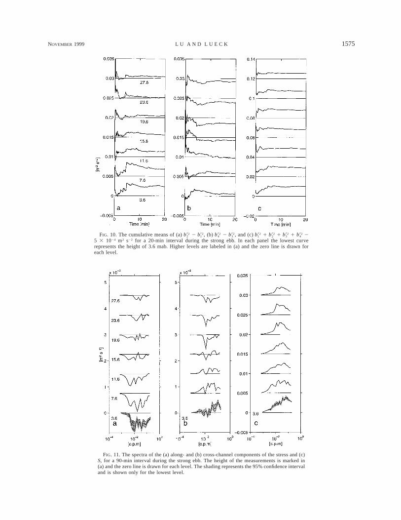
To illustrate the variations in uncertainty with heightabove the seabed, we show the cumulative means of

2 , 2 , and 1 1 1 2 5 32 2 2 2 2 2 2 2b9 b9 b9 b9 b9 b9 b9 b92 1 4 3 1 2 3 4

1024 m2 s22 at seven heights for the 20-min intervalduring the strong ebb (Fig. 10). Note that the cumulativemeans of 2 are nearly constant after 10 min at2 2b9 b92 1

all levels (Fig. 10a). The cumulative means of 22b94are also nearly constant except at z 5 11.6 mab,2b93

where it changes sign at 10 min (Fig. 10b). Note thatz 5 11.6 mab is also the height at which the verticalprofile of the cross-channel stress changes sign, and thusits true value may be zero. For 1 1 12 2 2 2b9 b9 b9 b91 2 3 4

2 5 3 1024 m2 s22, the cumulative means become con-stant after 5 min at all levels (Fig. 10c). Note that duringthis interval 1 1 1 2 5 3 1024 m2 s222 2 2 2b9 b9 b9 b91 2 3 4

is nearly independent of height.

5. Turbulence spectra

The spectra of Reynolds stress and S are obtained bysubtracting and adding the spectra of beam velocitiesaccording to (1)–(3). Spectra were computed for sevenheights using 90 min of stationary data taken during thestrong ebb on day 23.91 (Fig. 11). The horizontal axisin this figure is the wavenumber k calculated with thestreamwise velocity at each height using Taylor’s frozenturbulence hypothesis. Each spectrum, calculated witha fast Fourier transform (FFT) length of 20 min and50% overlap, is averaged over 20 evenly distributedintervals in the log10k domain. A uniform level of 3 31023 m2 s21, corresponding to a bias of 5 3 1024 m2

s22 in the estimates of S, is removed from the spectraof S.


FIG. 10. The cumulative means of (a) 2 , (b) 2 , and (c) 1 1 1 22 2 2 2 2 2 2 2b9 b9 b9 b9 b9 b9 b9 b92 1 4 3 1 2 3 4

5 3 1024 m2 s22 for a 20-min interval during the strong ebb. In each panel the lowest curverepresents the height of 3.6 mab. Higher levels are labeled in (a) and the zero line is drawn foreach level.

FIG. 11. The spectra of the (a) along- and (b) cross-channel components of the stress and (c)S, for a 90-min interval during the strong ebb. The height of the measurements is marked in(a) and the zero line is drawn for each level. The shading represents the 95% confidence intervaland is shown only for the lowest level.


The signs of both components of the Reynolds stressspectra do not change over the resolved wavenumberrange, except and only for the cross-channel stress at15.6 mab where the spectrum is weak. The signs of thecross-channel stress spectra change from positive belowmiddepth to negative above middepth, and this changecorresponds to the change of sign of the transverse shear(Fig. 11, Part I). The wavenumber ranges contributingto the Reynolds stress spectra are fully resolved (Figs.11a,b). The spectra of S are also resolved, except at thehigh-wavenumber end for heights less than 7.6 m. Be-low middepth, there is a noticeable shifting of the peakof the spectra toward smaller wavenumbers with in-creasing distance from the seabed. The analysis of an-other 90 min of stationary data, the strong flood startingat day 24.15, provides spectra of the along-channelstress and S that are similar to those shown in Fig. 11.However, the spectra of the cross-channel stress areweak and ‘‘noisy’’ due to the small cross-channel shearduring the flood (Fig. 11, Part I).

6. Estimates of turbulent quantities

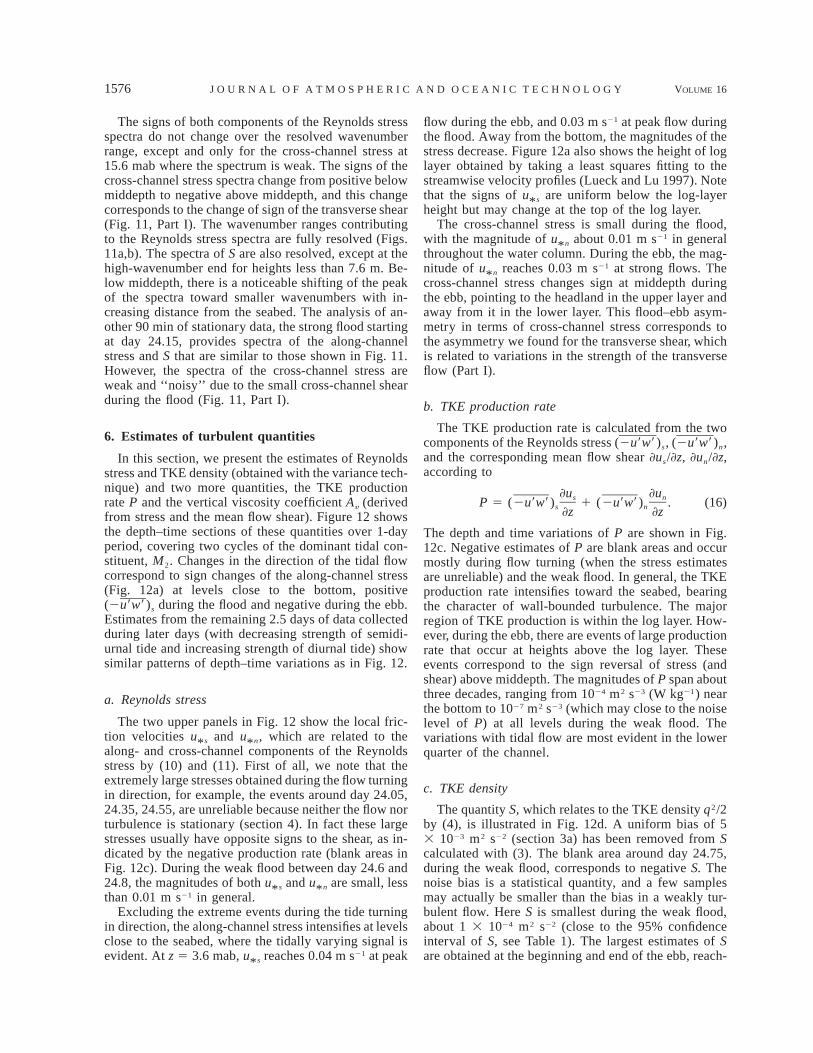
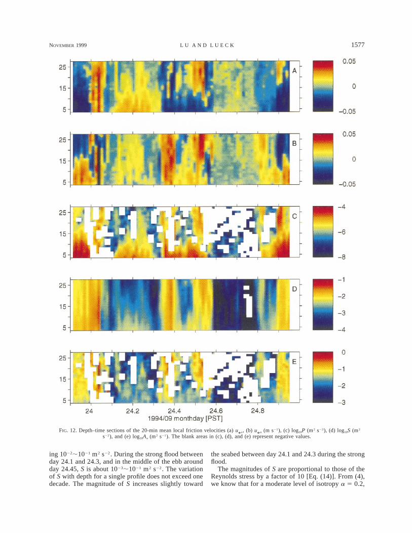
In this section, we present the estimates of Reynoldsstress and TKE density (obtained with the variance tech-nique) and two more quantities, the TKE productionrate P and the vertical viscosity coefficient Ay (derivedfrom stress and the mean flow shear). Figure 12 showsthe depth–time sections of these quantities over 1-dayperiod, covering two cycles of the dominant tidal con-stituent, M2. Changes in the direction of the tidal flowcorrespond to sign changes of the along-channel stress(Fig. 12a) at levels close to the bottom, positive(2u9w9)s during the flood and negative during the ebb.Estimates from the remaining 2.5 days of data collectedduring later days (with decreasing strength of semidi-urnal tide and increasing strength of diurnal tide) showsimilar patterns of depth–time variations as in Fig. 12.

a. Reynolds stress

The two upper panels in Fig. 12 show the local fric-tion velocities u*s and u*n, which are related to thealong- and cross-channel components of the Reynoldsstress by (10) and (11). First of all, we note that theextremely large stresses obtained during the flow turningin direction, for example, the events around day 24.05,24.35, 24.55, are unreliable because neither the flow norturbulence is stationary (section 4). In fact these largestresses usually have opposite signs to the shear, as in-dicated by the negative production rate (blank areas inFig. 12c). During the weak flood between day 24.6 and24.8, the magnitudes of both u*s and u*n are small, lessthan 0.01 m s21 in general.

Excluding the extreme events during the tide turningin direction, the along-channel stress intensifies at levelsclose to the seabed, where the tidally varying signal isevident. At z 5 3.6 mab, u*s reaches 0.04 m s21 at peak

flow during the ebb, and 0.03 m s21 at peak flow duringthe flood. Away from the bottom, the magnitudes of thestress decrease. Figure 12a also shows the height of loglayer obtained by taking a least squares fitting to thestreamwise velocity profiles (Lueck and Lu 1997). Notethat the signs of u*s are uniform below the log-layerheight but may change at the top of the log layer.

The cross-channel stress is small during the flood,with the magnitude of u*n about 0.01 m s21 in generalthroughout the water column. During the ebb, the mag-nitude of u*n reaches 0.03 m s21 at strong flows. Thecross-channel stress changes sign at middepth duringthe ebb, pointing to the headland in the upper layer andaway from it in the lower layer. This flood–ebb asym-metry in terms of cross-channel stress corresponds tothe asymmetry we found for the transverse shear, whichis related to variations in the strength of the transverseflow (Part I).

b. TKE production rate

The TKE production rate is calculated from the twocomponents of the Reynolds stress (2u9w9)s, (2u9w9)n,and the corresponding mean flow shear ]us/]z, ]un/]z,according to

]u ]us nP 5 (2u9w9) 1 (2u9w9) . (16)s n]z ]z

The depth and time variations of P are shown in Fig.12c. Negative estimates of P are blank areas and occurmostly during flow turning (when the stress estimatesare unreliable) and the weak flood. In general, the TKEproduction rate intensifies toward the seabed, bearingthe character of wall-bounded turbulence. The majorregion of TKE production is within the log layer. How-ever, during the ebb, there are events of large productionrate that occur at heights above the log layer. Theseevents correspond to the sign reversal of stress (andshear) above middepth. The magnitudes of P span aboutthree decades, ranging from 1024 m2 s23 (W kg21) nearthe bottom to 1027 m2 s23 (which may close to the noiselevel of P) at all levels during the weak flood. Thevariations with tidal flow are most evident in the lowerquarter of the channel.

c. TKE density

The quantity S, which relates to the TKE density q2/2by (4), is illustrated in Fig. 12d. A uniform bias of 53 1023 m2 s22 (section 3a) has been removed from Scalculated with (3). The blank area around day 24.75,during the weak flood, corresponds to negative S. Thenoise bias is a statistical quantity, and a few samplesmay actually be smaller than the bias in a weakly tur-bulent flow. Here S is smallest during the weak flood,about 1 3 1024 m2 s22 (close to the 95% confidenceinterval of S, see Table 1). The largest estimates of Sare obtained at the beginning and end of the ebb, reach-


FIG. 12. Depth–time sections of the 20-min mean local friction velocities (a) u*s, (b) u

*n (m s21), (c) log10P (m2 s23), (d) log10S (m2

s22), and (e) log10Ay (m2 s21). The blank areas in (c), (d), and (e) represent negative values.

ing 1022;1021 m2 s22. During the strong flood betweenday 24.1 and 24.3, and in the middle of the ebb aroundday 24.45, S is about 1023;1021 m2 s22. The variationof S with depth for a single profile does not exceed onedecade. The magnitude of S increases slightly toward

the seabed between day 24.1 and 24.3 during the strongflood.

The magnitudes of S are proportional to those of theReynolds stress by a factor of 10 [Eq. (14)]. From (4),we know that for a moderate level of isotropy a 5 0.2,


S 5 1.8q2/2. If this is the case, then from (14) we haveq2/2 5 5.6|2u9w9 |, which is close to what Gross andNowell (1983) got from measurements in the near-bot-tom region of tidal boundary layer.

d. Turbulent viscosity

In principle, an estimate of the vertical viscosity co-efficient Ay can be readily obtained from one componentof Reynolds stress and the corresponding shear, that is,

]usA 5 (2u9w9) , (17)y s@1 2]z

or

]unA 5 (2u9w9) . (18)y n@1 2]z

Alternatively, Ay can be calculated from the TKE pro-duction rate and the magnitude of shear, that is,

2 2]u ]un sA 5 P 1 . (19)y @ 1 2 1 2[ ]]z ]z

By using (19), the sign of Ay is the same as P. In theoptimal case the estimates from (17), (18), and (19)should be consistent, and this is found to hold statisti-cally for the present dataset. The estimates of Ay aresubject to large uncertainties, particularly when themagnitudes of the shear are small. Figure 12e indicatesa variation of Ay with tidal flow, ranging from about1023 m2 s21 during the weak flood to 0.1–0.3 m2 s21

during the ebb. During the strong flood between day24.1 and 24.3, Ay is about 0.03 m2 s21. The turbulentviscosity increases with increasing height in the lowerhalf of the water column, and reaches a maximum nearmiddepth.

7. Summary

The variances of the along-beam velocities from astandard ADCP with four beams provide estimates oftwo components of the Reynolds stress and a quantityproportional to the TKE density. To apply the variancetechnique one needs to assume that the mean flow andthe second-order moments of turbulent velocity fluc-tuations are statistically homogeneous in horizontalspace over the distances separating the beams. TheADCP needs to be rigidly mounted for turbulence mea-surements to avoid contamination due to correlation ofinstrument motions and turbulent velocity fluctuations.Doppler noise brings a bias to the estimate of TKEdensity, but not to stress estimates if the Doppler noisein opposing beams is identical. For our unit, this biasis less than 64 3 1025 m2 s22. For a four-beam unit,the bias due to pitch and roll angles cannot be removedand may be significant for tilt angles larger than a fewdegrees in anisotropic turbulence.

The uncertainty levels of the stress estimates aremainly due to turbulent fluctuations and increase withincreasing turbulent intensity. The influence of Dopplernoise emerges when turbulent intensities are low. Thehighest signal-to-noise ratio is obtained at levels closeto the seabed, where the stress magnitudes are large.Contributions from velocity fluctuations at periods lon-ger than 20 min add little to the estimates of Reynoldsstress and TKE density. The spectral ranges of the Reyn-olds stress and TKE density were usually resolved withour sampling interval of 3 s. The high wavenumber endof the spectrum of TKE density was not resolved nearthe seabed.

The combination of the Reynolds stress and meanshear provides estimates of the rate of production ofTKE density and the vertical eddy viscosity. Excludingintervals during the turning of the tide, the measurementcaptures the depth and time variations of turbulence inthe channel. The Reynolds stress shows a clear tidalsignal in the near-bottom layer for the along-channelcomponent and presents a clear ebb–flood asymmetryin the cross-channel component. The TKE productionrate is bottom enhanced, ranging from 1024 m2 s23 (Wkg21) during strong flows to 1027 m2 s23 during weakflows. The TKE density is approximately proportionalto the stress magnitude. The eddy viscosity increaseswith increasing flow speed, and also with increasingheight in the lower half of the water column.

Acknowledgments. We would like to thank D. New-man and J. Box for their technical support to the fieldprogram, and A. Adrian for the deployment and recov-ery of the ADCP. We thank the reviewers for motivatingus to revisit the issue of noise bias in the stress estimates.This work was supported by the U.S. Office of NavalResearch under Grant N00014-93-1-0362.

REFERENCES

Efron, B., and R. J. Tibshirani, 1993: An Introduction to the Bootstrap.Chapman and Hall, 436 pp.

Fleury, M., and R. G. Lueck, 1994: Direct heat flux estimates usinga towed vehicle. J. Phys. Oceanogr., 24, 801–818.

Gargett, A. E., 1988: A ‘‘large-eddy’’ approach to acoustic remotesensing of turbulence kinetic energy dissipation rate e. Atmos.–Ocean, 26, 483–508., 1994: Observing turbulence with a modified acoustic Dopplercurrent profiler. J. Atmos. Oceanic Technol., 11, 1592–1610.

Gross, T. F., and A. R. M. Nowell, 1983: Mean flow and turbulencescaling in a tidal boundary layer. Contin. Shelf Res., 2, 109–126., and , 1985: Spectral scaling in a tidal boundary layer. J.Phys. Oceanogr., 15, 496–508.

Lohrmann A., B. Hackett, and L. P. Roed, 1990: High resolutionmeasurements of turbulence, velocity and stress using a pulse-to-pulse coherent sonar. J. Atmos. Oceanic Technol., 7, 19–37.

Lu, Y., and R. G. Lueck, 1999: Using a broadband ADCP in a tidalchannel. Part I: Mean flow and shear. J. Atmos. Oceanic Technol.,16, 1556–1567.

Lueck, R. G., and Y. Lu, 1997: The logarithmic layer in a tidalchannel. Contin. Shelf Res., 34, 1677–1688., and F. Wolk, 1999: An efficient method for determining thesignificance of covariance estimates. J. Atmos. Oceanic Technol.,16, 773–775.


McPhee, M. G., 1994: On the turbulent mixing length in the oceanicboundary layer. J. Phys. Oceanogr., 24, 2014–2031.

Osborn, T. R., and W. R. Crawford, 1980: An airfoil probe for mea-suring turbulent velocity fluctuations in water. Air–Sea Inter-actions: Instruments and Methods, F. Dobson, L. Hasse, and R.Davis, Eds., Plenum, 801 pp.

Stacey, M. T., 1996: Turbulent mixing and residual circulation in apartially stratified estuary. Ph.D. thesis, Stanford University, 209pp.

van Haren, H., N. Oakey, and C. Garrett, 1994: Measurements ofinternal wave band eddy fluxes above a sloping bottom. J. Mar.Res., 92, 909–946.

Using a Broadband ADCP in a Tidal Channel. Part II: Turbulence

Documents

Transcript of Using a Broadband ADCP in a Tidal Channel. Part II: Turbulence