Usage of the LEGO Mindstorms EV3 Robot - ČVUT DSpace
99
Bachelor Thesis Czech Technical University in Prague F3 Faculty of Electrical Engineering Department of Cybernetics Usage of the LEGO Mindstorms EV3 Robot Design and Realization of the "Ball-riding robot" for the Promotion of the Faculty Jakub Malý Supervisor: Ing. Martin Hlinovský, Ph.D. May 2018
-
Upload
khangminh22 -
Category
Documents
-
view
4 -
download
0
Transcript of Usage of the LEGO Mindstorms EV3 Robot - ČVUT DSpace
Bachelor Thesis
CzechTechnicalUniversityin Prague
F3 Faculty of Electrical EngineeringDepartment of Cybernetics
Usage of the LEGO Mindstorms EV3 Robot
Design and Realization of the "Ball-riding robot"for the Promotion of the Faculty
Jakub Malý
Supervisor: Ing. Martin Hlinovský, Ph.D.May 2018

ii

BACHELOR‘S THESIS ASSIGNMENT
I. Personal and study details
457194Personal ID number:Malý JakubStudent's name:
Faculty of Electrical EngineeringFaculty / Institute:
Department / Institute: Department of Cybernetics
Cybernetics and RoboticsStudy program:
RoboticsBranch of study:
II. Bachelor’s thesis details
Bachelor’s thesis title in English:
Usage of the LEGO Mindstorms EV3 Robot - Design and Realization of the "Ball-riding robot" for thePromotion of the Faculty
Bachelor’s thesis title in Czech:
Využití robota LEGO Mindstorms EV3 - návrh a realizace robota "Ball-riding robot" pro propagačníúčely fakulty
Guidelines:1. Learn about the Lego Mindstorms Education EV3 robot (current status, HW and SW equipment).2. Design and implement the Ball-riding robot for promotional purposes of the faculty.3. Create a website for the tasks you have done (task description, design of the controller or principle of operation,explanation of the proposed software, photogallery and, if necessary, instructions for building the robot).
Bibliography / sources:[1] James Floyd Kelly - LEGO MINDSTORMS NXT-G programming Guide, Second Edition[2] Daniele Benedettelli - Programming LEGO NXT Robots using NXC[3] https://www.youtube.com/watch?v=mt-9AmD_yrk
Name and workplace of bachelor’s thesis supervisor:
Ing. Martin Hlinovský, Ph.D., Department of Control Engineering, FEE
Name and workplace of second bachelor’s thesis supervisor or consultant:
Deadline for bachelor thesis submission: 25.05.2018Date of bachelor’s thesis assignment: 12.01.2018
Assignment valid until: 30.09.2019
_________________________________________________________________________________prof. Ing. Pavel Ripka, CSc.
Dean’s signaturedoc. Ing. Tomáš Svoboda, Ph.D.
Head of department’s signatureIng. Martin Hlinovský, Ph.D.
Supervisor’s signature
III. Assignment receiptThe student acknowledges that the bachelor’s thesis is an individual work. The student must produce his thesis without the assistance of others,with the exception of provided consultations. Within the bachelor’s thesis, the author must state the names of consultants and include a list of references.
.Date of assignment receipt Student’s signature
© ČVUT v Praze, Design: ČVUT v Praze, VICCVUT-CZ-ZBP-2015.1

iv

AcknowledgementsI would like to express my immensegratitude to my advisor Ing. MartinHlinovský, Ph.D. for his patience, motiva-tion, and continuous support throughoutmy Bachelor study. His constructivecriticism and friendy advice helped mein times of need. Without the educationprovided by CTU FEL, the successfulcompletion of this project would not havebeen possible. I thank all those whohelped me in this work, and the schoolitself for the provision of the materialsfor robot construction.
Last, I would like to thank my family:my parents, my sister, and my girlfriendfor supporting me continuously. Thisaccomplishment would not have beenpossible without them.
DeclarationIdeclare that the presented work was de-veloped independently and that I havelisted all sources of information usedwithin it in accordance with the methodi-cal instructions for observing the ethicalprinciples in the preparation of universitytheses.
Prague, May 25, 2018
Prohlašuji, že jsem předloženou prácivypracoval samostatně a že jsem uvedlveškeré použité informační zdroje vsouladu s Metodickým pokynem o do-držování etických principů při přípravěvysokoškolských závěrečných prací.
V Praze, 25. května 2018
v
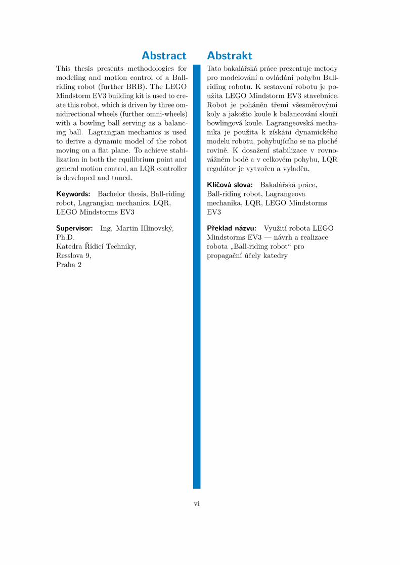
AbstractThis thesis presents methodologies formodeling and motion control of a Ball-riding robot (further BRB). The LEGOMindstorm EV3 building kit is used to cre-ate this robot, which is driven by three om-nidirectional wheels (further omni-wheels)with a bowling ball serving as a balanc-ing ball. Lagrangian mechanics is usedto derive a dynamic model of the robotmoving on a flat plane. To achieve stabi-lization in both the equilibrium point andgeneral motion control, an LQR controlleris developed and tuned.
Keywords: Bachelor thesis, Ball-ridingrobot, Lagrangian mechanics, LQR,LEGO Mindstorms EV3
Supervisor: Ing. Martin Hlinovský,Ph.D.Katedra Řídicí Techniky,Resslova 9,Praha 2
AbstraktTato bakalářská práce prezentuje metodypro modelování a ovládání pohybu Ball-riding robotu. K sestavení robotu je po-užita LEGO Mindstorm EV3 stavebnice.Robot je poháněn třemi všesměrovýmikoly a jakožto koule k balancování sloužíbowlingová koule. Lagrangeovská mecha-nika je použita k získání dynamickéhomodelu robotu, pohybujícího se na plochérovině. K dosažení stabilizace v rovno-vážném bodě a v celkovém pohybu, LQRregulátor je vytvořen a vyladěn.
Klíčová slova: Bakalářská práce,Ball-riding robot, Lagrangeovamechanika, LQR, LEGO MindstormsEV3
Překlad názvu: Využití robota LEGOMindstorms EV3 — návrh a realizacerobota „Ball-riding robot“ propropagační účely katedry
vi
Contents1 Introduction 11.1 Why this thesis was created . . . . . 11.2 Thesis structure . . . . . . . . . . . . . . . 11.3 What is a BRB? . . . . . . . . . . . . . . . 21.4 Previously created BRBs . . . . . . . 21.5 Main thesis goals . . . . . . . . . . . . . . 32 2D model 52.1 Assumptions . . . . . . . . . . . . . . . . . . 52.2 Model description . . . . . . . . . . . . . . 62.3 Coordinates . . . . . . . . . . . . . . . . . . . 72.3.1 Minimal coordinates . . . . . . . . . 72.3.2 Cartesian coordinates for they-z/x-z planes . . . . . . . . . . . . . . . . . . 7
2.3.3 Cartesian coordinates for thex-y plane . . . . . . . . . . . . . . . . . . . . . . 8
2.4 Conversion of virtual parameters . 82.4.1 Torques generated by the realdrive system . . . . . . . . . . . . . . . . . . 10
2.4.2 Torques generated by thevirtual drive system . . . . . . . . . . . . 11
2.4.3 Conclusion . . . . . . . . . . . . . . . . 112.5 Equations of motion for the y-z/x-zplanes . . . . . . . . . . . . . . . . . . . . . . . . . 122.5.1 Kinetic and potential energy 122.5.2 External torques . . . . . . . . . . . 142.5.3 Lagrangian mechanics . . . . . . 152.5.4 Linearization . . . . . . . . . . . . . . 15
2.6 Equations of motion for the x-yplane . . . . . . . . . . . . . . . . . . . . . . . . . . 172.6.1 Kinetic and potential energy 172.6.2 External torques . . . . . . . . . . . 182.6.3 Lagrangian mechanics . . . . . . 182.6.4 Linearization . . . . . . . . . . . . . . 19
2.7 Calculation of parameters . . . . . . 192.7.1 Moment of inertia of the ball 192.7.2 Moment of inertia of the body 202.7.3 Moment of inertia of the virtualwheel . . . . . . . . . . . . . . . . . . . . . . . . 21
2.7.4 Mass of the virtual wheel . . . 222.7.5 Angle α . . . . . . . . . . . . . . . . . . . 222.7.6 Overview of parameters . . . . . 22
2.8 Simulations . . . . . . . . . . . . . . . . . . 243 3D model 293.1 Assumptions . . . . . . . . . . . . . . . . . 293.2 Model description . . . . . . . . . . . . . 303.3 Coordinates . . . . . . . . . . . . . . . . . . 30
3.3.1 Minimal coordinates . . . . . . . . 303.3.2 Coordinate frames . . . . . . . . . 303.3.3 Transformations . . . . . . . . . . . 32
3.4 Variables . . . . . . . . . . . . . . . . . . . . 323.4.1 Velocities of the ball . . . . . . . . 343.4.2 Velocities of the body . . . . . . 353.4.3 Angular velocities of theomni-wheels . . . . . . . . . . . . . . . . . . 35
3.5 Equations of motion . . . . . . . . . . 373.5.1 Kinetic and potential energy 373.5.2 External torques . . . . . . . . . . . 383.5.3 Lagrangian mechanics . . . . . . 383.5.4 Linearization . . . . . . . . . . . . . . 38
3.6 Calculation of parameters . . . . . . 393.6.1 Intertia tensor of the ball . . . 403.6.2 Intertia tensor of the body . . 40
3.7 Simulations . . . . . . . . . . . . . . . . . . 404 Controller design 434.1 Controllers of previously createdBRBs . . . . . . . . . . . . . . . . . . . . . . . . . 43
4.2 Requirements and approach . . . . 444.2.1 Design requirements . . . . . . . . 444.2.2 Design approach . . . . . . . . . . . 44
4.3 LQR controller design . . . . . . . . . 444.3.1 LQR control theory . . . . . . . . 454.3.2 Application on the BRB . . . . 464.3.3 Separation of torques . . . . . . . 474.3.4 Frequency domain requirementsverification . . . . . . . . . . . . . . . . . . . 48
4.3.5 Simulations . . . . . . . . . . . . . . . 535 Robot design 575.1 Design requirements . . . . . . . . . . 575.2 LEGO Mindstorms EV3 buildingkit . . . . . . . . . . . . . . . . . . . . . . . . . . . . 585.2.1 What is LEGO? . . . . . . . . . . . 585.2.2 What is Mindstorms EV3? . . 585.2.3 Parts . . . . . . . . . . . . . . . . . . . . . 58
5.3 The body . . . . . . . . . . . . . . . . . . . . 615.3.1 Upper part . . . . . . . . . . . . . . . . 625.3.2 Middle part . . . . . . . . . . . . . . . 625.3.3 Lower part . . . . . . . . . . . . . . . . 625.3.4 Frames . . . . . . . . . . . . . . . . . . . 635.3.5 Omi-wheels . . . . . . . . . . . . . . . 63
5.4 The ball . . . . . . . . . . . . . . . . . . . . . 64
vii

6 Controller implementation 656.1 Programming language . . . . . . . . 656.1.1 List of functions . . . . . . . . . . . 656.1.2 Establishment ofcommunication . . . . . . . . . . . . . . . . 66
6.2 State vector ~x . . . . . . . . . . . . . . . . 676.2.1 Angles and angular velocities ofthe body . . . . . . . . . . . . . . . . . . . . . 67
6.2.2 Positions and linear velocities ofthe ball . . . . . . . . . . . . . . . . . . . . . . 69
6.3 Driving a single motor . . . . . . . . . 706.4 Touch sensor holder . . . . . . . . . . . 716.5 Final program . . . . . . . . . . . . . . . . 716.6 Real-time simulations . . . . . . . . . 727 Conclusion 77A Derivations 81B Content of the enclosed CD 85C Bibliography 87
viii

Figures1.1 Simplified model of the BRBsystem . . . . . . . . . . . . . . . . . . . . . . . . . 2
1.2 An overview of previously createdBRBs . . . . . . . . . . . . . . . . . . . . . . . . . . 4
2.1 Illustration of 2D planes in 3Dspace . . . . . . . . . . . . . . . . . . . . . . . . . . . 6
2.2 Sketches of 2D planes - inspired by[11] . . . . . . . . . . . . . . . . . . . . . . . . . . . . 7
2.3 Sketches of torques generated bythe real drive system - inspired by[11] . . . . . . . . . . . . . . . . . . . . . . . . . . . . 9
2.4 Sketches of torques generated bythe virtual drive system - inspired by[11] . . . . . . . . . . . . . . . . . . . . . . . . . . . . 9
2.5 Sketches of the angular rates of theomni-wheels - inspired by [11] . . . . 21
2.6 Physical model - course of θx -ψx(t = 0) = 0.1◦ . . . . . . . . . . . . . . . . 24
2.7 Comparison for θx -ψx(t = 0) = 0.1◦ . . . . . . . . . . . . . . . . 24
2.8 Physical model - course of ψx -ψx(t = 0) = 0.1◦ . . . . . . . . . . . . . . . . 25
2.9 Comparison for ψx -ψx(t = 0) = 0.1◦ . . . . . . . . . . . . . . . . 25
2.10 Comparison for θx -u = 0.01N/m . . . . . . . . . . . . . . . . . . . 26
2.11 Comparison for ψx -u = 0.01N/m . . . . . . . . . . . . . . . . . . . 26
2.12 Comparison for ψz -u = 0.001N/m . . . . . . . . . . . . . . . . . . 27
2.13 Comparison for ψz -u = 0.001N/m . . . . . . . . . . . . . . . . . . 27
3.1 3D illustration of the BRB . . . . . 303.2 Illustration of coordinate frames -taken from [11] . . . . . . . . . . . . . . . . . 31
3.3 Comparison for ψx -ψx(t = 0) = 0.1◦ . . . . . . . . . . . . . . . . 41
3.4 Comparison for yS -ψx(t = 0) = 0.1◦ . . . . . . . . . . . . . . . . 41
3.5 Comparison for ψx -uy = 0.01N/m . . . . . . . . . . . . . . . . . . 42
3.6 Comparison for yS -uy = 0.01N/m . . . . . . . . . . . . . . . . . . 42
4.1 The closed loop system . . . . . . . . 45
4.2 Meeting the fourth requirement . 474.3 Meeting the second requirement(ρ = 0.01) . . . . . . . . . . . . . . . . . . . . . . 484.4 Meeting the second requirement(ρ = 0.005) . . . . . . . . . . . . . . . . . . . . . 494.5 Meeting the second requirement(ρ = 0.001) . . . . . . . . . . . . . . . . . . . . . 494.6 Meeting the third requirement(ρ = 0.005) . . . . . . . . . . . . . . . . . . . . . 504.7 Meeting the third requirement(ρ = 0.001) . . . . . . . . . . . . . . . . . . . . . 504.8 Meeting the second requirement(ρ = 0.004) . . . . . . . . . . . . . . . . . . . . . 514.9 Meeting the third requirement(ρ = 0.004) . . . . . . . . . . . . . . . . . . . . . 514.10 Meeting the fourth requirement(ρ = 0.004) . . . . . . . . . . . . . . . . . . . . . 524.11 Bode plot of the first CL transferfunction . . . . . . . . . . . . . . . . . . . . . . . 52
4.12 Disturbance sinus signal used forangles ψx and ψy . . . . . . . . . . . . . . . 54
4.13 Torques for disturbance signal inψx . . . . . . . . . . . . . . . . . . . . . . . . . . . . 54
4.14 Torques for disturbance signal inψy . . . . . . . . . . . . . . . . . . . . . . . . . . . . 55
4.15 Tracking of given trajectory . . . 554.16 Torques for tracking of giventrajectory . . . . . . . . . . . . . . . . . . . . . . 56
5.1 LEGO Mindstorms Education EV3Core Set - Source [16] . . . . . . . . . . . 58
5.2 EV3 Intelligent Brick - Source [18] 595.3 EV3 Sensors - Source [19], [20] . 605.4 EV3 Large Servo Motor - Source[21] . . . . . . . . . . . . . . . . . . . . . . . . . . . 61
5.5 Composite upper part . . . . . . . . . 625.6 Composite middle part . . . . . . . . 625.7 Composite one piece of lower part 635.8 Composite frames . . . . . . . . . . . . . 635.9 Hitechnic RotacasterMulti-directional wheel - Source [22] 63
5.10 EBONITE: Maxim - Night SkyBowling Ball - Source [23] . . . . . . . . 64
6.1 Used Simulink sensor blocks . . . . 666.2 Used Simulink motor blocks . . . . 66
ix
6.3 Edimax EW-7811Un WiFi Dongle -Source [27] . . . . . . . . . . . . . . . . . . . . . 66
6.4 Obtaining and setting the IPaddress . . . . . . . . . . . . . . . . . . . . . . . . 67
6.5 Measurement of the value of thegyro sensor . . . . . . . . . . . . . . . . . . . . 67
6.6 Content of the Calibrate Offsetblock . . . . . . . . . . . . . . . . . . . . . . . . . . 68
6.7 Content of the Compute Angleblock . . . . . . . . . . . . . . . . . . . . . . . . . . 68
6.8 PWM regulator . . . . . . . . . . . . . . 716.9 Touch sensor holder block . . . . . . 716.10 Balancing - angles ψx, ψy . . . . . 726.11 Balancing - angle ψz . . . . . . . . . 726.12 Balancing - angular rates ω1, ω2,ω3 . . . . . . . . . . . . . . . . . . . . . . . . . . . . 73
6.13 Balancing with disturbances -angle ψz . . . . . . . . . . . . . . . . . . . . . . . 73
6.14 Balancing with disturbances -angles ψx, ψy . . . . . . . . . . . . . . . . . . . 74
6.15 Balancing with disturbances -angular rates ω1, ω2, ω3 . . . . . . . . . 74
6.16 Pivoting - angles ψx, ψy . . . . . . 756.17 Pivoting - angle ψz . . . . . . . . . . . 756.18 Pivoting - angular rates ω1, ω2,ω3 . . . . . . . . . . . . . . . . . . . . . . . . . . . . 75
7.1 BRB CTU . . . . . . . . . . . . . . . . . . . 79
Tables2.1 Table of 2D parameters . . . . . . . . 23
3.1 Table of markings . . . . . . . . . . . . . 33
x
Chapter 1Introduction
1.1 Why this thesis was created
At the beginning of the fifth semester of my studies at the Czech TechnicalUniversity in Prague, I started looking for the topic of my bachelor thesis. AsI have always been interested in the concept of robots, and there were severalmodules on the topic throughout my studies, I decided to create my own. Iwrote to one of the lecturers of these subjects and asked if we could agreeon a topic for my work. After receiving a warm reply, and meeting with theguarantor, the theme was agreed upon. My task is to design and realize a"Ball-riding robot", further BRB, for promotional purposes. Thus the thesisis a report of an accomplishment of this difficult challenge and presented asmy final work, ending my three-year undergraduate study.
1.2 Thesis structure
The thesis consists of 7 chapters. Each chapter addresses an important issueand is divided into several sections and subsections. In the first chapter, anintroduction to the subject takes place. The reason for creating this thesishas already been clarified, and the BRB system will be discussed in thischapter. The "2D model" chapter aims at modeling the BRB in decoupledplains and describes a reduced dynamic model and the basics of linearization.The reduced dynamic model is the main element in deriving the complexmodel used in the "3D model" chapter. After obtaining such a model, thelinearization is done again and an appropriate controller is designed in thefollowing chapter: "Controller design". The design of the robot and its twoparts - the body and the ball - is listed in the "Robot design" chapter. In thechapter "Controller implementation", it is shown how the controller designedin the fourth chapter can be applied to a realistic robot. A conclusion ispresented followed by the Appendices which contain derivations, a list of thecontent of the enclosed CD and finally an overview of all bibliography.
1

1. Introduction .....................................1.3 What is a BRB?
Figure 1.1: Simplified model of the BRB system
BRB, as already mentioned, is an abbreviation of Ball-Riding roBot. Ball-riding robots are robots which balance on top of a ball. Driving the balland balancing the robot is done using multiple omni-wheels (usually 3 or 4)and angular sensors attached to the body of the robot. In our case, threeomni-wheels will be used along with two gyroscopes for each axis to estimateangular rates and angles of the body. The velocity and the position of the ballis derived by mathematical operations using the angles of the omni-wheels.Due to the lack of a transmission between the omni-wheel and the motor,the rotation angle of a single motor is equal to the rotation angle of a singleomni-wheel.
1.4 Previously created BRBs
The BRB is not a new concept in technical spheres. Several studies havebeen done by multiple universities, including:. Carnegie Mellon University (CMU) in the United States developed the
first BRB (shown in Fig. 1.2a) in 2006. The robot is human sized, andaimed at interaction with humans. In the final version of the robot, apair of arms were added, and a total of 5 DC motors were needed tomaintain system balance despite the fact that the robot was not able torotate around the vertical axis z. The relevant references are [1], [2], [3],[4], and [5].. Tohoku Gakuin University (TGU) in Japan developed a BRB (shownin Fig. 1.2b) in 2008. Only three motors were needed to complete thegoals of the CMU robot as well as allowing rotation around the verticalaxis z. This robot is able to carry loads in excess of 10kg. Referencesare [6] and [7].
2
...................................1.5. Main thesis goals
. The University of Adelaide (UA) in Australia developed a BRB usingLEGO Mindstorms NXT (shown in Fig. 1.2c) in 2009. This robot is asmall sized robot built completely out of LEGO. It uses a pair of normalwheels to balance on a plastic ball, which limits its performance andmakes pivoting around the vertical axis z impossible. More in [8].. The Swiss Federal Institute of Technology in Zurich (ETH) in Switzerlanddeveloped a BRB (shown in Fig. 1.2d) in 2010. The BRB was namedRezero and is the result of work by several students. Similar to theTGU robot, Rezero uses three omni-wheels to drive. In references [9],[12] a video is included, which demonstrates the robot’s high dynamicrobustness and the future goals for the project.. The National Chung Hsing University (NCHU) in Taiwan developed aBRB (shown in Fig. 1.2e) in 2012. This robot is very similar to theTGU robot. It is about the same size, construction, and also uses threeomni-wheels to perform drive actions. Corresponding references are [10].. The University of Twente (UT) in Enschede in the Netherlands developeda BRB (shown in Fig. 1.2f) in 2014. The robot also uses only threeomni-wheels, and is designed for use in fairs. The original text is givenin [11].
When equations and procedures derived and developed in these studies havebeen used in this thesis, the original source was referenced in IEEE standard.
1.5 Main thesis goals
The goals of this bachelor thesis are: to describe system dynamics, derive alinearized model, develop a controller for point stabilization and trajectorytracking, build a robot from the LEGO EV3 building kit, adjust the bowlingball, and successfully implement the developed controller.
3

1. Introduction .....................................
(a) : BRB CMU (b) : BRB TGU
(c) : BRB UA (d) : BRB ETH
(e) : BRB NCHU (f) : BRB UT
Figure 1.2: An overview of previously created BRBs
4

Chapter 22D model
This chapter aims to describe the system structure and physical model ofthe BRB. The dynamic model with equations of motion is derived usingLagrangian mechanics and is then converted into a linearized model. Whilelinearizing, an equilibrium point in a balancing position is used. While the 2Dmodel is insufficient as an overall control solution, it does allow for a betterunderstanding of dynamic problems, and serves as a basis for the 3D model.
2.1 Assumptions
Note that everything in this chapter is based on the following assumptions:.Rigid bodiesThe BRB is composed of two rigid bodies: the body and the ball.Deformation of these bodies is negligible..Rigid floorDeformation of the floor is negligible..Horizontal floorThe BRB moves only on horizontal floor, thus the ball has no potentialenergy.. FrictionBesides static friction, which guarantees the "No slip" assumption, allother types of frictions are negligible..No slipThere is no slip between the body and the ball and between the ball andthe floor..Omni-wheelsUsing 2-row omni-wheels with more than one contact point can bemodeled as 1-row omni-wheels with a single contact point..Negligible time delayThe time delay between the measurements of the sensors and the controlof the motors is negligible.
5

2. 2D model ....................................... Independent vertical planes
The two designed vertical planes (x-z, y-z) are assumed to be independent.
These or similar assumptions can be found in references up to [11].
2.2 Model description
To obtain a 2D model of a 3D system some simplifications, as done in [6], [9],[10], and [11], are needed. The first is that the whole model is divided intothree planes (shown in Fig. 2.1): two vertical (x-z, y-z) and one horizontal(x-y). Each plane describes, using its generalized coordinates, a 2D motionwhich takes place within the plane. Secondly, the omni-wheels together withmotors and shafts are modeled as virtual wheels. Each plane is affected byone virtual wheel, which rotates around the orthogonal axis to that plane.For the vertical planes, the ball is modeled as a disk, which rotates aroundthe orthogonal axis to the plane. The virtual wheel and the centre of mass(further COM) of the body are attached to the rotation axis of the disk with arigid rod. The body rotates around the rigid rod independent of the rotationof the disk, creating an inverted pendulum system (shown in Fig. 2.2a). Forthe horizontal plane, the ball is also modeled as a disk and rotates around theorthogonal axis to the plane. The virtual wheel is attached to the rotationaxis of the disk with a rigid rod. The COM of the body is attached to therod and shares the same coordinate system as the centre of the disk (shownin Fig. 2.2b). Lastly, the independence of rotational motion is assumed.
x− y
x− z y − z
y
x
z
Figure 2.1: Illustration of 2D planes in 3D space
6

..................................... 2.3. Coordinates
IS
IW
IB
θx
ψxφx
l
rS
rW
x
z
(a) : Sketch of the y-z plane
IS
IW,xy
IB,xy
ψz
rS
φz
x
y
(b) : Sketch of the x-y plane
Figure 2.2: Sketches of 2D planes - inspired by [11]
2.3 Coordinates
It is necessary to define the coordinates for future procedures. The coordinateswill be defined as they are shown in Fig. 2.2.
2.3.1 Minimal coordinates
From Fig. 2.2, it can be seen that the vertical planes have two DOFs (Degreesof Freedom - the rotation of the ball and the body) and the horizontal planehas only one DOF (the rotation of the body). Hence the minimal coordinatescan be defined as:
~qyz =[θxψx
](2.1)
~qxz =[θyψy
](2.2)
~qxy =[ψx]
(2.3)
2.3.2 Cartesian coordinates for the y-z/x-z planes
The position of the ball expressed in Cartesian coordinates:[ySzS
]=[rSθx
0
](2.4)
Of the body: [yBzB
]=[rSθx + l sin(ψx)
l cos(ψx)
](2.5)
7

2. 2D model ......................................Of the virtual wheel:[
yWzW
]=[rSθx + (rS + rW ) sin(ψx)
(rS + rW ) cos(ψx)
](2.6)
For the x-z plane the Cartesian coordinates have the same form, substitutingx for y and vice versa.
These equations, along with Eq. (2.7), appear in many texts, but theiracquisition is considered to be elementary and familiar. Hence no reference isquoted.
2.3.3 Cartesian coordinates for the x-y plane
The body in the x-y plane only rotates, making its position invariable. There-fore, only the position of the virtual wheel needs to be determined:[
xW,xyyW,xy
]=[(rS + rW ) cos(ψz)(rS + rW ) sin(ψz)
](2.7)
2.4 Conversion of virtual parameters
Before the equations of motion can be looked at, it is necessary to clarify therelation between torques of virtual wheels and torques of real omni-wheelsand vice versa. As in [9] and [11], it can be shown that the resulting torqueof the body is conserved. Mathematically:
~τB,x + ~τB,y + ~τB,z = ~τB,1 + ~τB,2 + ~τB,3 (2.8)
Where ~τB,i; i = 1, 2, 3 is the torque vector of the body, generated by the i-thomni-wheel with size of τi and the ~τB,j ; j = x, y, z is the torque vector of thebody, generated by the virtual wheel in the direction of the j-th axis.
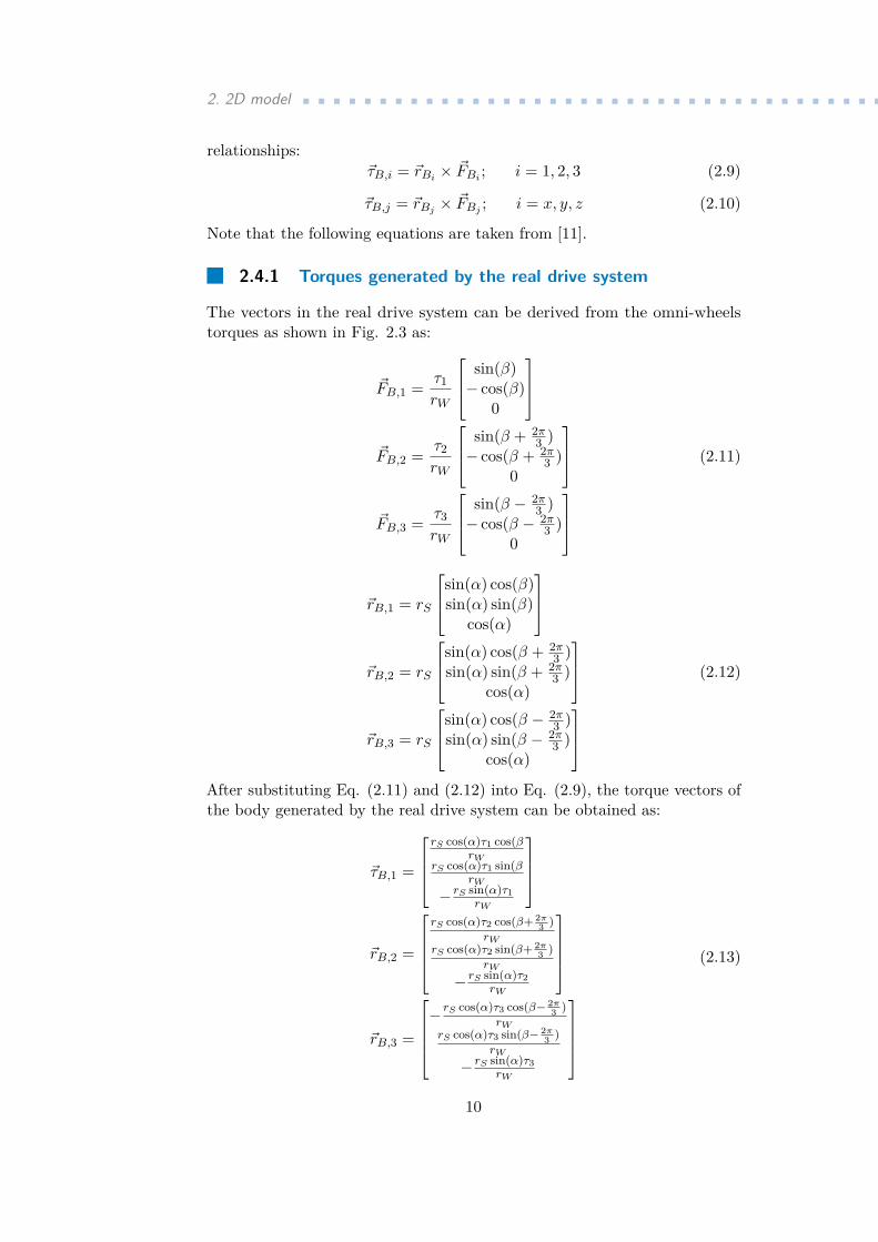
In the next figures, ~FB,i is a force generated by the torque of the i-th omni-wheel, orthogonal to the ~τB,i, and ~rB,i is a vector from the center of the planedisk to the beginning of the force. Parameter α denotes the angle for verticalposition of the omni-wheels and β the angle for horizontal position of the firstomni-wheel. The omni-wheels are placed with equal spacing (120 degrees)between them.
8

............................ 2.4. Conversion of virtual parameters
~τB,x
~rB,xα
y
z
(a) : Side view
~τB,1
β~FB,1
~τB,2
~FB,2
~τB,3
~FB,3
x
y
(b) : Top view
Figure 2.3: Sketches of torques generated by the real drive system - inspired by[11]
For the virtual case, ~FB,j is defined as a force generated by the torque of thej-th virtual wheel, orthogonal to the ~τB,j and also having ~rB,j as a vectorfrom the centre of the plane disk to the beginning of the force.
~τB,x
~rB,x
~FB,x
φx
y
z
(a) : Side view
~τB,x ~rB,z
~FB,zφz
x
y
(b) : Top view
Figure 2.4: Sketches of torques generated by the virtual drive system - inspiredby [11]
With upper definitions, the torque vectors can be calculated using the following
9
2. 2D model ......................................relationships:
~τB,i = ~rBi × ~FBi ; i = 1, 2, 3 (2.9)
~τB,j = ~rBj × ~FBj ; i = x, y, z (2.10)
Note that the following equations are taken from [11].
2.4.1 Torques generated by the real drive system
The vectors in the real drive system can be derived from the omni-wheelstorques as shown in Fig. 2.3 as:
~FB,1 = τ1rW
sin(β)− cos(β)
0
~FB,2 = τ2
rW
sin(β + 2π3 )
− cos(β + 2π3 )
0
~FB,3 = τ3
rW
sin(β − 2π3 )
− cos(β − 2π3 )
0
(2.11)
~rB,1 = rS
sin(α) cos(β)sin(α) sin(β)
cos(α)
~rB,2 = rS
sin(α) cos(β + 2π3 )
sin(α) sin(β + 2π3 )
cos(α)
~rB,3 = rS
sin(α) cos(β − 2π3 )
sin(α) sin(β − 2π3 )
cos(α)
(2.12)
After substituting Eq. (2.11) and (2.12) into Eq. (2.9), the torque vectors ofthe body generated by the real drive system can be obtained as:
~τB,1 =
rS cos(α)τ1 cos(β
rWrS cos(α)τ1 sin(β
rW
− rS sin(α)τ1rW
~rB,2 =
rS cos(α)τ2 cos(β+ 2π
3 )rW
rS cos(α)τ2 sin(β+ 2π3 )
rW
− rS sin(α)τ2rW
~rB,3 =
− rS cos(α)τ3 cos(β− 2π
3 )rW
rS cos(α)τ3 sin(β− 2π3 )
rW
− rS sin(α)τ3rW
(2.13)
10

............................ 2.4. Conversion of virtual parameters
2.4.2 Torques generated by the virtual drive system
In the virtual drive system (shown in Fig. 2.4), the vectors can also be derivedfrom wheels torques, in this case from the torques of the virtual wheels as:
~FB,x = τxrW
0−10
~FB,y = τy
rW
100
~FB,z = τz
rW
sin(β)− cos(β)
0
(2.14)
~rB,x = rS
001
~rB,y = rS
001
~rB,z = rS
cos(β)sin(β)
0
(2.15)
Now substituting Eq (2.14) and (2.15) into Eq. (2.10), the torque vectors ofthe body, generated by the virtual drive system, can be worked out as:
~τB,x =
rSτxrW00
~rB,y =
0rSτyrW0
~rB,z =
00
− rSτzrW
(2.16)
2.4.3 Conclusion
Substituing previously derived equations of torque vectors into Eq. (2.8) andsolving for the torques generated by the real drive system and the virtualdrive system separately yields two equations. These equations describe therelationship between the two drive systems and serves for conversion between
11
2. 2D model ......................................them. τ1
τ2τ3
= J ·
τxτyτz
(2.17)
τxτyτz
= JT ·
τ1τ2τ3
(2.18)
Where J is a Jacobian matrix and JT its transposition:
J =
2 cos(β)3 cos(α)
2 sin(β)3 cos(α)
13 sin(α)
− cos(β)+√
3 sin(β)3 cos(α) − sin(β)+
√3 cos(β)
3 cos(α)1
3 sin(α)
− cos(β)+√
3 sin(β)3 cos(α) − sin(β)+
√3 cos(β)
3 cos(α)1
3 sin(α)
(2.19)
JT =
cos(α) cos(β) − cos(α)[cos(β)+√
3 sin(β)]2 − cos(α)[cos(β)−
√3 sin(β)]
2cos(α) sin(β) − cos(α)[sin(β)−
√3 cos(β)]
2 − cos(α)[sin(β)+√
3 cos(β)]2
sin(α) sin(α) sin(α)
(2.20)
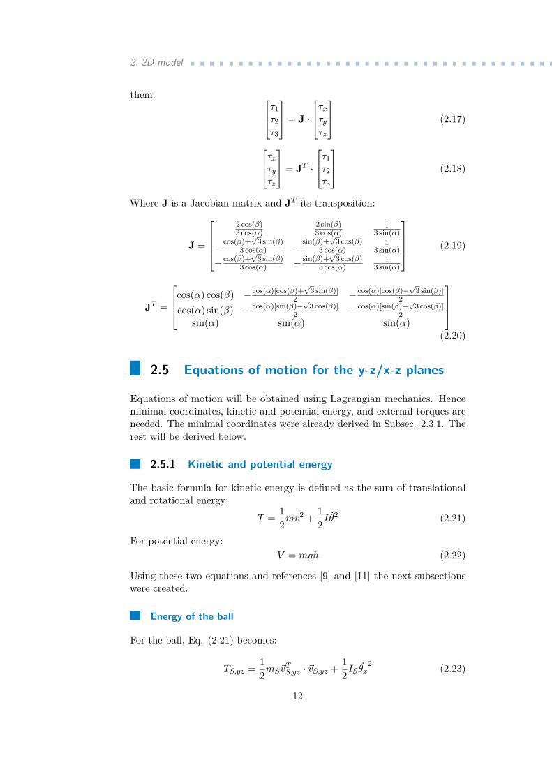
2.5 Equations of motion for the y-z/x-z planes
Equations of motion will be obtained using Lagrangian mechanics. Henceminimal coordinates, kinetic and potential energy, and external torques areneeded. The minimal coordinates were already derived in Subsec. 2.3.1. Therest will be derived below.
2.5.1 Kinetic and potential energy
The basic formula for kinetic energy is defined as the sum of translationaland rotational energy:
T = 12mv
2 + 12Iθ
2 (2.21)
For potential energy:V = mgh (2.22)
Using these two equations and references [9] and [11] the next subsectionswere created.
Energy of the ball
For the ball, Eq. (2.21) becomes:
TS,yz = 12mS~v
TS,yz · ~vS,yz + 1
2IS θx2 (2.23)
12

........................2.5. Equations of motion for the y-z/x-z planes
mS is defined as the mass of the ball, ~vS,yz as the velocity of the ball, IS asalready mentioned is the moment of inertia of the ball, and ~vTS,yz · ~vS,yz isdefined as:
~vTS,yz · ~vS,yz = |vS,yz|2
= y2S + z2
S
= r2S θ
2x
(2.24)
Hence the final form of the kinetic energy of the ball is:
TS,yz = 12mSr
2S θ
2x + 1
2IS θx2 (2.25)
Due to Assumption 3, the potential energy of the ball is equal to zero:
VS,yz = 0 (2.26)
Energy of the body
Similarly, the kinetic energy of the body is defined as:
TB,yz = 12mB~v
TB,yz · ~vB,yz + 1
2IBψx2 (2.27)
Where mB is the mass of the body, ~vB,yz the velocity of the body, IB themoment of inertia of the body mentioned earlier and ~vTB,yz · ~vB,yz is definedas:
~vTB,yz · ~vB,yz = |vB,yz|2
= y2B + z2
B
= r2S θ
2x + 2rSlθxψx cos(ψx) + l2ψ2
x
(2.28)
(A more detailed calculation can be found in Appendix A.)
The equation in its final form is:
TB,yz = 12mB
(r2S θ
2x + 2rSlθxψx cos(ψx) + l2ψ2
x
)+ 1
2IBψx2
= 12mB
(r2S θ
2x + 2rSlθxψx cos(ψx)
)+ 1
2(IB +mB + l2)ψx2
= 12mB
(r2S θ
2x + 2rSlθxψx cos(ψx)
)+ 1
2I′Bψx
2
(2.29)
Where I ′B is the moment of inertia of the body around the axis the bodyrotates (axis through the centre of the wheel).
The potential energy of the body is calculated as:
VB,yz = mBgl cos(ψz) (2.30)
13
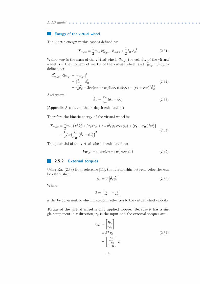
2. 2D model ......................................Energy of the virtual wheel
The kinetic energy in this case is defined as:
TW,yz = 12mW~v
TW,yz · ~vW,yz + 1
2IW φx2 (2.31)
Where mW is the mass of the virtual wheel, ~vW,yz the velocity of the virtualwheel, IW the moment of inertia of the virtual wheel, and ~vTW,yz · ~vW,yz isdefined as:
~vTW,yz · ~vW,yz = |vW,yz|2
= y2W + z2
W
= r2S θ
2x + 2rS(rS + rW )θxψx cos(ψx) + (rS + rW )2ψ2
x
(2.32)
And where:φx = rS
rW(θx − ψz) (2.33)
(Appendix A contains the in-depth calculation.)
Therefore the kinetic energy of the virtual wheel is:
TW,yz = 12mW
(r2S θ
2x + 2rS(rS + rW )θxψx cos(ψx) + (rS + rW )2ψ2
x
)+ 1
2IW( rSrW
(θx − ψz))2 (2.34)
The potential of the virtual wheel is calculated as:
VW,yz = mW g(rS + rW ) cos(ψz) (2.35)
2.5.2 External torques
Using Eq. (2.33) from reference [11], the relationship between velocities canbe established.
φx = J[θxψz
](2.36)
Where
J =[rSrW
− rSrW
]is the Jacobian matrix which maps joint velocities to the virtual wheel velocity.
Torque of the virtual wheel is only applied torque. Because it has a sin-gle component in x direction, τx is the input and the external torques are:
~τext =[τθxτψx
]= JT τx
=[
rSrW− rSrW
]τx
(2.37)
14
........................2.5. Equations of motion for the y-z/x-z planes
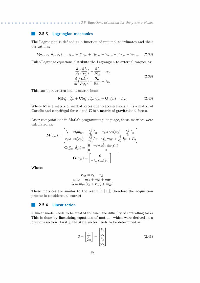
2.5.3 Lagrangian mechanics
The Lagrangian is defined as a function of minimal coordinates and theirderivations:
L(θx, ψx, θx, ψx) = TS,yz + TB,yz + TW,yz − VS,yz − VB,yz − VW,yz (2.38)
Euler-Lagrange equations distribute the Lagrangian to external torques as:
d
dt
( ∂L∂θx
)− ∂L
∂θx= τθx
d
dt
( ∂L∂ψx
)− ∂L
∂ψx= τψx
(2.39)
This can be rewritten into a matrix form:
M(~qyz)~qyz + C(~qyz, ~qyz)~qyz + G(~qyz) = ~τext (2.40)
Where M is a matrix of inertial forces due to accelerations, C is a matrix ofCoriolis and centrifugal forces, and G is a matrix of gravitational forces.
After computations in Matlab programming language, these matrices werecalculated as:
M(~qyz) =
IS + r2Smtot + r2
S
r2WIW rSλ cos(ψx)− r2
S
r2WIW
rSλ cos(ψx)− r2S
r2WIW r2
totmW + r2S
r2WIW + I ′B
C(~qyz, ~qyz) =
[0 −rSλψx sin(ψx)0 0
]
G(~qyz) =[
0−λg sin(ψz)
]Where:
rtot = rS + rBmtot = mS +mB +mW
λ = mW (rS + rW ) +mBl
These matrices are similar to the result in [11], therefore the acquisitionprocess is considered as correct.
2.5.4 Linearization
A linear model needs to be created to lessen the difficulty of controlling tasks.This is done by linearizing equations of motion, which were derived in aprevious section. Firstly, the state vector needs to be determined as:
~x =[~qyz~qyz
]=
θxψxθxψx
(2.41)
15
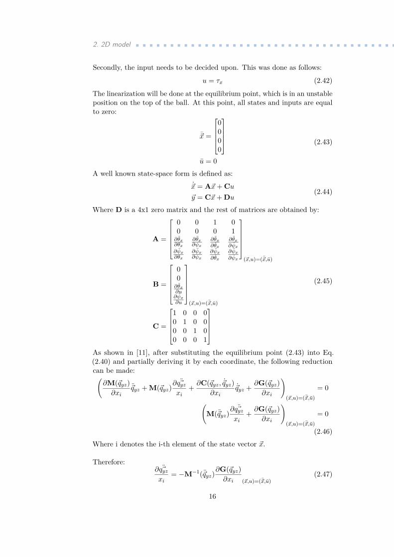
2. 2D model ......................................Secondly, the input needs to be decided upon. This was done as follows:
u = τx (2.42)
The linearization will be done at the equilibrium point, which is in an unstableposition on the top of the ball. At this point, all states and inputs are equalto zero:
~x =
0000
u = 0
(2.43)
A well known state-space form is defined as:
~x = A~x+ Cu~y = C~x+ Du
(2.44)
Where D is a 4x1 zero matrix and the rest of matrices are obtained by:
A =
0 0 1 00 0 0 1∂θx∂θx
∂θx∂ψx
∂θx∂θx
∂θx∂ψx
∂ψx∂θx
∂ψx∂ψx
∂ψx∂θx
∂ψx∂ψx
(~x,u)=(~x,u)
B =
00∂θx∂u∂ψx∂u
(~x,u)=(~x,u)
C =
1 0 0 00 1 0 00 0 1 00 0 0 1
(2.45)
As shown in [11], after substituting the equilibrium point (2.43) into Eq.(2.40) and partially deriving it by each coordinate, the following reductioncan be made:(
∂M(~qyz)∂xi
~qyz + M(~qyz)∂ ~qyzxi
+ ∂C(~qyz, ~qyz)∂xi
~qyz + ∂G(~qyz)∂xi
)(~x,u)=(~x,u)
= 0
(M(~qyz)
∂ ~qyzxi
+ ∂G(~qyz)∂xi
)(~x,u)=(~x,u)
= 0
(2.46)
Where i denotes the i-th element of the state vector ~x.
Therefore:∂ ~qyzxi
= −M−1(~qyz)∂G(~qyz)∂xi (~x,u)=(~x,u)
(2.47)
16
.......................... 2.6. Equations of motion for the x-y plane
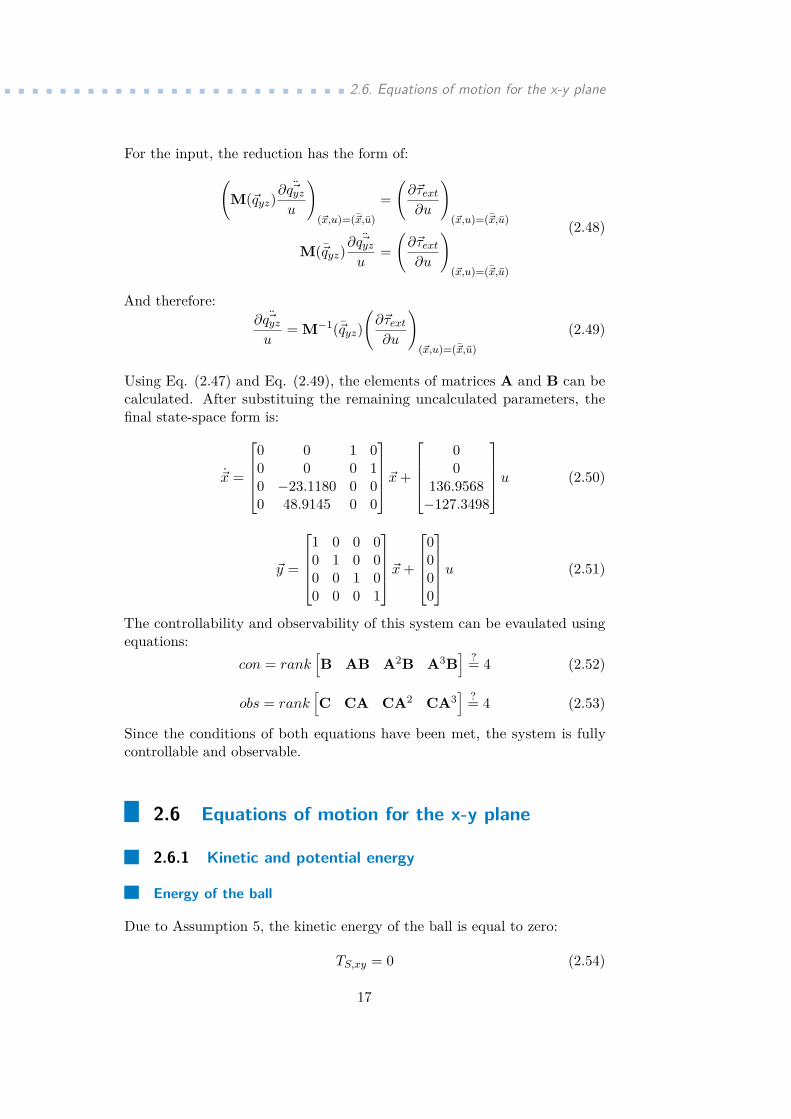
For the input, the reduction has the form of:(M(~qyz)
∂ ~qyzu
)(~x,u)=(~x,u)
=(∂~τext∂u
)(~x,u)=(~x,u)
M(~qyz)∂ ~qyzu
=(∂~τext∂u
)(~x,u)=(~x,u)
(2.48)
And therefore:∂ ~qyzu
= M−1(~qyz)(∂~τext∂u
)(~x,u)=(~x,u)
(2.49)
Using Eq. (2.47) and Eq. (2.49), the elements of matrices A and B can becalculated. After substituing the remaining uncalculated parameters, thefinal state-space form is:
~x =
0 0 1 00 0 0 10 −23.1180 0 00 48.9145 0 0
~x+
00
136.9568−127.3498
u (2.50)
~y =
1 0 0 00 1 0 00 0 1 00 0 0 1
~x+
0000
u (2.51)
The controllability and observability of this system can be evaulated usingequations:
con = rank[B AB A2B A3B
] ?= 4 (2.52)
obs = rank[C CA CA2 CA3
] ?= 4 (2.53)
Since the conditions of both equations have been met, the system is fullycontrollable and observable.
2.6 Equations of motion for the x-y plane
2.6.1 Kinetic and potential energy
Energy of the ball
Due to Assumption 5, the kinetic energy of the ball is equal to zero:
TS,xy = 0 (2.54)
17

2. 2D model ......................................Energy of the body
Because the body only rotates, the kinetic energy will consist purely ofrotational energy:
TB,xz = 12IB,xyψ
2x (2.55)
Energy of the virtual wheel
The kinetic energy in this case is defined as:
TW,yz = 12mW~v
TW,xy · ~vW,xy + 1
2IW,xyφz2 (2.56)
Where:
~vTW,xy · ~vW,xy = |vW,xy|2
= x2W,xy + y2
W,xy
= (rS + rW )2ψ2z
(2.57)
And where:φz = − rS
rWψz (2.58)
(The entire calculation can be found in Appendix A.)
Therefore the kinetic energy of the virtual wheel is:
TW,xy = 12mW (rS + rW )2ψ2
z + 12IW,xy
(− rSrW
ψz)2
= 12
(mW (rS + rW )2 + IW,xy
( rSrW
)2)ψ2z
(2.59)
The potential energy in all cases is equal to zero.
2.6.2 External torques
The only input in the x-y plane is τz. From Eq. (2.58), the Jacobian isalready known. Hence, the relationship between external torques and τz canbe rewritten as:
τext,xy = JT τz
τext,xy = − rSrW
τz(2.60)
2.6.3 Lagrangian mechanics
The Lagrangian in this case is:
L(ψz, ψz) = TB,yz + TW,yz (2.61)
18

............................... 2.7. Calculation of parameters
Euler-Lagrange equation distributes the Lagragian to external torques as:
d
dt
( ∂L∂ψz
)− ∂L
∂ψz= τext,xy (2.62)
In the matrix form:M(~qyz)~qyz = τext,xy (2.63)
Where:M(~qyz) = IB,xy +mW (rS + rW )2 + IW,xy
( rSrW
)2(2.64)
2.6.4 Linearization
The state vector is defined as:
~x =[ψzψz
](2.65)
With the input:u = τz (2.66)
Solving Eq. (2.63) for ψz yields:
ψz = − rSu
IB,xyr2W +mW (rS + rW )2r2
W + IW,xyr2S
(2.67)
After deriving and substituing, the state-space form is:
~x =[0 10 0
]~x+
[0
−28006.1898
]u (2.68)
~y =[1 00 1
]~x+
[00
]u (2.69)
Also in this case, the controllability and observability was checked. Thesystem is fully controllable and observable.
2.7 Calculation of parameters
In previous sections, many of the parameters were listed. This section aimsto calculate them exactly or with an acceptable error.
2.7.1 Moment of inertia of the ball
The moment of inertia of the full ball with mass m and radius r is defined as:
I = 25mr
2 (2.70)
Thus the moment of inertia of the used ball is:
IS = 25mSr
2S (2.71)
19

2. 2D model ......................................2.7.2 Moment of inertia of the body
Because the body can not be exactly described geometrically, an approxi-mation is made. The body is indentified as a cuboid with mass mB, widthwB, height hB, and COM as height rB. The computation of the moment ofinertia of the cuboid rotation around the axis through its COM is:
I = 112m(w2 + h2) (2.72)
Therefore the moment of inertia in the y-z/x-z planes is defined as:
IB = 112mB(w2
B + h2B) (2.73)
For the calculation of the moment of inertia about the axis the body rotatesaround, as in [11] the parallel axis theorem [13] is used. It states that:
I ′ = I +ml2 (2.74)
Where l is in our case defined as the height difference between the COM ofthe ball and the COM of the body. Hence:
l = rS + rB (2.75)
And the moment:I ′B = IB +mBl
2 (2.76)
In the x-y plane, the moment of inertia of the body is defined as:
I = 16mw
2 (2.77)
Therefore:IB,xy = 1
6mBw2B (2.78)
20

............................... 2.7. Calculation of parameters
2.7.3 Moment of inertia of the virtual wheel
ωOW1ωOW1,x
ωOW1,y
φx
φz
αα
x
z
(a) : Side view
ωOW1ωOW1,x
ωOW1,y
ωOW2
ωOW2,x
ωOW2,y
ωOW3
ωOW3,x
ωOW3,y
π/3π/3 x
y
(b) : Top view
Figure 2.5: Sketches of the angular rates of the omni-wheels - inspired by [11]
As shown in Fig. 2.5, the angular rates of the virtual omni-wheels are splitinto individual components in the direction of the axis. This task is doneaccording to [6], [9], [10], and [11].
The angular rates around the x axis are:
ωOW1,x = φx cos(α)
ωOW2,x = ωOW3,x = cos(π
3)(−φx) cos(α)
= −12 φx cos(α)
(2.79)
Around the y axis they are:
ωOW1,y = 0
ωOW2,y = sin(π
3)φy cos(α)
=√
32 φy cos(α)
ωOW3,y = sin(π
3)(−φy) cos(α)
= −√
32 φy cos(α)
(2.80)
And finally around the z axis they are:
ωOW1,z = ωOW2,z = ωOW3,z = cos(π
2 − α)φz
= sin(α)φz(2.81)
21
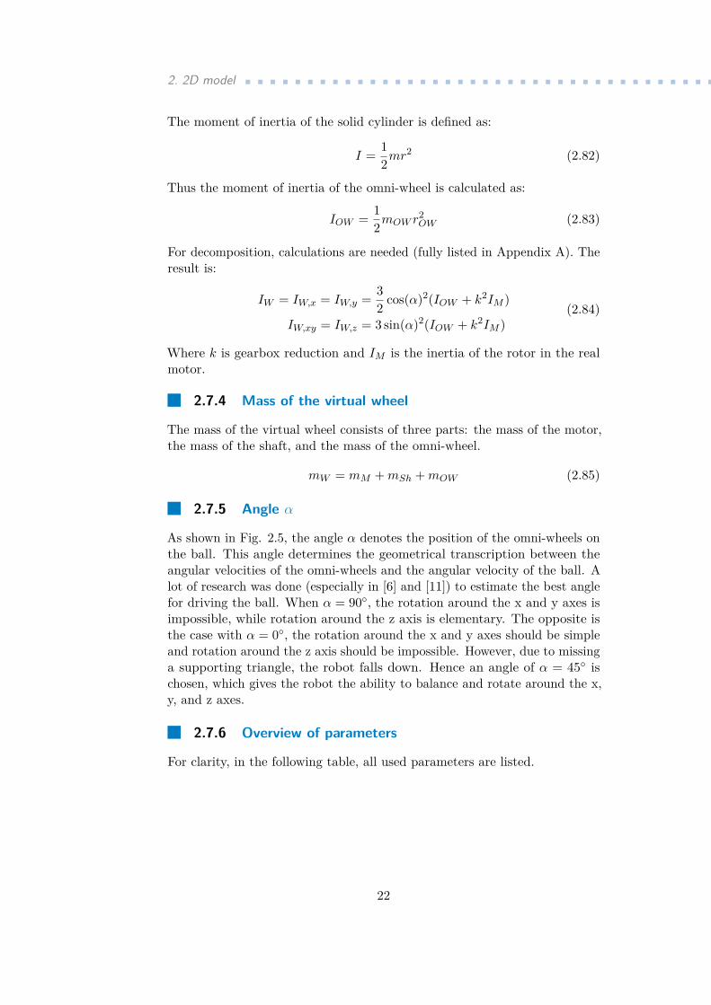
2. 2D model ......................................The moment of inertia of the solid cylinder is defined as:
I = 12mr
2 (2.82)
Thus the moment of inertia of the omni-wheel is calculated as:
IOW = 12mOW r
2OW (2.83)
For decomposition, calculations are needed (fully listed in Appendix A). Theresult is:
IW = IW,x = IW,y = 32 cos(α)2(IOW + k2IM )
IW,xy = IW,z = 3 sin(α)2(IOW + k2IM )(2.84)
Where k is gearbox reduction and IM is the inertia of the rotor in the realmotor.
2.7.4 Mass of the virtual wheel
The mass of the virtual wheel consists of three parts: the mass of the motor,the mass of the shaft, and the mass of the omni-wheel.
mW = mM +mSh +mOW (2.85)
2.7.5 Angle α
As shown in Fig. 2.5, the angle α denotes the position of the omni-wheels onthe ball. This angle determines the geometrical transcription between theangular velocities of the omni-wheels and the angular velocity of the ball. Alot of research was done (especially in [6] and [11]) to estimate the best anglefor driving the ball. When α = 90◦, the rotation around the x and y axes isimpossible, while rotation around the z axis is elementary. The opposite isthe case with α = 0◦, the rotation around the x and y axes should be simpleand rotation around the z axis should be impossible. However, due to missinga supporting triangle, the robot falls down. Hence an angle of α = 45◦ ischosen, which gives the robot the ability to balance and rotate around the x,y, and z axes.
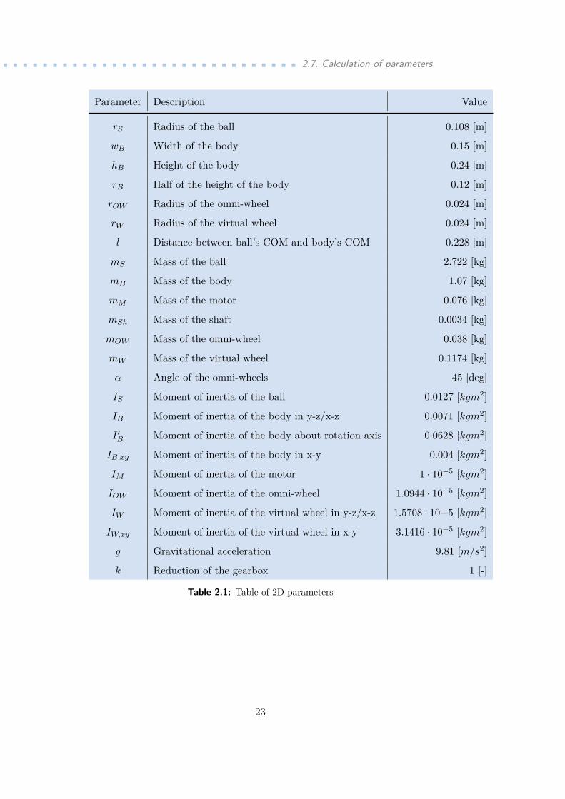
2.7.6 Overview of parameters
For clarity, in the following table, all used parameters are listed.
22
............................... 2.7. Calculation of parameters
Parameter Description Value
rS Radius of the ball 0.108 [m]
wB Width of the body 0.15 [m]
hB Height of the body 0.24 [m]
rB Half of the height of the body 0.12 [m]
rOW Radius of the omni-wheel 0.024 [m]
rW Radius of the virtual wheel 0.024 [m]
l Distance between ball’s COM and body’s COM 0.228 [m]
mS Mass of the ball 2.722 [kg]
mB Mass of the body 1.07 [kg]
mM Mass of the motor 0.076 [kg]
mSh Mass of the shaft 0.0034 [kg]
mOW Mass of the omni-wheel 0.038 [kg]
mW Mass of the virtual wheel 0.1174 [kg]
α Angle of the omni-wheels 45 [deg]
IS Moment of inertia of the ball 0.0127 [kgm2]
IB Moment of inertia of the body in y-z/x-z 0.0071 [kgm2]
I ′B Moment of inertia of the body about rotation axis 0.0628 [kgm2]
IB,xy Moment of inertia of the body in x-y 0.004 [kgm2]
IM Moment of inertia of the motor 1 · 10−5 [kgm2]
IOW Moment of inertia of the omni-wheel 1.0944 · 10−5 [kgm2]
IW Moment of inertia of the virtual wheel in y-z/x-z 1.5708 · 10−5 [kgm2]
IW,xy Moment of inertia of the virtual wheel in x-y 3.1416 · 10−5 [kgm2]
g Gravitational acceleration 9.81 [m/s2]
k Reduction of the gearbox 1 [-]
Table 2.1: Table of 2D parameters
23

2. 2D model ......................................2.8 Simulations
With computed parameters, the simulations of the physical and linearizedmodels can be made. Simulations are carried out to see whether the linearizedmodel is a good replacement for the physical model, as well as to see whetherthere are any deviations and determine their size. Because the model isidentical in y-z and x-z planes, only y-z plane with x-y plane are simulated. Inthe first simulation, the initial condition of the angle ψx was set 0.1◦. Belowthe courses for angles are shown:
t [s]
0 1 2 3 4 5 6 7 8 9 10
angle
[deg]
-160
-140
-120
-100
-80
-60
-40
-20
0
20Physical model
θx -physical model
Figure 2.6: Physical model - course of θx - ψx(t = 0) = 0.1◦
t [s]
0 0.2 0.4 0.6 0.8 1 1.2
angle
[deg]
-120
-100
-80
-60
-40
-20
0Comparison of models
θx -physical model
θy -linearized model
limit angle
Figure 2.7: Comparison for θx - ψx(t = 0) = 0.1◦
24

..................................... 2.8. Simulations
t [s]
0 1 2 3 4 5 6 7 8 9 10
angle
[deg]
0
50
100
150
200
250
300
350
400Physical model
ψx -physical model
Figure 2.8: Physical model - course of ψx - ψx(t = 0) = 0.1◦
t [s]
0 0.2 0.4 0.6 0.8 1 1.2
angle
[deg]
0
50
100
150
200
250Comparison of models
ψx -physical model
ψx -linearized model
limit angle
Figure 2.9: Comparison for ψx - ψx(t = 0) = 0.1◦
In Fig. 2.6 and 2.8 oscillations can be seen. The robot falls through the floorand starts to oscillate around the centre of the ball. This is due to a lackof floor definition. In Fig. 2.7 and 2.9 a limit angle of 10◦ is observed (seeSubsec. 4.3.2 for more information on the limit angle).
25

2. 2D model ......................................In the second simulation, the input of each system was changed to 0.01N/m.As before, the angles θx and ψx were inspected for both systems.
t [s]
0 0.1 0.2 0.3 0.4 0.5 0.6 0.7
angle
[deg]
0
10
20
30
40
50
60Comparison of models
θx -physical model
θy -linearized model
limit angle
Figure 2.10: Comparison for θx - u = 0.01N/m
t [s]
0 0.1 0.2 0.3 0.4 0.5 0.6 0.7
angle
[deg]
-100
-90
-80
-70
-60
-50
-40
-30
-20
-10
0Comparison of models
ψx -physical model
ψx -linearized model
limit angle
Figure 2.11: Comparison for ψx - u = 0.01N/m
26

..................................... 2.8. Simulations
Thirdly, the x-y plane was observed with an input of 0.001N/m.
t [s]
0 0.1 0.2 0.3 0.4 0.5 0.6 0.7 0.8 0.9 1
angle
[deg]
-900
-800
-700
-600
-500
-400
-300
-200
-100
0Comparison of models
ψz -physical model
ψz -linearized model
Figure 2.12: Comparison for ψz - u = 0.001N/m
t [s]
0 0.1 0.2 0.3 0.4 0.5 0.6 0.7 0.8 0.9 1
angula
r velo
city [deg/s
]
-1800
-1600
-1400
-1200
-1000
-800
-600
-400
-200
0Comparison of models
ψz -physical model
ψz -linearized model
Figure 2.13: Comparison for ψz - u = 0.001N/m
From these observations a conclusion can be made. The linearized model is asatisfactory replacement for the physical model within the controlling limits.
27

28

Chapter 33D model
This chapter aims to describe the structure of the system and physical modelof the BRB. As before, the dynamic model with equations of motion is derivedusing Lagrangian mechanics and converted into a linearized model. Whilelinearizing, an equilibrium point in a balancing position is used. However, the3D model cancels the assumption that the vertical planes are independent.Therefore an approach is difficult and the calculations quite demanding.
3.1 Assumptions
The assumptions for the 3D model are identical to those for the 2D modelexcept the assumption of independent vertical planes. Shortly:.Rigid bodies
.Rigid floor
.Horizontal floor
. Friction
.No slip
.Omni-wheels
.Negligible time delay
Detailed information can be found in Sec. 2.1.
29
3. 3D model ......................................3.2 Model description
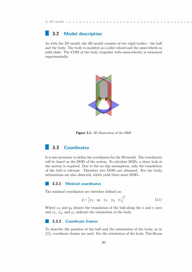
As with the 2D model, the 3D model consists of two rigid bodies - the balland the body. The body is modeled as a solid cuboid and the omni-wheels assolid disks. The COM of the body (together with omni-wheels) is estimatedexperimentally.
Figure 3.1: 3D illustration of the BRB
3.3 Coordinates
It is also necessary to define the coordinates for the 3D model. The coordinateswill be based on the DOFs of the system. To calculate DOFs, a closer look atthe system is required. Due to the no slip assumption, only the translationof the ball is relevant. Therefore two DOFs are obtained. For the body,orientations are also observed, which yield three more DOFs.
3.3.1 Minimal coordinates
The minimal coordinates are therefore defined as:
~q =[xS yS ψx ψy ψz
]T(3.1)
Where xS and yS denote the translation of the ball along the x and y axesand ψx, ψy, and ψz indicate the orientation of the body.
3.3.2 Coordinate frames
To describe the position of the ball and the orientation of the body, as in[11], coordinate frames are used. For the orientation of the body, Tait-Bryan
30

..................................... 3.3. Coordinates
(Yaw-Pitch-Roll) angles, a special case of Euler angles, are used. In total, sixcoordinate frames are defined:. Inertial frame I
The basic inertial frame..Coordinate frame 1Translation of the inertial frame with xS along its x axis..Coordinate frame 2Translation of the coordinate frame 1 with yS along its y axis. Note thatthis frame is located in the COM of the ball..Coordinate frame 3Counterclockwise rotation of the coordinate frame 2 with ψz around itsz axis..Coordinate frame 4Counterclockwise rotation of the coordinate frame 3 with ψy around itsy axis..Coordinate frame 5Clockwise rotation of the coordinate frame 4 with ψx around its x-axistogether with translation of value l along its z-axis.
Figure 3.2: Illustration of coordinate frames - taken from [11]
31
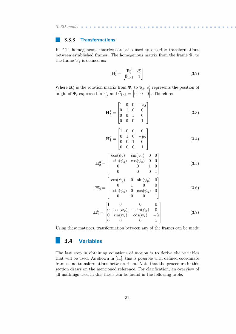
3. 3D model ......................................3.3.3 Transformations
In [11], homogeneous matrices are also used to describe transformationsbetween established frames. The homogenous matrix from the frame Ψi tothe frame Ψj is defined as:
Hji =
[Rji ~oji
~01×3 1
](3.2)
Where Rji is the rotation matrix from Ψi to Ψj , ~oji represents the position of
origin of Ψi expressed in Ψj and ~01×3 =[0 0 0
]. Therefore:
H1I =
1 0 0 −xS0 1 0 00 0 1 00 0 0 1
(3.3)
H21 =
1 0 0 00 1 0 −yS0 0 1 00 0 0 1
(3.4)
H32 =
cos(ψz) sin(ψz) 0 0− sin(ψz) cos(ψz) 0 0
0 0 1 00 0 0 1
(3.5)
H43 =
cos(ψy) 0 sin(ψy) 0
0 1 0 0− sin(ψy) 0 cos(ψy) 0
0 0 0 1
(3.6)
H54 =
1 0 0 00 cos(ψx) − sin(ψx) 00 sin(ψx) cos(ψx) −ů0 0 0 1
(3.7)
Using these matrices, transformation between any of the frames can be made.
3.4 Variables
The last step in obtaining equations of motion is to derive the variablesthat will be used. As shown in [11], this is possible with defined coordinateframes and transformations between them. Note that the procedure in thissection draws on the mentioned reference. For clarification, an overview ofall markings used in this thesis can be found in the following table.
32

...................................... 3.4. Variables
Marking Description
Hji Homogeneous matrix form Ψi to Ψj
Rji Rotation matrix form Ψi to Ψj
~oji Position of origin of Ψi expressed in Ψj
~ri,jk Position of Ψk w.r.t. Ψj , expressed in Ψi
~vi,jk Linear velocity of Ψk w.r.t. Ψj , expressed in Ψi
~ωi,jk Angular velocity of Ψk w.r.t. Ψj , expressed in Ψi
~T i,jk Twist of Ψk w.r.t. Ψj , expressed in Ψi
IiO Inertia tensor of an object O around its COM chosen in Ψi
~IO Moment of inertia of an object O around its COM~I ′O Moment of inertia of an object O around its rotation axis
AdHji
Adjoint matrix of Hji that maps twist from Ψi to Ψj
Table 3.1: Table of markings
Where w.r.t. stands for "with relation to".
The twist vector is defined as a conjunction of the angular velocity vec-tor and of the linear velocity vector:
~T i,jk =[~ωi,jk~vi,jk
](3.8)
A coordinate change of a twist ~T i,jk to coordinate frame n is defined as:
~Tn,jk = AdHni· ~T i,jk (3.9)
With the adjoint matrix:
AdHni
=[
Rni 03×3
oni ·Rni Rn
i
](3.10)
Where 03×3 is 3x3 zero matrix and:
oni =
0 −oz oyoz 0 −ox−oy ox 0
(3.11)
The elements of this matrix are obtained from:
~oni =[ox oy oz
]T(3.12)
33

3. 3D model ......................................3.4.1 Velocities of the ball
Linear velocity of the ball w.r.t. ΨI , expressed in the same frame, is markedas the linear velocity of Ψ2 w.r.t. ΨI , also expressed in the same frame:
~vI,I2 =
xSyS0
(3.13)
Due to the lack of rotation of Ψ2 w.r.t. ΨI , the angular velocity ~ωI,I2 is equalto zero:
~ωI,I2 =
000
(3.14)
Note that this angular velocity is not the angular velocity of the ball.Hence the twist ~T I,I2 w.r.t ΨI , expressed in ΨI is:
~T I,I2 =
000xSyS0
(3.15)
Using this twist, the twist Ψ2 w.r.t. ΨI , expressed in Ψ2 can be introducedas:
~T 2,I2 = AdH2
I· ~T I,I2 (3.16)
For later calculations, the twist Ψ2 w.r.t. ΨI , expressed in Ψ5 is needed. Thedefinition is as follows:
~T 5,I2 = AdH5
I· ~T I,I2 (3.17)
Now the angular velocity of the ball remains to be clarified.With help of the auxiliary vector:
~rT =
00rS
(3.18)
And basic formula for the angular velocity:
~ω = ~r × ~v|~r|2
(3.19)
The angular velocity of the ball w.r.t ΨI , expressed in Ψ2 is calculated as:
~ω2,IS = ~rT × ~v2,I
2|~rT |2
=
ySrS− xSrS0
(3.20)
34

...................................... 3.4. Variables
3.4.2 Velocities of the body
The twist of the body w.r.t. ΨI , expressed also in ΨI is marked as the twistof the frame Ψ5 w.r.t. ΨI , expressed in ΨI . Therefore:
~T I,I5 = J · ~qj (3.21)
Where J is the Jacobian matrix, which maps the joint velocities to the bodyof the BRB. Due to Tait-Bryan angles, the velocities are defined as:
~qj =[xS yS ψz ψy ψx
]T(3.22)
and the Jacobian as:
J =[~T I,I1
~T I,12~T I,23
~T I,34~T I,45
]=[~T I,I1 AdH1
1· ~T I,12 AdHI
2· ~T 2,2
3 AdHI3· ~T 3,3
4 AdHI4· ~T 4,4
5
] (3.23)
The twists for its computation, using Fig. 3.2, are derived as:
~T I,I1 =[0 0 0 1 0 0
]T~T 1,1
2 =[0 0 0 0 1 0
]T~T 2,2
3 =[0 0 1 0 0 0
]T~T 3,3
4 =[0 1 0 l 0 0
]T~T 4,4
5 =[−1 0 0 0 l 0
]T(3.24)
Where the linear velocity of the twist ~T 3,34 is computed as:
~v3,34 =
(~ω3,3
4 ×R34 ·~lT
)And respectively, the linear velocity of the twist ~T 4,4
5 as:
~v4,45 =
(~ω4,4
5 ×R45 ·~lT
)Where ~lT =
[0 0 l
]T.
Having solved Eq. (3.21), the twist of the body w.r.t. ΨI , expressed inΨ5 can be calculated:
~T 5,I5 = AdH5
I· ~T I,I5 (3.25)
3.4.3 Angular velocities of the omni-wheels
Due to assumption 5, the circumferential velocity of the omni-wheel is identicalto the circumferential velocity of the ball in the direction of that omni-wheel.Let us define φi as the angular velocity of the i-th omni-wheel with a positive
35

3. 3D model ......................................counterclockwise rotation. Therefore, with Eq. (2.12) (derived in Sec. 2.4)and setting angle β = 0◦, the vectors from the centre of the ball to eachomni-wheel are defined as:
~rW,1 = rS
sin(α)0
cos(α)
~rW,2 = rS
−12 sin(α)√3
2 sin(α)cos(α)
~rW,3 = rS
−12 sin(α)
−√
32 sin(α)cos(α)
(3.26)
Together with unit vectors in the direction of each omni-wheel:
~uW,1 =
010
~uW,2 =
−√
32−1
20
~uW,3 =
√
32−1
20
(3.27)
The circumferential velocities can be calculated and the angular velocity ofthe omni-wheel defined as:
φirW = (~ω5,5S × ~rW,i) · ~uW,i
φi = 1rW
((~ω5,5S × ~rW,i) · ~uW,i
) (3.28)
Where i = 1, 2, 3 and:
~ω5,5S = ~ω5,I
S − ~ω5,I5
= R52 · ~ω
2,IS − ~ω
5,I5
(3.29)
36

................................. 3.5. Equations of motion
3.5 Equations of motion
As for the 2D model, the equations of motion will be also obtained usingLagrangian mechanics. The kinetic and potential energy for relevant parts ofthe BRB and external torques are listed below.
3.5.1 Kinetic and potential energy
In the case of the 3D system, the energies were obtained using [11].
Energy of the ball
The kinetic energy of the ball is defined as:
TS = 12~T 2,IT
2 ·[
I2S 03×3
03×3 mSI3×3
]· ~T 2,I
2 + 12~ω
2,ITS · I2
S · ~ω2,IS
= 12~ω
2,IT2 · I2
S · ~ω2,I2 + 1
2mS~v2,IT2 · ~v2,I
2 + 12~ω
2,ITS · I2
S · ~ω2,IS
= 12mS~v
2,IT2 · ~v2,I
2 + 12(R2I · ~ω
I,IS
)T· I2S ·(R2I~ω
I,IS
)(3.30)
Where I3×3 is a 3x3 identity matrix.
Also in the 3D model, Assumption 3 causes the potential energy of theball to be equal to zero.
VS = 0 (3.31)
Energy of the body
For the body, the kinetic energy is defined similarly as:
TB = 12~T 5,IT
5 ·[
I5B 03×3
03×3 mSI3×3
]· ~T 5,I
5
= 12~ω
5,IT5 · I5
B · ~ω5,I5 + 1
2mB~v5,IT5 · ~v5,I
5
(3.32)
The potential energy has the form:
VB = mB
[0 0 g
]RI
5
00l
(3.33)
Energy of the omni-wheels
The energy of i-th omni-wheel is denoted by its rotational energy as:
TWi = 12IOW φ
2i + 1
2IM (kφi)2 (3.34)
And the potential energy is equal to zero.
VWi = 0 (3.35)
37
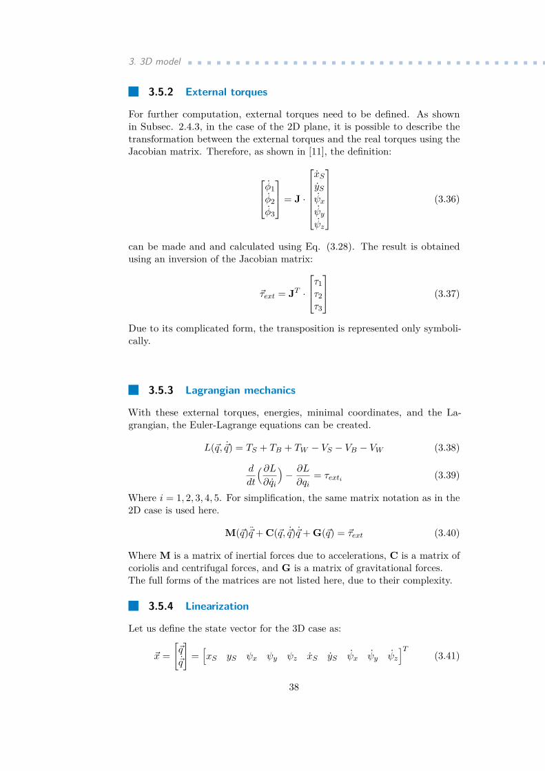
3. 3D model ......................................3.5.2 External torques
For further computation, external torques need to be defined. As shownin Subsec. 2.4.3, in the case of the 2D plane, it is possible to describe thetransformation between the external torques and the real torques using theJacobian matrix. Therefore, as shown in [11], the definition:
φ1φ2φ3
= J ·
xSySψxψyψz
(3.36)
can be made and and calculated using Eq. (3.28). The result is obtainedusing an inversion of the Jacobian matrix:
~τext = JT ·
τ1τ2τ3
(3.37)
Due to its complicated form, the transposition is represented only symboli-cally.
3.5.3 Lagrangian mechanics
With these external torques, energies, minimal coordinates, and the La-grangian, the Euler-Lagrange equations can be created.
L(~q, ~q) = TS + TB + TW − VS − VB − VW (3.38)
d
dt
(∂L∂qi
)− ∂L
∂qi= τexti (3.39)
Where i = 1, 2, 3, 4, 5. For simplification, the same matrix notation as in the2D case is used here.
M(~q)~q + C(~q, ~q)~q + G(~q) = ~τext (3.40)
Where M is a matrix of inertial forces due to accelerations, C is a matrix ofcoriolis and centrifugal forces, and G is a matrix of gravitational forces.The full forms of the matrices are not listed here, due to their complexity.
3.5.4 Linearization
Let us define the state vector for the 3D case as:
~x =[~q
~q
]=[xS yS ψx ψy ψz xS yS ψx ψy ψz
]T(3.41)
38

............................... 3.6. Calculation of parameters
and the input vector as:
~u =
τ1τ2τ3
(3.42)
As before, the linearization will be done on an unstable equilibrium point onthe top of the ball, with all states and inputs equal to zero.
~x =[0 0 0 0 0 0 0 0 0 0
]T~u =
[0 0 0
]T (3.43)
The state-space representation is given by:
~x = A · ~x+ C · ~u~y = C · ~x+ D · ~u
(3.44)
Where C is a 10x10 identity matrix, D is a 10x3 zero matrix, and othermatrices are computed in the same way as in Subsec. 2.5.4. Therefore, aftersubstitusions and calculations, their forms are:
A =
0 0 0 0 0 1 0 0 0 00 0 0 0 0 0 1 0 0 00 0 0 0 0 0 0 1 0 00 0 0 0 0 0 0 0 1 00 0 0 0 0 0 0 0 0 10 0 0 −1.8433 0 0 0 0 0 00 0 −1.8433 0 0 0 0 0 0 00 0 14.3425 0 0 0 0 0 0 00 0 0 14.3425 0 0 0 0 0 00 0 0 0 0 0 0 0 0 0
B =
0 0 00 0 00 0 00 0 00 0 00 7.0841 −7.0841
−8.1800 4.0900 4.09003.6237 −1.8119 −1.8119
0 −3.1383 3.1383−684.4921 −684.4921 −684.4921
(3.45)
Further calculations show that the system is fully controllable and observable.
3.6 Calculation of parameters
In the previous section, many parameters were used. The majority of themhave been listed in Tab. 2.1. Two of them, however, still need to be defined
39

3. 3D model ......................................and calculated [11].
3.6.1 Intertia tensor of the ball
Let us define the inertia tensor of the ball as:
I2S =
IS 0 00 IS 00 0 IS
(3.46)
Where IS is the moment of inertia of the ball (listed in the reference table2.1).
3.6.2 Intertia tensor of the body
We define the inertia tensor of the body as:
I5B =
IB,x 0 00 IB,y 00 0 IB,z
(3.47)
Where IB,i is the moment of inertia of the body about the i-th axis of thecoordinate frame of its COM.
Defined in Subsec. 2.7.2, the moment of inertia of a cuboid of width wand heigth w, about the x or y axis is given by:
Ix,y = m(w2 + h2
12 (3.48)
And about the z axis as:Iz = mw2
6 (3.49)
Therefore, the moments of inertia of the body about the i-th axis of the COMare:
IB,x = 112mB(w2
B + h2B)
IB,y = 112mB(w2
B + h2B)
IB,z = 16mBw
2B
(3.50)
Note that the total mass of the body consists of the mass of the frame, motors,shafts, and omni-wheels.
3.7 Simulations
Several simulations determine the accuracy of the linearized model were made.Similar to simulations of the 2D model, two basic tests were done.
The first test is with initial condition of ψx = 0.1◦:
40

..................................... 3.7. Simulations
t [s]
0 0.5 1 1.5
angle
[deg]
0
5
10
15Comparison of models
θx -physical model
θy -linearized model
limit angle
Figure 3.3: Comparison for ψx - ψx(t = 0) = 0.1◦
t [s]
0 0.5 1 1.5
dis
tance [m
]
-0.035
-0.03
-0.025
-0.02
-0.015
-0.01
-0.005
0Comparison of models
yS -physical model
yS -linearized model
Figure 3.4: Comparison for yS - ψx(t = 0) = 0.1◦
As can be seen, even after the limit angle is exceeded, the linearized model isa very accurate replacement of the physical model.
41

3. 3D model ......................................The second test is with constant imnput uy = 0.01N/m and zero initialconditions:
t [s]
0 0.5 1 1.5
angle
[deg]
-12
-10
-8
-6
-4
-2
0Comparison of models
θx -physical model
θy -linearized model
limit angle
Figure 3.5: Comparison for ψx - uy = 0.01N/m
t [s]
0 0.5 1 1.5
dis
tance [m
]
0
0.01
0.02
0.03
0.04
0.05
0.06
0.07Comparison of models
yS -physical model
yS -linearized model
Figure 3.6: Comparison for yS - uy = 0.01N/m
Even with constant input, the linearized system acts accurately and can be asatisfactory substitution for the physical model for the limits in which theBRB operates.
42

Chapter 4Controller design
In this chapter a controller is designed using the 3D model derived in theprevious chapter. The main aims of the controller are to keep the robot stableon the top of the ball and track its trajectory.
In the first section, the methods used in contemporary literature are de-scribed. The second section discusses the controller requirements and designapproach. Lastly, a Linear-Quadratic Regulator (LQR) controller is designedin the third section.
4.1 Controllers of previously created BRBs
.CMUBalancing controller: PID controllerPosition controller: PID controller with offline trajectory planning.TGUBalancing and position controller: Two PD controllers.UABalancing and position controller: LQR controller with full state feedbackand two extra Integral states. ETHBalancing controller: Non-linear controller based on LQR theoryPosition controller: Non-linear controller based on LQR theory withfeedforward.NCHUBalancing and position controller: LQR controller with full state feedback.UTBalancing and position controller: LQR controller with full state feedbackand later SISO controller
43

4. Controller design ...................................4.2 Requirements and approach
At first, an assumption needs to be made: that the linearized model isapproximately equivalent to the nonlinear model in the proximity of theequilibrium point. The proof can be seen in Figures 3.3 - 3.6. Contemporaryliterature often shows that the angles of the body and position of the ballcan be controlled by a single linear controller. Thus this paper also aims todesign such a controller, using the same procedure as in [11], and adaptingit to the requirements of this project. So firstly, the controller requirementsneed to be defined.
4.2.1 Design requirements
A well-designed controller is considered to be one that satisfies the followingrules:. the system is internally stable - all the Closed Loop (CL) poles have a
negative real part. the sensitivity function attenuates disturbances up to 2Hz down by atleast 80%
mag2db(0.2) = −14dB
. the CL transfer function attenuates frequencies above 250Hz down byat least 80% (-14 dB), due to Nyquist-Shannon sampling theorem andsampling frequency 500Hz. the settling time of the step response of pitch and roll angle is betweentwo and four seconds for stabilization. the torque saturations of motors are minimized.
4.2.2 Design approach
Due to the short project length, simplicity is more important than performance.The LQR design method was therefore chosen due to its short calculatingtime, despite the fact that finding an optimal controller with LQR theory is adifficult task. However, a suboptimal controller can be found relatively easily.
4.3 LQR controller design
In this section a LQR controller is designed to control the angles of the bodyand position of the whole robot at the same time.
44

.................................4.3. LQR controller design
4.3.1 LQR control theory
LQR is an acronym for Linear-Quadratic Regulator. A special type ofproportional derivative controller with feedback and a single gain matrix K,implemented as ~u = K~e in the state-space form (3.44), where ~e is an errorvector defined as ~e = ~xref − ~x. This results in the CL system shown in Fig.4.1, with state representation expressed by the following equations:
~x = (A−BK)~x+ BK~xref
~y = C~x(4.1)
Torques States
Plant
Errors Torques
Controller
1
x_ref
1
y
x
Figure 4.1: The closed loop system
As has been mentioned, the implementation of the control matrix K is~u = K~e. The calculation of this matrix is done by minimizing the quadraticcost function given by:
J(~u) =∫ t1
t0(~eTQ~e+ ~uTρR~u)dt (4.2)
With Q defined as NTQ′N, where N defines the plant outputs which need tobe controlled and Q′ is the weighting matrix of the controlled outputs. MatrixR is the weighting matrix of controller outputs, ρ is a positive constant, andthe time interval bounds are t0 = 0, t1 =∞.
As there is no way to find the optimal matrices Q, R, and constant ρ,Bryson’s rule [14] is used to estimate the initial values of matrices Q′ and R.Diagonal elements of these matrices are chosen as follows:
Q′ii = 1e2i,max
(4.3)
Rjj = 1u2j,max
(4.4)
Where ei,max is the maximum possible value of the error with respect to thereference value of the state i, and uj,max is the maximum possible value ofthe input j. Moreover the parameter ρ also needs to be estimated. WhenρR >> Q, the control effort cost function is dominant. Similarly whenρR << Q, the error cost function is dominant. A mid-point between thesetwo extremes is needed, so the controller focuses on minimizing both extremes.For the beginning state of design, ρ = 1 was chosen and further adjusted tosatisfy the requirements given in 4.2.1.
45

4. Controller design ...................................4.3.2 Application on the BRB
Due to the linearized model of BRB in Subsec. 3.5.4, all states are controlled.Thus matrix N is a 10x10 identity matrix. The maximum possible values ofthe errors were set approximately to:
eSx,Sx = eSy ,Sy = 0.5 [m]eψx,ψx = eψy ,ψy = 10 [deg]
eψz ,ψz = 360 [deg]
and their derivatives to three times the previous values:
eSx,Sx = eSy ,Sy = 1.5 [m/s]eψx,ψx = eψy ,ψy = 30 [deg/s]
eψz ,ψz = 1080 [deg/s]
Hence the matrix Q′ can be extimated as:
Q′ =
10.52 0 0 0 0 0 0 0 0 00 1
0.52 0 0 0 0 0 0 0 00 0 1802
(10π)2 0 0 0 0 0 0 00 0 0 1802
(10π)2 0 0 0 0 0 00 0 0 0 1802
(360π)2 0 0 0 0 00 0 0 0 0 1
1.52 0 0 0 00 0 0 0 0 0 1
1.52 0 0 00 0 0 0 0 0 0 1802
(30π)2 0 00 0 0 0 0 0 0 0 1802
(30π)2 00 0 0 0 0 0 0 0 0 1802
(1080π)2
(4.5)
For driving the omni-wheels, three EV3 Large Servo Motors are used, onefor each wheel. The maximum torque for a motor of this type is 30 oz/in,which equals roughly 0.21 N/m [21]. The omni-wheels are directly attachedto the motors without a transmission. Thus, the maximum torque of a singleomni-wheel is identical to the maximum torque of a single motor. Therefore,the matrix R is estimated as:
R =
10.212 0 0
0 10.212 0
0 0 10.212
(4.6)
The parameter ρ now needs to be tuned. For this purpose, nine values werechosen and nine LQR controllers computed with them. The requirementsstated in 4.2.1 have been complied with, and the best controller was chosen.
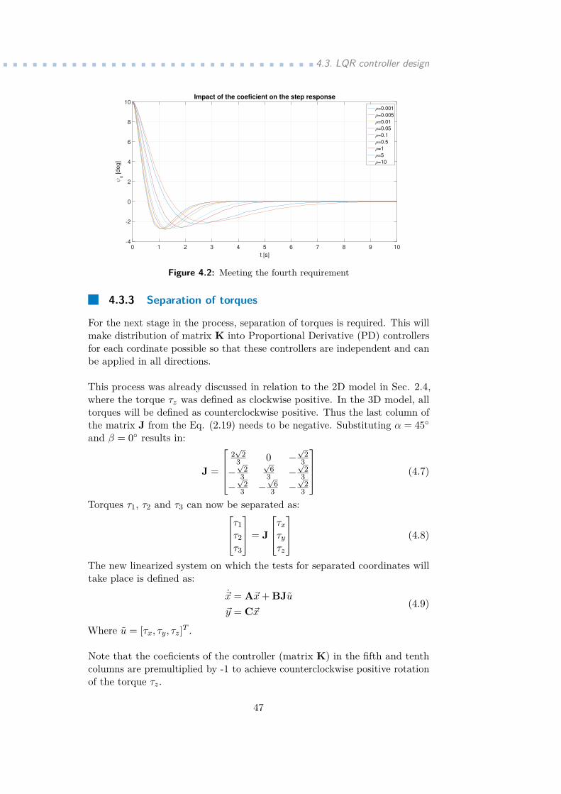
Figure 4.2 below shows the settling time of the step response of pitch anglefor a step signal of size 10◦. For ρ = 0.5 and above the fourth requirementwas not met.
46
.................................4.3. LQR controller design
t [s]
0 1 2 3 4 5 6 7 8 9 10
ψx [deg]
-4
-2
0
2
4
6
8
10Impact of the coeficient on the step response
ρ=0.001
ρ=0.005
ρ=0.01
ρ=0.05
ρ=0.1
ρ=0.5
ρ=1
ρ=5
ρ=10
Figure 4.2: Meeting the fourth requirement
4.3.3 Separation of torques
For the next stage in the process, separation of torques is required. This willmake distribution of matrix K into Proportional Derivative (PD) controllersfor each cordinate possible so that these controllers are independent and canbe applied in all directions.
This process was already discussed in relation to the 2D model in Sec. 2.4,where the torque τz was defined as clockwise positive. In the 3D model, alltorques will be defined as counterclockwise positive. Thus the last column ofthe matrix J from the Eq. (2.19) needs to be negative. Substituting α = 45◦and β = 0◦ results in:
J =
2√
23 0 −
√2
3−√
23
√6
3 −√
23
−√
23 −
√6
3 −√
23
(4.7)
Torques τ1, τ2 and τ3 can now be separated as:τ1τ2τ3
= J
τxτyτz
(4.8)
The new linearized system on which the tests for separated coordinates willtake place is defined as:
~x = A~x+ BJu~y = C~x
(4.9)
Where u = [τx, τy, τz]T .
Note that the coeficients of the controller (matrix K) in the fifth and tenthcolumns are premultiplied by -1 to achieve counterclockwise positive rotationof the torque τz.
47

4. Controller design ...................................4.3.4 Frequency domain requirements verification
The transfer function matrix of the state-space model is defined as:
P = C(sI−A)−1BJ (4.10)
where I is a 10x10 identity matrix.
The controller which controls the torques in x, y, and z directions is de-rived by:
Kx,y,z = J−1K (4.11)
By summing up the combination of gains with relevant coordinates and theirderivatives, PD controllers are created. With these controllers and the transferfunction matrix, all needed system transfer functions can be calculated. Notethat the transfer functions of xS and yS are identical. The same is also thecase for the transfer functions of ψx and ψy.
At the beginning, a value of ρ = 0.01 was chosen due to its meeting thefourth requirement. However, it can be seen in Figure 4.3 that the sensitivityfunction for this value does not satisfy the second requirement.
10-3
10-2
10-1
100
101
102
103
Magnitude (
dB
)
-30
-25
-20
-15
-10
-5
0
5
10
SxS , SyS
Sψx, Sψy
Sψz
Sensitivity functions
Frequency (Hz)
Figure 4.3: Meeting the second requirement (ρ = 0.01)
Thus, a new value was chosen to satisfy this requirement. The next twofigures show the sensitivity functions for ρ = 0.005 and ρ = 0.001.
48

.................................4.3. LQR controller design
10-3
10-2
10-1
100
101
102
103
Magnitude (
dB
)
-30
-25
-20
-15
-10
-5
0
5
10
SxS , SyS
Sψx, Sψy
Sψz
Sensitivity functions
Frequency (Hz)
Figure 4.4: Meeting the second requirement (ρ = 0.005)
10-3
10-2
10-1
100
101
102
103
Magnitude (
dB
)
-30
-25
-20
-15
-10
-5
0
5
10
SxS , SyS
Sψx, Sψy
Sψz
Sensitivity functions
Frequency (Hz)
Figure 4.5: Meeting the second requirement (ρ = 0.001)
As can be seen, in Figure 4.4 the criterion is almost met. In Figure 4.5 thecriterion is met with a large margin. Therefore, the optimal value for ρ willbe between these two values. The answer to which value should be chosen ishidden in satisfying the third requirement. Therefore the closed loop transferfunctions were obtained and their bode characteristics plotted.
49

4. Controller design ...................................
10-3
10-2
10-1
100
101
102
103
Magnitude (
dB
)
-30
-25
-20
-15
-10
-5
0
5
10T xS , T yS
T ψx, T ψy
T ψz
CL transfer functions
Frequency (Hz)
Figure 4.6: Meeting the third requirement (ρ = 0.005)
10-3
10-2
10-1
100
101
102
103
Magnitude (
dB
)
-30
-25
-20
-15
-10
-5
0
5
10T xS , T yS
T ψx, T ψy
T ψz
CL transfer functions
Frequency (Hz)
Figure 4.7: Meeting the third requirement (ρ = 0.001)
While not meeting the second requirement, ρ = 0.005 satisfies the thirdrequirement with a large margin. As can be seen, ρ = 0.001 is unsatisfactory.Thus the value of ρ will be a little less than 0.005. From these observations aconclusion can be drawn: ρ = 0.004. Below, ρ = 0.004 is shown to meet thesecond, third, and fourth requirements.
50

.................................4.3. LQR controller design
10-3
10-2
10-1
100
101
102
103
Magnitude (
dB
)
-30
-25
-20
-15
-10
-5
0
5
10
SxS , SyS
Sψx, Sψy
Sψz
Sensitivity functions
Frequency (Hz)
Figure 4.8: Meeting the second requirement (ρ = 0.004)
10-3
10-2
10-1
100
101
102
103
Magnitude (
dB
)
-30
-25
-20
-15
-10
-5
0
5
10T xS , T yS
T ψx, T ψy
T ψz
CL transfer functions
Frequency (Hz)
Figure 4.9: Meeting the third requirement (ρ = 0.004)
51

4. Controller design ...................................
t [s]
0 1 2 3 4 5 6 7 8 9 10
ψx [deg]
-4
-2
0
2
4
6
8
10Impact of the coeficient on the step response
ρ=0.004
Figure 4.10: Meeting the fourth requirement (ρ = 0.004)
Now it remains to verify the first and most important requirement - systemstability. To determine if the system is stable, the bode characteristics forall three CL transfer functions need to be observed. For demonstration, onlythe bode diagram for the first CL transfer function was plotted.
Magnitude (
dB
)
-40
-30
-20
-10
0
10
10-3
10-2
10-1
100
101
102
103
Phase (
deg)
-90
-45
0
First transfer function
Bode Diagram
Frequency (Hz)
Figure 4.11: Bode plot of the first CL transfer function
The transfer function has, in the Laplace transform, the form of:
Txy = 65.49s+ 64.98 (4.12)
Because the transfer functions of coordinate xS and yS are the same, the poleis doubled and rewritten in [rad/s] as:
p1 = −1.134p2 = −1.134
52
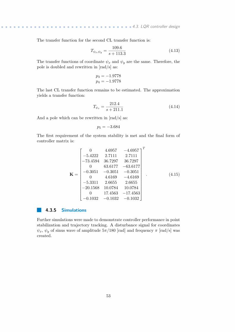
.................................4.3. LQR controller design
The transfer function for the second CL transfer function is:
Tψx,ψy = 109.6s+ 113.3 (4.13)
The transfer functions of coordinate ψx and ψy are the same. Therefore, thepole is doubled and rewritten in [rad/s] as:
p3 = −1.9778p4 = −1.9778
The last CL transfer function remains to be estimated. The approximationyields a transfer function:
Tψz = 212.4s+ 211.1 (4.14)
And a pole which can be rewritten in [rad/s] as:
p5 = −3.684
The first requirement of the system stability is met and the final form ofcontroller matrix is:
K =
0 4.6957 −4.6957−5.4222 2.7111 2.7111−73.4594 36.7297 36.7297
0 63.6177 −63.6177−0.3051 −0.3051 −0.3051
0 4.6169 −4.6169−5.3311 2.6655 2.6655−20.1568 10.0784 10.0784
0 17.4563 −17.4563−0.1032 −0.1032 −0.1032
T
. (4.15)
4.3.5 Simulations
Further simulations were made to demonstrate controller performance in pointstabilization and trajectory tracking. A disturbance signal for coordinatesψx, ψy of sinus wave of amplitude 5π/180 [rad] and frequency π [rad/s] wascreated.
53

4. Controller design ...................................
t [s]
0 1 2 3 4 5 6 7 8 9 10
ψx [ra
d]
-0.1
-0.08
-0.06
-0.04
-0.02
0
0.02
0.04
0.06
0.08
0.1Disturbance signal
Figure 4.12: Disturbance sinus signal used for angles ψx and ψy
This signal was gradually applied to the respective angles and the torqueswere monitored at the output of the controller.
t [s]
0 1 2 3 4 5 6 7 8 9 10
τ [N
m]
-0.25
-0.2
-0.15
-0.1
-0.05
0
0.05
0.1
0.15
0.2
0.25Applied torques
τ1
τ2
τ3
saturations
Figure 4.13: Torques for disturbance signal in ψx
54
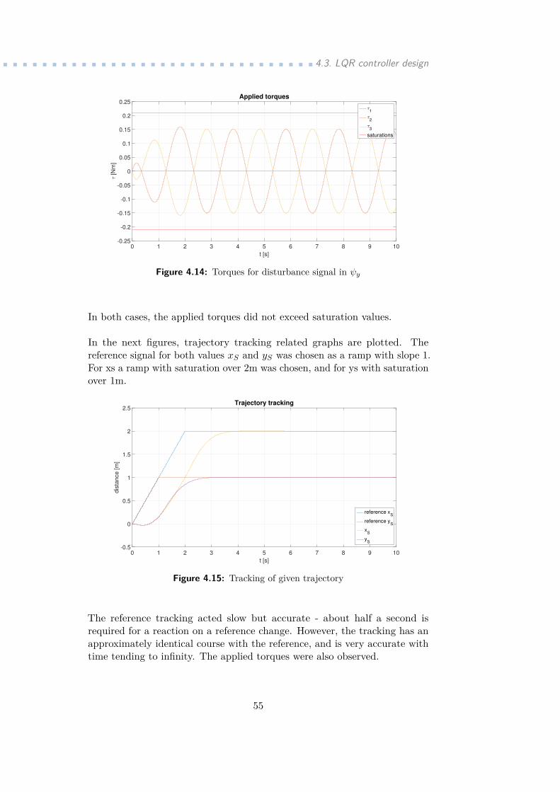
.................................4.3. LQR controller design
t [s]
0 1 2 3 4 5 6 7 8 9 10
τ [N
m]
-0.25
-0.2
-0.15
-0.1
-0.05
0
0.05
0.1
0.15
0.2
0.25Applied torques
τ1
τ2
τ3
saturations
Figure 4.14: Torques for disturbance signal in ψy
In both cases, the applied torques did not exceed saturation values.
In the next figures, trajectory tracking related graphs are plotted. Thereference signal for both values xS and yS was chosen as a ramp with slope 1.For xs a ramp with saturation over 2m was chosen, and for ys with saturationover 1m.
t [s]
0 1 2 3 4 5 6 7 8 9 10
dis
tance [m
]
-0.5
0
0.5
1
1.5
2
2.5Trajectory tracking
reference xS
reference yS
xS
yS
Figure 4.15: Tracking of given trajectory
The reference tracking acted slow but accurate - about half a second isrequired for a reaction on a reference change. However, the tracking has anapproximately identical course with the reference, and is very accurate withtime tending to infinity. The applied torques were also observed.
55

4. Controller design ...................................
t [s]
0 1 2 3 4 5 6 7 8 9 10
τ [N
m]
-0.25
-0.2
-0.15
-0.1
-0.05
0
0.05
0.1
0.15
0.2
0.25Applied torques
τ1
τ2
τ3
saturations
Figure 4.16: Torques for tracking of given trajectory
As in Figures 4.13 and 4.14, the torques were in acceptable range.
Due to this and previous results, the controller was found to be fully satisfac-tory and implemented into a physical model.
56

Chapter 5Robot design
As the title suggests, this chapter is dedicated to the robot design. Firstlythe requirements are set. After that, the LEGO Mindstorms EV3 buildingkit is introduced, followed by a description of the built robot. The buildinginstructions and other necessary steps are also listed.
5.1 Design requirements
Several requirements were stated in previous chapters. Together with request-ing LEGO as a building material, the list of requirements is:.Position of the COM of the body
The COM of the body is located in the centre of horizontal plane, whichintersects the body at a reasonable height..Position of gyroscopesGyroscopes are located near the COM of the body, fixed at the sameheight and oriented in the direction of x and y axes respectively..Position of omni-wheelsOmni-wheels are mounted to the body with a spacing of 120◦..Angle of omni-wheelsThe angle between the body and each omni-wheel is 45◦..Building materialThe whole body is built using the LEGO EV3 building kit.The ball is a bowling ball.
57

5. Robot design.....................................5.2 LEGO Mindstorms EV3 building kit
5.2.1 What is LEGO?
LEGO is a well-known Danish construction toy with worldwide popularity.Among its biggest advantages is the compatibility of all sets and cleverconnection of parts. It is therefore possible to combine sets to create structuresof any type or dismantle already assembled creations and reuse bricks withoutany additional costs. But there are also bad downsides, including: the weightof the bricks, and the complexity of constructing non-rectangular structures.
5.2.2 What is Mindstorms EV3?
Figure 5.1: LEGO Mindstorms Education EV3 Core Set - Source [16]
Mindstorm is a branch of LEGO products for creation of robots. Bothhardware and software are provided for controlling the "intelligent" parts.The EV3 stands for version of the platform. There are in total four platforms[15], sorted from the oldest: RIS, NXT, NXT 2.0, and EV3. The EV3 is thelatest and was introduced in 2013. For the purpose of this project, the EV3was choosen for its modernity and ability to run a selected programminglanguage.
5.2.3 Parts
Due to the robot’s complexity, together with the Core Set, the LEGO Mind-storms Education EV3 Expansion Set is also used. A list of all parts containedin these two sets can be found at [17]. Below, the most important parts aredescribed.
58
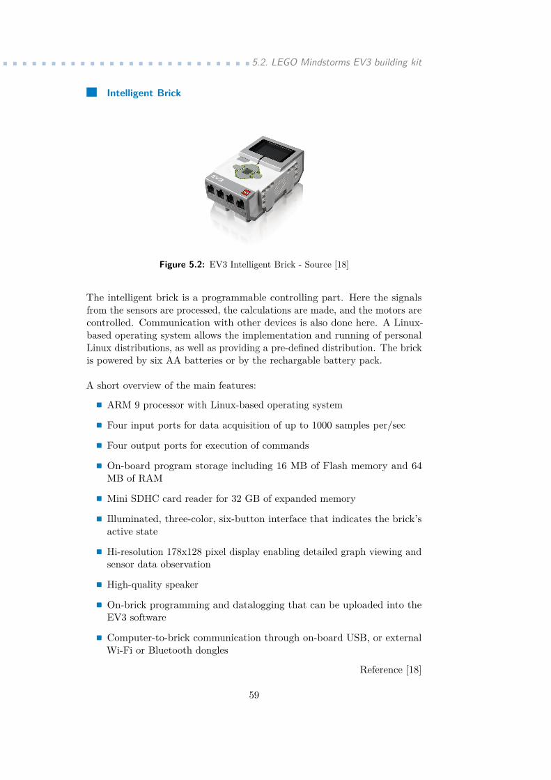
...........................5.2. LEGO Mindstorms EV3 building kit
Intelligent Brick
Figure 5.2: EV3 Intelligent Brick - Source [18]
The intelligent brick is a programmable controlling part. Here the signalsfrom the sensors are processed, the calculations are made, and the motors arecontrolled. Communication with other devices is also done here. A Linux-based operating system allows the implementation and running of personalLinux distributions, as well as providing a pre-defined distribution. The brickis powered by six AA batteries or by the rechargable battery pack.
A short overview of the main features:. ARM 9 processor with Linux-based operating system. Four input ports for data acquisition of up to 1000 samples per/sec. Four output ports for execution of commands.On-board program storage including 16 MB of Flash memory and 64MB of RAM.Mini SDHC card reader for 32 GB of expanded memory. Illuminated, three-color, six-button interface that indicates the brick’sactive state. Hi-resolution 178x128 pixel display enabling detailed graph viewing andsensor data observation. High-quality speaker.On-brick programming and datalogging that can be uploaded into theEV3 software. Computer-to-brick communication through on-board USB, or externalWi-Fi or Bluetooth dongles
Reference [18]
59
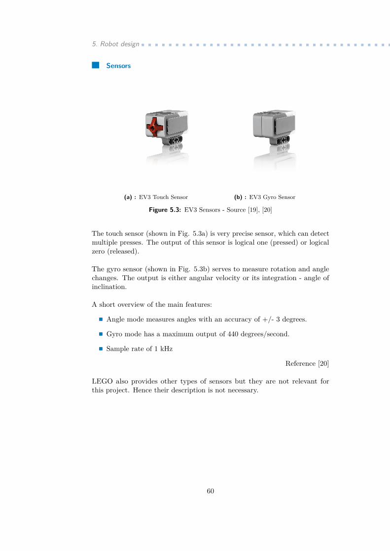
5. Robot design.....................................Sensors
(a) : EV3 Touch Sensor (b) : EV3 Gyro Sensor
Figure 5.3: EV3 Sensors - Source [19], [20]
The touch sensor (shown in Fig. 5.3a) is very precise sensor, which can detectmultiple presses. The output of this sensor is logical one (pressed) or logicalzero (released).
The gyro sensor (shown in Fig. 5.3b) serves to measure rotation and anglechanges. The output is either angular velocity or its integration - angle ofinclination.
A short overview of the main features:. Angle mode measures angles with an accuracy of +/- 3 degrees..Gyro mode has a maximum output of 440 degrees/second.. Sample rate of 1 kHz
Reference [20]
LEGO also provides other types of sensors but they are not relevant forthis project. Hence their description is not necessary.
60
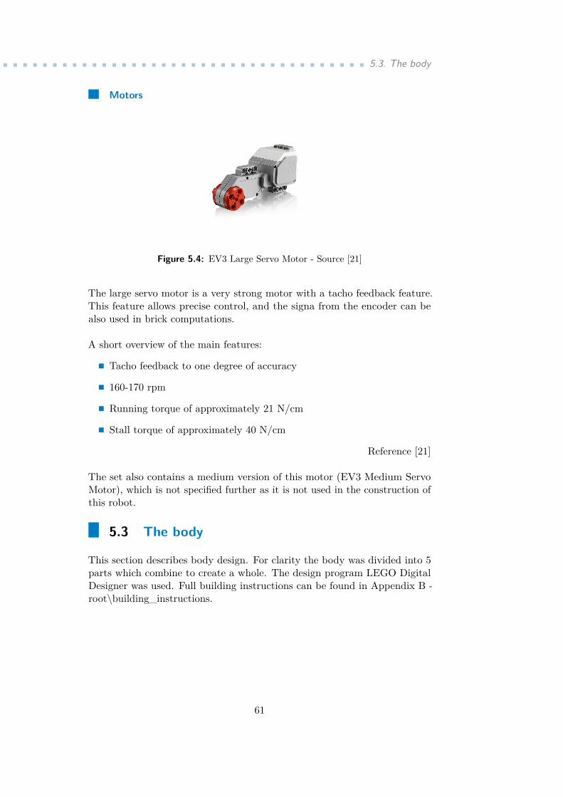
...................................... 5.3. The body
Motors
Figure 5.4: EV3 Large Servo Motor - Source [21]
The large servo motor is a very strong motor with a tacho feedback feature.This feature allows precise control, and the signa from the encoder can bealso used in brick computations.
A short overview of the main features:. Tacho feedback to one degree of accuracy. 160-170 rpm. Running torque of approximately 21 N/cm. Stall torque of approximately 40 N/cm
Reference [21]
The set also contains a medium version of this motor (EV3 Medium ServoMotor), which is not specified further as it is not used in the construction ofthis robot.
5.3 The body
This section describes body design. For clarity the body was divided into 5parts which combine to create a whole. The design program LEGO DigitalDesigner was used. Full building instructions can be found in Appendix B -root\building_instructions.
61

5. Robot design.....................................5.3.1 Upper part
The upper part contains the intelligent brick and the touch sensor. They aremounted on the middle part using additional small parts.
Figure 5.5: Composite upper part
5.3.2 Middle part
As required, the gyroscopes are placed on the central axis, where the COMof the whole body is located. The other requirement, β = 120◦ is met byforming imaginary triangles, on whose vertices the motors will be attached.
Figure 5.6: Composite middle part
5.3.3 Lower part
The lower part is composed of three identical parts, which are made of motors,omni-wheels, and struts. The angle of the omni-wheels requirement is met,and the mounting of the middle part on the lower part creates a supportingtriangle. for driving the ball. Note that due to the lack of a virtual model ofthe omni-wheel the model uses a normal wheel as a substitute.
62
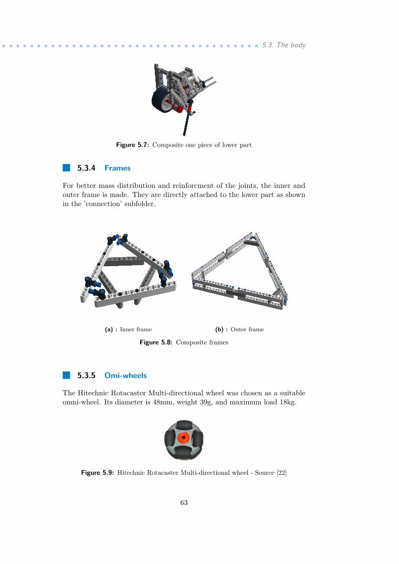
...................................... 5.3. The body
Figure 5.7: Composite one piece of lower part
5.3.4 Frames
For better mass distribution and reinforcment of the joints, the inner andouter frame is made. They are directly attached to the lower part as shownin the ’connection’ subfolder.
(a) : Inner frame (b) : Outer frame
Figure 5.8: Composite frames
5.3.5 Omi-wheels
The Hitechnic Rotacaster Multi-directional wheel was chosen as a suitableomni-wheel. Its diameter is 48mm, weight 39g, and maximum load 18kg.
Figure 5.9: Hitechnic Rotacaster Multi-directional wheel - Source [22]
63

5. Robot design.....................................5.4 The ball
As has been mentioned, the ball on which the robot balances is a bowlingball. Experimental simulations with different inflatable balls show that therobot bounces into the ball and has difficulty manipulating it. Therefore, thebowling ball was chosen because it is a ball of evenly distributed weight witha rigid surface. The mass of the ball was chosen to be 6Lbs and the brand asshown in the following figure:
Figure 5.10: EBONITE: Maxim - Night Sky Bowling Ball - Source [23]
To minimize slip, the whole ball was rubberized. Firstly a base layer toimprove adhesion (Body Plasto Fix 340) was applied. Secondly, (Body 950White) rubber spray was applied multiple times. Lastly, the blue CTU Logowas created at the side of the ball using a conventional blue spray.
64

Chapter 6Controller implementation
After completing the assembly of the body, the previously derived LQRcontroller needs to be implemented. For this, a programming language needsto be chosen, and communication between the computer and the intelligentbrick established. The last step before implementing the controller is obtainingthe state vector ~x.
6.1 Programming language
After several considerations, the Matlab Simulink Visual Programming Lan-guage (VPL) was chosen due to its support library for the LEGO MindstormsEV3, its low computational demands, and its well-arranged design. Like otherVPL’s, the Simulink lets users create programs by connecting pre-defined orcustom blocks. Therefore, the program is more clear for a wider audience.For more information about Simulink, see reference [24].
6.1.1 List of functions
The LEGO Mindstorms EV3 Support from Simulink [25] provides multipleblocks which implement many features. Full description of these features canbe found in Mathworks Documentation. For our purpose the following arerelevant:
Touch Sensor and Gyro Sensor blocks
The Touch Sensor block (shown in Fig. 6.1a) detects whether a selected EV3Touch Sensor is being pressed. As stated before, logical one means ’pressed’and logical zero ’released’.
The Gyro Sensor block (shown in Fig. 6.1b) measures the rate of rota-tion in degrees per second of a selected EV3 Gyro Sensor.
Note that both sensors are working with a user defined sample time. Thistime can be set to any number but no lower than the inverted value of thelimit frequency listed in Subsec. 5.2.3.
65

6. Controller implementation ...............................
Port 1
LEGO EV3
Touch Sensor
Port 1
LEGO EV3
Gyro Sensor
Figure 6.1: Used Simulink sensor blocks
Motor Control and Motor Encoder blocks
The Motor block (shown in Fig. 6.2a) controls the power and direction of aselected EV3 Motor. The block input is a Pulse Width Modulation (PWM)shown as an integer number from 100 to -100. Where 100 denotes full powerforward, 0 no power, and -100 full power reverse.
The Encoder block (shown in Fig. 6.2b) is actually also a sensor block.It measures the cumulative rotation of a selected EV3 Motor in degrees. Thisvalue does not wrap around after reaching 360 degrees and can be reset ateach sample time or by a user defined signal.
Port A
LEGO EV3
Motor
Port A
LEGO EV3
Encoder
Figure 6.2: Used Simulink motor blocks
6.1.2 Establishment of communication
To establish a communication between the computer and the intelligent bricka WiFi dongle is used. However the brick only supports a few models. Thesupported dongles are usually old versions with large bodies and low trans-mission speeds. Therefore, a fan-made articles describing possible extensionsof supported devices were made. One of them [26] uses a custom firmware tosupport the Edimax EW-7811Un WiFi Dongle. This small dongle more thansatisfies our speed and size requirements, and is therefore used for this project.The full tutorial, including instalation of the firmware and connection of theadapter is described in the above-mentioned reference.
Figure 6.3: Edimax EW-7811Un WiFi Dongle - Source [27]
The next step is setting the IP address of the brick in a Simulink model.After connecting the brick into a local WiFi network, the IP address can be
66

.................................... 6.2. State vector ~x
obtained from the brick (Settings Menu > Brick Info > IP Address). Thisaddress needs to be entered into the field (Tools > Run on Target Hardware >Prepare to Run... ’or’ Options... > Target hardware: ’LEGO MINDSTORMSEV3’ > IP address: ’IP address of the brick’ > Apply) in the Simulink model.When set, the programs can run in the brick directly.
(a) : The brick (b) : The Simulink model
Figure 6.4: Obtaining and setting the IP address
6.2 State vector ~x
6.2.1 Angles and angular velocities of the body
The state vector ~x consists of many elements. Two of the most important areangles and angular velocities (rates) of the body. With the EV3 Gyro Sensorthere is an option to measure the angular velocity directly. However, the gyrosensor has an offset and suffers from a gradual shift of this offset. Therefore, amore complicated measurement method is used. The gyro sensor is calibratedfor one second and the base offset value is determined (shown in Fig. 6.6).The robot needs to be at the equilibrium point and not move. This process isindicated by a red LED light. After this, another block runs with the angleand angular velocity computing, and the offset of the gyro sensor is updated(shown in Fig. 6.7). This process is indicated by an orange LED light and isexecuted for an indefinite period of time. With this measurement methodand a simple conversion between degrees and radians, the four elements ofthe state vector (ψx, ψy, ψx, ψy) are computed.
Port 2
LEGO EV3
Gyro Sensor
gyro_angular_rate [deg/s] gyro_offset [deg/s]
Calibrate Offset
>= 1
Compare
To Constant
12:34
Digital Clock
NOTLogical
Operator
gyro_offset [deg/s]
gyro_angular_rate [deg/s]
angle [deg]
angular_rate [deg/s]
Compute Angle
Line 1
LEGO EV3
Display
Line 3
LEGO EV3
Display1
Figure 6.5: Measurement of the value of the gyro sensor
67

6. Controller implementation ...............................Enable
ts
Gain
1
gyro_angular_rate [deg/s]
1
gyro_offset [deg/s]
Z-1
Delay
LEGO EV3
Status Light
2
Solid Red
Figure 6.6: Content of the Calibrate Offset block
Offset Update
Enable
1
gyro_offset [deg/s]
1
angle [deg]
2
gyro_angular_rate [deg/s]
K Ts
z-1
Discrete-Time
Integrator
-K-
Gain1
-K-
Gain2
Z-1
Delay
Z-1
Delay1
LEGO EV3
Status Light
3
Solid Orange
2
angular_rate [deg/s]
Figure 6.7: Content of the Compute Angle block
Due to the lack of the third gyro sensor, the angle ψz and the angular velocityψz are computed directly from the angles of the omni-wheels. As shown in[11], the possible way to compute these elements is to use the previouslyderived angles and angular velocities of the body with the angles and angularvelocities of the motors.
In Subsec. 4.3.3 the relation between the angular velocities of the omni-wheels and the decoupled angular velocities of the omni-wheels were defined
68

.................................... 6.2. State vector ~x
and computed. Similarly, a reverse relationship can be defined as:φxφyφz
= JT ·
φ1φ2φ3
(6.1)
Where:
JT =
2√
23 −
√2
3 −√
23
0√
63 −
√6
3−√
23 −
√2
3 −√
23
(6.2)
The integration of Eq. 6.1 yields:φxφyφz
= JT ·
φ1φ2φ3
(6.3)
With the fact that the traveled distance of the ball is opposite to the decoupledtraveled distance of the omni-wheels, the relation between them can be madeas:
rS
θxθyθz
= −rW
φxφyφz
(6.4)
It is important to state that the angle θz is due to the No slip assumption,equal to zero and in fact, only the body rotates around the z axis in the samedirection as the omni wheels. Therefore:
ψz = −θz= rWrW
φz(6.5)
The angular velocity ψz is the numerical derivation of this angle.
6.2.2 Positions and linear velocities of the ball
The other vector elements that remain to be determined are positions andlinear velocities of the ball. Similar to deriving ψz, the positions will bederived using the inverted Jacobian.
Using Eq. (6.4), the position of the ball can be derived from the anglesas: [
xSyS
]=[rSθy−rSθx
](6.6)
After substituting Eq. (6.3) into Eq. (6.6) the final form is:
[xSyS
]=[
0 −rW 0rW 0 0
]· JT ·
φ1φ2φ3
(6.7)
69

6. Controller implementation ...............................Note that the xS and yS are defined in the coordinate frame ΨI . However,the decoupled angles φx, φy, and φz are defined in the coordinate frame Ψ5.Therefore, a conversion needs to be made. Due to the fact that the body isbalancing, the influence of ψx and ψy is negligible. But ψz determines theorientation of the robot. Thus the equation is premultipled by the reducedrotational matrix Rz which ensures a rotation around the z axis:
Rz =[
cos(ψz) sin(ψz)− sin(ψz) cos(ψz)
](6.8)
Therefore, the positions of the ball are obtained as:
[xSyS
]= Rz ·
[0 rW 0−rW 0 0
]· JT ·
φ1φ2φ3
(6.9)
The linear velocities are the numerical derivations of these values.
6.3 Driving a single motor
The output of the controller are the torques, which need to be applied to themotors. As shown in Subsec. 3.5.2 the torques acting on the model are infact the angular rates of the omni-wheels. However, the EV3 Large ServoMotors are driven by the PWM signals. Therefore, a regulator for conversionbetween the angular rate and the PWM is created.
PWM regulator
The design of such a regulator has been the subject of several articles. Themost common way was to identify motor parameters and then use these tocalculate the current, which was then used as the input to the system. Withthe computed current a conversion to the desired voltage was made. The finalPWM was calculated using the desired voltage and the voltage of the battery(Resources [29] and [?]). However, in our case, the main goal is to drive themotor by the torque, which can actually be converted to the angular velocity.Experiments show that a simple Proportional (P) controller with a gain ofsize one and feedback can ensure system stability. Therefore the algorithmfor conversion between the angular velocity and the PWM is the following:
70

................................. 6.4. Touch sensor holder
K Ts
z-1
Discrete-Time
Integrator
Port A
LEGO EV3
Encoder
Line 1
LEGO EV3
Display
Port A
LEGO EV3
Motor
X
Desired Angular Rate Saturation
angle [deg]
phi [deg]
angular_rate [deg/s] PWM
Figure 6.8: PWM regulator
6.4 Touch sensor holder
As was mentioned before, the EV3 Touch Sensor returns the current state (1or 0). However, for the purposes of this project, the logical one is needed afteran odd number of presses, and the logical zero after an even number. Withthis functionality, a balancing loop can be started and stopped. Therefore, aSample and Hold block with negative feedback is added to provide the desiredfunctionality.
Port 1
LEGO EV3
Touch Sensor
In S/H
Sample
and Hold
Line 1
LEGO EV3
Display
Z-1
Delay
NOT
Logical
Operator
Figure 6.9: Touch sensor holder block
6.5 Final program
The final program can be found in Appendix B and includes some minorchanges to the program diagrams above. Firstly, the calibration time of theGyro Sensors was extended to a duration of 3 seconds to provide better results.Secondly, due to the smaller drift, the filter constant in the Offset Updatearea in the Calibrate Offset block was changed to 0.001. Lastly, several Stopblocks to stop simulation were added: one for the second press of the touchSensor and two for the pitch and roll angles to monitor the 10◦ limit.
71

6. Controller implementation ...............................6.6 Real-time simulations
Finally, the real time simulations can be done. Three tests are created andthe robot reaction to them is observed. The first test was balancing withoutany disturbance. Note that all tests were done with the stationary ball. Seethe conclusion for more information.
t [s]
0 5 10 15 20 25 30
angle
[deg]
-0.04
-0.03
-0.02
-0.01
0
0.01
0.02
0.03
0.04
0.05Pitch and Roll angles
ψx
ψy
Figure 6.10: Balancing - angles ψx, ψy
t [s]
0 5 10 15 20 25 30
angle
[deg]
-0.6
-0.5
-0.4
-0.3
-0.2
-0.1
0
0.1
0.2
0.3
0.4Yaw angle
ψz
Figure 6.11: Balancing - angle ψz
72

................................. 6.6. Real-time simulations
t [s]
0 5 10 15 20 25 30
angula
r ra
te [deg/s
]
-150
-100
-50
0
50
100
150Controller outputs - angular rates
ω1
ω2
ω3
Figure 6.12: Balancing - angular rates ω1, ω2, ω3
As can be seen, the balancing is successful. The Pitch, Roll and, Yaw angleswere minimally deflected. In Fig. 6.12 the trembling of the omni-wheelsis visible. However, on the real model this disorder does not appear. Thetrembling is further discussed in the conclusion.
The second test was balancing with disturbances. Two disturbances, first ineach of the axes (x and y) and second in the axis x were created by pushinginto the body of the robot.
t [s]
0 5 10 15
angle
[deg]
-0.6
-0.4
-0.2
0
0.2
0.4
0.6
0.8Yaw angle
ψz
Figure 6.13: Balancing with disturbances - angle ψz
73

6. Controller implementation ...............................
t [s]
0 5 10 15
angle
[deg]
-2
-1.5
-1
-0.5
0
0.5
1Pitch and Roll angles
ψx
ψy
Figure 6.14: Balancing with disturbances - angles ψx, ψy
t [s]
0 5 10 15
angula
r ra
te [deg/s
]
-400
-300
-200
-100
0
100
200
300
400Controller outputs - angular rates
ω1
ω2
ω3
Figure 6.15: Balancing with disturbances - angular rates ω1, ω2, ω3
Also in this test the angles were minimal deflected. The disturbances arevisible in Fig. 6.14. In Fig. 6.15, it can be seen that the controller tries tocompensate for the disturbances and keep the system in equilibrium.
In the third test the reference tracking was observed. Due to the braked ball,only a value of reference ψz was set to a non-zero value of 45◦.
74

................................. 6.6. Real-time simulations
t [s]
0 5 10 15 20 25 30
angle
[deg]
0
5
10
15
20
25
30
35
40
45Yaw angle
ψz
Figure 6.16: Pivoting - angles ψx, ψy
t [s]
0 5 10 15 20 25 30
angle
[deg]
-0.4
-0.3
-0.2
-0.1
0
0.1
0.2Pitch and Roll angles
ψx
ψy
Figure 6.17: Pivoting - angle ψz
t [s]
0 5 10 15 20 25 30
angula
r ra
te [deg/s
]
-200
-150
-100
-50
0
50
100
150Controller outputs - angular rates
ω1
ω2
ω3
Figure 6.18: Pivoting - angular rates ω1, ω2, ω3
In Fig. 6.16 the reference tracking can be seen. The controller attempts toachieve the angle of 45◦. However, due to the computation of ψz and themissing Integral (I) regulator term, the tracking is only approximate butsatisfactory.
75

76

Chapter 7Conclusion
The first goal of this bachelor thesis was to describe the system dynamics:found in chapter 2 for the 2D model and chapter 3 for the 3D model. Whilethe 2D model is insufficient as an overall control solution, it does allow for abetter understanding of dynamic problems, and serves as a basis for the 3Dmodel. The 3D model is a full-featured solution to the problem.
The next goal was to derive a linearized model. A linearization wassuccessfully done on both models. Both linearized models were observed andrecognized as sufficient compensation of the physical models at the equilibriumpoint on the top of the ball.
The third goal was to develop a controller for point stabilization andtrajectory tracking. A LQR controller was designed and needed to meetseveral requirements. The controller fulfilled the requirements with greatsuccess and was stated as a well-designed controller. Further simulations onthe linearized 3D model show that the controller can provide satisfactoryresults.
The fourth goal, the creation of a LEGO robot, was also fulfilled. Arobot (the body of the BRB) was successfully created and satisfied all designrequirements. Together with the ajusted bowling ball (the ball of the BRB),the whole BRB was created.
The last goal was to implement the developed controller. This task wasvery difficult and required a number of complicated steps. Firstly, reliableconversions between the hardware and software were needed. Therefore, theMeasurement of the value of the gyro sensor, PWM regulator, and Touchsensor holder diagrams were created. Together with the derived positionsof the ball, linear velocities of the ball, angle ψz, and angular velocity ψz,the state vector ~x was created. Using this state vector, the LQR controllerwith full state feedback of the real model could be formed and real-timesimulations done. As was mentioned before, the simulations were completedusing a stationary ball. The reason for such a move was the incapabilityof the regulator to stabilize the body on the moving ball. The cause ofthis behaviour is not known, but could be due to the limits of the LEGO:the gyroscopes and encoders generate big errors which are brought into thecontroller and which make a quick and smooth reaction impossible. Anotherreason could be the weight of the robot. Many of the studies referenced used
77

7. Conclusion......................................robots which are heavier than the ball. However, the robot designed in thisthesis is lighter than the ball, and therefore the robustness of the dynamicscould be disturbed. One solution common to both problems could be touse more accurate sensors and to create the robot from stronger parts toimprove load capacity. The design of the controller could also be a factor inthis behaviour. However, the simulations in the chapter on controller designsuggest that this is not the case. Therefore, at this point in time, the questionremains unanswered.
The trembling of the omni-wheels can be observed in any real-time simula-tion. However, as mentioned before, the effect on the real model is minimal.To reduce the trembling, more simulations would be needed, noise identified,and filters (low pass and high pass) designed to filter the noise. Due to thelack of time and a small consequence on the real model, this task remains tobe looked at in a future project.
Due to the stationary ball, the tracking of references (different to zero)could be only tested on angle ψz and angular velocity ψz. The simulationwith non-zero ψz reference was done with success. However, for a betterresult, the Integral (I) regulator term for tracking the angle could be added infuture. The simulation with a non-zero ψz reference failed, mainly due to theangular velocity ψz being derived from the angular rates of the omni wheel.One solution to this problem would be to add a third gyro sensor to the robotin the rotation of the axis z and obtaining the angle via flawless discreteintegrator and the angular velocity directly. Even with this failed simulation,the pivoting at the stable angular rate can be achieved by removing thefeedback of the angle ψz and settings its reference to the non-zero value.Future projects - having solved the stationary ball problem - could look atchanging the references wireless which would allow the robot to be easilycontrolled to desired positions.
78

...................................... 7. Conclusion
Figure 7.1: BRB CTU
79

80

Appendix ADerivations
Derivation of ~vTB,yz · ~vB,yz
~vTB,yz · ~vB,yz = |vB,yz|2
= y2B + z2
B
= [ ddt
(rSθx + l sin(ψx))]2 + [ ddt
(l cos(ψx))]2
= [rsθx + lψx cos(ψx)]2 + [−lψx sin(ψx)]2
= r2S θ
2x + 2rSlθxψx cos(ψx) + l2ψ2
x cos2(ψx) + l2ψ2x sin2(ψx)
= r2S θ
2x + 2rSlθxψx cos(ψx) + l2ψ2
x
(A.1)
Derivation of ~vTW,yz · ~vW,yz
~vTW,yz · ~vW,yz = |vW,yz|2
= y2W + z2
W
= [ ddt
(rSθx + (rS + rW ) sin(ψx))]2 + [ ddt
((rS + rW ) cos(ψx))]2
= [rsθx + (rS + rW )ψx cos(ψx)]2 + [−(rS + rW )ψx sin(ψx)]2
= r2S θ
2x + 2rS(rS + rW )θxψx cos(ψx) + (rS + rW )2ψ2
x cos2(ψx)+ (rS + rW )2ψ2
x sin2(ψx)= r2
S θ2x + 2rS(rS + rW )θxψx cos(ψx) + (rS + rW )2ψ2
x
(A.2)
Derivation of φx
The virtual actuating wheel rotates in a positive direction when the ballrotates in a positive direction. Equating the traveled distance yields:
rWφx = rSθx (A.3)
81

A. Derivations .....................................Also, the virtual actuating wheel rotates in a positive direction when thebody rotates in a negative direction. Equating the traveled distance yields:
rWφx = −rSψx (A.4)
Combining Eq. (A.3) and Eq. (A.4) yields:
rWφx = rSθx − rSψx= rS(θx − ψx)
(A.5)
Therefore, the derivation of φx is:
φx = rSrW
(θx − ψx) (A.6)
Derivation of ~vTW,xy · ~vW,xy
~vTW,xy · ~vW,xy = |vW,xy|2
= x2W,xy + y2
W,xy
= [ ddt
((rS + rW ) cos(ψz))]2 + [ ddt
((rS + rW ) sin(ψz))]2
= [−(rS + rW )ψz sin(ψz)]2 + [(rS + rW )ψz cos(ψz)]2
= (rS + rW )2ψ2z sin2(ψz) + (rS + rW )2ψ2
z cos2(ψz)= (rS + rW )2ψ2
z
(A.7)
Derivation of φz
Due to the No slip assumption, the virtual actuating wheel only rotates in apositive direction when the body rotates in a negative direction. Equatingthe traveled distance yields:
rWφz = −rSψz (A.8)
Therefore, the derivation of φz is:
φz = − rSrW
ψz (A.9)
Derivation of moments of inertia of virtual wheel
Energy equilibrium of rotational energies around the x axis:
12IW,xφ
2x = 1
2IOW (φ2x cos(α))2 + 1
2IM (kφx cos(α))2
+ 2[12IOW (−12 φx cos(α))2 + 1
2IM (−k12 φx cos(α))2]
= 12[IOW cos(α)2]φ2
x + 12[IMk2 cos(α)2]φ2
x
+ 12[2IOW
14 cos(α)2]φ2
x + 12[2IM
14k
2 cos(α)2]φ2x
(A.10)
82

...................................... A. Derivations
Therefore:
IW,x = cos(α)2(IOW + k2IM + 12IOW + 1
2k2IM )
= 32 cos(α)2(IOW + k2IM )
(A.11)
Energy equilibrium of rotational energies around the y axis:
12IW,yφ
2y = 1
2IOW (12√
3φy cos(α))2 + 12IM (k1
2√
3φy cos(α))2
+ 12IOW (−1
2√
3φy cos(α))2 + 12IM (−k1
2√
3φy cos(α))2
= 12[2IOW
34 cos(α)2]φ2
y + 12[2IMk2 3
4 cos(α)2]φ2y
(A.12)
Therefore:
IW,y = 32IOW cos(α)2 + 3
2IMk2 cos(α)2
= 32 cos(α)2(IOW + k2IM )
(A.13)
Energy equilibrium of rotational energies around the z axis:
12IW,zφ
2z = 3[12IOW (sin(α)φz)2 + 1
2IM (k sin(α)φz)2]
= 12[3IOW sin(α)2]φz + 1
2[3IMk2 sin(α)2]φz(A.14)
Therefore:IW,z = 3 sin(α)2(IOW + k2IM ) (A.15)
The derivations were taken from [11].
83

84

Appendix BContent of the enclosed CD
Below the folders and the most important files are listed:
root
building_instructions
upper_part
middle_part
lower_part
inner_frame
outer_frame
connection
programs
2d_model
3d_model
lqr
gyro_program
motor_program
touch_program
final_program
BRB.slx
website_czech
index.html
85

B. Content of the enclosed CD ..............................Extra folder ’website_czech’ contains construction and programming guidefor the robot in Czech language at the request of thesis supervisor.
86

Appendix CBibliography
[1] T. Lauwers, G. A. Kantor, and R. L. Hollis, A dynamically stablesingle-wheeled mobile robot with inverse mouse-ball drive, Robotics andAutomation, 2006. ICRA 2006. Proceedings 2006 IEEE InternationalConference on, pages 2884-2889. IEEE, 2006.
[2] U. Nagarajan, Dynamic constraint-based optimal shape trajectory plannerfor shapeaccelerated underactuated balancing systems, Robotics: Scienceand Systems. IEEE, 2010
[3] U. Nagarajan, A. Mampetta, G. A. Kantor, and R. L. Hollis, Statetransition, balancing, station keeping, and yaw control for a dynamicallystable single spherical wheel mobile robot, Robotics and Automation, 2009.ICRA’09. IEEE International Conference on, pages 998-1003. IEEE, 2009
[4] U. Nagarajan, G. Kantor, and R. Hollis, Integrated planning and controlfor graceful navigation of shape-accelerated underactuated balancing mo-bile robots, Robotics and Automation (ICRA), 2012 IEEE InternationalConference on, pages 136-141. IEEE, 2012
[5] U. Nagarajan, B. Kim, and R. Hollis, Planning in high-dimensional shapespace for a singlewheeled balancing mobile robot with arms, Roboticsand Automation (ICRA), 2012 IEEE International Conference on, pages130-135. IEEE, 2012
[6] M. Kumaga and T. Ochiai, Development of a robot balanced on a ball:Application of passive motion to transport, Robotics and Automation,2009. ICRA’09. IEEE International Conference on, pages 4106-4111.IEEE, 2009
[7] M. Kumagai and T. Ochiai, Development of a robot balancing on a ball,Control, Automation and Systems, 2008. ICCAS 2008. InternationalConference on, pages 433-438. IEEE, 2008
[8] J. Fong and S. Uppill, Ballbot: Preliminary report, Mechatronics honoursproject, University of Adelaide, 2009
[9] P. Fankhauser and C. Gwerder, Modeling and control of a ballbot, Bach-elor thesis, Swiss Federal Institute of Technology Zürich, 2010
87

C. Bibliography .....................................[10] C.-C. Tsai, C.-K. Chan, and L.-C. Kuo, Lqr motion control of a ball-riding
robot, Advanced Intelligent Mechatronics (AIM), 2012 IEEE/ASMEInternational Conference on, pages 861-866. IEEE, 2012
[11] Koos van der Blonk, Modeling and Control of a Ball-Balancing Robot,Internship & Master thesis at ALTEN Mechatronics, 2014
[12] Péter Fankhauser, Meet Rezero, the dancing ballbot, Available: https://www.youtube.com/watch?v=ACohrH64YKs
[13] J. Meriam and L. Kraige, Parallel axis theorem, Engineering Mechanics:Dynamics, volume 2, pages 651-655. John Wiley & Sons Incorporated,2012
[14] G. Franklin, J. Powell, and A. Emami-Naeini, Bryson’s rule, FeedbackControl of Dynamic Systems, volume 5, page 493. Pearson, 2006
[15] History of LEGO Robotics, Available: https://www.lego.com/cs-cz/mindstorms/history
[16] LEGO MINDSTORMS Education EV3 Core Set product descrip-tion, Available: https://education.lego.com/en-us/products/lego-mindstorms-education-ev3-core-set-/5003400
[17] What’s in the Box? LEGO MINDSTORMS Education EV3, Available:https://education.lego.com/en-us/support/mindstorms-ev3/whats-in-the-box
[18] EV3 Intelligent Brick product description, Available: https://education.lego.com/en-us/products/ev3-intelligent-brick/45500
[19] EV3 Touch Sensor product descriptio, Available: https://education.lego.com/en-us/products/ev3-touch-sensor/45507
[20] EV3 EV3 Gyro Sensor product description, Available: https://education.lego.com/en-us/products/ev3-gyro-sensor-/45505
[21] EV3 Large Servo Motor product description, Available: https://education.lego.com/en-us/products/ev3-large-servo-motor/45502
[22] A Catalog of Omni-directional or Holonomic Wheels for Lego Robots,Available: http://www.brickengineer.com/pages/2011/08/23/a-catalog-of-omni-directional-or-holonomic-wheels-for-lego-robots/
[23] EBONITE: Maxim - Night Sky overview, Available: http://www.ebonite.com/products/balls/retired-balls/maxim-night-sky
[24] Simulink - Simulation and Model-Based Desig, Available: https://www.mathworks.com/products/simulink.html
88

..................................... C. Bibliography
[25] LEGO MINDSTORMS EV3 Support from Simulink, Avail-able: https://www.mathworks.com/hardware-support/lego-mindstorms-ev3-simulink.html
[26] HOWTO Configure WiFi EDIMAX EW-7811Un on Mind-storms EV3, Available: http://thetechnicgear.com/2014/04/howto-configure-wifi-edimax-ew-7811un-mindstorms-ev3/
[27] EDIMAX EW-7811Un 150 Mbps Wireless IEEE 802.11b/g/n NanoUSB Adapter, Available: https://www.newegg.com/Product/Product.aspx?Item=N82E16833315091
[28] Ashley C. Mitchell, B.S.A.E, MODELING AND CONTROL OF AMOTOR SYSTEM USING THE LEGO EV3 ROBOT, Thesis Preparedfor the Degree of MASTER OF SCIENCE, UNIVERSITY OF NORTHTEXAS, August 2015
[29] Mathematical Model of Lego EV3 Motor, Avail-able: http://nxt-unroller.blogspot.cz/2015/03/mathematical-model-of-lego-ev3-motor.html
89