Urban Terrain Data Modeling with Adaptive Dual Marching Tetetrahedra and Feature Detecting Techniques

Gregory M. Nielson Arizona State University

Tempe, AZ, USA

nielson@asu.edu

Kun Lee Handong Global University Pohang, Kyungbuk, Korea

kunlee@handong.edu

ABSTRACT We describe some methods for developing mathematical models from data obtained from scanning (LIDAR) urban terrain environments consisting of a combination of man-made structures and natural geographic terrain. The methods exploit the efficiency provided by adaptive techniques and are based upon implicit mathematical models which permit the efficient implementation of some useful post processing operations. Also we introduce some new and very effective methods for detecting edges and corners implied by the data and use this information to extract conventional triangle mesh surfaces from the implicit models using the dual marching tetrahedra method.

Categories and Subject Descriptors I.3.3 [Computer Graphics]: Computational Geometry and Object Modeling – curve, surface and object representations; geometric algorithms; modeling packages.

General Terms Algorithms, Measurement, Theory, Performance.

Keywords Terrain Modeling, Data Modeling, Adaptive, Point Cloud Data, Dual Marching Tetrahedra, Features, Feature Detection, Urban Modeling, Scattered Data Modeling.

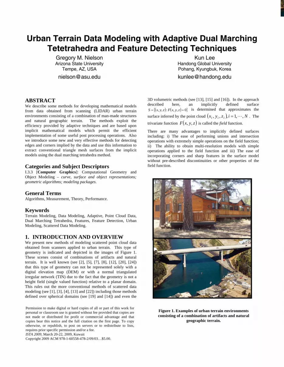
1. INTRODUCTION AND OVERVIEW We present new methods of modeling scattered point cloud data obtained from scanners applied to urban terrain. This type of geometry is indicated and depicted in the images of Figure 1. These scenes consist of combinations of artifacts and natural terrain. It is well known (see [2], [5], [7], [8], [12], [20], [24]) that this type of geometry can not be represented solely with a digital elevation map (DEM) or with a normal triangulated irregular network (TIN) due to the fact that the geometry is not a height field (single valued function) relative to a planar domain. This rules out the more conventional methods of scattered data modeling (see [1], [3], [4], [13] and [22]) including those methods defined over spherical domains (see [19] and [14]) and even the

3D volumetric methods (see [13], [15] and [16]). In the approach described here, an implicitly defined surface

( ) ( ){ }0,,:,, == zyxFzyxS is determined that approximates the

surface inferred by the point cloud ( ) Nizyx iii ,,1,,, L= . The

trivariate function ( )zy,xF , is called the field function.

There are many advantages to implicitly defined surfaces including: i) The ease of performing unions and intersection operations with extremely simple operations on the field function; ii) The ability to obtain multi-resolution models with simple operations applied to the field function and iii) The ease of incorporating corners and sharp features in the surface model without pre-described discontinuities or other properties of the field function.

Permission to make digital or hard copies of all or part of this work for personal or classroom use is granted without fee provided that copies are not made or distributed for profit or commercial advantage and that copies bear this notice and the full citation on the first page. To copy otherwise, or republish, to post on servers or to redistribute to lists, requires prior specific permission and/or a fee. ISTA 2009, March 20-22, 2009, Kuwait Copyright 2009 ACM 978-1-60558-478-2/09/03…$5.00.

Figure 1. Examples of urban terrain environments consisting of a combination of artifacts and natural

geographic terrain.

2. ADAPTIVE, IMPLICIT METHOD FOR FITTING POINT CLOUD DATA The method consists of two steps: Step 1. An adaptive, implicit, piecewise trivariate, quadratic model is fit to point cloud data and the normal vector estimates using least squares criteria. Step 2. A triangular mesh surface representation of the implicit model is obtained by using the dual marching tetrahedra method where the vertex of each active tetrahedron cell is determined by new feature (corners and edges) detecting technique. This two-step fitting process is illustrated in Figure 2. Here, only two-dimensional (and not three-dimensional) data is shown, but this is sufficient to convey the main ideas of our new method. The top image of Figure 2 shows the point cloud

and the initial domain decomposition consisting of two triangular cells. A piecewise defined field function is fit to the entire data. The cell with the largest error is subdivided and a new piecewise field function defined over the refined domain is fit to the data. This process continues until the overall error criteria are satisfied. For this example the final, overall approximation is shown in the middle image of Figure 2. Next the second step of the algorithm is invoked. For each cell containing a portion of the contour of the field function a corner detecting algorithm is applied to the scattered data lying in this cell. If a corner is found, a vertex for the final polygon fit is placed at the location of this vertex. If no corner is found, then a vertex is positioned at the midpoint of the best fitting, least squares line. If a cell contains no data points and yet the contour passes through this cell, then a vertex at the centroid is use. These vertices are then connected to form the polygon approximation to the scattered point cloud data. It is possible to have extraneous contours in regions where there are no data points (even the 2D example of Figure 2 has a small extraneous loop which is an artifact of the fitting process). Since the final surface is assumed to be a connected surface, these separated portions are not included in the final mesh surface. They are eliminated by context and empty cell determination.

( ) Niyx ii ,,1, L=

2.1 Step 1. Computing the Implicit Piecewise Quadratic Field Function It is clear that a single, globally defined field function can not capture the complex geometry of urban/terrain data. Also, it is well known that piecewise defined field functions over uniform lattices are not efficient because the complexity of the modeling function does not necessarily conform to the regions of complexity of the geometric data. Adaptive models which refine in regions of increased detail and complexity are much more efficient for this application. The refinement technique that we use is based upon the longest edge subdivision strategy. See [10], [11] and [21]. We start with a simple initial tetrahedronal containing the scattered point cloud data set. Often this consists of the CFK split (see [14] ) of a bounding box into 6 tetrahedra. When the adaptive error criteria call for the refinement of a tetrahedron cell, this is always accomplished by splitting the tetrahedron into two tetrahedra by

splitting the longest edge at its midpoint. This overall strategy has been successfully used extensively in other computational areas including the numerical solution of PDEs with the finite element approach. To avoid discontinuities in the field function, when a tetrahedron is split, its neighbors must also be split. The process can propagate through the tetrahedronal. While there are approaches that avoid or control this propagation, they often lead to poorly shaped cells which can be computationally problematic.

Figure 2. The two lower images illustrate the two steps of the adaptive fitting strategy in the case of two

dimensional data which is shown in the top image.

The field function is defined in a piecewise manner as a trivariate quadratic over each tetrahedron in the domain decomposition (achieved through the adaptive refinement process). For a given tetrahedron with vertices , , and the field

function is defined as ijklT iV jV kV lV

( )

lkklljjlkjjk

liukkiikjiij

llkkjjii

lkji

bbFbbFbbF

bbFbbFbbF

bFbFbFbF

bbbbFzyxF

+++

+++

+++

== ,,,),,(

(1)

where ( )αα VFF = and ⎟⎟⎠

⎞⎜⎜⎝

⎛ +=

2δβ

βδVV

FF and

( )

1

,,

=+++

+++=

lkji

llikkjji

bbbb

VbVbVbVbzyx

The use of the barycentric coordinates is particularly

useful for this application. There are very simple, effective methods for updating barycentric coordinates during the refinement process.

lkji bbbb ,,,

aV aa FVF =)(

adFda VVF =+ )2

(2

daad

VVV +=

dV dVF

dF=)(bV bb FVF =)(

cV cc FVF =)(

Figure 4. Depicting the notation of the implicit piecewise quadratic modeling function.

Figure 3. Illustrating the “longest edge” bisection strategy for refining the tetrahedronal. Top image

shows a simple two dimensional example. The middle image is a small three dimensional example. The

congruence of the tetrahedra repeats after 3 levels of subdivision as is illustrated in the bottom image.

Normal vector estimates, , at each data point are taken as the gradient of a local, least squares fitting plane. The closest

iF∇ iPM

points to are determined and the estimate of the normal vector is taken to be the normalized eigenvector associated with the smallest eigenvalue of the 3 matrix

{ } MkQk ,,1, L= iP

3×

. ( ) ( )∑=

−−M

kik

tikk PQPQw

1

~

The weights kw~ are chosen on the basis of inverse distance of

to . The inside/outside choice is determined by knowing the position and/or the direction of the scanner.

iP

kQ

The overall error and fitting criterion is the quantity

{ } ( ) ( )∑∑ ∇−∇+=i

iiiii

ibca FPFPFwFFE 22, ω

where the weights and iw iω are chosen to reflect the relative importance or accuracy of the data points as compared to the normal vector estimates. The task of minimizing is a linear least squares fitting problem which can be solved by conventional iterative techniques. Computation of the necessary quantities is facilitated by the following equations which relate derivatives taken with respect to barycentric coordinates to those in terms of conventional Cartesian coordinates.

{ bca FFE , }

xb

bF

xb

bF

xb

bF

xb

bF

xF l

l

k

k

j

j

i

i ∂∂

∂∂

+∂∂

∂∂

+∂

∂

∂∂

+∂∂

∂∂

=∂∂

( ) ( ) ⎟⎟⎠

⎞⎜⎜⎝

⎛∂∂

∂∂

∂∂

=∇=∇zF

yF

xFzyxFbbbbF lkji ,,,,,,,

⎥⎦⎤

⎢⎣⎡

∂∂

+∂∂

+⎥⎦⎤

⎢⎣⎡

∂∂

+∂∂

+

⎥⎦

⎤⎢⎣

⎡∂∂

+∂

∂+⎥⎦

⎤⎢⎣⎡

∂∂

+∂∂

+

⎥⎦

⎤⎢⎣

⎡∂∂

+∂

∂+⎥

⎦

⎤⎢⎣

⎡∂

∂+

∂∂

+

∂∂

+∂∂

+∂

∂+

∂∂

=∂∂

xbb

xbbF

xbb

xbbF

xbb

xb

bFxbb

xbbF

xbb

xb

bFxb

bxbbF

xbbF

xbbF

xb

bFxbbF

xF

lk

klkl

li

ilil

lj

jljl

ki

ikik

kj

jkjk

ji

ijij

lll

kkk

jjj

iii

2222

2222

2222

2222

(2)

Similar formulas hold for and . yF ∂∂ / yF ∂∂ /

A piece-wise defined trivariate quadratic will only lead to a global field function, but, in addition, we impose “near”

conditions which are included in the linear systems used for optimal fitting. The exact nature of these conditions is based upon the equation (2) above.

0C 1C

2.2 Step 2. Extracting a Triangle Mesh Surface Approximation to the Contour Surface Many post processing applications, including rendering, will be facilitated by a triangle mesh surface (TMS) representation of the fitting surface. In this regard, it is beneficial to have an efficient TMS approximation that maintains the features (corners) of the implicit piecewise quadratic fit. We have developed techniques with these properties which we now describe. They are based upon the newly presented dual marching tetrahedra method [17] which we briefly review in the next section.

2.2.1 Dual Marching Tetrahedra Method of Extracting the Contour Surface Model Let ( ) Nizyxp iiii ,,1,,, L== denote the grid points which are

segmented as marked or unmarked. We assume these points are not collectively coplanar. We assume that the grid points have been arranged into a collection of tetrahera to form a tetrahedronal. A tetrahedonal consists of a list of 4-tuples which we denote by . Each 4-tuple, tI tIijkl ∈

denotes a single tetrahedron with the four vertices which is denoted as . A valid

tetrahedronal requires: i) No tetrahedron lkj ppp ,,ip , ijklT

T tIijkl ijkl∈, is

degenerate, i. e. the points are not coplanar,

ii) The interiors of any two tetrahedra do not intersect and iii) The boundary of two tetrahedra can intersect only at a common triangular face. See [16] for a survey of methods for computing optimal (Delaunay) tetrahedronals for scattered 3D points.

lki ppp ,, jp ,

A tetrahedron is said to be active if among its 4 grid points there are both marked grid points and unmarked grid points. There are three distinct configurations for these active tetrahedra as shown in Figure 5. Similarly, a triangular face of an active tetrahedron is active provided it contains both marked and unmarked grid points. We now give the formal description of the polygon mesh surface, , which separates the marked grid points from the unmarked grid points. Interior to each active tetrahedron, , there is a vertex . For each

interior active triangular face, there is an edge of joining the two vertices of the two tetrahedra sharing this triangular face. If denotes the interior active triangular face

and and denote the two active

S

nF

kji nn

ikji nnnnT

kji nn

an

ikji nnnnV

S

nTbkji nnnnT ,,,

tetrahedra sharing this face then an edge joins and

akji nnnnV

bkji nnnnV

bkji nnnnVakji nnnnV

anP

bnP

inP

2.2.2 Corner and Edge Detecting Schemes Corner and edge detection from point clouds is a very desirable capability for many applications. Currently, it is also a very difficult problem with very few effective or useful techniques. Using discrete Lp norms, nonlinear optimization techniques and techniques related to the adaptive implicit fitting discussed above, we have recently developed a general approach and class of methods for analyzing the data yielding the positions of these corners. Unlike most of the work in computer vision which relates to this problem, our methods directly extend to any number of dimensions and are based upon geometric modeling concepts. We have written some demonstration programs for 2D and 3D which allow a user to test our techniques on some examples. The images of Figure 7, Figure 8, Figure 9 and Figure 10 show typical screen shots of these programs in action. The details of this new technique will be forthcoming in a future report, but presently, the demonstration programs can be downloaded which add additionally insight into how the methods are capable of being so effective.

Figure 6. The top image illustrates the notation of the tetrahedronal method and the bottom image shows the

results for a small example pointing out that the valence of each vertex of the tetrahedronal surface is 3 or 4.

Figure 5. The three cases of the dual marching tetrahedral method. From top to bottom: one, two and three points classified as being contained in the object.

Figure 7. Here are two examples where we have (from top to bottom) the first, second and final iterations of a

new iterative method of determining corners implied by scattered point cloud data. The method is based upon discrete Lp norms and nonlinear optimization. One example is shown in the left column and another is

shown in the right column. A demonstration program, Corner2D.exe, is available at

www.public.asu.edu/~nielson/ARO/.

Figure 8. From top to bottom, we have the data, an intermediate approximation and the final edge

determined by the new method of analyzing scattered data for determining features. A demonstration

program, Edge3D.exe, is available at www.public.asu.edu/~nielson/ARO/.

3. EXAMPLES In order to have a large variety of data sets in order to test our methods, we have developed some software that simulates the collection of point cloud data from scanners. The software allows the user to arbitrarily locate and position a scanner while specifying its attributes such as resolution, noise and accuracy. Input consists of an arbitrary triangle mesh surface as shown in the top image of Figure 11 or Figure 12. Once the scanner is positioned, oriented and actuated, the point cloud is displayed on the polygons from which the point was sampled. This is illustrated with the red point cloud on the blue polygon environment shown in the bottom image of Figure 12.

Figure 10. The data for an “outside” corner is shown in the left image of the top row. The first and final iterates are shown in the next two images (top to

bottom). The three different planes are red, green and blue. The intersections lines between these planes (the edges of the corner) are illustrated with yellow lines. The second column utilizes a point cloud that infers a

“notch” corner.

Figure 9. A second example of the new technique for determining edges from scattered point cloud data.

The top image is the input data, the middle image is the first iteration and the bottom image is the final

converged solution.

Two examples are illustrated in Figure 13 and Figure 14 respectively. Both examples include buildings combined with natural terrain. The point cloud of Figure 13 has approximately 1M points and that of Figure 14 has about .5M points. A sample (~1%) of the point cloud is shown in both examples. The normal vector estimates are based upon the nearest 43 points and inverse distance squared weights. In the lower example a blow-up of a corner of one of the buildings is shown so as to illustrate the corner/feature preservation properties of Step 2 involving the extraction of a TMS from the implicit piecewise quadratic model.

Figure 11. A street scene which is being scanned by the software simulator

Figure 12. A screen image of the scanner simulating software in action. Here, the frustrum indicating the position and orientation of two scanners can be seen; one in red and other in blue. The points collected by these respective scanners are shown on the surface

being scanned.

Figure 14. Bottom images show a point cloud data set

(1%) along with the extracted contour surface based upon the dual marching tetrahedral method and vertex

selection using corner detecting techniques.

Figure 13. Top images show a 1% rendering of a point cloud data set along with a rendering of the adaptive

implicit fit to the data.

4. ACKNOWLEDGMENTS We wish to acknowledge the support of the USA Army Research Office under contract W911NF-05-1-0301. We thank Ryan Holmes for his contributions to this project.

5. REFERENCES [1] Abbas,A and Nasri, A. Scattered Data Interpolation

Using Catmull-Clark Subdivision, Journal of Computer Aided Design and Applications, 2005, pp.123-456.

[2] Fowler, R. Topographic Lidar. In: Maune, D.F.: Digital Elevation Model Technologies and Applications: The DEM Users Manual, Bethesda, Maryland: American Society for Photogrammetry and Remote Sensing, 2001, pp. 207-236.

[3] Franke, R. and Nielson, G. M. Smooth Interpolation of Large Sets of Scattered Data, International Journal of Numerical Methods in Engineering 15, 1980, pp. 1691-1704.

[4] Franke, R. and Nielson, G. M. Scattered Data Interpolation and Applications: A Tutorial and Survey, In: Hagen, H., Roller, D., (eds) Geometric Modelling: Methods and Their Applications, Springer, 1990, pp. 131-160.

[5] Hodgson, M. E., Jensen, J. R., Schmidt, L., Schill, S. and Davis, B., An Evaluation of LIDAR- and IFSAR-Derived Digital Elevation Models in Leaf-on Conditions with USGS Level 1 and Level 2 DEMs. Remote Sensing of the Environment 84 2 , 2003, pp. 295- 299.

[6] Hoppe, L. H., DeRose, T., Duchamp, T. McDonald, J., Stuetzle, W., Surface Reconstruction from Unorganized Points, In: Proceedings of SIGGRAPH 1992, ACM Press/ACM SIGGRAPH, New York. Computer Graphics Proceedings, Annual Conference Series, ACM, 1991, pp. 71-78.

[7] Kelley, A., Nielson, G., and Malin, M., Terrain Simulation using a Model of Stream Erosion, SIGGRAPH, Computer Graphics, Vol. 22, No. 4, 1988, pp. 263-268.

[8] Lee, H. S. and Younan, N. H., DTM Extraction of Lidar Returns via Adaptive Processing. IEEE Transactions on Geoscience and Remote Sensing 41, 9, 2003, pp. 2063-2069.

[9] Maas, L.H., and Vosselman, G., Two Algorithms for Extracting Building Models from Raw Laser Altimetry Data, ISPRS Journal of Photogrammetry & Remote Sensing 54, 1999, pp. 153-163.

[10] Maubach, J. M., Local Bisection Refinement for N-Simplicial Grids Generated by Reflection, SIAM Journal of Scientific Computing, 16 1, 1995, pp. 210-227.

[11] Molino, N., Bridson, R. and Teran, J., A Crystalline, Red Green Strategy for Meshing Highly Deformable Objects with Tetrahedra, Proceedings, 12th International Meshing Roundtable, Sandia National Laboratories, 2003, pp. 103-114.

[12] Mueller, H., Surface Reconstruction – An introduction, In: Scientific Visualization ( Hagen, H., Nielson, G. and Post, F. eds.), IEEE Computer Society Press, 1999, pp. 239-242.

[13] Nielson, G. M., Scattered Data Modeling, Computer Graphics and Applications 13, 1993, pp. 60-70.

[14] Nielson, G. M., Modeling and Visualizing Volumetric and Surface-on-Surface Data, In: Focus on Scientific Visualization, H. Hagen, H. Mueller and G. M. Nielson (eds.), Springer, 1993, pp. 191-242.

[15] Nielson, G. M. and Tvedt, J., Comparing Methods of Interpolation for Scattered Volumetric Data, In: State of the Art in Computer Graphics – Aspects of Visualization, D. Rogers and R. A. Earnshaw (eds.), Springer, 1994, pp. 67-86

[16] Nielson, G. M., Tools for Triangulations and Tetrahedrizations and Constructing Functions Defined over Them, In: Scientific Visualization: Overviews, Methodologies Techniques, pp. 429-526, IEEE Computer Society Press, Los Alamitos, 1997.

[17] Nielson, G. M., Dual Marching Tetrahedra: Contouring in the Tetrahedronal Environment, Proceedings of International Symposium on Visual Computing, ISVC 2008, Springer, Part I, LNCS 5358, 2008, pp. 183-194

[18] Nielson, G. M. and Lee, K., Adaptive, Implicit Modeling of Urban Terrain Point Cloud Data, ACOMP 2008, Ho Chin Minh City, Vietnam, March 12-14, 2008, pp. 235-246.

[19] Nielson, G. M. and Ramaraj, R., Interpolation over a Sphere Based upon a Minimum Norm Network, Computer Aided Geometric Design, 4. 1987, pp 41-57.

[20] Petzold, B., Reiss, P. and Stössel, W., Laser Scanning––Surveying and Mapping Agencies are using a new Technique for the Derivation of Digital Terrain Models, ISPRS Journal of Photogrammetry & Remote Sensing 54 2/3, 1999, pp. 95-104.

[21] Rivara, M. C., Local Modification of Meshes for Adaptive and/or Multigrid Finite Element Methods, Journal of Computation and Applied Mathematics 36, 1991, pp. 79-89.

[22] Schumaker, L., Fitting Surfaces to Scattered Data, In Approximation Theory II, G. G. Lorentz, C. K. Chui and L. L. Schumaker, eds., 1976, pp. 203-268.

[23] Sarfraz, M., Fitting Curves to Planar Digital Data, Sixth International Conference on Information Visualisation (IV'02), 2002, pp. 663.

[24] Weibel, R., Models and Experiments for Adaptive Computer-Assisted Terrain Generalization, Cartography and Geographic Information Systems 19 3, 1992, pp. 1333-153.

.