Urban Land Systems: An Ecosystems Perspective - MDPI

Urban Land Systems: An Ecosystems Perspective

www.mdpi.com/journal/land

Edited by

Andrew Millington, Harini Nagendra and Monika KopeckáPrinted Edition of the Special Issue Published in Land

Urban Land Systems: An Ecosystems

Perspective

Special Issue EditorsAndrew MillingtonHarini NagendraMonika Kopecka

MDPI • Basel • Beijing • Wuhan • Barcelona • Belgrade

Special Issue Editors

Andrew Millington

Flinders University

Australia

Harini Nagendra

Azim Premji University

India

Monika Kopecka

Institute of Geography, Slovak Academy of Sciences

Slovakia

Editorial Office

MDPI

St. Alban-Anlage 66

Basel, Switzerland

This edition is a reprint of the Special Issue published online in the open access journal Land

(ISSN 2073-445X) from 2017–2018 (available at: http://www.mdpi.com/journal/land/special issues/

urbanlandsystems).

For citation purposes, cite each article independently as indicated on the article page online and as

indicated below:

Lastname, F.M.; Lastname, F.M. Article title. Journal Name Year, Article number, page range.

First Edition 2018

ISBN 978-3-03842-917-3 (Pbk)

ISBN 978-3-03842-918-0 (PDF)

Cover photo courtesy of Monika Kopecka.

Articles in this volume are Open Access and distributed under the Creative Commons Attribution (CC

BY) license, which allows users to download, copy and build upon published articles even

for commercial purposes, as long as the author and publisher are properly credited, which

ensures maximum dissemination and a wider impact of our publications. The book taken as a

whole is c© 2018 MDPI, Basel, Switzerland, distributed under the terms and conditions of the

Creative Commons license CC BY-NC-ND (http://creativecommons.org/licenses/by-nc-nd/4.0/).

Table of Contents

About the Special Issue Editors . . . . . . . . . . . . . . . . . . . . . . . . . . . . . . . . . . . . . v

Monika Kopecka, Harini Nagendra and Andrew Millington

Urban Land Systems: An Ecosystems Perspectivedoi: 10.3390/land7010005 . . . . . . . . . . . . . . . . . . . . . . . . . . . . . . . . . . . . . . . 1

Andrew MacLachlan, Eloise Biggs, Gareth Roberts and Bryan Boruff

Urban Growth Dynamics in Perth, Western Australia: Using Applied Remote Sensing forSustainable Future Planningdoi: 10.3390/land6010009 . . . . . . . . . . . . . . . . . . . . . . . . . . . . . . . . . . . . . . . 5

Suranga Wadduwage, Andrew Millington, Neville D. Crossman and Harpinder Sandhu

Agricultural Land Fragmentation at Urban Fringes: An Application of Urban-To-RuralGradient Analysis in Adelaidedoi: 10.3390/land6020028 . . . . . . . . . . . . . . . . . . . . . . . . . . . . . . . . . . . . . . . 19

Baolei Zhang, Qiaoyun Zhang, Chaoyang Feng, Qingyu Feng and Shumin Zhang

Understanding Land Use and Land Cover Dynamics from 1976 to 2014 in Yellow River Deltadoi: 10.3390/land6010020 . . . . . . . . . . . . . . . . . . . . . . . . . . . . . . . . . . . . . . . 37

Bhagawat Rimal, Lifu Zhang, Dongjie Fu, Ripu Kunwar and Yongguang Zhai

Monitoring Urban Growth and the Nepal Earthquake 2015 for Sustainability of KathmanduValley, Nepaldoi: 10.3390/land6020042 . . . . . . . . . . . . . . . . . . . . . . . . . . . . . . . . . . . . . . . 57

Kotaro Iizuka, Brian A. Johnson, Akio Onishi, Damasa B. Magcale-Macandog, Isao Endo

and Milben Bragais

Modeling Future Urban Sprawl and Landscape Change in the Laguna de Bay Area,Philippinesdoi: 10.3390/land6020026 . . . . . . . . . . . . . . . . . . . . . . . . . . . . . . . . . . . . . . . 80

Monika Kopecka, Daniel Szatmari and Konstantın Rosina

Analysis of Urban Green Spaces Based on Sentinel-2A: Case Studies from Slovakia †

doi: 10.3390/land6020025 . . . . . . . . . . . . . . . . . . . . . . . . . . . . . . . . . . . . . . . 101

Somajita Paul and Harini Nagendra

Factors Influencing Perceptions and Use of Urban Nature: Surveys of Park Visitors in Delhidoi: 10.3390/land6020027 . . . . . . . . . . . . . . . . . . . . . . . . . . . . . . . . . . . . . . . 118

Christoph D. D. Rupprecht

Informal Urban Green Space: Residents’ Perception, Use, and Management Preferences acrossFour Major Japanese Shrinking Citiesdoi: 10.3390/land6030059 . . . . . . . . . . . . . . . . . . . . . . . . . . . . . . . . . . . . . . . 141

Azad Rasul, Heiko Balzter, Claire Smith, John Remedios, Bashir Adamu, Jose A. Sobrino,

Manat Srivanit and Qihao Weng

A Review on Remote Sensing of Urban Heat and Cool Islandsdoi: 10.3390/land6020038 . . . . . . . . . . . . . . . . . . . . . . . . . . . . . . . . . . . . . . . 165

Muhammad Tauhidur Rahman, Adel S. Aldosary and Md. Golam Mortoja

Modeling Future Land Cover Changes and Their Effects on the Land Surface Temperaturesin the Saudi Arabian Eastern Coastal City of Dammamdoi: 10.3390/land6020036 . . . . . . . . . . . . . . . . . . . . . . . . . . . . . . . . . . . . . . . 175

iii

About the Special Issue Editors

Andrew Millington is a Professor in the College of Science and Engineering, Flinders University.

His research interests are in remote sensing, land-use dynamics, biogeography and human impacts

on the environment. Most of his work lies in the area described as coupled human-natural

systems in which he examine the influences of human systems on land use and its impacts on

things like vegetation change, landscape fragmentation and biodiversity. In 1978 he joined one

of Africa’s oldest universities (Fourah Bay College, University of Sierra Leone) as a lecturer in

the Geography Department. While teaching there he did his doctoral degree at the University of Sussex.

Harini Nagendra is a Professor of Sustainability at Azim Premji University. She is an ecologist who

uses satellite remote sensing coupled with field studies of biodiversity, archival research, institutional

analysis, and community interviews to examine the factors shaping the social-ecological sustainability

of forests and cities in the south Asian context. She completed her PhD from the Centre for Ecological

Sciences in the Indian Institute of Science in 1998.

Monika Kopecka, Ph.D., is a senior research scientist at the Institute of Geography, Slovak Academy

of Sciences and the Head of the Department of Geoinformatics. Her research is focused on land use

and land cover mapping, landscape changes, and landscape indicators. She participated in several

projects related to spatial analysis and assessment of landscape structure and its changes. Currently, her

research activities are oriented to monitoring of urban landscape dynamics and agricultural landscape

abandonment.

v

“By far the greatest and most admirable form of wisdom is that needed to plan and beautify cities and

human communities.”

Socrates

vii

land

Editorial

Urban Land Systems: An Ecosystems Perspective

Monika Kopecká 1,* ID , Harini Nagendra 2 ID and Andrew Millington 3 ID

1 Department of Geoinformatics, Institute of Geography, Slovak Academy of Sciences, Stefanikova 49,814 73 Bratislava, Slovakia

2 Azim Premji University, PES Institute of Technology Campus, Pixel Park, B Block, Electronics City,Hosur Road, Bangalore 560100, India; [email protected]

3 College of Science and Engineering, Flinders University, GPO Box 2100, Adelaide, SA 5001, Australia;[email protected]

* Correspondence: [email protected]; Tel.: +421-905-345-556

Received: 8 January 2018; Accepted: 9 January 2018; Published: 11 January 2018

1. Introduction

We live in an urbanizing world. Since 2008, more than half of humanity lives in cities, both largeand small, and old and new. We also live in a world that is becoming even more urbanized, it isexpected that by 2050, 66 per cent of the world’s population will live in cities [1]. The process ofurbanization, accompanied by the rapid expansion of cities and the sprawling growth of metropolitanregions over the world, is one of the most important transformations of a natural landscape.

In the context of land systems science, contemporary urbanisation is a set of land-use changeprocesses and the various contemporary cityscapes are the resulting land systems. Population growthincreases urban footprints with consequences on biodiversity and climate. Much of the explosiveurban growth has been unplanned and conflicting land-use demands often arise as land is a limitedresource. Increased requirements for living space and intensive landscape utilization constitute twoof the principal reasons for the environmental change, with significant impacts on quality of lifeand ecosystems.

This special issue of LAND explores urban land dynamics with particular regard to ecosystemstructure, and discusses consequent environmental changes and their impacts. The studies cover a widerange of countries and contexts, and draw on a number of disciplinary methods and interdisciplinaryapproaches from the social and natural sciences. The papers have been authored by 41 researchers from29 institutions in countries worldwide: from Australia, Bangladesh, China, India, Iraq, Italy, Japan,Nigeria, Philippines, Saudi Arabia, Slovakia, Spain, Thailand, the United Kingdom, and the USA.

2. Dynamics of Urban Land Systems

Earth observation data can contribute considerably in monitoring complex urban land coverpatterns for various applications in different environments. Several papers focus on the detection ofurban growth based on spaceborne remote sensing data at multiple scales, spatial and temporalresolutions, and the evaluation of environmental impacts through well-established concepts oflandscape metrics.

MacLachlan et al. [2] evaluate multi-temporal urban expansion for Perth, Western Australia,derived from Landsat imagery and the related decrease of natural resources. Their results indicatethat the spatial extent of the Perth Metropolitan Region has increased considerably in the periodof 1990–2015. Irreversible and unsustainable agricultural landscape changes related to urbangrowth in peri-urban areas of Adelaide city are assessed by Wadduwage et al. [3]. Fragmentationof agro-ecosystems due to urban expansion is analyzed using several landscape metrics indicators:percentage of land, mean parcel size, patch density, and modified Simpson´s Diversity.

Land 2018, 7, 5 1 www.mdpi.com/journal/land

Land 2018, 7, 5

Rapidly growing cities in the global south, particularly in Asia and Africa, represent the dominanturban footprint of the present and future. A great deal of attention is currently being focused on thesecities, about which we know relatively little in comparison to northern cities. In this special issue,Zhang et al. [4] use Landsat imagery to detect the changes in urban land use in the Yellow River Delta todocument systematic changes in natural wetlands in 1976, 1984, 1995, 2006 and 2014. Their cartographicoutputs document systematic wetland degradation, wetland conversion to salt pans and aquafarms,and significant urbanization.

Similarly, Landsat data are used by Rimal et al. [5] to analyze the spatiotemporal patterns ofurbanization and LULC changes in Kathmandu Valley, Nepal. Results show that the urban coverageof Kathmandu Valley has increased tremendously from 20.19 km2 in 1976 to 139.57 km2 in 2015,at the cost of cultivated lands and forests. This study also reports the impacts of the recent disastrousearthquake in the valley on the urban areas and discusses the high risks associated with differentgeological formations.

The third example illustrating rapidly developing countries in Asia is a land use/land coverchange assessment of the Laguna de Bay area in the Philippines. Iizuka et al. [6] present a visualinterpretation of the future changes in LULC classes of built-up, crop-grass, trees, and water up tothe year 2030. The probability of changes occurring in different years in the future is calculated usingthree different scenarios: business-as-usual, compact development, and high sprawl. In total, a largeproportion of the study area is modeled to be converted to urban built-up land cover classes by 2030,varying in extent depending on the development scenario.

3. Perception of Urban Green Spaces (UGS) and Ecosystem Services

Urban vegetation is essential for urban ecosystems and ecosystem services and can be determinedby well-established methods in remote sensing. In the light of past and future urbanization trends,accurate information on the state, accessibility, distribution, and supply of UGS plays an increasinglyimportant role in sustainable urban development, human well-being, and also for conservation ofecosystem functionality.

Kopecká et al. [7] demonstrate the potential for UGS extraction from newly available Sentinel-2Asatellite imagery, provided within the frame of the European Copernicus program. UGS classes aredescribed by the proportion of tree canopy and their ecosystem services. A comparative analysis ofthree cities in Slovakia indicates the relatively high importance of urban greenery in family housingareas, represented mainly by privately owned gardens.

Cultivated parks and urban gardens play an important role as providers of aesthetic andpsychological benefits that enrich human life, reduce stress, and increase physical and mental health.Paul and Nagendra [8] present the results of a survey of UGS perception by park visitors in themegalopolis of Delhi that aimed to understand the importance of parks for them. For example, largeparks tend to attract more visitors from further distances, despite their having small neighborhoodparks in the vicinity of their homes.

On the other hand, Rupprecht [9] points attention to residents‘ perceptions of informalUGS—vacant lots, street verges, brownfields, power line corridors, and waterside spaces—in fourshrinking cities in Japan. He proposes eight major planning principles derived from the findings as apotential basis for managing non-traditional green spaces to urban planners.

4. Urban Landscape Structure and Urban Heat Island (UHI) Effect

Urban areas influence the local microclimate in several ways, e.g., by air pollution, altered windspeeds and directions, heat stress, or changes in surface ozone concentrations. UHI describes thephenomenon that atmospheric and surface temperatures are higher in urban areas than in surroundingrural areas. Among the long-term consequences on microclimate, the UHI effect has received wideattention from geographers, urban planners, and climatologists over recent years. Rasul et al. [10]review the current research on this topic, methods, data, and techniques used in UHI detection.

2

Land 2018, 7, 5

They conclude with recommendations for conducting further research on surface urban cool islandsthat especially occur in arid and semi-arid climates.

Rahman et al. [11] investigate the increase of land surface temperature in Dammam city, the capitalof Saudi Arabia’s Eastern Province, due to urban expansion in the period 1990–2014. Based on landuse/land cover changes and predictive modeling, this study projects a dramatic increase of landsurface temperatures for the year 2026.

5. Conclusions

Global and local urbanization is creating very significant challenges for sustainability and humanwell-being. This special issue highlights some important aspects related to urban sprawl dynamicsand urban ecosystem management. Observations and studies presented in 10 papers show thaturbanization affects essential ecological, economic, and social landscape functions, whose importanceare often undervalued in cities across the globe.

The special issue arises from a session convened by the editors at the GLP Third Open ScienceMeeting in Beijing, October 2016. We believe that the results presented in these studies will provideuseful information for decision and policymakers involved in urban and spatial planning at local,regional, and national levels and can help better plan and design UGS, responding to the needs andpreferences of urban communities.

Acknowledgments: We are grateful to the many anonymous reviewers whose comments greatly improvedthe quality of the special issue. This work was supported by the project: “Effect of impermeable soil cover onurban climate in the context of climate change” (Slovak Research and Development Agency—Grant AgencyNo. APVV-15-0136). Harini Nagendra acknowledges funding from Azim Premji University’s Centre forUrban Sustainability. Andrew Millington acknowledges support from Flinders University College of Scienceand Engineering.

Author Contributions: Monika Kopecká, Harini Nagendra, and Andrew Millington conceptualized and wrotethis paper.

Conflicts of Interest: The authors declare no conflict of interest.

References

1. United Nations, Department of Economic and Social Affairs, Population Division. World UrbanizationProspects: The 2014 Revision, Highlights (ST/ESA/SER.A/352). 2014. Available online: https://esa.un.org/unpd/wup/Publications/Files/WUP2014-Highlights.pdf (accessed on 11 December 17).

2. MacLachlan, A.; Biggs, E.; Roberts, G.; Boruff, B. Urban Growth Dynamics in Perth, Western Australia: UsingApplied Remote Sensing for Sustainable Future Planning. Land 2017, 6, 9. [CrossRef]

3. Wadduwage, S.; Millington, A.; Crossman, N.; Sandhu, H. Agricultural Land Fragmentation at UrbanFringes: An Application of Urban-To-Rural Gradient Analysis in Adelaide. Land 2017, 6, 28. [CrossRef]

4. Zhang, B.; Zhang, Q.; Feng, C.; Feng, Q.; Zhang, S. Understanding Land Use and Land Cover Dynamicsfrom 1976 to 2014 in Yellow River Delta. Land 2017, 6, 20. [CrossRef]

5. Rimal, B.; Zhang, L.; Fu, D.; Kunwar, R.; Zhai, Y. Monitoring Urban Growth and the Nepal Earthquake 2015for Sustainability of Kathmandu Valley, Nepal. Land 2017, 6, 42. [CrossRef]

6. Iizuka, K.; Johnson, B.; Onishi, A.; Magcale-Macandog, D.; Endo, I.; Bragais, M. Modeling Future UrbanSprawl and Landscape Change in the Laguna de Bay Area, Philippines. Land 2017, 6, 26. [CrossRef]

7. Kopecká, M.; Szatmári, D.; Rosina, K. Analysis of Urban Green Spaces Based on Sentinel-2A: Case Studiesfrom Slovakia. Land 2017, 6, 25. [CrossRef]

8. Paul, S.; Nagendra, H. Factors Influencing Perceptions and Use of Urban Nature: Surveys of Park Visitors inDelhi. Land 2017, 6, 27. [CrossRef]

9. Rupprecht, C. Informal Urban Green Space: Residents’ Perception, Use, and Management Preferences acrossFour Major Japanese Shrinking Cities. Land 2017, 6, 59. [CrossRef]

3

Land 2018, 7, 5

10. Rasul, A.; Balzter, H.; Smith, C.; Remedios, J.; Adamu, B.; Sobrino, J.; Srivanit, M.; Weng, Q. A Review onRemote Sensing of Urban Heat and Cool Islands. Land 2017, 6, 38. [CrossRef]

11. Rahman, M.; Aldosary, A.; Mortoja, M. Modeling Future Land Cover Changes and Their Effects on the LandSurface Temperatures in the Saudi Arabian Eastern Coastal City of Dammam. Land 2017, 6, 36. [CrossRef]

© 2018 by the authors. Licensee MDPI, Basel, Switzerland. This article is an open accessarticle distributed under the terms and conditions of the Creative Commons Attribution(CC BY) license (http://creativecommons.org/licenses/by/4.0/).

4

land

Letter

Urban Growth Dynamics in Perth, Western Australia:Using Applied Remote Sensing for SustainableFuture Planning

Andrew MacLachlan 1,*, Eloise Biggs 2, Gareth Roberts 1 and Bryan Boruff 2

1 Geography and Environment Department, The University of Southampton, University Road,Southampton SO17 1BJ, UK; [email protected]

2 School of Agriculture and Environment, The University of Western Australia, Crawley WA 6009, Australia;[email protected] (E.B.); [email protected] (B.B.)


Academic Editors: Andrew Millington, Harini Nagendra and Monika KopeckaReceived: 16 December 2016; Accepted: 18 January 2017; Published: 24 January 2017

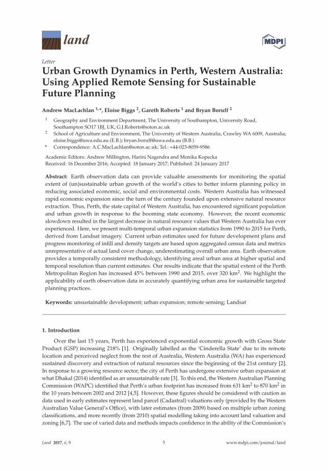
Abstract: Earth observation data can provide valuable assessments for monitoring the spatialextent of (un)sustainable urban growth of the world’s cities to better inform planning policy inreducing associated economic, social and environmental costs. Western Australia has witnessedrapid economic expansion since the turn of the century founded upon extensive natural resourceextraction. Thus, Perth, the state capital of Western Australia, has encountered significant populationand urban growth in response to the booming state economy. However, the recent economicslowdown resulted in the largest decrease in natural resource values that Western Australia has everexperienced. Here, we present multi-temporal urban expansion statistics from 1990 to 2015 for Perth,derived from Landsat imagery. Current urban estimates used for future development plans andprogress monitoring of infill and density targets are based upon aggregated census data and metricsunrepresentative of actual land cover change, underestimating overall urban area. Earth observationprovides a temporally consistent methodology, identifying areal urban area at higher spatial andtemporal resolution than current estimates. Our results indicate that the spatial extent of the PerthMetropolitan Region has increased 45% between 1990 and 2015, over 320 km2. We highlight theapplicability of earth observation data in accurately quantifying urban area for sustainable targetedplanning practices.

Keywords: unsustainable development; urban expansion; remote sensing; Landsat

1. Introduction

Over the last 15 years, Perth has experienced exponential economic growth with Gross StateProduct (GSP) increasing 218% [1]. Originally labelled as the ‘Cinderella State’ due to its remotelocation and perceived neglect from the rest of Australia, Western Australia (WA) has experiencedsustained discovery and extraction of natural resources since the beginning of the 21st century [2].In response to a growing resource sector, the city of Perth has undergone extensive urban expansion atwhat Dhakal (2014) identified as an unsustainable rate [3]. To this end, the Western Australian PlanningCommission (WAPC) identified that Perth’s urban footprint has increased from 631 km2 to 870 km2 inthe 10 years between 2002 and 2012 [4,5]. However, these figures should be considered with caution asdata used in early estimates represent land parcel (Cadastral) valuations only (provided by the WesternAustralian Value General’s Office), with later estimates (from 2009) based on multiple urban zoningclassifications, and more recently (from 2010) spatial modelling taking into account land valuation andzoning [6,7]. The use of varied data and methods impacts confidence in the ability of the Commission’s


Land 2017, 6, 9

estimates to represent actual change in urban extent, especially when urban zoning informationincludes land identified for growth but not necessarily developed. Such inconsistencies could havepotential to misinform future development decisions. Consequently, here we present a spatiotemporalassessment of change in areal urban growth based upon medium resolution remote sensing through asingle classification model. This provides the first accurate depiction of urban expansion for one ofthe world’s fastest growing cities—Perth, WA. We present our findings and discuss the implicationsof more accurately classified urban extents in facilitating scientifically evidence-based adaptive andtargeted planning policies to help reduce environmental and socio-economic consequences of poorlyplanned development.

1.1. Earth Observation for Monitoring Urban Change

Mapping the spatial extent and temporal profile of urban growth from medium resolution satelliteimagery facilitates a consistent, detailed characterisation of the actual urban footprint of a city [8,9].Other conventional spatial datasets such as Cadastral data provide information on freehold and Crownland parcel boundaries including attributes such as ownership and value for a singular temporalperiod [10]. However, attributed data for a singular year provides an ineffective portrayal of actualparcel land cover and temporal change. Thus, the methods and results presented in this study providefoundational information for the development of planning regulations that ensure sustainable growthof our cities, particularly in the reduction of environmental risks from ever-increasing expansionalong the wildland–urban interface [11]. Specifically, Earth Observation (EO) data allows spatiallydetailed identification of locations where (un)sustainable urban growth is occurring which enablesexpansion limits to be imposed through targeted policies [12]. In this theme, Schneider et al. (2005)determined the spatial distribution of development zones from 1978 to 2002 in Chengdu, Sichuanprovince, China in response to the Go West policy of the 1990s, aimed at economically boosting theWest of the country [13]. Whilst the policy was successful in raising Gross Domestic Product (GDP)levels, urbanisation concurrently increased, generating issues of urban management, including service,infrastructure and resource deficiency. Their results indicated spatial clustering, specialisation of landuse and peri urban development (not considered by the original policy) which were subsequentlyused to tailor policy in remediating issues, facilitating sustainable future urban development [13,14].Similarly, Hepinstall-Cymerman et al (2013) used classified Landsat data to monitor urban growth inregards to imposed growth boundaries in the Central Puget Sound, Washington, USA [15]. Surprisingly,more new development occurred outside the growth boundaries than inside within their last timeperiod, illustrating the ineffectiveness of the imposed policy leading to economic and ecologicalconsequences, including a loss of avian diversity in native forest species [15,16]. These studies highlightthe potential effectiveness of EO data in consistently monitoring the spatiotemporal dynamics of urbandevelopment for applied policy outcomes and ensuring sustainable future planning decisions, forwhich such outputs are unachievable from traditional datasets.

1.2. The Case of Perth

Perth’s dramatic urban expansion can be attributed to Australia’s minerals and energy boomcommencing at the turn of the century. Queensland (QLD) and WA were at the forefront of theboom contributing the largest proportion of the nation’s resources output, valued at 3.3% of GDP [1].In WA, mining and petroleum extraction dominate exports, peaking at 95% of the state’s exportearnings between 2010 and 2011 [17]. The increase in extraction was predominantly attributable togreater demand for raw materials from China, resulting in steady growth of the WA mineral andpetroleum industry from AUD 4.7 billion in 1996 to a peak of AUD 121.6 billion mid-2013. However, in2009, a 10.3% reduction in the overall value of mineral and petroleum resources resulted from fallingcommodity prices and the 2007–2009 global financial crisis [17]. Again in 2012, a further 9% reductionin resource value was observed as uncertainty in global economic conditions increased [17]. The largestdecline to date occurred between 2014 and 2015, with an additional 22% reduction in the value of

6

Land 2017, 6, 9

mineral and petroleum resources as a result of surplus capacity, decreased demand, and decline in thevalue of the Australian dollar [17]. The temporal trend in resource value indicates a stagnation anddecline since late 2013 (Figure 1).

Figure 1. Timeline of natural resource value (based on Department of Mines and Petroleum annualreports) fitted with a fourth order polynomial trend line and population (based on Australian Bureauof Statistics data) also indicating key milestones.

Perth is described as one of the most isolated cities in the world (pop. > 1 million) and wasAustralia’s fastest growing metropolis between 2007 and 2014; however, subsequent to a declinein natural resource value, a slowdown in population expansion soon followed (Figure 1) [2]. As aresult, 2015 population statistics highlight the lowest population increase since records began witha 0.5% increase from the previous year [1,2]. In comparison to other Australian state capitals, basedon the Australian Bureau of Statistics (ABS) 2011 population grid, Perth exhibits a relatively sparsespatial distribution of population with a maximum population density of only 3662 people persquare kilometre (Melbourne 10,827; Sydney 14,747). Such low density population has generatedhigh demand for dispersed housing, amenities and services, and has influenced changes to Perth’sland use patterns in a non-strategic, “lot-by-lot fashion” based on a car-dependent lifestyle [3].Anthropogenic modifications of the landscape from vegetation cover to human-made impervioussurfaces represent a critical driving force in both local and global environmental change [18,19].For example, abrupt, poorly planned and uncontrolled urban expansion can lead to environmentalimpacts which degrade ecological systems including habitat fragmentation and socio-economic issuesthat deteriorate efficiency of amenity provisioning, both of which can exacerbate localised climatechange [11,20]. Identifying impacts of Land Use and Land Cover (LULC) change on socio-ecologicalsystems is vital for future sustainable urban development; as reflected in the “sustainable cities andcommunities” 2030 sustainable development goal and the effective land use planning criteria ofthe City Resilience Framework (CRF) [19,21]. It is essential for Perth to adapt current practices ofoutward suburban expansion to achieve more sustainable urban growth and become city-smart foraccommodating the predicted additional half a million new residents by 2031, which will result in anoverall population exceeding 2.2 million [5].

7

Land 2017, 6, 9

2. Materials and Methods

2.1. Data Preprocesing

EO data have been extensively used to monitor the sustainability of urban areas [22,23]. However,accurate identification and temporal monitoring of urban land is frequently precluded due to thecoarse resolution (300 m–1 km) of a number of commonly used remotely sensed datasets includingnight time lights (1 km) and the Moderate Resolution Imaging Spectroradiometer (MODIS) land coverproduct (0.083◦) [22,24]. Whilst 30 m resolution data (e.g., Landsat) are more suitable to detect nuancesof urban development the majority of studies and classified products which have used these finerresolution products implement large temporal windows, negating the possibility of detailed temporalurban characterisation e.g., GloeLand30 [25–29]. This research provides the first comprehensivetemporal evolution analysis quantifying land cover change and associated urban expansion for thePerth Metropolitan Region (PMR) using 30 m Landsat imagery, the longest temporal record of mediumspatial resolution imagery, for seven sequential time snapshots between 1990 and 2015.

Cloud free imagery was acquired in or close to the month of July for 1990, 2000, 2003, 2005,2007, 2013 and 2015. Analysis of imagery acquired from WA winter season coincided with peakgreen-up which provided the greatest contrast between spectrally similar surfaces (e.g., bare earthand urban) [30–32]. Imagery date selection was founded upon the strong positive relationshipbetween Australian soil moisture (related to rainfall) and the Normalised Difference VegetationIndex (NDVI) [33], which exhibits an approximate one month lag between peak soil moisture andpeak NDVI [33].

Productive photosynthesising plants use energy in the visible red (VIS) portion of theelectromagnetic spectrum whilst reflecting in the near-infrared (NIR) region. NDVI ((NIR -VIS)/(NIR + VIS)) is a representative measure of growth allowing for the identification of green, healthyvegetation [33–35], as illustrative of Southwest WA’s winter months. A total of 14 images fromLandsat 5 Thematic Mapper (TM) (eight images), Landsat 7 Enhanced Thematic Mapper Plus (ETM+)(two images) and Landsat 8 Operational Land Imager (OLI) (four images) were acquired for thespecified years. Seamless images were produced based on Voroni diagrams that locate the bisectorbetween images; adjacent edges were identified as seamlines constraining effective mosaic polygonsthat specify inclusion pixels for the final mosaicked product, permitting less visible boundaries throughblending overlapping pixels [36]. Mosaicked images were subsequently clipped to the original PMRstudy area boundary.

The atmospherically corrected Landsat data used in this study were obtained from the LandsatEcosystem Disturbance Adaptive Processing System (LEDAPS) and the Landsat 8 Surface Reflectance(L8SR) algorithm [37,38]. Some inherent residual noise remained, for example, due to the differencesin modelled atmospheric correction parameters [39]. To correct for this, surface reflectance values werestandardised as1:

pi,b =px,b

maxb(1)

where pi,b is the standardised pixel value i, from band b based on the original surface reflectancex, standardised through division of a priori specific upper reflectance limit for each band (maxb):0.1 (blue; 0.48 μm), 0.11 (green; 0.56 μm), 0.12 (red; 0.66 μm), 0.225 (near-infrared; 0.84 μm), 0.205(shortwave-infrared; 1.65 μm), 0.150 (shortwave-infrared 2; 2.22 μm) [40]. Standardised values werethen normalised per pixel j through cross band sum division:

pj,b =pi,b

∑i pi,b(2)

1 Using the Interactive Data Language (IDL) version 8.3

8

Land 2017, 6, 9

where ∑i

pi,b is the sum of each standardised pixel across all bands [40]. Normalised Landsat data

obtained a statistically significant reduction of spectral variation per land cover class within (inter)and between (intra) each image (see Figure S1).

2.2. Data Classification

The normalised Landsat imagery was classified using the Import Vector Machine (IVM) whichbuilds upon the popular Support Vector Machine (SVM) methodology2 [41]. In order to obtain theoptimum classification, the IVM algorithm explores all possible subsets of training data for optimalselection (termed import vectors) which are derived through successively adding training data samplesuntil a given convergence criterion is met [41]. Data samples are selected according to their contributionto the classification solution. However, a pure forward system is unable to remove import vectorsthat become obsolete after addition of other vectors. Therefore the implemented version of IVMutilised here is a hybrid forward/backward strategy that adds import vectors whilst concurrentlytesting if they can be removed in each step, thus leading to a sparse and more accurate solution [41].Furthermore, the IVM selects data points from the entire distribution resulting in a smoother decisionboundary which is based on the optimal separating hyperplane in multidimensional space comparedto that of SVM algorithms [42]. The benefits of the IVM algorithm have resulted in this approachbeing successfully applied in a number of studies (e.g., [42–45]) due to its accuracy and performanceadvantages over alternative methodologies including SVM and the traditional Maximum Likelihood(ML) classifiers [44,45].

Model training samples were selected using the July 2005 Landsat 5 TM image coincidingwith the month post maximum rainfall of all considered Landsat 5 TM and 7 ETM+ to facilitateoptimum spectral seperability3 [33]. Land cover was defined as high albedo urban (e.g., concrete),low albedo urban (e.g., asphalt) or other. Two urban classes were initially identified in order toreduce confusion between spectrally similarly classes (e.g., urban and bare earth) being mergedpost-classification to represent complete urban coverage [46]. For each class, 250 pixels wererandomly selected as training data, which is consistent with Foody and Mathur (2006) and Paland Mather (2003) (see Supplementary S2). Training data parametrised the IVM algorithm, creating aclassification model of spectral profiles that are compared to Landsat spectral profiles for classification.The classification model was then applied to all Landsat 5 TM and Landsat 7 ETM+ images obtainingsimilar spectral wavebands, considered to be equivalent [47]. However, due to Landsat 8 OLIsampling different spectral regions, a new classification model was developed using the same trainingareas, as these were deemed to remain representative of the land cover, but with Landsat 8 OLIspectral wavebands [47,48]. Validation was performed through an accuracy assessment based onan independent dataset (Google Earth high resolution imagery) consistent with Landsat acquisitionmonths following previously published methods (e.g., [22,49–53]). For each land use category, 50 pixelsper class per year were visually identified and classified based on the majority land cover within thecoincident Landsat pixel from Google Earth imagery for the available years: 2000, 2003, 2005, 2007,2013 and 2015 consistent with recommended land cover accuracy sample size of Congalton (2001) [54].

3. Results

The spatial footprint of PMR development has increased 45% between 1990 and 2015, over 320 km2

(Figures 2 and 3), with a 37% increase occurring since 2000. The classification accuracy assessmentindicates an average overall accuracy of 84.1% and Kappa Coefficient of 0.73 being comparable toother studies (e.g., [52,55–57]) (see Tables S1 and S2). Urban expansion mirrors population increase

2 Using the open source Environmental Mapping and Analysis Program version 2.1.1 (EnMAP)3 Achieved in the ENvironment for Visualizing Images software version 5.2 (ENVI)

9

Land 2017, 6, 9

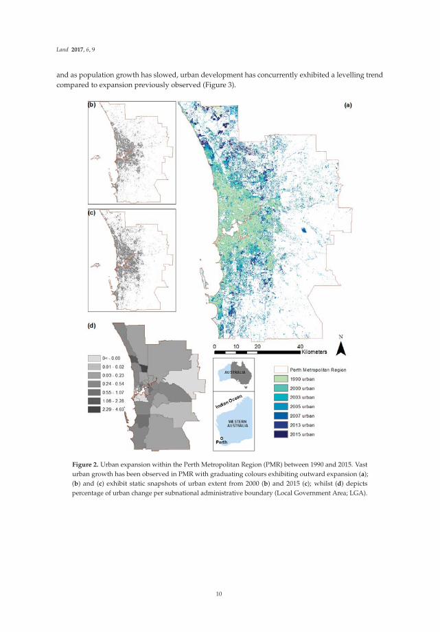
and as population growth has slowed, urban development has concurrently exhibited a levelling trendcompared to expansion previously observed (Figure 3).

Figure 2. Urban expansion within the Perth Metropolitan Region (PMR) between 1990 and 2015. Vasturban growth has been observed in PMR with graduating colours exhibiting outward expansion (a);(b) and (c) exhibit static snapshots of urban extent from 2000 (b) and 2015 (c); whilst (d) depictspercentage of urban change per subnational administrative boundary (Local Government Area; LGA).

10

Land 2017, 6, 9

Figure 3. Time line of urban expansion in kilometers squared derived from Earth observation data withassociated classification error derived from validation data (points indicating classified image years).Alongside population data in millions per year since 1988 (based on Australian Bureau of Statisticsdata, 2015 data is projected) with key natural resource milestones indicated, and average annual urbanand average annual population growth rate indicated between classified image years.

WAPC’s urban estimates of the PMR from Directions 2031 (the strategic plan for the Perth andPeel region) were provided for comparison to those produced within this study4 [5]. WAPC’s estimatesnote an expansion from 637 km2 to 813 km2 between 2001 and 2012. Our results indicate an expansionof 747 km2 to 1050 km2 from 2000 to 2013 illustrating an overall underestimation by WAPC figures(Figure 4). Within suburban areas surrounding the two major cities in the metropolitan region, Perthand Fremantle, WAPC’s estimates underrepresent the amount of urban area derived from EO, beingmore pronounced in 2013 than 2000. The Local Government Area (LGA)5 of Stirling South Easternrepresented the maximum overestimation in 2013 urban area with 34% (2000: 10%) additional urbanarea per km2 of LGA established on a difference of 2.89 km2, 40.2% (2000: 0.83 km2, 15%) between EOdata and WAPC’s estimates. Outer Northern and Southern LGA WAPC urban values were consistentlyunderestimated, with the LGA of Belmont representing the maximum underestimation of percent perkm2 of LGA in 2013 with 24% (2000: 13%) due to a difference of 9.37 km2, 40.39% (2000: 5 km2, 26.46%).Prior to 2009, WAPC’s estimates were solely based upon land parcel valuations from the WesternAustralian Value General’s Office, consequently valuation thresholds designating land to urban mayhave been inappropriately applied to outer suburban LGAs, where land might be developed but lessvaluable than central LGAs.

For urban estimates post 2005, two urban land zones, urban and urban deferred, are used withinthe Perth Metropolitan Region Scheme (MRS), the division of the State Planning Policy Frameworkapplicable to the PMR, pursuant to the Planning and Development Act (2005) that inform recent WAPC

4 Analysed in ArcGIS version 10.2.25 Outlines of LGAs are displayed in Figure S2

11

Land 2017, 6, 9

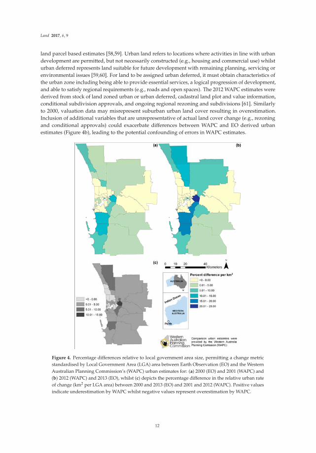
land parcel based estimates [58,59]. Urban land refers to locations where activities in line with urbandevelopment are permitted, but not necessarily constructed (e.g., housing and commercial use) whilsturban deferred represents land suitable for future development with remaining planning, servicing orenvironmental issues [59,60]. For land to be assigned urban deferred, it must obtain characteristics ofthe urban zone including being able to provide essential services, a logical progression of development,and able to satisfy regional requirements (e.g., roads and open spaces). The 2012 WAPC estimates werederived from stock of land zoned urban or urban deferred, cadastral land plot and value information,conditional subdivision approvals, and ongoing regional rezoning and subdivisions [61]. Similarlyto 2000, valuation data may misrepresent suburban urban land cover resulting in overestimation.Inclusion of additional variables that are unrepresentative of actual land cover change (e.g., rezoningand conditional approvals) could exacerbate differences between WAPC and EO derived urbanestimates (Figure 4b), leading to the potential confounding of errors in WAPC estimates.

Figure 4. Percentage differences relative to local government area size, permitting a change metricstandardised by Local Government Area (LGA) area between Earth Observation (EO) and the WesternAustralian Planning Commission’s (WAPC) urban estimates for: (a) 2000 (EO) and 2001 (WAPC) and(b) 2012 (WAPC) and 2013 (EO), whilst (c) depicts the percentage difference in the relative urban rateof change (km2 per LGA area) between 2000 and 2013 (EO) and 2001 and 2012 (WAPC). Positive valuesindicate underestimation by WAPC whilst negative values represent overestimation by WAPC.

12

Land 2017, 6, 9

4. Discussion

WA state government planning documentation states that the majority of new developmentwithin the PMR has occurred as low-density suburban growth, responding to consumer preferencesand market forces [4]. Additionally, sustainable policy objectives suggest that new developmentshould be managed and focused on current communities, making the most efficient use of existingurban areas [4,5]. Planning policy research has highlighted issues of outward urban expansion asbeing costly in economic, environmental and social terms based on dispersed service requirements,habitat fragmentation and neighbourhood segregation [20]. Thus, urban expansion in the PMRmay result in further economic, social and environmental costs associated with servicing andmaintaining low-density lifestyles, owing to the rapid outward urban growth estimates between2000 and 2007 [11,20].

In contrast, the witnessed slowdown of urban growth, population and natural resource valuesince 2013 indicates the possibility that the ‘boom’ of previous years has reached a turning point.Stagnation of urban growth implies that issues associated with spatially distributed urban areasmight be contained to the current urban extent. Nevertheless, it is conceivable that prosperous futureeconomic circumstances could initiate growth at a rate previously observed, and that the economicslowdown might be a temporary hiatus responding to current economic conditions [62]. For example,in 2014–2015, WA continued to attract the largest proportion of state mineral exploration expenditureat 58%, with QLD (the second ranked stated) obtaining only 20% [17]. Furthermore, as of September2015, WA had an estimated AUD 171 billion in mineral and petroleum projects under construction,with a further AUD 110 billion allocated for future expansion [17]. Comparatively, during the peak(mid-2013) in terms of total sales, WA only had an estimated AUD 160 billion worth of projects underconstruction and a further AUD 108 billion for future development [17]. Whilst 2014–2015 observedthe greatest decline in total sales of resources, sustained investment and improved global economicscould reinvigorate the industry and reinitiate urban expansion within the PMR.

Future development (urban and urban deferred) is guided by Directions 2031 amending the MRSand local planning schemes [5,63–66]. WAPC aims to achieve 47% of future development as infilland a 50% increase in average residential density by 2050 of 10 dwellings per urban zoned hectareand 15 per new urban zoned hectare [5]. In monitoring progress towards the infill target, zoneddevelopment land within the PMR is considered, including residential, industrial and commercialland uses [4]. Densities are defined as infill or Greenfield if above or below an undocumentedresidential threshold from census data [60]. Initial results from delivering directions 2031, 2014 reportindicate the requirement of a significant increase in infill development if the above targets are to bemet [67]. Similarly, average residential density monitoring has been achieved with land valuationdata (from the Valuer General’s Office) for major activity centres, being unrepresentative of actualdensity change and providing an incomplete metropolitan comparison [67]. Inclusion of EO datawould permit quantitative evidence of urban expansion, infill and density at a higher spatial andtemporal frequency than current census based estimates. This would facilitate credible, evidence-basedefficient targeted action founded upon improved representative urban area, insuring infill and densityattainment. In this theme, Schneider et al. (2005) and Hepinstall-Cymerman et al. (2013) used spatialmetrics (e.g., urban area mean patch size) based on classified Landsat data in either pre-definedcensus units [15] or development corridors [13] to monitor development type (infill or expansion)over time for adapting inappropriate static urban development policy. Using EO derived land coverdata in this manner aids in understanding dynamics of the urban environment through monitoring,planning and mitigating land use changes that impact natural assets and increase vulnerability of citysystems [14,15,68]. Information of this sort aligns with criteria of the CRF in improving city resiliencefrom effective land use planning, possible at lower expense and higher temporal frequencies than insitu measurements [21].

The universal methodology implemented within this research lends itself to credibly inform policyin a similar manner in other global cities through monitoring urban expansion in order to identify rapid,

13

Land 2017, 6, 9

unsustainable development. For example, Jakarta, obtaining the world’s second largest urban area witha population of 28 million, has yet to have any quantitative urban area delineation [69,70]. Identificationof actual urban growth in developing cities is vital to city planners, environment managers and policymakers due to the difference between planned growth and actual growth [14]. Such informationcould be of critical importance for regulating urban expansion due to extreme poverty and high levelof risk to environmental hazards, such as that posed from flooding [71,72]. EO data presents manyopportunities for added value within urban planning policy, and additional analyses could be pursuedinto specific human-induced environmental issues, such as detecting thermal changes in the urbanenvironment for planning issues associated with urban heat islands (e.g., cooling provisions) and theirimpact on human health (e.g., air quality).

5. Recommendations

Consistent and accurate LULC estimates are a vital aspect of sustainable urban developmentthroughout the world, especially considering the predicted additional 2.5 billion city dwellers by2050. LULC models that require agents that are representative of land use decisions can often fail inpracticality due to the difficulty in quantifying driving forces of change and multi-level relationships.Models of this nature are also temporally independent, with each annual iteration implementingnew data or data not representative of actual LULC change. EO data provides a replicable detailedrepresentation of the complete urban extent requiring no additional data. The use and application ofEO data reported within this paper highlights several improvements to WAPC policy for consistenturban area estimations with associated accuracy measures. Therefore it is recommended that planningauthorities, such as WAPC, integrate EO data to achieve the following: (1) provide scientific urbanestimates based on a temporally consistent model within future regional structure plans, metropolitanregion and local planning schemes; (2) monitor infill development at a higher temporal frequency thancensus years for policy targeting to meet key goals; (3) monitor urban density through areal urbanexpansion compared to current metrics using land valuations; and (4) restrict development based ontemporal urban analysis that degrades amenity efficiency and ecological systems whilst promotingdevelopment in locations to maximise efficiency and long-term sustainability. Additional EO datasets(e.g., finer resolution Sentinel 2 satellite imagery or aerial imagery) could be used to refine planningdecisions based on areas of concern identified from Landsat. For example, finer spatial resolutiondatasets could facilitate enhanced feature extraction, optimising sustainable planning decisions throughthe identification of candidate infill sites. EO data of this nature provides an essential tool for timelyplanning policy that is adaptive to changes in urban landscape to mitigate socio-environmental issuesassociated with poorly planned urban areas for the future sustainability of our cities.

Supplementary Materials: The following are available online at www.mdpi.com/2073-445X/6/1/9/s1.Additional methodological detail, full accuracy results and Local Government Area (LGA) outlines are reportedin the supplementary documentation. Figure S1 Inter year classification reflectance variation categorised byclassified output for each spectral band for: pre (a) and post (b) normalisation correction. Table S1 Classificationaccuracy and associated Kappa Coefficient per year of classified Landsat. Table S2 Producer’s and User’saccuracy per year of classified Landsat imagery. Figure S2 Local Government Areas (LGAs) located in PerthMetropolitan Region (a); with (b) exhibiting LGAs South and West of the Swan River and (c) LGAs North andEast of the Swan River. The classified data reported in this paper (doi:10.1594/PANGAEA.871017) are archivedat https://doi.pangaea.de/10.1594/PANGAEA.871017, the pangea open access data publisher for earth andenvironmental science.

Acknowledgments: This work was supported by the Economic and Social Research Council [grant numberES/J500161/1]. We would like to thank the World University Network (WUN) for facilitating institutionalvisits, the United States Geological Survey (USGS) for providing Landsat surface reflectance data and theWestern Australia Department of Planning, in particular Matt Devlin and Lisl van Aarde for urban estimates andsupplementary planning information.

Author Contributions: All authors assisted in conceiving and designing the experiments lead by AndrewMacLachlan; Andrew MacLachlan performed the experiments and analyzed the data; Eloise Biggs, Gareth Robertsand Bryan Boruff contributed reagents/materials/analysis tools; Andrew MacLachlan wrote the paper with inputand revisions from Eloise Biggs, Gareth Roberts and Bryan Boruff.

14

Land 2017, 6, 9

Conflicts of Interest: The authors declare no conflict of interest and the founding sponsors had no role in thedesign of the study; in the collection, analyses, or interpretation of data; in the writing of the manuscript, and inthe decision to publish the results.

References

1. ABS Australian National Accounts 1988–2015; Australian Bureau of Statistics: Belconnen, ACT, Australia, 2015.2. Kennewell, C.; Shaw, B.J. Perth, Western Australia. Cities 2008, 25, 243–255. [CrossRef]3. Dhakal, S.P. Glimpses of Sustainability in Perth, Western Australia: Capturing and Communicating the

Adaptive Capacity of an Activist Group. Cons. J. Sustain. Dev. 2014, 11, 167–182.4. Western Australian Planning Commission Perth and Peel @ 3.5 Million; Department of Planning, Government of

Western Australia: Perth, WA, Australia, 2015.5. Western Australian Planning Commission Directions 2031 and beyond: Metropolitan Planning beyond the Horizon;

Department of Planning, Government of Western Australia: Perth, WA, Australia, 2010.6. Western Australian Planning Commission Urban Growth Monitor: Perth Metropolitan, Peel and Greater Bunbury

Regions 2009; Department of Planning, Government of Western Australia: Perth, WA, Australia, 2009.7. Western Australian Planning Commission Urban Growth Monitor: Perth Metropolitan, Peel and Greater Bunbury

Regions 2010; Department of Planning, Government of Western Australia: Perth, WA, Australia, 2010.8. Angiuli, E.; Trianni, G. Urban Mapping in Landsat Images Based on Normalized Difference Spectral Vector.

IEEE Geosci. Remote Sens. Lett. 2013, 11, 661–665. [CrossRef]9. Bagan, H.; Yamagata, Y. Landsat analysis of urban growth: How Tokyo became the world’s largest megacity

during the last 40years. Remote Sens. Environ. 2012, 127, 210–222. [CrossRef]10. Thompson, R.J. A model for the creation and progressive improvement of a digitalcadastral data base.

Land Use Policy 2015, 49, 565–576. [CrossRef]11. Turner, B.; Lambin, E.; Reenberg, A. The emergence of land change science for global environmental change

and sustainability. Proc. Natl. Acad. Sci. USA 2010, 103, 13070–13075. [CrossRef] [PubMed]12. Bettencourt, L.; West, G. A unified theory of urban living. Nature 2010, 467, 9–10. [CrossRef] [PubMed]13. Schneider, A.; Seto, K.C.; Webster, D.R. Urban growth in Chengdu, western China: Application of remote

sensing to assess planning and policy outcomes. Environ. Plan. B Plan. Des. 2005, 32, 323–345. [CrossRef]14. Patino, J.E.; Duque, J.C. A review of regional science applications of satellite remote sensing in urban settings.

Comput. Environ. Urban Syst. 2013, 37, 1–17. [CrossRef]15. Hepinstall-Cymerman, J.; Coe, S.; Hutyra, L.R. Urban growth patterns and growth management boundaries

in the Central Puget Sound, Washington, 1986–2007. Urban Ecosyst. 2013, 16, 109–129. [CrossRef]16. Hepinstall, J.A.; Alberti, M.; Marzluff, J.M. Predicting land cover change and avian community responses in

rapidly urbanizing environments. Landsc. Ecol. 2008, 23, 1257–1276. [CrossRef]17. Western Australian Mineral and Petroleum Statistics Digest 1984–2015; Department of Mines and Petroleum,

Government of Western Australia: Perth, WA, Australia, 2015.18. Kalnay, E.; Cai, M. Impact of urbanization and land-use change on climate. Nature 2003, 423, 528–531.

[CrossRef] [PubMed]19. Vitousek, P.; Mooney, H.; Lubchenco, J.; Melillo, J. Human Domination of Earth Ecosystems. Science 1997,

277, 494–498. [CrossRef]20. Downs, A. Smart Growth: Why We Discuss It More than We Do It. J. Am. Plan. Assoc. 2005, 71, 367–378.

[CrossRef]21. ARUP City Resilience Framework—100 Resilient Cities; The Rockefeller Foundation: New York, NY, USA, 2015.22. Song, X.-P.; Sexton, J.O.; Huang, C.; Channan, S.; Townshend, J.R. Characterizing the magnitude,

timing and duration of urban growth from time series of Landsat-based estimates of impervious cover.Remote Sens. Environ. 2016, 175, 1–13. [CrossRef]

23. Li, X.; Gong, P.; Liang, L. A 30-year ( 1984–2013) record of annual urban dynamics of Beijing City derivedfrom Landsat data. Remote Sens. Environ. 2015, 166, 78–90. [CrossRef]

24. Potere, D.; Schneider, A.; Angel, S.; Civco, D. Mapping urban areas on a global scale: Which of the eightmaps now available is more accurate? Int. J. Remote Sens. 2009, 30, 6531–6558. [CrossRef]

25. Hu, Y.; Jia, G.; Hou, M.; Zhang, X.; Zheng, F.; Liu, Y. The cumulative effects of urban expansion on landsurface temperatures in metropolitan Jingjintang, China Yonghong. J. Geophys. Res. Atmos. 2015, 120,9932–9943. [CrossRef]

15

Land 2017, 6, 9

26. Masek, J.G.; Lindsay, F.E.; Goward, S.N. Dynamics of urban growth in the Washington DC metropolitanarea, 1973–1996, from Landsat observations. Int. J. Remote Sens. 2000, 21, 3473–3486. [CrossRef]

27. Van de Voorde, T.; Jacquet, W.; Canters, F. Mapping form and function in urban areas: An approach based onurban metrics and continuous impervious surface data. Landsc. Urban Plan. 2011, 102, 143–155. [CrossRef]

28. Xian, G.; Homer, C.; Bunde, B.; Danielson, P.; Dewitz, J.; Fry, J.; Pu, R. Quantifying urban land cover changebetween 2001 and 2006 in the Gulf of Mexico region. Geocarto Int. 2012, 27, 479–497. [CrossRef]

29. Suarez-Rubio, M.; Lookingbill, T.R.; Elmore, A.J. Exurban development derived from Landsat from 1986 to2009 surrounding the District of Columbia, USA. Remote Sens. Environ. 2012, 124, 360–370. [CrossRef]

30. Herold, M.; Gardner, M.; Hadley, B.; Roberts, D. The spectral dimension in urban land cover mapping fromhigh-resolution optical remote sensing data. In Proceedings of the 3rd Symposium on remote Sensing ofUrban Areas, Istanbul, Turkey, 11–13 June 2002; Volume 6, pp. 1–8.

31. Varshney, A.; Rajesh, E. A Comparative Study of Built-up Index Approaches for Automated Extraction ofBuilt-up Regions From Remote Sensing Data. J. Indian Soc. Remote Sens. 2014, 42, 659–663. [CrossRef]

32. Lu, D.; Moran, E.; Hetrick, S. Detection of impervious surface change with multitemporal Landsat images inan urban-rural frontier. ISPRS J. Photogramm. Remote Sens. 2011, 66, 298–306. [CrossRef] [PubMed]

33. Chen, T.; de Jeu, R.A.M.; Liu, Y.Y.; van der Werf, G.R.; Dolman, A.J. Using satellite based soil moisture toquantify the water driven variability in NDVI: A case study over mainland Australia. Remote Sens. Environ.2014, 140, 330–338. [CrossRef]

34. Myneni, R.B.; Keeling, C.D.; Tucker, C.J.; Asrar, G.; Nemani, R.R. Increased plant growth in the northernhigh latitudes from 1981 to 1991. Nature 1997, 386, 698–702. [CrossRef]

35. Piao, S.; Wang, X.; Ciais, P.; Zhu, B.; Wang, T.; Liu, J. Changes in satellite-derived vegetation growth trend intemperate and boreal Eurasia from 1982 to 2006. Glob. Chang. Biol. 2011, 17, 3228–3239. [CrossRef]

36. Pan, J.; Wang, M.; Li, D.; Li, J. Automatic Generation of Seamline Network Using Area Voronoi DiagramsWith Overlap. IEEE Trans. Geosci. Remote Sens. 2009, 47, 1737–1744. [CrossRef]

37. Hansen, M.C.; Loveland, T.R. A review of large area monitoring of land cover change using Landsat data.Remote Sens. Environ. 2012, 122, 66–74. [CrossRef]

38. USGS Product Guide Provisional Landsat 8 Surface Reflectance Product; Department of the Interior U.S. GeologicalSurvey: Sunrise Valley Drive Reston, VA, USA, 2015; pp. 1–27.

39. Ju, J.; Roy, D.P.; Vermote, E.; Masek, J.; Kovalskyy, V. Continental-scale validation of MODIS-based andLEDAPS Landsat ETM+ atmospheric correction methods. Remote Sens. Environ. 2012, 122, 175–184.[CrossRef]

40. Sexton, J.O.; Song, X.-P.; Huang, C.; Channan, S.; Baker, M.E.; Townshend, J.R. Urban growth of theWashington, D.C.–Baltimore, MD metropolitan region from 1984 to 2010 by annual, Landsat-based estimatesof impervious cover. Remote Sens. Environ. 2013, 129, 42–53. [CrossRef]

41. Roscher, R.; Förstner, W.; Waske, B. I2VM: Incremental import vector machines. Image Vis. Comput. 2012, 30,263–278. [CrossRef]

42. Braun, A.C.; Weidner, U.; Hinz, S. Classification in high-dimensional feature spaces-assessment using SVM,IVM and RVM with focus on simulated EnMAP data. IEEE J. Sel. Top. Appl. Earth Obs. Remote Sens. 2012, 5,436–443. [CrossRef]

43. Suess, S.; van der Linden, S.; Leitao, P.J.; Okujeni, A.; Waske, B.; Hostert, P. Import Vector Machines forQuantitative Analysis of Hyperspectral Data. IEEE Geosci. Remote Sens. Lett. 2014, 11, 449–453. [CrossRef]

44. Braun, A.C.; Weidner, U.; Hinz, S. Support vector machines, import vector machines and relevance vectormachines for hyperspectral classification—A comparison. In Proceedings of the IEEE 3rd Workshop onHyperspectral Image and Signal Processing: Evolution in Remote Sensing (WHISPERS), Lisbon, Portugal,6 June 2011; pp. 1–4.

45. Roscher, R.; Waske, B.; Forstner, W. Kernel discriminative Random fields for land cover classification.In Proceedings of the 2010 IAPR Workshop on Pattern Recognition in Remote Sensing (PRRS), Istanbul,Turkey, 22 August 2010.

46. Hu, X.; Weng, Q. Estimating impervious surfaces from medium spatial resolution imagery using theself-organizing map and multi-layer perceptron neural networks. Remote Sens. Environ. 2009, 113, 2089–2102.[CrossRef]

16

Land 2017, 6, 9

47. Flood, N. Continuity of Reflectance Data between Landsat-7 ETM+ and Landsat-8 OLI, for BothTop-of-Atmosphere and Surface Reflectance: A Study in the Australian Landscape. Remote Sens. 2014,6, 7952–7970. [CrossRef]

48. Roy, D.P.; Kovalskyy, V.; Zhang, H.K.; Vermote, E.F.; Yan, L.; Kumar, S.S.; Egorov, A. Characterizationof Landsat-7 to Landsat-8 reflective wavelength and normalized difference vegetation index continuity.Remote Sens. Environ. 2016, 185, 57–70. [CrossRef]

49. Dorais, A.; Cardille, J. Strategies for incorporating high-resolution google earth databases to guide andvalidate classifications: Understanding deforestation in Borneo. Remote Sens. 2011, 3, 1157–1176. [CrossRef]

50. Cunningham, S.; Rogan, J.; Martin, D.; DeLauer, V.; McCauley, S.; Shatz, A. Mapping land developmentthrough periods of economic bubble and bust in Massachusetts using Landsat time series data.GIScience Remote Sens. 2015, 52, 397–415. [CrossRef]

51. Sun, G.; Chen, X.; Jia, X.; Yao, Y.; Wang, Z. Combinational Build-Up Index (CBI) for Effective ImperviousSurface Mapping in Urban Areas. IEEE J. Sel. Top. Appl. Earth Obs. Remote Sens. 2016, 9, 2081–2092.[CrossRef]

52. Bagan, H.; Yamagata, Y. Land-cover change analysis in 50 global cities by using a combination of Landsatdata and analysis of grid cells. Environ. Res. Lett. 2014, 9, 064015. [CrossRef]

53. Zhu, Z.; Woodcock, C.E. Continuous change detection and classification of land cover using all availableLandsat data. Remote Sens. Environ. 2014, 144, 152–171. [CrossRef]

54. Congalton, R.G. Accuracy assessment and validation of remotely sensed and other spatial information. Int. J.Wildl. Fire 2001, 10, 321–328. [CrossRef]

55. Gislason, P.O.; Benediktsson, J.A.; Sveinsson, J.R. Random forests for land cover classification.Pattern Recognit. Lett. 2006, 27, 294–300. [CrossRef]

56. Sundarakumar, K.; Harika, M.; Begum, S.K.A.; Yamini, S.; Balakrishna, K. Land Use And Land CoverChange Detection And Urban Sprawl Analysis Of Vijayawada City Using Multitemporal Landsat. Int. J.Eng. Sci. Technol. 2012, 4, 170–178.

57. Luo, J.; Du, P.; Alim, S.; Xie, X.; Xue, Z. Annual Landsat analysis of urban growth of Nanjing City from 1980to 2013. In Proceedings of the 2014 3rd International Workshop on Earth Observation and Remote SensingApplications (EORSA), Changsha, China, 11–14 June 2014; pp. 357–361.

58. Western Australian Planning Commission Draft State Planning Policy 1, State Planning Framework (Variation No. 3);Department of Planning, Government of Western Australia: Perth, WA, Australia, 2016.

59. Western Australian Planning Commission Development Control Policy 1.9; Department of Planning, Governmentof Western Australia: Perth, WA, Australia, 2010; pp. 1–5.

60. Western Australian Planning Commission Western Australian Planning Commission Urban Growth Monitor:Perth Metropolitan, Peel and Greater Bunbury Regions 2016; Department of Planning, Government of WesternAustralia: Perth, WA, Australia, 2016.

61. Western Australian Planning Commission Urban Growth Monitor: Perth Metropolitan, Peel and Greater BunburyRegions 2012; Department of Planning, Government of Western Australia: Perth, WA, Australia, 2012.

62. Perry, M.; Rowe, J.E. Fly-in, fly-out, drive-in, drive-out: The Australian mining boom and its impacts on thelocal economy. Local Econ. 2014, 30, 139–148. [CrossRef]

63. Western Australian Planning Commission Central Sub-Regional Planning Framework; Department of Planning,Government of Western Australia: Perth, WA, Australia, 2015.

64. Western Australian Planning Commission North-West Sub-Regional Planning Framework; Department of Planning,Government of Western Australia: Perth, WA, Australia, 2015.

65. Western Australian Planning Commission North-East Sub-Regional Planning Framework; Department of Planning,Government of Western Australia: Perth, WA, Australia, 2015.

66. Western Australian Planning Commission South Metropolitan Peel Planning Framework; Department of Planning,Government of Western Australia: Perth, WA, Australia, 2015.

67. Western Australian Planning Commission Delivering Directions 2031 Report Card 2014; Department of Planning,Government of Western Australia: Perth, WA, Australia, 2014.

68. Miller, R.B.; Small, C. Cities from space: Potential applications of remote sensing in urban environmentalresearch and policy. Environ. Sci. Policy 2003, 6, 129–137. [CrossRef]

17

Land 2017, 6, 9

69. Pravitasari, A.E.; Saizen, I.; Tsutsumida, N.; Rustiadi, E.; Pribadi, D.O. Local Spatially Dependent DrivingForces of Urban Expansion in an Emerging Asian Megacity: The Case of Greater Jakarta (Jabodetabek).J. Sustain. Dev. 2015, 8, 108–120. [CrossRef]

70. Seto, K.; Fragkias, M.; Guneralp, B.; Reilly, M. A next-generation approach to the characterization of anon-model plant transcriptome. Curr. Sci. 2011, 101, 1435–1439.

71. Marfai, M.A.; Sekaranom, A.B.; Ward, P. Community responses and adaptation strategies toward floodhazard in Jakarta, Indonesia. Nat. Hazards 2014, 75, 1127–1144. [CrossRef]

72. Suryahadi, A.; Sumarto, S. Poverty and Vulnerability in Indonesia before and after the Economic Crisis.Asian Econ. J. 2003, 17, 45–64. [CrossRef]


18

land

Article

Agricultural Land Fragmentation at Urban Fringes:An Application of Urban-To-Rural Gradient Analysisin Adelaide

Suranga Wadduwage *, Andrew Millington, Neville D. Crossman and Harpinder Sandhu

School of the Environment, Flinders University, GPO Box 2100, Adelaide, SA 5001, Australia;[email protected] (A.M.); [email protected] (N.D.C.);[email protected] (H.S.)* Correspondence: [email protected]

Academic Editors: Harini Nagendra and Monika KopeckaReceived: 23 January 2017; Accepted: 11 April 2017; Published: 16 April 2017

Abstract: One of the major consequences of expansive urban growth is the degradation and loss ofproductive agricultural land and agroecosystem functions. Four landscape metrics—Percentage ofLand (PLAND), Mean Parcel Size (MPS), Parcel Density (PD), and Modified Simpson’s DiversityIndex (MSDI)—were calculated for 1 km × 1 km cells along three 50 km-long transects that extendout from the Adelaide CBD, in order to analyze variations in landscape structures. Each transect hasdifferent land uses beyond the built-up area, and they differ in topography, soils, and rates of urbanexpansion. Our new findings are that zones of agricultural land fragmentation can be identified bythe relationships between MPS and PD, that these occur in areas where PD ranges from 7 and 35,and that these occur regardless of distance along the transect, land use, topography, soils, or ratesof urban growth. This suggests a geometry of fragmentation that may be consistent, and indicatesthat quantification of both land use and land-use change in zones of fragmentation is potentiallyimportant in planning.

Keywords: urban-to-rural gradients; agricultural land-use; land fragmentation; urban fringe; MeanParcel Size; Parcel Density

1. Introduction

Projections suggest that over two-thirds of the world’s population will live in urban centres by2050 [1], and that a major part to this growth will be due to people migrating from the countryside [2–4].Over the last 30 years, the global rate of urban land occupation [5,6] has been double the rate ofurban population growth [7]. Agricultural land loss due to urbanization has been highlighted by anumber of researchers [8–14], and has raised a number of environmental concerns; e.g., decliningquality of soil and water assets, loss of natural habitat, decreased plant and animal diversity, andcompromised ecological functions [15,16]. The urban sprawl that can be anticipated (given urbanpopulation projections) will increase demands for land for housing, industry and infrastructure;thereby consuming more agricultural land at the edges of cities [2,17,18]. This will lead to irreversibleand unsustainable land–use transitions at the cost of productive agricultural land in peri-urbanareas [19–21], where open spaces and scarce remnant ecosystems with high ecological and conservationvalues are already threatened [22].

Urban fringes—the transitional zones between urban and rural areas [23]—are characterizedby highly dynamic, spatially heterogeneous land-use and land-cover changes [24,25]. This takesplace because of the relatively lower land prices in these zones and the high frequency of land tenurechange [26,27]. Compared to urban environments, the faster rates of housing and infrastructure growth


Land 2017, 6, 28

and the higher proportion of remnant ‘green’ spaces lead to different landscape structures at the fringe.Research has also demonstrated that urban growth leads to increased land fragmentation [28] andlandscape diversity [29] in these areas. The diverse arrays of land uses that result from these processescreate spatially heterogeneous, complex land-use configurations [30–34]. However, a concern forplanners and people implementing land management policies in urban fringe environments is that thequantitative land-use data they require is often accompanied by relatively low levels of accuracy [35,36].

A recent development in understanding the influence of urbanization on land use has been theuse of urban-to-rural gradient analysis [34,37,38]. This concept originated as a combination of elementsdrawn from landscape ecology and urban ecology [39,40], and has been used to synthesize complexanthropogenic land transitions worldwide [31,34,41–47]. The continuous representation of land-useintensity and the spatial arrangement of land use along gradients is more effective in land-use planningthan conventional, discrete spatial measurements [48]. Urban-to-rural gradient analysis is also usefulfor examining gradual landscape change at urban fringes. The approach has other advantages, e.g.,in environmental modeling it is used to minimize subjectivity in categorizing variability, and indescribing ecological processes at urban fringes [49]. It is also used to represent land-use as a gradientand for measuring the spatial attributes of land parcels along gradients, both of which improve ourability to interpret landscapes [31,50]. Geographically-referenced points along gradients enable spatialand non-spatial data to be aggregated for systematic landscape comparisons [51–53]. Finally, thesecontinuous information gradients can be utilized to understand landscape structures and potentialland-use variations in complex land systems.

Landscape metrics calculated along these gradients have been used to identify land structureelements, and their changing patterns, to describe the effects of urban development at the marginsof several cities [31,34,42]. Vizzari and Sigura [48] claim that gradient analyses enable interactionsbetween land-use types to be identified precisely when exploring land transitions. In this research,landscape structure is defined as the spatial configuration of land parcels (i.e., their size and spatialarrangement) and their composition (land-use presence and amount of each land parcel in thelandscape) [54].

This paper reports the application of urban-to-rural gradient analysis to understand agriculturalland fragmentation at the urban fringes of Adelaide. In previous research, landscape metrics have beenplotted along transects, but the relationships between them have not been integrated into gradientanalyses. Four landscape metrics—Parcel Density (PD), Mean Parcel Size (MPS), Percentage of Land(PLAND) and Modified Simpson’s Diversity Index (MSDI)—were used to quantify and characterizeland fragmentation along transects extending from the Adelaide CBD into surrounding rural areas.A novel element of the research is the quantitative analysis of agricultural land-use presence in zonesof active land fragmentation at the urban fringe. In this context, urban-to-rural transects were usedas georeferenced land-use information gradients that integrate measurements of land-use, whilesimultaneously examining landscape structure and land-use changes.


2.1. Study Area

Adelaide—the capital of South Australia—is a coastal city surrounded by sprawling residentialand modern industrial suburbs to the north and south. In addition, satellite towns to the east andnorth, Mount Barker and Gawler (Figure 1), are being incorporated into the urban fabric of themetropolitan area. Adelaide’s fringes are urban frontiers that impinge on intensive horticultureand dryland agriculture in the northern plains; a conservation green belt with mixed agriculturalland use in the Adelaide Hills to the east; and traditional agricultural areas focused around highvalue, globally-recognized wine regions to the south (McLaren Vale) and north-east (Barossa Valley).Population growth and economic diversification are increasing the demand for land for housing,

20

Land 2017, 6, 28

transport and industrial infrastructure. In turn, this has led to significant pressure on adjacentproductive agricultural land.

Figure 1. Land-use distribution in Adelaide and its surrounding areas (Source: DPTI 2014).The urban-to-rural transects are overlain in red. The inset map to the right shows an enlargement ofthe urban-to-rural transect south of the city.

The variations in rural land use at the northern, eastern and southern margins of Adelaideprovide a heterogeneous setting in which to test urban-to-rural gradient analysis. Transects wereused to sample land-use gradients 50 km outwards from the Adelaide CBD in northerly, easterly andsoutherly directions (Figure 1).

Previous researchers using gradient analysis [31,55] have mapped urban-to-rural gradients alongtransport corridors. It is probable that this leads to a bias toward the investigation of urban land use.However, as this paper’s research focus is on the incorporation of different types of agricultural landinto an expanding urban area, it was decided to maximize the agricultural land use considered in thegradient analysis. Therefore, they were not oriented along main routes out of Adelaide, but in threecardinal directions. In fact, there are many routes out of Adelaide, which are orientated in a varietyof directions. Therefore, each of these transects has some transport corridor influence. The transectswere sampled over 50 km so that they are comparable and of sufficient length to cover all the types ofparcels where agricultural land is being incorporated into the urban fabric of the city.

This study uses a single statewide cadastral dataset produced by the South AustralianGovernment’s Department of Planning, Transport and Infrastructure (DPTI) in 2014, which is publicallyavailable online (http://data.sa.gov.au). The primary purpose of this dataset is to assess council ratesand levies based on land parcel valuations. The attributes of the dataset that are pertinent to thisresearch are: land parcel identity codes; land-use categories; and the land-use classes occurring ineach of the land parcels. It contains nineteen land-use categories (Table 1), which were regrouped intoeight land-use classes for the purposes of this research. Sixteen categories were regrouped into fiveland-use classes—Conservation, Urban residential, Rural residential, Commercial and Services. Threecategories—Dryland agriculture, Livestock land and Horticulture land—were not changed.

21

Land 2017, 6, 28

Table 1. Scheme used to reclassify land-use categories in the cadastral dataset (2014) to land-use classesfor this research.

Original Land-Use Categories *Reclassified Land-Use Classes (the numbers in

parentheses are used in subsequent graphs)

Reserve, Forestry, Vacant Conservation (1)Agriculture Dryland agriculture (2)Livestock Livestock (3)

Horticulture Horticulture (4)Commercial, Food Industry, Mine and Quarry, Public Institution, Commercial (5)

Residential, Non private residential, Vacant residential Urban residential (6)Rural residential Rural residential (7)

Education, Golf, Recreation, Utility Industry Services (8)

* Land categories defined in the South Australian government cadastral data set in 2014.

2.2. Urban-To-Rural Gradients at Urban Fringes

Urban-to-rural gradients [34] were used to visualize and analyze land use along three 50 km longtransects, each of which comprise 50 1 km × 1 km cells. ArcGIS© 10.2.1 (ESRI: Redlands, CA, USA)was used for all spatial data analyses. The 1 km2 cell-based transects were produced using the Fishnettool by defining the spatial areas for cell references. They were overlain on the cadastral dataset andland-use information extracted for each cell. These data were then compiled using the tabulation toolin ArcGIS spatial analyst extension. Each cell in the resulting dataset includes a unique identifier andthe areas of each of land-use class (Table 1) within each cell.

Landscape metrics have been used extensively in conservation biology, but their applicationin land-use research to measure, characterize, analyze, and visualize landscape structure is far lesscommon, particularly in urban areas [41,56–58]. Four landscape metrics were calculated from theattributes for each cell in the three transects (Table 2). The percentage of each land-use class in eachcell (PLAND) provides data on compositional changes in land use along the gradients. MPS andthe PD are measurements of key spatial features along the transects. Finally, MSDI is a measureof the proportional abundance of the land-use classes in each cell, and is an indicator of land-usediversity. Plots of each of the metrics for each gradient enabled landscape structures to be visualizedand analyzed.

Table 2. Landscape metrics used for spatial feature characterization.

Metric Description Range Equation

Percent of land-use coverage(PLAND) [%]

The proportion of the totalarea occupied by a particular

land-use class.0< PLAND ≤ 100 Pi =

∑nj=1 aij

A (100)

Modified Simpson’s DiversityIndex (MSDI)

A measurement of land-usediversity in a cell determined

by the distribution of theproportional abundance of

different land-use types(parcel richness) extensively.

MSDI ≥ 0 MSDI = −lnn∑

i=1Pi

2

Mean Parcel Size (MPS) [ha] The average area of all landparcels in the landscape. MPS > 0 MPS =

∑Nj=1 aj

N1

10,000

Parcel Density (PD) [N/km2]The number of land parcels

per 100ha. PD > 1 PD = NA (10, 000)(100)

Pi = proportion of the landscape occupied by parcel land-use type i, aij = area (m2) of parcel ij, aj = area (m2) ofparcel j, A = total area of the landscape (m2)—cell, i = land-use class (1–8), j = number of parcels, n = ni = number ofparcels in the landscape (cell) of parcel land-use type I, N = number of parcels in the landscape. (McGarigal andMarks, 1995).

22

Land 2017, 6, 28

2.3. Landscape Matrix Analysis

The relationships between MPS and PD were investigated to examine the extent of landfragmentation with distance along each transect. The associations between MPS and PD demonstrateprobable land structure variations in the landscape, and trend lines were used to visualize the natureof the relationships between MPS and PD.

The study area contains the following median land parcel areas: LL (Livestock land) (59 ha), DL(Dryland cultivation) (50 ha), and HL (Horticultural land) (12 ha). HL has a minimum size of 2.5 ha,which probably represents intensive irrigated vegetable cultivation or small vineyards. The median(12 ha) to minimum (2.5 ha) size of HL land parcels allows the range in the number of agriculture-basedland parcels which are likely to occur in a 1 km2 (100 ha) cell to be estimated. Horticultural land (HL)was used to define the PD range between 7 and 35 N/km2, because it is the agricultural land-usetype with the smallest median parcel size. Therefore, it is the land-use class that will provide themaximum number of land parcels in a 1 km2 (100 ha) cell. It is believed that this range of valuesindicates a high potential for transforming agricultural to urban land-uses at urban fringes. Thisis due to high property values, proximity to built-up areas, and that they frequently experiencegovernment-promoted land subdivision and land re-zoning for urban development. Rauws andDe Roo [26] have identified these land-use change drivers as “pull factors” which are influenced byurban economies converting non-urban land uses to urban form at the peri-urban areas. Therefore, inthe scatter diagrams, a common range of PD from 7 to 35 N/km2 is used; where a 1 km2 cell can have7 to 35 land parcels/km2 that are highly vulnerable to change in land use. The agriculture-based landparcel information associated with the cells from the land cadastral dataset was extracted within thisrange of patch densities.

3. Results

Landscape metric values were plotted along the three urban-to-rural gradients; north (N), east (E)and south (S); PLAND in Figure 2, MPS and PD in Figure 3, and MSDI in Figure 4. PLAND values forthe eight land-use types (Figure 2) illustrate the variations in land-use composition along the transects,thereby demonstrating the urban, peri-urban and rural characteristics of these transects. The PLANDvalues along these three transects show high percentages of urban land uses near the city centre,a gradual change to higher percentages of agricultural land uses at the end of the transects, and aheterogeneous mix of land-use types in the peri-urban areas. MPS and PD have a negative relationship(Figure 3), with greater MPS values being associated with lower PD values. Figure 5a illustrates theassociation between MPS and PD of the land parcels for each transect. Figure 5b shows the relationshipbetween PD and MPS in the ranges 0–40 N/km2 and 0–80 ha, respectively, for each transect. MSDIis somewhat similar between transects (Figure 4), and shows that diversity generally declines withdistance from the CBD. However, it is noteworthy that the southern transect has relatively lowerlandscape diversity than the other two.

3.1. Agricultural Land-Use Presence

The PLAND values for Dryland agriculture (DL), Livestock land (LL) and Horticulture (HL) alongthe three transects are shown in Figure 6. The northern transect shows three distinctly different zonesof land use. The built-up area, between 0–15 km, has low agricultural PLAND for the three agriculturalland uses, and high PD and low MPS. Between 15 and 37 km the agricultural land-use percentagesare HL (61.4%), DL (31.6%), and LL (6.8%). These represent mainly intensive vegetable production,rain-fed cereal cultivation, and sheep and horse grazing, respectively. This 22-km long zone presentsa typical urban fringe landscape structure, with increasing MPS and decreasing PD. The landscapebeyond the fringe (>37 km) is dominated by Dryland agriculture, and mainly comprises rain-fed wheat,barley and olive groves, which occupy large land parcels in a rural landscape. Land-use presence inthe zones of high fragmentation is provided in Figure 7.

23

Land 2017, 6, 28

020406080100

12

34

56

78

910

1112

1314

1516

1718

1920

2122

2324

2526

2728

2930

3132

3334

3536

3738

3940

4142

4344

4546

4748

4950

N020406080100

12

34

56

78

910

1112

1314

1516

1718

1920

2122

2324

2526

2728

2930

3132

3334

3536

3738

3940

4142

4344

4546

4748

4950

E

020406080100

12

34

56

78

910

1112

1314

1516

1718

1920

2122

2324

2526

2728

2930

3132

3334

3536

3738

3940

4142

4344

4546

4748

4950

S

Cons

erva

tion

Dryl

and

(DL)

Live

stoc

k La

nd (L

L)Ho

rtic

ultu

ral L

and

(HL)

Com

mer

cial

Urb

an re

siden

tial

Rura

l Res

iden

tial

Serv

ices

Dist

ance

from

city

cen

tre

(km

)

Percentage of Land use

Fig

ure

2.

PLA

ND

:nor

th(N

),ea

st(E

)and

sout

h(S

)tra

nsec

ts.

24

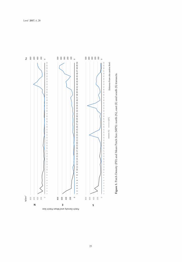
Land 2017, 6, 28

0200

400

600

800

0

200

400

600

800

12

34

56

78

910

1112

1314

1516

1718

1920

2122

2324

2526

2728

2930

3132

3334

3536

3738

3940

4142

4344

4546

4748

4950

0100

200

300

400

500

0

200

400

600

800

12

34

56

78

910

1112

1314

1516

1718

1920

2122

2324

2526

2728

2930

3132

3334

3536

3738

3940

4142

4344

4546

4748

4950

0100

200

300

400

500

0

200

400

600

800

12

34

56

78

910

1112

1314

1516

1718

1920

2122

2324

2526

2728

2930

3132

3334

3536

3738

3940

4142

4344

4546

4748

4950

PDM

PSDi

stan

ce fr

om c

ity c

entr

e (k

m)

ha

N/k

m2

N E S Patch Density and Mean Patch Size

Fig

ure

3.

Patc

hD

ensi

ty(P

D)a

ndM

ean

Patc

hSi

ze(M

PS):

nort

h(N

),ea

st(E

)and

sout

h(S

)tra

nsec

ts.

25

Land 2017, 6, 28

0

0.51

1.52

12

34

56

78

910

1112

1314

1516

1718

1920

2122

2324

2526

2728

2930

3132

3334

3536

3738

3940

4142

4344

4546

4748

4950

N0

0.51

1.52

12

34

56

78

910

1112

1314

1516

1718

1920

2122

2324

2526

2728

2930

3132

3334

3536

3738

3940

4142

4344

4546

4748

4950

E

0

0.51

1.52

12

34

56

78

910

1112

1314

1516

1718

1920

2122

2324

2526

2728

2930

3132

3334

3536

3738

3940

4142

4344

4546

4748

4950

S

MSD

ITr

endl

ine

base

d on

Pol

ynom

ial o

rder

6

Modified Simpson Diversity Index

Dist

ance

from

city

cen

tre

(km

)

Fig

ure

4.

Mod

ified

Sim

pson

Div

ersi

tyIn

dex:

nort

h(N

),ea

st(E

)and

sout

h(S

)tra

nsec

ts.

26

Land 2017, 6, 28

(a)

(b)

0

100

200

300

400

050

100

150

200

MPS (ha)

PD (

N/k

m2 )

N

0

100

200

300

400

050

100

150

200

MPS (ha)

PD (

N/k

m2 )

E

0

100

200

300

400

050

100

150

200

MPS (ha)

PD (

N/k

m2 )

S

020406080

010

2030

MPS (ha)

PD (

N/k

m2 )

N

020406080

010

2030

40

MPS (ha)

PD (

N/k

m2 )

E

020406080

010

2030

40

MPS (ha)

PD (

N/k

m2 )

S

Fig

ure

5.

(a)M

PS-P

Dpl

ots:

nort

h(N

),ea

st(E

)and

sout

h(S

)tra

nsec

ts.(

b)E

nlar

gem

ents

ofM

PS_P

Dpl

ots

inth

e7

<PD

<35

rang

e.

27

Land 2017, 6, 28

050100

12

34

56

78

910

1112

1314

1516

1718

1920

2122

2324

2526

2728

2930

3132

3334

3536

3738

3940

4142

4344

4546

4748

4950

N050100

12

34

56

78

910

1112

1314

1516

1718

1920

2122

2324

2526

2728

2930

3132

3334

3536

3738

3940

4142

4344

4546

4748

4950

E

050100

12

34

56

78

910

1112

1314

1516

1718

1920

2122

2324

2526

2728

2930

3132

3334

3536

3738

3940

4142

4344

4546

4748

4950

S

DLLL

HL

Percentage of Land use

Dist

ance

from

city

cen

tre

(km

)

Fig

ure

6.

Perc

enta

geof

the

tota

llan

dar

eaoc

cupi

edby

each

agri

cult

ural

land

-use

type

:nor

th(N

),ea

st(E

)and

sout

h(S

)tra

nsec

ts.

12

34

56

78

910

1112

1314

1516

1718

1920

2122

2324

2526

2728

2930

3132

3334

3536

3738

3940

4142

4344

4546

4748

4950

NE

SDi

stan

ce fr

om ci

ty ce

ntre

(km

)

Fig

ure

7.

Are

aspr

one

tola

ndfr

agm

enta

tion

betw

een

PD7

and

35fo

rea

chtr

anse

ct.

28

Land 2017, 6, 28

The first 10 km of the eastern transect represents the built-up areas of eastern Adelaide. The threeagricultural land-uses of the Adelaide Hills—sheep and cattle rearing (LL, 52.7%); vegetable cultivation,fruit orchards and wineries (HL, 38.5%); and rain-fed crops (DL, 8.7%) characterize the transect from11 to 32 km. The MPS of the land parcels in this hilly terrain are relatively small. Livestock land andDryland cultivation dominate the transect beyond 33 km.

The southern transect is significantly different from the northern or eastern transects in terms ofagricultural land use. Beyond the built-up area, which covers the first 18 km of the transect, LL andHL have much higher shares of the overall land use than DL. The landscape from 18 to 33 km has anagricultural land use split of HL (60.1%), LL (39.2%), and DL (0.7%). This combination characterizesthe complex land use of McLaren Vale, which has transitioned from a mixed grazing and horticulturalregion, to one of vineyards and olive groves, with some grazing being retained at the margins. Theamount of LL increases in the landscape beyond 33 km. However, in these final 17 km, PLANDvalues of Rural residential land and Urban residential land increase, leading to correspondingly higherMSDI values. The changes in these metrics demonstrate the influence of the town of Victor Harbor,which is located beyond the end of the transect. Table 3 summarizes agricultural land presence in thethree transects:

Table 3. Summary of the agricultural land along the three gradients.

Transect Built-Up Area Urban Fringe Areas Rural Areas

North0–15 km. Low PLAND,high PD and low MPS

for DL, LL and HL

15–37 km. HL (61.4%), DL (31.6%) and LL(6.8%) representing mainly intensive vegetable

production, rain-fed cereal cultivation, andsheep and horse grazing respectively.

>37 km. Dominated by DL (rain-fed wheat, barley andolives) which occupies large land parcels.

East0–10 km. Low PLAND,high PD and low MPS

for DL, LL, HL.

11–32 km. LL (52.7%), HL (38.5%) and DL(8.7%) representing sheep and cattle rearing;vegetable cultivation, orchards and wineries;

and rain-fed crops respectively. Relativelysmall MPS compared to other rural areas due

to hilly terrain.

>32 km. Dominated by LL and DL.

South0–18 km. Low PLAND,high PD and low MPS

for DL, LL, HL.

18–33 km. HL (60.1%), LL (39.2%) and DL(0.7%) representing the complex land use ofMcLaren Vale which has transitioned from amixed grazing and horticulture region to a

vineyards and olive groves with some grazingretained at the margins.

>33 km. High proportions of land in LL (cattle grazing).Increase in PLAND for residential land uses, and higher

MSDI values at the end ofthe transect due to theinfluence of the town of Victor Harbor.

The total amount of agricultural land in each transect is summarized in Figure 8. The easterntransect has the highest amount of agricultural land (2558 ha, 51.2%), comprised of 11% DL, 70% LLand 19% HL. The southern transect has the lowest amount of agricultural land (1583 ha, 31.6%: 4%DL, 53% LL, 3% HL). The northern transect has 1979 ha (39.6%) under the three types of agriculturalland-use, and is dominated by Dryland cultivation, accounting for 66% of all agricultural land.

N E S%HL 591.6 481.7 684.9%LL 70.9 1786.4 840.9%DL 1317.3 289.9 57.6

0.0

500.0

1000.0

1500.0

2000.0

2500.0

3000.0

Land

ext

ent (

ha)

Transect direction

Figure 8. Total agricultural land extent and the land use type percentages in the north (N), east (E) andsouth (S) transects.

29

Land 2017, 6, 28

3.2. Agricultural Land Fragmentation

MPS and PD were used to characterize agricultural land fragmentation along each transect. Inconsidering the zone where PD ranges from 7 to 35 N/km2, the critical zones for land fragmentationin the northern and eastern gradients extend for 15 km and 20 km, respectively (Figure 7). This zoneis disjunctive in the southern transect, and extends from 19 km to the end of the transect. Figure 9shows the amount of land occupied by the agricultural land uses in the zones of land fragmentationfor each transect, while Figure 9 shows the corresponding percentage data. The total amounts ofagricultural land of all types in the zones of high fragmentation are: 935.1 ha, 1311.9 ha and 825.7 hafor the northern, eastern and southern transects, respectively. Figure 10 displays the amount ofeach class of agricultural land in the zones of fragmentation. Horticultural land comprises a largecomponent in each transect, and dominates the northern transect. Livestock grazing accounts for thehighest proportions of agricultural land in the zones of high fragmentation in the eastern and southerntransects, but is a minor element in the northern transect. Dryland agriculture has a low presence inthe zones of fragmentation in all three transects. This is only encountered with any frequency in thenorthern transect, where there is significant contemporary urban fringe formation on land formerlyused for rain-fed cereal cultivation on the Northern Adelaide Plains.

N E S%HL 572.91 428.83 385.46%LL 61.27 777.85 394.84%DL 301.01 105.24 45.45

0.0

200.0

400.0

600.0

800.0

1000.0

1200.0

1400.0

Land

ext

ent (

ha)

Transect direction

Figure 9. The agricultural land extent and the land use type percentages in the zones of highland fragmentation.

0

400

800

1200

1600

2000

N E S0

400

800

1200

1600

2000

N E S

0

400

800

1200

1600

2000

N E S

Total DL

DL in fragmenting areas

Transect direction

Land

ext

ent (

ha)

Total HL

HL in fragmenting areas

Total LL

LL in fragmenting areas

Figure 10. The extent of DL, LL, HL in zones of high land fragmentation: north (N), east (E) and south(S) transects.

30

Land 2017, 6, 28

4. Discussion

Weng [42], in applying gradient analysis, found that landscape fragmentation is positivelycorrelated with the degree of urbanization, and results in agricultural land loss at urban fringes.Therefore, as agricultural land is generally the major land-use category beyond the fringe, it is themajor land reserve for meeting the land demands of urban development in sprawling cities such asAdelaide. Moreover, fragmentation is the key spatial manifestation of the process of incorporatingagricultural land into transitional, urban fringe landscapes.

This research confirms the presence of agricultural land along all three gradients, and thatfragmentation can be easily visualized and quantified using a combination of gradient analysisand landscape metrics. It is the first application of these techniques in the Australian context. Moreimportantly, this research provides an advance on previous analyses of the incorporation of agriculturalland into the urban fabric of cities, by comparing the conversion processes acting on three types ofagricultural land (Dryland agriculture, Livestock grazing and Horticulture).

4.1. Land Structure Analysis along Gradients

This research presents a novel method for investigating agricultural land fragmentation atthe urban fringe, by analyzing the associations between mean patch size and patch density.Notwithstanding the differences in the land-use geographies along the transects, scatter plots ofMPS and PD for the three transects showed similar patterns of cell organization with respect topatch density and mean patch size. Cells associated with the horizontal parts of the trend lines(Figure 5) indicate low levels of association between MPS and PD; e.g., a decline in MPS from 400 hato approximately 100 ha leads to very little increase in PD, which remains at <7 N/km2. When PDreaches approximately 35 N/km2, further increases are not accompanied by significant changes inMPS, i.e., the vertical parts of the trend lines in Figure 5. This means that the zone bounded by PDvalues of 7 to 35 N/km2 is a critical zone of land fragmentation in which the relationship between MPSand PD is very sensitive. For example, a decrease of one hectare in MPS leads to an increase in PDof 0.52 N/km2 (in the northern transect), 0.54 N/km2 (eastern transect), and 0.33 N/km2 (southerntransect) in this study.

The cell values that correspond to the zone of high fragmentation are well distributed in thenorthern and eastern transects (Figure 5b). This indicates that large land parcels are being fragmentedin a regular and incremental manner to create progressively smaller parcels, and that the resultingincreases in PD are responses to rapid urban development to the north and east of Adelaide. Moreclustered cell values in the southern transect indicate a differently organized landscape structure.The corresponding cell values in the southern transect cluster between a MPS of 22–70 and PD of7–5. It is believed that this pattern derives from an urban fringe that is characterized by larger landparcels that can be attributed to the size of vineyards and planning restrictions on the post-sale use ofvineyards due to the implementation of the Character Preservation (McLaren Vale) Act 2012 [59]. That is,fragmentation is not occurring at the same rate or in the same way as it is on the eastern and northernfringes of the city.

Overall, the results demonstrate that it is the contemporary land-use transformation processesthat explain the landscapes metrics measured. This validates the use of landscape metrics derived forcells along transects to characterize landscape structures. For example, the urban fringe to the southhas a lower MPS for agricultural land than in the north and east; and that the difference is due to thehigh frequency of vineyards in the south compared to the dominance of dryland cereal fields in thenorth, and extensive grazing areas and fruit orchards in the east. Furthermore, this method can beused to understand the influences of regional towns on land-use transitions—a point that is rarelyconsidered in peri-urban studies [48]. For example, in the southern transect, the influence of the townof Victor Harbor on land fragmentation and land-use changes near the end of the transect is clear incomparison to the other two transects.

31

Land 2017, 6, 28

If landscape metrics are to be used effectively in assessing land fragmentation at urban fringes,it is imperative that they are calculated for all cells and plotted along the entire transect, rather thansimply focusing on the peri-urban areas. This allows emerging and existing areas of fragmentation tobe identified objectively through the behavior of metrics.

4.2. Agricultural Land in the Areas of Fragmentation

The agricultural land types in the zones of high land fragmentation are, in order of decreasingarea, Horticulture, Livestock grazing and Dryland cultivation. This differs from the total distributionof agricultural land along the three transects, which in order of decreasing area, are Livestock grazing,Horticulture and Dryland cultivation. This change in order highlights the importance of quantifyingthe agricultural land in high fragmentation zones, rather than analyzing agricultural land along anentire transect—particularly if the results are being used to make strategic land-use decisions regardingurban fringes.

It can be argued that quantifying agricultural land in fragmenting areas, instead of the totalland presence, will improve planners’ understanding of the vulnerability of agricultural land in thesetransitional landscapes. For example, land under Dryland cultivation has the highest land-use presencein the northern transect, but only 20% of that land-use class in the transect is prone to fragmentation.The fact that agricultural land fragmentation occurring at the fringes of Adelaide can be identified andcharacterized using gradient analysis and landscape metrics (regardless of the different characteristicsof the northern, eastern and southern transects) is testament to the robustness of the method. Moreover,different spatial configurations of land parcel arrangements can be identified. Figure 10 providesdata on the proportions of different land-use classes in the three transects. These data reveal theimportance of quantifying the individual land-use class measurements to identify the detailed landstructure elements in these complex landscapes. Vizzari and Sigura [48] argue that whole gradientanalysis is required in rural-to-urban analyses. Urban expansion in Australian cities occurs in lesscomplex landscapes than those in world regions chararcterised by high levels of urbanization orrapid urbanization and unprecedented levels of development in tangled webs of complex rural-urbantransitions [10], e.g., Japan, eastern China, south-east Asia, western Europe, and parts of North America.Nevertheless, the usefulness of whole gradient analysis is again emphasised in this research.

Land-use responses to urbanization stimuli are dependent on geographical location, and landownership and land-use policies as integral parts of complex land systems [60]. Though this researchillustrates a higher probability of land fragmentation in some types of horticultural land, other areasare much less affected, e.g., protected heritage wine making regions with large capital investments.This indicates that other attributes of land-use classes are important in determining the extent offragmentation. In the northern transect, many intensively-cultivated vegetable farms are proximateto built-up areas, have relatively small investments currently, are operated by ageing land ownerswho are contemplating selling their farms, and are located in areas where local councils are activelyre-zoning land. Therefore, it is land attributes that lead to fragmentation, rather than simply the spatialcharacteristics. This demonstrates the importance of integrating local knowledge and current urbandevelopment policies into future urban-to-rural gradient analyses to improve outcomes.

The method outlined in this paper can be applied to different geographies, where a land dataset(or land-use maps derived from remotely sensed data) with land-use attributes exists to providejustifiable evidence for probable agricultural land transitions. An analytical approach such as this,which uses a single dataset, could overcome issues that exist with analyses based on multiple datasets [61], e.g., data incompatibility, error generation and variations in data definitions associated withprevious landscape studies. Though some limitations would still exist, such as human error in datacollection and spatial analysis.

Integration of the gradient method with the analysis of landscape metrics leads to two mainadvances. First, it improves the interpretability of transitional processes on agricultural land atcity fringes by focusing measurements on particular areas (e.g., agricultural land within zones of

32

Land 2017, 6, 28

fragmentation), while still analyzing the landscape structure in an urban-to-rural continuum. Secondly,it enhances information richness for improved peri-urban land-use planning strategies within planningand policy-making groups at different levels of land governance (e.g., local government to statelevel), as well as for other stakeholder groups who share common interests in effective managementof peri-urban land. These include primary industries, biological conservation, natural resourcemanagement and recreational opportunities.

5. Conclusions

This research integrated landscape metrics into urban-to-rural gradient analysis to deepen ourunderstanding of the geographies of agricultural land-use change at the urban fringes of Adelaide.The study reveals that less well-regulated horticultural land uses are the most vulnerable to urbanexpansion, though well-protected horticultural land experiences much lower levels of conversionand fragmentation. Land uses related to livestock grazing and rearing have a larger presence thanhorticulture, but are less likely to change. Dryland agriculture is the least vulnerable for urban sprawl.

The research findings confirm that integrating landscape metrics and urban-to-rural gradientanalysis provides a robust method that works equally well under different natural environments,rates of urban growth, and types of land use. A new finding is that MPS and PD can be used toidentify zones with high rates agricultural land fragmentation. These occur where PD ranges from 7 to35 N/km2, regardless of distance from the city centre, land use, topography, soils and rates of urbangrowth and suggest a geometry of fragmentation that may be consistent.

Integrating landscape metrics into gradient analysis has the potential to provide a wide rangeof stakeholders, ranging from planners to conservation and primary production groups, with a richsource of information on agricultural land-use configurations, and their interdependencies. Further itcan provide them with the ability to systematically compare spatially quantifiable land-use metricsalong urban-to-rural gradients. Nonetheless, we suggest there are further opportunities to test therobustness of this method in urban fringe landscapes in different types of cities around the world.

Acknowledgments: This research was funded by the doctoral study grant—Australian Postgraduate Award(APA)—from the Commonwealth Government of Australia to Suranga Wadduwage. We acknowledge theDepartment of Planning, Transport and Infrastructure (DPTI) in South Australia for providing raw data forthis study and the constructive comments made by the international land use researchers at the Global LandProject meetings in Taiwan and at the ‘Land Lab’ meetings at Flinders University. We appreciate the constructivecomments of the three anonymous reviewers, and the grammatical insights of Cécile Cutler.

Author Contributions: Suranga Wadduwage designed the study, analyzed the data and drafted the initialmanuscript. Andrew Millington made critical suggestions on the methods, results and the discussion, andredrafted some sections of the manuscript. Neville Crossman and Harpinder Sandhu contributed to drafting themanuscript in different stages to ensure compliance to contemporary land use research themes. All four authorscontributed to writing the paper.

Conflicts of Interest: The authors declare no conflict of interest. The sponsor had no role in the design of thestudy; in the collection, analyses or interpretation of data; in the writing of the manuscript; nor in the decision topublish the results.

References

1. United Nations. The State of Asian and Pacific Cities 2015 Urban Transformations Shifting from Quantity to Quality;United Nations: New York, NY, USA, 2015; p. 204.

2. Seto, K.C.; Fragkias, M.; Güneralp, B.; Reilly, M.K. A meta-analysis of global urban land expansion. PLoS ONE2011, 6, e23777. [CrossRef] [PubMed]

3. Schneider, A.; Mertes, C.; Tatem, A.; Tan, B.; Sulla-Menashe, D.; Graves, S.J.; Patel, N.N.; Horton, J.A.;Gaughan, A.E.; Rollo, J.T.; et al. A new urban landscape in East–Southeast Asia, 2000–2010. Environ. Res. Lett.2015, 10, 034002. [CrossRef]

4. Fragkias, M.; Langanke, T.; Boone, C.; Haase, D.; Marcotullio, P.J.; Munroe, D.; Olah, B.; Reenberg, A.;Seto, K.; Simon, D. Land Teleconnections in an Urbanizing World; GLP Workshop Report, GLP Report No. 5;Global Land Programme: Bern, Switzerland, 2012; p. 22.

33

Land 2017, 6, 28

5. Angel, S.; Parent, J.; Civco, D.L.; Blei, A.; Potere, D. The dimensions of global urban expansion: Estimatesand projections for all countries, 2000–2050. Prog. Plan. 2011, 75, 53–107. [CrossRef]

6. Stefan, B.; Helmut, S.; Walter, P.; O'Brien, M.; Garcia, F.; Sims, R.; Howarth, R.W.; Kauppi, L.; Swilling, M.;Herrick, J. ASSESSING GLOBAL LAND USE: Balancing Consumption With Sustainable Supply; UNEPPublication: Nairobi, Kenya, 2014; p. 131.

7. Seto, K.C.; Güneralp, B.; Hutyra, L.R. Global forecasts of urban expansion to 2030 and direct impacts onbiodiversity and carbon pools. Proc. Natl. Acad. Sci. USA 2012, 109, 16083–16088. [CrossRef] [PubMed]

8. Shi, Y.; Sun, X.; Zhu, X.; Li, Y.; Mei, L. Characterizing growth types and analyzing growth density distributionin response to urban growth patterns in peri-urban areas of Lianyungang City. Landsc. Urban Plan. 2012, 105,425–433. [CrossRef]

9. Debolini, M.; Valette, E.; François, M.; Chéry, J.-P. Mapping land use competition in the rural–urban fringeand future perspectives on land policies: A case study of Meknès (Morocco). Land Use Policy 2015, 47,373–381. [CrossRef]

10. Handayani, W. Rural-urban transition in Central Java: Population and economic structural changes basedon cluster analysis. Land 2013, 2, 419–436. [CrossRef]

11. Appiah, D.O.; Bugri, J.T.; Forkuor, E.K.; Boateng, P.K. Determinants of peri-urbanization and land use changepatterns in peri-urban Ghana. J. Sustain. Dev. 2014, 7, 95–109. [CrossRef]

12. Malaque, I.R.; Yokohari, M. Urbanization process and the changing agricultural landscape pattern in theurban fringe of Metro Manila, Philippines. Environ. Urban. 2007, 19, 191–206. [CrossRef]

13. Piorr, A. Peri-Urbanisation in Europe: Towards European Policies to Sustain Urban-Rural Futures; Synthesis Report;PLUREL [Sixth Framework Programme]; Forest & Landscape, University of Copenhagen: Copenhagen,Denmark, 2011.

14. Piorr, A.; Ravetz, J.; Tosics, I.; PLUREL. Peri-urbanisation in Europe: Towards European Policies to SustainUrban-Rural Futures: Synthesis Report; Forest & Landscape: Copenhagen, Denmark, 2011.

15. Matson, P.A.; Parton, W.J.; Power, A.; Swift, M. Agricultural intensification and ecosystem properties. Science1997, 277, 504–509. [CrossRef] [PubMed]

16. Flynn, D.F.; Gogol-Prokurat, M.; Nogeire, T.; Molinari, N.; Richers, B.T.; Lin, B.B.; Simpson, N.;Mayfield, M.M.; DeClerck, F. Loss of functional diversity under land use intensification across multiple taxa.Ecol. Lett. 2009, 12, 22–33. [CrossRef] [PubMed]

17. Xiao, J.; Shen, Y.; Ge, J.; Tateishi, R.; Tang, C.; Liang, Y.; Huang, Z. Evaluating urban expansion and landuse change in Shijiazhuang, China, by using GIS and remote sensing. Landsc. Urban Plan. 2006, 75, 69–80.[CrossRef]

18. Liu, J.; Hull, V.; Batistella, M.; DeFries, R.; Dietz, T.; Fu, F.; Hertel, T.W.; Izaurralde, R.C.; Lambin, E.F.;Li, S.; et al. Framing sustainability in a telecoupled world. Ecol. Soc. 2013, 18. [CrossRef]

19. Jiang, Y.; Swallow, S.K. Providing an ecologically sound community landscape at the urban–rural fringe: Aconceptual, integrated model. J. Land Use Sci. 2015, 10, 323–341. [CrossRef]

20. Pham, V.C.; Pham, T.-T.-H.; Tong, T.H.A.; Nguyen, T.T.H.; Pham, N.H. The conversion of agricultural land inthe peri-urban areas of Hanoi:(Vietnam): Patterns in space and time. J. Land Use Sci. 2014. [CrossRef]

21. D’Amour, C.B.; Reitsma, F.; Baiocchi, G.; Barthel, S.; Güneralp, B.; Erb, K.-H.; Haberl, H.; Creutzig, F.;Seto, K.C. Future urban land expansion and implications for global croplands. Proc. Natl. Acad. Sci. USA2016. [CrossRef]

22. Crossman, N.D.; Bryan, B.A.; Ostendorf, B.; Collins, S. Systematic landscape restoration in the rural–urbanfringe: Meeting conservation planning and policy goals. Biodivers. Conserv. 2007, 16, 3781–3802. [CrossRef]

23. Thapa, R.B.; Murayama, Y. Land evaluation for peri-urban agriculture using analytical hierarchical processand geographic information system techniques: A case study of Hanoi. Land Use Policy 2008, 25, 225–239.[CrossRef]

24. Seto, K.C.; Sánchez-Rodríguez, R.; Fragkias, M. The new geography of contemporary urbanization and theenvironment. Annu. Rev. Environ. Resour. 2010, 35, 167–194. [CrossRef]

25. Nagendra, H.; Unnikrishnan, H.; Sen, S. Villages in the city: Spatial and temporal heterogeneity in ruralityand urbanity in Bangalore, India. Land 2013, 3, 1–18. [CrossRef]

26. Rauws, W.; de Roo, G. Exploring transitions in the peri-urban area. Plan. Theory Pract. 2011, 12, 269–284.[CrossRef]

34

Land 2017, 6, 28

27. Liu, Y.; Feng, Y.; Pontius, R.G. Spatially-explicit simulation of urban growth through self-adaptive geneticalgorithm and cellular automata modelling. Land 2014, 3, 719–738. [CrossRef]

28. Irwin, E.G.; Bockstael, N.E. The evolution of urban sprawl: Evidence of spatial heterogeneity and increasingland fragmentation. Proc. Natl. Acad. Sci. USA 2007, 104, 20672–20677. [CrossRef] [PubMed]

29. Lambin, E.F.; Turner, B.L.; Geist, H.J.; Agbola, S.B.; Angelsen, A.; Bruce, J.W.; Coomes, O.T.; Rodolfo Dirzo, R.;Fischer, G.; Carl Folke, C.; et al. The causes of land-use and land-cover change: Moving beyond the myths.Glob. Environ. Chang. 2001, 11, 261–269. [CrossRef]

30. Allan, J.D. Landscapes and riverscapes: The influence of land use on stream ecosystems. Annu. Rev. Ecol.Evol. Syst. 2004, 257–284. [CrossRef]

31. Luck, M.; Wu, J. A gradient analysis of urban landscape pattern: A case study from the Phoenix metropolitanregion, Arizona, USA. Landsc. Ecol. 2002, 17, 327–339. [CrossRef]

32. Kuang, W.; Liu, J.; Dong, J.; Chi, W.; Zhang, C. The rapid and massive urban and industrial land expansionsin China between 1990 and 2010: A CLUD-based analysis of their trajectories, patterns, and drivers.Landsc. Urban Plan. 2016, 145, 21–33. [CrossRef]

33. Lambin, E.F.; Meyfroidt, P. Land use transitions: Socio-ecological feedback versus socio-economic change.Land Use Policy 2010, 27, 108–118. [CrossRef]

34. Haase, D.; Nuissl, H. The urban-to-rural gradient of land use change and impervious cover: A long-termtrajectory for the city of Leipzig. J. Land Use Sci. 2010, 5, 123–141. [CrossRef]

35. Bunker, R.; Houston, P. Prospects for the Rural-Urban Fringe in Australia: Observations from a Brief Historyof the Landscapes around Sydney and Adelaide. Aust. Geogr. Stud. 2003, 41, 303–323. [CrossRef]

36. Houston, P. Re-valuing the fringe: Some findings on the value of agricultural production in Australia’speri-urban regions. Geogr. Res. 2005, 43, 209–223. [CrossRef]

37. Kroll, F.; Müller, F.; Haase, D.; Fohrer, N. Rural–urban gradient analysis of ecosystem services supply anddemand dynamics. Land Use Policy 2012, 29, 521–535. [CrossRef]

38. Andersson, E.; Ahrné, K.; Pyykönen, M.; Elmqvist, T. Patterns and scale relations among urbanizationmeasures in Stockholm, Sweden. Landsc. Ecol. 2009, 24, 1331–1339. [CrossRef]

39. McGarigal, K.; Cushman, S. The Gradient Concept of Landscape Structure; Cambridge University Press:Cambridge, UK, 2005; Chapter 12.

40. Godron, M.; Forman, R. Landscape Modification and Changing Ecological Characteristics, in Disturbance andEcosystems; Springer: Berlin/Heidelberg, Germany, 1983; pp. 12–28.

41. McDonnell, M.J.; Pickett, S.T.; Groffman, P.; Bohlen, P.; Pouyat, R.V.; Zipperer, W.C.; Parmelee, R.W.;Carreiro, M.M.; Medley, K. Ecosystem processes along an urban-to-rural gradient. Urban Ecosyst. 1997, 1,21–36. [CrossRef]

42. Weng, Y. Spatiotemporal changes of landscape pattern in response to urbanization. Landsc. Urban Plan. 2007,81, 341–353. [CrossRef]

43. McDonnell, M.J.; Hahs, A.K. The use of gradient analysis studies in advancing our understanding of theecology of urbanizing landscapes: Current status and future directions. Landsc. Ecol. 2008, 23, 1143–1155.[CrossRef]

44. Larondelle, N.; Haase, D. Urban ecosystem services assessment along a rural–urban gradient: Across-analysis of European cities. Ecol. Indic. 2013, 29, 179–190. [CrossRef]

45. Vizzari, M.; Sigura, M.; Antognelli, S.; Kovacev, I. Ecosystem services demand, supply and budget alongthe urban-rural-natural gradient. In Proceedings of the 43rd International Symposium on AgriculturalEngineering, Actual Tasks on Agricultural Engineering, Opatija, Croatia, 24–27 February 2015.

46. Forman, R.T.; Godron, M. Landscape Ecology; John Wiley & Sons: New York, NY, USA, 1986; p. 619.47. McDonnell, M.J.; Pickett, S.T.; Pouyat, R.V. The Application of the Ecological Gradient Paradigm to the Study

of Urban Effects, in Humans as Components of Ecosystems; Springer: Berlin/Heidelberg, Germany, 1993;pp. 175–189.

48. Vizzari, M.; Sigura, M. Landscape sequences along the urban–rural–natural gradient: A novel geospatialapproach for identification and analysis. Landsc. Urban Plan. 2015, 140, 42–55. [CrossRef]

49. Bridges, L.M.; Crompton, A.E.; Schaefer, J.A. Landscapes as gradients: The spatial structure of terrestrialecosystem components in southern Ontario, Canada. Ecol. Complex. 2007, 4, 34–41. [CrossRef]

35

Land 2017, 6, 28

50. Warren, P.S.; Ryan, R.L.; Lerman, S.B.; Tooke, K.A. Social and institutional factors associated with land useand forest conservation along two urban gradients in Massachusetts. Landsc. Urban Plan. 2011, 102, 82–92.[CrossRef]

51. Shkaruba, A.; Kireyeu, V.; Likhacheva, O. Rural–urban peripheries under socioeconomic transitions:Changing planning contexts, lasting legacies, and growing pressure. Landsc. Urban Plan. 2016. [CrossRef]

52. Joo, W.; Gage, S.H.; Kasten, E.P. Analysis and interpretation of variability in soundscapes along anurban–rural gradient. Landsc. Urban Plan. 2011, 103, 259–276. [CrossRef]

53. Díaz-Varela, E.; Roces-Díaz, J.V.; Álvarez-Álvarez, P. Detection of landscape heterogeneity at multiple scales:Use of the Quadratic Entropy Index. Landsc. Urban Plan. 2016, 153, 149–159. [CrossRef]

54. McGarigal, K.; Marks, B.J. Spatial Pattern Analysis Program for Quantifying Landscape Structure; Gen. Tech. Rep.PNW-GTR-351; US Department of Agriculture, Forest Service, Pacific Northwest Research Station: Corvallis,OR, USA, 1995.

55. Zhang, Z.; Tu, Y.; Li, X. Quantifying the spatiotemporal patterns of urbanization along urban-rural gradientwith a roadscape transect approach: A case study in Shanghai, China. Sustainability 2016, 8, 862. [CrossRef]

56. Liu, Z.; He, C.; Wu, J. The relationship between habitat loss and fragmentation during urbanization: Anempirical evaluation from 16 World Cities. PLoS ONE 2016, 11, e0154613. [CrossRef] [PubMed]

57. Wrbka, T.; Erb, K.-H.; Schulz, N.B.; Peterseil, J.; Hahn, C.; Haberl, H. Linking pattern and process in culturallandscapes. An empirical study based on spatially explicit indicators. Land Use Policy 2004, 21, 289–306.[CrossRef]

58. Millington, A.C.; Velez-Liendo, X.M.; Bradley, A.V. Scale dependence in multitemporal mapping of forestfragmentation in Bolivia: Implications for explaining temporal trends in landscape ecology and applicationsto biodiversity conservation. ISPRS J. Photogramm. Remote Sens. 2003, 57, 289–299. [CrossRef]

59. South Australian Government (Ed.) Character Preservation (McLaren Vale) Act 2012; Government of SouthAustralia: Adelaide, SA, Australia, 2013.

60. Ornetsmüller, C.; Verburg, P.H.; Heinimann, A. Scenarios of land system change in the Lao PDR: Transitionsin response to alternative demands on goods and services provided by the land. Appl. Geogr. 2016, 75, 1–11.[CrossRef]

61. Walcott, J.J.; Zuo, H.; Loch, A.D.; Smart, R.V. Patterns and trends in Australian agriculture: A consistentset of agricultural statistics at small areas for analysing regional changes. J. Land Use Sci. 2013, 9, 453–473.[CrossRef]


36

land

Article

Understanding Land Use and Land Cover Dynamicsfrom 1976 to 2014 in Yellow River Delta

Baolei Zhang 1, Qiaoyun Zhang 1, Chaoyang Feng 2, Qingyu Feng 3 and Shumin Zhang 4,*

1 School of Geography and Environment, Shandong Normal University, 88 East Wenhua Rd,Jinan 250014, China; [email protected] (B.Z.); [email protected] (Q.Z.)

2 Chinese Research Academy of Environmental Sciences, Beijing 100012, China; [email protected] Agricultural and Biological Engineering, Purdue University, 225 S. University St, West Lafayette,

IN 47907-2093, USA; [email protected] Institute of Regional Economic Research, Shandong University of Finance and Economics,

7366 East Erhuan Rd, Jinan 250014, China* Correspondence: [email protected]

Academic Editors: Andrew Millington, Harini Nagendra and Monika KopeckaReceived: 10 February 2017; Accepted: 7 March 2017; Published: 13 March 2017

Abstract: Long-term intensive land use/cover changes (LUCCs) of the Yellow River Delta (YRD)have been happening since the 1960s. The land use patterns of the LUCCs are crucial for bio-diversityconservation and/or sustainable development. This study quantified patterns of the LUCCs, exploredthe systematic transitions, and identified wetland change trajectory for the period 1976–2014 in theYRD. Landsat imageries of 1976, 1984, 1995, 2006, and 2014 were used to derive nine land use classes.Post classification change detection analysis based on enhanced transition matrix was applied toidentify land use dynamics and trajectory of wetland change. The five cartographic outputs forchanges in land use underlined major decreases in natural wetland areas and increases in artificialwetland and non-wetland, especially aquafarms, salt pans and construction lands. The systematictransitions in the YRD were wetland degradation, wetland artificialization, and urbanization. Wetlandchange trajectory results demonstrated that the main wetland changes were wetland degradation andwetland artificialization. Coastline change is the subordinate reason for natural wetland degradationin comparison with human activities. The results of this study allowed for an improvement in theunderstanding of the LUCC processes and enabled researchers and planners to focus on the mostimportant signals of systematic landscape transitions while also allowing for a better understandingof the proximate causes of changes.

Keywords: land use dynamic; systematic transition; wetland change trajectory; imagery analysis;enhanced transition matrix; Yellow River Delta

1. Introduction

Land use/cover change (LUCC) is considered to be one of the most important components anddriving factors of global environmental change [1–4], and it is one of the most important indicators inunderstanding the interactions between human activities and the environment [5,6]. Understandingthe reorganization of land in order to adapt its use and spatial structure to social demands has becomecrucial to management and represents a major challenge to land use planning and public policies [7–9].

LUCC is defined as the transformation of the physical or biotic nature of a site, whereasland use change involves a modification in the way in which land is being used by humans [10].These transitions can be random or systematic [11,12], with random transitions representing thosecharacterized by abrupt changes or episodic processes of change and systematic transitions thosemarked by consistency and stable processes [13]. Land use transitions can be detected by statistical


Land 2017, 6, 20

evaluation by comparing different temporal pattern maps. A common method employs the useof a land use/cover transition matrix, which provides a cross-tabulation matrix including changequantities and directions, and allows identification of differences between random and systematicland use transitions [14–17]. However, matrix-based land use studies mainly focus on overall gainsand losses, and tend to ignore the spatial locations and swap changes of land use transitions [10,18].Furthermore, the maps or databases of these studies are sampled or classed at discrete intervals,and the analysis tends to focus on the adjacent periods, but ignore successive process of land usetransitions [19,20]. Therefore, establishing a better understanding of the fundamental processes of landuse transitions requires the detection of dominant systematic land cover transitions and an illustrationof the trajectory of the interest objects (land use types).

The Yellow River Delta (YRD)—located in the estuary of the Yellow River, with resource–richterritory of coastal wetlands—is the only habitat for several species of rare migratory birds andpreserves natural vegetation near several big cities [21]. As the key economic development area ofShandong province and one of the most important regions of petroleum production in China, theYRD has been subject to increasing human disturbance (e.g., petroleum exploitation and production,agricultural development, and urbanization) since the early 1960s [22,23]. Moreover, the runoff andsediment discharge from the Yellow River has decreased considerably since the 1950s, resulting infrequent and prolonged channel drying in the downstream area since the 1970s [24–26]. These twostressors led to dramatic land use changes, so the detection of LUCCs and the identification of thetrajectory of wetland change are fundamental for bio-diversity conservation and/or sustainabledevelopment of the YRD. In recent years, LUCCs in the YRD have received considerable attentionin China, and researchers at home and abroad have conducted numerous studies surrounding theaspects of land use change [27–29], landscape dynamics [30], wetland evolution [31–33], and impactsof anthropogenic activities [34] based on qualitative, quantitative, and modeling methods. However,these studies mainly focused on the concentration of land use status before 2009 and covered muchless the land use situation after 2010. More importantly, these studies paid more attention to the areachanges and driving forces, but ignored the systematic transitions of LUCCs and the trajectory ofwetland change.

This study aimed at the detection of LUCCs and the identification of the trajectory of wetlandchanges due to their importance for bio-diversity conservation and/or sustainable development ofthe YRD. Therefore, three specific objectives of this article were to (1) analyze spatial and temporaldynamics of land use patterns from 1976 to 2014; (2) explore the systematic transitions of land use ofthe YRD; and (3) illustrate the trajectory of wetland change and the driving factors. The followingsections of the paper are organized in the following ways: the study area and methods section providesdetails on case study area, data sources, and methods to quantify land use change, and trajectories ofwetland change; the results section presents the accuracy of our analysis, land use pattern detected, andthe wetland changes; the discussion section provides insights regarding the comparison of our studyand existing studies, the implication of our results, and ultimately this is followed by the conclusion ofthis study.

2. Study Area and Methods

2.1. Study Area

The YRD is the newly-formed fan-shaped delta of the Yellow River estuary area after the YellowRiver was diverted into the Bohai Sea in 1855. The delta (located in 118◦33′ E to 119◦18′ E and from37◦26′ N to 38◦09′ N) takes Ninghai as the vertex, starts from the Taoer Estuary in the north, andreaches the ZhimaiGou river in the south and Tuhai River in the west (Figure 1). It has a warmtemperate continental monsoon climate with distinctive seasonality. The annual temperatures andprecipitation is 11.7–12.6 ◦C and 530–630 mm, respectively [35]. However, average annual evaporationis almost 3.5 times the average yearly precipitation. Approximately 10.5 million tons of sand and

38

Land 2017, 6, 20

soil discharged by the river is deposited in the delta annually, forming a vast floodplain and specialwetland landscape [36]. The soil of the YRD is mainly composed of fine sand and is characteristicallyyoung, with a high groundwater table, low fertility, and a tendency towards secondary salinizationand desertification [37]. The average groundwater table is generally 2–3 m, and only 0.5–1.5 m alongthe coastline. The natural vegetation is composed of broadleaf deciduous forest (mainly Hankowwillow and weeping willow), shrubbery (mainly Chinese tamarisk), and shore coppice [38]. The YRDis one of six of the most beautiful wetlands in China and an important energy base with more than5 × 109 t petroleum and 2.3 × 1011 m natural gas [23,39].

Figure 1. Location of the modern Yellow River Delta (YRD).

2.2. Data Preparation and Acquisition

2.2.1. Satellite Image Selection and Pre-Processing

Generally, the selection of Landsat images was mainly based on availability, cloud coverpercentage, and correspondence [40]. However, the image features of land use types in the YRDare more likely to be affected by seasonal aspects and tidal conditions. The duration of seasonal tidalflows in YRD was always from January to April [41,42]. Therefore, the remotely sensed imageriesselected in this paper (Table 1) were not only cloud–free but also during the appropriate period. All theimageries were acquired from Earth Observation and Digital Earth Science Center of Chinese Academyof Sciences. The satellite images were corrected in order to remove atmospheric effects by subtractingthe radiance of a “dark pixel” within each band image [43], and then the images were geo-referencedusing between 15 and 30 ground control points distributed across each image. After geo-reference,the images had a Gaussian–Krueger projection and a Root Mean Squared Error (RMSE) of less thanone pixel.

39

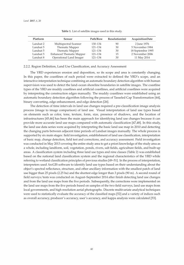
Land 2017, 6, 20

Table 1. List of satellite images used in this study.

Platform Sensor Path/Row Resolution(m) AcquisitionDate

Landsat 2 Multispectral Scanner 130–134 90 2 June 1976Landsat 5 Thematic Mapper 121–134 30 5 November 1984Landsat 5 Thematic Mapper 121–134 30 18 September 1995Landsat 5 Enhanced Thematic Mapper 121–134 15 2 November 2006Landsat 8 Operational Land Imager 121–134 30 11 May 2014

2.2.2. Region Definition, Land Use Classification, and Accuracy Assessment

The YRD experiences erosion and deposition, so its scope and area is constantly changing.In this paper, the coastlines of each period were extracted to defined the YRD’s scope, and aninteractive interpretation technique combining an automatic boundary detection algorithm with humansupervision was used to detect the land–ocean shoreline boundaries in satellite images. The coastlinetypes of the YRD are muddy coastlines and artificial coastlines, and artificial coastlines were acquiredby interpreting the construction edges manually. The muddy coastlines were established using anautomatic boundary detection algorithm following the process of Tasseled Cap Transformation [44],binary converting, edge enhancement, and edge detection [26].

The detection of time intervals in land use changes required a pre-classification image analysisprocess (image to image comparison) of land use. Visual interpretation of land use types basedon elements such as color, tone, texture, form, size, presence of shadows, and the location ofinfrastructures [45,46] has been the main approach for identifying land use changes because it canprovide more accurate land use maps compared with automatic classification [47,48]. In this study,the land use data series were acquired by interpreting the basic land use map in 2010 and detectingthe changing parts between adjacent time periods of Landsat images manually. The whole process issupported by six main stages: field investigation, establishment of land use classification, interpretationof basic map, change detection, field test and corrections, and accuracy assessment. Field investigationwas conducted in May 2013 covering the entire study area to get a priori knowledge of the study area asa whole, including landform, soil, vegetation, ponds, rivers, salt fields, agriculture fields, and built-upareas. A classification system including three land use types and nine classes (Table 2) was establishedbased on the national land classification system and the regional characteristics of the YRD whilereferring to wetland classification principles of previous studies [49–51]. In the process of interpretation,interpreters used ArcGIS software to identify land use types based on their understanding about theobject’s spectral reflectance, structure, and other ancillary information with the smallest patch of landuse bigger than 25 pixels (2.25 ha) and the shortest edge longer than 3 pixels (90 m). A second round offield surveys/tests was conducted on August–September 2014 after finish detecting land use changesand from the land use maps from the five periods. Subsequently, the corrections were implemented onthe land use maps from the five periods based on samples of the two field surveys, land use maps fromlocal governments, and high resolution aerial photographs. Discrete multivariate analytical techniqueswere used to statistically evaluate the accuracy of the classified maps [52] and a variety of indices suchas overall accuracy, producer’s accuracy, user’s accuracy, and kappa analysis were calculated [53].

40

Land 2017, 6, 20

Table 2. The classification key used in the present study.

Land Use Type Land Use Class Description Code

Naturalwetland

Beach Mucky, sandy, and gravel beach located between the estuary and tidal zone BC

Grassland Reeds, cattails (Typha orientalis), and other water-loving plant communitymembers located in rivers and estuaries, reservoirs, and lakes of flood land GL

Bushland Mainly Tamarix bush combined with the alkaline meadows such as Suaedaheteroptera, Salicornia, and Suaeda sals BL

River Permanent and seasonal rivers including their floodplains RV

Artificialwetland

Ditch andponds

A natural or artificial pond or lake used for the storage and regulation of water,including lake, reservoirs, and ponds DP

Aquafarm andsalt pan

Artificial built around shrimp, crabs and other aquatic ponds, etc.; Salt field incoastal areas and near estuaries AS

Non-wetland

Woodland Woodland composed of Populus, Salix, Black locust (Robinia pseudoacacia) andSalix (Salix integra) WL

Cultivated land Arable land that is worked by plowing and sowing and raising crops CL

Constructionland

Man-made impervious surface such as roads, urban, and rural residential land,industrial land, oil field infrastructure, etc. AL

2.3. Quantification of LUCC Based on Transition Matrix

In order to quantify the land use/cover dynamics, post classifications (map to map comparisons)were generated involving the successive sets of images cross-referenced to define land use transitionmatrixes and a series of evaluation indexes. In the process of generating land use transition matrixes,the union scope of five periods with an area of 6398 km2 was taken as the analysis scope and a newland use type of sea surface (SF) was added to represent the land that disappeared as a result ofcoastline erosion.

2.3.1. Land Use Transition Matrix

The land use transition matrix comes from system analysis aiming at quantitative descriptionof the system state and state transition, and it is the most common approach used to compare mapsof different sources, as it provides detailed “from-to” change class information [40]. The traditionalarea cross-tabulation matrix (transition matrix) was computed using overlay functions in ArcGIS 9.3software. The computed transition matrix consists of rows that display categories at time T1 andcolumns that display categories at time T2 (Table 3). The notation Aij is the area of the land thatexperiences transition from category i to category j. The diagonal elements (i.e., Aii) indicate the areaof the landscape that shows persistence of category i. Entries off the diagonal indicate a transitionfrom category i to a different category j. The area of the landscape in category i in time T1 (Ai+) is thesum of Aij over all j. Similarly, the area of the landscape in category j in time T2 (A+j) is the sum of Aij

over all i. The losses (Ai+ − Aii) were calculated as the differences between row totals and persistence.The gains (A+i − Aii) were calculated as the differences between the column totals and persistence.

Table 3. A sample of land use transition matrix.

T2Ai+ Loss

L1 L2 . . . Ln

T1

L1 A11 A12 . . . A1n A1+ A1+ − A11L2 A21 A22 . . . A2n A2+ A2+ − A22..

..

..

..

..

..

..

Ln An1 An2 . . . Ann An+ An+ − AnnA+i A+1 A+2 . . . A+n

Gain A+1 − A11 A+2 − A22 . . . A+n − Ann

41

Land 2017, 6, 20

2.3.2. Annual Rate of Change

The annual rate of change (RCi) for each land cover category i was calculated as [5,54]:

RCi = ((A+i/Ai+)1

T2−T1 − 1)× 100% (1)

where Ai+ and A+i are the areas (in ha) of a cover class at years T1 (initial time) and T2 (next timestep), respectively.

2.3.3. Stability Grade

To expresses the proportion of the landscape category i that had not experienced a transition toany different category of land use, the indicator stability grade (SGi) was defined as Equation (2) andthe total stability grade of the region (SG) was defined as Equation (3) [11]:

SGi =2 × Aii

A+i + Ai+× 100% (2)

SG =n

∑i=1

Aii/n

∑i=1

A+i × 100% (3)

2.3.4. Swap Change (SW) Percentage

Swap was a component of change which implied that a given area of a category was lost at onelocation, while the same area was gained at a different location. The amount of swap was calculated astwo times the minimum of the gain and loss [53]. The total change for each land class was calculatedas either the sum of the net change and the swap or the sum of the gains and losses. The percentage ofswap change (Rsw) was calculated as follow [11,40]:

Rsw =2 × Min(A+j − Ajj, Aj+ − Ajj)

A+j + Aj+ − 2Ajj× 100 (4)

2.3.5. Selection of Main Transition

Main transitions were identified as dominant conversions with bigger proportions of the totalchange. The proportion of the land (Pij) that experiences transition from category i to category jwas calculated, and the transitions with the proportion values larger than the average values wereselected as the main transition. The proportion of the transition and the comparison with the averageproportion were defined as follows in Equation (5):

⎧⎨⎩

Pij = Aij/n∑

i=1Aij × 100% i �= j

Pij >100%

n×(n−1)

(5)

in which n represents the number of land types.

2.4. Trajectories of Wetland Change

Swetnam [55] presented a method to explore land use change characteristics or trajectory usingthe combinations of the three spatial indices (similarity, turnover, and diversity) to classify the landuse change into six groups: stepped, cyclical, dynamic, no constant trend (NCT), and (stable) [56].In this study, trajectory analysis was made for natural wetland, artificial wetland, and non-wetlandclasses because of their ecological importance. Additionally, the original six groups were clustered andreclassified in the aspect of wetland landscape change. With three land cover classes (natural wetland,artificial wetland, and non-wetland classes) and five temporal image dates (1976, 1984, 1995, 2006,

42

Land 2017, 6, 20

and 2014), 61 out of 243 possible wetland land cover change trajectories were found. Finally, similartrajectories were clustered, resulting in six classes (Figure 2 and Table 4).

Figure 2. Land use maps based on image classifications by year: (a) 1976; (b) 1984; (c) 1995; (d) 2006;(e) 2014.

Table 4. Wetland change trajectories between 1976 and 2014.

No. Description Trajectories *

1 Stable wetland WWWWW, RRRRR

2 wetlandformation/restoration

NNNNR, NNNNW, NNNRR, NNNWW, NNRRR, NNWWW, NRRRR,NWWWW, NWNNW, NWNWW, NWWNW, NWWWW, RRNWW,WNNWW, WNWNW, WNWWW, WWNNW, WWNRR, WWRNR

3 Wetlandartificialization

NNNWR, NNWRR, NWNWR, NWRRR, NWWRR, NWWWR, WNNWR,WNRRR, WRRRR, WWNWR, WWRRR, WWWNR, WWWRR, WWWWR

4 Old degradation NRNNN, NWNNN, RRNNN, WNNNN, WRNNN, WWNNN

5 Recent degradationNNWNN, NNWRN, NNWWN, NRRNN, NRWNN, NRWWN, NWNWN,

NWWNN, NWWWN, RRRNN, RRWWN, WNNWN, WNWNN, WNWWN,WWNWN, WWRNN, WWRRN, WWWNN, WWWRN, WWWWN

6 Non-wetland NNNN

* The sequence represents the time periods 1976, 1984, 1995, 2006, and 2014. “W” stands for natural wetland class,“R” stands for artificial wetland, and “N” stands for non-wetland class.

43

Land 2017, 6, 20

3. Results

3.1. Accuracy Assessment

Figure 2 depicts the classified maps for 1976, 1984, 1995, 2006, and 2014. According to theconfusion matrix report (Table 5), 90.62% overall accuracy and a Kappa Coefficient (KC) value of 0.89were attained for the 2014 classified map. Similarly, overall classification accuracy levels achievedwere 91.63% (with a KC of 0.90) for the 2006, 94.74% (with KC of 0.94) for the 1995, 91.43% (with KC of0.89) for the 1984, and 93.16% (with KC of 0.91) for the 1976 image classifications. In general, the mapsmet the minimum accuracy requirements to be used for the subsequent post-classification operations.

Table 5. Confusion matrix (error matrix) for the 2014 classification map.

Classified Data BC GL BL RV DP AS CL WL ALRowTotal

User’sAccuracy

BC 40 2 2 2 46 87%GL 28 2 2 32 88%BL 2 27 1 30 90%RV 20 2 22 91%DP 1 18 19 95%AS 1 2 1 56 60 93%CL 1 3 2 1 87 94 93%WL 2 1 23 26 88%AL 2 2 1 39 44 89%

Column total 44 37 36 21 22 57 90 23 43 373Producer‘s accuracy 87% 88% 90% 91% 95% 93% 93% 88% 89% 91%

Overall accuracy = 90.62%, KC =0.89.

3.2. Temporal Patterns for Changes in Land Use

Figure 2 presents the land use classification for the five years/moments of image analysis(1976, 1984, 1995, 2006, and 2014). The cartographic outputs show a large change in different sectors ofthe YRD, with diverse trajectories. The analysis indicates some systematic transitions involving greatchanges of coastline shapes, as well as an increase in artificial wetland and construction land withurbanization and wetland artificialization characteristics. A more detailed observation emphasizesthat the landscape change is relevant, involving a significant decrease in the natural wetland area,in particular the beach, grassland, and bushland, an increase in construction areas, and a largetransformation from natural wetland to artificial wetland.

Table 6 shows the evolution of land use and occupation in the YRD, as represented by thelandscape patterns for the period analyzed. In analyzing areas of land use, certain systematic transitionswere observed, namely: an increase in artificial wetland with ditch, pond, aquafarm, and salt panunits; an increase in artificial land involving artificial wetland and non-wetland; a decrease of naturalwetland, in particular the areas and percentages of beach, grassland, and bushland. For naturalwetland, the area and percentage of beach, grassland, and bushland kept decreasing from 1976 to2014, while the river increased slightly. The total area of natural wetland decreased from 3488.2 km2 in1976 to 1120.9 km2 in 2014, with the annual decreasing rate of 62.3 km2/year. In contrast, both ditchand ponds (DP) and aquafarm and salt plains (AS) of artificial wetland kept increasing and showeda relative growth of 15 times of the original state. The areas of cultivated land and woodland bothincreased from 1976 to 2014 in spite of experiencing a decrease in the period 1995–2006. The area ofconstruction land kept increasing from 1976 to 2014, and showed a relative growth of 274% from theoriginal state.

44

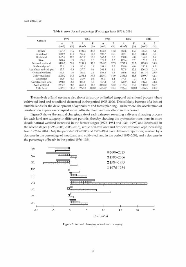
Land 2017, 6, 20

Table 6. Area (A) and percentage (P) changes from 1976 to 2014.

Classes1976 1984 1995 2006 2014

A(km2)

P(%)

A(km2)

P(%)

A(km2)

P(%)

A(km2)

P(%)

A(km2)

P(%)

Beach 1991.5 34.2 1402.6 23.5 852.9 14.2 813.6 13.7 480.6 8.1Grassland 639.9 11.0 724.2 12.2 903.7 15.1 612.1 10.3 342.2 5.8Bushland 747.4 12.8 891.2 15.0 362.3 6.0 238.0 4.0 169.6 2.9

River 109.4 1.9 136.8 2.3 129.3 2.2 129.4 2.2 128.5 2.2Natural wetland 3488.2 59.9 3154.9 53.0 2248.2 37.5 1792.9 30.2 1120.9 18.9Ditch and pond 75.6 1.3 112.6 1.9 194.1 3.2 238.8 4.0 250.1 4.2

Aquafarm and salt pan 17.7 0.3 37.7 0.6 364.3 6.1 717.8 12.1 1261.3 21.3Artificial wetland 93.3 1.6 150.3 2.5 558.3 9.3 956.6 16.1 1511.4 25.5Cultivated land 2030.2 34.9 2351.4 39.5 2636.1 44.0 2481.6 41.8 2499.7 42.1

Woodland 14.8 0.3 36.9 0.6 85.0 1.4 77.5 1.3 81.8 1.4Construction land 192.8 3.3 264.8 4.4 467.2 7.8 628.9 10.6 722.6 12.2

Non-wetland 2237.9 38.5 2653.1 44.5 3188.2 53.2 3188.0 53.7 3304.2 55.7YRD Area 5819.3 100.0 5958.2 100.0 5994.7 100.0 5937.5 100.0 5936.5 100.0

The analysis of land use areas also shows an abrupt or limited temporal transitional process wherecultivated land and woodland decreased in the period 1995–2006. This is likely because of a lack ofsuitable lands for the development of agriculture and forest planting. Furthermore, the acceleration ofconstruction expansion occupied more cultivated land and woodland in this period.

Figure 3 shows the annual changing rate of each category, revealing a diverse changing processfor each land use category in different periods, thereby showing the systematic transitions in moredetail: natural wetland increased in the former stages (1976–1984 and 1984–1995) and decreased inthe recent stages (1995–2006, 2006–2015), while non-wetland and artificial wetland kept increasingfrom 1976 to 2014. Only the periods 1995–2006 and 1976–1984 have different trajectories, marked by adecrease in the percentage of woodland and cultivated land in the period 1995–2006, and a decrease inthe percentage of beach in the period 1976–1984.

Figure 3. Annual changing rate of each category.

45

Land 2017, 6, 20

Although the increase of non-wetland and artificial wetland (on the left-hand side) in contrast tonatural wetland areas (on the right-hand side) was clear, the annual changing rates appeared differentin different periods from 1976 to 2014. During the period 1976–1984, woodland, cultivated land, andditch and ponds had the biggest annual increasing rate, while the river, bushland, and grasslandclassifications all had a positive annual increasing rate. During the 1984–1995 period, constructionland and aquafarm and salt pans had the biggest annual increasing rates, while bushland had thebiggest annual decreasing rate, and grassland had a positive annual increasing rate. During theperiod 1995–2006, none of the categories had the biggest annual increasing or increasing rate, but thewoodland and cultivated land annual changing rates were negative, showing a an opposite changingtrend. During 2006–2014, beach land and grassland had the biggest annual increasing rate.

3.3. Dynamic Analysis of Changes in Land Use

3.3.1. Stability Grade

The transformation matrices for 1976–1984, 1984–1995, 1995–2006, and 2006–2014 subsequentlymade possible a detailed study of the dynamics of land use and occupation in five periods of analysis.The stability grade (SG) of the land cover was calculated for each transformation matrix to show thepercentage of landscape that remained unchanged. About 73.2%, 62.3%, 81.2%, and 82.8% of thelandscape persisted or 28.0%, 39.3%, 18.8%, and 17.2% of the landscape has changed during the period1976–1984, 1984–1995, 1995–2006, and 2006–2014, respectively, indicating that persistence dominatesin all periods. However, the stability during the period 1976–2014 was only 38.0%, and 62.1% of theYRD experienced transition from one category to a different category. The stability grade values foreach land use type were calculated and are shown in Figure 4. There was a relative small stabilitygrade in the period 1984–1995 for all the land use types in comparison with the other three periods.The stability grade values were bigger than 50% except those of grassland, bushland, woodland, andaquafarm and salt pans in the period 1984–1995, which also indicated that persistence dominates in allperiods. Nevertheless, only cultivated land and river had stability grade values bigger than 60% inthe whole period of 1976–2014. Therefore, the cumulative process of LUCC has resulted in the YRDhaving undergone significant land use/cover alterations over the 38 years considered. The analysisalso showed that the land use class transfer does not take place all at once, but in a set of smallsequential steps.

Figure 4. Stability grade values for each land use type in different periods.

3.3.2. Swap Change

Percentages of swap change for each land use type in different periods and the whole YRD werecalculated and are shown in Figures 4 and 5. Swap change accounted for 57.6%, 53.4%, 46.0%, and34.8% of total change during the periods 1976–1984, 1984–1995, 1995–2006, and 2006–2014, respectively,

46

Land 2017, 6, 20

showing a LUCC evolution process from the change attributable to location to the change attributableto quantity. Swap change is greater than net change in the period before 1995, suggesting that theimportance of the swapping component and common methods of land use/cover change studywould miss these dynamics. During the period 1976–2014, changes in construction land experiencednet change dynamics, whereas the changes in all other categories consisted of both swap and netchanges. The river and sea surface both had relatively larger percentages of swap change, reflectingthe transforming effects on the trail channels by the Yellow River Mouth and the coastline changecaused by the accumulation of sediment and erosion. The type of change that each land use/coverexperienced differs from period to period, but landscape types of natural wetland tend to have biggerswap changes than artificial land types such as aquafarms, salt pans, and construction lands.

0

20

40

60

80

100

120

BC GL BL RV DP AS CL WL AL SF

Land use type

Perc

enta

ge o

f sw

ap c

hang

e(%

) 1976-1984 1984-1995 1995-2006

2006-2014 1976-2014

Figure 5. Percentages of swap change for each land use type in different periods.

3.3.3. Main Transitions

The landscapes of wetland, cultivated land, and construction land are closely related to ecologyprotection and human's survival and production depends. Based on the increase or decrease of thesethree landscapes, the main transitions were reclassified into seven categories, namely cultivated landto wetland, construction land expansion, wetland to cultivated land, internal transformation of naturalwetland, natural wetland formation, artificialization of natural wetland, and coastline erosion.

Figure 6 shows the distributions of the main transition categories in different period from 1976to 2014, and Table 7 shows the percentages and detailed compositions of theses main transitions.The transitions between sea surface and beach land were included in the main transitions in thefour periods, showing that the YRD has been experiencing the process of erosion and sedimentaccumulation. The main transition categories of land use dynamics from 1976 to 2014 were theartificialization of natural wetland, transition from wetland to cultivated land, and constructionland expansion, with the percentages of 32.6%, 20.3%, and 12.9%, respectively. During the periods1976–1984 and 1984–1995, the main transition categories were characterized by internal transformationof natural wetland, transition from wetland to cultivated land, and natural wetland’s formation anderosion. However, the main transition categories are predominantly natural wetland artificializationand construction expansion in the periods 1995–2006 and 2006–2014. The change of main transitioncategory also revealed a continuous increase in artificial areas, indicating that land use trajectorieswere veering towards artificial surfaces.

47

Land 2017, 6, 20

Figure 6. Distributions of main transition categories in different periods from 1976 to 2014.

48

Land 2017, 6, 20

Ta

ble

7.

The

perc

enta

ges

(P/%

)and

deta

ilco

mpo

siti

ons

ofm

ain

tran

siti

ons

indi

ffer

entp

erio

dfr

om19

76to

2014

.

Ma

inT

ran

siti

on

Ty

pe

19

76

–1

98

41

98

4–

19

95

19

95

–2

00

62

00

6–

20

14

19

76

–2

01

4

PD

eta

ils

PD

eta

ils

PD

eta

ils

PD

eta

ils

PD

eta

ils

Cul

tiva

ted

land

tow

etla

nd1.

4C

L-D

P(1

.4)

1.2

CL-

DP

(1.2

)6.

5C

L-D

P(3

.2)

CL-

GL

(1.8

)C

L-A

S(1

.5)

2.6

CL-

GL

(1.5

)C

L-A

S(1

.1)

1.4

CL-

DP

(1.4

)

Con

stru

ctio

nla

ndex

pans

ion

3.0

CL-

AL

(3.0

)6.

2C

L-A

L(3

.9)

BC-A

L(2

.3)

13.1

CL-

AL

(11.

6)BC

-AL

(1.5

)8.

1C

L-A

L(3

.1)

GL-

AL

(2.6

)BC

-AL

(2.4

)12

.9

CL-

AL

(6.9

)BC

-AL

(2.1

)G

L-A

L(1

.5)

SF-A

L(1

.3)

BL-A

L(1

.2)

Wet

land

tocu

ltiv

ated

land

23.3

BC-C

L(1

7.4)

GL-

CL

(3.3

)BL

-CL

(2.6

)17

.9G

L-C

L(8

.6)

BL-C

L(8

.0)

DP-

CL

(1.3

)4.

1G

L-C

L(4

.1)

9.4

GL-

CL

(7.9

)A

S-C

L(1

.5)

20.3

BC-C

L(8

.4)

GL-

CL

(6.7

)BL

-CL

(5.2

)

Inte

rnal

tran

sfor

mat

ion

ofna

tura

lw

etla

nd35

.7

BC-B

L(1

4.1)

BC-G

L(7

.0)

BL-G

L(6

.0)

GL-

BL(4

.0)

BL-G

L(3

.1)

BC-R

V(1

.5)

33.0

BL-G

L(1

3.6)

BC-B

L(1

0.5)

BC-G

L(7

.1)

BL-B

C(1

.8)

24.0

BL-B

C(7

.3)

GL-

BC(6

.7)

BC-B

L(3

.6)

BL-G

L(3

.5)

GL-

BL(2

.9)

5.1

BL-B

C(2

.0)

BC-B

L(1

.8)

BC-G

L(1

.3)

4.7

BC-G

L(2

.9)

BL-G

L(1

.8)

Nat

ural

wet

land

form

atio

n18

.1SF

-BC

(14.

4)SF

-BL

(2.4

)SF

-GL

(1.3

)6.

2SF

-BC

(6.2

)5.

3SF

-BC

(5.3

)5.

0SF

-BC

(3.9

)SF

-BL

(1.1

)8.

5SF

-BC

(5.0

)SF

-BL

(2.3

)SF

-GL

(1.2

)

Art

ifici

aliz

atio

nof

natu

ral

wet

land

17.8

BL-A

S(5

.8)

BC-A

S(5

.5)

GL-

AS

(2.8

)BL

-DP

(2.5

)G

L-D

P(1

.2)

29.4

GL-

AS

(15.

5)BC

-AS

(7.9

)BL

-AS

(6.0

)52

.9BC

-AS

(27.

6)G

L-A

S(1

6.1)

BL-A

S(9

.2)

32.6

BC-A

S(1

9.1)

BL-A

S(8

.0)

GL-

AS

(3.5

)BC

-DP

(2.0

)

Coa

stlin

eer

osio

n10

.1BC

-SF

(10.

1)5.

6BC

-SF

(5.6

)11

.4BC

-SF

(11.

4)5.

9BC

-SF

(5.9

)8.

0BC

-SF

(8.0

)To

tal

91.6

87.9

93.8

89.0

88.4

49

Land 2017, 6, 20

Although the main transition categories were characterized by artificialization, the compositiondetails of main transition categories appeared different in different periods from 1976 to 2014.During 1976–2014, the form of natural wetland artificialization was mainly aquafarm and salt pan.The form of the transition from cultivated land to wetland was ditches and ponds in the period1976–1984 and 1984–1995, The transitions of cultivated land to wetland were mainly in the formof the building of ditches and ponds in the periods 1976–1984 and 1984–1995, and there weresmall percentages of transitions from cultivated land to grassland and aquafarm land in the periods1995–2006 and 2006–2014 which were caused by the policy of returning farmland to wetland and anew agriculture-fishery mode. The main source of construction land expansion was cultivated landin the four periods, but beach land and grassland also became part of the main sources in the lastthree periods. Both the composition types and percentages of natural wetland internal transformationdecreased from early periods to late periods. The composition types only included the transition frombeach to grassland and the transition from bushland to grassland. These results revealed that naturalwetland internal transformation was the medium process of transition from the natural wetland toartificial land. The transitions from the beach, grassland, and bushland to cultivated land were themain transitions in the four periods, showing that the YRD had continuous agricultural developmentprocess from 1976 to 2014. The main land use types for the transitions from natural wetland to artificialwetland were aquafarm and salt pan which occurred in the last three periods. The main occupationland of construction land was cultivated land in the former periods (1976–1984 and 1984–1995), whilegrassland became the other main occupation source in the last period (2006–2014). The irrigation andwater conservancy construction in the period 1995–2006 was one of the major types of transfer.

3.4. Trajectory of Wetland Change

The maps of six wetland trajectory types were shown in Figure 5, and areas and percentages ofland use type in 1976 and 2014 for each wetland trajectory types were shown in Table 6. The resultsshow that the classes of wetland changed greatly, even for the area percentages of wetland classes ofstable wetland. The area of stable wetland was 746.7 km2, accounting for 28.4% of the total wetlandarea in 2014. Wetland artificialization was mainly distributed beside stable wetland had an area of1361.4km2 and the main destination class was aquafarm and salt pan, accounting for 89.2%. Olddegradation mainly distributed along the Yellow River and its old course was in the north (DiaokouDitch). Recent degradations displayed scattered distribution except for a concentrated distributionoutside the mouth of the Yellow River in the east. The area percentages for the old degraded andrecently degraded wetlands were caused by coastline change (percentage to sea surface in 2014) whichwere 23.3% and 42.5%, respectively, which indicated that human activities other than coastline changewere the main driving forces of wetland degradation. Wetland formation/restoration mainly camefrom the result of estuarine deposits in the mouth of the Yellow River (70.6%), followed by reservoirconstruction in the cultivated lands (13.2%).

During 1976–2014, the wetland change in the YRD included wetland formation/restoration,wetland degradation, and wetland artificialization, but the main wetland changes were wetlanddegradation and wetland artificialization (Figure 7 and Table 8). The areas of wetland degradation(1645.1 km2) and wetland artificialization (1361.4 km2) were much greater than that of the wetlandformation/ restoration (524.1 km2).

50

Land 2017, 6, 20

Figure 7. Wetland change trajectory map.

Table 8. Areas and percentages of land use type in 1976 and 2014 for each wetland change type.

Change Type TimeArea(km2)

Percentage (%)

BC GL BL RV DP AS CL WL AL SF

Non-wetland1976

2120.590.2 0.6 9.1 0.1

2014 77.4 1.0 21.7 0.0

Stable wetland1976

746.749.5 16.7 17.1 9.8 5.7 1.2

2014 37.5 33.8 9.2 12.5 5.9 1.0

Old degradation 19761234.4

51.9 20.0 16.7 2.2 2.5 0.7 0.7 5.42014 0.0 59.1 3.6 14.1 23.2

Recent degradation 1976410.6

32.3 21.8 13.0 0.5 0.6 0.1 1.1 30.52014 31.7 4.1 21.7 42.5

Wetlandformation/restoration

1976524.1

2.4 2.5 4.7 19.5 0.3 70.62014 38.3 17.1 19.2 6.7 13.2 5.5

Wetlandartificialization

19761361.4

61.4 12.2 24.7 0.5 0.2 1.02014 10.0 90.0

4. Discussion

The five cartographic outputs for changes in land use underline the major decrease in naturalwetland areas, the increase in artificial wetland and non-wetland, especially in regards to the aquafarms,salt pans, and construction lands. The land use dynamics from 1976 to 2014 are similar with theobservations before 2009 made by Zong [27], Zhang et al. [30], Sun et al. [28], Chen et al. [57], andWang et al. [58]. About 28.0%, 39.3%, 18.8%, and 17.2% of the landscape in the YRD had experienced

51

Land 2017, 6, 20

transition from one category to another category of land use/cover during the periods 1976–1984,1984–1995, 1995–2006, and 2006–2014, respectively, indicating that persistence dominates in eachperiod. However, the cumulative process of LUCCs had made the YRD undergo significant landuse/cover alterations, and about 62.1% of the YRD experienced transition from one category to adifferent category of land use/cover over the 38 years considered. Therefore, the analysis also showedthat the land use class transfer does not take place all at once, but in a set of small sequential steps.

Although an increase in all artificial land types (artificial wetland and non-wetland) was observedfrom 1976 to 2014, the aquafarm and salt pan land classification had the highest annual increasingarea and rate, followed by construction land. The ditches and ponds, woodland, and cultivated landclassifications mainly increased in the former two periods (1976–1984 and 1984 to 1995), and woodlandand cultivated land decreased in the period 1995–2006, which was mainly caused by the occupation ofconstruction land.

Swap change accounted for 57.6%, 53.4%, 46.0%, and 34.8% of total change during the period1976–1984, 1984–1995, 1995–2006, and 2006–2014, respectively, showing a LUCC evolution processfrom the change attributable to location to that attributable to quantity. Swap change is greater thannet change in the period before the 1995, demonstrating the importance of the swapping componentand suggesting that common methods of land use/cover change study would miss these dynamics.The type of change that each land use/cover experienced differs from period to period, but landscapetypes of natural wetland tend to have bigger swap changes than artificial land types such as aquafarm,salt pan, and construction land classifications.

During the periods 1976–1984 and 1984–1995, the main transitions were characterized byinternal transformation of natural wetland, transition from wetland to cultivated land, and naturalwetland’s formation and erosion. However, the main transitions are predominantly natural wetlandartificialization and construction expansion in the period 1995–2006 and 2006–2014. The main transitionvaluation also revealed a continuous increase in artificial areas, indicating that land use trajectorieswere veering towards artificial surfaces. During 1976–2014, the destination of natural wetlandartificialization was mainly aquafarm and salt pan, which will have likely exacerbated land subsidence,sea water invasion, and salinization [34,42,59].

Wetland change trajectory results demonstrate that the main wetland changes were wetlanddegradation and wetland artificialization. The percentages of old degradation and recent degradationtransferred to sea surface were 23.2% and 42.5%, respectively. Meanwhile, the overlay analysis ofwetland change trajectory map and coastline evaluation map shows 73.3% of old degradation wetlandand 53.8% of recent degradation wetland are distributed in the stable land from 1976 to 2014. Therefore,coastline change is the subordinate effect for natural wetland degradation in comparison with humanactivities. The transitions of cultivated land to wetland were mainly a result of the building of ditchesand ponds in the periods 1976–1984 and 1984–1995, and there were small percentages of transitionsfrom cultivated land to grassland and aquafarm land in the periods 1995–2006 and 2006–2014, whichwere caused by the policy of returning farmland to wetland and a new agriculture-fishery mode.

The footprint of human disturbance on the YRD is becoming larger and larger, and theartificialization rate of the YRD increased from 40.1% in 1976 to 81.1% in 2014. The wetlands inthe YRD are experiencing a continuous development and evolution process under the combined effectsof natural factors and human factors. It is certain that the degree of human disturbance tended toincrease with time, and the degree of influence has become deeper and deeper. Currently, the YRD is ina period of rapid development, and large-scale development and construction activities are inevitable.Although the establishment of Binzhou Shell Islands and Wetland Nature Reserve and the YellowRiver Delta Nature Reserve and implementation of wetland restoration projects for the protection ofcoastal wetlands plays important role in preventing wetlands from loss and degradation, the overallloss and degradation trend is unlikely to change in the short-term. As such, the protection of coastalwetland ecological environment remains very difficult and long-term.

52

Land 2017, 6, 20

5. Conclusions

This research quantified the LUCC process, explored the systematic transitions of land cover,and identified wetland change trajectory for the period 1976–2014 in the Yellow River Delta throughenhanced transition matrix and relevant quantitative indicators. This study provides reliable LUCCdata, which is useful for the detection and refinement of conservation policies aimed at protectingestuarine wetland. The main wetland changes were wetland degradation and wetland artificialization,and anthropogenic activities were the major driving forces of wetland degradation. Our findingssuggest that development of salt pan industry and the construction of built spaces occupying naturalwetland needs to be controlled and well managed in order to help maintain the natural habits andmitigate seawater intrusion and soil salinization. Finally, this study highlighted that the identification ofsystematic transitions and their spatial statistical modeling under GIS environment enable researchersand planners to focus on the most important signals of systematic landscape transitions and allow abetter understanding of the proximate causes of changes.

Acknowledgments: This research was supported by the National Natural Science Foundation of China(No. 41401663), the Natural Science Foundation of Shandong Province (No. ZR2016EEM18), the ScienceFoundation of Ministry of Education of China (No. 12YJC790254), and the Excellent Young Scholars ResearchFund of Shandong Normal University. We would like to thank the Editor and the anonymous reviewers forproviding constructive comments and suggestions.

Author Contributions: Baolei Zhang, Shumin Zhang, and Chaoyang Feng contributed to the research design.Qiaoyun Zhang contributed to data processing and analysis of datasets. Shumin Zhang and Baolei Zhangwrote the paper. Qingyu Feng and Chaoyang Feng reviewed the manuscript and offered useful insights forits improvement.


Abbreviations

The following abbreviations are used in this manuscript:

YRD Yellow River DeltaLUCC Land use/cover changeKC Kappa coefficientSG Stability gradeSW Swap changeBC BeachGL GrasslandBL BushlandRV RiverDP Ditch and pondsAS Aquafarm and salt panWL WoodlandCL Cultivated landAL Construction landSF Sea surface

References

1. Turner, B.L., II; Skole, D.; Sanderson, S.; Fischer, G.; Fresco, L.; Leemans, R. Land-Use and Land-CoverChange-Science/Research Plan; IGBP Report No.35 and HDP Report No.7; IGBP and HDP Secretariats:Stochkholm, Sweden; Geneva, Switzerland, 1995.

2. Houghton, R.A.; Hackler, J.L.; Lawrence, K.T. The US carbon budget: Contribution from land use change.Science 1999, 285, 574–578. [CrossRef] [PubMed]

3. Shi, P.J.; Gong, P.; Li, X.B. Methods and Practice of Land Use Changes in Research; Science Press: Beijing,China, 2000. (In Chinese)

53

Land 2017, 6, 20

4. Lawrence, P.L.; Chase, T.N. Investigating the climate impacts of global land cover change in the communityclimate system model. Int. J. Clim. 2010, 30, 2066–2087. [CrossRef]

5. Liu, J.Y.; Liu, M.L.; Deng, X.Z.; Zhuang, D.F.; Zhang, Z.X.; Luo, D. The land use and land cover changedatabase and its relative studies in China. J. Geogr. Sci. 2002, 12, 275–282.

6. Dewan, A.M.; Yamaguchi, Y.; Rahman, M.Z. Dynamics of land use/cover changes and the Analysis ofLandscape fragmentation in Dhaka Metropolitan, Bangladesh. GeoJournal 2012, 77, 315–330. [CrossRef]

7. Antrop, M. Why landscapes of the past are important for the future. Landsc. Urban Plan. 2005, 70, 21–34.[CrossRef]

8. Hasse, J.E.; Lathrop, R.G. Land resource impact indicators of urban sprawl. Appl. Geogr. 2003, 23, 159e175.[CrossRef]

9. Tavares, A.O.; Pato, R.L.; Magalhães, M.C. Spatial and temporal land use change and occupation over thelast half century in a peri-urban area. Appl. Geogr. 2012, 34, 432–444. [CrossRef]

10. Li, S.N.; Wang, G.X.; Deng, W.; Hu, Y.M.; Hu, W.W. Influence of hydrology process on wetland landscapepattern: A case study in the Yellow River Delta. Ecol. Eng. 2009, 35, 1719–1726. [CrossRef]

11. Pontius, R.G., Jr.; Shusas, E.; McEachern, M. Detecting important categorical land changes while accountingfor persistence. Agric. Ecosyst. Environ. 2004, 101, 251–268. [CrossRef]

12. Braimoh, A.K. Random and systematic land-cover transitions in northern Ghana. Agric. Ecosyst. Environ.2006, 113, 254–263. [CrossRef]

13. Lambin, E.F.; Geist, H.J.; Lepers, E. Dynamics of land-use and land-cover change in tropical regions. Ann. Rev.Environ. Resour. 2003, 28, 205–241. [CrossRef]

14. Lu, D.; Mausel, P.; Brondízio, E.; Moran, E. Change detection techniques. Int. J. Remote Sens. 2004, 25,2365–2407. [CrossRef]

15. Pontius, R.G.; Petrova, S.H. Assessing a predictive model of land change using uncertain data.Environ. Model. Softw. 2010, 25, 299–309. [CrossRef]

16. Manandhar, R.; Odeh, I.O.A.; Pontius, R.G. Analysis of twenty years of categorical land transitions in thelower hunter of new South Wales, Australia. Agric. Ecosyst. Environ. 2010, 135, 336–346. [CrossRef]

17. Isabel, P.; Cunha, M.; Pereira, L. Remote sensing based indicators of changes in a mountain rural landscapeof northeast Portugal. Appl. Geogr. 2011, 31, 871–880.

18. Johnson, B.G.; Zuleta, G.A. Land-use land-cover change and ecosystem loss in the Espinal ecoregion,Argentina. Agric. Ecosyst. Environ. 2013, 181, 31–40. [CrossRef]

19. Liu, R.; Zhu, D.L. Methods for detecting land use changes based on the land use transition matrix. Resour. Sci.2010, 32, 1544–1550.

20. Zhou, Q.; Li, B.; Kurban, A. Trajectory analysis of land cover change in arid environment of China. Int. J.Remote Sens. 2008, 29, 1093–1107. [CrossRef]

21. Wang, H.; Gao, Y.; Pu, R.L.; Ren, L.L.; Kong, Y.; Li, H.; Li, L. Natural and anthropogenic influences on ared-crowned crane habitat in the Yellow River Delta Natural Reserve, 1992–2008. Environ. Monit. Assess.2014, 186, 4013–4028. [CrossRef] [PubMed]

22. Wang, H.; Gao, Y.; Pu, R.L.; Ren, L.L.; Kong, Y.; Li, H.; Li, L. Assessment of the red-crowned crane habitat inthe Yellow River Delta Nature Reserve, East China. Reg. Environ. Chang. 2012, 31, 115–123. [CrossRef]

23. Bi, X.L.; Wang, B.; Lu, Q.S. Fragmentation effects of oil wells and roads on the Yellow River Delta, North China.Ocean Coast Manag. 2011, 54, 256–264. [CrossRef]

24. Fan, H.; Huang, H.J. Response of coastal marine eco-environment to river fluxes into the sea: A case study ofthe Huanghe (Yellow) River mouth and adjacent waters. Mar. Environ. Res. 2008, 65, 378–387. [CrossRef][PubMed]

25. He, X.H.; Hörmann, G.; Strehmel, A.; Guo, H.L.; Fohrer, N. Natural and Anthropogenic Causes of VegetationChanges in Riparian Wetlands Along the Lower Reaches of the Yellow River, China. Wetlands 2015, 35,391–399. [CrossRef]

26. Kong, D.X.; Miao, C.Y.; Borthwick, A.G.L.; Duan, Q.Y.; Liu, H.; Sun, Q.H.; Ye, A.Z.; Di, Z.H.; Gong, W.Evolution of the Yellow River Delta and its relationship with runoff and sediment load from 1983 to 2011.J. Hydrol. 2015, 520, 157–167. [CrossRef]

27. Zong, X.Y. Study on Dynamic Changes of Wetland Landscape Pattern in Yellow River Delta. J. Geo-inf. Sci.2009, 11, 91–97. [CrossRef]

54

Land 2017, 6, 20

28. Sun, X.Y.; Su, F.Z.; Lv, T.T. Analysis of temporal-spatial changes in wetlands over the Yellow River estuary.Resour. Sci. 2011, 33, 2277–2284.

29. Zhang, B.L.; Yin, L.; Zhang, S.M.; Feng, C.Y. Assessment on characteristics of LUCC process based oncomplex network in Modern Yellow River Delta, Shandong Province of China. Earth Sci. Inform. 2016, 9,83–93. [CrossRef]

30. Zhang, X.L.; Ye, S.Y.; Yin, P. Characters and successions of natural wetland vegetation in Yellow River Delta.Ecol. Environ. Sci. 2009, 18, 292–298.

31. Li, S.N.; Wang, G.X.; Deng, W.; Hu, Y.M. Effects of runoff and sediment variation on landscape pattern in theYellow River Delta of China. Adv. Water Sci. 2009, 20, 325–331.

32. Zhang, X.L.; Li, P.; Liu, L.J.; Li, P.Y. Degradation assessment of Modern Yellow River Delta coastal wetland.Mar. Sci. Bull. 2010, 29, 685–689.

33. Hong, J.; Lu, X.N.; Wang, L.L. Quantitative analysis of the factors driving evolution in the Yellow River DeltaWetand in the past 40 years. Acta Ecol. Sin. 2016, 36, 924–935.

34. Ottinger, M.; Kuenzer, C.; Liu, G.H.; Wang, S.Q.; Dech, S. Monitoring land cover dynamics in the YellowRiver Delta from 1995 to 2010 based on Landsat 5 TM. Appl. Geogr. 2013, 44, 53–68. [CrossRef]

35. Fang, H.; Liu, G.; Kearney, M. Georelational analysis of soil type, soil salt content, landform, and land use inthe Yellow River Delta, China. Environ. Manag. 2005, 35, 72–83. [CrossRef]

36. Xu, J.X. A study of thresholds of runoff and sediment for the land accretion of the Yellow River Delta.Geogr. Res. 2002, 21, 163–170.

37. Zhao, X.S.; Cui, B.S.; Sun, T.; He, Q. The relationship between the spatial distribution of vegetation andsoil environmental factors in the tidal creek areas of the Yellow River Delta. Ecol. Environ. Sci. 2010, 19,1855–1861.

38. Yu, J.B.; Chen, X.B.; Sun, Z.G.; Xie, W.J.; Mao, P.L.; Wu, C.F.; Dong, H.F.; Mu, X.J.; Li, Y.Z.; Guan, B.; et al.The spatial distribution characteristics of soil nutrients in new-born coastal wetland in Yellow River delta.Acta Sci. Circumst. 2010, 30, 855–861.

39. Kuenzer, C.; Ottinger, M.; Liu, G.H.; Sun, B.; Baumhauer, R.; Dech, S. Earth observation-based coastal zonemonitoring of the Yellow River Delta: Dynamics in China's second largest oil producing region overfourdecades. Appl. Geogr. 2014, 55, 92–107. [CrossRef]

40. Teferi, E.; Bewket, W.; Uhlenbrook, S.; Wenninger, J. Understanding recent land use and land cover dynamicsin the source region of the Upper Blue Nile, Ethiopia: Spatially explicit statistical modeling of systematictransitions. Agric. Ecosyst. Environ. 2013, 165, 98–117. [CrossRef]

41. Wan, H. Research on Wetland Information Extraction and Analysis of Yellow River Delta Based on RS and GIS;China University of Petroleum (East China): Dongying, China, 2009.

42. Liu, G.L.; Zhang, L.C.; Zhang, Q.; Musyimi, Z.; Jiang, Q.H. Spatio–temporal dynamics of wetland landscapepatterns based on remote sensing in Yellow River Delta,China. Wetlands 2014, 34, 787–801. [CrossRef]

43. Lavery, P.; Pattiaratchi, C.; Wyllie, A.; Hick, P. Water-Quality Monitoring in Estuarine Waters Using theLandsat Thematic Mapper. Remote Sens. Environ. 1993, 46, 268–280. [CrossRef]

44. Fan, Y.; Zhang, S.; Hou, C.; Zhang, L. Study on Method of Coastline Extraction from RemoteSensing—Taking Yellow River Mouth Reach and Diaokou Reach of Yellow River Delta Area as an Example.Remote Sens. Inform. 2009, 8, 67–70.

45. Piwowar, J.M. Digital Image Analysis. In Remote Sensing for GIS Managers; Aronoff, S., Ed.; ESRI Press:Redlands, CA, USA, 2005.

46. Ke, C.Q.; Zhang, D.; Wang, F.Q.; Chen, S.X.; Schmullius, C.; Boerner, W.M.; Wang, H. Analyzing coastalwetland change in the Yancheng National Nature Reserve, China. Reg. Environ. Chang. 2011, 11, 161–173.[CrossRef]

47. Liu, J.Y.; Liu, M.L.; Tian, H.Q.; Zhuang, D.F.; Zhang, Z.X.; Zhang, W.; Tang, X.M.; Deng, X.Z. Spatialand temporal patterns of China’s cropland during 1990–2000: An analysis based on Landsat TM data.Remote Sens. Environ. 2005, 98, 442–456. [CrossRef]

48. Wang, W.J.; Zhang, C.R.; Allen, J.M.; Li, W.D.; Boyer, M.A.; Segerson, K.; Silander, J.A., Jr. Analysis andprediction of land use changes related to invasive species and major driving forces in the state of Connecticut.Land 2016, 5, 25. [CrossRef]

49. Ni, J.R.; Yin, K.Q.; Zhao, Z.J. Comprehensive classification for wetlands I. Classification. J. Nat. Resour. 1998,13, 214–221.

55

Land 2017, 6, 20

50. Zhao, H.T.; Wang, L.R. Coastal wetland types in China. Mar. Sci. Bull. 2000, 19, 72–81.51. Tang, X.P.; Huang, G.L. Study on classification system for wetland types in China. For. Res. 2003, 16, 531–539.52. Foody, G.M. Status of land cover classification accuracy assessment. Remote Sens. Environ. 2002, 80, 185–201.

[CrossRef]53. Stehman, S.V. Selecting and interpreting measures of thematic classification accuracy. Remote Sens. Environ.

1997, 62, 77–89. [CrossRef]54. Aldwaik, S.Z.; Pontius, R.G. Intensity analysis to unify measurements of size and stationarity of land changes

by interval, category, and transition. Landsc. Urban Plan. 2012, 106, 103–114. [CrossRef]55. Swetnam, R.D. Rural land use in England and Wales between 1930 and 1998: Mapping trajectories of change

with a high resolution spatio-temporal dataset. Landsc. Urban Plan. 2007, 81, 91–103. [CrossRef]56. Wang, D.C.; Gong, J.H.; Chen, L.D.; Zhang, L.H.; Song, Y.Q.; Yue, Y.J. Spatio-temporal pattern analysis

of land use/cover change trajectories in Xihe watershed. Int. J. Appl. Earth Obs. Geoinf. 2012, 4, 12–21.[CrossRef]

57. Chen, J.; Wang, S.Y.; Mao, Z.P. Monitoring wetland changes in Yellow River Delta by remote sensing during1976–2008. Prog. Geogr. 2011, 30, 585–592.

58. Wang, Y.L.; Yu, J.B.; Dong, H.F.; Li, Y.Z.; Zhou, D.; Fu, Y.Q.; Han, G.X.; Mao, P.L. Spatial Evolution ofLandscape Pattern of Coastal Wetlands in Yellow River Delta. Sci. Geogr. Sin. 2012, 32, 717–724.

59. Higgins, S.; Overeem, I.; Tanaka, A.; Syvitski, J.P.M. Land subsidence at aquaculture facilities in the YellowRiver delta, China. Featur. Geophys. Res. Lett. 2013, 40, 3898–3902. [CrossRef]


56

land

Article

Monitoring Urban Growth and the Nepal Earthquake2015 for Sustainability of Kathmandu Valley, Nepal

Bhagawat Rimal 1, Lifu Zhang 1,*, Dongjie Fu 2, Ripu Kunwar 3 and Yongguang Zhai 1

1 The State Key Laboratory of Remote Sensing Science, Institute of Remote Sensing and Digital Earth, ChineseAcademy of Sciences, Beijing 100101, China; [email protected] (B.R.); [email protected] (Y.Z.)

2 State Key Laboratory of Resource and Environmental Information System, Institute of Geographic Sciencesand Natural Resources Research, Chinese Academy of Sciences, Beijing 100101, China; [email protected]

3 Cultural and Spatial Ecology, Department of Geosciences, Florida Atlantic University, Boca Raton, FL 33431,USA; [email protected]


Academic Editors: Andrew Millington, Harini Nagendra, Monika Kopecka and Karen C. SetoReceived: 8 June 2017; Accepted: 14 June 2017; Published: 17 June 2017

Abstract: The exodus of people from rural areas to cities brings many detrimental environmental, socialand cultural consequences. Monitoring spatiotemporal change by referencing the historical timeline orincidence has become an important way to analyze urbanization. This study has attempted to attainthe cross-sectional analysis of Kathmandu valley that has been plagued by rampant urbanization overthe last three decades. The research utilizes Landsat images of Kathmandu valley from 1976 to 2015for the transition analysis of land use, land cover and urban sprawl for the last four decades. Resultsshowed that the urban coverage of Kathmandu valley has tremendously increased from 20.19 km2 in1976 to 39.47 km2 in 1989 to 78.96 km2 in 2002 to 139.57 km2 in 2015, at the cost of cultivated lands, withan average annual urban growth rate of 7.34%, 7.70% and 5.90% in each temporal interval, respectively.In addition, the urban expansion orientation analysis concludes the significant urban concentration inthe eastern part, moderately medium in the southwest and relatively less in the western and northwestpart of the valley. Urbanization was solely accountable for the exploitation of extant forests, fertileand arable lands and indigenous and cultural landscapes. Unattended fallow lands in suburban areashave compounded the problem by welcoming invasive alien species. Overlaying the highly affectedgeological formations within the major city centers displays that unless the trend of rapid, unplannedurbanization is discontinued, the future of Kathmandu is at the high risk. Since land use management isa fundamental part of development, we advocate for the appropriate land use planning and policies forsustainable and secure future development.

Keywords: land use/land cover change; urban expansion; geology; earthquake; GIS/RS;Kathmandu valley

1. Introduction

The terms land use and land cover are often used interchangeably, but are conceptually different.The former is anthropogenically manipulated and concerned with the purpose the land serves. It dependson the way humans manage the landscape. The latter is physically designed and related to vegetation(natural or artificially modified) and its structure, as well as the other land types covering terrestrialland. The relation between these two disciplines is such that land cover may have multiple land uses,and land use affects the land cover [1]. Global land use has been changed significantly in the pastthree decades due to population growth and its footprints. Population growth inevitably increases theurban footprint with significant consequences on biodiversity, climate and environmental resources [2,3].The environmental implications of population and land use and land cover (LULC) changes have been


Land 2017, 6, 42

extensively and empirically examined because the exponential population growth exerts outpacedpressure on the local environmental resources [4]. Rapid urbanization has also been a commonphenomenon, especially in developing countries with an increasing desire for prosperity [5,6]. Urbangrowth, a complex phenomenon [7,8], and multiple driving forces are associated [9–11]. Urbanization isa feedback system that is economically motivated [12]. Urban areas have grown substantially in the lastseveral decades worldwide, but urbanization varies considerably in different geographic regions andcontexts [13].

Nepal is a country that has experienced population explosion and accelerated urbanization in thelast six decades. The number of urban centers in Nepal rose between 1952 and 2015 [14]. Kathmandu,the bowl-shaped capital city of the country, has become densely populated and juxtaposes rapidurbanization, resulting in land use and socio-economic change [15,16]. High population growth,dramatic land use change and socioeconomic transformations have brought the inconsistency of rapidurbanization and environmental consequences in Kathmandu valley [16,17]. For the management ofrapid urbanization, the development plan needs to be integrated in order to maintain the equilibriumamongst resources, users, managers and the environment [18,19]. We hypothesize that the ongoingurbanization in Kathmandu valley is discordant with its geology and geography, and the ongoing LULCchange foments the jeopardy of the human-nature integrity. This study aims to analyze the impactsaccompanied by the spatiotemporal patterns of urbanization and LULC changes in Kathmandu in thelast 40 years (1976, 1989, 2002 and 2015) using GIS and remote sensing tools at the nexus of rapid landuse change, population growth and urbanization and the 2015 earthquake impacts in the valley. Morespecific objectives of the study were to: (a) analyze the spatiotemporal dynamics of land use patternfrom 1976 to 2015 of landscape change; (b) identify the urbanization pattern and dynamically map theurban expansion area; (c) explore urban expansion rate, urban expansion orientation and analysis of thesignificant urban concentration zone; (d) explain and map the 2015 earthquake impact area of the valley.

2. Materials and Methodology

2.1. Study Area

Kathmandu valley is an inter-montane lesser Himalaya bowl-shaped basin. Its geology mostlyconsists of fluvio-lacustrine sediments of Plio-Pleistocene age [20,21], which has characteristics ofmagnifying seismic waves and being prone to liquefaction [22]. The vulnerability of liquefaction is dueto its high ground water level and potential strong earthquake motions in this area [23]. The valley issurrounded by Mahabharat mountain range associated with four hills namely Phulchowki (2762 m)in the southeast, Chandragiri/Champadevi in the southwest, Shivapuri (2762 m) in the northwestand Nagarkot in the northeast, formerly known as the forts of the valley [24]. The basement rocks ofPhulchowki and the Bhimphedi groups of the Kathmandu complex are formed by Precambrian toDevonian rocks [25,26]. These groups together form the Kathmandu complex, which is interpretedtectonically as thrust mass (allochthonous) with the underlying Paraautochthonous Nuwakot Complexconstituting the Mahabharat Synclinorium, the axis of which passes along the Phulchowki-Chandragirirange. The basement rocks are intersected by numerous faults systems; the geological formation of thevalley has been divided into different groups [25] (Figure 1).

Administratively, the valley consists of three districts: Kathmandu, Lalitpur and Bhaktapur. Mainlyfive municipals areas, namely Kathmandu, Lalitpur Bhaktapur, Kirtipur and Madhyapur-Thimi, areexponentially developed and populated. Kathmandu valley, the selected study area, lies between27◦24′14′′ and 27◦49′10′′ north latitude (the southern part of Thuladurlung village to the northern partof Gokarneshwor municipality) and 85◦11′18′′ and 85◦33′56′′ eastern longitude (the western part ofChandragiri municipality to the eastern part of Shankharapur municipality); however, nomenclature isbeing changed during the new local reconstruction process. The study area covers an area of 933.22 km2

within the vertical span 410 m to 2831 m above sea level. Figure 2a indicates the location map of the studyarea, and Figure 2b represents the main part of Kathmandu valley, which is divided into eight main areas.

58

Land 2017, 6, 42

The Kathmandu valley is facing potentially insurmountable challenges (both demographic andphysiographic) due to overpopulation led by immigration. Since 1971, the population of the valleyhas exploded from 0.6 million people to over 2.5 million (Table 1), with an annual growth rate of2.3%–5.8% [27].

Figure 1. Geological formation map of Kathmandu valley.

Figure 2. Cont.

59

Land 2017, 6, 42

(b)

Figure 2. (a) Location map of the study area; (b) urban expansion of Kathmandu valley in eightmain area.

Continuous haphazard urbanization has increased agricultural land loss and constrained thecoping capacity in the course of disaster management [28]. The mushroomed concrete buildingsconstructed in the valley reduce the percolation of surface water, increase the demand for water andcause a fall in the water level each year, making the valley at the brink of land subsidence [25].

Table 1. Population distribution of Kathmandu valley.

Districts 1971 1981 1991 2001 2011

Kathmandu District 353,756 422,237 675,341 1,081,845 1,744,240Lalitpur District 154,998 184,341 257,086 337,785 468,132

Bhaktapur District 110,157 159,767 172,952 225,461 304,651Kathmandu valley * 620,882 768,326 1,107,370 1,647,092 2,519,034

Source: Central Bureau of Statistics (CBS 2011), * includes Kathmandu, Lalitpur and Bhaktapur districts.

2.2. Data

This study has analyzed the spatiotemporal dynamics of urbanization of LULC and identifiedthe crosscutting impacts of the Nepal Earthquake, 2015. Four pairs of Landsat images were used forthe classification: (i) Landsat Image 2 (Multi-spectral Scanner (MSS), image with Path/Row152/41)28 October 1976; (ii) Landsat Image 5 image (Thematic Mapper (TM) with Path/Row 141/41) 31 October1989; (iii) Landsat Image 7 (Thematic Mapper Plus (ETM+) with Path/Row 141/41) 27 October 2002; and(iv) Landsat Image 8 (Operational Land Image (OLI) with Path/Row 141/41) of 24 January 2015. All datawere projected in the Universal Transverse Mercator World Geodetic System 1984. A topographicalmap published by the Survey Department, Government of Nepal, 1995 (scale 1:25,000), was used as thereference for image analyses. The Google Earth image was used for ground-truthing. A “region of interest”(ROI) boundary representing metropolitan, municipal and village level study area was delineated forremote sensing analysis. The study area boundary datasets were obtained from the Survey Department,Government of Nepal, and the administrative boundary of Kathmandu valley was imported in TerrSet.

60

Land 2017, 6, 42

2.3. Data Processing and Classification

All obtainable images, pre-processing, raster group (stacking), subset and classification wereaccomplished using Idrisi (TerrSet) developed by Clark Lab. Both unsupervised and supervisedapproaches with the maximum likelihood parameter (MLP) system were applied to improve theaccuracy of land use classification. Since no single classification system is used by most of the scientificcommunity [29,30], an adapted classification system recommended by Anderson et al., 1976 [31],was used for remotely-sensed data. In the study, land use is classified into six different classes: urban(built-up), water, open field, forest, bush and cultivated land. The Land Change Modeler (LCM) systemwas applied to analyze the changes and transitions matrix in LULC. The computed transition matrixconsists of the row and column of landscape categories at times T1 and T2.

2.4. Urban Expansion Direction

For the detailed exploration of urban expansion and its direction, the major administrative centerof the country, Singhadurbar is assumed as the central point, and the outward urban orientation of thevalley is conducted through the lines created by utilizing ArcGIS 10.1. The outcomes should answerthe questions: where and in which direction did the changes occur from the city core? The rays [30]consisting of eight subdivisions north, northeast, east, southeast, south, southwest, west, northwestand north (N-NE, NE-E, E-SE, SE-S, S-SW, SW-W, W-NW and WN-N), each representing 45◦, weredrawn, and 50 buffer zones were calculated at the regular intervals of 400 m.

2.5. Measuring Urban Expansion Rate

The urban expansion growth rate [32] of the study area is measured by calculating the totaltransformation of urban area. The urban expansion rate indicates the average annual urban areagrowth in the following years.

MUER = (Ut1 − Ut0)/(t1 − t0)

where MUER refers to measuring the urban expansion rate, U is urban area in km2, t1 is succeedingtime and t0 is preceding time.

2.6. Plotted of Earthquake Damage Area

Highly damaged localities were captured through GPS during the field observation, and the collectedinformation has been overlaid in the geological map of the valley and analyzed accordingly (Figure 3).The study excludes the statistical information of loss and damage during the Nepal Earthquake, 2015.

Figure 3. Methodological approach.

61

Land 2017, 6, 42

3. Results and Discussion

3.1. Urbanization in Kathmandu Valley

Random urbanization began to gain ground in the Kathmandu valley in the late 1950s [33], andaccelerated population growth and migration complemented the process. In 1981, 93% of Nepal’spopulation lived in rural areas, and the data came down to 83% in 2011 [27,34]. Since 2001, the averagepopulation density in the Kathmandu has vastly increased compared to the country as a whole.The population density of Kathmandu grew from 1837/km2 in 2001 to 2699/km2 in 2011, whereasNepal’s density of population only increased from 157/km2 to 180/km2 in the same time period.Consequently, the population density of Kathmandu was 1277/km2. While Nepal’s was 126/km2

in 1991, in 1981, it was 963/km2 in Kathmandu to 102/km2 in Nepal and 623/km2 against 79/km2

in 1971. This shows that the population density in the Kathmandu valley was rather aggressivelygrowing [24]. Urban population increased from 2.9% to 40.49% in a period of 63 years (1952–2015).The rural population of Nepal decreased from 97.1% down to 59.51% in the same period. The valleyrepresents 22.77% of the total urban population of the country (Figure 4). Table 2 and Figure 5 depictthe statistical comparison between national-level rural-urban population and the urban populationproportion of Kathmandu valley.

Figure 4. Urban and rural population of Nepal.

Table 2. Urban and rural population.

Year Urban CentersUrban Population

(%)Rural Population

(%)Urban Population of Valley (%) (of theTotal Urban Population of the Country)

1952/1954 10 2.9 97.1 82.61961 16 3.6 96.4 64.91971 16 4 96 541981 23 6.4 93.6 381991 33 9.2 90.8 35.32001 58 13.9 86.1 30.92011 58 17.1 82.9 31.58

2014/2015 217 40.49 59.51 22.77

Source: Central Bureau of Statistics (CBS 2003), International Centre for Integrated Mountain Development (ICIMOD,2007), (CBS, 2011), and (Ministry of Federal Affairs and Local Development|Nepal (MoFALD,2015). Note: Theadministrative boundary of the Village Development Committees and Municipality and the nomenclature are beingchanged due to the reconstruction and reclassification of the local-level administrative units. However, this study isbased on local development construction before March 2017.

62

Land 2017, 6, 42

Figure 5. Population distribution in different parts of the Kathmandu valley. Note: The administrativeboundary of Village Development Committees, Municipalities and their nomenclature are beingchanged due to the reconstruction and reclassification of the local-level administrative units, althoughthis study is based on local development construction before March 2017.

3.2. Land-Use Land-Cover Dynamics

LULC change analysis of Kathmandu valley showed that 17.51 km2 of cultivated land wereconverted into other land use classes between 1989 and 2002, whereas 55.01 km2 of cultivated landwere decreased between 2002 and 2015. Cultivated land was mostly transformed into urban/builtup area and bush land, whereas forest areas were intensively degraded in rural areas. A total areof 11.84 km2 was deforested between 1976 and 1989. The deforestation rate augmented (24.97 km2)between 1989 and 2002 and is shown in Table 3 and Figure 6.

The land use pattern in urban areas had rapidly changed, and the urban development pattern isenvironmentally unmanageable in Kathmandu valley [35]. Rapid population growth and urbanizationhave caused much agricultural land transformation of anthropogenic structures and has intensifiedoverexploitation of extant land covers. The escalated land use change is partially due to Nepalbecoming a more service-based economy [36]; yet, 70% of Nepal’s gross national product still depends

63

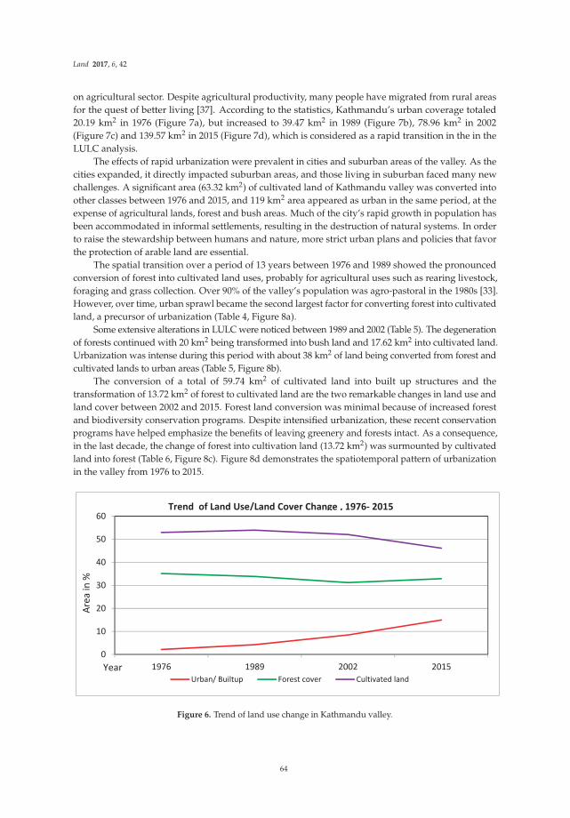
Land 2017, 6, 42

on agricultural sector. Despite agricultural productivity, many people have migrated from rural areasfor the quest of better living [37]. According to the statistics, Kathmandu’s urban coverage totaled20.19 km2 in 1976 (Figure 7a), but increased to 39.47 km2 in 1989 (Figure 7b), 78.96 km2 in 2002(Figure 7c) and 139.57 km2 in 2015 (Figure 7d), which is considered as a rapid transition in the in theLULC analysis.

The effects of rapid urbanization were prevalent in cities and suburban areas of the valley. As thecities expanded, it directly impacted suburban areas, and those living in suburban faced many newchallenges. A significant area (63.32 km2) of cultivated land of Kathmandu valley was converted intoother classes between 1976 and 2015, and 119 km2 area appeared as urban in the same period, at theexpense of agricultural lands, forest and bush areas. Much of the city’s rapid growth in population hasbeen accommodated in informal settlements, resulting in the destruction of natural systems. In orderto raise the stewardship between humans and nature, more strict urban plans and policies that favorthe protection of arable land are essential.

The spatial transition over a period of 13 years between 1976 and 1989 showed the pronouncedconversion of forest into cultivated land uses, probably for agricultural uses such as rearing livestock,foraging and grass collection. Over 90% of the valley’s population was agro-pastoral in the 1980s [33].However, over time, urban sprawl became the second largest factor for converting forest into cultivatedland, a precursor of urbanization (Table 4, Figure 8a).

Some extensive alterations in LULC were noticed between 1989 and 2002 (Table 5). The degenerationof forests continued with 20 km2 being transformed into bush land and 17.62 km2 into cultivated land.Urbanization was intense during this period with about 38 km2 of land being converted from forest andcultivated lands to urban areas (Table 5, Figure 8b).

The conversion of a total of 59.74 km2 of cultivated land into built up structures and thetransformation of 13.72 km2 of forest to cultivated land are the two remarkable changes in land use andland cover between 2002 and 2015. Forest land conversion was minimal because of increased forestand biodiversity conservation programs. Despite intensified urbanization, these recent conservationprograms have helped emphasize the benefits of leaving greenery and forests intact. As a consequence,in the last decade, the change of forest into cultivation land (13.72 km2) was surmounted by cultivatedland into forest (Table 6, Figure 8c). Figure 8d demonstrates the spatiotemporal pattern of urbanizationin the valley from 1976 to 2015.

Figure 6. Trend of land use change in Kathmandu valley.

64

Land 2017, 6, 42

(a)

(b)

Fig

ure

7.

Con

t.

65

Land 2017, 6, 42

(c)

(d)

Fig

ure

7.

LULC

map

ofK

athm

andu

valle

y:(a

)197

6;(b

)198

9;(c

)200

2;an

d(d

)201

5.

66

Land 2017, 6, 42

(a)

(b)

Fig

ure

8.

Con

t.

67

Land 2017, 6, 42

(c)

(d)

Fig

ure

8.

(a)T

rans

itio

nm

apfr

omal

llan

du

se/

land

cove

rcl

asse

sto

urb

anar

ea19

76–1

989;

(b)t

rans

itio

nm

apfr

omal

llan

du

se/

land

cove

rcl

asse

sto

urb

anar

ea19

89–2

002;

(c)t

rans

itio

nm

apfr

omal

llan

dus

e/la

ndco

ver

clas

ses

tour

ban

area

2002

–201

5;(d

)urb

anla

ndco

ver

dyna

mic

sof

the

valle

yfr

om19

76to

2015

.

68

Land 2017, 6, 42

Ta

ble

3.

Land

use/

land

cove

rst

atis

tics

,197

6–20

15.

Lan

dC

ov

er

1976

(Are

a)

1989

(Are

a)

Ch

an

ge

betw

een

1976

an

d1989

2002

(Are

a)

Ch

an

ge

betw

een

1989

an

d2002

2015

(Are

a)

Ch

an

ge

betw

een

2002

an

d2015

Ch

an

ge

betw

een

1976

an

d2015

km

2%

km

2%

km

2%

km

2%

Urb

an/b

uilt

up20

.19

2.16

39.4

74.

2319

.28

78.9

68.

4639

.48

139.

5714

.96

60.6

111

9.38

Wat

erbo

dy9.

501.

027.

200.

77−2

.30

6.59

0.71

−0.6

17.

510.

810.

93−1

.98

Ope

nfie

ld3.

230.

352.

490.

27−0

.74

1.99

0.21

−0.5

01.

750.

19−0

.24

−1.4

8Fo

rest

cove

r32

7.60

35.1

031

5.76

33.8

4−1

1.84

290.

8031

.16

−24.

9730

6.73

32.8

715

.93

−20.

88Bu

shar

ea78

.94

8.46

65.3

37.

00−1

3.61

69.4

37.

444.

1047

.22

5.06

−22.

22−3

1.72

Cul

tiva

ted

land

493.

7752

.91

502.

9753

.90

9.20

485.

4552

.02

−17.

5143

0.44

46.1

2−5

5.01

−63.

32

Tota

l93

3.22

100

933.

2210

093

3.22

100

933.

2210

0

Ta

ble

4.

Spat

iote

mpo

ralt

rans

itio

nof

LULC

,197

6–19

89.

Ye

ar

19

89

km

2

1976

LU

LC

Cla

sse

sU

rba

nW

ate

rO

pe

nfi

eld

Fo

rest

Bu

shC

ult

iva

ted

To

tal

Urb

an20

.08

00.

000.

010.

010.

0920

.19

Wat

er0.

486.

440.

000.

420.

052.

119.

50O

pen

field

0.12

0.00

1.59

0.03

0.10

1.39

3.23

Fore

st0.

230.

020.

0628

8.81

12.7

925

.68

327.

60Bu

sh0.

150.

000.

1416

.19

47.9

214

.53

78.9

4C

ulti

vate

d18

.42

0.73

0.70

10.3

14.

4645

9.15

493.

77

Tota

l39

.47

7.20

2.49

315.

7665

.33

502.

9793

3.22

Ta

ble

5.

Spat

iote

mpo

ralt

rans

itio

nof

LULC

,198

9–20

02.

Ye

ar

20

02

km

2

1989

LU

LC

Cla

sse

sU

rba

nW

ate

rO

pe

nfi

eld

Fo

rest

Bu

shC

ult

iva

ted

To

tal

Urb

an39

.47

0.00

0.00

0.01

0.00

0.00

39.4

7W

ater

0.18

6.54

0.03

0.02

0.00

0.43

7.20

Ope

nfie

ld0.

170.

001.

590.

020.

050.

662.

49Fo

rest

0.34

0.01

0.01

277.

2720

.52

17.6

231

5.76

Bush

0.15

0.00

0.00

6.35

43.7

215

.10

65.3

3C

ulti

vate

d38

.65

0.03

0.37

7.14

5.14

451.

6450

2.97

Tota

l78

.96

6.59

1.99

290.

8069

.43

485.

4593

3.22

69

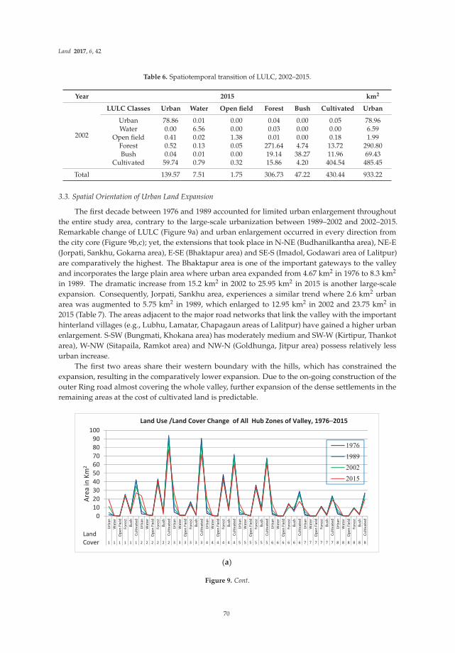
Land 2017, 6, 42

Table 6. Spatiotemporal transition of LULC, 2002–2015.

Year 2015 km2

2002

LULC Classes Urban Water Open field Forest Bush Cultivated Urban

Urban 78.86 0.01 0.00 0.04 0.00 0.05 78.96Water 0.00 6.56 0.00 0.03 0.00 0.00 6.59

Open field 0.41 0.02 1.38 0.01 0.00 0.18 1.99Forest 0.52 0.13 0.05 271.64 4.74 13.72 290.80Bush 0.04 0.01 0.00 19.14 38.27 11.96 69.43

Cultivated 59.74 0.79 0.32 15.86 4.20 404.54 485.45

Total 139.57 7.51 1.75 306.73 47.22 430.44 933.22

3.3. Spatial Orientation of Urban Land Expansion

The first decade between 1976 and 1989 accounted for limited urban enlargement throughoutthe entire study area, contrary to the large-scale urbanization between 1989–2002 and 2002–2015.Remarkable change of LULC (Figure 9a) and urban enlargement occurred in every direction fromthe city core (Figure 9b,c); yet, the extensions that took place in N-NE (Budhanilkantha area), NE-E(Jorpati, Sankhu, Gokarna area), E-SE (Bhaktapur area) and SE-S (Imadol, Godawari area of Lalitpur)are comparatively the highest. The Bhaktapur area is one of the important gateways to the valleyand incorporates the large plain area where urban area expanded from 4.67 km2 in 1976 to 8.3 km2

in 1989. The dramatic increase from 15.2 km2 in 2002 to 25.95 km2 in 2015 is another large-scaleexpansion. Consequently, Jorpati, Sankhu area, experiences a similar trend where 2.6 km2 urbanarea was augmented to 5.75 km2 in 1989, which enlarged to 12.95 km2 in 2002 and 23.75 km2 in2015 (Table 7). The areas adjacent to the major road networks that link the valley with the importanthinterland villages (e.g., Lubhu, Lamatar, Chapagaun areas of Lalitpur) have gained a higher urbanenlargement. S-SW (Bungmati, Khokana area) has moderately medium and SW-W (Kirtipur, Thankotarea), W-NW (Sitapaila, Ramkot area) and NW-N (Goldhunga, Jitpur area) possess relatively lessurban increase.

The first two areas share their western boundary with the hills, which has constrained theexpansion, resulting in the comparatively lower expansion. Due to the on-going construction of theouter Ring road almost covering the whole valley, further expansion of the dense settlements in theremaining areas at the cost of cultivated land is predictable.

(a)

Figure 9. Cont.

70

Land 2017, 6, 42

(b)

(c)

Figure 9. (a) Land cover change matric in all eight main zones in the valley, 1976–2015 (km2); (b) spiderdiagram of the urban expansion in eight directions in the valley, 1976–2015 (km2); (c) spatial orientationof urban land expansion in the valley, 1976–2015 (km2).

Table 7. Quantity of urban land expansion along 8 directions in the valley, 1976–2015 (km2).

Direction 1976 1989 2002 2015

N to NE 1.57 4.12 11.29 19.45NE to E 2.63 5.76 12.96 23.75E to SE 4.66 8.27 15.16 25.96

SE to South 3.16 5.93 11.28 20.69S to SW 1.94 4.26 8.1 14.24SW to W 1.93 3.78 7.11 14.35W to NW 1.11 2.33 5.1 7.98NW to N 2.58 4.36 7.07 11.9

71

Land 2017, 6, 42

3.4. Urban Expansion Rate

The total urban area of Kathmandu valley was 20.19 km2 in 1976, which extended by almosttwo-fold in 1989 with 39.47 km2, with an average growth rate of 7.34% per year in the following13 years. In 2002 and 2015, the urban are reached 78.96 km2 and 139.57 km2, respectively. The totalannual increase rate was 7.70% between 1989 and 2002 and 5.90% between 2002 and 2015. That is6.91-times higher than that in 1976.

3.5. Socioeconomic Impacts

Kathmandu valley is the central hub for the political, educational and economic activities,employment opportunities, air transport, cultural and historical heritage. The availability of urbanbasic services such as roads, electricity and telephone has influenced the population acceleration in thelast few decades. Thus, the fertile land has been confined due to the abrupt urbanization, and people’sinterest has shifted to commercial farming, mainly of horticulture and floriculture, from the substantialfarming in the limited land within the valley [25].

Multiple driving forces are considered responsible for the urbanization process in Kathmandu;however, they were specific at spatial scales [9,37]. Economic opportunities in the city’s core areas,population growth in the fringe and the political situation in the rural areas were identified as themajor drivers of urbanization. A previous study reported that [37] physical condition was trivial incontributing to the urbanization process; nevertheless, its role greatly varied from 18% in the city,to 27% in the fringes, to 55% in the rural areas. Economic opportunities contributed 47%, 31% and22% in urbanization in cities, fringes and rural areas, respectively. The land market business is highlyconcentrated in the rural and fringe in comparison to the city core due to the limited land availability.The land use-based approach is often regarded in sustainable urbanization [25].

3.6. Nepal Earthquake 2015

Nepal is listed as the 20th most disaster-prone country in the world, most vulnerable to the effectsof climate change, 11th most at risk for earthquake damage and 30th most vulnerable to floods [38].Kathmandu valley has the greatest earthquake risk among any of the 21 mega cities in the worldbecause it lies in a very active seismic zone within a high hazard intensity (Figure 10). Seismic recordsof Nepal, which date back to 1255 A.D., show that destructive earthquakes happened in 1408, 1681,1810, 1833, 1866, 1934, 1980, 1988 and 2011. The 1833 quake was the most destructive, and the 1934earthquake impacted Kathmandu the most, resulting in more than 8500 deaths and destroying 38,000buildings [38,39].

On Saturday, 25 April 2015, at 11:56 a.m. local time, a 7.6 magnitude (8.2 km depth) earthquakestruck Barpak, Gorkha, about 76 km northwest of Kathmandu, followed by many subsequentaftershocks, the largest occurring at 12:50 local time on 12 May 2015 in Barpak, Gorkha, and Sunkhani,Dolakha, with a magnitude of 7.3. The 2015 earthquake was the most powerful jolt to hit Nepal sincethe quake of 1934 [40]. This earthquake killed 1746 people and severely injured 13,102 in Kathmanduvalley alone. Altogether, 80,149 private properties and 321 government buildings were fully destroyedin Kathmandu alone; and 72,249 private houses and 545 government buildings partially crumbled [41].The earthquake damaged (Figure 11a,d presents the view in Google Earth images before and after theearthquake of Kathmandu valley) many of the country’s large administrative centers, including Singhdurbar, Sheetal Niwas, the Supreme Court, etc. Seven UNESCO heritage sites were also damaged.The nine-story historical landmark tower Dharahara, in Nepali language, which was constructedduring 1832 by the then Prime Minister Bhimsen Thapa, massively collapsed during the jolt, where alarge number of visitors lost their lives (Figure 11e). Much of the damage occurred because many ofthe buildings across the country are not built to seismic standards, and so, any major jolt can causethem to crumble. Tens of thousands of houses, buildings and structures are in such a precarious statethat a major jolt can result in harsh damage. Various structures are supported by bamboo, wooden

72

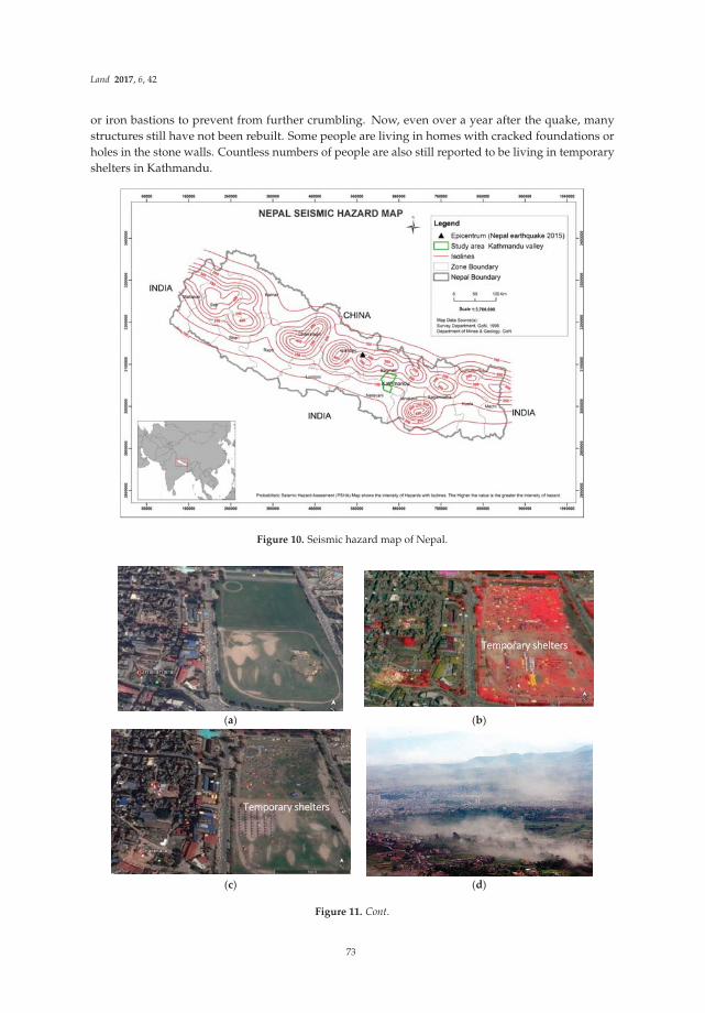
Land 2017, 6, 42

or iron bastions to prevent from further crumbling. Now, even over a year after the quake, manystructures still have not been rebuilt. Some people are living in homes with cracked foundations orholes in the stone walls. Countless numbers of people are also still reported to be living in temporaryshelters in Kathmandu.

Figure 10. Seismic hazard map of Nepal.

(a) (b)

(c) (d)

Figure 11. Cont.

73

Land 2017, 6, 42

(e) (f)

Figure 11. Google Image of Kathmandu, City (focus on Dharahara and Tudhikhel. (a) Before theearthquake, 1 December 2014; (b) after the earthquake, 26 April 2015; (c) Google Image, after theearthquake, 12 May 2015; (d) dusty sky of Kathmandu a few minutes after the quake, 2015, photo,Bikram Rai; Bhimsen Tower, Dharahara, (e) before and (f) after the earthquake: Google search:6 June 2016.

Due to the easy access of urban facilities, such as physical infrastructure, economic probabilityand advanced life, people are intending to move to city areas, resulting in villages being unattendedand full of ruderals [36]. The investment of land markets and real estate has played a vital role inmushrooming the settlements in urban areas. The urban sprawl and LULC change of Kathmanduoccurred without proper planning or policy, creating an area greatly at risk from earthquake damage.Limited understanding of earthquake disaster risk and lack of emergency preparedness are the majorhurdles of the effective disaster risk reduction and mitigation process. Due to the lack of proper landuse planning, unmanaged urban sprawl and risky settlements, many cultivable lands and forests areconverted into built-up areas. Incomplete land use planning puts people at higher risk in naturaldisasters and increases food insecurity, as much of the area’s cultivated land has been converted intoshoddily-constructed homes. Due to the lack of seismic technologies, trained masons and engineers andthe perceived cost of seismic-resilient construction, many buildings when constructed are seismicallyunsafe. To build seismically-resilient and LULC-friendly structures, effective disaster managementand construction protocols must be implemented by the Nepalese government. These policies shouldconsider mitigation and preparedness, emergency response and rehabilitation and reconstructionpolicies for post-disaster based on scientific criteria. Sustainable planning has the capacity to make thislast disaster an opportunity to rebuild a better Nepal.

3.7. Earthquake, Land Use and Geological Formation

Spatial analysis of the geology in Kathmandu valley showed that the Gokarna formation, Kalimatiformation and Chapagaun formation were all highly affected by the 2015 earthquake, while theChandragiri formation and Kulekhani formation were both moderately affected (Figures 12 and 13).Mostly the areas enclosed within the Kalimati, Gokarna and Chapagaun formation, mainly Gongabu,Jorpati, Gokarna, Bhaktapur, Bungmati, Chapagaun and Kirtipur periphery, are the remarkable areasthat obtain high urban orientation, as well as are highly impacted by the Nepal earthquake, 2015.The geological landscape affected the damage risk of Kathmandu valley, but housing constructionalso often determined how much damage a building experienced. Traditional homes constructed withbricks and mud mortar often suffered large amounts of damage, as well as the modern houses, whichare made up of bricks and concrete, fail to meet the earthquake resilience criteria. Although concrete isa more modern material, it is heavy and often became dislocated during the quake. Additionally, poor

74

Land 2017, 6, 42

equipment, unskilled labor, poor quality building materials and a lack of timely maintenance wererisk factors for the quake damage result in fragile homes. Through spatial analysis and geologicalsurveys, we conclude that the establishment of non-resilient, unregulated constructions on top ofhighly vulnerable geologic formations created the large amounts of loss and damage in Kathmanduvalley. Further research is needed to fully understand different land uses and geological formations’vulnerability to earthquakes.

Figure 12. Overlay map of the earthquake damage structure and geological map of Kathmandu valley.

75

Land 2017, 6, 42

Figure 13. Overlay map of earthquake damage structure and administrative boundary map ofKathmandu valley (including all three district boundaries).

3.8. Planning and Policy

The government of Nepal (GoN) has introduced different land use acts and policies regarding theLULC management (e.g., Civil Code 1843, amended in 1963, Land Right Acquiring Act 1951, Surveyand Measurement Act 1962, Land Act 1964, Land Administration Act and Land Revenue Act 1976, LandAcquisition Act 1977, Town Development Act 1989, National Agriculture Policy 2004, National UrbanPolicy 2007, Industrial Policy 2011, National Shelter Policy 2012, Agriculture Development Strategy(ADS) 2013, National Land Use Policy 2012 and 2015, Forest Policy 2015, Urban Planning and Building

76

Land 2017, 6, 42

Construction Guidelines, 2015); these are some of the noteworthy plans and policies promulgated bythe government [42]. Similarly, several scattered laws and regulations in one way or other deal withland and its use. In 2002, the government approved a long-term development plan for Kathmanduvalley prepared by the Kathmandu valley Town Development Committee. The plan was particularlybased on land use criteria [25]. The plan conceptualized a vision for developing Kathmandu throughthe year 2020. It aimed at de-concentrating economic investments and employment opportunitiesin the valley core to promote natural, historical, cultural, touristic environments and delineatingthe urban growth boundaries to control urban growth and limit capital investments. However, theplan was jeopardized by a lack of long-term strategies, political commitment and the sustainabilityof growth in the valley. In 2015, Nepal adopted the Settlement Development, Urban Planning andBuilding Construction Guidelines. These guidelines are scientifically based, and their implementationis urgently required. Fixed scientific measures are considered to be strictly adopted in terms ofinfrastructure development in these newly-developing urban, fringe and rural areas. Geologicalstudies and soil tests should be emphasized prior to construction of infrastructures. Specific roadstandards need to be maintained for road construction or the urban planning process. These guidelinesmust be followed closely for the protection of Kathmandu valley’s high productivity agricultural land,green outskirts and open spaces and to smoothen the resilient urban development process.

4. Conclusions and Future Steps

The high rates of migration and population growth have directly contributed to rapid, oftenunmanaged urban growth in Kathmandu valley. Urbanization has occurred at the cost of fertileagricultural lands and cultural sites. Land use change in the valley has been aggravated throughsporadic and persistent exploitations. Unattended fallow lands in suburban areas have worsenedland degradation by welcoming invasive alien species and compromising the indigenous landscapeand culture. The study area experienced rapid urbanization with the average annual urban growthrate of 7.34%, 7.70% and 5.90% between 1976, 1989, 2002 and 2015, respectively., The annual urbanexpansion growth rate indicates the level of urban area extension in the valley. Urban expansiondirection indicates the value of socio-economic movement. Relatively the highest, moderate and thelowest urban concentration over the time period occurred in the east, southwest and west along withthe northwest part of the valley, respectively.

This excessive trend of urban momentum in recent decades is being strengthened with the ongoingconstruction of the outer Ring-road and additional physical infrastructures, which are likely to convertthe whole valley into a dense jungle of concrete in the coming decades. The government needs tointroduce an effective urban plan to control the haphazard settlement practice in the city, fringe andrural areas. Geological studies, soil tests, building standards, road standards and wise land utilizationpractices should be conducted prior to the construction of private and public infrastructure

To this end, the monitoring of the urban expansion direction and variation through the applicationof multi-temporal images will be the crucial milestones, and geological information will remain as thestepping stones for the operative urban planning in the forthcoming days.

Since land use management is a fundamental part of development, our results advocate theessentiality of incorporating scientific urban planning and appropriate land use management practicefor the sustainable urban development of Kathmandu valley, as well as other cities of Nepal.

Acknowledgments: The research was supported by the Chinese Academy of Sciences (CAS) President’sInternational Fellowship Initiative (PIFI), Grant No. 2016PE022, and the National Natural Science Foundation ofChina (Grant No. 41471281, 41501396 and 41501473).The authors thank all of the scientists who have participatedin the establishment of the database. Chris Lebos and Sushila Rijal are acknowledged for language editing. Wewould like to thank the Editor and the anonymous reviewers for their constructive comments and suggestions.

Author Contributions: Bhagawat Rimal designed the research idea for the paper and took overall responsibilityfor the study, including data collection and image analysis, preparation of figures, and finalization of themanuscript. Lifu Zhang supervised the research and provided useful suggestions throughout the preparationof the manuscript. Dongjie Fu, and Yongguage Zhai carried out the comprehensive revision of the article and

77

Land 2017, 6, 42

gave useful advice. Ripu Kunwar contributed in putting the research in the local context. All authors revised andcontributed to finalizing the manuscript. In addition, all authors approved the final manuscript.


References

1. Michetti, M.; Zampieri, M. Climate–human–land interactions: A review of major modeling approaches. Land2014, 3, 793–833. [CrossRef]

2. Araya, Y.H.; Cabral, P. Analysis and modeling of urban land cover change in Setúbal and Sesimbra, Portugal.Remote Sens. 2010, 2, 1549–1563. [CrossRef]

3. Triantakonstantis, D.; Mountrakis, G. Urban growth prediction: A review of computational models andhuman perceptions. J. Geogr. Inf. Syst. 2012, 4, 555–587. [CrossRef]

4. Hunter, L.M.; de Manuel, J.; Gonzalez, G.; Stevenson, M.; Karish, K.S.; Toth, R.; Edwards, T.C., Jr.;Lilieholm, R.J.; Cablk, M. Population and land use change in the California Mojave: Natural habitatimplications of alternative futures. Popul. Res. Policy Rev. 2003, 22, 373–397. [CrossRef]

5. Li, J.J.; Wang, X.R.; Wang, X.J.; Ma, W.C.; Zhang, H. Remote sensing evaluation of urban heat island and itsspatial pattern of the Shanghai metropolitan area, China. Ecol. Complex. 2009, 6, 413–420. [CrossRef]

6. Zhang, H.; Zhou, L.G.; Chen, M.N.; Ma, W.C. Land Use Dynamics of the Fast-Growing Shanghai Metropolis,China (1979–2008) and its Implications for Land Use and Urban Planning Policy. Sensors 2011, 11, 1794–1809.[CrossRef] [PubMed]

7. Kanokporn, S.; Visut, I. Change of land use patterns in the areas close to the airport development area andsome implicating factors. Sustainability 2011, 3, 1517–1530.

8. Kityuttachai, K.; Tripathi, N.K.; Tipdecho, T.; Shrestha, R. CA-Markov analysis of constrained coastal urbangrowth modeling: Hua Hin Seaside City, Thailand. Sustainability 2013, 5, 1480–1500. [CrossRef]

9. Cheng, J. Modelling Spatial and Temporal Urban Growth. Ph.D. Thesis, Faculty of Geographical SciencesUtrecht University, Utrecht, The Netherlands, 2003.

10. Yin, J.; Yin, Z.; Zhong, H.; Xu, S.; Hu, X.; Wang, J.; Wu, J. Monitoring urban expansion and land use/landcoverchanges of Shanghai metropolitan area during the transitional economy (1979–2009) in China. Environ.Monit. Assess. 2011, 177, 609–621. [CrossRef] [PubMed]

11. Rimal, B.; Baral, H.; Stork, N.E.; Paudyal, K.; Rijal, S. Growing city and rapid land use transition: Assessingmultiple hazards and risk in the Pokhara Valley Nepal. Land 2015, 4, 957–978. [CrossRef]

12. Sexto, J.O.; Song, X.P.; Huang, C.; Channa, S.; Baker, M.E.; Townshend, J.R. Urban growth of the Washington,D.C.–Baltimore, MD metropolitan region from 1984 to 2010 by annual, Landsat-based estimates of imperviouscover. Remote Sens. Environ. 2013, 129, 42–53. [CrossRef]

13. Castrence, M.; Nong, D.H.; Tran, C.C.; Young, L.; Fox, J. Mapping urban transitions using multi-temporalLandsat and DMSP-OLS night-time lights imagery of the Red River Delta in Vietnam. Land 2014, 3, 148–166.[CrossRef]

14. Ministry of Federal Affairs and Local Development | Nepal Government. Available online: http://www.mofald.gov.np/en (accessed on 24 April 2017).

15. Sharma, P. Urbanization and development. In Population Monograph of Nepal; Central Bureau of Statistics:Kathmandu, Nepal, 2003; pp. 375–412.

16. Thapa, R.B.; Murayama, Y. Examining Spatiotemporal Urbanization Patterns in Kathmandu Valley, Nepal:Remote Sensing and Spatial Metrics Approaches. Remote Sens. 2009, 1, 534–556. [CrossRef]

17. Thapa, R.B.; Murayama, Y.; Ale, S. Kathmandu. Cities 2008, 25, 45–57. [CrossRef]18. TV, R.; Aithal, B.H.; Sanna, D.D. Insights to urban dynamics through landscape spatial pattern analysis.

Int. J. Appl. Earth Obs. 2012, 18, 329–343. [CrossRef]19. Tsutsumida, N.; Saizen, I.; Matsuoka, M.; Ishii, R. Land cover change detection in Ulaanbaatar using the

breaks for additive seasonal and trend method. Land 2013, 2, 534–549. [CrossRef]20. Yoshida, M.; Gautam, P. Magnetostratigraphy of Plio-Pleistocene Lacustrine Deposits in the Kathmandu

Valley Central Nepal. Proc. Indian Natl. Sci. Acad. 1988, 54, 410–417.21. Sakai, T.; Gajurel, A.P.; Tabata, H.; Upreti, B.N. Small-amplitude lake-level fluctuations recorded in aggrading

deltaic deposits of the Upper Pleistocene Thimi and Gokarna Formations, Kathmandu Valley, Nepal.J. Geol. Soc. 2001, 25, 43–51.

78

Land 2017, 6, 42

22. Botts, H.; Du, W.; Foust, B.; Ihinger, P.; Jeffery, T. Modeling Earthquake Risk-White Paper. Availableonline: http://www.corelogic.com/about-us/researchtrends/modeling-earthquake-risk-white-paper.aspx#.WUH9HNwlGpo (accessed on 24 April 2017).

23. Piya, B. Generation of Geological Database for the Liquefaction Hazard Analysis in Kathmandu Valley.Master’s Thesis, International Institute for Geoinformation Science and the Earth Observation (ITC),Enschede, The Netherlands, 2004.

24. Sakai, H. Stratigraphic division and sedimentary facies of the Kathmandu Basin sediments. J. Nepal Geol. Soc.2001, 25, 19–32.

25. International Centre for Integrated Mountain Development (ICIMOD). Kathmandu Valley Environment Outlook(KVEO); International Centre for Integrated Mountain Development (ICIMOD): Kathmanud, Nepal, 2007.

26. Stocklin, J.; Bhattarai, K.D. Geological Map of Kathmandu Area and Central Mahabharat Range (1:250,000);Department of Mines and Geology: Kathmandu, Nepal, 1986.

27. Central Bureau of Statistics (CBS). Environment Statistics of Nepal and Nepal Population Report; NationalPlanning Commission Secretariat, Government of Nepal: Kathmandu, Nepal, 2011.

28. Bhattarai, K.; Conway, D. Urban Vulnerabilities in the Kathmandu Valley, Nepal: Visualizations ofHuman/Hazard Interactions. J. Geogr. Inf. Syst. 2010, 2, 63–84. [CrossRef]

29. Zhang, Z.X.; Wang, X.; Zhao, X.L.; Liu, B.; Yi, L.; Zuo, L.J.; Wen, Q.K.; Liu, F.; Xu, J.Y.; Hu, S.G. A 2010 updateof National Land Use/Cover Database of China at 1:100,000 scale using medium spatial resolution satelliteimages. Remote Sens. Environ. 2014, 149, 142–154. [CrossRef]

30. Zhang, Z.; Li, N.; Wang, X.; Liu, F.; Yang, L. A Comparative Study of Urban Expansion in Beijing, Tianjinand Tangshan from the 1970s to 2013. Remote Sens. 2016, 8, 1–22. [CrossRef]

31. Anderson, J.R.; Hardy, E.E.; Roach, J.T.; Witmer, R.E. A Land Use and Land Cover Classification System for Usewith Remote Sensor Data; United States Government Printing Office: Washington, DC, USA, 1976.

32. Xiao, P.; Wang, X.; Feng, X.; Zhang, X.; Yang, Y. Decting China’s urban expantion over the past three decadesusing nighttime light data. IEEE J. Sel. Top. Appl. Earth Obs. Remote Sens. 2014, 7, 4095–4106. [CrossRef]

33. Toffin, G. Urban fringes: Squatter and slum settlement in the Kathmandu valley, Nepal. CNAS J. 2010, 372,151–168.

34. Goldstein, M.; Ross, J.; Schuler, S. From a mountain/rural to a plains/urban society: Implications of the 1981Nepalese consensus. Mt. Res. Dev. 1983, 3, 61–64. [CrossRef] [PubMed]

35. Muzzini, E.; Aparicio, G. Urban Growth and Spatial Transition in Nepal, An Initial Assessment; The World Bank:Washington, DC, USA, 2013.

36. Kunwar, R.M.; Baral, K.; Poudel, P.; Acharya, R.P.; Thapa-Magar, K.; Cameron, M.; Bussmann, R.W. Land-useand socioeconomic change, medicinal plant selection and biodiversity resilience in Far Western Nepal.PLoS ONE 2016, 11, e0169447. [CrossRef] [PubMed]

37. Thapa, R.B. Spatial Process of Urbanization in Kathmandu Valley, Nepal. Ph.D. Thesis, The Graduate Schoolof Life and Environmental Sciences, The University of Tsukuba, Tsukuba, Japan, 2009.

38. Ministry of Home Affairs (MoHA). Nepal Disaster Report; Ministry of Home Affairs, Government of Nepal:Kathmandu, Nepal, 2011.

39. National Society for Earthquake Technology—Nepal (NSET). The Kathmandu Valley Earthquake RiskManagement Action Plan; National Society for Earthquake Technology Nepal and GeoHazards International(GHI): Kathmandu, Nepal, 1999.

40. National Planning Commission. Nepal Earthquake 2015, Post Disaster Needs Assessment; Key Findings;Government of Nepal: Kathmandu, Nepal, 2015.

41. Government of Nepal. Nepal Disaster Risk Reduction Portal. Available online: https://drrportal.gov.np(accessed on 23 October 2015).

42. UN-Habitat. National Land Use Plan; Catalytic Support on Land Issues, Participatory Land Use Planning andImplementation; UN-Habitat: Pulchowk, Nepal, 2015.


79

land

Article

Modeling Future Urban Sprawl and LandscapeChange in the Laguna de Bay Area, Philippines

Kotaro Iizuka 1,*, Brian A. Johnson 2, Akio Onishi 3, Damasa B. Magcale-Macandog 4, Isao Endo 2

and Milben Bragais 4

1 Center for Southeast Asian Studies (CSEAS), Kyoto University, 46, Yoshida Shimoadachicho,Sakyo-ku Kyoto-shi, Kyoto 606-8501, Japan

2 Institute for Global Environmental Strategies (IGES), 2108-11 Kamiyamaguchi, Hayama,Kanagawa 240-0115, Japan; [email protected] (B.A.J.); [email protected] (I.E.)

3 Faculty of Environmental Studies, Tokyo City University, 3-3-1 Ushikubo-nishi, Tsuzuki-ku, Yokohama,Kanagawa 224-8551, Japan; [email protected]

4 Institute of Biological Sciences, University of the Philippines Los Baños, College, Laguna 4031, Philippines;[email protected] (D.B.M.-M.); [email protected] (M.B.)

* Correspondence: [email protected]

Academic Editors: Andrew Millington, Harini Nagendra and Monika KopeckaReceived: 6 March 2017; Accepted: 11 April 2017; Published: 14 April 2017

Abstract: This study uses a spatially-explicit land-use/land-cover (LULC) modeling approach tomodel and map the future (2016–2030) LULC of the area surrounding the Laguna de Bay of Philippinesunder three different scenarios: ‘business-as-usual’, ‘compact development’, and ‘high sprawl’scenarios. The Laguna de Bay is the largest lake in the Philippines and an important natural resourcefor the population in/around Metro Manila. The LULC around the lake is rapidly changing due tourban sprawl, so local and national government agencies situated in the area need an understandingof the future (likely) LULC changes and their associated hydrological impacts. The spatial modelingapproach involved three main steps: (1) mapping the locations of past LULC changes; (2) identifyingthe drivers of these past changes; and (3) identifying where and when future LULC changes arelikely to occur. Utilizing various publically-available spatial datasets representing potential driversof LULC changes, a LULC change model was calibrated using the Multilayer Perceptron (MLP)neural network algorithm. After calibrating the model, future LULC changes were modeled andmapped up to the year 2030. Our modeling results showed that the ‘built-up’ LULC class is likelyto experience the greatest increase in land area due to losses in ‘crop/grass’ (and to a lesser degree‘tree’) LULC, and this is attributed to continued urban sprawl.

Keywords: landuse; change; open data; landscape; remote sensing; GIS; Markov Chain

1. Introduction

Urban sprawl is occurring at an accelerated pace in many developing countries worldwidedue to rapid global economic and population growth coupled with globalization. Currently, 54%of the world’s population lives in urban areas, and the United Nations has predicted that by 2050,66% of the world’s population will live in urban areas [1]. This rapid increase in urban populationhas forced nations to meet the changing demands for necessities such as food, energy, land, andwater. A major concern related to this urban sprawl is land-use (LU)/land-cover (LC) change, whichcan dramatically alter the landscape in areas with high rates of urban expansion [2]. These LULCchanges are often based on the plans of local governments to increase economic development and tosupport their growing populations. However, such plans may fail to consider other factors, includingclimate conditions, water resources, and food security [3,4]. Since population increases are expected to


Land 2017, 6, 26

continue in many developing countries, governments need to take appropriate action to ensure thaturbanization measures consider these factors. Thus, policymakers need to understand the historicaltrends in LULC change and must visualize future LULC scenarios to ensure the safety and standard ofliving of the residents [4]. LULC changes and related problems will likely continue to be major issuesin the future [5,6], and, for governments to strategically plan future LULC development, they need toestimate the locations of LULC changes, the time scale of occurrence, and the factors driving thesechanges [7–9]. It is difficult to monitor LULC changes over large areas using field surveys or otherground-level data collection approaches, so many studies have instead detected and mapped LULCchanges from above using satellite or aerial remote sensing data [2,10,11].

Nowadays, a great deal of attention is being paid in particular to rapidly growing citiesin southeast Asia (and other regions), with the goal of understanding relationships between LULCchanges and other factors such as climate change [12] and forestry [13]. The Metro Manila area of thePhilippines is one of the most rapidly growing mega cities in the world [2], and, among other things,Manila’s urban sprawl has threatened the ecology of the agricultural lands located along the urbanfringe [14] and increased flood vulnerability in the area [15]. Other impacts related to food securityare also likely to emerge in this area if agricultural lands keeps decreasing and the population keepsincreasing [16]. Additionally, if Manila’s urban sprawl continues into the remaining forest/agro-forestareas surrounding the city, various ecosystem services provided by these forest systems [17] willcease or decline, while, if the forested areas are instead converted to agricultural lands, it may leadto land degradations that also significantly impact the environment (e.g., increased erosion) [18,19].Urbanization-related issues have large impacts on both human and environmental well-being, and it isclear that development in the region is causing various problems for both people and the environment.Thus, the LULC change trends in such a rapidly developing region should be monitored, and futureLULC changes should be estimated to assess the impacts of future LULC changes.

The Laguna de Bay, located to the southeast of Metro Manila, is the largest lake in the Philippinesand an important source of water for the population of Metro Manila and the surrounding cities andtowns. Several river basins drain into this lake, and the LULC conditions of these drainage basinscan have a significant effect on the lake water quality and quantity owing to different rainfall-runoffrates and pollutant loads of different LULC types [20]. Previous LULC change modeling studies inthis region have focused mostly on the Metro Manila area [14,15,21,22], which does not give the fullpicture of the changes affecting the lake. Some past studies have also focused on specific drainagebasins of the lake [19,23], but few works have studied the LULC changes of the entire surroundinglandscape of the Laguna de Bay. According to the Global Footprint Network [24] Ecological FootprintReport, the Laguna lake watershed has undergone LULC changes during the last 30 years, whereinlarge rural areas have been converted into commercial, residential, and industrial areas. It was notedthat the major LULC change occurred between 2003 and 2010, when the built up areas increased by116%. During this period, the closed forests, observed mostly in the west, northwest, and southernparts of the lake, were reduced by 35% [25]. The lake has been the catch basin of much of the runofffrom Metro Manila, so it has been heavily impacted by Metro Manila’s urbanization and populationincrease. As Metro Manila has developed, the lake’s water quality has deteriorated owing to increasesin agricultural, industrial, and domestic pollution. Moreover, previous studies have reported that 66%of the lake watershed is vulnerable to erosion caused by urban growth, deforestation, and miningactivities. Further, about four million tons of suspended solids flow into the lake annually [26]. Fromsuch perspectives, several local governments based along the lake as well as the national LagunaLake Development Authority (a national government agency) have expressed interest in future LULCpredictions and maps.

Using historical data, we can obtain information on past LULC changes that can be used to helpmodel future LULC changes [11,27–29]. LULC change modeling for territorial planning has a longhistory, and a variety of modeling methods have been assessed at various locations, time periods, andspatial scales/spatial resolutions [30]. In the general sense, land change approaches can be roughly

81

Land 2017, 6, 26

categorized into six types of approaches [31]; machine learning and statistical, cellular automata,sector-based economic, spatially disaggregated economic, agent-based, and hybrid approaches. In thiswork, we focused on the machine learning category, namely the Multilayer-Perceptron (MLP) ArtificialNeural Network (ANN) approach, which is gaining attention for modeling LULC changes. ANNare powerful tools for modeling complex behaviors [32] (e.g, relationships between land transitionsand their driving forces), and the usage of ANN for LULC change modeling has increased in recentyears. As one example, Grekousis et al. [33] demonstrated the use of ANN to model future urbangrowth based on demographic time-series data. Triantakonstantis and Stathakis [32] used MLP formodeling future LULC transition probabilities based on information on past LULC changes andgeomorphic drivers such as elevation, slope, and distance variables from specific land features, etc.Similar methods can be seen in a number of studies, although the number and types of driver variablesutilized vary [27,34–38].

Past studies have been conducted at various geographical locations and spatial extents, e.g.,the city level or provincial level. However, not many works have used the MLP method formodeling complex larger regions. In our case, we have focused on a larger ecological scale thatencompasses multiple municipalities and provinces, each of which have different development policies,infrastructure, topography, climatic conditions, etc. Therefore, the MLP method for modeling theLULC transitions throughout the region becomes a strong decision tool, even when prior knowledge islacking [31,37], and this is one of its advantages compared to other methods like SLEUTH (Slope, Landuse map, Excluded area, Urban area, Transportation map, Hillside area), which require coefficientvalues to be set [39], and other cellular automata methods that require a suitability map [40] based onprior knowledge of change behavior. MLP can also handle a large number of data sets, so it could be agood predictor for recognizing the patterns of the changes in the area.

Our main objective in this study is to model the future LULC changes in the river basins thatdrain into the Laguna de Bay up to year 2030. This work implements the MLP with the MarkovChain method embedded in the Land Change Modeler (LCM) of the TerrSet software package [41].This model is based on transition probabilities calculated using historical LULC change data and otherfreely/openly available geospatial datasets.

2. Study Area

The Philippines is one of the most rapidly developing countries in Asia. In particular,the Metropolitan Manila area has experienced large and rapid LULC changes owing to urbanarea expansion [2,6]. The Laguna de Bay, located just southeast of Manila, is the largest and mostimportant and dynamic lake in the Philippines owing to its vital economic, political, and socio-culturalsignificance. With a surface area of 900 km2, this lake is also one of the largest in Southeast Asia. Fromthe 21 major river systems, more than 100 rivers that traverse the 292,000 ha watershed flow intothe lake. The study area includes the municipalities surrounding the Laguna de Bay, located southeastof Metro Manila. Figure 1 shows that Metro Manila, situated to the northwest, has a denser urbanconcentration; while smaller, less densely populated cities and municipalities can be seen in the westand southwest areas surrounding the Laguna de Bay. The population of this area was estimated tobe about 15 million in 2010 [42]. Agricultural lands are distributed mainly along the southwestern,southeastern, and northeastern shores of the lake. Large forest areas are located on the east side ofthe lake with mountain ranges (300–600 m), the highest peak of which, Mt. Banahao (2170 m), islocated southeast of the lake. Just south of Laguna de Bay, Mt. Makilling (1090 m) is seen. The areais broad and the climate varies along different provinces of the area. Average annual temperaturesare cooler in the mountainous areas (23 ◦C) than in the lower altitude plains and cities (25 ◦C and27 ◦C respectively). Annual precipitation ranges from over 3000 mm in the east mountainous areas to1900 mm in the western area around Manila bay. The area in focus is approximately 60 km × 80 kmin the north-south and east-west directions, respectively, and it was chosen to visualize how urban

82

Land 2017, 6, 26

sprawl will affect the LULC in the areas surrounding the Laguna de Bay. Therefore, we have ignoredthe center and northern areas of Metro Manila, even though it also experienced urban sprawl.

Figure 1. Overview of the study area, the Laguna de Bay district, and the surrounding environment inthe Philippines. Metro Manila is shown in the northwest corner. Referenced from Google Earth [43].


3.1. Overview

As shown in Figure 2, the overall flowchart of the study details three main steps in generatingmaps of future LULC. The first step is to gather evidence of past LULC transitions by identifyingthe historical LULC changes in the area. For this, a map of recent LULC change from 2007 to 2015was generated by using optical and synthetic aperture radar (SAR) satellite images from 2007 and2015 and automated image classification techniques. Four LULC classes, including Built-up, Forests,Crop-Grass, and Water Bodies, were mapped for each year, and the LULC changes between 2007and 2015 were identified by overlaying the two maps. The full details of the LULC change mappingmethodology employed in this study are given in Johnson et al. [44], although brief information willbe stated about the methods and the result of the developed LULC change map. In the second step,drivers of these historical LULC changes were identified by using various ancillary spatial datasetscontaining demographic, topographic, and climate information. In the third and final step, the futureLULC of the area (2030) was modeled and mapped by using Markov Chain analysis.

In addition to the main procedure, the validity of the LULC change model was examined bycomparing a ‘simulated 2015 LULC map’ with a ‘reference 2015 LULC map’. The ‘simulated 2015LULC map’ was generated using similar methods to those mentioned above. First, LULC maps fromthe years 2007 and 2010 were utilized along with the ancillary spatial datasets to model the LULCconditions in the year 2015 LULC (i.e., simulated 2015 LULC map). This map was then compared withthe actual (i.e., reference) 2015 LULC map.

83

Land 2017, 6, 26

LULC 2007

LULC 2010

LULC 2015

Driver Variables

Transition Evidence

Transition Sub-Model

Markov Chain

Modeled 2015

Modeled 2030

Validation

Figure 2. Overall flowchart of the methodology used in this study.

3.2. LULC Maps of 2007, 2010 and 2015

To develop a categorical LULC change map of the study area, we utilized optical (Landsat 5and Landsat 8) and synthetic aperture radar (ALOS PALSAR-1 and PALSAR-2) satellite images fromthe years 2007, 2010, and 2015 and classified the pixels in the images from each year into one offour LULC classes (Built-up, Crop-Grass, Trees, and Water) using a semi-unsupervised classificationapproach [44]. Crop-Grass includes cropland, paddy fields, grassland, and pasture (however themajority lies within paddy and other agriculture). Trees includes forest and agroforestry plantations(e.g., coconut, banana, etc.). This four class LULC classification system, although relatively simple, waschosen because it was representative of the area and allowed us to maintain a relatively high LULCchange mapping accuracy (adding more specific LULC classes usually decreases LULC mappingaccuracy, and LULC change mapping accuracy even more so due to error propagation). The overallaccuracy of the 2007–2015 LULC change map was estimated as 90.2%.

3.3. Evidence of LULC Change Transition

By using the two different periods of the LULC change maps, the net change in area of each LULCclass was calculated, and the spatial distributions of all of the LULC changes were analyzed. The areasof transition and persistence of each LULC type within the 2007–2015 analysis was for both trainingand validation data with all of the driver variables when performing transition sub-modeling.

3.4. Collection and Processing of Data on Potential Driver Variables

Spatial data related to various potential drivers of LULC change were collected via the Internet.Only datasets which were openly available online were used, so our modeling approach can easily bereplicated by other researchers. The drivers influencing LULC change processes are extremely diverseas well as highly variable from one location to another [45,46]. What is known is that the changes aretypically the results of the local population’s responses to economic opportunities [45], which givesrelevance to various contextual features such as the distance from a location to nearby infrastructuralfeatures like major roads, town centers, and so forth, and many works show these kind of factors tobe used as potential drivers for calibrating the change probability. These context features are alsoconsidered in this work for the model calibration. However, as mentioned before, we are not soaware of all the LULC change drivers in the area, so we want to shed some light on the questionof ‘What factors influence the LULC transitions?’ Thus, data for a large number of possible driverswas collected to test which variables had the greatest levels of influence on LULC changes (a briefexplanation is made later for why each variable was considered as potentially relevant). Table 1 shows

84

Land 2017, 6, 26

the complete list of collected data related to these drivers; not all of these datasets were selected for thefinal LULC modeling.

Table 1. Complete list of all variables collected in this study.

Category Driver Abbreviation Unit Year Data Source

Climate

Annual Mean Temperature BIO1 ◦C

1960–1990 PhilGIS [47]

Mean Diurnal Range BIO2

Isothermality BIO3 %

Temperature Seasonality BIO4

◦C

Max. Temperature of Warmest Month BIO5Min. Temperature of Coldest Month BIO6Temperature Annual Range BIO7Mean Temperature of Wettest Quarter BIO8Mean Temperature of Driest Quarter BIO9Mean Temperature of Warmest Quarter BIO10Mean Temperature of Coldest Quarter BIO11

Annual Precipitation BIO12mmPrecipitation of Wettest Month BIO13

Precipitation of Driest Month BIO14

Precipitation Seasonality BIO15 %

Precipitation of Wettest Quarter BIO16

mmPrecipitation of Driest Quarter BIO17Precipitation of Warmest Quarter BIO18Precipitation of Coldest Quarter BIO19

TopographyElevation DEM m

2000 SRTM [48]Slope Slope degreesAspect Aspect

SpatialContext

Distance from Built-up Dist_Built

Lat/Longdegrees

2007 ClassifiedLULC 2007

Distance from Crop-Grass Dist_CropDistance from Trees Dist_TreeDistance from Water Dist_WaterDistance from Primary Road Dist_Road1

3 March 2016OpenStreetMap

[49]

Distance from Secondary Road Dist_Road2Distance from Tertiary Road Dist_Road3Distance from Other Roads Dist_Road4Distance from Canal Dist_CanalDistance from River Dist_RiverDistance from Stream Dist_StreamDistance from Golf Course Dist_Golf 2004

PhilGIS [47]Distance from Protected Area Dist_Protect 2013

NightlightData

Night Light Data 2007 NL_2007 DN 2007 NOAA EarthObservationGroup [50]

Night Light Data 2015 NL_2015nanoWatts/cm2/sr

2015Night Light Change 2007 to 2015 NL_Ch -

PopulationPopulation Map 2007 Pop_2007

People perhectare

2007 WorldPop[51]Population Map 2015 Pop_2015 2015

Population Change 2007 to 2015 Pop_Ch -

Gridded climate data with a 1 km resolution was obtained from the Philippine GIS DataClearinghouse (PhilGIS) [47] (the original global dataset is distributed at WorldClim [52]). We includedall of the climate data that was processed in the form of bioclimatic variables [53,54]. These climatevariables can be considered drivers of LULC change because the agro-climatic zones with differentclimatic conditions can affect the suitability of agricultural lands for its productivity [55]; thus, nopatterns of change in the preferred area might be identified relative to this factor. This is one challenge inour work since not many related studies implement climatic information in their calibration. The reasoncan be considered that, depending on the scale of the study area, the spatial variation of climatic factorsmight be too small to have any influence on LULC changes. However, our study area encompassesareas with different climatic conditions, which may allow us to identify if climate is affecting LULCchange. Topographic data including elevation, slope, and aspect were obtained from the ShuttleRadar Topography Mission (SRTM) 1 s (30 m) digital elevation model (DEM) [48]. Topography is

85

Land 2017, 6, 26

often a significant driver of LULC change [56] because areas with steep slopes are typically moredifficult and thus less likely than flatter areas to be converted to built-up land or cropland. TheSRTM DEM contains only elevation information; therefore, gridded slope and aspect data weregenerated by using the TerrSet software package [41]. Road and waterway data through March 03,2016, were collected from OpenStreetMap (OSM) [49], and a 25 m grid map containing the Euclideandistance of each pixel to the nearest road/waterway was calculated by using TerrSet software [41].The distance from roads in addition to other various LULC context features are often drivers of LULCchange because more developed road networks are found with a greater rate of conversion [57]. Thisstudy focuses not only on the roads in general but also on different types/functions of roads byseparating roads into detailed classes. It is expected that the importance of different road types couldfurther distinguish the patterns of transitions throughout the study region. The case is similar forthe waterways. Nightlight intensity information in the form of monthly average radiance compositeimages was obtained from the Visible Infrared Imaging Radiometer Suite (VIIRS) and Global DefenseMeteorological Satellite Program-Operational Linescan System (DMSP-OLS) nighttime lights timeseries dataset [50]. The nightlight changes from 2007 to 2015 were computed by performing radiometricnormalization of the images to ensure that the 2007 data had a radiance range similar to that of the2015 data. The differences in radiance at each pixel location were then calculated. Nightlight intensitywas considered a driver variable because it is strongly correlated with economic activity and the grossdomestic product (GDP) [58,59]. Changes in nightlight intensity over time can also be considered anindicator of economic growth. Polygon data on the locations of protected areas were collected fromthe PhilGIS [47]. By using this dataset, the distance from each pixel to the nearest protected area wascalculated in TerrSet [41], and all pixels located within a protected area were assumed to experienceno LULC conversions in the LULC change modeling process. Unique LULC data such as golf courseinformation were also collected and used to generate the distance information from those features.Compared to other unique LULC features such as markets and town centers, the location of a golfcourse would mostly not change over time, and there would be a lesser chance for new land areas to bedeveloped as golf courses, keeping the consistency of the patterns; therefore we have used those data.Gridded population data were obtained from WorldPop [51]. This data is based on census populationcounts at the Barangay level but were downscaled to a 100 m × 100 m grid level utilizing variousother spatial datasets, as outlined in Stevens et al. [60] and Linard et al. [61]. Population growth wascalculated on the basis of population change between 2007 and 2015. All of these gridded datasetswere resampled from their original resolutions to a 25 m resolution by using a cubic convolutionresampling approach to match the resolution of the LULC change map (25 m) of the area. For thevisual interpretation of the variables used in the model, summarized images are given in Figure S1 ofthe supplementary materials.

The explanatory power of all of these variables in relation to different LULC transitions wascomputed and examined by using Cramer’s V [38]. Also known as Cramer’s Coefficient (V),this method is used for quantifying the explanatory power of each variable, which is an optional quicktest used to determine whether the variables are worthy of consideration in the model [29]. The finalvariables used for the modeling will be considered on certain criteria of this value.

3.5. Processing Transition Sub-Models (MLP)

MLP, a type of ANN method widely used for modeling complex behaviors and patterns, usesthe back propagation algorithm to learn the characteristics of all the factors influencing the LULCtransitions. Several studies show the advantages of MLP compared to logistic regression and otherempirical models [62,63]. Further details of the MLP algorithm can be found in Riccioli et al. [37]. In ourstudy, MLP’s ability to handle a large number of input variables (some of which may be irrelevantand/or highly correlated with one another) in the model calibration process was very useful, as itallowed us to investigate over 20 explanatory variables. We focused on modeling the changes of threeLULC classes; Built-up, Crop-Grass, and Trees. For all of the variables measuring ‘distance from’

86

Land 2017, 6, 26

a pixel to some geographic feature (e.g., road, built-up area, etc.), the distances were recalculated at aone year interval using that year’s modeled LULC map. A random sample of 10,000 pixels from the2007–2015 LULC change map was used for the building model. Of these, 50% were used for trainingand 50% were used for testing through a cross-validation process.

3.6. Change Modeling (Three Scenarios)

The probability of changes occurring in different years in the future was calculated using MarkovChain analysis, a technique for predictive change modeling that is able to model future changesbased on past changes. On the basis of the observed data between the two periods (2007 and 2015in our case), the Markov Chain computes the probability that a pixel will change from one LULC typeto another within a specified period [64]. Table 2 shows the matrix of the probability that each LULCcategory will change to every other category (base rate), which is known as the transition probability.In this method, the probability is determined by the actual changes shown in the developed LULC map;further details have been reported by Takada et al. [65]. The target year of the modeling in the presentstudy was set to 2030; the transition for each year was also produced to review the continuous dynamicchanges in the study area. A total of three scenarios were output for the comparison. The base scenarioconsiders the transition rate to be the same as the 2007 to 2015 change rate (i.e., a ‘business-as-usualscenario’). The second scenario is if the development policy changes and the rate of LULC changereduces to half of the 2007–2015 transition rate (i.e., a ‘compact development scenario’). The thirdscenario is if the rate of LULC change further accelerates to twice the 2007–2015 rate (i.e., a ‘high sprawlscenario’). The deceleration and acceleration of the transition rates are controlled by simply half anddouble the values for each changing class in the transition probability matrix, respectively.

During the process of the simulation, the data of protected areas are used as constrain mapsto control the process of transitions. The transition potentials associated with each transition aremultiplied by the constraints map [64], so a value of 1 means unconstrained, while a values near to 0acts as a disincentive and above 1 acts as an incentive. The protected area is given the value of verynear 0 (i.e., 0.01).

Table 2. Markov transition probability matrix (business-as-usual scenario).

Probability of Changing to (2030):

Built-Up Crop-Grass Trees Water

LULCGiven(2015)

Built-Up 1.0000 0.0000 0.0000 0.0000Crop-Grass 0.1137 0.5745 0.3118 0.0000

Trees 0.0211 0.2372 0.7417 0.0000Water 0.0000 0.0000 0.0000 1.0000

3.7. Validation of Modeled Map

We assessed the validity of the model by comparing the simulated 2015 LULC (i.e., derivedfrom LULC modeling using the 2007–2010 LULC change data) with the reference (i.e., mapped) 2015LULC. Utilizing the 2007 and 2010 LULC maps, a LULC change model was calibrated using thesame driver variables as used in the 2007–2015 calibration. Using the 2007–2010 model, the year 2015LULC was simulated, and the projected 2015 map was compared with the reference 2015 map. Twostatistical indexes were calculated for the validation; Figure of Merit (FoM) [66] and Kappa Index [67].FoM determines the accuracy of LULC hits (model predicted change and actually observed change)compared with the sum of hits, misses (model predicted persistence but is observed change), andfalse alarms (model predicted change but it observed persistence), giving 0% for no match betweenthe modeled and the reference map and 100% for a perfect match. Kappa Index is widely used inthe remote sensing society for assessing the reliability of the map. Other than the standard Kappa(Kstandard), Kappa for no ability (Kno) and Kappa for location (Klocation) are computed. Kno considers

87

Land 2017, 6, 26

and fixes the major problems of the standard Kappa, wherein it penalizes for large quantification errorand fails to reward the simulation for specifying quantity [67]. Klocation indicates how well the gridcells are located on the landscape [64,67]. Kappa values range from −1 (no agreement) to 1 (perfectagreement). The water bodies were masked out for the computation.

4. Results

4.1. 2007–2015 LULC Changes

By using the Cross-Tabulation module, the transitions of each class from 2007 to 2015 werecomputed, as shown in Figure 3a. The gains and the losses for each LULC type, in ha, are alsoshown in Figure 3b. The transition map confirmed that the majority of changes in the Built-Up classare attributed to decreases in the Crop-Grass area, although a significant number of Trees areas areexpected to become Built-Up land outside the protected forest areas.

(a)

(b)

Figure 3. (a) Area of transitions occurring from 2007 to 2015 for each land-use/land-cover (LULC) type;(b) Total area of gains and losses computed within the study area for each LULC type.

For a visual understanding of the change patterns, Figure 4 shows the spatial variation ofthe different LULC transition trends. The spatial change pattern of the surface was created bycoding areas of change with 1 and areas of no change with 0, while treating the values in a similarmanner as that for quantitative values [64] and then interpolating them by using a 9th polynomialorder function. The transition trend map is shown for each class transitioning to another includingCrop-Grass to Built-Up, Trees to Built-Up, Trees to Crop-Grass, and Crop-Grass to Trees. This methodenables identification and understanding of the spatial trends of the transition, which can provide abetter comprehension of the sites of different changes at different spatial locations. The assumptionshows the change patterns that occurred in the area from 2007 to 2015. For the Built-Up class,significant changes were detected from north to south along the west side of the Laguna de Bay. Highprobabilities of transition were detected from the Trees (Crop-Grass) class to Built-Up class north(west) of the center of the study area. The trends for the Trees class changing into Crop-Grass weremost dominant north of the center of the study area, followed secondly by the southwest area andthirdly by the south to southeast area. The largest changes were recognized at the southwestern side;

88

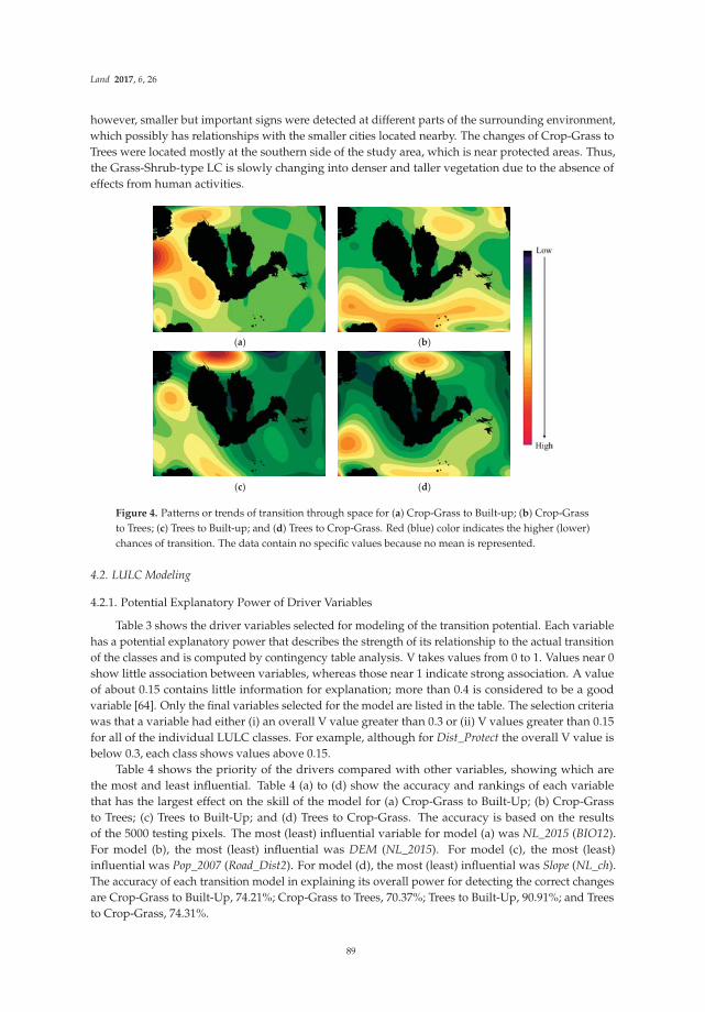
Land 2017, 6, 26

however, smaller but important signs were detected at different parts of the surrounding environment,which possibly has relationships with the smaller cities located nearby. The changes of Crop-Grass toTrees were located mostly at the southern side of the study area, which is near protected areas. Thus,the Grass-Shrub-type LC is slowly changing into denser and taller vegetation due to the absence ofeffects from human activities.

(a) (b)

(c) (d)

Figure 4. Patterns or trends of transition through space for (a) Crop-Grass to Built-up; (b) Crop-Grassto Trees; (c) Trees to Built-up; and (d) Trees to Crop-Grass. Red (blue) color indicates the higher (lower)chances of transition. The data contain no specific values because no mean is represented.

4.2. LULC Modeling

4.2.1. Potential Explanatory Power of Driver Variables

Table 3 shows the driver variables selected for modeling of the transition potential. Each variablehas a potential explanatory power that describes the strength of its relationship to the actual transitionof the classes and is computed by contingency table analysis. V takes values from 0 to 1. Values near 0show little association between variables, whereas those near 1 indicate strong association. A valueof about 0.15 contains little information for explanation; more than 0.4 is considered to be a goodvariable [64]. Only the final variables selected for the model are listed in the table. The selection criteriawas that a variable had either (i) an overall V value greater than 0.3 or (ii) V values greater than 0.15for all of the individual LULC classes. For example, although for Dist_Protect the overall V value isbelow 0.3, each class shows values above 0.15.

Table 4 shows the priority of the drivers compared with other variables, showing which arethe most and least influential. Table 4 (a) to (d) show the accuracy and rankings of each variablethat has the largest effect on the skill of the model for (a) Crop-Grass to Built-Up; (b) Crop-Grassto Trees; (c) Trees to Built-Up; and (d) Trees to Crop-Grass. The accuracy is based on the resultsof the 5000 testing pixels. The most (least) influential variable for model (a) was NL_2015 (BIO12).For model (b), the most (least) influential was DEM (NL_2015). For model (c), the most (least)influential was Pop_2007 (Road_Dist2). For model (d), the most (least) influential was Slope (NL_ch).The accuracy of each transition model in explaining its overall power for detecting the correct changesare Crop-Grass to Built-Up, 74.21%; Crop-Grass to Trees, 70.37%; Trees to Built-Up, 90.91%; and Treesto Crop-Grass, 74.31%.

89

Land 2017, 6, 26

Table 3. Test of the explanatory power (Cramer’s V) of each variable.

Variable

BIO3 BIO6 BIO7 BIO12 BIO15 BIO19 DEM Slope Dist-Built

Overall 0.3426 0.4680 0.4208 0.3250 0.4934 0.3757 0.6107 0.5649 0.3609Built-up 0.2769 0.2908 0.2815 0.2803 0.5390 0.2748 0.4411 0.3142 0.3517

Crop-Grass 0.1242 0.1934 0.2315 0.1095 0.2223 0.1603 0.3273 0.3434 0.3583Trees 0.4517 0.6166 0.6078 0.4476 0.6069 0.5680 0.6465 0.6220 0.2905Water 0.4382 0.6450 0.5032 0.3886 0.5268 0.4256 0.8902 0.8400 0.4193

Dist_Crop

Dist_Tree

Dist_Water

Road_Dist1

Road_Dist2

Road_Dist3

Road_Dist4

Road_River

Road_Canal

Overall 0.4469 0.5144 0.4352 0.3046 0.3767 0.3793 0.3921 0.3398 0.4165Built-Up 0.1702 0.1664 0.2347 0.3634 0.4570 0.3979 0.3749 0.2757 0.4865


Dist_Stream

Dist_GolfDist_

ProtectPop_2007

Pop_2015

P0p_ChNL_2007

NL_2015

NL_Ch

Overall 0.3612 0.3149 0.2484 0.4943 0.4910 0.5363 0.4659 0.4047 0.3218Built-Up 0.3735 0.3941 0.2070 0.7183 0.7180 0.7132 0.6368 0.6597 0.4658


Table 4. The sensitivity of the model in maintaining selected inputs. The output shows the accuracy ofthe case in which all combinations of variables were used except for one to remain constant. Together itshows the ranking of variables from most to least influential given to the models for (a) Crop-Grass toBuilt-Up; (b) Crop-Grass to Trees; (c) Trees to Built-Up; and (d) Trees to Crop-Grass.

Variable Name Model Accuracy (%) Influence Order

With all variables(a) (b) (c) (d) (a) (b) (c) (d)

74.21 70.37 90.91 74.31 N/A

BIO3 Var.1 constant 74.00 70.39 90.90 74.35 13 19 15 24BIO6 Var.2 constant 73.98 70.21 90.91 74.34 12 9 20 23BIO7 Var.3 constant 74.16 70.38 90.91 74.29 21 18 21 20BIO12 Var.4 constant 74.27 70.35 90.84 74.36 27 14 10 26BIO15 Var.5 constant 73.62 70.39 90.99 74.26 5 20 24 18BIO19 Var.6 constant 74.24 70.39 90.90 74.36 25 21 16 25DEM Var.7 constant 73.54 68.01 90.84 73.21 4 1 11 3Slope Var.8 constant 73.82 68.41 90.52 71.01 10 2 7 1

Dist_Built Var.9 constant 74.16 70.39 90.92 74.14 20 22 22 15Dist_Crop Var.10 constant 74.21 70.37 90.91 74.30 23 17 18 21Dist_Tree Var.11 constant 74.21 70.37 90.91 74.31 22 16 17 22

Dist_Water Var.12 constant 74.09 69.94 90.50 74.13 16 5 6 14Road_Dist1 Var.13 constant 74.15 70.31 90.99 74.02 17 10 25 6Road_Dist2 Var.14 constant 73.76 70.34 91.08 74.07 9 12 27 7Road_Dist3 Var.15 constant 74.08 70.21 91.00 73.92 15 8 26 5Road_Dist4 Var.16 constant 74.15 70.35 90.91 73.87 18 13 19 4Dist_Canal Var.17 constant 74.26 69.20 89.15 73.07 26 3 3 2Dist_River Var.18 constant 74.15 70.33 90.92 74.16 19 11 23 16

Dist_Stream Var.19 constant 74.24 70.41 90.89 74.10 24 24 13 10Dist_Golf Var.20 constant 74.06 70.43 90.82 74.13 14 25 9 13

Dist_Protect Var 21 constant 73.76 69.57 90.89 74.09 8 4 14 9NL_2007 Var.22 constant 73.67 70.36 90.12 74.10 7 15 5 11NL_2015 Var.23 constant 72.98 70.53 90.59 74.28 1 27 8 19NL_Ch Var.24 constant 73.38 70.47 90.85 74.37 3 26 12 27

Pop_2007 Var.25 constant 73.30 70.10 88.55 74.08 2 6 1 8Pop_2015 Var.26 constant 73.64 70.12 88.74 74.11 6 7 2 12Pop_Ch Var.27 constant 73.82 70.39 89.90 74.22 11 23 4 17

90

Land 2017, 6, 26

4.2.2. LULC Change Modeling and Its Landscape

For visual interpretation of the dynamic changes in LULC classes for each stage of the modeling(each year of 2016–2030), Video S1 is provided in the supplementary material (for business-as-usualscenario). Here, we discuss only the beginning (2015), middle (2023), and end (2030) years of the LULCmap. Figure 5 shows that changes occurred from the modeling at the Laguna de Bay region. A fewsignificant characteristic trends of change depending on each LULC class can be identified. Forthe Built-Up classes, the first large change is the expansion of urban areas spreading more southwardand expansion at the west side of the Laguna de Bay. This type of trend has occurred in the past.Google Earth images from the 1980s in those regions [68] show strong evidence of rapid LULC changein the southern part of Metro Manila and at the west side of the Laguna de Bay. Built-Up areas haveexpanded in the southwestern part of the study area near a smaller lake and show development alongroad infrastructures at the east side of this lake. At the east side of the Laguna de Bay, significantlyfewer LULC changes have occurred compared with the west side because the east side of the lakeconsists mainly of rural areas with low population density and less infrastructure that are thus notaffected by rapid development.

(a-1) (b-1) (c-1)

(d-1) (e-1) (f-1)

(a-2) (b-2) (c-2)

(d-2) (e-2) (f-2)

Figure 5. Cont.

91

Land 2017, 6, 26

(a-3) (b-3) (c-3)

(d-3) (e-3) (f-3)

Figure 5. Land-use/land-cover (LULC) modeling of the Laguna de Bay environment for (a) 2015;(b) 2023; and (c) 2030. (a–c) shows the hard classified map; (d–f) shows the percentage of each LULCclass within the study area. The numbers indicated after the alphabet represent the different modeledscenarios. Thus (a-1) is the business-as-usual scenario; (a-2) is the compact development scenario; and(a-3) is the high sprawl scenario. Legends in the pie-chart correspond to the colors of the LULC class inthe hard classified map.

For the Crop-Grass class, the main changes were detected in three areas. The first includeschanges along with the development of Built-Up areas at the west side of Laguna de Bay. In addition,the Crop-Grass class area has expanded and has ensured a considerable amount of area by invadingthe Trees class. The second site is at the east coast of the Laguna de Bay, where Built-Up areas havenot changed significantly, although the Crop-Grass class has again ensured its area by invadinglarge amounts of Trees class areas. The third location is at the center north of the Laguna de Bay,where a similar trend of Crop-Grass invading the Trees class was noted. Future scenarios can changedepending on whether countermeasures for protecting the forests were planned and implemented.Similar to using the protected areas as constraining images for unchanges, probability maps for specificregions can be applied to reduce the transition probabilities of those areas. These types of planningscenarios for the forested areas can be considered a strong decision tool for planning REDD+ (ReducingEmissions from Deforestation and forest Degradation in developing countries) actions [69] becausetotal changes in forests can be easily calculated quantitatively, enabling sound estimation of the CO2

uptakes in those regions.For the Trees class, the mountainous area at the east side of the Laguna de Bay and the protected

areas show increments of Trees Class transition from the Crop-Grass. This occurrence depends onth ages of the people living in those rural areas, which have higher elevations and rugged terrain.When the residents become older, the land becomes more difficult to access. Agricultural lands wouldthen begin to change into abandoned areas; thus, the trend in Crop-Grass LULC type would decrease.Other possible factors include the impact of the National Greening Program of the government [70].In other regions, the majority of the Trees class trend shows a decrease in total area owing to itstransition to the Built-Up and Crop-Grass classes.

4.2.3. LULC Change Statistics

Figure 6 shows the accumulated increase in land area of each transition class from the startingyear of 2015 to 2030 in yearly increments for the business-as-usual scenario, compact developmentscenario, and high sprawl scenario. In the business-as-usual scenario, most of the LULC change classes

92

Land 2017, 6, 26

showed increases in total area and different growing rates; however, the Crop-Grass to Trees classshowed a decrease in area beginning in 2026. The Trees to Crop-Grass and Crop-Grass to Trees classesshowed a polynomial-like increase, resulting in increases of 26,409 ha and 21,166 ha, respectively,in 2030. The Crop-Grass to Built-Up and Trees to Built-Up classes showed a linear increase of landarea, resulting in increases of 14,137 ha and 3946 ha, respectively, in 2030. These changes are limitedto the study area. More meaningful values might be extracted when areas are divided according toadministrative boundaries. In-depth information on the LULC changes for each municipal boundaryis given in Spreadsheet S1 in the supplementary material. For the compact development scenario,all of the classes show a linear-like increase compared to the business-as-usual scenario. The Treesto Crop-Grass and Crop-Grass to Trees classes shows increases of 18,274 and 16,036 ha respectively,which is about 70% of the business-as-usual scenario changes. The Crop-Grass to Built-up andTrees to Built-up showed 5783 and 2000 ha increases, indicating slightly less than 50% of their areasmodeled in the business-as-usual scenario. These values are similar to the modeled 2021 LULC in thebusiness-as-usual scenario. The high sprawl scenario shows a similar pattern to the business-as-usualscenario but with a steeper increase and faster point of decrease in increments for the Crop-Grass toTrees class. The Trees to Crop-Grass and Crop-Grass to Trees classes show increases of 30,021 and20,182 ha, respectively. The former class shows a 113% increase, but the latter remains at 95% of that ofthe business-as-usual scenario, showing that more Crop-Grass conversions are occurring. Crop-Grassto Built-up and Trees to Built-up classes also show an increase compared to business-as-usual scenario(26,446 and 7836 ha respectively, approximate double the area of business-as-usual scenario).

(a)

(b)

Figure 6. Cont.

93

Land 2017, 6, 26

(c)

Figure 6. Trends of LULC class and net area of increase at each stage of the modeling. The base year is2015. C2B, Crop-Grass to Built-up; T2B, Trees to Built-up; T2C, Trees to Crop-Grass; C2T, Crop-Grass toTrees. (a) Business-as-usual scenario; (b) compact development scenario; (c) high sprawl scenario.

4.3. 2007–2010 Model Validation

Firstly, FoM was carried out by computing hits, misses, and false alarms between the modeled andreference LULC maps of the year 2015. The total number of pixels with hits, misses, and false alarmswas 517,671, 642,064, and 964,127 respectively, resulting in a FoM of 24.37%. Secondly, Kappa statisticswere computed using the modeled and reference LULC maps. The calculated Kappa statistics were:Kstandard = 0.5825; Kno = 0.6620; and Klocation = 0.6217. A Kappa value of 1 indicates total agreementand 0 indicates totally by chance. This can be interpreted as for example using the Kstandard value thatthe modeled 2015 map is 58% better than a chance agreement.

5. Discussion

5.1. Influences of Driver Variables Overview

Generally, the topographical drivers such as DEM and SLOPE influenced the LULC transitionsfor all classes. As expected, areas of higher elevations and areas with steep slopes tended to experiencehigher rates of transition to trees, while lower and flatter areas were more likely to convert fromtree-covered areas to built-up or agricultural lands. Context drivers showed a strong influence forall LULC change classes other than the Crop-Grass to Built-up class, with the Dist_Canal variablebeing the top candidate for the other three transition classes. These transitions were thus affectedby water availability. Road infrastructure has shown also importance (and also road type), whichis logical because they are highly related to people’s mobility. The nightlight and population datashowed a straightforward result of influencing changes to Built-up land. For example, Crop-Grass toBuilt-up transitions occurred more frequently in areas with higher populations, while Trees to Built-uptransitions occurred more frequently in lower populated areas. Biophysical drivers (climatic variables)did not show as much influence as expected, although some relations were shown for variables suchas BIO15 (precipitation seasonality). Our primary expectation was that LULC changes to Crop-Grassmight have some relationship with climate, but this was not the case in our study (the slope andpopulation of the nearby area were much more significant drivers).

5.2. Scenarios of the Future

Comparing the three different scenarios of future changes that we modeled in this study, althoughthe locations of the transitions did not change significantly (because all three scenarios were based onthe same transition model), the quantity and rate of LULC changes differed. If we look at the compactdevelopment scenario, where the transition rate is half of business-as-usual scenario, the conversion

94

Land 2017, 6, 26

to Built-up in 2030 does not catch up even to that of 2022 in the business-as-usual scenario. On theother hand, if we double the rate, the development of built-up area would be mostly completed at2023 compared to 2030 for the business-as-usual scenario. Studies on the potential impacts of thesedevelopment scenarios on the local environment are still under progress, although we have concernsrelated to crop production, biodiversity loss (including losses of patches and corridors for wildlife),changes in local climate due to increasing heat fluxes, flood vulnerability, and river and lake waterquality. A work by Wijesekara et al. [71] shows good practice of how modeling results can be used asdecision/planning tools.

To achieve higher accuracy for the modeling results, two possible factors can be investigated;improving the accuracy of the LULC change map of the region and/or incorporating the zoningpolicies and development plans of the local governments into the modeling process. The developmentplans can help determine better scenarios and model areas with higher chances for transitions andthe manner of development. A limitation of future modeling, especially using Markov Chains thatpossess stationary distribution, is that the development rate is considered from past evidence of thechanges. If this rate remains constant, the trend is closer to actual trend of future change. However,past information does not always explain future modeling, meaning this can vary depending ondecisions by the government or local authorities.

5.3. Other Relating Works

In this section, we compare the results of our study with those of other similar studies. First of all,how does our LULC change modeling accuracy compare to that of other similar studies? As stated inthe results section, the FoM was calculated in our study as 24.37%. If we look at other similar studiesfor comparison, the FoM values range from 1% to 59% depending on the spatial resolution, spatialextent, and number of LULC classes mapped [40]. To compare with our study, the Twin Cities orDetroit case [40] would be the most appropriate, as these studies used maps with a similar spatialresolution, number of pixels, and number of LULC classes to our study. These two studies had FoMvalues of 11% and 15% respectively; slightly lower than our FoM, even though we included oneadditional LULC class. The studies with much higher FoM values typically had access to site-specificdriver variable information (local land allocation plans) and/or aggregated modeling results to coarserspatial resolutions (i.e., larger pixel sizes) to reduce the number of locational errors [40]. Althoughthe LULC models implemented differ among studies and have different reference characteristics, thiskind of comparison can give a general idea of the modeling accuracy of our study.

Comparing our study to others that used the same MLP Markov Chain modeling method thatwe used [32,34–38,72], we can find a few important aspects for discussion. One is that many previousstudies did not provide reasoning for why certain driver variables were considered or discuss whycertain factors were heavily influencing different types of LULC conversions. Although the numberand types of driver variables investigated differ among studies, the level of importance of each variableand the reasons why the variable is affecting LULC changes also likely varies due to different socialdemands and issues in each study area. By understanding the factors driving LULC conversions, localgovernments can have a better idea of the issues that region that is facing. We addressed this in ourstudy by first hypothesizing why each variable may be relevant and then by measuring the influence ofeach variable and discussing why certain variables were relevant for different types of LULC transitions.A second point that we would like to discuss is related to model behavior. Olmedo et al. [36] showedan important aspect of changes, which could not be simulated due to the acceleration of changesthat occurred in the reference year, which did not show during the calibration time period. The MLPmethod is a stationary model, so it is determined that it will keep the same transition rate. This means,if the development scenario changes in the future, it could either increase or decrease its changingrates, resulting in an inaccurate projection. This issue is one reason why we simulated three scenariosof the future LULC in our study area. However, most other works only simulate one future scenario.Due to this model behavior issue and also to provide useful options to government agencies in the

95

Land 2017, 6, 26

area, we recommend considering at least a few different scenarios in addition to the business-as-usualscenario. A third point we would like to emphasize is that there should be some general consensusfor presenting model validation results. For instance, one issue with Kappa and other traditionalLULC accuracy metrics is that they typically give high accuracy values in study areas with few LULCchanges and much lower accuracy values in areas with many LULC changes [37,38]. On the otherhand, because the FoM is a ratio metric, it is unaffected by the quantity of LULC changes, so it isa good practice to also report FoM in LULC change modeling studies (as we have done in this study).

5.4. Accomplished Tasks and Future Works

This work follows similar processes to other MLP Markov Chain studies to model the futurelandscape of Laguna de Bay. Using Landsat and SAR images, a spatial resolution of 25 m wasachieved, showing finer information compared to using Landsat data alone. Developing LULC mapsin tropical regions such as the Philippines, Indonesia, or other Southeast Asian countries is a difficulttask due to frequent cloud cover (which obstructs the view of the land surface for optical satelliteimages). Therefore utilizing SAR data was an advantage in developing the historical LULC changedata. We have worked on finding the characteristics of the changing pattern and compared thesewith other related studies. The 27 variables we considered was an enormous amount, around doublethe number of variables from the study that showed the highest number (14 drivers [72]). We havefound explainable relations with the drivers used, and the study gave a clear idea of how LULC islikely developing in this area. Although we did use a large number of driver variables, we could nottake into account the local zoning policies of the cities and towns in the study area (due to a lack ofdata availability), which also have a significant effect on LULC change. It is a very time-consumingand challenging task to visit all of the municipalities in the area to collect (and possibly digitize) theirzoning and development plans, but this would probably further enhance the modeling results.

We found that urban sprawl, which was the focus of this study, is expected to continue occurringthroughout the future timeframe that we considered (2016–2030). Looking at the surrounding area as acontinuous landscape, we were concerned especially with how the existing agricultural and forestedlands could be maintained in the future. We plan to continue the work to present a scientific standardfor how these lands should be preserved according to various social-environmental impacts, whichcould be caused by the future LULC changes.

6. Conclusions

The objectives of this study were to model and map the future LULC of the Laguna de Bay areaof the Philippines, which has a significant impact on the lake’s water quantity and water quality.The study area is significant mainly because of the importance of the lake to the population of MetroManila and the surrounding cities and towns. The future LULC was modeled and mapped by usingMarkov Chain analysis, and the transition probabilities were calculated by using historical LULCchange data and freely available data related to the drivers of the LULC changes such as demographic,economic, topographic, infrastructure, and climate variables. Three questions are addressed in thiswork: (1) Where are different LULC changes taking place?; (2) What are the variables that best explainthe changes (e.g., what are the drivers)?; and (3) What is the rate at which these changes are likelyto take place? The major LULC changes in the area included an increase in Built-Up areas at thewest side of the Laguna de Bay, south of Metro Manila, and changes of many areas between theCrop-Grass and Trees classes, owing to logging, cropland abandonment, reforestation, and otherfactors. In total, approximately 7800 to 44,000 ha of land within the study area are modeled to beconverted to the Built-Up class by 2030, depending on the development scenario. We tested threescenarios: ‘business-as-usual’, ‘compact development’, and ‘high urban sprawl’. The study has shownthe extent of the changed areas in addition to the patterns and the locations of these future changesand identified the variables considered to be significant drivers of these changes (which varied fordifferent types of LULC transitions). This information can be used by decision makers in deciding the

96

Land 2017, 6, 26

necessary actions for preventing issues that might arise if such developments occur. The increase inBuilt-Up areas can affect local environmental factors such as temperature, local climatic conditions,and ecological effects [73,74]. These issues could also directly affect biodiversity and health by leadingto an increase in the number of mosquitos carrying malaria and dengue fever [75,76]. Flooding is likelyto become more frequent owing to the increase in urban areas; therefore, more strategic measures needto be developed to mitigate the impacts. The method implemented in this study can be used as a toolfor making more informed decisions. Future work will assess the environmental impacts from futurechanges in the urban environments according to the various scenarios of development.

Supplementary Materials: The following are available online at www.mdpi.com/2073-445X/6/2/26/s1.Figure S1: Interpretation of all driver variables included in the model. (a) BIO3; (b) BIO6; (c) BIO7; (d) BIO12; (e)BIO15; (f) BIO19; (g) DEM; (h) SLOPE; (i) Dist_Built; (j); Dist_Crop; (k) Dist_Tree; (l) Dist_Water; (m) Road_Dist1;(n) Road_Dist2; (o) Road_Dist3; (p) Road_Dist4; (q) Dist_River; (r) Dist_Canal; (s) Dist_Stream; (t) Dist_Golf; (u)Dist_Protect; (v) Pop_2007; (w) Pop_2015; (x) Pop_Ch; (y) NL_2007; (z) NL_2015; (A) NL_Ch; Spreadsheet S1:Each LULC class total area (hectare) within each municipal boundaries for the ‘business-as-usual’, ‘compactdevelopment’, and ‘high urban sprawl’ scenarios; Video S1: LULC dynamics for Laguna de Bay region 2016–2030.

Author Contributions: K.I. designed, collected, and analyzed the data and took the lead in writing this article.B.A.J. collected and analyzed the data and edited the manuscript. A.O., D.B.M.-M., I.E., and M.B. gave criticalinformation and revisions to this manuscript in all sections to improve in the quality of the work.


References

1. World Urbanization Prospects: The 2014 Revision (ST/ESA/SER.A/352); Population Division, Department ofEconomic and Social Affairs, United Nations: New York, NY, USA, 2015.

2. Taubenböck, H.; Esch, T.; Felbier, A.; Wiesner, M.; Roth, A.; Dech, S. Monitoring urbanization in mega citiesfrom space. Remote Sens. Environ. 2012, 117, 162–176. [CrossRef]

3. Gill, S.E.; Handley, J.F.; Ennos, A.R.; Pauleit, S. Adapting Cities for Climate Change: The Role of the GreenInfrastructure. Built Environ. 2007, 33, 115–133. [CrossRef]

4. Satterthwaite, D.; McGranahan, G.; Tacoli, C. Urbanization and its implications for food and farming.Philos. Trans. R. Soc. B 2010, 365, 2809–2820. [CrossRef] [PubMed]

5. Oliver, T.H.; Morecroft, M.D. Interactions between climate change and land use change on biodiversity:Attribution problems, risks, and opportunities. WIREs Clim. Chang. 2014, 5, 317–335. [CrossRef]

6. Edelman, D.J. Managing the Urban Environment of Manila. Adv. Appl. Sociol. 2016, 6, 101–133. [CrossRef]7. Bürgi, M.; Hersperger, A.M.; Schneeberger, N. Driving forces of landscape change—Current and new

directions. Landsc. Ecol. 2004, 19, 857–868. [CrossRef]8. Figueroa, F.; Sánchez–Cordero, V.; Meave, J.A.; Trejo, I. Socioeconomic context of land use and land cover

change in Mexican biosphere reserves. Environ. Conserv. 2009, 36, 180–191. [CrossRef]9. Kolb, M.; Mas, J.F.; Galicia, L. Evaluating drivers and transition potential models in a complex landscape in

southern Mexico. Int. J. Geogr. Inf. Sci. 2013, 27, 1804–1827. [CrossRef]10. Seto, K.; Güneralp, B.; Hutyra, L. Global forecasts of urban expansion to 2030 and direct impacts on

biodiversity and carbon pools. Proc. Natl. Acad. Sci. USA 2012, 109, 16083–16088. [CrossRef] [PubMed]11. Han, H.; Yang, C.; Song, J. Scenario Simulation and the Prediction of Land Use and Land Cover Change in

Beijing, China. Sustainability 2015, 7, 4260–4279. [CrossRef]12. Pitman, A.J.; de Noblet-Ducoudré, N.; Avila, F.B.; Alexander, L.V.; Boisier, J.-P.; Brovkin, V.; Delire, C.;

Cruz, F.; Donat, M.G.; Gayler, V.; et al. Effects of land cover change on temperature and rainfall extremes inmulti-model ensemble simulations. Earth Syst. Dyn. 2012, 3, 213–231.

13. Lasco, R.D.; Pulhin, F.B. Forest land use change in the Philippines and climate change mitigation. Mitig. Adapt.Strateg. Glob. Chang. 2000, 5, 81–97. [CrossRef]

14. Malaque, I.R.; Yokohari, M. Urbanization process and the changing agricultural landscape pattern inthe urban fringe of Metro Manila, Philippines. Environ. Urban 2007, 19, 191–206. [CrossRef]

15. Murakami, A.; Palijon, A.M. Urban Sprawl and Land Use Characteristics in the Urban Fringe of MetroManila, Philippines. J. Asian Archit. Build. Eng. 2005, 1, 177–183. [CrossRef]

97

Land 2017, 6, 26

16. Alexandratos, N.; Bruinsma, J. World Agriculture towards 2030/2050: The 2012 Revision; ESA Working PaperNo. 12-03; FAO: Rome, Italy, 2012.

17. Perry, D.A.; Oren, R.; Hart, S.C. Forest Ecosystems, 2nd ed.; The Johns Hopkins University Press: Baltimore,MD, USA, 2008.

18. Rola, A.C.; Sajise, J.A.U.; Harder, D.; Alpuerto, J.M. Soil conservation decision and upland corn productivity:A Philippine case study. Asian J. Agric. Dev. 2009, 6, 1–19.

19. Briones, R.U.; Ella, V.B.; Bantayan, N.C. Hydrologic Impact Evaluation of Land Use and Land Cover Changein Palico Watershed, Batangas, Philippines Using the SWAT Model. J. Environ. Sci. Manag. 2016, 19, 96–107.

20. Tongson, E.E.; Faraon, A.A. Hydrologic Atlas of Laguna de Bay 2012; Laguna Lake Development Authority andWWF-Philippines: Quezon City, Philippines, 2012.

21. Murayama, Y.; Estoque, R.C.; Subasinghe, S.; Hou, H.; Gong, H. Land-Use/Land-Cover Changes in MajorAsian and African Cities. Ann. Rep. Multi Use Soc. Econ. Data Bank 2015, 92, 11–58.

22. Boori, M.S.; Choudhary, K.; Kupriyanov, A.; Kovelskiy, V. Satellite data for Singapore, Manila and KualaLumpur city growth analysis. Data Brief. 2016, 7, 1576–1583. [CrossRef] [PubMed]

23. Abino, A.C.; Kim, S.Y.; Jang, M.N.; Lee, Y.J.; Chung, J.S. Assessing land use and land cover of the Marikinasub-watershed, Philippines. Forest Sci. Technol. 2015, 11, 65–75. [CrossRef]

24. Global Footprint Network. Ecological Footprint Report: Restoring Balance in Laguna Lake Region; GlobalFootprint Network: Oakland, CA, USA, 2013.

25. Wealth Accounting and the Valuation of Ecosystem Services (WAVES). Ecosystem Accounts Inform Policiesfor Better Resource Management of Laguna de Bay. Available online: https://www.wavespartnership.org/en/knowledge-center/ecosystem-accounts-inform-policies-better-resource-management-laguna-de-bay(accessed on 20 March 2017).

26. Rañola, R.F., Jr.; Rañola, F.M.; Casin, C.S.; Tan, M.F.O. LakeHEAD Progress Report: The Social and Economic Basisfor Managing Environmental Risk for Sustainable Food and Health in Watershed Planning: The Case of Silang-Sta;Rosa Sub-Watershed Communities in Lake Laguna Region; Research Institute for Humanity and Nature:Kyoto, Japan, 2010–2011.

27. Mishra, V.N.; Rai, P.K.; Mohan, K. Prediction of land use changes based on land change modeler (LCM)using remote sensing: A case study of Muzaffarpur (Bihar), India. J. Geogr. Inst. Jovan Cvijic 2014, 64, 111–127.[CrossRef]

28. Fathizad, H.; Rostami, N.; Faramarzi, M. Detection and prediction of land cover changes using Markov chainmodel in semi-arid rangeland in western Iran. Environ. Monit. Assess. 2015, 187, 629. [CrossRef] [PubMed]

29. Megahed, Y.; Cabral, P.; Silva, J.; and Caetano, M. Land Cover Mapping Analysis and Urban GrowthModelling Using Remote Sensing Techniques in Greater Cairo Region—Egypt. ISPRS Int. J. Geo Inf. 2015, 4,1750–1769. [CrossRef]

30. Agarwal, C.; Green, G.M.; Grove, J.M.; Evans, T.P.; Schweik, C.M. A Review and Assessment of Land-Use ChangeModels Dynamics of Space, Time, and Human Choice; U.S. Department of Agriculture: Quilcene, WA, USA;Forest Service: Washington, DC, USA; Northeastern Research Station: Newtown Square, PA, USA, 2002.

31. National Research Council. Advancing Land Change Modeling: Opportunities and Research Requirements. Chapter:2 Land Change Modeling Approaches; The National Academies Press: Washington, DC, USA, 2014.

32. Triantakonstantis, D.; Stathakis, D. Urban growth prediction in Athens, Greece, using Artificial NeuralNetworks. Int. J. Civil Environ. Struct. Construct. Archit. Eng. 2015, 9, 234–238.

33. Grekousis, G.; Manetos, P.; Photis, Y.N. Modeling urban evolution using neural networks, fuzzy logic andGIS: The case of the Athens metropolitan area. Cities 2013, 30, 193–203. [CrossRef]

34. Zhai, R.; Zhang, C.; Li, W.; Boyer, M.A.; Hanink, D. Prediction of Land Use Change in Long Island SoundWatersheds Using Nighttime Light Data. Land 2016, 5, 44. [CrossRef]

35. Ahmed, B.; Ahmed, R. Modeling Urban Land Cover Growth Dynamics Using Multi-Temporal SatelliteImages: A Case Study of Dhaka, Bangladesh. ISPRS Int. J. Geo Inf. 2012, 1, 3–31. [CrossRef]

36. Olmedo, M.T.C.; Pontius, R.G., Jr.; Paegelow, M.; Mas, J.-M. Comparison of simulation models in terms ofquantity and allocation of land change. Environ. Model. Softw. 2015, 69, 214–221. [CrossRef]

37. Riccioli, F.; El Asmar, T.; El Asmar, J.P.; Fagarazzi, C.; Casini, L. Artificial neural network for multifunctionalareas. Environ. Monit. Assess. 2016, 188, 67. [CrossRef] [PubMed]

98

Land 2017, 6, 26

38. Wang, W.; Zhang, C.; Allen, J.M.; Li, W.; Boyer, M.A.; Segerson, K.; Silander, J.A. Analysis and Prediction ofLand Use Changes Related to Invasive Species and Major Driving Forces in the State of Connecticut. Land2016, 5, 25. [CrossRef]

39. Chaudhuri, G.; Clarke, K. The SLEUTH and land use change model: A review. Environ. Resour. Res. 2013, 1,88–105.

40. Pontius Jr, R.G.; Boersma, W.; Castella, J.-C.; Clarke, K.; de Nijs, T.; Dietzel, C.; Duan, Z.; Fotsing, E.;Goldstein, N.; Kok, K.; et al. Comparing the input, output, and validation maps for several models of landchange. Ann. Reg. Sci. 2008, 42, 11–47. [CrossRef]

41. Clark Labs. TerrSet Geospatial Monitoring and Modeling Software; Clark Labs, Clark University: Worcester, MA,USA, 2015.

42. Laguna Lake Development Authority, Water Quality Report: Laguna de Bay and Its Tributaries.Available online: http://www.llda.gov.ph/index.php?option=com_content&view=article&id=218&Itemid=679 (accessed on 20 March 2017).

43. Google Earth, V 7.1.8.3036. (24 March 2016), Laguna de Bay, Philippines, 14.340535◦N, 121.241762◦E, Eye alt62.90 km. DigitalGlobe 2016, Google 2016, CNES/Astrium 2016. Available online: http://www.earth.google.com (accessed on 20 March 2017).

44. Johnson, B.A.; Iizuka, K.; Bragais, M.; Endo, I.; Magcale-Macandog, D. Employing crowdsourced geographicdata and multi-temporal/multi-sensor satellite imagery to monitor land cover change: A case study in anurbanizing region of the Philippines. Comput. Environ. Urban Syst. 2017, 64, 184–193. [CrossRef]

45. Lambin, E.F.; Turner, B.L.; Geist, H.J.; Agbola, S.B.; Angelsen, A.; Bruce, J.W.; Coomes, O.T.; Dirzo, R.;Fischer, G.; Folke, C.; et al. The causes of land-use and land-cover change: Moving beyond the myths.Glob. Environ. Chang. 2001, 11, 261–269. [CrossRef]

46. Lambin, E.F.; Geist, H.J.; Lepers, E. Dynamics of land-use and land-cover change in tropical regions.Annu. Rev. Environ Resour. 2003, 28, 205–241. [CrossRef]

47. PhilGIS—Philippines GIS Data Clearinghouse. Available online: https://www.philgis.org/ (accessed on20 March 2017).

48. EarthExplorer (USGS). Available online: https://earthexplorer.usgs.gov/ (accessed on 20 March 2017).49. OpenStreetMap—GEOFABRIK Downloads. Available online: http://download.geofabrik.de/asia/

philippines.html (accessed on 3 March 2016 ).50. NOAA Earth Observtion Group (EOG). Available online: https://ngdc.noaa.gov/eog/ (accessed on

20 March 2017).51. WorldPop. Available online: http://www.worldpop.org.uk/ (accessed on 20 March 2017).52. WorldClim—Global Climate Data. Available online: http://www.worldclim.org/ (accessed on 20 March 2017).53. Hijmans, R.J.; Cameron, S.E.; Parra, J.L.; Jones, P.G.; Jarvis, A. Very high resolution interpolated climate

surfaces for global land areas. Int J Climatol. 2005, 25, 1965–1978. [CrossRef]54. O’Donnell, M.S.; Ignizio, D.A. Bioclimatic Predictors for Supporting Ecological Applications in the Conterminous

United States; U.S. Geological Survey Data Series 691; U.S. Geological Survey: Reston, VA, USA, 2012.55. Van Wart, J.; van Bussel, L.G.J.; Wolf, J.; Licker, R.; Grassini, P.; Nelson, A.; Boogaard, H.; Gerber, J.;

Mueller, N.D.; Claessens, L.; et al. Use of agro-climatic zones to upscale simulated crop yield potential.Field Crops Res. 2013, 143, 44–55. [CrossRef]

56. Kim, I.; Le, Q.B.; Park, S.J.; Tenhunen, J.; Koellner, T. Driving Forces in Archetypical Land-Use Changes in aMountainous Watershed in East Asia. Land 2014, 3, 957–980. [CrossRef]

57. Ruan, X.; Qiu, F.; Dyck, M. The effects of environmental and socioeconomic factors on land-use changes:A study of Alberta, Canada. Environ. Monit. Assess. 2016, 188, 446. [CrossRef] [PubMed]

58. Mellander, C.; Lobo, J.; Stolarick, K.; Matheson, Z. Night-Time Light Data: A Good Proxy Measure forEconomic Activity? PLoS ONE 2015, 10, e0139779. [CrossRef] [PubMed]

59. Stathakis, D. Forecasting Urban Expansion Based on Night Lights. Int. Arch. Photogramm. Remote Sens. Spat.Inf. Sci. 2016, XLI-B8, 1049–1054. [CrossRef]

60. Stevens, F.R.; Gaughan, A.E.; Linard, C.; Tatem, A.J. Disaggregating Census Data for Population MappingUsing Random Forests with Remotely-Sensed and Ancillary Data. PLoS ONE 2015, 10, e0107042. [CrossRef][PubMed]

61. Linard, C.; Gilbert, M.; Snow, R.W.; Noor, A.M.; Tatem, A.J. Population Distribution, Settlement Patterns andAccessibility across Africa in 2010. PLoS ONE 2012, 7, e31743. [CrossRef] [PubMed]

99

Land 2017, 6, 26

62. Mas, J.F.; Puig, H.; Palacio, J.L.; Lopez, A.S. Modelling deforestation using GIS and artificial neural networks.Environ. Model. Softw. 2004, 19, 461–471. [CrossRef]

63. Yuan, H.; Van Der Wiele, C.F.; Khorram, S. An automated artificial neural network system for land use/landcover classification from Landsat TM imagery. Remote Sens. 2009, 1, 243–265. [CrossRef]

64. Eastman, J.R. TerrSet Help File; Clark University: Worcester, MA, USA, 2015.65. Takada, T.; Miyamoto, A.; Hasegawa, F.S. Derivation of a yearly transition probability matrix for land-use

dynamics and its applications. Landsc Ecol. 2010, 24, 561–572. [CrossRef]66. Estoque, R.C.; Murayama, Y. Corrigendum to ‘Examining the potential impact of land use/cover changes

on the ecosystem services of Baguio city, the Philippines: A Scenario-based analysis’. Appl. Geogr. 2012, 35,316–326.

67. Pontius, R.G. Quantification error versus location error in comparison of categorical maps. Photogramm. Eng.Remote Sens. 2000, 66, 1011–1016.

68. Google Earth, V 7.1.8.3036. (31 December 1984; 30 December 1990; 31 December 1996; 31 December2002; 31 December 2008), Laguna de Bay, Philippines, 14.340535◦N, 121.241762◦E, Eye alt 62.90 km.Landsat/Copernicus. Available online: http://www.earth.google.com (accessed on 20 March 2017).

69. Iizuka, K.; Tateishi, R. Estimation of CO2 Sequestration by the Forests in Japan by Discriminating PreciseTree Age Category using Remote Sensing Techniques. Remote Sens. 2015, 7, 15082–15113. [CrossRef]

70. National Greening Program, Department of Environment and Natural Resrouces. Available online: http://www.denr.gov.ph/priority-programs/national-greening-program.html (accessed on 20 March 2017).

71. Wijesekara, G.N.; Farjad, B.; Gupta, A.; Qiao, Y.; Delaney, P.; Marceau, D.J. A comprehensiveland-use/hydrological modeling system for scenario simulations in the Elbow River Watershed, Alberta,Canada. Environ Manag. 2014, 53, 357–381. [CrossRef] [PubMed]

72. Losiri, C.; Nagai, M.; Ninsawat, S.; Shrestha, R.P. Modeling Urban Expansion in Bangkok MetropolitanRegion Using Demographic–Economic Data through Cellular Automata-Markov Chain and Multi-LayerPerceptron-Markov Chain Models. Sustainability 2016, 8, 686. [CrossRef]

73. Dale, V. The Relationship between Land-Use Change and Climate Change. Ecol. Appl. 1997, 7, 753–769.[CrossRef]

74. Zhang, Y.; Smith, J.A.; Luo, L.; Wang, Z.; Baeck, M.L. Urbanization and Rainfall Variability in the BeijingMetropolitan Region. J. Hydrometeorol. 2014, 15, 2219–2235. [CrossRef]

75. Bravo, L.; Roque, V.G.; Brett, J.; Dizon, R.; L’Azou, M. Epidemiology of Dengue Disease in the Philippines(2000–2011): A Systematic Literature Review. PLoS Negl. Trop. Dis. 2014, 8, e3027. [CrossRef] [PubMed]

76. Su, G. Correlation of Climatic Factors and Dengue Incidence in Metro Manila, Philippines. Ambio 2008, 37,292–294. [CrossRef]


100

land

Article

Analysis of Urban Green Spaces Based onSentinel-2A: Case Studies from Slovakia †

Monika Kopecká 1,*, Daniel Szatmári 1 and Konštantín Rosina 2

1 Institute of Geography, Slovak Academy of Sciences, Štefánikova 49, 814 73 Bratislava, Slovakia;[email protected]

2 Joint Research Centre, European Commission, Via E. Fermi 2749, I-21027 Ispra, Italy;[email protected]

* Correspondence: [email protected]; Tel.: +421-2-57510218† This paper is extended from the version presented at the 6th International Conference on Cartography and

GIS, Albena, Bulgaria, 13–17 June 2016.

Academic Editors: Andrew Millington and Harini NagendraReceived: 8 March 2017; Accepted: 10 April 2017; Published: 14 April 2017

Abstract: Urban expansion and its ecological footprint increases globally at an unprecedented scaleand consequently, the importance of urban greenery assessment grows. The diversity and qualityof urban green spaces (UGS) and human well-being are tightly linked, and UGS provide a widerange of ecosystem services (e.g., urban heat mitigation, stormwater infiltration, food security,physical recreation). Analyses and inter-city comparison of UGS patterns and their functions requiresnot only detailed information on their relative quantity but also a closer examination of UGS interms of quality and land use, which can be derived from the land cover composition and spatialstructure. In this study, we present an approach to UGS extraction from newly available Sentinel-2Asatellite imagery, provided in the frame of the European Copernicus program. We investigateand map the spatial distribution of UGS in three cities in Slovakia: Bratislava, Žilina and Trnava.Supervised maximum likelihood classification was used to identify UGS polygons. Based on theirfunction and physiognomy, each UGS polygon was assigned to one of the fifteen classes, and eachclass was further described by the proportion of tree canopy and its ecosystem services. Our resultsdocument that the substantial part of UGS is covered by the class Urban greenery in family housing areas(mainly including privately-owned gardens) with the class abundance between 17.7% and 42.2% ofthe total UGS area. The presented case studies showed the possibilities of semi-automatic extractionof UGS classes from Sentinel-2A data that may improve the transfer of scientific knowledge to localurban environmental monitoring and management.

Keywords: urban green spaces; Sentinel-2A; ecosystem services; Slovakia

1. Introduction

Urban expansion is occurring at an unprecedented rate. By 2020, approximately 80% of Europeanswill be living in urban areas, while in seven countries, the proportion is expected to be 90% or more [1].Although urban areas remain a relatively small fraction of the terrestrial surface (in 2012, artificialsurfaces covered 4.4% of land in Europe [2]), the urban ecological footprint widely extends beyondcity boundaries, and urban expansion is impacting heavily on ecological processes [3]. Ecologists havestudied the relationship between urban biodiversity and socioeconomic patterns in cities since the1970s [4]. For example, a study of vegetation in neighbourhoods in Chicago, Illinois, USA, relatedpatterns of tree species richness to census tract block data for the neighbourhoods [5]. Research onstreet and yard trees [6] aimed to identify census and other socioeconomic predictors of species richness.Two urban maps of the city of Osnabrück, Germany [7], represented the socio-economic distribution


Land 2017, 6, 25

of the human population and the distribution of plant communities. The comparison reveals that bothdistributions are closely linked. These studies attempted to relate patterns of biodiversity to specifictypes of neighbourhoods, thus building on ideas that were linked to theories about differentiation andspatial patterns in cities [4].

The diversity and quality of urban green spaces (UGS) such as parks, forests, green roofs, orcommunity gardens are tightly linked to human well-being as UGS provide a number of ecosystemservices for people. In recent years, many studies advanced our understanding of UGS in theirbiophysical, economic and socio-cultural dimensions. The crucial ecosystem service of urban vegetationis its regulatory effect on the urban microclimate [8]; other relevant benefits are stormwater infiltration,food security, physical recreation, and psychological well-being of residents [9–11]. It is also knownthat the percentage of green space in people’s living environment has a positive association with theperceived general health of residents [12].

By definition, ecosystem services have societal relevance: they provide benefits that humanswant or need. The Economics of Ecosystem Services and Biodiversity—TEEB Manual for Cities [13]grouped ecosystem services in four major categories: provisioning, regulating, habitat and culturaland amenity services. In the process of spatial planning, all these desired outcomes must be identifiedand compared to the current potential of the UGS. Analyses and inter-city comparison of UGS patternsand their functions require not only detailed information on their relative quantity but also a closerexamination of UGS in terms of quality and land use, which can be derived from the land covercomposition and spatial structure.

The spatial structure of impervious-vegetated mix is heterogeneous at much finer scale in urbanlandscape than elsewhere. As a result, for a long time, conventional methods of mapping urbanvegetation have relied on a visual interpretation of aerial images and fieldwork. More recently,developed very high resolution (VHR) satellite remote sensing systems (IKONOS, QuickBird, GeoEye,RapidEye, WorldView, Pleiades) are capable of providing imagery with similar detail to aerialphotography, and they offer opportunities to overcome the lack of reliable and reproducible informationon urban vegetation across large areas [14–16]. However, the disadvantage of VHR satellites is theirnarrow swath and therefore limited coverage of the Earth’s surface. Besides, the VHR satellites arecommercially oriented services, and the data cost is relatively high.

One of the most recent sources of information on land cover, including UGS, is Sentinel-2A (S2A),a high-resolution optical Earth observation mission. Although it has coarser spatial resolution than theVHR satellites, it offers higher spectral resolution and is provided free of charge. Sentinel missionsare part of the Copernicus program (previously called GMES), a joint initiative of the EuropeanCommission and European Space Agency to establish a European capacity for the provisioning anduse of information for environmental monitoring and security applications.

The objectives of this study are to:

1. Apply a methodical procedure of UGS extraction from S2A satellite imagery to selected study areas.2. Analyse the UGS composition in the context of ecosystem services and identify UGS major

components typical for cities in Slovakia.3. Present the results of UGS comparative analysis in three regional cities in Slovakia: Bratislava,

Trnava and Žilina.


2.1. Data

The S2A multispectral imager covers 13 spectral bands with a swath width of 290 km and spatialresolutions of 10 m (three visible and a near-infrared band), 20 m (6 red-edge/shortwave infraredbands) and 60 m (3 atmospheric correction bands). The mission is intended to monitor variability inland surface conditions, and its wide swath width and high revisit time (10 days with one satelliteand five days in full constellation with twin satellite Sentinel-2B) will support monitoring of changes

102

Land 2017, 6, 25

to vegetation within the growing season. It also provides data and applications for operational landmonitoring, emergency response, and security services. The coverage limits are from between latitudes56◦ south and 84◦ north.

The 100% cloud-free S2A scenes acquired in August 2015 (study area Bratislava) and in September2016 (study areas Trnava and Žilina) were downloaded from Copernicus Sentinels Scientific Data Hub(https://scihub.copernicus.eu/dhus/). We used orthorectified and radiometrically corrected images(processing level 1C). Since the study areas represent only a small fraction of the respective scene’sfootprint, we have assumed constant atmospheric conditions and no atmospheric corrections wereapplied. Each scene contains 13 spectral bands with native spatial resolutions of 10 m (blue, green, red,and near-infrared bands), 20 m (red edge bands), or 60 m (short wave infrared bands); all bands wereresampled to 10 m resolution for further processing.

2.2. Methodology

Since the proposed classification scheme of UGS is largely land use oriented, it is not viableto obtain the information by automatic methods. Therefore, aerial or very high resolution (VHR)satellite images are needed to perform on-screen interpretation and classification of individual UGSpolygons extracted from the S2A data. Finer than 10 m spatial resolution imagery is useful also in theprocess of selecting the training samples for supervised automatic classification of the S2A imagery(Figure 1) [17].

Figure 1. Scheme of the proposed methodology [17].

Given the spectral resolution and bandwidth of S2A data, we assumed that automatic classificationmethods have the potential to discriminate between a small number of spectrally different LC typeswith reasonable accuracy. We suggested a simple impervious-water-vegetation classification scheme;the vegetation was further divided into tree cover and non-woody classes. We preferred a supervisedapproach for higher accuracy. For each of the target land cover classes, a manually pre-classifiedtraining sample with a sufficient number of sample plots located evenly in the study area was created.The resulting set of total 435 sample plots (88 in Bratislava, 195 in Trnava and 152 in Žilina) was fedinto the commonly used maximum likelihood classifier that was finally employed to perform per-pixelclassification of the images. The S2A data were processed and classified using ESA SNAP 3.0 andESRI ArcGIS Desktop 10 software, respectively. An example of true colour (red-green-blue) (RGB)composite is displayed in Figure 2a. Results of the initial classification are presented in Figure 2b.Using the tools for post-classification accuracy assessment in ArcGIS Desktop 10.4 we created 239randomly sampled points. Reference values interpreted based on VHR satellite images and aerialimages available in ArcGIS online Base map were compared with the classification results at the samelocations. A summary of the accuracy assessment is presented in Table 1 in the form of a confusionmatrix (per study area). The diagonal values for each city represent the correctly classified pixels.The ratio of their sum to the total number of tested pixels gives the total accuracy of the classification.User’s accuracy (U Accuracy—rows of the table) shows pixels incorrectly classified as a given class.

103

Land 2017, 6, 25

Producer’s accuracy (P Accuracy—columns of the table) shows pixels of a known class classified assomething else. The Kappa coefficient (a real number from an interval [0,1]) is an overall assessment ofthe accuracy of the classification.

To extract the final UGS polygons from the classified images, these were reclassified into a binaryform vegetation/non-vegetation. Contiguous pixels classified as vegetation were grouped (based onqueen neighbourhood—each pixel can have maximum eight neighbours) and converted to vectorpolygons (Figure 2c). All polygon parts and holes smaller than 500 m2 were removed. The remainingpolygons were smoothed and generalised in order to remove pixelated borders, reduce the size, andimprove the visual appearance (see Figure 2d).

Figure 2. Six processing steps of the UGS extraction and classification (an example from studyarea Bratislava). (a) A true colour composite produced from S2A data; (b) result of the maximumlikelihood supervised automatic classification; (c) binary map of vegetation/non-vegetation land cover;(d) vectorised and visually enhanced polygons with the minimum mapping unit of 500 m2 applied;(e) result of UGS visual interpretation and polygon editing; (f) tree cover share estimated using (b,e)on a per-polygon basis [17].

From the perspective of ecosystem services and urban planning, it is important to consider howthe identified UGS are utilised by city residents, the degree of human cultivation/intervention, andlocation relative to the prevalent use of urban land (residential, public, industrial). Considering theserequirements, we recognised 15 classes presented and defined in Table 2. UGS polygons extracted

104

Land 2017, 6, 25

in the previous step were overlaid on top of recent aerial orthophotos and visually classified at thescale range 1:10,000–1:5000. Most of the polygons were classified as such by filling the attribute values.In some cases (especially in places with abundant vegetation), the extracted polygons were spanningover larger areas and included multiple UGS classes. In such cases, the polygons were cut so thateach polygon contains a single UGS class (see Figure 2e). Additional information useful for decisionmaking is the type of vegetation. We suggest that tree vegetation provides a wider range of ecosystemservices compared to herbaceous vegetation. We have therefore estimated the share of tree cover foreach polygon (Figure 2f) and UGS class (based on the initial automatic LC classification).

Table 1. Supervised classification accuracy assessment.

Class Name Water Impervious Tree CoverNon-WoodyVegetation

TotalU Accuracy

(%)P Accuracy

(%)

Water 20 0 0 0 20 100.00 100.00

Bratislava 10 0 0 0 10 100.00 100.00Trnava 0 0 0 0 0 - -Žilina 10 0 0 0 10 100.00 100.00

Impervious 0 107 1 5 113 94.69 94.69

Bratislava 0 51 0 1 52 98.08 96.23Trnava 0 33 1 2 36 91.67 94.29Žilina 0 23 0 2 25 92.00 92.00

Tree cover 0 2 39 4 45 86.67 84.78


Non-woody vegetation 0 4 6 51 61 83.61 85.00


Total 20 113 46 60 239

Bratislava 10 53 20 25 108Trnava 0 35 12 16 63

Žilina 10 25 14 19 68

Overall classification Accuracy (%): 90.79

Overall Kappa coefficient: 0.862

Urban ecosystem services have been classified in a variety of ways; most commonly, they aredivided into four categories: provisioning services, regulating services, habitat or supporting services,and cultural services [13].

1. Provisioning services are ecosystem services that describe the material or energy outputs fromecosystems. They include providing raw materials, fresh water, food and medicinal resources.

2. Regulating services are the services that ecosystems provide by acting as regulators of local climateand air quality, carbon sequestration and storage, moderation of extreme events, wastewatertreatment, erosion prevention and maintenance of soil fertility, pollination and biological control.

3. Cultural services include the nonmaterial, socio-ecological benefits (including psychological andcognitive benefits) people obtain from contact with the environment. They include recreation,physical and mental health (for example walking or playing sports in green areas), tourism,aesthetic appreciation and inspiration for culture, art and design, spiritual experience and senseof place (different sacred places or places with a religious meaning).

4. Habitat and supporting services underpin almost all other services by providing living spaces fororganisms. They provide habitats for species and contribute to the maintenance of genetic diversity.

105

Land 2017, 6, 25

Table 2. UGS classification and definition of UGS classes.

No. UGS Class Description Example Ecosystem Services

1. Urban forest/Uncultivated park

Areas characterised by more than 50%woody vegetation with no signs ofcultivation and without pavedroads/paths

Habitat

2. Cultivated parkAreas characterised by more than 50%woody vegetation with paved pathsand scattered lawns

Cultural

3. Cemetery Areas of cemeteries withdominant vegetation

Cultural

4. Urban public gardenAreas characterised by the regularshape of lawns, flowerbeds, shrubs,paths and scattered trees

Cultural

5. Stream bank/lakeshore vegetation

Green areas adjacent to ponds, lakes,rivers, or canals

Habitat/Regulating

6. Urban greenery inapartment housing areas

Public greenery in residential zonesbetween multi-flat houses and/orsmall commercial buildings

Regulating/Cultural

7. Urban greenery in familyhousing areas

Greenery in residential zones betweenfamily houses, mostly comprisingprivate horticultural gardens

Provisioning/Cultural

8. Urban greenery inpublic facilities

Greenery in compact areas withparticular public services, likehospitals, universities, schoolcampus, ZOO etc. Sports facilitiesare not included in this class

Cultural

9. Greenery insports facilities

Green areas used for sports andleisure mainly covered by grass,such as football field, golf course,playground, and horse race circuit

Cultural

10. Allotments

Area with small parcels of annualcrops, pastures, fallow land and/orpermanent crops, with scatteredgarden cabins

Provisioning/Cultural

11. Cropland/pastures

Agricultural areas with signs ofcultivation (e.g., tracks fromploughing or tractor use). This classcontains both cropped areas and areaswith grass in rotation, as well asorchards and vineyards

Provisioning

12. Railway androadside greenery

Verge with grass or othervegetation accompanying a railway,road or motorway

Regulating

13. Green areas inindustrial units

Areas covered by vegetation infactories with industrial production,storage facilities, logistic centres, etc.

Regulating

14. Airport greenery Grass areas of airports associatedwith runways

Regulating

15. Ruderal vegetation

Areas with grass, herbaceous, shruband/or scattered woody vegetationwith no signs of recent cultivation.Usually heterogeneous in texture andcolour. Fallow land and brownfieldscan also be part of this class

Regulating

106

Land 2017, 6, 25

Patterns of urban areas have significant implications for biodiversity and ecosystem functions.In this context, each UGS class was categorised according to their expected ecosystem services (Table 2).

Urban forests or uncultivated parks (class 1) as well as stream banks and lake shores (class 5) havebecome a refuge for many species, especially birds and amphibians. Cultivated parks, cemeteries andurban gardens (classes 2, 3 and 4) play an important role as providers of aesthetic and psychologicalbenefits that enrich human life, reducing stress and increasing physical and mental health [18,19].They are considered to be habitats in a city that truly demonstrate human expression and creativity [4].Some of them (e.g., botanical gardens) are used also for environmental education purposes. Greenery insports facilities, such as football pitches or aqua parks (class 9), increases the recreational potentialof a city. However, the recreational opportunities of urban ecosystems also vary with social criteria,including accessibility, penetrability, safety, privacy and comfort [20].

Ecological infrastructure in cities regulates local temperatures and buffers the effects of urban heatislands [21]. Water from plants absorbs heat as it evaporates, thus cooling the air in the process [22].Trees can also regulate local surface and air temperatures by reflecting solar radiation and shadingsurfaces, such as streets and sidewalks that would otherwise absorb heat. Decreasing the heat loadingof the city is among the most important regulating ecosystem services trees provide to cities [23].These regulating services are dominant in the classes Urban greenery in apartment housing areas andUrban greenery in public facilities (classes 6 and 8). Positive effects of vegetation on human health(cultural ecosystem services) are also important. For example, a view through a window looking outat green spaces could accelerate recovery from surgeries [24] and proximity of an individual’s hometo green spaces was correlated with fewer stress-related health problems and a higher general healthperception [25]. Increasing the impervious surface area in cities leads to increased volumes of surfacewater runoff, and thus increases the vulnerability to water flooding. Green areas reduce the pressureon urban drainage systems by percolating water.

Urban greenery in family housing areas (class 7) prevailingly consists of greenery in residentialzones between family houses, mostly comprising private horticultural gardens that offer multipleopportunities for family leisure activities. Traditionally, private gardens were important for theprovisioning of food (usually some sorts of fruits and vegetables) for the city residents. However, inthe recent two decades, a significant part of garden fruit trees was replaced by decorative conifers andonly a small fraction of food consumed by families is home produced. Similar ecosystem services areprovided by the class Allotments (10) represented by community gardens usually owned by peopleliving in multi-flat houses. Despite our effort to exclude agricultural land from the study areas, somecultivated fields cannot be omitted as they are situated within the city area itself (see Chapter 2.3 Studyarea). They belong to the class 11 Cropland/pastures with provisioning ecosystem services. Air pollutionfrom transportation and industry is one of the major problems for environmental quality and humanhealth in the urban environment. Vegetation in industrial zones, railway, roadside and airport greenery(classes 12, 13 and 14) with dominant regulating ecosystem service improves air quality by removingpollutants from the atmosphere [26]. Vegetation in these localities is also an important factor for noisereduction. Ruderal vegetation (class 15) is typical for unused or abandoned localities. They are oftencovered by herbs and shrubs that also contribute to the reduction of soil sealing negative effects.

2.3. Study Areas

We have selected cities Bratislava, Trnava and Žilina, three of eight regional capitals of Slovakia’sNUTS 3 administrative regions, as the study area (Figure 3).

The cities Bratislava and Žilina are located in large river valleys, and the diversified terrain isan important local climate factor; the city of Trnava is located in a flat area. The built-up area of thecities has increased significantly in recent twenty years due to the construction of new automobileplants (Volkswagen in Bratislava, Peugeot-Citroen in Trnava and Kia Motors in Žilina) and largeshopping centres in suburban areas. As the rapid increase of impervious surfaces may worsen urban

107

Land 2017, 6, 25

heat island effects, well-thought UGS management should play an important role in sustainabledevelopment of these cities.

Figure 3. Location of the study areas Bratislava, Trnava and Žilina (Digital Elevation Model OverEurope—EU DEM—Source: http://land.copernicus.eu/pan-european).

The Bratislava study area is situated in the south-west part of Slovakia bordering Austria inthe west and Hungary in the south. Bratislava is the capital of Slovakia, the country’s largest cityand it is the political, cultural and economic centre. Due to this fact and a good quality transportinfrastructure, it is a territory with high potential for territorial development. The limiting factorfor a further expansion of the city is the Little Carpathian mountain range located north of the citycentre. Bratislava lies on the both banks of the Danube River, which crosses the city from the west tothe south-east. The population of Bratislava at the end of 2015 was 422,453 inhabitants (7.78% of thepopulation in Slovakia).

Trnava is a city in western Slovakia, 47 km north-east of Bratislava. It is located in the DanubianLowland on the Trnávka River in the central part of Trnava Plain. Due to the character of relief, theclose position to the capital city of Bratislava and good transport infrastructure, it has a great potentialfor territorial development. However, the presence of top quality soils in the hinterland of the city isactually a limiting factor for its further expansion. The population of Trnava at the end of 2015 was65,596 inhabitants.

Žilina is a city in north-western Slovakia, around 200 km from the capital Bratislava, close toboth the Czech and Polish borders. It is the fourth largest city of Slovakia with a population of 81,114,an important industrial centre and the largest city on the Váh River. The city is surrounded by themountain ranges Malá Fatra, Súl’ovské vrchy, Javorníky and Kysucká vrchovina.

Definition of urban areas and their boundaries vary between countries and regions. Therefore, asthe first step of any urban comparative analysis, a common definition of “urban” should be specified.Although the administrative definition of cities has the benefit of wide data availability, suchboundaries often include large portions of rural landscape, mostly with agricultural and (semi-)

108

Land 2017, 6, 25

natural land cover, which cannot be considered as urban greenery. The focus of this study is on theservices and benefits provided by urban ecosystems. Therefore, we suggest that for UGS comparison,a city should be defined rather by its continuously built-up area, where the concentration of people isthe highest both during the daytime and night-time, and the density of buildings and other impervioussurfaces is so high, that it can alter the microclimate significantly [27]. In the European context, thecontiguously built-up area can be delineated based on open data from the Urban Atlas databasethat has harmonised definition, suitable spatial detail and is updated and validated regularly [28].Particularly, we extracted all the artificial surfaces from Urban Atlas 2012 (code 1xxxx), excludingroad and rail network (which is represented by a single extensive and complex polygon that spans thewhole urban region including the commuting hinterland). Consequently, the polygons were bufferedby 50 m and merged (to connect built-up blocks and join gaps in urban fabric up to 100 m wide).Holes in the resulting polygon were filled, and the result was buffered back by 50 m. This methodproduced an accurate picture of the selected cities (Figure 4), where only minor manual editing wasneeded. Additionally, this definition can be applied to any EU city and can be updated on a six-yearbasis to account for city expansion.

Figure 4. True colour composites (bands 4, 3, and 2 of cloud-free S2A images) of Bratislava (a), Trnava (b)and Žilina (c) study areas.

3. Results

The city of Bratislava is a densely populated capital city situated on both banks of a large river.According to the results of initial land cover classification, impervious surfaces covered 51.6% of theterritory, urban vegetation covered 46.5% (out of which trees covered around 54%), and water covered1.9%. Currently, the UGS area per capita is 121 m2.

The largest part was covered by the class Urban greenery in family housing areas (7) with an area ofmore than 1000 ha, in total over 20% of the urban greenery (Table 3). UGS defined as Urban greeneryin apartment housing areas (class 6) covered the second largest area of almost 680 ha, i.e., 13.2% ofUGS. However, this class was represented by the highest number of patches (823 out of total number2909 UGS polygons). On the other hand, the class Urban public garden (4) covered the smallest partof green areas within the city. Table 4 provides insight into the tree cover percentage for each class.

109

Land 2017, 6, 25

The highest proportions of woody vegetation were detected in class Urban forest/Uncultivated park (1)and Cemeteries (3). The lowest share of woody vegetation was found in class 14—Airport greenery (0.5%).

Table 3. UGS classification in Bratislava, Trnava and Žilina.

UGS ClassPolygon Count Class Area (Ha) Class Abundance (%)

Bratislava Trnava Žilina Bratislava Trnava Žilina Bratislava Trnava Žilina

1 36 6 13 469.55 29.71 67.06 9.2 4.0 6.12 39 19 3 74.63 43.94 9.82 1.5 6.0 0.93 10 7 12 58.57 6.51 11.97 1.1 0.9 1.14 7 3 2 12.43 2.54 1.22 0.2 0.3 0.15 64 5 29 149.54 8.29 59.87 2.9 1.1 5.46 823 151 112 679.34 73.96 139.27 13.2 10.0 12.67 589 215 120 1035.07 130.67 466.27 20.2 17.7 42.28 292 99 90 358.40 48.40 78.54 7.0 6.6 7.19 67 16 11 136.92 30.65 15.61 2.7 4.2 1.4

10 53 5 15 434.44 6.78 71.19 8.5 0.9 6.411 58 30 5 446.98 64.25 11.49 8.7 8.7 1.012 305 64 63 285.94 45.57 86.99 5.6 6.2 7.913 442 129 97 454.23 164.48 35.15 8.9 22.3 3.214 27 0 0 287.82 0.00 0.00 5.6 0.0 0.015 97 47 41 243.48 82.06 51.37 4.7 11.1 4.6

Total 2909 796 613 5127.34 737.82 1105.82 100.0 100.0 100.0

Table 4. Tree cover percentage and average patch size within UGS classes.

UGS ClassTree Cover Percentage (%) Average Patch Size (Ha)

Bratislava Trnava Žilina Bratislava Trnava Žilina

1 92.9 74.6 65.7 13.04 4.95 5.162 84.9 59.0 49.9 1.91 2.31 3.273 88.4 58.9 19.0 5.86 0.93 1.004 71.5 42.4 0.0 1.78 0.85 0.615 81.7 22.4 8.7 2.34 1.66 2.066 67.2 38.0 2.4 0.83 0.49 1.247 57.5 19.3 3.2 1.76 0.61 3.898 57.5 34.4 2.9 1.23 0.49 0.879 33.4 7.9 2.4 2.04 1.92 1.4210 51.4 2.7 23.3 8.20 1.36 4.7511 13.0 3.4 1.6 7.71 2.14 2.3012 66.0 29.2 1.9 0.94 0.71 1.3813 36.7 8.0 0.3 1.03 1.28 0.3614 0.5 0.0 0.0 10.66 0.00 0.0015 43.0 8.7 8.4 2.51 1.75 1.25

Total 53.2 22.1 9.0 1.76 0.93 1.80

Trnava is a compact city with the highest share of impervious surfaces—over 59%. The cityhas the lowest UGS area per capita—112 m2. The tree cover percentage is markedly lower than inBratislava—22.1% of UGS. Green areas in industrial units (class 13) has the highest UGS class abundance(over 22%), which is affected mainly by large land areas used during the construction of the automobilefactory in the south-east part of the city. The second largest area is covered by Urban greenery infamily housing areas (class abundance is 17.7% and it has the highest number of polygons, see Table 3).However, private gardens in Trnava are relatively fragmented—the average patch size is only 0.61 ha(compared to 1.76 ha in Bratislava and 3.89 ha in Žilina).

The total green space within the city of Žilina amounts to 1120 ha, representing 50.64% of the cityarea. The city has the highest area of UGS per capita—136 m2. However, UGS tree cover percentage is

110

Land 2017, 6, 25

the lowest—only 9%. Residential gardens (class 7) represent as much as 42% of urban greenery areain the city. Although often ignored by ecologists as significant habitats in urban landscapes, gardenscontribute to plant species richness and to insect and avian species diversity by providing criticalhabitat for nesting, food, and cover [4]. From this point of view, relatively compact class area playsthe important role. As in Bratislava, the second largest area is covered by Urban greenery in apartmenthousing area with similar class abundance 12.6% (Figure 5). These two cities have also similar UGSaverage patch size—Žilina 1.80 ha and Bratislava 1.76 ha.

Woody vegetation is necessary for urban heat mitigation and improves the quality of life inresidential areas. The share of tree cover in apartment housing areas (class 6) varies considerably inthe cities—it is the highest in Bratislava (67.2%), much lower in Trnava (38%) and extremely low inŽilina (2.4%). Similar differences in tree cover percentage were recorded in family housing areas (class7)—Bratislava 57.5 %, Trnava 19.3% and Žilina 3.2%; as well as in the surroundings of public facilities(class 8). The regulative function of woody vegetation is especially important along roads in the cities.While tree cover percentage in roadside greenery (class 12) in Bratislava is 66%, in Žilina it accountsonly for 1.9% of the class area.

000

005

010

015

020

025

030

035

040

045

1 2 3 4 5 6 7 8 9 10 11 12 13 14 15

%

UGS Class

Bratislava

Trnava

Žilina

Figure 5. Proportion of UGS classes (%) in Bratislava, Trnava and Žilina.

The process of urbanisation transforms the original landscapes. It fragments natural vegetationresulting in habitat loss and isolation. Assessments of patches of remnant vegetation show that patchconfiguration plays a significant role in determining plant species [4]. In general, larger remnant patchescontain more native species than smaller patches in urban landscapes. Consequently, conservationstrategies in urban landscapes favour preserving larger patches over smaller ones. More than 12%of the green space in Bratislava corresponds to the areas with important habitat ecosystem serviceswith a high proportion of natural vegetation. The average patch size for Urban forest/Uncultivated parkand shore vegetation was 13.04 ha and 2.34 ha, respectively. The map of urban greenery presented inFigure 6 provides information about the spatial distribution of the ecosystem services within the city.

111

Land 2017, 6, 25

Figure 6. Ecosystem services in the city of Bratislava.

In Trnava, only limited amounts of the UGS correspond to urban forests or shore vegetationwith the important habitat ecosystem services (ca. 5%). In Figure 7, areas with regulating ecosystemservices dominate. In the city of Žilina (Figure 8), UGS with multifunctional ecosystem services coverthe largest part of the territory.

Figure 7. Ecosystem services in the city of Trnava.

As the central parts of the cities with densely built-up historical cores mostly lack UGS, theabsence of ecosystem services is significant in the maps shown in Figures 6–8. Near the historicalcentres, small fragmented areas with cultural ecosystem services prevail. Multifunctional fragmentsof UGS are a typical feature of the urban landscape in residential zones adjacent to the city centre.Similar patterns can also be found in urban quarters that used to be separate villages in the past.Larger areas with cultural ecosystem services, such as parks, are located irregularly in different partsof the cities. Plots with production function are usually situated farther from the city centre and theyoften represent the localities of future development. UGS with regulating services are scattered along

112

Land 2017, 6, 25

the roads throughout the cities; larger compact areas can be found in the periphery (industrial zonesand the airport).

Figure 8. Ecosystem services in the city of Žilina.

4. Discussion

4.1. Processing of Sentinel-2A Data

The Sentinel-2 mission establishes a key European source of data for the Copernicus environmentalmonitoring program. Based on visual inspection of the results and comparison with VHR imagery, theoverall quality of UGS extraction seems to be satisfactory. However, the distinction between tree andnon-woody vegetation may be subject to commission and omission errors. The distinction is rather ofcontinuous than binary nature since there are many tree, shrub, and other plant species of various agesand phenological phases. The amount of tree cover can also be biased by the number, location, andselection of training samples.

The results of post-classification accuracy assessment (Table 1) show good overall accuracy(over 85%). Although at the class level, as expected, there is confusion mainly between the two classesof vegetation. This has implications for the reported share of tree cover (Table 4). While in Bratislavathere was commission error of 24%, in Trnava and Žilina, respective omission errors of 17% and 29%were estimated for the tree cover class. A likely source of the error is the temporal difference betweenthe classified image and image used for finding the ground truth, as well as inaccuracies in delineationand classification of the training samples. Consequently, the actual cover tree cover percentage in thestudy areas may differ from the reported values, but we do not expect that ranking of the study areaswould change (adjusted values of tree cover percentage: Bratislava 40%, Trnava 26% and Žilina 13%).

In addition, the morphology of the urban fabric may affect the results. In data derived fromremote sensing, the classes that are dominant in a particular area tend to be overestimated and viceversa [29]. This effect is caused by cross-pixel spectral contamination (backscattered radiation fromadjacent pixels influences the spectral response of a given pixel). Thus, cities with more fragmentedUGS can be underestimated. With increasing fragmentation and heterogeneity of the urban landscape,the proportion of mixed pixels increases (when 10 or 20 m pixels are considered), and the accuracy ofclassification decreases. Five-metre resolution satellite data would be perhaps more suitable for UGSmapping. However, the wide swath, frequent revisit, spectral richness, and free availability of S2Adata makes them very worthwhile to investigate their potential for monitoring built-up areas [30].

113

Land 2017, 6, 25

4.2. Assessment of Urban Ecosystem Services

Rapid urbanisation provides multiple opportunities to ensure basic human welfare and a viableglobal environment. According to some prognosis, more than 60 percent of the area projected to beurban in 2030 has yet to be built, and this presents opportunities to improve global sustainability,exploring how cities can be responsible stewards of biodiversity and ecosystem services within cityboundaries [31]. With the growing awareness of the value of biodiversity and ecosystem services, citiesshould ensure that their biodiversity is conserved. Based on our results, specific management schemesand tools can be recommended for areas with various ecosystem services. For example, managementpolicies could include leaving certain areas unmanaged (classes 1 and 5) while some areas could bemanaged lightly (class 3) and the others more intensively (classes 4 or 9). The spatially detailed andup to date information on the status of urban vegetation enables more efficient spending of limitedresources by prioritisation and targeting neighbourhoods with least sufficient vegetation. Especially incombination with other data sources, it is possible to obtain valuable insights. For instance, togetherwith demographic data, one can target vulnerable zones with a high proportion of elderly peoplesensitive to heat waves and an insufficient amount of tree coverage. Combined with noise exposuremaps, the results could help improve roadside vegetation where most needed. Urban planners canalso implement this information in planning frameworks including greenery coefficients (minimalshare of vegetation per zone) or built-up indices.

Biodiversity studies in urban areas are often conducted in public spaces where access is notlimited. However, comparative analysis of the three cities indicated the relatively high importanceof the class Urban greenery in family housing areas, represented mainly by privately owned gardens.By controlling the vegetation structure in their properties, the private owners can have a majorinfluence on urban biodiversity. Our results confirm the outputs of Goddard et al. [32] who pointout the fact that in many countries, private gardens are a major component of urban green space andcan provide considerable biodiversity benefits. They describe existing garden conservation strategiesand the importance of gardens for raising awareness about biodiversity and public understandingof science. They also argue that citizens have a huge potential for enhancing urban environments bycoordinating public management actions. The importance of privately managed UGS was confirmedalso by Andersson et al. [33], who examined the importance of management scale on diversity andsubsequently on ecosystem services in Stockholm, Sweden. They focused on three types of greenspaces in Stockholm, Sweden: parks, managed by the city; cemeteries, generally managed by theChurch of Sweden; and allotment gardens, managed by individuals. Those systems managed byindividuals—bottom up management—had the greatest diversity and abundance of pollinators anda different suite of seed dispersers and insectivores than systems managed by the city and the Churchof Sweden—top-down management. In this context, local authorities in the study areas should supportenvironmental awareness and they can motivate local people to get involved in biodiversity measures.In Slovakia, all the garden parcels are subject to real estate tax defined by the municipality, so the taxreduction for the gardens with natural full-grown trees could be one of the suitable tools.

The presented maps in Figures 6–8 reflect dominant ecosystem services as defined in the TEEBManual for Cities [13]. However, many UGS are multifunctional. Because city environments maybe stressful for inhabitants, the recreational aspects of urban ecosystems are among the highestvalued ecosystem services in cities. Nevertheless, cultivated parks are not only credited for theircultural ecosystem services and positive aesthetic and social values [34,35] but also act as hot spotsof biodiversity in urban areas [36]. Similarly, together with cultural and provisioning ecosystemservices, gardens provide habitat for many synanthropic species and support biodiversity [32].Therefore, preservation of different types of UGS, including allotments and privately owned gardens,could be a target goal for urban planning initiatives in Slovak cities. Our recent land cover changeanalysis between the years 2002 and 2011 in Trnava based on VHR satellite data [37] documentednot only intensive urban extension but also significant urban infill (UGS replaced by built-up areas).Presented results can serve as input data for the continuous monitoring of urban greenery in all three

114

Land 2017, 6, 25

cities. Sentinel 2 imagery in the next years will allow us to monitor changes in the size and spatialstructure of UGS classes and to evaluate the rate of urban infill. Although the initial classification ofautomatically extracted polygons is somewhat laborious, it is much less so for the future updates ofthe maps in which only a limited part of the polygons will need to be edited.

It is well known that vegetation abundance is negatively correlated to land surface temperature.Clustered or less fragmented UGS patterns lower surface temperature more effectively than dispersedpatterns [38]. Based on our results, the UGS in Trnava study area are more fragmented than in Bratislavaand Žilina. Another factor affecting the local microclimate is the tree cover proportion. While we havefound that it is very low in Žilina, the city is also less prone to experiencing heatwaves comparedto the other two study areas—thanks to its basin location and higher elevation, the average hightemperatures in summer are around 2 ◦C lower. Presented results of UGS assessment will serve as theinput data for the definition of the local climate zones [39], and the MUKLIMO model [40,41] will betested in the study areas. Further research oriented on the relationship between the spatial patternof urban features and land surface temperature in the study areas will bring deeper insight into theeffects of UGS on local urban microclimate.

5. Conclusions

UGS developing and planning green spaces is of great importance in urban planning becauseit provides a wide range of ecosystem services, reduces the urban heat island, cleans the urbanair, dampens noise, and absorbs CO2. Land cover indices derived from remote sensing are crucialurban indicators, which contribute to sustainable urban planning and management. The recentavailability of Sentinel-2 data is expected to bring land cover mapping and UGS monitoring toan unprecedented level. Among the main advantages of Sentinel-2, which make the satellite suitablefor mapping and monitoring human settlements at a global level, is the combination of the wideswath and the frequent revisiting time at relatively high spatial resolutions. The results presented inthis paper demonstrate the added-value of Sentinel-2 for mapping built-up areas in the context ofecosystem mapping and assessment. Current knowledge of ecosystem patterns and processes linkedwith landscape design enables not only planners and managers but also individual land owners tobuild sustainable landscapes for humans as well as urban flora and fauna. Presented comparativeanalyses of Bratislava, Trnava and Žilina can serve as a reference for decision- and policymakers inpreserving urban biodiversity and improving life quality as well as the basis for other environmentalresearch in these cities.

Acknowledgments: This paper is one of the outputs of the following projects: “Effect of impermeable soil coveron urban climate in the context of climate change” (Slovak Research and Development Agency—Grant AgencyNo. APVV-15-0136) and Changes in Agricultural Land Use: Assessment of the Dynamics and Causes ApplyingLand Cover Data and Selected Environmental Characteristics (VEGA—Grant Agency No. 2/0096/16) pursued atthe Institute of Geography of the Slovak Academy of Sciences.

Author Contributions: Monika Kopecká conceived the UGS classification and wrote the paper; Konštantín Rosinaproposed the methodology of UGS extraction and together with Monika Kopecká, analysed the data for theBratislava study area; Daniel Szatmári analysed the data for Trnava and Žilina and prepared the figures.


References

1. European Environmental Agency. Urban Sprawl in Europe. The Ignored Challenge; EEA Report No. 10/2006;Office for Official Publications of the European Communities: Luxembourg, 2006; p. 56.

2. Soukup, T.; Feranec, J.; Hazeu, G.; Jaffrain, G.; Jindrova, M.; Kopecky, M.; Orlitova, E. Corine Land Cover 1990(CLC 1990): Analysis and Assessment. In European Landscape Dynamics: Corine Land Cover Data; Feranec, J.,Soukup, T., Hazeu, G., Jaffrain, G., Eds.; CRC Press: Boca Raton, FL, USA, 2016; pp. 69–76.

3. Grimm, N.B.; Faeth, S.H.; Golubiewski, N.E.; Redman, C.L.; Wu, J.; Bai, X.; Briggs, J.M. Global change andthe ecology of cities. Science 2008, 319, 756–760. [CrossRef] [PubMed]

115

Land 2017, 6, 25

4. Müller, N.; Ignatieva, M.; Nilon, C.H.; Werner, P.; Zipperer, W.C. Patterns and Trends in Urban Biodiversityand Landscape Design. In Urbanization, Biodiversity and Ecosystem Services: Challenges and Opportunities:A Global Assessment; Elmqvist, T., Fragkias, M., Goodness, J., Güneralp, B., Marcotullio, P.J., McDonald, R.I.,Parnell, S., Schewenius, M., Sendstad, M., Seto, K.C., et al., Eds.; Springer: Dordrecht, The Netherlands;Heidelberg, Germany; New York, NY, USA; London, UK, 2013; pp. 123–174.

5. Schmid, J.A. Urban Vegetation: A Review and Chicago Case Study; Department of Geography Research PaperNo. 161; University of Chicago: Chicago, IL, USA, 1975; p. 266.

6. Whitney, G.G.; Adams, S.D. Man as a maker of new plant communities. J. Appl. Ecol. 1980, 17, 431–448.[CrossRef]

7. Hard, G. Vegetationsgeographie and Sozialökologie einer Stadt. Ein Vergleich zweier, Städtplane am Beispielvon Osnabrück. Geographische Zeitschrift 1985, 73, 125–144.

8. Lehman, I.; Mathey, J.; Rößler, S.; Bräuer, A.; Goldberg, V. Urban vegetation structure types as a methodologicalapproach for identifying ecosystem services—Application to the analysis of micro-climatic effects. Ecol. Indic.2014, 42, 58–72. [CrossRef]

9. Wolch, J.R.; Byrne, J.; Newell, J.P. Urban green space, public health and environmental justice: The challengeof making cities just green enough. Landsc. Urban Plan. 2014, 125, 234–244. [CrossRef]

10. Tzoulas, K.; Korpela, K.; Venn, S.; Yli-Pelkonen, V.; Kazmiercak, A.; Niemelä, J.; James, P. Promoting ecosystemand human health in urban areas using Green infrastructure. A literature review. Landsc. Urban Plan. 2007, 81,167–178. [CrossRef]

11. Niemela, J. Ecology of urban green spaces: The way forward in answering major research questions.Landsc. Urban Plan. 2014, 125, 298–303. [CrossRef]

12. Maas, J.; Verheij, R.A.; Groenewegen, P.P.; Vries, S.; Spreeuwenberg, P. Green space, urbanity, and health:How strong is the relation? J. Epidemiol. Community Health 2006, 60, 587–592. [CrossRef] [PubMed]

13. TEEB—The Economics of Ecosystems and Biodiversity. TEEB Manual for Cities: Ecosystem Services in UrbanManagement; TEEB: Geneva, Switzerland, 2011; p. 43. Available online: www.teebweb.org (accessed on20 February 2017).

14. Cheng, C.; Li, B.; Ma, T. The application of very high resolution satellite image in urban vegetation coverinvestigation: A case study of Xiamen City. J. Geogr. Sci. 2003, 13, 265–270.

15. Nichol, J.; Lee, C.M. Urban vegetation monitoring in Hong Kong using high resolution multispectral images.Int. J. Remote Sens. 2005, 26, 903–918. [CrossRef]

16. Tigges, J.; Lakes, T.; Hostert, P. Urban vegetation classification: Benefits of multitemporal RapidEye satellitedata. Remote Sens. Environ. 2013, 136, 66–75. [CrossRef]

17. Rosina, K.; Kopecká, M. Mapping of urban green spaces using Sentinel-2A data: Methodical aspects.In Proceedings of the 6th International conference on cartography and GIS, Albena, Bulgaria, 13–17 June 2016.

18. Ulrich, R.S. Natural versus urban sciences: Some psycho-physiological effects. Environ. Behav. 1981, 13,523–556. [CrossRef]

19. Kaplan, R. The analysis of perception via preference: A strategy for studying how the environment isexperienced. Landsc. Urban Plan. 1983, 12, 161–176. [CrossRef]

20. Gómez-Baggethun, E.; Gren, A.; Barton, D.N.; Langemeyer, J.; McPhearson, T.; O’Farrell, P.; Andersson, E.;Hamstead, Z.; Kremer, P. Urban Ecosystem Services. In Urbanization, Biodiversity and Ecosystem Services:Challenges and Opportunities: A Global Assessment; Elmqvist, T., Fragkias, M., Goodness, J., Güneralp, B.,Marcotullio, P.J., McDonald, R.I., Parnell, S., Schewenius, M., Sendstad, M., Seto, K.C., et al., Eds.; Springer:Dordrecht, The Netherlands; Heidelberg, Germany; New York, NY, USA; London, UK, 2013; pp. 175–252.

21. Moreno-Garcia, M.C. Intensity and form of the urban heat island in Barcelona. Int. J. Climatol. 1994, 14,705–710. [CrossRef]

22. Nowak, D.J.; Crane, D.E. Carbon storage and sequestration by urban trees in the USA. Environ. Pollut. 2002,116, 381–389. [CrossRef]

23. Wang, Y.; Bakker, F.; de Groot, R.; Wortche, H.; Leemans, R. Effects of urban trees on local outdoormicroclimate: Synthesizing field measurements by numerical modelling. Urban Ecosyst. 2015, 18, 1305–1331.[CrossRef]

24. Ulrich, R.S. View through a window may influence recovery from surgery. Science 1984, 224, 420–421.[CrossRef] [PubMed]

116

Land 2017, 6, 25

25. Van den Berg, A.E.; van Winsum-Westra, M.; de Vries, S.; van Dillen, S.M.E. Allotment gardening and health:A comparative survey among allotment gardeners and their neighbors without an allotment. Environ. Health2010, 9, 74. [CrossRef] [PubMed]

26. Kiss, M.; Takács, A.; Pogacsas, R.; Gulyas, A. The role of ecosystem services in climate and air quality inurban areas: Evaluating carbon sequestration and air pollution removal by street and park trees in Szeged(Hungary). Morav. Geogr. Rep. 2015, 23, 36–46. [CrossRef]

27. Vatseva, R.; Kopecká, M.; Otahel, J.; Rosina, K.; Kitev, A.; Genchev, S. Mapping urban green spaces basedon remote sensing data: Case studies in Bulgaria and Slovakia. In Proceedings of the 6th InternationalConference on Cartography and GIS, Albena, Bulgaria, 13–17 June 2016.

28. European Commission: Mapping Guide for a European Urban Atlas. Available online: https://cws-download.eea.europa.eu/local/ua2006/Urban_Atlas_2006_mapping_guide_v2_final.pdf (accessed on19 February 2017).

29. Hurbanek, P.; Atkinson, P.M.; Chockalingam, J.; Pazúr, R.; Rosina, K. Accuracy of Built-up Area Mappingin Europe at Varying Scales and Thresholds. In Proceedings of the Accuracy 2010: Ninth InternationalSymposium on Spatial Accuracy Assessment in Natural Resources and Environmental Sciences, Leicester,UK, 20–23 July 2010; pp. 385–388.

30. Pesaresi, M.; Corbane, C.; Julea, A.; Florczyk, A.J.; Syrris, V.; Soille, P. Assessment of the added-value ofSentinel-2 for detecting built-up areas. Remote Sens. 2016, 8, 299. [CrossRef]

31. Elmqvist, T.; Fragkias, M.; Goodness, J.; Güneralp, B.; Marcotullio, P.J.; McDonald, R.I.; Parnell, S.;Schewenius, M.; Sendstad, M.; Seto, K.C.; et al. (Eds.) Urbanization, Biodiversity and Ecosystem Services:Challenges and Opportunities: A Global Assessment; Springer: Dordrecht, The Netherlands; Heidelberg,Germany; New York, NY, USA; London, UK, 2013; p. 755.

32. Goddard, M.A.; Dougill, A.J.; Benton, T.G. Scaling up from gardens: Biodiversity conservation in urbanenvironments. Trends Ecol. Evol. 2009, 25, 90–98. [CrossRef] [PubMed]

33. Andersson, E.; Barthel, S.; Ahrné, K. Measuring social-ecological dynamics behind the generation ofecosystem services. Ecol. Appl. 2007, 17, 1267–1278. [CrossRef] [PubMed]

34. Bolund, P.; Hunhammar, S. Ecosystem services in urban areas. Ecol. Econ. 1999, 29, 293–301. [CrossRef]35. Chiesura, A. The role of urban parks for the sustainable city. Landsc. Urban Plan. 2004, 68, 129–138. [CrossRef]36. Cornelis, J.; Hermy, M. Biodiversity relationships in urban and suburban parks in Flanders. Landsc. Urban Plan.

2004, 69, 385–401. [CrossRef]37. Kopecká, M.; Rosina, K. Identifikácia zmien urbanizovanej krajiny na báze satelitných dát s vel’mi vysokým

rozlíšením (VHR): Záujmové územie Trnava. Geografický casopis 2014, 66, 247–267.38. Fan, C.; Myint, S.W.; Zheng, B. Measuring the spatial arrangement of urban vegetation and its impacts on

seasonal surface temperatures. Prog. Phys. Geogr. 2015, 39, 199–219. [CrossRef]39. Stewart, I.D.; Oke, T.R. Local Climate Zones for urban temperature studies. Bull. Am. Meteorol. Soc. 2012, 93,

1879–1900. [CrossRef]40. Sievers, U.; Zdunkowski, W. A microscale urban climate model. Contributions to atmospheric physics/Beiträge

Zur Physik Der Atmosphäre 1986, 59, 13–40.41. Geletic, J.; Lehnert, M.; Dobrovolný, M. Modelled spatio-temporal variability of air temperature in an urban

climate and its validation: A case study of Brno, Czech Republic. Hung. Geogr. Bull. 2016, 65, 169–180.[CrossRef]


117

land

Article

Factors Influencing Perceptions and Use of UrbanNature: Surveys of Park Visitors in Delhi

Somajita Paul 1,2,* and Harini Nagendra 3

1 Ashoka Trust for Research in Ecology and the Environment (ATREE), Royal Enclave, Jakkur Post,Srirampura, Bangalore 560064, India

2 Manipal Academy of Higher Education, Manipal 576104, India3 School of Development, Azim Premji University, PES Institute of Technology Campus, Pixel Park, B Block,

Electronics City, Hosur Road, Bangalore 560100, India; [email protected]* Correspondence: [email protected]; Tel.: +91-9312138242

Academic Editors: Andrew Millington and Monika KopeckaReceived: 5 February 2017; Accepted: 12 April 2017; Published: 18 April 2017

Abstract: Urban green spaces provide important recreational, social and psychological benefitsto stressed city residents. This paper aims to understand the importance of parks for visitors. Wefocus on Delhi, the world’s second most populous city, drawing on 123 interviews with park visitorsin four prominent city parks. Almost all respondents expressed the need for more green spaces.Visitors valued parks primarily for environmental and psychological/health benefits. They hadlimited awareness of biodiversity, with one out of three visitors unable to identify tree species and oneout of four visitors unable to identify animal species frequenting the park. Most of the daily visitorslived within 0.5 km of these parks, but a small fraction of visitors traveled over 10 km to visit thesemajor parks, despite having smaller neighbourhood parks in their vicinity. This study demonstratesthe importance of large, well-maintained, publicly accessible parks in a crowded city. The results canhelp to better plan and design urban green spaces, responding to the needs and preferences of urbancommunities. This research contributes to the severely limited information on people’s perceptionsof and requirements from urban nature in cities of the Global South.

Keywords: urban parks; public perception; recreation; visitors; environmental benefits

1. Introduction

With the increasing number of people living in urban areas, there are large-scale impacts on thesustainability of urban systems, impacting their biophysical and ecological components and eventuallyreducing human capacity for wellbeing. Increased urbanization and the consequent loss of green coverhas been linked to reduced ground water recharge [1], degradation of water bodies [2], decreasedbiodiversity due to habitat loss and fragmentation [3–6], pollution [7], modification of rainfall [8–10]and urban warming [11–14].

Urban green spaces can increase resilience and reduce vulnerabilities to urbanization. Vegetationin urban areas contributes positively towards ecological heath in an urban system. Green spacesin urban areas provide ecosystem services [15] and recreational venues for diverse users [16,17].Family recreation promotes the overall quality of family life and helps its members to develop life-longskills and values [18,19]. People staying close to nature are able to form stronger connections to nature,deriving both physical and psychological health benefits [20–24]. Urban green spaces facilitate socialinteraction and promote social cohesion, fostering a sense of place and belonging [25–27].

Various socio-demographic and environmental drivers of outdoor recreation have been identifiedby Bell et al. [28]. Proximity to recreational areas and parks is normally related to higher physicalactivity and healthier communities [29], and people derive health benefits [19]. The amount, quality


Land 2017, 6, 27

and distance to urban recreation areas and green space affect the uses of green space by citizensto satisfy their daily recreational needs [30,31]. Proximity to urban green spaces thus tends to increasehousing prices [32–34]. Some residents are also willing to pay for the use of urban green spacesfor the derived benefits [35,36].

Thus, there are a growing number of studies on the environmental implications of urbanizationand the benefits of urban nature. The greatest challenge lies in managing urban green spaces well,through the successful framing and implementation of environmental policies for sustainable urbannature. This would also help with the augmentation of public trust in the decision making process.Planning and management of urban nature is effective when it considers the diversity of knowledgeof the public and stakeholders and the understanding and consideration of the user opinions,preferences, and attitudes towards conservation [37]. Peoples’ perception and preferences for urbannature tend to vary from time to time and tend to be site specific. Hence, case studies are vital to bringout the local differences [38].

Most of the research on the use and importance of urban green spaces has been conducted inNorth America, Europe, and Australia [39–44]. There are also a growing number of studies from SouthEast Asia [45–51]. A knowledge gap exists in terms of perception, provision and access to green spacein Asia and specifically in India. This study attempts to fill this gap by understanding the relationshipbetween park visitors and green spaces in the megapolis of Delhi. The objectives of the studyare to (i) analyze the main uses of urban parks by different population groups; (ii) evaluate differencesin the perception of different population groups of the quality of nature; and (iii) analyze distance tothe green space and the relationship between distance to the green space and frequency of its use.


2.1. Study Area

The study sites are located in the heart of the National Capital Territory of Delhi (NCTD).Delhi is a rapidly expanding city with a high-density built-up area in the city centre and urbansprawl towards its periphery [52]. Delhi has a number of parks and gardens, spread over about8000 hectares in various locations all over Delhi [53]. Administratively, the NCTD is divided intonine districts and 27 administrative sub-divisions or tehsils. The NCTD is administered by threelocal bodies; (i) the New Delhi Municipal Council (NDMC); (ii) the Delhi Cantonment Board(DCB); and (iii) the Municipal Corporation Delhi (MCD). New Delhi district has a populationof 179,112 [54]. The British architect Edwin Lutyens designed the capital city of New Delhi, popularlyknown as Lutyens’ Delhi, following a geometrical plan with large open green spaces and wide roadsoriented along the main directions of the compass [55]. The NDMC administrative area correspondsto the New Delhi district. New Delhi district is the central and greenest part of the National CapitalTerritory of Delhi, which is now ‘an oasis of nature in the midst of a vast urban desert’ [56]. The largenumber of avenue trees, large parks, ‘colony parks’, green roundabouts, and bungalow gardensin Lutyens’ Delhi shape the ecological and cultural character of this region, which ‘nestles undera canopy of green’ [56]. Parks and green spaces in New Delhi are maintained by different authorities,including the New Delhi Municipal Council (NDMC), Central Public Works Department (CPWD),Delhi Development Authority (DDA), and the Archaeological Survey of India (ASI). New Delhi is themost popular recreational area in Delhi [57]. Due to its historical and archaeological importance and itbeing the capital of India, New Delhi attracts people from diverse cultures and backgrounds from allover Delhi as well as India and abroad [57]. New Delhi thus represents an ideal locale for studyingpeoples’ perceptions of urban green space in a crowded expanding city.

Within the New Delhi district, four large parks (Figure 1) managed by four different authoritieswere selected for study. The parks are (a) Buddha Jayanti Smarak Park (BJSP); (b) Lodhi Garden (LG);(c) Bhuli Bhatiyari Park (BBP), and (d) Safdarjung’s Tomb (ST).

119

Land 2017, 6, 27

Figure 1. Study area.

Buddha Jayanti Smarak Park (Figure 2a) covers an area of 100 acres and is situated in the westernpart of the New Delhi district. The park forms a part of the well-known Delhi ridge forests, containinga mix of dry thorny native scrub with planted vegetation on a rocky, undulating, partially flat plainwith high native biodiversity [58]. BJSP was established to commemorate the 2500th anniversaryof the enlightenment of Gautama Buddha in the year 1957. It is free for public entry and remainsopen from 5:30 a.m. to 7:00 p.m. every day. It is managed by the Central Public Works Departmentof Government of India (CPWD).

Figure 2. Four parks: (a) Buddha Jayanti Smarak park; (b) Lodhi garden; (c) Safdarjung’s tomb;and (d) Bhuli Bhatiyari park.

120

Land 2017, 6, 27

The Lodhi Garden (Figure 2b), having an area of 90 acres, is located in the southern partof the New Delhi district. This garden contains monuments established by the Sayyids and Lodhisbetween 15th and 16th century [59]. The park was developed during the British Period and wasinaugurated by Lady Willingdon in the year 1936. The park was initially named Lady Willingdon Park. J.A. Stein and Garrett Eckbo redesigned the park in 1968 [59]. It is free for all visitors from 6:00 a.m. to7:00 p.m. The monument is protected by the Archeological Survey of India (ASI) and the garden ismaintained by the New Delhi Municipal Council (NDMC).

Safdarjung’s Tomb (Figure 2c) has an enclosed garden around the tomb of Mirza Muqim AbulMansur Khan, who was popularly known as Safadarjung. The monument and the garden premises aremaintained by the ASI. The 32 acre garden is a Persian style or Charbagh Garden laid out in the formof four squares with wide foot paths and water tanks, which have been further subdivided intosmaller squares. This is a historical funerary garden remodeled into a public park and the ASItook up the horticultural improvement of the tomb in 1918–19 [60]. There is a nominal entry feefor the garden and it remains open all days of the week from 7:00 a.m. to 5:00 pm

Bhuli Bhatiyari park (Figure 2d) is located in the northern part of the district and also formsa part of the ridge. Emperor Firuz Shah (1351–88) of the Tughlaq dynasty had built a hunting lodgenamed Bhuli-Bhatiyari-ka-Mahal (palace). In 1989, this place was developed as an ideal touristlocation by the Delhi Tourism Development Corporation [61]. The remnants of the palace are protectedby the ASI, and the park of 60 acres is maintained by the Delhi Development Authority (DDA). Entryis free, and the park remains open all days from sunrise to sunset.

2.2. Methodology

Except for Safdarjung’s tomb, entry to the other three parks in the study area is free for visitors,hence the park administration does not maintain entry records of park visitors. Due to thenon-availability of visitor records and to maintain parity in the sampling methodology amongstthe parks, it was not possible to apply a simple random sampling technique to draw a true probabilitysample for the study [62]. Before beginning interviews, we conducted on-site observations of visitorsto the park and activities taking place within the boundaries of the park. Due to security concerns,which are considerable in isolated locations in Delhi, we conducted interviews in frequently visitedareas and not in the interior parts of the park, where visitors were fewer. We had an overall targetof approximately 250 interviews across four parks and therefore decided to conduct interviews [63]with all visitors until the desired number of 60 per park was reached. Although the targetof 60 interviews is admittedly not derived from a statistical estimate of sample size, we found thatthe responses did not vary appreciably after this point, which gave us confidence that the responseswe received were representative of the majority of the visitors to the park. The interviews wereconducted face to face, on weekends, weekday evenings, and other times when visitors were in largenumbers, thereby sampling across the representation available of gender, education, and professionalbackground. The survey was conducted on site by the lead author, both in English and Hindi. Onehundred and twenty-three interviews were carried out in Buddha Jayanti Smarak park (n = 26), Lodhigarden (n = 28), Safdarjung’s tomb (n = 32), and Bhuli Bhatiyari park (n = 37). Other researchers haveused a similar or lesser number of interviews to study visitor perceptions and have drawn inferencesfrom them. D’Souza and Nagendra [64] conducted 63 interviews of lake visitors, while Tucker et al. [63]and Krenichyn [65] interviewed 82 and 41 park visitors, respectively. The sample size of 123 hada maximum standard error of 0.045. The acceptable margin of error is 5%; thus a sample size thatachieves standard errors lower than 0.05 is acceptable [66]. A total of nine visitors did not respondto the survey (Buddha Jayanti Smarak park = 2; Lodhi garden = 2; Safdarjung’s tomb = 4, and BhuliBhatiyari park = 1). Amongst the non-respondents, three were female and six were male; the estimatedage of four respondents was below 25, while two of them were above 60 years of age.

Visitors were approached for participation and informed that the purpose of the survey wasto access the environmental awareness of the visitors and the distance to the park. It took five to seven

121

Land 2017, 6, 27

minutes for the visitors to answer the questionnaire and ensure that it reflected their immediateexperience. The surveys were conducted both on weekdays and weekends, in the mornings between8:30 a.m. and 10 a.m. to collect views of morning walkers and in the evenings from 5 p.m. to 6 p.m.for other respondents. Five visits each were made to Buddha Jayanti Smarak park and Lodhi garden,followed by seven visits each to Safdarjung‘s tomb and Bhuli Bhatiyari park to conduct interviews.

The response formats were either open, in ranking scale, or closed (dichotomous, multiplechoices, likert scale). Nineteen questions gauged the visitor‘s views on the quality of the park, usesof green space, environmental awareness, and distance to the green space (Table 1). Demographicand other information about the respondents were also collected, which included their name, age,gender, educational status, means of livelihood and information about companions. While it wasa discretionary response, ‘name’ helped in developing a familiarity, rapport, and a humane connectionwith the respondent. The authors prepared a questionnaire containing a set of questions assessing parkvisitors’ environmental awareness, main uses of green space, perception of the quality of the parksand distance to the parks, based in part on similar studies elsewhere [67–70]. The questionnaire wasinitially tested with a small group of park visitors before administering it to visitors to the four parks.This helped in further refining the questionnaire so that it ensured that the participants understoodthe questions uniformly and they were easily able to provide data for fulfilling the aim of the study. Thevisitor responses were further categorized for the ease of analysis. The distances of the closest park nearthe respondents’ residences have been categorized into four classes (<0.5 km; 0.5–1 km; 2–5 km; and>5 km). The distances travelled by the respondents to visit the parks have been categorized into five(<0.5; 0.5–1 km; 1–4 km; 5–10 km; and >10 km) classes. The frequency of park visits has been groupedinto six (everyday; several times a week; weekly; monthly; half yearly; yearly; and first time) classes.Thereafter, qualitative data analysis and interpretation of people’s perception was carried out, whichwas then associated with the potential predictors or group dependent variables (gender, age, education,occupation, and companion). ANOVA and t tests [71] were used to examine the relationships betweenthe variables.

122

Land 2017, 6, 27

Ta

ble

1.

Gre

ensp

aces

and

qual

ity

ofur

ban

life.

Cri

teri

on

De

scri

pti

on

Gro

up

so

fQ

ue

stio

ns

on

Su

rve

yT

yp

eo

fR

esp

on

seR

ole

Envi

ronm

enta

lA

war

enes

sPr

o–en

viro

nmen

tala

ttit

ude

tend

sto

shap

eec

olog

ical

beha

viou

r.

Do

you

have

plan

tsat

hom

e?D

icho

tom

ous

(Yes

/No)

Toas

sess

the

envi

ronm

enta

law

aren

ess

ofth

evi

sito

rs.

Do

you

feel

the

need

for

mor

egr

een

spac

es/p

arks

?D

icho

tom

ous

(Yes

/No)

Do

you

take

part

inpr

otec

ting

natu

rean

dho

w?

Dic

hoto

mou

s(Y

es/N

o)an

dop

en

Wha

tpla

ntan

dan

imal

spec

ies

have

you

noti

ced

inth

ispa

rk?

Ope

n

Mai

nus

esof

gree

nsp

ace

The

use

ofgr

een

spac

ere

flect

sth

ebe

nefit

sth

evi

sito

rsch

eris

hfr

omna

ture

.W

hata

reth

eus

esof

gree

nsp

aces

?O

pen

Wha

tasp

ects

the

visi

tors

valu

em

osti

ngr

een

spac

e.

Qua

lity

ofna

ture

Urb

angr

een

spac

essh

ould

appr

oach

leve

lsof

ecol

ogic

alan

den

viro

nmen

tal

qual

ity

desi

red

byvi

sito

rs

Wha

tis

your

asse

ssm

ento

fthe

qual

ity

ofth

ispa

rk?

Like

rtsc

ale

(i.V

ery

good

;ii.

Goo

d;iii

.Sat

isfa

ctor

y;iv

.Bad

;v.V

ery

bad)

Sati

sfac

tion

leve

loft

hevi

sito

rsw

ith

the

park

san

dth

eir

pref

eren

ces.

How

doyo

uth

ink

this

park

can

beim

prov

edso

that

mor

epe

ople

com

ehe

re?

Ope

n

Wha

tare

the

chan

ges

inpl

ants

and

anim

alsp

ecie

sov

erti

me?

Ope

n

Dis

tanc

eto

the

gree

nsp

ace

and

freq

uenc

yof

use

The

gree

nsp

ace

shou

ldbe

easi

lyac

cess

ible

,i.e

.,w

ithin

wal

king

dist

ance

ofth

eco

mm

unit

ies.

How

clos

edo

you

stay

toth

epa

rk?

Ope

n

Tode

term

ine

the

dist

ance

toth

egr

een

spac

e.H

owof

ten

doyo

uvi

sitt

his

park

?O

pen

How

far

isth

ecl

oses

tpar

kfr

omyo

urpl

ace

ofre

side

nce?

Ope

n

123

Land 2017, 6, 27

3. Results

3.1. Social Characteristics of the Visitors

As per the 2011 census, the density of population of the New Delhi district is 4057 persons/km2.About 54% of the population is male and 46% is female [54]. Most respondents (N = 123) in the surveywere male (57%; n = 70). The greatest (58%; n = 71) number of respondents were between25 to 55 years old, followed by the age group above 55 years (25%; n = 31). About 77% (n = 95)have received university-level education. The majority was employed (44%; n = 54), and 22 % (n = 27)were self-employed in business. Homemakers, retired people, and unemployed people constitutethe ‘at home’ category and account for 24% (n = 30) (Table 2). A majority (54%) of the respondents visitthe park with family, followed by those visiting alone.

Table 2. Overall socio-demographic characteristics.

Socio-Demographic Characteristics Percentage Number

Gender

Male 57% 70Female 43% 53

Age

<25 years 17% 2125–55 years 58% 71>55 years 25% 31

Occupation

Self-employed/business 22% 27Service 44% 54Student 10% 12At home 24% 30

Education

Under graduates 23% 28Graduates 56% 69Post graduates 21% 26

Companion

Alone 25% 31Family 54% 66Friends 21% 26

3.2. Environmental Awareness of the Users

A positive attitude of the respondents at all parks towards green spaces was found. The visitorswere asked whether they had ‘plants at home’. About 57% of the visitors had plants at home. Morethan 95% respondents felt that there is ‘need for more green spaces/parks’. Environmental awarenessand perception is also reflected in the level of participation in conserving nature. More than 63%of the respondents ‘took part in protecting nature’. In comparison to the older age groups, fewer youngadults (18%) took part in nature conservation measures (p = 0.043) (Table 3). The participants didit either by planting and nurturing trees at home or in the parks (43%), as a part of school/collegecurriculum (11%), making people aware of the usefulness of the green spaces (11%), asking peoplenot to harm trees (13%), by being a member of some green groups or by making monetarycontributions towards the protection and maintenance of the garden/parks (10%), or by not litteringand segregating wastes, recycling, and refraining from using polyethylene carry bags (12%). Eventhough the visitors were not asked why they don’t take part in the conservation of nature, 16% of thevisitors spontaneously cited ‘lack of time’ as a reason. Amongst all age groups, a significant proportion

124

Land 2017, 6, 27

(p = 0.004) of the younger (<25 years) visitors took part in nature conservation as a part of a schoolcurriculum. The overall visitors on average could recognize 1.79 plant species and 1.80 animal speciesin the parks. Knowledge of plants and animal species was analysed with relation to socio-demographicfactors, namely gender, age, education, occupation, and companion (Table 3). More than 30%of the visitors to the parks could not identify any plant species, while 21% of the visitors couldnot name any animal species in the park (Figure 3). It was also seen that 27% and 17% visitors couldname at least two plant and animal species respectively. No significant variation was found betweenthe socio-demographic variables in terms of (a) total number of identified species; (b) plant species; and(c) animal species. Even though insignificant, the average number of species identified by graduatesand undergraduates is 3.5, but postgraduates tend to identify a higher number (4.3) of species in theparks. Visitors taking part in activities related to the protection of nature tend to identify more speciesin the park (p < 0.005).

33%

15%

17%

20%

10%

4%

1%

1%

21%

20%

27%

17%

11%

1%

1%

0% 10% 20% 30% 40%

0

1

2

3

4

5

6

7

8

% respondents (N=123)

Num

ber

of

spec

ies

ide

ntifi

ed Animal species

Plant species

Figure 3. Number of plant and animal species identified by the visitors.

Table 3. Differences in environmental awareness among different socio-demographic groups.

Socio-Demographic Variables Took Part inNature Conservation

Average Number ofSpecies Identified

Plants Animal Total

GenderMale (n = 70) 53% (41) 1.54 1.76 3.30Female (n = 53) 47% (37) 2.11 1.84 3.96P (T-test) 0.30 0.07 0.23 0.32

Age groups

<25 years (n = 21) 18% (14) 1.71 1.48 3.1925 to 55 years (n = 71) 50% (39) 1.82 1.90 3.72>55 years (n = 31) 32% (25) 1.77 1.77 3.55P (ANOVA) 0.04 * 0.97 0.51 0.71

Education

Under graduation (n = 28) 22% (17) 1.75 1.79 3.54Graduation (n = 69) 51% (40) 1.67 1.68 3.35Post-graduation (n = 26) 27% (21) 2.15 2.12 4.27P (ANOVA) 0.12 0.43 0.44 0.28

Occupation

Business/Self-employed (n = 27) 23% (18) 1.93 2.04 3.96Service (n = 54) 36% (28) 1.48 1.69 3.17Students (n = 12) 10% (8) 2.58 1.75 4.33At home (n = 30) 31% (24) 1.90 1.80 3.70P (ANOVA) 0.08 0.16 0.80 0.36

Companion

Alone (n = 31) 26% (20) 1.77 1.74 3.52Family (n = 66) 50% (39) 1.68 1.89 3.58Friends (n = 26) 24% (19) 2.08 1.62 3.69P (ANOVA) 0.46 0.58 0.70 0.97

* p < 0.05.

125

Land 2017, 6, 27

The neem tree (Azadirachta indica) and sacred peepal tree (Ficus religiosa) were the most frequentlynamed plants, and peacocks (Pavocristatus) and dogs (Canis lupus familiaris) were the frequentlyidentified animal species (Table 4).

Table 4. Most frequently identified plant and animal species in the parks by the visitors.

Flora Fauna

Neem (Azadirachta indica) 44 (33%) Peacock (Pavo cristatus) 31 (17%)Peepal (Ficus religiosa) 17 (13%) Dogs (Canis lupus familiaris) 25 (14%)Keekar (Prosopis juliflora) 16 (12%) Swan (Cygnus atratus) 24 (13%)Jamun (Syzygium cumini) 15 (11%) Crow (Corvus splendens) 20 (11%)Palm (Arecaceae sp.) 11 (8%) Parrot (Psittacula krameri) 20 (11%)Ashoka (Saraca asoca) 7 (5%) Squirrel (Funambulus pal) 18 (10%)Mango (Mangifera indica) 6 (5%) Pigeons (Columba livia domestica) 14 (8%)Amla (Phyllanthus emblica) 6 (5%) Butterflies (Rhopalocera) 12 (7%)

3.3. Main Uses of Green Space as Ascertained by Different Population Groups.

The analysis of peoples’ perception of uses of green spaces reflects their demands andneeds/expectations from green spaces. The respondents were asked about the uses of green space.The visitors’ responses were varied. They are categorized into five groups to give us a betterunderstanding of how people value the urban green spaces. The first group, ‘social and recreationalbenefits’ comprises of benefits like ‘recreation’, ‘aesthetics’, ‘social bonding’, and ‘meeting friends’.‘Mental peace’, ‘spiritual benefit’, ‘connect to nature’, ‘relaxation’, ‘good for eyes’, ‘longevity’, and‘health benefits’ constitute the second category of ‘psychological and health benefits’. ‘Protection of theenvironment’, ‘oxygen generation’,’ pollution control’, ‘reduction of global warming’, ‘fresh air andbreeze’, ‘shade’, and ‘cooling’ have been grouped together to form the third category, ‘environmentalbenefits’. The fourth group includes ‘biodiversity benefits’. The fifth category, ‘other benefits’ comprisesof ‘economic benefits’, ‘furniture’, ‘fruits’, and ‘environmental education’.

About 87% respondents said that passive use for ‘environmental benefits’ constitutes the main useof urban green spaces, followed by ‘psychological and health benefits’ (68%), and about 45% and 13%state that green spaces are important for ‘social and recreational’ purposes and ‘biodiversity benefits’,respectively (Figure 4).

10%

13%

45%

68%

87%

0% 20% 40% 60% 80% 100%

Other benefits

Biodiversity benefits

Social and recreational benefits

Psychological and health benefits

Environmental benefits


Gree

n sp

ace

uses

Figure 4. Uses of green space.

There was considerable variation in the perception of green space use between visitors fromdifferent age groups (Table 5). Older visitors (>55 years) valued green spaces more for ‘environmental

126

Land 2017, 6, 27

benefits’ (p < 0.05) than younger visitors. Younger (<25 years) visitors (33%) were less awareof the ‘psychological and health benefits’ (p = 0.0005) than other age groups. However, younger(<25 years) visitors were more aware of the ‘other benefits’of green space use than the two olderage groups. Perception of uses of green space also varied significantly amongst different educationgroups (p = 0.01), occupation groups (p = 0.003), and companion groups (p = 0.01). Postgraduates (92%)appreciated the ‘psychological and health benefits’ of urban green space more than graduates andundergraduates. Students (25%) and visitors with friends (42%) did not appreciate the ‘psychologicaland health benefits’ of urban nature as much as other groups.

Table 5. Uses of green space by various socio-demographic groups.

Socio-Demographic GroupsSocial and

Recreational BenefitsEnvironmental Benefits

Psychological andHealth Benefits

Biodiversity Benefits Other Benefits

GenderMale (n = 70) 44% (31) 87% (61) 71% (50) 10% (7) 6% (4)Female (n = 53) 45% (24) 87% (46) 64% (34) 17% (9) 15% (8)P (T-test) 0.91 0.95 0.39 0.27 0.1

Age groups

<25 years (n = 21) 43% (9) 86% (18) 33% (7) 24% (5) 24% (5)25 to 55 years (n = 71) 45% (32) 83% (59) 76% (54) 13% (9) 8% (6)>55 years (n = 31) 45% (14) 97% (30) 74% (23) 6% (2) 3% (1)P (ANOVA) 0.98 0.02 * 0.0005 ** 0.19 0.04 *

Education

Under graduation (n = 28) 46% (13) 79% (22) 61% (17) 11% (3) 21%(6)Graduation (n = 69) 45% (31) 93% (64) 62% (43) 14% (10) 7% (5)Post-graduation (n = 26) 42% (11) 81% (21) 92% (24) 12% (3) 4% (1)P (ANOVA) 0.95 0.1 0.01 * 0.86 0.05

Occupation

Business/Self-employed (n = 27) 59% (16) 93% (25) 78% (21) 11% (3) 11% (3)Service (n = 54) 41% (22) 81% (44) 67% (36) 11% (6) 7% (4)Students (n = 12) 50% (6) 83% (10) 25% (3) 25% (3) 25% (3)At home (n = 30) 33% (10) 93% (28) 80% (25) 13% (4) 7% (2)P (ANOVA) 0.231 0.339 0.003 * 0.629 0.281

Companion

Alone (n = 31) 52% (16) 77% (24) 74% (23) 13% (4) 13% (4)Family (n = 66) 42% (28) 91% (60) 76% (50) 12% (8) 8% (5)Friends (n = 26) 42% (11) 88% (23) 42% (11) 15% (4) 12% (3)P (ANOVA) 0.68 0.18 0.01 * 0.91 0.54

* p < 0.05; ** p < 0.01.

3.4. Quality of Nature

The respondents were asked the question ‘What is your assessment of the quality of this park?’.About 49% male and 38% female respondents found the quality of the park to be good (Figure 5).The perception of quality of nature varied significantly in terms of gender and occupational groups(Table 6). Only the females (100%) considered the parks to be ‘bad’ (p < 0.0001). However very few(3%) students considered the parks to be ‘very good’ (p = 0.004). The perception of quality of naturealso varied according to the frequency of visits. A significant proportion (65%) of first time visitorsconsidered the parks to be good (p = 0.02). The respondents were then asked ‘How do you think thispark can be improved so that more people come here?’. About 33% of respondents wanted biodiversityimprovements in the park, including an increase in the number of trees and flowering plants andmore birds. A majority (66%) of the respondents would like infrastructural improvements, rangingfrom better security and accessibility to the provision of separate play areas for children and increasedadvertisement of the park. Twenty-six percent of the visitors who consider the park to be very gooddo not suggest any further improvements (p < 0.001). Visitors’ expectations for park improvement didnot vary across different socio-demographic groups (Table 6).

127

Land 2017, 6, 27

Table 6. Quality of nature and expected improvements by different socio-demographic groups.

Socio-Demographic GroupsQuality of Nature Expected Improvements

Very Good Good Satisfactory Bad Not Required Biodiversity Infrastructural

GenderMale (n = 70) 59% (24) 63%(34) 46% (12) 0% (0) 62% (10) 54% (20) 60% (51)

Female (n = 53) 41% (17) 37% (20) 54% (14) 100% (2) 38% (6) 46% (17) 40% (34)P (T-test) 0.46 0.42 0.11 <0.0001 * 0.23 0.39 0.28

Age groups

<25 years (n = 21) 10% (4) 18% (10) 23% (6) 50% (1) 14% (2) 16% (6) 15% (13)25 to 55 years (n = 71) 61% (25) 56% (30) 58% (15) 50% (1) 43% (7) 68% (25) 59% (50)

>55 years (n = 31) 29% (12) 26% (14) 19% (5) 0% (0) 43% (7) 16% (6) 26% (22)P (ANOVA) 0.30 0.90 0.57 0.41 0.19 0.28 0.74

Education

Under graduation (n = 28) 10% (4) 30% (16) 31% (8) 0% (0) 13% (2) 30% (11) 22% (19)Graduation (n = 69) 63% (26) 57% (31) 38% (10) 100% (2) 62% (10) 54% (20) 57% (48)

Post-graduation (n = 26) 27% (11) 13% (7) 31% (8) 0% (0) 25% (4) 16% (6) 21% (18)P (ANOVA) 0.05 0.08 0.12 0.46 0.58 0.42 0.99

Occupation

Business/Self-employed (n = 27) 39% (16) 15% (8) 12% (3) 0% (0) 25% (4) 16% (6) 22% (19)Service (n = 54) 34% (14) 56% (30) 35% (9) 50% (1) 44% (7) 54% (20) 44% (37)

Students (n = 12) 3% (1) 11% (6) 15% (4) 50% (1) 0% (0) 6% (2) 12% (10)At home (n = 30) 24% (10) 18% (10) 38% (10) 0% (0) 31% (5) 24% (9) 22% (19)

P (ANOVA) 0.004 * 0.08 0.11 0.23 0.54 0.39 0.66

Companion

Alone (n = 31) 27% (11) 28% (15) 19% (5) 0% (0) 31% (5) 27% (10) 25% (21)Family (n = 66) 56% (23) 50% (27) 58% (15) 50% (1) 56% (9) 57% (21) 54% (46)Friends (n = 26) 17% (7) 22% (12) 23% (6) 50% (1) 13% (2) 16% (6) 21% (18)

P (ANOVA) 0.74 0.76 0.73 0.52 0.63 0.68 0.98

* p < 0.01.

34%

49%

17%

32%

38%

26%

4%

0% 10% 20% 30% 40% 50% 60%

Very good (41)

Good (54)

Satisfactory (26)

Bad (2)


FemaleMale

Qua

lity

of p

ark

Figure 5. Quality of park according to the visitors.

3.5. Distance to Green Space and Frequency of Use

For about 36% of the respondents, the surveyed parks were closest to their place of residence.The number of total visitors to the surveyed park tends to increase with the distance of placeof residence from the parks. Only 7% of the visitors to the surveyed parks come from a distanceof <0.5 km, while the majority of the visitors travelled more than one km from their place ofresidence to visit the surveyed parks. Especially, 33% of the visitors travelled more than 10 kmto from their place of residence to visit the parks (Figure 6). There was not much variation in thedistance travelled by the respondents to visit the parks from their place of residence in terms of gender,education, and companion (Table 7). However there was significant variation amongst differentage and occupation groups. About 13% of older visitors traveled more than 10 km from their placeof residence to visit the park (p = 0.008), whereas 58% of younger adults (25–55 years) visited parkslocated at a distance beyond 10 km from their place of residence. In comparison to student visitors

128

Land 2017, 6, 27

(8%), a greater proportion of business and self-employed (37%) people traveled 5 to 10 km from theirplace of residence to visit parks (p = 0.034).

7% 7%

32%

22%

33%

0%

5%

10%

15%

20%

25%

30%

35%

< 0.5 0.5 to 1 1 to 4 5 to 10 > 10 km

% re

spon

dent

s (N

=123

)

Distance of the surveyed parks from visitor's place of residence

Figure 6. Distance of the surveyed parks from visitor’s place of residence.

Table 7. Distance travelled by different socio-demographic groups to visit surveyed parks.

Socio-Demographic GroupsDistance to the Surveyed Park from Place of Residence

<0.5 km 0.5 to 1 km 1 to 4 km 5 to 10 km >10 km

Gender

Male (n = 70) 62% (5) 67% (6) 62% (24) 59% (16) 48% (19)Female (n = 53) 38% (3) 33% (3) 38% (15) 41% (11) 52% (21)P (T-test) 0.21 0.07 0.35 0.40 0.23

Age groups

<25 years (n = 21) 25% (2) 11% (1) 10% (4) 8% (2) 30% (12)25 to 55 years (n = 71) 63% (5) 56% (5) 57% (22) 59% (16) 58% (23)>55 years (n = 31) 12% (1) 33% (3) 33% (13) 33% (9) 12% (5)P (ANOVA) 0.65 0.79 0.22 0.25 0.008 *

Education

Under graduation (n = 28) 25% (2) 11% (1) 18% (7) 26% (7) 27% (11)Graduation (n = 69) 38% (3) 45% (4) 56% (22) 59% (16) 60% (24)Post-graduation (n = 26) 37% (3) 44% (4) 26% (10) 15% (4) 13% (5)P (ANOVA) 0.45 0.19 0.57 0.65 0.25

Occupation

Business/Self-employed (n = 27) 25% (2) 0% (0) 28% (11) 37% (10) 10% (4)Service (n = 54) 50% (4) 67% (6) 49% (19) 22% (6) 48% (19)Students (n = 12) 0% (0) 0% (0) 8% (3) 8% (2) 17% (7)At home (n = 30) 25% (2) 33% (3) 15% (6) 33% (9) 25% (10)P (ANOVA) 0.82 0.21 0.33 0.034 * 0.05

Companion

Alone (n = 31) 13% (1) 33% (3) 33% (13) 22% (6) 20% (8)Family (n = 66) 62% (5) 45% (4) 46% (18) 70% (19) 50% (20)Friends (n = 26) 25% (2) 22% (2) 21% (8) 8% (2) 30% (12)P (ANOVA) 0.70 0.82 0.35 0.08 0.23

* p< 0.05.

About 24% of the respondents visited these parks daily, while 28% were first time visitors.The majority (63%) of the daily users resided within 0.5 km of the surveyed parks, and only 10%lived beyond a distance of 10 km from the parks. There was significant variation in the frequencyof green space use in terms of gender, education and companion (Table 8). A greater proportion of malerespondents (71%) visited the parks several times a week than the females (p = 0.03). In comparisonto the older age groups, a very small proportion (7%) of younger visitors visited the parks everyday(p = 0.012). Fifty-two percent of the visitors preferred to visit the park alone every day (p = 0.001).About 76% of the ‘first time’ visitors preferred to visit the park with family (p = 0.004), a greaterproportion of these being graduates (47%) (p = 0.037).

129

Land 2017, 6, 27

Table 8. Frequency of visits to the surveyed parks by different socio-demographic groups.

Frequency of Visits

Socio-Demographic Groups EverydaySeveral Timesa Week

Weekly MonthlyHalfYearly

Yearly First Time

GenderMale (n = 70) 62% (18) 71% (12) 68% (15) 45% (5) 50% (4) 50% (1) 44% (15)Female (n = 53) 38% (11) 29% (5) 32% (7) 55% (6) 50% (4) 50% (1) 56% (19)P (T-test) 0.29 0.03 * 0.07 0.05 0.15 0.15 0.11

Age groups

<25 years (n = 21) 7% (2) 0% (0) 23% (5) 36% (4) 38% (3) 0% (0) 20% (7)25 to 55 years (n = 71) 48% (14) 76% (13) 45% (10) 55% (6) 62% (5) 100% (2) 62% (21)>55 years (n = 31) 45% (13) 24% (4) 32% (7) 9% (1) 0% (0) 0% (0) 18% (6)P (ANOVA) 0.012 * 0.10 0.44 0.15 0.12 0.48 0.47

Education

Under graduation (n = 28) 21% (6) 12% (2) 4% (1) 36% (4) 25% (2) 0% (0) 38% (13)Graduation (n = 69) 48% (14) 53% (9) 73% (16) 55% (6) 75% (6) 100% (2) 47% (16)Post-graduation (n = 26) 31% (9) 35% (6) 23% (5) 9% (1) 0% (0) 0% (0) 15% (5)P(ANOVA) 0.33 0.23 0.07 0.41 0.31 0.46 0.04 *

Occupation

Business/Self-employed (n = 27) 28% (8) 29% (5) 27% (6) 18% (2) 25% (2) 0% (0) 12% (4)Service (n = 54) 45% (13) 53% (9) 28% (6) 46% (5) 25% (2) 50% (1) 53% (18)Students (n = 12) 3% (1) 0% (0) 18% (4) 9% (1) 38% (3) 0% (0) 9% (3)At home (n = 30) 24% (7) 18% (3) 27% (6) 27% (3) 12% (1) 50% (1) 26% (9)P(ANOVA) 0.56 0.37 0.26 0.99 0.05 0.76 0.36

Companion

Alone (n = 31) 52% (15) 23% (4) 27% (6) 0% (0) 25% (2) 50% (1) 9% (3)Family (n = 66) 31% (9) 65% (11) 46% (10) 64% (7) 25% (2) 50% (1) 76% (26)Friends (n = 26) 17% (5) 12% (2) 27% (6) 36% (4) 50% (4) 0% (0) 15% (5)P (ANOVA) 0.001 ** 0.53 0.66 0.10 0.10 0.63 0.005 **

* p < 0.05; ** p < 0.01.

Only 16% of the respondents had a neighbourhood park within 0.5 km of their residence, whilemore than 44% respondents had parks located at a distance greater than 2 km from their residence(Figure 7).

16%

31%

44%

9%

0%5%

10%15%20%25%30%35%40%45%50%

< 0.5km 0.5 to 1 km 2 to 5 km > 5 km% re

spon

dent

s (N

=123

)

Distance of the nearest park from visitor's residence.

Figure 7. Distance of neighbourhood parks from the respondent’s place of residence.

Even though only 16% of respondents had other smaller parks in their closest vicinity (<0.5 km),50% of respondents were daily visitors to the surveyed parks (Figure 8). Thus we find that even thoughthe nearest park was within easy reach (<0.5 km) to most visitors, their preference was for visiting thesurveyed parks, possibly because these represent large, well-maintained, and attractive green spaces.

130

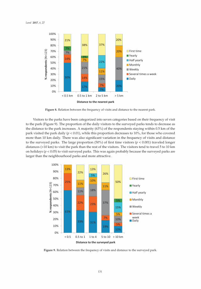
Land 2017, 6, 27

50%

17%7%

20%

14%

14%

7%

7%

21%

15%

40%

7%

11%

20%

22%

7%

3%

21%38% 37%

20%

0%

10%

20%

30%

40%

50%

60%

70%

80%

90%

100%

< 0.5 km 0.5 to 1 km 2 to 5 km > 5 km

% re

spon

dent

s (N

=123

)

Distance to the nearest park

First timeYearlyHalf yearlyMonthlyWeeklySeveral times a weekDaily

Figure 8. Relation between the frequency of visits and distance to the nearest park.

Visitors to the parks have been categorized into seven categories based on their frequency of visitto the park (Figure 9). The proportion of the daily visitors to the surveyed parks tends to decrease asthe distance to the park increases. A majority (63%) of the respondents staying within 0.5 km of thepark visited the park daily (p < 0.01), while this proportion decreases to 10%, for those who coveredmore than 10 km daily. There was also significant variation in the frequency of visits and distanceto the surveyed parks. The large proportion (50%) of first time visitors (p < 0.001) traveled longerdistances (>10 km) to visit the park than the rest of the visitors. The visitors tend to travel 5 to 10 kmon holidays (p < 0.05) to visit surveyed parks. This was again probably because the surveyed parks arelarger than the neighbourhood parks and more attractive.

63%

33% 31%19%

10%

25%

22% 23%

7%

5%

11% 18%

37%

10%

13%

11%10%

11%

5%

5%

15%

5%

22%13%

26%

50%

0%

10%

20%

30%

40%

50%

60%

70%

80%

90%

100%

< 0.5 0.5 to 1 1 to 4 5 to 10 > 10 km

% re

spon

dent

s (N

=123

)

Distance to the surveyed park

First time

Yearly

Half yearly

Monthly

Weekly

Several times aweekDaily

Figure 9. Relation between the frequency of visits and distance to the surveyed park.

131

Land 2017, 6, 27

4. Discussion

4.1. Visitor Characteristics

It is very important to understand the socio-demographic characteristics of visitors to the parkbecause personal characteristics, companion, work and living situations tend to determine recreationactivity response [72]. The population of the New Delhi district is thinly spread in comparisonto the National Capital Territory of Delhi. All four surveyed parks are known to be visited bypeople from a range of socio-economic backgrounds, Lodhi garden having higher visitation by thebureaucrats, politicians, wealthier and more influential visitors. Amongst the visitors, it is seen thata lesser proportion of women visitors visit the park than men, which is probably because womenperceive more constraints to outdoor recreation participation like personal safety concerns, inadequatefacilities and preoccupation with office and household work [73] than men do. A majority of therespondents had attained university level education, which is in contrary with the study by Jim andChen [36] in Guangzhou, China. Most of the visitors were employed, are from the age group of25 years to 55 years, and probably visit the park to relax and escape the stressful and polluted Delhicity life. A female, aged 65 said that ‘park ke swach bwatabaran mein humko bahut shanti milti hai aur Dillike dhul aur pradushan se mukti milti hai’, i.e. ‘my mind gets lot of peace in the clean environment of thepark and it also gives respite from the dust and pollution of Delhi’. A lesser proportion of visitors werefrom the age group of >55 years. It has been observed in a study of 20 countries, including India [74],that physical activity declines with age. The visitors were mostly accompanied by family members asparks are attractive places to do recreational activities with families and contribute to enhanced socialinteraction [75]. Single people are reasonably well represented in the study, conforming to the studyby Jim and Chen [36].

4.2. Environmental Awareness of the Users

Environmental awareness is a dynamic process aimed at augmenting our knowledge andunderstanding of the environment [76]. The emotional involvement of individuals tends to shapeenvironmental awareness and attitudes [77]. The association of attitudes and behavior has ledto interest in environmental attitudes as predictors of environmentally based actions and participationdecisions [78]. A pro-environmental attitude is a powerful predictor of ecological behavior [79].Pro-environmental attitudes tend to be related to resilient faith on honest intentions for speciesprotection [78]. It was observed that many of the visitors took part in protection of nature, but a lesserproportion of young adults took part in conservation of nature. On the contrary, a study in Cleveland,Ohio has shown that older age groups preferred recreation rather than conservation [80]. It has beenobserved that young people have a lesser attraction to and interest in nature due to their growingup in highly urbanized areas and in over protected environments [81]. Most of the respondents whotook park in nature conservation indicate that they were motivated to do so because of environmentaleducation components in their school educational curriculum. In India, environmental educationwas introduced as a compulsory school subject in 2003. Following this, various programs are heldin the schools to impart environmental education to students; for example, trees are planted andnurtured in the school and within the premises of houses [82]. Hence we find that a significantnumber of young adults attribute their participation in nature conservation to the school curriculum.A study by Kudryavtsev et al. [83] in the Bronx, New York shows that environmental educationenhances environmental stewardship in urban communities. Lack of time is the main hindrancefor not taking part in the conservation of nature in cities, as corroborated in studies by Mowen andConfer [84]. A study by Qiu et al. [85] shows that ecological knowledge tends to have a positiveinfluence on a preference for biodiversity. The respondents were able to identify more animals thanplant species in the parks, as also observed in Singapore [69], where the interviewees’ knowledgeof plants was less than their knowledge of animal species. A study by Rupprecht et al. [47] in Brisbaneand Sapporo reveals that the respondents didn’t consider themselves very conversant about local

132

Land 2017, 6, 27

nature when it comes to knowledge of wild plants, wild animals, and birds. The people taking partin the protection of nature tend to identify more species, as observed in Singapore [69], with membersof nature societies tending to identify a greater number of species. The poor knowledge of the plantsand animals of most visitors can be attributed to their limited encounters with nature and learningopportunities in the urban concrete built environment, which has eventually led to detachment fromand insensitiveness to their natural surroundings [36]. The neem tree and the peacock are more widelyrecognized by the visitors than the other plant and animal species in the parks. It is probably becausethe neem tree is deeply interwoven with the fabric of Indian culture [86] and widely used for its naturaltherapeutic properties in India [87], whereas the peacock, with its distinctive plumage and being thenational bird of India, is easily recognized by the visitors to the parks.

4.3. Main Uses of Green Spaces as Ascertained by Different Population Groups

Studies carried out by Swamy and Devy [88] in Bengaluru show that large urban heritage parks aremuch valued for their environmental benefits like ‘regulation of noise and temperature’ and ‘fresh airand breeze’. A similar pattern of responses can also be observed in our study. ‘Recreation’, ‘aesthetics’and ‘socializing’ together appear more valued by the respondents in Bengaluru, while in Delhi it isobserved that a much greater proportion of visitors appreciate green space for ‘Psychological andhealth benefits’. This can be related to the severe levels of air pollution in Delhi, which has beendescribed as one of the world’s most polluted cities [89].

The uses of green spaces are not perceived similarly by all individuals in a population. The oldervisitors and visitors with higher education tend to appreciate the ‘psychological and health benefits’of urban green space more than the rest of the population in Delhi. Perceptions tend to vary withsocio-economic and demographic factors, as shown by several different studies [68,90]. In Guangzhou,China, women are more reluctant to participate in outdoor recreation than men [91]. In Delhi, giventhe overall insecurity of women’s safety in public places, women do not access green spaces as muchas men. Women tend to value green spaces for passive recreational activities such as socializing [92].It is evident that social interaction contributes to better social cohesion [93]. Parks also serve as refugesfor visitors wanting to escape the stress of the city [20,94].

Priego et al.’s [67] study of three countries reveals that people with different social and culturalbackgrounds use and perceive the urban landscape in different ways. Age, gender, education level,income, retirement status, residential neighbourhood and length of stay tend to influence peoples’perception [16,91,95–97]. Varied responses to nature have also been noted between communitiesvarying in race or class [90,98]. However, Qureshi et al. [97] in study in Karachi found no impact of agegroup or gender on the behavioural pattern of respondents.

4.4. Quality of Nature

The majority of the visitors are happy with the quality of the park, but only females considerthe parks to be ‘bad’. Thus there is prevalence of negative emotions amongst the female park visitorsin Delhi. The ‘bad’ assessment of the parks may be the outcome of perceived social dangers by thefemale visitors [99]. The first time visitors rated the parks to be ‘good’. It is seen that the differentdegrees of visitors’ familiarity with the parks also leads to differences in their evaluative appraisal [100].There is a clear preference for safety, cleanliness and maintenance in the parks, as found in otherstudies like one in Los Angeles [101]. Concerns about safety have been voiced by urban residentsin Los Angeles [101] and Hong Kong [96]. Increased maintenance tends to increase the preference andsense of safety [102]. Visitors prefer promotion and advertisement for parks in order to enhance theiruse by the public. A study by Scott and Jackson [103] in Cleveland, Ohio confirmed that improvedpromotion encourages park use.

133

Land 2017, 6, 27

4.5. Distance to Green Space and Frequency of Use

Smaller distance to green spaces in urban areas is important because it contributes to improvedhuman health and wellbeing [104] and is also a key planning and management issue [105]. Thesurveyed parks are located in the New Delhi district, and visitors come from both the New Delhidistrict and places far from the New Delhi district. Only 19% of the total visitors have access to greenspaces within a distance of 500 m. This confirms that the accessibility in terms of the distance to greenspace is very low in Delhi in comparison to other countries, where the distance to green spaces isrelatively lower [68,106]. We find that the proportion of visitors increases with distance. It is likely to beas a result of the attractiveness of large parks. This confirms studies in Perth [40] and Bengaluru [88]that found that the access to large attractive green spaces is associated with higher level of walking,and distance alone is not a deterrent. This study finds that younger visitors travel longer distancesthan older visitors, and male visitors tend to visit the parks several times a week. Women face greaterconstraints to outdoor recreation participation than men [107]. With age and reduced mobility, olderpeople are reluctant to travel longer distances. This is in congruence with the study by Lo and Jim [96],in which less mobile retired people were not willing to travel longer distances to visit large parks.At the same time, students are not very enthusiastic about traveling longer distances to visit theparks. Studies have shown that the lively social environments of the parks tend to attract students,and their park use is strongly guided by their friends’ park use [108]. The number of daily visitorstends to decrease with the increase in distance to the park, which has been corroborated by studiesin Denmark [68] and Belgium [72]. Mowen and Confer [84] stated that shorter distances are criticalfor establishing a stronger user base. At the same time, a large proportion of first time and weeklyvisitors travel longer distances to visit the surveyed parks because they are larger and more attractivethan their neighbourhood parks [109]. A study by Swamy [88] also established the fact that largeattractive parks tend to attract visitors from far and wide. New Delhi park visitors who visit the parksevery day do so without family and friends. Similarly in Guangzhou [110], single visitors visit parksregularly, yet a large number of ‘first time’ visitors visit the parks with their family. The surveyedparks are attractive tourist destinations, and people are motivated to travel to attractive tourist placesas a family as it gives them the opportunity to be together [111].

5. Conclusions

This survey of park visitors in the megalopolis of Delhi aims to understand perceptions of andexpectations from nature in urban communities living in a crowded Indian city. This study addsto information that can help in the better design of parks in response to peoples’ expectations in Delhi.It also contributes to the rather limited information on peoples’ perceptions and needs from urbangreen spaces in cities in the Global South, in contrast to the relatively greater information availablefrom cities in Europe and North America [16,67,68], and adds to a small but steadily growing databaseof studies from Asia [88,91,97]. Some findings, such as the increased attractiveness of large parks withmore visitors, specifically women and families, due to considerations of safety, may be specific to citiessuch as Delhi, with its relatively high rate of crime and insecurity for women. Other findings, suchas the tendency of daily visitors to visit alone but for one-time visitors to visit with family, are trendsthat can be seen across other parks. Further research in parks across Delhi and other cities in Indiais required to understand the Delhi-specific and India-specific characteristics of the case study and,consequently, the implications for planning policies in other urban contexts.

In the stressful and polluted city life of Delhi, visitors value urban green spaces most forthe ‘environmental benefits’. Older adults and postgraduate educated visitors especially tendto appreciate the ‘psychological and health. We also find that the accessibility in terms of distanceto green space is very low in Delhi compared to other cities. Large parks tend to attract morevisitors from further distances, despite their having small neighbourhood parks in the vicinity of theirhomes. The visitors want better quality parks with proper maintenance and better infrastructuralfacilities like separate play areas for children and better security. There are various barriers to park

134

Land 2017, 6, 27

use like lack of time, transport problem, poverty, lack of companion, and safety. Safety representsa constraint on the use of parks, particularly for women and families and especially in places like Delhi,where the interior areas of these large parks are often ‘safe havens’ for criminals after sunset [112].An increased focus on security will help residents to access the parks in greater numbers withoutcompromising their personal safety. Such measures will be likely to increase the uses of greenspace by a diverse mix of gender and age groups. This will ensure socially favourable urban parksfor the wellbeing of the urban community. Public perceptions of green spaces in Delhi throw up aninteresting mix of requirements, with an increased focus on the aesthetic and the environmental benefitsin preference to biodiversity. This study has policy implications for planners and urban designers,as well as for environmental organizations. The pro-environmental attitude of the respondents isexpressed by the presence of ‘plants at home’, taking part in ‘conservation of nature’, and theirawareness for ‘need for more parks/green spaces’. Due to India’s age-old tradition and cultureof using neem for various purposes, this tree is easily identified by park visitors, but still there is a gapin the public understanding of biodiversity in Delhi’s parks, with the result that one out of three visitorscannot name a single plant species, while one out of four visitors were unable to name a single commonanimal or insect that they had observed in the park. Further research is required to understand andtake into account the opinion of visitors, capture the views of diverse age, gender, and ethnic-culturalgroups in the planning and designing of urban parks and green spaces. It will be interesting to lookat the differences of perception of the visitors residing in the New Delhi district and visitors to theNew Delhi district. Further analysis combining survey data on socio-economic information withsocio-economic data from the census, based on visitors’ places of residence, is necessary to find outwhether our results hold up for a larger sample of the population and in more recent years. Thiswill ensure effective plans and designs capable of satisfying the needs of the urban community. Themethodological approach of the study has exportability, and the empirical information obtainedin study has comparability to other Indian cities and cities of the Global South. Given the rapidurbanization currently underway in India, concomitant with the disappearance of trees, wetlands,and green spaces, access to parks provides an increasingly rare opportunity for exposure to naturefor many Indian urbanites. This study aims to contribute to an increased focus on the importanceof green spaces in the urban context in India, where the current focus on smart cities [113] threatensto obscure the importance of low-technology options for improving urban resilience and wellbeingthrough a renewed focus on urban green spaces.

Acknowledgments: We thank the Royal Norwegian Embassy (RNE: IND-3025 1210050) and the Tata SocialWelfare Trust (TSWT:TSWT/IG/SP/BM/sm/CM/24/MNRL/2011-12) for doctoral research support to SomajitaPaul, and we thank Azim Premji University for research support to Harini Nagendra.

Author Contributions: Harini Nagendra and Somajita Paul jointly conceived the study and wrote the paper;Somajita Paul surveyed and analyzed the data; and Harini Nagendra supervised the study.

Conflicts of Interest: The authors declare no conflict of interest. The founding sponsors had no role in the designof the study; in the collection, analyses, or interpretation of data; in the writing of the manuscript; or in the decisionto publish the results.

References

1. Rose, S.; Peters, N.E. Effects of urbanization on streamflow in the Atlanta area (Georgia, USA): A comparativehydrological approach. Hydrol. Process. 2001, 15, 1441–1457. [CrossRef]

2. Booth, D.B.; Jackson, C.R. Urbanization of aquatic systems: Degradation thresholds, storm water detection,and the limits of mitigation. JAWRA J. Am. Water Resour. Assoc. 1997, 33, 1077–1090. [CrossRef]

3. Khera, N.; Mehta, V.; Sabata, B. Interrelationship of birds and habitat features in urban greenspaces in Delhi,India. Urban For. Urban Green. 2009, 8, 187–196. [CrossRef]

4. Riley, S.P.; Sauvajot, R.M.; Fuller, T.K.; York, E.C.; Kamradt, D.A.; Bromley, C.; Wayne, R.K. Effectsof urbanization and habitat fragmentation on bobcats and coyotes in southern California. Conserv. Biol. 2003,17, 566–576. [CrossRef]

135

Land 2017, 6, 27

5. McKinney, M.L. Urbanization, biodiversity, and conservation: The impacts of urbanization on native speciesare poorly studied, but educating a highly urbanized human population about these impacts can greatlyimprove species conservation in all ecosystems. Bioscience 2002, 52, 883–890. [CrossRef]

6. Wang, L.; Lyons, J.; Kanehl, P.; Bannerman, R. Impacts of urbanization on stream habitat and fish acrossmultiple spatial scales. Environ. Manag. 2001, 28, 255–266. [CrossRef]

7. Vailshery, L.S.; Jaganmohan, M.; Nagendra, H. Effect of street trees on microclimate and air pollutionin a tropical city. Urban For. Urban Green. 2013, 12, 408–415. [CrossRef]

8. Shepherd, J.M.; Pierce, H.; Negri, A.J. Rainfall modification by major urban areas: Observations fromspaceborne rain radar on the TRMM satellite. J. Appl. Meteorol. 2002, 41, 689–701. [CrossRef]

9. Huff, F.; Changnon, S.A., Jr. Climatological assessment of urban effects on precipitation at St. Louis.J. Appl. Meteorol. 1972, 11, 823–842. [CrossRef]

10. Kaufmann, R.K.; Seto, K.C.; Schneider, A.; Liu, Z.; Zhou, L.; Wang, W. Climate response to rapid urbangrowth: Evidence of a human-induced precipitation deficit. J. Clim. 2007, 20, 2299–2306. [CrossRef]

11. Li, J.; Song, C.; Cao, L.; Zhu, F.; Meng, X.; Wu, J. Impacts of landscape structure on surface urban heat islands:A case study of Shanghai, China. Remote Sens. Environ. 2011, 115, 3249–3263. [CrossRef]

12. Grimmond, S. Urbanization and global environmental change: Local effects of urban warming. Geogr. J.2007, 173, 83–88. [CrossRef]

13. Baker, L.A.; Brazel, A.J.; Selover, N.; Martin, C.; McIntyre, N.; Steiner, F.R.; Nelson, A.; Musacchio, L.Urbanization and warming of Phoenix (Arizona, USA): Impacts, feedbacks and mitigation. Urban Ecosyst.2002, 6, 183–203. [CrossRef]

14. Saitoh, T.; Shimada, T.; Hoshi, H. Modeling and simulation of the Tokyo urban heat island. Atmos. Environ.1996, 30, 3431–3442. [CrossRef]

15. Bolund, P.; Hunhammar, S. Ecosystem services in urban areas. Ecol. Econ. 1999, 29, 293–301. [CrossRef]16. Chiesura, A. The role of urban parks for the sustainable city. Landsc. Urban Plan. 2004, 68, 129–138. [CrossRef]17. Gobster, P.H. Perception and use of a metropolitan greenway system for recreation. Landsc. Urban Plan. 1995,

33, 401–413. [CrossRef]18. Mactavish, J.B.; Schleien, S.J. Playing together growing together: Parent’s perspectives on the benefits of family

recreation in families that include children with a developmental disability. Ther. Recreat. J. 1998, 32, 207.19. Pretty, J.; Peacock, J.; Hine, R.; Sellens, M.; South, N.; Griffin, M. Green exercise in the UK countryside: Effects

on health and psychological well-being, and implications for policy and planning. J. Environ. Plan. Man.2007, 50, 211–231. [CrossRef]

20. De Vries, S.; Verheij, R.A.; Groenewegen, P.P.; Spreeuwenberg, P. Natural environments—healthyenvironments? An exploratory analysis of the relationship between greenspace and health. Environ. Plan. A2003, 35, 1717–1731. [CrossRef]

21. Lee, A.C.; Maheswaran, R. The health benefits of urban green spaces: A review of the evidence. J. Public Health2011, 33, 212–222. [CrossRef] [PubMed]

22. Nielsen, T.S.; Hansen, K.B. Do green areas affect health? Results from a Danish survey on the use of greenareas and health indicators. Health Place 2007, 13, 839–850. [CrossRef] [PubMed]

23. Fuller, R.A.; Irvine, K.N.; Devine-Wright, P.; Warren, P.H.; Gaston, K.J. Psychological benefits of greenspaceincrease with biodiversity. Biol. Lett. 2007, 3, 390–394. [CrossRef] [PubMed]

24. Van den Berg, A.E.; Maas, J.; Verheij, R.A.; Groenewegen, P.P. Green space as a buffer between stressful lifeevents and health. Soc. Sci. Med. 2010, 70, 1203–1210. [CrossRef] [PubMed]

25. Cattell, V.; Dines, N.; Gesler, W.; Curtis, S. Mingling, observing, and lingering: Everyday public spaces andtheir implications for well-being and social relations. Health Place 2008, 14, 544–561. [CrossRef] [PubMed]

26. Maas, J.; Van Dillen, S.M.; Verheij, R.A.; Groenewegen, P.P. Social contacts as a possible mechanism behindthe relation between green space and health. Health Place 2009, 15, 586–595. [CrossRef] [PubMed]

27. Peters, K.; Elands, B.; Buijs, A. Social interactions in urban parks: Stimulating social cohesion?Urban For. Urban Green. 2010, 9, 93–100. [CrossRef]

28. Bell, S.; Tyrväinen, L.; Sievänen, T.; Pröbstl, U.; Simpson, M. Outdoor recreation and nature tourism:A European perspective. Living Rev. Landsc. Res. 2007, 1, 1–46. [CrossRef]

29. Kaczynski, A.T.; Henderson, K.A. Environmental correlates of physical activity: A review of evidence aboutparks and recreation. Leis. Sci. 2007, 29, 315–354. [CrossRef]

136

Land 2017, 6, 27

30. Tyrväinen, L.; Väänänen, H. The economic value of urban forest amenities: An application of the contingentvaluation method. Landsc. Urban Plan. 1998, 43, 105–118. [CrossRef]

31. Van Herzele, A.; Wiedemann, T. A monitoring tool for the provision of accessible and attractive urban greenspaces. Landsc. Urban Plan. 2003, 63, 109–126. [CrossRef]

32. Tajima, K. New estimates of the demand for urban green space: Implications for valuing the environmentalbenefits of Boston’s big dig project. J. Urban Aff. 2003, 25, 641–655. [CrossRef]

33. Conway, D.; Li, C.Q.; Wolch, J.; Kahle, C.; Jerrett, M. A spatial autocorrelation approach for examiningthe effects of urban greenspace on residential property values. J. Real Estate Financ. Econom. 2010, 41,150–169. [CrossRef]

34. Morancho, A.B. A hedonic valuation of urban green areas. Landsc. Urban Plan. 2003, 66, 35–41. [CrossRef]35. Tyrväinen, L. Economic valuation of urban forest benefits in Finland. J. Environ. Manag. 2001, 62, 75–92.

[CrossRef] [PubMed]36. Jim, C.; Chen, W.Y. Perception and attitude of residents toward urban green spaces in Guangzhou (China).

Environ. Manag. 2006, 38, 338–349. [CrossRef] [PubMed]37. Martín-López, B.; Montes, C.; Benayas, J. The non-economic motives behind the willingness to pay for

biodiversity conservation. Biol. Conserv. 2007, 139, 67–82. [CrossRef]38. Lamarque, P.; Tappeiner, U.; Turner, C.; Steinbacher, M.; Bardgett, R.D.; Szukics, U.; Schermer, M.; Lavorel, S.

Stakeholder perceptions of grassland ecosystem services in relation to knowledge on soil fertility andbiodiversity. Reg. Environ. Chang. 2011, 11, 791–804. [CrossRef]

39. Matsuoka, R.H.; Kaplan, R. People needs in the urban Landscape Urban Plann: Analysis of landscape andurban planning contributions. Landsc. Urban Plan. 2008, 84, 7–19. [CrossRef]

40. Giles-Corti, B.; Broomhall, M.H.; Knuiman, M.; Collins, C.; Douglas, K.; Ng, K.; Lange, A.; Donovan, R.J.Increasing walking: How important is distance to, attractiveness, and size of public open space?Am. J. Prev. Med. 2005, 28, 169–176. [CrossRef] [PubMed]

41. Nutsford, D.; Pearson, A.L.; Kingham, S. An ecological study investigating the association between accessto urban green space and mental health. Public Health 2013, 127, 1005–1011. [CrossRef] [PubMed]

42. Boone, C.G.; Buckley, G.L.; Grove, J.M.; Sister, C. Parks and People: An Environmental Justice Inquiryin Baltimore, Maryland. Assoc. Am. Geogr. 2009, 99, 767–787. [CrossRef]

43. Lin, B.; Fuller, R.A.; Bush, R.; Gaston, K.J.; Shanahan, D.F. Opportunity or Orientation? Who Uses UrbanParks and Why. PLoS ONE 2014, 9, e87422. [CrossRef] [PubMed]

44. Larson, L.R.; Jennings, V.; Cloutier, S.A. Public Parks and Wellbeing in Urban Areas of the United States.PLoS ONE 2016, 11, e0153211. [CrossRef] [PubMed]

45. Thaiutsa, B.; Puangchit, L.; Kjelgren, R.; Arunpraparut, W. Urban green space, street tree and heritage largetree assessment in Bangkok, Thailand. Urban For. Urban Green. 2008, 7, 219–229. [CrossRef]

46. Yuen, B.; Hien, W.N. Resident perceptions and expectations of rooftop gardens in Singapore.Landsc. Urban Plan. 2005, 73, 263–276. [CrossRef]

47. Rupprecht, C.D.; Byrne, J.A.; Ueda, H.; Lo, A.Y. ‘It’s real, not fake like a park’: Residents’ perception anduse of informal urban green-space in Brisbane, Australia and Sapporo, Japan. Landsc. Urban Plan. 2015, 143,205–218. [CrossRef]

48. Chang, H.-S.; Chen, T.-L. Decision making on allocating urban green spaces based upon spatially-varyingrelationships between urban green spaces and urban compaction degree. Sustainability 2015, 7, 13399–13415.[CrossRef]

49. Yang, J.; Li, C.; Li, Y.; Xi, J.; Ge, Q.; Li, X. Urban green space, uneven development and accessibility: A caseof Dalian’s Xigang District. Chin. Geogr. Sci. 2015, 25, 644–656. [CrossRef]

50. Tan, P.Y.; Ismail, M.R.B. The effects of urban forms on photosynthetically active radiation and urban greeneryin a compact city. Urban Ecosyst. 2015, 18, 937–961. [CrossRef]

51. Lin, B.; Meyers, J.; Barnett, G. Understanding the potential loss and inequities of green space distributionwith urban densification. Urban For. Urban Green. 2015, 14, 952–958. [CrossRef]

52. Paul, S.; Nagendra, H. Vegetation change and fragmentation in the mega city of Delhi: Mapping 25 yearsof change. Appl. Geogr. 2015, 58, 153–166. [CrossRef]

53. Government of NCT of Delhi. Available online: http://www.delhi.gov.in/wps/wcm/connect/doit_dpg/DoIT_DPG/Home (accessed on 20 November 2014).

137

Land 2017, 6, 27

54. Chandramouli, C.; General, R. Census of India 2011. In Provisional Population Totals; Government of India:New Delhi, India, 2011.

55. Dupont, V. Conflicting stakes and governance in the peripheries of large Indian metropolises–an introduction.Cities 2007, 24, 89–94. [CrossRef]

56. Buch, M. Lutyens’ New Delhi—yesterday, today and tomorrow. India Int. Cent. Q. 2003, 30, 29–40.57. Prasad, G.; Kumar, D.; Nain, G. New Delhi as a Tourism Region. Glob. J. Res. Anal. 2015, 4, 8.58. Mohan, M. Climate change: Evaluation of ecological restoration of Delhi ridge using remote sensing and

GIS technologies. Int. Arch. Photogramm. Remote Sens. 2000, 33, 886–894.59. Lodi, B. Lodi dynasty. Available online: https://www.revolvy.com/main/index.php?s=Lodi%20Dynasty&

item_type=topic (accessed on 5 March 2017).60. Sharma, J.P. The British treatment of historic gardens in the Indian subcontinent: The transformation of

Delhi’s nawab Safdarjung’s tomb complex from a funerary garden into a public park. Gard. Hist. 2007, 35,210–228.

61. Feilden, B.M. Bhuli Bhatiyari ka Mahal, Delhi. Archit. Plus Des. 1992, 9, 63.62. Rosenthal, R.; Rosnow, R.L. Essentials of Behavioral Research: Methods and Data Analysis; McGraw-Hill:

New York, NY, USA, 1991.63. Tucker, P.; Gilliland, J.; Irwin, J.D. Splashpads, swings, and shade: Parents’ preferences for neighbourhood

parks. Can. J. Public Health. 2007, 98, 198–202. [PubMed]64. D’Souza, R.; Nagendra, H. Changes in public commons as a consequence of urbanization: The Agara lake

in Bangalore, India. Environ. Manag. 2011, 47, 840. [CrossRef] [PubMed]65. Krenichyn, K. ‘The only place to go and be in the city’: Women talk about exercise, being outdoors, and the

meanings of a large urban park. Health Place 2006, 12, 631–643. [CrossRef] [PubMed]66. Nordh, H.; Alalouch, C.; Hartig, T. Assessing restorative components of small urban parks using conjoint

methodology. Urban For. Urban Green. 2011, 10, 95–103. [CrossRef]67. Priego, C.; Breuste, J.; Rojas, J. Perception and value of nature in urban landscapes: A comparative analysis

of cities in Germany, Chile and Spain. Landsc. Online 2008, 7, 22. [CrossRef]68. Schipperijn, J.; Ekholm, O.; Stigsdotter, U.K.; Toftager, M.; Bentsen, P.; Kamper-Jørgensen, F.; Randrup, T.B.

Factors influencing the use of green space: Results from a Danish national representative survey.Landsc. Urban Plan. 2010, 95, 130–137. [CrossRef]

69. Briffett, C.; Sodhi, N.; Yuen, B.; Kong, L. Green corridors and the quality of urban life in Singapore.In Proceedings the 4th International Urban Wildlife Symposium, Arizona, AR, USA, 1–5 May 2004; pp. 56–63.

70. Randler, C.; Höllwarth, A.; Schaal, S. Urban park visitors and their knowledge of animal species. Anthrozoos2007, 20, 65–74. [CrossRef]

71. Cressie, N. Statistics for Spatial Data; John Wiley Sons: New York, NY, USA, 2015.72. Roovers, P.; Hermy, M.; Gulinck, H. Visitor profile, perceptions and expectations in forests from a gradient

of increasing urbanisation in central Belgium. Landsc. Urban Plan. 2002, 59, 129–145. [CrossRef]73. Huda, S.S.M.S.; Akhtar, A. Leisure behaviour of working women of Dhaka, Bangladesh. Int. J. Urban

Labour Leis. 2005, 7, 1–30.74. Bauman, A.; Bull, F.; Chey, T.; Craig, C.L.; Ainsworth, B.E.; Sallis, J.F.; Pratt, M. The international prevalence

study on physical activity: Results from 20 countries. Int. J. Behav. Nutr. Phys. Act. 2009, 6, 21. [CrossRef][PubMed]

75. Ujang, N.; Moulay, A.; Zakariya, K. Sense of well-being indicators: Attachment to public parks in Putrajaya,Malaysia. Procedia-Soc. Behav. Sci. 2015, 202, 487–494. [CrossRef]

76. Rego, A.B.; Muthoka, M.G. Education for environmental awareness. Soc. Relig. Concerns East Afr.A Wajibu Anthol. 2005, 10, 197.

77. Kollmuss, A.; Agyeman, J. Mind the gap: Why do people act environmentally and what are the barriersto pro-environmental behavior? Environ. Educ. Res. 2002, 8, 239–260. [CrossRef]

78. Kotchen, M.J.; Reiling, S.D. Environmental attitudes, motivations, and contingent valuation of nonuse values:A case study involving endangered species. Ecol. Econ. 2000, 32, 93–107. [CrossRef]

79. Kaiser, F.G.; Ranney, M.; Hartig, T.; Bowler, P.A. Ecological behavior, environmental attitude, and feelingsof responsibility for the environment. Eur. Psychol. 1999, 4, 59. [CrossRef]

80. Payne, L.L.; Mowen, A.J.; Orsega-Smith, E. An examination of park preferences and behaviors among urbanresidents: The role of residential location, race, and age. Leis. Sci. 2002, 24, 181–198. [CrossRef]

138

Land 2017, 6, 27

81. Kong, L.; Yuen, B.; Sodhi, N.S.; Briffett, C. The construction and experience of nature: Perspectives of urbanyouths. Tijdschr. Econ. Soc. Geogr. 1999, 90, 3–16. [CrossRef]

82. Sonowal, C.J. Environmental education in schools: The Indian scenario. J. Hum. Ecol. 2009, 28, 15–36.83. Kudryavtsev, A.; Krasny, M.E.; Stedman, R.C. The impact of environmental education on sense of place

among urban youth. Ecosphere 2012, 3, 1–15. [CrossRef]84. Mowen, A.J.; Confer, J.J. The relationship between perceptions, distance, and socio-demographic

characteristics upon public use of an urban park “in-fill”. J. Park Recreat. Adm. 2003, 21, 58–74.85. Qiu, L.; Lindberg, S.; Nielsen, A.B. Is biodiversity attractive?—On-site perception of recreational and

biodiversity values in urban green space. Landsc. Urban Plan. 2013, 119, 136–146. [CrossRef]86. Marden, E. The neem tree patent: International conflict over the commodification of life. Boston Coll. Int.

Comp. Law Rev. 1999, 22, 279.87. Verma, V.C.; Gond, S.K.; Kumar, A.; Kharwar, R.N.; Strobel, G. The endophytic mycoflora of bark, leaf, and

stem tissues of Azadirachta indica A. Juss (Neem) from Varanasi (India). Microb. Ecol. 2007, 54, 119–125.[CrossRef] [PubMed]

88. Swamy, S.; Devy, S. Forests, heritage green spaces, and neighbourhood parks: Citizen’s attitude andperception towards ecosystem services in Bengaluru. J. Resour. Energy Dev. 2010, 7, 117–122.

89. Guttikunda, S.K.; Calori, G. A gis based emissions inventory at 1 km × 1 km spatial resolution for airpollution analysis in Delhi, India. Atmos. Environ. 2013, 67, 101–111. [CrossRef]

90. Crow, T.; Brown, T.; De Young, R. The riverside and Berwyn experience: Contrasts in landscape structure,perceptions of the urban landscape, and their effects on people. Lands. Urban Plan. 2006, 75, 282–299.[CrossRef]

91. Jim, C.; Shan, X. Socioeconomic effect on perception of urban green spaces in Guangzhou, China. Cities 2013,31, 123–131. [CrossRef]

92. Björk, J.; Albin, M.; Grahn, P.; Jacobsson, H.; Ardö, J.; Wadbro, J.; Östergren, P.-O.; Skärbäck, E. Recreationalvalues of the natural environment in relation to neighbourhood satisfaction, physical activity, obesity andwellbeing. J. Epidemiol. Community Health 2008, 62, e2. [CrossRef] [PubMed]

93. Maloutas, T. Editorial: Urban segregation and the European context. Greek Rev. Soc. Res. 2004, 113, 3–24.[CrossRef]

94. Bishop, I.; Ye, W.-S.; Karadaglis, C. Experiential approaches to perception response in virtual worlds.Landsc. Urban Plan. 2001, 54, 117–125. [CrossRef]

95. Tyrväinen, L.; Mäkinen, K. Tools for Mapping Social Values and Meaning of Urban Woodlands and Other OpenSpace; COST Action C11 Green Structures and Urban Planning–Final report; COST: Brussels, Belgium, 2004.

96. Lo, A.Y.; Jim, C.Y. Citizen attitude and expectation towards greenspace provision in compact urban milieu.Land Use Policy 2012, 29, 577–586. [CrossRef]

97. Qureshi, S.; Breuste, J.H.; Jim, C. Differential community and the perception of urban green spaces and theircontents in the megacity of Karachi, Pakistan. Urban Ecosyst. 2013, 16, 853–870. [CrossRef]

98. Pincetl, S.; Gearin, E. The reinvention of public green space. Urban Geogr. 2005, 26, 365–384. [CrossRef]99. Sreetheran, M.; Van Den Bosch, C.C.K. A socio-ecological exploration of fear of crime in urban green

spaces–A systematic review. Urban For. Urban Green. 2014, 13, 1–18. [CrossRef]100. Wong, K.K.; Domroes, M. The visual quality of urban park scenes of Kowloon Park, Hong Kong: Likeability,

affective appraisal, and cross-cultural perspectives. Environ. Plan. B Plan Des. 2005, 32, 617–632. [CrossRef]101. Gearin, E.; Kahle, C. Teen and adult perceptions of urban green space Los Angeles. Child. Youth Environ.

2006, 16, 25–48.102. Kuo, F.E.; Bacaicoa, M.; Sullivan, W.C. Transforming inner-city landscapes trees, sense of safety, and

preference. Environ. Behav. 1998, 30, 28–59. [CrossRef]103. Scott, D.; Jackson, E.L. Factors that limit and strategies that might encourage people’s use of public parks.

J. Park Recreat. Adm. 1996, 14, 1–17.104. Sotoudehnia, F.; Comber, A. Poverty and Environmental Justice: A GIS Analysis of Urban Greenspace

Accessibility for Different Economic Groups. In Proceedings of the 13th AGILE Int Conf on GeographicInformation Science, Guimaraes, Portugal, 11–14 May 2010; pp. 10–14.

105. Allison, M.T. Culture, Conflict, and Communication in the Wildland-Urban Interface; Access and boundarymaintenance: Serving culturally diverse populations; Eastview Press: Boulder, CO, USA, 1992; pp. 99–108.

139

Land 2017, 6, 27

106. Barbosa, O.; Tratalos, J.A.; Armsworth, P.R.; Davies, R.G.; Fuller, R.A.; Johnson, P.; Gaston, K.J. Who benefitsfrom access to green space? A case study from Sheffield, UK. Landsc. Urban Plan. 2007, 83, 187–195.[CrossRef]

107. Johnson, C.Y.; Bowker, J.M.; Cordell, H.K. Outdoor recreation constraints: An examination of race, gender,and rural dwelling. South. Rural Sociol. 2001, 7, 111–133.

108. Ries, A.V.; Voorhees, C.C.; Roche, K.M.; Gittelsohn, J.; Yan, A.F.; Astone, N.M. A quantitative examination ofpark characteristics related to park use and physical activity among urban youth. J. Adolesc. Health 2009, 45,S64–S70. [CrossRef] [PubMed]

109. Chaudhry, P.; Bagra, K.; Singh, B. Urban greenery status of some Indian cities: A short communication. Int. J.Environ. Sci. Dev. 2011, 2, 98. [CrossRef]

110. Jim, C.Y.; Chen, W.Y. Recreation–amenity use and contingent valuation of urban greenspaces in Guangzhou,China. Landsc. Urban Plan. 2006, 75, 81–96. [CrossRef]

111. Yoon, Y.; Uysal, M. An examination of the effects of motivation and satisfaction on destination loyalty:A structural model. Tour. Manag. 2005, 26, 45–56. [CrossRef]

112. Pankhuri, Y. Times of India. Available online: http://timesofindia.indiatimes.com/city/delhi/parks-safe-haven-for-criminals-at-night/articleshow/57239080.cms (accessed on 4 April 2017).

113. Government of India. Ministry of Urban Development. Available online: http://moud.gov.in/cms/schemes-or-programmes.php (accessed on 1 February 2017).


140

land

Article

Informal Urban Green Space: Residents’ Perception,Use, and Management Preferences across Four MajorJapanese Shrinking Cities

Christoph D. D. Rupprecht ID

FEAST Project, Research Institute for Humanity and Nature, Kyoto 6038047, Japan; [email protected];Tel.: +81-75-707-2499

Received: 3 August 2017; Accepted: 22 August 2017; Published: 25 August 2017

Abstract: Urban residents’ health depends on green infrastructure to cope with climate change.Shrinking cities could utilize vacant land to provide more green space, but declining tax revenuespreclude new park development—a situation pronounced in Japan, where some cities are projected toshrink by over ten percent, but lack green space. Could informal urban green spaces (IGS; vacant lots,street verges, brownfields etc.) supplement parks in shrinking cities? This study analyzes residents’perception, use, and management preferences (management goals, approaches to participatorymanagement, willingness to participate) for IGS using a large, representative online survey (n = 1000)across four major shrinking Japanese cities: Sapporo, Nagano, Kyoto and Kitakyushu. Results showthat residents saw IGS as a common element of the urban landscape and their daily lives, but theirevaluation was mixed. Recreation and urban agriculture were preferred to redevelopment andnon-management. For participative management, residents saw a need for the city administrationto mediate usage and liability, and expected an improved appearance, but emphasized the needfor financial and non-financial support. A small but significant minority (~10%) were willing toparticipate in management activities. On this basis, eight principles for participatory informal greenspace planning are proposed.

Keywords: vacant land; land use; urban planning; Japan; wasteland; green infrastructure; recreation;landscape; participatory management; depopulation

1. Introduction

Urban green spaces as an essential element of green infrastructure are increasingly linked tohuman wellbeing [1–5]. However, the benefits they provide come at a price, from maintenanceof facilities and vegetation to day-to-day management [6]. This financial burden is particularlypronounced in countries such as Japan, where municipalities face a shrinking tax base due todemographic trends of aging and depopulation [7]. Furthermore, maintenance costs for urban greenspaces in Japan are rising, as parks created during the 1960s and 1970s period of economic andpopulation growth are increasingly in need of refurbishment [8]. On the other hand, Japanese citiesprovide residents only with a comparatively low amount of green space (ca. 10 m2 per person inmajor cities [9]). This raises the question of how local governments can procure additional green spaceareas, not least to adapt to climate change, rising temperatures and associated heat waves. Citiesin North America and Europe have been looking toward participative vacant land management tomeet residents’ needs [10–14]. However, despite introducing participative management for formalgreen spaces since the 1990s [15], local governments in Japan have been slow to explore this directionfor non-traditional green spaces. Yet such schemes might create more recreational green space,provide benefits associated with green infrastructure, and could simultaneously alleviate the costs ofmaintenance. One reason for the lack of similar initiatives in Japan may lie in the scarcity of related


Land 2017, 6, 59

research—we still know little about what residents in Japan think of informal urban green spaces suchas vacant lots, street verges or brownfields, let alone participative management approaches. To fillthis gap, this paper seeks to provide some insight by analyzing how residents in four major shrinkingJapanese cities perceive and use informal urban green spaces, what management goals and approachesthey prefer, and how willing they are to participate in managing such spaces.

Japanese cities are facing a major demographic challenge with consequences for urban land andgreen space management. This makes the country a useful object of study, because similar demographictrends are expected in other countries such as South Korea or China as the population peaks and theeconomy enters the post-growth stage. Until 2040, many are projected to experience both rapid agingand population decline, with some likely to lose over 10% of their total population [16]. The majoreffects of this trend are fourfold. First, the cumulative effects of aging and depopulation are erodingcities’ tax base, which in turn forces them to balance expenses for maintaining green spaces withcompeting demands such as aging water infrastructure. This puts budgets for green space underscrutiny and leaves them at risk of being cut, even though many Japanese cities already fail to providethe 10 m2 of park area per person set in governmental standards [17]. Second, the number of bothvacant houses and vacant lots are increasing [18], a trend that will likely accelerate as populationdecline intensifies. While this process could be seen as an opportunity for municipalities to buyland at a moderate price to increase public green space, their financial situation makes this difficult.In fact, strategic park planning in Japan has recently focused on protecting current levels of greenspace rather than expanding them, as cities are struggling to cover maintenance costs for parks builtduring the decades of high population and economic growth. Third, as the population demographicschange, so do people’s green space and nature needs [19]. Recent years have seen a strong demandfor recreational urban agriculture, with long waiting lists for community garden parcels being acommon occurrence. While some cities such as Yokohama have started retrofitting parks with areas forgrowing vegetables, such initiatives are still rare. Finally, Japanese cities will need to invest heavily intogreen infrastructure to adapt to and mitigate the effects of rising global temperatures due to climatechange [20–22]. The cities’ aging population is particular at risk from heat-related health problems,making this also an urgent issue of public health. These demographic transition-related major effectshave led researchers to investigate the potential of non-traditional green spaces [23].

Recent research has shown that both in Japan and abroad, informal urban green spaces (IGS) suchas vacant lots, street verges, brownfields, power line corridors and waterside spaces can make upabout 5% of urban land [24]. Moreover, residents are already using these spaces for recreation, bothas adults and children [23,25]. However, not all residents evaluate these spaces favorably as they arelargely unmanaged. In particular, the aesthetics of wild nature do not necessarily directly translatefrom a Western to a Japanese cultural context [26], where many residents prefer to see a humantouch as evidence of human care and attention for a space. Against an international backgroundof residents using and re-using—often spontaneously—land considered derelict or unwanted byconventional urban planning [27–29], researchers have thus called for exploring ways informal greenspaces in shrinking Japanese cities could be managed by the local community using participatoryapproaches [23]. However, a number of questions about participatory IGS management in Japanremain unanswered. Addressing the following gaps in the literature will support municipalitiesin planning and implementing such management approaches, with the intention of contributing toresidents’ wellbeing.

Under what circumstances and in what form might participatory IGS management be feasible inshrinking Japanese cities? To answer these questions, two major gaps in the existing literature need tobe addressed. First, existing exploratory studies [23,25] on how residents in Japan perceive, use, andevaluate IGS have been limited in scope (single city) and sample size (<200), were not representativeand, as mail-back surveys, may have suffered from bias where only residents interested in the topicresponded. Second, we know little about how residents think of participatory IGS management, fromtheir preferred management goals and approaches to acceptable levels and forms of participation.

142

Land 2017, 6, 59

This paper thus focuses on the following questions: (1) how do residents perceive, use andevaluate IGS across major shrinking Japanese cities; (2) what management goals do residents prefer forIGS; (3) how do residents think about different ways, approaches and circumstances in participatoryIGS management; and (4) how willing are residents to engage in participatory IGS management?Addressing these questions is important, because the resulting findings and insights may inform urbanplanning, climate adaptation and participatory management in post-growth industrialized countries,using Japan as a case where depopulation is most advanced. The study thus contributes to the local(site-specific), national and international discourse.


2.1. Study Sites

This study focused on the Japanese cities Sapporo, Kyoto, Kitakyushu and Nagano, all fourprojected to lose over 10% of their current population until 2040 [16]. They were selected to representthe regional Japanese cities expected to shrink most severely as a result of Japan’s projected nationalpopulation decline. Differences in city age, population size, population density and green space percapita (Table 1) and geographic location (Figure 1) provide a range variety of geographic context.Additionally, including Sapporo allows comparison of results with previous research on IGS in the city,in particular addressing potential nonresponse bias in the previous mail-back survey.

Figure 1. Location of the four targeted shrinking cities in Japan (green).

143

Land 2017, 6, 59

Table 1. Comparison of study sites.

Characteristics Sapporo Kyoto Kitakyushu Nagano

City status 1902(founded 1824)

1889 (founded~600 AD)

1963 (formerly Mojigaseki,founded ~645 AD)

1897 (founded~642 AD)

Population (2015) 1.95 million 1.48 million 961,000 378,000

Projected population (2040) 1.71 million 1.28 million 784,000 302,000

Area (km2) 1121 828 492 835

Population density(inhabitants/km2) 1741 1782 1954 452

Climate (Köppen-Geiger) Dfa Cfa Cfa Cfa

Green space per capita (2015) 12.5 4.4 12.0 9.4

Sources: Wikipedia Japan [16], IPSS 2013, Statistics Japan 2015 (https://www.e-stat.go.jp/SG1/estat/eStatTopPortalE.do)

2.2. Data Collection, Survey Instrument and Data Analysis

The survey was conducted across the four study sites through an online survey coordinatedthrough Rakuten Research, a major Japanese online polling service. Respondents were recruited fromthe service’s panel, consented to and received compensation for their participation in accordanceto the service’s policies (the exact compensation is not disclosed by the company, but is less than¥1000/US$10/10 €). Responses were collected over a period of two weeks in late 2016, and sampled tobe representative for the population demographic of the respective cities. The study was approved bythe home institution’s research ethics committee (RIHN2017-1).

The survey instrument (see File S1) consisted of 24 questions in four parts: (1) respondents’perception, recreational use and evaluation of IGS; (2) respondents’ preferences for IGS managementgoals, management approaches, and willingness to participate in management; (3) respondents’opinion about the value of urban nature and general preferences for urban land use directions inshrinking cities; and (4) respondents’ socio-demographic data. Question types included multiplechoice, Likert-scale, modified Likert-scale (agree with option A or B) and open comment questions.The cover page of the survey instrument contained a brief explanation of what IGS are alongside atypology with color photographs (Figure 2; File S1). Native Japanese speakers helped to ensure thesurvey instrument was linguistically correct and easy to read. Questions in part one drew on previousresearch about residents’ perception, use and evaluation of IGS in Sapporo and Brisbane [23] and useda modified version of this study’s survey instrument [30]. Multiple-choice questions were replaced byLikert scales to improve measurement precision. Questions in part two address calls in the literatureto explore participative IGS and urban green space management approaches [23,25].

Choices for management goals ranged from urban greening, recreation and conservation toredevelopment, parking space (a common use for vacant land in Japan) and an option to forgomanagement altogether. Regarding management approaches, questions sought to clarify whorespondents believe is responsible for managing IGS, whether existing green space managementapproaches are appropriate for IGS, what participatory IGS management would mean for its aestheticsand issues such as liability, whether use could be temporary, and what degree of support (financial,training) residents-as-managers would require from authorities. Willingness to participate in IGSmanagement was tested using questions adopted from recent Japanese research on volunteers’willingness to work in participatory green space conservation [31]. Questions covered willingnessto contribute time or money, participation frequency, willingness to assume a leadership role, and avariety of participatory activities. Questions in part three consisted of a modified NEP scale developedfor prior research on IGS [23], while also asking respondents what strategic planning goals theypreferred for shrinking cities (growth, larger housing, more recreational green space, more urbanagriculture, or returning space to nature). These questions were intended to create a larger normativebackground against which more concrete, local scale IGS management goals and approaches can be

144

Land 2017, 6, 59

discussed. Finally, questions in part four asked for respondents’ socio-demographic data, includingtype of housing and residential green space, length of local residency, level of educational attainment,yearly income and post code.

Figure 2. Typology of IGS (translated to English) with example photographs of different IGS types,as shown to respondents in the online survey. From top left, clockwise: street verge, gap, vacant lot,waterside, power-line corridor, brownfield, structural IGS, railway verge.

Data was analyzed using descriptive and inferential statistics following procedures describedby Field and colleagues [32] using R [33] and its packages likert [34] and FactoMineR [35] as well asJASP [36] and jamovi [37]. The map of study locations (Figure 1) was created with QGIS [38], but nospatial analysis was performed for this study. The analyzed data set is available as supplementarymaterial. Multiple correspondence analysis was used to explore the multivariate relationship of keyIGS and demographic variables. Non-parametric tests (chi-square, Wilcoxon rank-sum, Kruskal-Wallis,Spearman) were used as analysis indicated data did not fulfill the assumptions of parametrictests (normal distribution, homogeneity). Post-hoc corrections for pairwise comparisons with theKruskal-Wallis test were performed using the Dwass-Steel-Critchlow-Fligner test to identify significantdifferences between individual pairs, which are reported in the text using abbreviated study locationpairs (e.g., Sapporo-Nagano (SP-NA), Kyoto-Kitakyushu (KY-KK)). The reliability of core scales(IGS benefits, IGS problems, management goals, management styles, willingness to participate) wasadequate or better (Cronbach’s alpha > 0.7). The analyzed data set is available as supplementarymaterial (File S2).

3. Results

3.1. Sample Characteristics

A representative sample for the population demographic of the respective cities with a totalof 1000 valid responses was collected (see Table 2). Income and length of residency did not differsignificantly between cities. Level of educational attainment differed significantly (X2(12) = 23.93,p < 0.05), with Kyoto (71%) having the most and Kitakyushu (57%) the least respondents with auniversity or post-graduate degree. Housing also differed significantly (X2(12) = 149.0, p < 0.001).

145

Land 2017, 6, 59

In Nagano, most respondents were living in a house with garden (67%), while in Sapporo mostwere living in an apartment without shared green space (46%). In Kyoto, a quarter of respondents(24%) lived in a house without garden, whereas in all other cities less than 10% of respondents did.Respondents had been living in their respective city for 20 years on average (range 0–69), with nosignificant difference between cities.

Table 2. Demographic characteristics of respondents (n = 1000).

Age Mean/SD/Lowest/Highest 46/13/20/69

Respondents in their 20s 16%Respondents in their 30s 19%Respondents in their 40s 23%Respondents in their 50s 20%Respondents in their 60s 22%

SexFemale 50%Male 50%

Education (highest attained)

Junior high school 2%High school 31%University 57%

Postgraduate 7%Other 4%

Housing

Detached with garden 43%Detached without garden 10%

Apartment, shared green space 12%Apartment, no shared green

space 33%

Other 1%

Income

Under ¥2 million 10%¥2–4 million 24%

¥400–600 million 19%¥600–800 million 13%¥800–1000 million 9%

¥1000–1250 million 4%Over ¥1250 million 3%

Don’t know/Don’t want toanswer 19%

Asked about their attitude towards urban nature, respondents highly valued urban nature(Figure 3), with no significant differences between cities or respondent sex. With increasing age,respondents valued green space in their neighborhood more (Figure 3, Q3; p < 0.05, rs = −0.07;the negative effect size results from the coding of agreement (low) to disagreement (high)), were morelikely to agree nature has intrinsic value (Figure 3, Q2; p < 0.05, rs = −0.06), and were more willingto donate (Figure 3, Q1, p < 0.05, rs = −0.06). Asked about their opinion on how to proceed whencities shrink, respondents preferred converting the land to green space (for recreation or agriculture)over increased housing size or growth at all cost (Figure 4). The only significant difference betweenthe four cities was respondents’ support for urban agriculture (Figure 4, Q5; H(3) = 8.30, p < 0.05;significant pairwise differences: Sapporo-Nagano (SP-NA), p = 0.005). Sex had no effect on opinionabout shrinking cities. In contrast to their attitude towards urban nature, with rising age respondentswere less likely to support using space in shrinking cities to increase green space (Figure 4, Q4; p < 0.001,rs = 0.11).

146

Land 2017, 6, 59

21%

45%

53%

60%

60%

27%

11%

10%

6%

6%

52%

45%

37%

34%

35%

The green space in myneighborhood is very

important to me.Urban nature has value within

itself, regardless of anyvalue humans may place on it.

We have an obligation topreserve urban nature for

future generations.

I would contribute money topreserve urban nature.

Urban animals and plants haveas much right as humans to

exist.

100 50 0 50 100Percentage

Response strongly agree agree neutral disagree strongly disagree

Please tell us how you think about urban nature.

Figure 3. Respondents’ attitude toward urban nature.

18%22%24%21%

25%24%23%23%

57%54%53%56%

34%34%32%28%

12%14%13%13%

54%52%55%59%

9%16%12%18%

36%40%37%33%

55%45%51%49%

31%38%37%36%

12%14%12%10%

56%48%51%54%

30%39%35%36%

14%8%14%11%

56%53%51%53%

...the space should be used to increase urban agriculture and community farms.*

...the space should be used to increase green space for leisure and play.

...the space should be used to build bigger houses and apartments.

...the space should be returned to nature.

...growth should be pursued no matter what.

100 50 0 50 100

SapporoNagano

KyotoKitakyushu

SapporoNagano

KyotoKitakyushu

SapporoNagano

KyotoKitakyushu

SapporoNagano

KyotoKitakyushu

SapporoNagano

KyotoKitakyushu

Percentage


When cities shrink...

Figure 4. Respondents’ opinion on how to proceed when cities are shrinking.

3.2. Respondents’ Perception, Use, and Evaluation of IGS

Most respondents (70%) knew IGS in their neighborhood (Table 3). Among those, vacant lots,street verges, waterside and gap spaces were reported most often. Almost half of the respondentswho knew IGS in their neighborhood perceived it as relatively biodiverse. Familiarity with IGS in the

147

Land 2017, 6, 59

neighborhood did not differ significantly between cities, but perceived biodiversity did (X2(12) = 29.37,p < 0.01)). Nagano had the highest perceived biodiversity, Sapporo the lowest. Sex had no effect onfamiliarity or perceived biodiversity.

Most respondents who knew of IGS in their neighborhood did not use it for recreational purposes(79%, Table 4), but some reported using it weekly or daily. Use frequency did not differ betweenthe four cities. Respondents used IGS for wide variety of activities, including going for a stroll,exercise-oriented walking, playing with children, walking the dog, BBQs, general exercise, takinga rest, collecting insects, taking photos, observing plants and animals, fishing, doing nothing, andusing it as a shortcut on the way to somewhere else. The most common reasons IGS users gave forpreferring it over parks or gardens were that IGS was close to their home, was not crowded, had nouse restrictions, and was wild and exciting with many and/or different species of plants and animalsaround. Most IGS users reported no problems with using IGS for recreational purposes, while litteringwas the most commonly mentioned problem encountered. Respondents (including non-users) had awide variety of ideas to make using IGS easier. Main ideas included a minimum level of maintenanceand management (such as picking up trash, removing dog droppings, planting flowers, mowing),adding facilities such as seating, improving accessibility by removing barriers such as fences, addingsigns to show the space may be used, improve safety and/or safe appearance, and converting it toformal green space (e.g., park, community garden). However, some also emphasized there was no needto do anything, voicing concerns that increased use could cause IGS to lose its special characteristics(see also Section 3.3).

Table 3. Respondents’ perception of IGS.

Question Asked Response Options 1 Answers (%)

How many informal green spaces(as introduced above) exist in your

neighborhood? (n = 1000)

None 30.4A few (1–5) 44.5Some (5–10) 14.8

Many (over 10) 10.3

What types of informal greenspaces do you know of in your

neighborhood? Please only selectspaces with vegetation other thanparks, gardens or plazas. (multiple

answers possible; n = 696)

Vacant lots 73.6Structures (overgrown walls, fences, roofs etc.) 34.8

Railway verges 29.2Street verges 68.0Brownfields 10.8

Waterside (river banks, river beds etc.) 54.7Power-line corridors 15.8

Gaps (between walls or fences etc.) 44.8

How many species of animals andplants do you think live in

informal green spaces? (n = 696)

Very few 4.5Few 31.0

Many 38.8Very many 9.9

I don’t know 15.81 Response options are listed in order of appearance in the survey instrument.

Table 4. Respondents’ use of IGS for recreational purposes.


How often do you useinformal green space for

recreation, exercise or playetc.? (n = 696)

Never 78.7Daily 0.9

Once a week 6.2Once a month 5.0

A few times per year 9.2

148

Land 2017, 6, 59

Table 4. Cont.


Why do you use informalgreen space and not a park or

garden? (n = 148)

It’s near my home 66.2It’s wild and exciting 19.6

It’s not crowded 39.2There are more or different animals or plants 19.6

It has better privacy (nobody watching) 9.5There are no use restrictions(e.g., no dogs, no ball play) 23.6

It can be used for many things (e.g., gardening) 11.5There are no nice parks near my home 12.2

I don’t have a garden or similar green space 14.9Other 6.8

Did you experience anyproblems when using informal

green space? (n = 148)

No 62.8Hard to access (fence, signs etc.) 8.8

I was scared to use it 8.8Dangerous animals 5.4Dangerous plants 4.1Danger of injury 10.1

Lots of litter 19.6Conflict with the owner 3.4

Conflict with police 0.0Conflict with other users 2.7Criminals were present 0.7

Drug users were present 0.0Prostitutes were present 0.0

Other 2.01 Response options are listed in order of appearance in the survey instrument.

Benefits respondents most commonly associated with IGS were related to city greening, ecosystemservices such as air filtration and cooling, wildlife habitat, and providing an opportunity for naturecontact (Figure 5). While more respondents saw IGS as a space children can use to play, this was nottrue for leisure activities in general. Food-related benefits received the lowest agreement. Residents’opinion on IGS benefits differed between the four cities only regarding the ability of IGS to sequestercarbon (Figure 5, Q15; H(3) = 10.06, p < 0.05; SP-NA, p = 0.002), with agreement strongest in Nagano(54%) and weakest in Sapporo (39%). Women felt more strongly than men (W = 134,895, p < 0.05)that every bit of green in the city is good (Figure 5, Q17), while other IGS benefit perceptions werenot affected by sex. With increasing age respondents agreed significantly less with a number of IGSbenefits related to recreation, child play, a more interesting neighborhood and the general benefit ofgreen in the city (Figure 5, Q4/8/3/17; p < 0.01 to p < 0.001), but effect sizes were limited (rs = 0.07 tors = 0.13).

In contrast, respondents perceived littering, weeds and pest animals, as well as a disorderlylook to be the main potential problems associated with IGS (Figure 6). However, IGS was mostlynot perceived as a waste of space. Likewise, the common Japanese social issue of conflicts aroundnoise associated with children’s play was not seen as a problem related to IGS by most respondents.Five problems were perceived differently between the study locations: pest animals (Figure 6, Q2;H(3) = 28.46, p < 0.001; SP-NA, p < 0.001; SP-KY, p < 0.001; SP-KK, p = 0.006), weeds (Figure 6, Q6;H(3) = 24.06, p < 0.001; all study location pairs p < 0.03 except KY-KK), fire hazard (Figure 6, Q5;H(3) = 14.15, p < 0.01; SP-NA, p = 0.033; SP-KY, p < 0.001; SP-KK, p = 0.002), littering (Figure 6, Q9;H(3) = 14.07, p < 0.01; SP-NA, p < 0.001; NA-KY, p = 0.014), and disorderly appearance (Figure 6, Q10;H(3) = 14.61, p < 0.01; SP-NA, p < 0.001; SP-KY, p = 0.006). Women felt more strongly about liability,vandalism, criminals, danger to children, unwanted individuals and fire hazard than men (Figure 6,Q8/12/4/11/1/5; p < 0.05 to p < 0.001), similar to how with increasing age respondents felt more

149

Land 2017, 6, 59

strongly about vandalism, graffiti, disorderly appearance, danger to children and fire hazard (Figure 6,Q12/7/10/11/5; p < 0.05 to p < 0.001; rs = 0.07 to rs = 0.14).

Overall, respondents felt that IGS affected their daily lives to different degrees. Of all respondents,40.1% felt IGS did not affect their daily lives for the better or the worse. On the other hand, 15.5%answered IGS made their daily life better, and 10.6% disagreed, stating it made their daily life worse.Finally, 33.8% perceived IGS as both a positive and negative influence on their daily lives. Respondents’IGS evaluation did not differ significantly between the four cities. While a detailed analysis ofqualitative answers about the reasons how respondents felt IGS affected their daily lives goes beyondthe scope of this paper, overall themes brought up were as follows. Overall, the ambiguity of IGS interms of management, responsibility, ownership, and usability was perceived as a source of problems.Many respondents noted that some IGS influenced their daily lives positively, others negatively, leadingto their overall evaluation of “both” in the previous question. Others commented such evaluationwould likely depend not only on the IGS in question, but also on individual aesthetic and recreationalpreferences as well as individual attitudes in general and towards nature in particular, and on howIGS would be used.

18%

21%

25%

28%

35%

32%

39%

43%

42%

41%

43%

42%

48%

41%

47%

56%

66%

45%

38%

34%

33%

29%

29%

26%

24%

24%

23%

23%

21%

18%

18%

16%

14%

8%

37%

41%

41%

38%

36%

39%

34%

33%

34%

36%

34%

37%

34%

41%

37%

30%

26%

The grasses, trees andflowers are nice to look at.

Wildlife can live in them.

It makes the neighbourhoodmore interesting.

It can be used for leisureactivities.

The plants filter the air andproduce oxygen.

It provides a place fornature experience.

It provides a place to relax.

It provides a place to escapethe city.

We can grow food.

We can find food (wild herbs,berries etc.).

Children can use it to play.

Children can experiencenature in the city.

The green space helps to coolthe city.

The plants help to capturecarbon and mitigate climate

change.

The plants and animalscontribute to urban

biodiversity.

Great chance to observe birdsand other wildlife.

Every bit of green in thecity is good

100 50 0 50 100Percentage


What kind of benefits do you think informal greenspace can have?

Figure 5. Respondents’ level of agreement to potential IGS benefits.

150

Land 2017, 6, 59

36%40%48%45%

14%20%14%13%

50%40%38%42%

45%62%64%54%

12%8%7%8%

44%30%29%38%

24%22%28%24%

30%37%33%27%

45%42%40%50%

36%46%43%41%

18%21%19%15%

46%33%38%44%

29%40%43%37%

22%21%14%12%

48%39%43%50%

59%74%68%67%

9%4%7%5%

32%21%25%28%

41%51%48%49%

18%24%19%15%

42%25%32%36%

36%43%43%42%

13%16%9%10%

50%41%48%48%

72%82%78%79%

4%6%5%5%

23%12%18%16%

45%60%58%52%

13%11%12%12%

42%29%30%36%

35%46%39%43%

17%16%19%13%

48%37%42%44%

39%44%43%48%

18%20%18%16%

42%35%39%37%

20%30%28%24%

33%32%36%32%

48%38%36%44%

Waste of space and should be developed

Vandalism

Unsafe for children

Looks filthy and unorderly**

Littering**

Liability (e.g. insurance) conflicts

Graffiti

Full of weeds***

Fire hazard**

Criminals may use it

Children and teenagers there make noise

Breeding ground for pest animals***

Attracts unwanted individuals

100 50 0 50 100

SapporoNagano

KyotoKitakyushu

SapporoNagano

KyotoKitakyushu

SapporoNagano

KyotoKitakyushu

SapporoNagano

KyotoKitakyushu

SapporoNagano

KyotoKitakyushu

SapporoNagano

KyotoKitakyushu

SapporoNagano

KyotoKitakyushu

SapporoNagano

KyotoKitakyushu

SapporoNagano

KyotoKitakyushu

SapporoNagano

KyotoKitakyushu

SapporoNagano

KyotoKitakyushu

SapporoNagano

KyotoKitakyushu

SapporoNagano

KyotoKitakyushu

Percentage


What kind of problems do you think informal greenspace can pose?

Figure 6. Respondents’ level of agreement to potential IGS problems. Significant differences betweenthe four cities are noted as * (p < 0.05), ** (p < 0.01), and *** (p < 0.001).

3.3. Respondents’ Preferences for IGS Management: Goals, Approaches, Willingness to Participate

Regarding management goals for IGS, respondents clearly favored preserving IGS as green spaceover redevelopment (Figure 7). On the other hand, not managing IGS was clearly disfavored. Opinionsdiffered signficiantly between the four cities regarding the management goals of beautification (Figure 7,Q2; H(3) = 11.78, p < 0.01; SP-NA, p < 0.001; SP-KY, p = 0.009; SP-KK, p = 0.036), urban agriculture(Figure 7, Q10; H(3) = 17.59, p < 0.01; SP-NA, p < 0.001; SP-KK, p = 0.002; NA-KY, p = 0.006; KY-KK,

151

Land 2017, 6, 59

p = 0.018), and parking space (Figure 7, Q7; H(3) = 9.98, p < 0.05; SP-KK, p = 0.004; KY-KK, p = 0.011).Women were more strongly opposed to not managing IGS (Figure 7, Q6; W=115669, p < 0.05). Withrising age, respondents were more strongly opposed to child recreation, animal conservation but alsoredevelopment as IGS management goals (Figure 7, Q5/1/9; p < 0.05 to p < 0.001, rs = 0.07 to 0.11).Respondents suggested a number of additional or alternative management goals, including using IGSfor temporary events such as live music by indie bands or flea markets, off-leash areas for dogs, powergeneration (e.g., using solar panels), and building child-care or aged-care centers.

35%35%34%35%

18%20%18%15%

48%45%48%50%

54%64%64%62%

9%5%4%7%

38%31%32%32%

51%56%60%49%

10%10%8%8%

38%34%32%43%

32%41%38%38%

20%15%20%20%

48%44%42%42%

46%55%52%50%

14%10%16%10%

40%35%32%40%

12%13%14%10%

46%56%46%45%

42%32%40%45%

15%21%18%27%

41%39%41%34%

44%40%42%39%

47%44%49%48%

12%16%10%9%

41%41%41%44%

20%23%23%24%

30%32%29%28%

50%45%48%48%

39%53%44%51%

15%9%14%8%

46%38%42%40%

Urban agriculture, community or vegetable gardens**

Redevelopment

Plant conservation

Parking space*

No need to manage, it should be left as it is.

Informal play and recreation for children

Informal play and recreation for adults

Convert into formal park

Beautification (flowerbeds, lawn etc.)**

Animal conservation

100 50 0 50 100

SapporoNagano

KyotoKitakyushu

SapporoNagano

KyotoKitakyushu

SapporoNagano

KyotoKitakyushu

SapporoNagano

KyotoKitakyushu

SapporoNagano

KyotoKitakyushu

SapporoNagano

KyotoKitakyushu

SapporoNagano

KyotoKitakyushu

SapporoNagano

KyotoKitakyushu

SapporoNagano

KyotoKitakyushu

SapporoNagano

KyotoKitakyushu

Percentage


In general, what kind of purpose should sufficiently largeinformal greenspace be managed for?

Figure 7. Respondents’ preferred management goals for IGS. Significant differences between the fourcities are noted as * (p < 0.05) and ** (p < 0.01).

In regard to management approaches (Figure 8), respondents thought IGS management was anissue of concern for residents in the neighborhood. Yet while residents were perceived to know betterhow to manage IGS than the city administration, respondents still thought the administration to beresponsible for management. Qualitative responses clarified that this seemingly contradictory resultwas partly based on the perception that the city administration was shirking responsibilities, leaving

152

Land 2017, 6, 59

residents to deal with problems without sufficient support. Overall, respondents were slightly infavor of stricter management and IGS use only with permission, while placing the liability with users.Respondents largely agreed participatory IGS management would improve its appearance, but feltboth financial and other support by the city administration to be necessary. They also favored usingIGS long-term over temporary use.

Significant differences in opinions on management approaches were found between the cities forsome questions, and the extremes in opinion were as follows. Respondents rejected IGS use withoutpermission in Kyoto (35% vs. 17%) more strongly than in Kitakyushu (24% vs. 24%; Figure 8, Q5;H(3) = 10.01, p < 0.05; NA-KY, p = 0.041, KY-KK, p = 0.003). Respondents were most optimistic thatresident IGS management would improve its appearance in Nagano (38% vs. 8%), but least optimisticin Kyoto (27% vs. 14%; Figure 8, Q7; H(3) = 11.00, p < 0.05; SP-NA, p = 0.008, NA-KY, p = 0.003; NA-KK,p = 0.049). Similarly, respondents were more convinced financial support for management would benecessary in Nagano (43% vs. 9%) than in Kyoto (36% vs. 14%; Figure 8, Q8; H(3) = 8.95, p < 0.05;SP-NA, p = 0.035; NA-KY, p = 0.015; KY-KK, p = 0.042). Finally, long-term IGS use had the highestsupport over temporary use in Nagano (41% vs. 8%) and the lowest in Kyoto (32% vs. 11%; Figure 8,Q10; H(3) = 10.13, p < 0.05; NA-KY, p = 0.012; KY-KK, p = 0.005). Women were less strongly in favor ofplacing the liability with users than men (Figure 8, Q6; W = 115,950, p < 0.05), but sex did not affectpreference for other management approaches. With rising age, respondents favored IGS managementfollowing strict rules (Figure 8, Q4; p < 0.05, rs = −0.07) and requiring permission before using IGS(Figure 8, Q5; p < 0.01, rs = −0.10).

IGS management should be

...only of concern for the land owner.

In general, IGS management should be

...mainly responsibility of the city administration.

The people who know best how to manage IGS are

...the city administration.

IGS management should ...follow strict rules.

Residents in the neighborhood should

Liability for damagesrelated to IGS should

If residents manage IGS,its appearance will

If residents manage IGS,financial support by thecity administration is

If residents manage IGS,support (e.g., training) bythe city administration is

If IGS can be used, thetimeframe for using it

...not be able to use IGS without permission.

Answer A

...lie with the users.

...become worse.

...not necessary.

... not necessary.

...can be just temporary.

...also of concern for residents in the neighborhood.

...mainly responsibility of residents in the neighborhood.

...residents in the neighborhood.

...depend on the circumstances and occur informally.

...be able to use IGS without permission.

...lie with the land owner.

...improve.

...necessary.

...necessary.

...should be long-term.

Answer B

Figure 8. Respondents’ opinion on approaches to IGS management.

Willingness to participate in participatory IGS management showed that less than 20% ofrespondents wanted to contribute, and less than 10% wanted to try organizing or leading suchactivities (Figure 9). On the other hand, when asked about concrete activities, respondents were morepositive towards participation. However, a large number of respondents strongly disagreed acrossall types of participation. The only significant differences in responses between the four cities was inwillingness to pick up trash (Figure 9, Q6; H(3) = 12.36, p < 0.01; SP-NA, p = 0.004; NA-KY, p = 0.004)and willingness to plant flowers or trees (Figure 9, Q8; H(3) = 12.25, p < 0.01; SP-NA, p < 0.001; NA-KY,p = 0.016). Men were more willing to contribute time, skills, and money to IGS management, were

153

Land 2017, 6, 59

more willing to participate monthly or weekly, try themselves at organizing or leading, and weremore willing to mow, build equipment or collaborate in research (Figure 9, Q1–5/7/9–10; p < 0.05 formoney, p < 0.01 for all others). With rising age, respondents were less willing to participate in plantingactivities (Figure 9, Q8; p < 0.05, rs = 0.08) or in building play equipment (Figure 9, Q9; p < 0.001,rs = 0.12). Respondents commented in qualitative responses that participative IGS managementcould be integrated into traditional local structures of community management (e.g., neighborhoodassociations), but also stressed that participation should not become a community duty (such ascleaning street gutters still is in many urban neighborhoods).

10%16%11%14%

48%50%54%47%

42%34%35%39%

10%18%14%15%

50%47%50%44%

40%36%36%42%

11%18%9%

16%

50%48%52%45%

39%35%38%38%

6%12%5%8%

55%54%57%51%

40%34%38%41%

4%7%5%6%

63%64%62%58%

33%29%33%36%

20%35%21%28%

41%32%41%33%

39%33%38%39%

17%26%16%23%

43%40%44%42%

40%34%40%34%

20%32%22%25%

43%32%39%34%

37%36%39%41%

12%19%16%16%

47%42%46%44%

41%38%38%40%

14%14%15%18%

48%47%46%45%

38%39%39%37%

I want to collaborate in research surveys (e.g., plant diversity).

I want to build benches and play equipment.

I want to plant flowers or trees.**

I want to do mowing or weeding.

I want to pick up trash.**

I want to try organizing activities or being a leader.

I want to participate more than one hour per week.

I want to participate more than one hour per month.

I want to contribute to management by offering financial support such as donations.

I want to contribute to management by offering my time and skills.

100 50 0 50 100

SapporoNagano

KyotoKitakyushu

SapporoNagano

KyotoKitakyushu

SapporoNagano

KyotoKitakyushu

SapporoNagano

KyotoKitakyushu

SapporoNagano

KyotoKitakyushu

SapporoNagano

KyotoKitakyushu

SapporoNagano

KyotoKitakyushu

SapporoNagano

KyotoKitakyushu

SapporoNagano

KyotoKitakyushu

SapporoNagano

KyotoKitakyushu

Percentage


Would you like to participate in informal green space management in your neighborhood?

Figure 9. Respondents’ willingness to participate IGS management. Significant differences betweenthe four cities are noted as ** (p < 0.01).

154

Land 2017, 6, 59

3.4. Multiple Correspondence Analysis of Key IGS and Demographic Variables

A multiple correspondence analysis of key IGS variables (number of IGS known in theneighborhood, perceived number of species living in IGS, perceived influence of IGS on everydaylife, frequency of recreational IGS use) and demographic variables (level of educational attainment,household income, housing type, study location) was performed to explore relationships in the datathrough multivariate analysis. Likert-scale questions (perception of benefits and problems of IGS,attitude toward management goals and style) were excluded, as their addition did not substantiallyincrease the variation explained and their inter-scale relationships were already analyzed usingCronbach’s alpha. The results (Figure 10) show a clear distinction between respondents who knew anddid not know IGS in their neighborhood. Furthermore, number of IGS known in the neighborhoodseemed to be associated with perceived number of species in IGS, frequency of recreational use, anddemographic characteristics such as detached housing with garden, higher educational attainmentlevel, higher household income and the study location Nagano. However, the displayed first twodimensions only explain a cumulative variation of 14% (unadjusted).

Figure 10. Multiple correspondence analysis of key IGS and demographic variables.

4. Discussion

4.1. Perception, Evaluation, and Use of IGS

The results of this survey suggest IGS is a part of everyday life and a common feature of the urbanlandscape, not only in Sapporo, where IGS in Japan was first studied, but also across shrinking Japanesecities. Furthermore, the findings provide strong evidence supporting the following conclusions from

155

Land 2017, 6, 59

prior IGS research in Japan [23,25]. Many respondents perceive IGS to be biodiverse and to possess arange of potential benefits, from ecosystem services such as air filtration and cooling to wildlife habitatand opportunities for nature contact. Despite the near-absent discussion of recreational IGS use in theJapanese literature, every fifth respondent across all cities reported already engaging in such use—amajority of them without encountering problems. Proximity was again the most common reason whyrespondents used IGS, a topic that merits renewed attention as Japan’s population ages and its mobilitydeclines. On the other hand, as in prior research [23], many respondents felt IGS affected their dailylives in both positive and negative ways, with littering, weeds and pest animals, and the aestheticappearance of IGS identified as major potential problems. These findings underline how important itis both to realize the potential of IGS and develop adequate approaches to manage it, especially inshrinking Japanese cities.

Differences between earlier results and this study were mostly in degree, not direction. Overall,fewer respondents knew IGS in their neighborhood or used it for recreational purposes in Sapporoin this study than in the postal survey conducted in 2012 [23]. These differences could be the resultof a slight bias in responses of the original postal survey towards residents interested in the topic.In contrast, differences were less pronounced in regard to evaluation as well as perceived benefits andproblems. Following the recommendations outlined in the earlier study, it is thus important to take acloser look at residents’ preferences for management goals and approaches.

4.2. Preferred Management Goals

Respondents preferred active IGS management to a hands-off approach. Furthermore, theystrongly favored management as green space over conversion to parking space or other urban landuse. One such management goal is the creation of new parks using IGS where size and characteristicsare suitable. These results are in line with earlier research that found Japanese respondents are overallhesitant to embrace the concept of urban wilderness, a concept that has figured prominently in workon IGS from Europe, North America and Australia [27,28,39–50]. Yet this does not imply that residentsdo not perceive the value of IGS as a different kind of urban green space. However, it suggests culturalfactors could be influencing residents’ perception and evaluation of IGS, something that has beensuggested before in more general discussions of nature perception and culture [26,51]. This, again,may be a matter of degree rather than direction, as some respondents critical of IGS in Australiaalso mentioned impressions of neglect and abandonment as reasons for their negative perception ofIGS. What follows is a dilemma: on one hand, vacancy often has negative cultural associations [52],while on the other hand a freedom of purpose can be a freedom from purpose, opening up space andpossibilities that would otherwise not exist. Such notions have been explored in detail in prior work onIGS [53–55]. This issue then brings into focus more general opinions on using space in shrinking cities.

In their opinions about strategic directions for shrinking cities in general, respondents not onlyfavored using space that becomes available for recreational green space and urban agriculture, theyalso supported giving up land use for human purposes to return it to nature. In contrast, respondentsrejected using space opened up through population decline to increase housing size, even thoughJapanese houses and apartments are on average much smaller than housing in Western cities. Theseopinions align well with calls by researchers to focus on contact with nature and green infrastructureas a source of improved human wellbeing [4,56]. In a larger context, the results may reflect a shift infocus from material wealth to non-material wellbeing in the Japanese public that has occurred sincethe early 1970s (Figure 11, [57]). Overall, respondents’ opinions signal support for Japanese urbangreen planning to expand its ambitions beyond the unambitious current policies, which often targetonly preserving existing green space rather than creating new ones. As budget constraints are partlyto blame, the question then is to what degree participatory management approaches are supportedby residents.

156

Land 2017, 6, 59

Figure 11. Long-term shift in life goals from material to non-material wellbeing in the Japanesepublic [57].

4.3. Preferred Management Approaches

Despite numerous benefits participatory IGS management could provide (e.g., realizingrecreational potential, reducing financial burden to public funding etc.), the results of this surveysuggest that residents will only accept such arrangements if they think it will improve IGSappearance—a primary concern reflected throughout perceived IGS benefits and problems as well aspreferred IGS management goals. However, respondents did expect IGS appearance would improvethrough participatory management. Having residents manage IGS then stops being simply a strategyproposed by scholars to solve surrounding issues, and emerges as a new management approachsupported by both professionals and stakeholders. This expected positive outcome also provides thebasis on which the details of participatory IGS management can be discussed.

Principal issues of participatory IGS management are the questions of whom it should concern,and who should be responsible for it. It is not surprising that most respondents identified IGSmanagement as a topic of concern for those living in the neighborhood, not just the land owner, asmany knew of IGS in their neighborhood and felt it affected their daily lives. Yet at the same time, mostsaw the main responsibility for managing IGS lying with the city administration—even though overallrespondents thought residents in the neighborhood would know better than the administration howsuch management should happen. This shows IGS management is situated in a triangle of concernedparties—owners (whether present/known or absent), neighbors and the city administration.

The opinion that taking care of land is an issue of concern to neighbors is not unique to IGS.Regulations across different countries affect everything from how houses may be built to how privategreen space should look. However, with IGS a number of complicating factors are introduced. First,depending on the type of IGS, the degree to which appearance and management is considered an issuelikely varies, both among land owners and neighbors—a gap between walls or fences likely drawsless attention than an overgrown vacant lot or fence. The issue becomes even more problematic if theowner is absent (e.g., living in a different area, corporate or public owner) or unknown, a problem

157

Land 2017, 6, 59

that has lead the Japanese Ministry of Land, Infrastructure and Transport to produce over 300 pagesof guidelines for dealing with unclear land ownership [58]. Not only does this mean the owner maybe less invested in managing the space, neighbors may also have a harder time communicating theirconcerns about the space. This trend is to some degree exacerbated by land ownership fragmentation,which can lead to the generation of informal green spaces even in growing cities such as Tokyo [59].Furthermore, eminent domain (or resumption/expropriation) is an exceedingly complicated issue inJapan [60,61]. On the other hand, social pressure can be perceived by owners as meddling in someoneelse’s affairs. In the context of rapid aging, property maintenance can also be a task older people mayno longer be physically able to carry out, creating a potential source of neighborhood friction. Even ifrelevant regulations exist, it may be difficult for the city administration to enforce them, and providingassistance in managing privately owned IGS would require using already strained public funding.A participatory IGS management framework would thus need to mediate between neighbors andspace owners without the city administration abdicating from the responsibility respondents perceiveit to have.

Three core issues are likely to play an important role in the outcome of participatory IGSmanagement. First, the variety of IGS characteristics (type, size, ownership etc.), the inherentsubjectivity of IGS evaluation, and the social nature of the relationships involved would favor aflexible approach to management. However, survey results show a plurality of respondents favoredstrict rules over case-by-case and informal management. This further supports a role of the cityadministration in providing a framework for IGS management, even though such a frameworkwould need enough inherent flexibility to process diverse cases. Second, a principal goal of IGSmanagement should be to realize its potential for recreation [29] and conservation [62,63]—a goal thissurvey shows is supported by respondents. However, a plurality of respondents rejected allowingresidents to use IGS without permission. This means participatory IGS management would require amechanism to establish consent to IGS use, whether through communal opt-in or opt-out approachesor incentive/disincentive-based arrangements. For temporary uses, agents involved in the eventplanning can facilitate this process [64], while in other cases non-governmental organizations fillthis role (e.g., 596 Acres in New York). Third, because the issue of liability has been identified as animportant barrier to IGS use, participatory IGS management should attempt to at least amelioratethis problem. Liability has a long history alongside a record of court decisions seeking to solve thisproblem [65]. However, current arrangements often require land owners to make IGS inaccessible toavoid liability, thus reducing its use value for recreation (for conservation, the outcome likely dependson the particular species and types of barriers to movement involved). In this case, respondents ingeneral saw IGS users liable for damages, suggesting that this issue could be ameliorated, possiblyby offering reduced owner liability in exchange for consenting to IGS use by residents. Once thethree core issues above have been addressed, what remains to be discussed are necessary support andtimeframes of IGS use.

The history of participatory green space management shows that simply handing over suchtasks to residents can easily fail without necessary support. While participatory approaches are oftenintended to reduce financial pressure on strained public finances, respondents were clear in theirassessment that financial support by the city administration would be necessary if residents wereto manage IGS. This has been pointed out by Arnstein in her “ladder of citizen participation” asearly as 1969 [66], but actual implementation has been slow. On the other hand, financial support islikely not sufficient. Respondents acknowledged this, and while the need for non-financial supportthrough training opportunities, knowledge sharing or provision of facilities may seem obvious, itmerits confirmation to ensure such support is made part of participatory management arrangements.

4.4. Willingness to Volunteer

Participatory IGS management in principle draws on resources provided by residents to achieveits goals, meaning its viability depends on how willing residents are to engage in such activities. Only

158

Land 2017, 6, 59

a minority of respondents was willing to participate in IGS management either through contributingtime or money. Yet over 10% of respondents were willing to participate one hour or more per month.In comparison, Takase and colleagues [67–70], who have done extensive work on participatory greenspace in Japan, found in a survey of residents interested in participatory green space activities thattheir average willingness to work was 11.6 days per year [31]. On this basis, they recommended afrequency of one activity per month. This could prove sufficient, as managing IGS likely requires lesseffort than ordinary green space maintenance. Prior research even warns of the danger of applyingtraditional planning tools or standards to IGS, which can lead to diminished recreational potential asattractive features of IGS are lost [71]. Even in a Japanese context, where wild urban nature seems to beless valued in comparison to Europe, respondents emphasized in this study that even a minimal levelof IGS management could improve both perception and recreational value of IGS. Some participantsalso voiced concerns that over-management might risk losing the characteristics making IGS special.

In regard to possible ways of organizing participation, respondents proposed drawing upontraditional institutions of local self-management such as neighborhood associations (chonaikai). Theseassociations seem to be an obvious choice, but on further examination a number of problems emerge.First, the very process of depopulation that drives an increase in vacant lots and other IGS is,together with other changes to Japan’s social fabric, leading to a decline in organization level amongneighborhood associations. Furthermore, neighborhood association membership is often limited bysocial class or housing type, where apartment dwellers and/or renters are not invited to participateas they are seen as transitory residents with no stake in the neighborhood. Second, neighborhoodassociations also have a history of resisting changes to the status quo, which leads back to theirconservative background as a state co-opted tool of maintaining the public order during the secondworld war [72]. During the 1970s environmental pollution protests, neighborhood associations oftenacted to suppress protest and thus constituted an important barrier to institutionalization. As a result,it might be prudent to avoid framing participatory IGS management as a civic duty, but rather organizeit based on interest and by emphasizing benefits to participating. Indeed, Takase and colleaguesshow that participation in green space conservation efforts is associated with benefits similar to thoseattributed to IGS [31]. Research on community gardens has also found that participatory managementcan help to strengthen community ties [73–75], a process that might alleviate some of the issuesresulting from social change and depopulation. Existing examples from Japan could serve as referencesfor implementing participatory arrangements, such as the conversion of power-line corridor IGSinto a community garden in Nagoya or the informal urban agriculture practiced along a riverbankin Sapporo [76]. Such examples also propose a potential solution to the problem of environmentalgentrification associated with increasing traditional types of urban green spaces [56,77].

4.5. Main Contributions of This Study to Our Understanding of IGS

This study contributes to our understanding of IGS in three major ways. First, unlike existingexploratory work [23,25], this study is based on a representative sample, so the results can (withsome limitations, see below) be generalized for the four cities. The results thus make a compellingargument for the importance of IGS in general and IGS planning specifically. Second, this study is thefirst comprehensive examination of residents’ preferences for IGS management goals and approachesusing a large sample rather than exploratory or qualitative (e.g., case studies, interviews etc.) methods.The study thus provides insight into residents’ attitudes that goes beyond common methods inparticipatory planning (such as public consultations, which usually employ an opt-in approach). Third,the study probes the feasibility of participatory IGS management by examining residents’ willingnessto participate, applying prior groundbreaking work on participatory green space management in Japanto informal green spaces for the first time. These major contributions provide a solid basis on whichmore general principles for IGS planning can be proposed. This task is taken up in the conclusion.

159

Land 2017, 6, 59

4.6. Limitations

This study has a number of limitations. While the sample is representative for the four studylocations, all of these cities are projected to be shrinking, so results could differ for urban areas stillexperiencing growth (e.g., Nagoya, Tokyo). As the survey was conducted online, the opinion ofresidents without Internet access may not be adequately represented. However, research has shownonline surveys to be in general robust and reliable. Another limitation is the age range of respondents(20–69 years). Past research, as well as response in this survey, has shown that IGS plays an importantrole for children’s recreation, but due to constraints by the survey provider, this study was not ableto collect data underage respondents. What role IGS plays for recreation of adults over 70 is unclear,but this age group was also not included in this study. The sample also showed a large numberof respondents to have a neutral opinion about many questions. While this may indicate a lack ofinterest in the topic, including these responses avoids the potential non-response bias found in postalsurveys. Due to budget constraints, this survey was limited to shrinking cities in Japan, even thoughparticipatory management is likely also of interest to shrinking municipalities in other countries.The scarcity of prior research on both IGS in Japan and participatory IGS management in general alsolimits comparisons and possible discussion of similarities and differences, an issue that should beaddressed by additional future research.

5. Conclusions

This study has analyzed perception, use and management preferences of residents in four majorshrinking Japanese cities on the basis of a large-scale (n = 1000) representative online survey. The resultshave important implications for planning and management of IGS in shrinking Japanese cities, andprovide clear directions for managing non-traditional green spaces to urban planners. Drawing uponthe reported findings, the following eight major planning principles derived from the findings areproposed as a potential basis of future strategic IGS planning policy in Japan:

1. IGS is an integral part of the everyday urban landscape and residents’ daily lives. As such,planners should consider ways to integrate it into existing green plans.

2. IGS has a wide variety of potential benefits and problems, but whether IGS affects residents’positively or negatively depends on how it is managed. Current (non-)management producespositive outcomes for some residents, but remains suboptimal.

3. Residents strongly support recreation, urban agriculture and conservation as three centralfunctions and goals for IGS management. These preferences should form the basis of IGSmanagement planning.

4. Residents strongly support recreation, urban agriculture and returning space to nature asoverarching uses for space opened up through urban shrinkage. These preferences questioncurrent efforts of national, regional and local governments to attract new residents and halt oreven reverse urban shrinkage. Instead, residents’ preferences should form the basis for largerstrategic urban planning.

5. The city administration is expected to play a role in managing IGS, even in participatory planningarrangements. Participatory management should not lead to a complete retreat of governmentinvolvement in managing IGS, but actively draw on the local knowledge of residents.

6. Realizing the potential of IGS for recreation likely requires a clear framework of rules aroundIGS use, mechanisms of consent to improve accessibility, and strategies to ameliorate liabilityissues. These three requirements indicate an important role to play for planners and greenspace managers.

7. Participatory IGS management is expected to improve the urban landscape aesthetic.To achieve this outcome, residents require both financial and non-financial support from thecity administration.

160

Land 2017, 6, 59

8. A small but significant minority (~10%) of residents is willing to participate through offering time,skills and donations. As IGS only requires limited management to be evaluated considerablyhigher by residents, the basis of participatory IGS management likely exists. Participation shouldbe voluntary, not forced.

The important role IGS plays for residents and as a common type of space in the urban landscapesuggests further research is necessary to address questions that could not be covered in this study.First, it remains unclear whether IGS perception, use, and management preferences of residents inshrinking cities are identical or similar to those of residents in Japanese cities with growing population(e.g., Nagoya, Tokyo). Future research should explore what role this and other factors play, bothin Japan and internationally. Second, we still know little about perception, use, and managementpreference of underage residents and residents over 70 years of age. Such research would likely needto draw on non-internet-based research methods. Third, despite recent work on the topic, examplesof participatory IGS management are understudied, making it difficult for planners to learn fromreal-world cases. A detailed case comparison study could provide valuable insights on benefits anddrawbacks of different levels of informality or regulation in IGS management, ideally identifyingbest-practice examples. Fourth, the recent attention on green infrastructure has raised the question ofhow IGS can function as one type of green infrastructure, including in comparison to private greenspaces and associated participatory management approaches. Finally, the thorough understanding ofresidents’ attitude toward participatory IGS management on which the proposed planning principlesare based is currently limited to Japan. Further research is necessary to understand to what degree theprinciples hold true in other geographic and cultural contexts.

Supplementary Materials: The following are available online at www.mdpi.com/2073-445X/6/3/59/s1, File S1:Survey instrument (In Japanese), File S2: Raw survey dataset (In Japanese).

Acknowledgments: I would like to thank all respondents for participating in this study, and the membersof the FEAST Project for their assistance with this study. This research was supported by the FEAST Project(No. 14200116), Research Institute for Humanity and Nature (RIHN), an Early Career Researcher Support Grantby RIHN, and by JSPS KAKENHI Grant Numbers JP17K08179, JP17K15407.

Conflicts of Interest: The author declares no conflict of interest. The funding sponsors had no role in the designof the study; in the collection, analyses, or interpretation of data; in the writing of the manuscript, and in thedecision to publish the results.

References

1. Keniger, L.; Gaston, K.; Irvine, K.; Fuller, R. What are the Benefits of Interacting with Nature? Int. J. Environ.Res. Public Health 2013, 10, 913–935. [CrossRef] [PubMed]

2. Lee, A.C.K.; Maheswaran, R. The health benefits of urban green spaces: A review of the evidence.J. Public Health 2011, 33, 212–222. [CrossRef] [PubMed]

3. Bratman, G.N.; Daily, G.C.; Levy, B.J.; Gross, J.J. The benefits of nature experience: Improved affect andcognition. Landsc. Urban Plan. 2015, 138, 41–50. [CrossRef]

4. Tzoulas, K.; Korpela, K.; Venn, S.; Yli-Pelkonen, V.; Kazmierczak, A.; Niemela, J.; James, P. Promoting ecosystemand human health in urban areas using Green Infrastructure: A literature review. Landsc. Urban Plan. 2007, 81,167–178. [CrossRef]

5. Van den Berg, M.; Wendel-Vos, W.; van Poppel, M.; Kemper, H.; van Mechelen, W.; Maas, J. Health Benefitsof Green Spaces in the Living Environment: A Systematic Review of Epidemiological Studies. Urban For.Urban Green. 2015, 14, 806–816. [CrossRef]

6. Naumann, S.; Davis, M.; Kaphengst, T.; Pieterse, M.; Rayment, M. Design, Implementation and Cost Elements ofGreen Infrastructure Projects; Ecologic Institute and GHK Consulting: Berlin, Germany, 2010.

7. Yokohari, M.; Bolthouse, J. Planning for the slow lane: The need to restore working greenspaces in maturingcontexts. Landsc. Urban Plan. 2011, 100, 421–424. [CrossRef]

8. Kobayashi, R.; Sakai, A. Study on transition of regenerating for city park in Sapporo city. J. City Plan. Inst. Jpn.2008, 43.3, 583–588. [CrossRef]

161

Land 2017, 6, 59

9. 2014 Status of Urban Green Space per Capita on Prefectural Basis. Available online:http://www.webcitation.org/query?url=https%3A%2F%2Fwww.mlit.go.jp%2Fcrd%2Fpark%2Fjoho%2Fdatabase%2Ft_kouen%2Fpdf%2F04_h26.pdf&date=2017-08-24 (accessed on 24 August 2017).

10. Eanes, F.; Ventura, S.J. Inventorying Land Availability and Suitability for Community Gardens in Madison,Wisconsin. Cities Environ. CATE 2015, 8, 2.

11. Savino, S.D.M. Facilitating Social-Ecological Transformation of a Vacant Lot on an Urban Campus:The Houston-Congolese Connection. Cities Environ. CATE 2015, 8, 4.

12. Delgado, C. Answer to the Portuguese Crisis: Turning Vacant Land into Urban Agriculture. Cities Environ.CATE 2015, 8, 5.

13. Dennis, M.; James, P. User participation in urban green commons: Exploring the links between access,voluntarism, biodiversity and well being. Urban For. Urban Green. 2016, 15, 22–31. [CrossRef]

14. Gasperi, D.; Pennisi, G.; Rizzati, N.; Magrefi, F.; Bazzocchi, G.; Mezzacapo, U.; Centrone Stefani, M.;Sanyé-Mengual, E.; Orsini, F.; Gianquinto, G. Towards Regenerated and Productive Vacant Areas throughUrban Horticulture: Lessons from Bologna, Italy. Sustainability 2016, 8, 1347. [CrossRef]

15. Sugita, S.; Doi, Y. A Fundamental Study on Stewardship of Public Space by Local Community Groups. J. CityPlan. Inst. Jpn. 2012, 47, 469–474. [CrossRef]

16. IPSS Regional Population Projections for Japan: 2010–2040 (March 2013). Available online: http://www.ipss.go.jp/pp-shicyoson/e/shicyoson13/t-page.asp (accessed on 19 April 2016).

17. Japanese Ministry of Land, Infrastructure and Transport. Toshi Koenho Unyo Shishin (dai 2 ban) (In Japanese;Urban Park Law Operation Guidelines, 2nd Edition). 2012. Available online: https://www.mlit.go.jp/crd/townscape/pdf/koen-shishin01.pdf (accessed on 24 August 2017).

18. Yamada, C.; Terada, T.; Tanaka, T.; Yokohari, M. Directions for Vacant Lot Management in the Outer Suburbsof the Tokyo Metropolitan Region. Urban Reg. Plan. Rev. 2016, 3, 66–84. [CrossRef]

19. Takano, T.; Nakamura, K.; Watanabe, M. Urban residential environments and senior citizens’ longevity inmegacity areas: The importance of walkable green spaces. J. Epidemiol. Community Health 2002, 56, 913–918.[CrossRef] [PubMed]

20. Gill, S.E.; Handley, J.F.; Ennos, A.R.; Pauleit, S. Adapting cities for climate change: The role of the greeninfrastructure. Built Environ. 2007, 33, 115–133. [CrossRef]

21. Byrne, J.; Ambrey, C.; Portanger, C.; Lo, A.; Matthews, T.; Baker, D.; Davison, A. Could urban greeningmitigate suburban thermal inequity?: The role of residents’ dispositions and household practices.Environ. Res. Lett. 2016, 11, 95014. [CrossRef]

22. Kusaka, H.; Hara, M.; Takane, Y. Urban Climate Projection by the WRF Model at 3-km Horizontal GridIncrement: Dynamical Downscaling and Predicting Heat Stress in the 2070’s August for Tokyo, Osaka, andNagoya Metropolises. J. Meteorol. Soc. Jpn. Ser. II 2012, 90, 47–63. [CrossRef]

23. Rupprecht, C.D.D.; Byrne, J.A.; Ueda, H.; Lo, A.Y.H. “It”s real, not fake like a park’: Residents’ perceptionand use of informal urban green-space in Brisbane, Australia and Sapporo, Japan. Landsc. Urban Plan. 2015,143, 205–218. [CrossRef]

24. Rupprecht, C.D.D.; Byrne, J.A. Informal urban green-space: Comparison of quantity and characteristics inBrisbane, Australia and Sapporo, Japan. PLoS ONE 2014, 9, e99784. [CrossRef] [PubMed]

25. Rupprecht, C.D.D.; Byrne, J.A.; Lo, A.Y.H. Memories of vacant lots: How and why residents used informalurban greenspace as children and teenagers in Brisbane, Australia and Sapporo, Japan. Child. Geogr. 2016,14, 340–355. [CrossRef]

26. Flint, C.G.; Kunze, I.; Muhar, A.; Yoshida, Y.; Penker, M. Exploring empirical typologies of human–naturerelationships and linkages to the ecosystem services concept. Landsc. Urban Plan. 2013, 120, 208–217. [CrossRef]

27. Jorgensen, A.; Keenan, R. (Eds.) Urban Wildscapes; Routledge: Abingdon, UK, 2012; ISBN 978-0-415-58106-6.28. Campo, D. The Accidental Playground; Fordham University Press: New York, NY, USA, 2013.29. Rupprecht, C.D.D.; Byrne, J.A. Informal urban greenspace: A typology and trilingual systematic review of

its role for urban residents and trends in the literature. Urban For. Urban Green. 2014, 13, 597–611. [CrossRef]30. Informal Urban Greenspace Perception and Use: Survey Instrument. Available online: https://doi.org:

10.13140/RG.2.1.3830.7448 (accessed on 24 August 2017).31. Takase, Y.; Furuya, K.; Sakuraba, S. The Relationship between Citizens’ Willingness to Work for Participation

in Green Space Conservation Activities and Attributes, Citizens’ Willingness to Work and Attitude towardParticipation. J. Jpn. Inst. Landsc. Archit. 2015, 78, 619–624. [CrossRef]

162

Land 2017, 6, 59

32. Field, A.; Miles, J.; Field, Z. Discovering Statistics Using R; SAGE: Newcastle upon Tyne, UK, 2012;ISBN 978-1-4462-5846-0.

33. R Development Core Team R: A Language and Environment for Statistical Computing. 2017. Availableonline: http://www.r-project.org (accessed on 24 August 2017).

34. Bryer, J.; Speerschneider, K.; Bryer, M.J. Package “Likert”. 2016. Available online: http://cran.pau.edu.tr/web/packages/likert/likert.pdf (accessed on 24 August 2017).

35. Husson, F. Package “FactoMineR”. 2017. Available online: https://cran.r-project.org/web/packages/FactoMineR/FactoMineR.pdf (accessed on 24 August 2017).

36. JASP Team. T. JASP (Version 0.8.1.1). 2017. Available online: https://jasp-stats.org/ (accessed on24 August 2017).

37. Jamovi Team. T. Jamovi (Version 0.7.5.7). 2017. Available online: https://www.jamovi.org (accessed on24 August 2017).

38. QGIS Development Team QGIS Geographic Information System; Open Source Geospatial Foundation. 2017.Available online: http://qgis.osgeo.org (accessed on 24 August 2017).

39. Jorgensen, A.; Tylecote, M. Ambivalent landscapes—Wilderness in the urban interstices. Landsc. Res. 2007,32, 443–462. [CrossRef]

40. Buijs, A.E.; Elands, B.H.M.; Langers, F. No wilderness for immigrants: Cultural differences in images ofnature and landscape preferences. Landsc. Urban Plan. 2009, 91, 113–123. [CrossRef]

41. Konijnendijk, C. Between fascination and fear—The impacts of urban wilderness on human health andwellbeing. Socialmed. Tidskr. 2012, 89, 289–295.

42. Mathey, J.; Rink, D. Urban Wastelands–A Chance for Biodiversity in Cities? Ecological Aspects, SocialPerceptions andAcceptance of Wilderness by Residents. In Urban Biodiversity and Design; Müller, N.,Werner, P., Kelcey, J.G., Eds.; Wiley-Blackwell: Oxford, UK, 2010; pp. 406–424.

43. Rink, D.; Herbst, H. From wasteland to wilderness—Aspects of a new form of urban nature. In Applied UrbanEcology: A Global Framework; Richter, M., Weiland, U., Eds.; Wiley-Blackwell: Chichester, UK, 2011; pp. 82–92.

44. Vicenzotti, V.; Trepl, L. City as Wilderness: The Wilderness Metaphor from Wilhelm Heinrich Riehl toContemporary Urban Designers. Landsc. Res. 2009, 34, 379–396. [CrossRef]

45. Jeans, D.N. Wilderness, Nature and Society: Contributions to the history of an environmental attitude.Aust. Geogr. Stud. 1983, 21, 170–182. [CrossRef]

46. Head, L.; Muir, P. Suburban life and the boundaries of nature: Resilience and rupture in Australian backyardgardens. Trans. Inst. Br. Geogr. 2006, 31, 505–524. [CrossRef]

47. Instone, L. Encountering Native Grasslands: Matters of Concern in an Urban Park. Aust. Humanit. Rev. 2010,49, 91–117.

48. Foster, J. Restoration of the Don Valley Brick Works: Whose Restoration? Whose Space? J. Urban Des. 2005,10, 331–351. [CrossRef]

49. Kowarik, I. Urban wilderness: Supply, demand, and access. Urban For. Urban Green. 2017. [CrossRef]50. Davis, M. Dead Cities: And Other Tales; New Press: New York, NY, USA, 2002.51. Kellert, S.R. Attitudes, Knowledge, and Behavior Toward Wildlife Among the Industrial Superpowers:

United States, Japan, and Germany. J. Soc. Issues 1993, 49, 53–69. [CrossRef]52. Corbin, C.I. Vacancy and the Landscape: Cultural Context and Design Response. Landsc. J. 2003, 22, 12–24.

[CrossRef]53. Franck, K.A.; Stevens, Q. (Eds.) Loose Space: Possibility and Diversity in Urban Life; Routledge: Abingdon,

UK, 2007.54. Schneekloth, L. Unruly and Robust: An abandoned industrial river. In Loose Space: Possibility and Diversity in

Urban Life; Franck, K.A., Stevens, Q., Eds.; Routledge: Abingdon, UK, 2007; pp. 253–270.55. Unt, A.-L.; Travlou, P.; Bell, S. Blank Space: Exploring the Sublime Qualities of Urban Wilderness at the

Former Fishing Harbour in Tallinn, Estonia. Landsc. Res. 2013, 39, 267–286. [CrossRef]56. Wolch, J.R.; Byrne, J.; Newell, J.P. Urban green space, public health, and environmental justice: The challenge

of making cities “just green enough”. Landsc. Urban Plan. 2014, 125, 234–244. [CrossRef]57. Cabinet Office Japan. Kokumin Seikatsu ni Kansuru Yoron Chosa (In Japanese; Public Opinion Poll on

the Public’s Everyday Life). Available online: http://survey.gov-online.go.jp/h26/h26-life/index.html(accessed on 19 June 2017).

163

Land 2017, 6, 59

58. Guidelines for Discovery and Use of Land in Cases of Unclear Ownership. Available online:http://www.webcitation.org/query?url=http%3A%2F%2Fwww.mlit.go.jp%2Fcommon%2F001178691.pdf&date=2017-08-24 (accessed on 24 August 2017).

59. Rahmann, H.; Jonas, M. Void Potential: Spatial Dynamics and Cultural Manifestations of Residual Spaces.In Terrain Vague: Interstices at the Edge of the Pale; Mariani, M., Barron, P., Eds.; Routledge: Abingdon, UK,2013; pp. 89–104.

60. Sorensen, A. Conflict, consensus or consent: Implications of Japanese land readjustment practice fordeveloping countries. Habitat Int. 2000, 24, 51–73. [CrossRef]

61. Funabiki, T. A Study on the Relations between Land Use Regulation and Public Compensation in theMethods of Green-space Acquisition and Enhancement System. Pap. Environ. Inf. Sci. 2009, 23, 13–18.[CrossRef]

62. Rupprecht, C.D.D.; Byrne, J.A.; Garden, J.G.; Hero, J.-M. Informal urban green space: A trilingual systematicreview of its role for biodiversity and trends in the literature. Urban For. Urban Green. 2015, 14, 883–908.[CrossRef]

63. Bonthoux, S.; Brun, M.; di Pietro, F.; Greulich, S.; Bouché-Pillon, S. How can wastelands promote biodiversityin cities? A review. Landsc. Urban Plan. 2014, 132, 79–88. [CrossRef]

64. Oswalt, P.; Overmeyer, K.; Misselwitz, P. Patterns of the Unplanned. In Pop Up City; Schwarz, T., Rugare, S.,Eds.; Cleveland Urban Design Collaborative: Cleveland, OH, USA, 2009; pp. 5–18.

65. Explosives. Dumping Refuse on Vacant Lots. Injury to Children. Travell v. Bannerman, 75 N.Y. Supp. 866.Yale Law J. 1902, 12, 47. [CrossRef]

66. Arnstein, S.R. A Ladder Of Citizen Participation. J. Am. Inst. Plann. 1969, 35, 216–224. [CrossRef]67. Takase, Y.; Furuya, K. Issues in Promoting Participation in Open Space Conservation Activities and Priority

Ranking of Solutions from University Students’ Perspectives. J. Jpn. Inst. Landsc. Archit. 2013, 76, 717–722.[CrossRef]

68. Takase, Y.; Furuya, K.; Sakuraba, S. Promotion Process for Green Space Conservation Activity Participationfrom Residents’ Perspectives. J. Archit. Plan. Trans. AIJ 2014, 79, 2241–2249. [CrossRef]

69. Takase, Y.; Furuya, K.; Sakuraba, S. Challenges to Promote Participation in Conservation Activities Based ondifferences of attitude between Citizens and Open space Conservation Activity Organizations. J. Jpn. Inst.Landsc. Archit. 2014, 77, 553–558. [CrossRef]

70. Takase, Y.; Furuya, K. Study on promoting public participation in green space conservation activities run bylocal governments. J. City Plan. Inst. Jpn. 2016, 51, 1016–1023. [CrossRef]

71. Qviström, M. Taming the wild: Gyllin’s Garden and the urbanization of a wildscape. In Urban Wildscapes;Jorgensen, A., Keenan, R., Eds.; Routledge: Abingdon, UK, 2012; pp. 187–200.

72. Sorensen, A. Centralization, urban planning governance, and citizen participation in Japan. In Cities,Autonomy, and Decentralization in Japan; Hein, C., Pelletier, P., Eds.; Routledge: Abingdon, UK, 2006;pp. 101–127.

73. DelSesto, M. Cities, Gardening, and Urban Citizenship: Transforming Vacant Acres into CommunityResources. Cities Environ. CATE 2015, 8, 3.

74. Rosol, M. Grassroots Gardening Initiatives: Community Gardens in Berlin. In Enterprising Communities:Grassroots Sustainability Innovations; Robertson, D.P., Ed.; Emerald Group Publishing Limited: Bingley, UK,2012; pp. 123–143.

75. Chan, J.; DuBois, B.; Tidball, K.G. Refuges of local resilience: Community gardens in post-Sandy New YorkCity. Urban For. Urban Green. 2015, 14, 625–635. [CrossRef]

76. Rupprecht, C.D.D.; Byrne, J.A. Informal urban green space as anti-gentrification strategy? In Just GreenEnough: Urban Development and Environmental Gentrification; Routledge Equity, Justice and the SustainableCity; Curran, W., Hamilton, T., Eds.; Routledge: London, UK, 2017.

77. Curran, W.; Hamilton, T. Just green enough: Contesting environmental gentrification in Greenpoint, Brooklyn.Local Environ. 2012, 17, 1027–1042. [CrossRef]

© 2017 by the author. Licensee MDPI, Basel, Switzerland. This article is an open accessarticle distributed under the terms and conditions of the Creative Commons Attribution(CC BY) license (http://creativecommons.org/licenses/by/4.0/).

164

land

Review

A Review on Remote Sensing of Urban Heat andCool Islands

Azad Rasul 1,2,*, Heiko Balzter 2,3, Claire Smith 2, John Remedios 3, Bashir Adamu 2,4,

José A. Sobrino 5, Manat Srivanit 6 and Qihao Weng 7

1 Department of Geography, Soran University, Kawa Street, Soran 44008, Erbil, Iraq2 Department of Geography, Centre for Landscape and Climate Research, University of Leicester,

University Road, Leicester LE1 7RH, UK; [email protected] (H.B.); [email protected] (C.S.);[email protected] (B.A.)

3 National Centre for Earth Observation, University of Leicester, University Road, Leicester LE1 7RH, UK;[email protected]

4 Department of Geography, Modibbo Adama University of Technology, Yola P.M.B. 2076, Nigeria5 Global Change Unit, Department of Thermodynamics, Faculty of Physics, University of Valencia,

Valencia E-46071, Spain; [email protected] Faculty of Architecture and Planning, Thammasat University, Pathumthani 12121, Thailand;

[email protected] Department of Earth and Environmental Systems, College of Arts and Sciences, Indiana State University,

St. Terre Haute, IN 47809, USA; [email protected]* Correspondence: [email protected] or [email protected]; Tel.: +964-(0)750-735-8574

Academic Editors: Andrew Millington, Harini Nagendra and Monika KopeckaReceived: 20 April 2017; Accepted: 6 June 2017; Published: 9 June 2017

Abstract: The variation between land surface temperature (LST) within a city and its surroundingarea is a result of variations in surface cover, thermal capacity and three-dimensional geometry.The objective of this research is to review the state of knowledge and current research to quantifysurface urban heat islands (SUHI) and surface urban cool islands (SUCI). In order to identify openissues and gaps remaining in this field, we review research on SUHI/SUCI, the models for simulatingUHIs/UCIs and techniques used in this field were appraised. The appraisal has revealed somegreat progress made in surface UHI mapping of cities located in humid and vegetated (temperate)regions, whilst few studies have investigated the spatiotemporal variation of surface SUHI/SUCIand the effect of land use/land cover (LULC) change on LST in arid and semi-arid climates. Whilesome progress has been made, models for simulating UHI/UCI have been advancing only slowly.We conclude and suggest that SUHI/SUCI in arid and semi-arid areas requires more in-depth study.

Keywords: land surface temperature (LST); urban climate; surface urban cool island (SUCI); remotesensing; review

1. Introduction

Surface urban heat islands (SUHI) are one of the crucial topics in urban climatology studies.The comfort of the urban inhabitants is influenced by surface temperature through modified airtemperature of the lowest layer of the urban atmosphere [1]. The land surface is a complex feature thatcan be described as a combination of green vegetation, water surfaces, impervious surface materialsand exposed soils. As a result of this complexity, LST varies spatially and temporally. Impervioussurface differs considerably between urban and suburban areas and it is the main contributor to theSUHI effect [2–4]. The results by Rasul et al. [5,6] from Landsat and MODIS LST indicate the existenceof SUCI in semi-arid cities during different times of the day and not only in the morning as stated inother literature [7–10].


Land 2017, 6, 38

Since the early 1900s, the UHI intensity of hundreds of urban areas around the world havebeen assessed [11] and this field remains an extensive area of study within urban climatology [12].The growth and strength of the heat island areas during this time bring challenges for energy, thehealth of urban residents, water supplies, urban infrastructure and social comfort [13]. In addition,it exacerbates heat waves and creates a negative effect on life expectancy on urban inhabitants [14].

Ignoring atmospheric correction means assuming that atmospheric effects are the same in allplaces, while in reality, water vapor and pollutant contents vary horizontally in urban areas. If theatmospheric correction is neglected or is incorrectly, estimated surface temperature SUHI intensitymay be incorrectly derived [15,16]. Typically, the average surface emissivity in urban areas is about 2%lower than the typical rural areas [17]. Without emissivity correction and neglecting this difference,temperature retrievals of urban-rural environments can show differences of 1.5 ◦C or more. Therefore,the urban heat island effect can typically be underestimated [15].

Reviews of the retrieval of LST, SUHI, generating, determination and mitigation UHI was carriedout by a number of authors [18–20]. However, a review of the SUHI/SUCI in dry climate and methodsused for studying the SUHI is still lacking.

The objective of this paper is to review the state of knowledge and current research to quantifythe SUHI/SUCI. This paper provided knowledge on the techniques used for SUHI and SUHI/SUCIthat were based on different climatic regions, specifically for the arid and semi-arid climates.

The articles reviewed in this paper are based on techniques and methods. Moreover, samplingof research for different remote sensing data and SUHI/SUCI from different climatic regions wasreviewed. There extensive research on UHI in humid regions, thus this paper focused on SUHI/SUCIin dry climate.

2. Techniques and Statistics Used in Urban Heat Island Studies

2.1. Methods to Compare Multi-Temporal LST Images

In the literature, various techniques have been applied for analyzing the temporal change ofsatellite based LST. In the first technique, some researchers directly compare two or more LST imageswithout any modification [21]. This approach lacks scientific rigor because the atmospheric situationis not the same at the time of image acquisition. Having a high temperature in the second imagecompared to the first one, for example, does not mean the temperature has increased because it ispossible that at that time the temperature was high for other reasons. The second technique to accountfor this and to better establish the SUHI is through the normalization of the temperature based onthe mean and standard deviation in high and low temperature areas [22,23]. The third technique iscommon normalization of temperature based on min and max LST of the same image in the sameway as for NDVI [24]. A Normalized Ratio Scale (NRS) technique is proposed by Rasul et al. [25], tonormalize the value of each pixel-based ratio to make the LST images from different times comparableand at the same time maintaining the original values.

2.2. Determining the Urban Heat Island

Researchers used various methods to assess UHI; for instance, Tran et al. [26] have used satellitedata to assess maximum SUHI. Hafner and Kidder [27] have used a model to assess SUHI. UHI wasdetermined in some studies as a comparison of the mean and maximum temperature between urbanand rural areas. Others compared temperature during times such as a season, a month, a year or somedays. In some cases, it was selected as temperature changes over time [28]. Moreover, Magee et al. [29]selected UHI as the average changed temperature for both the urban and the rural areas [20].

For determination of SUHI, the comparison of mean urban and rural patterns provides robustresults. The use of trends of LST before and after urbanized areas illustrated the significant influenceof urbanization on the UHI but many cities have no historic records of LST before urbanization whichcreates an obstacle for SUHI studies.

166

Land 2017, 6, 38

2.3. Statistical Analyses of Urban Heat Islands

Weng et al. [30] conducted pixel-by-pixel correlation analysis between surface temperature on theone hand, and NDVI, green vegetation (GV), and impervious surface fractions on the other hand.

Linear regression has been used extensively in UHI studies to show the relationship betweenLST and NDVI [31–33]. Szymanowski and Kryza [34] conducted Multiple Linear Regression (MLR) tostate the land-use situation of the UHI, but inaccurate results have been obtained when the processtended towards non-stationary variables such as the impact of the wind. The common character ofmeteorological data is non-stationary, hence the application algorithm can be largely limited in casethe technique is unable to manipulate it. According to Szymanowski and Kryza [34] and Su et al. [35],geographically weighted regression (GWR) is better suited than MLR and other conventional regressionanalyses. GWR shows the relationship between temperature and land covers more clearly and it ismore successful in the spatial modelling of UHI.

For spatial modelling of the UHI, Szymanowski and Kryza [34] suggested the combined GWRresidual kriging (GWRK) method as an alternative to the extensively used MLR model. Florio et al. [36]emphasized that the kriging models estimates temperature better than MLR. RK errors are neutralwhile regression models are inclined to give biased predicted values. RK and GWR methods havebeen also been applied to LST [37,38].

3. Surface Urban Heat Island

Surface urban heat island intensity (SUHII) is determined by variations of surface temperaturebetween urban and surrounding rural areas with similar geographic characteristics. Remote sensingsensors, thermal images and field data have all been used to assess the SUHII of urban areas.

3.1. Satellite Measurements of Urban Heat Island

In order to ascertain surface temperature through radiation the traditional technique of aerialsurveillance is commonly used [39–41]. Thereafter, Wark et al. [42] and Rao and Winston [43] attemptedto utilize satellites to measure surface temperatures. Through data obtained from the TelevisionInfrared Observation Satellite (TIROS II), they found that measuring surface temperature is possiblein clear and dry areas [44]. Primarily, LST and SUHI have been derived from the National Oceanicand Atmospheric Administration’s (NOAA) AVHRR data [30]. After that, Landsat’s Thematic Mapper(TM) and Landsat’s Enhanced Thematic Mapper Plus (ETM+) were widely employed to retrievesurface temperatures [30,45,46]. Srivastava et al. [47] estimated surface temperature in the SinghbhumShear Zone of India. The results indicated that emissivity has a strong relationship with the reflectanceof ETM+ band 3. They compared field data with estimated LST from different algorithms. It was foundthat the use of Valor’s emissivity and single channel equations increase the accuracy of the result andis closer to field truth temperature.

Surface UHI can be derived from remote sensing images as a captivating and possibly valuablesource [2,15]. Rao [48] reported the first study of SUHI based on imagery data. Through the study ofsurface temperature patterns of the mid-Atlantic coast of USA, the study utilized thermal InfraredRadiometer (IR) data of the Improved TIROS Operational Satellite (ITOS-1). The research found thatthe center of the city is the warmest part. Matson et al. [49] and Price [50] detected the UHI by utilizingsatellite data. Since then, the SUHI and surface temperature have been observed through utilizingdifferent sensors such as satellites, aircrafts, and ground-based sensors. Later, in 1989, Roth et al. [19]studied the thermal urban climates.

The AVHRR sensor has been used to discern the surface temperature [51–53] and to analyze theregional-scale of UHI effects [22,54,55]. Airborne acquired high-resolution images were also used toassess the thermal determiners of urban surfaces such as sky view factor and surface materials [19].The ASTER is another sensor of the TIR image that collects both daytime and night-time data and hasbeen used for determining the UHI effect in many cities [56–58].

167

Land 2017, 6, 38

Landsat images are widely used to investigate the growth of SUHIs and to assess the relationshipbetween LST and land use/land cover (LULC) [59–61]. Unfortunately, calibration problems withLandsat 8 TIRS have restricted its use. Clinton and Gong [62] used MODIS at 1 km special resolutionwith high temporal resolution to investigate UHIs and Urban Heat Sinks (UHSs) of cities on a globalscale. Furthermore, MODIS data has been used to analyze daily differences of LST and UHI in AbuDhabi. Standard nocturnal UHIs were found in the city, while during the day the city center was coolerthan its surroundings [63].

The selection of LST data for SUHI studies varies based on the purpose of the research and theavailability of remotely sensed data. Landsat images (with 30 m spatial resolution) are appropriatefor investigating the spatial variation of SUCI/SUHI and the effect of LULC change from differentsamples of classes on LST, whereas MODIS LST (with higher temporal resolution) is effective forstudying the temporal variation of SUHI/SUHI (e.g., diurnal, seasonal and decadal) at coarser scales.ASTER LST with high spatial resolution is appropriate for quantifying the variation of SUHI betweenday and night. In general, aircraft-based LST data have higher resolution, but it is expensive and theareal coverage is irregular and it is a non-standardized product while satellite-based LST has extensivespatial coverage, limited spatiotemporal resolution and is influenced by atmospheric effects on thesignal [64].

The result of comparison LST of the urban and rural surroundings may vary based on day/night,location and different climatic patterns of the cities (Table 1). The table illustrates the highest SUHIexists in cities with the “Dwa” and “Csb” Köppen climate types while the highest SUCI is found incities located in “Bwh” and “BSh” climates.

Table 1. A summary of surface UHII/UCII in different areas of the world.

Type Study Area Climate Reference Study Approach UHII/UCII ◦C

Daytime SUHI

Beijing, China Dwa: Hot SummerContinental Tran et al. [26] Satellite data 10

Vancouver,Canada

Csb: Warm-summerMediterranean Roth et al. [15] Satellite data 7.5

Medellin,Colombia Af: Tropical Rainforest Peng et al. [65] Satellite data 7

Athens, Greece Csa: Dry-summer Subtropical Stathopoulou andCartalis [66] Satellite data 3.3

NighttimeSUHI

Madrid, Spain Csa: Dry-summer Subtropical Sobrino et al. [67] Airborne 5

Birmingham,UK Cfb: Marine West Coast Tomlinson et al. [68] Satellite data 5

Erbil, Iraq BSh: Subtropical Semiarid(Hot Steppe) Rasul et al. [6] Satellite data 4.59

Manila,Philippines Aw: Tropical Savanna Tiangco et al. [57] Satellite data 2.96

Atlanta, USA Cfa: Humid Subtropical Hafner and Kidder [27] Modeling 1.2

Daytime SUCI

Abu Dhabi,UAE Bwh: Subtropical Desert Lazzarini et al. [63] Satellite data −6

Dubai, UAE Bwh: Subtropical Desert Frey et al. [69] Satellite data −5

Erbil, Iraq BSh: Subtropical Semiarid(Hot Steppe) Rasul et al. [5] Satellite data −3.9

Cairo, Egypt Bwh: Subtropical Desert Shahraiyni et al. [70] Satellite data −3.1

Central India Cfa: Humid subtropical and(Aw) tropical wet and dry Shastri et al. [71] Satellite data −2.5

3.2. Urban Heat Island in Arid and Semi-Arid Climate

SUHI studies pay more attention to urban areas located in tropical, Mediterranean and coldclimatic regions whereas arid regions with extreme high temperatures have been less focused on [72].Moreover, the effect of LULC change on LST has been widely assessed for cities in the humid climatewhile in cities located in semi-arid environments requires more focus to be better quantified and

168

Land 2017, 6, 38

understood. Some of the few UHI studies in the literature based in arid regions were carried out inPhoenix and Tucson, Arizona by Tarleton and Katz [73], Kuwait City by Nasrallah et al. [74], Erbil Cityby Rasul et al. [6] and the Al Ahsa oasis by Al-Ali [72]. The effect of land cover on UHII of the Al Ahsaoasis in Saudi Arabia has been assessed by using both ground data and satellite images. The limitationof approach in such research is in comparing urban area with nearby towns to study UHI and ignoringthe bare soil and desert sand surrounding the city that has high LST in arid and semi-arid regions.In semi-arid regions, the importance of changing aridity soil moisture in the rural areas in modifyingheat islands has not been studied extensively.

4. Urban Cool Islands

The general conviction that the air temperature in green sites can be cooler than non-green siteswas confirmed by many studies on the temperature of parks and forest cover [75]. To explain the effectof parks on the temperature of cities in detail, more research is necessary on the design of urban greenarea, distribution and type of greening. Studies on many parks indicated that the temperature is coolerin larger parks and those with trees [75]. On average, larger parks are cooler than smaller ones butnot always, while the urban cool islands (UCI) of the parks is more related to the characteristics ofthe parks [76]. The results from the study indicate that 61 parks in Taipei city were confirmed as UCIswhereas around one-fifth of parks with ≥50% paved coverage and little tree and shrub cover, havebeen warmer than their urban surrounding at midday during the summertime [77]. Several studieshave confirmed that this so-called “oasis” exhibits the cold island effect [78,79]. In some environmentssuch as arid, semi-arid, arctic and subarctic, cities have been reported as UCIs (negative UHI) duringcertain times of the day or during particular seasons [27,80,81].

During the dry season the daytime SUHI intensity in some cities such as Mexico City andReykjavik is very weak and sometimes exhibits a cold island. As a result of high thermal inertia, urbanplaces in arid areas have the capability of showing both nocturnal SUHIs and diurnal SUCIs [62].The amount of soil moisture and humidity in urban areas have an effect because evaporation via latentheat reduces LST. As such, the investigation proved the existence of UCIs in Dubai compared to thedesert areas [77,82,83].

To date, plenty of research has investigated SUHI and SUCI in green spaces and water bodieswithin cities whereas only a few studies have investigated Surface Urban Cool Island across a wholeurban area so it is requiring greater comprehension. Usually, research of atmospheric UHI usesmeasured air temperature of some points in and around the city that not represent the study areaentirely. However, because SUHI studies usually use remote sensing data it represents the temperatureof the whole of the study area with some consistency.

5. Future Research Directions

There is a need to utilize remote sensing data in investigating surface temperatures of cities in dryand semi-dry environments on a large scale. That study is a necessary requirement in the descriptionof surface characteristics in this specific environmental climate class. Furthermore, since urban climatearchipelagos produces an aggregate impact on temperature, moisture or precipitation [84], futurestudies should focus on SUHI archipelagos.

Even higher spatial resolution with more temporal sampling and improved better calibrated datawould be very useful. The application of higher resolution remote sensing data facilitates study on UHIcharacteristics and urban climate. Moreover, a future sensor improving on Landsat and aircraft thermaldata are some possible options. On the other hand, in order to determine a temporal variation of LSTusing satellite data at restricted overpass times, it appears necessary to use field data to investigatediurnal UHI in dry environments. Future research should improve methods to simultaneously deriveLST and LSE from hyperspectral TIR, multi spectral-temporal, TIR-microwave data, and methodsshould consider aerosol and cirrus effects [18].

169

Land 2017, 6, 38

In addition, another viable angle of future studies should focus on mitigation strategies fornight-time SUHI and explore surface materials that can reduce surface temperature in urbanised areasin dry regions. Research should look more closely at different parts of the city. Finally, the area needsthe development of more research on techniques to reduce LST in rural areas surrounding the citiesin dry regions such as the effect of irrigated vegetation in the dry season and increased soil moisturethrough artificial streams.

Acknowledgments: The authors would like to thank the HCDP Scholarship Programme and Soran Universityfor their financial support of this research. H. Balzter was supported by the Royal Society Wolfson Research MeritAward, 2011/R3 and the NERC National Centre for Earth Observation.

Author Contributions: Azad Rasul conceived the review research. Azad Rasul, Heiko Balzter and Claire Smith allcontributed in designing the review, writing and editing it. All other authors contributed in evaluating, improvingand editing the paper. The list of authors from the fifth author to the end ordered alphabetically.


References

1. Srivanit, M.; Hokao, K. Thermal Infrared Remote Sensing for Urban Climate and Environmental Studies:An Application for the City of Bangkok, Thailand. J. Archit. Plan. Res. Stud. 2012, 9, 83–100.

2. Zhang, Z.; Ji, M.; Shu, J.; Deng, Z.; Wu, Y. Surface Urban Heat Island in Shanghai, China: Examining theRelationship between Land Surface Temperature and Impervious Surface Fractions Derived from LandsatETM+ imagery. Int. Arch. Photogramm. Remote Sens. Spat. Inf. Sci. 2008, 37, 601–606.

3. Zhang, Y.; Balzter, H.; Liu, B.; Chen, Y. Analyzing the Impacts of Urbanization and Seasonal Variation onLand Surface Temperature Based on Subpixel Fractional Covers Using Landsat Images. IEEE J. Sel. Top. Appl.Earth Obs. Remote Sens. 2017, 10, 1344–1356. [CrossRef]

4. Zhang, Y.; Harris, A.; Balzter, H. Characterizing fractional vegetation cover and land surface temperaturebased on sub-pixel fractional impervious surfaces from Landsat TM/ETM+. Int. J. Remote Sens. 2015, 36,4213–4232. [CrossRef]

5. Rasul, A.; Balzter, H.; Smith, C. Spatial variation of the daytime Surface Urban Cool Island during the dryseason in Erbil, Iraqi Kurdistan, from Landsat 8. Urban Clim. 2015, 14, 176–186. [CrossRef]

6. Rasul, A.; Balzter, H.; Smith, C. Diurnal and Seasonal Variation of Surface Urban Cool and Heat Islands inthe Semi-Arid City of Erbil, Iraq. Climate 2016, 4, 42. [CrossRef]

7. Bornstein, R. Observations of the Urban Heat Island Effect in New York City. Am. Meteorol. Soc. 1968, 7,575–582. [CrossRef]

8. Oke, T.R. The energetic basis of the urban heat island. Q. J. R. Meteorol. Soc. 1982, 108, 1–24. [CrossRef]9. Morris, C.J.G.; Simmonds, I. Associations between varying magnitudes of the urban heat island and the

synoptic climatology in Melbourne, Australia. Int. J. Clim. 2000, 20, 1931–1954. [CrossRef]10. Miao, S.; Chen, F.; LeMone, M.; Tewari, M.; Li, Q.; Wang, Y. An observational and modeling study of

characteristics of urban heat island and boundary layer structures in Beijing. J. Appl. Meteorol. Clim. 2009, 48,484–501. [CrossRef]

11. Stewart, I.; Oke, T. Newly developed “thermal climate zones” for defining and measuring urban heat islandmagnitude in the canopy layer. In Proceedings of the T.R. Oke Symposium: Urban Scales, Urban Systemsand the Urban Heat Island (Joint between the Timothy R. Oke Symposium and the Eighth Symposium onthe Urban Environment), Garmisch-Partenkirchen, Germany, 12 January 2009.

12. Souch, C.; Grimmond, S. Applied climatology: Urban climate. Prog. Phys. Geogr. 2006, 30, 270–279.[CrossRef]

13. Ukwattage, N.L.; Dayawansa, N.D.K. Urban Heat Islands and the Energy Demand: An Analysis for ColomboCity of Sri Lanka Using Thermal Remote Sensing Data; Department of Agricultural Engineering, Faculty ofAgriculture, University of Peradeniya: Colombo, Sri Lanka, 2012; pp. 124–131.

14. Tan, J.; Zheng, Y.; Tang, X.; Guo, C.; Li, L.; Song, G.; Zhen, X.; Yuan, D.; Kalkstein, A.; Li, F.; et al. The urbanheat island and its impact on heat waves and human health in Shanghai. Int. J. Biometeorol. 2010, 54, 75–84.[CrossRef] [PubMed]

15. Roth, M.; Oke, T.; Emery, W. Satellite-derived urban heat islands from three coastal cities and the utilizationof such data in urban climatology. Int. J. Remote Sens. 1989, 10, 1699–1720. [CrossRef]

170

Land 2017, 6, 38

16. Barsi, J.A.; Barker, J.L.; Schott, J.R. An Atmospheric Correction Parameter Calculator for a Single ThermalBand Earth-Sensing Instrument. In Proceedings of the 2003 IEEE International Geoscience and RemoteSensing Symposium, Toulouse, France, 21–25 July 2003.

17. Arnfield, A.J. An approach to the estimation of the surface radiative properties and radiation budgets ofcities. Phys. Geogr. 1982, 3, 97–122.

18. Li, Z.-L.; Tang, B.H.; Wu, H.; Ren, H.; Yan, G.; Wan, Z.; Trigo, I.F.; Sobrino, J.A. Satellite-derived land surfacetemperature: Current status and perspectives. Remote Sens. Environ. 2013, 131, 14–37. [CrossRef]

19. Voogt, J.A.; Oke, T.R. Thermal remote sensing of urban climates. Remote Sens. Environ. 2003, 86, 370–384.[CrossRef]

20. Rizwan, A.M.; Dennis, L.Y.C.; Liu, C. A review on the generation, determination and mitigation of UrbanHeat Island. J. Environ. Sci. 2008, 20, 120–128. [CrossRef]

21. Abdullah, H. The Use of Landsat 5 TM Imagery to Detect Urban Expansion and Its Impact on Land SurfaceTemperatures in The City of Erbil, Iraqi Kurdistan. Master’s Thesis, University of Leicester, Leicester,UK, 2012.

22. Streutker, D.R. A remote sensing study of the urban heat island of Houston, Texas. Int. J. Remote Sens. 2002,23, 2595–2608. [CrossRef]

23. Zhang, J.; Wang, Y.; Wang, Z. Change analysis of land surface temperature based on robust statistics in theestuarine area of Pearl River (China) from 1990 to 2000 by Landsat TM/ETM+ data. Int. J. Remote Sens. 2007,28, 2383–2390. [CrossRef]

24. Khandelwal, S.; Goyal, R.; Kaul, N.; Singhal, V. Study of Land Surface Temperature Variations with Distancefrom Hot Spots for Urban Heat Island Analysis. In Proceedings of the Geospatial World Forum: Dimensionsand Directions of Geospatial Industry, Hyderabad, India, 18–21 January 2011.

25. Rasul, A.; Balzter, H.; Smith, C. Applying a Normalized Ratio Scale Technique to Assess Influences ofUrban Expansion on Land Surface Temperature of the Semi-Arid City of Erbil. Int. J. Remote Sens. 2017, 38,3960–3980. [CrossRef]

26. Tran, H.; Uchihama, D.; Ochi, S.; Yasuoka, Y. Assessment with satellite data of the urban heat island effectsin Asian mega cities. Int. J. Appl. Earth Obs. Geoinf. 2006, 8, 34–48. [CrossRef]

27. Hafner, J.; Kidder, S.Q. Urban Heat Island Modeling in Conjunction with Satellite-Derived Surface/SoilParameters. J. Appl. Meteorol. 1999, 38, 448–465. [CrossRef]

28. Mochida, A.; Murakami, S.; Ojima, T.; Kim, S.; Ooka, R.; Sugiyama, H. CFD analysis of mesoscale climate inthe Greater Tokyo area. J. Wind Eng. Ind. Aerodyn. 1997, 67, 459–477. [CrossRef]

29. Magee, N.; Curtis, J.; Wendler, G. The urban heat island effect at Fairbanks, Alaska. Theor. Appl. Clim. 1999,64, 39–47. [CrossRef]

30. Weng, Q.; Lu, D.; Schubring, J. Estimation of land surface temperature—Vegetation abundance relationshipfor urban heat island studies. Remote Sens. Environ. 2004, 89, 467–483. [CrossRef]

31. Sun, D.; Kafatos, M. Note on the NDVI-LST relationship and the use of temperature-related drought indicesover North America. Geophys. Res. Lett. 2007, 34, L24406. [CrossRef]

32. Weng, Q.; Lu, D. A sub-pixel analysis of urbanization effect on land surface temperature and its interplaywith impervious surface and vegetation coverage in Indianapolis, United States. Int. J. Appl. Earth Obs. Geoinf.2008, 10, 68–83. [CrossRef]

33. Schwarz, N.; Schlink, U.; Franck, U.; Großmann, K. Relationship of land surface and air temperatures and itsimplications for quantifying urban heat island indicators—An application for the city of Leipzig (Germany).Ecol. Indic. 2012, 18, 693–704. [CrossRef]

34. Szymanowski, M.; Kryza, M. GIS-based techniques for urban heat island spatialization. Clim. Res. 2009, 38,171–187. [CrossRef]

35. Su, Y.F.; Foody, G.M.; Cheng, K.S. Spatial non-stationarity in the relationships between land cover and surfacetemperature in an urban heat island and its impacts on thermally sensitive populations. Landsc. Urban Plan.2012, 107, 172–180. [CrossRef]

36. Florio, E.N.; Lele, S.R.; Chi Chang, Y.; Sterner, R.; Glass, G.E. Integrating AVHRR satellite data and NOAAground observations to predict surface air temperature: A statistical approach. Int. J. Remote Sens. 2004, 25,2979–2994. [CrossRef]

171

Land 2017, 6, 38

37. Mukherjee, S.; Joshi, P.K.; Garg, R.D. Regression-Kriging technique to downscale satellite-derived landsurface temperature in heterogeneous agricultural landscape. IEEE J. Sel. Top. Appl. Earth Obs. Remote Sens.2015, 8, 1245–1250. [CrossRef]

38. Kalota, D. Exploring relation of land surface temperature with selected variables using geographicallyweighted regression and ordinary least square methods in Manipur State, India. Geocarto Int. 2016. [CrossRef]

39. Albrecht, F. Mikrometeorologische Temperaturmessungen vom Flugzeug aus; Deutscher Wetterdienst: Hesse,Germany, 1952.

40. Combs, A.C. Techniques and Results of Infrared Surface-Temperature Measurements in New Jersey and Greenland;U.S. Army Signal Research and Development Laboratory: Fort Monmouth, NJ, USA, 1961.

41. Lorenz, D. Messungen der Bodenoberflächentemperatur vom Hubschrauber aus:(mit 9 Tabellen im Text); Selbstverlagdes Deutschen Wetterdienstes: Hesse, Germany, 1962.

42. Wark, D.Q.; Yamamoto, G.; Lienesch, J. Methods of estimating infrared flux and surface temperature frommeteorological satellites. J. Atmos. Sci. 1962, 19, 369–384. [CrossRef]

43. Rao, P.; Winston, J.S. An Investigation of Some Synoptic Capabilities of Atmospheric “Window“ Measurmentsfrom Satellite TIROSII. Appl. Meteorol. 1963, 2, 12–23. [CrossRef]

44. Lenschow, D.H.; Dutton, J.A. Surface temperature variations measured from an airplane over several surfacetypes. J. Appl. Meteorol. 1964, 3, 65–69. [CrossRef]

45. Chen, X.L.; Zhao, H.M.; Li, P.X.; Yin, Z.Y. Remote sensing image-based analysis of the relationship betweenurban heat island and land use/cover changes. Remote Sens. Environ. 2006, 104, 133–146. [CrossRef]

46. Shahmohamadi, P.; Cubasch, U.; Sodoudi, S.; Che-Ani, A.I. Mitigating Urban Heat Island Effects in TehranMetropolitan Area; In Tech Open: Rijeka, Croatia, 2012.

47. Srivastava, P.K.; Majumdar, T.J.; Bhattacharya, A.K. Surface temperature estimation in Singhbhum ShearZone of India using Landsat-7 ETM+ thermal infrared data. Adv. Space Res. 2009, 43, 1563–1574. [CrossRef]

48. Rao, P. Remote sensing of urban heat islands from an environmental satellite. Bull. Am. Meterol. Soc. 1972,53, 647–648.

49. Matson, M.; Mcclain, E.P.; McGinnis, D.F., Jr.; Pritchard, J.A. Satellite Detection of Urban Heat Islands.Mon. Weather Rev. 1978, 106, 1725–1734. [CrossRef]

50. Price, J.C. Assessment of the urban heat island effect through the use of satellite data. Mon. Weather Rev.1979, 107, 1554–1557. [CrossRef]

51. Ottlé, C.; Vidal-Madjar, D. Estimation of land surface temperature with NOAA9 data. Remote Sens. Environ.1992, 40, 27–41. [CrossRef]

52. Gutman, G.G. Multi-annual time series of AVHRR-derived land surface temperature. Adv. Space Res. 1994,14, 27–30. [CrossRef]

53. Pinheiro, A.C.T.; Mahoney, R.; Privette, J.L.; Tucker, C.J. Development of a daily long term record of NOAA-14AVHRR land surface temperature over Africa. Remote Sens. Environ. 2006, 103, 153–164. [CrossRef]

54. Lopez Garcia, M.J.; CASELLES, V.; Melia, J.; PEREZCUEVA, A. NOAA-AVHRR contribution to the analysisof urban heat islands. In Proceedings of the 5th International Colloquium Physical Measurements andSignatures in Remote Sensing, Courchevel, France, 14–18 Januray 1991; pp. 501–504.

55. Lee, H.Y. An application of NOAA AVHRR thermal data to the study of urban heat islands. Atmos. Environ.Part B Urban Atmos. 1993, 27, 1–13. [CrossRef]

56. Nichol, J. Remote sensing of urban heat islands by day and night. Photogramm. Eng. Remote Sens. 2005, 71,613–621. [CrossRef]

57. Tiangco, M.; Lagmay, A.M.F.; Argete, J. ASTER-based study of the night-time urban heat island effect inMetro Manila. Int. J. Remote Sens. 2008, 29, 2799–2818. [CrossRef]

58. Liu, L.; Zhang, Y. Urban Heat Island Analysis Using the Landsat TM Data and ASTER Data: A Case Studyin Hong Kong. Remote Sens. 2011, 3, 1535–1552. [CrossRef]

59. Xu, Y.; Qin, Z.; Lv, J. Comparative analysis of urban heat island and associated land cover change basedin Suzhou city using landsat data. In Proceedings of the 2008 International Workshop on EducationTechnology and Training & 2008 International Workshop on Geoscience and Remote Sensing, Shanghai,China, 21–22 December 2008.

60. Bajaj, D.N.; Inamdar, A.B.; Vaibhav, V. Temporal Variation of Urban Heat Island Using Landsat Data: A CaseStudy of Ahmedabad, India. In Proceedings of the 33rd Asian Conference on Remote Sensing, Pattaya,Thailand, 26–30 November 2012.

172

Land 2017, 6, 38

61. Li, Y.Y.; Zhang, H.; Kainz, W. Monitoring patterns of urban heat islands of the fast-growing Shanghaimetropolis, China: Using time-series of Landsat TM/ETM+ data. Int. J. Appl. Earth Obs. Geoinf. 2012, 19,127–138. [CrossRef]

62. Clinton, N.; Gong, P. MODIS detected surface urban heat islands and sinks: Global locations and controls.Remote Sens. Environ. 2013, 134, 294–304. [CrossRef]

63. Lazzarini, M.; Marpu, P.R.; Ghedira, H. Temperature-land cover interactions: The inversion of urban heatisland phenomenon in desert city areas. Remote Sens. Environ. 2013, 130, 136–152. [CrossRef]

64. Voogt, J. How Researchers Measure Urban Heat Islands. Available online: https://swap.stanford.edu/20120109061918/http://www.epa.gov/heatisland/resources/pdf/EPA_How_to_measure_a_UHI.pdf(accessed on 20 April 2017).

65. Peng, S.; Piao, S.; Ciais, P.; Friedlingstein, P.; Ottle, C.; Breon, F.M.; Nan, H.; Zhou, L.; Myneni, R.B. Surfaceurban heat island across 419 global big cities. Environ. Sci. Technol. 2012, 46, 696–703. [CrossRef] [PubMed]

66. Stathopoulou, M.; Cartalis, C. Daytime urban heat islands from Landsat ETM+ and Corine land cover data:An application to major cities in Greece. Sol. Energy 2007, 81, 358–368. [CrossRef]

67. Sobrino, J.A.; Oltra-Carrió, R.; Sòria, G.; Jiménez-Muñoz, J.C.; Franch, B.; Hidalgo, V.; Mattar, C.; Julien, Y.;Cuenca, J.; Romaguera, M.; et al. Evaluation of the surface urban heat island effect in the city of Madrid bythermal remote sensing. Int. J. Remote Sens. 2013, 34, 3177–3192. [CrossRef]

68. Tomlinson, C.J.; Chapman, L.; Thornes, J.E.; Baker, C.J. Derivation of Birmingham's summer surface urbanheat island from MODIS satellite images. Int. J. Climatol. 2012, 32, 214–224. [CrossRef]

69. Frey, C.M.; Rigo, G.; Parlow, E. Urban radiation balance of two coastal cities in a hot and dry environment.Int. J. Remote Sens. 2007, 28, 2695–2712. [CrossRef]

70. Shahraiyni, H.T.; Sodoudi, S.; El-Zafarany, A.; Abou El Seoud, T.; Ashraf, H.; Krone, K. A ComprehensiveStatistical Study on Daytime Surface Urban Heat Island during Summer in Urban Areas, Case Study: Cairoand Its New Towns. Remote Sens. 2016, 8, 643. [CrossRef]

71. Shastri, H.; Barik, B.; Ghosh, S.; Venkataraman, C.; Sadavarte, P. Flip flop of Day-night and Summer-WinterSurface Urban Heat Island Intensity in India. Sci. Rep. 2017, 7, 40178. [CrossRef] [PubMed]

72. Al-Ali, A.; Mubarak, H. The Effect of Land Cover on the Air and Surface Urban Heat Island of a DesertOasis. Ph.D. Thesis, Durham University, Durham, UK, 2015.

73. Tarleton, L.F.; Katz, R.W. Statistical explanation for trends in extreme summer temperatures at Phoenix,Arizona. J. Clim. 1995, 8, 1704–1708. [CrossRef]

74. Nasrallah, H.A.; Brazel, A.J.; Balling, R.C. Analysis of the Kuwait City urban heat island. Int. J. Clim. 1990,10, 401–405. [CrossRef]

75. Bowler, D.E.; Buyung-Ali, L.; Knight, T.M.; Pullin, A.S. Urban greening to cool towns and cities: A systematicreview of the empirical evidence. Landsc. Urban Plan. 2010, 97, 147–155. [CrossRef]

76. Chang, C.-R.; Li, M.-H.; Chang, S.-D. A preliminary study on the local cool-island intensity of Taipei cityparks. Landsc. Urban Plan. 2007, 80, 386–395. [CrossRef]

77. Frey, C.M.; Rigo, G.; Parlow, E. Investigation of the Daily Urban Cooling Island (UCI) inTwo Coastal Cities in an Arid Environment: Dubai and Abu Dhabi (UAE). Available online:https://www.researchgate.net/profile/E_Parlow/publication/242551628_INVESTIGATION_OF_THE_DAILY_URBAN_COOLING_ISLAND_UCI_IN_TWO_COASTAL_CITIES_IN_AN_ARID_ENVIRONMENT_DUBAI_AND_ABU_DHABI_UAE/links/00b7d5298b3c511cac000000/INVESTIGATION-OF-THE-DAILY-URBAN-COOLING-ISLAND-UCI-IN-TWO-COASTAL-CITIES-IN-AN-ARID-ENVIRONMENT-DUBAI-AND-ABU-DHABI-UAE.pdf (accessed on 20 April 2017).

78. Wen, L.J.; Lü, S.H.; Chen, S.Q.; Meng, X.H.; Bao, Y. Numerical simulation of cold island effect in Jinta Oasissummer. Plateau Meteorol. 2005, 24, 865–871.

79. Li, S.; Mo, H.; Dai, Y. Spatio-temporal pattern of urban cool island intensity and its eco-environmentalresponse in Chang-Zhu-Tan urban agglomeration. Commun. Inf. Sci. Manag. Eng. 2011, 1, 1–6.

80. Steinecke, K. Urban climatological studies in the ReykjavmHk subarctic environment. Atmos. Environ. 1999,33, 4157–4162. [CrossRef]

81. Keramitsoglou, I.; Kiranoudis, C.T.; Ceriola, G.; Weng, Q.; Rajasekar, U. Identification and analysis of urbansurface temperature patterns in Greater Athens, Greece, using MODIS imagery. Remote Sens. Environ. 2011,115, 3080–3090. [CrossRef]

173

Land 2017, 6, 38

82. Frey, C.M.; Rigo, G.; Parlow, E.; Marçal, A. The cooling effect of cities in a hot and dry environment. In Globaldevelopments in environmental earth observation from space, Proceedings of the 25th Annual Symposiumof the European Association of Remote Sensing Laboratories, Porto, Portugal, 6–11 June 2005.

83. Pielke, R.A.; Davey, C.; Morgan, J. Assessing “global warming” with surface heat content. EOS Trans. Am.Geophys. Union 2004, 85, 210–211. [CrossRef]

84. Shepherd, J.M.; Andersen, T.; Strother, C.; Horst, A.; Bounoua, L.; Mitra, C. Urban Climate Archipelagos:A New Framework for Urban Impacts on Climate. Available online: https://earthzine.org/2013/11/29/urban-climate-archipelagos-a-new-framework-for-urban-impacts-on-climate/ (accessed on 20 April 2017).


174

land

Article

Modeling Future Land Cover Changes and TheirEffects on the Land Surface Temperatures in theSaudi Arabian Eastern Coastal City of Dammam

Muhammad Tauhidur Rahman 1,*, Adel S. Aldosary 1 and Md. Golam Mortoja 2

1 Department of City and Regional Planning, King Fahd University of Petroleum and Minerals,KFUPM Box 5053, Dhahran 31261, Saudi Arabia; [email protected]

2 ICT-GIS Division, Institute of Water Modelling, House #496, Road # 32, New DOHS, Mohakhali, Dhaka 1206,Bangladesh; [email protected]


Academic Editor: Andrew MillingtonReceived: 30 April 2017; Accepted: 25 May 2017; Published: 29 May 2017

Abstract: Over the past several decades, Saudi cities have experienced rapid urban developmentsand land use and land cover (LULC) changes. These developments will have numerous short- andlong-term consequences including increasing the land surface temperature (LST) of these cities.This study investigated the effects of LULC changes on the LST for the eastern coastal city ofDammam. Using Landsat imagery, the study first detected the LULC using the maximum likelihoodclassification method and derived the LSTs for the years 1990, 2002, and 2014. Using the classifiedresults, it then modeled the future LULC for 2026 using the Cellular Automata Markov (CAM) model.Finally, using three thematic indices and linear regression analysis, it then modeled the LST for 2026as well. The built-up area in Dammam increased by 28.9% between 1990 and 2014. During this period,the average LSTs for the LULC classes increased as well, with bare soil and built-up area having thehighest LST. By 2026, the urban area is expected to encompass 55% of the city and 98% of the landcover is envisioned to have average LSTs over 41 ◦C. Such high temperatures will make it difficult forthe residents to live in the area.

Keywords: land use and land cover change; urban growth modeling; Cellular Automata Markov(CAM) model; land surface temperature; Saudi Arabia; urban heat island

1. Introduction

Every year, human migrations to cities are causing urban areas to grow and bringing rapid changesto their ecosystem, biodiversity, natural landscapes, and the environment [1,2]. While such growthis a sign of the region’s employment growth and economic prosperity, it has numerous short- andlong-term consequences. Among the long-term consequences, increases in the city’s land surfacetemperature (LST) from growing urban built-up areas have received wide attention from geographers,urban planners, and climatologists over the past decade [3,4]. Studies show that urban expansion tendsto increase urban areas’ LSTs by an average of 2–4 ◦C when compared to their outskirt rural areas [5].Rising LSTs and urban heat island (UHI) formations have been linked to high energy consumption,air pollution, and human health problems including asthma and heat-stroke related deaths of childrenand elders [6,7].

Over the past several decades, cities in the Kingdom of Saudi Arabia have been rapidly expandingfrom economic prosperity and increasing migrating population from villages and working expatriatesfrom neighboring Asian countries [8]. In 1950, only 21% of the Kingdom’s residents lived in a majorcity [9]. That number increased to 58% in 1975, and today, urban areas house 82% of the country’s


Land 2017, 6, 36

population, with many of the urban residents having migrated to the cities in an effort to seek a modernlifestyle, better employment, and/or educational opportunities [9,10]. To fulfill the needs of the settlingresidents, multi-story apartment buildings and private villas along with commercial and industrialfacilities were built, and areas that were small villages in the 1940s transformed into present day majorcities and metropolitan areas. The eastern coastal city of Dammam is one such city; it was a smallfishing village in the 1940s that rapidly expanded in the last three decades due to the booming of oilindustries and became a major metropolitan city (with its neighboring cities of Dhahran and Khobar)and the capitol of the Eastern Province of Saudi Arabia [11]. Such expansions significantly changedthe land use and land cover (LULC) and are expected to affect and increase the city’s LSTs.

Examining LULC changes has become an increasing concern throughout the recent decadesbecause of their roles in reducing biodiversity, modifying the ecosystem, and altering the pattern andcomposition of the regional and global climate [12]. Detecting and monitoring LULC changes throughdirect field visits can be difficult, time consuming, and are prone to producing inaccurate results.Improvements and integration of remote sensing and Geographic Information Systems (GIS) in thepast several decades have resolved some of these limitations and today are powerful tools for assessing,monitoring, and modelling LULC changes [13–16]. They have been utilized to examine LULC changesin Saudi cities as well. Using Landsat TM data, Alwashe and Bokhari [17] studied the changes invegetation in the city of Al Madinah. Also using Landsat TM data, Al-Rowili et al. [18] monitored andidentified decadal urban areal changes in Jeddah between 1988 and 1998. Aljoufie et al. [19] tried toassess the relationships between transportation systems and urban expansion for Jeddah by aerialphotographs, SPOT imagery, and the city’s Master plan. For the city of Tabuk, Al-Harbi [20] measuredagricultural land use changes based on Landsat TM and Spot 5 imagery collected from 1988 to 2008.Al-Gaadi et al. [21] monitored changes from 1990 to 2006 of Dirab region from Landsat data. Finally,Rahman [8] also used Landsat TM, ETM+, and OLI data to examine growth in Al-Khobar from 1990and 2013.

Since the early 1970s, the application of remote sensing technologies for measuring LSTsand examining the formation and spatial distribution of UHIs has also been quite promising [22].Using the various available thermal infrared sensors that can collect data at various spatial resolutions,researchers have studied the LST characteristics (per LULC categories) in different urban settings.Using Landsat TM data collected over Twin Cities, Minnesota, Yuan and Bauer [23] studied therelationships among LSTs, normalized difference vegetation index (NDVI), and percentage ofimpervious surface area (ISA). Xiao et al. [24] measured LSTs from Landsat TM sensor and determinedtheir quantitative relationships with several biophysical and demographic variables for Beijing city.Also in Beijing, Li et al. [25] observed the correlations between the spatio-temporal trends in LSTsobtained from Landsat TM sensor and the configuration of greenspaces (classified from SPOT imagery).By collecting LSTs retrieved from the AVHRR sensor and combining it with land coverage classifiedfrom SPOT-HRV data, Dousset and Gourmelon [26] studied the relationships between different landcovers and LSTs in the metropolises of Los Angeles and Paris. Recently, Chaudhuri and Mishra [27]compared the LSTs (from Landsat data) among the various types of land coverage in the border citiesof Calcutta (India) and Khulna (Bangladesh). Also for Bangladesh, Ahmed et al. [28] first measuredthe LSTs and the decadal LULC changes in Dhaka metropolitan area from Landsat sensors. They thenmodelled the growth of the city and simulated the LSTs of the built-up areas for 2029. Among theMiddle Eastern cities, El Abidine et al. [29] modelled the heat waves by examining the relationshipsbetween LST and the variations among the LULC categories in the entire state of Qatar. A similarstudy was also conducted by Rasul et al. [30] using Landsat 8 data to compare LSTs in different LULCcategories in the northern Kurdistan Iraqi city of Erbil. Lazzarini et al. [31] combined MODIS, ASTER,and Landsat ETM+ data and found the association between LST, NDVI, and surface UHI at the city anddistrict level for the city of Abu Dhabi, United Arab Emirates. For the Kingdom of Bahrain, Radhi andSharples [32] used a combination of Landsat imagery, statistics, and weather station data to examineurban developments and their impacts in forming UHIs during the last few decades.

176

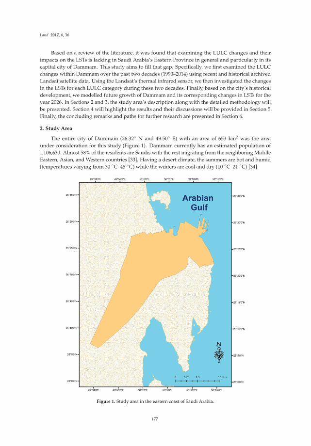
Land 2017, 6, 36

Based on a review of the literature, it was found that examining the LULC changes and theirimpacts on the LSTs is lacking in Saudi Arabia’s Eastern Province in general and particularly in itscapital city of Dammam. This study aims to fill that gap. Specifically, we first examined the LULCchanges within Dammam over the past two decades (1990–2014) using recent and historical archivedLandsat satellite data. Using the Landsat’s thermal infrared sensor, we then investigated the changesin the LSTs for each LULC category during these two decades. Finally, based on the city’s historicaldevelopment, we modelled future growth of Dammam and its corresponding changes in LSTs for theyear 2026. In Sections 2 and 3, the study area’s description along with the detailed methodology willbe presented. Section 4 will highlight the results and their discussions will be provided in Section 5.Finally, the concluding remarks and paths for further research are presented in Section 6.

2. Study Area

The entire city of Dammam (26.32◦ N and 49.50◦ E) with an area of 653 km2 was the areaunder consideration for this study (Figure 1). Dammam currently has an estimated population of1,106,630. Almost 58% of the residents are Saudis with the rest migrating from the neighboring MiddleEastern, Asian, and Western countries [33]. Having a desert climate, the summers are hot and humid(temperatures varying from 30 ◦C–45 ◦C) while the winters are cool and dry (10 ◦C–21 ◦C) [34].

Figure 1. Study area in the eastern coast of Saudi Arabia.

177

Land 2017, 6, 36

3. Methodology

3.1. Data Collection, Classification, Accuracy Assessments

Three Landsat images processed at level-one terrain-corrected (L1T) level collected over the cityof Dammam from the years 1990, 2002, and 2014 were gathered from the United States GeologicalSurvey’s (USGS) EarthExplorer website to estimate the LULC changes and calculate the LSTs for therespective years (Table 1). Since L1T data are delivered with corrected radiometric and geometricdistortions, no additional geo-rectification or image-to-image registrations were performed. Also,USGS resampled and provided all the Landsat thermal bands to 30 m to align with the multispectralbands of the sensors [35]. Finally, a recent high resolution GeoEye image was acquired for classificationand accuracy assessments.

Table 1. Characteristics of Landsat data sets for the study.

Date of Acquisition Path and Row Landsat SensorSpatial Resolution ofMulti-Spectral Bands

Spatial Resolution ofThermal Bands

16 August 1990 164/42 TM 30 m 120 m (resampled to 30 m)24 July 2002 164/42 ETM+ 30 m 60 m (resampled to 30 m)

2 August 2014 164/42 OLI 30 m 100 m (resampled to 30 m)

The imagery was classified into four separate LULC classes based on Level 1 of the AndersonClassification scheme. It is the preferred classification system for classifying Landsat data [36].Table 2 highlights the LULC features included for each class. To classify the LULC from the threepre-processed Landsat images, the Maximum Likelihood Classification (MLC) technique was usedwith signatures collected among the four classes identified through field surveys, GeoEye image,and Google Earth imagery.

Table 2. Scheme for land cover classifications.

Land Cover Class Description

Built-up Residential, industrial, transportation networks, and commercial infrastructures.Bare soil Sand, vacant lands, bare soils.

Vegetation Trees, parks, playgrounds, grasslands.Water body Lakes and coastal water.

To examine the classification accuracies, 295 ground truth reference points were sampled(through stratified random sampling method) across the study area. Historical LULC paper maps(with scales of 1:32,258) were also collected from the Ad-Dammam municipality’s office. Thesehistorical maps, ground truth reference points, and high resolution GeoEye and Google Earth imageswere all utilized in combination to measure the overall classification accuracies. For comparison ofaccuracy results, error matrices were created. The classified results had overall accuracies of 86%(1990), 89% (2002), and 93% (2014) with Kappa coefficients of 0.87, 0.90, and 0.94. Finally, the changesbetween the classified data sets were examined using a post-classification change detection method.

3.2. Derivation of LSTs

The LSTs for this study were obtained from Landsat’s thermal band(s). Landsat TM and ETM+provide thermal information based on a single long-wave infrared (LWIR) band, whereas it is capturedwith two LWIR bands by the Landsat OLI sensor [37]. Therefore, two separate methods were used toderive the LSTs from the three sensors. For deriving the LSTs from Landsat TM and ETM+ sensors,

178

Land 2017, 6, 36

the Spectral Radiance Scaling Method was used [38]. The method first uses the following equation toconvert digital numbers (DNs) into spectral radiance (Lλ):

Lλ =(LMAXλ − LMINλ)× (DN − QCALMIN)

QCALMAX − QCALMIN+ LMINλ (1)

where DN values range between 0 and 255; LMINλ and LMAXλ are the minimum and maximumspectral radiances, respectively; and QCALMIN and QCALMAX are quantized minimum andmaximum calibrated pixel values, respectively.

The second step involved utilizing Equation (2) to convert the spectral radiance to BrightnessTemperature (in Kelvin) [39,40]. Temperatures were then converted to degrees Celsius.

TK =K2

ln( K1Lλ

+ 1)(2)

To derive the LSTs for the year 2014 from the Landsat OLI data, Equations (3) and (4) wereused [41]:

TOAr = mx + b (3)

where TOAr is the top of atmospheric radiance; m is the radiance multiplier (0.0003342); x is the rawband; and b is the radiance add (0.1) [42].

TK =K2

ln( K1TOAr

+ 1)(4)

where TK is the Temperature in degrees Kelvin; K1 = 774.89 and K2 = 1321.08. Temperatures wereconverted to degrees Celsius as well.

3.3. Modeling the Land Cover for 2026

Numerous urban growth prediction models (UGPMs) are available for modelling the future landuse and land cover of an urban area [43]. In this study, modelling the LULC for the year 2026 wascompleted using IDRISI Selva GIS software package. To choose the most accurate modeling techniquefor forecasting the LULC of Dammam for 2026, we simulated the LULC of Dammam for 2014 usingthree separate but popular LULC modeling methods (Cellular Automata Markov (CAM), Multi-LayerPerception Markov (MLPM), and Stochastic Markov (SM)) and examined their accuracies. In all of thethree models, the LULC for 2014 was simulated using the classification results from 1990 (earlier landcover) and 2002 (later land cover).

To model using the CAM method, a combination of Cellular Automata (CA) with Markov ChainAnalysis was utilized. It first involved using the classified LULC data from 1990 and 2002 to producethe Markovian conditional probability areas. Then, Boolean images for each LULC type were generatedusing the 2002 classified results. Euclidean distances for each Boolean image were then calculated andsuitability images using “FUZZY Factor Standardization” were generated. Finally, the CAM methodutilized the Markovian conditional probability areas and suitability images to generate the LULCmodel for 2014. The CAM modeling technique has successfully modelled future LULC changes inseveral major cities in the world [44–47].

The MLPM modelling method utilizes and combines the concepts of Artificial Neural Network(ANN) and Markov Chain Analysis (MCA). To model, it first calculated the changes in the LULCbetween 1990 and 2002 and selected the driver variables (distance from bare soil; distance fromvegetation; distance form water body; distance from built-up area; and empirical likelihood) topredict the transitions or changes. The strength of each variable was measured using Cramer’s Value.The transition sub-model was created and modified until a maximum accuracy of 82.05% was achieved.The models showed that the LULC exhibited three potential transitional forms: bare soil to built-up

179

Land 2017, 6, 36

areas, vegetation to built-up areas, and built-up areas to bare soil. It should be highlighted thatconversion of built-up areas to bare soil/sand is usually rare. However, the study area experiencesfrequent sand-storms and strong winds and roads and highways are frequently found covered withsands due to these natural meteorological phenomena. It is possible for these areas to be classifiedas built-up areas in one year (when sands are not present) but as soil/sand at a later year whensands cover them. Hence conversion of built-up area to bare soil was found to be a valid potentialtransitional form. The transition potential map for each transition was produced and the LULCs for2014 were modeled. Previous studies have found MLPM to produce better prediction accuracies inareas featuring stable and slow LULC changes [48]. Finally, in the SM model, Markovian conditionalprobability images from the years 1990 to 2002 were produced using the Markov module of IDRISI.The Stochastic choice was then applied to materialize the conditional probability images generatedfrom Markov analysis.

Once the LULCs for 2014 were modeled using the three methods, the Map Comparison Kit (MCK)software was utilized to find the best-fit model. To select the best-fit model, the overall Kappa, Khisto,Klocation, and Fraction correct was calculated and examined [49]. The calculated results are shown inTable 3. Since the CAM model had the highest overall Kappa coefficients and Fraction correct, it wasused to simulate the LULC for 2026.

Table 3. Comparison of overall Kappa statistics for three modeling results for 2014.

Kappa Components CAM SM MLPM

Overall Kappa 0.56 0.30 0.45Overall Klocation 0.67 0.36 0.62

Overall Khisto 0.83 0.83 0.73Fraction Correct 0.75 0.60 0.69

3.4. Modeling of LST for 2026

After simulating the LULC for 2026, this study modified the methodology proposed by [28] tomodel and map the distribution of the LSTs across Dammam city. First, several land cover indices ofeach LULC type for the years 1990, 2002, and 2014 were derived. The indices were the NormalizedDifference Bare Soil Index (NDBsI), NDVI, Soil Adjustment Vegetation Index (SAVI), NormalizedDifference Water Body Index (NDWI), Modified Normalized Difference Water Body Index (MNDWI),and Normalized Difference Built-up Area Index (NDBI). The equations used to calculate the indicesalong with their references are given in Table 4.

Table 4. Indices used to model land surface temperature (LST) for 2026.

IndexEquation

ReferenceLandsat TM and ETM+ Landsat OLI

NDBsI B5 − B6B5 + B6

B6 − B10B6 + B10 [50]

NDVI B4 − B3B4 + B3

B5 − B4B5 + B4 [50]

SAVI 1.5 (B4 − B3)B4 + B3 + 0.5

1.5 (B5 − B4)B5 + B4 + 0.5 [51]

NDWI B2 − B4B2 + B4

B3 − B5B3 + B5 [52]

MNDWI B2 − B5B2 + B5

B3 − B6B3 + B6 [53]

NDBI B5 − B4B5 + B4

B6 − B5B6 + B5 [54]

Once the indices were derived, simple linear regression analysis was performed to examine theirrelations with LSTs to select the indices that contribute the most for LST modeling. In the regressionanalysis, indices were the independent variables and LST was the dependent variable. The NDBI,

180

Land 2017, 6, 36

NDBsI, and MNDWI were found to be the major significant indices (p < 0.05) contributing to LSTs.The three indices were normalized on a scale of 0 to 1 and reclassified into 20 equal classes to fit forthe usage of “Markov Chain Analysis”. We then conducted “Markov Chain Analysis” and combinedStochastic Choice with Markov Chain Analysis to simulate the selected indices for the year 2026.Using the three normalized indices data and the LST for 2014, the following equation (with r2 = 0.729)was formulated to explain their relationships:

LST = 81.81 − (17.92 × NDBsI) − (4.79 × NDBI) − (60.39 × MNDWI) (5)

where NDBsI, NDBI, and MNDWI are the corresponding indices and LST is the land surfacetemperature. Finally, the equation and simulated 2026 indices were used to model and map theLST for 2026.

4. Results

4.1. Changes in LULC in Dammam

The classified LULC results for the years 1990, 2002, and 2014 are given in Figure 2 whileTable 5 shows their areal statistics, and changes among classes between the years are provided inTables 6 and 7. From 1990 to 2014, the amount of bare soil declined significantly (by 16,632 ha or 25.5%).During the same period, the built-up area increased by 18,899 ha (28.9% of the study area). The amountof vegetation declined from the years 1990 to 2002 (by 1415 ha or 2.16% of the study area). However,an increase in vegetation was observed between 2002 and 2014 (by 671 ha or 1% of the study area).Finally, the areas of water slightly increased by 380 ha (0.6% of the study area) between 1990 and 2002and decreased by 1903 ha (3% of the study area) from 2002 to 2014.

Table 5. Areal statistics (in hectares) of classified land cover for 1990, 2002, and 2014.

Land Cover Class1990 2002 2014

Area % Area % Area %

Bare soil/sand 48,863 74.79 44,227 67.69 32,231 49.33Built-up area 9368 14.34 15,039 23.02 28,267 43.27

Vegetation 1785 2.73 370 0.57 1041 1.59Water body 5317 8.14 5697 8.72 3794 5.81

Total 65,333 100 65,333 100 65,333 100

Table 6. Change detection matrix showing the class changes (in hectares) between 1990 and 2002.

2002

Bare Soil/Sand Built-Up Area Vegetation Water Body Total

1990

Bare soil/sand 42,803 5969 74 17 48,863Built-up area 883 8061 37 387 9368

Vegetation 438 949 252 146 1785Water body 103 60 7 5147 5317

Total 44,227 15,039 370 5697 65,333

Table 7. Change detection matrix showing the class changes (in hectares) between 2002 and 2014.

2014

Bare Soil/Sand Built-Up Area Vegetation Water Body Total

2002

Bare soil/sand 30,131 13,824 250 22 44,227Built-up area 995 13,427 608 9 15,039

Vegetation 49 147 174 0 370Water body 1056 869 9 3763 5697

Total 32,231 28,267 1041 3794 65,333

181

Land 2017, 6, 36

Figure 2. The study area’s classification results for (a) 1990, (b) 2002, and (c) 2014.

4.2. Distribution and Changes of LST in LULC in Dammam

The average LSTs of individual LULC classes are provided in Table 8. It was observed that for eachyear, bare soil had the highest LST followed by built-up area, vegetation, and water bodies. The resultsalso show that the average temperature for all the classes increased between 1990 and 2014. However,while the average temperature for water body increased slightly by 1.6 ◦C, the average temperaturefor bare soil, built-up area, and vegetation increased by an average of 7.5 ◦C. When we examinedthe changes in the decadal average temperature per class, significant increases (by 7 ◦C) were seenbetween 1990 and 2002 for bare soil and built-up area. The rate of increase reduced to 0.7 ◦C for theseclasses between 2002 and 2014. For vegetation class, the rates of increase were 3.14 ◦C (between 1990and 2002) and 4.16 ◦C (between 2002 and 2014).

182

Land 2017, 6, 36

Table 8. Average LSTs in 1990, 2002, and 2014 for different land cover classes.

Land Cover Class 1990 2002 2014

Bare Soil 37.62 44.41 45.09Built-Up Area 36.42 43.42 44.12

Vegetation 35.71 38.85 43.01Water Body 29.04 30.69 30.64

The spatial distributions of the temperatures for 1990, 2002, and 2014 are given in Figure 3, whilethe relationship between temperature and areal coverage is provided in Table 9. In 1990, the entirestudy area had LSTs less than 40 ◦C, with the majority (87.07%) of the land cover having LSTs between36 ◦C and 40 ◦C. In 2002, 77% of the land cover had LSTs between 41 ◦C and 50 ◦C. However,the percentage of LSTs between 41 ◦C and 50 ◦C increased to 91.26% in 2014, suggesting the studyarea’s LSTs increased between 1990 and 2014, although it increased more in the last decade.

Figure 3. LST distributions for (a) 1990, (b) 2002, and (c) 2014.

183

Land 2017, 6, 36

Table 9. Distribution of areal coverage among different LST ranges for 1990, 2002, 2014, and 2026.

Ranges of LST (◦C)Areal Coverage (%)

1990 2002 2014 2026

≤30 7.86 6.14 3.81 031 to 35 5.07 6.44 2.3 0.2936 to 40 87.07 9.9 2.58 1.3841 to 45 0 36.11 58.69 2.3546 to 50 0 40.9 32.57 35.06

>50 0 0.51 0.05 60.92

4.3. Modeling of LULC and LST for 2026

Figure 4 shows the simulated LULC for the year 2026 and Table 10 provides their areal statistics.The modeled LULC shows that 35,986 ha (55% of the study area) will change to built-up area,an increase of almost 27.3% from 2014. This increase will mostly occur in the city’s northern andsoutheastern parts. Vegetation will also increase in the city from 1041 ha in 2014 to 3240 ha in 2026(a gain of 211%) in central northern parts of Dammam and along the northern coastline. This increasein built-up area and vegetation will reduce the amount of bare soil by 8306 ha (a net loss of almost 26%)and water bodies by 1612 ha (loss of roughly 42.5%) from 2014 to 2026. Water bodies will be mostly lostdue to new construction of residential and commercial zones along the eastern seashores of the city.

Figure 4. Modeled land use and land cover (LULC) for Dammam for 2026.

The spatial distribution of the modeled 2026 LST is provided in Figure 5 and the areal percentagestatistics by LST range is shown in the last column of Table 9. Compared to the LST ranges of 1990, 2002,and 2014, most of the land coverage (98%) is predicted to have LSTs over 41 ◦C in 2026. The averageLSTs for built-up area are forecasted to be 46 ◦C.

184

Land 2017, 6, 36

Figure 5. Distribution of the indices ((a) NDBI; (b) MNDWI; and (c) NDBsI) used to model the 2026LST (d) for Dammam.

Table 10. Modelled areal statistics (in hectares) of land cover for 2026.

Land Cover Class Area %

Bare soil 23,925 36.62Built-up area 35,986 55.08

Vegetation 3240 4.96Water body 2182 3.34

Total 65,333 100

5. Discussions

5.1. Changes in LULC and LSTs

This paper first examined the changes in the LULC in the city of Dammam between 1990 and2014. The city’s urban areas expanded by 61% from 1990 to 2002 and 88% between 2002 and 2014.

185

Land 2017, 6, 36

Such decadal growth is higher than other cities in Saudi Arabia [19,55]. It is also higher than otherdeveloping cities in the world, including Kathmandu [13], Tripoli [56], and Dhaka [57]. Rapidpopulation growth and economic prosperity are the primary reasons for such rapid urban growth [58].Dammam’s population increased from 127,844 (1974) to 260,048 (1986), and finally to 918,154 in2010 [33,59] due to rapid migration of refugees during and after the 1991 Gulf war from neighboringcountries of Iraq and Kuwait. The results also show that the vegetation in the study area decreasedbetween 1990 and 2002 and increased between 2002 and 2014. Previous studies have also found similarpatterns of decreasing vegetation coverage between the early 1990s and 2000 and an increase from theearly 2000s to 2014 in other Saudi cities [55,60]. They suggested that increasing population resulted invegetation increases in Saudi cities [60].

In tropical and sub-tropical urban environments, the LSTs are dependent upon the LULC,with urban built-up areas having the highest LSTs and significantly contributing to the formationof UHIs [24,28]. However, having a desert climate, the study area’s bare soil (mostly sands) hadthe highest mean LSTs during the day followed by urban built-up areas in the all of the three yearsconsidered. The mean LSTs for vegetative areas were lower than urban built-up areas. Similar resultingpatterns were also found in other neighboring desert cities of Abu Dhabi and Dubai, suggesting aninversion of UHIs where city centers are generally cooler than the outskirts of the city due to lowvegetation coverage and sand being the main reflecting surface [31,61]. In both cities, a reduction of5 ◦C (Abu Dhabi) to 12 ◦C (Dubai) of mean LSTs were due to the presence of green vegetative areas.For our study area, the vegetative areas lowered the mean LSTs by an average of 2 ◦C. We believe thisslight lowering is due to the very low amount of vegetation present in Dammam (only 1042 ha in 2014),indicating that the reduction in LSTs is correlated to the amount of vegetation present in an area.

It was also found in this study that the mean LSTs of 2014 increased by an average of 7.5 ◦Cwhen compared to the mean LSTs of 1990. Increases of mean LSTs were also found in Dubai andthe semi-arid desert city of Santiago, Chile [61,62]. As highlighted by previous studies, the rapidpopulation growth along with the urban expansion could be the contributing factors to such increasesin the temperatures [63].

5.2. LULC and LST Modeling for 2026

The land use and land cover of Dammam are expected to change over the next decade, as 27%of the current LULC is modelled to be converted into urban built-up areas. This decadal growth rateis comparable to other cities in the world, including Setubal and Sesimbra (in Protugal with 25%),Asmara (in Eritrea with 25%), and Beijing (with 31%) [64–66]. Such growth will lead to urban sprawland will have several benefits and consequences. The benefits include development of industrialinfrastructures and facilities which can provide employment opportunities for the residents from smallcities and rural areas of the kingdom as well as from other neighboring Arab countries and developingcountries of South and Southeast Asia (i.e., Pakistan, Bangladesh, Indonesia, and the Philippines).The expansion can also provide better business, educational, and medical facilities for its residents.

The negative impacts are numerous and most often they outweigh the benefits of the urbanexpansions. With increasing employment opportunities, the population is projected to grow by almost20% over the next decade (1,057,256 in 2015 to 1,264,227 in 2025) [33]. Due to increasing population andcity expansions, travelling distances for the residents are expected to increase, resulting in more fuelconsumption and traffic congestions. The high fuel consumptions will result in rising air pollution andcause various health problems for the elderly and children of the city. The cost for providing publicutility services is also expected to rise. Urbanization has also been known to cause social disparitiesamong the residents [67]. Finally, the LST of the city is expected to increase as well from the increasingbuilt-up areas.

The LSTs modelled in this study for 2026 show that the majority of the city will have LSTsover 41 ◦C, with the average LSTs for built-up areas forecasted to be 46 ◦C. This is significantlyhigher than the modelled LSTs of cities in the tropical regions of the world [28]. Recently, Pal and

186

Land 2017, 6, 36

Eltahir [68] simulated the dry and wet-bulb temperatures for Middle Eastern cities between theyears 2071–2100 using a regional climate model. Their study shows that by 2100, the regionalaverage wet-bulb temperature will exceed 35 ◦C several times in the year and the average maximumdry-bulb temperature exceeding 45 ◦C in the low lying coastal cities of the region (i.e., Abu Dhabi,Dammam/Dhahran, and Dubai) will become the norm in the July, August, and September summermonths. The LSTs modelled in this study are 1 ◦C higher than the dry-bulb temperature estimatedby Pal and Eltahir [68]. This is to be expected, since LSTs and air-temperatures are highly correlatedand as the air temperature increases, LST values will tend to be higher than the air temperature [69].Such extreme high temperatures will be dangerous for human health as well as for animal and plantspecies. Instead of the end of the century as predicted by Pal and Eltahir [68], these results of this studysuggest that Dammam city may experience very high temperatures that may be difficult for humaninhabitability within the next one to two decades.

6. Conclusions

This study compared three separate Landsat images to evaluate LULC changes over the last twodecades in Dammam, the capitol of Saudi Arabia’s Eastern Province. It also examined the trends in theLSTs during these periods and their relationships with the four major LULC classes. Finally, based onthe changes, this study projected the LULC and the LSTs for the year 2026. Since 1990, the urban areain Dammam has increased, resulting in decreasing bare soil. The results also show that the averageLSTs have increased in the last two decades. If such a trend continues, built-up areas along with theLSTs will continue to increase over the next decade. Such increases in built up areas along with theirtemperatures will have numerous medical, environmental, and social impacts and consequences.

The study results will be beneficial for Dammam’s government officials and planners, who canensure that the city is growing in a restrictive manner by utilizing and comparing this study’s mapswith the city’s future master plan. They can also create rules and regulations and create strategiesthat can reduce the LSTs in the city. Future studies should examine in detail the consequences andproblems faced by the residents of Dammam due to urban expansions and LST increases as well ashow to mitigate them. The growth and the distribution of LSTs of other cities in Saudi Arabia shouldalso be examined and modeled to ensure they are growing in a sustainable manner.

Acknowledgments: The authors acknowledge and appreciate the financial support provided by King AbdulazizCity for Science and Technology (KACST) through the Science & Technology Unit at King Fahd University ofPetroleum & Minerals (KFUPM) for funding this work through project number 13-ENE198-04 as part of the“National Science, Technology and Innovation Plan (NSTIP)” program. They also thank the King Fahd Universityof Petroleum and Minerals for providing the equipment and technical resources and funds to publish this study.Finally, we would also like to thank the two anonymous referees and the editors for their valuable comments forimproving this manuscript.

Author Contributions: M.T. Rahman wrote Sections 1, 2 and 4–6 and edited the entire manuscript. A.S. Aldosaryand M.G. Mortoja formulated the research design and edited the manuscript. M.G. Mortoja wrote Section 3 andcollected and processed all the data for the study.


References

1. McKinney, M.L. Urbanization, Biodiversity, and Conservation. Bioscience 2002, 52, 883. [CrossRef]2. Uttara, S.; Elliot, S. Impacts of Urbanization on Environment. Int. J. Res. Eng. Appl. Sci. 2012, 2, 1637–1645.3. Maimaitiyiming, M.; Ghulam, A.; Tiyip, T.; Pla, F.; Latorre-Carmona, P.; Halik, Ü.; Sawut, M.; Caetano, M.

Effects of green space spatial pattern on land surface temperature: Implications for sustainable urbanplanning and climate change adaptation. ISPRS J. Photogramm. Remote Sens. 2014, 89, 59–66. [CrossRef]

4. Gaffin, S.R.; Rosenzweig, C.; Khanbilvardi, R.; Parshall, L.; Mahani, S.; Glickman, H.; Goldberg, R.; Blake, R.;Slosberg, R.B.; Hillel, D. Variations in New York city’s urban heat island strength over time and space.Theor. Appl. Climatol. 2008, 94, 1–11. [CrossRef]

187

Land 2017, 6, 36

5. Wong, N.H.; Jusuf, S.K. GIS-based greenery evaluation on campus master plan. Landsc. Urban Plan. 2008, 84,166–182. [CrossRef]

6. Lai, L.W.; Cheng, W.L. Urban heat island and air pollution–an emerging role for hospital respiratoryadmissions in an urban area. J. Environ. Health 2010, 72, 32–35. [PubMed]

7. Priyadarsini, R. Urban Heat Island and its Impact on Building Energy Consumption. Adv. Build. Energy Res.2009, 3, 261–270. [CrossRef]

8. Rahman, M.T. Detection of Land Use/Land Cover Changes and Urban Sprawl in Al-Khobar, Saudi Arabia:An Analysis of Multi-Temporal Remote Sensing Data. ISPRS Int. J. Geo-Inf. 2016, 5, 15. [CrossRef]

9. Al-Ahmadi, F.; Hames, A. Comparison of Four Classification Methods to Extract Land Use and Land Coverfrom Raw Satellite Images for Some Remote Arid Areas, Kingdom of Saudi Arabia. J. King Abdulaziz Univ. Sci.2009, 20, 167–191. [CrossRef]

10. Madugundu, R.; Al-Gaadi, K.A.; Patil, V.C.; Tola, E. Detection of Land Use and Land Cover Changes in DirabRegion of Saudi Arabia Using Remotely Sensed Imageries. Am. J. Environ. Sci. 2014, 10, 8–18. [CrossRef]

11. Al-Hathloul, S.; Rahman, M.A. Dynamism of metropolitan areas: The case of metropolitan Dammam, SaudiArabia. J. Gulf Arab. Penins. Stud. 2003, 29, 11–43.

12. Aguilar, A.G.; Ward, P. Globalization, regional development, and mega-city expansion in Latin America:Analyzing Mexico City’s peri-urban hinterland. Cities 2003, 20, 3–21. [CrossRef]

13. Thapa, R.B.; Murayama, Y. Examining Spatiotemporal Urbanization Patterns in Kathmandu Valley, Nepal:Remote Sensing and Spatial Metrics Approaches. Remote Sens. 2009, 1, 534–556. [CrossRef]

14. Dewan, A.M.; Yamaguchi, Y. Land use and land cover change in Greater Dhaka, Bangladesh: Using remotesensing to promote sustainable urbanization. Appl. Geogr. 2009, 29, 390–401. [CrossRef]

15. Jamali, N.A.; Rahman, M.T. Utilization of Remote Sensing and GIS to Examine Urban Growth in the City ofRiyadh, Saudi Arabia. J. Adv. Inf. Technol. 2016, 7, 297–301.

16. Rahman, M.T.; Rashed, T. Urban tree damage estimation using airborne laser scanner data and geographicinformation systems: An example from 2007 Oklahoma ice storm. Urban For. Urban Green. 2015, 14, 562–572.[CrossRef]

17. Alwashe, M.A.; Bokhari, A.Y. Monitoring vegetation changes in Al Madinah, Saudi Arabia, using ThematicMapper data. Int. J. Remote Sens. 1993, 14, 191–197. [CrossRef]

18. Al-Rowili, M.S.; Fadda, E.H.; Vaughan, R.A. A Comparison of Data Fusion and Unsupervised Classificationfor Change Detection in Jeddah, Saudi Arabia. In Proceedings of the 22nd Symposium of the EuropeanAssociation of Remote Sensing Laboratories, Prague, Czech Republic, 4–6 June 2002.

19. Aljoufie, M.; Zuidgeest, M.; Brussel, M.; Maarseveen, M.V. Spatial–temporal analysis of urban growth andtransportation in Jeddah City, Saudi Arabia. Cities 2013, 31, 57–68. [CrossRef]

20. Al-Harbi, K.M. Monitoring of agricultural area trend in Tabuk region—Saudi Arabia using Landsat TM andSPOT data. Egypt. J. Remote Sens. Sp. Sci. 2010, 13, 37–42. [CrossRef]

21. Al-Gaadi, K.A.; Samdani, M.S.; Patil, V.C. Assessment of Temporal Land Cover Changes in Saudi ArabiaUsing Remotely Sensed Data Precision Agriculture Research Chair, College of Food and Agriculture Sciences.Middle-East J. Sci. Res. 2011, 9, 711–717.

22. Rao, P.K. Remote sensing of urban “heat islands” from an environmental satellite. Bull. Am. Meteorol. Soc.1972, 53, 647–648.

23. Yuan, F.; Bauer, M.E. Comparison of impervious surface area and normalized difference vegetation index asindicators of surface urban heat island effects in Landsat imagery. Remote Sens. Environ. 2007, 106, 375–386.[CrossRef]

24. Xiao, R.B.; Weng, Q.H.; Ouyang, Z.Y.; Li, W.F.; Schienke, E.W.; Zhang, Z.M. Land surface temperaturevariation and major factors in Beijing, China. Photogramm. Eng. Remote Sens. 2008, 74, 451–461. [CrossRef]

25. Li, X.; Zhou, W.; Ouyang, Z.; Xu, W.; Zheng, H. Spatial pattern of greenspace affects land surface temperature:Evidence from the heavily urbanized Beijing metropolitan area, China. Landsc. Ecol. 2012, 27, 887–898.[CrossRef]

26. Dousset, B.; Gourmelon, F. Satellite multi-sensor data analysis of urban surface temperatures and landcover.J. Photogramm. Remote Sens. 2003, 58, 43–54. [CrossRef]

27. Chaudhuri, G.; Mishra, N.B. Spatio-temporal dynamics of land cover and land surface temperature inGanges-Brahmaputra delta: A comparative analysis between India and Bangladesh. Appl. Geogr. 2016, 68,68–83. [CrossRef]

188

Land 2017, 6, 36

28. Ahmed, B.; Kamruzzaman, M.; Zhu, X.; Rahman, M.S.; Choi, K. Simulating Land Cover Changes and TheirImpacts on Land Surface Temperature in Dhaka, Bangladesh. Remote Sens. 2013, 5, 5969–5998. [CrossRef]

29. El Abidine, E.M.Z.; Mohieldeen, Y.E.; Mohamed, A.A.; Modawi, O.; AL-Sulaiti, M.H. Heat wave hazardmodelling: Qatar case study. QScience Connect 2014. [CrossRef]

30. Rasul, A.; Balzter, H.; Smith, C. Spatial variation of the daytime Surface Urban Cool Island during the dryseason in Erbil, Iraqi Kurdistan, from Landsat 8. Urban Clim. 2015, 14, 176–186. [CrossRef]

31. Lazzarini, M.; Marpu, P.R.; Ghedira, H. Temperature-land cover interactions: The inversion of urban heatisland phenomenon in desert city areas. Remote Sens. Environ. 2013, 130, 136–152. [CrossRef]

32. Radhi, H.; Sharples, S. Quantifying the domestic electricity consumption for air-conditioning due to urbanheat islands in hot arid regions. Appl. Energy 2013, 112, 371–380. [CrossRef]

33. General Authority for Statistics Population Statistics. Available online: http://www.stats.gov.sa/en/(accessed on 15 October 2014).

34. WeatherSpark Historical Weather for 2014 in Dammam, Saudi Arabia. Available online:https://weatherspark.com/history/32759/2014/Dammam-Eastern-Province-Saudi-Arabia (accessed on1 January 2015).

35. NASA Landsat 4–7 Thermal Data to be Resampled to 30 Meters. Available online: https://landsat.gsfc.nasa.gov/landsat-4--7-thermal-data-to-be-resampled-to-30-meters/ (accessed on 30 April 2017).

36. Rozenstein, O.; Karnieli, A. Comparison of methods for land-use classification incorporating remote sensingand GIS inputs. Appl. Geogr. 2011, 31, 533–544. [CrossRef]

37. Rozenstein, O.; Qin, Z.; Derimian, Y.; Karnieli, A. Derivation of land surface temperature for landsat-8 TIRSusing a split window algorithm. Sensors (Switzerland) 2014, 14, 5768–5780. [CrossRef] [PubMed]

38. Coll, C.; Galve, J.M.; Sánchez, J.M.; Caselles, V. Validation of Landsat-7/ETM+ Thermal-Band Calibrationand Atmospheric Correction With Ground-Based Measurements. IEEE Trans. Geosci. Remote Sens. 2010, 48,547–555. [CrossRef]

39. Ma, Y.; Kuang, Y.; Huang, N. Coupling urbanization analyses for studying urban thermal environment andits interplay with biophysical parameters based on TM/ETM+ imagery. Int. J. Appl. Earth Obs. Geoinf. 2010,12, 110–118. [CrossRef]

40. Wukelic, G.E.; Gibbons, D.E.; Martucci, H.P.; Foote, H.P. Radiometric calibration of Landsat Thematic Mapperthermal band. Remote Sens. Environ. 1989, 28, 339–347. [CrossRef]

41. Butler, K. Deriving Temperature from Landsat 8 Thermal Bands (TIRS). Available online: http://blogs.esri.com/esri/arcgis/2014/01/06/deriving-temperature-from-landsat-8-thermal-bands-tirs/ (accessed on3 January 2015).

42. Almutairi, M.K. Derivation of Urban Heat Island for Landsat-8 TIRS Riyadh City (KSA). J. Geosci.Environ. Prot. 2015, 3, 18–23. [CrossRef]

43. Triantakonstantis, D.; Mountrakis, G. Urban Growth Prediction: A Review of Computational Models andHuman Perceptions. J. Geogr. Inf. Syst. 2012, 4, 555–587. [CrossRef]

44. Guan, D.G.; Li, H.F.; Inohae, T.; Su, W.; Nagaie, T.; Hokao, K. Modeling urban land use change by theintegration of cellular automaton and Markov model. Ecol. Modell. 2011, 222, 3761–3772. [CrossRef]

45. Moghadam, H.S.; Helbich, M. Spatiotemporal urbanization processes in the megacity of Mumbai, India:A Markov chains-cellular automata urban growth model. Appl. Geogr. 2013, 40, 140–149. [CrossRef]

46. Gong, W.; Li, Y.; Fan, W.; Stott, P. Analysis and simulation of land use spatial pattern in Harbin prefecturebased on trajectories and cellular automata-Markov modelling. Int. J. Appl. Earth Obs. Geoinf. 2015, 34,207–216. [CrossRef]

47. Halmy, M.W.A.; Gessler, P.E.; Hicke, J.A.; Salem, B.B. Land use/land cover change detection and predictionin the north-western coastal desert of Egypt using Markov-CA. Appl. Geogr. 2015, 63, 101–112. [CrossRef]

48. Roy, H.G.; Fox, D.M.; Emsellem, K. Predicting Land Cover Change in a Mediterranean Catchment atDifferent Time Scales. In Proceedings of the 14th International Conference on Computational Scienceand Its Applications (ICCSA 2014), Guimarães, Portugal, 30 June–3 July 2014; Murgante, B., Misra, S.,Rocha, A.M.A.C., Torre, C., Rocha, J.G., Falcao, M.I., Taniar, D., Apduhan, B.O., Gervasi, O., Eds.; SpringerInternational: Cham, Switzerland, 2014.; Volume 8582, pp. 315–330.

49. Visser, H.; Najs, T.D. The Map Comparison Kit. Environ. Model. Softw. 2006, 21, 346–358. [CrossRef]50. Chen, X.-L.; Zhao, H.-M.; Li, P.-X.; Yin, Z.-Y. Remote sensing image-based analysis of the relationship

between urban heat island and land use/cover changes. Remote Sens. Environ. 2006, 104, 133–146. [CrossRef]

189

Land 2017, 6, 36

51. Huete, A.R. A soil-adjusted vegetation index (SAVI). Remote Sens. Environ. 1988, 25, 295–309. [CrossRef]52. McFeeters, S.K. The use of the Normalized Difference Water Index (NDWI) in the delineation of open water

features. Int. J. Remote Sens. 1996, 17, 1425–1432. [CrossRef]53. Xu, H. A Study on Information Extraction of Water Body with the Modified Normalized Difference Water

Index (MNDWI). J. Remote Sens. 2005, 9, 511–517.54. Zha, Y.; Gao, J.; Ni, S. Use of normalized difference built-up index in automatically mapping urban areas

from TM imagery. Int. J. Remote Sens. 2003, 24, 583–594. [CrossRef]55. Alqurashi, A.F.; Kumar, L. Land Use and Land Cover Change Detection in the Saudi Arabian Desert Cities

of Makkah and Al-Taif Using Satellite Data. Adv. Remote Sens. 2014, 3, 106–119. [CrossRef]56. Al-sharif, A.A.A.; Pradhan, B.; Shafri, H.Z.M.; Mansor, S. Spatio-temporal analysis of urban and population

growths in tripoli using remotely sensed data and GIS. Indian J. Sci. Technol. 2013, 6, 5134–5142.57. Corner, R.J.; Dewan, A.M.; Chakma, S. Monitoring and Prediction of Land-Use and Land-Cover (LULC)

Change. In Dhaka Megacity: Geospatial Perspectives on Urbanisation, Environment and Health; Dewan, A.M.,Corner, R.J., Eds.; Springer: Dordrecht, The Netherlands, 2014; pp. 75–97.

58. Abou-Korin, A.A. Impacts of Rapid Urbanisation in the Arab World: the Case of Dammam Metropolitan Area,Saudi Arabia. In 5th Int’l Conference and Workshop on Built Environment in Developing Countries (ICBEDC 2011);University Sains Malaysia: Pulao Pinang, Malaysia, 2011; pp. 1–25.

59. Al-Hathloul, S.; Mughal, M.A. Urban growth management-the Saudi experience. Habitat Int. 2004, 28,609–623. [CrossRef]

60. Aina, Y.A.; Merwe, J.H.V.; Alshuwaikhat, H.M. Urban Spatial Growth and Land Use Change in Riyadh:Comparing Spectral Angle Mapping and Band Ratioing Techniques. In Proceedings of the Academic Trackof the 2008 Free and Open Source Software for Geospatial (FOSS4G) Conference, Incorporating the GISSA2008 Conference, Cape Town, South Africa, 29 September–4 October 2008; pp. 51–57.

61. Abdi, A. Using Landsat ETM+ to Assess Land Cover and Land Surface Temperature Change in Dubaibetween 1999 and 2009. Available online: http://www.hakimabdi.com/20120729/using-landsat-etm-to-assess-land-cover-and-land-surface-temperature-change-in-dubai-between-1999-and-2009/ (accessed on3 March 2016).

62. Peña, M.A. Examination of the Land Surface Temperature Response for Santiago, Chile. Photogramm. Eng.Remote Sens. 2009, 75, 1191–1200. [CrossRef]

63. Brazel, A.; Selover, N.; Vose, R.; Heisler, G. The tale of two climates—Baltimore and Phoenix urban LTERsites. Clim. Res. 2000, 15, 123–135. [CrossRef]

64. Tewolde, M.G.; Cabral, P. Urban Sprawl Analysis and Modeling in Asmara, Eritrea. Remote Sens. 2011, 3,2148–2165. [CrossRef]

65. Araya, Y.H.; Cabral, P. Analysis and Modeling of Urban Land Cover Change in Setúbal and Sesimbra,Portugal. Remote Sens. 2010, 2, 1549–1563. [CrossRef]

66. Han, H.; Yang, C.; Song, J. Scenario Simulation and the Prediction of Land Use and Land Cover Change inBeijing, China. Sustainability 2015, 7, 4260–4279. [CrossRef]

67. Bhatta, B. Causes and Consequences of Urban Growth and Sprawl. In Analysis of Urban Growth and Sprawlfrom Remote Sensing Data; Advances in Geographic Information Science; Springer: Berlin/Heidelberg,Germany, 2010; pp. 17–36.

68. Pal, J.S.; Eltahir, E.A.B. Future temperature in southwest Asia projected to exceed a threshold for humanadaptability. Nat. Clim. Chang. 2016, 6, 197–200. [CrossRef]

69. Li, Z.; Guo, X.; Dixon, P.; He, Y. Applicability of Land Surface Temperature (LST) estimates from AVHRRsatellite image composites in northern Canada. Prairie Perspect. 2008, 11, 119–130.


190

MDPI St. Alban-Anlage 66

4052 Basel Switzerland

Tel. +41 61 683 77 34 Fax +41 61 302 89 18

www.mdpi.com

Land Editorial Office

E-mail: [email protected]/journal/land

MDPI St. Alban-Anlage 66 4052 Basel Switzerland

Tel: +41 61 683 77 34 Fax: +41 61 302 89 18

www.mdpi.com ISBN 978-3-03842-918-0

Urban Land Systems: An Ecosystems Perspective - MDPI

Documents

Transcript of Urban Land Systems: An Ecosystems Perspective - MDPI